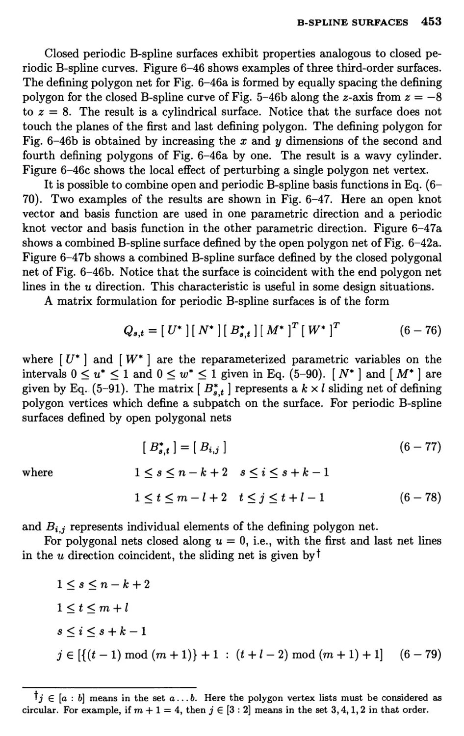
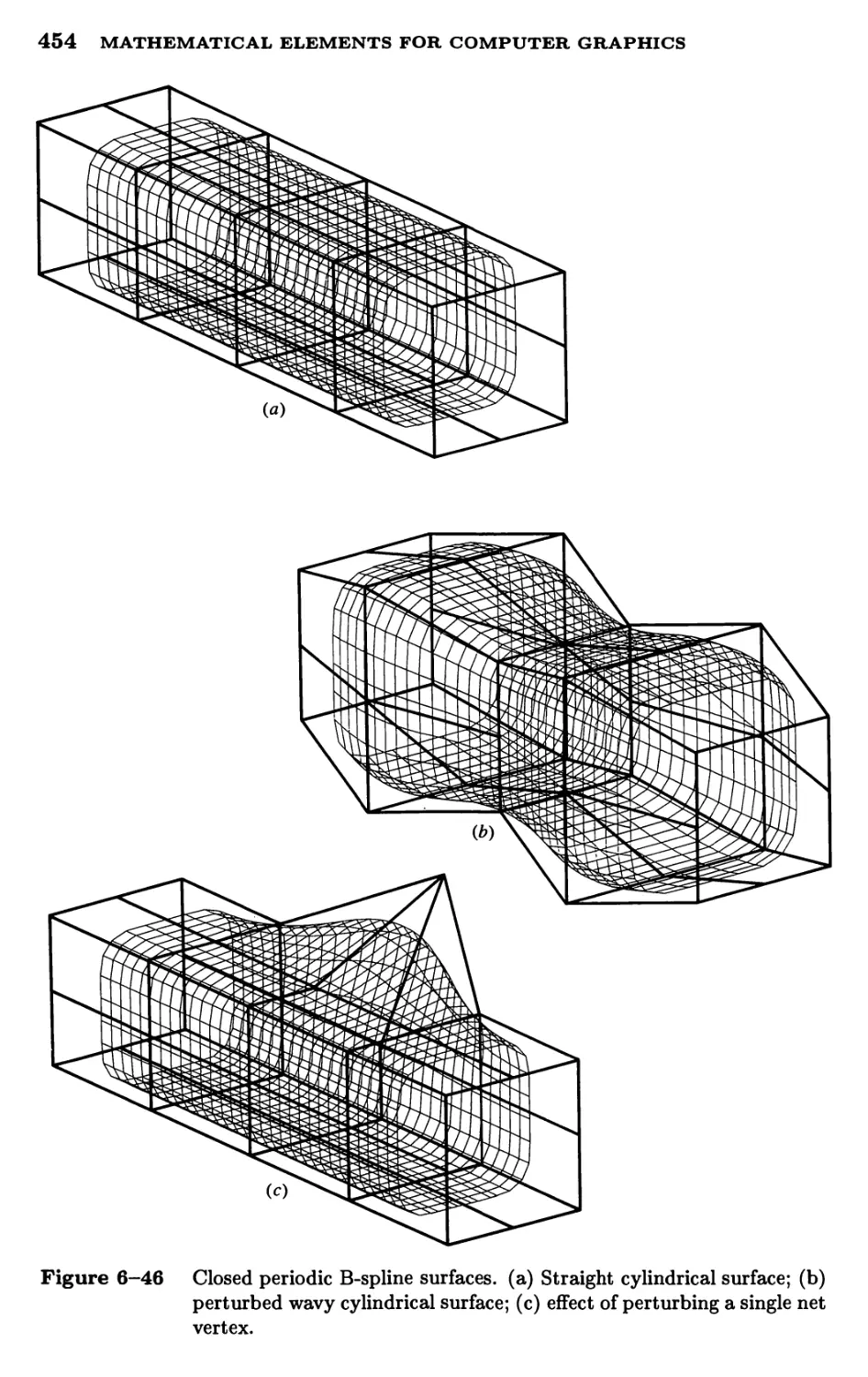
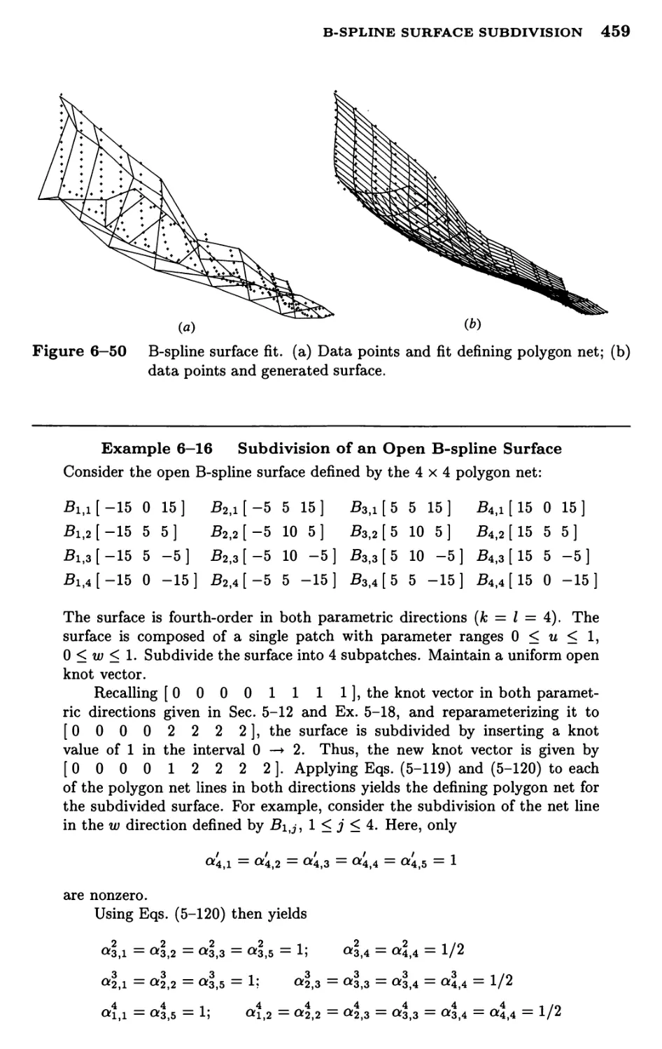
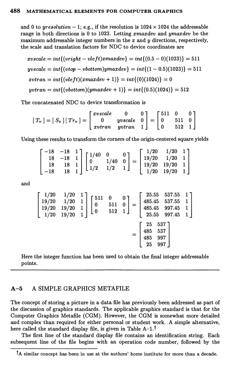
/


Автор: Rogers David F. Adams J. Alan
Теги: программирование математика кибернетика компьютерная графика
ISBN: 0-07-053529-9
Год: 1990

Текст
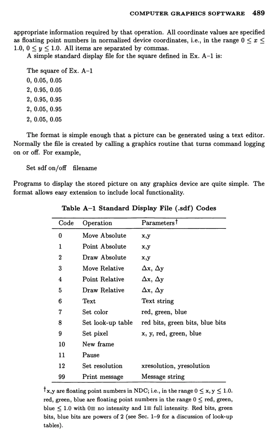
a he aid
for
SECOND EDITION
>
V^
avit F. •ogers
J. A Ian A dams
MATHEMATICAL ELEMENTS FOR
COMPUTER GRAPHICS
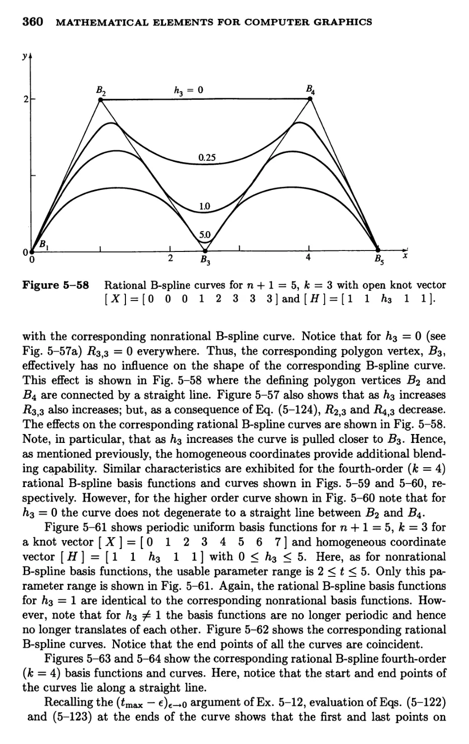
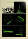
The America's Cup yacht Stars & Stripes defined as a B-spline surface,
(a) Defining polygon net; (b) body, buttock and waterlines;
(c) parametric net. (Courtesy of George Hazen.)
MATHEMATICAL
ELEMENTS
FOR
COMPUTER
GRAPHICS
Second Edition
David F. Rogers
Professor of Aerospace Engineering
United States Naval Academy, Annapolis, Md.
J. Alan Adams
Professor of Mechanical Engineering
United States Naval Academy, Annapolis, Md.
McGraw-Hill, Inc.
New York St. Louis San Francisco Auckland Bogota
Caracas Lisbon London Madrid Mexico Milan
Montreal New Delhi Paris San Juan Singapore
Sydney Tokyo Toronto
This book was computer typeset by Nancy A. Rogers using TJjjK.
The font is Computer Modern Roman. Phototypesetting was done at the AMS.
The editor was B. J. Clark;
the production supervisor was Louise Karam.
The cover was designed by Caliber Design Planning, Inc. and David F. Rogers.
Printed and bound by Impersora Donneco Internacional S. A. de C. V.
a division of R. R. Donnelley & Sons, Inc.
MATHEMATICAL ELEMENTS FOR COMPUTER GRAPHICS
Copyright © 1990, 1976 by McGraw-Hill, Inc. All rights reserved. Typeset in the
United States of America. Except as permitted under the United States Copyright Act
of 1976, no part of this publication may be reproduced or distributed in any form or
by any means, or stored in a data base or retrieval system, without the prior written
permission of the publisher.
4 5 6 7 8 9 10 DOR DOR 998765432
ISBN 0-07-05352^ -Chard cover}
ISBN 0-07-053530-2 {soft cover}
Cover/dust jacket illustration credits:
Front cover/dust jacket: A sphere and its defining rational B-spline polygon net. (David
F. Rogers)
Back cover/dust jacket: The America's Cup yacht Stars & Stripes defined as a B-spline
surface. (George Hazen).
Manufactured in Mexico.
Library of Congress Cataloging in Publication Data
Rogers, David F., (date).
Mathematical elements for computer graphics /David F. Rogers
and J. Alan Adams — 2nd ed.
p. cm.
Bibliography: p.
Includes index.
ISBN 0-07-053529-9 ISBN 0-07-053530-2 (soft)
1. Computer graphics. I. Adams, J. Alan (James Alan), (date).
II. Title.
T385.R6 1990
006.6 - dcl9 89-2308
To our wives
Nancy A. Rogers and Virginia F. Adams
and our families
Stephen, Karen and Ransom Rogers
and
Lynne, David and Alan Adams
CONTENTS
Chapter 1
l-l
1-2
1-3
1-4
1-5
1-6
1-7
1-8
1-9
1-10
1-11
1-12
1-13
1-14
1-15
1-16
1-17
1-18
1-19
1-20
1-21
1-22
1-23
Foreword to the First Edition
Preface
Preface to the First Edition
Introduction To Computer Graphics
Overview of Computer Graphics
Representing Pictures
Preparing Pictures For Presentation
Presenting Previously Prepared Pictures
Interacting with the Picture
Description of Some Graphics Devices
Storage Tube Graphics Displays
Calligraphic Refresh Graphics Displays
Raster Refresh Graphics Displays
Cathode Ray Tube Basics
Color CRT Raster Scan Basics
Video Basics
Flat Panel Displays
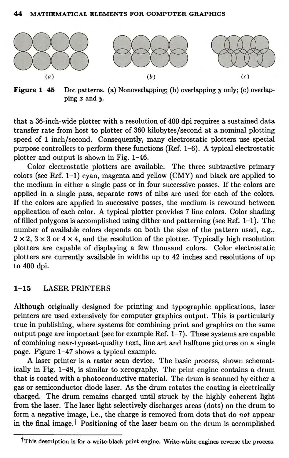
Electrostatic Plotters
Laser Printers
Dot Matrix Plotters
Ink Jet Plotters
Thermal Plotters
Pen and Ink Plotters
Color Film Cameras
Active and Passive Graphics Devices
Computer Graphics Software
References
xi
xiii
xvii
1
3
3
5
6
9
18
18
19
24
30
31
32
35
42
44
47
49
50
52
56
57
58
59
vii
viii MATHEMATICAL ELEMENTS FOR COMPUTER GRAPHICS
Chapter 2
2-1
2-2
2-3
2-4
2-5
2-6
2-7
2-8
2-9
2-10
2-11
2-12
2-13
2-14
2-15
2-16
2-17
2-18
2-19
2-20
2-21
2-22
Chapter 3
3-1
3-2
3-3
3-4
3-5
3-6
3-7
3-8
3-9
3-10
3-11
3-12
3-13
3-14
3-15
3-16
3-17
3-18
Two-Dimensional Transformations
Introduction
Representation of Points
Transformations and Matrices
Transformation of Points
Transformation of Straight Lines
Midpoint Transformation
Transformation of Parallel Lines
Transformation of Intersecting Lines
Rotation
Reflection
Scaling
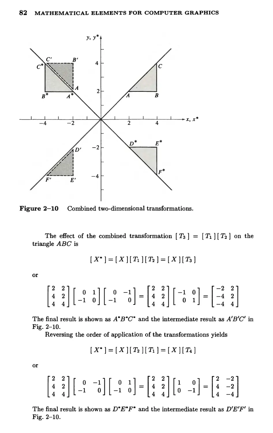
Combined Transformations
Transformation of The Unit Square
Solid Body Transformations
Translations and Homogeneous Coordinates
Rotation About an Arbitrary Point
Reflection Through an Arbitrary Line
Projection - A Geometric Interpretation of
Homogeneous Coordinates
Overall Scaling
Points At Infinity
Transformation Conventions
References
Three-Dimensional Transformations
Introduction
Three-Dimensional Scaling
Three-Dimensional Shearing
Three-Dimensional Rotation
Three-Dimensional Reflection
Three-Dimensional Translation
Multiple Transformations
Rotations About an Axis Parallel to a
Coordinate Axis
Rotation About an Arbitrary Axis in Space
Reflection Through an Arbitrary Plane
Affine and Perspective Geometry
Orthographic Projections
Axonometric Projections
Oblique Projections
Perspective Transformations
Techniques For Generating Perspective Views
Vanishing Points
Photography and The Perspective Transformation
61
61
61
62
62
65
66
68
69
72
76
78
80
83
86
87
88
89
90
94
95
98
100
101
101
102
106
107
113
115
115
117
121
128
132
135
141
151
157
171
179
185
CONTENTS ix
3-19
3-20
3-21
3-22
Chapter 4
4-1
4-2
4-3
4-4
4-5
4-6
4-7
4-8
4-9
4-10
4-11
Chapter 5
5-1
5-2
5-3
5-4
5-5
5-6
5-7
5-8
5-9
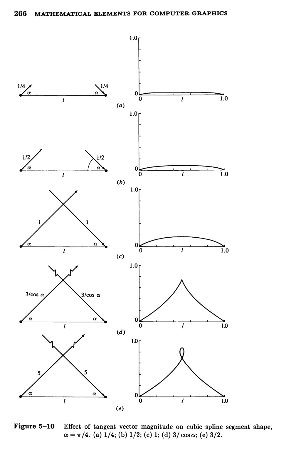
5-10
5-11
5-12
5-13
5-14
Chapter 6
6-1
6-2
6-3
6-4
6-5
6-6
6-7
6-8
6-9
Stereographic Projection
Comparison of Object Fixed and Center of
Projection Fixed Projections
Reconstruction of Three-Dimensional Images
References
Plane Curves
Introduction
Curve Representation
Nonparametric Curves
Parametric Curves
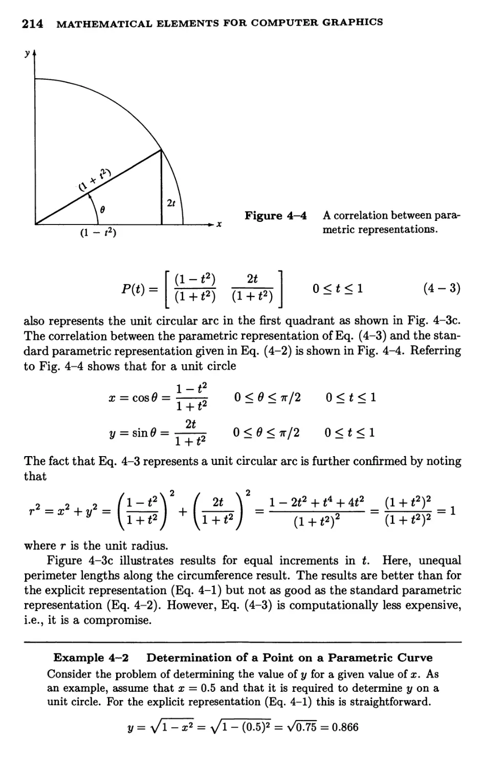
Parametric Representation of a Circle
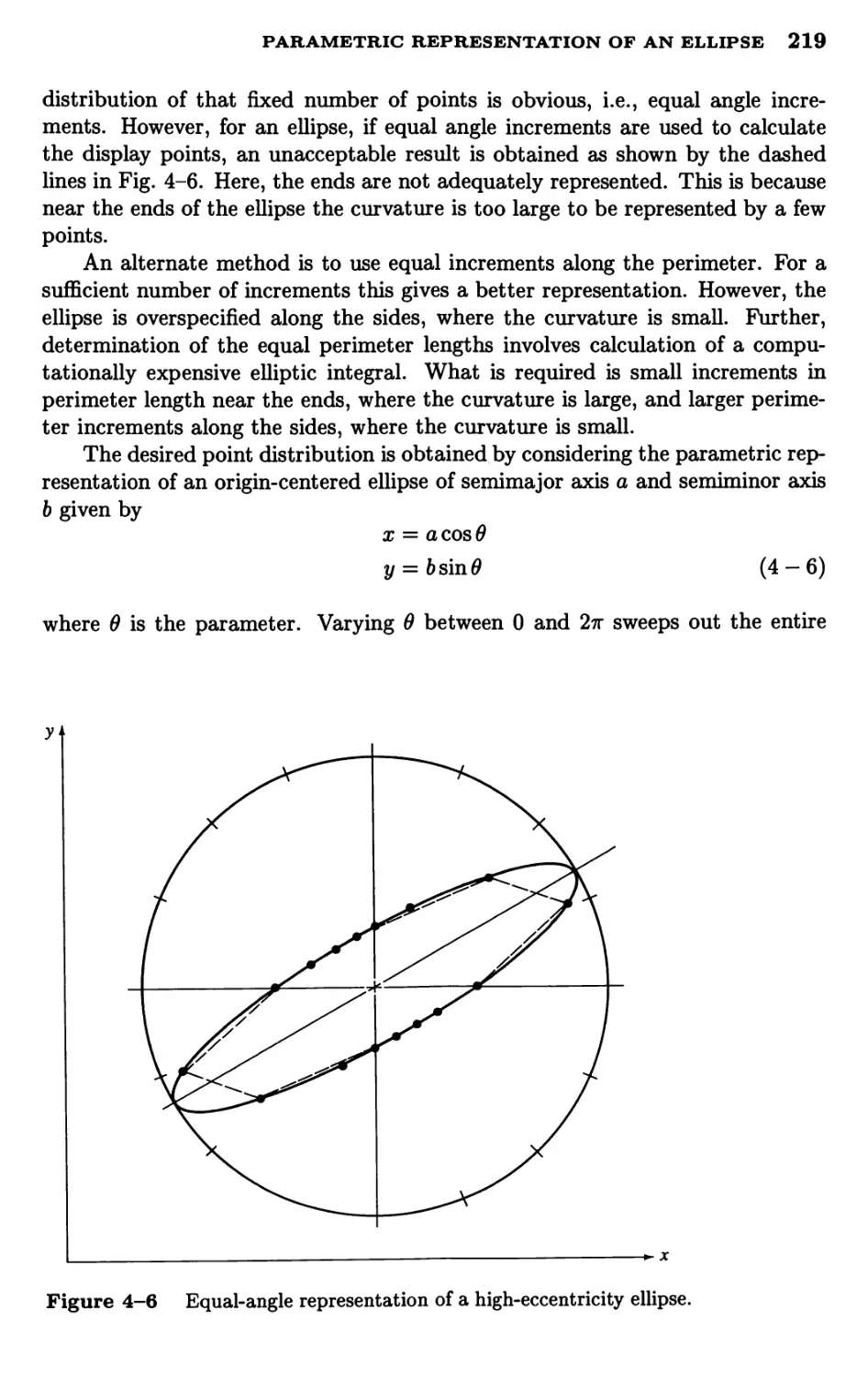
Parametric Representation of an Ellipse
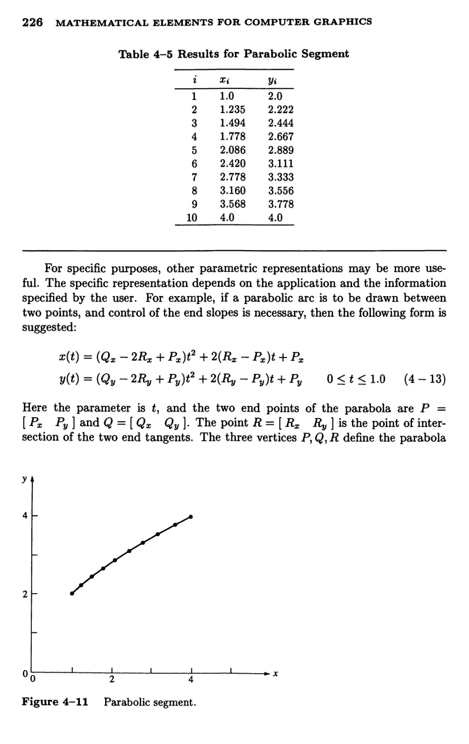
Parametric Representation of a Parabola
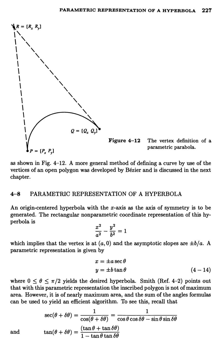
Parametric Representation of a Hyperbola
A Procedure For Using Conic Sections
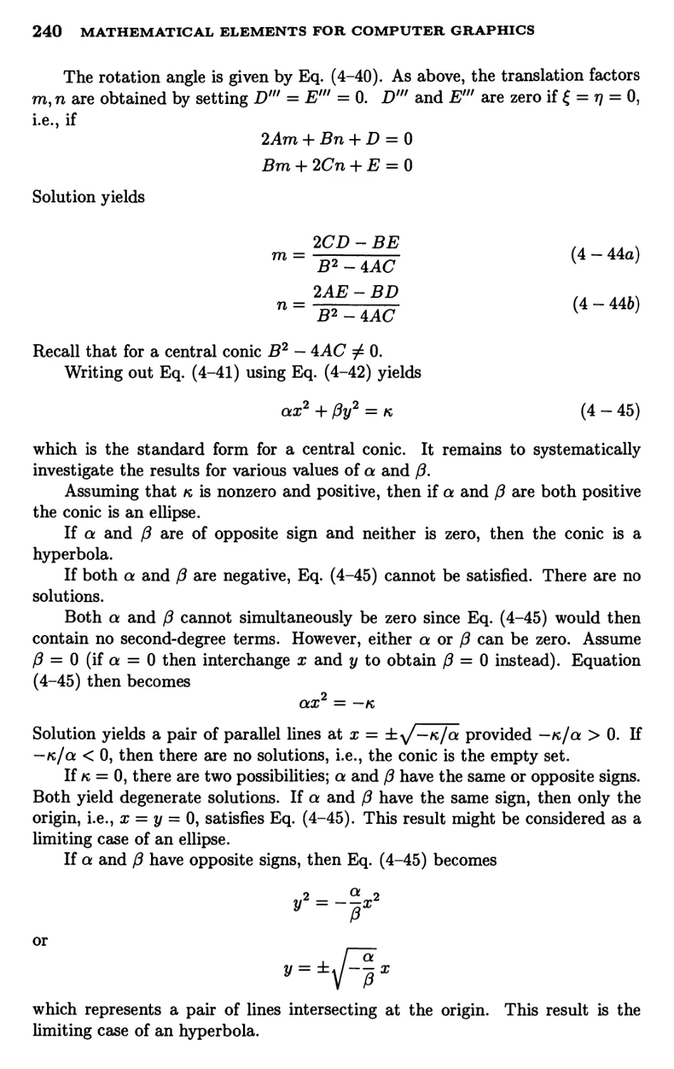
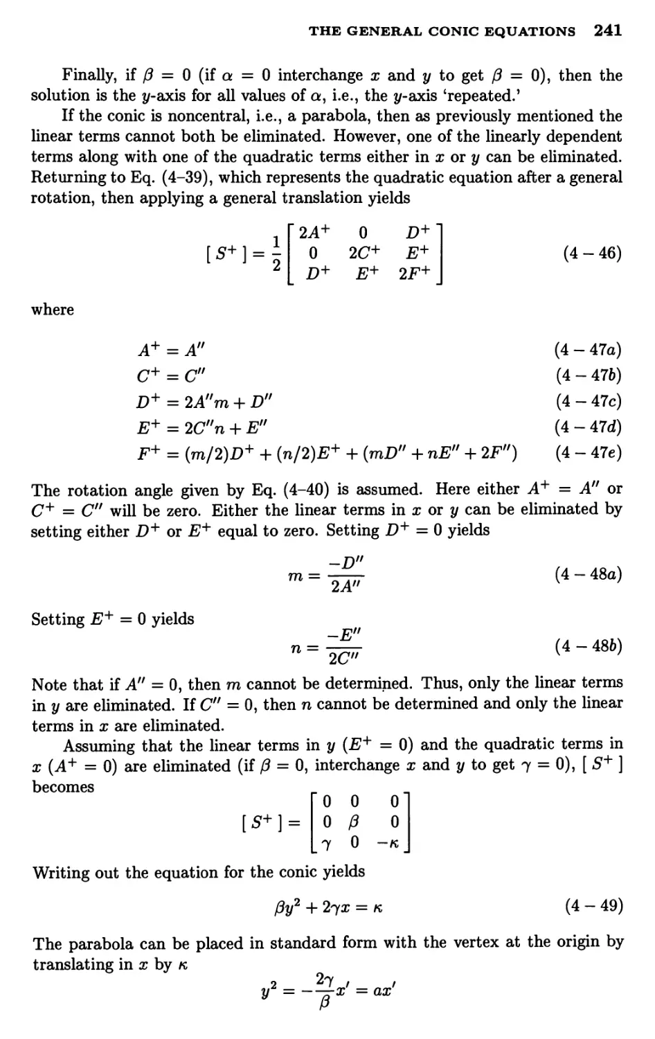
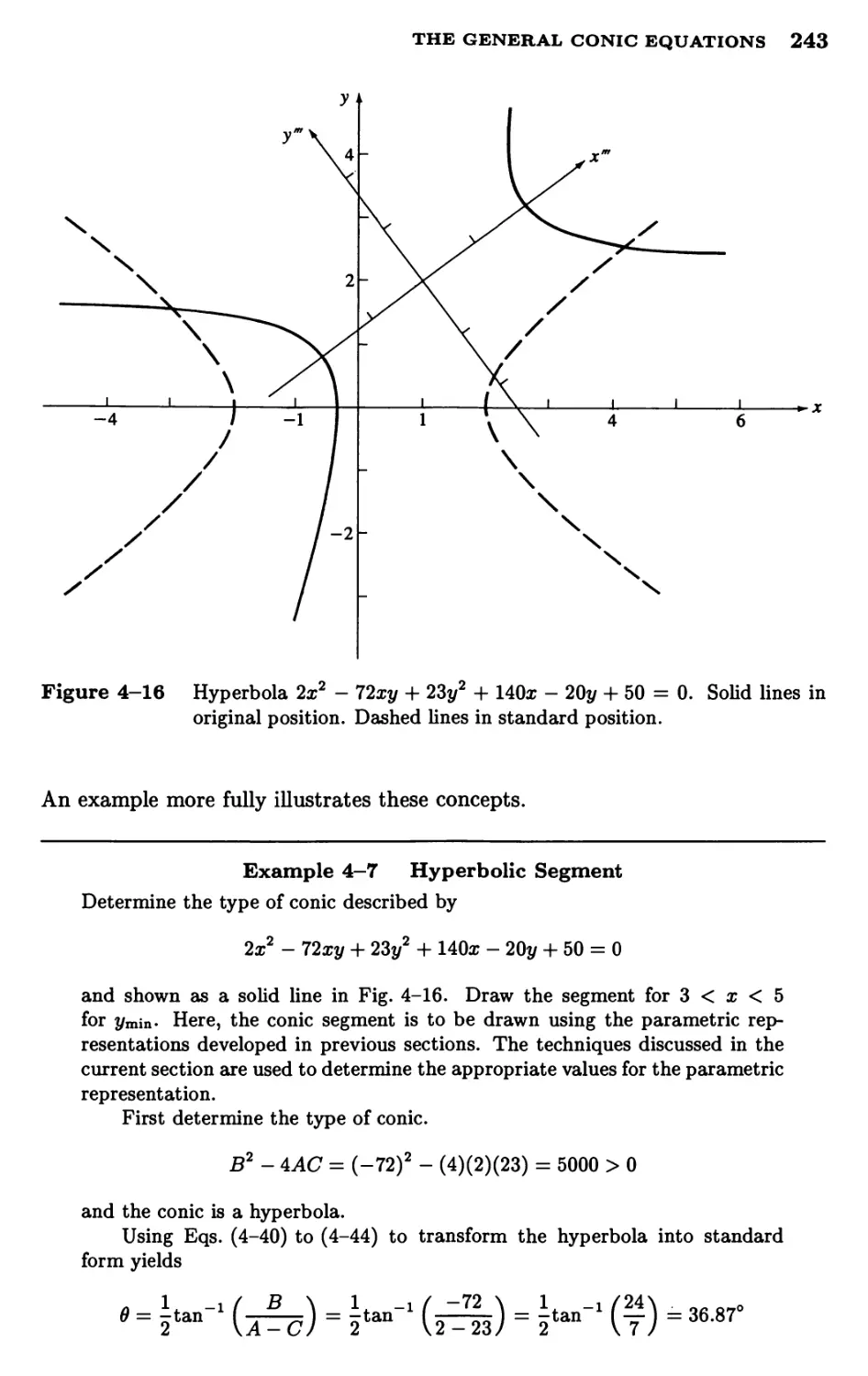
The General Conic Equations
References
Space Curves
Introduction
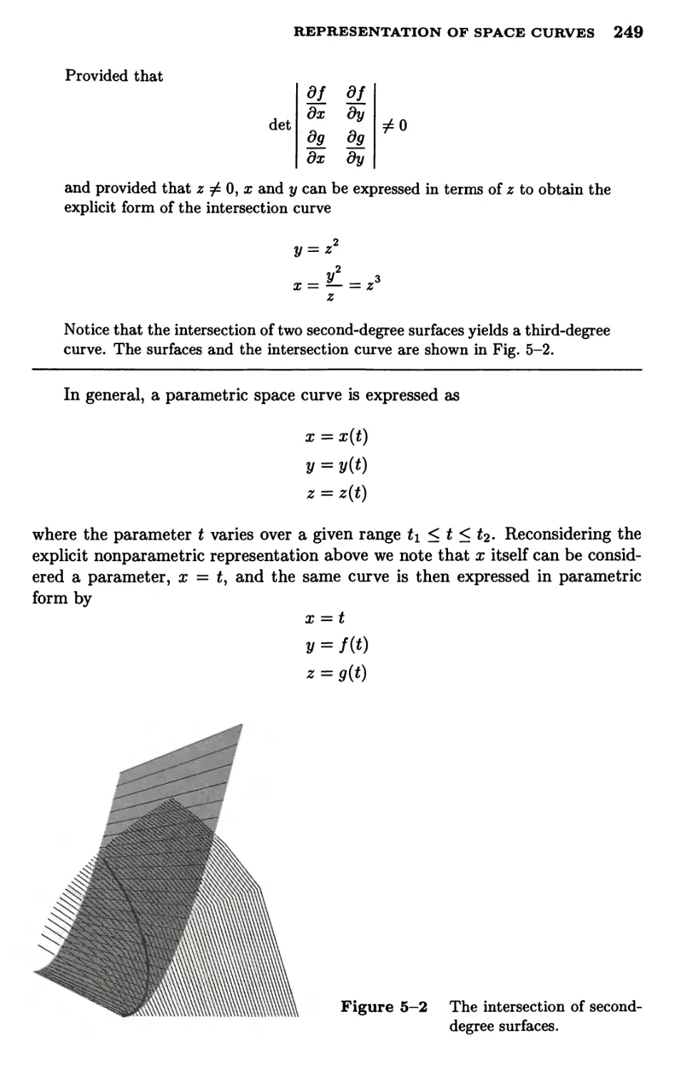
Representation of Space Curves
Cubic Splines
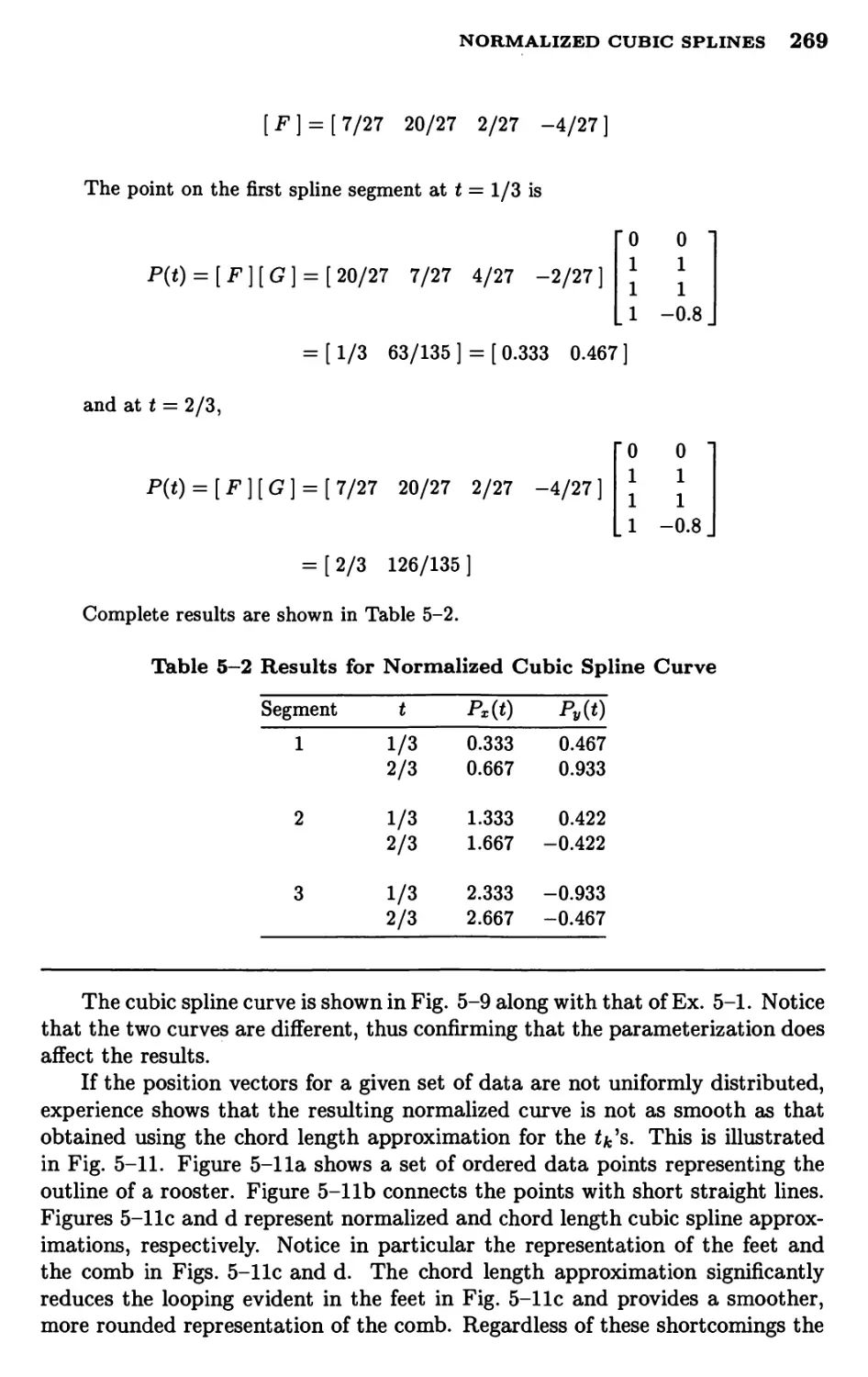
Normalized Cubic Splines
Alternate Cubic Spline End Conditions
Parabolic Blending
Generalized Parabolic Blending
Bezier Curves
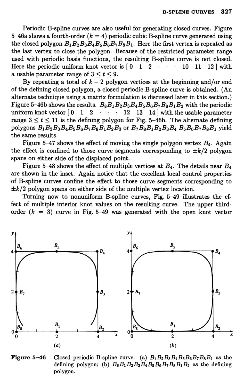
B-spline Curves
End Conditions For Periodic B-spline Curves
B-spline Curve Fit
B-spline Curve Subdivision
Rational B-spline Curves
References
Surface Description and Generation
Introduction
Surfaces of Revolution
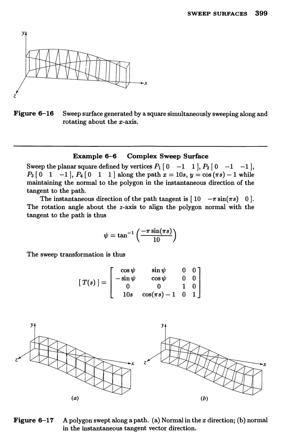
Sweep Surfaces
Quadric Surfaces
Piecewise Surface Representation
Mapping Parametric Surfaces
Bilinear Surface
Ruled and Developable Surfaces
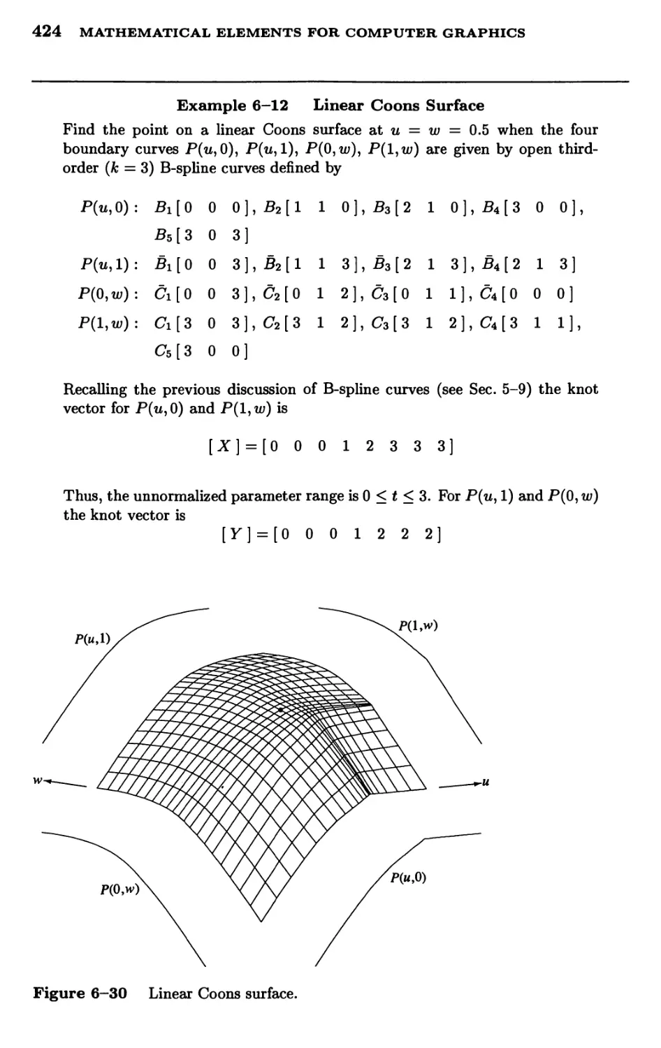
Linear Coons Surface
187
195
200
206
207
207
207
209
211
215
218
223
227
231
231
246
247
247
248
250
267
271
278
284
289
305
339
346
351
356
375
379
379
380
394
400
408
411
414
417
422
X MATHEMATICAL ELEMENTS FOR COMPUTER GRAPHICS
6-10
6-11
6-12
6-13
6-14
6-15
6-16
6-17
Coons Bicubic Surface
Bezier Surfaces
B-spline Surfaces
B-spline Surface Fitting
B-spline Surface Subdivision
Gaussian Curvature and Surface Fairness
Rational B-spline Surfaces
References
Appendices
Appendix A
Appendix B
Appendix C
Appendix D
Appendix E
Appendix F
Appendix G
Computer Graphics Software
Matrix Methods
Pseudocode
B-spline Surface File Format
Problems
Programming Projects
Algorithms
426
435
445
456
458
461
465
477
481
481
503
507
513
517
527
541
Index
599
FOREWORD
To the First Edition
Since its inception more than a decade ago, the field of computer graphics has
captured the imagination and technical interest of rapidly increasing numbers
of individuals from many disciplines. A high percentage of the growing ranks
of computer graphics professionals has given primary attention to computer-
oriented problems in programming, system design, hardware, etc. This was
pointed out by Dr. Ivan Sutherland in his introduction to Mr. Prince's book,
Interactive Graphics for Computer-aided Design in 1971 and it is still true today.
I believe that an inadequate balance of attention has been given to application-
oriented problems. There has been a dearth of production of useful information
that bears directly on the development and implementation of truly productive
applications. Understanding the practical aspects of computer graphics with
regard to both the nature and use of applications represents an essential and
ultimate requirement in the development of practical computer graphics systems.
Mathematical techniques, especially principles of geometry and transformations,
are indigenous to most computer graphic applications. Yet, large numbers of
graphic programmers and analysts struggle over or gloss over the basic as well as
the complex problems of the mathematical elements. Furthermore, the full
operational potential of computer graphics is often unrealized whenever the
mathematical relationships, constraints, and options are inadequately exploited. By
their authorship of this text, Drs. Rogers and Adams have recognized the
valuable relevance of their background to these practical considerations. Their text
is concise, is comprehensive and is written in a style unusually conducive to ease
of reading, understanding and use. It exemplifies the rare type of work that most
practitioners should wish to place in a prominent location within their library
since it should prove to be an invaluable ready reference for most disciplines.
It is also well suited as the basis for a course in computer science education
curriculum.
I congratulate the authors in producing an excellent and needed text,
Mathematical Elements for Computer Graphics.
S. H. "Chas" Chasen
Lockheed Georgia Company, Inc.
xi
PREFACE
In the fourteen years since the first edition of this book was published,
computer graphics has both changed and come of age. Computer graphics is now an
important discipline for computer scientists, engineers, scientists, mathemamati-
cians, physicians and artists, to name only a few. Old concepts have matured
and new concepts have developed. However, much of the underlying mathematics
remains virtually unchanged. As then, mastery of the fundamental
mathematical concepts is still central to understanding and to continued development of
computer graphics. This book provides the material necessary to master these
concepts.
This second edition is not just a revision; it is almost a total rewrite. A large
number of new illustrations and more detailed examples are included. Suggested
problems and programming projects are provided. Algorithms which implement
the mathematical theory are now presented in pseudocode. The book is typeset.
Chapter 1 includes new coverage of raster refresh and flat panel displays,
laser printers, ink jet and thermal plotters, and color film cameras, as well as
expanded coverage of previous topics related to computer hardware.
Chapter 2 provides expanded coverage of two dimensional transformations,
including new topics in solid body transformations, reflections and geometric
interpretation of homogeneous coordinates.
Chapter 3 has been greatly expanded. New topics or discussions of multiple
transformations, rotation about arbitrary axes, reflections through an arbitrary
plane, oblique projections, including the details of cabinet and cavalier
projections, vanishing points, photographic transformations, an expanded discussion of
stereo and a comparison of object fixed and center of projection fixed techniques
for generating perspective projections are included.
Chapter 4 now provides an expanded discussion of conies. A detailed
discussion of techniques for the use of conic sections appears in this edition.
Chapter 5 has been rewritten for increased clarity and understanding. More
complete discussions of parabolic blending, Bezier and B-spline curves are
included. A discussion of generalized parabolic blending is given. A discussion
of periodic uniform B-spline curves is now included, as are discussions of B-
spline curve fitting and subdivision. Extensive discussion of rational uniform
and nonuniform B-spline curves (NURBS) has been added.
xiii
Xiv MATHEMATICAL ELEMENTS FOR COMPUTER GRAPHICS
Chapter 6 has also been almost totally rewritten. The discussions of Coons
surfaces, both linear and bicubic, and of ruled and developable surfaces have
been expanded. New discussions of surfaces of revolution, sweep, quadric, Bezier
and B-spline surfaces, B-spline surface fitting, surface subdivision and Gaussian
curvature and mathematical surface fairness are included. Both nonrational
and rational uniform and nonuniform B-spline surfaces (NURBS) are thoroughly
discussed.
Extensive appendices on computer graphics software, matrix methods, a
pseudocode definition, a B-spline surface file format, problems, programming
projects and pseudocoded algorithms are included.
The new topics have been carefully arranged and presented to insure that the
text is still suitable for undergraduate as well as graduate students. The material
in the book can be used for a semester-long formal course in computer graphics
at either the senior undergraduate or graduate level. A second semester course
based on its companion volume Procedural Elements for Computer Graphics
naturally follows. This is the way it is used by the authors. If broader material
coverage in a single semester course is desired, then the two volumes can be used
together. Suggested topical coverage is: Chapter 1 of both volumes, followed
by Chapters 2 and 3 with selected topics from Chapter 4 (e.g., 4-1 to 4-8) of
the present volume; then selected topics from Chapter 2 (e.g., 2-1 to 2-5, 2-7,
2-15 to 2-19, 2-22, 2-23 and 2-28), Chapter 3 (e.g., 3-1, 3-2, 3-4 to 3-6, 3-9,
3-11, 3-15 and 3-16), Chapter 4 (e.g., 4-1, part of 4-2 for backplane culling,
4-3, 4-4, 4-7, 4-9, 4-11 and 4-13) and Chapter 5 (e.g., 5-1 to 5-3, 5-5, 5-
6 and 5-14) of Procedural Elements for Computer Graphics. The first author
has successfully used this arrangement both for formal and for short courses.
The book is also designed to be useful to professional programmers, engineers
and scientists. Further, the detailed algorithms, worked examples and numerous
illustrations make it particularly suitable for self-study at any level. Sufficient
background is provided by college-level mathematics through calculus and a
knowledge of a higher-level programming language.
A word about the production of the book may be of interest. The book
was computer typeset using T^X by Nancy A. Rogers. The Computer Modern
Roman family of fonts was used. Macros necessary to conform to McGraw-Hill
Publishing Co. specifications were written by David F. Rogers. Two computers
were used: an IBM AT and a Zenith 386. The manuscript was coded directly
from handwritten copy. After screen previewing, galleys and page proofs were
produced on a 300 dpi laser printer for editing and page makeup. The final
madeup pages, ready for art insertion, in the form of TfeX .dvi files were photo-
typeset by the American Mathematical Society.
No book is ever written without the assistance of many individuals. Thanks
are due the first author's students at the Johns Hopkins University Applied
Physics Laboratory Center who reviewed an early version of the first five chapters
of the book. Their many suggestions and comments were especially helpful.
Special thanks are due John Dill and Fred Munchmeyer, two valued and
much appreciated long time colleagues, who read the entire manuscript, red pen
in hand. Their many suggestions and comments served to make this a better
XV
book. Special thanks are due our colleague Linda Adlum who not only read the
entire manuscript but also checked all the examples. Thanks are extended to
Stephen D. Rogers who read the manuscript and checked the examples in the
first five chapters. Mike Gigante's comments on the first five chapters are also
greatly appreciated. Bill Gordon's review of the work on Bezier and B-spline
curves and surfaces was most useful.
Virginia Adams' efforts in proofreading the final copy are also appreciated.
Thanks are due Barbara Beeton for her unfailing patience in answering questions
about the details of T^X. A special note of appreciation to Joost Zalmstra, whose
timely development of TfeX page makeup macros made that task immensely
easier. The usually fine McGraw-Hill editing was supervised by Jim Bradley.
The very extensive illustration program was expertly supervised by Mel Haber.
A very special thanks are due B. J. Clark who has been our editor at McGraw-
Hill for nearly two decades. He has always been receptive to our sometimes
rather unorthodox ideas.
David F. Rogers
J. Alan Adams
Annapolis
February 1989
PREFACE
To the First Edition
A new and rapidly expanding field called "computer graphics" is emerging. This
field combines both the old and the new: the age-old art of graphical
communication and the new technology of computers. Almost everyone can expect to be
affected by this rapidly expanding technology. A new era in the use of computer
graphics, not just by the large companies and agencies who made many of the
initial advances in software and hardware, but by the general user, is beginning.
Low-cost graphics terminals, time sharing, plus advances in mini- and
microcomputers have made this possible. Today, computer graphics is practical, reliable,
cost effective and readily available.
The purpose of this book is to present an introduction to the mathematical
theory underlying computer graphics techniques in a unified manner. Although
new ways of presenting material are given, no actual 'new' mathematical
material is presented. All the material in this book exists scattered throughout the
technical literature. This book attempts to bring it all together in one place in
one notation.
In selecting material, we chose techniques which were fundamentally
mathematical in nature rather than those which were more procedural in nature. For
this reason the reader will find more extensive discussions of rotation,
translation, perspective and curve and surface description than of clipping or hidden line
and surface removal. First-year college mathematics is a sufficient prerequisite
for the major part of the text.
After a discussion of current computer graphics technology in Chapter 1,
the manipulation of graphical elements represented in matrix form using
homogeneous coordinates is described. A discussion of existing techniques for
representing points, lines, curves and surfaces within a digital computer, as well as
computer software procedures for manipulating and displaying computer output
in graphical form, is then presented in the following chapters.
Mathematical techniques for producing axonometric and perspective views
are given, along with generalized techniques for rotation, translation and scaling
of geometric figures. Curve definition procedures for both explicit and parametric
xvii
Xviii MATHEMATICAL ELEMENTS FOR COMPUTER GRAPHICS
representations are presented for both two-dimensional and three-dimensional
curves. Curve definition techniques include the use of conic sections, circular
arc interpolation, cubic splines, parabolic blending, Bezier curves and curves
based on B-splines. An introduction to the mathematics of surface description
is included.
Computer algorithms for most of the fundamental elements in an interactive
graphics package are given in an appendix as BASIC t language subprograms.
However, these algorithms deliberately stop short of the coding necessary to
actually display the results. Unfortunately there are no standard language
commands or subroutines available for graphic display. Although some preliminary
discussion of graphic primitives and graphic elements is given in Appendix A,
each user will, in general, find it necessary to work within the confines of the
computer system and graphics devices available to him or her.
The fundamental ideas in this book have been used as the foundation for an
introductory course in computer graphics given to students majoring in technical
or scientific fields at the the undergraduate level. It is suitable for use in this
manner at both universities and schools of technology. It is also suitable as a
supplementary text in more advanced computer programming courses or as a
supplementary text in some advanced mathematics courses. Further, it can be
profitably used by individuals engaged in professional programming. Finally, the
documented computer programs should be of use to computer users interested
in developing computer graphics capability.
Acknowledgments
The authors gratefully acknowledge the encouragement and support of the
United States Naval Academy. The academic environment provided by the
administration, the faculty, and especially the midshipmen was conducive to the
development of the material in this book.
No book is ever written without the assistance of a great many people. Here
we would like to acknowledge a few of them. First, Steve Coons who reviewed
the entire manuscript and made many valuable suggestions, Rich Reisenfeld who
reviewed the material on B-spline curves and surfaces, Professor Pierre Bezier
who reviewed the material on Bezier curves and surfaces and Ivan Sutherland
who provided the impetus for the three-dimensional reconstruction techniques
discussed in Chapter 3. Special acknowledgement is due past and present
members of the CAD Group at Cambridge University. Specifically, work done with
Robin Forrest, Charles Lang, and Tony Nut bourne provided greater insight into
the subject of computer graphics. Finally, to Louie Knapp who provided an
original Fortran program for B-spline curves.
The authors would also like to acknowledge the assistance of many
individuals at the Evans and Sutherland Computer Corporation. Specifically, Jim
tBASIC is a registered trade mark of Dartmouth College
xix
Callan who authored the document from which many of the ideas on
representing, preparing, presenting and interacting with pictures is based. Special thanks
are also due Lee Billow who prepared all of the line drawings.
Much of the art work for Chapter 1 has been provided through the good
offices of various computer graphics equipment manufacturers. Specific
acknowledgment is made as follows:
Evans and Sutherland Computer Corporation.
Adage Inc.
Adage Inc.
Vector General, Inc.
Xynetics, Inc.
CALCOMP, California Computer Products, Inc.
Gould, Inc.
Tektronix, Inc.
Evans and Sutherland Computer Corporation.
CALCOMP, California Computer Products, Inc.
David F. Rogers
J. Alan Adams
Fig.
Fig.
Fig.
Fig.
Fig.
Fig.
Fig.
Fig.
Fig.
Fig.
1-3
1-5
1-7
1-8
1-11
1-12
1-15
1-16
1-17
1-18
CHAPTER
ONE
INTRODUCTION TO COMPUTER GRAPHICS
Computer graphics is now a mature technology. However, a number of terms and
definitions are still rather loosely used in this field. In particular, computer aided
design (CAD), interactive graphics (IG), computer graphics (CG) and computer
aided manufacturing (CAM) are frequently used interchangeably or in such a
manner that considerable confusion exists as to the precise meaning. Of these
terms CAD is the most general. CAD may be defined as any use of the computer
to aid in the design of an individual part, a subsystem or a total system. The
use does not have to involve graphics. The design process may be at the system
concept level or at the detail part design level. It may also involve an interface
with CAM.
Computer aided manufacturing is the use of a computer to aid in the
manufacture or production of a part exclusive of the design process. CAM requires the
use of geometric description and motion control part programming languages,
such as APT (Automatic Programmed Tools), to generate the necessary
commands to control a machine tool. The machine tool controller is generally a
micro- or minicomputer. The CAD system may generate the required machine
control commands directly. Alternately, a standard data format, e.g., the Initial
Graphics Exchange Standard (IGES), may be generated. A separate program is
subsequently used to convert this data to the required format for the machine
controller. Figure 1-1 shows a typical numerically controlled machining center
and its controller.
Computer graphics is the use of a computer to define, store, manipulate,
interrogate and present pictorial output. This is essentially a passive operation.
The computer prepares and presents stored information to an observer in the
form of pictures. The observer has no direct control over the picture being
presented. The application may be as simple as the presentation of the graph of
a single function or as complex as the simulation of the automatic reentry and
landing of a space vehicle or an aircraft.
Dynamic interactive computer graphics (hereafter called interactive graphics
1
2 MATHEMATICAL ELEMENTS FOR COMPUTER GRAPHICS
for short) also uses the computer to prepare and present pictorial material.
However, in interactive graphics the observer can influence the picture as it is being
presented; i.e., the observer interacts with the picture in real time. To see the
importance of the real time restriction, consider the problem of rotating a
reasonably complex three-dimensional picture composed of 1000 lines at a reasonable
rate, say, 15°/second. As we shall see subsequently, the 1000 lines of the
picture are most conveniently represented by a 1000 x 4 matrix of homogeneous
coordinates of the end points of the lines, and the rotation is most conveniently
accomplished by multiplying this 1000 x 4 matrix by a 4 x 4 transformation
matrix. Accomplishing the required matrix multiplication requires 16,000
multiplications, 12,000 additions and 1000 divisions. If this matrix multiplication is
accomplished in software, the time may be significant. To see this, consider a
single user general purpose computer with a hardware floating-point accelerator
that requires 3.6 microseconds to multiply two numbers, 2.6 microseconds to add
two numbers, and 5.2 microseconds to divide two numbers. Thus, the matrix
multiplication requires approximately 0.1 seconds.
Since computer displays that allow dynamic motion require that the picture
be redrawn (refreshed) at least 30 times each second in order to avoid flicker,
fcap
'■•. : ■ . ' ;" : 'I '■'"
Figure 1—1 Numerically controlled machining center.
REPRESENTING PICTURES 3
it is obvious that the picture cannot change smoothly. Even if it is assumed
that the picture is recalculated (updated) only 15 times each second, i.e., every
degree, it is still not possible to accomplish a smooth rotation in software. Thus,
this is no longer real time dynamic interactive graphics. To regain the ability to
interactively present the picture several things can be done. A faster computer,
at additional expense, can be used. Clever programming can reduce the time to
accomplish the required matrix multiplication. However, a point will be reached
where this is no longer possible. The complexity of the picture can be reduced.
In this case, the resulting picture may not be acceptable. However, the matrix
multiplication required to manipulate the above example picture and indeed for
more complex pictures can be accomplished by using microcoded or special-
purpose digital hardware matrix multipliers. Historically, and currently, this is
the most performance and cost effective approach.
With this terminology in mind the remainder of the chapter gives an
overview of computer graphics and discusses the various types of graphic devices
available.
1-1 OVERVIEW OF COMPUTER GRAPHICS
Computer graphics is a complex and diversified technology. To begin to
understand the technology it is necessary to subdivide it into manageable parts. This
can be accomplished by considering that the end product of computer graphics
is a picture. The picture may, of course, be used for a large variety of purposes;
e.g., it may be an engineering drawing, an exploded parts illustration for a service
manual, a business graph, an architectural rendering for a proposed construction
or design project, an advertising illustration, or a single frame from an animated
movie. The picture is the fundamental cohesive concept in computer graphics.
We must therefore consider how:
Pictures are represented in computer graphics.
Pictures are prepared for presentation.
Previously prepared pictures are presented.
Interaction with the picture is accomplished.
Here 'picture' is used in its broadest sense to mean any collection of lines, points,
text, etc. displayed on a graphics device.
1-2 REPRESENTING PICTURES
Although many algorithms accept picture data as polygons or edges, each
polygon or edge can in turn be represented by points. Points, then, are the
fundamental building blocks of picture representation. Of equal fundamental importance
is the algorithm which explains how to organize these points. To illustrate this,
consider a unit square in the first quadrant. The unit square can be represented
by its four corner points (see Fig. 1-2):
4 MATHEMATICAL ELEMENTS FOR COMPUTER GRAPHICS
Pi(0,0) P2(1,0) P3(M) ^4(0,1)
An associated algorithmic description might be
Connect P1P2P3P4P1 in sequence
The unit square can also be described by its four edges:
E1=P1P2 E2=P2Ps E3 = P3P4 EA = P4Pi
Here, the algorithmic description is
Display EiE2E3E4 in sequence
Finally, either the points or edges can be used to describe the unit square as a
single polygon, e.g.,
Si = P1P2P3P4P1 or P1P4P3P2Pi or Si = E1E2E3E4
The fundamental building blocks, i.e., points, can be represented as either pairs
or triplets of numbers depending on whether the data are two- or
three-dimensional. Thus, (£1,2/1) or (#1,2/1,21) would represent a point in either two- or
three-dimensional space. Two points would represent a line or edge, and a
collection of three or more points a polygon. The representation of curved lines is
usually accomplished by approximating them by short straight line segments.
The representation of textual material is quite complex, involving in many
cases curved lines or dot matrices. However, fundamentally textual material is
again represented by collections of lines and points and an organizing algorithm.
Unless the user is concerned with pattern recognition, the design of special
character fonts or the design of graphic hardware, he or she need not be concerned
with these details, since almost all graphic devices have built-in hardware or
software character generators.
1.0
*4
*i
A
lf4 E3 P3
Si k
b .
0 E, 1.0
Figure 1-2 Picture data descriptions.
PREPARING PICTURES FOR PRESENTATION 5
1-3 PREPARING PICTURES FOR PRESENTATION
Pictures ultimately consist of points and a drawing algorithm to display them.
This information is generally stored in a file prior to being used to present the
picture. This file is called a data base. Very complex pictures require very complex
data bases, which require a complex algorithm to access them. These complex
data bases contain data organized in various ways, e.g., ring structures, B-tree
structures, quadtree structures, etc., generally referred to as a data structure.
The data base itself may contain pointers, substructures and other nongraphic
data. The design of these data bases and the algorithms which access them is an
ongoing topic of research, a topic which is clearly beyond the scope of this text.
However, many computer graphics applications involve much simpler pictures
for which the user can readily invent simple data structures which can be easily
accessed. The simplest is, of course, a lineal list. Surprisingly, this simplest of
data structures is quite adequate for many reasonably complex pictures.
Since points are the basic building blocks of a graphic data base, the
fundamental operations for manipulating these points are of interest. There are
three fundamental operations when treating a point as a (geometric) graphic
entity: move the beam, pen, cursor, plotting head (hereafter called the cursor)
invisibly to the point; draw a visible line to a point from an initial point; or
display a dot at that point. Fundamentally there are two ways to specify the
position of a point: absolute or relative (incremental) coordinates. In relative
or incremental coordinates the position of a point is defined by giving the
displacement of the point with respect to the previous point. All computer graphics
software is based on these fundamental operations. Section 1-22 and Appendix
A more fully discuss computer graphics software fundamentals.
When specifying the position of a point, either real (floating point) numbers
or integers may be used. If integers are used, difficulties arise because of the
limited word length of most graphics support computers. For integer coordinate
specification, a full computer word is generally used. The largest positive integer,
assuming equal positive and negative ranges, that can be specified by a full
computer word is 2n_1 — 1, where n is the number of bits in the word. For
a 16-bit word this number is 32767. For many applications this is acceptable.
However, difficulties are encountered when larger integer numbers than can be
specified are required. At first, we might expect to overcome this difficulty by
using relative coordinates to specify a number such as 60,000, i.e., using an
absolute coordinate specification to position the cursor to (30000,30000) and
then a relative coordinate specification of (30000,30000) to position the cursor
to the final desired point of (60000,60000). However, this does not work, since
an attempt to accumulate relative position specifications beyond the maximum
representable integer value results in integer overflow. On most machines integer
overflow results in the generation of a number of opposite sign and erroneous
magnitude.
The way out of this dilemma is to use homogeneous coordinates to
represent the data. The use of homogeneous coordinates introduces some additional
6 MATHEMATICAL ELEMENTS FOR COMPUTER GRAPHICS
complexity, some loss in speed and some loss in resolution. However, these
disadvantages are far outweighed by the advantage of being able to represent large
integer numbers with a computer of limited word size. For this reason, as well
as others presented later, homogeneous coordinate representations are generally
used in this book.
In homogeneous coordinates an ra-dimensional space is represented by n + 1
dimensions; i.e., three-dimensional data, where the position of a point is given by
the triplet (#,?/, z), is represented by four coordinates (hx,hy, ftz,/i), where /&,
the homogeneous coordinate, is an arbitrary number.
If each of the coordinate positions represented in a 16-bit computer were
less than 32767, then h would be made equal to 1 and the coordinate positions
represented directly. If, however, one of the coordinates is larger than 32767,
say, x = 60000, then the power of homogeneous coordinates becomes apparent.
In this case we let h = 1/2; and the coordinates of the point are then defined as
(30000, ?//2,z/2,1/2), all acceptable numbers for a 16-bit computer. However,
some resolution is lost since x = 60000 and x = 60001 are both represented by
the same homogeneous coordinate. In fact, resolution is lost in all the coordinates
even if only one of them exceeds the maximum expressible integer number of a
particular computer.
1-4 PRESENTING PREVIOUSLY PREPARED PICTURES
The data used to prepare the picture for presentation is rarely the same as that
used to present the picture. The data used to present the picture is frequently
called a display file. The display file represents some portion, view or scene of
the picture represented by the total data base. The displayed picture is
usually formed by rotating, translating, scaling and performing various projections
on the data. These basic orientation or viewing preparations are generally
performed using a 4 x 4 transformation matrix operating on the data represented in
homogeneous coordinates (see Chapters 2 and 3). When a sequence of
transformations is required, each individual transformation matrix can be sequentially
applied to the points to achieve the desired result. If, however, the number of
points is substantial, this is inefficient. An alternate, and more desirable, method
is to multiply the individual matrices for each transformation together. The
result is a single combined (or concatenated) transformation matrix. This matrix
operation is called concatenation. The points are then multiplied by the single
combined 4x4 transformation matrix to yield the transformed points. This
technique results in significant time savings when performing compound matrix
operations on sets of data points.
Hidden line or hidden surface removal, shading, transparency, texture or
color effects may be added before final presentation of the picture. If the picture
represented by the entire data base is not to be presented, the appropriate portion
must be selected. This is a process called clipping. Clipping may be two- or three-
dimensional, as appropriate. In some cases, the clipping window or volume may
have holes in it or may be irregularly shaped. Clipping to standard two- and
PRESENTING PREVIOUSLY PREPARED PICTURES 7
three-dimensional regions is frequently implemented in hardware. A complete
discussion of these effects is beyond the scope of the present text. They are
thoroughly discussed by Rogers in Ref. 1-1.
Two important concepts associated with presenting a picture are windows
and viewports. Windowing is the process of extracting a portion of a data base
by clipping the data base to the boundaries of the window. Performance of the
windowing or the clipping operation in software generally is sufficiently time
consuming that real-time interactive graphics is not possible. Again, sophisticated
graphics devices perform this function in special-purpose hardware or microcode.
Clipping involves determining which lines or portions of lines in the picture lie
outside the window. Those lines or portions of lines are then discarded and not
displayed; i.e., they are not passed on to the display device.
In two dimensions a window is specified by values for the left, right, bottom
and top edges of a rectangle. The window edge values are specified in user
or world coordinates, i.e., the coordinates in which the data base is specified.
Floating point numbers are usually used.
Clipping is easiest if the edges of the rectangle are parallel to the coordinate
axes. Such a window is called a regular clipping window. Irregular windows are
also of interest for many applications (see Ref. 1-1). Two-dimensional clipping is
represented in Fig. 1-3. Lines are retained, deleted or partially deleted,
depending on whether they are completely within or without the window or partially
within or without the window. In three dimensions a regular window or clipping
volume consists of a rectangular parallelepiped (a box) or for perspective views
Line partially within window:
part from a-b displayed;
part from b-c not displayed
Line entirely
within
window:
entire line
displayed
Line partially within
window: part from b — c
displayed; parts a — b, c—d
not displayed
Line entirely
outside of
window: not
displayed
Figure 1-3 Two-dimensional windowing (clipping).
8 MATHEMATICAL ELEMENTS FOR COMPUTER GRAPHICS
a frustum of vision. A typical frustum of vision is shown in Fig. 1-4. In Fig. 1-4
the near (hither) boundary is at AT, the far (yon) boundary at F and the sides
at SL, SR, ST and SB.
A viewport is an area of the display device on which the window data are
presented. A two-dimensional regular viewport is specified by giving the left,
right, bottom and top edges of a rectangle. Viewport values may be given in
actual physical device coordinates. When specified in actual physical device
coordinates they are frequently given using integers. Viewport coordinates may be
normalized to some arbitrary range, e.g., 0 < x < 1.0, 0 < y < 1.0, and specified
by floating point numbers. The contents of a single window may be displayed in
multiple viewports on a single display device as shown in Fig. 1-5. Keeping the
proportions of the window and viewport(s) the same prevents distortion. The
mapping of windowed (clipped) data into a viewport involves translation and
scaling (see Appendix A).
An additional requirement for most pictures is the presentation of
alphanumeric or character data. There are in general two methods of generating
characters — software and hardware. If characters are generated in software using
lines, they are treated in the same manner as any other picture element. In fact,
this is necessary if they are to be clipped and then transformed along with other
picture elements. However, many graphics devices have hardware character
generators. When hardware character generators are used, the actual characters
are generated just prior to being drawn. Up until this point they are treated
as character codes. Hardware character generation yields significant efficiencies.
However, it is less flexible than software character generation, since it does not
allow for clipping or general transformation; e.g., usually only limited rotations
and sizes are possible.
Figure 1-4 Three-dimensional frustum of vision.
INTERACTING WITH THE PICTURE 9
World coordinate
data base
Window
Viewport A
4>
Display device
Viewport B
Figure 1-5 Multiple viewports displaying a single window.
When a hardware character generator is used, the program which drives
the graphics device must first specify size, orientation and the position where
the character or text string is to begin. The character codes specifying these
characteristics are then added to the display file. Upon being processed the
character generator interprets the text string, looks up in hardware the necessary
information to draw each character, and draws the characters on the display
device.
1-5 INTERACTING WITH THE PICTURE
Once the picture has been presented, interaction with, or modification of, the
picture is required. To meet this requirement a number of interactive devices
have been developed. Among these devices are tablets, light pens, joysticks,
mice, control dials, function switches or buttons and of course the common
alphanumeric keyboard. Before discussing these physical devices it is appropriate
to discuss the functional capabilities of interactive graphics devices. The
functional capabilities are generally considered to be of four or five logical types (see
Refs. 1-2 to 1-4). The logical interaction devices, as opposed to the physical
devices discussed below, are a locator, a valuator, a pick and a button. A fifth
functional capability called keyboard is frequently included because of the general
availability of the alphanumeric keyboard. In fact, a keyboard can conceptually
and functionally be considered as a collection of buttons.
The locator function provides coordinate information in either two or three
dimensions. Generally the coordinate numbers returned are in normalized
coordinates and may be either relative or absolute. The valuator function provides
a single value. Generally this value is a real number between zero and some
real maximum. The button function is used to select and activate events or
procedures which control the interactive flow. It generally provides only binary
(on or off) digital information. The pick function identifies or selects objects or
subpictures within the displayed picture. The logical keyboard processes textual
information. A typical physical keyboard is shown in Fig. 1-6.
10 MATHEMATICAL ELEMENTS FOR COMPUTER GRAPHICS
Figure 1-6 An alphanumeric keyboard. (Courtesy of Evans & Sutherland Computer
Corp.)
The tablet is the most common locator device. A typical tablet is shown in
Fig. 1-7. Tablets may be used either in conjunction with a CRT graphics display
or stand alone. In the latter case they are frequently referred to as digitizers.
The tablet itself consists of a flat surface and a penlike stylus (or puck) which is
used to indicate a location on the tablet surface. Usually the proximity of the
stylus to the tablet surface is also sensed. When used in conjunction with a CRT
display, feedback from the CRT face is provided by means of a small tracking
symbol called a cursor, which follows the movement of the stylus on the tablet
surface. When used as a stand-alone digitizer, feedback is provided by digital
readouts.
Tablets provide either two- or three-dimensional coordinate information. A
three-dimensional tablet is shown in Fig. 1-8. The values returned are in tablet
coordinates. Software converts the tablet coordinates to user or world
coordinates. Typical resolution and accuracy is 0.01 to 0.001 inch.
A number of different principles have been used to implement tablets. The
original RAND tablet (see Ref. 1-5) used an orthogonal matrix of individual
wires beneath the tablet surface. Each wire was individually coded such that
the stylus acting as a receiver picked up a unique digital code at each intersection.
Decoding yielded the x,y coordinates of the stylus. The obvious limitations on
the resolution of such a matrix-encoded tablet were the density of the wires and
the receiver's ability to resolve a unique code. The accuracy was limited by the
INTERACTING WITH THE PICTURE 11
Figure 1-7 A typical tablet. (Courtesy of Adage, Inc.)
linearity of the individual wires as well as the parallelism of the wires in the two
orthogonal directions.
Another interesting implementation for a tablet used sound waves. A stylus
was used to create a spark which generated a sound wave. The sound wave
moved outward from the stylus on the surface of the tablet in a circular wave
Figure 1-8 A three-dimensional sonic tablet. (Courtesy ofScience Accessories Corp.)
12 MATHEMATICAL ELEMENTS FOR COMPUTER GRAPHICS
front. Two sensitive ribbon microphones were mounted on adjacent sides of
the tablet. Thus, they were at right angles. By accurately measuring the time
that it took the sound wave to travel from the stylus to the microphones, the
coordinate distances were determined. This technique could be extended to three
dimensions (see Fig. 1-8).
The most popular tablet implementation is based on a magnetic principle.
In this tablet implementation strain wave pulses travel through a grid of wires
beneath the tablet surface. Appropriate counters and a stylus containing a
pickup are used to determine the time it takes for alternate pulses parallel to the x
and y coordinate axes to travel from the edge of the tablet to the stylus. These
times are readily converted into x,y coordinates.
A locator device similar to a tablet is the touch panel. In a typical touch
panel, light emitters are mounted on two adjacent edges with companion light
detectors mounted in the opposite edges. Anything, e.g., a finger, interrupting
the two orthogonal light beams yields an x,y coordinate pair. Because of its poor
resolution, the touch panel is most useful for gross pointing operations. In this
capacity it is frequently mounted in front of a CRT screen.
Locator devices such as the joystick, track ball and mouse are frequently
implemented using sensitive variable resistors or potentiometers as part of a voltage
divider. Control dials which are valuators are similarly implemented. The
accuracy is dependent on the quality of the potentiometer, typically 0.1 to 10 percent
of full throw. Although resolution of the potentiometer is basically infinite, use
in a digital system requires analog-to-digital (A/D) conversion. Typically the
resolution of the A/D converter ranges from 8 to 14 bits, i.e., from 1 part in 28
(256) to 1 part in 214 (16384). Valuators are also implemented with digital shaft
encoders which, of course, provide a direct digital output for each incremental
rotation of the shaft. Typical resolutions are 1 part in 28 (256) to 1 part in 210
(1024) for each incremental rotation of the shaft.
A typical locator is the joystick. A joystick is shown in Fig. 1-9. A
movable joystick is generally implemented with two valuators, either potentiometers
or digital shaft encoders, mounted in the base. The valuators provide results
proportional to the movement of the shaft. A third dimension can readily be
incorporated into a joystick, e.g., by using a third valuator to sense rotation of
the shaft. A tracking symbol is normally used for feedback.
The track ball shown in Fig. 1-10 is similar to the joystick. It is most often
seen in radar installations, e.g., in air traffic control. Here, a spherical ball is
mounted in a base with only a portion projecting above the surface. The ball
is free to rotate in any direction. Two valuators, either potentiometers or shaft
encoders, mounted in the base sense the rotation of the ball and provide results
proportional to its relative position. In addition to feedback from the normal
tracking symbol, users obtain tactile feedback from the rotation rate or angular
momentum of the ball.
The joystick has a fixed location with a fixed origin. The mouse and track
ball, on the other hand, have only a relative origin. A typical mouse consists of
an upside-down track ball mounted in a small, lightweight box. As the mouse is
moved across a surface, the ball rotates and drives the shafts of two valuators,
INTERACTING WITH THE PICTURE 13
Figure 1-9 Joystick. (Courtesy of Measurement Systems, Inc.)
either potentiometers or digital shaft encoders. The cumulative movement of
the shafts provides x,y coordinates. A typical mouse is shown in Fig. 1-11. The
mouse can be picked up, moved and set back down in a different orientation. In
this case the coordinate system in which data is generated, i.e., the mouse, is
changed, but not the data coordinate system itself. Under these circumstances
Figure 1—10 Track ball. (Courtesy of Measurement Systems, Inc.)
14 MATHEMATICAL ELEMENTS FOR COMPUTER GRAPHICS
Figure 1—11 Mouse. (Courtesy of Apple Computer, Inc.)
the tracking symbol used for feedback does not move when the mouse is not in
contact with the surface. The mouse suffers from inaccuracies due to slippage.
Recently mice that work on both optical and magnetic principles have become
available, eliminating the inaccuracies due to slippage.
Perhaps the simplest of the valuators is the control dial. Control dials, shown
in Fig. 1-12, are essentially sensitive rotating potentiometers "or accurate digital
shaft encoders. They generally are used in groups and are particularly useful for
activating rotation, translation, scaling or zoom functions.
Buttons or function switches, shown in Fig. 1-13, are either toggle or
pushbutton switches. They may be either continuously closed/continuously open or
momentary-contact switches. The most convenient type of function switch
incorporates both capabilities. Software-controlled lights indicating which switches
or buttons are active are usually provided. Buttons and switches are frequently
incorporated into other devices. For example, the stylus of a tablet usually has
a switch in the tip activated by pushing down on the stylus. A mouse also
incorporates one or more buttons.
The light pen is the only true pick device. The pen, shown schematically in
Fig. 1-14, contains a sensitive photoelectric cell and associated circuitry. Since
the basic information provided by the light pen is timing, it depends on the
picture being repeatedly produced in a predictable manner. This precludes its
use with a storage tube CRT display. (See Sec. 1-7.) The use of a light pen is
limited to refresh displays, either line drawing or raster scan.
INTERACTING WITH THE PICTURE 15
\
s
\
■■* ,C<AV
Figure 1-12 Control dials. (Courtesy of Evans & Sutherland Computer Corp.)
On a line drawing refresh display (see Sec. 1-8), if the light pen is activated
and placed over an area of the CRT which is subsequently written on, the change
in intensity sends a signal to the display controller. This signal allows the
particular instruction in the display buffer being executed at that time, and hence,
e.g., the particular line segment, object or subpicture that was picked, to be
determined. A light pen can also be used as a locator on a line drawing refresh
device by using a tracking symbol.
Figure 1-13 Function switches. (Courtesy of Adage, Inc.)
16 MATHEMATICAL ELEMENTS FOR COMPUTER GRAPHICS
r-C
Holder
/HplSlBO^
I 1 Fiber optic
1 1 bundle
^^y Photomultiplier
'^——^ tube
Pulse-shaping circuitry
Field of view
• <*
— —>r l *
Shutter
button
To display
controller
Figure 1—14 Schematic of a light pen.
Since in a raster scan display the picture is generated in a fixed sequence,
the light pen is used to determine the horizontal scan line (y coordinate) and the
position on the scan line (x coordinate). Again, this allows the particular line
segment, object or subpicture to be determined. The actual process is somewhat
complicated by the interlace scheme (see Sec. 1-12). The above description also
indicates that, on a raster scan device, a light pen can be used as a locator rather
than as a pick device.
Although physical devices are available to implement all the logical
interactive devices, an individual graphics device may not have the appropriate physical
devices available. Thus, simulation of the logical interactive devices is required.
An example is shown in Fig. 1-15, where a light pen is being used to simulate a
logical button function by picking light buttons from a menu.
The tablet is one of the most versatile of the physical devices. It can be
used as a digitizer to provide x,y coordinate information. In addition, it can
readily be used to simulate all the logical interactive functions. This is shown in
Fig. 1-16. The tablet itself is a locator (a in Fig. 1-16). The button function can
be implemented by using a tracking symbol. The tracking symbol is positioned
at or near menu buttons using the tablet stylus. The tablet coordinates are
compared with the known (x, y) coordinates of the menu buttons. If a match
is obtained, then that button is activated (b in Fig. 1-16). A keyboard can be
implemented in a similar manner (c in Fig. 1-16).
A single valuator is usually implemented in combination with a button. The
particular function for evaluation is selected by a button, usually in a menu.
The valuator is then simulated by a 'number line' or 'sliderbar' (d in Fig. 1-16).
Moving the tracking symbol along the line generates x and y coordinates, one
of which is interpreted as a percentage of the valuator's range.
INTERACTING WITH THE PICTURE 17
P 1
A light pen used to simulate
a logical button function via
menu picking. (Courtesy of
Adage, Inc.)
CRT screen
Figure 1—16 A tablet used to simulate all the logical interactive functions, (a) Locator;
(b) button; (c) keyboard; (d) valuator; (e) pick.
18 MATHEMATICAL ELEMENTS FOR COMPUTER GRAPHICS
The pick function can be implemented using a locator by defining the relative
x and y coordinates of a small 'hit window.' The hit window is then made the
tracking symbol, and the stylus is used to position it. The x,y coordinates of
each of the line segments, objects or subpictures of interest are then compared
with those of the current location of the hit window. If a match is obtained then
that entity is picked. Implemented in software, this can be slow for complex
pictures. Implemented in hardware, there is no noticeable delay. Although a
light pen or a mouse cannot be used as a digitizer, like the tablet they can also
be used to simulate all the logical interactive functions.
1-6 DESCRIPTION OF SOME GRAPHICS DEVICES
The display medium for computer graphics-generated pictures has become widely
diversified. Typical examples are cathode ray tube (CRT) displays, flat panel
displays, pen-and-ink plotters, dot matrix, electrostatic or laser printer plotters
and film. In addition to display devices, image capture devices are becoming of
increasing importance.
The three most common types of CRT display technologies are direct-view
storage tube (line drawing), calligraphic (line drawing) refresh and raster scan
(point plotting) refresh displays. The most common types of flat panel
displays include plasma-gas discharge, electroluminescent, liquid crystal and light-
emitting diode technologies. With recent advances, an individual display may
incorporate more than one technology. In discussing the various displays we
take a user's, or conceptual, point of view; i.e., we are generally concerned with
functional capabilities.
1-7 STORAGE TUBE GRAPHICS DISPLAYS
The direct-view storage tubet is conceptually the simplest of the CRT displays.
The storage tube display, also called a bistable storage tube, can be considered
a CRT with a long-persistence phosphor. A line or character remains visible (up
to an hour) until erased. A typical display is shown in Fig. 1-17. To draw a line
or character on the display the electron beam intensity is increased sufficiently
to cause the phosphor to assume its bright 'storage state'. The display is erased
by flooding the entire tube with a specific voltage, which causes the phosphor
to assume its dark state. Erasure takes about 1/2 second. Because the entire
tube is flooded, all lines and characters are erased. Thus, individual lines and
characters cannot be erased, and the display of dynamic motion or animation
is not possible. An intermediate state (write-through mode) is sometimes used
to provide limited refresh capability (see below). Here, the electron beam is
intensified to a point that is just below the threshold that will cause permanent
storage but is still sufficient to brighten the phosphor. Because the image in this
f Storage tube graphics displays are no longer manufactured. However, there are still literally
thousands of them in use, hence the discussion.
CALLIGRAPHIC REFRESH GRAPHICS DISPLAYS 19
Figure 1-17 Storage tube graphics display. (Courtesy of Tektronix Inc.)
mode does not store, it must be redrawn or repainted continuously in order for
it to be visible.
A storage tube display is flicker-free (see below) and capable of displaying
an 'unlimited' number of vectors. Resolution is 1024 x 1024 addressable points
(10 bits) on an 8 x 8 inch square (11-inch-diagonal) CRT or 4096 x 4096 points
(12 bits) on either a 14 x 14 inch square (19-inch-diagonal) CRT or an 18 x 18
inch square (25-inch-diagonal) CRT. Typically only 78 percent of the addressable
area is viewable in the vertical direction.
A storage tube display is a line drawing or random scan display. This means
that a line (vector) can be drawn directly from any addressable point to any
other addressable point. Hard copy is relatively easy, fast and inexpensive to
obtain. Conceptually, a storage tube display is somewhat easier to program
than a calligraphic or raster scan refresh display. Storage tube CRT displays
can be combined with microcomputers into stand-alone computer graphics
systems or incorporated into graphics terminals. When incorporated into terminals,
alphanumeric and graphic information are passed to the terminal by a host
computer over an interface. Although parallel interfaces are available, typically a
serial interface which passes information 1 bit at a time is used. Because of the
typically low interface speed and the erasure characteristics, the level of
interactivity with a storage tube display is lower than with either a refresh or raster
scan display.
1-8 CALLIGRAPHIC REFRESH GRAPHICS DISPLAYS
In contrast to the storage tube display, a calligraphic (line drawing or vector)
refresh CRT display uses a very short persistence phosphor. These displays are
frequently called random scan displays. Because of the short persistence of the
phosphor, the picture painted on the CRT must be repainted or refreshed many
20 MATHEMATICAL ELEMENTS FOR COMPUTER GRAPHICS
times each second. The minimum refresh rate is at least 30 times each second,
with a recommended rate of 40 to 50 times each second. Refresh rates much
lower than 30 times each second result in a flickering image. The effect is similar
to that observed when a movie film is run too slowly. The resulting picture is
difficult to use and disagreeable to look at.
The basic calligraphic refresh display requires two elements in addition to
the CRT. These are the display buffer and the display controller. The display
buffer is contiguous computer memory containing all the information required to
draw the picture on the CRT. The display controller's function is to repeatedly
cycle through this information at the refresh rate. Two factors which limit the
complexity (number of vectors displayed) of the picture are the size of the display
buffer and the speed of the display controller. A further limitation is the speed
at which picture information can be processed, i.e., transformed and clipped,
and textual information generated.
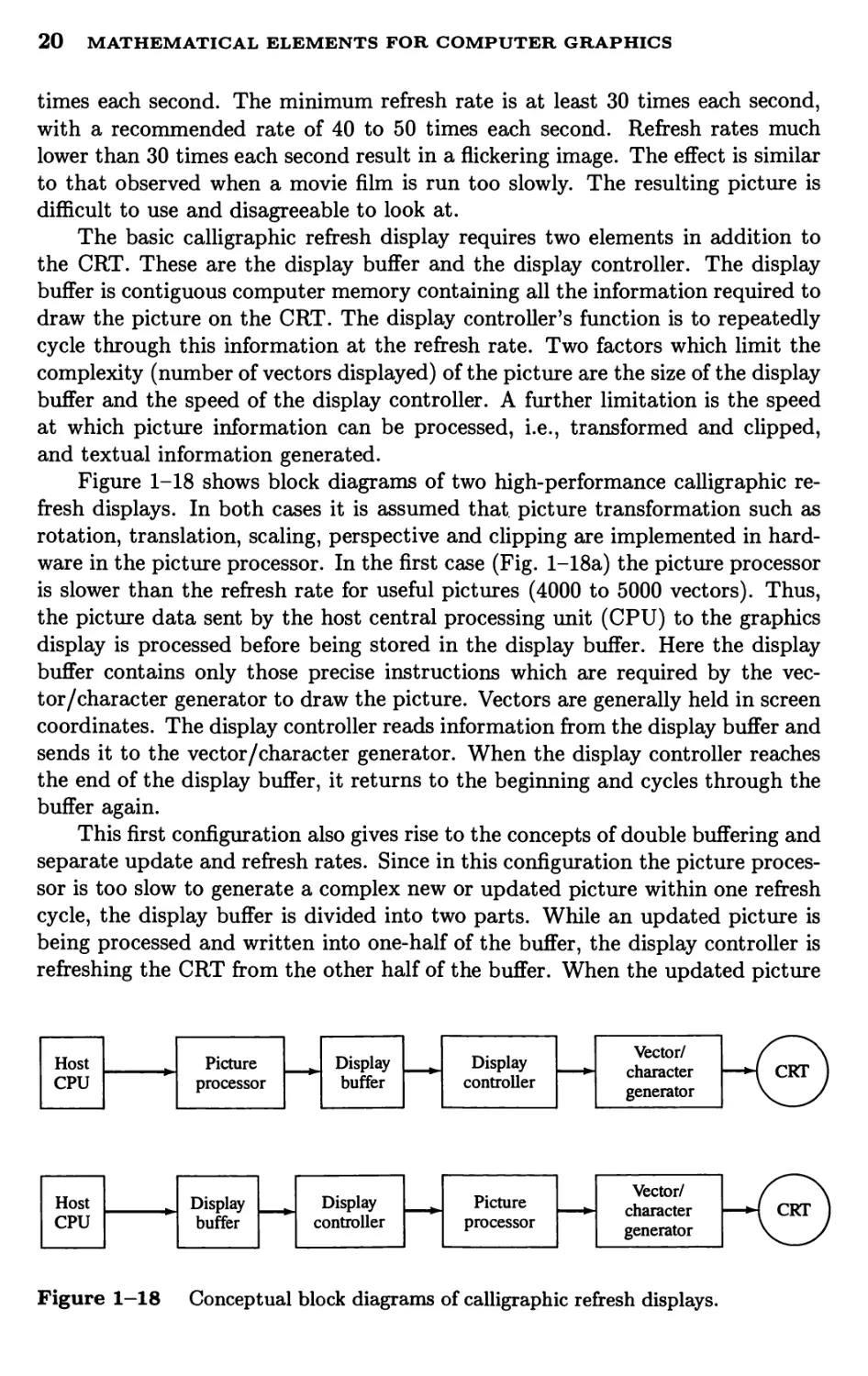
Figure 1-18 shows block diagrams of two high-performance calligraphic
refresh displays. In both cases it is assumed that picture transformation such as
rotation, translation, scaling, perspective and clipping are implemented in
hardware in the picture processor. In the first case (Fig. l-18a) the picture processor
is slower than the refresh rate for useful pictures (4000 to 5000 vectors). Thus,
the picture data sent by the host central processing unit (CPU) to the graphics
display is processed before being stored in the display buffer. Here the display
buffer contains only those precise instructions which are required by the
vector/character generator to draw the picture. Vectors are generally held in screen
coordinates. The display controller reads information from the display buffer and
sends it to the vector/character generator. When the display controller reaches
the end of the display buffer, it returns to the beginning and cycles through the
buffer again.
This first configuration also gives rise to the concepts of double buffering and
separate update and refresh rates. Since in this configuration the picture
processor is too slow to generate a complex new or updated picture within one refresh
cycle, the display buffer is divided into two parts. While an updated picture is
being processed and written into one-half of the buffer, the display controller is
refreshing the CRT from the other half of the buffer. When the updated picture
Host
CPU
Picture
processor
»
Display
buffer
»
Display
controller
»
Vector/
character
generator
k-*4 CRT j
Host
CPU
Display
buffer
»
Display
controller
»
Picture
processor
>
Vector/
character
generator
hv CRT )
Figure 1—18 Conceptual block diagrams of calligraphic refresh displays.
CALLIGRAPHIC REFRESH GRAPHICS DISPLAYS 21
is complete, the buffers are swapped and the process is repeated. Thus, a new
or updated picture may be generated every second, third, fourth, etc. refresh
cycle. Double buffering prevents part of the old picture being displayed along
with part of the new updated picture during one or more refresh cycles.
In the second configuration (see Fig. l-18b) the picture processor is faster
than the refresh rate for complex pictures. Here, the original picture data sent
from the host CPU is held directly in the display buffer. Vectors are generally
held in user (world) coordinates as floating point numbers. The display controller
reads information from the display buffer, passes it through the picture processor
and sends it to the vector generator in one refresh cycle. This implies that picture
transformations are performed 'on the fly' within one refresh cycle.
In either configuration, each vector, character and picture drawing
instruction exists in the display buffer. Hence, any individual element may be changed
independent of any other element. This feature, in combination with the short
persistence of the CRT phosphor, allows the display of dynamic motion.
Figure 1-19 illustrates this concept. Figure 1-19 shows the picture displayed during
four successive refresh cycles. The visible solid line is the displayed line for the
current refresh cycle, and the invisible dotted line is for the previous refresh
cycle. Between refresh cycles the location of the end of the line B is changed. The
line appears to rotate about the point A.
In many pictures only portions of the picture are dynamic. In fact, in many
applications the majority of the picture is static. This leads to the concept of
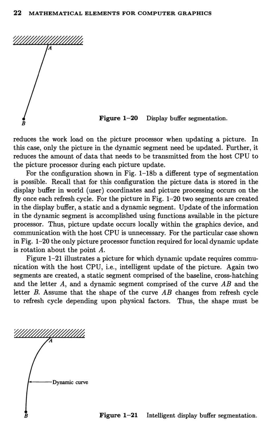
segmentation of the display buffer. Figure 1-20 illustrates this idea. Here, the
baseline, the cross-hatching and the letter A used to show the support for the
line AB are static; i.e., they do not change from refresh cycle to refresh cycle.
In contrast, the location of the end of the line AB and the letter B change from
refresh cycle to refresh cycle to show dynamic motion. These separate portions
of the picture are placed in separate segments of the display buffer. Since the
static segment of the display buffer does not change, it can be ignored by the
picture processor for the configuration shown in Fig. 1-18. This significantly
(a) (b) (c) {d)
Figure 1-19 Dynamic motion.
22 MATHEMATICAL ELEMENTS FOR COMPUTER GRAPHICS
Figure 1—20 Display buffer segmentation.
reduces the work load on the picture processor when updating a picture. In
this case, only the picture in the dynamic segment need be updated. Further, it
reduces the amount of data that needs to be transmitted from the host CPU to
the picture processor during each picture update.
For the configuration shown in Fig. l-18b a different type of segmentation
is possible. Recall that for this configuration the picture data is stored in the
display buffer in world (user) coordinates and picture processing occurs on the
fly once each refresh cycle. For the picture in Fig. 1-20 two segments are created
in the display buffer, a static and a dynamic segment. Update of the information
in the dynamic segment is accomplished using functions available in the picture
processor. Thus, picture update occurs locally within the graphics device, and
communication with the host CPU is unnecessary. For the particular case shown
in Fig. 1-20 the only picture processor function required for local dynamic update
is rotation about the point A.
Figure 1-21 illustrates a picture for which dynamic update requires
communication with the host CPU, i.e., intelligent update of the picture. Again two
segments are created, a static segment comprised of the baseline, cross-hatching
and the letter A, and a dynamic segment comprised of the curve AB and the
letter B. Assume that the shape of the curve AB changes from refresh cycle
to refresh cycle depending upon physical factors. Thus, the shape must be
-Dynamic curve
Figure 1—21 Intelligent display buffer segmentation.
CALLIGRAPHIC REFRESH GRAPHICS DISPLAYS 23
computed by an application program running in the host CPU. In order to
update the dynamic picture segment, new data, e.g., curve shape, must be sent
to and stored in the display buffer.
Although the concept of picture segmentation has been introduced through
dynamic motion examples, it is not limited to dynamic motion or animation.
Any picture can be segmented. Picture segmentation is particularly useful for
interactive graphics programs. The concept is similar to modular programming.
The choice of modular picture segments, their size and their complexity depends
on the particular application. Individual picture elements can be as simple as
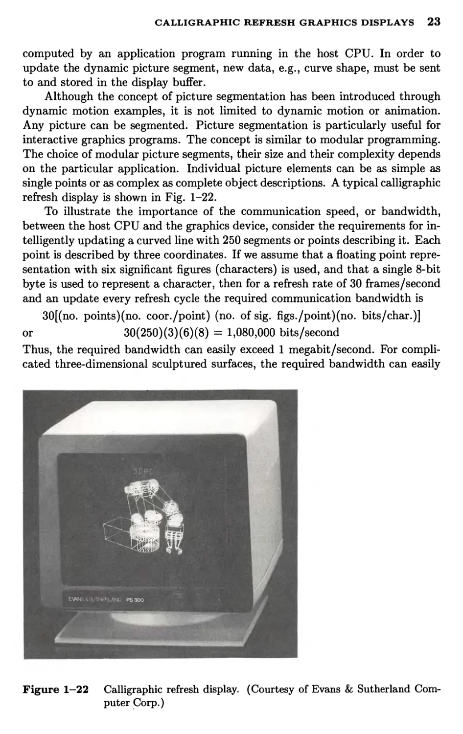
single points or as complex as complete object descriptions. A typical calligraphic
refresh display is shown in Fig. 1-22.
To illustrate the importance of the communication speed, or bandwidth,
between the host CPU and the graphics device, consider the requirements for
intelligently updating a curved line with 250 segments or points describing it. Each
point is described by three coordinates. If we assume that a floating point
representation with six significant figures (characters) is used, and that a single 8-bit
byte is used to represent a character, then for a refresh rate of 30 frames/second
and an update every refresh cycle the required communication bandwidth is
30[(no. points)(no. coor./point) (no. of sig. figs./point)(no. bits/char.)]
or 30(250)(3)(6)(8) = 1,080,000 bits/second
Thus, the required bandwidth can easily exceed 1 megabit/second. For
complicated three-dimensional sculptured surfaces, the required bandwidth can easily
* - lis ii
EW* =tt " PS300
Figure 1—22 Calligraphic refresh display. (Courtesy of Evans & Sutherland
Computer Corp.)
24 MATHEMATICAL ELEMENTS FOR COMPUTER GRAPHICS
exceed 10 times this, i.e., 10 megabits/second. In most cases this dictates a
parallel or direct memory access (DMA) interface between the host CPU and
the graphics device to support real-time intelligent dynamic graphics.
1-9 RASTER REFRESH GRAPHICS DISPLAYS
Both the storage tube CRT display and the calligraphic (random scan) refresh
display are line drawing devices. That is, a straight line can be drawn directly
from any addressable point to any other addressable point. In contrast, the
raster CRT graphics display is a point plotting device. A raster graphics device
can be considered a matrix of discrete cells, each of which can be made bright. It
is not possible, except in special cases, to directly draw a straight line from one
addressable point, or pixel,t in the matrix to another addressable point or pixel.
The line can only be approximated by a series of dots (pixels) close to the path
of the line. Figure l-23a illustrates the basic concept. Only in the special cases
of completely horizontal, vertical or, for square pixels, 45° lines does a straight
line of dots or pixels result. This is shown in Fig. l-23b. All other lines appear
as a series of stair steps. This is called aliasing or the 'jaggies'. Antialiasing
techniques are discussed in Ref. 1-1.
The most common method of implementing a raster CRT graphics device
uses a frame buffer. A frame buffer is a large, contiguous piece of computer
memory. As a minimum there is one memory bit for each pixel (picture element)
in the raster. This amount of memory is called a bit plane. A 512 x 512 element
square raster requires 218 (29 = 512; 218 = 512 x 512) or 262,144 memory
bits in a single bit plane. The picture is built up in the frame buffer 1 bit at
a time. Since a memory bit has only two states (binary 0 or 1), a single bit
plane yields a black-and-white (monochrome) display. Since the frame buffer is
a digital device, while the raster CRT is an analog device, conversion from a
digital representation to an analog signal must take place when information is
read from the frame buffer and displayed on the raster CRT graphics device.
This is accomplished by a digital-to-analog converter (DAC). Each pixel in the
frame buffer must be accessed and converted before it is visible on the raster
CRT. A schematic diagram of a single-bit-plane, black-and-white frame buffer,
raster CRT graphics device is shown in Fig. 1-24.
Color or gray levels are incorporated into a frame buffer raster graphics
device by using additional bit planes. Figure 1-25 schematically shows an N-
bit-plane gray level frame buffer. The intensity of each pixel on the CRT is
controlled by a corresponding pixel location in each of the N bit planes. The
binary value (0 or 1) from each of the N bit planes is loaded into corresponding
positions in a register. The resulting binary number is interpreted as an intensity
level between 0 (dark) and 2^ — 1 (full intensity). This is converted into an analog
tA pixel is addressed or identified by its lower left corner. It occupies a finite area to the
right and above this point. Addressing starts at 0,0. This means that the pixels in an n x n
raster are addressed in the range 0 to n — 1. Thus, e.g., the top and right-most lines in Fig. 1-23
do not represent addressable pixel locations.
RASTER REFRESH GRAPHICS DISPLAYS 25
-
B
«-■"
Picture element, or pixel
Addressable point
Rasterized approximation
to line AB
i\\\\\\\y\
WWW \y\\
K
LK
Lki
J4
LH
K
Ld_ 1.
W (b)
Figure 1-23 Rasterization, (a) General line; (b) special cases.
voltage between 0 and the maximum voltage of the electron gun by the DAC. A
total of 2N intensity levels are possible. Figure 1-25 illustrates a system with 3
bit planes for a total of 8 (23) intensity levels. Each bit plane requires the full
complement of memory for a given raster resolution; e.g., a 3-bit-plane frame
buffer for a 512 x 512 raster requires 786,432 (3 x 512 x 512) memory bits.
An increase in the number of available intensity levels is achieved for a
modest increase in required memory by using a lookup table. This is shown
schematically in Fig. 1-26. Upon reading the bit planes in the frame buffer, the
resulting number is used as an index into the lookup table. The lookup table
must contain 2^ entries. Each entry in the lookup table is W bits wide. W may
be greater than N. When this occurs, 2W intensities are available; but only 2^
different intensities are available at one time. To get additional intensities the
lookup table must be changed (reloaded).
Since- there are three primary colors, a simple color frame buffer is
implemented with three bit planes, one for each primary color. Each bit plane drives
Frame buffer
Register
CRT
raster
Figure 1—24 A single-bit-plane black-and-white frame buffer raster CRT graphics
device.
26 MATHEMATICAL
ELEMENTS FOR COMPUTER GRAPHICS
y
s
Register
■ N
2"DAC
N=3 2" levels
Frame buffer
Electron gun
raster
Figure 1-25 An TV-bit-plane gray level frame buffer.
an individual color gun for each of the three primary colors used in color video.
These three primaries (red, green and blue) are combined at the CRT to yield
eight colors as shown in Table 1-1. A simple color raster frame buffer is shown
schematically in Fig. 1-27.
Additional bit planes can be used for each of the three color guns. A
schematic of a multiple-bit-plane color frame buffer with 8 bit planes per color,
i.e., a 24-bit-plane frame buffer, is shown in Fig. 1-28. Each group of bit planes
drives an 8-bit DAC. Each group generates 256 (28) shades or intensities of red,
green or blue. These are combined into 16,777,216 [(28)3 = 224] possible colors.
This is a 'full' color frame buffer.
The full color frame buffer can be further expanded by using the groups of bit
planes as indices to color lookup tables. This is shown schematically in Fig. 1-29.
Table 1-1 Simple 3-bit plane frame buffer color combinations
Black
Red
Green
Blue
Yellow
Cyan
Magenta
White
Red
0
1
0
0
1
0
1
1
Green
0
0
1
0
1
1
0
1
Blue
0
0
0
1
0
1
1
1
RASTER REFRESH GRAPHICS DISPLAYS 27
Look-up table
W -
2W intensity levels
2N at a time
CRT
raster
Figure 1-26 An TV-bit-plane gray level frame buffer with a W-bit-wide lookup table.
y
/'
Registers Color guns
DAC
DAC
ON DAC
Frame buffer
CRT
raster
Figure 1-27 Simple color frame buffer.
28 MATHEMATICAL ELEMENTS FOR COMPUTER GRAPHICS
Frame buffer
Figure 1—28 A 24-bit-plane color frame buffer.
For N bit planes/color with W-bit-wide color lookup tables, (23)N colors from
a palette of (23)w possible colors can be shown at any one time. For example,
for a 24-bit-plane (N = 8) frame buffer with three 10-bit-wide (W = 10) color
lookup tables, 16,777,216 (224) colors from a palette of 1,073,741,824 (230) colors,
i.e., about 17 million colors from a palette of a little more than 1 billion, can
be obtained. Although three separate lookup tables are schematically shown in
Fig. 1-29, for small numbers of physical bit planes (up to about 12) it is more
advantageous if the lookup tables are implemented contiguously with (23)N table
entries.
Because of the large number of pixels in a raster scan graphics device,
achieving real-time performance and acceptable refresh or frame rates is difficult. For
example, if pixels are accessed individually with an average access time of 200
nanoseconds (200 x 10~9 second), then it requires 0.0524 second to access all
the pixels in a 512 x 512 frame buffer. This is equivalent to a refresh rate of
19 frames (pictures)/second, well below the required minimum refresh rate of 30
frames/second. A 1024 x 1024 frame buffer contains slightly more than 1
million bits (1 megabit) and, at 200 nanoseconds average access time, requires 0.21
second to access all the pixels. This is 5 frames/second. A 4096 x 4096 frame
buffer contains 16.78 million bits per memory plane! At a 200-nanosecond access
time per pixel it requires 3 seconds to access all the pixels. To achieve a refresh
RASTER REFRESH GRAPHICS DISPLAYS 29
/
r
V
rrn
2N
entries
W-w= 10—H
H w-
Red
cm
rrn
L-FF=10-J
Green
L-w^lO-J
Color
|— look-up
tables
bit DAC H "-H W-bit DAC h H W-bit DAC
Blue
Blue
Green
Red
Color guns
Figure 1—29 A 24-bit-plane color frame buffer with 10-bit-wide lookup tables.
30 MATHEMATICAL ELEMENTS FOR COMPUTER GRAPHICS
rate of 30 frames/second a 4096 x 4096 raster requires an average effective access
rate of 2 nanoseconds/pixel. Recall that light travels two feet in this small time
period.
Real-time performance with raster scan devices is achieved by accessing
pixels in groups of 16, 32, 64 or more simultaneously. In the case of color frame
buffers each pixel may contain up to 32 bits; i.e., all bit planes for an individual
pixel are accessed together. With an average access time of 1600 nanoseconds
for each group of pixels, real-time performance for 512 x 512 and 1024 x 1024
frame buffers is possible.
Although real-time performance with acceptable refresh rates is more
difficult to achieve with a raster CRT device than with a calligraphic or line drawing
refresh display, solid figure representation with a raster device is conceptually
simple. This is shown in Fig. 1-30. Here a representation of the solid figure
bounded by the lines LI, L2, L3, L4 is achieved by setting all the pixels within
the bounding polygon to the appropriate code in the frame buffer. This is
called solid area scan conversion. Algorithms for scan conversion are discussed
in Ref. 1-1.
1-10 CATHODE RAY TUBE BASICS
A frame buffer as described above is not itself a display device. It is simply used
to assemble and hold a digital representation of the picture. The most common
display device used with a frame buffer is a video (TV) monitor. An
understanding of raster displays, and to some extent line drawing refresh displays, requires
a basic understanding of CRTs and video display techniques.
The CRT used in video monitors is shown schematically in Fig. 1-31. A
cathode (negatively charged) is heated until electrons 'boil' off in a diverging
cloud (electrons repel each other because they have the same charge). These
electrons are attracted to a highly charged positive anode. This is the phosphor
coating on the inside of the face of the large end of the CRT. If allowed to
continue uninterrupted, the electrons simply flood the entire face of the CRT
with a bright glow, However, the cloud of electrons is focused into a narrow,
k.
ii i ii 11' 111 4111!i'11111 ii
'1 ! M ! 1 ! 1 1 I
II
11111111111 i 1111111111111
111111111 11 / 111111 1111111
Figure 1—30 Solid figures with a raster
graphics device.
COLOR CRT RASTER SCAN BASICS 31
Electron
focusing
lens
Horizontal
deflection
amplifier
Deflected
electron beam
Cathode
Vertical
deflection
amplifier
Anode
"(phosphor
coating)
Electron beam
Figure 1-31 Cathode ray tube.
precisely collimated beam with an electron lens. At this point the focused
electron beam produces a single bright spot at the center of the CRT. The electron
beam is deflected or positioned to the left or right of the center and/or above or
below the center by means of horizontal and vertical deflection amplifiers.
It is at this point that line drawing displays, both storage and refresh, and
raster scan displays differ. In a line drawing display the electron beam may be
deflected directly from any arbitrary position to any other arbitrary position on
the face of the CRT (anode). A perfectly straight line results. In contrast, in
a raster scan display the beam is deflected in a set, rigidly controlled pattern.
This pattern comprises the video picture.
1-11 COLOR CRT RASTER SCAN BASICS
A color raster scan CRT is similar to the standard black-and-white CRT
described in the previous section. In the color raster scan CRT there are three
electron guns, one for each of the three primary colors, red, green and blue. The
electron guns are frequently arranged in a triangular pattern corresponding to
a similar triangular pattern of red, green and blue phosphor dots on the face of
the CRT (see Fig. 1-32). To ensure that the individual electron guns excite the
correct phosphor dots (e.g., the red gun excites only the red phosphor dot), a
perforated metal grid is placed between the electron guns and the face of the
CRT. This is the shadow mask of the standard shadow mask color CRT. The
perforations in the shadow mask are arranged in the same triangular pattern as
the phosphor dots. The distance between perforations is called the pitch. The
color guns are arranged so that the individual beams converge and intersect at
the shadow mask (see Fig. 1-33). Upon passing through the hole in the shadow
mask the red beam, for example, is prevented or masked from intersecting either
the green or blue phosphor dot. It can only intersect the red phosphor dot.
By varying the strength of the electron beam for each individual primary color,
different shades (intensities) are obtained. These primary color shades can be
combined into a large number of colors for each pixel. For a high-resolution
display there are usually two to three color triads for each pixel.
32 MATHEMATICAL ELEMENTS FOR COMPUTER GRAPHICS
IW WWWWWWWW
B00 0jS^
10 0 0 ®JS
F) 0 0 © 0-^
1 ^ r^ r^\ /t\ r?\
^0 0 0(3
4)0 0 01
^)000G
/T\ /T\ /T\ ,T\
Figure 1-32 Phosphor dot pattern for a shadow mask CRT.
1-12 VIDEO BASICS
The process of converting the rasterized picture stored in a frame buffer to the
rigid display pattern of video is called scan conversion. The scanning pattern and
the frequency of repetition are based on both visual perception and electronic
principles. The human visual perception system requires a finite amount of time
to resolve the elements of a picture. If individual images are presented at a
rate greater than the time required for the visual system to resolve individual
images, one image persists while the next is being presented. This persistence
of vision is used to achieve flicker-fusion. The result is perceived as a continuous
presentation. A number of factors affect flicker, including image brightness and
the particular CRT screen phosphor used. Experience indicates that a practical
minimum picture presentation or update rate is 25 frames/second, provided the
minimum refresh or repetition rate is twice this, i.e., 50 frames/second. This
is actually what is done with movie film. With movie film 24 frames/second
are presented, but the presentation of each frame is interrupted so that it is
Shadow mask
-CRT face:
red, green, blue
phosphor dots
Beam convergence
Figure 1-33 Color CRT electron gun and shadow mask arrangement.
VIDEO BASICS 33
presented twice for an effective repetition rate of 48 frames/second. Thus, for
film the update rate is 24 and the refresh rate is 48. The same effect is achieved
in video using a technique called interlacing.
Video is a raster scan technique. The American standard video system uses a
total of 525 horizontal lines with a frame or viewing aspect ratio of 4:3; i.e., the
viewing area is three-quarters as high as it is wide. The repetition or frame
rate is 30 frames/second. However, each frame is divided into two fields, each
containing one-half of the picture. The two fields are interlaced or interwoven.
The fields are presented alternately every other 1/60 second. One field contains
all the odd-numbered scan lines (1, 3, 5,... ), and the other the even-numbered
scan lines (2, 4, 6,... ). The scanning pattern begins at the upper left corner
of the screen with the odd field. Each line in the field is scanned or presented
from the left to the right. As the electron beam moves across the screen from
left to right, it also moves vertically downward but at a much slower rate. Thus,
the 'horizontal' scan line is in fact slightly slanted. When the beam reaches the
right edge of the screen, it is made invisible and rapidly returned to the left edge.
This is the horizontal retrace which usually requires approximately 17 percent
of the time allowed for one scan line. The process is then repeated with the next
odd scan line. Since half of 525 is 262 V2 lines, the beam is at the bottom center
of the screen when the odd scan line field is complete (see Figs. 1-34 and 1-35).
The beam is then quickly returned to the top center of the screen. This is the
odd field vertical retrace. The time required for the vertical retrace is equivalent
to that for 21 lines. The even scan line field is then presented. The even scan line
field ends in the lower right hand corner. The even field vertical retrace returns
the beam to the upper left hand corner, and the entire sequence is repeated.
Thus, two fields are presented for each frame, i.e., 60 fields per second. Since the
eye perceives the field repetition rate, this technique significantly reduces flicker.
Figure 1-34 Schematic of a 7-line interlaced scan line pattern. The odd field begins
with line 1. The horizontal retrace is shown dashed. The odd field
vertical retrace starts at the bottom center. The even field vertical
retrace starts at the bottom right.
34 MATHEMATICAL ELEMENTS FOR COMPUTER GRAPHICS
Odd sc
1 Visible odd
scan lines
1
—^
| 24 ly lines
Figure 1-35
262
an-
-y
At
lin
line
e field
Odd scan-line
vertical retrace
""""* ^*» *^,
^>
21 lines
;s
Frame
I
525 lines
Even s
Visible even
scan lines
— — ^-"^
24 ly lines
)25-line standard frame schematic.
26:
can-lir
Zylin
le field
Even scan-line 1
vertical retrace
21 lines |
es
Although the American standard video system calls for 525 lines, only 483
lines are actually visible because a time equivalent to 21 lines is required to
accomplish the vertical retrace for each field.t During this time the electron
beam is invisible or blanked. The time available for each scan line is calculated
for a frame repetition rate of 30 as
1/30 second/frame x 1/525 frame/scan lines = 63^2 microseconds/scan line
Since approximately 10 xji microseconds is required for horizontal retrace, the
visible portion of each scan line must be completed in 53 microseconds. With
a normal video aspect ratio of 4:3, there are 644 pixels on each scan line. The
time available to access and display a pixel is thus
53 microseconds/scan line x 1/644 scan line/pixels = 82 nanoseconds
Many frame buffer-based raster scan displays sample the picture at a
resolution of 512 pixels per scan line. At this resolution approximately 103 nanoseconds
is available to access and display a pixel. Equivalent results are obtained for the
625-line 25-frame repetition rate used in Great Britain and in most of Europe.
The interlaced technique described above is not required when presenting
a video picture. However, this noninterlaced picture is not compatible with a
standard television set. In fact, most high quality raster scan graphics devices
present a noninterlaced picture. To prevent flicker, noninterlaced displays require
a repetition rate of 60 frames/second. This, of course, reduces the available
pixel access and display time by a factor of 2. Higher scan line and pixel-per-
line resolutions also decrease the available pixel access and display time, e.g., a
1024 x 1024 resolution requires a pixel access and display time a quarter of that
required by a 512 x 512 resolution — approximately 25 nanoseconds. Thus, a
very fast frame buffer memory, a very fast frame buffer controller, an equally
fast DAC and a very high bandwidth monitor are required.
TMany raster scan graphics devices use this time for processing other information.
FLAT PANEL DISPLAYS 35
1-13 FLAT PANEL DISPLAYS
Although today the CRT is unrivaled as the computer graphics display of choice,
it is bulky, heavy, fragile, and currently limited in size to about 30 inches
diagonally. For these as well as other reasons, flat panel displays are becoming of
increasing importance. All flat panel displays are raster refresh displays.
Flat panel displays are broadly divided into those based on active (light-
emitting) and passive (light-modulating) technologies. Among the active
technologies are flat CRTs, plasma-gas discharge, electroluminescent (EL) and
vacuum fluorescent displays. Liquid crystal (LC) and light-emitting diodes (LED)
are representative of the passive technologies.
Of the active flat panel display technologies, plasma-gas discharge and
electroluminescent based displays are currently most suitable for the relatively large
sizes and high resolutions required by computer graphics applications. Except
for applications with special requirements, e.g., avionics where light emitting
diode-based displays have certain advantages, liquid crystal based displays are
the most suitable of the passive technologies.
As shown in Fig. 1-36, a flat CRT is obtained by initially projecting the
electron beam parallel to the screen and then reflecting it through 90°.
Reflecting the electron beam significantly reduces the depth of the CRT bottle and
consequently of the display. The flat CRT has all the performance advantages
of the conventional CRT. Currently, flat CRTs are only available in relatively
small sizes. The length of the 'neck' may limit their utility in larger sizes. The
utility of vacuum fluorescent displays is also currently size limited.
Plasma-gas discharge, electroluminescent and liquid crystal displays have
several operating characteristics in common. Each consists of a matrix of
individual pixel locations on a raster. Each pixel must contain some mechanism,
or material, activated by application of either a voltage or a current, that
either emits light or modulates incident light. The required voltage or current is
supplied to the pixel using an individual electronic switching device, e.g., a thin
Optional deflection coils
/ Electrostatic
Phosphor
Figure 1-36 Flat CRT schematic.
36 MATHEMATICAL ELEMENTS FOR COMPUTER GRAPHICS
film transistor, diode or metal-insulator-metal nonlinear resistor, located at each
pixel. Displays using this technology are called active matrix displays.
An alternate, and more common, technique that significantly reduces the
number of switches or drivers, uses row-column addressing of the raster. This
technique requires that the display material have a switching threshold. Only
when the switching threshold is exceeded does emission or modification of light
occur. Part of the voltage or current required to activate an individual pixel is
applied through the appropriate row and the other part through the appropriate
column. The individual row or column voltage or current supplied is below the
switching threshold. Together, it is above the switching threshold. Consequently,
unwanted pixels along either the row or column are not activated. Only the
desired pixel at the intersection of the row and column receives enough voltage
or current to exceed the switching threshold and hence is activated.
When using row-column addressing, bistable pixel memory is highly
desirable. With bistable memory, once activated a pixel remains activated until
explicitly turned off. Bistable pixel memory eliminates the necessity of constantly
refreshing pixels. Consequently, no external memory is required to refresh the
display. In addition, the display controller is simplified.
The basic technology of a plasma or gas discharge display is quite simple.
Essentially the display consists of a matrix of cells (the raster) in a glass envelope.
Each cell is filled with a gas (usually neon or a neon/argon mixture) at low
pressure (below atmospheric). When a sufficiently high voltage is applied, the
gas dissociates, i.e., electrons are stripped from the atoms. The dissociated
gas is called a plasma, hence the name — plasma display. When the electrons
recombine, energy is released in the form of photons; and the gas glows with
the characteristic bright orange-red hue. A typical plasma display is shown in
Fig. 1-37.
Plasma displays can be AC or DC or combined AC/DC activated. AC,
DC and hybrid AC/DC activated plasma displays are shown schematically in
Figs. 1-38 a, b and c, respectively. The DC activated display is simpler than
the AC display. It consists of a dielectric spacer plate containing the gas cavities
sandwiched between plates containing the row-column conductors. The electric
field is applied directly to the gas. A DC activated plasma display requires
continuous refreshing.
In the AC activated plasma display a dielectric layer is placed between the
conductors and the gas. Thus, the only coupling between the gas and the
conductors is capacitive. Hence, an AC voltage is required to dissociate the gas.
AC activated plasma displays have bistable memory. Thus, the necessity to
continuously refresh the display is eliminated. Bistable memory is obtained by
using a low AC keep alive voltage. The characteristic capacitive coupling
provides enough voltage to maintain the activity in the conducting pixels, but not
enough to activate nonconducting pixels.
A hybrid AC/DC plasma display (see Fig. l-38c) uses DC voltage to 'prime'
the gas and make it more easily activated by the AC voltage. The principal
advantage of the hybrid AC/DC plasma display is reduced driver circuitry. Large
FLAT PANEL DISPLAYS 37
Figure 1-37 Typical plasma display. (Courtesy of Thomson-CSF Electron Tubes
and Devices Corp.)
size (3x3 meters at 4096 x 4096 pixels) plasma displays are available as are high
resolution (100 pixels/inch) displays. Gray scale and color systems are possible.
In an electroluminescent display a phosphorescent material emits light when
excited by either an AC or DC electric field. Because the phosphorescent material
is typically zinc sulfide doped with manganese, electroluminescent displays have
a yellow color. Pixel addressing uses the row-column technique discussed above
for plasma displays. When the applied voltage exceeds the switching threshold,
the manganese dopant electrons are excited. When an excited atom returns to a
lower energy state, it emits a photon which causes the characteristic yellow color.
Good 'gray' scale is obtainable since the luminescence varies with the voltage and
frequency of the applied electric field. By using alternate dopants other colors are
possible. Consequently, using multiple phosphorescent layers yields a color
display. The phosphorescent material is either deposited macroscopically as a
powder yielding a thick film or as molecular scale particles yielding a thin film. An AC
or DC excited thin film electroluminescent display is most frequently used in
computer graphics applications. The basic structure of an electroluminescent display
is shown in Fig. 1-39. A typical display is shown in Fig. 1-40. Reasonable sized
displays with resolutions of approximately 100 pixels/inch are currently available.
While plasma and electroluminescent displays are examples of active flat
panel technologies, the liquid crystal display is an example of a passive
technology. A liquid crystal display either transmits or reflects incident light. The
polarizing characteristics of certain organic compounds are used to modify the
characteristics of the incident light.
The basic principles of polarized light are shown in Fig. 1-41. In Fig. l-41a
noncoherent light is passed through the first (left) polarizer.. The resulting
transmitted light is polarized in the xy plane. Since the polarizing axis of the second
38 MATHEMATICAL ELEMENTS FOR COMPUTER GRAPHICS
Glass
Spacer
Conductors
Cathodes
Dielectric
spacer
plate
Gas cavity
Transparent anodes
(a)
Kb)
Transparent thin-
film conductor
with thick-film
conductive stripe
Priming plate
with thin-film
overcoat
Thick-film
dielectric
y with thin-film
overcoat
Glow
isolator
Devitrified
glass spacer
Scanning anodes
Glass scanning plate
Scanning
cathodes
Figure 1-38 Basic structure of gas discharge-plasma displays, (a) AC activated; (b)
DC activated; (c) AC/DC activated.
FLAT PANEL DISPLAYS 39
Black layer
Transparent electrodes
Glass cover
Metallic electrodes
^3^^ Phosphoric layer
(zinc sulfide: manganese)
\ Dielectric
f "^Glass
Viewing direction
Figure 1-39 Basic structure of an AC excited electroluminescent display.
u$
-.vvVVVVt i' t ,i.t j
Figure 1-40 Electroluminescent display. (Courtesy of Hewlett Packard Company)
40 MATHEMATICAL ELEMENTS FOR COMPUTER GRAPHICS
polarizer is also aligned with the xy plane, the light continues through the second
polarizer. In Fig. l-41b the polarizing axis of the second polarizer is rotated 90°
to that of the first. Consequently, the plane polarized light that passed through
the first polarizer is absorbed by the second.
Certain organic compounds which exist in the mesophase are stable at
temperatures between the liquid and solid phases, hence the name liquid crystal.
Liquid crystals exhibit three types of mesophase: smetic, nematic and cholesteric.
In the nematic phase, the long axis of the Hquid crystal molecules align parallel
to each other. The alignment direction is sensitive to temperature, surface
tension, pressure and, most important for display technology, electric and magnetic
fields. The optical characteristics of the liquid crystal are also sensitive to these
effects.
The key to one type of liquid crystal display technology is the creation of
a twisted nematic crystal sandwich in which the alignment axis of the crystals
rotates or twists through 90° from one face of the sandwich to the other. The
basic structure of a reflective twisted nematic liquid crystal display is shown in
Fig. 1-42. The two plates at the top and bottom of the liquid crystal sandwich
are grooved. The top plate is grooved in one direction and the bottom at ninety
degrees to that direction. The liquid crystals adjacent to the plate surface align
with the grooves as shown in Fig. 1-42.
4v
Plane
polarized
light
transmitted
(a)
y<
MM
^r 1
III y
III "*—
—*-x
i
Light
absorbed
(*)
Figure 1-41 Polarization of light.
FLAT PANEL DISPLAYS 41
Twisted nematic structure Alignment of liquid
of liquid crystal for an crystal molecules
"off" pixel of an "on" pixel
Figure 1-42 Basic structure of a twisted nematic liquid crystal display.
The display contains two plane polarizers, one on each side of the sandwich
aligned at 90° to each other. With a display pixel in its off or twisted state,
light entering the display is plane polarized by the first polarizer, passes through
the liquid crystal sandwich where it is twisted through 90°, passes through the
second polarizer and is reflected back out the display. The pixel appears light.
Turning the pixel on by applying an electric field to the liquid crystal
sandwich causes the crystal to untwist. Now light entering the display is plane
polarized by the first polarizer, passes through the liquid crystal sandwich where it
is not twisted and hence is absorbed by the second polarizer. The pixel appears
dark. Twisted nematic liquid crystal displays require constant refreshing.
A bistable liquid crystal display using smetic liquid crystals is also possible.
Two stable orientations of the smetic liquid crystal molecules have different
optical properties, e.g., absorption. This difference in optical properties produces an
optical contrast. A voltage pulse causes the molecules to change state. Bistable
liquid crystal displays do not require refreshing.
Color liquid crystal displays are possible using colored filters or phosphors
with twisted-nematic technology or using guest-host (dye) technology. Guest-
host liquid crystal displays combine dichroic-dye guest molecules with the host
42 MATHEMATICAL ELEMENTS FOR COMPUTER GRAPHICS
liquid crystal molecules. The spectral characteristics of different guest molecules
are used to produce different colors. Here, the application of an electric field
realigns the orientation of both the guest and host molecules to allow
transmission of light. A typical guest-host transmissive liquid crystal display is shown
schematically in Fig. 1-43. Note that only a single polarizer is required.
Reflective guest-host liquid crystal displays are also possible.
Liquid crystal displays are either row-column addressed or contain active
matrix elements, e.g., individual transistors or diodes at each pixel. Resolutions
up to 100 pixels/inch are currently available.
1-14 ELECTROSTATIC PLOTTERS
An electrostatic plotter is a raster scan device (see Sees. 1-9, 1-12). Basically
it operates by depositing small particles of toner onto electrostatically charged
areas of a special paper. Figure 1-44 shows the general scheme employed.
In more detail, a specially coated medium that will hold an electrostatic
charge is passed over a writing head which contains from 1 to 3 rows of small
writing nibs or styli. From 72 to 400 styli per inch are typical. Higher densities
Dichroic-dye molecule
Light source ^x^^l
(random t^S I
polarization)
*
Polarizer
Liquid-crystal molecule
Observer
v^ Off
(a)
^\ <4ZS57\
*
^<3Kr
-*- Observer
(b)
Figure 1-43 Guest-host liquid crystal display dye and molecules aligned to (a) block
transmission and (b) allow transmission.
ELECTROSTATIC PLOTTERS 43
Paper
supply
/
Writing
head
Magenta
toner
fountain
Yellow
toner
applied
Cyan
toner
fountain
Black
toner
fountain
Wiper
roller
Liquid
toner
applied
Liquid
toner
applied
Liquid
toner
applied
Liquid
toner
applied
Figure 1-44 Conceptual description of multiple pass color electrostatic plotter.
require multiple rows of styli. As the medium is passed over the styli, an
individual dot of negative electrostatic charge is deposited by each stylus. The medium
is then passed over a toner applicator, where positively charged particles of
liquid toner are attracted to the negatively charged dots on the medium, making
them visible. The carbon toner particles are subsequently dried and fixed to the
medium to make them permanent. Available plotting media include opaque and
translucent vellum paper, and clear and matte polyester films.
Electrostatic plotters are available in widths up to 72 inches. The length of
the plot is limited only by the length of the media roll (500 feet). The resolution
of an electrostatic plotter is given by the number of styli or dots per inch (dpi).
Accuracy is defined in a somewhat different way. Assuming that the direction
of media movement can be reversed, accuracy is defined as the error that occurs
in the position of two dots made by the same stylus on two successive passes of
the medium.
An electrostatic plotter is a raster device, consequently aliasing occurs (see
Ref. 1-1). High resolution devices attempt to minimize the effects of aliasing by
overlapping the individual dots. Figure 1-45 shows typical dot patterns. Typical
dot overlap is 30 to 50 percent. 'Since an electrostatic plotter is a raster scan
device, picture elements, e.g., lines and polygons, must be rasterized and the
picture organized into raster scan order: top to bottom, left to right. Although
preparation of the picture in raster format can be accomplished by the host
computer, it poses severe computational requirements. Further, communication
of the rasterized picture to the plotter at sufficient speed to fully utilize the
plotter's capability requires a very high speed interface. For example, consider
44 MATHEMATICAL ELEMENTS FOR COMPUTER GRAPHICS
(a) (b) (c)
Figure 1—45 Dot patterns, (a) Nonoverlapping; (b) overlapping y only; (c)
overlapping x and y.
that a 36-inch-wide plotter with a resolution of 400 dpi requires a sustained data
transfer rate from host to plotter of 360 kilobytes/second at a nominal plotting
speed of 1 inch/second. Consequently, many electrostatic plotters use special
purpose controllers to perform these functions (Ref. 1-6). A typical electrostatic
plotter and output is shown in Fig. 1-46.
Color electrostatic plotters are available. The three subtractive primary
colors (see Ref. 1-1) cyan, magenta and yellow (CMY) and black are applied to
the medium in either a single pass or in four successive passes. If the colors are
applied in a single pass, separate rows of nibs are used for each of the colors.
If the colors are applied in successive passes, the medium is rewound between
application of each color. A typical plotter provides 7 line colors. Color shading
of filled polygons is accomplished using dither and patterning (see Ref. 1-1). The
number of available colors depends on both the size of the pattern used, e.g.,
2x2,3x3 or 4x4, and the resolution of the plotter. Typically high resolution
plotters are capable of displaying a few thousand colors. Color electrostatic
plotters are currently available in widths up to 42 inches and resolutions of up
to 400 dpi.
1-15 LASER PRINTERS
Although originally designed for printing and typographic applications, laser
printers are used extensively for computer graphics output. This is particularly
true in publishing, where systems for combining print and graphics on the same
output page are important (see for example Ref. 1-7). These systems are capable
of combining near-typeset-quality text, line art and halftone pictures on a single
page. Figure 1-47 shows a typical example.
A laser printer is a raster scan device. The basic process, shown
schematically in Fig. 1-48, is similar to xerography. The print engine contains a drum
that is coated with a photoconductive material. The drum is scanned by either a
gas or semiconductor diode laser. As the drum rotates the coating is electrically
charged. The drum remains charged until struck by the highly coherent light
from the laser. The laser light selectively discharges areas (dots) on the drum to
form a negative image, i.e., the charge is removed from dots that do not appear
in the final image.t Positioning of the laser beam on the drum is accomplished
tThis description is for a write-black print engine. Write-white engines reverse the process.
LASER PRINTERS 45
(a)
W
Figure 1-46 Electrostatic plotter (a). (Courtesy of Versatec Corp.) Typical output:
(b) low resolution 100 dpi; (c) high resolution 400 dpi. (Courtesy of
Versatec Corp.)
46 MATHEMATICAL ELEMENTS FOR COMPUTER GRAPHICS
The picture (top left) was made
with the rlineto command and
the arc command. Then by scaling
and rotating the picture we can
make other interesting and
different designs.
By defining a variable called
box, we can print it in many
different ways. Using the stroke,
the setgray, and the fill commands,
we can print the same box in many
other shades and positions.
Figure 1—47 Laser printer-generated page showing a combination of text, line art
and halftone picture. (Courtesy of QMS, Inc.)
using a rotating polygonal mirror. A black plastic-based powder called toner is
attracted to the remaining charged areas on the drum. The image on the drum
is then transferred to the oppositely precharged paper. Finally, the toner is fused
to the paper, using heat and pressure to form the permanent image.
Laser printers are currently available with resolutions from 240 x 240 dpi up
to 600 x 600 dpi with a 300 x 300 dpi resolution typical. Laboratory experiments
indicate that a practical upper limit is 800 to 1000 dpi. At higher resolutions
the toner particles fuse together. Although extensively used for typesetting, the
resolution of typical laser printers is considerably less than that of good quality
phototypesetters (1200 to 5000 dpi). Current laser printers are limited to a
single dot size. Laboratory experiments with variable dot sizes are encouraging.
Laser Correcting optics
Photosensitive
drum
Figure 1—48 Schematic of a laser print engine.
DOT MATRIX PLOTTERS 47
Variable dot size allows increased flexibility in generating halftone images (see
Ref. 1-1). Although laser printers typically produce correspondence-sized pages,
they are available in up to 36 inch widths at 400 dpi that produce D-size (22 x 44
inch) and E-size (34 x 44 inch) drawings.
Laser printing is a continuous process. Once printing of a page starts it must
continue at a constant speed. Because of the high resolution, very high
continuous data rates are required. For example, a 300 x 300 dpi printer producing
a 7V2 x IOV2 inch printed area on an 8V2 x 11 inch page at 8 pages/minute
requires a sustained data rate to the laser print engine of 1 megabit/second.
Because of these high data rates the laser printer, like the electrostatic plotter, uses
a separate controller. The general scheme is shown in Fig. 1-49. Here, the host
computer provides a description of the page using a higher level page description
language (see for example Ref. 1-7). The image processor-controller takes care
of generating individual font characters, lines or half tone patterns and sending
the required bit (dot) stream to the print engine.
Figure 1- 50 shows a typical laser printer. Figure 1-51 shows examples of
typical laser printer generated line drawings and halftones.
1-16 DOT MATRIX PLOTTERS
Printers have been used for computer graphics from the very beginning of the
field. Initially the standard line printer, which is a raster scan device, was used.
Line drawings, plots and even patterned halftoned pictures were generated. With
a resolution of 1/6 inch vertically and 1/10 inch horizontally the results, by
current standards, were crude.
A number of current mechanical printer technologies, e.g., band or belt
printers, drum printers, train printers or chain printers, and daisy wheel printers are
used for computer graphics. However, the most popular and versatile is the dot
matrix printer.
In a dot matrix printer the printing mechanism is a matrix of thin nibs
or wires arranged on a print head that moves horizontally across the paper.
The basic print mechanism involves the electromagnetic release of one or more
of the spring steel mounted wires or hammers. In a captured hammer design
the hammers are drawn away from the ribbon by a permanent magnet. An
electromagnet is used to neutralize the field of the permanent magnet. When
this happens the spring steel hammer flies forward, causing the wire to impact
the ribbon, which prints a dot on the paper held between the ribbon and the
Host
system
Page
description
language
Image
processor/
controller
Dot
stream
Laser print
engine
Figure 1-49 Laser printer system schematic.
48 MATHEMATICAL ELEMENTS FOR COMPUTER GRAPHICS
-ssai *
pv,ci*w£
\
Figure 1—50 Laser printer. (Courtesy of Toshiba America, Inc.)
/*
JSf.,
V
(a) (b)
Figure 1—51 Laser printer output, (a) Line drawing; (b) patterned halftone.
INK JET PLOTTERS 49
platen. The electromagnet is then disabled so that the hammer is captured by
the permanent magnet when it rebounds. In a noncaptured hammer design, the
hammer is both pulled back to energize it and released using an electromagnet.
Various configurations of the wires are used as shown in Fig. 1-52. For lower
wire densities the typical wire size is 0.012 to 0.013 inch, which yields a dot size
of 0.014 to 0.015 inch. These configurations yield a dot density or resolution of 60
to 85 dpi. The highest wire densities use 0.008 inch wires which yield a 0.009 to
0.010 inch dot. For graphics applications these configurations yield a dot density
of 180-dpi. From these numbers, it is easy to see that for high wire densities
dots are printed in overlapping patterns. From 20 to 50 percent overlap is used
depending on the dot density. Since printing overlapping dots reduces aliasing
or stair stepping (see Ref. 1-1), image quality is improved. Typical output from
a 70-dpi and a 180-dpi dot matrix printer, shown in Fig. 1-53, illustrates this
effect.
Color with dot matrix printers is obtained by using multicolored ribbons.
Because paper is a reflective medium, a four-color ribbon containing the sub-
tractive primaries cyan, magenta and yellow (CMY) and black is used. Use of
dither and patterning techniques (see Refs. 1-1 and 1-8) allows the production
of many shades of color.
1-17 INK JET PLOTTERS
Ink jet printers are raster scan devices. They are particularly suited for
generating low cost color output. The basic idea is to shoot tiny droplets of ink onto
a medium. There are basically two types of ink jet printers, continuous flow and
drop-on-demand.
The continuous flow ink jet produces a stream of droplets by spraying ink
out of a nozzle. The stream of ink from the nozzle is broken up into droplets
by ultrasonic waves. If ink is desired on the medium, selected droplets are
electrostatically charged. Deflection plates are used to then direct the droplet
onto the medium. If not, the droplet is deflected into a gutter where the ink is
returned to the reservoir. Paper and transparency film are typical media. This
system is shown schematically in Fig. l-54a.
Drop-on-demand technology, as its name implies, fires ink at the medium
only if a dot is required at a particular location. Here, ink from a reservoir is
7 wire 9 wire 9 wire 18 wire 18 wire
staggered staggered parallel
Figure 1-52 Selected dot matrix print wire geometries.
24 wire
staggered
50 MATHEMATICAL ELEMENTS FOR COMPUTER GRAPHICS
Figure 1—53 Comparison of dot matrix printer graphics output, (a) 9-pin printer at
70 dpi; (b) 24-pin printer at 180 dpi.
supplied to a nozzle under pressure. The ink is fired on demand by applying
an electric voltage to a piezoelectric crystal as the head makes a pass across the
medium. When a voltage is applied, the piezoelectric crystal expands, decreasing
the volume of the ink chamber. This causes a drop of ink to squirt out of
the nozzle. Release of the voltage causes the piezoelectric crystal to contract,
decreasing the volume of the reservoir and sucking the ink back into the nozzle.
A typical arrangement is shown schematically in Fig. l-54b.
The resolution of ink jet printers is determined by the size of the droplet and
hence of the nozzle. Because of the extremely small nozzle size required, nozzle
clogging, ink contamination and air bubbles in the ink are significant problems.
Typical resolutions are from 120 to 400 dpi. Laboratory experiments show that
resolutions of up to 1000 dpi are possible.
Color ink jet printers typically use four nozzles, three for the subtractive
primary colors cyan, magenta and yellow and one for black. One of the
advantages of color ink jet technology is its ability to blend colors. Because liquid
droplets of ink are used in a single pass across the medium, the droplets blend
together before drying. This gives ink jet colors a depth and vibrancy not found
in other reflective technologies. Again, patterning and dither techniques are used
to produce several thousand colors (see Refs. 1-1 and 1-8).
1-18 THERMAL PLOTTERS
There are basically two thermal printing or plotting techniques, direct thermal
transfer and indirect thermal transfer. The direct thermal transfer technique
uses a temperature sensitive paper that changes color when heated. The image
is formed by print head elements that selectively heat dots on the paper as the
head moves across it. Either dot matrix print heads or full row nib heads similar
THERMAL PLOTTERS 51
Deflection
electrode
(a)
Piezoelectric crystal
Discharged
Ink supply
c—L-"^
) w |<- ■>! n
i \ ' Ml
h
To prevent
backflow
1 1
1 « 1
1 x
i n ~*— 1
| 1
^^-
Figure 1-54
(b)
Schematics of various ink jet printer technologies, (a) Continuous; (b)
drop-on-demand.
to those in electrostatic plotters are used. Resolutions of 400 dpi are available.
The chief and most serious limitation of the direct thermal transfer technique is
the special paper that unfortunately fades with time.
The indirect thermal transfer technique uses a thin film or paper ribbon
coated with a wax-based ink. Heating elements which are usually located behind
the ribbon melt the wax coating. The pigmented ink is then rolled onto the
paper. Either dot matrix print heads that move across the medium or a full
row of nib heads are used. Figure 1-55 schematically illustrates this technique.
52 MATHEMATICAL ELEMENTS FOR COMPUTER GRAPHICS
Thermal transfer
me
jdium
^—-.
1 i
Plain
printhead
1
Ribbon
ZZ.
Ink in
wax binder
- ■ H I"I
pape
r
/ 1
V
Transferred
ink
Figure 1-55 Indirect thermal transfer technique.
The medium is ordinary paper. Color is obtained by using multicolored ribbons.
Typically seven colors are obtained directly by combining the CMY primaries
from the ribbon, plus black. Patterning and dither are used to expand the color
palette (see Refs. 1-1 and 1-8). Since the inks are not absorbed by the paper,
quite brilliant colors are obtained. Typical resolutions are from 100 to 400 dpi.
Indirect thermal transfer inks have excellent longevity.
1-19 PEN AND INK PLOTTERS
Digital pen and ink plotters are of three basic types, flatbed, drum and pinch
roller. The basic mechanisms are shown schematically in Fig. 1-56.
In a moving-arm flatbed plotter (see Fig. l-56a) the medium is fixed in
position on the bed of the plotter. Two-dimensional motion of the plotting head
is obtained by movement of an arm suspended across the width of the plotter
bed. This provides motion in one direction. Motion in the second direction is
obtained by moving the plotting head along the suspended arm. Figure 1-57
shows a typical moving arm flatbed plotter.
A moving head flatbed plotter (see Fig. l-56b) uses a plotting tool carriage
suspended above the bed by magnetic forces that are counterbalanced by an air
bearing. This arrangement provides nearly frictionless movement. Movement of
the head in two dimensions is controlled electromagnetically, using the Sawyer
motor principle. Figure 1-58 shows an example.
Large flatbed plotters usually fix the medium to the plotter bed using
vacuum. Large flatbed plotters have resolutions and plotting speeds as high as
0.0004 inch and 3600 inch/minute, respectively. Flatbed plotters are available in
sizes from 8V2 x 11 inches up to several tens of feet in length and width. A large
variety of plotting media can be used, e.g., paper, vellum, Mylar, photographic
film, scribe coat, sheet metal and cloth. Combined with this large variety of
media is an accompanying variety of plotting tools including ballpoint, felt tip
and wet ink pens, photographic and laser light beams, engraving tools, scribe
and cloth cutters and laser cutting beams. As the wide variety of available media
PEN AND INK PLOTTERS 53
Air bearing
(a)
Drum
Writing surface^^^"^ Free moving
x-y motor
<*>
Paper Pen
Pinch roller
Grit wheel
Vacuum chamber
(d)
Figure 1-56 Schematic diagrams of pen and ink plotter types, (a) Flatbed — moving
arm; (b) flatbed — moving head; (c) drum; (d) pinch roller.
Figure 1—57 Moving arm flatbed plotter. (Courtesy Xynetics, Inc.)
54 MATHEMATICAL ELEMENTS FOR COMPUTER GRAPHICS
Figure 1-58 Moving-head flatbed plotter.
and tools suggests, flatbed plotters are used in a wide variety of applications. In
addition to traditional pen and ink plots, large flatbed plotters are used to
generate masks for printed circuit boards and integrated circuits. Here, the plotting
medium is photographic film, and the plotting tool is a light beam. Adaptations
of flatbed plotters are also used to cut out men's and ladies' apparel and even
sailboat sails. Here, the medium is an appropriate cloth and the plotting tool a
knife or laser cutting beam.
Smaller lower cost flatbed plotters are less versatile, have lower resolutions
and lower plotting speeds. They also typically use an electrostatic hold-down
system for the media, which are generally limited to paper, vellum and
transparency film.
Drum plotters (see Fig. l-56c) are mechanically more complex than flatbed
plotters. Here, the plotting head moves along a fixed arm to provide one
dimension. The medium itself is rolled back and forth under the fixed arm to provide
the second dimension.
The medium is fixed to the drum using either a vacuum or tensioned supply
and takeup rollers. Media types are limited to those that are easily rolled.
Typically, the drum plotter medium is either paper or vellum. Only the width
of the medium is fixed. The length of a plot is limited only by the length of
the medium roll. Although resolutions are similar to those for flatbed plotters
(0.0005 inch), plotting speeds are typically considerably lower.
The pinch roller plotter is a hybrid of the flatbed and drum plotters. The
drawing medium is held at each edge between a pinch wheel and the plotting
surface (see Fig. l-56d). The plotting surface is cylindrical. As the pinch wheel
rotates, the medium moves back and forth under a fixed arm on which the
plotting head moves. These plotters use either cut or roll stock, which is usually
limited to paper, vellum or transparency film. Typical resolutions are 0.001
inch, with plotting speeds of 180 inches/minute. A pinch roll plotter is shown in
Fig. 1-59.
PEN AND INK PLOTTERS 55
Figure 1-59 Pinch roll plotter. (Courtesy of Hewlett-Packard Co.)
Most pen and ink plotters operate in an incremental mode driven by stepping
motors. The plotting tool moves across the plotting surface in a series of small
steps. The number of movement directions is limited to eight, horizontal, vertical
and diagonal, as shown in Fig. 1-60. This results in lines other than those in
the directions shown in Fig. 1-60, appearing as a series of stair steps. This
stairstep, or j aggies, effect is a manifestation of a fundamental phenomenon called
aliasing (see Ref. 1-1). The algorithm usually chosen to select the one of eight
movement directions that most nearly approximates the direction of the line is
Figure 1-60 Directions for incremental
plotters.
56 MATHEMATICAL ELEMENTS FOR COMPUTER
Bresenham's algorithm (see Ref. 1-1). Although ^T^^^^
often associated with raster scan displays, it was originally developed for digital
^TutmoSntections are obtained by using servomotors to drive the
plotting head. In this case, a feedback servocircuit constantly modulates both drive
motors simultaneously to yield smooth lines. „inttinir
Although speed is important in a plotter, the acceleration of the plotting
hJi gentHy more important for overall throughput Fundamental this; is
because'the typical drawing is made up of short straight line »g™£*^
quently, the plotter must start and stop between segments High acceleration
altows the plotter to attain full speed more quickly. Accelerations of up to 4g are
currently possible. Many plotter controllers are also equpped with look-ahead
software designed to prevent the plotter from unnecessarily stopping e.g when
a series of short connected straight line segments is used to k^*™™&
Pen and ink plotters produce the highest quality line drawing output of any
graphics device. An example is shown in Fig. 1-61.
1-20 COLOR FILM CAMERAS
With the advent of high quality color raster displays coupled ^h full^ color
frame buffers (see Sec. 1-9) capable of displaying over 16 million colors, the need
arTfofa technique for preserving these results Currently the on y avaUabk
techniques are based on color photographic film. In computer graphics the most
frequently used device is a color camera. ..... p.ff , fi2 ;s auite
Conceptually, a color camera, shown schematically in Fig. 1-62 * quite
simple. The technique is called field sequential recording. A small (5-incn-
Tmeter) precision flat-faced monochrome (white) CRT is used. First a red
Figure 1-61 Typical output from a digital incremental plott(
ACTIVE AND PASSIVE GRAPHICS DEVICES 57
CRT with white phosphor Color filter wheel
Figure 1-62 Schematic of a color camera.
photographic filter is placed in the optical path from a camera to the CRT.
Then only the red intensity signal for the picture is fed to the CRT. The film is
exposed. The CRT is erased, the red filter removed and a green filter rotated
into position. Then only the green intensity signal for the picture is fed to the
CRT. Without advancing, the film is exposed a second time. Finally, the process
is repeated for the blue component of the picture. This triply exposed film now
contains the complete picture.
The quality of the CRT is critical to the success of the technique (see
Ref. 1-1). A flat-faced CRT is used, rather than the curved CRT used in most
monitors, to eliminate distortions. The glass used in the CRT must also be of
high quality, free of bubbles, striations and other defects. To allow nearly equal
response to all three signals (RGB) a broadband phosphor is used. The
phosphor layer must be free of blemishes and patterns, fine grained and smoothly
textured. The CRT beam spot size must be as small as practical for increased
resolution and the electromagnetic focusing system must be of highest quality.
With care, practical resolutions of 3000 to 5000 dpi per side on a 5-inch
monitor are possible. Note that resolution and addressability are not the same.
Resolution measures the number of separately distinguishable spots, whereas
addressability measures the number of distinct positions at which the electron
beam can be placed. Because of the characteristics of the eye, a picture made
with higher addressability than resolvability will look better, even though the
points are not resolved.
1-21 ACTIVE AND PASSIVE GRAPHICS DEVICES
Let's consider the difference between a passive and an active graphics device.
A passive graphics device simply draws pictures under computer control; i.e., it
allows the computer to communicate graphically with the user. Examples are
dot matrix printers, an electrostatic plotter, pen and ink plotters, film recorders
and storage tube refresh and raster CRT displays. Examples of some of these
devices and the typical pictures that they might generate are shown in Figs.
1-17, 1-22, 1-37, 1-40, 1-46, 1-50, 1-51, 1-53, 1-57, 1-58, 1-59 and 1-61.
58 MATHEMATICAL ELEMENTS FOR COMPUTER GRAPHICS
An active graphics device allows the user to communicate with the computer
graphically. Generally, this implies that the user is supplying coordinate
information in some indirect manner, i.e., by means other than typing the appropriate
numbers. Since a picture, curve or surface can be considered a matrix of
coordinate data, the user is supplying true pictorial information. Usually an active
graphics device has the ability to reposition the cursor and read its new position.
Typical active graphics devices include alphanumeric keyboards (Fig. 1-6),
function buttons (Fig. 1-13) or thumb wheels, control dials (Fig. 1-12), digitizer or
analog tablets (Figs. 1-7 and 1-8), light pens (Fig. 1-15), joysticks (Fig. 1-9),
trackball (Fig. 1-10) or mouse (Fig. 1-11). Although these devices may
sometimes be used alone, they usually require some type of passive graphics device
for support. This support graphics device is frequently based on a CRT.
1-22 COMPUTER GRAPHICS SOFTWARE
The totality of computer graphics software encompasses not only the concepts
presented in this book and in Ref. 1-1, but also concepts from data structures,
from data base design and management, from the psychology and ergonometrics
of the man-machine interface and from programming languages and operating
systems. These topics are well beyond the scope of this book. However, they are
considerations in the design of computer graphics systems.
Numerous computer graphics standards have been and will be developed
and considered. In general, these standards can currently be grouped into three
general categories. First is the graphics application interface, where ideas are
translated into a form understandable by a computer system. Current
representative standards are the Graphical Kernel System (GKS), GKS-3D, the
Programmer's Hierarchical Interactive Graphics Standard (PHIGS) and PHIGS+
(see Appendix A).
The second is concerned with the storage and transmission of data between
graphics systems and between graphics-based computer aided design and
computer aided manufacturing systems. The current standard in this area is the
Initial Graphics Exchange Specification (IGES).
Third is a standard for defining an interface between the graphics software
system or the data storage and transmission system and the requirements of
the device-dependent hardware drivers. Current standards in this area are the
Computer Graphics Metafile (CGM) and the Virtual Device Interface (VDI).
These standards are extremely important. They attempt to insure
portability of programs, programmers and data. A more complete but not extensive
discussion of these standards is given in Appendix A. Figure 1-63 shows the
general layout of a computer graphics software system and how each standard
fits into it. However, the purpose of this book and of Ref. 1-1 is not to discuss
standards but to develop the underlying concepts and mathematical and
procedural elements of computer graphics. Consequently, the view taken of computer
graphics software is fundamental and minimal. A computer graphics software
system that embodies these concepts is given in Appendices A and G. With
REFERENCES 59
Application
data
base
Application
programmer's
flanguage)
interface
Figure 1-63 Schematic of a computer graphics software system.
those concepts and the ones subsequently discussed in this book and in Ref. 1-1,
along with appropriate concepts from data structures and data base design, a
complete computer graphics software system can be designed and built or an
existing system understood.
1-23 REFERENCES
1-1 Rogers, D.F., Procedural Elements for Computer Graphics, McGraw-Hill
Book Co., New York, 1985.
1-2 Foley, J.D., and Wallace, V.L., "The Art of Natural Man-Machine
Conversation," Proc. IEEE, Vol. 62, pp. 462-471, 1974.
1-3 Wallace, V.L., "The Semantics of Graphic Input Devices," Comp. Graph.,
Vol. 10, pp. 61-65, 1976.
1-4 Ohlson, M., "System Design Considerations for Graphics Input Devices,"
Computer, pp. 9-18, Nov. 1978.
1-5 Davis, M.R., and Ellis, T.O., "The RAND Tablet: A Man-Machine
Graphical Communication Device," AFIPS Conf Proc, Vol. 26, Part I, 1964
FJCC, pp. 325-332, 1964.
60 MATHEMATICAL ELEMENTS FOR COMPUTER GRAPHICS
1-6 Ben-Dor, A., and Jones, B., "New Graphics Controller for Electrostatic
Plotting," IEEE Comp. Graph, k Appl, Vol. 6, No. 1, pp. 16-25, 1986.
1-7 Adobe Systems Inc., Postscript Language Reference Manual,
Addison-Wesley Publishing Co., Reading, MA, 1985.
1-8 Kubo, S., "Continuous Color Presentation Using a Low-Cost Ink Jet
Printer," Proc. Comp. Graph. Tokyo 84, 24-27 Apr. 1984, Tokyo, Japan, T3-6,
pp. 1-10, 1984.
1-9 Constantine, J.M., Jr., "Electron Optical Technique for an Ultra High
Resolution Color Film Recorder," Journal of Photooptical Instrument Engineers,
1984.
CHAPTER
TWO
TWO-DIMENSIONAL TRANSFORMATIONS
2-1 INTRODUCTION
We begin our study of the fundamentals of the mathematics underlying computer
graphics by considering the representation and transformation of points and
lines. Points and the lines which join them, along with an appropriate drawing
algorithm, are used to represent objects or to display information graphically.
The ability to transform these points and lines is basic to computer graphics.
When visualizing an object, it may be desirable to scale, rotate, translate, distort
or develop a perspective view of the object. All of these transformations can be
accomplished using the mathematical techniques discussed in this and the next
chapter.
2-2 REPRESENTATION OF POINTS
A point is represented in two dimensions by its coordinates. These two values
are specified as the elements of a 1-row, 2-column matrix:
[x y]
In three dimensions a 1 x 3 matrix
[x y z]
is used. Alternately, a point is represented by a 2-row, 1-column matrix
in two dimensions or by
x
y
z
61
62 MATHEMATICAL ELEMENTS FOR COMPUTER GRAPHICS
in three dimensions. Row matrices like
[x y]
or column matrices like
I x
[y
are frequently called position vectors. In this book a row matrix formulation of
the position vectors is used.
A series of points, each of which is a position vector relative to some
coordinate system, is stored in a computer as a matrix or array of numbers. The
position of these points is controlled by manipulating the matrix which defines
the points. Lines are drawn between the points to generate lines, curves or
pictures.
2-3 TRANSFORMATIONS AND MATRICES
Matrix elements can represent various quantities, such as a number store, a
network or the coefficients of a set of equations. The rules of matrix algebra
define allowable operations on these matrices (see Appendix B). Many physical
problems lead to a matrix formulation. For models of physical systems, the
problem is formulated as: given the matrices [ A ] and [ B ] find the solution
matrix [ T ], i.e., [ A ] [ T ) = [ B ]. In this case the solution is [ T ] = [ A ]_1 [ B ],
where [A J-1 is the inverse of the square matrix [ A ] (see Ref. 2-1).
An alternate interpretation is to treat the matrix [ T ] as a geometric
operator. Here matrix multiplication is used to perform a geometrical transformation
on a set of points represented by the position vectors contained in [ A ]. The
matrices [ A ] and [ T ] are assumed known. It is required to determine the
elements of the matrix [B]. The interpretation of the matrix [ T ] as a geometrical
operator is the foundation of mathematical transformations useful in computer
graphics.
2-4 TRANSFORMATION OF POINTS
Consider the results of the multiplication of a matrix [ x y] containing the
coordinates of a point P and a general 2x2 transformation matrix:
[X)[T) = [x y]
a b
c d
= [(ax + cy) (bx + dy)] = [x* y* } (2-1)
This mathematical notation means that the initial coordinates x and y are
transformed to x* and y*, where x* = (ax+cy) and y* = (bx+dy).^ We are interested
tSee Appendix B for the details of matrix multiplication.
TRANSFORMATION OF POINTS 63
in the implications of considering x* and y* as the transformed coordinates of
the point P. We begin by investigating several special cases.
Consider the case where a = d = 1 and c = b = 0. The transformation
matrix [ T ] then reduces to the identity matrix. Thus,
[X][T] = [x y]
1 0
0 1
= [ x y] = [x* y*]
(2-2)
and no change in the coordinates of the point P occurs. Since in matrix algebra
multiplying by the identity matrix is equivalent to multiplying by 1 in ordinary
algebra, this result is expected.
Next consider d = 1, 6 = c = 0, i.e.,
[X)[T] = [x y]
a 0
0 1
= [ax y ] = [ x* y*]
(2-3)
which, since x* = ax, produces a scale change in the x component of the position
vector. The effect of this transformation is shown in Fig. 2-la. Now consider
b = c = 0, i.e.,
[X][T] = [x y]
a 0
0 d
= [ax dy ] = [ x* y* ]
(2-4)
This yields a scaling of both the x and y coordinates of the original position
vector P, as shown in Fig. 2-lb. If a ^ a7, then the scalings are not equal. If
a = d > 1, then a pure enlargement or scaling of the coordinates of P occurs. If
0 < a = d < 1, then a compression of the coordinates of P occurs.
If a and/or d are negative, reflections through an axis or plane occur. To see
this, consider 6 = c = 0, d = 1 and a = — 1. Then
[X][T] = [x y]
-1 0
0 1
= [-x y] = [x* y*]
(2-5)
and a reflection through the y-axis results, as shown in Fig. 2-lc. If b = c =
0, a = 1, and d = — 1, then a reflection through the x-axis occurs. If b = c =
0, a = d < 0, then a reflection through the origin occurs. This is shown in
Fig. 2-ld, with a = — 1, d = -1. Note that both reflection and scaling of the
coordinates involve only the diagonal terms of the transformation matrix.
Now consider the effects of the off-diagonal terms. First consider a = d = 1
and c = 0. Thus,
X][T] = [x y]
1 b
0 1
= x
[x (bx + y)] = [x* y*]
(2-6)
Note that the x coordinate of the point P is unchanged, while y* depends linearly
on the original coordinates. This effect is called shear, as shown in Fig. 2-le.
64 MATHEMATICAL ELEMENTS FOR COMPUTER GRAPHICS
yry\
yry]
p*
/
_| l_
0 1
y'y
o i
2
(a)
-1 0 1
(c)
~X, X*
y* = bx + y
J -x, jc*
4
P
_i i_
2
(b)
yTy\
3
yry
(d)
x* = cy + x
2 3
(e)
Figure 2-1 Transformation of points.
o l
2
(/)
TRANSFORMATION OF STRAIGHT LINES 65
Similarly, when a = d = 1, 6 = 0, the transformation produces shear
proportional to the y coordinate, as shown in Fig. 2—If. Thus, we see that the
off-diagonal terms produce a shearing effect on the coordinates of the position
vector for P.
Before completing our discussion of the transformation of points, consider
the effect of the general 2x2 transformation given by Eq. (2-1) when applied
to the origin, i.e.,
[x y
or for the origin,
= [ (ax + cy) (bx + dy)) = [ x* y* ]
[0 0]
= [0 0] = [x* y*]
Here we see that the origin is invariant under a general 2x2 transformation. This
is a limitation which will be overcome by the use of homogeneous coordinates.
2-5 TRANSFORMATION OF STRAIGHT LINES
A straight line can be defined by two position vectors which specify the
coordinates of its end points. The position and orientation of the line joining these
two points can be changed by operating on these two position vectors. The
actual operation of drawing a line between two points depends on the display
device used. Here, we consider only the mathematical operations on the position
vectors of the end points.
A straight line between two points A and B in a two-dimensional plane is
drawn in Fig. 2-2. The position vectors of points A and B are [ A ] = [ 0 1 ]
and [ B ] = [ 2 3 ], respectively. Now consider the transformation matrix
[T} =
1 2
3 1
(2-7)
y, y
Figure 2-2 Transformation of straight lines.
66 MATHEMATICAL ELEMENTS FOR COMPUTER GRAPHICS
which we recall from our previous discussion produces a shearing effect.
Transforming the position vectors for A and B using [ T ] produces new transformed
position vectors A* and B* given by
and
[A][T] = [0 1]
[B][T] = [2 3]
1—1
3
i—l
3
2l
1
i—l
2l
—i
i—i
= [3 1) = [A*]
= [11 7] = [B*]
(2-8)
(2-9)
Thus, the resulting coordinates for A* are x* = 3 and y* = 1. Similarly, B* is a
new point with coordinates x* = 11 and y* = 7. More compactly the line AB
may be represented by the 2x2 matrix
L) =
0 1
2 3
Matrix multiplication by [ T ] then yields
[L][T] =
"0 1"
2 3
1 2'
3 1
=
3 1"
11 7
= [L*]
(2 -10)
where the components of [ L* ] represent the transformed position vectors [ A* ]
and [ B* ]. The transformation of A to A* and B to 5* is shown in Fig. 2-2. The
initial axes are x,y and the transformed axes are x*y*. Figure 2-2 shows that
the shearing transformation [ T ] increased the length of the line and changed
its orientation.
2-6 MIDPOINT TRANSFORMATION
Figure 2-2 shows that the 2x2 transformation matrix (see Eq. 2-7) transforms
the straight line y = x + 1, between points A and B, into another straight line
y = (3/4)# — 5/4, between A* and B*. In fact a 2 x 2 matrix transforms any
straight line into a second straight line. Points on the second line have a one-to-
one correspondence with points on the first line. We have already shown this to
be true for the end points of the line. To further confirm this we consider the
transformation of the midpoint of the straight line between A and B. Letting
[A] = [Xl 2/i ] [B] = [x2 2/2]
and
T] =
a b
c d
and transforming both end points simultaneously yields
'A'
B
[T} =
=
xi 2/i
. x2 2/2 .
ax\ + q
ax2 + ex
/1
h
a b
c d
bxi -\
bx2 -\
-dy1'
-dy2 .
=
'A*'
B*
(2-11)
MIDPOINT TRANSFORMATION 67
Hence, the end points of the transformed line A*B* are
[ A* ] = [ axi + q/i bxx + dy1 ] = [x*x y{]
[ B* ] = [ ax2 + q/2 bx2 + dy2 ] = [ x\ y\ ] (2 - 12)
The midpoint of the transformed line A*B* calculated from the transformed end
points is
i< yi] = [2±£i yi±yi]
_ [ (axi + cyi) + (ax2 + cy2) (bxi + dy\) + (bx2 + dy2) 1
1-2 2-1
- [ -(xi + x2) . .(yi + tfe) Jxi+x2) ,(yi +
Returning to the original line AB the midpoint is
Using [ T ] the transformation of the midpoint of AB is
]
(2 - 13)
(2 - 14)
[*m Vm][T]=[
2 2 J I c d
= [ _ (xi + x2) c(yi + y2) fc(xi+x2) + rf(yi + y2)
-[.!
(2 - 15)
Comparing Eqs. (2-13) and (2-15) shows that they are identical.
Consequently, the midpoint of the line AB transforms into the midpoint of the line
A*B*. This process can be applied recursively to segments of the divided line.
Thus, a one-to-one correspondence between points on the line AB and A*B* is
assured.
Example 2-1 Midpoint of a Line
Consider the line AB shown in Fig. 2-2. The position vectors of the end points
are
[A] = [0 1] [B) = [2 3]
The transformation
rl 2
\T} =
3 1
yields the position vectors of the end points of the transformed line A*B* as
"A
B
[T] =
'o r
2 3
"l 2'
3 1
=
3 r
11 7
=
'a*'
B*
68 MATHEMATICAL ELEMENTS FOR COMPUTER GRAPHICS
The midpoint of A*B* is
The midpoint of the original untransformed line AB is
r , r 0 + 2 1 + 31 M 01
Transforming this midpoint yields
1 2
3 1
[xm ym][T] = [l 2]
which is the same as our previous result.
* „.*
= [7 *] = [x'm y;
For computer graphics applications these results show that any straight line
can be transformed into any other straight line in any position by simply
transforming its end points and redrawing the line between the end points.
2-7 TRANSFORMATION OF PARALLEL LINES
When a 2 x 2 matrix is used to transform a pair of parallel lines, the result is a
second pair of parallel lines. To see this, consider a line between [ A ] = [ xi yi]
and [ B ] = [ x2 y2 ] and a line parallel to AB between E and F. To show that
these lines and any transformation of them are parallel, examine the slopes of
AB, EF, A*B* and E*F*. Since they are parallel, the slope of both AB and
EF is
m =
V2-yi
X2 — X\
(2 - 16)
Transforming the end points of AB using a general 2x2 transformation
yields the end points of A*B*:
'A'
B
[T} =
xi yi
mx2 yi
a b
c d
ax\ + cyi bxi + dy\
ax2 + q
/2
bx2 4
-dy2
x2
2/1
2/2
A*
B*
Using the transformed end points, the slope of A*B* is then
♦ _ (bx2 + dy2) - (feci + dy{) _ b(x2 - xi) + d(y2 - yi)
(ax2 + cy2) - (axi + cj/i) a(x2 - xi) + c(y2 - yi)
(2 - 17)
TRANSFORMATION OF INTERSECTING LINES 69
or
b + d
m =
(l/2 ~ l/i)
{x2 — X\) _ b + dm
a + c
(l/2 - Vi) a + cm
(x2 -xi)
(2 - 18)
Since the slope ra* is independent of £i,#252/i and y2, and since m, a, 6,
c and d are the same for EF and AB, it follows that m* is the same for
both E*F* and A*B*. Thus, parallel lines remain parallel after
transformation. This means that parallelograms transform into other parallelograms when
operated on by a general 2x2 transformation matrix. These simple results
begin to show the power of using matrix multiplication to produce graphical
effects.
2-8 TRANSFORMATION OF INTERSECTING LINES
When a general 2x2 matrix is used to transform a pair of intersecting straight
lines, the result is also a pair of intersecting straight lines. To see this consider
a pair of lines, e.g., the dashed lines in Fig. 2-3, represented by
y = m\X + 61
y = m2x + 62
Reformulating these equations in matrix notation yields
[x y]
—mi —rri2
1 1
\X]\M] = \B
= [h b2
or ^j^j-^j (2-19)
If a solution to this pair of equations exists, then the lines intersect. If not, then
they are parallel. A solution can be obtained by matrix inversion. Specifically,
[Xi] = [xi yi] = [B}[M}-1 (2-20)
The inverse of [ M ] is
1 m2
M]~1 =
m2 — m\
-1
m2 — ttii
—mi
(2-21)
|_ m2 — m\ m2 — m\ J
since [MJtM]-1 = [/], the identity matrix. Hence, the intersection of the
two lines is
[ Xi ] = [ Xi yi] = [bi b2]
m2
m2 — mi
-1
m2 — mi
—mi
[ Xi ] = [ Xi yi] =
m2 — mi m2 — mi
bi — b2 bim2 — b2mi
m2 — mi m2 — mi
(2 - 22)
70 MATHEMATICAL ELEMENTS FOR COMPUTER GRAPHICS
10
y,y* 6
(-hi)E
U
I i i
-4 -2 y
(-1,-1M«^
-2
-4
fF*
\
*
L^2x - 3y = 1
I L_
2 4
\^r + y = 1
^F(3, -2)
x, x'
A£*
Figure 2-3 Transformation of intersecting lines.
If these two lines are now transformed using a general 2x2 transformation
matrix given by
a b
[T) =
c d
then they have the form
y* = m\x* + bl
y = m2x + b2
It is relatively easy to show that
b + drrii
a + crrii
771; =
and
b* = bi{d — cm*) = bi
ad — be
a + crrii
t = l,2
(2 - 23)
(2 - 24)
TRANSFORMATION OF INTERSECTING LINES 71
The intersection of the transformed lines is obtained in the same manner as that
for the untransformed lines. Thus,
[*;] = [*; tf]
m2 ~~ ml m2~ ml
Rewriting the components of the intersection point using Eqs. (2-23) and (2-24)
yields
[*;] = [*: tf]
a(bi - b2) + c{b1m2 - b2m{) b(bi - b2) + d(bim2 - b2mi)
m2 — mi
7712 — TTii
(2 - 25)
Returning now to the untransformed intersection point [Xi yi] and applying
the same general 2x2 transformation we have
K v:] = [*i yi][T]
61 — b2 bim2 — b2mi
m2 — TTii 7712 — TTli
a b
c d
a(bi — b2) + c(bim2 - b2mi) b(bi
m2 — m\
— b2) + d{b\m2 — b2mi)
m2 — mi
(2 - 26)
Comparing Eqs. (2-25) and (2-26) shows that they are identical. Consequently,
the intersection point transforms into the intersection point.
Example 2-2 Intersecting Lines
Consider the two dashed lines AB and EF shown in Fig. 2-3 with end points
and
[A] = [-l -1] [B} = [3 5/3]
[E] = [-l/2 3/2] [F] = [3 -2]
The equation of the line AB is -(2/3)x + y = -(1/3) and of the line
EF, x + y = 1. In matrix notation the pair of lines is represented by
[z y]
-2/3 1
1 1
= [-1/3 1]
Using matrix inversion (see Eq. 2-21) the intersection of these lines is
[xi y«] = [-l/3 1]
= [4/5 1/5]
-3/5 -3/5
3/5 2/5
72 MATHEMATICAL ELEMENTS FOR COMPUTER GRAPHICS
Now consider the transformation of these lines using
\T} =
1 2
1 -3
The resulting lines are shown as A*B* and E*F* in Fig. 2-3. In matrix
form the equations of the transformed lines are
y
1 0
0 1
= fl 1
with intersection point at [ x\ y* ] = [ 1 1 ].
Transforming the intersection point of the untransformed lines yields
K V"i] = \xi Vi\[T]
= [4/5 1/5]
1 2
1 -3
= fl 1'
which is identical to the intersection point of the transformed lines.
Examination of Fig. 2-3 and Ex. 2-2 shows that the original pair of
untransformed dashed lines AB and EF are not perpendicular. However, the
transformed solid lines A*B* and E*F* are perpendicular. Thus, the
transformation [ T ] changed a pair of intersecting nonperpendicular lines into a pair
of intersecting perpendicular lines. By implication, [T]~ the inverse of the
transformation, changes a pair of intersecting perpendicular lines into a pair of
intersecting nonperpendicular lines. This effect can have disastrous geometrical
consequences. It is thus of considerable interest to determine under what
conditions perpendicular lines transform into perpendicular lines. We will return to
this question in Sec. 2-14 when a little more background has been presented.
Additional examination of Fig. 2-3 and Ex. 2-2 shows that the
transformation [ T ] involved a rotation, a reflection and a scaling. Let's consider each of
these effects individually.
2-9 ROTATION
Consider the plane triangle ABC shown in Fig. 2-4. The triangle ABC is rotated
through 90° about the origin in a counterclockwise sense by the transformation
T\ =
0 1
-1 0
If we use a 3 x 2 matrix containing the x and y coordinates of the triangle's
vertices, then
[3 -1"
4 1
2 1
0 1"
-1 0
=
1 3]
-1 4
-1 2 J
ROTATION 73
3
\ .y*
6
B*
c*
^
^
i i
-2
-2
-4
-
>
>v4*
^
k i
ZL
1 1
6
i i t
8
Figure 2-4 Rotation.
which produces the triangle A*B*C*. A
tained by using the transformation
180° rotation about the origin is ob-
[T] =
-1 0
0 -1
0 -1
1 0
and a 270° rotation about the origin by using
[T] =
Of course, the identity matrix
[T] =
1 0
0 1
corresponds to a rotation about the origin of either 0° or 360°. Note that neither
scaling nor reflection has occurred in these examples.
These example transformations produce specific rotations about the origin:
0°,90°, 180°, 270°. What about rotation about the origin by an arbitrary angle
6 ? To obtain this result consider the position vector from the origin to the point
P shown in Fig. 2-5. The length of the vector is r at an angle $ to the x-axis.
The position vector P is rotated about the origin by the angle 6 to P*.
74 MATHEMATICAL ELEMENTS FOR COMPUTER GRAPHICS
>
y..
y*
*
:
>
* V* J
* X - *
./>
Figure 2-5 Rotation of a position vector.
Writing the position vectors for P and P* we have
P = [ x y ] = [ r cos (j> r sin (j) ]
and P* = [ x* y* ] = [ r cos(0 + 6) r sin(</> + 0) ]
Using the sum of the angles formulas t allows writing P* as
P* = [ x* y* ] = [ r(cos 0 cos 0 — sin 0 sin 0) r(cos (/) sin 0 + sin 0 cos 0) ]
Using the definitions of x and y allows rewriting P* as
P* = [x* y* ] = [ x cos 0 — y sin 6 x sin 9 + y cos 0 ]
Thus, the transformed point has components
In matrix form
x* = zcos0 - ysinO
y* = x sin 0 + y cos 0
[X*] = [X][T] = [z* y*}
_ r , [ cos0 sin0
~[X yl\ -sin0 cos(9
tcos(<£ ± 0) = cos <£ cos 9 =F sin <£ sin 0
sin(<£ ± 0) = cos <t> sin 0 ± sin <£ cos 0
(2 - 27a)
(2 - 276)
(2 - 28)
ROTATION 75
Thus, the transformation for a general rotation about the origin by an arbitrary
angle 0 is
cos 0 sin 0
— sin 0 cos 0
T} =
(2 - 29)
Rotations are positive counterclockwise about the origin, as shown in Fig. 2-5.
Evaluation of the determinant of the general rotation matrix yields
det [ T ] = cos2 0 + sin2 0 = 1
(2 - 30)
In general, transformations with a determinant identically equal to +1 yield pure
rotations.
Suppose now that we wish to rotate the point P* back to P, i.e., perform
the inverse transformation. The required rotation angle is obviously —0. From
Eq. (2-29) the required transformation matrix is
Tl"^
cos(-0) sin(-0)
-sin(-0) cos(-0)
cos 0 — sin 0
sin 0 cos 0
(2-31)
since cos(-0) = cos0 and sin(—0) = — sin0. [T ]-1 is a formal way of writing
'the inverse of [ T ]. We can show that [ T J-1 is the inverse of [ T ] by recalling
that the product of a matrix and its inverse yields the identity matrix. Here,
Tifrr^
cos 0 sin 0
— sin 0 cos 0
cos 0 - sin 0
sin 0 cos 0
cos2 0 + sin2 0 — cos 0 sin 0 + cos 0 sin 0
— cos 0 sin 0 + cos 0 sin 0 cos2 0 + sin2 0
1 0
0 1
= f/l
where [ J ] is the identity matrix.
Examining Eqs. (2-29) and (2-31) reveals another interesting and useful
result. Recall that the transpose of a matrix is obtained by interchanging its rows
and columns. Forming the transpose of [ T ], i.e., [ T ] , and comparing it with
[ T]7 shows that
T]T =
cos 0 — sin 0
sin 0 cos 0
= [T\-
(2 - 32)
The inverse of the general rotation matrix [ T ] is its transpose. Since
formally determining the inverse of a matrix is more computationally expensive
than determining its transpose, Eq. (2-32) is an important and useful result. In
general, the inverse of any pure rotation matrix, i.e., one with a determinant
identically equal to +1, is its transposed
tsuch matrices axe said to be orthogonal.
76 MATHEMATICAL ELEMENTS FOR COMPUTER GRAPHICS
y,y*\
D+
D
i i i I I I I i_
-2
-2
Figure 2-6 Reflection.
2-10 REFLECTION
F*
D*
E*
Whereas a pure two-dimensional rotation in the xy plane occurs entirely in the
two-dimensional plane about an axis normal to the xy plane, a reflection is a
180° rotation out into three space and back into two space about an axis in
the xy plane. Two reflections of the triangle DEF are shown in Fig. 2-6. A
reflection about y = 0, the x-axis, is obtained by using
[T} =
1 0
0 -1
In this case the new vertices D*E*F* for the triangle are given by
[8 1"
7 3
[6 2
"1 0"
0 -1
=
"8 -1"
7 -3
6 -2j
Similarly reflection about x = 0, the y-axis, is given by
[T]=\-1 °
1 J 0 1
(2 - 33)
(2-34)
REFLECTION 77
A reflection about the line y = x occurs for
\T\ =
0 1
1 0
The transformed, new vertices D+E+F+ are given by
rs r
7 3
[6 2
"0 1"
1 0
=
"1 8"
3 7
2 6
Similarly, a reflection about the line y = — x is given by
fri =
o
-l
(2 - 35)
(2 - 36)
Each of these reflection matrices has a determinant that is identically — 1.
In general, if the determinant of a transformation matrix is identically —1, then
the transformation produces a pure reflection.
If two pure reflection transformations about lines passing through the origin
are applied successively, the result is a pure rotation about the origin. To see
this, consider the following example.
Example 2-3 Reflection and Rotation
Consider the triangle ABC shown in Fig. 2-7, first reflected about the x axis
(see Eq. 2-33) and then about the line y = -x (see Eq. 2-36). Specifically,
the result of the reflection about the x-axis is
[4 1"
5 2
U 3.
"l 0"
0 -1
=
"4 -1]
5 -2
.4 -3 J
[X'] = [X][Ti) =
Reflecting the triangle A*B*C* about the line y = -x yields
[X+] = [X'][T2] =
r4
5
L4
-1"
-2
-3 J
0
-1
-1"
n
=
'i
2
L3
-4"
-5
-4 J
Rotation about the origin by an angle 9 = 270° (see Eq. 2-29) yields the
identical result, i.e.,
[X+] = [X)[Ta) =
[4 1"
5 2
U 3.
"o
1
-l"
0
"1
2
3
-4]
-5
-4 J
78 MATHEMATICAL ELEMENTS FOR COMPUTER GRAPHICS
Figure 2-7 Combined reflections yield rotations.
Note that the reflection matrices given above in Eqs. (2-33) and (2-36) are
•thogonal; i.e., the transpose is also the inverse. For example,
0
1—1
-1
0
0
-1
-1
0
0
-1
-1
0
1 -1
2-11 SCALING
Recalling our discussion of the transformation of points, we see that scaling is
controlled by the magnitude of the two terms on the primary diagonal of the
matrix. If the matrix
"2 0
[T] =
0 2
is used as an operator on the vertices of a triangle, a l2-times' enlargement, or
uniform scaling, occurs about the origin. If the magnitudes are unequal, a
distortion occurs. These effects are shown in Fig. 2-8. Triangle ABC is transformed
by
"2 0
[T} =
0 2
SCALING 79
y,y*
10
8
6
4
2
0
-
-
C* B*
_. _
/ X /
7 X /
/ \/
/ v
/ /\
CI B/ \
X^ 1
X\
X \
/
A*
/^^F" ^~~-_ E*
<C ^ ,
D*
J l l l l l l l l l l iii.
0 2 4 6 8 10
Figure 2-8 Uniform and nonuniform scaling or distortion.
12
14
+~x, x
to yield A*B*C* where a uniform scaling occurs. Transforming triangle ABC
by
1/2 0
0 3
to D*E*F* shows distortion due to the nonuniform scale factors.
In general, if
[T} =
a b
c d
(2 - 37)
with a = d, 6 = c = 0, a uniform scaling occurs; and if a ^ d, b = c = 0,
a nonuniform scaling occurs. For a uniform scaling, if a = d > 1, a uniform
expansion occurs; i.e., the figure gets larger. If a = d < 1, then a uniform
compression occurs; i.e., the figure gets smaller. Nonuniform expansions and
compressions occur, depending on whether a and d are individually > 1 or < 1.
Figure 2-8 also reveals what at first glance is an apparent translation of the
transformed triangles. This apparent translation is easily understood if we recall
that the position vectors, not the points, are scaled with respect to the origin.
To see this more clearly examine the transformation of ABC to D*E*F*
more closely. Specifically,
80 MATHEMATICAL ELEMENTS FOR COMPUTER GRAPHICS
[4 2"
4 4
^2 4
1/2 0"
0 3
=
"2 6]
2 12
1 12 J
[X*] = [X][T} =
Note that each of the x components of the position vectors of DEF is increased
by a scale factor of 3 and the y components of the position vectors by a scale
factor of 2.
To obtain a pure scaling without apparent translation, the centroid of the
figure must be at the origin. This effect is shown in Fig. 2-9, where the triangle
ABC with the centroid coordinates (1/3 the base and 1/3 the height) at the
origin is scaled by a factor of 2. Specifically,
[X*] = [X][T] =
-1 -1
2 -1
-1 2
2 0
0 2
-2 -2
4 -2
-2 4
2-12 COMBINED TRANSFORMATIONS
The power of the matrix methods described in the previous sections is clear. By
performing matrix operations on the position vectors which define the vertices,
the shape and position of the surface can be controlled. However, a desired
orientation may require more than one transformation. Since matrix multiplication
is noncommutative, the order of application of the transformations is important.
c
1
-3
A
C
A
*
y>y*
4
v 3
-3
1
c N. ^ Centroid
\ \ 3 4
B X
B*
— X, X*
Figure 2-9 Uniform scaling without apparent translation.
COMBINED TRANSFORMATIONS 81
In order to illustrate the effect of noncommutative matrix multiplication,
consider the operations of rotation and reflection on the position vector [ x y\.
If a 90° rotation, [ 2\ ], is followed by reflection through the line y = —x, [ T2 ],
these two consecutive transformations give
0 1
-1 0
= [-y x.
0 -1
-1 0
[X'] = [X][T1] = [x y]
and then
[X*) = [X'][T2} = [-y x]\_; ~n\=[-x y
On the other hand, if reflection is followed by rotation, the results given by
[X>] = [X][T2] = [x y][_J ~l]=[-V -x)
and [X*] = [X'][T1] = [-y -x]
0 1
-1 0
= [x -y _
are obtained. The results are different, confirming that the order of application
of matrix transformations is important.
Another important point is illustrated by the above results and by the
example given below. Above, the individual transformation matrices were successively
applied to the successively obtained position vectors, e.g.,
and
[x y][2i]-[s' y'}
W y')[T2]^[x* y*}
In the example below the individual transformations are first combined or
concatenated and then the concatenated transformation is applied to the original
position vector, e.g., [ 7\ ] [ T2 ] -> [ T3 ] and [ x y][T3]^>[x* y* ].
Example 2-4 Combined Two-Dimensional Transformations
Consider the triangle ABC shown in Fig. 2-10. The two transformations are
a +90° rotation about the origin:
[Ti]
and a reflection through the line y = -x
0 1
-1 0
0 -1
-1 0
82 MATHEMATICAL ELEMENTS FOR COMPUTER GRAPHICS
Figure 2-10 Combined two-dimensional transformations.
The effect of the combined transformation [ T3 ] = [ T\ ] [ Ti ] on the
triangle ABC is
[X'] = [X][Ti][Ta] = [X][Ta]
or
2 2
4 2
4 4
0 1 0-1
-10-1 0
=
"2 2"
4 2
.4 4.
"-1 O"
0 1
=
"-2 2]
-4 2
.-4 4 J
The final result is shown as A*B*C* and the intermediate result as A'B'C in
Fig. 2-10.
Reversing the order of application of the transformations yields
[X'] = [X}[T2][T1) = {X}[T4)
or
2 2
4 2
4 4
0-101
-1 0-10
=
"2 2"
4 2
.4 4.
"l O"
0 -1
=
"2 -2]
4 -2
.4 -4 J
The final result is shown as D*E*F* and the intermediate result as D'E'F' in
Fig. 2-10.
TRANSFORMATION OF THE UNIT SQUARE 83
The results are different, again confirming that the order of application
of the transformations is important. Note also that det[Ta] = -1 and
det[T4 ] = — 1, indicating that both results can be obtained by a single
reflection. A*B*C* can be obtained from ABC by reflection through the y-axis
(see [T3 ] and Eq. 2-34). D*E*F* can be obtained from ABC by reflection
through the x-axis (see [ T4 ] and Eq. 2-33).
2-13 TRANSFORMATION OF THE UNIT SQUARE
So far we have concentrated on the behavior of points and lines to determine
the effect of simple matrix transformations. However, the matrix is correctly
considered to operate on every point in the plane. As has been shown, the only
point that remains invariant under a 2 x 2 matrix transformation is the origin.
All other points within the plane are transformed. This transformation may be
interpreted as a stretching of the original plane and coordinate system into a
new shape. More formally, we say that the transformation causes a mapping
from one coordinate space into a second.
Consider a square-grid network consisting of unit squares in the xy plane as
shown in Fig. 2-11. The four position vectors of a unit square with one corner
at the origin of the coordinate system are
r°
i
i
[o
0]
o
1—1
—1
1—1
origin of the coordinates — A
unit point on the rc-axis — B
outer corner — C
unit point on the y-axis — D
A
Id
m i
\C
B
»
*-
0 1
(a)
(b)
Figure 2—11 General transformation of unit square, (a) Before transformation; (b)
after transformation.
84 MATHEMATICAL ELEMENTS FOR COMPUTER GRAPHICS
This unit square is shown in Fig. 2-1 la. Application of a general 2x2 matrix
transformation to the unit square yields
A
B
C
D
The results of this transformation are shown in Fig. 2-1 lb. First notice from
Eq. (2-38) that the origin is not affected by the transformation, i.e., [A] =
[>!*]= [0 0 ]. Further, notice that the coordinates of B* are equal to the
first row in the general transformation matrix, and the coordinates of D* are
equal to the second row in the general transformation matrix. Thus, once the
coordinates of B* and D* (the transformed unit vectors [1 0 ] and [0 1 ],
respectively) are known, the general transformation matrix is determined. Since
the sides of the unit square are originally parallel, and since we have previously
shown that parallel lines transform into parallel lines, the transformed figure is
a parallelogram.
The effect of the terms a, 6, c and d in the 2x2 matrix can be identified
separately. The terms b and c cause a shearing (see Sec. 2-4) of the initial
square in the y and x directions, respectively, as can be seen in Fig. 2-1 lb. The
terms a and d act as scale factors, as noted earlier. Thus, the general 2x2
matrix produces a combination of shearing and scaling.
It is also possible to easily determine the area of A*B*C*D* the
parallelogram shown in Fig. 2-1 lb. The area within the parallelogram can be calculated
as follows:
Ap = (a + c)(b + d) - ~{ab) - -(cd) - ^(b + b + d) - -(c + a + c)
which yields
Ap = ad — be = det
It can be shown that the area of any parallelogram Ap, formed by transforming
a square, is a function of the transformation matrix determinant and is related
to the area of the initial square As by the simple relationship
Ap = As(ad - be) = As det [ T ] (2 - 40)
In fact, since the area of a general figure is the sum of unit squares, the area of
any transformed figure At is related to the area of the initial figure Ai by
At = Ai(ad-bc) (2-41)
This is a useful technique for determining the areas of arbitrary shapes.
"o o"
1 0
1 1
[o i
a b
c d
0 0
a b
a + c b + d
c d
A*
B*
C*
D*
(2 - 38)
a b
c d
(2 - 39)
TRANSFORMATION OF THE UNIT SQUARE 85
Example 2-5 Area Scaling
The triangle ABC with position vectors [1 0 ], [ 0 1] and [-1 0 ], is
transformed by
3 2
\T} =
-1 2
to create a second triangle A*B*C* as shown in Fig. 2-12.
The area of the triangle ABC is
Ai = ±(base)(height) = |(2)(1) = 1
Using Eq. (2-41) the area of the transformed triangle A*B*C* is
At = Ai(ad- be) = 1(6 + 2) = 8
Now the vertices of the transformed triangle A*B*C* are
r i o"
0 1
L-i oj
r 3 2]
-1 2
=
■ 3
-1
L-3
2]
2
-2 J
Calculating the area from the transformed vertices yields
At = -{base){
which confirms the previous result
At = ±(base)(height) = ±(4)(4) = 8
Figure 2-12 Area scaling.
86 MATHEMATICAL ELEMENTS FOR COMPUTER GRAPHICS
2-14 SOLID BODY TRANSFORMATIONS
We now return to the question posed in Sec. 2-8, i.e., when do perpendicular
lines transform as perpendicular lines? First consider the somewhat more general
question of when is the angle between intersecting lines preserved?
Recall that the dot or scalar product of two vectors is
Vi-V2 = VlxV2x + VlyV2y = |Vi| |V2|cos0
(2 - 42)
and the cross product of two vectors confined to the two-dimensional xy plane
is
VixV2 = (VlxV2y - V2xVly)k = |Vi||V2|*sin0 (2 - 43)
where the subscripts x, y refer to the _# and y components of the vector, 0 is the
acute angle between the vectors and k is the unit vector perpendicular to the xy
plane.
Transforming V\ and V2 using a general 2x2 transformation yields
Vi
V2
T} =
Vlx Vly
V2x V2y
a b
c d
aVlx + cVly bVlx + dVly
aV2x + cV2y bV2x + dV2y
vii
(2 - 44)
The cross product of V£ and V2 is
Vi*xV2* = (ad - cb)(VlxV2y - V2xVly)k = \V*\ |V2*|*sinfl (2 - 45)
Similarly the scalar product is
Vf-Vf = (a2 + b2)VixV2x + (c2 + d2)VlyV2y + (ac + bd)(VlxV2y + VlyV2x)
= \Vf\\V2*\co80
(2-46)
Requiring that the magnitude of the vectors, as well as the angle between them,
remains unchanged, comparing Eqs. (2-42) and (2-46) and Eqs. (2-43) and (2-
45) and equating coefficients of like terms yields
a2 + b2 = l
c2+d2 = l
ac + bd = 0
ad-bc = +1
(2 - 47a)
(2 - 476)
(2 - 47c)
(2 - 48)
Equations (2-47a,6,c) correspond to the conditions that a matrix be orthogonal,
[T}[T]-1 = [T][T}T = [I}
TRANSLATIONS AND HOMOGENEOUS COORDINATES 87
or
a b
c d
a c
b d
a2 +b2 ac + bd
ac + bd c2 + d2
1 0
0 1
Equation (2-48) requires that the determinant of the transformation matrix be
+1.
Thus, the angles between intersecting lines are preserved by pure rotation.
Since reflective transformations are also orthogonal with a determinant of — 1,
these results are easily extended. In this case the magnitude of the vectors is
preserved, but the angle between the transformed vectors is technically 2ir — 6.
Hence, the angle is technically not preserved. Still, perpendicular lines transform
as perpendicular lines. Since sin(27r-0) = -sin0, ad-bc= —1. Pure rotations
and reflections are called rigid body transformations. In addition, a few minutes'
thought or experimentation reveals that uniform scalings also preserve the angle
between intersecting lines but not the magnitudes of the transformed vectors.t
2-15 TRANSLATIONS AND HOMOGENEOUS COORDINATES
A number of transformations governed by the general 2x2 transformation
matrix, e.g., rotation, reflection, scaling, shearing etc., were discussed in the
previous sections. As noted previously, the origin of the coordinate system is invariant
with respect to all of these transformations. However, it is necessary to be able
to modify the position of the origin, i.e., to transform every point in the two-
dimensional plane. This can be accomplished by translating the origin or any
other point in the two-dimensional plane, i.e.,
x* = ax + cy + m
y* = bx + dy + n
Unfortunately, it is not possible to introduce the constants of translation m, n
into the general 2x2 transformation matrix; there is no room!
This difficulty can be overcome by introducing homogeneous coordinates.
The homogeneous coordinates of a nonhomogeneous position vector [ x y] are
[ x' y' h] where x = x'/h and y = y'/h and h is any real number. Note that
h = 0 has special meaning. One set of homogeneous coordinates is always of the
form [ x y 1 ]. We choose this form to represent the position vector [ x y]
in the physical xy plane. All other homogeneous coordinates are of the form
[ hx hy h ]. There is no unique homogeneous coordinate representation, e.g.,
[6 4 2 ], [ 12 8 4 ], [ 3 2 1 ] all represent the physical point (3,2).
The general transformation matrix is now 3x3. Specifically,
[T} =
a b 0
c d 0
m n 1
(2 - 49)
tSince an orthogonal matrix preserves both the angle between the vectors and their
magnitudes, the uniform scaling transformation matrix is not orthogonal.
88 MATHEMATICAL ELEMENTS FOR COMPUTER GRAPHICS
1] =
[x
y
i]
l
0
m
0
1
n
0
0
1
where the elements a, 6, c, d of the upper left 2x2 submatrix have exactly the
same effects revealed by our previous discussions, m, n are the translation factors
in the x and y directions, respectively. The pure two-dimensional translation
matrix is
= [ x + m y + n 1 ] (2-50)
Notice that now every point in the two-dimensional plane, even the origin (x = y
= 0), can be transformed.
2-16 ROTATION ABOUT AN ARBITRARY POINT
Previously we have considered rotations as occurring about the origin.
Homogeneous coordinates provide a mechanism for accomplishing rotations about points
other than the origin. In general, a rotation about an arbitrary point can be
accomplished by first translating the point to the origin, performing the required
rotation, and then translating the result back to the original center of rotation.
Thus, rotation of the position vector [ x y 1 ] about the point m, n through
an arbitrary angle can be accomplished by
1—1
0
m
0 0
1 0
-n 1
COS0
-sin0
0
sine 0
cos0 0
0 1
i—i
0
m
0 0
1 0
n 1
[x* y* l] = [x y 1]
By carrying out the two interior matrix products we can write
[x* y* l] = [x y 1]
(2 - 51)
cos 0 sin 0 0
-sin0 cos0 0
ra(cos0-l)l f-n(cos0-l)l
+n sin 0 J I -msin0 /
(2 - 52)
An example illustrates this result.
Example 2-6 Rotation About an Arbitrary Point.
Suppose the center of an object is at [ 4 3 ] and it is desired to rotate the
object 90° counterclockwise about its center. Using the matrix
0 1 0
-10 0
0 0 1
REFLECTION THROUGH AN ARBITRARY LINE 89
causes a rotation about the origin, not the object center. The necessary
procedure is to first translate the object so that the desired center of rotation is
at the origin by using the translation matrix
1 0 0
0 1 0
-4 -3 1
Next apply the rotation matrix, and finally translate the results of the rotation
back to the original center by means of the inverse translation matrix. The
entire operation
y' l] = [x y 1]
can be combined into one matrix operation by concatenating the
transformation matrices, i.e.,
1
0
4
0 0]
1 0
-3 1.
0 1 0]
1 0 0
0 0 1.
ri o on
0 1 0
.4 3 lj
[xm y* l] = [x y 1]
0 1 0
-10 0
7 -1 1
2-17 REFLECTION THROUGH AN ARBITRARY LINE
Previously (see Sec. 2-10) reflection through lines that passed through the origin
was discussed. Occasionally reflection of an object through a line that does not
pass through the origin is required. This can be accomplished using a procedure
similar to that for rotation about an arbitrary point. Specifically,
Translate the line and the object so that the line passes through the origin.
Rotate the line and the object about the origin until the line is coincident
with one of the coordinate axes.
Reflect through the coordinate axis.
Apply the inverse rotation about the origin.
Translate back to the original location.
In matrix notation the resulting concatenated matrix is
[T] = [T'][R][R!][R]-1[T'r1 (2-53)
where
X" is the translation matrix
R is the rotation matrix about the origin
R' is the reflection matrix
The translations, rotations and reflections are also applied to the figure to be
transformed. An example is given below.
90 MATHEMATICAL ELEMENTS FOR COMPUTER GRAPHICS
Example 2-7 Reflection Through an Arbitrary Line
Consider the line L and the triangle ABC shown in Fig. 2-13a. The equation
of the line L is
y=i(x + 4)
The position vectors [2 4 1 ], [ 4 6 1 ] and [2 6 1 ] describe the
vertices of the triangle ABC.
The line L will pass through the origin by translating it -2 units in the
y direction. The resulting line can be made coincident with the x-axis by
rotating it by -tan_1(^) = -26.57° about the origin. Equation (2-33) is
then used to reflect the triangle through the x-axis. The transformed position
vectors of the triangle are then rotated and translated back to the original
orientation. The combined transformation is
T} =
1—1
0
0
0 01
1 0
-2 1.
2/\/5 -l/\/5 0
l/x/5 2/\/5 0
0 0 1
1 0 01
0-10
0 0 1
2/Vb l/\/5 0
-l/x/5 2/V5 0
0 0 1
1 0 0
0 1 0
0 2 1
T} =
3/5 4/5 0
4/5 -3/5 0
-8/5 16/5 1
and the transformed position vectors for the triangle A*B*C* are
[2 4 1]
4 6 1
.2 6 1.
3/5
4/5
8/5
4/5 0"
-3/5 0
16/5 1
=
14/5 12/5 1
28/5 14/5 1
22/5 6/5 1
as shown in Fig. 2-13a. Figures 2-13b through 2-13e show the various steps
in the transformation.
2-18 PROJECTION - A GEOMETRIC INTERPRETATION OF
HOMOGENEOUS COORDINATES
The general 3x3 transformation matrix for two-dimensional homogeneous
coordinates can be subdivided into four parts:
Tl =
a
c
b
d
P
Q
(2 - 54)
m
n
GEOMETRIC INTERPRETATION OF HOMOGENEOUS COORDINATES 91
y. y*
6
4
2
i i i
-2
-2
i
C
/4
<S^A*^
i i i
2
5
C*
i i
4
■V
1 „
6
a; jc*
(a)
y, y*
6
4
2
i i i
-2^^
^^ -2
L
-
X*^
C 5
/
2
i i
4
^, k
i ,
6
JC, JC*
Translation
(b)
y*y*
-2
-2
i i i i i i
~JC,Jt*
Rotation
(c)
y. y
4h
2h
J I I I I L_
Reflection
id)
Inverse rotation
(e)
Figure 2-13 Reflection through an arbitrary line, (a) Original and final position; (b)
translate line through origin; (c) rotate line to x-axis; (d) reflect about
x-axis; (e) undo rotation; (a) undo translation.
92 MATHEMATICAL ELEMENTS FOR COMPUTER GRAPHICS
Recall that a, 6, c and d produce scaling, rotation, reflection and shearing; and
m and n produce translation. In the previous two sections p = q = 0 and 5 = 1.
Suppose p and q are not zero. What are the effects? A geometric interpretation
is useful.
When p = q = 0 and 5 = 1, the homogeneous coordinate of the transformed
position vectors is always h = 1. Geometrically this result is interpreted as
confining the transformation to the h = 1 physical plane.
To show the effect of p ^ 0, q ^ 0 in the third column in the general 3x3
transformation matrix, consider the following:
[X Y h] = [hx hy h] = [x y 1]
= [ x y (px + qy + 1) ]
1—1
1
o
L°
0
l
0
p]
Q
lj
(2 - 55)
Here X = hx, Y = hy and h = px + qy + 1. The transformed position vector
expressed in homogeneous coordinates now lies in a plane in three-dimensional
space defined by h = px + qy + 1. This transformation is shown in Fig. 2-14,
where the line AB in the physical (h = 1) plane is transformed to the line CD
in the h ^ 1 plane, i.e., pX + qY — h + 1 = 0.
Figure 2-14 Transformation from the physical (h = 1) plane into the h ^ 1 plane
and projection from the h ^ 1 plane back into the physical plane.
GEOMETRIC INTERPRETATION OF HOMOGENEOUS COORDINATES 93
However, the results of interest are those in the physical plane corresponding
to ft = 1. These results can be obtained by geometrically projecting CD from
the ft ^ 1 plane back onto the ft = 1 plane using a pencil of rays through the
origin. From Fig. 2-14, using similar triangles,
X ~T
y =
or in homogeneous coordinates
[x- V H=[f | l]
Now, normalizing Eq. (2-55) by dividing through by the homogeneous
coordinate value ft yields
'** *" 1|=[f J »]-[^+T
y
px + qy + 1
or
x* = - =
ft px + qy + 1
y
ft px + qy + 1
The details are given in the example below.
] (2-56)
(2 - 57a)
(2 - 576)
Example 2—8 Projection in Homogeneous Coordinates
For the line AB in Fig. 2-14 we have, with p — q=l,[A] — [l 3 1] and
[B] = [A 1 1],
' c'
D
=
'a'
B
[T] =
"l 3 l"
4 1 1
"10 1"
0 1 1
.0 0 1.
=
'l3 5l
4 1 6j
Thus, [ C ] = [ 1 3 5 ] and [ D ] = [ 4 1 6 ] in the plane ft = x + y + 1.
Projecting back onto the ft = 1 physical plane by dividing through by the
homogeneous coordinate factor yields the two-dimensional transformed points
[ C* ] = [ 1 3 5 ] = [ 1/5 3/5 1 ]
[ D* ] = [ 4 1 6 ] = [ 2/3 1/6 1 ]
The result is shown in Fig. 2-14.
94 MATHEMATICAL ELEMENTS FOR COMPUTER GRAPHICS
2-19 OVERALL SCALING
The remaining unexplained element in the general 3x3 transformation matrix
(see Eq. 2-54), s, produces overall scaling; i.e., all components of the position
vector are equally scaled. To show this, consider the transformation
[X Y h] = [x y 1]
[1
0
[o
0
1
0
0]
0
s \
=[x y s]
(2 - 58)
Here, X = #, Y = y and h = s. After normalizing, this yields
and
X* = -
s
y* = y.
Thus, the transformation is [ # y 1][T] = [j ^ 1 ], a uniform scaling
of the position vector. If s < 1, then an expansion occurs; and if s > 1, a
compression occurs.
Note that this is also a transformation out of the h = 1 plane. Here, h = s =
constant. Hence, the h ^ 1 plane is parallel to the h = 1 plane. A geometric
interpretation of this effect is shown in Fig. 2-15. If s < 1, then the h =
constant plane lies between the h = 1 and h = 0 planes. Consequently, when the
transformed line AB is projected back onto the h = 1 plane to A*B* it becomes
larger. Similarly, if s > 1, then the h = constant plane lies beyond the h = 1
plane along the /i-axis. When the transformed line CD is projected back onto
the h = 1 plane to C*D* it becomes smaller.
h = 2
Figure 2-15 A geometric interpretation of overall scaling.
POINTS AT INFINITY 95
2-20 POINTS AT INFINITY
Homogeneous coordinates provide a convenient and efficient technique for
mapping a set of points from one coordinate system into a corresponding set in an
alternate coordinate system. Frequently, an infinite range in one coordinate
system is mapped into a finite range in an alternate coordinate system. Unless the
mappings are carefully chosen, parallel lines may not map into parallel lines.
However, intersection points map into intersection points. This property is used
to determine the homogeneous coordinate representation of a point at infinity.
We begin by considering the pair of intersecting lines given by
x + y = 1
2x - 3y = 0
which have an intersection point at x = 3/5, y = 2/5. Writing the equations as
x + y — 1 = 0 and 2x - 3y = 0 and casting them in matrix form yields
[x y 1]
1 2
1 -3
-1 0
= [0 0]
or
X][M') = [R]
If [ M' ] were square, the intersection could be obtained by matrix inversion.
This can be accomplished by slightly rewriting the system of original equations.
Specifically,
x+y-1=0
2x - 3y = 0
1 = 1
In matrix form this is
i.e.,
X]\M] = \R-
[x y 1]
The inverse of this square matrix is t
1 2 0
1-3 0
1 0 1
= [0 0 1]
3/5
1/5
3/5
2/5 0"
-1/5 0
2/5 1
1
= ^
3 2 0
1 -1 0
3 2 5
TMatrix inversion techniques are discussed in Ref. 2-1 or any good linear algebra book.
96 MATHEMATICAL ELEMENTS FOR COMPUTER GRAPHICS
Multiplying both sides of the equation by [ M ] 1 and noting that [ M ] [ M ]
= [ J ], the identity matrix, yields
x y l]=g[0 0 1]
3 2 0
1 -1 0
3 2 5
= [3/5 2/5 1 ]
Thus, the intersection point is again x = 3/5 and y = 2/5.
Now consider two parallel lines defined by
x + y = 1
x + y = 0
By definition, in Euclidean (common) geometric space, the intersection point of
this pair of parallel lines occurs at infinity. Proceeding, as above, to calculate
the intersection point of these lines leads to the matrix formulation
[x y 1]
1 1 0
1 1 0
-1 0 1
= [0 0 1]
However, even though the matrix is square it does not have an inverse, since
two rows are identical. The matrix is said to be singular. Another alternate
formulation is possible which does have an invertible matrix. This is obtained
by rewriting the system of equations as
x+y-l=o
x + y = 0
x = x
In matrix form this is
[x y 1]
1 1 1
1 1 0
-10 0
= [0 0 x]
Here, the matrix is not singular; the inverse exists and is
M]~1 =
0 0-1
0 1 1
1 -1 0
Multiplying both sides of the equation by the inverse yields
[x y 1] = [0 0 x]
1 -1
1 1
-1 0
= \x -x 01 = x[ 1 -1 0"
POINTS AT INFINITY 97
The resulting homogeneous coordinates [1 -1 0 ] represent the 'point of
intersection' for the two parallel lines, i.e., a point at infinity. Specifically it
represents the point at infinity in the direction [1 -1 ] in the two-dimensional plane.
In general, the two-dimensional homogeneous vector [a b 0 ] represents the
point at infinity on the line ay — bx = 0. Some examples are:
[10 0] on the positive x-axis
[ -1 0 0 ] on the negative x-axis
[010] on the positive y-axis
[0 —1 0 ] on the negative y-axis
[1 1 0 ] along the line y = x in the direction [1 1 ]
The fact that a vector with the homogeneous component h = 0 does indeed
represent a point at infinity can also be illustrated by the limiting process shown
in Table 2-1. Consider the line y* = (3/4)x* and the point [X Y h] =
[4 3 1 ]. Recalling that a unique representation of a position vector does
not exist in homogeneous coordinates, the point [4 3 1 ] is represented in
homogeneous coordinates in all the ways shown in Table 2-1. Note that in Table
2-1 as h —> 0, the ratio of y*/x* remains at 3/4, as is required by the governing
equation. Further, note that successive pairs of (x*y*) all of which fall on the line
V* = (3/4)#*, become closer to infinity. Thus, in the limit as h —> 0, the point
at infinity is given by [ X Y h] = [A 3 0]in homogeneous coordinates.
By recalling Fig. 2-15, a geometrical interpretation of the limiting process as
h —► 0 is also easily illustrated. Consider a line of unit length from x = 0, y = 0
in the direction [1 0 ], in the plane h = s (s < 1). As s —> 0 the projection
of this line back onto the h = 1 physical plane by a pencil of rays through the
origin becomes of infinite length. Consequently, the end point of the line must
represent the point at infinity on the x-axis.
Table 2-1 Homogeneous Coordinates for the Point [4 3 ]
~~h 7* ^* X Y
"~I 4 3 4 3
1/2 8 6 4 3
1/3 12 9 4 3
1/10 40 30 4 3
1/100 400 300 4 3
98 MATHEMATICAL ELEMENTS FOR COMPUTER GRAPHICS
2-21 TRANSFORMATION CONVENTIONS
Various conventions are used to represent data and to perform transformations
with matrix multiplication. Extreme care is necessary in defining the problem
and interpreting the results. For example, before performing a rotation the
following decisions must be made:
Are the position vectors (vertices) to be rotated defined relative to a right-
hand coordinate or a left-hand coordinate system?
Is the object or the coordinate system being rotated?
How are positive and negative rotations defined?
Are the position vectors stored as a row matrix or as a column matrix?
About what line, or axis, is rotation to occur?
In this text a right-hand coordinate system is used, the object is rotated
in a fixed coordinate system, positive rotation is defined using the right-hand
rule, i.e., clockwise about an axis as seen by an observer at the origin looking
outward along the positive axis, and position vectors are represented as row
matrices.
Equation (2-29) gives the transformation for positive rotation about the
origin or about the z-axis. Since position vectors are represented as row
matrices, the transformation matrix appears after the data or position vector matrix.
This is a post-multiplication transformation. Using homogeneous coordinates
for positive rotation by an angle 8 of an object about the origin (z-axis) using a
post-multiplication transformation gives
[X*) = [X)[R]
[x* y* l] = [x y 1]
cos 0 sin 0 0
- sin 0 cosO 0
0 0 1
(2 - 59)
If we choose to represent the position vectors in homogeneous coordinates as a
column matrix, then the same rotation is performed using
[X*} = [R]-1[X]
X*'
</*
1
=
COS0
sin0
0
-sin^ 0"
cos0 0
0 1
X
y
i—i
(2 - 60)
Equation (2-60) is called a premultiplication transformation because the
transformation matrix appears before the column position vector or data matrix.
Notice that the 3x3 matrix in Eq. (2-60) is also the transpose of the 3x3 matrix
in Eq. (2-59). That is, the rows and columns have been interchanged.
TRANSFORMATION CONVENTIONS 99
To rotate the coordinate system and keep the position vectors fixed, simply
replace 0 with -0 in Eq. (2-59). Recall that sin0 = -sin(-0) and cos0 =
cos(-0). Equation (2-59) is then
[x* y* l] = [x y 1]
cos 0 - sin 0 0
sin 0 cos 0 0
0 0 1
(2-61)
Notice that the 3x3 matrix is again the inverse and also the transpose of that
in Eq. (2-59).
If the coordinate system is rotated and a left-hand coordinate system used,
then the replacement of 0 with -0 is made twice and Eq. (2-59) is again valid,
assuming a post-multiplication transformation is used on a row data matrix.
Note that, as shown in Fig. 2-16, a counterclockwise rotation of the vertices
which represent an object is identical to a clockwise rotation of the coordinate
axes for a fixed object. Again, no change occurs in the 3x3 transformation
Figure 2-16 Equivalence of position vector and coordinate system rotation.
100 MATHEMATICAL ELEMENTS FOR COMPUTER GRAPHICS
matrix if no other options are modified. These few examples show how careful
we must be when performing matrix transformations.
2-22 REFERENCES
2-1 Fox, L., An Introduction to Numerical Linear Algebra, Oxford University
Press, London, 1964.
2-2 Forrest, A. R., "Co-ordinates, Transformations, and Visualization
Techniques," CAD Group Document No. 23, Cambridge University, June 1969.
CHAPTER
THREE
THREE-DIMENSIONAL TRANSFORMATIONS
AND PROJECTIONS
3-1 INTRODUCTION
The ability to represent or display a three-dimensional object is fundamental
to the understanding of the shape of that object. Furthermore, the ability to
rotate, translate, and project views of that object is also, in many cases,
fundamental to the understanding of its shape. This is easily demonstrated by picking
up a relatively complex unfamiliar object. Immediately it is rotated, held at
arm's length, moved up and down, back and forth, etc., in order to obtain an
understanding of its shape. To do this with a computer we must extend our
previous two-dimensional analysis to three dimensions. Based on our previous
experience, we immediately introduce homogeneous coordinates. Hence, a point
in three-dimensional space [ x y z ] is represented by a four-dimensional
position vector
[x' y' z' h] = [x y z 1][T]
where [ T ] is some transformation matrix. Again, the transformation from
homogeneous coordinates to ordinary coordinates is given by
i] =
£. t z- i
h h h
(3-1)
The generalized 4x4 transformation matrix for three-dimensional
homogeneous coordinates is
Tl =
a b c p
d e f q
g i j r
I m n s
(3-2)
101
102 MATHEMATICAL ELEMENTS FOR COMPUTER GRAPHICS
The 4x4 transformation matrix in Eq. (3-2) can be partitioned into four
separate sections:
3x3
1 x3
3
x
1
lxl
The upper left 3x3 submatrix produces a linear transformation t in the form of
scaling, shearing, reflection and rotation. The 1x3 lower left submatrix produces
translation, and the upper right 3x1 submatrix produces a perspective
transformation. The final lower right-hand lxl submatrix produces overall scaling.
The total transformation obtained after operating on a homogeneous position
vector with this 4x4 matrix and obtaining the ordinary coordinate is called a
bilinear transformation, t In general, this transformation yields a combination of
shearing, local scaling, rotation, reflection, translation, perspective and overall
scaling.
3-2 THREE-DIMENSIONAL SCALING
The diagonal terms of the general 4x4 transformation produce local and overall
scaling. To illustrate this, consider the transformation
0 0 0'
[X][T] = [x y z 1]
0
3
0
= [ax ey jz l] = [x* y* z* 1 ]
which shows the local scaling effect. An example follows.
(3-3)
Example 3-1 Local Scaling
Consider the rectangular parallelepiped (RPP) shown in Fig. 3-la with
homogeneous position vectors:
■*i =
0
2
2
0
0
2
2
0
0
0
3
3
0
0
3
3
1
1
1
1
0
0
0
0
1
1
1
1
1
1
1
1
tA linear transformation is one which transforms an initial linear combination of vectors
into the same linear combination of transformed vectors.
bilinear transformation results from two sequential linear transformations.
THREE-DIMENSIONAL SCALING 103
,*4
id)
Figure 3-1 Three-dimensional scale transformations.
104 MATHEMATICAL ELEMENTS FOR COMPUTER GRAPHICS
Locally scaling the RPP to yield a unit cube requires scale factors of 1/2, 1/3,
1 along the x, y, z axes, respectively. The local scaling transformation is
\T} =
1/2 0 0 0
0 1/3 0 0
0 0 10
0 0 0 1
The resulting cube has homogeneous position vectors
X*] = \X]\T} =
0
2
2
0
0
2
2
0
0
0
3
3
0
0
3
3
1
1
1
1
0
0
0
0
l"
1
1
1
1
1
1
1
1/2 0 0 0
0 1/3 0 0
0 0 10
0 0 0 1
0
1
1
0
0
1
1
0
0
0
1
1
0
0
1
1
1
1
1
1
0
0
0
0
1
1
1
1
1
1
1
1
Notice that the homogeneous coordinate factor h is unity for each of the
transformed position vectors. The result is shown in Fig. 3-lb.
Overall scaling is obtained by using the fourth diagonal element, i.e.,
[X][T] = [x y z 1]
The ordinary or physical coordinates are
10 0 0
0 10 0
0 0 10
0 0 0 5
= [x' y' z' s) (3-4)
[x* y* ** 1] =
Again, an example illustrates the effect.
*L t i. i
s s s
Example 3-2 Overall Scaling
Uniformly scaling the unit cube shown in Fig. 3-lb by a factor of two (doubling
the size) requires the transformation (see Eq. 3-4)
THREE-DIMENSIONAL SCALING 105
\T} =
10 0 0
0 10 0
0 0 10
0 0 0 1/2
The resulting RPP has homogeneous position vectors given by
X'] = \X'}\T} =
0
1
1
0
0
1
1
0
0
0
1
1
0
0
1
1
1
1
1
1
0
0
0
0
r
1
1
1
1
1
1
1
10 0 0
0 10 0
0 0 10
|_0 0 0 1/2
0
1
1
0
0
1
1
0
0
0
1
1
0
0
1
1
1
1
1
1
0
0
0
0
0.5
0.5
0.5
0.5
0.5
0.5
0.5
0.5
Notice that the homogeneous coordinate factor for each of the transformed position
vectors is h = 0.5. Thus, to obtain the ordinary or physical coordinates each position
vector must be divided by h. The result, shown in Fig. 3-lc, is
[X'] =
0
2
2
0
0
2
2
0
0
2
2
0
0
2
2
2
2
2
0
0
0
1
1
1
1
1
1
1
0 2 0 1
Notice here, as in the two-dimensional overall scaling transformation, that
the homogeneous coordinate factor is not unity. By analogy with the previous
discussion (see Sec. 2-18) this represents transformation out of the physical h = 1
volume into another volume in 4-space. The transformed physical coordinates
are obtained by projecting back into the physical h = 1 volume through the
center of the 4-space coordinate system. Again, if s < 1, a uniform expansion
of the position vectors occurs. If s > 1, a uniform compression of the position
vectors occurs.
106 MATHEMATICAL ELEMENTS FOR COMPUTER GRAPHICS
1/5
0
0
0
0
l/s
0
0
0
0
l/s
0
0
0
0
1
The same effect can be obtained by means of equal local scalings. In this
case the transformation matrix is
T} =
Notice that here the homogeneous coordinate factor is unity, i.e., h = 1. Thus,
the entire transformation takes place in the h = 1 physical volume.
3-3 THREE-DIMENSIONAL SHEARING
The off-diagonal terms in the upper left 3x3 submatrix of the generalized 4x4
transformation matrix produce shear in three dimensions, i.e.,
1 b c 0'
[X][T] = [x y z 1]
d 1
9 i
0 0
c
f
1
0
= [ x + yd + gz bx + y + iz ex + fy + z 1 ] (3-5)
An example clarifies these results.
Example 3-3 Shearing
Again consider the unit cube shown in Fig. 3-lb. Applying the shearing
transformation
1 -0.85 0.25 0"
-0.75 1 0.7 0
0.5 1 1 0
0 0 0 1
\T} =
yields
•X'] = \X]\T] =
0 0 1
1 0 1
1 1 1
0 1 1
0 0 0
1 0 0
1 1 0
0 10
0.5
1.5
0.75
-0.25
0
1
0.25
-0.75
1
0.15
1.15
2
0
-0.85
0.15
1
1
-0.75
0.5
0
-0.85 0.25 0
1 0.7 0
1 1 0
0 0 1
1
1.25
1.95
1.7
0
0.25
0.95
0.7
THREE-DIMENSIONAL ROTATION 107
The result is shown in Fig. 3-ld. Notice that in all three examples the origin
is unaffected by the transformation.
3-4 THREE-DIMENSIONAL ROTATION
Before considering three-dimensional rotation about an arbitrary axis, we
examine rotation about each of the coordinate axes. For rotation about the x-axis,
the x coordinates of the position vectors do not change. In effect, the rotation
occurs in planes perpendicular to the x-axis. Similarly, rotation about the y-
and z-axes occurs in planes perpendicular to the y- and z-axes, respectively.
The transformation of the position vectors in each of these planes is governed by
the general two-dimensional rotation matrix given in Eq. (2-29). Recalling that
matrix, and again noting that for rotation about the x-axis the x coordinate of
the transformed position vectors does not change, allows writing down the 4x4
homogeneous coordinate transformation by the angle 0 as
[T] =
1
0
0
0
0
COS0
— sinO
0
0
sin#
cosO
0
0
0
0
1
(3-6)
Rotation is assumed positive in a right-hand sense, i.e., clockwise as one
looks outward from the origin in the positive direction along the rotation axis.t
The block shown in Fig. 3-2b is the result of a -90° rotation about the x-axis
of the block shown in Fig. 3-2a.
In a similar manner, the transformation matrix for rotation by an angle ip
about the z-axis is
cos^ sin^ 0 0
— sin^ cos^ 0 0
0 0 10
0 0 0 1
T} =
(3-7)
For rotation by an angle <\> about the y-axis, the transformation is
[T) =
cos</> 0
0 1
sin0 0
0 0
- sin <j> 0
0 0
cos</> 0
0 1
(3-8)
Note that in Eq. 3-8 the signs of the sine terms are reversed from those of
Eqs. (3-6) and (3-7). This is required to maintain the positive right-hand rule
convention.
Examining Eqs. (3-6) to (3-8) shows that the determinant of each
transformation matrix is +1 as required for pure rotation. An example more fully
illustrates these results.
tThe right-hand rule for rotation is stated as follows: align the thumb of the right hand with
the positive direction of the rotation axis. The natural curl of the fingers gives the positive
rotation direction.
108 MATHEMATICAL ELEMENTS FOR COMPUTER GRAPHICS
Example 3-4 Rotation
Consider the rectangular parallelepiped shown in Fig. 3-2a. The matrix of
position vectors [ X ] is
X] =
0
3
3
0
0
3
3
0
0
0
2
2
0
0
2
2
1
1
1
1
0
0
0
0
1
1
1
1
1
1
1
1
Here, the row labeled A in the position matrix [ X ] corresponds to the point
A in Fig. 3-2. For rotation by 0 = -90° about the x-axis Eq. (3-6) yields
[T]
10 0 0
0 0-10
0 1 0 0
0 0 0 1
Applying the transformation gives the new position vectors
X*] = \X]\T] =
0
3
3
0
0
3
3
0
0
0
2
2
0
0
2
2
1
1
1
1
0
0
0
0
r
1
1
1
1
1
1
1
10 0 0
0 0-10
0 1 0 0
0 0 0 1
0
3
3
0
0
3
3
0
1
1
1
1
0
0
0
0
0
0
-2
-2
0
0
-2
-2
1
1
1
1
1
1
1
1
A*
Notice that the x components of [ X ] and [ X* ] are identical as required.
The result is shown in Fig. 3-2b.
For rotation by <j) = 90° about the y-axis, Eq. (3-7) yields
;t']
0 0-10
0 1 0 0
10 0 0
0 0 0 1
THREE-DIMENSIONAL ROTATION 109
J L
-90°
J L
ib)
(a)
+90°
Figure 3-2 Three-dimensional rotations.
Again applying the transformation to the original block yields the new position
vectors, i.e.,
"o 0 1 l"
3 0 11
3 2 1 1 I [0 0 -1 0
0 2 110 1 0 0
000110 00
300l| LOO 01
3 2 0 1
0 2 0 1
[X*'] = [X)[T'] =
110 MATHEMATICAL ELEMENTS FOR COMPUTER GRAPHICS
1
1
1
1
0
0
0
0
0
0
2
2
0
0
2
2
0
-3
-3
0
0
-3
-3
0
1
1
1
1
1
1
1
1
A*
Notice that in this case the y components of [ X ] and [ X*1 ] are identical.
The result is shown in Fig. 3-2c.
Since three-dimensional rotations are obtained using matrix multiplication, they
are noncommutative; i.e., the order of multiplication affects the final result (see
Sec. 2-12). In order to show this, consider a rotation about the x-axis followed
by an equal rotation about the y-axis. Using Eqs. (3-6) and (3-8) with 0 = <p,
we have
[T} =
1 0
0 cos0
0 -sin^
0 0
cosO
sin20
cos 0 sin 0
0
0 0
sin0 0
cos0 0
0 1
COS0
0
sin0
0
0 -sin0
cos 8 cos 6 sin
— sin 0 cos28
0
0
0 -
1
0
0
0'
6 0
0
1
-sin0
0
COS0
0
0
0
0
1
(3-9)
On the other hand, the reverse operation, i.e., a rotation about the y-axis
followed by an equal rotation about the x-axis with 6 = <p, yields
[T] =
cos0 0
0 1
sin0 0
0 0
COS0
0
sin#
0
sin0
0
COS0
0
0'
0
0
i—l
sin2 6
cosO
■ cos 6 sin 6
0
10 0 0
0 cos0 sin0 0
0 -sine cose 0
0 0 0 1
- cos 6 sin 6 0
sine 0
cos2 e 0
0 1
(3 - 10)
Comparison of the right-hand sides of Eqs. (3-9) and (3-10) shows that they are
not the same. The fact that three-dimensional rotations are noncommutative
must be kept in mind when more than one rotation is to be made.
THREE-DIMENSIONAL ROTATION 111
The result of transformation of the object in Fig. 3-3a consisting of two 90°
rotations using the matrix product given in Eq. (3-9) is shown dashed in Figs.
3-3c and 3-3d. When the opposite order of rotation as specified by Eq. (3-10)
is used, the solid figures shown in Figs. 3-3b and 3-3d graphically demonstrate
that different results are obtained by changing the order of rotation. A numerical
example further illustrates this concept.
+90°
(a)
+ 90°
• l
+90°
^<*
(c)
id)
Figure 3—3 Three-dimensional rotations are noncommutative.
112 MATHEMATICAL ELEMENTS FOR COMPUTER GRAPHICS
Example 3-5 Combined Rotations
The object in Fig. 3-3a has position vectors
X} =
0
2
2
0
0
2
2
0
0
0
3
2
0
0
3
2
1
1
1
1
0
0
0
0
1
1
1
1
1
1
1
1
The concatenated matrix for a rotation about the x-axis by 6 = 90° followed
by a rotation about the y-axis by <f> = 90° is given by Eq. (3-9) as
\T} =
0 0-10
10 0 0
0-1 0 0
0 0 0 1
The transformed position vectors are
[X'] = [X][T] =
0
2
2
0
0
2
2
0
0
0
3
2
0
0
3
2
1
1
1
1
0
0
0
0
1
1
1
1
1
1
1
1
'0
1
0
.0
0
0
-1
0
-1
0
0
0
0
0
0
1
0-1 0 1
0-1-2 1
3
2
0
0
3
2
-1
-1
0
0
0
0
-2
0
0
-2
-2
0
1
1
1
1
1
1
The transformed object is shown dashed in Fig. 3-3d.
The concatenated matrix for a rotation about the y-axis by <f> = 90°
followed by a rotation about the x-axis by 6 = 90° is given by Eq. (3-10) as
[T'l =
0 10 0
0 0 10
10 0 0
0 0 0 1
THREE DIMENSIONAL REFLECTION 113
Here, the resulting transformed position vectors are
\X"] = \X]\r] =
0
2
2
0
0
2
2
0
0
0
3
2
0
0
3
2
1
1
1
1
0
0
0
0
ll
1
1
1
1
1
1
1J
[0 10 0]
0 0 10
10 0 0
[o o o i.
=
1
1
1
1
0
0
0
0
0
2
2
0
0
2
2
0
0
0
3
2
0
0
3
2
1
1
1
1
1
1
1
1
A*'
The transformed object is shown by solid lines in Fig. 3-3d.
Comparing the two numerical results also clearly shows that the
orientation of the transformed objects is considerably different. Hence, the order of
matrix multiplication is important.
3-5 THREE DIMENSIONAL REFLECTION
Some orientations of a three-dimensional object cannot be obtained using pure
rotations; they require reflections. In three dimensions, reflections occur through
a plane. By analogy with the previous discussion of two-dimensional reflection
(see Sec. 2-10), three-dimensional reflection through a plane is equivalent to
rotation about an axis in three-dimensional space out into four-dimensional space
and back into the original three-dimensional space. For a pure reflection the
determinant of the reflection matrix is identically — 1.
In a reflection through the xy plane, only the z coordinate values of the
object's position vectors change. In fact, they are reversed in sign. Thus, the
transformation matrix for a reflection through the xy plane is
[T] =
1 0
0 1
0 0
0 0
0 0
0 0
-1 0
0 1
(3-H)
The reflection of a unit cube through the xy plane is shown in Fig. 3-4. For a
reflection through the yz plane,
"-1
T} =
and for a reflection through the xz plane,
[T} =
1 0
0 -1
0 0
0 0
(3 - 12)
(3 - 13)
A numerical example further illustrates these results.
114 MATHEMATICAL ELEMENTS FOR COMPUTER GRAPHICS
Example 3-6 Reflection
The block ABCDEFGH shown in Fig. 3-4 has position vectors
X\ =
1
2
2
1
1
2
2
1
0
0
1
1
0
0
1
1
-1
-1
-1
-1
-2
-2
-2
-2
1
1
1
1
1
1
1
1
The transformation matrix for reflection through the xy plane is given by
Eq. (3-11). After reflection the transformed position vectors are
[X'] = [X][T] =
1 0
2 0
2 1
1 1
1 0
2 0
2 1
1 1
-1
-1
-1
-1
-2
-2
-2
-2
1
1
1
1
1
1
1
1
ri o
0 1
0 0
0 0
0 0]
0 0
-1 0
0 1
1
2
2
1
1
2
2
1
0 1 1
0 1 1
1 1 1
1 1 1
0 2 1
0 2 1
1 2 1
1 2 1
The result A*B*C*D*E*F*G*H* is shown in Fig. 3-4.
y,y
H
E\
z,z*
£* F*
Figure 3-4 Three-dimensional reflection through the xy plane.
MULTIPLE TRANSFORMATIONS 115
3-6 THREE DIMENSIONAL TRANSLATION
The three-dimensional translation matrix is
Tl =
10 0 0
0 10 0
0 0 10
1 m n 1
The translated homogeneous coordinates are obtained by writing
[xf y' z' h] = [x y z 1]
1 0
0 1
0 0 1
1 m n
0 0
0 0
0
1
When expanded this yields
[x' y' z' h] = [(x + l) (y + m) (z + n) 1 ]
It follows that the transformed physical coordinates are
x* = x + I
y* =y + m
z* = z + n
(3-14)
(3 - 15)
3-7 MULTIPLE TRANSFORMATIONS
Successive transformations can be combined or concatenated into a single 4 x
4 transformation that yields the same result. Since matrix multiplication is
noncommutative, the order of application is important (in general [ A ] [ B ] ^
[ B ] [ A ]). The proper order is determined by the position of the individual
transformation matrix relative to the position vector matrix. The matrix nearest
the position vector matrix generates the first individual transformation, and the
farthest, the last individual transformation. Mathematically this is expressed as
where
X][T] = [X)[T1][T2][T3][T4
[T] = [T1][T2}[T3}[Ti]---
and the [ Ti ] are any combination of scaling, shearing, rotation, reflection,
translation, perspective and projective matrices. Since perspective transformations
distort geometric objects (see Sec. 3-15) and projective transformations result in
lost information (see Sec. 3-12), if these matrices are included, they must occur
next to last and last in the order, respectively.
The example below explicitly illustrates this concept.
116 MATHEMATICAL ELEMENTS FOR COMPUTER GRAPHICS
Example 3-7 Multiple Transformations
Consider the effect of a translation in the x,y,z directions by — 1, — 1, — 1,
respectively, followed successively by a +30° rotation about the x-axis, and a
+45° rotation about the y-axis on the homogeneous coordinate position vector
[3 2 11].
First derive the concatenated transformation matrix. Using Eqs. (3-14),
(3-6) and (3-8) yields
[T]
Tr][Rx][Ry
[10 0 0]
0 10 0
0 0 10
11 m n 1 _
]
'1
0
0
.0
0
COS0
-sin0
0
0 0
sin0 0
cos0 0
0 1
cos</> 0 -sin</> 0
0 1 0 0
sin</> 0 cos</> 0
0 0 0 1
1
0
0
I
0
1
0
m
0
0
1
n
01
0
0
1.
cos <f> 0 — sin </> 0
sin <f> sin 0 cos 6 cos</>sin0 0
sin <j> cos 0 — sin 6 cos</>cos0 0
0 0 0 1
COS0
sin <j> sin 0
sin <j> cos 0
Icoscp
+ra sin <j> sin 6
+n sin <j> cos 6
0
COS0
-sin#
771COS0
—n sin 6
— sm<j>
cos <j) sin 0
cos <j> cos 0
—lsin(f)
+ra cos <j) sin 0
+71 COS <j) COS 0
0
0
0
1
(3 - 16)
where 0, <j> are the rotation angles about the x- and y-axes, respectively; and
J, m,n are the translation factors in the x,y,z directions, respectively.
For a general position vector we have
[X][T] = [x y z 1]
COS0
sin <f> sin 0
sin (f> cos 0
lcos<f>
+ra sin <j> sin 0
+n sin <j> cos 0
0
COS0
-sin#
racostf
—n sin 0
— sm<j>
cos (f> sin 0
cos </> cos 0
—Isincj)
+ra cos <t> sin 0
+71 COS <f) COS 0
0
0
0
1
(x + i)cos<j) (y + ra)cos0 -(x + J)sin</> 1
+(y + m) sin </> sin 0 -(z + n) sin 0 +(y + m) cos 0 sin 0
+(z + n) sin <j> cos 0 +(z + n) cos </> cos 0
For specific values of 0 = +30°, <t> = +45°, / = -1, m = -1, n = -1 the
transformed position vector is [ 3 2 1 1 ].
ROTATIONS ABOUT AN AXIS PARALLEL TO A COORDINATE AXIS 117
X]\T] = \3 2 1 1
0.707 0 -0.707 0
0.354 0.866 0.354 0
0.612 -0.5 0.612 0
-1.673 -0.366 -0.259 1
1
0
0
-1
0
1
0
-1
0
0
1
-1
0
0
0
1
[X][T] = [1.768 0.866 -1.061 1]
To confirm that the concatenated matrix yields the same result as individually
applied matrices consider
[X'] = [X)[Tr]
= [3 2 1 1]
=[2 1 0 1]
[X"] = [X'][R.] = [2 1 0 1]
= [ 2 0.866 0.5 1 ]
[X'"] = [X"}[RV] = [2 0.866 .5 1]
1
0
0
0
0
0.866
-0.5
0
0
0.5
0.866
0
0
0
0
1
0.707 0 -0.707 0
0 10 0
0.707 0 0.707 0
0 0 0 1
[ X'" ] = [ 1.768 0.866 -1.061 1]
which confirms our previous result.
3-8 ROTATIONS ABOUT AN AXIS PARALLEL TO A COORDINATE
AXIS
The transformations given in Eqs. (3-6) to (3-8) cause rotation about the #, y
and z coordinate axes. Often it is necessary to rotate an object about an axis
other than these. Here, the special case of an axis that is parallel to one of the
#, y or z coordinate axes is considered. Figure 3-5 shows a body with a local
axis system x'y'z' parallel to the fixed global axis system xyz. Rotation of the
body about any of the individual x', y' or z' local axes is accomplished using
the following procedure:
Translate the body until the local axis is coincident with the coordinate axis
in the same direction.
118 MATHEMATICAL ELEMENTS FOR COMPUTER GRAPHICS
(a) (b)
Figure 3-5 Rotation about an axis parallel to one of the coordinate axes.
Rotate about the specified axis.
Translate the transformed body back to its original position.
Mathematically
[X*) = [X][Tr][Rx][Tr]
-1
where
X* ] represents the transformed body
X ] is the untransformed body
XV ] is the translation matrix
Rx ] is the appropriate rotation matrix
Tr]~~ is the inverse of the translation matrix
An illustrative example is given below.
Example 3-8 Single Relative Rotation
Consider the block in Fig. 3-5a defined by the position vectors
■*i =
1
2
2
1
i—i
2
2
i—i
i—i
1
2
2
1
1
2
2
2
2
2
2
1
1
1
1
1
1
1
1
1
1
1
1
A
B
C
D
E
F
G
H
ROTATIONS ABOUT AN AXIS PARALLEL TO A COORDINATE AXIS 119
relative to the global xyz-axis system. Let's rotate the block 0 = +30° about
the local x'-axis passing through the centroid of the block. The origin of the
local axis system is assumed to be the centroid of the block.
The centroid of the block is [ xc yc zc 1] = [3/2 3/2 3/2 1 ].
The rotation is accomplished by
where
[X*] = [X][Tr][R][TrY
[IV] =
10 0 0
0 10 0
0 0 10
0 -yc -zc 1
10 0 0
0 1 0 0
0 0 10
0 -3/2 -3/2 1
IRX} =
10 0 0
0 cos0 sin0 0
0 -sin0 cos0 0
0 0 0 1
10 0 0
0 0.866 0.5 0
0 -0.5 0.866 0
0 0 0 1
and
'Tr]-l =
1
0
0
0
0
1
0
yc
0
0
i
Zc
0"
0
0
1.
10 0 0
0 10 0
0 0 10
L0 3/2 3/2 1
The first matrix [ Tr ] translates the block parallel to the x = 0 plane
until the x'-axis is coincident with the x-axis. The second matrix [ Rx ]
performs the required rotation about the x-axis, and the third matrix [TV ]_1
translates the x'-axis and hence the rotated block back to its original position.
Concatenating these three matrices yields
[T) = [Tr)[Rx)[Tr]-1
10 0 0
0 cos0 sin0 0
0 -sin0 cos0 0
0 yc(l - cos0) + zcsin0 zc(l - cos0) - yc sin6 1
After substituting numerical values the transformed coordinates are
rx'i = r*ifTi =
1
2
2
1
1
2
2
1
1
1
2
2
1
1
2
2
2
2
2
2
1
1
1
1
1
1
1
1
1
1
1
1
'1
0
0
_0
0
0.866
-0.5
0.951
0
0.5
0.866
-0.549
0
0
0
1
120 MATHEMATICAL ELEMENTS FOR COMPUTER GRAPHICS
:*']
The result is shown in Fig. 3-5b.
1
2
2
1
1
2
2
1
0.817
0.817
1.683
1.683
1.317
1.317
2.183
2.183
1.683
1.683
2.183
2.183
0.817
0.817
1.317
1.317
1
1
1
1
1
1
1
1
A
B
C
D
E
F
G
H
In the previous example only rotation about a single axis parallel to one
of the coordinate axes was required. Thus, it was only necessary to make the
rotation axis coincident with the corresponding coordinate axis. If multiple
rotations in a local axis system parallel to the global axis system are required,
then the origin of the local axis system must be made coincident with that of
the global axis system. Specifically, the rotations can be accomplished with the
following procedure:
Translate the origin of the local axis system to make it coincident with that
of the global coordinate system.
Perform the required rotations.
Translate the local axis system back to its original position.
The example below illustrates this procedure.
Example 3-9 Multiple Relative Rotations
Again consider the block shown on Fig. 3-5a. To rotate the block <f> = -45°
about the y'-axis, followed by a rotation of 0 = +30° about the x'-axis,
requires that the origin of the x'yV-axis system be made coincident with the
origin of the xyz-axis system, the rotations performed and then the result
translated back to the original position.
The combined transformation is
lX'} = [X}lT} = [X][Tr}[Ry}[Rx][Tr)-1
Specifically,
rTl =
10 0 0
0 10 0
0 0 10
-xc -yc -zc 1
cos<f> 0 -sincj) 0
0 1 0 0
sin</> 0 cos<f> 0
0 0 0 1
10 0 0"
0 cos0 sin0 0
0 -sin0 cos0 0
0 0 0 1
10 0 0
0 10 0
0 0 10
L^c Vc Zc 1
ROTATION ABOUT AN ARBITRARY AXIS IN SPACE 121
where <j> and 0 represent the rotation angle about the y'- and x'-axes
respectively. Concatenating these matrices yields
[T]
COS(f)
0
sin</>
sin <j> sin 0
COS0
- cos <j> sin 0
- sin <f) cos 0
sin#
cos (f> cos 0
xc(l — cos<t>) — #csin</>sin0 #csin</>cos0
-zcsin</> +yc(l-cos#) -ycsin#
+zc cos <j>sin0 +zc (1 - cos <j> cos 0)
(3 - 17)
The transformed position vectors are then
X'\ =
0.707 -0.354 0.612 0
0 0.866 0.5 0
-0.707 -0.354 0.612 0
1.5 1.262 -1.087 1
[X'] =
0.793
1.5
1.5
0.793
1.5
2.207
2.207
1.5
1.067
0.713
1.579
1.933
1.421
1.067
1.933
2.287
1.25
1.862
2.362
1.75
0.638
1.25
1.75
1.138
The result is shown in Fig. 3-6.
3-9 ROTATION ABOUT AN ARBITRARY AXIS IN SPACE
The general case of rotation about an arbitrary axis in space frequently occurs,
e.g., in robotics, animation, and simulation. Following the previous discussion,
rotation about an arbitrary axis in space is accomplished with a procedure using
translations and simple rotations about the coordinate axes. Since the technique
for rotation about a coordinate axis is known, the underlying procedural idea is
to make the arbitrary rotation axis coincident with one of the coordinate axes.
Assume an arbitrary axis in space passing through the point (xo,yo,zo)
with direction cosines (cx,cy,cz). Rotation about this axis by some angle 6 is
accomplished using the following procedure:
122 MATHEMATICAL ELEMENTS FOR COMPUTER GRAPHICS
Figure 3-6 Multiple rotations about a local axis system.
Translate so that the point (#o,2/o52o) 1S at the origm of the coordinate
system.
Perform appropriate rotations to make the axis of rotation coincident with
the z-axis.t
Rotate about the z-axis by the angle 6.
Perform the inverse of the combined rotation transformation.
Perform the inverse of the translation.
In general, making an arbitrary axis passing through the origin coincident
with one of the coordinate axes requires two successive rotations about the other
two coordinate axes. To make the arbitrary rotation axis coincident with the
z-axis, first rotate about the x-axis and then about the y-axis. To determine
the rotation angle, a, about the x-axis used to place the arbitrary axis in the xz
plane, first project the unit vector along the axis onto the yz plane as shown in
Fig. 3-7a. The y and z components of the projected vector are cy and cz, the
direction cosines of the unit vector along the arbitrary axis. From Fig. 3-7a we
have that
d = yjcy2 + cz2 (3 - 18)
and
cos a = -f sin a = -p (3-19)
a a
tThe choice of the z-axis is arbitrary.
ROTATION ABOUT AN ARBITRARY AXIS IN SPACE 123
After rotation about the x-axis into the xz plane, the z component of the
unit vector is d , and the x component is cx, the direction cosine in the x direction
as shown in Fig. 3-7b. The length of the unit vector is, of course, 1. Thus, the
rotation angle /? about the y-axis required to make the arbitrary axis coincident
with the z-axis is
cos p = d smp = cx (3-20)
The complete transformation is then
[M] = [T][Rx][Ry][Rl][Ry]-1[Rx]-1[TY
(3 - 21)
where the required translation matrix is
T] =
1
0
0
-Xo
0
1
0
-yo
0
0
l
-zo
0
0
0
1
(3 - 22)
the transformation matrix for rotation about the x-axis is
Rx} =
1
0
0
0
0
cos a
-sin a
0
0
sin a
cos a
0
0
0
0
1
1
0
0
0
0
cz/d
-cy/d
0
0
Cy/d
cz/d
0
0
0
0
1
(3 - 23)
(a)
P(cx, 0, d)
Figure 3—7 Rotations required to make the unit vector OP coincident with the z-axis.
(a) Rotation about x\ (b) rotation about y.
124 MATHEMATICAL ELEMENTS FOR COMPUTER GRAPHICS
and about the y-axis
Ry] =
cos (-/?) 0
0 1
sin(-/3) 0
0 0
-sin(-/3) 0'
0 0
cos(-/3) 0
0 1
d 0 cx 0
0 10 0
-cx 0 d 0
0 0 0 1
(3 - 24)
Finally, the rotation about the arbitrary axis is given by a z-axis rotation matrix
Rs) =
cos 6
— sin 6
0
0
sin 6
cos 6
0
0
(3 - 25)
In practice, the angles a and /? are not explicitly calculated. The
elements of the rotation matrices [ Rx ] and [ Ry ] in Eq. (3-21) are obtained from
Eqs. (3-18) to (3-20) at the expense of two divisions and a square root
calculation. Although developed with the arbitrary axis in the first quadrant, these
results are applicable in all quadrants.
If the direction cosines of the arbitrary axis are not known, they can be
obtained knowing a second point on the axis (#1,2/1,21) by normalizing the
vector from the first to the second point. Specifically, the vector along the axis
from (x0,yo,z0) to (#1,2/1,21) is
[ V ] = [ (#1 - #0) (2/1 - 2/o) (*i - *o) ]
Normalized, it yields the direction cosines
[ (#1 - #0) (2/1 - 2/0) (*i - *o) ]
[Cx
c,] =
[(#1 - #o)2 + (2/1 - 2/o)2 + (*i - zo)2]*
An example more fully illustrates the procedure.
(3 - 26)
Example 3-10 Rotation About an Arbitrary Axis
Consider the cube with one corner removed shown in Fig. 3-8a. Position
vectors for the vertices are
r*i =
2
3
3
2.5
2
2
3
3
2
3
1
1
1.5
2
2
1
1
2
2
2
2
2
2
2
2
1.5
1]
1
1
1
1
1
1
1
1
1
A
B
C
D
E
F
G
H
I
J
ROTATION ABOUT AN ARBITRARY AXIS IN SPACE 125
(«)
(c)
Figure 3-8 Rotation about an arbitrary axis.
126 MATHEMATICAL ELEMENTS FOR COMPUTER GRAPHICS
The cube is to be rotated by -45° about a local axis passing through the
point F and the diagonally opposite corner. The axis is directed from F to
the opposite corner and passes through the center of the corner face.
First, determine the direction cosines of the rotation axis. Observing that
the corner cut off by the triangle CD J also lies on the axis, Eq. (3-26) yields
[(3-2) (2-1) (2-1)]
((3-2)2 + (2-l)2 + (2-l)2)*
[ CX Cy C;
= [i/V5 i/Vs i/Vs]
Using Eqs. (3-18) to (3-20) yields
d = y/(l/V3)2 + (I/VS)2 = a/2/3
and
a = cos
-l(l/Vs/y/2/3) = cos-^l/v^) = 45°
/? = cos-1(v/273) = 35.26°
Since the point F lies on the rotation axis, the translation matrix is
T]
10 0 0
0 10 0
0 0 10
-2 -1 -1 1
The rotation matrices to make the arbitrary axis coincident with the z-axis
are then
"10 0 0"
0 l/\/2 l/\/2 0
0 -l/\/2 l/\/2 0
.0 0 0 1.
Rx] =
and
:«*] =
2/y/E 0 l/x/3 0
0 10 0
-I/a/3 0 2/y/6 0
0 0 0 1J
[ Rx ] l , [ Ry ] X, and [ T ] l are obtained by substituting -a, -(3 and
(zo,2/o,2o) for a, (3 and (-xo, -yo, ~^o), respectively, in Eqs. (3-22) to (3-
24).
Concatenating [ T ] [ Rx ] [ Ry ] yields
[M] = [T)[Rx][Ry] =
2/>/6 0 l/x/3 0
-l/v/6 l/v/2 l/y/3 0
-l/v/6 -l/v/2 l/v/3 0
-2/>/6 0 -4/\/3 1
ROTATION ABOUT AN ARBITRARY AXIS IN SPACE 127
The transformed intermediate position vectors are
[X][M] =
0.408
0.408
0.204
0.408
0.816
0
0.816
0.408
0.408
0.204
-0.707
-0.707
-0.354
0
0
0
0
0.707
0.707
0.354
0.577
1.155
1.443
1.443
1.155
0
0.577
1.155
0.577
1.443
i—i
1
1
i—i
i—i
i—i
i—i
1
1
i—i
This intermediate result is shown in Fig. 3-8b. Notice that point F is at
(0,0,0).
The rotation about the arbitrary axis is now given by the equivalent
rotation about the z-axis. Hence (see Eq. 3-7)
R*] =
v/2/2 -\/2/2 0 0
\/2/2 v/2/2 0 0
0 0 10
0 0 0 1
The transformed object is returned to its 'original' position in space, using
[Mr1^^]-1!^]-^]-^
2/\/6 -l/y/6 -l/\/6 0
0 l/\/2 -1/V2 0
l/\/3 l/\/3 1/VS 0
2 111
This result can be obtained either by concatenating the inverses of the
individual component matrices of [ M ] or by formally taking the inverse of [ M ].
Incidentally, notice that [ Rx ] [ Ry ] is a pure rotation. The upper left 3x3
submatrix of [ M ]-1 is just the transpose of the upper left 3x3 submatrix of
[M\.
The resulting position vectors are
[X)[M][R6\[M]-l =
1.689
2.494
2.747
2.598
2.195
2
2.805
3.311
2.506
3.155
1.506
1.195
1.598
2.155
2.311
1
0.689
1.494
1.805
1.747
1.805
2.311
2.155
1.747
1.494
1
1.506
1.195
.0.689
1.598
i—i
i—i
i—i
1
1
i—i
i—i
i—i
i—i
i—i
128 MATHEMATICAL ELEMENTS FOR COMPUTER GRAPHICS
where
0.805 -0.311 0.506 0
0.506 0.805 -0.311 0
-0.311 0.506 0.805 0
0.195 0.311 -0.506 1
The transformed object is shown in Fig. 3-8c.
3-10 REFLECTION THROUGH AN ARBITRARY PLANE
The transformations given in Eqs. (3-11) to (3-13) cause reflection through
the # = 0, 2/ = 0, z = 0 coordinate planes, respectively. Often it is necessary
to reflect an object through a plane other than one of these. Again, this can
be accomplished using a procedure incorporating the previously defined simple
transformations. One possible procedure is:
Translate a known point P, that lies in the reflection plane, to the origin of
the coordinate system.
Rotate the normal vector to the reflection plane at the origin until it is
coincident with the H-z-axis (see Sec. 3-9, Eqs. 3-23 and 3-24); this makes
the reflection plane the z = 0 coordinate plane.
After also applying the above transformations to the object, reflect the object
through the z = 0 coordinate plane (see Eq. 3-11).
Perform the inverse transformations to those given above to achieve the
desired result.
The general transformation is then
[M} = [T}[Rx}[Ry}[Rfltz][Ry}-1[Rx}-1[T]-1
where the matrices [ T ], [ Rx ], [ Ry ] are given by Eqs. (3-22) to (3-24),
respectively. (xo,yo,zo) = (Px,Py,Pz), the components of point P in the reflection
plane; and (cx,cy,cz) are the direction cosines of the normal to the reflection
plane, t
An example more fully illustrates the procedure.
Example 3—11 Reflection
Again consider the cube with one corner removed shown in Fig. 3-8a. Reflect
the cube through the plane containing the triangle CD J.
the equation of the reflection plane ax + by + cz + d = 0 is known, then the unit normal
to the plane is
r~i r l [a b c]
[n] = [cx cy cz]= J
Vaz + bz + c2
See Ref. 3-1 for more details.
[MURiUM]-^
REFLECTION THROUGH AN ARBITRARY PLANE 129
Recalling the position vectors for the cube, and choosing to translate the
point C to the origin, yields the translation matrix
\T} =
10 0 0
0 1 0 0
0 0 10
-3 -3/2 -2 1
The normal to the reflection plane is obtained using the position vectors
C, D, J (see Ref. 3-1). Specifically, taking the cross product of the vectors
CJ and CD prior to translation yields
n = ([J]-[C])x([D]-[C])
= [ (3 - 3) (2 - 1.5) (1.5 - 2) ] x [ (2.5 - 3) (2 - 1.5) (2 - 2) ]
= [0 1/2 -1/2] x [-1/2 1/2 0]
= [1/4 1/4 1/4]
Normalizing yields
n = [l/y/S 1/V5 1/VS]
Using Eqs. (3-19) and (3-20) gives
and
d = yjnl + n\ = y/(l/V3)2 + (1/VS)2 = yfiji
13 = 35.26°
a = 45°
The rotation matrices to make the normal at C coincide with the z-axis are
(see Eqs. 3-23 and 3-24)
'Rx] =
Rv} =
10 0 0
0 l/\/2 l/>/2 0
0 -l/\/2 l/v/2 0
L0 0 0 1
2/V6 0 1/V3 0
0 10 0
-I/a/3 0 2/\/6 0
0 0 0 1J
The matrices [ Rx p,1 [Ry]~l and [ T ]~l are obtained by substituting -a,
-/?, and [ xo y0 z0] = [C] into Eqs. (3-22) to (3-24).
Concatenating [ T ], [ Rx ] and [ Ry ] yields
'M'
rTlfABlfft,l =
2/y/E 0 l/\/3 0
-l/\/6 l/v/2 l/\/3 0
-l/\/6 -l/\/2 l/v/3 0
-5/2V/6 l/2\/2 -13/2\/3 1
130 MATHEMATICAL ELEMENTS FOR COMPUTER GRAPHICS
The transformed intermediate position vectors are
[X][M] =
-0.612
0.204
0
-0.612
-1.021
-0.204
0.612
0.204
-0.612
0
-0.354
-0.354
0
0.354
U.354
0.354
0.354
1.061
1.061
0.707
-0.876
-0.287
0
0
-0.287
-1.443
-0.876
-0.287
-0.876
0
1-H
1-H
1-H
1
1
1-H
1
1
1
1
This intermediate result is shown in Fig. 3-9b. Notice that the point C
is at the origin and the z-axis points out of the page.
Reflection through the arbitrary plane is now given by reflection through
the z = 0 plane. Hence (see Eq. 3-11)
[Rflt] =
Returning the transformed object to its 'original' position in space requires
1
0
0
0
0
1
0
0
0
0
-1
0
0
0
0
1
[Mr1 = [*irr1[«.r1[T]-l =
2/Ve -i/Ve -l/Ve o
0 l/v/2 -lfy/2 0
I/a/3 1/V3 l/\/3 0
3 3/2 2 1
The resulting position vectors are
\X)[M][Rflt)[M\-x
where
[M][Rflt][M]~1 =
=
1
-2
-2
13
'323
10/3 4/3 7/3
3 3/2 2
5/2 2 2
7/3 7/3 7/3
11/3 8/3 8/3
4 2 2
10/3 7/3 4/3
3 3 2
3 2 3/2
/3 -2/3 -2/3
/3 1/3 -2/3
/3 -2/3 1/3
/3 13/3 13/3
1
1
1
1
1
1
1
1
1
1
0"
0
0
1.
The transformed object is shown in Fig. 3-9c.
REFLECTION THROUGH AN ARBITRARY PLANE 131
(«
Figure 3-9 Reflection through an arbitrary plane.
132 MATHEMATICAL ELEMENTS FOR COMPUTER GRAPHICS
As this and the previous section show, complex manipulative
transformations can easily be constructed using procedures involving simple single-action
transformations. This is the recommended approach. Generally it is less error
prone and is computationally more efficient than a direct mathematical approach.
3-11 AFFINE AND PERSPECTIVE GEOMETRY
Geometric theorems have been developed for both perspective and afBne
geometry. The theorems of afBne geometry are identical to those for Euclidean
geometry. In both afBne and Euclidean geometry parallelism is an important
concept. In perspective geometry, lines are generally nonparallel.
An afBne transformation is a combination of linear transformations, e.g.,
rotation followed by translation. For an afBne transformation, the last column in
the general 4x4 transformation matrix is [ 0 0 0 1 ]T. Otherwise, as shown
in Sec. 3-15 below, the transformed homogeneous coordinate ft is not unity;
and there is not a one-to-one correspondence between the afBne transformation
and the 4x4 matrix operator. AfBne transformations form a useful subset
of bilinear transformations, since the product of two afBne transformations is
also afBne. This allows the general transformation of a set of points relative
to an arbitrary coordinate system while maintaining a value of unity for the
homogeneous coordinate ft.
Since Euclidean geometry has been taught in schools for many years, drawing
and sketching techniques based on Euclidean geometry have become standard
methods for graphical communication. Although perspective views are often
used by artists and architects to yield more realistic pictures, because of the
difficulty of manual construction they are seldom used in technical work. However,
with the use of homogeneous coordinates to define an object, both affine and
perspective transformations are obtained with equal ease.
Both affine and perspective transformations are three-dimensional, i.e., they
are transformations from one three space to another three space. However,
viewing the results on a two-dimensional surface requires a projection from three
space to two space. The result is called a plane geometric projection. Figure 3-10
illustrates the hierarchy of plane geometric projections. The projection matrix
from three space to two space always contains a column of zeros. Consequently
the determinant of a projective transformation is always zero.
Plane geometric projections of objects are formed by the intersection of lines
called projectors with a plane called the projection plane. Projectors are lines
from an arbitrary point called the center of projection, through each point in
an object. If the center of projection is located at a finite point in three space,
the result is a perspective projection. If the center of projection is located at
infinity, all the projectors are parallel and the result is a parallel projection. Plane
geometric projections provide the basis for descriptive geometry. Nonplanar
and nongeometric projections are also useful; e.g., they are used extensively in
cartography.
In developing the various transformations shown in Fig. 3-10 two alternate
approaches can be used. The first assumes that the center of projection or eye
AFFINE AND PERSPECTIVE GEOMETRY 133
Plane geometric projections
parallel
orthographic
perspective
axonometnc
tnmetnc
oblique
1
r
cavalier
1
cabinet
dimetric
isometric
single-point
two-point
1
three-point
Figure 3-10 Hierarchy of plane geometric projections.
point is fixed and that the plane of projection is perpendicular to the viewing
direction as shown in Fig. 3-1 la. The object is manipulated to obtain any
required view. The second assumes that the object is fixed, that the center of
projection is free to move anywhere in three space, and that the plane of
projection is not necessarily perpendicular to the viewing direction. An example is
shown in Fig. 3-1 lb. Both approaches are mathematically equivalent
By analogy the first approach is similar to the actions of a human observer
when asked to describe a small object, e.g., a book. The object is picked up,
rotated and translated in order to view all sides and aspects of the object. The
center of projection is fixed and the object is manipulated. The second approach
is similar to the actions of the human observer when asked to describe a large
object, e.g., an automobile. The observer walks around the object to view the
various sides, climbs up on a ladder to view the top, and kneels down to look at
the bottom. Here the object is fixed, and the center of projection and eye point
are moved.
When designing or viewing an object on a computer graphics display the
location of the eye is typically fixed and the plane of projection, i.e., the face
of the CRT, is typically perpendicular to the viewing direction. Hence, the first
approach is generally more appropriate. However, if the graphics display is used
to simulate the motion of a vehicle or of an observer moving through a computer
generated model, as is the case for vehicle simulators, or for an observer strolling
through an architectured model, then the second approach is more appropriate.
A fixed center of projection, movable object approach is used in this book.
The fixed object, movable center of projection approach is nicely developed by
Carlbom and Paciorek (Ref. 3-2).
We begin our discussion of plane geometric projections (see Fig. 3-10) by
first considering the parallel projections.
134 MATHEMATICAL ELEMENTS FOR COMPUTER GRAPHICS
Figure 3—11 Plane projections, (a) Center of projection fixed; (b) object fixed.
ORTHOGRAPHIC PROJECTIONS 135
3-12 ORTHOGRAPHIC PROJECTIONS
The simplest of the parallel projections is the orthographic projection, commonly
used for engineering drawings. They accurately show the correct or 'true' size
and shape of a single plane face of an object. Orthographic projections are
projections onto one of the coordinate planes x = 0, y = 0 or z = 0. The matrix
for projection onto the z = 0 plane is
[Pz} =
10 0 0
0 10 0
0 0 0 0
0 0 0 1
(3 - 27)
Notice that the third column (the z column) is all zeros. Consequently, the effect
of the transformation is to set the z coordinate of a position vector to zero.
Similarly, the matrices for projection onto the x = 0 and y = 0 planes are
[p*} =
0 0 0 0
0 10 0
0 0 10
0 0 0 1
(3 - 28)
and
.Py} =
10 0 0
0 0 0 0
0 0 10
0 0 0 1
(3 - 29)
Orthographic projections of the object in Fig. 3-12a onto the x = 0, y = 0 and
z = 0 planes from centers of projection at infinity on the +#-, +y- and +z-axes
are shown in Figs. 3-12b, 3-12c and 3-12d respectively.
A single orthographic projection does not provide sufficient information to
visually and practically reconstruct the shape of an object. Consequently,
multiple orthographic projections are necessary. These multiview orthographic
projections are by conventiont arranged as shown in Fig. 3-13. The front, right side
and top views are obtained by projection onto the z = 0, x = 0 and y = 0 planes
from centers of projection at infinity on the +z-, +x- and H-y-axes. The rear,
left side and bottom view projections are obtained by projection onto the z = 0,
x = 0, y = 0 planes from centers of projection at infinity on the —z-, — x- and
—y-axes. The coordinate axes are not normally shown on the views.
As shown in Fig. 3-13, by convention hidden lines are shown dashed. All
six views are normally not required to adequately convey the shape of an object.
The front, top and right side views are most frequently used. Even when all six
views are not used, the ones that are used appear in the locations shown. The
tThis is the convention used in the United States.
136 MATHEMATICAL ELEMENTS FOR COMPUTER GRAPHICS
(a)
(«
(c) (J)
Figure 3-12 Orthographic projections onto (b) y = 0, (c) z = 0 and (d) x = 0 planes.
front and side views are sometimes called the front and side elevations. The top
view is sometimes called the plan view.
It is interesting and important to note that all six views can be obtained
by combinations of reflection, rotation and translation, followed by projection
onto the z = 0 plane from a center of projection at infinity on the H-z-axis. For
example, the rear view is obtained by reflection through the z = 0 plane, followed
by projection onto the z = 0 plane. Similarly, the left side view is obtained by
rotation about the y-axis by +90°, followed by projection onto the z = 0 plane.
For objects with planes that are not parallel to one of the coordinate planes,
the standard orthographic views do not show the correct or true shape of these
planes. Auxiliary views are used for this purpose. An auxiliary view is formed
by rotating and translating the object so that the normal to the auxiliary plane
ORTHOGRAPHIC PROJECTIONS 137
>
\
\
\
—I
Rear
Left side
Front
Right side
A
/
/
/
/
/
Bottom
Figure 3-13 Multiview orthographic projection.
is coincident with one of the coordinate axes (see Sec. 3-9). The result is then
projected onto the coordinate plane perpendicular to that axis. Figure 3-14c
shows an auxiliary plane illustrating the true shape of the triangular corner of
the block shown in Fig. 3-13.
138 MATHEMATICAL ELEMENTS FOR COMPUTER GRAPHICS
An example more fully illustrates these constructions.
Example 3-12 Auxiliary View
Develop an auxiliary view showing the true shape of the triangular corner for
the object shown in Fig. 3-14a. The position vectors for the object are
\X] =
0
1
1
0.5
0
0
1
1
0
1
0
0.25
0.25
0
0
0.25
0.25
0
0
0
0.5
1
1
0
0
1
1
1
0
0
0.5
0.5
0
0
0.5
0.5
1
1
1
1
1
0
0
0
0
0.5
0.6
0.6
0.6
0.6
0.4
0.4
0.4
0.4
1
1
1
1
1
1
1
1
1
1
1
1
1
1
1
1
1
1
The vertex numbers shown in Fig. 3-14 correspond to the rows in the position
vector matrix [ X ].
The unit outward normal to the triangular face has direction cosines
[ex cy cz]=[ 1/V3 l/x/3 l/v/3 ]
and passes through the origin and the point [0.83333 0.83333 0.83333].
Recalling the results of Sec. 3-9 and Ex. 3-10, the normal is made coincident
with the z-axis by rotation about the x-axis by an angle
a = cos'1 (cz/d) = cos"1 (l/\/2) = +45°
followed by rotation about the y-axis by an angle
P = cos~l(d) = cos"1 (2/\/6) = +35.26°
Here, the concatenated transformation matrix is
'T] =
2/y/6 0 l/x/3 0
-l/>/6 l/x/2 l/x/3 0
-l/y/6 -l/\/2 1/VS 0
0 0 0 1
ORTHOGRAPHIC PROJECTIONS 139.
The transformed position vectors are
X'] = IX}\T] =
-0.408
0.408
0.204
■0.408
0.816
0
0.816
0.408
0.408
0.204
0.245
0.041
0.245
0.449
0.163
0.041
0.163
0.367
-0.707
-0.707
-0.354
0
0
0
0
0.707
0.707
0.354
-0.424
-0.424
-0.071
-0.071
-0.283
-0.283
0.071
0.071
0.577
1.155
1.443
1.443
1.155
0
0.577
1.155
0.577
1.443
0.354
0.491
0.779
0.635
0.231
0.375
0.664
0.52
1
1
1
1
1
1
1
1
1
1
1
1
1
1
1
i—i
1
1
The result is shown in Fig. 3-14b. The auxiliary view is created by projecting
this intermediate result onto the z = 0 plane using Eq. (3-27), i.e.,
Pz\ =
10 0 0
0 10 0
0 0 0 0
0 0 0 1
The transformation matrices [ T ] and [ Pz ] are concatenated to yield
\T'\ = \T\\PZ\ =
2/V6 0 0 0
-1/V6 l/%/2 0 0
-1/VS -l/%/2 0 0
0 0 0 1
Notice the column of zeros. The auxiliary view is then created by
[X") = [X][T'\
[ X" ] is the same as [ X' ] except that the third column is all zeros, i.e., the
effect of the projection is to neglect the z coordinate. The result is shown in
Fig. 3-14c. Hidden lines are shown solid. Notice that the true shape of the
triangle, which is equilateral, is shown.
For complex objects it is frequently necessary to show details of the interior.
This is accomplished using a sectional view. A sectional view is constructed
by passing a plane, called the section or 'cutting' plane, through the object,
140 MATHEMATICAL ELEMENTS FOR COMPUTER GRAPHICS
1 2
(c)
Figure 3—14 Development of an auxiliary view, (a) IVimetric view; (b) normal
coincident with the z-axis; (c) projected onto the z = 0 plane.
removing the part of the object on one side of the plane and projecting the
remainder onto the section plane. Again, a sectional view can be constructed by
making the normal to the section plane coincident with one of the coordinate axes
(see Sec. 3-9), clipping the object to one side of the section plane (see Ref. 3-1),
and finally projecting the result onto the coordinate plane perpendicular to the
axis.
Figure 3-15 shows a section plane passing through the notch on the left side
of the object of Fig. 3-13. The arrows are used to show the section plane and
the viewing direction.
AXONOMETRIC PROJECTIONS 141
w
(c)
Figure 3-15 Development of a sectional view, (a) Complete object; (b) portion
between the section plane and the center of projection removed; (c)
projected onto the z — 0 plane.
3-13 AXONOMETRIC PROJECTIONS
A single orthographic projection fails to illustrate the general three-dimensional
shape of an object. Axonometric projections overcome this limitation. An ax-
onometric projection is constructed by manipulating the object, using rotations
and translations, such that at least three adjacent faces are shown.t The result
is then projected from a center of projection at infinity onto one of the
coordinate planes, usually the z — 0 plane. Unless a face is parallel to the plane of
projection, an axonometric projection does not show its true shape. However,
tThe minimal number of faces occurs for simple cuboidal objects such as are used in most
illustrations in this chapter.
142 MATHEMATICAL ELEMENTS FOR COMPUTER GRAPHICS
the relative lengths of originally parallel lines remain constant, i.e., parallel lines
are equally foreshortened. The foreshortening factor is the ratio of the projected
length of a line to its true length. There are three axonometric projections of
interest: trimetric, dimetric, and isometric, as shown in Fig. 3-10. The tri-
metric projection is the least restrictive and the isometric projection the most
restrictive. In fact, as shown below, an isometric projection is a special case of
a dimetric projection, and a dimetric projection is a special case of a trimetric
projection.
A trimetric projection is formed by arbitrary rotations, in arbitrary order,
about any or all of the coordinate axes, followed by parallel projection onto the
z = 0 plane. Most of the illustrations in this book are trimetric projections.
Figure 3-16 shows several different trimetric projections. Each projection was
formed by first rotating about the y-axis and then about the a;-axis, followed by
parallel projection onto the z = 0 plane.
The foreshortening ratios for each projected principal axis (x, y and z) are
all different in a general trimetric projection. Here, a principal axis is used
in the sense of an axis or edge of the object originally parallel to one of the
x, y or z coordinate axes. The wide variety of trimetric projections precludes
giving a general equation for these ratios. However, for any specific trimetric
projection, the foreshortening ratios are obtained by applying the concatenated
transformation matrix to the unit vectors along the principal axes. Specifically,
[U][T] =
1 0 0
0 1 0
0 0 1
xl vl
**z y*z
r
i—i
i—i
0
0
0
f
1 1
1—1 1—1 1—1
(3 - 30)
where [ U ] is the matrix of unit vectors along the untransformed x, y and z
axes, respectively, and [ T ] is the concatenated trimetric projection matrix. The
foreshortening factors along the projected principal axes are then
fv = )/*? +It2
f + yf
(3 - 31a)
(3 - 316)
(3 - 31c)
Example 3-13 provides the details of a trimetric projection.
Example 3-13 Trimetric Projection
Consider the center illustration of Fig. 3-16 formed by a <j> — 30° rotation
about the y-axis, followed by a 0 — 45° rotation about the x-axis, and then
<t> 15°
AXONOMETRIC PROJECTIONS 143
30° 45°
rp^
p
p
Figure 3-16 Trimetric projections.
144 MATHEMATICAL ELEMENTS FOR COMPUTER GRAPHICS
parallel projection onto the z = 0 plane. The position vectors for the cube
with one corner removed are
X} =
0
1
1
0.5
0
0
1
1
0
1
0
0
0.5
1
1
0
0
1
1
1
0
0
0
0
0.5
The concatenated trimetric projection is (see Eqs. 3-8, 3-6, and 3-27)
[T) = [Ry][Rx][Pz]
cos<f> 0 -sm<f> 0
0 1 0
sin<f> 0 cos<f> 0
0 0 0 1
10 0 0
0 cos0 sin0 0
0 -sin0 cos0 0
0 0 0 1
10 0 0
0 10 0
0 0 0 0
0 0 0 1
COS0
0
sin (f> sin 6 0 0
cos 0 0 0
sin0 — cos 0 sin 0 0 0
0
0
0 1
V5/2
0
1/2
0
V2/4 0 0
V2/2 0 0
-Ve/4 o o
0 0 1
Thus, the transformed position vectors are
rX*] = \X]\T} =
0.5
1.366
1.366
0.933
0.5
0
0.866
0.866
0
1.116
-0.612
-0.259
0.095
0.272
0.095
0
0.354
1.061
0.707
0.754
The foreshortening ratios are
[U][T] =
1—1
0
0
0 0 1"
1 0 1
0 1 1.
v/3/2 x/2/4 0 0
0 \/2/2 0 0
1/2 -Ve/4 o o
0 0 0 1
v/3/2 V2/4 0 1
0 V2/2 0 1
1/2 -V6/4 0 1
AXONOMETRIC PROJECTIONS 145
and
fx = \f(V3/2)* + (v^/4)2 = 0.935
fy = v^/2 = 0.707
/* = \/(l/2)2 + (-V6/4)2 = 0.791
A dimetric projection is a trimetric projection with two of the three
foreshortening factors equal; the third is arbitrary. A dimetric projection is
constructed by a rotation about the y-axis through an angle <\> followed by rotation
about the x-axis through an angle 0 and projection from a center of projection
at infinity onto the z = 0 plane. The specific rotation angles are as yet unknown.
Using Eqs. (3-8), (3-6) and (3-27), the resulting transformation is
[T] = [Ry][Rx][Pz]
cos<j> 0
0 1
sin</> 0
0 0
— sin <j> 0
0 0
cos(f> 0
0 1
1
0
0
0
0
COS0
— sin0
0
0
sin0
COS0
0
0
0
0
1
10 0 0
0 10 0
0 0 0 0
0 0 0 1
cos</>
0
sin</>
0
sin <j> sin 0
COS0
— cos </> sin 0
0
0
0
0
0
0
0
0
1
Concatenation yields
[T} =
The unit vectors on the x, y, and z principal axes transform to
[U*] = [U][T} =
[U*] =
(3 - 32)
10 0 1'
0 10 1
0 0 11
cos</>
0
sin</>
0
sin (j) sin 0
COS0
— cos <f> sin 0
0
0
0
0
0
0
0
0
1
cos(f> sin</>sin0 0 1
0 cos0 0 1
sin</> — cos 0 sin 0 0 1
(3 - 33)
The square of the length of the original unit vector along the x-axis, i.e., the
square of the foreshortening factor, is now
fl = (*» + Vl) = cos2 4> + sin2 0 sin2 6
(3-34)
Similarly, the squares of the lengths of the original unit vectors along the y-
146 MATHEMATICAL ELEMENTS FOR COMPUTER GRAPHICS
and z-axes are given by
42 = (<+2/;2)=cos2^ (3~35)
fz = (xf + yf) = sin2 <f> + cos2 <£sin2 0 (3 - 36)
Equating the foreshortening factors along the x and y principal axest yields
one equation in the two unknown rotation angles <\> and 0. Specifically,
cos2 <f> + sin2 </> sin2 0 = cos2 0
Using the identities cos2 </> = 1 — sin2 <\> and cos2 0 = 1 — sin2 0 yields
sin' 0 = -J- (3 - 37)
1 - sin 0
A second relation between <\> and 0 is obtained by choosing the foreshortening
factor along the z principal axis fz. Combining Eqs. (3-36) and (3-37) using
cos2 </> = 1 — sin2 <f> yields
2sin2 0 - 2sin4 0 - (1 - sin2 0)/2 = 0
or 2 sin4 0 - (2 + ft) sin2 0 + /2 = 0 (3 - 38)
After letting n = sin2 0, solution yields
sin20 = /z2/2, 1
Since the sin2 0 = 1 solution yields an infinite result when substituted into
Eq. (3-37), it is discarded. Hence,
0 = sin-1(±/z/\/2) (3-39)
Substituting into Eq. (3-37) yields
<t> = sin"1 ( ± fz/y/2^f2 ) (3 _ 40)
This result shows that the range of foreshortening factors is 0 < fz < l.t Further,
note that each foreshortening factor fz yields four possible dimetric projections.
Figure 3-17 shows dimetric projections for various foreshortening factors.
For each foreshortening factor, the dimetric projection corresponding to a
positive rotation about the y-axis followed by a positive rotation about the x-axis
was chosen.
t Any two of the three principal axes could have been used.
+Negative foreshortening factors are not sensible.
AXONOMETRIC PROJECTIONS 147
Figure 3-17 Dimetric projections for various foreshortening factors, (a) 0; (b) 1/4;
(c) 3/8; (d) 1/2; (e) 5/8; (f) 3/4; (g) 1.
Figure 3-18 shows the four possible dimetric projections for a foreshortening
factor of 5/8.
An example illustrates specific results.
Example 3-14 Dimetric Projections
For the cube with the corner cut off, determine the dimetric projection for a
foreshortening factor along the z-axis of 1/2.
From Eq. (3-39)
0 = sm-1(±fz/V?)
= sin~1 (±1/2^)
= sin_1(±0.35355)
From Eq. (3-40)
= ±20.705°
0 = sin-1(±/2/i/2-/22)
= sin-1(±l/2/v/7/4)
= sin"1 (±0.378)
= ±22.208°
Choosing <f> = +22.208° and 0 = +20.705°, Eq. (3-32) yields the dimetric
148 MATHEMATICAL ELEMENTS FOR COMPUTER GRAPHICS
Figure 3-18 Four possible dimetric projections for a foreshortening factor of 5/8
and rotation angles <f> = ±29.52°, 6 = ±26.23°. (a) <f> = -29.52°, 6 =
+26.23°; (b)<f> = -29.52°, 6 = -26.23°; (c) (/> = +29.52°, 0 = +26.23°;
(d)<£ = +29.52°, 0 =-26.23°.
projection matrix
0.926
0
0.378
0
0.134
0.935
-0.327
0
0
0
0
0
0
0
0
1
[T] =
Recalling the position vectors for the cube with the corner cut off [ X ] (see
Ex. 3-13), the transformed position vectors are
'X'] = \X]\T] =
0.378
1.304
1.304
0.841
0.378
0
0.926
0.926
0
1.115
-0.327
-0.194
0.274
0.675
0.608
0
0.134
1.069
0.935
0.905
0
0
0
0
0
0
0
0
0
0
1
1
1
1
1
1
1
1
1
1
The result is shown in Fig. 3-17d.
AXONOMETRIC PROJECTIONS 149
A dimetric projection allows two of the three transformed principal axes to be
measured with the same scale factor. Measurements along the third transformed
principal axis require a different scale factor. If accurate scaling of the dimensions
of the projected object is required, this can lead to both confusion and error.
An isometric projection eliminates this problem.
In an isometric projection all three foreshortening factors are equal.
Recalling Eqs. (3-34) to (3-36) and equating Eqs. (3-34) and (3-35) again yields Eq.
(3-37), i.e.,
sin20=/in2^ (3-37)
1 - sin2 0
Equating Eqs. (3-35) and (3-36) yields
sin <\> =
l-2sin20
(3-41)
1 - sin2 0
Prom Eqs. (3-37) and (3-41) it follows that sin2 0 = 1/3 or sin0 = ±y/T/3 and
0 = ±35.26°. Then
^ 1/3
sin <j> =
= 1/2
1-1/3
and <t> = ±45°. Again note that there are four possible isometric projections.
These are shown in Fig. 3-19. The foreshortening factor for an isometric
projection is (see Eq. 3-35)
/ = vW 0 = yplfl = 0.8165
In fact, an isometric projection is a special case of a dimetric projection with
fz = 0.8165.
The angle that the projected x-axis makes with the horizontal is important
in manual construction of isometric projections. Transforming the unit vector
along the x-axis using the isometric projection matrix yields
[U*x] = [l 0 0 1]
= [ cos <j> sin </> sin 0 0 1]
The angle between the projected x-axis and the horizontal is then
sin </> sin 0
COS(f>
0
sin</>
0
sin <\> sin 0
COS0
— cos <f> sin 0
0
0
0
0
0
0
0
0
1
tan a = — =
COS(f>
= ±sin0
(3-42)
since sin</> = cos<f> for (j> = 45°. Alpha is then
a = tan-^isin 35.26439°) = ±30°
A plastic right triangle with included angles of 30° and 60° is a commonly used
tool for manually constructing isometric projections. An example illustrates the
details.
150 MATHEMATICAL ELEMENTS FOR COMPUTER GRAPHICS
Figure 3-19 Four possible isometric projections with rotation angles <j> = ±45°
0 = ±35.26°. (a) <f> = -45°, 0 = +35.26°; (b) <f> = -45°, 0 = -35.26°
(c) <t> = +45°, 0 = +35.26°; (d) <f> = +45°, 0 = -35.26°.
Example 3-15 Isometric Projection
Again considering the cube with the corner cut off (see Ex. 3-13), determine
the isometric projection for <j> = -45° and 6 = +35.26439°. From Eq. (3-32)
the isometric projection transformation is
[T]
r 0.707 -0.408
0 0.816
-0.707 -0.408
[ 0 0
0 0"
0 0
0 0
0 1
3 [ X ], the transformed pc
T} =
-0.707 -
0
0
-0.354
-0.707
0
0.707 -
0.707
0
0.354
-0.408
-0.816
-0.408
0.204
0.408
0
-0.408
0.408
0.816
0.204
)siti
0
0
0
0
0
0
0
0
0
0
on
1
1
1
1
1
1
1
1
1
1
The result is shown in Fig. 3-19a.
OBLIQUE PROJECTIONS 151
3-14 OBLIQUE PROJECTIONS
In contrast to the orthographic and axonometric projections for which the
projectors are perpendicular to the plane of projection, an oblique projection is
formed by parallel projectors from a center of projection at infinity that
intersect the plane of projection at an oblique angle. The general scheme is shown in
Fig. 3-20.
Oblique projections illustrate the general three-dimensional shape of the
object. However, only faces of the object parallel to the plane of projection are
shown at their true size and shape, i.e., angles and lengths are preserved for
these faces only. In fact, the oblique projection of these faces is equivalent to
an orthographic front view. Faces not parallel to the plane of projection are
distorted.
Two oblique projections, cavalier and cabinet, are of particular interest. A
cavalier projection is obtained when the angle between the oblique projectors
and the plane of projection is 45°. In a cavalier projection the foreshortening
factors for all three principal directions are equal. The resulting figure appears
too thick. A cabinet projection is used to 'correct' this deficiency.
An oblique projection for which the foreshortening factor for edges
perpendicular to the plane of projection is one-half is called a cabinet projection. As is
shown below, for a cabinet projection the angle between the projectors and the
plane of projection is cot-1 (1/2) = 63.43°.
Figure 3-20 Oblique projection.
152 MATHEMATICAL ELEMENTS FOR COMPUTER GRAPHICS
To develop the transformation matrix for an oblique projection, consider the
unit vector [0 0 1 ] along the z-axis shown in Fig. 3-21. For an orthographic
or axonometric projection onto the z = 0 plane the vector PO gives the direction
of projection. For an oblique projection, the projectors make an angle with the
plane of projection. Typical oblique projectors, P\0 and PPi, are shown in
Fig. 3-21. P\0 and PPi make an angle /? with the plane of projection z = 0.
Note that all possible projectors through P or O making an angle /? with the
z = 0 plane lie on the surface of a cone with apex at P or O. Thus, there are an
infinite number of oblique projections for a given angle /?.
The projector P^O can be obtained from PO by translating the point P
to the point Pi at [ —a —b 1 ]. In the two-dimensional plane through P
perpendicular to the z-axis, the 3x3 transformation matrix is
[T'] =
1 0 0
0 1 0
-a -b 1
In three dimensions this two-dimensional translation is equivalent to a shearing
of the vector PO in the x and y directions. The required transformation to
accomplish this is
[T"] =
1
0
a
0
0
1
-b
0
0
0
1
0
0
0
0
1
P [0 0 1]
Figure 3-21 Direction of the oblique projection matrix.
OBLIQUE PROJECTIONS 153
Projection onto the z = 0 plane yields
T] =
1 0 0 0
0 10 0
-a -b 0 0
0 0 0 1
Prom Fig. 3-21
a = f cos a
b = / sin a
where / is the projected length of the z-axis unit vector, i.e., the foreshortening
factor, and a is the angle between the horizontal and the projected z-axis. Figure
3-21 also shows that /?, the angle between the oblique projectors and the plane
of projection, is
/3 = cot"1(/) (3-43)
Thus, the transformation for an oblique projection is
T} =
1
0
/cos a
0
0
1
—/sin a
0
0
0
0
0
0
0
0
1
(3-44)
If / = 0, (3 = 90°, then an orthographic projection results. If / = 1, the edges
perpendicular to the projection plane are not foreshortened. This is the condition
for a cavalier projection. From Eq. (3-43)
/3 = cot-1(l) = 45°
For a cavalier projection, notice that a is still a free parameter. Figure 3-22
shows cavalier projections for several values of a. Commonly used values of a
are 30° and 45°. Values of 180° - a are also acceptable.
A cabinet projection is obtained when the foreshortening factor / = 1/2.
Here
/3 = cot"1(l/2) = 63.435°
Again, as shown in Fig. 3-23, a is variable. Common values are 30° and 45°.
Values of 180° — a are also acceptable. Figure 3-24 shows oblique projections
for foreshortening factors / = 1, 7/8, 3/4, 5/8, 1/2, with a = 45°.
Because one face is shown in its true shape, oblique projections are
particularly suited for illustration of objects with circular or otherwise curved faces.
Faces with these characteristics should be parallel to the plane of projection to
avoid unwanted distortions. Similarly, as in all parallel projections, objects with
one dimension significantly larger than the others suffer significant distortion
unless the long dimension is parallel to the projection plane. These effects are
illustrated in Fig. 3-25.
A detailed example is given below.
154 MATHEMATICAL ELEMENTS FOR COMPUTER GRAPHICS
ot = -45
a = +45c
Figure 3-22 Cavalier projections. Top to bottom, a = -45° to +45° at 15° intervals
with 0 = 45°.
OBLIQUE PROJECTIONS 155
^
a = -45°
-15c
Vl
+15c
+ 30c
a = +45c
Figure 3-23 Cabinet projections. Top to bottom, a = -45° to +45° at 15° intervals
with / = 0.5.
156 MATHEMATICAL ELEMENTS FOR COMPUTER GRAPHICS
Figure 3-24
Oblique projections.
a = 45°.
Left to right, / = 1, 7/8, 3/4, 5/8, 1/2, with
Example 3-16 Oblique Projections
Develop cavalier and cabinet projections for the cube with one corner cut off
(see Ex. 3-13).
Recalling that a cavalier projection is an oblique projection with (3 = 45°,
i.e., a foreshortening factor / = 1, and choosing a horizontal inclination angle
a = 30°, Eq. (3-44) yields the transformation matrix
\T] =
1 0 0 0
0 10 0
-/cos a —/sin a 0 0
0 0 0 1
1 0 0 0
0 10 0
-0.866 -0.5 0 0
0 0 0 1
Recalling the position vectors for the cube with the corner cut off [ X ] (see
Ex. 3-13), the transformed position vectors are
(*)
id)
Figure 3-25 Distortion in oblique projections, / = 5/8, a = 45°. (a) Circular face
parallel to projection plane; (b) circular face perpendicular to projection
plane; (c) long dimension perpendicular to projection plane; (d) long
dimension parallel to projection plane.
PERSPECTIVE TRANSFORMATIONS 157
[X'] = [X)[T] =
-0.866
0.134
0.134
-0.366
-0.866
0
i—i
i—i
0
0.567
-0.5
-0.5
0
0.5
0.5
0
0
1
1
0.75
0
0
0
0
0
0
0
0
0
0
i—i
1
1
1
1
1
1
1
1
1
The result is shown in Fig. 3-22.
Turning now to the cabinet projection, and recalling that the
foreshortening factor is 1/2, Eq. (3-43) yields
)9 = cot"1 (1/2) = tan"1 (2) = 63.435°
Again choosing a = 30° Eq. (3-44) becomes
\T} =
1 0 0 0
0 10 0
—/cos a —/sin a 0 0
0 0 0 1
1 0
0 1
-0.433 -0.25
0 0
0 0
0 0
0 0
0 1
The transformed position vectors for the cabinet projection of the cube with
the corner cut off are
[X*] = [X][T] =
-0.433
0.567
0.567
0.067
-0.433
0
1
1
0
0.783
-0.25
-0.25
0.25
0.75
0.75
0
0
1
1
0.875
The result is shown in Fig. 3-23.
Notice that for both the cavalier and cabinet projections the triangular
corner is not shown either true size or true shape because it is not parallel to
the plane of projection {z = 0).
3-15 PERSPECTIVE TRANSFORMATIONS
When any of the first three elements of the fourth column of the general 4x4
homogeneous coordinate transformation matrix is nonzero, a perspective
transformation results. As previously mentioned (see Sec. 3-11), a perspective
transformation is a transformation from one three space to another three space. In
contrast to the parallel transformations previously discussed, in perspective
transformations parallel lines converge, object size is reduced with increasing distance
158 MATHEMATICAL ELEMENTS FOR COMPUTER GRAPHICS
from the center of projection, and nonuniform foreshortening of lines in the
object as a function of orientation and distance of the object from the center of
projection occurs. All of these effects aid the depth perception of the human
visual system, but the shape of the object is not preserved.
A single-point perspective transformation is given by
[x y z 1]
10 0 0
0 10 0
0 0 1 r
0 0 0 1
= [ x y z rz + 1 ]
(3-45)
Here h = rz + 1 ^ 1. The ordinary coordinates are obtained by dividing through
by h, to yield
[x* 2/* z* 1] =
rz + 1 rz + 1 rz + 1
1
(3-46)
A perspective projection onto some two-dimensional viewing plane is
obtained by concatenating an orthographic projection with the perspective
transformation. For example, a perspective projection onto the z = 0 plane is given
by
[T] = [Pr][PZ]
1
0
0
0
0
1
0
0
0
0
1
0
0"
0
r
1
1
0
0
0
0
1
0
0
0
0
0
0
0"
0
0
1
10 0 0
0 10 0
0 0 0 r
0 0 0 1
(3-47)
and
[x y z 1]
10 0 0
0 10 0
0 0 0 r
0 0 0 1
= x
[x y 0 rz + 1 ]
(3-48)
The ordinary coordinates are
[x* y*
1] =
y
rz + l tz + 1
0 1
(3-49)
To show that Eq. (3-47) produces a perspective projection onto the z =
0 plane, consider Fig. 3-26, which illustrates the geometry for a perspective
projection of the three-dimensional point P onto a z = z* = 0 plane at P* from
a center of projection at zc on the z-axis. The coordinates of the projected point
P* are obtained using similar triangles. From Fig. 3-26
zc zc- z
PERSPECTIVE TRANSFORMATIONS 159
or
and
or
x =
1--2-
y _ y
V/X*2 + z\ y/x* + (zc - z)2
y
y =rrr
z* is, of course, zero.
Letting r = — l/zc yields results identical to those obtained using Eq. (3-47).
Thus, Eq. (3-47) produces a perspective projection onto the z = 0 plane from
a center of projection at (—1/r) on the z-axis. Notice that as zc approaches
infinity, r approaches zero and an axonometric projection onto the z = 0 plane
results. Further, notice that for points in the plane of projection, i.e., z = 0, the
perspective transformation has no effect. Also note that the origin (x = y = z =
0) is unaffected. Consequently, if the plane of projection (z = 0) passes through
an object, then that section of the object is shown at true size and true shape.
All other parts of the object are distorted.
Figure 3-26 Perspective projection of a point.
160 MATHEMATICAL ELEMENTS FOR COMPUTER GRAPHICS
To help understand the effects of a perspective transformation consider
Fig. 3-27. Figure 3-27 shows the perspective projection onto the z = 0 plane
of the line AB originally parallel to the z-axis, into the line A*B* in the z = 0
plane, from a center of projection at —1/r on the z-axis. The transformation can
be considered in two steps (see Eq. 3-47). First, the perspective transformation
of the line AB yields the three-dimensional transformed line A'B' (see Fig. 3-27
below). Subsequent orthographic projection of the line A'B1 in three-dimensional
perspective space onto the z = 0 plane from a center of projection at infinity on
the z-axis yields the line A*B*
Examination of Fig. 3-27 shows that the line A'B' intersects the z = 0 plane
at the same point as the line AB. It also intersects the z-axis at z = H-l/r.
Effectively then, the perspective transformation (see Eqs. 3-45 and 3-46) has
transformed the intersection point at infinity of the line AB parallel to the z-
axis and the z-axis itself into the finite point at z = 1/r on the z-axis. This
point is called the vanishing pointt Notice that the vanishing point lies an
equal distance on the opposite side of the plane of projection from the center of
projection, e.g., if z = 0 is the projection plane and the center of projection is
at z = — 1/r, the vanishing point is at z = H-l/r.
To confirm this observation consider the perspective transformation of the
point at infinity on the + z-axis, i.e.,
[0 0 10]
10 0 0
0 10 0
0 0 1 r
0 0 0 1
= [0 0 1 r]
(3 - 50)
The point [ x* y* z* 1] = [0 0 1/r 1], corresponding to the
transformed point at infinity on the positive z-axis, is now a finite point on the
positive z-axis. This means that the entire semi-infinite positive space (0 < z < oo)
is transformed to the finite positive half space 0 < z* < 1/r. Further, all lines
originally parallel to the z-axis now pass through the point [0 0 1/r 1 ], the
vanishing point.
Before presenting some illustrative examples the single-point perspective
transformations with centers of projection and vanishing points on the x- and
2/-axes are given for completeness. The single-point perspective transformation
[x y z 1]
1 0 0 p
0 10 0
0 0 10
0 0 0 1
with ordinary coordinates
[x* y* z* 1] =
= [x y z (px + 1) ]
y
px + 1 px + 1 px + 1
(3-51)
(3 - 52)
tlntuitively the vanishing point is that point in the 'distance' to which parallel lines 'appear'
to converge and 'vanish'. A practical example is a long straight railroad track.
PERSPECTIVE TRANSFORMATIONS 161
Vanishing
point
Center of
projection
Figure 3-27 Projection of a line parallel to the z-axis.
has a center of projection at [ — 1/p 0 0 1] and a vanishing point located on
the x-axis at [ 1/p 0 0 1 ].
The single-point perspective transformation
[x y z 1]
10 0 0
0 1 0 q
0 0 10
0 0 0 1
= [x y z (qy + 1)] (3-53)
with ordinary coordinates
[** 2/* z* 1] =
y
qy +1 qy +1 qy +1
(3-54)
has a center of projection at [ 0 —l/q 0 1 ] and a vanishing point located on
the y-axis at [ 0 l/q 0 1 ].
162 MATHEMATICAL ELEMENTS FOR COMPUTER GRAPHICS
Example 3-17 Perspective Transformation of a Line Parallel
to the 2-Axis
Consider the line segment AB in Fig. 3-27 parallel to the z-axis with end
points A [ 3 2 4 1 ] and B [ 3 2 8 1 ]. Perform a perspective
projection onto the z = 0 plane from a center of projection at zc = -2. The
perspective transformation of AB to A'B' with r = 0.5 is
A
B
3 2 4
3 2 8
1
0
0
0
0
1
0
0
0
0
1
0
0 1
0
0.5
1
3 2 4 3
3 2 8 5
1 0.667 1.333 1
0.6 0.4 1.6 1
A'
B'
The parametric equation of the line segment A'B' is
P(t) = [ A' ] + [ B' - A' ] t 0 < * < 1
or P(t) = [ 1 0.667 1.333 1 ] + [ -0.4 -0.267 0.267 0 ] t
Intersection of this line with the x = 0, y = 0 and z = 0 planes yields
x(t) = 0 = 1- 0.4* -♦ t = 2.50
y(t) = 0 = 0.667 - 0.267* -♦ t = 2.50
z(t) = 0 = 1.333 + 0.267* -♦ * = -5.0
Substituting * = 2.5 into the parametric equation of the line A'B' yields
z(2.5) = 1.333 + (0.267)(2.5) = 2.0
which represents the intersection of the line A'B' with the z-axis at z = +l/r,
the vanishing point. Now substituting * = —5.0 into the x and y component
equations yields the intersection with the z = 0 plane, i.e.,
x(-5.0) = 1 - (0.4)(-5.0) = 3.0
2/(-5.0) = 0.667 - (0.267)(-5.0) = 2.0
which is the same as the intersection of the line AB with the z = 0 plane.
Projection of line A'B' into the line A*B* in the z = 0 plane is given by
A'
B'
1 0.667 1.333 1
0.6 0.4 1.6 1
1
0
0
0
0
1
0
0
0
0
0
0
01
0
0
1.
1 0.667 0 1
0.6 0.4 0 1
A*
B*
An example using a simple cube is given below.
PERSPECTIVE TRANSFORMATIONS 163
Example 3-18 Single-Point Perspective Transformation of a Cube
Perform a perspective projection onto the z = 0 plane of the unit cube shown
in Fig. 3-28a from a center of projection at zc = 10 on the z-axis.
The single-point perspective factor r is
r = -l/zc = -1/10 = -0.1
y
H
A
A
i
VL_
~~A
f
A
G
F
B
(a)
D'
y>
H'
A
z_
Vl
~A
/
A
G'
F'
D*
H*
Si*
A^
G*|
A*E*
F* B*
(b)
To C.P. at z = 10
-* ^^^___^
Projector
_ * ^
z* -*
C,
A, B
D
A*
B*E
C*D*
G, H
G* H*
E>F
:*f*
(c)
D\ C
x z*
To V.P. at z = -10
G', H'
A\B' E\F'
'A' B'
z (d) (e)
Figure 3-28 Single-point perspective projection of a unit cube.
164 MATHEMATICAL ELEMENTS FOR COMPUTER GRAPHICS
From Eq. (3-48) the transformation is
T} =
10 0 0
0 10 0
0 0 0 -0.1
0 0 0 1
\X*] = \X]\T] =
0
1
1—1
0
0
1
1—1
0
0
0
1
1
0
0
1
1
1
1
1
1
0
0
0
0
1"
1
1
1
1
1
1
1.
10 0 0
0 10 0
0 0 0 -0.1
0 0 0 1
0
1
1
0
0
1
1
0
0
0
1
1
0
0
1
1
0
0
0
0
0
0
0
0
0.9-
0.9
0.9
0.9
1
1
1
1 .
0 0
1.11 0
0
0
1.11 1.11 0
0 1.11 0
0 0
1 0
1 1
0 1
The result is shown in Fig. 3-28b. Notice that since the center of
projection is on the positive z-axis the front face of the cube ABCD projects larger
than the back face. Figure 3-28c, which is a parallel projection of the original
cube onto the x = 0 plane, shows why.
Notice also that because the vanishing point lies on the z-axis the line
C*G* in Fig. 3-28b passes through the origin.
An alternate and equivalent approach to that above is to first perform
the perspective transformation to obtain a distorted object in three space and
then to orthographically project the result onto some plane. The distorted
object is obtained by
;X'] = [X][Pr) =
0 0
1 0
1 1
0 1
0 0
1 0
1 1
0 1
0 0
1 0
1 1
0 1
0 0
1 0
1 1
0 1
1
1
1
1
0
0
0
0
1
1
1
1
0
0
0
0
1"
1
1
1
1
1
1
1.
ri
0
0
Lo
0.9"
0.9
0.9
0.9
1
1
1
1
0 0
1 0
0 1
0 0
■o
l.n
l.n
0
0
i
i
.0
0 "
0
-0.1
1
0 1.11 1
0 1.11 1
1.11 1.11 1
1.11 1.11 1
0 0 1
0 0 1
1 0 1
1
0 1
PERSPECTIVE TRANSFORMATIONS 165
The result is shown using an oblique projection in Fig. 3-28d. Notice that the
'front' face (A'B'C'D') is larger than the 'rear' face (E'F'G'H'). Subsequent
orthographic projection onto the z = 0 plane yields the same result for [ X* ]
as given above and illustrated in Fig. 3-28c.
Figure 3-28e, which is an orthographic projection of the distorted object
of Fig. 3-28d onto the x = 0 plane, shows that the edges of the distorted
object originally parallel to the z-axis now converge to the vanishing point at
z = -10.
Figure 3-28b does not convey the three-dimensional character of the cube.
A more satisfactory result is obtained by centering the cube. This is illustrated
in the next example.
Example 3-19 Single-Point Perspective Transformation of a
Centered Cube
The cube shown in Fig. 3-28a can be centered on the z-axis by translating it
— 1/2 unit in the x and y directions. The resulting transformation is
\T] = \Trx
Prz} =
1 0 0 0
0 10 0
0 0 10
-0.5 -0.5 0 1
1 0 0 0
0 10 0
0 0 0 -0.1
-0.5 -0.5 0 1
10 0 0
0 10 0
0 0 0 -0.1
0 0 0 1
The translated cube is shown in Fig. 3-29a.
The transformed ordinary coordinates are
[X'] = [X][T] =
0 0
1 0
1 1
0 1
0 0
1 0
1 1
0 1
-0.5
0.5
0.5
-0.5
-0.5
0.5
0.5
-0.5
1 1"
1 1
1 1
1 1
0 1
0 1
0 1
0 lj
-0.5
-0.5
0.5
0.5
-0.5
-0.5
0.5
0.5
0
0
0
0
0
0
0
0
1 0 0 0
0 10 0
0 0 0 -0.1
-0.5 -0.5 0 1
0.9 ~
0.9
0.9
0.9
1
1
1
1
=
-0.56
0.56
0.56
-0.56
-0.5
0.5
0.5
-0.5
-0.56
-0.56
0.56
0.56
-0.5
-0.5
0.5
0.5
0
0
0
0
0
0
0
0
1
1
1
1
1
1
1
1
166 MATHEMATICAL ELEMENTS FOR COMPUTER GRAPHICS
The result is shown in Fig. 3-29b. Notice that the lines originally parallel to
the z-axis connecting the corners of the front and rear faces now converge to
intersect the z-axis (x = 0, y = 0) in Fig. 3-29b.
Unfortunately, the resulting display still does not provide an adequate
perception of the three-dimensional shape of the object. Consequently, we turn our
attention to more complex perspective transformations.
If two terms in the first three rows of the fourth column of the 4x4
transformation matrix are nonzero, the result is called a two-point perspective
transformation. The two-point perspective transformation
[x y z 1]
1 0 0 p
0 1 0 q
0 0 10
0 0 0 1
= [ x y z (px + qy + 1)] (3-55)
with ordinary coordinates,
[x* y* z* 1] =
px + qy + 1 px + qy + 1 px + qy + 1
(3 - 56)
has two centers of projection: one on the x-axis at [ — 1/p 0 0 1] and one
on the 2/-axis at [ 0 — 1/q 0 1 ], and two vanishing points: one on the x-axis
at [ 1/p 0 0 1] and one on the y-axis at [ 0 1/q 0 1 ]. Note that the
two-point perspective transformation given by Eq. (3-55) can be obtained by
concatenation of two single-point perspective transformations. Specifically,
[PPq] = [Pp}[Pq]
= [Pq][PP]
where [ Ppq ] is given by Eq. (3-55), [ Pp ] by Eq. (3-53) and [ Pq ] by Eq. (3-51).
The next example shows the details of a two-point perspective projection.
Example 3-20 Two-Point Perspective Projections
Again consider the cube described in Ex. 3-18 transformed by a two-point
perspective transformation with centers of projection at x = -10 and y =
-10 projected onto the z = 0 plane. The transformation is obtained by
concatenating Eqs. (3-55) and (3-27). Specifically,
\T] = \PV(
.Pz} =
1
0
0
0
0
1
0
0
0
0
1
0
p~
Q
0
1.
10 0 0
0 10 0
0 0 0 0
0 0 0 1
1 0 0 p
0 1 0 q
0 0 0 0
0 0 0 1
PERSPECTIVE TRANSFORMATIONS 167
y\
/
E
v.
}-
7\
C
/
D*
B
W
y * A
\ 7
\\h*
||b*
G1
F*|
It .. ^
Figure 3-29 Single-point perspective projection of a centered unit cube.
Here p and q are
p = -l/(-10) = 0.1 q = -l/(-10) = 0.1
The transformed coordinates of the cube are
[X'] = [X][T) =
0
1
1
0
0
1
1
0
0
0
1
1
0
0
1
1
1
1
1
1
0
0
0
0
r
i
i
i
i
i
i
i.
1 0 0 0.1
0 1 0 0.1
0 0 0 0
0 0 0 1
168 MATHEMATICAL ELEMENTS FOR COMPUTER GRAPHICS
0
1
1—1
0
0
1
1
0
0
0
1
1
0
0
1
1
0
0
0
0
0
0
0
0
1—1
1.1
1.2
1.1
1
1.1
1.2
1.1
0
0.909
0.833
0
0
0.909
0.833
0
0
0
0.833
0.909
0
0
0.833
0.909
0
0
0
0
0
0
0
0
i—i
1
1
1
1
1
1
1
The results are shown in Fig. 3-30a. The two vanishing points are at x = 10
and y = 10.
Centering the cube on the z-axis by translating —0.5 in x and y as was
done in Ex. 3-18 yields the concatenated transformation matrix
T] = [Txy}[Ppq}[P2]
0 0
0 0
1 0
-0.5 -0.5 0 1
1
0
0
0
0
1—1
0
0
0
0
1
0
0.11
0.1
0
1—1
10 0 0
0 10 0
0 0 0 0
0 0 0 1
1
0
0
-0.5
0 0 0.1
1 0 0.1
0 0 0
-0.5 0 0.9
where projection onto the z = 0 plane has been assumed. Notice that here the
overall scaling factor (see Eq. 3-4) is no longer unity, i.e., there is an apparent
scaling of the cube caused by translation. The transformed coordinates are
[X*) = [X][T] =
ro o
1 0
i i
0 1
0 0
1 0
1 1
Lo i
1 11
1 1
1 1
1 1
0 1
0 1
0 1
0 lj
1 0 0 0.1
0 1 0 0.1
0 0 0 0
-0.5 -0.5 0 0.9
0.5
0.5
0.5
0.5
0.5
0.5
0.5
0.5
-0.5
-0.5
0.5
0.5
-0.5
-0.5
0.5
0.5
0
0
0
0
0
0
0
0
0.9
1
1.1
1
0.9
1
1.1
1
-0.56
0.5
0.46
-0.5
-0.56
0.5
0.46
-0.5
-0.56
-0.5
0.46
0.5
-0.56
-0.5
0.46
0.5
0
0
0
0
0
0
0
0
i—i
1
1
1
1
1
1
1
The results are shown in Fig. 3-30b.
PERSPECTIVE TRANSFORMATIONS 169
/
V.
\A
y
7\
/
y*'
* H*
\
To V.P. on y axis
1 at y = 10
\C* G*
1 To V.P. on x axis
I at x = 10
—J » x
B*F*
t
1 D* H*
A* E*
\
j
B*
To VP. on the
y axis at y = 10
C*G*
To V.P on the
x axis at * = 10
F*
(a) (b)
Figure 3-30 Two-point perspective projections, (a) Non-centered; (b) centered.
Again the resulting display does not provide an adequate perception of the
three-dimensional shape of the object. Hence we turn our attention to three-
point perspective transformations.
If three terms in the first three rows of the fourth column of the 4x4
transformation matrix are nonzero, then a three-point perspective is obtained.
The three-point perspective transformation
[x y z 1]
1 0 0 p
0 1 0 q
0 0 1 r
0 0 0 1
= [ x y z (px + qy + rz + 1) ] (3-57)
with ordinary coordinates
170 MATHEMATICAL ELEMENTS FOR COMPUTER GRAPHICS
[x* 2/* z* 1] =
x y z 1
px + qy + rz + 1 pa: + gy + rz + 1 pa; + gy + rz + 1
(3 - 58)
has three centers of projection: one on the a;-axis at [ — 1/p 0 0 1 ], one on
the y-axis at [ 0 —l/q 0 1 ], and one on the z-axis at [ 0 0 —1/r 1 ], and
three vanishing points: one on the a>axis at [ 1/p 0 0 1 ], one on the y-axis
at [ 0 l/q 0 1 ], and one on the z-axis at [ 0 0 1/r 1 ].
Again, note that the three-point perspective transformation given by Eq. (3-
57) can be obtained by concatenation of three single-point perspective
transformations, one for each of the coordinate axes. An example illustrates the
generation of a three-point perspective.
Example 3-21 Three-Point Perspective Transformation
Consider the cube described in Ex. 3-18 transformed by a three-point
perspective transformation with centers of projection at x = -10, y = -10 and
z = 10 projected onto the z = 0 plane. Vanishing points are at £ = 10,?/= 10
and z = —10. The transformation matrix is
[T] =
The transformed coordinates
[X'] = [X][T] =
"o
1
1
0
0
1
1
0
"o
1
1
0
0
1
1
0
0
0
1
1
0
0
1
1
0
0
1
1
0
0
1
1
The result is shown in Fig. 3-31
transformation, is shown in Fig. 1
1—1
0
0
.0
oft
1
1
1
1
0
0
0
0
0
0
0
0
0
0
0
0
0
0
o.r
1 0 0.1
0 0 -0.1
0 0 1
tie cube are
r
1
1
i—i i—i
1
1
1
ri o o
0 10
0 0 0
Lo o o
0.9"
1
1.1
1
1
1.1
1.2
1.1
'o
i
0.909
0
0
0.909
0.833
0
0.1"
0.1
-0.1
1
0
0
0.90!
1
0
0
0.83;
0.90!
b. The distorted object, a
3-3lc. Note the convergence
0
0
1 0
0
0
0
3 0
? 0
r
1
1
1
1
1
1
1
:ter perspective
of the edges.
Again, although mathematically correct the resulting view is not
informative. Appropriate techniques for generating perspective views are discussed in
Sec. 3-16.
TECHNIQUES FOR GENERATING PERSPECTIVE VIEWS 171
y
/
/
\z
I
H
E
~A
(
/
G
F
B
To V.P. on y axis
at y = 10
(c)
Figure 3-31 Three-point perspective, (a) The original cube; (b) perspective
projection onto the z = 0 plane; (c) the distorted cube.
3-16 TECHNIQUES FOR GENERATING PERSPECTIVE VIEWS
The perspective projection views shown in the previous section were uninforma-
tive because in each case only one face of the cube was visible from each center of
projection. For an observer to perceive the three-dimensional shape of an object
from a single view, it is necessary that multiple faces of the object be visible.
For simple cuboidal objects, a minimum of three faces must be visible. For a
fixed center of projection with the projection plane perpendicular to the viewing
direction, a single-point perspective projection, preceded by translation and/or
rotation of the object, provides the required multiple face view. Then, provided
the center of projection is not too close to the object, a realistic view is obtained.
172 MATHEMATICAL ELEMENTS FOR COMPUTER GRAPHICS
First, consider simple translation of the object followed by a single-point
perspective projection from a center of projection at z — zc onto the z = 0
plane. The required transformation is
Tl =
Txyz \ 1 ■*!rz \ —
"l
0
0
0 10
0 0 1
I m n
10 0 0
0 10 0
0 0 0 r
I m 0 1 + rn
"l
0
0
I
0'
0
0
1
i—l
0
0
0
0 0
1 0
0 0
m
C
0 0 0
1 0 0
0 0 r
0 0 1
0
0
-l/*c
1 - n/zc
(3 - 59)
where r = —l/zc.
Equation (3-59), along with Fig. 3-32, shows that translation in the x and
y directions reveals additional faces of the object. Translation in both x and y is
required to reveal three faces of a simple cuboidal object. Figure 3-32 shows the
results of translating an origin-centered unit cube along the line y = x, followed
by a single-point perspective projection onto the z = 0 plane. Notice that the
front face is shown true size and shape.
y
4
2
i i i i i r~
-4 -2 |_
a "2
/
J3>
t 0
/
: D
1 1 1 1 1 1
_J 2 4
-
/
Figure 3-32 Single-point perspective projection with x and y translations.
TECHNIQUES FOR GENERATING PERSPECTIVE VIEWS 173
Equation (3-59) also shows that translation in the z direction, i.e., toward
or away from the center of projection, results in an apparent scale change (as
shown by the term 1 — n/zc). This effect corresponds to physical reality, since
objects that are farther away from an observer appear smaller. Notice that as the
center of projection approaches infinity the scale effect disappears. Figure 3-33
schematically illustrates the effect. As shown in Fig. 3-33, the object can be on
either side of the center of projection. If the object and the plane of projection
are on the same side of the center of projection, as shown in Fig. 3-33, then an
upright image results. However, if the object and the plane of projection are on
opposite sides of the center of projection an inverted image results.
Figure 3-34 illustrates the effects of translation in all three directions. Here,
a cube is translated along the three-dimensional line from —x = —y = —z to
x = y = z. Notice the apparent size increase. Also notice that the true shape
but not the true size of the front face is shown in all views.
An example more fully illustrates these concepts.
Example 3-22 Single-Point Perspective Projection with Translation
Consider an origin-centered unit cube with position vectors given by
■*i =
-0.5
0.5
0.5
-0.5
-0.5
0.5
0.5
-0.5
-0.5
-0.5
0.5
0.5
-0.5
-0.5
0.5
0.5
0.5
0.5
0.5
0.5
-0.5
-0.5
-0.5
-0.5
1
1
1
1
1
1
1
1
Translate the cube 5 units in the x and y directions and perform a single-
point perspective projection onto the z = 0 plane from a center of projection
at z = zc = 10.
From Eq. (3-59) the concatenated transformation matrix is
[X'] = [X][T] =
[T] =
'10 0
0 "
0 10 0
0 0 0 -0.1
.5 5 0 1
d position vectors are
[4.5 4.5 0 0.95 ~
5.5 4.5 0 0.95
5.5 5.5 0 0.95
4.5 5.5 0 0.95
4.5 4.5 0 1.05
5.5 4.5 0 1.05
5.5 5.5 0 1.05
[4.5 5
5 0 1.05
" 4.737
5.789
5.789
4.737
4.286
5.238
5.238
4.286
4.737 0 1
4.737 0 1
5.789 0 1
5.789 0 1
4.286 0 1
4.286 0 1
5.238 0 1
5.238 0 1
174 MATHEMATICAL ELEMENTS FOR COMPUTER GRAPHICS
Z-*
Center of
projection
Projection
plane
Figure 3—33 Scale effect of z translation for a single-point perspective projection.
The result is shown as the upper right hand object in Fig. 3-32.
If the original object is translated by 5 units in the x, y and z directions
and a single-point perspective projection onto the z = 0 plane from a center of
projection at z = zc = 20 is performed, then from Eq. (3-59) the concatenated
transformation matrix is
T] =
10 0 0
0 10 0
0 0 0 -0.05
5 5 0 0.75
Notice the overall scaling indicated by the value of 0.75 in the lower right hand
element of the transformation matrix.
The resulting transformed position vectors are
[X*] = [X][T] =
4.5
5.5
5.5
4.5
4.5
5.5
5.5
4.5
4.5
4.5
5.5
5.5
4.5
4.5
5.5
5.5
0
0
0
0
0
0
0
0
0.725
0.725
0.725
0.725
0.775
0.775
0.775
0.775
6.207
7.586
7.586
6.207
5.806
7.097
7.097
5.806
6.207
6.207
7.586
7.586
5.806
5.806
7.097
7.097
0
0
0
0
0
0
0
0
1
1
1
1
1
1
1
1
The result is shown as the upper right hand object in Fig. 3-34.
TECHNIQUES FOR GENERATING PERSPECTIVE VIEWS 175
Figure 3-34 Single-point perspective projection with x, y and z translations.
Multiple faces of an object are also revealed by rotation of the object. A
single rotation reveals at least two faces of an object, while two or more rotations
about separate axes reveal a minimum of three faces.
The transformation matrix for rotation about the y-axis by an angleN<ft,
followed by a single-point perspective projection onto the z = 0 plane from a
center of projection at z = zci is given by
[T] = [Ry)[Prz] =
cos<f> 0
0 1
sin</> 0
0 0
— sin0
0
COS0
0
0'
0
0
1
1
0
0
0
0
1
0
0
0
0
0
0
0
0
-l/*c
1
cos <ft 0 0
0 1 0
sin<ft 0 0
0 0 0
sin <ft
zc
0
COS (ft
Zc
1
(3 - 60)
176 MATHEMATICAL ELEMENTS FOR COMPUTER GRAPHICS
Similarly, the transformation matrix for rotation about the x-axis by an angle
0, followed by a single-point perspective projection onto the z = 0 plane from a
center of projection at z = zCl is
T] = [Rx][Prz] =
1
0
0
0
1
0
0
0
0
cos 6
— sin 6
0
0
cos 9
— sin 6
0
0
sinfl
cos 6
0
0
0 -
0 -
0
0
0
0
1
o ■
sin#
cos 6
Zc
1
1
0
0
0
0
1
0
0
0
0
0
0
0
0
-1/z,
1
(3-61)
In both Eqs. (3-60) and (3-61) two of the perspective terms in the fourth
column of the transformation matrix are nonzero. Thus, a single rotation about
a principal axis perpendicular to that on which the center of projection lies is
equivalent to a two-point perspective transformation. Rotation about the axis
on which the center of projection lies does not have this effect. Notice that for
a single rotation the perspective term for the axis of rotation is unchanged, e.g.,
in Eqs. (3-60) and (3-61) q and p, respectively, remain zero.
Rotation about a single principal axis does not in general reveal the
minimum three faces for an adequate three-dimensional representation. In general,
rotation about a single principal axis must be combined with translation along
the axis to obtain an adequate three-dimensional representation. The next
example illustrates this.
Example 3-23 Two-Point Perspective Projection Using Rotation About
a Single Principal Axis
Consider the cube shown in Fig. 3-35a rotated about the y-axis by <j> = 60°
to reveal the left-hand face and translated —2 units in y to reveal the top face
projected onto the z = 0 plane from a center of projection at z = zc = 2.5.
Using Eq. (3-38) with <t> = 60°, Eq. (3-47) with zc = 2.5 and Eq. (3-14)
with n = I = 0, m = -2 yields
[T] = [Rv}[Tr}[Prz]
0.5 0 -0.866 0
0 10 0
0.866 0 0.5 0
0 0 0 1
0.5 0 0 0.346
0 10 0
0.866 0 0 -0.2
0 -2 0 1
1
0
0
0
0
1
0
-2
0
0
1
0
01
0
0
1.
10 0 0
0 10 0
0 0 0 -0.4
0 0 0 1
TECHNIQUES FOR GENERATING PERSPECTIVE VIEWS 177
The transformed position vectors are
,X*] = [X)[T] =
0
1
1
0
0
1
1
0
0
0
1
1
0
0
1
1
1—1
1
1
1
0
0
0
0
1—1
1
1
1
1
1
1
1
0.5 0 0 0.346
0 10 0
0.866 0 0 -0.2
0 -2 0 1
0.866
1.366
1.366
0.866
0
0.5
0.5
0
-2
-2
-1
-1
-2
-2
-1
-1
0
0
0
0
0
0
0
0
0.8
1.146
1.146
0.8
1
1.346
1.346
1
1.083
1.192
1.192
1.083
0
0.371
0.371
0
-2.5
-1.745
-0.872
-1.25
-2
-1.485
-0.743
-1
0
0
0
0
0
0
0
0
1
1
1
1
1
1
1
1
The result is shown in Fig. 3-35b. The distortion is the result of the
center of projection being very close to the cube. Notice the convergence of
lines originally parallel to the x and z axes to vanishing points that lie on the
x-axis. These vanishing points are determined in Ex. 3-25 in Sec. 3-17.
Similarly, a three-point perspective transformation is obtained by rotating
about two or more of the principal axes and then performing a single-point
perspective transformation. For example, rotation about the y-axis followed by
rotation about the x-axis and a perspective projection onto the z = 0 plane from
a center of projection at z = zc yields the concatenated transformation matrix
[T] = [Ry][Rx][Prz]
cos</> 0 — sin</> 0
0 1 0 0
sin</> 0 cos</> 0
0 0 0 1
COS(f)
0
sin</>
0
sin <f> sin 0 0
cos0 0
-cos (f) sin 0 0
0 0
0 0 0
cos0 sin0 0
- sin 0 cos 0 0
0 0 1
sin <f> cos 0
sinfl
z~T
cos <\> cos 0
1 0 0
0 1 0
0 0 0
0 0 0
0
0
-II zc
1
(3 - 62)
Notice the three nonzero perspective terms. The object may also be translated. If
translation occurs after rotation, then the resulting concatenated transformation
178 MATHEMATICAL ELEMENTS FOR COMPUTER GRAPHICS
\J-\7
Figure 3-35 Two-point perspective projection with rotation about a single axis.
matrix is
[T} = [Ry][Rx][Tr}[Prz]
cos <t> sin <j> sin 0 0
0 cos0 0
sin <f> —cos <j> sin 0 0
1 m 0
sin (f> cos 0
sing
Zc
COS </) COS 0
>-z,
(3 - 63)
Here, note the apparent scaling effect of translation in z. If the order of the
rotations is reversed or if translation occurs before rotation, the results are different.
VANISHING POINTS 179
Example 3-24 Three-Point Perspective Projection with Rotation
About Two Axes
Consider the cube shown in Fig. 3-35a rotated about the y-axis by <f> = —30°,
about the x-axis by 6 = 45° and projected onto the z = 0 plane from a center
of projection at z = zc = 2.5.
Using Eq. (3-62) yields
\T} =
0.866 -0.354 0 -0.141
0 0.707 0 -0.283
-0.5 -0.612 0 -0.245
0 0 0 1
The transformed position vectors are
[X*] = [X][T} =
-0.5
0.366
0.366
-0.5
0
0.866
0.866
0
0
1—1
1
0
0
1
1
0
0
0
1
1
0
0
1
1
1
1
1
1
0
0
0
0
r
1
1
1
1
1
1
1
-0.612
-0.966
-0.259
0.095
0
-0.354
0.354
0.707
0.866 -0.354 0 -0.141
0 0.707 0 -0.283
-0.5 -0.612 0 -0.245
L 0 0 0 1
0.755
0.614
0.331
0.472
1
0.859
0.576
0.717
-0.662
0.596
1.107
-1.059
0
1.009
1.504
0
-0.811
-1.574
-0.782
0.201
0
-0.412
0.614
0.986
0
0
0
0
0
0
0
0
1
1
1
1
1
1
1
1
The result is shown in Fig. 3-36.
From these results it is clear that one-, two- or three-point perspective
transformations can be constructed using rotations and translations about and along
the principal axes, followed by a single-point perspective transformation from a
center of projection on one of the principal axes. These results also follow for
rotation about a general axis in space. Consequently, in implementing a
graphics system using a fixed center of projection object manipulation paradigm, it is
only necessary to provide for a single-point perspective projection onto the z = 0
plane from a center of projection on the 2-axis.
3-17 VANISHING POINTS
When a perspective view of an object is created a horizontal reference line,
normally at eye level, as shown in Fig. 3-37a is used. Principal vanishing points
180 MATHEMATICAL ELEMENTS FOR COMPUTER GRAPHICS
Figure 3-36 Three-point perspective projection with rotation about two axes.
are points on the horizontal reference line at which lines originally parallel to the
untransformed principal axes converge. In general, different sets of parallel lines
have different principal vanishing points. This is illustrated in Fig. 3-37b. For
planes of an object which are tilted relative to the untransformed principal axes,
the vanishing points fall above or below the horizontal reference line. These are
often called trace points, as shown in Fig. 3-37c.
Two methods for determining vanishing points are of general interest. The
first simply calculates the intersection point of a pair of transformed projected
parallel lines. The second is more complex but numerically more accurate. Here,
an object with sides originally parallel to the principal axes is transformed to
the desired position and orientation. A single-point perspective projection is
applied. The final concatenated transformation matrix (see Eq. 3-63) is then
used to transform the points at infinity on the principal axes. The resulting
ordinary coordinates are the principal vanishing points for that object. For trace
points resulting from inclined planes, the points at infinity in the directions of
the edges of the inclined plane are first found and then transformed.
Several examples illustrate these techniques. The first uses intersection of
the transformed lines to find the vanishing points.
Example 3-25 Principal Vanishing Points by Line Intersection
Recalling Ex. 3-23, the transformed position vectors for the pair of line
segments with one line through the point A (see Fig. 3-35a) originally parallel to
VANISHING POINTS 181
/
/
/
Horizon ^^'^^^:r-' —
V.P. ^T1^-—
K
^-^^\V.P. Eye level
W
V V.P.
w
Figure 3-37 Trace points and vanishing points.
182 MATHEMATICAL ELEMENTS FOR COMPUTER GRAPHICS
the x- and z-axes, respectively, are
®
®
®
®
r 1.083
1.192
0
.0.371
-1.25 0 1]
-0.872 0 1
-1 0 1
0.743 0 1.
and
' 1.192
0.371
1.083
.0
-0.872 0 1"
-0.743 0 1
-1.25 0 1
-1 0 lj
®
®
®
®
Here, the numbers in circles refer to the rows in the original and transformed
data matrices given in Ex. 3-23. The equations of the pair of lines originally
parallel to the x-axis are
y = 3.468x - 5.006
y = 0.693x - 1
Solution yields [ VPX ] = [ 1.444 0 ].
The equations of the pair of lines originally parallel to the z-axis are
j/=-0.157x-0.685
y = -0.231s - 1
Solution yields [ VPZ ] = [ -4.333 0 ].
These vanishing points are shown in Fig. 3-35b.
The second example uses transformation of the points at infinity on the
principal axes to find the vanishing point.
Example 3-26 Principal Vanishing Points by Transformation
Recalling Ex. 3-24 the concatenated complete transformation was
rTl =
0.866 -0.354 0 -0.141
0 0.707 0 -0.283
-0.5 -0.612 0 -0.245
0 0 0 1
Transforming the points at infinity on the x-, y- and z-axes yields
VP 1 f T 1 =
ri o o o"
0 10 0
Lo o i o.
0.866 -0.354 0
0
-0.5
0
1"-6.142 2.5 0 1]
0 -2.5 0 1
L 2.04 2.
5
0 lj
0.707 0
-0.612 0
0 0
-0.141
-0.283
-0.245
1
These vanishing points are shown in Fig. 3-36.
VANISHING POINTS 183
This third example uses transformation of the points at infinity for skew
planes to find trace points.
Example 3-27 Trace Points by Transformation
Consider the simple triangular prism shown in Fig. 3-38a. The position
vectors for the prism are
[X] =
0
1—1
0.5
0
1
0.5
0 1
0 1
0.5 1
0 0
0 0
0.5 0
i—i
i—i
i—i
i—i
i—i
i—i
Applying the concatenated transformation of Ex. 3-24 yields transformed
position vectors
[X*] = [X][T]
0.866 -0.354 0 -0.141
0 0.707 0 -0.283
-0.5 -0.612 0 -0.245
0 0 0 1
0
1—1
0.5
0
1
0.5
0
0
0.5
0
0
0.5
i—i
1
1
0
0
0
1—1
1
1
1
1
1
0.5
0.366
0.067
0
0.866
0.433
0.662
0.596
0.123
0
1.009
0.55
-0.612
-0.966
-0.436
0
-0.354
0.177
-0.811
-1.574
-0.802
0
-0.412
0.224
0
0
0
0
0
0
0
0
0
0
0
0
0.755
0.614
0.543
1
0.859
0.788
r
1
1
1
1
1
The transformed prism is shown in Fig. 3-38b.
The direction cosines for the inclined edges of the left-hand plane forming
the top of the untransformed prism are [0.5 0.5 0]. Thus, the point at
infinity in this direction is [ 1 1 0 0 ].
Similarly, [ —0.5 0.5 0 ] are the direction cosines for the inclined edges
of the right-hand plane forming the top of the untransformed prism. Thus,
the point at infinity in this direction is [ — 1 1 0 0 ].
184 MATHEMATICAL ELEMENTS FOR COMPUTER GRAPHICS
To T.R.„
(*)
Figure 3-38 Trace points.
PHOTOGRAPHY AND THE PERSPECTIVE TRANSFORMATION 185
Transforming these infinite points along with those for the principal axes
yields
VP]\T] =
r i o
0 1
0 0
1 1
L-i i
1" 0.866
0
-0.5
0.866
[ -0.866
f -6.142
0
2.041
-2.041
6.142
0 0"
0 0
1 0
0 0
0 0.
-0.354
0.707
-0.612
0.354
1.061
2.5
-2.5
2.5
-0.833
-7.5
0.866 -0.354
0
0.707
-0.5 -0.612
. 0 0
0
0
0
0
0
0
0
0
0
0
-0.141"
-0.283
-0.245
-0.424
-0.141.
1"
1
1
1
1
VPX
VPy
VPz
TPi
TPr
0
0
0
0
-0.141
-0.283
-0.245
1
The vanishing and trace points are also shown in Fig. 3-38b. Notice that as
expected VPXi VPV and VPZ are the same as found in Ex. 3-26.
3-18 PHOTOGRAPHY AND THE PERSPECTIVE TRANSFORMATION
A photograph is a perspective projection. The general case for a pinhole camera
is illustrated in Fig. 3-39. The center of projection is the focal point of the
camera lens. It is convenient to consider the creation of the original photographic
negative and of a print from that negative as two separate cases.
Figure 3-40a illustrates the geometry for creation of the original negative.
Here it is convenient to place the negative at the z = 0 plane with the center of
projection and the scene located in the negative half space z < 0. Perspective
Negative
Object
Center
of
projection
Print
Figure 3-39 A photograph as a perspective projection.
186 MATHEMATICAL ELEMENTS FOR COMPUTER GRAPHICS
Object
Negative
Negative
C
Center
of
projection «—-—-—
«• s ►
Object
A
1 *"
z = 0
(b)
Figure 3-40 Photographic perspective geometry, (a) Creation of the original
negative; (b) creation of a print.
projection onto the z = 0 plane (the negative) yields the transformation
Tn} =
ri o o o
0 10 0
0 0 0 1//
0 0 0 1
(3-64)
where / is the focal length of the lens. Note that an inverted image of the object
is formed on the negative. Specifically,
[x y z 1]
10 0 0
0 10 0
0 0 0 1//
0 0 0 1
= [x y 0 ! + *//]
and
x =
xf
y =
yf
f+z * f+z
Here, for / + z < 0, x* and y* are of opposite sign to x and y, and an inverted
image is formed on the negative.
STEREOGRAPHIC PROJECTION 187
Figure 3-40b illustrates the geometry for creation of a print from a
photographic negative. Here s is the distance from the focal point of the enlarger lens
to the paper. The paper is assumed to be located at z = 0. The perspective
projection transformation is then
[TP] =
1 0 0
0 1 0
0 0 0
0 0 0
0
0
-l/s
1
(3 - 65)
Note that an upright image of the object is formed on the print. Specifically,
[x y z 1]
10 0 0
0 10 0
0 0 0 -l/s
0 0 0 1
= [x y z l-£]
and
x =
xs
s — z
ys
s — z
For the object z < 0, s — z > 0 and x*2/* are of the same sign as x,2/, i.e., an
upright image is formed.
3-19 STEREOGRAPHIC PROJECTION
Increasing the perception of three-dimensional depth in a scene is important in
many applications. There are two basic types of depth perception cues used by
the eye-brain system: monocular and binocular, depending on whether they are
apparent when one or two eyes are used. The principal monocular cues are:
Perspective — convergence of parallel lines.
Movement parallax — when the head is moved laterally, near objects appear
to move more against a projection plane than far
objects.
Relative size of known objects.
Overlap — a closer object overlaps and appears in front of a more distant
object.
Highlights and shadows.
Atmospheric attenuation of, and the inability of the eye to resolve, fine detail
in distant objects.
Focusing accommodation — objects at different distances require different
tension in the focusing muscles of the eye.
The principal binocular cues are:
The convergence angles of the optical axes of the eyes.
188 MATHEMATICAL ELEMENTS FOR COMPUTER GRAPHICS
Retinal disparity — the different location of objects projected on the eye's
retina is interpreted as differences in distance from the
eye.
The monocular cues produce only weak perceptions of three-dimensional depth.
However, because the eye-brain system fuses the two separate and distinct
images produced by each eye into a single image, the binocular cues produce very
strong three-dimensional depth perceptions. Stereography attempts to produce
an image with characteristics analogous to those for true binocular vision. There
are several techniques for generating stereo images (see Refs. 3-4 and 3-5). All
depend upon supplying the left and right eyes with separate images.
Two methods, called chromatic anaglyphic and polarized anaglyphic, use
filters to insure reception of correct and separate images by the left and right eyes.
Briefly, the chromatic anaglyphic technique creates two images in two different
colors, one for the left eye and one for the right eye. When viewed through
corresponding filters the left eye sees only the left image and the right eye only
the right image. The eye-brain system combines both two-dimensional images
into a single three-dimensional image with the correct colors. The polarized
anaglyphic method uses polarizing filters instead of color filters.
A third technique uses a flicker system to alternately project a left and a
right eye view. An associated viewing device is synchronized to block the light
to the opposite eye.
A fourth method, autostereoscopy, does not require any special viewing
equipment. The method depends on the use of line or lenticular screens. The
images are called parallax stereograms, parallax panoramagrams and panoramic
parallax stereograms. The details are given in Ref. 3-5.
All of these techniques require projection of an object onto a plane from
two different centers of projection, one for the right eye and one for the left eye.
Figure 3-41 shows a projection of the point P onto the z = 0 plane from centers
of projection at E^-e , 0 , de) and Eji{e , 0 , de) corresponding to the left and
right eye, respectively.
For convenience, the center of projection for the left eye is translated so that
it lies on the z-axis as shown in Fig. 3-41b. Using similar triangles then yields
xl _ x
de de — z
and
*/ _ x _ x
L ~ 1 - z/de ~ 1 + rz
where r = —l/de
Similarly, translating the center of projection for the right eye so that it lies
on the z-axis as shown in Fig. 3-41c, and again using similar triangles, yields
R
de de — z
STEREOGRAPHIC PROJECTION 189
P(x y z)
P{x'yyyz)
P(x'\ y, z)
Figure 3-41 Stereographic projection onto z = 0.
190 MATHEMATICAL ELEMENTS FOR COMPUTER GRAPHICS
and
XR —
1 — z/de 1 + rz
Since each eye is at y = 0, the projected values of y are both
* = y = y
V 1 - z/de 1 + rz
The equivalent 4x4 transformation matrices for the left and right eye views
are
[SL] = [Trx][Prz] =
and
rl
0
0
L e
rl
0
0
L e
rz J
0
1
0
0
0
1
0
0
0
0
1
0
0
0
0
0
o-
0
0
1.
■1
0
0
.0
o ■
0
-l/de
1 .
1 0 0
0 1 0
0 0 0
e
0
0
0
1
0
0
-
0
0
0 •
0
o ■
0
1/de
1 .
0' 1
0
-1/de
1 J
(3 - 66)
(3 - 67)
Consequently, a stereographic projection is obtained by transforming the scene
using Eqs. (3-66) and (3-67) and displaying both images.
Stereographic projections are displayed in a number of ways. For many
individuals a stereo image can be created without any viewing aid. One technique,
which takes a bit of practice, is to first focus the eyes at infinity; then, without
changing the focus, gradually move the stereo pairs, held at about arm's length,
into view.
Binocular fusion of the stereo pairs is improved by using a small opaque
mask, e.g., a strip of black cardboard about an inch wide. As illustrated in
Fig. 3-42, the mask is placed between the eyes and the stereo pair and moved
back and forth until it is in the position shown. When the mask is in the position
shown, the left eye sees only the left image and the right eye only the right image
of the stereo pair.
Two more formal devices for viewing stereo pairs are shown in Figs. 3-43a
and 3-43b. Figure 3-43a shows a Brewster stereopticon popular in the early part
of this century. Figure 3-43b shows a typical modern laboratory stereoscope.
Both devices are examples of simple focal plane lens stereoscopes.
Although Eqs. (3-66) and (3-67) provide the basic transformation for
generating stereo pairs, it is necessary to modify this basic transformation to
accommodate the geometry of various stereo viewing devices. The geometry for a
simple focal plane stereoscope is shown in Fig. 3-44. Here the stereo pairs are
STEREOGRAPHIC PROJECTION 191
Left eye
Figure 3-42 Simple stereo pair viewing method.
located at the focal distance / of the lenses. The stereo image is reconstructed
at a distance J from the lenses. As mentioned previously, the stereo convergence
angle 7, which is one of the strongest binocular fusion cues, is associated with the
convergence of the optical axes of the eyes. For a normal human the inter-pupil
distance of the eyes is about 60 millimeters. Experiments (Ref. 3-4) have shown
that the strongest stereo effect occurs at a normal viewing distance of about 600
millimeters. Consequently, the strongest stereo effect occurs for tan(7/2) = 1/5.
If, as shown in Fig. 3-44, the stereo pairs are located at the focal distance /,
they must be separated by an amount 2w to achieve binocular fusion.
From Fig. 3-44 with 2D as the distance between the lenses of the stereoscope,
similar triangles show that
D-w_£ _ 1
?
■'■". \
(a)
(b)
Figure 3-43 Stereoscopes, (a) Brewster stereopticon; (b) typical laboratory
instrument.
192 MATHEMATICAL ELEMENTS FOR COMPUTER GRAPHICS
-2D-
Right lens
Left lens
Lens focal
-2w-
plane
Right stereo
image
k— D-w—J
Left stereo
image
Stereo image plane
Figure 3-44 Geometry for a focal plane stereoscope.
Thus, a separation of
w = D-J-
5
(3 - 68)
yields the strongest stereo effect. For a stereo pair to be viewed with a simple
lens stereoscope, Eqs. (3-66) and (3-67) become
SL] =
and
[Sr] =
1 0 0
0 1 0
0 0 0
w 0 0
1 0 0
0 1 0
0 0 0
-w 0 0
0
0
-1//
1
0
0
-1//
1
(3 - 69a)
(3 - 696)
A typical stereo pair for a simple lens stereoscope is shown in Fig. 3-45.
The separations obtained from Eq. (3-68) for typical values of D and / are
quite small. Thus, only small stereo pair images are viewable. To allow viewing
larger images, mirrors or prisms are used to increase the separation distance. A
typical mirrored stereoscope is shown in Fig. 3-43b. The associated geometry is
shown in Fig. 3-46. Again using similar triangles, the stereo pair separation is
wq — w
and
w =
7 "
Wq- f
(3 - 70)
An example illustrates the generation of a typical stereo pair.
STEREOGRAPHIC PROJECTION 193
Figure 3-45 Stereo pair.
Example 3-28 Stereo Pair Generation
Consider a simple three-dimensional wire frame image with position vectors
\X} =
0
1
1
1
0
0
0
-1
-1
-1
-1
0
0
0
1
1
1
0
0
0
0
1
0
0
1
1
1
2
2
2
0
0
0
1
1
1
1
1
1
1
1
1
1
1
as shown in Fig. 3-45. The figure is first rotated about the j/-axis by 20°
and then translated —1.5 units in the z direction for viewing purposes. The
resulting transformation is
V] = [RV
10 0 0
0 10 0
0 0 10
0 0 -1.5 1
0.94 0 -0.342 0
0 10 0
0.342 0 0.94 0
0 0 0 1
0.94 0 -0.342 0
0 10 0
0.342 0 0.94 0
0 0 -1.5 1
A stereo pair is constructed for viewing through a simple lens focal plane
stereoscope. The lens separation 2D — 4 inches and the focal length is also 4
inches. From Eq. (3-68) the stereo pair separation is
w = 2 - 4/5 = 1.2"
194 MATHEMATICAL ELEMENTS FOR COMPUTER GRAPHICS
Focal plane
of lens
Figure 3-46 Geometry for a mirrored stereoscope.
Using Eq. (3-69), the right and left stereo image transformations are
[Sl] =
10 0 0
0 10 0
0 0 0 -0.25
1.2 0 0 1
and
Sr} =
10 0 0'
0 10 0
0 0 0 -0.25
-1.2 0 0 1
The combined viewing and left and right image transformations are
[Cl] = [V][Sl] and [CR] = [V][SR]
OBJECT FIXED AND CENTER OF PROJECTION FIXED PROJECTIONS 195
\Cl] =
and
CR] =
0.94 0 0 0.086
0 10 0
0.342 0 0 -0.235
1.2 0 0 1.38
0.94 0 0 0.086
0 10 0
0.342 0 0 -0.235
-1.2 0 0 1.375
The transformed position vectors for the left and right images are
[XI) = {X){Cl] and [XR] = [X][CR]
\xu =
0.873
1.465
2.025
2.025
1.353
2.081
2.081
1.152
0.202
0.202
0.202
0
0
0
0.816
0.877
1.105
0
0
0
0
0.775
0
0
0
0
0
0
0
0
0
0
0
1
1
1
1
1
1
1
1
1
1
1
and [X'R} =
-0.873
-0.178
0.067
0.067
-0.753
-0.57
-0.57
-1.776
-1.659
-1.659
-1.659
0
0
0
0.816
0.877
1.105
0
0
0
0
0.775
0
0
0
0
0
0
0
0
0
0
0
1
1
1
1
1
1
1
1
1
1
1
The result is shown in Fig. 3-45. Note that in generating the final image the
results must be scaled for each particular output device to yield the correct
physical dimensions for w.
3-20 COMPARISON OF OBJECT FIXED AND CENTER OF
PROJECTION FIXED PROJECTIONS
An object fixed movable center of projection technique is easily converted to the
movable object fixed center of projection technique previously discussed. There
are two cases of interest. The first and simpler assumes that the projection plane
is perpendicular to the sight vector from the center of projection into the scene.
The second eliminates the perpendicular projection plane assumption. Only the
first is discussed here.
When the projection plane is perpendicular to the sight vector, the
following procedure yields the equivalent movable object fixed center of projection
transformation:
Determine the intersection of the sight vector and the projection plane.
196 MATHEMATICAL ELEMENTS FOR COMPUTER GRAPHICS
Translate the intersection point to the origin.
Rotate the sight vector so that it is coincident with the +z-axis and pointed
towards the origin (see Sec. 3-9).
Apply the concatenated transformations to the scene.
Perform a single-point perspective projection onto the z = 0 plane from the
transformed center of projection on the z-axis.
A relatively simple example serves to illustrate the technique.
Example 3-29 Object Fixed Perspective Projection onto a
Perpendicular Projection Plane
Consider the cube with one corner removed, previously discussed in Ex. 3-10.
Project the cube from a center of projection at [ 10 10 10 ] onto the plane
passing through the point [ — 1 —1 — 1 ] and perpendicular to the sight
vector as shown in Fig. 3-47.
The equation for the projection plane can be obtained from its normal
(see Ref. 3-1 for alternate techniques). Here the normal is in the opposite
direction to the sight vector.
The direction of the sight vector is given by
[S] = [-i -i -i]
The normal to the projection plane through [ — 1 —1 — 1 ] perpendicular to
the sight vector is then
[»] = [! 1 1]
The general form of a plane equation is
ax + by + cz + d = 0
The normal to the general plane is given by
[ n ] = [ a b c]
The value of d in the plane equation is obtained from any point in the plane.
The equation for the projection plane through [ — 1 —1 — 1 ] is then
x+y+z+d=0
and
d=-x-y-z = l + l + l = 3
Hence,
x+y+z+3=0
is the equation for the projection plane.
The intersection of the sight vector and the projection plane is obtained
by writing the parametric equation of the sight vector, substituting into the
plane equation, and solving for the parameter value.
OBJECT FIXED AND CENTER OF PROJECTION FIXED PROJECTIONS 197
Center of projection
Line of sight
Projection plane
Figure 3-47 Perspective projection from movable center of projection.
The parametric equation of the sight vector is
[S(t)] = [x(t) y(t) z(t)]
= [10 10 10]+ [-11 -11 -11]* 0<t<l
Substituting into the plane equation yields
x(t) + y(t) + z(t) + 3 = (10 - lit) + (10 - lit) + (10 - lit) + 3 = 0
Solving for t yields the parameter value for the intersection point, i.e.,
-33t + 33 = 0 -* t = 1.0
The intersection is obtained by substituting t into [ S(t) ]. Specifically,
[J] = [5(1)] = [10 10 10]+ [-11 -11 -11] (1.0)
= [-1
-1 -1
The intersection point is at x = y = z = —las expected from simple geometric
considerations.
The required translation matrix is
[Tr].
10 0 0
0 10 0
0 0 10
1111
198 MATHEMATICAL ELEMENTS FOR COMPUTER GRAPHICS
After translation the center of projection is at [ 11 11 11 ] and the sight
vector passes through the origin.
Using the results of Sec. 3-9, a rotation about the x-axis of a = 45°
followed by a rotation about the y-axis by fi = 35.26° makes the sight vector
coincident with the z-axis. The rotation matrices are
[R*} =
10 0 0
0 1/V2 1/V2 0
0 -l/v^ l/y/2 0
0 0 0 1
and [ Ry ] =
2/V& 0 1/v^ 0
0 10 0
-I/a/3 0 2/v/6 0
0 0
and the concatenated transformation matrix is
[M] = [Tr}{Rx][Rv) =
2/v/6
-i/V5
-l/v/6
0
0
1/V2
-W2
0
l/v/3 0
1/V3 0
i/Vs o
3/V3 1
Transforming the center of projection yields
[ Cp ][ M ] = [ 10 10 10 1 ]
= [ 0 0 33/y/3 1 ]
2/>/6 0 l/v/3 0
-1/V5 l/y/2 l/>/3 0
-1/V6 -l/v/2 1/V3 0
0 0 3/V3 1
The transformation for a single-point perspective projection from a center
of projection at z = 33/y/3 onto the z = 0 plane is
Prz] =
10 0 0
0 10 0
0 0 0 -v/3/33
0 0 0 1
Concatenation with [ M ] yields
[T] = [M][Prz} =
2/V6 0 l/v/3 0
-l/v/6 l/v/2 1/V5 0
-l/v/6 -l/v/2 l/v/3 0
0 0 3/v/3 1
2/v/6 0 0 -1/33
-l/v/6 l/>/2 0 -1/33
-l/v/6 -l/>/2 0 -1/33
0 0 0 30/33
10 0 0
0 10 0
0 0 0 -\/3/33
0 0 0 1
OBJECT FIXED AND CENTER OF PROJECTION FIXED PROJECTIONS 199
The transformed ordinary coordinates of the projected object are
[X'] = [X][T] =
0 0
1 0
1 0.5
0.5 1
0 1
0 0
1 0
1 1
0 1
1 1
-0.408
0.408
0.204
-0.408
-0.816
0
0.816
0.408
-0.408
0.204
-0.465
0.481
0.245
-0.490
-0.962
0
0.929
0.481
-0.465
0.245
0 1
0 1
0 1
0 1
0.5 1_
-0.707
-0.707
-0.354
0
0
0
0
0.707
0.707
0.354
-0.805
-0.833
-0.424
0
0
0
0
0.833
0.805
0.424
0
0
0
0
0
0
0
0
0
0
0
0
0
0
0
0
0
0
0
0
0.816
-0.408
-0.408
0
0.879'
0.848
0.833
0.833
0.848
0.909
0.879
0.848
0.879
0.833.
1"
1
1
1
1
1
1
1
1
1.
0 0
0.707 0
-0.707 0
0 0
-0.030
-0.030
-0.030
0.909
The result is shown in Fig. 3-48.
Figure 3-48 Result for Ex. 3-29.
200 MATHEMATICAL ELEMENTS FOR COMPUTER GRAPHICS
3-21 RECONSTRUCTION OF THREE-DIMENSIONAL IMAGES
The reconstruction of a three-dimensional object or position in space is a
common problem. For example, it occurs continuously in utilizing mechanical
drawings which are orthographic projections. The method of reconstructing a three-
dimensional object or position from two or more views (orthographic projections)
given on a mechanical drawing is well known. However, the technique of
reconstructing a three-dimensional position vector from two perspective projections,
for example, two photographs, is not as well known. Of course, if the method is
valid for perspective projections, then it is also valid for the simpler orthographic
projections, and in fact for all the projections mentioned in previous sections.
Further, as is shown below, if certain other information is available, then no
direct knowledge about the transformation is required.
Before considering the more general problem we consider the special case
of reconstruction of the three-dimensional coordinates of a point from two or
more orthographic projections. Front, right-side and top orthographic views
(projections) of an object are shown in Fig. 3-49. In determining the three-
dimensional coordinates of point A, the front view yields values for x and y, the
right-side view for y and z, and the top view for x and z, i.e.,
front : Xf yf
right side : yT zT
top : xt zt
Notice that two values are obtained for each coordinate. In any measurement
system, in general x/ ^ xtl y/ ^ yr, zr ^ ztS Since neither value is necessarily
correct, the most reasonable solution is to average the values. Mathematically,
the problem is said to be overspecified. Here only three independent values
need be determined, but six conditions (equations) determining those values are
available.
Turning now to reconstruction of three-dimensional coordinates from
perspective projections, recall that the general perspective transformation is
represented as a 4 x 4 matrix. Thus,
[x y z l][T'] = [x' y' z' h]
where
rpl rpl rpl "I
•M2 -M3 -M4
rpl rpl rpl
±22 ^23 12A \
rpl rpl rpl
^32 ^33 ^34
rpl rpl rpl
•M2 -M3 -M4 J
tFor this reason mechanical drawings are explicitly dimensioned.
T'] =
Til
Vi
RECONSTRUCTION OF THREE-DIMENSIONAL IMAGES 201
Figure 3—49 Three-dimensional reconstruction from orthographic projections.
The results can be projected onto a two-dimensional plane, say z — 0, using
[T"} =
10 0 0
0 10 0
0 0 0 0
0 0 0 1
Concatenation of the two matrices yields
[T] = [T"][T'] =
Tn Ti2 0 Tu
T21 T22 0 T24
T31 T32 0 T34
Tu T42 0 T44
It is useful to write the transformation as
[x y z 1]
Tu T12 0 T14
T21 T22 0 T24
T31 I32 0 T34
L T41 T42 0 T44 J
= [x' y' 0 h]
= h[x* y* 0 1] (3-71)
202 MATHEMATICAL ELEMENTS FOR COMPUTER GRAPHICS
Note that x* and y* are the coordinates of the perspective projection onto the
z = 0 plane. Projections onto the x = 0 or y = 0 planes could also be used.
Writing out Eq. (3-71) yields
Tnx + T21y + T31z + T41 = hx* (3 - 72a)
T12x + T22y + T32z + T42 = hy* (3 - 726)
Ti4x + r242/ + T3*z + T44 = h (3 - 72c)
Using ft from Eq. (3-72c) and substituting into Eqs. (3-72a,) and (3-726,) yields
(Tn - T14x*)x + (T21 - T24x*)y + (T31 - T34x*)z + (T4i - T44x*) = 0
(3 - 73a)
(T12 - r142/> + (T22 - T24y*)y + (T32 - T34y*)z + (T42 - T442/*) = 0
(3 - 736)
As suggested by Sutherland (Ref. 3-4), this pair of equations can be considered
in three different ways. First assume T and x, y, z are known. Then there are
two equations in the two unknowns x* and y*. Thus, they may be used to solve
directly for the coordinates of the perspective projection. This is the approach
taken in all the previous discussions in this chapter.
Alternately T, x*, y* can be assumed known. In this case two equations in
the three unknown space coordinates x, y, z result. The system of equations
cannot be solved. However, if two perspective projections, say two photographs,
are available, then Eq. (3-73) can be written for both projections. This yields
(Tu ~ Tlx*x)x + (I* - T^x^y + (T& - Tkx*l)z + (2* - T^x*1) = 0
(ri, - TiV1)* + (T& - t2Vx)j/ + (732 - TaV1)* + (ri - r4Vx) = o
(I?i - Tlx")x + (I* - T*4x*2)y + (T^ - T24x*2)z + (2* - r24z*2) = 0
m22 - T2Ay*2)x + (T22 - T2V2)y + (T22 - T^2)z + (T22 - T24y*2) = 0
where the superscripts 1 and 2 indicate the first and second perspective
projections. Note that the transformations [ T1 ] and [ T2 ] need not be the same.
These equations can be rewritten in matrix form as
[A][X] = [B] (3-74)
where
[ rpl _rpl *1 rpl rpl ^l rpl rpl * 1 "I
r a i = r1'2" r"y*1 T22" T2iV*x r*a" T*iV*1
■• ^ T2 — T2 <r*2 T2 — T2 t*2 T2 T2 <r*2
^11 1l±x ^21 ^24x ^31 — i34x
Lt?8-i?4»*2 Th-TW1 r322-r3V2J
[ A" ]r = [ x y z]
[B]T=[T}4x*l-Ti\ T4\y*l-T}2 Tlx^-Tl T2Ay*2-T22]
RECONSTRUCTION OF THREE-DIMENSIONAL IMAGES 203
Equation (3-74) represents four equations in the three unknown space
coordinates x, 2/, z. [A] is not a square matrix and consequently cannot be inverted
to obtain the solution for [ X ]. Again, as in the case of reconstructing three-
dimensional coordinates from orthographic projections, the problem is overspec-
ified and thus can be solved only in some mean or best-fit sense.
A mean solution is computed by recalling that a matrix times its transpose
is always square. Thus, multiplying both sides of Eq. (3-74) by [ A }T yields
[A)T[A][X) = [A)T[B]
Taking the inverse of [ [ A ]T [ A ] ] yields a mean solution for [ X ], i.e.,
[X]=[[A]T[A]]-1[A)T[B] (3-75)
If no solution for [ X ] results, then the imposed conditions are redundant and no
unique solution which yields a least error condition exists. An example illustrates
this technique.
Example 3—30 Three-Dimensional Reconstruction
Assume that the measured position of a point in one perspective projection is
[ 0.836 -1.836 0 1 ] and is [ 0.6548 0 0.2886 1 ] in a second
perspective projection. The first perspective projection transformation is known to
be the result of a 60° rotation about the y-axis, followed by a translation of
2 units in the negative y direction. The point of projection is at z = — 1, and
the result is projected onto the z — 0 plane. This is effectively a two-point
perspective projection. The second perspective projection is the result of a
30° rotation about each of the x- and y-axes. The point of projection is at
y = — 1 and the result is projected onto the y = 0 plane, i.e., effectively a
three-point perspective projection. [T1 ] and [T2 ] are thus
0.87 0 -0.5 0 ]
0.25 0 0.43 0.87
0.43 0 0.75 -0.5
0 0 0 1 J
First noting that the last two rows of [ A ] and [ B ] must be rewritten to
account for [ T2 ] being a projection onto the y = 0 plane, the A-matrix is
[ 1.22 0 0.45]
r a l = _1-59 l °-92
1 J 0.87 -0.32 0.76
|_ -0.5 0.18 0.89 J
and [£]T = [0.84 0.16 0.65 0.29]
Solution yields [ X ] = [ 0.5 0.5 0.5 ], i.e., the center of the unit cube.
[TM =
0.5 0 0 -0.87
0 10 0
0.87 0 0 0.5
0 -2 0 1
and [T21 =
204 MATHEMATICAL ELEMENTS FOR COMPUTER GRAPHICS
As a third way of considering Eq. (3-73) note that if the location of several
points which appear in the perspective projection are known in object space and
in the perspective projection, then it is possible to determine the transformation
elements, i.e., the Tij's. These transformation elements can subsequently be
used to determine the location of unknown points using the second technique
described above. To see this, rewrite Eq. (3-73) as
Tnx + T21y + T3Xz + T4i - T14xx* - T24yx* - T34zx* - T44x* = 0 (3 - 76a)
T12x + T22y + T32z + T42 - Tuxy* - T24yy* - T34zy* - T44y* = 0 (3 - 766)
Assuming that x* and y* as well as x, y, z are known, Eqs. (3-76a) and
(3-766,) represent two equations in the 12 unknown transformation elements Tij.
Applying these equations to 6 noncoplanar known locations in object space and in
the perspective projection yields a system of 12 equations in 12 unknowns. These
equations can be solved exactly for the T^-'s. Thus, the transformation that
produced the perspective projection, for example, a photograph, is determined.
Notice that in this case no prior knowledge of the transformation is required. If,
for example, the perspective projections are photographs, neither the location
nor the orientation of the camera is required. In matrix form the system of 12
equations is written as
Xi
0
X2
0
X3
0
X\
0
X5
0
x6
0
0
Xl
0
X2
0
X3
0
X\
0
X5
0
X6
—x\x\
-xiy*
—xix\
-x*y\
—xzx\
-xzyl
—X4X4
-x4yl
—xsxl
-xsyl
—x$xl
-xeye
yi
0
2/2
0
2/3
0
J/4
0
J/5
0
J/6
0
0
2/i
0
J/2
0
J/3
0
J/4
0
J/5
0
J/6
-yixl
-J/1 J/1
-y2xi
-J/2 J/2
-J/3Z3
-J/3 J/5
-J/4Z4
-J/4J/4
-ysx*5
-J/5 J/5
-yex&
-J/6J/S
Z\
0
Zl
0
23
0
24
0
25
0
26
0
0
Z\
0
Zl
0
zz
0
24
0
25
0
*6
-z\x\
-ziy*
—Z2X2
-22J/J
-Z3X3
-23J/3"
— Z4X4
-ZAyl
-zsxl
-zsyZ
-zexl
-zeye
1
0
1
0
1
0
1
0
1
0
1
0
0
1
0
1
0
1
0
1
0
1
0
1
-xl]
-J/1
— x2
-y'2
"*3*
-yt
-xl
-yl
-xl
-yt
-X*6
-yt]
[Tu
T12
T14
T21
T22
T24
T31
T32
T34
T41
T42
\_T44
(3 - 77)
where the subscripts correspond to points with known locations. Equations (3-
77) are written in more compact form as
[A')[T} = 0
Since Eqs. (3-77) are homogeneous, they contain an arbitrary scale factor. Hence
T44 may, for example, be defined as unity and the resulting transformation
normalized. This reduces the requirement to 11 equations or 5 1/2 points. If the
transformation is normalized, then the last column in [ A! ] is moved to the right-
hand side and the nonhomogeneous matrix equation is solved. An example is
given below.
RECONSTRUCTION OF THREE-DIMENSIONAL IMAGES 205
Example 3-31 Elements for Reconstruction
As a specific example, consider the unit cube with the six known corner points
in the physical plane given by
P} =
The corresponding points in the transformed view are marked by a dot as
shown in Fig. 3-50. The corresponding transformed coordinates of these
points are
[0
0
0
0
1
[l
0
0
1
1
0
0
o"
1
1
0
0
1J
luation
[0 0
0 0
0 0
0 0
0 0
0 0
0 0
0 0
1 0
0 1
1 0
L° l
(3-77) then becomes
0
0
0
0
0
0
0
0
-0.44
1.75
-0.83
1.22
0 0
0 0
0 0
0 0
1 0
0 1
1 0
0 1
0 0
0 0
0 0
0 0
0
0
0
0
-0.3'
0.4
0
0.5
0
0
0
0
0
0.34 -
0.34 -
0
0.44 -
_ 0.83 -
0 0
0 0
1 0
0 1
1 1 0
0 1
0 0
0 0
0 0
0 0
1 0
0 1
1—1
1
-0.8
-0.4
-0.5
-1.75
-1.22
0
0
-0.3'
0.8
-0.3'
0.4
0
0
0
0
-0.8;
1.2:
1 0
0 1
1 1 0
0 1
1 1 0
0 1
1 0
0 1
1 0
0 1
J 1 0
2 0 1
0 1
1
-0.34
0.8
-0.34
0.4
0
0.5
-0.44
1.75
-0.83
1.22 J
[Tn
T12
Tu
T2i
T22
T24
T31
T32
T34
T41
T42
\_T44
Solution for the 12 unknown 7V,'s yields
[Tnl
T12
T14
T21
T22
T24
T31
T32
T34
T41
T42
LT44 _
0.25 1
0
-0.43
0
0.5
0
0.43
0
0.25
0
-1
1 J
= 0
206 MATHEMATICAL ELEMENTS FOR COMPUTER GRAPHICS
-21-
Figure 3-50 Determining the transformation from a perspective projection.
Substituting these results into the 4x4 [ T ] matrix yields
T} =
0.25 0 0 -0.43
0 0.5 0 0
0.43 0 0 0.25
0-101
3-22 REFERENCES
3-1 Rogers, D.F., Procedural Elements for Computer Graphics, McGraw-Hill
Book Co., New York, 1985.
3-2 Carlbom, I., and Paciorek, J., "Planar Geometric Projections and Viewing
Transformations," ACM Comp. Surv., Vol. 10, No.4, pp. 465-502, 1978.
3-3 Sutherland, I.E., "Three Dimensional Data Input by Tablet," Proc. IEEE,
Vol. 62, No. 2, pp. 453-461, 1974.
3-4 Slama, C. (ed.), Manual of Photogrammetry, American Society of Pho-
togrammetry, 1980.
3-5 Kingslake, R. (ed.), Applied Optics and Optical Engineering, Vol. 2,
Academic Press, New York, 1965.
CHAPTER
FOUR
PLANE CURVES
4-1 INTRODUCTION
A multitude of techniques are available for drawing and designing curves
manually. A wide variety of pencils, pens, brushes, knives, etc., along with
straightedges, French curves, compasses, splines, templates, etc., are used to aid the
designer. Each tool has its function and use. No single tool is sufficient for all
tasks. Similarly, a variety of techniques and tools are useful for curve design and
generation in computer graphics. Two-dimensional curve generation techniques
are discussed in this chapter. A curve is two-dimensional if it lies in its entirety
in a single plane. Here, the discussion is limited to the conic sections.
4-2 CURVE REPRESENTATION
The previous two chapters treated the transformation of points. A curve may be
represented as a collection of points. Provided the points are properly spaced,
connection of the points by short straight line segments yields an adequate visual
representation of the curve. Figure 4-1 shows two alternate point representations
of the same plane curve. Points along the curve in Fig. 4-la are equally spaced
along the curve length. Notice that connection of the points by short straight
(«) (b)
Figure 4-1 Point representations of curves, (a) Equal point density along the curve
length; (b) point density increases with decreasing radius of curvature.
207
208 MATHEMATICAL ELEMENTS FOR COMPUTER GRAPHICS
line segments yields a poor representation of the curve. The representation is
especially poor where the radius of curvature is small. Increasing the point
density in these regions, as shown in Fig. 4-lb, improves the representation.
Although, as shown above, curves can be adequately represented as a
collection of points, an analytical representation has several advantages. Some
of these are precision, compact storage and ease of calculation of intermediate
points. With an analytical representation, curve properties such as slope and
radius of curvature are easily determined. However, with a point representation,
numerical differentiation, a notably inaccurate procedure, is required. Contrast
the storage required for a point representation of a circle with 32 points on its
circumference, to that for the center coordinates and the radius required by an
analytical representation. Any point on an analytically represented curve can be
precisely determined. When represented by a collection of points, intermediate
points must be obtained using interpolation. In general, the resulting point does
not actually lie on the curve.
Experience has shown that drawings of analytically represented curves are
more easily produced. An analytical representation has also proven more useful
when continuous alteration of curve shape is required to meet design criteria.
Various techniques for analytically representing two-dimensional curves are
considered below.
Analytical representations of curves originally defined by points are
frequently required. Prom a mathematical point of view, the problem of analytically
defining a curve from a known set of data points is one of interpolation. A curve
that passes through all known data points is said to fit the data. One
common technique for curve fitting is piecewise polynomial approximation. This
technique requires determining the coefficients of a polynomial of some degree.
The actual shape between data points depends on the degree of the polynomial
and the imposed boundary conditions. Piecewise polynomial approximation is
discussed in Chapter 5.
Alternately, if the data points are only approximations to some unknown
true values, e.g., values obtained from experimental measurement or observed
data, then a curve that shows the correct trend of the data is required. In
general, the curve may not actually pass through any of the data points. The
curve is said to fair the data.
One common curve fairing technique is the method of least squares
approximation (Ref. 4-1). The method of least squares approximation produces a curve
of the form y = f(x) that minimizes the sum of the y-squared deviations between
the data and the derived curve. The chosen form y = f(x) is usually based on a
knowledge of the phenomenon that produced the data.
The curve forms used in the least squares technique are typically power,
exponential and polynomial functions, e.g., y = axb, y = aebx or y = c\ +
C2X + C3X2 + • • • + cn+ixn, where a, b and the q's are constants. Regardless
of the chosen curve form the least squares technique requires solving a set of
simultaneous, linear algebraic equations to determine the unknown constants.
More details are given in Ref. 4-1 and in standard numerical analysis books.
NONPARAMETRIC CURVES 209
4-3 NONPARAMETRIC CURVES
Mathematically, either a parametric or a nonparametric form is used to represent
a curve. A nonparametric representation is either explicit or implicit. For a plane
curve, an explicit, nonparametric form is given by
V = f{x)
An example is the equation of a straight line, y = mx + b. In this form, for each
x-value only one y-value is obtained. Consequently, closed or multiple-value
curves, e.g., a circle, cannot be represented explicitly. Implicit representations
of the form
f(x,y) = Q
do not have this limitation.
A general second-degree implicit equation written as
ax2 + 2bxy + cy2 + 2dx + 2ey + / = 0
provides a variety of two-dimensional curve forms called conic sections. The
three types of conic sections are the parabola, the hyperbola and the ellipse,
as shown in Fig. 4-2. A circle is a special case of an ellipse. By defining the
constant coefficients a, 6, c, d, e and /, several different types of conic sections
are produced. If the conic section is defined relative to a local coordinate system
and passes through the origin, then / = 0. Geometric boundary conditions are
used to establish a particular curve through specific points.
If c = 1.0 in the general equation, then, to define a curve segment between
two points, five independent conditions must be specified to determine the values
of the remaining five coefficients a, 6, c, d, e and /. One choice is to specify the
position of the two end points, the slope of the curve segment at each end point,
and an intermediate point through which the curve must pass.
If instead 6 = 0 and c = 1.0, then the analytical description of the resulting
curve is fixed by specifying only four additional conditions, e.g., the two end
points and the two end slopes. An even simpler curve is defined by first setting
a = 1.0, b = 0 and c = 1.0. Then the form of the curve is
x2 + y2 + 2dx + 2ey + / = 0
The three conditions required to fix d, e and / are, e.g., the two end points
and either the slope at the beginning or the slope at the end of the curve segment.
An alternate choice is to specify the two end points and a third internal point
through which the curve must pass.
A straight line is obtained by setting a = 6 = c = 0. The equation is then
dx + ey + / = 0
or y = —( -)x — — = mx + b
where, as usual, m is the slope of the line and b' is its y intercept.
210 MATHEMATICAL ELEMENTS FOR COMPUTER GRAPHICS
Hyperbola Parabola
(a) (b)
Ellipse Circle
(c) {d)
Figure 4—2 Conic sections.
Both explicit and implicit nonparametric curve representations are axis-
dependent. Thus, the choice of coordinate system affects the ease of use. For
example, if, in the chosen coordinate system, an infinite slope is required as a
boundary condition, difficulties arise. This infinite slope cannot be directly used
as a numerical boundary condition. Either the chosen coordinate system must
be changed or the infinite slope numerically represented by a large positive or
negative value.
Further, when points on an axis-dependent nonparametric curve are
calculated at equal increments in x or y, they are not evenly distributed along the
curve length. This unequal distribution of points affects the quality and accuracy
of graphical representation. In spite of these limitations, nonparametric
representations are useful. However, their limitations lead to an interest in parametric
curve representations.
PARAMETRIC CURVES 211
4-4 PARAMETRIC CURVES
In parametric form each coordinate of a point on a curve is represented as a
function of a single parameter. The position vector of a point on the curve is
fixed by the value of the parameter. For a two-dimensional curve with t as the
parameter, the Cartesian coordinates of a point on the curve are
x = x(t)
y = y(t)
The position vector of a point on the curve is then
P(t) = [x(t) y(t)}
The nonparametric form is obtained from the parametric form by eliminating
the parameter to obtain a single equation in terms of x and y.
The parametric form is suitable for representing closed and multiple valued
curves. The derivative or tangent vector on a parametric curve is given by
P'(t) = [x'(t) y'(t)]
where the ' denotes differentiation with respect to the parameter. The slope of
the curve, dy/dx, is
dy = dy/dt = y'{t)
dx dx/dt x'(t)
Note that when x'(t) = 0 the slope is infinite. Hence an infinite slope is specified
by letting one component of the tangent vector be zero. Thus, computational
difficulties are avoided by using the parametric derivative.
Since a point on a parametric curve is specified by a single value of the
parameter, the parametric form is axis-independent. The curve end points and
length are fixed by the parameter range. Often it is convenient to normalize
the parameter range for the curve segment of interest to 0 < t < 1. Because
a parametric curve is axis-independent, it is easily manipulated using the affine
manipulation transformations discussed in Chapters 2 and 3.
The simplest parametric 'curve' representation is for a straight line. For
two position vectors Pi and P2, a parametric representation of the straight line
segment between them is
P(t) = Pi + (P2 - Pi)* 0 < t < 1
Since P(t) is a position vector, each of the components of P(t) has a parametric
representation x(t) and y(t) between Pi and P2, i.e.,
x(t) = xi + (x2 - xx)t 0<t<l
2/W = 2/1+ (2/2-2/i)*
212 MATHEMATICAL ELEMENTS FOR COMPUTER GRAPHICS
Example 4-1 Parametric Representation of a Straight Line
For the position vectors Pi [ 1 2 ] and P2 [ 4 3 ] determine the parametric
representation of the line segment between them. Also determine the slope
and tangent vector of the line segment.
A parametric representation is
P(t) = Pi + (P2-Pi)t = [l 2]+ ([4 3]-[l 2])* 0<t<l
P(t) = [ 1 2 ] + [ 3 1]* 0 < t < 1
Parametric representations of the x and y components are
x(t) = xi + (x2 - xi)t = 1 + 3* 0 < t < 1
y(t) = yi + (y2-yi)t = 2 + t
The tangent vector is obtained by differentiating P(t). Specifically,
P'(t) = [x'(t) y'(t)) = [3 1]
or
Vi = 3i+j
where Vt is the tangent vector and i, j are unit vectors in the x, y directions,
respectively.
The slope of the line segment is
dy = dy/dt = y'(t) = 1
dx dx/dt x'{t) 3
A comparison of nonparametric and parametric representations for a circle
in the first quadrant are shown in Fig. 4-3. The nonparametric representation
of the unit circle in the first quadrant given by
y = Wl~x2 0<x<l (4-1)
is shown in Fig. 4-3a. Equal increments in x were used to obtain the points on
the arc. Notice that the resulting arc lengths along the curve are unequal. A
poor visual representation of the circle results. Further, calculation of the square
root is computationally expensive.
The standard parametric form for a unit circle is
x = cos 9 0 < 6 < 2?r
y = sin 0
or
P(0) = [x y] = [cos9 sin&] 0 < 9 < 2n (4-2)
PARAMETRIC CURVES 213
y
1.0.
0
f ^^>v
" / / \
/ / x
/ / / \
- / / / \
/ / / A
fe-r' ■ ■ i \ t
0 1.0
x = cos 6 y = sin 0 0 < 6 < *72
w
1 +12 1 + t2
Figure 4-3 Circle representations for the first quadrant.
where the parameter 9 is associated with the geometric angle measured
counterclockwise from the positive x-axis. Equal increments in the parameter 0 for the
range 0 < 0 < n/2 were used to obtain points on the arc shown in Fig. 4-3b.
Since for this parametric representation equal parameter increments produce
equal arc lengths along the circumference of the circle, the appearance is quite
good. However, computation of the trigonometric functions is expensive. (A
computationally less expensive technique is described below in Sec. 4-5.)
There is no unique parametric representation for a curve. For example,
214 MATHEMATICAL ELEMENTS FOR COMPUTER GRAPHICS
Figure 4—4 A correlation between
parametric representations.
p(t) =
(1 -12) 2t
(l + <2) (1 + *2)
0<f < 1
(4-3)
also represents the unit circular arc in the first quadrant as shown in Fig. 4-3c.
The correlation between the parametric representation of Eq. (4-3) and the
standard parametric representation given in Eq. (4-2) is shown in Fig. 4-4. Referring
to Fig. 4-4 shows that for a unit circle
x = cos 6 =
y = sin 6 =
l-t2
1 + *2
2t
0<6<tt/2
0 < 0 < tt/2
0<t< 1
0<t< 1
1-M2
The fact that Eq. 4-3 represents a unit circular arc is further confirmed by noting
that
2 / \ 2
— ■ - (l + t2)2
2 2 ,
r = x' +
2/2 = (itf) + (rf^
1 - 2t2 + t4 + 4*2
(1 + *2)2
(1 + *2)5
= 1
where r is the unit radius.
Figure 4-3c illustrates results for equal increments in t. Here, unequal
perimeter lengths along the circumference result. The results are better than for
the explicit representation (Eq. 4-1) but not as good as the standard parametric
representation (Eq. 4-2). However, Eq. (4-3) is computationally less expensive,
i.e., it is a compromise.
Example 4-2 Determination of a Point on a Parametric Curve
Consider the problem of determining the value of y for a given value of x. As
an example, assume that x = 0.5 and that it is required to determine y on a
unit circle. For the explicit representation (Eq. 4-1) this is straightforward.
y = y/l-x2 = y/l - (0.5)2 = \/()7r5 = 0.866
PARAMETRIC REPRESENTATION OF A CIRCLE 215
For the parametric representation it is first necessary to solve for the
parameter t in terms of x and then use this value to obtain y. Specifically, the
parametric representation of Eq. (4-2) is
x = cos 6
y = sin 6
Thus,
0 = cos_1(x) = cos_1(0.5) = 60°
y = sin(60°) = 0.866
Alternately, from Eq. (4-3)
a
x =
1-t
1 + t2
- 2t
y~l+t2
Solving the first of these equations for t yields
1/2
'= \TT^I =4= =0.57735
and thus
For more complex parametric representations, an iterative technique may be
more convenient for finding the unknown value of an explicit variable.
Parametric representations of the conic sections are axis-independent and
yield visually more acceptable representations than nonparametric
representations. However, neither parametric nor nonparametric representations are a
panacea. Both have advantages and disadvantages, and both find useful
applications in computer graphics.
4-5 PARAMETRIC REPRESENTATION OF A CIRCLE
An origin-centered circle of radius r is parametrically represented by
x = rcos0 O<0<2?r
y = r sin 0 (4 — 4)
where 0 is the parameter. Previously we remarked that although equal
increments in 0 produced excellent visual output, the algorithm was inefficient because
it required repeated calculation of the trigonometric functions. By eliminating
this requirement (Ref. 4-2) an efficient algorithm is obtained.
216 MATHEMATICAL ELEMENTS FOR COMPUTER GRAPHICS
Noting that a circle is completely swept out for a range of the parameter 0
* from 0 to 27r, and assuming that a fixed number of uniformly spaced points on the
fircumference are calculated, then 60, the parameter increment between points,
is a constant. The Cartesian coordinates of any point on an origin-centered circle
are then
Xi+i = rcos(0i + 60)
y<+1 =rsin(0i + <50)
where 0» is the value of the parameter that yields the point at Xi, yi.
Using the sum of the angles formulas yields
£i+i = r (cos 0i cos 60 — sin 0» sin £0)
2/i+1 = r(cos 0i sin 60 + cos 60 sin 0i)
But recalling Eq. (4-4) with 0 = 0*
Xi = r cos 0i
yi = r sin 0*
gives the recursion equations
£i+i = Xi cos 60 — yi sin 60
2/i+i = Xi sin 60 + yi cos 60 (4 - 5)
which represent the rotation of the point X{,yi by an amount 60.
Since 60 is constant and equal to 27r/(n — 1) where n is the number of
uniformly spaced points on the circle, the values of sin 60 and cos 60 need to be
calculated only once. The resulting algorithm requires only four multiplies, an
add and a subtract in the inner loop. It is very efficient, t The results, shown in
Fig. 4-5, are identical to those given by Eq. (4-4).
A non-origin-centered circle is obtained by translating an origin-centered
circle of the appropriate radius. For some applications a further simplification is
possible. Here a single origin-centered unit circle is generated. Circles of
arbitrary radius r and center (ft, k) are obtained by combined scaling and translation.
Example 4-3 Parametric Circle Generation
Generate a circle of radius 2 with center located at (2,2). Two approaches
are considered. First, generate an origin-centered circle of radius 2 and then
translate the result 2 units in x and y. Alternately, an origin-centered unit
circle is generated, then scaled by a factor of 2 and finally translated by 2
units in x and y. The second approach is illustrated here. To conserve space
only eight unique points on the circle are calculated. Normally a much larger
tA note of caution: As with any recursive algorithm, the results for large n may be
numerically sensitive.
PARAMETRIC REPRESENTATION OF A CIRCLE 217
0 2 4
Figure 4-5 Parametric unit circle with n = 8.
number of points is required. In fact, for display purposes, the number of
points depends on the radius of the circle.
Since a circle is a closed curve, the first point (0 = 0) and the last point
(0 = 27r) coincide. Thus, to obtain n unique points on the circle it is necessary
to calculate n + 1 points. For open curves this is not necessary.
Thus, 60 is
27T 27T _ 27T _ 7T
T~ ~8~~ 4
60 =
(n + 1 - 1) rt
Using Eq. (4-4) and starting at 0 = 0 yields initial values for x and y.
Specifically,
x\ = r cos 0i = (l)cos(O) = 1
j/i = r sin 0\ = (l)sin(O) = 0
Now using Eq. (4-5) the other seven unique points are obtained. First
sin 60 = sin T = —-
4 2
cos 60 = cos — = —-
4 2
and
x2 = xi cos 60 - 2/1 sin60 = (l)(\/2/2) - 0(^2/2) = (\/2/2)
2/2 = xi sin60 + 2/1 cos 60 = (l)(\/2/2) + 0(^2/2) = (\/2/2)
Results for the other points are shown in Table 4-1.
218 MATHEMATICAL ELEMENTS FOR COMPUTER GRAPHICS
Table 4-1 Results for Unit Circle
i
1
2
3
4
5
6
7
8
9
Xi
1
V2/2
0
-V2/2
-1
-V2/2
0
V2/2
1
J/i
0
V2/2
1
V2/2
0
-V2/2
-1
-V2/2
0
Recalling the results for two-dimensional transformations previously
derived in Chapter 2, the combined 3x3 transformation that first locally scales
these results by a factor of 2 and then translates the center of the circle to the
point (2,2) is
[T] = [S)[Trxv]
Applying the first of these transformations to the point (x, y) yields
[2 0 0]
[xx 2/1 1][T] = [1 0 1] 0 2 0 =[4 2 1]
L2 2 lj
as expected. The complete results are shown in Table 4-2 and in Fig. 4-5.
[2 0 0]
0 2 0
Lo o i.
r i o oi
0 1 0
.2 2 1.
=
[2 0 0]
0 2 0
.2 2 lj
Table 4-2 Results for Circle of Radius 2 with Center at (2,2)
Xi
1
2
3
4
5
6
7
8
9
4
3.414
2
0.586
0
0.586
2
3.414
4
2
3.414
4
3.414
2
0.586
0
0.586
2
By restricting the range of the parameter 0, the algorithm generates circular
arcs. For example, for 0 < 0 < 7r/2, the quarter circle in the first quadrant is
obtained. Similarly, n < 0 < 37r/2 yields the quarter circle in the third quadrant.
4-6 PARAMETRIC REPRESENTATION OF AN ELLIPSE
For the circle, a fixed number of uniformly spaced points provides a good
visual representation when connected by short straight lines. With a circle, the
PARAMETRIC REPRESENTATION OF AN ELLIPSE 219
distribution of that fixed number of points is obvious, i.e., equal angle
increments. However, for an ellipse, if equal angle increments are used to calculate
the display points, an unacceptable result is obtained as shown by the dashed
lines in Fig. 4-6. Here, the ends are not adequately represented. This is because
near the ends of the ellipse the curvature is too large to be represented by a few
points.
An alternate method is to use equal increments along the perimeter. For a
sufficient number of increments this gives a better representation. However, the
ellipse is overspecified along the sides, where the curvature is small. Further,
determination of the equal perimeter lengths involves calculation of a
computationally expensive elliptic integral. What is required is small increments in
perimeter length near the ends, where the curvature is large, and larger
perimeter increments along the sides, where the curvature is small.
The desired point distribution is obtained by considering the parametric
representation of an origin-centered ellipse of semimajor axis a and semiminor axis
b given by
x = a cos 6
y = bsin9 (4-6)
where 0 is the parameter. Varying 6 between 0 and 2n sweeps out the entire
Figure 4-6 Equal-angle representation of a high-eccentricity ellipse.
220 MATHEMATICAL ELEMENTS FOR COMPUTER GRAPHICS
ellipse. A specified number of points along the perimeter of the ellipse is obtained
by taking uniform increments in the parameter 9.
Examining the derivatives of x and y
dx = — asin0d0
dy = b cos 9d9 (4-7)
shows that the desired perimeter increments are automatically obtained. When
9 is near 0 or 7r, i.e., near the ends, \dx\ « 0 and \dy\ « bd9. When 9 is near
7r/2 or 37r/2, i.e., along the sides, \dx\ « ad9 and \dy\ « 0. Thus, near the ends,
where the curvature is high, more points are generated; while along the sides,
where the curvature is low, fewer points are generated. In fact, the ratio of the
perimeter increment size at the ends to that along the sides is approximately b/a.
Further, note that in the case of a circle where b = a the optimum representation
results, i.e., equal perimeter or equal angle increments.
Again assuming a fixed number of points on the ellipse perimeter allows
development of an efficient algorithm using the sum of the angles formulas
(Ref. 4-2). The Cartesian coordinates of any point on an origin-centered ellipse
are then
Xi+i = acos(9i +69)
yi+1=bsm(9i + 69)
where 69 = 27r/(n - 1) is the fixed increment in 0, n is the number of points on
the perimeter and 9i is the value of the parameter for the point at £j, y{.
Using the sum of the angles formulas yields
Xi+i = a(cos 9i cos 69 — sin 9{ sin 69)
2/i+i = b(cos 9i sin 69 + cos 69 sin 9{)
Recalling Eq. (4-4) with 9 = 9{ allows rewriting these equations as
Xi+i = X{ cos 69 — ( - J yi sin 69
yi+i = ( - J Xi sin 69 + y{ cos 69 (4 - 8)
Since 69 and a and b are constant, an efficient algorithm, again utilizing only
four multiplies, an add and a subtract within the inner loop, is obtained. Smith
(Ref. 4-2) has shown that the algorithm yields the polygon with maximum
inscribed area. Figure 4-7 illustrates the results.
Non-origin-centered ellipses with major axes inclined to the horizontal are
obtained by first rotating about the origin to the desired angle and then
translating the origin to the desired location.
Example 4-4 Parametric Ellipse Generation
Generate an ellipse with semimajor axis a = 4 and semiminor axis 6=1
inclined 30° to the horizontal with center at (2,2).
PARAMETRIC REPRESENTATION OF AN ELLIPSE 221
Figure 4-7 Parametric representation of an ellipse.
First an origin-centered ellipse is generated. To illustrate the results, 32
unique points on the ellipse are generated requiring n = 33 because the first
and last points are coincident. However, to conserve space only points in the
first quadrant are illustrated here. Thus, the parameter range is 0 < 0 < tt/2.
First
60 =
2tt
2tt
(n - 1) 32 16
Using Eq. (4-6) and starting at 0 = 0, initial values for x and y are
xi = a cos 0i = (4) cos(0) = 4
2/i =6 sin 0i = (l)sin(O) = 0
Then, a/b = 4, b/a = 1/4 and
sin 60 = sin ^- =0.195
lb
cos 69 = cos ^r =0.981
lb
Now using Eq. (4-8) the second point is
x2 = xi cos 60 - (|)yi sin<50 = (4)(0.981) - (4)(0)(0.195) = 3.92
2/2 = (%)xi sin 60 + yi cos 60 = (1/4)(4)(0.195) + (0)(0.981) = 0.195
Results for the other points in the first quadrant are shown in Table 4-3 and
in Fig. 4-7.
Recalling the results for the two-dimensional transformations derived in
Chapter 2 yields the combined 3x3 transformation that first rotates about
the origin by a = 30° and then translates the center to the point (2,2).
222 MATHEMATICAL ELEMENTS FOR COMPUTER GRAPHICS
Table 4-3 First Quadrant Points for an Origin-Centered Ellipse
%
1
2
3
4
5
6
7
8
9
Xi
4.0
3.923
3.696
3.326
2.828
2.222
1.531
0.780
0
Vi
0
0.195
0.383
0.556
0.707
0.831
0.924
0.981
1.0
Specifically,
\T\ = \R\\Tr„\ =
cos a
sin a
0
sin a
cos a
0
01
0
1
r i
0
m
0
1
n
0
0
1
0.866 0.5 0
-0.5 0.866 0
0 0 1
1 0 0
0 1 0
2 2 1
0.866
-0.5
2
0.5 0
0.866 0
2 1
Applying this transformation to (xi,2/i) and (#2,2/2) yields
xi 2/1 1
X2 2/2 1
\T] =
4 0 1
3.923 0.195 1
5.464 4 1
5.3 4.131 1
0.866 0.5 0
-0.5 0.866 0
2 2 1
Results are shown in Table 4-4 and Fig. 4-8.
Table 4-4 Results for Rotated and Translated Ellipse
i
1
2
3
4
5
6
7
8
9
Xi
5.464
5.3
5.009
4.603
4.096
3.509
2.864
2.185
1.5
Vi
4.0
4.131
4.179
4.144
4.027
3.831
3.565
3.240
2.866
PARAMETRIC REPRESENTATION OF A PARABOLA 223
Figure 4-8 Rotated and translated ellipse.
4-7 PARAMETRIC REPRESENTATION OF A PARABOLA
Consider an origin-centered parabola opening to the right, i.e., with the axis of
symmetry the positive x-axis. The upper limb of such a parabola is shown in
Fig. 4-9. In rectangular coordinates the parabola is represented in nonparamet-
ric form by
y2 = 4ax
A parametric representation is given by
x = tan 0
y = ±2y/ata,n(j)
where 0 < <\> < tt/2. Although this provides an adequate representation of
a parabola, Smith (Ref. 4-2) points out that it does not yield a figure with
maximum inscribed area and thus is not the most efficient visual representation.
An alternate parametric representation which does yield maximum inscribed
area is
x = a92
y = 2a0
(4-9)
224 MATHEMATICAL ELEMENTS FOR COMPUTER GRAPHICS
Vertex
7
Focus
Figure 4-9 Parabola.
where 0 < 0 < oo sweeps out the entire upper limb of the parabola. The
parabola, however, unlike the ellipse, is not a closed curve. Thus, the amount
of the parabola to be displayed must be limited by choosing a minimum or
maximum value for 0. This can be done in a variety of ways. If the range of the
x coordinate is limited, then
0mi„ = ^f *max = ^P (4-10)
If the range of the y coordinate is limited, then
a 2/min /j 2/max (A 11x
6mia = ~2^ 6max = ^r (4_11)
Having established 0m{n and/or 0max, the parabola in the first quadrant is
generated. Parabolas in other quadrants with displaced centers or at other orientations
are obtained using reflection, rotation and translation.
This parabola can also be generated incrementally. Assuming a fixed number
of points on the parabola yields a fixed increment in 0. For 0i+i = 0{ + 60,
Eqs. (4-9) become
xi+i = a0i2 + 2a0iS0 + a(60)2
2/i+i = 2a0i + 2a60
Using Eqs. (4-9) with 0 = 0{ allows rewriting these equations as
Xi+i = *i + Vi60 + a{60)2
2/i+i = Vi + 2a60 (4 - 12)
Here a new point on the parabola is obtained at the cost of three adds and a
multiply within the algorithm's inner loop. Figure 4-10 shows an example of a
parabola generated using the recursion relations in Eqs. (4-12).
PARAMETRIC REPRESENTATION OF A PARABOLA 225
Figure 4-10 Parametrically generated parabola.
Example 4—5 Parametric Parabola Generation
Generate the parabolic segment in the first quadrant for 1 < x < 4 for the
parabola given by
x = a62 = 62 y = 2a0 = 20
i.e., for a = 1.
First it is necessary to determine the limits of 0. Using Eq. (4-10) to
determine both 0min and 0max yields
For 10 points on the parabolic segment
X/j vmax ~ flmin 2—1 1
69 ~ n-l " 10 = 1 _ 9
Starting at 9\ = 0min, xi = 1, Eq. (4-9) yields
yi = 2a0! = (2)(1) = 2
Prom Eqs. (4-12)
x2=Xl + yi60 + (69)2 = 1 + (2)(i) + (i)2 = 1.235
V2 = yi + 269 = 2 + (2) (i) = 2.222
Complete results are shown in Table 4-5 and Fig. 4-11.
226 MATHEMATICAL ELEMENTS FOR COMPUTER GRAPHICS
Table 4-5 Results for Parabolic Segment
i
1
2
3
4
5
6
7
8
9
10
Xi
1.0
1.235
1.494
1.778
2.086
2.420
2.778
3.160
3.568
4.0
Vi
2.0
2.222
2.444
2.667
2.889
3.111
3.333
3.556
3.778
4.0
For specific purposes, other parametric representations may be more
useful. The specific representation depends on the application and the information
specified by the user. For example, if a parabolic arc is to be drawn between
two points, and control of the end slopes is necessary, then the following form is
suggested:
z(t) = (Qx - 2RX + Px)t2 + 2{RX - Px)t + Px
2/W = (Qy - 2Ry + Py)? + 2(i^ - Py)t + Py 0<t< 1.0 (4 - 13)
Here the parameter is £, and the two end points of the parabola are P =
[Px Py] and Q = [QX Qy). The point R = [ Rx Ry ] is the point of
intersection of the two end tangents. The three vertices F, Q,R define the parabola
u0 2 4
Figure 4-11 Parabolic segment.
PARAMETRIC REPRESENTATION OF A HYPERBOLA 227
./ Figure 4-12 The vertex definition of a
I , parametric parabola.
lP=[PxPy]
as shown in Fig. 4-12. A more general method of defining a curve by use of the
vertices of an open polygon was developed by Bezier and is discussed in the next
chapter.
4-8 PARAMETRIC REPRESENTATION OF A HYPERBOLA
An origin-centered hyperbola with the x-axis as the axis of symmetry is to be
generated. The rectangular nonparametric coordinate representation of this
hyperbola is
a2 b2
which implies that the vertex is at (a, 0) and the asymptotic slopes are ±b/a. A
parametric representation is given by
x = ±a sec 6
2/ = ±6tan0 (4-14)
where 0 < 6 < tt/2 yields the desired hyperbola. Smith (Ref. 4-2) points out
that with this parametric representation the inscribed polygon is not of maximum
area. However, it is of nearly maximum area, and the sum of the angles formulas
can be used to yield an efficient algorithm. To see this, recall that
sec((9 + 66) = 1 *
and tan(0 + 66) =
cos(0 + 66) cos 6 cos 66 — sin 6 sin 66
(tan0 + tan 66)
1 — tan 6 tan 66
228 MATHEMATICAL ELEMENTS FOR COMPUTER GRAPHICS
Substituting into Eqs. (4-14) yields
a6/cos0
xi+i = ±asec(0 + 69) = ±
b cos 69 — b tan 9 sin 69
r/,x , 6tan0 + 6tan<50
Using Eqs. (4-14) with 9 = 0» allows rewriting these equations as
bxi
xi+i = ±
b cos 69 — yi sin 69
»(, + >.«,») (4.15)
b — yi tan 69
An alternate parametric representation of a hyperbola which yields the
polygon with maximum inscribed area is
x = a cosh 0
y = bsmh9 (4-16)
The hyperbolic functions are defined as cosh0 = (ed + e~e)/2 and sinh0 =
(ed — e~d)/2. As 0 varies from 0 to oo the hyperbola is traced out. The sum of
the angles formulas for cosh and sinh are
cosh(0 + 69) = cosh 0 cosh 69 + sinh 0 sinh 69
sinh(0 + 69) = sinh 0 cosh 69 + cosh 0 sinh (50
These allow writing Eqs. (4-16) as
Xi+i = a(cosh 0 cosh 69 + sinh 0 sinh (50)
2/i+i = 6(sinh 0 cosh (50 + cosh 0 sinh (50)
or
Xi+i = Xi cosh 50 + [-r)yi sinh 50
2/i+i = (-jXi sinh 69 + yi cosh69 (4-17)
Again the maximum and minimum values of 0 must be set in order to limit the
extent of the hyperbola. Considering the branch of the hyperbola in the first and
fourth quadrants and plotting the portion of the hyperbola for xmin < x < xmax,
then
flmta = coeh-1(^)
0max = cosh"1 (£=S) (4 - 18)
where the inverse hyperbolic cosine is obtained from
cosh"1 x = ln(x + y/x2 - 1) (4 - 19)
Other limits are similarly determined. An example of the first quadrant portion
of a hyperbola generated using this technique is shown in Fig. 4-13.
PARAMETRIC REPRESENTATION OF A HYPERBOLA 229
0 2 4
Figure 4-13 Parametric hyperbola.
Example 4-6 Parametric Hyperbola
Use the parametric representation given in Eqs. (4-16) to generate eight points
on the hyperbolic segment in the first quadrant with a = 2, b = 1 for 4 < x < 8.
First, the parameter limits are determined. Using Eqs. (4-18) and (4-19)
yields
<W = cosh- (*=*) = in (*=* + V/(^)2-l)
= ln(4 + vTcPTl )
= 2.063
Similarly,
Thus,
Pmin — l.oli
™ Cx ~ ^min 2.063 - 1.317
ou = = z
n- 1 7
= 0.107
230 MATHEMATICAL ELEMENTS FOR COMPUTER GRAPHICS
and sinh(<$0) = sinh(0.107)
Using Eqs.
(4-16)
cosh(66)
With 01 = 0min
Xi =
e0.107 _ e-0.107
2
= 0.107
= cosh(0.107)
e0.107 + e-0.107
2
= 1.006
yields
acosh(0min)
(2)cosh(1.317)
4.000
2/i = &sinh(0min)
= (l)sinh(1.317)
= 1.732
Then from Eqs. (4-17)
X2 = xi cosh(60) + (a>/b)yi sinh(£0)
= (4)(1.006) + (2)(1.732)(0.107)
= 4.393
2/2 = (b/a)xi sinh(69) + y\ cosh(^0)
= (1/2)(4)(0.107) + (1.732)(1.006) = 1.956
Complete results are shown in Table 4-6 and as the heavy line in Fig. 4-13.
Table 4-6 Results for Hyperbolic Segment
i
1
2
3
4
5
6
7
8
Xi
4
4.393
4.836
5.334
5.892
6.518
7.218
8
Vi
1.732
1.956
2.201
2.472
2.771
3.102
3.468
3.873
A PROCEDURE FOR USING CONIC SECTIONS 231
4-9 A PROCEDURE FOR USING CONIC SECTIONS
A number of common applications in computer graphics involve planar geometric
constructions. Examples are machine part design and computer aided drafting
systems. Problems of particular concern are determining the location of a conic
section and its intersection and/or point of tangency with another conic section or
with a line. At first glance the problems appear to be trivial or relatively simple.
However, if the geometric elements are arbitrarily located in the two-dimensional
plane, multiple solutions may exist, selection of the appropriate solution may
not be obvious, and the resulting mathematics is frequently nonlinear. The
techniques discussed below eliminate the nonlinear mathematics and simplify
the resulting linear mathematics. Further, when multiple solutions exist, the
logic structure required to select a particular solution is clarified.
The underlying philosophy is to use computer graphics manipulation
techniques, in particular, two-dimensional rotations and translations, to place the
geometry into the first quadrant in a standard configuration. If the geometry
involves conic sections, the center of one (in the case of a parabola or hyperbola,
the vertex) is placed at the origin of the coordinate system. In general, nonpara-
metric forms of the equations are used to solve for the unknown centers, vertices,
tangency or intersection points. A parametric form is used to draw the conic
sections. This divorces the calculation procedure from the drawing procedure,
thus utilizing the most efficient aspects of both representations.
The philosophy and power of the technique is best illustrated by a detailed
example. One of the simplest and most common geometric requirements is to
draw a circle through three points. The geometry is shown in Fig. 4-14, where
-Pl(£i»2/i), P2(x2ly2), -P3(£3j2/3) are the specified points. The location of the
center and the radius of the circle through the three points are to be determined.
A direct solution technique is to write the three simultaneous nonlinear equations
in ft, fc, the x and y coordinates of the center of the circle, and i2, the radius, i.e.,
(xi - h)2 + (2/1 - fc)2 = R2 (4 - 20a)
(x2 - h)2 + (2/2 - fc)2 = R2 (4 - 206)
(x3 - h)2 + (y3 - fc)2 = R2 (4 - 20c)
A solution algorithm which first subtracts Eq. (4-20b) from Eqs. (4-20a) and (4-
20c) reduces the solution to a linear problem. Specifically, the solution algorithm
is [(a) — (b)](xs — x2) — [(c) — (b)](xi — x2) where the letters in brackets refer to
Eqs. (4-20). The resulting equation in the unknown fc is
k = [{x\ - x\) + {y2 - 2/f )](s3 - x2)
2[(2/i - 2/2XZ3 - x2) - (2/3 - 2/2XZ1 - £2)]
[{xl-x2) + {yl-y2)}{x1-x2) (4-21)
2[(yi - y2)(x3 - x2) - (y3 - y2)(x! - x2)]
232 MATHEMATICAL ELEMENTS FOR COMPUTER GRAPHICS
y | y\
x"
t|^ -^- *~x
Figure 4-14 Circle through three points.
Similarly, h is calculated from [(a) — (b)] and Eq. (4-21) as
,._(*!- *1) + (2/i ~ 2/1) - 2fc(2/i - y2) (A 99,
2(*i-z2) (4"22)
i? is determined from any of Eqs. 4-20 .
Examination of Eqs. (4-21) and (4-22) reveals some difficulties. In
particular, if the denominator of either equation is zero, then alternate methods must
be used. Further, the condition to check for an infinite radius or for colinear
points is not immediately obvious.
The complexity of the resulting equations for h and k is reduced by first
translating the three points such that P\ lies at the origin of the coordinate
system (see Fig. 4-14). Here, the governing equations are
ti2 + k'2 = R2 (4 - 23a)
(x'2 - ti)2 + {y'2 - k')2 = R2 (4 - 236)
(x3-h')2 + (yf3-k')2 = R2 (4-23c)
Subtracting (a) from (b) and (c) yields two simultaneous linear'equations.
The solution algorithm is [(b) - (a)]x3f - [(c) - (a)]x2', which yields
l./= W&2W2 - x's) + y224 - 2/324]
2(2/2*3 - 2/3*2)
fc' =
(4-24)
„>2
/2
^=4 +2/2 -2t/2fc
2x'0
(4-25)
A PROCEDURE FOR USING CONIC SECTIONS 233
R = (h'2 + k'2)* (4-26)
Translating h!, k1 back to the original coordinate system yields ft, k. This
technique again has difficulties if the denominator of either Eq. (4-24) or (4-25) is
zero. In addition, the condition for an infinite radius or for colinear points is
again not immediately obvious. To overcome these difficulties the following
solution procedure is adopted:
Translate such that one of the points is at the origin of the coordinate system.
Rotate about the origin such that one of the other points lies on the positive
x-axis.
Check for colinear points.
Solve in the translated and rotated coordinate system for the center and
radius of the circle.
Rotate about the origin back to the intermediate coordinate system.
Translate back to the original coordinate system to get the center of the
circle in the original coordinate system.
Figure 4-14 illustrates this technique where P± has been translated to the origin
and P2 rotated to the positive x-axis. The governing equations in the (x", y")
coordinate system are
h"2 + k"2 = R2 (4-27a)
(x'2' - h"f + k"2 = R2 (4 - 276)
(*3-n2 + (2/3'-fc")2=*2 (4-27c)
Subtracting Eq. (4-27a) from Eq. (4-276J yields
xf - 2x'2'/i" = 0
or h" = x'i/2 (4 - 28)
Subtracting Eq. (4-27aj from Eq. (4-27cj and substituting Eq. (4-28) yields
fc^^^-^ + f (4-29)
and from Eq. (4-27aj
R = [h"2 + fc"2)1/2 (4-30)
Examination of Eq. 4-29 reveals that if 2/3" = 0 then k is infinite. However, 2/3"
can only be zero if the three points are colinear. Thus, there is a simple obvious
check for the colinear case.
The circle through three points is a simple example. No decision tree is
required to select the desired solution from among multiple solutions. However,
most geometric constructions involving the conic sections and lines have multiple
234 MATHEMATICAL ELEMENTS FOR COMPUTER GRAPHICS
solutions. A technique for distinguishing among the solutions is suggested by
Rogers (Ref. 4-3).
Following Rogers, in the context of the solution technique discussed here, left,
right, near, far, inside, outside are used to distinguish among multiple solutions.
Left and right are used with respect to a direction established by looking from
one known point to another. Near and far are established with respect to a
crossing line. Inside and outside are established with respect to a circle.
These concepts remain the same, both in the user orientation, i.e., any
arbitrary location in space, and in the standard solution configuration in the first
quadrant. A simple example illustrating the concepts of left-right and near-far
is to determine the location of the center and the tangency points for a circle
of known radius R tangent to two intersecting lines P and L. In practice this
problem arises when a fillet or radius corner is required. There are four solutions,
all of which are possible for any given radius. The solution strategy is:
Solve for the intersection point of the two lines. If there is no solution, the
lines are parallel.
Translate such that the center of the coordinate system is at the intersection
point.
Rotate about the new origin such that one of the lines is coincident with the
x-axis.
Determine the angle between the other line and the positive x-axis.
Rotate about the new origin such that the positive x-axis is the bisector of
the intersecting lines.
Solve for the center and tangency points.
Transform back to the original location.
Figure 4-15 shows this case in the standard configuration. The two intersecting
lines are P and L with end points designated as Pi, P2, Li, L2, respectively.
For each of the possible solutions one of the center coordinates of the circle
(ft, k) lies on one of the coordinate axes. The appropriate solution is selected by
designating whether it is to the left or right of the line P looking from Pi to P2
and whether it is on the near or far side of the line L looking from Pi to P2. In
Fig. 4-15 C\ is right and far and C3 is left and near. From the geometry shown
in Fig. 4-15 the center of C± is
h = R/sin0
fc = 0
where 6 is the acute angle between the positive x-axis and P. The tangency
points with the lines P and L are
xt = h — RsmO
yt = ±Rcos9
A PROCEDURE FOR USING CONIC SECTIONS 235
Figure 4-15 Circle tangent to two intersecting lines.
Table 4-7 Circle Tangent to Two Intersecting Lines
Orientation
with respect
to line P
Left
Left
Right
Right
Orientation
with respect
to line L
Far
Near
Far
Near
Center location
h=0
k = i*/sin(90 - 6)
= R/cos(6)
h= -R/sm{0)
fc=0
h= -R/sm{0)
fc=0
h=0
k = -i*/sin(90 - 6)
= -R/coa(0)
Tangency points
xt= ±R cos (90-0)
= ±Rsm(0)
yt = k — R cos(0)
xt=h + Rsm{0)
yt = ±Rcos(0)
xt= h — R sm(6)
yt = ±Rcos(6)
xt=±Rcos(9O-0)
= ±Rsin(e)
yt = k + R cos(9)
236 MATHEMATICAL ELEMENTS FOR COMPUTER GRAPHICS
Complete results are given in Table 4-7. More complex circle-line constructions
illustrating the* application of the concepts of inside and outside are given in
Ref. 4-3. Extension to other conic sections is possible. An alternate formulation
of this and similar problems using a vector approach is given in Ref. 4-4.
4-10 THE GENERAL CONIC EQUATIONS
The conic curves discussed in the previous sections are each special cases of the
curves described by the general second-degree equation
Ax2 + Bxy + Cy2 +Dx + Ey + F = 0 (4 - 31)
where A, £, C, Z>, J5, F are constants.t A conic is any plane curve that
satisfies this equation. The general equation is not only of interest itself, but also
as background for subsequent discussions of rational conic curves and of quadric
surfaces. A matrix algebra approach is used for both completeness and
convenience.
Conic curves or sections are either central or noncentral. The central forms
are those with a center, specifically the ellipse and the hyperbola. (A circle is
a special case of an ellipse.) The parabola is the only noncentral conic. It does
not have a center. In addition to these well-recognized conic forms there are
several degenerate forms. All of the degenerate forms are central. The objective
here is to determine, for specific values of the constants A through F, whether
Eq. (4-31) represents a central or noncentral conic, i.e., whether it represents an
ellipse, a hyperbola or a parabola. Identification of all the degenerate forms is
also required.
To begin, notice that Eq. (4-31) can be written in matrix form as
A B/2 D/2'
B/2 C E/2
D/2 E/2 F
X
y
l
[x y 1] | B/2 C E/2 \ \ y\ =0
that is
[X][S][X]T = 0 (4-32)
Notice also that [ S ] is symmetric about the main diagonal.
The first task is to transform the conic into standard form. For a central
conic (ellipse or hyperbola) the standard form places the center of the conic
at the origin with its axes aligned with the coordinate axes. For a noncentral
conic (parabola) the standard form is with the axis of symmetry of the parabola
coincident with the positive x-axis, with the vertex at the origin and the parabola
opening to the right. Translations and rotations are used to transform the general
conic into the standard form.
T Equation (4-31) is a modified version of the second-degree implicit equation given
Sec. 4-3 with A = a, B = 26, C = c, D = 2d, E = 2e and F = f.
THE GENERAL CONIC EQUATIONS 237
If the conic is central, the linear terms are eliminated from Eqs. (4-31) or
(4-32) by translating the center of the conic to the origin. After translation
Eq. (4-32) becomes
[X][Tr][S}[Tr]T[X]T = 0
(4-33)
where the translation matrix [ Tr ] is
[Tr) =
1 0 0
0 10
m n 1
After concatenating the translation and coefficient matrices, the transformed
equation becomes
[X][S')[X]T = 0
where
[S'] = [Tr][S][Tr]T=(\)
2A' B' D'
B' 2C" E'
D' E' IF'
(4-34)
(4-35)
and
A1 = A
B' = B
C = C
D1 = 2 Am + Bn + D
E' = Bm + 2Cn + E
2Ff = mD' + nEf + (Dm + En + 2F)
Note that [ S' ] is also symmetric.
Hence Eq. (4-31) transforms to
A'x2 + B'xy + C'y2 + D'x + E'y + F' = 0
The translation factors m and n required to eliminate the linear terms are
obtained by setting D' = E' = 0. Hence
2 Am + Bn + D = 0
Bm + 2Cn + E = 0
or in matrix form
[ m n]
2A B
B 2C
-D
-E
(4-36)
which may be written as [ M ] [ L ] = [ Q ].
If [ L ] is invertible, a solution for [ M ] exists and the conic is central, i.e., an
ellipse or a hyperbola. If [ L ] is not invertible, i.e., singular, a solution for [ M ]
238 MATHEMATICAL ELEMENTS FOR COMPUTER GRAPHICS
does not exist and the conic is noncentral, i.e., a parabola. If [ L ] is singular,
its determinant is zero. Hence
or
det[L] = |L| = | 2AB
B2 - AAC = 0
B
2C
= 0
(4-37)
Thus, Eq. (4-31) represents a parabola if B2 — 4 AC = 0 and a central conic if
B2 - AAC ^ 0. If the conic is central and if B2 - 4AC < 0, then Eq. (4-31)
represents an ellipse, and if B2 — 4AC > 0, a hyperbola.
Whether [ L ] is invertible or not, the axes of the conic can be made parallel
to the coordinate axes by rotation. Returning to Eq. (4-32) and applying a
general two-dimensional homogeneous coordinate rotation matrix [ R ] yields
[X][R][S)[R]T[X]T = 0
(4-38)
where for a rotation angle 0
[R) =
cos0 sin0 0
— sin0 cos0 0
0 0 1
Concatenating the matrices yields
[X][S"][Xf = 0
(4-39)
where
and
[S»] = [R][S][.R]T = (\)
2A"
B"
D"
B"
2C"
E"
D"
E"
2F"
A" = Acos20 + £cos0sin0 + Csin20
B" = 2{C - A) cos 0 sin0 + £(cos2 0 - sin2 0)
C" = Asia2 0 - £cos0sin0 + Ccos2 0
D" = DcoaO + EsinO
E" = Ecos0-Dsm0
F" = F
Again note that [ S" ] is symmetric. If the axes of the conic are parallel to the
coordinate axes, then the cross-product term Bxy in Eq. (4-31) is not present.
Thus, setting the coefficient B" = 0 yields the required rotation angle.
Specifically,
2(C - A) cos 0 sin 0 + £(cos2 0 - sin2 0) = 0
or
(C - A)sin20 + .Bcos20 = 0
THE GENERAL CONIC EQUATIONS 239
Solving for 0, the rotation angle, gives
'-i"-'^)
(4 - 40)
For this rotation angle, [ S" ] becomes
2A" 0
n-i-(i)
D"
0 2C" E"
D" E" IF"
O^tan-H-zZc)
Equation (4-37) allows determining whether the conic is central or not. If
the conic is central, then it is placed in the standard form by a combination of
translation and rotation. Translation followed by rotation yields
[X}[Tr}[R}[S}[R]T[Tr]T[X}T = 0
Concatenating the central matrices yields
[S'"} = [Tr}[R][S][R}T[Trf
-(I)
2A'"
B'"
D'"
A'"
0
0
0
C"
0
B'"
2C"
E'"
0
0
pin
D'"~
E">
2F'"
=
"a 0
o p
0
0
0"
0
— K J
with
where
A'" = Acos29 + B cos0sin0 + Csin2 6
B'" = 2(C - A) cos 9 sin6 + B(cos2 6 - sin2 6)
C" = Asm2 9 - Bcos6sin6 + Ccos26
D'" = ZcosO + r)sm9
£"' = 7/cos0-£sin0
£ = 2 Am + Bn + D
T) = Bm + 2Cn + E
< = Dm + En + 2F
(4-41)
(4 - 42)
(4 - 43a)
(4 - 436)
(4 - 43c)
(4 - 43d)
(4 - 43e)
(4-43/)
(4-43$)
(4 - 43/i)
(4 - 43i)
Notice that this is a diagonal matrix, i.e., all the off-diagonal terms are zero.
The explanation is that rotation eliminated the cross-product term (B'" = 0)
and subsequent translation eliminated the linear terms (£>"' = E'" = 0) from
the central conic.
240 MATHEMATICAL ELEMENTS FOR COMPUTER GRAPHICS
The rotation angle is given by Eq. (4-40). As above, the translation factors
m, n are obtained by setting D'" = Em = 0. D'" and Em are zero if f = 77 = 0,
i.e., if
2 Am + Bn + D = 0
Bm + 2Cn + E = 0
Solution yields
_ 2CD - BE
m~ B2-\AC
_ 2AE - BD
71 " B2-4AC
Recall that for a central conic B2 — \AC ^ 0.
Writing out Eq. (4-41) using Eq. (4-42) yie]
ax2 + Py2 = k
which is the standard form for a central conic. It remains to systematically
investigate the results for various values of a and /?.
Assuming that k is nonzero and positive, then if a and /3 are both positive
the conic is an ellipse.
If a and (3 are of opposite sign and neither is zero, then the conic is a
hyperbola.
If both a and (3 are negative, Eq. (4-45) cannot be satisfied. There are no
solutions.
Both a and ft cannot simultaneously be zero since Eq. (4-45) would then
contain no second-degree terms. However, either a or ft can be zero. Assume
(3 = 0 (if a = 0 then interchange x and y to obtain /? = 0 instead). Equation
(4-45) then becomes
ax2 = — k
Solution yields a pair of parallel lines at x = ±y/—K,/a provided — kJol > 0. If
—KJa < 0, then there are no solutions, i.e., the conic is the empty set.
If k = 0, there are two possibilities; a and (3 have the same or opposite signs.
Both yield degenerate solutions. If a and (3 have the same sign, then only the
origin, i.e., x = y = 0, satisfies Eq. (4-45). This result might be considered as a
limiting case of an ellipse.
If a and (3 have opposite signs, then Eq. (4-45) becomes
2 a 2
y =-f
or
y = ±fjix
which represents a pair of lines intersecting at the origin. This result is the
limiting case of an hyperbola.
(4 - 44a)
(4 - 446)
(4 - 45)
THE GENERAL CONIC EQUATIONS 241
Finally, if /? = 0 (if a = 0 interchange x and y to get /? = 0), then the
solution is the y-axis for all values of a, i.e., the t/-axis 'repeated.'
If the conic is noncentral, i.e., a parabola, then as previously mentioned the
linear terms cannot both be eliminated. However, one of the linearly dependent
terms along with one of the quadratic terms either in x or y can be eliminated.
Returning to Eq. (4-39), which represents the quadratic equation after a general
rotation, then applying a general translation yields
where
[S+] = \
' 2A+ 0 D+'
0 2C+ E+
D+ e+ 2F+
A+ = A"
C+ = C"
D+ = 2A"m + D"
E+ = 2C"n + E"
F+ = (m/2)D+ + (n/2)E+ + (mD" + nE" + 2F")
(4 - 46)
(4 - 47a)
(4 - 476)
(4 - 47c)
(4 - 47d)
(4 - 47e)
The rotation angle given by Eq. (4-40) is assumed. Here either A+ = A" or
C+ = C" will be zero. Either the linear terms in x or y can be eliminated by
setting either D+ or E+ equal to zero. Setting D+ = 0 yields
m =
-D"
2A"
Setting E+ = 0 yields
n =
-E"
2C"~
(4 - 48a)
(4 - 486)
Note that if A" = 0, then m cannot be determined. Thus, only the linear terms
in y are eliminated. If C" = 0, then n cannot be determined and only the linear
terms in x are eliminated.
Assuming that the linear terms in y (E+ = 0) and the quadratic terms in
x {A+ = 0) are eliminated (if /? = 0, interchange x and y to get 7 = 0), [ S+ ]
becomes
[0 0 0
[ S+ ] = 0 P 0
[7 0 -k
Writing out the equation for the conic yields
py2 + 2-yx = K
(4 - 49)
The parabola can be placed in standard form with the vertex at the origin by
translating in x by k
2 27 / /
y2 = -—x' = ax'
242 MATHEMATICAL ELEMENTS FOR COMPUTER GRAPHICS
All the degenerate forms are central conies. Hence the parabola is the only
noncentral conic. Table 4-8 summarizes the results.
Table 4-8 Summary of Conic Sections t
Name
Equation Conditions Type
Sketch
Ellipse
Parabola
ax2 + (3y2 = k /c, a, (3 > 0 Central
Hyperbola ax2 + fiy2 = k /3 < 0 < k, a Central
ay2 + px = 0
/3x2 + ay = 0
m
Noncentral
Empty set ax2 + (3y2 = k a, /? < 0 < k (Central) (No sketch)
Point
ax2 + py2 = 0 a, 0 > 0 Central
Pair of lines ax2 + (3y2 = 0 /?<0<a Central
Parallel lines ax2 = k
a, k > 0 Central
Empty set ax2 = k
'Repeated' line ax2 = 0
a < 0 < k (Central) (No sketch)
Central
tThe ellipse, hyperbola and parabola are the nondegenerate conies, all the rest being called
degenerate.
THE GENERAL CONIC EQUATIONS 243
Figure 4-16 Hyperbola 2x2 - 72xy + 23y2 + 140x - 20y + 50 = 0. Solid lines in
original position. Dashed lines in standard position.
An example more fully illustrates these concepts.
Example 4-7 Hyperbolic Segment
Determine the type of conic described by
2x2 - 72xy + 23y2 + 140x - 20y + 50 = 0
and shown as a solid line in Fig. 4-16. Draw the segment for 3 < x < 5
for 2/min- Here, the conic segment is to be drawn using the parametric
representations developed in previous sections. The techniques discussed in the
current section are used to determine the appropriate values for the parametric
representation.
First determine the type of conic.
B2 - AAC = (-72)2 - (4)(2)(23) = 5000 > 0
and the conic is a hyperbola.
Using Eqs. (4-40) to (4-44) to transform the hyperbola into standard
form yields
• -i--' (ih) -i--1 (i3i) -S-- (t)=«"•
244 MATHEMATICAL ELEMENTS FOR COMPUTER GRAPHICS
for the rotation angle.
Noting that cos0 = 4/5, sin0 = 3/5 yields
A!" = Acos2 6 + Bcos6sinO + Csin2 0
= (2)(4/5)2 + (-72)(4/5)(3/5) + (23)(3/5)2
= -625/25
= -25
C" = Asin2 0 - £cos0sin0 + Ccos2 0
= (2)(3/5)2 - (-72)(4/5)(3/5) + (23)(4/5)2
= 1250/25
= 50
The translation factors m and n are then
_ 2CD -BE _ (2)(23)(140) - (-72)(-20) _ 5000
m " B2 - AAC " 5000 " 5000
= 1
_ 2AE -BD _ (2)(2)(-20) - (-72)(140) _ 10000 _
n~ B2-AAC " 5000 " 5000
Since £ = rj = 0, the constant term is
p,„ C (Dm + En + 2F)
F =2= 2
= (140)(l) + (-20)(2) + (2)(50) = 200 =
2 2
The equation of the hyperbola is then
-25x2 + 50y2 + 100 = 0
In standard form ax2 + f3y2 + « = 0 the result is
-x2 + 2y2 + 4 = 0 => x2 - 2y2 = 4
In the form
k 2
1
(!)-«)-
we have
4 2
which yields a = 2, 6 = \/2-
Parametrically the hyperbola is represented by (see Eq. 4-16)
x = a cosh(J)
y = 6sinh(J)
THE GENERAL CONIC EQUATIONS 245
where here t is the parameter. Drawing the hyperbola parametrically
requires determining the values of t corresponding to x = 3,5. Noting that
the transformations used to place the conic in the standard form transform
the axes rather than the conic itself, the corresponding transformed x values
are obtained by using the inverse of these transformations. The resulting
concatenated transformation is
\TR] = \T]\R] =
1
0
m
0
1
—n
o"
0
1
cos0 sin(-0) 0
-sin(-0) cos0 0
0 0 1
COS0
sin0
—(mcos0 + nsin0)
- sin 0 0
cos0 0
m sin 0 — n cos 0 1
4/5 -3/5 0
3/5 4/5 0
-2 -1 1
The transformed x coordinates are
3 2.871 1
5 2.476 1
4/5
3/5
2
-3/5 0
4/5 0
-1 1
=
2.123 -0.503
3.486 -2.019
where the y coordinates have also been included. The parametric values are
then
tmin = t\x=3 = COSh"1 (|j = COSh"1 (^"-J = 0.2
1.3486
W = t\x=5 = cosh"1 (|) = cosh"1 (^^) = 1-1539
Using these parametric values for tmin and tm&x yielded the results shown in
Table 4-9 and in Fig. 4-16.
Table 4-9 Hyperbolic Segment in the Standard Position
t
0.349
0.438
0.528
0.617
0.706
0.796
0.885
0.975
1.064
1.153
X
2.123
2.195
2.285
2.393
2.520
2.668
2.837
3.028
3.244
3.486
y
-0.503
-0.640
-0.781
-0.929
-1.084
-1.248
-1.422
-1.608
-1.806
-2.019
246 MATHEMATICAL ELEMENTS FOR COMPUTER GRAPHICS
These results are then transformed to the original position using the inverse
transformation
" 4/5 3/5 01
'TR]~l = | -3/5 4/5 0
1 2 1
The results are shown in Table 4-10 and in Fig. 4-16.
Table 4-10 Hyperbolic Segment in Original Position
t
0.349
0.438
0.528
0.617
0.706
0.796
0.885
0.975
1.064
1.153
X
3.000
3.140
3.297
3.472
3.667
3.883
4.123
4.387
4.679
5.000
y
2.871
2.805
2.746
2.693
2.645
2.602
2.564
2.531
2.502
2.476
4-11 REFERENCES
4-1 Lancaster, P., and Salkauskas, K., Curve and Surface Fitting, An
Introduction, Academic Press, 1987.
4-2 Smith, L.B., "Drawing Ellipses, Hyperbolas, or Parabolas With a Fixed
Number of Points and Maximum Inscribed Area," Comp. J., Vol. 14, pp.
81-86, 1969.
4-3 Rogers, D.F., "Interactive Graphics and Numerical Control," Comp. Aid.
Des., Vol. 12, pp. 253-261, 1980.
4-4 Middleditch, A.E., and Stacey, T.W., "Robust Computation of Tangent
Lines and Circles," Comp. Aid. Des., Vol. 19, pp. 503-507, 1987.
CHAPTER
FIVE
SPACE CURVES
5-1 INTRODUCTION
Three-dimensional, or space, curves and surfaces play an important role in the
engineering, design and manufacture of a diverse range of products, e.g.,
automobiles, ship hulls, aircraft fuselages and wings, propeller blades, shoes, bottles,
buildings, etc.. They also play an important role in the description and
interpretation of physical phenomena, e.g., in geology, physics and medical science.
Prior to the development of mathematical and computer models to support
engineering, design and manufacturing, descriptive geometry was used. Many of
these geometric design techniques have been carried over into computer aided
geometric design.
Surfaces are frequently described by a net of curves lying in orthogonal
cutting planes plus three-dimensional feature or detail lines. An example is
shown in Fig. 5-1. These section curves are obtained by digitizing a physical
model or a drawing and then fitting a mathematical curve to the digitized data.
Two techniques for obtaining a mathematical curve model from digitized data are
discussed in this chapter: cubic spline and parabolically blended curves. Many
others exist (see, for example, Ref. 5-1). These methods are generally referred to
as curve fitting techniques. They are characterized by the fact that the derived
mathematical curve passes through each and every data point.
Alternatively, the mathematical description of a space curve is generated
ab initio, i.e., without any prior knowledge of the curve shape or form. Again
two techniques are discussed in this chapter: Bezier curves, and their powerful
generalization to £-spline curves. These two techniques are characterized by the
fact that few if any points on the curve pass through the control points used
to define the curve. These methods are frequently referred to as curve fairing
techniques.
Although generally used to obtain a mathematical curve description from
247
248 MATHEMATICAL ELEMENTS FOR COMPUTER GRAPHICS
Figure 5—1 A surface described as a net of orthogonal planar curves. (Courtesy of
George Hazen.)
known data, curve fitting techniques can be and are used for ab initio design.
Curve fairing techniques, as we shall show, can also be used to fit a mathematical
curve to known data.
5-2 REPRESENTATION OF SPACE CURVES
Three-dimensional space curves are represented nonparametrically or paramet-
rically. An explicit nonparametric representation is
x = x
V = f{x)
z = 9(x)
Alternatively, a nonparametric implicit representation of the curve as the
intersection of two surfaces is given by
f(x,y,z) = 0
g{x,y,z) = 0
Example 5-1 A Space Curve
Determine the curve described by the intersection of the two second-degree
surfaces described by
f(x,y,z) = y-z2 = o
9(x,y,z) = zx-y2 = 0
REPRESENTATION OF SPACE CURVES 249
Provided that
det
\d±
dx
\d1
dx
dl\
dy
dg\
dy
#o
and provided that z ^ 0, x and y can be expressed in terms of z to obtain the
explicit form of the intersection curve
2
y = z
x = — = z
z
Notice that the intersection of two second-degree surfaces yields a third-degree
curve. The surfaces and the intersection curve are shown in Fig. 5-2.
In general, a parametric space curve is expressed as
x = x(t)
y = y(t)
z = z(t)
where the parameter t varies over a given range t± < t < fe. Reconsidering the
explicit nonparametric representation above we note that x itself can be
considered a parameter, x = £, and the same curve is then expressed in parametric
form by
x = t
y = /(*)
z = g(t)
Figure 5-2 The intersection of second-
degree surfaces.
250 MATHEMATICAL ELEMENTS FOR COMPUTER GRAPHICS
Further, if the nonparametric implicit representation given in Ex. 5-1 is
reconsidered, we see that by letting z = t the parametric equations for that curve
are
x = t3
y = t>
z = t
Some useful parametric space curves have known analytic solutions. For
example, the curve that describes the seam on a tennis or baseball is given by
x = A[acos(0 + ^) - & cos 3(0 + j)]
y = fi[asin(0 + j) - 6sin3(0 + j)]
z = csin(20)
where A = 1 + dsin(20) = 1 + d(-)
c
/i = l-dsin(20) = l-d(-)
c
and the parameter 0 = 27r£, and 0 < t < 1.0. If d = 0 and c2 = 4a6, then the
curve lies on a sphere of radius a + b. An example for a = 1, b = 1, c = 2, and
d = 0, where the curve lies on a sphere of radius 2 is shown in Fig. 5-3a.
Another example of a parametric space curve is the circular helix. The
parametric equations are given by
x = r cos t
y = rsintf
z = bt
for r and 6^0 and — oo < t < oo. This curve lies on the surface of a right
circular cylinder of radius \r\. The effect of the equation z = bt is to move the
points of the curve infinitely in the z direction. After each 2tt interval in the
parameter t, the variables x and y return to their initial values, but z increases
or decreases by 27r|6|, depending upon the sign of b. This change in z is called
the pitch of the helix. An example is shown in Fig. 5-3b.
5-3 CUBIC SPLINES
In many industries, e.g., shipbuilding, automotive and aircraft, the final full or
nearly full size shape is determined by a process called lofting.t Early in the
development of mathematical tools for computer aided geometric design there was
considerable interest in developing a mathematical model of this process. As a
Tin the shipbuilding industry, as well as others, it is necessary to determine the shape of
the ship with more accuracy than possible on a small 'paper' drawing. Thus, it is common
practice to redraw the ship's lines at full or nearly full size on a large wooden floor located in
the 'mold loft'. The skilled craftsmen who perform this task are known as 'loftsmen' and the
process as 'lofting'.
CUBIC SPLINES 251
Figure 5-3 Examples of parametric space curves, (a) Baseball seam; (b) circular
helix.
result, the form of the mathematical spline is derived from its physical
counterpart — the loftsman's spline (Fig. 5-4). A physical spline is a long, narrow strip
of wood or plastic used to fit curves through specified data points. The splines
are shaped by lead weights called 'ducks'. By varying the number and position
of the lead weights the spline is made to pass through the specified data such
that the resulting curve appears 'smooth,' or 'fair,' and 'pleasing to the eye'.t
tThere is no commonly agreed definition of the 'fairness,' 'smoothness' or 'sweetness' of
a curve. Here it is used in the qualitative sense of 'pleasing to the eye'. No attempt at a
mathematical definition is made. Any such attempt would lead to 'howls of protest' from at
least half the interested scientific community!
252 MATHEMATICAL ELEMENTS FOR COMPUTER GRAPHICS
Figure 5-4 Physical spline and ducks.
Considering the physical spline as a thin elastic beam, the shape of the
spline, corresponding to the deflection of the beam y, is obtained from Euler's
equation (see Ref. 5-2) for the bending moment M(x) along the length of the
beam. Specifically,
M(x) = -^T
v ; R(x)
where E is Young's modulus (determined by the material properties of the beam),
J is the moment of inertia (determined by the cross-sectional shape of the beam)
and R(x) is the radius of curvature of the beam.
For small deflections (yf « 1) the radius of curvature is approximated by
i y"
R(x) (i + 1,'2)3/2
where the prime denotes differentiation with respect to x, the distance along
the beam, and y represents the deflection of the beam. Euler's equation then
becomes
M(x)
y EI
Assuming that the ducks act as simple supports, the bending moment M(x) is
known to vary linearly between supports. Substituting M(x) = Ax + B, Euler's
equation becomes
„ _ Ax + B
V EI
Integrating twice yields
y = Aix3 + B±x2 + dx + £>i
for the deflection of the beam. This result shows that the shape of the physical
CUBIC SPLINES 253
spline between ducks is mathematically described by cubic polynomials. Thus
we consider a mathematical spline modeled using cubic polynomials.
In general, the mathematical spline is a piecewise polynomial of degree K
with continuity of derivatives of order K — 1 at the common joints between
segments. Thus, the cubic spline has second-order or C2 continuity at the joints.
Piecewise splines of low-degree polynomials are most useful for curve fitting
because low-degree polynomials both reduce the computational requirements and
also reduce numerical instabilities that arise with higher degree curves. These
instabilities cause undesirable oscillations when several points are joined in a
common curve. However, since low-degree polynomials cannot span an arbitrary
series of points, adjacent polynomial segments are used. Based on these
considerations and the analogy with the physical spline, a common technique is to use
a series of cubic spline segments with each segment spanning only two points.
Further, the cubic spline is advantageous since it is the lowest degree curve which
allows a point of inflection and which has the ability to twist through space.
The equation for a single parametric cubic spline segment is given by
4
P(t) = ^Bi t*'1 h<t<t2 (5-1)
i=l
where t\ and t2 are the parameter values at the beginning and end of the segment.
P(t) is the position vector of any point on the cubic spline segment. P(t) =
[ x{t) y(t) z(t) ] is a vector valued function. The three components of P(t)
are the Cartesian coordinates of the position vector, t Each component has a
similar formulation to P(t), i.e.,
4
x{t) = Y,Bixti-1 h<t<t2
i=i
4
y{t) = Y,Biyti-1 h<t<t2
i-1
4
z{t) = Y,BUti~1 h<t<t2
i=l
The constant coefficients B{ are determined by specifying four boundary
conditions for the spline segment. Writing out Eq. (5-1) yields
P(t) = B± + B2t + B3t2 + B4t3 h<t<t2 (5-2)
Let Pi and P2 be the position vectors at the ends of the spline segment (see
tp(t) = [ r(t) 0(t) z(t) ], where T(t),9{i),z(i) are considered components of a
cylindrical coordinate system, is also perfectly acceptable, as are representations in other coordinate
systems. (See Prob. 5-8.)
254 MATHEMATICAL ELEMENTS FOR COMPUTER GRAPHICS
Fig. 5-5). Also let P[ and P^ the derivatives with respect to t, be the tangent
vectors at the ends of the spline segment. Differentiating Eq. (5-1) yields
4
P'(t) = [x'(t) y'{t) z'{t)] = Y,Bi(i-l)ti-2 h<t<t2 (5-3)
Writing this result out gives
Pf(t) = B2 + 2B3t + W4t2 h<t<t2 (5-4)
Assuming, without loss of generality, that ti = 0, and applying the four
boundary conditions,
P(0) = Pi
P{h) = p2
P'(0) = P[
P'(t2) = Pi
ields four equations for the unknown B^s. Specifically,
P(0) = B1=P1
P'(0) = T(i-l)ti-2Bi\ =B2 = P[
(5 - 5a)
(5 - 5b)
(5 - 5c)
(5 - 5d)
(5 - 6a)
(5 - 66)
4
i=0
p(*2) = Y\ Bi f -1 = B± + B2t2 + B3t22 + B4tl (5 - 6c)
4
F'(*2) = ]T (* ~ 1)fi'2Bi\ =B2 + 2B3t2 + W4tl (5 - 6d)
11—ii
t=i
^
f1' ^P2> *2
*>,,',
Figure 5-5 Single cubic spline segment.
CUBIC SPLINES 255
Solving for B3 and P4 yields
B _ 3(Pa-Pi) 2P{ P2
B3 -2 — (5 - 7a)
and
_2(Px-Pa) . P{ , P^ ,_ _M
fi4 - 75 + -72 + 7T (5-76)
6 2 ^2 62
These values of Pi, B2, B3 and B± determine the cubic spline segment. Note
that the shape of the segment depends on the position and tangent vectors at
the ends of the segment. Further, notice that the value of the parameter t = t2
at the end of the segment occurs in the results. Since each of the end position
and tangent vectors has three components, the parametric equation for a cubic
space curve depends on twelve vector components and the parameter value t2 at
the end of the segment.
Substituting Eqs. (5-6) and (5-7) into Eq. (5-1) yields the equation for a
single cubic spline segment:
3(P2-Pi) 2P[ P£ia
2(Pi - Pa) , P[ , Pji
'<<>=^-P#^-f-£]<
Rp+t+t]'3 <-«
Equation (5-8) is for a single cubic spline segment. However, to represent a
complete curve, multiple segments are joined together. Two adjacent segments
are shown in Fig. 5-6. Provided that the position vectors Pi, P2, P3, the tangent
vectors P[, P2, P3 and the parameter values t2, £3 are known, then Eq. (5-8),
applied to each of the two segments, yields their shapes. However, it is
unlikely that the tangent vector P'2 at the internal joint between the two segments
is known. Fortunately, the internal tangent vector P^ can be determined by
imposing a continuity condition at the internal joint.
Recall that a piecewise spline of degree K has continuity of order K—1 at the
internal joints. Thus, a cubic spline has second-order continuity at the internal
joints. This means that the second derivative P2{t) is continuous across the
joint; i.e., the curvature is continuous across the joint. Differentiating Eq. (5-1)
twice yields
4
p"(t) = Y, d ~ 1)(* - 2)Bi ^"3 h<t<t2 (5-9)
Noting that for the first cubic spline segment the parameter range is 0 < t < t2,
evaluating Eq. (5-9) at the end of the segment where t = t2 gives
p" = 6P4*2 + 2P3
256 MATHEMATICAL ELEMENTS FOR COMPUTER GRAPHICS
Pvh
^3
Pi-h
Figure 5-6 Two piecewise cubic spline segments.
For the second cubic spline segment the parameter range is 0 < t < t3.
Evaluating Eq. (5-9)at the beginning of this second segment where t = 0 yields
P" = 2B3
Equating these two results and using Eqs. (5-6a, b) and (5-7a) yields
6*2
2(P1-P2) + P{ + P£
^2 ^2.
t\
+2
3(P2 - Pi) _ 2P[ _ P|
<2 *2
tl
= 2
3(F3-P2)_2^
*3
t2
l3
P'
£_3
Here the left-hand side of the equation represents the curvature at the end of
the first segment and the right-hand side the curvature at the beginning of the
second segment. Multiplying by t2t3 and collecting terms gives
t3P[ + 2(*3 + h)P^ + *2i>3 = 77- [^(p3 - P2) + t23(P2 - PO] (5 - 10)
&2&3
which can be solved for P^ the unknown tangent vector at the internal joint.
Again notice that the end values of the parameter £, i.e., t2 and £3, occur in the
resulting equation.
These results can be generalized for n data points to give n — 1 piecewise
cubic spline segments with position, slope and curvature, i.e., C2 continuity
at the internal joints. Using the notation shown in Fig. 5-7 the generalized
equations for any two adjacent cubic spline segments Pk{t) and Pk+iitf are:
T Rather than introduce additional notation, the following convention is adopted: Pk(t) refers
to the parametric curve between the position vectors P^ and -Pfc+i; i-e-j *ne functional
parametric notation is used in referring to the curve and is not used when referring to position
vectors.
CUBIC SPLINES 257
rk + 2
fk+2
pk + i(0
W)
P{+1
Figure 5-7 Notation for multiple piecewise cubic spline segments.
Pk(t) = Pk+Pk*+
3(Pfc+1 - Pk) 2P'k P'k+i
tk+1 tk+1
t2
lk+l
2(Pk-Pk+1) P'k P'k+i
lk+l
t2
t2
lk+l J
for the first segment, and
2(Pk+2-Pk+l) 2Pk+l P'k+2
tk+2
tk+2 tk+2
(5-11)
2(Pfc+i - Pk+2) Pk+i Pk+2
I" .0 I
t3
lk+2
t2
lk+2
t2
lk+2
(5-12)
for the second segment. Recalling that the parameter range begins at zero for
each segment, for the first segment 0 < t < tk+i and for the second 0 < t < tk+2>
For any two adjacent spline segments, equating the second derivatives at
the common internal joint, i.e., letting Pk{tk) = -Ffc'+iW' yields the generalized
result, equivalent to Eq. (5-10), i.e.,
tk+2Pk + 2(^+i + tk+2)Pk+i + tk+iP'k+2
3
tk+ltk+2
[tk+i(Pk+2 - ft+i) + t2k+2{Pk+1 - Pfc)] 1 < k < n - 2
(5-13)
for determining the tangent vector at the internal joint between any two spline
segments Pk and Pk+\.
258 MATHEMATICAL ELEMENTS FOR COMPUTER GRAPHICS
Applying Eq. (5-13) recursively over all the spline segments yields n — 2
equations for the tangent vectors P'k, 2 < k < n - 1. In matrix form the result
is
*3 2(*2 + *3) t2 0
0 U 2(*3 + *4) *3 0 •
0 0 *5 2(*4 + *5) U 0
0 tn 2(*n + *n_i) *n_i
or
pi
pi
^{^3-p2) + <i(p2-Pi)}
±-{tl(p4-p3)+tl(p3-p2)}
*n—l*n
{tl-l(Pn ~ Pn-l) + ^(Pn-1 " Pn-2)}
(5-14)
[M*][P'] = [R]
Since there are only n—2 equations for the n tangent vectors, [ M* ] is not square
and thus cannot be inverted to obtain the solution for [ P' ]; i.e., the problem is
indeterminate. By assuming that the end tangent vectors P[ and P'n are known,
the problem becomes determinant. The matrix formulation is now
10
*3 2(*2 + *3) t2 0
0 *4 2(*3 + *4) *3 0
0 0 t5 2(*4 + *s) *4 0
0 tn 2(tn+*n_!) tn^
0 1
CUBIC SPLINES 259
P{
P'l
P'z
P' ■
n J
P[
^f3{tl(p3-p2)+tl(p2-p1)}
JL{tl{p4-p3)+t\{p3-p2)}
T—r {*n-l(^» - Pn-l) + ^(Pn-1 - Pn-2)}
P'
(5 - 15)
or
[M][P'] = [R]
where [ M ] is now square and invertible. Notice also that [ M ] is tridiagonal, t
which reduces the computational work required to invert it. Further, [ M ] is
diagonally dominant.t Hence it is nonsingular, and inversion yields a unique
solution. The solution for [ P' ] is thus
[P'] = [M]-L[R]
(5-16)
Once the P^s are known, the B{ coefficients for each spline segment can be
determined. Generalizing Eqs. (5-6) - (5-11) yields
Blk = Pk
B2k = P'k
B3k = *(pk+i-pk) __ ™1
_2(A-ft+i) PL
B4k - 73 + 72—
lk+l lk+l
P'
_ k+l
tk+1
P'
t2
lk+l
Recalling that the iYs and P^s are vector valued confirms that the B^s are also
vector valued; i.e., if the iVs and P^s have x, y, z components then the B^s
also have x, y, z components.
tA tridiagonal matrix is one in which coefficients appear only on the main, first upper and
first lower diagonals.
+ In a diagonally dominant matrix the magnitude of the terms on the main diagonal exceed
that of the off-diagonal terms on the same row.
260 MATHEMATICAL ELEMENTS FOR COMPUTER GRAPHICS
In matrix form these equations for any spline segment k are
[B} =
B\k '
&2k
B$k
B*k -
1
0
3
0
1
2
t2k+1 tk+1
2
1
tk+i **+i
0
0
3
tk+l
2
lk+l
0
0
1
tk+1
1
t2
lk+l _
-Pk 1
P'k
Pk+l
p'
L rk+i J
(5-17)
To generate a piecewise cubic spline through n given position vectors Pfe, 1 <
fc < n, with end tangent vectors P[ and F^, Eq. (5-16) is used to determine
the internal tangent vectors P^ 2 < k < n— 1. Then for each piecewise cubic
spline segment the end position and tangent vectors for that segment are used
to determine the Bik's, 1 < i < 4 for that segment using Eq. (5-17). Finally the
generalization of Eq. (5-1)
Pk{t) = Y^Bikti-1 0<t<tk+u l<k<n-l
(5 - 18)
t=i
is used to determine points on the spline segment.
In matrix form Eq. (5-18) becomes
Pk(t) = [l t t* t3]
B\k
B2k
B^k
B4k
0<t< tk+1
(5-19)
Substituting Eq. (5-17) and rearranging yields
Pk(r) = [F1(r) F2(t) F3(r) F4(r) ]
Pk
Pk+i
. P'
0<T < 1
l<k<n-l
(5 - 20)
where
r = (t/tk+i)
CUBIC SPLINES 261
Fu(t) = 2r3 - 3r2 + 1
F2fe(r) = -2r3+3r2
^3fe(r)=r(r2-2r + l)<fc+1
i?4fc(r)=r(r2-r)<fc+1
(5 - 21a)
(5 - 216)
(5-21c)
(5 - 21d)
axe called blending or weighting functions.
Using the definitions of the blending functions, Eq. (5-20) is written in
matrix form as
Pk{r) = [F][G] (5-22)
where [ F ] is a blending function matrix given by
[F] = [F1(t) F2{r) F3(t) F4(t)}
and
[G]T = [Pk Pk+1 P'k P'k+1]
(5 - 23)
(5-24)
contains the geometric information. As we shall see, equations of the form of
Eqs. (5-22), i.e., a matrix of blending functions times a matrix of geometric
conditions, frequently appear in curve and surface descriptions.
Notice from Eqs. (5-21) that each of the blending functions is a cubic. Any
point on a cubic spline segment is a weighted sum of the end position and tangent
vectors. The F^'s act as the blending or weighting functions. Figure 5-8 shows
Figure 5-8 Cubic spline blending functions for tk+i = 1.0.
262 MATHEMATICAL ELEMENTS FOR COMPUTER GRAPHICS
the JVs for tk+1 = 1.0. Notice from Fig. 5-8 that Fi(0) = 1 and F2(0) = F3(0) =
F4(0) = 0. Thus, the curve passes through the end position vector Pi. Similarly
F2(l) = 1 and Fi(l) = F3(l) = F4(l) = 0. Thus, the curve also passes through
the end position vector P2. Further, note the symmetry of Fi and F2 and of F3
and F4. In fact, F2(r) = 1 — Fi(r). Finally, note the relative magnitudes of Fi
and F2 and of F3 and F4. This significant difference in magnitude shows that
in general the end position vectors have relatively more influence than the end
tangent vectors.
Recall that a piecewise cubic spline curve is determined by the position
vectors, tangent vectors and the parameter values, i.e., the t^s at the end of
each segment. The choice of the t^s affects the curve smoothness.
Continuity of the second derivatives at the internal joints does not in itself
produce a fair or smooth cubic spline curve in the sense of minimum curvature
along the curve. To obtain minimum curvature and hence maximum smoothness,
the coefficients £3 and B4 must be minimized for each segment by choosing
appropriate values for the t^s for each segment. This additional computational
effort is normally not required. Simpler methods, such as those described here,
are used to generate curves smooth and fair enough for most practical purposes.
One approach used to determine the t^s is to set the parameter values equal
to the chord lengths between successive data points. Acceptably smooth curves
for most practical purposes are obtained using this technique. A second approach
is to normalize the variation by choosing tk = 1.0 for each cubic segment. This
choice simplifies the computational requirements (see Sec. 5-4). As can be seen
from the previous equations, each choice of tk produces different coefficient values
and, hence, different curves through the given data points.
An example more fully illustrates the procedure.t
Example 5-2 Cubic Spline Curve
Considering the four two-dimensional position vectors Pi [ 0 0 ], P2 [ 1 1 ],
Pz [ 2 — 1 ] and P\ [ 3 0 ] (see Fig. 5-9), determine the piecewise cubic spline
curve through them using the chord approximation for the t^s. The tangent
vectors at the ends are P{ [ 1 1 ] and Pi [ 1 1 ]. Calculate intermediate
points at r = 1/3, 2/3 for each segment.
To begin, determine the t/k's:
fa = y/(x2 - xi)2 + (3/2 - yi)2 = \/(l)2 + (I)2 = v^
*3 = \A*3 - x2)2 + (2/3 - y2)2 = \/(l)2 + ("2)2 = v^
U = Vfa - x3)2 + (2/4 - yz)2 = y/(l)2 + (l)2 = V2
• Two-dimensional examples are used throughout this chapter to simplify the calculations
and the presentation of results. Three dimensions is a simple extension (see the problems for
Chapter 5).
CUBIC SPLINES 263
The internal tangent vectors Pi and Pi are found using Eq. (5-15).
Specifically,
r i o oo
<3 2(t2+t3) <2 0
0 U 2(t3+U) t3
L 0 0 0 1 J
Pi
Pi
Pi
Pi
Pi
~{tl(P3-P2) + tUP2-Pl)}
~{tl(P4-Pz) + tl(P3-P2)}
Pi
Substituting yields
10 0
VE 2(y/2 + VE) y/2
0 y/2
0 0
0
0
2(VE + y/2) VE
0 1
Pi
Pi
Pi
Pi
[1 1]
3
y/2y/E
3
VEV2
L[i i]
[1 1]
3
V2y/5
3
VEV2
L[i i]
{2([2 -1]-[1 1]) + 5([1 l]-[0 0])}
{5([3 0]-[2 -l]) + 2([2 -1]-[1 1])}
{[2 -4] + [5 5]}
{[5 5] + [2 -4]}
[1 1]
0.949 [7 1 ]
0.949 [7 1 ]
[1 1]
or
1
2.236
0
0
0 0 0 '
7.300 1.414 0
1.414 7.300 2.236
0 0 1
Pi'
Pi
Pi
.pl
"l 1
6.641 0.949
6.641 0.949
1 1
264 MATHEMATICAL ELEMENTS FOR COMPUTER GRAPHICS
Inverting and premultiplying yields the tangent vectors
Pl'l
Pi
Pi
Pi.
' 1
-0.318
0.062
0
'1
0.505
0.505 -
1
0
0
0.142 -0.028
-0.028 0.142
0
1
-0.148
-0.148
1
0
0
0.062
-0.318
1
'1 1
6.641 0.949
6.641 0.949
1 1
Recalling Eqs. (5-21)the blending functions for the first segment are
Fi(l/3) = 2(l/3)3 - 3(l/3)2 + 1 = P = 0.741
F2(l/3) = -2(l/3)3 + 3(l/3)2 = ^= = 0.259
27
4v^2
F3(l/3) = (l/3)[(l/3)2 - 2(1/3) + 1]^2 = ^ = 0.210
27
F4(l/3) = (l/3)[(l/3)2 - 1/3]V2 = -%r = -0.105
2v^2
27
and at r = 2/3
Fi(2/3) = 2(2/3)3 - 3(2/3)2 + 1 = ±- = 0.259
27
20
F2(2/3) = -2(2/3)3 + 3(2/3)2 = £ = 0.741
F3(2/3) = (2/3)[(2/3)2 - 2(2/3) + 1]V2 = ^ = 0.105
F4(2/3) = (2/3)[(2/3)2 - 2/3]^2 = ^* = -0.210
27
The point on the first spline segment at r = 1/3 is given by Eq. (5-22),
P(t) = [F][G], where here
P(l/3) =■[ 0.741 0.259 0.210 -0.105]
= [ 0.416 0.484 ]
and at r = 2/3 by
0 0
1 1
1 1
0.505 -0.148
P(2/3) = [ 0.259 0.741 0.105
= [ 0.740 0.876 ]
-0.2101
0 0
1 1
1 1
0.505 -0.148
CUBIC SPLINES 265
Table 5-1 Results for Cubic Spline Curve
Segment
1
2
3
r
1/3
2/3
1/3
2/3
1/3
2/3
Px(r)
0.416
0.740
1.343
1.657
2.260
2.584
Py(r)
0.484
0.876
0.457
-0.457
-0.876
-0.484
Complete results are shown in Table 5-1. The cubic spline curve is shown in
Fig. 5-9.
Although the blending functions (see Eq. 5-21) indicate that the end tangent
vectors have less influence than the end position vectors on the shape of the spline
segment, the effect can still be significant. Figure 5-10 shows a single plane
symmetric spline segment with constant tangent vector directions and varying
magnitudes. The tangent vector directions are indicated by the angle a, and
the relative magnitudes by the length of the vectors. When the magnitude is
a small fraction of the chord length Z, the curve is convex at the ends and lies
Figure 5-9 Piecewise cubic spline, (a) tk determined using the chord approximation;
(b) tk normalized to 1.
266 MATHEMATICAL ELEMENTS FOR COMPUTER GRAPHICS
l.Or
1/4X
\l/4
(a)
l.Or
1/2
(b)
1.0
(c)
(d)
' '
1.0
1.0
_l I L_
1.0
(e)
Figure 5-10 Effect of tangent vector magnitude on cubic spline segment shape,
a = tt/4. (a) 1/4; (b) 1/2; (c) 1; (d) 3/cos a; (e) 3/2.
NORMALIZED CUBIC SPLINES 267
within the triangle formed by the chord and the tangent vector directions. As the
magnitude increases, the curve eventually becomes concave at the ends and lies
outside the triangle. For this special case, an apex in the curve is formed when
the tangent vector magnitude is 3/cosa (see Fig. 5-10d). For magnitudes larger
than this value a loop is formed as shown in Fig. 5-10e. A heuristic approach,
sometimes used to improve the shape of the curve, is to restrict the tangent
vector magnitude to less than or equal to the chord length.
5-4 NORMALIZED CUBIC SPLINES
An alternate approximation for the tk spline segment parameter values to that
previously suggested is to normalize them to unity. Thus, 0 < t < 1 for all
segments.
The blending functions (see Eq. 5-21) now become t
F!(*) = 2*3-3*2 + l (5-25a)
F2(t) = -2t3 + 3*2 (5 - 256)
F3{t) = t3-2t2+t (5-25c)
FA(t) = t3-t2 (5 - 25d)
For the normalized cubic spline the blending function matrix is now written as
2-2 1 f
[F] = [T][N] = [fi t2 t x]
-3
0
1
3
0
0
-2
1
0
-1
0
0
(5 - 26)
The matrix equation for a cubic spline segment (see Eq. 5-22) can now be written
as
P(t) = [F}[G] = [T][N][G] (5-27)
Notice that [ T ] and [ N ] are constant for all cubic spline segments. Only the
geometry matrix [ G ] changes from segment to segment.
Equation (5-15), used to determine the internal tangent vectors required in
[ G ], now becomes
"1 0 • •
14 10- •
0 14 10-
• 0 14 1
• 0 1.
■P[-
Pk
-K.
-3{(P3-P2) + (P2-Pi)}
3{(P4-P3) + (P3-P2)}
.3{{Pn-Pn-1) + {Pn-1-
Pn-2)}
(5 - 28)
t These blending functions are the cubic Hermite polynomial blending functions on the
interval 0 < t < 1.
268 MATHEMATICAL ELEMENTS FOR COMPUTER GRAPHICS
The solution is again given by Eq. (5-16). However, here [ M ] is constant and
need only be inverted once. When the number of position vectors is large, this
represents a considerable savings in computational expense.
An example illustrates these results.
Example 5-3 Normalized Cubic Spline Curve
Again consider the four two-dimensional position vectors of Ex. 5-2, i.e.,
Pi[0 0],P2[1 l],ft[2 -l]andP4[3 0 ] with tangent vectors P{ [ 1 1]
and Pi [ 1 1 ]. Determine the normalized piecewise cubic spline curve through
them.
Here the tk parameter values are t2=tz = t± = 1.0.
The internal tangent vectors are obtained using Eq. (5-28), i.e.,
[i i]
3{[2 -1]-[1 1] + [1 l]-[0 0]}
3{[3 0]-[2 -l] + [2 -1]-[1 1]}
[1 1]
1 0 0 01
14 10
0 14 1
0 0 0 1.
r«i
H
Pi
Pi
ri
6
6
[1
1]
-3
-3
lj
Inverting and premultiplying yields
Pi
Pi
Pi
Pi\
r i
-0.267
0.067
0
ri i
1 -0.8
1 -0.8
1 1
0 0 0
0.267 -0.067 0.067
-0.067 0.267 -0.267
0 0 1
[1 1]
6-3
6-3
Ll 1J
Notice that here the internal tangent vectors P^, Pi are considerably different
from those determined with the chord approximation used in Ex. 5-2.
Using Eq. (5-26) the blending function matrix for the first segment at
t = 1/3 is
[F] = [T][N] = [l/27 1/9 1/3 1]
[20/27 7/27 4/27 -2/27]
2-211
-3 3 -2 -1
0 0 10
10 0 0
and at t = 2/3,
NORMALIZED CUBIC SPLINES 269
1 -0.8
[F] = [7/27 20/27 2/27 -4/27]
The point on the first spline segment at t = 1/3 is
P(t) = [F][G] = [ 20/27 7/27 4/27 -2/27 ]
= [ 1/3 63/135 ] = [ 0.333 0.467 ]
and at t = 2/3,
P(t) = [F][G] = [7/27 20/27 2/27 -4/27]
= [2/3 126/135 ]
Complete results are shown in Table 5-2.
Table 5-2 Results for Normalized Cubic Spline Curve
ro
i
i
Li
0 ]
1
1
-0.8 J
Segment
1
2
3
t
1/3
2/3
1/3
2/3
1/3
2/3
Px(t)
0.333
0.667
1.333
1.667
2.333
2.667
Py{t)
0.467
0.933
0.422
-0.422
-0.933
-0.467
The cubic spline curve is shown in Fig. 5-9 along with that of Ex. 5-1. Notice
that the two curves are different, thus confirming that the parameterization does
affect the results.
If the position vectors for a given set of data are not uniformly distributed,
experience shows that the resulting normalized curve is not as smooth as that
obtained using the chord length approximation for the t^s. This is illustrated
in Fig. 5-11. Figure 5-1 la shows a set of ordered data points representing the
outline of a rooster. Figure 5-1 lb connects the points with short straight lines.
Figures 5-llc and d represent normalized and chord length cubic spline
approximations, respectively. Notice in particular the representation of the feet and
the comb in Figs. 5-llc and d. The chord length approximation significantly
reduces the looping evident in the feet in Fig. 5-llc and provides a smoother,
more rounded representation of the comb. Regardless of these shortcomings the
270 MATHEMATICAL ELEMENTS FOR COMPUTER GRAPHICS
<«)
(*)
3tf
0)
-spj
•v
r—y. •'. .
4— • V
(c)
yt
%i
:*?...••"-
} •
W)
Figure 5-11 Comparison of cubic spline approximations, (a) Data; (b) connected
with straight lines; (c) normalized approximation for J^'s; (d) chord
length approximation for t^s.
ALTERNATE CUBIC SPLINE END CONDITIONS 271
normalized formulation finds use in creating cubic boundary curves for three-
dimensional surface patches as discussed in Chapter 6.
One final point is of interest. If, for the normalized spline, the matrix
[ B ] = [ Bi B2 B3 B4 ] is known, then the geometry matrix for the spline
segment, i.e., [ G ], is given by
[G] = [N]~l[B]
where [ N ] , the inverse of [ N ], is
[N]~x =
0 0 0 1
1111
0 0 10
3 2 10
(5 - 29)
Points along the spline segment are again obtained using Eq. (5-27).
5-5 ALTERNATE CUBIC SPLINE END CONDITIONS
In the previous discussions the tangent vectors P[ and P„ at the ends of the piece-
wise cubic spline curve were assumed known. This boundary condition is called
the clamped end condition. Solution for the unknown internal tangent vectors is
given by inversion of the tridiagonal matrix [ M ] described in Eq. (5-15).
If only a few data points are known, or if physical constraints require accurate
control of the curve shape at the ends, alternate boundary conditions may be
desired. One alternative is to specify the curvature at the ends of the spline
curve. When the curvature is zero, a relaxed or natural end condition is obtained.
Approximating the curvature by the second derivative and recalling Eq. (5-9)
yields
4
P"(t) = ^2 (* - !)(* " 2 W~3 0 < t < tk+1
i=i
At the beginning of the first spline segment t = 0. Here, note that only the i = 3
term contributes to the result. Using Eq. (5-17)
"'<°—<^-f-§)=
0
Rearranging yields
^T'i^-^
The first row in the matrices [ M ] and [ R ] (see Eq. 5-15) is now
(5 - 30)
fl 1/2 0 ■■■MPn =
w^-p^
272 MATHEMATICAL ELEMENTS FOR COMPUTER GRAPHICS
At the end of the last segment t = tn, k = n-l. Here, both the i = 3 and i = 4
terms in Eq. (5-9) contribute to the result. Specifically,
or using Eq. (5-17),
Rearranging yields
P"(tn) = 2B3 + 6B4tn = 0
£(^1-^ + ^ + ^=0
ln In <"n
2^-i + 4p; = -(p„-p„_i)
(5 - 31)
The last row of the matrices [ M ] and [ R ] (see Eq. 5-15) is now
L- 0 2 4JL^J =
f(p„-p„-l)
In
Note that clamped and relaxed end conditions can be mixed for a given piecewise
cubic spline curve, e.g., an initial relaxed end condition and a final clamped end
condition or vice versa. An example more fully illustrates these results.
Example 5-4 Cubic Spline with Relaxed End Conditions
Assume that the three position vectors Pi [ 0 0 ], ft [ 1 2 ] and ft [ 3 2 ]
are known. Determine the cubic spline curve through these points using
relaxed end conditions. Use the chord length approximation for the tjt's.
The Jfc's are
t2 = ^(x2-xi)2 + (2/2-2/i)2 = \/(l)2 + (2)2 = VI
U = y/(x3 - x2f + (2/3 - 2/2)2 = y/(Z - l)2 + (0)2 = 2
Using Eqs. (5-30) and (5-31) for relaxed end conditions to modify the
matrices [M] and [ R ] of Eq. (5-15) yields the equation of the internal tangent
vector at P^. Specifically,
1
2
0
0.5
8.472
2
0 1
2.236
4
'H
Pi
Pi
5±g([l 2]-[0 0])
^={5([3 2]-[l 2]) + 4([l 2]-[0 0])}
L3([3 2]-[l 2])
0.671 1.342
9.391 5.367
6 0
ALTERNATE CUBIC SPLINE END CONDITIONS 273
Solving for the derivatives by inverting the 3x3 matrix and premultiplying
yields
P{
Pi
P3_
=
=
" 1.157
-0.315
0.157
" 0.301
0.739
.1.131 -
-0.07£
) 0.044"
0.157 -0.088
-0.07£
1.131'
0.422
-0.211.
) 0.294.
" 0.671 1.342 1
9.391 5.367
.6 0 J
Using Eq. (5-21) the blending functions at r = 1/3, 2/3 for the first segment
are
[ F ]T=1/3 = [ 0.741 0.259 0.331 -0.166]
[ F ]T=2/3 = [ 0.259 0.741 0.166 -0.331 ]
Equation (5-22) then yields the points on the first segment, i.e.,
P(l/3) = [ 0.741 0.259 0.331 -0.166 ]
0 0
1 2
0.301 1.131
0.739 0.422
Similarly
= [ 0.237 0.823 ]
P(2/3) = [ 0.546 1.529 ]
The blending functions at r = 1/3, 2/3 for the second segment are
[ F ]T=1/3 = [ 0.741 0.259 0.296 -0.148]
[ F ]T=2/3 = [ 0.259 0.741 0.148 -0.296]
and Eq. (5-22) yields
P(l/3) = [ 1.570 2.156 ]
P(2/3) = [ 2.256 2.125 ]
The results are shown in Fig. 5-12.
Two other boundary conditions of interest are the cyclic and anticyclic end
conditions. A cyclic spline is used to produce a closed curve or a portion of a
curve that repeats at intervals. The cyclic end condition requires that both the
tangent vector and the curvature at the two ends be equal, i.e.,
P{(0) = PL(tn) (5-32)
Pi'(0) = P,:(tn)
(5 - 33)
274 MATHEMATICAL ELEMENTS FOR COMPUTER GRAPHICS
0 1 2 3 x
Figure 5-12 Cubic spline fit for Ex. 5-4.
Recalling Eqs. (5-3) and (5-9) and using Eqs. (5-17), Eq. (5-32) becomes
p'-pi - Of r3(fl»-Pn-l) _ 1P'n-l _ K]
*1 rn-l - LZn I /2 —- I
,«. r2(^n-l - Pn) , -^n-1 , ^nl /* o^n
+ 3*»[ g + -tT + w\ (5"34)
"n "n '
Similarly, Eq. (5-33) becomes
3(P2-Pi) 2P{ i?l_0r3(Pn-Pn_1) 2Pi_! P;
r3(P2-Pi) 2Pj J^-i _ r
t2
-^1
, ,. r2(Pn-l-Pn) . Pi-1 , Pil
+6M—a—+-^r+^J
(5 - 35)
"n "n '
Combining Eqs. (5-34) and (5-35) by multiplying Eq. (5-35) by tn and
subtracting it from Eq. (5-34) yields
y P, 9f [3(Pa-Pi) 2P{ P2i
i-P„-i-2«»[ ^| 17-^J
_ o+2 f2(Pn-l-Pn) , P„-i , P^
4 W
+ -2—L +
tl
.. til
^r2(Pn-!-pn) j*_t J»i
ALTERNATE CUBIC SPLINE END CONDITIONS 275
Recalling that P[ = P'n and rearranging the terms gives
2(1 + £)P[ + ±Pl + PU = 3^(P2 - ft) - Upn^ - Pn) (5 - 36)
The tangent vectors at the internal joints are again obtained using Eq. (5-15).
However, because all the tangent vectors are no longer independent (recall P[ =
F^), [ M ] is now (n - 1) x (n - 1) with the first row given by the coefficients of
Eq. (5-36); i.e.,
2(1 + ^) h 0 0
t2 t2
*3
2{t2+t3) h
0 tn 2(tn + tn-i) tn-i J
pk
p'
3*|(P2-Pi)-£(P„-i-P„)
-i-{t»(P3-P2) + *§(P2-P1)}
t2t3
^-{f§(P4-P3) + <l(P3-P2)} | (5-37)
T-r {£-i(P« - P»-i) + tf (P«-i - P«-2)}
Note that the matrix is no longer tridiagonal.
The anticyclic spline is similar to the cyclic spline except that
PJ(0) = ~K(tn) (5 - 38)
PJ'(0) = -KiU) (5-39)
Following the same procedure used for the cyclic end conditions yields
2(1 + £)P[ + *fl% - P^ = 3^(P2 - PO + l(Pn_! - Pn) (5 - 40)
t2 t2 l2 *>n
Equation (5-40) shows that the only effect of imposing the anticyclic end
condition is to change the sign of the 1 at M(l,n — 1) in the [ M ] matrix and to
change the sign of the second term at iJ(l, 1) in Eq. (5-37). Anticyclic splines are
useful for producing parallel end spans with end tangent vectors that are equal in
magnitude but opposite in direction. A practical example is a laminated wooden
tennis racket. Table 5-3 summarizes end conditions for cubic splines.
276 MATHEMATICAL ELEMENTS FOR COMPUTER GRAPHICS
Table 5-3 Cubic Spline End Conditions
End
Condition
Clamped
Relaxed
Cyclic
Anticyclic
Nonzero Elements in
the First and Last
Rows of [ M ]
M(l,l) = l
M(n,n) = 1
M(l,l) = l
M(l,2) = l/2
M(n,n-1) = 2
M(n, n) = 4
M(l,l) = 2(l+£)
M(l,n-l) = l
M(l,l) = 2(l + £)
M{l,2) = tf
M(l,n-1) = -1
First and Last
Rows of [ R ]
R(1,1) = P{
R{l,l) = ^(P2-Pi)
R(n,l) = ?-(Pn-Pn-1)
tn
ii(l,l) = 3(|)(P2-P1)
-f(Pn_!-Pn)
R(n, 1) undefined
fl(l,l) = 3(|)(ft-P1)
+f(Pn_1-Pn)
R{n, 1) undefined
Cubic spline curves have continuous first and second derivatives with any
type of end conditions. However, if the number of data points is large, the
computation time required to invert the tangent vector matrix can be excessive.
Figure 5-13 shows two cubic spline curves through the same five data points,
one with clamped end conditions and the other with relaxed end conditions. The
specified end tangent vectors for the two clamped ends are [ — 1 1 ] and [1 1 ],
respectively. For this case not a great deal of difference exists between the two
curves. Other end tangent vectors significantly modify the shape of the curve
with clamped ends, e.g., [1 1 ] and [1 1 ].
Figure 5-14 shows the effect of changing the magnitude, but not the
direction, of the end tangent vectors for a closed, cubic spline curve through five
points, where the first and last points are identical. These cubic spline curves
are symmetrical since the square matrix in Eq. (5-15) is tridiagonal.
Figure 5-15 shows a relaxed and a cyclic spline curve for the same five points
used in Fig. 5-14. Notice that the relaxed spline curve is symmetrical but the
cyclic spline curve is not.
Figure 5-16 compares a relaxed end condition to a cyclic end condition. This
illustrates that a cyclic end condition can be used with an open curve. Here,
ALTERNATE CUBIC SPLINE END CONDITIONS 277
Clamped
Figure 5-13 Comparison of clamped and relaxed end conditions for normalized,
piece wise cubic splines.
even though the curve is open, the direction of the initial end tangent vector on
the curve with cyclic end conditions is the same as the direction of the final end
tangent vector.
Although parametric piecewise cubic spline curves have proven useful in a
number of applications, e.g., in the automotive, shipbuilding and aircraft
industries, a number of disadvantages exist. Specifically, parametric cubics never
reduce exactly to a conic section; they poorly approximate asymptotic curves;
and, if not carefully controlled, they frequently exhibit spurious oscillations.
Oscillations occur since the cubic spline is influenced locally by each data point
along the curve, and the third derivative is only piecewise constant.
Discontinuities in third derivatives can thus induce unwanted inflection points at certain
locations along the curve. Although such an oscillating curve is C2 continuous,
it is not fair.
One attempt to reduce the occurrence of oscillations yields a mathematical
analog to the physical phenomenon of adding tension along the direction of
the spline curve. To see this, consider a physical spline supported by ducks at
certain points. If the thin, flexible beam has small oscillations, one way to remove
them is to apply tension to the ends of the beam to smooth out the spline. A
discussion of splines under tension is beyond the scope of this text. However,
a few remarks are in order. The earliest attempts by Schwiekert (Ref. 5-6)
and Cline (Ref. 5-7) resulted in exponentially based alternatives to the natural
spline. These exponential splines were expensive to calculate. Nielson (Ref. 5-8)
developed a polynomial alternative which he called the i/-spline. The effect of
adding tension to a cubic spline is shown in Fig. 5-17.
278 MATHEMATICAL ELEMENTS FOR COMPUTER GRAPHICS
y>
10
8
6
4
2
0
i \
- [ j
\\ //
\ \ / /
Yv //
i i i^y i ' i
-2
10
Figure 5-14 The effect of tangent vector magnitude on normalized, piecewise cubic
spline curves, (a) Pi [0 l],Pi[0 -l];(b)Pi[0 10],P2'[0 -10].
5-6 PARABOLIC BLENDING
Although cubic spline curves have proven both powerful and useful, they do have
certain disadvantages. Among these disadvantages are the nonintuitive effects of
varying tangent vector direction and magnitude, the necessity of prespecifying
all the data points on the curve before it is drawn, and a lack of local control
of the curve shape. The lack of local control is particularly important for
interactive design. Because cubic spline fitting requires inversion of a large matrix
dependent upon all the spline segments, a change in any one segment affects all
segments. Although these effects diminish as the distance along the curve away
from the perturbed point increases, the subtle effects that remain are a
problem. Parabolically blended curves solve most of these problems at the expense
of being only C1 continuous, i.e., only first-derivative continuity is maintained
at the internal joints. However, C1 continuity is sufficient for many applications.
Further, a parabolically blended curve is computationally inexpensive.
Parabolic blending was first presented by A. W. Overhausert (Ref. 5-9).
TOverhauser's original derivation was basically repeated in the first edition of this book.
PARABOLIC BLENDING 279
0 4 8 x
Figure 5-15 Comparison of relaxed and cyclic end conditions for normalized, piece-
wise cubic spline curves.
Figure 5-16 Comparison of relaxed and cyclic end conditions for open curves.
280 MATHEMATICAL ELEMENTS FOR COMPUTER GRAPHICS
Overhauser used geometric considerations to derive the blended curve. The basic
idea is to linearly blend the overlapping portion of two parabolas denned by a set
of four consecutive points. The first parabola is defined by the first three points;
the second, by the last three points. The overlapping portion is between the
second and third points. Although each parabola is a planar curve, the linearly
blended curve is a cubic which may twist in space, as Fig. 5-18 shows.
Brewer and Anderson (Ref. 5-10) provided an alternate derivation for one of
a family of parabolically blended curves using matrix methods. A
computationally more efficient algorithm resulted. A generalized derivation for the complete
family is given here.
A parabolically blended curve is given by
C(t) = (l-t)p(r) + tq(s) (5-41)
where r, s and t are parameters. p(r), q(s) are parametric parabolas through
Pu P2, P3 and P2, P3, P±, respectively, as shown in Fig. 5-19. For clarity the
parabolas in Fig. 5-19 both lie in the same plane. However, as Fig. 5-18 shows,
this is not necessary.
The parametric representation of p(r) and q(s) is
p(r) = [r2 r 1][B] (5-42)
q(s) = [s* s 1][D] (5-43)
where [ B ] and [ D ] are matrices involving the position vectors Pi, P2, P3 and
P2, P3, P4, respectively. The blended curve is cubic. Parametrically the curve
C(t) is
C(t) = [t* e t 1][A][G] = [T][A][G] (5-44)
where [ T ] [ A ] is a blending function matrix and [ G ] is a geometry matrix
involving the position vectors Pi, P2, P3, P4. To determine [ B ] and [ D ] and
(a) (b)
Figure 5—17 Effect of adding tension to a piece wise cubic spline curve, (a) No tension;
(b) with tension.
PARABOLIC BLENDING 281
C(r)
P(r)
Figure 5-18 Parabolic blending.
hence [ A ] and [ G ] it is necessary to establish a relationship between the
parameters r, s and t. Looking at Fig. 5-19, and noting that r varies from 0 to 1
from Pi to Pz along p(r), s varies from 0 to 1 from P2 to F4 along q(s) and *
varies from 0 to 1 from P2 to F3 along C(£), it seems reasonable to assume that
r and t and 5 and t are linearly related. Hence, assume
r = kit + k2 s = k%t + &4
(5 - 45)
where the fc» are constants determined from boundary conditions at Pi, F2,
F3 and F4. Noting that data is frequently evenly or nearly evenly spaced and
-q(s)
,p(r)
*C{t)
Figure 5-19 Notation for parabolic blending.
282 MATHEMATICAL ELEMENTS FOR COMPUTER GRAPHICS
assuming that the parameter ranges are normalized, i.e., 0 < r,s,t < 1, it is
reasonable to assume that
p(0) = Pi p(l/2) = P2 p(l) = P3
9(0) = Pi 9(1/2) = P3 q(l) = P4
C(0) = Pi C{\) = P3
(5 - 46a)
(5 - 466)
(5 - 46c)
The key assumptions here are that for r = 1/2, p(r) = Pi and for s = 1/2,
q(s) = P3. These are the assumptions made in Ref. 5-10. The result is a single
member of a family of parabolically blended curves as shown below.
Using these assumptions in Eqs. (5-45) yields
jfci = 1/2
Pi
p3
Pi
Pz
r = 1/2, t = 0
r = 1, t = 1
s = 0, t = 0
s = 1/2, t = 1
={► ki = 1/2
=► kx + k2 = 1
=> k4=0
={► k3 = 1/2
Thus,
r(t) = \(l + t) s(t) = ±t
(5-47)
Recalling Eq. (5-42) and using Eq. (5-46a) yields [ B ] in terms of Pi, Pi,
P3. Specifically,
p(0) = P! = [0 0 l][B]
p(l/2) = Pi = [ 1/4 1/2 1][B]
p(l) = P3 = [l 1 l][B]
(5 - 48a)
(5 - 486)
(5 - 48c)
Rewriting as a single matrix gives
Pi
Pi
P3
0 0 1
1/4 1/2 1
111
[B] = [M][B]
Hence
[B] = [M]-1
Pi
Pi
P3
2
-3
1
-4
4
0
2"
-1
0
'Pil
Pi
P3J
(5 - 49)
[ D ] is found in terms of P2, P3, Pa in exactly an analogous manner. Hence
using Eq. (5-466)
9(0) = P2 = [0 0' 1][D]
a(l/2) = P3 = [ 1/4 1/2 l][D]
g(l) = P4 = [l 1 1][D]
(5 - 50a)
(5 - 506)
(5 - 50c)
PARABOLIC BLENDING 283
Comparing with Eqs. (5-48) immediately yields
[D] = [M]~1
p2
p3
Pi
=
2
-3
1
-4
4
0
2
-1
0
P2
P3
Pi
(5 - 51)
Recalling Eq. (5-41) and substituting Eqs. (5-42) and (5-43) results in
C(t) = {l-t)[r2 r l][B] + t[s2 s 1][D]
Using Eqs. (5-47) to rewrite this in terms of the parameter t only gives
C(t) = [-\(t3 + t2-t-l) -±(<2-l) l-t][B] +
Substituting for [ B ] and [ D ] using Eqs. (5-49) and (5-51) yields
t t ,
4 2
D)
C(t) =
-— + t2-- t3-t2-t + l -—+ -
2 +* 2 t t t + l 2 +2J
J~lt2 + t ~t3 + 2t2 T-T
Rewriting to include all four points Pi, P2, P3, P4,
C(<) =
f3
-— + t2-- t3-t2-t + l -—+ - 0
0 ^-|<-+« -t* + 2t2 ^-^
Pi
P2
P3
P2
P3
P4
rPi
p2
p3
lp4
rPi
Pi
Pz
Pi
Finally, rewriting this result in the form of Eq. (5-44) yields
C(<) = [«3 t2 t 1][A][G] = [T][A][G]
where
-'■©
-1 3-3 1
2-5 4-1
-10 10
0 2 0 0
and
(5 - 44)
(5 - 52)
(5 - 53)
[G]1 =[Pi P2 P3 P4]
Notice that again (see Sec. 5-3 and Eq. 5-22) the form of the result is given as
a blending function matrix times a geometry matrix. The blending functions
[ F ] = [ T ] [ A ] are shown in Fig. 5-20. The resulting algorithm is very simple
to implement. An example illustrates the details.
284 MATHEMATICAL ELEMENTS FOR COMPUTER GRAPHICS
i
l\ "*^^^ °-4
>v ^^^40^4
h
1
10Fi^^
1 """""^
0.8^-
Figure 5-20 Blending functions for parabolically blended curves a = f3 = 0.5.
Example 5-5 Parabolic Blending
Again consider the four two-dimensional position vectors Pi [ 0 0 ], P2 [ 1 1 ],
P3 [ 2 -1 ] and P4 [ 3 0 ] previously used in Exs. 5-2 and 5-3 (see Fig. 5-21).
Determine the parabolically blended curve between P2 and ft- Calculate
intermediate points at t = 1/3, 2/3.
Using Eqs. (5-44), (5-52) and (5-53) for t = 1/3 yields
-I! 11
-13-3 1
2-5 4-1
-10 10
0 2 0 0
0 0
1 1
2 -1
3 0
Similarly at t = 2/3, C(2/3) = [ 5/3 -4/9 ]. The resulting curve is shown in
Fig. 5-21.
5-7 GENERALIZED PARABOLIC BLENDING
The parabolically blended curve developed in Sec. 5-6 assumed a specific value
of 1/2 for the parameters r and s at P2 and P3, respectively. If the position
GENERALIZED PARABOLIC BLENDING 285
Figure 5-21 Parabolic blended curve for Ex. 5-5.
vectors (data) to be fit are not nearly evenly spaced, the smoothness or fairness
of the resulting curve is decreased. A more reasonable assumption is to use a
normalized chord length approximation. Thus, let
a =
\[P2]-[Pl}\
and
|[^3]-[P2]| + |[P2]-[Pl]|
|[^3]-[P2]|
0<a< 1
(5 - 54)
" \[Pa]-[Pi]\ +
Then Eqs. (5-46) become
p(0) = Pi
«(0) = P2
C(0) = P2
|[Pa]-[P2]| "^^
p(a) = P2 p(l) = P3
q((3) = P3 q(l) = P4
C(l) = P3
\U OO)
(5 - 56o)
(5 - 566)
(5 - 56c)
Using these assumptions the linear relations r(t) and s(t) (see Eq. 5-47) become
r(t) = {l-a)t + a s(t) = pt (5 - 57)
286 MATHEMATICAL ELEMENTS FOR COMPUTER GRAPHICS
Proceeding to find [ B ] by recalling Eq. (5-42) and now using Eq. (5-56a) yields
Hence, here
[S] = [M]-M
[Pi'
Pi
LPs.
=
r o o i"
a2 a 1
L 1 1 1.
[B] = [M][B]
Pi]
p2
.p3J
—
1
a
-(l + a)
a
1
-1 1
a(l — a) 1 — a
1 -a
a(l — a) 1 — a
0 0
[Pil
P2
P3J
(5 - 58)
Similarly,
[D} =
-1
0 p{l-0) 1-/3
-(! + /?) 1 -/?
/? 0(1-13) 1-/3
1 0 0
P2
P3
LP4
(5 - 59)
Recalling Eq. (5-41) and substituting Eqs. (5-58) and (5-59) yields
C(t) = (1 - *) [ {(1 - a)t + a}2 (l-a)« + a 1] x
+ t[{0tf fit 1]
1
a
-(l+a)
a
1
1
P
-(! + /?)
-1
a(l — a)
1
a(l — a)
0
-1
0(1-/3)
1
1
1-a
—a
1-a
0
1
1-0
-0
/3 /3(l-/3) 1-/3
1 0 0
Pi
P2
P3
P2
P3
P4
Following the procedure in the previous section this may be rewritten in matrix
form as
C(t) = [t* t* t 1][A][G] = [T][A][G]
(5 - 44)
GENERALIZED PARABOLIC BLENDING 287
where here
[A) =
"-(1-a)2
a
2(1 - a)2
a
-(i-g)2
a
0
(1 - a) + a/3
a
-2(1 - a) - ap
a
(l-2a)
a
1
2(1
-(1-a)-
1-/3
-a)-/3(1
(1-/3)
OL
0
a/3
-2a)
/?2
1-/3
-/?2
1-/3
0
0 J
and again
[G]T = [P1 P2 P3 Pa]
F^t) = (1 _a)2(-<3 + 2*2 - t)
a
(5 - 60)
(5 - 53)
(5 - 61a)
= [(1 - a) + a/3]f3 + [-2(1 - a) - a/3]f2 + (l-2a)f + l
a a a
m = [-(l-a)-^ + [2(l-a)-/3(l-2a)]f2 + ^
P4« =
1-/3
1-/3
(t3 - *2)
a
(5 - 61c)
(5 - 61d)
Figure 5-22 shows the blending functions Fi(t) for the special case of /3 =
1-a, which implies that the chord distance from Pi to P2 be equal to that from
P3 to P4; i.e., I [ P2 - Pi ] I = I [ P4 - P$ ] I-
An example illustrates these results.
Example 5-6 Generalized Parabolic Blending
Again consider the four two-dimensional position vectors Pi [ 0 0 ], P2 [ 1 1 ],
P3 [2 —1 ] and P4 [ 3 0 ] previously used in Exs. 5-2, 5-3 and 5-5 (see
Fig. 5-22). Determine the parabolically blended curve between P2 and P3
using the generalized formulation. Calculate intermediate points at t = 1/3,
t = 2/3.
First calculating a and /3 using Eqs. (5-54) and (5-55).
C21 = I [ P2 ] - [ Pi ] I = V(X2 ~ *l)2 + (j/2 - yi)2
= V(l - 0)2 + (1 - 0)2 = V2
C32 = I [ P» ] - [ P2 ] I = V'Ors - X2)2 + (2/3 - V2)2
= V(2 - I)2 + (-1 - I)2 = v^
C43 = I [ P4 ] - [ P3 ] I = V(X* - ^3)2 + (2/4 - 2/3)2
V(3 - 2)2 + (0 + l)2 = V2
288 MATHEMATICAL ELEMENTS FOR COMPUTER GRAPHICS
1.0
I J I
0.6
0.3
-lh
0.6
|8 = 0.9
0.3
_j i i_
1.0 t
(a)
(*)
jS = 0.9
(c)
W)
Figure 5-22 Generalized parabolic blending functions, a = 1 - /?. (a) Fi; (b) F2;
(c) F3; (d) Fa.
Thus
a =
0 =
C21
^
C32 + C21 y/E-\-y/2
C32
vs
C43 + C32 y/2 + y/E
= 0.387
= 0.613
Note that here (3 = 1 - a.
From Eq. (5-60),
■Al =
r -0.969 2.194 -2.194 0.969
1.937 -3.775 2.806 -0.969
-0.969 0.581 0.387 0
0 10 0
and from Eq. (5-44),
0 0
1 1
2 -1
L3 0
= [ 1.360 0.496 ]
b£zier curves 289
Similarly at t = 2/3, C(2/3) = [ 1.640 -0.496 ]. The resulting curve along
with that from Ex. 5-5 is shown in Fig. 5-23. Note the additional fullness
near the data points.
Figure 5-24 illustrates the local control exhibited by parabolically blended
curves. Here there are 11 data points or position vectors and 9 parabolic blended
segments. The center point has been moved to three positions. Notice that the
influence of moving the point on the curve shape is limited to ±2 segments.
Although the results presented here are a generalization of those in Sec. 5-6,
they are not the same as those originally derived by Overhauser in Ref. (5-9).
A further generalization using the chord distance for the maximum parameter
value is required to reproduce those results. The details are left to the problems
(see Probs 5-10 and 5-11).
5-8 BEZIER CURVES
The previously discussed techniques for curve generation constrained the curves
to pass through existing data points; i.e., they are curve fitting techniques. In
many cases excellent results are achieved with these methods. They are
particularly suited to shape description, where the basic shape is arrived at by
experimental evaluation or mathematical calculation. Examples are aircraft wings,
Figure 5-23 Comparison of results for parabolically blended curves, (a) Ex. 5-5,
a = 0= 1/2; (b) Ex. 5-6, a=l-0.
290 MATHEMATICAL ELEMENTS FOR COMPUTER GRAPHICS
02468
Figure 5—24 Local control with parabolically blended curves.
engine manifolds, mechanical and/or structural parts. However, there is another
class of shape design problems that depends on both aesthetic and functional
requirements. These problems are frequently termed ab initio design. Examples
are the 'skin' of car bodies, aircraft fuselages, ship hulls, furniture and glassware.
Ab initio design problems cannot be formulated entirely in terms of quantitative
criteria but must be resolved by a judicious combination of computational and
heuristic methods. These methods are most effective when implemented in a
real time interactive graphics environment.
The curve fitting techniques, e.g., the cubic spline fitting method previously
discussed, are rendered ineffective for interactive ab initio design. Numerical
specification of both direction and magnitude of tangent derivatives to control
the shape does not provide the intuitive 'feel' required for ab initio design. An
obvious relationship between the numbers and the curve shape does not always
exist.
An alternate method of shape description suitable for ab initio design of
free-form curves and surfaces was developed by Pierre Bezier. Although Bezier
originally derived the mathematical basis of the technique from geometrical
considerations (Refs. 5-11 to 5-13), Forrest (Ref. 5-14) and Gordon and Riesenfeld
(Ref. 5-15) have shown that the result is equivalent to the Bernstein basis or
polynomial approximation function.
A Bezier curve is determined by a defining polygon, e.g., that shown in
Fig. 5-25. Because the Bezier basis is also the Bernstein basis, several properties
b£zier curves 291
Figure 5-25 A Bezier curve and its defining polygon.
of Bezier curves are immediately known. For example:
The basis functions are real.
The degree of the polynomial defining the curve segment is one less than the
number of defining polygon points.
The curve generally follows the shape of the defining polygon.
The first and last points on the curve are coincident with the first and last
points of the defining polygon.
The tangent vectors at the ends of the curve have the same direction as the
first and last polygon spans, respectively.
The curve is contained within the convex hull of the defining polygon,
i.e., within the largest convex polygon defined by the polygon vertices. In
Fig. 5-25, the convex hull is shown by the polygon and the dashed line.
The curve exhibits the variation diminishing property. Basically this means
that the curve does not oscillate about any straight line more often than the
defining polygon.
The curve is invariant under an affine transformation.
Several four-point Bezier polygons and the resulting cubic curves are shown in
Fig. 5-26. With just the information given above a user quickly learns to predict
the shape of a curve generated by a Bezier polygon.
Mathematically a parametric Bezier curve is defined by
n
P(t) = ^Bi Jnji{t) 0 < * < 1 (5-62)
i=0
where the Bezier or Bernstein basis or blending function is
Jn,i(t)= ("W -0n_< (5-63)
with
292 MATHEMATICAL ELEMENTS FOR COMPUTER GRAPHICS
t = 0
t = 1
r = 0
t = 0
Figure 5-26 Bezier polygons for cubics.
fn\ _ n\
\ij i\ (n — i
t = 1
(5 - 64)
Jn,i(t) IS *^e ^h ^th-order Bernstein basis function. Here n, the degree of the
defining Bernstein basis function and thus of the polynomial curve segment, is
one less than the number of points in the defining Bezier polygon. The vertices
of the Bezier polygon are numbered from 0 to n as shown in Fig. 5-25. t Also
(0)° = landO! =1.
Figure 5-27 shows the blending functions for several values of n. Notice the
symmetry of the functions. Each of the blending functions is of degree n. For
tThis notation and polygon numbering scheme is chosen to be consistent with the vast
body of existing literature on Bezier curves and Bernstein basis functions. For programming
purposes an alternate formulation is somewhat more convenient, i.e.,
where
and
1=1
^,/ = (^;11)t/-id-oN-/
\)\{N-I)\
The polygon points are numbered from 1 to N. The transformations n = N — 1 and i = I — 1
convert between the two notations.
BEZIER CURVES 293
example, each of the four blending functions shown in Fig. 5-27b for n = 3 is a
cubic. The maximum value of each blending function occurs at t = i/n and is
given in Ref. 5-14 by
fi\_ fn\ii(n-i)n-i
(5 - 65)
For example, for a cubic n = 3. The maximum values for J^i and Js}2 occur at
1/3 and 2/3, respectively, with values
W 9
Figure 5-27b illustrates this result.
(!H
' 0
1 0
(a)
W
(c)
W)
Figure 5-27 Bezier/Bernstein blending functions, (a) Three polygon points, n = 2;
(b) four polygon points, n = 3; (c) five polygon points, n = 4; (d) six
polygon points, n = 5.
294 MATHEMATICAL ELEMENTS FOR COMPUTER GRAPHICS
Examining Eqs. (5-62) to (5-64) for the first point on the curve, i.e., at
t = 0, shows that
n!(l)(l-0r-°
<Ai,o(°) = : = 1 2 = 0
n!
- ri(y(i-ar-.D
2! (n - 2)!
Thus, P(0) = BoJ».o(0) = #o
and the first point on the Bezier curve and on its defining polygon are coincident
as previously claimed.
Similarly, for the last point on the curve, i.e., at t = 1,
nl(l)»(0)»-»
n'nUj n!(l)
21 (n — 2J!
Thus, P(l) = Bn Jn,n(l) = ,Bn
and the last point on the Bezier curve and the last point on its defining polygon
are coincident. The blending functions shown in Fig. 5-27 illustrate these results.
Further, it can be shown that for any given value of the parameter t, the
summation of the basis functions is precisely one; i.e.,
£jn,;(*) = l (5-66)
i=0
An example illustrates the technique for determining a Bezier curve.
Example 5-7 B£zier Curve
Given B0[l l],#i[2 3],52[4 3 ] and B3 [ 3 1 ] the vertices of a Bezier
polygon (see Fig. 5-28), determine seven points on the Bezier curve.
Recall Eqs. (5-62) to (5-64):
where
P(t) = J2BiJn,i(t)
i=0
BEZIER CURVES 295
_L
0 2
Figure 5-28 Results for Bezier curve segment for Ex. 5-7.
Here n = 3, since there are four vertices. Hence
[ij [ij fl(3-0!
and Js,o(0 = (l)t°(l - t)3 = (1 - t)3
J3,i(t) = 3t(l-t)2
J3,2(t) = 3t2(l-t)
Js,3(0 = t3
Thus, P(t) = B0J3to + BiJ3ti + B2 J3,2 + 53 J3>3
= (1 - t)3P0 + 3*(1 - t)2Pi + 3*2(1 - *)ft + t3P3
A table of Jn,i for various values of t is given below.
The points on the curve are then
P(0) = £b = [l 1]
P(0.15) = 0.614^0 + 0.3255i + 0.058£2 + 0.003£3 = [ 1.5 1.765 ]
P(0.35) = 0.275£0 + 0.4445i + 0.239£2 + 0.042£3 = [ 2.248 2.367 ]
P(0.5) = 0.125£0 + 0.375£i + 0.375£2 + 0.125£3 = [ 2.75 2.5 ]
P(0.65) = 0.042£0 + 0.239£i + 0.444£2 + 0.275£3 = [ 3.122 2.367 ]
P(0.85) = 0.003£0 + 0.0585i + 0.325£2 + 0.614£3 = [ 3.248 1.765 ]
P(1) = B3 = [3 1]
296 MATHEMATICAL ELEMENTS FOR COMPUTER GRAPHICS
Table 5-4 Coefficients for a B£zier curve
t
0
0.15
0.35
0.5
0.65
0.85
1
t/3,0
1
0.614
0.275
0.125
0.042
0.003
0
Js,i
0
0.325
0.444
0.375
0.239
0.058
0
t/3,2
0
0.058
0.239
0.375
0.444
0.325
0
t/3,3
0
0.003
0.042
0.125
0.275
0.614
1
These points are shown along with the defining polygon in Fig. 5-28.
The equation for a Bezier curve can be expressed in a matrix form similar
to those for cubic splines and parabolically blended curves (see Eqs. 5-27 and
5-44), i.e., as
P(t) = [T][N][G] = [F][G]
(5-67)
Here [F] = [Jnfi J„,i • • • J„,„ ] and [ G f = [ B0 Bi • • • Bn ].
The specific matrix forms for low values of n are of interest. For four defining
polygon points (n = 3), the cubic Bezier curve is given by
P(t) = [{l-t)3 3t(l-t)2 3t2(l-t) t3]
Bo
Bi
B2
B3
Collecting the coefficients of the parameter terms allows rewriting this as
P(t) = [T][N][G] = [t3 t2 t 1]
-1
3
-3
1
3
-6
3
0
-3
3
0
0
1
0
0
0
Bo
Bi
B2
B3
(5 - 68)
Similarly, the quartic (n = 4) Bezier curve corresponding to five Bezier polygon
points is
P{t) = [ti t3 t2 t 1]
1-4 6-4 1
-4 12 -12 4 0
6 -12 6 0 0
-4 4 0 0 0
L 1 0 0 0 0
Bo
Bi
B2
B3
Bi
(5 - 69)
Cohen and Riesenfeld (Ref. 5-19) have generalized this representation to
P(t) = [T][N][G]
BEZIER CURVES 297
where here
[N] =
[ T ] = [ tn t"-1 ■■■ t 1 ]
(:)(:>-»■ (")(»-0<-ir' •
(:)(")<-'>' (")("o')(-i,°
/n\ (n — n\
\nj \n — nj
(-if
[G] is again [ BQ Bi
(5 - 70)
Bn ]. The individual terms in [ N ] are given by
f-irH 0<i + j <n
0 otherwise
Equation (5-70) can be decomposed into a sometimes more convenient form,
(5-71)
where
(Ni+1,j+1)lj=0 = i (J(n_<-J< 1)n *"
I 0
[C] =
[N] = [C][D]
(n-O^-1 (r)(::2)(-i)n"2
\nj \n — nj
(")("»I)(-I)"
(o)
£]=
(")
(n)
298 MATHEMATICAL ELEMENTS FOR COMPUTER GRAPHICS
Equation (5-70) or (5-71) is more convenient to evaluate for arbitrary values
of n. Notice that for each value of n the matrix [ N ] is symmetrical about the
main diagonal and that the lower right triangular corner is all zeros.
Although it is not necessary to numerically specify the tangent vectors at the
ends of an individual Bezier curve, maintaining slope and curvature continuity
when joining Bezier curves, determining surface normals for lighting or
numerical control tool path calculation, or local curvature for smoothness or fairness
calculations requires a knowledge of both the first and second derivatives of a
Bezier curve.
Recalling Eq. (5-62), the first derivative of a Bezier curve is
P'{t) = J2BiJ'n,i(t) (5"72)
t=0
The second derivative is given by
p"(*)=i>c(*) <5-73)
t=0
The derivatives of the basis function are obtained by formally differentiating
Eq. (5-63). Specifically,
-O-«>"-<{{-f£}}
Similarly the second derivative is
Jn,iW = | t2(l-*)2 ]JnAt) (5 " 75)
At the beginning and the ends of a Bezier curve, i.e., at t = 0 and t = 1,
numerical evaluation of Eqs. (5-74) and (5-75) creates difBculties.t
An alternate evaluation for the rth derivative at t = 0 is given by
TAlgeb raic evaluation of Jn,i(t) and substitution before numerical evaluation yields correct
results (see Ex. 5-8).
BEZIER CURVES 299
and at t = 1 by
Thus, the first derivatives at the ends are
P'(0) = n(B1 - B0) (5 - 78)
and P'(l) = n(Bn - Bn_i) (5 - 79)
This illustrates that the tangent vector for a Bezier curve at the initial and final
points has the same direction as the initial and final polygon spans.
Similarly the second derivatives at the ends are
P"(0) = n(n - 1)(B0 - 2BX + B2) (5 - 80a)
and P"(l) = n(n - l)(Bn - 2Bn.1 + Bn-2) (5 - 806)
Thus, the second derivative of the Bezier curve at the initial and final points
depends on the two nearest polygon spans, i.e., on the nearest three polygon
vertices. In general, the rth derivative at an end point or starting point is
determined by the end or starting point and its r neighboring polygon vertices.
An example provides a more explicit illustration.
Example 5-8 Derivatives of Bezier Curves
Consider a four-point Bezier polygon as shown, for example, in Figs. 5-26 and
5-28. Recall that the Bezier curve is given by
P(t) = Bo J3|0(«) + Bi J3ji (t) + B2Jz,2(t) + B3J3|3(0
Hence the first derivative is
P(t) = BoJsi0(t) + Bi Jj,i(t) + B2 J3j2(*) + B3J^3(t)
Recalling Ex. 5-7 and differentiating the basis functions directly yields
J3io(t) = (1 - t)3 => J3j0(t) = -3(1 - tf
J3,i(t) = 3«(1 - t)2 => J3|i(«)= 3(1 - t)2 - 6t(l - t)
J3i2(t) = 3*2(1 -t) => Jii2(t) = 6t(l -t)- St2
J3i3(t) = t3 => J3|3(«)= 3t2
Evaluating these results at t = 0 yields
J3j0(0) = -3 J3jl(0) = 3 J3j2(0) = 0 J3j3(0) = 0
Substituting yields
P'(0) = -3P0 + 3Pi = 3(Pi - Po)
300 MATHEMATICAL ELEMENTS FOR COMPUTER GRAPHICS
Thus, the direction of the tangent vector at the beginning of the curve is the
same as that of the first polygon span (see Fig. 5-28).
At the end of the curve, t = 1 and
■Js,o(l) = 0 Js.i(l) = 0 Jjl2(l) = -3 J3|3(l) = 3
Substituting yields
P'(l) = -3P2 + 3P3 = 3(P3 - ft)
Thus, the direction of the tangent vector at the end of the curve is the same
as that of the last polygon span.
The basis functions given above along with Eqs. (5-74) and (5-75) can
be used to evaluate the derivatives along the curve. Specifically, the first
derivatives are
•^.oW = |^(l "*)' = "3(1-*)'
Js,i(t) = ^T^OW1 - *)' = 3(! - 3t)(! - *) = 3(1 - « + 3<2)
Js.a(t) = §rr|(3*2)(1 " *) = 3t(2 - 3t)
Notice that there is no difficulty in evaluating these results at either t = 0 or
t = 1. Substituting into Eq. (5-72) yields the first derivative at any point on
the curve. For example, at t = 1/2,
',fi)—(-i),*«('-!)('-i)**(!)('-!)*^*
= -jB0 - jBi + -AB2 + jB3 = -f (Bo + Bi - B2 - B3)
4 4 4 4 4
Complete results for Bo, Bi, B2, B3 given in Ex. 5-7 are shown in Fig. 5-29.
Similarly, the second derivatives are
4:.«)=((;,3('1)l",)f)(i-<)'-6(i-l)
* W = '"-^y-^WO - if - -6(2 - 3.)
* (o - ((2-3"',r(r:,^(i-2')}(3.'Ki - 0=e(1. 3„
BtiZIER CURVES 301
Using Eq. (3-73) for t = 1/2, these results yield
P"{^)=^-\)Bo-e(2-l)Bl+6(l-l)Bi + 3B3
= 3£0 - 3£i - 3B2 + 3£3 = 3(B0 - Bx - B2 + B3)
Complete results for (Bo, Bi, B2, Bz) given in Ex. 5-7 are also shown in
Fig. 5-29. Notice that a vector from the origin to any point on each of these
curves represents the direction and magnitude of the position, tangent and
approximate curvature, respectively, of that point on the curve.
Continuity conditions between adjacent Bezier curves are simply specified.
If one Bezier curve P(t) of degree n is defined by vertices B\ and an adjacent
Bezier curve Q(s) of degree m by vertices Ci, then first-derivative continuity at
the joint between the curves is given by
i"(l) = 9Q'(0)
where g is a scalar. Using Eqs. (5-78) and (5-79) yields
C\ — Co = —(Bn — Bn-i)
m
Since positional continuity is implied at the joint, Co = Bn and
72
C\ = —(Bn — Bn-i) 4- Bn
y
5
i i i
-15 -5 y
Pit)
-10
p'U)
B, \
boJ-Ib2
' / 5 x
Figure 5-29 Bezier curve and its derivatives, (a) P(t); (b) P'(t); (c) P"(t).
302 MATHEMATICAL ELEMENTS FOR COMPUTER GRAPHICS
Thus, the tangent vector directions at the joint are the same if the three
vertices Bn-\, Bn = Co, C\ are colinear; i.e., Bn need only lie somewhere on
the line between Bn-i and C\. If both direction and magnitude of the tangent
vectors at the joint are to be equal, then, for equal degree curves (n = ra),
Bn = Co must be the midpoint of the line joining Bn-i and Ci, i.e.,
C\ — Co = Bn — Bn-i = Co — Bn-i
or d + Bn-x =2C0 = 2Bn
Figure 5-30 illustrates this for n = m = 3, i.e., for two cubic Bezier curves.
Second-derivative continuity between adjacent Bezier curves is given by
m(m - 1)(C0 - 2Ci 4- C2) = n{n - l)(fln_2 - 2Bn-i + Bn)
Using the conditions for C° and C1 continuity at the joint given above yields
m(m — 1) Im(m-l) m) I m m(m-l)J
the position of the third defining vertex in the second defining polygon in terms
of the last three defining vertices in the first defining polygon. This result shows
that the polygon vertices 2?n-2, #n-i> Bn = Co, Ci, C2 must either form a
convex polygon or be colinear to maintain C2 continuity across the joint. For
cubic Bezier curves (n = m = 3) this result reduces to
C2 = Bn-\ — 4(j0n_i — Bn)
A few minutes' work with pencil and paper shows that this requirement places
significant restrictions on overall piecewise curve design. Consequently,
practical design using Bezier curves results in higher degree polynomial curves when
second-derivative continuity is required. An example of second-derivative
continuity is shown in Fig. 5-31 for two five point adjacent Bezier curves.
Figure 5-30 First-derivative continuity between cubic Bezier curves.
BEZIER CURVES 303
Figure 5-31 Second-derivative continuity between quartic Bezier curves.
If a Bezier curve with additional flexibility is required, the degree of the
defining polynomial can be increased by increasing the number of defining
polygon points. For every point on a Bezier curve with n defining polygon vertices
Bo,• • •,Bn the same point on a new Bezier curve with n+1 defining polygon
vertices B£, • • •, 2?*+1 is given by
n n+1
P(t) = Y, BiJnM = J2 BtJn+lAt) (5 - 81)
i=0 i=0
where Bq = B0
B; = caBi-i + (1 - ai)Bi
This technique, given in Ref. 5-14, can be applied successively. In the limit
the polygon converges to the curve. Additional flexibility can also be obtained
by subdividing a Bezier curve into two new Bezier curves that, combined, are
identical with the original curve. The task is to determine the defining polygons
for the two new curves in terms of those for the original curve. Barsky (Refs. 5-16
oti =
n + 1
i = 1,- • -,n
304 MATHEMATICAL ELEMENTS FOR COMPUTER GRAPHICS
and 5-18) has shown that a Bezier curve can be divided at any parameter value
in the range 0 < t < 1. The simplest choice is at the midpoint, i.e., t = 1/2 (see
Ref. 5-18). Here the results for midpoint subdivision are derived for the special
case of cubic Bezier curves.
A cubic Bezier curve (see Ex. 5-7) is given by
P(t) = (1 - t)3B0 + 3*(1 - tfBi + St2(l - t)B2 + t3B3 0 < * < 1
with defining polygon given by Bo, B\, B2, B3. The polygon Co, Ci, C2, C3
then defines the Bezier curve Q(u), 0 < u < 1 corresponding to the first half of
the original curve; i.e., P(t), 0 < t < 1/2 is required . Similarly, the polygon
Do, Z?i, D2, D3 that defines the Bezier curve R(v), 0 < v < 1 corresponding to
the second half of the original curve; i.e., P(t), 1/2 < t < 1 is also required. The
new defining polygon vertices Ci and Di are obtained by equating the position
and tangent vectors at u = 0, t = 0; u = 1, t = 1/2 and v = 0, t = 1/2; v = 1,
t = 1. Using Eqs. (5-62) and (5-72) yields
Co = Bo
3(C1-C0) = |(Bi-Bo)
3(C3 - C2) = |(B3 + B2 - Bx - B0)
C3 = -(£3 + 3B2 + 3BX + B0)
O
Solution of these equations gives
Co = Bo
<71 = i(B1 + B0)
C2 = -(j?2 + 2BX + B0)
C3 = x(B3 + 3B2 + 3£i + B0)
O
Similarly,
Do = -{B3 + W2 4- 3£i + Bo)
o
Di = -(B3 + 2B2 + Bi)
D2 = i(B3 + B2)
D3 = B3
B-SPLINE CURVES 305
These results generalize to
C' = EH§ i = 0,l,.-.,n (5-82o)
A = EC:!)^ i = ^'-;n (5-826)
Applied successively, the defining polygons converge to the Bezier curve itself.
5-9 B-SPLINE CURVES
From a mathematical point of view, a curve generated by using the vertices of
a defining polygon is dependent on some interpolation or approximation scheme
to establish the relationship between the curve and the polygon. This scheme
is provided by the choice of basis function. As noted in Sec. 5-8, the Bernstein
basis produces Bezier curves generated by Eq. (5-62). Two characteristics of the
Bernstein basis, however, limit the flexibility of the resulting curves. First the
number of specified polygon vertices fixes the order of the resulting polynomial
which defines the curve. For example, a cubic curve must be defined by a polygon
with four vertices and three spans. A polygon with six vertices always produces
a fifth-degree curve. The only way to reduce the degree of the curve is to reduce
the number of vertices, and conversely the only way to increase the degree of the
curve is to increase the number of vertices.
The second limiting characteristic is due to the global nature of the
Bernstein basis. This means that the value of the blending function Jnti(t) given by
Eq. (5-63) is nonzero for all parameter values over the entire curve. Since any
point on a Bezier curve is a result of blending the values of all defining vertices,
a change in one vertex is felt throughout the entire curve. This eliminates the
ability to produce a local change within a curve.
For example, since the end slopes of a Bezier curve are established by the
directions of the first and last polygon spans, it is possible to change the middle
vertex of a five-point polygon without changing the direction of the end slopes.
However, the shape of the total curve is affected due to the global nature of the
Bernstein basis. This lack of local control is detrimental in some applications.
There is another basis, called the B-spline basis (from Basis spline), which
contains the Bernstein basis as a special case. This basis is generally nonglobal.
The nonglobal behavior of B-spline curves is due to the fact that each vertex Bi is
associated with a unique basis function. Thus, each vertex affects the shape of a
curve only over a range of parameter values where its associated basis function is
nonzero. The B-spline basis also allows the order of the basis function and hence
the degree of the resulting curve to be changed without changing the number
of defining polygon vertices. The theory for B-splines was first suggested by
Schoenberg (Ref. 5-20). A recursive definition useful for numerical computation
306 MATHEMATICAL ELEMENTS FOR COMPUTER GRAPHICS
was independently discovered by Cox (Ref. 5-21) and by de Boor (Ref. 5-22).
Gordon and Riesenfeld (Refs. 5-15 and 5-23) applied the B-spline basis to curve
definition.
Again letting P(t) be the position vectors along the curve as a function of
the parameter t, a B-spline curve is given by
n+l
P{t) = Y, BiNitk{t) tmi„ < * < *max, 2 < k < n + 1 (5-83)
i=i
where the Bi are the position vectors of the n + l defining polygon vertices and
the Nitk are the normalized B-spline basis functions.
For the zth normalized B-spline basis function of order k (degree k — 1),
the basis functions Ni^it) are defined by the Cox-deBoor recursion formulas.
Specifically,
1,1 w lO otherwise v '
and
Ni k{t) = (« - *«)M,»-i(«) + («H* - t)Ni+i,k-i(t) {5_m)
#i+fc-l - Xi #i+fc - #i+i
The values of xi are elements of a knot vector satisfying the relation X{ < #i+i.
The parameter t varies from tm[n to tmax along the curve P(t)J The convention
0/0 = 0 is adopted.
Formally a B-spline curve is defined as a polynomial spline function of order
k (degree k — 1) since it satisfies the following two conditions:
The function P(t) is a polynomial of degree k — 1 on each interval X{ < t <
P(i) and its derivatives of order 1,2, • • •, k — 2 are all continuous over the
entire curve.
Thus, for example, a fourth-order B-spline curve is a piecewise cubic curve.
Because a B-spline basis is used to describe a B-spline curve, several
properties in addition to those already mentioned above are immediately known:
The sum of the B-spline basis functions for any parameter value t can be
shown (see Refs. 5-15 and 5-22) to be
n+l
£^,fe(i) = l (5-85)
1=1
Each basis function is positive or zero for all parameter values, i.e., iV^fc > 0.
Except for k = 1 each basis function has precisely one maximum value.
t Here note that, in contrast to the B6zier curve, the defining polygon vertices or points are
numbered from 1 to n + 1.
B-SPLINE CURVES 307
The maximum order of the curve is equal to the number of defining polygon
vertices.
The curve exhibits the variation diminishing property. Thus the curve does
not oscillate about any straight line more often than its defining polygon.
The curve generally follows the shape of the defining polygon.
Any affine transformation can be applied to the curve by applying it to the
defining polygon vertices; i.e., the curve is transformed by transforming the
defining polygon vertices.
The curve lies within the convex hull of its defining polygon.
In fact, the convex hull property of B-spline curves is stronger than that for
Bezier curves. For a B-spline curve of order k (degree k — 1) a point on the
curve lies within the convex hull of k neighboring points. Thus, all points on
a B-spline curve must lie within the union of all such convex hulls formed by
taking k successive defining polygon vertices. Figure 5-32, where the convex
hulls are shown shaded, illustrates this effect for different values of k. Notice
in particular that for k = 2 the convex hull is just the defining polygon itself.
Hence, the B-spline curve is also just the defining polygon itself.
Using the convex hull property it is easy to see that if all the defining polygon
vertices are colinear, then the resulting B-spline curve is a straight line for all
orders k. Further, if / colinear polygon vertices occur in a noncolinear defining
polygon, then the straight portions of the defining curve (if any) start and end
at least k — 2 spans from the beginning and end of the series of colinear polygon
vertices. If the series of colinear polygon vertices is completely contained within
a noncolinear defining polygon, then the number of colinear curve spans is at
least / — 2fc 4- 3. If the series of colinear polygon vertices occurs at the end of a
noncolinear defining polygon, then the number of colinear curve spans is at least
/ - k 4-1. Figure 5-33 illustrates these results.
If at least k — 1 coincident defining polygon vertices occur, i.e., Bi = Bi+i • • •
= 2?i+fc_2, then the convex hull of Bi to Bi+k-2 is the vertex itself. Hence, the
resulting B-spline curve must pass through the vertex Bi. Figure 5-34
illustrates this point for k = 3. Further, since a B-spline curve is everywhere Ck~2
continuous, it is Ck~2 continuous at Bi.
Finally, note that because of these continuity properties B-spline curves
smoothly transition, with Ck~2 continuity, into embedded straight segments as
shown in Fig. 5-35.
Equations (5-84) clearly show that the choice of knot vector has a
significant influence on the B-spline basis functions Ni^it) and hence on the resulting
B-spline curve. The only requirement for a knot vector is that it satisfy the
relation Xi < x»+i; i.e., it is a monotonically increasing series of real numbers.
Fundamentally three types of knot vector are used: uniform, open uniform (or
open) and nonuniform.
In a uniform knot vector, individual knot values are evenly spaced. Examples
are
[01234]
MATHEMATICAL ELEMENTS FOR COMPUTER GRAPHICS
k = 2
y
\
\
v
/
/
/ k=3
/
/
k = 4
k = 8
Figure 5-32 Convex hull properties of B-spline curves.
B-SPLINE CURVES 309
U—Colinear curve segment—4
X
Colinear polygon vertices -
► * = 3
(a)
Colinear polygon vertices
• • • •
-Colinear curve segment
k = 3
(b)
Figure 5-33 B-spline convex hull properties for colinear curve segments, (a) Within
the defining polygon vertices; (b) at the end of the defining polygon
vertices.
[-0.2 -0.1 0 0.1 0.2]
In practice, uniform knot vectors generally begin at zero and are incremented by
1 to some maximum value or are normalized in the range between 0 and 1, i.e.,
equal decimal intervals, e.g.,
[0 0.25 0.5 0.75 1.0]
For a given order fc, uniform knot vectors yield periodic uniform basis functions
for which
Ni,k(t) = Ni.hk(t - 1) = Ni+hk(t + 1)
Thus each basis function is a translate of the other. Figure 5-36 illustrates this.
Figure 5-34 Convex hull for coincident polygon vertices, k = 3.
310 MATHEMATICAL ELEMENTS FOR COMPUTER GRAPHICS
Figure 5-35 Smooth (C ) transition into straight segments.
An open uniform knot vector has multiplicity of knot values at the ends
equal to the order k of the B-spline basis function. Internal knot values are
evenly spaced. Some examples using integer increments are
fc = 2 [0012344]
fc = 3 [00012333]
fc = 4 [000012222]
Figure 5-36 Periodic uniform B-spline basis functions, [ X ] = [ 0 12 3 4 5 6],
n +1 = 4, k = 3.
B-SPLINE CURVES 311
or for normalized increments
fc = 2 [0 0 1/4 1/2 3/4 11]
fc = 3 [0 0 0 1/3 2/3 111]
fc = 4 [00001/21111]
Formally, an open uniform knot vector is given by
Xi = 0 1 < i < k
Xi = i — k k + 1 <i <n + l
Xi=n-k + 2 n + 2<i<n + k + l
The resulting open uniform basis functions yield curves that behave most nearly
like Bezier curves. In fact, when the number of defining polygon vertices is equal
to the order of the B-spline basis and an open uniform knot vector is used, the
B-spline basis reduces to the Bernstein basis. Hence, the resulting B-spline curve
is a Bezier curve. In that case, the knot vector is just k zeros followed by k ones.
For example, for four polygon vertices the fourth order (k = 4) open uniform
knot vector is
[00001111]
A cubic Bezier/B-spline curve results. The corresponding open uniform basis
functions are shown in Fig. 5-27b. Additional open uniform basis functions are
shown in Fig. 5-37.
Figure 5-37 Open uniform B-spline basis functions, [ A" ] = [ 0 0 0 1 2 2 2],
k = 3, n +1 = 4.
312 MATHEMATICAL ELEMENTS FOR COMPUTER GRAPHICS
Nonuniform knot vectors may have either unequally spaced and/or multiple
internal knot values. They may be periodic or open. Examples are
[00011222]
[012234]
[0 0.28 0.5 0.72 1]
Figures 5-38b to e show several nonuniform B-spline basis functions for order
k = 3. The knot vectors used to generate the basis functions all have multiplicity
of k equal values at the ends. Figure 5-38a gives the basis functions for an open
uniform knot vector for comparison. Notice the symmetry of the basis functions
in Figs. 5-38a and b and how that symmetry is lost for the nonuniform basis
functions in Figs. 5-38c to e. Notice also that for multiple knot values within the
knot vector a cusp occurs in one of the basis functions. Further, in Figs. 5-38d
and e notice the shift of the location of the cusp corresponding to the change in
location of the multiple knot value in the knot vector.
Because the Cox-deBoor formula (see Eq. 5-84) used to calculate B-spline
basis functions is a recursion relation, a basis function of a given order k depends
on lower order basis functions down to order 1. For a given basis function N^k
this dependence forms a triangular pattern given by
Nitk-i Ni+lik-i
Ni,k-2 ATi+i)fe_2 iVi+2,fc-2
Niti JVi+1,1 JVi+2,1 JVi+3|1 • JVi+fe-i,!
The inverse dependence, i.e., the influence of a single first-order basis function
Niti on higher order basis functions, is given by
-Ni-fc+i.fc • JVi+fc-i.fc Niik iVi+i,fc • Ni+k-it
JVi-1,2 Ni92 iVt+1,2
Nitl
Examples more fully illustrate the calculation procedure for basis function.
Example 5-9 Calculating Periodic Basis Functions
Calculate the four third-order (k = 3) basis functions Ni^t), i = 1,2,3,4.
Here ra+1, the number of basis functions, is 4. The basis function dependencies
B-SPLINE CURVES 313
t 0
0 12 3 0 12 3
(a) (b)
(c)
id)
1.0
-
-
-
\"l,3
-^n
"2,3
1
N«/\
y Wit
V°/-
/ /\ V
(*)
Figure 5-38 Nonuniform basis functions forra+l = 5,A; = 3.
(a)[X] = [0 0 0 1 2 3 3 3];
(b)[X] = [0 0 0 .4 2.6 3 3 3];
(c)[X] = [0 0 0 1.8 2.2 3 3 3];
(d)[X] = [0 0 0 1 1 3 3 3];
(e)[X] = [0 0 0 2 2 3 3 3].
314 MATHEMATICAL ELEMENTS FOR COMPUTER GRAPHICS
for Nij are given by the following diagram:
•Wl,3 N2,3
Nl,2 N2,2
N1A N,A
dependencies
Nl,3 N2,3
Nl,2 N2,2
NiA N2,i
N3,3
N3,2
N3,i
for i > 1
N3,3
N3,2
N»A
N*,3
Ni,2 N5,2
N4,i N,,i
are given by
N4,3 Ns,3
N4,2 Ns,2
JV4.1
N6,i
N6,3
Now, what is the knot vector range needed for this calculation? Equation (5-
84) shows that the calculation of 7V6,i requires knot values xe and £7, while
calculation of TVi.i requires x\ and £2- Thus, knot values from 0 to n + k are
required. The number of knot values is thus n + k + 1. Hence the knot vector
for these periodic basis functions is
[X] = [0 1 2 3 4 5 6]
where x\ = 0, • • •, £7 = 6. The parameter range is 0 < t < 6. Using Eq. (5-84)
and the dependency diagram above, the basis functions for various parameter
ranges are
0 <t < 1
JVifi(t) = l; AM*) = 0, t#l
Nlt2(t) = t; Nit2(t) = 0, t#l
tfi,s(t) = y; AM*) = 0, t#l
1 <t <2
iV2ii(t) = l; ^,1(0 = 0, i#2
Nli2(t) = (2 - t); 7V2j2(t) = (t - 1); Nif2(t) = 0, i # 1,2
M,3(*) = |(2-t)+(^)(t-l);
^2,3(t) = i^^; ^,3(0 = 0, t* 1,2,3
2 <*<3
iV3fi(t) = l; iVifi(t) = 0, i#3
N2t2(t) = (3 - t); iV3j2(*) = (t - 2); 7Vij2(*) = 0, % # 2,3
AM*) = (t ~2) ; JV4,s(t) = 0, *#l,2,3
B-SPLINE CURVES 315
3<t<4
N»,,{t
^a,s(t;
4<t<5
NsAt
N4,2(t
N3,3(t
N*,3(t
Ni,3(t
5<t<6
N4,3(t) =
= 1; Nitl(t) = 0, i#4
= (4-*); N4,2(t) = {t - 3); ATi)2(t) = 0, i#3,4
(t-3)2
7Vi,3(t) = 0, i^2,3,4
= 1; ATi,1(t) = 0, i#5
= (5-t); 7Vs,2(t) = (t-4);
_(5-<)2,
" 2 '
(t-3)(5-t) (6-t)(t-4).
"22'
= 0, i#3,4
= 1; Ni,!(t) = 0, i^6
= (6 - t); JVil2(t) = 0, i ^ 5
^^; M.8(t) = 0, t#4
^,2(0 = 0, i#4,5
Note that because of the < sign in the definition of iVi.i, all basis functions
are precisely zero at t = 6.
These results are shown in Fig. 5-36 and Fig. 5-39c. Note that each
one of the basis functions is a piecewise parabolic (quadratic) curve. Here,
three piecewise parabolic segments on the intervals x, —► ij+i, Xt+i —»ii+2,
Xi+2 —+ Xi+3 are joined together to form each Ni,3 basis function. Further,
note that each of the basis functions is simply a translate of the other.
Using the results of Ex. 5-9, the buildup of the higher order basis functions
Nit3 from lower order basis functions is easily illustrated. Figure 5-39a shows the
first-order basis functions determined in Ex. 5-9, Fig. 5-39b shows the second-
order basis functions and Fig. 5-39c repeats the third-order basis functions of
Fig. 5-36 for completeness. Notice how the range of nonzero basis function values
spreads with increasing order. The basis function is said to provide support on
the interval Xi to Xi+k-
Examining Fig. 5-36 closely reveals an important property of uniform basis
functions. Recalling from Eq. 5-85 that X)^t,fc(*) = 1 at any parameter value
t shows that a complete set of periodic basis functions for k = 3 is defined only
in the range 2 < t < 4. Outside of this range the J2 Ni,k(t) / 1 • For a uniform
knot vector beginning at 0 with integer spacings the usable parameter range is
fc — 1 < t < (n + k) — (k — 1) = n + 1. For more general or normalized knot
vectors, the reduction in usable parameter range corresponds to the loss of fc — 1
knot value intervals at each end of the knot vector.
316 MATHEMATICAL ELEMENTS FOR COMPUTER GRAPHICS
ltf.
_l I L_
]N.
2,1
_l I I l_
^i
0
lr
_| 1 l_
_| 1 | ^ t
\N*
J i i_
0
lr
0
lr
\NA
J L
— t 0
_l I L_
N.
_i i i_
5,1
2 4 6
(a)
-+t 0
_i i i_
4
5,2
(C)
Figure 5-39 Periodic basis function buildup n + 1 = 4. (a) k = 1; (b) k = 2; (c)
A; = 3.
B-SPLINE CURVES 317
Example 5-10 Calculating Open Uniform Basis Functions
Calculate the four (n = 3) third-order (k = 3) basis functions Ni^ii), i =
1,2,3,4 with an open knot vector.
Recalling that formally an open knot vector with integer intervals between
internal knot values is given by
Xi = 0 1 <i < k
Xi = i — k k + 1 <i <n + l
Xi = n- k + 2 n + 2<i <n + k + l
The parameter range is 0 < t < n — A; + 2, i.e., from zero to the maximum
knot value. Again, as in Ex. 5-9, the number of knot values is n + k + 1. Using
integer knot values, the knot vector for the current example is
[X] = [0 0 0 1 2 2 2]
where x\ = 0, • • •, x-j = 2. The parameter range is from 0 < t < 2.
Using Eqs. (5-84) and the dependency diagrams, the basis functions for
various parameter ranges are
0<t< 1
N3il(t) = l; Nitl(t) = 0, i^S
AM*) = 1 - t; AM*) = *i AM*) = 0, i # 2,3
AM*) = (1 - *)2; AM*) = t(l - t) + ^^*;
AM*) = y; AM*) = 0, i^ 1,2,3
l<t<2
JV4fi(t) = l; AM*) = 0, «#4
7V3j2(*) = (2 - *); 7V4j2W = (* " 1); AM*) = 0, i # 3,4
am*) = ^^; AM*) = ^^ + (2 -t)(* -1);
AM*) = (*"1)2; ATij3(0 = 0, i#2,3,4
These results are shown in Fig. 5-40.
Comparing the results from Ex. 5-10 shown in Fig. 5-40 with those from
Ex. 5-9 shown in Fig. 5-39 illustrates that significantly different results are
obtained when using periodic uniform or open uniform knot vectors. In
particular, note that for open uniform knot vectors a complete set of basis
functions is defined for the entire parameter range; i.e., S-^i.feW = 1 f°r a^ *»
0 < t < n — k + 2. Notice also the reduction in parameter range compared to
that for a periodic uniform knot vector.
318 MATHEMATICAL ELEMENTS FOR COMPUTER GRAPHICS
lr
K
1.1
lr
* 0
"..2
2 0
V °o
M
2.1
-* 0
2 0
- ' 0
2 0
-' 0
2 0
2 0
^
/ 0
N,
4.2
2 0
/ 0
K
4.3
2 0
(O
N,
M
5,2
■y % 2
lr
0
Ak
0 2
(a)
Figure 5-40 Open basis function buildup n + 1 = 4. (a) A; = 1; (b) k = 2; (c) k = 3.
B-SPLINE CURVES 319
Example 5-11 Calculating Nonuniform Basis Functions
Calculate the five (n + 1 = 5) third-order (k = 3) basis functions Nit3(t),
i = 1,2,3,4,5 using the knot vector [X ] = [0 0 0 113 3 3 ] which
contains an interior repeated knot value. Using Eqs. (5-84) and the
dependency diagrams, the basis functions are
0<t < 1
JV3ii(t) = l; Niti(t) = 0, i±2
N2,2(t) = 1 - t; N3i2(t) = t; Nii2(t) = 0, i # 2,3
Nli3(t) = (1 - *)2; N2,3(t) = *(1 " 0 + (1 - t)t = 2t(l - 0;
JV3i3(t) = t2; 7Vij3(*) = 0, t# 1,2,3
1 <«< 1
JVifi(t) = 0, all t
Ni,2(t) = 0, all i
Ni,3(t) = 0, all i
Notice specifically that as a consequence of the multiple knot value, N^iit) = 0
for all t.
1 <t<3
JV5ii(t) = l; 7Vijl(0 = 0, i#5
^4,2(t) = ^=^; iV5,2(t) = ^^; ^,2(0 = 0, i#4,5
AT m - ft - ^ - *) , (3 - *X* - 1) - (3 - *)ft - 1).
AM*) 1 + J g '
7V5j3(t) = (*~1} ; Nil3(t) = 0, i # 3,4,5
The results are shown in Fig. 5-38d.
Notice that for each value of t the ]T)iViffc(t) = 1-0- For example, with
0<t< 1
5
^ 7Vij3(*) = (1 - tf + 2«(1 - t) + *2 = 1 - 2t + *2 + 2t - 2t2 +t2 = 1
i=i
Similarly, for 1 < * < 3
$>i|3(*) = j[(3 - t)2 + 2(3 - 0ft - 1) + ft - l)2]
i=i
= i[9 - 6* + *2 - 6 + St - 2t2 + 1 - 2t +12]
320 MATHEMATICAL ELEMENTS FOR COMPUTER GRAPHICS
The above discussion shows the significant influence of the choice of knot
vector on the shape of the B-spline basis functions and hence on the shape of
any resulting B-spline curve.
Because of the flexibility of B-spline basis functions and hence of the resulting
B-spline curves, different types of control 'handles' are used to influence the shape
of the curve. Control is achieved by:
Changing the type of knot vector and hence basis function: periodic uniform,
open uniform or nonuniform.
Changing the order k of the basis function.
Changing the number and position of the defining polygon vertices.
Using multiple polygon vertices.
Using multiple knot values in the knot vector.
These effects are illustrated first with open B-spline curves and then with periodic
B-spline curves and finally with nonuniform B-spline curves.
The behavior of an open B-spline curve is in many respects analogous to
that of a Bezier curve. In fact, as has previously been mentioned, when the
order of a B-spline curve is equal to the number of defining polygon vertices,
the B-spline basis reduces to the Bernstein basis. Consequently, the resulting
B-spline curve is identical to a Bezier curve. For an open B-spline curve of any
order (k > 2) the first and last points on the curve are coincident with the first
and last polygon vertices. Further, the slope of the B-spline curve at the first
and last polygon vertices is equal to the slope of the first and last polygon spans.
Figure 5-41 shows three open B-spline curves of different order, each defined
by the same four polygon vertices. The fourth-order curve corresponds to the
Bezier curve. This curve is a single cubic polynomial segment. The third-order
curve is composed of two parabolic curve segments joined at the center of the
second span with C1 continuity. The second-order curve reproduces the defining
polygon. It consists of three linear 'curve' segments joined at the second and
third polygon vertices with C° continuity. Notice that all three curves have the
same end slopes, determined by the slope of the first and last spans of the defining
polygon. Notice also that as the order of the curve increases, the resulting curve
looks less like the defining polygon. Thus, increasing the order 'tightens' or
'smooths' the curve.
Figure 5-42 illustrates the effect of multiple or coincident vertices on the
defining polygon. The B-spline curves are all of the order k = 4. The
lowest curve is defined by four polygon vertices as shown. Here the knot vector is
[00001111]. The intermediate curve is defined by five polygon
vertices with two coincident vertices at the second polygon vertex, i.e., [3 9 ].
The knot vector for this curve is [000012222]. The
highest curve is defined by six polygon vertices with three coincident vertices at
[3 9]. The knot vector is [0 00012333 3 ]. Thus, the
defining polygons for the three curves are Bi,B2,B^,B^; B\,B2,B2,B$,B± and
B1,B2,B2,B2,B3,B4, respectively.
B-SPLINE CURVES 321
5h
L
1 1/
]/bx ,
*2
/ 2\
/ Sk= 4
i i i
B3
1 | 1
*4
1 |__
*-
°6 2 4 6 8
Figure 5-41 Effect of varying order on B-spline curves.
The lowest curve is composed of a single cubic segment. The intermediate
curve is composed of two segments joined midway between B2 and B3. The
highest curve is composed of three segments. The first is from B\ to B2, the
second from B2 to midway between B2 and B3. The final segment is from midway
between B2 and B3 to B±. Notice that as the number of multiple vertices at
B2 increases, the curve is pulled closer to B2. If the number of multiple vertices
is k — 1, then a sharp corner or cusp is created. This sharp corner is predicted
by the convex hull properties of B-spline curves. Close examination of Fig. 5-42
shows that on both sides of the multiple vertex location a linear segment occurs.
1
1A ■
B2
A^ 3 multiple vertices
/ \^^-^-^2 multiple vertices
/ aN* —^
^No multiple vertices V^
B3
1 1 1 1 1 1 1
*4
1 *-
0
0 2 4 6 8 *
Figure 5-42 Effect of multiple vertices at B2 on a B-spline curve , k = 4.
322 MATHEMATICAL ELEMENTS FOR COMPUTER GRAPHICS
Although a cusp exists when k — 1 multiple vertices occur, the Ck~2
differentiability of the curve is maintained. At first glance, this might seem
contradictory. However, a cusp is defined by a zero tangent vector. But a zero tangent
vector does not preclude the tangent vector varying continuously. The ability to
include sharp corners or cusps within a continuously Ck~2 differentiable curve
is an important characteristic of B-spline curves.
Finally notice that each of the curves has the same slope at the ends.
Figure 5-43 shows three fourth-order B-spline curves. The defining polygons
each have eight vertices as indicated. The three curves shown are obtained by
moving the polygon vertex B& successively to Bf5 and B^. Note that moving
B5 influences the curve only over a limited region. Specifically, only the curve
segments corresponding to the polygon spans B3B4, B4B5 and B^Bq, B§Bi are
affected by the movement of B5. In general, the curve is affected only over those
curve segments corresponding to ±fc/2 polygon spans around the displaced point.
A detailed example more fully illustrates the technique for calculating open
B-spline curves.
Example 5-12 Calculating an Open B-spline Curve
Consider the same defining polygon used previously in Ex. 5-7 to determine
a Bezier curve, i.e., Bx [ 1 1 ], B2 [ 2 3 ], B3 [ 4 3 ], £4 [ 3 1 ]. Calculate
both second- and fourth-order B-spline curves.
For k = 2 the open knot vector is
[001233]
Figure 5-43 Local control of B-spline curves.
B-SPLINE CURVES 323
where x\ = 0, x2 = 0, • • •, x& = 3. The parameter range is 0 < t < 3. The
curve is composed of three linear (k — 1 = 1) segments. For 0 < t < 3 the
basis functions are:
0<t< 1
7V2jl(*) = l; Ni,1(t) = 0, i #2
Nli2(t) = l-t; N2,2(t) = t; Nii2(t) = 0, t # 1,2
1 < * < 2
JV3ii(t) = l; 7Vijl(*) = 0, i#3
AM*) = 2 - *; 7V3j2(0 = (t - 1); Nil2(t) = 0, i # 2,3
2<*<3
iV4ii(t) = l; JVifi(t) = 0, i#4
iV3i2(t) = (3 - t); AM*) = (t - 2); AM*) = 0, t # 3,4
Using Eq. (5-83) the parametric B-spline curve is
P(*) = BiM,2(t) + B2N2,2(t) + B3N3l2(t) + B4N4l2(t)
For each of these intervals the curve is given by
P(*) = (1 - *)£i + *£2 = £1 + (B2 - Bi)t 0 < t < 1
P(*) = (2 - *)#2 + (t - l)B3 = B2 + (£3 - £2)* 1 < t < 2
P(*) = (3 - t)B3 + (* - 2)£4 = £3 + (£4 - £3)* 2 < * < 3
In each case the result is the equation of the parametric straight line for the
polygon span, i.e., the 'curve' is the defining polygon.
The last point on the curve (t = tmsx = 3) requires special consideration.
Because of the open right-hand interval in Eq. (5-84a) all the basis functions
Ni,k at t = 3 are zero. Consequently, the last polygon point does not
technically lie on the B-spline curve. However, practically it does. Consider t = 3 — e
where e is an infinitesimal value. Letting e —♦ 0 shows that in the limit the
last point on the curve and the last polygon point are coincident. Practically,
this result is incorporated by either artificially adding the last polygon point
to the curve description or by defining N(t = tm&x) = 1.0.
For k = 4 the order of the curve is equal to the number of defining polygon
vertices. Thus the B-spline curve reduces to a Bezier curve. The knot vector
with *max = n-fc + 2 = 3-4 + 2 = 1 is [0 0 0 0 1 1 1 1]. The
basis functions are
0<t < 1
JV4ii(t) = l; AMt) = 0, i#4
N3,2(t) = (1 " *); AM*) = *; AM*) = 0, i # 3,4
N2,3(t) = (1 - *)2; AM*) = 2t(l - t);
AM*) = *2; 7Vij3(*) = 0, i#2,3,4
AM*) = (1 - *)3; AM*) = «(1 - t)2 + 2«(1 - tf = 3«(1 - 02;
^3,4(0 = 2*2(1 -«) + (!- *)*2 = 3*2(1 - 0; AM*) = *3
324 MATHEMATICAL ELEMENTS FOR COMPUTER GRAPHICS
Using Eq. (5-83) the parametric B-spline is
P(t) = BxN1A(t) + B2N2At) + B3N3A(t) + B4AMO
P(t) = (1 - tfBx + 3«(1 - *)2£2 + 3t2(l - *)£3 + t3Bi
Thus, at * = 0
P(0) = Bi
and at t = 1/2
and
^H'1 1]+I[2 3]+i[4 3]+l[3 1]
= [11/4 5/2]
Comparison with Ex. 5-7 shows that the current results are identical. The
resulting curve is shown in Fig. 5-28.
Turning now to periodic B-spline curves, Fig. 5-44 shows three periodic B-
spline curves of different orders. Each of the curves is defined by the same
polygon vertices as the open B-spline curves in Fig. 5-41. For k = 2 the B-
spline curve again coincides with the defining polygon. However, notice that
for periodic B-spline curves for k > 2 the first and last points on the B-spline
curve do not correspond to the first and last defining polygon vertices. Nor in
general is the slope at the first and last points the same as that of the first and
last defining polygon spans. For k = 3 the B-spline curve starts at the midpoint
of the first polygon span and ends at the midpoint of the last polygon span as
indicated by the arrows. These effects are a result of the reduced parameter
range for periodic B-spline basis functions. For k = 2 the periodic knot vector is
[0 1 2 3 4 5 ] with a parameter range of 1 < t < 4. For k = 3 the periodic
knot vector is[0 1 2 3 4 5 6] with parameter range of 2 < t < 4. For
k = 4 the periodic knot vector is [01234567] with parameter
range of 3 < t < 4. Comparing these results with those for open knot vectors
in Fig. 5-41 shows that the multiple knot values at the ends of the open knot
vector permit the curve to be defined over the full range of parameter values.
The effect is to *puir the curve out to the ends of the defining polygon.
Here again the fourth-order curve consists of a single cubic polynomial
segment, the third-order curve of two parabolic segments joined at the center of the
second polygon span with C1 continuity, and the second-order 4curve' of three
linear segments joined at the second and third polygon vertices with C°
continuity. Notice that again increasing order has a Smoothing' effect on the curve,
but here it also decreases the curve length.
Figure 5-45 illustrates that the effect of multiple vertices in the defining
polygon is similar for periodic and open B-spline curves. The small inset shows
the details near B2.
B-SPLINE CURVES 325
Figure 5-44 Effect of varying order on periodic B-spline curves.
Figure 5-45 Effect of multiple vertices on a periodic B-spline curve, k = 4.
326 MATHEMATICAL ELEMENTS FOR COMPUTER GRAPHICS
Example 5-13 Calculating a Periodic B-spline Curve
Again consider the defining polygon shown in Fig. 5-44. The polygon vertices
are Bi [ 0 0 ], B2 [ 3 9 ], B3 [ 6 3 ], B4 [ 9 6 ]. Determine the fourth-order
(k = 4) periodic B-spline curve defined by this polygon.
For A; = 4, [ 0 1 2 3 4 5 6 7] with parameter range 3 < t < 4 is
the knot vector for the periodic basis functions. The first-order basis functions
for this parameter range are (see Eq. 5-84a)
3<*<4
JV4ii(t) = l; ^,1(0 = 0, i#4
From Eq. (5-846) the higher order basis functions are then
= (4 - t); AM*) = (t " 3); Nil2(t) = 0, i # 3,4
AM*
AM*
AM*;
AM*
AM*
AM*
AM*
(4
(*-
(4
-t)2
2
-3)2
2
-0*
N3At)=it-2f-tK{5-tf-3);
Nit3{t) = 0, i + 2,3,4
_ (t-l)(4-t)2 (5-«)(4-t)(t-2) (5-t)2(<-3),
6 + 6 + 6
_ (t-2)2(4-t) («-2)(t-3)(5-t) (6-t)(t-3)2,
6 + 6 + 6
= (t-3)3
6
At t = 3
*m-*=?--\
N2a(3)
= (3-l)(4-3)2 ; (5-3)(4-3)(3-2) ( (5 - 3)2(3 - 3) _ 2
6
6
_ (3-2)2(4-3) (3-2)(3-3)(5-3) (6 - 3)(3 - 3)2 _ 1
JVM(3) g + g + g g
JVm(3) = ^^ = 0
The point on the B-spline curve at t = 3 is thus
P(3)=|Bi + |B2 + iB3 + 0B4
= |[0 0] + |[3 9] + |[6 3]+0[9 6]
= [3 6.5]
The complete curve is shown in Fig. 5-44.
B-SPLINE CURVES 327
Periodic B-spline curves are also useful for generating closed curves. Figure
5-46a shows a fourth-order (fc = 4) periodic cubic B-spline curve generated using
the closed polygon BiB2BzBaBbBqB-jB^Bi. Here the first vertex is repeated as
the last vertex to close the polygon. Because of the restricted parameter range
used with periodic basis functions, the resulting B-spline curve is not closed.
Here the periodic uniform knot vector is [ 0 1 2 • • • 10 11 12 ] with
a usable parameter range of 3 < t < 9.
By repeating a total oik — 2 polygon vertices at the beginning and/or end
of the defining closed polygon, a closed periodic B-spline curve is obtained. (An
alternate technique using a matrix formulation is discussed later in this section.)
Figure 5-46b shows the results. B%BiB2BzB^B^BqBjB^BiB2 with the periodic
uniform knot vector [ 0 1 2 • • • 12 13 14 ] with the usable parameter
range 3 < t < 11 is the defining polygon for Fig. 5-46b. The alternate defining
polygons B1B2B3B4B5B6B7BsB1B2B3 or B1B%B1B2BZB4 B^B^BiB^Bx yield
the same results.
Figure 5-47 shows the effect of moving the single polygon vertex 2?4. Again
the effect is confined to those curve segments corresponding to ±fc/2 polygon
spans on either side of the displaced point.
Figure 5-48 shows the effect of multiple vertices at B±. The details near B4
are shown in the inset. Again notice that the excellent local control properties
of B-spline curves confine the effect to those curve segments corresponding to
±fc/2 polygon spans on either side of the multiple vertex location.
Turning now to nonuniform B-spline curves, Fig. 5-49 illustrates the
effect of multiple interior knot values on the resulting curve. The upper third-
order (k = 3) curve in Fig. 5-49 was generated with the open knot vector
Figure 5-46 Closed periodic B-spline curve, (a) B1B2B3B4B5B6B7B8B1 as the
defining polygon; (b) BSB1B2B3B4B5B6B7B8B1B2 as the defining
polygon.
328 MATHEMATICAL ELEMENTS FOR COMPUTER GRAPHICS
Figure 5-47 Effect of moving a single polygon vertex on a closed periodic B-spline
curve.
[0 0 0 1 2 3 3 3 ]. The basis functions for this curve are shown in
Fig. 5-38a. The lower third-order curve in Fig. 5-49 was generated with the
nonuniform knot vector [0 0 0 1 1 3 3 3]. The basis functions are
shown in Fig. 5-38d. An identical curve is obtained with the nonuniform knot
vector [00022333] and the basis functions shown in Fig. 5-38e.
Figure 5-49 shows that the multiple interior knot value yields a sharp
corner or cusp at B3. A multiple knot value introduces a span of zero length.
Consequently, the width of support of the basis functions is reduced. Further,
multiple interior knot values, in contrast to multiple polygon vertices, reduce
the differentiability of the basis function at xi to Ck~m~1 where m < k — 1
is the multiplicity of the interior knot value. Locally, the nonuniform curve in
Fig. 5-49 isC°(fc — ra — 1 = 3 — 2 —1 = 0) continuous near B$. Thus, a position
discontinuity or Corner' in the curve occurs.
Figure 5-50 shows third-order (k = 3) open nonuniform B-spline curves
generated using a knot vector with interior knot values proportional to the chord
distances between polygon vertices. Specifically, the knot vector is given by
Xi = 0 1 < i < k
Xi+k
1=1
Xi = n — fc + 2 n + 1 <i <n + k
fc + 2) l<i<n-fc + l
(5 - 86)
B-SPLINE CURVES 329
Triple vertex-
Double vertex-
0 2
Figure 5—48 Effect of multiple vertices on a closed periodic B-spline curve.
Figure 5-49 Nonuniform B-spline curves, k = 3. (a) [X] = [0 0 0 12 3 3 3];
(b)[X] = [0 0 0 1 1 3 3 3].
330 MATHEMATICAL ELEMENTS FOR COMPUTER GRAPHICS
Figure 5-50 Comparison of open nonuniform B-spline curves, (a) Uniform knot
vector; (b) nonuniform chord distance proportional knot vector; (c)
nonuniform chord distance proportional knot vector with double vertex
at B2.
where Ci = |2?i+i — Bi\. For equally spaced polygon vertices the result reduces
to equally spaced integer interior knot values, i.e., an open uniform knot vector.
Hartley and Judd (Ref. 5-25) have suggested a similar scheme that yields distinct
interior knot values. The curve generated with an open uniform knot vector is
shown for comparison. Also shown is the curve obtained with a pair of coincident
vertices at B2.
From these results it appears that nonuniform B-spline curves do not greatly
differ from uniform B-spline curves unless the relative distances between polygon
vertices vary radically. An example illustrates these effects.
Example 5-14 Nonuniform B-spline Curve
Using a nonuniform knot vector with knot values proportional to the chord
distances between defining polygon vertices determine the third-order open
B-spline curve defined by £i[0 0], B2[2 6], B3[4 3], £4[6 6], B5[8 6].
B-SPLINE CURVES 331
First determine the chord lengths:
ci = y/(2 - 0)2 + (6 - 0)2 = \/40 = 6.325
c2 = >/(4 " 2)2 + (3 " 6)2 = >/l3 = 3.606
c3 = v/(6 - 4)2 + (6 - 3)2 = VT3 = 3.606
c4 = >/(8 - 6)2 + (6 - 6)2 = y/i = 2.0
The total chord length is
4
^Ci = 15.537
i=i
Using Eq. (5-86) the interior knot values are
(3) = 1.453
#4 =
XS =
15.537
2-^^c^c2
(3) = 2.382
15.537
The knot vector is thus
[ x ] = [ 0 0 0 1.45 2.382 3 3 3]
where xi = 0, x2 = 0, • • • ,xs = 3. The parameter range is 0 < t < 3. The
curve is composed of three parabolic (k — 1 = 2) segments.
For 0 < t < 1.453 the basis functions are
NzAt
N2,2(t
NiAt
N3,3(t
For 1.453
NAti(t
N3,2(t
N4,2(t
N2,3(t
N3,3(t
N4l3(t
= 1; Ni,1(t) = 0, i#3
_ (1.453-Q, t .
" 1.453 ' ^W-IiS'
(1.453-t)2 _r ,. t
(1.453)2
4.1
(2.382)(1.453)'
< t < 2.382 the basis functions are
= 1; Niil(t) = 0, i^4
= (2.382 -1)
~ (2.382 - 1.453)'
= ft-1.453)
~ (2.382)(1.453)'
(2.382 - t)2
(1.453)2
7Vij3ft) = 0, t#l,2,3
7Vij2ft) = 0, i#2,3
(2.382 - t)t
(1.453 - t) + ,o ooowi ^Tq>
(2.382)(1.453)'
Wi,2ft) = 0, *#3,4
2.382(2.382-1.453)'
* (2.382 -1)
+
(3-t) ft - 1.453)
2.382 (2.382 - 1.453) (3 - 1.453) (2.382 - 1.453)'
ft - 1.453)2
(3-1.453)(2.382-1.453)'
Wi|3ft) = 0, 2^2,3,4
332 MATHEMATICAL ELEMENTS FOR COMPUTER GRAPHICS
For 2.382 < t < 3
JV5.i(t) = 1; M,i(t) = 0, i # 5
AT m (3~*)2
3,3 w (3-1.453)(3-2.382)'
_ (« - 1.453)(3 - «) (3 - «)(« - 2.382),
4'3W (3 - 1.453)(3 - 2.382) (3 - 2.382)2 '
N>^ = l^$-> Ni'3{t) = 0' ^3'4'5
Recalling that a point on the B-spline curve is given by
P(t) = Nlt3(t)Bi + N2,3(t)B2 + N3,3{t)B3 + iV4,3(t)B4 + N5,3(t)B5
then for * = 1/2
PG) = °-430Sl + 0A9SB* + 0-072^3 + (0)B4 + (0)£5
= 0.430 [0 0] + 0.498[2 6 ] + 0.072 [ 4 3]
= [ 1.284 3.202 ]
and for t = 2
P(2) = (0)£i + O.O66B2 + 0.726^3 + 0.208£4 + (0)B5
= 0.066 [2 6] + 0.726[4 3 ] + 0.208 [ 6 6]
= [ 4.284 3.822 ]
Complete results are shown in Fig. 5-50.
The equations for B-spline curves can be expressed in a matrix form similar
to those for cubic spline curves, parabolically blended curves and Bezier curves
(see Eqs. 5-27, 5-44 and 5-67). The matrix form is particularly simple for
periodic B-spline curves.
Recall that periodic B-spline basis functions are all translates of each other
(see Fig. 5-36) and that the Spread' or influence of a given basis function is
limited to k intervals. Thus, for integer knot values all periodic basis functions
on the unit interval 0 < t* < 1 have the same form, N*k(t*). Thus, it is
sometimes convenient to reparameterize the basis functions to this interval. A
B-SPLINE CURVES 333
point on a parametric B-spline curve on the reparameterized unit interval is
given by
k-l
Pj(f) = E W+iA^J+i 1 < i < * - k + 1, 0 < f < 1 (5-87)
i=0
where j counts the curve segments. Again, n is one less than the number of
defining polygon vertices. Notice that when written out Eq. (5-87) has only k
terms; i.e.,
Pj(f) = KkBJ + KkBi+i + • • • + KkBJ+k-i
For fc = 3 the reparameterized basis functions on the interval 0 < t* < 1 are
K3(t*) =
-It*1 + 2t* + 1
+*2
W) = T
Equation (5-87) then becomes
2Pj{t*) = (1 - 2t* + t*2)Bj + (-2t*2 + It* + l)Bj+i + t*2Bj+2
= t*2 ( Bj - 2Bj+1 + Bj+2)
+ t* ( -2Bj + 2Bj+i + 0.£i+2)
+ ( Bj + Bj+1 + O.Bj+2)
Rewriting in matrix form yields
Pj(t*) = [T*][N*}[G]
= l[t*2 t* i;
1
-2
1
-2
2
1
1"
0
0
\Bj 1
Bj+i
_ Bj+2 J
(5 - 88)
Similarly, for fc = 4 the reparameterized basis functions on the interval 0 < t* < 1
ivr,4(o = ^+3r2-3<*+1
K4(n =
N*3A(t*) =
6
St*3 + 6t*2 + 4
6
-t*3 + St*2 + St * + 1
+»3
NlA(t*) = -T-
334 MATHEMATICAL ELEMENTS FOR COMPUTER GRAPHICS
For k = 4 the matrix form is
Pj(n = [T*][N*][G]
1
= ;[<
*3 **2
t* 1]
-1 3-3 1
3-630
-3030
14 10
Bj
Bj+i
Bj+2
Bj+3
(5 - 89)
Notice that Eqs. (5-87) and (5-89) are of the form of a blending function times
a geometry matrix (see Eqs. 5-27, 5-44 and 5-67); i.e.,
Pj(t*) = [T*][N*}[G] = [F][G]
where here
[T*] = [t*k~1 t*k~2 •
l<j<n-k + l,
0 < t* < 1
(5 - 90)
t* 1]
0 < t* < 1
[ G ] = [ Bj • • • Bj+k-i ] contains the geometry represented by the
defining polygon vertices, and [ F ] is composed of the appropriate B-spline basis
functions.
For periodic B-spline curves Cohen and Riesenfeld (Ref. 5-19) have shown
that the generalized form of [ N ] is
where
[JV*] = [JV?+lti+1]
(5-91)
at;.
«+i, j+i
(*-i)i
n,
_,x,"i+l,j+l
= jrhjr (* 7 ')§(t" "+1))>(-irii - i) °s '•ji k - >
Recall that for closed periodic B-spline curves it is necessary to repeat some
of the defining polygon vertices to close the curve. A matrix formulation makes
this more convenient. A closed periodic B-spline curve is given by
k-l
Pi+i(i*) = 5^;+iffc(0*((j+i) mod (n+i)) + 1 0 < j < n (5-92)
i=0
Or in matrix form
Pj+1(t*) = [T*][N*}
B(j mod (n+l))+l
-^((i+1) mod (n+l))+l
B{
(O'+l+n-fc) mod (n+l))+l
(5 - 93)
B-SPLINE CURVES 335
where [ T* ] and [ N* ] are as given in Eq. (5-90), and mod is the modulo or
remainder function; e.g., 3 mod 2 = 1.
While open B-spline curves can also be represented in matrix form, the
existence of multiple knot values at the ends precludes obtaining as compact a
result as for periodic B-splines. In general, the matrix representation of an open
B-spline curve with integer knot values is given by
P(t) = [F][G] = [T][N][G]
(5 - 94)
where
[Gf = [B1
Bn+1 ]
and the elements of [ F ] or [ N ] are obtained using the Cox-deBoor algorithm
(see Eq. 5-84) for each nonzero interval in the knot vector [ X ]. For low-order B-
spline curves described by polygons with large numbers of vertices, most of the
terms in [ F ] are zero. Significant computational efficiencies result by taking
advantage of this fact.t Cohen and Riesenfeld (Ref. 5-19) give a generalized
formulation for [ N* ] on the reparameterized interval 0 < t* < 1. However,
because of the multiplicity of knot values at the ends of the knot vector, the first
and last k — 1 [ N* ] matrices are special cases. The matrices for the interior
intervals are given by Eq. (5-91).
An example illustrates the matrix method.
Example 5-15 Calculating a Closed B-spline Curve
Determine the fourth-order (k = 4) closed B-spline curve defined by the
polygon shown in Fig. 5-46. Use the matrix formulation. The polygon
vertices are Bx [ 2 0],£2[4 0 ], B3 [4 2],B4[4 4],B5[2 4 ], B6 [ 0 4],
B7[0 2], B8[0 0], B9[2 0]. Thus n = 8.
For each unit interval 0 < t* < 1, Eqs. (5-89) and (5-93) yield
^■+i(0 = J[f3 t*2 ** i]
-1 3 -3
3-6 3
-3 0 3
1 4 1
B(j mod 8)+l
#((j+l) mod 8)+l
#(0+2) mod 8)+l
#((j+3) mod 8)+l
At t* = 1/2 on the first segment (J = 0) of the curve the result is
MS)-HI I \ •]
-[1 23 23 1]
-1 3 -3
3-6 3
-3 0 3
1 4 1
2 0
4 0
4 2
4 4
1]
0
0
oj
rBii
B2
B3
IBi]
= ± [ 190 50 ] = [ 3.958 1.042 ]
t See the algorithm in Appendix G.
336 MATHEMATICAL ELEMENTS FOR COMPUTER GRAPHICS
At t* = 1/2 on segment eight (J = 7) the result is
P*(l) = T8[1 23 23 *]
Bi
B2
B3
= -[1 23 23 1]
= -^ [ 142 2 ] = [ 2.958 0.417 ]
48
ro
2
4
L4
0]
0
0
2j
Complete results are shown in Fig. 5-46b.
The derivatives of a B-spline curve at any point on the curve are obtained
by formal differentiation. Specifically recalling Eq. (5-83), i.e.,
the first derivative is
n+l
p(t) = £fW,fc(t)
i=l
n+l
p'(t) = J2BiKk(t)
i=i
(5 - 83)
while the second derivative is
n+l
P"(t) = Y/BiN"k(t)
1 = 1
(5 - 95)
(5 - 96)
Here, the primes denote differentiation with respect to the parameter t.
The derivatives of the basis functions are also obtained by formal
differentiation. Differentiating Eqs. (5-84) once yields
JViffc-i(0 + (* - Xi)N[j^) (xi+fe - *)JV*+iffc-i(*) - ^i,fe-iW
-Wi.fcW = — ZTT. ' Z.—~^~.
Zi+fc-1 - Xi
#i+fc - #i+i
(5-97)
Note from Eq. (5-84a) that JV/fl(t) = 0 for all t. Consequently, for fc = 2,
Eq. (5-97) reduces to
Ni2it)= *M«) - *W>
(5 - 98)
B-SPLINE CURVES 337
Differentiating Eq. (5-97) yields the second derivative of the basis function:
N„{t) = 2^-i(«) + («-«i)^-i(0
| (xi+k-t)N^lik_1(t)-2Nl+lik_1(t) (5_99)
Here, note that both N^i(t) = 0 and N"2(t) = 0 for all t. Consequently, for
k = 3, Eq. (5-97) reduces to
*#)-*( iV"") - ";'"(" ) (5-100)
Figure 5-51 shows several B-spline basis functions and their first and second
derivatives for fc = 4. Notice that for fc = 4 each B-spline basis function is
described by piecewise cubic equations, the first derivatives by piecewise parabolic
equations and the second derivatives by piecewise linear equations. The third
derivative, if shown, would be described by discontinuous constant values.
An example is instructive.
Example 5-16 Calculating B-spline Curve Derivatives
Consider the defining polygon previously used in Ex. 5-12 to calculate the
open B-spline curve, i.e., Bx [ 1 1 ], B2 [ 2 3 ], B3 [ 4 3 ], £4 [ 3 1 ].
Determine the first derivative of the second-order curve (fc = 2).
For k = 2 the open knot vector is
[001233]
where x\ = 0, x2 = 0, • • • ,#6 = 3. The parameter range is 0 < t < 3. From
Eq. (5-95) the first derivative of the curve for n = 3, k = 2 is
P\t) = BxNi^t) + B2Nii2(t) + B3N^2(t) + B4Nii2(t)
From Eq. (5-98)
N'i2(t)= N"® **»■'<*>
Xt+fc-i - X{ Xi+fc - £i+i
Using results from Ex. 5-12 yields for 0 < t < 1
W2ji(*) = 1; AM*) = 0, «#2
and
N{i2(t) = -i] ^f2(t) = i; ^,2(0 = 0, 2/1,2
338 MATHEMATICAL ELEMENTS FOR COMPUTER GRAPHICS
(c)
Figure 5-51 B-spline basis functions and their first and second derivatives, k = 4,
n = 6. (a) Basis functions; (b) first derivative; (c) second derivative.
Thus,
P'{t) = B2 - B!
which is the slope (tangent vector) of the first polygon span as it should be.
For 1 < t < 2
JV3ii(t) = l; Nitl(t) = 0 t#3
and
JVji2(t) = -l; JVji2(t) = l; Nli2(t) = 0 i/2,3
which yields
P\t) = B3-B2
END CONDITIONS FOR PERIODIC B-SPLINE CURVES 339
which is the slope (tangent vector) of the second polygon span.
Finally for 2 < t < 3
JV4,i(t) = l; Nitl(t) = 0 t#4
and
tfji2(t) = -l; iV4i2(t) = l; K2(t) = 0 i #3,4
which yields
P\t) = B4-B3
the slope (tangent vector) of the last polygon span.
At t = 3, iVi,i(3) = 0 for all i. Consequently, formally P'(3) = 0.
However, again considering the limiting result for £ = 3 — e,e—► 0 shows that
practically P'(3) = (B4 - B3).
5-10 END CONDITIONS FOR PERIODIC B-SPLINE CURVES
As previously shown, periodic B-spline curves do not start and end at the first
and last vertices of the defining polygon. Two questions thus occur. First, where
do they start and end and what are the conditions (derivatives) at these points?
Second, how can the starting and ending points and conditions at those points
be controlled? Baxsky (Ref. 5-24) has studied these conditions for the specific
case of cubic (fc = 4) B-spline curves. The present discussion is somewhat more
general.
In general, a periodic B-spline curve starts at Ps = P(t = Xk) and ends at
Pe = P(t = xn+i). For integer knot values beginning at zero Ps = P(t = fc)
and Pe = P(t = n). Recalling Eqs. (5-87) and (5-91) and that any point on
a B-spline curve is affected by only fc defining polygon vertices, then for the
reparameterized interval 0 < t*< 1, the starting point occurs for t*= 0. Thus,
Pe = why.{N*>lBl + N^B2 + '" + N*>kBk)
Noting that N£k = 0 for all fc yields
Ps = jj^-^(K1B1 + NZt2B2 + --- + NZtk_1Bk-1) n>k (5-101)
At the end of the reparameterized interval t* = 1. Noting that Y%=i ^i*i = 0
the end point is given by
- • fe fe fc \
Pe = TlTTui E^Bn-t+3 + $>?3JBn_fc+4 + • • • + 5>?fcBn+1) n > k
(5 - 102)
340 MATHEMATICAL ELEMENTS FOR COMPUTER GRAPHICS
For quadratic (fc = 3) periodic B-spline curves Eqs. (5-101) and (5-102)
yield
Pe = o^n + ^+l)
Thus, quadratic periodic B-spline curves start and end at the midpoint of the
first and last spans of the defining polygon, respectively.
For cubic (fc = 4) periodic B-spline curves the start and end points are
Pe = i(Bn_i + 4Bn + Bn+1)
0
Recalling Eq. (5-90) the first derivative at the starting point is
P's = {T*']t.=0[N*][G]
(5 - 103)
since N^_1 fc = 0 for all fc. The first derivative at the end point is
Pe = [T*']t.=1[N*}[G}
rk-1
« -fc+3
-(^(^"W-2**-'
fe-1 fe-1 v
+ J> - i)iV;i35n_fe+4 + • • • + J> - i)NlkBn&l J (5 - 104)
i=i i=i '
where [ T*# ] = [ (fc - 1)**(fe_2) (fc - 2)r<fc-3> • • • 1 0 ] is the derivative
of the parameter vector.
For quadratic (fc = 3) periodic B-spline curves these results reduce to
P'S = ^(-2B1 + 2B2) = B2-B1
Pe = 9 (~2j0n + 25n+i) = 2?n+i - Bn
the tangent vectors (slopes) of the first and last polygon spans.
For cubic (fc = 4) curves the results are
P,. = \{-W1 + ZB3) = \{B3-Bl)
Pe = -z(—3Bn-2 + 3Bn+i) = -(2?n+1 — Bn-i)
D A
END CONDITIONS FOR PERIODIC B-SPLINE CURVES 341
Here, the tangent vectors (slopes) are given by the tangent vectors (slopes) of
the lines from the first to the third and the third from last to the last defining
polygon vertices.
The second derivatives at the start and end points are
Ps=[T*"]t.=0[N*][G]
= Jj^y (Wfc-2,1*1 + ^fc-2,2^2 + • • • + N£_2<k-lBk-l)
(5 - 105)
n' = [T*"]t.=1[N*][G]
,k-2
fc-2
+ ^(fc-i)(fc-i-i)Ar*3JBn_fe+4
1=1
fe-2 v
+ • • • + E(fc - o(* -{- ^^i) (5 -106)
where [ T*" ] = [(*- l)**(fc~2) (k - 2)r<fc-3> • • • 1 0 ] is the second
derivative of the parameter vector.
For cubic (k = 4) curves Eqs. (5-105) and (5-106) yield
p'J = i(6#i - 12£2 + 6£3) = Bx - 2B2 4- B3
6
Pe = -z(6Bn-i — 12Bn 4- 62?n+i) = 2?n_i — 2Bn 4- #n+i
D
Techniques for controlling the position of the start and end points and the
conditions at those points fall into two categories: multiple vertices and pseu-
dovertices.
Defining multiple coincident vertices at an end of a periodic B-spline curve
pulls the starting and ending point of the curve closer to the vertex. When
k — 1 multiple coincident vertices are defined, then the end point of the curve is
coincident with the vertices and the tangent vector (slope) of the curve is given
by the direction of the adjacent nonzero length polygon span.
For example, for k = 3 with double vertices at the ends, i.e., with B\ = B2
and Bn = Bn+U Eqs. (5-101) and (5-102) yield
P3 = ±(B1 + B2) = ±(2B1) = B1
Pe = 2^n ~*~ ^n+1) = 'o&Bn+\) = Bn+i
342 MATHEMATICAL ELEMENTS FOR COMPUTER GRAPHICS
For k = 4 with double vertices at the ends, Eqs. (5-101) and (5-102) yield
P. = ^(5fli+fl3)
Pe = 7r(Pn-l + 52?n+i)
Thus, the starting point is one-sixth of the distance along the span from B\ to
2?3, and the end point is five-sixths of the distance along the span from Pn_i to
Pn+1-
With triple vertices at the ends, i.e., with B\ = B2 = P3 and Pn-i = Bn =
Pn+i, the results for k = 4 are
Ps = \(B1+*B1+B1) = B1
Pe = -(Bn+i + 42?n+i + Bn+i) = Bn+i
D
The curve starts and ends at the first and last polygon vertices. Figure 5-52
shows the effect of multiple coincident vertices at the beginning and end of the
defining polygon.
With triple vertices at the ends, the first and last B-spline curve segments
for k = 4 are given by (see Eq. 5-89)
Pi(**) = £1 + ^[#4 - Pi] = B3 + ^[P4 - £3] 0 < t* < 1
D D
and Pn(f) = 5n+1 + (1~* \Bn - Bn+1)
D
Inspection shows that the first and last segments are linear. The first curve
segment is coincident with and extends one-sixth of the distance along the span
from Bi = B2 = B3 to P4. The last segment is coincident with and extends from
five-sixths of the distance along the span from Pn_2 to Pn_i = Bn = Pn+i.
Although this short straight curve segment can be made arbitrarily small,
it can cause difficulties in certain design applications. Open B-spline curves do
not exhibit this characteristic and thus may be more suitable for these design
applications.
Instead of multiple vertices at the ends of a periodic B-spline curve,
pseudovertices can be constructed to control both the location of, and conditions at,
the start and end points. Generally these pseudovertices are neither displayed
nor can a user manipulate them. Here, as shown in Fig. 5-53, Bq and Pn+2 are
used to designate the pseudovertices at the start and end of a B-spline curve.
With this notation Eqs. (5-101) and (5-102) become
p° = {j^SN*<iBo+N*k<2Bl + '''+N*k'k-iBk-2) n-k (5_107)
and
Pe = Ik^lY (£NhBn-k+i +£NZ3Bn-k+5 + •..+£NlkBn+2) n > k
^ '* M=l i=l »=1 '
(5 - 108)
END CONDITIONS FOR PERIODIC B-SPLINE CURVES 343
<«)
A
i-
M^— 1
B2
1
«3
1 1
B*
1 | |_
B5-B6
'
(b)
8 x
(c)
Figure 5-52 Effect of multiple coincident vertices at the ends of the defining polygon
(k = 4). (a) No multiple vertices; (b) two multiple vertices; (c) three
multiple vertices and the corresponding open B-spline curves.
344 MATHEMATICAL ELEMENTS FOR COMPUTER GRAPHICS
With Ps = B\ and Pe = Bn+i these equations yield
B0 = ((k - 1)! - Nl2>\B1-(Nl3B2 + • • • + iVfe*ife_15fe_2) n > k (5 - 109)
and
Bn+2=((k-l)\-J2N*,k-l)Bn+l
/ K K \
-(EiV^n-fe+4+- +E^-25n) n>fc
M=l i=l '
(5 - 110)
where the fact that N£ x = 1 and ^2i=1 N*k = 1 has been used.
For k = 3 Eqs. (5-109) and (5-110) yield B0 = Bx and Bn+2 = £n+i, i-e.,
duplicate vertices at the ends!
For k = 4 the results are
and
B0 = (6 - 4)£i - B2 = 2Bi - B2
Bn+2 = (6 — 4)2?n+i — Bn = 22?n+i — 2?n
Figure 5-53 illustrates these results.
The first and second derivatives at the ends of the curve are given by
Eqs. (5-103) and (5-104) appropriately modified to account for the
pseudovertices. As an example, after using the above results for Bo, Eqs. (5-103) and
(5-104) for k = 4 yield
P* = \{B2 - Bo) = \{B2 - (2BX - B2)} = B2-BX
Figure 5-53 Pseudovertices control start and end points of periodic B-spline curves.
END CONDITIONS FOR PERIODIC B-SPLINE CURVES 345
and
Pe = 9 (^n+2 — Bn) = -{22?n+i — Bn — Bn} = Bn+i — Bn
Thus, the curve is tangent to the first and last defining polygon spans.
Similarly, for k = 4, after using the above results for Bo and 2?n+2, Eqs.
(5-105) and (5-106) yield
P" = B0- 2£i + B2 = 2£i - B2 - 2BX + B2 = 0
Pe = Bn + 2jBn+i + Bn+2 = Bn — 2£n+i 4- 22?n+i — 2?n = 0
Thus, the 'curvature' at the ends is zero.
Rewriting Eqs. (5-103) and (5-104) allows the determination of pseudover-
tices that yield specified tangent vectors at the ends of the curve. Specifically,
Eq. (5-103) yields
A> = J^-x{(k ~ 1)' ps ~ W-ijBi + *'' + JVfc-iffc-ift-2)} n > k
(5-111)
and Eq. (5-104) yields
^n+2 " fcZT
" {(fc-l)!^e
/K 1 fe 1 V X
(5 - 112)
For k = 4, Eqs. (5-111) and (5-112) reduce to
B0 = B2- 2P'S
Bn+2 = 2Pe 4- Bn
Typical results are shown in Fig. 5-54. The start and end points for the resulting
curve are obtained by substituting these values into Eqs. (5-107) and (5-108).
Notice from Fig. 5-54 that the start and end points for the curve with specified
tangent vectors at the ends, defined by B0B1B2B3B4B5, are quite different from
those for the curve defined only by B\B2B^B^ (marked by x's).
The second derivative or approximate curvature at the start and end points
of the curve is controlled by rewriting Eqs. (5-105) and (5-106) to yield
Bo = —rj-{^^ P? - (NUjBi + • • • + iVfc*_2ifc_xBfc_2)| n > k
(5 - 113)
346 MATHEMATICAL ELEMENTS FOR COMPUTER GRAPHICS
0 2468
Figure 5-54 Tangent vector control for periodic B-spline curves, k = 4.
and
Bn+2 =
fe-i
2>-i)(*-*-i)jvr,ib
fe-2
|(fc-l)!P;
+ * * * + X> - 1)(* - * - l^fc-iBn+i) } n > k
(5 - 114)
For k = 4, Eqs. (5-113) and (5-114) yield
2?o = Ps 4- 25i — 2?2
#n+2 = ^e + 2#n+l ~ #n
Again the start and end points are obtained by substituting these values into
Eqs. (5-107) and (5-108). Similarly, the tangent vectors are obtained by using
Eqs. (5-103) and (5-104) rewritten in terms of Bq to £n+2.
5-11 B-SPLINE CURVE FIT
The previous sections discussed the generation of a B-spline curve from its
defining polygon. Here, determining a polygon that generates a B-spline curve for a
B-SPLINE CURVE FIT 347
set of known data points is considered. The problem is shown schematically in
Fig. 5-55.
If a data point lies on the B-spline curve, then it must satisfy Eq. (5-83).
Writing Eq. (5-83) for each of j data points yields
£>l(*l) = Nlik(t1)B1 + N2,k(h)B2 + • • • + JVn+i.fcfaJfln+l
D2(t2) = Nljk(t2)B1 + N2jk{t2)B2 + • • • + JVn+i,fe(*2)£n+i
Dj(tj) = Nlik(tj)B1 + N2jk(tj)B2 + • • • + JVn+i,fe(i,)£n+i
where 2<fc<n+l<jf. This system of equations is more compactly written
in matrix form as
[D] = [N][B]
where
[D)T = [D1(t1) D2(t2)
Djitj) ]
[B}T = [B1 B2
Nltk
■Bn+l ]
[N} =
Ni)k(tj)
iVn+l,fc(*l)
Wn+l,fc(*j)
(5 - 115)
If2<fc<n + l=j, then the matrix [ N ] is square and the defining
polygon is obtained directly by matrix inversion, i.e.,
[B] = [N]~1[D] 2<k<n+l = j
(5 - 116)
X
X
X
Figure 5-55 Determining a B-spline polygon for a known data set.
348 MATHEMATICAL ELEMENTS FOR COMPUTER GRAPHICS
In this case, the resulting B-spline curve passes through each data point, i.e., a
curve fit is obtained. Although the continuity of the resulting curve is everywhere
Cfe~2, it may not be 'smooth', or 'sweet' or 'fair'. The fitted curve may develop
unwanted wiggles or undulations.
A fairer or smoother curve is obtained by specifying fewer defining polygon
points than data points, i.e., 2<fc<n + l<j. Here, [ N ] is no longer square,
the problem is overspecified and can only be solved in a mean sense. Recalling
that a matrix times its transpose is always square (see Sec. 3-21), the defining
polygon vertices for a B-spline curve that fairs or smooths the data are given by
[D] = [N][B]
[Nf[D] = [N}T[N][B]
and [B] = [[N]T [N ] ]_1 [N]T [D ] (5-117)
Both of these techniques assume that the matrix [ N ] is known. Provided that
the order of the B-spline basis fc, the number of defining polygon points n +1,
and the parameter value along the curve are known, then the basis functions
Ni,k(tj) and hence the matrix [N] can be obtained. Within the restrictions
2<fc<n + l<i7, the order and number of polygon vertices are arbitrary.
The parameter value tj for each data point is a measure of the data point's
distance along the B-spline curve. One useful approximation for this parameter
value uses the chord length between data points. Specifically, for j data points
the parameter value at the Zth data point is
*i = 0
53|Da-Da_i|
-**- = l=2 l>2
2ji>a-i>a_i|
3 = 2
The maximum parameter value £max is usually taken as the maximum value
of the knot vector. Similar schemes are mentioned in Refs. (5-15) and (5-22).
For an open uniform knot vector with multiplicity of the knot values at the
ends equal to fc, a Bezier curve is obtained when n = k.
An example illustrates these techniques.
Example 5-17 B-spline Curve Fit
For the five data points Dx [ 0 0], L>2 [ 1.5 2], D3[3 2.5], L>4 [ 4.5 2],
D$ [ 6 0 ] determine the third-order (k = 3) defining polygons having five
and four polygon vertices that generate a B-spline curve 'through' the data
points. Use the chord length approximation for the parameter values along
the B-spline curve corresponding to the data points.
B-SPLINE CURVE FIT 349
First determine the chord lengths.
D21 = \D2 - Dx\ = v/(z2-xi)2 + (2/2-yi)2 = ^(l-S)2 + (2)2 = V^25 = 2.5
D32 = \D3 - D2\ = v/(1.5)2 + (.5)2 = 1.58
D43 = \DA - D3\ = V(l-5)2 + (--5)2 = 1.58
Thus
£>54 = \D5 - DA\ = V(l-5)2 + (-2)2 = 2.5
, 5
JZ (Ds " A,"l) = Dsi = 8'16
3 = 2
ti =0
J2_ = fti = 2X_ = Q 31
tmax Dsi 8.16
t3 = An = (2.5 + 1.58) = Q 5
tmax -D51 8.16
U _£uL= (2.5 + 1.58 + 1.58)
tmax -D51 8.16
U #51
= 0.69
t„
Dhl
= 1
For five polygon vertices, the maximum value of the knot vector for a
third-order B-spline curve isra-fc + 2 = 4-3 + 2 = 3. nis one less than the
number of polygon vertices. The knot vector with multiplicity k at the ends
is
[000 12333]
With these values Eq. (5-115) becomes
[D] = [N][B]
[0 0
1.5 2
3 2.5
4.5 2
[6 0
=
1
0.007
0
0
0
0
0.571
0.125
0
0
0
0.422
0.75
0.422
0
0
0
0.125
0.571
0
0
0
0
0.007
1
Solving for [ B ] yields
B] = \N]-1\D}
10 0 0 0
-0.013 2.037 -1.307 0.286 -0.002
0.003 -0.387 1.769 -0.387 0.003
-0.002 0.286 -1.307 2.037 -0.013
0 0 0 0 1
0 0
1.5 2
3 2.5
4.5 2
6 0
350 MATHEMATICAL ELEMENTS FOR COMPUTER GRAPHICS
B] =
0
0.409
3
5.591
6
0
1.378
2.874
1.377
0
Figure 5-56a shows the original data points, the calculated polygon
vertices and the resulting curve.
For four polygon vertices, the knot vector with multiplicity k at the ends
is
[0001222]
[ N ] becomes
[N] =
10 0 0
0.15 0.662 0.188 0
0 0.5 0.5 0
0 0.188 0.662 0.15
0 0 0 1
Multiplying by [ N ]T and taking the inverse yields
[[NflN]]-^
[ 0.995 -0.21 0.106
-0.21 2.684 -1.855
0.106 -1.855 2.684
L -0.005 0.106 -0.21
-0.005 1
0.106
-0.21
0.995 J
Equation (5-117) then gives
B] = \\N]
N]
Nf[D]
=
ro o ]
0.788 2.414
5.212 2.414
.6 0 J
The original data, the calculated polygon vertices and the resulting curve
are shown in Fig. 5-56b. Notice that except at the ends the curve does not
pass through the original data points.
The above fitting technique allows each of the determined defining polygon
points for the B-spline curve to be located anywhere in three space. In some
design situations it is more useful to constrain the defining polygon points to
lie at a particular coordinate value, say x = constant. An example of such a
design situation is in fitting B-spline curves to existing ships' lines. Rogers and
Fog (Ref. 5-26) have developed such a technique for both curves and surfaces.
Essentially, the technique iterates the parameter value of the fixed coordinate
until the value on the B-spline curve at the assumed parameter value calculated
with the defining polygons obtained using the above fitting technique is within
some specified amount of the fixed value, i.e., |xfiXed — #caic| < error. The
resulting fit is less accurate but more convenient for subsequent modification.
B-SPLINE CURVE SUBDIVISION 351
Figure 5-56 Results for Ex. 5-17. (a) Five polygon vertices; (b) four polygon vertices.
5-12 B-SPLINE CURVE SUBDIVISION
The flexibility of a Bezier curve is increased by raising the degree of the defining
polynomial curve by adding an additional vertex to the defining polygon (see
Sec. 5-8). The flexibility of a B-spline curve can also be increased by raising
the order of the defining B-spline basis and hence of the defining polynomial
segments. Cohen et al. (Ref. 5-27) provide both the theory and an algorithm
for degree raising of B-spline curves.
352 MATHEMATICAL ELEMENTS FOR COMPUTER GRAPHICS
As an alternate to degree raising, the flexibility of a B-spline curve can be
increased by inserting additional knot values into the defining knot vector. The
effect is to locally split a piecewise polynomial segment for a given knot value
interval (parametric interval) into two piecewise polynomial segments over that
interval. There are two basic methods for accomplishing knot value insertion. The
first, the so-called Oslo algorithm, due to Cohen et al. (Refs. 5-28 and 5-29),
simultaneously inserts multiple knot values into the defining knot vector. The
second, due to Bohm (Refs. 5-30 and 5-31), sequentially inserts single knot
values into the defining knot vector. Here, only the Oslo algorithm is presented.
The basic idea behind either degree raising or knot insertion is to increase
the flexibility of the defining curve (or surface) basis and hence of the curve
without changing the shape of the curve (or surface). The success of the idea
depends on the fact that there are an infinite number of defining polygons with
more than the minimum number of vertices that represent identical B-spline
curves. Subsequent manipulation of the newly defined polygon vertices is used
to change the curve shape.
Consider the original curve P(t) defined by
n+l
P(t) = Y,BiNi,k(t)
i=l
with knot vector
[ X ] = [ xi x2 ••• xn+k+i ]
After knot insertion the new curve is R(s) defined by
m+l
R(s)=Y,CJMjA*) (5-118)
3 = 1
with the new knot vector
[ Y ] = [ 2/1 2/2 • • • 2/m+fc+i ]
where m> n. The objective is to determine the new defining polygon vertices
Cj such that P(t) = R{s). By the Oslo algorithm (see Ref. 5-29) the new C/s
are
n+l
Cj = ^2 atjBi l<i<n, 1 < j < m (5 - 119)
i=l
where the ajj's are given by the recursion relation
Qii = (i xtcyj<Xi+1 (5-120a)
1,0 I 0 otherwise
,J Xi+k-l - Xi 'J Xi+k - Xi+i T ,J
B-SPLINE CURVE SUBDIVISION 353
Note that £r+1 alj = 1.
At first glance it appears that if the original knot vector is uniform, either
periodic or open, then the final knot vector, after insertion of a knot value(s),
is nonuniform. However, a uniform knot vector can be maintained by inserting
multiple knot values midway in each existing nonzero interval. An example
serves to more fully illustrate this subdivision technique.
Example 5-18 General Subdivision of a B-spline Curve
Consider an open third-order (k = 3) B-spline curve initially defined by four
(n + 1 = 4) polygon vertices Bx [ 0 0 ], B2 [ 1 1 ], B3 [ 2 1 ], B4 [ 3 0 ].
Subdivide the curve while maintaining an open uniform knot vector.
Initially the open uniform knot vector is defined by
[X'] = [0 0 0 1 2 2 2]
where the two nonzero knot intervals 0 —> 1 and 1 —> 2 yield two piecewise
parabolic segments comprising the B-spline curve. For convenience, a uniform
knot vector with integer intervals is required after subdivision. Thus, the curve
is reparameterized by multiplying each knot value in [ X' ] by 2 to obtain
[X] = [0 0 0 2 4 4 4]
with x\ = 0, X2 = 0, • • •, x-j — 4. The resulting curve is exactly the same.
The original curve is subdivided, while maintaining a uniform knot
vector, by inserting knot values of 1 and 3 in the intervals 0 —> 2 and 2 —> 4
respectively. The new knot vector is
[Y] = [0 0 0 1 2 3 4 4 4]
with yi = 0, 2/2 = 0, • • •, yg = 4.
Four piecewise parabolic segments now comprise the B-spline curve.
The six new defining polygon vertices, Cj, are given by Eq. (5-119).
The aij 's are obtained by using the recursion relations given in Eq. (5-120).
Specifically, Eq. (5-120a) shows that the only nonzero first-order (k = 1) a]tj 's
are
<*3,1 = 0^3,2 = <*3,3 = <*3,4 = 0^5 = Qf4j6 = 1
From Eq. (5-1206) the nonzero second-order (k = 2) afj 's are
i = i
2 2/2 ~ S3 ^,1 0-0/iN _n
a3,i = —a3,i = *—nW ~ °
2 X±- 2/2 1 2-0. v _ 1
<*2,1 = " —Of3|1 = ~ t(1) - 1
£4 — £3 Z — U
2 #4 — 2/3 1 2 — 0, .
<*2,2 = " 1-<*3,1 = ^ f{(l) = 1
#4 — #3 Z — U
354 MATHEMATICAL ELEMENTS FOR COMPUTER GRAPHICS
2 _ 2/3 ~ X3 _i _
#3,2 — #3,2 —
#4 — X3
0-0
2-0
(1) = 0
J = 3
2 2/4 ~ X3 ^ 1
<*3,3 = 1-^3,3 =
X4 — X3
2 Z4-J/4 1
#2,3 = »3,3 =
#4 — £3
2-0V ; 2
2-0V ; 2
i = 4
2 _ 2/5 - x3 ^ 1 _
<*3,4 = <*3,4 =
£4 — X3
2 _ X4-ys 1
<*2,4 = <*3,4 =
X4 — X3
2-0
2-0
2-2
2-0
(1) = 1
(1) = 0
i = 5
2 2/6 ~ X4 ^ 1
<*4,5 = a4j5 =
£5 — £4
2 _ X5 - 2/6 ^ 1
a3,5 = T"«4,5 =
£5 — £4
4-2V ; 2
4-2V ; 2
i = 6
2 _ 2/7 - X4 _i
<*4,6 = 0^4,6 =
£5 — £4
2 _ ^5 ~ 2/7 ^,1
<*3,6 - «4,6 =
£5 — £4
4-2
4-2
4-4
4-2
(1) = 1
(1) = 0
The required third-order (k = 3) a3^ 's are
i = i
rv3 - y3
#2,1 —
£4 — X2
X2 2 0-0/iN _n
<*2,1 = ^ ^(1) = 0
2-0'
3 X4-J/3 2 2-0, ^ _
2-0v
i = 2
£4 ~ £2 Z — U Z
3 2/4 - £2 2 1-0
<*2,2 = <*2,2 =
X4 — X2
0^=2
i = 3
3 y5-X3 2 2-0
a3,3 = Z ~a3,3 =
^3
<*2,3 =
#5 — #3
2/5 -S2
£4 — X2
4-0
gh
3 X4 — 2/5 3 2 — 2
«1,3 = T"a2,3 =
£4 — £2
°«+»..=HG)+£GH+K
GH
2-0'
B-SPLINE CURVE SUBDIVISION 355
j = 4
3 2/6 - £3 2 3 —0/lN 3
£5 — #3 4 — 0 4
3 _Xj-y7,2 _ 4-4^1^ _n
a3's = W^r3Q3'* + ^^Ia4'5 = 4^o (2) + 4=2 UJ = 2
2/7 - X4 2 _4~2/1
«4,5 = «4,5 =
X6-X4 '° 4-2
GH
3 = 6
3 »8-£4 5 i-?/^ 1
a4-6 = ^^Ia4-6 4^2(1) = 1
3 _ ^6 - 2/8 .2 _£-i/n-n
a3'6-^^Ia4'6-432(1)-°
The new polygon vertices are given by Eq. (5-119); e.g.,
n+l
ci = YL a^iBi = a*>iBi+a*>iB2+a*>iB3+a*>iB4
= a?rlBi = £1 = [ 0 0]
Similarly,
C2 = \(B1+B2) = ±([0 0] + [l l])=[i 5]
C, = Jft + iB, = |[l l] + i[2 l]=[f l]
C4=1B2+3B3=1[1 1] + |[2 1]=[7 xj
C5 = i(B3 + B4) = i([2 l] + [3 0]) = [| I]
C6 = JB4 = [3 0]
The result is increased flexibility of the entire curve.
The next example illustrates the addition of a single knot value to an initially
open uniform knot vector. The result is a nonuniform knot vector.
Example 5-19 Local Subdivision of a B-spline Curve
Consider the open third-order (k = 3) B-spline curve of Ex. 5-18. Subdivide
the curve by inserting the knot value 1 in the interval 0 —► 1 of the knot vector:
356 MATHEMATICAL ELEMENTS FOR COMPUTER GRAPHICS
[X] = [0 0 0 12 2 2]
with xi = 0, x2 = 0, • • •, £7 = 2. The new knot vector is
[Y] = [0 0 0 1 1 2 2 2]
with 2/1 = 0, 2/2 = 0, • • •, 2/8 = 2. There are five new polygon vertices
d ••• C5.
The nonzero a* j 's required to determine the Cj 's are
k = l
<*3,1 = a3,2 = <*3,3 = a3j4 = a4j5 = 1
A; = 2
00022
<*2,1 = 0^2,2 = <*3,3 = <*3,4 = ^4,5 = 1
fc = 3
O Q Q Q Q Q J.
«i,i = «2,2 = <*3,4 = a4j5 = 1, a3j3 = a2j3 = 2
The new polygon vertices are
Ci = ai,iBi = Bi = [ 0 0]
C2 = a33i2B2 = B2 = [ 1 1 ]
C3 = a5i3B2+aSi3B3 = i(B2 + B3) = i([l l]+.[2 1 ]) = [ | l]
C4 = aij4B3 = B3 = [2 1]
C5 = a4|5B4 = B4 = [3 0]
If C3 is moved to coincide with C2, i.e., C2 = C3 = [ 1 1 ], both a double
vertex and a double knot value corresponding to C2 = Cz exist. The resulting
B-spline curve for k = 3 has a cusp or sharp corner at C2 — Cz (see Prob. 5-
30). .
5-13 RATIONAL B-SPLINE CURVES
Rational curve and surface descriptions were first introduced into the computer
graphics literature by Coons (Ref. 5-32). Rational forms of the cubic spline and
Bezier curves previously discussed in this chapter are well known in the
literature (see Refs. 5-33 to 5-37). Rational forms of the conic sections are also
well known (see Ref. 5-38). Both because of space limitations and because they
form a unifying foundation, the current discussion is limited to rational B-spline
curves. Rational B-splines provide a single precise mathematical form capable of
RATIONAL B-SPLINE CURVES 357
representing the common analytical shapes—lines, planes, conic curves
including circles, free-form curves, quadric and sculptured surfaces—used in computer
graphics and computer aided design.
Versprille (Ref. 5-39) was the first to discuss rational B-splines. The
seminal papers by Tiller (Ref. 5-40) and Piegl and Tiller (Ref. 5-41) form the basis
of the current discussion. Interestingly enough, nonuniform rational B-splines
(NURBS) have been an Initial Graphics Exchange Specification (IGES)
standard since 1983 (see Ref. 5-42). IGES is the standard for the interchange of
design information between various computer aided design systems and between
computer aided design and computer aided manufacturing systems. Rational
B-splines have been incorporated into a number of geometric modeling systems.
They have also been implemented in hardware (VLSI or microcode) by a number
of graphics workstation manufacturers.
A rational B-spline curve is the projection of a nonrational (polynomial)
B-spline curve defined in four-dimensional (4D) homogeneous coordinate space
back into three-dimensional (3D) physical space. Specifically,
n+l
P(t) = Y,BiNi,k(t) (5-121)
i=l
where the B^s are the 4D homogeneous defining polygon vertices for the non-
rational 4D B-spline curve. Ni^it) is the nonrational B-spline basis function
previously given in Eq. (5-84).
Projecting back into three-dimensional space by dividing through by the
homogeneous coordinate yields the rational B-spline curve
n+l
J>MW) n+1
pw = ^ti = E ****(*) (5 -122)
where the 2V s are the 3D defining polygon vertices for the rational B-spline
curve and the
*m*)=jaNiAt) (s-123)
i=i
are the rational B-spline basis functions. Here, hi > 0 for all values of i.t
As can be seen from Eqs. (5-121) to (5-123), rational B-spline basis functions
and curves are a generalization of nonrational B-spline basis functions and curves.
They carry forward nearly all the analytic and geometric characteristics of their
nonrational B-spline counterparts. In particular:
Each rational basis function is positive or zero for all parameter values, i.e.,
Ri,k > 0.
t Note that rational B-spline basis functions for hi < 0 are valid (see Ref. 5-39) but are not
convenient in terms of the current discussion.
358 MATHEMATICAL ELEMENTS FOR COMPUTER GRAPHICS
The sum of the rational B-spline basis functions for any parameter value t
is one, i.e.,
n+l
Y,Ri,k{t) = l (5-124)
1=1
Except for k = 1, each rational basis function has precisely one maximum.
A rational B-spline curve of order k (degree k — 1) is Ck~2 continuous
everywhere.
The maximum order of the rational B-spline curve is equal to the number
of defining polygon vertices.
A rational B-spline curve exhibits the variation diminishing property.
A rational B-spline curve generally follows the shape of the defining polygon.
A rational B-spline curve lies within the union of convex hulls formed by k
successive defining polygon vertices.
Any projective transformation is applied to a rational B-spline curve by
applying it to the defining polygon vertices; i.e., the curve is invariant with
respect to a projective transformation. Note that this is a stronger condition
than that for a nonrational B-spline which is only invariant with respect to
an affine transformation.
From Eqs. (5-85) and (5-123) it is clear that when all ft» = 1, Ritk{t) = Niik(t).
Thus, nonrational B-spline basis functions and curves are included as a special
case of rational B-spline basis functions and curves. Further, it is easy to show
that an open rational B-spline curve with order equal to the number of defining
polygon vertices is a rational Bezier curve. For the case of all hi = 1, the
rational Bezier curve reduces to a nonrational Bezier curve. Thus, both rational
and nonrational Bezier curves are included as special cases of rational B-spline
curves.
Since rational B-splines are a four-dimensional generalization of nonrational
B-splines, algorithms for degree-raising (see Ref. 5-27 and Ex. 6-18), subdivision
(see Sec. 5-12 and Refs. 5-28 to 5-31) and curve fitting (see Sec. 5-11) of non-
rational B-spline curves are valid for rational B-splines simply by applying them
to the 4D defining polygon vertices.
Open uniform, periodic uniform and nonuniform knot vectors can be used
to generate rational B-spline basis functions and rational B-spline curves.
In Eqs. (5-122) and (5-123) the homogeneous coordinates hi (occasionally
called weights) provide additional blending capability, ft = 1 is called the affine
space. By convention it corresponds to physical space. The effect of the
homogeneous coordinates h on the rational B-spline basis functions is shown in Fig. 5-57.
Here, an open uniform knot vector [ 0 0 0 1 2 3 3 3](ra+l = 5,fc = 3)
is used with a homogeneous coordinate vector hi = 1, i ^ 3. Values of h^ range
from 0 to 5. The rational B-spline basis functions shown in Fig. 5-57c with
h = 1 are identical to the corresponding nonrational B-spline basis functions.
The rational B-spline curve for h$ = 1, shown in Fig. 5-58, is also identical
RATIONAL B-SPLINE CURVES 359
Figure 5-57 Rational B-spline basis functions forra + l = 5,fc = 3 with open knot
vector [X] = [0 0 0 1 2 3 3 3 ], [ H ] = [ 1 1 h3 1 1 ].
(a) h3 = 0; (b) h3 = 0.25; (c) h3 = 1.0; (d) h3 = 5.0.
360 MATHEMATICAL ELEMENTS FOR COMPUTER GRAPHICS
i
1 /
jfil
*2
1
h3 = 0
\^ 0.25 ^^
i 4^—'
*4
|
m »'
*5
Figure 5-58 Rational B-spline curves for n + 1 = 5, k = 3 with open knot vector
[X] = [0 0 0 1 2 3 3 3] and [if] = [1 1 h3 1 1 ].
with the corresponding nonrational B-spline curve. Notice that for h3 = 0 (see
Fig. 5-57a) R3j3 = 0 everywhere. Thus, the corresponding polygon vertex, 2?3,
effectively has no influence on the shape of the corresponding B-spline curve.
This effect is shown in Fig. 5-58 where the defining polygon vertices B2 and
B4 are connected by a straight line. Figure 5-57 also shows that as h3 increases
i?3t3 also increases; but, as a consequence of Eq. (5-124), #2,3 and R^ decrease.
The effects on the corresponding rational B-spline curves are shown in Fig. 5-58.
Note, in particular, that as h3 increases the curve is pulled closer to B3. Hence,
as mentioned previously, the homogeneous coordinates provide additional
blending capability. Similar characteristics are exhibited for the fourth-order (k = 4)
rational B-spline basis functions and curves shown in Figs. 5-59 and 5-60,
respectively. However, for the higher order curve shown in Fig. 5-60 note that for
A3 = 0 the curve does not degenerate to a straight line between B2 and B4.
Figure 5-61 shows periodic uniform basis functions for n +1 = 5, k = 3 for
a knot vector [ X ] = [ 0 1 2 3 4 5 6 7] and homogeneous coordinate
vector [ H ] = [ 1 1 h3 1 1 ] with 0 < h3 < 5. Here, as for nonrational
B-spline basis functions, the usable parameter range is 2 < t < 5. Only this
parameter range is shown in Fig. 5-61. Again, the rational B-spline basis functions
for h3 = 1 are identical to the corresponding nonrational basis functions.
However, note that for h3 ^ 1 the basis functions are no longer periodic and hence
no longer translates of each other. Figure 5-62 shows the corresponding rational
B-spline curves. Notice that the end points of all the curves are coincident.
Figures 5-63 and 5-64 show the corresponding rational B-spline fourth-order
(k = 4) basis functions and curves. Here, notice that the start and end points of
the curves lie along a straight line.
Recalling the (tmgtx - e)c_>0 argument of Ex. 5-12, evaluation of Eqs. (5-122)
and (5-123) at the ends of the curve shows that the first and last points on
RATIONAL B-SPLINE CURVES 361
(c)
0 1 2
id)
Figure 5-59 Rational B-spline basis functions for n + 1 = 5, k = 4 with open knot
vector [X] = [0 0 0 0 1 2 2 2 2], [ H] = [ 1 1 /i3 1 1 ]•
(a) /i3 = 0; (b) /i3 = 0.25; (c) h3 = 1.0; (d) h3 = 5.0.
362 MATHEMATICAL ELEMENTS FOR COMPUTER GRAPHICS
Figure 5-60 Rational B-spline curves forra+l = 5,A; = 4 with open knot vector
[X} = [0 0 0 0 1 2 2 2 2],[H] = [1 1 h3 1 1 ].
an open rational B-spline curve are coincident with the first and last defining
polygon vertices. Specifically,
P(0) = £i and P(tm«) = P{n-k + 2) = Bn+1
Figure 5-65 shows that the effect of moving a single polygon vertex is similar
to the results for nonrational B-splines. Here, [ H ] = [ 1 1 0.25 1 1 ]. If
/&3 = 0, moving B3 has no effect on tiAe curve. As the value of h^ increases the
effect of moving B% increases.
Figure 5-66 shows the effect of multiple coincident vertices at B$ on a fourth-
order rational B-spline curve. Note that, like their nonrational counterparts,
k — 1 coincident vertices yield a sharp corner, or cusp. Further, since multiple
coincident vertices yield spans of zero length, the existence of the sharp corner
or cusp is independent of the values of hi > 0 corresponding to the multiple
vertices (see Prob. 5-33).
An example more fully illustrates the procedure for calculation of rational
B-splines.
Example 5-20 Calculation of Open Rational B-spline Curves
Consider the defining polygon given by the vertices Bi [ 0 1 ], Bi [ 1 2 ],
B3 [ 2.5 0 ], B4 [ 4 2 ], B5 [ 5 0 ]. Determine the point at t = 3/2 for the
third-order (k = 3) open rational B-spline curve with homogeneous vectors
given by [H ] = [1 1 h3 1 1 ],/13 = 0,1/4,1,5.
The knot vector is[0 0 0 1 2 3 3 3 ]. The parameter range is
0 < t < 3. The curves are composed of three piecewise rational quadratics,
one for each of the interior intervals in the knot vector.
RATIONAL B-SPLINE CURVES 363
(c)
Figure 5-61 Rational B-spline basis functions forra + l = 5,A; = 3 with
periodic knot vector [X] = [0 1 2 3 4 5 6 7 ] and [ JJ ] =
[ 1 1 h3 1 1 ]. (a) h3 = 0; (b) h3 = 0.25; (c) h3 = 1.0; (d)
h3 = 5.0.
364 MATHEMATICAL ELEMENTS FOR COMPUTER GRAPHICS
Figure 5-62 Rational B-spline curves forra+l = 5,fc = 4 with periodic knot vector
[X] = [0 1 2 3 4 5 6 7] and [if] = [1 1 h3 1 11.
Using Eq. (5-84) on the interval 1 < t < 2, the nonrational B-spline basis
functions are
1 < t<2
7V4|i(*) = l; NiA(t) = 0, i/4
N3,2(t) = (2 - *); 7V4j2W = (t- 1); Nii2(t) = 0, i^ 3,4
^4,3(0 = ^2^; ^3W = 0' *# 2,3,4
Prom Eq. (5-123) and these results, after first determining the
denominator,
n+1
S = ^2 MM*) = hiNit3(t) + h2N2,3(t) + hiNi,3(t) + h5N5,3(t)
= h2N2,3(t) + WV4,3(*)
= (2 - t)2 (t - l)2 = 2t2 - 6t 4- 5
2 2 2
the rational B-spline basis functions are
1 < t<2
h3 = 0
RATIONAL B-SPLINE CURVES 365
Figure 5-63 Rational B-spline basis functions forra + l = 5,fc = 4 with
periodic knot vector [X] = [0 1 2 3 4 5 6 7 8 ] and [ if ] =
[1 1 h3 1 1 ]. (a) h3 = 0; (b) h3 = 0.25; (c) h3 = 1.0; (d)
h3 = 5.0.
366 MATHEMATICAL ELEMENTS FOR COMPUTER GRAPHICS
y
2
o<
Ai
B2
1 ^ \,,^*,,
/ \ \
/ ^ ^"sJV
/ N ^O
\ %
\
N
1
V
L
A3 =
NX
N
0
0.25^^^^
1 ^y^/yf
yj i
/\^^ '
AX '
/
/
*4
/ \
_J
0
B,
B,
Figure 5-64 Rational B-spline curves forn + l = 5,A; = 4 with periodic knot vector
[X] = [0 1 2 3 4 5 6 7 S],[H] = [1 1 h3 1 1].
y>
6
4
2
0<
,
_
_
/B,
f l
*2j
I
\
A
/ \
/ \
/ \
/ \
/
/
/
/
/
/
/^Z^—~
pp^^j^**^^
*~ \ a
\
\
\
\
\
\
1_
\
\
h \
w
. X \
\ \
_\>o
<<^\
• ^^- ^" 1
/ ^cg
t 7*^
\
b /
/
/
/
\ /
V 1 l
<*4
T> »'•
0 2 B3 4
Figure 5-65 Effect of moving a single polygon vertex on a rational B-spline curve,
n + l = 5, * = 4, [H] = [l 1 0.25 1 1].
RATIONAL B-SPLINE CURVES 367
Figure 5-66 Effect of multiple vertices at B3 on a rational B-spline curve, n +1 = 5,
k = 4. (a) Single vertex [ H ] = [ 1 1 0.25 11]; (b) double
vertex [ H ] = [ 1 1 0.25 0.25 1 1 ]; (c) triple vertex [ H ] =
[1 1 0.25 0.25 0.25 1 1 ].
Ri,z(t) = 0
p M h2N2,3(t) __ (2-t)2
i*3,3(t) = 0
/uAM*) _ (*~1)2
*4.3(t) - g - 2t2_6t + 5
ifef3(*) = 0
h3 = 1/4
5 = h2N2,3(t) + h3N3l3(t) + JuAMO
^(2-t)2 t(2-t) (3-t)(t-l) (t-1)2
2 8 8 2
= 6t2 - 18* + 17
8
RiAt) = 0
^2.3(0 =
4(2-t)2
6*2 - 18t + 17
, . t(2 - Q + (3 - t)(t - 1) = -2t2 + 6* - 3
«3,3l«; 6^ _ 18< + 17 6^ _ 1St + 17
#4,3(0 =
4ft-If
6*2 - 18t + 17
i*5j3(t) = 0
/i3 = l
5 = 1
i*i|3(0 = 0
368 MATHEMATICAL ELEMENTS FOR COMPUTER GRAPHICS
2
#2,3(t) = N2,3(t) = ^y^
IU,3(t) = Ni>3(t) = ^ft
R5,3(t) = 0
h3 = 5
(2-t)2 5t(2-t) 5(3-t)(t-l) (t-1)
6__2~ + 2 + 2 + ~2~
= -At2 + 12* - 5
#l,s(t) = 0
fl2,3(<) ~ 2(-4t* + 12t-5)
, . 5t(2 -1) + 5(3 - t)(t - 1) 5(-2t2 + 6* - 3)
"WW 2(_4t2 + 12t - 5) " 2(-4t2 + 12* - 5)
JMt)= (t_1)2
2(-4<2 + lit - 5)
Rs,3(t) = 0
Complete results are shown in Fig. 5-57.
Evaluating these results at t = 3/2 yields
h3 = 0: #i,3(3/2) = 0; ifc,3(3/2) = i; #3,3(3/2) = 0;
#4,3(3/2) = |; #5,3(3/2) = 0
h3=\: #1,3(3/2) = 0; #2,3(3/2) = |; #3,3(3/2) = |;
#4,3(3/2) = |; #5,3(3/2) = 0
h3=l: #!,3(3/2) = 0; #2,3(3/2) = i; #3,3(3/2) = ^;
o 4
#4,3(3/2) =|; #s,3(3/2) = 0
h3 = 5: #ll3(3/2) = 0; #2,3(3/2) = ^; #3,3(3/2) = ^;
#4,3(3/2) = i; #5,3(3/2) = 0
The corresponding points on the rational B-spline curves are
h3 = 0: P(3/2)=|[l 2] + |[4 2]=[| 2]
h3=-:
\: #(3/2)=f[l 2] + f[| 0]+|[4 2]=[| f]
RATIONAL B-SPLINE CURVES 369
.3 = 1: P(3/2)=i[l 2] + |[f 0]+|[4 2]=[f I]
,3 = 5: P(3/2)=-L[l 2] + g[| o]+£[4 2]=[f \]
Complete results are shown in Fig. 5-58.
The derivatives of rational B-spline curves are obtained by formal
differentiation of Eqs. (5-122) and (5-123). Specifically,
n+l
1=1
n+l
P'(t) = Y,BiR'i,k(t) (5-125)
with
i=l
n+l /n+l \ :
^w-^5^- ,.J" >, 9-m
Evaluating these results at t = 0 and t = n — k + 2 yields
i*(0) = (k-l)Ji(B2-Bi) (5-127)
P'(n - k + 2) = (fc - l)-^-(Bn+1 - fln) (5 - 128)
which shows that the direction of the slope is along the first and last polygon
spans, respectively.
Higher order derivatives are obtained in a similar manner (see Probs. 5-35
and 5-36).
A simple example illustrates these results.
Example 5-21 Derivatives of Open Rational B-spline Curves
Consider the defining polygon previously used in Ex. 5-16. The polygon
vertices were Bx [ 1 1 ], B2 [ 2 3 ], B3 [ 4 3 ], B* [ 3 1 ]. Determine the
first derivative of the second order rational B-spline curve (k = 2) with
[H] = [l 1/2 1 1].
The knot vector is [ X ] = [ 0 0 1 2 3 3 ]. The parameter range is
0 < t < 3. Prom Eq. (5-125) the first derivative is
P'(t) = Bii*i|2(0 + B2B!2i2(t) + ftiitaW + &**&,*(*)
Prom Eqs. (5-12) and (5-16) the nonrational basis functions and their
derivatives are
0<t< 1
Nll2(t) = 1 - t; N2l2(t) = t\ Nit2(t) = 0, 2/1,2
<2(*) = -i; #2,2(0 = 1; <2(0 = o, t# 1,2
370 MATHEMATICAL ELEMENTS FOR COMPUTER GRAPHICS
Using Eq. (5-126) the rational basis functions and their derivatives are
n+1 o_* 2±i i
-2
*.»-G)(^){-'£Hj}-ir
#.a(*) = 0, t#l,2
t)2
Thus P'(t) = -—-j(B2 - Si)
_2_
(2-«)a
Note here, in contrast to the nonrational B-spline curve of Ex. 5-16, that
although the direction is that of the first polygon span, the magnitude now
varies along the curve length. At t = 0, the beginning of the curve,
P\t)=\{B2-Bl)
which shows that the magnitude is half that found for the nonrational B-spline
curve in Ex. 5-16.
For the interval
1 <t <2
N2,2(t) = 2 - t; N3,2(t) = t-1\ Nil2(t) = 0, t#2,3
^2,2(t) = -l; ^3,2(0 = 1; Nlt2(t) = 0, i#2,3
Here
n+1 n+1
J2hiNi* = b Y,hiN*.* = b
i=l i=l
«w-(!)(!){<-)-c-o(})}-J
«;,«)=f{d)-(«-i)(i)} = |
R'i,2(t) = 0, t#2,3
Thus JyW = £(A-B2)
For the interval
2<*<3
JV3|2(«) = 3-«; ^4,2(0 = *-2; Nil2(t) = 0, t#3,4
^3,2(*) = -l; ^4,2(0 = 1; ^',2(0 = 0, t#3,4
RATIONAL B-SPLINE CURVES 371
With
n+1 n+1
i*3,2« = K2(t) = "I; <2« = <2« = 1;
J*5,2(t) = 0, *#3,4
Hence P'(«) = B4 - B3
Using the t = (3 - e), e -> 0 argument yields the same result at t = 3.
As mentioned previously, rational B-spline curves can be used to represent
all the conic sections. Further, they provide a single mathematical description
capable of blending the conic sections into free-form curves. Since the conic
sections are described by quadratic equations, it is convenient to first consider a
quadratic rational B-spline (k = 3) defined by three polygon vertices (n+1 = 3)
with knot vector [ X ] = [ 0 0 0 1 1 1 ]. Writing this out yields
pm = h1Nli3(t)B1 + h2N2)3(t)B2 + h3N3j3(t)B3 _
W hiN1)3(t) + h2N2,3(t) + h3N3,3(t) {° l*>
which, in fact, is a third-order rational Bezier curve (see Fig. 5-67). It is
convenient to assume hi = /13 = 1. Equation (5-129) then reduces to
n/jN JVM(QBi + h2N2,3(t)B2 + N3i3(t)B3 ,,_,„„,
w~ AM*) + MM*) + AM*) [ '
Now, if h2 = 0, a straight line between B\ and B3 results. If h2 —► oo, the
defining polygon is reproduced. When h2 = 0 and t = 1/2 the midpoint of the
line BiB3, labelled M in Fig. 5-67, is obtained. Similarly, when h2 —► oo, t = 1/2
yields the polygon point at B2. For 0 < h2 < oo, the point S corresponding to
the point at t = 1/2 on the curve P(t) moves along the straight line connecting
M and B2. S is called the shoulder point. The value of h2 determines the type
of conic section. Lee (Ref. 5-43) has shown that if
h2 = 0 a straight line results.
0 < h2 < 1 an elliptic curve segment results.
h2 = 1 a parabolic curve segment results.
h2 > 1 a hyperbolic curve segment results.
Using Eq. (5-84) and substituting t = 1/2 into Eq. (5-130) yields
(1 - t)2Bx + 2M(1 - t)B2 + t2B3
P(t) =
(1 - t)2 + 2M(1 ~t) + t2
372 MATHEMATICAL ELEMENTS FOR COMPUTER GRAPHICS
Figure 5-67 Conic sections defined by rational B-spline (Bezier) curves, (a) Straight
line, /12 = 0; (b) elliptic, /12 = 0.25; (c) parabolic, /12 = 1; (d) hyperbolic,
/i2 = 3.
M +^Vb2
(5 - 131)
For t = 1/2, P(t) = S which yields
5^ 1 Bx + B3 h2 B =
l + h2 2 l + h2 2 l + h2 ' l + h2
Writing the parametric equation of the straight line between M and B2 gives
S = (1 - s)M + sB2 (5 - 132)
where s is the parameter. Equating coefficients of Eqs. (5-131) and (5-132)
shows that
s =
l + h2
and
h2 =
M-S
1-5 S-B2
(5 - 133)
The parameter s controls the shape of the curve and its conic form. Hence, it is
a good design tool.
Since a circle is a special case of an ellipse, for a particular value of h2
Eq. (5-130) yields a circular arc. Because of symmetry B\, B2 and B3 for a
circular arc form an isosceles triangle as shown in Fig. 5-68. The required value
of h2 is determined from the geometry shown in Fig. 5-68.
Because the triangle BiB2B$ is isosceles, S is the maximum point on the
curve. Hence the tangent at S is parallel to the line B1B3. The triangle B\qS is
RATIONAL B-SPLINE CURVES 373
also isosceles with equal base angles LSB\q and IBiSq, labelled 0/2 in Fig. 5-68.
Since the tangent at S is parallel to the line BiB$ the angles LqSB\ and LSBiM
are equal. Thus, the angle ISBiM = 0/2 is half the base angle of the isosceles
triangle formed by B\, B2 and B3.
From Eq. (5-133) and these results h2 is
h2 =
M-S
S-B2
etan
(0
/ sin 0 — e tan
(0
Recalling that tan(0/2) = sin 0/(1 + cos0) yields
h2 =
esin0
1 + cosfl
/sin0-
esin0
1 + COS0
-m ^ = — = cos 0
/(l + cos(9)-e /
(5 - 134)
The portion of the circle subtended by the arc is twice the angle 6. For an arc
of 120°, 6 = 60° and h2 = 1/2. For this particular case the radius of the circle
is 2(5 -M).
A full circle is formed by piecing together multiple segments. Specifically, a
full circle is given by the three rational quadratic B-spline curve segments, each
subtending 120°. The defining polygon points form an equilateral triangle, as
0 «■ 1 2
Figure 5-68 Circular arc formed as a rational B-spline curve.
374 MATHEMATICAL ELEMENTS FOR COMPUTER GRAPHICS
(a) (b)
Figure 5-69 Rational B-spline circles, (a) Three 120° segments; (b) four 90°
segments.
shown in Fig. 5-69a. The nonuniform knot and homogeneous coordinate vectors
are
[X] = [0 0 0 112 2 3 3 3]
[H] = [l 1/2 1 1/2 1 1/2 1]
Similarly, a full circle is also given by the four rational quadratic B-spline curve
segments each subtending 90° with defining polygon points forming a square, as
shown in Fig. 5-69b. Here, the nonuniform knot and homogeneous coordinate
vectors are
[X] = [0 0011223344 4]
[ JET] = [ 1 V2/2 1 V2/2 1 V2/2 1 V5/2 1]
An example illustrates the techniques for generating conic sections using
rational B-splines and blending them with free-form curves.
Example 5-22 Conic Sections Using Rational B-splines
Construct a single third-order rational B-spline curve that blends a 90°
circular arc defined by a quadratic rational B-spline curve with polygon vertices
Bi [ 0 0 ], B2 [ 0 2 ], B3 [ 2 2 ] with the third-order quadratic rational B-
spline curve defined by B3 [ 2 2 ], B4 [ 4 2 ], B5 [ 6 3 ], B6 [ 7 5 ] with
hi = 1, 4 < i < 7.
The 90° circular arc has knot vector [0 0 0 1 1 1 ] and
homogeneous coordinate vector [ 1 \/2/2 1 ]. The rational B-spline curve defined
by £3, £4, £5, &6 has knot vector [0001222] with homogeneous
coordinate vector [1 1 1 1 ].
REFERENCES 375
0 2 4 6
Figure 5-70 Blended quadratic rational B-spline curve.
[ X ] = [ 0 0 0 1 1 2 3 3 3] is the nonuniform knot vector for
the combined curve, with [ 1 y/2/2 1111] the homogeneous
coordinate vector. The result is shown in Fig. 5-70.
5-14 REFERENCES
5-1 Bohm, W., Farin, G., and Kahmann, J., "A Survey of Curve and Surface
Methods in CAGD," Comp. Aid. Geom. Des., Vol. 1, pp. 1-60, 1984.
5-2 Higdon, A., Ohlsen, E., Stiles, W., and Weese, J., Mechanics of Materials,
2d ed., John Wiley & Sons, New York, 1967.
5-3 South, N.E., and Kelly, J.P., "Analytic Surface Methods," Ford Motor
Company N/C Development Unit, Product Engineering Office, December
1965.
5-4 Nutbourne, A.W., "A Cubic Spline Package Part 2 - The Mathematics,"
Comp. Aid. Des., Vol. 5, No. 1, January 1973.
5-5 Adams, J.A., "A Comparison of Methods for Cubic Spline Curve Fitting,"
Comp. Aid. Des., Vol. 6, pp. 1-9, 1974.
5-6 Schweikert, D.C., "An Interpolation Curve Using a Spline in Tension,"
J. Math. Phys., Vol. 45, pp. 312-317, 1966.
376 MATHEMATICAL ELEMENTS FOR COMPUTER GRAPHICS
5-7 Cline, A.K., "Curve Fitting Using Splines Under Tension," Atmos. Tech.,
No. 3, pp. 60-65, 1973.
5-8 Nielson, G., "Some Piecewise Polynomial Alternatives to Splines Under
Tension," Computer Aided Geometric Design, Barnhill, R.E., and Riesen-
feld, R.F. (eds.), pp. 209-235, Academic Press, New York, 1974.
5-9 Overhauser, A.W., "Analytic Definition of Curves and Surfaces by
Parabolic Blending," Tech. Rep. No. SL68-40, Ford Motor Company Scientific
Laboratory, May 8, 1968.
5-10 Brewer, J.A., and Anderson, D.C., "Visual Interaction with Overhauser
Curves and Surfaces," Comp. Graph., Vol. 11, pp. 132-137, 1977 (SIG-
GRAPH 77).
5-11 Bezier, P.E., "How Renault Uses Numerical Control for Car Body
Design and Tooling," SAE paper 680010, Society of Automotive Engineers'
Congress, Detroit, MI, 1968.
5-12 Bezier, P.E., "Example of an Existing System in the Motor Industry: The
Unisurf System," Proc. Roy. Soc. {London), Vol. A321, pp. 207-218,1971.
5-13 Bezier, P.E., Emploi des Machines a Commande Numerique, Masson et
Cie, Paris, 1970. Translated by Forrest, A.R., and Pankhurst, A.F., as
Bezier, P.E., Numerical Control Mathematics and Applications, John Wiley
& Sons, London, 1972.
5-14 Forrest, A.R., "Interactive Interpolation and Approximation by Bezier
Polynomials," Comp. J., Vol. 15, pp. 71-79, 1972.
5-15 Gordon, W.J., and Riesenfeld, R.F., "Bernstein-Bezier Methods for the
Computer Aided Design of Free-form Curves and Surfaces," J. ACM,
Vol. 21, pp. 293-310, 1974.
5-16 Bartels, R.H., Beatty, J.C., and Barsky, B.A., Splines For Use in Computer
Graphics & Geometric Modeling, Morgan Kaufman, Los Altos, CA, 1987.
5-17 Barsky, B.A., "Arbitrary Subdivision of Bezier Curves," TR UCB/CSD
85/265, Comp. Sci. Div., Univ. of Cal, Berkeley, November 1985.
5-18 Clark, J.H.,"A Fast Scanline Algorithm for Rendering Parametric
Surfaces", Comp. Graph., Vol. 14, pp. 7-12, 1979 [addendum to SIGGRAPH
79 Conf. Proc. — "papers to be published in the CACM"].
5-19 Cohen, E., and Riesenfeld, R.F., "General Matrix Representations for
Bezier and B-Spline Curves," Comp. in Indus., Vol. 3, pp. 9-15, 1982.
5-20 Schoenberg, I.J., "Contributions to the Problem of Approximation of
Equidistant Data by Analytic Functions," Q. Appl. Math., Vol. 4, pp. 45-99;
pp. 112-141, 1946.
5-21 Cox, M.G., "The Numerical Evaluation of B-Splines," National Physical
Laboratory DNAC 4, August 1971.
5-22 de Boor, C, "On Calculation with B-splines," J. Approx. Theory, Vol. 6,
pp. 50-62, 1972.
5-23 Riesenfeld, R.F., "Application of B-Spline Approximation to Geometric
Problems of Computer Aided Design," PhD dissertation, Syracuse Univ.,
REFERENCES 377
Syracuse, NY, 1972. Also available as U. of Utah, UTEC-CSc-73-126,
March 1973.
5-24 Barsky, B.A., "End Conditions and Boundary Conditions for Uniform
B-Spline Curve and Surface Representations," Comp. in Indus., Vol. 3,
pp. 17-29, 1982.
5-25 Hartley, P.J., and Judd, C.J., "Parameterization of Bezier Type B-spline
Curves and Surfaces," Comp. Aid. Des., Vol. 10, pp. 130-134, 1978.
5-26 Rogers, D.F., and Fog, N.G., "Constrained B-spline Curve and Surface
Fitting," CADJ, Vol. 21, pp. 641-648, 1989.
5-27 Cohen, E., Lyche, T., and Schumacher, L.L., "Algorithms for Degree-
Raising of Splines," ACM Trans, on Graph., Vol. 4, pp. 171-181, 1985.
5-28 Cohen, E., Lyche, T., and Riesenfeld, R.F., "Discrete B-Splines and
Subdivision Techniques in Computer Aided Geometric Design and Computer
Graphics," Comp. Graph. Imag. Proc, Vol. 14, pp. 87-111, 1980.
5-29 Prautzsch, H., "A Short Proof of the Oslo Algorithm," Comp. Aid. Geom.
Des., Vol. 1, pp. 95-96, 1984.
5-30 Bohm, W., "Inserting New Knots into B-spline Curves," Comp. Aid. Des.,
Vol. 12, pp. 199-201, 1980.
5-31 Bohm, W., and Prautzsch, H., "The Insertion Algorithm," Comp. Aid.
Des., Vol. 17, pp. 58-59, 1985.
5-32 Coons, S.A., "Surfaces for Computer Aided Design of Space Forms," MIT
Project MAC-TR-41, 1967.
5-33 Farouki, R., and Hinds, J., "A Hierarchy of Geometric Forms," IEEE
Comp. Graph. & Appl, Vol. 5, No. 5, pp. 51-78, 1985.
5-34 Piegl, L., "A Geometric Investigation of the Rational Bezier Scheme of
Computer Aided Design," Comp. in Indust., Vol. 7, pp. 401-410, 1986.
5-35 Forrest, A.R.,"The Twisted Cubic Curve: A Computer Aided Geometric
Design Approach," Comp. Aid. Des.., Vol. 12, pp. 165-172, 1980.
5-36 Bohm, W., "On Cubics: A Survey," Comp. Graph. Imag. Proc, Vol. 19,
pp. 201-226, 1982.
5-37 Forrest, A.R.,"Curves and Surfaces for Computer-Aided Design," PhD
Dissertation, Cambridge Univ., 1968.
5-38 Ball, A.A., "Consurf I-III," Comp. Aid. Des.., Vol. 6, pp. 243-249, 1974;
Vol. 7, pp. 237-242, 1975; Vol. 9, pp. 9-12, 1977.
5-39 Versprille, K.J., "Computer-Aided Design Applications of the Rational B-
spline Approximation Form," PhD dissertation, Syracuse Univ., Syracuse,
NY, February 1975.
5-40 Tiller, W., "Rational B-splines for Curve and Surface Representation,"
IEEE Comp. Graph. & Appl., Vol. 3, No. 6, pp. 61-69, September 1983.
5-41 Piegl, L., and Tiller, W., "Curve and Surface Constructions Using Rational
B-splines," Comp. Aid. Des.., Vol. 19, pp. 485-498, 1987.
378 MATHEMATICAL ELEMENTS FOR COMPUTER GRAPHICS
5-42 IGES 'Initial Graphics Exchange Specifications, Version 3.0,' Doc. No. NB-
SIR 86-3359 Nat. Bur. of Stds., Gaithersburg, MD, USA, 1986.
5-43 Lee, E., "Rational Bezier Representation for Conies," in Geometric
Modeling, Farin, G. (ed.), SIAM, pp. 3-27, 1986.
CHAPTER
SIX
SURFACES
6-1 INTRODUCTION
Surfaces and their description play a critical role in design and manufacturing.
The design and manufacture of automobile bodies, ship hulls, aircraft fuselages
and wings; propeller, turbine, compressor and fan blades; glassware and bottles;
furniture, and shoes are obvious examples. Surface shape or geometry is the
essence of design for either functional or aesthetic reasons. Surface description
also plays an important role in the representation of data obtained from medical,
geological, physical and other natural phenomena.
In design and engineering the traditional way of representing a surface is
to use multiple orthogonal projections. In effect, the surface is defined by a
net or mesh of orthogonal plane curves lying in plane sections plus multiple
orthogonal projections of certain three-dimensional 'feature' lines (see Fig. 5-1).
The curves may originally be designed on paper or they may be taken (digitized)
from a three-dimensional model, e.g., the clay stylist's model traditionally used
in the automotive industry.
In computer graphics and computer aided design it is advantageous to
develop a 'true' three-dimensional mathematical model of a surface. Such a model
allows early and relatively easy analysis of surface characteristics, e.g.,
curvature, or of physical quantities that depend on the surface, e.g., volume, surface
area, moment of inertia, etc. Visual rendering of the surface (see Ref. 6-1) for
design or design verification is simplified. Further, generation of the necessary
information required to fabricate the surface, e.g., numerical control codes, is
also considerably simplified as compared to the traditional net of lines approach.
Early work by Bezier (Ref. 6-2), Sabin (Ref. 6-3) and Peters (Ref. 6-4) among
others demonstrated the feasibility of this approach. Recently surface
description techniques have advanced to the point where it is 'almost' possible to abolish
the traditional net of lines surface description.
There are two basic philosophies embedded in surface description techniques.
379
380 MATHEMATICAL ELEMENTS FOR COMPUTER GRAPHICS
The first, mostly associated with the name of Coons, seeks to create a
mathematical surface from known data. The second, mostly associated with the name
of Bezier, seeks to create a mathematical surface ab initio. Initially, disciplines
that depended upon numerical parameters, e.g., engineering, were attracted to
the first approach, while disciplines that depended upon visual, tactile or
aesthetic factors, e.g., stylists and graphic artists, were attracted to the ab initio
techniques. Recent work by Rogers (Refs. 6-5 to 6-7) with real-time
interactive systems for design of ship hulls and by Cohen (Ref. 6-8) for general surface
design shows that the two approaches are compatible.
The elements of mathematical parametric surface representation as used in
computer graphics and computer aided design are given in the following sections.
6-2 SURFACES OF REVOLUTION
Perhaps the simplest method for generating a three-dimensional surface is to
revolve a two-dimensional entity, e.g., a line or a plane curve, about an axis in
space. Such surfaces are called surfaces of revolution. For simplicity, initially
the axis of rotation is assumed coincident with the x-axis and in the positive
direction. The point, line or plane curve to be rotated is assumed to lie in the
xy plane. Later a procedure to remove these restrictions is developed.
The simplest entity that can be rotated about an axis is a point. Provided
that the point does not lie on the axis, rotation through an angle of 2tt (360°)
yields a circle. Rotation through an angle less than 2tt (360°) yields a circular
arc.
Next in complexity is a line segment parallel to and not coincident with
the axis of rotation. Rotation through an angle of 27r (360°) yields a circular
cylinder. The radius of the cylinder is the perpendicular distance from the line
to the rotation axis. The length of the cylinder is the length of the line segment.
An example is shown in Fig. 6-1.
(a) (b)
Figure 6-1 Cylindrical surface of revolution, (a) Schematic; (b) result.
SURFACES OF REVOLUTION 381
If the line segment and the axis of rotation are coplanar and the line segment
is not parallel to the rotation axis, then rotation about the axis through 2ir (360°)
yields a truncated right circular cone. The radius of the cone at each end is the
perpendicular distance from the end points of the line segment to the axis of
rotation. The length of the cone is the projected length of the line segment on
the rotation axis. An example is shown in Fig. 6-2.
Again if the line segment and the axis of rotation are coplanar and the line
segment is perpendicular to the axis of rotation, then rotation through 2tt (360°)
yields a planar disc. If the line segment intersects (or touches) the axis of
rotation, a solid disc results; otherwise the disc has a circular hole in it. Examples
are shown in Fig. 6-3.
Finally if the line segment is skew to the axis of rotation, i.e., not coplanar,
then rotation through 2tt (360°) yields a hyperboloid of one sheet (see Sees. 6-4
and 6-7).
Closed or open polygons can also be used to generate surfaces of revolution.
An example representing a cone with a cylindrical hole in it is shown in Fig. 6-4.
The parametric equation for a point on a surface of revolution is developed
by recalling that the parametric equation of the entity to be rotated, e.g.,
P{t) = [x(t) y(t) z(t)] 0<t<tmax
is a function of the single parameter t. Rotation about an axis causes the location
of the point to also be a function of the rotation angle <j>. Thus, a point on a
surface of revolution is specified by two parameters t and </>. It is a biparametric
function as shown in Fig. 6-5.
For the specific case at hand, i.e., rotation about the x-axis of an entity
(a) (b)
Figure 6-2 Conical surface of revolution, (a) Schematic; (b) result.
382 MATHEMATICAL ELEMENTS FOR COMPUTER GRAPHICS
(a) <*)
Figure 6-3 A disc as a surface of revolution, (a) Schematic; (b) result.
initially lying in the xy plane, the surface equation ist
Q(t,4>) = [x(t) y(t) cos <j> y{t)sm<j>] (6-1)
Note that here the x coordinate does not change. An example is illustrative.
Example 6-1 Simple Surface of Revolution
Consider the line segment with end points Pi [ 1 1 0 ] and P2 [ 6 2 0 ]
lying in the xy plane. Rotating the line about the x-axis yields a conical
surface. Determine the point on this surface at t = 0.5, <\> = 7r/3 (60°).
The parametric equation for the line segment from Pi to Pi is
P(t) = [x(t) y(t) *(«)] = ft+ (ft-ft)t 0<t<l
with Cartesian components
x(t) = xi + (x2 - x\)t = 1 + 5*
y(t) = yi + (2/2 - yi)t = i + t
z(t) = z1 + (z2-zi)t = 0
Using Eq. (6-1), the point Q (l/2,7r/3) on the surface of revolution is
Q(l/2, tt/3) = [ 1 + 5* (1 + t) cos <t> (1 +1) sin </> ]
= 11 fcosG9 !sinGDl
= \i 1 b/i 1=[ 3.5 0.75 1.3 ]
L 2 4 4 J
• Note that Q(t, </>) is a vector valued function. Thus, in vector form
Q(t, <j>) = x(t)i + y(t) cos <£j + y(t) sin <pk
where i, j, k are unit vectors in the x, y, z directions, respectively.
SURFACES OF REVOLUTION 383
(a) (b)
Figure 6-4 A surface of revolution from a closed polygon, (a) Schematic; (b) result.
Rotating plane curves also yields surfaces of revolution. A sphere is obtained
by rotating an origin-centered semicircle in the xy plane about the x-axis as
shown in Fig. 6-6a. Recalling the parametric equation of the circle (see Sec. 4-5)
x = rcos0 O<0<tt (4-4)
y = r sin 6
the parametric equation of the sphere is
Q{0,4>) = [z{0) y(0)cos<j> y{0) sin <t>]
= [rcos0 rsinflcos^ rsinflsin^] 0 < 6 < n
0 < <j> < 2tt (6-2)
An ellipsoid of revolution is obtained if the parametric equation of an origin
centered semiellipse in the xy plane is substituted for that of the circle.
Specifically recalling the parametric equation of the semiellipse (see Sec. 4-6)
x = acos0 O<0<tt (4-6)
y = b sin 6
gives the parametric equation for any point on the ellipsoid of revolution as
Q{6,<j>) = [acos0 6sin0cos0 6sin0sin0] 0 < 6 < n
0<<f><2ir (6-3)
If a = b = r, then Eq. (6-3) reduces to Eq. (6-2) for a sphere. An ellipsoid of
revolution is shown in Fig. 6-6b.
384 MATHEMATICAL ELEMENTS FOR COMPUTER GRAPHICS
Figure 6-5 Biparametric surface of revolution.
If the axis of rotation does not pass through the center of a complete circle
or ellipse, then rotation about the axis generates a torus with a circular or
elliptical cross section as appropriate. Noting that the parametric equation of a
non-origin-centered ellipse in the xy plane is
x = ft + acos0 O<0<2tt
y = k + 6sin0
where (ft, k) are the x and y coordinates of the center of the ellipse, the parametric
equation for any point on the torus is
Q{0,4>) = [ft + acos0 (fc + &sin0)cos<£ (k + 6sin0)sin0 ] (6-4)
(a) (b)
Figure 6-6 Surfaces of revolution, (a) Sphere; (b) ellipsoid.
SURFACES OF REVOLUTION 385
where 0 < 0 < 2tt, 0 < </> < 2tt. If a = b = r, Eq. (6-4) yields a torus with
a circular cross section. If a ^ 6, then a torus with an elliptical cross section
results. Figure 6-7 shows both a circular and an elliptical cross section torus.
A paraboloid of revolution is obtained by rotating the parametric parabola
(see Sec. 4-7)
x = a02 0 < 0 < 0max (4 - 9)
y = 2a0
about the x-axis. The parametric surface is given by
Q(0, <t>) = [ aO2 2a0 cos (/> 2a0 sin <j> ] O<0< 0max
0 < <j> < 2?r (6-5)
A hyperboloid of revolution is obtained by rotating the parametric hyperbola
x = asec0 O<0<0max (4-14)
y = 6tan0
about the x-axis. The parametric surface is given by
Q(0,<j>) = [ asec0 6tan0cos0 6tan0sin0] 0 < 0 < 0max
0 < <t> < 2?r (6-6)
Examples are shown in Fig. 6-8.
(a) ib)
Figure 6-7 Tori, (a) Circular cross section; (b) elliptical cross section.
386 MATHEMATICAL ELEMENTS FOR COMPUTER GRAPHICS
(a)
ib)
Figure 6-8 Surfaces of revolution, (a) Paraboloid; (b) hyperboloid.
Any parametric curve can be used to create a surface of revolution.
Obvious possibilities are cubic spline, parabolically blended, Bezier and B-spline
curves. Figure 6-9 shows a surface of revolution created using a relatively
simple parabolically blended curve. Figure 6-10 shows a handleless mug created as
a surface of revolution using a complex open B-spline curve. Notice that the
mug has both an inside and an outside. Here rotation is about the y-axis.t
Recall that in matrix form a parametric space curve (see Eqs. (5-27), (5-44),
(5-67) and (5-94)) is given by
P(t) = [T)[N][G]
where [ T ], [ N ] and [ G ] are parameter, blending function and geometry
matrices, respectively. The general form of the matrix equation for a surface of
revolution is thus
Q(t,<f>) = [T][N)[G}[S} (6-7)
where [ S ] represents the contribution due to rotation about an axis by the angle
<f>. For the specific case of rotation about the x-axis
S} =
10 0 0
0 cos<f> sin<f> 0
0 0 0 0
0 0 0 1
(6-8)
An example illustrates these techniques.
• The method used to design the B-spline curve for the mug shown in Fig. 6-10 may be of
interest. A sketch of a pottery mug used by the first author was first made on graph paper.
Thirty-four points were digitized from the sketch. An initial B-spline polygon (k = 4, n + 1 = 21)
was derived using the fitting technique described in Sec. 5-11. The defining polygon vertices
were then transferred to a real time interactive graphics system for final design (see Ref. 6-7). A
B-spline curve created from the final 25 polygon vertices was used to generate the surface of
revolution shown. The defining polygon vertices are [ 0 0.684 ], [ 0.302 0.684 ], [ 0.302 0.684 ],
[1.598 -0.288], [1.088 0.405 ],[ 0.374 0.773 ],[ 0.848 0.993 ],[ 1.232 1.446 ],[ 1.451 1.875],
[1.502 2.631 ],[ 1.448 3.308 ],[ 1.226 4.076 ],[ 1.397 4.449 ],[ 1.398 4.592 ],[ 1.268 4.572],
[1.241 4.485], [1.109 4.170 ],[ 1.214 3.669 ],[ 1.313 2.889 ],[ 1.310 2.280 ],[ 1.172 1.575],
[ 0.629 1.119 ], [ 0.281 0.882 ], [ 0.278 0.891 ], [ 0 0.897 ].
SURFACES OF REVOLUTION 387
(a)
<*)
Figure 6-9 Parabolically blended surface of revolution, (a) Generating curve; (b)
surface.
Example 6-2 Parabolically Blended Surface of Revolution
Consider the parabolically blended curve defined by the points Pi [ 0 1 0],
P2 [ 2 3 0 ], ft [ 4 1 0 ], P4 [ 5 2 0 ]. Rotate this curve about the x-
axis through 2-k to obtain a surface of revolution. Calculate the surface point
at* = 0.5, 0 = tt/3(6O°).
Using Eqs. (6-7) and (6-8) the parametric equation of the surface of
revolution is
Q(t,</>) = [T][A][G}[S]
where [ 5 ], [ T ], [ A ] and [ G ] are given by Eqs. (5-44),(5-52) and (5-53),
respectively.
Specifically
«(*,*) = (5) I*8 t* t i]
-1 3-3 1
2-5 4-1
-10 10
0 2 0 0
0 10 1
2 3 0 1
4 10 1
5 2 0 1
10 0 0
0 cos0 sin(/> 0
0 0 0 0
0 0 0 1
«<*.*> =(£)
t3 t2 t 1
1—1
1—1
4
4
7
-11
0
6
0
0
0
0
1—1
1
1
1
10 0 0
0 cos0 sin<t> 0
0 0 0 0
0 0 0 1
388 MATHEMATICAL ELEMENTS FOR COMPUTER GRAPHICS
(ft)
<*)
(c)
Figure 6—10 B-spline surface of revolution, (a) Polygon vertices; (b) B-spline curve;
(c) surface.
For t = 0.5 and <\> = ?r/3 (60°)
Q0>.M/3) = i[i ill]
1—1
1-1
4
4
7
-11
0
6
0
0
0
0
1]
1
1
1
10 0 0
0 1/2 V3/2 0
0 0 0 0
0 0 0 1
SURFACES OF REVOLUTION 389
= T 49 33 33>/3 1 = r 3 Q625 x 03125 1.786181 11
L 16 32 32 J
Complete results are shown in Fig. 6-9. The resulting surface could be the
design of a bowl or even a wind tunnel or rocket nozzle.
The above results have been obtained by rotating a point, line, polygon or
curve about a coordinate axis, specifically the x-axis. The more general case
of rotation about an arbitrary axis in space is addressed using translations and
rotations to position a surface of revolution first generated in a convenient local
coordinate system.
Figure 6-11 shows a parametric curve P(t) rotated about an arbitrary axis
in space passing through the points ao and a\ with direction from clq to a±.
After being generated in a convenient coordinate system the following procedure
is used to position the surface of revolution:
Translate the point ao to the origin.
Perform appropriate rotations to make the a-axis coincident with the +z-axis
(see Sec. 5-9).
Figure 6-11 A surface of revolution about an arbitrary axis.
390 MATHEMATICAL ELEMENTS FOR COMPUTER GRAPHICS
Rotate about the 2/-axis by 4-90° to make the a-axis coincident with the
x-axis. t
The above three steps are needed only to determine the inverse transformations
required to place the surface of revolution correctly in three space. Having
generated the surface of revolution by rotation about the x-axis, the following
three steps correctly place it in three space:
Translate in x to place the center of the surface of revolution at the correct
location on the a-axis.
Apply the inverse of the combined rotation transformations to the surface
of revolution.
Perform the inverse of the translation of the point a^ to the surface of
revolution.
A point on the surface of revolution is then given by
Q(t,4>) = [Q][Tr][Ry}-1[Ry)-1
RtV^Tr]-1
(6-9)
1-1
where [ Tr ], [ Rx ], [Ry ] are given by Eqs. (3-22) to (3-24). [Ry]~~ is given
by Eq. (3-8), and [ Q ] is given in the form of Eq. (6-7) with the geometry in
[ G ] represented in homogeneous coordinates. [ S ] is now a 4 x 4 matrix given
by
"10 0 0
0 cos<£ sin<£ 0
0 0 0 0
0 0 0 1
51 =
(6-10)
An example illustrates the procedure.
Example 6—3 Surface of Revolution About an Arbitrary Axis
Determine the point at t = 7r/2, <j> = 7r/6 on a surface of revolution formed by
rotating an ellipse with major axis inclined to the axis of revolution. The axis
of revolution passes through the center of the ellipse and lies in the plane of
the ellipse. The angle of inclination is i = 7r/4. The semimajor and semiminor
axes are a = 5, 6 = 1, respectively. The axis passes through the points
ao [ 0 10 10 ] and a\ [ 10 10 0 ]. The center of the ellipse is at a\.
First the direction cosines of the axis of rotation are (see Eq. 3-26)
[ex cy cz] = [l/V2 0 -1/V5]
and (see Eq. 3-18)
y/cy2 + cz2 ■
l/y/2
Thus, using Eqs. (3-22) to (3-24)
tThis step is necessary only to be consistent with previous work. The surface of revolution
could as easily be generated about the z-axis.
SURFACES OF REVOLUTION 391
[M1} = [Tr}[Rx)[Rv}
1
0
0
0
0
1
0
-10
0 0"
0 0
1 0
-10 1_
'1
0
0
.0
0
-1
0
0
0 0"
0 0
-1 0
o i.
l/>/2 0 l/>/2 0
0 10 0
-l/>/2 0 l/>/2 0
. 0 0 0 1
1/V2 0 l/>/2 0
0-100
l/>/2 0 -l/>/2 0
-10/>/2 10 10/V^ 1
makes the rotation axis coincident with the z-axis. Rotating about y by 90°
yields
M2} = [Tr][Rx][Ry][Ry]
1/V2 0 1/V2 0
0-100
1/^2 0 -1/V2 0
-10/>/2 10 10/v^ 1
l/>/2 0 -l/>/2 0
0-100
-1/V2 0 -1/V2 0
10/>/2 10 10/v^ 1
0 0-10
0 1 0 0
10 0 0
0 0 0 1
Using [ M2 ] and the homogeneous coordinates, the center of the ellipse
originally at a is now
10 10 10 1]
l/>/2 0 l/>/2 0
0-100
l/>/2 0 -l/>/2 0
-10/v^ 10 10/ y/2 1
= [ 20/v^ 0 0 1
i.e., at h = 20/V^ on the x-axis.
Recalling Ex. 4-4 of Sec. 4-6, rotating an origin-centered ellipse about
the origin by the angle i yields the parametric equations
x = a cos t cos i — b sin t sin i 0 < t < 2-k
y = a cos t sin z + 6 sin £ cos z
which may be written in the form of Eq. (6-7) as
[cost sin* 0 1]
a
0
0
0
0
6
0
0
0
0
0
0
0'
0
0
1.
cos i sin i 0 0
— sin i cos i 0 0
0 0 10
0 0 0 1
392 MATHEMATICAL ELEMENTS FOR COMPUTER GRAPHICS
The surface of revolution is then
[Q) = [T][N)[G)[S)
= [ cos t sin t 0 1 ]
a
0
0
0
0
6
0
0
0
0
0
0
0'
0
0
1.
cos i sin i 0 0
-sin i cos i 0 0
0 0 10
0 0 0 1
10 0 0
0 cos0 sin</> 0
0 0 0 0
0 0 0 1
For a = 5, 6 = 1, i = 7r/4
[Q] = [cost sin* 0 1]
5>/2/2 5>/2/2 0 0
V2/2 >/2/2 0 0
0 0 0 0
0 0 0 1
10 0 0"
0 cos0 sin<£ 0
0 0 0 0
0 0 0 1
Translating the origin to (/i, n) on the x-axis and noting that
[M2}-1 = [Ry]-1[Ry]-1[Rx}-1[Tr}-1
>/2/2 0 -y/2/2 0
0-100
-y/2/2 0 -y/2/2 0
0 10 10 1
yields [Q] = [T}[N}[G][S}[Trx}[M2]-1
The point at Q(t, <j>) is
Q(t,<t>) = [Q,ost sin* 0 1]
5>/2/2 5>/2/2 0 0
>/2/2 >/2/2 0 0
0 0 0 0
0 0 0 1
10 0 0
0 cos0 sin0 0
0 0 0 0
0 0 0 1
1 0 0 0
0 10 0
0 0 10
20/V2 0 0 lj
>/2/2 0 ->/2/2 0"
0-100
->/2/2 0 ->/2/2 0
. 0 10 10 1
SURFACES OF REVOLUTION 393
or
Q{t,(t>)= (-) [cost sin* 0 l]x
5(1-sin 0) -5\/2cos<£ -5(1 + sin </>) 0
-(l + sin<£) -V^cos^ (l-sin<£) 0
0
20
0
20
For t = 7r/2, 4> = 7r/6
Q(tt/2, tt/6) = (±)[0 10 1]
5/2 -5>/6/2 -15/2 0
-3/2 ->/6/2 1/2 0
0 0 0 0
20 20 0 1J
= [37/4 10-V6/4 1/4 1]
= [ 9.25 9.388 0.25 1 ]
The resulting surface is shown in Fig. 6-12. Notice that the surface is both
self-intersecting and complex.
Formally differentiating Eq. (6-7) yields the parametric derivatives for a
surface of revolution. Specifically, the derivative in the axial direction is
Qt(t,<t>) = [T'][N][G][S]
(6-11)
Figure 6-12 Complex elliptical surface of revolution for Ex. 6-3.
394 MATHEMATICAL ELEMENTS FOR COMPUTER GRAPHICS
and in the radial direction
Q*(t,4>) = [T][N][G][S']
(6-12)
where the prime denotes appropriate differentiation.
The surface normal is given by the cross product of the parametric
derivatives, i.e.,
n = QtxQ<f> (6 - 13)
6-3 SWEEP SURFACES
A three-dimensional surface is also obtained by traversing an entity, e.g., a line,
polygon or curve, along a path in space. The resulting surfaces are called sweep
surfaces. Sweep surface generation is frequently used in geometric modeling. The
simplest sweep entity is a point. The result of sweeping a point along a path is,
of course, not a surface but a space curve. However, it serves to illustrate the
fundamental technique.
Consider the position vector P [ x y z 1 ] swept along the path
represented by the sweep transformation [ T(s) ]. The position vector Q(s)
representing the resulting curve is given by
Q(s) = P[T(s)}
Si < S < S2
(6-14)
The transformation [ T(s) ] determines the shape of the curve. For example, if
the path is a straight line of length n parallel to the z-axis, then (see Eq. 3-14)
[T(s)] =
10 0 0
0 10 0
0 0 10
0 0 ns 1
0<5<1
If the path is an origin-centered circle in a z = constant plane, then (see Eq. 3-8)
[T(s)} =
(-)cos{27r(s + Sj)} 0 0 0
0 (-) sin{27r(s + a*)} 0 0
0
0
0
0
1 0
0 1
0<5<1
where Si = (l/27r)tan-1(j/i/xi) and for P[ x y z 1 ], r = ^/x2 + y2. Here,
the subscript i is used to indicate the initial or starting point.
Complex paths can be developed by combining simple paths. For example,
combining the two previous path transformations yields a single turn of a helical
SWEEP SURFACES 395
path along the z-axis, i.e.,
[T{s)} =
0 0
(-) cos{2tt(s + s^} 0
0 (-) sin{27r(s + s^} 0 0
1 0
ns 1
0<s<l
The simplest sweep surface is obtained by traversing a line segment along a
path. Recalling that the parametric equation of a line segment is
P(t) = Pi + (P2 - Pi)f 0 < t < 1
The corresponding sweep surface is given by
Q(t,s) = P(t)[T(s)] 0<t<l, S!<s<s2
(6-15)
(6 - 16)
where again [ T(s) ] is the sweep transformation. If the sweep transformation
contains only translations and/or local or overall scalings, the resulting surface
is planar. If the sweep transformation contains rotations, the resulting surface
is non-planar. Figure 6-13 shows the helical sweep surface obtained by
simultaneously translating along and rotating about the x-axis a line originally parallel
to the 2/-axis. An example more fully explains the technique.
Example 6-4 Line Sweep Surface
Consider the line segment in the xy plane and parallel to the y-axis defined by
end points Pi [ 0 0 0 ] and Pi [ 0 3 0 ]. Determine the point at t = 0.5,
s = 0.5 on the sweep surface generated by simultaneously translating the line
10 units along the x-axis and rotating it through 2-k about the x-axis.
Figure 6-13 A helical sweep surface.
396 MATHEMATICAL ELEMENTS FOR COMPUTER GRAPHICS
Here the sweep transformation matrix is a translation followed by a
rotation given byt
[T(s)] =
10 0 0
0 cos(27rs) sin(27rs) 0
0 — sin(27rs) cos(27rs) 0
Is 0 0 1
The parametric equation of the line segment is
P(t) = P1 + (P2-Pi)t = [0 0 0 l] + [0-0 3-0 0-0 l-l]t
= [ 0 3t 0 1 ]
Prom Eq. (6-15) the sweep surface is given by
Q(t1s) = [P(t)][T(s)}
= [ 0 St 0 1 ]
10 0 0
0 cos(27rs) sin(27rs) 0
0 — sin(27rs) cos(27rs) 0
Is 0 0 1
and
Q(0.5, 0.5) = [ 0 1.5 0 1]
10 0 0
0-1 0 0
0 0-10
5 0 0 1
= [5 -1.5 0 1]
Complete results are shown in Fig. 6-13.
Parametric curves, e.g., cubic splines, parabolically blended, Bezier and B-
spline curves, are also used to generate sweep surfaces. The surface equation is
identical to Eq. (6-16) where now P(t) represents the parametric curve. Figure
6-14 shows a sweep surface generated from a single cubic spline curve segment
swept parallel to the z-axis. An example illustrates the technique.
Example 6-5 Cubic Spline Sweep Surface
Sweep the normalized cubic spline curve segment defined by Pi [ 0 3 0 1 ],
P2[3 0 0 1], P{[3 0 0 0], Pz[3 0 0 0 ] t 10 units along the z-
axis.
The sweep surface is given by
Q(t,s) = [C(t)}[T(s)] 0<t<l, 0<5<l
tThe same matrix results from a rotation followed by a translation.
♦ In homogeneous coordinates a tangent vector has a zero homogeneous coordinate factor.
SWEEP SURFACES 397
The normalized cubic spline segment is given by (see Eq. 5-27)
\C(t)] = [t3 t2 t 1]
The curve segment is shown in Fig. 6-14a.
The sweep transformation is (see Eq. 3-14)
2
-3
0
1
-2
3
0
0
1
-2
1
0
1]
1
0
0
ro
3
3
3
3
0
0
0
0
0
0
0
1
1
0
0
[T(s)} =
10 0 0
0 10 0
0 0 10
0 0 715 1
Hence,
Q(M) = [*3 t2 t 1]
For t = 0.5, s = 0.5
Q(0.5, 0.5) = [ 0.125 0.25 0.5 1 ]
= [3 1.5 5 1]
Complete results are shown in Fig. 6-14b.
0
6
3
0
6
-9
0
3
0
0
0
0
0]
0
0
1.
10 0 0
0 10 0
0 0 10
0 0 105 1
6
-9
0
3
0
0
0
0
0]
0
0
1.
10 0 0
0 10 0
0 0 10
0 0 5 1
(b)
Figure 6-14 A cubic spline based sweep surface, (a) Curve; (b) surface.
398 MATHEMATICAL ELEMENTS FOR COMPUTER GRAPHICS
Care must be taken to avoid degenerate surfaces or parts of surfaces in
generating sweep surfaces from lines and curves. An example is shown in Fig. 6-15.
Here an s-shaped curve lying in the xy plane is swept parallel to the x-axis.
Notice that the 'tails' at the left and right sides are degenerate (i.e., lines) of zero
area. Such degenerate surface parts can cause difficulty in geometric modeling
systems.
In addition to open curves, closed polygons and curves are used to create
sweep surfaces. If the end surfaces are included, then the sweep surface encloses
a finite volume. Many geometric modeling systems create primitive volumes in
this way. A square or rectangle swept along a straight path yields a rectangular
parallelepiped. A circle swept along a straight path yields a cylinder. A circle of
decreasing radius swept along a straight path yields a cone. Rotation about the
sweep axis is also possible. Figure 6-16 shows the sweep surface resulting from a
plane square perpendicular to the x-axis being swept along and simultaneously
rotated through 90° about the x-axis.
In sweeping a planar polygon or closed curve along an arbitrary path there
are two important considerations. The first is, what point in the polygon
continuously lies on the path? In general, any point in a polygon or on a closed curve
can continuously lie on the path. For different points, the resulting surfaces are
different.
The second is, what is the direction of the normal to the polygon or closed
curve as the path is swept out? Here, two approaches are typically taken. The
normal to the polygon or closed curve is in the direction of the instantaneous
tangent to the path. Alternately, the normal direction is specified independent of
the path. This latter alternate is extremely flexible. Two examples are shown in
Fig. 6-17. Figure 6-17 shows the sweep surface generated by a square centered
on the x-axis swept along the path x = Is, y = cos(7rs) — 1. In Fig. 6-17a the
normal is maintained in the direction of the x-axis. In Fig. 6-17b the normal is
maintained in the direction of the instantaneous tangent to the path. Notice the
difference between the two sweep surfaces. A detailed example further illustrates
this concept.
y\
Figure 6-15 A sweep surface with degenerate parts.
SWEEP SURFACES 399
Figure 6-16 Sweep surface generated by a square simultaneously sweeping along and
rotating about the x-axis.
Example 6-6 Complex Sweep Surface
Sweep the planar square defined by vertices Pi [ 0 —1 1 ], P2 [ 0 —1 —1],
P3[0 1 -1], P4[0 1 1 ] along the path x = 10s, y = cos (ns) - 1 while
maintaining the normal to the polygon in the instantaneous direction of the
tangent to the path.
The instantaneous direction of the path tangent is [ 10 — 7rsin(7rs) 0 ].
The rotation angle about the z-axis to align the polygon normal with the
tangent to the path is thus
tp = tan
-1 / —7T Sin(7T5) \
V io )
The sweep transformation is thus
[T(s)) =
cosip
sintp
0
105
sinV'
cos^
0
COS(7TS) — 1
0
0
1
0
0
0
0
1
Figure 6-17 A polygon swept along a path, (a) Normal in the x direction; (b) normal
in the instantaneous tangent vector direction.
400 MATHEMATICAL ELEMENTS FOR COMPUTER GRAPHICS
At s = 0.5 the rotation angle is
^ = tan-i (-*rin0r/2)) = tan-i(_T/10) = _17.44»
The polygonal square at s = 0.5 is thus given by
0.954 -0.3 0 0]
0.3 0.954 0 0
0 0 10
5 -1 0 lj
[4.7 -1.954 1 1]
4.7 -1.954 -1 1
~ 5.3 -0.046 -1 1
[5.3 -0.046 1 lj
Complete results are shown in Fig. 6-17b.
Additional information on sweep surfaces is given in Refs. 6-9 and 6-10 and
the references therein.
6-4 QUADRIC SURFACES
The natural quadric surfaces, the sphere, cone, cylinder, ellipsoid, paraboloid
of revolution and the hyperboloid of revolution, are also surfaces of revolution
(see Sec. 6-2). These natural quadric surfaces, especially the sphere, cone, and
cylinder, play an important part in the manufacture of mechanical parts. The
natural quadrics also play an important part in the description of manufactured
surfaces. For example, basket- and soccer ballst are spherical, funnels are conical,
beer cans are cylindrical, and satellite antennas are parabolic. Quadric surfaces
also are important in the description of more complex surfaces. For example,
the fuselage of the North American P-51 fighter aircraft of WWII vintage was
described using conical surface segments (Ref. 6-11). The technique is called
conic lofting.
There are two methods for representing quadric surfaces, algebraically
(including the parametric representations) and geometrically. Geometric
descriptions are usually confined to the natural quadrics. Algebraically the general
quadric surface is given by
Ax2 4- By2 4- Cz2 4- Dxy 4- Eyz 4- Fxz + Gx + Hy + Jz + K = 0 (6-17)
where A, B, C, £>, E, F, G, if, J, K are constants. Equation (6-17) is a
generalization of the general conic equation (see Eq. 4-31) to three dimensions.
The general quadric equation can be written in matrix form as
[_X][S][Xf = 0 (6-18)
• Soccer is the American name for the game known throughout the rest of the world as
football.
Q =
0-1 11
0-1-11
0 1-11
0111
QUADRIC SURFACES 401
where [ X ] = [ x y z 1 ] and
[S} =
A
D/2
F/2
G/2
D/2
B
E/2
H/2
F/2
E/2
C
J/2
G/2
H/2
J/2
K
-t1-)
\2)
~2A
D
F
G
D
2B
E
H
F
E
2(7
J
G
H
J
2K
Similar to the conic sections, the quadric surfaces are either central or non-
central. The central quadrics are the ellipsoid and the hyperboloid.t The
paraboloids are noncentral. If a quadric is central, its center can be translated
to the origin. If this is not possible, the quadric is noncentral, i.e., a paraboloid.
Translation to the origin eliminates the linear terms in Eq. (6-17).
After translation Eq. (6-18) becomes
[1
0
0
Il
2A'
D'
F>
G'
0
1
0
m
D'
2B'
E'
H'
0
0
1
n
0
0
0
1
F'
E'
2C
J'
G'
H'
J'
2K'
[X][Tr][S][Tr)T[X]T = [X}[S'][X}T = 0
where the translation matrix is
[IV] =
The transformed matrix [ 5' ] is
with A' = A,B' = B, C = C,D' = D, E' = E,F' = F and
G' = 2Al + Dm + Fn + G
H' = Dl + 2Bm + En + H
J' = Fl + Em + 2Cn 4- J
2K' = IG' 4- mH' 4- nJ' 4- (Gl + Hm + Jn + 2K)
Eliminating the linear terms, i.e., setting G' = H' = J' = 0, yields
2AI 4- Dm 4- Fn 4- G = 0
Dl 4- 2Bm + En + H = 0
Fl 4- Em 4- 2Cn 4- J = 0
(6-19)
(6 - 20)
tThe sphere is a special case of the ellipsoid. The cylinder is a limiting case of either an
ellipsoid or a hyperboloid.
402 MATHEMATICAL ELEMENTS FOR COMPUTER GRAPHICS
or
[I m n ]
which may be written as
[ 2 A D F'
\ D 2B E
IF E 2C.
[M][L] = [G]
=
' -G
-H
-J
(6-21)
If [ L ] is invertible, a solution exists and the quadric is central, i.e., an ellipsoid
or a hyperboloid. If [ L ] is singular, a solution does not exist and the quadric is
a paraboloid. Setting the determinant of [ L ] to zero yields the condition for a
paraboloid. Thus
[2A D F1
det [ L ] = \ D IB £ = 0 (6-22)
IF E 2C]
A(E2 - BC)+B(F2 - AC)+C(D2 - AB)-(ABC + DEF) = 0 is the condition
for a paraboloid. Further, if det [ L ] > 0 a hyperboloid results and if det [ L ] < 0
an ellipsoid is obtained.
As with the conic sections (see Sec. 4-10) whether [ L ] is invertible or not,
the axes of a quadric can be made parallel to the coordinate axes by rotation.
Here, three rotations are required, two to make one of the axes of the quadric
parallel to a coordinate axis (see Sec. 3-9) and a final rotation about this axis to
make the other two axes of the quadric parallel to the other coordinate axes. The
solution of the resulting equations for the required rotation angles for a general
quadric is nontrivial. It is not given here.
Similarly, if the quadric is noncentral, i.e., a paraboloid, as mentioned
previously the linear terms cannot all be eliminated. However, two of the three linear
terms can be eliminated. Again, solution of the resulting equations is nontrivial
and is not given here.
The result of the above operations is to place the quadric in the standard
form. For the central quadric the standard form is with the center at the origin
and axis aligned with the coordinate axes. In matrix form the resulting standard
form equation is
[X]
a
0
0
0
0
P
0
0
0
0
7
0
0
0
0
— K
[Xf = 0
(6 - 23)
or
ax2 + 0y2 + jz2 = k
(6-24)
Ifo:7^^^7>0, K>0a general ellipsoid results (see Fig. 6-18a). The largest
of a, /?, 7 determines the major axis. If two of the three constants are equal,
e.g., a = (3 ^ 7 > 0, then an ellipsoid of revolution is obtained. The axis of
revolution is associated with the unique constant. If a = /? = 7 > 0, a sphere of
radius y/kJcl results.
(fl)
General
ellipsoid
a * P * y
QUADRIC SURFACES 403
(e)
Hyperboloid
of two sheets
a * P
Elliptic
■*- cylinder
a * P
<*)
Cone asymptotic
to both hyperboloids
k = 0
Double
cone
a * P
Elliptic
paraboloid
<*)
Hyperboloid
of one sheet
a * P
(d) (h)
Hyperbolic
paraboloid
Figure 6-18 Quadric surfaces, (a) General ellipsoid a ^ /3 ^ 7; (b) elliptic cylinder
a ^ /?; (c) double cone a ^ /?; (d) hyperboloid of one sheet a ^ f3\
(e) hyperboloid of two sheets a ^ /?; (f) cone asymptotic to both
hyperboloids k = 0; (g) elliptic paraboloid; (h) hyperbolic paraboloid.
404 MATHEMATICAL ELEMENTS FOR COMPUTER GRAPHICS
Rewriting Eq. (6-24) as
x2 y2 z2 ,
a2 + b2 + C2
and letting one of the constants a, 6, c approach infinity yields a cylinder as the
limiting case of an ellipsoid. The 'axis' of the ellipsoid, given by the missing
coordinate, is 'infinitely' long. If the two remaining constants are equal, e.g.,
a = /?, a circular cylinder is obtained. If they are unequal, e.g., a ^ /?, an
elliptic cylinder results. Here, Eq. (6-24) becomes
ax2 + (3y2 = k
An example is shown in Fig. 6-18b. If k = 0, the cylinder is imaginary because
the sum of the squares of two real numbers cannot be zero.
If k = 0 with one of the remaining constants negative and the others positive,
e.g., a, (3 > 0, 7 < 0, a double cone is obtained. The axis of the cone is associated
with the coordinate of the negative constant. If a = /?, a right circular cone is
obtained. If a ^ (3 an elliptic cone results. Here, Eq. (6-24) becomes
ax2 + (3y2 = 7Z2
An example is shown in Fig. 6-18c.
If k, = 0 and a, /?, 7 ^ 0, then the cone is imaginary, because the sum of the
squares of three real numbers cannot be zero.
If a, /?, 7 > 0 and k < 0, an imaginary ellipsoid results because again the
sum of the squares of three real numbers cannot be negative.
If one of the constants in Eq. (6-24) is negative, e.g., 7 < 0, and the others
positive, the resulting quadric surface is a hyperboloid of one sheet. The axis
of the hyperboloid is associated with the negative constant, e.g., if 7 < 0, the
hyperboloid's axis is the z coordinate axis. An example is shown in Fig. 6-18d.
If the two positive constants are equal, e.g., a = /?, a hyperboloid of revolution
results. If not, an elliptic hyperboloid is obtained. The hyperboloid is said to
have one sheet because it is possible to connect any point to any other point
without leaving the surface. In the limit as the negative constant approaches
zero a cylinder, either circular or elliptic, results. A hyperboloid of one sheet is a
doubly ruled surface (see Sec. 6-8). In contrast is the hyperboloid of two sheets.
Here, two of the constants a, /?, 7 are negative, e.g., a, (3 < 0, and the other
positive. The axis of the hyperboloid is associated with the positive constant.
An example is shown in Fig. 6-18e. It is not possible to connect every point
to every other point without leaving the surface. For a, (3 < 0; 7, k > 0, the
vertices of the two sheets are at
/a/fax1/6
QUADRIC SURFACES 405
on the z axis.t If the negative constants are equal, a hyperboloid of revolution
is obtained. If not, the surface is an elliptic hyperboloid. Note that the number
of negative constants equals the number of sheets for the hyperboloid.
If k = 0, both hyperboloids degenerate to a cone asymptotic to both of them
as shown in Fig. 6-18f.
Now consider the noncentral quadric surfaces, specifically the paraboloids.
In standard form, where z is the axis of the paraboloid, these are represented by
[X]
a 0 0 01
0 /? 0 0
0 0 0 0
0 0 7 0J
[ X ]T = 0 (6-25)
or ax2 + Py + 72 = 0 (6 - 26)
If a, (3 > 0, an elliptic paraboloid is obtained as shown in Fig. 6-18g. If a =
(3 > 0, a paraboloid of revolution results. The vertex of the paraboloid is at the
origin. For 7 < 0 the surface 'opens' along the positive z-axis. Similarly, for
7 > 0 the surface opens along the negative z-axis. If 7 = 0, the surface reduces
to an ellipse. If either a or (3 < 0, then a hyperbolic paraboloid is obtained as
shown in Fig. 6-18h. If a > 0, (3 < 0, the focal axis is the y-sxis. Similarly,
if a < 0, (3 > 0, the focal axis is the x-axis. If 7 < 0, the saddle is upward
as shown in Fig. 6-18h. If 7 > 0, the surface is reflected through the z = 0
plane and the saddle is downward. If 7 = 0, the surface reduces to a hyperbola.
The hyperbolic paraboloid is sometimes called a saddle surface. Note that even
if a = /?, the hyperbolic paraboloid is not a surface of revolution. However, a
hyperbolic paraboloid is a doubly ruled surface (see Sec. 6-8).
Finally, if either a or (3 = 0, a parabolic cylinder is obtained. Further
information on quadric surfaces and their properties is given in Refs. 6-12 to
6-14.
Although the explicit forms of the quadric surfaces are frequently useful
for determining real properties, as with the conic sections the parametric forms
yield more pleasing and convincing graphics displays. For quadric surfaces in
the standard orientation, parametric representations are given by
Ellipsoid:
x = acos0sin<£ 0 < 0 < 2?r (6-27)
y = b sin 0 sin <f> 0 < 0 < 27r
z = c cos <t>
Hyperboloid of one sheet:
x = a cos0cosh<£ 0 < 6 < 2tt (6-28)
: [ —-- J = ±c when the equation for an hyperboloid of two sheets is written in the
z" x y
less general notation -r- - — —-• = 1.
cz az bz
406 MATHEMATICAL ELEMENTS FOR COMPUTER GRAPHICS
y = b sin 0 sinh <j> — n < (/> < n
z = c sinh (j>
Hyperboloid of two sheets:
x = ±acosh(j) O<0<2tt (6-29)
y = b sin 0 sinh (/> — n < <t> < n
z — c cos 0 sinh <j>
Elliptic paraboloid:
x = a</>cos0 O<0<2tt (6-30)
y = b <t>s'mO 0 < <j> < (j>max
z = <t>2
Hyperbolic paraboloid:
x = a <t> cosh 0 — 7r < 6 < 7r (6 — 31)
y = b 0sinh0 <^min < <f> < (j>max
z = <t>2
Elliptic cone:
x = a<t>cos0 O<0<2tt (6-32)
y = b 0sin0 ^min < <t> < fcax
z = c 0
Elliptic cylinder:
x = acos0 O<0<2tt (6-33)
2/ = b sin0 <^min < <t> < ^max
Z = (j)
Parabolic cylinder:
x = a02 O<0< 0max (6 - 34)
y = 2a 0 <l>min < <t>< 0max
Z = (j)
Both a parametrically generated ellipsoid and a piece of a hyperbolic paraboloid
are shown in Fig. 6-19.
Although it is convenient to use the general second-degree equation (see
Eq. 6-17) to represent all the quadric surfaces, and the parametric
representations given above are convenient for generating them, for computer modeling
the quadrics are most accurately represented geometrically (see Refs. 6-15 and
6-17). Geometrically every quadric surface is represented by a point, two
orthogonal (unit) vectors and three scalars. The point, either center or vertex, fixes
the location of the surface. The vectors and their cross product determine its
axes or orientation. The scalars determine its dimensions or size. For example,
a sphere is represented by its center and a radius, a right cylinder by a vector
representing its axis, a point on the axis and a radius, an ellipsoid by its center,
QUADRIC SURFACES 407
two vectors representing two of its three orthogonal axes and three scalars
representing the lengths along the axes, etc. Table 6-1 lists geometric descriptions
of quadric surfaces.
When manipulating geometrically defined quadric surfaces, only the
defining points and vectors need be transformed. Scalar quantities remain constant.
Thus, they do not accumulate numerical errors due to the finite arithmetic used
Table 6-1 Geometric Descriptions of Quadric Surfaces
Surface
Plane
Sphere
Right circular
cone
Right circular
cylinder
Right elliptic
cylinder
Right parabolic
cylinder
Elliptic cone
Ellipsoid
Elliptic
paraboloid
Hyperbolic
paraboloid
Hyperboloid of
one sheet
Hyperboloid of
two sheets
Scalars
None
Radius
Half angle
Radius
Lengths of
elliptic axes (2)
Focal distance
Lengths of
elliptic axes (2)
Length of axes (3)
Lengths of
elliptic axes (2)
Hyperbolic and
parabolic foci (3)
Lengths of elliptic
axes (2)
Hyperbolic focus
along the principal
axis
Lengths of axes (2)
Location of the
vertex along the
symmetric axis (1)
Point
Any on
the plane
Center
Center
(vertex)
Any on
the axis
Any on
the axis
Vertex
Center
Center
Vertex
Vertex
Center
Center
Vectors
Unit normal
None
Unit vector parallel
to the axis
Unit vector parallel
to the axis
Unit vector parallel
to the axis
Unit vector parallel
to the axis
Unit vector parallel
to the axis
Two unit vectors
parallel to two of
the three axes
Unit vector parallel
to the axis
Unit vector parallel
to the axis
Unit vector parallel
to the axis
Unit vector parallel
to the axis
408 MATHEMATICAL ELEMENTS FOR COMPUTER GRAPHICS
(a) (b)
Figure 6—19 Parametric quadric surfaces, (a) Ellipsoid; (b) hyperbolic paraboloid.
in computers. For example, the geometrically defined radius of a sphere is
always R. However, the radius of a sphere derived from a transformed algebraic
representation (see Eq. 6-17) is R ± e where e is a small numerical error. The
numerical stability of the defining scalars is of considerable importance, e.g., in
determining the character of the intersection curve of two quadric surfaces or
whether two surfaces are identical (see Ref. 6-15).
6-5 PIECEWISE SURFACE REPRESENTATION
The previous sections have discussed the generation and characteristics of
surfaces for which known analytical descriptions exist. There are, however, many
surfaces for which analytical descriptions do not exist. Typical examples are
automobile bodies, aircraft fuselages and wings, ship hulls, sculpture, bottles,
shoes, etc. These surfaces are represented in a piecewise fashion, i.e., similar to a
patchwork quilt. A vector valued parametric representation is used because it is
axis-independent, avoids infinite slope values with respect to some arbitrary axis
system, allows the unambiguous representation of multivalued surfaces or space
functions, facilitates the representation of surfaces in homogeneous coordinates
and is compatible with the use of the three-dimensional homogeneous coordinate
transformations discussed in Chapter 3.
The remainder of this chapter is concerned with a discussion of the
techniques and methods of mathematically describing surface patches. The
intention is to join individual patches together along their edges to create a complete
surface. The discussion closely follows and draws upon that of piecewise curve
representation given in Chapter 5. Interestingly enough our discussion begins by
considering a portion or patch of an analytical surface, specifically the sphere.
Some properties of curves useful in surface definition are demonstrated by
considering a spherical surface. Specific curves on the surface are defined by
planes intersecting the sphere. As an example consider the intersection of a unit
PIECEWISE SURFACE REPRESENTATION 409
sphere and the plane defined by the surface equation z = cos <j>i = ai = constant
shown in Fig. 6-20a. The resulting curve is a parallel of latitude. The
equation for the parallel of latitude is obtained by solving the two surface equations
simultaneously. The nonparametric equation for a unit sphere is
Thus,
x2 4- y2 4- z2 = 1.0
2 , 2 i 2
x* 4- y = 1 - a{
defines the intersection.
In Fig. 6-20b, the plane 0 = 0o = constant is defined by
x sin 0o —y cos 0O = 0
or c\x — b\y = 0
The intersection of this plane and a sphere yields a meridian of longitude. Solving
these equations simultaneously yields the resulting curve; i.e.,
m
4-1
4- z2 = 1.0
The boundaries of a spherical surface patch on a unit sphere can be formed by
four planes, two parallels of latitude and two meridians of longitude, intersecting
the sphere, as shown in Fig. 6-21. The vector valued parametric equation for
the resulting surface patch Q(0, $) is
Q{Q,<j>) = [cosflsin^ sin0sin0 cos^] 0i < 0 < 02,
<t>i < $ < <t>2
(6 - 35)
(a)
fx sin 60-y cos 0O=O
A
6=6
'/
ib)
Figure 6-20 Intersections of a plane and sphere, (a) Parallel of latitude; (b) meridian
of longitude.
410 MATHEMATICAL ELEMENTS FOR COMPUTER GRAPHICS
Figure 6-21 Spherical surface patch.
The surface patch is the locus of a point in three-dimensional space which
moves with two degrees of freedom controlled by the two parameter variables 6
and 0, i.e., it is a biparametric function.
The parametric representation of a unit spherical surface is (see Eq. 6-27
with a = b = c = 1)
x = cos 6 sin <j>
y = sin 0 sin </>
z = cos <j>
The patch shown in Fig. 6-21 is defined for 0 < 0 < tt/2 and ?r/4 < </> < tt/2.
The boundaries or edges of the patch are defined by the curves AB, BC, CD and
DA. For the spherical patch of Fig. 6-21 these curves are circular arcs. Each
curve can be defined by two end points and the tangent vectors at the ends.
Consequently the four patch boundary curves are defined by the four position
vectors at the corners, and eight tangent vectors, two at each corner.
For the spherical patch of Fig. 6-21 the tangent vectors are given by the
parametric derivatives of Q(0,0), i.e.,
Qe{0,<t>) = S(°^) = [-sin0sin0 cos0sin<£ 0] (6-36)
Uu
and Q<f>(0, <j>) = [ cos 0 cos <t> sin 0cos<f> — sin <j> ] (6 - 37)
The tangent vectors at each corner are shown in Fig. 6-21.
The shape of the interior of the surface near each corner is controlled by the
MAPPING PARAMETRIC SURFACES 411
twist vector or cross derivative at the corner. For the spherical surface patch
given in Fig. 6-21 the cross derivative or twist vector is
d20 d20
QM(M) = ^ = ^ = [-sin0cos<£ cos0cos<£ 0] (6-38)
Evaluation at the corners of the patch yields the twist vectors at the corners. The
interior of the patch is given by Eq. (6-35). Equation (6-35) can be considered
a spherical blending function. Consequently a quadrilateral surface patch can be
completely described by
The 4 position vectors at the corners.
The 8 tangent vectors, two at each corner.
The 4 twist vectors at the corners.
and the blending function given by Eq. (6-35).
The normal to a surface patch at any point is given by the cross product of
the parametric derivatives. Specifically for a spherical surface
I i J k
QQ x Q^ = - sin 0 sin <j> cos 0 sin <j> 0
cos 0 cos <t> sin 0 cos <t> — sin <t> |
= [ — cos 0 sin2 0 sin 0 sin2 $ — sin (j> cos $ ] (6 — 39)
On a surface patch isoparametric lines, i.e., lines of constant parameter values,
are orthogonal. Consequently the dot product of the parametric derivatives is
zero. For example, for a spherical surface
Qo-Q(i> = [ -sin0sin0 cos0sin0 O]-[cos0cos0 sin0cos0 -sin0] = O
= [—sin0sin0 cos0sin0 O][cos0cos0 sin0cos0 — sin0] =0
= [ -cos0sin0cos0sin</> cos0sin0cos<j>sin<t> 0] = 0 (6-40)
6-6 MAPPING PARAMETRIC SURFACES
The methods of parametric surface description are most conveniently described
in terms of the mapping of a two parameter planar surface in uw parametric
space into three-dimensional xyz object space. Here the discussion is restricted
to mapping the rectangular planar surface in parametric space shown in Fig. 6-22
and given by
u = d C3<w<C4
u = C2 C3<w<C4
w = C3 C1<u<C2
w = C4 C1<u<C2
412 MATHEMATICAL ELEMENTS FOR COMPUTER GRAPHICS
A surface in object space is represented by the functions that map this parametric
surface into xyz object space, i.e.,
x = x(u,w)
y = y(u,w)
z = z(u, w)
A simple two-dimensional example serves to illustrate the technique.
Example 6-7 Two-Dimensional Surface Mapping
Map the surface described by
x = 3u + w
y = 2u + 3w + uw
z = 0
0<u<l
0<w<l
in parametric space into object space. First note that since z = constant = 0,
the surface in object space is also two-dimensional lying in the z = 0 plane.
The boundaries of the surface in object space are defined by mapping the
boundaries of the rectangle in parametric space to object space. Thus, for
u = 0
u = l
w = 0
w = 1
x = w, y = 3w and y = 3x
x = w + 3, y = 2(2w + 1) and y = 2(2x - 5)
x = 3u, y = 2u and y = (2/3)x
x = 3u + 1, y = 3u + 3 and y = x + 2
Figure 6—22 Rectangular parametric planar surface.
MAPPING PARAMETRIC SURFACES 413
In each case the value of the parameter (u or w) was eliminated to obtain
V = y(x)- The results are shown in Fig. 6-23.
As shown in the example above, holding a single parametric value constant
yields a curve on the surface in object space. The curve is called an
isoparametric or parametric line. Specifying one parameter as a function of the other
in parametric space, i.e., u = u(w), also yields a curve on the surface in object
space. For example, the functions
u = w 0 <w<1
u = 1 — w
represent the diagonals of the unit square in parametric space.
Specifying both parametric values yields a point on the surface in object
space. Alternately, a point (or points) is specified by the intersection of two
curves in parametric space, e.g., f{u,w) = 0 and g{u,w) = 0. The intersection
in parametric space maps or transforms into the intersection in object space.
0
o l
<*)
Figure 6-23 Two-dimensional surface mapping, (a) Parametric space; (b) object
space.
414 MATHEMATICAL ELEMENTS FOR COMPUTER GRAPHICS
A more complex three-dimensional example further illustrates the mapping
concept.
Example 6—8 Three-Dimensional Surface Mapping
Map the surface described by
x(u, w) = (u- w)2 0 < u < 1
y(u, w) = u — w 0 <w < 1
z(u,w) = uw
in parametric space into object space. Calculate the coordinates of the point
at u = w = 0.5 on the surface in object space.
First determine the boundary curves
u = 0
u=l
w = 0
w = 1
2 2
x = w , y = —w , z = 0 and x = — y, z = 0
x = (1 — tu)2, y = 1 — w2, 2 = w and x = (1 — z)2 y = 1 — 2:2
x = u , y = u, z = 0 and x = y , z = 0
x = (m — 1) , j/ = u — 1, 2 = ti and x = y , z = 1 + y
The boundary curves are shown by heavy lines in Fig. 6-24d. Writing the
parametric surface as the vector valued function
Q(u,w) = [x(u,w) y(u,w) z(u,w) ] = [ (u — w)2 u — w2 uw]
yields Q(0.5,0.5) = [0 0.25 0.25]
as the coordinates of the point at u = w = 0.5 shown as the dot in Fig. 6-24d.
Notice that each of the components of the surface in object space is also a
function of the parameters w, w. Each of these individual components is shown
in Figs. 6-24a, b, c. The total surface shown in Fig. 6-24d is a composite of
each of the individual mapped components.
Finally, the mappings for the degenerate patches corresponding to a point
and a line are of interest. For a point the mapping is
x = constant, y = constant, z = constant
For a line the mapping is of the form x = u, y = constant, z = constant.
6-7 BILINEAR SURFACE
One of the simplest surfaces is the bilinear surface. A bilinear surface is
constructed from the four corner points of the unit square in parametric space, i.e.,
P(0,0), P(0,1), P(l,l) and P(1,0). Any point in the interior of the surface
is specified by linearly interpolating between opposite boundaries of the unit
square as shown in Fig. 6-25. Any point in the interior of the parametric square
is given by
Q(u, w) = P(0,0)(1 - u)(l -w) + P(0,1)(1 - u)w + P(l, 0)u(l - w) + P(1, l)uw
(6-41)
BILINEAR SURFACE 415
(a)
Figure 6-24 Three-dimensional surface mapping, (a) x component; (b) y component;
(c) z component; (d) complete.
In matrix form
Q(u,w) = [ 1 — u u]
P(0,0)
P(1,0)
P(0,1)
^(1,1)
1 — w
w
(6-42)
It is necessary that the blended or interpolated surface yield the input data.
Here it is easy to verify that corner points are included, i.e., Q(0,0) = P(0,0),
etc.
Equation (6-42) is in the form of the general matrix representation of a
blended surface, specifically a blending matrix in one of the biparametric
variables, a geometry matrix representing the input data and a blending matrix in
the other biparametric variable. This form will appear again and again in our
study of parametric blended surfaces.
If the position vectors of the four defining points of a bilinear surface are
given in three-dimensional object space, the resulting bilinear surface obtained
by mapping from parametric space to object space is also three-dimensional. If
the four defining points are nonplanar, the bilinear surface is also nonplanar.
In fact, it is generally highly curved. An example is shown in Fig. 6-26. The
defining points are the ends of the opposite diagonals on opposite faces of a unit
416 MATHEMATICAL ELEMENTS FOR COMPUTER GRAPHICS
•
Q(u,w
)
1
>P(1,1)
1 *►
P(0,0) P(1,0)
Figure 6—25 Bilinear interpolation in parametric space.
cube. The resulting surface is a hyperbolic paraboloid. An example illustrates
this.
Example 6-9 Bilinear Surface.
Determine the point on the bilinear surface defined by P(0,0) = [ 0 0 1 ],
P(0,1) = [1 1 1],P(1,0) = [1 0 0],P(1,1) = [0 1 0], i.e., the
ends of opposite diagonals on opposite faces of a unit cube in object space,
corresponding to u = w = 0.5 in parametric space.
Recalling that the surface in object space is a vector valued function
Q(u, w) = [ x(u, w) y(u,w) z(u,w)]
then from Eq. (6-41) we have
Q(0.5,0.5) = [0 0 l](l-0.5)(l-0.5) + [l 1 1 ] (1 - 0.5)(0.5)
+ [1 0 0](0.5)(l-0.5) + [0 1 0](0.5)(0.5)
= 0.25[0 0 1]+0.25[1 1 1]
+ 0.25[1 0 0]+0.25[0 1 0]
= [0.5 0.5 0.5]
Complete results are shown in Fig. 6-26b.
Notice that every isoparametric line on a bilinear surface is a straight line.
In fact, the surface is doubly ruled (see Sec. 6-8).
RULED AND DEVELOPABLE SURFACES 417
Figure 6-26 Bilinear surface, (a) Defining corner points; (b) surface.
6-8 RULED AND DEVELOPABLE SURFACES
Ruled surfaces are frequently used in both the aircraft and the shipbuilding
industries. For example, most aircraft wings are cylindrical ruled surfaces.
Technically a ruled surface is generated by a straight line moving along a path with one
degree of freedom. Alternately a ruled surface is identified using the following
technique. At any point on the surface, rotate a plane containing the normal
to the surface at that point about the normal (see Fig. 6-27). If in at least one
orientation every point on the edge of the plane contacts the surface, the surface
is ruled in that direction. If the edge of the rotating plane completely touches
the surface in more than one orientation, the surface is multiply ruled at that
point.
a
Figure 6-27 Characteristics of a ruled
surface.
418 MATHEMATICAL ELEMENTS FOR COMPUTER GRAPHICS
The simplest ruled surface is a plane. Of the quadric surfaces, the cones
and cylinders are singly ruled; the hyperboloid of one sheet and the hyperbolic
paraboloid are doubly ruled.
In the context of a mapping from tx, w parametric space to object space, a
ruled surface is obtained by linearly interpolating between two known boundary
curves associated with the opposite sides of the unit square in parametric space,
say P(u, 0) and P(u, 1). The surface is given by
Q(u, w) = P{u, 0)(1 -w) + P(u, l)w (6 - 43)
01 [Q] = [x(u,'w) y(u,w) z(u, w) ] = [ 1 - w w]
Again note that Q(0,0) = P(0,0), etc., i.e., the ends of the specified curves and
the corners of the surface, are coincident. Further, note that two of the edges
of the blended or interpolated surface are coincident with the given curves, i.e.,
Q(u, 0) = P(u, 0) and Q(u, 1) = P(u, 1).
Alternately, the curves corresponding to P(0,w) and P(l,iu) are assumed
known. The ruled surface is then given by
Q(u, w) = P(0, w){l -u) + P(l, w)u (6 - 44)
or [ Q] = [x(u,w) y{u,w) z(u,w) ] = [ 1 - u u]
Again the corners of the surface are coincident with the ends of the given curve,
and the appropriate edges of the blended surface are coincident with the given
boundary curves. An example of a ruled surface is shown in Fig. 6-28. Here the
edge curves shown offset from the surface are third-order B-spline curves (see
Sec. 5-9). An example illustrates the technique.
P(u,0)
P(u,l)
P(l,w)
Figure 6-28 Example of a ruled surface.
RULED AND DEVELOPABLE SURFACES 419
Example 6-10 Ruled Surface
Consider a ruled surface formed by linearly blending the curves P(0,w) and
P(l,w). Determine the point on the surface Q(u,w) at u = w = 0.5.
P(0, w) is a third-order (k = 3) open B-spline curve with defining polygon
vertices given by £i [ 0 0 0 ], B2 [ 1 1 0],B3[1 1 0], B4[2 1 0]
and £5 [ 3 0 0 ] (see Sec. 5-9). Notice the double vertex B2 = B3 which
yields a cusp in the curve. P(l,w) is also a third-order open B-spline curve.
Its defining polygon vertices are £1 [ 0 0 6 ], B2 [ 1 1 6 ], B3 [ 2 1 6 ],
£4 [3 0 6].
Recalling the previous discussion of B-spline curves yields open uniform
knot vectors for P(0,w) and P(l,w), respectively, of
[X] = [0 0 0 12 3 3 3]
[y] = [0 0 0 12 2 2]
Note that the unnormalized parameter ranges for the two curves are different,
0 < t < 3 for P(0,w) and 0 < s < 2 for P(l,w). The /normalized' parameter
value for the ruled surface Q at w = 0.5 corresponds to t = 1.5 for P(0,w)
and to s = 1.0 forP(l,w).
Using Eqs. (5-83) and (5-84) to obtain P(0, w) yields
P(0,u;) = P(0
= BiJVi>3(0 + B2N2,z(i) + B3N3,3(t) + BAN^(t) + B5N5i3(t)
Atw = 0.5 or * = 1.5
P(0,0.5) = P(1.5) = (0)£i + 0.125^2 + 0.75£3 + 0.125£4 + (0)£5
= 0.125 [1 1 0]+0.75[l 1 0]+ 0.125 [2 1 0]
= [1.125 1 0]
Similarly,
P(l,w) = P(s)
= BiNi,3(s) + B2N2AS) + B3N3,3(s) + .84^4,3(5)
At w = 0.5 or s = 1.0
P(l,0.5) = P(1.0) = (0)5i + 0.5^2 + 0.5^3 + (0)B4
= 0.5[1 1 6]+0.5[2 1 6]
= [1.5 1 6]
Using Eq. (6-44) to obtain the point on the ruled surface yields
Q(u, w) = P(0, u/)(l - u) + P(l, w)u
420 MATHEMATICAL ELEMENTS FOR COMPUTER GRAPHICS
and Q(0.5,0.5) = P(0,0.5)(1 - 0.5) + P(l, 0.5)(0.5)
= 0.5 [1.125 1 0]+0.5 [1.5 1 6]
= [ 1.3125 1 3 ]
Complete results are shown in Fig. 6-28. The point on the surface
corresponding to Q(0.5,0.5) is marked with a dot. Notice how the curve containing the
cusp, P(0,w), is smoothly blended into the continuous curve P(l,w).
Of particular practical interest is whether a ruled surface is developable. Not
all ruled surfaces are developable. However, all developable surfaces are ruled
surfaces. If a surface is developable, then, by a succession of small rotations of the
surface about the generating line, the surface can be unfolded or developed onto
a plane without stretching or tearing. Developable surfaces are of considerable
importance to sheet-metal- or plate-metal-based industries and to a less extent
to fabric-based industries.
It is clear that among the ruled quadric surfaces both the cones and
cylinders are developable. However, a few moments' reflection confirms that neither
the hyperbola of one sheet (see Fig. 6-18d) nor the hyperbolic paraboloid (see
Fig. 6-26), both of which are ruled surfaces, is a developable surface.
To determine if a surface or a portion of a surface is developable, it is
necessary to consider the curvature of a parametric surface. At any point P on a
surface, the curve of intersection of a plane containing the normal to the surface
at P and the surface has a curvature k (see Fig. 6-29). As the plane is rotated
about the normal, the curvature changes. Euler, the great Swiss
mathematician, showed that unique directions for which the curvature is a minimum and
a maximum exists. The curvatures in these directions are called the principal
curvatures, Km{n and Kmax. Further, the principal curvature directions are
orthogonal. Two combinations of the principal curvatures are of particular interest,
the average and the Gaussian curvatures:
H = Kmin + *max (6 - 45)
K = tfminttmax (6 - 46)
For a developable surface the Gaussian curvature K is everywhere zero, i.e.,
K = 0. Dill (Ref. 6-18) has shown that for biparametric surfaces the average
and Gaussian curvatures are given byt
„ A\QW\2-2BQU.QW + C\QU\*
H= 2\QU x Q„|3 <6-47)
tHere subscript notation is used for partial derivatives, i.e., Qu = dQ/du etc.
RULED AND DEVELOPABLE SURFACES 421
Figure 6-29 Curvature of a biparametric surface.
K =
AC-B2
where
\Qu x Qw\*
(ABC) = [QuxQw]*[Quu Quw Qww]
(6 - 48)
As shown in Table 6-2 the sign of the Gaussian curvature serves to characterize
the local shape of the surface: elliptic, hyperbolic, cylindrical or conical. Since
the Gaussian curvature of a developable surface must be zero, the surface must be
composed of cylindrical, conical or planar pieces. An example helps to illustrate
this discussion.
Table 6-2 Surface Types
^min'^max
K Shape
Same sign > 0 Elliptic (bump or hollow)
Opposite sign < 0 Hyperbolic (saddle point)
One or 0 Cylindrical/conical
both zero (ridge, hollow, plane)
422 MATHEMATICAL ELEMENTS FOR COMPUTER GRAPHICS
Example 6-11 Developable Surface
Show that an elliptic cone is a developable surface.
Rewriting Eq. (6-32) for a parametric elliptic cone in terms of u and w
yields
Q(u, w) = [ au cos w businw cu]
The partial derivatives are
Qu = [acosw bsinw c]
Qw = [ — ausinw bu cos w 0]
Quw = [ — asinw bcosw 0]
Quu = [0 0 0 ]
Qww = [ — aucosw —bu sin w 0]
Qu x Qw = [ —bcucosw —acusinw abu ]
\Qu x Qw\2 = (abu)2{(-cos wj + (^sinw) + 1 j # 0 u>0
and
A = [ — bcucosw —acusinw abu ] • [ 0 0 0] = 0
B = [—bcucosw —acusinw abu ]•[ —asinw; bcosw 0]
= abcu sin w cos w — abcu sin w cos w = 0
C = [—bcucosw —acusinw abu] •[—aucosw —bu sin w 0]
= a6cw2 cos2 w + a6cw2 sin2 w = abcu2
Hence, using Eqs. (6-48)
AC-i?2 _ (0)(a6cn2) - (0) =
|QuXQ„|4 \Qu*Qw\4
everywhere on the surface, and the surface is developable. Incidentally, note
that although for u = 0, \QU x Qw\2 = 0, use of L'Hopital's rule shows that
K = 0/0 = 0 at u = 0.
6-9 LINEAR COONS SURFACE
If the four boundary curves P(u, 0), P(u, 1), P(0, w) and P(l, w) are known, and
a bilinear blending function is used for the interior of the surface patch, a linear
Coons surface is obtained. At first glance it might be assumed that a simple
sum of the singly ruled surfaces (Eqs. (6-43) and (6-44)) in the two directions
LINEAR COONS SURFACE 423
u, w would yield the desired result. If this is done, then
Q(u, w) = P(u, 0)(1 -w) + P(u, l)w 4- P(0, iu)(l -u) + P(l, w)u
However, examination of this result at the corners of the surface patch yields,
e.ff.
0(0,0) = P(0,0) 4- P(0,0) = 2P(0,0)
and at the edges, e.g.,
Q(0, w) = P(0,0)(1 - w) 4- P(0, l)w 4- P(0, w)
neither of which corresponds to the original data as they should. The problem
occurs because the corner points are counted twice, because P(0,0) is contained
in both the P(tx, 0) and P(0, w) boundary curves.
The correct result is obtained by subtracting the excess contribution to the
surface due to duplication of the corner points. This yields
Q(u, w) = P(u, 0)(1 -w) + P{u, l)w 4- P(0,iu)(l -u) + P(l, w)u
- P(0,0)(1 - m)(1 -w)- P(0,1)(1 - u)w
- P(l, 0)u(l -w)- P(l, l)uw
(6 - 49)
Here, at the corners,
and along the boundaries,
Q(0,0) = P(0,0), etc.
O(0,w) = P(0,w)
Q(u,l) = P(u,l)
etc.
In matrix form Eq. (6-49) is
Q(u,w) = [ 1 — u u]
+ [P(u,0) P(u,l)]
— f 1 — u u
[P(hw)\
P(0,0) P(0,1)
P(1,0) P(1,1)J
1 — w
w
1 — w
w
or more compactly as
Q(u,w) = [ 1 — u u 1 ]
-P(0,0) -P(0,1)
-P(1,0) -P(l,l)
L P(u,0) P(u,l)
P(0,w)-
P(l,w)
0 .
1 — w 1
10
1 J
(6 - 50)
The functions (1 — u), u, (1 — w), and iy are called blending functions because
they blend the boundary curves to produce the internal shape of the surface.
A linear Coons surface is shown in Fig. 6-30. The linear Coons surface is the
simplest of the Coons surfaces. A more general Coons surface is discussed in
Sec. 6-10. An example illustrates the method.
424 MATHEMATICAL ELEMENTS FOR COMPUTER GRAPHICS
Example 6-12 Linear Coons Surface
Find the point on a linear Coons surface at u = w = 0.5 when the four
boundary curves P(w, 0), P(w, 1), P(0,w), P(l,w) are given by open third-
order (k = 3) B-spline curves defined by
P(u,0): £i[0 0 0],£2[l 1 0],£3[2 1 0],£4[3 0 0],
B5 [ 3 0 3 ]
P(u, 1) : 5i [ 0 0 3 ], B2 [ 1 1 3 ], B3 [ 2 1 3 ], B4 [ 2 1 3 ]
P(0,w): Ci[0 0 3],(?2[0 1 2],C3[0 1 1 ], C4 [ 0 0 0]
P(l,ti/): Ci[3 0 3],C2[3 1 2 ], C3 [ 3 1 2 ], C4 [ 3 1 1],
C5 [ 3 0 0 ]
Recalling the previous discussion of B-spline curves (see Sec. 5-9) the knot
vector for P(w,0) and P(l,w) is
[X] = [0 0 0 12 3 3 3]
Thus, the unnormalized parameter range is 0 < t < 3. For P(w, 1) and P(0, w)
the knot vector is
[F] = [0 0 0 12 2 2]
Figure 6-30 Linear Coons surface.
LINEAR COONS SURFACE 425
with an unnormalized parameter range of 0 < s < 2. The corresponding
values for the normalized parameter ranges of 0 < u, w < 1 are t = 1.5 and
s = 1.0.
Using Eqs. (5-83) and (5-84) yields
P(u,0) = P(t) = BtN^it) + B2N2,3(t) + B3N3,3(t) + B4N4,3(t) + B5N5f3(t)
P(0.5,0) = P(1.5) = (0)£i + 0.125^2 + 0.75£3 + 0.125£4 + (0)B5
= 0.125 [1 1 3]+0.75[2 1 3]+0.125 [2 1 3]
= [1.875 1 3]
P(u, 1) = P(s) = fii#il3(«) + B2N2As) + S3N3l3(s) + B4N4l3(s)
P(0.5,1) = P(1.0) = (0)5i + 0.552 + 0.553 + (0)B4
= 0.5[1 1 0] + 0.5[2 1 0]
= [1.5 1 0]
P(0,W) = P(S) = &Ni,3(*) + C2N2A*) + C3N3f3(S) + C4iV4,3(5)
P(0,0.5) = P(1.0) = (0)Ci + 0.5C2 + 0.5C3 + (0)C4
= 0.5[0 1 2] + 0.5[0 1 1]
= [0 1 1.5]
P(l,w) = P(t) = CiNltz(t) + C2N2A*) + C3N3t3(t) + C4N4A*) + CtN5tz(t)
P(l, 0.5) = P(1.5) = (0)Ci + 0.125C2 + 0.75C3 + 0.125C4 + (0)C5
= 0.125 [3 1 2] + 0.75[3 1 2] + 0.125[3 1 1]
= [ 3 1 1.875 ]
Now using Eq. (6-50)
1 — w'
Q(u,w) = [ 1 - u u 1 ]
-P(0,0) -P(0,1) P(0,w)
-P(1,0) -P(l,l) P(l,w)
P(t*,0) P(t*,l) 0
w
1
0(0.5,0.5) = [0.5 0.5 l]x
-[003] -[000] [0 1 1.5]
-[303] -[300] [3 1 1.875]
[1.875 13] [1.5 1 0] 0
= [ 1.6375 2.25 1.6375 ]
0.5
0.5
1
Complete results are shown in Fig. 6-30. Notice the flat area. The Gaussian
curvature is zero in this area. Consequently, this part of the surface is
developable. Elsewhere the Gaussian curvature is positive and the surface is not
developable.
426 MATHEMATICAL ELEMENTS FOR COMPUTER GRAPHICS
6-10 COONS BICUBIC SURFACE
Although analytic surfaces, e.g., quadric surfaces, ruled surfaces, and the simple
linearly blended surface patches discussed in previous sections, are important for
design and manufacturing, they are not sufficiently flexible for many applications.
The surface descriptions discussed in this and the remaining sections of the
chapter provide the required flexibility by using higher degree polynomials for
both the patch boundary curves and the interior blending functions. Surfaces
generated by combining patches of this nature are referred to as sculptured
surfaces. Of these surface descriptions the Coons bicubic patch is of fundamental
importance (see Ref. 6-19).
The Coons bicubic surface patch uses normalized cubic splines (see Sec. 5-4)
for all four boundary curves. Cubic blending functions are used to define the
interior of the patch. Thus, each boundary curve is of the general form
P(t) = B1+ B2t + B3t2 + B4t3 0<t<l
(5-2)
For a single normalized cubic spline segment with known tangent and position
vectors at the ends, each of the four boundary curves, P(u, 0), P(u, 1), P(0, w)
and P(l,w), is given by (see Eqs. (5-24), (5-26), (5-27))
P(t) = [
0<t<l
(5-27)
where t becomes u or w as appropriate and Pi, P2, P[, P'2 are the position and
tangent vectors at the ends of the appropriate boundary curve (see Fig. 6-31).
The cubic blending function used for both parametric directions is identical to
the one used to blend the interior of a normalized cubic spline curve; i.e.,
T][N][G]
t3 t2 t 1]
2
-3
0
1
-2
3
0
0
1
-2
1
0
l'
-1
0
0
'Pi
p2
Pi
p*
[F] = [F1(t) F2(t) F3(t) F4(t)] = [T][N]
= [t3 t2
(5 - 26)
2 t 1]
2 -2
-3 3
0 0
1 0
ctions yields
Fi(t) = 2t3 - 3<2 + 1
F2(t) = -2t3 + 3<2
F3(t) =t3 -2t2 + t
F4(t) = t
5-<2
1
-2
1
0
1
-1
0
0
(5 - 25a)
(5 - 256)
(5 - 25c)
(5 - 25d)
COONS BICUBIC SURFACE 427
where t is either u or w as appropriate. These blending functions are shown in
Fig. 5-8. The definition for a Coons bicubic patch is then
Q(u,w) = [F1(u) F2(u) F3(u) F4(u)]x
P(0,0) P(0,1) Pw(0,0) PW(0,1)'
P(1,0) P(l,l) PW(1,0) P„(l,l)
P«(0,0) PU(0,1) Puw{0,0) PUW{0,1)
P„(1,0) Pu(l,l) PUW(1,0) P.„(l,l).
~Fi(w)m
F2(w)
F3(w)
. F4(w).
(6-
51)
for 0 < u < 1 and 0 < w < 1. Using Eq. (5-26) the definition can be more
compactly written as
Q(u,w) = [U][N}[P][N)T[W}
(6 - 52)
where [ U ] = [ u3 u2 u 1 ] and [ W ]T = [ w3 w2
w
n
The [ P ] matrix in Eq. (6-51) contains all the geometric information
required to generate a single Coons bicubic patch. The 2x2 submatrices in each
corner of f P 1 contain
p\ =
corner
position
vectors
u — tangent
vectors
w — tangent
vectors
twist
vectors
Thus, a bicubic surface patch is defined by the four position vectors at the
corners, eight tangent vectors, two at each corner, the four twist vectors at the
corners, and the four cubic blending functions Fi, F2, F3 and F4.
An example of a bicubic surface patch is shown in Fig. 6-32. Note that
each of the isoparametric lines shown in Fig. 6-32 is a normalized cubic spline
curve. Multiple Coons bicubic patches can be joined along their boundaries with
C1 continuity to form more complex surfaces that are everywhere C1
continuous. Reference 6-19 discusses the conditions for joining multiple bicubic surface
patches in detail.
The parametric derivatives at any point on a bicubic surface are obtained
by formally differentiating Eq. (6-52) to yield
Qu(u,w) = [U'][N][P][N]T[W]
Qw(u,w) = [U)[N][P}[N)T\
W]
QuW(u,w) = [U'}[N][P][N}T[W>]
Quu(u,w) = [U"][N}[P}[N}T[W}
Qww(u,w) = [U][N][P][N]T[W"]
(6 - 53)
(6 - 54)
(6 - 55)
(6 - 56)
(6-57)
428 MATHEMATICAL ELEMENTS FOR COMPUTER GRAPHICS
mi)
P(M'iL--^r^
\
\
Cubic \
blending \
function \
>^(1,1)
^^
vv\
^'
Cubic
—boundary
curve
\p(1,w)
.U-f
P(0,w)\
Twist
vector
\
P(l,i
P(M,0)
Tangent
vector mO)
_Tangent
vector
Figure 6-31 Geometry for a bicubic Coons surface patch.
where the primes denote differentiation with respect to the appropriate variable
and
[[/'] = [3u2 2u 1 0]
[W'f = [3w2 2w 1 0]
[U"] = [Gu 2 0 0]
[W"f = [6w 2 0 0]
The normal to the surface, which is important in hidden surface, illumination
model (see Ref. 1-1) and numerical control calculations, is given by
n = QuxQw
A detailed example is illustrative of the calculation procedure for bicubic patches.
Figure 6-32 Coons bicubic surface patch.
COONS BICUBIC SURFACE 429
Example 6-13 Coons Bicubic Surface Patch
Determine the point on a Coons bicubic surface patch corresponding tow =
w = 0.5. The position vectors for the four corners are P(0,0) = [ -100 0 100 ],
P(0,l) = [-100 -100 -100], P(1,0) = [100 -100 100], P(l,l) =
[100 0 -100]. The tangent vectors are Pu(0,0) = [ 100 100 0],PU(0,1) =
[1 1 0], PU(1,0) = [1 -1 0], Pu(l,l) = [1 -1 0], P„(0,0) =
[0 10 -10],P„(0,1) = [0 -1 -1],P„(1,0) = [0 1 -1],P„(1,1) =
[0 -1 -1]. The twist vectors are Puw,(0,0) = [0 0 0], PUW,(0,1) =
[0.1 0.1 0.1], P™(1,0) = [0.1 -0.1 -0.1], Puw,(l,l) = [0 0 0].
Determine the parametric derivatives Qu, Qw and the normal vector at u =
w = 0.5.
Using the matrix formulation given in Eq. (6-51) yields
Q(u,w) = [U][N]
-100 0 100]
100 -100 100]
100 100 0 ]
1 -1 01
[-loo -loo -loo;
[100 0 -100]
[1 1 0]
[1 -1 0]
0 10 -10]
:o i -l]
0 0 0]
0.1 -0.1 -0.1]
[0 -1 -1]
[0 -1 -1]
[0.1 0.1 0.1
fo o ol
N]T\W]T
For u = 0.5 the blending functions in u are
[U)[N) = [u*
u 1]
= [0.125 0.25 0.5 1]
= [0.5 0.5 0.125 -0.125]
For w = 0.5 the blending functions in w are
2
3
0
i—i
i 1
L J
-2
3
0
0
r 2
-3
0
1
i—i
-2
1
0
-2
3
0
0
i—i
-1
0
0_
1
-2
1
0
1
-1
0
0
IN'
\W] =
r 2
-2
i
L i
CS|
-2
1
L l
-3
3
-2
-1
-3
3
-2
-1
0
0
1
0
0
0
1
0
1"
0
0
0.
1"
0
0
0.
r^3i
w2
w
.1
'0.125
0.25
0.5
_1
= [0.5 0.5 0.125 -0.125 ]7
430 MATHEMATICAL ELEMENTS FOR COMPUTER GRAPHICS
100 0
100 0
1 0
1 0.1
0 '
0
0.1
0
' 0.5 1
0.5
0.125
_ -0.125 J
0.5
0.5
0.125
-0.125
Thus the x component of Q(u, w) at u = w = 0.5 is
Q*(0.5,0.5) = [0.5 0.5 0.125 -0.125 ] x
-100
100
100
1
= [ 12.375 0 -0.0125 0.0125 ]
= 6.18
Similarly the y and z components are
Qy(0.5,0.5) = [0.5 0.5 0.125 -0.125 ] x
0
-100
100
_-l
= -42.75
Q2(0.5,0.5) = [0.5 0.5 0.125 -0.125 ] x
100 -100 -10
100 -100 -1
0 0 0
0 0 -0.1
= -0.56
Thus, Q(0.5,0.5) = [6.18 -42.75 -0.56]. Complete results are shown in
Fig. 6-32.
Turning now to the derivatives and recalling Eqs. (6-53) to (6-55) and
noting that
[U'][N] = [3u2 2u 1 0][N]
-100
0
1—1
-1
10
1—1
0
-0.1
-1
-1
0.1
0
' 0.5
0.5
0.125
. -0.125
-1 "
-1
0.1
0
" 0.5 1
0.5
0.125
. -0.125 .
= [ 0.75 110]
2
3
0
i—i
-2
3
0
0
i—i
-2
1
0
i—i
-1
0
0
[N]T[W'] = [N]T[3w2
1.5 1.5 -0.25 -0.25]
2w 1 0 ]T
2-3 0
-2 3 0
1 -2 1
1 -1 0
1—1
0
0
0.
'0.75"
1
1
_0
= [-1.5 1.5 -0.25 -0.25 ]q
COONS BICUBIC SURFACE 431
the parametric derivatives at u = w = 0.5 are
QUx (0.5,0.5) = [ -1.5 1.5 -0.25 -0.25 ] x
-100 -100 0 0
100 100 0 0
100 1 0 0.1
1 1 0.1 0
0.5
0.5
0.125
-0.125
= [ 274.75 299.5 -0.025 -0.025 ]
= 287.13
Quv and QUz are found in a similar fashion. The result is
Qu(0.5,0.5) = [ 287.13 -14.06 1.69 ]
Now
(3^(0.5,0.5) = [0.5 0.5 0.125 -0.125 ] x
-100 -100 0 0 '
100 100 0 0
100 1 0 0.1
1 1 0.1 0
0.5
0.5
0.125
-0.125
r-1.5 ]
1.5
-0.25
_ -0.25 .
= [ 12.38 0 -0.0125 0.0125 ]
-1.5
1.5
-0.25
-0.25
= -18.56
QWy and QWz are found in a similar fashion to yield
g„(0.5,0.5) = [ -18.56 -19.69 -298.38 ]
Finally, the normal vector is
i J k
287.13 -14.06 1.69
-18.56 -19.69 -298.38
I i J k
n = QuxQw = \ QUx QUy QUz
I Qwx Qwy Qwz
= 4227.5 i + 85641.2 j - 5915.5 k
The unit normal is
n = [ 0.049 0.996 -0.069 ]
Note that the twist vectors at the corners have slightly displaced the normal
from the y direction.
432 MATHEMATICAL ELEMENTS FOR COMPUTER GRAPHICS
One of the difficulties in using bicubic surface patches is the disparate
magnitudes of position, tangent and twist vectors. All are generally of different
orders of magnitude. For example, for a patch 10 units on a side, the tangent
vectors might have a magnitude of 10 units, the twist vectors a magnitude of 100
units and the position vectors a magnitude of 1000 units. Further, the effects of
changing the magnitude and direction of either tangent and/or twist vectors is
not always obvious.
Figure 6-33 shows the effect of varying the magnitude of the tangent vectors
at the corners of a bicubic surface patch. The position vectors of the corners
of the patch lie in the y = 0 plane centered about the origin at ±100x, z. The
tangent vectors lie in planes perpendicular to the plane of the corner position
vectors and contain adjacent corners of the patch. The direction of the tangent
vectors is such as to make the center of the cubic boundary curve convex upward
('hump up'), e.g., Pu(0,0) = [1 1 0], PU(1,0) = [1 -1 0], etc. The
magnitude of the twist vectors is zero. If the magnitude of the y component of
each tangent vector is zero, the patch is flat; if it is nonzero the patch is bowed.
Figure 6-33a shows the resulting bicubic surface patch with unit tangent
vector component magnitudes. Although the surface appears flat, it is in fact
smoothly rounded. The y component at the surface center, i.e., at x = z = 0,
(a) (b)
(c) W
Figure 6-33 Effect of varying tangent vector magnitude on a bicubic surface patch.
The tangent vector component magnitudes are (a) 1; (b) 10; (c) 100;
(d) 1000.
COONS BICUBIC SURFACE 433
is 0.5. Figures 6-33b to d show the resulting bicubic surfaces when the tangent
vector component magnitudes are increased by 1, 2 and 3 orders of magnitude,
respectively, i.e., to 10, 100 and 1000. The center values are now 5, 50 and 500.
Note that the center values also increase by an order of magnitude each time the
tangent vector magnitude increases.
Figure 6-33d is of particular interest. The surface is self-intersecting. The
key to understanding this result is to recall the discussion of cubic spline curves
in Sec. 5-3 and in particular Fig. 5-10. Further, recall that each isoparametric
line on the surface is a cubic spline curve. Each of the isoparametric lines forms
a loop indicating that the tangent vector magnitude at the corner has exceeded
the critical value.
The effect of changing the direction of/ the tangent vector at a corner is
shown in Fig. 6-34. Here, the signs of the y I components of the tangent vectors
at P(1,0) have been changed; the magnitude^ are 100. Notice that in Fig. 6-34
the right front corner of the surface is now cbncave rather than convex as in
Fig. 6-33c.
Twist was mentioned previously in Sec. 6-5 in discussing a spherical surface
patch. There it was identified as the cross derivative of the surface at the
corners. In effect the twist vector at a corner allows modification of the interior
of a surface without modifying the tangent vectors at the corner. Figure 6-35
shows the effect of modifying the twist vector at a single corner, P(0,0), on the
surface. For each of the surfaces in Fig. 6-35, P(0,0) is the lowest corner. The
surface is the same as that in Fig. 6-33b with the exception of the nonzero twist
vector at P((0,0). Figures 6-35a and b, with twist vector component
magnitudes of 10 and 100, respectively, show little apparent effect of the nonzero twist
vector. In Fig. 6-35c the surface exhibits a definite convex shape due to the
nonzero twist vector. Figure 6-35d illustrates the effects of large twist vector
magnitudes. However, note that in contrast to Fig. 6-33d the surface does not
intersect itself. Further careful examination of Fig. 6-35d shows that the surface
is slightly concave at the three corners with zero twist.
A surface with zero twist at a corner is locally 'flat' at that corner. A surface
with zero twist at all four corners, as shown in Fig. 6-33, is called a Ferguson
or F patch (Ref. 6-20). When joined together to form more complex surfaces,
the corner locations of the patches are quite obvious. For this reason they are
seldom used in practice.
Although the discussion here is confined to quadrilateral patches, as shown
in Fig. 6-36 other patch shapes are important. Triangular patches are discussed
Figure 6-34 Effect of changing tangent
vector direction on a bicubic
surface patch.
434 MATHEMATICAL ELEMENTS FOR COMPUTER GRAPHICS
Figure 6-35 Effect of twist vector on a bicubic surface patch. The magnitude of
the twist vector component at P(0,0) is (a) 10; (b) 100; (c) 1000; (d)
10,000.
(a) (b)
Figure 6-36 Nonquadrilateral patches, (a) Pentagonal; (b) triangular.
BEZIER SURFACES 435
by Barnhill in Refs. 6-21 and 6-22. Pentagonal patches are discussed by Charrot
and Gregory in Ref. 6-23.
6-11 BEZIER SURFACES
Coons bicubic surfaces provide a flexible and powerful surface design tool.
However, as with cubic spline curves, practical usage suffers from the necessity of
specifying precise, nonintuitive mathematical information, e.g., position,
tangent and twist vectors. Figures 6-33 to 6-35 amply illustrate some of the
difficulties. Most of these difficulties are overcome by the extension of Bezier curves
to surfaces.
A Cartesian or tensor product Bezier surface is given by
Q(ti, w) = Y, Yl BijJn4u)Kmyj(w) (6 - 58)
i=0 j=0
where Jn,i(u) and Kmj(w) are the Bernstein basis functions in the u and w
parametric directions (see Eqs. 5-63 and 5-64). Repeating the definition previously
given in Sec. 5-8 for convenience yields
•M«) =(")«*(* "«)""' (5-63)
Wlth {H) = ^-V <5-64)
\ij i\{n — i)\
fm\ __ ml
\j J ~~ jl(rn-j)\
The Bij's are the vertices of a defining polygon net as shown in Fig. 6-37.
The indices n and m are one less than the number of polygon vertices in the
u and w directions, respectively. For quadrilateral surface patches the defining
polygon net must be topologically rectangular, i.e., the net must have the same
number of vertices in each 'row'.
Again, as when defining Bezier curves, because the Bernstein basis is used
for the surface blending functions, many properties of the surface are known.
For example:
The degree of the surface in each parametric direction is one less than the
number of defining polygon vertices in that direction.
The continuity of the surface in each parametric direction is two less than
436 MATHEMATICAL ELEMENTS FOR COMPUTER GRAPHICS
Figure 6-37 Bezier surface nomenclature.
the number of defining polygon vertices in that direction.
The surface generally follows the shape of the defining polygon net.
Only the corner points of the defining polygon net and the surface are
coincident.
The surface is contained within the convex hull of the defining polygon net.
The surface does not exhibit the variation diminishing property. The
variation diminishing property for bivariant surfaces is both undefined and
unknown.
The surface is invariant under an affine transformation.
Each of the boundary curves of a Bezier surface is a Bezier curve. Keeping
this fact in mind and considering the defining polygon net for a 4 x 4 bicubic
Bezier surface shown schematically in Fig. 6-38, it is easy to see that the tangent
vectors at the patch corners are controlled both in direction and magnitude by
the position of adjacent points along the edges of the net. Specifically, the
tangent vectors in the tx, w directions at A are controlled by the polygon net
vertices J5o,i and #1,0, respectively. Similarly, the polygon net vertices J52,o>
#3,i> -#3,2, -#2,3 and J5i,3, #0,2 control the tangent vectors in the u, w directions
at the corners J5, C, D, respectively. The four interior polygon net vertices, J5i,i,
#2,i> -#2,2 and J5i)2, influence the direction and magnitude of the twist vectors
at the corners A, J5, C, D, respectively, of the patch. Consequently, the user can
control the shape of the surface patch without an intimate knowledge of tangent
or twist vectors.
Figure 6-39 shows several bicubic Bezier surfaces and their defining polygon
BEZIER SURFACES 437
1
Id
*1,3
[a
4
*2,3
BU2
Bl{
r»
c
52,2
*2,1
B
<
'"3,3
3,2
fi3,.
► ►
?0,0 ^1,0 ^2,0 ^3,0
Figure 6-38 Schematic of the defining polygon net for a 4 x 4 Bezier surface.
nets. The base polygon net is 4 x 4, centered at the origin with corners at ±15
in x, z. The y component of the corner vertices is zero. All other vertices have
a y component of five. The base polygon net and the resulting Bezier surface
are shown in Fig. 6-39a. In Fig. 6-39 J9o,o is the leftmost corner vertex, and
#3,3 is the rightmost corner vertex. Notice that the center vertices of the base
polygon net form a planar cross (shown shaded). Consequently the center of the
resulting surface, although not flat, is minimally curved.
Figure 6-39b illustrates the effect of increasing the tangent vector
magnitudes at #o,o in both the u and w parametric directions by a factor of 2 by
moving J5i)0 and J5o,i- The twist has not been changed. Notice the increased
curvature of the boundary curves corresponding to u = 0 and w = 0 and the
resulting change in the interior of the surface.
Figure 6-39c shows the effect of reversing the directions of the tangent
vectors at J5o,3 in both the u and w parameter directions by moving #2,3 and £3,2.
Notice the resulting reverse curvature of the boundary curves near J5o,3 and of
the interior of the surface compared with that of the base surface.
Figure 6-39d illustrates the effect of doubling the magnitude of the twist
vector at J5o,o without changing its direction. Here, only B\^ was moved. The
effects are subtle but nonetheless important for design. Careful comparison with
the base surface in Fig. 6-39a shows that the parametric lines near J3o,o have
more curvature. The effect extends nearly to the center of the surface.
In matrix form a Cartesian product Bezier surface is given by
Q(ti, w) = [ U ] [ N ] [ B ] [ M f [ W } (6-59)
438 MATHEMATICAL ELEMENTS FOR COMPUTER GRAPHICS
Figure 6—39 Bicubic Bezier surfaces, (a) Base surface; (b) effect of a change in both
tangent vector magnitudes at Boto\ (c) effect of a change in tangent
vector direction at #0,3; (d) effect of a change in twist vector magnitude
at Bq,q.
BEZIER SURFACES 439
where
[U] = [un un~l ■■■ 1]
[W] = [wm wm-x ■■■ 1]T
J5o,o • • • Bo,m
B] =
|_ #n,0 * * * Bn,m J
[ N ] and [ M ] are given by Eq. (5-70) or (5-71).
For the specific case of a 4 x 4 bicubic Bezier surface Eq. (6-59) reduces to
Q(u, w) = [ u3 u2 u 1 ]
3 -3 1
3 -6
-3 3
1 0
#0,0 #0,1 #0,2
#1,0 #1,1 #1,2
#2,0 #2,1 #2,2
L #3,0 #3,1 #3,2
3 0
0 0
0 0
#0,3
#1,3
#2,3
#3,3
-1
3
-3
1
3
-6
3
0
3 l"
3 0
0 0
0 0
~w3 1
w2
w
.1 J
(6 - 60)
A Bezier surface need not be square. For a 5 x 3 net Eq. (6-59) yields
Q(u, w) = [ u4 u3 u2
1]
1 -4
-4 -12
6 -12
-4 4
1 0
6 -4 1
-12 4 0
6 0 0
0 0 0
0 0 0
#0,0 #0,1 #0,2
#1,0 #1,1 #1,2
#2,0 #2,1 #2,2
#:
3,0
#3,1 #:
3,2
#4,0 #4,1 #4,2 J
1
2
1
-2 r
2 0
0 0
w2 1
w
_1 J
(6-61)
The 5x3 Bezier surface is composed of quartic polynomial curves in the
u parametric direction and quadratic polynomial curves in the w parametric
direction. An example of a 5 x 3 Bezier surface is shown in Fig. 6-40. Here
as shown by Fig. 6-40b changing the central polygon vertex on the defining net
side with five defining vertices does not affect the tangent vectors at the corners.
440 MATHEMATICAL ELEMENTS FOR COMPUTER GRAPHICS
Figure 6-40 5x3 Bezier surface, (a) Base surface; (b) effect of changing the central
polygon vertex on the side with five vertices.
The derivatives of a Bezier surface are obtained by formal differentiation of
Eq. (6-58) or (6-59). Specifically using Eq. (6-58) the first and second
parametric derivatives are
Qu{u,w
Qw(u,w
Quw(u,w
Quu{u,w
Qww(u,W
i=0 j=0
n m
i=0 j=0
n 77i
i=o j=o
n 77i
= EEBuJ»>)w«o
i=0 j=0
n m
i=0 j'=0
(6 - 62)
(6 - 63)
(6 - 64)
(6 - 65)
(6 - 66)
BEZIER SURFACES 441
where .the prime denotes differentiation with respect to the parametric variable.
The derivatives of the Bernstein basis functions J'ni, J^, Kfmj and K^j are
given by Eqs. (5-74) and (5-75).
The relationship between a bicubic Bezier and a bicubic Coons surface is
easily found. Recalling Eqs. (6-52) and (6-59) and equating them yields
QcoonsK ™) = QBtzieifaw)
[U][Nc][P][Nc]T[W] = [U][NB][B][NB]T[W]
where [ Nc ] is given by Eq. (5-76) and [ NB ] by Eq. (5-70). Hence the bicubic
Coons surface geometric matrix [ P ] is given in terms of the Bezier surface
polygon net as
P] = [NC}-1[NB}[B}[NB}T[[NC]T]
-1
or
P(0,0)
P(1,0)
P«(0,0)
P«(1,0)
P(0,1)
P(hl)
P«(0,1)
p«(l,l)
P»(0,0)
P«(1,0)
P„„,(0,0)
P«w(l,0)
P«(0,1)
p«(l,l)
P«»(0,1)
p«„(l,l).
■Bo.o
■83,0
3(-Biio — Bo,o)
3(S3)o — -82,0)
Bo,3
£3,3
3(Bi,3 -
3(^3,3 "
" -80,3)
- -^2,3)
3(#o,i — #0,0) 3(£0)3 — #0,2)
3(#3)i — #3,0) 3(-B3>3 — B3)2)
9(#o,o — #1,0 — £0,1 + #1,1) 9(£0)2 — #1,2 — #o,3 4- #1,3)
9(#2,o — #3,0 — #2,1 4- £3,1) 9(52)2 — #3,2 — #2,3 + #3,3)
(6 - 67)
Examining the lower right 2x2 submatrix in Eq. (6-67) confirms that the
center four defining polygon net vertices influence the twist at the bicubic Bezier
patch corners. However, the twist at a corner is controlled by not only the center
polygon vertices but also by the adjacent tangent vectors. In fact, the twist at
the corner is controlled by the shape of the nonplanar quadrilateral formed by
the corner, the two adjacent boundary points and the adjacent center point.
Using Eqs. (6-62) to (6-64) shows that
P(0,0)
P(0,1) P„(0,0) P., (0,1) 1
P(1,0) P(l,l) P„(1,0) P„(l,l)
P«(0,0) P«(0,1) Pu„(0,0) P«„(0,1)
P„(1,0) P„(l,l) P^l.O) PttI0(l,l).
■Q(0,0) 3(0,1) Q„(0,0) Q„(0,1) "
Q(1,0) Q(l,l) Q„(1,0) Q„(l,l)
Q«(0,0) <?«(0,1) Qtt„,(0,0) Qtt„,(0,l)
.Q«(1,0) Q«(l,l) Q«„(1,0)
Q«»(1,1)J
(6 - 68)
442 MATHEMATICAL ELEMENTS FOR COMPUTER GRAPHICS
(I)
Similarly the inverse relationship between [ P ] and [ B ] which gives the Bezier
polygon net vertices in terms of the Coons bicubic surface parameters is
#0,0 #0,1 #0,2 #0,3
#1,0 #1,1 #1,2 #1,3
#2,0 #2,1 #2,2 #2,3
#3,0 #3,1 #3,2 #3,3
3P(0,0) 3P(0,0)4-P„(0,0)
3P(0,0) 4- P„(0,0) !{P™(0,0) 4- 9P(0,0) - 3(P„(0,0) 4- P„(0,0))}
3P(1,0) - Pu(l, 0) ±{puw(1, 0) 4- 9P(1,0) 4- 3(P„(1,0) - Ptt(l, 0))}
3P(1,0) 3P(1,0)4-P„(1,0)
3P(0,1)-PW{0,1) 3P(0,1)
\{Puw(0,1) 4- 9P(0,1) + 3(Pu(0,1) - P„(0,1))} 3P(0,1) 4- P„(0,1)
§{*W1,1) + 9P(1,1) - 3(PU(1,1) 4- Pw(l, 1))} 3P(1,1) - Ptt(l, 1)
3P(1,1)-PW(1,1) 3P(1,1)
(6 - 69)
An example more fully illustrates the Bezier surface concept.
Example 6-14 Bezier Surface
For the Bezier surface shown in Fig. 6-39a determine the surface point and the
first derivatives in both the u and w parametric directions for the parameter
values u = w = 0.5. Also determine the surface point and the derivatives
for the modified surface shown in Fig. 6-39d. Compare the results (also see
Prob.6-24). The 4x4 Bezier polygon vertices are
p[-15 0 15] [-15 5 5] [-15 5 -5] [-15 0 -15;
[-5 5 15] [-5 5 5] [-55-5] [-5 5 -15]
[5 5 15] [5 5 5] [5 5-5] [5 5 -15]
L [15 0 15] [15 5 5] [15 5 -5] [ 15 0 -15 ]
#1 =
For the modified surface shown in Fig. 6-39d, only the Biyi [0 10 0 ] vertex
changes, i.e., only the twist at the i?o,o corner is influenced.
Recall the matrix formulation given in Eqs. (6-59) and (6-60), i.e.,
Q(u,w) = [U][N][B][N]T[W]
BEZIER SURFACES 443
1—1
3
3
i—i
3
-6
3
0
-3 1"
3 0
0 0
0 0.
[B]
' -1
3
-3
1
3
-6
3
0
-3 1
3 0
0 0
0 0
Here
[N][B][N]T =
[0 0 0] [0 0 0] [0 0 0] [0 0 0]
[0 0 0] [0 -45 0] [0 45 0] [0 -15 0]
[0 0 0] [0 45 0] [0 -45 0] [30 15 0]
[0 0 0] [0 -15 0] [0 15 -30] [-15 0 15]
The surface point is thus
Q(0.5,0.5) = [0.125 0.25 0.5 1 ] [N ] [ B ] [ N ]7
= [ 0 4.6875 0 ]
The derivatives in the parametric directions are
Qu(0.5,0.5) = [3u2 2u 1 0][N][B][N]T
= [0.75 1 1 0][N][B][N]T
= [ 30 0 0 ]
(3^(0.5,0.5) = [u3 u2 u l][N][B][N]T
0.125
0.25
0.5
1
w
w
1
0.125
0.25
0.5
1
3w2
2w
1
0
= [0.125 0.25 0.5 1][N][B][N]T
= [ 0 0 -30 ]
0.75
1
1
0
444 MATHEMATICAL ELEMENTS FOR COMPUTER GRAPHICS
Notice that Qu and Qw are orthogonal.
The modified surface of Fig. 6-39d changes only the value Bi,i of the
standard surface. The new value is B\,\ [0 10 0 ]. The new value of
[N][B][N]T =
[ [ 45 45 -45 ] [ -90 -90 90 ] [ 45 45 -45 ] [ 0 0 0 ] ]
[-90-90 90] [180 135-180] [-90-45 90] [0-15 0]
[45 45 -45 ] [ -90 -45 90 ] [ 45 0 -45 ] [ 30 15 0 ]
[[0 0 0] [0-15 0] [0 15-30] [-15 0 15] J
The new surface point at u = w = 0.5 is
Q(0.5,0.5) = [ 0.703 . 5.391 -0.703 ]
The new parametric derivatives at u = w = 0.5 are
Q„(0.5,0.5) = [ 28.594 -1.406 1.406 ]
Q„(0.5,0.5) = [ -1.406 -1.406 -28.594 ]
Here, notice that since the defining polygon net is no longer symmetrical about
the y-axis, the surface is no longer symmetrical about the y-axis. Further,
notice that although Qu and Qw are still orthogonal, both their magnitudes
and directions are different. These results show that the twist vector at a
single corner has a subtle, but significant, influence on the shape of the entire
surface.
The above discussion of Bezier surfaces concentrates on the definition and
characteristics of a single surface patch. For more complex surfaces multiple
Bezier surface patches must be joined together. A complete discussion is beyond
the scope of this text. The interested reader is referred to Refs. 6-24 and 6-25.
The difficulties of joining Bezier surface patches while maintaining continuity
across the edges is illustrated by considering joining two bicubic Bezier surface
patches along a single edge as shown in Fig. 6-41.
For positional or C° continuity along the edge it is necessary for the two
boundary curves and hence the two boundary polygons along the edge to be
coincident.t To maintain slope or tangent vector or C1 continuity across the
patch boundary the surface normal direction along the boundary edge must be
the same for both patches. Two conditions may be used to achieve this. The first
requires that the four polygon net lines that meet at and cross the boundary edge
be colinear as shown by the heavy lines in Fig. 6-4la. The second less restrictive
condition requires that only the three polygon net edges meeting at the ends of
the boundary curve be coplanar as shown by the heavy lines in Fig. 6-41b.
t Recall the discussion in Sec. 5-8 on the continuity of Bezier curve segments.
B-SPLINE SURFACES 445
Boundary edge
<*)
Figure 6-41 Continuity across Bezier surface patches, (a) Net lines colinear; (b)
polygon edges coplanar.
6-12 B-SPLINE SURFACES
The natural extension of the Bezier surface is the Cartesian product B-spline
surface defined by
n+l ra+l
Q(u, w) = £ Y, BidNitk(u)Mjtl(w) (6 - 70)
i=l i=l
446 MATHEMATICAL ELEMENTS FOR COMPUTER GRAPHICS
where Niyk(u) and Mjj(w) are the B-spline basis functions in the biparametric
u and w directions, respectively (see Eq. 5-84). The definition for the basis
functions given previously in Sec. 5-9 is repeated here for convenience.
NiA(u)
and Mjti(w)
Mjti{w)
where the Xi and yj are elements of knot vectors as discussed in Sec. 5-9. Again,
the Bij's are the vertices of a defining polygon net. For quadrilateral surface
'patches' the defining polygon net must be topologically rectangular. The indices
n and m are one less than the number of defining polygon vertices in the u and
w parametric directions, respectively.
As with B-spline curves the shape and character of a B-spline surface is
significantly influenced by the knot vectors [ X ] and [ Y ]. Open, periodic and
nonuniform knot vectors are used. Although it is common to use the same type
of knot vector in both parametric directions, it is not required. For example, it
is possible to use an open knot vector and its associated B-spline basis functions
for one parametric direction and a periodic knot vector and its associated B-
spline basis functions for the other. A practical example is a cylindrical surface
of varying cross-sectional area.
Because the B-spline basis is used to describe both the boundary curves and
to blend the interior of the surface, several properties of the B-spline surface are
immediately known:
The maximum order of the surface in each parametric direction is equal to
the number of defining polygon vertices in that direction.
The continuity of the surface in each parametric direction is two less than
the order in each direction; i.e., Ck~2 and Cl~2 in the u and w directions,
respectively.
The surface is invariant with respect to an affine transformation; i.e., the
surface is transformed by transforming the defining polygon net.
The variation diminishing property for B-spline surfaces is currently not
known.
The influence of a single polygon net vertex is limited to ±k/2, ±1/2 spans
in each parametric direction.
If the number of defining polygon net vertices is equal to the order in each
parametric direction and there are no interior knot values, then the B-spline
surface reduces to a Bezier surface (see Fig. 6-39).
fl iixi<u<xi+1 (5-84a)
I 0 otherwise
= (u - xJNij-^u) + (a?i+fc-M)JVi+i|fc-i(M) _
Xi+k-l - Si Xi+k - Xi+i
fl iiyj<w<yj+1 (5-84a)
I 0 otherwise
= (^-|/j)%-iM + (yj+i-w)Mj+hi-1(w) _
Vj+i-i ~ Vj Vj+i - Vj+i
B-SPLINE SURFACES 447
If triangulated, the defining polygon net forms a planar approximation to
the surface.
The surface lies within the convex hull of the defining polygon net formed by
taking the union of all convex hulls of fc, I neighboring polygon net vertices.
Recalling the previous discussion of the convex hull properties of B-spline
curves (see Sec. 5-9) immediately shows that as a consequence of these strong
convex hull properties a B-spline surface can contain imbedded flat regions and
lines of sharp discontinuity. This is a particularly desirable characteristic for
many design situations. Figures 6-42a to d show a series of open B-spline surfaces
and their defining polygon nets that are third-order in each parametric direction.
Notice that each of the defining polygon net lines in the w direction is a straight
line with four vertices. The resulting surface is ruled in the w direction. The
B-spline surface shown in Fig. 6-42a, defined by four polygon net vertices in the
u direction, is smoothly curved in that direction.
The B-spline surface shown in Fig. 6-42b is defined by five polygon net
vertices in the u direction. The three central vertices are colinear. Notice that
the center of the resulting surface is flat. Similarly, five of the seven defining
polygon net vertices in the u direction for the surface shown in Fig. 6-42c are
colinear. Again, the surface is flat in the central region. The flat area is larger
than in Fig. 6-42b.
Figure 6-42d shows that these very strong convex hull properties extend to
both parametric directions. Thus, a flat region can be imbedded in the interior
of a sculptured surface. The flat region becomes smaller as the order of the
surface increases.
Figure 6-43 illustrates the effect of coincident net lines. In Figure 6-43a
three coincident net lines are used to generate a hard line or knuckle in the
center of a fourth-order B-spline surface. Figure 6-43b shows the result when
three coincident net lines are used in both parametric directions. Here, the fourth-
order B-spline surface contains two ridges that rise to a point in the center of
the surface. As with B-spline curves, a hard line or knuckle is formed if k — 1 or
I — 1 net lines are coincident. Further, because a B-spline surface is everywhere
Ck~2/Cl~2 continuous, it is continuous at the hard line or knuckle. In addition,
this property insures that the transition from curved surface to flat surface is
also Ck~2/Cl~2 continuous.
The excellent local control properties of B-spline curves (see Sec. 5-9) carry
over to B-spline surfaces. An example is shown in Fig. 6-44. Here, an open
bicubic (k = I = 4) B-spline surface is defined by a 9 x 9 (m = n = 8) polygon
net. The polygon net, shown as the upper surface in Fig. 6-44, is flat except
for the center point. The open knot vector in both parametric directions is
[0000123456666]. Thus, there are six parametric
spans in each direction, i.e., 0 — 1, 1 — 2, • • •, 5 — 6. Each parametric
quadrilateral, e.g., 0 < tz < 1, 0 < tu < 1, forms a B-spline surface subpatch.t The
TSome authors designate each subpatch as a B-spline surface. Here, the surface is considered
the entity defined by the complete polygon net taken as an entity.
448 MATHEMATICAL ELEMENTS FOR COMPUTER GRAPHICS
id)
Figure 6-42 Third-order B-spline surfaces, (a) Smooth ruled surface; (b) small
interior flat region caused by three colinear net vertices in u\ (c) larger
interior flat region caused by five colinear net vertices in u\ (d) flat region
imbedded within a sculptured surface.
B-SPLINE SURFACES 449
Figure 6-43 Fourth-order B-spline surfaces with multiple coincident net lines.
middle surface shown in Fig. 6-44 is composed of parametric lines at the ends of
each parametric interval, i.e., at u,w = 0,1,2,3,4,5,6. Each quadrilateral
represents a subpatch. Notice that the influence of the displaced point is confined
to ±fc/2,1/2 spans or subpatches.
The parametric derivatives of a B-spline surface are obtained by formally
Figure 6-44 Local control in B-spline surfaces.
450 MATHEMATICAL ELEMENTS FOR COMPUTER GRAPHICS
differentiating Eq. (6-70) to yield
Qu(u,w)
Qw(u,w)
Quw{u,w)
Quu(u,w)
Qww{u,w)
n+lm+1
= £ £ BijNlMMjjiw)
n+1 ra+l
= E E BijNiAuW'jjM
n+lm+1
= E E BidN!tk{u)M'jtl{w)
i=l j=l
n+lm+1
= EE 5i,3iv;;fc(u)Mj,J(^)
i=l j=l
n+17n+l
= EE BijNMMfriw)
i=l j=l
(6-71)
(6 - 72)
(6 - 73)
(6-74)
(6-75)
where the prime denotes differentiation with respect to the appropriate
parameter. The derivatives of the B-spline basis functions are given by Eqs. (5-97) to
(5-100).
An example illustrates the method for calculating a B-spline surface.
Example 6-15 Calculating an Open B-spline Surface
Consider the B-spline surface defined by the 4x4 polygon net:
£M[-15 0 15] B2,i[-5 5 15] £3,1 [ 5 5 15] £4,1 [ 15 0 15]
£1,2 [-15 5 5] £2,2 [-5 10 5] £3,2 [ 5 10 5] £4,2 [ 15 5 5]
£1,3 [-15 5 -5] £2,3 [-5 10 -5] £3,3 [5 10 -5] £4,3 [ 15 5 -5]
£1,4 [-15 0 -15] £2,4 [-5 5 -15] £3,4 [5 5 -15] £4,4 [ 15 0 -15]
The surface is fourth-order in the u direction (k = 4) and third-order in the
w direction (/ = 3). Thus, the surface is composed of two subpatches: one for
0 < u < 1, 0 <w <1 and the other for 0 < u < 1, 1 < w < 2. Determine the
surface point at the center of the surface, i.e., at u = 1/2, w = 1.
Writing out Eq. (6-70) yields
4 4
Q(u, w) = ^2 £ BitjNit4(u)Mjl3(w)
t=l 3-1
= NiA(BlylMi,3 + Bi,2M2,3 + £i,3M3,3 + £i,4M4,3)
+ iV"2,4(£2,lMi,3 + £2,2M2,3 + #2,3M3,3 + £2,4-^4,3)
+ iV"3,4(i?3,lMi,3 + i?3,2M2,3 + #3,3-^3,3 + #3,4.^4,3)
+ N4,4(£4,lMi,3 + £4,2M2,3 + 54)3M3,3 + £4,4.^4,3)
B-SPLINE SURFACES 451
Here, the knot vector in the u direction is [ X ] = [ 0 0 0 0 1111].
Recalling Ex. (5-12) yields the basis functions; i.e.,
Mi)-<'->■-(£)'-!
Mi)-»*-',-»(i)(i),-l
«,..(i)=3„'(1-„) = (3,(i)I(i)=|
Mi)-"-a)'-J
Similarly, the knot vector in the w direction is [ F ] = [ 0 0 0 1 2 2 2 ].
Recalling Ex. (5-10) yields the basis functions; i.e.,
MM(1) = 0
(2 - wf _ (2 - l)2 _ 1
M2,3(l) =
M3t3(l) =
2 2 2
(2 - w)(3w - 2) _ (2-l)(3-2) _ 1
M4)3(l) = (w - l)2 = (1 - 1) = 0
Thus Q(l/2,1) = i{(0)£i,i + ^1,2 + |£M + (0)BM}
+ |{(0)52ll + ^2,2 + ^2,3 + (0)^2,4}
+ f {(0)£3li + ^3,2 + |b3i3 + (0)B3t4}
+ i{(0)S4ll + 2^4,2 + ^4,3 + (0)^4,4}
Q(l/2,1) = ^(JBif2 + Bii3) + ^(£2,2 + B2i3)
+ 4(^3,2 + B3t3) + 7^(#4,2 + #4,8 )
lb lb
= -^{[-15 5 5] +[-15 5 -5]}
+ ^{[-5 10 5]+ [-5 10 -5]}
+ j|{[5 10 5] + [5 10 _5]}
+ ^[15 5 5 ] + [ 15 5 -5]}
= [0 35/4 0 ]
452 MATHEMATICAL ELEMENTS FOR COMPUTER GRAPHICS
Periodic B-spline surfaces are easily generated using periodic knot vectors
to obtain periodic basis functions for use in Eq. (6-70). Figure 6-45 shows
several examples of periodic B-spline surfaces formed by open defining polygon
nets. The defining polygon nets for Figs. 6-45a and b correspond to that of
Figs. 6-42a and c and that of Fig. 6-45c to Fig. 6-43b. Notice that in each case,
as for periodic B-spline curves, because of the reduced parameter range used for
periodic B-spline basis functions, the edge of the surface and the polygon edge
do not coincide.
Figure 6-45 Periodic B-spline surfaces for open defining polygons, (a) Third-order
smooth ruled surface; (b) third-order large interior flat region caused by
five colinear net vertices in u\ (c) point in a fourth-order surface caused
by multiple intersecting net lines.
B-SPLINE SURFACES 453
Closed periodic B-spline surfaces exhibit properties analogous to closed
periodic B-spline curves. Figure 6-46 shows examples of three third-order surfaces.
The defining polygon net for Fig. 6-46a is formed by equally spacing the defining
polygon for the closed B-spline curve of Fig. 5-46b along the z-axis from z = — 8
to z = 8. The result is a cylindrical surface. Notice that the surface does not
touch the planes of the first and last defining polygon. The defining polygon for
Fig. 6-46b is obtained by increasing the x and y dimensions of the second and
fourth defining polygons of Fig. 6-46a by one. The result is a wavy cylinder.
Figure 6-46c shows the local effect of perturbing a single polygon net vertex.
It is possible to combine open and periodic B-spline basis functions in Eq. (6-
70). Two examples of the results are shown in Fig. 6-47. Here an open knot
vector and basis function are used in one parametric direction and a periodic
knot vector and basis function in the other parametric direction. Figure 6-47a
shows a combined B-spline surface defined by the open polygon net of Fig. 6-42a.
Figure 6-47b shows a combined B-spline surface defined by the closed polygonal
net of Fig. 6-46b. Notice that the surface is coincident with the end polygon net
lines in the u direction. This characteristic is useful in some design situations.
A matrix formulation for periodic B-spline surfaces is of the form
Qs,t = \U*][N*]\B*a<t)[M*]T[W*)T (6-76)
where [ U* ] and [ W* ] are the reparameterized parametric variables on the
intervals 0 < u* < 1 and 0 < w* < 1 given in Eq. (5-90). [ N* ] and [ M* ] are
given by Eq.. (5-91). The matrix [ B*t ] represents a k x I sliding net of defining
polygon vertices which define a subpatch on the surface. For periodic B-spline
surfaces defined by open polygonal nets
[B*tt] = [BiJ] (6-77)
where 1 < s <n — k + 2 s <i < s + k — 1
l<t<m-l + 2 t<j <t + l-l (6-78)
and B{tj represents individual elements of the defining polygon net.
For polygonal nets closed along u = 0, i.e., with the first and last net lines
in the u direction coincident, the sliding net is given byt
l<s <n-k + 2
1 <t<m + l
s <i < s + k — 1
j E [{{t - 1) mod (m + 1)} + 1 : (t + l-2) mod (m + 1) + 1] (6 - 79)
*j € [a : 6] means in the set a... b. Here the polygon vertex lists must be considered as
circular. For example, if m + 1 = 4, then j € [3 : 2] means in the set 3,4,1,2 in that order.
454 MATHEMATICAL ELEMENTS FOR COMPUTER GRAPHICS
Figure 6-46 Closed periodic B-spline surfaces, (a) Straight cylindrical surface; (b)
perturbed wavy cylindrical surface; (c) effect of perturbing a single net
vertex.
B-SPLINE SURFACES 455
Figure 6-47 Third-order combined B-spline surfaces, (a) Open polygon net; (b)
closed polygon net.
Similarly, for polygonal nets closed along w = 0 the sliding net is given by
1 <5 <n + l
1 <*<ra-Z + 2
i e [{(s - 1) mod (n 4-1)} 4-1 : (s 4- k - 2) mod (n 4-1) 4-1]
t<j<t + l-l (6-80)
Finally, for polygonal nets closed along both u = 0 and w = 0 the sliding net is
given by
l<s<n-k+2
1 <t<m-l + 2
i e [{(s - 1) mod (n 4-1)} 4-1 : (s 4- k - 2) mod (n + 1) + 1]
j £ [{(t - 1) mod (m + 1)} + 1 : (t 4-1 - 2) mod (m + 1) + 1] (6 - 81)
Here a completely closed surface is formed. An example is shown in Fig. 6-48.
The defining polygon net shown in Fig. 6-48a is formed by translating the
defining polygon vertices for the periodic B-spline curve of Fig. 5-47 —2 units in x
and 4-4 units in y and then rotating 360° about the x-axis in increments of 45°.
The closed periodic bicubic (k = I = 4) B-spline surface shown in Fig. 6-48b is
toroidal in shape.
The matrix formulation for open B-spline surfaces is of the same form as
Eq. (6-76). However, as with the matrix formulation for open B-spline curves,
the existence of multiple knot values at the ends of the knot vector makes the
result both less compact and less useful than for periodic B-spline surfaces.
Consequently, the details are not given here.
456 MATHEMATICAL ELEMENTS FOR COMPUTER GRAPHICS
{a) (b)
Figure 6-48 Closed toroidal bicubic (k = I = 4) B-spline surface, (a) Defining
polygon net; (b) surface.
6-13 B-SPLINE SURFACE FITTING
The previous sections discussed the characteristics and generation of B-spline
surfaces from a known defining polygon net. The inverse problem is also of
interest; i.e., given a known set of data on a surface, determine the defining polygon
net for a B-spline surface that best interpolates that data. Since the edges of the
surface represented by the data are generally known, only open B-spline surfaces
are considered here. Development of an analogous method for closed surfaces
using periodic B-spline surfaces is obvious. Here the discussion is confined to
topologically rectangular nets; i.e., the data can conceptually be arranged to
occupy the intersections of a rectangular grid. The problem is shown schematically
in Fig. 6-49 where a 4 x 4 defining polygon net for an 8 x 8 data matrix is
illustrated. This problem has been studied by Rogers and Satterfield (Ref. 6-5)
and by Barsky and Greenberg (Ref. 6-26). Barsky and Greenberg exploited the
known characteristics of bicubic B-spline surfaces to obtain additional
computational efficiencies. The approach taken here is more straight forward but less
computationally efficient (see Sec. 5-11).
Recall Eq. (6-70) and note that here the Q(u, w)'s are the known surface
data points. The N^kiu) and Mjj(w) basis functions can be determined for a
known order and a known number of defining polygon net vertices in each
B-SPLINE SURFACE FITTING 457
51,4 52,4 53,4 S4,4
^.,8
T * *
T • *
T * *
T • •
T * *
T * *
• •
• •
52,3
• •
• •
'*2,2
• •
• •
• • T
*3,3 I
• • T
• • T
'fi3,2 I
• • •
Bl,\ 52,1 53,1 54,1
Figure 6-49 Determining a B-spline surface from a known data set.
parametric direction provided that the parametric values u, w are known at the
surface data points. Hence, for each known surface data point Eq. (6-70)
provides a linear equation in the unknown defining polygon net vertices Bi}j. Writing
Eq. (6-70) out for a single surface data point yields
£>i,i(ui,wi) =
Nltk(ui)[Mu(wi)Blyl + M2}i(w1)B1}24- • • • +Mm+i,j(wi)#i,m+i] +
JVn+lffc(t*l) [Mltl(wl)Bn+l,l + M2tl(w1)Bn+lt2 + ' ' ' + Mm+i,,(wi)Bn+l,m+l ]
where for an r x 5 topologically rectangular set of data 2 < k <n + l <r and
2<Z<ra+l<s. Writing an equation of this form for each data point yields
a system of simultaneous equations. In matrix form the result is
[D] = [C][B] (6-82)
where dj = NiykMj}i. For r x 5 topologically rectangular surface point data,
[ D ] is an r * 5 x 3 matrix containing the three-dimensional coordinates of the
surface point data, [C] is an r*5xn*m matrix of the products of the B-
spline basis functions, and [ B ] is an n * m x 3 matrix of the three-dimensional
coordinates of the required polygon net points.
458 MATHEMATICAL ELEMENTS FOR COMPUTER GRAPHICS
If [ C ] is square, the defining polygon net is obtained directly by matrix
inversion, i.e.,
[B} = [C}-1[D] (6-83)
In this case the resulting surface passes through each data point. Although the
resulting surface will be everywhere Ck~2,Cl~2 continuous, it may not be fair.
Experience has shown that, in general, the fewer the defining polygon net points
the fairer the surface.
If [ C ] is not square the problem is overspecified and a solution can only be
obtained in some mean sense. In particular the solution is given by
[B}=[[C]T[C}]-1[C]T[D} (6-84)
The u and w parametric values for each surface data point are obtained using
a chord length approximation (see Sec. 5-11). Specifically, for r data points the
parameter value at the Zth data point in the u parametric direction is
i
ZL\D9,S -Dg-lta\
Ul g=2
U!=0
"max ^—^
9=2
Similarly, for s data points in the w parametric direction
i
Wl g=2
Wi = 0
Wn
Z2\Dr}9 -Drtg-i\
9=2
where umax and wma,x are the maximum values of the appropriate knot vectors.
Figure 6-50a shows surface data and the defining polygon net generated using
this technique. Figure 6-50b shows the B-spline surface generated from this net.
As previously pointed out for B-spline curve fitting (see Sec. 5-11), neither
this technique, nor that of Ref. 6-5, can yield hard points or hard lines
(discontinuities in the first or second derivatives) in the resulting surface.
Notice from Fig. 6-50 that the defining polygon net vertices obtained using
Eq. (6-84) lie anywhere in the three-dimensional plane. If the surface is to
subsequently be modified, this is inconvenient. Rogers and Fog (Ref. 6-27) have
developed a technique for iterating on the parametric values tx, w that confines
the defining polygon net vertices to lie in planes or along lines in three space.
6-14 B-SPLINE SURFACE SUBDIVISION
A B-spline surface is subdivided by separately subdividing each defining polygon
net line in one or both parametric directions. Any of the B-spline curve
subdivision techniques can be used (see Sec. 5-12). The technique is best illustrated
by an example.
B-SPLINE SURFACE SUBDIVISION 459
Figure 6-50 B-spline surface fit. (a) Data points and fit defining polygon net; (b)
data points and generated surface.
Example 6-16 Subdivision of an Open B-spline Surface
Consider the open B-spline surface defined by the 4x4 polygon net:
£i,i[-15 0 15] £2,1 [-5 5 15] £3,1 [5 5 15] J34,i [ 15 0 15]
£1,2 [-15 5 5] £2,2 [-5 10 5] £3,2 [ 5 10 5] 54,2(15 5 5]
£1,3 [-15 5 -5] £2,3 [-5 10 -5] £3,3 [ 5 10 -5] £4,3 [ 15 5 -5]
£1,4 [-15 0 -15] £2>4 [ -5 5 -15] £3,4 [ 5 5 -15] £4)4 [ 15 0 -15]
The surface is fourth-order in both parametric directions (k = I = 4). The
surface is composed of a single patch with parameter ranges 0 < u < 1,
0 < w < 1. Subdivide the surface into 4 subpatches. Maintain a uniform open
knot vector.
Recalling [0 0 0 0 1 1 1 1 ], the knot vector in both
parametric directions given in Sec. 5-12 and Ex. 5-18, and reparameterizing it to
[0 0 0 0 2 2 2 2 ], the surface is subdivided by inserting a knot
value of 1 in the interval 0 —> 2. Thus, the new knot vector is given by
[000012222]. Applying Eqs. (5-119) and (5-120) to each
of the polygon net lines in both directions yields the defining polygon net for
the subdivided surface. For example, consider the subdivision of the net line
in the w direction defined by Bij, 1 < j < 4. Here, only
#4,1 = #4,2 = #4,3 = #4,4 = <*4,5 = 1
are nonzero.
Using Eqs. (5-120) then yields
«3,1 = <*3,2 = <*3,3 = <*3,5 = lj <*3,4 = <*4,4 = 1/2
3 3 3i 3 3 3 3i/n
<*2,1 = #2,2 = #3,5 = 1? #2,3 = #3,3 = #3,4 = <*4,4 = *■/Z
4 4 -, 4 4 4 4 4 4 -, /0
<*1,1 = <*3,5 = 1; <*1,2 = <*2,2 = <*2,3 = <*3,3 = <*3,4 = <*4,4 = 1/2
460 MATHEMATICAL ELEMENTS FOR COMPUTER GRAPHICS
Equation (5-119) then yields the new defining polygon vertices. In particular,
Ci.i = a},i J3i,i + atABli2 + a3|1 £i|3 + a4>i£i,4
= J5i,i = [ -15 0 15]
Cl,2 = aij25l,l + «2,2^1,2 + ^3,2-^1,3 + #4,2^1,4
= ±(£i,i + £i)2) = [-15 2.5 10]
Cl,3 = ^1,3-^1,1 + ^2,3-^1,2 + ^3,3-^1,3 + ^4,3-^1,4
= ±(£i,2 + £i)3) = [-15 5 0]
Ci,4 = «1,4^1,1 + ^2,4-^1,2 + ^3,4-^1,3 + «4,4^1,4
= i(Bi|3 + Bi|4) = [-15 2.5 -10]
Ci,5 = ai>5Bi,i + a2|5-Bi,2 + a3i5Bi,3 + a4>5-Bi,4
= -Bi.4 = [ —15 0 -15]
After performing the same operation on each of the net lines in the w direction,
the defining 4x5 polygon net for the surface, which consists of two subpatches
in the w direction and one in the u direction, is
Ci,i[-15 0 15] C2,i[-5 5 15] C3,i[5 5 15] C4>i[15 0 15]
Ci,2[-15 2.5 10] C2)2[-5 7.5 10] C3)2 [ 5 7.5 10] C4|2[15 2.5 10]
Ci,3[-15 5 0] C2)3[-5 10 0] C3)3[5 10 0] C4)3[15 5 0]
Ci,4[-15 2.5 -10] C2)4[-5 7.5 -10] C3)4 [ 5 7.5 -10] C4)4[15 2.5 -10]
Ci,5[-15 0 -15] C2|5[-5 5 -15] C3,5[5 5-15] C4|5 [15 0 -15]
The a*fJ- 's given above also apply when subdividing the surface in the u
direction. The 5x4 defining polygon net is then
Ci,i[-15 0 15] C2,i[-10 2.5 15]
Ci,2[-15 5 5] C2|2[-10 7.5 5]
Ci,3[-15 5 -5] C2|3[-10 7.5 -5]
Ci,4[-15 0 -15] C2)4[-10 2.5 -15]
C3,i[0 5 15] C4,i[10 2.5 15] C5|i[15 0 15]
C3)2[0 10 5] C4)2[10 7.5 5] C5,2[15 5 5]
C3,3[0 10 -5] C4)3[10 7.5-5] C5>3[15 5 -5]
C3)4[0 5 -15] C4)4[10 2.5 -15] C5)4[15 0 -15]
Here, the surface consists of two subpatches in the u direction and one in the
w direction.
GAUSSIAN CURVATURE AND SURFACE FAIRNESS 461
Subdividing the surface in both the u and w directions yields a 5 x 5
defining polygon net given by
Ci.i [-15 0 15] C2,i
Ci,2 [-15 2.5 10] C2,2
Ci,3 [-15 5 0] C2,3
Ci,4[-15 2.5 -10] C2,4
Ci,5[-15 0 -15] C2,5
^3,1
C3,2
C3,3
^3,4
^3,5
-10 2.5 15]
-10 5 10]
-10 7.5 0]
-10 5 -10]
-10 2.5 -15]
0 5 15] C4,i [10 2.5 15]
0 7.5 10] C4)2 [10 5 10]
0 10 0] C4,3 [10 7.5 0]
0 7.5 -10] C4)4[10 5 -10]
0 5 -15] C4)5[10 2.5 -15]
C5,i [15 0 15]
C5)2[15 2.5 10]
C5,3 [15 5 0]
C5)4 [15 2.5 -10]
C5,5 [15 0 -15]
Note that this net is derivable from either of the two above using Eqs. (5-119)
and (5-120).
The original surface and all three of the subdivided surface nets are shown
in Fig. 6-51. Each of the surfaces is identical to the original surface.
Clearly, as the surface is further subdivided the defining polygon net
converges to the surface.
6-15 GAUSSIAN CURVATURE AND SURFACE FAIRNESS
Of fundamental concern in computer aided design is development of
appropriate techniques for determining and/or visualizing the fairness or smoothness
of surfaces. It is well known that the bicubic surfaces (Coons, Bezier or B-
spline) commonly used, although C2 continuous everywhere, can exhibit unfair
bumps, flat spots or undulations. Currently the best mathematical techniques
for determining surface fairness use Eulerian (orthogonal) nets of minimum and
maximum curvature (see Refs. 6-28 and 6-29) and of Gaussian curvature (see
Refs. 6-28 to 6-32, and Sec. 6-8).
Recalling the discussion of Sec. 6-8, two combinations of the principal
curvatures, called the average and the Gaussian (total) curvatures, characterize the
local shape of the surface. The average curvature is
K>a —
+ «n
(6 - 45)
The Gaussian curvature is
K>a — Kn
(6 - 46)
where Km[n and «max are the principal curvatures. The Gaussian curvature at a
point on the surface indicates whether the surface is locally elliptic, hyperbolic
or parabolic (Gaussian curvature positive, negative or zero).
462 MATHEMATICAL ELEMENTS FOR COMPUTER GRAPHICS
Figure 6-51 B-spline surface subdivision, (a) Surface; (b) original defining polygon
net; (c) net subdivided in w; (d) net subdivided in u; (e) net subdivided
in both u and w.
GAUSSIAN CURVATURE AND SURFACE FAIRNESS 463
Here it is interesting to note that if the Gaussian curvature is zero, then
the surface is developable; i.e., it can be unfolded onto a plane. A developable
surface is singly curved, e.g., a cone or cylinder such as a beverage can. This
implies that one of the principal curvatures, Kmin or «maX) is zero. Hence, the
Gaussian curvature is zero.
The average and Gaussian curvature for a surface can be presented using a
number of techniques. If display capabilities are limited to line drawings, then
contour plots are most useful (see Refs. 6-28 and 6-29). Dill (Ref. 6-30) and
Dill and Rogers (Ref. 6-32) showed that color or gray scale encoded Gaussian
curvature raster displays are an effective technique.
Figure 6-52 shows gray scale encodedt Gaussian curvature images of several
test surfaces along with corresponding defining polygon and wire frame
parametric representations of the surfaces. The surfaces are all bicubic (k = I = 4)
B-spline surfaces. The three surfaces shown in Fig. 6-52 represent increasing
degrees of discontinuity in the smoothness or fairness of the surface. Figure 6-
52a is completely smooth and fair. In Fig. 6-52b the two pronounced ridges of
decreased smoothness are caused by the three coincident polygon net lines at
each end. In Fig. 6-52c the extended 'hard' line in the middle of the surface
results from the three coincident polygon net lines extending across several interior
polygon lines shown in the defining polygon net.
In general, the encoded Gaussian curvature images make the character of
the surfaces more obvious. For example, Figs. 6-52a and b show a large
negative value at the corners. This negative curvature is a result of constraining the
boundaries of the surface to be straight and flat while the interior is full and
positively curved. The encoded Gaussian curvature image in Fig. 6-52b
emphasizes the flatness of the area between the ridges. Note that since the Gaussian
curvature is zero in this region, this portion of the surface is developable. Note
also that the defining polygon net in this region is developable. Finally, the band
across the middle of the Gaussian encoded image in Fig. 6-52c shows that in this
region the surface is a plane folded in the middle. The fact that the fold is a
straight line explains the vanishing of the Gaussian curvature along the line.
An example illustrates the technique for calculating the Gaussian curvature.
Example 6-17 Gaussian Curvature
Determine the Gaussian curvature at u — 1/2, w — 1 for the open B-spline
surface previously defined in Ex. 6-15.
First recall the basis functions Ni,4 and M^i from Ex. 6-15. From these
results the first and second derivatives needed to determine Qu, Qw, Quw,
TThese images are monochrome renderings of color images in Ref. 6-33. In encoding the
Gaussian curvature images, curvature values at the four vertices of a dense quadrilateral
approximation of the surface were averaged. The average value was assigned to each polygon.
The curvature range was divided into a number of equal intervals (except at the ends)
corresponding to the available intensity range. A legend giving this range is shown to the right of
the image. The aliasing (staircase-like boundaries between different intensities) is due to the
limited number of available intensities and not to the polygonal approximation.
464 MATHEMATICAL ELEMENTS FOR COMPUTER GRAPHICS
Polygon net
Gaussian curvature
Polygon net
Gaussian curvature
Polygon net
Gaussian curvature
Figure 6-52 Gaussian curvature, (a) Smooth surface; (b) short 'hard' line; (c) longer
'hard' line. (Courtesy J. C. Dill and D. F. Rogers.)
Quu and Qww, and subsequently the Gaussian curvature, can be calculated.
Specifically,
N1A = (1 - uf
iV2|4 = 3u(l - uf
JV3|4 = 3u2(l - u)
i\r4|4 = u3
and
Mi,3 = 0
M3.3 = (2-W>f»-2>
Af4|3 = [w - if
N{A = -3(1 - uf
NiA = 3(1 - u)(l - 3u)
^3,4 = 3^(2 - 3u)
Nit4 = 3u2
Af{,3 = 0
Mz.3 = w - 2
Af3i3 = 4 - 3w
Mi,z = 2(w - 1)
Nlt4 = 6(1 - u)
NgA = 6(3u - 2)
^,4 = 6(1 - 3u)
Ni't4 = 6u
Mi'3 = 0
M'lz = 1
Affo = "3
M'is = 2
RATIONAL B-SPLINE SURFACES 465
Evaluating the derivatives at u — 1/2, w = 1, and substituting into Eqs. (6-71)
to (6-75), yields
0(1/2,1) = [0 35/4 0]
Q„(l/2,1) = [30 0 0]
Q„(l/2,1) = [0 0 10]
Qu„(l/2,1) = [0 0 0]
Quu(l/2,1) = [0 -30 0]
Qww(l/2,1) = [0 -10 10]
The components of Eq. (6-48) for the Gaussian curvature are
Qu x Qw = [ 30 0 0 ] x [ 0 0 10 ] = [ 0 -300 0 ]
|QuxQ„|4 = (300)4
A=[QuxQw] .Quu = [ 0 -300 0 ] - [ 0 -30 0 ] = 9000
B = [QuxQw] -Quw = [ 0 -300 0 ] - [ 0 0 0 ] = 0
C=[QuxQw]-Qww = [0 -300 0].[0 -10 10] = 3000
Using Eq. (6-48) the Gaussian curvature is
_ AC-B2 _ (9000)(3000) - (0) ,
9 " \Qu x Q„\4 ~ (3007 " *M X 1U
Since k,9 > 0, the surface is locally elliptical.
6-16 RATIONAL B-SPLINE SURFACES
As with rational curves, rational forms of the quadric surfaces, of Coons bicubic
surfaces and of Bezier surfaces are possible. However, both because of space
limitations and because they represent a generalization of all these forms, only
rational B-spline surfaces are considered.
A Cartesian product rational B-spline surface in four-dimensional
homogeneous coordinate space is given by
n+l m+1
Q(u, w) = £ £ B^Ni9k(v)MJ9i(w) (6 - 85)
<=i i=i
where the B^s are the 4D homogeneous defining polygon vertices and Ni9k{u)
and Mjj(w) are the nonrational B-spline basis functions previously given in
Eq. (5-84).
466 MATHEMATICAL ELEMENTS FOR COMPUTER GRAPHICS
Projecting back into three-dimensional space by dividing through by the
homogeneous coordinate gives the rational B-spline surface
n+l m+1
n+lm+l
2 2ft*JB*JA*.*(ti)JMi.«M
$(«'<") = t=n+l=m+l = H S BijSij(u,w)
£ £ hijN^MMijW i=1 J=1 (6 - 86)
2=1 j = l
where the Stj's are the 3D defining polygon net points and the Sij(u,w) are
the bivariant rational B-spline surface basis functions
6i,i(ti, ™) - n+1 m+1 (6 - 87)
ti=i ji=i
It is convenient to assume hij > 0 for all i,j.
Here, it is important to note that Sij(u,w) is not the product of Ri^iw)
and Rj,i(w) (see Eq. 5-123). However, the Sij(u,w) have similar shapes and
analytic properties to the product function Ni^(u)Mj^(w). Hence, rational B-
spline surfaces have similar analytic and geometric properties to their nonrational
counterparts. Specifically,
The sum of the rational surface basis functions for any u, w values is
n+l m+1
££Si,>,™) = l (6-88)
t=i i=i
Each rational surface basis function is positive or zero for all parameter
values u, w, i.e., Sij > 0.
Except for k = 1 or I = 1, each rational surface basis function has precisely
one maximum.
The maximum order of a rational B-spline surface in each parametric
direction is equal to. the number of defining polygon vertices in that direction.
A rational B-spline surface of order k,l (degree k — 1, I — 1) is Ck~2, Cl~2
continuous everywhere.
A rational B-spline surface is invariant with respect to a projective
transformation; i.e., any projective transformation can be applied to the surface by
applying it to the defining polygon net. Note this is a stronger condition
than that for a nonrational B-spline surface.
The surface lies within the convex hull of the defining polygon net formed by
taking the union of all convex hulls of k, I neighboring polygon net vertices.
The variation diminishing property is not known for rational B-spline sur-
RATIONAL B-SPLINE SURFACES 467
The influence of a single polygon net vertex is limited to ±fc/2, ±1/2 spans
in each parametric direction.
If triangulated, the defining polygon net forms a planar approximation to
the surface.
If the number of defining polygon net vertices is equal to the order in each
parametric direction and there are no duplicate interior knot values, the
rational B-spline surface is a rational Bezier surface.
From Eqs. (6-86) and (6-87) it is clear that when all hij = 1, Sij(u,w) =
Ni^(u)Mjj(w). Thus, rational B-spline surface basis functions and surfaces
reduce to their nonrational counterparts. Consequently, rational B-spline surfaces
represent a proper generalization of nonrational B-spline surfaces and of rational
and nonrational Bezier surfaces.
Again, as is the case for rational B-spline curves, algorithms for degree
raising, subdivision (see Sec. 6-14) and surface fitting (see Sec. 6-13) of nonrational
B-spline surfaces are applicable by simply applying them to the 4D defining
polygon net vertices.
Open uniform, periodic uniform and nonuniform knot vectors can be used to
generate rational B-spline basis functions and rational B-spline surfaces. Knot
vector types can be mixed. For example, an open uniform knot vector can
be used in the u parametric direction and a nonuniform knot vector in the w
direction. Here we initially concentrate on open uniform knot vectors.
Figure 6-53 shows a bicubic (k = I = 4) rational B-spline surface and
its defining polygon net for hi^ = ^2,3 = 0,1,5. Figure 6-53c, with hi^ =
^2,3 = 1, is identical to the nonrational B-spline surface. The effects of
varying the homogeneous coordinate values can be seen by comparing Fig. 6-53c to
Figs. 6-53b and d. The effects are analogous to, but not as striking as, those for
rational B-spline curves (see Sec. 5-13). Here the effects are reduced by the fact
that Sij(u,w) is a bivariate blending function.
Figures 6-54a and b illustrate the effect obtained by setting all interior hij's
= 0 and 500, respectively; i.e., ^2,2 = ^2,3 = ^3,2 = ^3,3 = ^4,2 = ^4,3 = 0,500.
All other ft^j's = 1. The defining polygon net is shown in Fig. 6-53a. Setting
all the interior Ajj's = 0 effectively ignores the interior defining polygon net
vertices. Only the edge vertices are interpolated. In contrast, setting all the
interior hi^s = 500 reduces the influence of the edge vertices to a minimum.
Note that changing the ftij's affects the parameterization of the surface. This
effect is illustrated by the clustering of the parametric lines near the edges of the
surface when the interior fct^'s = 0 (see Fig. 6-54a) and in the interior of the
surface when the interior ftjj's = 500 (see Fig. 6-54b).
The effects of multiple vertices or net lines are analogous to those for non-
rational B-spline surfaces (see Sec. 6-12) and of rational B-spline curves (see
Sec. 5-13). The results of moving a single vertex on the surface are also
analogous.
One of the strong attractions of rational B-spline surfaces is their ability
to represent quadric surfaces and to blend them smoothly into higher degree
468 MATHEMATICAL ELEMENTS FOR COMPUTER GRAPHICS
(a) (b)
(c) {d)
Figure 6-53 Rational B-spline surfaces with n + l = 5,m+l = 4,fc = J = 4. (a)
Defining polygonal net; (b) h\^ = /&2,3 = 0; (c) /ii,3 = /i2,3 = 1; (d)
^1,3 = ^2,3 = 5.
sculptured surfaces. As a simple example of a quadric surface consider a general
cylinder formed by sweeping a curve. It is clear that the surface must be second
order, i.e., a straight line, in the sweep direction. Consequently, with the
surface swept out in the u parametric direction, the surface representation is (see
Ref. 6-33)
2 m+1
Q(u,w) = £ 5Z BijSijiu.w) (6 - 89)
where Sij(u, w) is of the order of the curve in the w parametric direction and of
order 2 in the u parametric direction. Further, the defining polygon net vertices
in the u direction are Bij = Bj and B2J = Bj + sD, where D gives the direction
and distance to be swept, s is a parameter in the range 0 < s < 1. The B^s are
the defining polygon vertices for the swept curve. The homogeneous coordinates
are maintained constant in the sweep direction; i.e., h\j = Ji2j = hj where hj is
RATIONAL B-SPLINE SURFACES 469
51,1 51,1
(a) (b)
Figure 6-54 Rational B-spline surfaces with n+l = 5,ra+l = 4, k = I = A. (a)
All interior /iz./s = 0; (b) all interior hij's — 500.
the homogeneous coordinate for the swept curve. Figure 6-55 shows an elliptic
cylinder generated using the elliptic curve given in Fig. 5-67b. The swept curve
is shown offset at each end.
Rational B-spline surfaces are also used to generate ruled surfaces. The
elliptic cylinder shown in Fig. 6-55 is of course a ruled surface. The conditions
required to generate a more general ruled surface, using rational B-splines,
require that both curves be of the same order (degree), have the same knot vector
and have the same number of defining polygon vertices. If the curves are not of
the same order (degree) the degree of the lower order curve is raised (see Sec. 5-8
and Ex. 6-18). The required knot vector is the union of the knot vectors of the
two curves. Any multiplicity of knot values for either curve is included in the
Figure 6-55 Rational B-spline elliptic cylinder generated by sweeping the rational
elliptic curve of Fig. 5-67b.
470 MATHEMATICAL ELEMENTS FOR COMPUTER GRAPHICS
final knot vector. Knot insertion (see Sec. 5-12) is used to insure that both knot
vectors are identical. Degree raising and knot insertion insure that the number
of defining polygon vertices is identical for both curves. The resulting rational
B-spline ruled surface is described by Eq. (6-89) with
m+l m+1
Pi(ti;) = Q(0, w) = ^2 BltjRjti(w) and P2(w) = ^ B2tjRjti(w) = Q(l, w)
j=i j=i
Figure 6-56 shows an example of a ruled surface blending a quarter circle into a
fourth order rational B-spline curve. The curves and their defining polygons are
shown offset at each end. An example better illustrates the technique.
Example 6-18 Rational B-spline Ruled Surface
Determine the point atu = w = 0.5ona ruled surface formed by blending a
120° circular arc represented by a third order rational B-spline curve defined by
Bi,i[0 0 0], J3if2 [ 1 \/3 0], £i>3 [2 0 0]and[tf] = [l 1/2 l ],
with a fourth order rational curve defined by £2,1 [ 0 0 10 ], £2,2 [ 1 1 10],
£3,2 [2 0 10], £4,2 [3 1 10] with [if] = [1 3/4 5 1 ].
First it is necessary to raise the degree of the circular arc. The circular
arc is in fact a rational Bezier curve. For the rational case the degree raising
technique discussed in Sec. 5-8 is applied to the 4D homogeneous coordinates.
The results are:
£?* = £?
B1}* = aiBti + (1 " <*i)B* on = -!— i = 2, • •., n
n + 1
oh* D^l
Figure 6-56 Rational B-spline ruled surface.
RATIONAL B-SPLINE SURFACES 471
Projecting back into 3D space yields
Bl = B1
„ aihi-iBi-i + (1 - ai)hiBi
B% = 7 7T rr 2 = 2, •••,n
aihi-i + (1 - aij/ii
/i* = ctihi-i + (1 — ou)hi
Using these results to raise the degree of the 120° arc yields
fti.i = ^1,1 = 1
BU = J3i,i = [ 0 0 0 ]
«,-{i(.)|. » .] + |(i)[i v. .,}/(!) = [! * „]
«*-(i)(s) + (i)m-i
^1,4 = ^1,3 = 1
J3I|4 = Bi|3 = [ 2 0 0]
Each curve now has four defining polygon vertices. The knot vector for each
curve is [ -X" ] = [ y ] = [ 0 0 0 0 1 1 1 1 ]. Hence knot insertion is
unnecessary
For u = w = 0.5 Eq. (5-84) yields
JVi,2 = 0.5; JV2)2 = 0.5
Mi,4 = 0.125; M2)4 = 0.375; M3)4 = 0.375; M4)4 = 0.125
Eq. (6-87) then yields
5i,i = 0.0396; Si,2 = 0.0792 5i|3 = 0.0792 SM = 0.0396
52,i = 0.0396; 52)2 = 0.0891 52)3 = 0.594 52)4 = 0.0396
The surface point is
Q(0.5,0.5) = [1.634 0.266 7.624]
Complete results are shown in Fig. 6-56.
Surfaces of revolution can also be represented by rational B-splines.
Assuming that
m+l
p(w) = J2 BjRj,iW
472 MATHEMATICAL ELEMENTS FOR COMPUTER GRAPHICS
with knot vector [ Y ] is a rational B-spline curve, and recalling that a full circle
is obtained by combining four quarter circles defined by nine polygon vertices
(see Sec. 5-13), leads to a rational B-spline surface of revolution defined by (see
Ref. 6-33)
9 m+1
Q(u,w) = 2 £ BijSid(u,w) (6 - 90)
where the knot vector [X] = [0 0 0 11 2 233444].
Assuming that rotation occurs about the z-axis and that the curve P(w) is defined
in the xz plane, the Sij's are given by Bij = Bj for fixed j with 1 < i < 9.
The defining polygon vertices form the corners and midpoints of a square lying
in a plane perpendicular to the z-axis with side dimension twice the radius of
the circle of revolution. The homogeneous weighting factors are the product of
those for the defining rational B-spline curve and those required to define the
circle of revolution. Specifically, for fixed j, hij = ftj, /&2,j = hjy/2/2, h$j = ftj,
Ji4j = hjy/2/2, • • •, hgj = hj. Figure 6-57 shows the defining polygon net and
curve for the rational B-spline curve to be rotated and the circle of revolution.
Also shown in Fig. 6-57 is the composite surface defining polygon net and the
surface itself.
The common quadric surfaces of revolution, e.g., the torus and the sphere
along with their defining polygon nets, are shown in Figs. 6-58 and 6-59. The
torus is generated by revolving an offset circle about one of the axes. The sphere
is generated by revolving a semicircle composed of two 90° arcs about an axis
which is a diameter of the semicircle.
As mentioned above, one of the most powerful characteristics of rational
versus nonrational B-spline surfaces is their ability to 'bury' or include quadric
surface elements within a general sculptured surface. For example, a cylindrical
surface element can be included as a part of a more general surface. Figure
6-60 shows three examples. The central portion of each fourth order surface is a
section of a circular cylinder. Figure 6-60a might represent the leading edge of a
wing or turbine blade.t Figure 6-60b might represent the cylindrical bow (stem)
of a ship. Both surfaces are generated by first defining a third order circular
arc (see Sec. 5-13), raising the degree of the arc (see Ex. 6-18), making a ruled
surface from the arc and including it between the two fourth order side surface
elements. Incidentally, both of the surfaces shown in Figs. 6-60a and b are ruled
developable surfaces. Figure 6-60c shows the cylindrical element buried in a
more general surface.
The derivatives of a rational B-spline surface are obtained by formal
differentiation of Eq. (6-86). The results are
N (Nu Du\
Qu = d[w--d) (6"91a)
tNACA airfoil sections use a circular arc to define the leading edge.
RATIONAL B-SPLINE SURFACES 473
(c)
*6, *7,
z 2 4
(b)
id)
\BIJ-B9A
Figure 6-57 Rational B-spline surface of revolution, (a) Generating curve and
defining net; (b) circle of revolution; (c) defining surface polygon net;
(d) surface of revolution.
474 MATHEMATICAL ELEMENTS FOR COMPUTER GRAPHICS
(b)
(d)
Figure 6-58 Torus generated as a rational B-spline surface, (a) Offset circle and
defining polygon; (b) circle of revolution and defining polygon; (c)
defining polygon net for torus; (d) torus.
Vt" ~ D \ N D ,
f>. I ™uw 1*11 J-^w -L*w -Lsu c% -Lsu -Lsii} J-^uw
n _N(Nuu 0NuDu Dl Duu\
D\ N N D D2 D I
^ww - ~5 \ ~ ~ IF d +W~T~
(6 - 916)
(6 - 91c)
(6 - 91d)
(6 - 91e)
RATIONAL B-SPLINE SURFACES 475
z
6
2
?!
BU5
^x '
" \
j
- J
\S
PB1.4
>B1,3
>
—+*X
Bu 2 Ki
(a)
(c)
Figure 6-59 Sphere generated as a rational B-spline surface, (a) Offset circle and
defining polygon; (b) circle of revolution and defining polygon; (c)
defining polygon net and sphere.
where N and D are the numerator and denominator, respectively, of Eq. (6-86)
with derivatives
n+l m+1
#« = E E hitjB^Nlk{u)Mu{w)
2 = 1 j = l
n+l m+1
^ = EE hijBijN^i^M^w)
2 = 1 j = l
n+l m+1
Nuw = E E KiBitjNlk{u)M'jtl{w)
476 MATHEMATICAL ELEMENTS FOR COMPUTER GRAPHICS
Figure 6—60 A quadric surface element within a more general rational B-spline
surface. Airfoil leading edge, (a) Polygon net; (b) surface. Ship stern,
(c) Polygon net; (d) surface. A cylinder as part of a more general surface,
(e) Polygon net; (f) surface.
n+lm+l
#«. = £ £ fHjBidNi'tk(u)MjJL(w)
i=l j=l
n+lm+l
#™ = £ £ kijBidNitk(v)Mh(w)
2 = 1 j = l
n+lm+l
i=l j=l
REFERENCES 477
n+1 m+1
D™ = E E h^Ni,k{u)M^{w)
i=l j=l
n+1 m+1
2=1 j = l
n+1 m+1
i=l j=l
n+1 m+1
i=l j=l
The prime denotes a derivative with respect to the appropriate parametric
variable. The Nlk{u)M'u(w), N([k{u),M^{wys are given by Eq. (5-97) to (5-100).
These derivatives are useful in determining the Gaussian curvature (see
Sec. 6-15) of the surface, as well as other characteristics.
6-17 REFERENCES
6-1 Rogers, D.F., Procedural Elements for Computer Graphics, McGraw-Hill,
New York, 1985.
6-2 Bezier, P.E., Emploi des Machines a Commande Numerique, Masson et
Cie, Paris, France, 1970; Bezier, P.E., "Example of an Existing System
in the Motor Industry: The Unisurf System," Proc. Roy. Soc. {London),
Vol. A321, pp. 207-218, 1971.
6-3 Sabin, M.A., "An Existing System in the Aircraft Industry. The British
Aircraft Corporation Numerical Master Geometry System," Proc. Roy.
Soc. {London), Vol. A321, pp. 197-205, 1971.
6-4 Peters, G.J., "Interactive Computer Graphics Application of the Bicubic
Parametric Surface to Engineering Design Problems," McDonnell Douglas
Automation Company, St. Louis, Missouri, presented at SIAM 1973
National Meeting, Hampton, Va., 18-21 June 1973.
6-5 Rogers, D.F., and Satterfield, S.G., "Dynamic B-Spline Surfaces," Proc. of
the Fourth International Conference on Computer Applications in the
Automation of Shipyard Operation and Ship Design (ICCAS 82), 7-10 June
1982, Annapolis, Maryland, pp. 189-196, North Holland, 1982.
6-6 Rogers, D.F., and Satterfield, S.G., "B-Spline Surfaces for Ship Hull
Design," Comp. Graph., Vol. 14, pp. 211-217, 1980, (SIGGRAPH 80).
6-7 Rogers, D.F., Rodriguez, F., and Satterfield, S.G., "Computer Aided Ship
Design and the Numerically Controlled Production of Towing Tank
Models," Proc. of 16th Des. Auto. Conf, San Diego, California, 24-27 June
1979.
6-8 Cohen, E., "Some Mathematical Tools for a Modeler's Workbench," IEEE
Comp. Graph. & Appl, Vol. 3, pp. 63-66, October 1983.
478 MATHEMATICAL ELEMENTS FOR COMPUTER GRAPHICS
6-9 Tan, S.T., Yuen, M.F., and Hui, K.C., "Modeling Solids with Sweep
Primitives," Comp. Mech. Eng., Vol. 6, pp. 60-72, 1987.
6-10 Coquillart, S., "A Control-Point-Based Sweeping Technique," IEEE Comp.
Graph. & Appl, Vol. 7, pp. 36-45, November 1987.
6-11 Patton, D., Dept. of Mech. and Prod. Engr., Royal Melbourne Inst, of
Tech., Melbourne, Australia, private communication, 1988.
6-12 Dresden, A., Solid Analytic Geometry and Determinants, Dover
Publications, New York, 1964.
6-13 Sommerville, D.M.Y., Analytical Geometry of Three Dimensions,
Cambridge Univ. Press, 1959.
6-14 Snyder, V., and Sisam, C.H., Analytic Geometry of Space, Henry Holt and
Co., New York, 1914.
6-15 Goldman, R.N., "Two Approaches to a Computer Model for Quadric
Surfaces," IEEE Comp. Graph. & Appl, Vol. 3, pp. 21-24, September 1983.
6-16 Wilson, P.R., "Conic Representation for Shape Description," IEEE Comp.
Graph. & Appl, Vol. 7, pp. 23-30, 1987.
6-17 Miller, J.R., "Geometric Approaches to Non-planar Quadric Surfaces
Intersection Curves," ACM Trans, on Graph., Vol. 6, pp. 274-307, 1987.
6-18 Dill, J.C., "An Application of Color Graphics to the Display of Surface
Curvature," Comp. Graph., Vol. 15, pp. 153-161, 1981, (SIGGRAPH 81).
6-19 Coons, S., "Surfaces for Computer-Aided Design of Space Forms," M. I. T.
Proj. MAC, MAC-TR-41, June 1967. (Also as AD 663 504).
6-20 Ferguson, J.C., "Multivariate Curve Interpolation," J. ACM, Vol. 2, pp.
221-228, April 1964.
6-21 Barnhill, R.E., "Smooth Interpolation over Triangles," in Computer Aided
Geometric Design, Barnhill, R.E., and Riesenfeld, R.F. (eds.), Academic
Press, New York, pp. 45-70, 1974.
6-22 Barnhill, R.E., "Coons Patches," Comp. in Ind., Vol. 3, pp. 37-43, 1982.
6-23 Charrot, P., and Gregory, J., "A Pentagonal Surface Patch for Computer
Aided Geometric Design," Comp. Aid. Geom. Des., Vol. 1, pp. 87-94,
1984.
6-24 Faux, I.D., and Pratt, M.J., Computational Geometry for Design and
Manufacture, Ellis Horwood (John Wiley k Sons), 1979.
6-25 Bezier, P.E., The Mathematical Basis of the Unisurf CAD System, Butter-
worth, London, 1986.
6-26 Barsky, B.A., and Greenberg, D.P., "Determining a Set of B-spline Control
Vertices to Generate an Interpolating Surface," Comp. Graph. Imag. Proc,
Vol. 14, pp. 203-226, 1980.
6-27 Rogers, D.F., and Fog, N.G., "Constrained B-spline Curve and Surface
Fitting," CADJ, Vol. 21, pp. 641-648, 1989.
6-28 Munchmeyer, F.C., Schubert, C, and Nowacki, H., "Interactive Design of
Fair Hull Surfaces Using B-splines," Proc. of the Third International
Conference on Computer Applications in the Automation of Shipyard Operation
and Ship Design (ICCAS 79), 18-21 June 1979, University of Strathclyde,
Glasgow, Scotland, pp. 67-76, North Holland, 1979.
REFERENCES 479
6-29 Munchmeyer, F.C., "The Gaussian Curvature of Coons Biquintic Patches,"
Proc. ASME Century 2 Inter. Comp. Tech. Conf, 12-15 August 1980.
6-30 Dill, J.C., "An Application of Color Graphics to the Display of Surface
Curvature," Comp. Graph., Vol. 15, pp. 153-161, 1981, (SIGGRAPH 81).
6-31 Forrest, A.R., "On the Rendering of Surfaces," Comp. Graph., Vol. 13,
pp. 253-259, 1979, (SIGGRAPH 79).
6-32 Dill, J.C., and Rogers, D.F.,"Color Graphics and Ship Hull Surface
Curvature," Proc. of the Fourth International Conference on Computer
Applications in the Automation of Shipyard Operation and Ship Design (ICCAS
82), pp. 197-205, North Holland, 1982.
6-33 Piegl, L., and Tiller, W., "Curve and Surface Constructions Using Rational
B-splines," Comp. Aid. Des., Vol. 19, pp. 485-498, 1987.
APPENDIX
A
COMPUTER GRAPHICS SOFTWARE
A-l INTRODUCTION
In developing the concepts for computer graphics software it is convenient to think in
terms of the pipeline shown by the heavy arrows in Fig. 1-63. The pipeline begins
with an application program and its associated data base, flows through a computer
graphics support package and its associated graphical data base, is processed by
appropriate device interface software, to generate a picture on a physical graphics device
with which a user may or may not interact. Along the pipeline there are two critical
software interfaces: the application programmer's interface and the device interface.
Both interfaces are currently the subject of international standards efforts.
The application programmer's interface is usually represented by a subroutine or
function package implemented in a higher level programming language, e.g.,
FORTRAN, C, BASIC or PASCAL. The user interface is usually written using the
application programmer's interface subroutines and functions. The application programmer's
interface is currently represented by four major standards efforts: the Graphical Kernel
System (GKS) (see Refs. A-l to A-3), GKS-3D (see Ref. A-4), the Programmer's
Hierarchical Interactive Graphics System (PHIGS) (see Refs. A-5 and A-6) and PHIGS+
(see Ref. A-7). Many of the routines and functions provided by the application
programmer's interface are the main subject of this book and of Ref. A-8. Examples are
rotation, translation, perspective projection, clipping, hidden lines and hidden surfaces.
The device interface operates at a much lower level than the application
programmer's interface. It is concerned with generating the necessary codes (binary bit
patterns) required to drive a specific physical or virtual graphics device. Generally
systems programmers or implementors of the application programmer's interface routines
and functions are concerned with the device interface. Examples of standard device
interfaces are the Computer Graphics Metafile (CGM) (see Refs. A-9 to A-ll), the
Computer Graphics Interface (CGI) (see Refs. A-10 to A-12) and the Virtual Device
Interface (VDI) (see Ref. A-13).
A detailed discussion of the various standards is beyond the scope of this text. Such
discussions are provided in the cited references. Here, only brief general descriptions
are given.
481
482 MATHEMATICAL ELEMENTS FOR COMPUTER GRAPHICS
GKS is a two-dimensional viewing standard; no modeling is included. Only two-
dimensional primitives are provided, e.g., polyline, rotation, translation and scaling.
Three-dimensional manipulations must be accomplished outside the standard, e.g., a
3D to 2D projection performed (see Chapter 3) and the result displayed using 2D GKS
routines. GKS supports a wide variety of graphical input and output devices (see
Chapter 1), e.g., monochrome and color CRT displays, printers, plotters, mice, tablets,
control dials, function switches, etc. Access to GKS routines is provided in a number of
higher-level programming languages, e.g., FORTRAN, PASCAL, ADA and C. GKS is
currently both an official International Standards Organization (ISO) and an American
National Standards Institute (ANSI) standard (see Ref. A-l).
GKS-3D is an extension of GKS that provides facilities for viewing and defining 3D
objects. Again, no modeling functions are provided. Hidden lines and hidden surface
capability as well as parallel and perspective projection are included. The GKS-3D
standard is still under development (see Ref. A-4).
PHIGS, in contrast to GKS and GKS-3D, was originally designed as both a three-
dimensional manipulation and viewing standard and as a three-dimensional geometric
modeling standard. The emphasis is on support for very highly interactive
graphics environments, e.g., CADCAM, molecular modeling, solid modeling and
simulation and control. PHIGS allows building, manipulating, modifying and storing three-
dimensional geometric models. The PHIGS standard is currently under development
(see Ref. A-5).
PHIGS+ extends PHIGS to include lighting, shading and depth cueing as well
as curves and surfaces, e.g., rational B-splines (see Sec. 5-13 and 6-16). PHIGS+ is
specifically designed to take advantage of the capabilities of highly interactive graphics
workstations. For example, rendering effects such as Gouraud and Phong shading are
included, as are new geometric attributes such as vertex normals.
The CGI provides the functionality to convert the device independent information
generated by the application programmer's standard to the device dependent
information required to 'drive' a specific graphics device. The CGI defines a Virtual Device
Interface; i.e., an idealized standard graphics device that accepts user input, generates
and manipulates graphics information. There is a strong interconnected relationship
between GKS and the CGI. The CGM captures and stores graphical information at
the CGI level. The result is a formatted file containing 'a picture' that can be stored
on a disc or tape and transmitted over telephone lines or computer networks.
Rather than discuss each of the standards in all of their changing details, it is more
advantageous to take a fundamental and conceptual view.
A-2 COMPUTER GRAPHICS PRIMITIVES
In developing any computer graphics software system the physical (or virtual) graphics
device is controlled by low-level primitive device dependent commands. A graphics
primitive command executes a single action. The graphics primitives generally fall
into three areas: cursor control, device state control and graphics input. Here cursor
and state are used in a very general sense. From these graphics primitives several
compound (multiple action) graphics commands called graphics elements are developed
in Sec. A-3. The graphics elements are device independent.
There are two graphics primitives associated with cursor control. They are:
Move the cursor — move (x,y).
COMPUTER GRAPHICS SOFTWARE 483
Turn the cursor on/off — onoff (i).
The functions of these primitives are self-explanatory.
The graphics primitives associated with device state control are many and varied.
They are given the generic name Set. Some examples are:
Set alphanumeric mode.
Set graphics mode.
Set absolute coordinate mode.
Set relative coordinate mode.
Set color (r, g, b).
Set clear screen.
etc.
Fundamentally there is only one graphics primitive, Set, with various arguments. Before
continuing, a word about the function of each of these various device states helps clarify
the intent.
Alphanumeric and graphics modes are generally associated with devices which
can interpret a data stream as either alphanumeric (ASCII) characters or graphics
commands. Absolute and relative coordinate modes determine whether Cartesian
coordinates specified in the graphics primitive, Move, are to be interpreted with respect
to an absolute or relative coordinate origin. The Set color command determines the
color of the cursor for subsequent commands, e.g., line, point, etc. The Set clear screen
command resets the entire display to the default (background) color.
The graphics primitive associated with graphic input is given the generic name,
Get.
Get (value).
It is clear from the above that fundamentally there are only four graphics
primitives. Generally they may be represented as:
Onoff (control variable).
Move (coordinate,coordinate).
Set (control variable, <argument 1>, <argument 2>, • • •).
Get (value).
where < > is used to represent optional arguments.
A-3 COMPUTER GRAPHICS ELEMENTS
The computer graphics primitives discussed in Sec. A-2 can be combined into
computer graphics elements. In general these are compound operations; i.e., they involve
484 MATHEMATICAL ELEMENTS FOR COMPUTER GRAPHICS
more than one of the graphics primitives. Properly implemented, they are device
independent.
Again, as with the graphics primitives, the graphics elements divide into three
groups: drawing functions, device or picture control functions and interactive input
control functions. The drawing functions are derived from the action of a pencil, on
or moving over a sheet of paper. A pencil can be moved over a sheet of paper without
making a mark. While in contact with the paper, movement of the pencil draws a line.
The pencil can also be moved over the paper to some location, then placed in contact
with the paper to make a point. It is convenient to be able to specify the movement
over the paper or drawing surface of the pencil or cursor in either absolute or relative
coordinates. These concepts give rise to six drawing functions or graphics elements:
Move Absolute (x,y).
Move Relative (Ax,Ay).
Draw Absolute (x,y).
Draw Relative (Ax,Ay).
Point Absolute (x,y).
Point Relative (Ax,Ay).
The ability to print character or textual material on the graphics surface is also
required, say,
Text (string).
In each case it is convenient to assume that the action initiates from the current location
of the cursor. Functionally each of these graphics elements can be described in terms
of graphics primitives. For example, the Move Absolute algorithm might be:
Set absolute coordinate mode.
Set graphics mode.
Turn cursor off.
Move the cursor to the specified coordinates.
The Point Absolute algorithm might be:
Set absolute coordinate mode.
Set graphics mode.
Turn cursor off.
Move the cursor to the specified coordinates.
Turn cursor on.
The Draw Absolute algorithm might be:
COMPUTER GRAPHICS SOFTWARE 485
Set absolute coordinate mode.
Set graphics mode.
Turn cursor on.
Move the cursor to the specified coordinates.
The relative algorithms are identical with the substitution of Set relative coordinate
mode.
The device or picture control elements are initializing the device and starting a
new frame or picture. For example:
Initialize the Device.
Begin Frame.
could serve these purposes. Functionally, the Initialize the Device command serves to
set default conditions. Begin Frame serves to notify a refresh graphics device that the
current picture is complete, to set the device to the background color and to begin
presenting the next picture, to erase the screen on a storage tube CRT device, to
indicate a new plot for pen and ink devices, etc.
The control of graphic input needs to be more sophisticated than the simple Get
graphics primitive discussed in Sec. A-2. Some examples of graphic input elements
are:
Get Mouse (x,y).
Get Valuator (value).
Get Tablet (x,y).
Get Function Switch (i).
etc.
The graphics primitives can be combined to provide this functionality. Two example
algorithms are illustrative. The first is the Get Valuator command. The algorithm
might be:
Set absolute coordinate mode.
Set graphics mode.
Get (value).
The Get Mouse command algorithm might be:
Set absolute coordinate mode.
Set graphics mode.
Get (x value).
Get (y value).
486 MATHEMATICAL ELEMENTS FOR COMPUTER GRAPHICS
In all of the above there has been no discussion of the type of graphics device
nor of pixels or scan lines etc. The reader may wonder why Set pixel and Get pixel
commands are not explicitly included. However, a moment's thought reveals that in
the context of a graphics device a pixel is a point. Consequently, the point commands
conceptually suffice for the pixel commands.
The graphics elements are generally the lowest level graphics commands of interest
to the application programmer. In many cases the application programmer is unaware
of the graphics primitives. They may in fact be unavailable to him. However, they are
of interest to the systems programmer. If the total graphics system is broken down into
levels or shells, then the graphics elements occupy level 1 or shell 1 and the graphics
primitives level 0 or shell 0 (0 because it is hidden from the application programmer).
A-4 COORDINATE SYSTEMS
In the context of a computer graphics software system there are three coordinate
systems of interest — world or user coordinates, a pseudospace with normalized device
coordinates and device coordinates. World coordinates are those in which the
application is given or specified. They are usually given as floating point numbers. Device
coordinates are those understood by the particular graphics device — pixels,
addressable points, indies, cm, etc. They may be specified by integer numbers. Normalized
device space is a pseudospace used to obtain device independence. Normalized
device coordinates are given as floating point numbers in the first quadrant in the range
0 < ndcx < 1.0, 0 < ndcy < 1.0. Thus, the origin is in the lower left-hand corner.
As shown in Fig. A-l and discussed in Chapter 1, specification, manipulation and
clipping of the data base occurs in world coordinates. The 'window' on the data base
thus formed is transformed to normalized device coordinates and then to device
coordinates. The window extents are specified in world coordinates. The viewport extents
are specified in normalized device coordinates to provide device independence. Both
the transformation from world to normalized device coordinates and from normalized
device coordinates to device coordinates involve only simple translations and scalings.t
An example serves to illustrate the various coordinate systems and
transformations.
Example A-l Coordinate Transformation
Display an origin-centered square 36 units on a side in the upper left quadrant
of a graphics device with 1024 x 1024 resolution.
To allow some space around the square, define a window with left, right,
bottom, top edges given by wleft = —20, wright = 20, wbottom = —20,
wtop = 20. It is really the window, not the image, that determines the
transformation.
In normalized device coordinates the upper left quadrant is specified by
vleft = 0, vright = 0.5, vbottom = 0.5, vtop = 1.0.
Transforming from world coordinates to normalized device coordinates
requires scaling the window coordinates and then translating the result to the
T Perspective transformation is assumed to be accomplished before clipping.
COMPUTER GRAPHICS SOFTWARE 487
User space
Window^ (110,100)
Y\ (110,100)
(-30,-40^^^ ^^J
Normalized device
k~. __coordinates (Q 8 0 8)
(0.5,0.5) T^x \
(0.1,0.1)-
-^"""
( ~c
\ Device space"
■ I .** '"
1 e
6
\ S< 7^
1 lzr
□
□
□
(0,0)
Figure A-l Transformations in the graphics pipeline.
first quadrant. The scale factors are
1
xwscale =
ywscale =
1 _ ±_
wright - wleft ~ 20 - (-20) ~ 40
1 1 l_
40
= -(-20) = 1
wright - wleft 20 - (-20) 2
wtop - wbottom 20 - (-20)
The translation factors are
—wleft
xwtran =
wi
-wbottom -(-20) 1
vwtran = = —;——r = —
wtop - wbottom 20 - (-20) 2
The concatenated 3 x 3 2D window to NDC transformation is
xwscale 0 0"
0 ywscale 0
xwtran ywtran 1.
1/40 0 0
0 1/40 0
1/2 1/2 1J
Transforming from normalized device coordinates to device coordinates again
involves a scale and a translate. When device coordinates are specified using
integer numbers special care is required in determining the scale and
translation factors.
Although the resolution of an integer addressable device is xresolution x
yresolution the addressable range of integer numbers is 0 to xresolution — 1
[Tw] = [Sw][Trw] =
488 MATHEMATICAL ELEMENTS FOR COMPUTER GRAPHICS
and 0 to yresolution — 1; e.g., if the resolution is 1024 x 1024 the addressable
range in both directions is 0 to 1023. Letting xmaxdev and ymaxdev be the
maximum addressable integer numbers in the x and y directions, respectively,
the scale and translation factors for NDC to device coordinates are
xvscale = int{(vright - vleft)xmaxdev} = mt{(0.5 - 0)(1023)} = 511
yvscale = int{(vtop - vbottom)ymaxdev} = int{(l - 0.5)(1023)} = 511
xvtran = int {(vie ft) (xmaxdev + 1)} = mt{(0)(1024)} = 0
yvtran = int{(vbottom)(ymaxdev + 1)} = mt{(0.5)(1024)} = 512
The concatenated NDC to device transformation is
[Tv] = [Sv][Trv] =
xvscale 0 0
0 yvscale 0
|_ xvtran yvtran 1
511 0 0
0 511 0
0 512 1
Using these results to transform the corners of the origin-centered square yields
1/20 1/20 1
19/20 1/20 1
19/20 19/20 1
1/20 19/20 1
and
'-18
18
18
_-18
1/20
19/20
19/20
1/20
-18 11
-18 1
18 1
18 1_
1/20
1/20
19/20
19/20
LI
L
L
lj
1/40 0 01
0 1/40 0
1/2 1/2 1J
=
511
0
0
0 01
511 0
512 1.
=
25.55 537.55 1
485.45 537.55 1
485.45 997.45 1
25.55 997.45 1
25 537
485 537
485 997
25 997
Here the integer function has been used to obtain the final integer addressable
points.
A-5 A SIMPLE GRAPHICS METAFILE
The concept of storing a picture in a data file has previously been addressed as part of
the discussion of graphics standards. The applicable graphics standard is that for the
Computer Graphics Metafile (CGM). However, the CGM is somewhat more detailed
and complex than required for either personal or student work. A simple alternative,
here called the standard display file, is given in Table A-l.t
The first line of the standard display file contains an identification string. Each
subsequent line of the file begins with an operation code number, followed by the
tA similar concept has been in use at the authors' home institute for more than a decade.
COMPUTER GRAPHICS SOFTWARE 489
appropriate information required by that operation. All coordinate values are specified
as floating point numbers in normalized device coordinates, i.e., in the range 0 < x <
1.0, 0 < y < 1.0. All items are separated by commas.
A simple standard display file for the square defined in Ex. A-l is:
The square of Ex. A-l
0, 0.05, 0.05
2, 0.95, 0.05
2, 0.95, 0.95
2, 0.05, 0.95
2, 0.05, 0.05
The format is simple enough that a picture can be generated using a text editor.
Normally the file is created by calling a graphics routine that turns command logging
on or off. For example,
Set sdf on/ofF filename
Programs to display the stored picture on any graphics device are quite simple. The
format allows easy extension to include local functionality.
Table A-l Standard Display File (.sdf) Codes
Code
0
1
2
3
4
5
6
7
8
9
10
11
12
99
Operation
Move Absolute
Point Absolute
Draw Absolute
Move Relative
Point Relative
Draw Relative
Text
Set color
Set look-up table
Set pixel
New frame
Pause
Set resolution
Print message
Parameters t
x,y
x,y
x,y
Ax, Ay
Ax, Ay
Ax, Ay
Text string
red, green, blue
red bits, green bits, blue bits
x, y, red, green, blue
xresolution, yresolution
Message string
tx,y are floating point numbers in NDC; i.e., in the range 0 < x, y < 1.0.
red, green, blue are floating point numbers in the range 0 < red, green,
blue < 1.0 with 0= no intensity and 1= full intensity. Red bits, green
bits, blue bits are powers of 2 (see Sec. 1-9 for a discussion of look-up
tables).
490 MATHEMATICAL ELEMENTS FOR COMPUTER GRAPHICS
The power of normalized device coordinates and a graphics metafile is illustrated
by Fig. A-2. The graphics, including the lettering, were designed and proofed on a
storage tube. The resulting picture was stored in a standard display file. The standard
display file was transferred to a computer used as a real time controller for a numerically
controlled machining center (see Fig. 1-1). A program read in the standard display file
and generated the necessary codes to drive the machining center. The result was the
engraving shown in Fig. A-2.
A-6 SIMPLE GRAPHICS INPUT FILE FORMATS
In any computer graphics software system standard input file formats are a necessity.
For complex or very large data bases the formalism of data structures and data base
management systems is required. However, for relatively small data bases simpler
formats based on sequential file access are sufficient. Two are suggested here.
The first input file format, called the 'standard graphics format' (.sgf) and defined
in Table A-2, is best suited to plotting and to two- or three-dimensional wire frame
displays. The second, defined in Table A-3, is called the 'standard polygon format'.
This format is particularly useful for raster displays or as input to hidden line or
hidden surface algorithms. Note that when the .spf format is used to generate wire
frame drawings each line is drawn twice. In both cases rendering attributes, e.g., line
or polygon color, polygon or solid reflection coefficients, etc., are contained in separate
companion files.
Table A-2 Standard Graphics Format (.sgf)
The standard graphics format is a very simple and general-purpose format for
describing any two- or three-dimensional data that can be expressed as a list
of x,y pairs or x,y,z triplets. Blank lines are allowed in the file. The general
form is:
descriptive string descriptive string
£i,2/i £1,2/1,2:1
£2,2/2 £2,2/2,22
£n, 2/n %n, 2/n, Zn
Ie37,le37 Ie37,le37,le37
A group of pairs or triplets is terminated by the delimiter Ie37,le37 or le37,
Ie37,le37.t Additional groups may follow. The last line in the file does not
have to be a delimiter.
Typically, this file format is interpreted to mean that the graphics device
moves to the first point of a group and draws to the remaining points forming
a connected line until the le37 delimiter is found.
tThe delimiter value is historical.
COMPUTER GRAPHICS SOFTWARE 491
Table A-3 Simple Polygon File Format (.spf)
A general description of the polygon file format is first given, followed by a
detailed example. The file naturally divides into two parts. The first part is a
description of all the position vectors in the scene, the second is a description of
the polygon characteristics. Blank lines are allowed in the file. A line-by-line
description of the file is
an identifying string
number of position vectors, polygons
x,y,z position vector list
polygon list
Each entry consists of two types of data on a single line: number
of points in the polygon, followed by a vertex list with each number
corresponding to a row in the position vector list.
A specific example is
polygon with a hole
14,2
4,4
4,26
20,26
28,18
28,4
21,4
21,8
10,8
10,4
10,12
10,20
17,20
21,16
21,12
9,1,2,3,4,5,6,7,8,9
5,10,11,12,13,14
This is a single polygon with a hole.
There are 14 position vectors or polygon vertices and two polygons.
The first polygon has 9 vertices.
The second polygon has 5 vertices.
Note that polygons are assumed to be closed; i.e., the first point need not be
respecified to close the polygon.
492 MATHEMATICAL ELEMENTS FOR COMPUTER GRAPHICS
Figure A—2 Engraving machined from a standard display file.
Both file formats contain an implied drawing or construction algorithm.t The .sgf
format drawing is:
In absolute coordinates move to the first point and then draw to each succeeding
point until the delimiter is found.
Repeat until the end of file is found.
The drawing algorithm for the .spf format is given as part of the polygon specification:
Move in absolute coordinates to the point specified by the first index.
Connect (draw to) the points specified by each succeeding index on the list.
Connect the point specified by the last index to that specified by the first index to
close the polygon.
It is generally convenient to be consistent in the direction, either counterclockwise or
clockwise, in specifying the polygon vertices.
A-7 SIMPLE CONNECTIVITY ALGORITHMS
Both the .sgf and .spf file formats specify a simple and limited connectivity or drawing
algorithm. Two alternate simple, but separately specified, drawing algorithms are of
practical interest. Assuming that the three-dimensional data base of position vectors
is represented as a single n x 4 matrix, then a one-dimensional control array, C(j),
defining the drawing algorithm is specified as follows:
TBoth the standard graphics format (.sgf) and the standard polygon format (.spf) have been
in use at the authors' home institute for more than a decade.
COMPUTER GRAPHICS SOFTWARE 493
The value of the number, C(j), is used as an index specifying the row in the
position vector matrix.
The sign of the number, C(j), is used to specify the drawing operation,
C{j) < 0 - Move Absolute.
C(j) > ° " Draw Absolute.
Although adequate, the above scheme is somewhat limited. A more flexible and
powerful scheme uses a two-dimensional control array, C(i,j). The drawing algorithm
is specified as follows:
The value of the number, C(i, 1) is used as an index specifying the row in the
position vector matrix.
The value of the number, C(i, 2) defines the drawing operation to be performed
Table A-l).
C(»,2) = 0 -
C(t,2) = l -
C(»,2) = 2 -
C(»,2) = 3 -
C(t,2) = 4 -
C(»,2) = 5 -
Move Absolute.
Move Relative.
Draw Absolute.
Draw Relative.
Point Absolute.
Point Relative.
A-8 A SIMPLE GRAPHICS PACKAGE
In teaching or in learning a new subject it is generally considered best to start with
simple topics and concepts. Providing a minimal set of routines and building upon
them using concepts developed in this book and in Ref. A-8 makes pedagogical sense.
The Raster Display Graphics Package (RDGP) (see Ref. A-14) is such a minimal set
of graphics routines. The routines have been implemented in four languages: ANSI
BASIC, FORTRAN 77, C and PASCAL. Specifications for all four languages are given
for each of the routines. The specifications are given first for ANSI BASIC, then for
FORTRAN 77, C and PASCAL, in that order. Specifications for each routine are
separated by horizontal lines. Variable types are indicated for each of the parameters
for each routine.
RDGP - RASTER DISPLAY GRAPHICS PACKAGEt
The routines fall naturally into three groups: display state, pixel manipulation and
line drawing. The routines are discussed in this order.
T Copyright ©1985 by David F. Rogers and Stephen D. Rogers.
RDGP routines in TRUE BASIC, FORTRAN 77 and C for IBM PC's and compatibles are
available from the first author. Send a self-ad dressed stamped envelope to Prof. David F. Rogers,
817 Holly Dr. E., Rt.10, Annapolis, MD 21401, USA for details.
494 MATHEMATICAL ELEMENTS FOR COMPUTER GRAPHICS
name:
purpose:
declaration:
comments:
rdinit (Raster display initialize)
Initialize the raster display graphics package and the graphics
device.
sub rdinit
subroutine rdinit
rdinit ()
procedure rdinit;
rdinit should be called only once at the beginning of the program.
name: erase (Erase the screen)
purpose: Erase the graphics screen with the specified color.
declaration: sub erase(r,g,b)
subroutine erase(r,g,b)
real r,g,b
erase(r,g,b)
double r,g,b;
procedure erase(r,g,b : real);
comments: r, g, b are the red, green, and blue components of the color, r,
g, b are values in the range 0 to 1. (r,g,b) = (0.,0.,0.) is black
and (r,g,b) = (l.,l.,l.) is white.
name: setrsl (Set resolution)
purpose: Set the pseudoresolution of the display raster.
declaration: sub setrsl(xres,yres)
subroutine setrsl(xres,yres)
integer xres,yres
setrsl(xres,yres)
int xres,yres;
procedure setrsl(xres,yres : integer);
comments: xres is the pseudoresolution of the display raster in the x or
horizontal direction, xres is between 1 and the maximum physical
resolution of the display raster in the horizontal direction.
yres is the pseudoresolution of the display raster in the y or
vertical direction, yres is between 1 and the maximum physical
resolution of the display raster in the vertical direction.
COMPUTER GRAPHICS SOFTWARE 495
The pseudoraster is centered in the physical display space.
Pixels are square or as square as it is possible to make them
within the limitations of the physical display.
setrsl should be called only once at the beginning of the program.
name: setrgb (Set rgb)
purpose: Set the current drawing color.
declaration: sub setrgb(r,g,b)
subroutine setrgb(r,g,b)
real r,g,b
setrgb(r,g,b)
double r,g,b;
procedure setrgb(r,g,b : real);
comments: r, g, b are the red, green, and blue components of the color, r,
g, b are values in the range 0 to 1. (r,g,b) = (0.,0.,0.) is black
and (r,g,b) = (l.,l.,l.) is white.
This command is generally used to set the color for the drawing
commands ma, pa, da, mr, pr, dr and text given below. Note,
however, that calls to setpxl and setscn may change the drawing
color.
name: setlut (Set the lookup table)
purpose: Set the color lookup table (LUT).
declaration: sub setlut(table$,rbits,gbits,bbits)
subroutine setlut(table,rbits,gbits,bbits)
character table(*)
integer rbits,gbits,bbits
setlut(table,rbits,gbits,bbits)
char *table;
int rbits,gbits,bbits;
rdString = lstring(255);
procedure setlut (table : rdString;
rbits,gbits,bbits : integer);
comments: Table is a string which indicates the specific lookup table to be
set. Possible values are: default (the default lookup table), gray
and color.
rbits, gbits and bbits are the number of bit planes assigned to
each of the red, green and blue components of the frame buffer.
496 MATHEMATICAL ELEMENTS FOR COMPUTER GRAPHICS
The number of pure shades for each color is 2blts. rbits, gbits,
bbits must each individually be less than or equal to the width
of the color lookup table (LUT). The sum of rbits, gbits and
bbits must be less than the number of physical bit planes n in
the frame buffer. The total number of colors displayable at any
one time is 2^rbit9+9bit3+bbit^ out of a possible palette of 2(3*™)
where w > n is the width of the LUT.
For a gray-level lookup table the gray bits are taken as equal to
rbits. The maximum number of gray bits is w.
name:
purpose:
declaration:
comments:
setdm (Set the display mode)
Control the display mode.
sub setdm(str$)
subroutine setdm(str)
character str(*)
setdm(str)
char *str;
rdString = lstring(255);
procedure setdm(str : rdString);
The default strings are: monitor (the standard alphanumeric
device) and graphics (the standard graphics device).
name: setpxl (Set pixel)
purpose: Set a single pixel on a scanline.
declaration: sub setpxl(x,y,r,g,b)
subroutine setpxl(x,y,r,g,b)
integer x,y
real r,g,b
setpxl(x,y,r,g,b)
int x,y;
double r,g,b;
procedure setpxl(x,y : integer; r,g,b : real);
comments: x and y are the coordinates of the lower left-hand corner of a
pseudopixel as defined by setrsl. The pixel covers an area to the
right and above the location x, y. r, g, b are the red, green and
blue components of the color for the pixel, r, g, b are values
in the range 0 to 1. (r,g,b) = (0.,0.,0.) is black and (r,g,b) =
(l.,l.,l.) is white.
COMPUTER GRAPHICS SOFTWARE 497
name: setscn (Set scanline)
purpose: Set a group of pixels on a scanline.
declaration: sub setscn(y,ra,ga,ba,xstart,xstop)
subroutine setscn(y,ra,ga,ba,xstart,xstop)
integer y,xstart,xstop
real ra(*),ga(*),ba(*)
setscn(y,ra,ga,ba,xst art ,xstop)
int y,xstart,xstop;
double ra[ ], ga[ ], ba[ ];
rdScanline = array [ 0 • • • xmax ] of real;
procedure setscn(y : integer; ra,ga,ba : rdScanline; xstart,xstop
: integer);
comments: y is the pseudoscanline to be set.
xstart is the starting location of the pixels,
xstop is the location of the last pixel.
ra, ga, ba are arrays containing the red, green and blue values
for the pixels to be set. The elements of ra, ga and ba are in the
range 0 to 1 with (0.,0.,0.) as black and (l.,l.,l.) as white. The
first element in each of the arrays is used for the pixel at xstart.
Succeeding pixels along the scanline use the values in succeeding
elements of the array.
name: getpxl (Get pixel)
purpose: Get a single pixel on a scanline.
declaration: sub getpxl(x,y,r,g,b)
subroutine getpxl(x,y,r,g,b)
integer x,y
real r,g,b
getpxl(x,y,r,g,b)
int x,y;
double *r,*g,*b;
procedure getpxl(x,y : integer; var r,g,b : real);
comments: x and y are the coordinates of the lower left-hand corner of a
pseudopixel as defined by setrsl. The pixel covers an area to the
right and above the location x, y.
r, g, b are (in C pointers to) the red, green, and blue components
498 MATHEMATICAL ELEMENTS FOR COMPUTER GRAPHICS
of the color for the pixel, r, g, b are values in the range 0 to 1.
(r,g,b) = (0.,0.,0.) is black and (r,g,b) = (l.,l.,l.) is white.
name: getscn (Get scanline)
purpose: Get a group of pixels on a scanline.
declaration: sub getscn(y,ra,ga,ba,xstart,xstop)
subroutine getscn(y,ra,ga,ba,xstart,xstop)
integer y,xstart,xstop
real ra(*),ga(*),ba(*)
getscn(y,ra,ga,ba,xstart,xstop)
int y,xstart,xstop;
double ra[ ],ga[ ],ba[ ];
rdScanline = array[0...xmax] of real;
procedure getscn(y : integer; var ra,ga,ba : rdScanline;
xstart,xstop : integer);
comments: y is the pseudo scanline to be read.
xstart is the starting location of the pixels,
xstop is the location of the last pixel.
ra, ga, ba are arrays which receive the red, green, and blue values
for the pixels to be read, ra, ga, and ba are in the range 0 to
1 with (ra,ga,ba) = (0.,0.,0.) as black and (l.,l.,l.) as white.
The first element in the arrays is the value for the pixel at
xstart. Succeeding elements of the array contain the values for
succeeding pixels.
text (Text)
Display text.
sub text(str$)
subroutine text(str)
character str(*)
text(str)
char *str;
rdString = lstring(255);
procedure txt(str : rdString);
Text is displayed at the last cursor position in the default
character size. The cursor position is the lower left corner of the first
character cell. The cursor is left at the lower right of the last
character cell of the text string.
purpose:
declaration:
comments:
COMPUTER GRAPHICS SOFTWARE 499
Note: The text/character string in FORTRAN 77 must end with
a $, e.g. HELLOS is used to display HELLO.
Note: Because text is a reserved word in PASCAL the
abbreviation txt is used.
name: ma (Move absolute)
purpose: Move the cursor invisibly to the absolute location x, y.
declaration: sub ma(x,y)
subroutine ma(x,y)
real x,y
ma(x,y)
double x,y;
procedure ma(x,y : real);
comments: x and y are real numbers, x and y are in absolute coordinates
for the pseudoraster set in setrsl. 0, 0 is the lower left corner of
the pseudoraster.
name: mr (Move relative)
purpose: Move the cursor invisibly by the relative amounts dx, dy.
declaration: sub mr(dx,dy)
subroutine mr(dx,dy)
real dx,dy
mr(dx,dy)
double dx,dy;
procedure mr(dx,dy : real);
comments: dx and dy are real numbers. Movement is relative to the last
location of the cursor in the dimensions of the pseudoraster set
in setrsl.
name: da (Draw absolute)
purpose: Draw a thin line in absolute coordinates.
declaration: sub da(x,y)
subroutine da(x,y)
real x,y
da(x,y)
double x,y;
500 MATHEMATICAL ELEMENTS FOR COMPUTER GRAPHICS
procedure da(x,y : real);
comments: x and y are real numbers given in the dimensions of the pseudo-
raster set in setrsl. A thin (1 physical pixel wide) line is drawn
from the cursor location to x, y. x, y are given in absolute
coordinates with 0, 0 as the lower left corner of the pseudoraster set
in setrsl.
The current color is used to draw the line, setrgb is used to set
the current color.
name: dr (Draw relative)
purpose: Draw a thin line using relative coordinates.
declaration: sub dr(dx,dy)
subroutine dr(dx,dy)
real dx,dy
dr(dx,dy)
double dx,dy;
procedure dr(dx,dy : real);
comments: dx and dy are real numbers given in the dimensions of the
pseudoraster set in setrsl. A thin (1 physical pixel wide) line is drawn
from the last cursor location xO, yO to xO + dx, yO + dy. dx and
dy are given in relative coordinates with xO, yO as the last cursor
position.
The current color is used to draw the line, setrgb is used to set
the current color.
name: pa (Point absolute)
purpose: Display a point in absolute coordinates.
declaration: sub pa(x,y)
subroutine pa(x,y)
real x,y
pa(x,y)
double x,y;
procedure pa(x,y : real);
comments: x and y are real numbers given in the dimensions of the pseudo-
raster set in setrsl. A small dot (1 physical pixel size) is displayed
at the location x, y. x, y are given in absolute coordinates with
(0,0) as the lower left corner of the pseudoraster set in setrsl.
COMPUTER GRAPHICS SOFTWARE 501
The current color is used to display the dot. setrgb is used to
set the current color.
name: pr (Point relative)
purpose: Display a point using relative coordinates.
declaration: sub pr(dx,dy)
subroutine pr(dx,dy)
real dx,dy
pr(dx,dy)
double dx,dy;
procedure pr(dx,dy : real);
comments: dx and dy are real numbers given in the dimensions of the pseu-
doraster set in setrsl. A small dot (1 physical pixel size) is
displayed at the location xO + dx, yO + dy. dx, dy are relative
coordinates with respect to the last cursor location xO, yO.
The current color is used to display the dot. setrgb is used to
set the current color.
A-9 REFERENCES t
A-l "Graphical Kernel System (GKS)," ISO 7942, 15 August 1985; also, ANSI
X3.124-1985, 24 June 1985.
A-2 Bono, P., and Herman, I. (eds.), GKS Theory and Practice, Springer-Verlag,
Heidelberg, 1987.
A-3 Enderle, G., Kansy, K., and Pfaff, G., Computer Graphics Programming, GKS-
The Graphics Standard, Springer-Verlag, Heidelberg, 2nd ed., 1987.
A-4 "Graphical Kernel System for Three Dimensions (GKS-3D)," ISO DIS 8805, July
1987.
A-5 "Programmer's Hierarchical Interactive Graphics System (PHIGS)," ISO DIS
9592, December 1987; also, dpANS X3.144.
A-6 Brown, M., and Heck, M., Understanding PHIGS, Megatek Corp., San Diego,
1985.
A-7 Van Dam, A., "PHIGS+, Functional Description Revision 3.0," Comp. Graph.,
Vol. 22, pp. 125-218, 1988.
A-8 Rogers, D.F., Procedural Elements for Computer Graphics, McGraw-Hill, New
York, 1985.
A-9 "Computer Graphics Metafile for the Storage and Transfer of Picture Description
Information (CGM)," ISO 8632-Parts 1 through 4: 1987; also, ANSI/X3.122-
1986.
A-10 Arnold, D.B., and Bono, P.R., CGM and CGI, Springer-Verlag, Heidelberg,
1988.
502 MATHEMATICAL ELEMENTS FOR COMPUTER GRAPHICS
A-11 McKay, L., CGI/CGM PRIMER, Nova Graphics International, Austin, TX
1987.
A-12 "Computer Graphics Interfacing Techniques for Dialogues with Graphical
Devices (CGI)," ISO DP 9636, 6 December 1986; also, dpANS X3.161.
A-13 International Organization for Standardization: Information Processing Systems
— Computer Graphics — Interface Techniques for Dialogues with Graphical
Devices. Baseline Document. ISO/TC97 N1511 (1985).
A-14 Rogers, D. F., and Rogers, S. D., "A Raster Display Graphics Package for
Education," IEEE Corny. Graph. & Appl, Vol. 6, pp. 51-58, April 1986.
t These documents are available from a variety of sources:
The published ANSI standards (viz., GKS and CGM) and the ISO
documents (CGI, CGM, GKS, GKS-3D, PHIGS) can be obtained from ANSI,
1430 Broadway, New York, NY 10018. Outside the United States, ISO
documents can be obtained from the national standardization
organization (e.g., BSI in the UK, AFNOR in France, DIN in Germany and JIS
in Japan).
The draft ANSI standards (CGI, GKS-3D and PHIGS) can be obtained
from the X3 Secretariat, CBEMA, 311 First Street, Suite 500,
Washington, DC 20001.
The IGES and PDES documents can be obtained from the IGES
Committee Chairman, Mr. Bradford Smith, National Bureau of Standards,
Gaithersburg, MD 20760.
APPENDIX
B
MATRIX OPERATIONS
A few simple rules from matrix algebra are given here for convenience. A matrix is
simply a rectangular array of numbers governed by these rules.
B-l TERMINOLOGY
The numbers which make up a matrix are called its elements. These elements form
rows and columns within a matrix. If the number of rows and columns are equal the
matrix is square. Consider the 4x4 square matrix given by
flu
fl21
fl31
fl4l
Ol2
fl22
032
042
Ol3
fl23
fl33
fl43
Ol4
fl24
fl34
fl44
The elements of the matrix are referred to by a,ij. The first subscript refers to the
row and the second to the column. Thus, a34 is the matrix element in the third row
and fourth column. A matrix of m rows and n columns has dimensions m x n. In the
square matrix above, m = n. The elements an, a22, 033 and 0,44 of the matrix above,
i.e., ay, i = j, are called diagonal elements. The sum of the diagonal elements in a
square matrix is its trace.
A diagonal matrix is a square matrix in which only the diagonal elements are
nonzero, i.e., a%j = 0, i 7^ j. An identity matrix is a diagonal matrix with all ones on
= j. An example of a 3 x 3 identity matrix
the diagonal, i.e., a%j = 0, i 7
is
I j; dij =
1, « = i-
"10 0
0 1 0
0 0 1
Every element of a zero or null matrix is zero, i.e., dij = 0. Two matrices are equal
only when every element in one is equal to the corresponding element in the other, i.e.,
an = bi
A symmetrical matrix is a square matrix with a%j = aj%. For example,
"2 3 6'
3 17 5
6 5 12
503
504 MATHEMATICAL ELEMENTS FOR COMPUTER GRAPHICS
A row matrix is a 1 x n matrix. Row matrices are occasionally called row vectors or
just vectors. A column matrix is an n x 1 matrix. Column matrices are occasionally
called column vectors or just vectors.
A scalar is a 1 x 1 matrix.
B-2 ADDITION AND SUBTRACTION
If two matrices have the same dimension, then addition and subtraction are defined. To
add or subtract two matrices, each of the corresponding elements is added or subtracted,
i.e., Cij = dij + bij or dj = aij — bij, respectively. As an example,
and
1 2 3"
4 5 6
7 8 9.
1 2 3"
4 5 6
7 8 9.
+
-
"1
2
.3
"1
2
.3
4
5
6
4
5
6
7"
8
9.
7"
8
9.
=
=
" 2 6
6 10
.10 14
"0 -2
2 0
.4 2
10]
14
18 J
-4]
-2
oj
The negative of a matrix means that bij = —aij.
B-3 MULTIPLICATION
Matrix multiplication is the most useful operation for computer graphics. Consider a
matrix of order n x m and a second matrix of order r x s. For multiplication of two
matrices to be defined, the value of m must equal the value of r. That is, the number
of columns in the first matrix must equal the number of rows in the second matrix.
The rules for matrix multiplication are best described by the following example.
If [ A ] is a 4 x 3 matrix and [ B ] is a 3 x 3 square matrix then the matrix product
[ A ] [ B ] is defined by
an ai2 ai3
021 A22 023
031 0-32 033
0,41 Q>42 0,43
bu 612 613
621 622 623
631 632 633
aii&n + ai2&2i + 013631
Q>2lbu + a22&21 + A23&31
031611 + 032621 + 033631
L 041611 + 042621 + 043631
an6i2 + 012622 + 013632
021612 + 022622 + 023632
031612 + 032622 + 033632
041612 + 042622 + 043632
011613 + 012623 + 013633
021613 + 022623 + 023633
031613 + 032623 + 033633
041613 + 042623 + 043633 J
Specifically, each element in successive rows of [ A ] is multiplied element-by-element
with the elements of successive columns of [ B ], and the results are added to yield a
single element of the result [ C ]. Notice that a 4 x 3 matrix multiplied by a 3 x 3
matrix produces a 4 x 3 matrix. In general, an n x m matrix times an r x s matrix,
where m = r, produces an n x s matrix. As a numerical example, consider
"1 + 9 2 + 12
4+6 8+8
1+3 2+4
6+12 12 + 16
3+6 6+8
1—1
4
1
6
3
3"
2
1
4
2
_
1
3
..
2
4
—
=
'10 14"
10 16
4 6
18 28
9 14 _
MATRIX OPERATIONS 505
The operation of matrix multiplication is not commutative. That is, in general,
[ A ] [ B ] is not equal to [ B ] [ A ]. Thus, the order (sequence) of multiplication is
important. Matrix operations follow the first and second distributive laws,- e.g., A(B +
C) = AB + AC and (A + B)C = AC + BC. Also, the associative law A(BC) = {AB)C
applies.
B-4 DETERMINANT OF A SQUARE MATRIX
The determinant of a square matrix [ A ] is denoted by \A\. The determinant has many
useful properties in matrix theory. For our purpose, it is sufficient to illustrate the
method for finding the determinant of a 3 x 3 square matrix. For the matrix
M =
an ai2 ai3
021 0-22 023
031 Q>32 033
= an
fl22
fl32
fl23
fl33
— Ol2
fl21
fl31
fl23
A33
+ Ol3
fl21
fl31
fl22
fl32
the determinant is
flu fli2 ai3
fl21 A22 A23
fl31 A32 A33
= 011(022^33 — 023^32) — 012(021^33 — 023031) + 013(021032 — 022031)
This gives a single numerical value for the determinant. As an example consider the
evaluation of
3 9 4
6 1 8
2 5 3
The result is
3(3 - 40) - 9(18 - 16) + 4(30 - 2) = 3(-37) - 9(2) + 4(28) = -17
B-5 TRANSPOSE OF A MATRIX
The transpose of a matrix is the original matrix with the rows and columns
interchanged, i.e., bij = dji. For example,
16 3 7
2 8 11 4
6 3 2 1
ri 26
6 8 3
3 11 2
l_7 4 1
where the superscript T indicates the transpose. Notice that if the original matrix had
dimensions m x n the transposed matrix has dimensions n x m.
506 MATHEMATICAL ELEMENTS FOR COMPUTER GRAPHICS
B-6 INVERSE OF A SQUARE MATRIX
In algebra, where single variables are considered, if ax = y, then x = a-1y, where
a"1 is simply the reciprocal of a, i.e., a"1 = 1/a. In matrix algebra division is not
defined, and the reciprocal of a matrix does not exist. However, if [ A ] [ X ] = [ Y ],
then [ X ] = [ A J"1 [ Y ], where [ A ]-1 is the inverse of the square matrix [ A ].
A matrix inverse exists if the matrix is square and if the matrix is nonsingular.
Thus, not every square matrix has an inverse. However, if the determinant of the square
matrix is nonzero and an inverse exists, then that inverse is unique. If the inverse exists
then [ A ] [ A J-1 = [J], where [ / ] is the identity matrix.
Consider the matrix product of the two 3x3 matrices
"1
=
"10 0'
0 1 0
.0 0 1.
ri 2 3"
13 3
.12 4.
r
If this product is represented by [ A ] [ B ] = [I], then [ B ] = [A]'1; i.e., [ B ] is the
inverse of [ A ].
There are numerous techniques for calculating the inverse of a square matrix. Most
computer languages have functions or subroutines which perform the repetitive
calculations necessary to evaluate the elements of the inverse of a given matrix. Inclusion
of these techniques is beyond the scope of these brief notes.
APPENDIX
c
PSEUDOCODE
The pseudocode described is intended as an aid in understanding and implementing
the algorithms presented in the text. It is not intended as a precise syntactically
correct complete language. The elements of the pseudocode are drawn from several
common computer programming languages: BASIC, FORTRAN, PASCAL, C, etc.
The pseudocode contains structured constructs, specifically if-then-else and while.
The common unconditional go to statement is included for convenience. The for-
next loop statement is taken from BASIC. Subroutine modules are included. Matrix
functions are included. Special functions and routines, e.g., Min, Max, Push, Pop
are individually defined within the algorithms.
The general conventions used in presenting the algorithms are briefly given here.
All key words are set in boldface, lower case characters. All statements within the
body of an if-then-else, while, or for-next loop are indented. All comments are set
in italics and indented, along with the statements to which they refer. Variable names
longer than one character are generally set in lower case. Single character variables may
be either lower case or upper case. Functions are set boldface with the first character
capitalized. Detailed descriptions of these conventions follow.
C-l COMMENTS
Comment statements are set in italic. They are indented, along with the statements
to which they refer. Sufficient comments are given at the beginning of an algorithm to
briefly describe its purpose and to define the variables used.
C-2 CONSTANTS
All constants are decimal numbers unless specified otherwise in comments. For
example, 9, -3, 6.732, 1. x 10"9, 3.
507
508 MATHEMATICAL ELEMENTS FOR COMPUTER GRAPHICS
C-3 VARIABLES
A variable is a name used to store a value. This value may change. The characters
of a long variable name characters are set in lower case unless the use of a capitalized
character aids in understanding by comparison with the notation used in the body of
the text. Single character variables may be either lower case or upper case. Subscripted
characters may be used for understanding. Typical examples are flag, Pi,x,y.
C-4 ARRAY VARIABLES
An array variable is the name for an indexed collection of values. Naming conventions
are the same as those for variables. An entire array is referenced by its variable name
alone. Individual elements of the array are referenced by the variable name followed
by a subscript in parentheses. Examples are window, window(l, 3).
C-5 ASSIGNMENT STATEMENT
The equal sign is used to assign the value of the expression on the right-hand side to
the variable on the left-hand side.
C-6 ARITHMETIC EXPRESSIONS
The common arithmetic operators, multiplication, division, addition, subtraction and
exponentiation are indicated by *, /, +, —, ~.
C-7 LOGICAL AND RELATIONAL OPERATORS
The logical operators and and or are set in boldface lower case, as shown. The
relational operators equal, not equal, less than, greater than, less than or equal, greater
than or equal are indicated by =, 7^, <, >, <, >, respectively. These operators are
used for testing purposes. The result of the test is either true or false.
C-8 THE finish STATEMENT
The finish statement is used to show termination of the algorithm.
C-9 THE while AND end while STATEMENTS
The statements within the while-end while block are executed repeatedly while some
condition is true. The condition is tested at the beginning of the block. When the
condition is no longer true, execution continues with the statement following the end
while. The end while statement is used to indicate the end of a block. All statements
within a while-end while block are indented. The general form is
PSEUDOCODE 509
while (condition)
[statements to be executed]
end while
As an example
i = 0
while (i < 5)
x = x + 5
i = i+ 1
end while
finish
C-10 THE if-then STATEMENT
The if-then statement is used to select an alternate execution path or to assign an
alternate value to a variable depending on whether a condition is true or false.
If the argument of the then is a statement number, and if the condition is true,
execution continues with that statement. If not, execution continues with the next
sequential statement. Statement numbers are labels.
If the argument of the then is an assignment statement, and if the condition is
true, then the assignment statement is executed. If not, the assignment statement is
not executed and execution continues with the next sequential statement. The general
forms are
if (condition) then (statement number)
if (condition) then (assignment statement)
Examples are
if (i < 10) then 3
if (i < 10) then x = x + 1
C-ll THE if-then-else AND end if STATEMENTS
The if-then-else statement is used to select alternate blocks of statements for execution
depending on whether a condition is true or false. The end if statement is used to
indicate the end of the if-then-else block. The if-then-else statement does not imply
repetition. Only one of the alternate statement blocks is executed. Execution then
continues with the next sequential statement after the end if statement. All statements
within the if-then-else block are indented. The general form is
if (condition) then
[statements to be executed if the condition is true]
else
[ statements to be executed if the condition is false]
end if
510 MATHEMATICAL ELEMENTS FOR COMPUTER GRAPHICS
An example is
if (i > 0) then
x = x + 1
else
x = x — 1
end if
If an if-then-else statement is written on a single line the end if statement is
omitted. Note also that if the else and the second group of statements is omitted, a
block if-then statement results.
C-12 THE for-next STATEMENT
Loop control is achieved with a for-next statement as well as the while statement.
Execution of the statements within the body of the for-next loop occurs repeatedly
while the index value is within the specified range. All statements within the body of
the loop are indented. The general form is
for (index variable) = (initial value) to (final value) step (index value increment)
[ statements to be executed]
next (index variable)
If step is absent the increment is assumed to be one. Negative step values are allowed.
The initial, final and increment values may be variables. An example is
for x = 1 to n step a
y = y + x
next x
C-13 THE go to STATEMENT
The go to statement causes an unconditional branch to the statement identified by its
argument. The general form is
go to (statement number)
Statement numbers are labels. They are positioned at the extreme left edge of the
statement.
C-14 SUBROUTINE MODULES
A subroutine is a separate program module. It is invoked by means of the call
statement. The beginning of a subroutine is defined by the subroutine statement. Exit
from a subroutine module is indicated by the return statement. Upon exit from the
subroutine module, control returns to the next sequential statement after the call
statement in the calling program. The subroutine statement contains a list of input
and a list of output variables. Communication between the calling program and the
PSEUDOCODE 511
subroutine module occurs only through these variables. All other variables within a
subroutine module are local to the module. The general form of the call, subroutine
and return statements is
call name(input variables; output variables)
subroutine name(input variables; output variables)
return
The input and output variable lists for the call and subroutine statements are
separated by a ;. The lists must match. Subroutine names are set in boldface lower case.
An example of a subroutine module is
subroutine check(x,y; flag)
if x < y then
flag = 0
else
flag = l
end if
return
C-15 TRIGONOMETRIC FUNCTIONS
The arguments for the common trigonometric functions, e.g., Sin(0), Cos(0), Tan(0),
and their inverses, e.g., Arcsin(x), Arccos(x), Arctan(x), take and return values in
degrees if the option angle degrees switch is set. The common hyperbolic
functions and their inverses, e.g., Sinh(0), Cosh(0), tanh(0), Arcsinh(x), Arccosh(x),
Arctanh(x) also take and return values in degrees if the option angle degrees switch
is set. Otherwise, they take and return values in radians. Trigonometric and hyperbolic
functions are set in boldface type with their first letter capitalized.
C-16 MATRIX FUNCTIONS
The matrix functions are used to perform the typical operations of matrix algebra, e.g.,
addition, subtraction, multiplication, inversion and transpose. The matrix functions
manipulate entire arrays. Each array argument in a matrix function must be of the
proper dimensions for the specified operation. The matrix that results from the
specified operation is of the proper dimension. For example, the result of postmultiplying
a [3x2] matrix by a [ 2 x 3 ] matrix is a [ 3 x 3 ] matrix. Matrix arrays are read
and written in row major order. Matrix arrays can be redimensioned during program
execution. A matrix array can appear on both sides of an assignment statement.
Matrix functions are set in boldface type with their first letter capitalized. The matrix
functions are
addition Mat A = B + C
subtraction Mat A = B - C
multiplication Mat A = A*B
inverse Mat A = Inv(B)
transpose Mat A = Trn(B)
512 MATHEMATICAL ELEMENTS FOR COMPUTER GRAPHICS
determinant Value = Det(B)
identity matrix Mat A = Idn
zero matrix Mat A = Zer(nl,n2)
constant matrix Mat A = Con(nl)
dot product Value = Dot(A,B)
The Zer function redimensions the matrix array to [ nl x n2 ] and fills it with zeros.
The Con function fills a previously dimensioned array with the constant value nl.
C-17 SPECIAL FUNCTIONS
Various special functions are defined within specific algorithms. Again the function
names are set in boldface type with the first letter capitalized. An example is
Max(xi, x2)
which returns the larger of the values of xi and X2.
APPENDIX
D
B-SPLINE SURFACE FILE FORMAT
With the considerable current interest in B-spline surfaces a number of diverse file
formats for the interchange of surface descriptions have developed. Another is proposed
in Table D-l. Four-dimensional homogeneous coordinates are used to specify the
defining polygon net points. This allows incorporating both the three-dimensional physical
polygon net point location and the homogeneous coordinate (weighting) factor into a
single specification. The proposed format is general enough to handle rational uniform
and nonuniform, periodic and open B-spline surfaces. Nonrational B-spline surfaces
are specified by setting all the homogeneous coordinate factors (weights) to unity.
Rational Bezier surfaces are specified by using uniform open knot vectors of the form
[ k zeros k ones ] with appropriate homogeneous coordinate factors. Nonrational
Bezier surfaces are specified by using the appropriate knot vectors and setting all the
homogeneous coordinate factors (weights) to unity. Multiple surfaces are specified by
simply repeating the complete description for each separate surface. Note that this
allows specifying different types of B-spline and Bezier surfaces in the same file. The
commas must be present as shown. Spaces and blank lines are allowed.
Table D-l Formal B-spline Surface File Format Description
Surface identification string for example: hull number (see Fig. 6-50)
nonrational, rational rational or nonrational in u, w, respectively
open, periodic open, periodic, nonuniform in u, w, respectively
order of basis, order of basis order in u, order in w
no. net pts., no. net pts. no. net pts. in u dir., no. net pts. in w dir.
knot vector in u sequence of numbers 1, 2, 3, ...
knot vector in w sequence of numbers 1, 2, 3, ...
4D net points list B(i,j) a ((no. net pts. in u)x(no. net pts. in w),4)
array. For B(i,j), j varies fastest with fixed i.
Each row contains x,y,z,h components of B(i,j)
where h is the homogeneous (weighting) factor
for each net point.
Note: For nonrational B-splines, all h = 1.
513
514 MATHEMATICAL ELEMENTS FOR COMPUTER GRAPHICS
Example File
Example Surface (see Fig. 6-50)
nonrational, nonrational
open, open
4,4
8,8
0, 0, 0, 0, 1, 2, 3, 4, 5, 5, 5, 5
0, 0, 0, 0, 1, 2, 3, 4, 5, 5, 5, 5
The surface is nonrational in both directions.
Open basis functions are used in both directions.
Fourth-order in both directions.
An 8 x 8 defining polygon net is used.
Open uniform knot vector for u direction.
Open uniform knot vector for w direction.
, 62.7896
, 58.3546
, 50.7321
, 37.2752
, 24.6114
, 12.2841
0.9638
, -0.02351
, 57.2518
, 50.7918
, 52.4931
, 33.3121
, 14.3331
, 13.4063
1.8224
, -0.4589
, 57.6166
, 55.5365
, 48.282
, 40.1302
, 21.5281
7.0775
0.7293
0.08977
, 53.3467
, 54.1187
, 48.1403
, 35.461
, 17.3787
6.64932
, -0.7182
, -0.03143
, 50.5464
, 47.4467
, 36.9685
, 19.6017
, 11.186
2.5924
, -0.4150
, -0.04313
, 48.1632
-14.2345
-11.7746
-7.7246
-0.7445
0.2266
-.7321
-4.2096
-0.06207
0
0
0
0
0
0
0
0
13.5
13.5
13.5
13.5
13.5
13.5
13.5
13.5
54
54
54
54
54
54
54
54
108
108
108
108
108
108
108
108
162
1 Net points B(i,j), j varies fastest
1 with fixed i.
B-SPLINE SURFACE FILE FORMAT 515
39.6319
38.6344
33.8422
28.2826
18.2607
4.4469
0.1344
40.4748
41.1403
40.9666
41.4111
34.093
16.9322
5.55319
0.06208
40.536
40.8065
39.8169
41.8009
37.0837
13.1546
7.0730
0.07475
39.2661
30.4192
16.8768
6.96425
-1.0973
0.2564
0.01421
47.8315
43.5986
30.6183
14.9213
0.2635
0.9311
0.167384
-0.07885
47.9986
41.4721
33.6058
13.1977
0.3062
1.2999
-0.2726
-0.04795
162
162
162
162
162
162
162
216
216
216
216
216
216
216
216
270
270
270
270
270
270
270
270
APPENDIX
E
PROBLEMS
Because computer graphics is very much a learn by doing discipline, a number of
problems and programming projects are included. Problems generally attempt to confirm
or extend a concept presented in the text or to provide computational experience with
a technique. They generally are focused on a single aspect of the material. They may
or may not require programming.
Programming projects are designed to not only illustrate concepts and techniques
presented in the text but also to provide experience in developing a reasonably complex
computer graphics program. Properly executed, they result in the development of a
toolbox of useful graphics routines. Completed projects frequently result in generally
useful programs.
This appendix contains problems. Appendix F contains programming projects.
Problems and projects are grouped by chapter.
CHAPTER 2
2-1 Show that a 2D reflection through the x-axis, followed by a 2D reflection through
the line y = — x, is equivalent to a pure rotation about the origin.
2-2 For the position vectors Pi [ 1 l],ft[3 1 ], P3 [ 4 2],P4[2 3 ] that define
a 2D polygon, develop a single transformation matrix that
Reflects about the line x = 0.
Translates by —1 in both the x and y directions.
Rotates about the origin by 180°.
Using this transformation, determine the transformed position vectors. Plot both the
original and the transformed polygon on the same graph.
2-3 Show that the 2 x 2 matrix
\T] =
l-t2
1 + t2
-It
It
1 + t2
l-t2
1 + t2 1 + t2
represents a pure rotation.
517
518 MATHEMATICAL ELEMENTS FOR COMPUTER GRAPHICS
2-4 A unit square is transformed by a 2 x 2 transformation matrix. The resulting
position vectors are
ro
2
8
L6
01
3
4
1_
What was the transformation matrix?
2-5 Show that for x = t2, y = t the transformation
[0-2 2
[x y 1] -2 2-2
L i o i
yields points that lie on a unit circle.
CHAPTER 3
3-1 Show that to obtain the same transformed effect on an object by preconcate-
nating matrices requires that they be applied in reverse order to that when postcon-
catenation is used; i.e.,
[Tr][Rx][Ry][ Data ] = [ Data ][Ry][Rx][Tr]
where [ Data ] is the data matrix for the object.
3-2 Derive the concatenated transformation matrix for: translation by m, n, / in
the x, y, z directions, respectively; rotation about the y-axis by the angle <f>\ rotation
about the x-axis by the angle 0; followed by a single-point perspective projection onto
the z = 0 plane from a center of projection on the 2-axis at z = k. Compare the result
to Eq. (3-63).
3—3 Reverse the order of application of the rotation in Prob. 3-2. Compare the
results.
3-4 For the cube of Ex. 3-23, determine the position vectors after transformation
using the concatenated matrix derived in Prob. 3-2 with m = l = n = 0, <f> = 60°,
0 = 30° and k = 2.5. Compare the results to those of Ex. 3-23 by plotting both results
side by side on a single piece of graph paper.
3-5 Reverse the order of application of the rotation in Prob. 3-4. Compare the
results to those of Prob. 3-4 and of Ex. 3-23 by plotting the three results side by side
on a single piece of graph paper.
3-6 Develop the 4x4 transformation matrix for the object defined by the position
vectors
0
2
2
1
0
0
2
2
0
2
0
0
1
2
2
0
0
2
2
2
2
2
2
2
2
0
0
0
0
1
1
1
1
1
1
1
1
1
1
1
PROBLEMS 519
with connectivity algorithm (see Sec. A-7)
C(j) = -1, 2, 3, 4, 5, 1, -6, 7, 8, 9, 6, -1, 6, -2, 7, -5, 9, -4, 10, 8, -10, 3
as viewed from an eye position (center of projection) 50 units to the right, 60 units
above and 150 units in front of the object's center. Remember, we see in perspective.
3-7 Rotate the cube with the corner cut off (see Prob. 3-6) 30° about an axis through
the points Pi [ — 3 —3 2 ] and P2 [ -3 —2 — 2 ]. Determine the transformed
position vectors. Draw the result using a dimetric projection with a foreshortening factor
of 0.625. Assume both dimetric rotation angles are positive.
3-8 Show that any combination of pure rotations and/or an even number of
reflections can be represented by at most 3 rotations about the coordinate axes.
3-9 Extend the analysis of Sec. 3-20 to the case where the sight vector from the
center of projection is not perpendicular to the plane of projection.
CHAPTER 4
4-1 Derive the relationship between the number of points, the radius and the
tolerance when representing a circle by its inscribed polygon. The tolerance is defined as
the maximum perpendicular distance from the arc to the chord between two points on
the circumference of the circle.
4—2 A Lame oval is described by
X-+V-=\
C\ C2
Determine the equation of the oval through the three points Pi [ 0 6 ], P2 [ 5 5 ],
P3 [ 6 0 ]. Determine the intersection of this oval with the circle of radius 3 centered
at x = 6, y = 0.
4—3 Calculate an equal number of points on the perimeter of the quarter circle in
the first quadrant using a nonparametric explicit (Eq. 4-1), a trigonometric
parametric (Eq. 4-2) and the alternate parametric (Eq. 4-3) analysis. Plot and compare the
results.
4-4 Derive Eq. 4-13.
4-5 Develop and implement an algorithm for the vertex definition of a parametric
parabola given by Eq. 4-13.
4-6 Extend the method of Sec. 4-9 to the case of a circle through a point tangent
to a line.
4-7 Extend the method of Sec. 4-9 to the case of a line through a point tangent to
a circle of known radius and location.
4-8 Extend the method of Sec. 4-9 to the case of a circle of known radius tangent to
two circles of known radius and known location. Hints: There are 16 possible solutions.
Construct a decision tree of possible solutions depending on the radius of the tangent
circle and the distance between the two known circles.
520 MATHEMATICAL ELEMENTS FOR COMPUTER GRAPHICS
4-9 Extend the method of Sec. 4-9 to the case of a circle of known radius
simultaneously tangent to a line and a circle of known radius and location. Hints: There are
8 possible solutions. The line may or may not intersect the circle.
4—10 Extend the method of Sec. 4-9 to the case of an ellipse of known semimajor
and semiminor axes tangent to two intersecting lines. What additional information, if
any, is required?
4—11 For each of Probs. 4-5 to 4-8, substitute an ellipse of known semimajor and
semiminor axes for each of the circles. In each case state what additional information,
if any, is required.
4—12 What type of conic section is represented by each of the following equations:
x2 + y2 + 4x - 2y = 10
x2 + y2 + xy - x + y = 3
x2 — 4xy + 4y2 + 3x = 6
2x2 - y2 + 4xy + 2x - 3y = 6
x2 - 4xy + Sy2 + by = 7
x2-y2 = l
4-13 Transform each of the equations in Prob. 4-12 into standard form.
4-14 Show that Eq. (4-33) is equivalent to
A(x + m)2 + B{y + n)(x + m) + C(y + n)2 + F(x + m) + G(y + n) + H = 0
4—15 Show that the following quadratic equation is a parabola and draw the segment
between x = 1 and x = 3 for ymin'-
16z2 - 24xy + 9y2 - 60x - SOy + 20 = 0
4-16 The first quadrant of a unit circle is parametrically represented by
= (1-V2)t2 + (V5-2)t + l
(2 - y/2)t2 + (x/2 - 2)t + 1
(1 - y/2)t2 + y/2t
V~(2-V2)t2 + (y/2-2)t + l
Determine the value of y for x = 0.5. Hint: use an iterative technique to first find t for
x = 0.5.
CHAPTER 5
5-1 Generate the parametric curves shown in Fig. 5-3.
5-2 Given the four position vectors Pi [ 0 0 0 ], P2[l 1 1], P3[2 -1 -1],
P4 [ 3 0 0 ], determine the piecewise cubic spline curve through them using the chord
length approximation for the tk's. The tangent vectors at the ends are P{[1 1 1 ]
and P4 [ 1 1 1 ]. Calculate 7 points on each spline segment. Compare the results for
r = 1/3, 2/3 with those of Ex. 5-2, the 2D analog of this problem.
PROBLEMS 521
5—3 Using the position vectors of Ex. 5-2, calculate and compare the cubic spline
curve shapes for tangent vectors at Pi of P[ [ \/2cos0 \/2sin0 ] for 0 = 0°, 22.5°, 45°,
67.5°, 90° while keeping P2 [ 1 1 ] constant. Compare these results to those obtained
by varying both P{ [ %/2cos0 \/2sin0 ] and P2' [ >/2cos0 v/2sin0 ]. Notice that the
magnitude of the tangent vectors is constant; only the direction changes.
5-4 Using the position vectors of Ex. 5-2, calculate and compare the cubic spline
curve shapes for tangent vectors at Pi and P2 of P[ [ a a], Pi [a a ] for a = 1/4,
1/2, 1, 2, 4, 8. Notice that the direction of the tangent vectors is constant but the
magnitude changes.
5-5 Using the position vectors of Ex. 5-2, calculate and compare the cubic spline
curve shapes for relaxed end conditions. Compare the results to those of Prob. 5-2 and
Ex. 5-2.
5-6 Given the five 2D position vectors
0
0.5
1.0
1.5
1.0
0
0.6
1.0
0.8
0
along with the two end tangent vectors P[ = [1 1 ] and Pi = [ 0 — 1 ], determine
P(0.5) for each of the four cubic spline segments using the normalized approximation,
i.e., 0 < t < 1
5-7 Repeat Prob. 5-2 using the normalized approximation for the tfc's, i.e., tk = 1.0.
Compare the results with those of Prob. 5-2 and with Ex. 5-2, the 2D analog of this
problem.
5-8 Determine the cubic spline curve through the 5 position vectors Pi [ 1 7r/4 0 ],
P2[l 3tt/4 1],P3[1 5tt/4 2 ], P4 [ 1 7tt/4 3],P5[1 tt/4 4 ], where the
position vector components are given in cylindrical coordinates, i.e., Pi[r 6 z]. Use
relaxed end conditions.
5-9 Calculate the parabolically blended curve through the data points given in
Prob. 5-2. Use the technique described in Sec. 5-6. Compare the results with those of
Prob. 5-2 and Ex. 5-2.
5-10 Derive the [ A ] matrix (see Eq. 5-60) for a parabolically blended curve using
the chord lengths as the maximum parameter value, i.e., assume
p(r)=[r2 r 1][B] 0 < r < d13
q(s)=[s2 s 1][D] 0<s<d24
C(t)=[t3 t2 t 1][A][G] 0<t<d23
where di2, ^23, ^34 are the chord lengths for P1P2, P2P3, P3P4 and d±3 = di2 + ^23,
d24 = d23 + ^34- Note that this is still not precisely Overhauser's result.
5-11 Derive Overhauser's result using the matrix methods of Sec. 5-7.
5-12 Determine the Bezier curve using the position vectors defined in Ex. 5-2 as
the defining polygons. Calculate results for parametric values of 0, 1/3, 2/3, 1.
522 MATHEMATICAL ELEMENTS FOR COMPUTER GRAPHICS
5-13 Determine the position vector Pz that gives tangent vector continuity across
the joint between the two Bezier curve segments otherwise defined by Pi [ 0 0 0 ],
P2[2 2 -2], P4[4 0 0]andQi[4 0 0], Q2 [ 6 -2 1 ], Q3[S -3 2],
Q4 [10 0 1]
5-14 For the Bezier curve defined by the polygon vertices of Ex. 5-7, determine the
defining polygon vertices required to generate the sixth-degree Bezier curve equivalent
to the fourth-degree curve of Ex. 5-7. Hint: Raise the degree in successive steps.
5-15 Determine the defining polygon vertices that subdivide the Bezier curve defined
in Ex. 5-7 into two cubic Bezier curves.
5-16 Apply the Bezier curve subdivision technique successively to the Bezier curve
and its defining polygon vertices of Ex. 5-7, and show by example that the defining
polygon and the curve converge.
5-17 Repeat Ex. 5-11 for the knot vector [00022333]. The results
are shown in Fig. 5-38e. Compare these results with those of Ex. 5-11 and Fig. 5-38d.
5-18 Determine algebraic relations for the nonuniform basis functions obtained with
knot vectors [ 0 0 0 0.4 2.6 3 3 3 ] and [ 0 0 0 1.8 2.2 3 3 3]. The
results are shown in Figs. 5-38b and c. Compare the results with each other and with
those of Figs. 5-38d and e.
5-19 Illustrate the dependencies of the B-spline basis functions for curves of orders
4 and 5 defined by six polygon vertices. Use a technique similar to that in Sec. 5-9.
5-20 Determine the fourth-order B-spline curve using the position vectors of Ex. 5-2
as the defining polygons. Compare the results to the Bezier curve calculated in
Prob. 5-12.
5-21 Determine the third-order B-spline curve using the position vectors defined in
Ex. 5-2 as the defining polygons. Use parameter values of 0, 1/2, 1, 3/2, 2.
5-22 For the defining polygon given in Ex. 5-13, determine the pseudovertices
necessary to make the end points of the periodic B-spline curve coincide with B\ and £4,
respectively. Compare the results with those shown in Fig. 5-54.
5-23 For the defining polygon given in Ex. 5-13, determine the pseudovertices
necessary to make the tangent vectors at the ends of the curve be [ — 1 1 ] and [1 — 1 ],
respectively. Also calculate the starting and ending points of the curve. Compare the
results with those shown in Fig. 5-54.
5-24 Using the chord length approximation discussed in Sec. 5-9, determine the
fourth-order open B-spline curve for the defining polygon given in Ex. 5-14. Compare
the results to those given in Ex. 5-14.
5-25 Using the chord length approximation discussed in Sec. 5-9, determine the
third-order periodic B-spline curve for the defining polygon given in Ex. 5-14. Compare
the results to those given in Ex. 5-14.
5-26 Using the chord length approximation discussed in Sec. 5-9, determine the
fourth-order periodic B-spline curve for the defining polygon given in Ex. 5-14.
Compare the results to those given in Ex. 5-14 and in Prob. 5-24 above.
PROBLEMS 523
5-27 Show that the two B-spline curves defined in Ex. 5-18 by polygon vertices
Bi [ 0 0 ], B2 [ 1 1 ], B3 [ 2 1 ], BA [ 3 0 ] with alternate knot vectors defined by
[X'] = [0 0 0 1 2 2 2 ] and [ X ] = [ 0 0 0 2 4 4 4] are identical.
Hint: Calculate a number of points on the first curve 0 < t' < 2 and on the second
curve 0 < t = 2t' < 4, and compare the results.
5-28 Show that the subdivided B-spline curve in Ex. 5-18 is the same as the original
curve. Hint: Calculate several points on the two curves, and plot them to the same
scale.
5-29 Show that the subdivided B-spline curve in Ex. 5-19 is the same as the original
curve. Hint: Calculate several points on the two curves, and plot them to the same
scale.
5-30 Show that if, after the original curve in Ex. 5-19 is subdivided, the new polygon
vertex C$ is moved to coincide with C2, then the resulting curve has a sharp corner at
C2 = C3.
5-31 To obtain a better understanding of the nature of a vector valued function such
as P(t) = [ x(t) y(t) ], plot graphs of x{t) vs t, y{i) vs t and y(i) vs x(t) for the fourth-
order (k = 4) B-spline curve defined by £1 [ 0 0], B2[2 2 ], B3 [ 4 2], B4[6 0]
with the open knot vector [0 0 0 0 1 1 1 1]. Repeat for the third-order
(k = 3) B-spline curve with the open knot vector [0 0 0 1 2 2 2 ].
5-32 Determine the analytical expressions for the second derivative along a rational
B-spline curve. Evaluate the results for t = 0 and t = n + k — 2.
5-33 Generate the rational B-spline curves for defining polygon vertices B\ [ 0 0 ],
B2[l 2], £3 [2.5 0],£4[2.5 0],£5[2.5 0 ], B6 [ 4 2 ], B7 [ 5 0], with [ if ] =
[1 1 /13 /14 /15 1 1 ] for values of /13 = /14 = /15 = 0, 0.25, 1, 5. Compare the
results to Fig. 5-66.
5-34 Do Ex. 5-20 for k = 4.
5-35 Determine the first and second derivatives at t = 0 and t = 3 for the defining
polygon in Ex. 5-20.
5-36 Determine the first and second derivatives at t = 0 and t = 2 for k = 4 for the
defining polygon in Ex. 5-20.
5-37 Generate a torus as a rational B-spline surface by rotating the circle of radius
1 centered at x = 5, z = 1 about the z-axis. (See Fig. 6-58.)
5-38 Generate a sphere of radius 1 as a rational B-spline surface by rotating the
semicircle of radius 1 centered at x = 0, z = 1 about the 2-axis. (See Fig. 6-59.)
CHAPTER 6
6-1 Generate the surfaces shown in Fig. 6-6.
6-2 Generate surfaces of revolution for the curves calculated in Probs. 5-6 and 5-9.
6-3 Generate the mug shown in Fig. 6-10.
6-4 Add a handle to the mug shown in Fig. 6-10 using a sweep surface.
524 MATHEMATICAL ELEMENTS FOR COMPUTER GRAPHICS
6-5 Generate the sweep surface shown in Fig. 6-16.
6-6 Determine the type of quadric surface defined by each of these equations:
2x2 - 2yz + 2zx - 2xy -x-2y + 3z-2 = 0
x2 +z2 + 2xy + 2xz - 2yz - 2x + 4y - 4 = 0
x2 + 4y2 + z2 - iyz - Ylzx + 24xy + 4x + 16y - 26* - 3 = 0
4x2 + y2 + z2 - 4xy + 6z + 8 = 0
4y2 + 4*2 + 4xy - 2x - Uy - 22z + 33 = 0
6-7 Using a parametric representation, generate a hyperbolic paraboloid.
6-8 Draw the individual component mapped surfaces, i.e., Q{u,v,x), Q{u,v,y),
Q(u,v,z) (see Fig. 6-24), and the complete surface Q(x,y,z), for a point, a line and a
plane.
6-9 For the ruled surface with edge curves defined by
z = 0 y = 0.25 cos(27rx) 0 < x < 1
z = 1 y = 0.25 sin(27rx) 0 < x < 1
determine the surface point at Q(0.5,0.5).
6-10 Construct the bilinear surface corresponding to the four points P(0,0) =
[0.25 0], P(l,0) = [0.75 0], P(0,l) = [0.75 0.9 ], P(0,0) = [ 0.25 0.8].
6-11 Construct the bilinear surfaces that correspond to the four points defined by
the opposite ends of the diameters of two unit circles lying in parallel planes 1 unit
apart as they rotate in opposite directions through 180° at 15° intervals.
6-12 Generate the complete ruled surface shown in Fig. 6-28 and discussed in
Ex. 6-10. Is the surface developable?
6-13 Generate the complete ruled surface shown in Fig. 6-30 and discussed in
Ex. 6-12. Show that the corner part of the surface is developable.
6-14 Show by example that a planar Coons bicubic surface results when the position,
tangent and twist vectors all lie in the same plane.
6-15 Find the matrix [ P ] that yields a cylindrical Coons bicubic surface patch.
6-16 Find the matrix [ P ] that yields a general ruled Coons bicubic surface patch.
6-17 Determine the surface point at u = w = 0.5 for the Coons bicubic surface
with the following position: P(0,0) = [-100 0 100], P(0,1) = [100 -100 100],
P(l,l) = [-100 0 -100], P(1,0) = [-100 -100 -100]; u-tangent P^°(0,0) =
[10 10 0],P1'°(0,1) = [-1 -1 0],P1'°(1,1) = [-1 1 0], P1'°(1,0) = [1 -1 0];
w-tangentP°'1(0,0) = [0 -10 -10 ], P°^(0,1) = [ 0 1 -1 ], P°«1(1,1) = [0 1 1 ],
P0,1(1,0) = [0 1 1 ]; and twist vectors given by P1'1 (0,0) = [0 0 0 ], PM(0,1) =
[0.1 0.1 0.1], P1'1(1,1) = [0 0 0], PM(1,0) = [-0.1 -0.1 -0.1 ].
Systematically vary the tangent and twist vectors, and compare the results.
6—18 Extend the analysis of parabolically blended curves to parabolically blended
surfaces (see Ref. 5-10). Hint: Use parabolically blended curves for the four boundary
curves and a Coons linear surface style formulation with blending functions given by
Fi(t) = 1 - 3*2 + 2*3, F2(t) = 3t2 - 2t3. Note that the resulting surface is controlled
by the four corner points and by two additional pseudovertices at each corner that
PROBLEMS 525
control the tangent vectors at the ends of the boundary curves. What is the continuity
of individual patches? What degree of continuity can be maintained across patch
boundaries? What is the extent of the influence of moving a single point on a surface
built up of multiple patches?
6-19 Show for a 4 x 4 bicubic Bezier surface that for u = w = 0
Quw(0,0) = 9 [ (Bi.i - B0|i) - (Bi|0 - B0|0) ]
Compare the result to the appropriate term in Eq. (6-60).
6—20 Determine the 4x4 defining Bezier polygon net vertices that yield the bicubic
Coons surface patch of Ex. 6-13.
6—21 Generate the Bezier surface of Ex. 6-14 without using matrix methods.
6—22 Show that neither a hyperbolic paraboloid nor a hyperbola of one sheet is a
developable surface.
6—23 For the surface in Ex. 6-12, show that the Gaussian curvature is zero in the
flat area and positive elsewhere.
6—24 Determine the Gaussian curvature at u = w = 0.5 for the surfaces described
in Ex. 6-14 and shown in Figs. 6-39a to d. Compare the results.
6—25 Generate the closed periodic B-spline surfaces shown in Fig. 6-46.
6—26 Generate the combined open and periodic B-spline surface shown in Fig. 6-47.
6—27 Generate the closed periodic B-spline torroidal surface shown in Fig. 6-48.
6—28 Compute the fourth order B-spline surface for the 4x5 defining polygon net
given by
Bi,i[0 0 100] £2,1 [25 0 150] B3,i [ 50 0 100]
B4li [ 75 0 50] £5,1 [100 0 100]
£1,2 [0 33 150] £2,2 [25 33 200] £3,2 [ 50 33 100]
£4,2 [75 33 50] J35>2 [ 100 33 50]
£1,3 [0 66 50] £2,3 [25 66 25] £3,3 [ 50 66 100]
£4,3 [75 66 150] £5,3 [100 66 150]
£M [0 100 100] £2,4 [25 100 50] B3A [ 50 100 100]
J34>4[75 100 150] £5,4 [ 100 100 100]
Determine by hand calculation the point in the center of an 11 x 15 parametric surface
net.
Write a program to compute the two diagonal parametric lines u = 2w and u = 2(1—w).
List the points from (0, 0) to (2, 1) for u = 2w and from (0, 1) to (2, 0) for u = 2(l-w).
List 11 values for each diagonal.
Compute and display the 11 x 15 parametric surface. List 15 u and 11 w values.
Use an appropriate viewing transformation. Suggestion: Output the results to a file in
either standard graphics format (.sgf) or standard polygon format (.spf) and use the
three-dimensional manipulator developed in Proj. 3-1 to display the surface.
APPENDIX
F
PROGRAMMING PROJECTS
Programming projects are designed to not only illustrate concepts and techniques
presented in the text but also to provide experience in developing a reasonably complex
computer graphics program. Properly executed, they result in the development of a
toolbox of useful graphics routines. Many of the routines and techniques developed
for one project are usable in developing subsequent projects. Completed projects
frequently result in generally useful programs. The projects are grouped by chapter.
Two of the projects are particularly recommended. The first is the scientific
plotting program (Proj. 2-4). Writing a good scientific plotting program is a nontrivial
task. However, it is well within the capabilities of either undergraduate or graduate
students. It is recommended that for undergraduates it be assigned as one of two term
projects (the other being the three-dimensional manipulator (Proj. 3-1)). Graduate
students should be allowed approximately three weeks to complete the project.
The second is the three-dimensional manipulator (Proj. 3-1). A three-dimensional
manipulator allows the display and manipulation (rotation, translation, scaling,
projection, etc.) of three-dimensional objects. A three-dimensional manipulator significantly
aids in the visualization of objects. Further, it improves the ability to visualize in three
dimensions. Finally, it is useful in developing an understanding of the material on
three-dimensional curves and surfaces presented in Chapters 5 and 6. For
undergraduates this should be the second of two term projects. Again, for graduate students this
is about a three week project.
In designing and developing these programs the concepts of structured
programming and in particular modular programming must be emphasized. Each of the projects
is easily broken down into a reasonably small set of graphics tool type modules. For
example, most of the graphics tools for the three-dimensional manipulator are given
as pseudocode in Appendix G. The implementation language is unimportant. All the
projects have been implemented, by students, on a variety of machines in a variety of
languages.
Good documentation is required. An example of an acceptable documentation
header is shown in Table F-l. Copious internal documentation is also required.
527
528 MATHEMATICAL ELEMENTS FOR COMPUTER GRAPHICS
Table F-l Program Documentation Header
name:
programmer:
date:
history:
purpose:
method:
system:
language:
subroutines called:
input files:
compile command:
link command:
calling arguments:
variable list:
Since a number of projects are intended to be interactive, a word about user
interfaces is appropriate. In a nonreal time graphics environment, the alphanumeric
keyboard is the most frequently used interactive device. In this environment, a properly
designed keyboard interface is easy to learn, fast and efficient.
Unless a numeric value is specifically required, a keyboard interface should accept
alphabetic words for inputs. Numbered lists of responses are unacceptable. The
fundamental reason is that the user thinks in terms of words and phrases, not numbered
items on a list. For example, if the desired action is to rotate an object, the user thinks
rotate and not item 3 on the option list.
Not all individuals are touch typists. Consequently, the number of characters
required to initiate a command should be kept to a minimum. However, individuals who
are touch typists should not be placed at a disadvantage (annoyed) by the use of odd
sequences of characters. One solution is to allow full words as input and then truncate
those words to the minimum number of characters necessary to uniquely define the
command. For example, the command rotate is truncated to the first two characters,
i.e., ro. Acceptable truncation that yields unique character sequences is indicated
by parentheses, e.g., (ro)tate. Numeric input must be accepted in free format; i.e.,
decimal points are not required for floating point numbers. For example, 30 and 30. are
equivalent.
A command menu should be provided. The question of how and when it is provided
is important. It should be displayed once upon initial execution of the program and
upon request thereafter. It should not be redisplayed after each command is accepted.
Doing so is both annoying and time consuming. The command menu should occupy a
single screen. Appropriate command menus should be provided at all levels within the
program that accept commands. In lieu of continuous display of the command menu a
single command line is used. The command line consists of a single word or character,
e.g., ? or Option? or Command?
There are as many ways of requesting a command or help menu (screen) as there
are programmers, e.g., typing h or help or ? or ?? or menu or whatever! Discovering
PROJECTS 529
the appropriate command is often rather interesting. A simple solution is to accept
any of them or a simple carriage return. Implementation is simple. If, in parsing the
command input, a legal input is not found, then the command menu (help screen)
appropriate to that level is displayed.
The efficiency of the interface is increased by a concept called 'command stacking'.
The concept is best illustrated by an example. For the three-dimensional manipulator
project (see Proj. 3-1) the rotate command might require the specification of the axis of
rotation (x, y, 2, or general) and the rotation angle in degrees. The top level command
processor accepts the rotate command and invokes a lower level command processor
that asks for and accepts the axis and angle inputs. Command stacking allows the
familiar user to type
ro x 30
where here the command responses are separated by spaces. The top level command
processor parses the input string, determines if the first command ro is acceptable
and, if acceptable, passes the remaining commands to lower level command processors.
Command stacking allows the familiar user to accomplish multiple manipulations with
little input and minimal waiting while allowing the occasional user access to the same
capabilities. As an example, with command stacking
sc o 2
ro x 30
ro y —45
dr
scales the object by a factor of 2 using overall scaling, rotates about the x-axis by 30°,
rotates about the y-axis by -45° and draws the result on the z = 0 plane using an
orthographic projection.
Finally, a user interface must be consistent at all levels. It must also adhere to the
'principle of least astonishment'. The principle of least astonishment, simply stated, is
that when a response to a command can be implemented in multiple ways the choice
is made on the basis of 'what response will least astonish the user'.
CHAPTER 2
The first two projects are designed to familiarize students with the local graphics
package and to begin the development of a basic toolbox of graphics modules. The third is
designed to provide experience with the concepts of window and viewport and to begin
the development of manipulative transformations. The fourth is the development of a
scientific plotting program.
2-1 Design and implement a program to draw the closed polygon with vertices
Pi [ 0 0 ], P2 [ 2 -2 ], P3 [ 2 1 ], PA [ 0 3 ], P5 [ -2 1 ], P6 [ -2 -2 ] taken in
order counterclockwise. Use a window and/or viewport command as appropriate to
make the polygon fill the display area. Be careful to maintain the correct geometric
relationships; i.e., 1 unit on the x-axis is equal to 1 unit on the y-axis. Include axes
through the origin. Place tick marks on the axes at unit intervals. Label the tick
marks.
As part of the program design and implementation include modules to:
Draw axes through the point xO, yO for x-min to x-max and for y-min to y-max.
530 MATHEMATICAL ELEMENTS FOR COMPUTER GRAPHICS
Place left, right or through the axis tick marks on an x- or y-axis of a specified
length passing through a specified location at specified intervals.
Label the tick marks with the appropriate values.
Draw an arbitrary polygon. Hint: See Appendix A-7.
2—2 Design and develop a program to generate and display the curves described by
the parametric equations:
a. x = {2 + 7cos(sin(0) + sin(1210)} cos(0) tt/2500 < 0 < 2tt
y = {2 + 7cos(sin(0) + sin(1210)} sin(0)
b. x = {11/10 + cos(80)19} cos(0) tt/2000 < 6 < 2tt
y = {l.l + cos(80)19}sin(0)
c. x = {1 + 2sin(170/4)} cos(0) tt/500 < 9 < 8tt
y = {l + 2sin(170/4)}sin(0)
d. x = {-0sin(7r0)/8}cos(0) 9tt/1000 < 0 < 36tt
y = {-0sin(7r0)/8}sin(0)
e. x = {sin(13^/4} cos(0) tt/100 < 0 < IOOtt
y = {sin(13^/4}sin(^)
Use a window and/or viewport command as appropriate to make the figure fill the
display area. Be careful to maintain the correct geometric relationships, i.e., 1 unit on
the x-axis is equal to 1 unit on the y-axis. Include axes through the origin. Place tick
marks on the axes at unit intervals. Label the tick marks. Allow the user to turn the
axes off.
As part of the program design and implementation include modules to:
Draw axes through the point xO, y0 for x-min to x-max and for y-min to y-max.
Place left, right or through the axis tick marks on an x or y axis of a specified
length passing through a specified location at specified intervals.
Label the tick marks with the appropriate values.
Draw the figure. Hint: See Appendix A-7.
2-3 Perform the following transformations individually on the pair of lines P1P2 and
P3P4 defined by Pi [-2 -1 ], P2 [ 1 2], P3[-l -1 ], P4 [-1 2]
a. Rotate through -60°.
b. Reflect about the line y = x.
c. Scale by a factor of 2.
Perform the following transformations individually on a second pair of lines P5P6 and
P7P8 defined by P5 [-1 -1 ], P6 [ 2 2], P7 [-3 -1],P8[0 2]
a. Rotate through 60° followed by reflection through the x-axis.
b. Reflect through the x-axis followed by rotation through 60°.
c. Apply the transformation
-1 3
2 4
Obtain the indicated results by hand calculation.
PROJECTS 531
Design and develop a program to display the results on a single screen in the format
shown in the sketch below. The three left hand boxes in the lower row each contain the
first pair of untransformed lines. The three right hand boxes contain the second pair
of untransformed lines. The upper row contains the corresponding transformed lines.
Each box is to contain an axis with tick marks. Because of space limitations it may be
desirable to not label the individual tick marks. However, it is necessary to indicate,
in some manner, the value of each tick mark in each box. The display is to be labeled
as indicated.
Transformed
III
III
III
III
1 1 1
1 1 1
1 1 1
1 1 1
1 1 1
1 1 1
1 1 1
1 1 1
1 1 1
1 1 1
1 1 1
1 1 1
1 1 1
1 1 1
1 1 1
1 1 1
1 1 1
1 1 1
1 1 1
1 1 1
1 1 1
1 1 1
1 1 1
1 1 1
1 1 1
1 1 1
1 1 1
1 1 1
1 1 1
1 1 1
1 1 1
III
III
1 1 1
la lb Ic Ha lib lie
Untransformed
In designing and implementing this program good use is made of the concepts of window
and viewport discussed in Sec. 1-4 and Appendix A-4. Except for the window size, the
placement of the box on the screen and the application of a transformation, if any, the
operations required to generate each of the boxes is identical. Thus, the main program
consists of:
for i = 1 to 6
apply transformation, if any
determine window size
call window
for j = 1 to 2
call viewport (j)
call box
call axes
call tick
call label
call drawlines(j)
next j
next i
As part of the program design and implementation include modules to:
Determine the required window size.
532 MATHEMATICAL ELEMENTS FOR COMPUTER GRAPHICS
Draw a box around the window.
Draw axes through the point xO, yO from x-min to x-max and from y-min to y-max.
Place left, right or through the axis tick marks on an x or y axis of a specified
length passing through a specified location at specified intervals.
Label the tick marks with the appropriate values.
Draw the lines.
Also be sure to implement general two-dimensional rotation, reflection and scaling
modules (see Appendix G). Use these modules to generate the required transformation
matrices within the program. When multiple transformations are required (items a
and b for the second pair of lines) concatenate the matrices before applying them to
the original pair of lines.
2—4 Design and implement a scientific plotting program that accepts input data in
the form of a two-dimensional .sgf file as described in Table A-2 of Appendix A-6.
The user interface comments at the beginning of this appendix are appropriate to the
design of the program. The required characteristics and options for the program are:
input Inputs data from a two-dimensional .sgf file.
plot Display the graph according to range, labels, annotation, etc.
specifications. Defaults are autoranging, data connected by solid lines, no
labels, box with no grid and no annotation. (See below.)
labels Label the graph, the x-axis and the y-axis.
axes Both axes linear, one or both axes log. Neat axis ranges are required.
Possible axis ranges begin or end at 0, ±1, ±2, ±5. Thus, an axis
may have a range of 0 —► 1, 0 —► 2, 0 —► 5, — 1 —► 1, — 1 —► 5,
—2 —> 5, etc. Odd axis ranges, e.g., 0 —► 1.736, are not permitted
unless specifically requested via the range command. Axis labels are
of order of magnitude 1. The magnitude of the labels is indicated by
a multiplier located next to the last tick label on the axis. It is of
the form xlO2. Log axes are labeled only at intervals corresponding
to 1, 5, and 10.
range Change the range of the graph, x and y minimums and maximums
are requested.
autorange Automatically determine appropriate x- and y-axis ranges. (See
axes.)
style Select a line style for a specified curve. A menu of available styles is
presented. As a minimum, a dashed line, a solid line, a dot at each
point, a star at each point, a plus at each point or an x at each point
is provided. Combinations of a point and line style are allowed.
tick Select a style of tick mark. A menu of available styles is presented.
As a minimum, ticks on the left or right side of the axis looking from
the origin in the positive axis direction, ticks on both sides of the
axis, long ticks at major axis divisions and short ticks at minor axis
divisions are provided.
PROJECTS 533
ylabel Toggles the y-axis label to read from the side or vertically downward.
The default is vertically downward.
grid Toggle a grid on/off.
square Provides a square graph that preserves geometric relations, i.e., 1
unit on the x-axis equals 1 unit on the y-axis.
box Toggles between a box graph with axes and tick marks on all four
sides and one with only coordinate axes and tick marks.
scale Change the graph size by specifying x and y scale factors.
color Color each data curve separately by mixing a palette of red, green
and blue values. Red, green and blue values are given in the range
0 < r,g, b < 1 where 0 is no contribution and 1 is the maximum
contribution of that component.
annotate Place appropriate annotation on the graph at arbitrary locations.
Both automatic and interactive placement of the annotation is
possible. The automatic option prompts for input strings and displays
them in the upper left hand corner of the graph. The interactive
option allows positioning each entered annotation string by requesting
x, y coordinates for the lower left corner of the string. A menu of
available annotation fonts is presented. (See fonts.)
undo Allows any previous command to be turned off, e.g., labels,
annotation, range, etc., specifically including the last command. A menu of
undo options is presented.
reset Resets all options to the default values. (See plot.)
font Select alternate font styles. A menu of available fonts is presented.
hardcopy Make a hardcopy of the displayed graph. A menu of available options
is presented. Output to an .sdf (see Table A-l of Appendix A-5)
format file is included.
save Save the current graph in a file.
restore Load a previously saved graph from a file. Further modification of
the graph is allowed.
fit Generate a curve fit for individual data curves. A menu of available
fitting techniques is presented. Among these should be polynomial,
power law and exponential least-squares, cubic spline, Bezier and
B-spline fitting techniques.
quit Terminate the program and return to the operating system.
CHAPTER 3
The single project here is the design and development of a three-dimensional
manipulator. The assumption is that objects are displayed using a wire frame style. Input
of multiple objects is allowed. Successful implementation requires the development of
a suite of modules for three-dimensional rotation, translation, scaling, etc., as well as
those for orthographic, oblique and perspective projection, etc.
534 MATHEMATICAL ELEMENTS FOR COMPUTER GRAPHICS
3-1 Design and implement a three-dimensional manipulator program that accepts
input data in the form of either an .sgf or .spf file as described in Table A-2 and A-3
of Appendix A-6. The user interface comments at the beginning of this appendix are
appropriate to the design of the program. The required characteristics and options for
the program are:
input Input object data from a file in either .sgf or .spf format.
delete # Delete the object(s) specified by #.
rotation Rotate the object(s) about the x, y or z coordinate axes or about
a general rotation axis. The general rotation axis is specified by
either a point and three direction cosines or by two points on the
axis. The general rotation is built-up from rotations about the
coordinate axes. Rotations occur about either the world coordinate
axes or about local body axes.
translation Translate the object(s) in the x, y or z direction.
reflection Reflect the object(s) through the x = 0, y = 0 or z = 0 planes.
scale Scale the object(s) either locally, i.e., in the individual x, y or z
directions or overall, i.e., equally in all directions.
axis Two types of three-dimensional axes are required: body and fixed.
Either or both are displayable at any one time. Size is variable.
Tick marks may optionally be on or off. Body axes are fixed to
the centroid of an object or of a group of objects. They move,
i.e., rotate, translate, reflect, etc., with the object. The fixed axes
are located at the origin of the world coordinate system. They
are subject to the scene transformation, e.g., isometric, dimetric,
oblique or perspective projection.
projection Projection of the object(s) onto the z = 0 plane using an isometric,
dimetric, oblique, cabinet, cavalier or single-point perspective
projection. Isometric and dimetric transformations provide a choice of
positive or negative rotation about both the x- and y-axes.
Dimetric and oblique projections allow for variable foreshortening factors.
Oblique, cabinet and cavalier projections allow for variable angle
with the horizontal (a). Only a single-point perspective projection
onto the z = 0 plane with variable center of projection on the z-axis
is implemented.
zoom Zoom in or out on the entire scene. Note: this is not the same as
scaling the object(s).
original Restore the original object data.
draw Draw the transformed object(s) using an orthographic projection
onto the z = 0 plane.
output Save the current transformed data points in a file in either .sgf or
.spf format, as appropriate.
savmat
Save the current transformation matrix in a file.
PROJECTS 535
shade Create a shaded image J Requires that data be entered in .spf
format.
hidden Create a hidden line/surface display J Requires that the data be
entered in .spf format.
hardcopy Make a hardcopy of the displayed image. A menu of available
output devices is presented. Output to an .sdf format file is required
(see Table A-l of Appendix A-5).
center Display object(s) centered about the geometric center of the data.
object # Turns individual or groups of objects specified by # on/off.
4view Creates four views of the object(s): front, side and top orthographic
projections in the lower left, lower right and upper left quadrants of
the screen, plus the current projection in the upper right quadrant.
background Deletes any background items on the display, e.g., menus.
quit Terminate the program and return to the operating system.
The program is structured such that all transformation matrices are concatenated
until either a draw command or one of the projection commands is executed. Upon
execution of either the draw or one of the projection commands, the concatenated
transformation matrix is applied to the data base and the resulting transformed two-
dimensional position vectors are drawn on the output device. The original three-
dimensional data base is not modified by a draw or projection command.
The main program basically consists of an option loop of the form:
Quit = arbitrary string
while Quit <> q then
print Option ? to the screen
input Response from the keyboard
truncate Response to first two characters
convert Response to lower case character
if Response = ro then call rotation submenu
if Response = re then call reflection submenu
if Response = pr then call projection submenu
print main help screen
end while
A typical submenu program might look like
TSee Rogers, D.F., Procedural Elements for Computer Graphics, McGraw-Hill Book Co.,
New York, 1985, Chapter 4.
536 MATHEMATICAL ELEMENTS FOR COMPUTER GRAPHICS
Quit = arbitrary string
while Quit <> q then
print Rotation about what axis?
input Response from the keyboard
truncate Response to first character
convert Response to all lower case characters
if Response = x then call x-rotation routine
if Response = y then call y-rotation routine
if Response = z then call z-rotation routine
if Response = g then call general rotation routine
print local help screen
end while
With this basic concept it is easy to see that the program has at least three
operational levels. The first selects the principle operation, e.g., rotation, the second
selects the specific operation, e.g., the axis of rotation, and the third performs the
operation.
If required, the scope of the project can be reduced by deleting requirements.
As a specific test example consider the T-block defined by
r°
4
4
3
3
1
1
0
0
4
4
3
3
1
1
Lo
0
0
2
2
4
4
2
2
0
0
2
2
4
4
2
2
41
4
4
4
4
4
4
4
0
0
0
0
0
0
0
oJ
A
B
C
D
E
F
G
H
I
J
K
L
M
N
O
P
Develop a single transformation matrix which:
Reduces the size by 1/2.
Rotates about the x-axis by 30°.
Rotates about the y-axis by -30°.
Translates -2 units in the y direction.
Performs a single-point perspective projection on to z = 0 from z = 10.
First develop and then apply the concatenated transformation matrix for these
operations to the data base by hand calculation. Plot the result on graph paper. Calculate
PROJECTS 537
and plot any vanishing points. Use these hand calculations to verify the operation of
the three-dimensional manipulator.
CHAPTER 4
The single project here is based on extensions of the material in Sec. 4-9. Suggested
extensions are given in Problems 4-6 to 4-10. Similar constructions are required in
computer aided drafting systems and in numerical control applications.
4-1 Design and implement a program to interactively define the geometry specified
in Sec. 4-9 and/or its extensions given in Problems 4-6 to 4-10. Be careful to maintain
the correct geometric relationship when displaying the results; e.g., circles should look
like circles, not ellipses. The user interface comments at the beginning of this appendix
are appropriate to the design of the program. The required characteristics and options
for the program are:
line Define a line by its two end points.
circle Define a circle by its radius and center (h, k).
add Add a circle or line to the geometry.
delete Delete a circle or line from the geometry.
move Move a previously defined circle or line.
axes Turn axes on/off.
ticks Turn axis tick marks on/off.
labels Turn axis tick mark labels on/off.
solution Select the appropriate solution from the possible solutions using
concepts such as left, right, near, far, inside and outside as presented
in Sec. 4-9.
As part of the program design and implementation, include modules to:
Draw axes through the point xO, yO for x-min to x-max and for y-min to y-max.
Place left, right or through the axis tick marks on an x- or y-axis of a specified
length passing through a specified location at specified intervals.
Label the tick marks with the appropriate values.
Generate and draw a circle or circular arc.
Also be sure to develop the necessary two-dimensional manipulation modules, e.g.,
rotation, translation, reflection, etc., required to place the geometry in a standard
orientation. When multiple transformations are required, concatenate the matrices
before applying them to the geometry. Develop the necessary modules to support
traversing the decision tree required to select the necessary solution, determine if the
selected solution is physically possible and perform the necessary calculations required
to determine any unknown geometric values.
CHAPTER 5
The project here is a curve generation and manipulation program. Any of the curves
discussed in Chapter 5, e.g., cubic spline, parabolically blended, Bezier or B-spline
curves, both nonrational and rational, are used as the basis of the program. Including
538 MATHEMATICAL ELEMENTS FOR COMPUTER GRAPHICS
the ability to generate multiple curve types within the same program makes comparison
particularly convenient.
5-1 Design and implement a three-dimensional curve generation and manipulation
program that accepts input data in the form of a three-dimensional .sgf file as described
in Table A-2 of Appendix A-6. The generated three-dimensional curve(s) are plotted
using an orthographic projection onto the z = 0 plane. The user interface comments
at the beginning of this appendix are appropriate to the design of the program. The
required characteristics and options for the program are:
input Input data from a file in three-dimensional .sgf format.
type Selects the type of curve to be generated. A menu of available curve
types, e.g., cubic spline, parabolically blended, Bezier and B-spline,
is presented. For cubic spline curves, both normalized and chord-
wise approximations with at least clamped and relaxed end
conditions are implemented. For parabolically blended curves, variable
a and chord wise approximation of a and f3 are implemented. The
default value of a is 0.5. For Bezier and B-spline curves, both nonra-
tional and rational variants as well as degree raising and subdivision
capabilities are implemented.
polygon Draws straight lines between the input data points. For Bezier and
B-spline curves, this shows the defining polygon.
label Display labels next to the individual input data points, e.g., Pi, P2,
P3, etc.
add Add a data point. Be sure to allow for adding a point before the
first data point.
delete Delete a data point.
move Move a data point.
erase Toggles whether or not the screen is erased before the current curve
is drawn.
axes Toggles the graph axes on/off. The axes include appropriate tick
marks and labels.
range Change the range of the graph, x and y minimums and maximums
are requested.
autorange Automatically determine appropriate x and y axis ranges.
style Select a line style for a specified curve. A menu of available styles
is presented. As a minimum, a dashed line and a solid line are
provided.
curve # Turns individual or groups of curves specified by # on/off.
remove # Remove the curve(s) specified by # from the program database.
original Restore the original curve data.
PROJECTS 539
print Print the curve constructive data to the screen, e.g., the defining
polygon for a Bezier or B-spline curve.
hardcopy Make a hardcopy of the displayed image. A menu of available
output devices is presented. Output to an .sdf format file is required
(see Table A-l of Appendix A-5).
output Save the generated three-dimensional curve data points in a file in
three-dimensional .sgf format for subsequent display and
manipulation using the three-dimensional manipulator (see Project 3-1).
quit Terminate the program and return to the operating system.
If desired, the scope of the project can be reduced by deleting requirements.
Use the calculations of Ex. 5-2 and Problems 5-2, 5-5, 5-7, 5-9, 5-10, 5-12,
5-20 and 5-21 to verify the operation of the three-dimensional curve generator and
manipulator program.
5-2 Add the capability for Bezier and B-spline curve fitting, both nonrational and
rational to Project 5-1. Data is input from an .sgf format file.
CHAPTER 6
The project here is a surface generation and manipulation program. It is very similar to
the curve generation and manipulation program for Chapter 5. It has many of the same
characteristics of that program. It can also be built on top of the three-dimensional
manipulator program of Proj. 3-1. In that case surface generation and manipulation
are simply additional functions.
Any of the surfaces discussed in Chapter 6, e.g., bilinear, ruled, linear or bicubic
Coons, Bezier or B-spline surfaces, both nonrational and rational, are used as the basis
of the program. Including the ability to generate and display multiple surfaces makes
investigation of the effects of input data variations particularly convenient.
6-1 Design and implement a three-dimensional surface generation and manipulation
program that accepts input data in the form of a three-dimensional .sgf file, as described
in Table A-2 of Appendix A-6 or for Bezier and B-spline surface polygon net point
file in the form of a .pnp file, as described in Table D-l of Appendix D. The generated
surfaces are displayed using an appropriate projection onto the z = 0 plane, e.g.,
isometric, dimetric, cabinet or cavalier. Output of results in either .sgf or .spf format
allows subsequent use. The user interface comments at the beginning of this appendix
are appropriate to the design of the program. The required characteristics and options
for the program are:
input Input data from a file in three-dimensional .sgf or .pnp format.
surface Generates the surface. For Bezier and B-spline surfaces both
nonrational and rational variants as well as degree raising and subdivision
capabilities are implemented. (See Probs. 6-17 and 6-28 for
suggested test surfaces.)
boundary Calculate and display the four boundary curves for the surface.
diagonals Calculate and display the two diagonal curves for the surface.
540 MATHEMATICAL ELEMENTS FOR COMPUTER GRAPHICS
parametric Calculate and display an orthogonal net of isoparametric lines on
the surface. The number of lines in each parametric direction is
requested.
draw Display the surface using an appropriate projection, e.g., isometric,
dimetric, cabinet or cavalier.
polygon Draws straight lines between the input data points. Implemented
for Bezier and B-spline surfaces to show the defining polygon.
axis Two types of three-dimensional axes are required: body and fixed.
Either or both are displayable at any one time. Size is variable.
Tick marks may optionally be on or off. Body axes are fixed to
the centroid of an object or of a group of objects. They move,
i.e., rotate, translate, reflect, etc., with the object. The fixed axes
are located at the origin of the world coordinate system. They are
subject to the scene transformation, e.g., isometric, dimetric, oblique
or perspective projection.
label Display labels next to the individual input data points, e.g., Pi, P2,
P3, etc.
modify Modify the characteristics of the surface. A menu of possible
modifications, of which one is to move the position vector, is presented.
For a bicubic Coons surface, modification of the tangent and twist
vectors is also included.
zoom Zoom in or out on the entire scene. Note: this is not the same as
scaling the surface.
erase Toggles whether or not the screen is erased before the current surface
is drawn.
original Restore the original surface data.
print Print the surface constructive data to the screen, e.g., the defining
polygon net for a Bezier or B-spline surface.
hardcopy Make a hardcopy of the displayed image. A menu of available output
devices is presented. Output to an .sdf format file is required (see
Table A-l of Appendix A-5).
output Save the generated surface data points in a file in .sgf or .spf format
for subsequent display and manipulation using the three-dimensional
manipulator (see Project 3-1).
quit Terminate the program and return to the operating system.
If desired, the scope of the project can be reduced by deleting requirements.
Use the calculations of Exs. 6-9, 6-10, 6-12 to 6-15 and 6-18 and Problems 6-9
to 6-11 to verify the operation of the surface generator and manipulator program.
6-2 Add the capability for three-dimensional surface fitting to Project 6-1.
Input data in the form of a three-dimensional .sgf file as described in Table A-2 of
Appendix A-6.
APPENDIX
G
ALGORITHMS
Gathered here are a number of useful algorithms. The algorithms are presented using
the pseudocode described in Appendix C. The choice of 'language' to use in presenting
the algorithms was difficult. Pascal, Fortran, C and ANSI Basic were all strong
candidates. Each language has its strengths and weaknesses for computer graphics. Each
has its strong supporters and proponents and its equally strong detractors. The final
decision was made on pedagogical grounds. Presentation using pseudocode requires
that the algorithms be translated into a 'real' programming language. Hopefully, this
process increases the understanding of the algorithms and hence of the underlying
mathematics.
The pseudocode versions of the algorithms were algorithmic ally derived from
working programs. Hopefully, this process resulted in more accurate algorithms. However,
errors may have been introduced in the typesetting process. Consequently,
implement ers should carefully check the algorithms against the mathematics presented in
the text.
The algorithms are designed to be educational, i.e., they are intended to
support the mathematical techniques discussed in the text. They are not intended to
be the most efficient implementations possible. Frequently, computational
inefficiencies are accepted if the resulting algorithm more closely follows the discussion in the
text. Computational inefficiencies are also accepted to reduce memory requirements.
Consequently, programs derived from the implemented algorithms are usable with
microcomputer operating systems having limited memory access. An example is the
B-spline surface algorithm bsplsurf. In the pseudocode algorithm given below, the
B-spline basis functions for each parameter value are calculated inside the main loop.
This reduces memory requirements. However, it is computationally more efficient to
calculate all of the basis functions externally to the main loop, form their products and
store them in a large array. Appropriate elements of the array are then used within the
541
542 MATHEMATICAL ELEMENTS FOR COMPUTER GRAPHICS
main loop to calculate position vectors on the surface. A few minutes thought shows
that, for reasonably complex surfaces, the array size becomes quite large. However, the
algorithm runs several times faster than the pseudocode algorithm presented. When
implementing the pseudocode algorithms, it is suggested that the algorithm first be
implemented as given.t Once the program is proven correct, then both the underlying
mathematics and the algorithm should be closely examined to determine methods for
increasing efficiency.
The algorithms are grouped by chapter and alphabetically within each chapter.
CHAPTER 2
The algorithms given here perform the basic two dimensional manipulations. In
alphabetical order these are: reflt2d, rot2d, scale2d, tran2d.
reflt2d
Subroutine to form and concatenate a 2D reflection matrix with the current
transformation matrix (see Eqs. 2-34 to 2-36).
reflt(,) = reflection matrix
rfltcode = reflection code
1 = thru x-axis
2 = thru y-axis
t(,) = current transfomation matrix with which the translation matrix
is to be concatenated
subroutine reflt2d(rfltcode; t(,))
dimension reflt(3,3)
Mat refit = Idn
if rfltcode = 1 then reflt(2,2) = — 1 set the appropriate element to —1
if rfltcode = 2 then reflt(l,l) = -1
Mat t = t*reflt concatenate the matrices
return
rot2d
Subroutine to form and concatenate a 2D rotation matrix with the current
transformation matrix (see Eq. 2-29).
rot(,) = rotation matrix
theta = rotation angle in degrees
t(,) = applied matrix with which the rotation matrix
is to be concatenated
tFor information on implementations in ANSI Basic (True Basic), C and Fortran, send a
self-addressed, stamped envelope to: David F. Rogers, 817 Holly Drive E., Rt. 10, Annapolis,
MD 21401, USA.
ALGORITHMS 543
subroutine rot2d(theta; t(,))
option angle degrees
dimension rot(3,3)
Mat rot = Idn
rot(l,l) = Cos(theta)
rot(l,2) = Sin(theta)
rot(2,2) = rot(l,l)
rot(2,l) = -rot(l,2)
Mat t = t*rot
return
scale2d
Subroutine to form and concatenate a 2D scaling matrix with the current
transformation matrix (see Eqs. 2-37 and 2-58).
a,d = x and y stretching factors a,d > 1 stretches; a,d < 1 contracts
s = overall scaling factor s > 1 enlarges, s < 1 reduces
Scale(,) = scaling matrix
t(}) = current transformation matrix with which the translation matrix
is to be concatenated
subroutine scale2d(a,d,s; t(,))
dimension scale(3,3)
Mat scale = Idn
scale(l,l) = a set up the scaling matrix
scale(2,2) = d
scale(3,3) = 1/s
Mat t = t*scale concatenate the matrices
return
tran2d
Subroutine to form and concatenate a 2D translation matrix with the current
transformation matrix (see Eq. 2-50).
771,n = translation factors in x and y respectively
t(,) = current transformation matrix with which the translation matrix
is to be concatenated
tran(}) = translation matrix
subroutine tran2d(m,n; t(,))
dimension tran(3,3)
Mat tran = Idn
tran(3,l) = m set up the translation matrix
tran(3,2) = n
Mat t = t*tran concatenate the matrices
set up the rotation matrix
concatenate the matrices
return
544 MATHEMATICAL ELEMENTS FOR COMPUTER GRAPHICS
CHAPTER 3
The algorithms given here perform the basic three dimensional manipulations. A
number of algorithms for projection onto a two-dimensional plane are also given. In
alphabetical order these are: cabinet, cavalier, dimetric, genrot, isometric, oblique,
perspective, project, reflt3d, scale3d, tran3d, xrot, yrot, zrot.
cabinet
Subroutine to form and concatenate a cabinet projection matrix with the current
transformation matrix (see p. 175 and Ex. 3-16).
alpha = the angle between the horizontal and the projected z-axis
t(,) = current transformation matrix with which the cabinet matrix
is to be concatenated
subroutine cabinet (alpha; t(,))
option angle degrees
perform the cabinet projection by calling oblique with f= 0.5
call oblique(alpha,0.5; t(,))
return
cavalier
Subroutine to form and concatenate a cavalier projection matrix with the current
transformation matrix (see p. 175 and Ex. 3-16).
alpha = the angle between the horizontal and the projected z-axis.
t(,) = current transformation matrix with which the cavalier matrix
is to be concatenated
subroutine cavalier (alpha; t(,))
option angle degrees
perform the cavalier projection by calling oblique with / = 1
call oblique(alpha,l; t(,))
return
dimetric
Subroutine to form and concatenate a dimetric projection matrix with the current
transformation matrix (see Eqs. 3-32, 3-39, 3-40 and Ex. 3-14).
/ = foreshortening factor in z direction
t(,) = current transformation matrix with which the dimetric matrix
is to be concatenated
xcode = x rotation code
0 = negative rotation angle
1 = positive rotation angle
ycode = y rotation code
0 = negative rotation angle
1 = positive rotation angle
ALGORITHMS 545
subroutine dimetric(ycode,xcode,f; t(,))
option angle degrees
find the rotation angles
phi = Arcsin(f/(Sqrt(2-f*f)))
theta = Arcsin(f/Sqrt(2))
set up the rotation directions
if ycode = 0 then phi = —phi
if xcode = 0 then theta = —theta
perform the dimetric transformation by calling yrot, xrot and project
call yrot(phi; t)
call xrot(theta; t)
call project(3; t)
return
genrot
Subroutine to form and concatenate a 3D rotation matrix about a general axis in
space, not parallel to a coordinate axis, with the current transformation matrix.
The technique is to make the rotation axis coincident with the z-axis (see Eqs. 3-21
and 3-23 to 3-26).
a(,) = array containing two points of the rotation axis
delta = rotation angle about the general axis in degrees
t(}) = current transformation matrix with which the general rotation matrix
is to be concatenated
subroutine genrot(a(,),delta; t(,))
option angle degrees
dimension rx(4,4),ry(4,4),rdelta(4,4),rxinv(4,4),ryinv(4,4)
dimension tran(4,4),traninv(4,4)
dimension m(4,4),minv(4,4)
dimension templ(4,4),temp2(4,4)
Mat rx = Idn
Mat ry = Idn
Mat rdelta = Idn
Mat tran = Idn
Mat rxinv = Idn
Mat ryinv = Idn
Mat traninv = Idn
calculate the direction cosines
ex = a(2,l) - a(l,l)
cy = a(2,2) - a(l,2)
cz = a(2,3) - a(l,3)
nfactor = Sqrt(cx*cx + cy*cy + cz*cz)
ex = cx/nfactor
cy = cy/nfactor
cz = cz/nfactor
546 MATHEMATICAL ELEMENTS FOR COMPUTER GRAPHICS
d = Sqrt(cy*cy + cz*cz)
set up the various matrices
note that because rx and ry are pure rotations the inverse is the transpose
tran(4,l) = -a(l,l)
tran(4,2) = -a(l,2)
tran(4,3) = -a(l,3)
traninv(4,l) = a(l,l)
traninv(4,2) = a(l,2)
traninv(4,3) = a(l,3)
rx(2,2) = cz/d
rx(2,3) = cy/d
rx(3,2) = -rx(2,3)
rx(3,3) = rx(2,2)
Mat rxinv = Trn(rx)
ry(l,l) = d
ry(l,3) = ex
ry(3,l) = -ex
ry(3,3) = d
Mat ryinv = Trn(ry)
rdelta(l,l) = Cos(delta)
rdelta(2,2) = rdelta(l,l)
rdelta(l,2) = Sin(delta)
rdelta(2,l) = -rdelta(l,2)
concatenate the various matrices
Mat tempi = rx*ry
Mat m = tran*tempi
Mat temp2 = rxinv*traninv
Mat minv = ryinv*temp2
Mat tempi = rdelta*minv
Mat temp2 = m*templ
Mat t = t*temp2
return
isometric
Subroutine to form and concatenate an isometric projection matrix with the
current transformation matrix (see Eqs. 3-32, 3-41 and Ex. 3-15).
t(}) = current transformation matrix with which the isometric matrix
is to be concatenated
xcode = x rotation code
0 = negative rotation angle
1 = positive rotation angle
ycode = y rotation code
0 = negative rotation angle
1 = positive rotation angle
subroutine isometric(ycode,xcode; t(,))
option angle degrees
ALGORITHMS 547
set up the rotation directions
if ycode = 0 then phi = -45
if ycode = 1 then phi = 45
if xcode = 0 then theta = -35.26439
if xcode = 1 then theta = 35.26439
perform the isometric transformation by calling yrot, xrot and project
call yrot(phi; t)
call xrot (theta; t)
call project(3; t)
return
oblique
Subroutine to form and concatenate an oblique projection matrix with the current
transformation matrix (see Eq. 3-44).
alpha = the angle between the horizontal and the projected z-axis
f = foreshortening factor in z direction
t(,) = current transformation matrix with which the oblique matrix
is to be concatenated
subroutine oblique(alpha,f; t(,))
option angle degrees
dimension oblique(4,4)
Mat oblique = Idn
oblique(3,3) = 0 set up the transformation matrix
oblique(3,l) = -f*Cos( alpha)
oblique(3,2) = -f*Sin(alpha)
Mat t = t*oblique concatenate the matrices
return
perspective
Subroutine to form and concatenate a single point perspective projection on to the
z = 0 plane matrix with the current transformation matrix (see Eq. 3-47).
cp = center of projection on the z-axis
t(,) = current transformation matrix with which the perspective matrix
is to be concatenated
subroutine perspective(cp; t(,))
option angle degrees
dimension perspective(4,4)
Mat perspective = Idn
perspective(3,3) = 0 set up the single point perspective projection matrix
perspective(3,4) = -1/cp
Mat t = t*perspective concatenate the matrices
return
548 MATHEMATICAL ELEMENTS FOR COMPUTER GRAPHICS
project
Subroutine to form a simple orthographic projection onto one of the coordinate
planes and concatenate it with the current transformation matrix (see Eqs. 3-27
to 3-29).
proj(}) = projection matrix
projcode = projection code
1 = onto x=0 plane
2 = onto y=0 plane
3 = onto z=0 plane
t(,) = current transfomation matrix with which the projection matrix
is to be concatenated
subroutine project(projcode; t(,))
dimension proj(4,4)
Mat proj = Idn
if projcode = 1 then proj(l,l) = 0 set the appropriate matrix element to zero
if projcode = 2 then proj(2,2) = 0
if projcode = 3 then proj(3,3) = 0
Mat t = t*proj concatenate the matrices
return
reflt3d
Subroutine to form and concatenate a 3D reflection matrix with the current
transformation matrix (see Eqs. 3-11 to 3-13).
rfltcode = reflection code
1 = thru x=0 plane
2 = thru y=0 plane
3 = thru z=0 plane
reflt(f) = reflection matrix
t(}) = current transfomation matrix with which the translation matrix
is to be concatenated
subroutine refit 3d (rfltcode; t(,))
dimension reflt(4,4)
Mat refit = Idn
if rfltcode = 1 then reflt(l,l) = —1 make the appropriate term
if rfltcode = 2 then reflt(2,2) = —1 in the reflection matrix —1
if rfltcode = 3 then reflt(3,3) = -1
Mat t = t*reflt concatenate the matrices
return
scale3d
Subroutine to form and concatenate a 3D scaling matrix with the current
transformation matrix (see Eqs. 3-3 and 3-4).
a = x stretching factor a > 1 stretches, a < 1 contracts
ALGORITHMS 549
e — y stretching factor e > 1 stretches, e < 1 contracts
j = z stretching factor j > 1 stretches, j < 1 contracts
s = overall scaling factor s > 1 enlarges, s < 1 reduces
scale = scaling matrix
t(,) = current transformation matrix with which the scaling matrix
is to be concatenated
subroutine scale3d(a,e,j,s; t(,))
option angle degrees
dimension scale(4,4)
Mat scale = Zer
scale(l,l) = a set up the scaling matrix
scale(2,2) = e
scale(3,3) = j
scale(4,4) = 1/s
Mat t = t*scale concatenate the matrics
return
tran3d
Subroutine to form and concatenate a 3D translation matrix with the current
transformation matrix (see Eq. 3-14).
I = x translation factor
m = V translation factor
n = z translation factor
tran{,) = translation matrix
t(,) = current transformation matrix with which the translation matrix
is to be concatenated
subroutine tran3d(l,m,n; t(,))
dimension tran(4,4)
Mat tran = Idn
tran(4,l) = 1 set up the translation matrix
tran(4,2) = m
tran(4,3) = n
Mat t = t*tran concatenate the matrices
return
xrot
Subroutine to form and concatenate a 3D rotation matrix about the x-axis with
the current transformation matrix (see Eq. 3-6).
rot(,) = rotation matrix
theta = rotation angle in degrees
t(,) = current transformation matrix with which the x rotation matrix
is to be concatenated
subroutine xrot(theta; t(,))
550 MATHEMATICAL ELEMENTS FOR COMPUTER GRAPHICS
option angle degrees
dimension rot(4,4)
Mat rot = Idn
rot(2,2) = Cos(theta) set up the rotation matrix
rot(2,3) = Sin(theta)
rot(3,3) = rot(2,2)
rot(3,2) = -rot(2,3)
Mat t = t*rot concatenate the matrices
return
yrot
Subroutine to form and concatenate a 3D rotation matrix about the y-axis with
the applied matrix (see Eq. 3-8).
phi = rotation angle in degrees
rot(,) = rotation matrix
t(}) = current transformation matrix with which the y rotation matrix
is to be concatenated
subroutine yrot(phi; t(,))
option angle degrees
dimension rot(4,4)
Mat rot = Idn
rot(l,l) = Cos(phi) set up the rotation matrix
rot(3,l) = Sin(phi)
rot(3,3) = rot(l,l)
rot(l,3) = -rot(3,l)
Mat t = t*rot concatenate the matrices
return
zrot
Subroutine to form and concatenate a 3D rotation matrix about the x-axis with
the current transformation matrix (see Eq. 3-7).
rot(,) = rotation matrix
theta = rotation angle in degrees
t(}) = current transformation matrix with which the x rotation matrix
is to be concatenated
subroutine zrot(theta; t(,))
option angle degrees
dimension rot(4,4)
Mat rot = Idn
rot(1,1) = Cos(theta) set up the rotation matrix
rot(l,2) = Sin(theta)
rot(2,2) = rot(l,l)
rot(2,l) = -rot(l,2)
Mat t = t*rot concatenate the matrices
return
ALGORITHMS 551
CHAPTER 4
The algorithms given here are used to generate points on the perimeter of the conic
sections. In alphabetical order these are: circle, ellipse, hyperl, hyper2, parabola.
Each of these algorithms is easily modified to generate points on only a portion of the
conic section.
circle
Subroutine to generate points on the circumference of a circle (see Eq. 4-5).
cdtheta = cos(dtheta)
circ(}) = array containing the 2D points
circ( ,1) = x coordinate
circ( ,2) = y coordinate
dtheta = increment in theta
h = x coordinate of the center of the circle
k = y coordinate of the center of the circle
n = number of points on the circle
r = radius
sdtheta = sin(dtheta)
tcirc{,) = array containing the 2D points
tcirc( ,1) = x coordinate
tcirc{ ,2) = y coordinate
tcirc( ,3) = 1, the homogenous coordinate
t(,) = 3 x 3 2D translation matrix
subroutine circle(h,k,r,n; circ(,))
option angle degrees
dimension t(3,3),tcirc(256,3)
redimension and fill the transformation and temporary tcirc arrays
Mat t = Idn
Mat tcirc = Zer(n,3)
Mat tcirc = Con(n,3)
determine the constants
dtheta = 360/(n-l)
cdtheta = Cos(dtheta)
sdtheta = Sin(dtheta)
determine the initial point
tcirc(l,l) = r
tcirc (1,2) = 0
calculate the points on an origin-centered circle
for i = 2 to n
tcirc(i,l) = cdtheta*tcirc(i-l,l) — sdtheta*tcirc(i-l,2)
tcirc(i,2) = sdtheta*tcirc(i—1,1) + cdtheta*tcirc(i-l,2)
next i
translate the results to h,k
552 MATHEMATICAL ELEMENTS FOR COMPUTER GRAPHICS
call tran2d(h,k; t)
Mat tcirc = tcirc*t
assign translated values to the 2D circ array
for i = 1 to n
circ(i,l) = tcirc(i,l)
circ(i,2) = tcirc(i,2)
next i
return
ellipse
Subroutine to generate points on the perimeter of a ellipse (see Eq.
a = length of semi-major axis
b = length of semi-minor axis
cl = constant - (a/b)* cdtheta
c2 = constant - (b/a)*sdtheta
cdtheta = constant - cos (dtheta)
dtheta = increment in the parameter
ellip(,) = array containing the points on the ellipse
ellip( ,1) = x component
ellip( ,2) = y component
h = x coordinate of center of the ellipse
inclin = inclination angle of major axis in degrees
k — V coordinate of center of the ellipse
n = number of points on ellipse
sdtheta = constant - sin(dtheta)
tellip(,) = array containing the 3D homogeneous points
tellip( ,1) = x coordinate
tellip( ,2) = y coordinate
tellip( ,3) = 1, the homogenous coordinate
t(,) = 3 x 3 2D transformation matrix
subroutine ellipse(h,k,a,b,inclin,n; ellip(,))
option angle degrees
dimension t(3,3),tellip(256,3)
redimension and fill the transformation and temporary tellip arrays
Mat t = Idn
Mat tellip = Zer(n,3)
Mat tellip = Con(n,3)
determine the constants
dtheta = 360/(n-l)
cdtheta = Cos(dtheta)
sdtheta = Sin(dtheta)
cl = (a/b)*sdtheta
c2 = (b/a)*sdtheta
determine the initial point
tellip(l,l) = a
ALGORITHMS 553
tellip(l,2) = 0
calculate the points on the origin-centered ellipse
for i = 2 to n
tellip(i,l) = tellip(i-l,l)*cdtheta - cl*tellip(i—1,2)
tellip(i,2) = c2*tellip(i—1,1) + tellip(i-l,2)*cdtheta
next i
rotate by i and translate the results to h,k
call rot2d(inclin; t)
call tran2d(h,k; t)
Mat tellip = tellip*t
assign translated values to the 2D circ array
for i = 1 to n
ellip(i,l) = tellip(i,l)
ellip(i,2) = tellip(i,2)
next i
return
hyper 1
Subroutine to generate points on a hyperbola (see Eq. 4-15). Only the hyperbola
in the first quadrant, opening to the right with the x-axis as the axis of symmetry
is generated. The complete hyperbola is externally obtained by reflection, first
about the x-axis and then about the y-axis. Arbitrary orientations and center
positions are obtained by appropriate rotations and translations.
a = distance from the center of the hyperbola to the vertex
b = determines the slope of the asymptotes = ± b/a
cl = constant - b*tdtheta
c2 = constant - b*cdtheta
cdtheta = constant - cos(dtheta)
dtheta = increment in the parameter
hyper(,) = array containing the points on the hyperbola
hyper( ,1) = x component
hyper( ,2) = y component
n = number of points on hyperbola
tdtheta = constant - tan(dtheta)
sdtheta = constant - sin(dtheta)
subroutine hyperl(a,b,n; hyper(,))
redimension and fill the hyper array with zeros
Mat hyper = Zer(n,2)
determine the constants
dtheta = (Pi/2)/(n-l)
cdtheta = Cos(dtheta)
sdtheta = Sin(dtheta)
tdtheta = Tan(dtheta)
cl = b*tdtheta
c2 = b*cdtheta
554 MATHEMATICAL ELEMENTS FOR COMPUTER GRAPHICS
determine the initial point
hyper(l,l) = a
hyper(l,2) = 0
calculate the points on the origin-centered hyperbola
for i = 2 to n
hyper(i,l) = b*hyper(i-l,l)/(c2-sdtheta*hyper(i-l,2))
hyper(i,2) = b*(hyper(i-l,2)+cl)/(b-hyper(i-l,2)*tdtheta)
next i
return
hyper2
Subroutine to generate points on a hyperbola using hyperbolic functions (see
Eq. 4-17). Only the hyperbola in the first quadrant, opening to the right with
the x-axis as the axis of symmetry is generated. The complete hyperbola is
subsequently obtained by reflection, first about the x-axis and then about the y-axis.
Arbitrary orientations and center positions are obtained by appropriate rotations
and translations.
a = distance from the center of the hyperbola to the vertex
b = determines the slope of the asymptotes = ±b/a
cl = constant - (a/b)*sdtheta
c2 = constant - (b/a)* sdtheta
cdtheta = constant - cosh(dtheta)
dtheta = increment in the parameter
hyper (,) = array containing the points on the hyperbola
hyper( ,1) = x component
hyper( ,2) = y component
n = number of points on hyperbola
sdtheta = constant - sinh(dtheta)
thetamax = maximum parameter value
subroutine hyper2(a,b,thetamax,n; hyper(,))
redimension and fill the hyper array with zeros
Mat hyper = Zer(n,2)
determine the constants
dtheta = thetamax/ (n—1)
cdtheta = Cosh(dtheta)
sdtheta = Sinh(dtheta)
cl = (a/b)*sdtheta
c2 = (b/a)*sdtheta
determine the initial point
hyper(l,l) = a
hyper(l,2) = 0
calculate the points on the origin-centered hyperbola
for i = 2 to n
hyper(i,l) = hyper(i-l,l)*cdtheta + cl*hyper(i-l,2)
ALGORITHMS 555
hyper(i,2) = c2*hyper(i-l,l) + hyper(i-l,2)*cdtheta
next i
return
parabola
Subroutine to generate points on a parabola in the first quadrant symmetrical
about the x-axis opening to the right (see Eq. 4-12). Appropriate reflection,
rotation and translation transformations are subsequently applied to generate the
complete parabola and place it in the proper position and orientation.
a = distance from focus to vertex of parabola
al = constant - a*dtheta*dtheta
bl = constant - 2* a* dtheta
dtheta = increment in the parameter
n = number of points on the parabola
para(,) = array containing the 2D points on the parabola
para{ ,1) = x coordinate
para( ,2) = y coordinate
thetamax = maximum value of the parameter
subroutine parabola(a,thetamax,n; para(,))
redimension and fill the para array with zeros
Mat para = Zer(n,2)
determine the constants
dtheta = thetamax/ (n—1)
al = a*dtheta*dtheta
bl = 2*a*dtheta
determine the initial point
para(l,l) = 0
para(l,2) = 0
calculate the points on the parabola
for i = 2 to n
para(i,l) = para(i—1,1) + dtheta*para(i—1,2) + al
para(i,2) = para(i—1,2) + bl
next i
return
CHAPTER 5
The algorithms given here encompass both curve fitting and fairing techniques. Curve
fitting algorithms are given for cubic spline, parabolically blended and B-spline curves.
Curve fairing algorithms for both Bezier and nonrational and rational B-spline curves
are included along with supporting algorithms for the generation of open and periodic
uniform and nonuniform knot vectors and B-spline basis functions. In alphabetic order
these are: basis, bezier, bsplfit, bspline, bsplineu, cblend, cspline, dbasis, dba-
sisu, dbezier, dbspline, dbsplineu, knot, knotc, knotu, matpbspl, nmatrix,
parabld, param, rbasis, rbspline, rbsplinu.
556 MATHEMATICAL ELEMENTS FOR COMPUTER GRAPHICS
Subroutine to generate B-spline basis functions for open uniform knot vectors (see
Eq. 5-84).
c = order of the B-spline basis function
d = first term of the basis function recursion relation
e = second term of the basis function recursion relation
npts = number of defining polygon vertices
n(,) = array containing the basis functions
n(l,l) contains the basis function associated with B\ etc.
nplusc = constant - npts + c - maximum number of knot values
t = parameter value
temp() = temporary array
x() = knot vector
subroutine basis(c,t,npts,x(); n(,))
dimension temp(20) allows for 20 polygon vertices
nplusc = npts+c
calculate the first order basis functions 7Vi,i (see Eq. 5-84a)
for i = 1 to nplusc-1
if t >= x(i) and t < x(i+l) then
temp(i) = 1
else
temp(i) = 0
end if
next i
calculate the higher order basis functions (see Eq. 5-84b)
for k = 2 to c
for i = 1 to nplusc—k
if temp(i) ^ 0 then if basis function is zero skip the calculation
d = ((t-x(i))*temp(i))/(x(i+k-l)-x(i))
else
d = 0
end if
if temp(i+l) ^ 0 then if basis function is zero skip the calculation
e = ((x(i+k)-t)*temp(i+l))/(x(i+k)-x(i+l))
else
e = 0
end if
temp(i) = d + e
next i
next k
if t = x(nplusc) then temp(npts) = 1
put in n array
for i = 1 to npts
pick up last point
ALGORITHMS 557
n(l,i) = temp(i)
next i
if t = x(nplusc) then n(l,npts) = 1 pick up last point
return
bezier
Subroutine to calculate a Bezier curve (see Eq. 5-62).
&(,) = array containing the defining polygon vertices
b( ,1) contains the x component of the vertex
b( ,2) contains the y component of the vertex
b( ,3) contains the z component of the vertex
Basis = function to calculate the Bernstein basis value (see Eq. 5-63)
cpts = number of points to be calculated on the curve
Factrl = function to calculate the factorial of a number
j(,) = Bernstein basis function
Ni = factorial function for the Bernstein basis
npts = number of defining polygon vertices
p(,) = array containing the curve points
p( ,1) contains the x component of the point
p( ,2) contains the y component of the point
p( ,3) contains the z component of the point
t = parameter value 0 < t < 1
subroutine bezier(npts,b(,),cpts; p(,))
def Ni(n,i) = Factrl(n)/(Factrl(i)*Factrl(n-i)) factorial function
def Basis(n,i,t) = Ni(n,i)*(t~i)*((l-t)~(n-i)) Bernstein basis function
dimension j(l,20) allows for 20 polygon vertices
dimension temp(l,3)
icount = 0
Mat j = Zer(l,npts)
for t = 0 to 1 step l/(cpts-l)
icount = icount+1
determine the Bernstein basis function (see Eq. 5-63)
for i = 1 to npts
j(l,i) = Basis(npts—l,i—l,t)
next i
determine a point on the curve
Mat temp = j*b
place in array
for i = 1 to 3
p(icount,i) = temp(l,i)
next i
next t
return
558 MATHEMATICAL ELEMENTS FOR COMPUTER GRAPHICS
bsplfit
Subroutine to fit a B-spline curve using an open uniform knot vector (see Eq. 5-
117).
&(,) = array containing the defining polygon vertices
b( ,1) contains the x component of the vertex
b( ,2) contains the y component of the vertex
b( ,3) contains the z component of the vertex
dpts = number of data points
d(,) = array containing the data points
d{ ,1) contains the x component of the data point
d( ,2) contains the y component of the data point
d( ,3) contains the z component of the data point
k = order of the B-spline basis function
n = matrix of basis function
nbasis = array containing the basis functions for a single value of t
ninv = inverse of trn(n) x n
nplusc = number of knot values
npts = number of defining polygon vertices
ntemp = temporary matrix to hold trn(n) x n
ntmp = temporary matrix to hold inverse of trn(n) x n x d
ntrn = transpose of the n matrix
t = parameter value 0 < t < 1
tpar() = array containing the chordwise approximation to the parameter values
x() = array containing the knot vector
subroutine bsplfit(dpts,d(,),npts,k; b(,))
dimension nbasis(l,20),x(30),n(20,20),temp(l,3) allow for 20 data points
dimension tpar(20),ninv(20,20),ntrn(20,20),ntemp(20,20),ntmp(20,3)
zero and redimension the matrices
Mat nbasis = Zer(l,npts)
Mat x = Zer(npts+k)
Mat n = Zer(dpts,npts)
Mat ntrn = Zer(npts,dpts)
Mat ntemp = Zer(npts,npts)
Mat ntmp = Zer(npts,2)
Mat ninv = Zer(npts,npts)
Mat tpar = Zer(dpts)
call knot(npts,k;,x())
call param(dpts,d; tpar)
nplusc = npts+k
generate the matrix of basis functions
for i = 1 to dpts
t = tpar(i)*x(nplusc)
call basis(k,t,npts,x; nbasis)
for j = 1 to npts
n(i,j) = nbasis(lj)
next j
next i
calculate the parameter value for one row
calculate the basis function for one row
build the matrix row by row
ALGORITHMS 559
generate the defining polygon vertices using the least squares technique
Mat ntrn = trn(n) find the transpose of the matrix of basis functions
Mat ntemp = ntrn*n trn(n) x n
Mat ninv = Inv(ntemp) inverse of trn(n) x n
Mat ntmp = ntrn*d inverse of trn(n) x n x d
Mat b = ninv*ntmp calculate the defining polygon vertices
return
bspline
Subroutine to generate a B-spline curve using an open uniform knot vector (see
Eq. 5-83).
&(,) = array containing the defining polygon vertices
b( ,1) contains the x component of the vertex
b( ,2) contains the y component of the vertex
&( ,3) contains the z component of the vertex
k = order of the B-spline basis function
nbasis = array containing the basis functions for a single value of t
nplusc = number of knot values
npts = number of defining polygon vertices
p{,) = array containing the curve points
p( ,1) contains the x component of the point
p{ ,2) contains the y component of the point
p( ,3) contains the z component of the point
pi = number of points to be calculated on the curve
t = parameter value 0 < t < 1
x() = array containing the knot vector
subroutine bspline(npts,k,pl,b(,); p(,))
dimension nbasis(l,20),x(30),temp(l,3) allows for 20 polygon vertices
with basis function of order 5
nplusc = npts+k
zero and redimension the knot vector and the basis array
Mat nbasis = Zer(l,npts)
Mat x = Zer(nplusc)
generate the uniform open knot vector
call knot(npts,k; x)
icount = 0
calculate the points on the B-spline curve
for t = 0 to x(npts+k) step x(npts+k)/(pl-l)
icount = icount+1
call basis(k,t,npts,x; nbasis) generate the basis function for this value of t
Mat temp = nbasis*b generate the point on the curve
p(icount,l) = temp(l,l) assign the current value of the point on the curve
p(icount,2) = temp(l,2) to the curve array
p(icount,3) = temp(l,3)
next t
return
560 MATHEMATICAL ELEMENTS FOR COMPUTER GRAPHICS
bsplineu
Subroutine to generate a B-spline curve using an periodic uniform knot vector (see
Eq. 5-83).
&(,) = array containing the defining polygon vertices
b{ ,1) contains the x component of the vertex
b( ,2) contains the y component of the vertex
b( ,3) contains the z component of the vertex
k = order of the B-spline basis function
nbasis = array containing the basis functions for a single value of t
nplusc = number of knot values
npts = number of defining polygon vertices
p(,) = array containing the curve points
p( ,1) contains the x component of the point
p( ,2) contains the y component of the point
p( ,3) contains the z component of the point
pi = number of points to be calculated on the curve
t = parameter value 0 < t < 1
xQ = array containing the knot vector
subroutine bsplineu(npts,k,pl,b(,); p(,))
dimension nbasis(l,20),x(30),temp(l,3) allows for 20 polygon vertices
with basis function of order 5
zero and redimension the knot vector and the basis array
Mat nbasis = Zer(l,npts)
Mat x = Zer(npts+k)
nplusc = npts+k
generate the uniform periodic knot vector
call knotu(npts,k; x)
icount = 0
calculate the points on the B-spline curve
for t = (k-1) to (npts-1+1) step ((npts-l+l)-(k-l))/(pl-l)
icount = icount+1
call basis(k,t,npts,x; nbasis) generate the basis function for this value of t
Mat temp = nbasis*b generate the point on the curve
p(icount,l) = temp(1,1) assign the current value of the point on the curve
p(icount,2) = temp(l,2) to the curve array
next t
return
cblend
Subroutine to calculate the normalized cubic blending functions (see Eq. 5-21).
/(,) = 1x4 array containing the blending functions
f(l,l) contains F\
f(l,2) contains F2
f{l,3) contains Fz
f(l,4) contains Fa
ALGORITHMS 561
tau = normalized parameter value 0 < tau < 1
subroutine cblend(tau; f(,))
f(l,l) = 2*(tau)-3 - 3*(tau)-2 + 1
f(l,2) = -2*(tau)-3 + 3*(tau)-2
f(l,3) = tau*((tau)-2 - 2*tau + 1)
f(l,4) = tau*((tau)-2 - tau)
return
cspline
Subroutine to calculate a cubic spline curve (see Eq. 5-1).
bcflag
bcflag
bcflag
/(,)
9
icount
m(})
minv(})
npts
p(,)
boundary condition flag
1 - clamped end conditions
2 - relaxed end conditions
array containing the data points to be fit
d( ,1) contains the x component of the point
d( ,2) contains the y component of the point
d( ,3) contains the z component of the point
1x4 array containing the blending functions
f(l,l) contains F\
f(l,2) contains Fz
f(l,3) contains F3
f(l,4) contains F4
geometry matrix
counter for the number of points on the curve
coefficient matrix [M] (see Eq. 5-15)
inverse of the coefficient matrix [ M ]
number of points to be fit
array containing the curve points
p( ,1) contains the x component of the point
p( ,2) contains the y component of the point
p( ,3) contains the z component of the point
point(f) = single point on the curve
point(ljl) contains the x component of the point
point(l,2) contains the y component of the point
point(l,3) contains the z component of the point
number of points to be calculated on each curve span
right hand side matrix [R] (see Eq. 5-15)
chordwise approximated parameter matrix
tangent vector matrix (see Eq. 5-15)
normalized parameter value 0 < tau < 1
subroutine cspline(npts,pl,d(,),bcflag,icount,tangent(,); p(,))
dimension t(20),m(20,20),minv(20,20),r(20,3) allows for 20 data points
dimension g(4,3),point(l,3),f(l,4)
Mat m = Zer(npts,npts)
Mat minv = Zer(npts,npts)
Mat r = Zer(npts,3)
pi
r{.)
*G)
tangent (f) =
tau =
562 MATHEMATICAL ELEMENTS FOR COMPUTER GRAPHICS
Mat t = Zer(npts)
determine the parameter values using a chord approximation (see Ex. 5-2)
for i = 2 to npts
t(i) = Sqrt((d(i,l)-d(i-l,l))-2 + (d(i,2)-d(i-l,2))-2)
next i
set up the coefficient matrix [M] (see Eq. 5-15).
for i = 2 to npts—1
m(i,i-l) = t(i-hl)
m(i,i) = 2*(t(i) + t(i+l))
m(i,i+l) = t(i)
next i
set up the right hand side matrix [R] (see Eq. 5-15)
for i = 2 to npts-1
coeff = (3/(t(i)*t(i+l)))
for j = 1 to 3
r(i,j) = coefF*((t(i)-2)*(d(i+l,j)-d(i, j)) + (t(i+l)-2)*(d(i,j)-d(i-l,j)))
next j
next i
add the boundary conditions to the matrices (see Table 5-3)
bcflag = 1 - clamped end conditions
bcflag = 2 - relaxed end conditions
cyclic and anticyclic boundary conditions are left as an exercise.
if bcflag = 1 then
m(l,l) = 1
m(npts,npts) = 1
for j = 1 to 3
r(l,j) = tangent(lj)
r(npts,j) = tangent(nptsj)
next j
end if
if bcflag = 2 then
m(l,l) = 1
m(l,2) = 1/2
m(npts,npts—1) = 2
m(npts,npts) = 4
for j = 1 to 3
r(l,j) = (3/(2*t(2)))*(d(2,j)-d(l,j))
r(npts,j) = (6/t(npts))*(d(npts,j)-d(npts-l,j))
next j
end if
invert the coefficient matrix [M] (see Eq. 5-16)
Mat minv = Inv(m)
calculate the internal tangent vectors [M]_1[R]
Mat tangent = minv*r
generate the points on the cubic spline curve (see Eq. 5-22)
ALGORITHMS 563
restrict interval to prevent calculating point at the end of the span twice
pick up the last point later
icount = 0
for i = 2 to npts
for tau = 0 to l-(l/(pl-l)) step l/(pl -1) pi > 1 or an error results
icount = icount+1
set up the blending function matrix {see Eq. 5-21)
f(l,l) = 2*(tau-3) - 3*(tau-2) + 1
f(l,2) = -2*(tau-3) + 3*(tau-2)
f(l,3) = tau*(tau-2 - 2*tau+l)*t(i)
f(l,4) = tau*(tau~2 - tau)*t(i)
set up the geometry matrix {see Eq. 5-20)
for j = 1 to 3
g(l, j) = d(i-l,j)
g(2,j) = d(i, j)
g(3,j) = tangent(i-lj)
g(4,j) = tangent(ij)
next j
calculate a single point on the curve {see Eq. 5-22)
Mat point = f*g
assign to position vector matrix
for j = 1 to 3
p(icountj) = point(lj)
next j
next tau
next i
pick up the last point specially
icount = icount+1
for j = 1 to 3
p(icountj) = d(npts,j)
next j
return
dbasis
Subroutine to generate B-spline basis functions and their derivatives for uniform
open knot vectors (see Eqs. 5-84 and 5-97 to 5-100).
bl = first term of the basis function
b2 = second term of the basis function
c = order of the B-spline basis function
dl{,) = array containing the derivative of the basis functions
dl{ljl) contains the derivative of the basis function for B\ etc.
d2{}) = array containing the derivative of the basis functions
d2{l,l) contains the derivative of the basis function for B\ etc.
fl = first term of the first derivative of the basis function
564 MATHEMATICAL ELEMENTS FOR COMPUTER GRAPHICS
f2 = second term of the first derivative of the basis function
fS = third term of the first derivative of the basis function
f4 = fourth term of the first derivative of the basis function
npts = number of defining polygon vertices
n(,) = array containing the basis functions
n(l,l) contains the basis function for B\ etc.
nplusc = constant - npts + c - maximum knot value
si = first term of the second derivative of the basis function
s2 = second term of the second derivative of the basis function
s3 = third term of the second derivative of the basis function
s4 = fourth term of the second derivative of the basis function
t = parameter value
tempQ = temporary array
x() = knot vector
subroutine dbasis(c,t,npts,x(); n(,),dl(,),d2(,))
dimension temp(20),tempi(20),temp2(20) up to 20 defining polygon vertices
nplusc = npts+c
zero the temporary arrays
Mat temp = Zer(npts+c)
Mat tempi = Zer(npts+c)
Mat temp2 = Zer(npts+c)
calculate the first order basis functions n(i,l) (see Eq. 5-84o)
for i = 1 to nplusc—1
if t > x(i) and t < x(i+l) then
temp(i) = 1
else
temp(i) = 0
end if
next i
if t = x(nplusc) then temp(npts) = 1 handle the end specially
calculate higher order basis functions and their derivatives
(see Eqs. 5-84b and 5-97 to 5-100)
for k = 2 to c
for i = 1 to nplusc—k
calculate basis function
if temp(i) ^ 0 then if basis function is zero, skip the calculation
bl = ((t-x(i))*temp(i))/(x(i+k-l)-x(i))
else
bl = 0
end if
if temp(i+l) ^ 0 then if basis function is zero, skip the calculation
b2 = ((x(i+k)-t)*temp(i+l))/(x(i+k)-x(i+l))
else
b2 = 0
end if
calculate first derivative
ALGORITHMS 565
if temp(i) ^ 0 then if basis function is zero, skip the calculation
fl = temp(i)/(x(i+k-l)-x(i))
else
fl = 0
end if
if temp(i+l) ^ 0 then if basis function is zero, skip the calculation
f2 = -temp(i+l)/(x(i+k)-x(i+l))
else
f2 = 0
end if
if templ(i) ^ 0 then if basis function is zero, skip the calculation
f3 = (t-x(i))*templ(i)/(x(i+k-l)-x(i))
else
f3 = 0
end if
if templ(i+l) ^ 0 then if basis function is zero, skip the calculation
f4 = (x(i+k)-t)*templ(i+l)/(x(i+k)-x(i+l))
else
f4 = 0
end if
calculate second derivative
if templ(i) ^ 0 then if basis function is zero, skip the calculation
si = 2*templ(i)/(x(i+k-l)-x(i))
else
si = 0
end if
if templ(i+l) ^ 0 then if basis function is zero, skip the calculation
s2 = -2*templ(i+l)/(x(i+k)-x(i+l))
else
s2 = 0
end if
if temp2(i) ^ 0 then if basis function is zero, skip the calculation
s3 = (t-x(i))*temp2(i)/(x(i+k-l)-x(i))
else
s3 = 0
end if
if temp2(i+l) ^ 0 then if basis function is zero, skip the calculation
s4 = (x(i+k)-t)*temp2(i+l)/(x(i+k)-x(i+l))
else
s4 = 0
end if
temp(i) = bl + b2
templ(i) = fl + f2 + f3 + f4
temp2(i) = si + s2 + s3 + s4
next i
next k
put in arrays
for i = 1 to npts
n(l,i) = temp(i)
566 MATHEMATICAL ELEMENTS FOR COMPUTER GRAPHICS
dl(l,i) = templ(i)
d2(l,i) = temp2(i)
next i
return
dbasisu
Subroutine to generate B-spline basis functions and their derivatives for uniform
periodic knot vectors (see Eqs. 5-84 and 5-97 to 5-100).
bl = first term of the basis function
b2 = second term of the basis function
c = order of the B-spline basis function
dl(}) = array containing the derivative of the basis functions
dl(l,l) contains the derivative of the basis function for B\ etc.
d2(}) = array containing the derivative of the basis functions
d2(l,l) contains the derivative of the basis function for Bi etc.
fl = first term of the first derivative of the basis function
f2 = second term of the first derivative of the basis function
fS = third term of the first derivative of the basis function
f4 = fourth term of the first derivative of the basis function
npts = number of defining polygon vertices
n(,) = array containing the basis functions
n(l,l) contains the basis function for B\ etc.
nplusc = constant - npts + c - maximum knot value
si = first term of the second derivative of the basis function
s2 = second term of the second derivative of the basis function
s3 = third term of the second derivative of the basis function
s4 = fourth term of the second derivative of the basis function
t = parameter value
tempQ = temporary array
x() = knot vector
subroutine dbasisu(c,t,npts,x(); n(,),dl(,),d2(,))
dimension temp(20),templ(20),temp2(20) up to 20 defining polygon vertices
nplusc = npts+c
zero the temporary arrays
Mat temp = Zer(nplusc)
Mat tempi = Zer(nplusc)
Mat temp2 = Zer(nplusc)
calculate the first order basis functions Niy\(see Eq. 5-84a)
for i = 1 to nplusc-1
if t > x(i) and t < x(i+l) then
temp(i) = 1
else
temp(i) = 0
end if
next i
ALGORITHMS 567
if t = x(npts+l) then handle the end specially by resetting the
temp(npts) = 1 first order basis functions.
temp(npts+l) = 0
end if
calculate higher order basis functions and their derivatives
(see Eqs. 5-84b and 5-97 to 5-100)
for k = 2 to c
for i = 1 to nplusc—k
calculate basis function
if temp(i) ^ 0 then if basis function is zero, skip the calculation
bl = ((t-x(i))*temp(i))/(x(i+k-l)-x(i))
else
bl = 0
end if
if temp(i+l) ^ 0 then if basis function is zero, skip the calculation
b2 = ((x(i+k)-t)*temp(i+l))/(x(i+k)-x(i+l))
else
b2 = 0
end if
calculate first derivative
if temp(i) ^ 0 then if basis function is zero, skip the calculation
fl = temp(i)/(x(i+k-l)-x(i))
else
fl = 0
end if
if temp(i+l) ^ 0 then if basis function is zero, skip the calculation
f2 = -temp(i+l)/(x(i+k)-x(i+l))
else
f2 = 0
end if
if tempi(i) ^ 0 then if basis function is zero, skip the calculation
f3 = (t-x(i))*templ(i)/(x(i+k-l)-x(i))
else
f3 = 0
end if
if templ(i+l) ^ 0 then if basis function is zero, skip the calculation
f4 = (x(i+k)-t)*templ(i+l)/(x(i+k)-x(i+l))
else
f4 = 0
end if
calculate second derivative
if tempi(i) ^ 0 then if basis function is zero, skip the calculation
si = 2*templ(i)/(x(i+k-l)-x(i))
else
si = 0
end if
if templ(i+l) ^ 0 then if basis function is zero, skip the calculation
s2 = -2*templ(i+l)/(x(i+k)-x(i+l))
568 MATHEMATICAL ELEMENTS FOR COMPUTER GRAPHICS
else
s2 = 0
end if
if temp2(i) ^ 0 then if basis function is zero, skip the calculation
s3 = (t-x(i))*temp2(i)/(x(i+k-l)-x(i))
else
s3 = 0
end if
if temp2(i+l) ^ 0 then if basis function is zero, skip the calculation
s4 = (x(i+k)-t)*temp2(i+l)/(x(i+k)-x(i+l))
else
s4 = 0
end if
temp(i) = bl + b2
templ(i) = f 1 + f2 + f3 + f4
temp2(i) = si + s2 + s3 + s4
next i
next k
put in arrays
for i = 1 to npts
n(l,i) = temp(i)
dl(l,i) = templ(i)
d2(l,i) = temp2(i)
next i
return
dbezier
Subroutine to calculate a Bezier curve and its first and second derivatives (see
Eqs. 5-62, 5-72 and 5-73)
b(,) = array containing the defining polygon vertices
b( ,1) contains the x component of the vertex
b{ ,2) contains the y component of the vertex
b{ ,3) contains the z component of the vertex
Basis = function to calculate the Bernstein basis value
cpts = number of points to be calculated on the curve
dl(,) = array containing the first derivative of the curve
dl( ,1) contains the x component of the derivative
dl{ ,2) contains the y component of the derivative
dl( ,3) contains the z component of the derivative
d2{,) = array containing the second derivative of the curve
d2( ,1) contains the x component of the derivative
d2{ ,2) contains the y component of the derivative
d2{ ,3) contains the z component of the derivative
Factrl = function to calculate the factorial of a number
j(,) = Bernstein basis function
jl(,) = first derivative of the Bernstein basis function
j2(,) = second derivative of the Bernstein basis function
Ni = factorial function for the Bernstein basis
ALGORITHMS 569
factorial function
Bernstein basis function
allows for 20 polygon vertices
npts = number of defining polygon vertices
p(,) — array containing the curve points
p( ,1) contains the x component of the point
p( ,2) contains the y component of the point
p( ,3) contains the z component of the point
t — parameter value 0 < t < 1
subroutine dbezier(npts,b(,),cpts; p(,),dl(,),d2(,))
def Ni(n,i) = Factrl(n)/(Factrl(i)*Factrl(n-i))
def Basis(n,i,t) = Ni(n,i)*(t-i)*((l-t)-(n-i))
dimension j(l,20),jl(l,20)J2(l,20)
dimension temp(l,3),templ(l,3),temp2(l,3)
zero and redimension matrices
Mat j = Zer(l,npts)
Mat jl = Zer(l,npts)
Mat j2 = Zer(l,npts)
for t = 0 to 1 step l/(cpts-l)
icount = icount+1
if icount = cpts then t = 1 necessary to handle incremental calculation of t
determine the Bernstein basis function and its first and second derivative
{see Eqs. 5-63, 5-74 and 5-75)
for i = 1 to npts
j(l,i) = Basis(npts—l,i—l,t)
if t ^ 0 and t ^ 1 then handle the end points specially
jl(l,i) = (((i-l)-(npts-l)*t)/(t*(l-t)))*j(l,i)
j2(l,i) = ((i-l)-(npts-l)*t)-2 - (npts-l)*t*t - (i-l)*(l-2*t)
j2(l,i) = j(l,i)*j2(U)/(t*t*(l-t)*(l-t))
end if
next i
determine a point on the curve
Mat temp = j*b
determine the curve first and second derivatives (Eqs. 5-62, 5-72 and 5-73)
if t <> 0 and t ^ 1 then handle the end points specially
Mat tempi = jl*b
Mat temp2 = j2*b
else
if t = 0 then
templ(l,l) = (npts-l)*(b(2,l)-b(l,l))
templ(l,2) = (npts-l)*(b(2,2)-b(l,2))
end if
if t = 0 then
temp2(l,l) = (npts-l)*(npts-2)*(b(l,l)-2*b(2,l)+b(3,l))
temp2(l,2) = (npts-l)*(npts-2)*(b(l,2)-2*b(2,2)+b(3,2))
end if
if t = 1 then
templ(l,l) = (npts-l)*(b(npts,l)-b(npts-l,l))
templ(l,2) = (npts-l)*(b(npts,2)-b(npts-l,2))
570 MATHEMATICAL ELEMENTS FOR COMPUTER GRAPHICS
end if
if t = 1 then
temp2(l,l) = (b(npts,l)-2*b(npts-l,l)+b(npts-2,l))
temp2(l,l) = (npts-l)*(npts-2)*temp2(l,l)
temp2(l,2) = (b(npts,2)-2*b(npts-l,2)+b(npts-2,2))
temp2(l,2) = (npts-l)*(npts-2)*temp2(l,2)
end if
end if
place in arrays
for i = 1 to 3
p(icount,i) = temp(l,i)
dl(icount,i) = templ(l,i)
d2(icount,i) = temp2(l,i)
next i
next t
return
dbspline
Subroutine to generate a B-spline curve and its derivatives using an open uniform
knot vector (see Eqs. 5-83, 5-95 and 5-96).
&(,) = array containing the defining polygon vertices
b( ,1) contains the x component of the vertex
b( ,2) contains the y component of the vertex
b( ,3) contains the z component of the vertex
array containing the first derivative of the curve
dl( ,1) contains the x component
dl{ ,2) contains the y component
dl( ,3) contains the z component
array containing the second derivative of the curve
d2( ,1) contains the x component
d2{ ,2) contains the y component
d3( ,3) contains the z component
first derivative of the basis functions for a single value of t
second derivative of the basis functions for a single value of t
order of the B-spline basis function
array containing the basis functions for a single value of t
number of knot values
number of defining polygon vertices
array containing the curve points
p( ,1) contains the x component of the point
p( ,2) contains the y component of the point
p( ,3) contains the z component of the point
number of points to be calculated on the curve
parameter value 0 < t < 1
array containing the knot vector
subroutine dbspline(npts,k,pl,b(,); p(,),dl(,),d2(,))
allows for 20 polygon vertices with basis function of order 5
dimension x(30),nbasis(l,20),dlnbasis(l,20),d2nbasis(l,20)
dimension temp(l,3),templ(l,3),temp2(l,3)
dlQ
d2(,)
dlnbasis(})
d2nbasis(})
k
nbasis
nplusc
npts
pG)
Pi
t
x()
ALGORITHMS 571
zero and redimension the knot vector, basis, curve and derivative arrays
Mat p = Zer(pl,3)
Mat dl = Zer(pl,3)
Mat d2 = Zer(pl,3)
Mat nbasis = Zer(l,npts)
Mat dlnbasis = Zer(l,npts)
Mat d2nbasis = Zer(l,npts)
Mat x = Zer(npts+k)
nplusc = npts+k
generate the uniform open knot vector
call knot(npts,k; x)
icount = 0
calculate the points on the B-spline curve and their first and second derivatives
for t = 0 to x(nplusc) step x(nplusc)/(pl-l)
icount = icount+1
if icount = pi then t = x(nplusc) compensate for incremental calculation of t
generate the basis function and its derivatives for this value of t
(see Eqs. 5-84 and 5-97 to 5-100)
call dbasis(k,t,npts,x; nbasis,dlnbasis,d2nbasis)
Mat temp = nbasis*b generate the point on the curve
Mat tempi = dlnbasis*b first derivative at that point on the curve
Mat temp2 = d2nbasis*b second derivative at that point on the curve
p(icount,l) = temp(l,l) assign the current value of the point on the curve
p(icount,2) = temp(l,2) to the curve array
dl (icount, 1) = temp 1(1,1) assign the current value of the derivative at that
dl(icount,2) = templ(l,2) point on the curve to the derivative array
d2(icount, 1) = temp2(l,l) assign the current value of the derivative at that
d2(icount,2) = temp2(l,2) point on the curve to the derivative array
next t
return
dbsplineu
Subroutine to generate a B-spline curve and its derivatives using an open uniform
knot vector (see Eqs. 5-83, 5-95 and 5-96).
&(,) = array containing the defining polygon vertices
b( ,1) contains the x component of the vertex
b( ,2) contains the y component of the vertex
b( ,3) contains the z component of the vertex
dl(,) = array containing the first derivative of the curve
dl( ,1) contains the x component
dl( ,2) contains the y component
dl( ,3) contains the z component
d2(,) = array containing the second derivative of the curve
d2( ,1) contains the x component
572 MATHEMATICAL ELEMENTS FOR COMPUTER GRAPHICS
d2( ,2) contains the y component
d3( ,3) contains the z component
dlnbasis(,) = first derivative of the basis functions for a single value of t
d2nbasis(,) = second derivative of the basis functions for a single value of t
k = order of the B-spline basis function
nbasis = array containing the basis functions for a single value of t
nplusc = number of knot values
npts = number of defining polygon vertices
p(,) = array containing the curve points
p{ ,1) contains the x component of the point
p( ,2) contains the y component of the point
p( ,3) contains the z component of the point
pi = number of points to be calculated on the curve
t = parameter value 0 < t < 1
x() = array containing the knot vector
subroutine dbsplineu(npts,k,pl,b(,); p(,),dl(,),d2(,))
allows for 20 polygon vertices with basis function of order 5
dimension x(30),nbasis(l,20),dlnbasis(l,20),d2nbasis(l,20)
dimension temp(l,3),templ(l,3),temp2(l,3)
zero and redimension the knot vector, basis, curve and derivative arrays
Mat p = Zer(pl,3)
Mat dl = Zer(pl,3)
Mat d2 = Zer(pl,3)
Mat nbasis = Zer(l,npts)
Mat dl nbasis = Zer(l,npts)
Mat d2nbasis = Zer(l,npts)
Mat x = Zer(npts+k)
nplusc = npts+k
generate the open uniform knot vector
call knotu(npts,k; x)
icount = 0
calculate the points on the B-spline curve and their first and second derivatives
(see Eqs. 5-84, 5-93 and 5-94)
for t = (k-1) to npts step (npts-(k-l))/(pl-l)
icount = icount+1
if icount = pi then t = npts compensate for incremental calculation of t
generate the basis function and its derivatives for this value of t
call dbasisu(k,t,npts,x; nbasis,dlnbasis,d2nbasis)
Mat temp = nbasis*b generate the point on the curve
Mat tempi = dlnbasis*b first derivative at that point on the curve
Mat temp2 = d2nbasis*b second derivative at that point on the curve
p(icount,l) = temp(l,l) assign the current value of the point on the curve
p(icount,2) = temp(1,2) to the curve array
discount,1) = templ(l,l) assign the current value of the derivative at that
dl (icount,2) = tempi (1,2) point on the curve to the derivative array
d2(icount,!) = temp2(l,l) assign the current value of the derivative at that
ALGORITHMS 573
d2(icount,2) = temp2(l,2) point on the curve to the derivative array
next t
return
knot
Subroutine to generate a B-spline open knot vector with multiplicity k at the ends
(see p. 311).
c = order of the basis function
n = the number of defining polygon vertices
nplus2 = index of x() for the first occurrence of the maximum knot vector value
nplusc = maximum value of the knot vector - n + c
x() = array containing the knot vector
subroutine knot(n,c; x())
nplusc = n+c
nplus2 = n+2
x(l) = 0
for i = 2 to nplusc
if i > c and i < nplus2 then
x(i) = x(i-l) + 1
else
x(i) = x(i-l)
end if
next i
return
knotc
Subroutine to generate a nonuniform open knot vector proportional to the chord
lengths between defining polygon vertices (see Eq. 5-86).
&(,) = array containing the defining polygon vertices
b( ,1) contains the x component of the vertex
b{ ,2) contains the y component of the vertex
b( ,3) contains the z component of the vertex
c = order of the basis function
chord = chord distance between defining polygon vertices
csum = accumulated sum of the chord distances
maxchord = sum of the chord distances between defining polygon vertices
npts = the number of defining polygon vertices
nplusc = maximum value of the knot vector -n + c
numerator = numerator of Eq. (5-86)
xQ = array containing the knot vector
xchord = x component of the distance between defining polygon vertices
ychord = y component of the distance between defining polygon vertices
subroutine knotc(npts,c,b(,); x())
dimension chord(20)
nplusc = npts+c
574 MATHEMATICAL ELEMENTS FOR COMPUTER GRAPHICS
n = npts—1
zero and redimension the knot vector and chord values
Mat chord=Zer(n)
determine chord distance between defining polygon vertices and their sum
maxchord = 0
for i = 2 to npts
xchord = b(i,l) - b(i-l,l)
ychord = b(i,2) - b(i-l,2)
chord(i—1) = Sqrt( xchord* xchord + ychord*ychord)
maxchord = maxchord + chord(i—1)
next i
multiplicity of k zeros at the beginning of the open knot vector
for i = 1 to c
x(i)=0
next i
generate the internal knot values
for i = 1 to n-c+1
csum = 0
for j = 1 to i
csum = csum+chord(j)
next j
numerator = (i/(n—c+2))*chord(i+l) + csum
x(c+i) = (numerator/maxchord)*(n—c+2)
next i
multiplicity of k zeros at the end of the open knot vector
for i = n+2 to nplusc
x(i) = n-c+2
next i
return
knotu
Subroutine to generate a B-spline periodic uniform knot vector (see p. 307).
c = order of the basis function
n = the number of defining polygon vertices
nplusc = maximum value of the knot vector - n + c
x() = array containing the knot vector
subroutine knotu(n,c; x())
nplusc = n+c
for i = 1 to nplusc
x(i) = i-1
next i
return
ALGORITHMS 575
matpbspl
Subroutine to generate a B-spline curve using matrix methods and a periodic
uniform knot vector (see Eq. 5-93).
&(,) = array containing the defining polygon vertices in the sliding window
b( ,1) contains the x component of the vertex in the sliding window
b( ,2) contains the y component of the vertex in the sliding window
b( ,3) contains the z component of the vertex in the sliding window
d{,) = array containing the defining polygon vertices
d( ,1) contains the x component of the vertex
d{ ,2) contains the y component of the vertex
d( ,3) contains the z component of the vertex
fcoeff = coefficient for the integer N* matrix
k = order of the B-spline basis function
nbasis = array containing the basis functions for a single value of t
nplusc = number of knot values
npts = number of defining polygon vertices
p(,) = array containing the curve points
p( ,1) contains the x component of the point
p( ,2) contains the y component of the point
p{ ,3) contains the z component of the point
pi = number of points to be calculated on the span of the curve
ptemp(}) = temporary matrix containing a single curve point - t*n*b
t(,) = parameter matrix
temp(,) = temporary matrix - t*n
u = normalized parameter value 0 < u < 1
subroutine matpbspl(k,npts,pl,d(,); p(,))
dimension t(l,9),b(9,3),n(9,9),temp(l,9),ptemp(l,3) allows for 9th order
zero and redimension matrices
Mat b = Zer(k,3)
Mat n = Zer(k,k)
Mat t = Zer(l,k)
Mat temp = Zer(l,k)
set up the [N] matrix
call nmatrix(k; fcoeff,n)
set up the sliding polygon vertex matrix and calculate the points
icount = 0
for j = 0 to npts set up sliding polygon vertex matrix
for 1 = 0 to k-1
b(l+l,l)=d(mod(j+l,npts)+l,l)
b(l+l,2)=d(mod(j+l,npts)+l,2)
b(l+l,3)=d(mod(j+l,npts)+l,3)
next 1
for u = 0 to 1 -(l/(pl-l)) step l/(pl-l)
icount = icount+1
for i = 1 to k set up the parameter matrix
t(l,i) = u-(k-i)
576 MATHEMATICAL ELEMENTS FOR COMPUTER GRAPHICS
next i
Mat t = fcoeff*t
Mat temp = t*n
Mat ptemp = temp*b
p(icount,l) = ptemp(l,l)
p(icount,2) = ptemp(l,2)
p(icount,3) = ptemp(l,3)
next u
next j
return
nmatrix
Subroutine to calculate the general B-spline periodic basis matrix (see Eq. 5-91).
Factrl = function that calculates the factorial of a number
fcoeff = coefficient of the integer matrix - \/{k — 1)!
k = order of the periodic basis function
n(,) = integer form of the [N* ] matrix
Ni(n,i) = function that calculates (^J
subroutine nmatrix(k; fcoeff,n(,))
def Ni(n,i) = Factrl(n)/(Factrl(i)*Factrl(n-i))
zero and redimension the [ N ] matrix
Mat n = Zer(k,k)
fcoeff = 1/Factrl(k—1) calculate the constant multiplicative factor
set up the matrix
for i = 0 to k-1
temp = Ni(k-l,i)
for j = 0 to k-1
sum = 0
for 1 = j to k-1
suml = (k -(l+l))-i
sum2 = (-1WH)
sum3 = Ni(k,l-j)
sum = sum + suml*sum2*sum3
next 1
n(i+l,j+l) = temp*sum
next j
next i
return
parabld
Subroutine to perform parabolic blending - alpha ^ beta - using a chord length
approximation (see Eq. 5-44 and Ex. 5-6).
The assumption is that this routine is provided with data points four at a time.
Points along the interior span on the parabolically blended curve are calculated.
calculate the points on this segment
assign the current value of the point
on the curve to the curve array
ALGORITHMS
a(,) = the 4 x 4 parabolic blending function matrix
alpha = r parameter value at P2
beta = s parameter value at P3
c{,) = array containing points on the blended curve
c( ,1) contains the x component of a point on the curve
c( ,2) contains the y component of a point on the curve
c( ,3) contains the z component of a point on the curve
cl2 = chord distance between points 1 & 2
c23 = chord distance between points 2 & 3
c34 = chord distance between points 3 & 4
icount = counter for the number of points on the blended curve
inter(,) = intermediate matrix [ A ] [ G ]
p{,) = array containing four data points
p( ,1) contains the x component of the point
p( ,2) contains the y component of the point
p( ,3) contains the z component of the point
point(,) = single point on the blended curve
point(l,l) contains the x component of the point
point(1,2) contains the y component of the point
point(1,3) contains the z component of the point
pi = number of points to be calculated on this span
t(,) = cubic parameter matrix
tl = parameter value along the blended curve
subroutine parabld(p(,); c(,),pl,icount)
dimension a(4,4),t(l,4),inter(4,3),point(l,3)
calculate chord lengths
cl2 = Sqrt((p(2,l)-p(l,D)-2 + (p(2,2)-p(l,2))-2)
c23 = Sqrt((p(3,l)-p(2,l))-2 + (p(3,2)-p(2,2))-2)
c34 = Sqrt((p(4,l)-p(3,l))-2 + (p(4,2)-p(3,2))-2)
calculate alpha and beta
alpha = cl2/(c23+cl2)
beta = c23/(c23+c34)
calculate [A]
a(l,l) =
a(2,l) =
a(3,l) =
a(4,l) =
a(l,2) =
a(2,2) =
a(3,2) =
a(4,2) =
a(l,3) -
a(2,3) =
a(3,3) =
a(4,3) =
= -((1-
= 2*((1-
= a(l,l)
= 0
-alpha) ^2) /alpha
-alpha) ~2) /alpha
■ ((1—alpha) + alpha*beta)/alpha
= —(2*(1— alpha) + alpha*beta)/alpha
= (l-2*alpha)/alpha
= 1
= (-(1-
= (2*(1-
= alpha
= 0
-alpha) — alpha*beta)/(l—beta)
-alpha) - beta*(l-2*alpha))/(l-beta)
578 MATHEMATICAL ELEMENTS FOR COMPUTER GRAPHICS
a(l,4) = (beta-2)/(l-beta)
a(2,4) = -a(l,4)
a(3,4) = 0
a(4,4) = 0
calculate the matrix [ A ] [ G ]
Mat inter = a*p
determine the points on the curve segment
for tl = 0 to l-(l/(pl-l)) step l/(pl-l)
set up the [T] matrix
t(l,l) = tl-3
t(l,2) = tl-2
t(l,3) = tl
t(l,4) = 1
calculate a point on the blended curve and assign it to C(t)
Mat point = t*inter
icount = icount+1
for i = 1 to 3
c(icount,i) = point(l,i)
next i
next tl
return
param
Subroutine to calculate parameter values based on chord distances.
d(}) = array containing the data points
dpts = number of data points
isum = incremental sum of the chord distances
sum = sum of all the chord distances
tparmQ = array containing the parameter values
subroutine param(dpts,d(,); tparm())
sum = 0
isum = 0
tparm(l) = 0
calculate the sum of the chord distances for all the data points
for i = 2 to dpts
sum = sum + Sqrt((d(i,l)-d(i-l,l))~2 + (d(i,2)-d(i-l,2))-2)
next i
calculate the parameter values
for i = 2 to dpts
isum = isum + Sqrt((d(i,l)-d(i-l,l))-2 + (d(i,2)-d(i-l,2))-2)
tparm(i) = isum/sum
next i
return
ALGORITHMS 579
rbasis
Subroutine to generate a rational B-spline basis function for open knot vectors (see
Eq. 5-123).
c = order of the B-spline basis function
d = first term of the basis function recursion relation
e = second term of the basis function recursion relation
h() = array containing the homogeneous coordinate weighting factors
npts = number of defining polygon vertices
nplusc = constant - npts + c - maximum number of knot values
r(,) = array containing the basis functions
r(l,l) contains the basis function associated with Bi etc.
sum = sum of the products of the nonrational basis functions and the
homogeneous coordinate weighting factors
t = parameter value
tempi) = temporary array
x() = knot vector
subroutine rbasis(c,t,npts,x(),h(); r(,))
dimension temp(20) allows for 20 polygon vertices
nplusc = npts+c
calculate the first order nonrational basis functions Nia (see Eq. 5-8^0)
for i = 1 to nplusc—1
if t > x(i) and t < x(i+l) then
temp(i) = 1
else
temp(i) = 0
end if
next i
calculate the higher order nonrational basis functions (see Eq. 5-84b)
for k = 2 to c
for i = 1 to nplusc—k
if temp(i) ^ 0 then if zero skip the calculation
d = ((t-x(i))*temp(i))/(x(i+k-l)-x(i))
else
d = 0
end if
if temp(i+l) ^ 0 then if zero skip the calculation
e = ((x(i+k)-t)*temp(i+l))/(x(i+k)-x(i+l))
else
e = 0
end if
temp(i) = d + e
next i
next k
if t = x(nplusc) then temp(npts) = 1 pick up last point
calculate sum for denominator of rational basis functions (see Eq. 5-123)
sum = 0
580 MATHEMATICAL ELEMENTS FOR COMPUTER GRAPHICS
for i = 1 to npts
sum = sum + temp(i)*h(i)
next i
form rational basis functions and put in r vector (see Eq. 5-123)
for i = 1 to npts
if sum ^ 0 then
r(l,i) = temp(i)*h(i)/sum
else
r(l,i) = 0
end if
next i
return
rbspline
Subroutine to generate a rational B-spline curve using an open uniform knot vector
(see Eqs. 5-122 and 5-124).
&(,) = array containing the defining polygon vertices
b( ,1) contains the x component of the vertex
b( ,2) contains the y component of the vertex
b( ,3) contains the z component of the vertex
h() = array containing the homogeneous coordinate weighting factors
k = order of the B-spline basis function
nbasis = array containing the rational basis functions for a single value of t
nplusc = number of knot values
npts = number of defining polygon vertices
p(}) = array containing the curve points
p( ,1) contains the x component of the point
p( ,2) contains the y component of the point
p( ,3) contains the z component of the point
pi = number of points to be calculated on the curve
t = parameter value 0 < t < 1
x() = array containing the knot vector
subroutine rbspline(npts,k,pl,b(,),h(); p(,))
dimension nbasis(l,20),x(30),temp(l,3) allows for 20 data points with basis
function of order 5
nplusc = npts+k
zero and redimension the knot vector and the basis array
Mat nbasis = Zer(l,npts)
Mat x = Zer(nplusc)
generate the open uniform knot vector
call knot (npts,k; x)
icount = 0
calculate the points on the rational B-spline curve
for t = 0 to x(npts+k) step x(npts+k)/(pl-l)
icount = icount+1
ALGORITHMS 581
call rbasis(k,t,npts,x,h; nbasis) rational basis functions for this value of t
Mat temp = nbasis*b generate the point on the curve
p(icount,l) = temp(l,l) assign the current value of the point on the curve
p(icount,2) = temp(l,2) to the curve array
p(icount,3) = temp(l,3)
next t
return
rbsplinu
Subroutine to generate a rational B-spline curve using a periodic uniform knot
vector (see Eqs. 5-123 and 5-124).
&(,) = array containing the defining polygon vertices
b( ,1) contains the x component of the vertex
6( ,2) contains the y component of the vertex
b( ,3) contains the z component of the vertex
h{) = array containing the homogeneous coordinate weighting factors
k = order of the B-spline basis function ^---
nbasis = array containing the rational basis functions for a single value of t
nplusc = number of knot values
npts = number of defining polygon vertices
p(}) = array containing the curve points
p{ ,1) contains the x component of the point
p( ,2) contains the y component of the point
p( ,3) contains the z component of the point
pi = number of points to be calculated on the curve
t = parameter value 0 < t < 1
x() = array containing the knot vector
subroutine rbsplinu(npts,k,pl,b(,),h(); p(,))
dimension nbasis(l,20),x(30),temp(l,3) allows for 20 data points with basis
function of order 5
nplusc = npts+k
zero and redimension the knot vector and the basis array
Mat nbasis = Zer(l,npts)
Mat x = Zer(nplusc)
generate the open uniform knot vector
call knotu(npts,k; x)
icount = 0
calculate the points on the rational B-spline curve
for t = (k-1) to (npts-1+1) step ((npts-l+l)-(k-l))/(pl-l)
icount = icount+1
call rbasis(k,t,npts,x,h; nbasis) rational basis functions for this value of t
Mat temp = nbasis*b generate the point on the curve
p(icount,l) = temp(1,1) assign the current value of the point on the curve
p(icount,2) = temp(l,2) to the curve array
582 MATHEMATICAL ELEMENTS FOR COMPUTER GRAPHICS
p(icount,3) = temp(l,3)
next t
return
CHAPTER 6
The algorithms given here generate three dimensional surfaces. Algorithms for bilinear,
ruled, Coons linear and bicubic, Bezier and both nonrational and rational B-spline
surfaces are included. In alphabetical order the algorithms are: bilinear, bsplsurf,
bspsurfu, coonslin, dbicubic, dbsurf, loftlinu, loftlinw, mbezsurf, rbspsurf,
sumrbas.
bezsurf
Subroutine to calculate a Bezier surface (see Eq. 6-58).
&(,) = array containing the polygon vertices
b( ,1) contains the x component of the vertex
b( ,2) contains the y component of the vertex
b( ,3) contains the z component of the vertex
Note: Bij = &(,) has dimensions of n*m x 3 with j varying fastest
Basis = function to calculate the Bernstein basis value
Factrl= function to calculate the factorial of a number
jin = Bernstein basis function in the u direction (see Eq. 5-63)
kjm = Bernstein basis function in the w direction (see Eq. 5-63)
m = one less than the number of polygon vertices in w direction
n = one less than the number of polygon vertices in u direction
Ni = factorial function for the Bernstein basis
pi = number of parametric lines in the u direction
p2 = number of parametric lines in the w direction
q(j) = position vectors for points on the surface
q( ,1) contains the x component of the vector
q( ,2) contains the y component of the vector
q( ,3) contains the z component of the vector
for a fixed value of u the next m elements contain
the values for the curve q(v,i,w) q has dimensions
of pl*p2 x 3
subroutine bezsurf(b(,),n,m,pl,p2; q(,))
def Ni(n,i) = Factrl(n)/(Factrl(i)*Factrl(n-i))
def Basis(n,i,t) = Ni(n,i)*(t-i)*((l-t)-(n-i))
icount = 0
for u = 0 to 1 step l/(pl—1) for fixed u calculate various w's
for w = 0 to 1 step l/(p2-l)
icount = icount+1
for i = 0 to n
jin = Basis(n,i,u) Bernstein basis function in the u direction
for j = 0 to m
jl = (m+l)*i + (j+1)
ALGORITHMS 583
kjm = Basis(m, j,w) Bernstein basis function in the w direction
for k = 1 to 3
q(icount,k) = q(icount,k) + b(jl,k)*jin*kjm calculate surface point
next k
next j
next i
next w
next u
return
bicubic
Subroutine to generate a Coons bicubic surface (see Eq. 6-51).
n(,) = 4 x 4 blending function matrix (see Eq. 6-31)
p(}) = 4*4 boundary condition matrix (see Eq. 6-36)
pi = number of points along u-direction
p2 = number of points along w-direction
q(,) = matrix containing the position vectors for the
bicubic surface, has dimensions of pl*p2 x 3
first column is x component
second column is y component
third column is z component
first p2 elements for u = 0
second p2 elements for u = l/(pl-l), etc.
u(,) =1x4 cubic blending vector (see Eq. 6-37)
w(,) = 4 x 1 cubic blending vector (see Eq. 6-37)
x(,) = 4 x 4 array containing the x components of the
p boundary condition matrix (see Eq. 6-36)
y(>) — 4 x 4 array containing the y components of the
p boundary condition matrix (see Eq. 6-36)
' zd) = 4 x 4 array containing the z components of the
p boundary condition matrix (see Eq. 6-36)
subroutine bicubic(pl,p2,x(,),y(,),z(,); q(,))
dimension p(4,4),n(4,4),ntrn(4,4),u(l,4),w(4,l)
dimension templ(4,4),temp2(4,4),temp3(l,4),temp4(l,l)
redimension matrices and fill with zeros
Mat p = Zer(4,4)
Mat n = Zer(4,4)
Mat u = Zer(l,4)
Mat w = Zer(4,l)
Mat q = Zer(pl*p2,3)
Mat tempi = Zer(4,l)
Mat temp2 = Zer(4,l)
Mat temp3 = Zer(4,l)
Mat temp4 = Zer(l,l)
set up n-matrix
n(l,l) = 2
n(l,2) = -2
584 MATHEMATICAL ELEMENTS FOR COMPUTER GRAPHICS
n(l,3) = 1
n(l,4) = 1
n(2,l) = -3
n(2,2) = 3
n(2,3) = -2
n(2,4) = -1
n(3,3) = 1
n(4,l) = 1
calculate transpose of n-matrix
Mat ntrn = trn(n)
for k = 1 to 3
icount = 0
if k = 1 then Mat p = x
if k = 2 then Mat p = y
if k = 3 then Mat p = z
Mat tempi = p*ntrn
Mat temp2 = n*tempi
for ul = 0 to 1 step l/(pl-l)
u(l,l) = ul*ul*ul
u(l,2) = ul*ul
u(l,3) = ul
u(l,4) = 1
for wl = 0 to 1 step l/(p2-l)
icount = icount+1
w(l,l) = wl*wl*wl
w(2,l) = wl*wl
w(3,l) = wl
w(4,l) = 1
Mat temp3 = u*temp2
Mat temp4 = temp3*w
q(icount,k) = temp4(l,l)
next wl
next ul
next k
return
calculate p*ntrn
calculate n*p*ntrn
constant for all u,w
constant for all u,w
set up u-matrix
set up w-matrix
calculate u*n*p*nirn
calculate q(u,w)
store q(u,w)
bilinear
Subroutine to calculate a bilinear surface (see Eq. 6-41).
n = number of increments in u
m = number of increments in w
p(,) = contains the coordinates of the corner points
p has dimensions of 4 x 3. The first column contains
x components, the second y components, the third
z components of the corner position vectors.
q(,) = contains the coordinates of the interpolated surface
ALGORITHMS 585
q has dimensions of m*n x 3
the first m coordinates correspond to u = 0 = constant
the second m coordinates correspond to u = l/(n—l) = constant
third m coordinates correspond to u = 2/(n—l) = constant,
etc.
subroutine bilinear(n,m,p(,); q(,))
Mat q = Zer(n*m,3)
icount = 0
calculate the surface
for u = 0 to 1 step l/(n-l)
for w = 0 to 1 step l/(m-l)
icount = icount+1
redimension q and fill with zeros
set up u = constant loop
set up w loop
increment point counter
q(icount,l) = p(l,l)*(l-u)*(l-w) + p(2,l)*(l-u)*w + p(3,l)*u*(l-w)
q(icount,l) = q(icount,l) 4- p(4,l)*u*w
q(icount,2) = p(l,2)*(l-u)*(l-w) + p(2,2)*(l-u)*w 4- p(3,2)*u*(l-w)
q(icount,2) = q(icount,2) 4- p(4,2)*u*w
q(icount,3) = p(l,3)*(l-u)*(l-w) + p(2,3)*(l-u)*w 4- p(3,3)*u*(l-w)
q(icount,3) = q(icount,3) 4- p(4,3)*u*w
next w
next u
return
bsplsurf
Subroutine to calculate a Cartesian product B-spline surface using open uniform
knot vectors (see Eq. 6-58).
6() = array containing the polygon net points
b( ,1) contains the x component of the vertex
b( ,2) contains the y component of the vertex
b( ,3) contains the z component of the vertex
Note: Bij = &(,) has dimensions of n*m x 3 with j varying fastest
The polygon net is n x m
k = order in the u direction
I = order in the w direction
mbasis(,) = nonrational basis functions for one value of w (see Eq. 5-84)
mpts = the number of polygon vertices in w direction
nbasis(,) = nonrational basis functions for one value of u (see Eq. 5-84)
npts = the number of polygon vertices in u direction
pi = number of parametric lines in the u direction
p2 = number of parametric lines in the w direction
q() = array containing the resulting surface
q( ,1) contains the x component of the vector
q( ,2) contains the y component of the vector
q( ,3) contains the z component of the vector
for a fixed value of u the next m elements contain
the values for the curve q(iii,w) q has dimensions
of pl*p2 x 3. The display surface is pi x p2
586 MATHEMATICAL ELEMENTS FOR COMPUTER GRAPHICS
subroutine bsplsurf(b(,),k,l,npts,mpts,pl,p2; q(,))
allows for 20 data points with basis function of order 5
dimension x(30),y(30),nbasis(l,20),mbasis(l,20)
zero and redimension the arrays
Mat x = Zer(npts+k)
Mat y = Zer(mpts+1)
Mat nbasis = Zer(l,npts)
Mat mbasis = Zer(l,mpts)
Mat q = Zer(pl*p2,3)
generate the open uniform knot vectors
call knot(npts,k; x()) calculate u knot vector
call knot(mpts,l; y()) calculate w knot vector
nplusc = npts+k
mplusc = mpts+1
icount = 0
calculate the points on the B-spline surface
for u = 0 to x(nplusc) step x(nplusc)/(pl-l)
call basis(k,u,npts,x; nbasis) basis function for this value of u
for w = 0 to y(mplusc) step y(mplusc)/(p2-l)
call basis(l,w,mpts,y; mbasis) basis function for this value of w
icount = icount + 1
for i = 1 to npts
for j = 1 to mpts
jl = mpts*(i-l) + j
for s = 1 to 3
q(icount,s) = q(icount,s) + b(jl,s)*nbasis(l,i)*mbasis(l,j)
next s
next j
next i
next w
next u
return
bspsurfu
Subroutine to calculate a Cartesian product B-spline surface using periodic uniform
knot vectors (see Eq. 6-58).
6() = array containing the polygon net points
b( ,1) contains the x component of the vertex
b( ,2) contains the y component of the vertex
b( ,3) contains the z component of the vertex
Note: Bij = &(,) has dimensions of n*m x 3 with j varying fastest
The polygon net is n x m
q() = array containing the resulting surface
q( ,1) contains the x component of the vector
ALGORITHMS 587
q( ,2) contains the y component of the vector
q( ,3) contains the z component of the vector
for a fixed value of u the next m elements contain
the values for the curve q(v,i,w) q has dimensions
of pl*p2 x 3. The display surface is pi x p2
k = order in the u direction
I = order in the w direction
mbasis(}) = nonrational basis functions for one value of w (see Eq. 5-84)
mpts = the number of polygon vertices in w direction
nbasis(,) = nonrational basis functions for one value of u (see Eq. 5-84)
npts = the number of polygon vertices in u direction
pi = number of parametric lines in the u direction
p2 = number of parametric lines in the w direction
subroutine bspsurfu(b(,),k,l,npts,mpts,pl,p2; q(,))
allows for 20 data points with basis function of order 5
dimension x(30),y(30),nbasis(l,20),mbasis(l,20)
zero and redimension the arrays
Mat x = Zer(npts+k)
Mat y = Zer(mpts+1)
Mat nbasis = Zer(l,npts)
Mat mbasis = Zer(l,mpts)
Mat q = Zer(pl*p2,3)
generate the periodic uniform knot vectors
call knotu(npts,k; x()) calculate u knot vector
call knotu(mpts,l; y()) calculate w knot vector
nplusc = npts+k
mplusc = mpts+1
icount = 0
calculate the points on the B-spline surface
for u = (k-1) to (npts-1+1) step ((npts-l+l)-(k-l))/(pl-l)
call basis(k,u,npts,x; nbasis) basis function for this value of u
for w = (1-1) to (mpts-1+1) step ((mpts-l+l)-(l-l))/(p2-l)
call basis(l,w,mpts,y; mbasis) basis function for this value of w
icount = icount+1
for i = 1 to npts
for j = 1 to mpts
for s = 1 to 3
jl = mpts*(i— l)+j
q(icount,s) = q(icount,s) + b(jl,s)*nbasis(l,i)*mbasis(l,j)
next s
next j
next i
next w
next u
return
588 MATHEMATICAL ELEMENTS FOR COMPUTER GRAPHICS
coonslin
Subroutine to calculate a linear Coons surface (see Eq. 6-49).
a(,) = array containing the points on the p(u,0) curve
has dimensions of n x 3
&(,) = array containing the points on the p(u,l) curve
has dimensions of n x 3
c(,) = array containing the points on the p(0,w) curve
has dimensions of m x 3
d(,) = array containing the points on the p(l,w) curve
has dimensions of m x 3
n = number of points on the p(u,0) and p(u,l) boundary curves
m = number of points on the p(0,w) and p(l,w) boundary curves
q(,) = array containing the curves which describe the surface
has dimensions of n*m x 3. the format is for a fixed
value of u, the next m rows of the q matrix contain
the values for variable w
subroutine coonslin(n,m,a(,),b(,),c(,),d(,); q(,))
Mat q = Zer(n*m,3) redimension q and fill with zeros
calculate the surface
for u = 0 to 1 step l/(m-l)
for w = 0 to 1 step l/(n-l)
icount = icount+1
for 1 = 1 to 3
q(icount,l) = a(k,l)*(l-w) + b(k,l)*w + c(j,l)*(l-u) + d(j,l)*u
q(icount,l) = q(icount,l) - a(l,l)*(l-u)*(l-w) - b(l,l)*(l-u)*w
q(icount,l) = q(icount,l) — a(n,l)*u*(l—w) — b(n,l)*u*w
next 1
next w
next u
return
dbicubic
Subroutine to calculate a Coons bicubic surface and its derivatives (see Eq. 6-51
and Eqs. 6-53 to 6-57).
du{,) =1x4 derivative blending vector (see Eq. 6-53)
dw(,) =4x1 derivative blending vector (see Eq. 6-54)
n(,) = 4 x 4 blending function matrix (see Eq. 5-26)
p(,) =4x4 boundary condition matrix (see Eq. 6-51)
pi = no of points along u direction
p2 = no of points along w direction
q(j) = matrix containing the position vectors for the
bicubic surface, has dimensions of pl*p2 x 3
first column is x component
second column is y component
third column is z component
first p2 elements for u = 0
ALGORITHMS
second p2 elements for u = l/(pl — 1), etc.
all the derivatives are arranged in a similar manner
qu(,) = matrix containing the u derivative vectors for the
bicubic surface, has dimensions of pl*p2 x 3
qw(,) = matrix containing the w derivative vectors for the
bicubic surface, has dimensions of pl*p2 x 3
quu(,) = matrix containing the uu derivative vectors for the
bicubic surface, has dimensions of pl*p2 x 3
quw(,) = matrix containing the uw derivative vectors for the
bicubic surface, has dimensions of pl*p2 x 3
qww(,) = matrix containing the ww derivative vectors for the
bicubic surface, has dimensions of pl*p2 x 3
u(,) =1x4 cubic blending vector (see Eq. 5-26)
w(,) = 4x1 cubic blending vector (see Eq. 5-26)
x(,) = 4 x 4 array containing the x components of the
p boundary condition matrix (see Eq. 6-36)
y(,) = 4 x 4 array containing the y components of the
p boundary condition matrix (see Eq. 6-36)
z(,) = 4 x 4 array containing the z components of the
p boundary condition matrix (see Eq. 6-36)
subroutine dbicubic(pl,p2,x(,),y(,),z(,); q(,),qu(,), qw(,),quu(,),quw(,),qww(,))
dimension p(4,4),n(4,4),ntrn(4,4),u(l,4),w(4,l)
dimension du(l,4),dw(4,l),duu(l,4),dww(l,4)
dimension templ(4,4),temp2(4,4),temp3(l,4),temp4(4,l)
dimension temp5(4,l),temp6(4,l),temp7(4,l)
dimension dtempl(l,l),dtemp2(l,l),dtemp3(l,l),dtemp4(l,l),dtemp5(l,l)
redimension matrices and fill with zeros
Mat p = Zer(4,4)
Mat n = Zer(4,4)
Mat u = Zer(l,4)
Mat w = Zer(4,l)
Mat q = Zer(pl*p2,3)
Mat qu = Zer(pl*p2,3)
Mat qw = Zer(pl*p2,3)
Mat quu = Zer(pl*p2,3)
Mat quw = Zer(pl*p2,3)
Mat qww = Zer(pl*p2,3)
Mat tempi = Zer(4,4)
Mat temp2 = Zer(4,4)
Mat temp3 = Zer(l,4)
Mat temp4 = Zer(4,l)
Mat temp5 = Zer(l,l)
Mat dtempl = Zer(l,l)
Mat dtemp2 = Zer(l,l)
set up n matrix
n(l,l) = 2
11(1,2) = -2
11(1,3) = 1
590 MATHEMATICAL ELEMENTS FOR COMPUTER GRAPHICS
n(l,4) = 1
11(2,1) = -3
n(2,2) = 3
n(2,3) = -2
11(2,4) = -1
n(3,3) = 1
n(4,l) = 1
calculate transpose of n matrix
Mat ntrn = Trn(n)
for k = 1 to 3
icount = 0
if k = 1 then Mat p = x
if k = 2 then Mat p = y
if k = 3 then Mat p = z
Mat tempi = p*ntrn
Mat temp2 = n*tempi
for ul = 0 to 1 step l/(pl-l)
u(l,l) = ul*ul*ul
u(l,2) = ul*ul
u(l,3) = ul
u(l,4) = 1
du(l,l) = 3*ul*ul
du(l,2) = 2*ul
du(l,3) = 1
du(l,4) = 0
duu(l,l) = 6*ul
duu(l,2) = 2
duu(l,3) = 0
duu(l,4) = 0
for wl = 0 to 1 step l/(p2
icount = icount+1
w(l,l) = wl*wl*wl
w(2,l) = wl*wl
w(3,l) = wl
w(4,l) = 1
dw(l,l) = 3*wl*wl
dw(2,l) = 2*wl
dw(3,l) = 1
dw(4,l) = 0
dw(l,l) = 6*wl
dw(2,l) = 2
dw(3,l) = 0
dw(4,l) = 0
Mat temp3 = u*temp2
Mat temp4 = temp2*w
Mat temp5 = du*temp2
Mat temp6 = temp2*dw
Mat temp7 = temp3*w
calculate p*ntrn - constant for all u,w
calculate n*p*ntrn - constant for all u,w
set up u matrix
set up du matrix
-i)
set up duu matrix
set up w matrix
set up dw matrix
set up dww matrix
calculate u*n*p*ntrn
calculate n*p*ntrn*w
calculate du*n*p*ntrn
calculate n*p*ntrn*dw
calculate q(u,w)
ALGORITHMS 591
Mat dtempl =
Mac dtemp2 =
Mat dtemp3 =
Mat dtemp4 =
Mat dtemp5 =
q(icount,k) =
qu(icount,k) =
qw(icount,k) =
quw(icount,k)
quu(icount,k)
qww(icount,k)
next wl
next ul
xt k
= du*temp4
= temp3*dw
= temp5*dw
= duu*temp4
= temp3*dww
temp7(l,l)
: dtempl(l,l)
= dtemp2(l,l)
= dtemp3(l,l)
= dtemp4(l,l)
= dtemp5(l,l)
calculate qu(u,w)
calculate qw(u,w)
calculate quw(u,w)
calculate quu(u,w)
calculate qww(u,w)
store surface point q
store surface derivative qu
store surface derivative qw
store surface derivative quw
store surface derivative quu
store surface derivative qww
return
dbsurf
Subroutine
using open
6()
dlmbasis(,)
dlnbasis(f)
d2mbasis(,)
d2nbasis{,)
k
I
mbasis(,)
mpts
nbasis(f)
nptw
pi
p2
q()
qu(>)
to calculate a Cartesian product B-spline surface and its derivatives
uniform knot vectors (see Eq. 6-58 and Eqs. 6-62 to 6-66).
= array containing the polygon net points
b( ,1) contains the x component of the vertex
b( ,2) contains the y component of the vertex
b( ,3) contains the z component of the vertex
Note: Bi,j = b(,) has dimensions of n*m x 3 j varies fastest
The polygon net is n x m
first derivative of the basis functions for w (see Eq. 5-95)
first derivative of the basis functions for u (see Eq. 5-95)
second derivative of the basis functions for w (see Eq. 5-96)
second derivative of the basis functions for u (see Eq. 5-96)
order in the u direction
order in the w direction
basis functions for w (see Eq. 5-84)
the number of polygon vertices in w direction (see Eq. 5-83)
basis functions for u (see Eq. 5-84)
the number of polygon vertices in u direction (see Eq. 5-83)
number of parametric lines in the u direction
number of parametric lines in the w direction
resulting surface (see Eq. 6-58)
q( ,1) contains the x component of the vector
q( ,2) contains the y component of the vector
q( ,3) contains the z component of the vector
for a fixed value of u the next m elements contain
the values for the curve q(u(sub i),w) q has dimensions
of pl*p2 x 3. The display surface is pi x p2
u derivative vectors for the
B-spline surface, has dimensions of pl*p2 x 3 (see Eq. 6-62)
w derivative vectors for the
B-spline surface, has dimensions of pl*p2 x 3 (see Eq. 6-63)
592 MATHEMATICAL ELEMENTS FOR COMPUTER GRAPHICS
quu(,) = uu derivative vectors for the
B-spline surface, has dimensions of pl*p2 x 3 {see Eq. 6-64)
quw(,) = uw derivative vectors for the
B-spline surface, has dimensions of pl*p2 x 3 (see Eq. 6-65)
qww(}) = ww derivative vectors for the
B-spline surface, has dimensions of pl*p2 x 3 (see Eq. 6-66)
subroutine dbsurf(b(,),k,l,npts,mpts,pl,p2; q(,),qu(,),qw(,),quw(,),quu(,),qww(,))
allows for 20 data points with basis function of order 5
dimension x(30),y(30)
dimension nbasis(l,20),mbasis(l,20)
dimension dlnbasis(l,20),dlmbasis(l,20)
dimension d2nbasis(l,20),d2mbasis(l,20)
zero and redimension the arrays
Mat x = Zer(npts+k)
Mat y = Zer(mpts+1)
Mat nbasis = Zer(l,npts)
Mat mbasis = Zer(l,mpts)
Mat dlnbasis = Zer(l,npts)
Mat dlmbasis = Zer(l,mpts)
Mat d2nbasis = Zer(l,npts)
Mat d2mbasis = Zer(l,mpts)
Mat q = Zer(pl*p2,3)
Mat qu = Zer(pl*p2,3)
Mat qw = Zer(pl*p2,3)
Mat quw = Zer(pl*p2,3)
Mat quu = Zer(pl*p2,3)
Mat qww = Zer(pl*p2,3)
generate the open uniform knot vectors
call knot(npts,k; x()) calculate u knot vector
call knot(mpts,l; y()) calculate w knot vector
nplusc = npts+k
mplusc = mpts+1
icount = 0
calculate the points on the B-spline surface
for u = 0 to x(nplusc) step x(nplusc)/(pl-l)
call dbasis(k,u,npts,x; nbasis,dlnbasis,d2nbasis) basis function h derivatives
for w = 0 to y(mplusc) step y(mplusc)/(p2-l)
call dbasis (l,w,mpts,y; mbasis,dlnibasis,d2mbasis)
icount = icount+1
for i = 1 to npts
for j = 1 to mpts
for s = 1 to 3
jl = mpts*(i-l) + j
q(icount,s) = q(icount,s) + b(jl,s)*nbasis(l,i)*mbasis(l,j)
qu(icount,s) = qu(icount,s) + b(jl,s)*dlnbasis(l,i)*mbasis(l,j)
qw(icount,s) = qw(icount,s) + b(jl,s)*nbasis(l,i)*dlmbasis(l,j)
quw(icount,s) = quw(icount,s) + b(jl,s)*dlnbasis(l,i)*dlmbasis(l,j)
ALGORITHMS 593
quu(icount,s)
qww(icount,s)
next s
next j
next i
next w
next u
return
loftlinu
Subroutine to calculate ruled surface in the u direction (see Eq. 6-43).
a(,) = array containing the points on the p(u,0) curve
has dimensions of n x 3.
&(,) = array containing the points on the p(u,l) curve
has dimensions of n x 3
inum = number of points on each ruled line
n = number of points on the boundary curves
q(,) = array containing points on the intermediate curves
has dimensions of n*inum x 3
subroutine loftlinu(n,a(,),b(,),inum; q(,))
icount = 0
calculate the surface
for w = 0 to 1 step l/(inum-l)
for 1 = 1 to n
icount = icount+1
for k = 1 to 3
q(icount,k) = a(l,k)*(l—w) + b(l,k)*w calculate surface (see Eq. 6~43)
next k
next 1
next w
return
loftlinw
Subroutine to calculate ruled surface in the w direction (see Eq. 6-44).
a(,) = array containing the points on the p(0,w) curve
has dimensions of n x 3.
&(,) = array containing the points on the p(l,w) curve
has dimensions of n x 3
inum = number of points on the ruled line
n = number of points on the boundary curves
p(,) = array containing points on the ruled lines
has dimensions of n*inum x 3
subroutine loftlinw(n,a(,),b(,),inum; p(,))
calculate the surface
= quu(icount,s) + b(jl,s)*d2nbasis(l,i)*mbasis(l,j)
= qww(icount,s) + b(jl,s)*nbasis(l,i)*d2mbasis(l,j)
594 MATHEMATICAL ELEMENTS FOR COMPUTER GRAPHICS
for u = 0 to 1 step l/(inum-l)
for 1 = 1 to n
icount = icount+1
for k = 1 to 3
p(icount,k) = a(l,k)*(l—u) + b(l,k)*u calculate surface (see Eq. 6-44)
next k
next 1
next u
return
mbezsurf
Subroutine to calculate a Bezier surface using matrix methods (see Eq. 6-59).
b(,) = array containing the polygon vertices
b( ,1) contains the x component of the vertex
b( ,2) contains the y component of the vertex
b( ,3) contains the z component of the vertex
Note: Bij = &(,) has dimensions of n*m x 3 j varies fastest
jin = Bernstein basis function in the u direction (see Eq. 5-63)
kjm = Bernstein basis function in the w direction (see Eq. 5-63)
m(,) = the [M] matrix (see Eq. 6-59)
ml = one less than the number of polygon vertices in w direction
nl = one less than the number of polygon vertices in u direction
Factrl = function that calculates the factorial of a number
n(,) = the [N] matrix (see Eq. 6-59)
Ni(n,i) = function that calculates (™) (see Eq. 5-64)
pi = number of parametric lines in the u direction
p2 = number of parametric lines in the w direction
Q(>) = position vectors for points on the surface
q( ,1) contains the x component of the vector
q( ,2) contains the y component of the vector
q( ,3) contains the z component of the vector
for a fixed value of u the next m elements contain
the values for the curve q(iii,w) q has dimensions
of pl*p2 x 3
u(>) = [U] parameter matrix (see Eq. 6-59)
w()) = [W] parameter matrix (see Eq. 6-59)
subroutine mbezsurf(b(,),nl,ml,pl,p2; q(,))
allows for a 10 x 10 Bezier net
dimension x(10,10),y(10,10),z(10,10),g(10,10)
dimension n(10,10),m(10,10),u(l,10),w(10,l)
dimension templ(10,10),temp2(10,10),temp3(l,10),temp4(l,l)
def Ni(n,i) = Factrl(n)/(Factrl(i)*Factrl(n-i))
redimension matrices and fill with zeros
Mat n = Zer(nl+l,nl+l)
Mat m = Zer(ml+l,ml+l)
Mat x = Zer(nl+l,ml+l)
ALGORITHMS 595
Mat y = Zer(nl+l,ml+l)
Mat z = Zer(nl+l,ml+l)
Mat g = Zer(nl+l,ml+l)
Mat u = Zer(l,nl+1)
Mat w = Zer(ml+l,l)
Mat tempi = Zer(nl+l,ml+l)
Mat temp2 = Zer(nl+l,ml+l)
Mat temp3 = Zer(l,ml+1)
Mat temp4 = Zer(l,l)
set up the x,y,z matrices, i.e., the components of [B]
for i = 1 to nl+1
for j = 1 to ml+1
ij = (ml+l)*(i-l) +j
x(i,j) = b(ij,l)
y(i,j) = b(ij,2)
z(i,j) = b(ij,3)
next j
next i
set up the [N] and [M] matrices
for i = 0 to nl
for j = 0 to nl
if i+j <= nl then
n(i+l,j+l) = Ni(nl,j)*Ni(nl-j,nl-i-j)*(-l)-(nl-i-j)
else
n(i+l,j+l) = 0
end if
next j
next i
for i = 0 to ml
for j = 0 to ml
if i+j <= ml then
m(i+l,j+l) = Ni(ml,j)*Ni(ml-j,ml-i-j)*(-l)-(ml-i-j)
else
m(i+l,j+l) = 0
end if
next j
next i
Mat m = Trn(m) transpose of [ M ] for later use
for k = 1 to 3
icount = 0 reset the surface point counter
if k = 1 then Mat g = x assign each component of [ B ] in turn to [ G ]
if k = 2 then Mat g = y
if k = 3 then Mat g = z
set up the unchanging [N][B][M] matrix for each pass (recall [M] = [M]T)
Mat tempi = g*m [ B ] [ M ]T
Mat temp2 = n*templ [N][B][M]T
for t = 0 to 1 step l/(pl—1) set up the u matrix
596 MATHEMATICAL ELEMENTS FOR COMPUTER GRAPHICS
for i = 0 to nl
u(l,i+l) = t-(nl-i)
next i
Mat temp3 = u*temp2 [U][N][B][M]T - constant for this u value
for s = 0 to 1 step l/(p2—1) set up the w matrix
icount = icount+1
for i = 0 to ml
w(i+l,l) = s-(ml-i)
next i
Mat temp4 = temp3*w calculate the surface point
q(icount,k) = temp4(l,l) assign the point to the q array
next s
next t
next k
return
rbspsurf
Subroutine to calculate a Cartesian product rational B-spline surface using an open
uniform knot vector (see Eq. 6-85).
b() = array containing the polygon net points
b( ,1) contains the x component of the vertex
b( ,2) contains the y component of the vertex
b( ,3) contains the z component of the vertex
b( ,4) contains the homogeneous coordinate weighting factor
Note: Bij = 6(,) has dimensions of n*m x 4 with j varying fastest
The polygon net is n xm
k = order in the u direction
I = order in the w direction
mbasis(}) = array containing the nonrational basis functions for w (see Eq. 5-84)
mpts = the number of polygon vertices in w direction
nbasis(,) = array containing the nonrational basis functions for u (see Eq. 5-84)
npts = the number of polygon vertices in u direction
pi = number of parametric lines in the u direction
p2 = number of parametric lines in the w direction
q() = array containing the resulting surface
q( ,1) contains the x component of the vector
q( ,2) contains the y component of the vector
q( ,3) contains the z component of the vector
for a fixed value of u the next m elements contain
the values for the curve q(iii,w) q has dimensions
of pl*p2 x 3. The display surface is pi x p2
sum = summation of the rational surface basis functions
subroutine rbspsurf(b(,),k,l,npts,mpts,pl,p2; q(,))
allows for 20 data points with basis function of order 5
dimension x(30),y(30),nbasis(l,20),mbasis(l,20)
zero and redimension the arrays
ALGORITHMS 597
Mat x = Zer(npts+k)
Mat y = Zer(mpts+1)
Mat nbasis = Zer(l,npts)
Mat mbasis = Zer(l,mpts)
Mat q = Zer(pl*p2,3)
generate the open uniform knot vectors
call knot(npts,k; x()) calculate u knot vector
call knot(mpts,l; y()) calculate w knot vector
nplusc = npts+k
mplusc = mpts+1
icount = 0
calculate the points on the B-spline surface
for u = 0 to x(nplusc) step x(nplusc)/(pl-l)
call basis(k,u,npts,x; nbasis) nonrational basis function for u
for w = 0 to y(mplusc) step y(mplusc)/(p2—1)
call basis(l,w,mpts,y; mbasis) nonrational basis function for w
call sumrbas(b,nbasis,mbasis,npts,mpts; sum) sum of basis functions
icount = icount+1
for i = 1 to npts
for j = 1 to mpts
for s = 1 to 3
jl = mpts*(i-l) + j
qtemp = b(jl,4)*b(jl,s)*nbasis(l,i)*mbasis(l, j)/sum surface point
q(icount,s) = q(icount,s) + qtemp assign to surface array
next s
next j
next i
next w
next u
return
sumrbas
Subroutine to calculate the sum of the nonrational basis functions (see Eq. 6-87).
&() = array containing the polygon net points
b( ,1) contains the x component of the vertex
b( ,2) contains the y component of the vertex
b( ,3) contains the z component of the vertex
b( ,4) contains the homogeneous coordinate weighting factor
Note: Bij = &(,) has dimensions of n*m x 4 j varies fastest
The polygon net is n x m
mbasis(f) = the nonrational basis functions for w
mpts = the number of polygon vertices in w direction
nbasis(,) = the nonrational basis functions for u
npts = the number of polygon vertices in u direction
sum = sum of the basis functions
subroutine sumrbas(b(,),nbasis(,),mbasis(,),npts,mpts; sum)
598 MATHEMATICAL ELEMENTS FOR COMPUTER GRAPHICS
sum = 0
for i = 1 to npts
for j = 1 to mpts
jl = mpts*(i-l) + j
sum = sum + b(jl,4)*nbasis(l,i)*mbasis(l,j) calculate the sum
next j
next i
return
INDEX
Absolute coordinates, 5
Active graphics, 57, 58
Addressability, 57
Addressing row column, 36
Affine geometry, 132
Affine space, 358
Affine transformation, 132, 291, 307,
358
Algorithm, drawing, 492
Aliasing, 24, 43, 55
Alphanumeric keyboard 9, 10
Anderson, D., 280
Antialiasing, 24
Apparent scaling, 178
Application programmer's
interface, 481
Arbitrary rotation axis, 122
Area, 84
Area scaling, 85
Arithmetic expressions, 508
Array variable, 508
Assignment statement, 508
Associative, 505
Automatic Programmed Tools, 1
Autostereoscopy, 188
Auxiliary plane, 137
Auxiliary views, 136, 138-140
Axis-dependent, 210
Axis-independent, 211
Axonometric projections
(see Projection)
Band width, 23
Barnhill, R., 435
Barsky, B., 339, 456
Basis function, 291, 294, 306, 309, 312,
315
Bernstein, 290, 292, 293, 299, 305, 435
derivatives, 290, 299, 300
B-spline, 305, 334, 338, 357
buildup, 318
dependency diagram, 317
derivative, 336-338
diffentiability, 328
first order, 312
inverse dependency diagram, 312
local control, 305, 322, 327
normalized basis functions for, 306
nonuniform, 312, 313, 319
rational, 357, 358, 360, 361, 363,
365
derivative, 370
reparameterized, 333, 339
uniform open, 311, 315, 317, 360
uniform periodic, 309, 326, 332, 360
Basis, global, 305
Basis, nonglobal, 305
Bezier, P., 290, 379
Bezier polygon, 292
Bezier surface (see Surface, Bezier)
Bicubic surface (see Surface, Coons,
bicubic)
Bilinear surface (see Surface, bilinear)
Bilinear transformation, 102
Binocular cues, 187
Binocular fusion, 190, 191
Binocular vision, 188
Biparametric function, 381, 410
Biparametric surface of revolution, 384
Bistable liquid crystal display, 41
Bistable pixel memory, 36
600 MATHEMATICAL ELEMENTS FOR COMPUTER GRAPHICS
Bit plane, 24
Blending function, 261, 267, 283, 291,
334, 423
Bezier, 292-294
cubic, 426
Hermite, 267
matrix form, 280
parabolic, 287
Blending matrix, 415
Bohm, W., 352
Bottom view, 135
Boundary conditions, 253
Boundary curves, 410, 414
Bresenham's algorithm, 56
Brewer, J., 280
Brewster stereopticon, 190
B-spline surface (see Surface)
Button function, 9
Cabinet projection, 151, 153, 155
(See also Projection)
Calligraphic refresh display, 18, 23
Cathode ray tube, 30, 31
display, 18, 30
525 line standard, 34
horizontal retrace, 33
pitch, 31
shadow mask, 31
triads, 31
vertical retrace, 33
Cavalier projection, 151, 153, 154
(See also Projection)
Center of projection, 132, 159, 166,
170, 173, 185
at infinity, 135, 160
movable, 133, 134, 197
movable object, 133, 134
Centered perspective projection, 169
Central conic, 236, 236, 239
Central quadrics, 401
Centroid, 119
CGI (see Computer Graphics Interface)
CGM (see Computer Graphics Metafile)
Character generator, 4, 9
Characters, 8
Charrot, P., 435
Cholesteric mesophase, 40
Chord length approximation, 269, 328,
348
Chromatic anaglyphic, 188
Circle:
arc, 214, 218
non-origin-centered, 216
nonparametric, 212
parametric, 212
representations, 209, 213
tangent to two intersecting lines, 235
through three points, 232, 233
unit, 212, 218
Circular cylinder, 380, 404
Cline, A., 277
Clipping, 6, 8
Clipping window, 7
Cohen, E., 296, 334, 335, 351, 380
Collection of points, 207
Color, 24
Color film camera, 56, 57
Color frame buffer, 27
Color gun, 26
Color liquid crystal display, 41
Color raster scan, 31
Combined:
reflections, 78
rotations, 112
2D transformations, 81
Command menu, 528
Command stacking, 529
Comment statements, 507
Commutative, 505
Compound operations, 483
Compression, 94
Computer aided design, 1
Computer aided manufacturing, 1
Computer graphics, 1
Computer graphics elements, 483-486
Computer Graphics Interface, 481, 482
Computer Graphics Metafile, 58, 481,
482, 488
Computer graphics primitives, 482, 483
Concatenation, 6, 81
Cone, 398
Conic:
degenerate, 242
equation, 400
forms, 236
noncentral, 238
nondegenerate, 242
sections, 209, 210, 231, 242
Conic sections, 371
INDEX 601
Conic sections (Cont.):
rational (see B-spline, rational)
Conical surface of revolution, 381
Connectivity algorithm, 4, 492
Construction projects, 537
Continuity, 253, 278
Bezier curves, 301, 302
B-spline curves, 307, 320
conditions, 301
cubic spline, 256
first derivative, 301, 302
rational B-splines, 358
second derivative, 255, 302
slope continuity, 298
Control dials, 9, 12-15
Convergence angles, 187
Convex hull properties, 291, 307-309,
358, 447
Coons, S., 356
Coons surface (see Surface, Coons)
Coordinate system, 486-488
Coordinate system, left-hand, 99
Coordinate transformation, 486
Cox, W., 306
Cox-deBoor formula, 306, 312, 335
Cross product, 86, 129
Cubic spline (see Curve, cubic spline)
Cuboidal objects, 171
Cursor, 5, 10
Cursor control, 482
Curvature, 256, 271
average, 420, 463
biparametric surface, 421
continuity, 298
Eulerian, 461
parametric surface, 420
radius of, 252
surface:
average, 463
Gaussian, 420, 421, 425, 461, 463,
464 (See also Surface, fairness)
Curve:
analytical representation of, 208
apex, 267
Bezier, 289-305, 358
continuity, 301, 302
degree raising, 351
derivatives, 299, 301
matrix form, 296
polygon, 292
Curve, Bezier (Cont.):
rational, 358, 371 (See also
B-splines, rational)
rational conies (see B-splines,
rational)
subdivision, 303-305
tangent vector, 291, 299, 300, 302
B-spline, 305-339, 357
basis function, (see Basis function)
closed, 327, 334, 335
coincident vertices, 307, 309, 320
span of zero length, 328
colinear segments of polygon, 307,
309
colinear vertices, 307
continuity, 307, 320
convex hull, 307-309
cusp, 322, 356
degree raising, 351
derivative, 336, 369
fit, 346-351
knot insertion, 352
knot vector, 309
last point on, 323
linear segments in, 320, 321, 324
maximum order, 307
multiple vertices, effect of, 320, 324,
327-329, 341, 367
nonuniform, 320, 327, 328, 330
multiple interior knot values,
effect of, 327
order of, 306, 321, 325
periodic, 312, 315, 316, 320,
324-329, 332, 334, 340, 342,
346
end conditions, 339-346
matrix form, 334, 335
multiple knot values, effect of,
324
order of, 325
rational, 356-376
basis functions, 357, 358, 361,
363, 365
blended quadratic, 375
circle, 372-374
conic sections, 371, 372, 374
shoulder point, 371
continuity of, 358
convex hull, 358
derivative, 369
602 MATHEMATICAL ELEMENTS FOR COMPUTER GRAPHICS
Curve, B-spline, rational (Cont.):
ellipse, 372
maximum order of, 358
multiple coincident vertices, 341,
343, 362, 367
nonuniform, 357
open uniform, 358
periodic uniform, 358
variation diminishing, 358
vertex, effect of moving, 366
weights, 358
slope, 320, 324
straight line, 307
subdivision, 351-356
variation diminishing property, 307
closed, 211, 217
cubic spline, 250-277
anticyclic, 273, 275, 276
blending functions, 264, 273
matrix for, 268
boundary conditions, 254
chord length approximation, 269
continuity, 256, 262
end:
curvature, 345, 345
derivatives, 344
double vertices, 342
first derivative, 340
second derivative, 341, 345
slopes, 320
tangent vectors, 255, 257, 258,
266, 267, 275, 278, 345
end conditions, 271-277, 279
anticyclic, 275, 276
clamped, 271, 272, 276
cyclic, 273, 275, 276, 279
natural, 271
for normalized splines, 277
relaxed, 271, 272, 276, 279
fit, 274
matrix of geometric conditions, 261,
271
minimum curvature, 262
normalized, 262, 267-271, 426
tangent vector, 255, 258, 260-263,
265
matrix for, 267
in tension, 277
vertex, effect of moving, 327
vertex, influence of, 322
Curve (Cont.):
display program, 530
fairing, 208, 247
fitting, 208, 247, 253, 289, 348
generation program, 537
lines, 4
multiple valued, 211
nonparametric, 209-211, 248
parabolic blended, 278-289,
generalized, 283-289
geometry matrix, 280, 283, 334
local control, 278, 289
normalized chord length, 285
parametric, 211-215, 249-251
representation, 207
Cusp, 312, 321, 328, 362
Cutting plane, 139
Cylinder, 398
Cylindrical surfaces, 380
Data base, 5, 6, 7
Data structure, 5
de Boor, C, 306
Degenerate forms, 236
Degenerate surfaces, 398
Degree raising, 351
Depth perception, 188
Derivative:
Bezier curve, 299
Bezier surface, 440
bicubic surface, 427
B-spline basis function, 336
B-spline curve, 336, 369
B-spline surface, 449
parametric curve, 211
rational B-spline surface, 472
surface of revolution, 393
Design ab initio, 248, 290
Determinant, 505
Developable surface, 420, 463
Device coordinates, 486
Device interface, 481
Device state control, 483
Diagonal elements, 503
Digital-to-analog converter, 24
Digitizer, 16
Dill, J., 420, 463
Dimetric projections, 142, 145, 147
(See also Projection)
INDEX
Direct memory access, 24
Direct view storage tube, 18
Direction cosines, 122, 126, 128
Disk, 382
Display:
buffer, 15, 20, 21
buffer segmentation, 21, 22
controller, 20, 21
file, 6, 9
flat panel, 35-42
electroluminescent, 18, 35, 37, 38
light-emitting diode, 18
liquid crystal, 18, 37, 40-42
plasma, 18, 35-38
line drawing, 19
monochrome, 24
program, 531
random scan, 19
raster scan, 18, 28
refresh line drawing, 18, 19
storage tube, 18
Distorted cube, 171
Distortion in oblique projections, 156
Distributive, 505
Documentation header, 528
Dot matrix:
patterns, 44
printer, 47, 49
Double buffering, 20, 21
Double cone, 404
Drawing algorithm, 4, 5, 61, 492
Drawing functions, 484
Drawing program, 529
Drum plotter, 52-54 (See also Plotter)
Ducks, 251, 252
Dynamic interactive graphics, 3
Dynamic motion, 21
Edges, 4
Electroluminescent display (see Display)
Electrostatic plotter, 43, 45 (See also
Plotter)
Elements for reconstruction, 205
Ellipse, 209, 236, 238, 240
limiting case, 240
non-origin-centered, 220
origin-centered, 222
parametric, 218, 220, 221
rotated, 223
Ellipse (Cont.):
translated, 223
Ellipsoid, 383, 384, 402, 405
Elliptic:
cone, 404
cylinder, 404, 469
hyperboloid, 404
paraboloid, 405
End points, 209
End-if statement, 509
End-while statement, 508
Enlarger lens, 187
Equation:
of a sphere, 383
of a straight line, 209
of a torus, 384
Euclidean geometric space, 96
Euclidean geometry, 132
Euler's equation, 252
Expansion, 94
Exponential functions, 208
Exponential splines, 277
Eye-brain system, 188
Fairness, 251, 277, 285, 298, 348, 461
Ferguson patch, 433
File formats, 513
Finish statement, 508
Flat panel displays (see Displays)
Flatbed plotter, 52
Flicker, 2, 32, 188
Flicker fusion, 32
Flicker storage tube, 18
Focal length, 186
Focal plane stereoscope, 192
Focal point, 185, 187
Focusing accommodation, 187
Fog, N. G., 458
Foreshortening factor, 142, 146, 153
For-next statement, 510
Forrest, A., 290
F-patch (see Ferguson patch)
Frame buffer, 24, 30, 32, 34
24-bit color, 26, 28, 29
controller, 34
full color, 26, 28
look-up table, 27-29
memory, 34
N-bit-plane, 24, 25, 27
604 MATHEMATICAL ELEMENTS FOR COMPUTER GRAPHICS
Frame buffer (Cont.):
simple color, 25-27
single bit plane, 24, 25
Front elevation, 136
Front view, 135
Frustum of vision, 8
Function buttons (see Interactive
device)
Function switches (see Interactive
device)
Gas discharge display, 36
Gaussian curvature (see Curvature)
General conic equations, 236
General quadric surface, 400
General transformation matrix, 87
Geometric boundary conditions, 209
Geometric construction, 231 (See also
Circle, representations)
Geometric modeling standard, 482
Geometry matrix, 415
Get Mouse command, 485
Get Valuator command, 485
GKS (see Graphical Kernel System)
GKS-3D (see Graphical Kernel System)
Global axis system, 120
Gordon, W., 290, 306
Go to statement, 510
Graphic input, 483
Graphic standards, 58
Graphical Kernel System, 58, 481, 482
Graphics:
device:
active, 57, 58
passive, 57
elements, 483
metafile, 490
pipeline, 487
primitives, 482
Gray level frame buffer, 24, 27
Greenberg, D., 456
Gregory, J., 435
Hardware character generation, 8
Helical path, 394
Helical sweep surface, 395
(See also Surface, sweep)
Helix, 250
Help menu, 528
Highlights, 187
Hit window, 18
Homogeneous coordinates, 5, 6, 87, 101,
132, 357, 358, 360, 465
four-dimensional, 470
geometric interpretation, 90, 92, 93
example, 93
point, 97
translation with, 87, 88
Homogeneous weighting factors, 472
Horizontal retrace, 33, 34
Hyperbola, 209, 236, 238, 240, 243-246
limiting case, 240
parametric, 227, 229, 230
Hyperbolic:
functions, 228
paraboloid, 405, 416
segment, 243
Hyperboloid, 402
of one sheet, 381, 403, 404
of revolution, 385, 405
of two sheets, 403, 404
Identity matrix, 63, 503, 506
If-then statement, 509
If-then-else statement, 509
IGES (see Initial Graphics Exchange
Standard)
Imaginary cone, 404
Imaginary cylinder, 404
Imaginary ellipsoid, 404
Implicit representation, 209
Infinite points, 185
Infinite slope, 210
Initial Graphics Exchange Standard,
1, 58, 357
Ink jet printer, 49-51
color, 50
continuous flow, 49
drop-on-demand, 49
Input file formats, 490
Integer coordinate, 5
Interactive computer graphics, 1
Interactive device:
alphanumeric keyboard, 9
control dial, 9, 14, 15
function switch, 9, 14, 15
joystick, 9, 13
INDEX 605
Interactive device (Cont.):
light pen, 9, 14-18
locator, 10-12
logical, 16
logical button, 16
mouse, 9, 14, 18
pick, 14
tablet, 9, 17
touch panel, 12
track ball, 12, 13
valuator, 12
Interlace field, 33
Interlace frame repetition rate, 34
Intermediate point, 209
Interpolation, 208
Interpolation surface, 414
Interpupil distance, 191
Intersection:
lines, 69, 71
parallel lines, 97
plane and sphere, 409
point, 71
Inverted image, 173, 186
Isometric projection (see Projection)
Isoparametric lines, 411 416
Joystick, 9, 12, 13
Keyboard, 9
Knot value:
insertion, 352
interior, 328
interior repeated, 319
multiple, 319
Knot vector, 306, 307, 309, 312, 314,
360, 362
nonuniform, 307, 312, 328, 330
normalized, 312, 315
parameter range, 317
uniform, 307, 309
uniform open, 307, 310, 317, 330, 359
uniform periodic, 310, 317, 324, 326,
327, 363, 364
(See also Curve, B-spline)
Knuckle, 447
Laser printer, 44, 45, 47, 48
Least squares approximation, 208
Left side view, 135
Left-hand coordinate system, 99
Light pen, 9, 14-18
Light, polarization of, 40
Light-emitting diodes, 35
Line drawing, 24
Line drawing display, 31
Line printer, 47
Linear transformation, 102
Liquid crystal display, 35, 40, 41
Local axis system, 120
Local control of B-spline surface, 447-
449
Local scaling, 63, 102, 104, 106
Locator, 9, 15, 16
Lofting, 250
Logical operators, 508
Lookup table, 25, 27-29
Mapping, 83, 95, 411
Mapping surface, 411-414
Matrix:
addition, 504
concatenated, 6, 112
diagonally dominant, 259
function, 283, 511
geometry, 271, 280, 283, 334
identity, 63
inversion, 69, 347
multiplication, negative of, 504
null, 503
orthogonal, 75, 87
reflection, determinant of, 113
rotation, determinant of, 107
subtraction, 504
transpose, 75
tridiagonal matrix, 259
Maximum inscribed area, 220, 223, 228
Mean solution, 203
Meridian of longitude, 409
Metafile, 488
Midpoint of a line, 67
Midpoint transformation, 66
Mirrored stereoscope, 192, 194
Monocular cues, 187
Mouse, 9, 12, 13, 14, 18
Movable center of projection, 133, 134,
197
606 MATHEMATICAL ELEMENTS FOR COMPUTER GRAPHICS
Movement parallax, 187
Nematic mesophase, 40
Nielson, G., 277
Non-centered perspective projection,
169
Noncentral conic, 236, 238
Noncentral quadric surfaces, 401, 405
Noncommutative matrix multiplication,
81, 110
Nonparametric curve, 209-211, 248
Nonparametric hyperbola, 223, 227
Nonquadrilateral patches, 434
Nonuniform scaling, 79
Normalized coordinates, 9
Normalized device coordinates, 486
Normalized parameter range, 211
Numerical control, 1, 2
NURBS (see B-spline, rational)
Nu-spline, 277
Object space, 412, 413
Oblique projection (see Projection)
One-dimensional control array, 492
Ordinary coordinates, 158
Organizing algorithm, 4
Orthographic projections (see
Projection)
Oslo algorithm, 352 (See also Curve,
B-spline, subdivision)
Overall scaling, 94, 102, 104
Overhauser A., 278, 280, 289
Panoramic parallax stereograms, 188
Parabola, 209, 223-226, 236, 238, 241
Parabolic cylinder, 405
Parabolic segment, 226
Paraboloid, 402
of revolution, 385, 405
Parallax panoramagrams, 188
Parallax stereograms, 188
Parallel lines, 68, 69, 96
Parallel of latitude, 409
Parallel projection (see Projection)
Parameter range, 211
Parametric:
bicubic surface, derivative
(see Derivative)
Parametric (Cont.):
blended surfaces, 415
B-spline surface, derivative
(see Derivative)
circle, 212, 215-218
curve, 211-215, 249-251
ellipse, 218, 220, 221
equation of ellipsoid, 383
form, 211
hyperbola, 227, 229, 230
parabola, 223-225
quadric surface, 405, 406, 408
representation, 214
straight line, 211
surface, 380
unique, 213
space, 411, 412
Passive graphics, 57
Pen and ink plotters, 52-56
Periodic B-spline surfaces (see Surface)
Perpendicular lines, 72, 86
Persistence of vision, 32
Perspective:
geometry, 132
projection (see Projection)
transformation (see Transformation)
transformation of a line, 162
view, techniques for generating,
171-179
Peters, G., 379
PHIGS (see Programmers Hierarchical
Interactive Standard)
PHIGS+ (see Programmers Hierarchical
Interactive Standard)
Photograph (see Projection, perspective)
Photographic negative, 185
Photographic perspective geometry, 186
Physical coordinates, 104, 105
Physical plane, 92
Physical space, 357
Physical volume, 104
Pick device, 14 (See also Interactive
device)
Pick function, 9
Picture, 3, 5, 482
Picture control, 485
Piecewise polynomial approximation,
208
Piecewise surfaces, 408
Piegl, L., 357
INDEX 607
Pinch roller plotters (see Plotter)
Pinhole camera, 185
Pixel, 24
Plan view, 136
Planar disc, 381
Plane curve, 207
Plane geometric projection
(see Projection)
Plane of projection, 133, 159, 160, 173
Plane polarizer, 41
Plasma display, 35-37
Plotter:
drum, 52-54
electrostatic, 43, 45
color, 44
flatbed, 52-54
ink jet (see Ink jet printer)
pen and ink, 52-56
pinch roller, 52-55
thermal, 50
direct, 50, 51
indirect, 50-52
Point, 3, 5, 61
algorithm, 3
at infinity, 95-97, 183
fundamental operations on, 5
on parametric curve, 211
on surface of revolution, 381, 390
representations of curves, 207
Polarized anaglyphic, 188
Polarized light, 37
Polygon:
file format, 491
net, 437
normal, 398
Polynomial functions, 208, 290, 306
Position vectors, 62, 79, 211, 253, 255,
306
Positional continuity, 444
Post-multiplication, 98, 99
Power functions, 208
Pre-multiplication, 98
Principal axis, 142, 146
Principal curvature, 420, 461
Principal vanishing points, 180
Programmer's Hierarchical Interactive
Graphics Standard, 58, 481, 482
Projection:
axonometric, 141, 159
center of projection, fixed 195-200
Projection (Cont.):
dimetric, 145-149
example, 147, 148
foreshortening factors, 147
possible, 146
isometric, 142, 145, 149, 150
example, 150
possible, 149
line of, 161
object fixed, 195-200
oblique, 151-157
cabinet, 151, 153, 155, 156
example, 156, 157
cavalier, 151, 153, 154, 156
example, 156, 157
orthographic, 135, 136, 200
auxiliary view, 139
multiview, 135, 136
parallel, 133, 135, 142
perspective, 132, 158, 159, 169
photograph, 185, 186, 1887
single-point, 153, 160, 164, 165,
167, 171, 172, 175, 198
plane geometric, 132, 133
with rotation, 175-179
with translation, 172-175
plane, 132, 134
plane geometric, 132
sterographic, 187-195
trimetric, 142-145
Projectors, 132
Pseudocode, 507
Quadric surface, 400-408
algebraic description, 400
double cone, 403
elements, 472, 476
ellipsoid, 403
elliptic:
cylinder, 403
paraboloid, 403
general equation, 400
matrix form, 400
geometric-
description, 400, 406, 407
representation, 406
hyperbolic paraboloid, 403
hyperboloid:
one sheet, 403
608 MATHEMATICAL ELEMENTS FOR COMPUTER GRAPHICS
Quadric surface, hyperboloid (Cont.):
two sheets, 403, 404
natural, 400
parametric representations, 405, 406,
408
revolution, 472
Rand tablet, 10
Random scan displays, 19, 31
Raster Display Graphics Package, 493
Rasterization, 25
Real time, 2, 3, 7, 28-30
Rear view, 135
Reconstruction:
images, 200-206
example, 203, 205, 206
orthographic projections, 200
perspective projections, 200
Rectangular parallelepiped, 398
Reflection, 63, 76, 77, 78, 87, 102, 113,
114
through arbitrary line, 89, 91
through arbitrary plane, 128-132
through the xy plane, 114
Refresh rate, 20, 28
Relational operators, 508
Relative coordinates, 5
Remainder function, 335
Resolution, 57, 487
Retinal disparity, 188
Return statement, 510
Riesenfeld, R., 290, 296, 306, 334, 335
Right circular cone, 404
Right side view, 135
Right-hand rule, 98, 107
Rigid body transformations, 87
Rogers, D., 7, 234, 380, 456, 458, 463
Rotation, 72-76, 98, 102, 108, 110
about arbitrary axis, 121-128
example, 124-128
about arbitrary point, 88, 89
about the origin, 75
about parallel axis, 117-121
example, 118-120
combined example, 112, 113
example, 77, 108-110
local axis system, 122
matrix, 75
multiple, 120
Rotation (Cont.):
noncommutative, 110
of a position vector, 74
x-axis, 107
y-axis, 107
2-axis, 107
Row matrix, 504
Row vectors, 504
Ruled surface, 416-422, 469
developable, 472
multiply, 417
Sabin, M., 379
Saddle surface, 405
Satterfield, S., 456
Scalar, 504
Scalar product, 86
Scaling, 63, 78-80, 84, 102-106
effect of z translation, 174
local, 102, 104, 106
nonuniform, 79
overall, 94, 102, 104
uniform, 79, 80, 87, 94
Scan conversion, 32
Scan line, 33
Schoenberg, I., 305
Schwickert, D., 277
Scientific plotting program, 527, 532
Sculptured surfaces, 426
Second-degree equation, 236
Second-degree implicit equation, 209
Sectional view, 139, 140
Segmentation picture, 23
Shadow mask, 31, 32
Shadows, 187
Shearing, 63, 66, 84, 102, 106
Ships' lines, 350
Shoulder point, 371
Side elevation, 136
Sight vector, 195, 196
Single relative rotation, 118
Single-point perspective (see Projection)
(See also Transformation)
Skew planes, 183
Sliding net, 453
Slope, 68
Slope of curve segment, 209
Smetic mesophase, 40
Smith, L., 220, 223, 227
INDEX 609
Smoothness, 251, 348, 461
(See also Fairness)
Software character generation, 8
Software fundamentals, 5
Software system, 59
Solid area scan conversion, 30
Solid figure, 30
Special functions, 512
Sphere, 383, 384, 402, 472, 475
Spherical blending function, 411
Spline, cubic (see Curve, cubic spline)
Spline, mathematical, 251, 253
Spline, physical, 251-253
Spline, under tension, 277
Square matrix, 503
Standard display file, 488, 489
Standard form, 236
quadric, 402
Standard graphics format, 490
Standard polygon format, 490
Stereo images, 188
Stereo pair, 190-193
Stereography, 188 (See also Projection)
Stereopticon, 190, 191
Stereoscope, 190-192, 194
Storage tube, 18, 19
Straight line, 65
Subroutine modules, 510
Successive transformations, 115
Surface:
B-spline, 445-456
basis functions for, 446, 466
coincident net lines, effect of, 447,
448, 452
combined, 445
continuity of, 446
convex hull for, 447
example, 450, 451
file format for, 512-515
fitting, 456-459, 456
imbedded discontinuities, 447
imbedded flat regions, 447, 448, 452
intersection of, 249
local control of, 447, 448
matrix form, 453, 455
periodic, 452, 456
rational, 465-477
basis functions, 466
continuity of, 466
convex hull of, 466
Surface, B-spline, rational (Cont.):
degree raising, 467, 470
example, 470, 471
derivatives, 474-477
Gaussian curvature, 477
invariance of, 358
knot insertion, 467
quadric, 467, 476
revolution, 471, 473, 474
ruled surface, 468, 470
sphere, 472, 475
subdivision, 467
surface fitting, 467
sweep surface, 468, 469
toroidal, 456
variation diminishing property,
466
vertex, effect of moving, 467
of revolution, 338
ruled, 447, 448, 452
subdivision, 458-462
example, 459-461
subpatch, 447
variation diminishing property, 446
Bezier, 380, 435-444
bicubic, 438
boundary curves for, 437
continuity of, 435, 444, 445
convex hull for, 436
defining polygon net, 437
derivatives of, 440, 443, 444
equivalent Coons bicubic, 441
example, 442-444
matrix form for, 437
nomenclature for, 436
tangent vectors, 436
tangent vectors, effect of, 438
twist, control of, 441
twist vectors, 436, 437
twist vectors, effect of, 438
variation diminishing property, 436
vertex, effect of moving, 440
bilinear, 414-417
Coons bicubic, 422-427
derivatives, 427
matrix form, 427
Coons linear, 422-426
description, 379
developable, 417-422 (See also
Surface, ruled)
610 MATHEMATICAL ELEMENTS FOR COMPUTER GRAPHICS
Surface (Cont.):
fairness, 461-465 (See also Gaussian
curvature)
file format, 513
generation program, 539
mapping, 412, 415
mathematical model, 379
normal, 394, 411, 428
patches, 408
nonquadrilateral, 433-435
piecewise, 408
quadric (see Quadric surface)
of revolution, 380-394
about arbitrary axis, 389-393
B-spline curve, 388
closed polygon, 383
conical, 381, 382
ellipsoid, 383, 384
elliptical, 393
hyperboloid, 385, 386
of one sheet, 381
line segment, 380, 381
matrix equation for, 386
parabolically blended, 387
paraboloid, 385, 386
parametric derivatives, 393
planar, 381, 382
sphere, 383, 384
torus, 384, 385
ruled, 417-422
spherical, 408-411
subdivision, 458
sweep, 394-400
circle, 398
cubic spline, 396, 397
degenerate, 398
helical path, 394, 395
line segment, 395, 396
non-planar, 395
path for, 398
planar, 395
point, 394
rectangle, 398, 399
of revolution, 380, 471
Sutherland, I., 202
Sweep surface (see Surface)
Sweep transformation, 395
Sweeping, 469
Switching threshold, 36
Symmetrical matrix, 503
Tablet, 9-12, 17
Tangency points for a circle, 234
Tangent vector, 211, 432
on Bezier surface, 436
continuity, 444
direction, 433
effect of, 432
magnitude, 432
on a sphere, 410
zero magnitude, 322
Textural material, 4
Three-dimensional:
manipulator, 527, 533
object, 101
reconstruction, 201, 203
reflection, 113
rotation, 107, 109, 111
scaling, 103
translation, 115
Three-point perspective, 169, 171, 177
projection, 179, 180
transformation, 170
Tiller, W., 357
Top view, 135
Torus, 384, 385, 472, 474
Touch panel, 12
Trace points, 180, 181, 184
points example, 183, 185
by transformation, 183
Track ball, 12, 13
Transformation:
affine, 291, 307, 358
combined, 80-83
concatenated, 81
conventions, 98-100
intersecting lines, 69-71
invariant, 358
example, 71, 72
matrix, 62, 65, 101
rotation, 107
multiple, 115-117
parallel lines, 68, 69
perpendicular lines, 72
perspective, 102, 157-171, 185
line parallel to axis, 162
single-point, 158, 160-167
three-point, 169-171
two-point, 166-169, 176, 178
points, 64
post-multiplication, 98, 99
INDEX 611
Transformation (Cont.):
reflection, 87
scale, 63, 78-80, 102-106
solid body, 86, 87
stereo, 190, 192-194
of straight lines, 65, 66
successive, 115
of unit square, 83-85
Transformed coordinates, 63, 105
Translation, 87, 88, 102
factors, 88
matrix, 88
Transpose, 505
Trigonometric functions, 511
Trimetric projection, 142-145
True shape, 141, 151, 173
True size, 151, 172
Truncated right circular cone, 381
Twist vector, 411, 432-434, 438, 441
Two-dimensional control array, 493
Two-dimensional curve, 207
Two-dimensional primitives, 482
Two-point perspective (see
Transformation)
Uniform compression, 79, 105
Uniform expansion, 79, 105
Uniform scaling, 80, 94
Unit:
circle, 212, 218
circular arc, 214, 218
normal, 128
spherical surface, 410
square, 83
Unit (Cont.):
vector, 145, 149
Update, dynamic, 23
Update, intelligent, 23, 24
Update rate, 3, 20
User coordinates, 486
User interface, 481
Valuator, 9, 16
Vanishing point, 160, 164, 166, 179-182,
185
Vanishing point, principal, 179, 180, 182
Variables, 508
VDI (see Virtual Device Interface)
Vector, sight, 195
Versprille, K., 357
Vertex, parametric parabola, definition,
227
Vertical retrace, 33
Video monitor, 30, 31, 33
Viewing system:
center of projection fixed, 133, 134
object fixed, 133, 134
Viewport, 7, 8, 486, 487
Virtual Device Interface, 58, 481, 482
Weighting functions (see Surfaces)
While statement, 508
Window, 7, 486, 487
Window clipping, 7
World coordinates, 7, 486
do
POP
8.
E
»■*
o
o
3
c
s
m a)
a. q
s s
3 Q.
SB
Front cover: A sphere and its defining
rational B-spline polygon net. i
Back cover: The America's Cup yacht
Stars & Stripes defined as a B-spline
surface, (a) Defining polygon net;
(b) Body, buttock, and waterlines;
(c) Parametric net. |
(Courtesy George Hazen)
ISBN D-D7-D5353D-E
90000
9n780070N535305