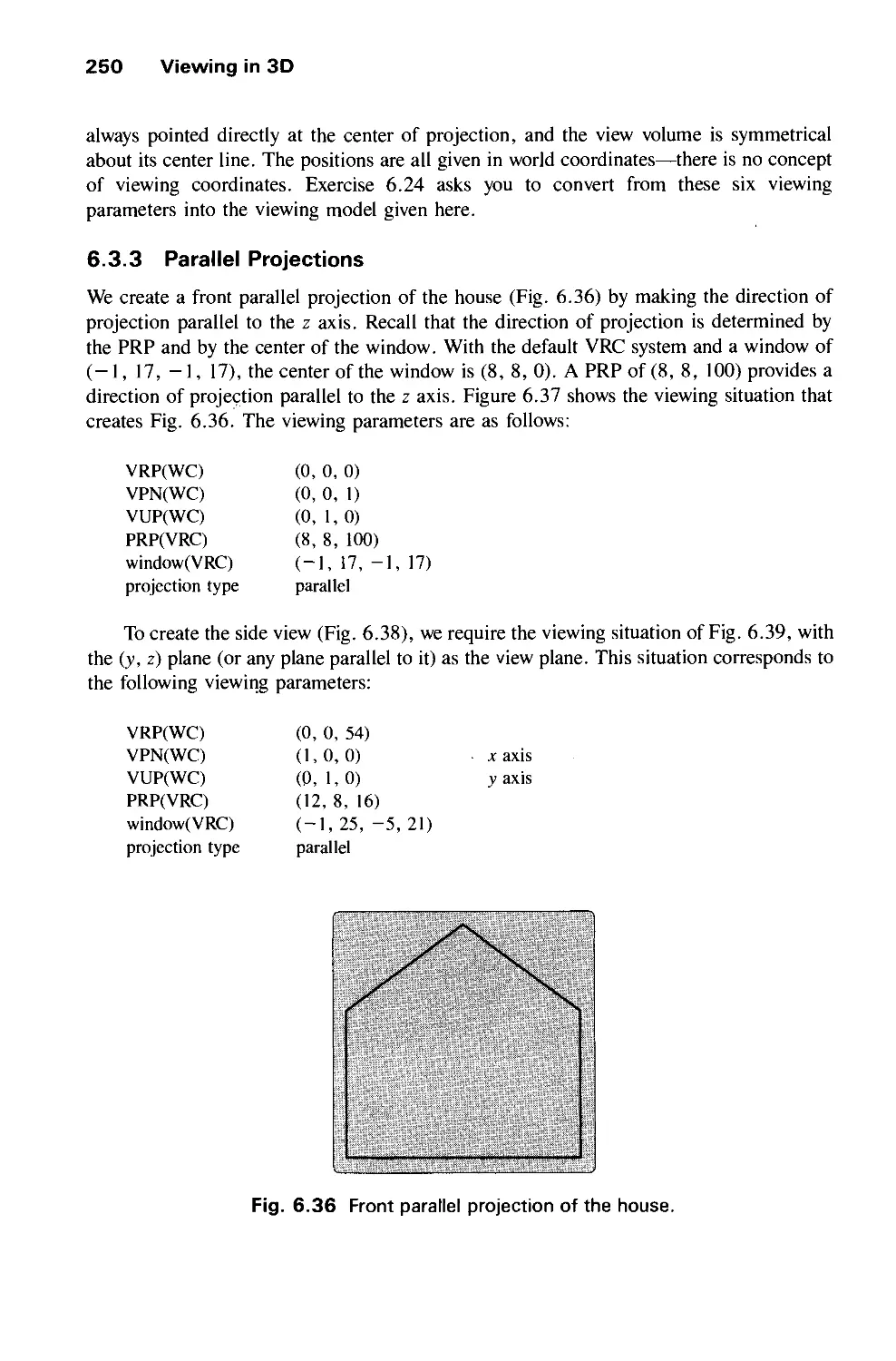
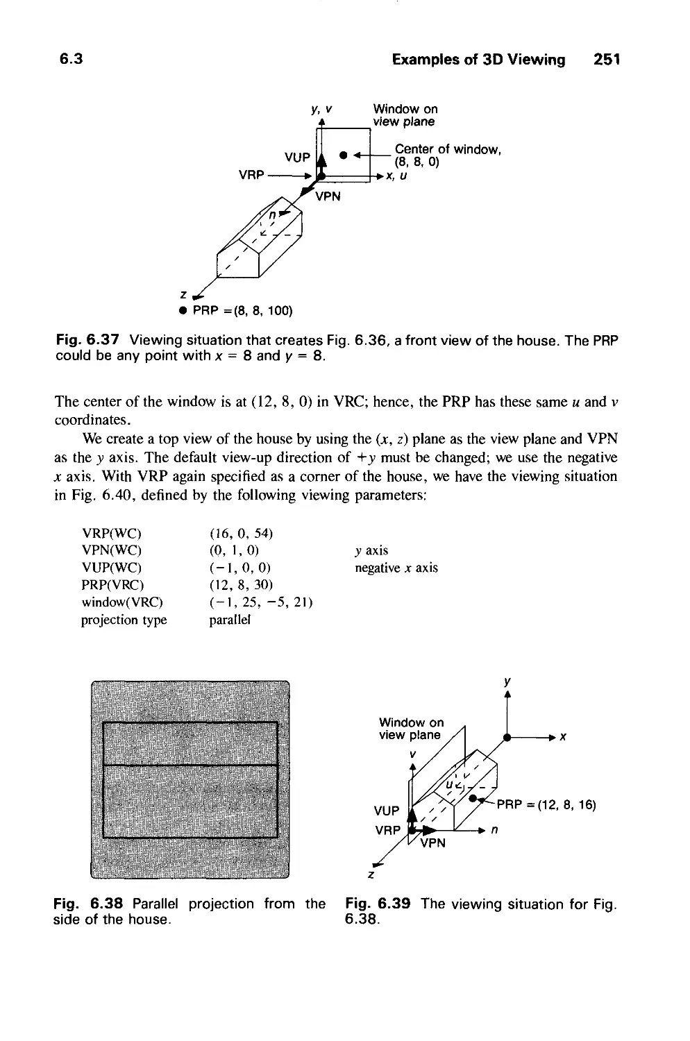
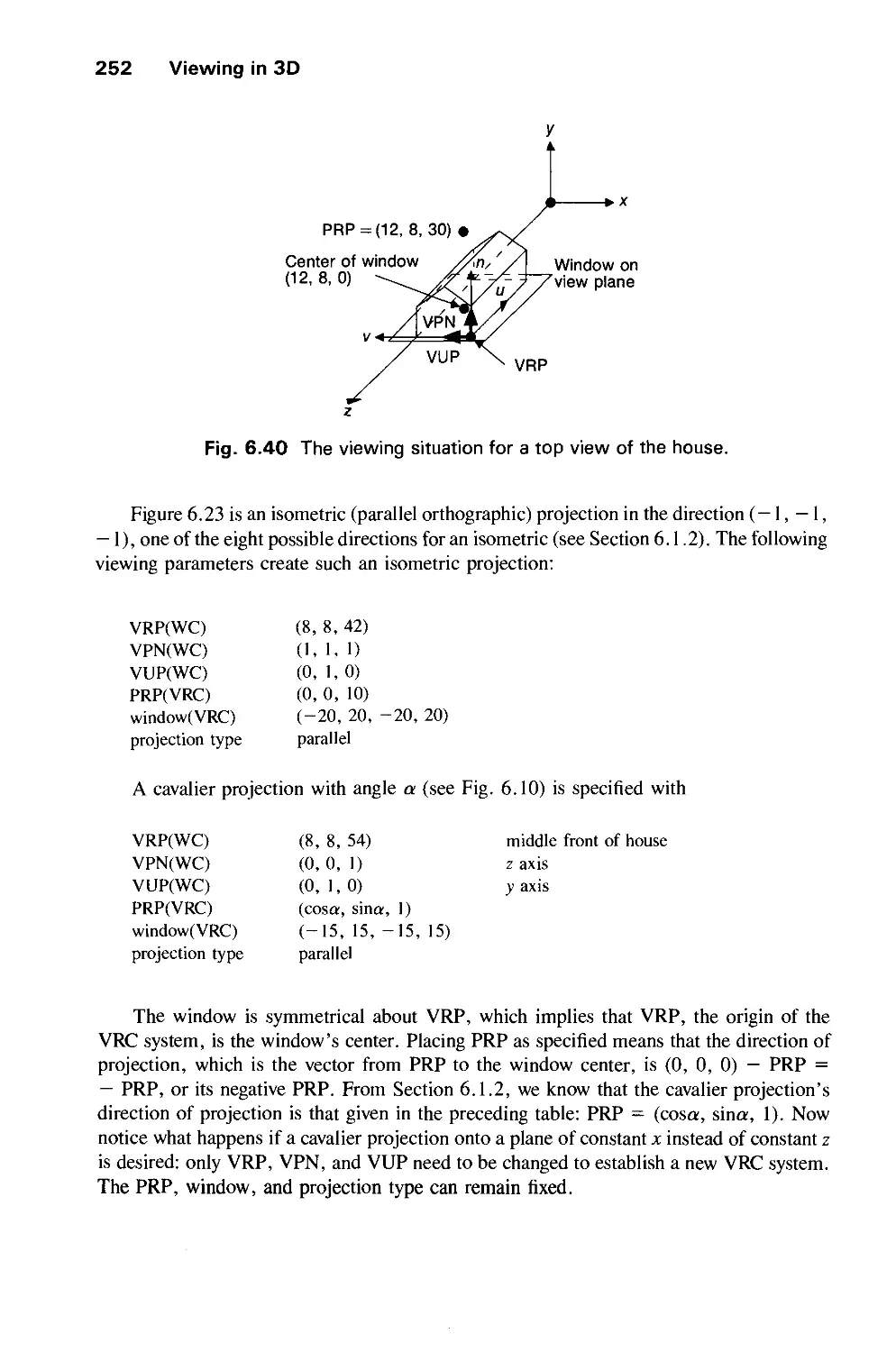
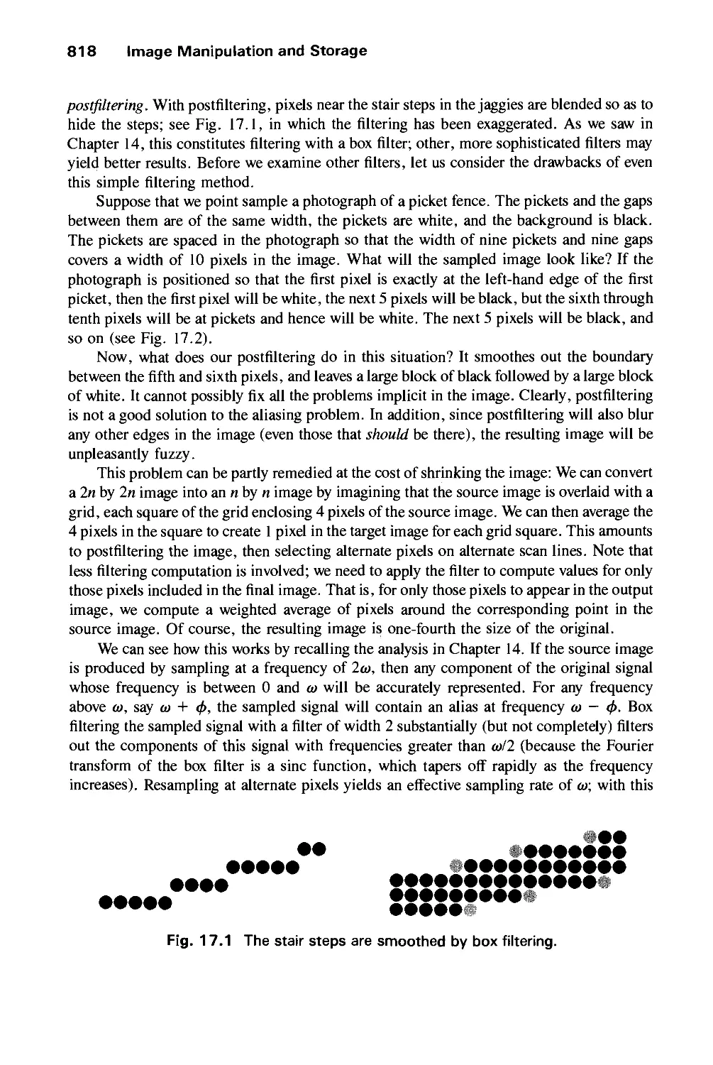
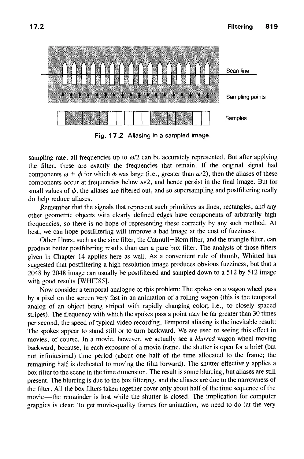
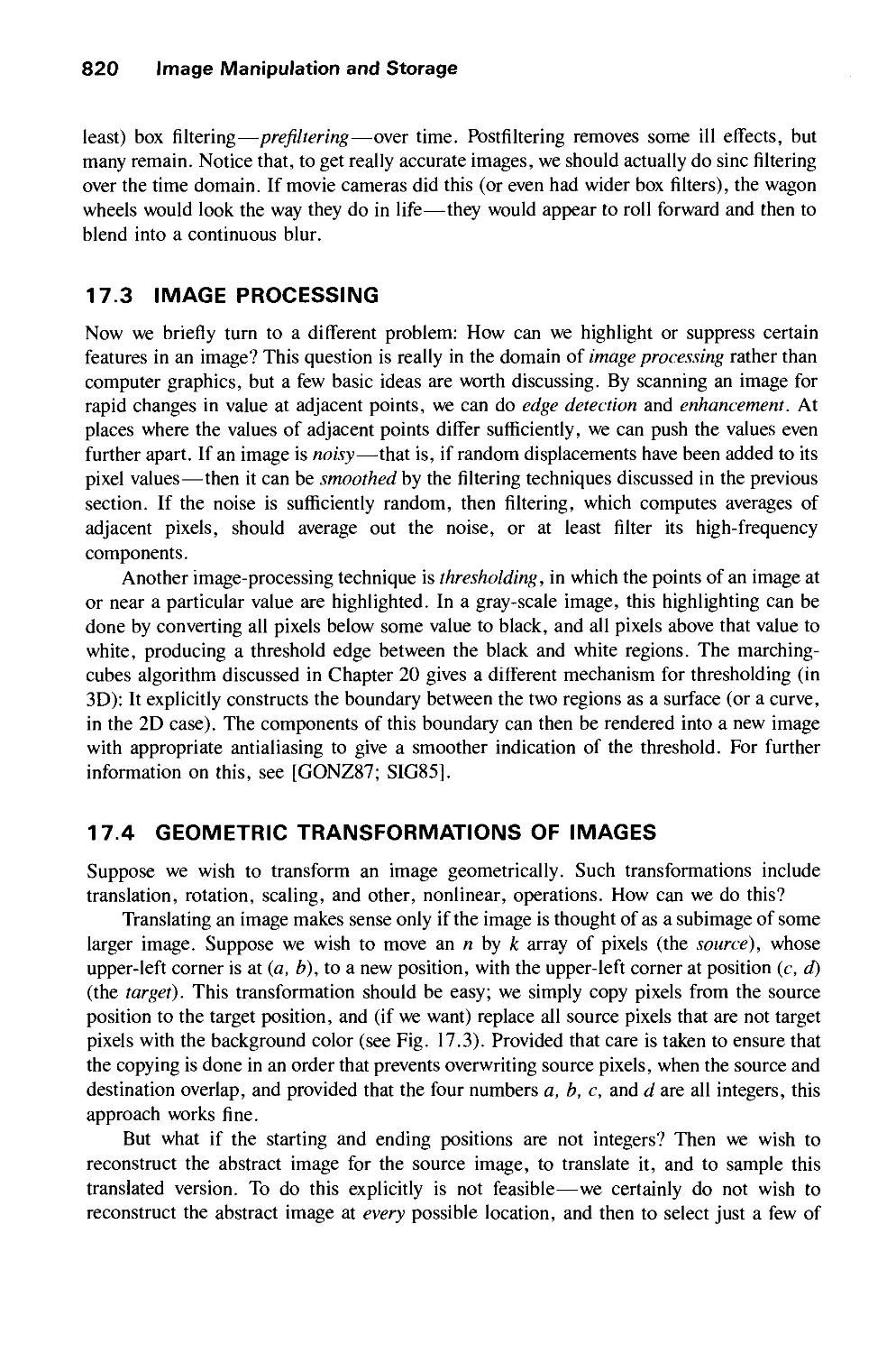
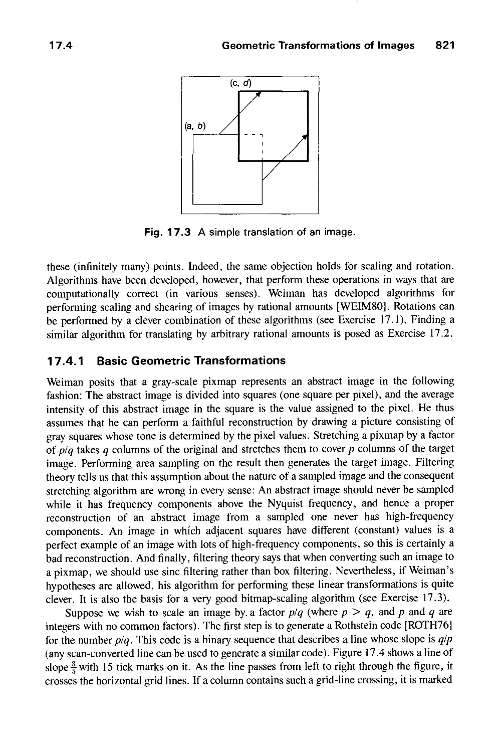
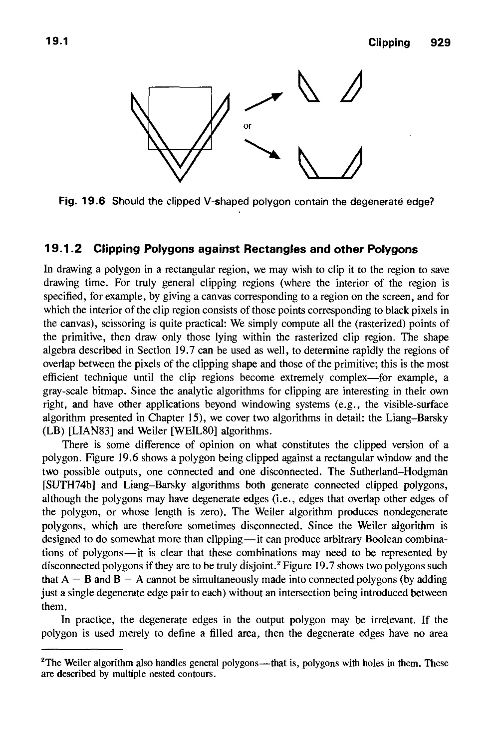
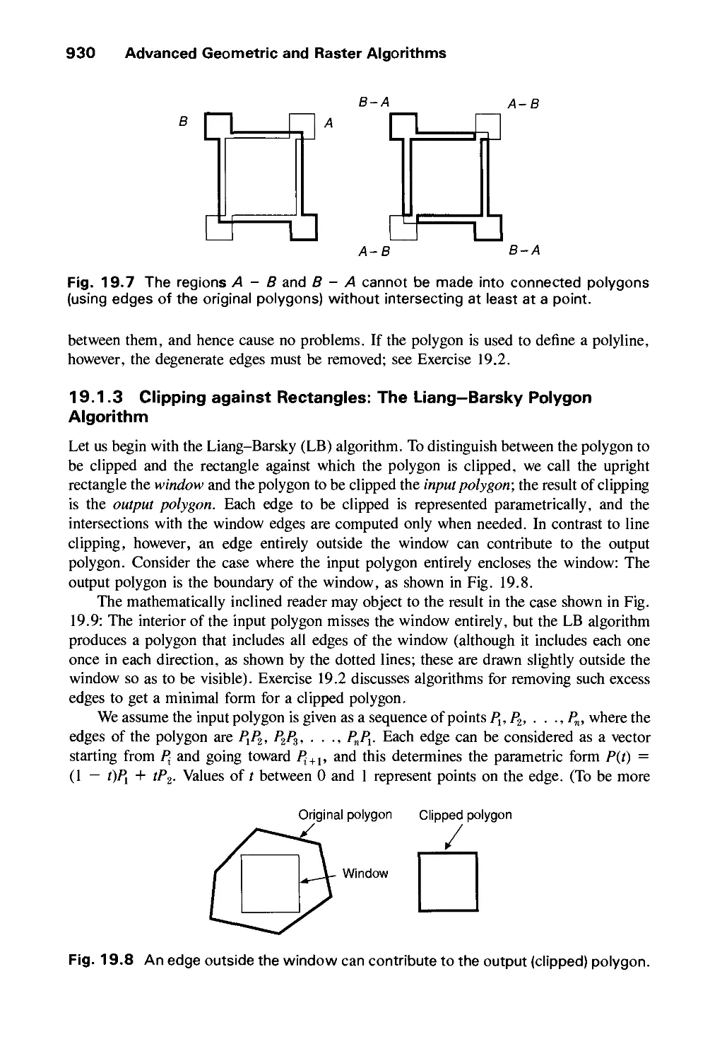
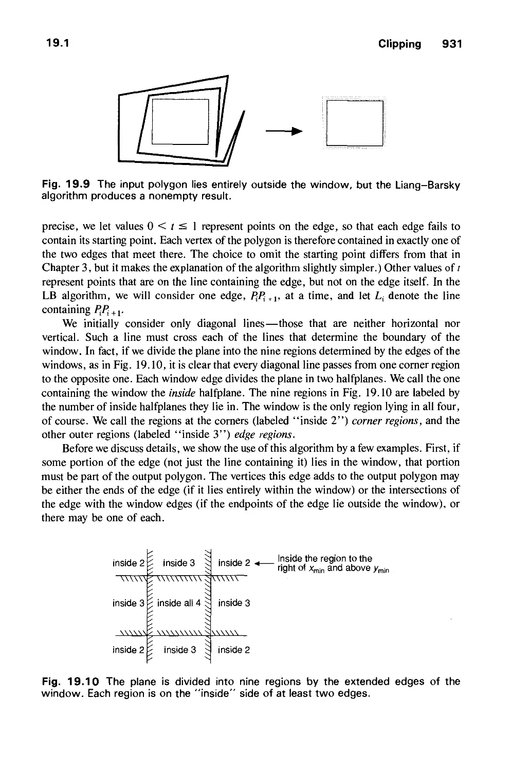
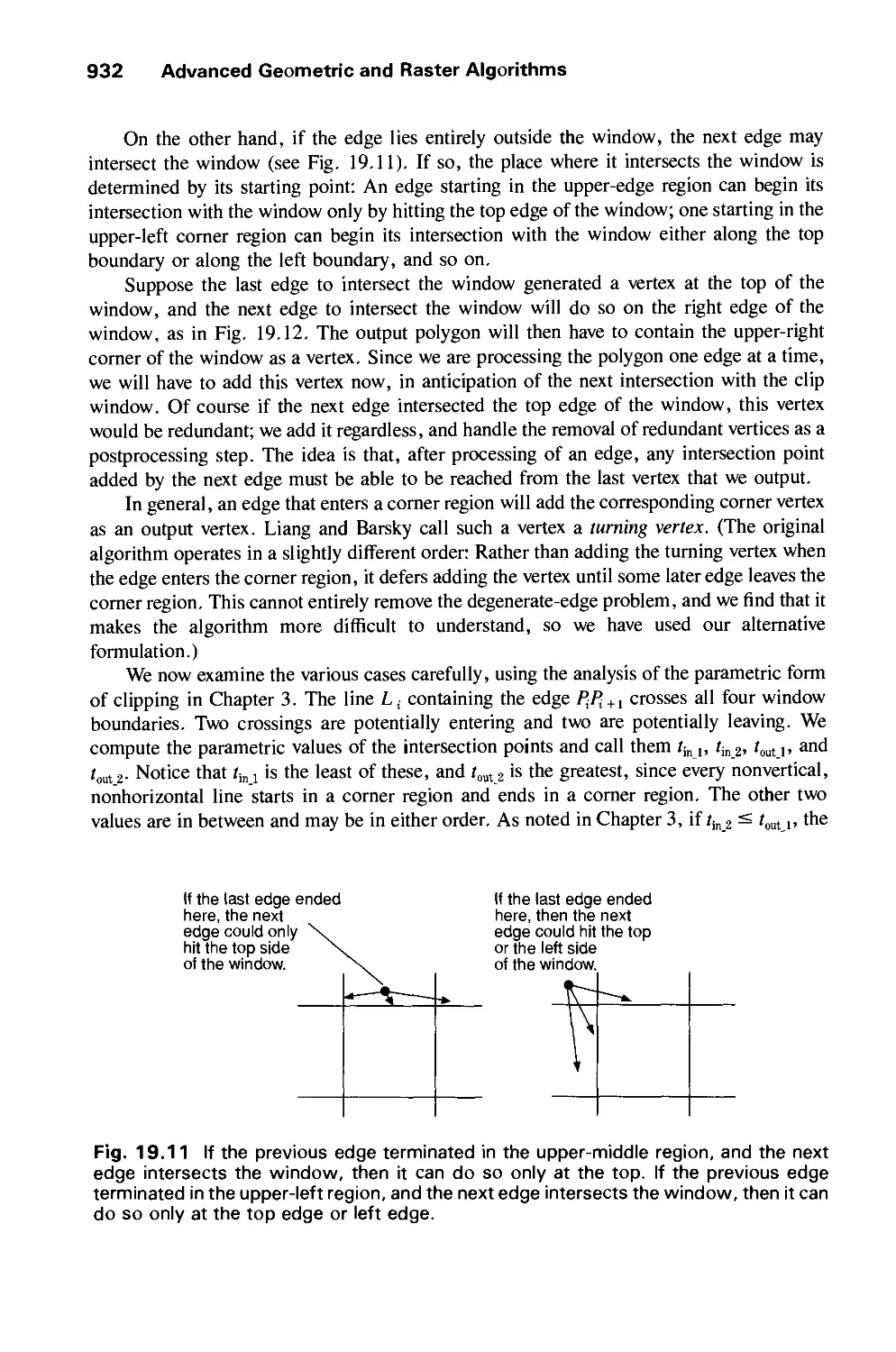
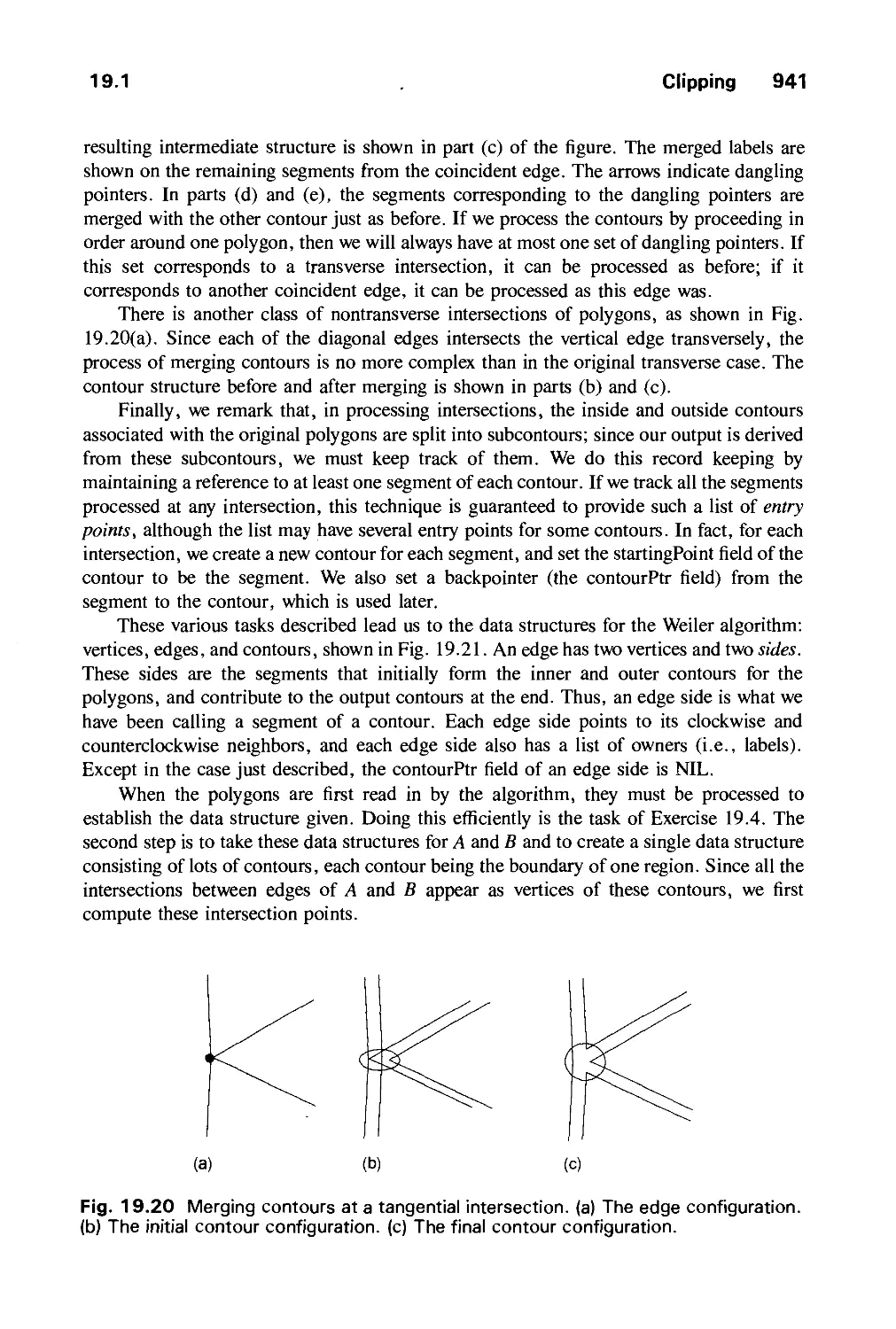
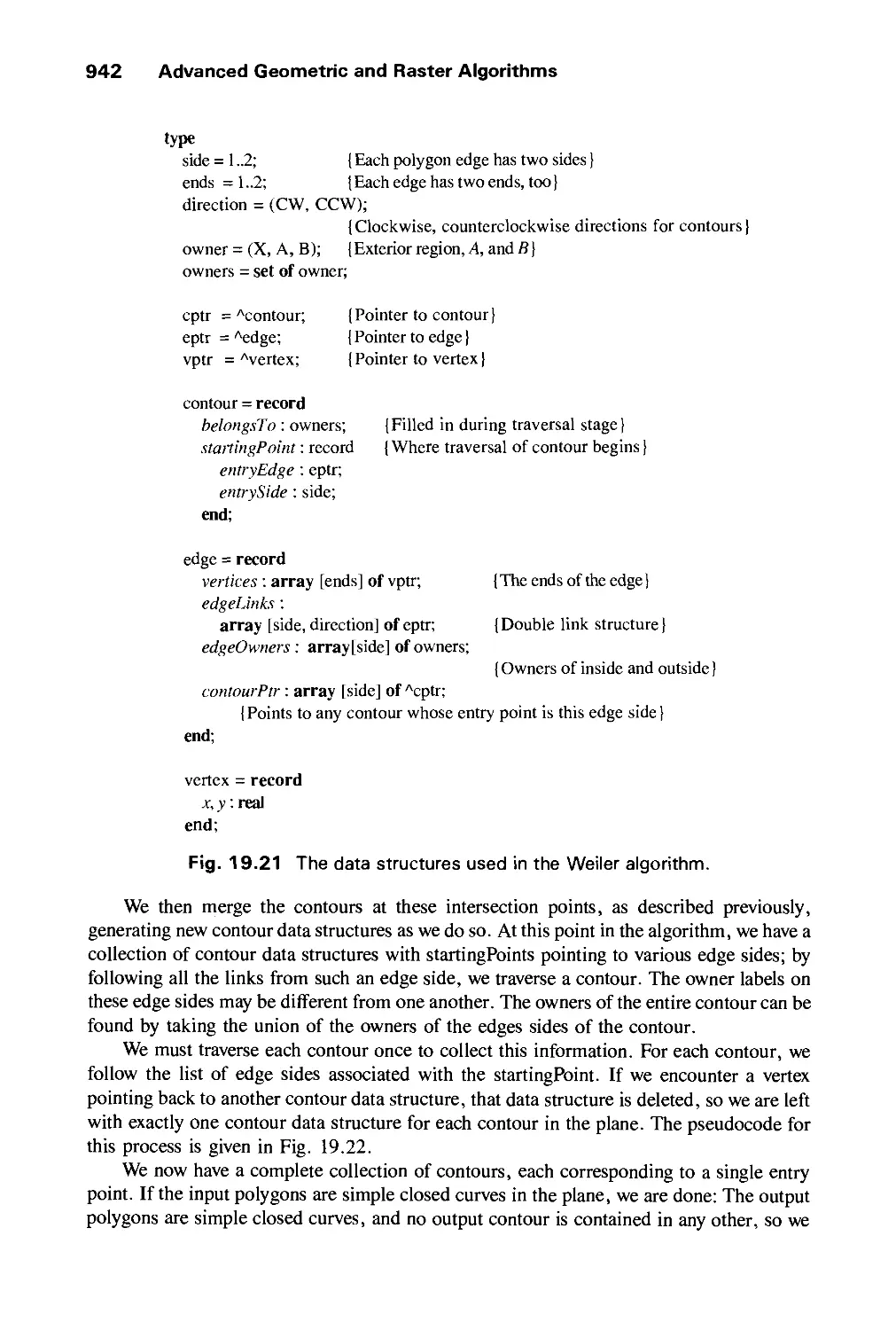
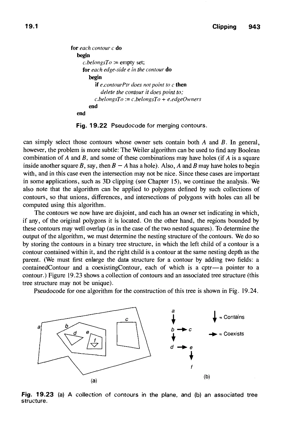
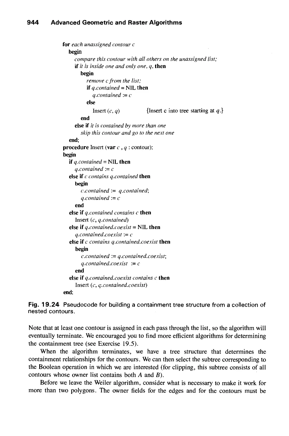
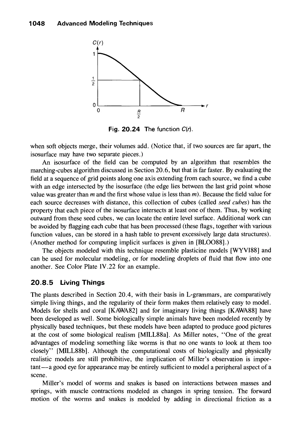
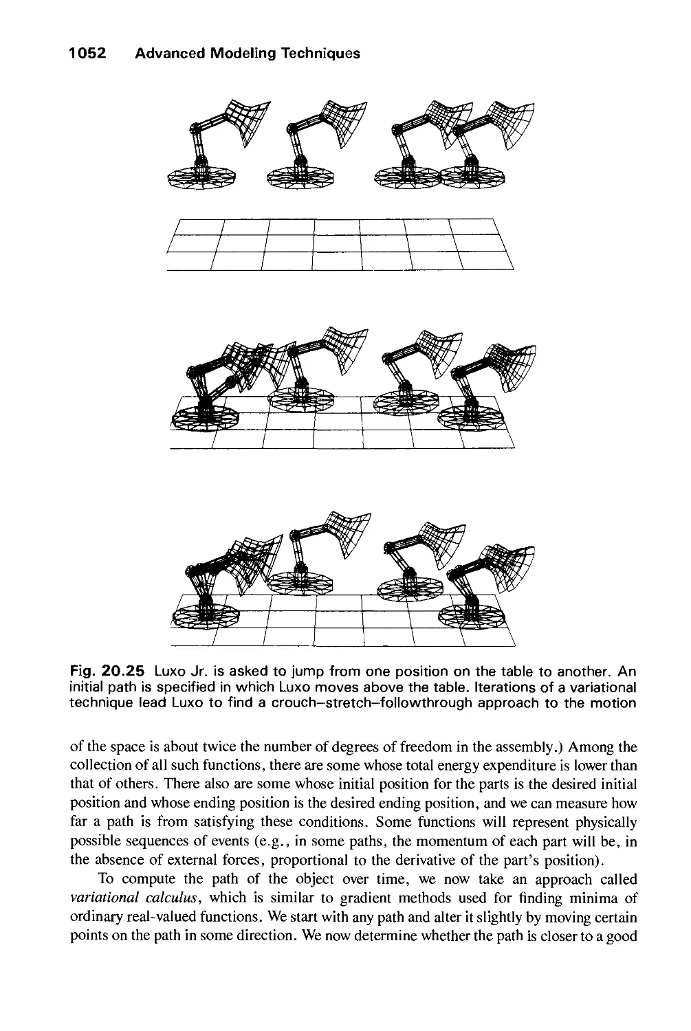
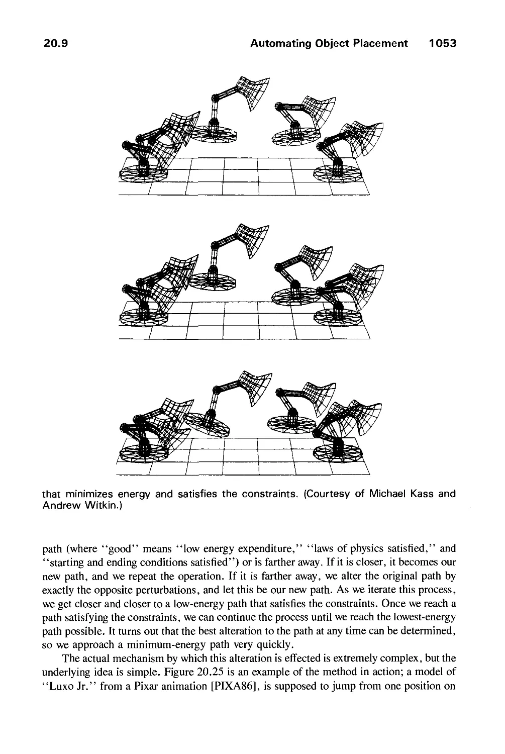
/


Автор: Foley J.D. Dam A.Van Hughes J.F. Feiner S.K.
Теги: computer graphics
ISBN: 0-201-12110-7
Год: 1990


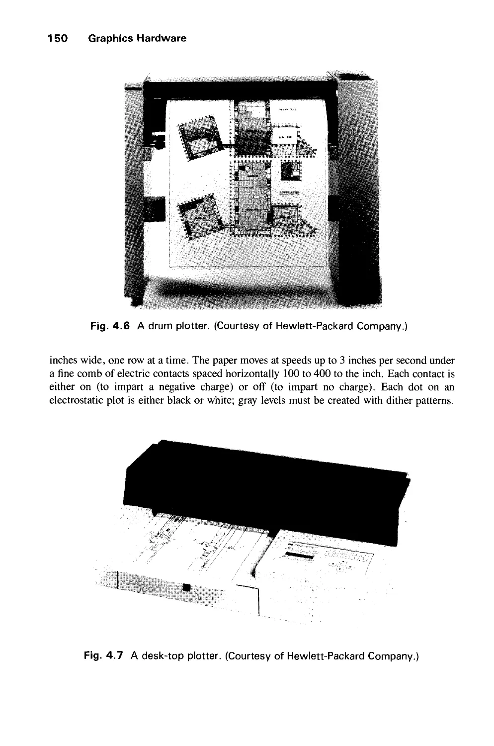
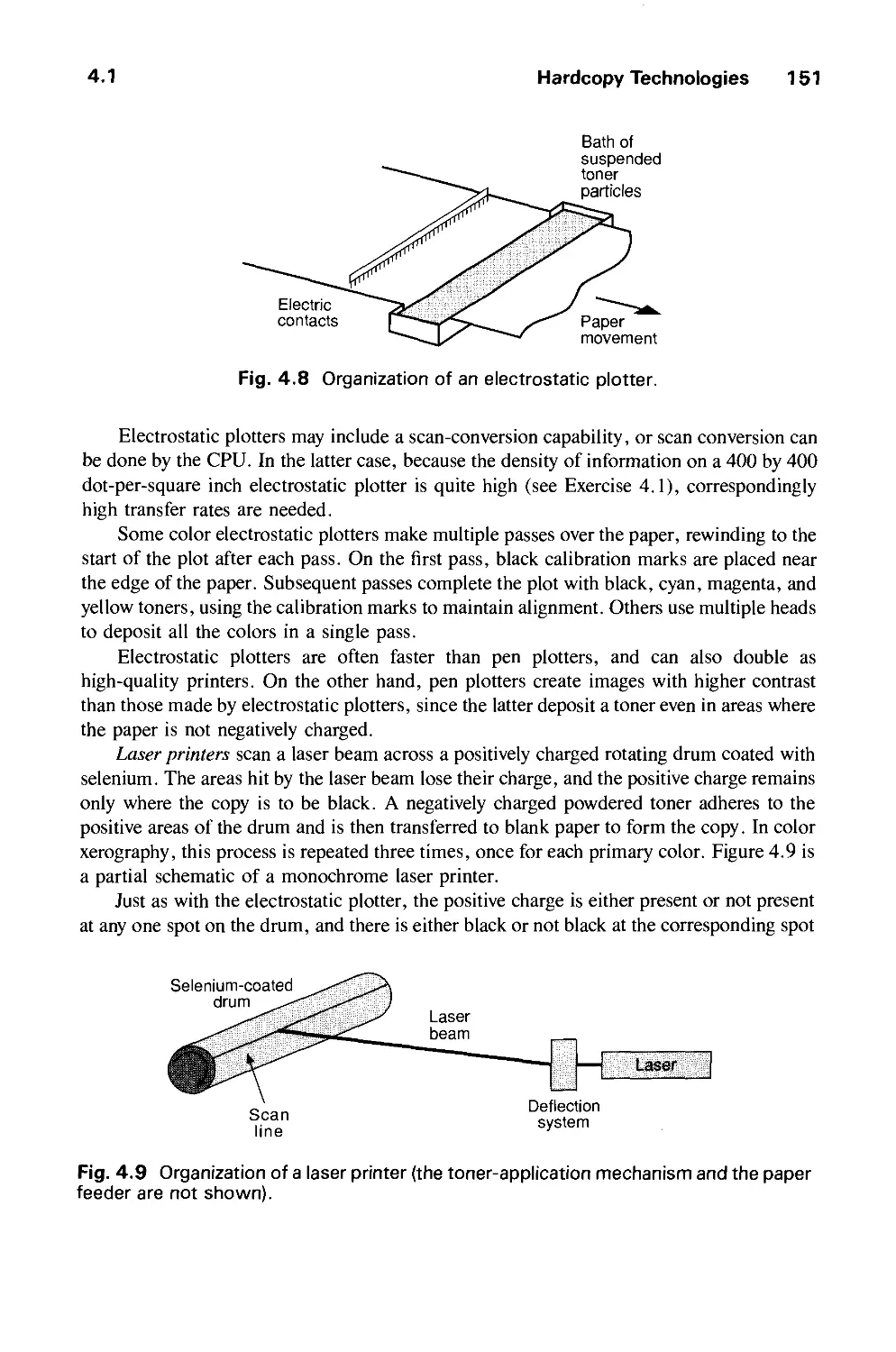
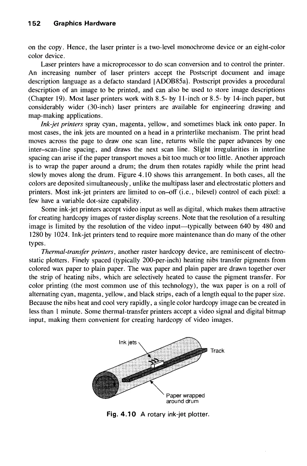
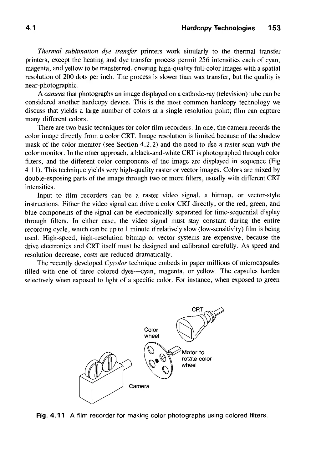
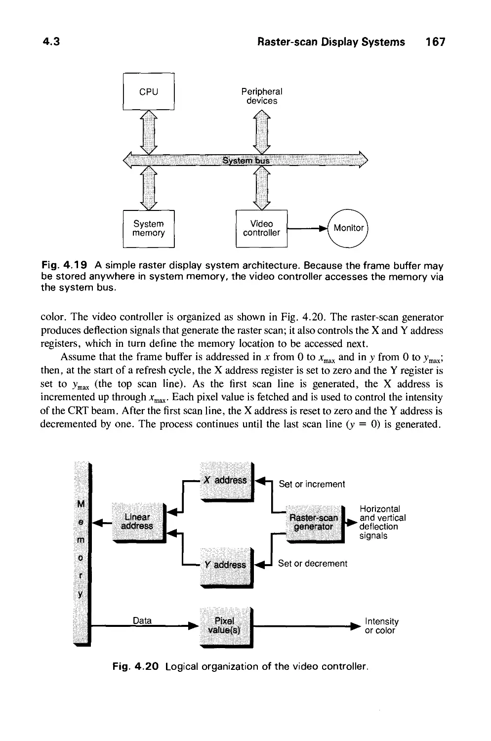
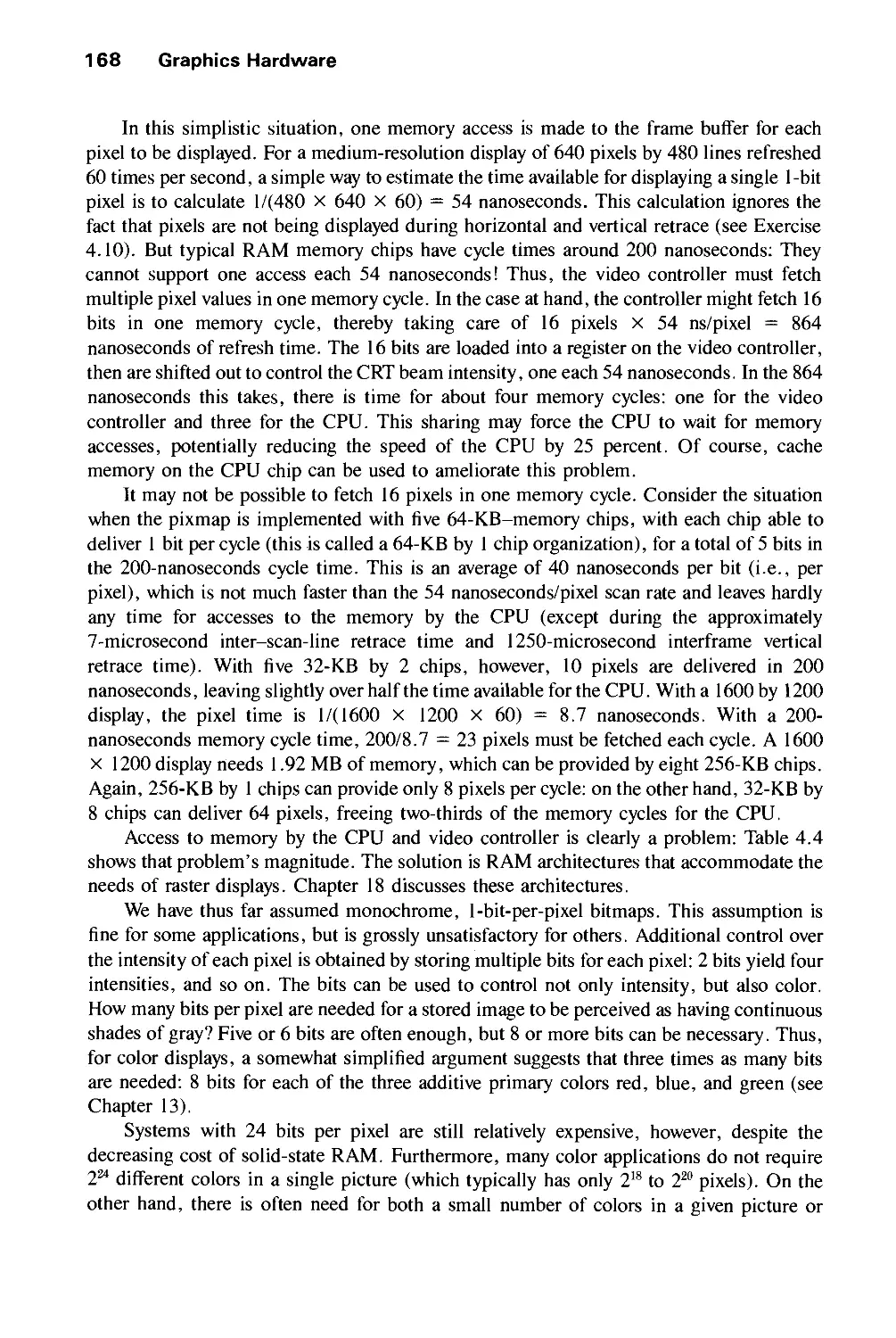
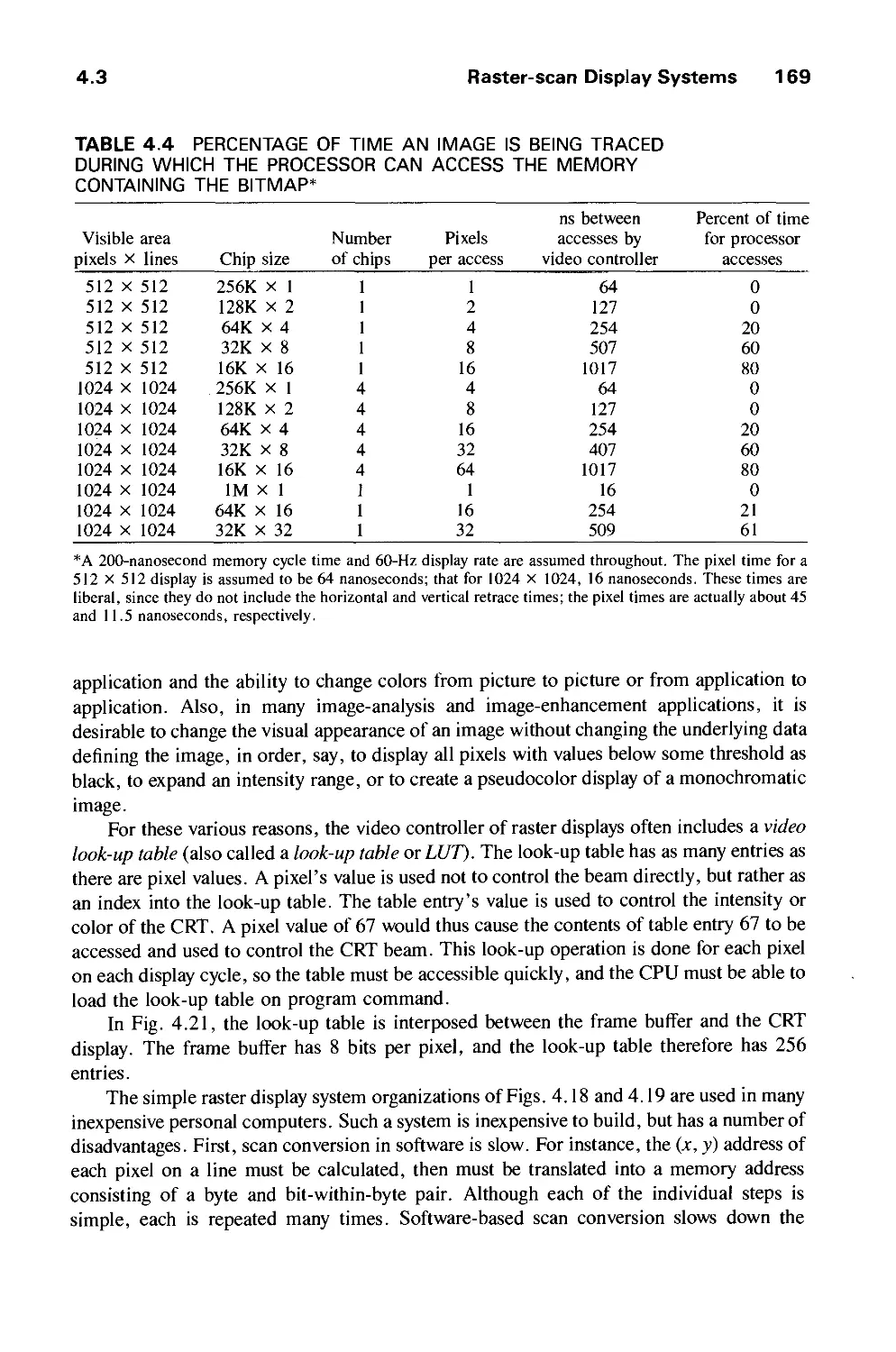
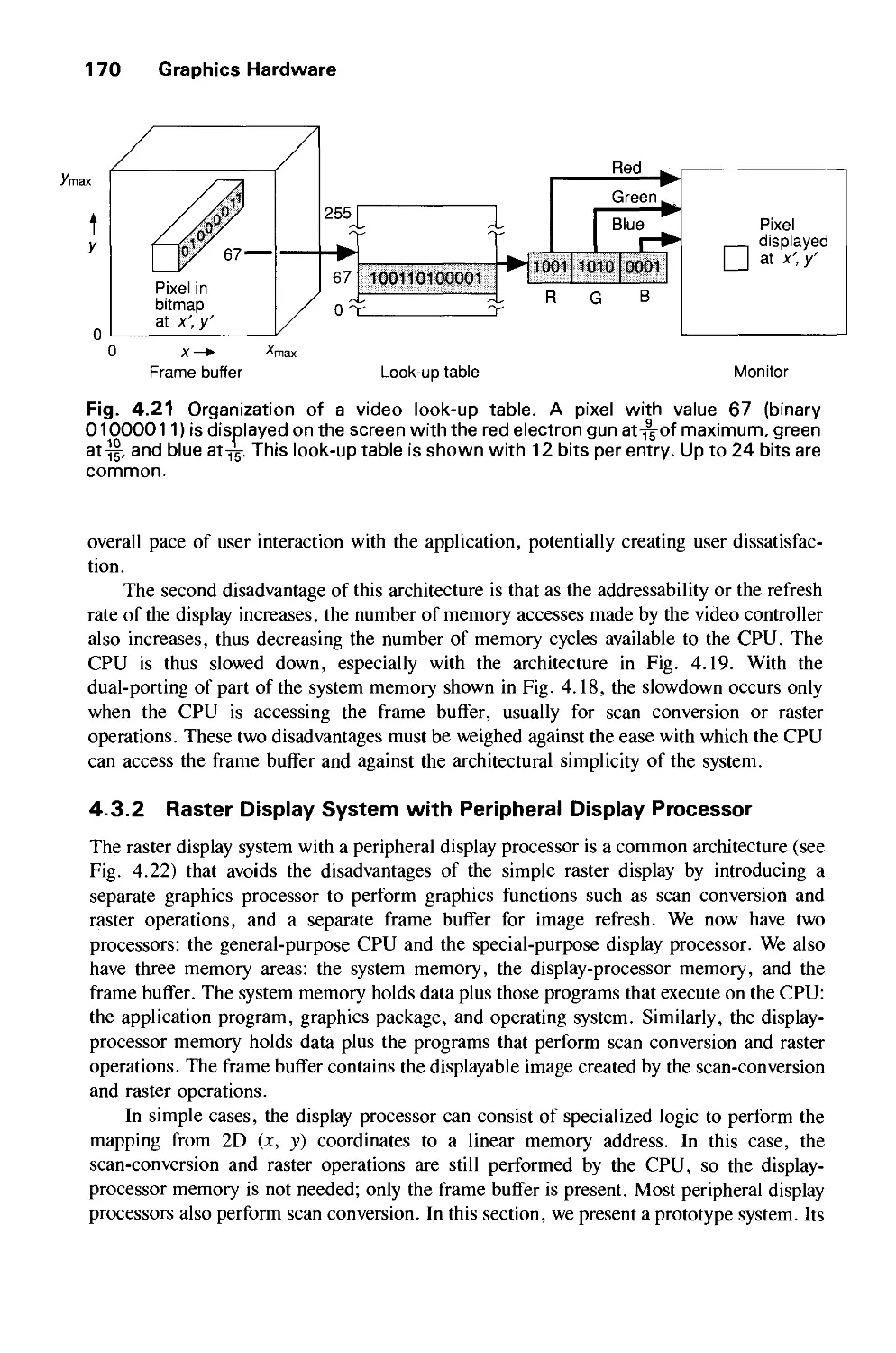
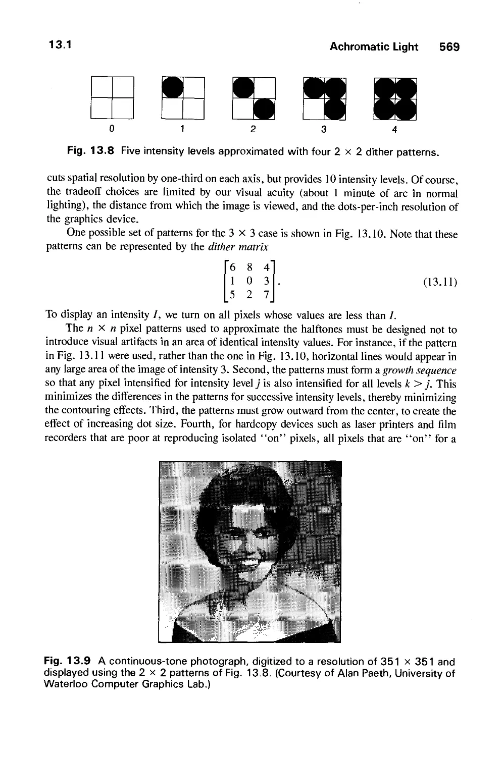
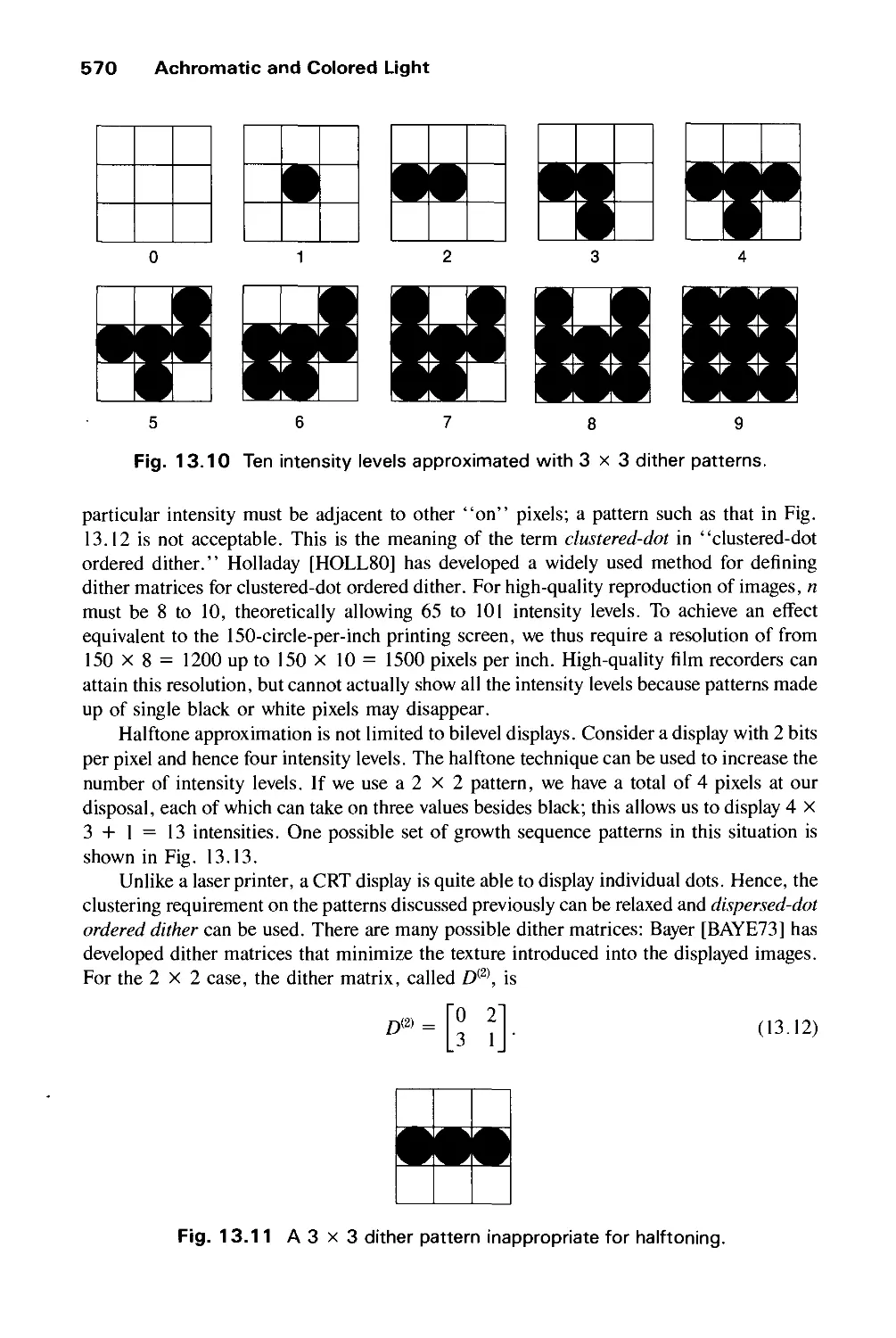
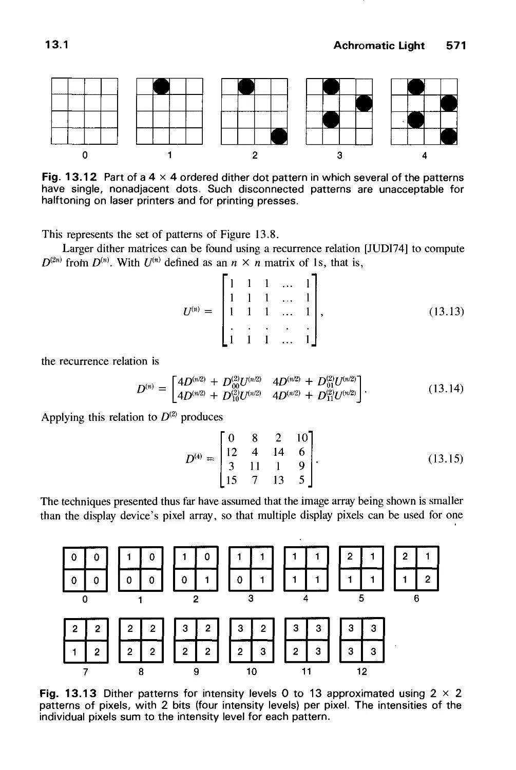
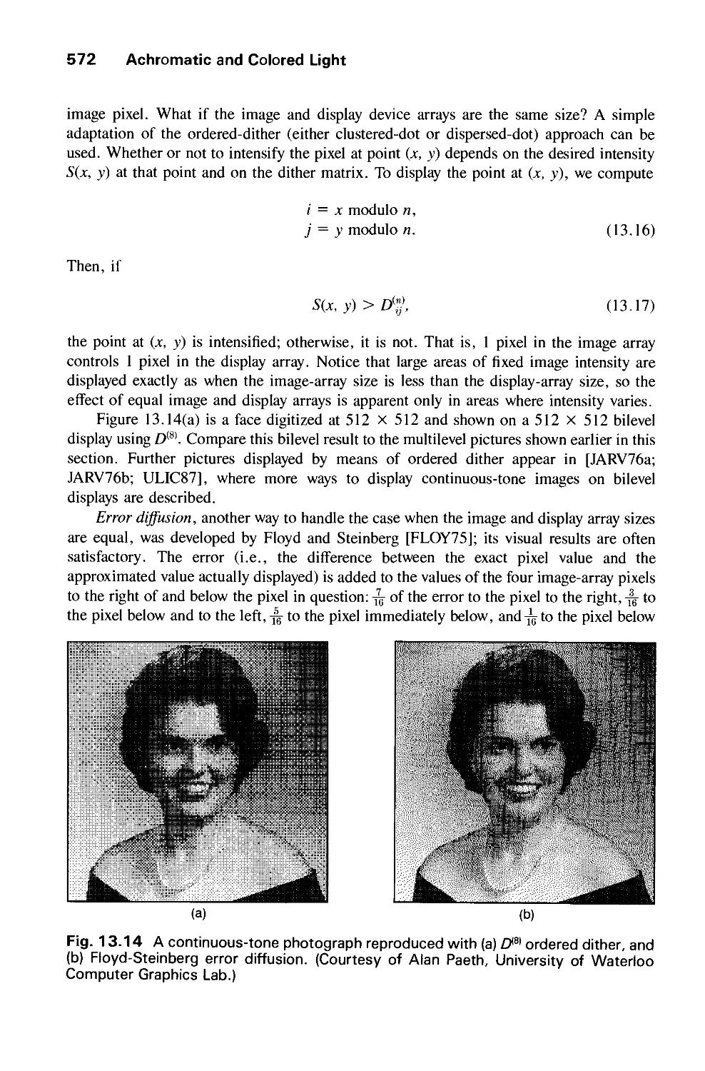
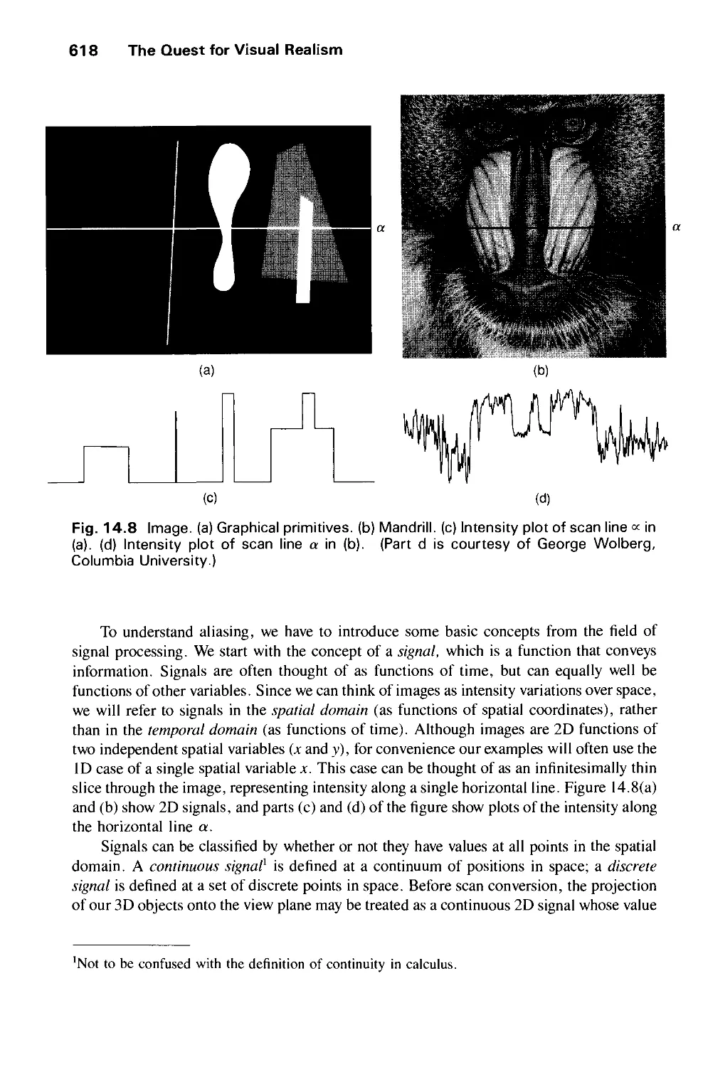
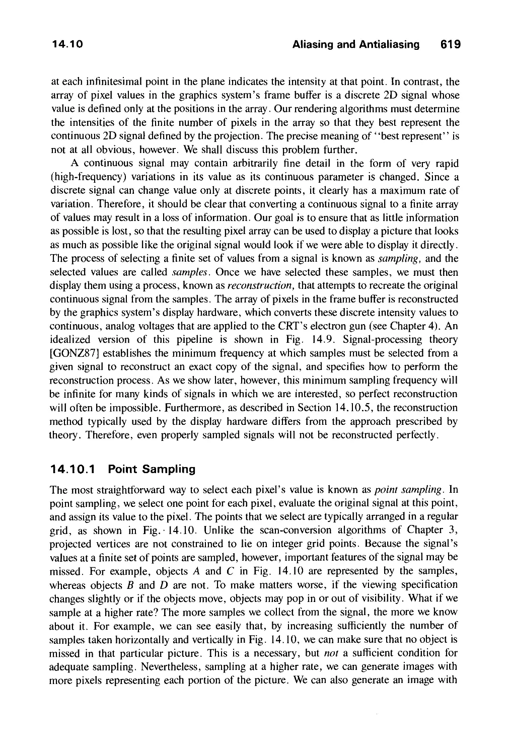
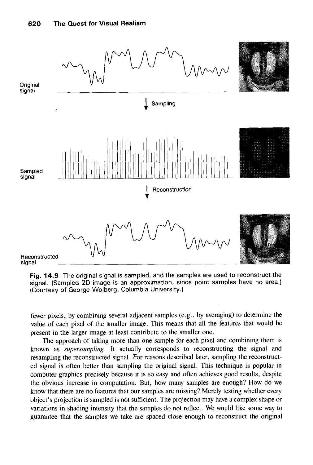
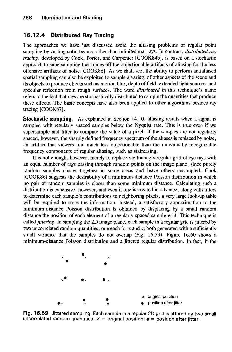
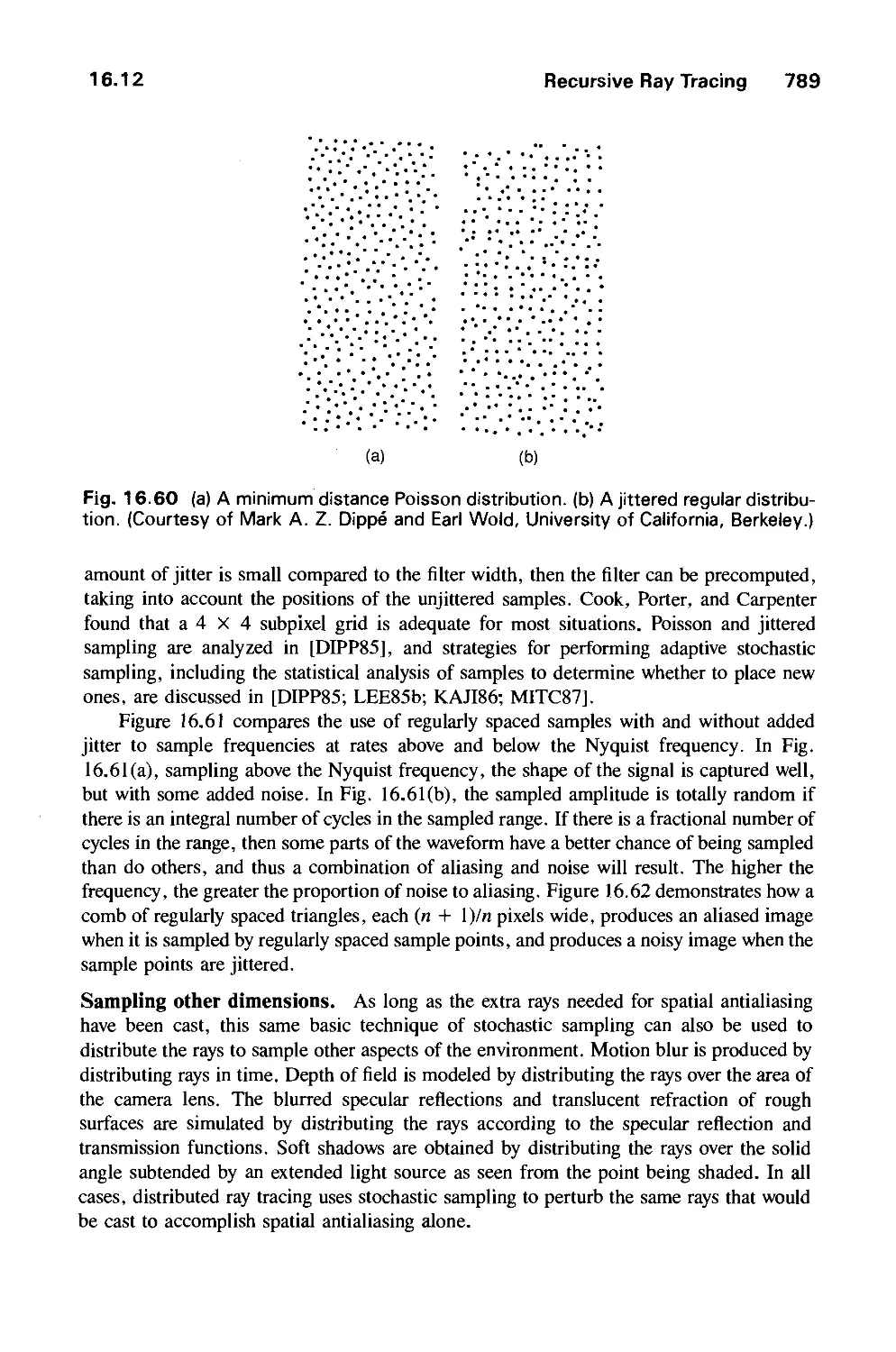
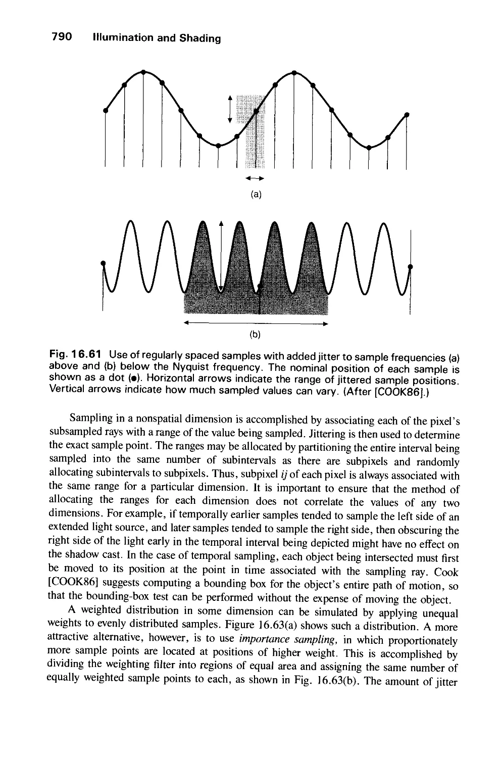
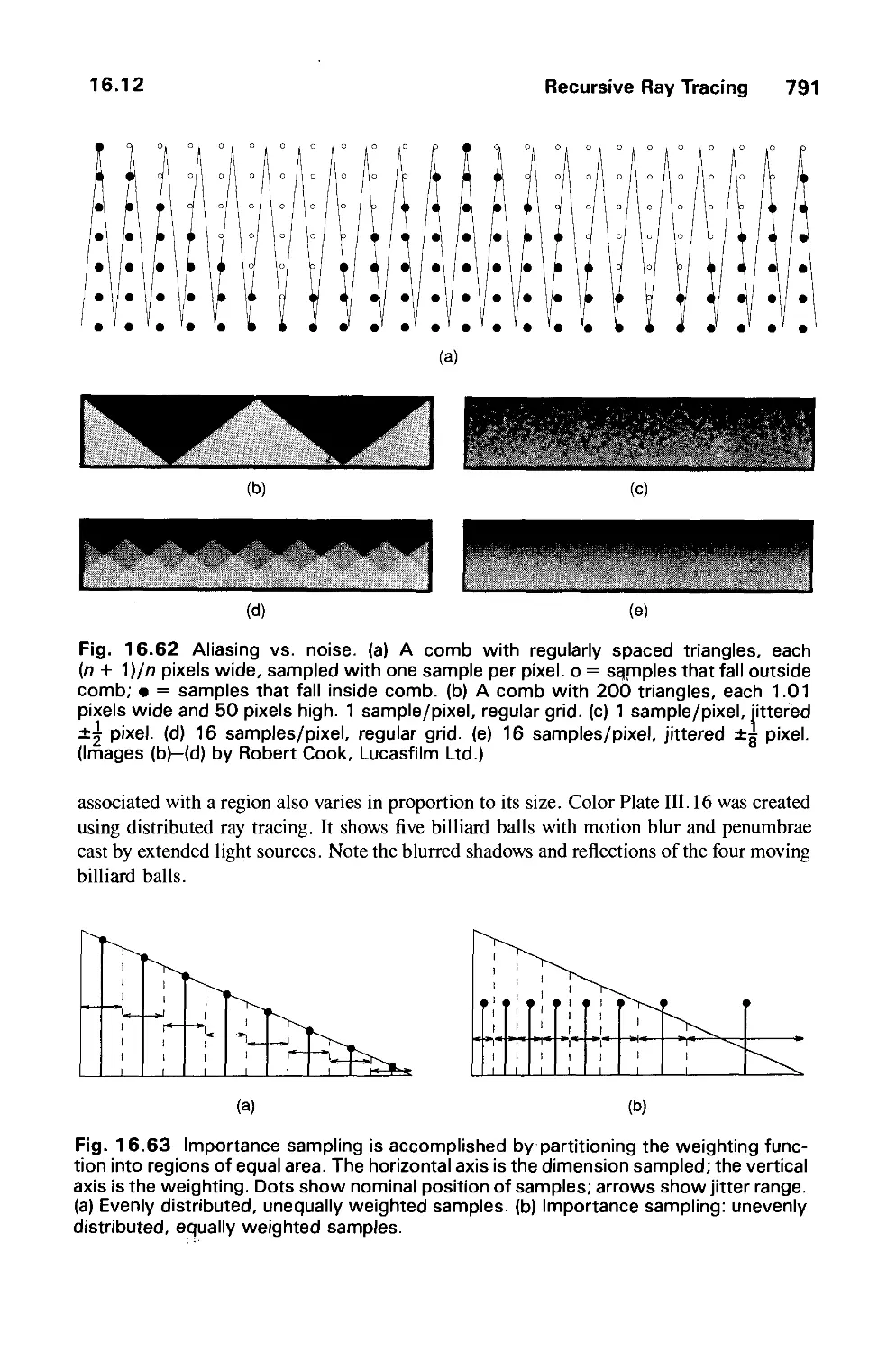
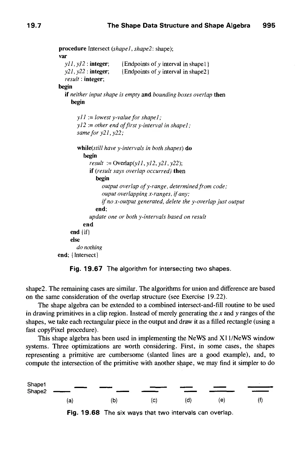
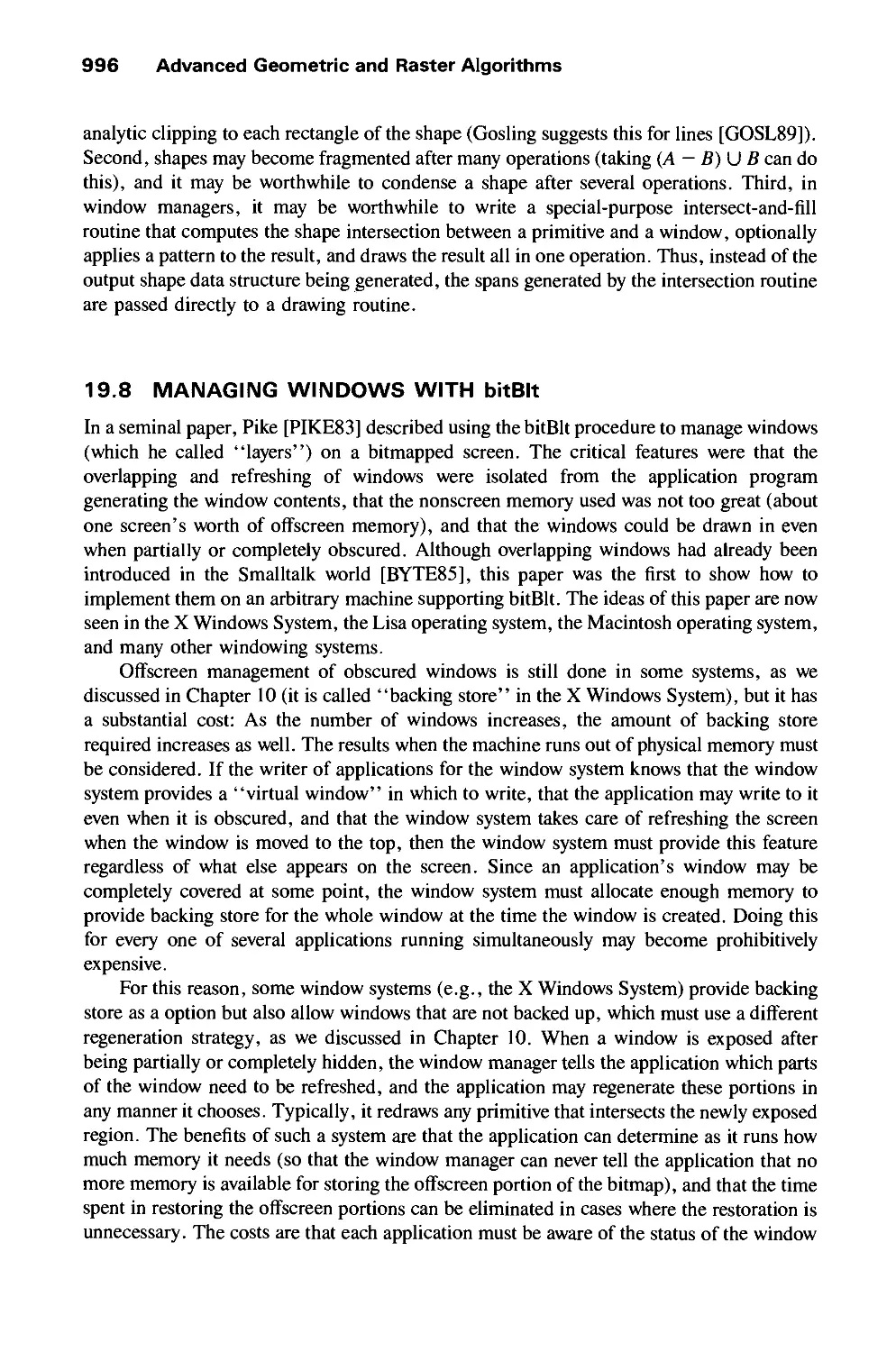
Текст
THE
SYSTEMS
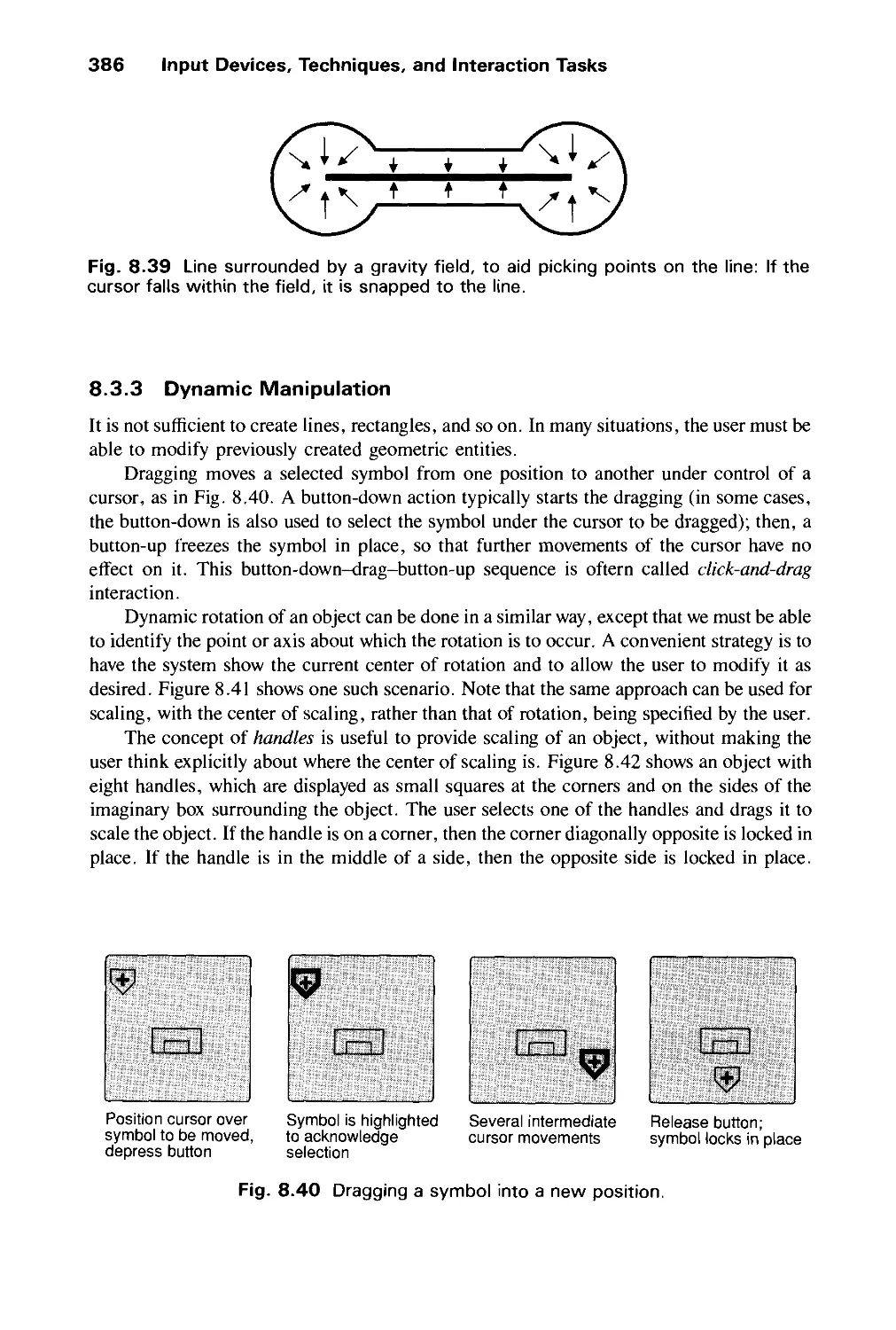
PROG G
SERIES
Computer
Graphics:
' iplesand
-ctice
Second Edition
Foley ♦ van Dam ♦ Feiner ♦ Hughes
SECOND EDITION
Computer Graphics
PRINCIPLES AND PRACTICE
SECOND EDITION
Computer Graphics
PRINCIPLES AND PRACTICE
James D. Foley
The George Washington University
Andries van Dam
Brown University
Steven K. Feiner
Columbia University
John F. Hughes
Brown University
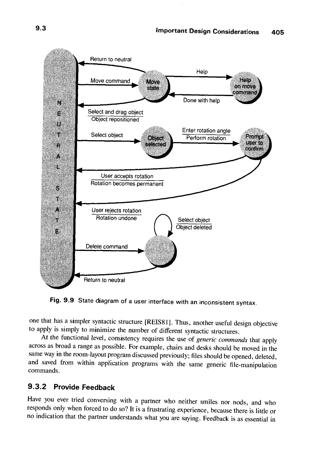
A
TT
ADDISON-WESLEY PUBLISHING COMPANY
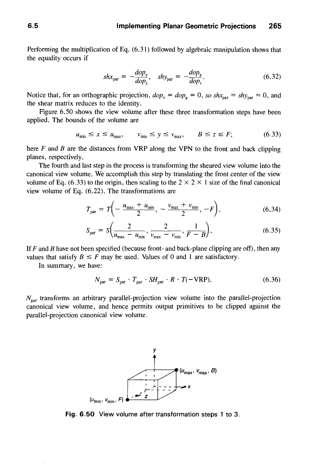
Reading, Massachusetts ♦ Menlo Park, California ♦ New York
Don Mills, Ontario ♦ Wokingham, England ♦ Amsterdam ♦ Bonn
Sydney ♦ Singapore ♦ Tokyo ♦ Madrid ♦ San Juan
Sponsoring Editor: Keith Wollman
Production Supervisor: Bette J. Aaronson
Copy Editor: Lyn Dupre
Text Designer: Herb Caswell
Technical Art Consultant: Joseph K. Vetere
Illustrators: C&C Associates
Cover Designer: Marshall Henrichs
Manufacturing Manager: Roy Logan
This book is in the Addison-Wesley Systems Programming Series
Consulting editors: IBM Editorial Board
Library of Congress Cataloging-in-Publication Data
Computer graphics: principles and practice/James D. Foley . . . [et
al.].—2nd ed.
p. cm.
Includes bibliographical references.
ISBN 0-201-12110-7
1. Computer graphics. I. Foley, James D., 1942-.
T385.C587 1990
006.6—dc20 89-35281
CIP
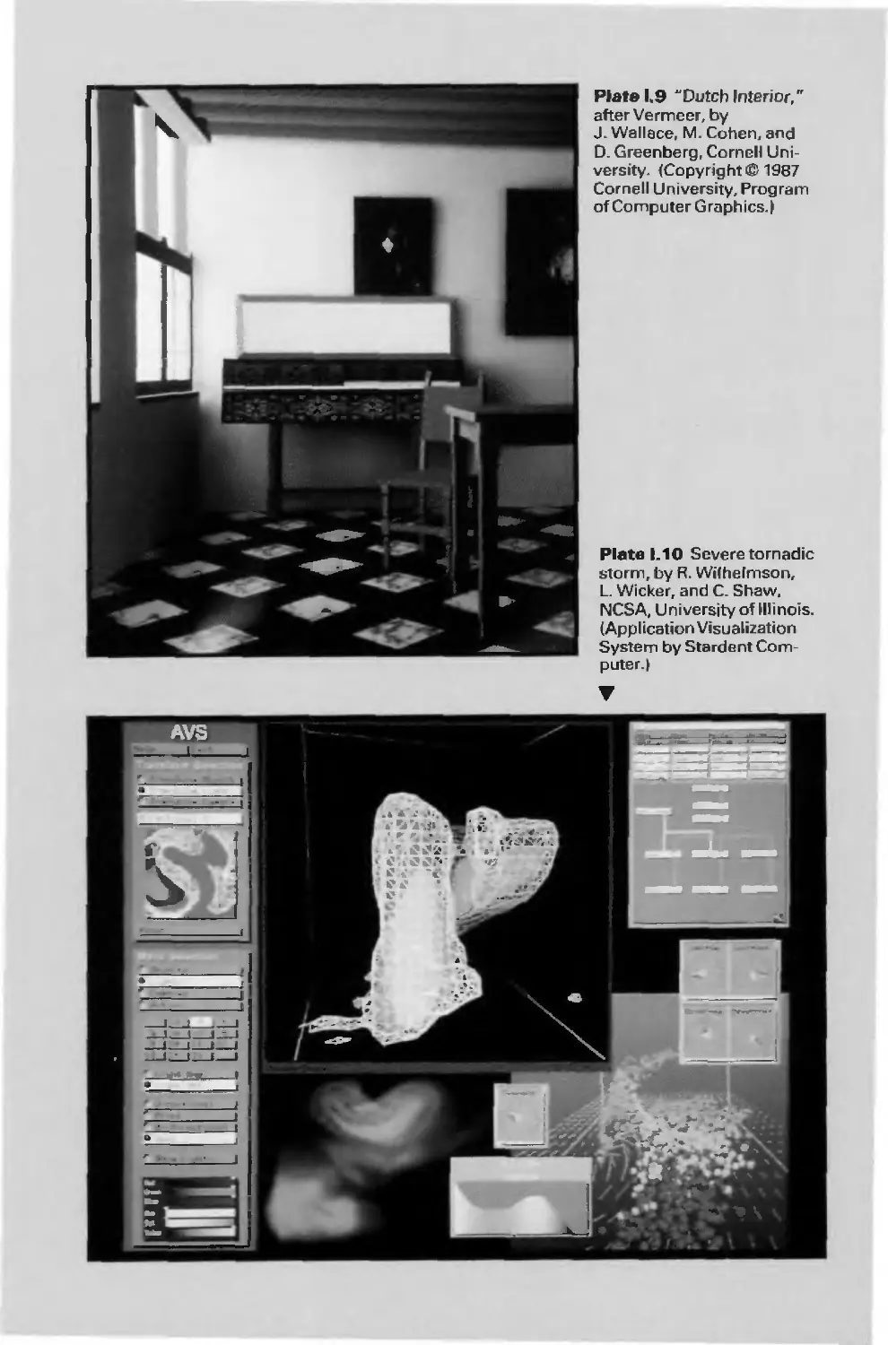
Cover: "Dutch Interior," after Vermeer, by J. Wallace, M. Cohen, and D. Greenberg, Cornell University
(Copyright © 1987 Cornell University, Program of Computer Graphics.)
Many of the designations used by manufacturers and sellers to distinguish their products are claimed as
trademarks. Where those designations appear in this book, and Addison-Wesley was aware of a trademark
claim, the designations have been printed in initial caps or all caps.
The programs and applications presented in this book have been included for their instructional value. They are
not guaranteed for any particular purpose. The publisher and the author do not offer any warranties or
representations, nor do they accept any liabilities with respect to the programs or applications.
Copyright © 1990 by Addison-Wesley Publishing Company, Inc.
All rights reserved. No part of this publication may be reproduced, stored in a retrieval system, or transmitted,
in any form or by any means, electronic, mechanical, photocopying, recording, or otherwise, without the prior
written permission of the publisher. Printed in the United States of America.
ABCDEFGHIJ-DO-943210
To Marylou, Heather, Jenn, my parents, and my teachers
Jim
To Debbie, my father, my mother in memoriam, and
my children Elisa, Lori, and Katrin
Andy
To Jenni, my parents, and my teachers
Steve
To my family, my teacher Rob Kirby, and
my father in memoriam
John
And to all of our students.
THE SYSTEMS PROGRAMMING SERIES
Communications Architecture for Distributed Systems R.J. Cypser
An Introduction to Database Systems, Volume I, C.J. Date
Fifth Edition
An Introduction to Database Systems, Volume II
Computer Graphics: Principles and Practice,
Second Edition
Structured Programming: Theory and Practice
C.J. Date
James D. Foley
Andries van Dam
Steven K. Feiner
John F. Hughes
Richard C. Linger
Harlan D. Mills
Bernard I. Witt
Conceptual Structures: Information Processing in
Mind and Machines
John F. Sowa
IBM EDITORIAL BOARD
Chairman:
Gene F. Hoffnagle
Foreword
The field of systems programming primarily grew out of the efforts of many programmers
and managers whose creative energy went into producing practical, utilitarian systems
programs needed by the rapidly growing computer industry. Programming was practiced as
an art where each programmer invented his own solutions to problems with little guidance
beyond that provided by his immediate associates. In 1968, the late Ascher Opler, then at
IBM, recognized that it was necessary to bring programming knowledge together in a form
that would be accessible to all systems programmers. Surveying the state of the art, he
decided that enough useful material existed to justify a significant codification effort. On his
recommendation, IBM decided to sponsor The Systems Programming Series as a long term
project to collect, organize, and publish those principles and techniques that would have
lasting value throughout the industry. Since 1968 eighteen titles have been published in the
Series, of which six are currently in print.
The Series consists of an open-ended collection of text-reference books. The contents
of each book represent the individual author's view of the subject area and do not
necessarily reflect the views of the IBM Corporation. Each is organized for course use but is
detailed enough for reference.
Representative topic areas already published, or that are contemplated to be covered by
the Series, include: database systems, communication systems, graphics systems, expert
systems, and programming process management. Other topic areas will be included as the
systems programming discipline evolves and develops.
The Editorial Board
IX
Preface
Interactive graphics is a field whose time has come. Until recently it was an esoteric
specialty involving expensive display hardware, substantial computer resources, and
idiosyncratic software. In the last few years, however, it has benefited from the steady
and sometimes even spectacular reduction in the hardware price/performance ratio
(e.g., personal computers for home or office with their standard graphics terminals),
and from the development of high-level, device-independent graphics packages that
help make graphics programming rational and straighforward. Interactive graphics
packages that help make graphics programming rational and straightforward.
Interactive graphics is now finally ready to fulfill its promise to provide us with
pictorial communication and thus to become a major facilitator of man/machine
interaction. (From preface, Fundamentals of Interactive Computer Graphics, James
Foley and Andries van Dam, 1982)
This assertion that computer graphics had finally arrived was made before the revolution in
computer culture sparked by Apple's Macintosh and the IBM PC and its clones. Now even
preschool children are comfortable with interactive-graphics techniques, such as the
desktop metaphor for window manipulation and menu and icon selection with a mouse.
Graphics-based user interfaces have made productive users of neophytes, and the desk
without its graphics computer is increasingly rare.
At the same time that interactive graphics has become common in user interfaces and
visualization of data and objects, the rendering of 3D objects has become dramatically
more realistic, as evidenced by the ubiquitous computer-generated commercials and movie
special effects. Techniques that were experimental in the early eighties are now standard
practice, and more remarkable "photorealistic" effects are around the corner. The simpler
kinds of pseudorealism, which took hours of computer time per image in the early eighties,
now are done routinely at animation rates (ten or more frames/second) on personal
computers. Thus "real-time" vector displays in 1981 showed moving wire-frame objects
made of tens of thousands of vectors without hidden-edge removal; in 1990 real-time raster
displays can show not only the same kinds of line drawings but also moving objects
composed of as many as one hundred thousand triangles rendered with Gouraud or Phong
shading and specular highlights and with full hidden-surface removal. The highest-
performance systems provide real-time texture mapping, antialiasing, atmospheric
attenuation for fog and haze, and other advanced effects.
Graphics software standards have also advanced significantly since our first edition.
The SIGGRAPH Core '79 package, on which the first edition's SGP package was based,
has all but disappeared, along with direct-view storage tube and refresh vector displays. The
much more powerful PHIGS package, supporting storage and editing of structure hierarchy,
has become an official ANSI and ISO standard, and it is widely available for real-time
XI
xii Preface
geometric graphics in scientific and engineering applications, along with PHIGS+, which
supports lighting, shading, curves, and surfaces. Official graphics standards complement
lower-level, more efficient de facto standards, such as Apple's QuickDraw, X Window
System's Xlib 2D integer raster graphics packages, and Silicon Graphics' GL 3D library.
Also widely available are implementations of Pixar's RenderMan interface for
photorealistic rendering and PostScript interpreters for hardcopy page and screen image description.
Better graphics software has been used to make dramatic improvements in the "look and
feel "of user interfaces, and we may expect increasing use of 3D effects, both for aesthetic
reasons and for providing new metaphors for organizing and presenting, and through
navigating information.
Perhaps the most important new movement in graphics is the increasing concern for
modeling objects, not just for creating their pictures. Furthermore, interest is growing in
describing the time-varying geometry and behavior of 3D objects. Thus graphics is
increasingly concerned with simulation, animation, and a "back to physics" movement in
both modeling and rendering in order to create objects that look and behave as realistically
as possible.
As the tools and capabilities available become more and more sophisticated and
complex, we need to be able to apply them effectively. Rendering is no longer the
bottleneck. Therefore researchers are beginning to apply artificial-intelligence techniques to
assist in the design of object models, in motion planning, and in the layout of effective 2D
and 3D graphical presentations.
Today the frontiers of graphics are moving very rapidly, and a text that sets out to be a
standard reference work must periodically be updated and expanded. This book is almost a
total rewrite of the Fundamentals of Interactive Computer Graphics, and although this
second edition contains nearly double the original 623 pages, we remain painfully aware of
how much material we have been forced to omit.
Major differences from the first edition include the following:
■ The vector-graphics orientation is replaced by a raster orientation.
■ The simple 2D floating-point graphics package (SGP) is replaced by two packages—
SRGP and SPHIGS—that reflect the two major schools of interactive graphics
programming. SRGP combines features of the QuickDraw and Xlib 2D integer raster
graphics packages. SPHIGS, based on PHIGS, provides the fundamental features of a 3D
floating-point package with hierarchical display lists. We explain how to do applications
programming in each of these packages and show how to implement the basic clipping,
scan-conversion, viewing, and display list traversal algorithms that underlie these
systems.
■ User-interface issues are discussed at considerable length, both for 2D desktop metaphors
and for 3D interaction devices.
■ Coverage of modeling is expanded to include NURB (nonuniform rational B-spline)
curves and surfaces, a chapter on solid modeling, and a chapter on advanced modeling
techniques, such as physically based modeling, procedural models, fractal, L-grammar
systems, and particle systems.
■ Increased coverage of rendering includes a detailed treatment of antialiasing and greatly
Preface xiii
expanded chapters on visible-surface determination, illumination, and shading, including
physically based illumination models, ray tracing, and radiosity.
■ Material is added on advanced raster graphics architectures and algorithms, including
clipping and scan-conversion of complex primitives and simple image-processing
operations, such as compositing.
■ A brief introduction to animation is added.
This text can be used by those without prior background in graphics and only some
background in Pascal programming, basic data structures and algorithms, computer
architecture, and simple linear algebra. An appendix reviews the necessary mathematical
foundations. The book covers enough material for a full-year course, but is partitioned into
groups to make selective coverage possible. The reader, therefore, can progress through a
carefully designed sequence of units, starting with simple, generally applicable
fundamentals and ending with more complex and specialized subjects.
Basic Group. Chapter 1 provides a historical perspective and some fundamental issues in
hardware, software, and applications. Chapters 2 and 3 describe, respectively, the use and
the implementation of SRGP, a simple 2D integer graphics package. Chapter 4 introduces
graphics hardware, including some hints about how to use hardware in implementing the
operations described in the preceding chapters. The next two chapters, 5 and 6, introduce
the ideas of transformations in the plane and 3-space, representations by matrices, the use
of homogeneous coordinates to unify linear and affine transformations, and the description
of 3D views, including the transformations from arbitrary view volumes to canonical view
volumes. Finally, Chapter 7 introduces SPHIGS, a 3D floating-point hierarchical graphics
package that is a simplified version of the PHIGS standard, and describes its use in some
basic modeling operations. Chapter 7 also discusses the advantages and disadvantages of the
hierarchy available in PHIGS and the structure of applications that use this graphics
package.
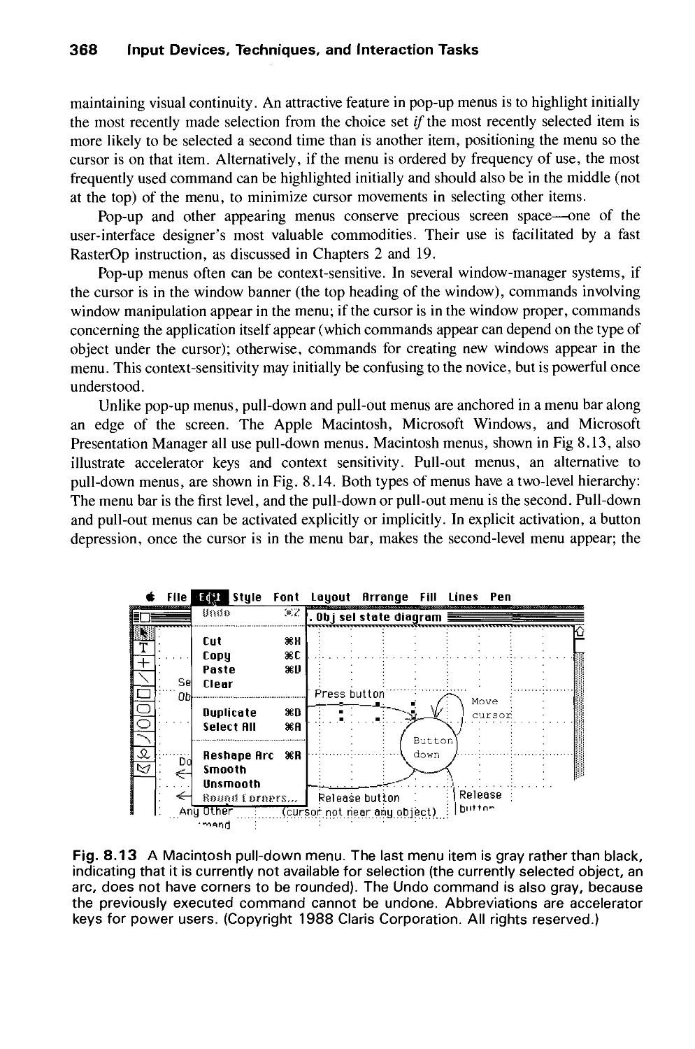
User Interface Group. Chapters 8-10 describe the current technology of interaction
devices and then address the higher-level issues in user-interface design. Various popular
user-interface paradigms are described and critiqued. In the final chapter user-interface
software, such as window managers, interaction technique-libraries, and user-interface
management systems, is addressed.
Model Definition Group. The first two modeling chapters, 11 and 12, describe the
current technologies used in geometric modeling: the representation of curves and surfaces
by parametric functions, especially cubic splines, and the representation of solids by
various techniques, including boundary representations and CSG models. Chapter 13
introduces the human color-vision system, various color-description systems, and
conversion from one to another. This chapter also briefly addresses rules for the effective use of
color.
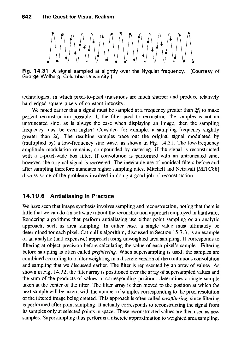
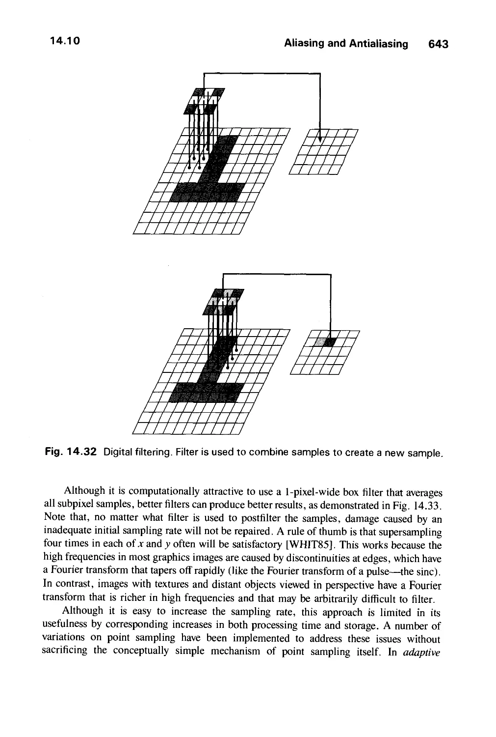
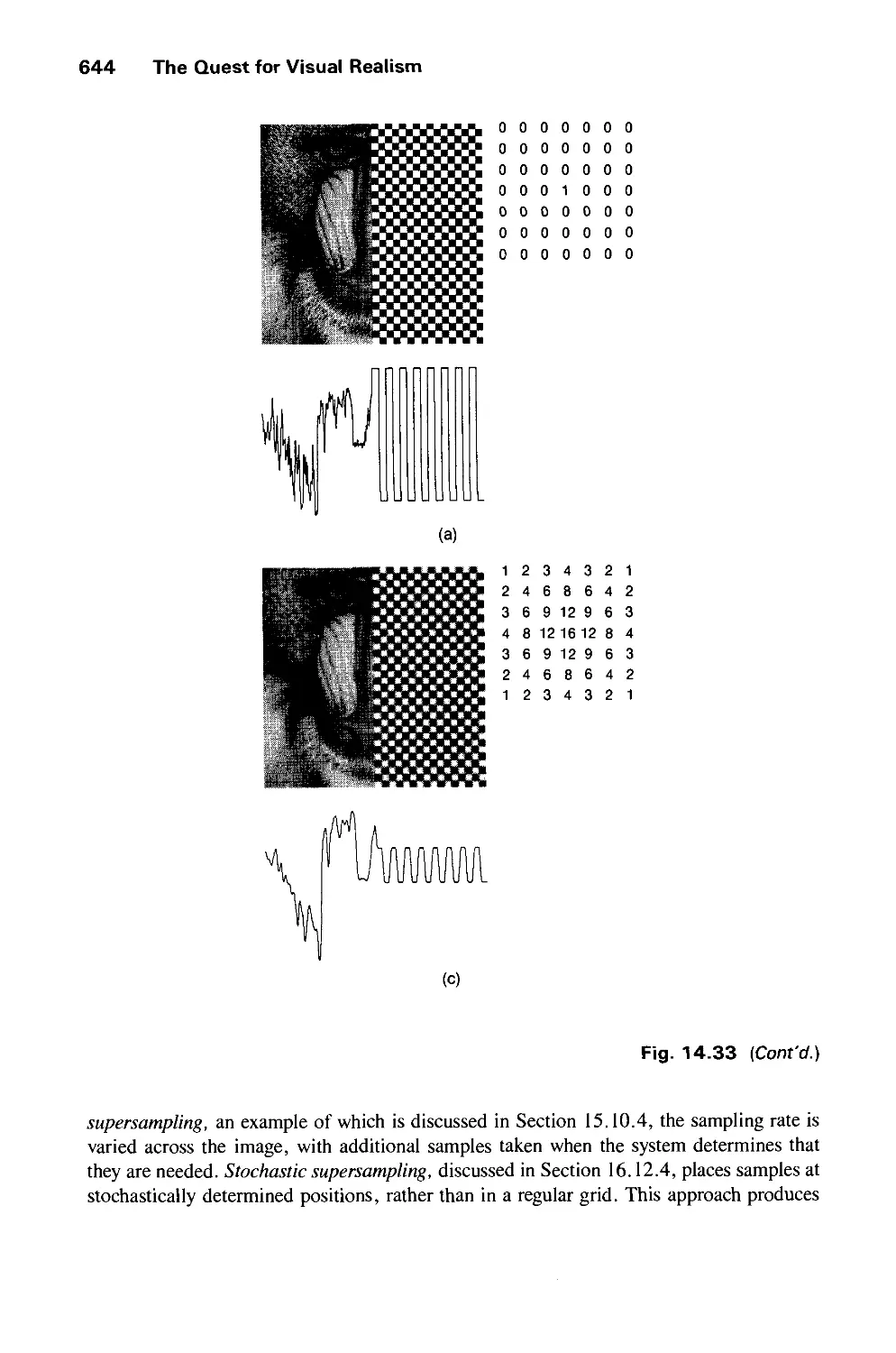
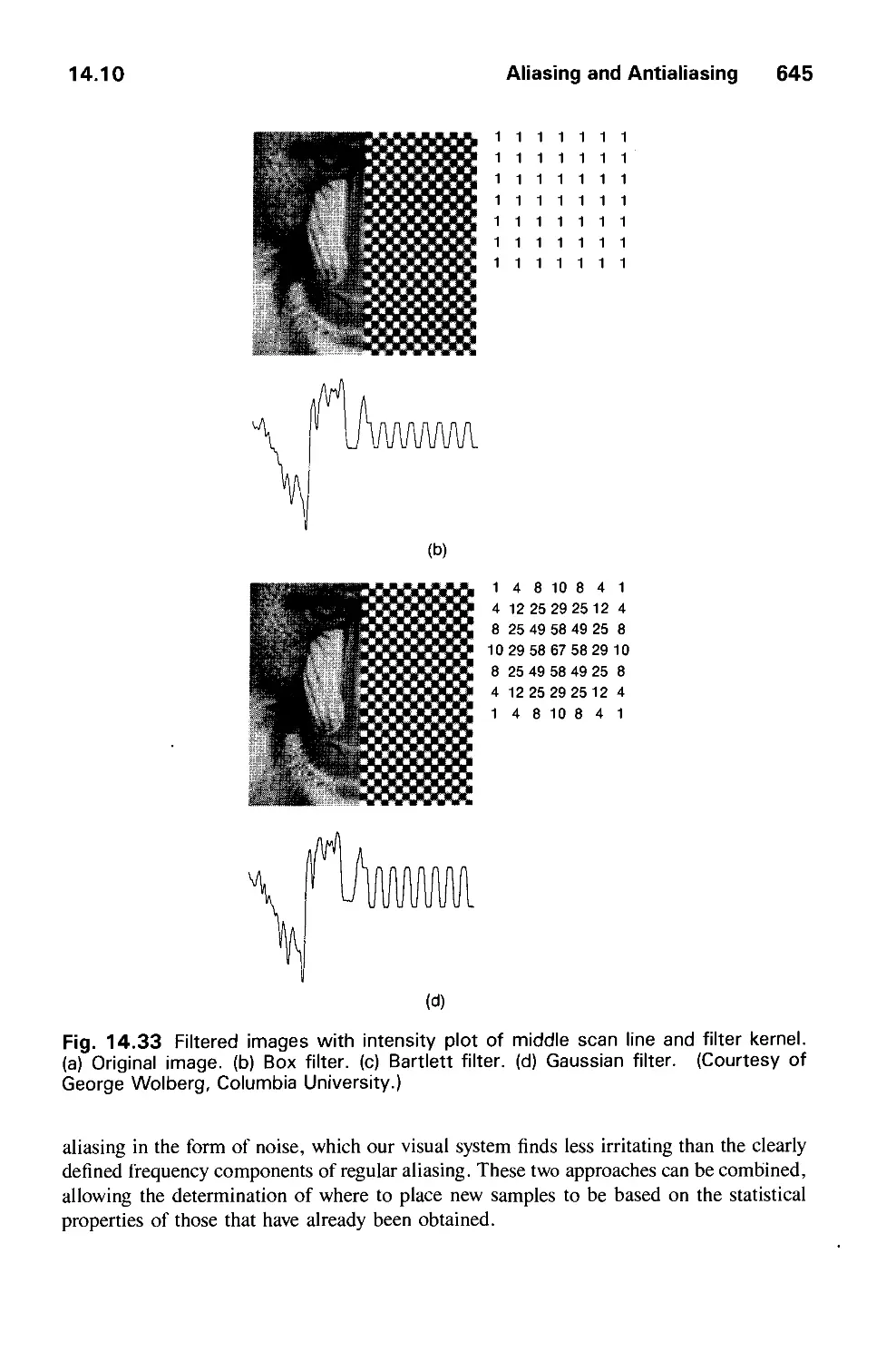
Image Synthesis Group. Chapter 14, the first in a four-chapter sequence, describes
the quest for realism from the earliest vector drawings to state-of-the-art shaded graphics.
The artifacts caused by aliasing are of crucial concern in raster graphics, and this
chapter discusses their causes and cures in considerable detail by introducing the Fourier
xiv Preface
transform and convolution. Chapter 15 describes a variety of strategies for visible-surface
determination in enough detail to allow the reader to implement some of the most
important ones. Illumination and shading algorithms are covered in detail in Chapter 16.
The early part of this chapter discusses algorithms most commonly found in current
hardware, while the remainder treats texture, shadows, transparency, reflections,
physically based illumination models, ray tracing, and radiosity methods. The last chapter in
this group, Chapter 17, describes both image manipulations, such as scaling, shearing,
and rotating pixmaps, and image storage techniques, including various
image-compression schemes.
Advanced Techniques Group. The last four chapters give an overview of the current
state of the art (a moving target, of course). Chapter 18 describes advanced graphics
hardware used in high-end commercial and research machines; this chapter was contributed
by Steven Molnar and Henry Fuchs, authorities on high-performance graphics
architectures. Chapter 19 describes the complex raster algorithms used for such tasks as
scan-converting arbitary conies, generating antialiased text, and implementing page-
description languages, such as PostScript. The final two chapters survey some of the most
important techniques in the fields of high-level modeling and computer animation.
The first two groups cover only elementary material and thus can be used for a basic
course at the undergraduate level. A follow-on course can then use the more advanced
chapters. Alternatively, instructors can assemble customized courses by picking chapters
out of the various groups.
For example, a course designed to introduce students to primarily 2D graphics would
include Chapters 1 and 2, simple scan conversion and clipping from Chapter 3, a
technology overview with emphasis on raster architectures and interaction devices from
Chapter 4, homogeneous mathematics from Chapter 5, and 3D viewing only form a "how
to use it" point of view form Sections 6.1 to 6.3. The User Interface Group, Chapters
8-10, would be followed by selected introductory sections and simple algorithms from the
Image Synthesis Group, Chapters 14, 15, and 16.
A one-course general overview of graphics would include Chapters 1 and 2, basic
algorithms from Chapter 3, raster architectures and interaction devices from Chapter 4,
Chapter 5, and most of Chapters 6 and 7 on viewing and SPHIGS. The second half of the
course would include sections on modeling from Chapters 11 and 13, on image synthesis
from Chapters 14, 15, and 16, and on advanced modeling form Chapter 20 to give breadth
of coverage in these slightly more advanced areas.
A course emphasizing 3D modeling and rendering would start with Chapter 3 sections
on scan converting, clipping of lines and polygons, and introducing antialiasing. The
course would then progress to Chapters 5 and 6 on the basic mathematics of
transformations and viewing and then cover the key Chapters 14, 15, and 16 in the Image Synthesis
Group. Coverage would be rounded off by selections on surface and solid modeling,
Chapter 20 on advanced modeling, and Chapter 21 on animation from the Advanced
Techniques Group.
Graphics Packages. The SRGP and SPHIGS graphics packages, designed by David
Sklar, coauthor of the two chapters on these packages, are available from the publisher for
Preface xv
the IBM PC (ISBN 0-201-54700-7), the Macintosh (ISBN 0-201-54701-5), and UNIX
workstations running XI1 (ISBN 0-201-54702-3), as are many of the algorithms for scan
conversion, clipping, and viewing.
Acknowledgments. This book could not have been produced without the dedicated
work and the indulgence of many friends and colleagues. We acknowledge here our debt to
those who have contributed significantly to one or more chapters; many others have helped
by commenting on individual chapters, and we are grateful to them as well. We regret any
inadvertent omissions. Katrina Avery and Lyn Dupr6 did a superb job of editing. Additional
valuable editing on multiple versions of multiple chapters was provided by Debbie van
Dam, Melissa Gold, and Clare Campbell. We are especially grateful to our production
supervisor, Bette Aaronson, our art director, Joe Vetere, and our editor, Keith Wollman,
not only for their great help in producing the book, but also for their patience and good
humor under admittedly adverse circumstances—if we ever made a promised deadline
during these frantic five years, we can't remember it!
Computer graphics has become too complex for even a team of four main authors and
three guest authors to be expert in all areas. We relied on colleagues and students to amplify
our knowledge, catch our mistakes and provide constructive criticism of form and content.
We take full responsibility for any remaining sins of omission and commission. Detailed
technical readings on one or more chapters were provided by John Airey, Kurt Akeley, Tom
Banchoff, Brian Barsky, David Bates, Cliff Beshers, Gary Bishop, Peter Bono, Marvin
Bunker, Bill Buxton, Edward Chang, Norman Chin, Michael F. Cohen, William Cowan,
John Dennis, Tom Dewald, Scott Draves, Steve Drucker, Tom Duff, Richard Economy,
David Ellsworth, Nick England, Jerry Farrell, Robin Forrest, Alain Fournier, Alan Freiden,
Christina Gibbs, Melissa Gold, Mark Green, Cathleen Greenberg, Margaret Hagen, Griff
Hamlin, Pat Hanrahan, John Heidema, Rob Jacob, Abid Kamran, Mide Kappel, Henry
Kaufman, Karen Kendler, David Kurlander, David Laidlaw, Keith Lantz, Hsien-Che Lee,
Aaron Marcus, Deborah Mayhew, Barbara Meier, Gary Meyer, Jim Michener, Jakob
Nielsen, Mark Nodine, Randy Pausch, Ari Requicha, David Rosenthal, David Salesin,
Hanan Samet, James Sanford, James Sargent, Robin Schaufler, Rogert Scheifler, John
Schnizlein, Michael Shantzis, Ben Shneiderman, Ken Shoemake, Judith Schrier, John
Sibert, Dave Simons, Jonathan Steinhart, Maureen Stone, Paul Strauss, Seth Tager, Peter
Tanner, Brice Tebbs, Ben Trumbore, Yi Tso, Greg Turk, Jeff Vroom, Colin Ware, Gary
Watkins, Chuck Weger, Kevin Weiler, Turner Whitted, George Wolberg, and Larry Wolff.
Several colleagues, including Jack Bresenham, Brian Barsky, Jerry Van Aken, Dilip
DaSilva (who suggested the uniform midpoint treatment of Chapter 3) and Don Hatfield,
not only read chapters closely but also provided detailed sugestions on algorithms.
Welcome word-processing relief was provided by Katrina Avery, Barbara Britten, Clare
Campbell, Tina Cantor, Joyce Cavatoni, Louisa Hogan, and Debbie van Dam. Drawings for
Chapters 1-3 were ably created by Dan Robbins, Scott Snibbe, Tina Cantor, and Clare
Campbell. Figure and image sequences created for this book were provided by Beth Cobb,
David Kurlander, Allen Paeth, and George Wolberg (with assistance from Peter Karp).
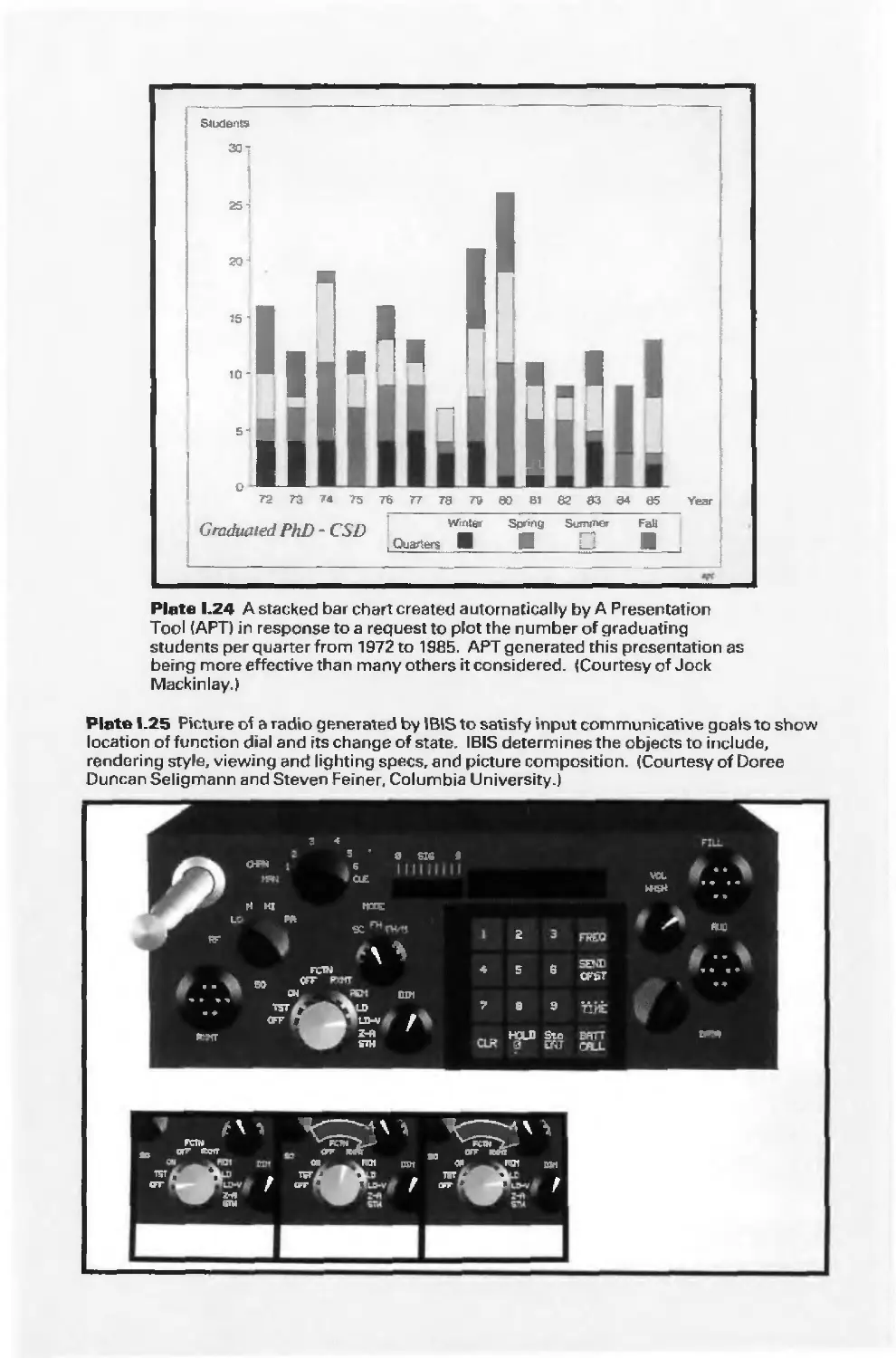
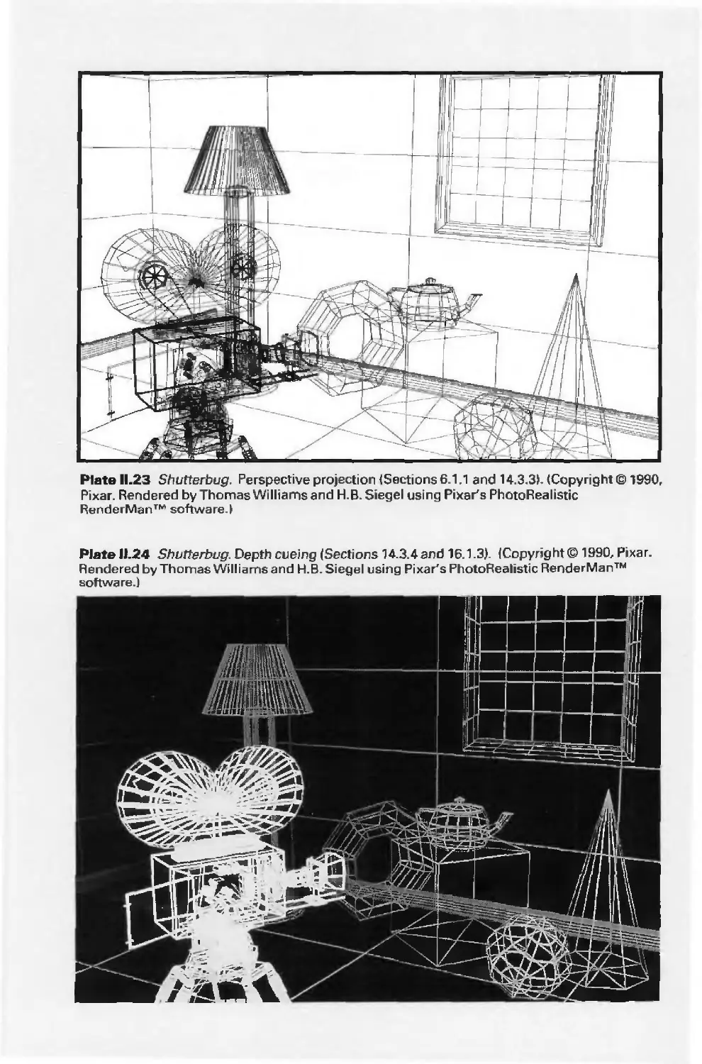
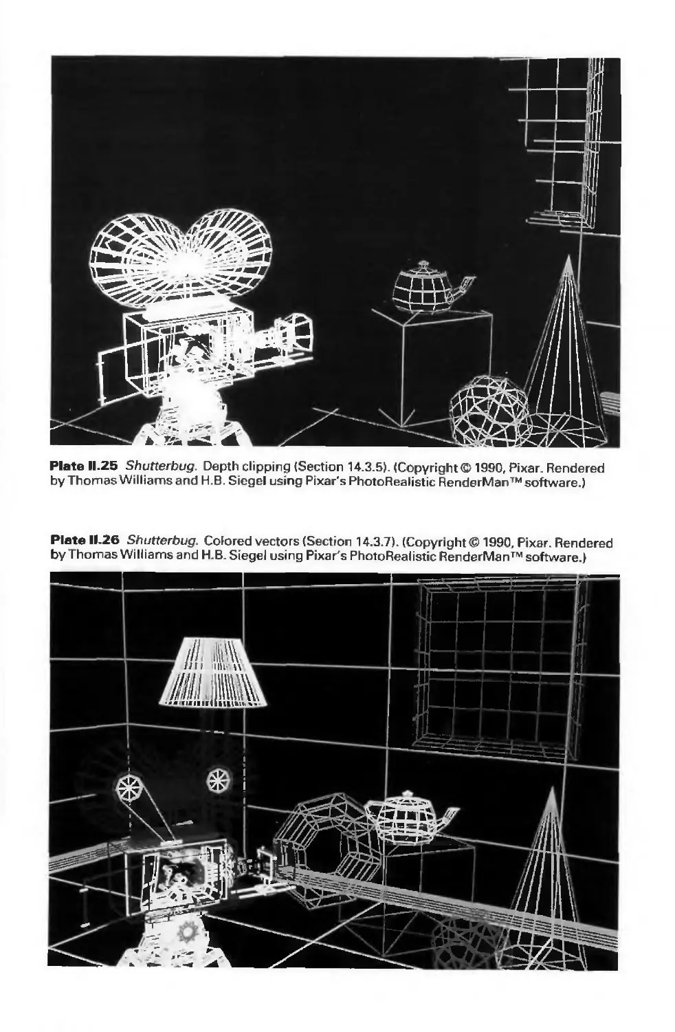
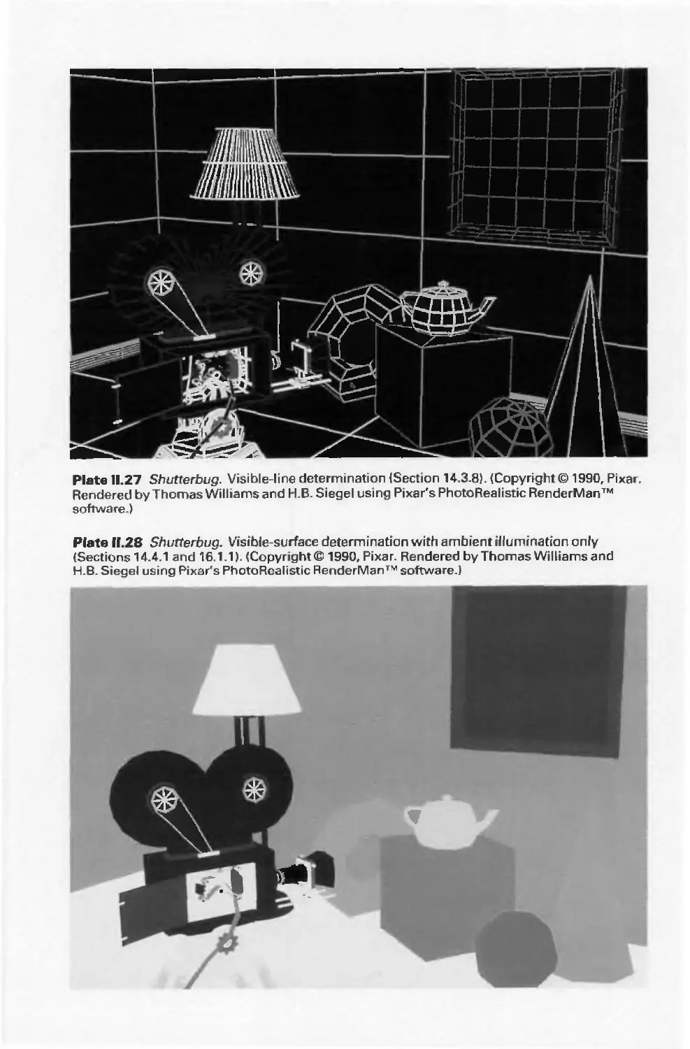
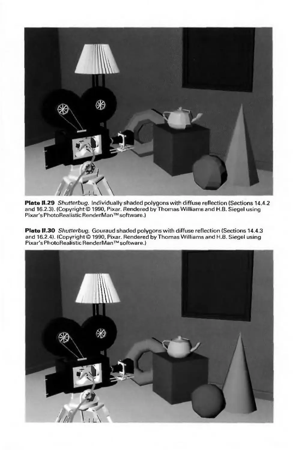
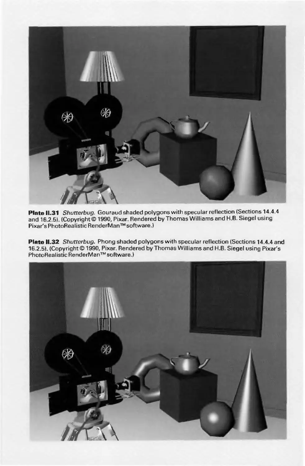
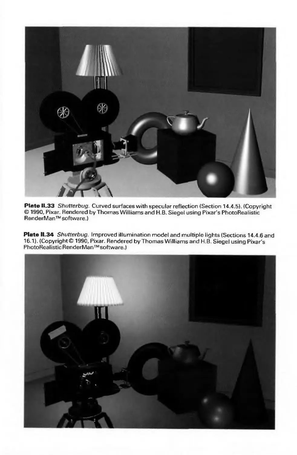
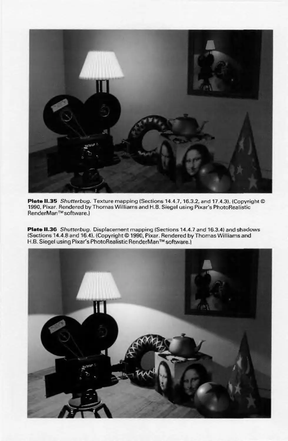
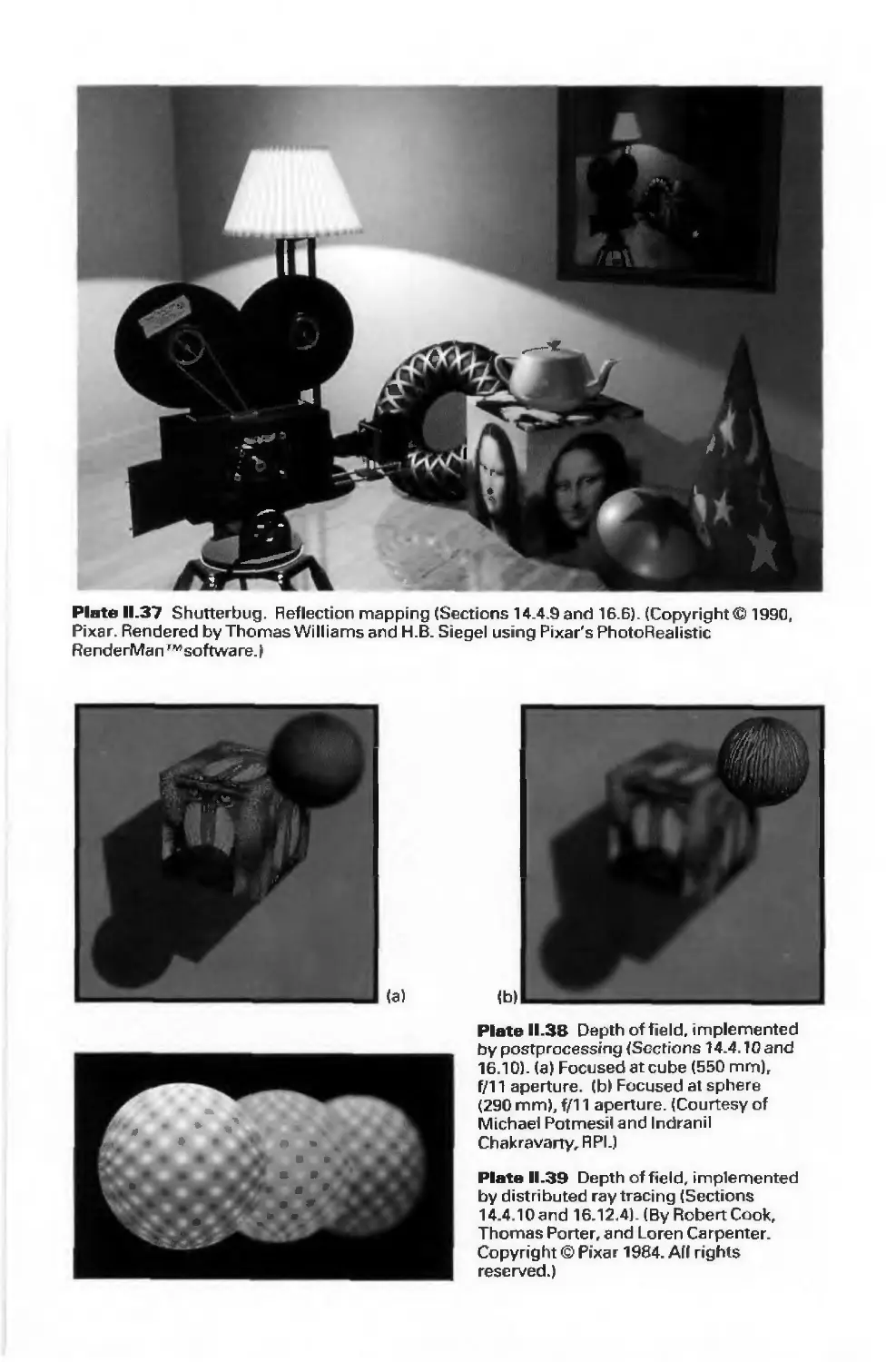
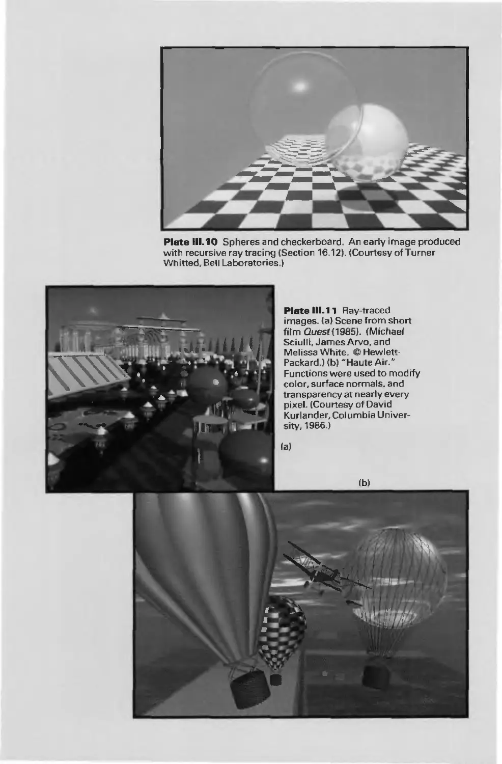
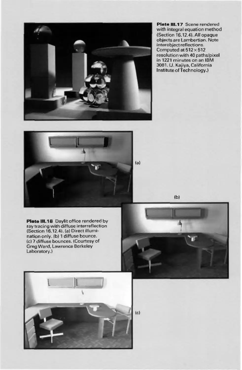
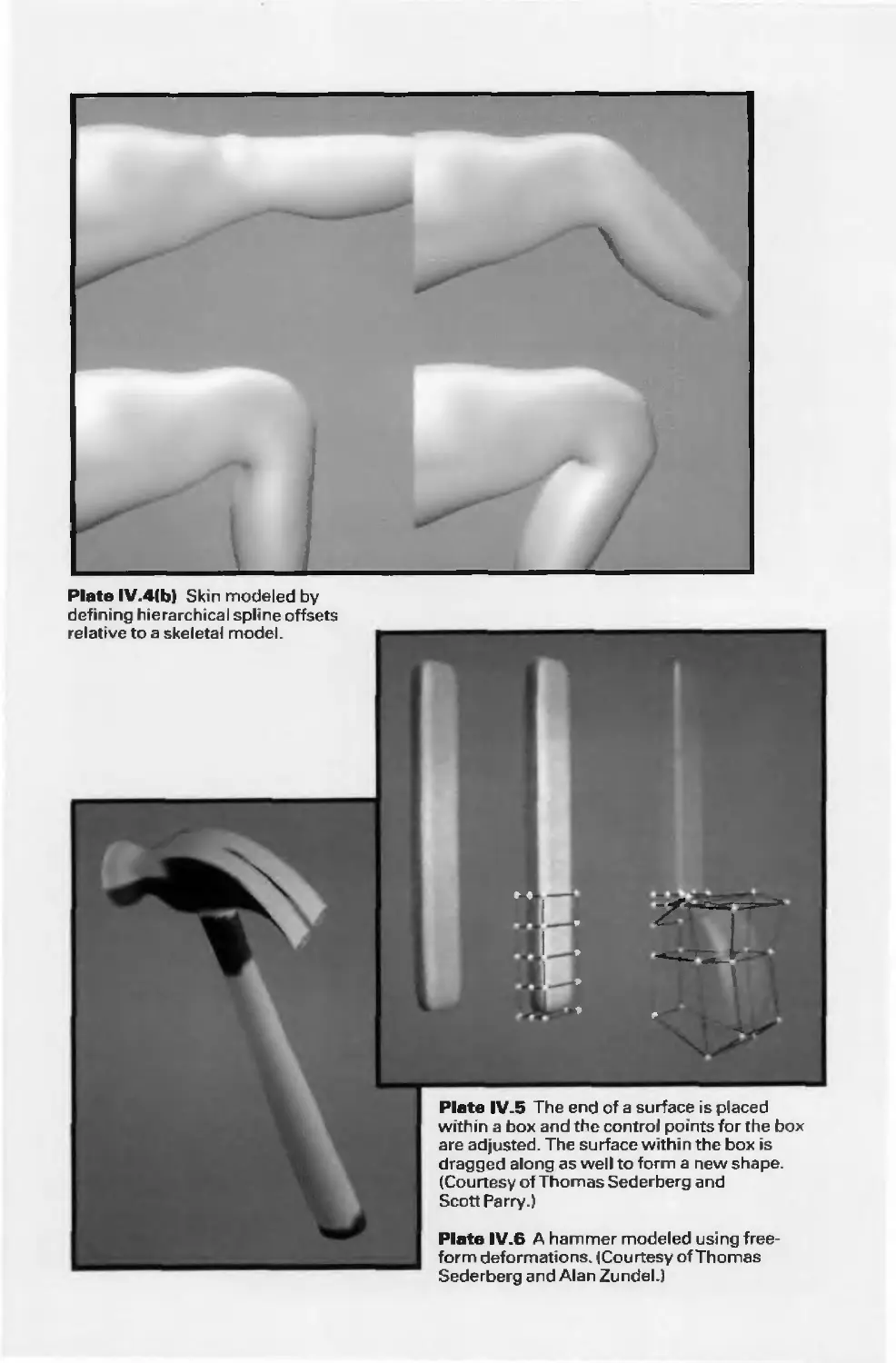
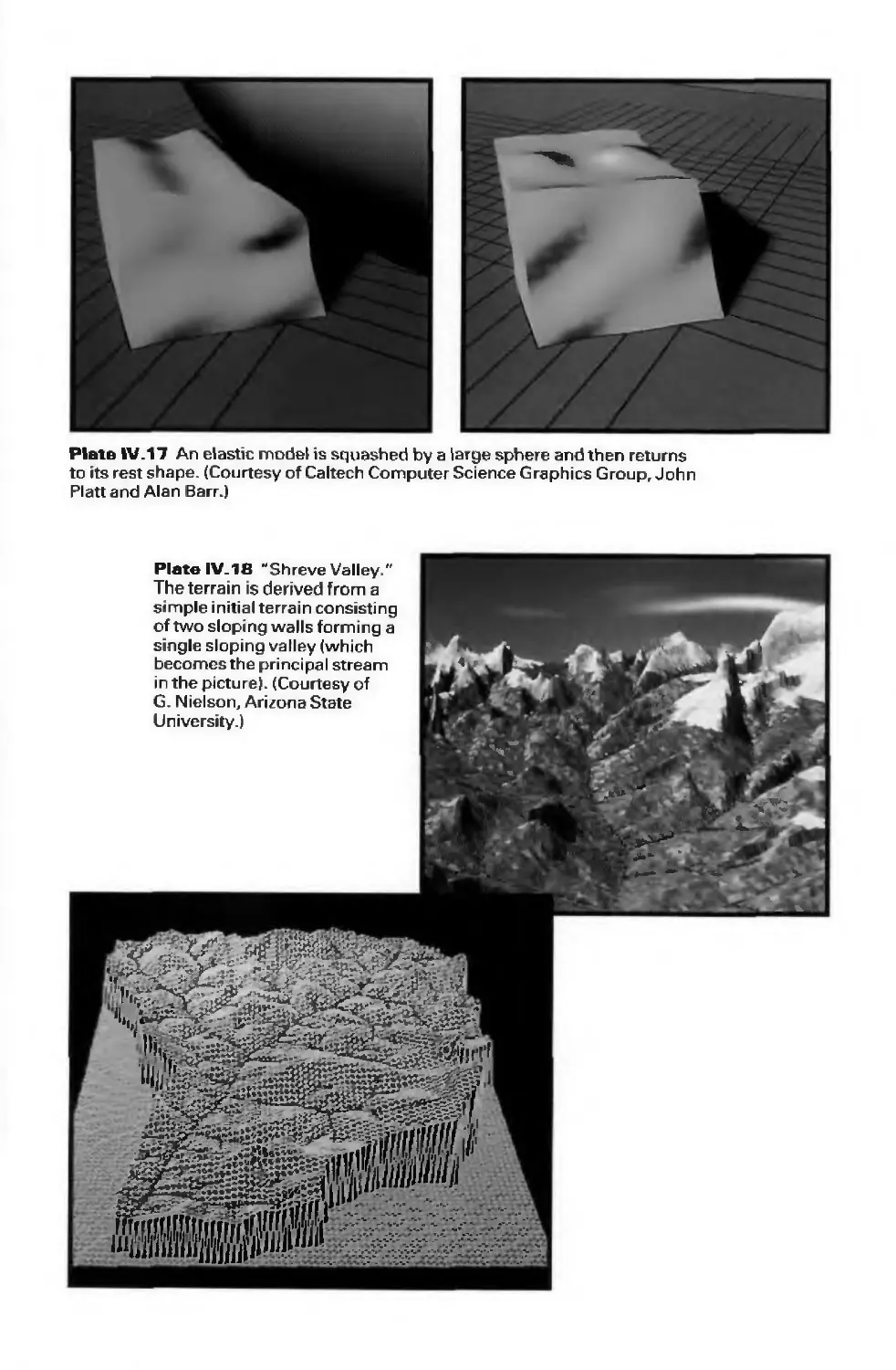
Plates 11.21-37, showing a progression of rendering techniques, were designed and
rendered at Pixar by Thomas Williams and H.B. Siegel, under the direction of M.W.
Mantle, using Pixar's PhotoRealistic RenderMan software. Thanks to Industrial Light &
Magic for the use of their laser scanner to create Plates 11.24-37, and to Norman Chin for
xvi Preface
computing vertex normals for Color Plates 11.30-32. L. Lu and Carles Castellsague' wrote
programs to make figures.
Jeff Vogel implemented the algorithms of Chapter 3, and he and Atul Butte verified the
code in Chapters 2 and 7. David Sklar wrote the Mac and XI1 implementations of SRGP
and SPHIGS with help from Ron Balsys, Scott Boyajian, Atul Butte, Alex Contovounesios,
and Scott Draves. Randy Pausch and his students ported the packages to the PC
environment.
Washington, D.C. J.D.F.
Providence, R.I. A.v.D.
New York, N.Y. S.K.F.
Providence, R.I. J.F.H.
Contents
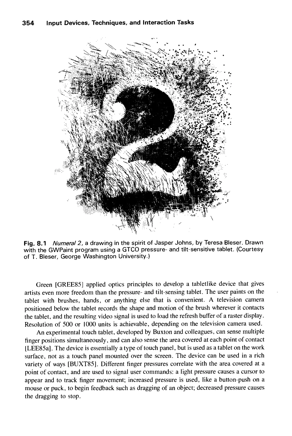
CHAPTER 1
INTRODUCTION 1
1.1 Image Processing as Picture Analysis 2
1.2 The Advantages of Interactive Graphics 3
1.3 Representative Uses of Computer Graphics 4
1.4 Classification of Applications 6
1.5 Development of Hardware and Software for Computer Graphics 8
1.6 Conceptual Framework for Interactive Graphics 17
1.7 Summary 21
Exercises 22
CHAPTER 2
PROGRAMMING IN THE SIMPLE RASTER
GRAPHICS PACKAGE (SRGP) 25
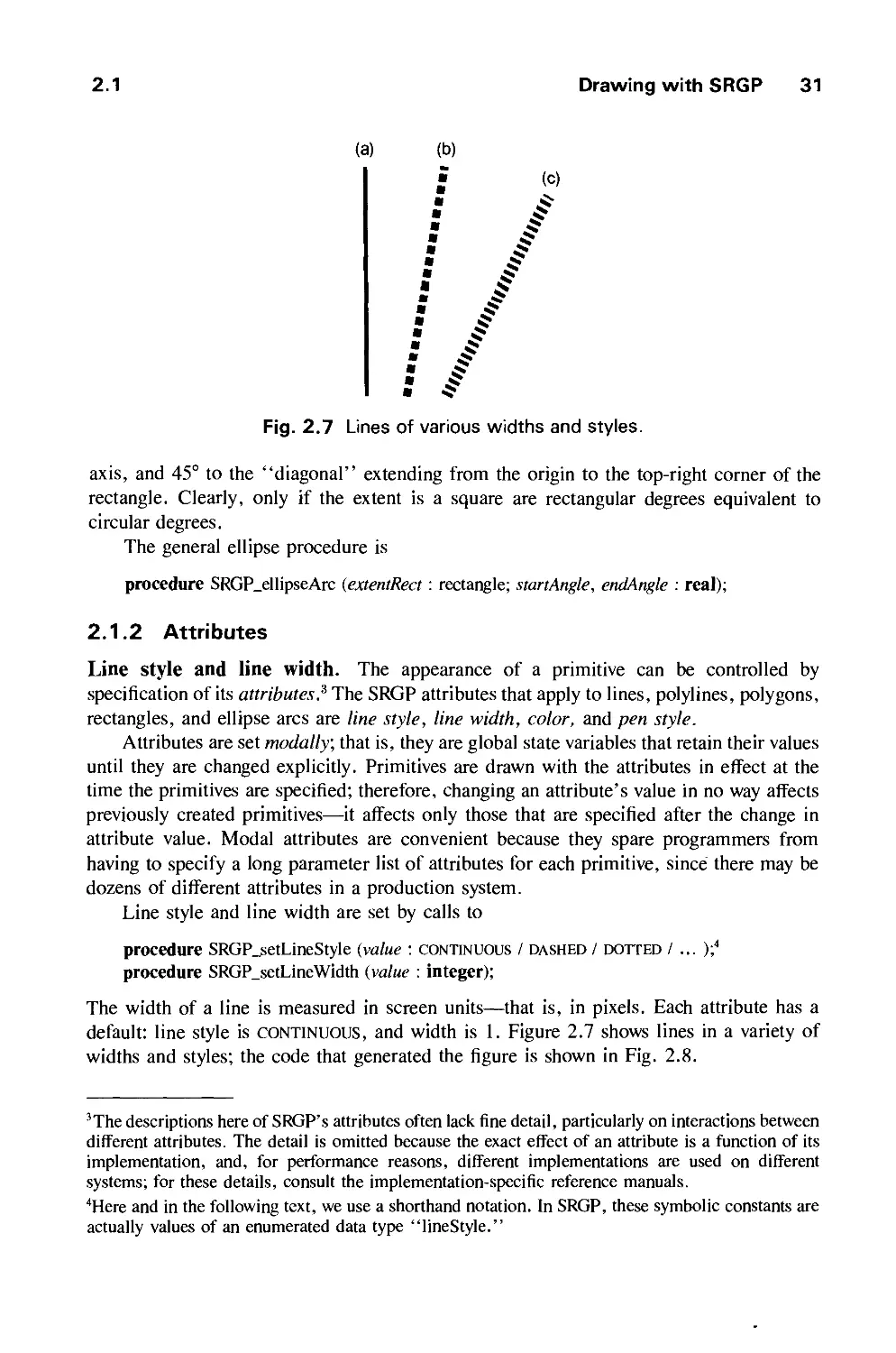
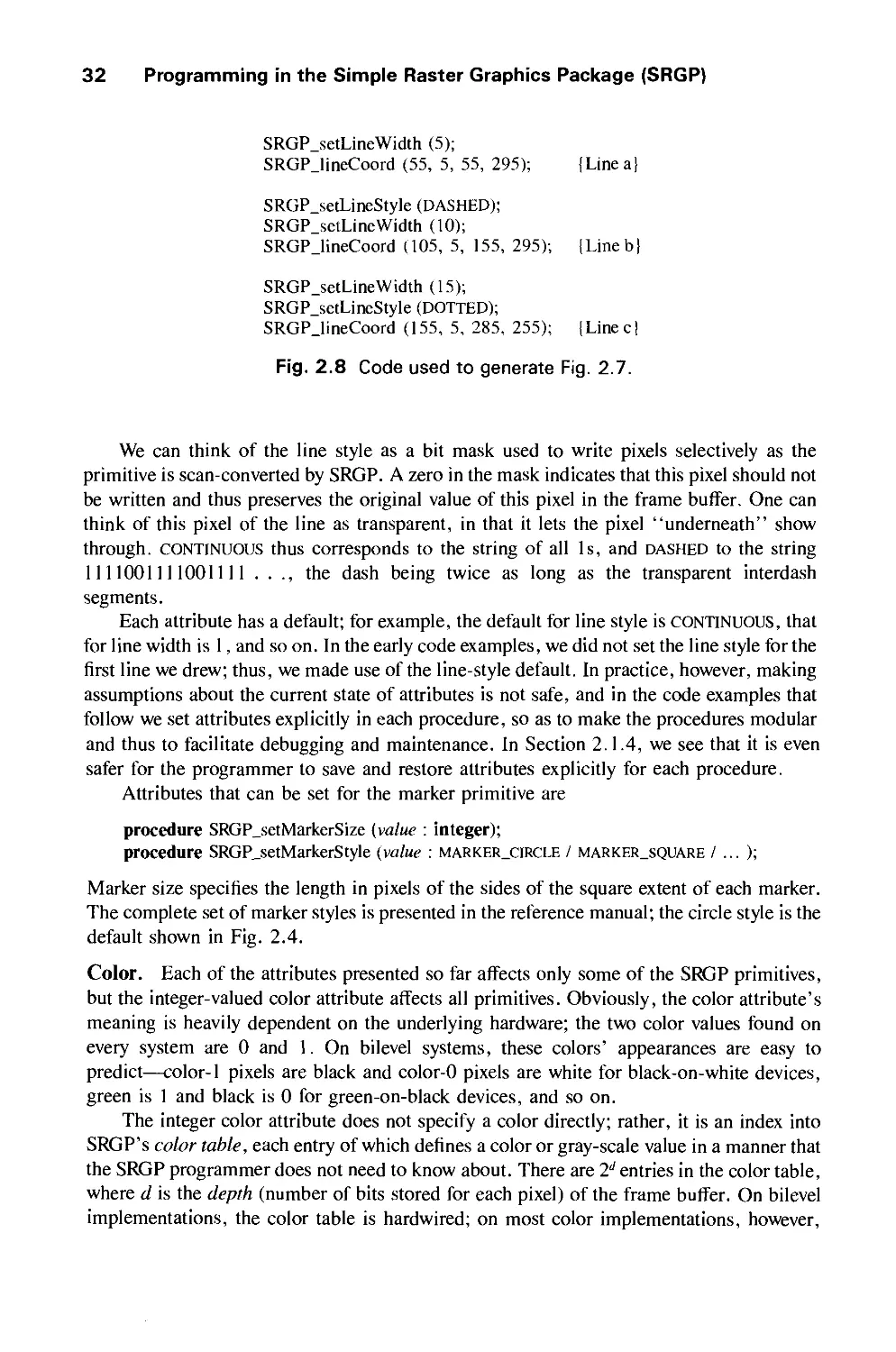
2.1 Drawing with SRGP 26
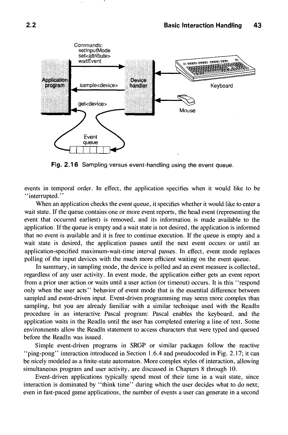
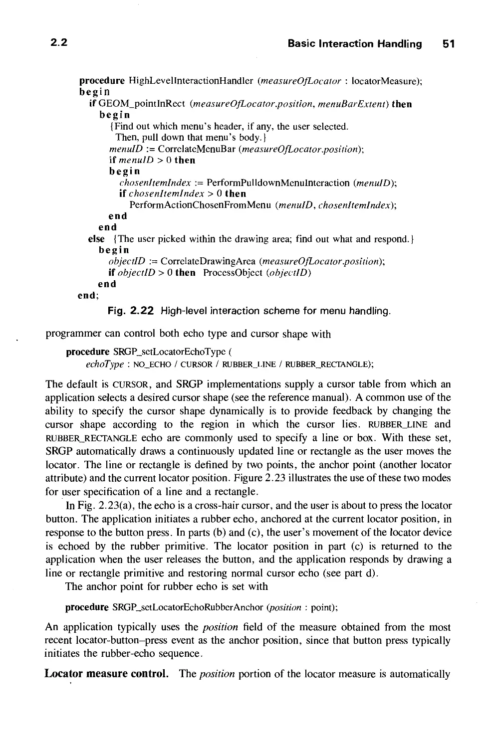
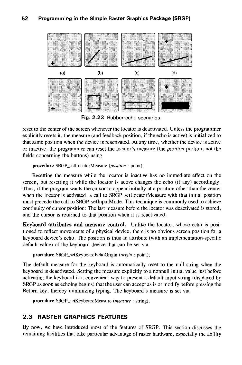
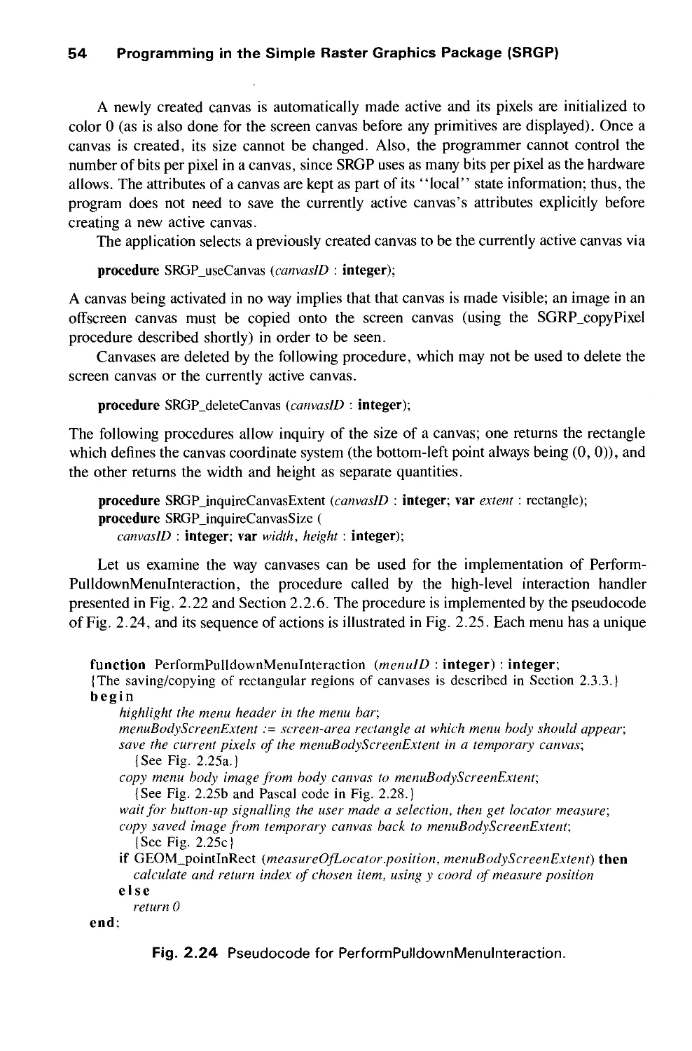
2.2 Basic Interaction Handling 40
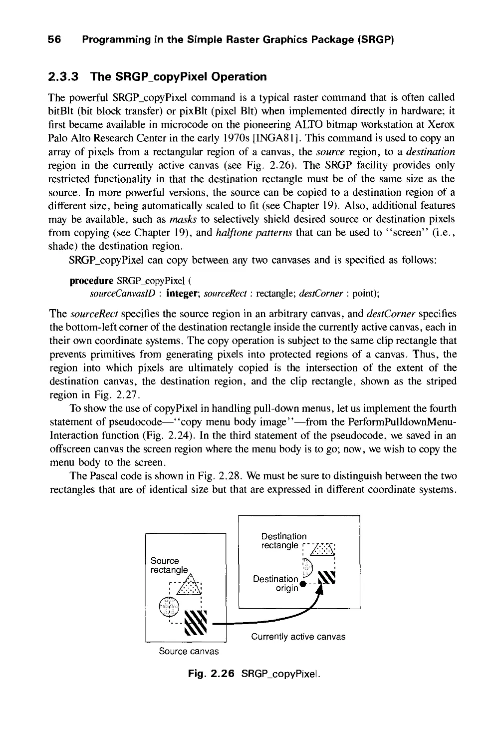
2.3 Raster Graphics Features 52
2.4 Limitations of SRGP 60
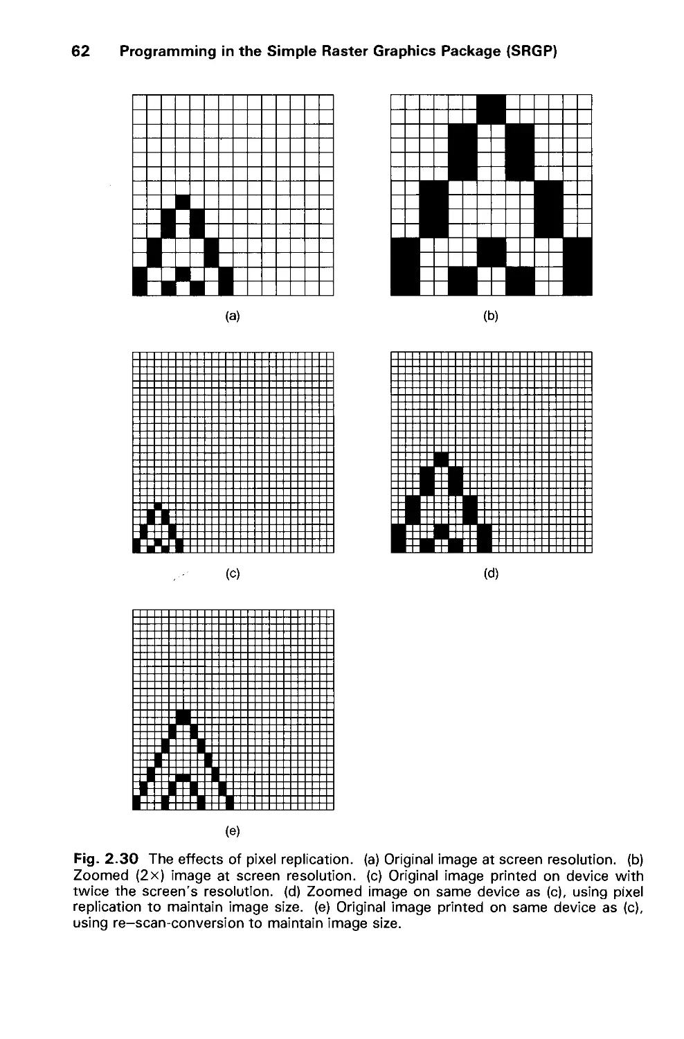
2.5 Summary 63
Exercises 64
CHAPTER 3
BASIC RASTER GRAPHICS ALGORITHMS
FOR DRAWING 2D PRIMITIVES 67
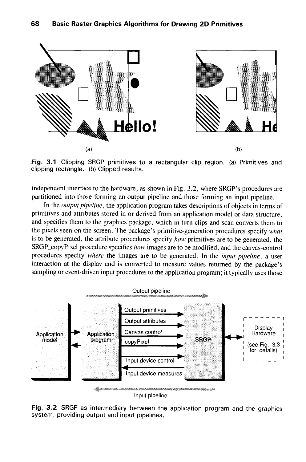
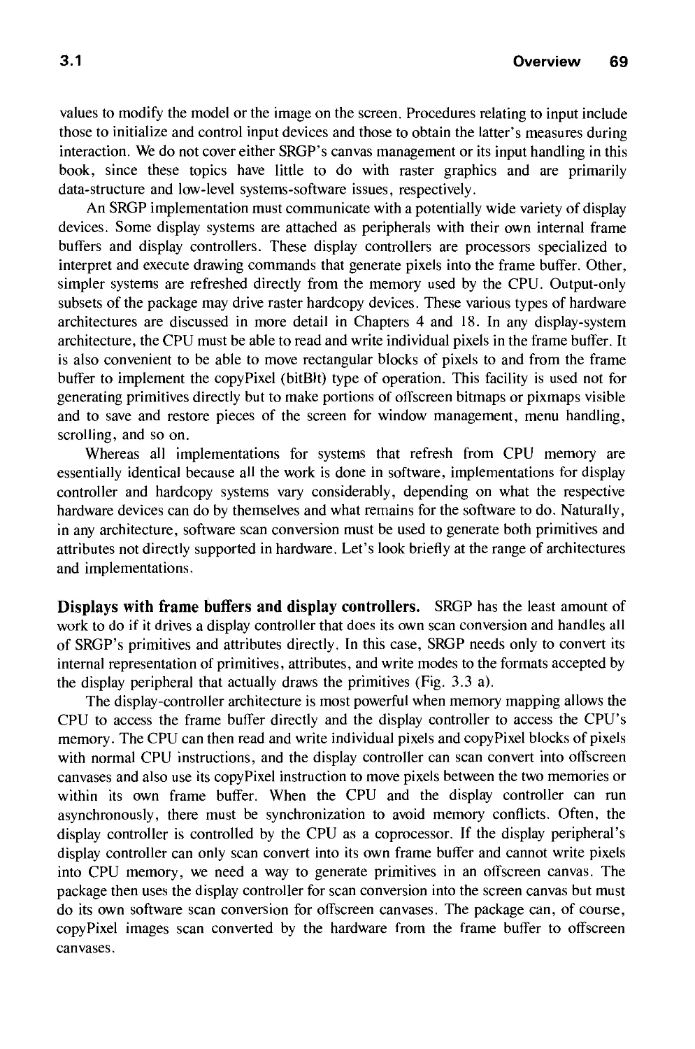
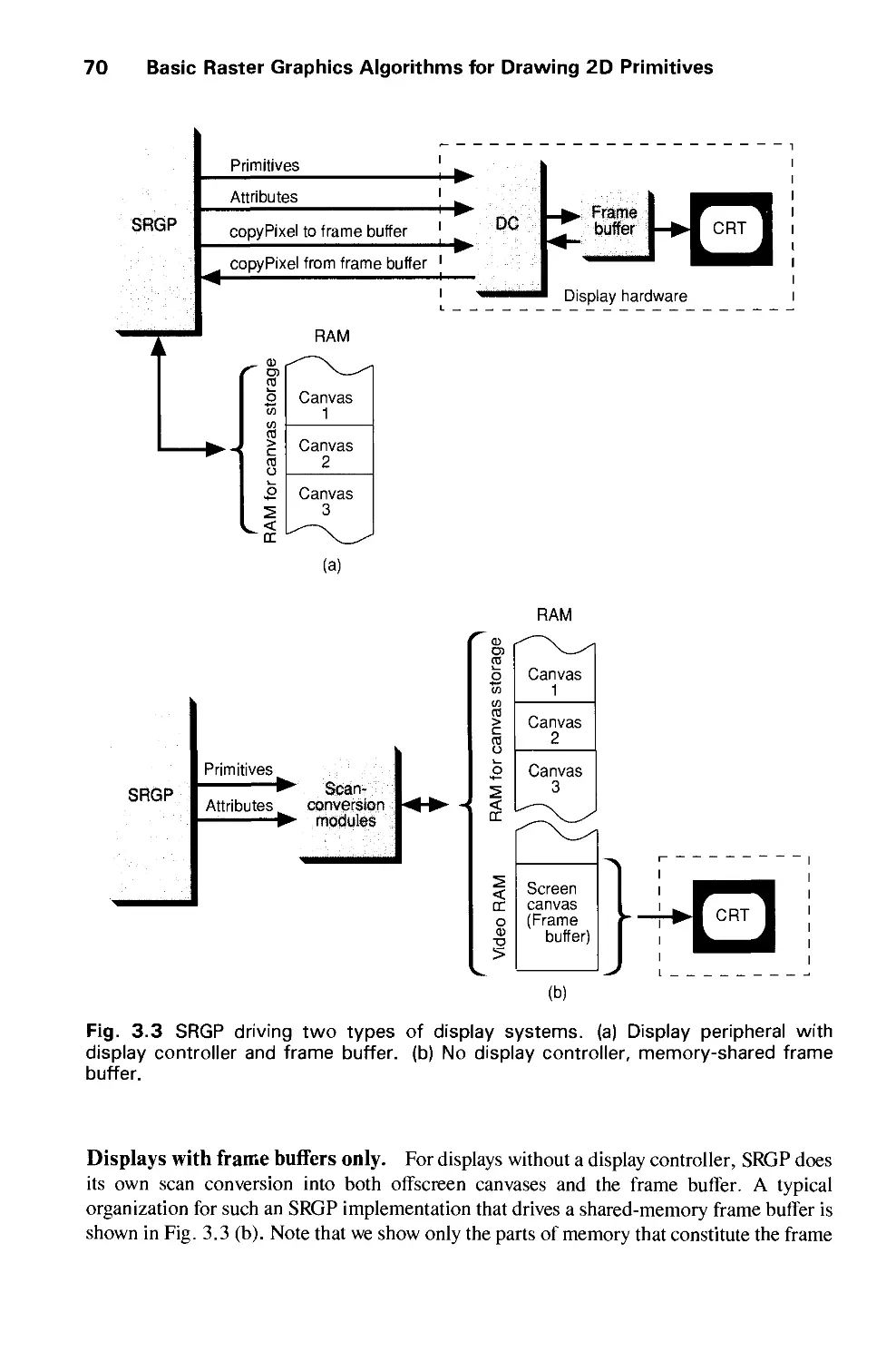
3.1 Overview 67
3.2 Scan Converting Lines 72
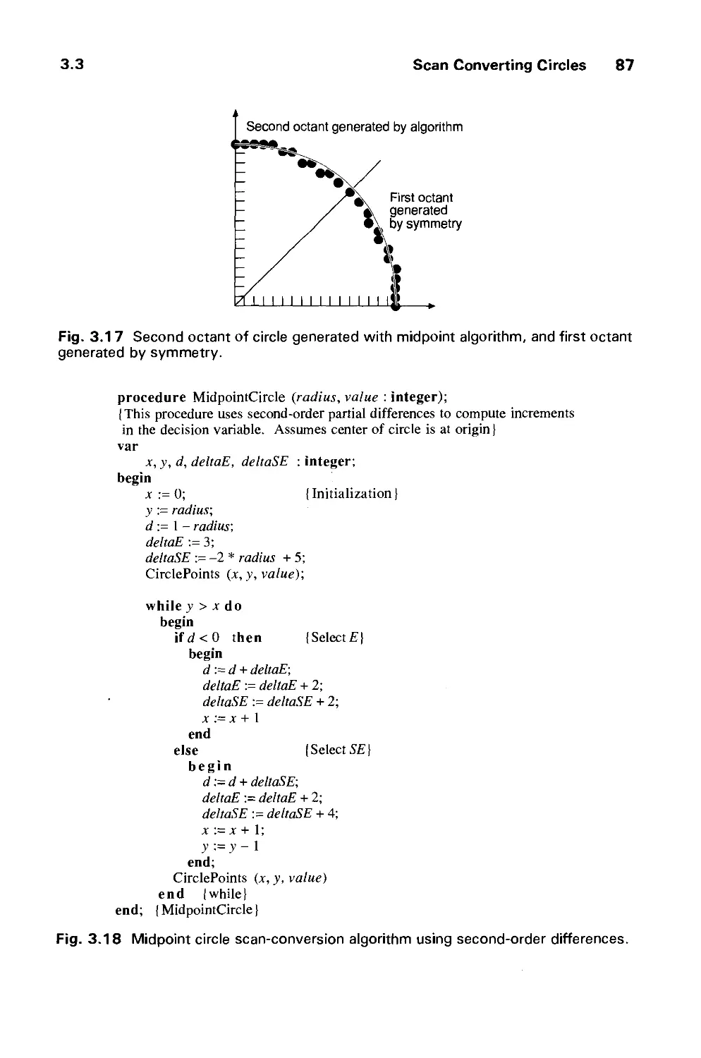
3.3 Scan Converting Circles 81
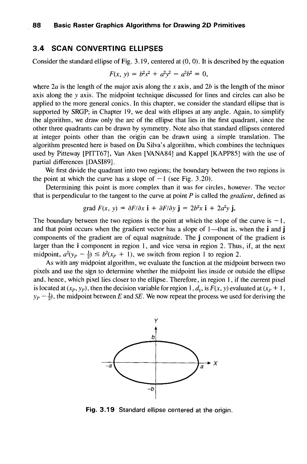
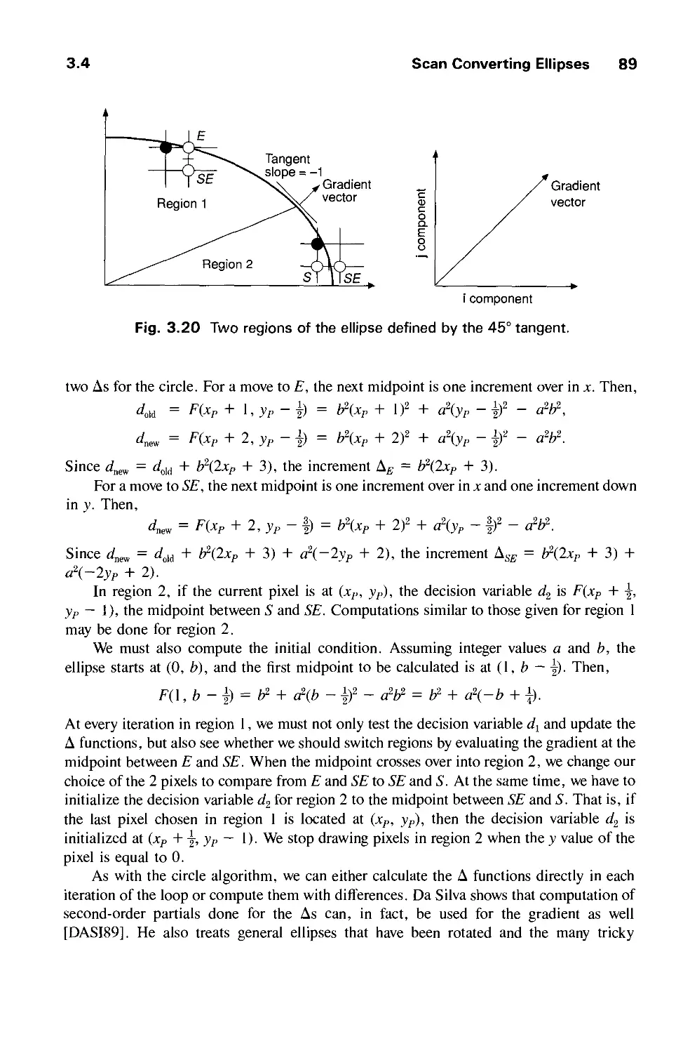
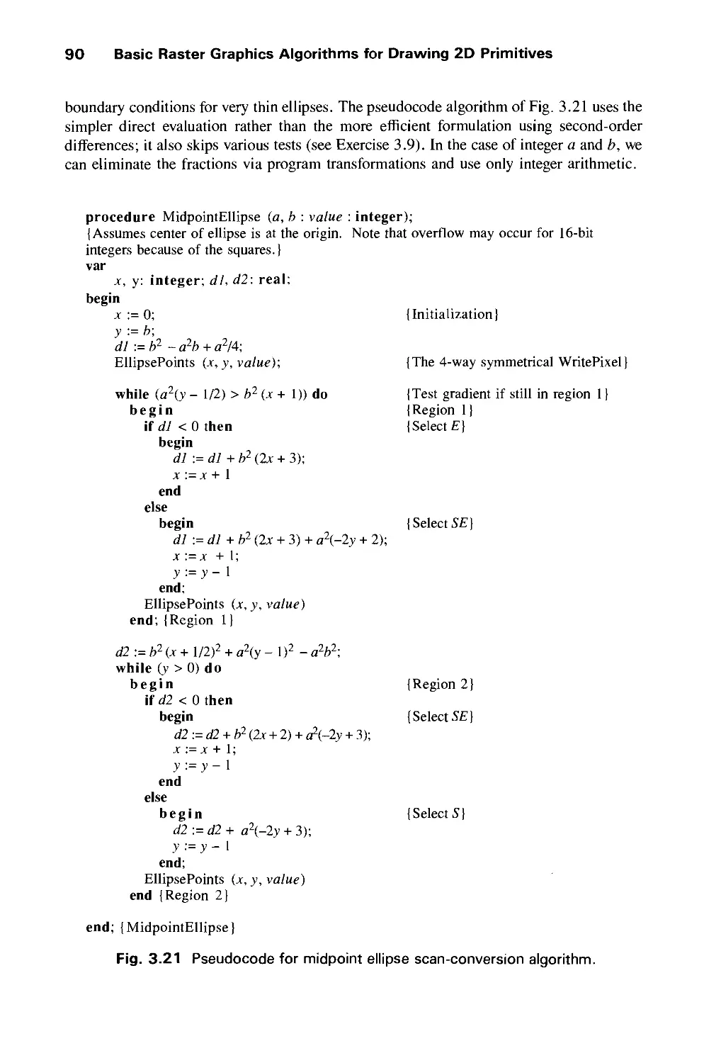
3.4 Scan Converting Ellipses 88
3.5 Filling Rectangles 91
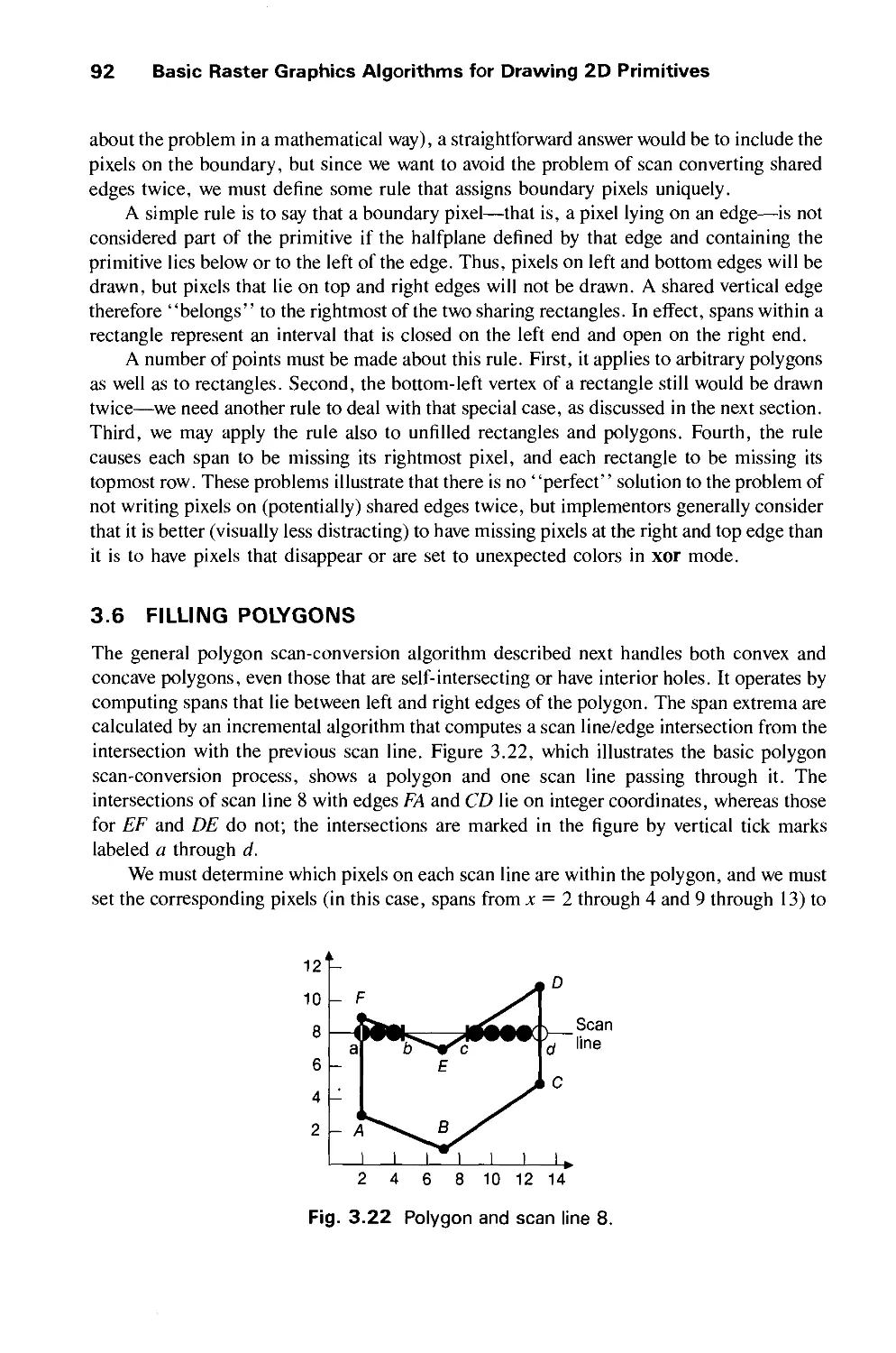
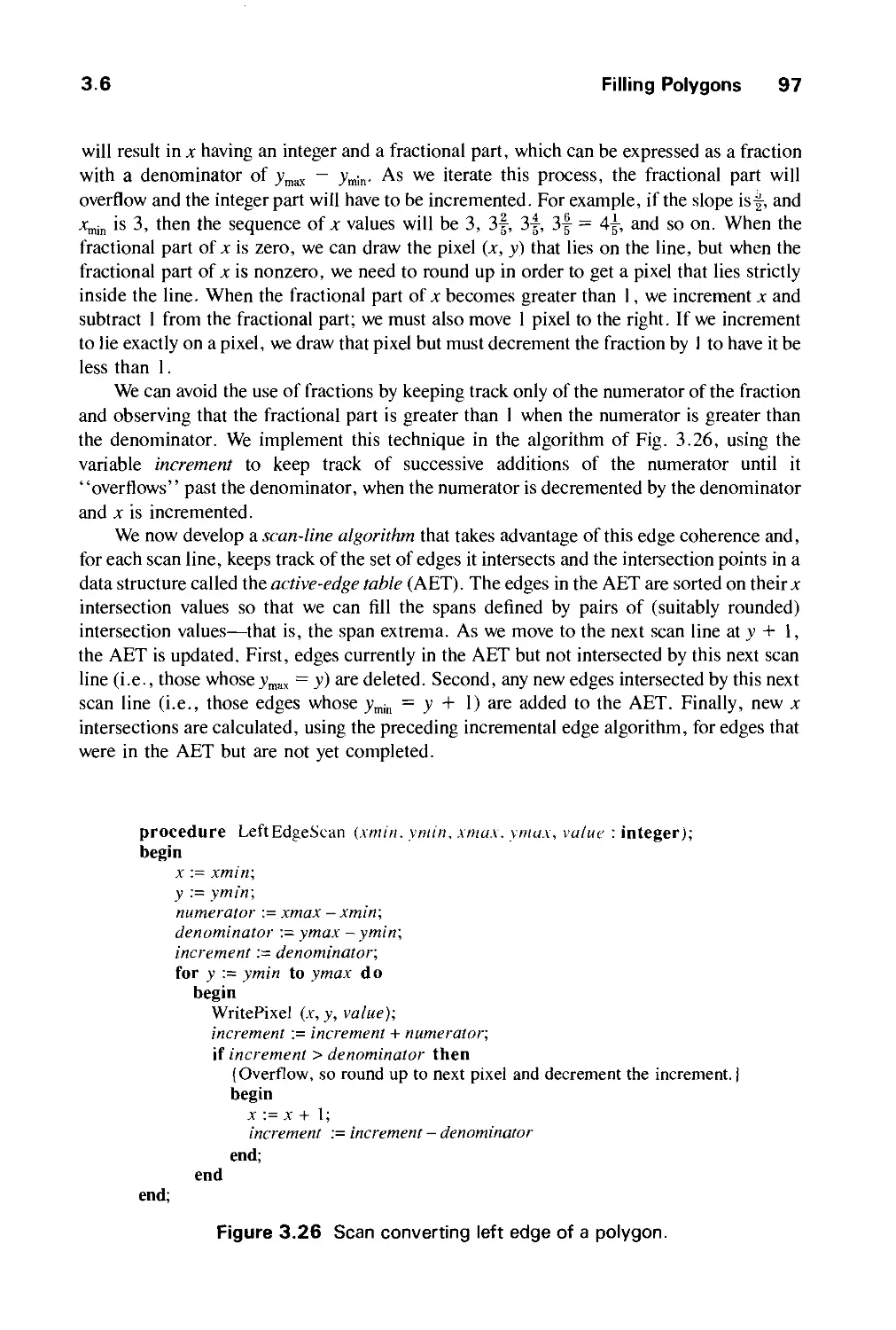
3.6 Filling Polygons 92
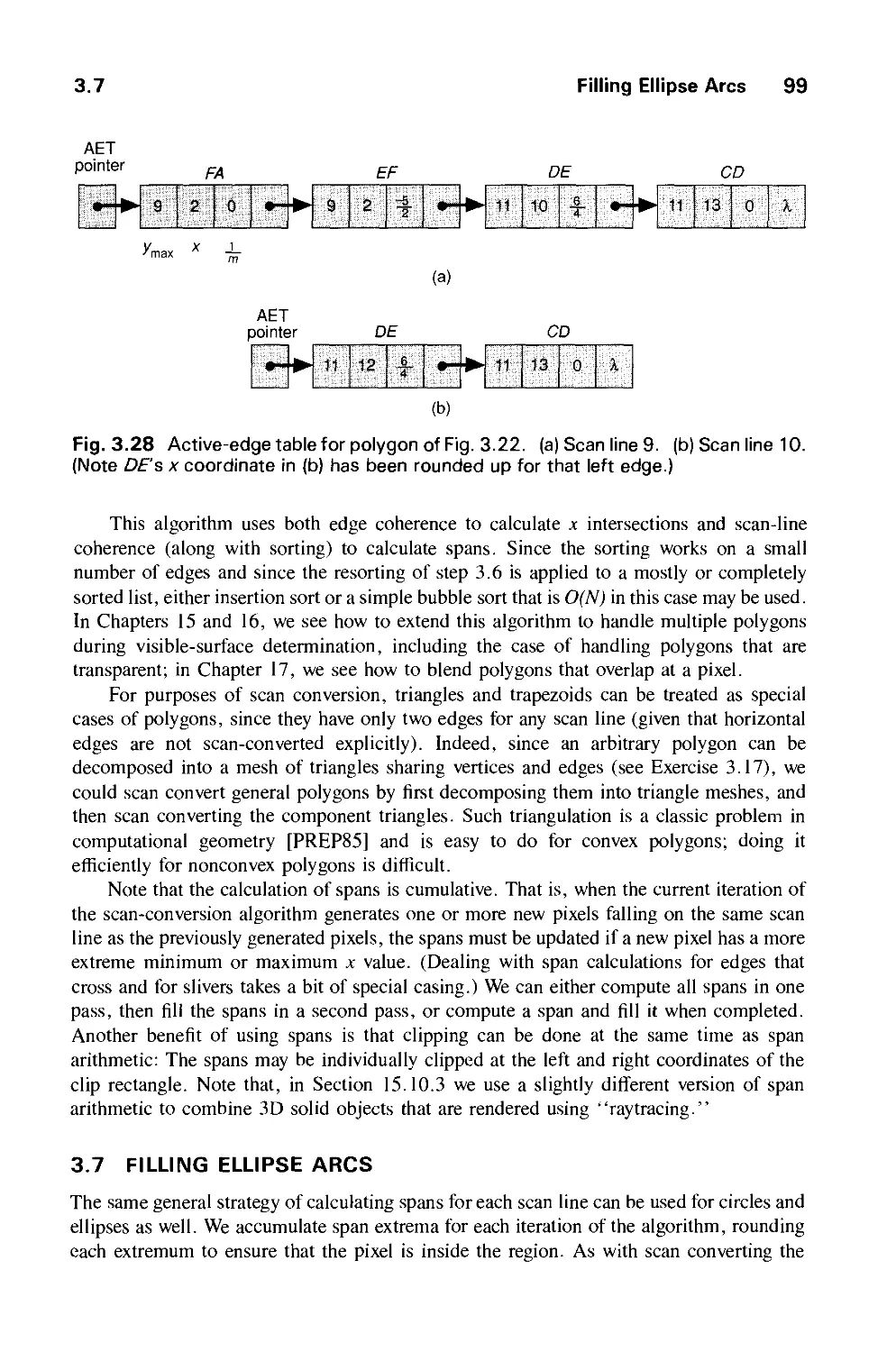
3.7 Filling Ellipse Arcs 99
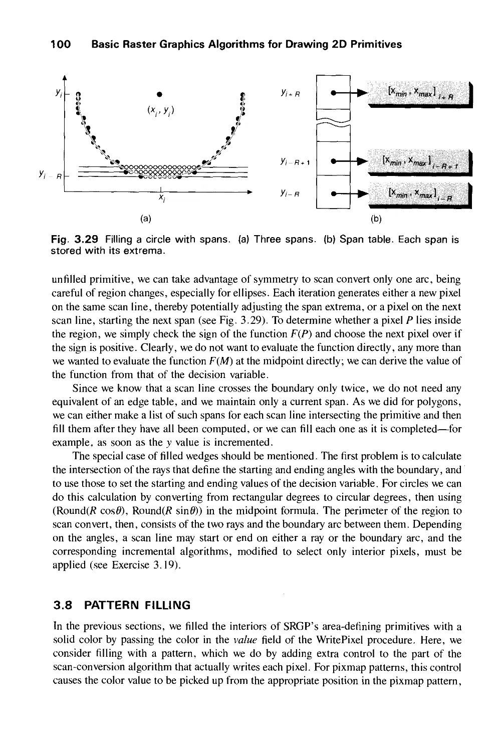
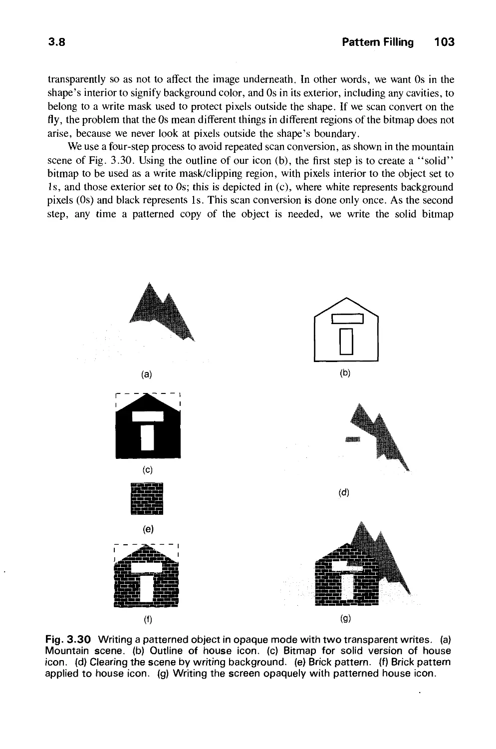
3.8 Pattern Filling 100
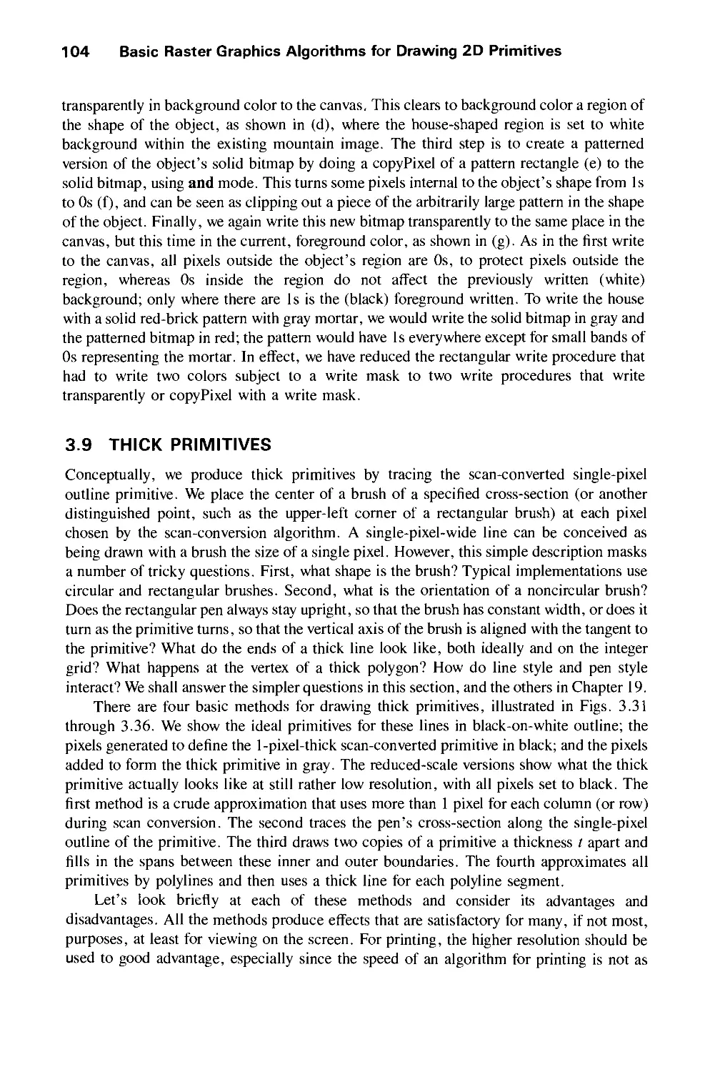
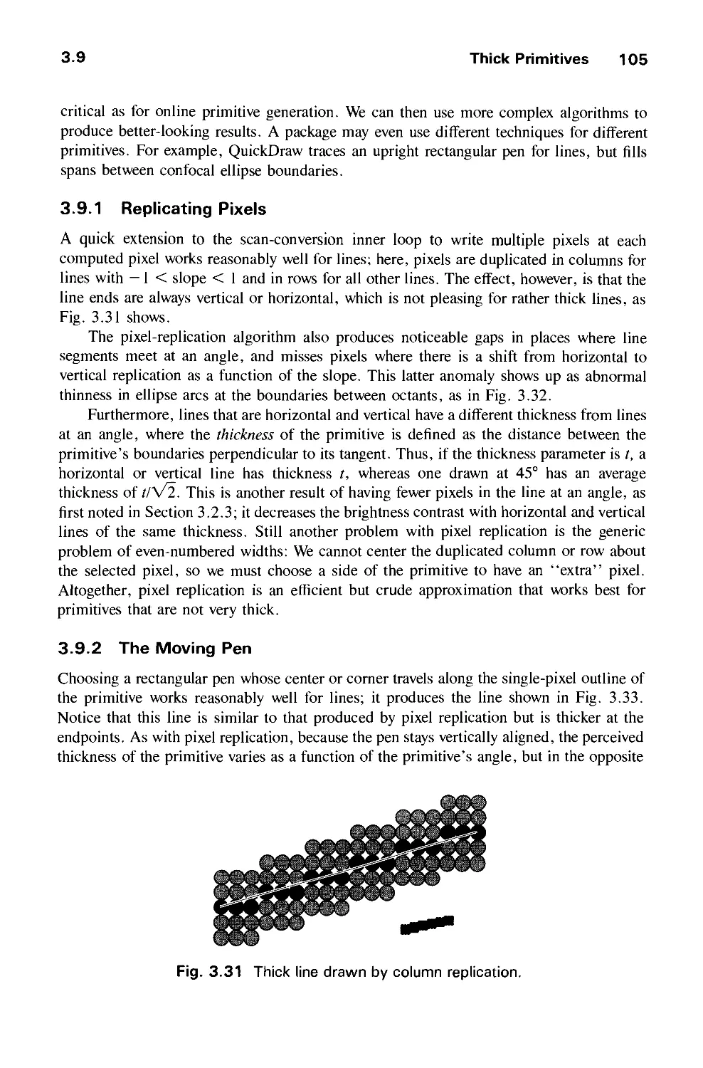
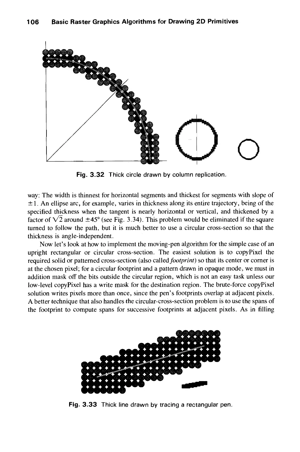
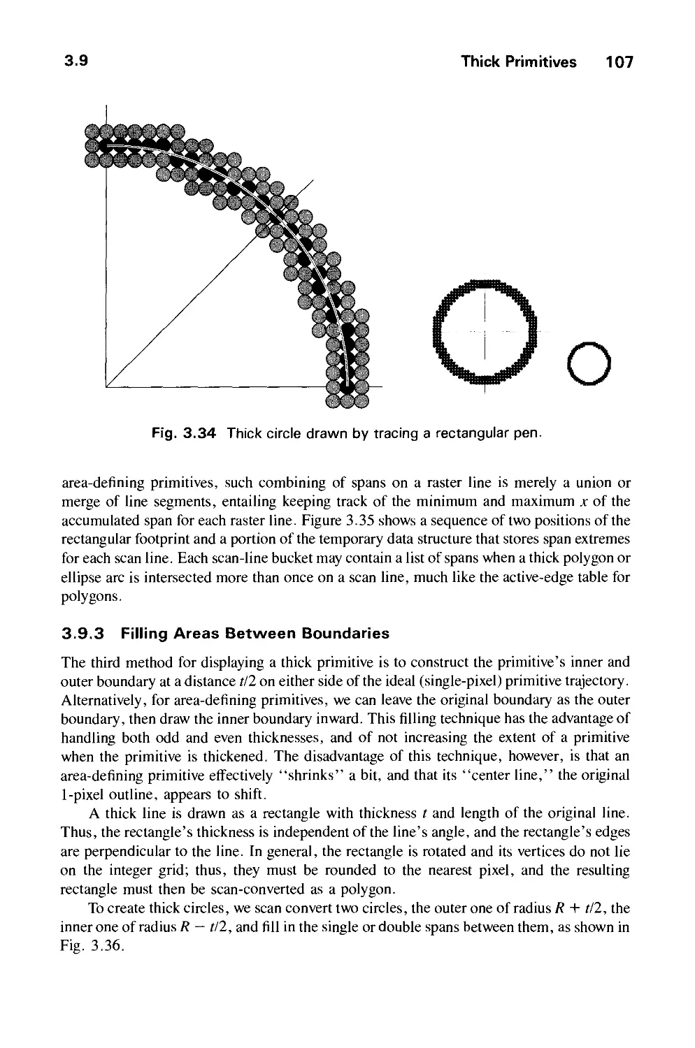
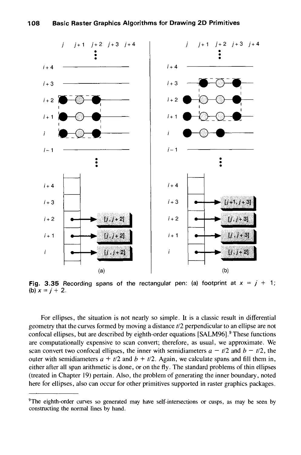
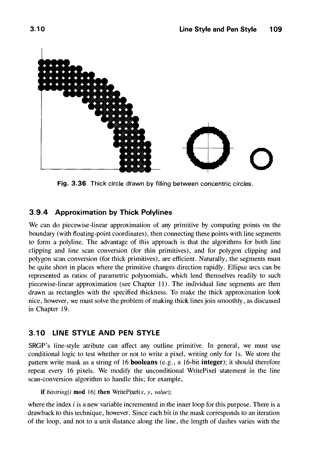
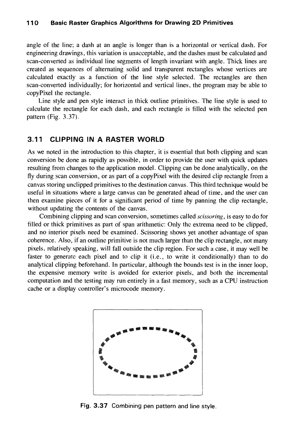
3.9 Thick Primitives 104
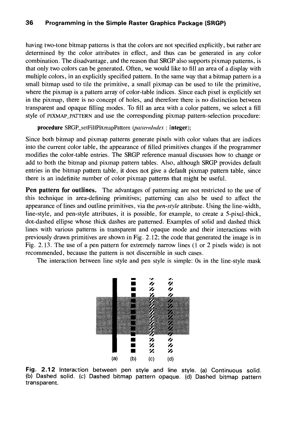
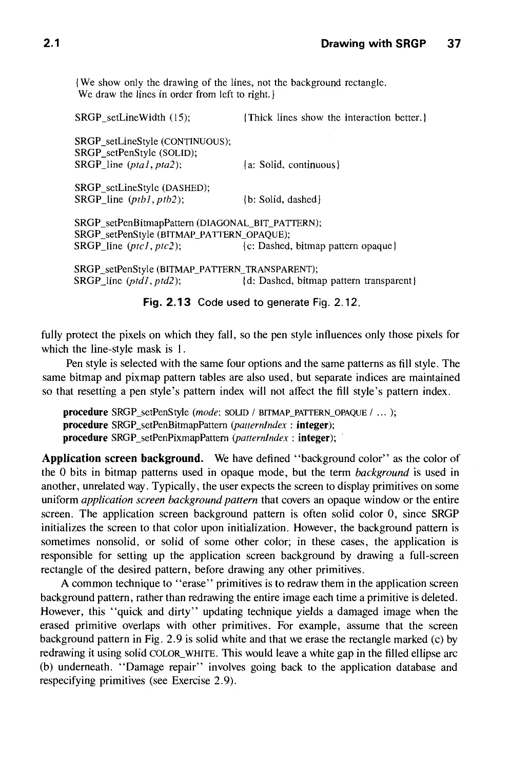
3.10 Line Style and Pen Style 109
3.11 Clipping in a Raster World 110
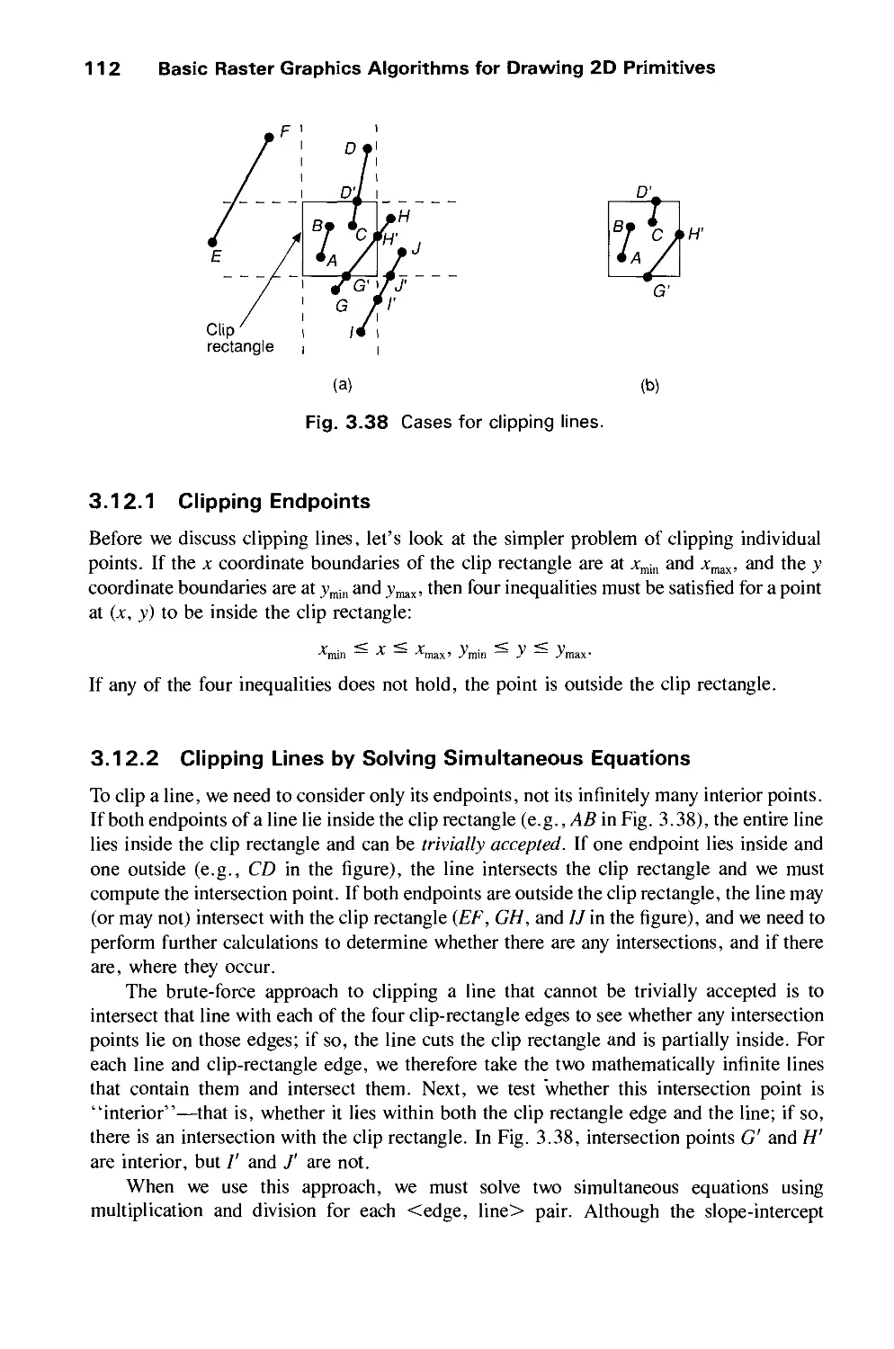
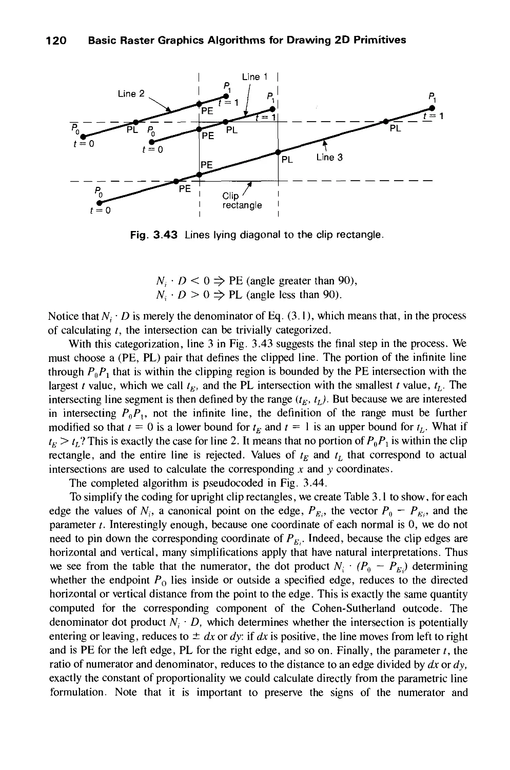
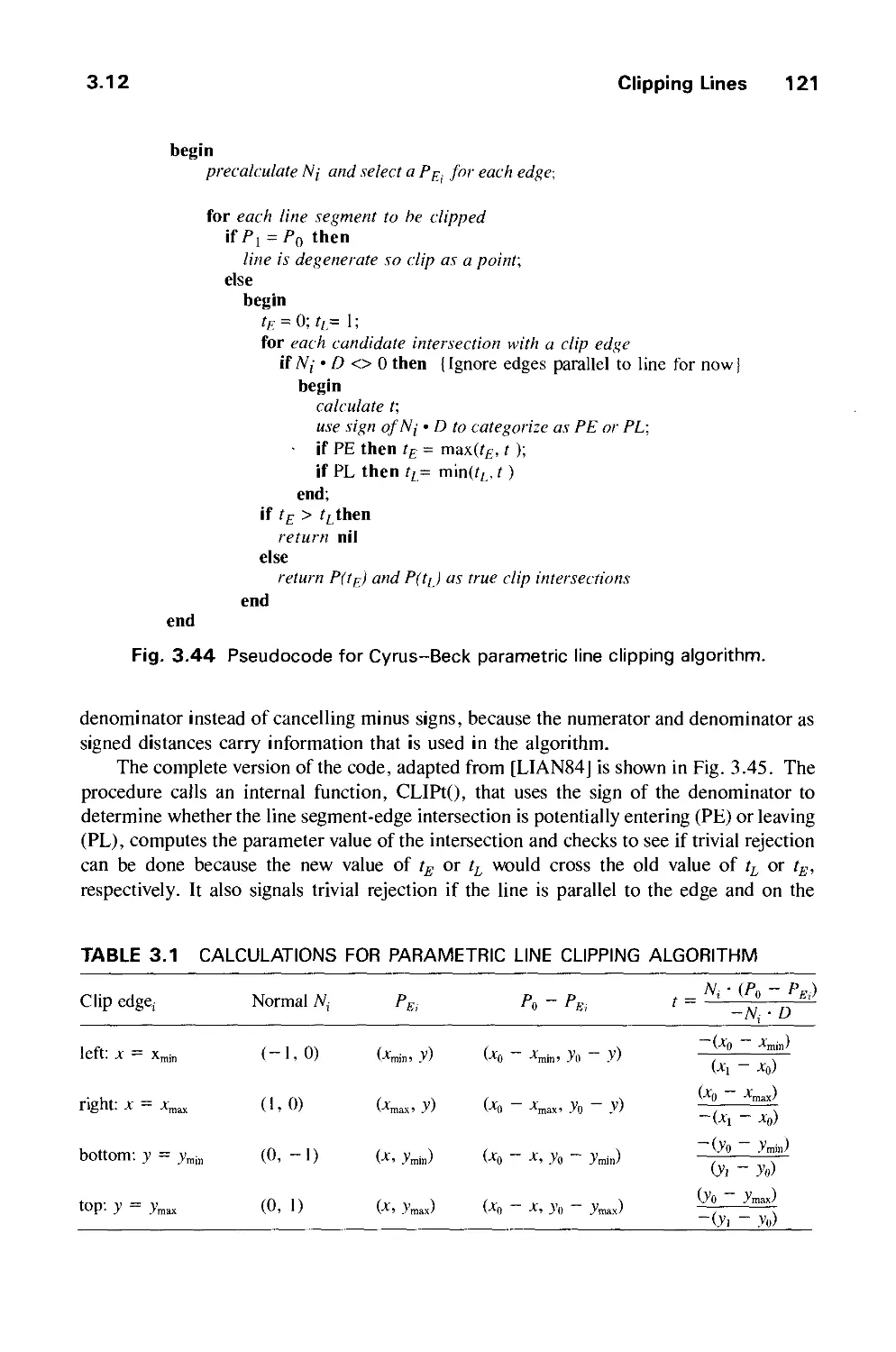
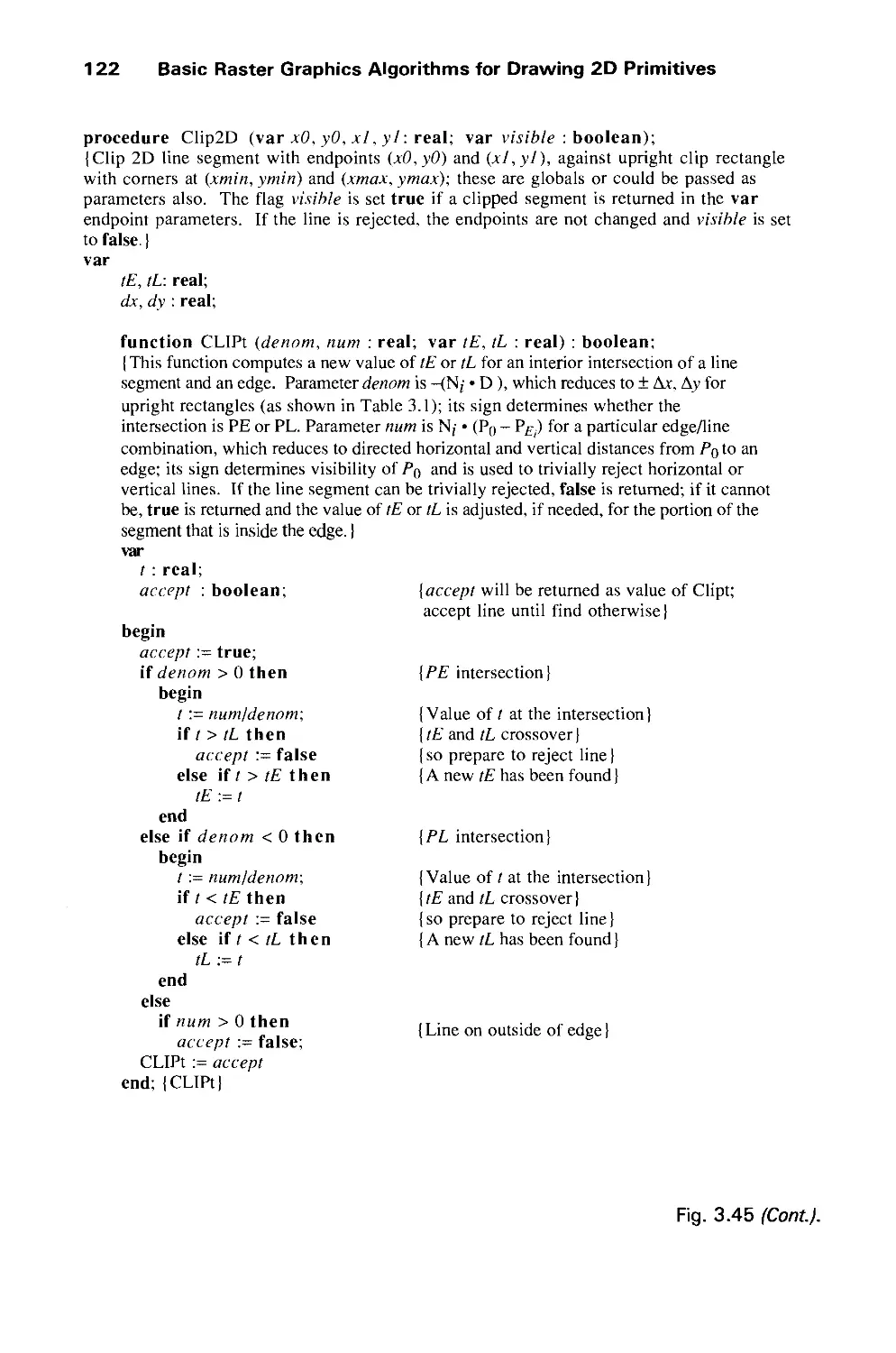
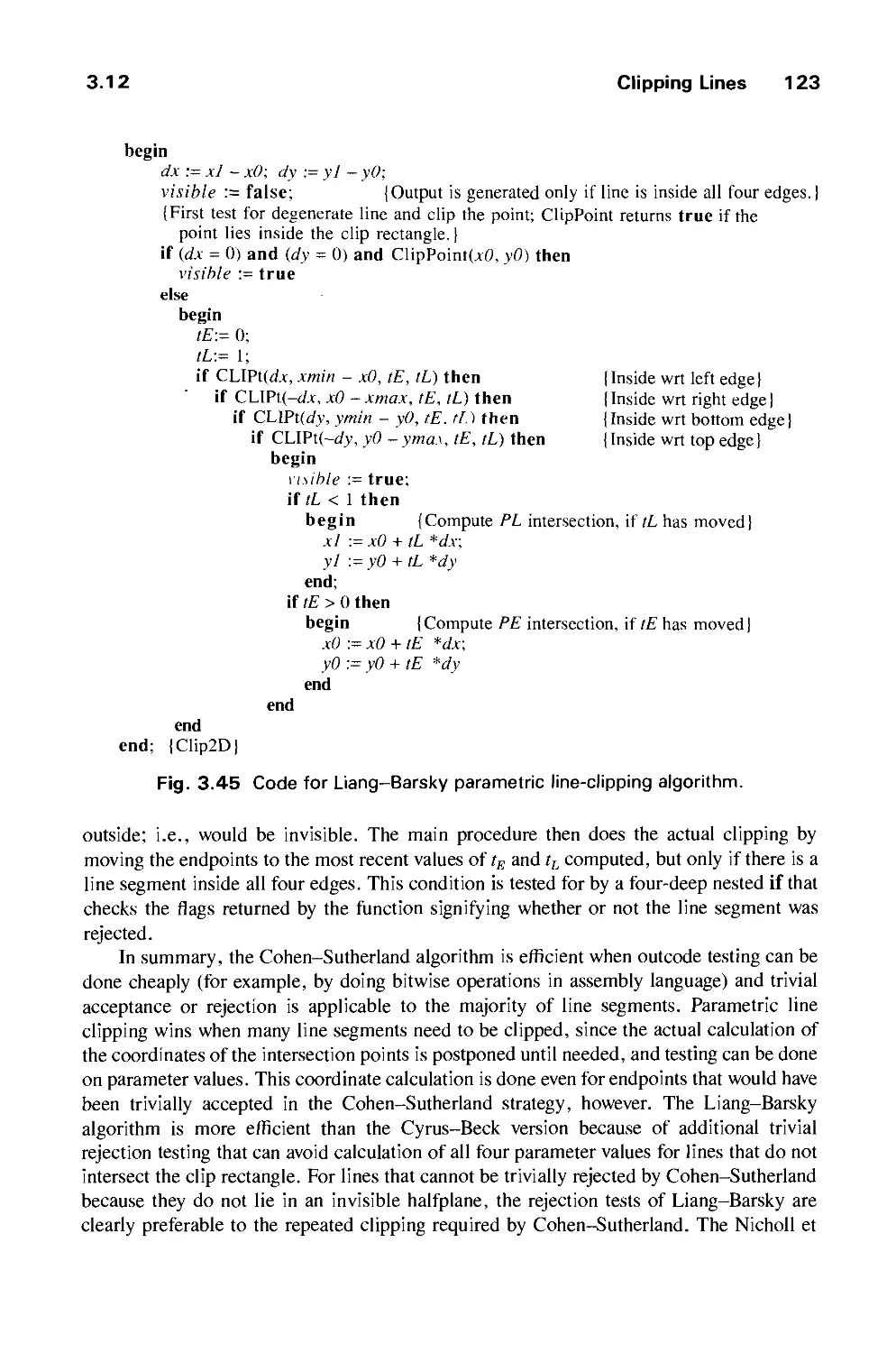
3.12 Clipping Lines Ill
xviii Contents
3.13 Clipping Circles and Ellipses 124
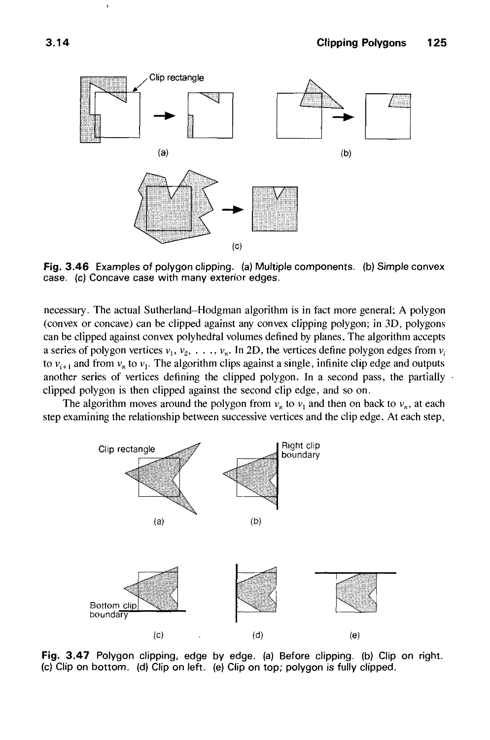
3.14 Clipping Polygons 124
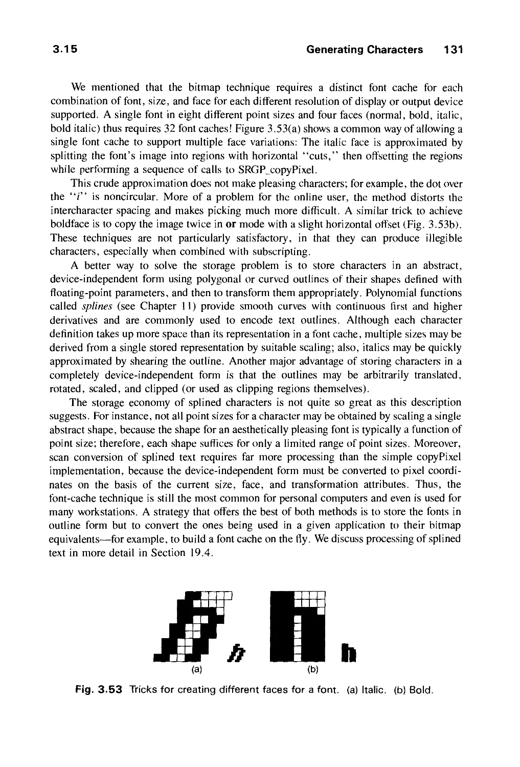
3.15 Generating Characters 127
3.16 SRGP_copyPixel 132
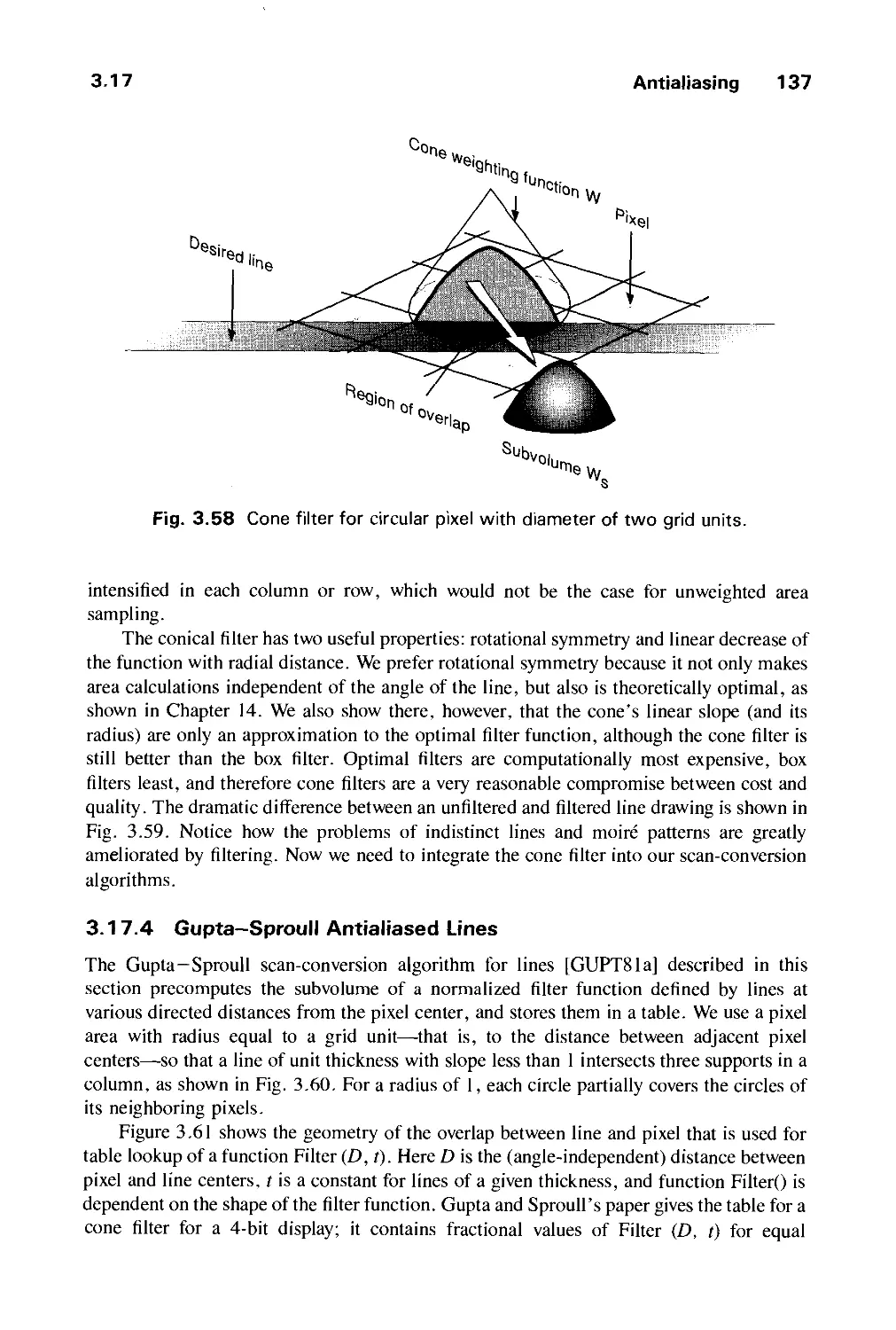
3.17 Antialiasing 132
3.18 Summary 140
Exercises 142
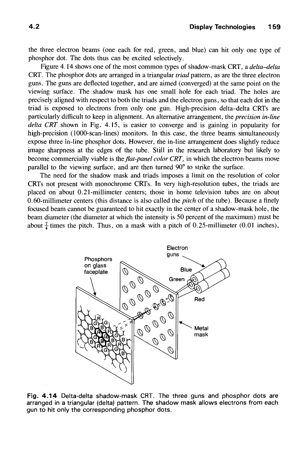
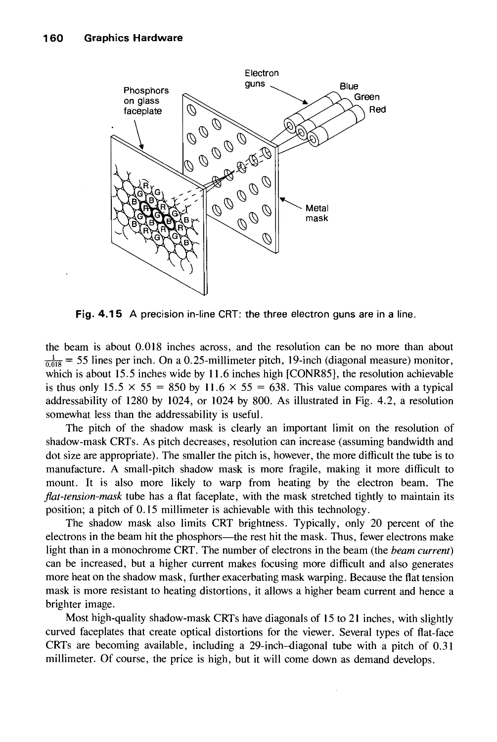
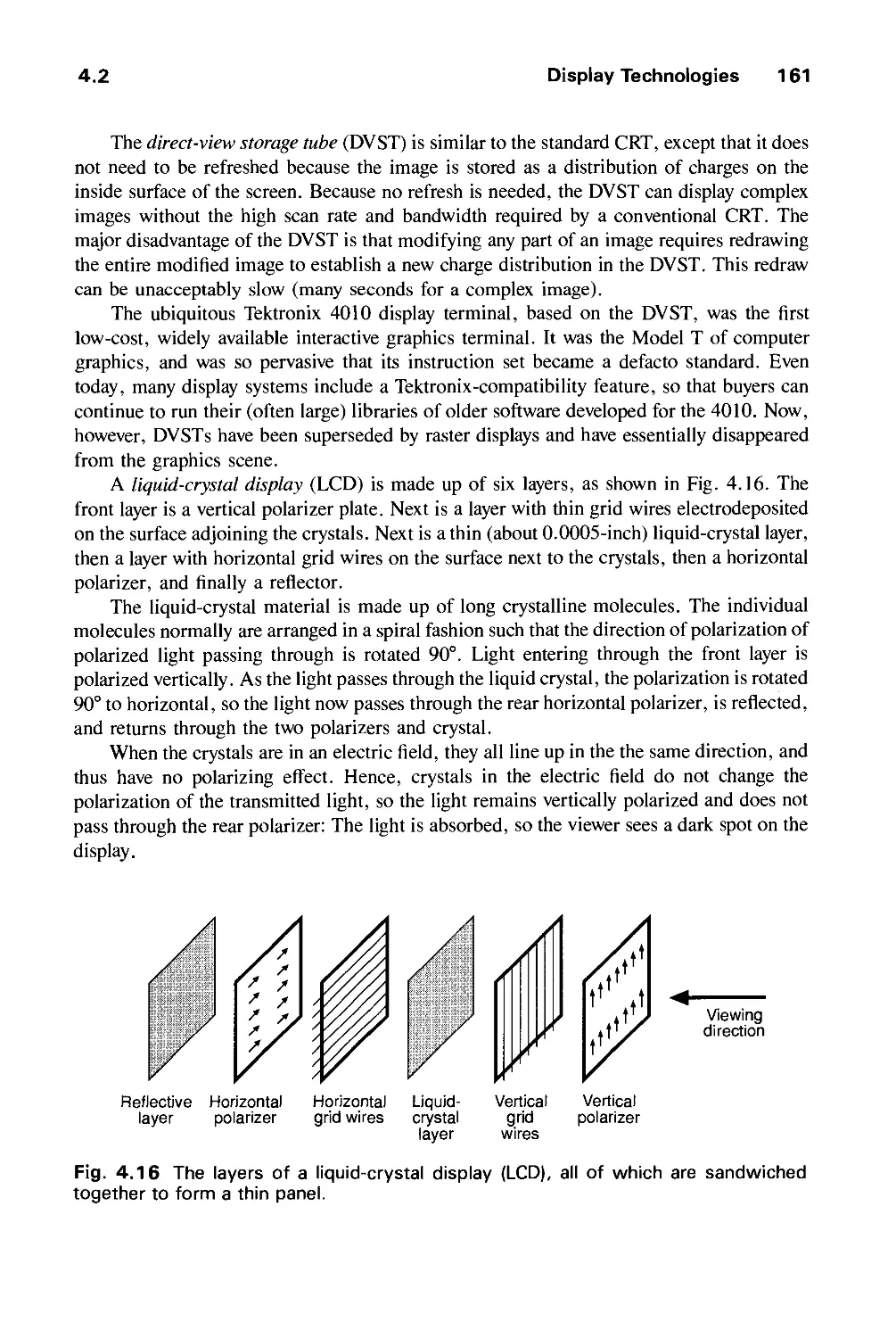
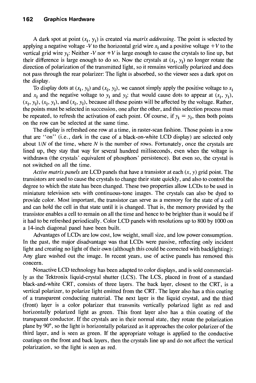
CHAPTER 4
GRAPHICS HARDWARE 145
4.1 Hardcopy Technologies 146
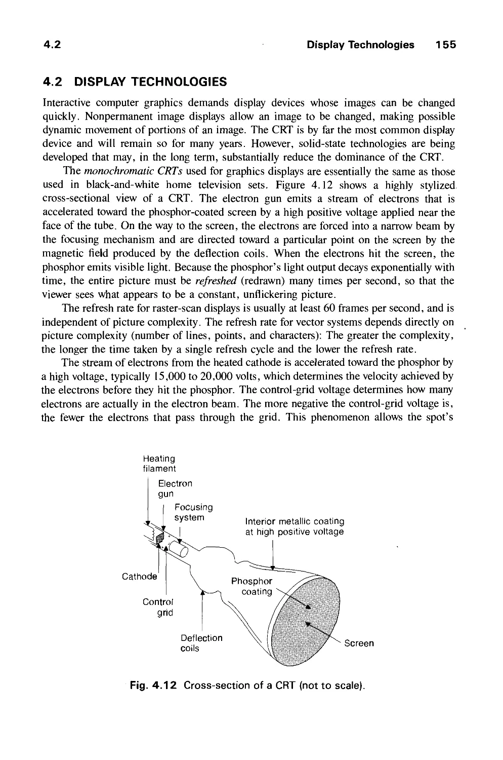
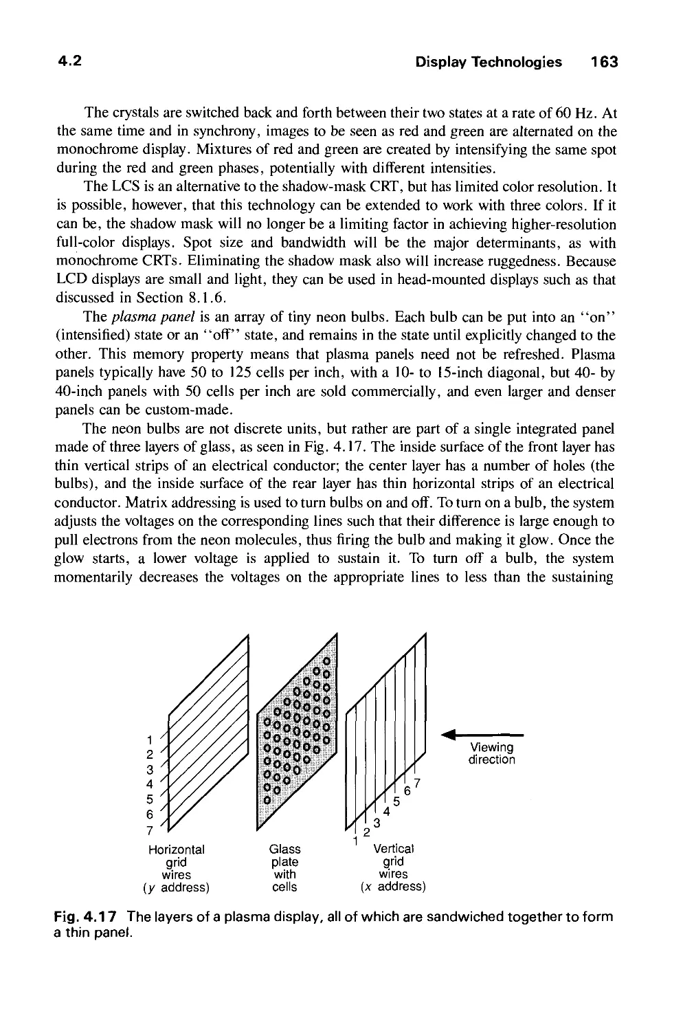
4.2 Display Technologies 155
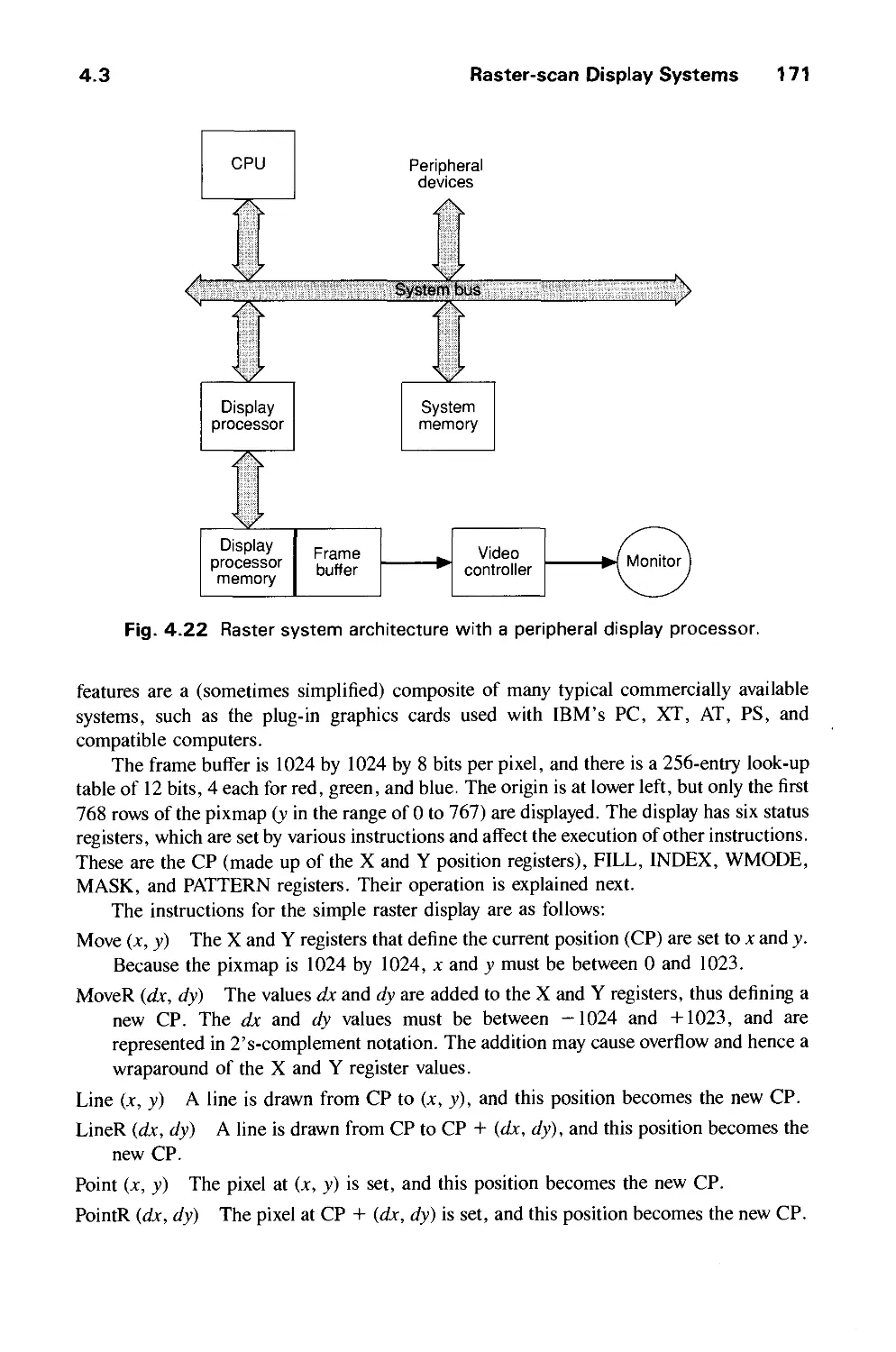
4.3 Raster-Scan Display Systems 165
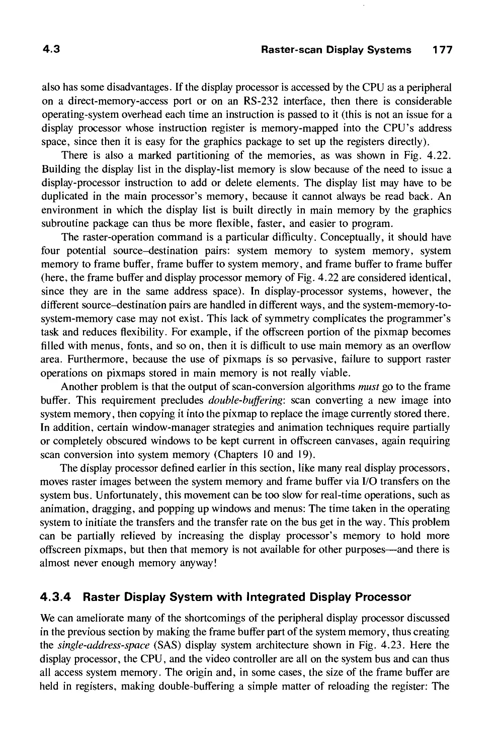
4.4 The Video Controller 179
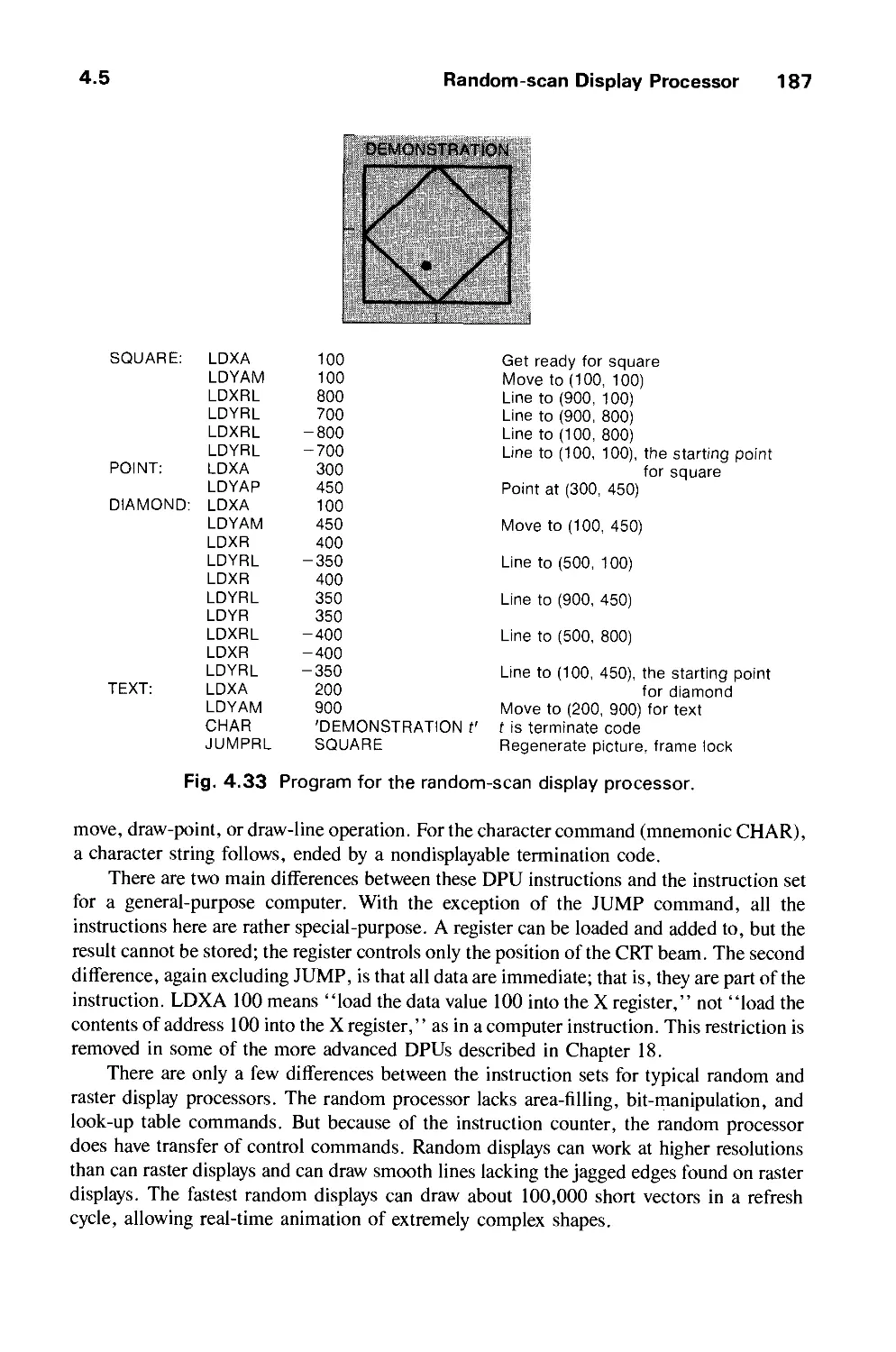
4.5 Random-Scan Display Processor 184
4.6 Input Devices for Operator Interaction 188
4.7 Image Scanners 195
Exercises 197
CHAPTER 5
GEOMETRICAL TRANSFORMATIONS 201
5.1 2D Transformations 201
5.2 Homogeneous Coordinates and Matrix Representation of
2D Transformations 204
5.3 Composition of 2D Transformations 208
5.4 The Window-to-Viewport Transformation 210
5.5 Efficiency 212
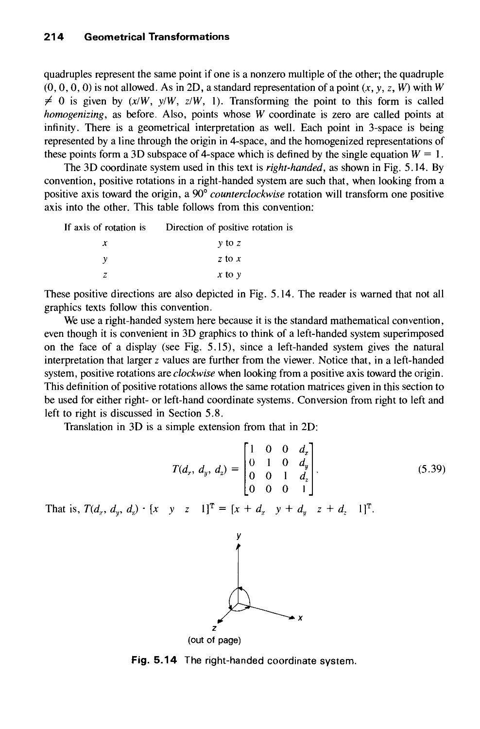
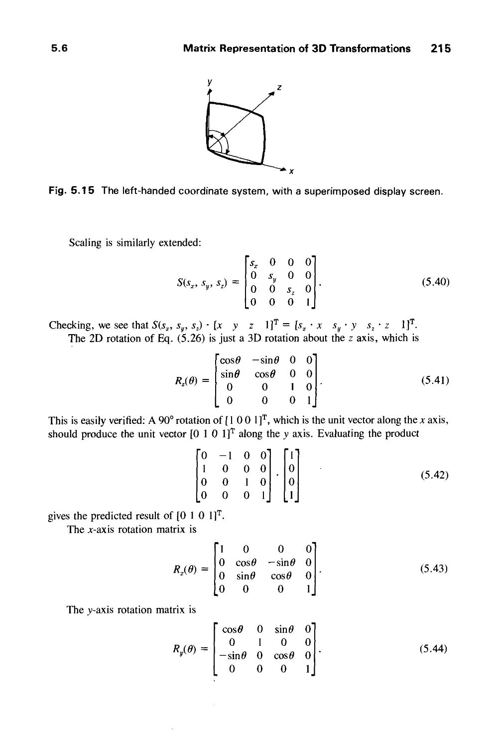
5.6 Matrix Representation of 3D Transformations 213
5.7 Composition of 3D Transformations 217
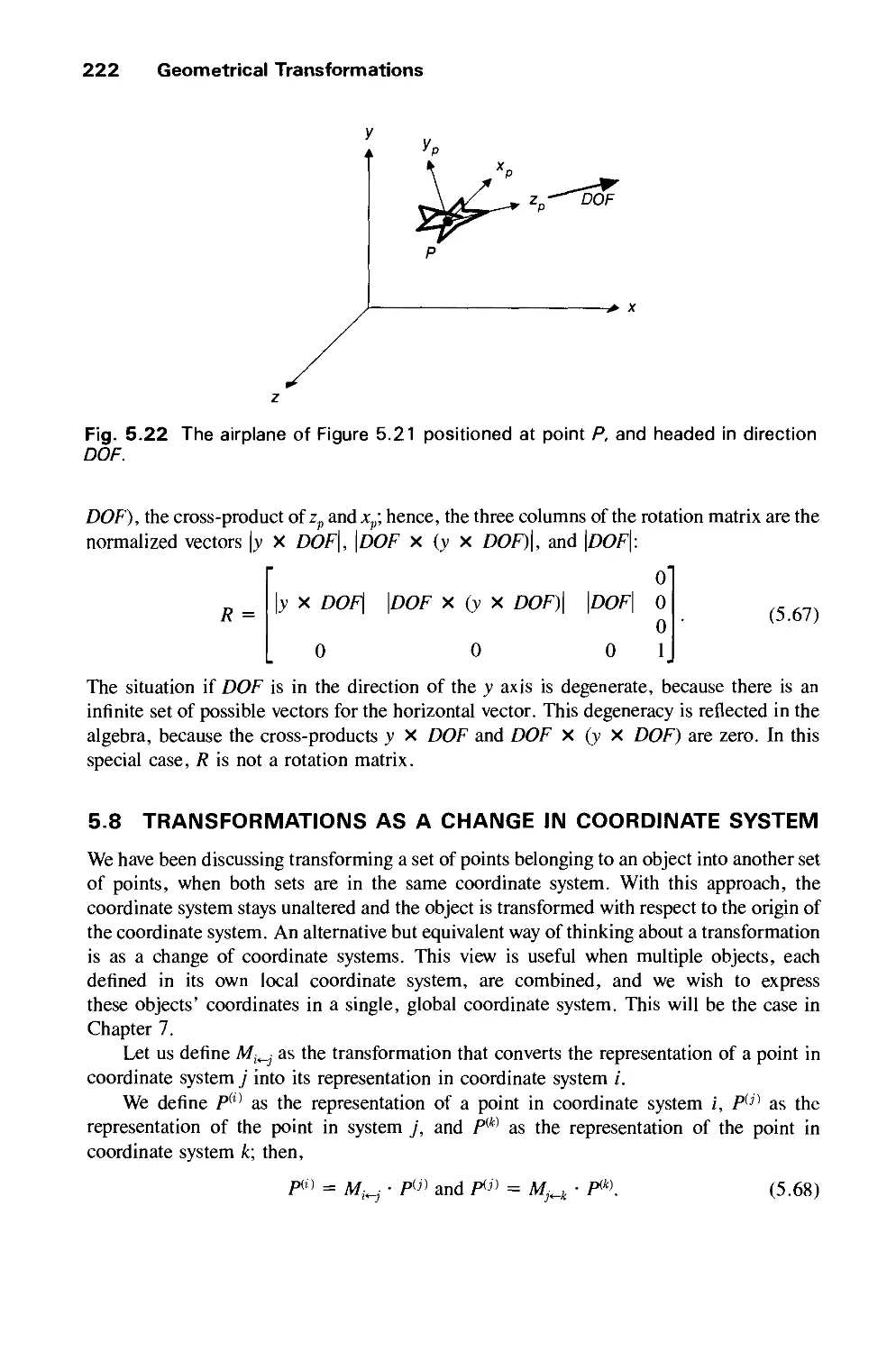
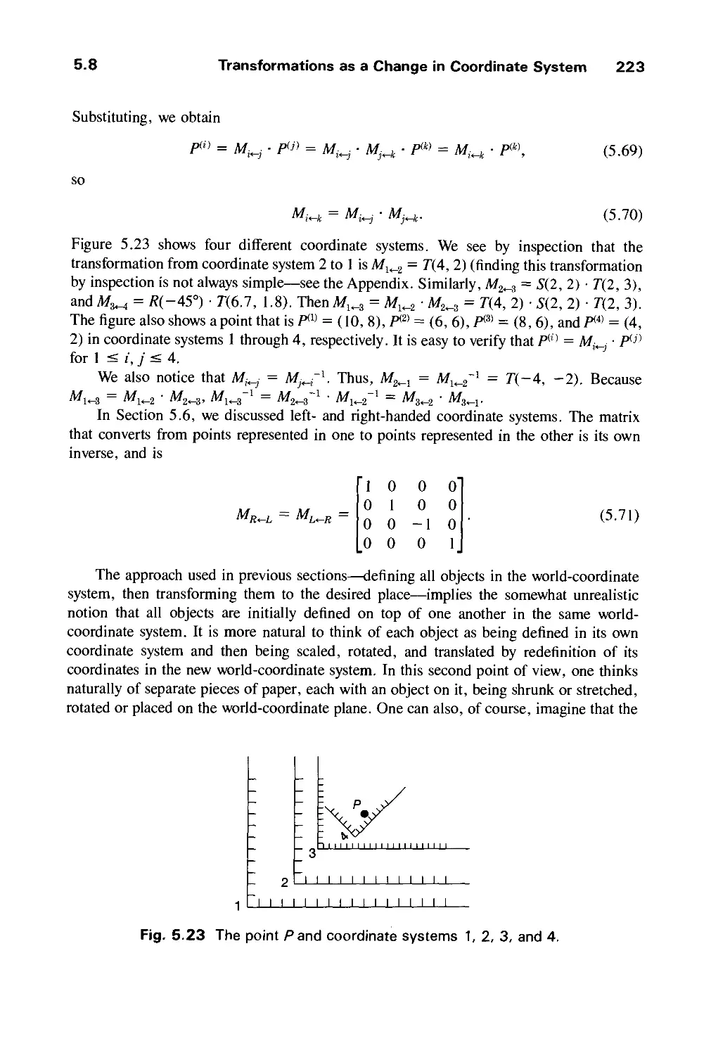
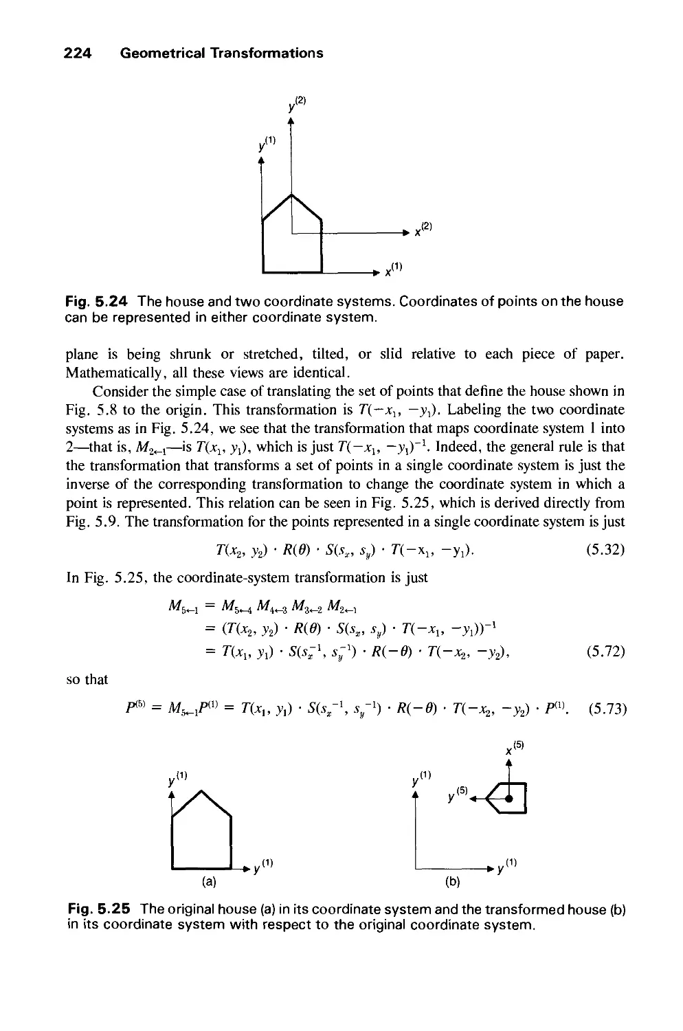
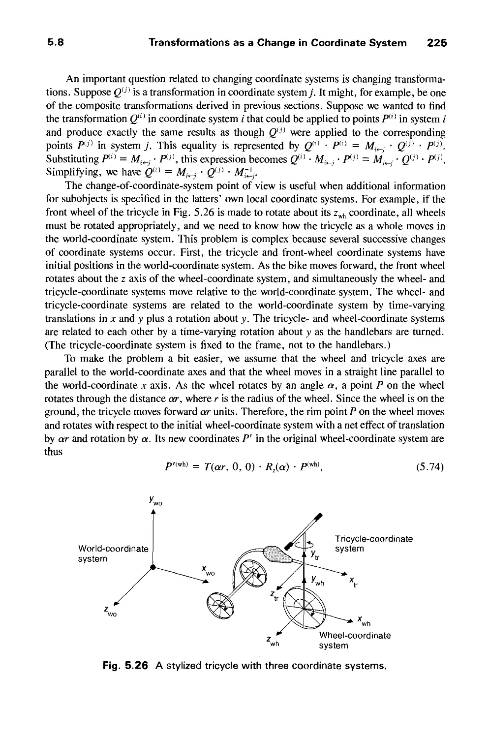
5.8 Transformations as a Change in Coordinate System 222
Exercises 226
CHAPTER 6
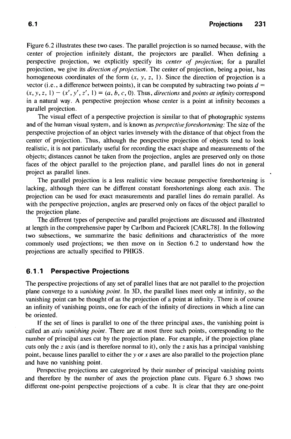
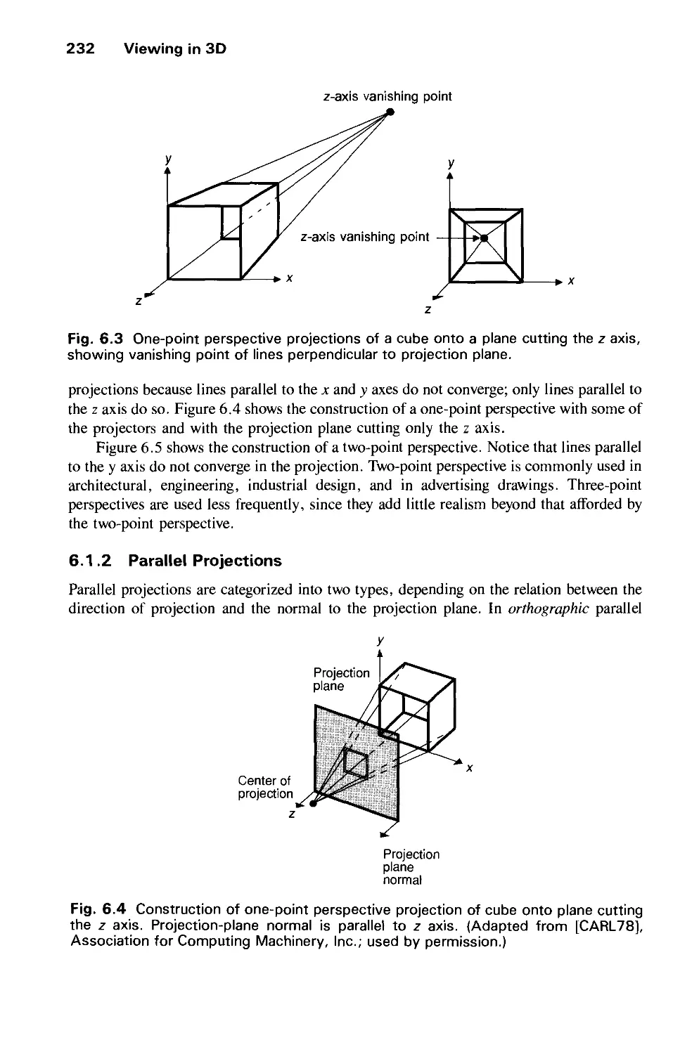
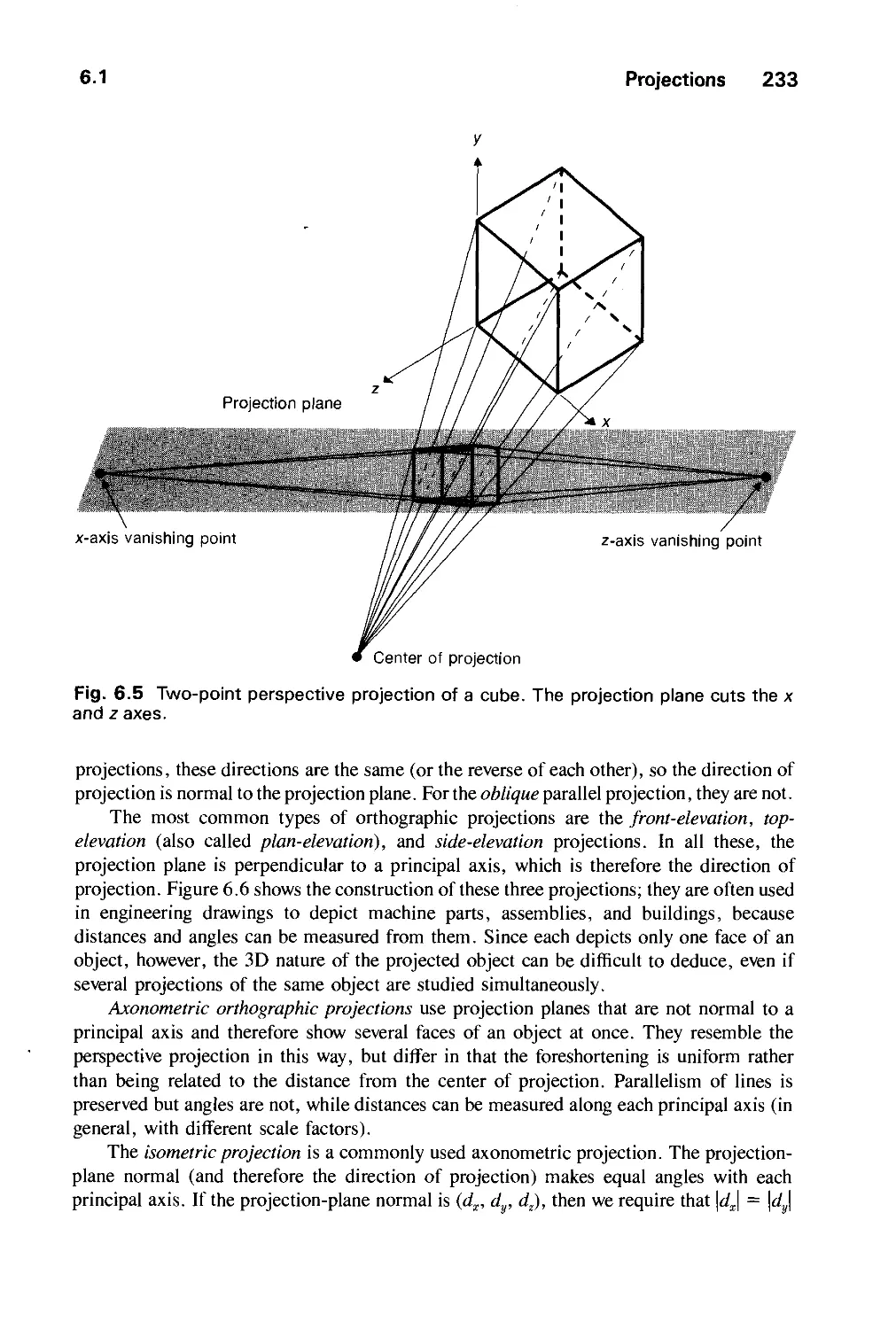
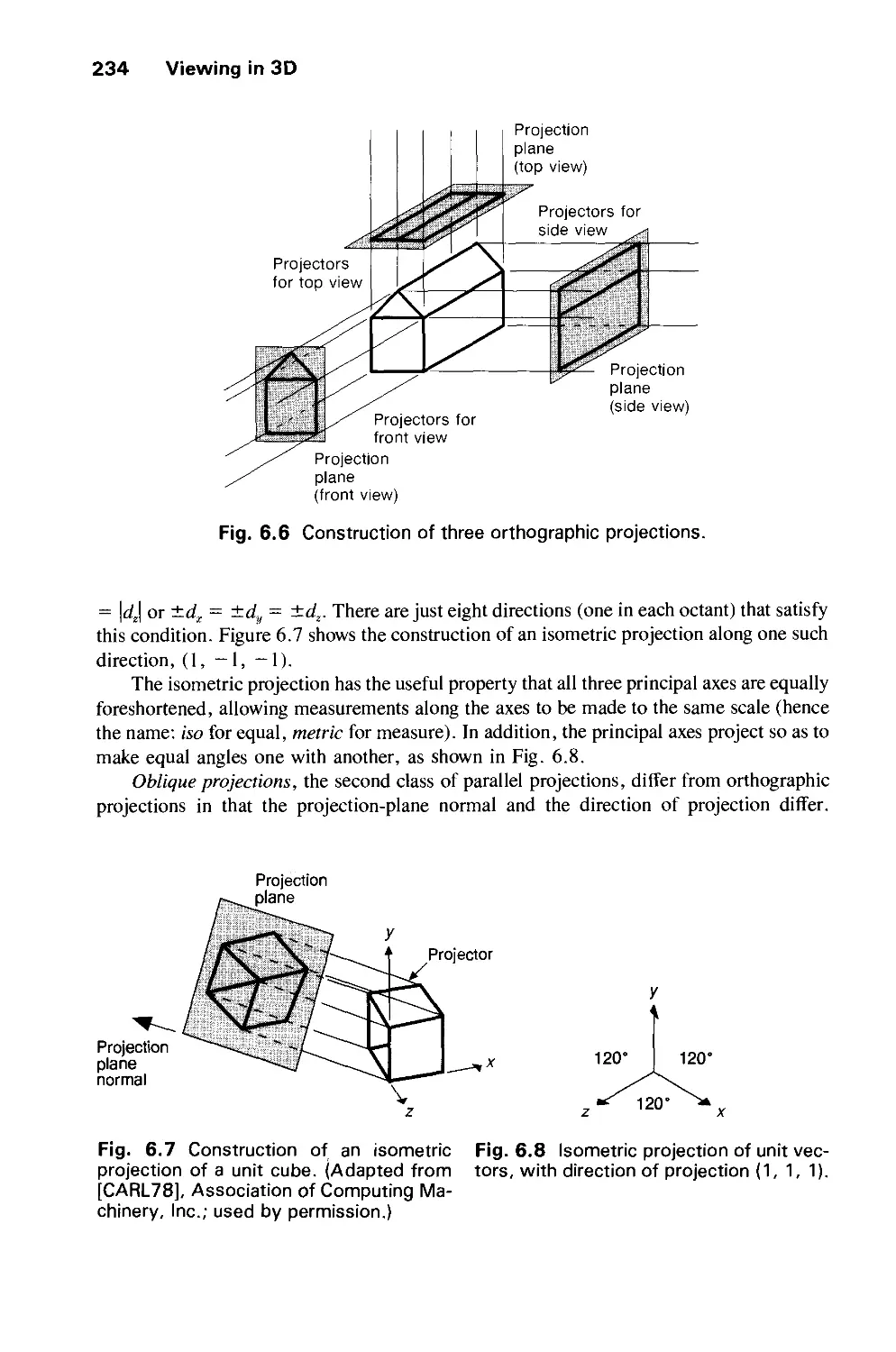
VIEWING IN 3D 229
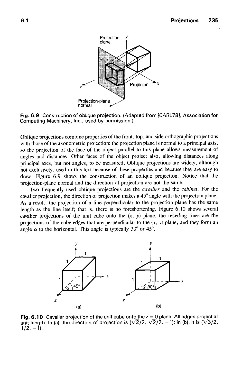
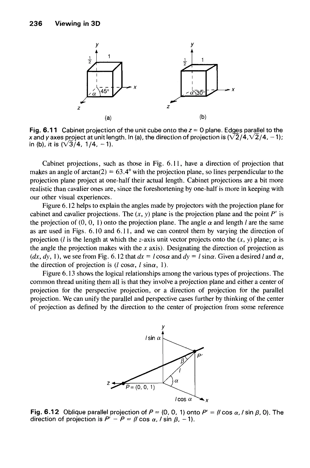
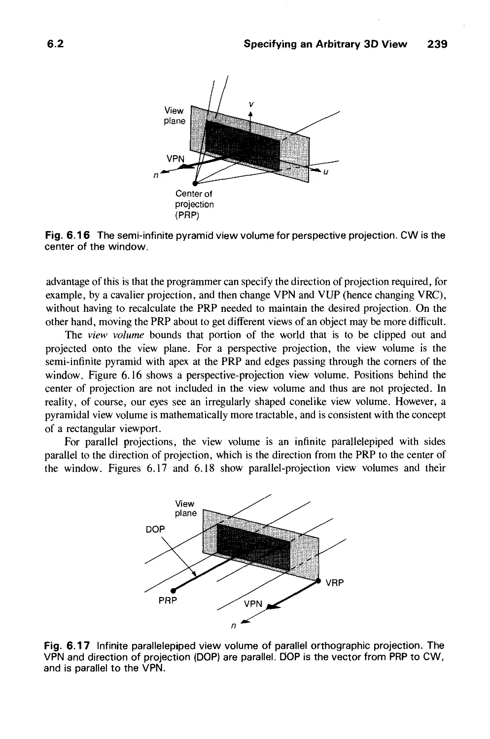
6.1 Projections 230
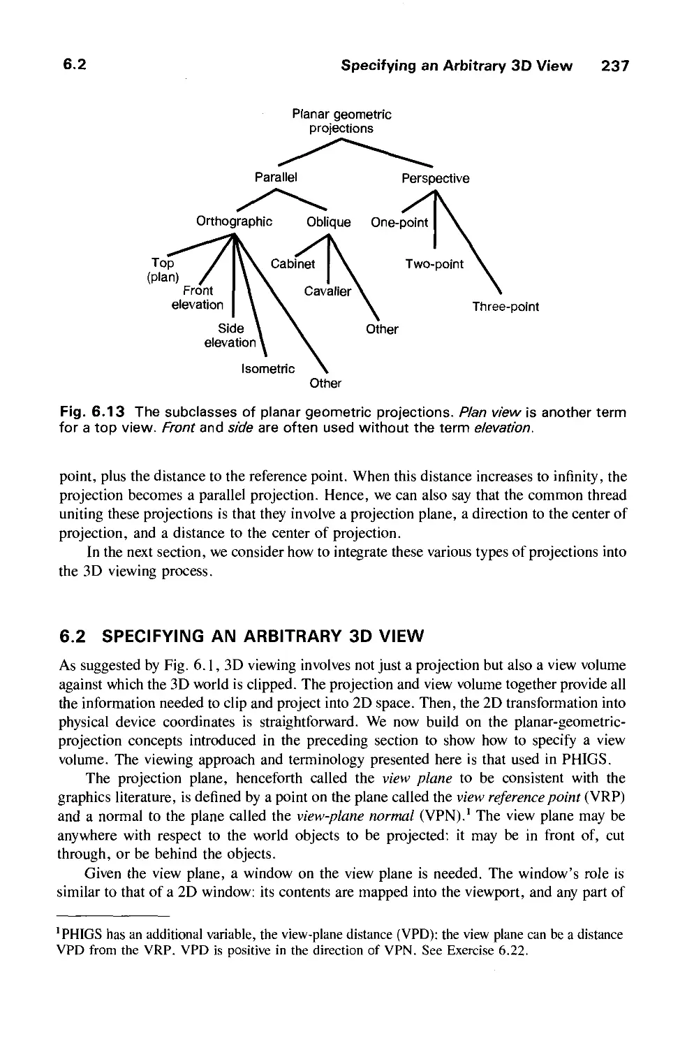
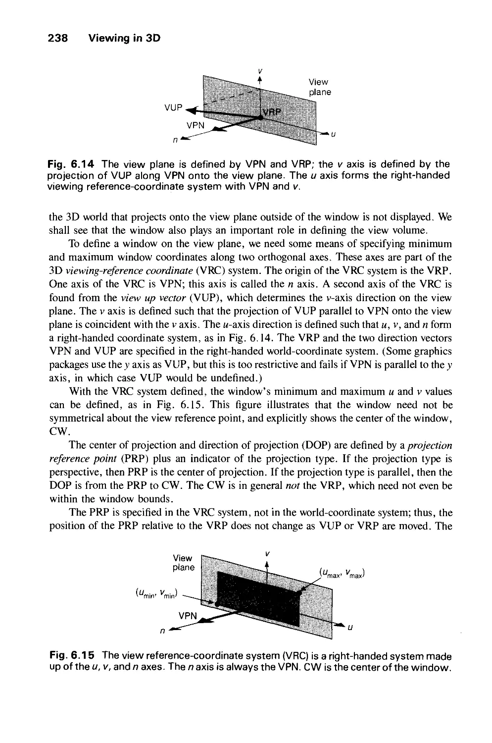
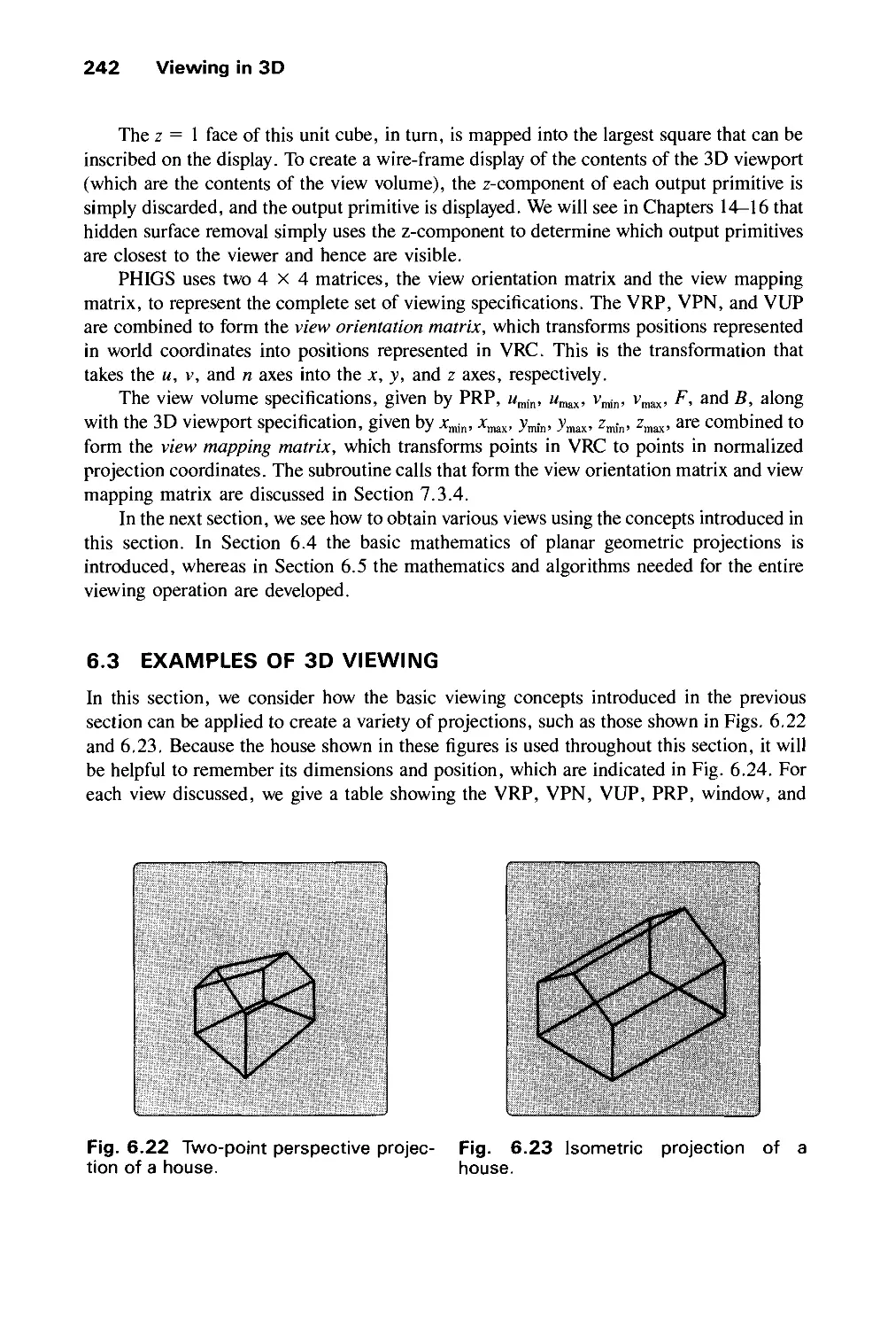
6.2 Specifying an Arbitrary 3D View 237
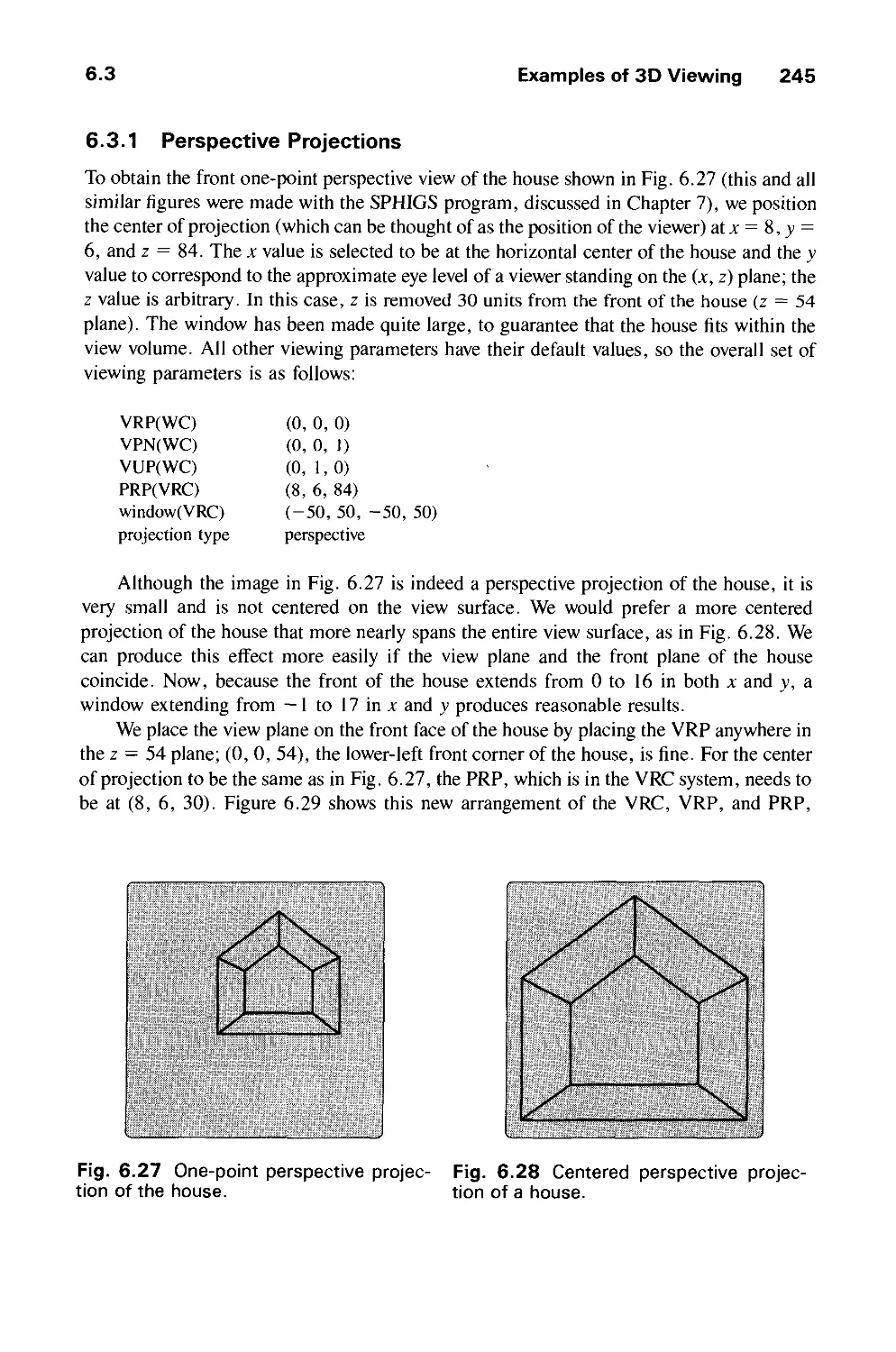
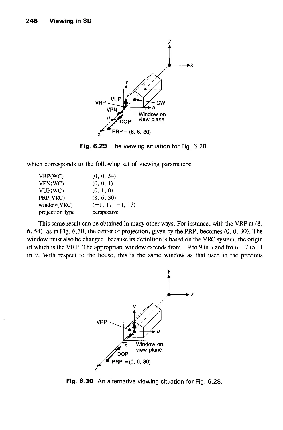
6.3 Examples of 3D Viewing 242
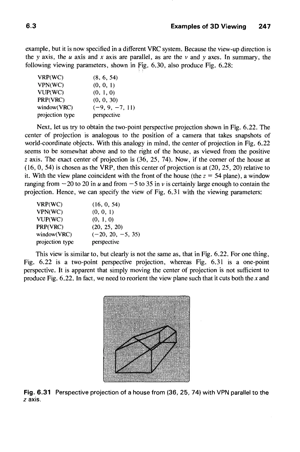
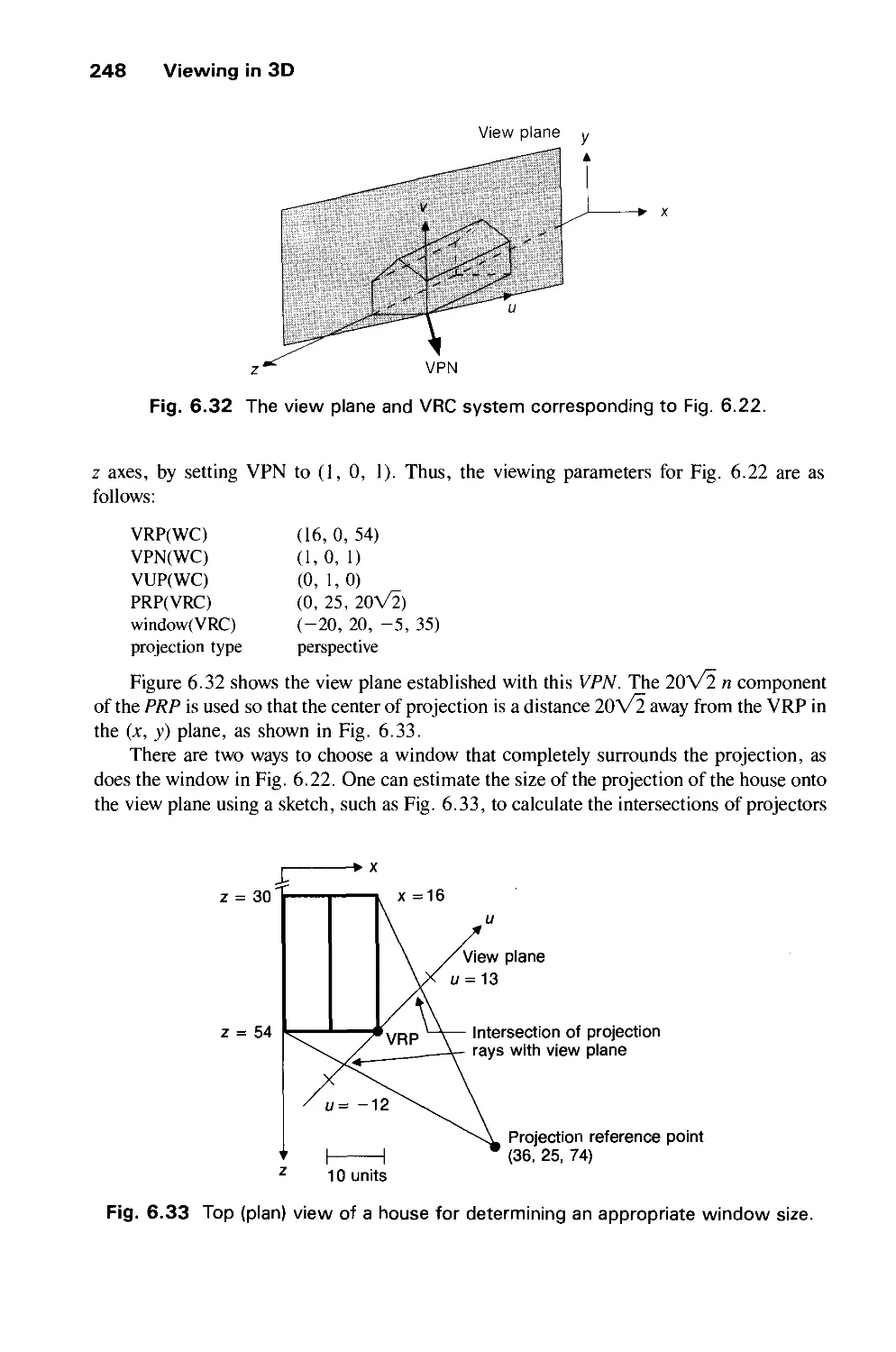
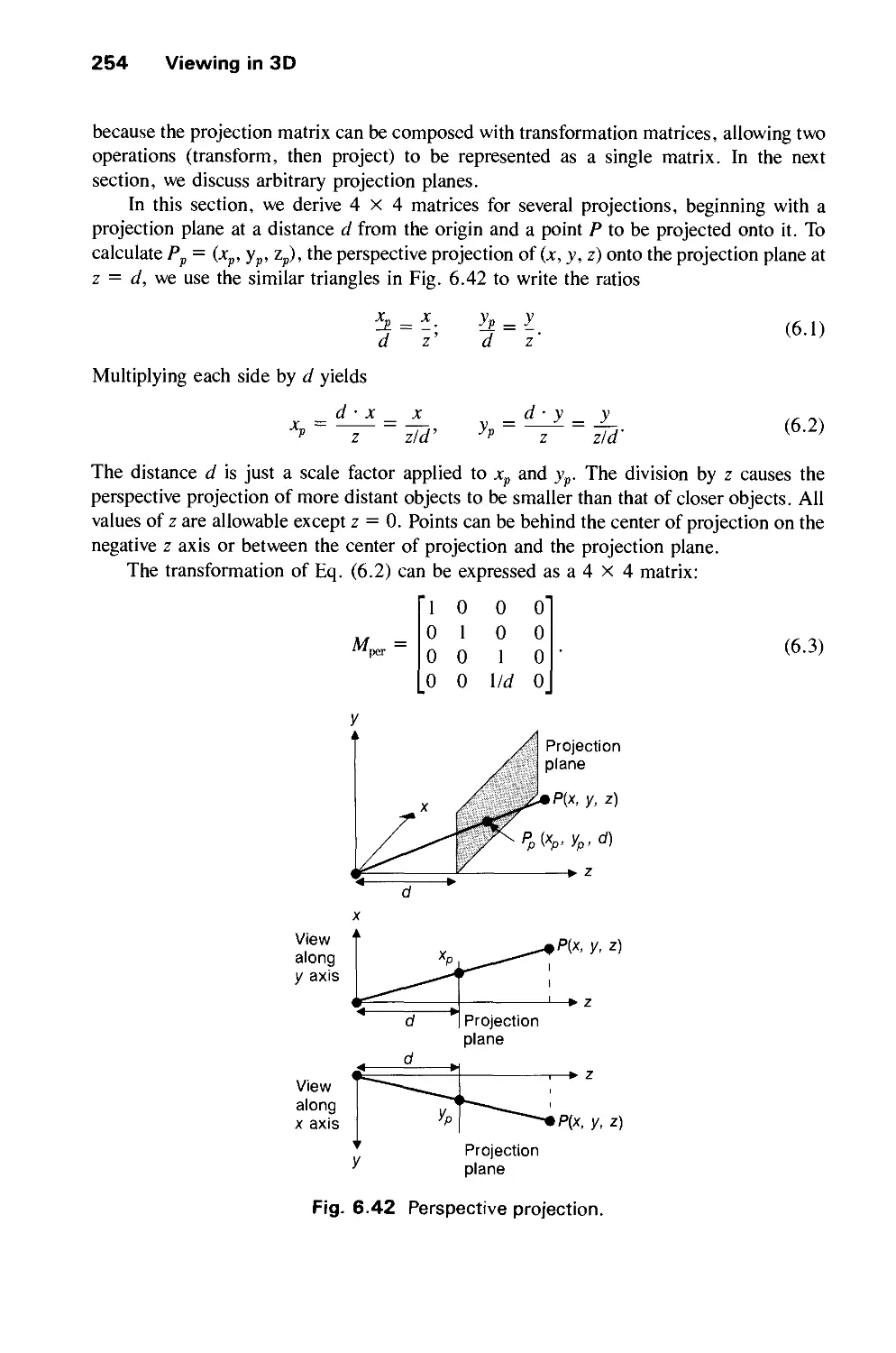
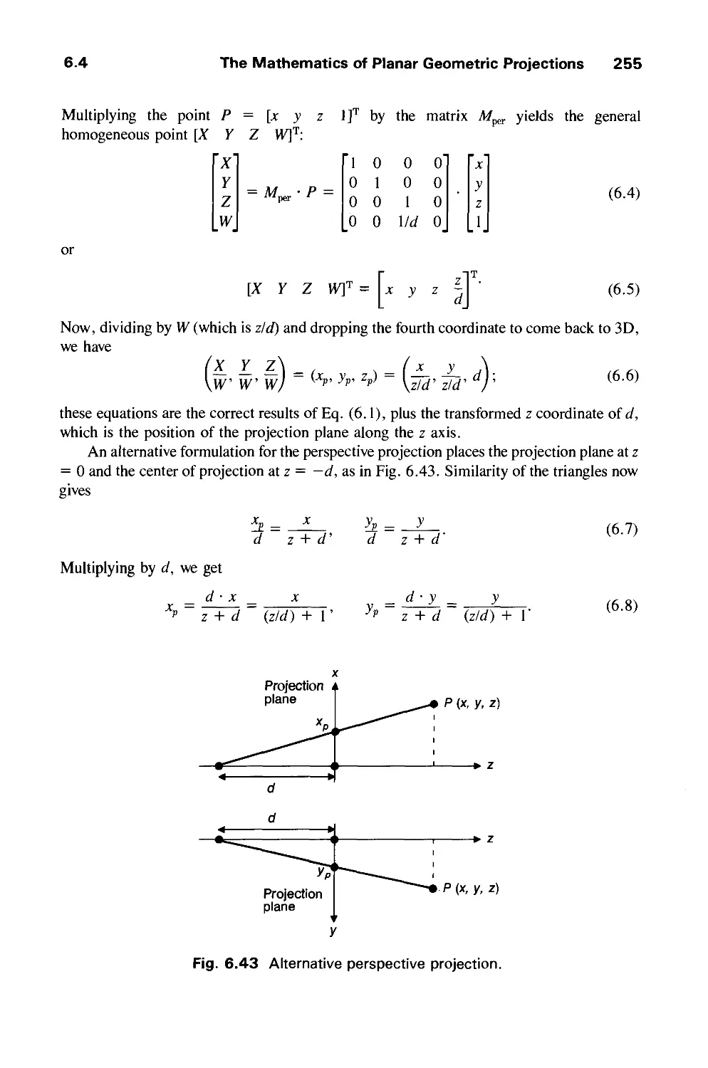
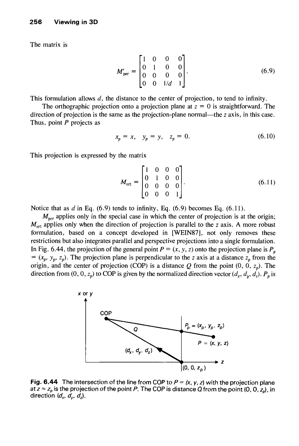
6.4 The Mathematics of Planar Geometric Projections 253
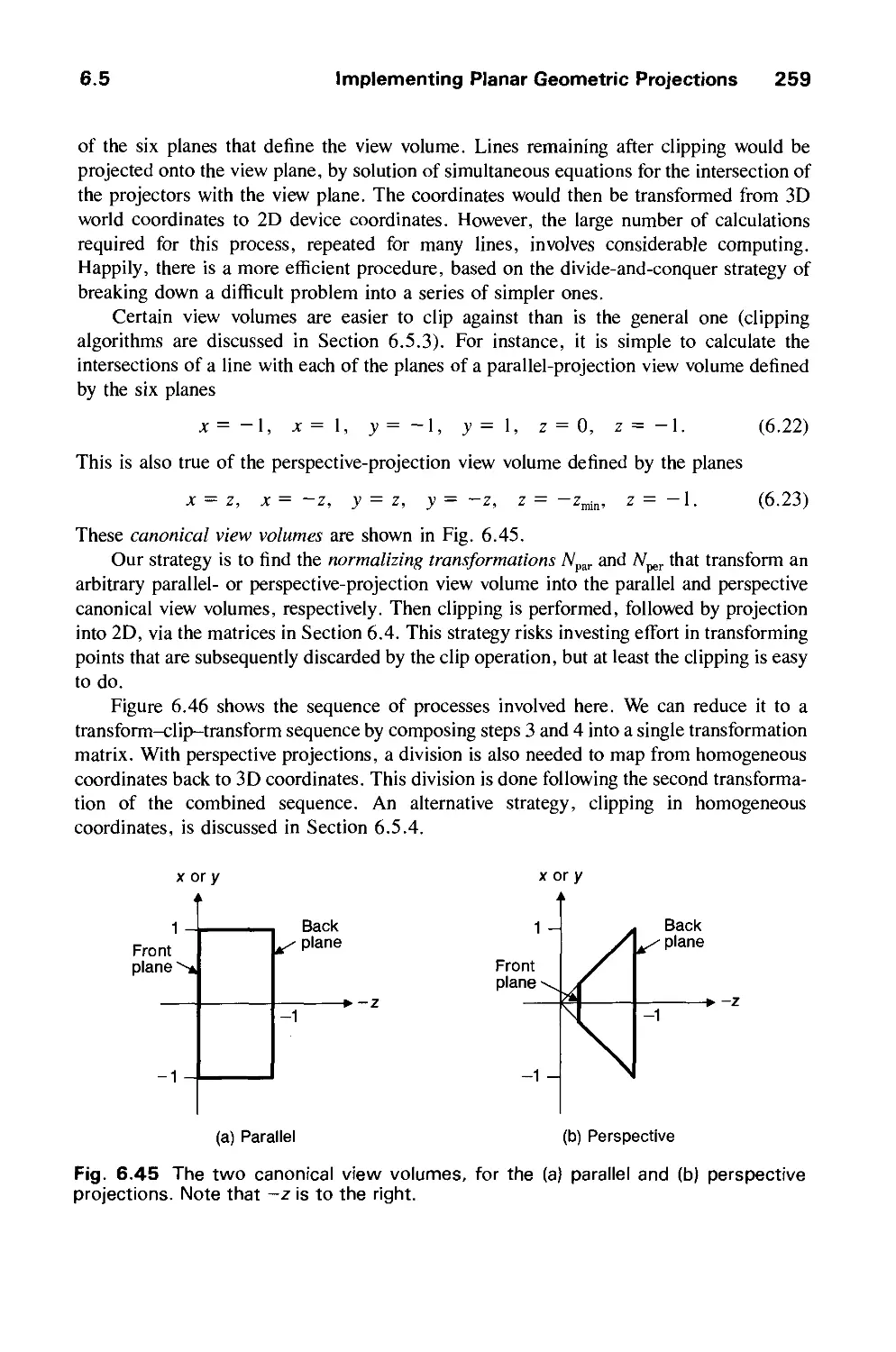
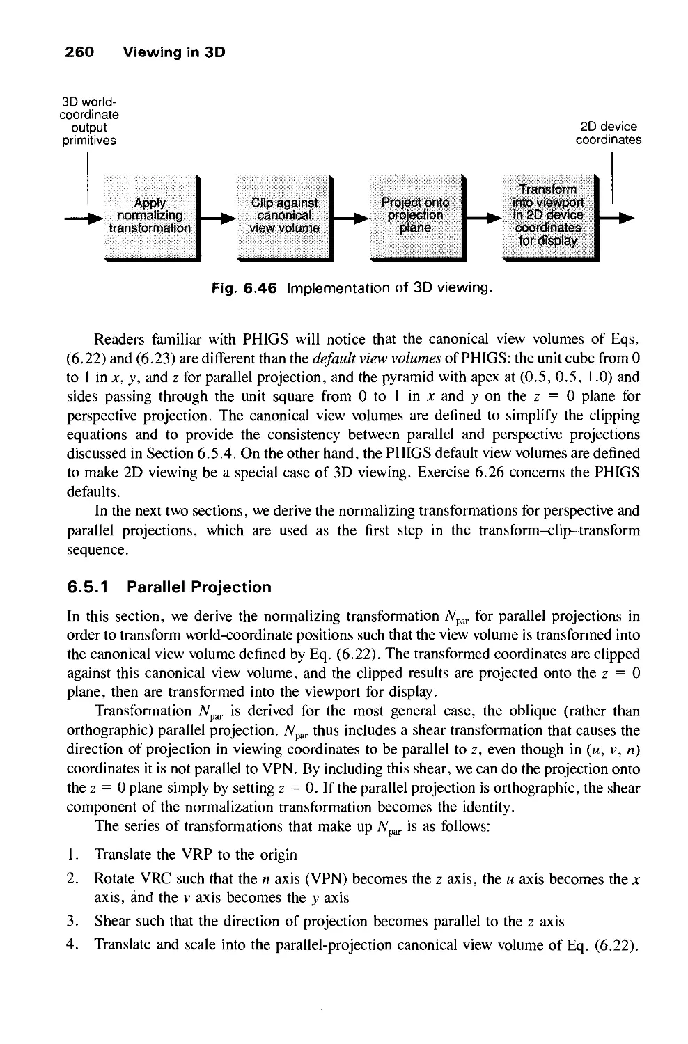
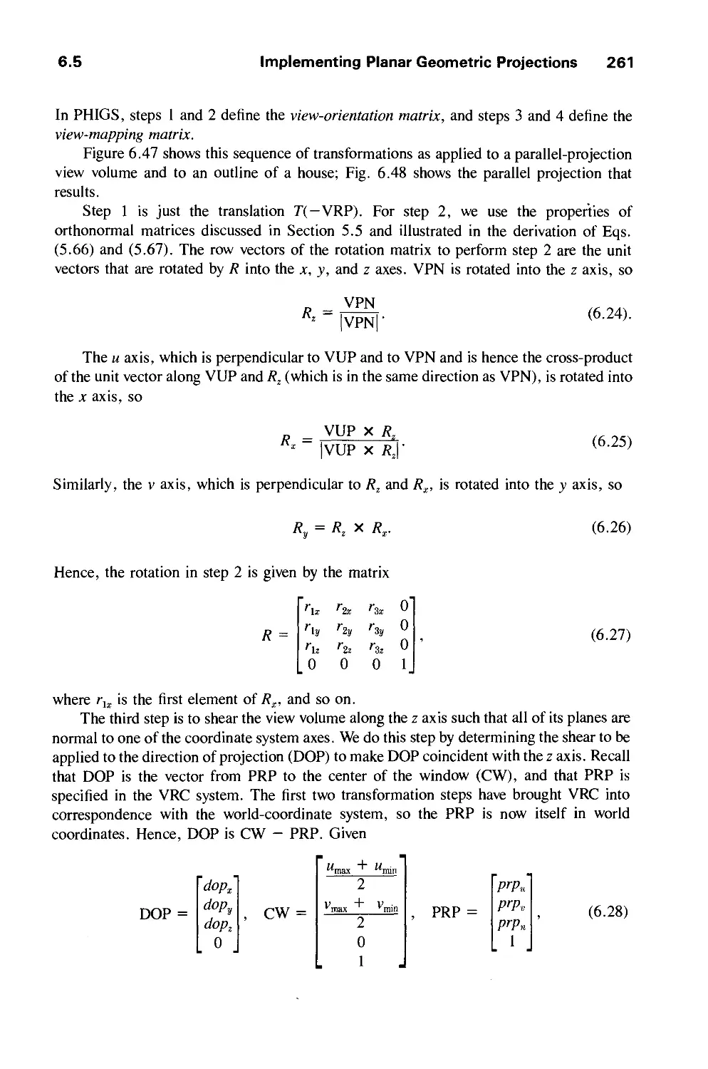
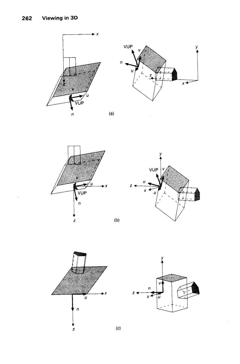
6.5 Implementing Planar Geometric Projections 258
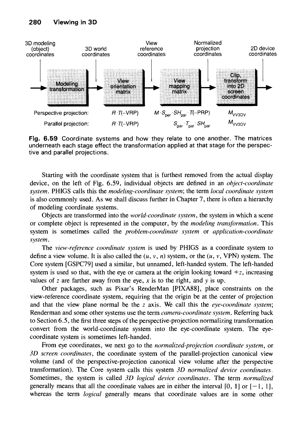
6.6 Coordinate Systems 279
Exercises 281
Contents xix
CHAPTER 7
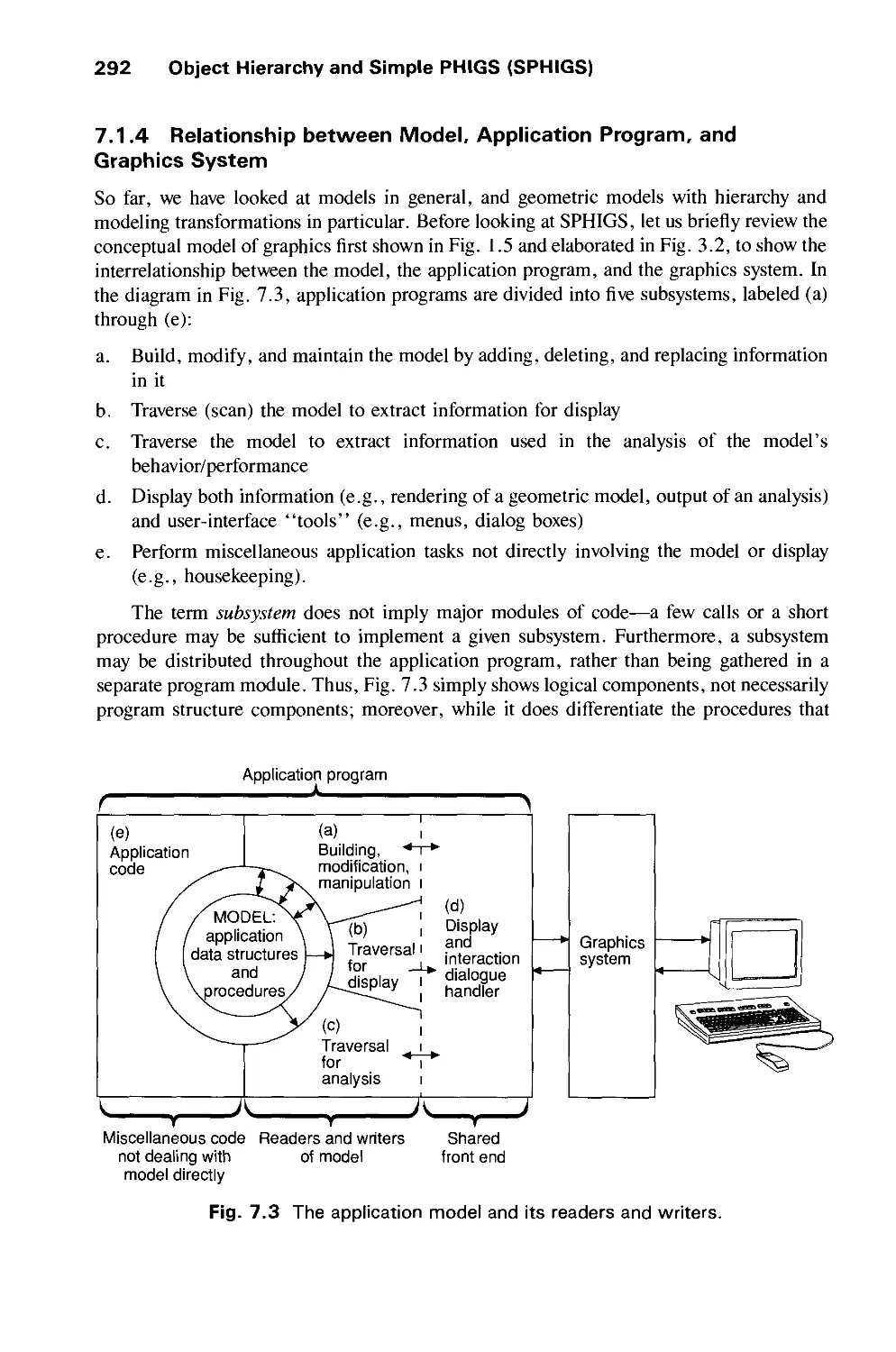
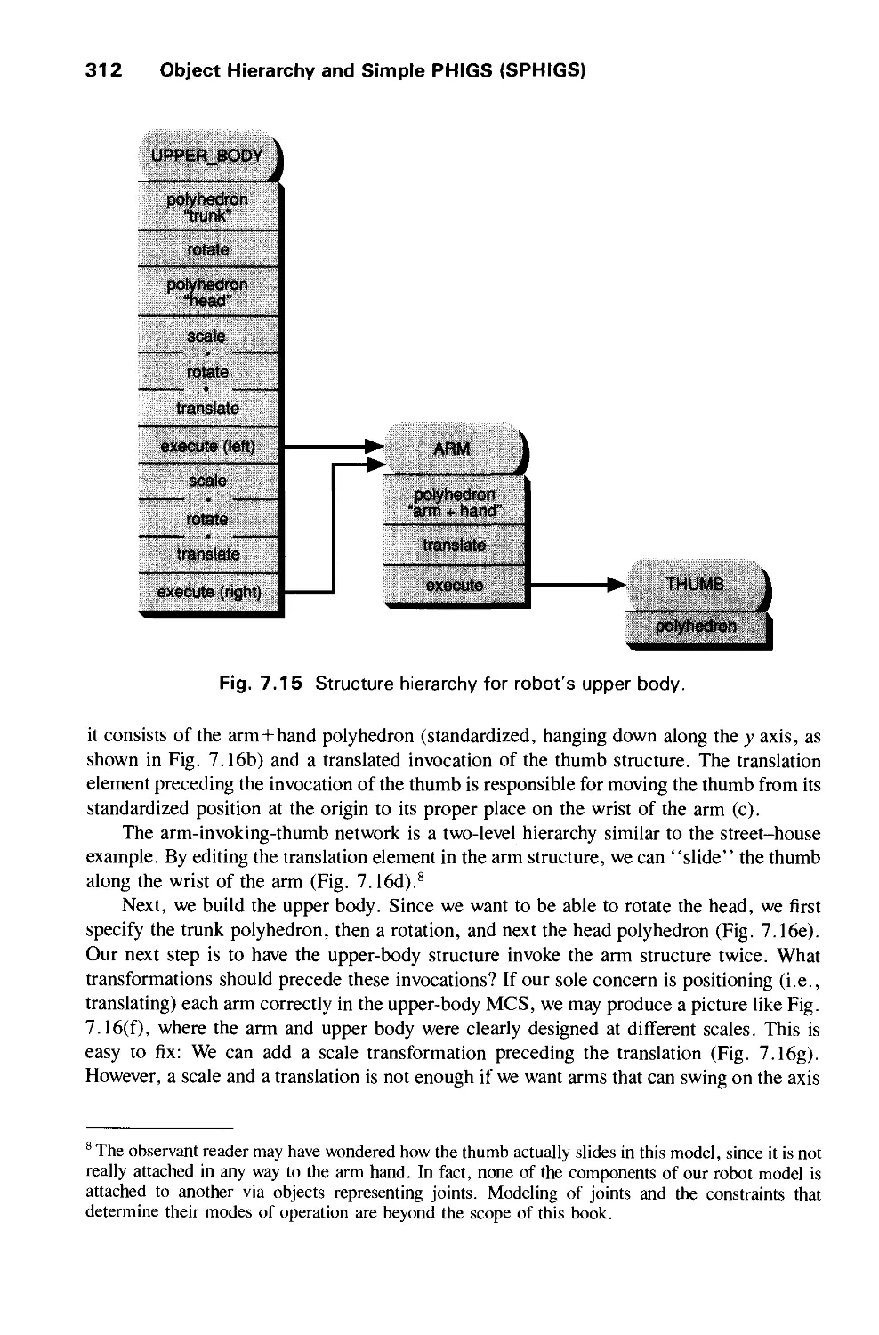
OBJECT HIERARCHY AND SIMPLE PHIGS (SPHIGS) 285
7.1 Geometric Modeling 286
7.2 Characteristics of Retained-Mode Graphics Packages 293
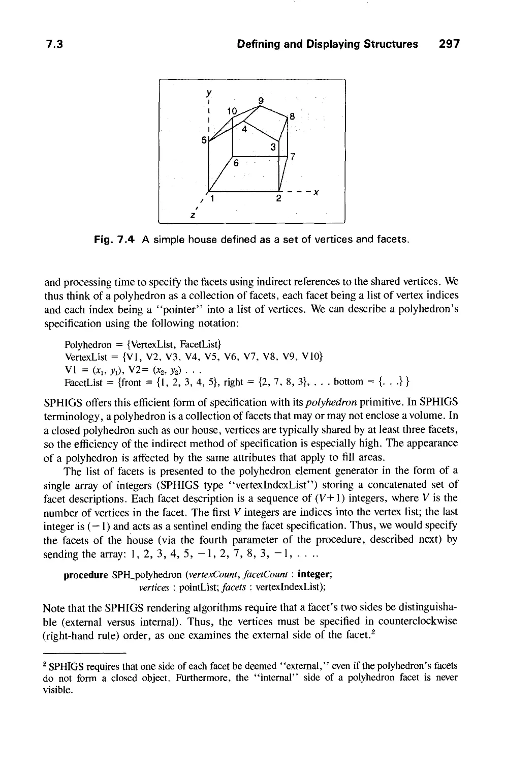
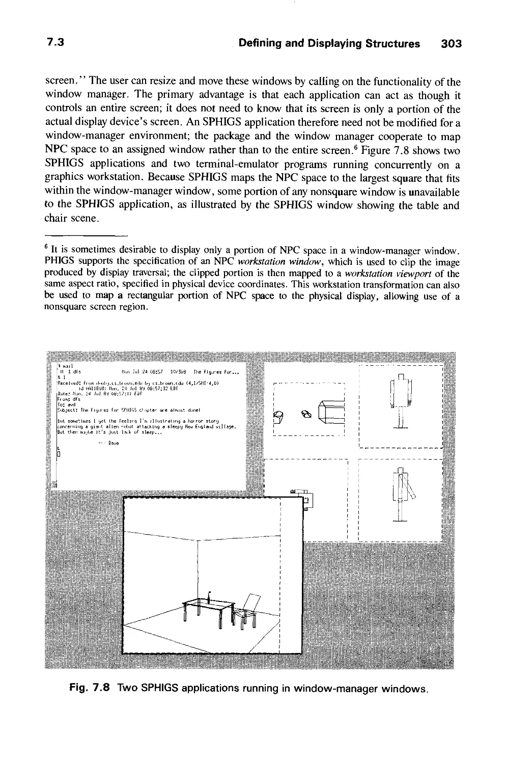
7.3 Defining and Displaying Structures 295
7.4 Modeling Transformations 304
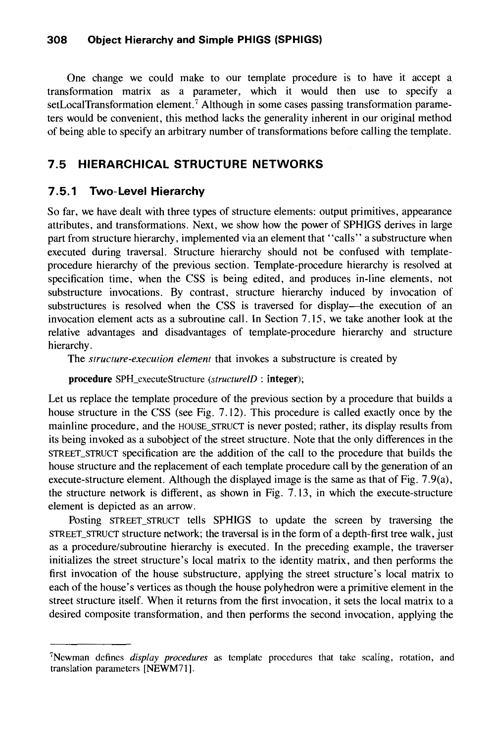
7.5 Hierarchical Structure Networks 308
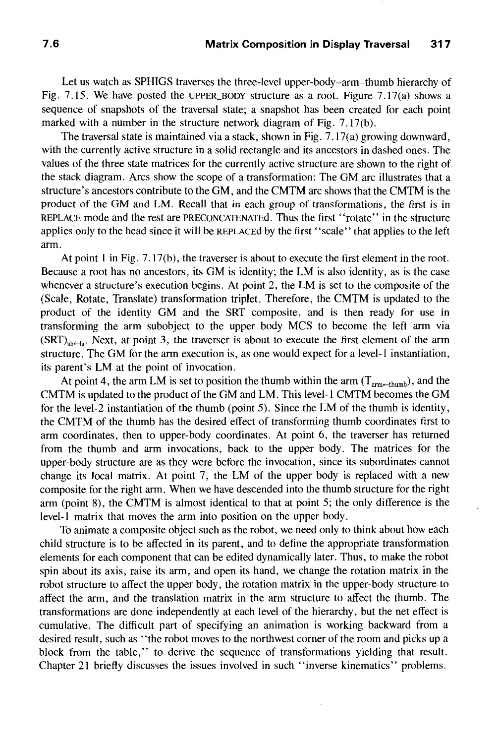
7.6 Matrix Composition in Display Traversal 315
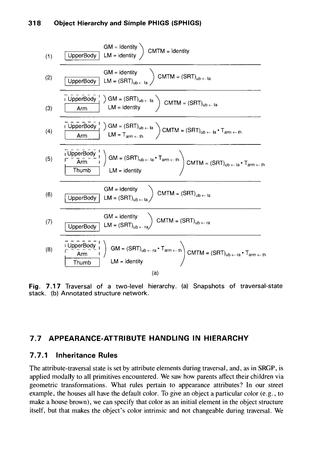
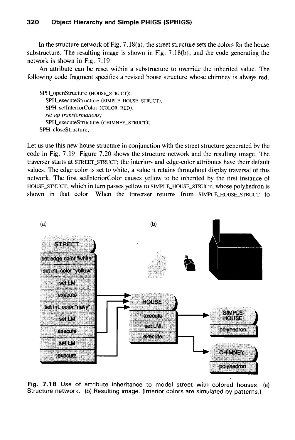
7.7 Appearance-Attribute Handling in Hierarchy 318
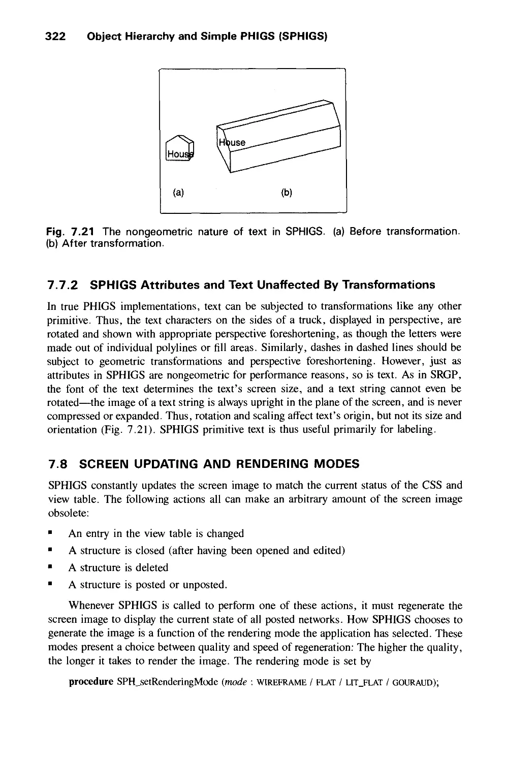
7.8 Screen Updating and Rendering Modes 322
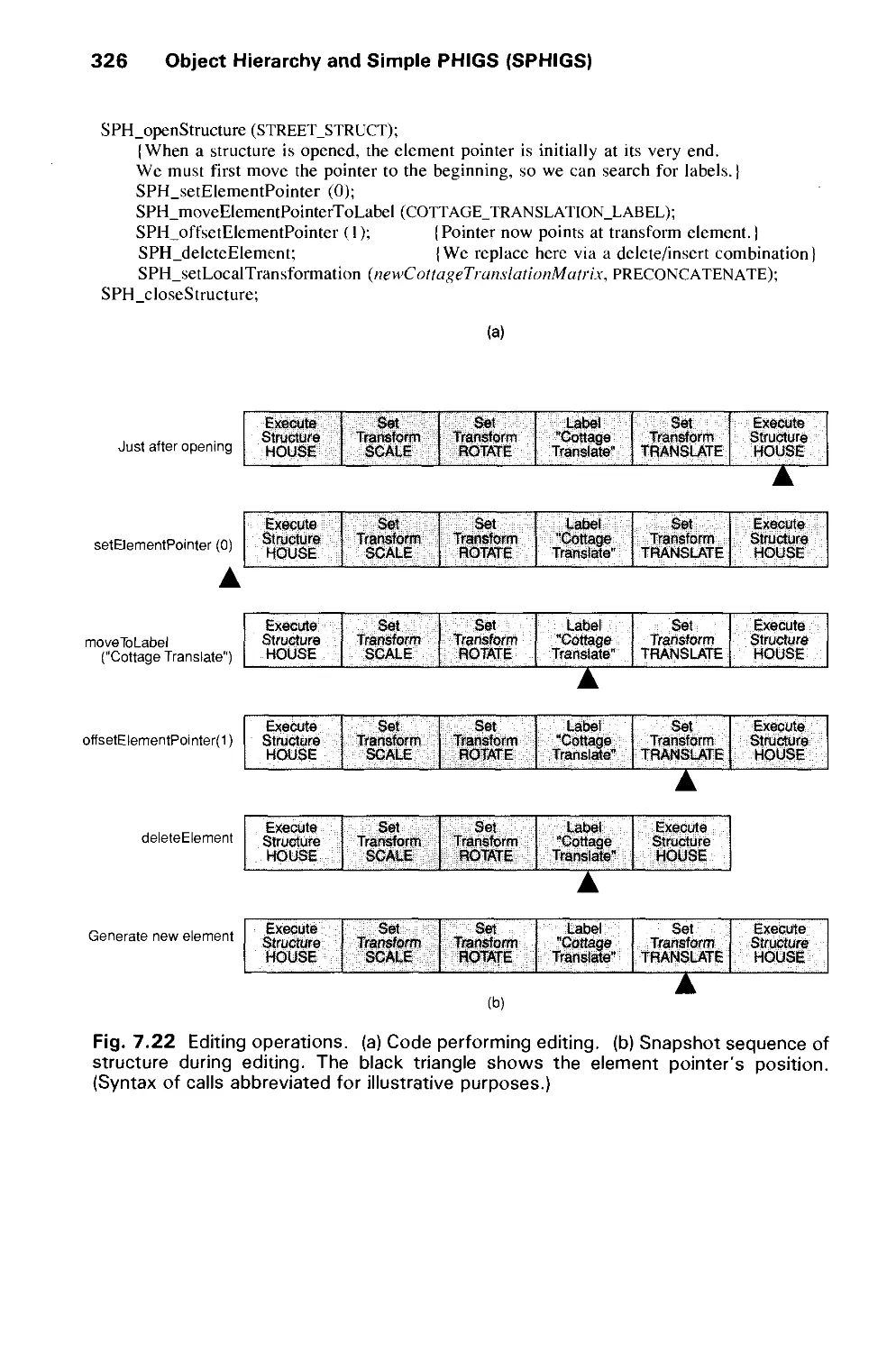
7.9 Structure Network Editing for Dynamic Effects 324
7.10 Interaction 328
7.11 Additional Output Features 332
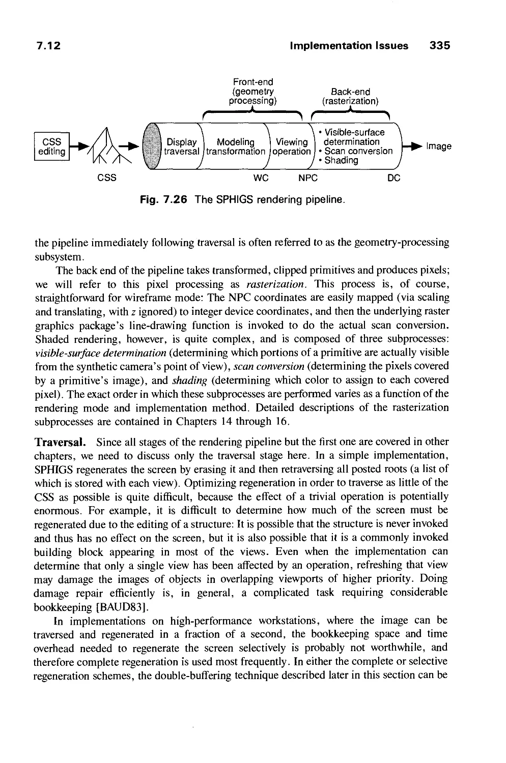
7.12 Implementation Issues 334
7.13 Optimizing Display of Hierarchical Models 340
7.14 Limitations of Hierarchical Modeling in PHIGS 341
7.15 Alternative Forms of Hierarchical Modeling 343
7.16 Summary 345
Exercises 346
CHAPTER 8
INPUT DEVICES. INTERACTION TECHNIQUES,
AND INTERACTION TASKS 347
8.1 Interaction Hardware 349
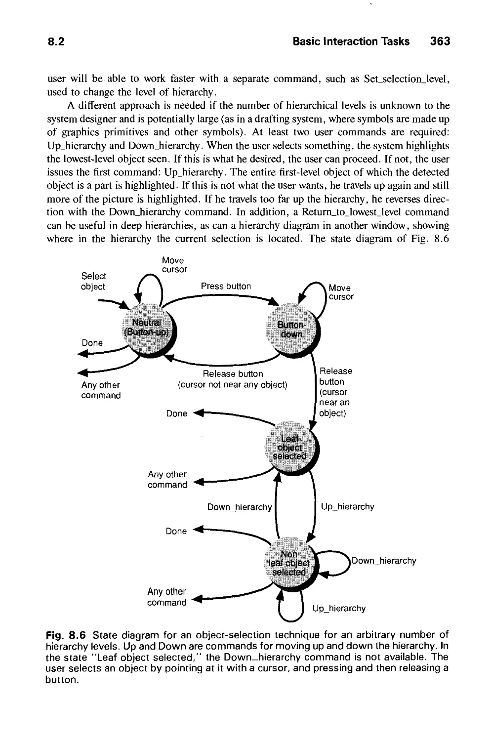
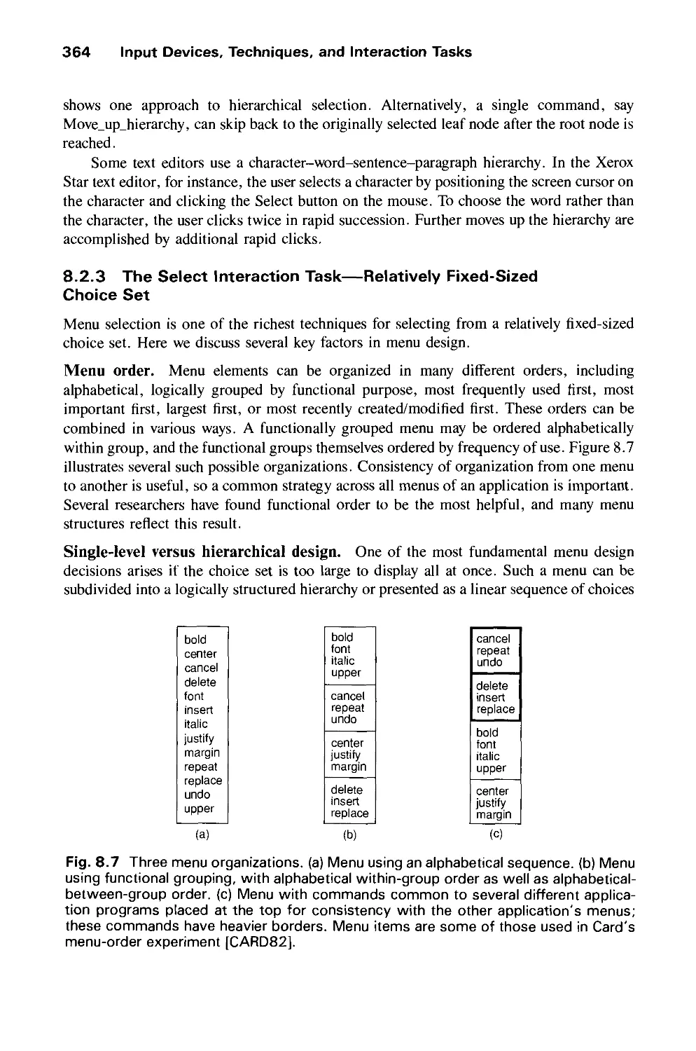
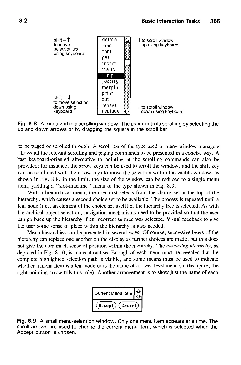
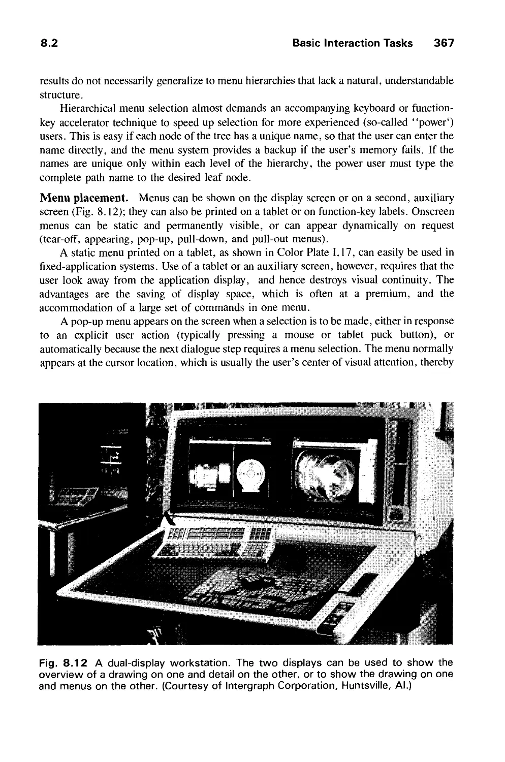
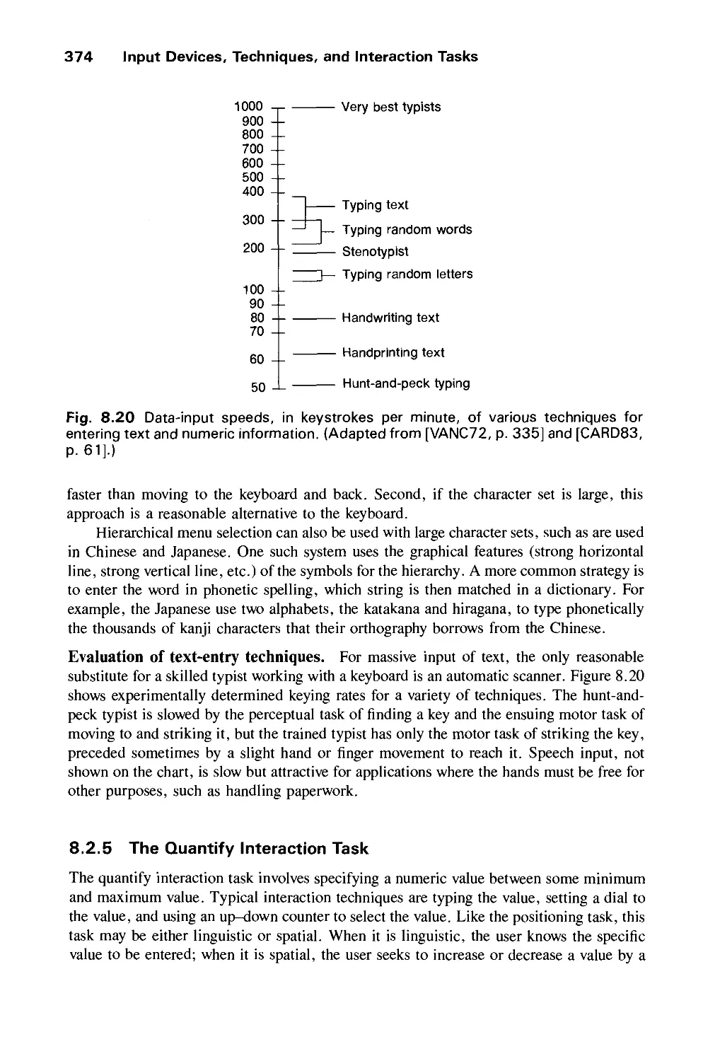
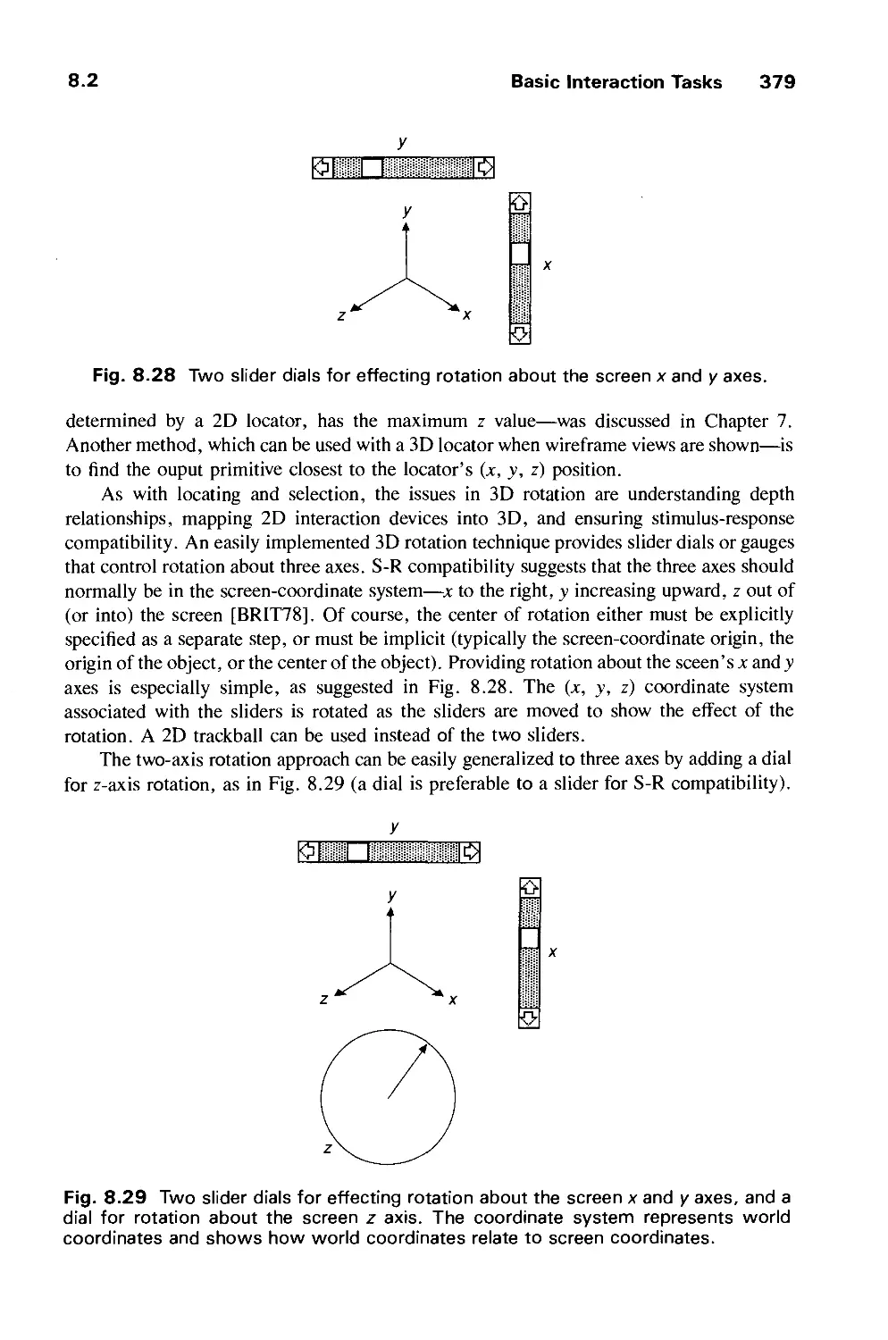
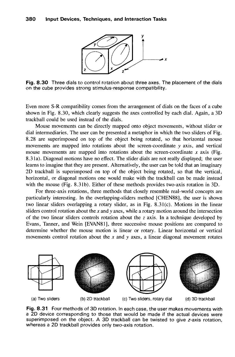
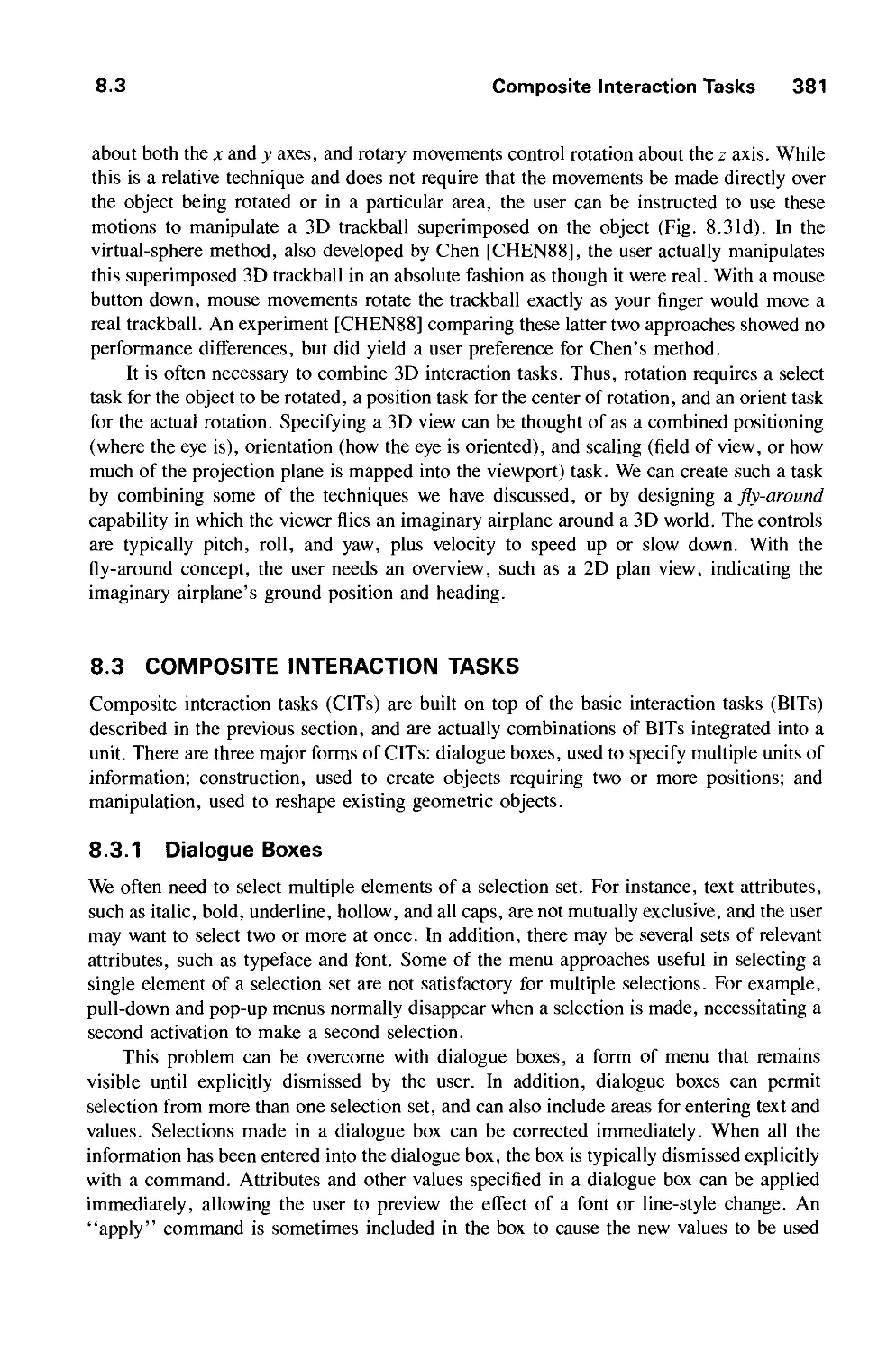
8.2 Basic Interaction Tasks 358
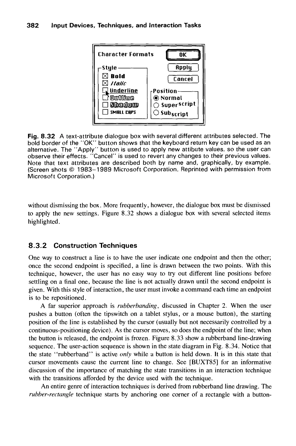
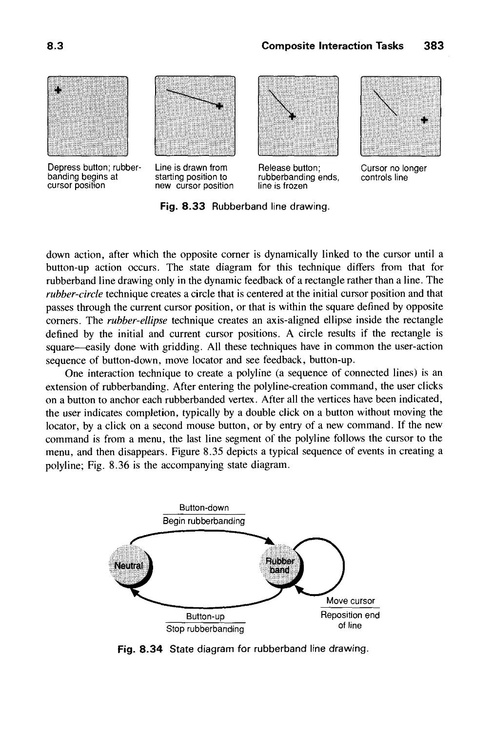
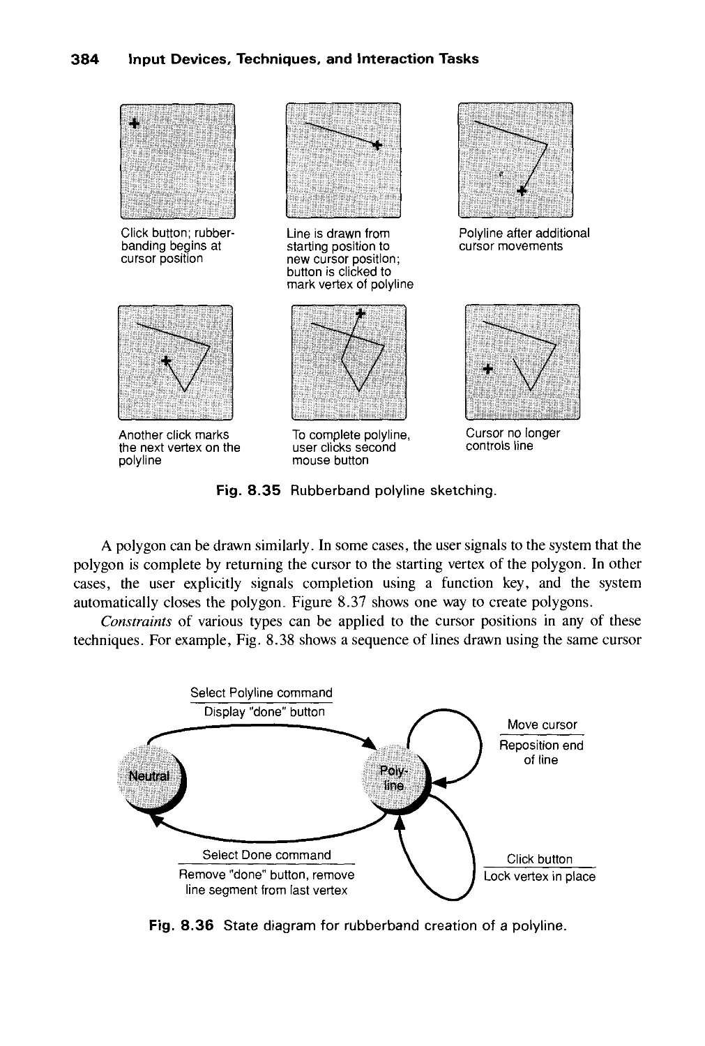
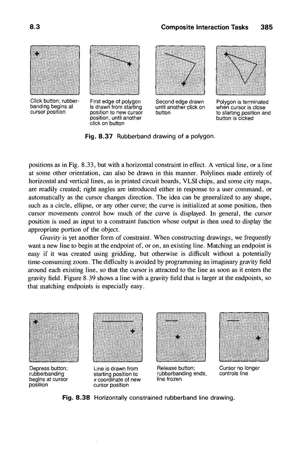
8.3 Composite Interaction Tasks 381
Exercises 388
CHAPTER 9
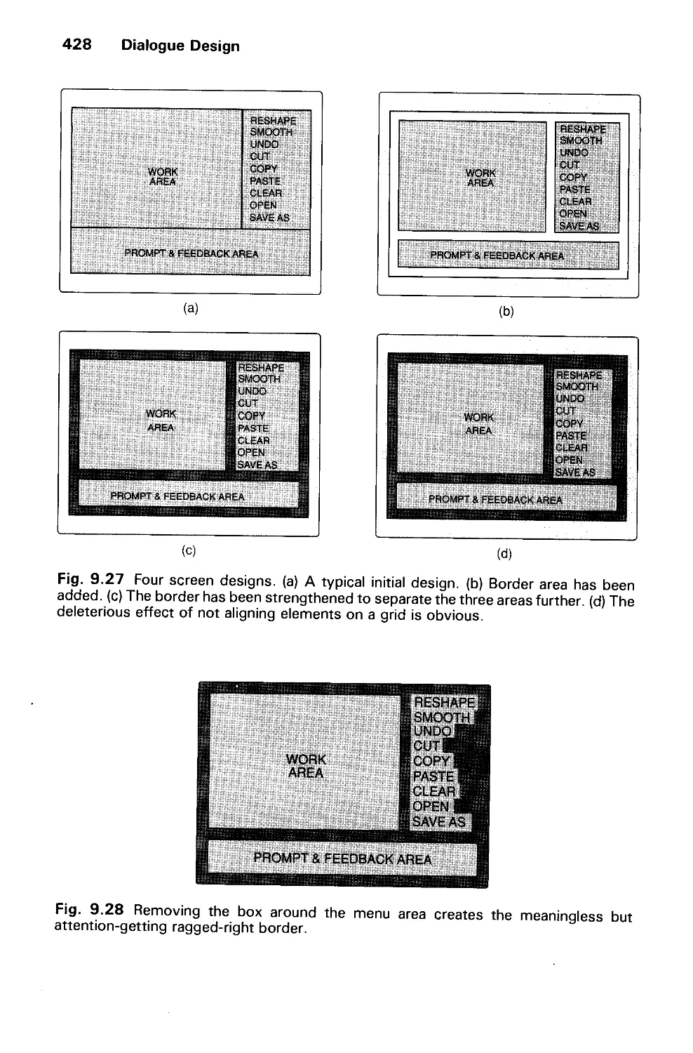
DIALOGUE DESIGN 391
9.1 The Form and Content of User-Computer Dialogues 392
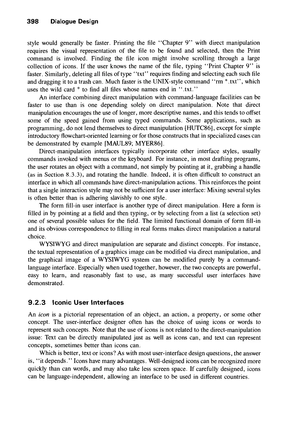
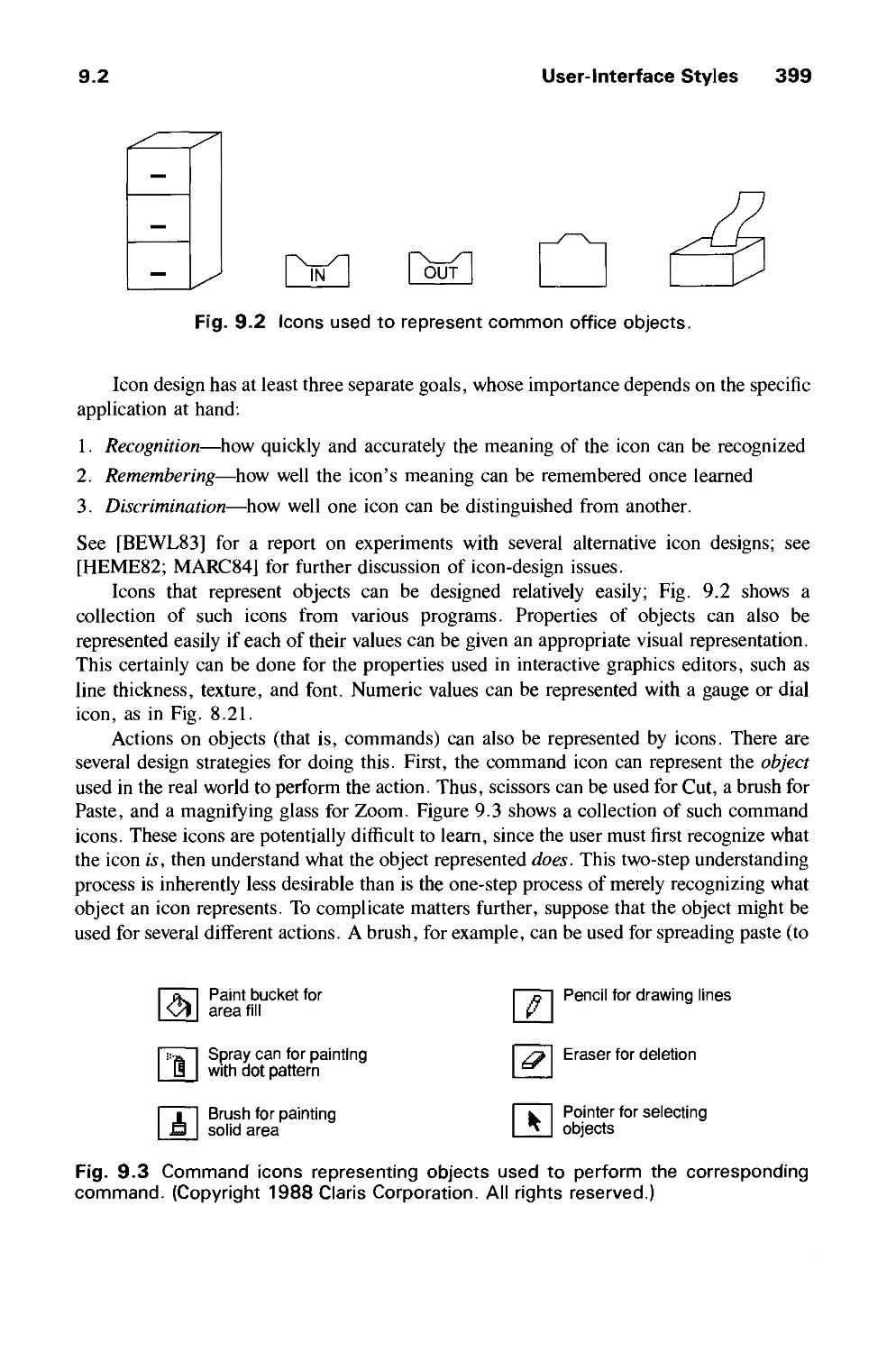
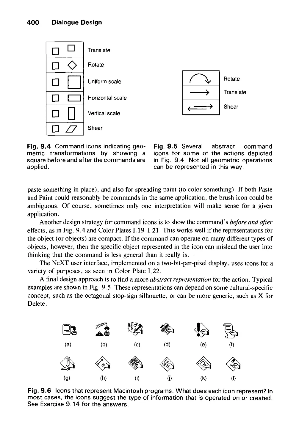
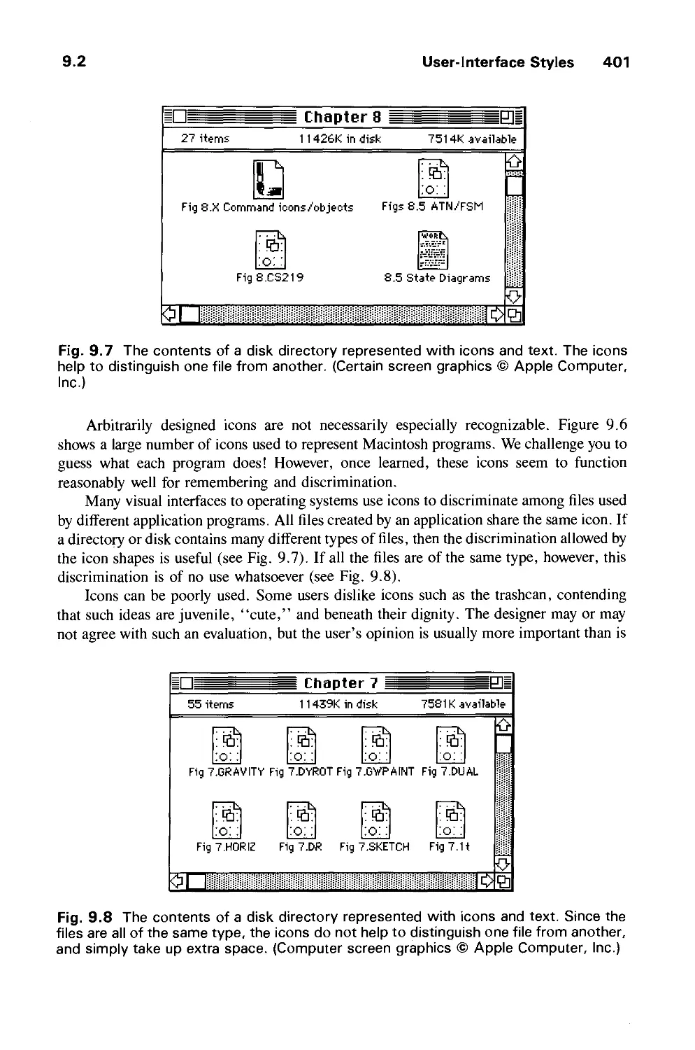
9.2 User-Interface Styles 395
9.3 Important Design Considerations 403
9.4 Modes and Syntax 414
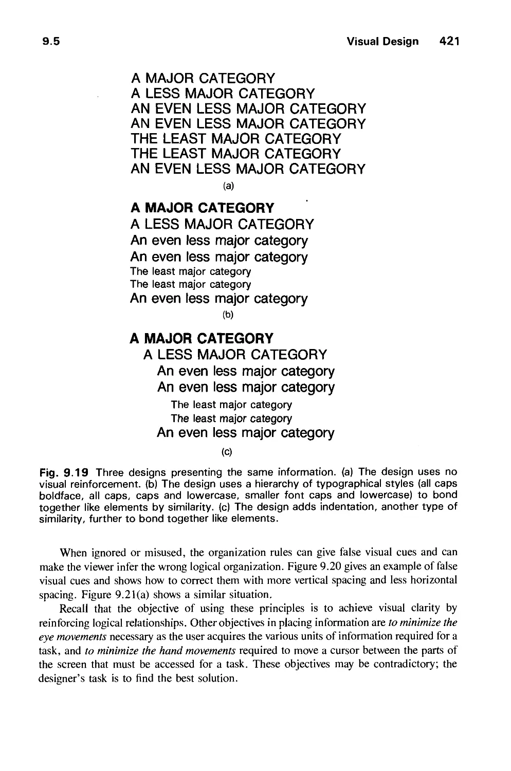
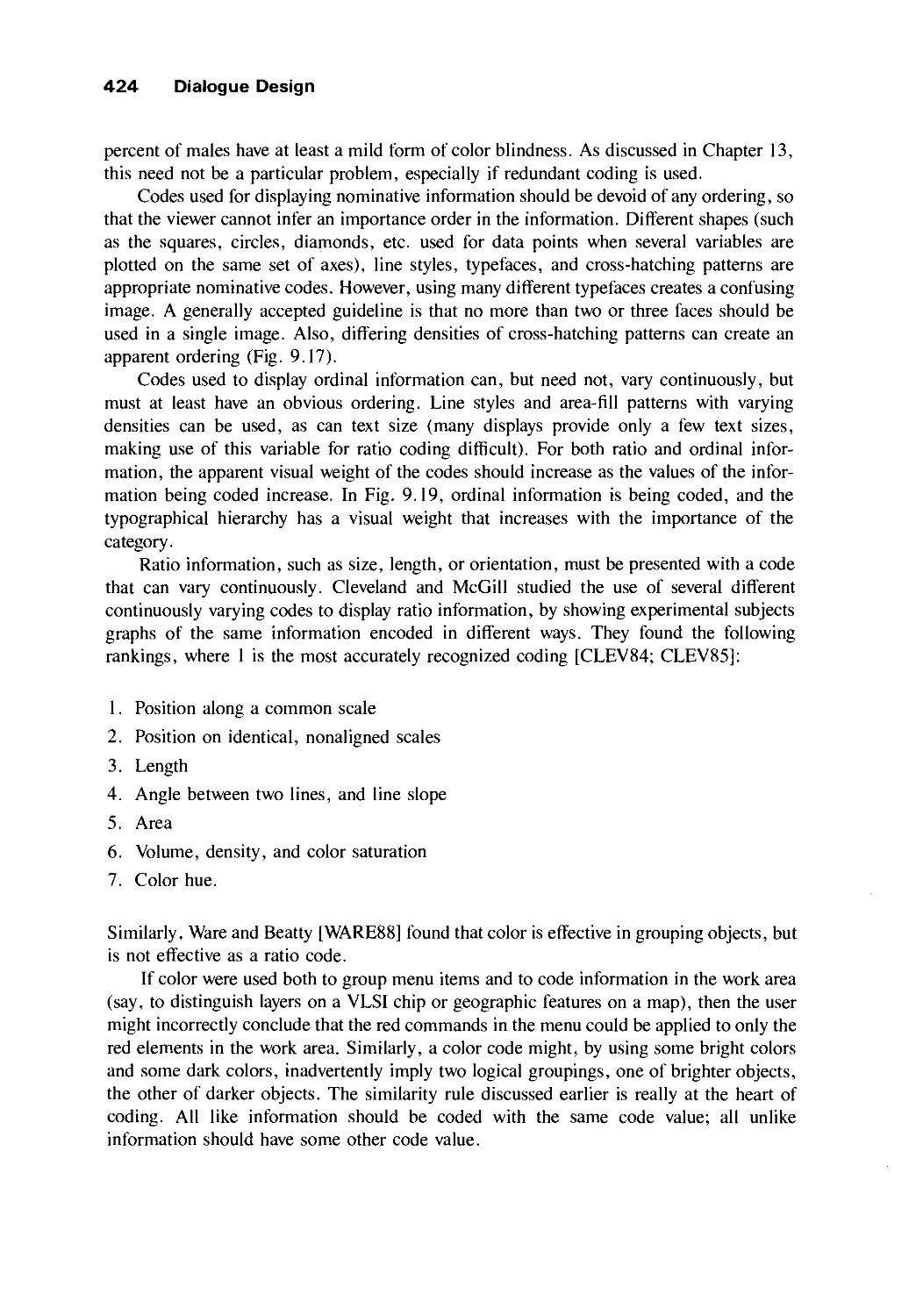
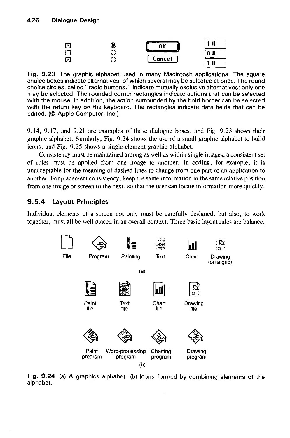
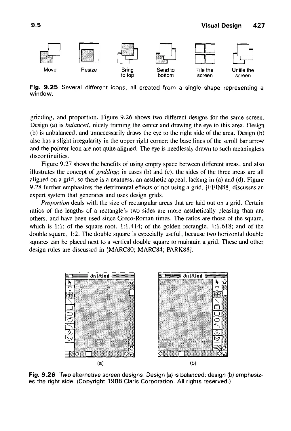
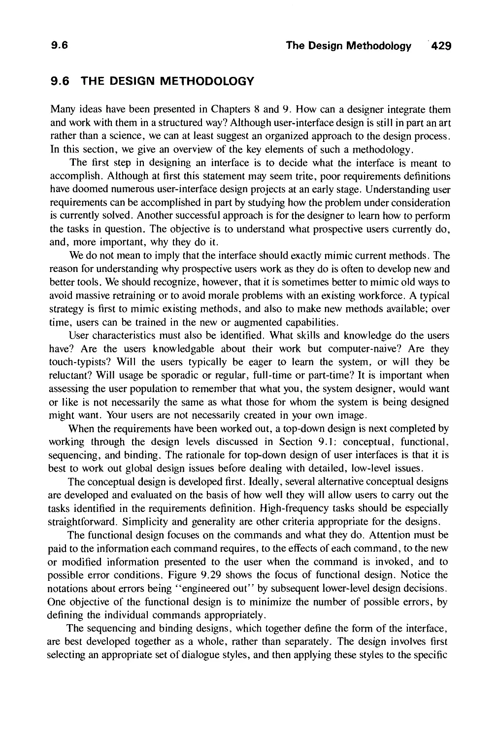
9.5 Visual Design 418
9.6 The Design Methodology 429
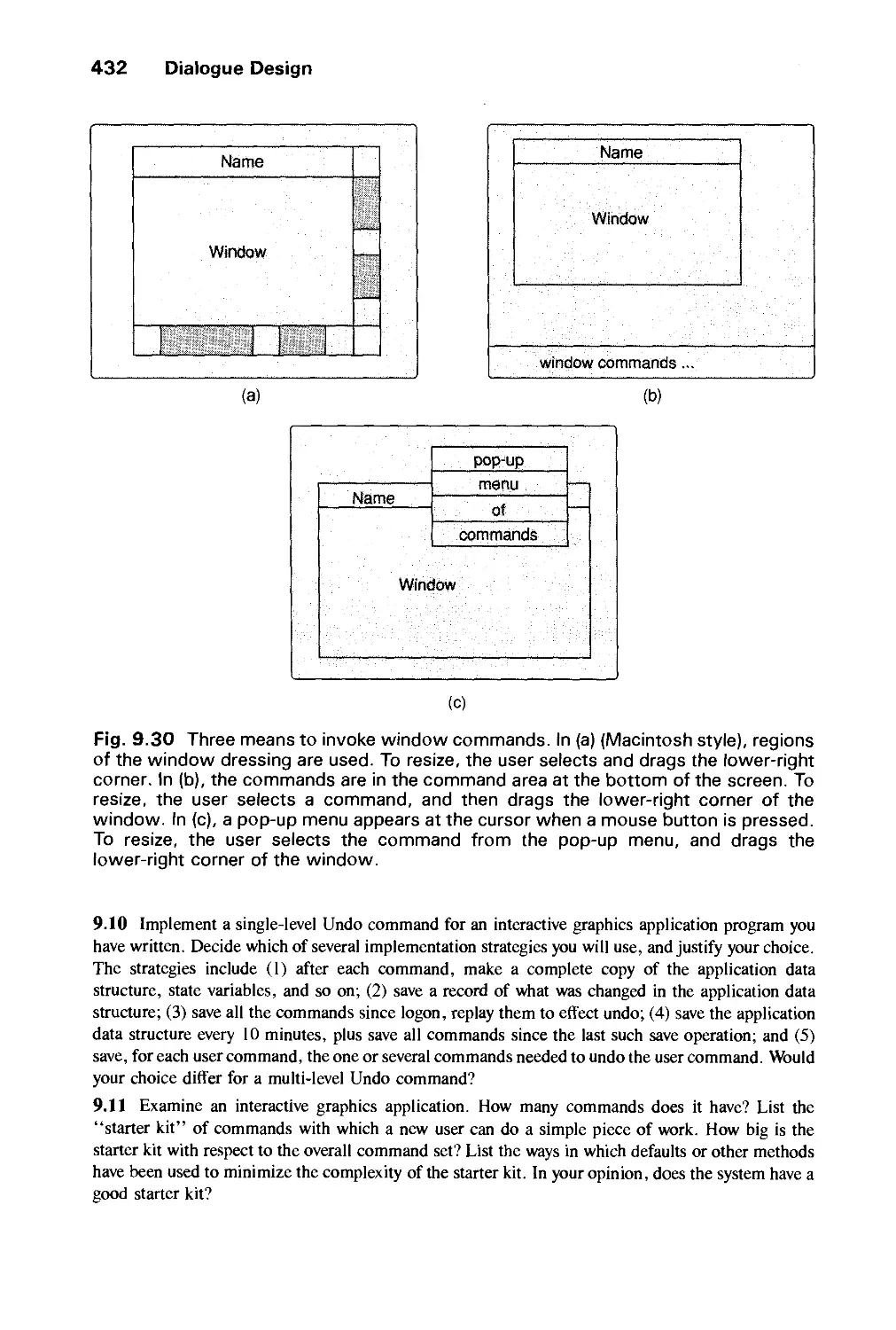
Exercises 431
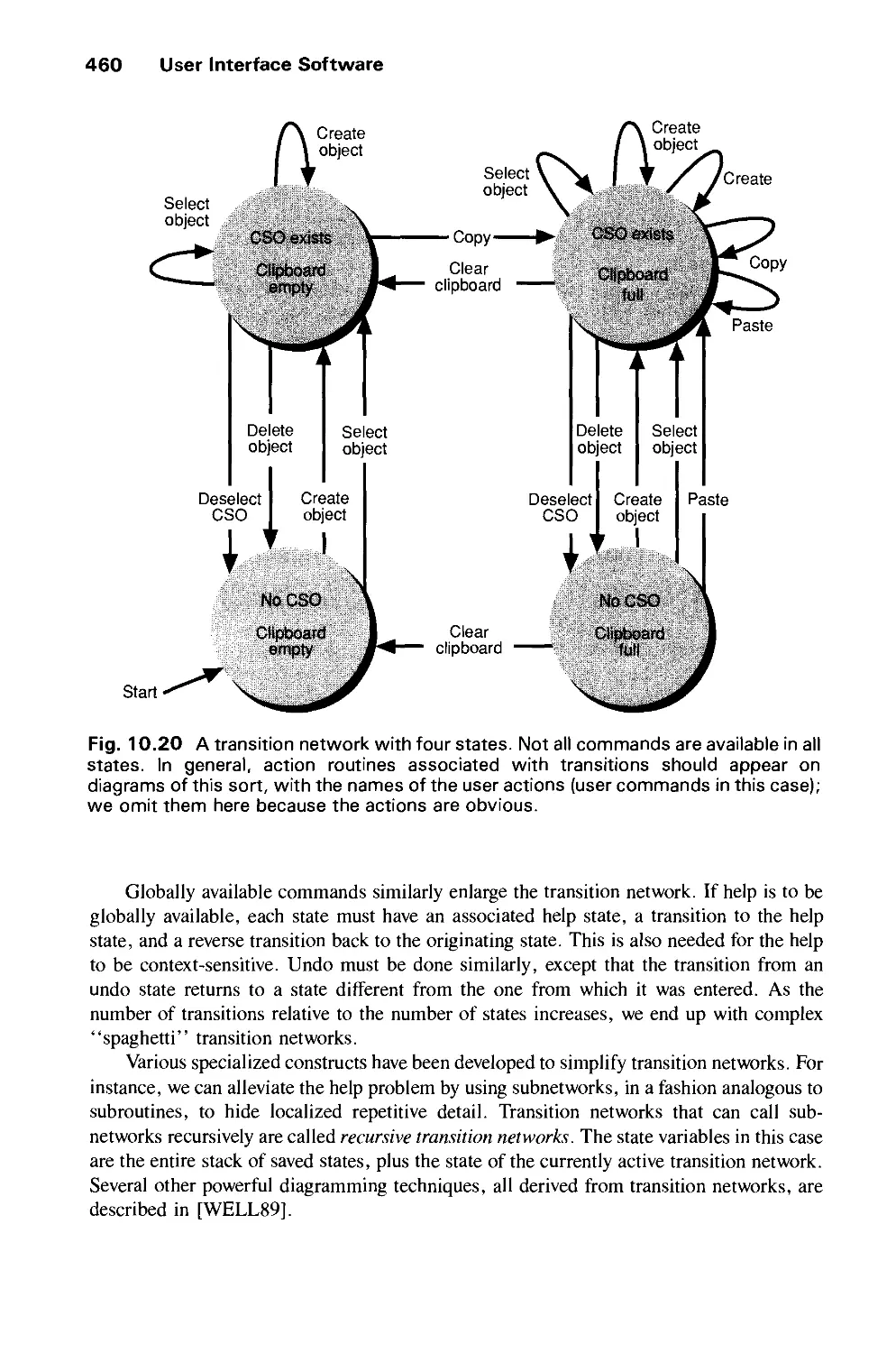
CHAPTER 10
USER INTERFACE SOFTWARE 435
10.1 Basic Interaction-Handling Models 436
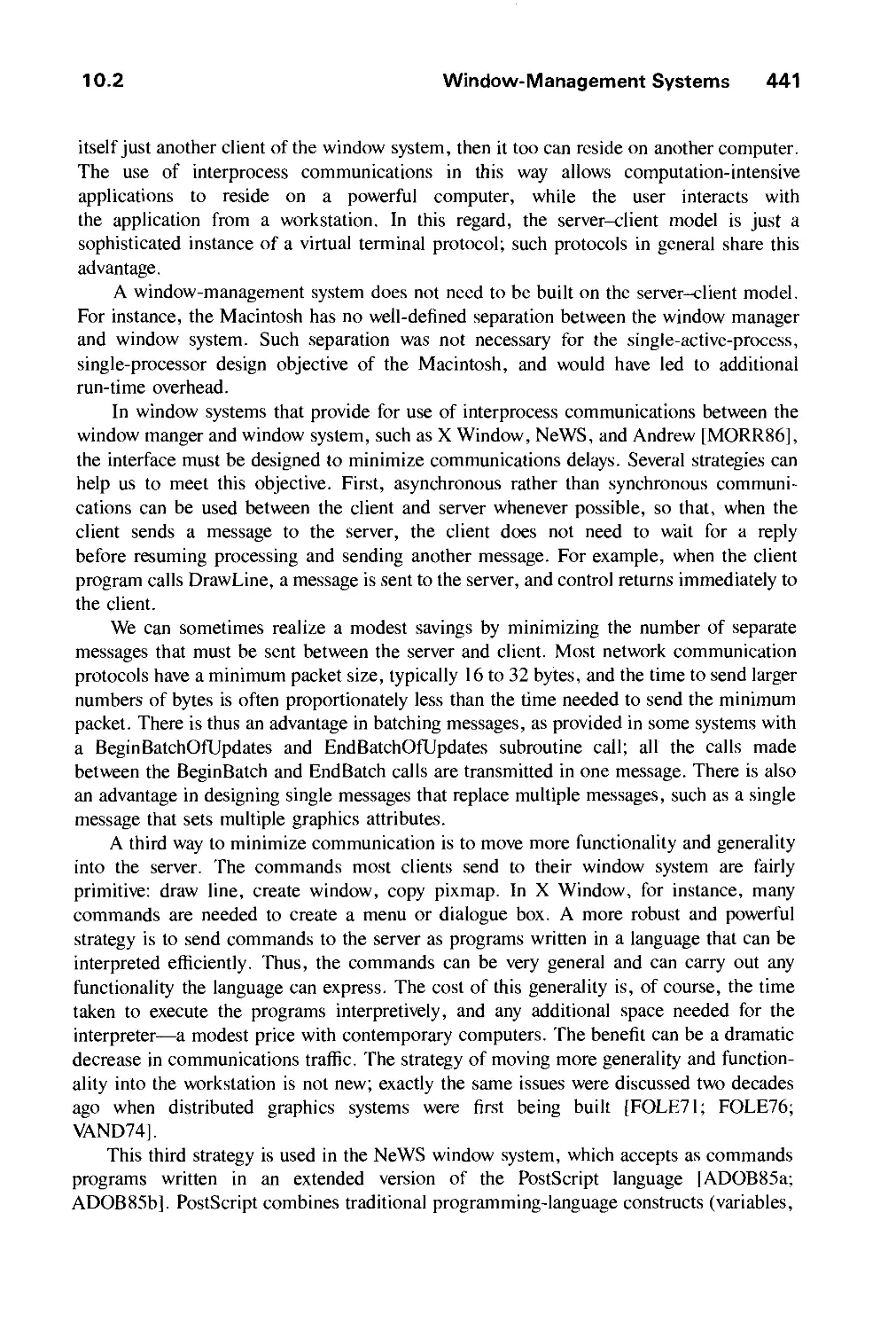
10.2 Window-Management Systems 439
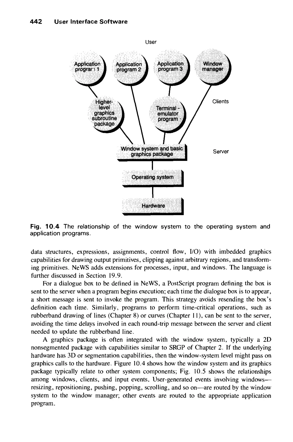
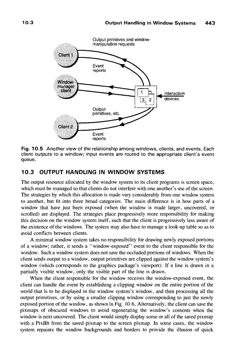
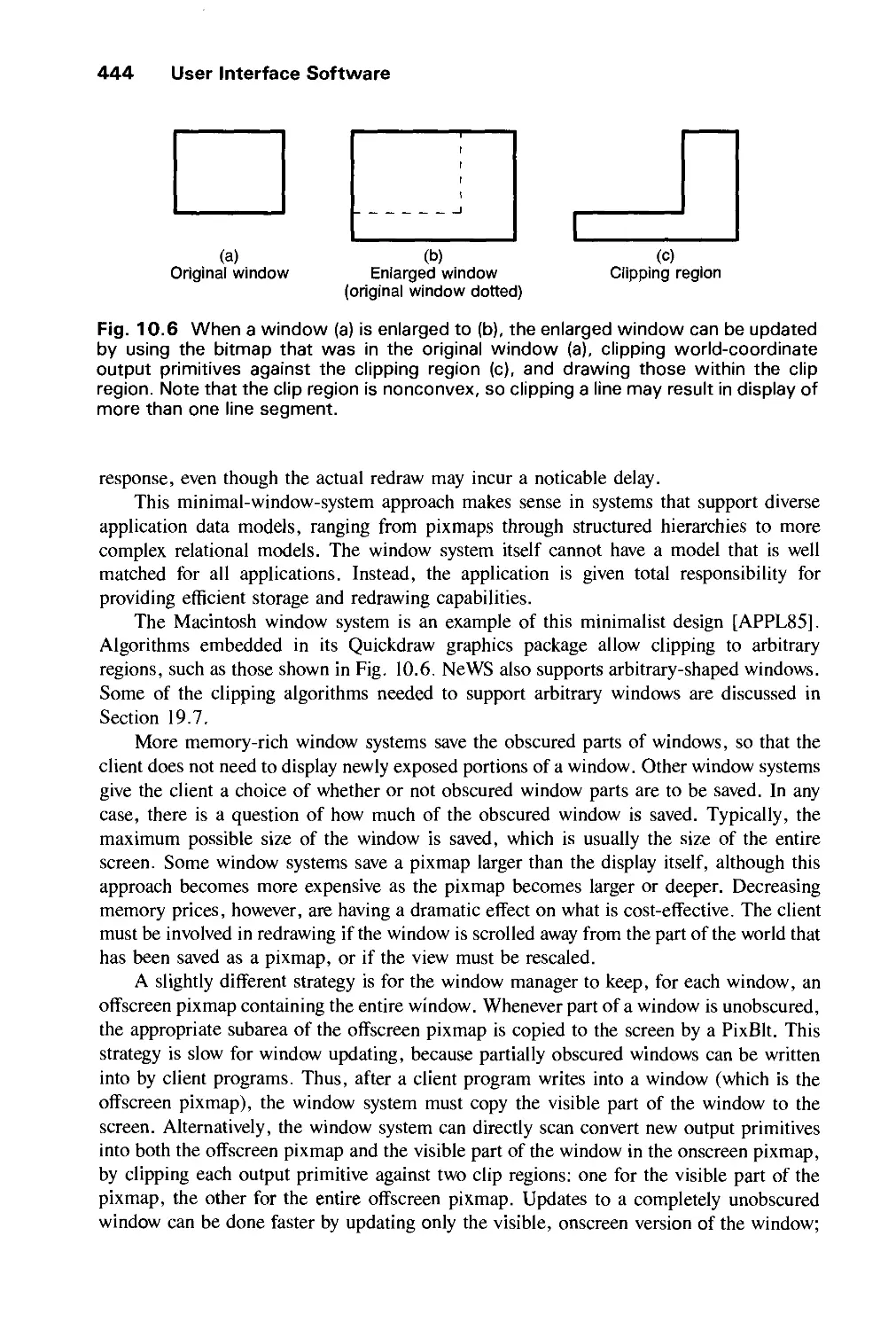
10.3 Output Handling in Window Systems 443
xx Contents
10.4 Input Handling in Window Systems 447
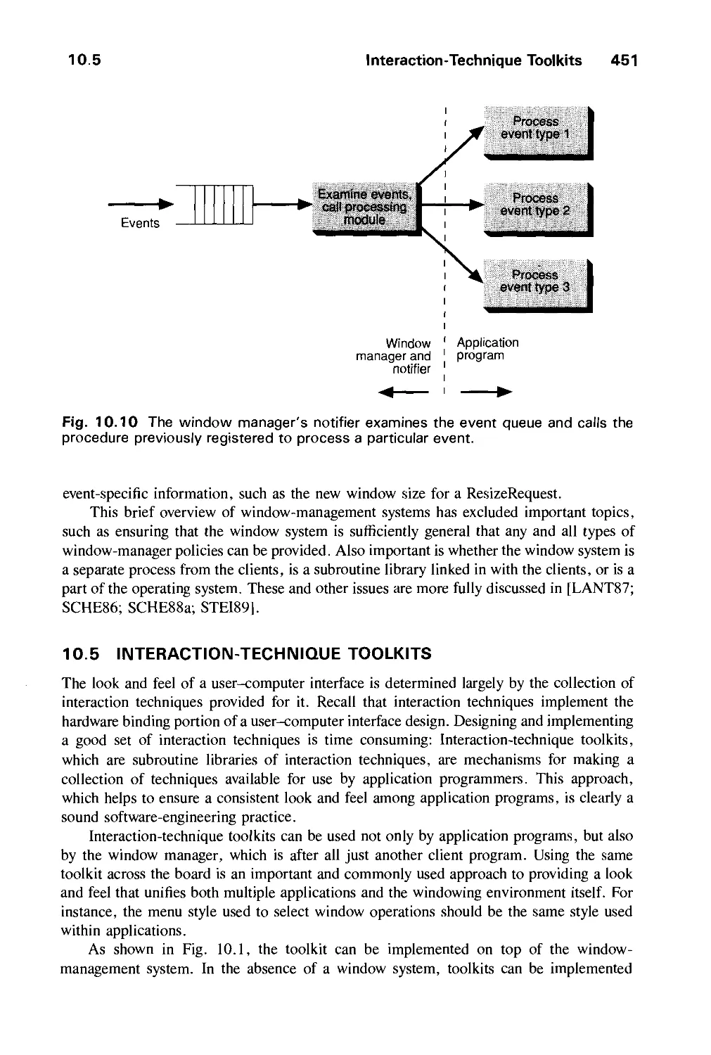
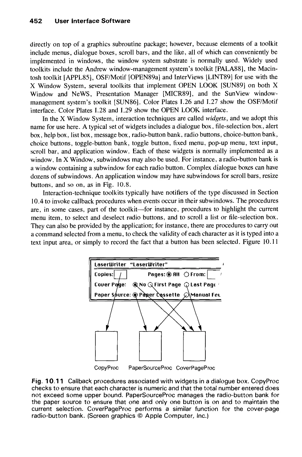
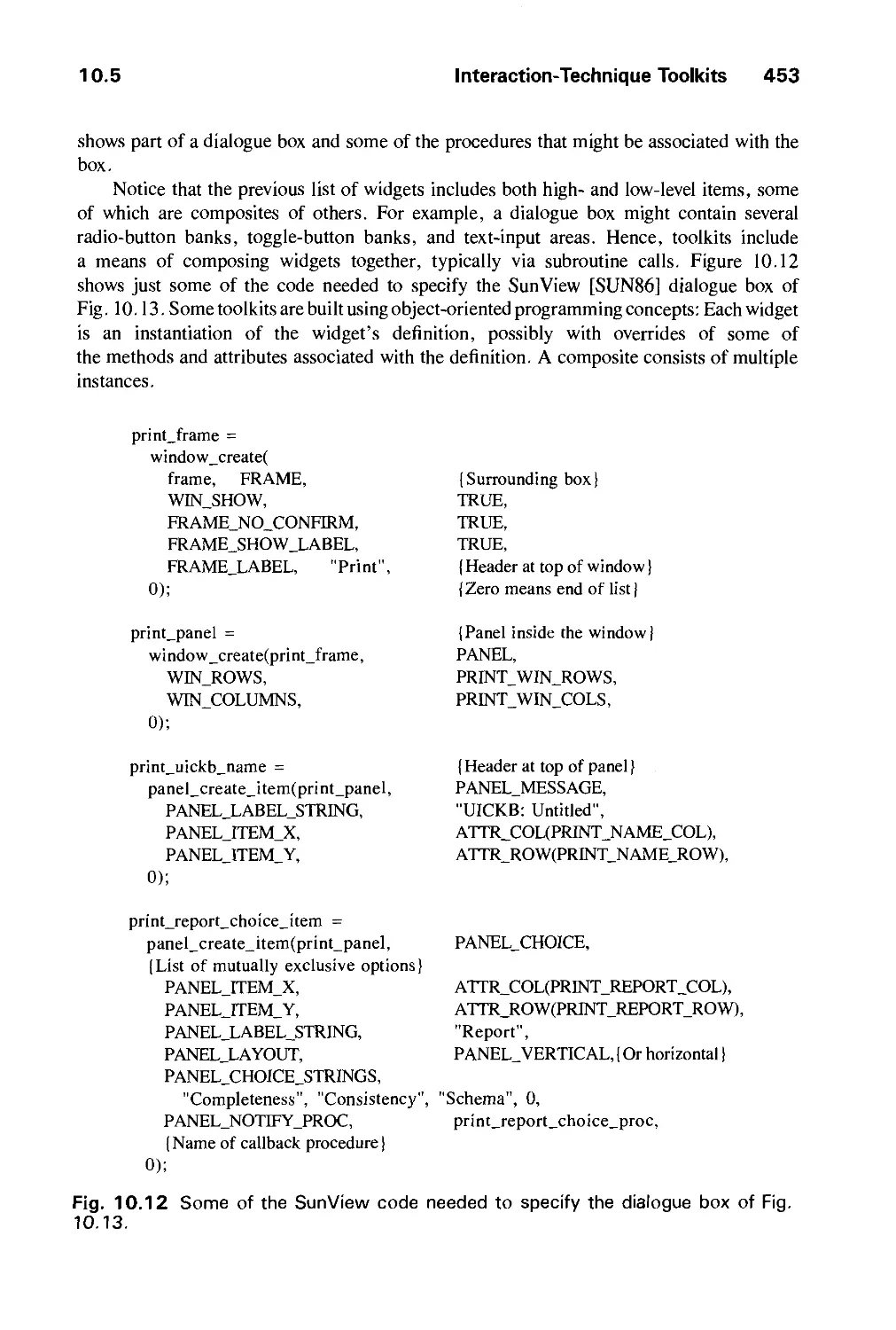
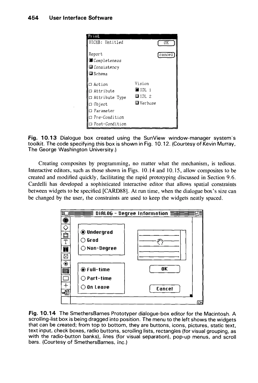
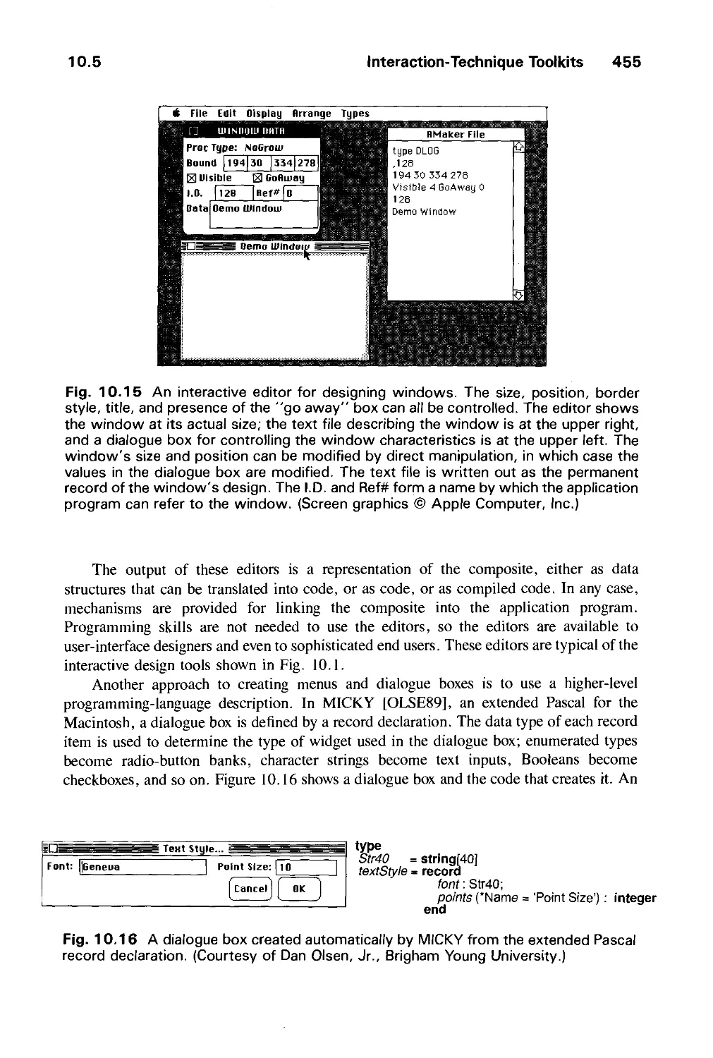
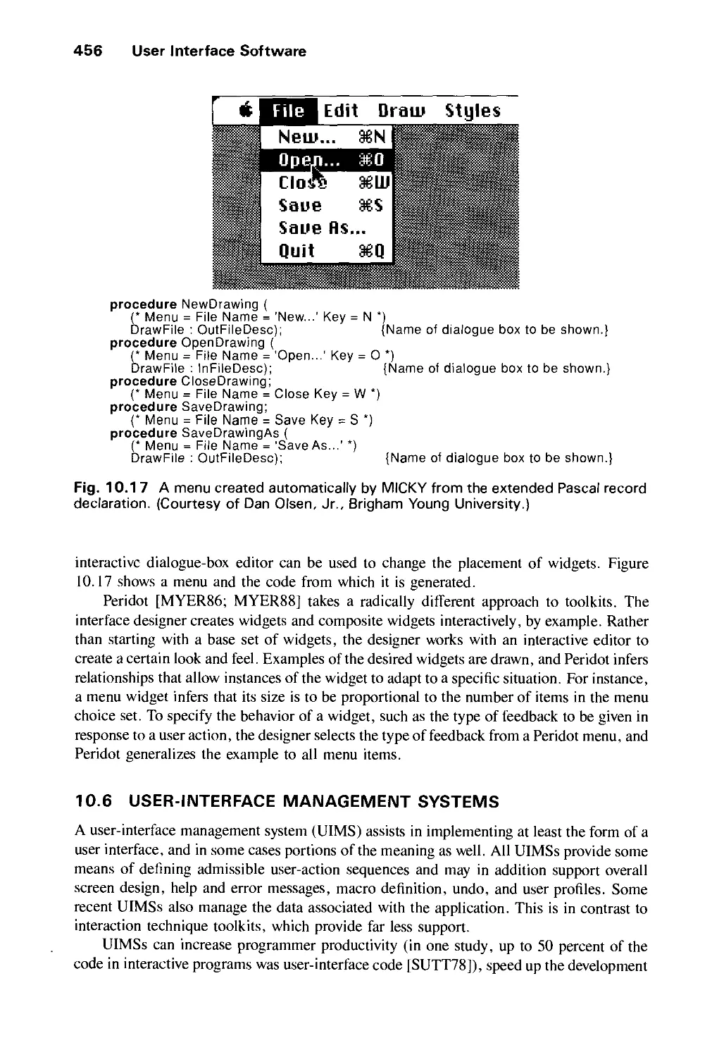
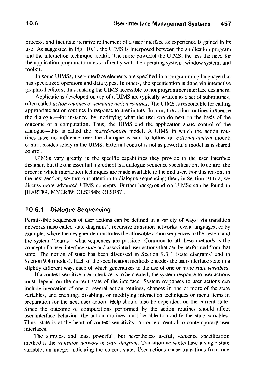
10.5 Interaction-Technique Toolkits 451
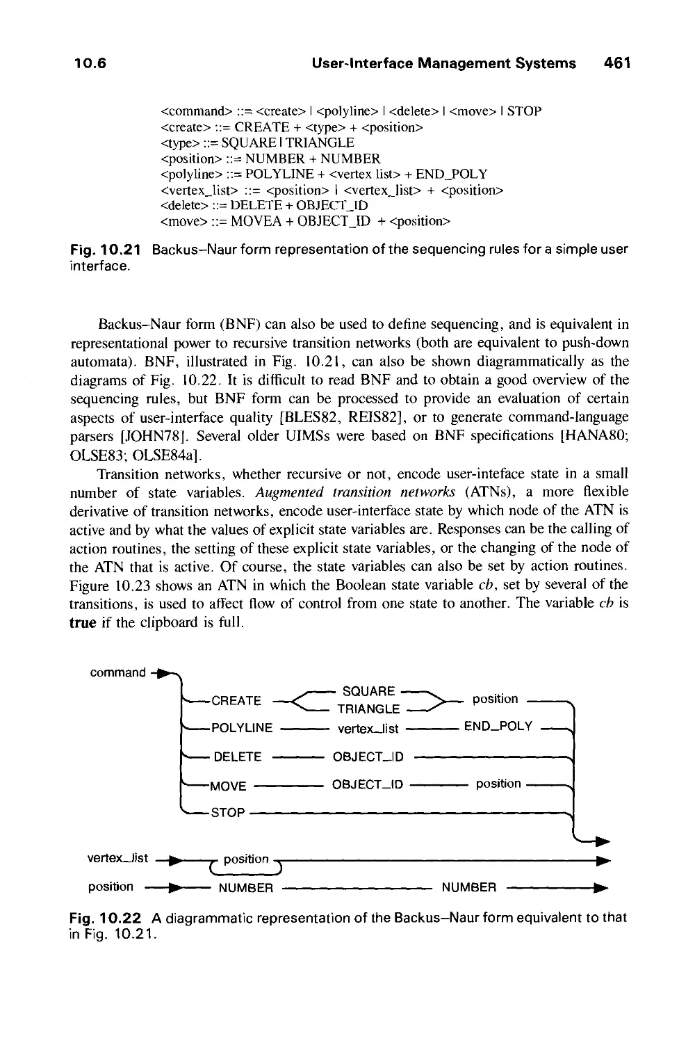
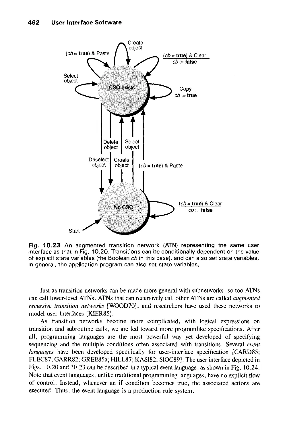
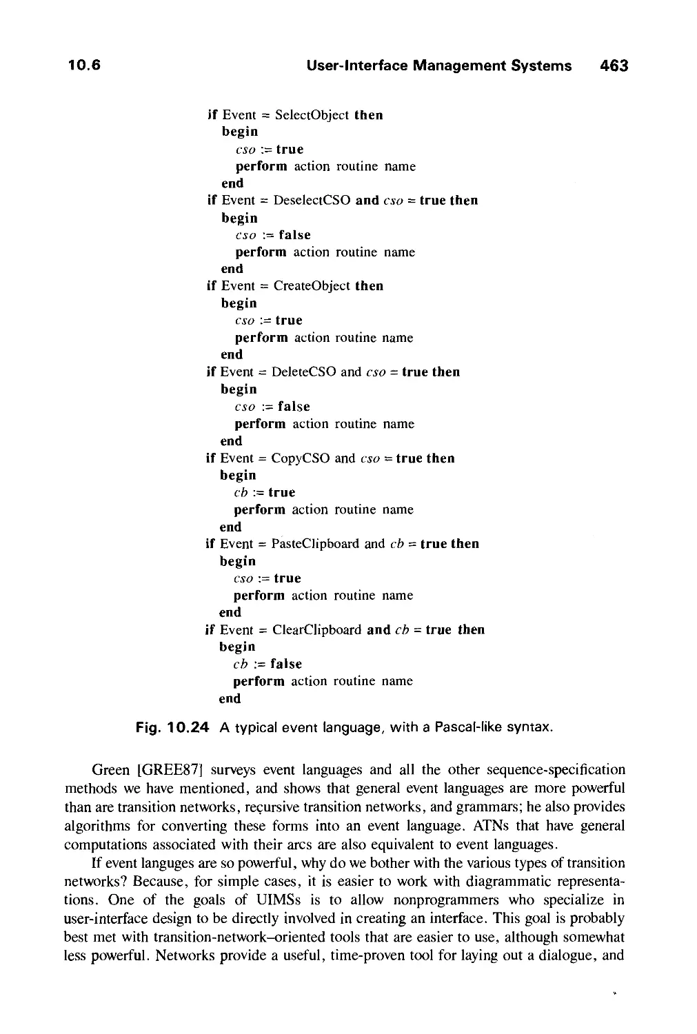
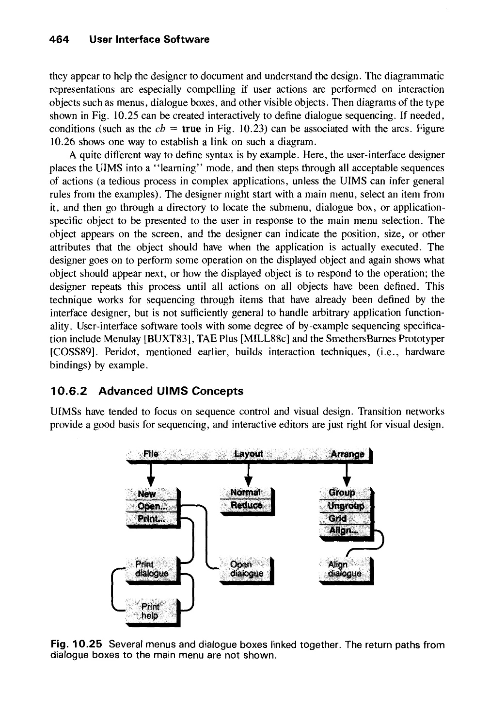
10.6 User-Interface Management Systems 456
Exercises 468
CHAPTER 11
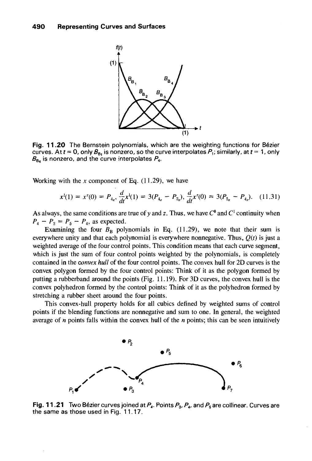
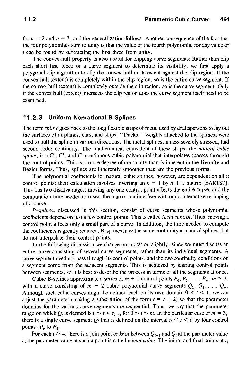
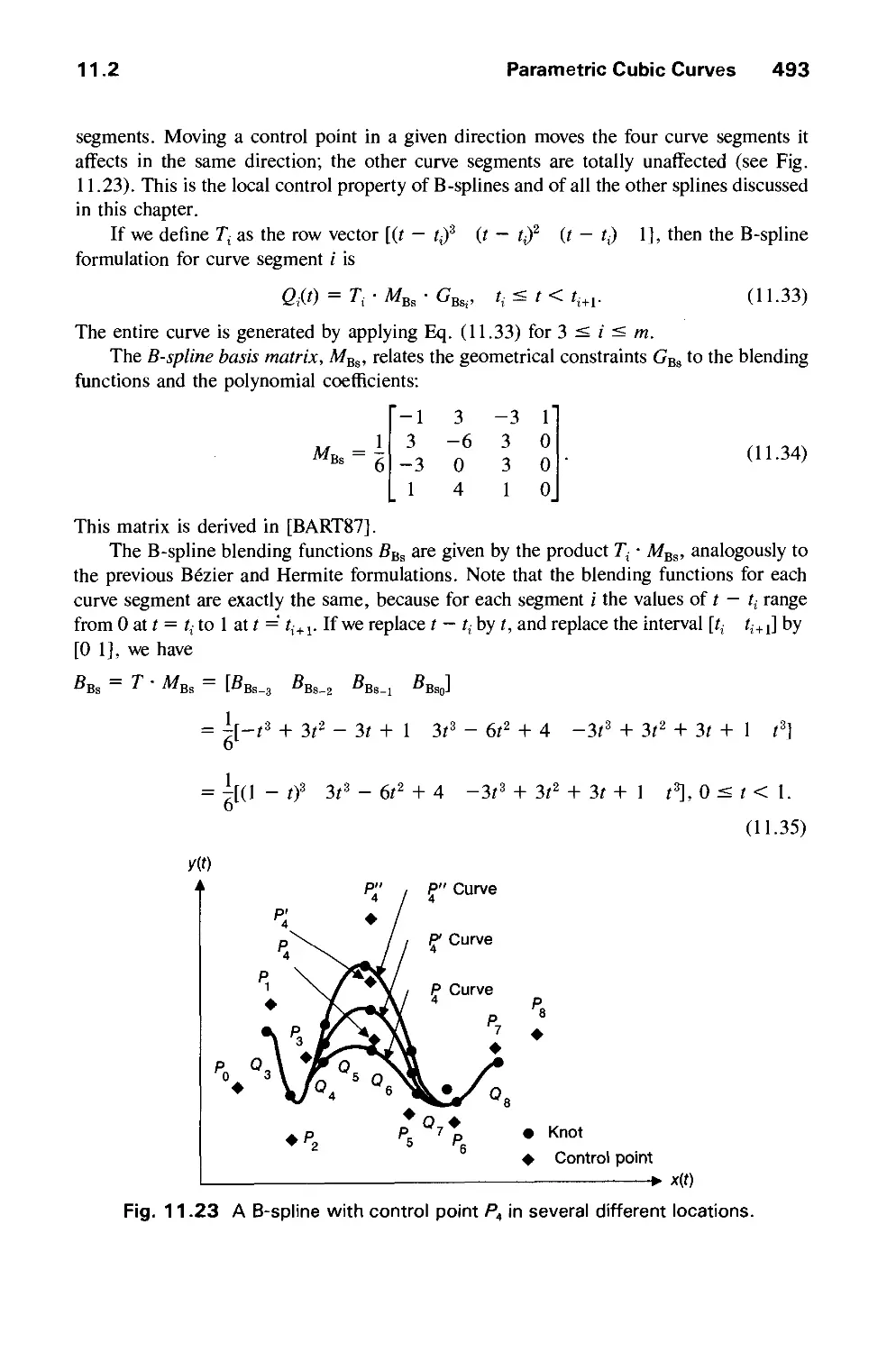
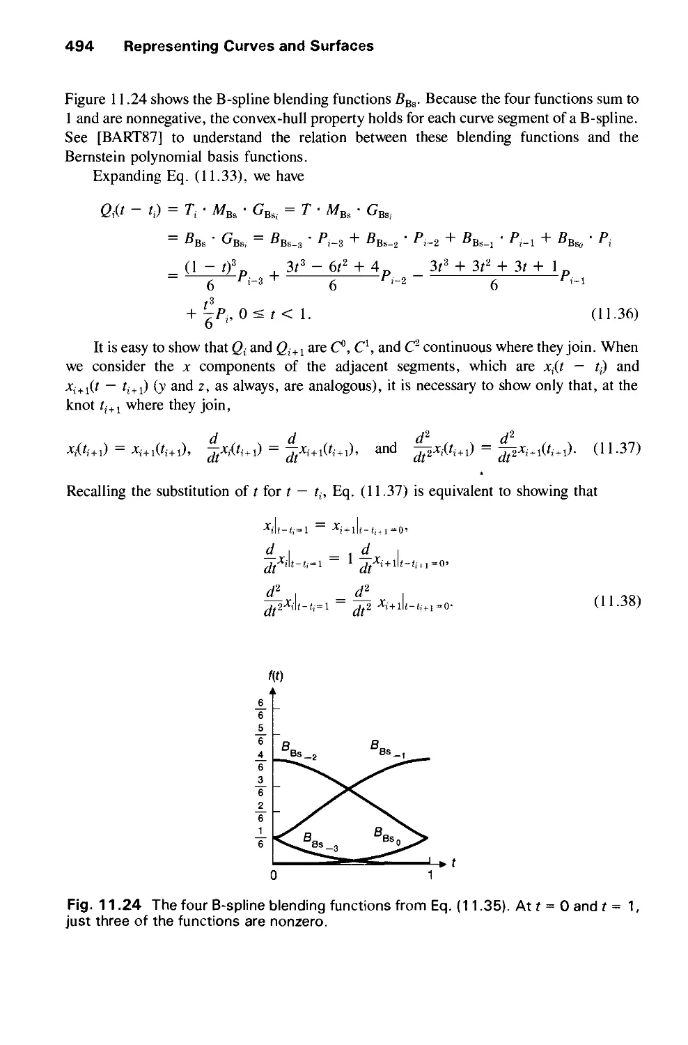
REPRESENTING CURVES AND SURFACES 471
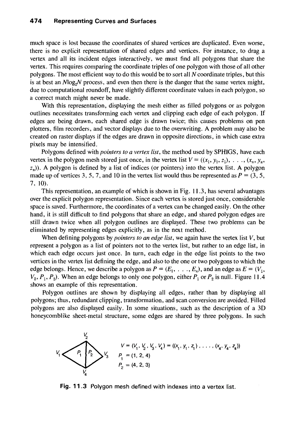
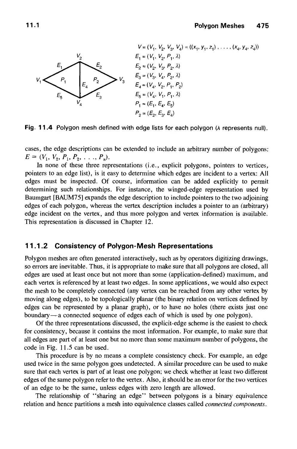
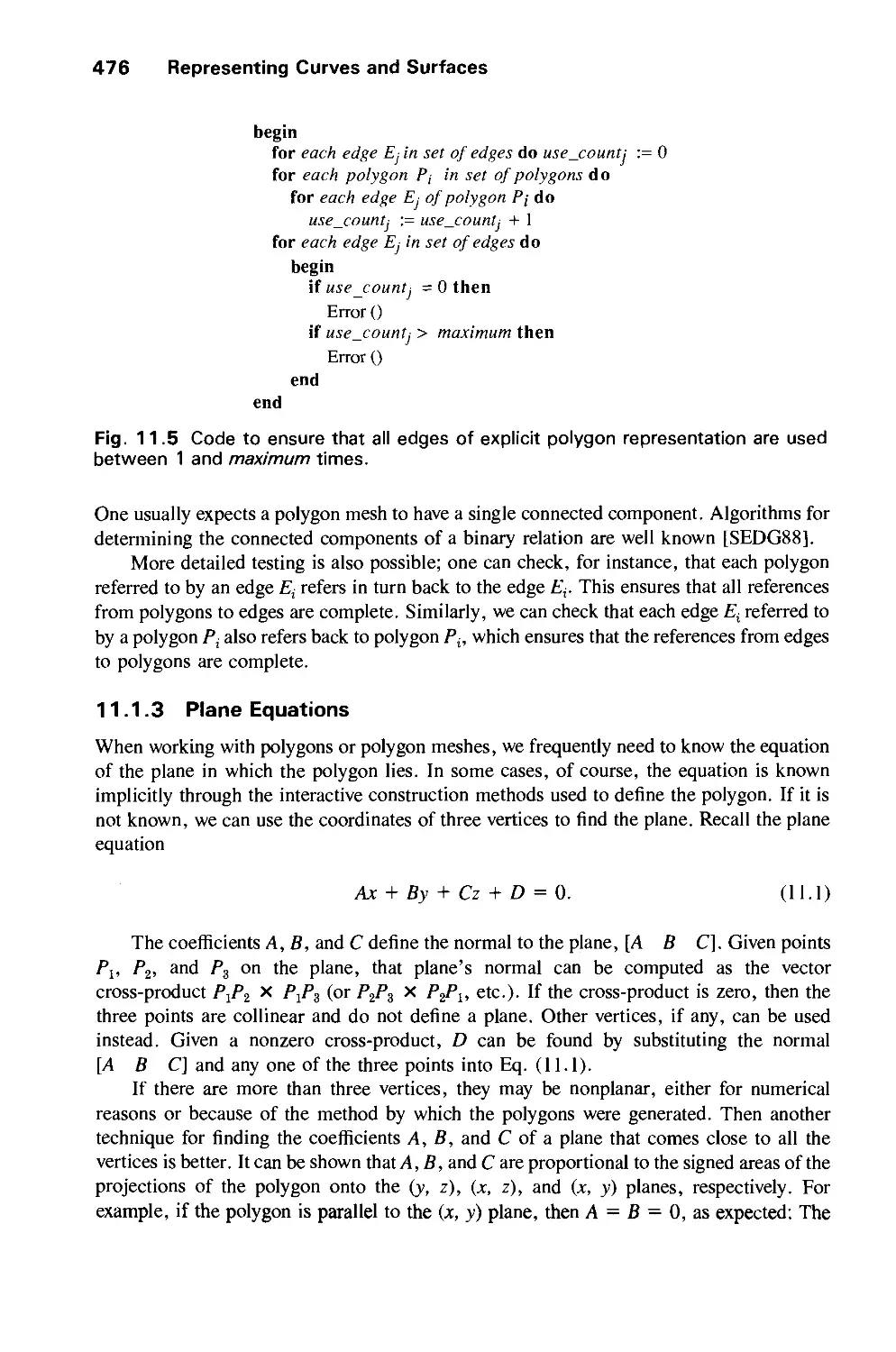
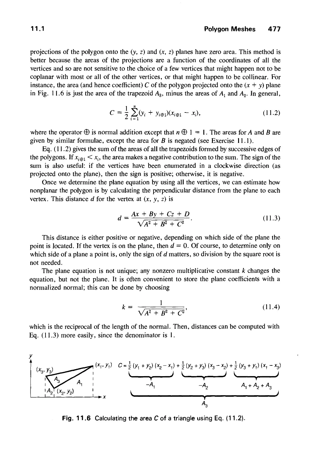
11.1 Polygon Meshes 473
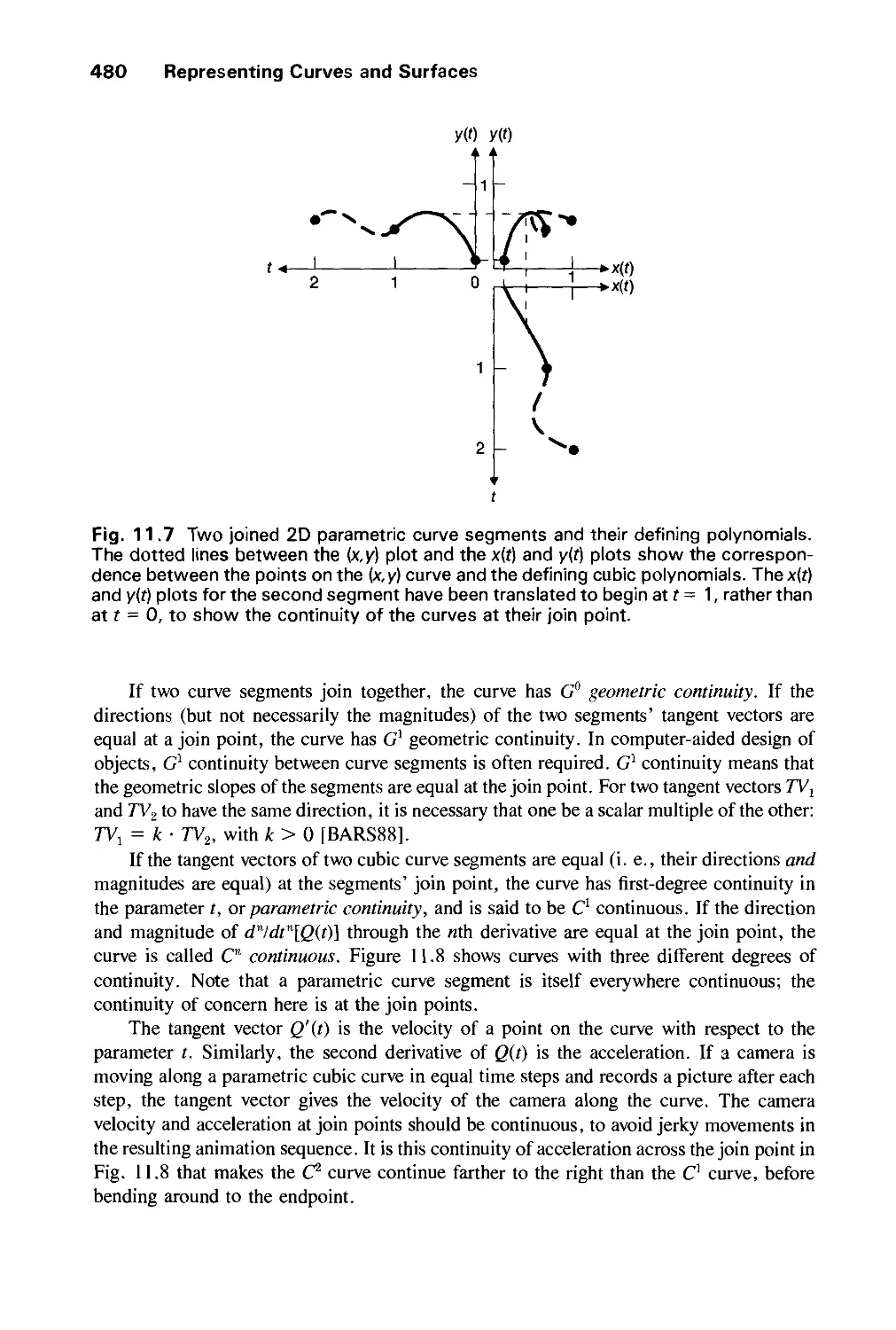
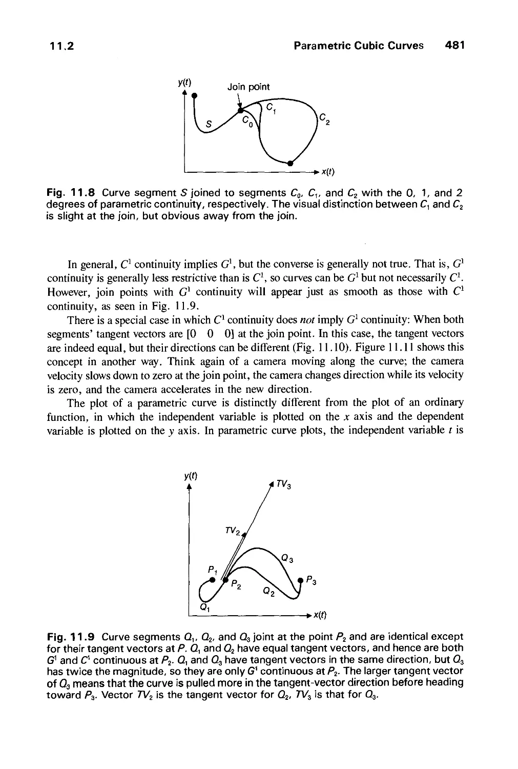
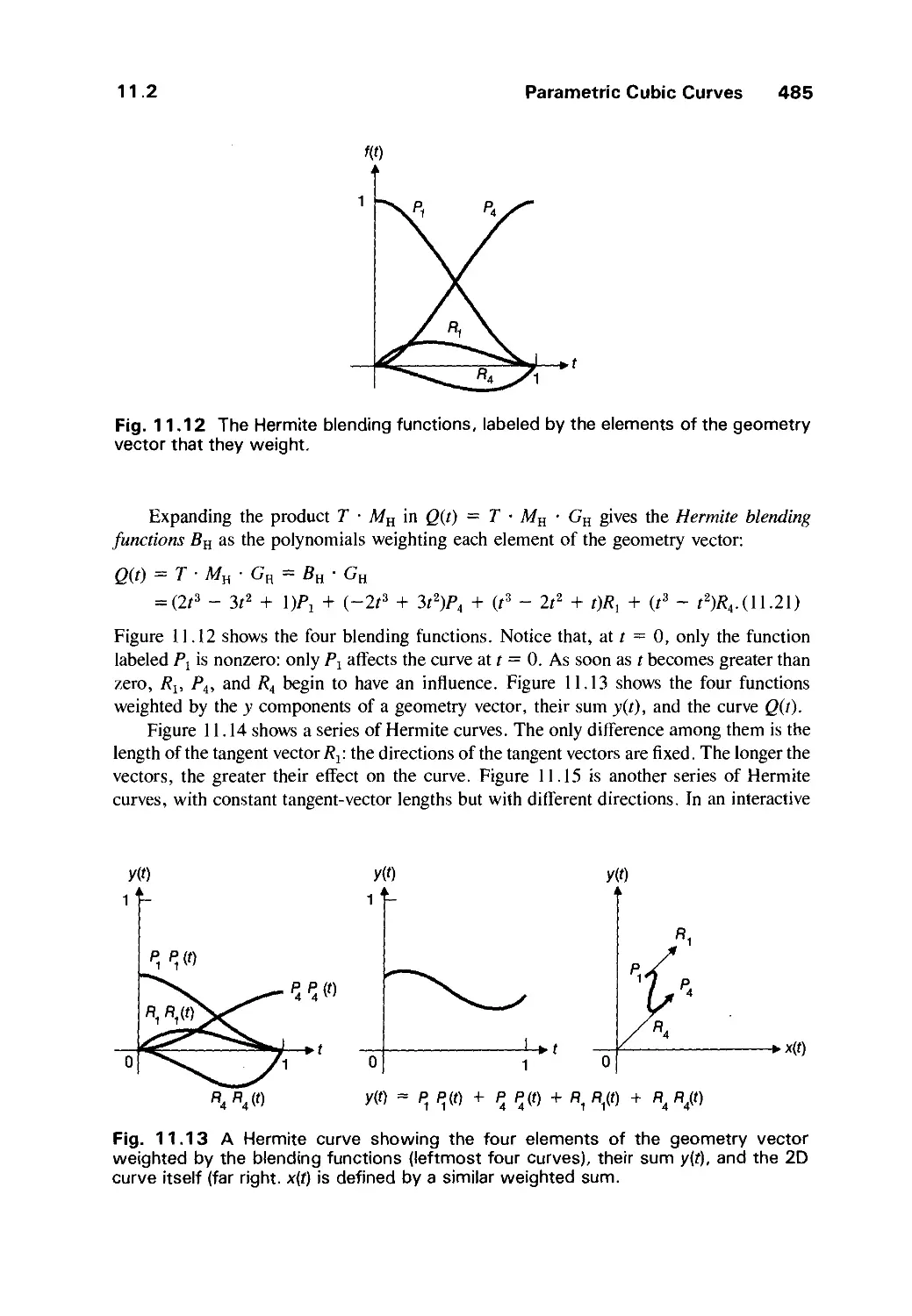
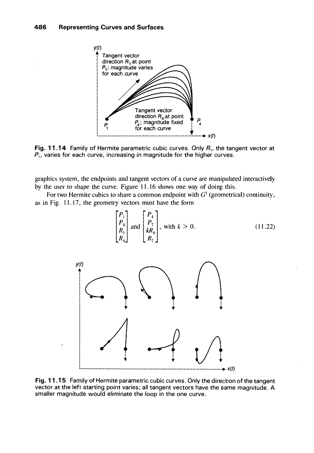
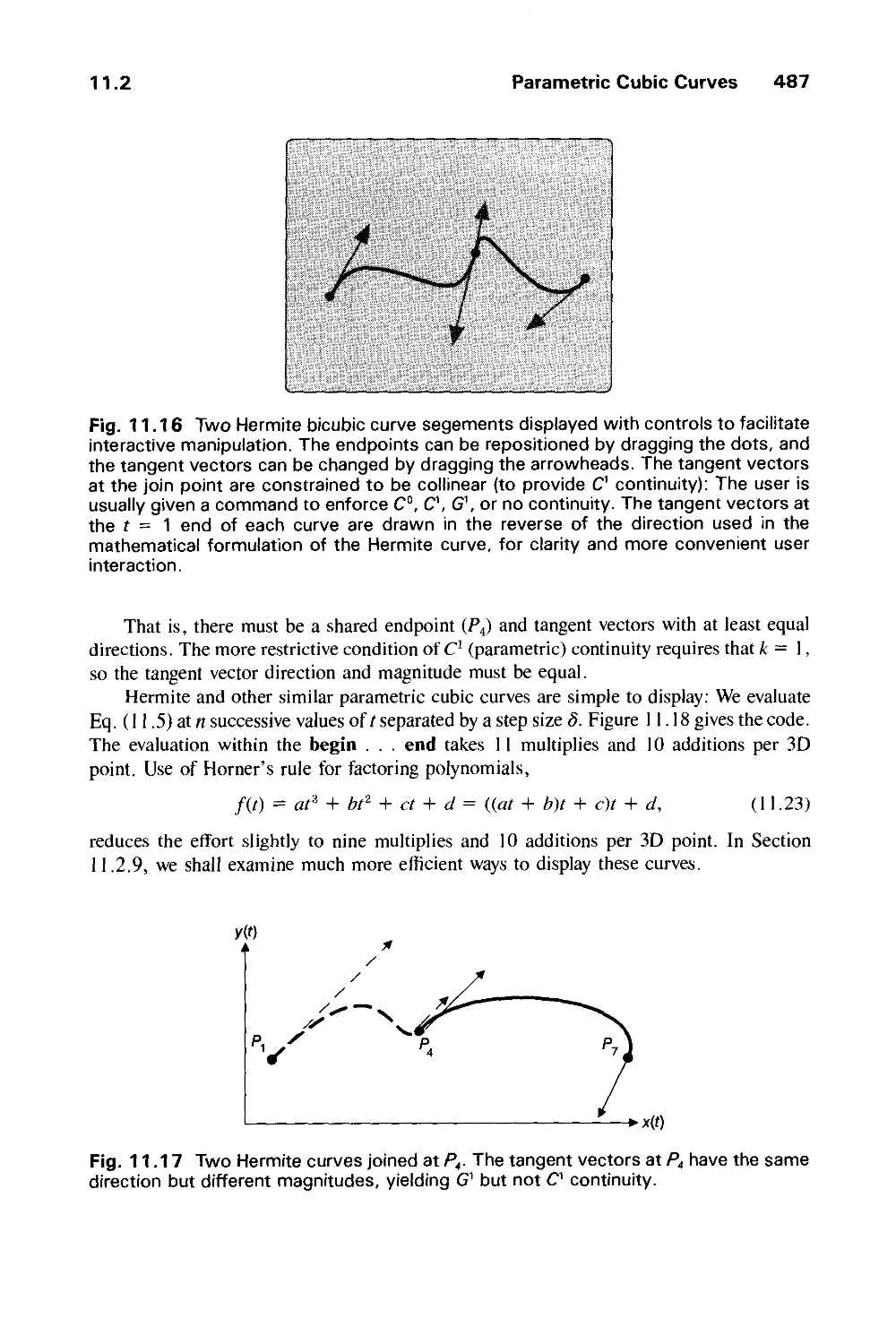
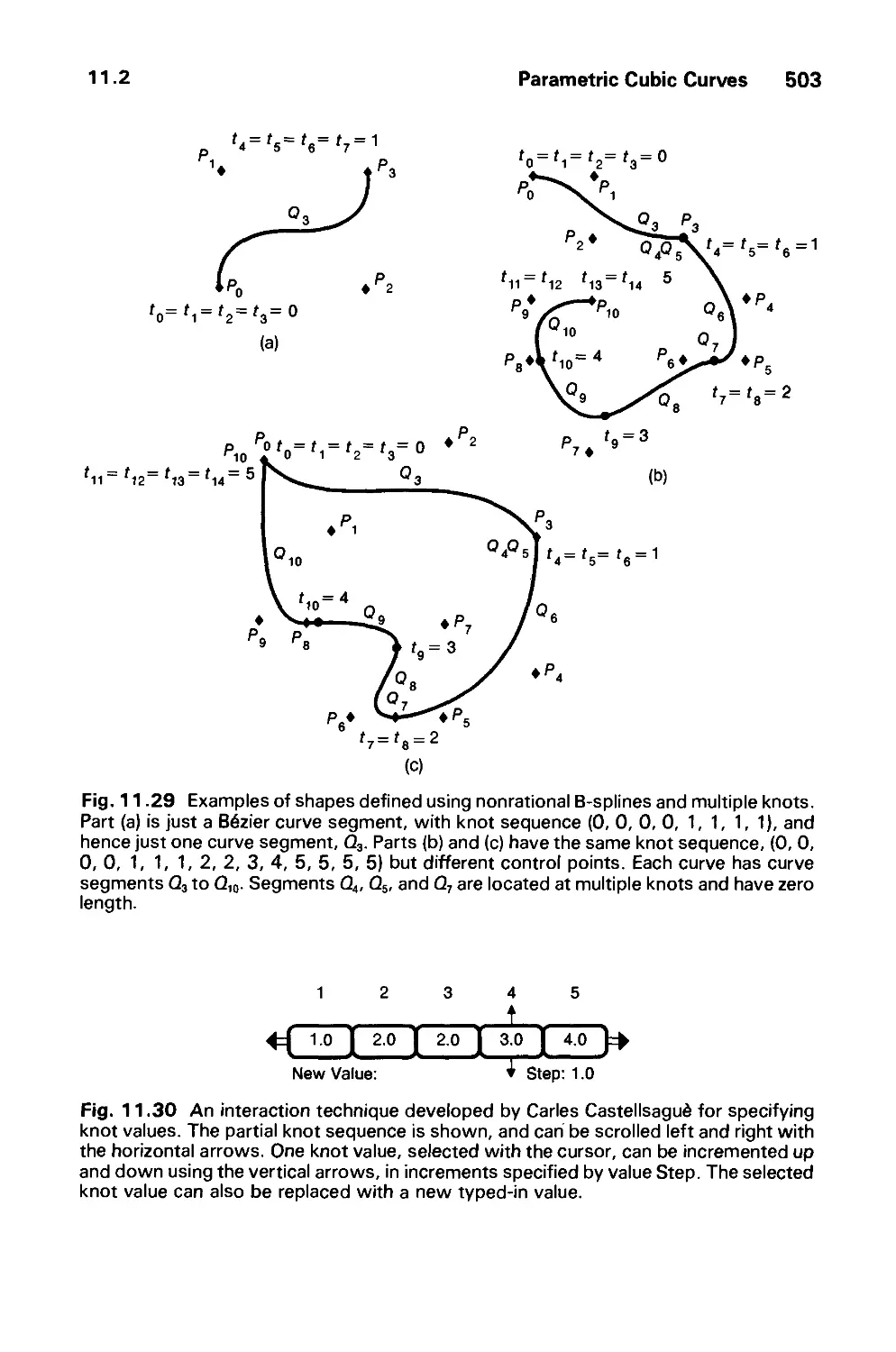
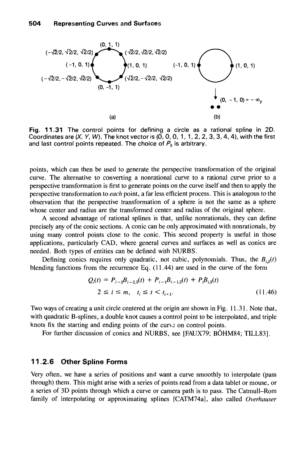
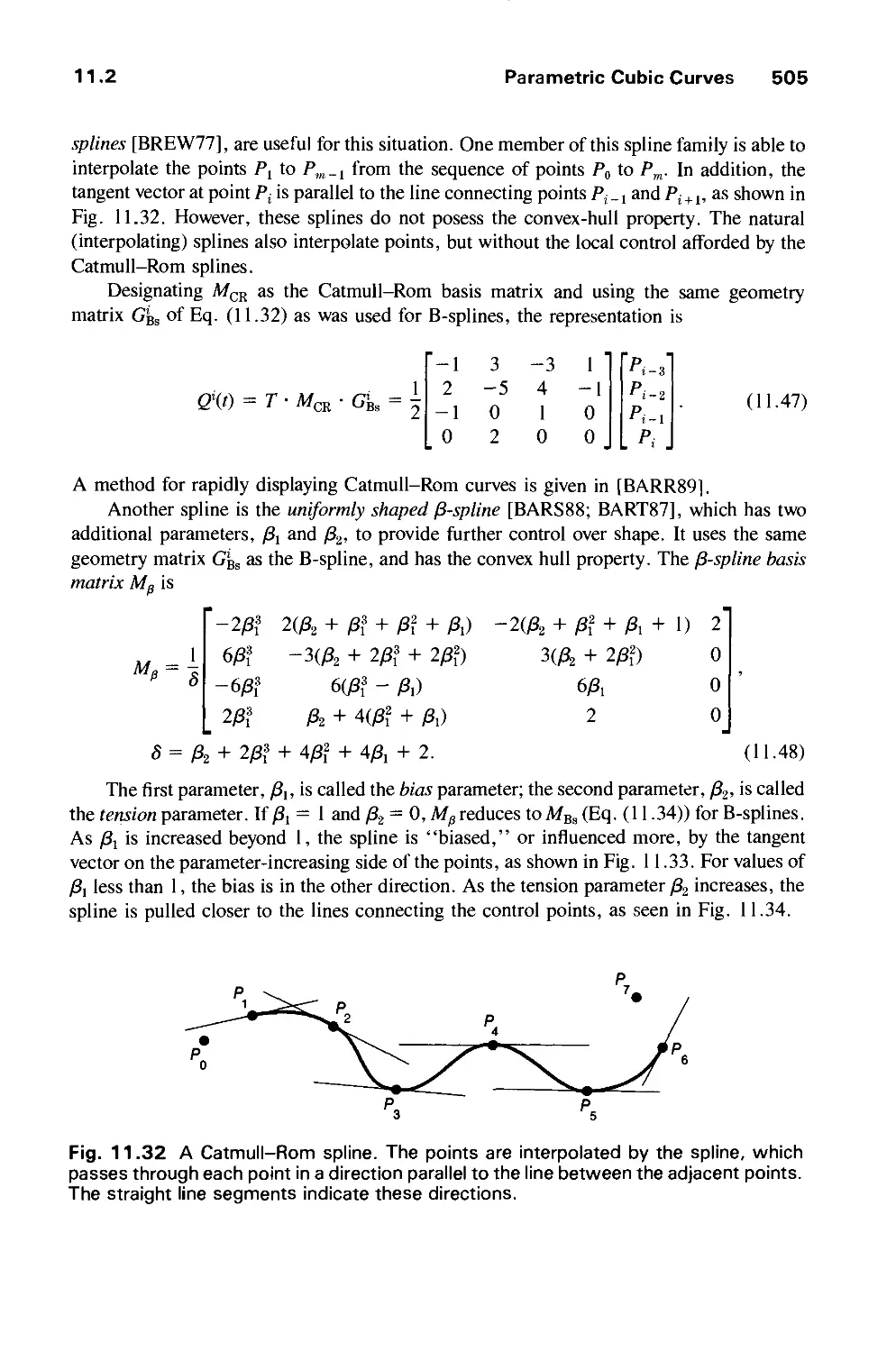
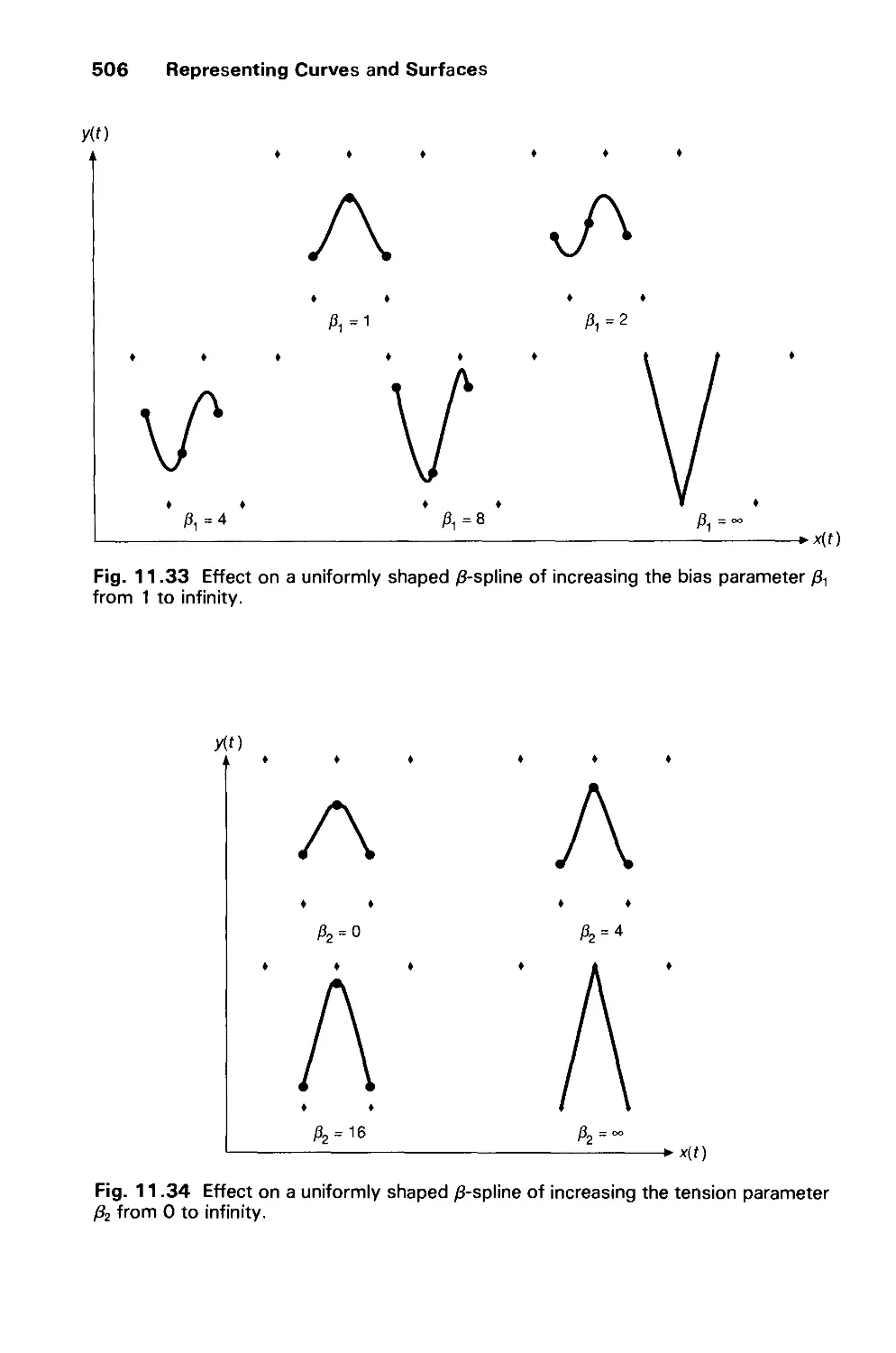
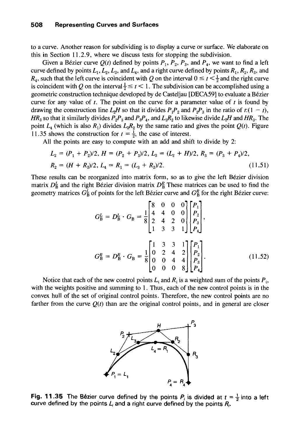
11.2 Parametric Cubic Curves 478
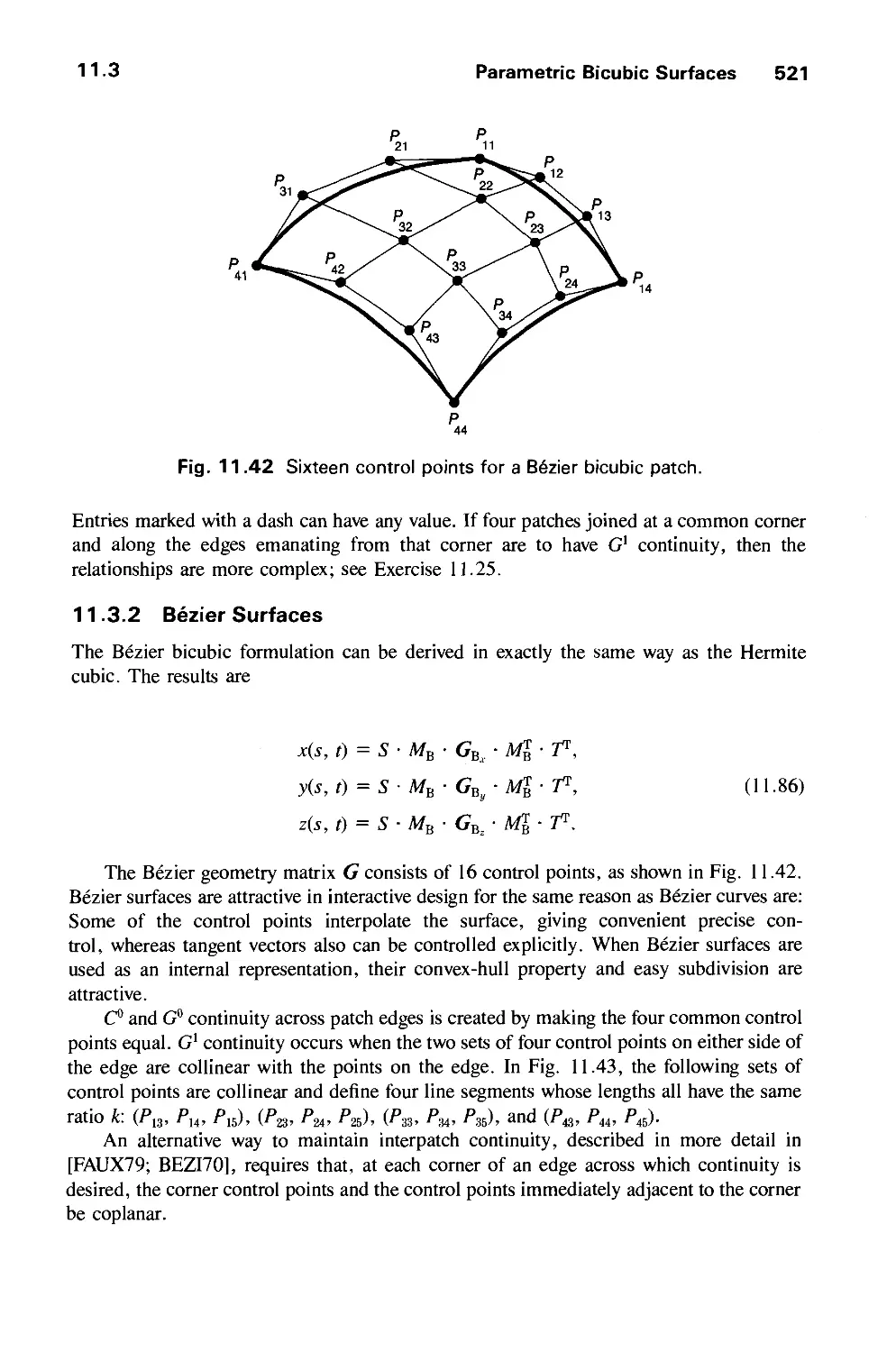
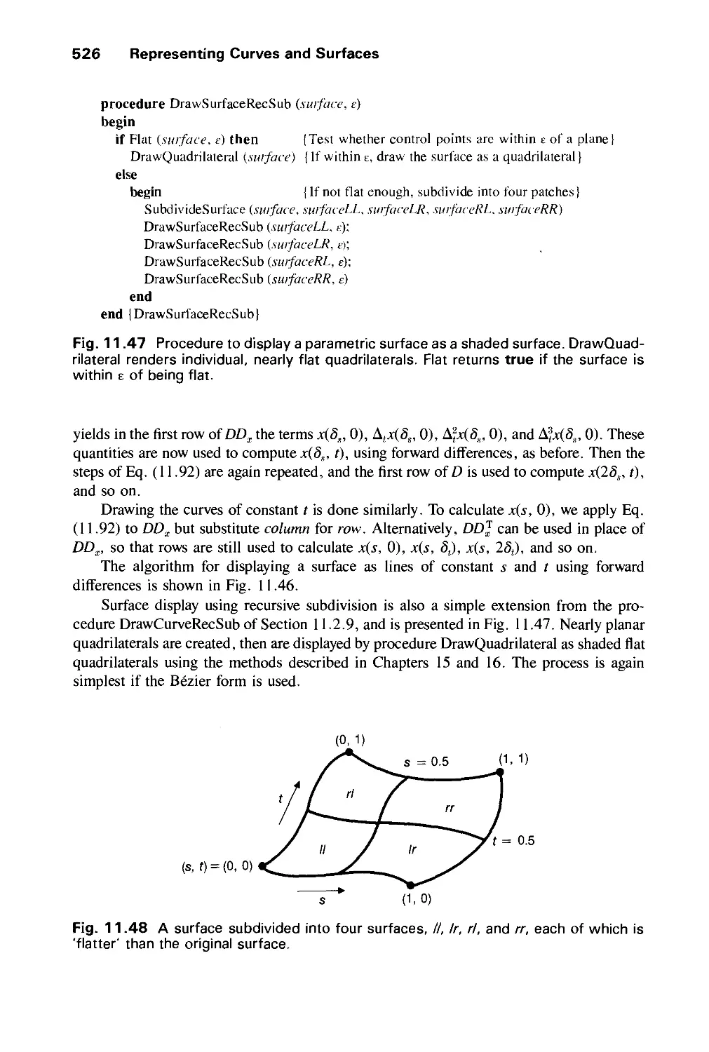
11.3 Parametric Bicubic Surfaces 516
11.4 Quadric Surfaces 528
11.5 Summary 529
Exercises 530
CHAPTER 12
SOLID MODELING 533
12.1 Representing Solids 534
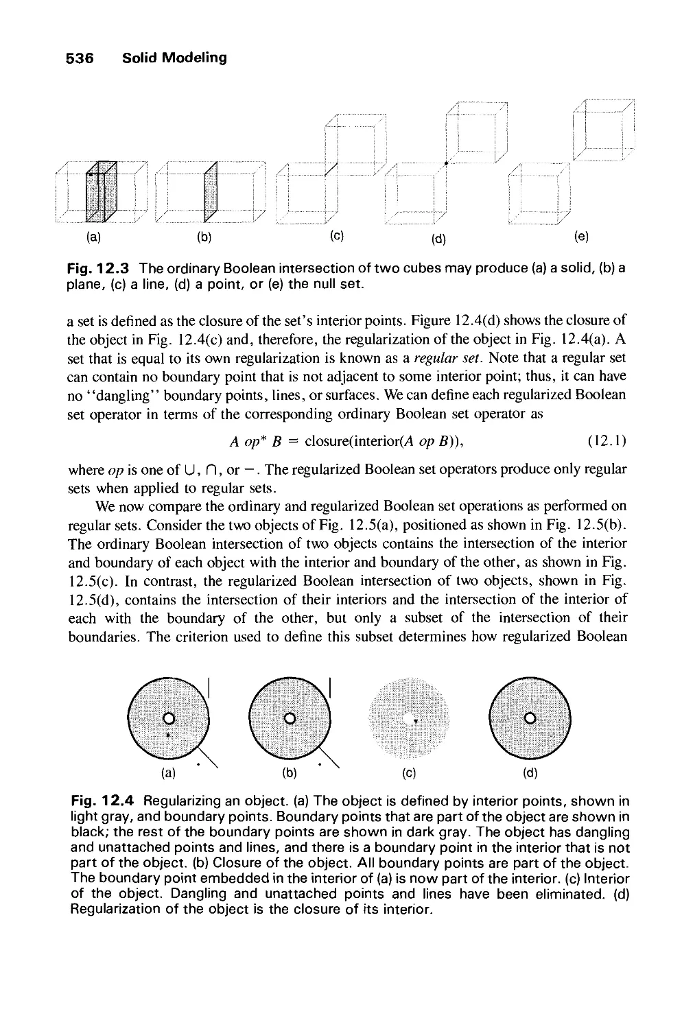
12.2 Regularized Boolean Set Operations 535
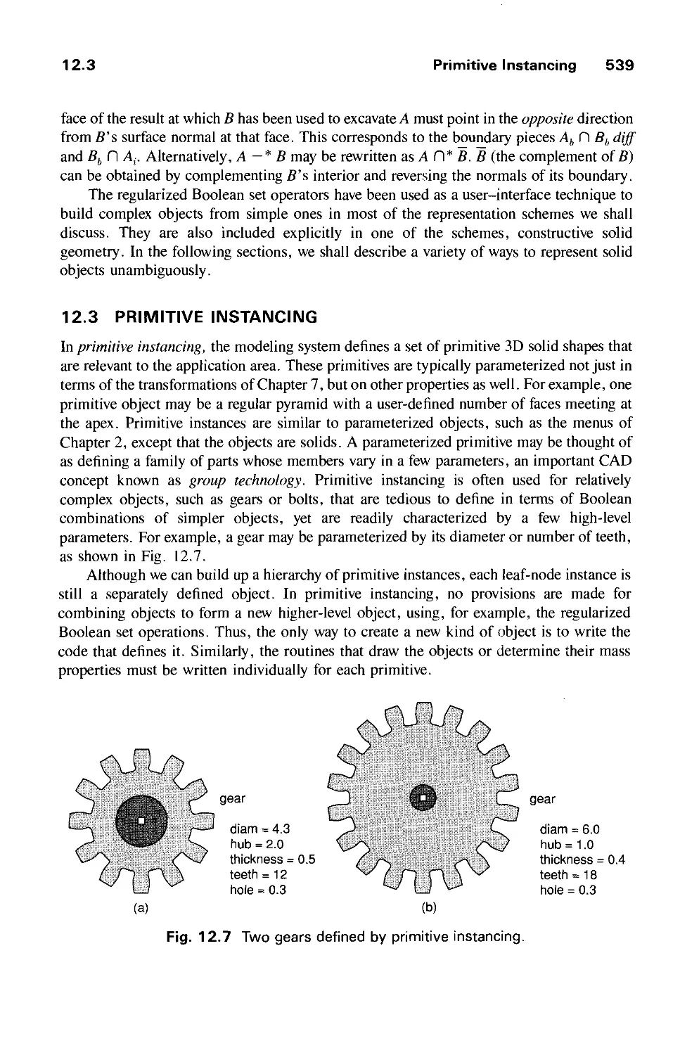
12.3 Primitive Instancing 539
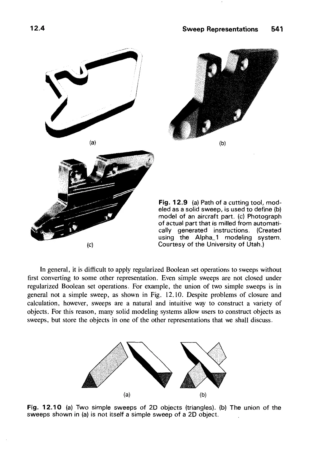
12.4 Sweep Representations 540
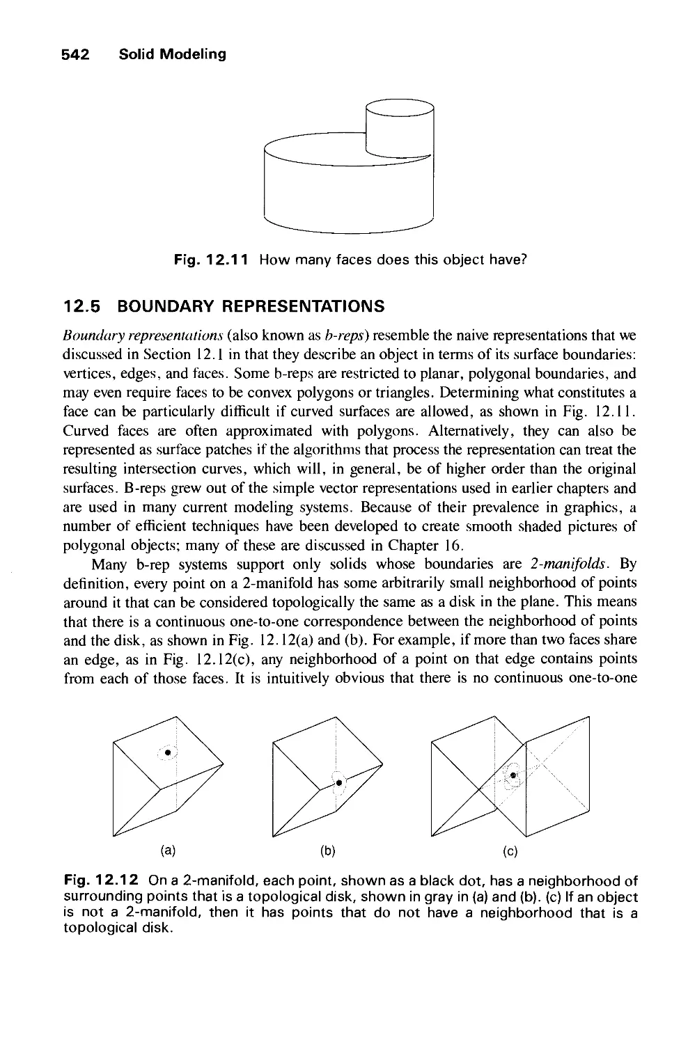
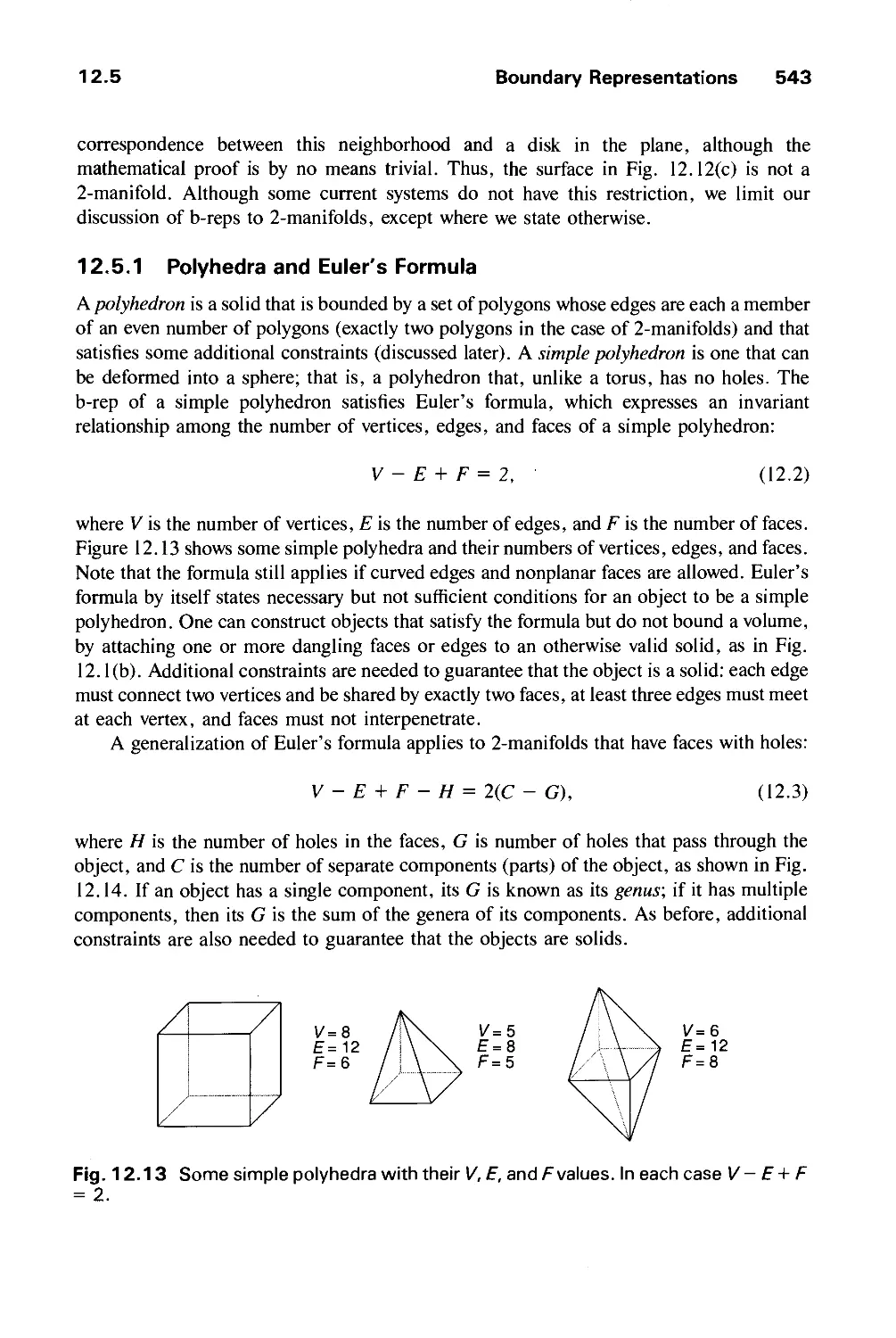
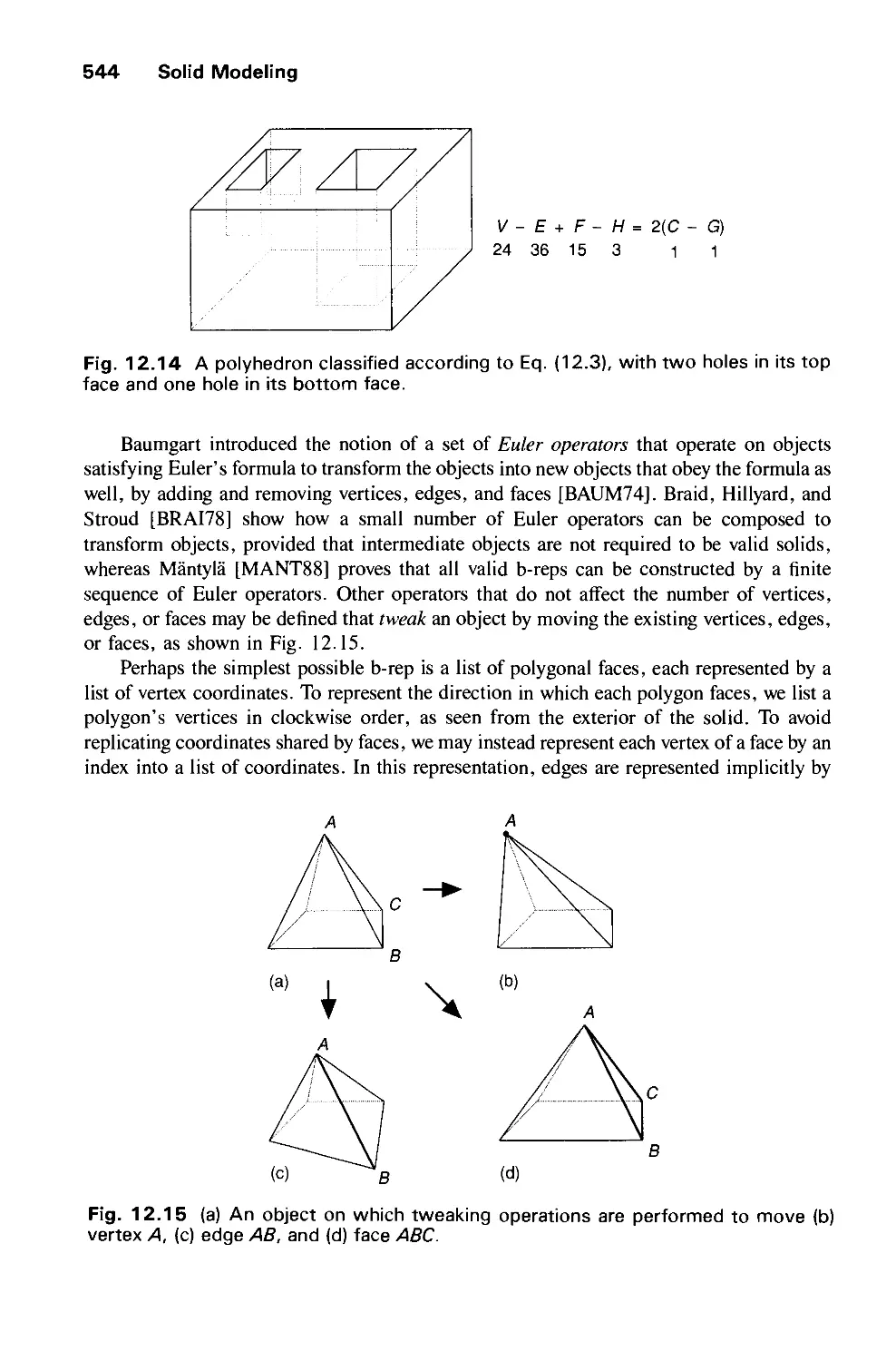
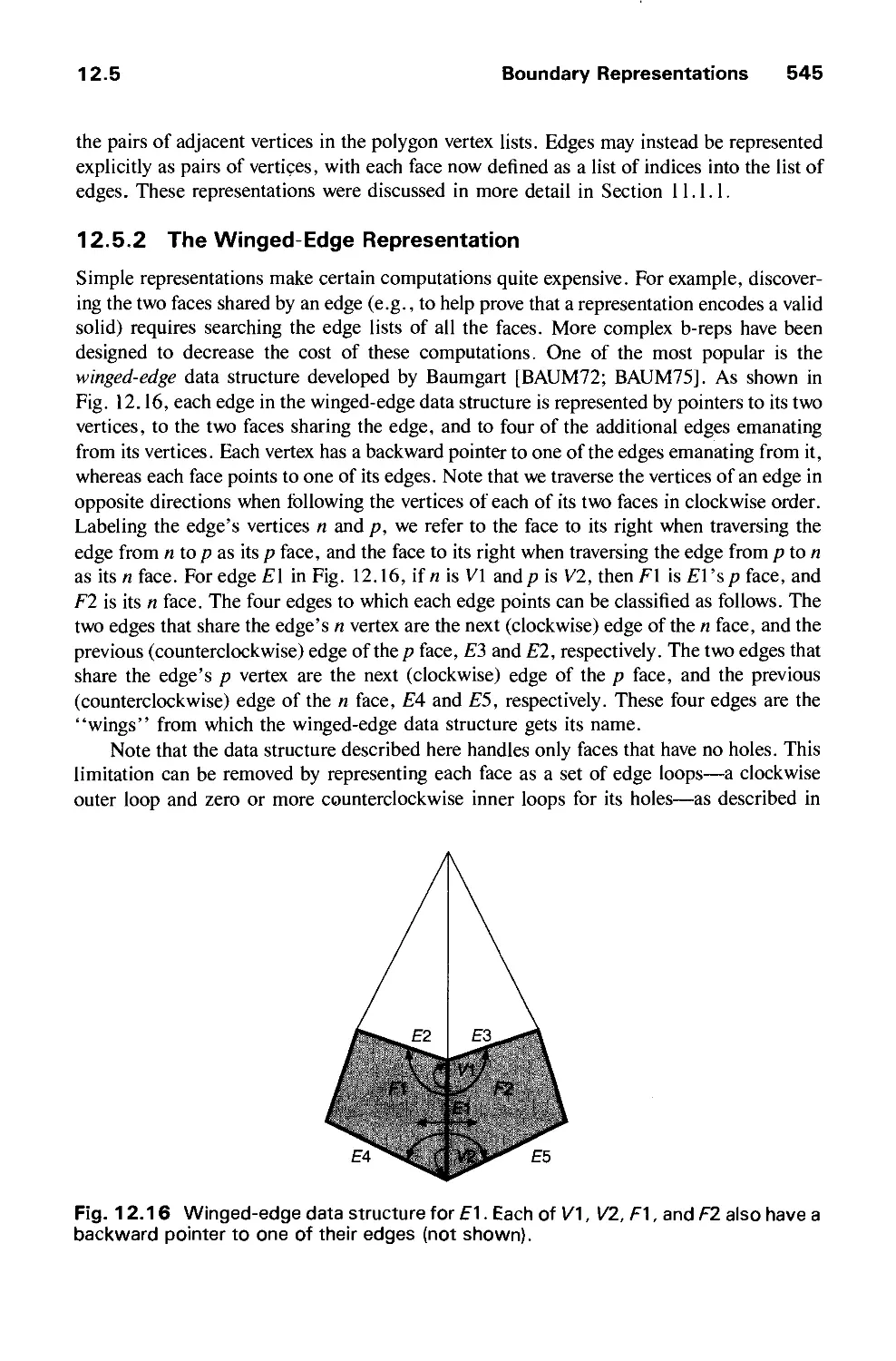
12.5 Boundary Representations 542
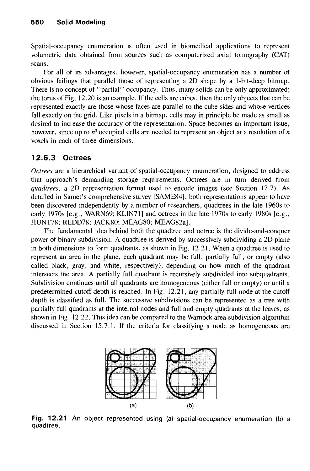
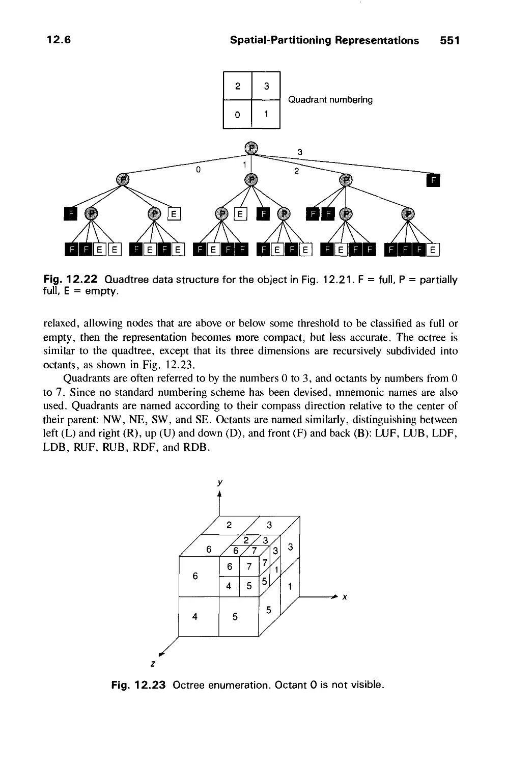
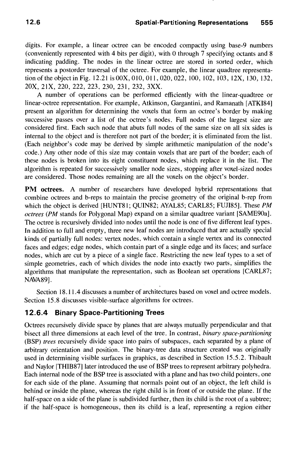
12.6 Spatial-Partitioning Representations 548
12.7 Constructive Solid Geometry 557
12.8 Comparison of Representations 558
12.9 User Interfaces for Solid Modeling 561
12.10 Summary 561
Exercises 562
CHAPTER 13
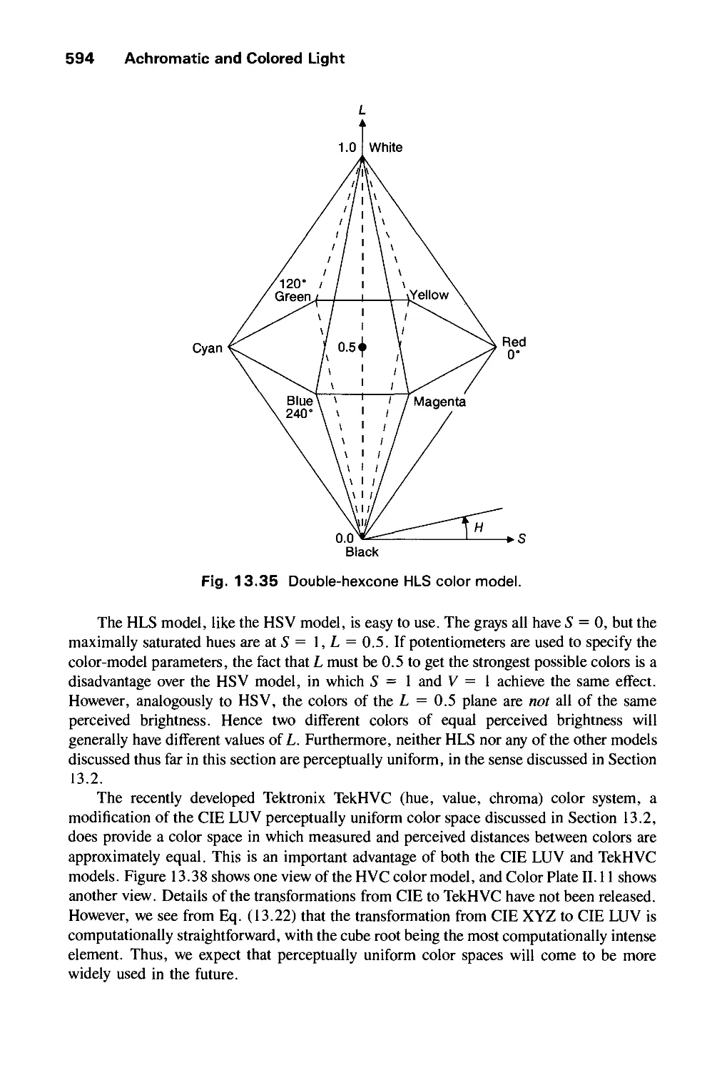
ACHROMATIC AND COLORED LIGHT 563
13.1 Achromatic Light 563
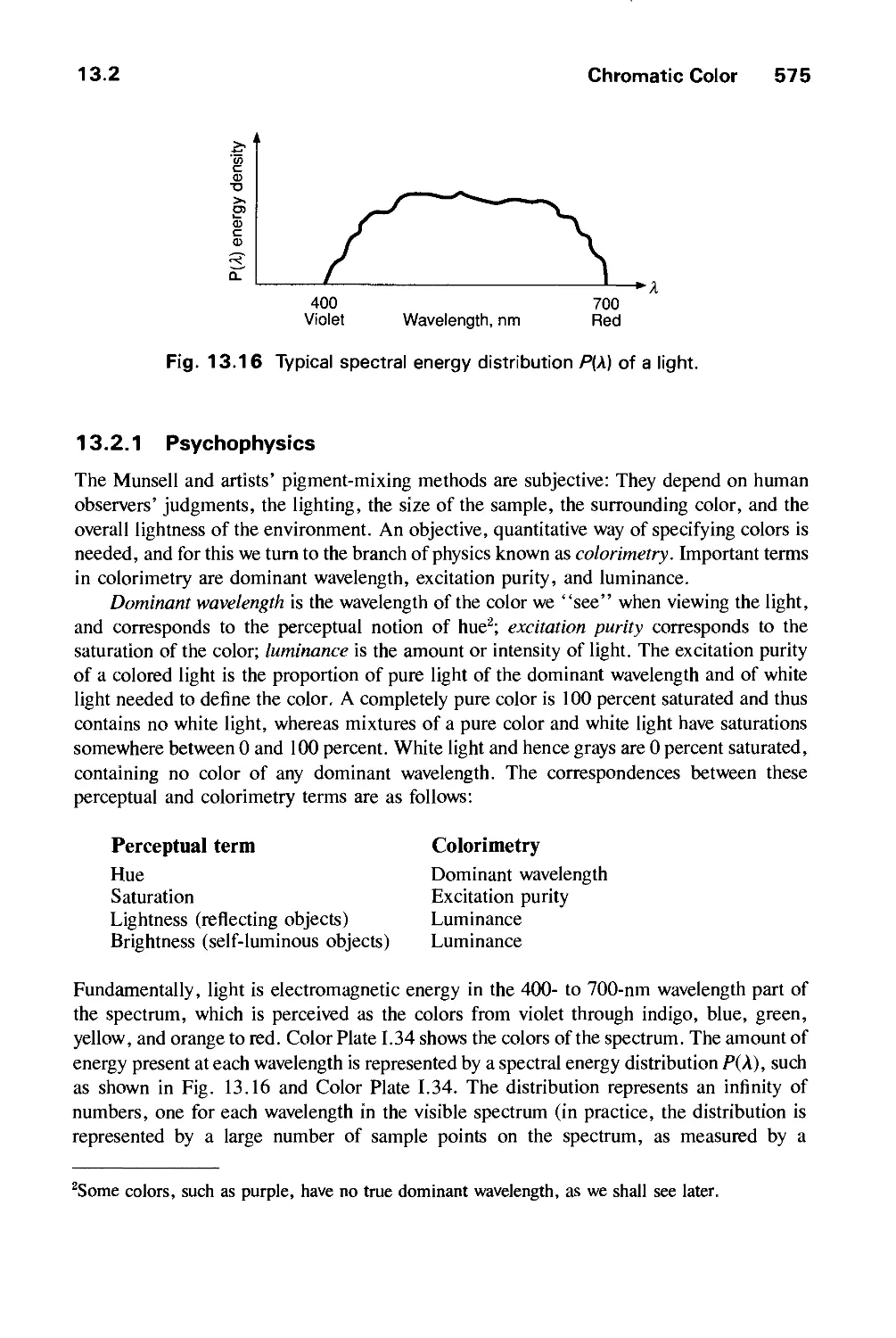
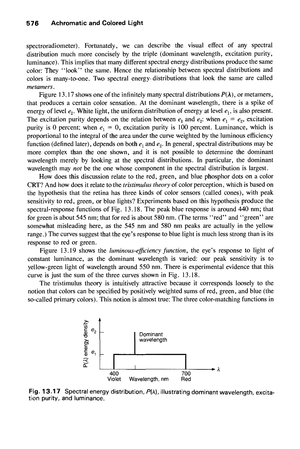
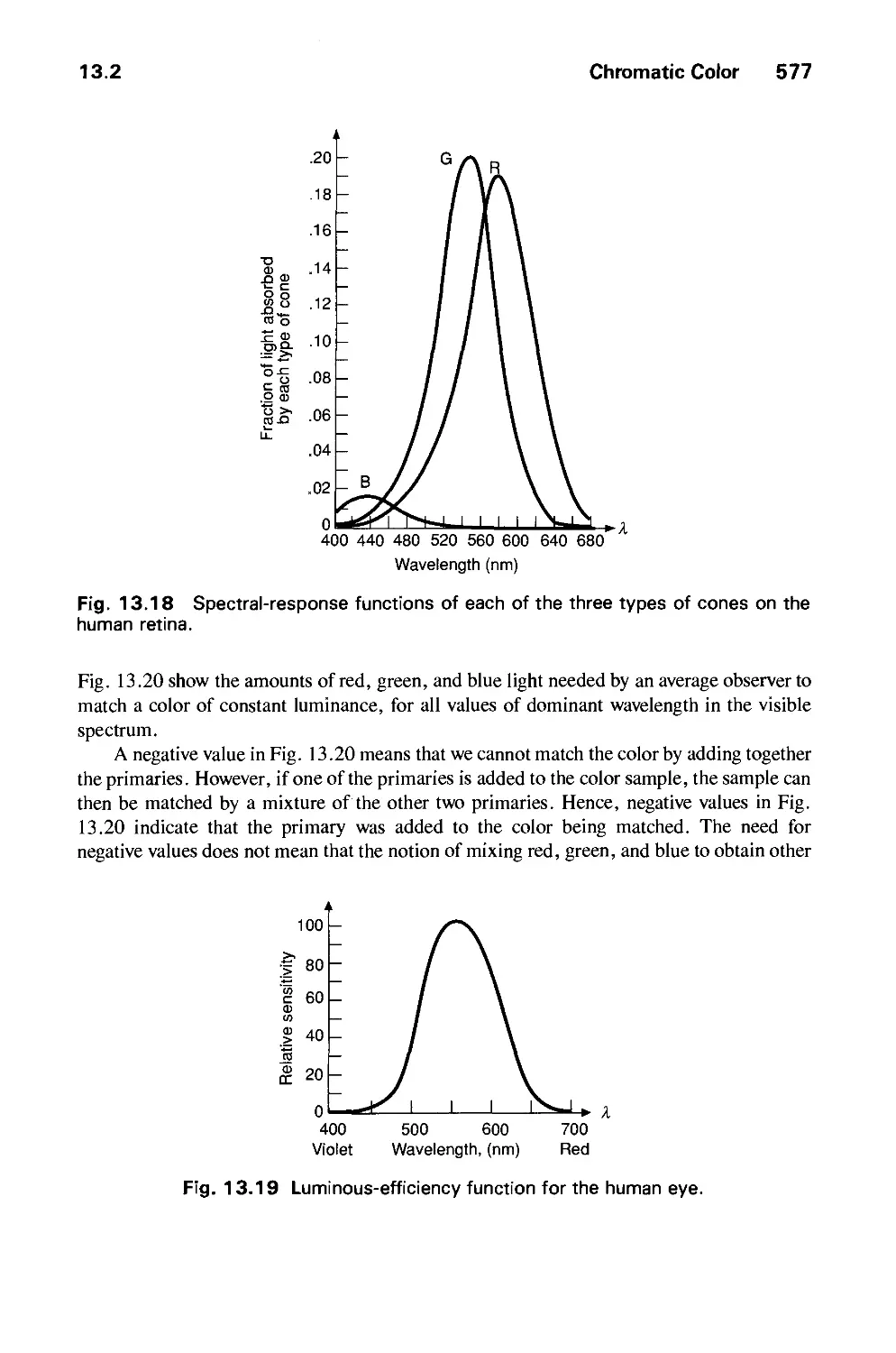
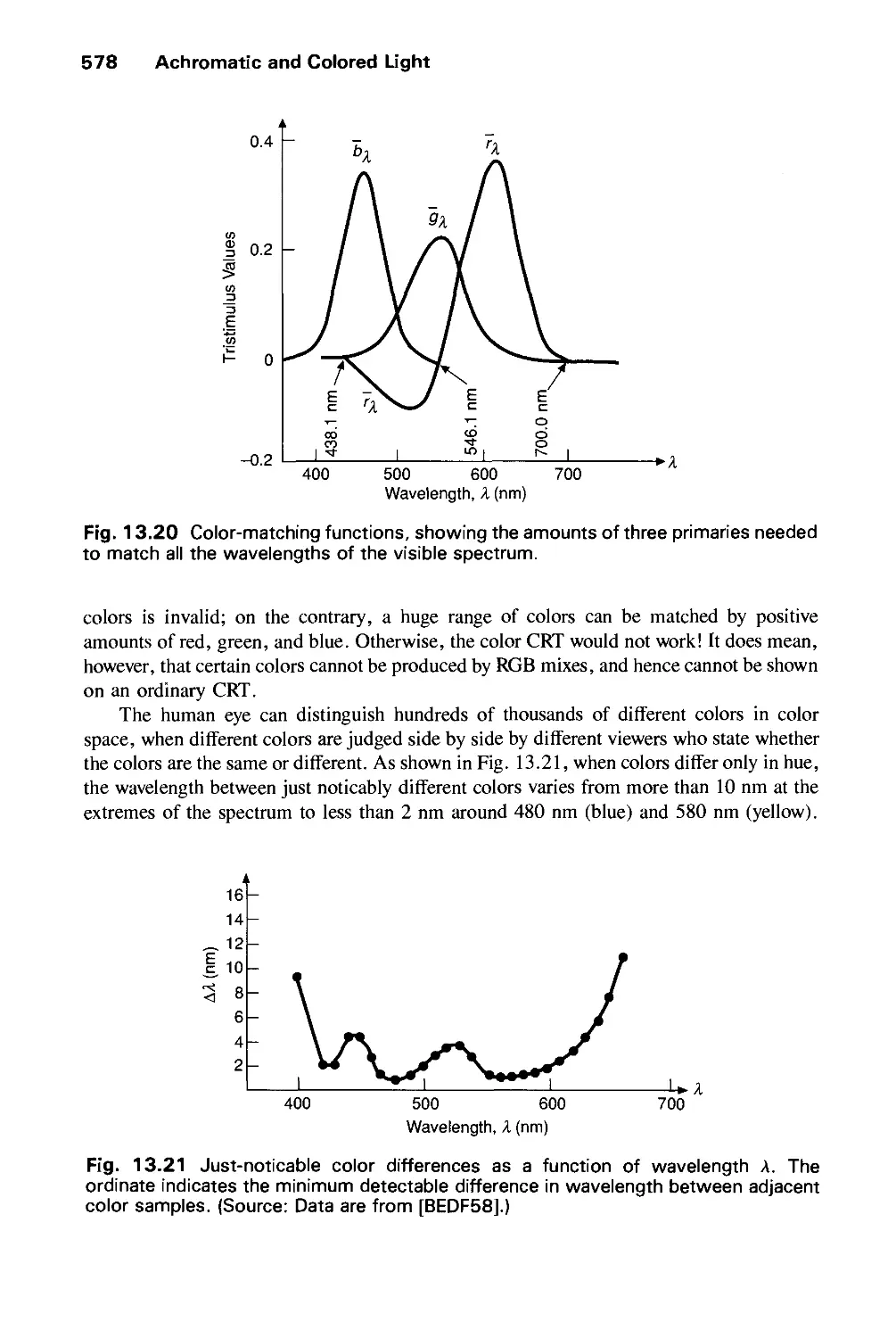
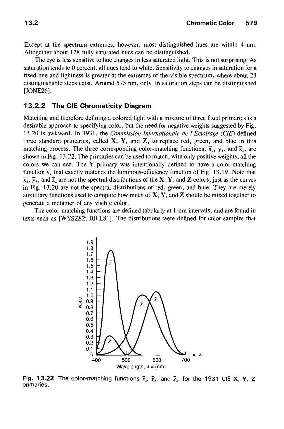
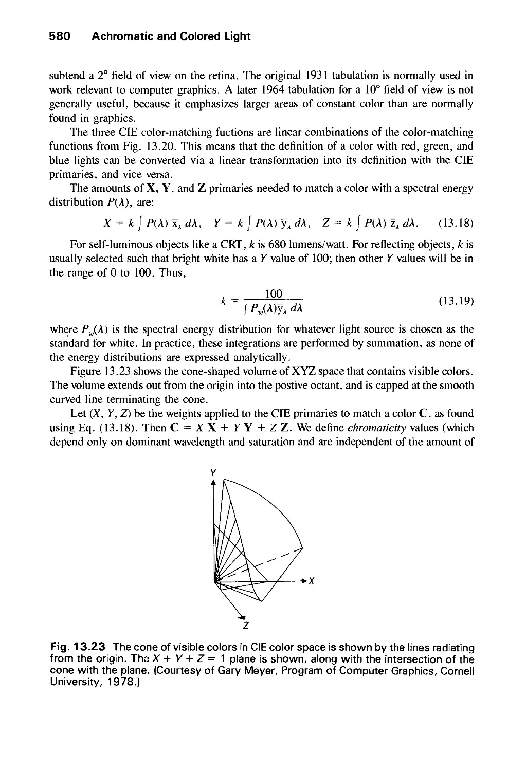
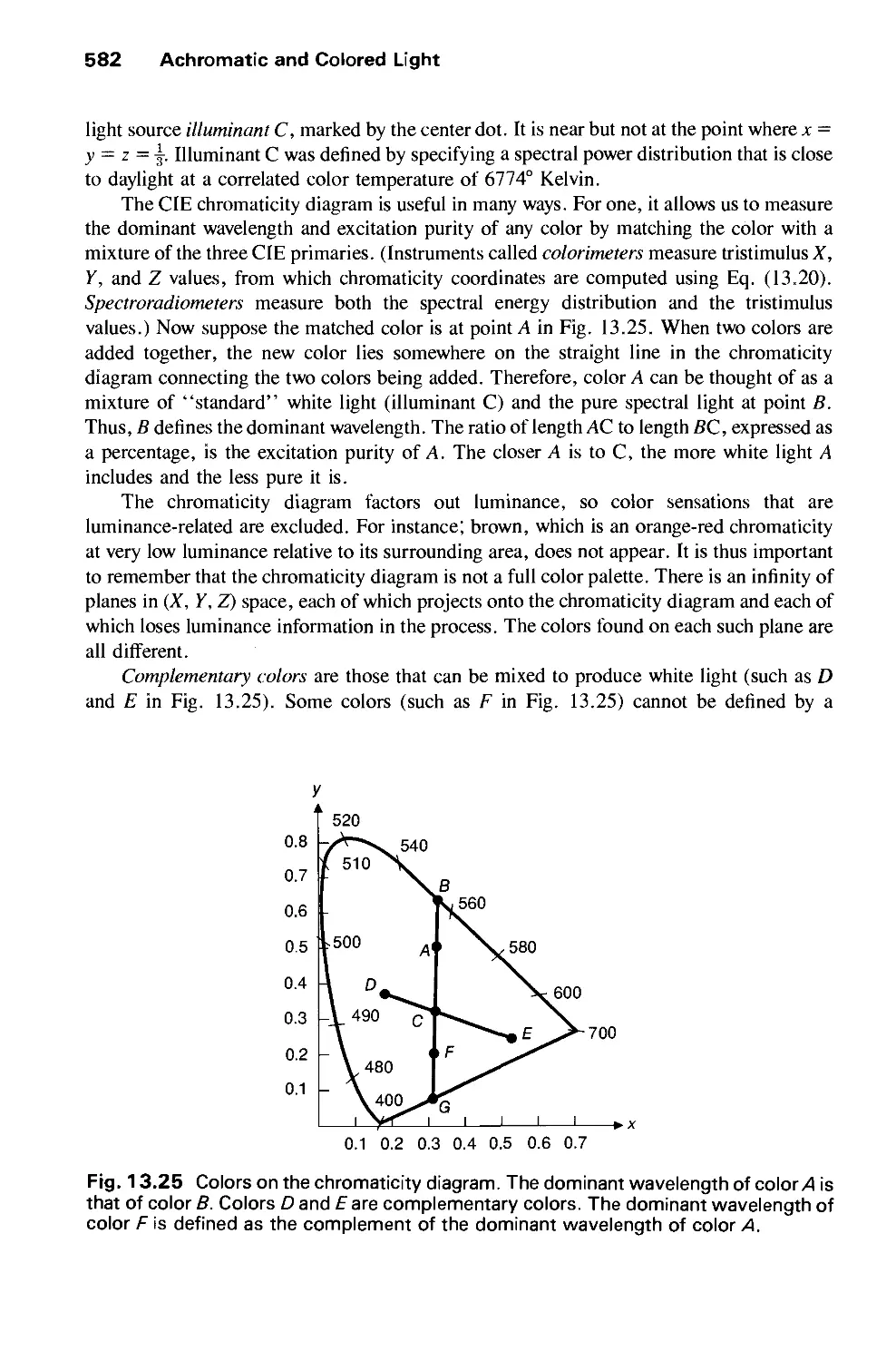
13.2 Chromatic Color 574
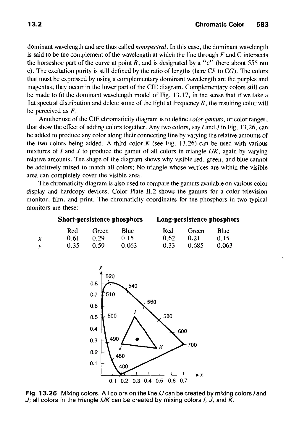
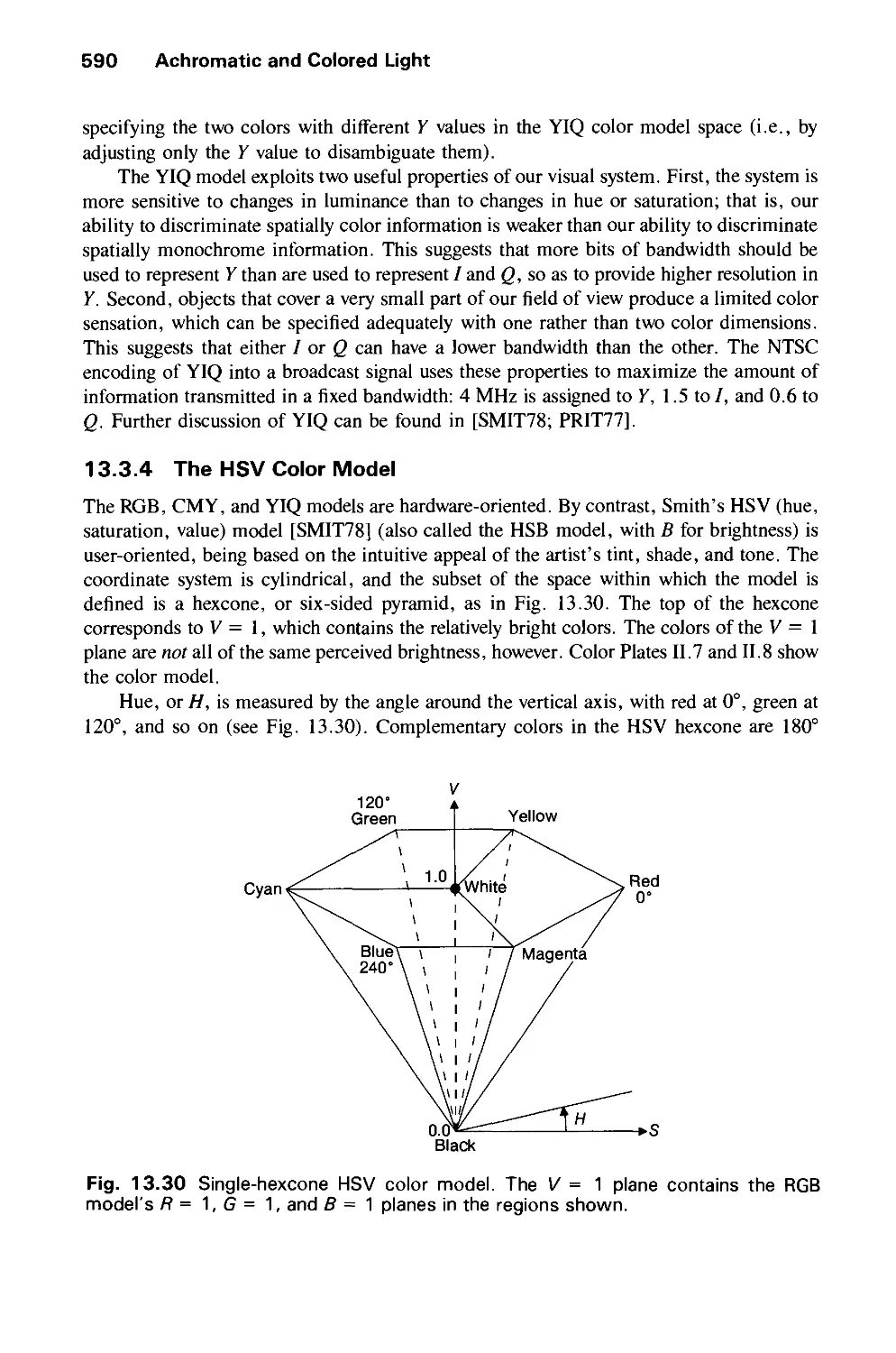
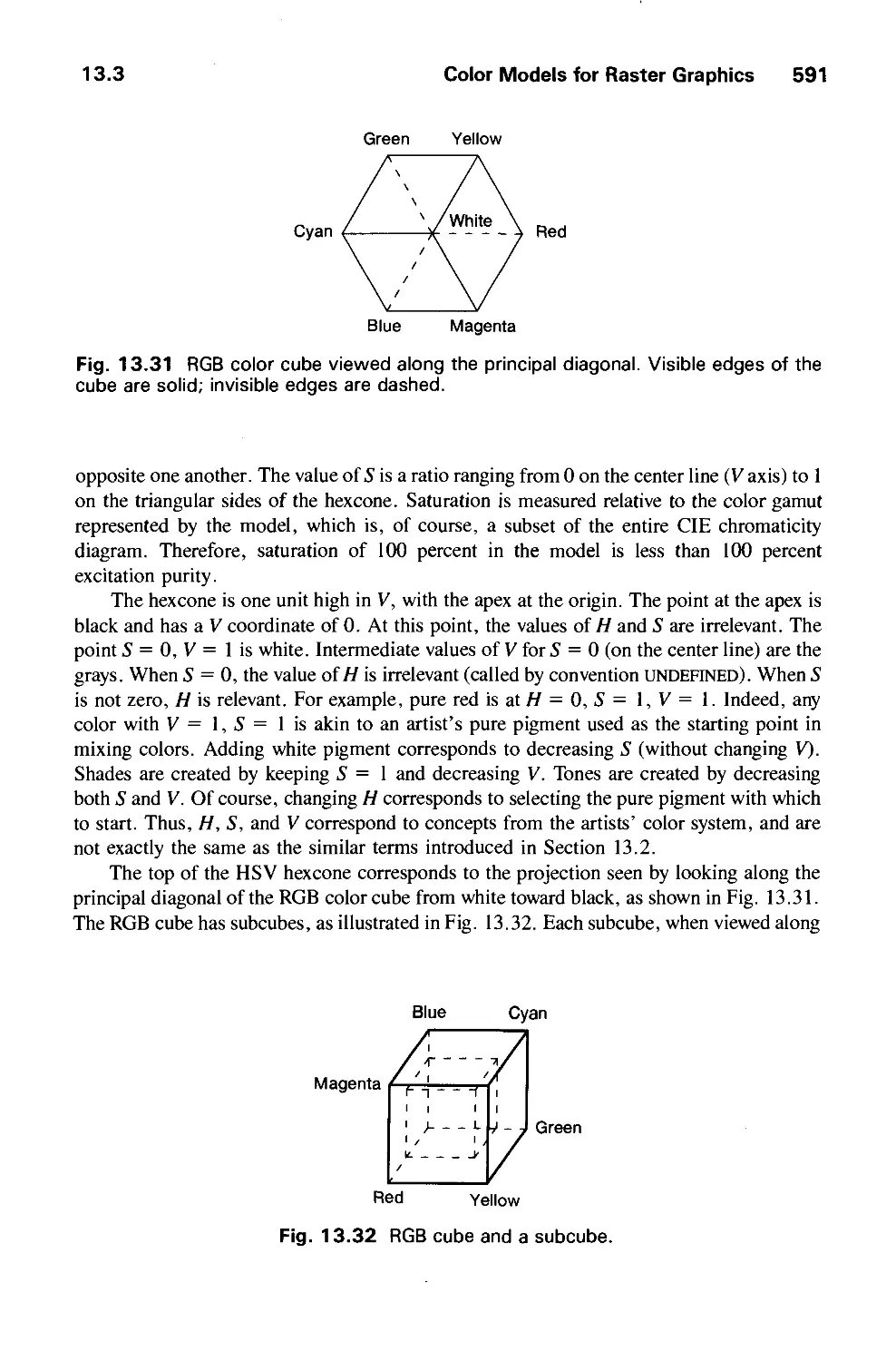
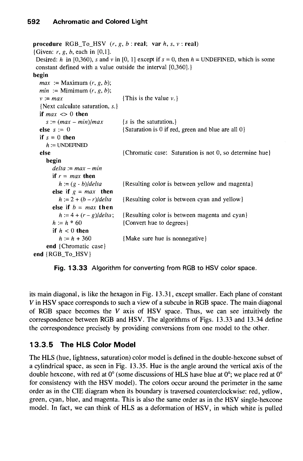
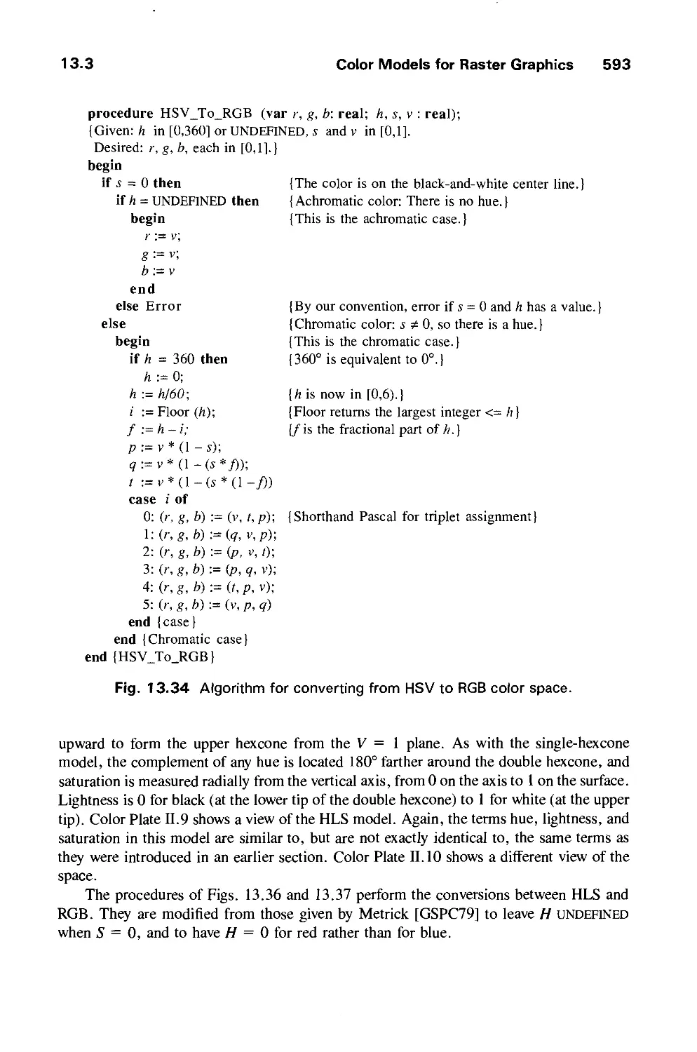
13.3 Color Models for Raster Graphics 584
13.4 Reproducing Color 599
13.5 Using Color in Computer Graphics 601
13.6 Summary 603
Exercises 603
CHAPTER 14
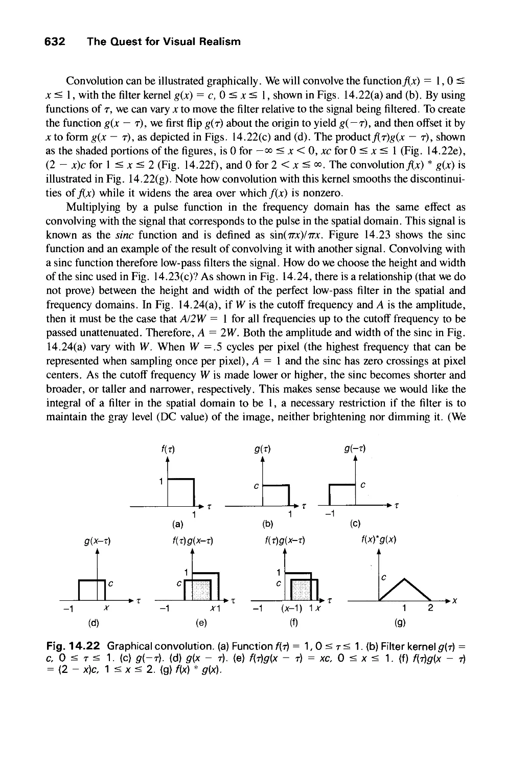
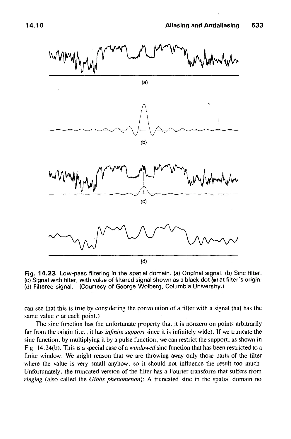
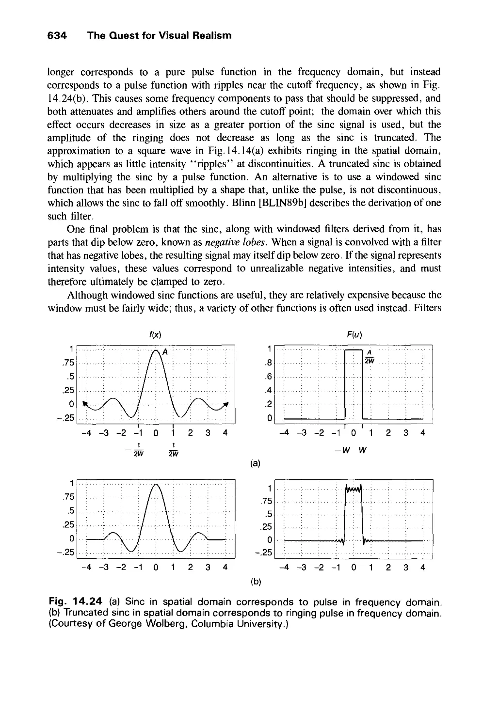
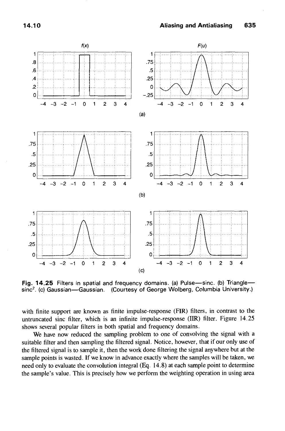
THE QUEST FOR VISUAL REALISM 605
14.1 Why Realism? 606
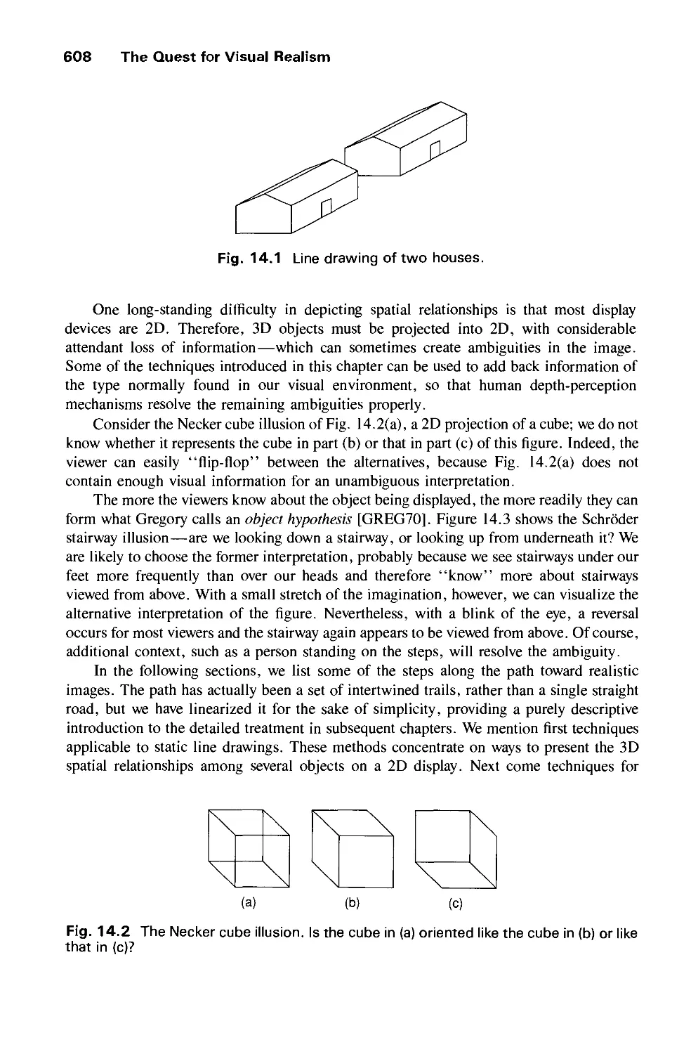
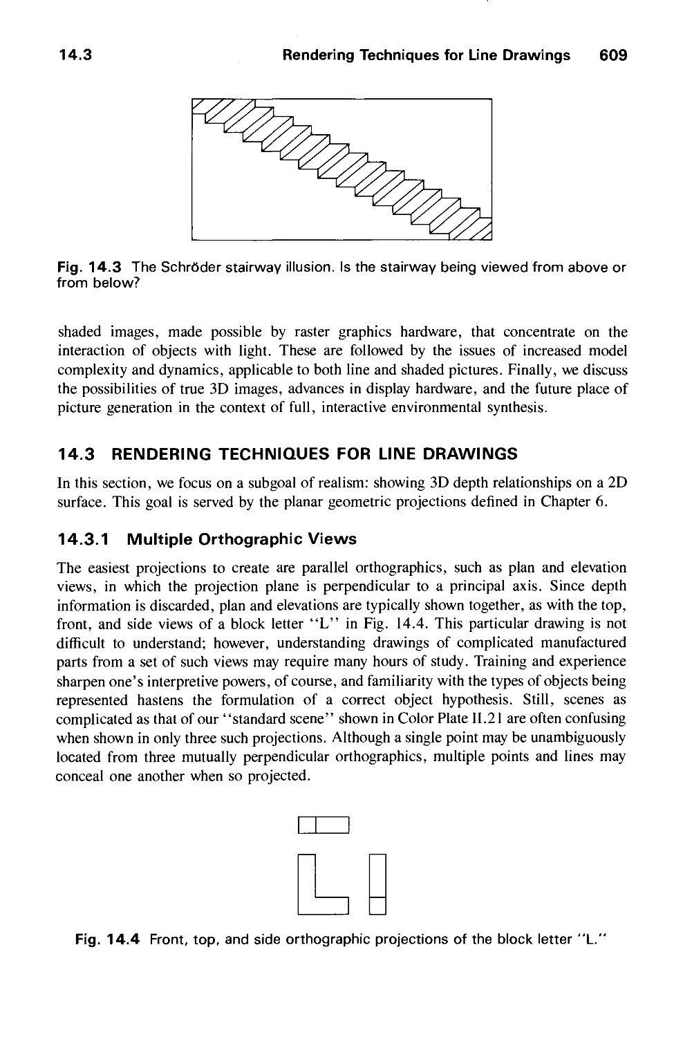
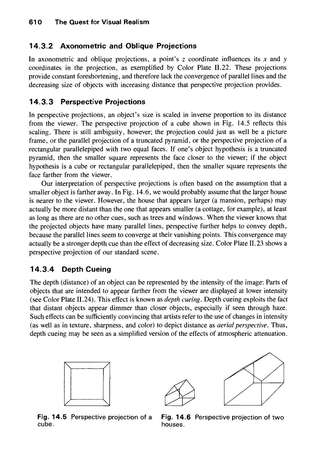
14.2 Fundamental Difficulties 607
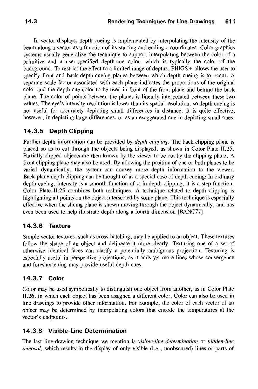
14.3 Rendering Techniques for Line Drawings 609
Contents xxi
14.4 Rendering Techniques for Shaded Images 612
14.5 Improved Object Models 615
14.6 Dynamics 615
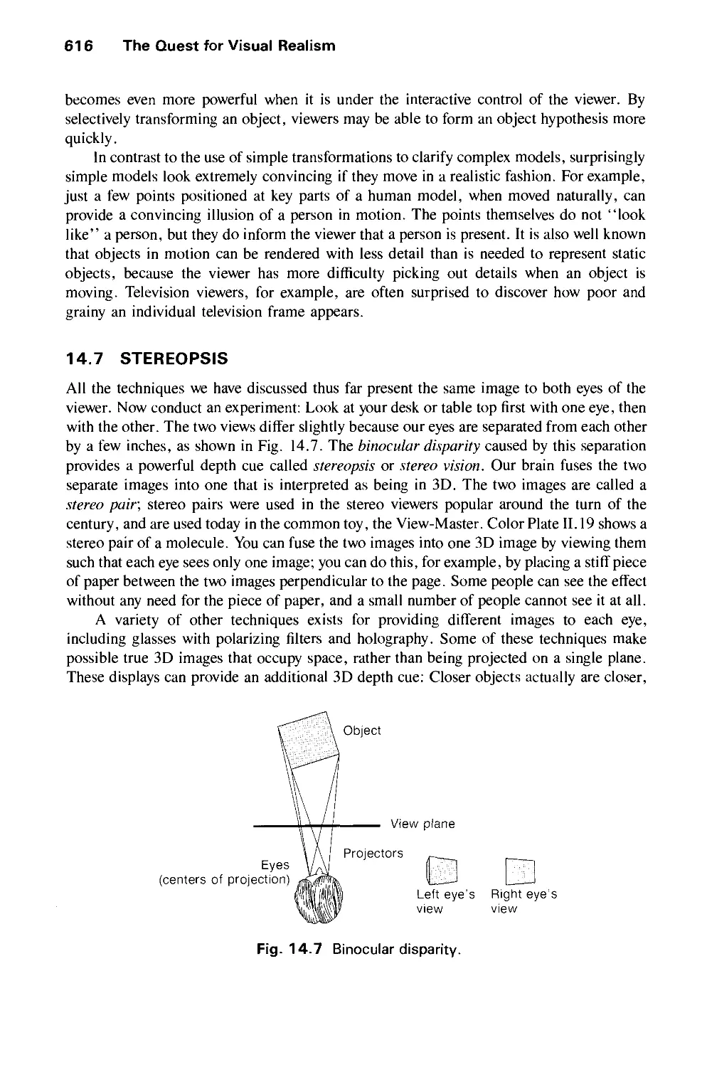
14.7 Stereopsis 616
14.8 Improved Displays 617
14.9 Interacting with Our Other Senses 617
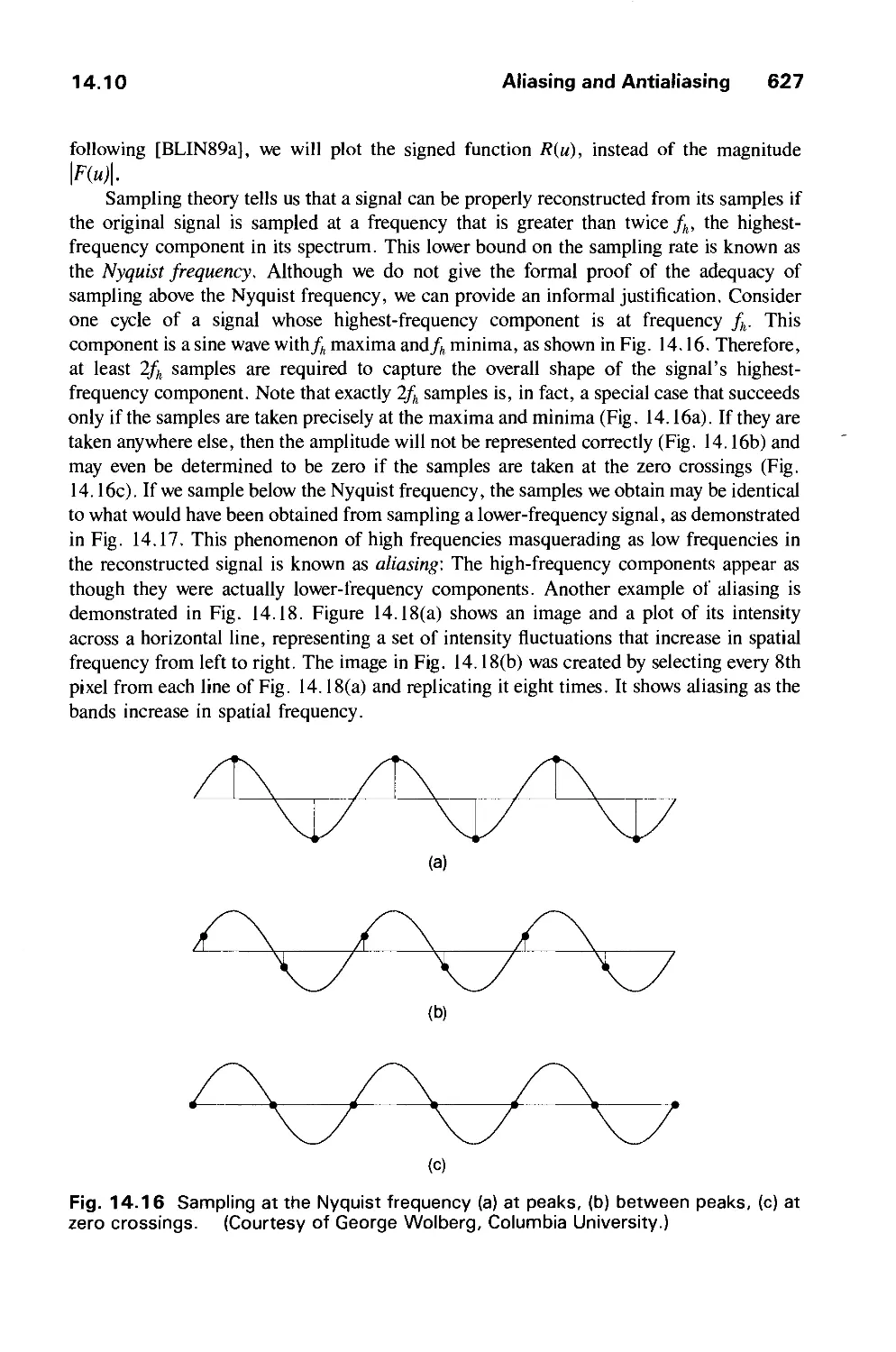
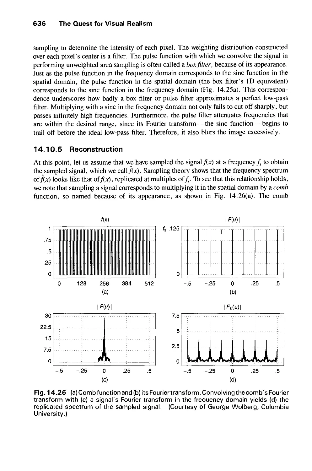
14.10 Aliasing and Antialiasing 617
14.11 Summary 646
Exercises 647
CHAPTER 15
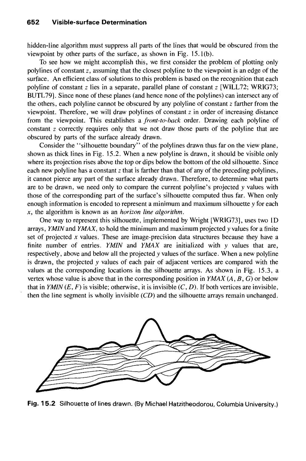
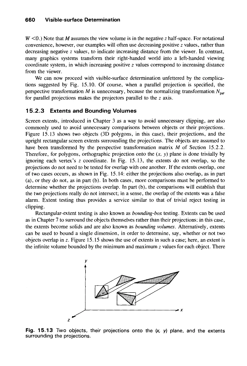
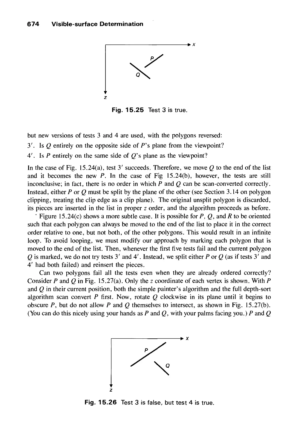
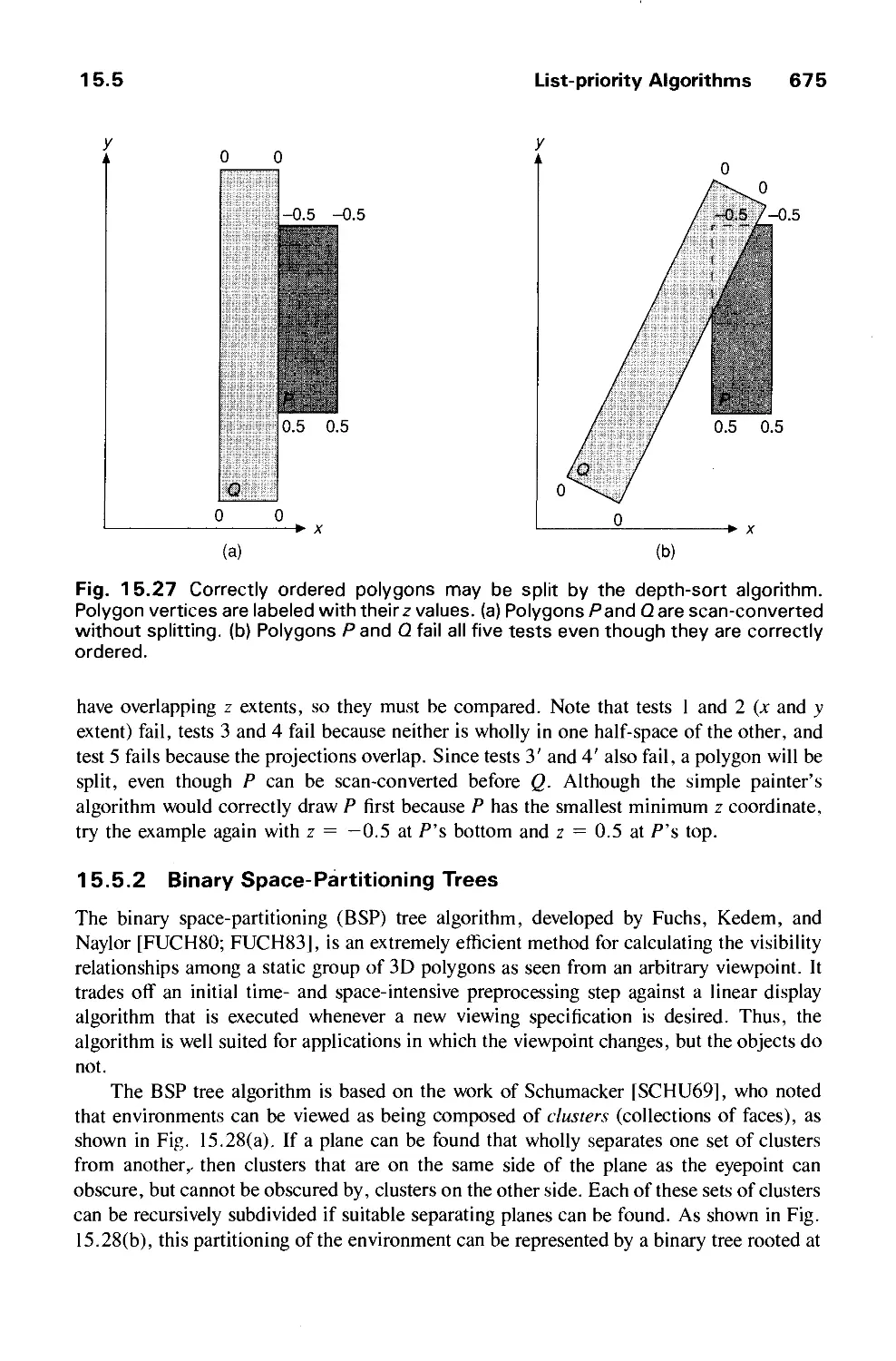
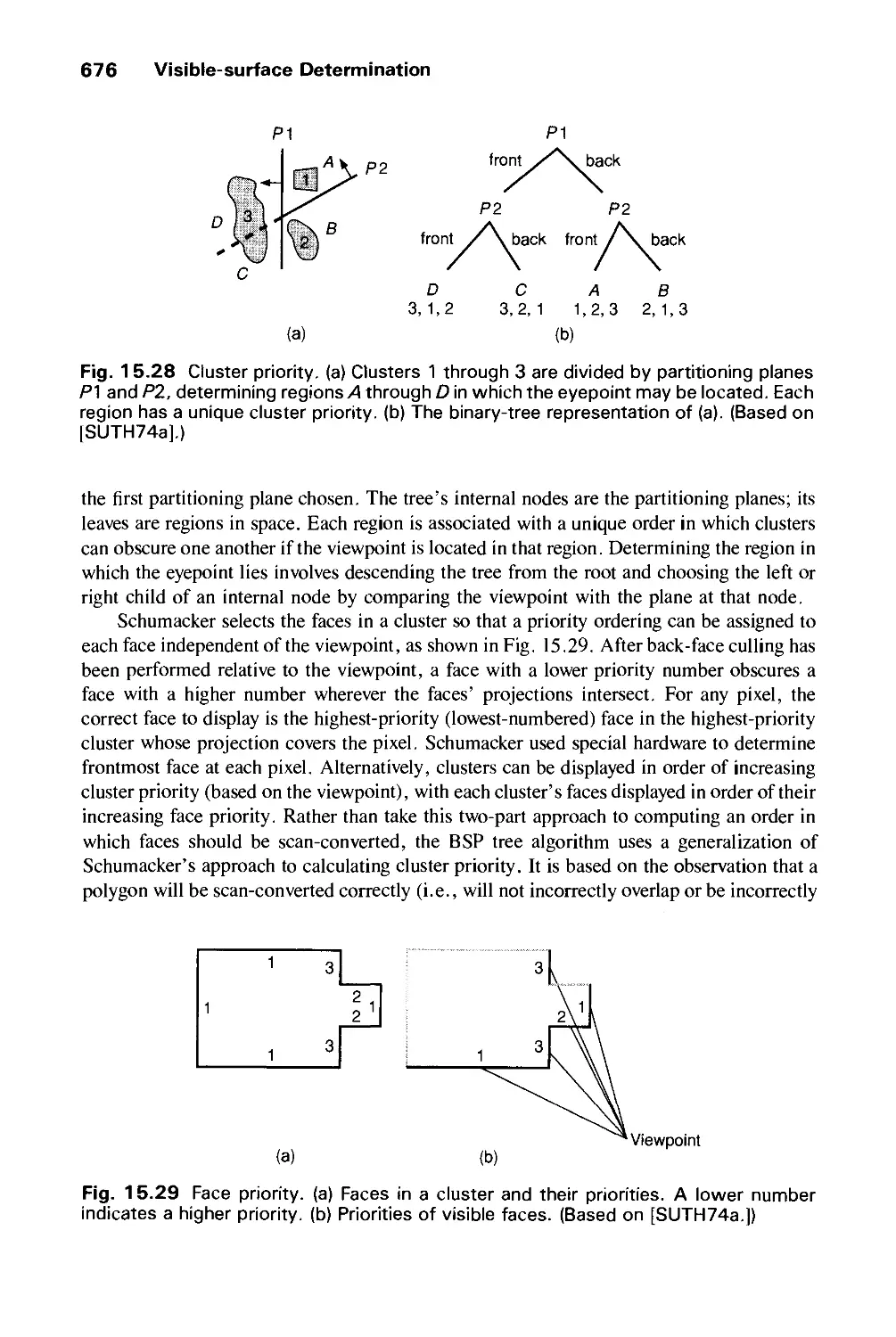
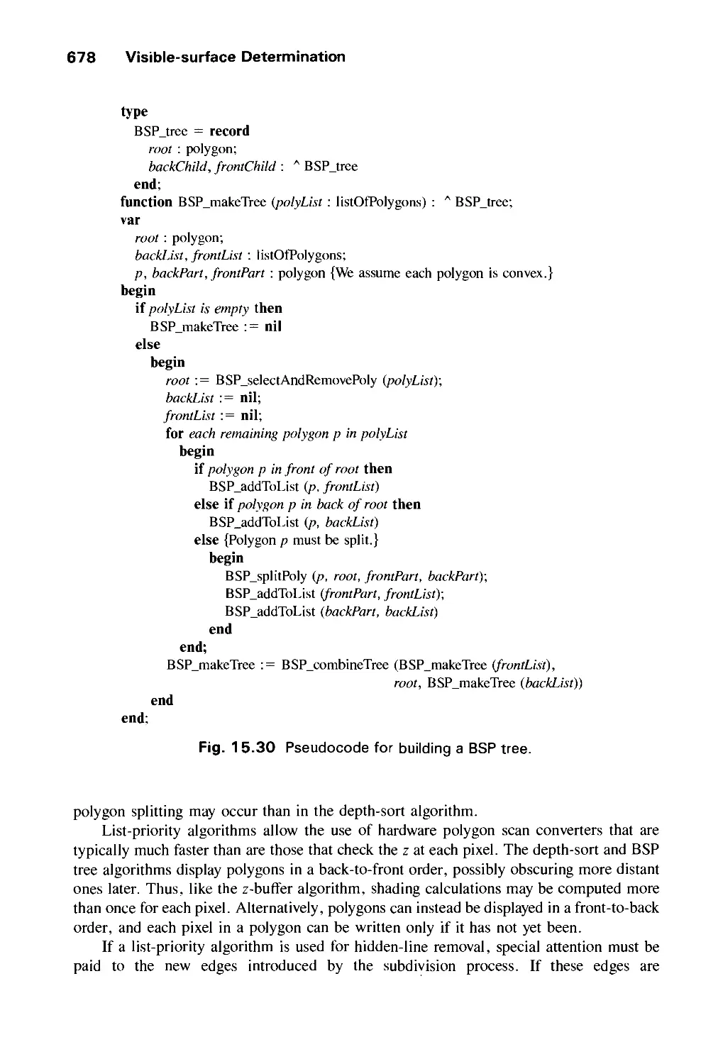
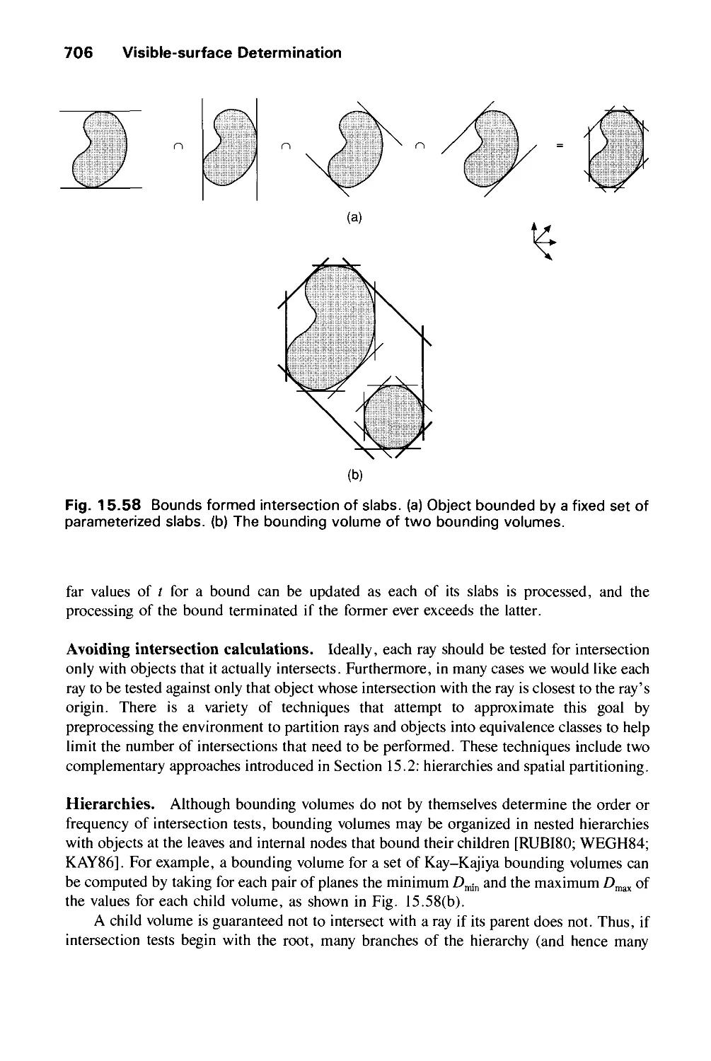
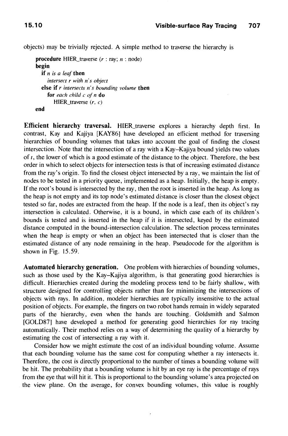
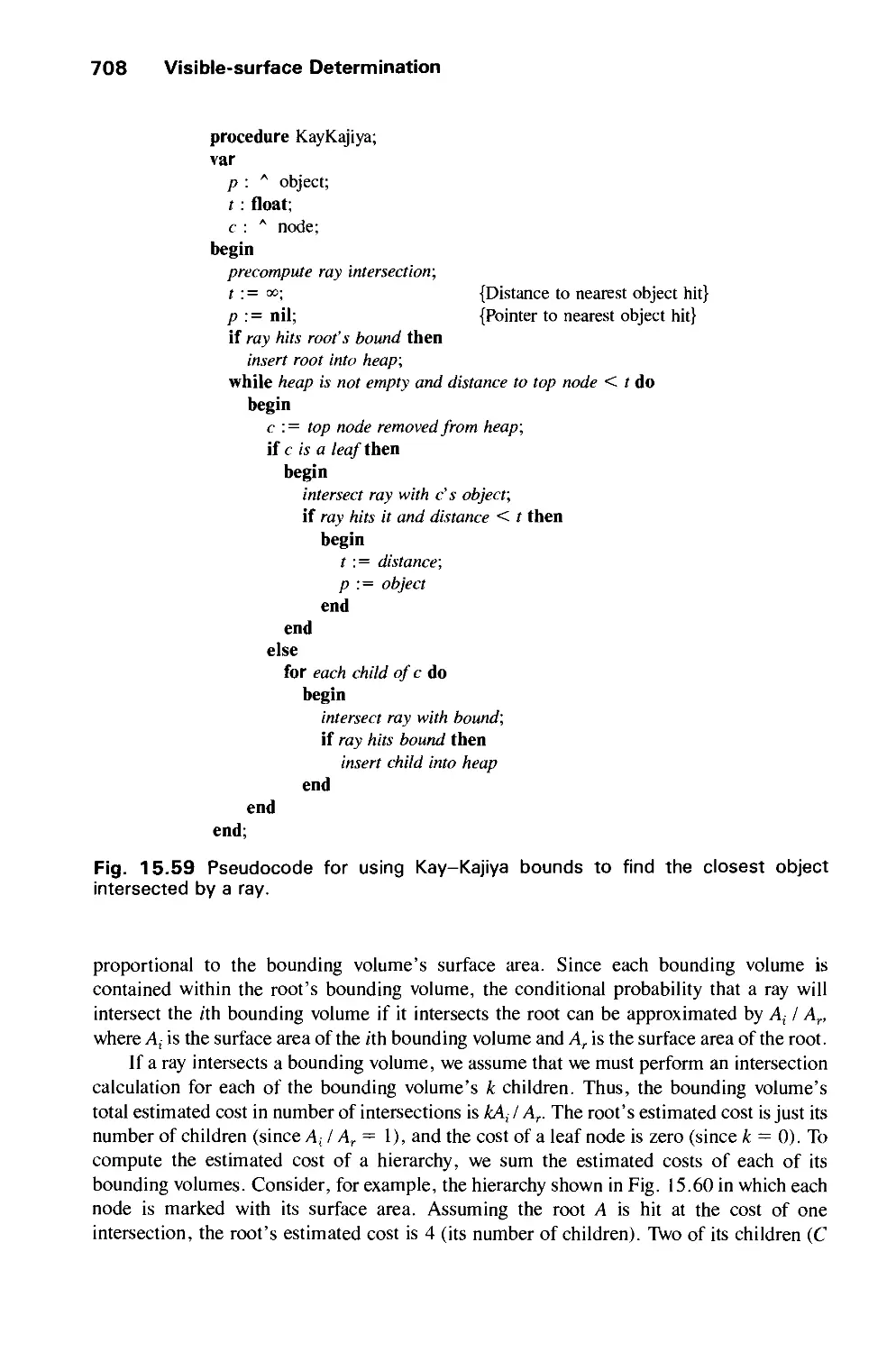
VISIBLE-SURFACE DETERMINATION 649
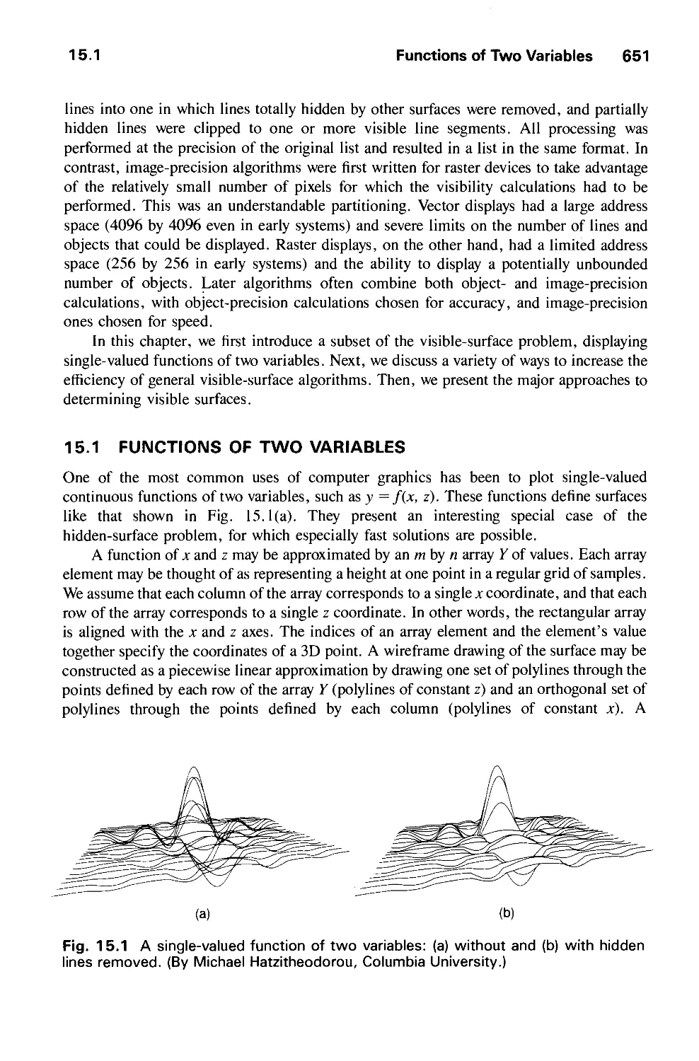
15.1 Functions of Two Variables 651
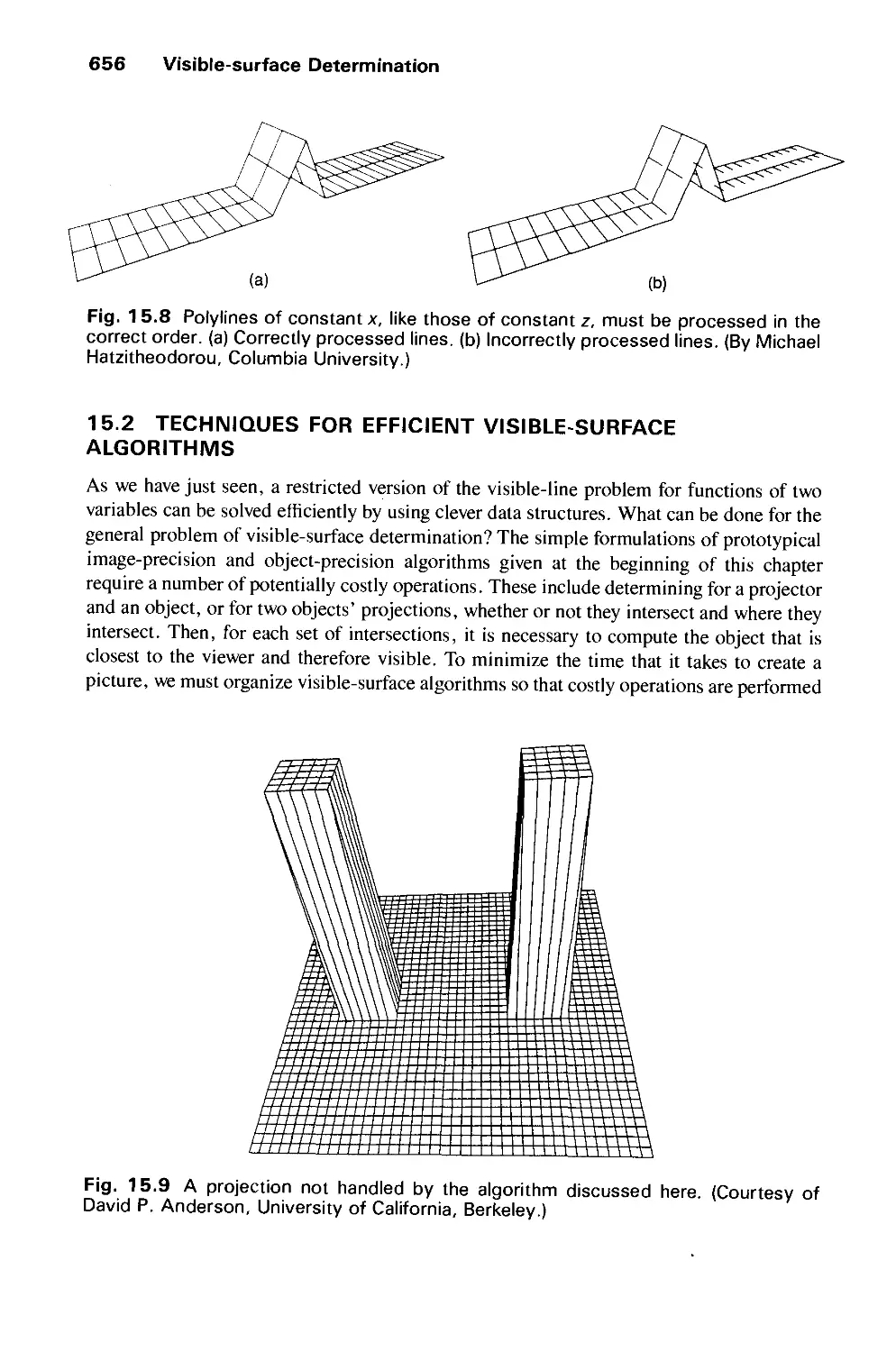
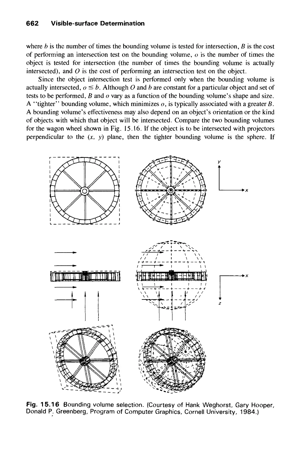
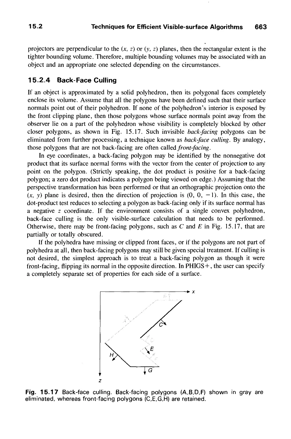
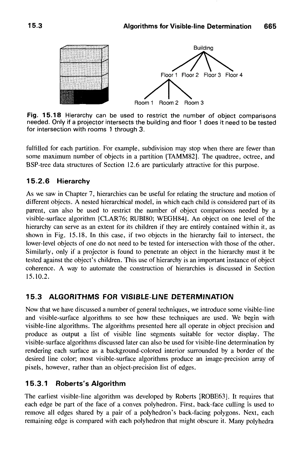
15.2 Techniques for Efficient Visible-Surface Algorithms 656
15.3 Algorithms for Visible-Line Determination 665
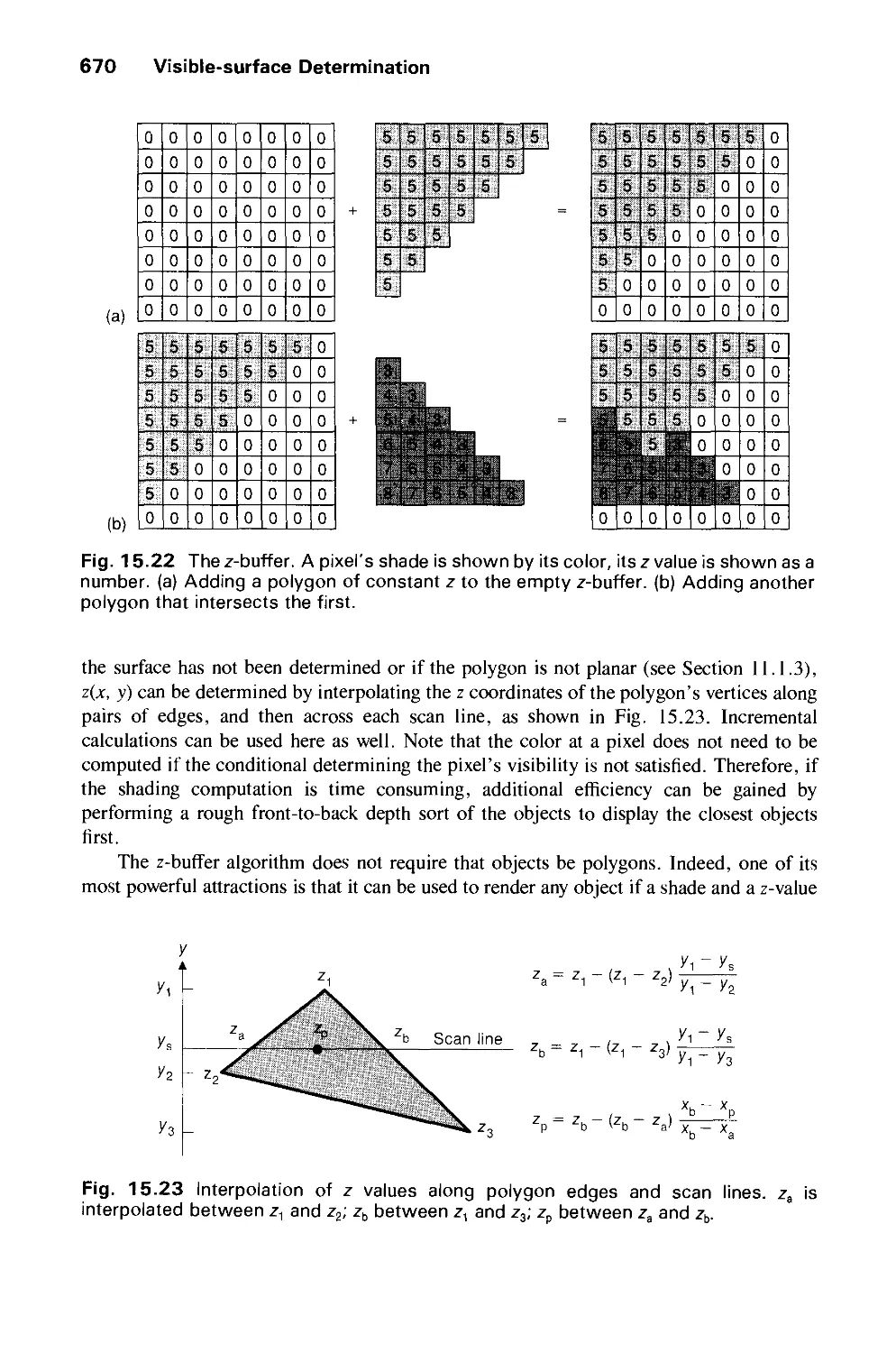
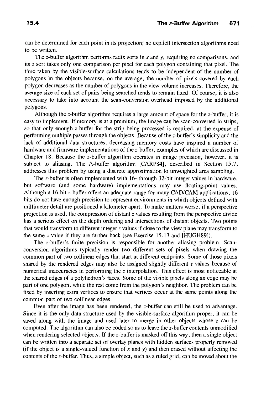
15.4 The z-Buffer Algorithm 668
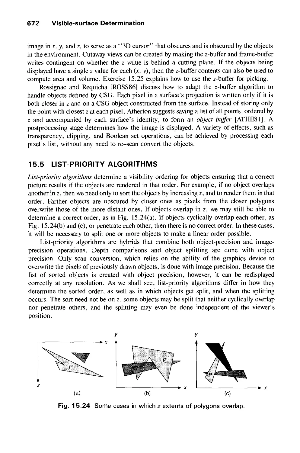
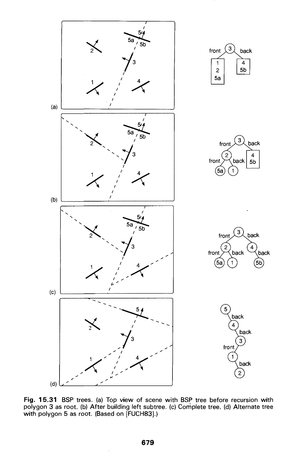
15.5 List-Priority Algorithms 672
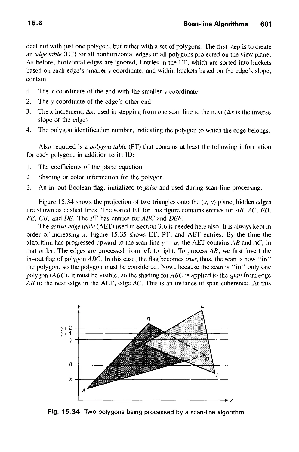
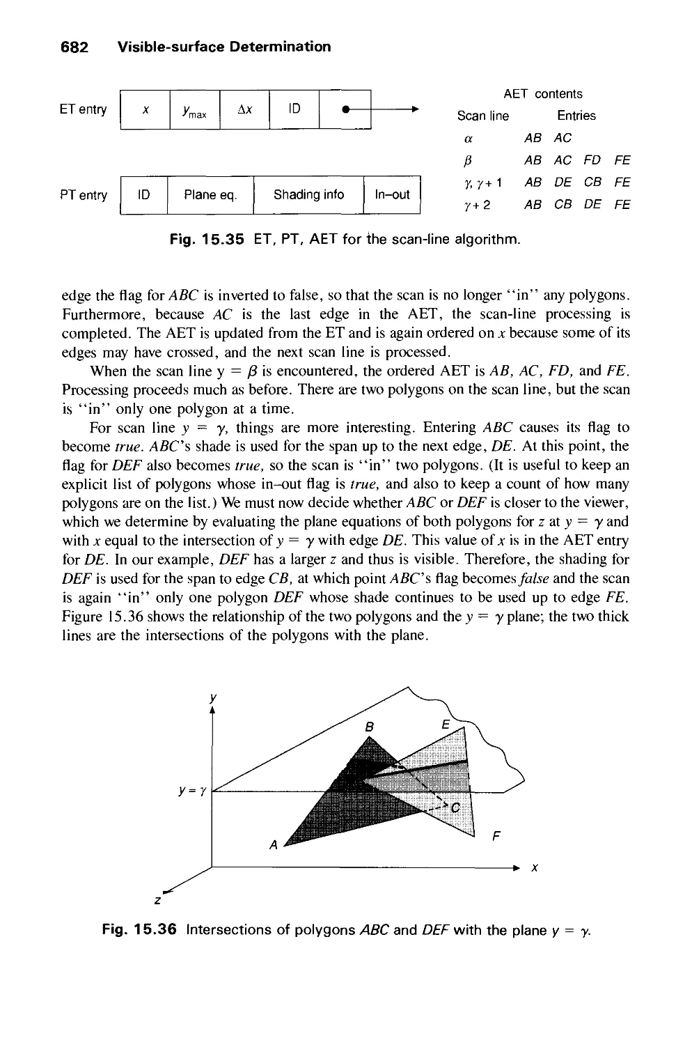
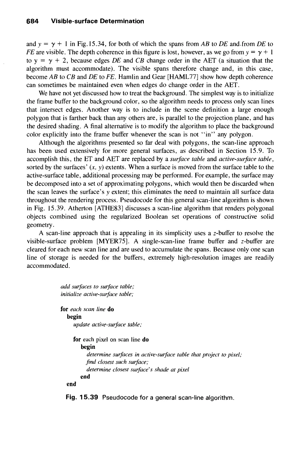
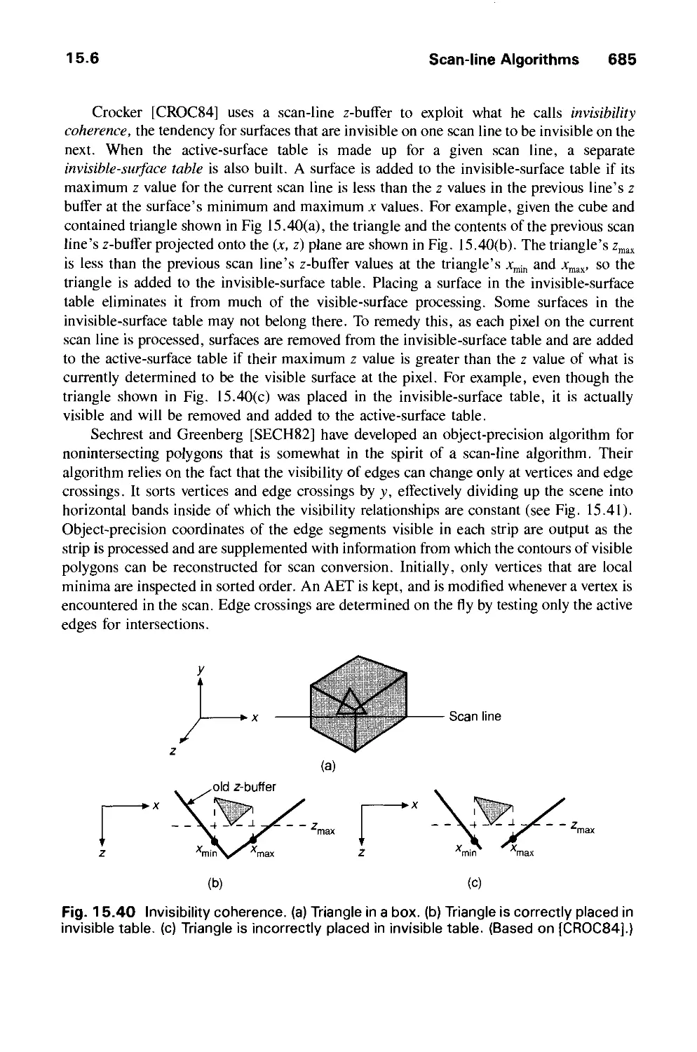
15.6 Scan-Line Algorithms 680
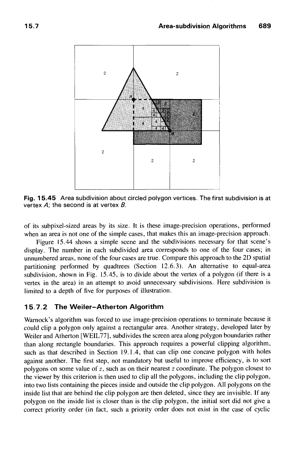
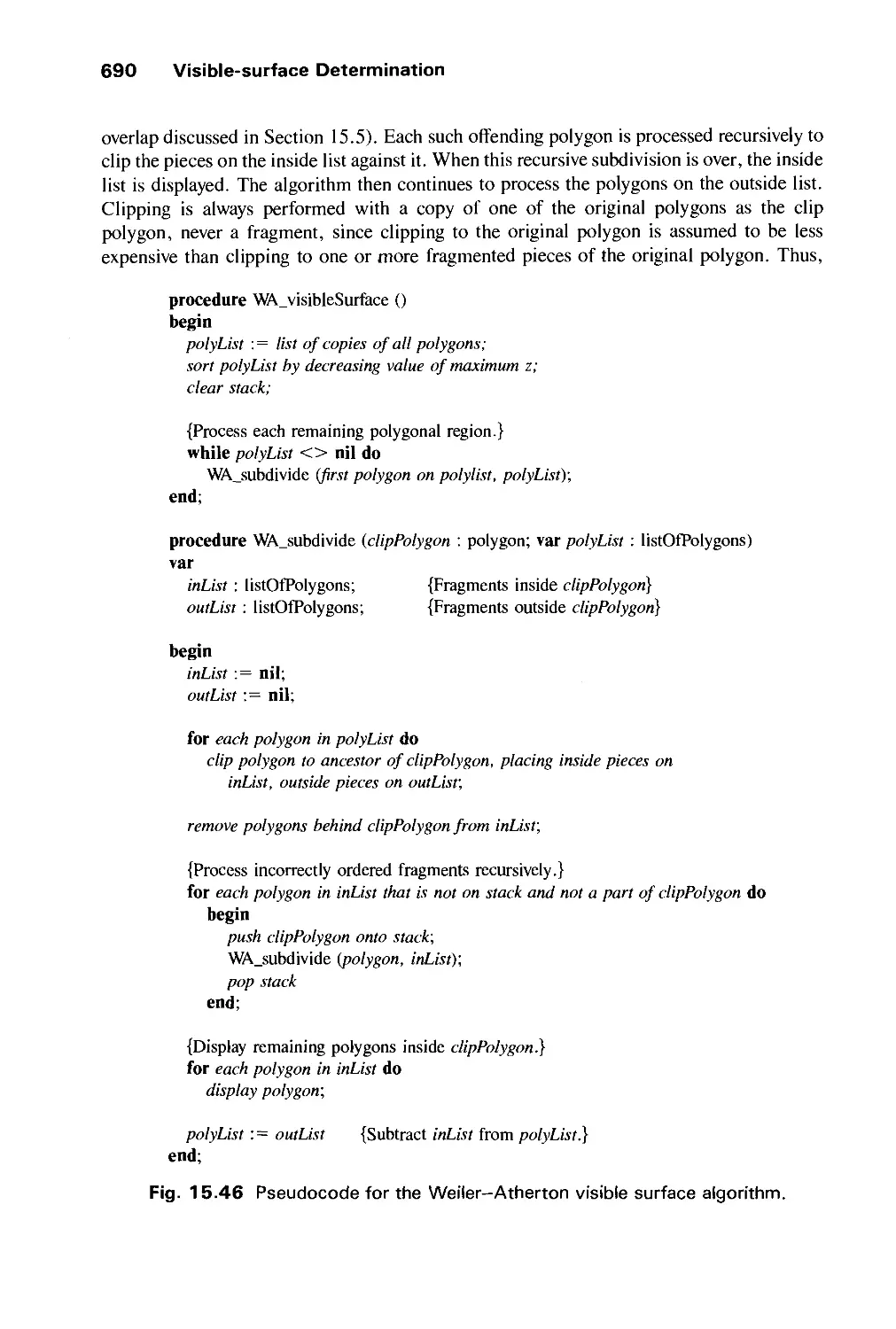
15.7 Area-Subdivision Algorithms 686
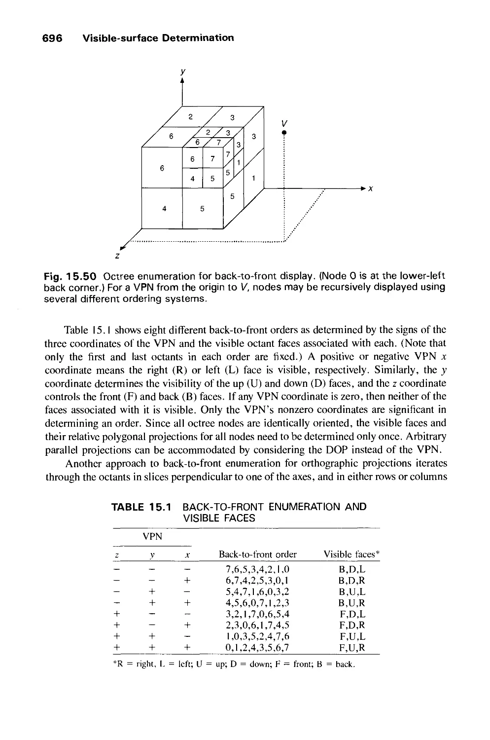
15.8 Algorithms for Octrees 695
15.9 Algorithms for Curved Surfaces 698
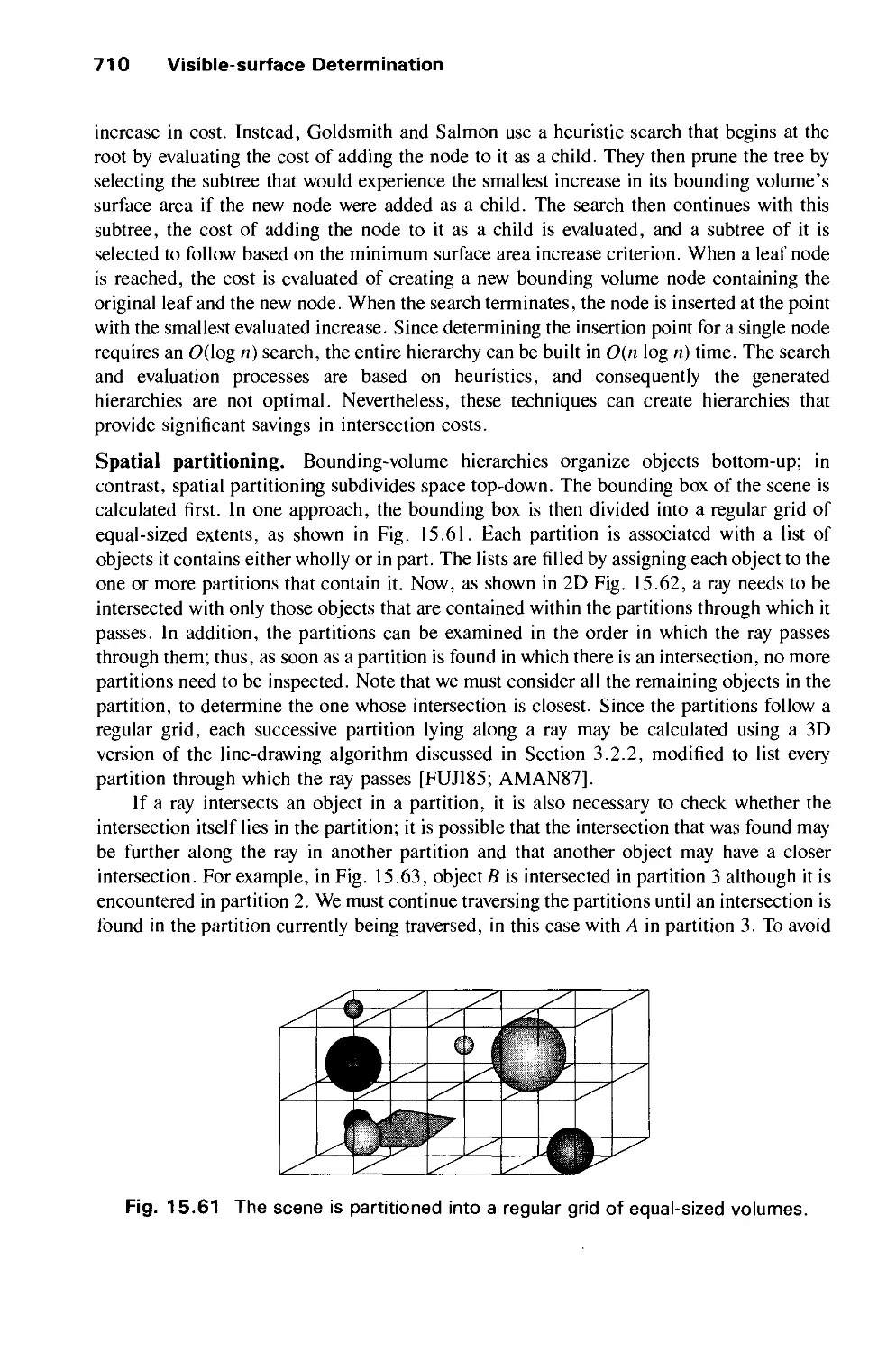
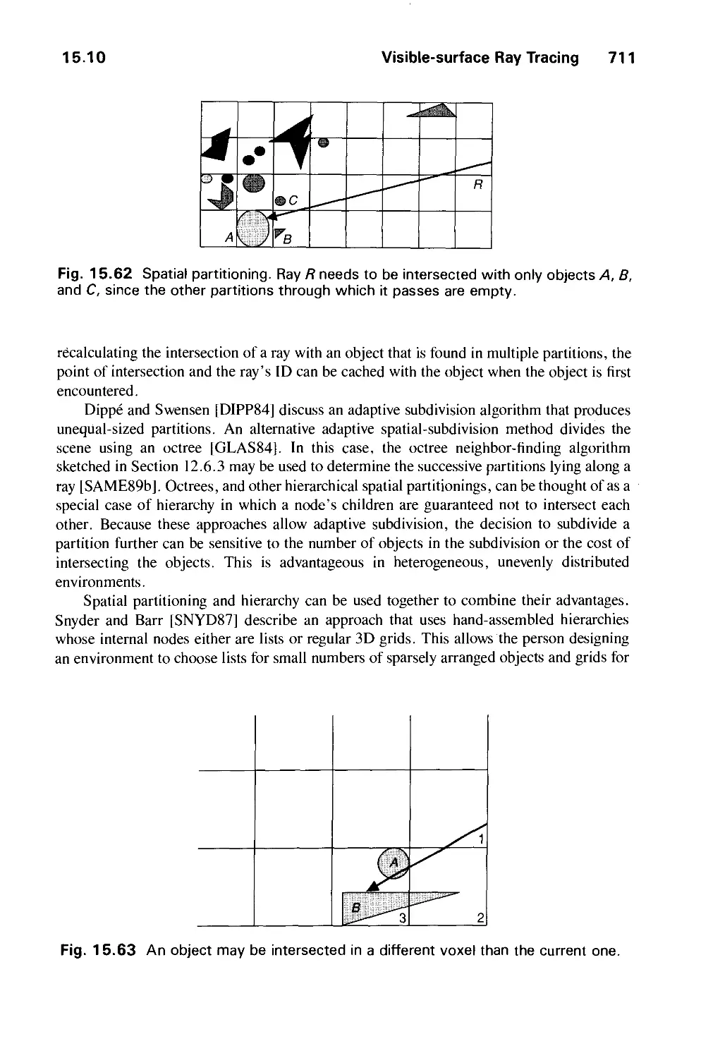
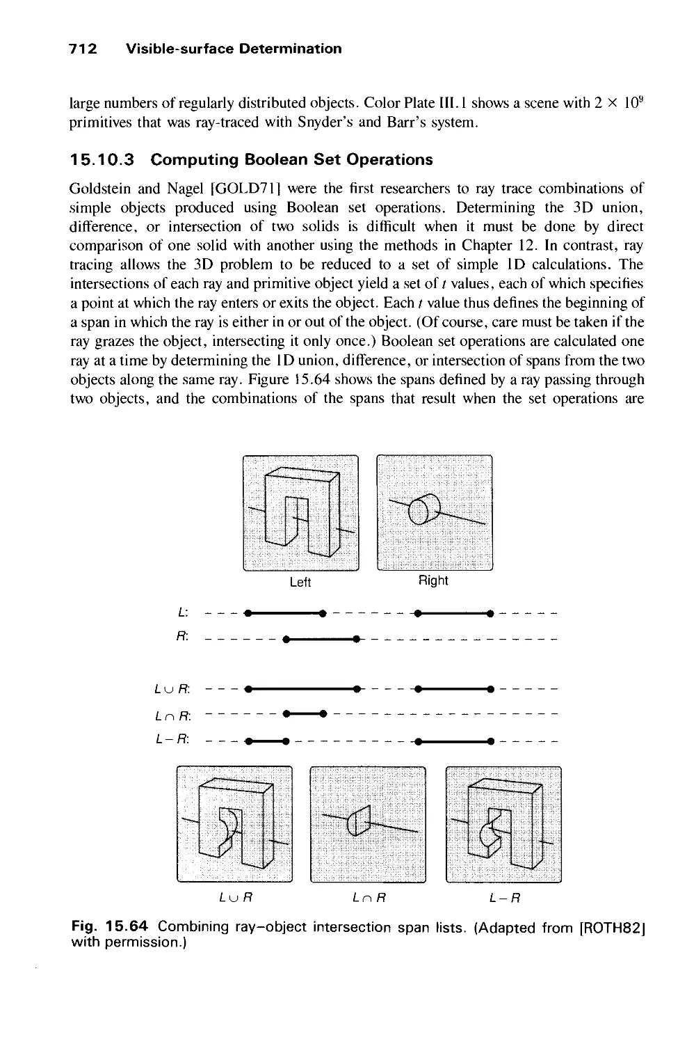
15.10 Visible-Surface Ray Tracing 701
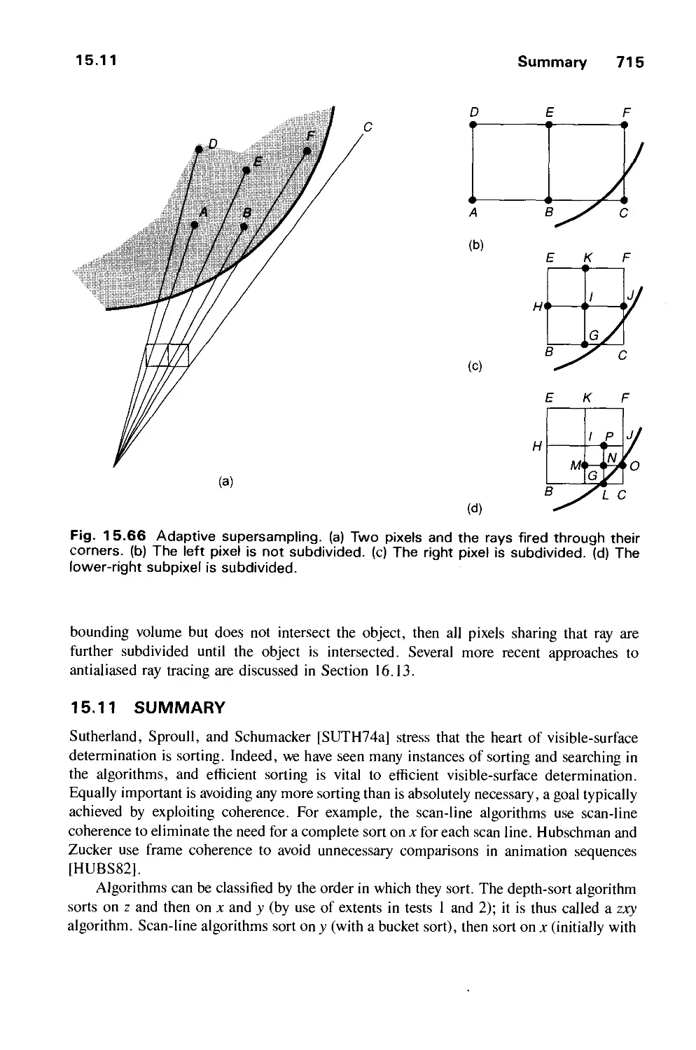
15.11 Summary 715
Exercises 718
CHAPTER 16
ILLUMINATION AND SHADING 721
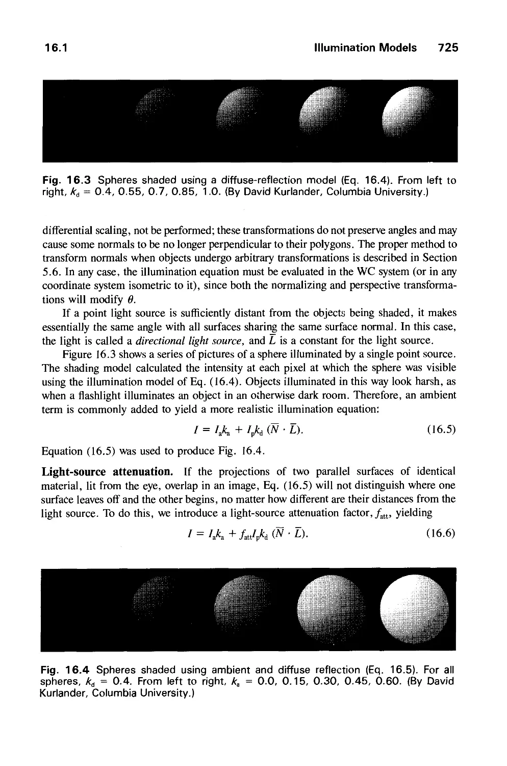
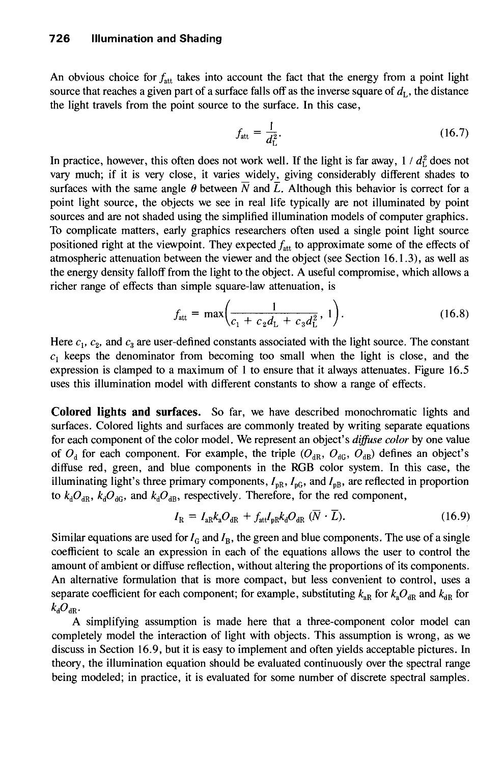
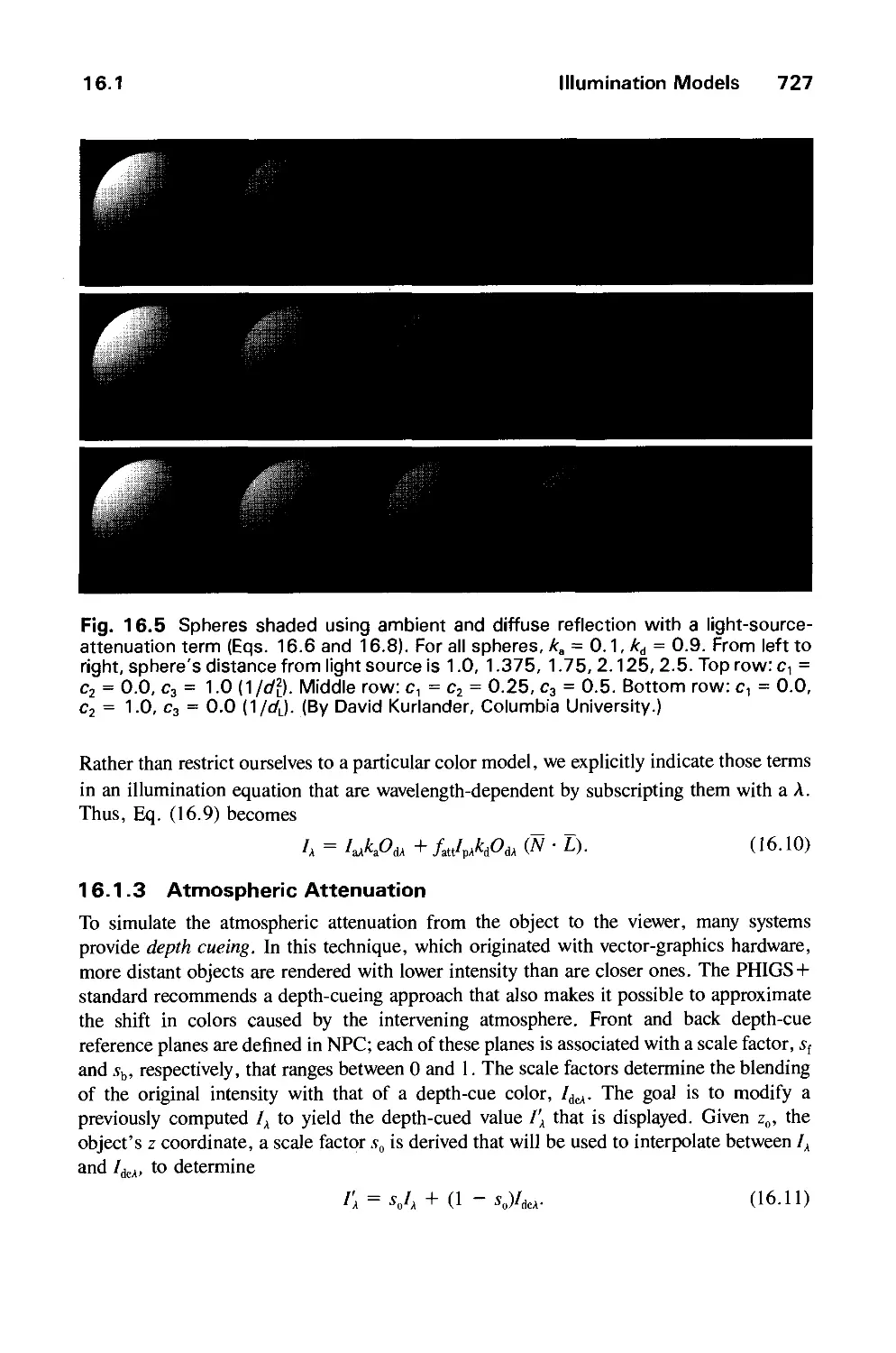
16.1 Illumination Models 722
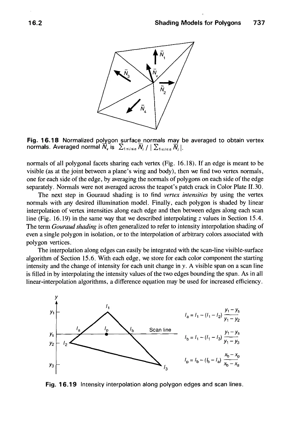
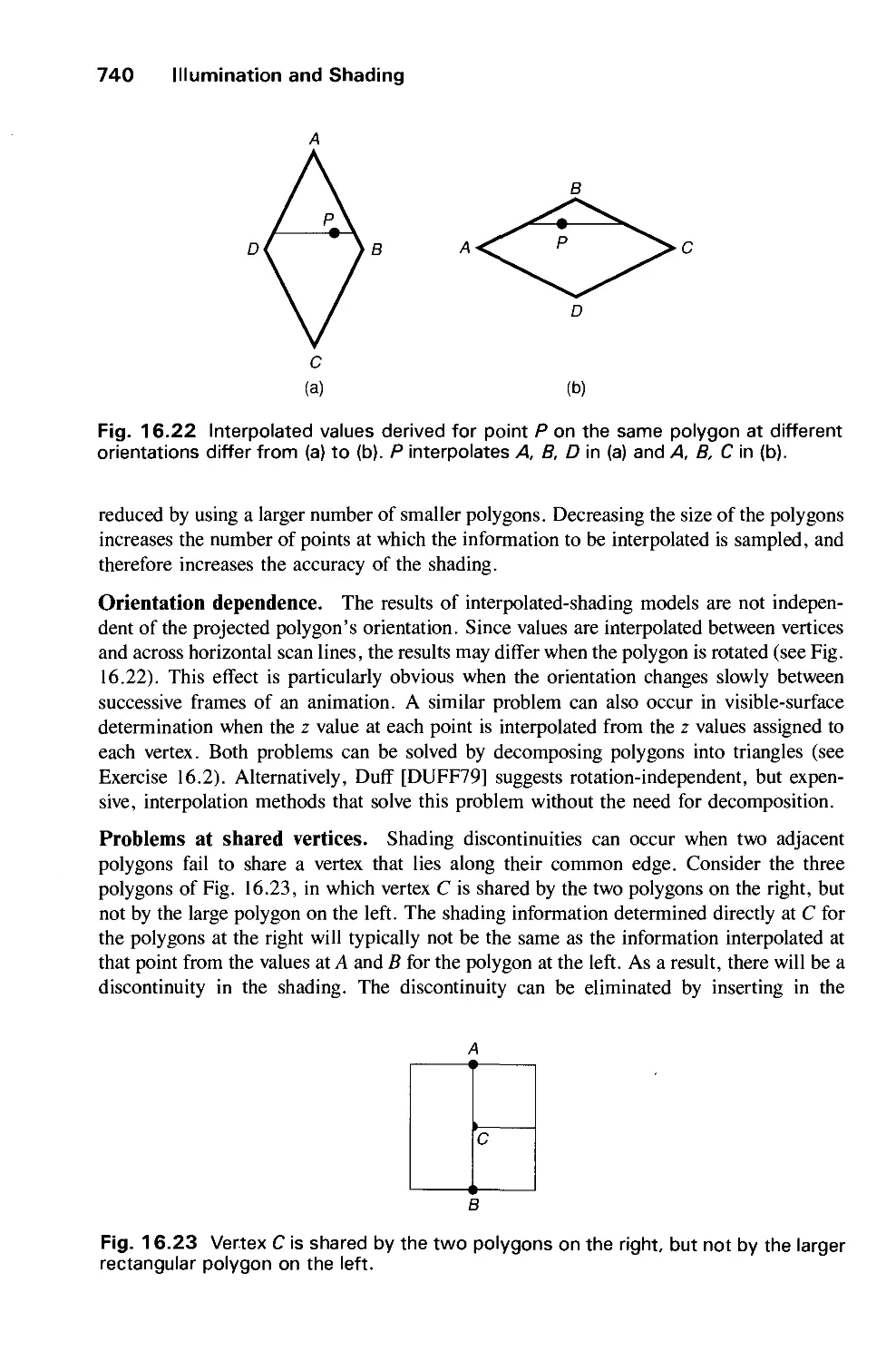
16.2 Shading Models for Polygons 734
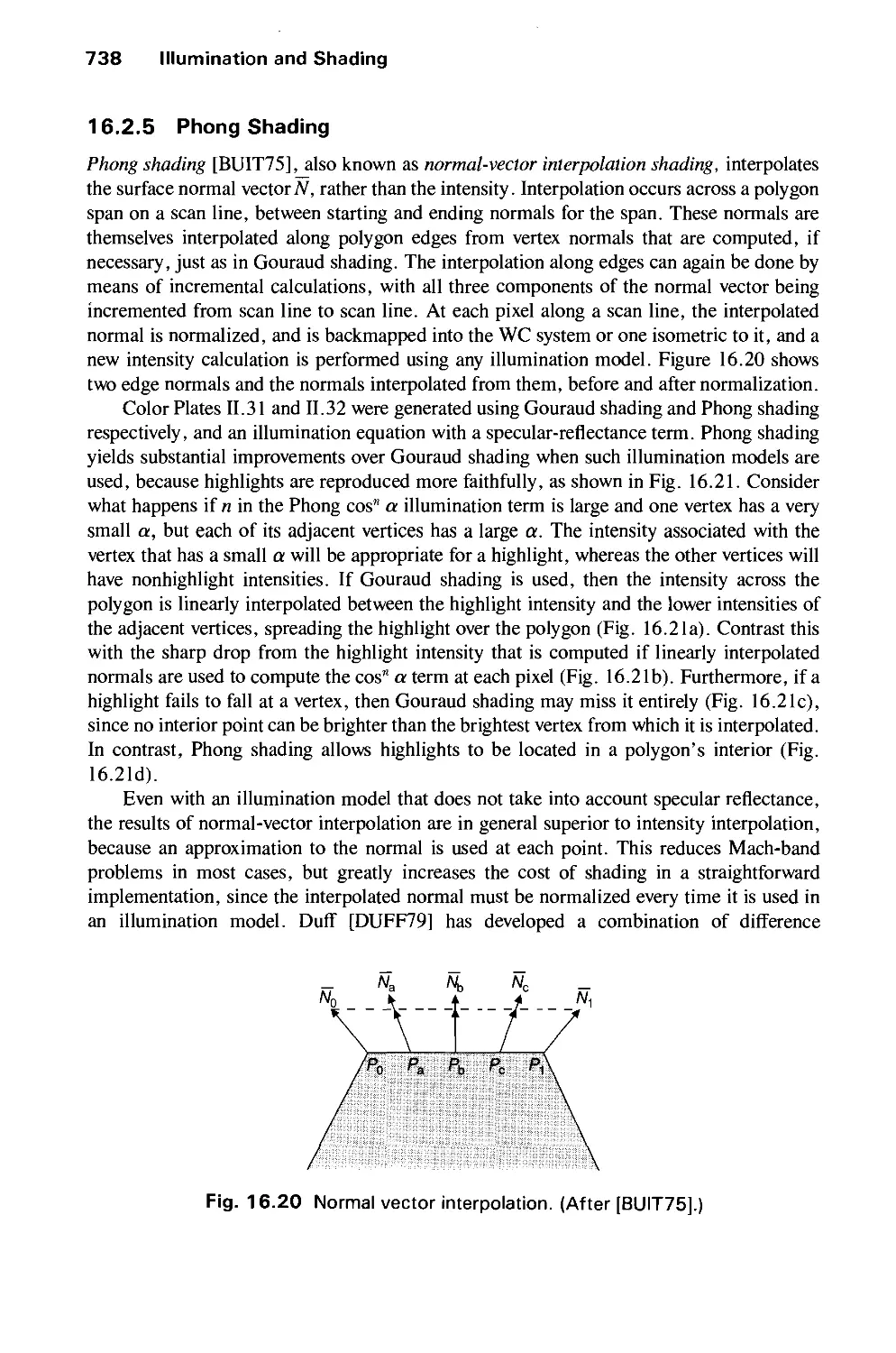
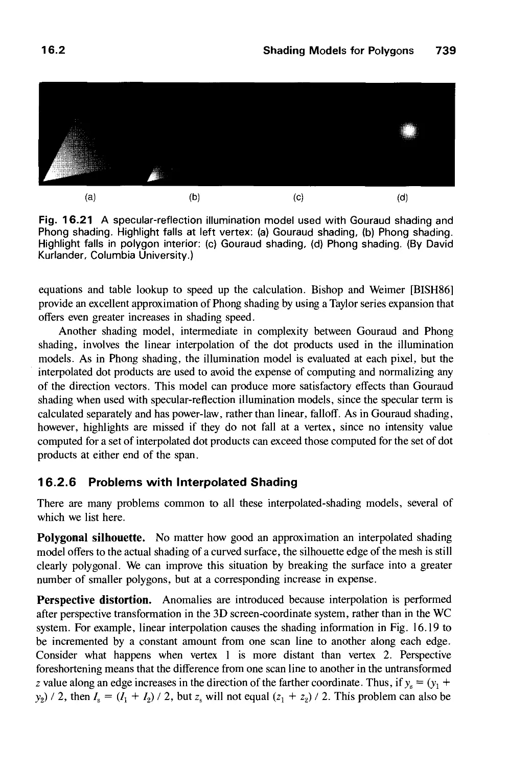
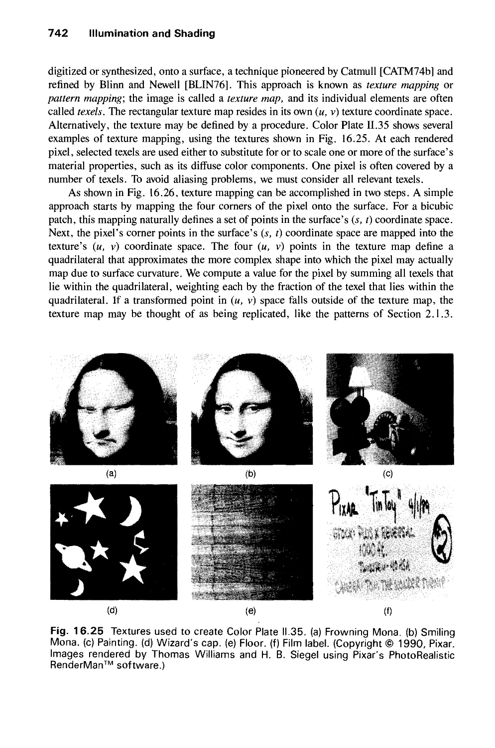
16.3 Surface Detail 741
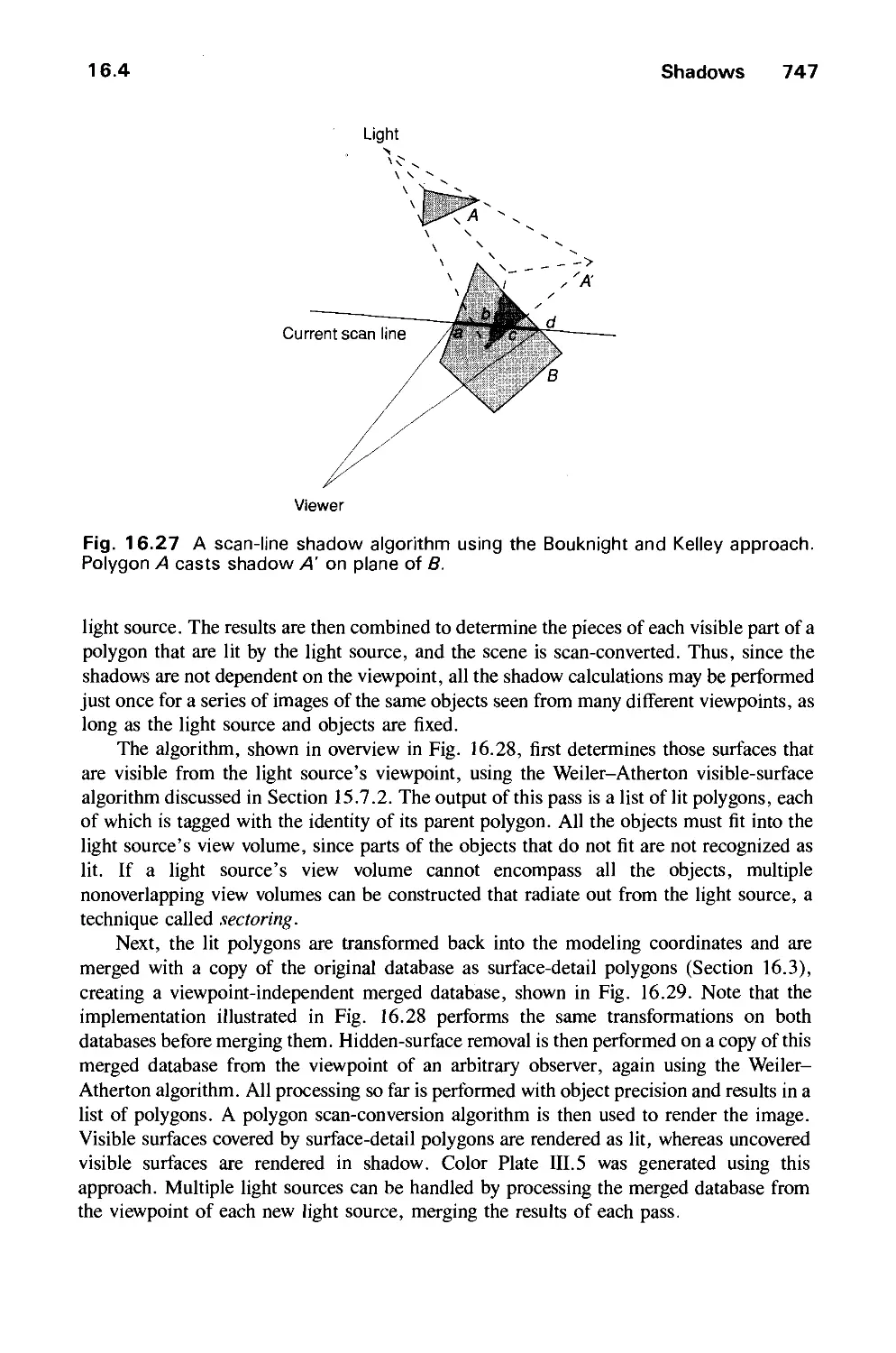
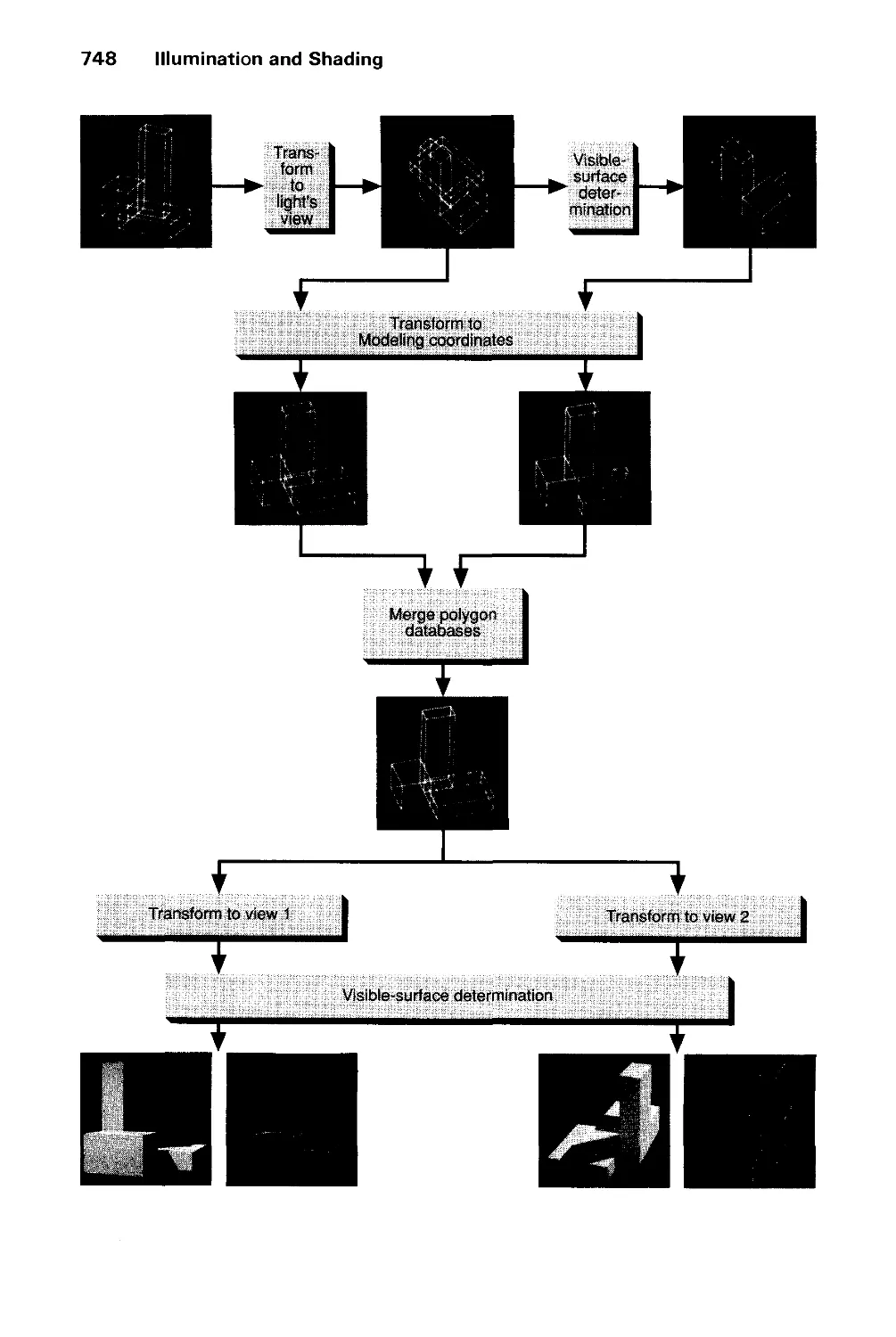
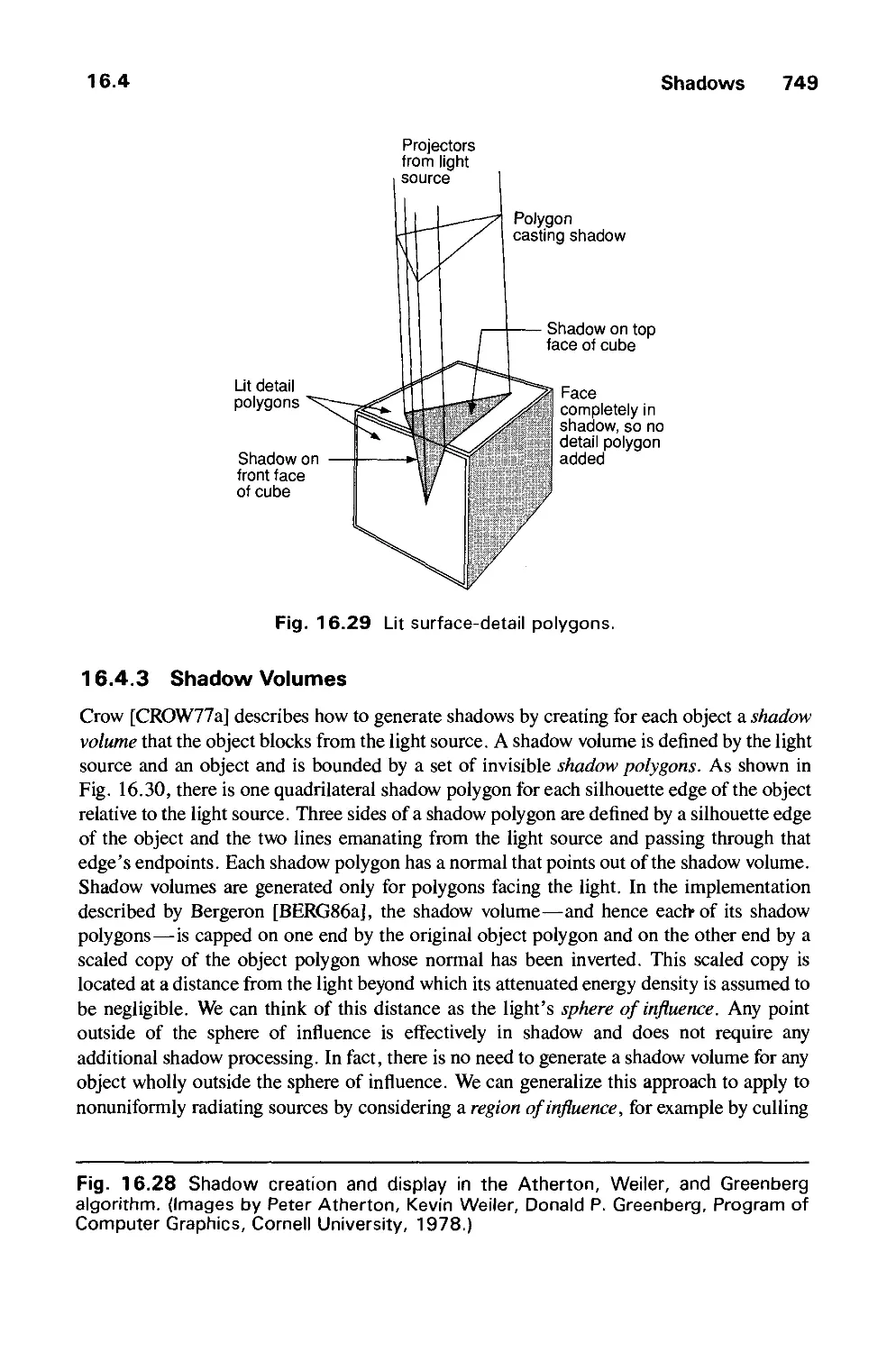
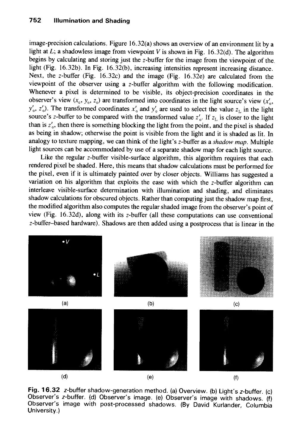
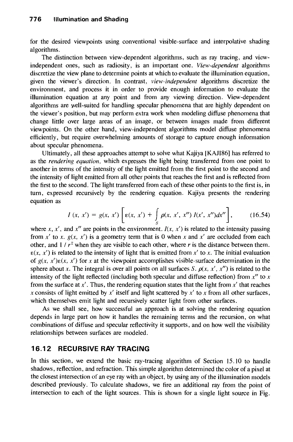
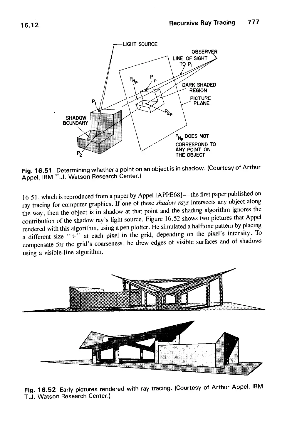
16.4 Shadows 745
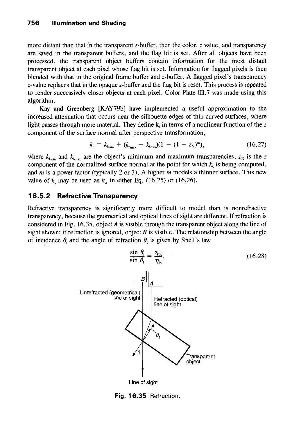
16.5 Transparency 754
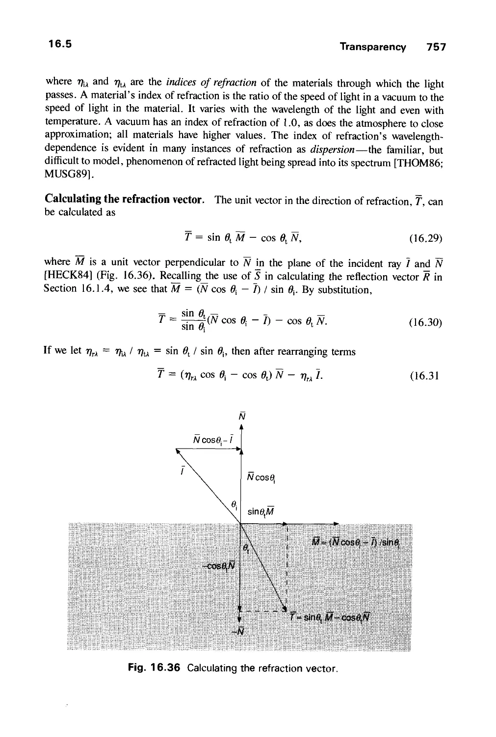
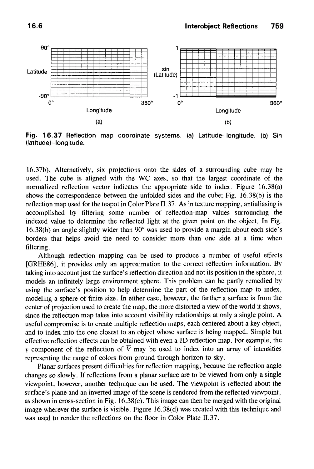
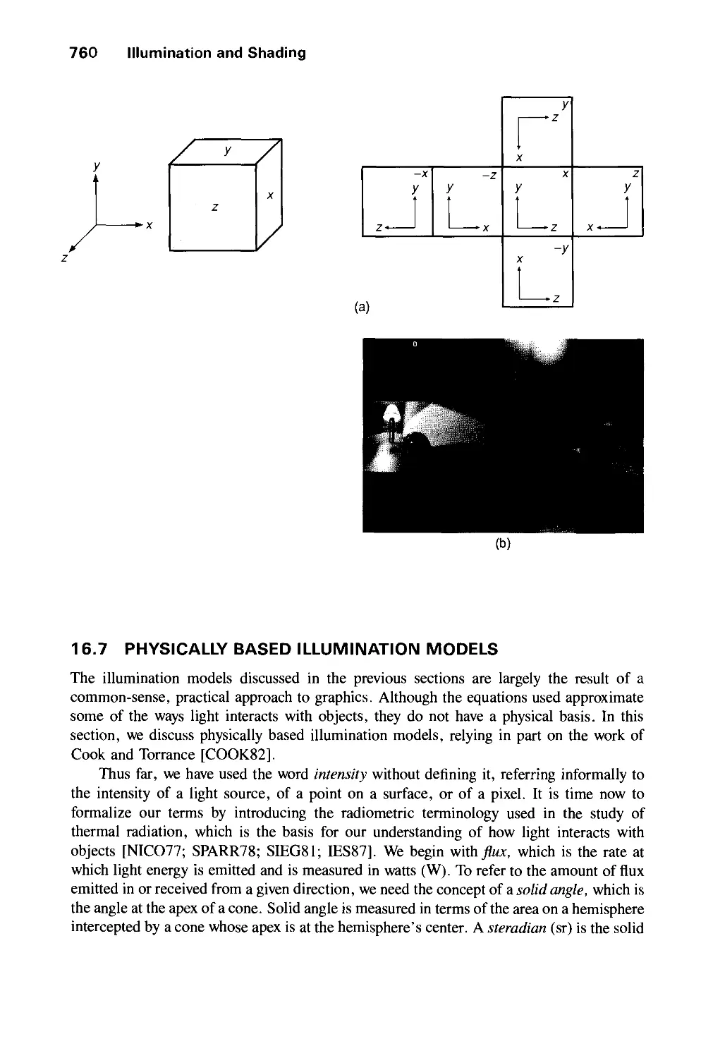
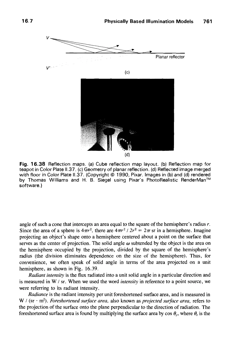
16.6 Interobject Reflections 758
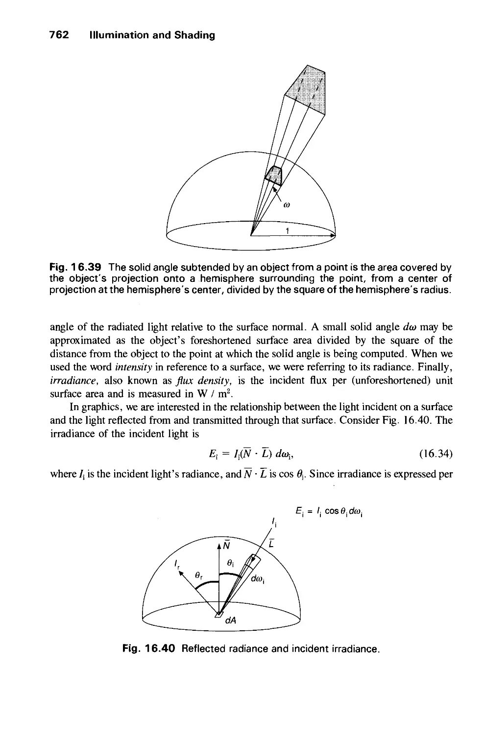
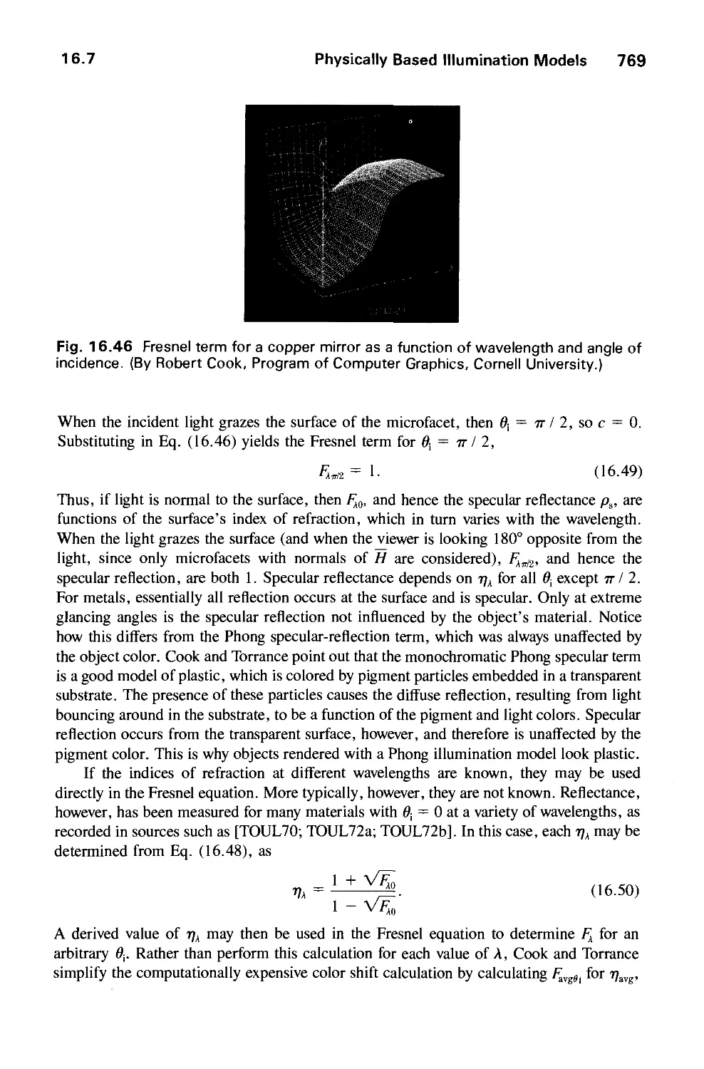
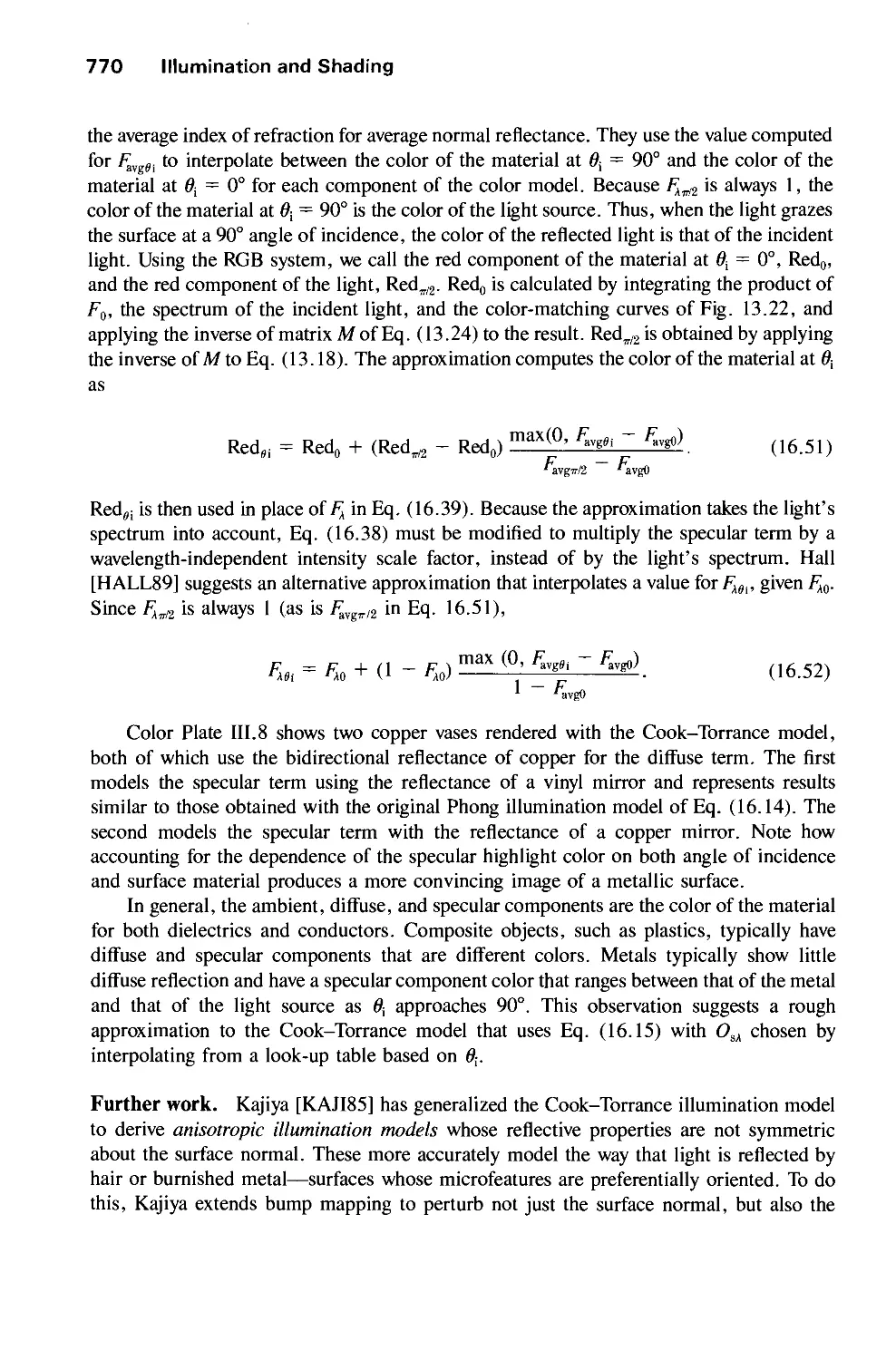
16.7 Physically Based Illumination Models 760
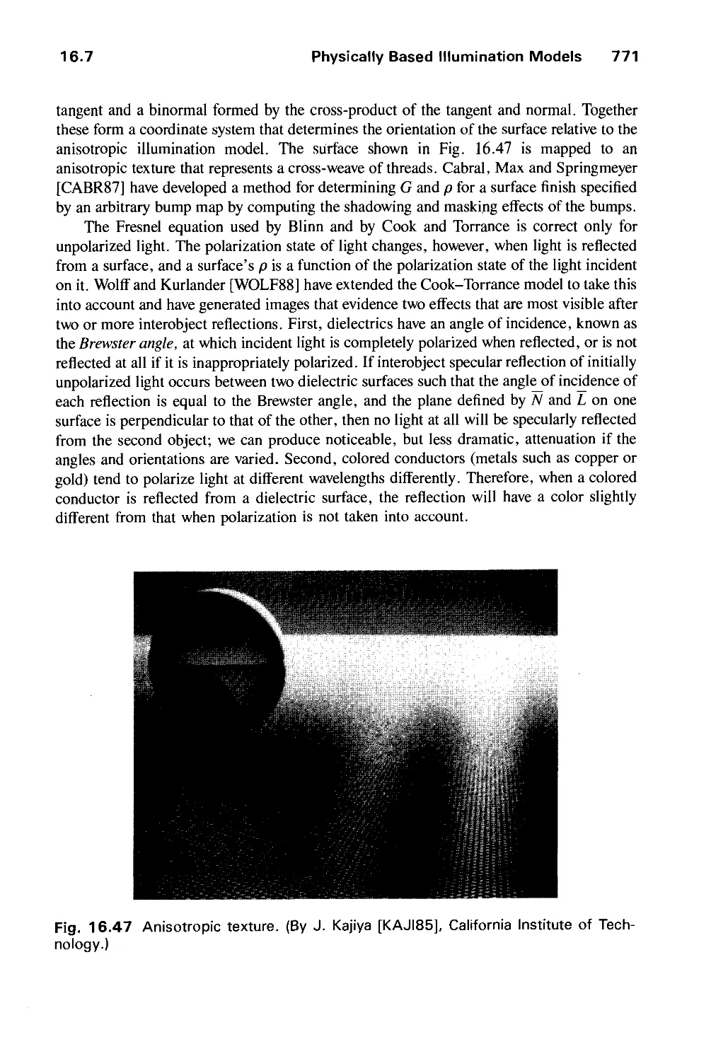
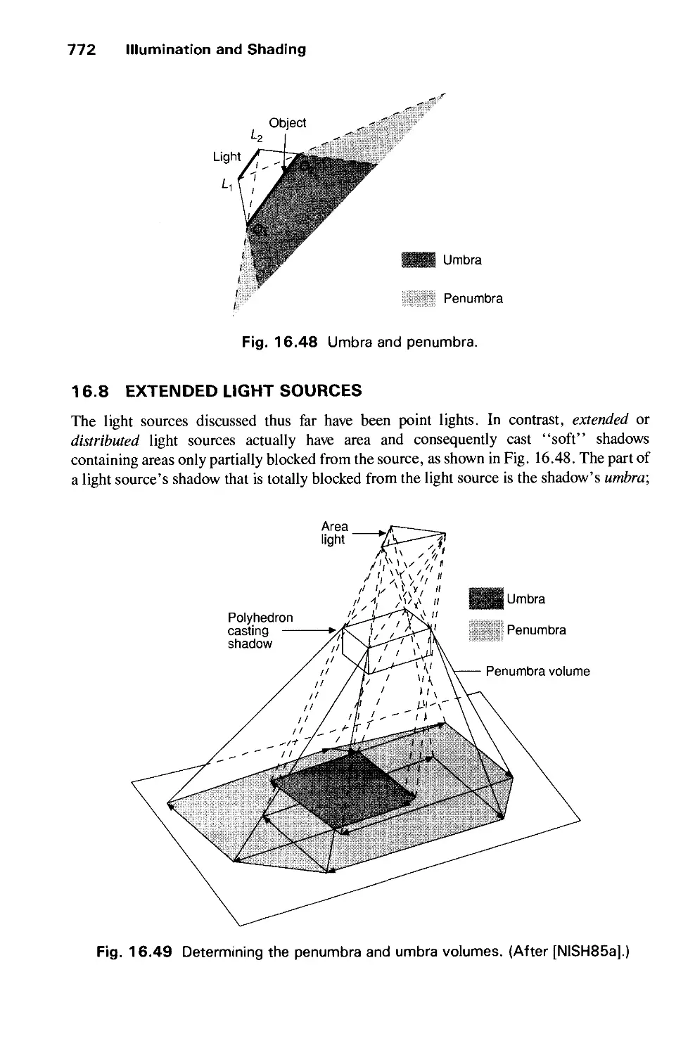
16.8 Extended Light Sources 772
16.9 Spectral Sampling 773
16.10 Improving the Camera Model 774
16.11 Global Illumination Algorithms 775
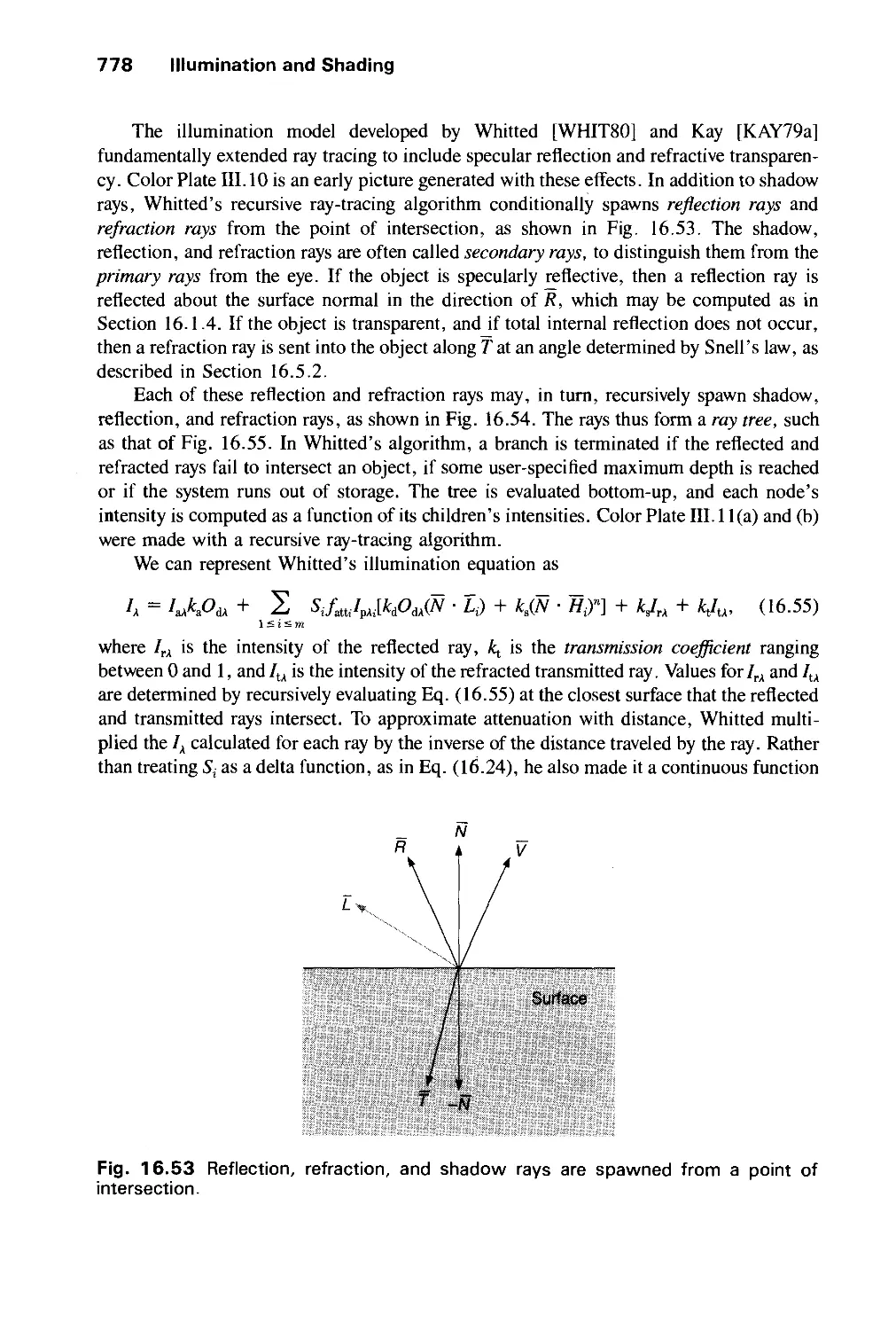
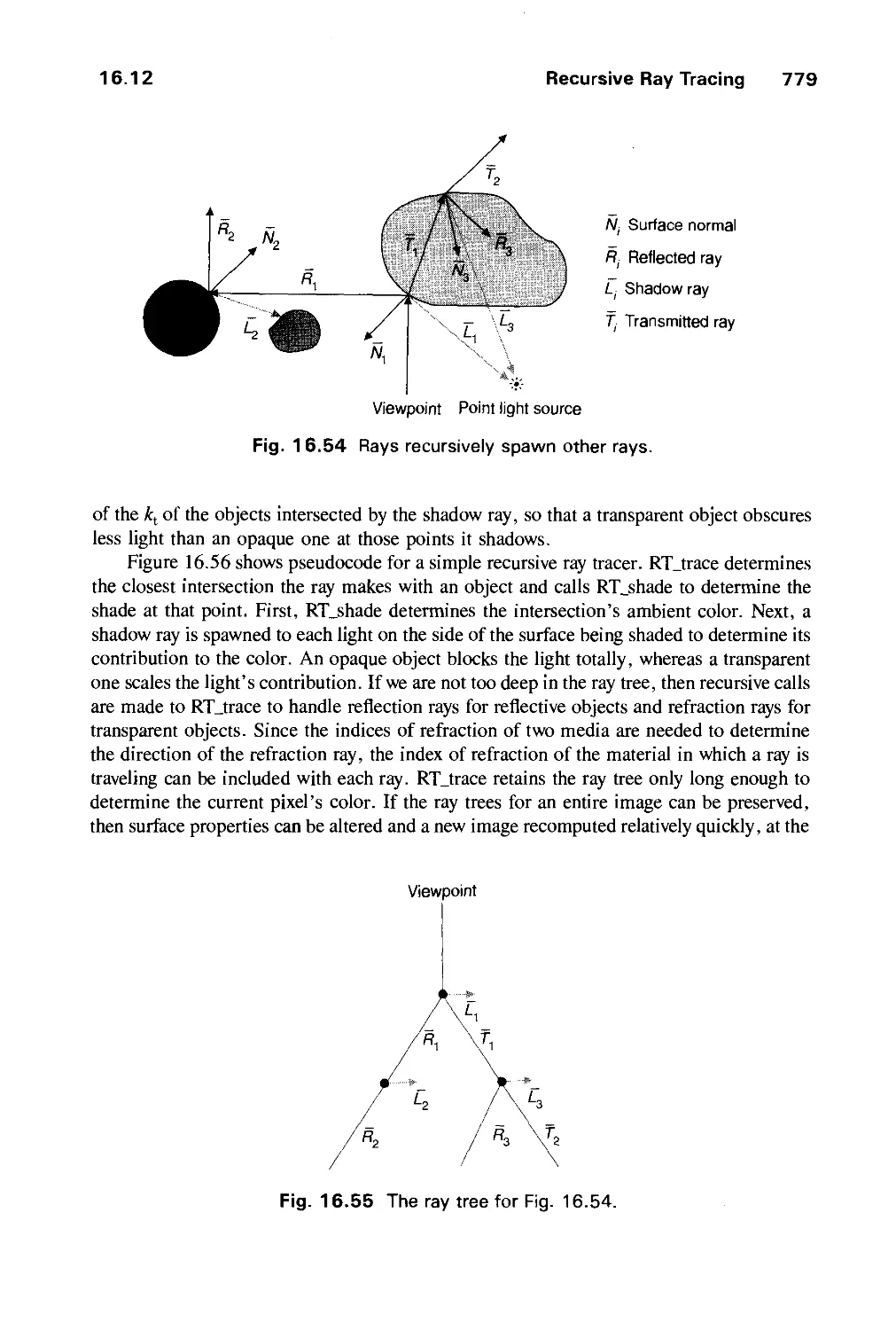
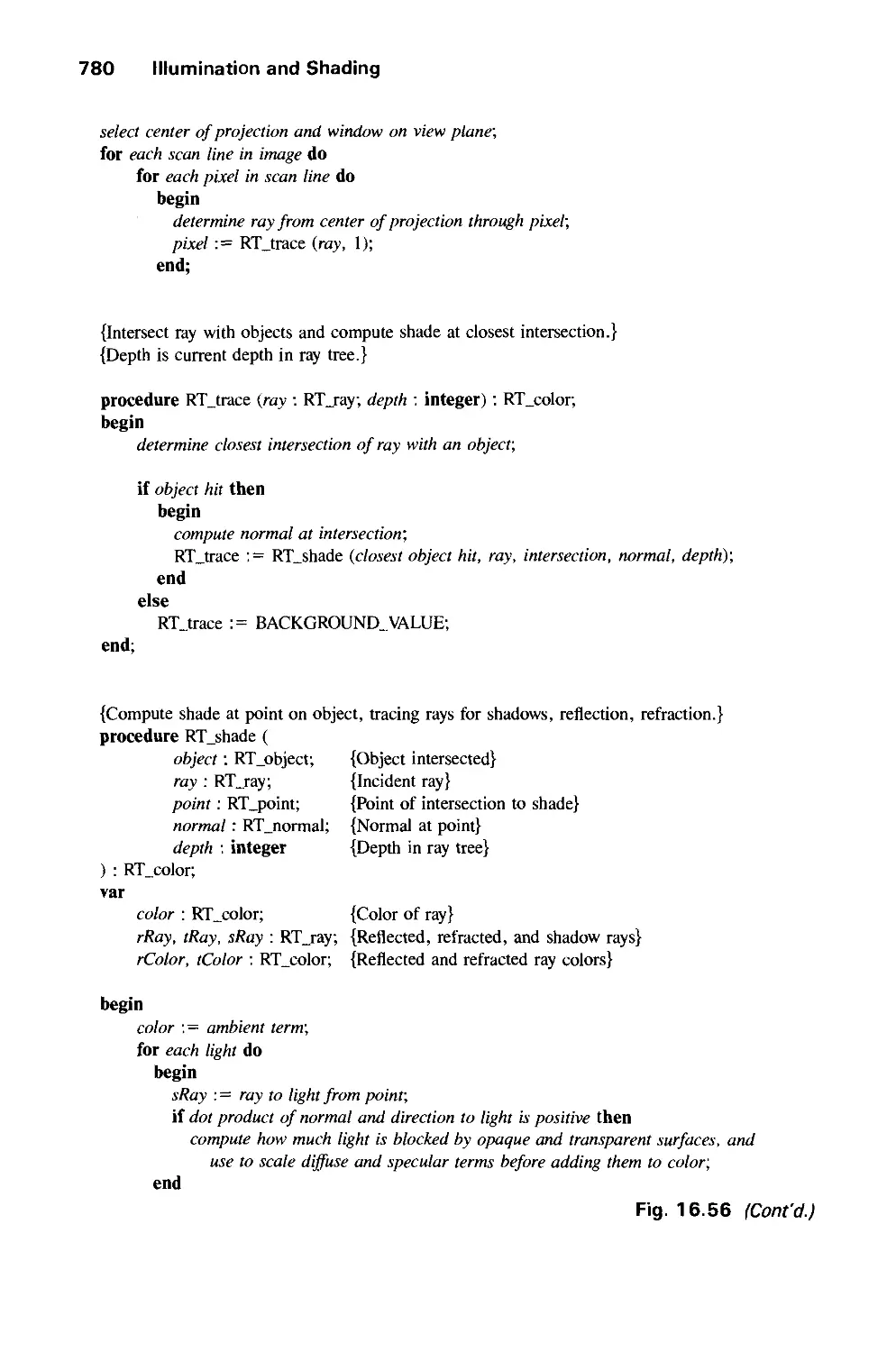
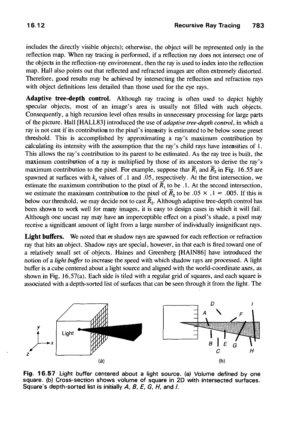
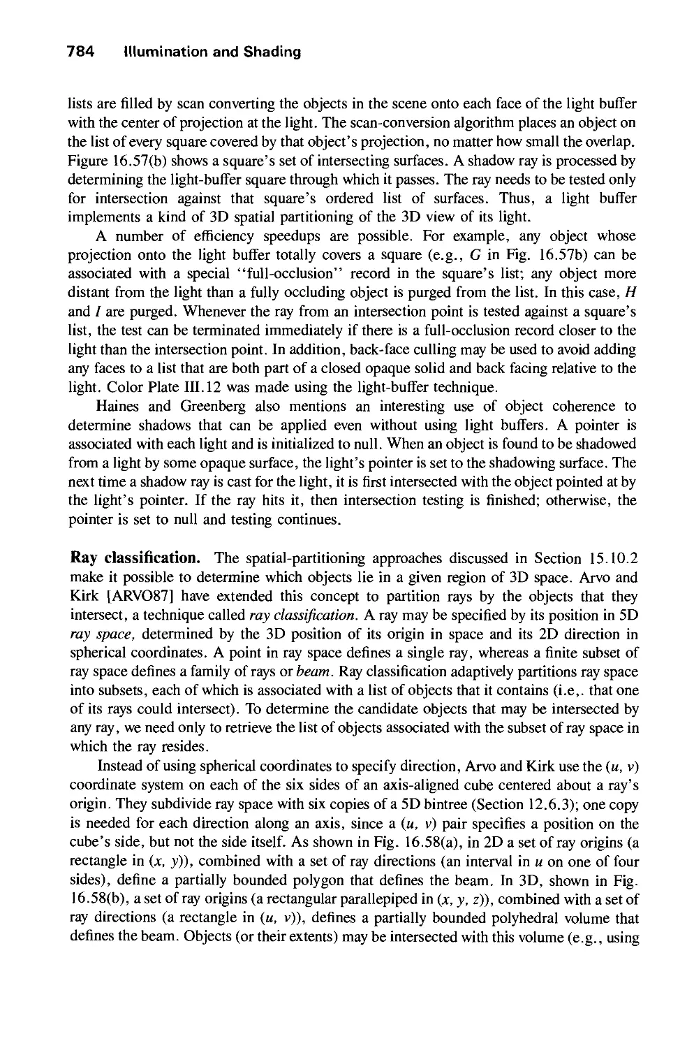
16.12 Recursive Ray Tracing 776
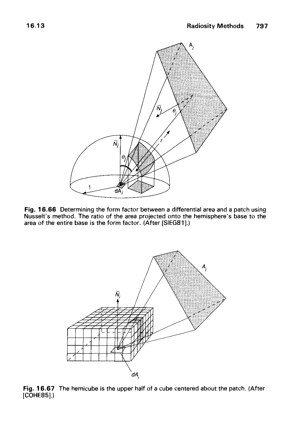
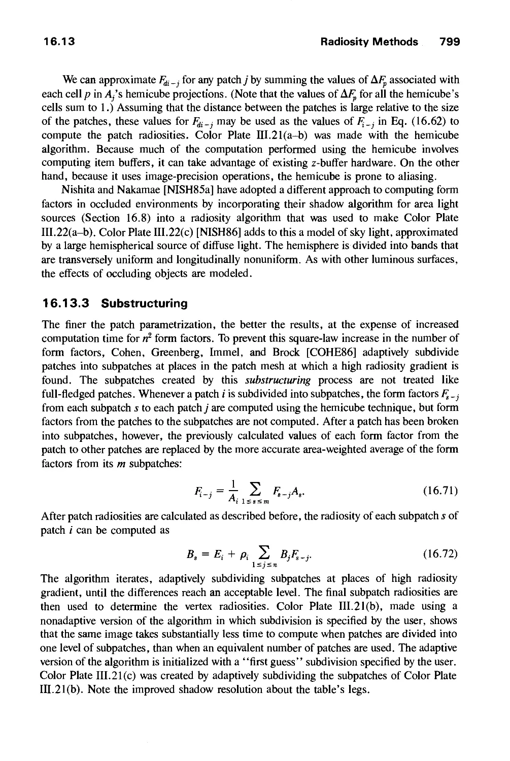
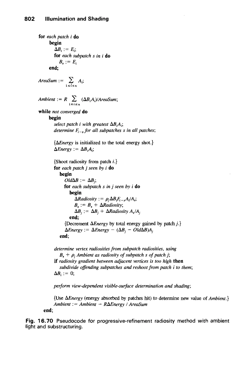
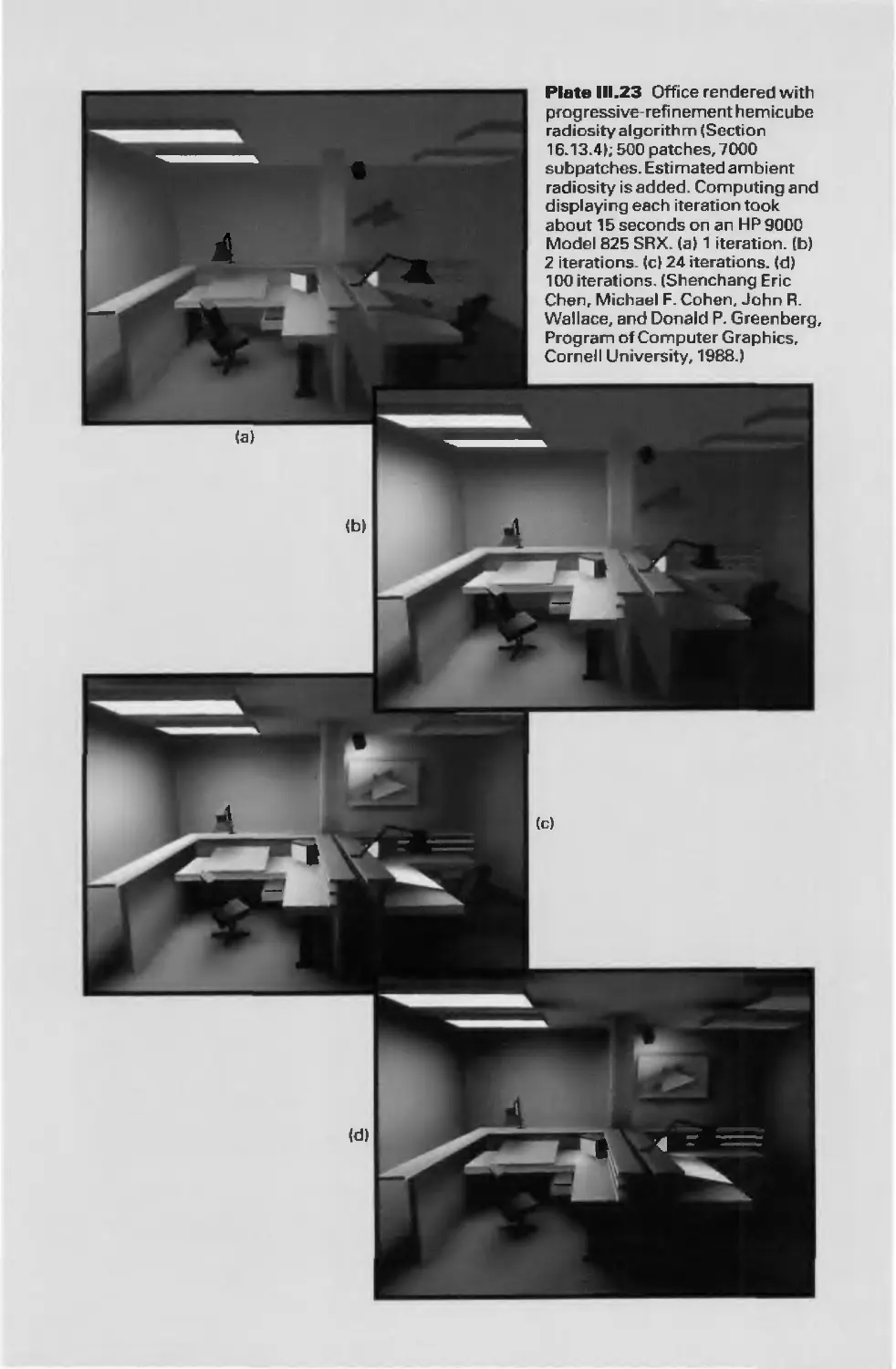
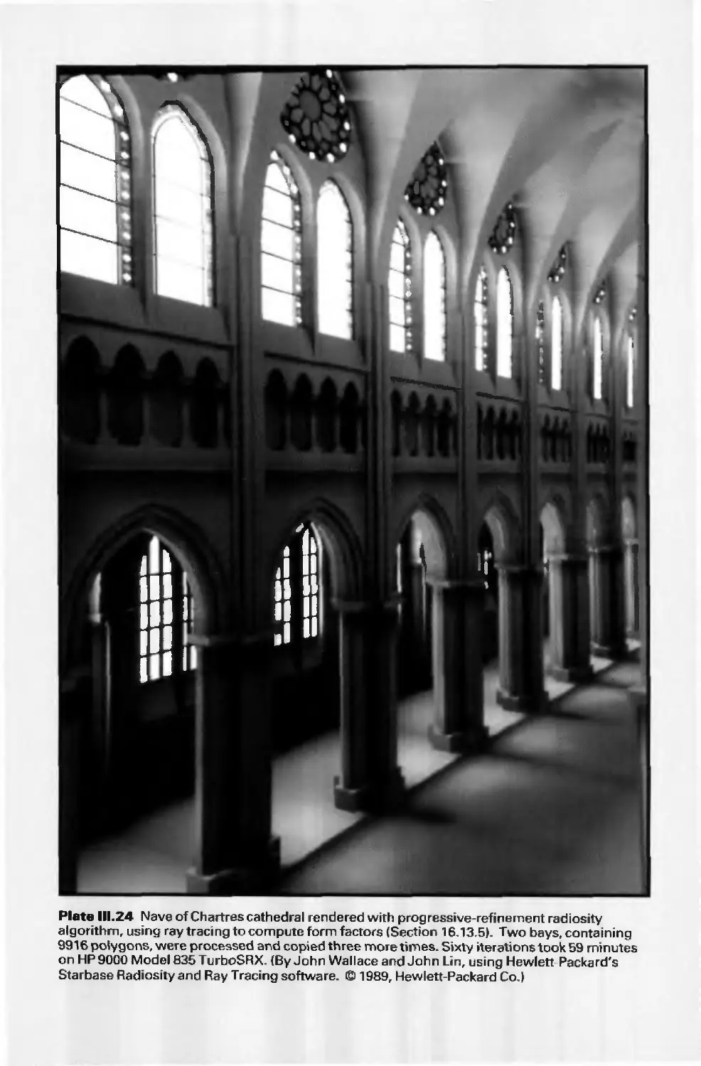
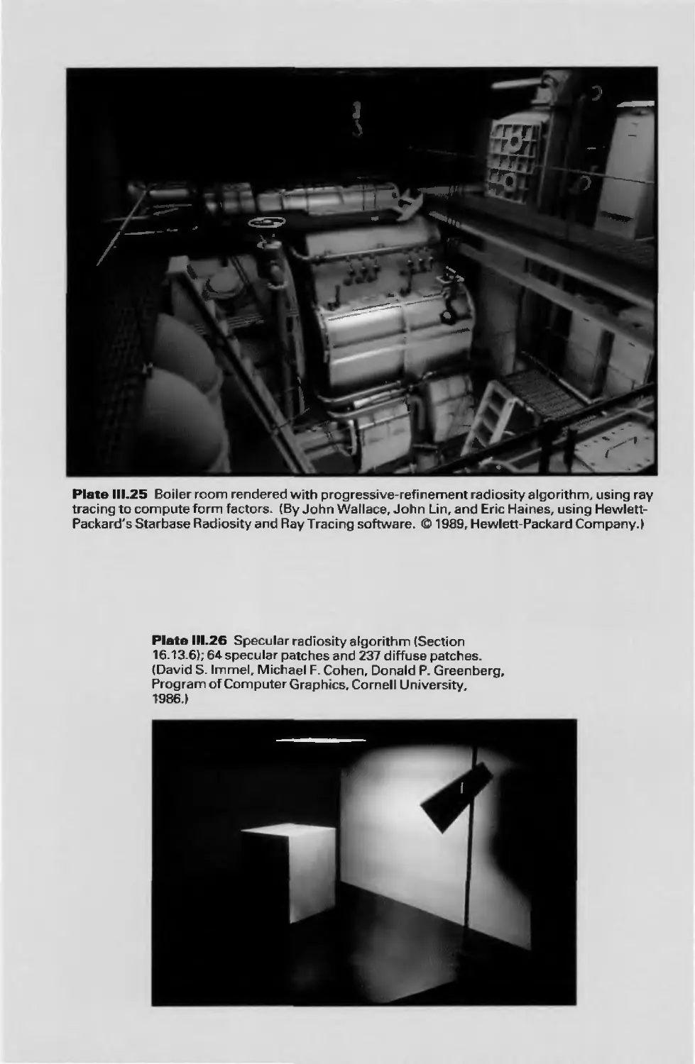
16.13 Radiosity Methods 793
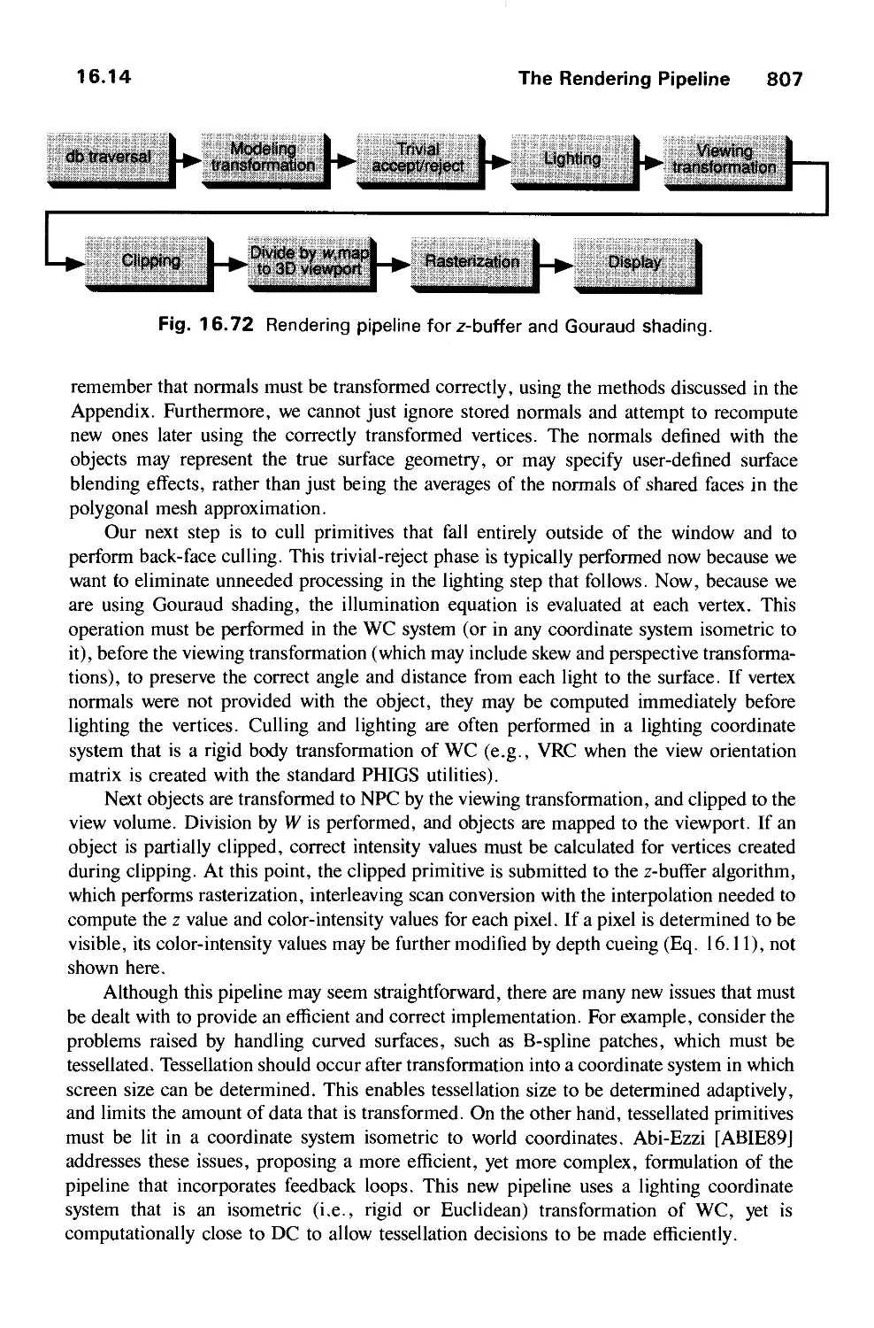
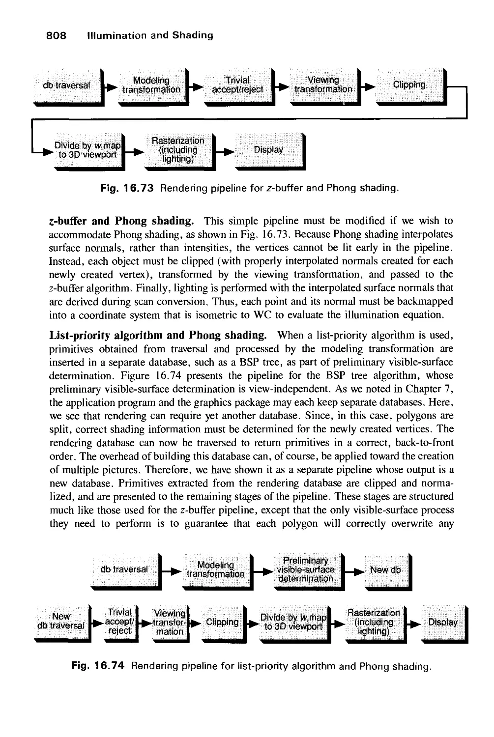
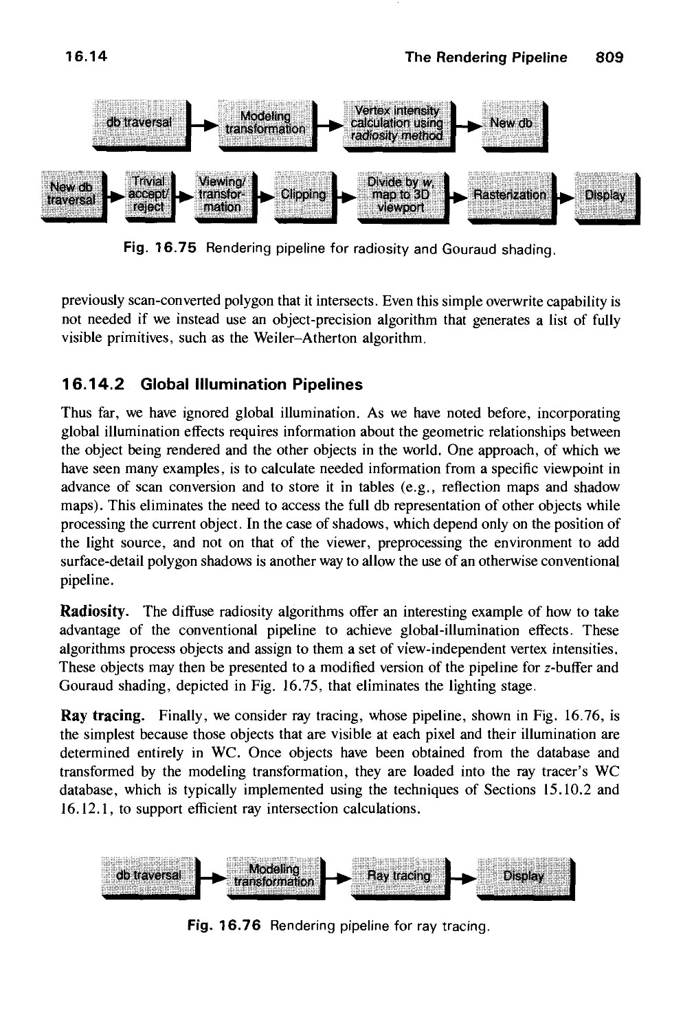
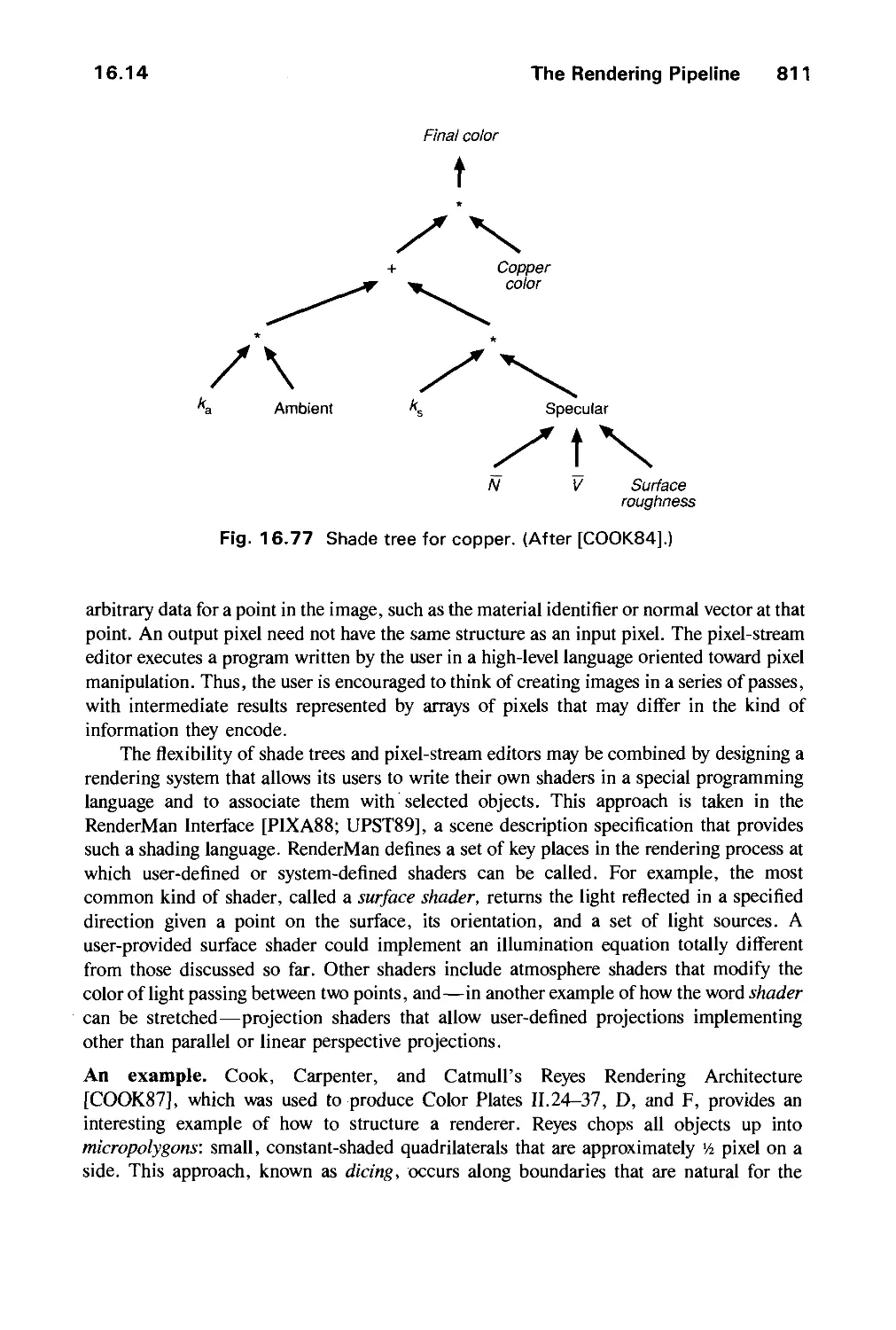
16.14 The Rendering Pipeline 806
16.15 Summary 813
Exercises 813
xxii Contents
CHAPTER 17
IMAGE MANIPULATION AND STORAGE 815
17.1 What Is an Image? 816
17.2 Filtering 817
17.3 Image Processing 820
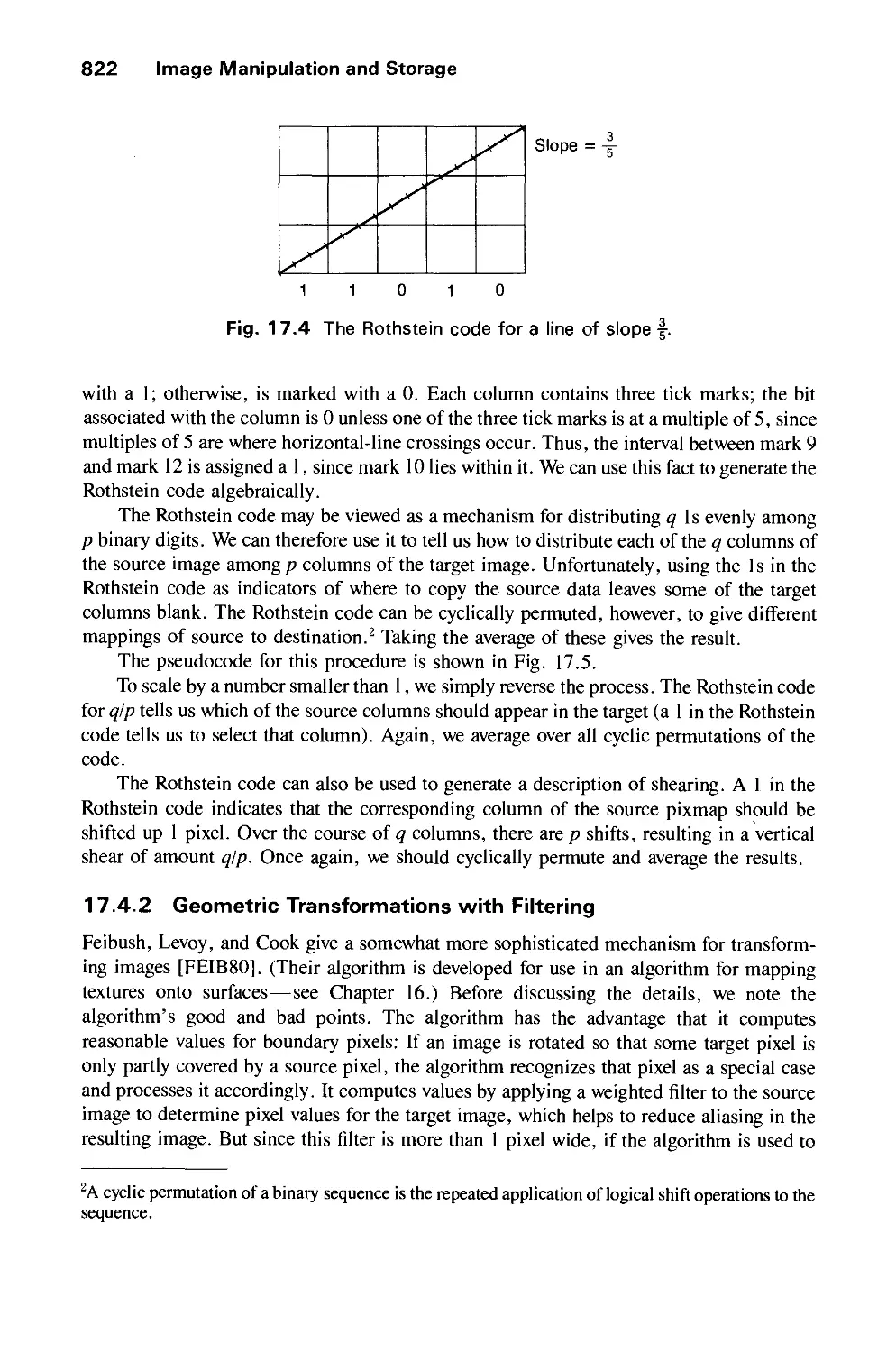
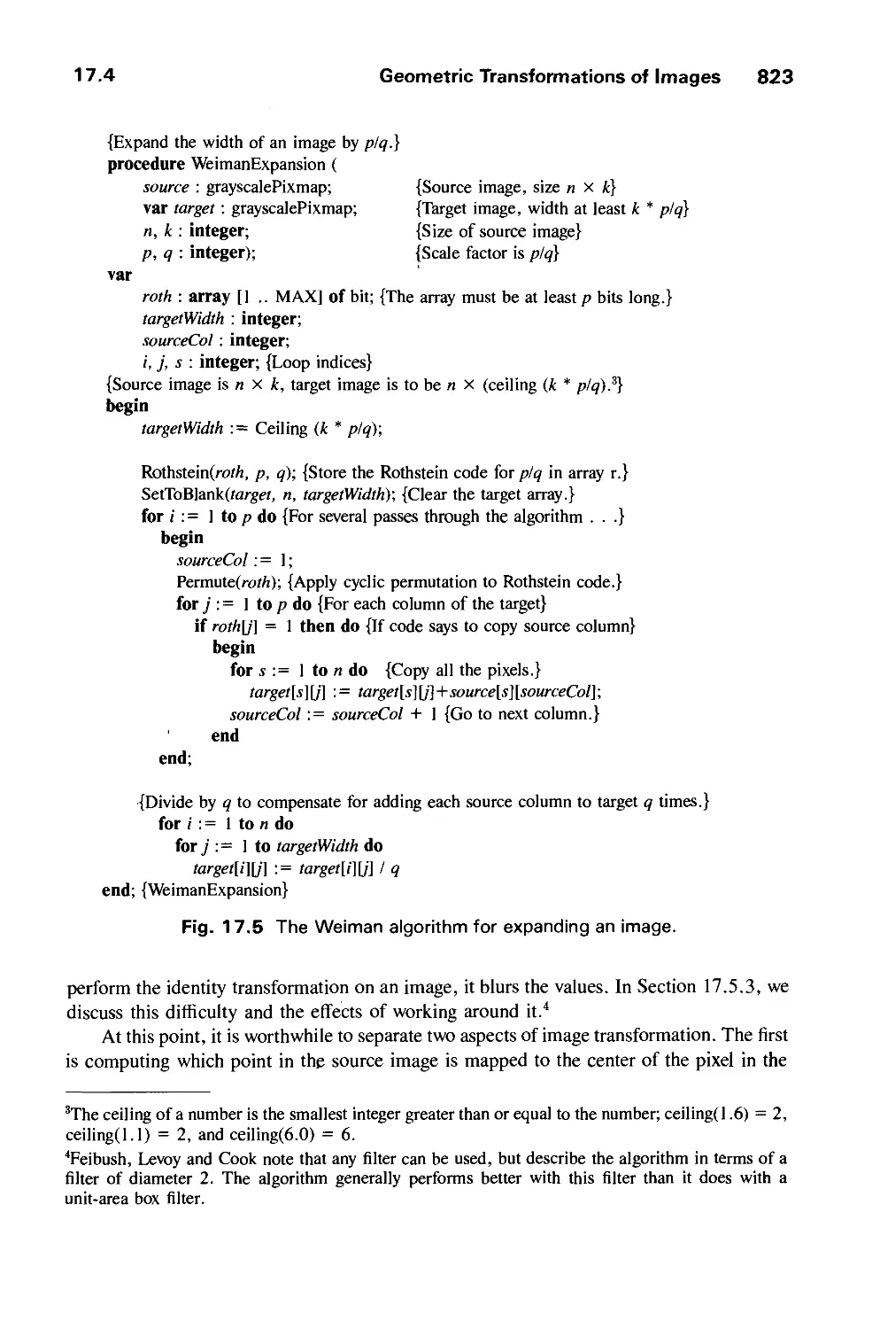
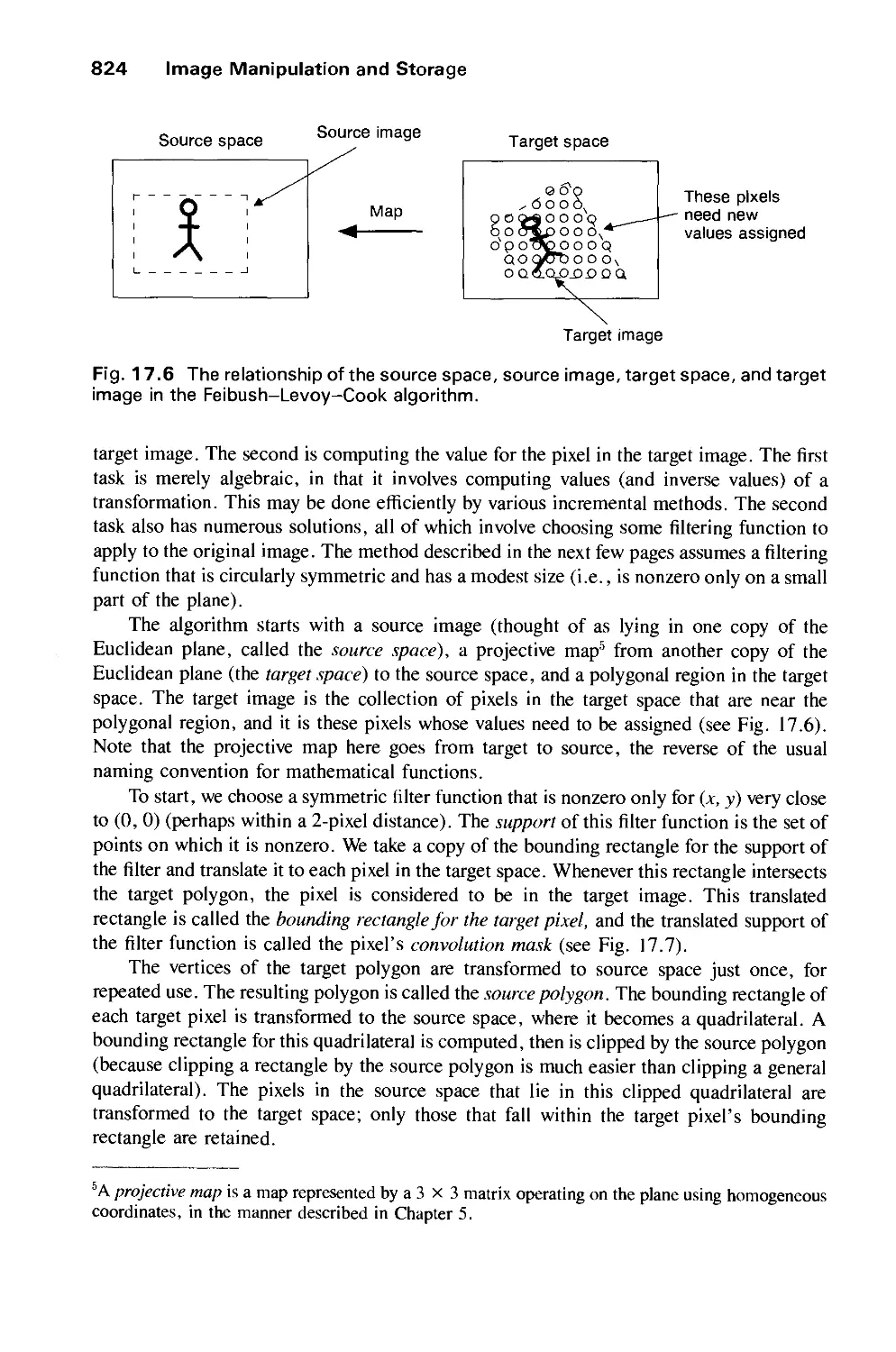
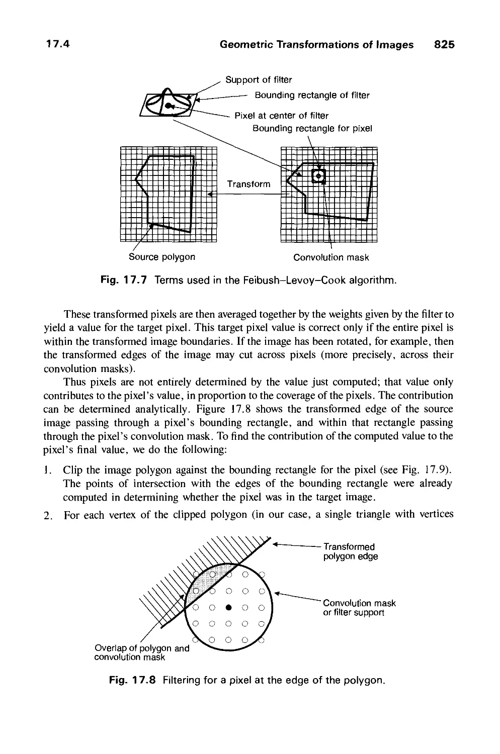
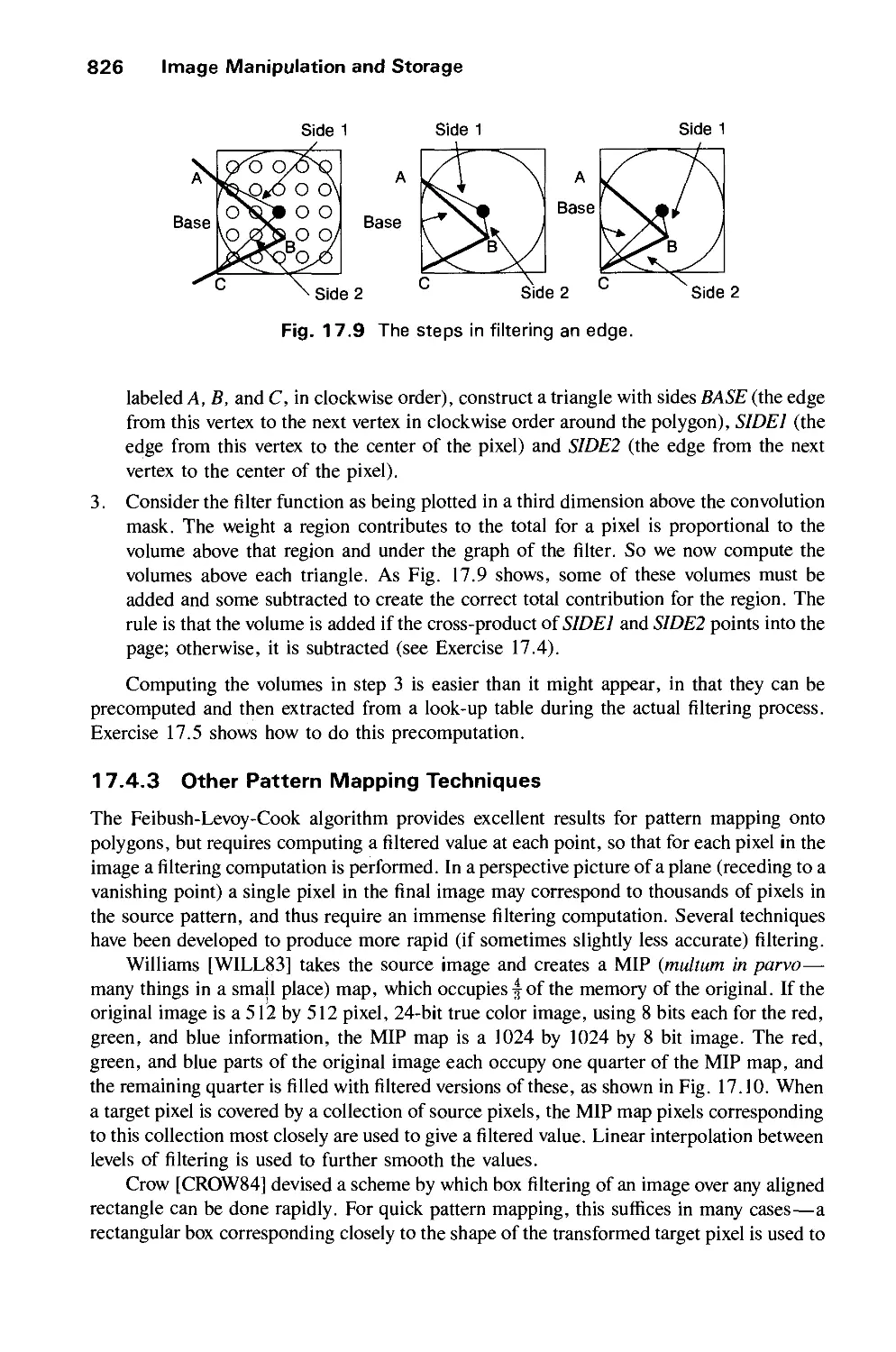
17.4 Geometric Transformations of Images 820
17.5 Multipass Transformations 828
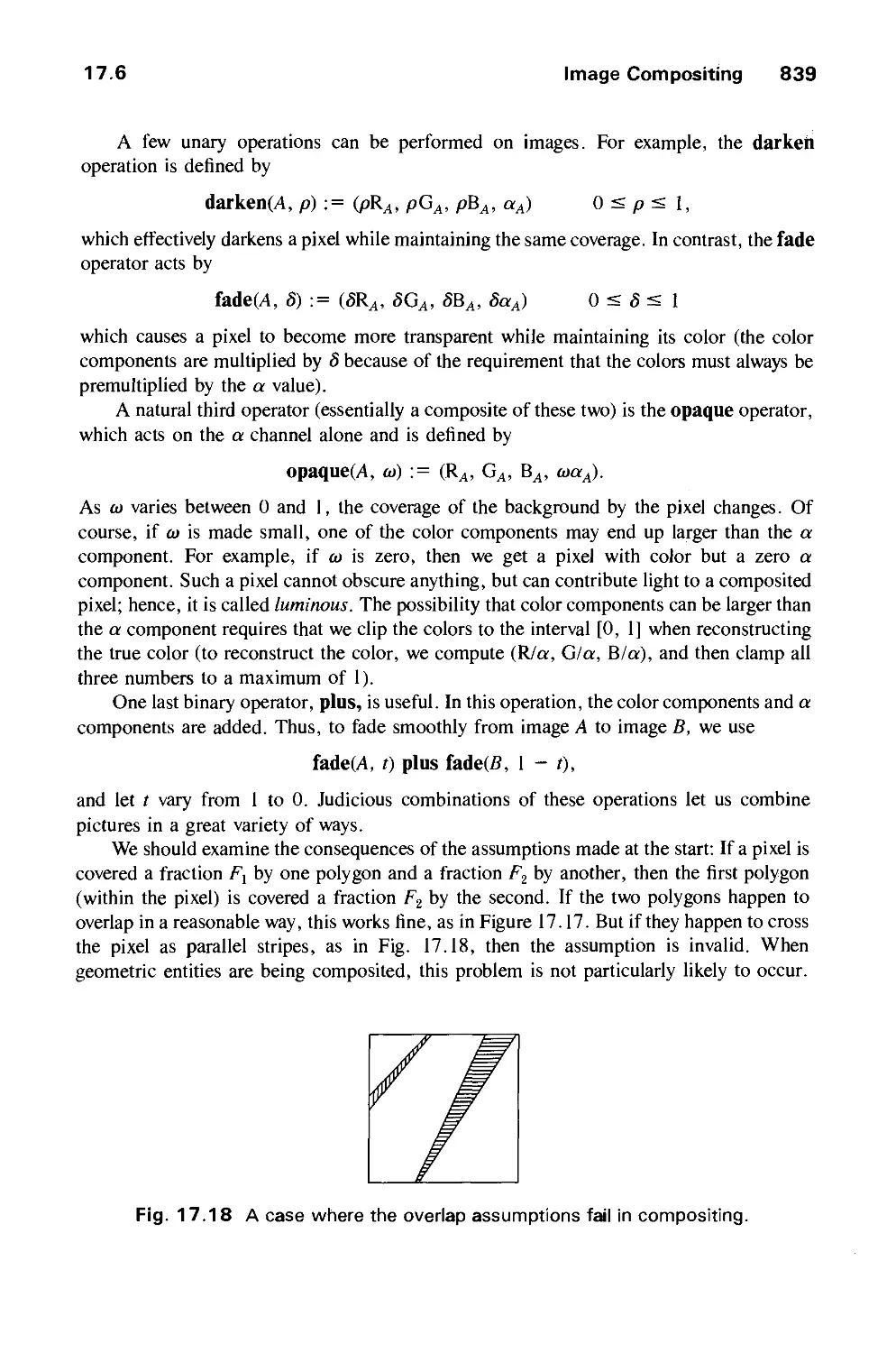
17.6 Image Compositing 835
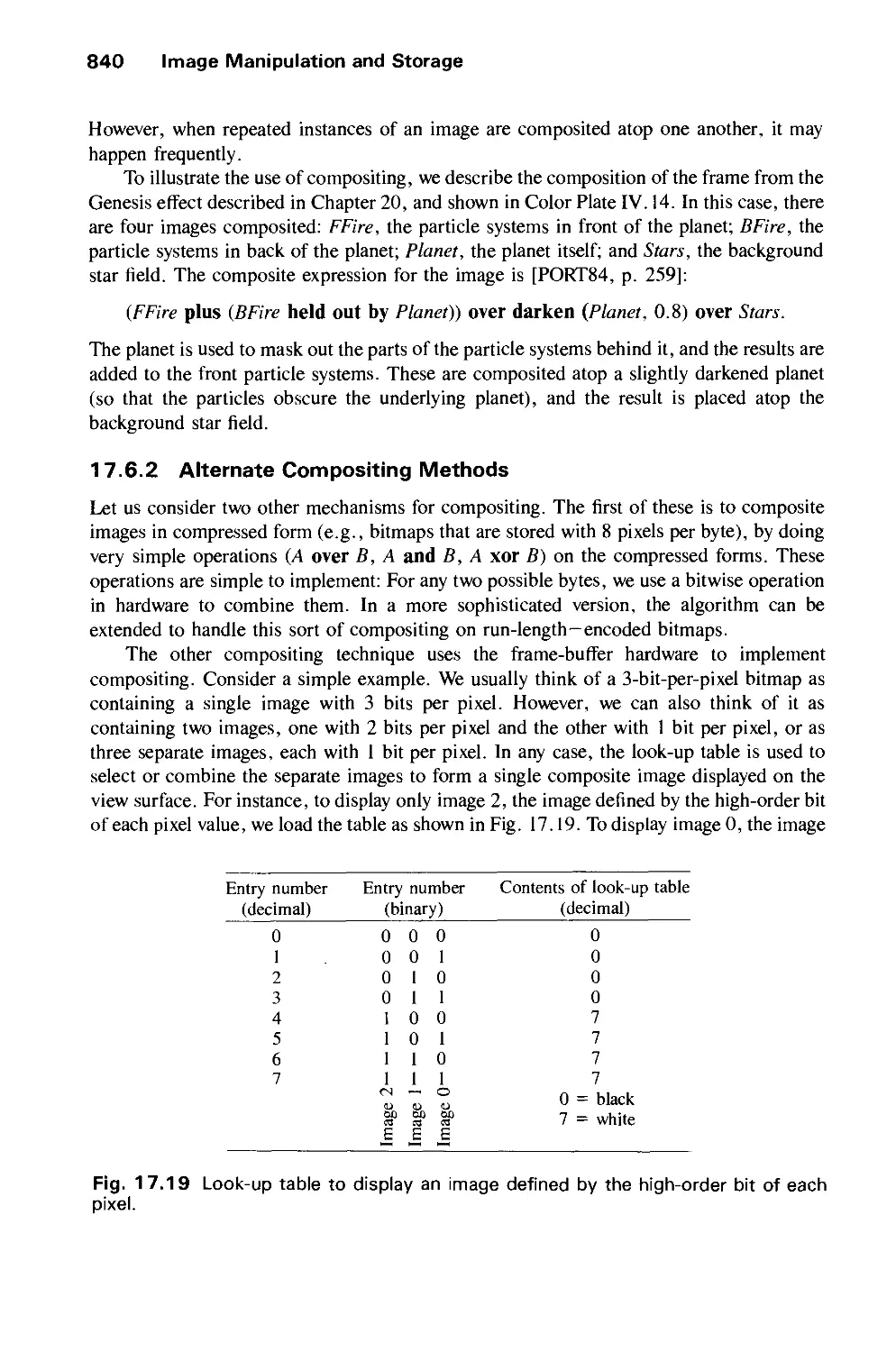
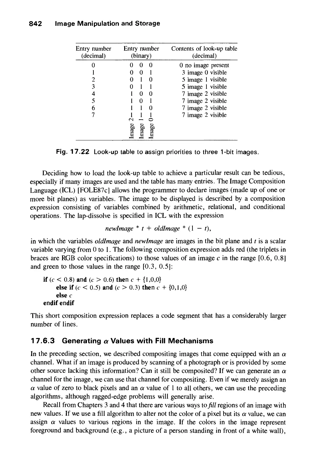
17.7 Mechanisms for Image Storage 843
17.8 Special Effects with Images 850
17.9 Summary 851
Exercises 851
CHAPTER 18
ADVANCED RASTER GRAPHICS ARCHITECTURE 855
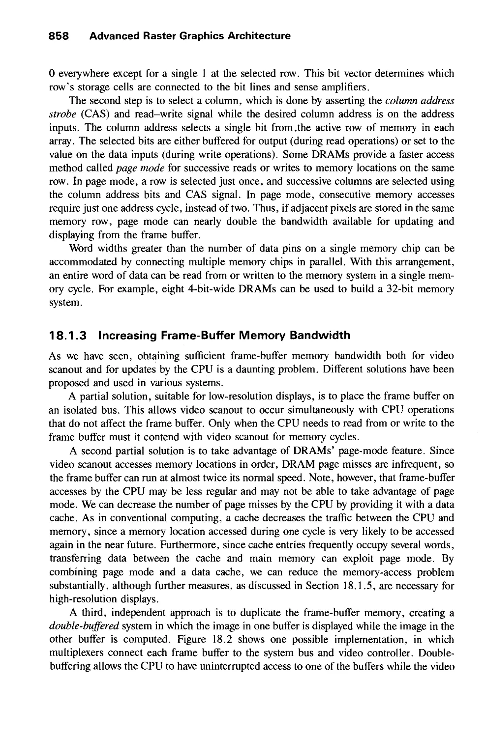
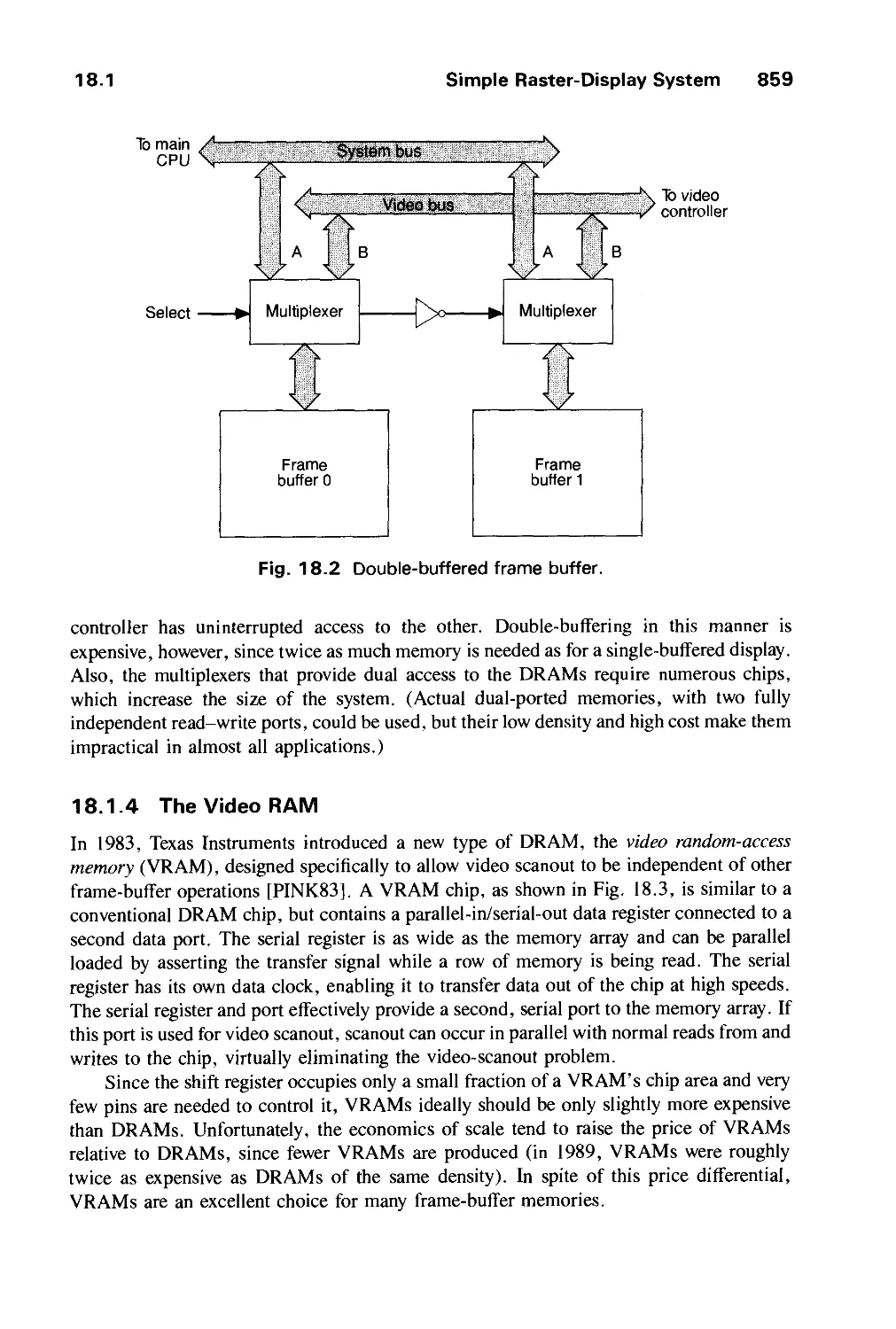
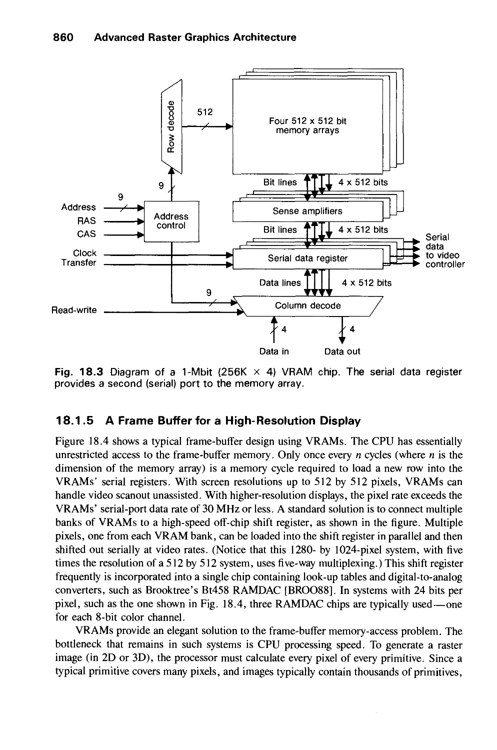
18.1 Simple Raster-Display System 856
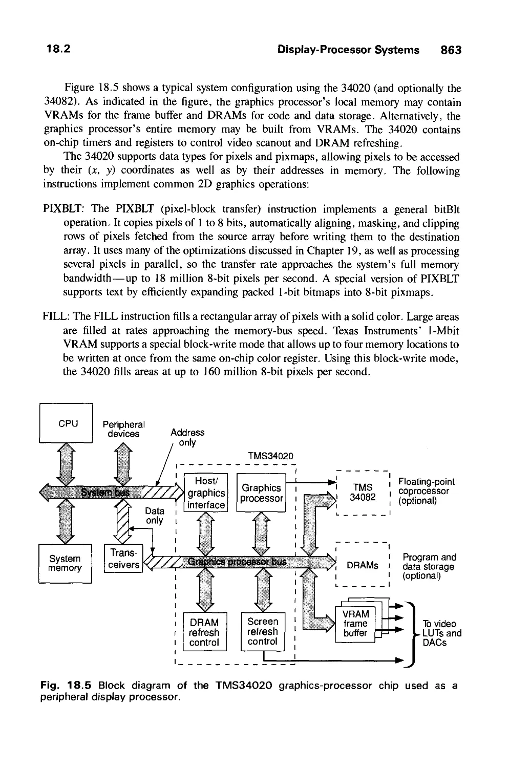
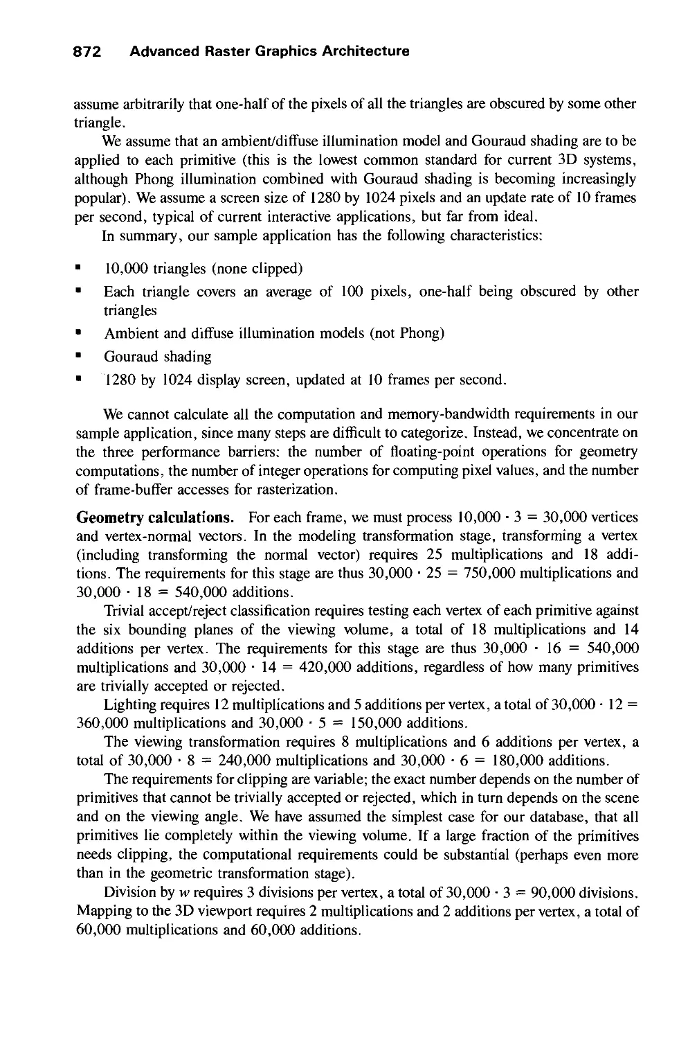
18.2 Display-Processor Systems 861
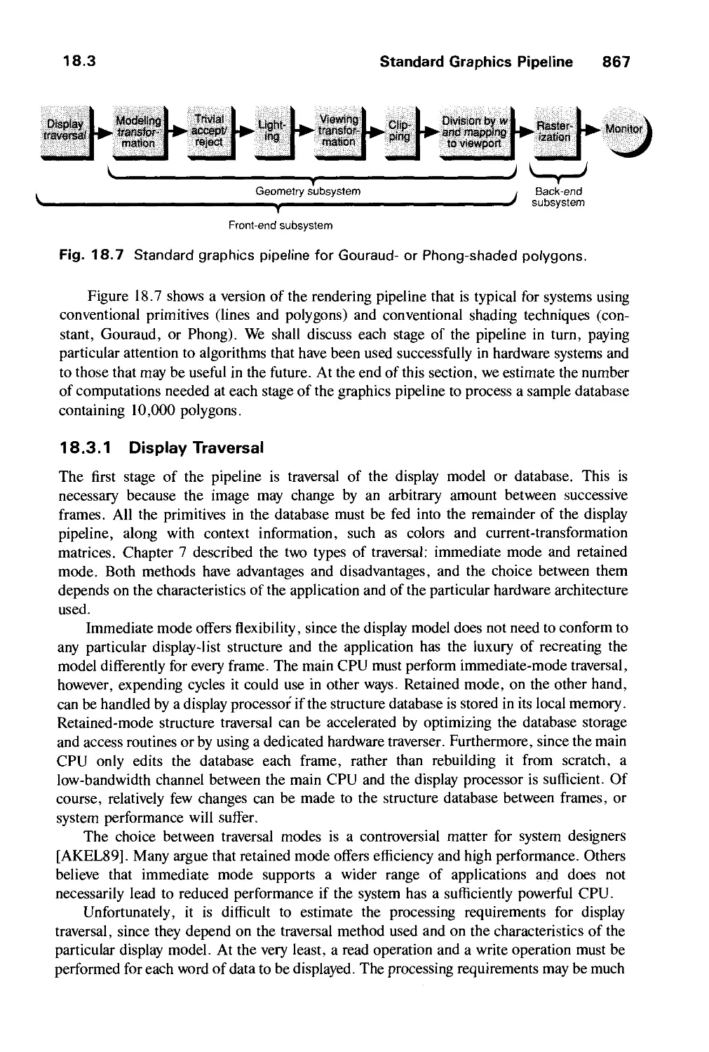
18.3 Standard Graphics Pipeline 866
18.4 Introduction to Multiprocessing 873
18.5 Pipeline Front-End Architectures 877
18.6 Parallel Front-End Architectures 880
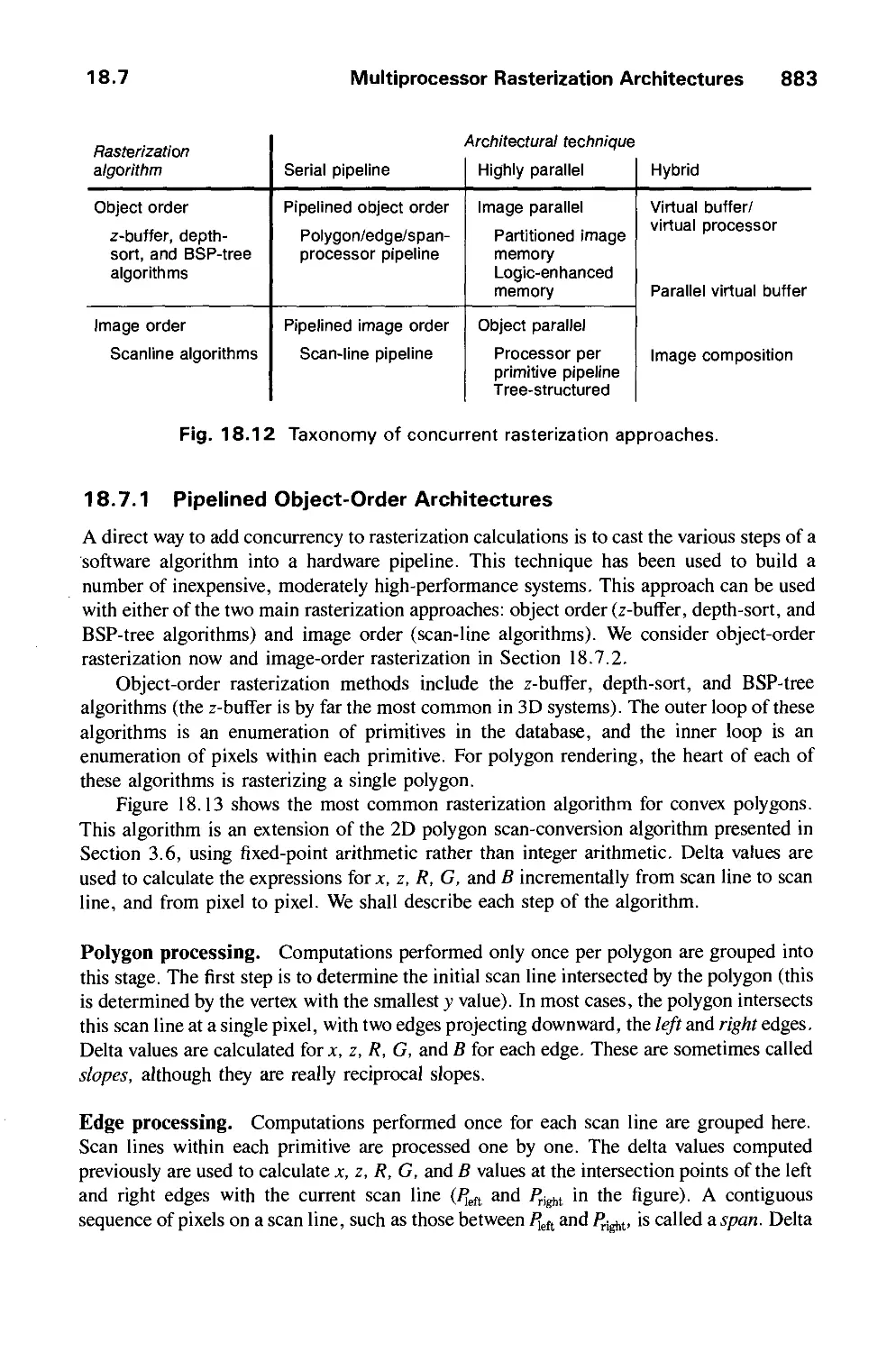
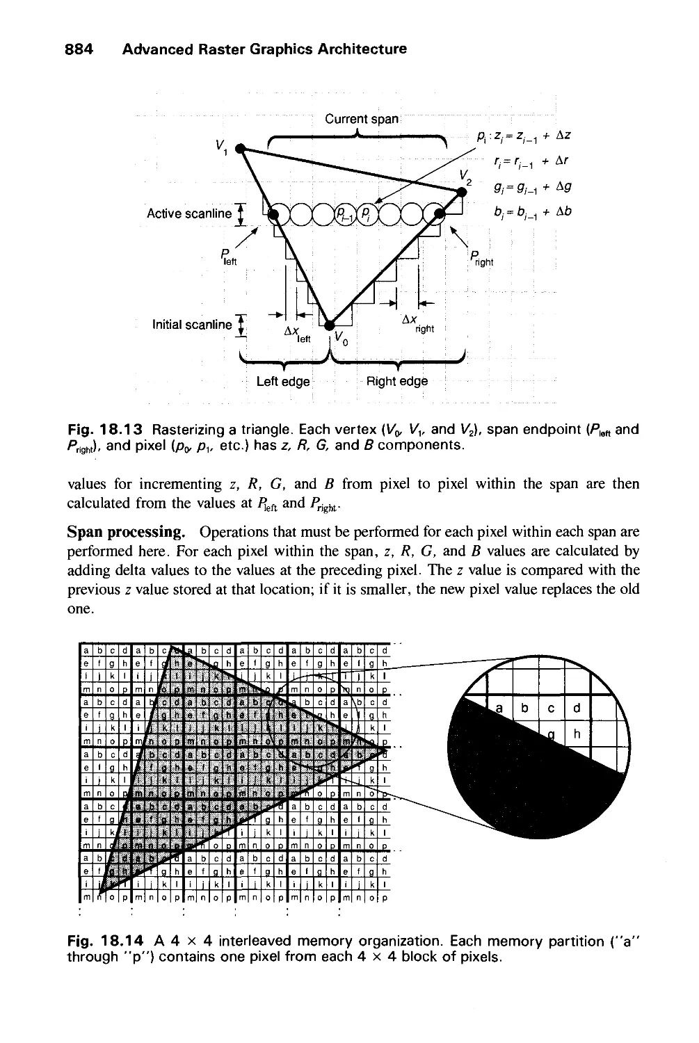
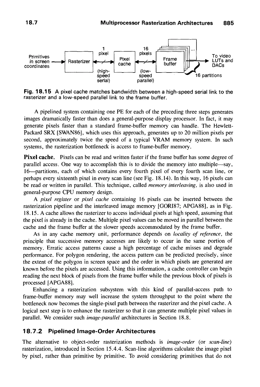
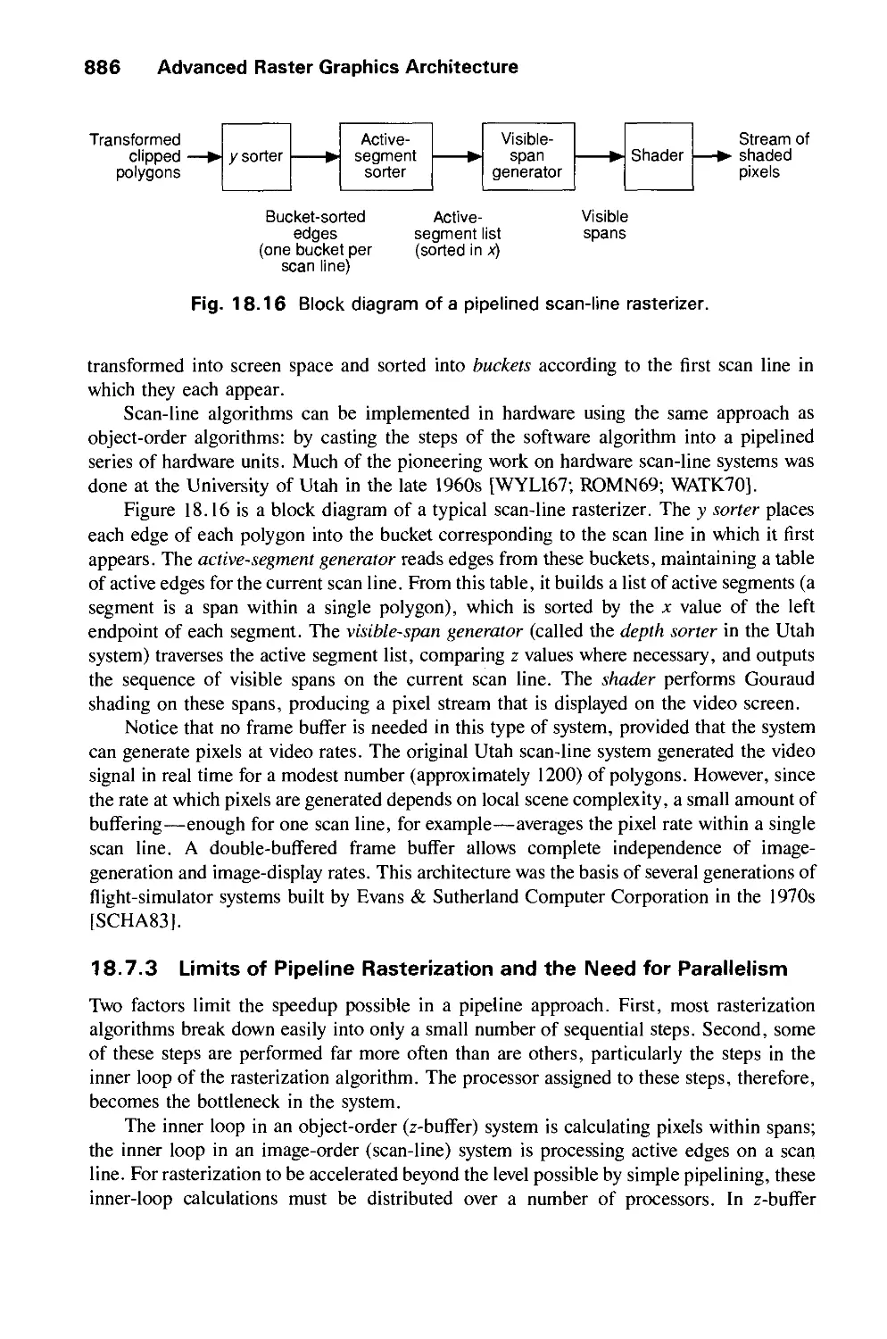
18.7 Multiprocessor Rasterization Architectures 882
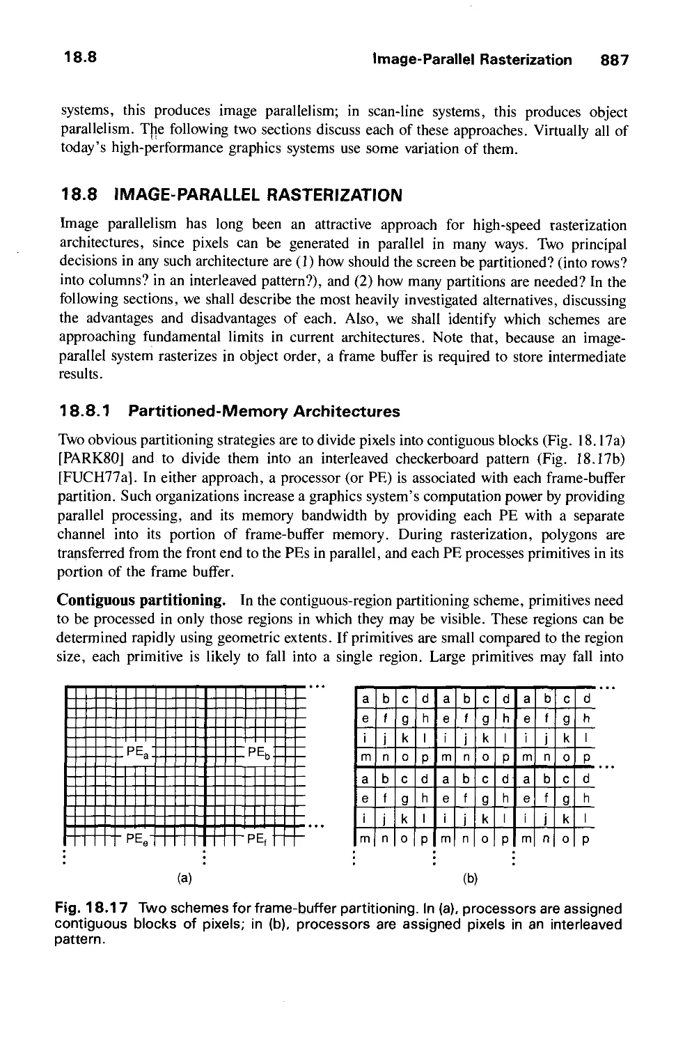
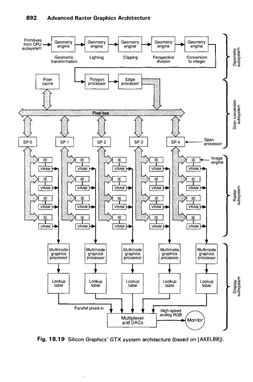
18.8 Image-Parallel Rasterization 887
18.9 Object-Parallel Rasterization 899
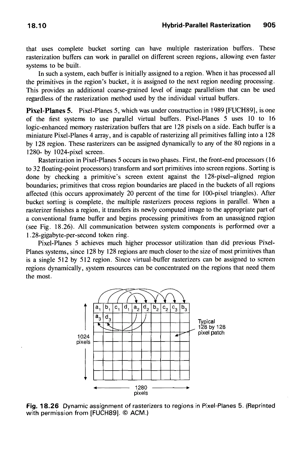
18.10 Hybrid-Parallel Rasterization 902
18.11 Enhanced Display Capabilities 907
18.12 Summary 920
Exercises 920
CHAPTER 19
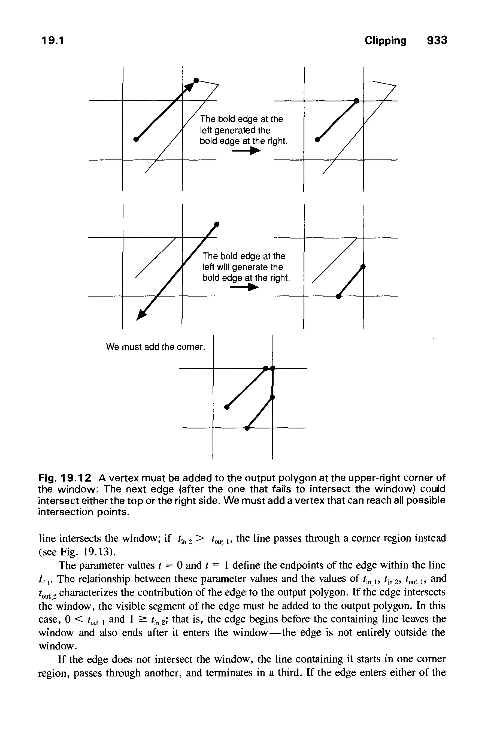
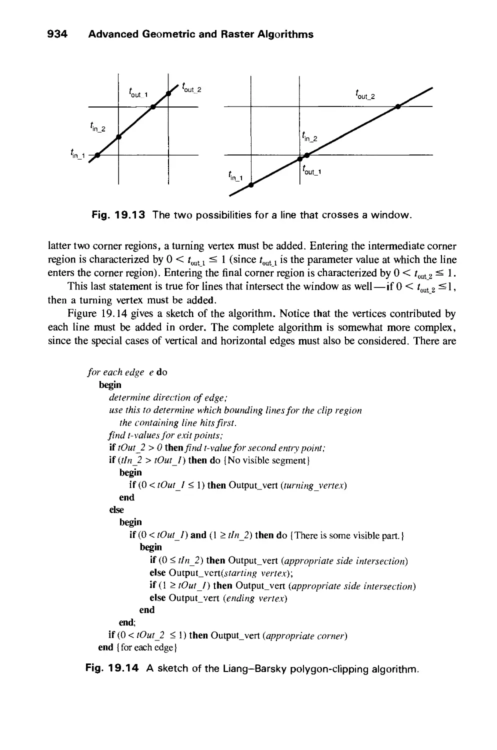
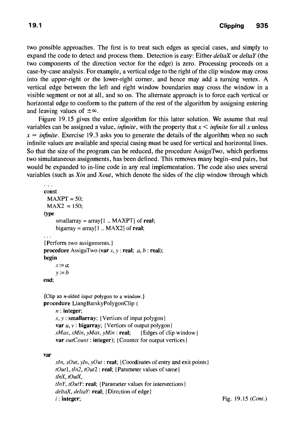
ADVANCED GEOMETRIC AND RASTER ALGORITHMS 923
19.1 Clipping 924
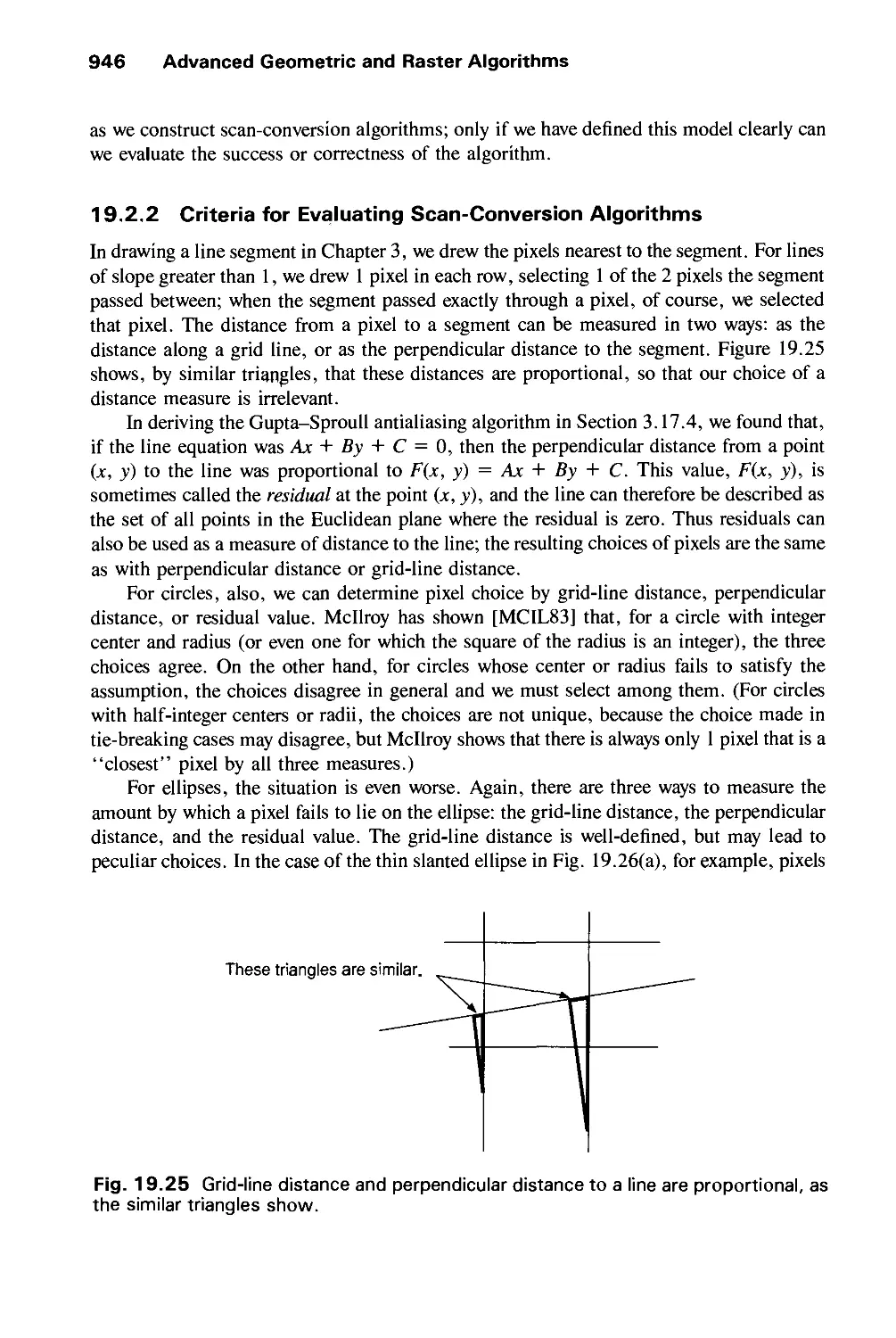
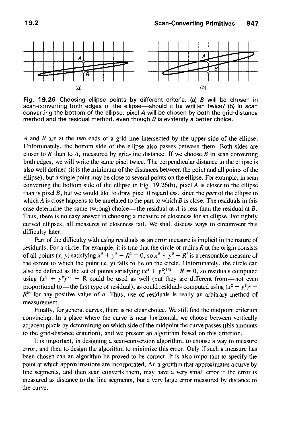
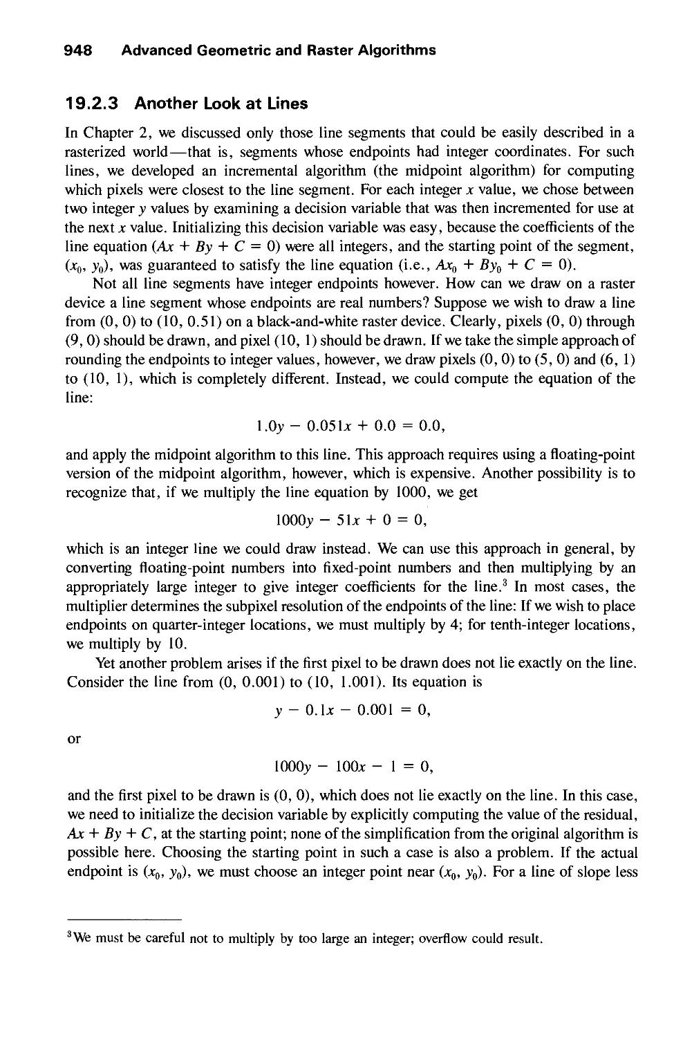
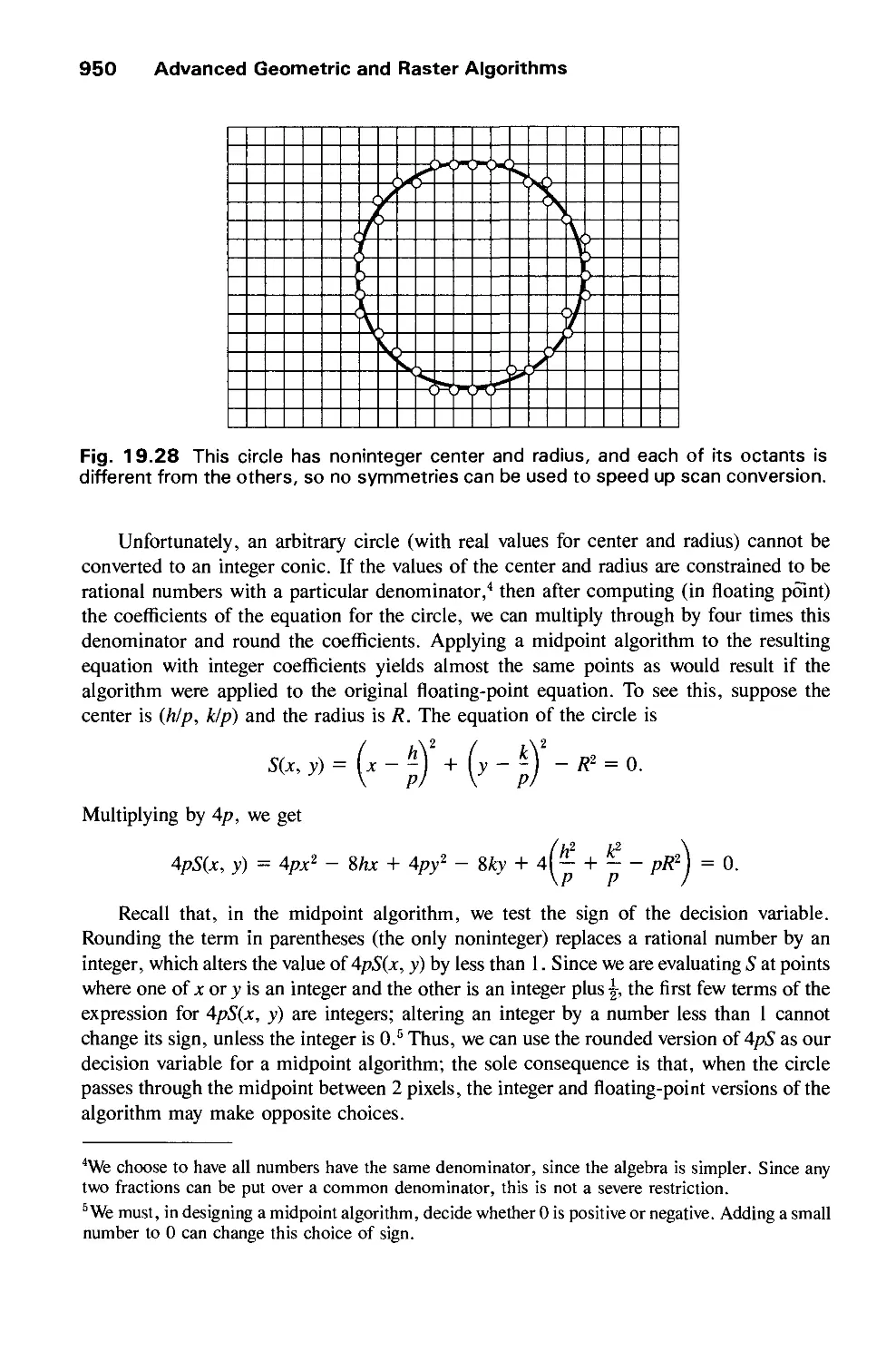
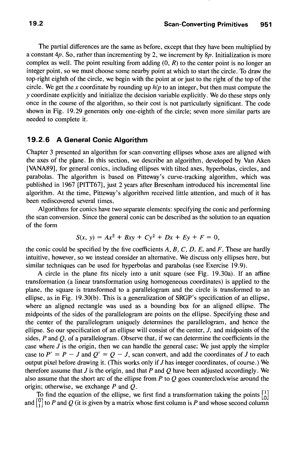
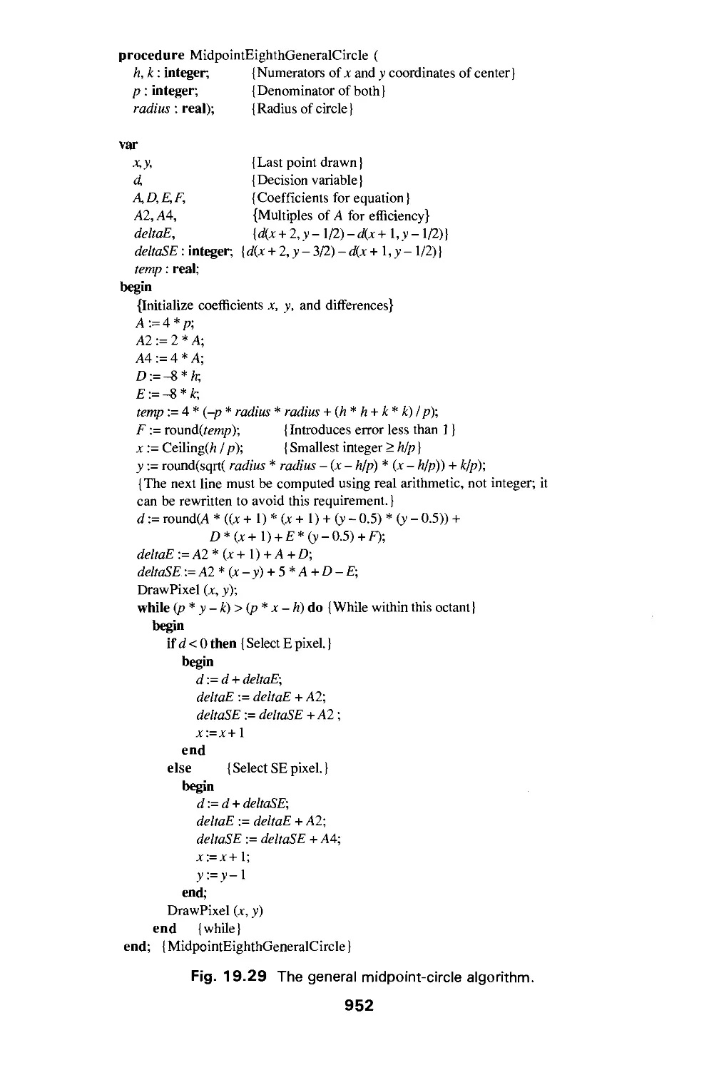
19.2 Scan-Converting Primitives 945
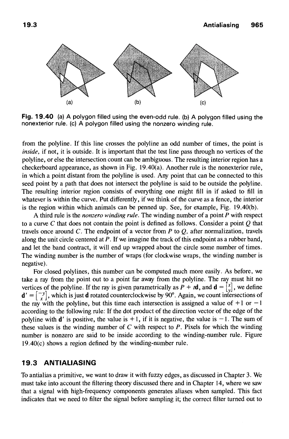
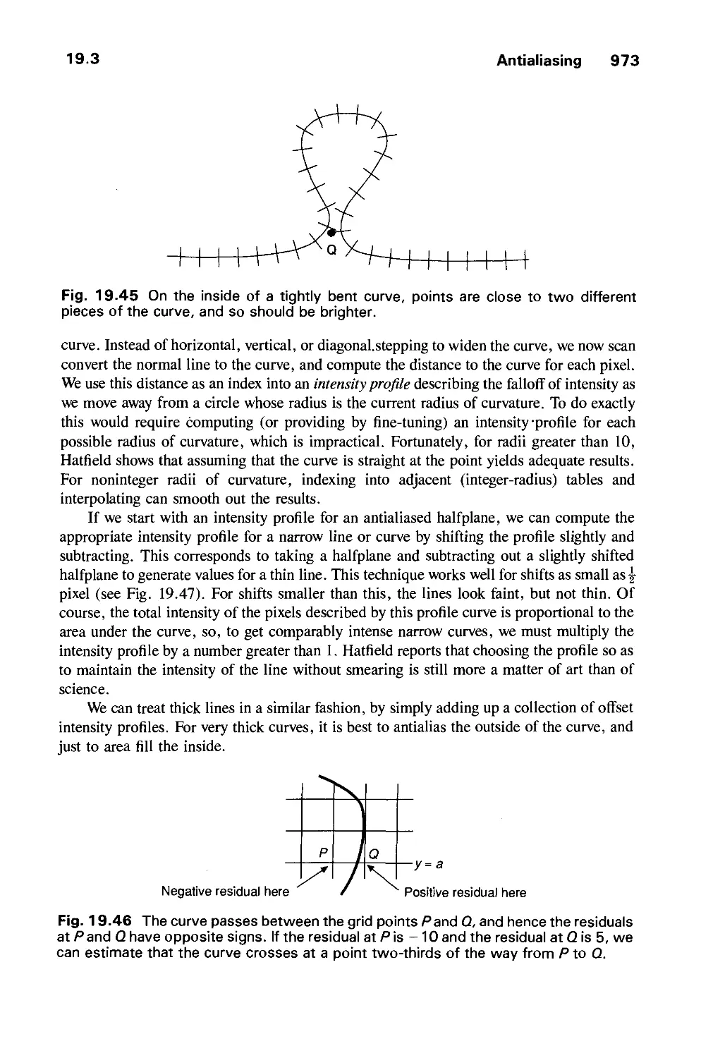
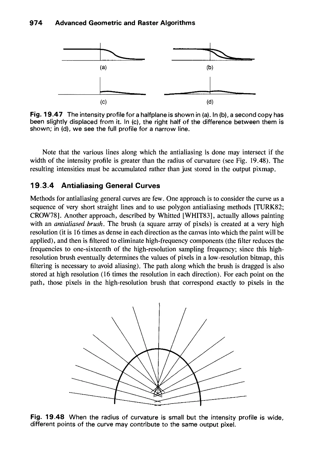
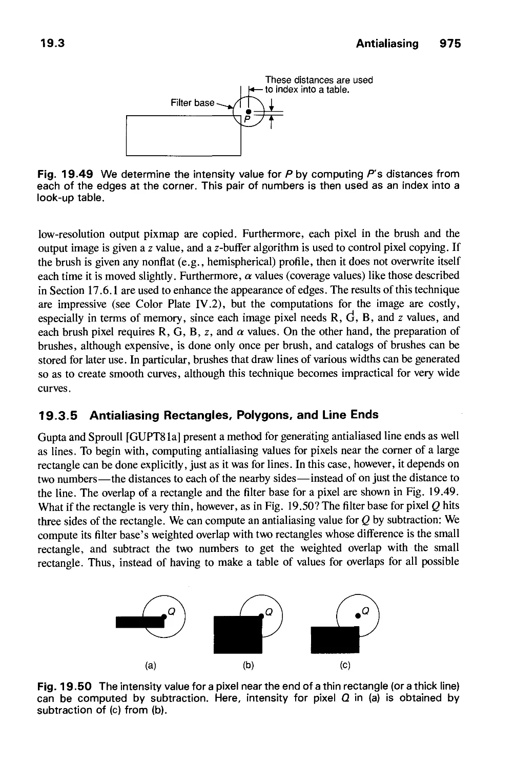
19.3 Antialiasing 965
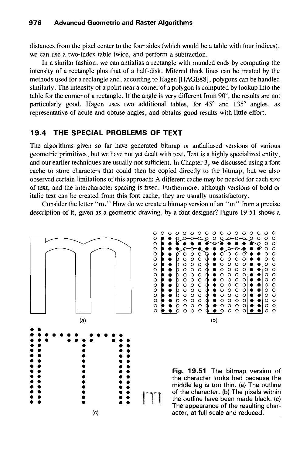
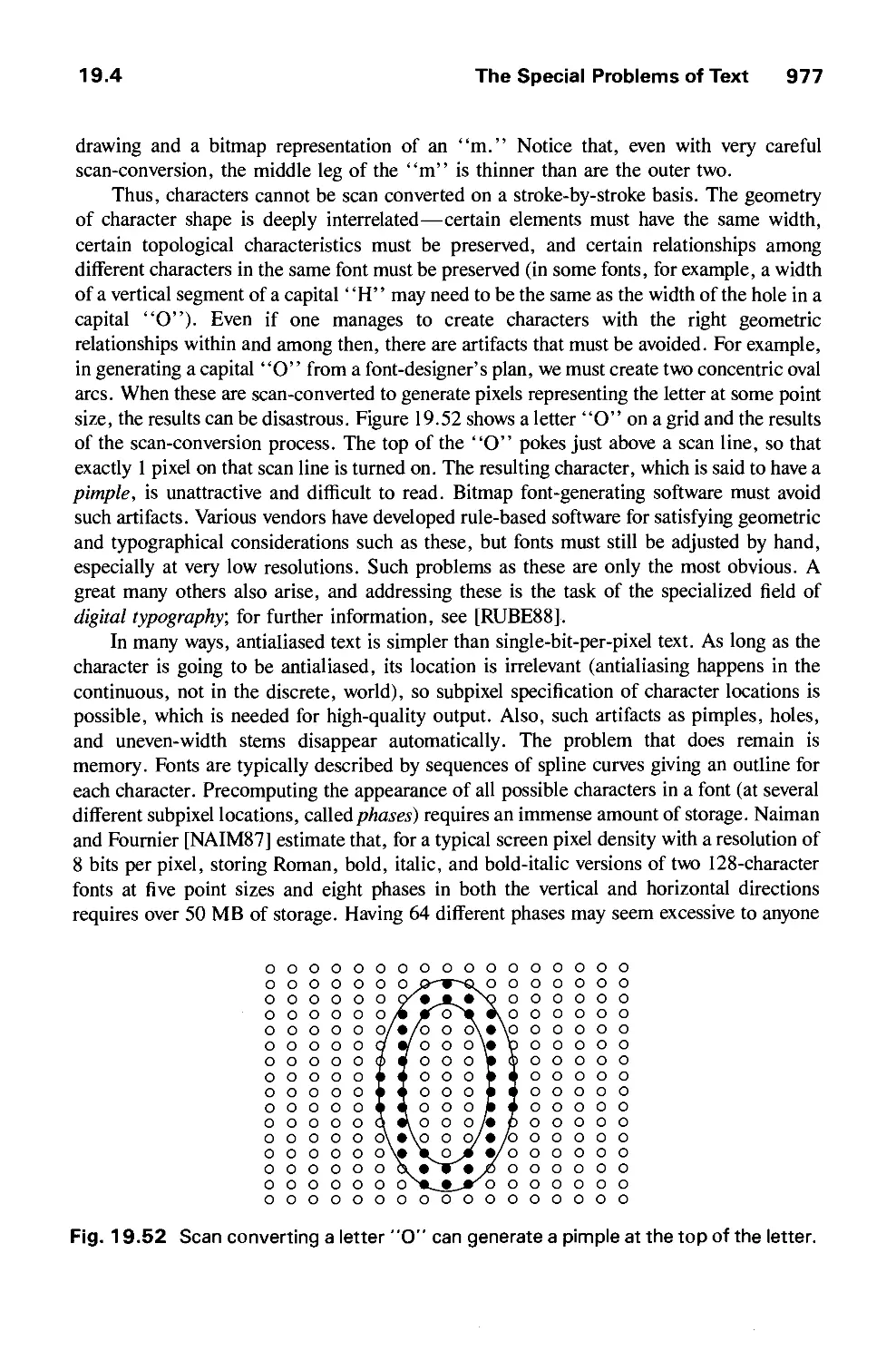
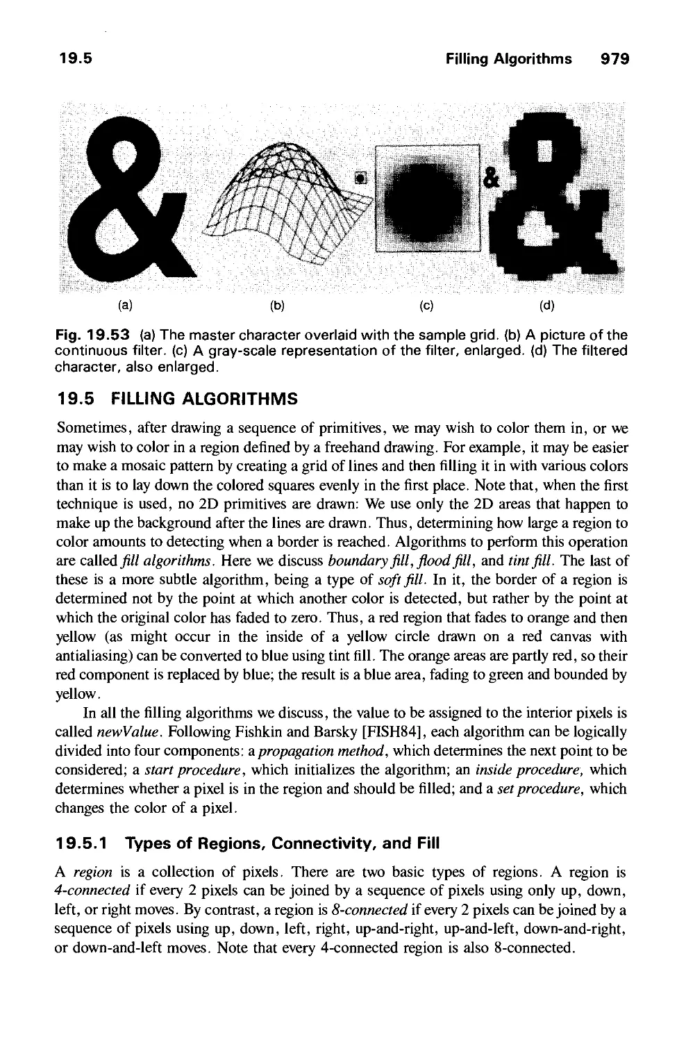
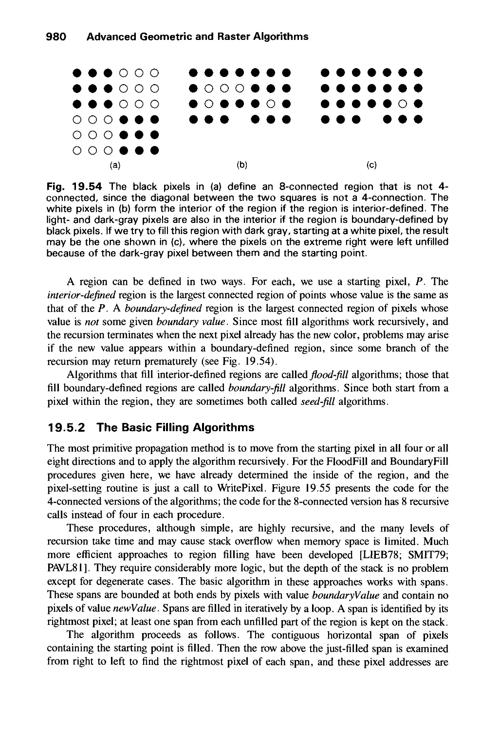
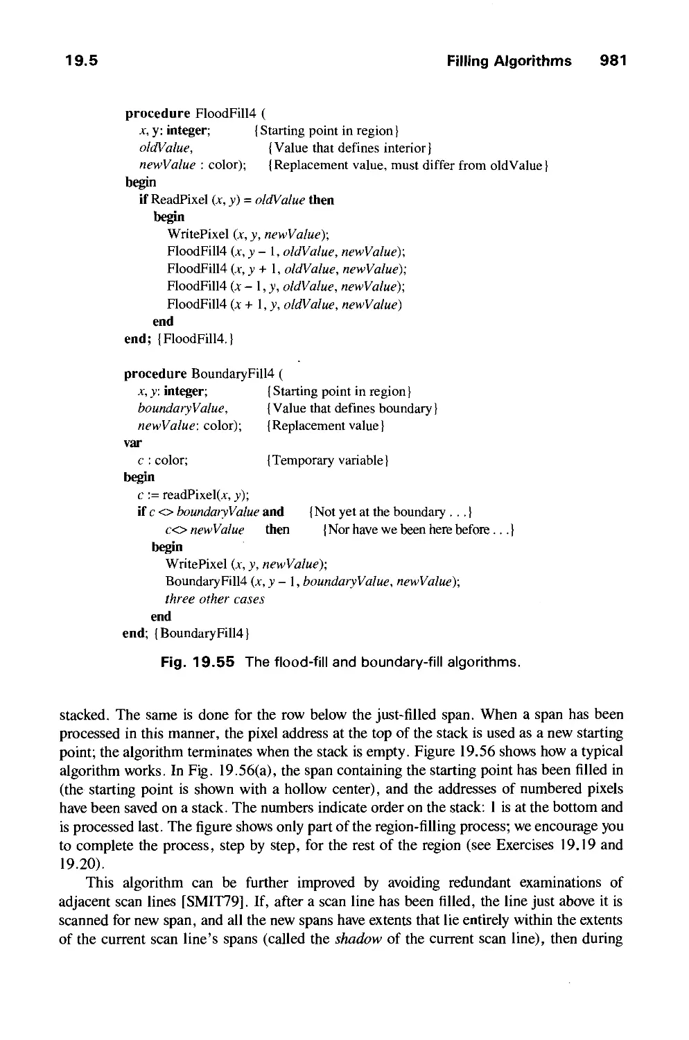
19.4 The Special Problems of Text 976
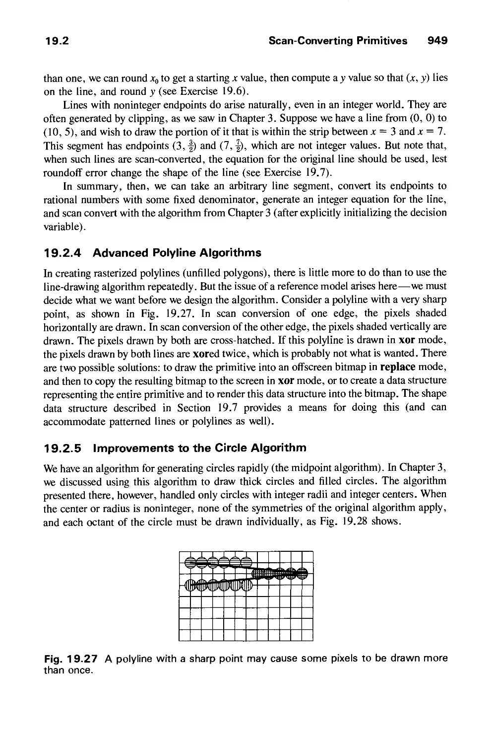
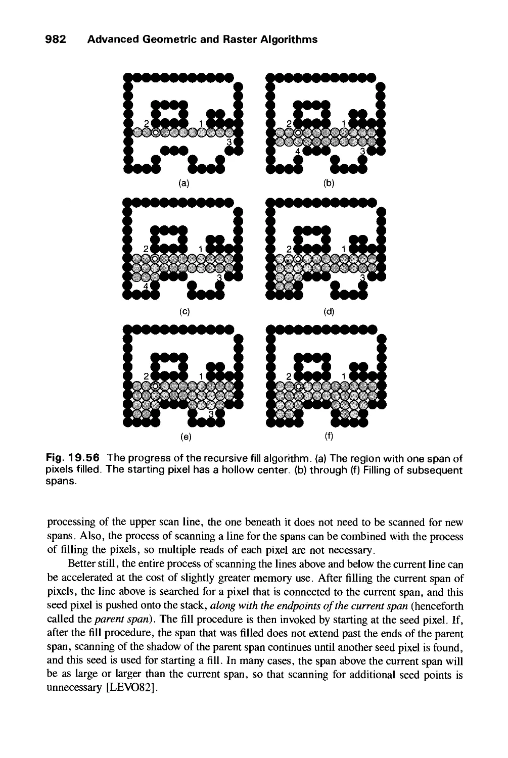
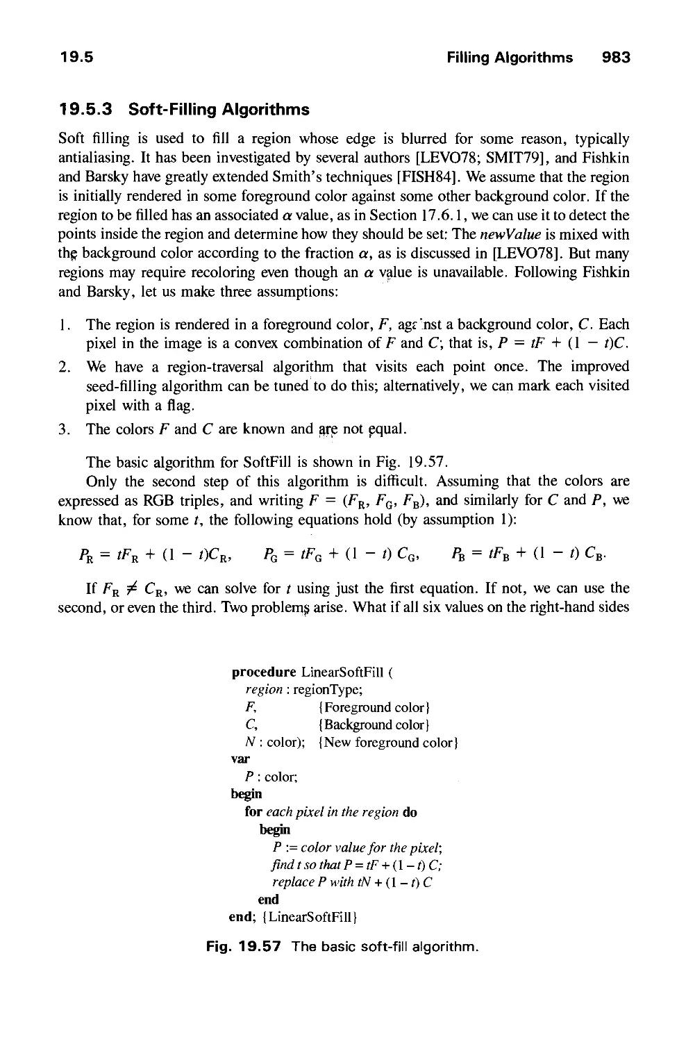
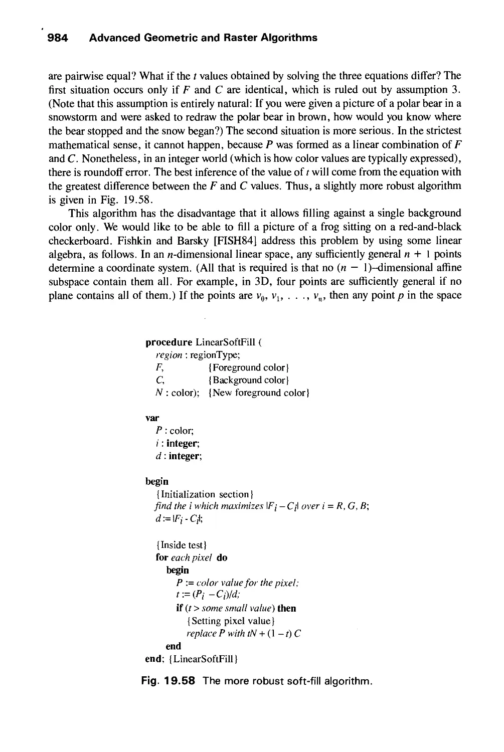
19.5 Filling Algorithms 979
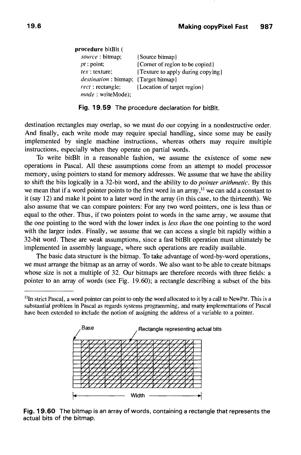
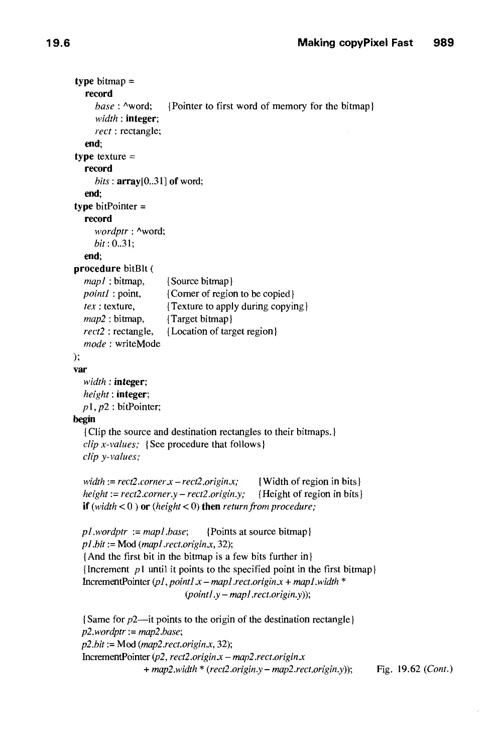
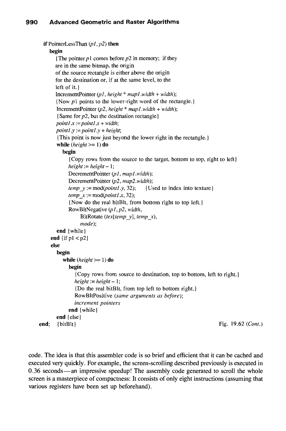
19.6 Making copyPixel Fast 986
19.7 The Shape Data Structure and Shape Algebra 992
19.8 Managing Windows with bitBlt 996
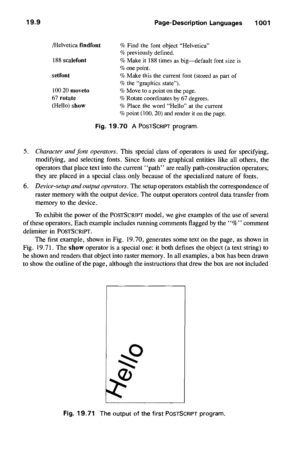
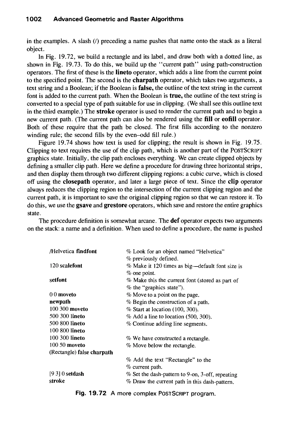
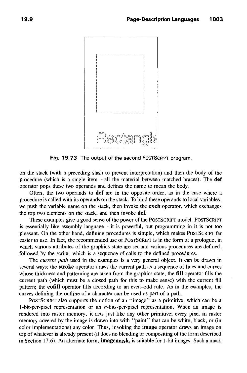
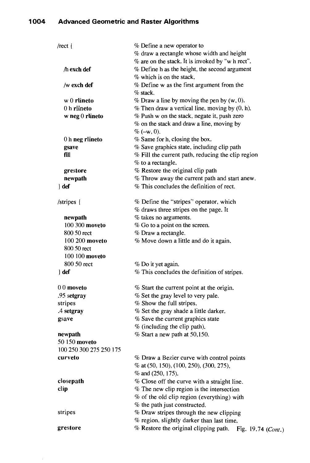
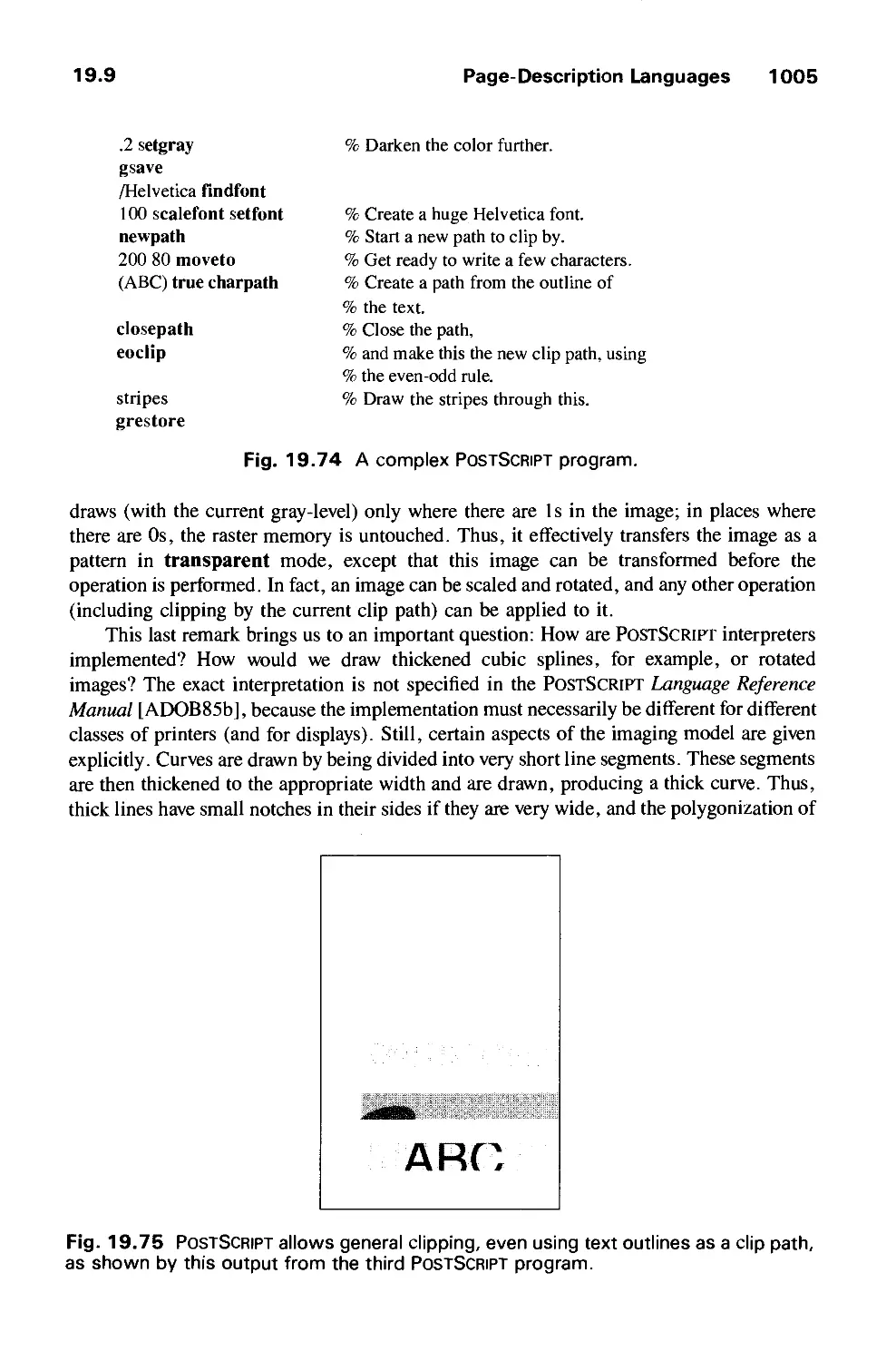
19.9 Page-Description Languages 998
19.10 Summary 1006
Exercises 1006
Contents xxiii
CHAPTER 20
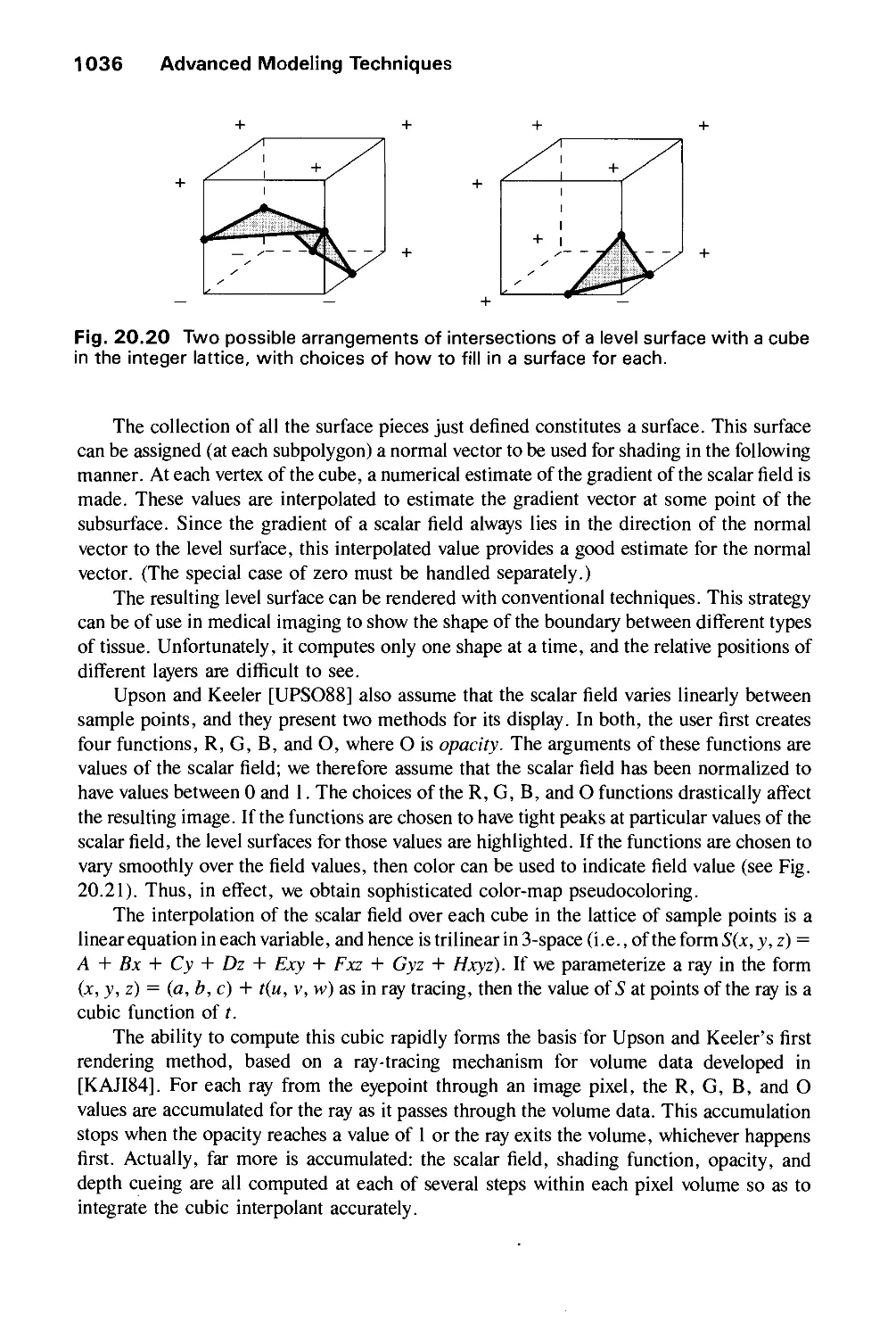
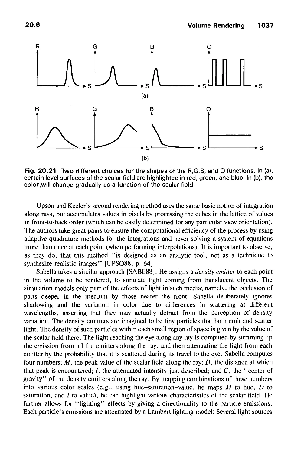
ADVANCED MODELING TECHNIQUES 1011
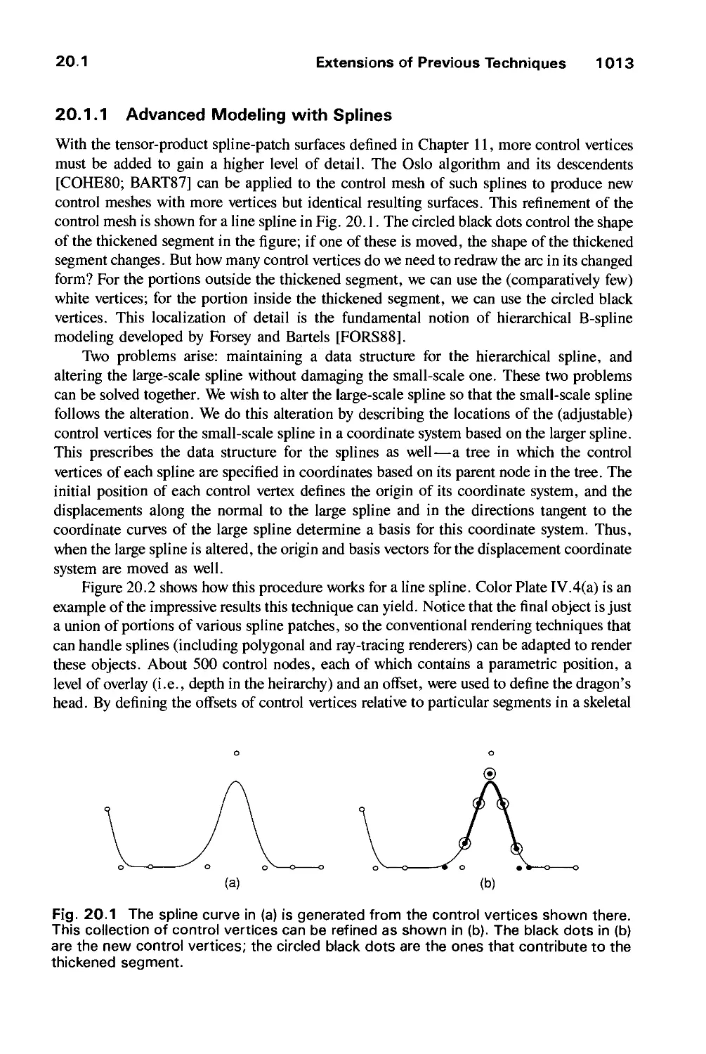
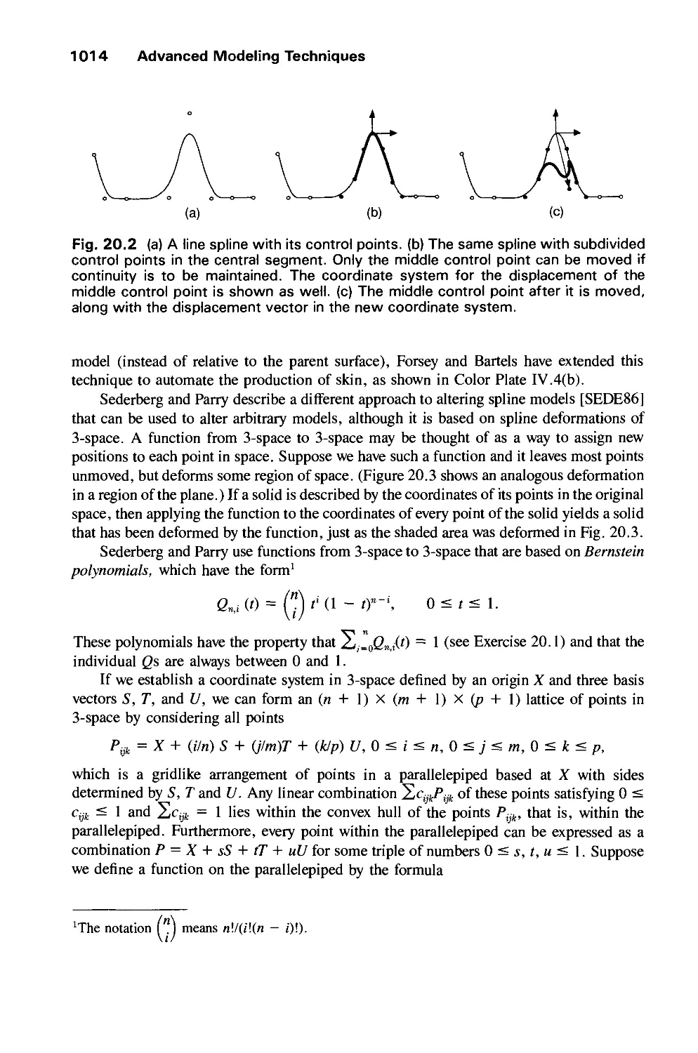
20.1 Extensions of Previous Techniques 1012
20.2 Procedural Models 1018
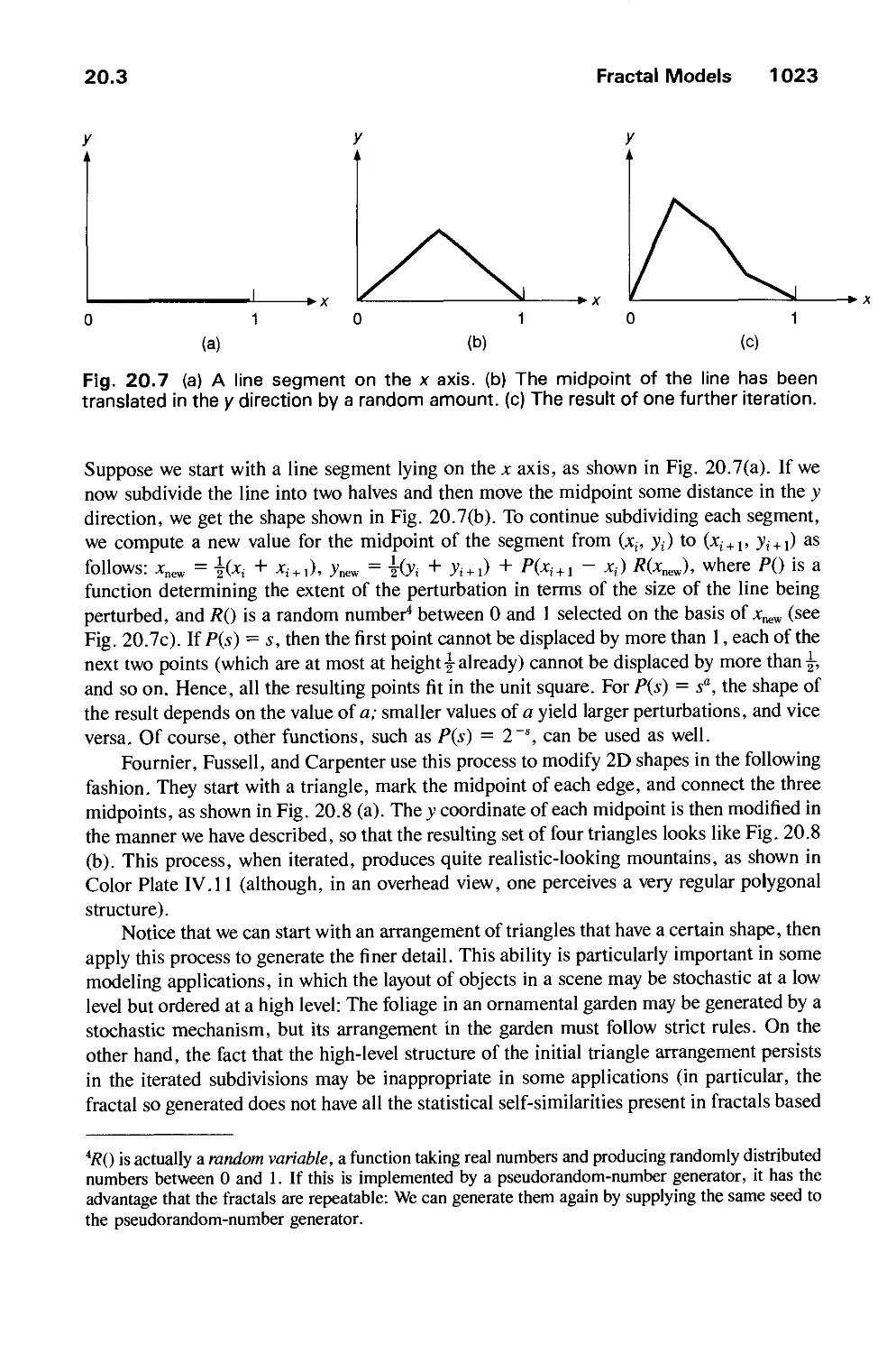
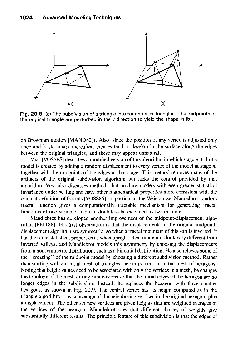
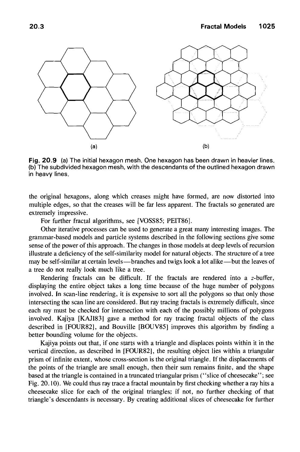
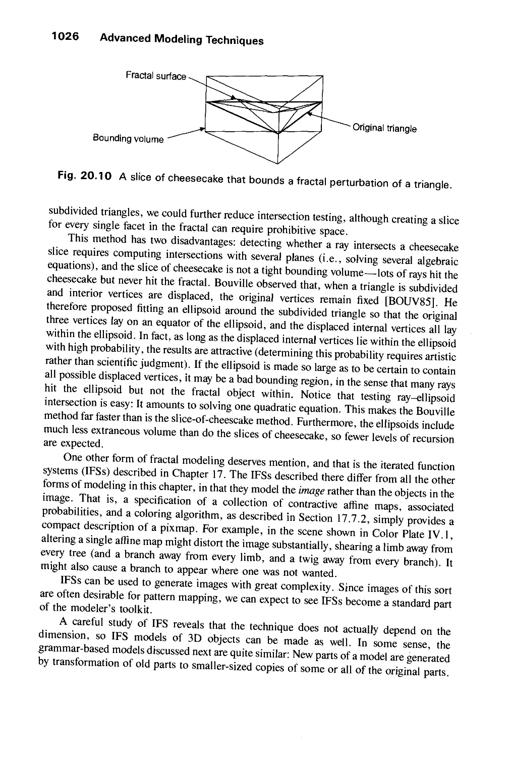
20.3 Fractal Models 1020
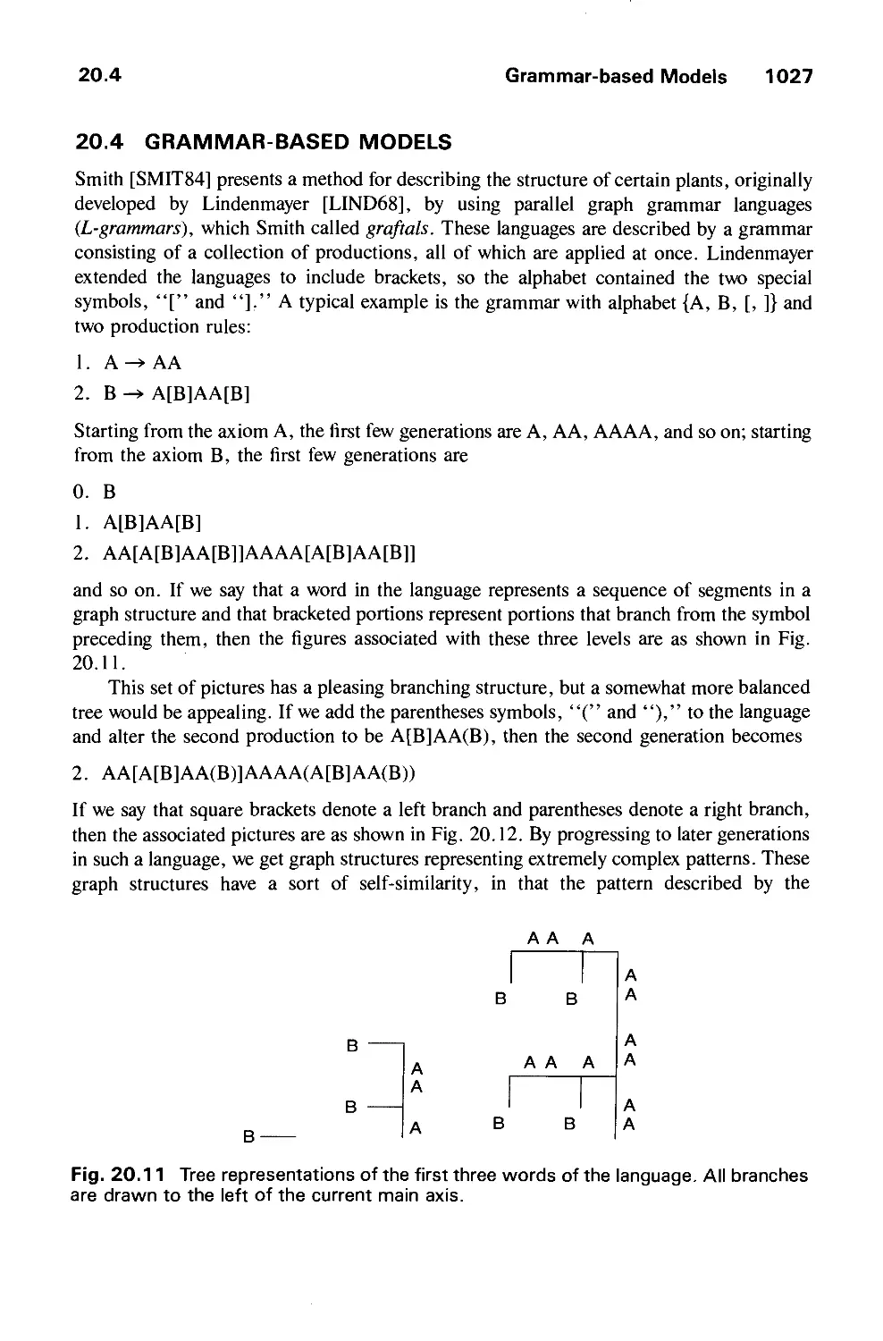
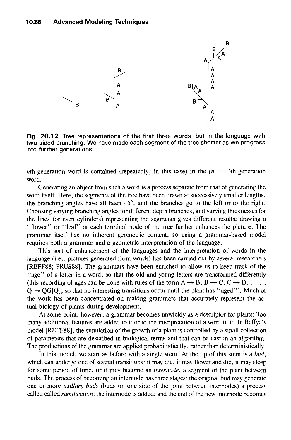
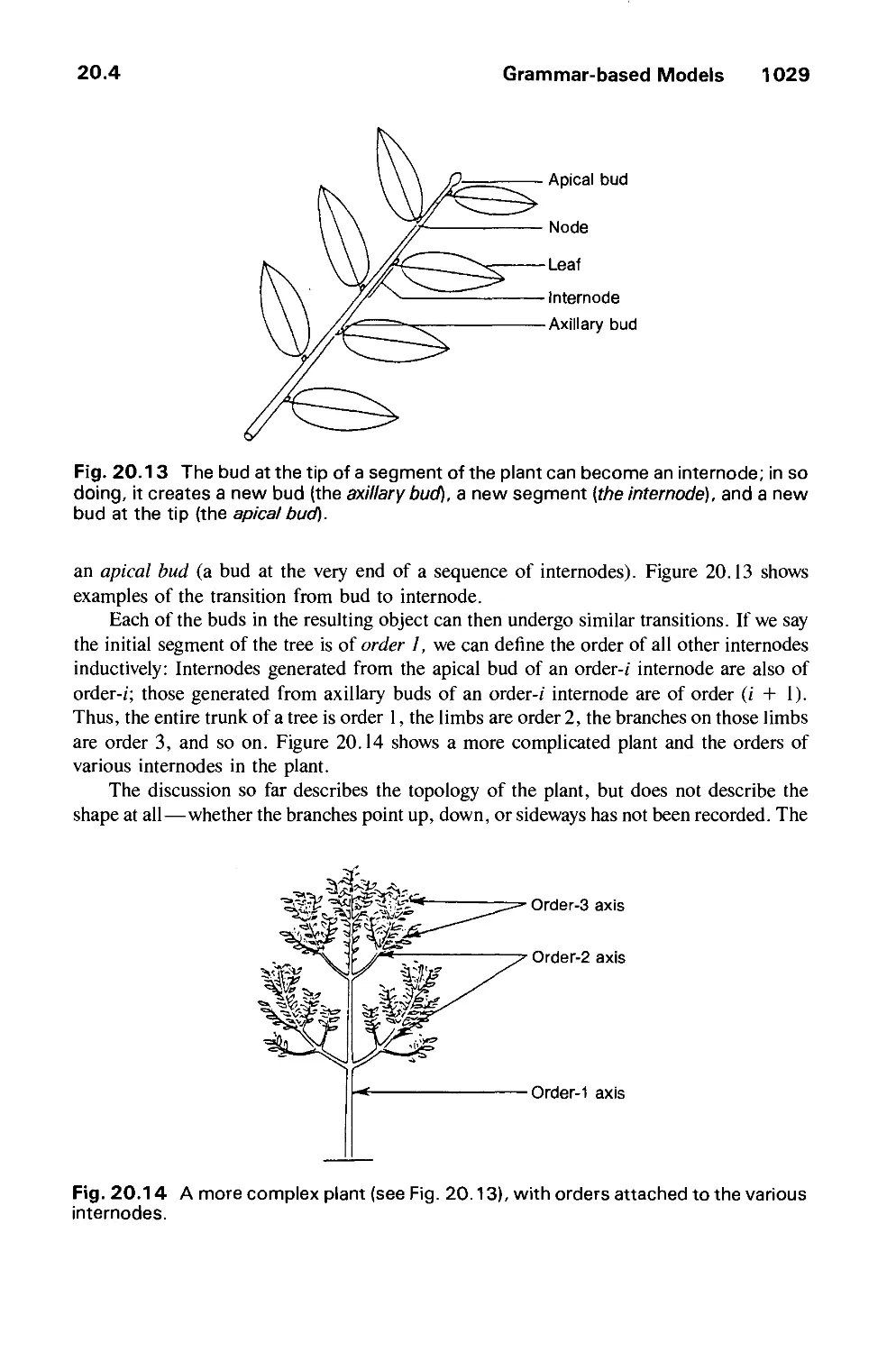
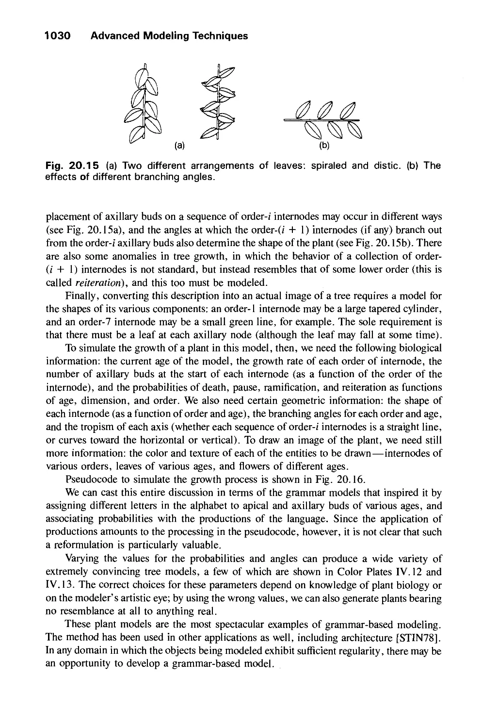
20.4 Grammar-Based Models 1027
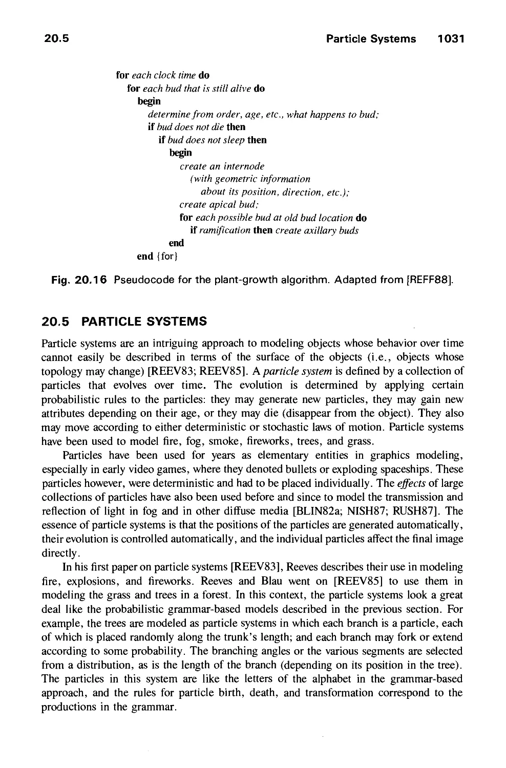
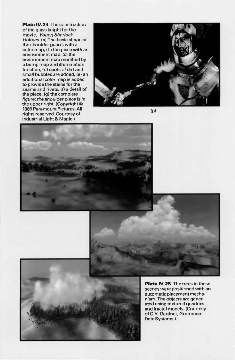
20.5 Particle Systems 1031
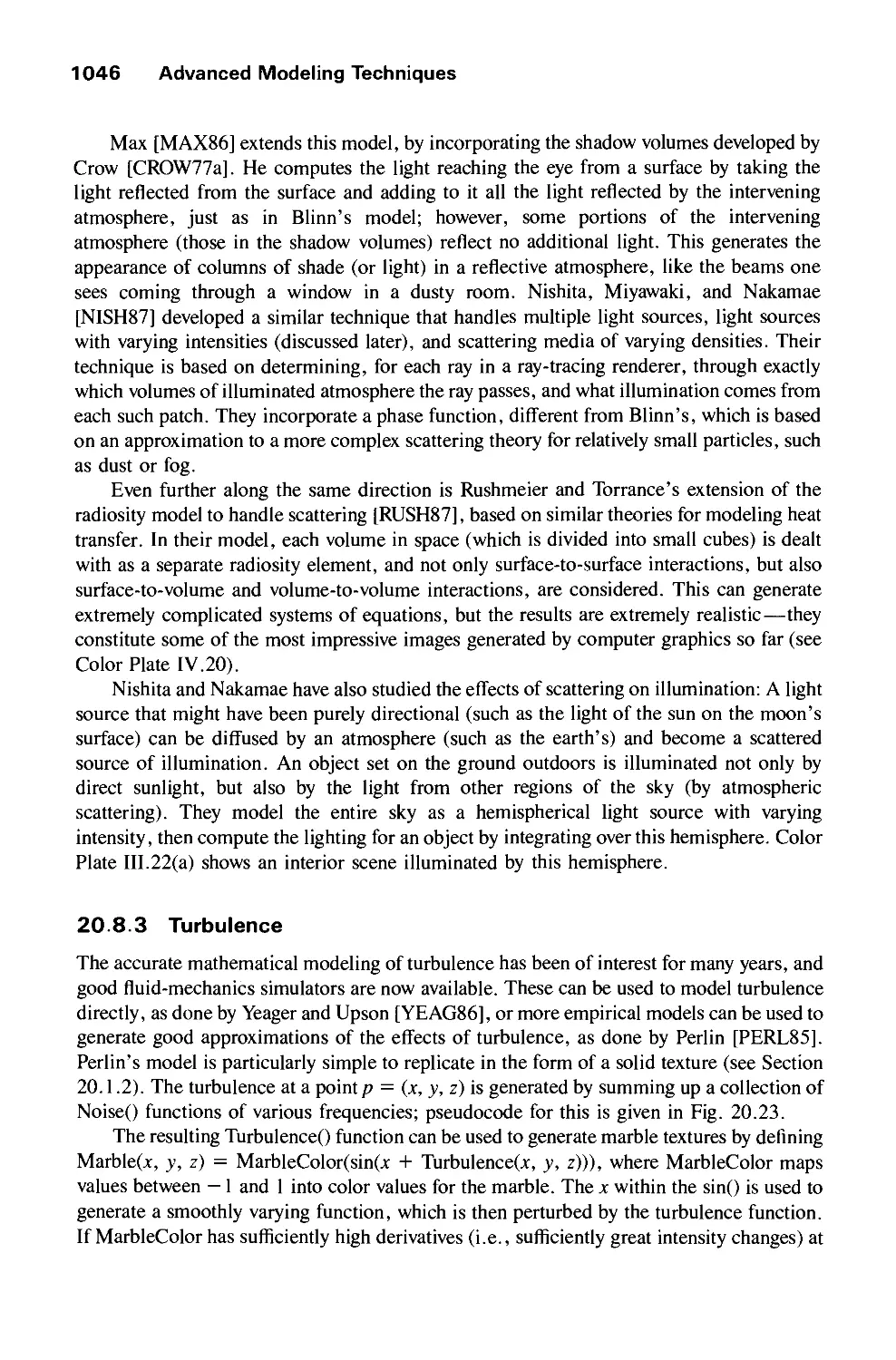
20.6 Volume Rendering 1034
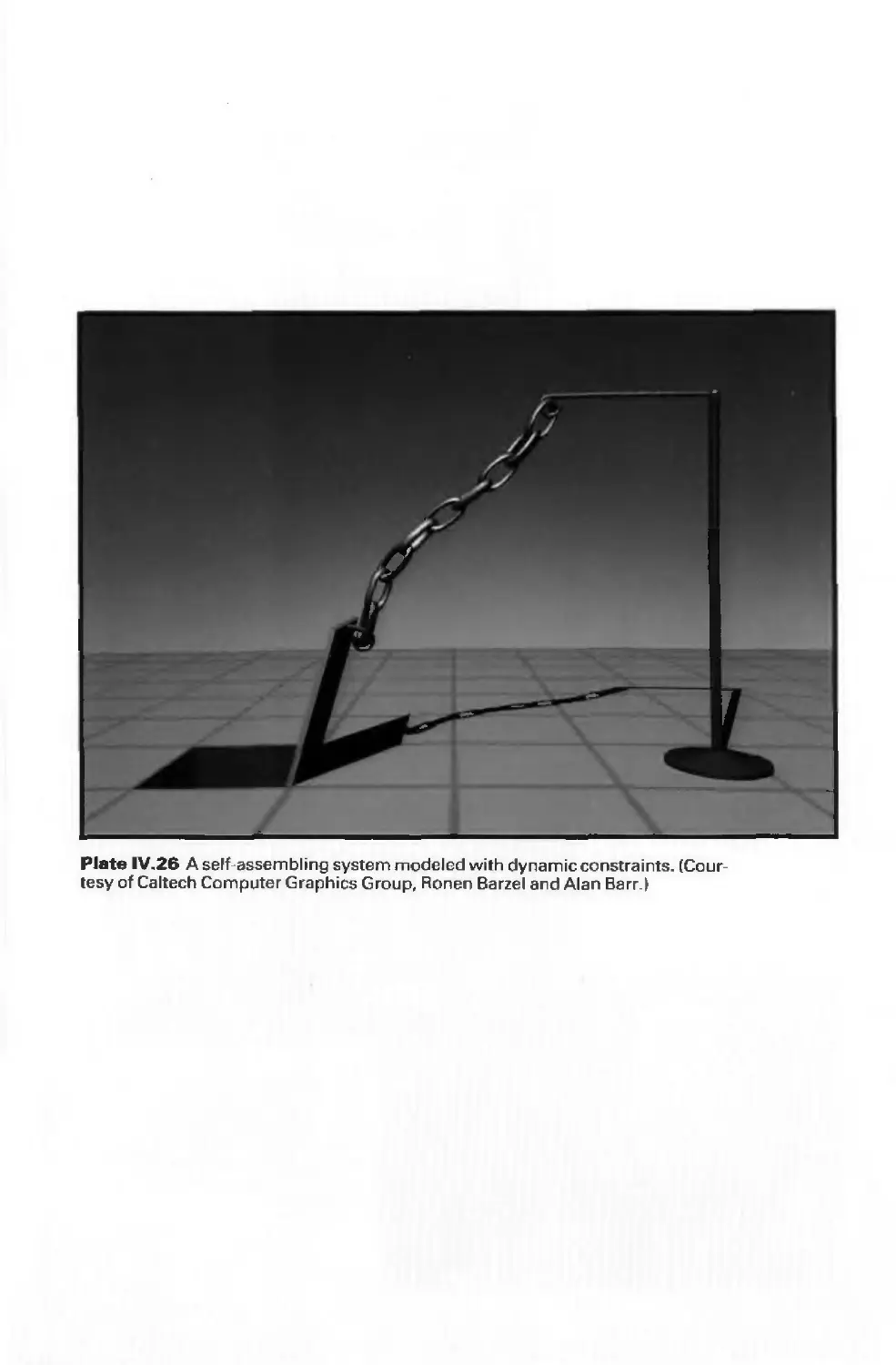
20.7 Physically Based Modeling 1039
20.8 Special Models for Natural and Synthetic Objects 1043
20.9 Automating Object Placement 1050
20.10 Summary 1054
Exercises 1054
CHAPTER 21
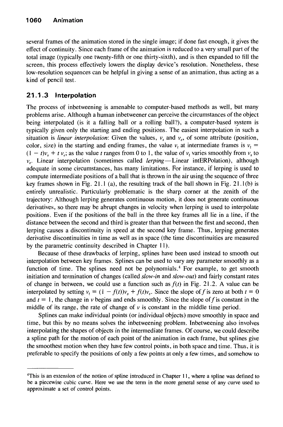
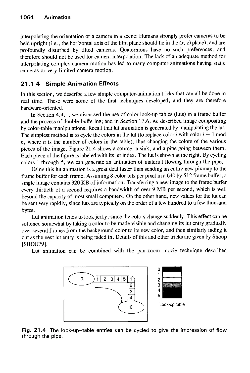
ANIMATION 1057
21.1 Conventional and Computer-Assisted Animation 1058
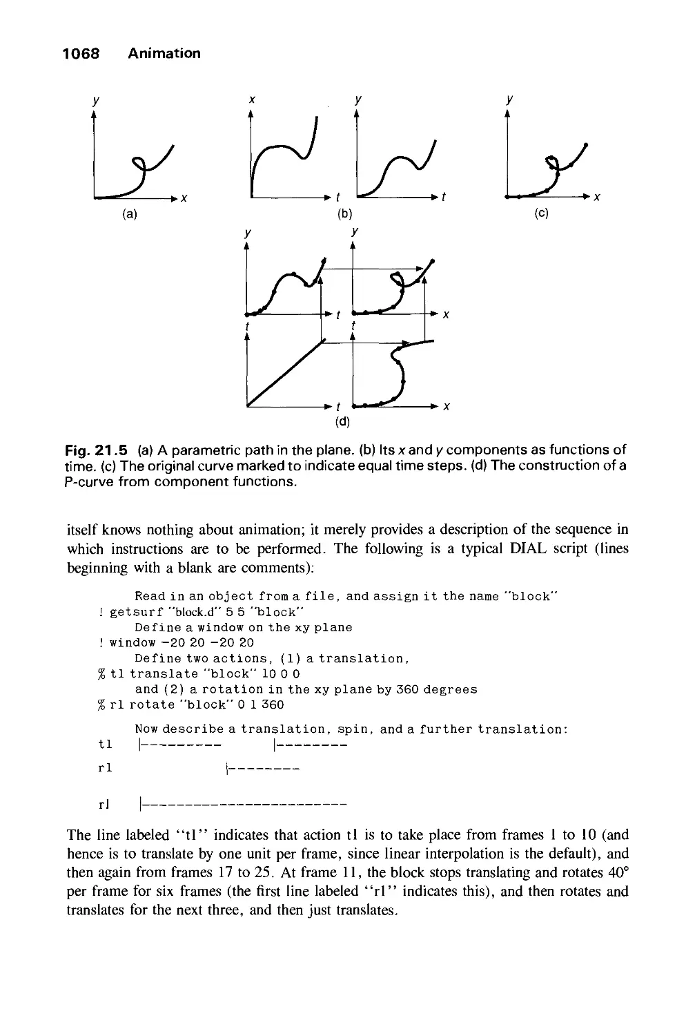
21.2 Animation Languages 1065
21.3 Methods of Controlling Animation 1070
21.4 Basic Rules of Animation 1077
21.5 Problems Peculiar to Animation 1078
21.6 Summary 1080
Exercises 1080
APPENDIX: MATHEMATICS FOR COMPUTER GRAPHICS 1083
A.l Vector Spaces and Affine Spaces 1083
A.2 Some Standard Constructions in Vector Spaces 1091
A.3 Dot Products and Distances 1094
A.4 Matrices 1103
A.5 Linear and Affine Transformations 1106
A.6 Eigenvalues and Eigenvectors 1108
A.7 Newton-Raphson Iteration for Root Finding 1109
Exercises 1111
BIBLIOGRAPHY 1113
INDEX 1153
1
Introduction
Computer graphics started with the display of data on hardcopy plotters and cathode ray
tube (CRT) screens soon after the introduction of computers themselves. It has grown to
include the creation, storage, and manipulation of models and images of objects. These
models come from a diverse and expanding set of fields, and include physical,
mathematical, engineering, architectural, and even conceptual (abstract) structures, natural
phenomena, and so on. Computer graphics today is largely interactive: The user controls the
contents, structure, and appearance of objects and of their displayed images by using input
devices, such as a keyboard, mouse, or touch-sensitive panel on the screen. Because of the
close relationship between the input devices and the display, the handling of such devices is
included in the study of computer graphics.
Until the early 1980s, computer graphics was a small, specialized field, largely because
the hardware was expensive and graphics-based application programs that were easy to use
and cost-effective were few. Then, personal computers with built-in raster graphics
displays—such as the Xerox Star and, later, the mass-produced, even less expensive Apple
Macintosh and the IBM PC and its clones—popularized the use of bitmap graphics for
user-computer interaction. A bitmap is a ones and zeros representation of the rectangular
array of points (pixels or pels, short for "picture elements") on the screen. Once bitmap
graphics became affordable, an explosion of easy-to-use and inexpensive graphics-based
applications soon followed. Graphics-based user interfaces allowed millions of new users to
control simple, low-cost application programs, such as spreadsheets, word processors, and
drawing programs.
The concept of a "desktop" now became a popular metaphor for organizing screen
space. By means of a window manager, the user could create, position, and resize
1
2 Introduction
rectangular screen areas, called windows, that acted as virtual graphics terminals, each
running an application. This allowed users to switch among multiple activities just by
pointing at the desired window, typically with the mouse. Like pieces of paper on a messy
desk, windows could overlap arbitrarily. Also part of this desktop metaphor were displays
of icons that represented not just data files and application programs, but also common
office objects, such as file cabinets, mailboxes, printers, and trashcans, that performed the
computer-operation equivalents of their real-life counterparts. Direct manipulation of
objects via "pointing and clicking" replaced much of the typing of the arcane commands
used in earlier operating systems and computer applications. Thus, users could select icons
to activate the corresponding programs or objects, or select buttons on pull-down or pop-up
screen menus to make choices. Today, almost all interactive application programs, even
those for manipulating text (e.g., word processors) or numerical data (e.g., spreadsheet
programs), use graphics extensively in the user interface and for visualizing and
manipulating the application-specific objects. Graphical interaction via raster displays
(displays using bitmaps) has replaced most textual interaction with alphanumeric terminals.
Even people who do not use computers in their daily work encounter computer
graphics in television commercials and as cinematic special effects. Computer graphics is
no longer a rarity. It is an integral part of all computer user interfaces, and is indispensable
for visualizing two-dimensional (2D), three-dimensional (3D), and higher-dimensional
objects: Areas as diverse as education, science, engineering, medicine, commerce, the
military, advertising, and entertainment all rely on computer graphics. Learning how to
program and use computers now includes learning how to use simple 2D graphics as a
matter of routine.
1.1 IMAGE PROCESSING AS PICTURE ANALYSIS
Computer graphics concerns the pictorial synthesis of real or imaginary objects from their
computer-based models, whereas the related field of image processing (also called picture
processing) treats the converse process: the analysis of scenes, or the reconstruction of
models of 2D or 3D objects from their pictures. Picture analysis is important in many
arenas: aerial surveillance photographs, slow-scan television images of the moon or of
planets gathered from space probes, television images taken from an industrial robot's
"eye," chromosome scans, X-ray images, computerized axial tomography (CAT) scans,
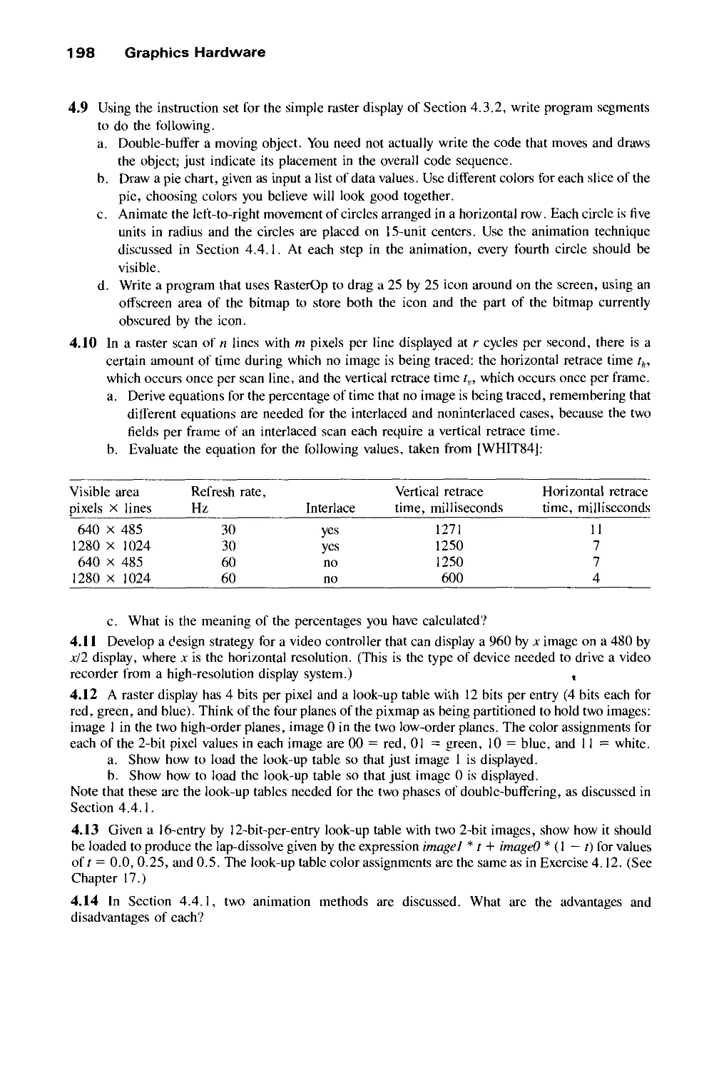
and fingerprint analysis all exploit image-processing technology (see Color Plate 1.1).
Image processing has the subareas image enhancement, pattern detection and recognition,
and scene analysis and computer vision. Image enhancement deals with improving image
quality by eliminating noise (extraneous or missing pixel data) or by enhancing contrast.
Pattern detection and recognition deal with detecting and clarifying standard patterns and
finding deviations (distortions) from these patterns. A particularly important example is
optical character recognition (OCR) technology, which allows for the economical bulk
input of pages of typeset, typewritten, or even handprinted characters. Scene analysis and
computer vision allow scientists to recognize and reconstruct a 3D model of a scene from
several 2D images. An example is an industrial robot sensing the relative sizes, shapes,
positions, and colors of parts on a conveyor belt.
1.2
The Advantages of Interactive Graphics 3
Although both computer graphics and image processing deal with computer processing
of pictures, they have until recently been quite separate disciplines. Now that they both use
raster displays, however, the overlap between the two is growing, as is particularly evident in
two areas. First, in interactive image processing, human input via menus and other
graphical interaction techniques helps to control various subprocesses while
transformations of continuous-tone images are shown on the screen in real time. For example,
scanned-in photographs are electronically touched up, cropped, and combined with others
(even with synthetically generated images) before publication. Second, simple image-
processing operations are often used in computer graphics to help synthesize the image of a
model. Certain ways of transforming and combining synthetic images depend largely on
image-processing operations.
1.2 THE ADVANTAGES OF INTERACTIVE GRAPHICS
Graphics provides one of the most natural means of communicating with a computer, since
our highly developed 2D and 3D pattern-recognition abilities allow us to perceive and
process pictorial data rapidly and efficiently. In many design, implementation, and
construction processes today, the information pictures can give is virtually indispensable.
Scientific visualization became an important field in the late 1980s, when scientists and
engineers realized that they could not interpret the prodigious quantities of data produced in
supercomputer runs without summarizing the data and highlighting trends and phenomena
in various kinds of graphical representations.
Creating and reproducing pictures, however, presented technical problems that stood in
the way of their widespread use. Thus, the ancient Chinese proverb "a picture is worth ten
thousand words" became a cliche in our society only after the advent of inexpensive and
simple technology for producing pictures—first the printing press, then photography.
Interactive computer graphics is the most important means of producing pictures since
the invention of photography and television; it has the added advantage that, with the
computer, we can make pictures not only of concrete, "real-world" objects but also of
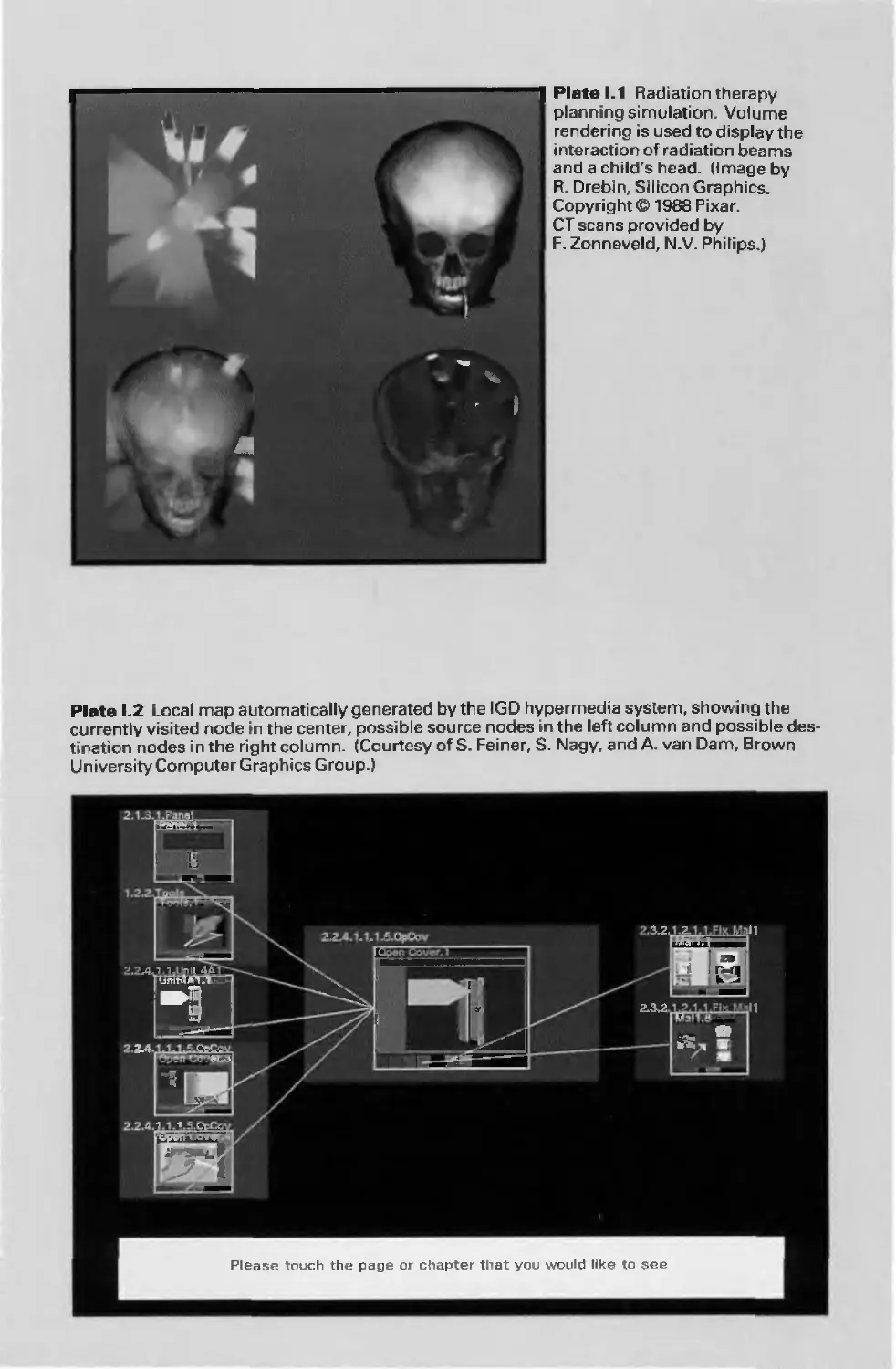
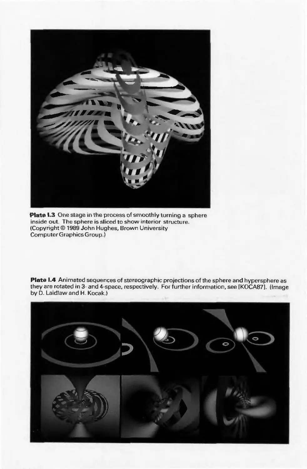
abstract, synthetic objects, such as mathematical surfaces in 4D (see Color Plates 1.3 and
1.4), and of data that have no inherent geometry, such as survey results. Furthermore, we
are not confined to static images. Although static pictures are a good means of
communicating information, dynamically varying pictures are frequently even better—to
coin a phrase, a moving picture is worth ten thousand static ones. This is especially true for
time-varying phenomena, both real (e.g., the deflection of an aircraft wing in supersonic
flight, or the development of a human face from childhood through old age) and abstract
(e.g., growth trends, such as nuclear energy use in the United States or population
movement from cities to suburbs and back to the cities). Thus, a movie can show changes
over time more graphically than can a sequence of slides. Similarly, a sequence of frames
displayed on a screen at more than 15 frames per second can convey smooth motion or
changing form better than can a jerky sequence, with several seconds between individual
frames. The use of dynamics is especially effective when the user can control the animation
by adjusting the speed, the portion of the total scene in view, the amount of detail shown,
the geometric relationship of the objects in the scene to one another, and so on. Much of
4 Introduction
interactive graphics technology therefore contains hardware and software for user-
controlled motion dynamics and update dynamics.
With motion dynamics, objects can be moved and tumbled with respect to a stationary
observer. The objects can also remain stationary and the viewer can move around them, pan
to select the portion in view, and zoom in or out for more or less detail, as though looking
through the viewfinder of a rapidly moving video camera. In many cases, both the objects
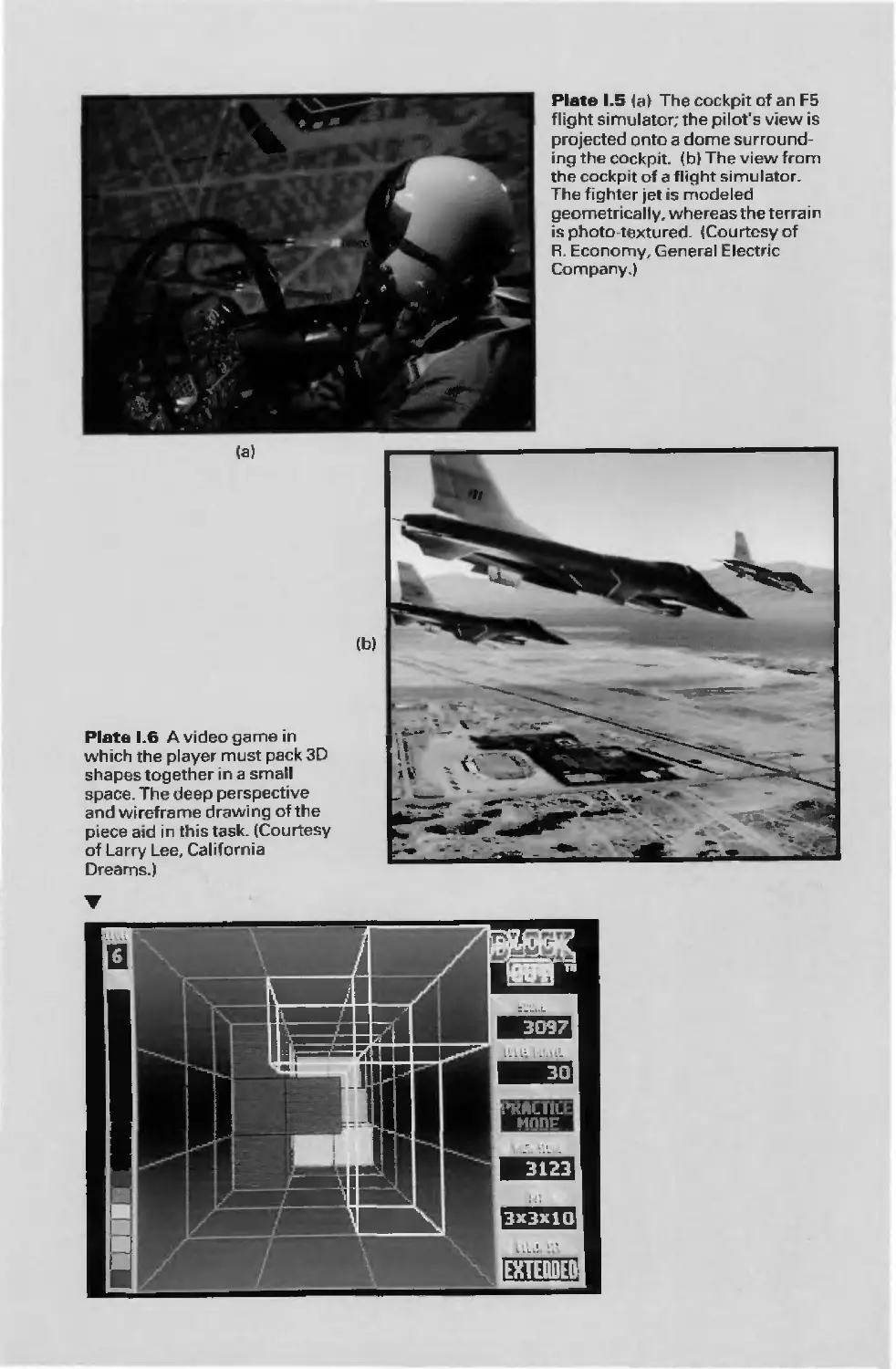
and the camera are moving. A typical example is the flight simulator (Color Plates 1.5a and
1.5b), which combines a mechanical platform supporting a mock cockpit with display
screens for windows. Computers control platform motion, gauges, and the simulated world
of both stationary and moving objects through which the pilot navigates. These
multimillion-dollar systems train pilots by letting the pilots maneuver a simulated craft over
a simulated 3D landscape and around simulated vehicles. Much simpler flight simulators
are among the most popular games on personal computers and workstations. Amusement
parks also offer "motion-simulator" rides through simulated terrestrial and extraterrestrial
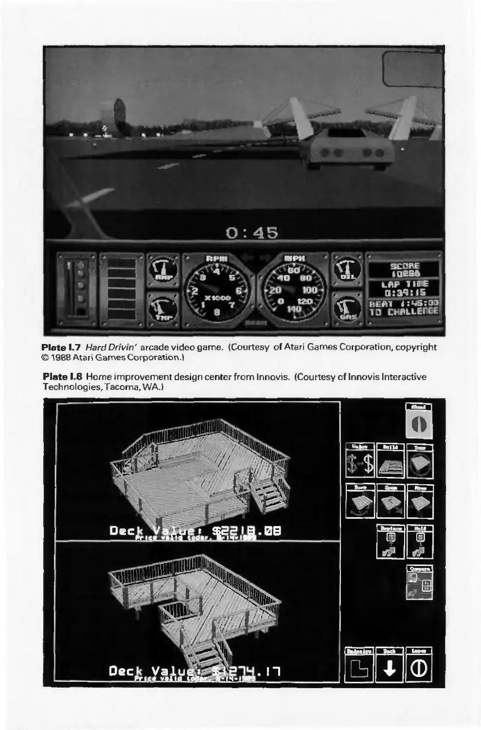
landscapes. Video arcades offer graphics-based dexterity games (see Color Plate 1.6) and
racecar-driving simulators, video games exploiting interactive motion dynamics: The player
can change speed and direction with the "gas pedal" and "steering wheel," as trees,
buildings, and other cars go whizzing by (see Color Plate 1.7). Similarly, motion dynamics
lets the user fly around and through buildings, molecules, and 3D or 4D mathematical
space. In another type of motion dynamics, the "camera" is held fixed, and the objects in
the scene are moved relative to it. For example, a complex mechanical linkage, such as the
linkage on a steam engine, can be animated by moving or rotating all the pieces appropriately.
Update dynamics is the actual change of the shape, color, or other properties of the
objects being viewed. For instance, a system can display the deformations of an airplane
structure in flight or the state changes in a block diagram of a nuclear reactor in response to
the operator's manipulation of graphical representations of the many control mechanisms.
The smoother the change, the more realistic and meaningful the result. Dynamic interactive
graphics offers a large number of user-controllable modes with which to encode and
communicate information: the 2D or 3D shape of objects in a picture, their gray scale or
color, and the time variations of these properties. With the recent development of digital
signal processing (DSP) and audio synthesis chips, audio feedback can now be provided to
augment the graphical feedback and to make the simulated environment even more
realistic.
Interactive computer graphics thus permits extensive, high-bandwidth user-computer
interaction. This significantly enhances our ability to understand data, to perceive trends,
and to visualize real or imaginary objects—indeed, to create "virtual worlds" that we can
explore from arbitrary points of view (see Color Plate B). By making communication more
efficient, graphics makes possible higher-quality and more precise results or products,
greater productivity, and lower analysis and design costs.
1.3 REPRESENTATIVE USES OF COMPUTER GRAPHICS
Computer graphics is used today in many different areas of industry, business, government,
education, entertainment, and, most recently, the home. The list of applications is
1.3
Representative Uses of Computer Graphics 5
enormous and is growing rapidly as computers with graphics capabilities become
commodity products. Let's look at a representative sample of these areas.
■ User interfaces. As we mentioned, most applications that run on personal computers
and workstations, and even those that run on terminals attached to time-shared computers
and network compute servers, have user interfaces that rely on desktop window systems to
manage multiple simultaneous activities, and on point-and-click facilities to allow users to
select menu items, icons, and objects on the screen; typing is necessary only to input text to
be stored and manipulated. Word-processing, spreadsheet, and desktop-publishing
programs are typical applications that take advantage of such user-interface techniques. The
authors of this book used such programs to create both the text and the figures; then, the
publisher and their contractors produced the book using similar typesetting, drawing, and
page-layout software.
■ (Interactive) plotting in business, science, and technology. The next most common use
of graphics today is probably to create 2D and 3D graphs of mathematical, physical, and
economic functions; histograms, bar and pie charts; task-scheduling charts; inventory and
production charts; and the like. All these are used to present meaningfully and concisely the
trends and patterns gleaned from data, so as to clarify complex phenomena and to facilitate
informed decision making.
■ Office automation and electronic publishing. The use of graphics for the creation and
dissemination of information has increased enormously since the advent of desktop
publishing on personal computers. Many organizations whose publications used to be
printed by outside specialists can now produce printed materials inhouse. Office
automation and electronic publishing can produce both traditional printed (hardcopy) documents
and electronic (softcopy) documents that contain text, tables, graphs, and other forms of
drawn or scanned-in graphics. Hypermedia systems that allow browsing of networks of
interlinked multimedia documents are proliferating (see Color Plate 1.2).
■ Computer-aided drafting and design. In computer-aided design (CAD), interactive
graphics is used to design components and systems of mechanical, electrical,
electromechanical, and electronic devices, including structures such as buildings, automobile bodies,
airplane and ship hulls, very large-scale-integrated (VLSI) chips, optical systems, and
telephone and computer networks. Sometimes, the user merely wants to produce the precise
drawings of components and assemblies, as for online drafting or architectural blueprints.
Color Plate 1.8 shows an example of such a 3D design program, intended for
nonprofessionals: a "customize your own patio deck" program used in lumber yards. More frequently,
however, the emphasis is on interacting with a computer-based model of the component or
system being designed in order to test, for example, its structural, electrical, or thermal
properties. Often, the model is interpreted by a simulator that feeds back the behavior of the
system to the user for further interactive design and test cycles. After objects have been
designed, utility programs can postprocess the design database to make parts lists, to
process "bills of materials," to define numerical control tapes for cutting or drilling parts,
and so on.
■ Simulation and animation for scientific visualization and entertainment. Computer-
produced animated movies and displays of the time-varying behavior of real and simulated
6 Introduction
objects are becoming increasingly popular for scientific and engineering visualization (see
Color Plate 1.10). We can use them to study abstract mathematical entities as well as
mathematical models of such phenomena as fluid flow, relativity, nuclear and chemical
reactions, physiological system and organ function, and deformation of mechanical
structures under various kinds of loads. Another advanced-technology area is interactive
cartooning. The simpler kinds of systems for producing "flat" cartoons are becoming
cost-effective in creating routine "in-between" frames that interpolate between two
explicitly specified "key frames." Cartoon characters will increasingly be modeled in the
computer as 3D shape descriptions whose movements are controlled by computer
commands, rather than by the figures being drawn manually by cartoonists (see Color
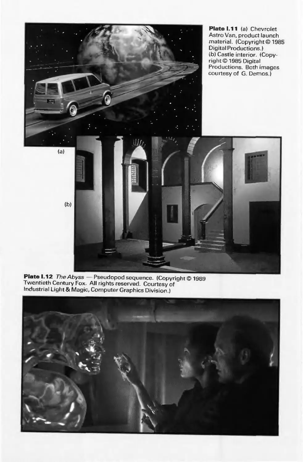
Plates A, D, F). Television commercials featuring flying logos and more exotic visual
trickery have become common, as have elegant special effects in movies (see Color Plates
1.11 —1.13, C and G). Sophisticated mechanisms are available to model the objects and to
represent light and shadows.
■ Art and commerce. Overlapping the previous category is the use of computer graphics
in art and advertising; here, computer graphics is used to produce pictures that express a
message and attract attention (see Color Plates 1.9 and H). Personal computers and Teletext
and Videotex terminals in public places such as museums, transportation terminals,
supermarkets, and hotels, as well as in private homes, offer much simpler but still
informative pictures that let users orient themselves, make choices, or even "teleshop" and
conduct other business transactions. Finally, slide production for commercial, scientific, or
educational presentations is another cost-effective use of graphics, given the steeply rising
labor costs of the traditional means of creating such material.
■ Process control. Whereas flight simulators or arcade games let users interact with a
simulation of a real or artificial world, many other applications enable people to interact
with some aspect of the real world itself. Status displays in refineries, power plants, and
computer networks show data values from sensors attached to critical system components,
so that operators can respond to problematic conditions. For example, military
commanders view field data—number and position of vehicles, weapons launched, troop movements,
casualties—on command and control displays to revise their tactics as needed; flight
controllers at airports see computer-generated identification and status information for the
aircraft blips on their radar scopes, and can thus control traffic more quickly and accurately
than they could with the unannotated radar data alone; spacecraft controllers monitor
telemetry data and take corrective action as needed.
■ Cartography. Computer graphics is used to produce both accurate and schematic
representations of geographical and other natural phenomena from measurement data.
Examples include geographic maps, relief maps, exploration maps for drilling and mining,
oceanographic charts, weather maps, contour maps, and population-density maps.
1.4 CLASSIFICATION OF APPLICATIONS
The diverse uses of computer graphics listed in the previous section differ in a variety of
ways, and a number of classifications may be used to categorize them. The first
1 -4 Classification of Applications 7
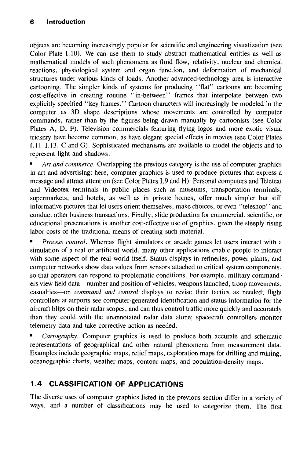
classification is by type (dimensionality) of the object to be represented and the kind of
picture to be produced. The range of possible combinations is indicated in Table 1.1.
Some of the objects represented graphically are clearly abstract, some are real;
similarly, the pictures can be purely symbolic (a simple 2D graph) or realistic (a rendition
of a still life). The same object can, of course, be represented in a variety of ways. For
example, an electronic printed circuit board populated with integrated circuits can be
portrayed by many different 2D symbolic representations or by 3D synthetic photographs of
the board.
The second classification is by the type of interaction, which determines the user's
degree of control over the object and its image. The range here includes offline plotting, with
a predefined database produced by other application programs or digitized from physical
models; interactive plotting, in which the user controls iterations of "supply some
parameters, plot, alter parameters, replot"; predefining or calculating the object and flying
around it in real time under user control, as in real-time animation systems used for
scientific visualization and flight simulators; and interactive designing, in which the user
starts with a blank screen, defines new objects (typically by assembling them from
predefined components), and then moves around to get a desired view.
The third classification is by the role of the picture, or the degree to which the picture is
an end in itself or is merely a means to an end. In cartography, drafting, raster painting,
animation, and artwork, for example, the drawing is the end product; in many CAD
applications, however, the drawing is merely a representation of the geometric properties of
the object being designed or analyzed. Here the drawing or construction phase is an
important but small part of a larger process, the goal of which is to create and postprocess a
common database using an integrated suite of application programs.
A good example of graphics in CAD is the creation of a VLSI chip. The engineer
makes a preliminary chip design using a CAD package. Once all the gates are laid, she then
subjects the chip to hours of simulated use. From the first run, for instance, she learns that
the chip works only at clock speeds above 80 nanoseconds (ns). Since the target clock speed
of the machine is 50 ns, the engineer calls up the initial layout and redesigns a portion of the
logic to reduce its number of stages. On the second simulation run, she learns that the chip
will not work at speeds below 60 ns. Once again, she calls up the drawing and redesigns a
portion of the chip. Once the chip passes all the simulation tests, she invokes a
postprocessor to create a database of information for the manufacturer about design and
materials specifications, such as conductor path routing and assembly drawings. In this
TABLE 1.1 CLASSIFICATION OF COMPUTER GRAPHICS BY
OBJECT AND PICTURE
Type of object Pictorial representation Example
2D Line drawing Fig. l.l
Gray scale image Fig. 17.10
Color image Color Plate 1.2
3D Line drawing (or wireframe) Color Plates II.21-11.23
Line drawing, with various effects Color Plates 11.24—11.27
Shaded, color image with various effects Color Plates II.28-11.38
8 Introduction
example, the representation of the chip's geometry produces output beyond the picture
itself. In fact, the geometry shown on the screen may contain less detail than the underlying
database.
A final categorization arises from the logical and temporal relationship between objects
and their pictures. The user may deal, for example, with only one picture at a time (typical
in plotting), with a time-varying sequence of related pictures (as in motion or update
dynamics), or with a structured collection of objects (as in many CAD applications that
contain hierarchies of assembly and subassembly drawings).
1.5 DEVELOPMENT OF HARDWARE AND SOFTWARE FOR
COMPUTER GRAPHICS
This book concentrates on fundamental principles and techniques that were derived in the
past and are still applicable today—and generally will be applicable in the future. In this
section, we take a brief look at the historical development of computer graphics, to place
today's systems in context. Fuller treatments of the interesting evolution of this field are
presented in [PRIN71], [MACH78], [CHAS81], and [CACM84]. It is easier to chronicle
the evolution of hardware than to document that of software, since hardware evolution has
had a greater influence on how the field developed. Thus, we begin with hardware.
Crude plotting on hardcopy devices such as teletypes and line printers dates from the
early days of computing. The Whirlwind Computer developed in 1950 at the Massachusetts
Institute of Technology (MIT) had computer-driven CRT displays for output, both for
operator use and for cameras producing hardcopy. The SAGE air-defense system developed
in the middle 1950s was the first to use command and control CRT display consoles on
which operators identified targets with light pens (hand-held pointing devices that sense
light emitted by objects on the screen). The beginnings of modern interactive graphics,
however, are found in Ivan Sutherland's seminal doctoral work on the Sketchpad drawing
system [SUTH63]. He introduced data structures for storing symbol hierarchies built up via
easy replication of standard components, a technique akin to the use of plastic templates for
drawing circuit symbols. He also developed interaction techniques that used the keyboard
and light pen for making choices, pointing, and drawing, and formulated many other
fundamental ideas and techniques still in use today. Indeed, many of the features
introduced in Sketchpad are found in the PHIGS graphics package discussed in Chapter 7.
At the same time, it was becoming clear to computer, automobile, and aerospace
manufacturers that CAD and computer-aided manufacturing (CAM) activities had
enormous potential for automating drafting and other drawing-intensive activities. The General
Motors DAC system [JACK64] for automobile design, and the Itek Digitek system
[CHAS81] for lens design, were pioneering efforts that showed the utility of graphical
interaction in the iterative design cycles common in engineering. By the mid-sixties, a
number of research projects and commercial products had appeared.
Since at that time computer input/output (I/O) was done primarily in batch mode using
punched cards, hopes were high for a breakthrough in interactive user-computer
communication. Interactive graphics, as "the window on the computer," was to be an integral part
of vastly accelerated interactive design cycles. The results were not nearly so dramatic,
1.5 Development of Hardware and Software for Computer Graphics 9
however, since interactive graphics remained beyond the resources of all but the most
technology-intensive organizations. Among the reasons for this were these:
■ The high cost of the graphics hardware, when produced without benefit of economies
of scale—at a time when automobiles cost a few thousand dollars, computers cost several
millions of dollars, and the first commercial computer displays cost more than a hundred
thousand dollars
■ The need for large-scale, expensive computing resources to support massive design
databases, interactive picture manipulation, and the typically large suite of postprocessing
programs whose input came from the graphics-design phase
■ The difficulty of writing large, interactive programs for the new time-sharing
environment at a time when both graphics and interaction were new to predominantly batch-
oriented FORTRAN programmers
■ One-of-a-kind, nonportable software, typically written for a particular manufacturer's
display device and produced without the benefit of modern software-engineering principles
for building modular, structured systems; when software is nonportable, moving to new
display devices necessitates expensive and time-consuming rewriting of working programs.
It was the advent of graphics-based personal computers, such as the Apple Macintosh
and the IBM PC, that finally drove down the costs of both hardware and software so
dramatically that millions of graphics computers were sold as "appliances" for office and
home; when the field started in the early sixties, its practitioners never dreamed that
personal computers featuring graphical interaction would become so common so soon.
1.5.1 Output Technology
The display devices developed in the mid-sixties and in common use until the mid-eighties
are called vector, stroke, line drawing, or calligraphic displays. The term vector is used as a
synonym for line here; a stroke is a short line, and characters are made of sequences of such
strokes. We shall look briefly at vector-system architecture, because many modern raster
graphics systems use similar techniques. A typical vector system consists of a display
processor connected as an I/O peripheral to the central processing unit (CPU), a display
buffer memory, and a CRT. The buffer stores the computer-produced display list or display
program; it contains point- and line-plotting commands with (jc, y) or (jc, y, z) endpoint
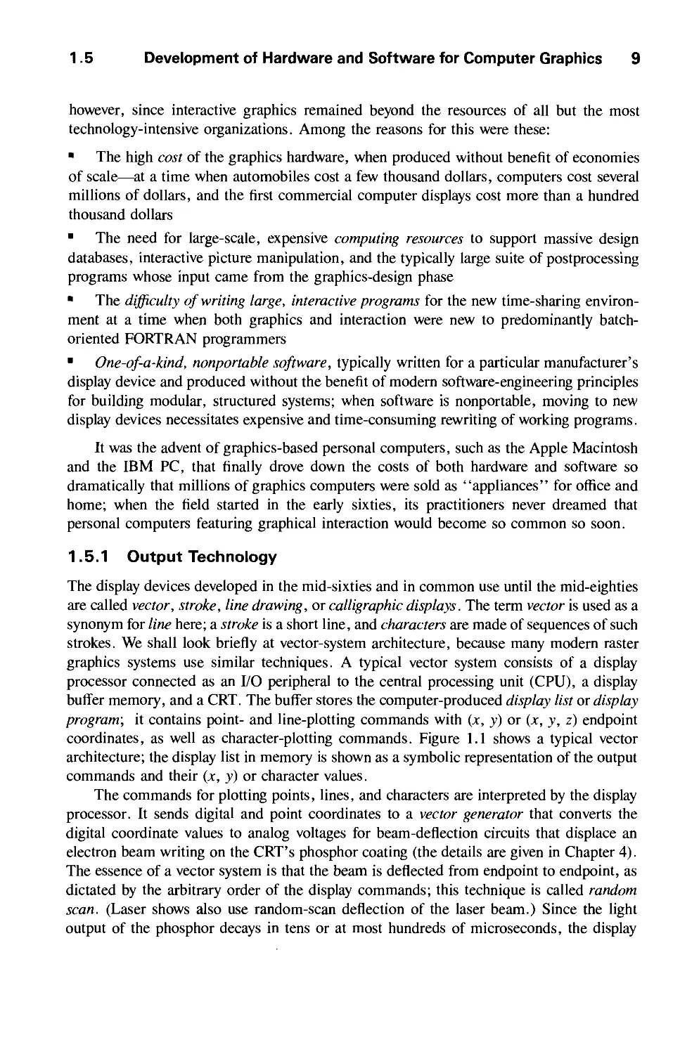
coordinates, as well as character-plotting commands. Figure 1.1 shows a typical vector
architecture; the display list in memory is shown as a symbolic representation of the output
commands and their (jc, y) or character values.
The commands for plotting points, lines, and characters are interpreted by the display
processor. It sends digital and point coordinates to a vector generator that converts the
digital coordinate values to analog voltages for beam-deflection circuits that displace an
electron beam writing on the CRT's phosphor coating (the details are given in Chapter 4).
The essence of a vector system is that the beam is deflected from endpoint to endpoint, as
dictated by the arbitrary order of the display commands; this technique is called random
scan. (Laser shows also use random-scan deflection of the laser beam.) Since the light
output of the phosphor decays in tens or at most hundreds of microseconds, the display
10 Introduction
Interface with host computer
I I
(Display commands) (Interaction data)
:<*-
MOVE
10
15
LINE
400
300
CHAR
Lu
cy
LINE
JMP
— 1
m J
Refresh buffer
Fig. 1.1 Architecture of a vector display.
processor must cycle through the display list to refresh the phosphor at least 30 times per
second (30 Hz) to avoid flicker; hence, the buffer holding the display list is usually called a
refresh buffer. Note that, in Fig. l.l, the jump instruction loops back to the top of the
display list to provide the cyclic refresh.
In the sixties, buffer memory and processors fast enough to refresh at (at least) 30 Hz
were expensive, and only a few thousand lines could be shown without noticeable flicker.
Then, in the late sixties, the direct-view storage tube (DVST) obviated both the buffer and
the refresh process, and eliminated all flicker. This was the vital step in making interactive
graphics affordable. A DVST stores an image by writing that image once with a relatively
slow-moving electron beam on a storage mesh in which the phosphor is embedded. The
small, self-sufficient DVST terminal was an order of magnitude less expensive than was the
typical refresh system; further, it was ideal for a low-speed (300- tol200-baud) telephone
interface to time-sharing systems. DVST terminals introduced many users and
programmers to interactive graphics.
Another major hardware advance of the late sixties was attaching the display to a
minicomputer; with this configuration, the central time-sharing computer was relieved of
the heavy demands of refreshed display devices, especially user-interaction handling, and
updating the image on the screen. The minicomputer typically ran application programs as
1.5 Development of Hardware and Software for Computer Graphics 11
well, and could in turn be connected to the larger central mainframe to run large analysis
programs. Both minicomputer and DVST configurations led to installations of thousands of
graphics systems. Also at this time, the hardware of the display processor itself was
becoming more sophisticated, taking over many routine but time-consuming jobs from the
graphics software. Foremost among such devices was the invention in 1968 of refresh
display hardware for geometric transformations that could scale, rotate, and translate points
and lines on the screen in real time, could perform 2D and 3D clipping, and could produce
parallel and perspective projections (see Chapter 6).
The development in the early seventies of inexpensive raster graphics, based on
television technology, contributed more to the growth of the field than did any other
technology. Raster displays store the display primitives (such as lines, characters, and
solidly shaded or patterned areas) in a refresh buffer in terms of their component pixels, as
shown in Fig. 1.2. In some raster displays, there is a hardware display controller that
receives and interprets sequences of output commands similar to those of the vector displays
(as shown in the figure); in simpler, more common systems, such as those in personal
computers, the display controller exists only as a software component of the graphics
library package, and the refresh buffer is just a piece of the CPU's memory that can be read
out by the image display subsystem (often called the video controller) that produces the
actual image on the screen.
The complete image on a raster display is formed from the raster, which is a set of
horizontal raster lines, each a row of individual pixels; the raster is thus stored as a matrix
of pixels representing the entire screen area. The entire image is scanned out sequentially by
Interface with host computer
I t
(Display commands) (Interaction data)
I
000000000000000000000000000000000000
000000000000000000000001110000000000
000000000000000000000111000000000000
000000000000000000000011 000000000000
000000000000000000000000110000000000
000000000000000011100000000000000000
0000000000001 UUUUU 0000000000000
000000011111111111111111111100000000
000000011111110000000111111100000000
000000011111111111111111111100000000
000000011111111100011111111100000000
000000011111111100011111111100000000
000000011111111100011111111100000000
000000011111111100011111111100000000
000000011111111111111111111100000000
000000000000000000000000000000000000
fc Display controller
"^ (DC)
Keyboard
Mouse
Video controller
n
Refresh buffer
Fig. 1.2 Architecture of a raster display.
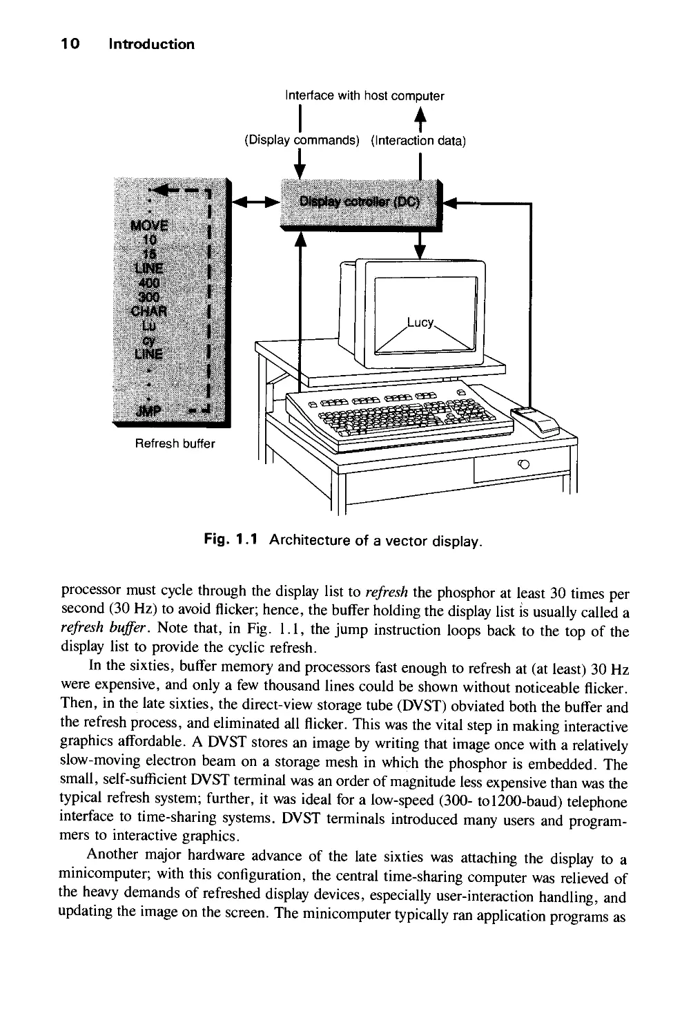
12 Introduction
the video controller, one raster line at a time, from top to bottom and then back to the top
(as shown in Fig. 1.3). At each pixel, the beam's intensity is set to reflect the pixel's
intensity; in color systems, three beams are controlled—one each for the red, green, and
blue primary colors—as specified by the three color components of each pixel's value (see
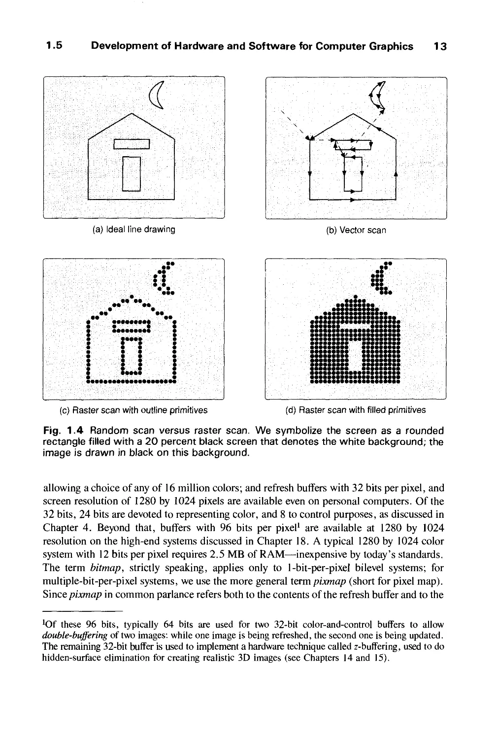
Chapters 4 and 13). Figure 1.4 shows the difference between random and raster scan for
displaying a simple 2D line drawing of a house (part a). In part (b), the vector arcs are
notated with arrowheads showing the random deflection of the beam. Dotted lines denote
deflection of the beam, which is not turned on ("blanked"), so that no vector is drawn. Part
(c) shows the unfilled house rendered by rectangles, polygons, and arcs, whereas part (d)
shows a filled version. Note the jagged appearance of the lines and arcs in the raster scan
images of parts (c) and (d); we shall discuss that visual artifact shortly.
In the early days of raster graphics, refreshing was done at television rates of 30 Hz;
today, a 60^Hz or higher refresh rate is used to avoid flickering of the image. Whereas in a
vector system the refresh buffer stored op-codes and endpoint coordinate values, in a raster
system the entire image of, say, 1024 lines of 1024 pixels each must be stored explicitly.
The term bitmap is still in common use to describe both the refresh buffer and the array of
pixel values that map one for one to pixels on the screen. Bitmap graphics has the advantage
over vector graphics that the actual display of the image is handled by inexpensive scan-out
logic: The regular, repetitive raster scan is far easier and less expensive to implement than is
the random scan of vector systems, whose vector generators must be highly accurate to
provide linearity and repeatability of the beam's deflection.
The availability of inexpensive solid-state random-access memory (RAM) for bitmaps
in the early seventies was the breakthrough needed to make raster graphics the dominant
hardware technology. Bilevel (also called monochrome) CRTs draw images in black and
white or black and green; some plasma panels use orange and black. Bilevel bitmaps contain
a single bit per pixel, and the entire bitmap for a screen with a resolution of 1024 by 1024
pixels is only 220 bits, or about 128,000 bytes. Low-end color systems have 8 bits per pixel,
allowing 256 colors simultaneously; more expensive systems have 24 bits per pixel,
Scan line
Horizontal retrace
/
*ss „--«- — -"""
x\ _----•"""""
— — — ""K*~ * ~"
- - - v ~ "* ~~ " "* "
— — — — — "^ "~ ~~
\ — — -_v" "~ """
X. _------"""'^
--^----'-"~"
Vertical retrace
Fig. 1.3 Raster scan.
1.5 Development of Hardware and Software for Computer Graphics 13
(a) Ideal line drawing
(b) Vector scan
•t
••
•
•
•
t
•
•
•
•
•
••
••
••
• •
• •
• •
• •
•••
•• ••
••
• •
: :
• •
• •
• •
• •
:...:
•••••••••••••••••••••
•••••
•••••••••
••••••••••a
••• •••••• •# ••'
••••••••••••••••••a
••••••••••••••I *
tm±tmttt|4|is
•••••••••
••••••••••••••••
•••••••••••••••••••a*
•••••••••••••••••••a*
(c) Raster scan with outline primitives
(d) Raster scan with filled primitives
Fig. 1.4 Random scan versus raster scan. We symbolize the screen as a rounded
rectangle filled with a 20 percent black screen that denotes the white background; the
image is drawn in black on this background.
allowing a choice of any of 16 million colors; and refresh buffers with 32 bits per pixel, and
screen resolution of 1280 by 1024 pixels are available even on personal computers. Of the
32 bits, 24 bits are devoted to representing color, and 8 to control purposes, as discussed in
Chapter 4. Beyond that, buffers with 96 bits per pixel1 are available at 1280 by 1024
resolution on the high-end systems discussed in Chapter 18. A typical 1280 by 1024 color
system with 12 bits per pixel requires 2.5 MB of RAM—inexpensive by today's standards.
The term bitmap, strictly speaking, applies only to 1-bit-per-pixel bilevel systems; for
multiple-bit-per-pixel systems, we use the more general term pixmap (short for pixel map).
Since pixmap in common parlance refers both to the contents of the refresh buffer and to the
'Of these 96 bits, typically 64 bits are used for two 32-bit color-and-control buffers to allow
double-buffering of two images: while one image is being refreshed, the second one is being updated.
The remaining 32-bit buffer is used to implement a hardware technique called z-buffering, used to do
hidden-surface elimination for creating realistic 3D images (see Chapters 14 and 15).
14 Introduction
buffer memory itself, we use the term frame buffer when we mean the actual buffer
memory.
The major advantages of raster graphics over vector graphics include lower cost and the
ability to display areas filled with solid colors or patterns, an especially rich means of
communicating information that is essential for realistic images of 3D objects.
Furthermore, the refresh process is independent of the complexity (number of polygons, etc.) of
the image, since the hardware is fast enough that each pixel in the buffer can be read out on
each refresh cycle. Most people do not perceive flicker on screens refreshed above 70 Hz. In
contrast, vector displays flicker when the number of primitives in the buffer becomes too
large; typically a maximum of a few hundred thousand short vectors may be displayed
flicker-free.
The major disadvantage of raster systems compared to vector systems arises from the
discrete nature of the pixel representation. First, primitives such as lines and polygons are
specified in terms of their endpoints (vertices) and must be scan-converted into their
component pixels in the frame buffer. The term derives from the notion that the
programmer specifies endpoint or vertex coordinates in random-scan mode, and this
information must be reduced by the system to pixels for raster-scan-mode display. Scan
conversion is commonly done with software in personal computers and low-end
workstations, where the microprocessor CPU is responsible for all graphics. For higher
performance, scan conversion can be done by special-purpose hardware, including raster
image processor chips used as coprocessors or accelerators.
Because each primitive must be scan-converted, real-time dynamics is far more
computationally demanding on raster systems than on vector systems. First, transforming
1000 lines on a vector system can mean transforming 2000 endpoints in the worst case. In
the next refresh cycle, the vector-generator hardware automatically redraws the transformed
lines in their new positions. In a raster system, however, not only must the endpoints be
transformed (using hardware transformation units identical to those used by vector
systems), but also each transformed primitive must then be scan-converted using its new
endpoints, which define its new size and position. None of the contents of the frame buffer
can be salvaged. When the CPU is responsible for both endpoint transformation and scan
conversion, only a small number of primitives can be transformed in real time.
Transformation and scan-conversion hardware is thus needed for dynamics in raster
systems; as a result of steady progress in VLSI, that has become feasible even in low-end
systems.
The second drawback of raster systems arises from the nature of the raster itself.
Whereas a vector system can draw a continuous, smooth line (and even some smooth
curves) from essentially any point on the CRT face to any other, the raster system can
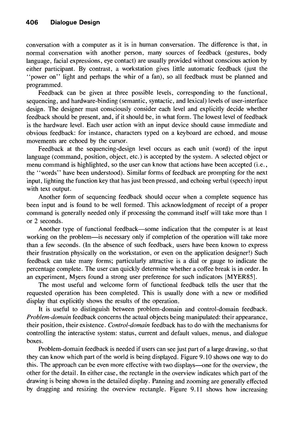
display mathematically smooth lines, polygons, and boundaries of curved primitives such
as circles and ellipses only by approximating them with pixels on the raster grid. This
causes the familiar problem of "jaggies" or "staircasing," as shown in Fig. 1.4 (c) and
(d). This visual artifact is a manifestation of a sampling error called aliasing in
signal-processing theory; such artifacts occur when a function of a continuous variable that
contains sharp changes in intensity is approximated with discrete samples. Both theory and
practice in modern computer graphics are concerned with techniques for antialiasing on
1.5 Development of Hardware and Software for Computer Graphics 15
gray-scale or color systems. These techniques specify gradations in intensity of neighboring
pixels at edges of primitives, rather than setting pixels to maximum or zero intensity only;
see Chapters 3, 14, and 19 for further discussion of this important topic.
1.5.2 Input Technology
Input technology has also improved greatly over the years. The clumsy, fragile light pen of
vector systems has been replaced by the ubiquitous mouse (first developed by office-
automation pioneer Doug Engelbart in the mid-sixties [ENGE68]), the data tablet, and the
transparent, touch-sensitive panel mounted on the screen. Even fancier input devices that
supply not just (x, y) locations on the screen, but also 3D and even higher-dimensional input
values (degrees of freedom), are becoming common, as discussed in Chapter 8. Audio
communication also has exciting potential, since it allows hands-free input and natural
output of simple instructions, feedback, and so on. With the standard input devices, the
user can specify operations or picture components by typing or drawing new information or
by pointing to existing information on the screen. These interactions require no knowledge
of programming and only a little keyboard use: The user makes choices simply by selecting
menu buttons or icons, answers questions by checking options or typing a few characters in
a form, places copies of predefined symbols on the screen, draws by indicating consecutive
endpoints to be connected by straight lines or interpolated by smooth curves, paints by
moving the cursor over the screen, and fills closed areas bounded by polygons or paint
contours with shades of gray, colors, or various patterns.
1.5.3 Software Portability and Graphics Standards
Steady advances in hardware technology have thus made possible the evolution of graphics
displays from one-of-a-kind special output devices to the standard human interface to the
computer. We may well wonder whether software has kept pace. For example, to what
extent have early difficulties with overly complex, cumbersome, and expensive graphics
systems and application software been resolved? Many of these difficulties arose from the
primitive graphics software that was available, and in general there has been a long, slow
process of maturation in such software. We have moved from low-level, device-dependent
packages supplied by manufacturers for their particular display devices to higher-level,
device-independent packages. These packages can drive a wide variety of display devices,
from laser printers and plotters to film recorders and high-performance real-time displays.
The main purpose of using a device-independent package in conjunction with a high-level
programming language is to promote application-program portability. This portability is
provided in much the same way as a high-level, machine-independent language (such as
FORTRAN, Pascal, or C) provides portability: by isolating the programmer from most
machine peculiarities and providing language features readily implemented on a broad
range of processors. "Programmer portability" is also enhanced in that programmers can
now move from system to system, or even from installation to installation, and find familiar
software.
A general awareness of the need for standards in such device-independent graphics
packages arose in the mid-seventies and culminated in a specification for a 3D Core
16 Introduction
Graphics System (the Core, for short) produced by an ACM SIGGRAPH2 Committee in
1977 [GSPC77] and refined in 1979 [GSPC79]. The first three authors of this book were
actively involved in the design and documentation of the 1977 Core.
The Core specification fulfilled its intended role as a baseline specification. Not only
did it have many implementations, but also it was used as input to official (governmental)
standards projects within both ANSI (the American National Standards Institute) and ISO
(the International Standards Organization). The first graphics specification to be officially
standardized was GKS (the Graphical Kernel System [ANSI85b]), an elaborated, cleaned-
up version of the Core that, unlike the Core, was restricted to 2D. In 1988, GKS-3D
[INTE88], a 3D extension of GKS, became an official standard, as did a much more
sophisticated but even more complex graphics system called PHIGS (Programmer's
Hierarchical Interactive Graphics System [ANSI88]). GKS supports the grouping of
logically related primitives—such as lines, polygons, and character strings—and their
attributes into collections called segments; these segments may not be nested. PHIGS, as its
name implies, does support nested hierarchical groupings of 3D primitives, called
structures. In PHIGS, all primitives, including invocations of substructures, are subject to
geometric transformations (scaling, rotation, and translation) to accomplish dynamic
movement. PHIGS also supports a retained database of structures that the programmer may
edit selectively; PHIGS automatically updates the screen whenever the database has been
altered. PHIGS has been extended with a set of features for modern, pseudorealistic
rendering3 of objects on raster displays; this extension is called PHIGS+ [PHIG88]. PHIGS
implementations are large packages, due to the many features and to the complexity of the
specification. PHIGS and especially PHIGS + implementations run best when there is
hardware support for their transformation, clipping, and rendering features.
This book discusses graphics software standards at some length. We first study SRGP
(the Simple Raster Graphics Package), which borrows features from Apple's popular
QuickDraw integer raster graphics package [ROSE85] and MIT's X Window System
[SCHE88a] for output and from GKS and PHIGS for input. Having looked at simple
applications in this low-level raster graphics package, we then study the scan-conversion
and clipping algorithms such packages use to generate images of primitives in the frame
buffer. Then, after building a mathematical foundation for 2D and 3D geometric
transformations and for parallel and perspective viewing in 3D, we study a far more
powerful package called SPHIGS (Simple PHIGS). SPHIGS is a subset of PHIGS that
operates on primitives defined in a floating-point, abstract, 3D world-coordinate system
2SIGGRAPH is the Special Interest Group on Graphics, one of the professional groups within ACM,
the Association for Computing Machinery. ACM is one of the two major professional societies for
computer professionals; the IEEE Computer Society is the other. SIGGRAPH publishes a research
journal and sponsors an annual conference that features presentations of research papers in the field
and an equipment exhibition. The Computer Society also publishes a research journal in graphics.
3A pseudorealistic rendering is one that simulates the simple laws of optics describing how light is
reflected by objects. Photorealistic rendering uses better approximations to the way objects reflect
and refract light; these approximations require more computation but produce images that are more
nearly photographic in quality (see Color Plate E).
1.6 Conceptual Framework for Interactive Graphics 17
independent of any type of display technology, and that supports some simple PHIGS +
features. We have oriented our discussion to PHIGS and PHIGS+ because we believe they
will have much more influence on interactive 3D graphics than will GKS-3D, especially
given the increasing availability of hardware that supports real-time transformations and
rendering of pseudorealistic images.
1.6 CONCEPTUAL FRAMEWORK FOR INTERACTIVE GRAPHICS
1.6.1 Overview
The high-level conceptual framework shown in Fig. 1.5 can be used to describe almost any
interactive graphics system. At the hardware level (not shown explicitly in the diagram), a
computer receives input from interaction devices, and outputs images to a display device.
The software has three components. The first is the application program; it creates, stores
into, and retrieves from the second component, the application model, which represents the
data or objects to be pictured on the screen. The application program also handles user
input. It produces views by sending to the third component, the graphics system, a series of
graphics output commands that contain both a detailed geometric description of what is to
be viewed and the attributes describing how the objects should appear. The graphics system
is responsible for actually producing the picture from the detailed descriptions and for
passing the user's input to the application program for processing.
The graphics system is thus an intermediary between the application program and the
display hardware that effects an output transformation from objects in the application model
to a view of the model. Symmetrically, it effects an input transformation from user actions
to inputs to the application program that will cause the application to make changes in the
model and/or picture. The fundamental task of the designer of an interactive graphics
application program is to specify what classes of data items or objects are to be generated
and represented pictorially, and how the user and the application program are to interact in
order to create and modify the model and its visual representation. Most of the
programmer's task concerns creating and editing the model and handling user interaction,
not actually creating views, since that is handled by the graphics system.
Application
model
Fig. 1.5 Conceptual framework for interactive graphics.
18 Introduction
1.6.2 Application Modeling
The application model captures all the data, objects, and relationships among them that are
relevant to the display and interaction part of the application program and to any
nongraphical postprocessing modules. Examples of such postprocessing modules are
analyses of the transient behavior of a circuit or of the stresses in an aircraft wing,
simulation of a population model or a weather system, and pricing computations for a
building. In the class of applications typified by "painting" programs such as MacPaint
and PCPaint, the intent of the program is to produce an image by letting the user set or
modify individual pixels. Here an explicit application model is not needed—the picture is
both means and end, and the displayed bitmap or pixmap serves in effect as the application
model.
More typically, however, there is an identifiable application model representing
application objects through some combination of data and procedural description that is
independent of a particular display device. Procedural descriptions are used, for example, to
define fractals, as described in Section 20.3. A data model can be as rudimentary as an
array of data points or as complex as a linked list representing a network data structure or a
relational database storing a set of relations. We often speak of storing the application
model in the application database; the terms are used interchangeably here. Models
typically store descriptions of primitives (points, lines and polygons in 2D or 3D, and
polyhedra and free-form surfaces in 3D) that define the shape of components of the object,
object attributes such as line style, color, or surface texture; and connectivity relationships
and positioning data that describe how the components fit together.
The objects stored in the model can differ greatly in the amount of intrinsic geometry
needed to specify them. At the geometry-is-everything end of the spectrum, an industrial
robot of the type discussed in Chapter 7 is described almost completely in terms of the
geometry of its component polyhedra, each of which is a collection of 3D polygonal facets
connected at common edges defined in terms of common vertices and enclosing a volume.
A spreadsheet has much less intrinsic geometry. The spatial relationships between adjacent
cells are stored, but the exact size or placement of each cell on the "paper" is not stored;
instead, these values are determined dynamically by the spreadsheet program as a function
of the contents of cells. At the geometry-free end of the spectrum, a demographic model
storing statistics, such as income and age of individuals in some population, has no intrinsic
geometry. These statistics can then be operated on by a procedure to derive some
geometrical interpretation, such as a 2D graph, scatter diagram, or histogram.
Another class of applications without intrinsic geometry deals with the directed-graph
networks used in various fields such as engineering and project management. These
networks may be represented internally by adjacency matrices describing how nodes are
connected, plus some property data for nodes and edges, and the application must then
derive a layout in a predefined format in order to create a view of the graph. This
representation might be created once and subsequently edited, as for a VLSI circuit layout
computed over many hours. The model would then contain both a nongeometric and an
almost purely geometric description of the circuit. Alternatively, if a layout for a particular
application is simple and fast enough to derive, such as a project-scheduling chart with
1.6
Conceptual Framework for Interactive Graphics 19
labeled boxes and arrows, it can be created on the fly each time the data on which it is based
change.
Geometric data in the application model often are accompanied by nongeometric
textual or numeric property information useful to a postprocessing program or the
interactive user. Examples of such data in CAD applications include manufacturing data;
"price and supplier" data; thermal, mechanical, electrical, or electronic properties; and
mechanical or electrical tolerances.
1.6.3 Describing to the Graphics System What Is to Be Viewed
The application program creates the application model either a priori as a result of prior
computation, as in an engineering or scientific simulation on a supercomputer, or as part of
an interactive session at the display device during which the user guides the construction
process step by step to choose components and geometric and nongeometric property data.
The user can ask the application program at any time to show a view of the model it has
created so far. (The word view is used intentionally here both in the sense of a visual
rendering of some geometric properties of the objects being modeled and in the technical
database sense of a 2D presentation of some properties of some subset of the model.)
Models are application-specific and are created independently of any particular display
system. Therefore, the application program must convert a description of the portion of the
model to be viewed from the internal representation of the geometry (whether explicitly
stored in the model or derived on the fly) to whatever procedure calls or commands the
graphics system uses to create an image. This conversion process has two phases. First, the
application program traverses the application database that stores the model in order to
extract the portions to be viewed, using some selection or query criteria. Then, the
extracted geometry is put in a format that can be sent to the graphics system. The selection
criteria can be geometric in nature (e.g., the portion of the model to be viewed has been
shifted via the graphics equivalent of a pan or zoom camera operation), or they can be
similar to traditional database query criteria (e.g., create a view of all the activities after
March 15, 1989 in the scheduling chart for producing this book).
The data extracted during the database traversal must either be geometric in nature or
must be converted to geometric data; the data can be described to the graphics system in
terms of both primitives that the system can display directly and attributes that control the
primitives' appearance. Display primitives typically match those stored in geometric
models: lines, rectangles, polygons, circles, ellipses, and text in 2D, and polygons,
polyhedra, and text in 3D. Advanced graphics systems such as PHIGS+ support additional
primitives, including curves and surfaces defined by polynomials of higher degrees.
If the model stores geometric primitives not directly supported by the graphics
package, the application program must reduce them to those that are accepted by the
system. For example, if spheres and free-form surfaces are not supported, the application
must approximate such surfaces by tiling or tesselating them with meshes of polygons that
the graphics system can handle. Appearance attributes supported by the graphics package
also tend to correspond to the ones stored in the model, such as color, line style, and line
width. In addition to primitives and attributes, advanced graphics packages such as PHIGS
20 Introduction
support facilities for specifying geometric transformations for scaling, rotating, and
positioning components, for specifying how components are to be viewed in 3D, and for
grouping logically related primitives, attributes, and transformations so that they can be
invoked by a single reference to a named structure.
The graphics system typically consists of a set of output subroutines corresponding to
the various primitives, attributes, and other elements. These are collected in a graphics-
subroutine library or package or can be called from high-level languages such as C, Pascal,
or LISP. The application program specifies geometric primitives and attributes to these
subroutines, and the subroutines then drive the specific display device and cause it to display
the image. Much as conventional I/O systems create logical I/O units to shield the
application programmer from the messy details of hardware and device drivers, graphics
systems create a logical display device. Thus, the graphics programmer can ignore such
details as which part of image generation is done in the display hardware and which is done
by the graphics package, or what the coordinate system of the display is. This abstraction of
the display device pertains both to the output of images and to interaction via logical input
devices. For example, the mouse, data tablet, touch panel, 2D joystick, or trackball can all
be treated as the locator logical input device that returns an (x, y) screen location. The
application program can ask the graphics system either to sample the input devices or to
wait at a specified point until an event is generated when the user activates a device being
waited on. With input values obtained from sampling or waiting for an event, the
application program can handle user interactions that alter the model or the display or that
change its operating mode.
1.6.4 Interaction Handling
The typical application-program schema for interaction handling is the event-driven loop. It
is easily visualized as a finite-state machine with a central wait state and transitions to other
states that are caused by user-input events. Processing a command may entail nested event
loops of the same format that have their own states and input transitions. An application
program may also sample input devices such as the locator by asking for their values at any
time; the program then uses the returned value as input to a processing procedure that also
changes the state of the application program, the image, or the database. The event-driven
loop is characterized by the following pseudocode schema:
generate initial display, derived from application model as appropriate
repeat
enable selection of commands or objects
{Program pauses indefinitely in "wait state" until user acts}
wait for user selection
case on selection
process selection to complete command or process completed command,
updating model and screen as needed
until quit {User has selected the "quit" option}
Let's examine the application's reaction to input in more detail. The application program
typically responds to user interactions in one of two modes. First, the user action may
require only that the screen be updated—for example, by highlighting of a selected object
1.7
Summary 21
or by making available a new menu of choices. The application then needs only to update its
internal state and to call the graphics package to update the screen; it does not need not to
update the database. If, however, the user action calls for a change in the model—for
example, by adding or deleting a component—the application must update the model and
then call the graphics package to update the screen from the model. Either the entire model
is retraversed to regenerate the image from scratch, or, with more sophisticated incremen-
tal-update algorithms, the screen is updated selectively. It is important to understand that
no significant change can take place in the objects on the screen without a corresponding
change in the model. The screen is indeed the window on the computer in that the user, in
general, is manipulating not an image but the model that is literally and figuratively behind
the image. Only in painting and image-enhancement applications are the model and the
image identical. Therefore, it is the application's job to interpret user input. The graphics
system has no responsibility for building or modifying the model, either initially or in
response to user interaction; its only job is to create images from geometric descriptions and
to pass aloiig'the user's input data.
The event-loop model, although fundamental to current practice in computer graphics,
is limited in that the user—computer dialogue is a sequential, ping-pong model of alternating
user actions and computer reactions. In the future, we may expect to see more of parallel
conversations, in which simultaneous input and output using multiple communications
channels—for example, both graphics and voice—take place. Formalisms, not to mention
programming-language constructs, for such free-form conversations are not yet well
developed; we shall not discuss them further here.
1.7 SUMMARY
Graphical interfaces have replaced textual interfaces as the standard means for user-
computer interaction. Graphics has also become a key technology for communicating
ideas, data, and trends in most areas of commerce, science, engineering, and education.
With graphics, we can create artificial realities, each a computer-based "exploratorium"
for examining objects and phenomena in a natural and intuitive way that exploits our highly
developed skills in visual-pattern recognition.
Until the late eighties, the bulk of computer-graphics applications dealt with 2D
objects; 3D applications were relatively rare, both because 3D software is intrinsically far
more complex than is 2D software and because a great deal of computing power is required
to render pseudorealistic images. Therefore, until recently, real-time user interaction with
3D models and pseudorealistic images was feasible on only very expensive high-
performance workstations with dedicated, special-purpose graphics hardware. The
spectacular progress of VLSI semiconductor technology that was responsible for the advent of
inexpensive microprocessors and memory led in the early 1980s to the creation of 2D,
bitmap-graphics-based personal computers. That same technology has made it possible,
less than a decade later, to create subsystems of only a few chips that do real-time 3D
animation with color-shaded images of complex objects, typically described by thousands
of polygons. These subsystems can be added as 3D accelerators to workstations or even to
personal computers using commodity microprocessors. It is clear that an explosive growth
of 3D applications will parallel the current growth in 2D applications. Furthermore, topics
22 Introduction
such as photorealistic rendering that were considered exotic in the 1982 edition of this book
are now part of the state of the art and are available routinely in graphics software and
increasingly in graphics hardware.
Much of the task of creating effective graphic communication, whether 2D or 3D, lies
in modeling the objects whose images we want to produce. The graphics system acts as the
intermediary between the application model and the output device. The application
program is responsible for creating and updating the model based on user interaction; the
graphics system does the best-understood, most routine part of the job when it creates views
of objects and passes user events to the application. It is important to note that, although
this separation between modeling and graphics was accepted practice at the time this book
was written, our chapters on modeling (Chapters 11, 12, and 20) and animation (Chapter
21), as well as the growing literature on various types of physically based modeling, show
that graphics is evolving to include a great deal more than rendering and interaction
handling. Images and animations are no longer merely illustrations in science and
engineering—they have become part of the content of science and engineering and are
influencing how scientists and engineers conduct their daily work.
EXERCISES
1.1 List the interactive graphics programs you use on a routine basis in your "knowledge work":
writing, calculating, graphing, programming, debugging, and so on. Which of these programs would
work almost as well on an alphanumerics-only terminal?
1.2 The phrase "look and feel" has been applied extensively to the user interface of graphics
programs. Itemize the major components—such as icons, windows, scroll bars, and menus—of the
look of the graphics interface of your favorite word-processing or window-manager program. List the
kinds of graphics capabilities these "widgets" require. What opportunities do you see for applying
color and 3D depictions to the look? For example, how might a "cluttered office'' be a more powerful
spatial metaphor for organizing and accessing information than is a "messy desktop?"
1.3 In a similar vein to that of Exercise 1.2, what opportunities do you see for dynamic icons to
augment or even to replace the static icons of current desktop metaphors?
1.4 Break down your favorite graphics application into its major modules, using the conceptual
model of Figure 1.5 as a guide. How much of the application actually deals with graphics per se? How
much deals with data-structure creation and maintainance? How much deals with calculations, such
as simulation?
1.5 The terms simulation and animation are often used together and even interchangeably in
computer graphics. This is natural when the behavioral (or structural) changes over time of some
physical or abstract system are being visualized. Construct some examples of systems that could
benefit from such visualizations. Specify what form the simulations would take and how they would
be executed.
1.6 As a variation on Exercise 1.5, create a high-level design of a graphical "exploratorium" for a
nontrivial topic in science, mathematics, or engineering. Discuss how the interaction sequences
would work and what facilities the user should have for experimentation.
1.7 Consider an image containing a set of 10,000 1-inch unconnected vectors. Contrast the storage
required for a vector display I ist with that for a I -bit raster image for a 1024-by-1024 bilevel display to
store this image. Assume that it takes a 8-bit "op-code" to specify "vector-draw," and four 10-bit
Exercises 23
coordinates (i.e., 6 bytes) to store a vector in the vector display list. How do these numbers vary as a
function of the number and size of the vectors, the number of bits per pixel, and the resolution of the
raster display? What conclusion can you draw about the relative sizes of refresh memory required?
1.8 Without peeking at Chapter 3, construct a straightforward algorithm for scan converting a line in
the first quadrant.
1.9 Aliasing is a serious problem in that it produces unpleasant or even misleading visual artifacts.
Discuss situations in which these artifacts matter, and those in which they do not. Discuss various
ways to minimize the effects of jaggies, and explain what the "costs" of those remedies might be.
2
Programming in
the Simple Raster
Graphics Package (SRGP)
Andries van Dam
and David F. Sklar
In Chapter 1, we saw that vector and raster displays are two substantially different hardware
technologies for creating images on the screen. Raster displays are now the dominant
hardware technology, because they support several features that are essential to the majority
of modern applications. First, raster displays can fill areas with a uniform color or a
repeated pattern in two or more colors; vector displays can, at best, only simulate filled
areas with closely spaced sequences of parallel vectors. Second, raster displays store images
in a way that allows manipulation at a fine level: individual pixels can be read or written,
and arbitrary portions of the image can be copied or moved.
The first graphics package we discuss, SRGP (Simple Raster Graphics Package), is a
device-independent graphics package that exploits raster capabilities. SRGP's repertoire of
primitives (lines, rectangles, circles and ellipses, and text strings) is similar to that of the
popular Macintosh QuickDraw raster package and that of the Xlib package of the X
Window System. Its interaction-handling features, on the other hand, are a subset of those
of SPHIGS, the higher-level graphics package for displaying 3D primitives (covered in
Chapter 7). SPHIGS (Simple PHIGS) is a simplified dialect of the standard PHIGS
graphics package (Programmer's Hierarchical Interactive Graphics System) designed for
both raster and vector hardware. Although SRGP and SPHIGS were written specifically for
this text, they are also very much in the spirit of mainstream graphics packages, and most of
what you will learn here is immediately applicable to commercial packages. In this book,
we introduce both packages; for a more complete description, you should consult the
reference manuals distributed with the software packages.
We start our discussion of SRGP by examining the operations that applications perform
in order to draw on the screen: the specification of primitives and of the attributes that affect
25
26 Programming in the Simple Raster Graphics Package (SRGP)
their image. (Since graphics printers display information essentially as raster displays do,
we need not concern ourselves with them until we look more closely at hardware in Chapter
4.) Next we learn how to make applications interactive using SRGP's input procedures.
Then we cover the utility of pixel manipulation, available only in raster displays. We
conclude by discussing some limitations of integer raster graphics packages such as SRGP.
Although our discussion of SRGP assumes that it controls the entire screen, the
package has been designed to run in window environments (see Chapter 10), in which case
it controls the interior of a window as though it were a virtual screen. The application
programmer therefore does not need to be concerned about the details of running under
control of a window manager.
2.1 DRAWING WITH SRGP
2.1.1 Specification of Graphics Primitives
Drawing in integer raster graphics packages such as SRGP is like plotting graphs on graph
paper with a very fine grid. The grid varies from 80 to 120 points per inch on conventional
displays to 300 or more on high-resolution displays. The higher the resolution, the better the
appearance of fine detail. Figure 2.1 shows a display screen (or the surface of a printer's
paper or film) ruled in SRGP's integer Cartesian coordinate system. Note that pixels in
SRGP lie at the intersection of grid lines.
The origin (0, 0) is at the bottom left of the screen; positive x increases toward the right
and positive y increases toward the top. The pixel at the upper-right corner is (width-1,
height—1), where width and height are the device-dependent dimensions of the screen.
On graph paper, we can draw a continuous line between two points located anywhere
on the paper; on raster displays, however, we can draw lines only between grid points, and
the line must be approximated by intensifying the grid-point pixels lying on it or nearest to
it. Similarly, solid figures such as filled polygons or circles are created by intensifying the
pixels in their interiors and on their boundaries. Since specifying each pixel of a line or
closed figure would be far too onerous, graphics packages let the programmer specify
primitives such as lines and polygons via their vertices; the package then fills in the details
using scan-conversion algorithms, discussed in Chapter 3.
y
799
5
4
3
2
1
0 ..
01 23456789 1023
Fig. 2.1 Cartesian coordinate system of a screen 1024 pixels wide by 800 pixels high.
Pixel (7, 3) is shown.
•
2.1
Drawing with SRGP 27
SRGP supports a basic collection of primitives: lines, polygons, circles and ellipses,
and text.1 To specify a primitive, the application sends the coordinates defining the
primitive's shape to the appropriate SRGP primitive-generator procedure. It is legal for a
specified point to lie outside the screen's bounded rectangular area; of course, only those
portions of a primitive that lie inside the screen bounds will be visible.
Lines and polylines. The following SRGP procedure draws a line from (xl, yl) to
(x2, y2):
procedure SRGP_lineCoord (xl, yl, x2, y2 : integer);2
Thus, to plot a line from (0, 0) to (100, 300), we simply call
SRGP_ lineCoord (0, 0, 100, 300);
Because it is often more natural to think in terms of endpoints rather than of individual x
and y coordinates, SRGP provides an alternate line-drawing procedure:
procedure SRGP_line (ptl, pt2 : point);
Here "point" is a defined type, a record of two integers holding the point's x and Rvalues:
type
point = record
x, y : integer
end;
A sequence of lines connecting successive vertices is called a. polyline. Although polylines
can be created by repeated calls to the line-drawing procedures, SRGP includes them as a
special case. There are two polyline procedures, analogous to the coordinate and point
forms of the line-drawing procedures. These take arrays as parameters:
procedure SRGP_polyLineCoord (
vertexCount : integer; xArmy, yArray : vertexCoordinateList);
procedure SRGP_polyLine (vertexCount : integer; vertices : vertexList);
where "vertexCoordinateList" and "vertexList" are types defined by the SRGP package—
arrays of integers and points, respectively.
The first parameter in both of these polyline calls tells SRGP how many vertices to
expect. In the first call, the second and third parameters are integer arrays of paired x and y
values, and the polyline is drawn from vertex (xArray[0], yArray[0]), to vertex (xArray[\],
yArray[\]), to vertex (xArray[2], yArray[2]), and so on. This form is convenient, for
instance, when plotting data on a standard set of axes, where xArray is a predetermined set
'Specialized procedures that draw a single pixel or an array of pixels are described in the SRGP
reference manual.
2We use Pascal with the following typesetting conventions. Pascal keywords and built-in types are in
boldface and user-defined types are in normal face. Symbolic constants are in uppercase type, and
variables are italicized. Comments are in braces, and pseudocode is italicized. For brevity,
declarations of constants and variables are omitted when obvious.
28 Programming in the Simple Raster Graphics Package (SRGP)
of values of the independent variable and yArray is the set of data being computed or input
by the user. As an example, let us plot the output of an economic analysis program that
computes month-by-month trade figures and stores them in the 12-entry integer data array
balanceOfTrade. We will start our plot at (200, 200). To be able to see the differences
between successive points, we will graph them 10 pixels apart on the x axis. Thus, we will
create an integer array, months, to represent the 12 months, and will set the entries to the
desiredx values, 200, 210, . . .,310. Similarly, we must increment each value in the data
array by 200 to put the 12 y coordinates in the right place. Then, the graph in Fig. 2.2 is
plotted with the following code:
{Plot the axes}
SRGP_ lineCoord (50, 200, 350, 200);
SRGP_lineCoord (200, 50, 200, 350);
{Plot the data}
SRGP_polyLineCoord (12, months, balanceOfTrade);
We can use the second polyline form to draw shapes by specifying pairs of x and y values
together as points, passing an array of such points to SRGP. We create the bowtie in Fig.
2.3 by calling
SRGP_polyLine (7, bowtieArray);
The table in Fig. 2.3 shows how bowtieArray was defined.
Markers and polymarkers. It is often convenient to place markers (e.g., dots,
asterisks, or circles) at the data points on graphs. SRGP therefore offers companions to the
line and polyline procedures. The following procedures will create a marker symbol
centered at (x, y):
procedure SRGP_markerCoord (x, y : integer);
procedure SRGP_marker (pt : point);
The marker's style and size can be changed as well, as explained in Section 2.1.2. To create
x y
100
100
120
140
140
120
100
100
60
76
60
100
84
100
bowtieArray
Fig. 2.2 Graphing a data array. Fig. 2.3 Drawing a polyline.
2.1
Drawing with SRGP 29
a sequence of identical markers at a set of points, we call either of
procedure SRGP_polyMarkerCoord (
vertexCount : integer; xArray, yArray : vertexCoordinateList);
procedure SRGP_polyMarker (vertexCount : integer; vertices : vertexList);
Thus, the following additional call will add markers to the graph of Fig. 2.2 to produce Fig.
2.4.
SRGP_polyMarkerCoord (12, months, balanceOfTrade);
Polygons and rectangles. To draw an outline polygon, we can either specify a polyline
that closes on itself by making the first and last vertices identical (as we did to draw the
bowtie in Fig. 2.3), or we can use the following specialized SRGP call:
procedure SRGP_polygon (vertexCount : integer; vertices : vertexList);
This call automatically closes the figure by drawing a line from the last vertex to the first. To
draw the bowtie in Fig. 2.3 as a polygon, we use the following call, where bowtieArray is
now an array of only six points:
SRGP_polygon (6, bowtieArray);
Any rectangle can be specified as a polygon having four vertices, but an upright rectangle
(one whose edges are parallel to the screen's edges) can also be specified with the SRGP
"rectangle" primitive using only two vertices (the lower-left and the upper-right corners).
procedure SRGP_rectangleCoord (leftX, bottomY, rightX, topY : integer);
procedure SRGP_rectanglePt (bottomLeft, topRight: point);
procedure SRGP_rectangle (red : rectangle);
The "rectangle" record stores the bottom-left and top-right corners:
type
rectangle = record
bottomLeft, topRight: point
end;
Fig. 2.4 Graphing the data array using markers.
30 Programming in the Simple Raster Graphics Package (SRGP)
oo
(a) (b) (c)
Fig. 2.5 Ellipse arcs.
Thus the following call draws an upright rectangle 101 pixels wide and 151 pixels high:
SRGP_rectangleCoord (50, 25, 150, 175);
SRGP provides the following utilities for creating rectangles and points from coordinate
data.
procedure SRGP_defPoint (x, y : integer; var pt : point);
procedure SRGP_defRectangle (
leftX, bottomY, rightX, topY : integer; var red : rectangle);
Our example rectangle could thus have been drawn by
SRGP_defRectangle (50, 25, 150, 175, red);
SRGP_rectangle (reel);
Circles and ellipses. Figure 2.5 shows circular and elliptical arcs drawn by SRGP. Since
circles are a special case of ellipses, we use the term ellipse arc for all these forms, whether
circular or elliptical, closed or partial arcs. SRGP can draw only standard ellipses, those
whose major and minor axes are parallel to the coordinate axes.
Although there are many mathematically equivalent methods for specifying ellipse
arcs, it is convenient for the programmer to specify arcs via the upright rectangles in which
they are inscribed (see Fig. 2.6); these upright rectangles are called bounding boxes or
extents.
The width and height of the extent determine the shape of the ellipse. Whether or not
the arc is closed depends on a pair of angles that specify where the arc starts and ends. For
convenience, each angle is measured in rectangular degrees that run counterclockwise, with
0° corresponding to the positive portion of the x axis, 90° to the positive portion of the y
extentRect ^ 45°
startAngle
*►• 0°
▼ endAngle
270°
Fig. 2.6 Specifying ellipse arcs.
2.1
Drawing with SRGP 31
(a) (b)
■ (c)
/
■ -?
Fig. 2.7 Lines of various widths and styles.
axis, and 45° to the "diagonal" extending from the origin to the top-right corner of the
rectangle. Clearly, only if the extent is a square are rectangular degrees equivalent to
circular degrees.
The general ellipse procedure is
procedure SRGP_ellipseArc (extentRect: rectangle; startAngle, endAngle : real);
2.1.2 Attributes
Line style and line width. The appearance of a primitive can be controlled by
specification of its attributes? The SRGP attributes that apply to lines, polylines, polygons,
rectangles, and ellipse arcs are line style, line width, color, and pen style.
Attributes are set modally; that is, they are global state variables that retain their values
until they are changed explicitly. Primitives are drawn with the attributes in effect at the
time the primitives are specified; therefore, changing an attribute's value in no way affects
previously created primitives—it affects only those that are specified after the change in
attribute value. Modal attributes are convenient because they spare programmers from
having to specify a long parameter list of attributes for each primitive, since there may be
dozens of different attributes in a production system.
Line style and line width are set by calls to
procedure SRGP_setLineStyle (value : continuous / dashed / dotted / ... );4
procedure SRGP_setLineWidth (value : integer);
The width of a line is measured in screen units—that is, in pixels. Each attribute has a
default: line style is continuous, and width is 1. Figure 2.7 shows lines in a variety of
widths and styles; the code that generated the figure is shown in Fig. 2.8.
3The descriptions here of SRGP's attributes often lack fine detail, particularly on interactions between
different attributes. The detail is omitted because the exact effect of an attribute is a function of its
implementation, and, for performance reasons, different implementations are used on different
systems; for these details, consult the implementation-specific reference manuals.
4Here and in the following text, we use a shorthand notation. In SRGP, these symbolic constants are
actually values of an enumerated data type "lineStyle."
32 Programming in the Simple Raster Graphics Package (SRGP)
SRGP_setLineWidth (5);
SRGPJineCoord (55, 5, 55, 295); {Line a)
SRGP_setLineStyle (DASHED);
SRGP_setLineWidth (10);
SRGPJineCoord (105, 5, 155, 295); (Lineb)
SRGP_setLineWidth (15);
SRGP_setLineStyle (DOTTED);
SRGPJineCoord (155, 5, 285, 255); (Lined
Fig. 2.8 Code used to generate Fig. 2.7.
We can think of the line style as a bit mask used to write pixels selectively as the
primitive is scan-converted by SRGP. A zero in the mask indicates that this pixel should not
be written and thus preserves the original value of this pixel in the frame buffer. One can
think of this pixel of the line as transparent, in that it lets the pixel "underneath" show
through. CONTINUOUS thus corresponds to the string of all Is, and dashed to the string
1111001111001111 . . ., the dash being twice as long as the transparent interdash
segments.
Each attribute has a default; for example, the default for line style is continuous, that
for line width is 1, and so on. In the early code examples, we did not set the line style for the
first line we drew; thus, we made use of the line-style default. In practice, however, making
assumptions about the current state of attributes is not safe, and in the code examples that
follow we set attributes explicitly in each procedure, so as to make the procedures modular
and thus to facilitate debugging and maintenance. In Section 2.1.4, we see that it is even
safer for the programmer to save and restore attributes explicitly for each procedure.
Attributes that can be set for the marker primitive are
procedure SRGP_setMarkerSize (value : integer);
procedure SRGP_setMarkerStyle (value : marker_circle / marker_square /...);
Marker size specifies the length in pixels of the sides of the square extent of each marker.
The complete set of marker styles is presented in the reference manual; the circle style is the
default shown in Fig. 2.4.
Color. Each of the attributes presented so far affects only some of the SRGP primitives,
but the integer-valued color attribute affects all primitives. Obviously, the color attribute's
meaning is heavily dependent on the underlying hardware; the two color values found on
every system are 0 and 1. On bilevel systems, these colors' appearances are easy to
predict—color-1 pixels are black and color-0 pixels are white for black-on-white devices,
green is 1 and black is 0 for green-on-black devices, and so on.
The integer color attribute does not specify a color directly; rather, it is an index into
SRGP's color table, each entry of which defines a color or gray-scale value in a manner that
the SRGP programmer does not need to know about. There are 2d entries in the color table,
where d is the depth (number of bits stored for each pixel) of the frame buffer. On bilevel
implementations, the color table is hardwired; on most color implementations, however,
2.1
Drawing with SRGP 33
SRGP allows the application to modify the table. Some of the many uses for the
indirectness provided by color tables are explored in Chapters 4, 17, and 21.
There are two methods that applications can use to specify colors. An application for
which machine independence is important should use the integers 0 and 1 directly; it will
then run on all bilevel and color displays. If the application assumes color support or is
written for a particular display device, then it can use the implementation-dependent color
names supported by SRGP. These names are symbolic constants that show where certain
standard colors have been placed within the default color table for that display device. For
instance, a black-on-white implementation provides the two color names color_BLACK (1)
and color_WHITE (0); we use these two values in the sample code fragments in this
chapter. Note that color names are not useful to applications that modify the color table.
We select a color by calling
procedure SRGP_setColor (colorlndex : integer);
2.1.3 Filled Primitives and Their Attributes
Primitives that enclose areas (the so-called area-defining primitives) can be drawn in two
ways: outlined or filled. The procedures described in the previous section generate the
former style: closed outlines with unfilled interiors. SRGP's filled versions of area-defining
primitives draw the interior pixels with no outline. Figure 2.9 shows SRGP's repertoire of
filled primitives, including the filled ellipse arc, or pie slice.
Note that SRGP does not draw a contrasting outline, such as a 1-pixel-thick solid
boundary, around the interior; applications wanting such an outline must draw it explicitly.
There is also a subtle issue of whether pixels on the border of an area-defining primitive
should actually be drawn or whether only pixels that lie strictly in the interior should. This
problem is discussed in detail in Sections 3.5 and 3.6.
To generate a filled polygon, we use SRGP_fillPolygon or SRGP_fillPolygonCoord,
with the same parameter lists used in the unfilled versions of these calls. We define the other
area-filling primitives in the same way, by prefixing "fill" to their names. Since polygons
Fig. 2.9 Filled primitives, (a-c) Bitmap pattern opaque, (d) Bitmap pattern
transparent, (e) Solid.
34 Programming in the Simple Raster Graphics Package (SRGP)
may be concave or even self-intersecting, we need a rule for specifying what regions are
interior and thus should be rilled, and what regions are exterior. SRGP polygons follow the
odd-parity rule. To determine whether a region lies inside or outside a given polygon,
choose as a test point any point inside the particular region. Next, choose a ray that starts at
the test point and extends infinitely in any direction, and that does not pass through any
vertices. If this ray intersects the polygon outline an odd number of times, the region is
considered to be interior (see Fig. 2.10).
SRGP does not actually perform this test for each pixel while drawing; rather, it uses
the optimized polygon scan-conversion techniques described in Chapter 3, in which the
odd-parity rule is efficiently applied to an entire row of adjacent pixels that lie either inside
or outside. Also, the odd-parity ray-intersection test is used in a process called pick
correlation to determine the object a user is selecting with the cursor, as described in
Chapter 7.
Fill style and fill pattern for areas. The fill-style attribute can be used to control the
appearance of a filled primitive's interior in four different ways, using
procedure SRGP_setFillStyle (
mode: solid / bitmap_pattern_opaque / bitmap_pattern_transparent /
PIXMAP_PATTERN);
The first option, SOLID, produces a primitive uniformly filled with the current value of the
color attribute (Fig. 2.9e, with color set to color_white). The second two options,
BITMAP_PATTERN_OPAQUE and BITMAP_PATTERN_TRANSPARENT, fill primitives with a
regular, nonsolid pattern, the former rewriting all pixels underneath in either the current
color, or another color (Fig. 2.9c), the latter rewriting some pixels underneath the primitive
in the current color, but letting others show through (Fig. 2.9d). The last option,
PIXMAP_PATTERN, writes patterns containing an arbitrary number of colors, always in
opaque mode.
Bitmap fill patterns are bitmap arrays of Is and 0s chosen from a table of available
v2
v4 v5
"► 2 Exterior
points ha
even nur
of crossings
points have an
"► 4 even number
-► 1 Interior
points have an
w odd number
"^* 3 0f crossings
"1 v3
Fig. 2.10 Odd-parity rule for determining interior of a polygon.
2.1
Drawing with SRGP 35
patterns by specifying
procedure SRGP_setFiIlBitmapPattern (patternlndex : integer);
Each entry in the pattern table stores a unique pattern; the ones provided with SRGP, shown
in the reference manual, include gray-scale tones (ranging from nearly black to nearly
white) and various regular and random patterns. In transparent mode, these patterns are
generated as follows. Consider any pattern in the pattern table as a small bitmap—say, 8 by
8—to be repeated as needed (tiled) to fill the primitive. On a bilevel system, the current
color (in effect, the foreground color) is written where there are Is in the pattern; where
there are Os—the "holes"—the corresponding pixels of the original image are not written,
and thus "show through" the partially transparent primitive written on top. Thus, the
bitmap pattern acts as a "memory write-enable mask" for patterns in transparent mode,
much as the line-style bit mask did for lines and outline primitives.
In the more commonly used BlTMAP_PATTERN_OPAQUE mode, the Is are written in the
current color, but the Os are written in another color, the background color, previously set
by
procedure SRGP_setBackgroundColor (colorlndex : integer);
On bilevel displays, each bitmap pattern in OPAQUE mode can generate only two distinctive
fill patterns. For example, a bitmap pattern of mostly Is can be used on a black-and-white
display to generate a dark-gray fill pattern if the current color is set to black (and the
background to white), and a light-gray fill pattern if the current color is set to white (and the
background to black). On a color display, any combination of a foreground and a
background color may be used for a variety of two-tone effects. A typical application on a
bilevel display always sets the background color whenever it sets the foreground color, since
opaque bitmap patterns are not visible if the two are equal; an application could create a
SetColor procedure to set the background color automatically to contrast with the
foreground whenever the foreground color is set explicitly.
Figure 2.9 was created by the code fragment shown in Fig. 2. II. The advantage of
SRGP_setFillStyle(BITMAP_PATTERN_OPAQUE);
SRGP_setFillBitmapPattern (BRICK_BIT_PATTERN); {Brick pattern)
SRGP_fillPolygon (3, triangle_coords); {a)
SRGP_setFillBitmapPattern (MEDIUM_GRAY_BIT_PATTERN); {50 percent gray j
SRGP.fillEllipseArc (ellipseArcRect, 60.0, 290.0); {bj
SRGP_setFillBitmapPattern(DIAGONAL_BIT_PATTERN);
SRGP_fillRectangle (opaqueFilledRect); {c}
SRGP_setFillStyle(BITMAP_PATTERN_TRANSPARENT);
SRGP_fillRectangle (transparentFilledRect); {d}
SRGP.setFillStyle (SOLID);
SRGP_setColor (COLORJWHITE);
SRGP_fillEllipse (circleRect); {e}
Fig. 2.11 Code used to generate Fig. 2.9.
36 Programming in the Simple Raster Graphics Package (SRGP)
having two-tone bitmap patterns is that the colors are not specified explicitly, but rather are
determined by the color attributes in effect, and thus can be generated in any color
combination. The disadvantage, and the reason that SRGP also supports pixmap patterns, is
that only two colors can be generated. Often, we would like to fill an area of a display with
multiple colors, in an explicitly specified pattern. In the same way that a bitmap pattern is a
small bitmap used to tile the primitive, a small pixmap can be used to tile the primitive,
where the pixmap is a pattern array of color-table indices. Since each pixel is explicitly set
in the pixmap, there is no concept of holes, and therefore there is no distinction between
transparent and opaque filling modes. To fill an area with a color pattern, we select a fill
style of pixmap_pattern and use the corresponding pixmap pattern-selection procedure:
procedure SRGP_setFilIPixmapPattern (patternlndex : integer);
Since both bitmap and pixmap patterns generate pixels with color values that are indices
into the current color table, the appearance of filled primitives changes if the programmer
modifies the color-table entries. The SRGP reference manual discusses how to change or
add to both the bitmap and pixmap pattern tables. Also, although SRGP provides default
entries in the bitmap pattern table, it does not give a default pixmap pattern table, since
there is an indefinite number of color pixmap patterns that might be useful.
Pen pattern for outlines. The advantages of patterning are not restricted to the use of
this technique in area-defining primitives; patterning can also be used to affect the
appearance of lines and outline primitives, via the pen-style attribute. Using the line-width,
line-style, and pen-style attributes, it is possible, for example, to create a 5-pixel-thick,
dot-dashed ellipse whose thick dashes are patterned. Examples of solid and dashed thick
lines with various patterns in transparent and opaque mode and their interactions with
previously drawn primitives are shown in Fig. 2.12; the code that generated the image is in
Fig. 2.13. The use of a pen pattern for extremely narrow lines (1 or 2 pixels wide) is not
recommended, because the pattern is not discernible in such cases.
The interaction between line style and pen style is simple: Os in the line-style mask
m
Yj
Yj
A
A
*/.
A
'/
O
'/
>,
Yj
'A
Y.
V.
O
Yj
*4>
y*
y*
sc
**
r*
9
f*
Yj
Yj
Yj
(a) (b) (c) (d)
Fig. 2.12 Interaction between pen style and line style, (a) Continuous solid,
(b) Dashed solid, (c) Dashed bitmap pattern opaque, (d) Dashed bitmap pattern
transparent.
2.1
Drawing with SRGP 37
{We show only the drawing of the lines, not the background rectangle.
We draw the lines in order from left to right.)
SRGP_setLineWidth (15); {Thick lines show the interaction better.)
SRGP_setLineStyle (CONTINUOUS);
SRGP_setPenStyle (SOLID);
SRGP_line (ptal,pta2); ja: Solid, continuous)
SRGP_setLineStyle (DASHED);
SRGPJine (ptbl,ptb2); {b: Solid, dashed)
SRGP_setPenBitmapPattern(DIAGONAL_BIT_PATTERN);
SRGP_setPenStyle(BITMAP_PATTERN_OPAQUE);
SRGPJine (ptcl,ptc2); {c: Dashed, bitmap pattern opaque)
SRGP_setPenStyle(BITMAP_PATTERN_TRANSPARENT);
SRGPJine (ptdl,ptd2); {d: Dashed, bitmap pattern transparent)
Fig. 2.13 Code used to generate Fig. 2.12.
fully protect the pixels on which they fall, so the pen style influences only those pixels for
which the line-style mask is 1.
Pen style is selected with the same four options and the same patterns as fill style. The
same bitmap and pixmap pattern tables are also used, but separate indices are maintained
so that resetting a pen style's pattern index will not affect the fill style's pattern index.
procedure SRGP_setPenStyle {mode: SOLID / bitmap_pattern_OPAQue /...);
procedure SRGP_setPenBitmapPattern {pattemlndex : integer);
procedure SRGP_setPenPixmapPattern {pattemlndex : integer);
Application screen background. We have defined "background color" as the color of
the 0 bits in bitmap patterns used in opaque mode, but the term background is used in
another, unrelated way. Typically, the user expects the screen to display primitives on some
uniform application screen background pattern that covers an opaque window or the entire
screen. The application screen background pattern is often solid color 0, since SRGP
initializes the screen to that color upon initialization. However, the background pattern is
sometimes nonsolid, or solid of some other color; in these cases, the application is
responsible for setting up the application screen background by drawing a full-screen
rectangle of the desired pattern, before drawing any other primitives.
A common technique to "erase" primitives is to redraw them in the application screen
background pattern, rather than redrawing the entire image each time a primitive is deleted.
However, this "quick and dirty" updating technique yields a damaged image when the
erased primitive overlaps with other primitives. For example, assume that the screen
background pattern in Fig. 2.9 is solid white and that we erase the rectangle marked (c) by
redrawing it using solid COLOR_white. This would leave a white gap in the filled ellipse arc
(b) underneath. "Damage repair" involves going back to the application database and
respecifying primitives (see Exercise 2.9).
38 Programming in the Simple Raster Graphics Package (SRGP)
2.1.4 Saving and Restoring Attributes
As you can see, SRGP supports a variety of attributes for its various primitives. Individual
attributes can be saved for later restoration; this feature is especially useful in designing
application procedures that perform their functions without side effects—that is, without
affecting the global attribute state. For each attribute-setting SRGP procedure, there is a
corresponding inquiry procedure that can be used to determine the current value; for
example,
procedure SRGP_inquireLineStyle (var value : continuous / dashed /...);
For convenience, SRGP allows the inquiry and restoration of the entire set of attributes—
called the attribute group—via
procedure SRGPJnquireAttributes (var group : attributeGroup);
procedure SRGP_restoreAttributes (group : attributeGroup);
The application program does not have access to the fields of the SRGP-defined
"attributeGroup" record; the record returned by the inquiry procedure can be used only for
later restoration.
2.1.5 Text
Specifying and implementing text drawing is always complex in a graphics package,
because of the large number of options and attributes text can have. Among these are the
style or font of the characters (Times Roman, Helvetica, Clarinda, etc.), their
appearance ("Roman," bold, italic, underlined, etc.), their size (typically measured in
points5) and widths, the intercharacter spacing, the spacing between consecutive lines, the
angle at which characters are drawn (horizontal, vertical, or at a specified angle), and so on.
The most rudimentary facility, typically found in simple hardware and software, is
fixed-width, monospace character spacing, in which all characters occupy the same width,
and the spacing between them is constant. At the other end of the spectrum, proportional
spacing varies both the width of characters and the spacing between them to make the text
as legible and aesthetically pleasing as possible. Books, magazines, and newspapers all use
proportional spacing, as do most raster graphics displays and laser printers. SRGP provides
in-between functionality: Text is horizontally aligned, character widths vary, but space
between characters is constant. With this simple form of proportional spacing, the
application can annotate graphics diagrams, interact with the user via textual menus and
fill-in forms, and even implement simple word processors. Text-intensive applications,
however, such as desktop-publishing programs for high-quality documents, need
specialized packages that offer more control over text specification and attributes than does SRGP.
PostScript [ADOB87] offers many such advanced features and has become an industry
standard for describing text and other primitives with a large variety of options and
attributes.
5 A point is a unit commonly used in the publishing industry; it is equal to approximately V72 inch.
2.1
Drawing with SRGP 39
Text is generated by a call to
procedure SRGP_text (origin : point; text: string);
The location of a text primitive is controlled by specification of its origin, also known as its
anchor point. The x coordinate of the origin marks the left edge of the first character, and
the y coordinate specifies where the baseline of the string should appear. (The baseline is
the hypothetical line on which characters rest, as shown in the textual menu buttons of Fig.
2.14. Some characters, such as "y" and "q," have a tail, called the descender, that goes
below the baseline.)
A text primitive's appearance is determined by only two attributes, the current color
and the font, which is an index into an implementation-dependent table of fonts in various
sizes and styles:
procedure SRGP_setFont (value : integer);
Each character in a font is defined as a rectangular bitmap, and SRGP draws a character by
filling a rectangle using the character's bitmap as a pattern, in bitmap-pattern-transparent
mode. The Is in the bitmap define the character's interior, and the Os specify the
surrounding space and gaps such as the hole in "o." (Some more sophisticated packages
define characters in pixmaps, allowing a character's interior to be patterned.)
Formatting text. Because SRGP implementations offer a restricted repertoire of fonts
and sizes, and because implementations on different hardware rarely offer equivalent
repertoires, an application has limited control over the height and width of text strings.
Since text-extent information is needed in order to produce well-balanced compositions (for
instance, to center a text string within a rectangular frame), SRGP provides the following
procedure for querying the extent of a given string using the current value of the font
attribute:
procedure SRGP_inquireTextExtent (
text : string; var width, height, descent: integer);
Although SRGP does not support bitmap opaque mode for writing characters, such a mode
can be simulated easily. As an example, the procedure in Fig. 2.15 shows how extent
Computed
text origin
Computed center
of button's extent
Height
Baseline
Descent
Fig. 2.14 Dimensions of text centered within a rectangular button and points
computed from these dimensions for centering purposes.
40 Programming in the Simple Raster Graphics Package (SRGP)
procedure MakeQuitButton (buttonRect ; rectangle);
var
centerOfButton, textOrigin : point;
width, height, descent : integer;
begin
SRGP_setFillStyle (SOLID);
SRGP.setColor (COLOR.WHITE);
SRGP_fillRectangle (buttonRect);
SRGP_setColor (COLOR_BLACK);
SRGP_setLineWidth (2);
SRGP_Rectangle (buttonRect);
SRGP_inquireTextExtent ('quit', width, height, descent);
centerOfButton.x := (buttonRect.bottomLeft.x + buttonRect.topRight.x) div 2;
centerOfButton.y := (buttonRect.bottomLeft.y + buttonRect.topRight.y) div 2;
textOrigin.x ;= centerOfButton.x - (width div 2);
textOrigin.y := centerOfButton.y - (height div 2);
SRGP_setColor (COLOR_BLACK);
SRGP_text (textOrigin, 'quit')
end;
Fig. 2.15 Code used to create Fig. 2.14.
information and text-specific attributes can be used to produce black text, in the current
font, centered within a white enclosing rectangle, as shown in Fig. 2.14. The procedure
first creates the background button rectangle of the specified size, with a separate border,
and then centers the text within it. Exercise 2.10 is a variation on this theme.
2.2 BASIC INTERACTION HANDLING
Now that we know how to draw basic shapes and text, the next step is to learn how to write
interactive programs that communicate effectively with the user, using input devices such as
the keyboard and the mouse. First, we look at general guidelines for making effective and
pleasant-to-use interactive programs; then, we discuss the fundamental notion of logical
(abstract) input devices. Finally, we look at SRGP's mechanisms for dealing with various
aspects of interaction handling.
2.2.1 Human Factors
The designer of an interactive program must deal with many matters that do not arise in a
noninteractive, batch program. These are the so-called human factors of a program, such as
its interaction style (often called "look and feel") and its ease of learning and of use, and
they are as important as its functional completeness and correctness. Techniques for
user-computer interaction that exhibit good human factors are studied in more detail in
Chapters 8 and 9. The guidelines discussed there include these:
2.2
Basic Interaction Handling 41
■ Provide simple and consistent interaction sequences.
■ Do not overload the user with too many different options and styles.
■ Show the available options clearly at every stage of the interaction.
■ Give appropriate feedback to the user.
■ Allow the users to recover gracefully from mistakes.
We attempt to follow these guidelines for good human factors in our sample programs. For
example, we typically use menus to allow the user to indicate the next function he wants to
execute by picking a text button in a menu of such buttons with a mouse. Also common are
palettes (iconic menus) of basic geometric primitives, application-specific symbols, or fill
patterns. Menus and palettes satisfy our first three guidelines in that their entries prompt the
user with the list of available options and provide a single, consistent way of choosing
among these options. Unavailable options may be either deleted temporarily or "grayed
out" by being drawn in a low-intensity gray-scale pattern rather than a solid color (see
Exercise 2.15).
Feedback occurs at every step of a menu operation to satisfy the fourth guideline: The
application program will highlight the menu choice or object selection—for example,
display it in inverse video or framed in a rectangle—to draw attention to it. The package
itself may also provide an echo that gives an immediate response to the manipulation of an
input device. For example, characters appear immediately at the position of the cursor as
keyboard input is typed; as the mouse is moved on the table or desktop, a cursor echoes the
corresponding location on the screen. Graphics packages offer a variety of cursor shapes
that can be used by the application program to reflect the state of the program. In many
display systems, the cursor shape can be varied dynamically as a function of the cursor's
position on the screen. In many word-processing programs, for example, the cursor is
shown as an arrow in menu areas and as a blinking vertical bar in text areas.
Graceful error recovery, our fifth guideline, is usually provided through cancel and
undo/redo features. These require the application program to maintain a record of
operations (see Chapter 9).
2.2.2 Logical Input Devices
Device types in SRGP. A major goal in designing graphics packages is device-
independence, which enhances portability of applications. SRGP achieves this goal for
graphics output by providing primitives specified in terms of an abstract integer coordinate
system, thus shielding the application from the need to set the individual pixels in the frame
buffer. To provide a level of abstraction for graphics input, SRGP supports a set of logical
input devices that shield the application from the details of the physical input devices
available. The two logical devices supported by SRGP are
■ Locator, a device for specifying screen coordinates and the state of one or more
associated buttons
■ Keyboard, a device for specifying character string input
42 Programming in the Simple Raster Graphics Package (SRGP)
SRGP maps the logical devices onto the physical devices available (e.g., the locator could
map to a mouse, joystick, tablet, or touch-sensitive screen). This mapping of logical to
physical is familiar from conventional procedural languages and operating systems, where
I/O devices such as terminals, disks, and tape drives are abstracted to logical data files to
achieve both device-independence and simplicity of application programming.
Device handling in other packages. SRGP's input model is essentially a subset of the
GKS and PHIGS input models. SRGP implementations support only one logical locator
and one keyboard device, whereas GKS and PHIGS allow multiple devices of each type.
Those packages also support additional device types: the stroke device (returning a polyline
of cursor positions entered with the physical locator), the choice device (abstracting a
function-key pad and returning a key identifier), the valuator (abstracting a slider or control
dial and returning a floating-point number), and the pick device (abstracting a pointing
device, such as a mouse or data tablet, with an associated button to signify a selection, and
returning the identification of the logical entity picked). Other packages, such as
QuickDraw and the X Window System, handle input devices in a more device-dependent
way that gives the programmer finer control over an individual device's operation, at the
cost of greater application-program complexity.
Chapter 8 presents the history of logical devices and elaborates further on their
properties. Here, we briefly summarize modes of interacting with logical devices in
general, then examine SRGP's interaction procedures in more detail.
2.2.3 Sampling Versus Event-Driven Processing
There are two fundamental techniques for receiving information created by user
interactions. In sampling (also called polling), the application program queries a logical input
device's current value (called the measure of the device) and continues execution. The
sampling is performed regardless of whether the device's measure has changed since the last
sampling; indeed, only by continuous sampling of the device will changes in the device's
state be known to the application. This mode is costly for interactive applications, because
they would spend most of their CPU cycles in tight sampling loops waiting for measure
changes.
An alternative to the CPU-intensive polling loop is the use of interrupt-driven
interaction; in this technique, the application enables one or more devices for input and then
continues normal execution until interrupted by some input event (a change in a device's
state caused by user action); control then passes asynchronously to an interrupt procedure,
which responds to the event. For each input device, an event trigger is defined; the event
trigger is the user action that causes an event to occur. Typically, the trigger is a button
push, such as a press of the mouse button ("mouse down") or a press of a keyboard key.
To free applications programmers from the tricky and difficult aspects of asynchronous
transfer of control, many graphics packages, including GKS, PHIGS, and SRGP, offer
event-driven interaction as a synchronous simulation of interrupt-driven interaction. In this
technique, an application enables devices and then continues execution. In the background,
the package monitors the devices and stores information about each event in an event queue
(Fig. 2.16). The application, at its convenience, checks the event queue and processes the
2.2 Basic Interaction Handling 43
Application
program
Commands:
setlnputMode
set<attribute>
waitEvent
Device
sample<device> handler
get<device>
Keyboard
Mouse
Fig. 2.16 Sampling versus event-handling using the event queue.
events in temporal order. In effect, the application specifies when it would like to be
"interrupted."
When an application checks the event queue, it specifies whether it would like to enter a
wait state. If the queue contains one or more event reports, the head event (representing the
event that occurred earliest) is removed, and its information is made available to the
application. If the queue is empty and a wait state is not desired, the application is informed
that no event is available and it is free to continue execution. If the queue is empty and a
wait state is desired, the application pauses until the next event occurs or until an
application-specified maximum-wait-time interval passes. In effect, event mode replaces
polling of the input devices with the much more efficient waiting on the event queue.
In summary, in sampling mode, the device is polled and an event measure is collected,
regardless of any user activity. In event mode, the application either gets an event report
from a prior user action or waits until a user action (or timeout) occurs. It is this "respond
only when the user acts" behavior of event mode that is the essential difference between
sampled and event-driven input. Event-driven programming may seem more complex than
sampling, but you are already familiar with a similar technique used with the Readln
procedure in an interactive Pascal program: Pascal enables the keyboard, and the
application waits in the Readln until the user has completed entering a line of text. Some
environments allow the Readln statement to access characters that were typed and queued
before the Readln was issued.
Simple event-driven programs in SRGP or similar packages follow the reactive
"ping-pong" interaction introduced in Section l .6.4 and pseudocoded in Fig. 2.17; it can
be nicely modeled as a finite-state automaton. More complex styles of interaction, allowing
simultaneous program and user activity, are discussed in Chapters 8 through 10.
Event-driven applications typically spend most of their time in a wait state, since
interaction is dominated by "think time" during which the user decides what to do next;
even in fast-paced game applications, the number of events a user can generate in a second
44 Programming in the Simple Raster Graphics Package (SRGP)
initialize, including generating the initial image;
activate interactive device(s) in event mode;
repeat {main event loop}
wait for user-triggered event on any of several devices;
case which device caused event of
DEVICE_1: collect DEVICE_1 event measure data, process, respond;
DEVICE_2: collect DEVICE_2 event measure data, process, respond;
end
until user requests quit
Fig. 2.17 Event-driven interaction scheme.
is a fraction of what the application could handle. Since SRGP typically implements event
mode using true (hardware) interrupts, the wait state effectively uses no CPU time. On a
multitasking system, the advantage is obvious: The event-mode application requires CPU
time only for short bursts of activity immediately following user action, thereby freeing the
CPU for other tasks.
One other point, about correct use of event mode, should be mentioned. Although the
queueing mechanism does allow program and user to operate asynchronously, the user
should not be allowed to get too far ahead of the program, because each event should result
in an echo as well as some feedback from the application program. It is true that
experienced users have learned to use "typeahead" to type in parameters such as file names
or even operating-system commands while the system is processing earlier requests,
especially if at least a character-by-character echo is provided immediately. In contrast,
"mouseahead" for graphical commands is generally not as useful (and is much more
dangerous), because the user usually needs to see the screen updated to reflect the
application model's current state before the next graphical interaction.
2.2.4 Sample Mode
Activating, deactivating, and setting the mode of a device. The following procedure
is used to activate or deactivate a device; it takes a device and a mode as parameters:
procedure SRGP_setInputMode (
device : locator / keyboard; mode : inactive / sample / event);
Thus, to set the locator to sample mode, we call
SRGP_setInputMode (locator, sample);
Initially, both devices are inactive. Placing a device in a mode in no way affects the other
input device—both may be active simultaneously and even then need not be in the same
mode.
The locator's measure. The locator is a logical abstraction of a mouse or data tablet,
returning the cursor position as a screen (x, y) coordinate pair, the number of the button
which most recently experienced a transition, and the state of the buttons as a chord array
(since multiple buttons can be pressed simultaneously). The second field lets the application
know which button caused the trigger for that event.
2.2 Basic Interaction Handling 45
type
locatorMeasure = record
position : point;
buttonOfMostRecentTransition : 1. .MAX_BUTTON_COUNT; {Typically 3}
buttonChord : array [1..Max_button_count] of (UP, down)
end;
Having activated the locator in sample mode with the SRGP_setInputMode procedure, we
can ask its current measure using
procedure SRGP_sampleLocator (var measure : locatorMeasure);
Let us examine the prototype sampling application shown in Fig. 2.18: a simple
"painting" loop involving only button 1 on the locator. Such painting entails leaving a trail
of paint where the user has dragged the locator while holding down this button; the locator
is sampled in a loop as the user moves it. First, we must detect when the user starts painting
by sampling the button until it is depressed; then, we place the paint (a filled rectangle in
our simple example) at each sample point until the user releases the button.
The results of this sequence are crude: the paint rectangles are arbitrarily close together
or far apart, with their density completely dependent on how far the locator was moved
between consecutive samples. The sampling rate is determined essentially by the speed at
which the CPU runs the operating system, the package, and the application.
Sample mode is available for both logical devices; however, the keyboard device is
almost always operated in event mode, so techniques for sampling it are not addressed here.
2.2.5 Event Mode
Using event mode for initiation of sampling loop. Although the two sampling loops
of the painting example (one to detect the button-down transition, the other to paint until
set up color/pattern attributes, and brush size in halfBrushHeight and halfBrushWidth;
SRGP_setInputMode (LOCATOR, SAMPLE);
{First, sample until the button goes down.}
repeat
SRGP_sampleLocator {locMeasure)
until locMeasure.buttonChord[\] = DOWN;
{Perform the painting loop:
Continuously place brush and then sample, until button is released.}
repeat
with locMeasure.position do
SRGP_defRectangle (
x-halfBrushWidth, y-halfBrushHeight,
x+halfBrushWidth, y+halfBrushHeight,
red);
SRGP_fillRectangle (red);
SRGP_sampleLocator (locMeasure)
until locMeasure.buttonChord[\] = UP;
Fig. 2.18 Sampling loop for painting.
46 Programming in the Simple Raster Graphics Package (SRGP)
the button-up transition) certainly do the job, they put an unnecessary load on the CPU.
Although this may not be a serious concern in a personal computer, it is not advisable in a
system running multiple tasks, let alone doing time-sharing. Although it is certainly
necessary to sample the locator repetitively for the painting loop itself (because we need to
know the position of the locator at all times while the button is down), we do not need to use
a sampling loop to wait for the button-down event that initiates the painting interaction.
Event mode can be used when there is no need for measure information while waiting for an
event.
SRGP.waitEvent. At any time after SRGP_setInputMode has activated a device in event
mode, the program may inspect the event queue by entering the wait state with
procedure SRGP_waitEvent (maxWaitTime : integer;
var device : locator / keyboard / no_device);
The procedure returns immediately if the queue is not empty; otherwise, the first parameter
specifies the maximum amount of time (measured in Vfeo second) for which the procedure
should wait for an event if the queue is empty. A negative maxWaitTime (specified by the
symbolic constant INDEFINITE) causes the procedure to wait indefinitely, whereas a value of
zero causes it to return immediately, regardless of the state of the queue.
The identity of the device that issued the head event is returned in the device parameter.
The special value ncldevice is returned if no event was available within the specified time
limit—that is, if the device timed out. The device type can then be tested to determine how
the head event's measure should be retrieved (described later in this section).
The keyboard device. The trigger event for the keyboard device depends on the
processing mode in which the keyboard device has been placed. EDIT mode is used when the
application receives strings (e.g., file names, commands) from the user, who types and
edits the string and then presses the Return key to trigger the event. In raw mode, used for
interactions in which the keyboard must be monitored closely, every key press triggers an
event. The application uses the following procedure to set the processing mode.
procedure SRGP_setKeyboardProcessingMode (mode : edit / RAW);
In EDIT mode, the user can type entire strings, correcting them with the backspace key
as necessary, and then use the Return (or Enter) key as trigger. This mode is used when the
user is to type in an entire string, such as a file name or a figure label. All control keys
except backspace and Return are ignored, and the measure is the string as it appears at the
time of the trigger. In raw mode, on the other hand, each character typed, including control
characters, is a trigger and is returned individually as the measure. This mode is used when
individual keyboard characters act as commands—for example, for moving the cursor, for
simple editing operations, or for video-game actions, raw mode provides no echo, whereas
EDIT mode echoes the string on the screen and displays a text cursor (such as an underscore
or block character) where the next character to be typed will appear. Each backspace causes
the text cursor to back up and to erase one character.
When SRGP.waitEvent returns the device code keyboard, the application obtains the
2.2
Basic Interaction Handling 47
measure associated with the event by calling
procedure SRGP_getKeyboard (measure : string);
When the keyboard device is active in RAW mode, its measure is always exactly one
character in length. In this case, the first character of the measure string returns the RAW
measure.
The program shown in Fig. 2.19 demonstrates the use of edit mode. It receives a list of
file names from the user, deleting each file so entered. When the user enters a null string (by
pressing Return without typing any other characters), the interaction ends. During the
interaction, the program waits indefinitely for the user to enter the next string.
Although this code explicitly specifies where the text prompt is to appear, it does not
specify where the user's input string is typed (and corrected with the backspace). The
location of this keyboard echo is specified by the programmer, as discussed in Section
2.2.7.
The locator device. The trigger event for the locator device is a press or release of a
mouse button. When SRGP_waitEvent returns the device code locator, the application
obtains the measure associated with the event by calling
procedure SRGP_getLocator (measure : locatorMeasure);
Typically, the position field of the measure is used to determine in which area of the screen
the user designated the point. For example, if the locator cursor is in a rectangular region
where a menu button is displayed, the event should be interpreted as a request for some
action; if it is in the main drawing area, the point might be inside a previously drawn object
to indicate it should be selected, or in an "empty" region to indicate where a new object
should be placed.
The pseudocode shown in Fig. 2.20 (similar to that shown previously for the keyboard)
implements another use of the locator, letting the user specify points at which markers are
to be placed. The user exits the marker-placing loop by pressing the locator button while the
cursor points to a screen button, a rectangle containing the text "quit."
In this example, only the user's pressing of locator button 1 is significant; releases of
the button are ignored. Note that the button must be released before the next button-press
event can take place—the event is triggered by a transition, not by a button state.
Furthermore, to ensure that events coming from the other buttons do not disturb this
SRGP_setInputMode (KEYBOARD, EVENT); {Assume only the keyboard is active.}
SRGP_setKeyboardProcessingMode (EDIT);
SRGP_text (100, 100, 'Specify one or more files to be deleted; to exit, press Return.');
{main event loop!
repeat
SRGP_waitEvent (INDEFINITE, device);
SRGP_getKeyboard (measure);
if measure <> '' then
DeleteFile (measure) {DeleteFile does confirmation, etc. 1
until measure = ''
Fig. 2.19 EDIT-mode keyboard interaction.
48 Programming in the Simple Raster Graphics Package (SRGP)
const
quit= 1;
create the on-screen Quit button;
SRGP_setLocatorButtonMask ([QUIT]);
SRGP_setInputMode (LOCATOR, EVENT); {Assume only locator is active. 1
{main event loop}
exit := false;
repeat
SRGP_waitEvent (INDEFINITE, device);
SRGP_getLocator {measure);
if measure.buttonChordlQUlT] = DOWN then
if PickedQuitButton (measure.position) then
exit := true
else
SRGP_marker (measure.position)
until exit
Fig. 2.20 Locator interaction.
interaction, the application tells SRGP which buttons are to trigger a locator event by calling
procedure SRGP_setLocatorButtonMask (activeButtons : set of 1..3);
The default locator-button mask is the set [1], but no matter what the mask is, all buttons
always have a measure. On implementations that support fewer than three buttons,
references to any nonexistent buttons are simply ignored by SRGP, and these buttons'
measures always contain UP.
The function PickedQuitButton compares the measure position against the bounds of
the quit button rectangle and returns a Boolean value signifying whether or not the user
picked the quit button. This process is a simple example of pick correlation, as discussed in
in the next section.
Waiting for multiple events. The code fragments in Figs. 2.19 and 2.20 did not
illustrate event mode's greatest advantage: the ability to wait for more than one device at the
same time. SRGP queues events of enabled devices in chronological order and lets the
application program take the first one off the queue when SRGP_waitEvent is called. Unlike
hardware interrupts, which are processed in order of priorities, events are thus processed
strictly in temporal order. The application examines the returned device code to determine
which device caused the event.
The procedure shown in Fig. 2.21 allows the user to place any number of small circle
markers anywhere within a rectangular drawing area. The user places a marker by pointing
to the desired position and pressing button 1; she requests that the interaction be terminated
by either pressing button 3 or typing "q" or "Q."
2.2.6 Pick Correlation for Interaction Handling
A graphics application customarily divides the screen area into regions dedicated to specific
purposes. When the user presses the locator button, the application must determine exactly
2.2
Basic Interaction Handling 49
const
PLACE_BUTTON = 1;
QUIT_BUTTON = 3;
generate initial screen layout;
SRGP_setInputMode (KEYBOARD, EVENT);
SRGP_setKeyboardProcessingMode (RAW);
SRGP_setInputMode (LOCATOR, EVENT);
SRGP_setLocatorButtonMask ([PLACE_BUTTON, QUIT_BUTTON]); {Ignore button 2.1
{Main event loop!
exit := false;
repeat
SRGP_waitEvent (INDEFINITE, device);
case device of
KEYBOARD:
begin
SRGP_getKeyboard (keyMeasure);
exit := (keyMeasure = 'q') or (keyMeasure = 'Q')
end;
LOCATOR:
begin
SRGP_getLocator (locMeasure);
with locMeasure do
case buttonOfMostRecentTransition of
PLACE_BUTTON :
if (buttonChord[ST ART]=DOWN) and InDrawingArea (position) then
SRGP_marker (position);
QUIT_BUTTON:
exit := true
end {button case}
end {locator handling}
end {device case}
until exit
Fig. 2.21 Use of several devices simultaneously.
what screen button, icon, or other object was selected, if any, so that it can respond
appropriately. This determination, called pick correlation, is a fundamental part of
interactive graphics.
An application program using SRGP performs pick correlation by determining in which
region the cursor is located, and then which object within that region, if any, the user is
selecting. Points in an empty subregion might be ignored (if the point is between menu
buttons in a menu, for example) or might specify the desired position for a new object (if the
point lies in the main drawing area). Since a great many regions on the screen are upright
rectangles, almost all the work for pick correlation can be done by a simple, frequently used
Boolean function that checks whether a given point lies in a given rectangle. The GEOM
package distributed with SRGP includes this function (GEOM_ptInRect) as well as other
utilities for coordinate arithmetic. (For more information on pick correlation, see Section
7.13.)
50 Programming in the Simple Raster Graphics Package (SRGP)
Let us look at a classic example of pick correlation. Consider a painting application
with a menu bar across the top of the screen. This menu bar contains the names of
pull-down menus, called menu headers. When the user picks a header (by placing the
cursor on top of the header's text string and pressing a locator button), the corresponding
menu body is displayed on the screen below the header and the header is highlighted. After
the user selects an entry on the menu (by releasing the locator button),6 the menu body
disappears and the header is unhighlighted. The rest of the screen contains the main
drawing area in which the user can place and pick objects. The application, in creating each
object, has assigned it a unique identifier (ID) that is returned by the pick-correlation
procedure for further processing of the object.
When a point is obtained from the locator via a button-down event, the high-level
interaction-handling schema shown in Fig. 2.22 is executed; it is essentially a dispatching
procedure that uses pick correlation within the menu bar or the main drawing area to divide
the work among menu- and object-picking procedures. First, if the cursor was in the menu
bar, a subsidiary correlation procedure determines whether the user selected a menu header.
If so, a procedure (detailed in Section 2.3.1) is called to perform the menu interaction; it
returns an index specifying which item within the menu's body (if any) was chosen. The
menu ID and item index together uniquely identify the action that should be taken in
response. If the cursor was not in the menu bar but rather in the main drawing area, another
subsidiary correlation procedure is called to determine what object was picked, if any. If an
object was picked, a processing procedure is called to respond appropriately.
The procedure CorrelateMenuBar performs a finer correlation by calling GEOM_point-
InRect once for each menu header in the menu bar; it accesses a database storing the
rectangular screen extent of each header. The procedure CorrelateDrawingArea must do
more sophisticated correlation because, typically, objects in the drawing area may overlap
and are not necessarily rectangular.
2.2.7 Setting Device Measure and Attributes
Each input device has its own set of attributes, and the application can set these attributes to
custom-tailor the feedback the device presents to the user. (The button mask presented
earlier is also an attribute; it differs from those presented here in that it does not affect
feedback.) Like output-primitive attributes, input-device attributes are set modally by
specific procedures. Attributes can be set at any time, whether or not the device is active.
In addition, each input device's measure, normally determined by the user's actions,
can also be set by the application. Unlike input-device attributes, an input device's measure
is reset to a default value when the device is deactivated; thus, upon reactivation, devices
initially have predictable values, a convenience to the programmer and to the user. This
automatic resetting can be overridden by explicitly setting a device's measure while it is
inactive.
Locator echo attributes. Several types of echo are useful for the locator. The
6This sequence, corresponding to the Macintosh menu-interaction style, is only one of many different
ways the user interface could be designed.
2.2 Basic Interaction Handling 51
procedure HighLevellnteractionHandler (measureOfLocator : locatorMeasure);
begin
if GEOM_pointInRect (measureOfLocator.position, menuBarExtent) then
begin
{Find out which menu's header, if any, the user selected.
Then, pull down that menu's body.}
menuID := CorrelateMenuBar (measureOfLocator.position);
if menuID > 0 then
begin
chosenltemlndex := PerformPulldownMenuInteraction (menuID);
if chosenltemlndex > 0 then
PerformActionChosenFromMenu (menuID, chosenltemlndex);
end
end
else {The user picked within the drawing area; find out what and respond. I
begin
objectlD := CorrelateDrawingArea (measureOfLocator.position);
if objectlD > 0 then ProcessObject (objectlD)
end
end;
Fig. 2.22 High-level interaction scheme for menu handling.
programmer can control both echo type and cursor shape with
procedure SRGP_setLocatorEchoType (
echoType : no_echo / cursor / rubber_line / rubber_rectangle);
The default is CURSOR, and SRGP implementations supply a cursor table from which an
application selects a desired cursor shape (see the reference manual). A common use of the
ability to specify the cursor shape dynamically is to provide feedback by changing the
cursor shape according to the region in which the cursor lies. rubber_line and
rubber_rectangle echo are commonly used to specify a line or box. With these set,
SRGP automatically draws a continuously updated line or rectangle as the user moves the
locator. The line or rectangle is defined by two points, the anchor point (another locator
attribute) and the current locator position. Figure 2.23 illustrates the use of these two modes
for user specification of a line and a rectangle.
In Fig. 2.23(a), the echo is a cross-hair cursor, and the user is about to press the locator
button. The application initiates a rubber echo, anchored at the current locator position, in
response to the button press. In parts (b) and (c), the user's movement of the locator device
is echoed by the rubber primitive. The locator position in part (c) is returned to the
application when the user releases the button, and the application responds by drawing a
line or rectangle primitive and restoring normal cursor echo (see part d).
The anchor point for rubber echo is set with
procedure SRGP_setLocatorEchoRubberAnchor (position : point);
An application typically uses the position field of the measure obtained from the most
recent locator-button-press event as the anchor position, since that button press typically
initiates the rubber-echo sequence.
Locator measure control. The position portion of the locator measure is automatically
52 Programming in the Simple Raster Graphics Package (SRGP)
/
(b)
(c)
(d)
□
Fig. 2.23 Rubber-echo scenarios.
reset to the center of the screen whenever the locator is deactivated. Unless the programmer
explicitly resets it, the measure (and feedback position, if the echo is active) is initialized to
that same position when the device is reactivated. At any time, whether the device is active
or inactive, the programmer can reset the locator's measure (the position portion, not the
fields concerning the buttons) using
procedure SRGP_setLocatorMeasure (position : point);
Resetting the measure while the locator is inactive has no immediate effect on the
screen, but resetting it while the locator is active changes the echo (if any) accordingly.
Thus, if the program wants the cursor to appear initially at a position other than the center
when the locator is activated, a call to SRGP_setLocatorMeasure with that initial position
must precede the call to SRGP_setInputMode. This technique is commonly used to achieve
continuity of cursor position: The last measure before the locator was deactivated is stored,
and the cursor is returned to that position when it is reactivated.
Keyboard attributes and measure control. Unlike the locator, whose echo is
positioned to reflect movements of a physical device, there is no obvious screen position for a
keyboard device's echo. The position is thus an attribute (with an implementation-specific
default value) of the keyboard device that can be set via
procedure SRGP_setKeyboardEchoOrigin (origin : point);
The default measure for the keyboard is automatically reset to the null string when the
keyboard is deactivated. Setting the measure explicitly to a nonnull initial value just before
activating the keyboard is a convenient way to present a default input string (displayed by
SRGP as soon as echoing begins) that the user can accept as is or modify before pressing the
Return key, thereby minimizing typing. The keyboard's measure is set via
procedure SRGP_setKeyboardMeasure (measure : string);
2.3 RASTER GRAPHICS FEATURES
By now, we have introduced most of the features of SRGP. This section discusses the
remaining facilities that take particular advantage of raster hardware, especially the ability
2.3
Raster Graphics Features 53
to save and restore pieces of the screen as they are overlaid by other images, such as
windows or temporary menus. Such image manipulations are done under control of
window- and menu-manager application programs. We also introduce offscreen bitmaps
(called canvases) for storing windows and menus, and we discuss the use of clipping
rectangles.
2.3.1 Canvases
The best way to make complex icons or menus appear and disappear quickly is to create
them once in memory and then to copy them onto the screen as needed. Raster graphics
packages do this by generating the primitives in invisible, offscreen bitmaps or pixmaps of
the requisite size, called canvases in SRGP, and then copying the canvases to and from
display memory. This technique is, in effect, a type of buffering. Moving blocks of pixels
back and forth is faster, in general, than is regenerating the information, given the existence
of the fast SRGP_copyPixel operation that we shall discuss soon.
An SRGP canvas is a data structure that stores an image as a 2D array of pixels. It also
stores some control information concerning the size and attributes of the image. Each
canvas represents its image in its own Cartesian coordinate system, which is identical to that
of the screen shown in Fig. 2.1; in fact, the screen is itself a canvas, special solely in that it
is the only canvas that is displayed. To make an image stored in an off-screen canvas visible,
the application must copy it onto the screen canvas. Beforehand, the portion of the screen
image where the new image—for example, a menu—will appear can be saved by copying
the pixels in that region to an offscreen canvas. When the menu selection has taken place,
the screen image is restored by copying back these pixels.
At any given time, there is one currently active canvas: the canvas into which new
primitives are drawn and to which new attribute settings apply. This canvas may be the
screen canvas (the default we have been using) or an offscreen canvas. The coordinates
passed to the primitive procedures are expressed in terms of the local coordinate space of
the currently active canvas. Each canvas also has its own complete set of SRGP attributes,
which affect all drawing on that canvas and are set to the standard default values when the
canvas is created. Calls to attribute-setting procedures modify only the attributes in the
currently active canvas. It is convenient to think of a canvas as a virtual screen of
program-specified dimensions, having its own associated pixmap, coordinate system, and
attribute group. These properties of the canvas are sometimes called the state or context of
the canvas.
When SRGP is initialized, the screen canvas is automatically created and made active.
All our programs thus far have generated primitives into only that canvas. It is the only
canvas visible on the screen, and its ID is SCREEN_CANVAS, an SRGP constant. A new
offscreen canvas is created by calling the following procedure, which returns the ID
allocated for the new canvas:
procedure SRGP_createCanvas (width, height : integer; var canvaslD : integer);
Like the screen, the new canvas's local coordinate system origin (0, 0) is at the bottom-left
corner and the top-right corner is at (width-l, height-l). A 1 by 1 canvas is therefore
defined by width and height of 1, and its bottom-left and top-right corners are both (0, 0)!
This is consistent with our treatment of pixels as being at grid intersections: The single pixel
in a 1 by 1 canvas is at (0, 0).
54 Programming in the Simple Raster Graphics Package (SRGP)
A newly created canvas is automatically made active and its pixels are initialized to
color 0 (as is also done for the screen canvas before any primitives are displayed). Once a
canvas is created, its size cannot be changed. Also, the programmer cannot control the
number of bits per pixel in a canvas, since SRGP uses as many bits per pixel as the hardware
allows. The attributes of a canvas are kept as part of its "local" state information; thus, the
program does not need to save the currently active canvas's attributes explicitly before
creating a new active canvas.
The application selects a previously created canvas to be the currently active canvas via
procedure SRGP_useCanvas (canvaslD : integer);
A canvas being activated in no way implies that that canvas is made visible; an image in an
offscreen canvas must be copied onto the screen canvas (using the SGRP_copyPixel
procedure described shortly) in order to be seen.
Canvases are deleted by the following procedure, which may not be used to delete the
screen canvas or the currently active canvas.
procedure SRGP_deleteCanvas (canvaslD : integer);
The following procedures allow inquiry of the size of a canvas; one returns the rectangle
which defines the canvas coordinate system (the bottom-left point always being (0, 0)), and
the other returns the width and height as separate quantities.
procedure SRGP_inquireCanvasExtent (canvaslD : integer; var extent : rectangle);
procedure SRGP_inquireCanvasSize (
canvaslD : integer; var width, height: integer);
Let us examine the way canvases can be used for the implementation of Perform-
PulldownMenuInteraction, the procedure called by the high-level interaction handler
presented in Fig. 2.22 and Section 2.2.6. The procedure is implemented by the pseudocode
of Fig. 2.24, and its sequence of actions is illustrated in Fig. 2.25. Each menu has a unique
function PerformPulldownMenuInteraction (menulD : integer) : integer;
{The saving/copying of rectangular regions of canvases is described in Section 2.3.3.)
begin
highlight the menu header in the menu bar;
menuBodyScreenExtent := screen-area rectangle at which menu body should appear;
save the current pixels of the menuBodyScreenExtent in a temporary canvas;
{See Fig. 2.25a.)
copy menu body image from body canvas to menuBodyScreenExtent;
{See Fig. 2.25b and Pascal code in Fig. 2.28.)
wait for button-up signalling the user made a selection, then get locator measure;
copy saved image from temporary canvas back to menuBodyScreenExtent;
{See Fig. 2.25c)
if GEOM_pointInRect (measureOfLocator.position, menuBodyScreenExtent) then
calculate and return index of chosen item, using y coord of measure position
else
return 0
end;
Fig. 2.24 Pseudocode for PerformPulldownMenuInteraction.
2.3
Raster Graphics Features 55
1
File j
Edit
Pen
shape
Save canvas
Menu body
canvases
Quit
Save
Open
Delete
Cut
Paste
•
■
/
mm
■Mi
File
menu
Edit
menu
Pen Shape Pattern
menu menu
Fig. 2.25 Saving and restoring area covered by menu body.
ID (returned by the CorrelateMenuBar function) that can be used to locate a database record
containing the following information about the appearance of the menu body:
■ The ID of the canvas storing the menu's body
■ The rectangular area (called menuBodyScreenExtent in the pseudocode), specified in
screen-canvas coordinates, in which the menu's body should appear when the user
pulls down the menu by clicking in its header
2.3.2 Clipping Rectangles
Often, it is desirable to restrict the effect of graphics primitives to a subregion of the active
canvas, to protect other portions of the canvas. To facilitate this, SRGP maintains a clip
rectangle attribute. All primitives are clipped to the boundaries of this rectangle; that is,
primitives (or portions of primitives) lying outside the clip rectangle are not drawn. Like any
attribute, the clip rectangle can be changed at any time, and its most recent setting is stored
with the canvas's attribute group. The default clipping rectangle (what we have used so far)
is the full canvas; it can be changed to be smaller than the canvas, but it cannot extend
beyond the canvas boundaries. The relevant set and inquiry calls for the clip rectangle are
procedure SRGP_setClipRectangIe (clipRect: rectangle);
procedure SRGPjnquireCIipRectangle (var clipRect: integer);
A painting application like that presented in Section 2.2.4 would use the clip rectangle to
restrict the placement of paint to the drawing region of the screen, ensuring that the
surrounding menu areas are not damaged. Although SRGP offers only a single upright
rectangle clipping boundary, some more sophisticated software such as PostScript offer
multiple, arbitrarily shaped clipping regions.
56 Programming in the Simple Raster Graphics Package (SRGP)
2.3.3 The SRGP_copyPixel Operation
The powerful SRGP_copyPixel command is a typical raster command that is often called
bitBlt (bit block transfer) or pixBlt (pixel Bit) when implemented directly in hardware; it
first became available in microcode on the pioneering ALTO bitmap workstation at Xerox
Palo Alto Research Center in the early 1970s [INGA81]. This command is used to copy an
array of pixels from a rectangular region of a canvas, the source region, to a destination
region in the currently active canvas (see Fig. 2.26). The SRGP facility provides only
restricted functionality in that the destination rectangle must be of the same size as the
source. In more powerful versions, the source can be copied to a destination region of a
different size, being automatically scaled to fit (see Chapter 19). Also, additional features
may be available, such as masks to selectively shield desired source or destination pixels
from copying (see Chapter 19), and halftone patterns that can be used to "screen" (i.e.,
shade) the destination region.
SRGP_copyPixel can copy between any two canvases and is specified as follows:
procedure SRGP_copyPixel (
sourceCanvaslD : integer; sourceRect: rectangle; destCorner : point);
The sourceRect specifies the source region in an arbitrary canvas, and destCorner specifies
the bottom-left corner of the destination rectangle inside the currently active canvas, each in
their own coordinate systems. The copy operation is subject to the same clip rectangle that
prevents primitives from generating pixels into protected regions of a canvas. Thus, the
region into which pixels are ultimately copied is the intersection of the extent of the
destination canvas, the destination region, and the clip rectangle, shown as the striped
region in Fig. 2.27.
To show the use of copyPixel in handling pull-down menus, let us implement the fourth
statement of pseudocode—"copy menu body image"—from the PerformPulldownMenu-
Interaction function (Fig. 2.24). In the third statement of the pseudocode, we saved in an
offscreen canvas the screen region where the menu body is to go; now, we wish to copy the
menu body to the screen.
The Pascal code is shown in Fig. 2.28. We must be sure to distinguish between the two
rectangles that are of identical size but that are expressed in different coordinate systems.
Source
rectangle
Destination
rectangle i~'/■■'■'■\',
d"":
Destination r^XJC
origin 2
Currently active canvas
Source canvas
Fig. 2.26 SRGP_copyPixel.
2.3
Raster Graphics Features 57
Destination
origin »"Tr
Extent of
destination
before clipping
-Clipped result
Currently active canvas
Source canvas
Fig. 2.27 Clipping during copyPixel.
The first rectangle, which we call menuBodyExtent in the code, is simply the extent of the
menu body's canvas in its own coordinate system. This extent is used as the source
rectangle in the SRGP_copyPixel operation that puts the menu on the screen. The
menuBodyScreenExtent is a rectangle of the same size that specifies in screen coordinates
the position in which the menu body should appear; that extent's bottom-left corner is
horizontally aligned with the left side of the menu header, and its top-right corner abuts the
bottom of the menu bar. (Figure 2.25 symbolizes the Edit menu's screen extent as a dotted
outline, and its body extent as a solid outline.) The menuBodyScreenExtent's bottom-left
point is used to specify the destination for the SRGP_copyPixel that copies the menu body.
It is also the source rectangle for the initial save of the screen area to be overlaid by the
menu body and the destination of the final restore.
{This code fragment copies a menu-body image onto screen,
at the screen position stored in the body's record.)
{Save the ID of the currently active canvas.)
saveCanvasID := SRGP_inquireActiveCanvas;
{Save the screen canvas' clip-rectangle attribute value.)
SRGP_useCanvas (SCREEN_CANVAS);
SRGP_inquireClipRectangle (saveClipRectangle);
{Temporarily set screen clip rectangle to allow writing to all of the screen.)
SRGP_setClipRectangle(SCREEN_EXTENT);
{Copy menu body from its canvas to its proper area below the header in the menu bar.)
SRGP_copyPixel (menuCanvasID, menuBodyExtent, menuBodyScreenExtent.lowerLeft);
{Restore screen attributes and active canvas.)
SRGP_setClipRectangle (saveClipRectangle);
SRGP_useCanvas (saveCanvasID);
Fig. 2.28 Code for copying the menu body to the screen.
58 Programming in the Simple Raster Graphics Package (SRGP)
Notice that the application's state is saved and restored to eliminate side effects. We set
the screen clip rectangle to screen_extent before copying; alternatively, we could set it to
the exact menuBodyScreenExtent.
2.3.4 Write Mode or RasterOp
SRGP_copyPixel can do more than just move an array of pixels from a source region to a
destination. It can also execute a logical (bitwise) operation between each corresponding
pair of pixels in the source and destination regions, then place the result in the destination
region. This operation can be symbolized as
D <r- S op D
where op, frequently called the RasterOp or write mode, consists in general of the 16
Boolean operators. Only the most common of these—replace, or, xor, and and—are
supported by SRGP; these are shown for a 1-bit-per-pixel image in Fig. 2.29.
Write mode affects not only SRGP_copyPixel, but also any new primitives written onto
a canvas. As each pixel (either of a source rectangle of a SRGP_copyPixel or of a primitive)
is stored in its memory location, either it is written in destructive replace mode or its value
is logically combined with the previously stored value of the pixel. (This bitwise
combination of source and destination values is similar to the way a CPU's hardware
performs arithmetic or logical operations on the contents of a memory location during a
read-modify-write memory cycle.) Although replace is by far the most common mode,
xor is quite useful for generating dynamic objects, such as cursors and rubberband echoes,
as we discuss shortly.
0 = White
1 = Black
replace
and
Fig. 2.29 Write modes for combining source and destination pixels.
2.3
Raster Graphics Features 59
We set the write-mode attribute with:
procedure SRGP_setWriteMode (
mode : WRITE_REPLACE / WRITE_XOR / WRITE_OR / WRITE_AND);
Since all primitives are generated according to the current write mode, the SRGP
programmer must be sure to set this mode explicitly and not to rely on the default setting of
WRITE_REPLACE.
To see how RasterOp works, we look at how the package actually stores and
manipulates pixels; this is the only place where hardware and implementation
considerations intrude on the abstract view of raster graphics that we have maintained so far.
RasterOps are performed on the pixel values, which are indices into the color table, not
on the hardware color specifications stored as entries in the color table. Thus, for a bilevel,
1-bit-per-pixel system, the RasterOp is done on two indices of 1 bit each. For an
8-bit-per-pixel color system, the RasterOp is done as a bitwise logical operation on two
8-bit indices.
Although the interpretation of the four basic operations on 1-bit-per-pixel monochrome
images shown in Fig. 2.29 is natural enough, the results of all but replace mode are not
nearly so natural for n-bit-per-pixel images (n > 1), since a bitwise logical operation on the
source and destination indices yields a third index whose color value may be wholly
unrelated to the source and destination colors.
The replace mode involves writing over what is already on the screen (or canvas). This
destructive write operation is the normal mode for drawing primitives, and is customarily
used to move and pop windows. It can also be used to "erase" old primitives by drawing
over them in the application screen background pattern.
The or mode on bilevel displays makes a nondestructive addition to what is already on
the canvas. With color 0 as white background and color 1 as black foreground, oring a gray
fill pattern onto a white background changes the underlying bits to show the gray pattern.
But oring the gray pattern over a black area has no effect on the screen. Thus, oring a
light-gray paint swath over a polygon filled with a brick pattern merely fills in the bricks
with the brush pattern; it does not erase the black edges of the bricks, as replace mode
would. Painting is often done in or mode for this reason (see Exercise 2.7).
The xor mode on bilevel displays inverts a destination region. For example, to highlight
a button selected by the user, we set xor mode and generate a filled rectangle primitive with
color 1, thereby toggling all pixels of the button: 0 xorl = 1,1 xor 1 = 0. To restore the
button's original status, we simply leave xor mode, set and draw the rectangle a second
time, thereby toggling the bits back to their original state. This technique is also used
internally by SRGP to provide the locator's rubber-line and rubber-rectangle echo modes
(see Exercise 2.4).
On many bilevel graphics displays, the xor technique is used by the underlying
hardware (or in some cases software) to display the locator's cursor image in a
nondestructive manner. There are some disadvantages to this simple technique; when the
cursor is on top of a background with a fine pattern that is almost 50 percent black and 50
percent white, it is possible for the cursor to be only barely noticeable. Therefore, many
60 Programming in the Simple Raster Graphics Package (SRGP)
bilevel displays and most color displays use replace mode for the cursor echo; this
technique complicates the echo hardware or software (see Exercise 2.5).
The and mode can be used, for example, to reset pixels selectively in the destination
region to color 0.
2.4 LIMITATIONS OF SRGP
Although SRGP is a powerful package supporting a large class of applications, inherent
limitations make it less than optimal for some applications. Most obviously, SRGP provides
no support for applications displaying 3D geometry. There are also more subtle limitations
that affect even many 2D applications:
■ The machine-dependent integer coordinate system of SRGP is too inflexible for those
applications that require the greater precision, range, and convenience of
floatingpoint.
■ SRGP stores an image in a canvas in a semantics-free manner as a matrix of
unconnected pixel values rather than as a collection of graphics objects (primitives),
and thus does not support object-level operations, such as "delete," "move,"
"change color." Because SRGP keeps no record of the actions that produced the
current screen image, it also cannot refresh a screen if the image is damaged by other
software, nor can it re-scan-convert the primitives to produce an image for display on a
device with a different resolution.
2.4.1 Application Coordinate Systems
In the previous chapter, we introduced the notion that, for most applications, drawings are
only a means to an end, and that the primary role of the application database is to support
such processes as analysis, simulation, verification, and manufacturing. The database must
therefore store geometric information using the range and precision required by these
processes, independent of the coordinate system and resolution of the display device. For
example, a VLSI CAD/CAM program may need to represent circuits that are l to 2
centimeters (cm) long at a precision of half a micron, whereas an astronomy program may
need a range of l to 109 light-years with a precision of a million miles. For maximum
flexibility and range, many applications use floating-point world coordinates for storing
geometry in their database.
Such an application could do the mapping from world to device coordinates itself;
however, considering the complexity of this mapping (which we shall discuss in Chapter 6),
it is convenient to use a graphics package that accepts primitives specified in world
coordinates and maps them to the display device in a machine-independent manner. The
recent availability of inexpensive floating-point chips offering roughly the performance of
integer arithmetic has significantly reduced the time penalty associated with the use of
floating-point—the flexibility makes it well worth its cost to the applications that need it.
For 2D graphics, the most common software that provides floating-point coordinates is
Adobe's PostScript (see Chapter 19), used both as the standard page-description language
for driving hardcopy printers and (in an extension called Display PostScript) as the graphics
2.4
Limitations of SRGP 61
package for windowing systems on some workstations. For 3D floating-point graphics,
PHIGS and PHIGS+ are now widely available, and various 3D extensions to PostScript are
appearing.
2.4.2 Storage of Primitives for Respecification
Consider what happens when an application using SRGP needs to redraw a picture at a
different size, or at the same size on a display device with a different resolution (such as a
higher-resolution printer). Because SRGP has no record of the primitives it has drawn, the
application must respecify the entire set of primitives to SRGP after scaling the coordinates.
If SRGP were enhanced to retain a record of all specified primitives, the application
could let SRGP regenerate them from its own storage. SRGP could then support another
commonly needed operation, refreshing the screen. On some graphics systems, the
application's screen image can be damaged by messages from other users or applications;
unless the screen canvas can be refreshed from a redundantly stored copy in an offscreen
canvas, respecification of the primitives is the only way to repair the damage.
The most important advantage of having the package store primitives is the support of
editing operations that are the essence of drawing or construction applications, a class of
programs that is quite different from the painting applications illustrated in this chapter's
examples. A painting program allows the user to paint arbitrary swaths using a brush of
varying size, shape, color, and pattern. More complete painting programs also allow
placement of such predefined shapes as rectangles, polygons, and circles. Any part of the
canvas can be subsequently edited at a pixel level; portions of an object can be covered with
paint, or arbitrary rectangular regions of the canvas can be copied or moved elsewhere. The
user cannot point to a previously drawn shape or to a painted swath and then delete or move
it as a coherent, indivisible object. This limitation exists because a painting program allows
an object, once placed on the canvas, to be mutilated and fragmented, losing its identity as
a coherent object. For example, what would it mean for the user to point to a fragment of an
object that had been split into pieces that were independently positioned in various areas of
the screen? Would the user be referring to the fragment itself, or to the entire original
object? In essence, the ability to affect individual pixels makes pick correlation—and
therefore object picking and editing—impossible.
A drawing program, conversely, allows the user to pick and edit any object at any time.
These applications, also called layout editors or graphical illustrators, allow a user to
position standard shapes (also called symbols, templates, or objects) and then to edit the
layout by deleting, moving, rotating, and scaling these shapes. Similar interactive programs
that allow users to assemble complex 3D objects from simpler ones are called geometric
editors or construction programs.
Scaling, screen refreshing, and object-level editing all require the storage and
respecification of primitives by the application or by the graphics package. If the application
stores the primitives, it can perform the respecification; however, these operations are more
complex than they may seem at first glance. For example, a primitive can be deleted
trivially by erasing the screen and respecifying all the primitives (except, of course, the
deleted one); however, a more efficient method is to erase the primitive's image by drawing
62 Programming in the Simple Raster Graphics Package (SRGP)
(a)
(b)
mV
(c)
(d)
(e)
Fig. 2.30 The effects of pixel replication, (a) Original image at screen resolution, (b)
Zoomed (2x) image at screen resolution, (c) Original image printed on device with
twice the screen's resolution, (d) Zoomed image on same device as (c), using pixel
replication to maintain image size, (e) Original image printed on same device as (c),
using re-scan-conversion to maintain image size.
2.5
Summary 63
the application screen background on top of it and then to respecify any primitives that may
have been damaged. Because these operations are both complex and frequently needed,
there is good reason for moving their functionality into the graphics package itself.
An object-level, geometric graphics package, such as GKS or PHIGS, lets the
application define objects using a 2D or 3D floating-point coordinate system. The package
stores objects internally, allows the application to edit the stored objects, and updates the
screen whenever necessary due to an editing operation. The package also performs pick
correlation, producing an object ID when given a screen coordinate. Because these
packages manipulate objects, they cannot permit pixel-level manipulations (copyPixel and
write mode)—this is the price of preserving object coherence. Thus, neither a raster
graphics package without primitive storage nor a geometric graphics package with primitive
storage satisfies all needs. Chapter 7 discusses the pros and cons of the retention of
primitives in the graphics package.
Image scaling via pixel replication. If neither the application nor the package has a
record of the primitives (as is typical of most painting programs), scaling cannot be done by
respecifying the primitives with scaled endpoint coordinates. All that can be done is to scale
the contents of the canvas using read-pixel and write-pixel operations. The simple, fast way
to scale up a bitmap/pixmap image (to make it larger) is via pixel replication, as shown in
Fig. 2.30(a,b); here, each pixel is replaced by an N by N block of pixels, thus enlarging the
image by a scale factor of N.
With pixel replication, the image becomes larger, but it also becomes coarser, since no
new information is provided beyond that contained in the original pixel-level representation
(compare Fig. 2.30a to Fig. 2.30b). Moreover, pixel replication can increase an image's
size by only an integer factor. We must use a second technique—area sampling and filtering
(discussed in Chapters 3, 14, 17, and 19)—to scale up by a noninteger factor or to scale
down by any amount. Filtering works best on pixmaps with depth > 1.
The problem of image scaling arises frequently, particularly when an image created by
a painting program is to be printed. Let us consider sending a canvas to a printer that
provides twice the resolution of the screen. Each pixel is now one-half its original size; thus,
we can show the original image with the same number of pixels at half the size (Fig. 2.30c),
or we can use pixel replication to produce an image of the original size without taking
advantage of the finer resolution of the printer (Fig. 2.30d). Either way, something is lost,
size or quality, and the only scaling method that does not sacrifice quality is respecification
(Fig. 2.30e).
2.5 SUMMARY
In this chapter, we have discussed a simple but powerful raster graphics package, SRGP. It
lets the application program draw 2D primitives subject to various attributes that affect the
appearance of those primitives. Drawing can be performed directly onto the screen canvas
or onto an offscreen canvas of any desired size. Drawing can be restricted to a rectangular
region of a canvas via the clip rectangle attribute. Besides the standard 2D shapes, SRGP
also supports intra- and intercanvas copying of rectangular regions. Copying and drawing
64 Programming in the Simple Raster Graphics Package (SRGP)
can be affected by the write-mode attribute, allowing a destination pixel's current value to
play a role in the determination of its new value.
SRGP also introduces the notion of logical input devices, which are high-level
abstractions of physical input devices. The SRGP keyboard device abstracts the physical
keyboard, and the locator device abstracts such devices as the mouse, the data tablet, and
the joystick. Logical devices may operate either in sampled (polled) mode or in event mode.
In event mode, a user action triggers the placing of an event report on the event queue,
which the application may examine at its own convenience. In sample mode, the
application continuously examines the device's measure for important changes.
Because SRGP scan converts primitives to their component pixels and does not store
their original geometry, the only editing SRGP permits is the alteration of individual pixels,
by drawing new primitives or by using the copy Pixel operation on blocks of pixels. Object
manipulations such as moving, deleting, or resizing must be done by the application
program itself, which must respecify the updated image to SRGP.
Other systems offer a different set of features for graphics. For example, the PostScript
language offers floating-point primitives and attributes, including far more general curved
shapes and clipping facilities. PHIGS is a subroutine package that offers manipulation of
hierarchically modeled objects, defined in a 3D floating-point world-coordinate system.
These objects are stored in an editable database; the package automatically regenerates the
image from this stored representation after any editing operation.
SRGP is a subroutine package, and many developers are finding that an interpreted
language such as Adobe's PostScript provides maximal power and flexibility. Also,
opinions differ on which should become standard—subroutine packages (integer or
floating-point, with or without retention of primitives) or display languages such as
PostScript that do not retain primitives. Each has its appropriate application domain, and
we expect each to persist for some time.
In the next chapter, we see how SRGP does its drawing via scan conversion and
clipping. In the following chapters, after an overview of hardware, we discuss the
mathematics of transformations and 3D viewing in preparation for learning about PHIGS.
EXERCISES
2.1 SRGP runs in window environments, but does not allow the application to take advantage of
multiple windows: The screen canvas is mapped to a single window on the screen, and no other
canvases are visible. What changes would you make to the SRGP design and application-programmer
interface to allow an application to take advantage of a window system?
2.2 An SRGP application can be fully machine-independent only if it uses solely the two colors 0 and
1. Develop a strategy for enhancing SRGP so that SRGP simulates color when necessary, allowing an
application to be designed to take advantage of color but still to operate in a useful way on a bilevel
display. Discuss the problems and conflicts that any such strategy creates.
2.3 Implement an animation sequence in which several trivial objects move and resize. First,
generate each frame by erasing the screen and then specifying the objects in their new positions.
Then, try double-buffering; use an offscreen canvas as a buffer into which each frame is drawn before
being copied to the screen canvas. Compare the two methods' results. Also, consider the use of
SRGP_copyPixel. Under what restricted circumstances is it useful for animation?
Exercises 65
2.4 Implement a rubber-echo interaction, without using the built-in locator echo. Watch for artifacts,
especially upon initiation and termination of the interaction feedback.
2.5 Implement nondestructive cursor tracking without using SRGP's built-in cursor echo. Use a
bitmap or pixmap pattern to store a cursor's image, with Os in the pattern representing transparency.
Implement an xor cursor on a bilevel display, and a replace-mode cursor on a bilevel or color display.
To test the tracking, you should perform a sampling loop with the SRGP locator device and move the
cursor over a nonempty screen background.
2.6 Consider implementing the following feature in a painting application: The user can paint an xor
swath that inverts the colors under the brush. It might seem that this is easily implemented by setting
the write mode and then executing the code of Fig. 2.18. What complications arise? Propose
solutions.
2.7 Some painting applications provide a "spray-painting" mode, in which passing the brush over
an area affects an apparently random minority of the pixels in the area. Each time the brush passes
over an area, different pixels are touched, so the more an area is touched by the brush, the "denser"
the paint becomes. Implement a spray-painting interaction for a bilevel display. (Beware: The most
obvious algorithms produce streaks or fail to provide increasing density. You will have to create a
library of sparse bitmaps or patterns; see the reference manual for information on making custom
patterns.)
2.8 Implement transparent-background text for bilevel displays, without using SRGP's built-in text
primitive. Use an offscreen canvas to store the bitmap shape for each character, but support no more
than six characters—this is not a lesson in font design! (Hint: You may have to use two different
algorithms to support both colors 0 and I.)
2.9 A drawing program can update the screen after a deletion operation by filling the deleted object's
shape with the application screen background pattern. This of course may damage other objects on
the screen. Why is it not sufficient to repair the damage by simply respecifying all objects whose
rectangular extents intersect the extent of the deleted object? Discuss solutions to the problem of
optimizing damage repair.
2.10 Implement a procedure that draws text centered within an opaque rectangle with a thin border.
Allow the caller to specify the colors for the text, background, and border; the screen position at
which the center of the "button" should be placed; a pair of min/max dimensions for both width and
height; and the font and the text string itself. If the string cannot fit on one line within the button at its
maximum length, break the string at appropriate places (e.g., spaces) to make multiline text for the
button.
2.11 Implement an onscreen valuator logical input device that allows the user to specify a
temperature by using the mouse to vary the length of a simulated column of mercury. The device's
attributes should include the range of the measure, the initial measure, the desired granularity of the
measure (e.g., accuracy to 2 F degrees), and the desired length and position of the thermometer's
screen image. To test your device, use an interaction that simulates an indefinite waitEvent where the
only active device is the valuator.
2.12 Imagine customizing an SRGP implementation by adding an onscreen valuator device (like that
described in Exercise 2.11) to the input model and supporting it for both event and sample modes.
What kinds of problems might arise if the implementation is installed on a workstation having only
one physical locator device? Propose solutions.
2.13 Implement a "rounded-rectangle"primitive—a rectangle whose corners are rounded, each
corner being an ellipse arc of 90 rectangular degrees. Allow the application to have control of the radii
of the ellipse arc. Support both outlined and filled versions.
66 Programming in the Simple Raster Graphics Package (SRGP)
PROGRAMMING PROJECTS
2.14 Implement the pull-down menu package whose high-level design is presented in code fragments
in Sections 2.2.6, 2.3.1, and 2.3.3. Have the package initialize the menu bar and menu bodies by
reading strings from an input file. Allow the program to deactivate a menu to make the header
disappear, and to activate a menu (with its horizontal position on the menu bar as a parameter) to
make that menu appear.
2.15 Enhance your menu package from Exercise 2.14 by implementing disabling of selected menu
items. Disabled items in a menu body should appear "grayed out;" since SRGP does not support the
drawing of text using a pen style, on a bilevel display you must paint over solid text using a write mode
in order to achieve this effect.
2.16 Enhance your menu package from Exercise 2.14 by highlighting the item to which the locator
currently points while the user is choosing an item from the menu body.
2.17 Implement a layout application that allows the user to place objects in a square subregion of the
screen. Ellipses, rectangles, and equilateral triangles should be supported. The user will click on a
screen button to select an object type or to initiate an action (redraw screen, save scene to file, restore
scene from file, or quit).
2.18 Add object editing to your layout application from Exercise 2.17. The user must be able to
delete, move, and resize or rescale objects. Use this simple pick-correlation method: scan the objects
in the application database and choose the first object whose rectangular extent encloses the locator
position. (Show that this naive method has a disturbing side effect: It is possible for a visible object to
be unpickable!) Be sure to give the user feedback by highlighting the currently selected object.
2.19 Add an extra half dimension to your layout application from Exercise 2.17 by implementing
overlap priority. The user must be able to push/pop an object (force its priority to be the very
lowest/highest). Enhance pick correlation to use overlap priority to resolve conflicts. How does the
push/pop functionality, along with the use of priority by the pick correlator, allow the user to override
the inaccuracy of naive pick correlation?
2.20 Optimize the screen-update algorithm of your layout application from Exercise 2.17 using the
results of Exercise 2.9, so that a minimum number of objects is respecified in response to an edit
operation.
2.21 Enhance your layout application from Exercise 2.17 so that the keyboard and locator are
enabled simultaneously, to provide keyboard abbreviations for common operations. For example,
pressing the "d" key could delete the currently selected object.
2.22 Design and implement analytical techniques for pick correlation for the three types of objects
supported by your layout application from Exercise 2.17. Your new techniques should provide full
accuracy; the user should no longer have to use pop/push to pick a visible low-priority object.
3
Basic Raster
Graphics Algorithms
for Drawing
2D Primitives
A raster graphics package approximates mathematical ("ideal") primitives, described in
terms of vertices on a Cartesian grid, by sets of pixels of the appropriate intensity of gray or
color. These pixels are stored as a bitmap or pixmap in CPU memory or in a frame buffer.
In the previous chapter, we studied the features of SRGP, a typical raster graphics package,
from an application programmer's point of view. The purpose of this chapter is to look at
SRGP from a package implementor's point of view—that is, in terms of the fundamental
algorithms for scan converting primitives to pixels, subject to their attributes, and for
clipping them against an upright clip rectangle. Examples of scan-converted and clipped
primitives are shown in Fig. 3.1.
More advanced algorithms that handle features not supported in SRGP are used in
more sophisticated and complex packages; such algorithms are treated in Chapter 19. The
algorithms in this chapter are discussed in terms of the 2D integer Cartesian grid, but most
of the scan-conversion algorithms can be extended to floating point, and the clipping
algorithms can be extended both to floating point and to 3D. The final section introduces
the concept of antialiasing—that is, minimizing jaggies by making use of a system's ability
to vary a pixel's intensity.
3.1 OVERVIEW
3.1.1 Implications of Display-System Architecture
The fundamental conceptual model of Section 1.7 presents a graphics package as the
system that mediates between the application program (and its application data structure/
model) and the display hardware. The package gives the application program a device-
67
68 Basic Raster Graphics Algorithms for Drawing 2D Primitives
(a)
Fig. 3.1 Clipping SRGP primitives to a rectangular clip region,
clipping rectangle, (b) Clipped results.
(b)
(a) Primitives and
independent interface to the hardware, as shown in Fig. 3.2, where SRGP's procedures are
partitioned into those forming an output pipeline and those forming an input pipeline.
In the output pipeline, the application program takes descriptions of objects in terms of
primitives and attributes stored in or derived from an application model or data structure,
and specifies them to the graphics package, which in turn clips and scan converts them to
the pixels seen on the screen. The package's primitive-generation procedures specify what
is to be generated, the attribute procedures specify how primitives are to be generated, the
SRGP_copyPixel procedure specifies how images are to be modified, and the canvas-control
procedures specify where the images are to be generated. In the input pipeline, a user
interaction at the display end is converted to measure values returned by the package's
sampling or event-driven input procedures to the application program; it typically uses those
Output pipeline
Application
model
Application
program
Output primitives
Output attributes
Canvas control
copyPixel
Input device control
Input device measures
SRGP
Display
Hardware
(see Fig. 3.3
for details)
Input pipeline
Fig. 3.2 SRGP as intermediary between the application program and the graphics
system, providing output and input pipelines.
3.1
Overview 69
values to modify the model or the image on the screen. Procedures relating to input include
those to initialize and control input devices and those to obtain the latter's measures during
interaction. We do not cover either SRGP's canvas management or its input handling in this
book, since these topics have little to do with raster graphics and are primarily
data-structure and low-level systems-software issues, respectively.
An SRGP implementation must communicate with a potentially wide variety of display
devices. Some display systems are attached as peripherals with their own internal frame
buffers and display controllers. These display controllers are processors specialized to
interpret and execute drawing commands that generate pixels into the frame buffer. Other,
simpler systems are refreshed directly from the memory used by the CPU. Output-only
subsets of the package may drive raster hardcopy devices. These various types of hardware
architectures are discussed in more detail in Chapters 4 and 18. In any display-system
architecture, the CPU must be able to read and write individual pixels in the frame buffer. It
is also convenient to be able to move rectangular blocks of pixels to and from the frame
buffer to implement the copyPixel (bitBlt) type of operation. This facility is used not for
generating primitives directly but to make portions of offscreen bitmaps or pixmaps visible
and to save and restore pieces of the screen for window management, menu handling,
scrolling, and so on.
Whereas all implementations for systems that refresh from CPU memory are
essentially identical because all the work is done in software, implementations for display
controller and hardcopy systems vary considerably, depending on what the respective
hardware devices can do by themselves and what remains for the software to do. Naturally,
in any architecture, software scan conversion must be used to generate both primitives and
attributes not directly supported in hardware. Let's look briefly at the range of architectures
and implementations.
Displays with frame buffers and display controllers. SRGP has the least amount of
work to do if it drives a display controller that does its own scan conversion and handles all
of SRGP's primitives and attributes directly. In this case, SRGP needs only to convert its
internal representation of primitives, attributes, and write modes to the formats accepted by
the display peripheral that actually draws the primitives (Fig. 3.3 a).
The display-controller architecture is most powerful when memory mapping allows the
CPU to access the frame buffer directly and the display controller to access the CPU's
memory. The CPU can then read and write individual pixels and copyPixel blocks of pixels
with normal CPU instructions, and the display controller can scan convert into offscreen
canvases and also use its copyPixel instruction to move pixels between the two memories or
within its own frame buffer. When the CPU and the display controller can run
asynchronously, there must be synchronization to avoid memory conflicts. Often, the
display controller is controlled by the CPU as a coprocessor. If the display peripheral's
display controller can only scan convert into its own frame buffer and cannot write pixels
into CPU memory, we need a way to generate primitives in an offscreen canvas. The
package then uses the display controller for scan conversion into the screen canvas but must
do its own software scan conversion for offscreen canvases. The package can, of course,
copyPixel images scan converted by the hardware from the frame buffer to offscreen
canvases.
70 Basic Raster Graphics Algorithms for Drawing 2D Primitives
SRGP
Primitives
Attributes
copyPixel to frame buffer
copyPixel from frame buffer
RAM
RAM
SRGP
Primitives
► Scan-
Attributes conversion
—► modules
<
o
5=
Screen
canvas
(Frame
buffer)
(b)
Fig. 3.3 SRGP driving two types of display systems, (a) Display peripheral with
display controller and frame buffer, (b) No display controller, memory-shared frame
buffer.
Displays with frame buffers only. For displays without a display controller, SRGP does
its own scan conversion into both offscreen canvases and the frame buffer. A typical
organization for such an SRGP implementation that drives a shared-memory frame buffer is
shown in Fig. 3.3 (b). Note that we show only the parts of memory that constitute the frame
3.1
Overview 71
buffer and store the canvases managed by SRGP; the rest of the memory is occupied by all
the usual software and data, including, of course, SRGP itself.
Hardcopy devices. As explained in Chapter 4, hardcopy devices range in their
capabilities along the same spectrum as display systems. The simplest devices accept only
one scan line at a time and rely on the software to provide that scan line exactly when it is to
be imaged on film or on paper. For such simple hardware, SRGP must generate a complete
bitmap or pixmap and scan it out one line at a time to the output device. Slightly smarter
devices can accept an entire frame (page) at a time. Yet more powerful equipment has
built-in scan-conversion hardware, often called raster image processors (RIPs). At the high
end of the scale, PostScript printers have internal "engines" that read PostScript programs
describing pages in a device-independent fashion; they interpret such programs to produce
the primitives and attributes that are then scan converted. The fundamental clipping and
scan-conversion algorithms are essentially independent of the raster device's output
technology; therefore, we need not address hardcopy devices further in this chapter.
3.1.2 The Output Pipeline in Software
Here we examine the output pipeline driving simple frame-buffer displays only in order to
address the problems of software clipping and scan conversion. The various algorithms
introduced are discussed at a general, machine-independent level, so they apply to both
software and hardware (or microcode) implementations.
As each output primitive is encountered by SRGP, the package scan converts the
primitive: Pixels are written in the current canvas according to their applicable attributes
and current write mode. The primitive is also clipped to the clip rectangle; that is, pixels
belonging to the primitive that are outside the clip region are not displayed. There are
several ways of doing clipping. The obvious technique is to clip a primitive prior to scan
conversion by computing its analytical intersections with the clip-rectangle boundaries;
these intersection points are then used to define new vertices for the clipped version of the
primitive. The advantage of clipping before scan converting is, of course, that the scan
converter must deal with only the clipped version of the primitive, not with the original
(possibly much larger) one. This technique is used most often for clipping lines, rectangles,
and polygons, for which clipping algorithms are fairly simple and efficient.
The simplest, brute-force clipping technique, called scissoring, is to scan convert the
entire primitive but to write only the visible pixels in the clip-rectangle region of the canvas.
In principle, this is done by checking each pixel's coordinates against the (x, y) bounds of
the rectangle before writing that pixel. In practice, there are shortcuts that obviate having to
check adjacent pixels on a scan line, as we shall see later. This type of clipping is thus
accomplished on the fly; if the bounds check can be done quickly (e.g., by a tight inner loop
running completely in microcode or in an instruction cache), this approach may actually be
faster than first clipping the primitive and then scan converting the resulting, clipped
portions. It also generalizes to arbitrary clip regions.
A third technique is to generate the entire collection of primitives into a temporary
canvas and then to copyPixel only the contents of the clip rectangle to the destination
canvas. This approach is wasteful of both space and time, but is easy to implement and is often
used for text. Data structures for minimizing this overhead are discussed in Chapter 19.
72 Basic Raster Graphics Algorithms for Drawing 2D Primitives
Raster displays invoke clipping and scan-conversion algorithms each time an image is
created or modified. Hence, these algorithms not only must create visually satisfactory
images, but also must execute as rapidly as possible. As discussed in detail in later sections,
scan-conversion algorithms use incremental methods to minimize the number of
calculations (especially multiplies and divides) performed during each iteration; further, these
calculations employ integer rather than floating-point arithmetic. As shown in Chapter 18,
speed can be increased even further by using multiple parallel processors to scan convert
simultaneously entire output primitives or pieces of them.
3.2 SCAN CONVERTING LINES
A scan-conversion algorithm for lines computes the coordinates of the pixels that lie on or
near an ideal, infinitely thin straight line imposed on a 2D raster grid. In principle, we
would like the sequence of pixels to lie as close to the ideal line as possible and to be as
straight as possible. Consider a 1-pixel-thick approximation to an ideal line; what properties
should it have? For lines with slopes between — 1 and 1 inclusive, exactly 1 pixel should be
illuminated in each column; for lines with slopes outside this range, exactly 1 pixel should
be illuminated in each row. All lines should be drawn with constant brightness, independent
of length and orientation, and as rapidly as possible. There should also be provisions for
drawing lines that are more than 1 pixel wide, centered on the ideal line, that are affected by
line-style and pen-style attributes, and that create other effects needed for high-quality
illustrations. For example, the shape of the endpoint regions should be under programmer
control to allow beveled, rounded, and mitered corners. We would even like to be able to
minimize the jaggies due to the discrete approximation of the ideal line by using
antialiasing techniques exploiting the ability to set the intensity of individual pixels on
n-bits-per-pixel displays.
For now, we consider only "optimal," 1-pixel-thick lines that have exactly 1 bilevel
pixel in each column (or row for steep lines). Later in the chapter, we consider thick
primitives and deal with styles.
To visualize the geometry, we recall that SRGP represents a pixel as a circular dot
centered at that pixel's (x, y) location on the integer grid. This representation is a convenient
approximation to the more or less circular cross-section of the CRT's electron beam, but the
exact spacing between the beam spots on an actual display can vary greatly among systems.
In some systems, adjacent spots overlap; in others, there may be space between adjacent
vertical pixels; in most systems, the spacing is tighter in the horizontal than in the vertical
direction. Another variation in coordinate-system representation arises in systems, such as
the Macintosh, that treat pixels as being centered in the rectangular box between adjacent
grid lines instead of on the grid lines themselves. In this scheme, rectangles are defined to
be all pixels interior to the mathematical rectangle defined by two corner points. This
definition allows zero-width (null) canvases: The rectangle from (x, y) to (x, y) contains no
pixels, unlike the SRGP canvas, which has a single pixel at that point. For now, we continue
to represent pixels as disjoint circles centered on a uniform grid, although we shall make
some minor changes when we discuss antialiasing.
Figure 3.4 shows a highly magnified view of a 1-pixel-thick line and of the ideal line
that it approximates. The intensified pixels are shown as filled circles and the nonintensified
3.2
Scan Converting Lines 73
^Wk-^V
Fig. 3.4 A scan-converted line showing intensified pixels as black circles.
pixels are shown as unfilled circles. On an actual screen, the diameter of the roughly
circular pixel is larger than the interpixel spacing, so our symbolic representation
exaggerates the discreteness of the pixels.
Since SRGP primitives are defined on an integer grid, the endpoints of a line have
integer coordinates. In fact, if we first clip the line to the clip rectangle, a line intersecting a
clip edge may actually have an endpoint with a noninteger coordinate value. The same is
true when we use a floating-point raster graphics package. (We discuss these noninteger
intersections in Section 3.2.3.) Assume that our line has slope |m| < 1; lines at other slopes
can be handled by suitable changes in the development that follows. Also, the most
common lines—those that are horizontal, are vertical, or have a slope of ±1—can be
handled as trivial special cases because these lines pass through only pixel centers (see
Exercise 3.1).
3.2.1 The Basic Incremental Algorithm
The simplest strategy for scan conversion of lines is to compute the slope m as Ay Ax, to
increment x by 1 starting with the leftmost point, to calculate y{ = mx{ + B for each x{, and
to intensify the pixel at (x{, Roundly,)), where Roundly,) = Floor(0.5 + yt). This
computation selects the closest pixel—that is, the pixel whose distance to the true line is
smallest.1 This brute-force strategy is inefficient, however, because each iteration requires a
floating-point (or binary fraction) multiply, addition, and invocation of Floor. We can
eliminate the multiplication by noting that
yi+i = mXi+i + B = m(x, + Ax) + B = y{ + mAx,
and, if Ax = 1, then yi+l — y{ + m.
Thus, a unit change in x changes y by m, which is the slope of the line. For all points
(x„ yt) on the line, we know that, if xi+, = xt + 1, then yi+, = y{ + m; that is, the values of x
and y are defined in terms of their previous values (see Fig. 3.5). This is what defines an
'In Chapter 19, we discuss various measures of closeness for lines and general curves (also called
error measures).
74 Basic Raster Graphics Algorithms for Drawing 2D Primitives
(x,, Round(y,))
Fig. 3.5 Incremental calculation of (x„ y,).
incremental algorithm: At each step, we make incremental calculations based on the
preceding step.
We initialize the incremental calculation with (x0, ;y0), the integer coordinates of an
endpoint. Note that this incremental technique avoids the need to deal with the y intercept,
B, explicitly. If \m\ > 1, a step in x creates a step in y that is greater than 1. Thus, we must
reverse the roles of x and y by assigning a unit step to y and incrementing x by Ax = Aym =
\lm. Line, the procedure in Fig. 3.6, implements this technique. The start point must be
the left endpoint. Also, it is limited to the case -1 s m < 1, but other slopes may be
accommodated by symmetry. The checking for the special cases of horizontal, vertical, or
diagonal lines is omitted.
WritePixel, used by Line, is a low-level procedure provided by the device-level
software; it places a value into a canvas for a pixel whose coordinates are given as the first
two arguments.2 We assume here that we scan convert only in replace mode; for SRGP's
other write modes, we must use a low-level ReadPixel procedure to read the pixel at the
destination location, logically combine that pixel with the source pixel, and then write the
result into the destination pixel with WritePixel.
This algorithm is often referred to as a digital differential analyzer (DDA) algorithm.
The DDA is a mechanical device that solves differential equations by numerical methods: It
traces out successive (x, y) values by simultaneously incrementing x and y by small steps
proportional to the first derivative of x and y. In our case, the x increment is 1, and the y
increment is dyldx = m. Since real variables have limited precision, summing an inexact m
repetitively introduces cumulative error buildup and eventually a drift away from a true
Round(y,); for most (short) lines, this will not present a problem.
3.2.2 Midpoint Line Algorithm
The drawbacks of procedure Line are that rounding y to an integer takes time, and that the
variables y and m must be real or fractional binary because the slope is a fraction.
Bresenham developed a classic algorithm [BRES65] that is attractive because it uses only
2If such a low-level procedure is not available, the SRGP_pointCoord procedure may be used, as
described in the SRGP reference manual.
3.2
Scan Converting Lines 75
procedure Line ( {Assumes -1 < m < \,x0 <xl]
xO, yO, {Left endpoint)
xl, yl, I Right endpoint)
value : integer); jValue to place in line's pixels)
var
x : integer; jxruns from xO to xl in unit increments.
dy, dx, y, m : real;
begin
dy := yl - yO;
dx := xl - xO;
m := dyldx;
y ~ yO;
for x := xO to xl do
begin
WritePixel (x, Round (y), value); (Set pixel to value]
v := y + m j Step y by slope m}
end
end; (Line)
Fig. 3.6 The incremental line scan-conversion algorithm.
integer arithmetic, thus avoiding the Round function, and allows the calculation for
(xi+l, yi+[) to be performed incrementally—that is, by using the calculation already done at
(*;, 3>{). A floating-point version of this algorithm can be applied to lines with arbitrary
real-valued endpoint coordinates. Furthermore, Bresenham's incremental technique may
be applied to the integer computation of circles as well, although it does not generalize
easily to arbitrary conies. We therefore use a slightly different formulation, the midpoint
technique, first published by Pitteway [PITT67] and adapted by Van Aken [VANA84] and
other researchers. For lines and integer circles, the midpoint formulation, as Van Aken
shows [VANA85], reduces to the Bresenham formulation and therefore generates the same
pixels. Bresenham showed that his line and integer circle algorithms provide the best-fit
approximations to true lines and circles by minimizing the error (distance) to the true
primitive [BRES77]. Kappel discusses the effects of various error criteria in [KAPP85].
We assume that the line's slope is between 0 and 1. Other slopes can be handled by
suitable reflections about the principal axes. We call the lower-left endpoint (x0, y0) and the
upper-right endpoint (x1, y{).
Consider the line in Fig. 3.7, where the previously selected pixel appears as a black
circle and the two pixels from which to choose at the next stage are shown as unfilled
circles. Assume that we have just selected the pixel P at (xP, yP) and now must choose
between the pixel one increment to the right (called the east pixel, E) or the pixel one
increment to the right and one increment up (called the northeast pixel, NE). Let Q be the
intersection point of the line being scan-converted with the grid line x = xP + 1. In
Bresenham's formulation, the difference between the vertical distances from E and NE to Q
is computed, and the sign of the difference is used to select the pixel whose distance from Q
is smaller as the best approximation to the line. In the midpoint formulation, we observe on
which side of the line the midpoint M lies. It is easy to see that, if the midpoint lies above
the line, pixel E is closer to the line; if the midpoint lies below the line, pixel NE is closer to
the line. The line may pass between E and NE, or both pixels may lie on one side, but in any
76 Basic Raster Graphics Algorithms for Drawing 2D Primitives
p = (xP.yP)
Previous Choices for Choices for
pixel current pixel next pixel
Fig. 3.7 The pixel grid for the midpoint line algorithm, showing the midpoint M, and the
£ and NE pixels to choose between.
case, the midpoint test chooses the closest pixel. Also, the error—that is, the vertical
distance between the chosen pixel and the actual line—is always s 1/2.
The algorithm chooses NE as the next pixel for the line shown in Fig. 3.7. Now all we
need is a way to calculate on which side of the line the midpoint lies. Let's represent the line
by an implicit function3 with coefficients a, b, and c: F(x, y) — ax + by + c = 0. (The b
coefficient of y is unrelated to the y intercept B in the slope-intercept form.) If dy = y1 — y0,
and dx = x1 ~ x0, the slope-intercept form can be written as
dy
y = fxx + B
therefore,
F(x, y) = dy ■ x — dx ■ y + B ■ dx = 0.
Here a = dy, b = —dx, and c — B ■ dx in the implicit form.4
It can easily be verified that F(x, y) is zero on the line, positive for points below the
line, and negative for points above the line. To apply the midpoint criterion, we need only to
compute F(M) = F(xP + 1, yP + |) and to test its sign. Because our decision is based on
the value of the function at (xP + 1, yP + j), we define a decision variable d — F (xP + 1,
yP+j>). By definition, d = a(xP + 1) + b(yP + -|) + c. Ifd > 0, we choose pixel NE; ifd<0,
we choose E; and if d = 0, we can choose either, so we pick E.
Next, we ask what happens to the location of M and therefore to the value of d for the
next grid line; both depend, of course, on whether we chose E or NE. If E is chosen, M is
3This functional form extends nicely to the implicit formulation of both circles and ellipses.
4It is important for the proper functioning of the midpoint algorithm to choose a to be positive; we
meet this criterion if dy is positive, since y1 > y0.
3.2
Scan Converting Lines 77
incremented by one step in the x direction. Then,
<L, = F(xP + 2, yP + }) = a(xP + 2) + b(yP + }) + c,
but
4>w = a(xP + 1) + b(yP + |) + c.
Subtracting dM from Jnew to get the incremental difference, we write dnew = dM + a.
We call the increment to add after E is chosen AE; AE = a = dy. In other words, we can
derive the value of the decision variable at the next step incrementally from the value at the
current step without having to compute F(M) directly, by merely adding AE.
If NE is chosen, M is incremented by one step each in both the x and y directions.
Then,
dnew = F(xP + 2,^+|) = a(xP + 2) + b(yP + f) + c.
Subtracting dold from dnew to get the incremental difference, we write
<4ew = dM + a + b.
We call the increment to add to d after NE is chosen A^; A^ = a + b = dy — dx.
Let's summarize the incremental midpoint technique. At each step, the algorithm
chooses between 2 pixels based on the sign of the decision variable calculated in the
previous iteration; then, it updates the decision variable by adding either AE or A^ to the
old value, depending on the choice of pixel.
Since the first pixel is simply the first endpoint (x0, y0), we can directly calculate the
initial value of d for choosing between E and NE. The first midpoint is at (x0 + 1, y0 + |),
and
F(x0 + 1, y0 + \) = a(x0 + 1) + b(y0 + \) + c
= ax0 + by0 + c + a + b/2
= F(x0, y0) + a + b/2.
But (x0, y0) is a point on the line and F(x0, y0) is therefore 0; hence, dstaH is just a + b/2 =
dy — dx/2. Using rfstart, we choose the second pixel, and so on. To eliminate the fraction in
4>tart> we redefine our original F by multiplying it by 2; F(x, y) = 2{ax + by + c). This
multiplies each constant and the decision variable by 2, but does not affect the sign of the
decision variable, which is all that matters for the midpoint test.
The arithmetic needed to evaluate dneK for any step is simple addition. No time-
consuming multiplication is involved. Further, the inner loop is quite simple, as seen in the
midpoint algorithm of Fig. 3.8. The first statement in the loop, the test of d, determines the
choice of pixel, but we actually increment x and y to that pixel location after updating the
decision variable (for compatibility with the circle and ellipse algorithms). Note that this
version of the algorithm works for only those lines with slope between 0 and 1; generalizing
the algorithm is left as Exercise 3.2. In [SPR082], Sproull gives an elegant derivation of
Bresenham's formulation of this algorithm as a series of program transformations from the
original brute-force algorithm. No equivalent of that derivation for circles or ellipses has yet
appeared, but the midpoint technique does generalize, as we shall see.
78 Basic Raster Graphics Algorithms for Drawing 2D Primitives
procedure MidpointLine (xO, yO, xl, yl, value: integer);
var
dx, dy, incrE, incrNE, d, x, y : integer;
begin
dx:=xl -xO;
dy := yl -y0\
d := 2 * dy - dx; (Initial value of d]
incrE := 2 * dy; I Increment used for move to E\
incrNE := 2 * (dy - dx); (Increment used for move to NE\
x := xO;
y := yO;
WritePixel (x, y, value); {The start pixel j
while x < xl do
begin
if d <= 0 then
begin j Choose E]
d:=d + incrE;
x := x + 1
end
else
begin j Choose NE]
d:= d + incrNE;
x := x + 1;
y:=y+\
end;
WritePixel (x,y, value) {The selected pixel closest to the line}
end (while)
end; j MidpointLine}
Fig. 3.8 The midpoint line scan-conversion algorithm.
For a line from point (5, 8) to point (9, 11), the successive values of d are 2, 0, 6, and
4, resulting in the selection of NE, E, NE, and then NE, respectively, as shown in Fig. 3.9.
The line appears abnormally jagged because of the enlarged scale of the drawing and the
artificially large interpixel spacing used to make the geometry of the algorithm clear. For
the same reason, the drawings in the following sections also make the primitives appear
blockier than they look on an actual screen.
3.2.3 Additional Issues
Endpoint order. Among the complications to consider is that we must ensure that a line
from P0 to Px contains the same set of pixels as the line from Px to P0, so that the appearance
of the line is independent of the order of specification of the endpoints. The only place
where the choice of pixel is dependent on the direction of the line is where the line passes
exactly through the midpoint and the decision variable is zero; going left to right, we chose
to pick E for this case. By symmetry, while going from right to left, we would also expect to
choose W for d = 0, but that would choose a pixel one unit up in y relative to the one chosen
for the left-to-right scan. We therefore need to choose SW when d = 0 for right-to-left
scanning. Similar adjustments need to be made for lines at other slopes.
3.2
Scan Converting Lines 79
A
&
¥
&
?
W
d
r
^
3456789 10
Fig. 3.9 The midpoint line from point (5, 8) to point (9, 11).
The alternative solution of switching a given line's endpoints as needed so that scan
conversion always proceeds in the same direction does not work when we use line styles.
The line style always "anchors" the specified write mask at the start point, which would be
the bottom-left point, independent of line direction. That does not necessarily produce the
desired visual effect. In particular, for a dot-dash line pattern of, say, 111100, we would
like to have the pattern start at whichever start point is specified, not automatically at the
bottom-left point. Also, if the algorithm always put endpoints in a canonical order, the
pattern might go left to right for one segment and right to left for the adjoining segment, as a
function of the second line's slope; this would create an unexpected discontinuity at the shared
vertex, where the pattern should follow seamlessly from one line segment to the next.
Starting at the edge of a clip rectangle. Another issue is that we must modify our
algorithm to accept a line that has been analytically clipped by one of the algorithms in
Section 3.12. Fig. 3.10(a) shows a line being clipped at the left edge, x = xmhl, of the clip
rectangle. The intersection point of the line with the edge has an integer x coordinate but a
real y coordinate. The pixel at the left edge, (xmin, Round(mjcmin + fi)), is the same pixel that
would be drawn at this x value for the undipped line by the incremental algorithm.5 Given
this initial pixel value, we must next initialize the decision variable at the midpoint between
the E and NE positions in the next column over. It is important to realize that this strategy
produces the correct sequence of pixels, while clipping the line at the xmin boundary and
then scan converting the clipped line from (xmin, Rpund(/nxmin + B)) to (xu yx) using the
integer midpoint line algorithm would not—that clipped line has a different slope!
The situation is more complicated if the line intersects a horizontal rather than a
vertical edge, as shown in Fig. 3.10 (b). For the type of shallow line shown, there will be
multiple pixels lying on the scan line y = ymin that correspond to the bottom edge of the clip
region. We want to count each of these as inside the clip region, but simply computing the
analytical intersection of the line with the y = >>min scan line and then rounding the x value of
the intersection point would produce pixel A, not the leftmost point of the span of pixels
shown, pixel B. From the figure, it is clear that the leftmost pixel of the span, B, is the one
5When mxmin + B = \, we actually must round down. This is a consequence of choosing pixel E when
d = 0.
80 Basic Raster Graphics Algorithms for Drawing 2D Primitives
Clip rectangle
y=ymin
(a)
Fig. 3.10 Starting the line at a clip boundary, (a) Intersection with a vertical edge,
(b) Intersection with a horizontal edge (gray pixels are on the line but are outside the
clip rectangle).
that lies just above and to the right of the place on the grid where the line first crosses above
the midpoint y = ymin — j. Therefore, we simply find the intersection of the line with the
horizontal line y = ymin — \, and round up the x value; the first pixel, B, is then the one at
(Round(xwi), ymin).
Finally, the incremental midpoint algorithm works even if endpoints are specified in a
floating-point raster graphics package; the only difference is that the increments are now
reals, and the arithmetic is done with reals.
Varying the intensity of a line as a function of slope. Consider the two scan converted
lines in Fig. 3.11. Line B, the diagonal line, has a slope of 1 and hence is V2 times as long
as A, the horizontal line. Yet the same number of pixels (10) is drawn to represent each line.
If the intensity of each pixel is /, then the intensity per unit length of line A is /, whereas for
linefi it is only //V2; this discrepancy is easily detected by the viewer. On a bilevel display,
there is no cure for this problem, but on an n-bits-per-pixel system we can compensate by
setting the intensity to be a function of the line's slope. Antialiasing, discussed in Section
3.17, achieves an even better result by treating the line as a thin rectangle and computing
3.3 Scan Converting Circles 81
1
1
*
d
J
'
in
T^
Lt
_A
_l
O Line 6
V
l>
pr
^
V
nrTTTwwww — <■
Fig. 3.11 Varying intensity of raster lines as a function of slope.
appropriate intensities for the multiple pixels in each column that lie in or near the
rectangle.
Treating the line as a rectangle is also a way to create thick lines. In Section 3.9, we
show how to modify the basic scan-conversion algorithms to deal with thick primitives and
with primitives whose appearance is affected by line-style and pen-style attributes. Chapter
19 treats several other enhancements of the fundamental algorithms, such as handling
endpoint shapes and creating joins between lines with multiple-pixel width.
Outline primitives composed of lines. Knowing how to scan convert lines, how do we
scan convert primitives made from lines? Polylines can be scan-converted one line segment
at a time. Scan converting rectangles and polygons as area-defining primitives could be
done a line segment at a time but that would result in some pixels being drawn that lie
outside a primitive's area—see Sections 3.5 and 3.6 for special algorithms to handle this
problem. Care must be taken to draw shared vertices of polylines only once, since drawing a
vertex twice causes it to change color or to be set to background when writing in xor mode
to a screen, or to be written at double intensity on a film recorder. In fact, other pixels may
be shared by two line segments that lie close together or cross as well. See Section 19.7 and
Exercise 3.8 for a discussion of this, and of the difference between a polyline and a
sequence of connected line segments.
3.3 SCAN CONVERTING CIRCLES
Although SRGP does not offer a circle primitive, the implementation will benefit from
treating the circular ellipse arc as a special case because of its eight-fold symmetry, both for
clipping and for scan conversion. The equation of a circle centered at the origin is x2 + y2 = R2.
Circles not centered at the origin may be translated to the origin by integer amounts and then
scan converted, with pixels written with the appropriate offset. There are several easy but
inefficient ways to scan convert a circle. Solving for y in the implicit circle equation, we get
the explicit y = fix) as
y= ±VR2 - x2.
To draw a quarter circle (the other quarters are drawn by symmetry), we can increment x
from 0 to R in unit steps, solving for +y at each step. This approach works, but it is
82 Basic Raster Graphics Algorithms for Drawing 2D Primitives
inefficient because of the multiply and square-root operations. Furthermore, the circle will
have large gaps for values of x close to R, because the slope of the circle becomes infinite
there (see Fig. 3.12). A similarly inefficient'method, which does, however, avoid the large
gaps, is to plot R cosfl or R sin0 by stepping 6 from 0° to 90°.
3.3.1 Eight-Way Symmetry
We can improve the drawing process of the previous section by taking greater advantage of
the symmetry in a circle. Consider first a circle centered at the origin. If the point (x, y) is
on the circle, then we can trivially compute seven other points on the circle, as shown in
Fig. 3.13. Therefore, we need to compute only one 45° segment to determine the circle
completely. For a circle centered at the origin, the eight symmetrical points can be displayed
with procedure CirclePoints (the procedure is easily generalized to the case of circles with
arbitrary origins):
procedure CirclePoints (x, y, value: integer);
begin
WritePixel (x, y, value);
WritePixel (y, x, value);
WritePixel (y, —x, value);
WritePixel (x, —y, value);
WritePixel (—x, —y, value);
WritePixel (—y,—x, value);
WritePixel (—y, x, value);
WritePixel (—x, y, value);
end; {CirclePoints}
We do not want to call CirclePoints when x = y, because each of four pixels would be
set twice; the code is easily modified to handle that boundary condition.
(0,17)
(17,0)
Fig. 3.12 A quarter circle generated with unit steps inx, and with y calculated and then
rounded. Unique values of y for each x produce gaps.
3.3
Scan Converting Circles 83
(-*. v) ■ u. y)
(-y, *)/ \(y. x)
(-y.-*)\ -42 T (y,-x)
{-x,-yT* *{x,~y)
Fig. 3.13 Eight symmetrical points on a circle.
3.3.2 Midpoint Circle Algorithm
Bresenham [BRES77] developed an incremental circle generator that is more efficient than
the methods we have discussed. Conceived for use with pen plotters, the algorithm
generates all points on a circle centered at the origin by incrementing all the way around the
circle. We derive a similar algorithm, again using the midpoint criterion, which, for the case
of integer center point and radius, generates the same, optimal set of pixels. Furthermore,
the resulting code is essentially the same as that specified in patent 4,371,933 [BRES83].
We consider only 45° of a circle, the second octant from x = 0tox = y= R/V2, and
use the CirclePoints procedure to display points on the entire circle. As with the midpoint
line algorithm, the strategy is to select which of 2 pixels is closer to the circle by evaluating
a function at the midpoint between the 2 pixels. In the second octant, if pixel P at (xP, yP)
has been previously chosen as closest to the circle, the choice of the next pixel is between
pixel E and SE (see Fig. 3.14).
Previous Choices for Choices for
pixel current pixel next pixel
Fig. 3.14 The pixel grid for the midpoint circle algorithm showing M and the pixels E
and SE to choose between.
84 Basic Raster Graphics Algorithms for Drawing 2D Primitives
Let F(x, y) = x2 + y2 — R2; this function is 0 on the circle, positive outside the circle,
and negative inside the circle. If the midpoint between the pixels E and SE is outside the
circle, then pixel SE is closer to the circle. On the other hand, if the midpoint is inside the
circle, pixel E is closer to the circle.
As for lines, we choose on the basis of the decision variable d, which is the value of the
function at the midpoint,
doiA = F(xP + 1, » -1) = (xP + l)2 + {yP- \f - R2.
If 4>id < 0, £ is chosen, and the next midpoint will be one increment over in x. Then,
dnew = F(xP + 2,yP-$ = (xP + 2)2 + (yP - \f - R\
and dnm = dM + (2xP + 3); therefore, the increment A£ = 2xP + 3.
If dM ^ 0, SE is chosen,6 and the next midpoint will be one increment over in x and one
increment down in y. Then
4*w = F(xP + 2,yP-i) = (xP + If + (yP - f-)2 - R2.
Since dnevl = dM + (2xP — 2yP + 5), the increment ASE = 2xv - 2yv + 5.
Recall that, in the linear case, A£ and A^ were constants; in the quadratic case,
however, AE and ASE vary at each step and are functions of the particular values of xP and yP
at the pixel chosen in the previous iteration. Because these functions are expressed in terms
of (xP, yP), we call P the point of evaluation. The A functions can be evaluated directly at
each step by plugging in the values of x and y for the pixel chosen in the previous iteration.
This direct evaluation is not expensive computationally, since the functions are only linear.
In summary, we do the same two steps at each iteration of the algorithm as we did for
the line: (1) choose the pixel based on the sign of the variable d computed during the
previous iteration, and (2) update the decision variable d with the A that corresponds to the
choice of pixel. The only difference from the line algorithm is that, in updating d, we
evaluate a linear function of the point of evaluation.
All that remains now is to compute the initial condition. By limiting the algorithm to
integer radii in the second octant, we know that the starting pixel lies on the circle at (0, R).
The next midpoint lies at (1, R -1), therefore, and F( 1, R - \) = 1 + (R2 - R +j) - R2 =
■f — R. Now we can implement the algorithm directly, as in Fig. 3.15. Notice how similar in
structure this algorithm is to the line algorithm.
The problem with this version is that we are forced to do real arithmetic because of the
fractional initialization of d. Although the procedure can be easily modified to handle
circles that are not located on integer centers or do not have integer radii, we would like a
more efficient, purely integer version. We thus do a simple program transformation to
eliminate fractions.
First, we define a new decision variable, h, by h — d — \, and we substitute h + jfor d
in the code. Now, the intialization is h = 1 - R, and the comparison d < 0 becomes h< -\.
6Choosing SE when d = 0 differs from our choice in the line algorithm and is arbitrary. The reader
may wish to simulate the algorithm by hand to see that, for R = 17, 1 pixel is changed by this
choice.
3.3
Scan Converting Circles 85
procedure MidpointCircle (radius, value : integer);
{Assumes center of circle is at origin}
var
x, y : integer; d : real;
begin
x := 0; (Initialization)
y '.= radius;
d := 5/4 - radius;
CirclePoints (x, y, value);
while y > x do
begin
ifd<0 then (Select£}
begin
d ;= d + 2 * x + 3;
x :=x+ 1
end
else
begin {SelectS£(
d :=d + 2 * (x-y) + 5;
x := x + 1;
y ■= y - i
end;
CirclePoints (x, y, value)
end |while}
end; {MidpointCircle |
Fig. 3.15 The midpoint circle scan-conversion algorithm.
However, since h starts out with an integer value and is incremented by integer values (AB
and ASB), we can change the comparison to just h < 0. We now have an integer algorithm in
terms of h; for consistency with the line algorithm, we will substitute d for h throughout.
The final, fully integer algorithm is shown in Fig. 3.16.
Figure 3.17 shows the second octant of a circle of radius 17 generated with the
algorithm, and the first octant generated by symmetry (compare the results to Fig. 3.12).
Second-order differences. We can improve the performance of the midpoint circle
algorithm by using the incremental computation technique even more extensively. We noted
that the A functions are linear equations, and we computed them directly. Any polynomial
can be computed incrementally, however, as we did with the decision variables for both the
line and the circle. In effect, we are calculating first- and second-order partial differences, a
useful technique that we encounter again in Chapters 11 and 19. The strategy is to evaluate
the function directly at two adjacent points, to calculate the difference (which, for
polynomials, is always a polynomial of lower degree), and to apply that difference in each
iteration.
If we choose E in the current iteration, the point of evaluation moves from (xP, yP) to
(xP + 1, yP). As we saw, the first-order difference is A£-ojd at (xp, yp) — 2jCp -h 3. Therefore,
A£ncw at (xP + 1, yP) = 2(xP + 1) + 3,
and the second-order difference is AF„„w — AF„IH = 2.
86 Basic Raster Graphics Algorithms for Drawing 2D Primitives
procedure MidpointCircle (radius, value: integer);
{Assumes center of circle is at origin. Integer arithmetic only}
var
x, y, d : integer;
begin
x := 0; (Initialization)
y := radius;
d := 1 - radius;
CirclePoints (x, y, value);
end
while y > x do
begin
ifd<0 then
begin
d:=d+2* x +
x := x + 1
end
else
begin
d:=d + 2*
x := x + 1;
y := y - 1
end;
CirclePoints (x
end (while)
(MidpointCircle)
(.v
y>
(Select E\
3;
| Select SE
-y) + 5;
value)
Fig. 3.16 The integer midpoint circle scan-conversion algorithm.
Similarly, ASEM at (xP, yP) = 2xP — 2yP + 5. Therefore,
AS£ncw at (xP + 1, yP) = 2(xP + 1) - 2yP + 5,
and the second-order difference is ASBncw - ASBokl = 2.
If we choose SE in the current iteration, the point of evaluation moves from (xP, yP) to
(xP + 1, yP — 1). Therefore,
A£ncw at (xP + 1, yP - 1) = 2(xP + 1) + 3,
and the second-order difference is ABntw — A#0l(1 = 2. Also,
AS£new at (xP + 1, yP - 1) = 2(xP + 1) - 2(>>P - 1) + 5,
and the second-order difference is ASBncw — ASBoM = 4.
The revised algorithm then consists of the following steps: (1) choose the pixel based
on the sign of the variable J computed during the previous iteration; (2) update the decision
variable d with either AB or ASB, using the value of the corresponding A computed during
the previous iteration; (3) update the As to take into account the move to the new pixel,
using the constant differences computed previously; and (4) do the move. AE and ASE are
initialized using the start pixel (0, R). The revised procedure using this technique is shown
in Fig. 3.18.
3.3
Scan Converting Circles 87
Second octant generated by algorithm
First octant
A generated
•\ by symmetry
Fig. 3.17 Second octant of circle generated with midpoint algorithm, and first octant
generated by symmetry.
procedure MidpointCircle (radius, value : integer);
{This procedure uses second-order partial differences to compute increments
in the decision variable. Assumes center of circle is at origin (
var
x, y, d, deltaE, deltaSE ; integer;
begin
x := 0; | Initialization (
y := radius;
d := 1 - radius;
deltaE := 3;
deltaSE ;= -2 * radius + 5;
CirclePoints (x, y, value);
end;
while y > x do
begin
ifd<0 then {Select^}
begin
d:=d + deltaE;
deltaE := deltaE + 2;
deltaSE := deltaSE + 2;
x := x + 1
end
else (Select SE\
begin
d:-d + deltaSE;
deltaE := deltaE +1;
deltaSE := deltaSE + 4;
x ;=x + 1;
y -=y- i
end;
CirclePoints (x, y, value)
end {while}
{MidpointCircle (
Fig. 3.18 Midpoint circle scan-conversion algorithm using second-order differences.
88 Basic Raster Graphics Algorithms for Drawing 2D Primitives
3.4 SCAN CONVERTING ELLIPSES
Consider the standard ellipse of Fig. 3.19, centered at (0, 0). It is described by the equation
F(x, y) = &j? + a2/ - aW = 0,
where 2a is the length of the major axis along the x axis, and 2b is the length of the minor
axis along the y axis. The midpoint technique discussed for lines and circles can also be
applied to the more general conies. In this chapter, we consider the standard ellipse that is
supported by SRGP; in Chapter 19, we deal with ellipses at any angle. Again, to simplify
the algorithm, we draw only the arc of the ellipse that lies in the first quadrant, since the
other three quadrants can be drawn by symmetry. Note also that standard ellipses centered
at integer points other than the origin can be drawn using a simple translation. The
algorithm presented here is based on Da Silva's algorithm, which combines the techniques
used by Pitteway [PITT67], Van Aken [VANA84] and Kappel [KAPP85] with the use of
partial differences [DASI89].
We first divide the quadrant into two regions; the boundary between the two regions is
the point at which the curve has a slope of — 1 (see Fig. 3.20).
Determining this point is more complex than it was for circles, however. The vector
that is perpendicular to the tangent to the curve at point P is called the gradient, defined as
grad F(x, y) = dFldx i + dF/dy j = 2tfx i + 2a2y j.
The boundary between the two regions is the point at which the slope of the curve is — 1,
and that point occurs when the gradient vector has a slope of 1—that is, when the i and j
components of the gradient are of equal magnitude. The j component of the gradient is
larger than the i component in region 1, and vice versa in region 2. Thus, if, at the next
midpoint, a\yP — j) < b\xP + 1), we switch from region 1 to region 2.
As with any midpoint algorithm, we evaluate the function at the midpoint between two
pixels and use the sign to determine whether the midpoint lies inside or outside the ellipse
and, hence, which pixel lies closer to the ellipse. Therefore, in region 1, if the current pixel
is located at (xP, yP), then the decision variable for region 1, d1, is F(x, y) evaluated at (xP+ 1,
yP — j), the midpoint between E and SE. We now repeat the process we used for deriving the
Fig. 3.19 Standard ellipse centered at the origin.
3.4
Scan Converting Ellipses 89
i component
Fig. 3.20 Two regions of the ellipse defined by the 45° tangent.
two As for the circle. For a move to E, the next midpoint is one increment over in x. Then,
dM = F(xP + 1, yP - |) = l?(xP + l)2 + a\yP - })2 - aW,
dnew = F(xP + 2, yP - \) = b\xP + 2f + a2(yP - if - a2b2.
Since Jnew = dM + b\2xP + 3), the increment AE = b2(2xP + 3).
For a move to SE, the next midpoint is one increment over in x and one increment down
in y. Then,
dnew = F(xP + 2,yP-\) = b\xP + If + a\yP - f)2 - a2tf.
Since Jnew = dM + tf(2xP + 3) + a\-2yP + 2), the increment ASE = tf(2xP + 3) +
a\-2yP + 2).
In region 2, if the current pixel is at (xP, yP), the decision variable d2 is F(xP + \,
yP — 1), the midpoint between S and SE. Computations similar to those given for region 1
may be done for region 2.
We must also compute the initial condition. Assuming integer values a and b, the
ellipse starts at (0, b), and the first midpoint to be calculated is at (1, b — j). Then,
F(\, b - j) = b2 + a\b - })2 - cPb2 = b2 + a\-b + {).
At every iteration in region 1, we must not only test the decision variable d1 and update the
A functions, but also see whether we should switch regions by evaluating the gradient at the
midpoint between E and SE. When the midpoint crosses over into region 2, we change our
choice of the 2 pixels to compare from E and SE to SE and S. At the same time, we have to
initialize the decision variable d2 for region 2 to the midpoint between SE and S. That is, if
the last pixel chosen in region 1 is located at (xP, yP), then the decision variable d2 is
initialized at (xP + \, yP — 1). We stop drawing pixels in region 2 when the y value of the
pixel is equal to 0.
As with the circle algorithm, we can either calculate the A functions directly in each
iteration of the loop or compute them with differences. Da Silva shows that computation of
second-order partials done for the As can, in fact, be used for the gradient as well
[DASI89]. He also treats general ellipses that have been rotated and the many tricky
90 Basic Raster Graphics Algorithms for Drawing 2D Primitives
boundary conditions for very thin ellipses. The pseudocode algorithm of Fig. 3.21 uses the
simpler direct evaluation rather than the more efficient formulation using second-order
differences; it also skips various tests (see Exercise 3.9). In the case of integer a and b, we
can eliminate the fractions via program transformations and use only integer arithmetic.
procedure MidpointEllipse (a, b : value : integer);
{Assumes center of ellipse is at the origin. Note that overflow may occur for 16-bit
integers because of the squares.)
(Initialization)
{The 4-way symmetrical WritePixel)
{Test gradient if still in region 1)
{Region 1)
{Select E\
{Select SE]
x, y: integer; dl, dl: real;
begin
x :=0;
y:=b-
dl :=b2 ~a2b + a2/4;
EllipsePoints (x, y, value);
while (a2(y - 1/2) > b2 (x + 1)) do
begin
if dl < 0 then
begin
dl := dl +b2(2x + 3);
x := x + 1
end
else
begin
dl := dl + b2 (2x + 3) + a2(-2y + 2);
x := x +1;
y.= y-\
end;
EllipsePoints (x, y, value)
end; {Region 1)
d2 := b2 (x + Ml)2 + a2(y - l)2 - a2b2\
while (y > 0) do
begin
if dl < 0 then
begin
dl := dl + b2 (Ix + 2) + a2(-2y + 3);
x := x + 1;
y :=y-\
end
else
begin
dl := dl + a2(-2y + 3);
y •'= y - i
end;
EllipsePoints (x, y, value)
end {Region 2)
end; (MidpointEllipse)
Fig. 3.21 Pseudocode for midpoint ellipse scan-conversion algorithm.
{Region 2)
{Select SE]
(SelectS)
3.5
Filling Rectangles 91
Now that we have seen how to scan convert lines 1 pixel thick as well as unfilled
primitives, we turn our attention to modifications of these algorithms that fill area-defining
primitives with a solid color or a pattern, or that draw unfilled primitives with a
combination of the line-width and pen-style attributes.
3.5 FILLING RECTANGLES
The task of filling primitives can be broken into two parts: the decision of which pixels to fill
(this depends on the shape of the primitive, as modified by clipping), and the easier
decision of with what value to fill them. We first discuss filling undipped primitives with a
solid color; we deal with pattern filling in Section 3.8. In general, determining which pixels
to fill consists of taking successive scan lines that intersect the primitive and filling in spans
of adjacent pixels that lie inside the primitive from left to right.
To fill a rectangle with a solid color, we set each pixel lying on a scan line running from
the left edge to the right edge to the same pixel value; i.e., fill each span from xmin to xmax.
Spans exploit a primitive's spatial coherence: the fact that primitives often do not change
from pixel to pixel within a span or from scan line to scan line. We exploit coherence in
general by looking for only those pixels at which changes occur. For a solidly shaded
primitive, all pixels on a span are set to the same value, which provides span coherence. The
solidly shaded rectangle also exhibits strong scan-line coherence in that consecutive scan
lines that intersect the rectangle are identical; later, we also use edge coherence for the edges
of general polygons. We take advantage of various types of coherence not only for scan
converting 2D primitives, but also for rendering 3D primitives, as discussed in Section
15.2.
Being able to treat multiple pixels in a span identically is especially important because
we should write the frame buffer one word at a time to minimize the number of
time-consuming memory accesses. For a bilevel display, we thus write 16 or 32 pixels at a
time; if spans are not word-aligned, the algorithm must do suitable masking of words
containing fewer than the full set of pixels. The need for writing memory efficiently is
entirely similar for implementing copyPixel, as briefly discussed in Section 3.16. In our
code, we concentrate on defining spans and ignore the issue of writing memory efficiently;
see Chapters 4 and 19 and Exercise 3.13.
Rectangle scan conversion is thus simply a nested for loop:
for y from y^n to ymia of the rectangle {By scan line}
for xfrom xmin to .rmax {By pixel in span}
WritePixel(j:, y, value)
An interesting problem arises in this straightforward solution, similar to the problem of scan
converting a polyline with line segments that share pixels. Consider two rectangles that
share a common edge. If we scan convert each rectangle in turn, we will write the pixels on
the shared edge twice, which is undesirable, as noted earlier. This problem is a
manifestation of a larger problem of area-defining primitives, that of defining which pixels
belong to a primitive and which pixels do not. Clearly, those pixels that lie in the
mathematical interior of an area-defining primitive belong to that primitive. But what about
those pixels on the boundary? If we were looking at a single rectangle (or just thinking
92 Basic Raster Graphics Algorithms for Drawing 2D Primitives
about the problem in a mathematical way), a straightforward answer would be to include the
pixels on the boundary, but since we want to avoid the problem of scan converting shared
edges twice, we must define some rule that assigns boundary pixels uniquely.
A simple rule is to say that a boundary pixel—that is, a pixel lying on an edge—is not
considered part of the primitive if the halfplane defined by that edge and containing the
primitive lies below or to the left of the edge. Thus, pixels on left and bottom edges will be
drawn, but pixels that lie on top and right edges will not be drawn. A shared vertical edge
therefore "belongs" to the rightmost of the two sharing rectangles. In effect, spans within a
rectangle represent an interval that is closed on the left end and open on the right end.
A number of points must be made about this rule. First, it applies to arbitrary polygons
as well as to rectangles. Second, the bottom-left vertex of a rectangle still would be drawn
twice—we need another rule to deal with that special case, as discussed in the next section.
Third, we may apply the rule also to unfilled rectangles and polygons. Fourth, the rule
causes each span to be missing its rightmost pixel, and each rectangle to be missing its
topmost row. These problems illustrate that there is no "perfect" solution to the problem of
not writing pixels on (potentially) shared edges twice, but implementors generally consider
that it is better (visually less distracting) to have missing pixels at the right and top edge than
it is to have pixels that disappear or are set to unexpected colors in xor mode.
3.6 FILLING POLYGONS
The general polygon scan-conversion algorithm described next handles both convex and
concave polygons, even those that are self-intersecting or have interior holes. It operates by
computing spans that lie between left and right edges of the polygon. The span extrema are
calculated by an incremental algorithm that computes a scan line/edge intersection from the
intersection with the previous scan line. Figure 3.22, which illustrates the basic polygon
scan-conversion process, shows a polygon and one scan line passing through it. The
intersections of scan line 8 with edges FA and CD lie on integer coordinates, whereas those
for EF and DE do not; the intersections are marked in the figure by vertical tick marks
labeled a through d.
We must determine which pixels on each scan line are within the polygon, and we must
set the corresponding pixels (in this case, spans from x = 2 through 4 and 9 through 13) to
12
10
8
6
4
2
2 4 6 8 10 12 14
Fig. 3.22 Polygon and scan line 8.
1
a
—
- /
fc*W.
iT*
i
j
^^AA/
*v^'w
E
1*1 1 1
,D
d
i C
1.
Scan
line
3.6
Filling Polygons 93
their appropriate values. By repeating this process for each scan line that intersects the
polygon, we scan convert the entire polygon, as shown for another polygon in Fig. 3.23.
Figure 3.23(a) shows the pixels defining the extrema of spans in black and the interior
pixels on the span in gray. A straightforward way of deriving the extrema is to use the
midpoint line scan-conversion algorithm on each edge and to keep a table of span extrema
for each scan line, updating an entry if a new pixel is produced for an edge that extends the
span. Note that this strategy produces some extrema pixels that lie outside the polygon; they
were chosen by the scan-conversion algorithm because they lie closest to an edge, without
regard to the side of the edge on which they lie—the line algorithm has no notions of
interior and exterior. We do not want to draw such pixels on the outside of a shared edge,
however, because they would intrude into the regions of neighboring polygons, and this
would look odd if these polygons had different colors. It is obviously preferable to draw
only those pixels that are strictly interior to the region, even when an exterior pixel would be
closer to the edge. We must therefore adjust the scan-conversion algorithm accordingly;
compare Fig. 3.23 (a) with Fig. 3.23 (b), and note that a number of pixels outside the ideal
primitive are not drawn in part (b).
With this technique, a polygon does not intrude (even by a single pixel) into the regions
defined by other primitives. We can apply the same technique to unfilled polygons for
consistency or can choose to scan convert rectangles and polygons a line segment at a time,
in which case unfilled and filled polygons do not contain the same boundary pixels!
As with the original midpoint algorithm, we use an incremental algorithm to calculate
the span extrema on one scan line from those at the previous scan line without having to
compute the intersections of a scan line with each polygon edge analytically. In scan line 8
of Fig. 3.22, for instance, there are two spans of pixels within the polygon. The spans can
be filled in by a three-step process:
(a) (b)
0 Span extrema
O Other pixels in the span
Fig. 3.23 Spans for a polygon. Extrema shown in black, interior pixels in gray,
(a) Extrema computed by midpoint algorithm, (b) Extrema interior to polygon.
94 Basic Raster Graphics Algorithms for Drawing 2D Primitives
1. Find the intersections of the scan line with all edges of the polygon.
2. Sort the intersections by increasing x coordinate.
3. Fill in all pixels between pairs of intersections that lie interior to the polygon, using the
odd-parity rule to determine that a point is inside a region: Parity is initially even, and
each intersection encountered thus inverts the parity bit—draw when parity is odd, do
not draw when it is even.
The first two steps of the process, finding intersections and sorting them, are treated in
the next section. Let's look now at the span-filling strategy. In Fig. 3.22, the sorted list of x
coordinates is (2, 4.5, 8.5, 13). Step 3 requires four elaborations:
3.1 Given an intersection with an arbitrary, fractional x value, how do we determine which
pixel on either side of that intersection is interior?
3.2 How do we deal with the special case of intersections at integer pixel coordinates?
3.3 How do we deal with the special case in 3.2 for shared vertices?
3.4 How do we deal with the special case in 3.2 in which the vertices define a horizontal
edge?
To handle case 3.1, we say that, if we are approaching a fractional intersection to the
right and are inside the polygon, we round down the x coordinate of the intersection to
define the interior pixel; if we are outside the polygon, we round up to be inside. We handle
case 3.2 by applying the criterion we used to avoid conflicts at shared edges of rectangles: If
the leftmost pixel in a span has integer x coordinate, we define it to be interior; if the
rightmost pixel has integer x coordinate, we define it to be exterior. For case 3.3, we count
the ymin vertex of an edge in the parity calculation but not the ymax vertex; therefore, a ymax
vertex is drawn only if it is the ymin vertex for the adjacent edge. Vertex A in Fig. 3.22, for
example, is counted once in the parity calculation because it is the ymin vertex for edge FA
but the ymax vertex for edge AB. Thus, both edges and spans are treated as intervals that are
closed at their minimum value and open at their maximum value. Clearly, the opposite rule
would work as well, but this rule seems more natural since it treats the minimum endpoint
as an entering point, and the maximum as a leaving point. When we treat case 3.4,
horizontal edges, the desired effect is that, as with rectangles, bottom edges are drawn but
top edges are not. As we show in the next section, this happens automatically if we do not
count the edges' vertices, since they are neither ymin nor ymax vertices.
Let's apply these rules to scan line 8 in Fig. 3.22, which hits no vertices. We fill in
pixels from point a, pixel (2, 8), to the first pixel to the left of point b, pixel (4, 8), and from
the first pixel to the right of point c, pixel (9, 8), to 1 pixel to the left of point d, pixel
(12, 8). For scan line 3, vertex A counts once because it is theymin vertex of edge FA but the
3Vax vertex of edge AB; this causes odd parity, so we draw the span from there to 1 pixel to
the left of the intersection with edge CB, where the parity is set to even and the span is
terminated. Scan line 1 hits only vertex B; edges AB and BC both have their ymin vertices at
B, which is therefore counted twice and leaves the parity even. This vertex acts as a null
span—enter at the vertex, draw the pixel, exit at the vertex. Although such local minima
3.6
Filling Polygons 95
draw a single pixel, no pixel is drawn at a local maximum, such as the intersection of scan
line 9 with the vertex F, shared by edges FA and EF. Both vertices are ymax vertices and
therefore do not affect the parity, which stays even.
3.6.1 Horizontal Edges
We deal properly with horizontal edges by not counting their vertices, as we can see by
examining various cases in Fig. 3.24. Consider bottom edge AB. Vertex A is aj>min vertex for
edge JA, and AB does not contribute. Therefore, the parity is odd and the span AB is drawn.
Vertical edge BC has its ymin at B, but again AB does not contribute. The parity becomes
even and the span is terminated. At vertex J, edge IJ has a ymin vertex but edge JA does not,
so the parity becomes odd and the span is drawn to edge BC. The span that starts at edge IJ
and hits C sees no change at C because C is a ymax vertex for BC, so the span continues along
bottom edge CD; at D, however, edge DE has ay,^ vertex, so the parity is reset to even and
the span ends. At /, edge IJ has its ymax vertex and edge HI also does not contribute, so
parity stays even and the top edge IH is not drawn. At H, however, edge GH has a ymin
vertex, the parity becomes odd, and the span is drawn from H to the pixel to the left of the
intersection with edge EF. Finally, there is no ymin vertex at G, nor is there one at F, so top
edge FG is not drawn.
Although the algorithm above handles self-intersecting polygons, it is designed not to
draw top and right boundary pixels, even for isolated primitives. Not only are the top and
right edge of a rectangle not drawn, but neither are pixels on the flat top on the inside of a
U-shaped concave polygon (see also Exercise 3.14); also, pixels at vertices that are local
maxima are not drawn. In essence, then, this algorithm ' 'misses'' pixels occasionally rather
than writing "wrong" pixels at shared edges, although it may err at vertices.
36.2 Slivers
There is another problem with our scan-conversion algorithm that is not resolved as
satisfactorily as is that of horizontal edges: polygons with edges that lie sufficiently close
together create a sliver—a polygonal area so thin that its interior does not contain a distinct
span for each scan line. Consider, for example, the triangle from (0, 0) to (3, 12) to (5, 12)
to (0, 0), shown in Fig. 3.25. Because of the rule that only pixels that lie interior or on a left
G F
A B
Fig. 3.24 Horizontal edges in a polygon.
96 Basic Raster Graphics Algorithms for Drawing 2D Primitives
or bottom edge are drawn, there will be many scan lines with only a single pixel or no
pixels. The problem of having "missing" pixels is yet another example of the aliasing
problem; that is, of representing a continuous signal with a discrete approximation. If we
had multiple bits per pixel, we could use antialiasing techniques, as introduced for lines in
Section 3.17 and for polygons in Section 19.3. Antialiasing would involve softening our
rule "draw only pixels that lie interior or on a left or bottom edge'' to allow boundary pixels
and even exterior pixels to take on intensity values that vary as a function of distance
between a pixel's center and the primitive; multiple primitives can then contribute to a
pixel's value.
3.6.3 Edge Coherence and the Scan-Line Algorithm
Step 1 in our procedure—calculating intersections—must be done cleverly lest it be slow.
In particular, we must avoid the brute-force technique of testing each polygon edge for
intersection with each new scan line. Very often, only a few of the edges are of interest for a
given scan line. Furthermore, we note that many edges intersected by scan line / are also
intersected by scan line i + 1. This edge coherence occurs along an edge for as many scan
lines as intersect the edge. As we move from one scan line to the next, we can compute the
new x intersection of the edge on the basis of the old x intersection, just as we computed the
next pixel from the current pixel in midpoint line scan conversion, by using
xi+l = xt+ Mm,
where m is the slope of the edge. In the midpoint algorithm for scan converting lines, we
avoided fractional arithmetic by computing an integer decision variable and checking only
its sign to choose the pixel closest to the mathematical line; here, we would like to use
integer arithmetic to do the required rounding for computing the closest interior pixel.
Consider lines with a slope greater than + 1 that are left edges; right edges and other
slopes are handled by similar arguments, and vertical edges are special cases. (Horizontal
edges are handled implicitly by the span rules, as we saw.) At the (xmin, ymis) endpoint, we
need to draw a pixel. As y is incremented, the x coordinate of the point on the ideal line will
increase by Mm, where m = (jmax - ym\n)l(xmia - xmin) is the slope of the line. This increase
(0,0)
Fig. 3.25 Scan converting slivers of polygons.
3.6
Filling Polygons 97
will result in x having an integer and a fractional part, which can be expressed as a fraction
with a denominator of ymax — ymin. As we iterate this process, the fractional part will
overflow and the integer part will have to be incremented. For example, if the slope is f, and
xmin is 3, then the sequence of x values will be 3, 3f, 3-f, 3f = A\, and so on. When the
fractional part of x is zero, we can draw the pixel (x, y) that lies on the line, but when the
fractional part of x is nonzero, we need to round up in order to get a pixel that lies strictly
inside the line. When the fractional part of x becomes greater than 1, we increment x and
subtract 1 from the fractional part; we must also move 1 pixel to the right. If we increment
to lie exactly on a pixel, we draw that pixel but must decrement the fraction by 1 to have it be
less than 1.
We can avoid the use of fractions by keeping track only of the numerator of the fraction
and observing that the fractional part is greater than 1 when the numerator is greater than
the denominator. We implement this technique in the algorithm of Fig. 3.26, using the
variable increment to keep track of successive additions of the numerator until it
"overflows" past the denominator, when the numerator is decremented by the denominator
and x is incremented.
We now develop a scan-line algorithm that takes advantage of this edge coherence and,
for each scan line, keeps track of the set of edges it intersects and the intersection points in a
data structure called the active-edge table (AET). The edges in the AET are sorted on their x
intersection values so that we can fill the spans defined by pairs of (suitably rounded)
intersection values—that is, the span extrema. As we move to the next scan line at y + 1,
the AET is updated. First, edges currently in the AET but not intersected by this next scan
line (i.e., those whose ym!iX = y) are deleted. Second, any new edges intersected by this next
scan line (i.e., those edges whose ymin = y + 1) are added to the AET. Finally, new x
intersections are calculated, using the preceding incremental edge algorithm, for edges that
were in the AET but are not yet completed.
procedure LeftEdgeSean (xmin. ymin, xmux. \niax, value : integer);
begin
x := xmin;
y := ymin;
numerator := xmax - xmin;
denominator := ymax -ymin;
increment := denominator;
for y := ymin to ymax do
begin
WritePixel (x, y, value);
increment := increment + numerator;
if increment > denominator then
{Overflow, so round up to next pixel and decrement the increment, j
begin
x := x + 1;
increment := increment - denominator
end;
end
end;
Figure 3.26 Scan converting left edge of a polygon.
98 Basic Raster Graphics Algorithms for Drawing 2D Primitives
To make the addition of edges to the AET efficient, we initially create a global edge
table (ET) containing all edges sorted by their smaller y coordinate. The ET is typically
built by using a bucket sort with as many buckets as there are scan lines. Within each
bucket, edges are kept in order of increasing x coordinate of the lower endpoint. Each entry
in the ET contains the ymax coordinate of the edge, the x coordinate of the bottom endpoint
(xmin), and the x increment used in stepping from one scan line to the next, Mm. Figure 3.27
shows how the six edges from the polygon of Fig. 3.22 would be sorted, and Fig. 3.28
shows the AET at scan lines 9 and 10 for that polygon. (In an actual implementation, we
would probably add a flag indicating left or right edge.)
Once the ET has been formed, the processing steps for the scan-line algorithm are as
follows:
1. Set y to the smallest y coordinate that has an entry in the ET; i.e., y for the first nonempty
bucket
2. Initialize the AET to be empty
3. Repeat until the AET and ET are empty:
3.1 Move from ET bucket y to the AET those edges whose ymin = y (entering edges),
maintaining AET sort order on x
3.2 Fill in desired pixel values on scan line y by using pairs of x coordinates from the AET
3.3 Remove from the AET those entries for which y = ymx (edges not involved in the next
scan line)
3.4 Increment y by 1 (to the coordinate of the next scan line)
3.5 For each nonvertical edge remaining in the AET, update x for the new y
3.6 Because the previous step may have caused the AET to become out of order on x,
resort the AET
11
10
9
8
c 7
■D
o 6
o
o
^ 5
4
2
1
0
X
X
X
I
X
*
X
X
X
EF DE
*< a i 7 "5 ! j' '' i ' : * ! A
CD
_L _i_ '. _J
FA
*l?J *■! ° i_*J
AB BC
fcl 1 i 7 ' ■"' I • I tol - i 7 ! R ' J 1
HJl'|?j 1 |-7|T.A|
j i '■-
Fig. 3.27 Bucket-sorted edge table for polygon of Fig. 3.22.
3.7
Filling Ellipse Arcs 99
AET
pointer
9
FA
2
0
-*►
9
EF
2
2
•-*►
11
DE
10
f
11
CD
13
0
X
(a)
AET
pointer
DE
CD
11
12
e
11
13
0
X
(b)
Fig. 3.28 Active-edge table for polygon of Fig. 3.22. (a) Scan line 9. (b) Scan line 10.
(Note DE's x coordinate in (b) has been rounded up for that left edge.)
This algorithm uses both edge coherence to calculate x intersections and scan-line
coherence (along with sorting) to calculate spans. Since the sorting works on a small
number of edges and since the resorting of step 3.6 is applied to a mostly or completely
sorted list, either insertion sort or a simple bubble sort that is O(N) in this case may be used.
In Chapters 15 and 16, we see how to extend this algorithm to handle multiple polygons
during visible-surface determination, including the case of handling polygons that are
transparent; in Chapter 17, we see how to blend polygons that overlap at a pixel.
For purposes of scan conversion, triangles and trapezoids can be treated as special
cases of polygons, since they have only two edges for any scan line (given that horizontal
edges are not scan-converted explicitly). Indeed, since an arbitrary polygon can be
decomposed into a mesh of triangles sharing vertices and edges (see Exercise 3.17), we
could scan convert general polygons by first decomposing them into triangle meshes, and
then scan converting the component triangles. Such triangulation is a classic problem in
computational geometry [PREP85] and is easy to do for convex polygons; doing it
efficiently for nonconvex polygons is difficult.
Note that the calculation of spans is cumulative. That is, when the current iteration of
the scan-conversion algorithm generates one or more new pixels falling on the same scan
line as the previously generated pixels, the spans must be updated if a new pixel has a more
extreme minimum or maximum x value. (Dealing with span calculations for edges that
cross and for slivers takes a bit of special casing.) We can either compute all spans in one
pass, then fill the spans in a second pass, or compute a span and fill it when completed.
Another benefit of using spans is that clipping can be done at the same time as span
arithmetic: The spans may be individually clipped at the left and right coordinates of the
clip rectangle. Note that, in Section 15.10.3 we use a slightly different version of span
arithmetic to combine 3D solid objects that are rendered using "raytracing."
3.7 FILLING ELLIPSE ARCS
The same general strategy of calculating spans for each scan line can be used for circles and
ellipses as well. We accumulate span extrema for each iteration of the algorithm, rounding
each extremum to ensure that the pixel is inside the region. As with scan converting the
100 Basic Raster Graphics Algorithms for Drawing 2D Primitives
(a) (b)
Fig. 3.29 Filling a circle with spans, (a) Three spans, (b) Span table. Each span is
stored with its extrema.
unfilled primitive, we can take advantage of symmetry to scan convert only one arc, being
careful of region changes, especially for ellipses. Each iteration generates either a new pixel
on the same scan line, thereby potentially adjusting the span extrema, or a pixel on the next
scan line, starting the next span (see Fig. 3.29). To determine whether a pixel P lies inside
the region, we simply check the sign of the function F(P) and choose the next pixel over if
the sign is positive. Clearly, we do not want to evaluate the function directly, any more than
we wanted to evaluate the function F(M) at the midpoint directly; we can derive the value of
the function from that of the decision variable.
Since we know that a scan line crosses the boundary only twice, we do not need any
equivalent of an edge table, and we maintain only a current span. As we did for polygons,
we can either make a list of such spans for each scan line intersecting the primitive and then
fill them after they have all been computed, or we can fill each one as it is completed—for
example, as soon as the y value is incremented.
The special case of filled wedges should be mentioned. The first problem is to calculate
the intersection of the rays that define the starting and ending angles with the boundary, and
to use those to set the starting and ending values of the decision variable. For circles we can
do this calculation by converting from rectangular degrees to circular degrees, then using
(Round(i? cos0), Round(i? sin#)) in the midpoint formula. The perimeter of the region to
scan convert, then, consists of the two rays and the boundary arc between them. Depending
on the angles, a scan line may start or end on either a ray or the boundary arc, and the
corresponding incremental algorithms, modified to select only interior pixels, must be
applied (see Exercise 3.19).
3.8 PATTERN FILLING
In the previous sections, we filled the interiors of SRGP's area-defining primitives with a
solid color by passing the color in the value field of the WritePixel procedure. Here, we
consider filling with a pattern, which we do by adding extra control to the part of the
scan-conversion algorithm that actually writes each pixel. For pixmap patterns, this control
causes the color value to be picked up from the appropriate position in the pixmap pattern,
3.8
Pattern Filling 101
as shown next. To write bitmap patterns transparently, we do a WritePixel with foreground
color at a pixel for a 1 in the pattern, and we inhibit the WritePixel for a 0, as with line style.
If, on the other hand, the bitmap pattern is applied in opaque mode, the Is and 0s select
foreground and background color, respectively.
The main issue for filling with patterns is the relation of the area of the pattern to that of
the primitive. In other words, we need to decide where the pattern is "anchored" so that we
know which pixel in the pattern corresponds to the current pixel of the primitive.
The first technique is to anchor the pattern at a vertex of a polygon by placing the
leftmost pixel in the pattern's first row there. This choice allows the pattern to move when
the primitive is moved, a visual effect that would be expected for patterns with a strong
geometric organization, such as the cross-hatches often used in drafting applications. But
there is no distinguished point on a polygon that is obviously right for such a relative
anchor, and no distinguished points at all on smoothly varying primitives such as circles and
ellipses. Therefore, the programmer must specify the anchor point as a point on or within
the primitive. In some systems, the anchor point may even be applied to a group of
primitives.
The second technique, used in SRGP, is to consider the entire screen as being tiled with
the pattern and to think of the primitive as consisting of an outline or filled area of
transparent bits that let the pattern show through. The standard position for such an absolute
anchor is the screen origin. The pixels of the primitive are then treated as Is that are anded
with the pattern. A side effect of this technique is that the pattern does not "stick to" the
primitive if the primitive is moved slightly. Instead, the primitive moves as though it were a
cutout on a fixed, patterned background, and thus its appearance may change as it is moved;
for regular patterns without a strong geometric orientation, users may not even be aware of
this effect. In addition to being computationally efficient, absolute anchoring allows
primitives to overlap and abut seamlessly.
To apply the pattern to the primitive, we index it with the current pixel's (x, y)
coordinates. Since patterns are defined as small M by N bitmaps or pixmaps, we use
modular arithmetic to make the pattern repeat. The pattern[0, 0] pixel is considered
coincident with the screen origin,7 and we can write, for example, a bitmap pattern in
transparent mode with the statement
if pattern[x mod M, y mod N] then WritePixel(x, y, value)
If we are filling an entire span in replace write mode, we can copy a whole row of the
pattern at once, assuming a low-level version of a copyPixel facility is available to write
multiple pixels. Let's say, for example, that the pattern is an 8 by 8 matrix. It thus repeats
for every span of 8 pixels. If the leftmost point of a span is byte-aligned—that is, if the x
value of the first pixel mod 8 is 0—then the entire first row of the pattern can be written out
with a copyPixel of a 1 by 8 array; this procedure is repeated as many times as is necessary
to fill the span. If either end of the span is not byte-aligned, the pixels not in the span must
be masked out. Implementors spend much time making special cases of raster algorithms
particularly efficient; for example, they test up-front to eliminate inner loops, and they write
7In window systems, the pattern is often anchored at the origin of the window coordinate system.
102 Basic Raster Graphics Algorithms for Drawing 2D Primitives
hand-tuned assembly-language code for inner loops that takes advantage of special
hardware features such as instruction caches or particularly efficient loop instructions. This
type of optimization is discussed in Chapter 19.
3.8.1 Pattern Filling Without Repeated Scan Conversion
So far, we have discussed filling in the context of scan conversion. Another technique is to
scan convert a primitive first into a rectangular work area, and then to write each pixel from
that bitmap to the appropriate place in the canvas. This so-called rectangle write to the
canvas is simply a nested for loop in which a 1 writes the current color and a 0 writes
nothing (for transparency) or writes the background color (for opacity). This two-step
process is twice as much work as filling during scan conversion, and therefore is not
worthwhile for primitives that are encountered and scan-converted only once. It pays off,
however, for primitives that would otherwise be scan-converted repeatedly. This is the case
for characters in a given font and size, which can be scan-converted ahead of time from their
outlines. For characters defined only as bitmap fonts, or for other objects, such as icons and
application symbols, that are painted or scanned in as bitmap images, scan conversion is
not used in any case, and the rectangle write of their bitmaps is the only applicable
technique. The advantage of a pre-scan-converted bitmap lies in the fact that it is clearly
faster to write each pixel in a rectangular region, without having to do any clipping or span
arithmetic, than to scan convert the primitive each time from scratch while doing such
clipping.8
But since we have to write a rectangular bitmap into the canvas, why not just copyPixel
the bitmap directly, rather than writing 1 pixel at a time? For bilevel displays, writing
current color 1, copyPixel works fine: For transparent mode, we use or write mode; for
opaque mode, we use replace write mode. For multilevel displays, we cannot write the
bitmap directly with a single bit per pixel, but must convert each bit to a full n-bit color
value that is then written.
Some systems have a more powerful copyPixel that can make copying subject to one or
more source-read or destination-write masks. We can make good use of such a facility for
transparent mode (used for characters in SRGP) if we can specify the bitmap as a
destination-write mask and the source as an array of constant (current) color. Then, pixels
are written in the current color only where the bitmap write mask has Is; the bitmap write
mask acts as an arbitrary clip region. In a sense, the explicit nested for loop for
implementing the rectangle write on n-bits-per-pixel systems simulates this more powerful
"copyPixel with write mask" facility.
Now consider another variation. We wish to draw a filled letter, or some other shape,
not with a solid interior but with a patterned one. For example, we would like to create a
thick letter "P" with a 50 percent gray stipple pattern (graying out the character), or a
house icon with a two-tone brick-and-mortar pattern. How can we write such an object in
opaque mode without having to scan convert it each time? The problem is that "holes"
interior to the region where there are 0s in the bitmap should be written in background
color, whereas holes outside the region (such as the cavity in the "P") must still be written
There are added complications in the case of antialiasing, as discussed in Chapter 19.
3.8
Pattern Filling 103
transparently so as not to affect the image underneath. In other words, we want Os in the
shape's interior to signify background color, and Os in its exterior, including any cavities, to
belong to a write mask used to protect pixels outside the shape. If we scan convert on the
fly, the problem that the Os mean different things in different regions of the bitmap does not
arise, because we never look at pixels outside the shape's boundary.
We use a four-step process to avoid repeated scan conversion, as shown in the mountain
scene of Fig. 3.30. Using the outline of our icon (b), the first step is to create a "solid"
bitmap to be used as a write mask/clipping region, with pixels interior to the object set to
Is, and those exterior set to Os; this is depicted in (c), where white represents background
pixels (Os) and black represents Is. This scan conversion is done only once. As the second
step, any time a patterned copy of the object is needed, we write the solid bitmap
J
(a)
*K
(d)
(e)
(f)
(g)
Fig. 3.30 Writing a patterned object in opaque mode with two transparent writes, (a)
Mountain scene, (b) Outline of house icon, (c) Bitmap for solid version of house
icon, (d) Clearing the scene by writing background, (e) Brick pattern, (f) Brick pattern
applied to house icon, (g) Writing the screen opaquely with patterned house icon.
104 Basic Raster Graphics Algorithms for Drawing 2D Primitives
transparently in background color to the canvas. This clears to background color a region of
the shape of the object, as shown in (d), where the house-shaped region is set to white
background within the existing mountain image. The third step is to create a patterned
version of the object's solid bitmap by doing a copyPixel of a pattern rectangle (e) to the
solid bitmap, using and mode. This turns some pixels internal to the object's shape from Is
to Os (f), and can be seen as clipping out a piece of the arbitrarily large pattern in the shape
of the object. Finally, we again write this new bitmap transparently to the same place in the
canvas, but this time in the current, foreground color, as shown in (g). As in the first write
to the canvas, all pixels outside the object's region are Os, to protect pixels outside the
region, whereas Os inside the region do not affect the previously written (white)
background; only where there are Is is the (black) foreground written. To write the house
with a solid red-brick pattern with gray mortar, we would write the solid bitmap in gray and
the patterned bitmap in red; the pattern would have Is everywhere except for small bands of
Os representing the mortar. In effect, we have reduced the rectangular write procedure that
had to write two colors subject to a write mask to two write procedures that write
transparently or copyPixel with a write mask.
3.9 THICK PRIMITIVES
Conceptually, we produce thick primitives by tracing the scan-converted single-pixel
outline primitive. We place the center of a brush of a specified cross-section (or another
distinguished point, such as the upper-left corner of a rectangular brush) at each pixel
chosen by the scan-conversion algorithm. A single-pixel-wide line can be conceived as
being drawn with a brush the size of a single pixel. However, this simple description masks
a number of tricky questions. First, what shape is the brush? Typical implementations use
circular and rectangular brushes. Second, what is the orientation of a noncircular brush?
Does the rectangular pen always stay upright, so that the brush has constant width, or does it
turn as the primitive turns, so that the vertical axis of the brush is aligned with the tangent to
the primitive? What do the ends of a thick line look like, both ideally and on the integer
grid? What happens at the vertex of a thick polygon? How do line style and pen style
interact? We shall answer the simpler questions in this section, and the others in Chapter 19.
There are four basic methods for drawing thick primitives, illustrated in Figs. 3.31
through 3.36. We show the ideal primitives for these lines in black-on-white outline; the
pixels generated to define the 1-pixel-thick scan-converted primitive in black; and the pixels
added to form the thick primitive in gray. The reduced-scale versions show what the thick
primitive actually looks like at still rather low resolution, with all pixels set to black. The
first method is a crude approximation that uses more than 1 pixel for each column (or row)
during scan conversion. The second traces the pen's cross-section along the single-pixel
outline of the primitive. The third draws two copies of a primitive a thickness / apart and
fills in the spans between these inner and outer boundaries. The fourth approximates all
primitives by polylines and then uses a thick line for each polyline segment.
Let's look briefly at each of these methods and consider its advantages and
disadvantages. All the methods produce effects that are satisfactory for many, if not most,
purposes, at least for viewing on the screen. For printing, the higher resolution should be
used to good advantage, especially since the speed of an algorithm for printing is not as
3.9
Thick Primitives 105
critical as for online primitive generation. We can then use more complex algorithms to
produce better-looking results. A package may even use different techniques for different
primitives. For example, QuickDraw traces an upright rectangular pen for lines, but fills
spans between confocal ellipse boundaries.
3.9.1 Replicating Pixels
A quick extension to the scan-conversion inner loop to write multiple pixels at each
computed pixel works reasonably well for lines; here, pixels are duplicated in columns for
lines with - 1 < slope < 1 and in rows for all other lines. The effect, however, is that the
line ends are always vertical or horizontal, which is not pleasing for rather thick lines, as
Fig. 3.31 shows.
The pixel-replication algorithm also produces noticeable gaps in places where line
segments meet at an angle, and misses pixels where there is a shift from horizontal to
vertical replication as a function of the slope. This latter anomaly shows up as abnormal
thinness in ellipse arcs at the boundaries between octants, as in Fig. 3.32.
Furthermore, lines that are horizontal and vertical have a different thickness from lines
at an angle, where the thickness of the primitive is defined as the distance between the
primitive's boundaries perpendicular to its tangent. Thus, if the thickness parameter is /, a
horizontal or vertical line has thickness /, whereas one drawn at 45° has an average
thickness of This is another result of having fewer pixels in the line at an angle, as
first noted in Section 3.2.3; it decreases the brightness contrast with horizontal and vertical
lines of the same thickness. Still another problem with pixel replication is the generic
problem of even-numbered widths: We cannot center the duplicated column or row about
the selected pixel, so we must choose a side of the primitive to have an "extra" pixel.
Altogether, pixel replication is an efficient but crude approximation that works best for
primitives that are not very thick.
392 The Moving Pen
Choosing a rectangular pen whose center or corner travels along the single-pixel outline of
the primitive works reasonably well for lines; it produces the line shown in Fig. 3.33.
Notice that this line is similar to that produced by pixel replication but is thicker at the
endpoints. As with pixel replication, because the pen stays vertically aligned, the perceived
thickness of the primitive varies as a function of the primitive's angle, but in the opposite
Fig. 3.31 Thick line drawn by column replication.
106 Basic Raster Graphics Algorithms for Drawing 2D Primitives
O
Fig. 3.32 Thick circle drawn by column replication.
way: The width is thinnest for horizontal segments and thickest for segments with slope of
± 1. An ellipse arc, for example, varies in thickness along its entire trajectory, being of the
specified thickness when the tangent is nearly horizontal or vertical, and thickened by a
factor of V2 around ±45° (see Fig. 3.34). This problem would be eliminated if the square
turned to follow the path, but it is much better to use a circular cross-section so that the
thickness is angle-independent.
Now let's look at how to implement the moving-pen algorithm for the simple case of an
upright rectangular or circular cross-section. The easiest solution is to copyPixel the
required solid or patterned cross-section (also called footprint) so that its center or corner is
at the chosen pixel; for a circular footprint and a pattern drawn in opaque mode, we must in
addition mask off the bits outside the circular region, which is not an easy task unless our
low-level copyPixel has a write mask for the destination region. The brute-force copyPixel
solution writes pixels more than once, since the pen's footprints overlap at adjacent pixels.
A better technique that also handles the circular-cross-section problem is to use the spans of
the footprint to compute spans for successive footprints at adjacent pixels. As in filling
Fig. 3.33 Thick line drawn by tracing a rectangular pen.
3.9
Thick Primitives 107
Fig. 3.34 Thick circle drawn by tracing a rectangular pen.
area-defining primitives, such combining of spans on a raster line is merely a union or
merge of line segments, entailing keeping track of the minimum and maximum x of the
accumulated span for each raster line. Figure 3.35 shows a sequence of two positions of the
rectangular footprint and a portion of the temporary data structure that stores span extremes
for each scan line. Each scan-line bucket may contain a list of spans when a thick polygon or
ellipse arc is intersected more than once on a scan line, much like the active-edge table for
polygons.
3.9.3 Filling Areas Between Boundaries
The third method for displaying a thick primitive is to construct the primitive's inner and
outer boundary at a distance t/2 on either side of the ideal (single-pixel) primitive trajectory.
Alternatively, for area-defining primitives, we can leave the original boundary as the outer
boundary, then draw the inner boundary inward. This filling technique has the advantage of
handling both odd and even thicknesses, and of not increasing the extent of a primitive
when the primitive is thickened. The disadvantage of this technique, however, is that an
area-defining primitive effectively "shrinks" a bit, and that its "center line," the original
1-pixel outline, appears to shift.
A thick line is drawn as a rectangle with thickness t and length of the original line.
Thus, the rectangle's thickness is independent of the line's angle, and the rectangle's edges
are perpendicular to the line. In general, the rectangle is rotated and its vertices do not lie
on the integer grid; thus, they must be rounded to the nearest pixel, and the resulting
rectangle must then be scan-converted as a polygon.
To create thick circles, we scan convert two circles, the outer one of radius R + t/2, the
inner one of radius R — t/2, and fill in the single or double spans between them, as shown in
Fig. 3.36.
108 Basic Raster Graphics Algorithms for Drawing 2D Primitives
/+4
/ + 3
/ + 2
;+i
i
i-1
j y+i y+2 y+3 y+4
y y +1 y+2 y + 3 y+4
/-1
i'+4
/ + 3
/ + 2
^ r / ; , ni
^ r; 1, ni
^ r; ; , ni
(a)
/ + 4
/ + 3
/+2
/+1
i
(b)
Fig. 3.35 Recording spans of the rectangular pen: (a) footprint at x = j + 1;
(b)x=y'+2.
For ellipses, the situation is not nearly so simple. It is a classic result in differential
geometry that the curves formed by moving a distance t/2 perpendicular to an ellipse are not
confocal ellipses, but are described by eighth-order equations [SALM96].9 These functions
are computationally expensive to scan convert; therefore, as usual, we approximate. We
scan convert two confocal ellipses, the inner with semidiameters a — t/2 and b — t/2, the
outer with semidiameters a + t/2 and b + t/2. Again, we calculate spans and fill them in,
either after all span arithmetic is done, or on the fly. The standard problems of thin ellipses
(treated in Chapter 19) pertain. Also, the problem of generating the inner boundary, noted
here for ellipses, also can occur for other primitives supported in raster graphics packages.
9The eighth-order curves so generated may have self-intersections or cusps, as may be seen by
constructing the normal lines by hand.
3.10
Line Style and Pen Style 109
0.
Fig. 3.36 Thick circle drawn by filling between concentric circles.
3.9.4 Approximation by Thick Polylines
We can do piecewise-linear approximation of any primitive by computing points on the
boundary (with floating-point coordinates), then connecting these points with line segments
to form a polyline. The advantage of this approach is that the algorithms for both line
clipping and line scan conversion (for thin primitives), and for polygon clipping and
polygon scan conversion (for thick primitives), are efficient. Naturally, the segments must
be quite short in places where the primitive changes direction rapidly. Ellipse arcs can be
represented as ratios of parametric polynomials, which lend themselves readily to such
piecewise-linear approximation (see Chapter 11). The individual line segments are then
drawn as rectangles with the specified thickness. To make the thick approximation look
nice, however, we must solve the problem of making thick lines join smoothly, as discussed
in Chapter 19.
3.10 LINE STYLE AND PEN STYLE
SRGP's line-style atribute can affect any outline primitive. In general, we must use
conditional logic to test whether or not to write a pixel, writing only for Is. We store the
pattern write mask as a string of 16 booleans (e.g., a 16-bit integer); it should therefore
repeat every 16 pixels. We modify the unconditional WritePixel statement in the line
scan-conversion algorithm to handle this; for example,
if bitstringli mod 16] then WritePixelfjc, y, value);
where the index / is a new variable incremented in the inner loop for this purpose. There is a
drawback to this technique, however. Since each bit in the mask corresponds to an iteration
of the loop, and not to a unit distance along the line, the length of dashes varies with the
110 Basic Raster Graphics Algorithms for Drawing 2D Primitives
angle of the line; a dash at an angle is longer than is a horizontal or vertical dash. For
engineering drawings, this variation is unacceptable, and the dashes must be calculated and
scan-converted as individual line segments of length invariant with angle. Thick lines are
created as sequences of alternating solid and transparent rectangles whose vertices are
calculated exactly as a function of the line style selected. The rectangles are then
scan-converted individually; for horizontal and vertical lines, the program may be able to
copyPixel the rectangle.
Line style and pen style interact in thick outline primitives. The line style is used to
calculate the rectangle for each dash, and each rectangle is filled with the selected pen
pattern (Fig. 3.37).
3.11 CLIPPING IN A RASTER WORLD
As we noted in the introduction to this chapter, it is essential that both clipping and scan
conversion be done as rapidly as possible, in order to provide the user with quick updates
resulting from changes to the application model. Clipping can be done analytically, on the
fly during scan conversion, or as part of a copyPixel with the desired clip rectangle from a
canvas storing undipped primitives to the destination canvas. This third technique would be
useful in situations where a large canvas can be generated ahead of time, and the user can
then examine pieces of it for a significant period of time by panning the clip rectangle,
without updating the contents of the canvas.
Combining clipping and scan conversion, sometimes called scissoring, is easy to do for
filled or thick primitives as part of span arithmetic: Only the extrema need to be clipped,
and no interior pixels need be examined. Scissoring shows yet another advantage of span
coherence. Also, if an outline primitive is not much larger than the clip rectangle, not many
pixels, relatively speaking, will fall outside the clip region. For such a case, it may well be
faster to generate each pixel and to clip it (i.e., to write it conditionally) than to do
analytical clipping beforehand. In particular, although the bounds test is in the inner loop,
the expensive memory write is avoided for exterior pixels, and both the incremental
computation and the testing may run entirely in a fast memory, such as a CPU instruction
cache or a display controller's microcode memory.
Fig. 3.37 Combining pen pattern and line style.
3.12
Clipping Lines 111
Other tricks may be useful. For example, one may "home in" on the intersection of a
line with a clip edge by doing the standard midpoint scan-conversion algorithm on every /th
pixel and testing the chosen pixel against the rectangle bounds until the first pixel that lies
inside the region is encountered. Then the algorithm has to back up, find the first pixel
inside, and to do the normal scan conversion thereafter. The last interior pixel could be
similarly determined, or each pixel could be tested as part of the scan-conversion loop and
scan conversion stopped the first time the test failed. Testing every eighth pixel works well,
since it is a good compromise between having too many tests and too many pixels to back up
(see Exercise 3.26).
For graphics packages that operate in floating point, it is best to clip analytically in the
floating-point coordinate system and then to scan convert the clipped primitives, being
careful to initialize decision variables correctly, as we did for lines in Section 3.2.3. For
integer graphics packages such as SRGP, there is a choice between preclipping and then
scan converting or doing clipping during scan conversion. Since it is relatively easy to do
analytical clipping for lines and polygons, clipping of those primitives is often done before
scan conversion, while it is faster to clip other primitives during scan conversion. Also,
it is quite common for a floating-point graphics package to do analytical clipping in its
coordinate system and then to call lower-level scan-conversion software that actually generates
the clipped primitives; this integer graphics software could then do an additional raster clip
to rectangular (or even arbitrary) window boundaries. Because analytic clipping of
primitives is both useful for integer graphics packages and essential for 2D and 3D
floatingpoint graphics packages, we discuss the basic analytical clipping algorithms in this chapter.
3.12 CLIPPING LINES
This section treats analytical clipping of lines against rectangles;10 algorithms for clipping
other primitives are handled in subsequent sections. Although there are specialized
algorithms for rectangle and polygon clipping, it is important to note that SRGP primitives
built out of lines (i.e., polylines, unfilled rectangles, and polygons) can be clipped by
repeated application of the line clipper. Furthermore, circles and ellipses may be piecewise-
linearly approximated with a sequence of very short lines, so that boundaries can be treated
as a single polyline or polygon for both clipping and scan conversion. Conies are
represented in some systems as ratios of parametric polynomials (see Chapter 11), a
representation that also lends itself readily to an incremental, piecewise linear
approximation suitable for a line-clipping algorithm. Clipping a rectangle against a rectangle results in
at most a single rectangle. Clipping a convex polygon against a rectangle results in at most a
single convex polygon, but clipping a concave polygon may produce more than one concave
polygon. Clipping a circle or ellipse against a rectangle results in as many as four arcs.
Lines intersecting a rectangular clip region (or any convex polygon) are always clipped
to a single line segment; lines lying on the clip rectangle's border are considered inside and
hence are displayed. Figure 3.38 shows several examples of clipped lines.
10 This chapter does not cover clipping primitives to multiple rectangles (as when windows overlap in a
windowing system) or to nonrectangular regions; the latter topic is discussed briefly in Section
19.7.
112 Basic Raster Graphics Algorithms for Drawing 2D Primitives
Clip i
rectangle
(a) (b)
Fig. 3.38 Cases for clipping lines.
3.12.1 Clipping Endpoints
Before we discuss clipping lines, let's look at the simpler problem of clipping individual
points. If the x coordinate boundaries of the clip rectangle are at xrajn and xraax, and the y
coordinate boundaries are at ymin and yraax, then four inequalities must be satisfied for a point
at (x, y) to be inside the clip rectangle:
"max' ^min
ym
y — /max-
If any of the four inequalities does not hold, the point is outside the clip rectangle.
3.12.2 Clipping Lines by Solving Simultaneous Equations
To clip a line, we need to consider only its endpoints, not its infinitely many interior points.
If both endpoints of a line lie inside the clip rectangle (e. g., AB in Fig. 3.38), the entire line
lies inside the clip rectangle and can be trivially accepted. If one endpoint lies inside and
one outside (e.g., CD in the figure), the line intersects the clip rectangle and we must
compute the intersection point. If both endpoints are outside the clip rectangle, the line may
(or may not) intersect with the clip rectangle (EF, GH, and I J in the figure), and we need to
perform further calculations to determine whether there are any intersections, and if there
are, where they occur.
The brute-force approach to clipping a line that cannot be trivially accepted is to
intersect that line with each of the four clip-rectangle edges to see whether any intersection
points lie on those edges; if so, the line cuts the clip rectangle and is partially inside. For
each line and clip-rectangle edge, we therefore take the two mathematically infinite lines
that contain them and intersect them. Next, we test whether this intersection point is
"interior"—that is, whether it lies within both the clip rectangle edge and the line; if so,
there is an intersection with the clip rectangle. In Fig. 3.38, intersection points G' and H'
are interior, but /' and J' are not.
When we use this approach, we must solve two simultaneous equations using
multiplication and division for each <edge, line> pair. Although the slope-intercept
3.12
Clipping Lines 113
formula for lines learned in analytic geometry could be used, it describes infinite lines,
whereas in graphics and clipping we deal with finite lines (called line segments in
mathematics). In addition, the slope-intercept formula does not deal with vertical lines—a
serious problem, given our upright clip rectangle. A parametric formulation for line
segments solves both problems:
x = x0 + /(xj - x0), y = y0 + t(y^ - y0).
These equations describe (x, y) on the directed line segment from (x0, y0) to (jc1; yj for the
parameter / in the range [0, 1], as simple substitution for / confirms. Two sets of
simultaneous equations of this parametric form can be solved for parameters teAge for the
edge and %ne for the line segment. The values of /edge and /line can then be checked to see
whether both lie in [0, 1]; if they do, the intersection point lies within both segments and is
a true clip-rectangle intersection. Furthermore, the special case of a line parallel to a
clip-rectangle edge must also be tested before the simultaneous equations can be solved.
Altogether, the brute-force approach involves considerable calculation and testing; it is thus
inefficient.
3.12.3 The Cohen-Sutherland Line-Clipping Algorithm
The more efficient Cohen-Sutherland algorithm performs initial tests on a line to determine
whether intersection calculations can be avoided. First, endpoint pairs are checked for
trivial acceptance. If the line cannot be trivially accepted, region checks are done. For
instance, two simple comparisons on x show that both endpoints of line EF in Fig. 3.38
have an x coordinate less than xrajn and thus lie in the region to the left of the clip rectangle
(i.e., in the outside halfplane defined by the left edge); therefore, line segment EF can be
trivially rejected and needs to be neither clipped nor displayed. Similarly, we can
trivially reject lines with both endpoints in regions to the right of xraax, below ymin, and above
./max'
If the line segment can be neither trivially accepted nor rejected, it is divided into two
segments at a clip edge, so that one segment can be trivially rejected. Thus, a segment is
iteratively clipped by testing for trivial acceptance or rejection, and is then subdivided if
neither test is successful, until what remains is completely inside the clip rectangle or can be
trivially rejected. The algorithm is particularly efficient for two common cases. In the first
case of a large clip rectangle enclosing all or most of the display area, most primitives can be
trivially accepted. In the second case of a small clip rectangle, almost all primitives can be
trivially rejected. This latter case arises in a standard method of doing pick correlation in
which a small rectangle surrounding the cursor, called the pick window, is used to clip
primitives to determine which primitives lie within a small (rectangular) neighborhood of
the cursor's pick point (see Section 7.12.2).
To perform trivial accept and reject tests, we extend the edges of the clip rectangle to
divide the plane of the clip rectangle into nine regions (see Fig. 3.39 ). Each region is
assigned a 4-bit code, determined by where the region lies with respect to the outside
halfplanes of the clip-rectangle edges. Each bit in the outcode is set to either 1 (true) or 0
(false); the 4 bits in the code correspond to the following conditions:
114 Basic Raster Graphics Algorithms for Drawing 2D Primitives
Clip
rectangle
Fig. 3.39 Region outcodes.
First bit outside halfplane of top edge, above top edge y > ymax
Second bit outside halfplane of bottom edge, below bottom edge y < ymi„
Third bit outside halfplane of right edge, to the right of right edge x > x^
Fourth bit outside halfplane of left edge, to the left of left edge x < xmiri
Since the region lying above and to the left of the clip rectangle, for example, lies in the
outside halfplane of the top and left edges, it is assigned a code of 1001. A particularly
efficient way to calculate the outcode derives from the observation that bit 1 is the sign bit of
(yraax - y); bit 2 is that of (y - yrain); bit 3 is that of (xraax - x); and bit 4 is that of (x - x^).
Each endpoint of the ljne segment is then assigned the code of the region in which it lies.
We can now use these endpoint codes to determine whether the line segment lies completely
inside the clip rectangle or in the outside halfplane of an edge. If both 4-bit codes of the
endpoints are zero, then the line lies completely inside the clip rectangle. However, if both
endpoints lie in the outside halfplane of a particular edge, as for EF in Fig. 3.38, the codes
for both endpoints each have the bit set showing that the point lies in the outside halfplane of
that edge. For EF, the outcodes are 0001 and 1001, respectively, showing with the fourth
bit that the line segment lies in the outside halfplane of the left edge. Therefore, if the
logical and of the codes of the endpoints is not zero, the line can be trivially rejected.
If a line cannot be trivially accepted or rejected, we must subdivide it into two segments
such that one or both segments can be discarded. We accomplish this subdivision by using
an edge that the line crosses to cut the line into two segments: The section lying in the
outside halfplane of the edge is thrown away. We can choose any order in which to test
edges, but we must, of course, use the same order each time in the algorithm; we shall use
the top-to-bottom, right-to-left order of the outcode. A key property of the outcode is that
bits that are set in a nonzero outcode correspond to edges crossed: If one endpoint lies in the
outside halfplane of an edge and the line segment fails the trivial-rejection tests, then the
other point must lie on the inside halfplane of that edge and the line segment must cross it.
Thus, the algorithm always chooses a point that lies outside and then uses an outcode bit
that is set to determine a clip edge; the edge chosen is the first in the top-to-bottom,
right-to-left order—that is, it is the leftmost bit that is set in the outcode.
The algorithm works as follows. We compute the outcodes of both endpoints and check
3.12
Clipping Lines 115
for trivial acceptance and rejection. If neither test is succesful, we find an endpoint that lies
outside (at least one will), and then test the outcode to find the edge that is crossed and to
determine the corresponding intersection point. We can then clip off the line segment from
the outside endpoint to the intersection point by replacing the outside endpoint with the
intersection point, and compute the outcode of this new endpoint to prepare for the next
iteration.
For example, consider the line segment AD in Fig. 3.40. Point A has outcode 0000 and
point D has outcode 1001. The line can be neither trivially accepted or rejected. Therefore,
the algorithm choses D as the outside point, whose outcode shows that the line crosses the
top edge and the left edge. By our testing order, we first use the top edge to clip AD to AB,
and we compute fi's outcode as 0000. In the next iteration, we apply the trivial
acceptance/rejection tests to AB, and it is trivially accepted and displayed.
Line EI requires multiple iterations. The first endpoint, E, has an outcode of 0100, so
the algorithm choses it as the outside point and tests the outcode to find that the first edge
against which the line is cut is the bottom edge, where EI is clipped to FI. In the second
iteration, FI cannot be trivially accepted or rejected. The outcode of the first endpoint, F, is
0000, so the algorithm chooses the outside point / that has outcode 1010. The first edge
clipped against is therefore the top edge, yielding FH. H's outcode is determined to be
0010, so the third iteration results in a clip against the right edge to FG. This is trivially
accepted in the fourth and final iteration and displayed. A different sequence of clips would
have resulted if we had picked / as the initial point: On the basis of its outcode, we would
have clipped against the top edge first, then the right edge, and finally the bottom edge.
In the code of Fig. 3.41, we use a Pascal set to represent the outcode, because this
representation is more natural than is an array of four booleans. We use an internal
procedure to calculate the outcode for modularity; to improve performance, we would, of
course, put this code in line.
We can improve the efficiency of the algorithm slightly by not recalculating slopes (see
Exercise 3.28). Even with this improvement, however, the algorithm is not the most
efficient one. Because testing and clipping are done in a fixed order, the algorithm will
sometimes perform needless clipping. Such clipping occurs when the intersection with a
rectangle edge is an "external intersection"; that is, when it does not lie on the
clip-rectangle boundary (e.g., point H on line El in Fig. 3.40). The Nicholl, Lee, and
D
Clip
rectangle
Fig. 3.40 Illustration of Cohen-Sutherland line clipping.
116 Basic Raster Graphics Algorithms for Drawing 2D Primitives
procedure CohenSutherlandLineClipAndDraw (
xO, yO, xl,yl, xmin, xmax, ymin, ymax: real; value : integer);
(Cohen-Sutherland clipping algorithm for line PO = (xO, yO) to PI = (xl,yl) and clip
rectangle with diagonal from (xmin, ymin) to (xmax, ymax).)
type
edge = (LEFT, RIGHT, BOTTOM, TOP);
outcode = set of edge;
var
accept, done : boolean;
outcodeO, outcodel, outcodeOut: outcode;
(Outcodes for PO, PI, and whichever point lies outside the clip rectangle}
x, y : real;
procedure CompOutCode (x, y : real; var code : outcode);
(Compute outcode for the point (x, y)}
begin
code := [];
if y > ymax then code := code + [TOP]
else if y < ymin then code := code + [BOTTOM];
if x > xmax then code := code + [RIGHT]
else if x <xmin then code := code + [LEFT]
end;
begin
accept := false; done := false;
CompOutCode (xO, yO, outcodeO); CompOutCode (xl,yl, outcodel);
repeat
if {outcodeO = []) and {outcodel = []) then (Trivial accept and exit}
begin accept := true; done := true end
else if {outcodeO * outcodel) o [] then
done := true (Logical intersection is true, so trivial reject and exit.}
else
(Failed both tests, so calculate the line segment to clip:
from an outside point to an intersection with clip edge.}
begin
(At least one endpoint is outside the clip rectangle; pick it.}
if outcodeO o [] then
outcodeOut := outcodeO else outcodeOut := outcodel;
(Now find intersection point;
use formulas y = yO + slope * (x - xO), x = xO + (Mslope) * {y - yO).}
if TOP in outcodeOut then
begin (Divide line at top of clip rectangle}
x:=xO + {xl -xO)*{ymax -yO) I (yl -yO);
y: = ymax
end
else if BOTTOM in outcodeOut then
begin (Divide line at bottom of clip rectangle}
x := xO + {xl - xO) * (ymin - yO) I (yl - yO);
y := ymin
end
else if RIGHT in outcodeOut then
begin (Divide line at right edge of clip rectangle}
y := yO + (yl - yO) * (xmax - xO) I (xl - xO);
x := xmax
end Fig. 3.41 (Cont.).
3.12
Clipping Lines 117
else if LEFT in outcodeOut then
begin (Divide line at left edge of clip rectangle}
y := yO + (yl -yO)* (xmin - xO) / {xl - xO);
x := xmin
end;
(Now we move outside point to intersection point to clip,
and get ready for next pass.}
if {outcodeOut = outcodeO) then
begin
xO := x; yO := y; CompOutCode (xO, yO, outcodeO)
end
else
begin
xl := x; yl := y; CompOutCode (xl, yl, outcodel)
end
end (Subdivide}
until done;
if accept then MidpointLineRealfjcO, yO, xl, yl, value) (Version for real coordinates}
end; {CohenSutherlandLineClipAndDraw}
Fig. 3.41 Cohen-Sutherland line-clipping algorithm.
Nicholl [NICH87] algorithm, by contrast, avoids calculating external intersections by
subdividing the plane into many more regions; it is discussed in Chapter 19. An advantage
of the much simpler Cohen-Sutherland algorithm is that its extension to a 3D orthographic
view volume is straightforward, as seen in Section 6.5.3
3.12.4 A Parametric Line-Clipping Algorithm
The Cohen-Sutherland algorithm is probably still the most commonly used line-clipping
algorithm because it has been around longest and has been published widely. In 1978,
Cyrus and Beck published an algorithm that takes a fundamentally different and generally
more efficient approach to line clipping [CYRU78]. The Cyrus-Beck technique can be used
to clip a 2D line against a rectangle or an arbitrary convex polygon in the plane, or a 3D line
against an arbitrary convex polyhedron in 3D space. Liang and Barsky later independently
developed a more efficient parametric line-clipping algorithm that is especially fast in the
special cases of upright 2D and 3D clip regions [LIAN84]. In addition to taking advantage
of these simple clip boundaries, they introduced more efficient trivial rejection tests that
work for general clip regions. Here we follow the original Cyrus-Beck development to
introduce parametric clipping. Since we are concerned only with upright clip rectangles,
however, we reduce the Cyrus-Beck formulation to the more efficient Liang-Barsky case at
the end of the development.
Recall that the Cohen-Sutherland algorithm, for lines that cannot be trivially accepted
or rejected, calculates the (x, y) intersection of a line segment with a clip edge by
substituting the known value of x or y for the vertical or horizontal clip edge, respectively.
The parametric line algorithm, however, finds the value of the parameter / in the parametric
118 Basic Raster Graphics Algorithms for Drawing 2D Primitives
representation of the line segment for the point at which that segment intersects the infinite
line on which the clip edge lies. Because all clip edges are in general intersected by the line,
four values of / are calculated. A series of simple comparisons is used to determine which
(if any) of the four values of / correspond to actual intersections. Only then are the (x, y)
values for one or two actual intersections calculated. In general, this approach saves time
over the Cohen-Sutherland intersection-calculation algorithm because it avoids the
repetitive looping needed to clip to multiple clip-rectangle edges. Also, calculations in ID
parameter space are simpler than those in 3D coordinate space. Liang and Barsky improve
on Cyrus-Beck by examining each /-value as it is generated, to reject some line segments
before all four /-values have been computed.
The Cyrus-Beck algorithm is based on the following formulation of the intersection
between two lines. Figure 3.42 shows a single edge E{ of the clip rectangle and that edge's
outward normal Ni (i.e., outward to the clip rectangle11), as well as the line segment from P0
to Pl that must be clipped to the edge. Either the edge or the line segment may have to be
extended to find the intersection point.
As before, this line is represented parametrically as
P{t) =P0 + (/>! - P0)t,
where / = 0 at P0 and / = 1 at Pl. Now, pick an arbitrary point PE. on edge £,- and consider
the three vectors P(t) - PEi from PE. to three designated points on the line from P0 to Px: the
intersection point to be determined, an endpoint of the line on the inside halfplane of the
edge, and an endpoint on the line in the outside halfplane of the edge. We can distinguish in
which region a point lies by looking at the value of the dot product TV, • [P(t) — PE]. This
value is negative for a point in the inside halfplane, zero for a point on the line containing
the edge, and positive for a point that lies in the outside halfplane. The definitions of inside
and outside halfplanes of an edge correspond to a counterclockwise enumeration of the
edges of the clip region, a convention we shall use throughout this book. Now we can solve
for the value of / at the intersection of P0P1 with the edge:
N, ■ [P(t) - PE} = 0.
First, substitute for P(t):
Nf ■ [P0 + (P, - P0)t - PEi] = 0.
Next, group terms and distribute the dot product:
Ni ■ [Po - Pe,] + ^ ■ [/>, - P0]t = 0.
Let D be the vector from P0 to P1 = (Pl — P0), and solve for /:
-Ni-D K '
Note that this gives a valid value of / only if the denominator of the expression is nonzero.
"Cyrus and Beck use inward normals, but we prefer to use outward normals for consistency with
plane normals in 3D, which are outward. Our formulation therefore differs only in the testing of a
sign.
3.12
Clipping Lines 119
Outside of clip region
Ni'[P(t)-PEi}>0
N,
Inside of clip rectangle
Edge £,
Pi(t)-PEi
Nr[P(t)-PEi]<o
W,-[P(f)-P£/.] = 0
Fig. 3.42 Dot products for three points outside, inside, and on the boundary of the clip
region.
For this to be true, the algorithm checks that
Nt 7^ 0 (that is, the normal should not be 0; this could occur only as a mistake),
D^O (that is, P1 ^ P0),
N{ ■ D 7^ 0 (that is, the edge Et and the line from P0 to Pl are not parallel. If they were
parallel, there can be no single intersection for this edge, so the algorithm moves on to
the next case.).
Equation (3.1) can be used to find the intersections between P0Pl and each edge of the
clip rectangle. We do this calculation by determining the normal and an arbitrary PB.—say,
an endpoint of the edge—for each clip edge, then using these values for all line segments.
Given the four values of / for a line segment, the next step is to determine which (if any) of
the values correspond to internal intersections of the line segment with edges of the clip
rectangle. As a first step, any value of / outside the interval [0, 1] can be discarded, since it
lies outside P0P\- Next, we need to determine whether the intersection lies on the clip
boundary.
We could try simply sorting the remaining values of /, choosing the intermediate
values of / for intersection points, as suggested in Fig. 3.43 for the case of line 1. But
how do we distinguish this case from that of line 2, in which no portion of the line
segment lies in the clip rectangle and the intermediate values of / correspond to points
not on the clip boundary? Also, which of the four intersections of line 3 are the ones on
the clip boundary?
The intersections in Fig. 3.43 are characterized as "potentially entering" (PE) or
"potentially leaving" (PL) the clip rectangle, as follows: If moving from P0 to P1 causes us
to cross a particular edge to enter the edge's inside halfplane, the intersection is PE; if it
causes us to leave the edge's inside halfplane, it is PL. Notice that, with this distinction,
two interior intersection points of a line intersecting the clip rectangle have opposing labels.
Formally, intersections can be classified as PE or PL on the basis of the angle between
P0Pl and TV,: If the angle is less than 90°, the intersection is PL; if it is greater than 90°, it is
PE. This information is contained in the sign of the dot product of TV, and P$P{.
120 Basic Raster Graphics Algorithms for Drawing 2D Primitives
Fig. 3.43 Lines lying diagonal to the clip rectangle.
N,■■ D < 0 => PE (angle greater than 90),
Nt ■ D > 0 => PL (angle less than 90).
Notice that N, • D is merely the denominator of Eq. (3.1), which means that, in the process
of calculating /, the intersection can be trivially categorized.
With this categorization, line 3 in Fig. 3.43 suggests the final step in the process. We
must choose a (PE, PL) pair that defines the clipped line. The portion of the infinite line
through P0Pl that is within the clipping region is bounded by the PE intersection with the
largest / value, which we call tE, and the PL intersection with the smallest / value, tL. The
intersecting line segment is then defined by the range (tE, tL). But because we are interested
in intersecting P0PU not the infinite line, the definition of the range must be further
modified so that / = 0 is a lower bound for tE and / = 1 is an upper bound for tL. What if
tE > tjl This is exactly the case for line 2. It means that no portion of P0P1 is within the clip
rectangle, and the entire line is rejected. Values of tE and tL that correspond to actual
intersections are used to calculate the corresponding x and y coordinates.
The completed algorithm is pseudocoded in Fig. 3.44.
To simplify the coding for upright clip rectangles, we create Table 3.1 to show, for each
edge the values of N{, a canonical point on the edge, PEj, the vector P0 — PEj, and the
parameter /. Interestingly enough, because one coordinate of each normal is 0, we do not
need to pin down the corresponding coordinate of PE . Indeed, because the clip edges are
horizontal and vertical, many simplifications apply that have natural interpretations. Thus
we see from the table that the numerator, the dot product N{ • (P0 — PE) determining
whether the endpoint P0 lies inside or outside a specified edge, reduces to the directed
horizontal or vertical distance from the point to the edge. This is exactly the same quantity
computed for the corresponding component of the Cohen-Sutherland outcode. The
denominator dot product N{ • D, which determines whether the intersection is potentially
entering or leaving, reduces to ± dx or dy: if dx is positive, the line moves from left to right
and is PE for the left edge, PL for the right edge, and so on. Finally, the parameter /, the
ratio of numerator and denominator, reduces to the distance to an edge divided by dx or dy,
exactly the constant of proportionality we could calculate directly from the parametric line
formulation. Note that it is important to preserve the signs of the numerator and
3.12
Clipping Lines 121
begin
precalculate N{ and select a PE. for each edge;
for each line segment to he clipped
\fP{ = P0 then
line is degenerate so clip as a point;
else
begin
tE = 0;tL=\;
for each candidate intersection with a clip edge
if N( • D o 0 then (Ignore edges parallel to line for now I
begin
calculate t;
use sign ofNj • D to categorize as PE or PL;
if PE then tE = max(r£, t);
if PL then tL= m'\n(tL, t)
end;
if tE > tLthen
return nil
else
return P(tE) and P(tL) as true clip intersections
end
end
Fig. 3.44 Pseudocode for Cyrus-Beck parametric line clipping algorithm.
denominator instead of cancelling minus signs, because the numerator and denominator as
signed distances carry information that is used in the algorithm.
The complete version of the code, adapted from [LIAN84] is shown in Fig. 3.45. The
procedure calls an internal function, CLIPt(), that uses the sign of the denominator to
determine whether the line segment-edge intersection is potentially entering (PE) or leaving
(PL), computes the parameter value of the intersection and checks to see if trivial rejection
can be done because the new value of tE or tL would cross the old value of tL or tE,
respectively. It also signals trivial rejection if the line is parallel to the edge and on the
TABLE 3.1
Clip edge,
CALCULATIONS FOR PARAMETRIC LINE CLIPPING ALGORITHM
Normal JV,- PB. />„ - PE, t = ^ilS^LM
left: x = xmi„
right: x = *max
bottom: y = ymin
top: y = )W
(-
(I,
(0,
(0,
1,0)
0)
-1)
1)
(Xmm, y)
(*max> y)
(x, ymin)
V*' ^'max/
Uo ■
(xa -
(x0 -
(-*(> -
- *min, y» - y)
' *max, % - V)
- x, y„ - ymin)
X, >'() — )Wx)
(Xp -*min)
C*l _ X0)
\Xp ~ Xm!ix)
~(Xi - X0)
-(yo - ymin)
Cvi - yo)
(y0 - ym»x)
-(yi _ >'o)
122 Basic Raster Graphics Algorithms for Drawing 2D Primitives
procedure Clip2D (var xO, yO, xl, yl: real; var visible : boolean);
{Clip 2D line segment with endpoints (xO,yO) and (xl,yl), against upright clip rectangle
with corners at (xmin, ymin) and (xmax, ymax); these are globals or could be passed as
parameters also. The flag visible is set true if a clipped segment is returned in the var
endpoint parameters. If the line is rejected, the endpoints are not changed and visible is set
to false.)
var
tE, tL: real;
dx, dy : real;
function CLIPt (denom, num : real; var tE, tL : real) : boolean;
{This function computes a new value of tE or tL for an interior intersection of a line
segment and an edge. Parameter denom is -(N/ • D ), which reduces to ± Ax, Av for
upright rectangles (as shown in Table 3.1); its sign determines whether the
intersection is PE or PL. Parameter num is N/ • (P() - P^.) for a particular edge/line
combination, which reduces to directed horizontal and vertical distances from Pq to an
edge; its sign determines visibility of P0 and is used to trivially reject horizontal or
vertical lines. If the line segment can be trivially rejected, false is returned; if it cannot
be, true is returned and the value of tE or tL is adjusted, if needed, for the portion of the
segment that is inside the edge.)
var
t : real;
accept :
boolean;
begin
accept := true;
if denom > 0 then
begin
t := num/denom;
if t > tL then
accept := false
else if t > tE then
tE:=t
end
else if denom < 0 then
begin
t := num/denom;
if t < tE then
accept := false
else if t < tL then
lL:=i
end
else
if num > 0 then
accept := false;
CLIPt := accept
end; {CLIPt)
{accept will be returned as value of Clipt;
accept line until find otherwise)
\PE intersection)
{Value of t at the intersection)
{tE and tL crossover)
{so prepare to reject line)
{A new tE has been found)
[PL intersection)
{Value of t at the intersection)
\tE and tL crossover)
{so prepare to reject line)
{A new tL has been found)
(Line on outside of edge)
Fig. 3.45 (Cont).
3.12
Clipping Lines 123
begin
dx := xl - xO; dy := yl - yO;
visible := false; (Output is generated only if line is inside all four edges.)
{First test for degenerate line and clip the point; ClipPoint returns true if the
point lies inside the clip rectangle.)
if (dx = 0) and (dy = 0) and ClipPoint(jrf), yO) then
visible := true
else
begin
tE:= 0;
tL:= 1;
if CLIPt(d*, xmin - xO, tE, tL) then {Inside wrt left edge)
if CLIPt(-oL*, xO - xmax, tE, tL) then {Inside wrt right edge)
if CLlPl(dy, ymin - yO, tE. tL) then {Inside wrt bottom edge)
if CLIPt(-rf>>, yO - yma.\, tE, tL) then {Inside wrt top edge)
begin
visible := true;
if tL < 1 then
begin {Compute PL intersection, if tL has moved)
xl := xO + tL *dx;
yl := yO + tL *dy
end;
if tE > 0 then
begin {Compute PE intersection, if tE has moved)
xO := xO + tE *dx;
y0:=y0 + tE *dy
end
end
end
end; |Clip2D)
Fig. 3.45 Code for Liang-Barsky parametric line-clipping algorithm.
outside; i.e., would be invisible. The main procedure then does the actual clipping by
moving the endpoints to the most recent values of tE and tL computed, but only if there is a
line segment inside all four edges. This condition is tested for by a four-deep nested if that
checks the flags returned by the function signifying whether or not the line segment was
rejected.
In summary, the Cohen-Sutherland algorithm is efficient when outcode testing can be
done cheaply (for example, by doing bitwise operations in assembly language) and trivial
acceptance or rejection is applicable to the majority of line segments. Parametric line
clipping wins when many line segments need to be clipped, since the actual calculation of
the coordinates of the intersection points is postponed until needed, and testing can be done
on parameter values. This coordinate calculation is done even for endpoints that would have
been trivially accepted in the Cohen-Sutherland strategy, however. The Liang-Barsky
algorithm is more efficient than the Cyrus-Beck version because of additional trivial
rejection testing that can avoid calculation of all four parameter values for lines that do not
intersect the clip rectangle. For lines that cannot be trivially rejected by Cohen-Sutherland
because they do not lie in an invisible halfplane, the rejection tests of Liang-Barsky are
clearly preferable to the repeated clipping required by Cohen-Sutherland. The Nicholl et
124 Basic Raster Graphics Algorithms for Drawing 2D Primitives
al. algorithm of Section 19.1.1 is generally preferable to either Cohen-Sutherland or
Liang-Barsky but does not generalize to 3D, as does parametric clipping. Speed-ups to
Cohen-Sutherland are discussed in [DUVA90]. Exercise 3.29 concerns instruction counting
for the two algorithms covered here, as a means of contrasting their efficiency under various
conditions.
3.13 CLIPPING CIRCLES AND ELLIPSES
To clip a circle against a rectangle, we can first do a trivial accept/reject test by intersecting
the circle's extent (a square of the size of the circle's diameter) with the clip rectangle, using
the algorithm in the next section for polygon clipping. If the circle intersects the rectangle,
we divide it into quadrants and do the trivial accept/reject test for each. These tests may lead
in turn to tests for octants. We can then compute the intersection of the circle and the edge
analytically by solving their equations simultaneously, and then scan convert the resulting
arcs using the appropriately initialized algorithm with the calculated (and suitably rounded)
starting and ending points. If scan conversion is fast, or if the circle is not too large, it is
probably more efficient to scissor on a pixel-by-pixel basis, testing each boundary pixel
against the rectangle bounds before it is written. An extent check would certainly be useful
in any case. If the circle is filled, spans of adjacent interior pixels on each scan line can be
filled without bounds checking by clipping each span and then filling its interior pixels, as
discussed in Section 3.7.
To clip ellipses, we use extent testing at least down to the quadrant level, as with circles.
We can then either compute the intersections of ellipse and rectangle analytically and use
those (suitably rounded) endpoints in the appropriately initialized scan-conversion
algorithm given in the next section, or clip as we scan convert.
3.14 CLIPPING POLYGONS
An algorithm that clips a polygon must deal with many different cases, as shown in Fig.
3.46. The case in part (a) is particularly noteworthy in that the concave polygon is clipped
into two separate polygons. All in all, the task of clipping seems rather complex. Each edge
of the polygon must be tested against each edge of the clip rectangle; new edges must be
added, and existing edges must be discarded, retained, or divided. Multiple polygons may
result from clipping a single polygon. We need an organized way to deal with all these
cases.
3.14.1 The Sutherland-Hodgman Polygon-Clipping Algorithm
Sutherland and Hodgman's polygon-clipping algorithm [SUTH74b] uses a divide-and-
conquer strategy: It solves a series of simple and identical problems that, when combined,
solve the overall problem. The simple problem is to clip a polygon against a single infinite
clip edge. Four clip edges, each defining one boundary of the clip rectangle (see Fig. 3.47),
successively clip a polygon against a clip rectangle.
Note the difference between this strategy for a polygon and the Cohen-Sutherland
algorithm for clipping a line: The polygon clipper clips against four edges in succession,
whereas the line clipper tests the outcode to see which edge is crossed, and clips only when
3.14
Clipping Polygons 125
r-._
/Clip rectangle
-
^
A
U
\
^
^
(a)
(b)
V
(c)
Fig. 3.46 Examples of polygon clipping, (a) Multiple components,
case, (c) Concave case with many exterior edges.
(b) Simple convex
necessary. The actual Sutherland-Hodgman algorithm is in fact more general: A polygon
(convex or concave) can be clipped against any convex clipping polygon; in 3D, polygons
can be clipped against convex polyhedral volumes defined by planes. The algorithm accepts
a series of polygon vertices v1
., vn. In 2D, the vertices define polygon edges from v,
to vi+| and from vn to Vj. The algorithm clips against a single, infinite clip edge and outputs
another series of vertices defining the clipped polygon. In a second pass, the partially
clipped polygon is then clipped against the second clip edge, and so on.
The algorithm moves around the polygon from vn to vl and then on back to vn, at each
step examining the relationship between successive vertices and the clip edge. At each step,
Clip rectande
<
Right clip
boundary
(a)
(b)
Bottom (
boundaTy^
(c)
(d)
Fig. 3.47 Polygon clipping, edge by edge, (a) Before clipping, (b) Clip on right,
(c) Clip on bottom, (d) Clip on left, (e) Clip on top; polygon is fully clipped.
126 Basic Raster Graphics Algorithms for Drawing 2D Primitives
zero, one, or two vertices are added to the output list of vertices that defines the clipped
polygon. Four possible cases must be analyzed, as shown in Fig. 3.48.
Let's consider the polygon edge from vertex ,v to vertex p in Fig. 3.48. Assume that
start point s has been dealt with in the previous iteration. In case l, when the polygon edge
is completely inside the clip boundary, vertex p is added to the output list. In case 2, the
intersection point / is output as a vertex because the edge intersects the boundary. In case 3,
both vertices are outside the boundary, so there is no output. In case 4, the intersection
point / and p are both added to the output list.
Procedure SutherlandHodgmanPolygonClip() in Fig. 3.49 accepts an array inVertex-
Array of vertices and creates another array outVertexArray of vertices. To keep the code
simple, we show no error checking on array bounds, and we use the procedure Output() to
place a vertex into outVertexArray. The procedure Intersect() calculates the intersection of
the polygon edge from vertex ,v to vertex p with clip Boundary, which is defined by two
vertices on the clip polygon's boundary. The function lnside() returns true if the vertex is
on the inside of the clip boundary, where "inside" is defined as "to the left of the clip
boundary when one looks from the first vertex to the second vertex of the clip boundary."
This sense corresponds to a counterclockwise enumeration of edges. To calculate whether a
point lies outside a clip boundary, we can test the sign of the dot product of the normal to
the clip boundary and the polygon edge, as described in Section 3.12.4. (For the simple
case of an upright clip rectangle, we need only test the sign of the horizontal or vertical
distance to its boundary.)
Sutherland and Hodgman show how to structure the algorithm so that it is reentrant
[SUTH74b|. As soon as a vertex is output, the clipper calls itself with that vertex. Clipping
is performed against the next clip boundary, so that no intermediate storage is necessary for
the partially clipped polygon: In essence, the polygon is passed through a "pipeline" of
clippers. Each step can be implemented as special-purpose hardware with no intervening
buffer space. This property (and its generality) makes the algorithm suitable for today's
hardware implementations. In the algorithm as it stands, however, new edges may be
introduced on the border of the clip rectangle. Consider Fig. 3,46 (a)—a new edge is
introduced by connecting the left top of the triangle and the left top of the rectangle, A
Inside Outside
Polygon
being
clipped +
p: output
Clip
boundary
Case 1
Inside Outside
/: output
Case 2
Inside Outside
Case 3
(no output)
Inside Outside
p: second
output
/: first
output
tC^\ s
Case 4
Fig. 3.48 Four cases of polygon clipping.
3.15
Generating Characters 127
postprocessing phase can eliminate these edges, as discussed in Chapter 19. A polygon-
clipping algorithm based on the parametric-line representation for clipping to upright
rectangular clip regions is discussed, along with the Weiler algorithm for clipping polygons
to polygons, in Section 19.1.
3.15 GENERATING CHARACTERS
3.15.1 Defining and Clipping Characters
There are two basic techniques for defining characters. The most general but most
computationally expensive way is to define each character as a curved or polygonal outline
and to scan convert it as needed. We first discuss the other, simpler way, in which each
character in a given font is specified as a small rectangular bitmap. Generating a character
then entails simply using a copyPixel to copy the character's image from an offscreen
canvas, called a font cache, into the frame buffer at the desired position.
The font cache may actually be in the frame buffer, as follows. In most graphics
systems in which the display is refreshed from a private frame buffer, that memory is larger
than is strictly required for storing the displayed image. For example, the pixels for a
rectangular screen may be stored in a square memory, leaving a rectangular strip of
"invisible"screen memory. Alternatively, there may be enough memory for two screens,
one of which is being refreshed and one of which is being drawn in, to double-buffer the
image. The font cache for the currently displayed font(s) is frequently stored in such
invisible screen memory because the display controller's copyPixel works fastest within
local image memory. A related use for such invisible memory is for saving screen areas
temporarily obscured by popped-up images, such as windows, menus, and forms.
The bitmaps for the font cache are usually created by scanning in enlarged pictures of
characters from typesetting fonts in various sizes; a typeface designer can then use a paint
program to touch up individual pixels in each character's bitmap as necessary.
Alternatively, the type designer may use a paint program to create, from scratch, fonts that are
especially designed for screens and low-resolution printers. Since small bitmaps do not
scale well, more than one bitmap must be defined for a given character in a given font just to
provide various standard sizes. Furthermore, each type face requires its own set of bitmaps.
Therefore, a distinct font cache is needed for each font loaded by the application.
Bitmap characters are clipped automatically by SRGP as part of its implementation of
copyPixel. Each character is clipped to the destination rectangle on a pixel-by-pixel basis, a
technique that lets us clip a character at any row or column of its bitmap. For systems with
slow copyPixel operations, a much faster, although cruder, method is to clip the character
or even the entire string on an all-or-nothing basis by doing a trivial accept of the character
or string extent. Only if the extent is trivially accepted is the copyPixel applied to the
character or string. For systems with a fast copyPixel, it is still useful to do trivial
accept/reject testing of the string extent as a precursor to clipping individual characters
during the copyPixel operation.
SRGP's simple bitmap font-cache technique stores the characters side by side in a
canvas that is quite wide but is only as tall as the tallest character; Fig. 3.50 shows a portion
128 Basic Raster Graphics Algorithms for Drawing 2D Primitives
type
vertex = point;
edge = array [1..2] of vertex;
vertexArray = array [1..MAX] of vertex;
procedure SutherlandHodgmanPolygonClip (
inVertexArray : vertexArray;
var outVertexArray : vertexArray;
inLength : integer;
var outLength : integer;
clipBoundary : edge);
var *
s, p,
i: vertex;
j : integer;
procedure Output (
newVertex : vertex;
var outLength : integer; var outVertexArray : vertexArray);
{Adds newVertex to outVertexArray and then updates outLength ]
begin
end;
function Inside (testVertex : vertex; clipBoundary : edge) : boolean;
{Checks whether the vertex lies inside the clip edge or not|
begin
end;
procedure Intersect (first, second : vertex; clipBoundary ; edge : var mtersectPt : vertex)
{Clips polygon edge (first, second) against clipBoundary, outputs the new point)
begin
end;
begin
outLength := 0;
.v := inVertexArray [inLength};
{Start with the last vertex in inVertexArray]
for / := 1 to inLength do
begin
p := inVertexArray [/]; {Now .s and p correspond to the vertices in Fig. 3.48}
if Inside (p, clipBoundary) then {Cases 1 and 4)
if Inside (s, clipBoundary) then
Output (p, outLength, outVertexArray) {Case 1}
else {Case 4}
begin
Intersect (s, p, clipBoundary, i);
Output (/, outLength, outVertexArray)
Output (p, outLength, outVertexArray)
end Fig. 3.49 (Cont.j.
{point holds real x, y}
{MAX is a declared constant}
{Input vertex array}
{Output vertex array}
{Number of entries in inVertexArray]
{Number of entries in outVertexArray]
{Edge of clip polygon}
{Start, end point of current polygon edge}
{Intersection point with a clip boundary}
{Vertex loop counter}
3.15
Generating Characters 129
el se
if Inside (s, clipBoundary) then
begin
Intersect (s, p, clipBoundary, /);
Output (/', outLength, outVertexArray)
end;
s:=p
end {for)
end; {SutherlandHodgmanPolygonClip}
{Cases 2 and 3}
{Case 2}
{No action for case 3}
{Advance to next pair of vertices}
Fig. 3.49 Sutherland-Hodgman polygon-clipping algorithm.
of the cache, along with discrete instances of the same characters at low resolution. Each
loaded font is described by a record (declared in Fig. 3.51) containing a reference to the
canvas that stores the characters' images, along with information on the height of the
characters and the amount of space to be placed between adjacent characters in a text string.
(Some packages store the space between characters as part of a character's width, to allow
variable intercharacter spacing.)
As described in Section 2.1.5, descender height and total height are constants for a
given font—the former is the number of rows of pixels at the bottom of the font cache used
only by descenders, and the latter is simply the height of the font-cache canvas. The width
of a character, on the other hand, is not considered a constant; thus, a character can occupy
the space that suits it, rather than being forced into a fixed-width character box. SRGP puts
a fixed amount of space between characters when it draws a text string, the amount being
specified as part of each font's descriptor. A word-processing application can display lines
of text by using SRGP to display individual words of text, and can right-justify lines by
using variable spacing between words and after punctuation to fill out lines so that their
rightmost characters are aligned at the right margin. This involves using the text-extent
inquiry facilities to determine where the right edge of each word is, in order to calculate the
start of the next word. Needless to say, SRGP's text-handling facilities are really too crude
for sophisticated word processing, let alone for typesetting programs, since such
applications require far finer control over the spacing of individual letters to deal with such effects
as sub- and superscripting, kerning, and printing text that is not horizontally aligned.
Mjk
Fig. 3.50 Portion of an example of a font cache.
130 Basic Raster Graphics Algorithms for Drawing 2D Primitives
type
charLocation = record
leftX, width : integer; {Horizontal location, width of image in font cache)
end;
fontCacheDescriptor = record
cache : canvaslndexlnteger;
descenderHeight, totalHeight : integer; {Height is a constant; width varies)
interCharacterSpacing : integer; {Measured in pixels)
locationTable : array [0.. 127] of charLocation {Explained in the text)
end;
Fig. 3.51 Type declarations for the font cache.
3.15.2 Implementation of a Text Output Primitive
In the code of Fig. 3.52, we show how SRGP text is implemented internally: Each character
in the given string is placed individually, and the space between characters is dictated by the
appropriate field in the font descriptor. Note that complexities such as dealing with mixed
fonts in a string must be handled by the application program.
procedure SRGP_characterText (
origin : point; {Where to place the character in the current canvas)
stringToPrint: string;
fontlnfo : fontCacheDescriptor);
var
fontCacheRectangle : rectangle;
charToPrint: char;
begin
{The origin specified by the application is for baseline and does not include descender}
origin.y := origin.y - fontlnfo.descenderHeight;
for / := 1 to LengthOfString(.?/rz'/7grofVz'«/) do
begin
charToPrint := StringToPrint [/'];
{Find the rectangular portion of the place within the cache where the character lies)
with fontlnfo.locationTable [charToPrint] do
begin
SRGP_defPoint (leftX, OJontCacheRectangle.bottomLeft);
SRGP_defPoint (leftX + width -\JontInfo.totalHeight - 1,
fontCacheRectangle. topRight);
SRGP_copyPixel {fontlnfo.cache, fontCacheRectangle, origin);
{Update the origin to move past the new character plus
intercharacter spacing}
origin.x := origin.x + width + interCharacterSpacing;
end {with}
end {for}
end;
Fig. 3.52 Implementation of character placement for SRGP's text primitive.
3.15
Generating Characters 131
We mentioned that the bitmap technique requires a distinct font cache for each
combination of font, size, and face for each different resolution of display or output device
supported. A single font in eight different point sizes and four faces (normal, bold, italic,
bold italic) thus requires 32 font caches! Figure 3.53(a) shows a common way of allowing a
single font cache to support multiple face variations: The italic face is approximated by
splitting the font's image into regions with horizontal "cuts," then offsetting the regions-
while performing a sequence of calls to SRGP^copyPixel.
This crude approximation does not make pleasing characters; for example, the dot over
the "/" is noncircular. More of a problem for the online user, the method distorts the
intercharacter spacing and makes picking much more difficult. A similar trick to achieve
boldface is to copy the image twice in or mode with a slight horizontal offset (Fig. 3.53b).
These techniques are not particularly satisfactory, in that they can produce illegible
characters, especially when combined with subscripting.
A better way to solve the storage problem is to store characters in an abstract,
device-independent form using polygonal or curved outlines of their shapes defined with
floating-point parameters, and then to transform them appropriately. Polynomial functions
called splines (see Chapter 11) provide smooth curves with continuous first and higher
derivatives and are commonly used to encode text outlines. Although each character
definition takes up more space than its representation in a font cache, multiple sizes may be
derived from a single stored representation by suitable scaling; also, italics may be quickly
approximated by shearing the outline. Another major advantage of storing characters in a
completely device-independent form is that the outlines may be arbitrarily translated,
rotated, scaled, and clipped (or used as clipping regions themselves).
The storage economy of splined characters is not quite so great as this description
suggests. For instance, not all point sizes for a character may be obtained by scaling a single
abstract shape, because the shape for an aesthetically pleasing font is typically a function of
point size; therefore, each shape suffices for only a limited range of point sizes. Moreover,
scan conversion of splined text requires far more processing than the simple copyPixel
implementation, because the device-independent form must be converted to pixel
coordinates on the basis of the current size, face, and transformation attributes. Thus, the
font-cache technique is still the most common for personal computers and even is used for
many workstations. A strategy that offers the best of both methods is to store the fonts in
outline form but to convert the ones being used in a given application to their bitmap
equivalents—for example, to build a font cache on the fly. We discuss processing of splined
text in more detail in Section 19.4.
h
Fig. 3.53 Tricks for creating different faces for a font, (a) Italic, (b) Bold.
132 Basic Raster Graphics Algorithms for Drawing 2D Primitives
3.16 SRGP_copyPixel
If only WritePixel and ReadPixel low-level procedures are available, the SRGP_copyPixel
procedure can be implemented as a doubly nested for loop for each pixel. For simplicity,
assume first that we are working with a bilevel display and do not need to deal with the
low-level considerations of writing bits that are not word-aligned; in Section 19.6, we cover
some of these more realistic issues that take hardware-memory organization into account.
In the inner loop of our simple SRGP_copyPixel, we do a ReadPixel of the source and
destination pixels, logically combine them according to the SRGP write mode, and then
WritePixel the result. Treating replace mode, the most common write mode, as a special
case allows a simpler inner loop that does only a ReadPixel/WritePixel of the source into the
destination, without having to do a logical operation. The clip rectangle is used during
address calculation to restrict the region into which destination pixels are written.
3.17 ANTIALIASING
3.17.1 Increasing Resolution
The primitives drawn so far have a common problem: They have jagged edges. This
undesirable effect, known as the jaggies or staircasing, is the result of an all-or-nothing
approach to scan conversion in which each pixel either is replaced with the primitive's color
or is left unchanged. Jaggies are an instance of a phenomenon known as aliasing. The
application of techniques that reduce or eliminate aliasing is referred to as antialiasing, and
primitives or images produced using these techniques are said to be antialiased. In Chapter
14, we discuss basic ideas from signal processing that explain how aliasing got its name,
why it occurs, and how to reduce or eliminate it when creating pictures. Here, we content
ourselves with a more intuitive explanation of why SRGP's primitives exhibit aliasing, and
describe how to modify the line scan-conversion algorithm developed in this chapter to
generate antialiased lines.
Consider using the midpoint algorithm to draw a 1-pixel-thick black line, with slope
between 0 and 1, on a white background. In each column through which the line passes, the
algorithm sets the color of the pixel that is closest to the line. Each time the line moves
between columns in which the pixels closest to the line are not in the same row, there is a
sharp jag in the line drawn into the canvas, as is clear in Fig. 3.54(a). The same is true for
other scan-converted primitives that can assign only one of two intensity values to pixels.
Suppose we now use a display device with twice the horizontal and vertical resolution.
As shown in Fig. 3.54 (b), the line passes through twice as many columns and therefore has
twice as many jags, but each jag is half as large in x and in y. Although the resulting picture
looks better, the improvement comes at the price of quadrupling the memory cost, memory
bandwidth, and scan-conversion time. Increasing resolution is an expensive solution that
only diminishes the problem of jaggies—it does not eliminate the problem. In the following
sections, we look at antialiasing techniques that are less costly, yet result in significantly
better images.
3.17.2 Unweighted Area Sampling
The first approach to improving picture quality can be developed by recognizing that,
although an ideal primitive such as the line has zero width, the primitive we are drawing has
3.17
Antialiasing 133
Fig. 3.54 (a) Standard midpoint line on a bilevel display, (b) Same line on a display that
has twice the linear resolution.
nonzero width. A scan-converted primitive occupies a finite area on the screen—even the
thinnest horizontal or vertical line on a display surface is 1 pixel thick and lines at other
angles have width that varies over the primitive. Thus, we think of any line as a rectangle of
a desired thickness covering a portion of the grid, as shown in Fig. 3.55. It follows that a
line should not set the intensity of only a single pixel in a column to black, but rather should
contribute some amount of intensity to each pixel in the columns whose area it intersects.
(Such varying intensity can be shown on only those displays with multiple bits per pixel, of
course.) Then, for 1-pixel-thick lines, only horizontal and vertical lines would affect exactly
1 pixel in their column or row. For lines at other angles, more than 1 pixel would now be set
in a column or row, each to an appropriate intensity.
But what is the geometry of a pixel? How large is it? How much intensity should a line
contribute to each pixel it intersects? It is computationally simple to assume that the pixels
form an array of nonoverlapping square tiles covering the screen, centered on grid points.
(When we refer to a primitive overlapping all or a portion of a pixel, we mean that it covers
(part of) the tile; to emphasize this we sometimes refer to the square as the area represented
by the pixel.) We also assume that a line contributes to each pixel's intensity an amount
^0^ ,
012345678 9 10 11
Figure 3.55 Line of nonzero width from point (1,1) to point (10,4).
134 Basic Raster Graphics Algorithms for Drawing 2D Primitives
proportional to the percentage of the pixel's tile it covers. A fully covered pixel on a black
and white display will be colored black, whereas a partially covered pixel will be colored a
gray whose intensity depends on the line's coverage of the pixel. This technique, as applied
to the line shown in Fig. 3.55, is shown in Fig. 3.56.
For a black line on a white background, pixel (1, 2) is about 70 percent black, whereas
pixel (1, 3) is about 25 percent black. Pixels such as (1, 4) not intersected by the line are
completely white. Setting a pixel's intensity in proportion to the amount of its area covered
by the primitive softens the harsh, on—off characteristic of the edge of the primitive and
yields a more gradual transition between full on and full off. This blurring makes a line look
better at a distance, despite the fact that it spreads the on-off transition over multiple pixels
in a column or row. A rough approximation to the area overlap can be found by dividing the
pixel into a finer grid of rectangular subpixels, then counting the number of subpixels inside
the line—for example, below the line's top edge or above its bottom edge (see Exercise
3.32).
We call the technique of setting intensity proportional to the amount of area covered
unweighted area sampling. This technique produces noticeably better results than does
setting pixels to full intensity or zero intensity, but there is an even more effective strategy
called weighted area sampling. To explain the difference between the two forms of area
sampling, we note that unweighted area sampling has the following three properties. First,
the intensity of a pixel intersected by a line edge decreases as the distance between the pixel
center and the edge increases: The farther away a primitive is, the less influence it has on a
pixel's intensity. This relation obviously holds because the intensity decreases as the area of
overlap decreases, and that area decreases as the line's edge moves away from the pixel's
center and toward the boundary of the pixel. When the line covers the pixel completely, the
overlap area and therefore the intensity are at a maximum; when the primitive edge is just
tangent to the boundary, the area and therefore the intensity are zero.
A second property of unweighted area sampling is that a primitive cannot influence the
intensity at a pixel at all if the primitive does not intersect the pixel—that is, if it does not
intersect the square tile represented by the pixel. A third property of unweighted area
J I I I I I I I I I L_
0 12 3456789 10 11
Fig. 3.56 Intensity proportional to area covered.
5
4
3
2
1
3.17
Antialiasing 135
sampling is that equal areas contribute equal intensity, regardless of the distance between
the pixel's center and the area; only the total amount of overlapped area matters. Thus, a
small area in the corner of the pixel contributes just as much as does an equal-sized area
near the pixel's center.
3.17.3 Weighted Area Sampling
In weighted area sampling, we keep unweighted area sampling's first and second properties
(intensity decreases with decreased area overlap, and primitives contribute only if they
overlap the area represented by the pixel), but we alter the third property. We let equal areas
contribute unequally: A small area closer to the pixel center has greater influence than does
one at a greater distance. A theoretical basis for this change is given in Chapter 14, where
we discuss weighted area sampling in the context of filtering theory.
To retain the second property, we must make the following change in the geometry of
the pixel. In unweighted area sampling, if an edge of a primitive is quite close to the
boundary of the square tile we have used to represent a pixel until now, but does not actually
intersect this boundary, it will not contribute to the pixel's intensity. In our new approach,
the pixel represents a circular area larger than the square tile; the primitive will intersect this
larger area; hence, it will contribute to the intensity of the pixel.
To explain the origin of the adjectives unweighted and weighted, we define a weighting
function that determines the influence on the intensity of a pixel of a given small area dA of
a primitive, as a function of dA's distance from the center of the pixel. This function is
constant for unweighted area sampling, and decreases with increasing distance for weighted
area sampling. Think of the weighting function as a function, W(x, y), on the plane, whose
height above the (x, y) plane gives the weight for the area dA at (x, y). For unweighted area
sampling with the pixels represented as square tiles, the graph of W is a box, as shown in
Fig. 3.57.
Fig. 3.57 Box filter for square pixel.
136 Basic Raster Graphics Algorithms for Drawing 2D Primitives
The figure shows square pixels, with centers indicated by crosses at the intersections of
grid lines; the weighting function is shown as a box whose base is that of the current pixel.
The intensity contributed by the area of the pixel covered by the primitive is the total of
intensity contributions from all small areas in the region of overlap between the primitive
and the pixel. The intensity contributed by each small area is proportional to the area
multiplied by the weight. Therefore, the total intensity is the integral of the weighting
function over the area of overlap. The volume represented by this integral, Ws, is always a
fraction between 0 and 1, and the pixel's intensity / is /max ■ Ws. In Fig. 3.57, Ws is a wedge
of the box. The weighting function is also called a filter function, and the box is also called a
box filter. For unweighted area sampling, the height of the box is normalized to 1, so that
the box's volume is 1, which causes a thick line covering the entire pixel to have an intensity
* 'max 'max'
Now let us construct a weighting function for weighted area sampling; it must give less
weight to small areas farther away from the pixel center than it does to those closer. Let's
pick a weighting function that is the simplest decreasing function of distance; for example,
we choose a function that has a maximum at the center of the pixel and decreases linearly
with increasing distance from the center. Because of rotational symmetry, the graph of this
function forms a circular cone. The circular base of the cone (often called the support of the
filter) should have a radius larger than you might expect; the filtering theory of Chapter 14
shows that a good choice for the radius is the unit distance of the integer grid. Thus, a
primitive fairly far from a pixel's center can still influence that pixel's intensity; also, the
supports associated with neighboring pixels overlap, and therefore a single small piece of a
primitive may actually contribute to several different pixels (see Fig. 3.58 ). This overlap
also ensures that there are no areas of the grid not covered by some pixel, which would be
the case if the circular pixels had a radius of only one-half of a grid unit.12
As with the box filter, the sum of all intensity contributions for the cone filter is the
volume under the cone and above the intersection of the cone's base and the primitive; this
volume Ws is a vertical section of the cone, as shown in Fig. 3.58. As with the box filter,
the height of the cone is first normalized so that the volume under the entire cone is 1; this
allows a pixel whose support is completely covered by a primitive to be displayed at
maximum intensity. Although contributions from areas of the primitive far from the pixel's
center but still intersecting the support are rather small, a pixel whose center is sufficiently
close to a line receives some intensity contribution from that line. Conversely, a pixel that,
in the square-geometry model, was entirely covered by a line of unit thickness13 is not quite
as bright as it used to be. The net effect of weighted area sampling is to decrease the contrast
between adjacent pixels, in order to provide smoother transitions. In particular, with
weighted area sampling, a horizontal or vertical line of unit thickness has more than 1 pixel
I2As noted in Section 3.2.1, pixels displayed on a CRT are roughly circular in cross-section, and
adjacent pixels typically overlap; the model of overlapping circles used in weighted area sampling,
however, is not directly related to this fact and holds even for display technologies, such as the plasma
panel, in which the physical pixels are actually nonoverlapping square tiles.
13We now say a "a line of unit thickness" rather than "a line 1 pixel thick" to make it clear that the
unit of line width is still that of the SRGP grid, whereas the pixel's support has grown to have a
two-unit diameter.
3.17
Antialiasing 137
^line
'■
Fig. 3.58 Cone filter for circular pixel with diameter of two grid units.
intensified in each column or row, which would not be the case for unweighted area
sampling.
The conical filter has two useful properties: rotational symmetry and linear decrease of
the function with radial distance. We prefer rotational symmetry because it not only makes
area calculations independent of the angle of the line, but also is theoretically optimal, as
shown in Chapter 14. We also show there, however, that the cone's linear slope (and its
radius) are only an approximation to the optimal filter function, although the cone filter is
still better than the box filter. Optimal filters are computationally most expensive, box
filters least, and therefore cone filters are a very reasonable compromise between cost and
quality. The dramatic difference between an unfiltered and filtered line drawing is shown in
Fig. 3.59. Notice how the problems of indistinct lines and moire patterns are greatly
ameliorated by filtering. Now we need to integrate the cone filter into our scan-conversion
algorithms.
3.17.4 Gupta—Sproull Antialiased Lines
The Gupta—Sproull scan-conversion algorithm for lines [GUPT81a] described in this
section precomputes the subvolume of a normalized filter function defined by lines at
various directed distances from the pixel center, and stores them in a table. We use a pixel
area with radius equal to a grid unit—that is, to the distance between adjacent pixel
centers—so that a line of unit thickness with slope less than l intersects three supports in a
column, as shown in Fig. 3.60. For a radius of l, each circle partially covers the circles of
its neighboring pixels.
Figure 3.61 shows the geometry of the overlap between line and pixel that is used for
table lookup of a function Filter (D, t). Here D is the (angle-independent) distance between
pixel and line centers,; is a constant for lines of a given thickness, and function Filter() is
dependent on the shape of the filter function. Gupta and Sproull's paper gives the table for a
cone filter for a 4-bit display; it contains fractional values of Filter (D, t) for equal
138 Basic Raster Graphics Algorithms for Drawing 2D Primitives
Fig. 3.59 Filtered line drawing. The front half is unfiltered; the rear half is filtered.
(Courtesy of Branko Gerovac, Digital Equipment Corporation.)
increments of D ranging from 0 to 1.5 and for / = 1. The function, by definition, is 0
outside the support, for D a 1 + \ = -f| in this case. The precision of the distance is only 1
in 16, because it need not be greater than that of the intensity—4 bits, in this case.
Now we are ready to modify the midpoint line scan-conversion algorithm. As before,
we use the decision variable d to choose between E and NE pixels, but must then set the
intensity of the chosen pixel and its two vertical neighbors, on the basis of the distances
from these pixels to the line. Figure 3.61 shows the relevant geometry; we can calculate the
Fig. 3.60 One-unit-thick line intersects 3-pixel supports.
3.17
Antialiasing 139
true, perpendicular distance D from the vertical distance v, using simple trigonometry.
Using similar triangles and knowing that the slope of the line is dyldx, we can see from
the diagram that
D = v cos<j) =
vdx
(3.2)
Vdx2 + dy2
The vertical distance v between a point on the line and the chosen pixel with the same x
coordinate is just the difference between their y coordinates. It is important to note that this
distance is a signed value. That is, if the line passes below the chosen pixel, v is negative; if
it passes above the chosen pixel, v is positive. We should therefore pass the absolute value of
the distance to the filter function. The chosen pixel is also the middle of the 3 pixels that
must be intensified. The pixel above the chosen one is a vertical distance 1 - v from the
line, whereas the pixel below is a vertical distance 1 + v from the line. You may want to
verify that these distances are valid regardless of the relative position of the line and the
pixels, because the distance v is a signed quantity.
Rather than computing v directly, our strategy is to use the incremental computation of
d = F(M) = F(xP + 1, yP + \). In general, if we know the x coordinate of a point on the
line, we can compute that point's y coordinate using the relation developed in Section
3.2.2, F(x, y) = 2(ax + by + c) = 0:
y = (ax + c)l—b.
For pixel E, x = xP + 1, and y = yP, and v = y -yP; thus
v = ((a(xp + 1) + c)l-b) - yP.
Now multiplying both sides by — b and collecting terms,
-bv = a(xP + 1) + byP + c = F(xP + 1, yP)l2.
But b = ~dx. Therefore, vdx = F(xP + 1, yP)l2. Note that vdx is the numerator of Eq.
(3.2) for/), and that the denominator is a constant that can be precomputed. Therefore, we
Fig. 3.61 Calculating distances to line in midpoint algorithm.
140 Basic Raster Graphics Algorithms for Drawing 2D Primitives
would like to compute vdx incrementally from the prior computation of d = F(M), and
avoid division by 2 to preserve integer arithmetic. Thus, for the pixel E,
2vdx = F(xP + \,yP) = 2a(xP + l) + 2byP + 2c
= 2a(xP + l) + 2b(yP + {) - 2b/2 + 2c
= d + dx.
Thus
_ d + dx
2Vx2 + y2
and the constant denominator is 1/(2 Vx2 + y2). The corresponding numerators for the
pixels at yP + 1 and yP - 1 are then easily obtained as 2( 1 - v)dx = 2dx - 2vdx, and
2(1 + v)dx = 2dx + 2vdx, respectively.
Similarly, for pixel NE,
2vdx = F(xP + \,yP+ 1) = 2a(xP + 1) + 2b(yP + \) + 2b/2 + 2c,
= d — dx,
and the corresponding numerators for the pixels at yP + 2 and yP are again 2(1 — v)dx =
2dx - 2vdx and 2(1 + v)dx = 2dx + 2vdx, respectively.
We have put a dot in front of the statements added to the midpoint algorithm of Section
3.2.2 to create the revised midpoint algorithm shown in Fig. 3.62. The WritePixel of £ or
NE has been replaced by a call to IntensifyPixel for the chosen pixel and its vertical
neighbors; IntensifyPixel does the table lookup that converts the absolute value of the
distance to weighted area overlap, a fraction of maximum intensity. In an actual
implementation, this simple code, of course, would be inline.
The Gupta-Sproull algorithm provides an efficient incremental method for antialiasing
lines, although fractional arithmetic is used in this version. The extension to antialiasing
endpoints by using a separate look-up table is covered in Section 19.3.5. Since the lookup
works for the intersection with the edge of the line, it can also be used for the edge of an
arbitrary polygon. The disadvantage is that a single look-up table applies to lines of a given
thickness only. Section 19.3.1 discusses more general techniques that consider any line as
two parallel edges an arbitrary distance apart. We also can antialias characters either by
filtering them (see Section 19.4) or, more crudely, by taking their scanned-in bitmaps and
manually softening pixels at edges.
3.18 SUMMARY
In this chapter, we have taken our first look at the fundamental clipping and scan-conversion
algorithms that are the meat and potatoes of raster graphics packages. We have covered only
the basics here; many elaborations and special cases must be considered for robust
implementations. Chapter 19 discusses some of these, as well as such topics as general
regions and region filling. Other algorithms that operate on bitmaps or pixmaps are
discussed in Chapter 17, and a fuller treatment of the theory and practice of antialiasing is
found in Chapters 14 and 19.
3.18
Summary 141
procedure AntiAliasedLineMidpoint (xl, yl, x2, y2 : integer);
{This algorithm uses Gupta-Sproull's table of intensity as a function of area coverage
for a circular support in the IntensifyPixel function. Note that overflow may occur in
the computation of the denominator for 16-bit integers, because of the squares.}
var
dx, dy, incrE, incrNE, d, x, y, two_v_dx ; integer;
invDenom , two_dxinvDenom : real;
procedure IntensifyPixel (x,y : integer; distance ; real);
var
intensity ; real;
begin
intensity ;- FilterfRoundfAbsfdwtawe)));
{Table lookup done on an integer index; thickness 1)
WritePixel (x, y, intensity)
end;
begin
dx
x2-xl;
dy := y2 - yl;
d := 2 * dy - dx;
incrE := 2 * dy;
incrNE := 2 * (dy - dx);
two v dx := 0;
{Initial value d„.
as before}
invDenom ;- 1/(2 *
two dx invDenom
x := xl;
y -=yi'
IntensifyPixel (x, y
IntensifyPixel (x, y
IntensifyPixel (x, y
while x < x2 do
begin
if d < 0 then
begin
two vjdx
d:=d + inc
x := x + 1
end
else
Sqrt (dx
= 2 * dx
,0);
+ 1, two
- 1, two
= d + dx;
E;
begin
two v dx := d -
d;=d+ incrNE
x := x + 1;
y := y + 1
end;
- dx;
* dx + dy * dy));
* invDenom;
dx invDenom);
dx invDenom)
{Increment used for move to E)
{Increment used for move to NE]
{Numerator; v = 0 for start pixel}
{Precomputed inverse denominator)
{Precomputed constant)
{Start pixel)
{Neighbor}
{Neighbor)
{Choose E\
{Choose NE)
end
{Now set chosen pixel and its neighbors)
IntensifyPixel (.v, y, two_v_dx * invDenom);
IntensifyPixel (x, y + 1, two_dxJnvDenom - two_
IntensifyPixel (x,y - 1, two_dxJnvDenom + two_
{while}
_dx * invDenom);
' dx * invDenom)
end;
Fig. 3.62 Gupta-Sproull algorithm for antialiased scan conversion of lines.
142 Basic Raster Graphics Algorithms for Drawing 2D Primitives
The most important idea of this chapter is that, since speed is essential in interactive
raster graphics, incremental scan-conversion algorithms using only integer operations in
their inner loops are usually the best. The basic algorithms can be extended to handle
thickness, as well as patterns for boundaries or for filling areas. Whereas the basic
algorithms that convert single-pixel-wide primitives try to minimize the error between
chosen pixels on the Cartesian grid and the ideal primitive defined on the plane, the
algorithms for thick primitives can trade off quality and "correctness" for speed. Although
much of 2D raster graphics today still operates, even on color displays, with single-bit-per-
pixel primitives, we expect that techniques for real-time antialiasing will soon become
prevalent.
EXERCISES
3.1 Implement the special-case code for scan converting horizontal and vertical lines, and lines with
slopes of ± 1.
3.2 Modify the midpoint algorithm for scan converting lines (Fig. 3.8) to handle lines at any angle.
3.3 Show why the point-to-line error is always < jfor me midpoint line scan-conversion algorithm.
3.4 Modify the midpoint algorithm for scan converting lines of Exercise 3.2 to handle endpoint
order and intersections with clip edges, as discussed in Section 3.2.3.
3.5 Modify the midpoint algorithm for scan converting lines (Exercise 3.2) to write pixels with
varying intensity as a function of line slope.
3.6 Modify the midpoint algorithm for scan converting lines (Exercise 3.2) to deal with endpoints
that do not have integer coordinates—this is easiest if you use floating point throughout your
algorithm. As a more difficult exercise, handle lines of rational endpoints using only integers.
3.7 Determine whether the midpoint algorithm for scan converting lines (Exercise 3.2) can take
advantage of symmetry by using the decision variable d to draw simultaneously from both ends of the
line toward the center. Does your algorithm consistently accommodate the case of equal error on an
arbitrary choice that arises when dx and dy have a largest common factor c and dxlc is even and dylc is
odd (0 < dy < dx), as in the line between (0, 0) and (24, 9)? Does it deal with the subset case in which
dx is an integer multiple of 2dy, such as for the line between (0, 0) and (16, 4)? (Contributed by J.
Bresenham.)
3.8 Show how polylines may share more than vertex pixels. Develop an algorithm that avoids writing
pixels twice. Hint: Consider scan conversion and writing to the canvas in xor mode as separate
phases.
3.9 Expand the pseudocode for midpoint ellipse scan conversion of Fig. 3.21 to code that tests
properly for various conditions that may arise.
3.10 Apply the technique of forward differencing shown for circles in Section 3.3.2 to develop the
second-order forward differences for scan converting standard ellipses. Write the code that
implements this technique.
3.11 Develop an alternative to the midpoint circle scan-conversion algorithm of Section 3.3.2 based
on a piecewise-linear approximation of the circle with a polyline.
3.12 Develop an algorithm for scan converting unfilled rounded rectangles with a specified radius for
the quarter-circle corners.
Exercises 143
3.13 Write a scan-conversion procedure for solidly filled upright rectangles at arbitrary screen
positions that writes a bilevel frame buffer efficiently, ari entire word of pixels at a time.
3.14 Construct examples of pixels that are "missing" from polygons, using the rules of Section 3.6.
Try to develop alternative, possibly more complex, rules that do not draw shared pixels on shared
edges twice, yet do not cause pixels to be missing. Are these rules worth the added overhead?
3.15 Implement the pseudocode of Section 3.6 for polygon scan conversion, taking into account in
the span bookkeeping of potential sliver polygons.
3.16 Develop scan-conversion algorithms for triangles and trapezoids that take advantage of the
simple nature of these shapes. Such algorithms are common in hardware.
3.17 Investigate triangulation algorithms for decomposing an arbitrary, possibly concave or
self-intersecting, polygon into a mesh of triangles whose vertices are shared. Does it help to restrict
the polygon to being, at worse, concave without self-intersections or interior holes? (See also
[PREP85].)
3.18 Extend the midpoint algorithm for scan converting circles (Fig. 3.16) to handle filled circles
and circular wedges (for pie charts), using span tables.
3.19 Extend the midpoint algorithm for scan converting ellipses (Fig. 3.21) to handle filled elliptical
wedges, using span tables.
3.20 Implement both absolute and relative anchor algorithms for polygon pattern filling, discussed in
Section 3.9, and contrast them in terms of visual effect and computational efficiency.
3.21 Apply the technique of Fig. 3.30 for writing characters filled with patterns in opaque mode.
Show how having a copyPixel with a write mask may be used to good advantage for this class of
problems.
3.22 Implement a technique for drawing various symbols such as cursor icons represented by small
bitmaps so that they can be seen regardless of the background on which they are written. Hint: Define
a mask for each symbol that "encloses" the symbol—that is, that covers more pixels than the
symbol—and that draws masks and symbols in separate passes.
3.23 Implement thick-line algorithms using the techniques listed in Section 3.9. Contrast their
efficiency and the quality of the results they produced.
3.24 Extend the midpoint algorithm for scan converting circles (Fig. 3.16) to handle thick circles.
3.25 Implement a thick-line algorithm that accommodates line style as well as pen style and pattern.
3.26 Implement scissoring as part of scan converting lines and unfilled polygons, using the
fast-scan-plus-backtracking technique of checking every ;'th pixel. Apply the technique to filled and
thick lines and to filled polygons. For these primitives, contrast the efficiency of this type of on-the-fly
clipping with that of analytical clipping.
3.27 Implement scissoring as part of scan converting unfilled and filled circles and ellipses. For these
primitives, contrast the feasibility and efficiency of this type of on-the-fly clipping with that of
analytical clipping.
3.28 Modify the Cohen-Sutherland line-clipping algorithm of Fig. 3.41 to avoid recalculation of
slopes during successive passes.
3.29 Contrast the efficiency of the Sutherland-Cohen and Cyrus-Beck algorithms for several typical
and atypical cases, using instruction counting. Are horizontal and vertical lines handled optimally?
3.30 Consider a convex polygon with n vertices being clipped against a clip rectangle. What is the
maximum number of vertices in the resulting clipped polygon? What is the minimum number?
Consider the same problem for a concave polygon. How many polygons might result? If a single
polygon results, what is the largest number of vertices it might have?
144 Basic Raster Graphics Algorithms for Drawing 2D Primitives
3.31 Explain why the Sutherland-Hodgman polygon-clipping algorithm works for only convex
clipping regions.
3.32 Devise a strategy for subdividing a pixel and counting the number of subpixels covered (at least
to a significant degree) by a line, as part of a line-drawing algorithm using unweighted area sampling.
3.33 Create tables with various decreasing functions of the distance between pixel center and line
center. Use them in the antialiased line algorithm of Fig. 3.62. Contrast the results produced with
those produced by a box-filtered line.
3.34 Generalize the antialiasing techniques for lines to polygons. How might you handle
nonpolygonal boundaries of curved primitives and characters?
4
Graphics
Hardware
In this chapter, we describe how the important hardware elements of a computer graphics
display system work. Section 4.1 covers hardcopy technologies: printers, pen plotters,
electrostatic plotters, laser printers, ink-jet plotters, thermal-transfer plotters, and film
recorders. The basic technological concepts behind each type of device are described
briefly, and a concluding section compares the various devices. Section 4.2, on display
technologies, discusses monochrome and color shadow-mask CRTs, the direct-view storage
tube (DVST), liquid-crystal displays (LCDs), plasma panels, electroluminescent displays,
and several more specialized technologies. Again, a concluding section discusses the pros
and cons of the various display technologies.
Raster display systems, which can use any of the display technologies discussed here,
are discussed in Section 4.3. A simple, straightforward raster system is first introduced, and
is then enhanced with respect to graphics functionality and integration of raster- and
general-purpose processors into the system address space. Section 4.4 describes the role of
the look-up table and video controller in image display, color control, animation, and
image mixing. The almost-obsolete vector (also called random, calligraphic, stroke)
display system is discussed briefly in Section 4.5, followed in Section 4.6 by user
interaction devices such as tablets, mice, touch panels, and so on. Again, operational
concepts rather than technological details are stressed. Section 4.7 briefly treats image-
input devices, such as film scanners, by means of which an existing image can by input to a
computer.
Figure 4.1 shows the relation of these hardware devices to one another. The key
element is the integrated CPU and display processor known as a graphics workstation,
typically consisting of a CPU capable of executing at least several million instructions per
second (MIPS), a large disk, and a display with resolution of at least 1000 by 800. The
145
146 Graphics Hardware
Plotter
T
CPU
T*
Raster
display
processor
Film
recorder
*z)
Interaction
devices
Disk
memory
Workstation
Local-area network— connects
to other workstations, file servers,
laser printers, high-resolution
film recorders, and so on.
Film
scanner
Fig. 4.1 Components of a typical interactive graphics system.
local-area network connects multiple workstations for file sharing, electronic mail, and
access to shared peripherals such as high-quality film plotters, large disks, gateways to other
networks, and higher-performance computers.
4.1 HARDCOPY TECHNOLOGIES
In this section, we discuss various hardcopy technologies, then summarize their
characteristics. Several important terms must be defined first.
The image quality achievable with display devices depends on both the addressability
and the dot size of the device. Dot size (also called spot size) is the diameter of a single dot
on the device's output. Addressability is the number of individual (not necessarily
distinguishable) dots per inch that can be created; it may differ in the horizontal and vertical
directions. Addressability in x is just the reciprocal of the distance between the centers of
dots at addresses (x, y) and (x + 1, y); addressability in y is defined similarly. Interdot
distance is the reciprocal of addressability.
4.1
Hardcopy Technologies 147
rfffmml rwV
(a) Interdot spacing (b) Interdot spacing (c) Interdot spacing (d) Interdot spacing
equal to dot size one-half dot size one-third dot size one-quarter dot size
Fig. 4.2 The effects of various ratios of the dot size to the interdot distance.
It is usually desirable that dot size be somewhat greater than the interdot distance, so
that smooth shapes can be created. Figure 4.2 illustrates this reasoning. Tradeoffs arise
here, however: dot size several times the interdot distance allows very smooth shapes to be
printed, whereas a smaller dot size allows finer detail.
Resolution, which is related to dot size and can be no greater than addressability, is the
number of distinguishable lines per inch that a device can create. Resolution is defined as
the closest spacing at which adjacent black and white lines can be distinguished by
observers (this again implies that horizontal and vertical resolution may differ). If 40 black
lines interleaved with 40 white lines can be distinguished across one inch, the resolution is
80 lines per inch (also referred to as 40 line-pairs per inch).
Resolution also depends on the cross-sectional intensity distribution of a spot. A spot
with sharply delineated edges yields higher resolution than does one with edges that trail
off, as shown in Fig. 4.3.
i i i
i i i
/XXDOCV
_l I I I I L_
(c) (d)
Fig. 4.3 The effect of cross-sectional spot intensity on resolution, (a) A spot with
well-defined edges, (b) Several such overlapping spots, (c) A wider spot, with less
height, since the energy is spread out over a larger area; its edges are not well defined,
as are those in (a), (d) Several of these spots overlapping. The distinction between the
peaks in (b) is much clearer in (d). The actual image intensity is the sum of each spot's
intensity.
148 Graphics Hardware
Many of the devices to be discussed can create only a few colors at any one point.
Additional colors can be obtained with dither patterns, described in Chapter 13, at the cost
of decreased spatial resolution of the resulting image.
Dot-matrix printers use a print head of from 7 to 24 pins (thin, stiff pieces of wire),
each of which can be individually fired, to strike a ribbon against the paper. The print head
moves across the paper one step at a time, the paper is advanced one line, and the print head
makes another pass across the paper. Hence, these printers are raster output devices,
requiring scan conversion of vector images prior to printing.
The addressability of a dot-matrix printer does not need to be limited by the physical
distance between pins on the print head. There can be two columns of pins, offset vertically
by one-half the interpin spacing, as seen in Fig. 4.4. Alternatively, two passes over the
paper can be used to achieve the same effect, by advancing the paper by one-half the
interpin spacing between the first and second passes.
Colored ribbons can be used to produce color hardcopy. Two approaches are possible.
The first is using multiple print heads, each head with a different color ribbon. Alternatively
and more commonly, a single print head is used with a multicolored ribbon.
More colors than are actually on the ribbon can be created by overstriking two different
colors at the same dot on the paper. The color on top may be somewhat stronger than that
underneath. Up to eight colors can be created at any one dot by overstriking with three
colors—typically cyan, magenta, and yellow. However, the black resulting from striking all
three is quite muddy, so a true black is often added to the ribbon.
Just as there are random and raster displays, so too there are random and raster plotters.
Pen plotters move a pen over a piece of paper in random, vector-drawing style. In drawing a
line, the pen is positioned at the start of the line, lowered to the paper, moved in a straight
path to the endpoint of the line, raised, and moved to the start of the next line. There are
two basic varieties of pen plotters. The flatbed plotter moves the pen in x and yona sheet of
paper spread out on a table and held down by electrostatic charge, by vacuum, or simply by
being stretched tightly (Fig. 4.5). A carriage moves longitudinally over the table. On the
carriage is a pen mount moving latitudinally along the carriage; the pen can be raised and
lowered. Flatbed plotters are available in sizes from 12 by 18 inches to 6 by 10 feet and
Print pins
Fig. 4.4 A dot-matrix print head with two columns of print pins, offset vertically by half
the interpin spacing to increase resolution.
4.1 Hardcopy Technologies 149
Fig. 4.5 A flatbed plotter. (Courtesy of CalComp-California Computer Products,
Inc.)
larger. In some cases, the "pen" is a light source for exposing photographic negatives or a
knife blade for scribing, and often pens of multiple colors or widths are used.
In contrast, drum plotters move the paper along one axis and the pen along the other
axis. Typically, the paper is stretched tightly across a drum, as shown in Fig. 4.6. Pins on
the drum engage prepunched holes in the paper to prevent slipping. The drum can rotate
both forward and backward. By contrast, many desk-top plotters move the paper back and
forth between pinch rollers, while the pen moves across the paper (Fig. 4.7).
Pen plotters include a microprocessor that accepts commands such as "draw line,"
"move," "draw circle," "draw text," "set line style," and "select pen." (The
microprocessor sometimes also optimizes pen movements to minimize the distance the pen
moves while up; Anderson [ANDE83] has developed an efficient algorithm for doing this.)
The microprocessor decomposes the output primitives into incremental pen movements in
any of the eight principal directions. A feedback system of position sensors and
servomotors implements the motion commands, and an electromagnet raises and lowers the
pen. Plotting speed depends on the acceleration and velocity with which the pen can be
moved. In turn, pen acceleration is partially a function of the mass of the plot head; many
multipen plotters keep all but the active pens at the side of the plotter to minimize this mass.
In contrast to the pen plotter, the electrostatic plotter places a negative charge on those
parts of white paper that are to be black, then flows positively charged black toner over the
paper (Fig. 4.8). The toner particles adhere to the paper where the charge has been
deposited. The charge is placed on the paper, which in current systems can be up to 72
150 Graphics Hardware
• *ft"*p jBMfr
V"-
>
S*r.wn:*:.*,w?^»,,::t?—\r'
Fig. 4.6 A drum plotter. (Courtesy of Hewlett-Packard Company.)
inches wide, one row at a time. The paper moves at speeds up to 3 inches per second under
a fine comb of electric contacts spaced horizontally 100 to 400 to the inch. Each contact is
either on (to impart a negative charge) or off (to impart no charge). Each dot on an
electrostatic plot is either black or white; gray levels must be created with dither patterns.
Fig. 4.7 A desk-top plotter. (Courtesy of Hewlett-Packard Company.)
4.1
Hardcopy Technologies 151
Bath of
suspended
toner
particles
Electric
contacts
Paper
movement
Fig. 4.8 Organization of an electrostatic plotter.
Electrostatic plotters may include a scan-conversion capability, or scan conversion can
be done by the CPU. In the latter case, because the density of information on a 400 by 400
dot-per-square inch electrostatic plotter is quite high (see Exercise 4.1), correspondingly
high transfer rates are needed.
Some color electrostatic plotters make multiple passes over the paper, rewinding to the
start of the plot after each pass. On the first pass, black calibration marks are placed near
the edge of the paper. Subsequent passes complete the plot with black, cyan, magenta, and
yellow toners, using the calibration marks to maintain alignment. Others use multiple heads
to deposit all the colors in a single pass.
Electrostatic plotters are often faster than pen plotters, and can also double as
high-quality printers. On the other hand, pen plotters create images with higher contrast
than those made by electrostatic plotters, since the latter deposit a toner even in areas where
the paper is not negatively charged.
Laser printers scan a laser beam across a positively charged rotating drum coated with
selenium. The areas hit by the laser beam lose their charge, and the positive charge remains
only where the copy is to be black. A negatively charged powdered toner adheres to the
positive areas of the drum and is then transferred to blank paper to form the copy. In color
xerography, this process is repeated three times, once for each primary color. Figure 4.9 is
a partial schematic of a monochrome laser printer.
Just as with the electrostatic plotter, the positive charge is either present or not present
at any one spot on the drum, and there is either black or not black at the corresponding spot
Selenium-coated ^^
drum ^^-^^^
Scan
line
^y Laser
_ beam
Deflec
syste
ion
m
Laser
Fig. 4.9 Organization of a laser printer (the toner-application mechanism and the paper
feeder are not shown).
152 Graphics Hardware
on the copy. Hence, the laser printer is a two-level monochrome device or an eight-color
color device.
Laser printers have a microprocessor to do scan conversion and to control the printer.
An increasing number of laser printers accept the Postscript document and image
description language as a defacto standard [ADOB85a]. Postscript provides a procedural
description of an image to be printed, and can also be used to store image descriptions
(Chapter 19). Most laser printers work with 8.5- by 11-inch or 8.5- by 14-inch paper, but
considerably wider (30-inch) laser printers are available for engineering drawing and
map-making applications.
Ink-jet printers spray cyan, magenta, yellow, and sometimes black ink onto paper. In
most cases, the ink jets are mounted on a head in a printerlike mechanism. The print head
moves across the page to draw one scan line, returns while the paper advances by one
inter-scan-line spacing, and draws the next scan line. Slight irregularities in interline
spacing can arise if the paper transport moves a bit too much or too little. Another approach
is to wrap the paper around a drum; the drum then rotates rapidly while the print head
slowly moves along the drum. Figure 4.10 shows this arrangement. In both cases, all the
colors are deposited simultaneously, unlike the multipass laser and electrostatic plotters and
printers. Most ink-jet printers are limited to on-off (i.e., bilevel) control of each pixel: a
few have a variable dot-size capability.
Some ink-jet printers accept video input as well as digital, which makes them attractive
for creating hardcopy images of raster display screens. Note that the resolution of a resulting
image is limited by the resolution of the video input—typically between 640 by 480 and
1280 by 1024. Ink-jet printers tend to require more maintenance than do many of the other
types.
Thermal-transfer printers, another raster hardcopy device, are reminiscent of
electrostatic plotters. Finely spaced (typically 200-per-inch) heating nibs transfer pigments from
colored wax paper to plain paper. The wax paper and plain paper are drawn together over
the strip of heating nibs, which are selectively heated to cause the pigment transfer. For
color printing (the most common use of this technology), the wax paper is on a roll of
alternating cyan, magenta, yellow, and black strips, each of a length equal to the paper size.
Because the nibs heat and cool very rapidly, a single color hardcopy image can be created in
less than 1 minute. Some thermal-transfer printers accept a video signal and digital bitmap
input, making them convenient for creating hardcopy of video images.
Ink jets... ,,--'"' \
Paper wrapped
around drum
Fig. 4.10 A rotary ink-jet plotter.
4.1
Hardcopy Technologies 153
Thermal sublimation dye transfer printers work similarly to the thermal transfer
printers, except the heating and dye transfer process permit 256 intensities each of cyan,
magenta, and yellow to be transferred, creating high-quality full-color images with a spatial
resolution of 200 dots per inch. The process is slower than wax transfer, but the quality is
near-photographic.
A camera that photographs an image displayed on a cathode-ray (television) tube can be
considered another hardcopy device. This is the most common hardcopy technology we
discuss that yields a large number of colors at a single resolution point; film can capture
many different colors.
There are two basic techniques for color film recorders. In one, the camera records the
color image directly from a color CRT. Image resolution is limited because of the shadow
mask of the color monitor (see Section 4.2.2) and the need to use a raster scan with the
color monitor. In the other approach, a black-and-white CRT is photographed through color
filters, and the different color components of the image are displayed in sequence (Fig
4.11). This technique yields very high-quality raster or vector images. Colors are mixed by
double-exposing parts of the image through two or more filters, usually with different CRT
intensities.
Input to film recorders can be a raster video signal, a bitmap, or vector-style
instructions. Either the video signal can drive a color CRT directly, or the red, green, and
blue components of the signal can be electronically separated for time-sequential display
through filters. In either case, the video signal must stay constant during the entire
recording cycle, which can be up to 1 minute if relatively slow (low-sensitivity) film is being
used. High-speed, high-resolution bitmap or vector systems are expensive, because the
drive electronics and CRT itself must be designed and calibrated carefully. As speed and
resolution decrease, costs are reduced dramatically.
The recently developed Cycolor technique embeds in paper millions of microcapsules
filled with one of three colored dyes—cyan, magenta, or yellow. The capsules harden
selectively when exposed to light of a specific color. For instance, when exposed to green
Fig. 4.11 A film recorder for making color photographs using colored filters.
154 Graphics Hardware
TABLE 4.1 A COMPARISON OF SEVERAL MONOCHROME HARDCOPY
TECHNOLOGIES*
intensity levels per dot
addressability, points per inch
dot size, thousandths of inch
relative cost range
relative cost per image
image quality
speed
*VL = very low, L = low, M =
Pen
plotter
2
1000+
6-15
L-M
L
L-M
L
medium, ]
Dot
matrix
2
to 250
10-18
VL-L
VL
L-M
M
H = high.
Electrostatic
2
to 400
8
M
M
M
H-H
Laser
2
to 1500
5
M-H
M
H
M-H
Ink
jet
2-many
to 200
8-20
L-M
L
M
M
Thermal
2
to 200
7-10
L-M
M
M
M
Photo
many
to 800
6-20
L-H
H
H
L
light, chemicals in the magenta-filled capsule cause that capsule to harden. The paper is
passed through pressure rollers and pressed against a sheet of plain paper. The unhardened
capsules (cyan and yellow, in this example) break, but the hardened capsule (magenta) does
not. The cyan and yellow colors mix and are transferred to the plain paper, creating a
high-quality green image. Unlike most other technologies, this one requires only a single
pass.
Table 4.1 summarizes the differences among black-and-white hardcopy devices; Table
4.2 covers most of the color hardcopy devices. Considerable detail on the technology of
hardcopy devices can be found in [DURB88]. The current pace of technological innovation
is, of course, so great that the relative advantages and disadvantages of some of these
devices will surely change. Also, some of the technologies are available in a wide range of
prices and performances. Film recorders and pen plotters, for instance, can cost from about
$1000 to $100,000.
Note that, of all the color devices, only the film recorder, Cycolor, and some ink-jet
printers can capture a wide range of colors. All the other technologies use essentially a
binary on-off control for the three or four colors they can record directly. Note also that
color control is tricky: there is no guarantee that the eight colors on one device will look
anything like the eight colors on the display or on another hardcopy device (Chapter 13).
Wide laser printers are becoming available: they will slowly preempt electrostatic
plotters, which have a lower contrast ratio between black and white and are more difficult to
maintain.
TABLE 4.2 A COMPARISON OF SEVERAL COLOR HARDCOPY TECHNOLOGIES*
color levels per dot
addressability, points per inch
dot size, thousandths of inch
relative cost range
relative cost per image
image quality
speed
Pen
plotter
to 16
1000+
15-6
L-M
L
L-M
L
Dot
matrix
8
to 250
18-10
VL
VL
L
L-M
Electrostatic
8
to 400
8
M-H
M
M
M
Laser
8
to 1500
5
M-H
M
H
M
Ink
jet
8-many
to 200
20-8
L-M
L
M
M
Thermal
8-many
to 200
10-7
M
M
M-H
L-M
Photo
many
to 800
20-6
M-H
H
M-H
L
*VL = very low, L = low, M = medium, H = high.
4.2
Display Technologies 155
4.2 DISPLAY TECHNOLOGIES
Interactive computer graphics demands display devices whose images can be changed
quickly. Nonpermanent image displays allow an image to be changed, making possible
dynamic movement of portions of an image. The CRT is by far the most common display
device and will remain so for many years. However, solid-state technologies are being
developed that may, in the long term, substantially reduce the dominance of the CRT.
The monochromatic CRTs used for graphics displays are essentially the same as those
used in black-and-white home television sets. Figure 4.12 shows a highly stylized
cross-sectional view of a CRT. The electron gun emits a stream of electrons that is
accelerated toward the phosphor-coated screen by a high positive voltage applied near the
face of the tube. On the way to the screen, the electrons are forced into a narrow beam by
the focusing mechanism and are directed toward a particular point on the screen by the
magnetic field produced by the deflection coils. When the electrons hit the screen, the
phosphor emits visible light. Because the phosphor's light output decays exponentially with
time, the entire picture must be refreshed (redrawn) many times per second, so that the
viewer sees what appears to be a constant, unflickering picture.
The refresh rate for raster-scan displays is usually at least 60 frames per second, and is
independent of picture complexity. The refresh rate for vector systems depends directly on
picture complexity (number of lines, points, and characters): The greater the complexity,
the longer the time taken by a single refresh cycle and the lower the refresh rate.
The stream of electrons from the heated cathode is accelerated toward the phosphor by
a high voltage, typically 15,000 to 20,000 volts, which determines the velocity achieved by
the electrons before they hit the phosphor. The control-grid voltage determines how many
electrons are actually in the electron beam. The more negative the control-grid voltage is,
the fewer the electrons that pass through the grid. This phenomenon allows the spot's
Heating
filament
Electron
gun
Focusing
system
Interior metallic coating
at high positive voltage
Cathode
Control
grid
Deflection
coils
Screen
Fig. 4.12 Cross-section of a CRT (not to scale).
1 56 Graphics Hardware
intensity to be controlled, because the light output of the phosphor decreases as the number
of electrons in the beam decreases.
The focusing system concentrates the electron beam so that the beam converges to a
small point when it hits the phosphor coating. It is not enough for the electrons in the beam
to move parallel to one another. They would diverge because of electron repulsion, so the
focusing system must make them converge to counteract the divergence. With the exception
of this tendency to diverge, focusing an electron beam is analogous to focusing a light
beam. An optical lens and an electron lens both have a focal distance, which in the case of
the CRT is set such that the beam is focused on the screen. The cross-sectional electron
density of the beam is Gaussian (that is, normal), and the intensity of the light spot created
on the phosphor has the same distribution, as was shown in Fig. 4.3. The spot thus has no
distinct edges, and hence spot size is usually specified as the diameter at which the intensity
is 50 percent of that at the center of the spot. The typical spot size in a high-resolution
monochrome CRT is 0.005 inches.
Figure 4.13 illustrates both the focusing system of and a difficulty with CRTs. The
beam is shown in two positions. In one case, the beam converges at the point at which it
strikes the screen. In the second case, however, the convergence point is behind the screen,
and the resulting image is therefore somewhat blurred. Why has this happened? The
faceplates of most CRTs are nearly flat, and hence have a radius of curvature far greater than
the distance from the lens to the screen. Thus, not all points on the screen are equidistant
from the lens, and if the beam is in focus when it is directed at the center of the screen, it is
not in focus anywhere else on the screen. The further the beam is deflected from the center,
the more defocused it is. In high-precision displays, the system solves this problem by
focusing the lens dynamically as a function of the beam's position; making CRTs with
sharply curved faceplates is not a good solution.
When the electron beam strikes the phosphor-coated screen of the CRT, the individual
electrons are moving with kinetic energy proportional to the acceleration voltage. Some of
this energy is dissipated as heat, but the rest is transferred to the electrons of the phosphor
Deflected beam
converges inside
faceplate
Focus
Undeflected beam
converges at
faceplate
Focal length
Fig. 4.13 Focusing of the electron beam. The focal length varies as a function of the
deflection angle.
4.2
Display Technologies 157
atoms, making them jump to higher quantum-energy levels. In returning to their previous
quantum levels, these excited electrons give up their extra energy in the form of light, at
frequencies (i.e., colors) predicted by quantum theory. Any given phosphor has several
different quantum levels to which electrons can be excited, each corresponding to a color
associated with the return to an unexcited state. Further, electrons on some levels are less
stable and return to the unexcited state more rapidly than others. A phosphor's fluorescence
is the light emitted as these very unstable electrons lose their excess energy while the
phosphor is being struck by electrons. Phosphorescence is the light given off by the return of
the relatively more stable excited electrons to their unexcited state once the electron beam
excitation is removed. With typical phosphors, most of the light emitted is
phosphorescence, since the excitation and hence the fluorescence usually last just a fraction of a
microsecond. A phosphor's persistence is defined as the time from the removal of excitation
to the moment when phosphorescence has decayed to 10 percent of the initial light output.
The range of persistence of different phosphors can reach many seconds, but for most
phosphors used in graphics equipment it is usually 10 to 60 microseconds. This light output
decays exponentially with time. Characteristics of phosphors are detailed in [SHER79].
The refresh rate of a CRT is the number of times per second the image is redrawn; it is
typically 60 per second for raster displays. As the refresh rate decreases, flicker develops
because the eye can no longer integrate the individual light impulses coming from a pixel.
The refresh rate above which a picture stops flickering and fuses into a steady image is
called the critical fusion frequency, or CFF. The process of fusion is familiar to all of us; it
occurs whenever we watch television or motion pictures. A flicker-free picture appears
constant or steady to the viewer, even though, in fact, any given point is "off" much longer
than it is "on."
One determinant of the CFF is the phosphor's persistence: The longer the persistence,
the lower the CFF. The relation between fusion frequency and persistence is nonlinear:
Doubling persistence does not halve the CFF. As persistence increases into the several-
second range, the fusion frequency becomes quite small. At the other extreme, even a
phosphor with absolutely no persistence at all can be used, since all the eye really requires is
to see some light for a short period of time, repeated at a frequency above the CFF.
Persistence is not the only factor affecting CFF. CFF also increases with image
intensity and with ambient room lighting, and varies with different wavelengths of emitted
light. Finally, it depends on the observer. Fusion is, after all, a physiological phenomenon,
and differences among viewers of up to 20 Hz in CFF have been reported [ROG083]. Cited
fusion frequencies are thus usually averages for a large number of observers. Eliminating
flicker for 99 percent of viewers of very high-intensity images (especially prevalent with
black-on-white raster displays) requires refresh rates of 80 to 90 Hz.
The horizontal scan rate is the number of scan lines per second that the circuitry driving
a CRT is able to display. The rate is approximately the product of the refresh rate and the
number of scan lines. For a given scan rate, an increase in the refresh rate means a decrease
in the number of scan lines.
The resolution of a monochromatic CRT is defined just as is resolution for hardcopy
devices. Resolution is usually measured with a shrinking raster: A known number of equally
spaced parallel lines that alternate between black and white are displayed, and the interline
spacing is uniformly decreased until the lines just begin to merge together into a uniform
158 Graphics Hardware
field of gray. This merging happens at about the point where the interline spacing is equal to
the diameter at which the spot intensity is 60 percent of the intensity at the center of the
spot. The resolution is the distance between the two outermost lines, divided by the number
of lines in the raster. There is a clear dependence between spot size and achievable
resolution: The larger the spot size, the lower the achievable resolution.
In the shrinking-raster process, the interline spacing is decreased not by modifying the
contents of a raster bitmap, but by changing the gain (amount of amplification) of the
vertical or horizontal deflection amplifiers, depending on whether the vertical or horizontal
resolution is being measured. These amplifiers control how large an area on the screen is
covered by the bitmap image. Thus, CRT resolution is (properly) not a function of the
bitmap resolution, but may be either higher or lower than that of the bitmap.
Resolution is not a constant. As the number of electrons in the beam increases,
resolution tends to decrease, because a bright line is wider than a dim line. This effect is a
result of bloom, the tendency of a phosphor's excitation to spread somewhat beyond the area
being bombarded, and also occurs because the spot size of an intense electron beam is
bigger than that of a weak beam. Vertical resolution on a raster monitor is determined
primarily by spot size; if the vertical resolution is n lines per inch, the spot size needs to be
about \ln inches. Horizontal resolution (in which the line-pairs are vertical) is determined
by both spot size and the speed with which the electron beam can be turned on and off as it
moves horizontally across the screen. This rate is related to the bandwidth of the display, as
discussed in the next paragraph. Research on defining the resolution of a display precisely
and on our ability to perceive images is ongoing. The modulation transfer function, used
extensively in this research, relates a device's input signal to its output signal [SNYD85].
The bandwidth of a monitor has to do with the speed with which the electron gun can be
turned on or off. To achieve a horizontal resolution of n pixels per scan line, it must be
possible to turn the electron gun on at least nil times and off another nil times in one scan
line, in order to create alternating on and off lines. Consider a raster scan of 1000 lines by
1000 pixels, displayed at a 60-Hz refresh rate. One pixel is drawn in about 11 nanoseconds
[WHIT84], so the period of an on-off cycle is about 22 nanoseconds, which corresponds to
a frequency of 45 MHz. This frequency is the minimum bandwidth needed to achieve 1000
lines (500 line-pairs) of resolution, but is not the actual bandwidth because we have ignored
the effect of spot size. The nonzero spot size must be compensated for with a higher
bandwidth which causes the beam to turn on and off more quickly, giving the pixels sharper
edges than they would have otherwise. It is not unusual for the actual bandwidth of a 1000
by 1000 monitor to be 100 MHz. The actual relationships among resolution, bandwidth,
and spot size are complex, and only recently has progress been made in quantifying them
[INFA85].
Color television sets and color raster displays use some form of shadow-mask CRT.
Here, the inside of the tube's viewing surface is covered with closely spaced groups of red,
green, and blue phosphor dots. The dot groups are so small that light emanating from the
individual dots is perceived by the viewer as a mixture of the three colors. Thus, a wide
range of colors can be produced by each group, depending on how strongly each individual
phosphor dot is excited. A shadow mask, which is a thin metal plate perforated with many
small holes and mounted close to the viewing surface, is carefully aligned so that each of
4.2
Display Technologies 1 59
the three electron beams (one each for red, green, and blue) can hit only one type of
phosphor dot. The dots thus can be excited selectively.
Figure 4.14 shows one of the most common types of shadow-mask CRT, a delta-delta
CRT. The phosphor dots are arranged in a triangular triad pattern, as are the three electron
guns. The guns are deflected together, and are aimed (converged) at the same point on the
viewing surface. The shadow mask has one small hole for each triad. The holes are
precisely aligned with respect to both the triads and the electron guns, so that each dot in the
triad is exposed to electrons from only one gun. High-precision delta-delta CRTs are
particularly difficult to keep in alignment. An alternative arrangement, the precision in-line
delta CRT shown in Fig. 4.15, is easier to converge and is gaining in popularity for
high-precision (1000-scan-lines) monitors. In this case, the three beams simultaneously
expose three in-line phosphor dots. However, the in-line arrangement does slightly reduce
image sharpness at the edges of the tube. Still in the research laboratory but likely to
become commercially viable is the flat-panel color CRT, in which the electron beams move
parallel to the viewing surface, and are then turned 90° to strike the surface.
The need for the shadow mask and triads imposes a limit on the resolution of color
CRTs not present with monochrome CRTs. In very high-resolution tubes, the triads are
placed on about 0.21-millimeter centers; those in home television tubes are on about
0.60-millimeter centers (this distance is also called the pitch of the tube). Because a finely
focused beam cannot be guaranteed to hit exactly in the center of a shadow-mask hole, the
beam diameter (the diameter at which the intensity is 50 percent of the maximum) must be
about j times the pitch. Thus, on a mask with a pitch of 0.25-millimeter (0.01 inches),
Fig. 4.14 Delta-delta shadow-mask CRT. The three guns and phosphor dots are
arranged in a triangular (delta) pattern. The shadow mask allows electrons from each
gun to hit only the corresponding phosphor dots.
160 Graphics Hardware
Fig. 4.15 A precision in-line CRT: the three electron guns are in a line.
the beam is about 0.018 inches across, and the resolution can be no more than about
Q-gjg- = 55 lines per inch. On a 0.25-millimeter pitch, 19-inch (diagonal measure) monitor,
which is about 15.5 inches wide by 11.6 inches high [CONR85], the resolution achievable
is thus only 15.5 x 55 = 850 by 11.6 x 55 = 638. This value compares with a typical
addressability of 1280 by 1024, or 1024 by 800. As illustrated in Fig. 4.2, a resolution
somewhat less than the addressability is useful.
The pitch of the shadow mask is clearly an important limit on the resolution of
shadow-mask CRTs. As pitch decreases, resolution can increase (assuming bandwidth and
dot size are appropriate). The smaller the pitch is, however, the more difficult the tube is to
manufacture. A small-pitch shadow mask is more fragile, making it more difficult to
mount. It is also more likely to warp from heating by the electron beam. The
flat-tension-mask tube has a flat faceplate, with the mask stretched tightly to maintain its
position; a pitch of 0.15 millimeter is achievable with this technology.
The shadow mask also limits CRT brightness. Typically, only 20 percent of the
electrons in the beam hit the phosphors—the rest hit the mask. Thus, fewer electrons make
light than in a monochrome CRT. The number of electrons in the beam (the beam current)
can be increased, but a higher current makes focusing more difficult and also generates
more heat on the shadow mask, further exacerbating mask warping. Because the flat tension
mask is more resistant to heating distortions, it allows a higher beam current and hence a
brighter image.
Most high-quality shadow-mask CRTs have diagonals of 15 to 21 inches, with slightly
curved faceplates that create optical distortions for the viewer. Several types of flat-face
CRTs are becoming available, including a 29-inch-diagonal tube with a pitch of 0.31
millimeter. Of course, the price is high, but it will come down as demand develops.
4.2
Display Technologies 161
The direct-view storage tube (DVST) is similar to the standard CRT, except that it does
not need to be refreshed because the image is stored as a distribution of charges on the
inside surface of the screen. Because no refresh is needed, the DVST can display complex
images without the high scan rate and bandwidth required by a conventional CRT. The
major disadvantage of the DVST is that modifying any part of an image requires redrawing
the entire modified image to establish a new charge distribution in the DVST. This redraw
can be unacceptably slow (many seconds for a complex image).
The ubiquitous Tektronix 4010 display terminal, based on the DVST, was the first
low-cost, widely available interactive graphics terminal. It was the Model T of computer
graphics, and was so pervasive that its instruction set became a defacto standard. Even
today, many display systems include a Tektronix-compatibility feature, so that buyers can
continue to run their (often large) libraries of older software developed for the 4010. Now,
however, DVSTs have been superseded by raster displays and have essentially disappeared
from the graphics scene.
A liquid-crystal display (LCD) is made up of six layers, as shown in Fig. 4.16. The
front layer is a vertical polarizer plate. Next is a layer with thin grid wires electrodeposited
on the surface adjoining the crystals. Next is a thin (about 0.0005-inch) liquid-crystal layer,
then a layer with horizontal grid wires on the surface next to the crystals, then a horizontal
polarizer, and finally a reflector.
The liquid-crystal material is made up of long crystalline molecules. The individual
molecules normally are arranged in a spiral fashion such that the direction of polarization of
polarized light passing through is rotated 90°. Light entering through the front layer is
polarized vertically. As the light passes through the liquid crystal, the polarization is rotated
90° to horizontal, so the light now passes through the rear horizontal polarizer, is reflected,
and returns through the two polarizers and crystal.
When the crystals are in an electric field, they all line up in the the same direction, and
thus have no polarizing effect. Hence, crystals in the electric field do not change the
polarization of the transmitted light, so the light remains vertically polarized and does not
pass through the rear polarizer: The light is absorbed, so the viewer sees a dark spot on the
display.
Reflective Horizontal Horizontal Liquid- Vertical Vertical
layer polarizer grid wires crystal grid polarizer
layer wires
Fig. 4.16 The layers of a liquid-crystal display (LCD), all of which are sandwiched
together to form a thin panel.
162 Graphics Hardware
A dark spot at point (x1; yj) is created via matrix addressing. The point is selected by
applying a negative voltage -V to the horizontal grid wire x1 and a positive voltage + V to the
vertical grid wire y{. Neither -V nor + V is large enough to cause the crystals to line up, but
their difference is large enough to do so. Now the crystals at (xl, y^ no longer rotate the
direction of polarization of the transmitted light, so it remains vertically polarized and does
not pass through the rear polarizer: The light is absorbed, so the viewer sees a dark spot on
the display.
To display dots at (x1; y{) and (x2, y2), we cannot simply apply the positive voltage to x1
and x2 and the negative voltage to y1 and y2: that would cause dots to appear at (x1, y^,
(xj, y2), (x2, yi), and (x2, y2), because all these points will be affected by the voltage. Rather,
the points must be selected in succession, one after the other, and this selection process must
be repeated, to refresh the activation of each point. Of course, if }\ = y2, then both points
on the row can be selected at the same time.
The display is refreshed one row at a time, in raster-scan fashion. Those points in a row
that are "on" (i.e., dark in the case of a black-on-white LCD display) are selected only
about \IN of the time, where N is the number of rows. Fortunately, once the crystals are
lined up, they stay that way for several hundred milliseconds, even when the voltage is
withdrawn (the crystals' equivalent of phosphors' persistence). But even so, the crystal is
not switched on all the time.
Active matrix panels are LCD panels that have a transistor at each (x, y) grid point. The
transistors are used to cause the crystals to change their state quickly, and also to control the
degree to which the state has been changed. These two properties allow LCDs to be used in
miniature television sets with continuous-tone images. The crystals can also be dyed to
provide color. Most important, the transistor can serve as a memory for the state of a cell
and can hold the cell in that state until it is changed. That is, the memory provided by the
transistor enables a cell to remain on all the time and hence to be brighter than it would be if
it had to be refreshed periodically. Color LCD panels with resolutions up to 800 by 1000 on
a 14-inch diagonal panel have been built.
Advantages of LCDs are low cost, low weight, small size, and low power consumption.
In the past, the major disadvantage was that LCDs were passive, reflecting only incident
light and creating no light of their own (although this could be corrected with backlighting):
Any glare washed out the image. In recent years, use of active panels has removed this
concern.
Nonactive LCD technology has been adapted to color displays, and is sold
commercially as the Tektronix liquid-crystal shutter (LCS). The LCS, placed in front of a standard
black-and-white CRT, consists of three layers. The back layer, closest to the CRT, is a
vertical polarizer, to polarize light emitted from the CRT. The layer also has a thin coating
of a transparent conducting material. The next layer is the liquid crystal, and the third
(front) layer is a color polarizer that transmits vertically polarized light as red and
horizontally polarized light as green. This front layer also has a thin coating of the
transparent conductor. If the crystals are in their normal state, they rotate the polarization
plane by 90°, so the light is horizontally polarized as it approaches the color polarizer of the
third layer, and is seen as green. If the appropriate voltage is applied to the conductive
coatings on the front and back layers, then the crystals line up and do not affect the vertical
polarization, so the light is seen as red.
4.2
Display Technologies 163
The crystals are switched back and forth between their two states at a rate of 60 Hz. At
the same time and in synchrony, images to be seen as red and green are alternated on the
monochrome display. Mixtures of red and green are created by intensifying the same spot
during the red and green phases, potentially with different intensities.
The LCS is an alternative to the shadow-mask CRT, but has limited color resolution. It
is possible, however, that this technology can be extended to work with three colors. If it
can be, the shadow mask will no longer be a limiting factor in achieving higher-resolution
full-color displays. Spot size and bandwidth will be the major determinants, as with
monochrome CRTs. Eliminating the shadow mask also will increase ruggedness. Because
LCD displays are small and light, they can be used in head-mounted displays such as that
discussed in Section 8.1.6.
The plasma panel is an array of tiny neon bulbs. Each bulb can be put into an "on"
(intensified) state or an "off" state, and remains in the state until explicitly changed to the
other. This memory property means that plasma panels need not be refreshed. Plasma
panels typically have 50 to 125 cells per inch, with a 10- to 15-inch diagonal, but 40- by
40-inch panels with 50 cells per inch are sold commercially, and even larger and denser
panels can be custom-made.
The neon bulbs are not discrete units, but rather are part of a single integrated panel
made of three layers of glass, as seen in Fig. 4.17. The inside surface of the front layer has
thin vertical strips of an electrical conductor; the center layer has a number of holes (the
bulbs), and the inside surface of the rear layer has thin horizontal strips of an electrical
conductor. Matrix addressing is used to turn bulbs on and off. To turn on a bulb, the system
adjusts the voltages on the corresponding lines such that their difference is large enough to
pull electrons from the neon molecules, thus firing the bulb and making it glow. Once the
glow starts, a lower voltage is applied to sustain it. To turn off a bulb, the system
momentarily decreases the voltages on the appropriate lines to less than the sustaining
Horizontal
grid
wires
(y address)
A A
4% A
O / .1 5
/ / 4
' / 3
K 2
Glass
plate
with
cells
Vertical
grid
wires
(x address)
Viewing
direction
Fig. 4.17 The layers of a plasma display, all of which are sandwiched together to form
a thin panel.
164 Graphics Hardware
voltage. Bulbs can be turned on or off in about 15 microseconds. In some panel designs, the
individual cells are replaced with an open cavity, because the neon glow is contained in a
localized area. In this case, the front and back glass layers are separated by spacers. Some
plasma panels can also display multiple gray levels.
The plasma panel has the advantages of being flat, transparent, and rugged, and of not
needing a bitmap refresh buffer. It can be used with a rear-projection system to mix
photographic slides as static background for computer-generated dynamic graphics, but has
found most use in military applications, where small size and ruggedness are important.
However, its cost, although continually decreasing, is still relatively high for its limited
resolution. Color has been demonstrated in the laboratory, but is not commercially
available.
Electroluminescent (EL) displays consist of the same gridlike structure as used in LCD
and plasma displays. Between the front and back panels is a thin (typically 500-nanometers)
layer of an electroluminescent material, such as zinc sulfide doped with manganese, that
emits light when in a high electric field (about 106 volts per centimeter). A point on the
panel is illuminated via the matrix-addressing scheme, several hundred volts being placed
across the horizontal and vertical selection lines. Color electroluminescent displays are also
available.
These displays are bright and can be switched on and off quickly, and transistors at each
pixel can be used to store the image. Typical panel sizes are 6 by 8 inches up to 12 by 16
inches, with 70 addressable dots per inch. These displays' major disadvantage is that their
power consumption is higher than that of the LCD panel. However, their brightness has led
to their use in some portable computers.
Electrophoretic displays use positively charged colored particles suspended in a solution
of a contrasting color, sealed between two parallel, closely spaced plates that have
matrix-addressing selection lines. A negative voltage on the front selection line and a
positive voltage on the rear selection line pulls the colored particles toward the front plate,
where they are seen instead of the colored liquid. Reversing the voltages pulls the particles
toward the rear plate, so the colored liquid is seen. The display has a memory: The particles
stay where they have been placed until moved explicitly.
Most large-screen displays use some form of projection CRT, in which the light from a
small (several-inch-diameter) but very bright monchrome CRT is magnified and projected
from a curved mirror. Color systems use three projectors with red, green, and blue filters.
A shadow-mask CRT does not create enough light to be projected onto a large
(2-meter-diagonal) screen.
The GE light-valve projection system is used for very large screens, where the light
output from the projection CRT would not be sufficient. A light valve is just what its name
implies: A mechanism for controlling how much light passes through a valve. The light
source can have much higher intensity than a CRT. In the most common approach, an
electron gun traces an image on a thin oil film on a piece of glass. The electron charge
causes the film to vary in thickness: A negatively charged area of the film is "stretched
out," as the electrons repel one another, causing the film to become thinner. Light from the
high-intensity source is directed at the glass, and is refracted in different directions because
of the variation in the thickness of the oil film. Optics involving Schlieren bars and lenses
project light that is refracted in certain directions on the screen, while other light is not
4.3 Raster-scan Display Systems 165
TABLE 4.3 COMPARISON OF DISPLAY TECHNOLOGIES
power consumption
screen size
depth
weight
ruggedness
brightness
addressability
contrast
intensity levels per dot
viewing angle
color capability
relative cost range
CRT
fair
excellent
poor
poor
fair-good
excellent
good-excellent
good-excellent
excellent
excellent
excellent
low
Electroluminescent
fair-good
good
excellent
excellent
good-excellent
excellent
good
good
fair
good
good
medium-high
Liquid
crystal
excellent
fair
excellent
excellent
excellent
fair-good
fair-good
fair
fair
poor
good
low
Plasma
panel
fair
excellent
good
excellent
excellent
excellent
good
good
fair
good-excellent
fair
high
projected. Color is possible with these systems, through use of either three projectors or a
more sophisticated set of optics with a single projector. More details are given in
[SHER79]. Other similar light-valve systems use LCDs to modulate the light beam.
Table 4.3 summarizes the characteristics of the four major display technologies. The
pace of technological innovation is such, however, that some of the relationships may
change over the next few years. Also, note that the liquid-crystal comparisons are for
passive addressing; with active matrix addressing; gray levels and colors are achievable.
More detailed information on these display technologies is given in [APT85; BALD85;
CONR85; PERR85; SHER79; and TANN85].
4.3 RASTER-SCAN DISPLAY SYSTEMS
The basic concepts of raster graphics systems were presented in Chapter 1, and Chapter 2
provided further insight into the types of operations possible with a raster display. In this
section, we discuss the various elements of a raster display, stressing two fundamental ways
in which various raster systems differ one from another.
First, most raster displays have some specialized hardware to assist in scan converting
output primitives into the pixmap, and to perform the raster operations of moving, copying,
and modifying pixels or blocks of pixels. We call this hardware a graphics display
processor. The fundamental difference among display systems is how much the display
processor does versus how much must be done by the graphics subroutine package
executing on the general-purpose CPU that drives the raster display. Note that the graphics
display processor is also sometimes called a graphics controller (emphasizing its similarity
to the control units for other peripheral devices) or a display coprocessor. The second key
differentiator in raster systems is the relationship between the pixmap and the address space
of the general-purpose computer's memory, whether the pixmap is part of the general-
purpose computer's memory or is separate.
In Section 4.3.1, we introduce a simple raster display consisting of a CPU containing
the pixmap as part of its memory, and a video controller driving a CRT. There is no display
processor, so the CPU does both the application and graphics work. In Section 4.3.2, a
166 Graphics Hardware
graphics processor with a separate pixmap is introduced, and a wide range of graphics-
processor functionalities is discussed in Section 4.3.3. Section 4.3.4 discusses ways in
which the pixmap can be integrated back into the CPU's address space, given the existence
of a graphics processor.
4.3.1 Simple Raster Display System
The simplest and most common raster display system organization is shown in Fig. 4.18.
The relation between memory and the CPU is exactly the same as in a nongraphics
computer system. However, a portion of the memory also serves as the pixmap. The video
controller displays the image defined in the frame buffer, accessing the memory through a
separate access port as often as the raster-scan rate dictates. In many systems, a fixed
portion of memory is permanently allocated to the frame buffer, whereas some systems
have several interchangeable memory areas (sometimes called pages in the personal-
computer world). Yet other systems can designate (via a register) any part of memory for the
frame buffer. In this case, the system may be organized as shown in Fig. 4.19, or the entire
system memory may be dual-ported.
The application program and graphics subroutine package share the system memory
and are executed by the CPU. The graphics package includes scan-conversion procedures,
so that when the application program calls, say, SRGP_ lineCoord (xl, yl, x2, y2), the
graphics package can set the appropriate pixels in the frame buffer (details on scan-
conversion procedures were given in Chapter 3). Because the frame buffer is in the address
space of the CPU, the graphics package can easily access it to set pixels and to implement
the PixBlt instructions described in Chapter 2.
The video controller cycles through the frame buffer, one scan line at a time, typically
60 times per second. Memory reference addresses are generated in synchrony with the
raster scan, and the contents of the memory are used to control the CRT beam's intensity or
CPU
C
7S
\s
Peripheral
devices
\Z
System
memory
Frame
buffer
Fig. 4.18 A common raster display system architecture. A dedicated portion of the
system memory is dual-ported, so that it can be accessed directly by the video
controller, without the system bus being tied up.
4.3
Raster-scan Display Systems 167
CPU
A
7\
\L
Peripheral
devices
\Z
v-
77
System bus
A
System
memory
"7T
Video
controller
Fig. 4.19 A simple raster display system architecture. Because the frame buffer may
be stored anywhere in system memory, the video controller accesses the memory via
the system bus.
color. The video controller is organized as shown in Fig. 4.20. The raster-scan generator
produces deflection signals that generate the raster scan; it also controls the X and Y address
registers, which in turn define the memory location to be accessed next.
Assume that the frame buffer is addressed in x from 0 to xmax and in y from 0 to ymax;
then, at the start of a refresh cycle, the X address register is set to zero and the Y register is
set to ymax (the top scan line). As the first scan line is generated, the X address is
incremented up through xmax. Each pixel value is fetched and is used to control the intensity
of the CRT beam. After the first scan line, the X address is reset to zero and the Y address is
decremented by one. The process continues until the last scan line (y = 0) is generated.
r— X address
Linear
address
K
h
Set or increment
Raster-scan
generator
r
Y address W-l Set or decreme
I-
Horizontal
and vertical
deflection
signals
Data
fc Pixel
"^ value(s)
fc Intensity
^ or color
Fig. 4.20 Logical organization of the video controller.
168 Graphics Hardware
In this simplistic situation, one memory access is made to the frame buffer for each
pixel to be displayed. For a medium-resolution display of 640 pixels by 480 lines refreshed
60 times per second, a simple way to estimate the time available for displaying a single 1-bit
pixel is to calculate 1/(480 X 640 X 60) = 54 nanoseconds. This calculation ignores the
fact that pixels are not being displayed during horizontal and vertical retrace (see Exercise
4.10). But typical RAM memory chips have cycle times around 200 nanoseconds: They
cannot support one access each 54 nanoseconds! Thus, the video controller must fetch
multiple pixel values in one memory cycle. In the case at hand, the controller might fetch 16
bits in one memory cycle, thereby taking care of 16 pixels X 54 ns/pixel = 864
nanoseconds of refresh time. The 16 bits are loaded into a register on the video controller,
then are shifted out to control the CRT beam intensity, one each 54 nanoseconds. In the 864
nanoseconds this takes, there is time for about four memory cycles: one for the video
controller and three for the CPU. This sharing may force the CPU to wait for memory
accesses, potentially reducing the speed of the CPU by 25 percent. Of course, cache
memory on the CPU chip can be used to ameliorate this problem.
It may not be possible to fetch 16 pixels in one memory cycle. Consider the situation
when the pixmap is implemented with five 64-KB-memory chips, with each chip able to
deliver 1 bit per cycle (this is called a 64-KB by 1 chip organization), for a total of 5 bits in
the 200-nanoseconds cycle time. This is an average of 40 nanoseconds per bit (i.e., per
pixel), which is not much faster than the 54 nanoseconds/pixel scan rate and leaves hardly
any time for accesses to the memory by the CPU (except during the approximately
7-microsecond inter-scan-line retrace time and 1250-microsecond interframe vertical
retrace time). With five 32-KB by 2 chips, however, 10 pixels are delivered in 200
nanoseconds, leaving slightly over half the time available for the CPU. With a 1600 by 1200
display, the pixel time is 1/(1600 X 1200 X 60) = 8.7 nanoseconds. With a 200-
nanoseconds memory cycle time, 200/8.7 = 23 pixels must be fetched each cycle. A 1600
X 1200 display needs 1.92 MB of memory, which can be provided by eight 256-KB chips.
Again, 256-KB by 1 chips can provide only 8 pixels per cycle: on the other hand, 32-KB by
8 chips can deliver 64 pixels, freeing two-thirds of the memory cycles for the CPU.
Access to memory by the CPU and video controller is clearly a problem: Table 4.4
shows that problem's magnitude. The solution is RAM architectures that accommodate the
needs of raster displays. Chapter 18 discusses these architectures.
We have thus far assumed monochrome, 1-bit-per-pixel bitmaps. This assumption is
fine for some applications, but is grossly unsatisfactory for others. Additional control over
the intensity of each pixel is obtained by storing multiple bits for each pixel: 2 bits yield four
intensities, and so on. The bits can be used to control not only intensity, but also color.
How many bits per pixel are needed for a stored image to be perceived as having continuous
shades of gray? Five or 6 bits are often enough, but 8 or more bits can be necessary. Thus,
for color displays, a somewhat simplified argument suggests that three times as many bits
are needed: 8 bits for each of the three additive primary colors red, blue, and green (see
Chapter 13).
Systems with 24 bits per pixel are still relatively expensive, however, despite the
decreasing cost of solid-state RAM. Furthermore, many color applications do not require
2M different colors in a single picture (which typically has only 218 to 220 pixels). On the
other hand, there is often need for both a small number of colors in a given picture or
4.3
Raster-scan Display Systems 169
TABLE 4.4 PERCENTAGE OF TIME AN IMAGE IS BEING TRACED
DURING WHICH THE PROCESSOR CAN ACCESS THE MEMORY
CONTAINING THE BITMAP*
Visible area
pixels x lines
512 x 512
512 x 512
512 x 512
512 x 512
512 x 512
1024 x 1024
1024 x 1024
1024 x 1024
1024 x 1024
1024 x 1024
1024 x 1024
1024 x 1024
1024 x 1024
Chip size
256K x 1
128K x 2
64K x 4
32K x 8
16K x 16
256K x l
128K x 2
64K x 4
32K x 8
16K x 16
1M x 1
64K x 16
32K x 32
Number
of chips
4
4
4
4
4
1
1
1
Pixels
per access
1
2
4
8
16
4
8
16
32
64
1
16
32
ns between
accesses by
video controller
64
127
254
507
1017
64
127
254
407
1017
16
254
509
Percent of time
for processor
accesses
0
0
20
60
80
0
0
20
60
80
0
21
61
*A 200-nanosecond memory cycle time and 60-Hz display rate are assumed throughout. The pixel time for a
512 X 512 display is assumed to be 64 nanoseconds; that for 1024 X 1024, 16 nanoseconds. These times are
liberal, since they do not include the horizontal and vertical retrace times; the pixel times are actually about 45
and 11.5 nanoseconds, respectively.
application and the ability to change colors from picture to picture or from application to
application. Also, in many image-analysis and image-enhancement applications, it is
desirable to change the visual appearance of an image without changing the underlying data
defining the image, in order, say, to display all pixels with values below some threshold as
black, to expand an intensity range, or to create a pseudocolor display of a monochromatic
image.
For these various reasons, the video controller of raster displays often includes a video
look-up table (also called a look-up table or LUT). The look-up table has as many entries as
there are pixel values. A pixel's value is used not to control the beam directly, but rather as
an index into the look-up table. The table entry's value is used to control the intensity or
color of the CRT. A pixel value of 67 would thus cause the contents of table entry 67 to be
accessed and used to control the CRT beam. This look-up operation is done for each pixel
on each display cycle, so the table must be accessible quickly, and the CPU must be able to
load the look-up table on program command.
In Fig. 4.21, the look-up table is interposed between the frame buffer and the CRT
display. The frame buffer has 8 bits per pixel, and the look-up table therefore has 256
entries.
The simple raster display system organizations of Figs. 4.18 and 4.19 are used in many
inexpensive personal computers. Such a system is inexpensive to build, but has a number of
disadvantages. First, scan conversion in software is slow. For instance, the (x, y) address of
each pixel on a line must be calculated, then must be translated into a memory address
consisting of a byte and bit-within-byte pair. Although each of the individual steps is
simple, each is repeated many times. Software-based scan conversion slows down the
170 Graphics Hardware
1
V
0
/&
«/ o/
Pixel in
bitmap
at x',y'
D
-rame buffer
/
RoH
255
67
100110100001
'
ki in
^| 10
01
Green _
Blue
1010
0001
/ „~L ~L H U B
max
Look-up table
Pixel
displayed
P | at x\ y'
Monitor
Fig. 4.21 Organization of a video look-up table. A pixel with value 67 (binary
01000011) is displayed on the screen with the red electron gun at^of maximum, green
at^f, and blue at^. This look-up table is shown with 12 bits per entry. Up to 24 bits are
common.
overall pace of user interaction with the application, potentially creating user
dissatisfaction.
The second disadvantage of this architecture is that as the addressability or the refresh
rate of the display increases, the number of memory accesses made by the video controller
also increases, thus decreasing the number of memory cycles available to the CPU. The
CPU is thus slowed down, especially with the architecture in Fig. 4.19. With the
dual-porting of part of the system memory shown in Fig. 4.18, the slowdown occurs only
when the CPU is accessing the frame buffer, usually for scan conversion or raster
operations. These two disadvantages must be weighed against the ease with which the CPU
can access the frame buffer and against the architectural simplicity of the system.
4.3.2 Raster Display System with Peripheral Display Processor
The raster display system with a peripheral display processor is a common architecture (see
Fig. 4.22) that avoids the disadvantages of the simple raster display by introducing a
separate graphics processor to perform graphics functions such as scan conversion and
raster operations, and a separate frame buffer for image refresh. We now have two
processors: the general-purpose CPU and the special-purpose display processor. We also
have three memory areas: the system memory, the display-processor memory, and the
frame buffer. The system memory holds data plus those programs that execute on the CPU:
the application program, graphics package, and operating system. Similarly, the display-
processor memory holds data plus the programs that perform scan conversion and raster
operations. The frame buffer contains the displayable image created by the scan-conversion
and raster operations.
In simple cases, the display processor can consist of specialized logic to perform the
mapping from 2D (x, y) coordinates to a linear memory address. In this case, the
scan-conversion and raster operations are still performed by the CPU, so the display-
processor memory is not needed; only the frame buffer is present. Most peripheral display
processors also perform scan conversion. In this section, we present a prototype system. Its
4.3
Raster-scan Display Systems 171
CPU
C
7\
iz.
"7X
SZ.
Display
processor
7\
SZ
Display
processor
memory
Frame
buffer
Peripheral
devices
±L
System bus
i
i
System
memory
-\
Fig. 4.22 Raster system architecture with a peripheral display processor.
features are a (sometimes simplified) composite of many typical commercially available
systems, such as the plug-in graphics cards used with IBM's PC, XT, AT, PS, and
compatible computers.
The frame buffer is 1024 by 1024 by 8 bits per pixel, and there is a 256-entry look-up
table of 12 bits, 4 each for red, green, and blue. The origin is at lower left, but only the first
768 rows of the pixmap (y in the range of 0 to 767) are displayed. The display has six status
registers, which are set by various instructions and affect the execution of other instructions.
These are the CP (made up of the X and Y position registers), FILL, INDEX, WMODE,
MASK, and PATTERN registers. Their operation is explained next.
The instructions for the simple raster display are as follows:
Move (x, y) The X and Y registers that define the current position (CP) are set to x and y.
Because the pixmap is 1024 by 1024, x and y must be between 0 and 1023.
MoveR (dx, dy) The values dx and dy are added to the X and Y registers, thus defining a
new CP. The dx and dy values must be between —1024 and +1023, and are
represented in 2's-complement notation. The addition may cause overflow and hence a
wraparound of the X and Y register values.
Line (x, y) A line is drawn from CP to (x, y), and this position becomes the new CP.
LineR (dx, dy) A line is drawn from CP to CP + (dx, dy), and this position becomes the
new CP.
Point (x, y) The pixel at (x, y) is set, and this position becomes the new CP.
PointR (dx, dy) The pixel at CP + (dx, dy) is set, and this position becomes the new CP.
172 Graphics Hardware
Rect (x, y) A rectangle is drawn between the CP and (x, y). The CP is unaffected.
RectR (dx, dy) A rectangle is drawn between the CP and CP + (dx, dy). The parameter dx
can be thought of as the rectangle width, and dy as the height. The CP is unaffected.
Text (n, address) The n characters at memory location address are displayed, starting at
the CP. Characters are defined on a 7- by 9-pixel grid, with 2 extra pixels of vertical
and horizontal spacing to separate characters and lines. The CP is updated to the
lower-left corner of the area in which character n + l would be displayed.
Circle (radius) A circle is drawn centered at the CP. The CP is unaffected.
Arc (radius, start Angle, endAngle) An arc of a circle centered at the CP is drawn. Angles
are in tenths of a degree, measured positively counterclockwise from the x axis. The
CP is unaffected.
CircleSector (radius, startAngle, endAngle) A ' 'pie slice'' is drawn consisting of a closed
area with lines going from the CP to the endpoints of the arc. The CP is unaffected.
Polygon (n, address) At address is stored a vertex list (x1,y1, x2, y2, x3, ys, . . . , xn, yn). A
polygon is drawn starting at (x1, yj, through all the vertexes up to (xn, yn), and then
back to (x1, yj. The CP is unaffected.
AreaFill (flag) The flag is used to set the FILL flag in the raster display. When the flag is
set to ON (by a nonzero value of flag), all the areas created by the commands Rect,
RectR, Circle, CircleSector, Polygon are filled in as they are created, using the pattern
defined with the Pattern command.
PixelValue (index) The pixel value index is loaded into the INDEX register. Its value is
loaded into the pixmap when any of the output primitives in the preceding list are
scan-converted.
Pattern (row J, row2, ..., row J 6) The 16 2-byte arguments define the pattern used to fill
areas created by Rect, RectR, Circle, CircleSector, and Polygon. The pattern is a 16 by
16 array of bits, stored in the PATTERN register. When a filled area is being created
and the FILL register is ON, then, if a bit in the PATTERN register is a 1, the pixel
value in the INDEX register is loaded into the pixmap; otherwise, the pixmap is
unaffected. A solid fill is created if all the bits of the PATTERN register are ON.
WBlockR (dx, dy, address) The 8-bit pixel values stored starting at address in main
memory are written into the rectangular region of the pixmap from CP to CP + (dx,
dy). Writing begins at the upper-left corner of the region and proceeds row by row, top
to bottom.
RBlockR (dx, dy, address) A rectangular region of the pixmap, from CP to CP + (dx,
dy), is read into the main memory area beginning at address. Reading begins at the
upper-left corner of the region and proceeds row by row, top to bottom.
RasterOp (dx, dy, xdest, ydest) A rectangular region of the frame buffer, from CP to CP +
(dx, dy), is combined with the region of the same size with lower-left corner at (xdest,
ydest), overwriting that region. The combination is controlled by the WMODE register.
WMode (mode) The value of mode is loaded into the WMODE register. This register
controls how pixels in the frame buffer are combined with any pixel value being written
into the frame buffer. There are four mode values: replace, xor, and, and or. The
4.3
Raster-scan Display Systems 173
modes behave as described in Chapter 2. Note that, for simplicity, the preceding
command descriptions have been written as though replace were the only write-mode
value. In xor mode, new values written into the frame buffer are combined with the
current value using a bit-by-bit exclusive-or operation.
Mask (mask) The 8-bit mask value is loaded into the MASK register. This register
controls which bits of the frame buffer are modified during writing to the frame buffer:
1 allows modification of the corresponding bit; 0 inhibits modification.
LuT (index, red, green, blue) Entry index in the look-up table is loaded with the given
color specification. The low-order 4 bits of each color component are loaded into the
table.
Table 4.5 summarizes these commands. Notice that the MASK and WMODE registers
affect all commands that write into the frame buffer.
The commands and immediate data are transferred to the display processor via a
first-in, first-out (FIFO) buffer (i.e., a queue) in a dedicated portion of the CPU address
space. The graphics package places commands into the queue, and the display accesses the
instructions and executes them. Pointers to the start and end of the buffer are also in specific
memory locations, accessible to both the CPU and display. The pointer to the start of the
buffer is modified by the display processor each time a byte is removed; the pointer to the
end of the buffer is modified by the CPU each time a byte is added. Appropriate testing is
done to ensure that an empty buffer is not read and that a full buffer is not written. Direct
memory access is used to fetch the addressed data for the instructions.
A queue is more attractive for command passing than is a single instruction register or
location accessed by the display. First, the variable length of the instructions favors the
queue concept. Second, the CPU can get ahead of the display, and queue up a number of
display commands. When the CPU has finished issuing display commands, it can proceed
to do other work while the display empties out the queue.
Programming examples. Programming the display is similar to using the SRGP package
of Chapter 2, so only a few examples will be given here. A "Z" means that a hexadecimal
value is being specified; an "A" means that the address of the following parenthetical list is
used.
A white line on a completely black background is created as follows:
LuT
LuT
WMode
AreaFill
Pattern
Mask
PixelValue
Move
Rect
PixelValue
Move
LineR
5, 0, 0, 0
6, Z'F'.Z'F', Z'F'
replace
true
32Z'FF'
Z'FF'
5
0,0
1023, 767
6
100, 100
500, 400
Look-up-table entry 5 is black
Look-up-table entry 6 is white
Turn on the FILL flag
32 bytes of all Is, for solid pattern
Enable writing to all planes
Scan convert using pixel value of 5
Visible part of frame buffer now black
Scan convert using pixel value of 6
Draw the line
TABLE 4.5 SUMMARY OF THE RASTER DISPLAY COMMANDS*
Command
mnemonic
Arguments
and lengths
How CP is
affected
Registers that
affect command
Move
MoveR
Line
LineR
Point
PointR
Rect
RectR
Text
Circle
Arc
CircleSector
Polygon
AreaFill
PixelValue
Pattern
WBlockR
RBlockR
RasterOp
Mask
WMode
LuT
42), y(2)
dx(2), dy(2)
42), y(2)
dxQ), dy(2)
42), y(2)
dx(2), dy(2)
42), y(2)
dx(2), dy(2)
n(\), address(4)
radius(2)
radius(2), startAngle(2),
radius(2), startAngle(2),
n(l), address(4)
flagd)
index(\)
address(A)
dx(2), dy(2), address(A)
dx{2), dy(2), address(A)
endAngle(2)
endAngle(2)
dx(2), dy(2), xdest(2), dest(2)
mask(l)
mode(\)
index(\), red(\), green(\), blue(l)
CP
CP
CP
CP
CP
CP
-
-
CP
-
-
-
-
-
-
-
-
-
-
-
-
-
= (x, y)
= CP + (dx, dy)
= (x, y)
= CP + (dx, dy)
= (x, y)
= CP + (dx, dy)
= next char pos'n
-
CP
CP, INDEX, WMODE, MASK
CP, INDEX, WMODE, MASK
CP, INDEX, WMODE, MASK
CP, INDEX, WMODE, MASK
CP, INDEX, WMODE, MASK, FILL,
CP, INDEX, WMODE, MASK, FILL,
CP, INDEX, WMODE, MASK
CP, INDEX, WMODE, MASK, FILL,
CP, INDEX, WMODE, MASK
CP, INDEX, WMODE, MASK, FILL,
CP, INDEX, WMODE, MASK, FILL,
-
-
-
CP, INDEX, WMODE, MASK
CP, INDEX, WMODE, MASK
CP, INDEX, WMODE, MASK
-
-
-
PATTERN
PATTERN
PATTERN
PATTERN
PATTERN
*The number in parentheses after each argument is the latter's length in bytes. Also indicated are the effect of the command on the CP, and which
registers affect how the command operates.
4.3
Raster-scan Display Systems 175
A red circle overlapping a blue triangle, all on a black background, are created with:
LuT
LuT
LuT
WMode
AreaFill
Pattern
Mask
PixelValue
Move
Rect
PixelValue
Polygon
PixelValue
Move
Circle
5, 0, 0, 0
7, Z'F', 0, 0
8, 0, 0, Z'F'
replace
Z'FF'
32Z'FF'
Z'FF'
5
0,0
1023, 767
8
3, A(200, 200, 800,
7
511, 383
100
Look-up-table entry 5 is black
Look-up-table entry 7 is red
Look-up-table entry 8 is blue
On
32 bytes of all Is, for solid pattern
Enable writing to all planes
Get ready for black rectangle
Visible part of frame buffer now black
Next do blue triangle as a three-vertex polygon
200, 500, 700)
Put red circle on top of triangle
Put CP at center of display
Radius-100 circle at CP
4.3.3 Additional Display-Processor Functionality
Our simple display processor performs only some of the graphics-related operations that
might be implemented. The temptation faced by the system designer is to offload the main
CPU more and more by adding functionality to the display processor, such as by using a
local memory to store lists of display instructions, by doing clipping and the window-to-
viewport transformation, and perhaps by providing pick-correlation logic and automatic
feedback when a segment is picked. Ultimately, the display processor becomes another
general-purpose CPU doing general interactive graphics work, and the designer is again
tempted to provide special-function hardware to offload the display processor.
This wheel of reincarnation was identified by Myer and Sutherland in 1968
[MYER68]. These authors' point was that there is a tradeoff between special-purpose and
general-purpose functionality. Special-purpose hardware usually does the job faster than
does a general-purpose processor. On the other hand, special-purpose hardware is more
expensive and cannot be used for other purposes. This tradeoff is an enduring theme in
graphics system design.
If clipping (Chapter 3) is added to the display processor, then output primitives can be
specified to the processor in coordinates other than device coordinates. This specification
can be done in floating-point coordinates, although some display processors operate on only
integers (this is changing rapidly as inexpensive floating-point chips become available). If
only integers are used, the coordinates used by the application program must be integer, or
the graphics package must map floating-point coordinates into integer coordinates. For this
mapping to be possible, the application program must give the graphics package a rectangle
guaranteed to enclose the coordinates of all output primitives specified to the package. The
rectangle must then be mapped into the maximum integer range, so that everything within
the rectangle is in the integer coordinate range.
If the subroutine package is 3D, then the display processor can perform the far more
complex 3D geometric transformations and clipping described in Chapters 5 and 6. Also, if
the package includes 3D surface primitives, such as polygonal areas, the display processor
176 Graphics Hardware
can also perform the visible surface-determination and rendering steps discussed in
Chapters 15 and 16. Chapter 18 discusses some of the fundamental approaches to
organizing general- and special-purpose VLSI chips to perform these steps quickly. Many
commercially available displays provide these features.
Another function that is often added to the display processor is local segment storage,
also called display list storage. Display instructions, grouped into named segments and
having undipped integer coordinates, are stored in the display-processor memory,
permitting the display processor to operate more autonomously from the CPU.
What exactly can a display processor do with these stored segments? It can transform
and redraw them, as in zooming or scrolling. Local dragging of segments into new positions
can be provided. Local picking can be implemented by having the display processor
compare the cursor position to all the graphics primitives (more efficient ways of doing this
are discussed in Chapter 7). Regeneration, required to fill in the holes created when a
segment is erased, can also be done from segment storage. Segments can be created,
deleted, edited, and made visible or invisible.
Segments can also be copied or referenced, both reducing the amount of information
that must be sent from the CPU to the display processor and economizing on storage in the
display processor itself. For instance, the display instructions to create a VLSI chip pad
configuration to be used many times in a drawing can be sent to the display processor just
once and can be stored as a segment. Each occurrence of the pad is then sent as a display
instruction referencing the segment. It is possible to build up a complex hierarchical data
structure using this capability, and many commercial display processors with local segment
memory can copy or reference other segments. When the segments are displayed, a
reference to another segment must be preceeded by saving the display processor's current
state, just as a subroutine call is preceeded by saving the CPU's current state. References
can be nested, giving rise to a structured display file or hierarchical display list, as in PHIGS
[ANSI88J, which is discussed further in Chapter 7. In the GKS graphics package
[ENDE87; HOPG86], which uses a linear, unnested display list, an existing segment can be
copied into a segment that is being created.
The segment data structures need not be in the the display-processor memory (Fig.
4.22): They can be built directly by the graphics package in system memory and accessed
by the display processor. This option, of course, requires that the display processor be able
to read from system memory, which implies that the display processor must be directly on
the system bus—RS-232 and Ethernet-speed connections are not viable.
If all the information being displayed is represented in a segment data structure, then
the display processor can also implement window-manager operations such as move, open,
close, resize, scroll, push, and pop. When a window is panned, the segments are
retraversed with a new viewing transformation in effect. At some point, the wheel of
reincarnation will again come into play, but we must also keep in mind the startlingly low
cost of special-purpose VLSI chips: By the time this book becomes outdated, window
manager chips are likely to cost only a few dollars each. Indeed, the pace of technological
innovation is such that the graphics functionality found in display processors will continue
its dramatic increase in scope and decrease in cost.
Although this raster display system architecture with its graphics display and separate
frame buffer has many advantages over the simple raster display system of Section 4.3.1, it
4.3
Raster-scan Display Systems 177
also has some disadvantages. If the display processor is accessed by the CPU as a peripheral
on a direct-memory-access port or on an RS-232 interface, then there is considerable
operating-system overhead each time an instruction is passed to it (this is not an issue for a
display processor whose instruction register is memory-mapped into the CPU's address
space, since then it is easy for the graphics package to set up the registers directly).
There is also a marked partitioning of the memories, as was shown in Fig. 4.22.
Building the display list in the display-list memory is slow because of the need to issue a
display-processor instruction to add or delete elements. The display list may have to be
duplicated in the main processor's memory, because it cannot always be read back. An
environment in which the display list is built directly in main memory by the graphics
subroutine package can thus be more flexible, faster, and easier to program.
The raster-operation command is a particular difficulty. Conceptually, it should have
four potential source-destination pairs: system memory to system memory, system
memory to frame buffer, frame buffer to system memory, and frame buffer to frame buffer
(here, the frame buffer and display processor memory of Fig. 4.22 are considered identical,
since they are in the same address space). In display-processor systems, however, the
different source-destination pairs are handled in different ways, and the system-memory-to-
system-memory case may not exist. This lack of symmetry complicates the programmer's
task and reduces flexibility. For example, if the offscreen portion of the pixmap becomes
filled with menus, fonts, and so on, then it is difficult to use main memory as an overflow
area. Furthermore, because the use of pixmaps is so pervasive, failure to support raster
operations on pixmaps stored in main memory is not really viable.
Another problem is that the output of scan-conversion algorithms must go to the frame
buffer. This requirement precludes double-buffering: scan converting a new image into
system memory, then copying it into the pixmap to replace the image currently stored there.
In addition, certain window-manager strategies and animation techniques require partially
or completely obscured windows to be kept current in offscreen canvases, again requiring
scan conversion into system memory (Chapters 10 and 19).
The display processor defined earlier in this section, like many real display processors,
moves raster images between the system memory and frame buffer via I/O transfers on the
system bus. Unfortunately, this movement can be too slow for real-time operations, such as
animation, dragging, and popping up windows and menus: The time taken in the operating
system to initiate the transfers and the transfer rate on the bus get in the way. This problem
can be partially relieved by increasing the display processor's memory to hold more
offscreen pixmaps, but then that memory is not available for other purposes—and there is
almost never enough memory anyway!
4.3.4 Raster Display System with Integrated Display Processor
We can ameliorate many of the shortcomings of the peripheral display processor discussed
in the previous section by making the frame buffer part of the system memory, thus creating
the single-address-space (SAS) display system architecture shown in Fig. 4.23. Here the
display processor, the CPU, and the video controller are all on the system bus and can thus
all access system memory. The origin and, in some cases, the size of the frame buffer are
held in registers, making double-buffering a simple matter of reloading the register: The
178 Graphics Hardware
Peripheral
devices
Fig. 4.23 A single-address-space (SAS) raster display system architecture with an
integral display processor. The display processor may have a private memory for
algorithms and working storage.
results of scan conversion can go either into the frame buffer for immediate display, or
elsewhere in system memory for later display. Similarly, the source and destination for
raster operations performed by the display processor can be anywhere in system memory
(now the only memory of interest to us). This arrangement is also attractive because the
CPU can directly manipulate pixels in the frame buffer simply by reading or writing the
appropriate bits.
SAS architecture has, however, a number of shortcomings. Contention for access to the
system memory is the most serious. We can solve this problem at least partially by
dedicating a special portion of system memory to be the frame buffer and by providing a
second access port to the frame buffer from the video controller, as shown in Fig. 4.24.
Another solution is to use a CPU chip containing instruction- or data-cache memories, thus
reducing the CPU's dependence on frequent and rapid access to the system memory. Of
course, these and other solutions can be integrated in various ingenious ways, as discussed
in more detail in Chapter 18. In the limit, the hardware PixBlt may work on only the frame
buffer. What the application programmer sees as a single PixBlt instruction may be treated
as several different cases, with software simulation if the source and destination are not
supported by the hardware. Some processors are actually fast enough to do this, especially
if they have an instruction-cache memory in which the tight inner loop of the software
simulation can remain.
As suggested earlier, nontraditional memory-chip organizations for frame buffers also
can help to avoid the memory-contention problem. One approach is to turn on all the pixels
on a scan line in one access time, thus reducing the number of memory cycles needed to
scan convert into memory, especially for filled areas. The video RAM (VRAM)
organization, developed by Texas Instruments, can read out all the pixels on a scan line in
one cycle, thus reducing the number of memory cycles needed to refresh the display. Again,
Chapter 18 gives more detail on these issues.
4.4
The Video Controller 179
t
CPU
.Li:
Display
processor
TV
\£.
Peripheral
devices
TV
\z_
System
memory
System bus
"TV
\7
Frame
buffer
Video
controller
—►( Monitor)
Fig. 4.24 A more common single-address-space raster display system architecture
with an integral display processor (compare to Fig. 4.23). The display processor may
have a private memory for algorithms and working storage. A dedicated portion of the
system memory is dual-ported so that it can be accessed directly by the video
controller, without the system bus being tied up.
Another design complication arises if the CPU has a virtual address space, as do the
commonly used Motorola 680x0 and Intel 80x86 families, and various reduced-instruction-
set-computer (RISC) processors. In this case memory addresses generated by the display
processor must go through the same dynamic address translation as other memory
addresses. In addition, many CPU architectures distinguish between a kernel operating
system virtual address space and an application program virtual address space. It is often
desirable for the frame buffer (canvas 0 in SRGP terminology) to be in the kernel space, so
that the operating system's display device driver can access it directly. However, the
canvases allocated by the application program must be in the application space. Therefore
display instructions which access the frame buffer must distinguish between the kernel and
application address spaces. If the kernel is to be accessed, then the display instruction must
be invoked by a time-consuming operating system service call rather than by a simple
subroutine call.
Despite these potential complications, more and more raster display systems do in fact
have a single-address-space architecture, typically of the type in Fig. 4.24. The flexibility
of allowing both the CPU and display processor to access any part of memory in a uniform
and homogeneous way is very compelling, and does simplify programming.
4.4 THE VIDEO CONTROLLER
The most important task for the video controller is the constant refresh of the display. There
are two fundamental types of refresh: interlaced and noninterlaced. The former is used in
broadcast television and in raster displays designed to drive regular televisions. The refresh
cycle is broken into two fields, each lasting •^■second; thus, a full refresh lasts-^second. All
180 Graphics Hardware
odd-numbered scan lines are displayed in the first field, and all even-numbered ones are
displayed in the second. The purpose of the interlaced scan is to place some new
information in all areas of the screen at a 60-Hz rate, since a 30-Hz refresh rate tends to
cause flicker. The net effect of interlacing is to produce a picture whose effective refresh rate
is closer to 60 than to 30 Hz. This technique works as long as adjacent scan lines do in fact
display similar information; an image consisting of horizontal lines on alternating scan lines
would flicker badly. Most video controllers refresh at 60 or more Hz and use a
noninterlaced scan.
The output from the video controller has one of three forms: RGB, monochrome, or
NTSC. For RGB (red, green, blue), separate cables carry the red, green, and blue signals to
control the three electron guns of a shadow-mask CRT, and another cable carries the
synchronization to signal the start of vertical and horizontal retrace. There are standards for
the voltages, wave shapes, and synchronization timings of RGB signals. For 480-scan-line
monochrome signals, RS-170 is the standard; for color, RS-170A; for higher-resolution
monochrome signals, RS-343. Frequently, the synchronization timings are included on the
same cable as the green signal, in which case the signals are called composite video.
Monochrome signals use the same standards but have only intensity and synchronization
cables, or merely a single cable carrying composite intensity and synchronization.
NTSC (National Television Standards Committee) video is the signal format used in
North American commercial television. Color, intensity, and synchronization information
is combined into a signal with a bandwidth of about 5 MHz, broadcast as 525 scan lines, in
two fields of 262.5 lines each. Just 480 lines are visible; the rest occur during the vertical
retrace periods at the end of each field. A monochrome television set uses the intensity and
synchronization information; a color television set also uses the color information to control
the three color guns. The bandwidth limit allows many different television channels to
broadcast over the frequency range allocated to television. Unfortunately, this bandwidth
limits picture quality to an effective resolution of about 350 by 350. Nevertheless, NTSC is
the standard for videotape-recording equipment. Matters may improve, however, with
increasing interest in 1000-line high-definition television (HDTV) for videotaping and
satellite broadcasting. European and Soviet television broadcast and videotape standards
are two 625-scan-line, 50-Hz standards, SECAM and PAL.
Some video controllers superimpose a programmable cursor, stored in a 16 by 16 or 32
by 32 pixmap, on top of the frame buffer. This avoids the need to PixBIt the cursor shape
into the frame buffer each refresh cycle, slightly reducing CPU overhead. Similarly, some
video controllers superimpose multiple small, fixed-size pixmaps (called sprites) on top of
the frame buffer. This feature is used often in video games.
4.4.1 Animation with the Lookup Table
Raster images can be animated in several ways. To show a rotating object, we can scan
convert into the pixmap successive views of the object from slightly different locations, one
after the other. This scan conversion must be done at least 10 (preferably 15 to 20) times per
second to give a reasonably smooth effect, and hence a new image must be created in no
more than 100 milliseconds. However, if scan-converting the object takes much of this 100
milliseconds—say 75 milliseconds—then the complete object can be displayed for only 25
4.4
The Video Controller 181
milliseconds before it must be erased and redrawn—a distracting effect. Double-buffering
is used to avoid this problem. The frame buffer is divided into two images, each with half of
the bits per pixel of the overall frame buffer. If we call the two halves of the pixmap imageO
and image J, we can describe the animation as follows:
Load look-up table to display all pixel values as background color
Scan convert object into imageO
Load look-up table to display only imageO
Repeat
Scan-convert object into imagel
Load look-up table to display only imagel
Rotate object data structure description
Scan convert object into imageO
Load look-up table to display only imageO
Rotate object data structure description
Until (termination condition)
Of course, if rotating and scan converting the object takes more than 100 milliseconds, the
animation is quite jerky, but the transition from one image to the next appears to be
instantaneous, as loading the look-up table typically takes less than 1 millisecond.
Another form of look-up-table animation displays a short, repetitive sequence of
images [SHOU79]. Suppose we want to display a bouncing ball. Figure 4.25 shows how the
frame buffer is loaded; the numbers indicate the pixel values placed in each region of the
frame buffer. Figure 4.26 shows how to load the look-up table at each step to display all but
one of the balls at background color 0. By cycling the contents of the look-up table, we can
achieve motion effects. Not only can balls be bounced, but the effect of moving lights on
movie marquees can be simulated, as can the motion of fluids through pipes and the rotation
of wheels. This is discussed further in Section 21.1.4.
For more complicated cyclic animation, such as rotating a complex wire-frame object,
it may be impossible to keep the separate images from overlapping in the frame buffer. In
that case, some of the displayed images will have "holes" in them. A few such holes are not
especially distracting, especially if realism is not essential. As more holes appear, however,
the animation loses its effectiveness and double-buffering becomes more attractive.
I ® 1
©
©
©
©
1
Fig. 4.25 Contents of the frame buffer for a bouncing-ball animation.
182 Graphics Hardware
Entry
number
0
1
2
3
4
5
6
7
1
white
black
red
2
white
black
red
Colors loaded
3
white
black
red
4
white
black
red
in table at each
5
white
black
red
6
white
black
red
step in animation
7
white
black
red
8
white
black
red
9
white
black
red
10
white
black
red
11
white
black
red
Fig. 4.26 Look-up table to bounce a red ball on a black surface against a white
background. Unspecified entries are all white.
4.4.2 Bitmap Transformations and Windowing
With some video controllers, the pixmap is decoupled from the view surface; that is, the
direct, fixed correspondence between positions in the frame buffer and positions on the
display is removed. An image transformation then defines the correspondence. The image
transformation transforms from the frame buffer to the view surface. The transformation
can, in general, include a translation, scaling, rotation, and an additional clipping
operation.
Figure 4.27 shows the type of transformation found on some raster displays. Part of the
frame buffer, defined by a rectangular clip region, is enlarged to fill the entire view surface.
The ratio between the size of the window and the view surface must be an integer (3, in the
figure). Pixels in the frame buffer outside the window are not used, and none of the pixel
values are modified; the transformations are applied by the video controller at the refresh
rate.
The image transformation can be changed many times per second so as to give the
real-time-dynamics effect of scrolling over or zooming into an image. Also, a sequence of
arbitrary images can be shown rapidly by loading each image into a different area of the
frame buffer. The image transformation is changed periodically to display a full-screen view
first of one area, then of the next, and so on.
The scaling needed to enlarge an image is trivially accomplished by repeating pixel
values from within the window as the image is displayed. For a scale factor of 2, each pixel
Clip region
on frame
buffer
Frame buffer View surface
<7
Blown-up
corner of
triangle
Fig. 4.27 Portion of the frame buffer enlarged on the view surface.
4.4
The Video Controller 183
X
Before scaling, as defined
in frame buffer
After scaling, as displayed
Fig. 4.28 Effect of scaling "P a pixmap by a factor of 2.
value is used four times, twice on each of two successive scan lines. Figure 4.28 shows the
effect of scaling up a letter and adjoining line by a factor of 2. Unless the image's storage
has higher resolution than does its display, scaling up does not reveal more detail: the image
is enlarged but has a more jagged appearance. Thus, this animation effect sacrifices spatial
resolution but maintains a full range of colors, whereas the double-buffering described in
the previous section maintains spatial resolution but decreases the number of colors
available in any one image.
In a more general application of image transformations, the scaled image covers only
the part of the view surface defined by a viewport, as in Fig. 4.29. Now we must define to
the system what is to appear on the view surface outside of the viewport. One possibility is
to display some constant color or intensity; another, shown in the figure, is to display the
frame buffer itself. The hardware implementation for the latter option is simple. Registers
containing the viewport boundary coordinates are compared to the X, Y registers defining
the raster scan's current position. If the beam is in the viewport, pixels are fetched from
within the window area of the frame buffer and are replicated as required. Otherwise, pixels
are fetched from the position in the frame buffer with the same (x, y) coordinates as the
beam.
Enlarged
viewport
Frame buffer
Clip region
on frame buffer
Monitor
Fig. 4.29 A portion of the frame buffer, specified by the clip region on the frame
buffer, scaled up by a factor of 2 and overlaid on the unsealed frame buffer.
184 Graphics Hardware
Frame I ► Video ■ ^ Monitor
buffer I ^ controller I ^ Monitor
r
Monitor 1
Video
signal
source
Fig. 4.30 A video controller mixing images from frame buffer and video-signal
source.
There are VLSI chips that implement many of these image display functions. These
various transformations are special cases of general window-manager operations that might
be desired. Window-manager chips are available for use in the video controller [SHIR86].
Each window has a separate pixmap in the system memory, and a data structure in the
memory defines window sizes and origins. As a scan line is displayed, the chip knows
which window is visible and hence knows from which pixmap to fetch pixels. These and
other more advanced hardware issues are discussed in Chapter 18.
4.4.3 Video Mixing
Another useful video-controller function is video mixing. Two images, one denned in the
frame buffer and the other denned by a video signal coming from a television camera,
recorder, or other source, can be merged to form a composite image. Examples of this
merging are seen regularly on television news, sports, and weather shows. Figure 4.30
shows the generic system organization.
There are two types of mixing. In one, a graphics image is set into a video image. The
chart or graph displayed over the shoulder of a newscaster is typical of this style. The mixing
is accomplished with hardware that treats a designated pixel value in the frame buffer as a
flag to indicate that the video signal should be shown instead of the signal from the frame
buffer. Normally, the designated pixel value corresponds to the background color of the
frame-buffer image, although interesting effects can be achieved by using some other pixel
value instead.
The second type of mixing places the video image on top of the frame-buffer image, as
when a weather reporter stands in front of a full-screen weather map. The reporter is
actually standing in front of a backdrop, whose color (typically blue) is used to control the
mixing: Whenever the incoming video is blue, the frame buffer is shown; otherwise, the
video image is shown. This technique works well as long as the reporter is not wearing a
blue tie or shirt!
4.5 RANDOM SCAN DISPLAY PROCESSOR
Figure 4.31 shows a typical random (vector) display system. It is generically similar to the
display-processor-based raster system architecture discussed in Section 4.3.2. There is of
course no pixmap for refreshing the display, and the display processor has no local memory
4.5
Random-scan Display Processor 185
v-
CPU
System bus
Peripheral
devices
o
7\
\7
System
memory
^
Fig. 4.31 Architecture of a random display system.
for scan-conversion algorithms, since that functionality is typically implemented using
programmed logic arrays or microcode.
The random-scan graphics-display processor is often called a display processing unit
(DPU), or a graphics controller. The DPU has an instruction set and instruction address
register, and goes through the classic instruction fetch, decode, execute cycle found in any
computer. Because there is no pixmap, the display processor must execute its program 30 to
60 times per second in order to provide a flicker-free display. The program executed by the
DPU is in main memory, which is shared by the general CPU and the DPU.
The application program and graphics subroutine package also reside in main memory
and execute on the general CPU. The graphics package creates a display program of DPU
instructions and tells the DPU where to start the program. The DPU then asynchronously
executes the display program until it is told to stop by the graphics package. A JUMP
instruction at the end of the display program transfers control back to its start, so that the
display continues to be refreshed without CPU intervention.
Figure 4.32 shows a set of instructions and mnemonics for a simple random-scan DPU.
The processor has X and Y registers and an instruction counter. The instructions are
defined for a 16-bit word length. The R/A (relative/absolute) modifier on the LD
instructions indicates whether the following coordinate is to be treated as an 11-bit relative
coordinate or a 10-bit absolute coordinate. In the former case, the 11 bits are added to
either the X or the Y register; in the latter, the 10 bits replace the register contents. (Eleven
bits are needed for relative moves for a 2's-complement representation of values in the range
-1024 to +1023.)
The same R/A interpretation is used for the JUMP instruction, except the instruction
counter is modified, thereby effecting a change in the flow of control. The SM, SP, and SL
instructions afford compact representation of contour lines, scatter plots, and the like.
186 Graphics Hardware
Mnemonic Meaning
LD {X/Y} {R/A} M Load & move
LD {X/Y} {R/A} P Load & point
LD {X/Y} {R/A} L Load & line
LD {X/Y} {R/A} Load
SM Short move
Instruction format
SP
SL
CHAR
Short point
Short line
Characters
10 1 —
110 —
1110
Char 2
AX
AX
AY
AY
Charl
Char 3
etc.
to terminate code
1111
L I
Absolute or relative address
JUMP {R/A} LI Jump
Key to notation
X/Y: 0 => Load X, 1 => Load Y
R/A: 0 => 11 bits of AX or AY, 1 => 10 bits of X or Y
{}: Choose one of, for use in mnemonic code
L: Frame lock bit, 1 => delay jump until next clock tick
I: Interrupt bit, 1 => interrupt CPU
Fig. 4.32 Instruction set for the random-scan display system.
Figure 4.33 is a simple DPU program, written in assembler style, that uses many of
these instructions. Notice how the square and diamond are drawn: The first move
instruction is absolute, but the rest are relative, so as to facilitate dragging the objects
around the screen. If relative instructions were not used, then dragging would require
modifying the coordinates of all the instructions used to display the object. The final
instruction jumps back to the start of the DPU program. Because the frame lock bit is set,
as indicated by the L modifier, execution of the jump is delayed until the next tick of a
30-Hz clock in order to allow the DPU to refresh at 30 Hz but to prevent more frequent
refreshing of small programs, which could burn the phosphor.
Notice that, with this instruction set, only one load command (mnemonic LD) is
needed to draw or move either horizontally or vertically, because the other coordinate is
held constant; oblique movements, however, require two load commands. The two loads
can be in either ;t-then-y or v-then-* order, with the second of the two always specifying a
4.5
Random-scan Display Processor 187
DEMONSTRATION
SQUARE: LDXA
LDYAM
LDXRL
LDYRL
LDXRL
LDYRL
POINT: LDXA
LDYAP
DIAMOND: LDXA
LDYAM
LDXR
LDYRL
LDXR
LDYRL
LDYR
LDXRL
LDXR
LDYRL
TEXT: LDXA
LDYAM
CHAR
JUMPRL
100
100
800
700
-800
^700
300
450
100
450
400
-350
400
350
350
-400
-400
-350
200
900
'DEMONSTRATION f
SQUARE
Get ready for square
Move to (100, 100)
Line to (900, 100)
Line to (900, 800)
Line to (100, 800)
Line to (100, 100), the starting point
for square
Point at (300, 450)
Move to (100, 450)
Line to (500, 100)
Line to (900, 450)
Line to (500, 800)
Line to (100, 450), the starting point
for diamond
Move to (200, 900) for text
f is terminate code
Regenerate picture, frame lock
Fig. 4.33 Program for the random-scan display processor.
move, draw-point, or draw-line operation. For the character command (mnemonic CHAR),
a character string follows, ended by a nondisplayable termination code.
There are two main differences between these DPU instructions and the instruction set
for a general-purpose computer. With the exception of the JUMP command, all the
instructions here are rather special-purpose. A register can be loaded and added to, but the
result cannot be stored; the register controls only the position of the CRT beam. The second
difference, again excluding JUMP, is that all data are immediate; that is, they are part of the
instruction. LDXA 100 means "load the data value 100 into the X register," not "load the
contents of address 100 into the X register," as in a computer instruction. This restriction is
removed in some of the more advanced DPUs described in Chapter 18.
There are only a few differences between the instruction sets for typical random and
raster display processors. The random processor lacks area-filling, bit-manipulation, and
look-up table commands. But because of the instruction counter, the random processor
does have transfer of control commands. Random displays can work at higher resolutions
than can raster displays and can draw smooth lines lacking the jagged edges found on raster
displays. The fastest random displays can draw about 100,000 short vectors in a refresh
cycle, allowing real-time animation of extremely complex shapes.
188 Graphics Hardware
4.6 INPUT DEVICES FOR OPERATOR INTERACTION
In this section, we describe the workings of the most common input devices. We present a
brief and high-level discussion of how the types of devices available work. In Chapter 8, we
discuss the advantages and disadvantages of the various devices, and also describe some
more advanced devices.
Our presentation is organized around the concept of logical devices, introduced in
Chapter 2 as part of SRGP and discussed further in Chapters 7 and 8. There are five basic
logical devices: the locator, to indicate a position or orientation; the pick, to select a
displayed entity; the valuator, to input a single real number; the keyboard, to input a
character string; and the choice, to select from a set of possible actions or choices. The
logical-device concept defines equivalence classes of devices on the basis of the type of
information the devices provide to the application program.
4.6.1 Locator Devices
Tablet. A tablet (or data tablet) is a flat surface, ranging in size from about 6 by 6 inches
up to 48 by 72 inches or more, which can detect the position of a movable stylus or puck
held in the user's hand. Figure 4.34 shows a small tablet with both a stylus and puck
(hereafter, we generally refer only to a stylus, although the discussion is relevant to either).
Most tablets use an electrical sensing mechanism to determine the position of the stylus. In
one such arrangement, a grid of wires on \- to |-inch centers is embedded in the tablet
surface. Electromagnetic signals generated by electrical pulses applied in sequence to the
wires in the grid induce an electrical signal in a wire coil in the stylus. The strength of the
Fig. 4.34 A data tablet with both a stylus and a puck. The stylus has a pressure-
sensitive switch in the tip, which closes when the stylus is pressed. The puck has
several pushbuttons for command entry, and a cross-hair cursor for accuracy in
digitizing drawings that are placed on the tablet. (Courtesy of Summagraphics
Corporation.)
4.6
Input Devices for Operator Interaction 189
signal induced by each pulse is used to determine the position of the stylus. The signal
strength is also used to determine roughly how far the stylus or cursor is from the tablet
("far," "near," (i.e., within about \ inch of the tablet), or "touching"). When the
answer is "near" or "touching," a cursor is usually shown on the display to provide visual
feedback to the user. A signal is sent to the computer when the stylus tip is pressed against
the tablet, or when any button on the puck (pucks have up to 16 buttons) is pressed.
The tablet's (x, y) position, button status, and nearness state (if the nearness state is
"far," then no (x, y) position is available) is normally obtained 30 to 60 times per second.
Some tablets can generate an interrupt when any of the following events occur:
■ t units of time have passed (thus, the tablet serves as a clock to trigger the updating of
the cursor position).
■ The puck or stylus has moved more than some distance d. This distance-interval
sampling is useful in digitizing drawings in order to avoid recording an excessive
number of points.
■ The nearness state has changed (some tablets do not report a change from "near" to
"far").
■ The tip switch or a puck button has been pressed or released. It is important to have
available both button-down and button-up events from the tablet and other such
devices. For instance, a button-down event might cause a displayed object to start
growing larger, and the button-up event then might stop the size change.
■ The cursor enters a specified rectangular area of the tablet surface.
Relevant parameters of tablets and other locator devices are their resolution (number of
distinguishable points per inch), linearity, repeatability, and size or range. These
parameters are particularly crucial for digitizing maps and drawings; they are of less
concern when the device is used only to position a screen cursor, because the user has the
feedback of the screen cursor position to guide his hand movements, and because the
resolution of a typical display is much less than that of even inexpensive tablets.
Other tablet technologies use sound (sonic) coupling and resistive coupling. The sonic
tablet uses sound waves to couple the stylus to microphones positioned on the periphery of
the digitizing area. Sound bursts are created by an electrical spark at the tip of the stylus.
The delay between when the spark occurs and when its sound arrives at each microphone is
proportional to the distance from the stylus to each microphone (see Fig. 4.35). The sonic
tablet is advantageous for digitizing drawings bound in thick books, where a normal tablet
stylus does not get close enough to the tablet to record an accurate position. Also, it does
not require a dedicated working area, as the other tablets do. Sonic coupling is also useful
in 3D positioning devices, as discussed in Chapter 8.
One type of resistive tablet uses a battery-powered stylus that emits high-frequency
radio signals. The tablet, which is just a piece of glass, is coated with a thin layer of
conducting material in which an electrical potential is induced by the radio signals. The
strength of the signals at the edges of the tablet is inversely proportional to the distance to
the stylus and can thus be used to calculate the stylus position. Another similar tablet uses a
resistive polymer mesh stretched across the faceplate of a CRT [SUNF86]. The stylus
190 Graphics Hardware
Microphone
Fig. 4.35 A 2D sound tablet. Sound waves emitted from the stylus are received by the
two microphones at the rear of the tablet.
applies an electrical potential to the mesh, and the stylus's position is determined from the
voltage drop across the mesh.
Most tablet styluses have to be connected to the tablet controller by a wire. The stylus
of the resistive tablet can be battery-powered, as shown in Fig. 4.36. Such a stylus is
attractive because there is no cord to get in the way. On the other hand, walking away with it
in your pocket is easy to do!
Several types of tablets are transparent, and thus can be back-lit for digitizing X-ray
films and photographic negatives, and can also be mounted directly over a CRT. The
resistive tablet is especially well suited for this, as it can be curved to the shape of the CRT.
Fig. 4.36 The Penmouse tablet with its cordless three-button, battery-powered stylus
and puck. (Courtesy of Kurta Corporation.)
4.6
Input Devices for Operator Interaction 191
Mouse. A mouse is a small hand-held device whose relative motion across a surface can
be measured. Mice differ in the number of buttons and in how relative motion is detected.
Other important differences between various types of mice are discussed in Section 8.1.7.
The motion of the roller in the base of a mechanical mouse is converted to digital values that
are used to determine the direction and magnitude of movement. The optical mouse is used
on a special pad having a grid of alternating light and dark lines. A light-emitting diode
(LED) on the bottom of the mouse directs a beam of light down onto the pad, from which it
is reflected and sensed by detectors on the bottom of the mouse. As the mouse is moved,
the reflected light beam is broken each time a dark line is crossed. The number of pulses so
generated, which is equal to the number of lines crossed, are used to report mouse
movements to the computer.
Because mice are relative devices, they can be picked up, moved, and then put down
again without any change in reported position. (A series of such movements is often called
"stroking" the mouse.) The relative nature of the mouse means that the computer must
maintain a "current mouse position," which is incremented or decremented by mouse
movements.
Trackball. The trackball, one of which is shown in Fig. 4.37, is often described as an
upside-down mechanical mouse. The motion of the trackball, which rotates freely within its
housing, is sensed by potentiometers or shaft encoders. The user typically rotates the
trackball by drawing the palm of her hand across the ball. Various switches are usually
mounted within finger reach of the trackball itself and are used in ways analogous to the use
of mouse and tablet-puck buttons.
Joystick. The joystick (Fig. 4.38) can be moved left or right, forward or backward; again,
potentiometers sense the movements. Springs are often used to return the joystick to its
home center position. Some joysticks, including the one pictured, have a third degree of
freedom: the stick can be twisted clockwise and counterclockwise. The isometric joystick,
Fig. 4.37 Trackball with several nearby switches. (Courtesy of Measurement
Systems, Inc.)
192 Graphics Hardware
Fig. 4.38 A joystick with a third degree of freedom. The joystick can be twisted
clockwise and counterclockwise. (Courtesy of Measurement Systems, Inc.)
shown in Fig. 4.39, is rigid: strain gauges on the shaft measure slight deflections caused by
force applied to the shaft.
It is difficult to use a joystick to control the absolute position of a screen cursor directly,
because a slight movement of the (usually) short shaft is amplified five or ten times in the
movement of the cursor. This makes the screen cursor's movements quite jerky and does
not allow quick and accurate fine positioning. Thus, the joystick is often used to control the
velocity of the cursor movement rather than the absolute cursor position. This means that
the current position of the screen cursor is changed at rates determined by the joystick.
The joyswitch, a variant of the joystick, is found in some home and arcade computer
games. The stick can be moved in any of eight directions: up, down, left, right, and the four
Fig. 4.39 An isometric joystick. (Courtesy of Measurement Systems, Inc.)
4.6
Input Devices for Operator Interaction 193
diagonal directions. Small switches sense in which of the eight directions the stick is being
pushed.
Touch panel. Mice, trackballs, and joysticks all take up work-surface area. The touch
panel allows the user to point at the screen directly with a finger to move the cursor around
on the screen. Several different technologies are used for touch panels. Low-resolution
panels (from 10 to 50 resolvable positions in each direction) use a series of infrared LEDs
and light sensors (photodiodes or phototransistors) to form a grid of invisible light beams
over the display area. Touching the screen breaks one or two vertical and horizontal light
beams, thereby indicating the finger's position. If two parallel beams are broken, the finger
is presumed to be centered between them; if one is broken, the finger is presumed to be on
the beam.
A capacitively coupled touch panel can provide about 100 resolvable positions in each
direction. When the user touches the conductively coated glass panel, electronic circuits
detect the touch position from the impedance change across the conductive coating
[INTE85].
One high-resolution panel (about 500 resolvable positions in each direction) uses
sonar-style ranging. Bursts of high-frequency sound waves traveling alternately horizontally
and vertically are introduced at the edge of a glass plate. The touch of a finger on the glass
causes part of the wave to be reflected back to its source. The distance to the finger can be
calculated from the interval between emission of the wave burst and its arrival back at the
source. Another high-resolution panel uses two slightly separated layers of transparent
material, one coated with a thin layer of conducting material and the other with resistive
material. Fingertip pressure forces the layers to touch, and the voltage drop across the
resistive substrate is measured and is used to calculate the coordinates of the touched
position. Low-resolution variations of this method use bars of conducting material or thin
wires embedded in the transparent material. Touch-panel technologies have been used to
make small positioning pads for keyboards.
The most significant touch-panel parameters are resolution, the amount of pressure
required for activation (not an issue for the light-beam panel), and transparency (again, not
an issue for the light-beam panel). An important issue with some of the technologies is
parallax: If the panel is \ inch away from the display, then users touch the position on the
panel that is aligned with their eyes and the desired point on the display, not at the position
on the panel directly perpendicular to the desired point on the display.
Users are accustomed to some type of tactile feedback, but touch panels of course offer
none. It is thus especially important that other forms of immediate feedback be provided,
such as an audible tone or highlighting of the designated target or position.
Light pen. Light pens were developed early in the history of interactive computer
graphics. The pen is misnamed; it detects light pulses, rather than emitting light as its name
implies. The event caused when the light pen sees a light pulse on a raster display can be
used to save the video controller's X and Y registers and interrupt the computer. By reading
the saved values, the graphics package can determine the coordinates of the pixel seen by
the light pen. The light pen cannot report the coordinates of a point that is completely black,
so special techniques are needed to use the light pen to indicate an arbitrary position: one is
to display, for a single frame time, a dark blue field in place of the regular image.
The light pen, when used with a vector display, acts as a pick rather than a positioning
194 Graphics Hardware
device. When the light pen senses light, the DPU is stopped and the CPU is interrupted.
The CPU then reads the DPU's instruction address register, the contents of which can be
used to determine which output primitive was being drawn when the interrupt occurred. As
with the raster display, a special technique, called light-pen tracking, is needed to indicate
positions within a single vector with the light pen [FOLE82].
The light pen is an aging technology with limited use. Unless properly adjusted, light
pens sometimes detect false targets, such as fluorescent lights or other nearby graphics
primitives (e.g., adjacent characters), and fail to detect intended targets. When used over
several hours, a light pen can be tiring for inexperienced users, because it must be picked
up, pointed, and set down for each use.
4.6.2 Keyboard Devices
The alphanumeric keyboard is the prototypical text input device. Several different
technologies are used to detect a key depression, including mechanical contact closure,
change in capacitance, and magnetic coupling. The important functional characteristic of a
keyboard device is that it creates a code (ASCII, EBCDIC, etc.) uniquely corresponding to
a pressed key. It is sometimes desirable to allow chording (pressing several keys at once) on
an alphanumeric keyboard, to give experienced users rapid access to many different
commands. This is in general not possible with the standard coded keyboard, which returns
an ASCII code per keystroke and returns nothing if two keys are pressed simultaneously
(unless the additional keys were shift, control, or other special keys). In contrast, an
unencoded keyboard returns the identity of all keys that are pressed simultaneously, thereby
allowing chording.
4.6.3 Valuator Devices
Most valuator devices that provide scalar values are based on potentiometers, like the
volume and tone controls of a stereo set. Valuators are usually rotary potentiometers (dials),
typically mounted in a group of eight or ten, as in Fig. 4.40. Simple rotary potentiometers
Fig. 4.40 A bank of eight rotary potentiometers. The readouts on the light-emitting
diodes (LED) above each dial can be used to label each dial, or to give the current
setting. (Courtesy of Evans and Sutherland Computer Corporation.)
4.7 Image Scanners 195
Fig. 4.41 Function keys with light-emitting diode (LED) labels, integrated with a
keyboard unit. (Courtesy of Evans and Sutherland Computer Corporation.)
can be rotated through about 330°; this may not be enough to provide both adequate range
and resolution. Continuous-turn potentiometers can be rotated freely in either direction,
and hence are unbounded in range. Linear potentiometers, which are of necessity bounded
devices, are used infrequently in graphics systems.
4.6.4 Choice Devices
Function keys are the most common choice device. They are sometimes built as a separate
unit, but more often are integrated with a keyboard. Other choice devices are the buttons
found on many tablet pucks and on the mouse. Choice devices are generally used to enter
commands or menu options a graphics program. Dedicated-purpose systems can use
function keys with permanent key-cap labels. So that labels can be changeable or "soft,"
function keys can include a small LCD or LED display next to each button or in the key caps
themselves, as shown in Fig. 4.41. Yet another alternative is to place buttons on the bezel of
the display, so that button labels can be shown on the display itself, right next to the physical
button.
4.7 IMAGE SCANNERS
Although data tablets can be used to digitize existing line drawings manually, this is a slow
and tedious process, unsuitable for more than a few simple drawings—and it does not work
at all for half-tone images. Image scanners provide an efficient solution. A television
camera used in conjunction with a digital frame grabber is an inexpensive way to obtain
moderate-resolution (1000 by 1000, with multiple intensity levels) raster images of
black-and-white or color photographs. Slow-scan charge-coupled-device (CCD) television
cameras can create a 2000 by 2000 image in about 30 seconds. An even lower-cost
approach uses a scan head, consisting of a grid of light-sensing cells, mounted on the print
head of a printer; it scans images at a resolution of about 80 units per inch. These
resolutions are not acceptable for high-quality publication work, however. In such cases, a
photo scanner is used. The photograph is mounted on a rotating drum. A finely collimated
light beam is directed at the photo, and the amount of light reflected is measured by a
photocell. For a negative, transmitted light is measured by a photocell inside the drum,
196 Graphics Hardware
Deflection
system
Fig. 4.42 A photo scanner. The light source is deflected along the drum axis, and the
amount of reflected light is measured.
which is transparent. As the drum rotates, the light source slowly moves from one end to the
other, thus doing a raster scan of the entire photograph (Fig. 4.42). For colored
photographs, multiple passes are made, using filters in front of the photocell to separate out
various colors. The highest-resolution scanners use laser light sources, and have resolutions
greater then 2000 units per inch.
Another class of scanner uses a long thin strip of CCDs, called a CCD array. A drawing
is digitized by passing it under the CCD array, incrementing the drawing's movement by
whatever resolution is required. Thus, a single pass, taking 1 or 2 minutes, is sufficient to
digitize a large drawing. Resolution of the CCD array is 200 to 1000 units per inch, which is
less than that of the photo scanner. Such a scanner is shown in Fig. 4.43.
Line drawings can easily be scanned using any of the approaches we have described.
The difficult part is distilling some meaning from the collection of pixels that results.
Vectorizing is the process of extracting lines, characters, and other geometric primitives
I
Fig. 4.43 A liquid-crystal display (LCD) scanner. The lens and linear LCD array in the
scanning head (top) move left to right to scan a photo or object. (Photographs provided
by Truvel Corporation.)
Exercises 197
from a raster image. This task requires appropriate algorithms, not scanning hardware, and
is essentially an image-processing problem involving several steps. First, thresholding and
edge enhancement are used to clean up the raster image—to eliminate smudges and smears
and to fill in gaps. Feature-extraction algorithms are then used to combine adjacent "on"
pixels into geometric primitives such as straight lines. At a second level of complexity,
pattern-recognition algorithms are used to combine the simple primitives into arcs, letters,
symbols, and so on. User interaction may be necessary to resolve ambiguities caused by
breaks in lines, dark smudges, and multiple lines intersecting near one another.
A more difficult problem is organizing a collection of geometric primitives into
meaningful data structures. A disorganized collection of lines is not particularly useful as
input to a CAD or topographic (mapping) application program. The higher-level geometric
constructs represented in the drawings need to be recognized. Thus, the lines defining the
outline of a county should be organized into a polygon primitive, and the small " + "
representing the center of an arc should be grouped with the arc itself. There are partial
solutions to these problems. Commercial systems depend on user intervention when the
going gets tough, although algorithms are improving continually.
EXERCISES
4.1 For an electrostatic plotter with 18-inch-wide paper, a resolution of 200 units to the inch in each
direction, and a paper speed of 3 inches per second, how many bits per second must be provided to
allow the paper to move at full speed?
4.2 If long-persistence phosphors decrease the fusion frequency, why not use them routinely?
4.3 Write a program to display test patterns on a raster display. Three different patterns should be
provided: (1) horizontal lines 1 pixel wide, separated by 0, 1, 2, or 3 pixels; (2) vertical lines 1 pixel
wide, separated by 0, 1, 2, or 3 pixels; and (3) a grid of 1-pixel dots on a grid spaced at 5-pixel
intervals. Each pattern should be displayable in white, red, green, or blue, as well as alternating color
bars. How does what you observe when the patterns are displayed relate to the discussion of raster
resolution?
4.4 Prepare»a report on technologies for large-screen displays.
4.5 How long would it take to load a 512 by 512 by I bitmap, assuming that the pixels are packed 8
to a byte and that bytes can be transferred and unpacked at the rate of 100,000 bytes per second? How
long would it take to load a 1024 by 1280 by 1 bitmap?
4.6 Design the logic of a hardware unit to convert from 2D raster addresses to byte plus bit-
within-byte addresses. The inputs to the unit are as follows: (1) (x, y), a raster address; (2) base, the
address of the memory byte that has raster address (0, 0) in bit 0; and (3) xmax, the maximum raster x
address (0 is the minimum). The outputs from the unit are as follows: (1) byte, the address of the byte
that contains (x, y) in one of its bits; and (2) bit, the bit within byte which contains (x, y). What
simplifications are possible if xmax + I is a power of 2?
4.7 Program a raster copy operation that goes from a bitmap into a virtual-memory area that is
scattered across several pages. The hardware raster copy on your display works only in physical
address space, so you must set up a scatter-write situation, with multiple moves invoked, one for each
logical page contained in the destination.
4.8 Design an efficient instruction-set encoding for the simple raster display instruction set of Section
4.3.2. By "efficient" is meant "minimizing the number of bits used per instruction."
198 Graphics Hardware
4.9 Using the instruction set for the simple raster display of Section 4.3.2, write program segments
to do the following.
a. Double-buffer a moving object. You need not actually write the code that moves and draws
the object; just indicate its placement in the overall code sequence.
b. Draw a pie chart, given as input a list of data values. Use different colors for each slice of the
pie, choosing colors you believe will look good together.
c. Animate the left-to-right movement of circles arranged in a horizontal row. Each circle is five
units in radius and the circles are placed on 15-unit centers. Use the animation technique
discussed in Section 4.4.1. At each step in the animation, every fourth circle should be
visible.
d. Write a program that uses RasterOp to drag a 25 by 25 icon around on the screen, using an
offscreen area of the bitmap to store both the icon and the part of the bitmap currently
obscured by the icon.
4.10 In a raster scan of n lines with m pixels per line displayed at r cycles per second, there is a
certain amount of time during which no image is being traced: the horizontal retrace time tk,
which occurs once per scan line, and the vertical retrace time tv, which occurs once per frame.
a. Derive equations for the percentage of time that no image is being traced, remembering that
different equations are needed for the interlaced and noninterlaced cases, because the two
fields per frame of an interlaced scan each require a vertical retrace time.
b. Evaluate the equation for the following values, taken from [WHIT84]:
Visible area
pixels X lines
640 x 485
1280 x 1024
640 x 485
1280 x 1024
Refresh rate,
Hz
30
30
60
60
Interlace
yes
yes
no
no
Vertical retrace
time,
milliseconds
1271
1250
1250
600
Horizontal retrace
time,
milliseconds
11
7
7
4
c. What is the meaning of the percentages you have calculated?
4.11 Develop a design strategy for a video controller that can display a 960 by x image on a 480 by
x/2 display, where x is the horizontal resolution. (This is the type of device needed to drive a video
recorder from a high-resolution display system.) ,
4.12 A raster display has 4 bits per pixel and a look-up table wiih 12 bits per entry (4 bits each for
red, green, and blue). Think of the four planes of the pixmap as being partitioned to hold two images:
image 1 in the two high-order planes, image 0 in the two low-order planes. The color assignments for
each of the 2-bit pixel values in each image are 00 = red, 01 = green, 10 = blue, and 11 = white.
a. Show how to load the look-up table so that just image 1 is displayed.
b. Show how to load the look-up table so that just image 0 is displayed.
Note that these are the look-up tables needed for the two phases of double-buffering, as discussed in
Section 4.4.1.
4.13 Given a 16-entry by 12-bit-per-entry look-up table with two 2-bit images, show how it should
be loaded to produce the lap-dissolve given by the expression imagel * t + imageO * (1 — t) for values
of t = 0.0, 0.25, and 0.5. The look-up table color assignments are the same as in Exercise 4.12. (See
Chapter 17.)
4.14 In Section 4.4.1, two animation methods are discussed. What are the advantages and
disadvantages of each?
Exercises 199
4.15 Redesign the simple DPU instruction set of Fig. 4.32 for a 16-bit word, assuming that all
opcodes are equal in length.
4.16 Consider means for picking (as with a light pen) a line on a raster display when all that can be
detected is a single pixel.
Plate 1.1 Radiation therapy
planning simulation. Volume
rendering is used to display the
interaction of radiation beams
and a child's head. (Image by
R. Drebin, Silicon Graphics.
Copyright © 1988 Pixar.
CT scans provided by
F. Zonneveld, N.V. Philips.)
Plate 1.2 Local map automatically generated by the IGD hypermedia system, showing the
currently visited node in the center, possible source nodes in the left column and possible
destination nodes in the right column. (Courtesy of S. Feiner, S. Nagy, and A. van Dam, Brown
University Computer Graphics Group.)
,4,1 1. nil dA
i^iiiil
2A
..'
I
?
. 1 1 - .,._
-r.l
-J
5
...... 3A 2 ■ u II
2.3,2 . II
Please touch the page or chapter that you would like to see
r ♦
»,
■ m
Plate 1.3 One stage in the process of smoothly turning a sphere
inside out. The sphere is sliced to show interior structure.
(Copyright© 1989 John Hughes, Brown University
Computer Graphics Group.)
Plata 1.4 Animated sequences of stereographic projections of the sphere and hypersphere as
they are rotated in 3- and 4-space, respectively. For further information, see [KOCA87]. (Image
by D. Laidlaw and H. Kocak.)
»
*
- \
Plate 1.5 (a) The cockpit of an F5
flight simulator; the pilot's view is
projected onto a dome
surrounding the cockpit, (b) The view from
the cockpit of a flight simulator.
The fighter jet is modeled
geometrically, whereas the terrain
is photo-textured. (Courtesy of
R. Economy, General Electric
Company.)
V^
»* >
(a)
\
(b)
Plata 1.6 A video game in
which the player must pack 3D
shapes together in a small
space. The deep perspective
and wireframe drawing of the
piece aid in this task. (Courtesy
of Larry Lee, California
Dreams.)
i
0:45
r&
R
^ "A' •
v8 B-
2
'. XtOOO ~
■IPK
, ',0 t2D,*
@
'^H
io£bb
LAP TIRE
a;3i:is
> PtLE
Plate 1.7 Hard Drivin' arcade videogame. (Courtesy of Atari Games Corporation, copyright
© 1988 Atari Games Corporation.)
Plate 1.8 Home improvement design center from Innovis. (Courtesy of Innovis Interactive
Technologies, Tacoma.WA.}
ULLul
. n
& u m
Piste 1.9 "DutchInterior,"
after Vermeer, by
J. Wallace, M. Cohen, and
D. Greenberg, Cornell
University. (Copyright© 1987
Cornell University, Program
of Computer Graphics.)
Z>
4
Plata 1.10 Severe tornadic
storm, by R. Wilhelmson,
L Wicker, and C. Shaw,
NCSA, University of Illinois.
(Application Visualization
System by Stardent
Computer.)
AVS
u_
r
■l i
-n
1 r f -
_l I I I
■* >\
> . -$V Plate ■-11 (a) Chevrolet
^ • Astro Van, product launch
" " " ■ " material. (Copyright© 1985
J ' , Digital Productions.!
1 \ '. (b) Castle interior. (Copy-
^/^ ^ right© 1985 Digital
—- _= Productions. Both images
— courtesy of G. Demos.)
1=3
Jir
(a)
V
\
(b)
Plate 1.12 The Abyss—Pseudopod sequence. (Copyright © 1989
Twentieth Century Fox. All rights reserved. Courtesy of
Industrial Light & Magic, Computer Graphics Division.)
4
'.:■ •* ,
\'
:--. ■**
»c
-* <^
^<4
*
Plate 1.13 Command ship from
The Last Starfighter. The texture-
mapped ship has 450,000
polygons. (Copyright ©1984
Digital Productions. Courtesy of
G. Demos.)
Plate 1.14 A spaceball six-degree
of freedom positioning device.
(Courtesy of Spatial Systems, Inc.)
V
Li
Plate 1.15 A data glove (right) and computer image of the glove. The data glove measures
finger movements and hand orientation and position. The computer image of the hand tracks
the changes. (Courtesy of Jaron Lanier, VPL.)
Plate 1.16 A user wearing a head-mounted stereo display, DataGloves, and microphone for
issuing commands. These devices are used to create a virtual reality for the user, by changing
the stereo display presentation as the head is moved, with the DataGloves used to manipulate
computer-generated objects. (Courtesy of Michael McGreevy and Scott Fisher, NASA Ames
Research Center, Moffett Field, CA.I
i-
"^ ,l \
^
i
*
\ V
'>
V
\
/
•
f
■/
4
*W**rw£«i
r^ ' -»r^-L-;"*-'t -i
□SI
Plate 1.17 Krueger's
Videotouch system, in
which a user's hand
movements are used to
manipulate an object.
The hands' outlines are
displayed along with the
objects to provide natural
feedback. (Courtesy of
Myron Krueger, Artificial
Reality Corp.)
Plate 1.18 A tablet-based
menu. Color is used to
group related menu items.
(Courtesy of Kurta Corpora
tion.)
Plate 1.19 A menu using a
hand to show operations.
The second and third rows use
before and after
representations of the object operated
upon to indicate the meaning.
From left to right, top to
bottom, the commands are:
File, Delete, Shear, Rotate,
Move, and Copy. (Courtesy
of Peter Tierney, © 1988
Cybermation, Inc.)
f
Plate 1.20 A menu of
operations on text. From left
to right, top to bottom, the
meanings are: select font, set
height, set width (using before
and after representation), slant
(using before and after
representation), set letter spacing,
set line spacing. (Courtesy
of Peter Tierney, © 1988
Cybermation, Inc.)
jFF F
F F F>
EFG
F6
* / ■ * .'■•""'
' ►
J
"V
\
Plate 1.21 A menu of
operations on geometric
objects, all showing before and
after representations. From left
to right, top to bottom, the
meanings are: move point,
change radius of an arc (or
change a line to an arc), add
vertex (one segment becomes
two), remove vertex (two line
segments become one), fillet
corner, and chamfer corner.
(Courtesy of Peter Tierney,
© 1988 Cybermation, Inc.)
q'
fwi
C,HgO,
m—
mohe-cule Vmal i ,kyu(,i)l\n
|H motScuie, fr NL/n^fccu/n. dim. of L
iriolcs mass]
(167S)
1: the smallesl particle of a substance that
retains all ihe properties of the substance
J and is composed of one or more atoms
2: a tiny nil: particle
<S> Thesaurus:
Plate 1.22 The NeXT user interface. (Courtesy of NeXT, Inc. © 1989 NeXT, Inc.)
GkfBtffOKin*
HJHufli Brs.-.k^pp
n..,»
fa
■wPtevsr
!^.
f-
Plate 1.23 Editable
graphical history in
Chimera, (a) Editor window
snows picture created by
Chimera's user, (b) History
window shows sequence of
before-after panel pairs
created by Chimera.
(Courtesy of David Kurlander
and Steven Feiner,
Columbia University.)
(a)
(b)
Greetings from the Empire State!
Adimndacks \ '
jmF
Buffalo Finger Lakes!
/ m
•
Big Apple
World
Center
hHlMJ-Cplo 0.- 1 Cvpy 1 4 1- lip -Ahuij] Y U I AtkJ Irtt t 1 Copy D I o. ale -1 1 Drag 0-1
i »»« -
&
W
\
ft
A
Ai(irtmddi:t.s
fl
«a
1
A
*
#"
Students
30!
II
3
nnW7S7!77717je0«ie!8JatBS Year
Graduated PhD -CSD
| Winter Spring Summer Fall
.Quarters B BOB
Plate 1.24 A stacked bar chart created automatically by A Presentation
Tool (APT) in response to a request to plot the number of graduating
students per quarter from 1972 to 1985. APT generated this presentation as
being more effective than many others it considered. (Courtesy of Jock
Mackinlay.)
Plate 1.25 Picture of a radio generated by IBIS to satisfy input communicative goats to show
location of function dial and its change of state. IBIS determines the objects to include,
rendering style, viewing and lighting specs, and picture composition. (Courtesy of Doree
Duncan Seligmann and Steven Feiner, Columbia University.)
VOL
fcin
«rr -■
<FF f
O
z-n '
sm
4 5 6
? 8 3
hxii s«
f\>
tfF Km _« OFF Hn
\^
rot
:L<
drnu
FrnnVfurt
I ■'-.*.-•*'
Hnrd_ProCc2iSOr
Hit I WW Vl«U Slttingi III* Hlip
r
OPEN StrTUflBE FIHPCPT1DH
Ci«l
h i li j j , Foundation [OSfi n *n i nreman uui
nrgdnlutun criarvd rodtfini f pec If icirionij develop
ludarihip ififtuart. and nakC »U4||4bia an opm, parrabi
jppllcjtlim ■nvirmvunt. Te nW>e If MSier rm
nl« and ntheii ctirpuriri ku iDfiuiri iron tunerem
lupptlcrt, rhi KF uiii *ddr«i rl* FOiiroing rinds:
" parrsbtiiiry
" Interoperability
» Sorbin * i »w
Jj?l.!I]JAl-!UJ
J l?\ IB | 131 CTJ j
Jilliiliiliili
Plate 1.26 The OSF/Motif user interface. In this image, different shades of blue are used to
distinguish visual elements. (Courtesy of Open Software Foundation.)
Plate 1.27 The OSF/Motif user interface. The color slider bars are used to define colors for
use in windows. Notice the use of shading on the edges of buttons, menus, and so forth, to
create a 3D effect. (Courtesy of Open Software Foundation.}
■a
■a*
5-J
23.
m
Ki+iL.tMt f ml
Graphic Editor
T1
View -) EdU *-J CI Bar j
J«1_1»J-
& ¥
moll
shell
Q Graphic Editor. Colors
ut**
J J
Text Editor
File -J VlewjJ Edlt^f
T"- there is hard.1
in the vorlC
da Vanci is i
all as an mi
Iaired as his
drawings are by eve
appeals most to the
imagination is trie
has been provided b
books that hf hod
technological innovations thai
piece hia ahead of his tine
Generalisation has beccae
unavoidable Be" s the fat bet o£
the airplane the helicopter,
the parachute, the suhoarine.
and the autonobile
Drawing Ls Ihe language wllh which
he commits hip ideas lo paper The way
he presents the structural and
aspects of a
a en aaaeubly
s itself to the
a model, thus
ny even the
concept or! Ene prototype
The heat example of,
Leonardo's use of a tod el
LEONARDO
DA VINCI
An ItttrzK?UL-kan iv
Carlo Pedrttti
_*
I
Pagp i
Plate 1.28 The OPEN LOOK user interface. Yellow is used to highlight selected text. Subdued
shades are used for the background and window borders. (Courtesy of Sun Microsystems.)
Q
Plate 1.29 The OPEN LOOK user interface. (Courtesy of Sun Microsystems.)
II? - lew Eon -
OPEN LOOK UI Features 3
Tort Editor. LoadJStof*
Directory: <sf /sosuffil /nome/ppflfltootc
F<le: presente* lor rjrjc
The OPEN LDO" graphical user
interface ivas designed from
(tie start to rur or a wide range
. of hortYvorenndsoftwere
platforms From PC's lo suoer
compulers. from Lni* lo OS/2
end tram block sia **rris to
' „-&£ Text Editor Text Properties
Font - polatino
Slw fl (Iq^ 12 I 14 I
j_g_tj_S_ ,24" 32 t
Stylo
Bold
Underscore
Untie
Strikeout
Tex( Cotor. 30*
Co la log
Bold clouc
Heading
Memo
| Quote
Plotn
Apply Reset j
eovanlage or looeys mulii-
loskirg operating system*
For exemoiH i^n -
is busy sov
JOme other
of Ine w ■
giving a c
trial ;ne v^i
spond Co
■allows ihe
in anot^ei
si e glonce
presentolion.dac aireadu, existc.
Vau con...
Store y)
Store As. J CcnC9l
Cr- color and grtyiCftl^ 5u5
*"rf. trie OPEN LOO* UIij-sp',
a 3-D des g,fr Bulion*.
Ii5i5 c cnoi.95. 'ris
scrollbar elevator ■anrjlinesmsrk-
irg te'.r npui are shown as
slightly raised from trie
surtetonf tnp rjispteu On the
other hono out Tons Ihai are
pressedflndchoicesinot ore
selected arg snown es oetng
pressed into the surface of
iripscreer Important n0ii4.es
rroject forward oUroelrng
Page 1 01 6 _,
^¥fl
**»
- ^ »- %
—■"—
"—■—
1 ■
L
-J--
""*"■ ra
«- _
*"■"" "■ » . —""
Plate 1.30 The Application Visualization System (AVS) interface. The data flow diagram
(middle center) is constructed interactively by the user from the menu of processing elements
(top center). In this example, inputs from the the control dials (to the right) control the display
ofXYZ. (Courtesy of Stardent, Inc.)
Plate 1.31 Objects modeled with
NURBS, using the Alpha_1 modeling
system. (Courtesy of University of Utah.)
Plate 1.32 Three views of a
3D nonmanifold
representation with blue faces, yellow
edges, and white vertices. In
model shown, two solid
cubes share a common face,
rightmost cube has two
dangling faces connected to a
cubic wireframe, and leftmost
cube has interior and exterior
finite-element-method mesh
wireframes. (Courtesy of
K. Weiler, D. McLachlan,
H.Thorvaldsdottir; created
using Dore, © 1989 Ardent
Computer Corporation.}
ANTONE1" PANTONE"
,C 4|i\MC
PANTONEk
OTC
PA^ONE"*
a»c
PANTONE™
4»MC
PANTONE*
•WMC
PANTONE
}0K.
PANTONE
d*«
ANTONE"
■^MC
PANTONE"
^»MC
PANTONE
4MC
PANTONE"
mc
PANTONE1*
»»MC
PANTONE
tf*MC
PANTONE ■ PANTONE
ANT0NET
PANTONE' pflNTONE
PANTONE"
PANTONE"
PANTONE*
PANTONE
PANTONE'
Plate 1.33 A portion of a PANTONE* Color Specifier 747XR page. Color names (obscured in
this reproduction) are shown along with the color samples. The color names are keyed to
mixtures of standard inks that will reproduce the color. (Courtesy of Pantone, Inc. PANTONE®
is Pantone, Inc.'s check-standard trademark for color reproduction and color reproduction
materials. Process color reproduction may not match PANTONE^-identified solid color
standards. Refer to current PANTONE® Color Publications for the accurate color.)
Plate 1.34 The colors of the
spectrum, from violet on the
left to red on the right. The
height of the curve is the
spectral power distribution
of illuminantC. (Courtesy
of Barbara Meier, Brown
University.)
5
Geometrical
Transformations
This chapter introduces the basic 2D and 3D geometrical transformations used in computer
graphics. The translation, scaling, and rotation transformations discussed here are essential
to many graphics applications and will be referred to extensively in succeeding chapters.
The transformations are used directly by application programs and within many
graphics subroutine packages. A city-planning application program would use translation to
place symbols for buildings and trees at appropriate positions, rotation to orient the
symbols, and scaling to size the symbols. In general, many applications use the geometric
transformations to change the position, orientation, and size of objects (also called symbols
or templates) in a drawing. In Chapter 6, 3D rotation, translation, and scaling will be used
as part of the process of creating 2D renditions of 3D objects. In Chapter 7, we see how a
contemporary graphics package uses transformations as part of its implementation and also
makes them available to application programs.
5.1 2D TRANSFORMATIONS
We can translate points in the (x, y) plane to new positions by adding translation amounts to
the coordinates of the points. For each point P(x, y) to be moved by dx units parallel to the x
axis and by dy units parallel to the y axis to the new point P'(x', y'), we can write
X'=X + dx, y'=y + dy. (5.1)
If we define the column vectors
P= X , P' = X\ ,T= dj , (5.2)
201
202 Geometrical Transformations
a
(4,5) (7,5)
i i i i '
(7,
l I I l
1)i__l(10, 1)
I T I I T I I I I
Before translation
Fig. 5.1
After translation
Translation of a house.
then (5.1) can be expressed more concisely as
P' = P + T.
(5.3)
We could translate an object by applying Eq. (5.1) to every point of the object. Because
each line in an object is made up of an infinite number of points, however, this process
would take an infinitely long time. Fortunately, we can translate all the points on a line by
translating only the line's endpoints and by drawing a new line between the translated
endpoints; this is also true of scaling (stretching) and rotation. Figure 5.1 shows the effect
of translating the outline of a house by (3, —4).
Points can be scaled (stretched) by sx along the x axis and by sy along the y axis into new
points by the multiplications
x = sx
x,
y =s*
In matrix form, this is
V
y.
=
.0 Sy.
X
_y_
Or P' = S ■ P,
(5.4)
(5.5)
where S is the matrix in Eq. (5.5).
In Fig. 5.2, the house is scaled by £in x and-fin y. Notice that the scaling is about the
origin: The house is smaller and is closer to the origin. If the scale factors were greater than
1, the house would be both larger and further from the origin. Techniques for scaling about
some point other than the origin are discussed in Section 5.2. The proportions of the house
have also changed: a differential scaling, in which sx ^ sy, has been used. With a uniform
scaling, in which sr = s , the proportions are unaffected.
0
(4, 5) (7, 5)
" i i i i i
■ (2. f)
Before scaling After scaling
Fig. 5.2 Scaling of a house. The scaling is nonuniform, and the house changes
position.
5.1
2D Transformations 203
y
A
- (5,2),
"mm
/\
i i i
,0,2)
»(4.9, 7.8)
(2.1,4.9)
i i i i i i i i i i i >x
Before rotation After rotation
Fig. 5.3 Rotation of a house. The house also changes position.
Points can be rotated through an angle 0 about the origin. A rotation is defined
mathematically by
x' = x ■ cos# — y • sin#, y' = x • sin# + y • cos#.
In matrix form, we have
cos# — sin#
sin# cos#
orP' = R- P,
(5.6)
(5.7)
where R is the rotation matrix in Eq. (5.7). Figure 5.3 shows the rotation of the house by
45°. As with scaling, rotation is about the origin; rotation about an arbitrary point is
discussed in Section 5.2.
Positive angles are measured counterclockwise from x toward y. For negative
(clockwise) angles, the identities cos(— 6) = cos# and sin(— ff) = — sinO can be used to modify
Eqs. (5.6) and (5.7).
Equation (5.5) is easily derived from Fig. 5.4, in which a rotation by 0 transforms P(x,
y) into P'(x', /). Because the rotation is about the origin, the distances from the origin to P
and to P', labeled r in the figure, are equal. By simple trigonometry, we find that
and
x = r • cos0, y = r • sin<£
x' = r • cos(0 +(/>) = r • cos0 • cos# — r • sin<£ ■ sin#,
y = r • sin(0 + (f>) = r • cos0 • sin# + r • sin<£ • cos#.
(5.8)
(5.9)
Substituting Eq. (5.8) into Eq. (5.9) yields Eq. (5.6).
P'(x', y)
rcos (6+ 0) rcos0
Fig. 5.4 Derivation of the rotation equation.
204 Geometrical Transformations
5.2 HOMOGENEOUS COORDINATES AND MATRIX
REPRESENTATION OF 2D TRANSFORMATIONS
The matrix representations for translation, scaling, and rotation are, respectively,
P' = T + P, (5.3)
P' = S ■ P, (5.5)
P' = R ■ P. (5.7)
Unfortunately, translation is treated differently (as an addition) from scaling and rotation
(as multiplications). We would like to be able to treat all three transformations in a
consistent way, so that they can be combined easily.
If points are expressed in homogeneous coordinates, all three transformations can be
treated as multiplications. Homogeneous coordinates were first developed in geometry
[MAXW46; MAXW51] and have been applied subsequently in graphics [ROBE65;
BLIN77b; BLIN78a]. Numerous graphics subroutine packages and display processors work
with homogeneous coordinates and transformations.
In homogeneous coordinates, we add a third coordinate to a point. Instead of being
represented by a pair of numbers (x, y), each point is represented by a triple (x, y, W). At the
same time, we say that two sets of homogeneous coordinates (x, y, W) and (x', /, W)
represent the same point if and only if one is a multiple of the other. Thus, (2, 3, 6) and (4,
6,12) are the same points represented by different coordinate triples. That is, each point has
many different homogeneous coordinate representations. Also, at least one of the
homogeneous coordinates must be nonzero: (0, 0, 0) is not allowed. If the W coordinate is
nonzero, we can divide through by if. (x, y, W) represents the same point as (x/W, y/W, 1).
When W is nonzero, we normally do this division, and the numbers x/W and y/W are called
the Cartesian coordinates of the homogeneous point. The points with W = 0 are called
points at infinity, and will not appear very often in our discussions.
Triples of coordinates typically represent points in 3-space, but here we are using them
to represent points in 2-space. The connection is this: If we take all the triples representing
the same point—that is, all triples of the form (tx, ty, tW), with / ^ 0—we get a line in
3-space. Thus, each homogeneous point represents a line in 3-space. If we homogenize the
point (divide by W), we get a point of the form (x, y, 1). Thus, the homogenized points
form the plane denned by the equation W = 1 in (x, y, W)-space. Figure 5.5 shows this
W P
-*• - —*x
* W = 1 plane
Y
Fig. 5.5 The XYW homogeneous coordinate space, with the W = 1 plane and point
P{X, Y, W) projected onto the W = 1 plane.
Homogeneous Coordinates and Matrix Representation of 2D Transformations 205
relationship. Points at infinity are not represented on this plane.
Because points are now three-element row vectors, transformation matrices, which
multiply a point vector to produce another point vector, must be 3 X 3. In the 3 X 3 matrix
form for homogeneous coordinates, the translation equations Eq. (5.1) are
1
1 0
0 1
0 0
d,
dy
'
X
y
IK
(5.10)
We caution the reader that some graphics textbooks, including [FOLE82], use a convention
of premultiplying matrixes by row vectors, rather than postmultiplying by column vectors.
Matrixes must be transposed to go from one convention to the other, just as the row and
column vectors are transposed:
(P ■ M)T = M? ■ PT-
Equation (5.10) can be expressed differently as
P' = T(dX, d^ ■ P,
where
(5.11)
T(dx, dv) =
1 0 dx
0 l dy
0 0 1
(5.12)
What happens if a point P is translated by T(dxl, dyi) to P' and then translated by T(dxl,
dy2) to P"? The result we expect intuitively is a net translation T(dxl + dX2, dyi + dy2). To
confirm this intuition, we start with the givens:
P' = T(dn, dyl) ■ P,
P"=T (dX2, dyl) ■ P'.
Now, substituting Eq. (5.13) into Eq. (5.14), we obtain
P" = T(dx2, dy,) ■ (T(dxl, dyl) ■ P) = (T(dx2, dy,) ■ T(dxl, d^) ■ P.
The matrix product T(dX2, dy2) • T(dn, dyl) is
1 0 d„
0 1 dn
0 0 1 _
1 0
0 1
0 0
dn
dn
1 _
=
1 0 dn $ dx
0 1 dn + dy
0 0 1
(5.13)
(5.14)
(5.15)
(5.16)
The net translation is indeed T(dxl + dx2, dyi + dy2). The matrix product is variously
referred to as the compounding, catenation, concatenation, or composition of T(dxl, dyl) and
T(dX2, dy2). Here, we shall normally use the term composition.
Similarly, the scaling equations Eq. (5.4) are represented in matrix form as
(5.17)
x'
y'
IK
=
sx 0 0
0 Sy 0
0 0 1_
X
y
206 Geometrical Transformations
Defining
S(sx, s„) =
0 0
sy 0
0 1
(5.18)
we have
P' = S(sx, syj-P. (5.19)
Just as successive translations are additive, we expect that successive scalings should be
multiplicative. Given
P' = S(sn, syi) ■ P,
P" = S(sX2, sy2) ■ P>,
then, substituting Eq. (5.20) into Eq. (5.21), we get
P* = S(sa, sy2) ■ (S(sx>, syl) ■ P) = (S(sX2, sy2)
The matrix product S(sn, sn) ■ S(sxl, syi) is
S(sxl, svl)) ■ P.
3X7
0
0
0
sn
0
0
0
1
sx\
0
0
0
sy
0
0
0
1
=
SX] ' SX2
0
0
0
Sy\ ' Sy2
0
0
0
1
Thus, the scalings are indeed multiplicative.
Finally, the rotation equations Eq. (5.6) can be represented as
COS0
sin#
0
-sin#
COS0
0
o'
0
1
X
y
_i_
Letting
we have
R(8) =
cos6 -sin0 0
sinO cosO 0
0 0 1
P' = R(6) ■ P.
(5.20)
(5.21)
(5.22)
(5.23)
(5.24)
(5.25)
(5.26)
Showing that two successive rotations are additive is left as Exercise 5.2.
In the upper-left 2x2 submatrix of Eq. (5.25), consider each of the two rows as
vectors. The vectors can be shown to have three properties:
1. Each is a unit vector
2. Each is perpendicular to the other (their dot product is zero)
3. The directions specified by the vectors, if rotated by R(6), lie on the positive x and y
axes (this is equivalent to the submatrix having a determinant of 1).
Homogeneous Coordinates and Matrix Representation of 2D Transformations 207
The first two properties are also true of the columns of the 2 X 2 submatrix. The two
directions are those into which vectors along the positive x and y axes are rotated. These
properties suggest two useful ways to go about deriving a rotation matrix when we know the
effect desired from the rotation. A matrix having these properties is called special
orthogonal.
A transformation matrix of the form
r21 r22 ty
0 0 1
(5.27)
where the upper 2x2 submatrix is orthogonal, preserves angles and lengths. That is, a unit
square remains a unit square, and becomes neither a diamond with unit sides, nor a square
with nonunit sides. Such transformations are also called rigid-body transformations,
because the body or object being transformed is not distorted in any way. An arbitrary
sequence of rotation and translation matrices creates a matrix of this form.
What can be said about the product of an arbitrary sequence of rotation, translation,
and scale matrices? They are called affine transformations, and have the property of
preserving parallelism of lines, but not lengths and angles. Figure 5.6 shows the results of
applying a 45° rotation and then a nonuniform scaling to the unit cube. It is clear that
neither angles nor lengths have been preserved by this sequence, but parallel lines have
remained parallel. Further rotation, scale, and translation operations will not cause the
parallel lines to cease being parallel. R(6), S(sx, sy), and T(dx, dy) are also affine.
Another type of primitive transformation, shear transformations, are also affine.
Two-dimensional shear transformations are of two kinds: a shear along the x axis and a
shear along the y axis. Figure 5.7 shows the effect of shearing the unit cube along each axis.
The operation is represented by the matrix
SH =
"l
0
0
a
1
0
0
0
1
(5.28)
The term a in the shear matrix is the proportionality constant. Notice that the product
LO
Q
^>
Original house
After translation
of P1 to origin
After rotation
After translation
to original P1
■*• x
Fig. 5.6 A unit cube is rotated by 45° and is nonuniformly scaled. The result is an affine
transformation of the unit cube, in which parallelism of lines is maintained, but neither
angles nor lengths are maintained.
208 Geometrical Transformations
Unit cube
Scale in x,
not in y
Fig. 5.7 The primitive-shear operations applied to the unit cube. In each case, the
lengths of the oblique lines are now greater than 1.
SHX [x y 1 ]T is [x + ay y 1 ]T, clearly demonstrating the proportional change in x as a
function of y.
Similarly, the matrix
SHy =
"l
b
0
0
1
0
o'
0
1_
(5.29)
shears along the y axis.
5.3 COMPOSITION OF 2D TRANSFORMATIONS
The idea of composition was introduced in the preceding section. Here, we use composition
to combine the fundamental R, S, and T matrices to produce desired general results. The
basic purpose of composing transformations is to gain efficiency by applying a single
composed transformation to a point, rather than applying a series of transformations, one
after the other.
Consider the rotation of an object about some arbitrary point Pv Because we know how
to rotate only about the origin, we convert our original (difficult) problem into three
separate (easy) problems. Thus, to rotate about Py, we need a sequence of three
fundamental transformations:
1. Translate such that PY is at the origin
2. Rotate
3. Translate such that the point at the origin returns to Pl.
This sequence is illustrated in Fig. 5.8, in which our house is rotated about Pfa, y^.
The first translation is by (—xl9 —y^, whereas the later translation is by the inverse {xy, y^.
The result is rather different from that of applying just the rotation.
The net transformation is
T(Xl, yi) ■ R(6) ■ T(-Xl, -yi)
1 0
0 1
0 0
COS0
sin#
0
Xl
yi
1_
—s
CO
(
•
in6»
s(9
)
COS0
sin#
0
*i(l
-sin0 0
cos6> 0
0 1_
- cos6>) +
— cos#) —
1
yfi
x{s\
1
0
0
n6»"
n6»
0
1
0
—x\
l
(5
5.3
Composition of 2D Transformations 209
The unit cube sheared in
the x direction
The unit cube sheared
in the y direction
Fig. 5.8 Rotation of a house about the point P, by an angle 6.
A similar approach is used to scale an object about an arbitrary point Pv First, translate
such that Pl goes to the origin, then scale, then translate back to Pl. In this case, the net
transformation is
T(xu y{) ■ S(sx, s) ■ T(-xu -y^ =
1 0 xi
o i yi
0 0 1
*
s
d Sy
0 0
0 0
0
1 0 -xl
o i -yi
0 0 1
■*x
0
0 0
0 x,(\- sx)
*y ?l(l - Sy)
1
(5.31)
Suppose we wish to scale, rotate, and position the house shown in Fig. 5.9 with P1 as
the center for the rotation and scaling. The sequence is to translate Px to the origin, to
perform the scaling and rotation, and then to translate from the origin to the new position P2
where the house is to be placed. A data structure that records this transformation might
contain the scale factor(s), rotation angle, and translation amounts, and the order in which
the transformations were applied, or it might simply record the composite transformation
matrix:
T(x2, y2) ■ R(6) ■ S(sx, s) ■ T(-xu ~y{).
(5.32)
If M1 and M2 each represent a fundamental translation, scaling, or rotation, when is M1
• M2 = M2 • Mj? That is, when do Mj and M2 commute? In general, of course, matrix
multiplication is not commutative. However, it is easy to show that, in the following special
cases, commutativity holds:
Original
house
Translate P1
to origin
6
<9
2<3
Scale
Rotate
Translate to
final position P2
Fig. 5.9 Rotation of a house about the point P1# and placement such that what was at
P, is at Pz.
210 Geometrical Transformations
M,
Translate
Scale
Rotate
Scale (with sx =
= sy)
M2
Translate
Scale
Rotate
Rotate
In these cases, we need not be concerned about the order of matrix manipulation.
5.4 THE WINDOW-TO-VIEWPORT TRANSFORMATION
Some graphics packages allow the programmer to specify output primitive coordinates in a
floating-point world-coordinate system, using whatever units are meaningful to the
application program: angstroms, microns, meters, miles, light-years, and so on. The term
world is used because the application program is representing a world that is being
interactively created or displayed to the user.
Given that output primitives are specified in world coordinates, the graphics subroutine
package must be told how to map world coordinates onto screen coordinates (we use the
specific term screen coordinates to relate this discussion specifically to SRGP, but that
hardcopy output devices might be used, in which case the term device coordinates would be
more appropriate). We could do this mapping by having the application programmer
provide the graphics package with a transformation matrix to effect the mapping. Another
way is to have the application programmer specify a rectangular region in world
coordinates, called the world-coordinate window, and a corresponding rectangular region in
screen coordinates, called the viewport, into which the world-coordinate window is to be
mapped. The transformation that maps the window into the viewport is applied to all of the
output primitives in world coordinates, thus mapping them into screen coordinates. Figure
5.10 shows this concept. As seen in this figure, if the window and viewport do not have the
same height-to-width ratio, a nonuniform scaling occurs. If the application program
changes the window or viewport, then new output primitives drawn onto the screen will be
affected by the change. Existing output primitives are not affected by such a change.
The modifier world-coordinate is used with window to emphasize that we are not
discussing a window-manager window, which is a different and more recent concept, and
Window
Maximum range
of screen
coordinates
World coordinates
Screen coordinates
Fig. 5.10 The window in world coordinates and the viewport in screen coordinates
determine the mapping that is applied to all the output primitives in world coordinates.
5.4
The Window-to-Viewport Transformation 211
Window
&
u
Viewport 2
Viewport 1
Maximum range
of screen
coordinates
World coordinates
Screen coordinates
Fig. 5.11 The effect of drawing output primitives with two viewports. Output
primitives specifying the house were first drawn with viewport 1, the viewport was
changed to viewport 2, and then the application program again called the graphics
package to draw the output primitives.
which unfortunately has the same name. Whenever there is no ambiguity as to which type
of window is meant, we will drop the modifier.
If SRGP were to provide world-coordinate output primitives, the viewport would be on
the current canvas, which defaults to canvas 0, the screen. The application program would
be able to change the window or the viewport at any time, in which case subsequently
specified output primitives would be subjected to a new transformation. If the change
included a different viewport, then the new output primitves would be located on the canvas
in positions different from those of the old ones, as shown in Fig. 5.11.
A window manager might map SRGP's canvas 0 into less than a full-screen window, in
which case not all of the canvas or even of the viewport would necessarily be visible. In
Chapter 10, we further discuss the relationships among world-coordinate windows,
viewports, and window-manager windows.
Given a window and viewport, what is the transformation matrix that maps the window
from world coordinates into the viewport in screen coordinates? This matrix can be
developed as a three-step transformation composition, as suggested in Fig. 5.12. The
l
(*mi
(*max ' y
n > Vmin t
max f
—> X
Window in
world coordinates
Window translated
to origin
Window scaled to
size of viewport
Maximum
range
of screen
coordinates
Translated by (umin,
vmin) to final position
Fig. 5.12 The steps in transforming a world-coordinate window into a viewport.
212 Geometrical Transformations
V v
A
Window
AAA
ULJU
World coordinates
0
AAA
Viewport
Screen coordinates
Maximum range
coordinates
Fig. 5.13 Output primitives in world coordinates are clipped against the window.
Those that remain are displayed in the viewport.
window, specified by its lower-left and upper-right corners, is first translated to the origin of
world coordinates. Next, the size of the window is scaled to be equal to the size of the
viewport. Finally, a translation is used to position the viewport. The overall matrix Mwv is:
M„ = T(umk[, vmin) ■ Si
"■ma-K "-m
* \ -^min* ./min/
1 0 um
0 1
0 0
Krmn
l
o
v — v •
/max /min
o l
1 0 -*mi„
0 1 -3W
0 0 1
-x ■
0
ym
ym
-y
+ u„
ym
ym
o o i
Multiplying P = Mwv [x y 1 ]T gives the expected result:
"[
(x
„)
'A — U ■
(y - 3U,)
V — V ■
' 'mm
y™
ym
i
(5.33)
(5.34)
Many graphics packages combine the window-viewport transformation with clipping
of output primitives against the window. The concept of clipping was introduced in Chapter
3; Fig. 5.13 illustrates clipping in the context of windows and viewports.
5.5 EFFICIENCY
The most general composition of R, S, and T operations produces a matrix of the form
M =
rll r12 K
r21 r22 ly
0 0 1
(5.35)
5.6
Matrix Representation of 3D Transformations 213
The upper 2X2 submatrix is a composite rotation and scale matrix, whereas tx and ty
are composite translations. Calculating M ■ P as a vector multiplied by a 3 X 3 matrix takes
nine multiplies and six adds. The fixed structure of the last row of Eq. (5.35), however,
simplifies the actual operations to
x' = x ■ rn + y ■ r12 + tx (5.36)
y' = x ■ r12 + y ■ r21 + ty,
reducing the process to four multiplies and four adds—a significant speedup, especially
since the operation can be applied to hundreds or even thousands of points per picture.
Thus, although 3X3 matrices are convenient and useful for composing 2D
transformations, we can use the final matrix most efficiently in a program by exploiting its special
structure. Some hardware matrix multipliers have parallel adders and multipliers, thereby
diminishing or removing this concern.
Another area where efficiency is important is creating successive views of an object,
such as a molecule or airplane, rotated a few degrees between each successive view. If each
view can be created and displayed quickly enough (30 to 100 milliseconds each), then the
object will appear to be rotating dynamically. To achieve this speed, we must transform
each individual point and line of the object as quickly as possible. The rotation equations
(Eq. (5.6)) require four multiplies and two adds. We can decrease the operation count by
recognizing that, because 6 is small (just a few degrees), cos0 is very close to 1. In this
approximation, Eq. (5.6) becomes
x' = x — y sinO, y' = x sinO + y, (5.37)
which requires just two multiplies and two adds. The savings of two multiplies can be
significant on computers lacking hardware multipliers.
Equation (5.37), however, is only an approximation to the correct values of x' and /: a
small error is built in. Each time the formulae are applied to the new values of x and y, the
error gets a bit larger. If we repeat the formulae indefinitely, the error will overwhelm the
correct values, and the rotating image will begin to look like a collection of randomly drawn
lines.
A better approximation is to use x' instead of x in the second equation:
x' = x — y sin0,
y' = x' sin^ + y = (x - y sin0)sin0 + y = x sin0 + y(\ - sin20) (5.38)
This is a better approximation than is Eq. (5.37) because the determinant of the
corresponding 2X2 matrix is 1, which means that the areas transformed by Eq. (5.38) are
unchanged.
5.6 MATRIX REPRESENTATION OF 3D TRANSFORMATIONS
Just as 2D transformations can be represented by 3 X 3 matrices using homogeneous
coordinates, so 3D transformations can be represented by 4 X 4 matrices, providing we use
homogeneous coordinate representations of points in 3-space as well. Thus, instead of
representing a point as (x, y, z), we represent it as (x, y, z, W), where two of these
214 Geometrical Transformations
quadruples represent the same point if one is a nonzero multiple of the other; the quadruple
(0,0,0,0) is not allowed. As in 2D, a standard representation of a point (x, y, z, W) with W
t^ 0 is given by (x/W, y/W, z/W, 1). Transforming the point to this form is called
homogenizing, as before. Also, points whose W coordinate is zero are called points at
infinity. There is a geometrical interpretation as well. Each point in 3-space is being
represented by a line through the origin in 4-space, and the homogenized representations of
these points form a 3D subspace of 4-space which is defined by the single equation W = 1.
The 3D coordinate system used in this text is right-handed, as shown in Fig. 5.14. By
convention, positive rotations in a right-handed system are such that, when looking from a
positive axis toward the origin, a 90° counterclockwise rotation will transform one positive
axis into the other. This table follows from this convention:
If axis of rotation is
x
y
Direction of positive rotation is
y to z
z to x
x to y
These positive directions are also depicted in Fig. 5.14. The reader is warned that not all
graphics texts follow this convention.
We use a right-handed system here because it is the standard mathematical convention,
even though it is convenient in 3D graphics to think of a left-handed system superimposed
on the face of a display (see Fig. 5.15), since a left-handed system gives the natural
interpretation that larger z values are further from the viewer. Notice that, in a left-handed
system, positive rotations are clockwise when looking from a positive axis toward the origin.
This definition of positive rotations allows the same rotation matrices given in this section to
be used for either right- or left-hand coordinate systems. Conversion from right to left and
left to right is discussed in Section 5.8.
Translation in 3D is a simple extension from that in 2D:
7X4, 4> 4) =
1004
0 10 4
0 0 14
0 0 0 1
(5.39)
That is, 7X4, 4, 4) ■ [* y z if = [•* + 4 y + 4 * + 4 if-
(out of page)
Fig. 5.14 The right-handed coordinate system.
5.6
Matrix Representation of 3D Transformations 215
Fig. 5.15 The left-handed coordinate system, with a superimposed display screen.
Scaling is similarly extended:
o(sx, sy, iz)
^000
0 sy 0 0
0 0 sz 0
0 0 0 1
(5.40)
Checking, we see that S(sx, sy, sj ■ [x y z 1]T = [sx • x sy • y sz- z 1]T.
The 2D rotation of Eq. (5.26) is just a 3D rotation about the z axis, which is
RXO) =
cos0 -sine 0 0
sintf costf 0 0
0 0 10
0 0 0 1
(5.41)
This is easily verified: A 90° rotation of [ 1 0 0 1 ]T, which is the unit vector along the x axis,
should produce the unit vector [0 1 0 1]T along the y axis. Evaluating the product
(5.42)
0
1
0
0
-1
0
0
0
0 0"
0 0
1 0
0 1
■f
0
0
1
gives the predicted result of [0 1 0 1]T.
The x-axis rotation matrix is
Rx(6) =
The y-axis rotation matrix is
RJLQ =
10 0 0
0 cos^ -sine 0
0 sine cose 0
0 0 0 1
cose 0 sine 0
0 10 0
-sine 0 cose 0
0 0 0 1
(5.43)
(5.44)
216 Geometrical Transformations
The columns (and the rows) of the upper-left 3x3 submatrix of Rz{6), Rx(6), and Ry(6) are
mutually perpendicular unit vectors and the submatrix has a determinant of 1, which means
the three matrices are special orthogonal, as discussed in Section 5.2. Also, the upper-left 3
X 3 submatrix formed by an arbitrary sequence of rotations is special orthogonal. Recall
that orthogonal transformations preserve distances and angles.
All these transformation matrices have inverses. The inverse for T is obtained by
negating dx, dy, and dz; for S, by replacing sx, sy, and sz by their reciprocals; that for each of
the three rotation matrices is obtained by negating the angle of rotation.
The inverse of any orthogonal matrix B is just B's transpose: B~l = BT. In fact, taking
the transpose does not need to involve even exchanging elements in the array that stores the
matrix—it is necessary only to exchange row and column indexes when accessing the array.
Notice that this method of finding an inverse is consistent with the result of negating 6 to
find the inverse of Rx, Ry, and Rz.
Any number of rotation, scaling, and translation matrices can be multiplied together.
The result always has the form
M =
rn
r2l
'31
0
rn
r22
r32
0
'"is
r23
r33
0
t,
',
t
1
(5.45)
As in the 2D case, the 3 X 3 upper-left submatrix R gives the aggregate rotation and
scaling, whereas T gives the subsequent aggregate translation. Some computational
efficiency is achieved by performing the transformation explicitly as
1
X
y'
z
= R ■
X
y
z_
+ T,
(5.46)
where R and T are submatrices from Eq. (5.45).
Corresponding to the two-dimensional shear matrices in Section 5.2 are three 3D shear
matrices. The (x, y) shear is
SHm(shx, shv) =
1 0 shx 0
0 1 shy 0
0 0 10
0 0 0 1
(5.47)
I]1
Applying SHxy to the point [x y z 1] , we have [x + shx • z y + shy • z
Shears along the x and y axes have a similar form.
So far, we have focused on transforming individual points. We transform lines, these
being defined by two points, by transforming the endpoints. Planes, if they are defined by
three points, may be handled the same way, but usually they are defined by a plane
equation, and the coefficients of this plane equation must be transformed differently. We
may also need to transform the plane normal. Let a plane be represented as the column
vector of plane-equation coefficients N = [A B C D]r. Then a plane is defined by all
points P such that N • P = 0, where • is the vector dot product and P = [x y z 1 ]T.
This dot product gives rise to the familiar plane equation Ax + By + Cz + D = Q, which
5.7
Composition of 3D Transformations 217
can also be expressed as the product of the row vector of plane-equation coefficients times
the column vector P: A^ • P = 0. Now suppose we transform all points P on the plane by
some matrix M. To maintain tP- ■ P = 0 for the transformed points, we would like to
transform N by some (to be determined) matrix Q, giving rise to the equation (Q ■ N)y ■ M ■
P = 0. This expression can in turn be rewritten as A^ • QT • M • P = 0, using the identity (Q
■ N)T = A^ • QT. The equation will hold if QT ■ M is a multiple of the identity matrix. If the
multiplier is 1, this leads to QT = AT1, or Q = (M'1)T. This means that the column vector
N' of coefficients for a plane transformed by M is given by
N' = (M-1)1
N.
(5.48)
The matrix (M'1)T need not in general exist, because the determinant of M might be
zero. This would happen if M includes a projection (we might want to investigate the effect
of a perspective projection on a plane). It is possible to use, instead of (M~ 1)T, the matrix of
cofactors of M used in finding the inverse of M using Cramer's rule. See the Appendix for
more details.
If just the normal of the plane is to be transformed (for example, to perform the shading
calculations discussed in Chapter 16) and if M consists of only the composition of
translation, rotation, and uniform scaling matrices, then the mathematics is even simpler.
Equation (5.48) can be simplified to [A' B' C 0]T. (With a zero W component, a
homogeneous point represents a point at infinity, which can be thought of as a direction.)
5.7 COMPOSITION OF 3D TRANSFORMATIONS
In this section, we discuss how to compose 3D transformation matrices, using an example
that will be useful in Section 6.4. The objective is to transform the directed line segments
P1P2 and P^P^ in Fig. 5.16 from their starting position in part (a) to their ending position in
part (b). Thus, point Pl is to be translated to the origin, P1P2 is to lie on the positive z axis,
and P:P3 is to lie in the positive y axis half of the (y, z) plane. The lengths of the lines are to
be unaffected by the transformation.
Two ways to achieve the desired transformation are presented. The first approach is to
compose the primitive transformations T, Rx, Ry, and Rz. This approach, although
somewhat tedious, is easy to illustrate, and understanding it will help us to build an
understanding of transformations. The second approach, using the properties of orthogonal
matrices described in the previous section, is explained more briefly but is more abstract.
(a) Initial position (b) Final position
Fig. 5.16 Transforming Pv P2, and P3 from their initial (a) to their final (b) position.
218 Geometrical Transformations
To work with the primitive transformations, we again break a difficult problem into
simpler subproblems. In this case, the desired transformation can be done in four steps:
1. Translate P1 to the origin
2. Rotate about the y axis such that P1P2 lies in the (y, z) plane
3. Rotate about the x axis such that PiP2 lies on the z axis
4. Rotate about the z axis such that P1P2 lies in the (y, z) plane.
Step 1: Translate Pl to the origin. The translation is
T(-Xl, -yv -z,)
Applying T to Pu P2, and Ps gives
P\ = T (-*„ -ylt -Zl) ■ A =
1 0 0 -*!
0 1 0 ->!
0 0 1 -zj
0 0 0 1
P'2 = T (-x„ -ylt -z,) • P2 =
X2 Xi
y2 - yi
Z2 - Zl
1
P\ = T (-*„ -ylt -z,) • Ps
x3
^3
(5.49)
(5.50)
(5.51)
(5.52)
Step 2: Rotate about the y axis. Figure 5.17 shows PlP2 after step 1, along with the
projection ofPiP2 onto the (x, z) plane. The angle of rotation is —(90 — 6) = 6 — 90. Then
cos(0 - 90) = sine = ff- = -2-rr1,
sin(0 - 90) = - cos^ = -^ = --2 ~ Xl
£>i
A
where
D, = V(z2')2 + (x2')2 = V(z2 - z,)2 + (x2 - x,)2.
When these values are substituted into Eq. (5.44), we get
PI = Ry(0 - 90) • P' = [0 y2- yi D, 1]T.
(5.53)
(5.54)
(5.55)
As expected, the x component of P2 is zero, and the z component is the length Dv
5.7
Composition of 3D Transformations 219
p'2(*'2,y2.*'2)
(x', 0, z')
Fig. 5.17 Rotation about the y axis: The projection of P\P'2, which has length D1# is
rotated into the z axis. The angle 8 shows the positive direction of rotation about the y
axis: The actual angle used is -(90 - 6).
Step 3: Rotate about the x axis. Figure 5.18 shows PlP2 after step 2. The angle of
rotation is <f>, for which
cos0 = ~, sin0 = yf,
D.
2
D9
(5.56)
where D2 = \P"P2\, the length of the line P"P2. But the length of line P"P2 is the same as
the length of line PlP2, because rotation and translation transformations preserve length, so
d2 = \P"P'A = \p,p2\ = V(x2 - x,)2 + (y2 - yO2 + (z2 ~ rf-
The result of the rotation in step 3 is
P'2" = RX(4>)- P'i = Rx(4»- Ry(0-9Q)-P2'
= Rx(4>) ■ Ry(6 -90)-T-P2=[0 0 |P,P2| If
That is, PiP2 now coincides with the positive z axis.
(5.57)
(5.58)
Step 4: Rotate about the z axis. Figure 5.19 shows PiP2 and P^ after step 3, with P2
on the z axis and Pg" at the position
P» = K y» 4" 1]T = U<t>) ■ RyW ~ 90) • T(-Xl, -yv -z,) • P3. (5.59)
Fig. 5.18 Rotation about the x axis: P\P'Z is rotated into the z axis by the positive angle
<j>. D2 is the length of the line segment. The line segment P,P3 is not shown, because it is
not used to determine the angles of rotation. Both lines are rotated by /?„(</>).
220 Geometrical Transformations
Fig. 5.19 Rotation about the z axis: The projection of P\P'Z, whose length is D3, is
rotated by the positive angle a into the y axis, bringing the line itself into the (y, z) plane.
D3 is the length of the projection.
The rotation is through the positive angle a, with
cosa = y,w/D„ sina = jtfVD,, D3 = V(xf2 + y'^.
Step 4 achieves the result shown in Fig. 5.12.
The composite matrix
Rz(ct) ■ Rx(<f>) ■ Ry(6 - 90) • T(-xu -yu -zx) = RT
(5.60)
(5.61)
is the required transformation, with R = Rz(a) • Rx(c/>) ■ Ry(6 — 90). We leave it to the
reader to apply this transformation to Pv P2, and P3 to verify that P1 is transformed to the
origin, P2 is transformed to the positive z axis, and P3 is transformed to the positive y half of
the (y, z) plane.
The second way to obtain the matrix R is to use the properties of orthogonal matrices
discussed in Section 5.2. Recall that the unit row vectors of R rotate into the principal axes.
Given
R =
r2y
Because Re is the unit vector along PlP2 that will rotate into the positive z axis,
K = K r%
rszi
IW
(5.62)
(5.63)
In addition, the Rx unit vector is perpendicular to the plane of Pu P2, and P3 and will rotate
into the positive x axis, so that Rx must be the normalized cross-product of two vectors in
the plane:
**=K r2t rsf = £0 ^ P/j, (5.64)
Finally,
\PA x W
Ry = K
rsf = RZX Rx
(5.65)
5.7
Composition of 3D Transformations 221
y
Ry /r
mp R
x
z
Fig. 5.20 The unit vectors Ftx, Ft y, and Ftz, which are transformed into the principal
axes.
will rotate into the positive y axis. The composite matrix is given by
' T(-xu -yu -z,) = R ■ T, (5.66)
where R and T are as in Eq. (5.61). Figure 5.20 shows the individual vectors Rx, Ry, and Re.
Let's consider another example. Figure 5.21 shows an airplane denned in the xp, yp, zp
coordinate system and centered at the origin. We want to transform the airplane so that it
heads in the direction given by the vector DOF (direction of flight), is centered at P, and is
not banked, as shown in Fig. 5.22. The transformation to do this consists of a rotation to
head the airplane in the proper direction, followed by a translation from the origin to P. To
find the rotation matrix, we just determine in what direction each of thexp, yp, and zp axes is
heading in Fig. 5.22, make sure the directions are normalized, and use them as column
vectors in a rotation matrix.
The zp axis must be transformed to the DOF direction, and the xp axis must be
transformed into a horizontal vector perpendicular to DOF—that is, in the direction of y X
DOF, the cross-product of y and DOF. The yp direction is given by zp X xp = DOF X (y X
yP
ZP
ru r2< rix 0
rh r2y rh 0
»b rb rS: 0
0 0 0 1
Fig. 5.21 An airplane in the (xp, yp, zp) coordinate system.
222 Geometrical Transformations
Fig. 5.22 The airplane of Figure 5.21 positioned at point P. and headed in direction
DOF.
DOF), the cross-product of zp andxp; hence, the three columns of the rotation matrix are the
normalized vectors \y X DOF\, \DOF X (y X DOF)\, and |D0F|:
0"
_ _ \y X DOF\ \DOF X (y X DOF)\ \DOF\ 0 ,. ,_,
K — _ . p.O/J
0 0 0 1.
The situation if DOF is in the direction of the y axis is degenerate, because there is an
infinite set of possible vectors for the horizontal vector. This degeneracy is reflected in the
algebra, because the cross-products y X DOF and DOF X (y X DOF) are zero. In this
special case, R is not a rotation matrix.
5.8 TRANSFORMATIONS AS A CHANGE IN COORDINATE SYSTEM
We have been discussing transforming a set of points belonging to an object into another set
of points, when both sets are in the same coordinate system. With this approach, the
coordinate system stays unaltered and the object is transformed with respect to the origin of
the coordinate system. An alternative but equivalent way of thinking about a transformation
is as a change of coordinate systems. This view is useful when multiple objects, each
denned in its own local coordinate system, are combined, and we wish to express
these objects' coordinates in a single, global coordinate system. This will be the case in
Chapter 7.
Let us define M^ as the transformation that converts the representation of a point in
coordinate system j into its representation in coordinate system i.
We define P(,) as the representation of a point in coordinate system i, P(;) as the
representation of the point in system j, and Z5*' as the representation of the point in
coordinate system k; then,
/*° = A/,- ■ • P(i) and P(» = M^k ■ P(4). (5.68)
5.8
Transformations as a Change in Coordinate System 223
Substituting, we obtain
so
M^k = MiH
M.
j*-k*
(5.69)
(5.70)
Figure 5.23 shows four different coordinate systems. We see by inspection that the
transformation from coordinate system 2 to 1 is Mlt_2 = T(4, 2) (finding this transformation
by inspection is not always simple—see the Appendix. Similarly, M2_g = S(2, 2) • T(2, 3),
and M3^ = R(-45°) • 7(6.7, 1.8). Then M^3 = M^2 • M2^3 = T(4, 2) • 5(2, 2) • T(2, 3).
The figure also shows a point that is P(1) = (10, 8), P(2) = (6, 6), P(3) = (8,6), and P(4) = (4,
2) in coordinate systems 1 through 4, respectively. It is easy to verify that P(t) = M{ ■ P(j)
for 1 < /, j < 4. '^
We also notice that MM = M^"1. Thus, M2^ = M^f1 = T(-4, -2). Because
MM = MM ■ M2^3, M^f1 = M^f1 ■ Mw' = M3_2 • M3^.
In Section 5.6, we discussed left- and right-handed coordinate systems. The matrix
that converts from points represented in one to points represented in the other is its own
inverse, and is
Af,
R*-L
M^R =
10 0 0
0 10 0
0 0-10
0 0 0 1
(5.71)
The approach used in previous sections—defining all objects in the world-coordinate
system, then transforming them to the desired place—implies the somewhat unrealistic
notion that all objects are initially defined on top of one another in the same world-
coordinate system. It is more natural to think of each object as being defined in its own
coordinate system and then being scaled, rotated, and translated by redefinition of its
coordinates in the new world-coordinate system. In this second point of view, one thinks
naturally of separate pieces of paper, each with an object on it, being shrunk or stretched,
rotated or placed on the world-coordinate plane. One can also, of course, imagine that the
111111 i
i i i i i i i i i i i
i i
Fig. 5.23 The point Pand coordinate systems 1, 2, 3, and 4.
224 Geometrical Transformations
,(2)
„<1)
/\
vP)
v(D
Fig. 5.24 The house and two coordinate systems. Coordinates of points on the house
can be represented in either coordinate system.
plane is being shrunk or stretched, tilted, or slid relative to each piece of paper.
Mathematically, all these views are identical.
Consider the simple case of translating the set of points that define the house shown in
Fig. 5.8 to the origin. This transformation is T(—xx, —y^). Labeling the two coordinate
systems as in Fig. 5.24, we see that the transformation that maps coordinate system 1 into
2—that is, M2^!—is T(xx, yx), which is just T(—xx, — y^'1- Indeed, the general rule is that
the transformation that transforms a set of points in a single coordinate system is just the
inverse of the corresponding transformation to change the coordinate system in which a
point is represented. This relation can be seen in Fig. 5.25, which is derived directly from
Fig. 5.9. The transformation for the points represented in a single coordinate system is just
T(x2, y2) ■ R{8) ■ S{s„ sy) ■ T(-xlt -y,).
In Fig. 5.25, the coordinate-system transformation is just
M6^ = M5^ AV3 M3_2 M2^
= (T(x2, yd ■ Riff) ■ S{sx, sy) ■ T{-xx, -yi)Y'
= T(xx, yd ■ S(s;\ s;1) ■ R(-ff) ■ T(-x2, -y2),
so that
(5.32)
(5.72)
P(5) = M5^Pm = T(Xl, yi) ■ S(sx
V1)
R(-ff)- T{-x2, -y2) ■ P(1». (5.73)
,(5)
,W
]/\
,<1)
,<5)
4]
(a)
-*■/
(1)
(b)
■*•/
(1)
Fig. 5.25 The original house (a) in its coordinate system and the transformed house (b)
in its coordinate system with respect to the original coordinate system.
5.8
Transformations as a Change in Coordinate System 225
An important question related to changing coordinate systems is changing
transformations. Suppose Qlj) is a transformation in coordinate system j. It might, for example, be one
of the composite transformations derived in previous sections. Suppose we wanted to find
the transformation Ql'} in coordinate system ;' that could be applied to points PM in system ;'
and produce exactly the same results as though Qlj) were applied to the corresponding
points Pi}) in system j. This equality is represented by Q('} ■ P(t) = Mit_j • Q{j> • P-j).
Substituting /*> = M^ ■ /*■>>, this expression becomes g(" • MiH ■ P(-" = MiH • Q{j) • P^K
Simplifying, we have Q(t) = MiH ■ Qij) ■ M^.
The change-of-coordinate-system point of view is useful when additional information
for subobjects is specified in the latters' own local coordinate systems. For example, if the
front wheel of the tricycle in Fig. 5.26 is made to rotate about its zwh coordinate, all wheels
must be rotated appropriately, and we need to know how the tricycle as a whole moves in
the world-coordinate system. This problem is complex because several successive changes
of coordinate systems occur. First, the tricycle and front-wheel coordinate systems have
initial positions in the world-coordinate system. As the bike moves forward, the front wheel
rotates about the z axis of the wheel-coordinate system, and simultaneously the wheel- and
tricycle-coordinate systems move relative to the world-coordinate system. The wheel- and
tricycle-coordinate systems are related to the world-coordinate system by time-varying
translations in x and y plus a rotation about y. The tricycle- and wheel-coordinate systems
are related to each other by a time-varying rotation about y as the handlebars are turned.
(The tricycle-coordinate system is fixed to the frame, not to the handlebars.)
To make the problem a bit easier, we assume that the wheel and tricycle axes are
parallel to the world-coordinate axes and that the wheel moves in a straight line parallel to
the world-coordinate x axis. As the wheel rotates by an angle a, a point P on the wheel
rotates through the distance ar, where r is the radius of the wheel. Since the wheel is on the
ground, the tricycle moves forward ar units. Therefore, the rim point P on the wheel moves
and rotates with respect to the initial wheel-coordinate system with a net effect of translation
by ar and rotation by a. Its new coordinates P' in the original wheel-coordinate system are
thus
P'(wh) = r(Q7% 0j 0) . ^(a) . p(*wi (5.74)
World-coordinate
system
Tricycle-coordinate
system
Wheel-coordinate
system
Fig. 5.26 A stylized tricycle with three coordinate systems.
226 Geometrical Transformations
and its coordinates in the new (translated) wheel-coordinate system are given by just the
rotation
p'(wh') = R^a) . p(wh)_ (5>75)
To find the points P(wo) and />'(wo) in the world-coordinate system, we transform from the
wheel to the world-coordinate system:
/*wo) = Mwo_h • /*wh> = Mwo^tr • Mtr_h • /><wh>. (5.76)
M^^,. and Mtr^„h are translations given by the initial positions of the tricycle and wheel.
/"(wo) is computed with Eqs. (5.74) and (5.76):
P'^> = Mwo^wh • /"(wh» = Mwo^wh • T(ar, 0, 0) • Rz(a) • P(wh). (5.77)
Alternatively, we recognize thatMw0^wh has been changed to Mwo^_wh. by the translation
of the wheel-coordinate system, and get the same result as Eq. (5.77), but in a different
way:
/"(wo) = Mwo^h, • /"<*> = (Mwo_h • Mwh^wh.) • (RjLa) • Pwh). (5.78)
In general, then, we derive the new Mwo^wh. and Mtr.^wh. from their previous values by
applying the appropriate transformations from the equations of motion of the tricycle parts.
We then apply these updated transformations to updated points in local coordinate systems
and derive the equivalent points in world-coordinate systems. We leave to the reader the
problem of turning the tricycle's front wheel to change direction and of computing rotation
angles for the rear wheels, using the wheels' radius and the tricycle's trajectory.
EXERCISES
5.1 Prove that we can transform a line by transforming its endpoints and then constructing a new
line between the transformed endpoints.
5.2 Prove that two successive 2D rotations are additive: /?(0j) ■ R(02) = R(8\ + 02)-
5.3 Prove that 2D rotation and scaling commute if sx = sy, and that otherwise they do not.
5.4 Find an expression relating the accumulated error in Eq. (5.37) to d and the number of
incremental rotations performed. Do the same for Eq. (5.38).
5.5 Write a program for your favorite computer to perform 2D incremental rotation. How much
time is needed per endpoint? Compare this value to the time needed per endpoint for absolute 2D
rotation.
5.6 A drawing consisting of N endpoints is to be rotated dynamically about a single axis.
Multiplication on your computer takes time tm; addition takes time ta. Write expressions for the time
needed to rotate the N points by using Eqs. (5.37), (5.38), and (5.7). Ignore control steps. Now
evaluate the expressions with N as a variable, using the actual instruction times for your computer.
5.7 Apply the transformations developed in Section 5.7 to the points /•,, P2, and P3 to verify that
these points transform as intended.
5.8 Rework Section 5.7, assuming that \PiP2\ = 1, l^i^sl = 1 and that direction cosines of PXP2 and
PlPs are given (direction cosines of a line are the cosines of the angles between the line and the x, y,
and z axes). For a line from the origin to (x, y, z), the direction cosines are (xld, yld, zld), where d is
the length of the line.
Exercises 227
5.9 Another reason that homogeneous coordinates are attractive is that 3D points at infinity in
Cartesian coordinates can be represented explicitly in homogeneous coordinates. How can this be
done?
5.10 Show that Eqs. (5.61) and (5.66) are equivalent.
5.11 Given a unit cube with one corner at (0, 0, 0) and the opposite corner at (1, 1, 1), derive the
transformations necessary to rotate the cube by 0 degrees about the main diagonal (from (0, 0, 0) to
(1, 1, 1)) in the counterclockwise direction when looking along the diagonal toward the origin.
5.12 Suppose that the base of the window is rotated at an angle 0 from the x axis, as in the Core
System [GSPC79]. What is the window-to-viewport mapping? Verify your answer by applying the
transformation to each corner of the window, to see that these corners are transformed to the
appropriate corners of the viewport.
5.13 Consider a line from the origin of a right-handed coordinate system to the point P(x, y, z). Find
the transformation matrices needed to rotate the line into the positive z axis in three different ways,
and show by algebraic manipulation that, in each case, the P does go to the z axis. For each method,
calculate the sines and cosines of the angles of rotation.
a. Rotate about the x axis into the (x, y) plane, then rotate about the y axis into the z axis.
b. Rotate about the y axis into the (y, z) plane, then rotate about the x axis into the z axis.
c. Rotate about the z axis into the (x, z) plane, then rotate about the y axis into the z axis.
5.14 An object is to be scaled by a factor S in the direction whose direction cosines are (a, /3, y).
Derive the transformation matrix.
5.15 Find the 4 X 4 transformation matrix that rotates by an angle 0 about an arbitrary direction
given by the direction vector U = (ux, uy, uz). Do this by composing the transformation matrix that
rotates U into the z axis (call this M) with a rotation by Rz(0), then composing this result with A/-1.
The result should be
ux + cos#(l — ux) uxuy(\ — cos#) + uzsin0 uzux(\ — cos#) + w^inf?
uxuy(\ — cos#) + «zsin# uy + cos#(l — uy) uyuz(\ — cos#) — w^sin^
uzux(\ — cos#) — uys\n0 uyuz(l — cos#) + uxsin0 u\ + cos0(l — uzz)
0 0 0
Verify that, if U is a principal axis, the matrix reduces to Rx, Ry, orRz. See [FAUX79] for a derivation
based on vector operations. Note that negating both U and 0 leave the result unchanged. Explain why
this is true.
5.16 Prove the properties of R(0) described at the end of Section 5.2.
5.17 Extend the incremental rotation discussed in Section 5.4 to 3D, forming a composite operation
for rotation about an arbitrary axis.
5.18 Suppose the lowest rate at which an object can be rotated without being annoyingly slow is 360°
over 30 seconds. Suppose also that, to be smooth, the rotation must be in steps of at most 4°. Use the
results from Exercise 5.6 to determine how many points can be rotated using absolute rotation, and
using incremental rotation.
.(5.79)
6
Viewing
in 3D
The 3D viewing process is inherently more complex than is the 2D viewing process. In 2D,
we simply specify a window on the 2D world and a viewport on the 2D view surface.
Conceptually, objects in the world are clipped against the window and are then transformed
into the viewport for display. The extra complexity of 3D viewing is caused in part by the
added dimension and in part by the fact that display devices are only 2D.
The solution to the mismatch between 3D objects and 2D displays is accomplished by
introducing projections, which transform 3D objects onto a 2D projection plane. Much of
this chapter is devoted to projections: what they are, their mathematics, and how they are
used in a current graphics subroutine package, PHIGS [ANSI88]. Their use is also
discussed further in Chapter 7.
In 3D viewing, we specify a view volume in the world, a projection onto a projection
plane, and a viewport on the view surface. Conceptually, objects in the 3D world are
clipped against the 3D view volume and are then projected. The contents of the projection
of the view volume onto the projection plane, called the window, are then transformed
(mapped) into the viewport for display. Figure 6.1 shows this conceptual model of the 3D
viewing process, which is the model presented to the users of numerous 3D graphics
subroutine packages. Just as with 2D viewing, a variety of strategies can be used to
implement the viewing process. The strategies need not be identical to the conceptual
model, so long as the results are those defined by the model. A typical implementation
strategy for wire-frame line drawings is described in Section 6.5. For graphics systems that
perform hidden-surface removal and shading, a somewhat different pipeline, discussed in
Chapter 16, is used.
229
230 Viewing in 3D
3D world-coordinate
output primitives
Clipped
world
coordinates
2D device
coordinates
Clip against
view
column
Project onto
projection
plane
Transform
into viewport
in 2D device
coordinates
for display
Fig. 6.1 Conceptual model of the 3D viewing process.
6.1 PROJECTIONS
In general, projections transform points in a coordinate system of dimension n into points in
a coordinate system of dimension less than n. In fact, computer graphics has long been used
for studying n-dimensional objects by projecting them into 2D for viewing [NOLL67J.
Here, we shall limit ourselves to the projection from 3D to 2D. The projection of a 3D
object is defined by straight projection rays (called projectors) emanating from a center of
projection, passing through each point of the object, and intersecting a projection plane to
form the projection. Figure 6.2 shows two different projections of the same line.
Fortunately, the projection of a line is itself a line, so only line endpoints need actually to
be projected.
The class of projections we deal with here is known as planar geometric projections
because the projection is onto a plane rather than some curved surface and uses straight
rather than curved projectors. Many cartographic projections are either nonplanar or
nongeometric. Similarly, the Omnimax film format requires a nongeometric projection
[MAX82].
Planar geometric projections, hereafter referred to simply as projections, can be
divided into two basic classes: perspective and parallel. The distinction is in the relation of
the center of projection to the projection plane. If the distance from the one to the other is
finite, then the projection is perspective: if the distance is infinite, the projection is parallel.
Projectors
\
Center of
projection
Projection
plane
Projectors
Center of ^^
projection
at infinity
Projection
plane
(a)
(b)
Fig. 6.2 (a) Line AB and its perspective projection A'B'. (b) Line AB and its parallel
projection A'B'. Projectors AA' and BB' are parallel.
6.1
Projections 231
Figure 6.2 illustrates these two cases. The parallel projection is so named because, with the
center of projection infinitely distant, the projectors are parallel. When defining a
perspective projection, we explicitly specify its center of projection; for a parallel
projection, we give its direction of projection. The center of projection, being a point, has
homogeneous coordinates of the form (x, y, z, 1). Since the direction of projection is a
vector (i.e., a difference between points), it can be computed by subtracting two points d =
(x, y, z, 1) — (x', y', z', 1) = (a, b, c, 0). Thus, directions and points at infinity correspond
in a natural way. A perspective projection whose center is a point at infinity becomes a
parallel projection.
The visual effect of a perspective projection is similar to that of photographic systems
and of the human visual system, and is known as perspective foreshortening: The size of the
perspective projection of an object varies inversely with the distance of that object from the
center of projection. Thus, although the perspective projection of objects tend to look
realistic, it is not particularly useful for recording the exact shape and measurements of the
objects; distances cannot be taken from the projection, angles are preserved only on those
faces of the object parallel to the projection plane, and parallel lines do not in general
project as parallel lines.
The parallel projection is a less realistic view because perspective foreshortening is
lacking, although there can be different constant foreshortenings along each axis. The
projection can be used for exact measurements and parallel lines do remain parallel. As
with the perspective projection, angles are preserved only on faces of the object parallel to
the projection plane.
The different types of perspective and parallel projections are discussed and illustrated
at length in the comprehensive paper by Carlbom and Paciorek [CARL78]. In the following
two subsections, we summarize the basic definitions and characteristics of the more
commonly used projections; we then move on in Section 6.2 to understand how the
projections are actually specified to PHIGS.
6.1.1 Perspective Projections
The perspective projections of any set of parallel lines that are not parallel to the projection
plane converge to a vanishing point. In 3D, the parallel lines meet only at infinity, so the
vanishing point can be thought of as the projection of a point at infinity. There is of course
an infinity of vanishing points, one for each of the infinity of directions in which a line can
be oriented.
If the set of lines is parallel to one of the three principal axes, the vanishing point is
called an axis vanishing point. There are at most three such points, corresponding to the
number of principal axes cut by the projection plane. For example, if the projection plane
cuts only the z axis (and is therefore normal to it), only the z axis.has a principal vanishing
point, because lines parallel to either the y or x axes are also parallel to the projection plane
and have no vanishing point.
Perspective projections are categorized by their number of principal vanishing points
and therefore by the number of axes the projection plane cuts. Figure 6.3 shows two
different one-point perspective projections of a cube. It is clear that they are one-point
232 Viewing in 3D
z-axis vanishing point
z-axis vanishing point
>• x
Fig. 6.3 One-point perspective projections of a cube onto a plane cutting the z axis,
showing vanishing point of lines perpendicular to projection plane.
projections because lines parallel to the x and y axes do not converge; only lines parallel to
the z axis do so. Figure 6.4 shows the construction of a one-point perspective with some of
the projectors and with the projection plane cutting only the z axis.
Figure 6.5 shows the construction of a two-point perspective. Notice that lines parallel
to the y axis do not converge in the projection. Two-point perspective is commonly used in
architectural, engineering, industrial design, and in advertising drawings. Three-point
perspectives are used less frequently, since they add little realism beyond that afforded by
the two-point perspective.
6.1.2 Parallel Projections
Parallel projections are categorized into two types, depending on the relation between the
direction of projection and the normal to the projection plane. In orthographic parallel
Projection
plane
Center of
projection
Projection
plane
normal
Fig. 6.4 Construction of one-point perspective projection of cube onto plane cutting
the z axis. Projection-plane normal is parallel to z axis. (Adapted from [CARL78],
Association for Computing Machinery, Inc.; used by permission.)
6.1
Projections 233
Fig. 6.5 Two-point perspective projection of a cube. The projection plane cuts the x
and zaxes.
projections, these directions are the same (or the reverse of each other), so the direction of
projection is normal to the projection plane. For the oblique parallel projection, they are not.
The most common types of orthographic projections are the front-elevation, top-
elevation (also called plan-elevation), and side-elevation projections. In all these, the
projection plane is perpendicular to a principal axis, which is therefore the direction of
projection. Figure 6.6 shows the construction of these three projections; they are often used
in engineering drawings to depict machine parts, assemblies, and buildings, because
distances and angles can be measured from them. Since each depicts only one face of an
object, however, the 3D nature of the projected object can be difficult to deduce, even if
several projections of the same object are studied simultaneously.
Axonometric orthographic projections use projection planes that are not normal to a
principal axis and therefore show several faces of an object at once. They resemble the
perspective projection in this way, but differ in that the foreshortening is uniform rather
than being related to the distance from the center of projection. Parallelism of lines is
preserved but angles are not, while distances can be measured along each principal axis (in
general, with different scale factors).
The isometric projection is a commonly used axonometric projection. The projection-
plane normal (and therefore the direction of projection) makes equal angles with each
principal axis. If the projection-plane normal is (dx, dy, dz), then we require that \dx\ = \dy\
234 Viewing in 3D
Projection
plane
(top view)
*"- front view
Projection
plane
(front view)
Fig. 6.6 Construction of three orthographic projections.
= \dz\ or ±dx = ±dy = ±dz. There are just eight directions (one in each octant) that satisfy
this condition. Figure 6.7 shows the construction of an isometric projection along one such
direction, (1, —1, —1).
The isometric projection has the useful property that all three principal axes are equally
foreshortened, allowing measurements along the axes to be made to the same scale (hence
the name: iso for equal, metric for measure). In addition, the principal axes project so as to
make equal angles one with another, as shown in Fig. 6.8.
Oblique projections, the second class of parallel projections, differ from orthographic
projections in that the projection-plane normal and the direction of projection differ.
Fig. 6.7 Construction of an isometric Fig. 6.8 Isometric projection of unit vec-
projection of a unit cube. (Adapted from tors, with direction of projection (1, 1, 1).
[CARL78], Association of Computing
Machinery, Inc.; used by permission.)
6.1
Projections 235
Projection /
plane
Projection-plane
normal >
Fig. 6.9 Construction of oblique projection. (Adapted from [CARL78], Association for
Computing Machinery, Inc.; used by permission.)
Oblique projections combine properties of the front, top, and side orthographic projections
with those of the axonometric projection: the projection plane is normal to a principal axis,
so the projection of the face of the object parallel to this plane allows measurement of
angles and distances. Other faces of the object project also, allowing distances along
principal axes, but not angles, to be measured. Oblique projections are widely, although
not exclusively, used in this text because of these properties and because they are easy to
draw. Figure 6.9 shows the construction of an oblique projection. Notice that the
projection-plane normal and the direction of projection are not the same.
Two frequently used oblique projections are the cavalier and the cabinet. For the
cavalier projection, the direction of projection makes a 45° angle with the projection plane.
As a result, the projection of a line perpendicular to the projection plane has the same
length as the line itself; that is, there is no foreshortening. Figure 6.10 shows several
cavalier projections of the unit cube onto the (x, y) plane; the receding lines are the
projections of the cube edges that are perpendicular to the (x, y) plane, and they form an
angle a to the horizontal. This angle is typically 30° or 45°.
,
,/
>
1
y
>-
/
/A45"
/
,
—■** X
1
^
.
1
/
I
I
I _
r -^30"
S
—
(a) (b)
Fig. 6.10 Cavalier projection of the unit cube onto the z= 0 plane. All edges project at
unit length. In (a), the direction of projection is (V2/2, V2/2, -1); in (b), it is (V3/2,
1/2, -1).
236 Viewing in 3D
(a) (b)
Fig. 6.11 Cabinet projection of the unit cube onto thez = 0 plane. Edges parallel to the
x and y axes project at unit length. In (a), the direction of projection is (V2/4, V2/4, -1 );
in (b), it is (V3/4, 1/4, -1).
Cabinet projections, such as those in Fig. 6.11, have a direction of projection that
makes an angle of arctan(2) = 63.4° with the projection plane, so lines perpendicular to the
projection plane project at one-half their actual length. Cabinet projections are a bit more
realistic than cavalier ones are, since the foreshortening by one-half is more in keeping with
our other visual experiences.
Figure 6.12 helps to explain the angles made by projectors with the projection plane for
cabinet and cavalier projections. The (x, y) plane is the projection plane and the point P' is
the projection of (0, 0, 1) onto the projection plane. The angle a and length / are the same
as are used in Figs. 6.10 and 6.11, and we can control them by varying the direction of
projection (/ is the length at which the z-axis unit vector projects onto the (x, y) plane; a is
the angle the projection makes with the x axis). Designating the direction of projection as
{dx, dy, 1), we see from Fig. 6.12 that dx = I cosa and dy = I sina. Given a desired / and a,
the direction of projection is (/ cosa, / sina, 1).
Figure 6.13 shows the logical relationships among the various types of projections. The
common thread uniting them all is that they involve a projection plane and either a center of
projection for the perspective projection, or a direction of projection for the parallel
projection. We can unify the parallel and perspective cases further by thinking of the center
of projection as defined by the direction to the center of projection from some reference
Fig. 6.12 Oblique parallel projection of P = (0, 0, 1) onto P
direction of projection is F - P = (I cos a, I sin p, -1).
(I cos a,/sin/?, 0). The
6.2
Specifying an Arbitrary 3D View 237
Planar geometric
projections
Parallel
Perspective
Orthographic Oblique One-point
Top
(plan)
Front
elevation
Two-point
Three-point
Side
elevation
Other
Isometric
Other
Fig. 6.13 The subclasses of planar geometric projections. Plan view is another term
for a top view. Front and side are often used without the term elevation.
point, plus the distance to the reference point. When this distance increases to infinity, the
projection becomes a parallel projection. Hence, we can also say that the common thread
uniting these projections is that they involve a projection plane, a direction to the center of
projection, and a distance to the center of projection.
In the next section, we consider how to integrate these various types of projections into
the 3D viewing process.
6.2 SPECIFYING AN ARBITRARY 3D VIEW
As suggested by Fig. 6.1, 3D viewing involves not just a projection but also a view volume
against which the 3D world is clipped. The projection and view volume together provide all
the information needed to clip and project into 2D space. Then, the 2D transformation into
physical device coordinates is straightforward. We now build on the planar-geometric-
projection concepts introduced in the preceding section to show how to specify a view
volume. The viewing approach and terminology presented here is that used in PHIGS.
The projection plane, henceforth called the view plane to be consistent with the
graphics literature, is defined by a point on the plane called the view reference point (VRP)
and a normal to the plane called the view-plane normal (VPN).1 The view plane may be
anywhere with respect to the world objects to be projected: it may be in front of, cut
through, or be behind the objects.
Given the view plane, a window on the view plane is needed. The window's role is
similar to that of a 2D window: its contents are mapped into the viewport, and any part of
'PHIGS has an additional variable, the view-plane distance (VPD): the view plane can be a distance
VPD from the VRP. VPD is positive in the direction of VPN. See Exercise 6.22.
238 Viewing in 3D
VUP
.lew
[Jane
iVRP
Fig. 6.14 The view plane is defined by VPN and VRP; the v axis is defined by the
projection of VUP along VPN onto the view plane. The u axis forms the right-handed
viewing reference-coordinate system with VPN and v.
the 3D world that projects onto the view plane outside of the window is not displayed. We
shall see that the window also plays an important role in defining the view volume.
To define a window on the view plane, we need some means of specifying minimum
and maximum window coordinates along two orthogonal axes. These axes are part of the
3D viewing-reference coordinate (VRC) system. The origin of the VRC system is the VRP.
One axis of the VRC is VPN; this axis is called the n axis. A second axis of the VRC is
found from the view up vector (VUP), which determines the v-axis direction on the view
plane. The v axis is defined such that the projection of VUP parallel to VPN onto the view
plane is coincident with the v axis. The w-axis direction is defined such that u, v, and n form
a right-handed coordinate system, as in Fig. 6.14. The VRP and the two direction vectors
VPN and VUP are specified in the right-handed world-coordinate system. (Some graphics
packages use the y axis as VUP, but this is too restrictive and fails if VPN is parallel to the y
axis, in which case VUP would be undefined.)
With the VRC system defined, the window's minimum and maximum u and v values
can be defined, as in Fig. 6.15. This figure illustrates that the window need not be
symmetrical about the view reference point, and explicitly shows the center of the window,
CW.
The center of projection and direction of projection (DOP) are defined by a projection
reference point (PRP) plus an indicator of the projection type. If the projection type is
perspective, then PRP is the center of projection. If the projection type is parallel, then the
DOP is from the PRP to CW. The CW is in general not the VRP, which need not even be
within the window bounds.
The PRP is specified in the VRC system, not in the world-coordinate system; thus, the
position of the PRP relative to the VRP does not change as VUP or VRP are moved. The
View
plane
Fig. 6.15 The view reference-coordinate system (VRC) is a right-handed system made
up of the u, v, and n axes. The n axis is always the VPN. CW is the center of the window.
6.2 Specifying an Arbitrary 3D View 239
Center of
projection
(PRP)
Fig. 6.16 The semi-infinite pyramid view volume for perspective projection. CW is the
center of the window.
advantage of this is that the programmer can specify the direction of projection required, for
example, by a cavalier projection, and then change VPN and VUP (hence changing VRC),
without having to recalculate the PRP needed to maintain the desired projection. On the
other hand, moving the PRP about to get different views of an object may be more difficult.
The view volume bounds that portion of the world that is to be clipped out and
projected onto the view plane. For a perspective projection, the view volume is the
semi-infinite pyramid with apex at the PRP and edges passing through the corners of the
window. Figure 6.16 shows a perspective-projection view volume. Positions behind the
center of projection are not included in the view volume and thus are not projected. In
reality, of course, our eyes see an irregularly shaped conelike view volume. However, a
pyramidal view volume is mathematically more tractable, and is consistent with the concept
of a rectangular viewport.
For parallel projections, the view volume is an infinite parallelepiped with sides
parallel to the direction of projection, which is the direction from the PRP to the center of
the window. Figures 6.17 and 6.18 show parallel-projection view volumes and their
Fig. 6.17 Infinite parallelepiped view volume of parallel orthographic projection. The
VPN and direction of projection (DOP) are parallel. DOP is the vector from PRP to CW,
and is parallel to the VPN.
240 Viewing in 3D
Fig. 6.18 Infinite parallelepiped view volume of oblique orthographic projection. The
direction of projection (DOP) is not parallel to the VPN.
relation to the view plane, window, and PRP. For orthographic parallel projections, but not
for oblique parallel projections, the sides of the view volume are normal to the view plane.
At times, we might want the view volume to be finite, in order to limit the number of
output primitives projected onto the view plane. Figures 6.19,6.20, and 6.21 show how the
view volume is made finite with a front clipping plane and back clipping plane.These
planes, sometimes called the hither and yon planes, are parallel to the view plane; their
normal is the VPN. The planes are specified by the signed quantities front distance (F) and
back distance (B) relative to the view reference point and along the VPN, with positive
distances in the direction of the VPN. For the view volume to be positive, the front distance
must be algebraically greater than the back distance.
Limiting the view volume in this way can be useful in order to eliminate extraneous
objects and to allow the user to concentrate on a particular portion of the world. Dynamic
modification of either the front or rear distances can give the viewer a good sense of the
spatial relationships between different parts of the object as these parts appear and disappear
from view (see Chapter 14). For perspective projections, there is an additional motivation.
An object very distant from the center of projection projects onto the view surface as a
Back
clipping
Fig. 6.19 Truncated view volume for an orthographic parallel projection. DOP is the
direction of projection.
6.2
Specifying an Arbitrary 3D View 241
View
Back
clipping
plane
Front
clipping
plane
DOP
Fig. 6.20 Truncated view volume for oblique parallel projection showing VPN oblique
to direction of projection (DOP); VPN is also normal to the front and back clipping
planes.
"blob" of no distinguishable form. In displaying such an object on a plotter, the pen can
wear through the paper; on a vector display, the CRT phosphor can be burned by the
electron beam; and on a film recorder, the high concentration of light causes a fuzzy white
area to appear. Also, an object very near the center of projection may extend across the
window like so many disconnected pick-up sticks, with no discernible structure. Specifying
the view volume appropriately can eliminate such problems.
How are the contents of the view volume mapped onto the display surface? First,
consider the unit cube extending from 0 to l in each of the three dimensions of normalized
projection coordinates (NPC). The view volume is transformed into the rectangular solid of
NPC, which extends from *min to *max along the x axis, from _ymin to _ymax along the y axis, and
from zmin to zmax along the z axis. The front clipping plane becomes the zmax plane and the
back clipping plane becomes the zmin plane. Similarly, the «min side of the view volume
becomes the *min plane and the «max side becomes the *max plane. Finally, the vmin side of the
view volume becomes the ymin plane and the vmin side becomes the ymax plane. This
rectangular solid portion of NPC, called a 3D viewport, is within the unit cube.
Back
clipping —,
plane /
Front V,iew — "^-*-
clipping P,ane -
plane ^^*~~-*-~.
F ^ VRP^>«C.
VPN
Fig. 6.21 Truncated view volume.
242 Viewing in 3D
The z = 1 face of this unit cube, in turn, is mapped into the largest square that can be
inscribed on the display. To create a wire-frame display of the contents of the 3D viewport
(which are the contents of the view volume), the z-component of each output primitive is
simply discarded, and the output primitive is displayed. We will see in Chapters 14-16 that
hidden surface removal simply uses the z-component to determine which output primitives
are closest to the viewer and hence are visible.
PHIGS uses two 4x4 matrices, the view orientation matrix and the view mapping
matrix, to represent the complete set of viewing specifications. The VRP, VPN, and VUP
are combined to form the view orientation matrix, which transforms positions represented
in world coordinates into positions represented in VRC. This is the transformation that
takes the u, v, and n axes into the x, y, and z axes, respectively.
The view volume specifications, given by PRP, wmin, wmax, vmin, vmax, F, and B, along
with the 3D viewport specification, given by *min, xmx, ymin, ymax, zm!n, zmax, are combined to
form the view mapping matrix, which transforms points in VRC to points in normalized
projection coordinates. The subroutine calls that form the view orientation matrix and view
mapping matrix are discussed in Section 7.3.4.
In the next section, we see how to obtain various views using the concepts introduced in
this section. In Section 6.4 the basic mathematics of planar geometric projections is
introduced, whereas in Section 6.5 the mathematics and algorithms needed for the entire
viewing operation are developed.
6.3 EXAMPLES OF 3D VIEWING
In this section, we consider how the basic viewing concepts introduced in the previous
section can be applied to create a variety of projections, such as those shown in Figs. 6.22
and 6.23. Because the house shown in these figures is used throughout this section, it will
be helpful to remember its dimensions and position, which are indicated in Fig. 6.24. For
each view discussed, we give a table showing the VRP, VPN, VUP, PRP, window, and
Fig. 6.22 Two-point perspective projec
tion of a house.
Fig. 6.23
house.
Isometric projection of a
6.3
Examples of 3D Viewing 243
(8, 16, 30)
(0, 10, 54)
-+■ x
(16, 10,30)
(16,0,30)
(16,0,54)
Fig. 6.24 The house extends from 30 to 54 in z, from 0 to 16 in z, and from 0 to 16
in y.
projection type (perspective or parallel). The 3D viewport default, which is the unit cube in
NPC, is assumed throughout this section. The notation (WC) or (VRC) is added to the table
as a reminder of the coordinate system in which the viewing parameter is given. The form of
the table is illustrated here for the default viewing specification used by PHIGS. The
defaults are shown in Fig. 6.25(a). The view volume corresponding to these defaults is
y. v
PRP
Window
*■ x, u
(a)
(b)
y. v
— ' » x, u
(c)
Fig. 6.25 (a) The default viewing specification: VRP is at the origin, VUP is the y axis,
and VPN is the z axis. This makes the VRC system of u, v, and n coincide with the x, y, z
world-coordinate system. The window extends from 0 to 1 along u and v, and PRP is at
(0.5, 0.5, 1.0). (b) Default parallel projection view volume, (c) View volume if default
projection were perspective.
244 Viewing in 3D
shown in Fig. 6.25(b). If the type of projection is perspective rather than parallel, then the
view volume is the pyramid shown in Fig. 6.25(c).
Viewing parameter
VRP(WC)
VPN(WC)
VUP(WC)
PRP(VRC)
window (VRC)
projection type
Readers wanting to review how all these parameters interrelate are encouraged to
construct a house, the world coordinate system, and the VRC system with Tinker Toys, as
pictured in Fig. 6.26. The idea is to position the VRC system in world coordinates as in the
viewing example and to imagine projectors from points on the house intersecting the view
plane. In our experience, this is a useful way to understand (and teach) 3D viewing
concepts.
(a)
Fig. 6.26 Stick models useful for understanding 3D viewing, (a) House and world-
coordinate system, (b) House and VRC system.
Value
(0, 0, 0)
(0, 0, 1)
(0, 1,0)
(0.5, 0.5, 1.0)
(0, 1,0, 1)
parallel
Comments
origin
z axis
y axis
6.3
Examples of 3D Viewing 245
6.3.1 Perspective Projections
To obtain the front one-point perspective view of the house shown in Fig. 6.27 (this and all
similar figures were made with the SPHIGS program, discussed in Chapter 7), we position
the center of projection (which can be thought of as the position of the viewer) at x = 8, y =
6, and z = 84. The x value is selected to be at the horizontal center of the house and the y
value to correspond to the approximate eye level of a viewer standing on the (x, z) plane; the
z value is arbitrary. In this case, z is removed 30 units from the front of the house (z = 54
plane). The window has been made quite large, to guarantee that the house fits within the
view volume. All other viewing parameters have their default values, so the overall set of
viewing parameters is as follows:
VRP(WC)
VPN(WC)
VUP(WC)
PRP(VRC)
window(VRC)
projection type
(0, 0, 0)
(0, 0, 1)
(0, 1,0)
(8, 6, 84)
(-50, 50, -50, 50)
perspective
Although the image in Fig. 6.27 is indeed a perspective projection of the house, it is
very small and is not centered on the view surface. We would prefer a more centered
projection of the house that more nearly spans the entire view surface, as in Fig. 6.28. We
can produce this effect more easily if the view plane and the front plane of the house
coincide. Now, because the front of the house extends from 0 to 16 in both x and y, a
window extending from —1 to 17 in x and y produces reasonable results.
We place the view plane on the front face of the house by placing the VRP anywhere in
the z — 54 plane; (0, 0, 54), the lower-left front corner of the house, is fine. For the center
of projection to be the same as in Fig. 6.27, the PRP, which is in the VRC system, needs to
be at (8, 6, 30). Figure 6.29 shows this new arrangement of the VRC, VRP, and PRP,
Fig. 6.27 One-point perspective projec- Fig. 6.28 Centered perspective
projection of the house. tion of a house.
246 Viewing in 3D
>x
VRP
"J?
yybov
~* PRP = (8, 6, 30)
Window on
view plane
Fig. 6.29 The viewing situation for Fig. 6.28.
which corresponds to the following set of viewing parameters:
VRP(WC)
VPN(WC)
VUP(WC)
PRP(VRC)
window(VRC)
projection type
(0, 0, 54)
(0, 0, 1)
(0, 1,0)
(8, 6, 30)
(-1, 17, -1,
perspective
17)
This same result can be obtained in many other ways. For instance, with the VRP at (8,
6, 54), as in Fig. 6.30, the center of projection, given by the PRP, becomes (0, 0, 30). The
window must also be changed, because its definition is based on the VRC system, the origin
of which is the VRP. The appropriate window extends from —9 to 9 in u and from —7 to 11
in v. With respect to the house, this is the same window as that used in the previous
>x
n Window on
view plane
DOP
PRP = (0, 0, 30)
Fig. 6.30 An alternative viewing situation for Fig. 6.28.
6.3
Examples of 3D Viewing 247
example, but it is now specified in a different VRC system. Because the view-up direction is
the y axis, the u axis and x axis are parallel, as are the v and y axes. In summary, the
following viewing parameters, shown in pig. 6.30, also produce Fig. 6.28:
VRP(WC)
VPN(WC)
VUP(WC)
PRP(VRC)
window(VRC)
projection type
(8, 6, 54)
(0, 0, 1)
(0, 1,0)
(0, 0, 30)
(-9,9, -7
perspective
11)
Next, let us try to obtain the two-point perspective projection shown in Fig. 6.22. The
center of projection is analogous to the position of a camera that takes snapshots of
world-coordinate objects. With this analogy in mind, the center of projection in Fig. 6.22
seems to be somewhat above and to the right of the house, as viewed from the positive
z axis. The exact center of projection is (36, 25, 74). Now, if the corner of the house at
(16, 0, 54) is chosen as the VRP, then this center of projection is at (20, 25, 20) relative to
it. With the view plane coincident with the front of the house (the z = 54 plane), a window
ranging from -20 to 20 in u and from -5 to 35 in v is certainly large enough to contain the
projection. Hence, we can specify the view of Fig. 6.31 with the viewing parameters:
VRP(WC)
VPN(WC)
VUP(WC)
PRP(VRC)
window(VRC)
projection type
(16, 0, 54)
(0,0, 1)
(0, 1,0)
(20, 25, 20)
(-20, 20, -5,
perspective
35)
This view is similar to, but clearly is not the same as, that in Fig. 6.22. For one thing,
Fig. 6.22 is a two-point perspective projection, whereas Fig. 6.31 is a one-point
perspective. It is apparent that simply moving the center of projection is not sufficient to
produce Fig. 6.22. In fact, we need to reorient the view plane such that it cuts both the x and
Fig. 6.31 Perspective projection of a house from (36, 25, 74) with VPN parallel to the
z axis.
248 Viewing in 3D
View plane y
z** VPN
Fig. 6.32 The view plane and VRC system corresponding to Fig. 6.22.
z axes, by setting VPN to (1, 0, 1). Thus, the viewing parameters for Fig. 6.22 are as
follows:
VRP(WC) (16, 0, 54)
VPN(WC) (1,0, 1)
VUP(WC) (0, 1, 0)
PRP(VRC) (0, 25, 20V2)
window(VRC) (-20, 20, -5, 35)
projection type perspective
Figure 6.32 shows the view plane established with this VPN. The 20V2 n component
of the PRP is used so that the center of projection is a distance 20V2 away from the VRP in
the (x, y) plane, as shown in Fig. 6.33.
There are two ways to choose a window that completely surrounds the projection, as
does the window in Fig. 6.22. One can estimate the size of the projection of the house onto
the view plane using a sketch, such as Fig. 6.33, to calculate the intersections of projectors
-*■ x
z = 30
View plane
u = 13
Intersection of projection
rays with view plane
Projection reference point
(36, 25, 74)
10 units
Fig. 6.33 Top (plan) view of a house for determining an appropriate window size.
6.3
Examples of 3D Viewing 249
Fig. 6.34 Projection of house produced by rotating VUP.
with the view plane. A better alternative, however, is to allow the window bounds to be
variables in a program that are determined interactively via a valuator or locator device.
Figure 6.34 is obtained from the same projection as is Fig. 6.22, but the window has a
different orientation. In all previous examples, the v axis of the VRC system was parallel to
the y axis of the world-coordinate system; thus, the window (two of whose sides are parallel
to the v axis) was nicely aligned with the vertical sides of the house. Figure 6.34 has exactly
the same viewing parameters as does Fig. 6.22, except that VUP has been rotated away
from the y axis by about 10°.
Another way to specify viewing parameters for perspective projections is suggested in
Fig. 6.35. This figure is modeled after the way a photographer might think about
positioning a camera. Six parameters are needed: the center of projection, which is the
camera position; the center of attention, which is a point at which the camera is aimed (the
VPN is the vector from the center of attention to the center of projection); VUP, the up
vector; D, the distance from the center of projection to the projection plane; W, the width of
the window on the projection plane, and H, the height of the window on the projection
plane. The center of attention need not be on the view plane. In this model, the VPN is
Up vector
Fig. 6.35 Another way to specify a view, with a camera position (the center of
projection), center of attention, up vector, distance from the center of projection to the
projection plane, and the height and width of the window on the projection plane. VPN
is parallel to the direction from the center of attention to the camera position.
250 Viewing in 3D
always pointed directly at the center of projection, and the view volume is symmetrical
about its center line. The positions are all given in world coordinates—there is no concept
of viewing coordinates. Exercise 6.24 asks you to convert from these six viewing
parameters into the viewing model given here.
6.3.3 Parallel Projections
We create a front parallel projection of the house (Fig. 6.36) by making the direction of
projection parallel to the z axis. Recall that the direction of projection is determined by
the PRP and by the center of the window. With the default VRC system and a window of
(-1,17,-1, 17), the center of the window is (8, 8, 0). A PRP of (8, 8, 100) provides a
direction of projection parallel to the z axis. Figure 6.37 shows the viewing situation that
creates Fig. 6.36. The viewing parameters are as follows:
VRP(WC)
VPN(WC)
VUP(WC)
PRP(VRC)
window(VRC)
projection type
(0, 0, 0)
(0, 0, 1)
(0, 1,0)
(8, 8, 100)
(-1, 17, -
parallel
17)
To create the side view (Fig. 6.38), we require the viewing situation of Fig. 6.39, with
the (y, z) plane (or any plane parallel to it) as the view plane. This situation corresponds to
the following viewing parameters:
VRP(WC)
VPN(WC)
VUP(WC)
PRP(VRC)
window(VRC)
projection type
(0, 0, 54)
(1,0,0)
(0, 1,0)
(12, 8, 16)
(-1, 25, -5, 21)
parallel
x axis
y axis
Fig. 6.36 Front parallel projection of the house.
6.3
Examples of 3D Viewing 251
Window on
view plane
Center of window,
(8, 8, 0)
= (8, 8, 100)
Fig. 6.37 Viewing situation that creates Fig. 6.36, a front view of the house. The PRP
could be any point with x = 8 and y = 8.
The center of the window is at (12, 8, 0) in VRC; hence, the PRP has these same u and v
coordinates.
We create a top view of the house by using the (jc, z) plane as the view plane and VPN
as the y axis. The default view-up direction of +y must be changed; we use the negative
x axis. With VRP again specified as a corner of the house, we have the viewing situation
in Fig. 6.40, defined by the following viewing parameters:
VRP(WC)
VPN(WC)
VUP(WC)
PRP(VRC)
window(VRC)
projection type
(16, 0, 54)
(0, 1,0)
(-1,0,0)
(12, 8, 30)
(-1, 25, -5, 21)
parallel
y axis
negative x axis
*-x
PRP =(12, 8, 16)
Fig. 6.38 Parallel
side of the house.
projection from the
Fig. 6.39 The viewing situation for Fig.
6.38.
252 Viewing in 3D
y
L
PRP = (12, 8, 30) • y^/
Center of window /firi/ '/\
(12,8,0) --^ /T¥S-T~7
Awn i
Window on
view plane
VUP
VRP
Fig. 6.40 The viewing situation for a top view of the house.
Figure 6.23 is an isometric (parallel orthographic) projection in the direction (— 1, — 1,
— 1), one of the eight possible directions for an isometric (see Section 6.1.2). The following
viewing parameters create such an isometric projection:
VRP(WC)
VPN(WC)
VUP(WC)
PRP(VRC)
window(VRC)
projection type
(8, 8, 42)
(1, 1, ')
(0, 1,0)
(0, 0, 10)
(-20, 20, -20, 20)
parallel
A cavalier projection with angle a (see Fig. 6.10) is specified with
VRP(WC)
VPN(WC)
VUP(WC)
PRP(VRC)
window(VRC)
projection type
(8, 8, 54)
(0, 0, 1)
(0, 1,0)
(cosa, sina, 1)
(-15, 15, -15, 15)
parallel
middle front of house
z axis
y axis
The window is symmetrical about VRP, which implies that VRP, the origin of the
VRC system, is the window's center. Placing PRP as specified means that the direction of
projection, which is the vector from PRP to the window center, is (0, 0, 0) — PRP =
— PRP, or its negative PRP. From Section 6.1.2, we know that the cavalier projection's
direction of projection is that given in the preceding table: PRP = (cosa, sina, 1). Now
notice what happens if a cavalier projection onto a plane of constant x instead of constant z
is desired: only VRP, VPN, and VUP need to be changed to establish a new VRC system.
The PRP, window, and projection type can remain fixed.
6.4
The Mathematics of Planar Geometric Projections 253
Fig. 6.41 Perspective projection of the house with back clipping plane at z = 31.
6.3.4 Finite View Volumes
In all the examples so far, the view volume has been assumed to be infinite. The front and
back clipping planes, described Section 6.2, help to determine a finite view volume. These
planes, both of which are parallel to the view plane, are at distances F and B respectively
from the view reference point, measured from VRP along VPN. To avoid a negative view
volume, we must ensure that F is algebraically greater than B.
A front perspective view of the house with the rear wall clipped away (Fig. 6.41) results
from the following viewing specification, in which F and B have been added. If a distance is
given, then clipping against the corresponding plane is assumed; otherwise, it is not. The
viewing specification is as follows:
VRP(WC)
VPN(WC)
VUP(WC)
PRP(VRC)
window(VRC)
projection type
F
B
(0, 0, 54)
(0, 0, 1)
(0, 1,0)
(8, 6, 30)
(-1, 17, -1
perspective
+ 1
-23
, 17)
lower-left front of house
z axis
y axis
one unit in front of house, at z = 54 +
one unit from back of house, at z = 54 -
= 55
- 23 = 31
The viewing situation for this case is the same as that in Fig. 6.29, except for the addition of
the clipping planes.
If the front and back clipping planes are moved dynamically, the 3D structure of the
object being viewed can often be discerned more readily than it can with a static view.
6.4 THE MATHEMATICS OF PLANAR GEOMETRIC PROJECTIONS
In this section, we introduce the basic mathematics of planar geometric projections. For
simplicity, we start by assuming that, in the perspective projection, the projection plane is
normal to the z axis at z = d, and that, in the parallel projection, the projection plane is the
z = 0 plane. Each of the projections can be defined by a 4 X 4 matrix. This is convenient,
254 Viewing in 3D
because the projection matrix can be composed with transformation matrices, allowing two
operations (transform, then project) to be represented as a single matrix. In the next
section, we discuss arbitrary projection planes.
In this section, we derive 4x4 matrices for several projections, beginning with a
projection plane at a distance d from the origin and a point P to be projected onto it. To
calculate Pp = (xp, yp, zp), the perspective projection of (x, y, z) onto the projection plane at
z = d, we use the similar triangles in Fig. 6.42 to write the ratios
xp - x.
d z'
iplying each side by d yields
d ■ x x
Xp z z/d'
yv -y
d z'
d-y
yP- /-
- y
z/d'
(6.1)
(6.2)
The distance d is just a scale factor applied to xp and yp. The division by z causes the
perspective projection of more distant objects to be smaller than that of closer objects. All
values of z are allowable except z = 0. Points can be behind the center of projection on the
negative z axis or between the center of projection and the projection plane.
The transformation of Eq. (6.2) can be expressed as a 4 X 4 matrix:
(6.3)
Mper
>
i
;
View '
along
y axis
View
along
x axis
i
.
f
i
<
L
'
1
=
d
d
d
1
0
0
.0
X
XP
yP
0
i
0
0
Pr
0 0
0 0
1 0
\ld 0_
/
Projection
plane
**?{*, y, z)
' P.(xp.yp,d)
^^~+P(x. y, z)
!
I ^ --
ojection
plane
I P £-
-^____^ '
^-•P(x, y, z)
Projection
pl
ane
Fig. 6.42 Perspective projection.
6.4
The Mathematics of Planar Geometric Projections 255
Multiplying the point P = [x y z 1]T by the matrix Mper yields the general
homogeneous point [X Y Z W]r:
= M^-P =
1 0
0 1
0 0
0 0
0 0"
0 0
1 0
lid 0
X
y
z
_1_
(6.4)
or
[X Y Z W]T =
x y z
(6.5)
Now, dividing by W (which is zld) and dropping the fourth coordinate to come back to 3D,
we have
'K.
Y_ Z_\ = ,/£!,)
" W WJ (X}" y^ Z"' \zld' zld' ) '
(6.6)
these equations are the correct results of Eq. (6.1), plus the transformed z coordinate of d,
which is the position of the projection plane along the z axis.
An alternative formulation for the perspective projection places the projection plane at z
= 0 and the center of projection at z = —d, as in Fig. 6.43. Similarity of the triangles now
gives
-*p _
+ d'
Multiplying by d, we get
d • x
X» z + d (zld) + 1'
y? = y
d z + d'
_ d-y _
yP =
z + d (zld) + 1'
(6.7)
(6.8)
Projection
plane
P (x, Y, z)
P {x, y, z)
Fig. 6.43 Alternative perspective projection.
256 Viewing in 3D
The matrix is
M'per =
"l
0
0
0
0
1
0
0
0
0
0
\ld
0
0
0
1.
(6.9)
This formulation allows d, the distance to the center of projection, to tend to infinity.
The orthographic projection onto a projection plane at z = 0 is straightforward. The
direction of projection is the same as the projection-plane normal—the z axis, in this case.
Thus, point P projects as
x = x, y= y,
zp = 0.
(6.10)
This projection is expressed by the matrix
A/m
10 0 0
0 10 0
0 0 0 0
0 0 0 1
(6.11)
Notice that as d in Eq. (6.9) tends to infinity, Eq. (6.9) becomes Eq. (6.11).
Mper applies only in the special case in which the center of projection is at the origin;
Mort applies only when the direction of projection is parallel to the z axis. A more robust
formulation, based on a concept developed in [WEIN87], not only removes these
restrictions but also integrates parallel and perspective projections into a single formulation.
In Fig. 6.44, the projection of the general point P = (x, y, z) onto the projection plane is P
= C*j» yp> zp)- The projection plane is perpendicular to the z axis at a distance zp from the
origin, and the center of projection (COP) is a distance Q from the point (0, 0, zp). The
direction from (0, 0, zp) to COP is given by the normalized direction vector (dx, dy, dz). Pp is
x or y
Fig. 6.44 The intersection of the line from COP to P = (x, y, z) with the projection plane
at z = zp is the projection of the point P. The COP is distance Q from the point (0,0, zp), in
direction (dxl dy, d2).
6.4
The Mathematics of Planar Geometric Projections 257
on the line between COP and P, which can be specified parametrically as
COP + t(P - COP), Osisl. (6.12)
Rewriting Eq. (6.12) as separate equations for the arbitrary point P' = (x\ y', z') on
the line, with COP = (0, 0, zp) + Q(dx, dy, dz), yields
x' = Qdx + (x-Qdx)t, (6.13)
y' = Qdy + (y-Qdy)t, (6.14)
z' = (z, + Q d,) + (z - (zp + Q d,))t. ■ (6.15)
We find the projection Pp of the point P, at the intersection of the line between COP
and P with the projection plane, by substituting z' = zp into Eq. (6.15) and solving for t:
2 - (zv + Q dz)
Substituting this value of t into Eq. (6.13) and Eq. (6.14) to findx' = xp and/ = yp yields
dr , dr
x~zj + z4
x? = -r^i '-• (6-17)
h 1 + i
2 4
y - 4+ 4
yP = -r^-z—-• (6-18)
h £ + i
Multiplying the identity zp = zp on the right-hand side by a fraction whose numerator and
denominator are both
^=^+1 (6.19)
Qdz
maintains the identity and gives zp the same denominator as xp and yp:
2
bra + i -23l_ + 4 + z»e rf.
Now Eqs. (6.17), (6.18), and (6.20) can be rewritten as a 4 x 4 matrix M ^^ arranged so
that the last row of Mgeneral multiplied by [x y z 1]T produces their common
258 Viewing in 3D
denominator, which is the homogeneous coordinate W and is hence the divisor of X, Y, and
Z.
M.
general
1
0
0
o
0
1
0
0
d
_u£
dz
d
-=*
d.
z
—-£T
Qdz
1
Qdz
dr
ZrTT
"dz
d
z.-f
pdt
4
■7^-r + zn
Qdz "
7^T+1
Qdz
(6.21)
h
0
d
0
Q
CO
d
d
\dx
[0
[0
[0
*,
0
0
0
rfj
-1]
-1]
-1]
^general specializes to all three of the previously derived projection matrixes Mper, M'^, and
Mort, given the following values:
Wort
'"per
M'
ir'per
When g ^ °°, A/general defines a one-point perspective projection. The vanishing point
of a perspective projection is calculated by multiplying the point at infinity on the z axis,
represented in homogeneous coordinates as [0 0 1 0]T, by Mgeneral. Taking this product
and dividing by W gives
x= Qdx, y = Qdy, z = zp.
Given a desired vanishing point (x, y) and a known distance (7 to the center of projection,
these equations uniquely define [dx dy dz], because \Qf+dJ+d} = 1.
Similarly, it is easy to show that, for cavalier and cabinet projections onto the (x, y)
plane, with a the angle shown in Figs. 6.10 and 6.11,
Q
Cavalier
Cabinet
0
0
\dx
[cosa
cosa
2
y
sina
sina
2
41
-1]
-.1
In this section, we have seen how to formulate M^, M'^, and Mort, all of which are
special cases of the more general Mgeneral. In all these cases, however, the projection plane is
perpendicular to the z axis. In the next section, we remove this restriction and consider the
clipping implied by finite view volumes.
6.5 IMPLEMENTING PLANAR GEOMETRIC PROJECTIONS
Given a view volume and a projection, let us consider how the viewing operation of clipping
and projecting is actually applied. As suggested by the conceptual model for viewing (Fig.
6.1), we could clip lines against the view volume by calculating their intersections with each
6.5
Implementing Planar Geometric Projections 259
of the six planes that define the view volume. Lines remaining after clipping would be
projected onto the view plane, by solution of simultaneous equations for the intersection of
the projectors with the view plane. The coordinates would then be transformed from 3D
world coordinates to 2D device coordinates. However, the large number of calculations
required for this process, repeated for many lines, involves considerable computing.
Happily, there is a more efficient procedure, based on the divide-and-conquer strategy of
breaking down a difficult problem into a series of simpler ones.
Certain view volumes are easier to clip against than is the general one (clipping
algorithms are discussed in Section 6.5.3). For instance, it is simple to calculate the
intersections of a line with each of the planes of a parallel-projection view volume defined
by the six planes
x = — 1, x = I, y = —I, y = I, z = 0, z = — 1.
This is also true of the perspective-projection view volume defined by the planes
x = —z,
y=-z, z = -zm
z = -1.
(6.22)
(6.23)
These canonical view volumes are shown in Fig. 6.45.
Our strategy is to find the normalizing transformations Nvar and NveT that transform an
arbitrary parallel- or perspective-projection view volume into the parallel and perspective
canonical view volumes, respectively. Then clipping is performed, followed by projection
into 2D, via the matrices in Section 6.4. This strategy risks investing effort in transforming
points that are subsequently discarded by the clip operation, but at least the clipping is easy
to do.
Figure 6.46 shows the sequence of processes involved here. We can reduce it to a
transform-clip-transform sequence by composing steps 3 and 4 into a single transformation
matrix. With perspective projections, a division is also needed to map from homogeneous
coordinates back to 3D coordinates. This division is done following the second
transformation of the combined sequence. An alternative strategy, clipping in homogeneous
coordinates, is discussed in Section 6.5.4.
Front
plane
Back
plane
x or y
Front
plane
Back
^s plane
*• -z
(a) Parallel
(b) Perspective
Fig. 6.45 The two canonical view volumes, for the (a) parallel and (b) perspective
projections. Note that -z is to the right.
260 Viewing in 3D
3D world-
coordinate
output
primitives
Apply
normalizing
transformation
Clip against
canonical
view volume
Project onto
projection
plane
Fig. 6.46 Implementation of 3D viewing.
2D device
coordinates
Transform
into viewport
in 2D device
coordinates
for display
Readers familiar with PHIGS will notice that the canonical view volumes of Eqs.
(6.22) and (6.23) are different than the default view volumes of PHIGS: the unit cube from 0
to 1 in x, y, and z for parallel projection, and the pyramid with apex at (0.5, 0.5, 1.0) and
sides passing through the unit square from 0 to 1 in x and y on the z = 0 plane for
perspective projection. The canonical view volumes are defined to simplify the clipping
equations and to provide the consistency between parallel and perspective projections
discussed in Section 6.5.4. On the other hand, the PHIGS default view volumes are defined
to make 2D viewing be a special case of 3D viewing. Exercise 6.26 concerns the PHIGS
defaults.
In the next two sections, we derive the normalizing transformations for perspective and
parallel projections, which are used as the first step in the transform-clip-transform
sequence.
6.5.1 Parallel Projection
In this section, we derive the normalizing transformation yVpar for parallel projections in
order to transform world-coordinate positions such that the view volume is transformed into
the canonical view volume defined by Eq. (6.22). The transformed coordinates are clipped
against this canonical view volume, and the clipped results are projected onto the z = 0
plane, then are transformed into the viewport for display.
Transformation N is derived for the most general case, the oblique (rather than
orthographic) parallel projection. ,/Vpar thus includes a shear transformation that causes the
direction of projection in viewing coordinates to be parallel to z, even though in (u, v, n)
coordinates it is not parallel to VPN. By including this shear, we can do the projection onto
the z = 0 plane simply by setting z = 0. If the parallel projection is orthographic, the shear
component of the normalization transformation becomes the identity.
The series of transformations that make up yVpar is as follows:
1. Translate the VRP to the origin
2. Rotate VRC such that the n axis (VPN) becomes the z axis, the u axis becomes the x
axis, and the v axis becomes the y axis
3. Shear such that the direction of projection becomes parallel to the z axis
4. Translate and scale into the parallel-projection canonical view volume of Eq. (6.22).
6.5
Implementing Planar Geometric Projections 261
In PHIGS, steps 1 and 2 define the view-orientation matrix, and steps 3 and 4 define the
view-mapping matrix.
Figure 6.47 shows this sequence of transformations as applied to a parallel-projection
view volume and to an outline of a house; Fig. 6.48 shows the parallel projection that
results.
Step 1 is just the translation T(—VRP). For step 2, we use the properties of
orthonormal matrices discussed in Section 5.5 and illustrated in the derivation of Eqs.
(5.66) and (5.67). The row vectors of the rotation matrix to perform step 2 are the unit
vectors that are rotated by R into the x, y, and z axes. VPN is rotated into the z axis, so
R, =
VPN
IVPNl
(6.24).
The u axis, which is perpendicular to VUP and to VPN and is hence the cross-product
of the unit vector along VUP and Rz (which is in the same direction as VPN), is rotated into
the x axis, so
Rr —
VUP X R,
(6.25)
|VUP x R,\-
Similarly, the v axis, which is perpendicular to Rz and Rx, is rotated into the ;y axis, so
R„ — R, X R„
(6.26)
Hence, the rotation in step 2 is given by the matrix
R =
'lx
'2x
r\y '2y
'U
'2z
0 0
rZx
%
rSz
0
0
0
0
1
(6.27)
where rlx is the first element of R
and so on.
The third step is to shear the view volume along the z axis such that all of its planes are
normal to one of the coordinate system axes. We do this step by determining the shear to be
applied to the direction of projection (DOP) to make DOP coincident with the z axis. Recall
that DOP is the vector from PRP to the center of the window (CW), and that PRP is
specified in the VRC system. The first two transformation steps have brought VRC into
correspondence with the world-coordinate system, so the PRP is now itself in world
coordinates. Hence, DOP is CW - PRP. Given
DOP =
dopx
dOPy
dopz
0
, CW =
^max "min
2
^max "min
2
0
1
, PRP =
prPn
prPv
prPn
1
(6.28)
262 Viewing in 3D
p
u
ih 1
'."-If^i
(a)
I I I __ --,
Ol'-rJ
(b)
/Qir 7
/
r
t
z
(c)
6.5
Implementing Planar Geometric Projections 263
(d)
\^ -\^
'
1
n
r
► x
♦• u
(e)
Fig. 6.47 Results at various stages in the parallel-projection viewing pipeline. A top
and off-axis parallel projection are shown in each case, (a) The original viewing situation,
(b) The VRP has been translated to the origin, (c) The (u, v, n) coordinate system has
been rotated to be aligned with the (x, y, z) system, (d) The view volume has been
sheared such that the direction of projection (DOP) is parallel to the z axis, (e) The view
volume has been translated and scaled into the canonical parallel-projection view
volume. The viewing parameters are VRP = (0.325, 0.8, 4.15), VPN = (.227, .267,
1.0), VUP = (.293, 1.0, .227), PRP = (0.6, 0.0, -1.0), Window = (-1.425, 1.0, -1.0,
1.0), F = 0.0, B = -1.75. (Figures made with program written by Mr. L. Lu, The George
Washington University.)
264 Viewing in 3D
Fig. 6.48 Final parallel projection of the clipped house.
then
DOP = CW - PRP
wmax ' ^min
0 1
- \prPu PrPv PrPn H-
(6.29)
Figure 6.49 shows the DOP so specified and the desired transformed DOP'.
The shear can be accomplished with the (x, y) shear matrix from Section 5.5 Eq.
(5.47). With coefficients shxva and shyvxt, the matrix is
SHxm = 5#„(.s/tt Shy ) =
1 0 shx,
0 1
0 0
0 0
^par
1
0
(6.30)
As described in Section 5.5, SHxy leaves z unaffected, while adding to x and y the terms z
shxvdJ. and z ■ shym. We want to find shxm and shyvsr such that
DOP' = [0 0 doPz 0]T = SH^ ■ DOP.
(6.31)
DOP
VPN
-z
—»—
DOP'
VPN
(b)
Fig. 6.49 Illustration of shearing using side view of view volume as example. The
parallelogram in (a) is sheared into the rectangle in (b); VPN is unchanged because it is
parallel to the z axis.
6.5
Implementing Planar Geometric Projections 265
Performing the multiplication of Eq. (6.31) followed by algebraic manipulation shows that
the equality occurs if
shx„
-fe *y„ = -doPi
dopz
dopz'
(6.32)
Notice that, for an orthographic projection, dopx = dopy = 0, so .s/upar = shyVdJ. = 0, and
the shear matrix reduces to the identity.
Figure 6.50 shows the view volume after these three transformation steps have been
applied. The bounds of the volume are
V ■ ^ V ^ V
mm — J — m
B < z<F\
(6.33)
here F and B are the distances from VRP along the VPN to the front and back clipping
planes, respectively.
The fourth and last step in the process is transforming the sheared view volume into the
canonical view volume. We accomplish this step by translating the front center of the view
volume of Eq. (6.33) to the origin, then scaling to the 2 x 2 x 1 size of the final canonical
view volume of Eq. (6.22). The transformations are
j1 _ j1! ^max ' "min
1 par 1 \ o '
\ar ^
v 4" v ■
^max *min
-'par
"max "min ^max wnin " "/
(6.34)
(6.35)
If F and B have not been specified (because front- and back-plane clipping are off), then any
values that satisfy B < F may be used. Values of 0 and 1 are satisfactory.
In summary, we have:
AU = Sm ■ Tmr ■ SHm ■ R ■ 7X-VRP).
(6.36)
JVpar transforms an arbitrary parallel-projection view volume into the parallel-projection
canonical view volume, and hence permits output primitives to be clipped against the
parallel-projection canonical view volume.
CW "min. ^ *
("max- "max- B)
Fig. 6.50 View volume after transformation steps 1 to 3.
266 Viewing in 3D
Fig. 6.51 Results at various stages in the perspective-projection viewing pipeline. A
top and off-axis parallel projection are shown in each case, (a) The original viewing
situation, (b) The VRP has been translated to the origin, (c) The (u, v, n) coordinate
system has been rotated to be aligned with the (x, y, z) system, (d) The center of
projection (COP) has been translated to the origin, (e) The view volume has been
sheared, so the direction of projection (DOP) is parallel to the z axis, (f) The view volume
6.5
Implementing Planar Geometric Projections 267
z (d)
has been scaled into the canonical perspective-projection view volume. The viewing
parameters are VRP = (1.0, 1.275, 2.6), VPN = (1.0, 0.253, 1.0), VUP = (0.414, 1.0,
0.253), PRP =(1.6, 0.0, 1.075), Window = (-1.325, 2.25, -0.575,0.575), F=0,B
= -1.2. (Figures made with program written by Mr. L. Lu, The George Washington
University.)
268 Viewing in 3D
6.5.2 Perspective Projection
We now develop the normalizing transformation N for perspective projections. N
transforms world-coordinate positions such that the view volume becomes the perspective-
projection canonical view volume, the truncated pyramid with apex at the origin defined by
Eq. (6.23). After N is applied, clipping is done against this canonical volume and the
results are projected onto the view plane using Mper (derived in Section 6.4).
The series of transformations making up Nver is as follows:
1. Translate VRP to the origin
2. Rotate VRC such that the n axis (VPN) becomes the z axis, the u axis becomes the x
axis, and the v axis becomes the y axis
3. Translate such that the center of projection (COP), given by the PRP, is at the origin
4. Shear such that the center line of the view volume becomes the z axis
5. Scale such that the view volume becomes the canonical perspective view volume, the
truncated right pyramid defined by the six planes of Eq. (6.23).
Figure 6.51 shows this sequence of transformations being applied to a perspective-
projection view volume and to a house. Figure 6.52 shows the resulting perspective
projection.
Steps 1 and 2 are the same as those for the parallel projection: R ■ T( — VRP). Step 3 is a
translation of the center of projection (COP) to the origin, as required for the canonical
perspective view volume. COP is specified relative to VRP in VRC by the PRP = (prpu,
prpv, prpj. Viewing-reference coordinates have been transformed into world coordinates
by steps 1 and 2, so the specification for COP in VRC is now also in world coordinates.
Hence, the translation for step 3 is just T(—PRP).
To compute the shear for step 4, we examine Fig. 6.53, which shows a side view of the
view volume after transformation steps 1 to 3. Notice that the center line of the view
volume, which goes through the origin and the center of the window, is not the same as the
—z axis. The purpose of the shear is to transform the center line into the —z axis. The
center line of the view volume goes from PRP (which is now at the origin) to CW, the center
1 \/ / Z .
Fig. 6.52 Final perspective projection of the clipped house.
6.5
Implementing Planar Geometric Projections 269
'' Center of
window
View volume
" center line
Fig. 6.53 Cross-section of view volume after transformation steps 1 to 3.
of the window. It is hence the same as the direction of projection for the parallel projection,
that is, CW - PRP. Therefore the shear matrix is 5//par, the same as that for the parallel
projection! Another way to think of this is that the translation by —PRP in step 3, which
took the center of projection to the origin, also translated CW by -PRP, so, after step 3,
the center line of the view volume goes through the origin and CW - PRP.
After the shear is applied, the window (and hence the view volume) is centered on the z
axis. The bounds of the window on the projection plane are
^max ^min < „ < ^max ^m
2 ~ 2
(6.37)
The VRP, which before step 3 was at the origin, has now been translated by step 3 and
sheared by step 4. Defining VRP' as VRP after the transformations of steps 3 and 4,
VRP' = 5//par • 7X-PRP) ■ [0 0 0 1]T
(6.38)
The z component of VRP', designated as vrpz', is equal to —prpn, because the (x, y) shear
5//par does not affect z coordinates.
The final step is a scaling along all three axes to create the canonical view volume
defined by Eq. (6.23), and shown in Fig. 6.54. Thus, scaling is best thought of as being
done in two substeps. In the first substep, we scale differentially in x and y, to give the
sloped planes bounding the view-volume unit slope. We accomplish this substep by scaling
the window so its half-height and half-width are both vrpz'. The appropriate x and y scale
factors are -2 • vrp2'/(wmax - umin) and -2 ■ vrp//(vmax - vmin), respectively. In the second
substep, we scale uniformly along all three axes (to maintain the unit slopes) such that the
back clipping plane at z = vrp' + B becomes the z = — 1 plane. The scale factor for this
substep is — \Hyrpt' + B). The scale factor has a negative sign so that the scale factor will
be positive, since vrp' + B is itself negative.
Bringing these two substeps together, we get the perspective scale transformation:
■Vr ~~ ^
2 vrp,'
2 vrp,'
1
("max - "min)(W7>/ + B)' (vmax - Vmin)(v/7>/ + B)' VrPz' + BJ
(6.39)
270 Viewing in 3D
y
1 —
Front
clipping
plane:
2 — zmin
-1
y=z \
\
(1,-D
Back
clipping
„ plane:
*^z = -1
-1
N
vView
plane at
Zproj
Y=-z^\
(a) Before scaling
(b) After scaling
Fig. 6.54 Cross-section of view volume before and after final scaling steps. In this
example, F and B have opposite signs, so the front and back planes are on opposite
sides of VRP.
Applying the scale to z changes the positions of the front clipping plane and projection plane
to the new positions:
z^=--^, zmi„=-^4 z„ = -^4±4= -1.(6.40)
vrp,' + B'
vrp/ + B'
vrpz' + B
In summary, the normalizing viewing transformation that takes the perspective-projection
view volume into the perspective-projection canonical view volume is
'^per "^per " ^**par
7X-PRP) ■ R ■ 7X-VRP).
(6.41)
Similarly, recall the normalizing viewing transformation that takes the parallel-projection
view volume into the parallel-projection canonical view volume:
* par par
S//par • R ■ 7X-VRP).
(6.36)
These transformations occur in homogeneous space. Under what conditions can we
now come back to 3D to clip? So long as we know that W > 0. This condition is easy to
understand. A negative W implies that, when we divide by W, the signs of Z and z will be
opposite. Points with negative Z will have positive z and might be displayed even though
they should have been clipped.
When can we be sure that we will have W > 0? Rotations, translations, scales, and
shears (as defined in Chapter 5) applied to points, lines, and planes will keep W > 0; in
fact, they will keep W = 1. Hence, neither Nper nor Npar affects the homogeneous coordinate
of transformed points, so division by W will not normally be necessary to map back into
6.5
Implementing Planar Geometric Projections 271
3D, and clipping against the appropriate canonical view volume can be performed. After
clipping against the perspective-projection canonical view volume, the perspective-
projection matrix M^, which involves division, must be applied.
It is possible to get W < 0 if output primitives include curves and surfaces that are
represented as functions in homogeneous coordinates and are displayed as connected
straight-line segments. If, for instance, the sign of the function for W changes from one
point on the curve to the next while the sign of X does not change, then X/W will have
different signs at the two points on the curve. The rational B-splines discussed in Chapter 11
are an example of such behavior. Negative W can also result from using some
transformations other than those discussed in Chapter 5, such as with "fake" shadows [BLIN88].
In the next section, several algorithms for clipping in 3D are discussed. Then, in
Section 6.5.4, we discuss how to clip when we cannot ensure that W > 0.
6.5.3 Clipping Against a Canonical View Volume in 3D
The canonical view volumes are the unit cube for parallel projections and the truncated right
regular pyramid for perspective projections. Both the Cohen-Sutherland and Cyrus-Beck
clipping algorithms discussed in Chapter 3 readily extend to 3D.
The extension of the 2D Cohen-Sutherland algorithm uses an outcode of 6 bits; a bit is
true (1) when the appropriate condition is satisfied:
bit 1—point is above view volume y > 1
bit 2—point is below view volume y < — 1
bit 3—point is right of view volume x > 1
bit A—point is left of view volume x < -1
bit 5—point is behind view volume z < — 1
bit 6—point is in front of view volume z > 0
As in 2D, a line is trivially accepted if both endpoints have a code of all zeros, and is
trivially rejected if the bit-by-bit logical and of the codes is not all zeros. Otherwise, the
process of line subdivision begins. Up to six intersections may have to be calculated, one for
each side of the view volume.
The intersection calculations use the parametric representation of a line from P0(x0, y0,
z0) to Px(xx, yx, z,):
x = x0 + t(xi — x0), (6.42)
y = y0 + t(yl- y0), (6.43)
z = z0 + t(zx - z0) 0 < t < 1. (6.44)
As t varies from 0 to 1, the three equations give the coordinates of all points on the line,
from P0 to Px.
To calculate the intersection of a line with the y — 1 plane of the view volume, we
replace the variable y of Eq. (6.43) with 1 and solve forf to findf = (1 — y^Kji — y0). If ^ is
outside the 0 to 1 interval, the intersection is on the infinite line through points P0 and Pj but
is not on the portion of the line between P0 and Px and hence is not of interest. If t is in
272 Viewing in 3D
[0, 1], then its value is substituted into the equations forx and z to find the intersection's
coordinates:
x = ^ + u-yMi-*Jt z = Zo + a-ftX*.-*.). ^.^
yi - yo yi~ yo
The algorithm uses outcodes to make the t in [0, 1] test unnecessary.
The outcode bits for clipping against the canonical perspective view volume are as
follows:
bit 1—point is above view volume y > — z
bit 2—point is below view volume v < z
bit 3—point is right of view volume x > — z
bit 4—point is left of view volume x < z
bit 5—point is behind view volume z < — 1
bit 6—point is in front of view volume z > zmill
Calculating the intersections of lines with the sloping planes is simple. On the y = z
plane, for which Eq. (6.43) must be equal to Eq. (6.44), y0 + t(yY - y0) = z0 + t(zY — z0).
Then,
t = -. ^T r. (6.46)
Oi - yo) - (zi - zo)
Substituting t into Eqs. (6.42) and (6.43) for x and y gives
X-Xo + (y1-y0)-(z1-zoy y-y' + (y1-y0)-(z1-zoy {6A1)
We know that z = y. The reason for choosing this canonical view volume is now clear: The
unit slopes of the planes make the intersection computations simpler than would arbitrary
slopes.
The Cyrus-Beck clipping algorithm was formulated for clipping a line against a general
convex 3D polyhedron, and specialized to the 3D viewing pyramid [CYRU78]. Liang and
Barsky later independently developed a more efficient and more specialized version for
upright 2D and 3D clip regions [LIAN84]. In 2D, at most four values of t are computed,
one for each of the four window edges; in 3D, at most six values. The values are kept or
discarded on the basis of exactly the same criteria as those for 2D until exactly two values of
t remain (the values will be in the interval [0, 1 ]). For any value of t that is neither 0 nor 1,
Eqs. (6.42), (6.43), and (6.44) are used to compute the values of x, y, and z. In the case of
the parallel-projection canonical view volume, we do the extension to 3D by working with
the code given in Section 3.12.4. In the case of the perspective-projection canonical view
volume, new values of N{, PEi, P0 — PEi, and t need to be found for the six planes; they are
given in Table 6.1. The actual code developed by Liang and Barsky but modified to be
consistent with our variable names and to use outward rather than inward normals is given
in Fig. 6.55. The correspondence between the numerator and denominator of the fractions
in the last column of Table 6.1 and the terms in the code can be seen by inspection. The sign
of Ni ' D, which is the denominator of t, is used by procedure Clipt in Fig. 6.55 to
determine whether the intersection is potentially entering or potentially leaving. Hence, in
TABLE 6.1 KEY VARIABLES AND EQUATIONS FOR CYRUS-BECK 3D CLIPPING AGAINST THE CANONICAL
PERSPECTIVE PROJECTION VIEW VOLUME*
Clip
edge
Outward
normal
Nt
Point on
edge, PEi
Po-
~ Pe,
t =
Ni
• (Po - PEd
N{ • D
right: x = —z
left: x = z
bottom: y = z
(1,0, 1)
(-1,0, 1)
(0, -1, 1)
(x, y, -x)
(x, y, x)
(x, y, y)
(Xo ~ x,y0-
(x0 - x, y0
(x0 - x, y0
- y, zo + x)
- y, z„ - x)
- y, zo - y)
(x, y, ~y) (xq - x,y0- y, z0 + y)
front: z = z^ (0, 0, 1) (x, y, zmir) (x0 - x, y„ - y, z0 - zmin)
back: z = -1 (0, 0, -1) (x, y, -1) (*„ - x, y0 - y, z0 + 1)
Uo - x) + (z0 + x) _ -Xp - z0
dx + dz dx + dz
_ -(x0 - x) + (z„ - *) x0 - z0
—dx + dz —dx + dz
_ -fa - y) + (z0 + y) _ y0 - z0
—rfy + rfz — dy + rfz
_ Oo - y) + (zp + y) _ ~y0 - z0
dy + dz dy + dz
_ (z0 ~ zmm) _ ~z0 "r Z^
rfz rfz
_ (z0 + 1) = -z0- 1
—dz —dz
*The variable D, which is P, — P0, is represented as (dx, dy, dz).
274 Viewing in 3D
procedure Clip3D (var xO, yO, zO, xl, yl, zl, zmin: real; var accept: boolean);
var tmin, tmax: real; dx, dy, dz: real;
begin (Clip3D)
accept := false; (Assume initially that none of the line is visible)
tmin := 0;
tmax := 1;
dx := xl - xO;
dz := zl - zO;
if Clipt (dx + dz, -xO - zO, tmin, tmax) then {Right side)
if Clipt (-dx + dz, xO - zO, tmin, tmax) then (Left side)
begin (If get this far, part of line is in -z < x < z}
dy := yl - yO
if Clipt (-dy + dz, yO - zO, tmin, tmax) then (Bottom)
if Clipt (dy + dz, -yO - zO, tmin, tmax) then (Top)
(If get this far, part of line is in -z < x < z, -z < y < z)
if Clipt (dz, -zO + zmin, tmin, tmax) then (Front)
if Clipt (-dz, -zO - 1, tmin, tmax) then (Back)
(If get here, part of line is visible in -z<x<z, -z<y <z,-1 <z<zmin)
begin
accept := true (Part of line is visible)
(If end point 1 (t = 1) is not in the region, compute intersection)
if tmax < 1 then
begin (Eqs. 6.37 to 6.39)
xl := xO + tmax * dx;
yl := yO + tmax * dy;
zl := zO + tmax * dz
end;
(If endpoint 0 (t - 0) is not in the region, compute intersection)
if tmin > 0 then
begin (Eqs. 6.37 to 6.39)
xO := xO + tmin * dx;
yO := yO + tmin * dy;
zO := zO + tmin * dz
end
end (Calculating intersections)
end
end (Clip3D)
Fig. 6.55 The Liang-Barsky 2D clipping algorithm, extended to the 3D canonical
perspective-projection view volume. The code is from [LIAN84]. The function Clipt is in
Chapter 3, Fig. 3.45.
the algebraic simplifications done in the table, the sign of the denominator of t is always
maintained.
The Sutherland-Hodgman polygon-clipping algorithm can be readily adapted to 3D.
We use six clipping planes rather than four, by making six calls to S_H_CLIP (Chapter 3)
instead of four.
Once the clipping is done, the surviving output primitives are projected onto the
projection plane with either Mort or M^T, and are transformed for display into the
physical-device-coordinate viewport.
6.5
Implementing Planar Geometric Projections 275
6.5.4 Clipping in Homogeneous Coordinates
There are two reasons to clip in homogeneous coordinates. The first has to do with
efficiency: It is possible to transform the perspective-projection canonical view volume into
the parallel-projection canonical view volume, so a single clip procedure, optimized for the
parallel-projection canonical view volume, can always be used. However, the clipping must
be done in homogeneous coordinates to ensure correct results. A single clip procedure is
typically provided in hardware implementations of the viewing operation (Chapter 18). The
second reason is that points that can occur as a result of unusual homogeneous
transformations and from use of rational parametric splines (Chapter 11) can have negative
W and can be clipped properly in homogeneous coordinates but not in 3D.
With regard to clipping, the transformation from the perspective-projection canonical
view volume to the parallel-projection canonical view volume is
M =
0 0
0 0
1 + zm
-1
1 + z„
0
(6.48)
Recall from Eq. (6.40) that zmin = -(vrp^ + F)/(vrp; + fl), and from Eq. (6.38) that VRP'
= SHm ■ 7X-PRP) ■ [0 0 0 1]T. Figure 6.56 shows the results of applying M to the
perspective-projection canonical view volume.
The matrix M is integrated with the perspective-projection normalizing transformation
N ■
1 * per-
N'per = M ■ Nver = M ■ Sper ■ SH^
7X-PRP) • R ■ 7X-VRP).
(6.49)
By using A?'per instead of N^ for perspective projections, and by continuing to use A?par for
parallel projections, we can clip against the parallel-projection canonical view volume
rather than against the perspective-projection canonical view volume.
4
Center of j
projection
y
ol^min
D
<d
(1, -1)
View
plane
(-1, -1)
Center of
projection <
at oo
i
\ A'
D
(1, -1)
View
plane
(-1, -1
(a)
(b)
Fig 6.56 Side views of normalized perspective view volume before (a) and after (b)
application of matrix M.
276 Viewing in 3D
The 3D parallel-projection view volume is defined by— I<jt<l,—1<)/<1—1 <
zsO, We find the corresponding inequalities in homogeneous coordinates by replacing x
by XIW, y by Y/W, and z by Z/W, which results in
-1 < XIW < 1, -1 < YIW < 1, -1 <Z/W< 0. (6.50)
The corresponding plane equations are
X = -W, X = W, Y = -W, Y = W,Z = -W, Z = 0. (6.51)
To understand how to use these limits and planes, we must consider separately the cases
of W > 0 and W < 0. In the first case, we can multiply the inequalities of Eq. (6.50) by W
without changing the sense of the inequalities. In the second case, the multiplication
changes the sense. This result can be expressed as
W > 0: -W < X < W, -W < Y < W, -W < Z < 0,
W < 0: -W > X > W, -W a K a W, -W
0.
(6.52)
(6.53)
In the case at hand—that of clipping ordinary lines and points—only the region given by
Eq. (6.52) needs to be used, because prior to application of M, all visible points have W > 0
(normally W = 1).
As we shall see in Chapter 11, however, it is sometimes desirable to represent points
directly in homogeneous coordinates with arbitrary W coordinates. Hence, we might have a
W < 0, meaning that clipping must be done against the regions given by Eqs. (6.52) and
(6.53). Figure 6.57 shows these as region A and region 6, and also shows why both regions
must be used.
P, = [1 3 2 4]T
Projection of P1
and P2 onto W= 1 plane
W =1
—>-Xor Y
P2 = [-1 -3 -2 -4]n
Fig. 6.57 The points P1 and P2 both map into the same point on the W = 1 plane, as do
all other points on the line through the origin and the two points. Clipping in
homogeneous coordinates against just region A will incorrectly reject P2.
6.5
Implementing Planar Geometric Projections 277
The point P, = [ 1 3 2 4]T in region A transforms into the 3D point (J, f, f), which
is in the canonical view volume —1 <x^ 1, —1 ^)S 1, —1 <z^0. The point P2 =
—P, = [— 1 —3 —2 — 4]T, which is not in region A but w in region B, transforms into
the same 3D point as P{, namely, (y, f, f). If clipping were only to region A, then P2 would
be discarded incorrectly. This possibility arises because the homogeneous coordinate points
Pl and P2 differ by a constant multiplier (—1), and we know that such homogeneous points
correspond to the same 3D point (on the W = 1 plane of homogeneous space).
There are two solutions to this problem of points in region B. One is to clip all points
twice, once against each region. But doing two clips is expensive. A better solution is to
negate points, such as P2, with negative W, and then to clip them. Similarly, we can clip
properly a line whose endpoints are both in region B of Fig. 6.57 by multiplying both
endpoints by — 1, to place the points in region A.
Another problem arises with lines such as P1P2, shown in Fig. 6.58, whose endpoints
have opposite values of W. The projection of the line onto the W = 1 plane is two segments,
one of which goes to +», the other to —00. The solution now is to clip twice, once against
each region, with the possibility that each clip will return a visible line segment. A simple
way to do this is to clip the line against region A, to negate both endpoints of the line, and to
clip again against region A. This approach preserves one of the original purposes of clipping
in homogeneous coordinates: using a single clip region. Interested readers are referred to
[BLIN78a] for further discussion.
W = -X
Invisible
segment
of line
— 00 — — — —
P2
Fig. 6.58 The line P1P2 projects onto two lines segments, one from /y to +», the other
from P,' to -00 (shown as solid thick lines where they are in the clip region, and as
dashed thick lines where they are outside the clip region). The line must be clipped
twice, once against each region.
W = x
W = 1 plane
278 Viewing in 3D
Given Eq. (6.51), the Cohen-Sutherland or Cyrus-Beck algorithm can be used for the
actual clipping. ([LIAN84] gives code for the Cyrus-Beck approach; see also Exercise
6.25.) The only difference is that the clipping is in 4D, as opposed to 3D.
6.5.5 Mapping into a Viewport
Output primitives are clipped in the normalized projection coordinate system, which is also
called the 3D screen coordinate system. We will assume for this discussion that the
canonical parallel projection view volume has been used for clipping (the perspective
projection M transforms the perspective projection view volume into the parallel projection
view volume if this assumption is incorrect). Hence the coordinates of all output primitives
that remain are in the view volume —1 ^ x ^ 1, —1 ^ y ^ 1, —1 < z < 0.
The PHIGS programmer specifies a 3D viewport into which the contents of this view
volume are mapped. The 3D viewport is contained in the unit cube 0 :£ x ^ l.O^j^ 1,
0 < z < 1. The z = 1 front face of the unit cube is mapped into the largest square that can
be inscribed on the display screen. We assume that the lower left corner of the square is at
(0, 0). For example, on a display device with a horizontal resolution of 1024 and a vertical
resolution of 800, the square is the region 0<j£ 799, 0 < y < 799. Points in the unit
cube are displayed by discarding their z coordinate. Hence the point (0.5,0.75,0.46) would
be displayed at the device coordinates (400, 599). In the case of hidden surface removal
(Chapter 15), the z coordinate of each output primitive is used to determine which
primitives are visible and which are obscured by other primitives with larger z.
Given a 3D viewport within the unit cube with coordinates xvmin, xv max, and so forth,
the mapping from the canonical parallel projection view volume into the 3D viewport can
be thought of as a three-step process. In the first step, the canonical parallel projection view
volume is translated so its lower-left corner, (—1, —1, 0), becomes the origin. This is
effected by the translation T( 1, 1,0). Next, the translated view volume is scaled into the size
of the view volume, with the scale
V-^v.max -^v.min ./v.max ./v.min zv.max ^v.min/
Finally, the properly scaled view volume is translated to the lower-left corner of the
viewport by the translation r(xvmin, >vmin> zz.min)- Hence the composite canonical view
volume to 3D viewport transformation is
( 2 2 1 \
^VV3DV = 7XXv.min> >Vmin> zv.min) ' S\~ ~ » ~ ~ > ~Z ~ J ' T(l, 1,0)
v*v.max -*v.min /v.max -Vv.min ^v.max ^v.min/ //: £A\
Note that this is similar to, but not the same as, the window to viewport transformation
Mwv developed in Section 5.4.
6.5.6 Implementation Summary
There are two generally used implementations of the overall viewing transformation, first,
depicted in Fig. 6.46 and discussed in Sections 6.5.1 through 6.5.3, is appropriate when
6.6
Coordinate Systems 279
output primitives are defined in 3D and the transformations applied to the output primitives
never create a negative W. Its steps are as follows:
1. Extend 3D coordinates to homogeneous coordinates
2. Apply normalizing transformation NfSI or N
3. Divide by W to map back to 3D (in some cases, it is known that W = 1, so the division
is not needed)
4. Clip in 3D against the parallel-projection or perspective-projection canonical view
volume, whichever is appropriate
5. Extend 3D coordinates to homogeneous coordinates
6. Perform parallel projection using Mon, Eq. (6.11), or perform perspective projection,
using A/per, Eq. (6.3) with d = 1
7. Translate and scale into device coordinates using Eq. (6.54)
8. Divide by W to map from homogeneous to 2D coordinates; the division effects the
perspective projection.
Steps 6 and 7 are performed by a single matrix multiplication, and correspond to stages 3
and 4 in Fig. 6.46.
The second way to implement the viewing operation is required whenever output
primitives are defined in homogeneous coordinates and might have W < 0, when the
transformations applied to the output primitives might create a negative W, or when a single
clip algorithm is implemented. As discussed in Section 6.5.4, its steps are as follows:
1. Extend 3D coordinates to homogeneous coordinates
2. Apply normalizing transformation A?par or N^' (which includes M, Eq. (6.48))
3. If W > 0, clip in homogeneous coordinates against the volume defined by Eq. 6.52;
else, clip in homogeneous coordinates against the two view volumes defined by Eqs.
(6.52) and (6.53)
4. Translate and scale into device coordinates using Eq. (6.54)
5. Divide by W to map from homogeneous coordinates to 2D coordinates; the division
effects the perspective projection.
6.6 COORDINATE SYSTEMS
Several different coordinate systems have been used in Chapters 5 and 6. In this section, we
summarize all the systems, and also discuss their relationships to one another. Synonyms
used in various references and graphics subroutine packages are also given. Figure 6.59
shows the progression of coordinate systems, using the terms generally used in this text; in
any particular graphics subroutine package, only some of the coordinate systems are
actually used. We have chosen names for the various coordinate systems to reflect common
usage; some of the names therefore are not logically consistent with one another. Note that
the term space is sometimes used as a synonym for system.
280 Viewing in 3D
3D modeling
(object)
coordinates
3D world
coordinates
View
reference
coordinates
Normalized
projection
coordinates
2D device
coordinates
Modeling
transformation
Perspective projection:
Parallel projection:
View
orientation
matrix
HT(-VRP)
HT(-VRP)
h
View
mapping
matrix
MS^SH^-n-PRP)
par par ° par
Clip.
transform
into 2D
screen
coordinates
M,
VV3DV
M,
VV3DV
Fig. 6.59 Coordinate systems and how they relate to one another. The matrices
underneath each stage effect the transformation applied at that stage for the
perspective and parallel projections.
Starting with the coordinate system that is furthest removed from the actual display
device, on the left of Fig. 6.59, individual objects are defined in an object-coordinate
system. PHIGS calls this the modeling-coordinate system; the term local coordinate system
is also commonly used. As we shall discuss further in Chapter 7, there is often a hierarchy
of modeling coordinate systems.
Objects are transformed into the world-coordinate system, the system in which a scene
or complete object is represented in the computer, by the modeling transformation. This
system is sometimes called the problem-coordinate system or application-coordinate
system.
The view-reference coordinate system is used by PHIGS as a coordinate system to
define a view volume. It is also called the (u, v, n) system, or the (u, v, VPN) system. The
Core system [GSPC79] used a similar, but unnamed, left-handed system. The left-handed
system is used so that, with the eye or camera at the origin looking toward +z, increasing
values of z are farther away from the eye, x is to the right, and y is up.
Other packages, such as Pixar's RenderMan [PIXA88], place constraints on the
view-reference coordinate system, requiring that the origin be at the center of projection
and that the view plane normal be the z axis. We call this the eye-coordinate system;
Renderman and some other systems use the term camera-coordinate system. Referring back
to Section 6.5, the first three steps of the perspective-projection normalizing transformation
convert from the world-coordinate system into the eye-coordinate system. The eye-
coordinate system is sometimes left-handed.
From eye coordinates, we next go to the normalized-projection coordinate system, or
3D screen coordinates, the coordinate system of the parallel-projection canonical view
volume (and of the perspective-projection canonical view volume after the perspective
transformation). The Core system calls this system 3D normalized device coordinates.
Sometimes, the system is called 3D logical device coordinates. The term normalized
generally means that all the coordinate values are in either the interval [0, 1] or [— 1, 1],
whereas the term logical generally means that coordinate values are in some other
Exercises 281
prespecified range, such as [0, 1023], which is typically defined to correspond to some
widely available device's coordinate system. In some cases, this system is not normalized.
Projecting from 3D into 2D creates what we call the 2D device coordinate system, also
called the normalized device-coordinate system, the image-coordinate system by [SUTH74],
or the screen-coordinate system by RenderMan. Other terms used include screen
coordinates, device coordinates, 2D device coordinates, physical device coordinates (in contrast to
the logical device coordinates mentioned previously). RenderMan calls the physical form of
the space raster coordinates.
Unfortunately, there is no single standard usage for many of these terms. For example,
the term screen-coordinate system is used by different authors to refer to the last three
systems discussed, covering both 2D and 3D coordinates, and both logical and physical
coordinates.
EXERCISES
6.1 Write a program that accepts a viewing specification, calculates either A?par or Nper, and displays
the house.
6.2 Program 3D clipping algorithms for parallel and perspective projections.
6.3 Show that, for a parallel projection with F = — °° and B = +c°, the result of clipping in 3D and
then projecting to 2D is the same as the result of projecting to 2D and then clipping in 2D.
6.4 Show that, if all objects are in front of the center of projection and if F = — c° and B = +c°,
then the result of clipping in 3D against the perspective-projection canonical view volume followed by
perspective projection is the same as first doing a perspective projection into 2D and then clipping in
2D.
6.5 Verify that Spa (Section 6.5.2) transforms the view volume of Fig. 6.54(a) into that of Fig.
6.54(b).
6.6 Write the code for 3D clipping against the unit cube. Generalize the code to clip against any
rectangular solid with faces normal to the principal axes. Is the generalized code more or less efficient
than that for the unit-cube case?
6.7 Write the code for 3D clipping against the perspective-projection canonical view volume. Now
generalize to the view volume defined by
-a ■ zv < xv S b ■ z„, -c ■ z„ < y, < d ■ z,„ zmin < z„ < zmax.
This is the general form of the view volume after steps 1 to 4 of the perspective normalizing
transformation. Which case is more efficient?
6.8 Write the code for 3D clipping against a general six-faced polyhedral view volume whose faces
are defined by
AfX + By + C{z + Di = 0, 1 < (' < 6.
Compare the computational effort needed with that required for each of the following:
a. Clipping against either of the canonical view volumes
b. Applying A?par and then clipping against the unit cube.
282 Viewing in 3D
6.9 Consider a line in 3D going from the world-coordinate points Pi (6, 10, 3) to P2 (—3, —5, 2)
and a semi-infinite viewing pyramid in the region —z<x<z, —z&y&z, which is bounded by the
planes z = +x, z = —x, z = + v, z = — v. The projection plane is at z = 1.
a. Clip the line in 3D (using parametric line equations), then project it onto the projection
plane. What are the clipped endpoints on the plane?
b. Project the line onto the plane, then clip the lines using 2D computations. What are the
clipped endpoints on the plane?
(Hint: If your answers to (a) and (b) are not identical, try again!)
6.10 Show what happens when an object "behind" the center of projection is projected by Mper and
then clipped. Your answer should demonstrate why, in general, one cannot project and then clip.
6.11 Consider the 2D viewing operation, with a rotated window. Devise a normalized
transformation to transform the window into the unit square. The window is specified by «min, vmin, «max, vmax in
the VRC coordinate system, as in Fig. 6.60. Show that this transformation is the same as that for the
general 3D Npar, when the projection plane is the (x, y) plane and VUP has an x component of — sin<?
and a y component of cos<? (i.e., the parallel projection of VUP onto the view plane is the v
axis).
6.12 The matrix Mpcr in Section 6.4 defines a one-point perspective projection. What is the form of
the 4 X 4 matrix that defines a two-point perspective? What is the form of the matrix that defines a
three-point perspective? (Hint: Try multiplying Mper by various rotation matrices.)
6.13 What is the effect of applying Mper to points whose z coordinate is less than zero?
6.14 Devise a clipping algorithm for a cone-shaped (having a circular cross-section) view volume.
The cone's apex is at the origin, its axis is the positive z axis, and it has a 90° interior angle. Consider
using a spherical coordinate system.
6.15 Design and implement a set of utility subroutines to generate a 4 x 4 transformation matrix
from an arbitrary sequence of R, S, and T primitive transformations.
6.16 Draw a decision tree to be used when determining the type of a projection used in creating an
image. Apply this decision tree to the figures in this chapter that are projections from 3D.
6.17 Evaluate the speed tradeoffs of performing 3D clipping by using the Cohen-Sutherland
algorithm versus using the 3D Cyrus-Beck algorithm. First, write an assembly-language version of
the program. Count operations executed for each fundamentally different case treated by the
algorithms, and weight the cases equally. (For example, in the Cohen-Sutherland algorithm, trivial
accept, trivial reject, and calculating 1, 2, 3, or 4 interesections are the fundamentally different cases.)
Ignore the time taken by subroutine calls (assume that in-line code is used). Differentiate instructions
by the number of cycles they require.
Fig. 6.60 A rotated window.
Exercises 283
xory
Back
plane
x or y
Front
plane
Back
plane
Front
plane
(a) Parallel
1
(b) Perspective
Fig. 6.61 The default view volumes used by PHIGS. The view volumes are slightly
different from those used in this chapter, as given in Fig. 6.45.
6.18 In Exercise 6.17, we made the assumption that all cases were equally likely. Is this a good
assumption? Explain your answer. Apply either of the algorithms to a variety of real objects, using
various view volumes, to get a sense of how the mix of cases varies in a realistic setting.
6.19 The canonical view volume for the parallel projection was taken to be the 2 x 2 x 1 rectangular
parallelepiped. Suppose the unit cube in the positive octant, with one corner at the origin, is used
instead.
a. Find the normalization Npsl' for this view volume.
b. Find the corresponding homogeneous-coordinate view volume.
6.20 Give the viewing parameters for top, front, and side views of the house with the VRP in the
middle of the window. Must the PRP be different for each of the views? Why or why not?
6.21 Verify that Eq. (6.48) does indeed transform the canonical perspective view volume of Fig.
6.56(a) into the canonical parallel view volume of Fig. 6.56(b).
6.22 In PHIGS, the viewing specification allows the view plane to be at a distance VPD from the
VRP. Redevelop the canonical viewing transformations Npar and N^ to include VPD. Set VPD = 0 to
make sure that your results specialize to those in the text.
6.23 Reformulate the derivations of N r and A?par to incorporate the matrix Mgeneral.
6.24 Show how to convert from the six viewing parameters of Fig. 6.35 into the viewing parameters
discussed in this chapter. Write and test a utility subroutine to effect the conversion.
6.25 For the homogeneous clip planes X = -W, X = W, Y = -W, Y = W, Z = 0, Z = -W,
complete a table like Table 6.1 for using the Cyrus-Beck clipping approach for the W > 0 region
given by W > 0, -W < X < W, -W < Y < W, -W < Z < 0.
6.26 PHIGS uses the default view volumes shown in Fig. 6.61. These are slightly different from the
canonical view volumes used in this chapter, as shown in Fig. 6.45. Modify the Npar and Afpcr
transformations to map into the PHIGS default.
6.27 Stereo pairs are two views of the same scene made from slightly different projection reference
points, but with the same view reference point. Let d be the stereo separation; that is, the distance
between the two reference points. If we think of the reference points as our eyes, then d is the distance
between our eyes. Let P be the point midway between our eyes. Given P, d, VRP, VPN, and VUP,
derive expressions for the two projection reference points.
7
Object Hierarchy
and Simple
PHIGS (SPHIGS)
Andries van Dam
and David Sklar
A graphics package is an intermediary between an application program and the graphics
hardware. The output primitives and interaction devices that a graphics package supports
can range from rudimentary to extremely rich. In Chapter 2, we described the fairly simple
and low-level SRGP package, and we noted some of its limitations. In this chapter, we
describe a package based on a considerably richer but more complex standard graphics
package, PHIGS (Programmer's Hierarchical Interactive Graphics System1). A standard
graphics package such as PHIGS or GKS (Graphical Kernel System) implements a
specification designated as standard by an official national or international standards body;
GKS and PHIGS have been so designated by ANSI (American National Standards Institute)
and ISO (International Standards Organization). The main purpose of such standards is to
promote portability of application programs and of programmers. Nonofficial standards are
also developed, promoted, and licensed by individual companies or by consortia of
companies and universities; Adobe's PostScript and MIT's X Window System are two of
the current industry standards.
The package described here is called SPHIGS (for Simple PHIGS; pronounced
"ess-figs") because it is essentially a subset of PHIGS. It preserves most of PHIGS'
capabilities and power, but simplifies or modifies various features to suit straightforward
applications. SPHIGS also includes several enhancements adapted from PHIGS +
extensions. Our aim in designing SPHIGS has been to introduce concepts in the simplest possible
'The term "PHIGS" in this chapter also includes a set of extensions to PHIGS, called PHIGS + , that
supports advanced geometric primitives such as polyhedra, curves, and surfaces, as well as rendering
techniques that use lighting, shading, and depth-cueing, discussed in Chapter 14.
285
286 Object Hierarchy and Simple PHIGS (SPHIGS)
way, not to provide a package that is strictly upward-compatible with PHIGS. However, an
SPHIGS application can easily be adapted to run with PHIGS. Footnotes present some of
the important differences between SPHIGS and PHIGS; in general, an SPHIGS feature is
also present in PHIGS unless otherwise noted.
There are three major differences between SPHIGS and integer raster packages, such as
SRGP or the Xlib package of the X Window System. First, to suit engineering and scientific
applications, SPHIGS uses a 3D, floating-point coordinate system, and implements the 3D
viewing pipeline discussed in Chapter 6.
The second, farther-reaching difference is that SPHIGS maintains a database of
structures. A structure is a logical grouping of primitives, attributes, and other information.
The programmer can modify structures in the database with a few editing commands;
SPHIGS ensures that the screen's image is an accurate representation of the contents of the
stored database. Structures contain not only specifications of primitives and attributes, but
also invocations of subordinate structures. They thus exhibit some of the properties of
procedures in programming languages. In particular, just as procedure hierarchy is induced
by procedures invoking subprocedures, structure hierarchy is induced by structures
invoking substructures. Such hierarchical composition is especially powerful when one can
control the geometry (position, orientation, size) and appearance (color, style, thickness,
etc.) of any invocation of a substructure.
The third difference is that SPHIGS operates in an abstract, 3D world-coordinate
system, not in 2D screen space, and therefore does not support direct pixel manipulation.
Because of these differences, SPHIGS and SRGP address different sets of needs and
applications; as we pointed out in Chapter 2, each has its place—no single graphics package
meets all needs.
Because of its ability to support structure hierarchy, SPHIGS is well suited to
applications based on models with component-subcomponent hierarchy; indeed, the
SPHIGS structure hierarchy can be viewed as a special-purpose modeling hierarchy. We
therefore look at modeling in general in Section 7.1, before discussing the specifics of
geometric modeling with SPHIGS. Sections 7.2 through 7.9 show how to create, display,
and edit the SPHIGS structure database. Section 7.10 discusses interaction, particularly
pick correlation. The remainder of the chapter presents PHIGS features not found in
SPHIGS, discusses implementation issues, and closes with evaluations of SPHIGS and of
alternative methods for encoding hierarchy.
7.1 GEOMETRIC MODELING
7.1.1 What Is a Model?
You have encountered many examples of models in courses in the physical and social
sciences. For example, you are probably familiar with the Bohr model of the atom, in which
spheres representing electrons orbit a spherical nucleus containing neutron and proton
spheres. Other examples are the exponential unconstrained growth model in biology, and
macro- or microeconometric models that purport to describe some aspect of an economy.
A model is a representation of some (not necessarily all) features of a concrete or abstract
entity. The purpose of a model of an entity is to allow people to visualize and understand
7.1
Geometric Modeling 287
the structure or behavior of the entity, and to provide a convenient vehicle for
"experimentation" with and prediction of the effects of inputs or changes to the model.
Quantitative models common in physical and social sciences and engineering are usually
expressed as systems of equations, and the modeler will experiment by varying the values of
independent variables, coefficients, and exponents. Often, models simplify the actual
structure or behavior of the modeled entity to make the model easier to visualize or, for
those models represented by systems of equations, to make the model computationally
tractable.
We restrict ourselves in this book to the discussion of computer-based models—in
particular, to those that lend themselves to graphic interpretation. Graphics can be used to
create and edit the model, to obtain values for its parameters, and to visualize its behavior
and structure. The model and the graphical means for creating and visualizing it are
distinct; models such as population models need not have any inherent graphical aspects.
Among common types of models for which computer graphics is used are these:
■ Organizational models are hierarchies representing institutional bureaucracies and
taxonomies, such as library classification schemes and biological taxonomies. These
models have various directed-graph representations, such as the organization chart.
■ Quantitative models are equations describing econometric, financial, sociological,
demographic, climatic, chemical, physical, and mathematical systems. These are often
depicted by graphs or statistical plots.
■ Geometric models are collections of components with well-defined geometry and,
often, interconnections between components, including engineering and architectural
structures, molecules and other chemical structures, geographic structures, and
vehicles. These models are usually depicted by block diagrams or by pseudorealistic
"synthetic photographs."
Computer-assisted modeling allows pharmaceutical drug designers to model the
chemical behavior of new compounds that may be effective against particular diseases,
aeronautical engineers to predict wing deformation during supersonic flight, pilots to learn
to fly, nuclear-reactor experts to predict the effects of various plant malfunctions and to
develop the appropriate remedies, and automobile designers to test the integrity of the
passenger compartment during crashes. In these and many other instances, it is far easier,
cheaper, and safer to experiment with a model than with a real entity. In fact, in many
situations, such as training of space-shuttle pilots and studies of nuclear-reactor safety,
modeling and simulation are the only feasible method for learning about the system. For
these reasons, computer modeling is replacing more traditional techniques, such as
wind-tunnel tests. Engineers and scientists now can perform many of their experiments with
digital wind tunnels, microscopes, telescopes, and so on. Such numerically based
simulation and animation of models is rapidly becoming a new paradigm in science, taking
its place beside the traditional branches of theory and physical experimentation. Needless to
say, the modeling and simulation are only as good as the model and its inputs—the caution
"garbage in, garbage out" pertains especially to modeling.
Models need not necessarily contain intrinsically geometric data; abstractions such as
organizational models are not spatially oriented. Nonetheless, most such models can be
288 Object Hierarchy and Simple PHIGS (SPHIGS)
represented geometrically; for example, an organizational model may be represented by an
organization chart, or the results of a clinical drug evaluation may be represented by a
histogram. Even when a model represents an intrinsically geometric object, no fixed
graphical representation in the model or view of that model is dictated. For example, we
can choose whether to represent a robot as a collection of polyhedra or of curved surfaces,
and we can specify how the robot is to be "photographed"—from which viewpoint, with
which type of geometric projection, and with what degree of realism. Also, we may choose
to show either the structure or the behavior of a model pictorially; for instance, we may
want to see both a VLSI circuit's physical layout on the chip and its electrical and logical
behaviors as functions of inputs and time.
7.1.2 Geometric Models
Geometric or graphical models describe components with inherent geometrical properties
and thus lend themselves naturally to graphical representation. Among the ingredients a
geometric model may represent are the following:
■ Spatial layout and shape of components (i.e., the geometry of the entity), and other
attributes affecting the appearance of components, such as color
■ Connectivity of components (i.e., the structure or topology of the entity); note that
connectivity information may be specified abstractly (say, in an adjacency matrix for
networks or in a tree structure for a hierarchy), or may have its own intrinsic geometry
(the dimensions of channels in an integrated circuit)
■ Application-specific data values and properties associated with components, such as
electrical characteristics or descriptive text.
Associated with the model may be processing algorithms, such as linear-circuit
analysis for discrete circuit models, finite-element analysis for mechanical structures, and
energy minimization for molecular models.
There is a tradeoff between what is stored explicitly in the model and what must be
computed prior to analysis or display—a classical space-time tradeoff. For example, a
model of computer network could store the connecting lines explicitly or could recompute
them from a connectivity matrix with a simple graph-layout algorithm each time a new view
is requested. Enough information must be kept with the model to allow analysis and
display, but the exact format and the choices of encoding techniques depend on the
application and on space-time tradeoffs.
7.1.3 Hierarchy in Geometric Models
Geometric models often have a hierarchical structure induced by a bottom-up construction
process: Components are used as building blocks to create higher-level entities, which in
turn serve as building blocks for yet higher-level entities, and so on. Like large
programming systems, hierarchies are seldom constructed strictly bottom-up or top-down;
what matters is the final hierarchy, not the exact construction process. Object hierarchies
are common because few entities are monolithic (indivisible); once we decompose an entity
into a collection of parts, we have created at least a two-level hierarchy. In the uncommon
7.1
Geometric Modeling 289
Fig. 7.1 Perspective view of simplified android robot.
case that each object is included only once in a higher-level object, the hierarchy can be
symbolized as a tree, with objects as nodes and inclusion relations between objects as
edges. In the more common case of objects included multiple times, the hierarchy is
symbolized by a directed acyclic graph (DAG). As a simple example of object hierarchy,
Fig. 7.1 shows a perspective view of a rudimentary "android" robot; Fig. 7.2(a) shows the
robot's structure as a DAG. Note that we can duplicate the multiply included objects to
convert the DAG to a tree (Fig. 7.2b). By convention, the arrows are left off as redundant
because the ordering relationship between nodes is indicated by the nodes' relative positions
in the tree—if node A is above node B, then A includes B.
The robot is composed of an upper body swiveling on a base. The upper body is
composed of a head that rotates relative to a trunk; the trunk also has attached to it two
identical arms that may rotate independently through a horizontal axis "at the shoulder."
The arm is composed of a fixed part, "the hand," and a thumb that slides parallel to the
hand to form a primitive gripper. Thus, the thumb object is invoked once in the arm, and
the arm object is invoked twice in the upper body. We discuss the creation of this robot
throughout this chapter; its shape is also presented in three orthographic projections in
windows 2-4 of the screen shown in Fig. 7.7(b).
robot
base
upperBody
u
arm
I
arm
thumb
robot
base
upperBody
arm arm
thumb thumb
(a) (b)
Fig. 7.2 Hierarchy of robot components, (a) Directed acyclic graph (DAG), (b) Tree.
290 Object Hierarchy and Simple PHIGS (SPHIGS)
Although an object in a hierarchy is composed of geometric primitives as well as
inclusions of lower-level subobjects, the DAG and the tree representing the robot's
hierarchy show only references to subobjects. This is analogous to the procedure-hierarchy
diagram commonly used to show the calling structure of a program in a high-level
procedural language. It is important to note that it is up to the designer to decide exactly how a
composite object is hierarchically constructed. For example, the robot could have been
modeled as a two-level hierarchy, with a root object consisting of a base, a head and a trunk
as geometric primitives (parallelepipeds, say), and two references to an "atomic" arm
object composed of geometric primitives only.
Many systems, such as computer networks or chemical plants, can be represented by
network diagrams, in which objects are not only included multiple times, but are also
interconnected arbitrarily. Such networks are also modeled as graphs, possibly even
containing cycles, but they can still exhibit properties of object-inclusion hierarchy when
subnetworks occur multiple times.
To simplify the task of building complex objects (and their models), we commonly use
application-specific atomic components as the basic building blocks. In 2D, these
components are often drawn by using plastic or computer-drawn templates of standard
symbolic shapes (also called symbols or stencils). In drawing programs, these shapes, in
turn, are composed of geometric primitives, such as lines, rectangles, polygons, ellipse
arcs, and so on. In 3D, shapes such as cylinders, parallelepipeds, spheres, pyramids, and
surfaces of revolution are used as basic building blocks. These 3D shapes may be defined in
terms of lower-level geometric primitives, such as 3D polygons; in this case, smoothly
curved surfaces must be approximated by polygonal ones, with attendant loss of resolution.
Alternatively, in advanced modeling systems that deal directly with free-form surfaces or
volumes, shapes such as parametric polynomial surfaces, and solids such as cylinders,
spheres, and cones, are themselves geometric primitives and are defined analytically,
without loss of resolution—see Chapters 11 and 12. We use the term object in this chapter
for those 2D or 3D components that are defined in their own modeling coordinate systems
in terms of geometric primitives and lower-level objects, and that usually have not only
geometrical data but also associated application data. An object is thus a (composite) shape
and all its data.
A hierarchy, then, is created for a variety of purposes:
■ To construct complex objects in a modular fashion, typically by repetitive invocations
of building blocks that vary in geometric and appearance attributes
■ To increase storage economy, since it suffices to store only references to objects that
are used repeatedly, rather than the complete object definition each time
■ To allow easy update propagation, because a change in the definition of one
building-block object is automatically propagated to all higher-level objects that use
that object (since they now refer to an updated version); the analogy between object
and procedure hierarchy is useful here, in that a change to the body of a procedure is
also reflected in all invocations of that procedure.
The application can use a variety of techniques to encode hierarchical models. For
example, a network or relational database can be used to store information on objects and
7.1
Geometric Modeling 291
on relationships between objects. Alternatively, a more efficient, customized linked-list
structure can be maintained by the application program, with records for objects and
pointers for relationships. In some models, connections between objects are objects in their
own right; they must also be represented with data records in the model. Yet another
alternative is to use an object-oriented database [ZDON90]. Object-oriented programming
environments such as SmallTalk [GOLD83], MacApp [SCHM86] and ET++ [WEIN88]
are increasingly being used to store modeling information for the geometric objects in
graphics application programs.
Interconnections. In most networks, objects are placed in specified locations (either
interactively by the user or automatically by the application program) and then are
interconnected. Interconnections may be abstract and thus of arbitrary shape (e.g., in
hierarchy or network diagrams, such as organization charts or project-scheduling charts), or
they may have significant geometry of their own (e.g., a VLSI chip). If connections are
abstract, we can use various standard conventions for laying out hierarchical or network
diagrams, and we can employ attributes such as line style, line width, or color to denote
various types of relationships (e.g., "dotted-line responsibility" in an organization chart).
Connections whose shape matters, such as the channels connecting transistors and other
components of a VLSI circuit, are essentially objects in their own right. Both abstract and
nonabstract connections are often constrained to have horizontal or vertical orientations
(sometimes called the Manhattan layout scheme) to simplify visualization and physical
construction.
Parameter passing in object hierarchy. Objects invoked as building blocks must be
positioned in exactly the right place in their parent objects, and, in order to fit, often must
be resized and reoriented as well. Homogeneous coordinate matrices were used to
transform primitives in Chapter 5 and to normalize the view volume in Chapter 6, and it
should come as no surprise that, in a hierarchical model, one frequently applies scaling,
rotation, and translation matrices to subobjects. Sutherland first used this capability for
graphical modeling in Sketchpad [SUTH63], coining the terms master for the definition of
an object and instance for a geometrically transformed invocation. As discussed in Section
4.3.3, graphics systems using hierarchical display lists (also called structured display files)
implement master-instance hierarchy in hardware, using subroutine jumps and high-speed
floating-point arithmetic units for transformations. Because we want to distinguish
geometric transformations used in normalizing the view volume from those used in
building object hierarchy, we often speak of the latter as modeling transformations.
Mathematically, of course, there is no difference between modeling and normalizing
transformations.
Once again, in analogy with procedure hierarchy, we sometimes speak of a parent
object "calling" a child object in a hierarchy, and passing it "geometric parameters"
corresponding to its scale, orientation, and position in the parent's coordinate system. As
we see shortly, graphics packages that support object hierarchy, such as SPHIGS, can store,
compose, and apply transformation matrices to vertices of primitives, as well as to vertices
of instantiated child objects. Furthermore, attributes affecting appearance can also be
passed to instantiated objects. In Section 7.5.3, however, we shall see that the SPHIGS
parameter-passing mechanism is not as general as is that of a procedural language.
292 Object Hierarchy and Simple PHIGS (SPHIGS)
7.1.4 Relationship between Model, Application Program, and
Graphics System
So far, we have looked at models in general, and geometric models with hierarchy and
modeling transformations in particular. Before looking at SPHIGS, let us briefly review the
conceptual model of graphics first shown in Fig. 1.5 and elaborated in Fig. 3.2, to show the
interrelationship between the model, the application program, and the graphics system. In
the diagram in Fig. 7.3, application programs are divided into five subsystems, labeled (a)
through (e):
a. Build, modify, and maintain the model by adding, deleting, and replacing information
in it
b. Traverse (scan) the model to extract information for display
c. Traverse the model to extract information used in the analysis of the model's
behavior/performance
d. Display both information (e.g., rendering of a geometric model, output of an analysis)
and user-interface "tools" (e.g., menus, dialog boxes)
e. Perform miscellaneous application tasks not directly involving the model or display
(e.g., housekeeping).
The term subsystem does not imply major modules of code—a few calls or a short
procedure may be sufficient to implement a given subsystem. Furthermore, a subsystem
may be distributed throughout the application program, rather than being gathered in a
separate program module. Thus, Fig. 7.3 simply shows logical components, not necessarily
program structure components; moreover, while it does differentiate the procedures that
Application program
Miscellaneous code
not dealing with
model directly
Readers and writers
of model
T
Shared
front end
Fig. 7.3 The application model and its readers and writers.
7.2 Characteristics of Retained-Mode Grapics Packages 293
build, modify, analyze, or display the model, although it is not always clear whether to call
a particular module part of the model or part of the model-maintenance code. It could be
argued, for example, that a circuit-analysis module is really part of the model's definition
because it describes how the circuit behaves. For a programmer using a traditional
procedural language such as Pascal or C, Fig. 7.3 works best if one thinks of the model as
primarily containing data. People familiar with object-oriented programming languages
will find the mixture of data and procedures a natural one.
In many application programs, especially industrial ones, an "80/20" rule holds: the
major portion of the program (80 percent) deals with modeling of entities, and only a minor
portion (20 percent) deals with making pictures of them. In other words, in many
applications such as CAD, pictorial representation of models is a means to an end, the end
being analysis, physical construction, numerically controlled machining, or some other
type of postprocessing. Naturally, there are also many applications for which "the picture
is the thing"—for example, painting, drafting, film and video production, and animation
of scenes for flight simulators. Of these, all but painting also require a model from which
the images are rendered. In short, most graphics involves significant modeling (and
simulation) and there is considerable support for the saying, "graphics is modeling";
Chapters 11, 12, and 20 are devoted to that important subject.
7.2 CHARACTERISTICS OF RETAINED-MODE GRAPHICS
PACKAGES
In discussing the roles of the application program, the application model, and the graphics
package, we glossed over exactly what capabilities the graphics package has and what
happens when the model is modified. As noted in Chapter 2, SRGP operates in immediate
mode and keeps no record of the primitives and attributes passed to it. Thus, deletions of
and changes to application objects necessitate the removal of information on the screen and
therefore either selective modification or complete regeneration of the screen; either of these
requires the application to respecify primitives from its model. PHIGS, on the other hand,
operates in retained mode: It keeps a record of all primitives and other related information
to allow subsequent editing and automatic updating of the display, thereby offloading the
application program.
7.2.1 Central Structure Storage and its Advantages
PHIGS stores information in a special-purpose database called the central structure storage
(CSS). A structure in PHIGS is a sequence of elements—primitives, appearance attributes,
transformation matrices, and invocations of subordinate structures—whose purpose is to
define a coherent geometric object. Thus, PHIGS effectively stores a special-purpose
modeling hierarchy, complete with modeling transformations and other attributes passed as
"parameters" to subordinate structures. Notice the similarities between the CSS modeling
hierarchy and a hardware hierarchical display list that stores a master-instance hierarchy. In
effect, PHIGS may be viewed as the specification of a device-independent hierarchical
display-list package; a given implementation is, of course, optimized for a particular display
device, but the application programmer need not be concerned with that. Whereas many
294 Object Hierarchy and Simple PHIGS (SPHIGS)
PHIGS implementations are purely software, there is increasing use of hardware to
implement part or all of the package.
As does a display list, the CSS duplicates geometric information stored in the
application's more general-purpose model/database to facilitate rapid display traversal—
that is, the traversal used to compute a new view of the model. The primary advantage of the
CSS, therefore, is rapid automatic screen regeneration whenever the application updates the
CSS. This feature alone may be worth the duplication of geometric data in the application
database and the CSS, especially when the PHIGS implementation uses a separate
processor as a "traversal engine" to offload display traversal from the CPU running the
application (see Chapter 18). Small edits, such as changing a transformation matrix, are
also done efficiently in PHIGS.
A second advantage of the CSS is automatic pick correlation: The package determines
the identity and place within the hierarchy of the primitive picked by the user (see Sections
7.10.2 and 7.12.2). The pick-correlation facility exemplifies a common technique of
moving frequently needed functionality into the underlying graphics package.
A third advantage of the CSS is that its editing facilities, in combination with the
features of hierarchical modeling, make it easy to create various dynamic effects—for
example, motion dynamics—in which time-varying transformations are used to scale,
rotate, and position subobjects within parent objects. For example, we can model our
simple robot so that each joint is represented by a rotation applied to a substructure (e.g.,
the arm is a rotated subordinate of the upper body), and dynamically rotate the arm by
editing a single rotation matrix.
7.2.2 Limitations of Retained-Mode Packages
Although the CSS (as a special-purpose entity built primarily for display and fast
incremental updating) facilitates certain common modeling operations, it is neither
necessary nor sufficient for all modeling purposes. It is not necessary because an application
can do its own screen regeneration when the model is changed, can do its own pick
correlation (albeit with considerable work), and can implement its own object hierarchy via
procedures defining objects and accepting transformations and other parameters. The CSS
is generally not sufficient because, in most applications, a separately built and updated
application data structure is still necessary to record all appropriate data for each
application object. Thus, there is duplication of all geometric data, and the two
representations must be synchronized properly. For all these reasons, some graphics
packages support floating-point coordinates and generalized 2D and 3D viewing facilities
without any type of structure storage. The rationale for such immediate-mode packages is
that maintaining the CSS is often not worth the overhead, since the application typically
maintains an application model sufficient for regenerating the screen image.
For applications in which there is significant structural change between successive
images, using a retained-mode package does not pay. For example, in a "digital-wind-
tunnel" analysis of an airplane wing, where the surface is represented by a mesh of
triangles, most of the vertices shift slightly in position as the wing is subjected to
aerodynamic forces. Editing a structure database for such a case makes no sense, since most
of the data are replaced for each new image. Indeed, editing the PHIGS structure database
is not advised unless the number of elements to be edited is small relative to the size of the
7.3
Defining and Displaying Structures 295
networks being displayed. The editing tools provided by PHIGS are rudimentary; for
example, it is easy to change a modeling transformation, but to change a vertex of a polygon
requires deleting the polygon and respecifying the changed version. Typically,
implementations are likely to be optimized for display traversal, since that is the most common
operation, rather than for massive editing. Furthermore, the application model must be
updated in any case, and it is easier and faster to update just one database than to update two
of them.
Because of these limitations, some implementations of PHIGS offer an immediate-
mode output facility, although for technical reasons that facility is not part of the official
PHIGS specification.
7.3 DEFINING AND DISPLAYING STRUCTURES
The previous section has discussed general properties of PHIGS and SPHIGS. With this
section, we begin describing the SPHIGS package in detail; unless otherwise noted, the
discussion is generally also applicable to PHIGS. The manipulations permitted on SPHIGS
structures include the following:
■ Opening (to initiate editing) and closing (to conclude editing)
■ Deleting
■ Inserting structure elements (the three primary types of structure elements are
primitives, attributes, including those that specify modeling transformations, and
elements that invoke substructures). An element is a data record that is created and
inserted into the currently open structure whenever an element-generator procedure is
called and that stores that procedure's parameters.
■ Deleting structure elements
■ Posting for display (by analogy to posting a snapshot on a bulletin board), subject to a
viewing operation that specifies how to map the floating-point coordinates to the
screen's coordinate system.
7.3.1 Opening and Closing Structures
To create a structure—for example, the collection of primitives and attributes forming the
arm component of the robot in Fig. 7.2—we bracket calls to the element-generator
procedures with calls to
procedure SPH_openStructure (structurelD : integer);
procedure SPH_closeStructure;
These procedures do for structures essentially what the standard open- and close-file
commands do for disk files. Unlike disk files, however, only one structure may be open at
any time, and all elements specified while it is open are stored in it. Once closed, structures
may be reopened for editing (see Section 7.9).
We note two additional properties of structures. First, primitives and attributes can be
specified only as elements of a structure (much as all statements in a Pascal program must
be specified in some procedure or function). There are no rules about how many elements
may be stored in a structure; a structure can be empty, or can contain an arbitrarily large
296 Object Hierarchy and Simple PHIGS (SPHIGS)
number of elements, limited only by memory space. Of course, the elements forming a
structure should be, in general, a logically cohesive set defining a single object.
Second, structure IDs are integers. Since they are normally used only by the
application program, not by the interactive user, they do not need to have the more general
form of character strings, although the application programmer is free to define symbolic
constants for structure IDs. Integer IDs also allow a convenient mapping between objects in
the application data structure and the objects' corresponding structure IDs.
7.3.2 Specifying Output Primitives and Their Attributes
The procedures that generate output-primitive elements look like their SRGP counterparts,
but there are important differences. First, points are specified with three floating-point
coordinates (x, y, and z). Moreover, these procedures place elements in the currently open
structure in the CSS rather than directly altering the screen image—displaying structures is
a separate operation described in Section 7.3.3. In this chapter, the term primitive is used as
shorthand for three related entities: an element-generation procedure, such as SPH_poly-
Line; the structure element generated by that procedure (for example, the polyLine
element); and the displayed image created when a primitive element is executed during
display traversal of central structure storage. SPHIGS executes a primitive element by
transforming the primitive's coordinates by modeling transformations and a viewing
operation, including clipping it to the view volume, and then rasterizing it (i.e., converting
it to pixels). Attributes are more specialized than in SRGP, in that each type of primitive
has its own attributes. Thus, attributes such as color and line style are in effect "typed," so
that the programmer can, for example, reset the current color for lines while preserving the
current colors for polyhedra and text.
Primitives. SPHIGS has fewer output primitives than SRGP does, because the 3D
"solid" equivalents of some of SRGP's primitives (e.g., an ellipsoid) are computationally
expensive to implement, especially with respect to transformations, clipping, and scan
conversion.
Most of the SPHIGS primitives are identical to their SRGP counterparts in their
specification methods (except that the points are 3D):
procedure SPH_polyLine (vertexCount : integer; vertices : pointList);
procedure SPH_polyMarker (vertexCount : integer; vertices : pointList);
procedure SPH_fillArea (vertexCount : integer; vertices : pointList);
{Like SRGP_polygon}
procedure SPH_text (origin : point; str : string);
{Not fully 3D; see Section 7.7.2}
Note that SPHIGS does not verify that fill areas (or facets, described next) are planar, and
the results are undefined if they are not.
Now, consider the definition of a simple house, shown in Fig. 7.4. We can describe this
house to SPHIGS by specifying each face (also called a facet) as a fill area, at the cost of
unnecessary duplication in the specification and storage (in CSS) of each shared vertex.
This duplication also slows down display generation, since the viewing-operation
calculation would be performed on a single vertex more than once. It is far more efficient in storage
7.3 Defining and Displaying Structures 297
3
/ 1 2
z
Fig. 7.4 A simple house defined as a set of vertices and facets.
and processing time to specify the facets using indirect references to the shared vertices. We
thus think of a polyhedron as a collection of facets, each facet being a list of vertex indices
and each index being a "pointer" into a list of vertices. We can describe a polyhedron's
specification using the following notation:
Polyhedron = {VertexList, FacetList}
VertexList = {VI, V2, V3, V4, V5, V6, V7, V8, V9, V10}
VI = 0clt yi), V2= (x2, y2) . . .
FacetList = {front = {1,2, 3, 4, 5}, right = {2, 7, 8, 3}, . . . bottom = {...}}
SPHIGS offers this efficient form of specification with its polyhedron primitive. In SPHIGS
terminology, a polyhedron is a collection of facets that may or may not enclose a volume. In
a closed polyhedron such as our house, vertices are typically shared by at least three facets,
so the efficiency of the indirect method of specification is especially high. The appearance
of a polyhedron is affected by the same attributes that apply to fill areas.
The list of facets is presented to the polyhedron element generator in the form of a
single array of integers (SPHIGS type "vertexIndexList") storing a concatenated set of
facet descriptions. Each facet description is a sequence of (V+1) integers, where V is the
number of vertices in the facet. The first V integers are indices into the vertex list; the last
integer is (— 1) and acts as a sentinel ending the facet specification. Thus, we would specify
the facets of the house (via the fourth parameter of the procedure, described next) by
sending the array: 1, 2, 3, 4, 5, -1, 2, 7, 8, 3, -1, . . ..
procedure SPH_polyhedron (vertexCount, facetCount : integer;
vertices : pointList; facets : vertexIndexList);
Note that the SPHIGS rendering algorithms require that a facet's two sides be
distinguishable (external versus internal). Thus, the vertices must be specified in counterclockwise
(right-hand rule) order, as one examines the external side of the facet.2
2 SPHIGS requires that one side of each facet be deemed "external," even if the polyhedron's facets
do not form a closed object. Furthermore, the "internal" side of a polyhedron facet is never
visible.
298 Object Hierarchy and Simple PHIGS (SPHIGS)
As a simple example, the following Pascal code creates a structure consisting of a
single polyhedron modeling the house of Fig. 7.4:
SPH_openStructure(HOUSE_STRUCT);
SPH_polyhedron (10, 7, houseVertexList, houseFacetDescriptions);
SPH_closeStructure;
In essence, SPHIGS supports polygonal geometry only. More advanced 3D modeling
primitives are covered later —polynomially defined smooth curves and surfaces in Chapter
11, and solid primitives in Chapter 12.
Attributes. The procedures listed in Fig. 7.5 generate attribute elements. During display
traversal, the execution of an attribute element changes the attribute's value in a modal
fashion: The new value stays in effect until it is changed explicitly. Attributes are bound to
primitives during display traversal, as discussed in the next section and in Section 7.7.
The attributes of fill areas are different from those in SRGP. Both fill-area and
polyhedron primitives have interiors and edges whose attributes are specified separately.
The interior has only the color attribute, whereas the edge has style, width, and color
attributes. Moreover, the visibility of edges can be turned off via the edge-flag attribute,
which is useful for various rendering modes, as discussed in Section 7.8.
Line/edge width and marker size are specified in a nongeometric manner: They are not
defined using world-coordinate—system units and therefore are not subject to geometric
transformations. Thus, modeling transformations and the viewing operation may change a
line's apparent length, but not its width. Similarly, the length of dashes in a noncontinuous
line style is independent of the transformations applied to the line. However, unlike in
SRGP, pixels are not used as the units of measurement, because their sizes are
device-dependent. Rather, a nominal width/size has been preset for each device, so that a
polyLine:
procedure SPH_setLineStyle (style : CONTINUOUS /DASHED /DOTTED /DOTJ3ASHED);
procedure SPH_setLineWidthScaleFactor (scaleFactor : real);
procedure SPH_setLineColor (colorlndex : integer);
fill area and polyhedron:
procedure SPH_setInteriorColor (colorlndex : integer);
procedure SPH_setEdgeFlag (flag : EDGE_VISIBLE / EDGEJNVISIBLE);
procedure SPH_setEdgeStyle (style : CONTINUOUS / DASHED / DOTTED / DOT_DASHED);
procedure SPH_setEdgeWidthScaleFactor (scaleFactor : real);
procedure SPH_setEdgeColor (colorlndex : integer);
polyMarker:
procedure SPH_setMarkerStyle (style : MARKERJTIRCLE / MARKER_SQUARE / ...);
procedure SPH_setMarkerSizeScaleFactor (scaleFactor : real);
procedure SPH_setMarkerColor (colorlndex : integer);
text:
procedure SPH_setTextFont (fontlndex : integer);
procedure SPH_setTextColor (colorlndex : integer);
Fig. 7.5 Procedures generating attribute elements.
7.3 Defining and Displaying Structures 299
unit of width/size will have roughly the same appearance on any output device; the SPHIGS
application specifies a (noninteger) multiple of that nominal width/size.
SPHIGS does not support patterns, for three reasons. First, SPHIGS reserves patterns
to simulate color shading on bilevel systems. Second, smooth shading of patterned areas on
a color system is much too computationally intensive for most display systems. Third, the
type of geometric pattern called "hatching" in PHIGS is also too time-consuming, even for
display systems with real-time transformation hardware.
7.3.3 Posting Structures for Display Traversal
SPHIGS records a newly created structure in the CSS, but does not display it until the
application posts the structure subject to a particular viewing specification.3 SPHIGS then
performs a display traversal of the structure's elements in the CSS, executing each element
in order from the first to the last. Executing a primitive element contributes to the screen
image (if a portion of the primitive is in view). Executing an attribute element (both
geometric transformations and appearance attributes) changes the collection of attributes
stored in a state vector (the attribute-traversal state) that is applied to subsequent primitives
as they are encountered, in modal fashion. Thus, attributes are applied to primitives in
display-traversal order.
The following procedure adds a structure to the list of posted structures maintained
internally by SPHIGS:
procedure SPH_postRoot (structurelD, viewlndex : integer);
The term root indicates that, in posting a structure S that invokes substructures, we are
actually posting the hierarchical DAG, called the structure network, whose root is S. Even if
a posted structure does not invoke substructures, it is called a root; all posted structures are
roots.
The viewlndex parameter chooses an entry in the table of views (discussed in the next
section); this entry specifies how the coordinates of the structure's primitives are to be
mapped to the screen's integer coordinate space.
We can erase an object's image from the screen by deleting structures (or elements)
from the CSS (see Section 7.9) or by using the less drastic SPH_unpostRoot procedure that
removes the root from the list of posted roots, without deleting it from the CSS:
procedure SPH_unpostRoot (structurelD, viewlndex : integer);
7.3.4 Viewing
The synthetic camera. It is helpful to think of a 3D graphics package as a synthetic
camera that takes "snapshots" of a 3D world inhabited by geometrically defined objects.
Creating a structure is equivalent to positioning an object in a photography studio; posting a
structure is analogous to activating an instant camera previously set up to point at the scene,
and then having the snapshot of the scene posted on a bulletin board. As we see shortly,
3This way of specifying structure display is the most significant difference between PHIGS and
SPHIGS. In PHIGS's more general mechanism, the view specification is a structure element; this
allows the view to be changed during display traversal and to be edited like any other element. Many
current PHIGS implementations also support the simpler SPHIGS-style posting mechanism.
300 Object Hierarchy and Simple PHIGS (SPHIGS)
each time anything changes in the scene, our synthetic camera automatically produces a
new, updated image that is posted in place of the old one. To create animation, we show
multiple static images in rapid succession, as a movie camera does.
Continuing the metaphor, let us consider how the synthetic picture is produced. First,
the camera operator must position and orient the camera; then, he must decide how much of
the scene should appear: For example, is the image to be a closeup of a portion of an object
of interest, or a long-distance view of the entire scene? Subsequently, the photographer
must decide how large a print to make for posting on the bulletin board: Is it to be a
wallet-sized print or a poster? Finally, the place on the bulletin board where the photograph
is to be posted must be determined. In SPHIGS, these criteria are represented in a view that
includes a specification of a viewing operation; this operation's viewport specifies the size
of the photograph and its position on the bulletin board. Not all objects in the structure
database need be photographed with the same "camera setting." Indeed, multiple views
may be specified for the bulletin board, as we shall see shortly.
The viewport. As discussed in the previous chapter, the viewport specifies a
parallelepiped in the NPC system to which the contents of the view volume defined in VRC is mapped.
Since the NPC system is mapped to the physical device's integer-coordinate system in a
fixed manner, the viewport also specifies where the image is to appear on the screen. The
3D NPC system is mapped to the 2D screen coordinate system in this manner: The NPC
unit cube having one corner at (0,0,0) and the opposing corner at (1, 1, 1) is mapped to the
largest square that can be inscribed on the screen, with the z coordinate simply ignored. For
example, on a display device having a resolution of 1024 horizontally and 800 vertically, a
point (0.5, 0.75, z)NPC is mapped to (512, 600)DC. Typically, an application never specifies
a viewport that extends beyond the NPC unit cube, and thus it is common for the rightmost
region of a rectangular screen to be unused for display of application objects. (SPHIGS in
fact uses this area for displaying messages and menus for its choice input device—see
Section 7.10.)
The view table. SPHIGS maintains a table of views that has an implementation-
dependent number of entries. Each view consists of a specification of the view volume and
viewport, called the view representation, and a list (initially empty) of the roots posted to it.
Entry 0 in the table defines a default view volume, which is an orthographic projection with
the direction of projection along the z axis and a cross-section covering a square region of
the (x, y) plane with corners at (0, 0, 0) and (1, 1,0). The viewport for this default view is
the NPC unit cube.
The view representations for all entries in the table (except view 0) may be edited by the
application via
procedure SPH_setViewRepresentation (
viewlndex : integer; voMatrix, vmMatrix : matrix_4x4;
NPCviewport_minX, NPCviewport_maxX,
NPCviewport_minY, NPCviewport_maxY,
NPCviewport_minZ, NPCviewport_maxZ : real);
The two 4x4 homogeneous-coordinate matrices are the view-orientation and view-
mapping matrices described in Chapter 6. They are produced by the procedures shown in
Fig. 7.6.
7.3
Defining and Displaying Structures 301
(To set up UVN viewing reference coordinate system}
procedure SPH_evaluateViewOrientationMatrix (
viewRefPoint : point;
viewPlaneNormal, viewUpVector : vector_3D;
var voMatrix : matrix_4x4);
(To set up view volume and to describe how it is to be mapped to NPC space)
procedure SPH_evaluateViewMappingMatrix (
(First, we specify the view-volume in VRC)
umin, umax, vmin, vmax : real; (View-plane boundaries}
projectionType : PARALLEL / PERSPECTIVE;
projectionReferencePoint : point; (In VRC)
frontPlaneDistance, backPlaneDistance : real; (Clipping planes in Z)
(Then, we specify the NPC viewport.)
NPCvpjninX, NPCvpjnaxX, NPCvpminY, NPCvpmaxY,
NPCvpjninZ, NPCvpjnaxZ : real;
var vmMatrix : matrix_4x4);
Fig. 7.6 Utilities for calculating viewing-transformation matrices.
Multiple views. The view index specified during posting refers to a specific NPC
viewport describing where on the screen (bulletin board) the image of the structure
(photograph) is to appear. Just as one can tack several photographic prints on a board, an
application can divide the screen into a number of viewports.
The use of multiple views is powerful in many ways. We can display several different
structures simultaneously in individual areas of the screen by posting them with different
views. In Fig: 7.7(a), we present a schematic representation of the view table, showing only
the pointers to the lists of structure networks posted to each view. We can see that there is
one view showing a street scene; also, there are three separate views of a robot. The robot
View
table
•
^ street
' house
fc robot
/^ base upperBody
1 1
arm
i
thumb
(a)
i
i
i A
ft * s
r ©_;
& II
□
®
(t
n
'TT
n
3)
©
®
Fig. 7.7 Multiple views sharing screen space, (a) Schematic diagram of view table.
Each view entry points to a list of the roots posted to that view, (b) Resulting image.
Dashed viewport extents and circled numbers show the viewports and their associated
view indices.
302 Object Hierarchy and Simple PHIGS (SPHIGS)
structure was posted three times, each time with a different view index. Figure 7.7(b) shows
the resulting screen image. The multiple views of the robot vary not only in their viewport
specifications, but also in their view-volume specifications.
The preceding scenario implies that each view has at most one posted structure; in fact,
however, any number of roots can be posted to a single view. Thus, we can display different
root structures in a single unified picture by posting them together to a view. In this case,
our metaphorical camera would take a single composite snapshot of a scene that contains
many different objects.
Another property of viewports is that, unlike real snapshots and window-manager
windows, they are transparent.4 In practice, many applications tile the viewports to avoid
overlapping; however, we can also use overlapping to advantage. For example, we can
"compose" two distinct images created by different viewing transformations or showing
objects defined in different units of measurement; thus, in building a close-up diagram of an
engine part, we could inset a small picture showing the entire engine (for context)
overlapping the large close-up picture. (To avoid confusion, we would do this by selecting
an area of the closeup that is just background.)
To regenerate the screen, SPHIGS displays the posted networks by traversing the roots
posted to each view in the view table, in increasing order of view index, starting with view
0; thus, the images of objects posted to view N have display priority over the images of
objects posted to a view with an index less than N, and therefore potentially overlap them.
This ordering is significant, of course, only when viewports actually overlap.5
Note that an application can manufacture many independent WC spaces and can use
any units of measurement desired. In Fig. 7.7, for example, the street structure is defined in
a WC space in which each increment on an axis represents 10 yards, whereas the robot is
defined in a wholly independent WC space measured in centimeters. Although each root
structure is modeled in its own WC space, there is only one NPC space per display device,
shared by all posted structures, since that space is an abstraction of the display device.
7.3.5 Graphics Applications Sharing a Screen via Window
Management
When the first standard graphics packages were being designed in the early 1970s, only a
single graphics application ran at a given time, and it used the entire screen. The design of
PHIGS began in the late 1970s, when this mode of operation was still dominant and before
window managers were generally available. Thus, the unit cube of the NPC space was
traditionally mapped to the screen in its entirety.
Modern graphics workstations with multitasking operating systems allow multiple
graphics applications to run simultaneously, sharing the workstation's resources, the
screen, and the set of input devices, under control of a window manager. In this
environment, each application is assigned to its own window, which acts as a "virtual
4 Some versions of PHIGS offer opaque viewports as an alternative to tiling; the term shielding is
typically used to refer to this nonstandard feature.
5 This trivial view-priority system is less sophisticated than that of PHIGS, which allows explicit view
priorities to be assigned by the application.
7.3
Defining and Displaying Structures 303
screen." The user can resize and move these windows by calling on the functionality of the
window manager. The primary advantage is that each application can act as though it
controls an entire screen; it does not need to know that its screen is only a portion of the
actual display device's screen. An SPHIGS application therefore need not be modified for a
window-manager environment; the package and the window manager cooperate to map
NPC space to an assigned window rather than to the entire screen.6 Figure 7.8 shows two
SPHIGS applications and two terminal-emulator programs running concurrently on a
graphics workstation. Because SPHIGS maps the NPC space to the largest square that fits
within the window-manager window, some portion of any nonsquare window is unavailable
to the SPHIGS application, as illustrated by the SPHIGS window showing the table and
chair scene.
6 It is sometimes desirable to display only a portion of NPC space in a window-manager window.
PHIGS supports the specification of an NPC workstation window, which is used to clip the image
produced by display traversal; the clipped portion is then mapped to a workstation viewport of the
same aspect ratio, specified in physical device coordinates. This workstation transformation can also
be used to map a rectangular portion of NPC space to the physical display, allowing use of a
nonsquare screen region.
•.1
Perel.cd: h..' .1....! i.cs.bi el. |.., s.b' ouu.i ,Ju (4. l/'.lll ■ *.0>
id KllUCl!!; Ik-r-, . S Jul <Si 0SJ;C:;J? LIll
Sate: ffun. 2t h>\ 8a M:'j7:ll EilF
Fro,.: dfs
Subject: Hie figces for SF'lllGS d^pter are almost donel
[ut sonetiues 1 yet tlie feeling I'ni illustrating a tioiror story
einiug a giant alien robot attacking a sleepy flew England vil
But tben majbe It's Just lack of sleep...
r-TO,
L=
Fig. 7.8 Two SPHIGS applications running in window-manager windows.
304 Object Hierarchy and Simple PHIGS (SPHIGS)
7.4 MODELING TRANSFORMATIONS
Section 7.3.2 contained a Pascal code fragment that created a simple structure modeling a
house. For simplicity's sake, we placed one of the house's corners at the origin, aligned the
house's sides with the principal axes, and gave it dimensions that were whole units. We
shall say that an object defined at the origin and (largely) aligned with the principal axes is
standardized; not only is it easier to define (determine the vertex coordinates of) a
standardized object than it is to define one arbitrarily positioned in space, but also it is
easier to manipulate the geometry of a standardized object in order to resize, reorient, or
reposition it.
Let us say we want our house to appear at a different location, not near the origin. We
could certainly recompute the house's vertices ourselves, and create the house structure
using the same Pascal code shown in Section 7.3.2 (changing only the vertex coordinates).
Instead, however, let us examine the powerful technique of transforming a standardized
building-block object in order to change its dimensions or placement.
As we saw in Chapter 5, we can transform a primitive such as a polygon by
multiplying each vertex, represented as a column vector [x, y, z, 1]T, by a 4 X 4
homogeneous-coordinate transformation matrix. The following utility functions create such
matrices:
function SPH_scale (scaleX, scaleY, scaleZ : real) : matrix_4x4;
function SPH_rotateX (angle : real) : matrix_4x4;
function SPH_rotateY (angle : real) : matrix_4x4;
function SPH_rotateZ (angle : real) : matrix_4x4;
function SPHjranslate (deltaX, deltaY, deltaZ : real) : matrix_4x4;
A different scale factor may be specified for each of the axes, so an object can be
"stretched" or "shrunk" nonuniformly. For rotation, the angle parameter, expressed in
degrees, represents counterclockwise motion about the designated principal axis, from the
point of view of someone looking along the axis from +°° toward the origin.
The matrices can be used to create a transformation element to be placed in a structure.
The following procedure is the element generator:
procedure SPH_setLocalTransformation (
matrix : matrix_4x4; mode : REPLACE / preconcatenate / postconcatenate);
The use of the prefix "local" here refers to how SPHIGS displays a structure. As SPHIGS
traverses a structure, it stores a local matrix as a piece of state information applicable to
only the structure being traversed. The local matrix is by default initialized to the identity
matrix. Whenever a setLocalTransformation element is encountered, the local matrix is
modified in some way: It either is replaced or is changed by a multiplication operation, as
specified by the mode parameter. Whenever a primitive is encountered during traversal,
each of its vertices is transformed by the local matrix and then is subjected to the viewing
transformation for display.
The following code creates a structure containing our house at an arbitrary location,
7.4 Modeling Transformations 305
and posts that structure for display using the default view. The house maintains its original
standardized size and orientation.
SPH_openStructure (HOUSE_STRUCT);
SPH_setLocalTransformation (SPH_translate(. . .), REPLACE);
SPH_polyhedron (. . .); {Vertices here are standardized as before}
SPH_closeStructure;
SPH_postRoot (HOUSE_STRUCT, 0);
Simple transformations like this one are uncommon. We typically wish not only to translate
the object, but also to affect its size and orientation. When multiple transformations of
primitives are desired, the application "builds" the local matrix by successively
concatenating (i.e., composing) individual transformation matrices in the exact order in which they
are to be applied. In general, standardized building-block objects are scaled, then rotated,
and finally translated to their desired location; as we saw in Chapter 5, this order avoids
unwanted translations or shearing.
The following code creates and posts a house structure that is moved away from the
origin and is rotated to a position where we see its side instead of its front:
SPH_openStructure (moved_house_struct);
SPH_setLocalTransformation (SPH_rotate(. . .), replace);
SPH_setLocalTransformation (SPH_translate(. . .), preconcatenate);
SPH_polyhedron (. . .); {Vertices here are standardized as before}
SPH_closeStructure;
SPH_postRoot (MOVED_HOUSE_STRUCT, 0);
The use of the preconcatenate mode for the translation matrix ensures that premultiplica-
tion is used to compose the translation matrix with the rotation matrix, and thus that the
translation's effect "follows" the rotation's. Premultiplication is thus a far more common
mode than is postmultiplication, since it corresponds to the order of the individual
transformation elements. Since SPHIGS performs scaling and rotation relative to the
principal axes, the programmer must generate the matrices needed to map an arbitrary axis
to one of the principal axes, as discussed in Chapter 5.
The composition of the transformation elements is performed by SPHIGS at traversal
time; thus, each time the display is regenerated, the composition must be performed. An
alternative method for specifying a contiguous sequence of transformations increases the
efficiency of the display-traversal process: Instead of making a structure element for each
one, we compose them ourselves at specification time and generate a single transformation
element. The following function does matrix multiplication at specification time:
function SPH_composeMatrix (mat!, mat2 : matrix_4x4) : matrix_4x4;
The two setLocalTransformation elements in the preceding code can thus be replaced by
SPH_setLocalTransformation (
SPH_composeMatrix(SPH_translate(. . .), SPH_rotate(. . .)), REPLACE);
306 Object Hierarchy and Simple PHIGS (SPHIGS)
The disadvantage of this method is that it is no longer possible to make a dynamic change to
the size, orientation, or position of a primitive by selectively "editing" the desired member
of the sequence of setLocalTransformation elements; rather, the entire composite must be
recomputed and respecified. The rule of thumb for efficiency is thus to use composition at
specification time unless the individual transformations are to be updated selectively, in
which case they should be specified individually.
Let us create the street structure that contains three copies of our simple house, as first
seen in Fig. 7.7. A perspective view of the "house" on the left, the "mansion" on the
right, and the "cottage" in the middle is shown in Fig. 7.9(a). We have added dotted lines
parallel to the x axis and tick marks for the x axis to indicate the relative positions of the
houses, and have used a display mode of SPHIGS that shows the wireframe edges of
polyhedra with hidden edges removed (see Section 7.8). The leftmost house in the figure is
an untransformed instance of our standardized house, and the other two copies differ in
size, orientation, and position.
The brute-force way to create this street structure is to specify the standardized house
polyhedron three times, preceded by the desired transformation elements, as shown in the
schematic representation of the structure of Fig. 7.9(b). We show a block of consecutive
transformation elements as a single unit; the first element uses REPLACE mode and all others
use preconcatenation mode, with the multiplication symbol (•) separating them to
indicate composition. The code generating the structure is shown in Fig. 7.10.
We can eliminate the redundant specifications of the standardized house polyhedron by
defining a Pascal procedure to perform the call generating the house polyhedron, as shown
in the pseudocode of Fig. 7.11. Because the house is defined by a single polyhedron call,
the efficiency of this technique is not obvious in this example; however, if our house were
STREET
polyhedron
"house"
scale
— • —
rotate
__ # ——
translate
polyhedron
"mansion"
scale
translate
polyhedron
"cottage"
J
Fig
(a) (b)
7.9 Modeling a street with three houses, (a) Perspective view, (b) Structure.
7.4
Modeling Transformations 307
SPH_openStructure(STREET_STRUCT);
{Define first house, in its standardized form}
SPH_polyhedron (...);
{Mansion is house scaled by 2 in x, 3 in y, 1 in z, rotated 90° about y, then translated;
note that its left side is subsequently front-facing and lies in the (x, y) plane. (
SPH_setLocalTransformation (SPH_scale(2.0, 3.0, 1.0), REPLACE);
SPH_setLocalTransformation (SPH_rotateY(90.0), PRECONCATENATE);
SPH_setLocalTransformation (SPH_translate(8.0, 0.0, 0.0), PRECONCATENATE);
SPH_polyhedron (...);
{Cottage is house uniformly scaled by 0.75, unrotated, set back in z and over in x\
SPH_setLocalTransformation (SPH_scale(0.75, 0.75, 0.75), REPLACE);
SPH_setLocalTransformation (SPH_translate(3.5, 0.0, -2.5), PRECONCATENATE);
SPH_polyhedron (...);
SPH_closeStructure;
SPH_postRoot (STREET_STRUCT, 0);
Fig. 7.10 Code used to generate Fig. 7.9.
more complex and required a series of attribute and primitive specifications, this method
clearly would require less Pascal code. Moreover, the technique provides another benefit of
modularization: We can change the house's shape or style by editing the House procedure
without having to edit the code that creates the street.
We call a procedure such as House that generates a sequence of elements defining a
standardized building block, and that is made to be used repetitively with arbitrary
geometrical transformations, a template procedure. The template procedure is a
convenience for the programmer and also represents good programming practice. Note, however,
that although the House procedure adds a level of procedure hierarchy to the Pascal
program, no structure hierarchy is created—the model of the street is still "flat." Indeed,
the structure network produced by the code of Fig. 7.11 is indistinguishable from that
produced by the code of Fig. 7.10. There is no "savings" in terms of the number of
elements produced for the structure.
procedure House;
begin
SPH_polyhedron (...)
end;
begin {Mainline}
SPH_openStructure(STREET_STRUCT);
House;
set local transformation matrix;
House;
set local transformation matrix;
House;
SPH_closeStructure;
SPH_postRoot (STREET_STRUCT, 0)
end.
Fig. 7.11 Use of a template procedure to model the street.
{First house}
{Mansion}
{Cottage}
308 Object Hierarchy and Simple PHIGS (SPHIGS)
One change we could make to our template procedure is to have it accept a
transformation matrix as a parameter, which it would then use to specify a
setLocalTransformation element.7 Although in some cases passing transformation
parameters would be convenient, this method lacks the generality inherent in our original method
of being able to specify an arbitrary number of transformations before calling the template.
7.5 HIERARCHICAL STRUCTURE NETWORKS
7.5.1 Two-Level Hierarchy
So far, we have dealt with three types of structure elements: output primitives, appearance
attributes, and transformations. Next, we show how the power of SPHIGS derives in large
part from structure hierarchy, implemented via an element that "calls" a substructure when
executed during traversal. Structure hierarchy should not be confused with template-
procedure hierarchy of the previous section. Template-procedure hierarchy is resolved at
specification time, when the CSS is being edited, and produces in-line elements, not
substructure invocations. By contrast, structure hierarchy induced by invocation of
substructures is resolved when the CSS is traversed for display—the execution of an
invocation element acts as a subroutine call. In Section 7.15, we take another look at the
relative advantages and disadvantages of template-procedure hierarchy and structure
hierarchy.
The structure-execution element that invokes a substructure is created by
procedure SPH_executeStructure (structurelD : integer);
Let us replace the template procedure of the previous section by a procedure that builds a
house structure in the CSS (see Fig. 7.12). This procedure is called exactly once by the
mainline procedure, and the house_struct is never posted; rather, its display results from
its being invoked as a subobject of the street structure. Note that the only differences in the
street_struct specification are the addition of the call to the procedure that builds the
house structure and the replacement of each template procedure call by the generation of an
execute-structure element. Although the displayed image is the same as that of Fig. 7.9(a),
the structure network is different, as shown in Fig. 7.13, in which the execute-structure
element is depicted as an arrow.
Posting street_struct tells SPHIGS to update the screen by traversing the
street_struct structure network; the traversal is in the form of a depth-first tree walk, just
as a procedure/subroutine hierarchy is executed. In the preceding example, the traverser
initializes the street structure's local matrix to the identity matrix, and then performs the
first invocation of the house substructure, applying the street structure's local matrix to
each of the house's vertices as though the house polyhedron were a primitive element in the
street structure itself. When it returns from the first invocation, it sets the local matrix to a
desired composite transformation, and then performs the second invocation, applying the
7Newman defines display procedures as template procedures that take scaling, rotation, and
translation parameters [NEWM71].
7.5 Hierarchial Structure Networks 309
procedure BuildStandardizedHouse;
begin
SPH_openStructure(HOUSE_STRUCT);
SPH_polyhedron (...);
SPH_closeStructure
end;
begin {Mainline}
BuildStandardizedHouse;
SPH_openStructure(STREET_STRUCT);
SPH_executeStructure (HOUSE_STRUCT); {First house (
set local transformation matrix;
SPH_executeStructure (HOUSE_STRUCT); {Mansion (
set local transformation matrix;
SPH_executeStructure (HOUSE_STRUCT); {Cottage (
SPH_closeStructure;
SPH_postRoot (STREET_STRUCT)
end.
Fig. 7.12 Use of a subordinate structure to model the street.
new composite matrix to the vertices of the house to create the second instantiation of the
house. When it returns, the local matrix is again changed; the new composite is applied to
the house's vertices to produce the third house instance.
We think of a structure as an independent object, with its primitives defined in its own
floating-point modeling-coordinate system (MCS); this way of thinking facilitates the
building of low-level standardized building blocks. As we noted in Section 5.8, a
transformation maps the vertices in one coordinate system into another; here, SPHIGS uses
the local matrix of structure S to transform the primitives of substructures into 5"s own
MCS.
STREET
J
execute
scale
rotate
translate
execute
scale
translate
execute
HOUSE
polyhedron
\
J
1
Fig. 7.13 Structure network showing invocation of subordinate structure.
310 Object Hierarchy and Simple PHIGS (SPHIGS)
7.5.2 Simple Three-Level Hierarchy
As a simple example of three-level hierarchy, we extend the house in our street example.
The new house is composed of the original standardized house (renamed
SIMPLE_H0USE_STRUCT) and a chimney suitably scaled and translated to lie in the right place
on top of the house. We could revise the house structure by adding the chimney's facets
directly to the original polyhedron, or by adding a second polyhedron to the structure, but
we choose here to induce three-level hierarchy by decomposing the house into two
subobjects. An advantage of this modularization is that we can define the chimney in a
standardized manner (at the origin, of unit size) in its own MCS (as shown in Fig. 7.14a),
STREET
execute
scale
rotate
translate
execute
scale
translate
execute
HOUSE
1
A
execute
scale
translate
execute
SIMPLE
HOUSE
polyhedron I
CHIMNEY
polyhedron
J
(a)
(b)
Fig. 7.14 Three-level hierarchy for street, (a) Standardized chimney, (b) Structure
network, (c) Resulting image.
7.5 Hierarchial Structure Networks 311
and then use scaling and translation to place it on the roof in the house's MCS. If we had to
define the chimney to fit exactly on the roof and to map into the house's MCS without
scaling, we would have to do messy calculations to compute the vertices explicitly. With
modularity, however, we simply define the standardized chimney such that its bottom facet
has the same slope as the roof itself; with that condition met, uniform scaling and arbitrary
translation can be applied.
The revised house structure is built via
SPH_openStructure (house_struct);
SPH_executeStructure (SIMPLE_HOUSE_STRUCT);
set local matrix to scale I translate standardized chimney onto roof of simple house;
SPH_executeStructure (CHIMNEY_STRUCT);
SPH_closeStructure;
What happens when this two-level house object is instantiated by the street structure with a
transformation to yield the three-level hierarchy shown in Fig. 7.14(b)? Since SPHIGS
transforms a parent by transforming the latter's component elements and substructures, we
are assured that the two component primitives (the simple house and the chimney) are
transformed together as a single unified object (Fig. 7.14c). The key point is that the
street-structure specification did not need to be changed at all. Thus, the designer of the
street structure does not need to be concerned with the internal details of how the house is
constructed or subsequently edited—it is a black box.
7.5.3 Bottom-Up Construction of the Four-Level Robot
Let us now look at a more interesting example, our simple robot, which combines the key
ideas of modeling using structure hierarchy and of repeated editing of transformations to
achieve motion dynamics. A complex object or system hierarchy is usually conceptualized
and informally described top-down. For example, a computer-science department building
is composed of floors, which are composed of offices and laboratories, which are composed
of furniture and equipment, and so on. Recall that our simple android robot is composed of
an upper body and a pedestal base; the upper body is composed of a trunk, a head, and two
identical arms, each of which is composed of a fixed hand and a "sliding" (translating)
thumb as gripper.
Even though we design top-down, wg often implement bottom-up, defining building
blocks for use in the definitions of higher-level building blocks, and so on, to create the
hierarchy of building blocks. Thus, in constructing the robot, we define the thumb building
block for the robot's arm, then the arm itself, and then join two instances of the arm
building block onto the upper body, and so on, as shown in the symbolic parts hierarchy of
Fig. 7.2 and in the more detailed structure network diagram of the upper body in Fig. 7.15.
Let us look at the bottom-up construction process in more detail to see what geometry
and transformations are involved. It makes sense to design the arm and thumb in the same
units of measurement, so that they fit together easily. We define the thumb structure in a
standardized position in its own MCS in which it "hangs" along the y axis (Fig.7.16a).
The arm structure is defined with the same unit of measurement as that used for the thumb;
312 Object Hierarchy and Simple PHIGS (SPHIGS)
UPPER_BODY
polyhedron
"trunk"
rotate
polyhedron
"head"
scale
rotate
translate
execute (left)
scale
rotate
translate
execute (right)
Fig. 7.
it consists of the arm+hand polyhedron (standardized, hanging down along the y axis, as
shown in Fig. 7.16b) and a translated invocation of the thumb structure. The translation
element preceding the invocation of the thumb is responsible for moving the thumb from its
standardized position at the origin to its proper place on the wrist of the arm (c).
The arm-invoking-thumb network is a two-level hierarchy similar to the street-house
example. By editing the translation element in the arm structure, we can "slide" the thumb
along the wrist of the arm (Fig. 7.16d).8
Next, we build the upper body. Since we want to be able to rotate the head, we first
specify the trunk polyhedron, then a rotation, and next the head polyhedron (Fig. 7.16e).
Our next step is to have the upper-body structure invoke the arm structure twice. What
transformations should precede these invocations? If our sole concern is positioning (i.e.,
translating) each arm correctly in the upper-body MCS, we may produce a picture like Fig.
7.16(f), where the arm and upper body were clearly designed at different scales. This is
easy to fix: We can add a scale transformation preceding the translation (Fig. 7.16g).
However, a scale and a translation is not enough if we want arms that can swing on the axis
8 The observant reader may have wondered how the thumb actually slides in this model, since it is not
really attached in any way to the arm hand. In fact, none of the components of our robot model is
attached to another via objects representing joints. Modeling of joints and the constraints that
determine their modes of operation are beyond the scope of this book.
)
ARM
A
polyhedron
"arm + hand"
translate
execute
THUMB \
polyhedron |
15 Structure hierarchy for robot's upper body.
7.5 Hierarchial Structure Networks 313
''
I
I
(a)
i
i
i
n
i
i
i
n
(b) (c)
Fig. 7.16 Constructing the robot's upper body, (a) Thumb, (b) Fixed arm plus
hand, (c) Completed arm. (d) Completed arm with translated thumb, (e) Trunk and
head, (f) Upper body with outsized arms, (g) Corrected arms, (h) Left arm rotated.
314 Object Hierarchy and Simple PHIGS (SPHIGS)
connecting the two shoulders (for movement much like that of the arm of a marching
soldier); for this, we place a rotation element in the structure, preceding the translation. We
have completed our definition of the upper-body structure; assembling the full robot is
Exercise 7.1. Fig. 7.16(h) shows the upper body as it looks when the left arm's rotation
element is nonzero.
Because each arm invocation is preceded by an independent sequence of
transformations, the motion of each arm can be controlled independently. One arm can be hanging
down while the other arm swings, as in Fig. 7.16(h). Indeed, the difference in the
transformations is what distinguishes the left and right arms. Notice, however, that the
movable thumb is not only on the same side of, but also is the same distance from, the fixed
hand on both left and right arms, because it is part of the arm's internal definition. (In fact,
if the application simply changes the translation element in the arm structure, all the thumbs
on all the robot instances suddenly move!) Thus we must rotate one of the arms 180° about
the y axis in order to make the arms symmetric. A structure invoking the arm can control
the arm's size, orientation, and position only as a whole, and cannot alter the arm's internal
construction in any way. As we said earlier, a substructure is essentially a black box; the
invoker needs to know what geometry is denned by the substructure, but it does not need to
know how the substructure was created, and indeed cannot affect any of the substructure's
internals. In Section 7.14.2, we discuss why it is impossible to control the two thumbs
independently with a single arm structure invoked twice, and we show how to solve this
problem by creating multiple arm structures that are identical in form but have potentially
differing internal transformations.
In summary, in specifying any structure, we deal with only what primitives and
lower-level substructures are included in it, what modeling transformations should be used
to position its component parts, and what attributes should be used to affect their
appearance. We need not, and cannot, deal with the internals of lower-level structures.
Furthermore, we design components without concern for how they will be used by invoking
structures, since transformations can be used to obtain desired size, orientation, and
position. In practice, it is helpful to standardize a component in its local MCS, so that it is
easy to scale and rotate about principal axes.
Two additional points must be mentioned. First, a programmer does not need to design
purely top-down and to implement purely bottom-up; by analogy to the programming
technique of using "stubs and drivers," dummy substructures can be used in the structure
hierarchy. A dummy can be an empty structure; in fact, SPHIGS allows a structure to
execute a substructure that has not (yet) been created, in which case SPHIGS automatically
creates the referenced substructure and initializes it to be empty. In some cases, it is
desirable for the dummy to be a simple object (say, a parallelepiped) of approximately the
same size as the more complex version that is specified later. This technique permits
top-down debugging of complex structure hierarchies before all components are denned
fully. Second, we have not yet compared structure hierarchy to template-procedure
hierarchy. For now, we say that structure hierarchy works well if we need to instantiate
multiple copies of a building block and to control (to a limited extent) the appearance and
placement of each copy but not its internal definition. We discuss the tradeoffs between
template procedure and structure hierarchy more fully in Section 7.15.
7.6 Matrix Composition in Display Traversal 315
7.5.4 Interactive Modeling Programs
Interactive 3D construction and modeling programs facilitate the construction of object
hierarchies through the bottom-up assembly process just described. Most such programs
offer a palette of icons representing the program's fundamental set of building blocks. If the
drawing program is application-specific, so are the building blocks; otherwise, they are
such common atoms as polylines, polygons, cubes, paralleleipipeds, cylinders, and
spheres. The user can select an icon in order to instantiate the associated building block,
and can then specify transformations to be applied to the building-block instance. Such
specification is typically done via input devices, such as the mouse or control dials, that let
the user experiment with the instance's size, orientation, and position until it "looks
right." Since it is difficult to judge spatial relationships in,2D projections of 3D scenes,
more sophisticated interaction techniques use 3D grids, often with "gravity fields"
surrounding intersection points, numerical scales, sliders of various types, numerical
feedback on the position of vertices, and so on (see Section 8.2.6). Some construction
programs allow the user to combine instances of fundamental graphical building blocks to
create a higher-level building block, which is then added to the building-block palette, to be
used in building even higher-level objects.
7.6 MATRIX COMPOSITION IN DISPLAY TRAVERSAL
So far, we have discussed how a programmer constructs a model, using top-down design
and (more or less) bottom-up implementation. Regardless of how the model was
constructed, SPHIGS displays the model by performing a top-down, depth-first search of
the DAG rooted at the posted structure. During traversal, SPHIGS processes all the
geometry specified by multiple levels of transformation and invocation. To see what is
involved, we observe that, during top-down traversal, when a root structure A invokes
structure B, which in turn invokes structure C, this is is tantamount to saying that B was
constructed bottom-up by transformation of primitives defined in C's MCS to B's MCS,
and that A was then similarly constructed by transformation of B's primitives (including any
defined via invocation of C) to A's MCS. The net effect was that C's primitives were
transformed twice, first from MCSC to MCSB and then from MCSB to MCSA.
Using the notation developed in Section 5.8, let Mg^ denote the value of the local
matrix for structure B that, at the time of invocation of C, maps vertices in MCSC to their
properly transformed positions in MCSB. Thus, to map a vertex from MCSC to MCSB, we
write V(B) = M^^ • V(c) (where Vm indicates the vector representing a vertex whose
coordinates are expressed in coordinate-system //), and similarly, V(A) = MA^B • V(B).
Thus, to mimic the bottom-up construction process, the traverser must successively apply
the transformations that map the vertices from C to B and then from B to A:
V(A) = MA^B • V(B» = MA^B ■ (MB^ • V(C») (7.1)
By matrix associativity, V(A) = (MA^B • Mg^) • V(C). Therefore, the traverser simply
composes the two local matrices and applies the resulting matrix to each of C's vertices.
316 Object Hierarchy and Simple PHIGS (SPHIGS)
Using tree notation, let the root be at level 1 and the successive children be at levels 2,
3,4, . . .. Then, by induction, for any structure at level,/ (j > 4), we can transform a vertex
V0) in that structure's MCS into the vertex V(1) in the root coordinate system via
V<» = (M^2 • M^3 . . . M,,_1M) • V0'> (7.2)
Since SPHIGS allows primitives to be transformed within the local MCS with the local
matrix, a vertex V<;) is obtained by applying the local matrix to the coordinate values of the
primitive:
ydi = m<;) • V(prim) (7.3)
We use M<;) to denote the local matrix while the structure is being traversed to show
that the matrix is being used to transform primitives into the structure's own level-/ MCS. If
the structure subsequently invokes a subordinate, the matrix's use changes; it is then used to
transform the invoked structure at level j + 1 into the level-/ MCS, and we denote it with
M;V(; + 1). This does not imply that the matrix's value changes—only its use does.
Combining Eqs. (7.2) and (7.3) using associativity, we get
V(1) = (M,_2 • M^3 . . . • M(j_i)H ■ M«>) • V("rim) (7.4)
Thus, to transform a primitive at level j in the hierarchy to the MCS of the root (which is the
world-coordinate space), all we need to do is to apply the composition of the current values
of the local matrix for each structure from the root down to the structure in which the
primitive is denned. This composite of local matrices—the term in parentheses in Eq.
(7.4)—is called the composite modeling transformation matrix (CMTM). When the state of
a traversal is such that a level-/ structure's elements are being executed, the CMTM is the
composition of j matrices. Only the last of those matrices (M(J)) may be changed by the
structure, because a structure may modify only its local matrix.9 Thus, while the structure
is active, the first/ — 1 matrices in the CMTM list are constant. The composite of these/ —
1 matrices is the global matrix (GM)—the term in parentheses in Eq. (7.2)—for the level-,/
structure being executed. It is convenient for SPHIGS to maintain the GM during the
traversal of a structure; when a setLocalTransformation element modifies the local matrix
(LM), SPHIGS can easily compute the new CMTM by postconcatenating the new local
matrix to the GM.
We can now summarize the traversal algorithm, to be elaborated in Section 7.12.1.
SPHIGS does a depth-first traversal, saving the CMTM, GM, and LM just before any
structure invocation; it then initializes the substructure's GM and CMTM to the inherited
CMTM, and its LM to the identity matrix. The CMTM is applied to vertices and is updated
by changes to the LM. Finally, when the traverser returns, it restores the CMTM, GM, and
LM of the parent structure and continues. Because of the saving and restoring of the
matrices, parents affect their children but not vice versa.
9We present the global matrix as a derived entity that cannot be modified by a structure. In true
PHIGS, a structure can modify the GM active during its execution, but this power is still "localized"
in the sense that it in no way affects the local matrices of its ancestors.
7.6 Matrix Composition in Display Traversal 317
Let us watch as SPHIGS traverses the three-level upper-body-arm-thumb hierarchy of
Fig. 7.15. We have posted the upper_body structure as a root. Figure 7.17(a) shows a
sequence of snapshots of the traversal state; a snapshot has been created for each point
marked with a number in the structure network diagram of Fig. 7.17(b).
The traversal state is maintained via a stack, shown in Fig. 7.17(a) growing downward,
with the currently active structure in a solid rectangle and its ancestors in dashed ones. The
values of the three state matrices for the currently active structure are shown to the right of
the stack diagram. Arcs show the scope of a transformation: The GM arc illustrates that a
structure's ancestors contribute to the GM, and the CMTM arc shows that the CMTM is the
product of the GM and LM. Recall that in each group of transformations, the first is in
REPLACE mode and the rest are PRECONCATENATEd. Thus the first "rotate" in the structure
applies only to the head since it will be REPLACEd by the first "scale" that applies to the left
arm.
At point 1 in Fig. 7.17(b), the traverser is about to execute the first element in the root.
Because a root has no ancestors, its GM is identity; the LM is also identity, as is the case
whenever a structure's execution begins. At point 2, the LM is set to the composite of the
(Scale, Rotate, Translate) transformation triplet. Therefore, the CMTM is updated to the
product of the identity GM and the SRT composite, and is then ready for use in
transforming the arm subobject to the upper body MCS to become the left arm via
(SRT)ub^,a. Next, at point 3, the traverser is about to execute the first element of the arm
structure. The GM for the arm execution is, as one would expect for a level-1 instantiation,
its parent's LM at the point of invocation.
At point 4, the arm LM is set to position the thumb within the arm (Tarm^thumb), and the
CMTM is updated to the product of the GM and LM. This level-1 CMTM becomes the GM
for the level-2 instantiation of the thumb (point 5). Since the LM of the thumb is identity,
the CMTM of the thumb has the desired effect of transforming thumb coordinates first to
arm coordinates, then to upper-body coordinates. At point 6, the traverser has returned
from the thumb and arm invocations, back to the upper body. The matrices for the
upper-body structure are as they were before the invocation, since its subordinates cannot
change its local matrix. At point 7, the LM of the upper body is replaced with a new
composite for the right arm. When we have descended into the thumb structure for the right
arm (point 8), the CMTM is almost identical to that at point 5; the only difference is the
level-1 matrix that moves the arm into position on the upper body.
To animate a composite object such as the robot, we need only to think about how each
child structure is to be affected in its parent, and to define the appropriate transformation
elements for each component that can be edited dynamically later. Thus, to make the robot
spin about its axis, raise its arm, and open its hand, we change the rotation matrix in the
robot structure to affect the upper body, the rotation matrix in the upper-body structure to
affect the arm, and the translation matrix in the arm structure to affect the thumb. The
transformations are done independently at each level of the hierarchy, but the net effect is
cumulative. The difficult part of specifying an animation is working backward from a
desired result, such as "the robot moves to the northwest corner of the room and picks up a
block from the table," to derive the sequence of transformations yielding that result.
Chapter 21 briefly discusses the issues involved in such "inverse kinematics" problems.
318 Object Hierarchy and Simple PHIGS (SPHIGS)
(1)
(2)
(3)
(4)
GM = identity \ „,ml ._, .
1 CMTM = identity
UpperBody LM = identity J
GM = identity
UpperBody LM = (SRT)ub <_ ,a
CMTM = (SRT)ub^la
UpperBody
Arm
)GM = (SRT)ub^la
LM = identity
CMTM = (SRT)ub^la
UpperBody , ) GM = (SRT)ub^,a
Arm
LM=Ta
CMTM = (SRT)ub^la.Tarm^th
Arm
Thumb
i UpperBody , ,
(5) r-7^.--! )GM = (SRTWla.Tarm^th
LM = identity
CMTM = (SRT)ub^la-Tarm^th
(6)
GM = identity
UpperBody LM = (SRT)ub^la
CMTM = (SRT)U
(7)
UpperBody
GM = identity
LM = (SRT)ub<
CMTM = (SRT)ub<
(8) ^-PP^- I GM = (SRT)ub _ ra • Tarm _ th .
' Arm i/ ) CMTM = (SRT)ub^ra-Tarm^th
Thumb
LM = identity
(a)
Fig. 7.17 Traversal of a two-level hierarchy, (a) Snapshots of traversal-state
stack, (b) Annotated structure network.
7.7 APPEARANCE-ATTRIBUTE HANDLING IN HIERARCHY
7.7.1 Inheritance Rules
The attribute-traversal state is set by attribute elements during traversal, and, as in SRGP, is
applied modally to all primitives encountered. We saw how parents affect their children via
geometric transformations. What rules pertain to appearance attributes? In our street
example, the houses all have the default color. To give an object a particular color (e.g., to
make a house brown), we can specify that color as an initial element in the object structure
itself, but that makes the object's color intrinsic and not changeable during traversal. We
7.7 Appearance-Attribute Handling in Hierarchy 319
Fig. 7.17 (Cont'd.)
UPPER BODY
polyhedron
trunk"
rotate
polyhedron
■'head'
scale
rotate
translate
execute "left"
scale
rotate
translate
execute "nght
would prefer to "pass the color as a parameter," so that the child can inherit it the way a
child inherits the CMTM as its GM.
Indeed, in SPHIGS, each substructure inherits the traversal state as the latter exists
at the time of the invocation of the substructure, and can then modify that state at will
without affecting its ancestors. In other words, attributes and transformations are bound
dynamically at traversal time, rather than statically at specification time. This dynamic
binding is one of the major features of SPHIGS, making it easy to customize instances of a
substructure.
What substructures do with the inherited state depends on type of data involved. We
saw that, for geometric transformations, the substructure inherits the GM but cannot
override its inheritance, since it can affect only its own local matrix. Attributes are simpler
in that the substructure inherits the parent's attributes as the initial values of its local
attribute state, but can change its local state subsequently. There is no need to distinguish
between global and local attributes, since there is no notion of composing attributes. Note
that this mechanism has the same problem we discovered with transformation inheritance-
just as our robot's two arm instances cannot have differing thumb transformations, its two
arm instances cannot have the same color for the fixed part but differing colors for the
thumb.
ARM
)
polyhedron
'arm +■ hand"
translate
execute
3
4
lh,\
THUMB
polyhedron
1
5,8
320 Object Hierarchy and Simple PHIGS (SPHIGS)
In the structure network of Fig. 7.18(a), the street structure sets the colors for the house
substructure. The resulting image is shown in Fig. 7.18(b), and the code generating the
network is shown in Fig. 7.19.
An attribute can be reset within a substructure to override the inherited value. The
following code fragment specifies a revised house structure whose chimney is always red.
SPH_openStructure (house_struct);
SPH_executeStructure (simple_house_struct);
SPH_setInteriorColor (color_RED);
set up transformations;
SPH_executeStructure (CHIMNEY_STRUCT);
SPH_closeStructure;
Let us use this new house structure in conjunction with the street structure generated by the
code in Fig. 7.19. Figure 7.20 shows the structure network and the resulting image. The
traverser starts at street_struct; the interior- and edge-color attributes have their default
values. The edge color is set to white, a value it retains throughout display traversal of this
network. The first setlnteriorColor causes yellow to be inherited by the first instance of
HOUSE_STRUCT, which in turn passes yellow to simple_house_struct, whose polyhedron is
shown in that color. When the traverser returns from SIMPLE_HOUSE_STRUCT to
(a)
STREET \
set edge color ''white"
set int. color "yellow"
setLM
execute
set int. color "navy"
setLM
execute
setLM
execute
Fig. 7.18 Use of attribute inheritance to model street with colored houses, (a)
Structure network, (b) Resulting image. (Interior colors are simulated by patterns.)
7.7
Appearance-Attribute Handling in Hierarchy 321
SPH_openStructure(STREET_STRUCT);
SPH_setEdgeColor (COLOR JWHITE);
SPH_setInteriorColor(COLOR_YELLOW);
set up transformations;
SPH_executeStructure(HOUSE_STRUCT);
SPH_setInteriorColor(COLOR_NAVY);
set up transformations;
SPH_executeStructure(HOUSE_STRUCT);
set up transformations;
SPH_executeStructure(HOUSE_STRUCT);
SPH_closeStructure;
Fig. 7.19 Code used to generate Fig. 7.18.
HOUSE_STRUCT, the interior-color attribute is immediately changed to red by the next
element. The invocation of chimney_struct therefore results in a red chimney with white
edges. None of these operations affect the attribute group for street_struct, of course;
when the traverser returns from HOUSE_struct, street_struct's interior-color attribute is
restored to yellow. The interior-color attribute is then changed to navy to prepare for
drawing two navy houses.
(a)
(b)
STREET
set edge color "white"
set int. color "yellow"
setLM
execute
set int. color "navy"
setLM
execute
setLM
execute
m
execute
set int. coic' red'
set LM
execute
—►
SIMPLE \
HOUSE 1
polyhedron 1
CHIMNEY J
polyhedron \
Fig. 7.20 Subordinate structure overriding an inherited attribute, (a) Structure
network, (b) Resulting view.
322 Object Hierarchy and Simple PHIGS (SPHIGS)
Fig. 7.21 The nongeometric nature of text in SPHIGS. (a) Before transformation,
(b) After transformation.
7.7.2 SPHIGS Attributes and Text Unaffected By Transformations
In true PHIGS implementations, text can be subjected to transformations like any other
primitive. Thus, the text characters on the sides of a truck, displayed in perspective, are
rotated and shown with appropriate perspective foreshortening, as though the letters were
made out of individual polylines or fill areas. Similarly, dashes in dashed lines should be
subject to geometric transformations and perspective foreshortening. However, just as
attributes in SPHIGS are nongeometric for performance reasons, so is text. As in SRGP,
the font of the text determines the text's screen size, and a text string cannot even be
rotated—the image of a text string is always upright in the plane of the screen, and is never
compressed or expanded. Thus, rotation and scaling affect text's origin, but not its size and
orientation (Fig. 7.21). SPHIGS primitive text is thus useful primarily for labeling.
7.8 SCREEN UPDATING AND RENDERING MODES
SPHIGS constantly updates the screen image to match the current status of the CSS and
view table. The following actions all can make an arbitrary amount of the screen image
obsolete:
■ An entry in the view table is changed
■ A structure is closed (after having been opened and edited)
■ A structure is deleted
■ A structure is posted or unposted.
Whenever SPHIGS is called to perform one of these actions, it must regenerate the
screen image to display the current state of all posted networks. How SPHIGS chooses to
generate the image is a function of the rendering mode the application has selected. These
modes present a choice between quality and speed of regeneration: The higher the quality,
the longer it takes to render the image. The rendering mode is set by
procedure SPH_setRenderingMode (mode : WIREFRAME / FLAT / LIT_FLAT / GOURAUD);
7.8 Screen Updating and Rendering Modes 323
We summarize the four SPHIGS rendering modes here; they are discussed much more fully
in Chapters 14 through 16.
Wireframe rendering mode, wireframe mode is the fastest but least realistic form of
display. Objects are drawn as though made of wire, with only their edges showing. The
visible (within the view volume) portions of all edges of all objects are shown in their
entirety, with no hidden-edge removal. Primitives are drawn in temporal order—that is, in
the order in which the traverser encounters them in the posted structure networks in the
database; this order is affected by the display-priority determined by the view index, as
mentioned in Section 7.3.4.
All edge attributes affect screen appearance in their designated way in this mode; in
fact, when the edge flag is set to edgejnvisible, fill areas and polyhedra are entirely
invisible in this mode.
Shaded rendering modes. In its other three rendering modes, SPHIGS displays fill areas
and polyhedra in a more realistic fashion by drawing fill areas and facets as filled polygons.
The addition of shaded areas to the rendering process increases the complexity
significantly, because spatial ordering becomes important—portions of objects that are hidden
(because they are obscured by portions of "closer" objects) must not be displayed.
Methods for determining visible surfaces (also known as hidden-surface removal) are
discussed in Chapter 15.
For the three shaded rendering modes, SPHIGS "shades" the interior pixels of visible
portions of the facets; the quality of the rendering varies with the mode. For flat shading,
the mode used often in this chapter's figures, all facets of a polyhedron are rendered in the
current interior color, without being influenced by any light sources in the scene. Visible
portions of edges are shown (if the edge flag is EDGE_VISIBLE) as they would appear in
WIREFRAME mode. If the interior color is set to match the screen background, only the
edges show—this use of flat rendering, which produced Figs. 7.9(a) and 7.14(c),
simulates wireframe with hidden-edge removal.
The two highest-quality rendering modes produce images illuminated by a light
source;10 illumination and shading models are discussed in Chapter 16. These images are
nonuniformly "shaded;" the colors of the pixels are based on, but are not exactly, the value
of the interior-color attribute. In lit_flat mode, all the pixels on a particular facet have the
same color, determined by the angle at which the light hits the facet. Because each facet is
of a uniform color, the image has a "faceted" look, and the contrast between adjacent faces
at their shared edge is noticeable. GOURAUD mode colors the pixels to provide a smooth
shaded appearance that eliminates the faceted look.
In FLAT mode, the edge-flag attribute should be set to EDGE_VISIBLE, because, without
visible edges, the viewer can determine only the silhouette boundary of the object. In the
two highest-quality modes, however, edge visibility is usually turned off, since the shading
helps the user to determine the shape of the object.
10 The PHIGS 4- extension provides many facilities for controlling rendering, including specification of
the placement and colors of multiple light sources, of the material properties of objects characterizing
their interaction with light, and so on; see Chapters 14 through 16.
324 Object Hierarchy and Simple PHIGS (SPHIGS)
7.9 STRUCTURE NETWORK EDITING FOR DYNAMIC EFFECTS
As with any database, we must be able not only to create and query (in order to display) the
SPHIGS structure database, but also to edit it in a convenient way. An application edits a
structure via the procedures described in this section; if the application also maintains an
application model, it must ensure that the two representations are edited in tandem. Motion
dynamics requires modification of viewing or modeling transformations; update dynamics
requires changes in or replacement of structures. The programmer may choose to edit a
structure's internal element list if the changes are relatively minor; otherwise, for major
editing, it is common to delete and then to respecify the structure in its entirety.
In the remainder of this section, we present methods for intrastructure editing; see the
SPHIGS reference manual for information on editing operations that affect entire structures
(e.g., deletion, emptying), and for more detailed descriptions of the procedures presented
here.
7.9.1 Accessing Elements with Indices and Labels
The rudimentary editing facilities of both SPHIGS and PHIGS resemble those of
old-fashioned line-oriented program editors that use line numbers. The elements in a
structure are indexed from l to A'; whenever an element is inserted or deleted, the index
associated with each higher-indexed element in the same structure is incremented or
decremented. The unique current element is that element whose index is stored in the
element-pointer state variable. When a structure is opened with the SPH_openStructure
call, the element pointer is set to A' (pointing to the last element) or to 0 for an empty
structure. The pointer is incremented when a new element is inserted after the current
element, and is decremented when the current element is deleted. The pointer may also be
set explicitly by the programmer using absolute and relative positioning commands:
procedure SPH_setElementPointer (index : integer);
procedure SPH_offsetElementPointer (delta : integer);
{+ for forward, — for backward}
Because the index of an element changes when a preceding element is added or deleted in its
parent structure, using element indices to position the element pointer is liable to error.
Thus, SPHIGS allows an application to place "landmark" elements, called labels, within a
structure. A label element is given an integer identifier when it is generated:
procedure SPH_ label (id : integer);
The application can move the element pointer via
procedure SPH_moveElementPointerToLabel (id : integer);
The pointer is then moved forward in search of the specified label. If the end of the structure
is reached before the label is found, the search terminates unsuccessfully. Thus, it is
advisable to move the pointer to the very front of the structure (index 0) before searching for
a label.
7.9 Structure Network Editing for Dynamic Effects 325
7.9.2 Intrastructure Editing Operations
The most common editing action is insertion of new elements into a structure. Whenever an
element-generating procedure is called, the new element is placed immediately after the
current element, and the element pointer is incremented to point to the new element.11
Another form of insertion entails copying all the elements of a given structure into the
open structure (immediately after the current element):
procedure SPH_copyStructure (structurelD : integer);
Elements are deleted by the following procedures:
procedure SPH_deleteElement;
procedure SPH_deleteElementsInRange (firstlndex, secondlndex : integer);
procedure SPH_deleteElementsBetweenLabels (firstLabel, secondLabel: integer);
In all cases, after the deletion is made, the element pointer is moved to the element
immediately preceding the ones deleted, and all survivors are renumbered. The first
procedure deletes the current element. The second procedure deletes the elements lying
between and including the two specified elements. The third procedure is similar, but does
not delete the two label elements.
Note that these editing facilities all affect an entire element or a set of elements; there
are no provisions for selective editing of data fields within an element. Thus, for example,
when a single vertex needs to be updated the programmer must respecify the entire
polyhedron.
An editing example. Let us look at a modification of our simple street example. Our
street now consists of only the first house and the cottage, the former being fixed and the
latter being movable. We create a label in front of the cottage, so we can subsequently edit
the transformation in order to move the cottage.
To move the cottage, we reopen the street structure, move the pointer to the label, and
then offset to the transformation element, replace the transformation element, and close the
structure. The screen is automatically updated after the structure is closed, to show the
cottage in its new position. This code is shown in Fig. 7.22(a), and its sequence of
operations is illustrated in (b).
7.9.3 Instance Blocks for Editing Convenience
The previous editing example suggests that we place a label in front of each element we wish
to edit, but creating so many labels is clearly too laborious. There are several techniques for
avoiding this tedium. The first is to bracket an editable group of elements with two labels,
and to use the labels in deleting or replacing the entire group. Another common technique is
to group the set of elements in a fixed format and to introduce the group with a single label.
"We show the use of insert "mode" in our editing examples; however, SPHIGS also supports a
"replace" editing mode in which new elements write over extant ones. See the reference manual for
details.
326 Object Hierarchy and Simple PHIGS (SPHIGS)
SPH_openStructure(STREET_STRUCT);
(When a structure is opened, the element pointer is initially at its very end.
We must first move the pointer to the beginning, so we can search for labels.)
SPH_setElementPointer (0);
SPH_moveElementPointerToLabel (COTTAGE_TRANSLATION_LABEL);
SPH_offsetElementPointer (1); j Pointer now points at transform element.)
SPH_deleteElement; (We replace here via a delete/insert combination!
SPH_setLocalTransformation (newCottageTranslationMatrix, PRECONCATENATE);
SPH_closeStructure;
(a)
Just after opening
Execute
Structure
HOUSE
Set
Transform
SCALE
Set
Transform
ROTATE
Label
"Cottage
Translate"
Set
Transform
TRANSLATE
Execute
Structure
HOUSE
setElementPointer (0)
Execute
Structure
HOUSE
Set
Transform
SCALE
Set
Transform
ROTATE
Label
"Cottage
Translate"
Set
Transform
TRANSLATE
IIS
moveToLabel
("Cottage Translate")
Execute
Structure
HOUSE
Set
Transform
SCALE
Set
Transform
ROTATE
Label
"Cottage
Translate"
Set
Transform
TRANSLATE
Execute
Structure
HOUSE
offsetElementPointer(1)
Execute
Structure
HOUSE
Set
Transform
SCALE
Set
Transform
ROTATE
Label
"Cottage
Translate"
Set
Transform
TRANSLATE
Execute
Structure
HOUSE
deleteElement
Execute
Structure
HOUSE
Set
Transform
SCALE
Set
Transform
ROTATE
Label
"Cottage
Translate"
Execute
Structure
HOUSE
Generate new element
Execute
Structure
HOUSE
Set
Transform
SCALE
Set
Transform
ROTATE
Label
"Cottage
Translate"
Set
Transform
TRANSLATE
Execute
Structure
HOUSE
(b)
Fig. 7.22 Editing operations, (a) Code performing editing, (b) Snapshot sequence of
structure during editing. The black triangle shows the element pointer's position.
(Syntax of calls abbreviated for illustrative purposes.)
7.9
Structure Network Editing for Dynamic Effects 327
INSTANCE "TlMS^ANCE
BLOCK BLOCW^L
INSTANCE
BLOCK
Set
Transform
ROTATE
Set
Transform
TRANSLATE
Execute
Structure
Fig. 7.23 Sample instance-block format.
To edit any member of the group, one moves the element pointer to the label, then offsets
the pointer from that label into the group itself. Because the group's format is fixed, the
offset is an easily determined small integer.
A special case of this technique is to design a standard way of instantiating
substructures by preceding the structure-execution element with a common list of
attribute-setting elements. A typical format of such a sequence of elements, called an
instance block, is shown in Fig. 7.23; first comes the label uniquely identifying the entire
block, then an interior-color setting, then the three basic transformations, and finally the
invocation of the symbol structure.
We can create a set of symbolic constants to provide the offsets:
const
INTERIOR_COLOR_OFFSET = 1;
SCALE_OFFSET = 2;
ROTATION_OFFSET = 3;
TRANSLAT10N_OFFSET = 4;
Using the fixed format for the block guarantees that a particular attribute is modified in the
same way for any instance. To change the rotation transformation of a particular instance,
we use the following code:
SPH_openStructure (ID of structure to be edited);
SPH_setElementPointer (0);
SPHjnoveElernentPointerToLabel (the desired instance-block label);
SPH_offsetElementPointer (rotation_Offset);
SPH_deleteElement;
SPH_setLocalTransformation (newMatrix, mode);
SPH_closeStructure;
Another nice feature of instance blocks is that the label introducing each block is easy to
define: If the application keeps an internal database identifying all instances of objects, as is
common, the label can be set to the unique number that the application itself uses to identify
the instance internally.
7.9.4 Controlling Automatic Regeneration of the Screen Image
SPHIGS constantly updates the screen image to reflect the current status of its structure
storage database and its view table. On occasion, however, we want to inhibit this
regeneration, either to increase efficiency or to avoid presenting the user with a continuously
328 Object Hierarchy and Simple PHIGS (SPHIGS)
changing image that is confusing and that shows irrelevant intermediate stages of editing.
As we have seen, SPHIGS itself suppresses regeneration during the editing of a
structure; no matter how many changes are made, an image is regenerated only when the
structure is closed. This "batching" of updates is done for efficiency, since any deletion or
transformation of a primitive can cause an arbitrary amount of damage to the screen
image—damage that requires either selective damage repair or brute-force retraversal of all
posted networks in one or more views. It is clearly faster for SPHIGS to calculate the
cumulative effect of a number of consecutive edits just once, before regeneration.
A similar situation arises when several consecutive changes are made to different
structures—for instance, when a structure and its substructures are deleted via consecutive
calls to deleteStructure. To avoid this problem, an application can suppress automatic
regeneration before making a series of changes, and allow it again afterward:
procedure SPH_setImplicitRegenerationMode (value : ALLOWED / suppressed);
Even while implicit regeneration is suppressed, the application may explicitly demand a
screen regeneration by calling
procedure SPH_regenerateScreen;
7.10 INTERACTION
Both SRGP's and SPHIGS' interaction modules are based on the PHIGS specification, and
thus they have the same facilities for setting device modes and attributes, and for obtaining
measures. The SPHIGS keyboard device is identical to that of SRGP, except that the echo
origin is specified in NPC space with the z coordinate ignored. The SPHIGS locator
device's measure has an additional field for the z coordinate, but is otherwise unchanged.
SPHIGS also adds two new interaction facilities. The first is pick correlation, augmenting
the locator functionality to provide identification of an object picked by the user. The
second is the choice device, described in the reference manual, which supports menus.
Section 10.1 provides a critical review of the PHIGS interaction devices in general.
7.10.1 Locator
The SPHIGS locator returns the cursor position in NPC coordinates, with zNPC = 0.12 It also
returns the index of the highest-priority view whose viewport encloses the cursor.
locatorMeasure = record
position : point; {[x, y, 0]NPC screen position}
viewlndex : integer; {Index of view whose viewport encloses the cursor}
buttonOfMostRecentTransition : l..MAX_BUTTON_COUNT;
buttonChord : array [1..max_button_count] of (up, down)
end;
12 In PHIGS, the locator returns points in the 3D world-coordinate system. Many implementations,
however, cannot return a meaningful z value; only high-performance workstations that support control
dials and multiple real-time views can offer a comfortable user interface for pointing in 3D (see
Chapter 8).
7.10
Interaction 329
When two viewports overlap and the cursor position lies in the intersection of their bounds,
the viewport having the highest index (in the view table) is returned in the second field.
Thus, the view index is used to establish view priority for input as well as for output. The
view-index field is useful for a variety of reasons. Consider an application that allows the
user to specify bounds of a viewport interactively, much as one can move or resize a
window manager's windows. In response to a prompt to resize, the user can pick any
location within the viewport. The application program can then use the viewlndex field to
determine which view was picked, rather than doing a point-in-rectangle test on viewport
boundaries. The view index is also used in applications with some output-only views; such
applications can examine the returned view index to determine whether the correlation
procedure even needs to be called.
7.10.2 Pick Correlation
Because the SPHIGS programmer thinks in terms of modeled objects rather than of the
pixels composing their images, it is useful for the application to be able to determine the
identity of an object whose image a user has picked. The primary use of the locator,
therefore, is to provide an NPC point for input to the pick-correlation procedure discussed
in this section. As we saw with SRGP, pick correlation in a flat-earth world is a
straightforward matter of detecting hits—primitives whose images lie close enough to the
locator position to be considered chosen by the user. If there is more than one hit, due to
overlapping primitives near the cursor, we disambiguate by choosing the one most recently
drawn, since that is the one that lies "on top." Thus, a 2D pick correlator examines the
primitives in inverse temporal order, and picks the first hit. Picking objects in a 3D,
hierarchical world is a great deal more complex, for the reasons described next; fortunately,
SPHIGS relieves an application of this task.
Picking in a hierarchy. Consider the complexity introduced by hierarchy. First, what
information should be returned by the pick-correlation utility to identify the picked object?
A structure ID is not enough, because it does not distinguish between multiple instances of
a structure. Only the full path—a description of the complete ancestry from root to picked
primitive—provides unique identification.
Second, when a particular primitive is picked, which level of the hierarchy did the user
mean? For example, if the cursor is placed near one of our robot's thumbs, does the user
mean to select the thumb, the arm, the upper body, or the entire robot? At times, the actual
primitive is intended, at times the leaf structure is intended, and any other level is possibly
intended, up to the very root! Some applications resolve this problem by providing a
feedback mechanism allowing the user to step through the levels from primitive to root, in
order to specify exactly which level is desired (see Exercise 7.13).
Comparison criterion. How is proximity to an object defined when the comparison
should really be done in 3D? Since the locator device effectively yields a 2D NPC value,
there is no basis for comparing the z coordinates of primitives to the locator position. Thus,
SPHIGS can compare the cursor position only to the screen images of the primitives, not to
the WC locations of the primitives. If a primitive is a hit, it is deemed a candidate for
correlation. In wireframe mode, SPHIGS picks the very first candidate encountered during
330 Object Hierarchy and Simple PHIGS (SPHIGS)
traversal; the reason for this strategy is that there is no obvious depth information in a
wireframe image, so the user does not expect pick correlation to take relative depth into
account. (A side effect of the strategy is that it optimizes pick correlation.) In shaded
rendering modes, SPHIGS picks the candidate whose hit point (the NPC point, on the
primitive's normalized (3D NPC) surface, to which the user pointed directly) is closest to
the viewpoint—the one "in front," as discussed in Section 7.12.2.
Pick-correlation utility. To perform pick correlation, the application program calls a
SPHIGS pick-correlation utility13 with an NPC point and a view index, typically returned
by a previous interaction with the locator:
procedure SPH_pickCorrelate (
position : point; viewlndex : integer; var picklnfo : picklnformation);
The returned information identifies the primitive picked and its ancestry via a pick path, as
described by Pascal data types in Fig. 7.24.
When no primitive is close enough to the cursor position, the value of pickLevel
returned is 0 and the path field is undefined. When pickLevel is greater than 0, it specifies
the length of the path from the root to the picked primitive—that is, the primitive's depth
within the network. In this latter case, entries [1] through [pickLevel] of the path array
return the identification of the structure elements involved in the path leading from root to
picked primitive. At the deepest level (entry [pickLevel]), the element identified is the
primitive that was picked; at all other levels (entries [pickLevel-l] through [1]), the
elements are all structure executions. Each entry in path identifies one element with a record
that gives the structure ID of the structure containing the element, the index of the element
13Full PHIGS has the Pick logical input device that returns the same measure as the
SPH_pickCorrelate procedure.
type
pickPathltem = record
structurelD : integer;
elementlndex : integer;
elementType : elementTypeCode;
{Enumerated type: polyline, polyhedron, execute-structure)
pickID : integer
end;
pickPath = array [ LMAX__HIERARCHY_LEVEL] of pickPathltem;
picklnformation = record
pickLevel : integer;
path : pickPath
end;
Fig. 7.24 Pick-path storage types.
7.10
Interaction 331
in that structure, a code presenting the type of the element, and the pick ID of the element
(discussed next).
Figure 7.25 uses the structure network of Fig. 7.15 for the robot's upper body, and
shows the pick information returned by several picks within the structure's displayed image.
How does the pick path uniquely identify each instance of a structure that is invoked
arbitrarily many times within the hierarchy? For example, how do we distinguish a pick on
the robot's left thumb from a pick on its right thumb? The pick paths for the two thumbs are
identical except at the root level, as demonstrated by points a and e in Fig. 7.25.
The pick identifier can provide pick correlation at a finer resolution than does a
structure ID. Although the element index can be used to identify individual elements, it is
subject to change when the structure is edited. Therefore, using the pick ID is easier,
because the pick ID is not affected by editing of other elements. It has a default value of 0
and is modally set within a structure. One generates a pick-ID element via
procedure SPH_setPickIdentifier (id : integer);
The pick-ID element is ignored during display traversal. Also, a pick ID has no notion of
inheritance: it is initially 0 when SPHIGS begins the traversal of any structure, whether it is
a root or a substructure. Because of these two aspects, pick IDs do not behave like
attributes. Multiple primitives within a structure may have unique IDs or share the same
one; this permits arbitrarily fine resolution of pick correlation within a structure, as needed
by the application. Although labels and pick IDs are thus different mechanisms, the former
used for editing and the latter for pick correlation, they are often used in conjunction. In
particular, when structures are organized using the instance-block technique described in
Section 7.9.2, a pick-ID element is also part of the block, and the pick ID itself is typically
set to the same integer value as that of the block label.
Refer to the structure network shown in Fig. 7.15.
(a) level = 3
path[1] : struct UPPER _BODY, element 7
path[2]: struct ARM, element 3
path[3]: struct THUMB, element 1
(b) level = 2
path[1]: struct UPPER_BODY, element 11
path[2]: struct ARM, element 1
(c) level = 1
path[1]: struct UPPER_BODY, element 1
(d) level = 0
(e) level = 3
path[1]: struct UPPER_BODY, element 11
path[2]: struct ARM, element 3
path[3] : struct THUMB, element 1
Fig. 7.25 Example of pick correlation.
332 Object Hierarchy and Simple PHIGS (SPHIGS)
7.11 ADDITIONAL OUTPUT FEATURES
7.11.1 Attribute Bundles
Standard PHIGS provides a mechanism for setting attribute values indirectly. An
application can, during its initialization sequence, store a collection of attribute values in an
attribute bundle. Each type of primitive has its own type of bundle, and a PHIGS package
provides storage for many bundles, each bundle identified by an integer ID. For example,
we could store a "favorite" polyline attribute set in bundle 1. Subsequently, while editing a
structure, we would prepare for the specification of a polyline primitive by inserting an
element that, when executed during traversal, specifies that polyline attributes are to be
taken from bundle 1 (rather than from the explicitly specified traversal attribute state).
Attribute bundles are often used as a "shorthand" to simplify the task of specifying
attributes. Consider an application in which a large number of unrelated primitives must
appear with identical attributes. Because the primitives are not related, the inheritance
mechanism does not help. Indeed, without attribute bundles, the application would have to
specify the desired attribute set redundantly, at various places throughout the structure
networks.
Implementors of PHIGS packages sometimes initialize the attribute bundles in order to
provide workstation-dependent preselected attribute sets that take advantage of the
workstation's best features. The application programmer can choose to accept the bundles'
initial values, as "suggestions" from the implementor, or to modify them with the
bundle-editing commands. Changing definitions of bundles in the bundle table without
changing structure networks is a simple mechanism for dynamically changing the
appearance of objects.
7.11.2 Name Sets for Highlighting and Invisibility
SPHIGS supports two traditional feedback techniques that applications commonly use in
conjunction with the SPHIGS picking facility: highlighting objects and making objects
invisible. The former technique is typically used to provide feedback when the user picks an
object; the latter declutters the screen by showing only desired detail. By default, all
primitives that are part of a posted network are visible and unhighlighted. A set of
primitives may be given an integer name, to identify the primitives for subsequent toggling
of their visibility or highlighting status.
Because a group of unrelated primitives can share a name, and because a single
primitive can have any number of names, the name feature can allow a complex object to be
organized in several ways orthogonal to the structure hierarchy induced by structure
invocation. For instance, an office-building model represented as a set of floor substructures
could also be represented as a union of several systems: the plumbing network, the electrical
wiring, and so on. Simply by giving all pipe primitives a common name (PLUMBING), we
ensure that, even though the pipe primitives may be scattered among the actual structure
hierarchy, we can nevertheless refer to them as a single unit.
When we want, say, to make the plumbing subsystem invisible, we add the name
PLUMBING to the global invisibility filter; the screen is immediately updated to remove
images of pipe objects. Similarly, by setting the invisibility filter to the names of all the
7.11 Additional Output Features 333
subsystems except the electrical subsystem, we can display the electrical subsystem in
isolation. The highlighting filter works similarly. Both filters are initially empty, and are
affected only by explicit calls that add or remove names.14 Note that changing a filter, like
changing a viewing specification, triggers screen regeneration; indeed, these operations
change the rendered view of the CSS much as queries in traditional database programs are
used to show different "views" of data.
The method used to bind names to primitives dynamically is very similar to the way
attributes are assigned to primitives. SPHIGS maintains, as part of display traversal state, a
traversal name set of zero or more names. A root inherits an empty name set. A child
inherits the parent's name set when it is invoked, as it does attributes in general; thus,
multiple instances of a building-block object can either share names or be named
individually. The SPHIGS reference manual describes structure elements that, when
executed during traversal, add names or remove names from this name set.
7.11.3 Picture Interchange and Metafiles
Although PHIGS and other standard graphics packages are system- and device-independent
to promote portability, a given implementation of such packages in a particular
environment is likely to be highly optimized in a nonportable way for performance reasons. The
internal representation of the CSS, for example, may contain machine-specific information
for structures and elements. To provide a medium of exchange among different
implementations of PHIGS, the graphics standards committee has defined an archive file format. This
portion of the standard is a machine- and environment-independent form of the contents of
the CSS, without any viewing information. The PHIGS archive file thus is a portable
snapshot of the structure database at a given time and permits PHIGS implementations to
share geometric models.
PHIGS implementations may also support the writing of a metafile, which can contain
a snapshot of what the application is currently presenting on the display surface. When
these metafiles conform to the ANSI and ISO Computer Graphics Metafile (CGM) standard
[ARNO88], the pictures contained in them can be transferred to such application
environments as desktop publishing and interactive graphics art enhancement workstations.
A CGM file is also a machine- and device-independent form of the CSS, but, unlike archive
files, viewing information is also used in the creation of the picture represented in the
CGM.
The CGM is typically created by having a PHIGS output device driver traverse the CSS
to produce code for the CGM "virtual device," much as an ordinary device driver produces
display code for a real display system. Other systems then can read the metafile into their
CSS via an input device driver that converts from the prescribed metafile format to whatever
is used by the particular implementation. Because the metafile is a 2D view of a 3D scene,
any application obtaining the picture information via a CGM will have only the 2D view to
work with: the original 3D geometry will be lost. If the 3D model is to be exchanged in a
standard format, archive files must be used.
14 The PHIGS detectability filter allows the application to specify primitives that cannot be picked.
Moreover, PHIGS' filter scheme is more powerful, having separate inclusion and exclusion filters.
334 Object Hierarchy and Simple PHIGS (SPHIGS)
Other types of metafiles might be useful for debugging and backup purposes. An audit
trail metafile is an historical transcript file containing a list of all calls to the graphics
package procedures (and the values sent to them as parameters) in temporal order. It would,
therefore, need to be run from start to finish, in order to recreate the CSS at the end of the
session. Another type of transcript file records user actions: Running the application
program with that transcript file reproduces the original sequence of PHIGS calls and thus
the same CSS/image. No standards exist nor are standards planned for such transcript files,
and neither a CGM nor a PHIGS archive file contains any historical information.
7.12 IMPLEMENTATION ISSUES
Much of the internal functionality of SPHIGS involves the maintenance (editing) and use
(traversal) of the view table and the CSS. We do not discuss maintenance here, since it is
essentially a conventional data-structures problem and not graphics-specific. Rather, this
section focuses on the mechanics of displaying structures and of doing pick correlation.
The display traverser is invoked whenever the screen image must be updated. When
implicit regeneration is allowed, the following operations prompt traversal." closing a
structure, posting and unposting, changing a viewing transformation, changing rendering
mode, and changing a filter. To generate the contents of a view, each structure posted to the
view is traversed.
To display a posted structure network, SPHIGS visits the component structures'
elements using a recursive descent, depth-first traversal, and performs the appropriate
action for each element, based on the element's type. This display process that maps a
model to an image on screen (or hardcopy) is referred to as display traversal in the context of
PHIGS, but more generally as rendering; its implementation in software and/or hardware is
referred to as the rendering pipeline.
Pick-correlation traversal is very similar to display traversal. The primitives
encountered during traversal are compared to the locator position to find candidates. Traversal can
be halted at the first candidate when wireframe rendering is being used; otherwise, a
complete traversal is performed and the candidate closest to the viewpoint in z is chosen.
7.12.1 Rendering
The conceptual rendering pipeline that implements display traversal is illustrated in Fig.
7.26. Its first stage is the actual depth-first traversal of the CSS itself. (Alternatively, if an
immediate-mode graphics package is used, the application may traverse the application
model or generate primitives and attributes procedurally.) Each primitive encountered
during traversal is passed through the remainder of the pipeline: First, the modeling
transformations (described in Chapter 5) are applied to map the primitive from modeling
coordinates to world coordinates. Then, the viewing operation is applied to transform and
clip the primitive to the canonical view volume, and then to map it to the NPC
parallelepiped (described in Chapter 6). Since these processes are independent of the
display device and deal with vertex geometry in floating-point coordinates, this portion of
7.12 Implementation Issues 335
Front-end
(geometry Back-end
processing) (rasterization)
t * > f *
CSS
editing
Display Modeling
I traversal transformation
T7~l
Viewing
operation
• Visible-surface \
determination
1 Scan conversion
\-&- Image
/ 7 • Shading J
CSS WC NPC DC
Fig. 7.26 The SPHIGS rendering pipeline.
the pipeline immediately following traversal is often referred to as the geometry-processing
subsystem.
The back end of the pipeline takes transformed, clipped primitives and produces pixels;
we will refer to this pixel processing as rasterization. This process is, of course,
straightforward for wireframe mode: The NPC coordinates are easily mapped (via scaling
and translating, with z ignored) to integer device coordinates, and then the underlying raster
graphics package's line-drawing function is invoked to do the actual scan conversion.
Shaded rendering, however, is quite complex, and is composed of three subprocesses:
visible-surface determination (determining which portions of a primitive are actually visible
from the synthetic camera's point of view), scan conversion (determining the pixels covered
by a primitive's image), and shading (determining which color to assign to each covered
pixel). The exact order in which these subprocesses are performed varies as a function of the
rendering mode and implementation method. Detailed descriptions of the rasterization
subprocesses are contained in Chapters 14 through 16.
Traversal. Since all stages of the rendering pipeline but the first one are covered in other
chapters, we need to discuss only the traversal stage here. In a simple implementation,
SPHIGS regenerates the screen by erasing it and then retraversing all posted roots (a list of
which is stored with each view). Optimizing regeneration in order to traverse as little of the
CSS as possible is quite difficult, because the effect of a trivial operation is potentially
enormous. For example, it is difficult to determine how much of the screen must be
regenerated due to the editing of a structure: It is possible that the structure is never invoked
and thus has no effect on the screen, but it is also possible that it is a commonly invoked
building block appearing in most of the views. Even when the implementation can
determine that only a single view has been affected by an operation, refreshing that view
may damage the images of objects in overlapping viewports of higher priority. Doing
damage repair efficiently is, in general, a complicated task requiring considerable
bookkeeping [BAUD83].
In implementations on high-performance workstations, where the image can be
traversed and regenerated in a fraction of a second, the bookkeeping space and time
overhead needed to regenerate the screen selectively is probably not worthwhile, and
therefore complete regeneration is used most frequently. In either the complete or selective
regeneration schemes, the double-buffering technique described later in this section can be
336 Object Hierarchy and Simple PHIGS (SPHIGS)
used to prevent annoying visual discontinuities on the screen during display traversal.
The traversal of a structure can be done in hardware or software; here, we show a
procedural-language implementation, the pseudocode for which is given in Fig. 7.27. The
procedure inherits a traversal state, which it then maintains as its local state for the duration
of its activation. The attribute values (including the name set) and three transformation
matrices (GM, LM, and their product, CMTM) form the traversal state, and the attributes
and the CMTM are passed down from parent activation to child activation. (The activation
of the procedure for a root structure inherits an identity GM and an attribute record filled
with default values). The procedure visits each element in the structure and performs an
operation based on the element's type, as indicated in Fig. 7.27.
Optimization via extent checking. The traversal strategy we have presented traverses a
network's contents unconditionally; during traversal, all structure invocations are executed,
and no part of the DAG is skipped. Frequently, however, not all of a network's objects are
visible, since modeling and viewing tranformations in effect when the traversal is performed
can cause large parts of a network to lie outside of the viewing volume.
What information do we need to trivially reject a subordinate structure during
traversal? Say we have come to an element "Execute structure S" and can quickly compute
the bounds of this instance, Siy in NPC space. We could then ask the question, "Does S, lie
completely outside of the NPC viewport?" If it does, we skip over the structure-execution
element and refrain from descending into structure S. Since structure S may be the root of
procedure TraverseStructureForDisplay (structID, attributeState, GM);
var CMTM, LM;
begin
initialize LM to the identity matrix, and CMTM to the inherited GM;
for each element in structure structID do
case (element type) of
attribute or name-set modification: update attributeState;
LM setting:
begin
replace or update LM;
update CMTM by postconcatenating LM to GM;
end;
primitive:
pass primitive through rest of rendering pipeline;
execute structure:
{A recursive call)
TraverseStructureForDisplay
{ID of structure to be executed, attributeState, CMTM);
otherwise:
ignore labels and picklDs;
end {casej
end;
Fig. 7.27 Pseudocode for display traversal.
7.12
Implementation Issues 337
an arbitrarily complex subnetwork, avoiding its traversal can reap potentially enormous
time savings. In fact, this method allows us to trivially reject an entire network by
comparing the root structure's NPC bounds with that of the viewport.
To implement this optimization, we need a simple method for computing the bounds of
an arbitrarily complex object, and an efficient way of comparing these bounds to the NPC
viewport. The representation that fits both these criteria is the NPC extent, defined as the
smallest bounding box that completely encloses the NPC version of the object and is aligned
with the principal axes. If we can show that the extent of an instance does not intersect with
the viewport, we have proved that the instance is completely invisible. The extent is ideal
because a viewport is itself an aligned box, and because it is very cheap to calculate the
intersection of two aligned boxes (see Exercise 7.5). Trivial rejection is not the only
optimization gained by the use of the NPC extent. We can also trivially accept—that is,
discover instances that lie completely within the view volume and thus do not need to be
clipped. The extent technique for trivial-accept/trivial-reject testing of substructures was
first used in hardware in the BUGS system [VAND74] and is described also in [CLAR76].
Because instances are not explicitly stored in the CSS, we must calculate an instance's
NPC extent from its structure's MC extent, which we store in the CSS. To perform extent
checking during traversal, we thus first transform the MC extent to NPC, to determine the
instance's NPC extent. Because a transformed extent box is not necessarily upright in NPC,
we must determine the NPC extent of the transformed MC extent; that NPC extent is what
we compare against the viewport.
To calculate the extent of a structure S, we must calculate the union of the extents of its
primitives and descendants. We can calculate the extent of a polyhedron or fill area by
traversing its MC vertex list, transformed by the local matrix, to determine minimum and
maximum values of x, y, and z. These six numbers determine the extent: the box with one
corner at (x^, ymin, zmin) and the opposite corner at (xmax, ymax, zmax).
There is one other issue involved in maintaining extent information. When should the
MC extent of a structure be calculated? It is not enough to do it whenever the structure is
edited; a structure's MC extent is affected not only by its contents but also by the contents
of any of its descendants. Thus, after each editing operation, an arbitrary number of
structure extents must be recalculated. Moreover, recalculation requires traversal of an
arbitrarily large subset of the CSS. We can optimize extent calculation by doing it not after
each edit but during normal display traversal. This technique has the advantage of updating
the extents of only those structures that are actually visible (part of a posted network), and it
ensures that no structure's extent is calculated more than once in response to an arbitrarily
large batch of editing operations. [SKLA90] presents this optimization technique in greater
detail.
Animation and double-buffering. Software implementations of SPHIGS are well suited
for rapidly producing animation prototypes, but are poorly suited for presenting high-
quality real-time animations, because rendering is inherently time-consuming and the
extent-checking optimization technique does not work well when a great deal of editing is
performed between "frames." Animation prototypes are usually rendered in wireframe
mode, with automatic regeneration disabled, using a cyclical algorithm: The application
338 Object Hierarchy and Simple PHIGS (SPHIGS)
edits the structure database to describe the next scene, explicitly requests regeneration, then
edits to describe the next scene, and so on. If the scene is not very complicated,
wireframe mode can be fast enough to present an almost-real-time animation of a modest
number of primitives with just software. With some hardware assistance, higher-quality
shading modes can perform in real-time.
One side effect of some simple implementations is that, between the "frames" of the
animation, viewers see the screen being erased and can (more or less) see the objects being
drawn as the traverser performs regeneration. An SPHIGS implementation can reduce this
visual artifact by double buffering: using an offscreen canvas/bitmap to store the next frame
while that frame is being drawn; then, when the regeneration is complete, the contents of
that canvas can be copied onto the screen. When this technique is used on a system with a
very fast copyPixel operation, the switch between frames is not noticeable, but there are still
discontinuities in the motion of the objects in the scene. In fact, the animation rate (i.e., the
number of frames per second) may decrease due to the increased overhead of the copyPixel,
but the decrease in visual artifacts in many cases justifies the cost. Hardware double-
buffering, as described in Section 4.4.1, is much better, since it avoids the copyPixel time.
7.12.2 Pick Correlation
In pick correlation, SPHIGS traverses those networks posted to the viewport in which the
specified NPC point lies. The traversal is nearly identical to that performed during display;
the modeling-transformation matrices are maintained, and much of the rendering pipeline
is performed. Moreover, the pick ID, ignored during display traversal, is maintained as part
of the local traversal state in the recursive traversal procedure. (The attribute group does not
need to be maintained because during hit detection SPHIGS does not take into account
attributes such as line thickness.)
Let us first examine pick correlation for wireframe rendering, where traversal is halted
at the very first hit. Because traversal is recursive, the pick path is easily determined the
moment the first hit is found: Each activation of the traversal procedure is responsible for
one level of information in the pick path. Each primitive is transformed to NPC before
being compared to the locator position for hit detection. (Hit-detection techniques are
described later in this section.) When a hit is discovered by an activation of the procedure, it
returns, and the recursion is unwound. Before returning, each activation stores its pick
information into one level of a global pick-information array. (See Exercise 7.9.)
In shaded rendering modes, the order in which primitives are encountered during
traversal has no bearing on whether they appear in front of or in back of other primitives
whose images map to the same part of the screen. Therefore, the SPHIGS pick-correlation
algorithm cannot simply choose the first hit detected. Rather, it must traverse all posted
structure networks, maintaining a list of candidate hits. When traversal is completed, the
candidates are compared to determine the candidate whose NPC hit point is closest to the
viewpoint—that is, the one whose z coordinate is algebraically largest. To calculate a
candidate's z coordinate at the hit point, we can plug the x and y coordinates of the locator
measure into the appropriate equations for each primitive: the (parametric) line equation for
edges, and the plane equation for facets (see Exercises 7.7 and 7.8). Another approach
7.12
Implementation Issues 339
using a hardware visible-surface determination algorithm is described in Section 15.4.
Pick-correlation traversal can, of course, be optimized in a variety of ways, including the
extent-checking techniques used to optimize display traversal.
Analytical hit detection. Two fundamental methods, analytical and clipping, are used
for hit detection. For analytical hit detection, algebraic equations are used to determine
whether the NPC primitive lies sufficiently close to the 2D NPC locator measure. We first
convert to 2D by ignoring the z coordinate for an orthographic projection or use the
perspective transform of Section 6.5.4 to create an orthographic view volume. Some
examples of analytical techniques follow:
■ In wireframe mode, a function PtNearLineSegment is used to compute the distance
in NPC from the cursor position to each edge of a facet or fill area, and to each line
segment of a polyline. This same function would be used in shaded rendering modes
for polyline primitives. The line equation is used for the computation (see Exercise
7.10).
■ In shaded rendering modes, a function PtlnPolygon is used to test for hits on fill areas
and facets. One popular algorithm for determining if the NPC cursor position lies
inside a polygon, based on the odd-parity rule described in Section 2.1.3, casts a ray
from the locator position and determines how many times the ray intersects the
polygon. The algorithm traverses the edge list, testing for intersections and special
cases (e.g., intersections at vertices, edge-ray colinearity). The polygon scan-
conversion algorithm described in Section 3.7 tackles a very similar problem and can
be adapted for use as a PtlnPolygon function (see Exercise 7.12). This algorithm
handles the general case of concave and self-intersecting polygons. Optimized
computational geometry algorithms are available if it can be guaranteed that polygons
do not self-intersect, or that a horizontal ray intersects only two edges, or that the
polygon is convex [PREP85].
■ Hit detection for nongeometric text is most easily performed by comparing the locator
position to the text's rectangular screen extent.
■ Packages that support primitives such as ellipses and curves and surfaces require more
complex pick-correlation algorithms of the sort mentioned in Chapters 11 and 19.
Furthermore, the problems are similar to those encountered in ray tracing, as described
in Chapter 15.
Hit detection via clipping. Some hardware clipping devices and optimized software
clipping utilities return state information, allowing an application to determine whether any
part of a primitive's image lies inside a 2D integer clip rectangle, without having actually to
draw the primitive. An SPHIGS implementation can use this type of clipping to test for
candidacy: The clip rectangle is set to a pick window—a small square surrounding the
cursor position—and then traversal is performed. Each primitive (transformed to integer
device coordinates) is given to the clipper, which returns a Boolean "hit-detection" result
(see Exercise 7.11). Alternatively, if the clipper does not return any such state information,
we can draw each primitive into an offscreen bitmap using the pick-window clip rectangle;
if any pixels are changed, the primitive is deemed a candidate.
340 Object Hierarchy and Simple PHIGS (SPHIGS)
7.13 OPTIMIZING DISPLAY OF HIERARCHICAL MODELS
7.13.1 Elision
We can model a building as a parts hierarchy by saying that it consists of floors, the floors
consist of offices, and so on; there are no primitives in the hierarchy's nodes until we get to
the level of bricks, planks, and concrete slabs that consist of polyhedra. Although this
representation might be useful for construction purposes, it is not as useful for display,
where we sometimes wish to see a cruder, simplified picture that eliminates confusing and
unneeded details (and that is faster to render). The term elision refers to the decision by a
display traverser to refrain from descending into a substructure.
Pruning. In Section 7.12.1, we showed how a display traverser can avoid executing a
subordinate structure by checking its NPC extent against the viewport, to determine
whether the substructure lies wholly outside (i.e., is fully clipped by) the view volume. This
type of elision, a typical feature of optimized display traversers, is called pruning.
Culling. In addition, a traverser can examine the size of the subordinate's NPC extent,
and can choose to elide the substructure if that substructure's extent is so small that, after
transformation and projection, the image of the object would be compressed into a few
pixels. This type of elision is called culling; on systems that support it, the application
typically can specify a minimum extent size, below which a substructure is culled.
When a substructure is pruned, it is not drawn at all; however, that is not the best
approach for culling. The object is being culled not because it is invisible from the current
point of view, but because its image is too tiny for its details to be discernible. Rather than
not draw it at all, most implementations draw it as an abstract form, typically a
paralJelipiped representing its WC extent, or simply a rectangle (the 2D projection of its
NPC extent).
Level-of-detail elision. Pruning and culling are optimization techniques, preventing
traversal that is unnecessary (pruning) or that would produce an unusable image (culling).
Elision can also be used to give the user control over the amount of detail presented in a
view of the CSS. For example, a user examining our building model could specify a low
level of detail in order to view the building as simply a set of parallelepipeds representing
the individual floors, or could increase the level of detail so as to see in addition the walls
that form office boundaries.
The MIDAS microprocessor architecture simulator [GURW81] was one of the earliest
systems in which alternate representations of subobjects were traversed automatically by the
display processor, depending on the size of the projection of the subobject on the screen.
This logical-zoom facility made successively more detail appear as the user dynamically
zoomed in on the processor block in the CPU architecture block diagram. Also, at
increased zoom factors, one could see digits representing address, data, and control bytes
moving from source to destination over system buses during the simulation of the
instruction cycle.
Elision in MIDAS was implemented using a conditional-execution facility of the BUGS
vector-graphics system [VAND74]: The hierarchical display list included a conditional
substructure execution element that tested the screen extent of the substructure. A similar
7.14
Limitations of Hierarchal Modeling in PHIGS 341
feature described in the 1988 specification of PHIGS + in the form of a conditional-
execution element, allowing pruning and culling to be performed explicitly by elements
within the CSS.
7.13.2 Structure Referral
Certain implementations of PHIGS and PHIGS + allow a nonstandard form of structure
execution, called referral, that bypasses the expensive state saving and restoring of the
ExecuteStructure mechanism. Whereas we could argue that a better, transparent approach
to increasing efficiency is to optimize the implementation of the ExecuteStructure operation
itself (so that the operation saves only as much state as required at any given time), it is
simpler to add a ReferStructure operation and to let the programmer use it for those cases
where an invoked child structure does not have any attribute-setting elements.
A second use of ReferStructure is to allow a child to influence its parents' attributes.
This is useful when a group of objects do not have a common parent, but do need to
"inherit" the same group of attributes, including potentially an arbitrary number of
modeling transformations. In this case, we can create a structure A that consists of
transformation and appearance attribute settings, and then have each of the object structures
refer to structure A. By editing structure A later, we indirectly affect all structures referring
to A. If only appearance attributes need to be affected, PHIGS attribute bundles provide an
alternative, standard mechanism for changing the appearance of diverse structures.
7 14 LIMITATIONS OF HIERARCHICAL MODELING IN PHIGS
Although this chapter has emphasized geometric modeling hierarchy, it is important to
realize that hierarchy is only one of many forms of data representation. In this section, we
discuss the limitations of hierarchy in general and in PHIGS in particular; in the next
section, we present some alternatives to structure hierarchy.
7.14.1 Limitations of Simple Hierarchy
As mentioned in Section 1.7.2, some applications have no real structure for their data
(e.g., data for scatter plots), or have at most a (partial) ordering in their data (e.g., a
function represented algebraically). Many other applications are more naturally expressed
as networks—that is, as general (directed) graphs (which may have hierarchial subnets).
Among these are circuit and electrical-wiring diagrams, transportation and
communications networks, and chemical-plant-piping diagrams. Another example of simple
hierarchy's insufficiency for certain types of models is Rubik's cube, a collection of
components in which the network and any hierarchy (say of layers, rows, and columns) is
fundamentally altered after any transformation.
For other types of models, a single hierarchy does not suffice. For example, the pen
holder on an (x, y) plotter is moved by, and therefore "belongs" to, both the horizontal and
vertical arms. In short, whether the application model exhibits pure hierarchy, pure network
without hierarchy, hierarchy in a network with cross-links, or multiple hierarchies, SPHIGS
can be used to display it, but we may not want, or be able, to use structure hierarchy in its
full generality.
342 Object Hierarchy and Simple PHIGS (SPHIGS)
7.14.2 Limitations of SPHIGS "Parameter Pasing"
The black-box nature of structures is good for modularity but, as shown in our robot
example, can be limiting. For example, how can we build a robot with two identical arms
and have the robot use its right arm to pick up a cylinder from a table and move away with
that cylinder? The pick-up operation can be performed by editing the arm structure to add
an invocation of the cylinder structure, so that as the robot or arm moves subsequently, the
cylinder moves along with it. But if we implement the robot by having a single arm structure
invoked twice by the upper-body structure, the result of that operation would be that both
the left and right arm would be holding a cylinder! Thus, we have no choice but to build two
separate arm structures, with unique structure IDs, each invoked only once. Let us extend
this example. If we wish to have an army of robots with independently controlled arms, we
must build two unique arm structures for each robot! Obviously, here is a case where
structure hierarchy is not as useful as we first thought.
The reason that structure hierarchy does not support instances of structures differing in
the settings of transformations at various hierarchical levels is that structure hierarchy has
neither the general parameter-passing mechanism of procedure hierarchy nor general
flow-of-control constructs. Rather, it is essentially a data organization with rudimentary
interactions between structures and at most limited conditional execution of structures (in
PHIGS+). We have seen that a parent's transformations are inherited by all the children,
and there is no provision for a particular child to be affected selectively.
By contrast, in a procedure hierarchy, a "root" procedure passes parameters that are
either used directly by procedures the root calls, or passed down by those procedures to
lower-level procedures. Thus, the root can pass down parameters arbitrarily deeply and
selectively via intermediate procedures. Furthermore, with parameters, a procedure can
control not just the data on which a lower-level procedure operates, but even the way in
which the lower-level procedure operates. To change its operation, the lower-level
procedure uses flow-of-control constructs to test parameters and selectively enables or
disables code segments. Because of structure hierarchy's lack of general parameter-passing
and flow-of-control mechanisms, our analogy between structure hierarchy and procedure
hierarchy in the introduction was a superficial one.
By augmenting the attribute-binding model of PHIGS, we could specify attributes for
selected object instances at arbitrary levels in a hierarchy. A system that has such a general
mechanism is SCEFO [STRA88], which allows the programmer to specify an attribute that
is to be applied when the traversal reaches a certain state, the state being represented by a
pathname similar to the pick path returned by the PHIGS pick device. With this facility, it
would be possible to control individually the colors or positions of the thumb instances in
our robot, without having to create two virtually identical arm masters, by making use of
the fact that the two thumb instances have unique pathnames.
Another limitation in the PHIGS parameter-passing mechanism is that it handles
transformations and appearance attributes for which inheritance rules are very simple. It
would not be easy to support operations more complex than geometric transformations; a
more general model is needed to support set operations on solid primitives (Chapter 12),
and deformation operations such as bend, taper, and twist (Chapter 20).
7.15
Alternative Forms of Hierarchal Modeling 343
7.15 ALTERNATIVE FORMS OF HIERARCHICAL MODELING
We have just concluded that structure hierarchy is only one way—and not always the best
way—to encode hierarchy. In this section, we discuss alternatives to structure hierarchy.
7.15.1 Procedure Hierarchy
In the spectrum from pure data hierarchy to pure procedure hierarchy, structure hierarchy is
almost all the way at the data end, since it lacks general flow of control. By contrast, a
template procedure (i.e., a procedure defining a template object, consisting of primitives or
of calls to subordinate template procedures) can use parameters and arbitrary flow of
control. Template procedures can be used in two different ways. First, they can be used with
a retained-mode graphics package such as SPHIGS. Here, they are used as a means to the
end of creating structure hierarchy. Second, they can be used to specify primitives and
attributes to an immediate-mode graphics package. Here, they are not means to ends, but
rather are ends in themselves; that is, they are the sole representation of the hierarchy used
for display. In this case, display traversal is effected by procedure traversal—practical only
if the CPU can provide a reasonable rate of retraversal. (In general, smooth dynamics
requires at least 15 frames per second; 30 frames per second looks noticeably better.) The
procedures themselves implement inheritance and maintain transformation matrices and
attribute states, using techniques similar to those presented in our discussion of traversal
implementation in Section 7.12. Newman's display procedures mentioned in Section 7.4
were an early example of the use of procedure hierarchy for dynamics.
Pick correlation is a bit tricky in dynamic procedure traversal, since it requires
retraversing the procedure hierarchy. If the first candidate is to be chosen (i.e., if the
rendering mode is wireframe), it is difficult to halt the traversal as soon as a hit is detected
and to return from an arbitrary level of the procedure activation stack. If a nonwire frame
rendering mode is used, there must be a way of interacting with the rendering pipeline to
obtain the candidates and their z values corresponding to the cursor position. Each
procedure is also complicated by the fact that it must be used both for display and for
correlation traversal.
We can combine procedure and structure hierarchy by using template procedures to
create structures. For example, our robot can be built using template procedures for each of
the parts; each procedure creates display commands or a SPHIGS structure, depending on
whether we choose immediate mode or retained structure mode, respectively. The
upper-body procedure can pass parameters to the arm and thumb procedures to initialize
their transformations individually and to allow the arms and thumbs to operate
independently. In retained mode, each invocation of the robot template procedure thus creates a
unique SPHIGS network, with unique names for all the child structures. For example, two
arm structures would be created, with their own, separate invocations of thumbs. Leaf
nodes such as the thumb can still be shared among multiple networks, since they can be
instanced with individual transforms by their callers. To create unique structure IDs, we can
assign a unique interval of integer space to each root, and can number its parts within that
interval.
344 Object Hierarchy and Simple PHIGS (SPHIGS)
What are the limitations of using only procedure hierarchy? First, unless the
programming environment supports dynamic code creation, it is difficult to edit or
construct procedures at run time. Creating new data structures is far easier. Therefore,
procedure hierarchy is typically used when the set of template objects is predefined and
only the attributes need to be varied dynamically. Structures created by template
procedures can, of course, be edited with all the PHIGS machinery.
Second, if the procedure hierarchy is used to create immediate-mode graphics, the
CPU, involved in constantly retraversing the procedure hierarchy, is much less available for
application processing. We can offload the CPU in a multiprocessor system by having
another CPU dedicated to procedure traversal. Alternatively, in retained mode, structure-
network traversal can be performed by a special-purpose hardware coprocessor or a separate
CPU.
Third, even for minor edits, an immediate-mode procedure hierarchy must be
retraversed in its entirety and all display primitives must be retransmitted to the graphics
packages. For display systems connected over networks or communication lines, this
requirement produces heavy communication traffic. It is far more efficient for minor edits,
for both the CPU and the communications system, to store and manage a structure database
in a display peripheral that can be modified incrementally and traversed rapidly.
7.15.2 Data Hierarchy
Unlike procedure hierarchy, data hierarchy is well suited to dynamic creation. Like
template-procedure hierarchy, it can be used in conjunction with either immediate- or
retained-mode graphics packages. If immediate mode is used, the CPU must retraverse the
application model and drive the package sufficiently quickly to provide dynamic update
rates. Objects are created and edited by changing the application model and retraversing it
to update the screen. The application must do its own pick correlation, by retraversal. As
with an immediate-mode procedure hierarchy, however, if the display subsystem is on a
communications network, retransmittal of graphics commands for any update is
considerably slower than is sending update commands to a structure database in the peripheral.
Like the structure-hierarchy technique, the data-hierarchy approach lacks the flexibility
of the procedure-hierarchy method due to the absence of general flow-of-control
mechanisms; these must be embodied via flags in the data structures. Object-oriented
environments with run-time code creation and binding offer an attractive, totally general
combination of data and procedure hierarchy; there is a natural match between the notion of
an object-subobject hierarchy and that of a class-instance hierarchy. As processor
performance improves, object-oriented environments are likely to become a dominant
paradigm in dynamic computer graphics.
7.15.3 Using Database Systems
Since a general-purpose database has more power than does a special-purpose one, we
should consider using standard database systems for computer graphics [WELL76;
GARR80]. Unfortunately, such databases are designed to work with large volumes of data
in secondary storage and to give response times measured on a human time scale. They are
7.16
Summary 345
designed to process user-input queries or even batch transactions with times measured, at
best, in milliseconds, whereas real-time graphics demands microsecond access to
elements. Using a memory-resident database would work best if the database were
optimized for fast traversal and had built-in graphics data types and operators. At least, it
would have to be able to invoke procedures for retrieved items, passing parameters extracted
from fields in the database.
Although several systems have used relational databases for graphics, the limitations on
the structure of the data imposed by the relational model, as well as the slowness of standard
relational databases, have restricted these systems to research environments. As object-
oriented environments are useful for combining data and procedures, such an environment
used in conjunction with an object-oriented database has the potential for removing the
restrictions of relational databases. The slow performance of object-oriented databases,
however, may make them infeasible for real-time graphics in the near term.
7.16 SUMMARY
This chapter has given a general introduction to geometric models, emphasizing
hierarchical models that represent parts assemblies. Although many types of data and objects are not
hierarchical, most human-made objects are at least partly so. PHIGS and our adaptation,
SPHIGS, are designed to provide efficient and natural representations of geometric objects
stored essentially as hierarchies of polygons and polyhedra. Because these packages store
an internal database of objects, a programmer can make small changes in the database with
little effort, and the package automatically produces an updated view. Thus, the application
program builds and edits the database, typically in response to user input, and the package
is responsible for producing specified views of the database. These views use a variety of
rendering techniques to provide quality-speed tradeoffs. The package also provides locator
and choice input devices, as well as pick correlation to allow the selection of objects at any
level in a hierarchy. Highlighting and visibility filters can be used for selective enabling and
disabling as another form of control over the appearance of objects.
Because the nature of structures and the means for searching and editing them are
restricted, such a special-purpose system is best suited to motion dynamics and light update
dynamics, especially if the structure database can be maintained in a display terminal
optimized to be a PHIGS peripheral. If much of the structure database must be updated
between successive images, or if the application database can be traversed rapidly and there
is no bottleneck between the computer and the display subsystem, it is more efficient to use
a graphics package in immediate mode, without retaining information.
Structure hierarchy lies between pure data and pure procedure hierarchy. It has the
advantage of dynamic editing that is characteristic of data hierarchy. It also allows a simple
form of parameter passing to substructures (of geometric or appearance attributes), using
the attribute-traversal state mechanism. Because of the lack of general flow-of-control
constructs, however, the parameter-passing mechanism is restricted, and structures cannot
selectively set different attributes in different instances of a substructure. Instead, template
procedures can be used to set up multiple copies of (hierarchical) structures that are
identical in structure but that differ in the geometric or appearance attributes of
substructures. Alternatively, they can be used to drive an immediate-mode package.
346 Object Hierarchy and Simple PHIGS (SPHIGS)
SPHIGS is oriented toward geometric models made essentially from polygons and
polyhedra, especially those that exhibit hierarchy; in Chapters 11 and 12, we look at
geometric models that have more complex primitives and combinations of primitives.
Before turning to those more advanced modeling topics, we first consider interaction tools,
techniques, and user interfaces.
EXERCISES
7.1 a. Complete the robot model of Fig. 7.16 by adding a base on which the upper body swivels
and create a simple animation of its movement through a room,
b. Create an SPHIGS application producing an animation in which a one-armed robot
approaches a table on which an object lies, picks up the object, and walks off with it (see
Section 7.14 for the reason for specifying a one-armed robot).
7.2 Enhance the robot animation to provide user interaction. Let there be a number of objects on
the table, and allow the user to choose (using the locator) the object that the robot should pick up.
7.3 Redesign the two-armed robot model so as to allow the thumbs on each arm to be controlled
individually, so that each arm can pick up objects individually.
7.4 Enhance a robot animation so that three views of the animation are shown simultaneously,
including one overhead orthographic view and one "robot's eye" view that shows us what the robot
itself "sees" as it moves.
7.5 Design the addition of pruning elision to the recursive display traverser of Fig. 7.27. Assume
the MC extent of a structure is stored in the structure's record. You must transform an MC extent box
into an NPC extent box, meeting the requirement that extent boxes be aligned with the principal axes.
7.6 Update our recursive display traverser so that it maintains the MC extent information stored for
each structure. Assume that, whenever a structure 5 is closed after being edited, a Boolean
"extentObsolete" field in 5"s record is set. Assume also that functions are available that, given any
primitive, return the primitive's NPC extent.
7.7 Design an algorithm for calculating analytically the hit point of a candidate line, given the line's
NPC endpoints and the locator measure.
7.8 Design an algorithm for calculating analytically the hit point of a candidate fill area.
7.9 Design, using pseudocode, a recursive pick-correlation traverser that supports only wireframe
mode.
7.10 Implement the function PtNearLineSegment analytically for use in pick correlation. To be a
candidate, the line segment's image must come within P pixels of the locator position.
7.11 Implement the function PtNearLineSegment using clipping. Modify the Liang-Barsky clipping
algorithm (of Fig. 3.45) to optimize it, because the clipped version of the segment is not
needed—only a Boolean value is to be returned.
7.12 Implement the function PtInPolygon for use in pick correlation. Treat the special cases of rays
that pass through vertices or are coincident with edges. See [PREP85] and [FORR85] for discussions
of the subtleties of this problem.
7.13 Design a user interface for picking that lets the user indicate the desired level of a hierarchy.
Implement and test your interface with the robot model by writing an application that allows the user
to highlight portions of the robot's anatomy, from individual parts to whole subsystems.
8
Input Devices,
Interaction Techniques,
and Interaction Tasks
This is the first of three chapters on designing and implementing graphical user-computer
interfaces. High-quality user interfaces are in many ways the "last frontier" in providing
computing to a wide variety of users, since hardware and software costs are now low
enough to bring significant computing capability to our offices and homes. Just as software
engineering has recently given structure to an activity that once was totally ad hoc, so too
the new area of user-interface engineering is generating user-interface principles and design
methodologies.
Interest in the quality of user-computer interfaces is new in the formal study of
computers. The emphasis until the early 1980s was on optimizing two scarce hardware
resources, computer time and memory. Program efficiency was the highest goal. With
today's plummeting hardware costs and increasingly powerful graphics-oriented personal-
computing environments (as discussed in Chapter 1), however, we can afford to optimize
user efficiency rather than computer efficiency. Thus, although many of the ideas presented
in this chapter require additional CPU cycles and memory space, the potential rewards in
user productivity and satisfaction well outweigh the modest additional cost of these
resources.
The quality of the user interface often determines whether users enjoy or despise a
system, whether the designers of the system are praised or damned, whether a system
succeeds or fails in the market. Indeed, in such critical applications as air-traffic control and
nuclear-power-plant monitoring, a poor user interface can contribute to and even cause
accidents of catastrophic proportions.
The desktop user-interface metaphor, with its windows, icons, and pull-down menus,
all making heavy use of raster graphics, is popular because it is easy to learn and requires
347
348 Input Devices, Techniques, and Interaction Tasks
little typing skill. Most users of such systems are not computer programmers and have little
sympathy for the old-style hard-to-learn keyboard-oriented command-language interfaces
that many programmers take for granted. The designer of an interactive graphics
application must be sensitive to users' desire for easy-to-learn yet powerful interfaces.
On the other hand, in the future, the level of computer sophistication of workers will
increase, as more users enter the workforce already computer-literate through computer use
at home and school. Developers of some educational and game software will continue to
design for the computer-naive user, while developers of workplace systems will be able to
assume an increased awareness of general computer concepts.
In this chapter, we discuss basic elements of user interfaces: input devices, interaction
techniques, and interaction tasks. Input devices were introduced in Chapters 2 and 4: here
we elaborate on their use. Interaction techniques are ways to use input devices to enter
information into the computer, whereas interaction tasks classify the fundamental types of
information entered with the interaction techniques. Interaction techniques are the primitive
building blocks from which a user interface is crafted.
In Chapter 9, we discuss the issues involved in putting together the building blocks into
a complete user-interface design. The emphasis is on a top-down design approach; first,
design objectives are identified, and the design is then developed through a stepwise
refinement process. The pros and cons of various dialogue styles—such as what you see is
what you get (WYSIWYG), command language, and direct manipulation—are discussed,
and window-manager issues that affect the user interface are also described. Design
guidelines, the dos and don'ts of interface design, are described and illustrated with various
positive and negative examples. Many of the topics in Chapters 8 and 9 are discussed in
much greater depth elsewhere; see the texts by Baecker and Buxton [BAEC87], Hutchins,
Hollins, and Norman [HUTC86], Mayhew [MAYH90], Norman [NORM88], Rubenstein
and Hersh [RUBE84], and Shneiderman [SHNE87]; the reference book by Salvendy
[SALV87]; and the survey by Foley, Wallace, and Chan [FOLE84],
Many of the examples used in Chapters 8 and 9 are taken from the user interface of
Apple Computer's Macintosh. Although the Macintosh user interface is not perfect, it is a
huge improvement over previous commonly available interfaces. Developed in the early
1980s, the Macintosh was built primarily on pioneering work at Xerox Corporation's Palo
Alto Research Center (PARC) in the mid-1970s, and has been imitated and in some cases
extended by systems such as Microsoft Windows, Presentation Manager, NeXT's NeXT
Step, the Commodore Amiga, Digital Research's GEM, and many others. (Much of this
book was written on the Macintosh, using Microsoft Word, and many of the figures were
drawn on the Macintosh using Freehand.)
Chapter 10 treats user-interface software. It is one thing to design graphic user
interfaces that are easy to learn and fast to use; it is quite another to implement them.
Having the right software tools is of critical importance. This chapter reviews the
input-handling capabilities of SRGP and SPHIGS, and then discusses more general and
more powerful input-handling capabilities. The internal structures and implementation
strategies of window managers, a critical element in many high-quality user interfaces, are
described. Finally, the key concepts of user-interface management systems (UIMSs) are
presented. UIMSs provide a means for interface designers and implementors quickly to
develop, try out, and modify their interface concepts, and thus decrease the cost of the
8.1
Interaction Hardware 349
essential testing and refinement steps in user-interface development.
We focus in this chapter on input devices—those pieces of hardware by which a user
enters information into a computer system. We have already discussed many such devices in
Chapter 4. In this chapter, we introduce additional devices, and discuss reasons for
preferring one device over another. In Section 8.1.6, we describe input devices oriented
specifically toward 3D interaction. We continue to use the logical device categories of
locator, keyboard, choice, valuator, and pick used by SRGP, SPHIGS, and other
device-independent graphics subroutine packages.
An interaction task is the entry of a unit of information by the user. The four basic
interaction tasks are position, text, select, and quantify. The unit of information input in a
position interaction task is of course a position. Similarly, the text task yields a text string;
the select task yields an object identification; and the quantify task yields a numeric value.
Many different interaction techniques can be used for a given interaction task. For instance,
a selection task can be carried out by using a mouse to select items from a menu, using a
keyboard to enter the name of the selection, pressing a function key, or using a speech
recognizer. Similarly, a single device can be used for different tasks: A mouse is often used
for both positioning and selecting.
Interaction tasks are distinct from the logical input devices discussed in earlier
chapters. Interaction tasks are defined by what the user accomplishes, whereas logical input
devices categorize how that task is accomplished by the application program and the
graphics package. Interaction tasks are user-centered, whereas logical input devices are a
programmer and graphics-package concept.
By analogy with a natural language, single actions with input devices are similar to the
individual letters of the alphabet from which words are formed. The sequence of
input-device actions that makes up an interaction technique is analogous to the sequence of
letters that makes up a word. A word is a unit of meaning; just as several interaction
techniques can be used to carry out the same interaction task, so too words that are
synonyms convey the same meaning. All the units of meaning entered by the user can be
categorized as one of the four basic interaction tasks, just as words can be categorized as
verb, noun, adjective, and so on. An interactive dialogue is made up of interaction-task
sequences, just as a sentence is constructed from word sequences.
8.1 INTERACTION HARDWARE
Here, we introduce some interaction devices not covered in Section 4.6, elaborate on how
they work, and discuss the advantages and disadvantages of various devices. The
presentation is organized around the logical-device categorization of Section 4.6, and can
be thought of as a more detailed continuation of that section.
The advantages and disadvantages of various interaction devices can be discussed on
three levels: device, task, and dialogue (i.e., sequence of several interaction tasks). The
device level centers on the hardware characteristics per se, and does not deal with aspects of
the device's use controlled by software. At the device level, for example, we note that one
mouse shape may be more comfortable to hold than another, and that a data tablet takes up
more space than a joystick.
350 Input Devices, Techniques, and Interaction Tasks
At the task level, we might compare interaction techniques using different devices for
the same task. Thus, we might assert that experienced users can often enter commands
more quickly via function keys or a keyboard than via menu selection, or that users can pick
displayed objects more quickly using a mouse than they can using a joystick or cursor
control keys.
At the dialogue level, we consider not just individual interaction tasks, but also
sequences of such tasks. Hand movements between devices take time: Although the
positioning task is generally faster with a mouse than with cursor-control keys, cursor-
control keys may be faster than a mouse if the user's hands are already on the keyboard and
will need to be on the keyboard for the next task in sequence after the cursor is repositioned.
Dialogue-level issues are discussed in Chapter 9, where we deal with constructing complete
user interfaces from the building blocks introduced in this chapter. Much confusion can be
avoided when we think about devices if we keep these three levels in mind.
Important considerations at the device level, discussed in this section, are the device
footprints (the footprint of a piece of equipment is the work area it occupies), operator
fatigue, and device resolution. Other important device issues—such as cost, reliability, and
maintainability—change too quickly with technological innovation to be discussed here.
Also omitted are the details of connecting devices to computers; by far the most common
means is the serial asynchronous RS-232 terminal interface, generally making interfacing
quite simple.
8.1.1 Locator Devices
It is useful to classify locator devices according to three independent characteristics:
absolute or relative, direct or indirect, and discrete or continuous.
Absolute devices, such as a data tablet or touch panel, have a frame of reference, or
origin, and report positions with respect to that origin. Relative devices—such as mice,
trackballs, and velocity-control joysticks—have no absolute origin and report only changes
from their former position. A relative device can be used to specify an arbitrarily large
change in position: A user can move a mouse along the desk top, lift it up and place it back
at its initial starting position, and move it again. A data tablet can be programmed to behave
as a relative device: The first (x, y) coordinate position read after the pen goes from ' 'far'' to
"near" state (i.e., close to the tablet) is subtracted from all subsequently read coordinates
to yield only the change in x and y, which is added to the previous (x, y) position. This
process is continued until the pen again goes to "far" state.
Relative devices cannot be used readily for digitizing drawings, whereas absolute
devices can be. The advantage of a relative device is that the application program can
reposition the cursor anywhere on the screen.
With a direct device—such as a light pen or touch screen—the user points directly at
the screen with a finger or surrogate finger; with an indirect device—such as a tablet,
mouse, or joystick—the user moves a cursor on the screen using a device not on the screen.
New forms of eye-hand coordination must be learned for the latter; the proliferation of
computer games in homes and arcades, however, is creating an environment in which many
casual computer users have already learned these skills. However, direct pointing can cause
arm fatigue, especially among casual users.
8.1 Interaction Hardware 351
A continuous device is one in which a smooth hand motion can create a smooth cursor
motion. Tablets, joysticks, and mice are all continuous devices, whereas cursor-control
keys are discrete devices. Continuous devices typically allow more natural, easier, and
faster cursor movement than do discrete devices. Most continuous devices also permit
easier movement in arbitrary directions than do cursor control keys.
Speed of cursor positioning with a continuous device is affected by the control-to-
display ratio, commonly called the C/D ratio [CHAP72]; it is the ratio between hand
movement (the control) and cursor movement (the display). A large ratio is good for
accurate positioning, but makes rapid movements tedious; a small ratio is good for speed
but not for accuracy. Fortunately, for a relative positioning device, the ratio need not be
constant, but can be changed adaptively as a function of control-movement speed. Rapid
movements indicate the user is making a gross hand movement, so a small ratio is used; as
the speed decreases, the C/D ratio is increased. This variation of C/D ratio can be set up so
that a user can use a mouse to postion a cursor accurately across a 15-inch screen without
repositioning her wrist! For indirect discrete devices (cursor-control keys), there is a similar
technique: the distance the cursor is moved per unit time is increased as a function of the
time the key has been held down.
Precise positioning is difficult with direct devices, if the arm is unsupported and
extended toward the screen. Try writing your name on a blackboard in this pose, and
compare the result to your normal signature. This problem can be mitigated if the screen is
angled close to horizontal. Indirect devices, on the other hand, allow the heel of the hand to
rest on a support, so that the fine motor control of the fingers can be used more effectively.
Not all continuous indirect devices are equally satisfactory for drawing, however. Try
writing your name with a joystick, a mouse, and a tablet pen stylus. Using the stylus is
fastest, and the result is most pleasing.
Other interesting positioning devices include the Versatron footmouse [VERS84],
which remains static on the floor: The user places the ball of his foot on the device, keeping
his heel on the floor, and controls the footmouse with left-right and forward-backward
movements. The experimental mole is a pivoted foot rest with integrated switches
[PEAR86, PEAR88] that, like the footmouse, leaves the hands free. The Personics
headmouse [PERS85] uses a head-mounted set of three microphones to measure the
distance to a sound source, translating small rotational movements of the head into cursor
movements. Eye trackers can determine where the eye is pointing and hence can cause a
cursor to move or the object pointed at to be selected [BOLT80; BOLT84; WARE87]. These
devices are often less accurate and considerably more expensive than are the more
traditional devices, and thus would normally be considered for only hands-free
applications. The 3D positioning devices discussed in Section 8.1.6 can also be used for 2D
positioning.
8.1.2 Keyboard Devices
The well-known QWERTY keyboard has been with us for many years. It is ironic that this
keyboard was originally designed to slow down typists, so that the typewriter hammers
would not be so likely to jam. Studies have shown that the newer Dvorak keyboard
[DVOR43], which places vowels and other high-frequency characters under the home
352 Input Devices, Techniques, and Interaction Tasks
positions of the fingers, is somewhat faster than is the QWERTY design [GREE87], It has
not been widely accepted. Alphabetically organized keyboards are sometimes used when
many of the users are nontypists. But more and more people are being exposed to
QWERTY keyboards, and several experiments have shown no advantage of alphabetic over
QWERTY keyboards [HIRS70; MICH71].
The chord keyboard has five keys similar to piano keys, and is operated with one hand,
by pressing one or more keys simultaneously to "play a chord." With five keys, 31 different
chords can be played. Learning to use a chord keyboard (and other similar stenographer-
style keyboards) takes longer than learning the QWERTY keyboard, but skilled users can
type quite rapidly, leaving the second hand free for other tasks. This increased training time
means, however, that such keyboards are not suitable substitutes for general use of the
standard alphanumeric keyboard.
Other keyboard-oriented considerations, involving not hardware but software design,
are arranging for a user to enter frequently used punctuation or correction characters
without needing simultaneously to press the control or shift keys, and assigning dangerous
actions (such as delete) to keys that are distant from other frequently used keys.
8.1.3 Valuator Devices
Some valuators are bounded, like the volume control on a radio—the dial can be turned
only so far before a stop is reached that prevents further turning. A bounded valuator inputs
an absolute quantity. A continuous-turn potentiometer, on the other hand, can be turned an
unbounded number of times in either direction. Given an initial value, the unbounded
potentiometer can be used to return absolute values; otherwise, the returned values are
treated as relative values. The provision of some sort of echo enables the user to determine
what relative or absolute value is currently being specified. The issue of C/D ratio,
discussed in the context of positioning devices, also arises in the use of slide and rotary
potentiometers to input values.
8.1.4 Choice Devices
Function keys are a common choice device. Their placement affects their usability: keys
mounted on the CRT bezel are harder to use than are keys mounted in the keyboard or in a
nearby separate unit. A foot switch can be used in applications in which the user's hands are
engaged yet a single switch closure must be frequently made. For example, used with a
headmouse (described in Section 8.1.1), a foot switch could easily provide functionality
equivalent to a single-button mouse.
8.1.5 Other Devices
Here we discuss some of the less common, and in some cases experimental, 2D interaction
devices. Voice recognizers, which are useful because they free the user's hands for other
uses, apply a pattern-recognition approach to the waveforms created when we speak a word.
The waveform is typically separated into a number of different frequency bands, and the
variation over time of the magnitude of the waveform in each band forms the basis for the
pattern matching. However, mistakes can occur in the pattern matching, so it is especially
8.1
Interaction Hardware 353
important that an application using a recognizer provide convenient correction capabilities.
Voice recognizers differ in whether or not they must be trained to recognize the
waveforms of a particular speaker, and whether they can recognize connected speech as
opposed to single words or phrases. Speaker-independent recognizers have very limited
vocabularies—typically, they include only the digits and 50 to 100 words. Some
discrete-word recognizers can recognize vocabularies of up to a few thousand different
words after appropriate training. But if the user has a cold, the recognizer must be
retrained. The user of a recognizer must pause for a fraction of a second after each word to
cue the system that a word end has occurred; the pause is typically 100 to 200 milliseconds,
and can be longer if the set of possible words is large. The more difficult task of recognizing
connected speech from a limited vocabulary can also be performed by commercial
hardware, but at a higher cost. The larger the vocabulary, however, the more artificial-
intelligence techniques are needed to use the context and meaning of a sequence of
sentences to remove ambiguity. A few systems with vocabularies of 20,000 or more words
can recognize sentences such as "Write Mrs. Wright a letter right now!"
Voice synthesizers create waveforms that approximate, with varying degrees of realism,
spoken words [KAPL85]. The simplest synthesizers use phonemes, the basic sound units
that form words. This approach creates an artificial-sounding, inflection-free voice. More
sophisticated phoneme-based systems add inflections. Other systems actually play back
digitized speech patterns. They sound realistic, but require thousands of bytes of memory to
store the digitized speech.
Now that several personal computers, including the Macintosh and NeXT, have
standard sound synthesizers that can create both voice and music, speech feedback from
computers is becoming quite common. Speech is best used to augment rather than to
replace visual feedback, and is most effective when used sparingly. For instance, a training
application could show a student a graphic animation of some process, along with a voice
narration describing what is being seen. See [SIMP85; SIMP87] for an extensive review of
speech recognition and generation, including additional guidelines for the effective
application of these functions in user-computer interfaces.
Sound generators can be used to generate musical tones and other effects, which can
call attention to specific situations, especially if the user is unlikely to be looking at the
display. For instance, "printer out of paper" or "memory nearly full" alarms might be
signaled by two different tones, in addition to messages on the screen. An attempt to
reorient a line that has been constrained to be parallel to another line might cause a warning
beep.
The data tablet has been extended in several ways. Many years ago, Herot and
Negroponte used an experimental pressure-sensitive stylus [HER076]: High pressure and a
slow drawing speed implied that the user was drawing a line with deliberation, in which case
the line was recorded exactly as drawn; low pressure and fast speed implied that the line was
being drawn quickly, in which case a straight line connecting the endpoints was recorded. A
more recent commercially available tablet [GTC082] senses not only stylus pressure but
orientation as well. The resulting 5 degrees of freedom reported by the tablet can be used in
various creative ways. For example, Bleser, Sibert, and McGee implemented the GWPaint
system to simulate various artist's tools, such as an italic pen, that are sensitive to pressure
and orientation [BLES88a]. Figure 8.1 shows the artistic creativity thus afforded.
354 Input Devices, Techniques, and Interaction Tasks
Fig. 8.1 Numeral 2, a drawing in the spirit of Jasper Johns, by Teresa Bleser. Drawn
with the GWPaint program using a GTCO pressure- and tilt-sensitive tablet. (Courtesy
of T. Bleser, George Washington University.)
Green [GREE85] applied optics principles to develop a tabletlike device that gives
artists even more freedom than the pressure- and tilt-sensing tablet. The user paints on the
tablet with brushes, hands, or anything else that is convenient. A television camera
positioned below the tablet records the shape and motion of the brush wherever it contacts
the tablet, and the resulting video signal is used to load the refresh buffer of a raster display.
Resolution of 500 or 1000 units is achievable, depending on the television camera used.
An experimental touch tablet, developed by Buxton and colleagues, can sense multiple
finger positions simultaneously, and can also sense the area covered at each point of contact
[LEE85a]. The device is essentially a type of touch panel, but is used as a tablet on the work
surface, not as a touch panel mounted over the screen. The device can be used in a rich
variety of ways [BUXT85]. Different finger pressures correlate with the area covered at a
point of contact, and are used to signal user commands: a light pressure causes a cursor to
appear and to track finger movement; increased pressure is used, like a button-push on a
mouse or puck, to begin feedback such as dragging of an object; decreased pressure causes
the dragging to stop.
8.1
Interaction Hardware 355
Another way to obtain more than just position information is to suspend a touch panel
in front of a display using a few metal support strips with strain gauges [HER078,
MINS84]. Pressure applied to the touch panel translates into strain measured by the gauges.
It is possible also to measure the direction of push and torque as well, by orienting the metal
strips in appropriate directions. The measurements can be used to cause displayed objects to
be rotated, scaled, and so on.
The decreasing costs of input devices and the increasing availability of computer power
are likely to lead to the continuing introduction of novel interaction devices. Douglas
Engelbart invented the mouse in the 1960s, and nearly 20 years passed before it became
popular [PERR89], What the next mouse will be is not yet clear, but we hope that it will
have a much shorter gestation period.
8.1.6 3D Interaction Devices
Some of the 2D interaction devices are readily extended to 3D. Joysticks can have a shaft
that twists for a third dimension (see Fig. 4.38). Trackballs can be made to sense rotation
about the vertical axis in addition to that about the two horizontal axes. In both cases,
however, there is no direct relationship between hand movements with the device and the
corresponding movement in 3-space.
The Spaceball (see Color Plate 1.14) is a rigid sphere containing strain gauges. The user
pushes or pulls the sphere in any direction, providing 3D translation and orientation. In this
case, at least the directions of movement correspond to the user's attempts at moving the
rigid sphere, although the hand does not actually move.
A number of devices, on the other hand, can record 3D hand movements. The
experimental Noll Box, developed by Michael Noll, permits movement of a knob in a
12-inch cube volume, sensed by slider mechanisms linked to potentiometers. The Polhemus
3SPACE three-dimensional position and orientation sensor uses electromagnetic coupling
between three transmitter antennas and three receiver antennas. The transmitter antenna
coils, which are at right angles to one another to form a Cartesian coordinate system, are
pulsed in turn. The receiver has three similarly arranged receiver antennas; each time a
transmitter coil is pulsed, a current is induced in each of the receiver coils. The strength of
the current depends both on the distance between the receiver and transmitter and on the
relative orientation of the transmitter and receiver coils. The combination of the nine
current values induced by the three successive pulses is used to calculate the 3D position
and orientation of the receiver. Figure 8.2 shows this device in use for one of its common
purposes: digitizing a 3D object.
The DataGlove records hand position and orientation as well as finger movements. As
shown in Fig. 8.3, it is a glove covered with small, lightweight sensors. Each sensor is a
short length of fiberoptic cable, with a light-emitting diode (LED) at one end and a
phototransistor at the other end. The surface of the cable is roughened in the area where it is
to be sensitive to bending. When the cable is flexed, some of the LED's light is lost, so less
light is received by the phototransistor. In addition, a Polhemus position and orientation
sensor records hand movements. Wearing the DataGlove, a user can grasp objects, move
and rotate them, and then release them, thus providing very natural interaction in 3D
[ZIMM87]. Color Plate 1.15 illustrates this concept.
356 Input Devices, Techniques, and Interaction Tasks
Fig. 8.2 (a) The Polhemus 3D position sensor being used to digitize a 3D object, (b) A
wireframe display of the result. (3Space digitizer courtesy of Polhemus, Inc.,
Colchester, VT.)
Fig. 8.3 The VPL data glove, showing the fiberoptic cables that are used to sense
finger movements, and the Polhemus position and orientation sensor. (From J. Foley,
Interfaces for Advanced Computing, Copyright © 1987 by SCIENTIFIC AMERICAN. Inc.
All rights reserved.)
8.1 Interaction Hardware 357
Considerable effort has been directed toward creating what are often called artificial
realites or virtual realities; these are completely computer-generated environments with
realistic appearance, behavior, and interaction techniques [FOLE87]. In one version, the
user wears a head-mounted stereo display to show proper left- and right-eye views, a
Polhemus sensor on the head allows changes in head position and orientation to cause
changes to the stereo display, a DataGlove permits 3D interaction, and a microphone is
used for issuing voice commands. Color Plate 1.16 shows this combination of equipment.
Several other technologies can be used to record 3D positions. The sonic-tablet
technology discussed in Section 4.6.1 can be extended to 3D to create a sonic pen. In one
approach, three orthogonal strip microphones are used. The hand-held pen sparks 20 to 40
times per second, and the time for the sound to arrive at each of the three microphones
determines the radius of the three cylinders on which the pen is located. The location is thus
computed as the intersection of three cylinders. A similar approach uses three or four
standard microphones; here, the pen location is computed as the intersection of spheres
with centers at the microphones and radii determined by the time the sound takes to arrive
at each microphone.
All these systems work in relatively small volumes—8 to 27 cubic feet. Optical sensors
can give even greater freedom of movement [BURT74; FUCH77a]. LEDs are mounted on
the user (either at a single point, such as the fingertip, or all over the body, to measure body
movements). Light sensors are mounted high in the corners of a small, semidarkened room
in which the user works, and each LED is intensified in turn. The sensors can determine the
plane in which the LED lies, and the location of the LED is thus at the intersection of three
planes. (A fourth sensor is normally used, in case one of the sensors cannot see the LED.)
Small reflectors on the fingertips and other points of interest can replace the LEDs; sensors
pick up reflected light rather than the LED's emitted light.
Krueger [KRUE83] has developed a sensor for recording hand and finger movements in
2D. A television camera records hand movements; image-processing techniques of
contrast-enhancement and edge detection are used to find the outline of the hand and
fingers. Different finger positions can be interpreted as commands, and the user can grasp
and manipulate objects, as in Color Plate 1.17. This technique could be extended to 3D
through use of multiple cameras.
8.1.7 Device-Level Human Factors
Not all interaction devices of the same type are equivalent from a human-factors point of
view (see [BUXT86] for an elaboration of this theme). For instance, mice differ in
important ways. First, the physical shapes are different, ranging from a hemisphere to an
elongated, low-profile rectangle. Buttons are positioned differently. Buttons on the side or
front of a mouse may cause the mouse to move a bit when the buttons are pressed; buttons
on the top of a mouse do not have this effect. The mouse is moved through small distances
by wrist and finger movements, with the fingers grasping the mouse toward its front. Yet the
part of the mouse whose position is sensed is often toward the rear, where fine control is
least possible. In fact, a small leftward movement of the mouse under the fingertips can
include a bit of rotation, so that the rear of the mouse, where the position sensors are,
actually moves a bit to the right!
358 Input Devices, Techniques, and Interaction Tasks
There is great variation among keyboards in design parameters, such as keycap shape,
distance between keys, pressure needed to press a key, travel distance for key depression,
key bounce, auditory feedback, the feeling of contact when the key is fully depressed, and
the placement and size of important keys such as'' return" or " enter.'' Improper choice of
parameters can decrease productivity and increase error rates. Making the "return" key too
small invites errors, as does placing a hardware "reset" key close to other keys. These and
other design parameters are discussed in [KLEM71; GREE87], and have been the subject
of recent international standardization efforts.
The tip of a short joystick shaft moves through a short distance, forcing use of a small
C/D ratio; if we try to compensate by using a longer joystick shaft, the user cannot rest the
heel of her hand on the work surface and thus does not have a steady platform from which to
make fine adjustments. Accuracy and speed therefore suffer.
The implication of these device differences is that it is not enough for a user interface
designer to specify a particular device class; specific device characteristics must be defined.
Unfortunately, not every user interface designer has the luxury of selecting devices; often,
the choice has already been made. Then the designer can only hope that the devices are well
designed, and attempt to compensate in software for any hardware deficiencies.
8.2 BASIC INTERACTION TASKS
With a basic interaction task, the user of an interactive system enters a unit of information
that is meaningful in the context of the application. How large or small is such a unit? For
instance, does moving a positioning device a small distance enter a unit of information?
Yes, if the new position is put to some application purpose, such as repositioning an object
or specifying the endpoint of a line. No, if the repositioning is just one of a sequence of
repositionings as the user moves the cursor to place it on top of a menu item: here, it is the
menu choice that is the unit of information.
Basic interaction tasks (BITs) are indivisible; that is, if they were decomposed into
smaller units of information, the smaller units would not in themselves be meaningful to the
application. BITs are discussed in this section. In the next section, we treat composite
interaction tasks (CITs), which are aggregates of the basic interaction tasks described here.
If one thinks of BITs as atoms, then CITs are molecules.
A complete set of BITs for interactive graphics is positioning, selecting, entering text,
and entering numeric quantities. Each BIT is described in this section, and some of the
many interaction techniques for each are discussed. However, there are far too many
interaction techniques for us to give an exhaustive list, and we cannot anticipate the
development of new techniques. Where possible, the pros and cons of each technique are
discussed; remember that a specific interaction technique may be good in some situations
and poor in otht.^
8.2.1 The Position Interaction Task
The positioning task involves specifying an (x, y) or (x, y, z) position to the application
program. The customary interaction techniques for carrying out this task involve either
moving a screen cursor to the desired location and then pushing a button, or typing the
8.2 Basic Interaction Tasks 359
desired position's coordinates on either a real or a simulated keyboard. The positioning
device can be direct or indirect, continuous or discrete, absolute or relative. In addition,
cursor-movement commands can be typed explicitly on a keyboard, as Up, Left, and so on,
or the same commands can be spoken to a voice-recognition unit. Furthermore, techniques
can be used together—a mouse controlling a cursor can be used for approximate
positioning, and arrow keys can be used to move the cursor a single screen unit at a time for
precise postioning.
A number of general issues transcend any one interaction technique. We first discuss
the general issues; we introduce specific positioning techniques as illustrations.
Coordinate systems. An important issue in positioning is the coordinate system in
which feedback is provided. If a locator device is moved to the right to drag an object, in
which direction should the object move? There are at least three possibilities: the object
could move along the increasing x direction in the screen-coordinate system, along the
increasing x direction in world coordinates, or along the increasing x direction in the
object's own coordinate system.
The first alternative, increasing screen-coordinate x direction, is the correct choice. For
the latter two options, consider that the increasing x direction need not in general be along
the screen coordinates' x axis. For instance, if the viewing transformation includes a 180°
rotation, then the world coordinates' x axis goes in the opposite direction to the screen
coordinates' x axis, so that the right-going movement of the locator would cause a left-going
movement of the object. Try positioning with this type of feedback by turning your mouse
180°! Such a system would be a gross violation of the human-factors principle of
stimulus-response compatibility (S-R compatibility), which states that system responses to
user actions must be in the same direction or same orientation, and that the magnitude of
the responses should be proportional to the actions. Similar problems can occur if a data
tablet is rotated with respect to the screen.
Resolution. The resolution required in a positioning task may vary from one part in a few
hundred to one part in millions. Clearly, keyboard typein of an (x, y) pair can provide
unlimited resolution: The typed digit strings can be as long as necessary. What resolution
can cursor-movement techniques achieve? The resolution of tablets, mice, and so on is
typically as least as great as the 500 to 2000 resolvable units of the display device. By using
the window-to-viewport transformation to zoom in on part of the world, it is possible to
arrange for one unit of screen resolution to correspond to an arbitrarily small unit of
world-coordinate resolution.
Touch panels present other interesting resolution issues. Some panels are accurate to
1000 units. But the user's finger is about|-inch wide, so how can this accuracy be achieved?
Using the first position the finger touches as the final position does not work. The user must
be able to drag a cursor around on the screen by moving or rolling his finger while it is in
contact with the touch panel. Because the finger obscures the exact position being indicated,
the cursor arms can be made longer than normal, or the cursor can be offset from the actual
point of contact. In an experiment, dragging an offset cursor was found to be more accurate,
albeit slower, than was using the first point contacted [POTT88]. In general, the touch panel
is not recommended for frequent high-resolution positioning tasks.
360 Input Devices, Techniques, and Interaction Tasks
Grids. An important visual aid in many positioning tasks is a grid superimposed (perhaps
at low intensity) on the work area, to help in aligning positions or objects. It can also be
useful to force endpoints of primitives to fall on the grid, as though each grid point were
surrounded by a gravity field. Gridding helps users to generate drawings with a neat
appearance. To enforce gridding, the application program simply rounds locator
coordinates to the nearest grid point (in some cases, only if the point is already close to a grid
point). Gridding is usually applied in world coordinates. Although grids often are regular
and span the entire display, irregular grids, different grids in different areas, as well as
rotated grids, are all useful in creating figures and illustrations [BIER86a; FEIN82a].
Feedback. There are two types of positioning tasks, spatial and linguistic. In a spatial
positioning task, the user knows where the intended position is, in spatial relation to nearby
elements, as in drawing a line between two rectangles or centering an object between two
others. In a linguistic positioning task, the user knows the numeric values of the (x, y)
coordinates of the position. In the former case, the user wants feedback showing the actual
position on the screen; in the latter case, the coordinates of the position are needed. If the
wrong form of feedback is provided, the user must mentally convert from one form to the
other. Both forms of feedback can be provided by displaying both the cursor and its numeric
coordinates, as in Fig 8.4.
Direction preference. Some positioning devices impede movement in arbitrary
directions; for example, certain joysticks and joyswitches give more resistance to movements off
the principal axes than they do to those on the axes. This is useful only if the positioning
task itself is generally constrained to horizontal and vertical movements.
Learning time. Learning the eye-hand coordination for indirect methods is essentially
the same process as learning to steer a car. Learning time is a common concern but turns
out to be a minor issue. Card and colleagues [CARD78] studied the mouse and joystick.
They found that, although practice improved both error rates and speed, even the novices'
performance was quite good. For instance, selection time with a mouse (move cursor to
target, press button) decreased with extensive practice from 2.2 to 1.7 seconds. It is true,
however, that some users find the indirect coordination very difficult, until they are
explicitly taught.
One specific type of postioning task is continuous positioning, in which a sequence of
positions is used to define a curve. The path taken by the locator is approximated by a
connected series of very short lines, as shown in Fig. 8.5. So that the appearance of
1.00
Fig. 8.4 Numeric feedback regarding size of an object being constructed. The height
and width are changed as the cursor (+) is moved, so the user can adjust the object to
the desired size.
8.2
Basic Interaction Tasks 361
+
Depress button, Curve drawn Release button; Cursor no longer
drawing begins following cursor drawing ends, affects curve
at cursor position motion curve frozen
Fig. 8.5 Continuous sketching.
smoothness is maintained, more lines may be used where the radius of curvature is small, or
individual dots may be displayed on the cursor's path, or a higher-order curve can be fitted
through the points (see Chapter 11).
Precise continuous positioning is easier with a stylus than with a mouse, because the
stylus can be controlled precisely with finger muscles, whereas the mouse is controlled
primarily with wrist muscles. Digitizing of drawings is difficult with a mouse for the same
reason; in addition, the mouse lacks both an absolute frame of reference and a cross-hair.
On the other hand, a mouse requires only a small table area and is less expensive than a
tablet.
8.2.2 The Select Interaction Task—Variable-Sized Set of Choices
The selection task is that of choosing an element from a choice set. Typical choice sets are
commands, attribute values, object classes, and object instances. For example, the
line-style menu in a typical paint program is a set of attribute values, and the object-type
(line, circle, rectangle, text, etc.) menu in such programs is a set of object classes. Some
interaction techniques can be used to select from any of these four types of choice sets;
others are less general. For example, pointing at a visual representation of a set element can
serve to select it, no matter what the set type. On the other hand, although function keys
often work quite well for selecting from a command, object class, or attribute set, it is
difficult to assign a separate function key to each object instance in a drawing, since the size
of the choice set is variable, often is large (larger than the number of available function
keys), and changes quite rapidly as the user creates and deletes objects.
We use the terms (relatively) fixed-sized choice set and varying-sized choice set. The first
term characterizes command, attribute, and object-class choice sets; the second, object-
instance choice sets. The "relatively" modifier recognizes that any of these sets can change
as new commands, attributes, or object classes (such as symbols in a drafting system) are
defined. But the set size does not change frequently, and usually does not change much.
Varying-sized choice sets, on the other hand, can become quite large, and can change
frequently.
In this section, we discuss techniques that are particularly well suited to potentially
large varying-sized choice sets; these include naming and pointing. In the following section,
we discuss selection techniques particularly well suited to (relatively) fixed-sized choice
sets. These sets tend to be small, except for the large (but relatively fixed-sized) command
362 Input Devices, Techniques, and Interaction Tasks
sets found in complex applications. The techniques discussed include typing or speaking
the name, abbreviation, or other code that represents the set element; pressing a function
key associated with the set element (this can be seen as identical to typing a single character
on the keyboard); pointing at a visual representation (textual or graphical) of the set element
in a menu; cycling through the set until the desired element is displayed; and making a
distinctive motion with a continuous positioning device.
Selecting objects by naming. The user can type the choice's name. The idea is simple,
but what if the user does not know the object's name, as could easily happen if hundreds of
objects are being displayed, or if the user has no reason to know names? Nevertheless, this
technique is useful in several situations. First, if the user is likely to know the names of
various objects, as a fleet commander would know the names of the fleet's ships, then
referring to them by name is reasonable, and can be faster than pointing, especially if the
user might need to scroll through the display to bring the desired object into view. Second,
if the display is so cluttered that picking by pointing is difficult and if zooming is not
feasible (perhaps because the graphics hardware does not support zooming and software
zoom is too slow), then naming may be a choice of last resort. If clutter is a problem, then a
command to turn object names on and off would be useful.
Typing allows us to make multiple selections through wild-card or don't-care
characters, if the choice set elements are named in a meaningful way. Selection by naming
is most appropriate for experienced, regular users, rather than for casual, infrequent users.
If naming by typing is necessary, a useful form of feedback is to display, immediately
after each keystroke, the list (or partial list, if the full list is too long) of names in the
selection set matching the sequence of characters typed so far. This can help the user to
remember just how the name is spelled, if he has recalled the first few characters. As soon
as an unambiguous match has been typed, the correct name can be automatically
highlighted on the list. Alternatively, the name can be automatically completed as soon as
an unambiguous match has been typed. This technique, called autocompletion, is
sometimes disconcerting to new users, so caution is advisable. A separate strategy for name
typein is spelling correction (sometimes called Do What I Mean, or DWIM). If the typed
name does not match one known to the system, other names that are close to the typed
name can be presented to the user as alternatives. Determining closeness can be as simple as
searching for single-character errors, or can include multiple-character and missing-
character errors.
With a voice recognizer, the user can speak, rather than type, a name, abbreviation, or
code. Voice input is a simple way to distinguish commands from data: Commands are
entered by voice, the data are entered by keyboard or other means. In a keyboard
environment, this eliminates the need for special characters or modes to distinguish data
and commands.
Selecting objects by pointing. Any of the pointing techniques mentioned in the
introduction to Section 8.2 can be used to select an object, by first pointing and then
indicating (typically via a button-push) that the desired object is being pointed at. But what
if the object has multiple levels of hierarchy, as did the robot of Chapter 7? If the cursor is
over the robot's hand, it is not clear whether the user is pointing at the hand, the arm, or the
entire robot. Commands like Select_robot and Select_arm can be used to specify the level of
hierarchy. On the other hand, if the level at which the user works changes infrequently, the
8.2
Basic Interaction Tasks 363
user will be able to work faster with a separate command, such as Set_selection_level,
used to change the level of hierarchy.
A different approach is needed if the number of hierarchical levels is unknown to the
system designer and is potentially large (as in a drafting system, where symbols are made up
of graphics primitives and other symbols). At least two user commands are required:
Upjiierarchy and Downjiierarchy. When the user selects something, the system highlights
the lowest-level object seen. If this is what he desired, the user can proceed. If not, the user
issues the first command: Upjiierarchy. The entire first-level object of which the detected
object is a part is highlighted. If this is not what the user wants, he travels up again and still
more of the picture is highlighted. If he travels too far up the hierarchy, he reverses
direction with the Downjiierarchy command. In addition, a Return_toJowestJevel command
can be useful in deep hierarchies, as can a hierarchy diagram in another window, showing
where in the hierarchy the current selection is located. The state diagram of Fig. 8.6
Select
object
Move
cursor
Press button
Button
down
Move
cursor
Any other
command
Release button
(cursor not near any object)
Done
Any other
command
Release
button
(cursor
near an
Up_hierarchy
Done
Any other
command
Downjiierarchy
Upjiierarchy
Fig. 8.6 State diagram for an object-selection technique for an arbitrary number of
hierarchy levels. Up and Down are commands for moving up and down the hierarchy. In
the state "Leaf object selected," the Down_hierarchy command is not available. The
user selects an object by pointing at it with a cursor, and pressing and then releasing a
button.
364 Input Devices, Techniques, and Interaction Tasks
shows one approach to hierarchical selection. Alternatively, a single command, say
Move_up_hierarchy, can skip back to the originally selected leaf node after the root node is
reached.
Some text editors use a character-word-sentence-paragraph hierarchy. In the Xerox
Star text editor, for instance, the user selects a character by positioning the screen cursor on
the character and clicking the Select button on the mouse. To choose the word rather than
the character, the user clicks twice in rapid succession. Further moves up the hierarchy are
accomplished by additional rapid clicks.
8.2.3 The Select Interaction Task—Relatively Fixed-Sized
Choice Set
Menu selection is one of the richest techniques for selecting from a relatively fixed-sized
choice set. Here we discuss several key factors in menu design.
Menu order. Menu elements can be organized in many different orders, including
alphabetical, logically grouped by functional purpose, most frequently used first, most
important first, largest first, or most recently created/modified first. These orders can be
combined in various ways. A functionally grouped menu may be ordered alphabetically
within group, and the functional groups themselves ordered by frequency of use. Figure 8.7
illustrates several such possible organizations. Consistency of organization from one menu
to another is useful, so a common strategy across all menus of an application is important.
Several researchers have found functional order to be the most helpful, and many menu
structures reflect this result.
Single-level versus hierarchical design. One of the most fundamental menu design
decisions arises if the choice set is too large to display all at once. Such a menu can be
subdivided into a logically structured hierarchy or presented as a linear sequence of choices
bold
center
cancel
delete
font
insert
italic
justify
margin
repeat
replace
undo
upper
(a)
bold
font
italic
upper
cancel
repeat
undo
center
justify
margin
delete
insert
replace
(b)
cancel
repeat
undo
delete
insert
replace
bold
font
italic
upper
center
justify
margin
(c)
Fig. 8.7 Three menu organizations, (a) Menu using an alphabetical sequence, (b) Menu
using functional grouping, with alphabetical within-group order as well as alphabetical-
between-group order, (c) Menu with commands common to several different
application programs placed at the top for consistency with the other application's menus;
these commands have heavier borders. Menu items are some of those used in Card's
menu-order experiment [CARD82].
8.2
Basic Interaction Tasks 365
shift - T
to move
selection up
using keyboard
delete
find
font
get
insert
italic
O
niEiE^H
justify
margin
print
put
repeat
replace
O
T to scroll window
up using keyboard
i to scroll window
down using keyboard
shift -I
to move selection
down using
keyboard
Fig. 8.8 A menu within a scrolling window. The user controls scrolling by selecting the
up and down arrows or by dragging the square in the scroll bar.
to be paged or scrolled through. A scroll bar of the type used in many window managers
allows all the relevant scrolling and paging commands to be presented in a concise way. A
fast keyboard-oriented alternative to pointing at the scrolling commands can also be
provided; for instance, the arrow keys can be used to scroll the window, and the shift key
can be combined with the arrow keys to move the selection within the visible window, as
shown in Fig. 8.8. In the limit, the size of the window can be reduced to a single menu
item, yielding a "slot-machine" menu of the type shown in Fig. 8.9.
With a hierarchical menu, the user first selects from the choice set at the top of the
hierarchy, which causes a second choice set to be available. The process is repeated until a
leaf node (i.e., an element of the choice set itself) of the hierarchy tree is selected. As with
hierarchical object selection, navigation mechanisms need to be provided so that the user
can go back up the hierarchy if an incorrect subtree was selected. Visual feedback to give
the user some sense of place within the hierarchy is also needed.
Menu hierarchies can be presented in several ways. Of course, successive levels of the
hierarchy can replace one another on the display as further choices are made, but this does
not give the user much sense of position within the hierarchy. The cascading hierarchy, as
depicted in Fig. 8.10, is more attractive. Enough of each menu must be revealed that the
complete highlighted selection path is visible, and some means must be used to indicate
whether a menu item is a leaf node or is the name of a lower-level menu (in the figure, the
right-pointing arrow fills this role). Another arrangement is to show just the name of each
Current Menu Item
(Accept") ("cancef)
Fig. 8.9 A small menu-selection window. Only one menu item appears at a time. The
scroll arrows are used to change the current menu item, which is selected when the
Accept button is chosen.
366 Input Devices, Techniques, and Interaction Tasks
Face
Helvetica -¥
Roman
Modern
-¥
-¥
Face
Helvetic
Roman
Modern
i
Size
a ->
12-»
14-»
Face
Helvetic
Roman
Modern
I
Sizt
a
■Q
I
Style
Plain
Italic
i
(a)
(b)
(c)
Fig. 8.10 A pop-up hierarchical menu, (a) The first menu appears where the cursor is,
in response to a button-down action. The cursor can be moved up and down to select
the desired typeface, (b) The cursor is then moved to the right to bring up the second
menu, (c) The process is repeated for the third menu.
selection made thus far in traversing down the hierarchy, plus all the selections available at
the current level.
A panel hierarchy is another way to depict a hierarchy, as shown in Fig. 8.11; it takes
up somewhat more room than the cascading hierarchy. If the hierarchy is not too large, an
explicit tree showing the entire hierarchy can also be displayed.
When we design a hierarchical menu, the issue of depth versus breadth is always
present. Snowberry et al. [SNOW83] found experimentally that selection time and accuracy
improve when broader menus with fewer levels of selection are used. Similar results are
reported by Landauer and Nachbar [LAND85] and by other researchers. However, these
Tiffany Medium
'• A atlriCi
F HV'Jt
•en-, i
. sn»ltrfo'"i3i
.ijrtp'jar..
otontSmf
r.4Kb0l
IMftJiJLAaH
Ml llUIP l'£'-l
?t-n 'tai.L
H-*."
^h*i^H
4
14
'1
Jb
46
6*
Fig. 8.11 A hierarchical-selection menu. The leftmost column represents the top level;
the children of the selected item in this column are shown in the next column; and so on.
If there is no selected item, then the columns to the right are blank. (Courtesy of NeXT,
Inc. © 1989 NeXT, Inc.)
8.2
Basic Interaction Tasks 367
results do not necessarily generalize to menu hierarchies that lack a natural, understandable
structure.
Hierarchical menu selection almost demands an accompanying keyboard or function-
key accelerator technique to speed up selection for more experienced (so-called ' 'power')
users. This is easy if each node of the tree has a unique name, so that the user can enter the
name directly, and the menu system provides a backup if the user's memory fails. If the
names are unique only within each level of the hierarchy, the power user must type the
complete path name to the desired leaf node.
Menu placement. Menus can be shown on the display screen or on a second, auxiliary
screen (Fig. 8.12); they can also be printed on a tablet or on function-key labels. Onscreen
menus can be static and permanently visible, or can appear dynamically on request
(tear-off, appearing, pop-up, pull-down, and pull-out menus).
A static menu printed on a tablet, as shown in Color Plate 1.17, can easily be used in
fixed-application systems. Use of a tablet or an auxiliary screen, however, requires that the
user look away from the application display, and hence destroys visual continuity. The
advantages are the saving of display space, which is often at a premium, and the
accommodation of a large set of commands in one menu.
A pop-up menu appears on the screen when a selection is to be made, either in response
to an explicit user action (typically pressing a mouse or tablet puck button), or
automatically because the next dialogue step requires a menu selection. The menu normally
appears at the cursor location, which is usually the user's center of visual attention, thereby
Fig. 8.12 A dual-display workstation. The two displays can be used to show the
overview of a drawing on one and detail on the other, or to show the drawing on one
and menus on the other. (Courtesy of Intergraph Corporation, Huntsville, Al.)
368 Input Devices, Techniques, and Interaction Tasks
maintaining visual continuity. An attractive feature in pop-up menus is to highlight initially
the most recently made selection from the choice set // the most recently selected item is
more likely to be selected a second time than is another item, positioning the menu so the
cursor is on that item. Alternatively, if the menu is ordered by frequency of use, the most
frequently used command can be highlighted initially and should also be in the middle (not
at the top) of the menu, to minimize cursor movements in selecting other items.
Pop-up and other appearing menus conserve precious screen space—one of the
user-interface designer's most valuable commodities. Their use is facilitated by a fast
RasterOp instruction, as discussed in Chapters 2 and 19.
Pop-up menus often can be context-sensitive. In several window-manager systems, if
the cursor is in the window banner (the top heading of the window), commands involving
window manipulation appear in the menu; if the cursor is in the window proper, commands
concerning the application itself appear (which commands appear can depend on the type of
object under the cursor); otherwise, commands for creating new windows appear in the
menu. This context-sensitivity may initially be confusing to the novice, but is powerful once
understood.
Unlike pop-up menus, pull-down and pull-out menus are anchored in a menu bar along
an edge of the screen. The Apple Macintosh, Microsoft Windows, and Microsoft
Presentation Manager all use pull-down menus. Macintosh menus, shown in Fig 8.13, also
illustrate accelerator keys and context sensitivity. Pull-out menus, an alternative to
pull-down menus, are shown in Fig. 8.14. Both types of menus have a two-level hierarchy:
The menu bar is the first level, and the pull-down or pull-out menu is the second. Pull-down
and pull-out menus can be activated explicitly or implicitly. In explicit activation, a button
depression, once the cursor is in the menu bar, makes the second-level menu appear; the
* File
Se
Ob
Do
Style Font Layout Arrange Fill Lines Pen
Undo
Cut
Copy
Paste
Clear
Duplicate
Select HII
sec
Reshape Hrc *R
Smooth
Unsmooth
Bound (i>rns>fs„,
. Obj sel state diagram
15
Press button
Move :
cursor!
, Release button : il Release
Any inner : (cursor not near any object). ; I bi|ffnl"
Fig. 8.13 A Macintosh pull-down menu. The last menu item is gray rather than black,
indicating that it is currently not available for selection (the currently selected object, an
arc, does not have corners to be rounded). The Undo command is also gray, because
the previously executed command cannot be undone. Abbreviations are accelerator
keys for power users. (Copyright 1988 Claris Corporation. All rights reserved.)
8.2
Basic Interaction Tasks 369
Fig. 8.14 A pull-out menu in which the leftmost, permanently displayed element
shows the current selection. The newly selected menu item (reversed background) will
become the current selection. This contrasts with most menu styles, in which the name
of the menu is permanently displayed and the current selection is not shown after the
adapted menu is dismissed. Menu is adapted from Jovanovic's Process Visualization
System [JOVA86]. (Courtesy of Branka Jovanovic.)
cursor is moved on top of the desired selection and the button is then released. In implicit
activation, moving the cursor into the heading causes the menu to appear; no button press is
needed. Either selecting an entry or moving the cursor out of the menu area dismisses the
menu. These menus, sometimes called "lazy" or "drop-down" menus, may also confuse
new users by their seemingly mysterious appearance.
A full-screen menu can be a good or bad solution, depending on the context within
which it is used. The disadvantage is that the application drawing will be obscured,
removing context that might help the user to make an appropriate choice. Even this concern
can be removed by using a raster display's look-up table to show the menu in a strong,
bright color, over a dimmed application drawing [FEIN82a].
Visual representation. The basic decision on representation is whether menus use
textual names or iconic or other graphical representations of elements of the choice set. Full
discussion of this topic is deferred to the next chapter; however, note that iconic menus can
be spatially organized in more flexible ways than can textual menus, because icons need not
be long and thin like text strings; see Fig. 8.15. Also, inherently graphical concepts
(particularly graphical attributes and geometrical primitives) are easily depicted.
Current selection. If a system has the concept of "currently selected element" of a
choice set, menu selection allows this element to be highlighted. In some cases, an initial
default setting is provided by the system and is used unless the user changes it. The
currently selected element can be shown in various ways. The radio-button interaction
370 Input Devices, Techniques, and Interaction Tasks
K
T
+
\
□
CD
O
^
A
fc?
Select
Text
Vert/Horz line
Diagonal line
Rectangle
Rectangle with rounded corners
Ellipse
Quarter ellipse
Curve
Polygon
Fig. 8.15 Iconic and textual menus for the same geometric primitives. The iconic menu
takes less space than does the textual menu. (Icons © 1988 Claris Corporation. All
rights reserved.)
technique, patterned after the tuning buttons on car radios, is one way (Fig. 8.16). Again,
some pop-up menus highlight the most recently selected item and place it under the cursor,
on the assumption that the user is more likely to reselect that item than she is to select any
other entry.
Size and shape of menu items. Pointing accuracy and speed are affected by the size of
each individual menu item. Larger items are faster to select, as predicted by Fitts' law
[FITT54; CARD83]; on the other hand, smaller items take less space and permit more
menu items to be displayed in a fixed area, but induce more errors during selection. Thus,
there is a conflict between using small menu items to preserve screen space versus using
larger ones to decrease selection time and to reduce errors.
Pop-up pie menus [CALL88], shown in Fig. 8.17, appear at the cursor. As the user
moves the mouse from the center of the pie toward the desired selection, the target width
becomes larger, decreasing the likelihood of error. Thus, the user has explicit control over
the speed-versus-error tradeoff. In addition, the distance to each menu item is the same.
Pattern recognition. In selection techniques involving pattern recognition, the user
makes sequences of movements with a continuous-positioning device, such as a tablet or
Shapes
C Sphere
C Cube
C Pyramid
C Cone
C Cylinder
Fig. 8.16 Radio-button technique for selecting from a set of mutually exclusive
alternatives. (Courtesy of NeXT, Inc. © 1989 NeXT, Inc.)
8.2
Basic Interaction Tasks 371
Fig. 8.17 A four-element pie menu.
mouse. The pattern recognizer automatically compares the sequence with a set of defined
patterns, each of which corresponds to an element of the selection set. Figure 8.18 shows
one set of sketch patterns and their related commands, taken from Wallace's SELMA
queueing analyzer [IRAN71]. Proofreader's marks indicating delete, capitalize, move, and
so on are attractive candidates for this approach [WOLF87].
The technique requires no typing skill and preserves tactile continuity. Furthermore, if
the command involves an object, the cursor position can be used for selection. The move
command used in many Macintosh applications is a good example: the cursor is positioned
on top of the object to be moved and the mouse button is pressed, selecting the object under
Delete
Move
\
\
i
Create random
branch
t
Create random
merge
Create priority
branch
<>\
\" -
\
i
/
Create priority
merge
Connect to
input port
Connect to
output port
Fig. 8.18 Motions, indicated as dotted lines, that are recognized as commands. From
Wallace's SELMA queuing analyzer [IRAN71].
372 Input Devices, Techniques, and Interaction Tasks
the cursor (it is displayed in reverse video for feedback). As the user moves the mouse (still
holding down the button), the object moves also. Releasing the mouse button detaches the
object from the mouse. Skilled operators can work very rapidly with this technique,
because hand movements between the work area and a command-entry device are
eliminated. Given a data tablet and stylus, this technique can be used with at least several
dozen patterns, but it is difficult for the user to learn a large number of different patterns.
Rhyne has recently combined a transparent tablet and liquid-crystal display into a
prototype of a portable, lap-top computer [RHYN87]. Patterns are entered on the
transparent tablet, and are recognized and interpreted as commands, numbers, and letters.
The position at which information is entered is also significant. Figure 8.19 shows the
device in use with a spreadsheet application.
Function keys. Elements of the choice set can be associated with function keys. (We can
think of single-keystroke inputs from a regular keyboard as function keys.) Unfortunately,
there never seem to be enough keys to go around! The keys can be used in a
hierarchical-selection fashion, and their meanings can be altered using chords, say by
depressing the keyboard shift and control keys along with the function key itself. Learning
exotic key combinations, such as "shift-option-control-L," for some commands is not
easy, however, and is left as an exercise for the regular user seeking the productivity gains
that typically result. Putting a "cheat-sheet" template on the keyboard to remind users of
Fig. 8.19 An IBM experimental display and transparent data tablet. A spreadsheet
application is executing. The user has just circled three numbers, and has indicated that
their sum is to be entered in the cell containing the sigma. A new column heading has
also been printed. The system recognizes the gestures and characters, and enters
appropriate commands to the spreadsheet application. (Courtesy IBM T. J. Watson
Research Laboratories.)
8.2
Basic Interaction Tasks 373
these obscure combinations can speed up the learning process. It is even sometimes
possible to define chords that make some sense, decreasing learning time. For instance,
Microsoft Word on the Macintosh uses " shift-option- >" to increase point size and the
symmetrical "shift-option-<" to decrease point size; "shift-option-I" italicizes plain text
and unitalicizes italicized text, whereas "shift-option-U" treats underlined text similarly.
One way to compensate for the lack of multiple buttons on a mouse is to use the
temporal dimension to expand the possible meanings of one button—for instance, by
distinguishing between a single click and two clicks made in rapid succession. If the
meaning of two clicks is logically related to that of one click, this technique can be
especially effective; otherwise, rote memory is needed to remember what one and two
clicks mean. Examples of this technique are common: one click on a file icon selects it; two
clicks opens the file. One click on the erase command enters erase mode; two clicks erase
the entire screen. This technique can also be applied to each of the buttons on a multibutton
mouse. Chording of mouse buttons or of keyboard keys with mouse buttons can also be
used to provide the logical (but not necessarily human-factors) equivalent of more buttons.
To be most useful, the organizing scheme for the chording patterns must be logical and easy
to remember.
8.2.4 The Text Interaction Task
The text-string input task entails entering a character string to which the application does
not ascribe any special meaning. Thus, typing a command name is not a text-entry task. In
contrast, typing legends for a graph and typing text into a word processor are text input
tasks. Clearly, the most common text-input technique is use of the QWERTY keyboard.
Character recognition. The user prints characters with a continuous-positioning device,
usually a tablet stylus, and the computer recognizes them. This is considerably easier than
recognizing scanned-in characters, because the tablet records the sequence, direction, and
sometimes speed and pressure of strokes, and a pattern-recognition algorithm can match
these to stored templates for each character. For instance, the capital letter "A" consists of
three strokes—typically, two downward strokes and one horizontal stroke. A recognizer can
be trained to identify different styles of block printing: the parameters of each character are
calculated from samples drawn by the user. Character recognizers have been used with
interactive graphics since the early 1960s [BROW64; TEIT64]. A simplified adaptation of
Teitelman's recognizer, developed by Ledeen, is described in [NEWM73]; a commercial
system is described in [WARD85; BLES86].
It is difficult to block print more than one or two characters per second (try it!), so
character recognition is not appropriate for massive input of text. We write cursive letters
faster than we print the same characters, but there are no simple recognition algorithms for
cursive letters: the great variability among individuals' handwrtiting and the difficulty of
segmenting words into individual letters are two of the problems.
Menu selection. A series of letters, syllables, or other basic units is displayed as a menu.
The user then inputs text by choosing letters from the menu with a selection device. This
technique is attractive in several situations. First, if only a short character string is to be
entered and the user's hands are already on a pointing device, then menu selection may be
374 Input Devices, Techniques, and Interaction Tasks
1000
900
800
700
600
500
400
300
200
100
90
80
70
60 --
50
Very best typists
Typing text
Typing random words
Stenotypist
Typing random letters
Handwriting text
Handprinting text
Hunt-and-peck typing
Fig. 8.20 Data-input speeds, in keystrokes per minute, of various techniques for
entering text and numeric information. (Adapted from [VANC72, p. 335] and [CARD83,
p. 61].)
faster than moving to the keyboard and back. Second, if the character set is large, this
approach is a reasonable alternative to the keyboard.
Hierarchical menu selection can also be used with large character sets, such as are used
in Chinese and Japanese. One such system uses the graphical features (strong horizontal
line, strong vertical line, etc.) of the symbols for the hierarchy. A more common strategy is
to enter the word in phonetic spelling, which string is then matched in a dictionary. For
example, the Japanese use two alphabets, the katakana and hiragana, to type phonetically
the thousands of kanji characters that their orthography borrows from the Chinese.
Evaluation of text-entry techniques. For massive input of text, the only reasonable
substitute for a skilled typist working with a keyboard is an automatic scanner. Figure 8.20
shows experimentally determined keying rates for a variety of techniques. The hunt-and-
peck typist is slowed by the perceptual task of finding a key and the ensuing motor task of
moving to and striking it, but the trained typist has only the motor task of striking the key,
preceded sometimes by a slight hand or finger movement to reach it. Speech input, not
shown on the chart, is slow but attractive for applications where the hands must be free for
other purposes, such as handling paperwork.
8.2.5 The Quantify Interaction Task
The quantify interaction task involves specifying a numeric value between some minimum
and maximum value. Typical interaction techniques are typing the value, setting a dial to
the value, and using an up-down counter to select the value. Like the positioning task, this
task may be either linguistic or spatial. When it is linguistic, the user knows the specific
value to be entered; when it is spatial, the user seeks to increase or decrease a value by a
8.2
Basic Interaction Tasks 375
certain amount, with perhaps an approximate idea of the desired end value. In the former
case, the interaction technique clearly must involve numeric feedback of the value being
selected (one way to do this is to have the user type the actual value); in the latter case, it is
more important to give a general impression of the approximate setting of the value. This is
typically accomplished with a spatially oriented feedback technique, such as display of a
dial or gauge on which the current (and perhaps previous) value is shown.
One means of entering values is the potentiometer. The decision of whether to use a
rotary or linear potentiometer should take into account whether the visual feedback of
changing a value is rotary (e.g., a turning clock hand) or linear (e.g., a rising temperature
gauge). The current position of one or a group of slide potentiometers is much more easily
comprehended at a glance than are those of rotary potentiometers, even if the knobs have
pointers; unfortunately, most graphics system manufacturers offer only rotary
potentiometers. On the other hand, rotary potentiometers are easier to adjust. Availability of both
linear and rotary potentiometers can help users to associate meanings with each device. It is
important to use directions consistently: clockwise or upward movements normally increase
a value.
With continuous-scale manipulation, the user points at the current-value indicator on a
displayed gauge or scale, presses the selection button, drags the indicator along the scale to
the desired value, and then releases the selection button. A pointer is typically used to
indicate the value selected on the scale, and a numeric echo may be given. Figure 8.21
shows several such dials and their associated feedback. The range or precision of values
entered in this way can be extended by using the positioning device as a relative rather than
absolute device and by using a nonconstant C/D ratio, as discussed in Section 8.1.1. Then it
becomes possible to increase a value by repeating a series of stroking actions: move to the
right, lift mouse, move to the left, put mouse down, and so on. Thornton's number wheel
[THOR79] is such a technique.
If the resolution needed is higher than the continuous-scale manipulation technique can
provide, or if screen space is at a premium, an up-down counter arrangement can be used,
as shown in Fig. 8.22.
I * I
0% 60% 100%
/"— \ 6
/ /\ 5
/ / \ 4
180" I / 4- 0- 3
1—-^ 0
270'
Fig. 8.21 Several dials that the user can use to input values by dragging the control
pointer. Feedback is given by the pointer and, in two cases, by numeric displays.
(Vertical sliders © Apple Computer, Inc.)
0
£
376 Input Devices, Techniques, and Interaction Tasks
Fig. 8.22 An up-down counter for specifying a value. The user positions the cursor on
" + " or "-" and holds down the selection button on the pointing device; the
corresponding digit increases or decreases until the button is released.
8.2.6 3D Interaction Tasks
Two of the four interaction tasks described previously for 2D applications become more
complicated in 3D: position and select. In this section, we also introduce an additional 3D
interaction task: rotate (in the sense of orienting an object in 3-space). The major reason for
the complication is the difficulty of perceiving 3D depth relationships of a cursor or object
relative to other displayed objects. This contrasts starkly with 2D interaction, where the user
can readily perceive that the cursor is above, next to, or on an object. A secondary
complication arises because the commonly available interaction devices, such as mice and
tablets, are only 2D devices, and we need a way to map movements of these 2D devices into
3D.
Display of stereo pairs, corresponding to left- and right-eye views, is helpful for
understanding general depth relationships, but is of limited accuracy as a precise locating
method. Methods for presenting stereo pairs to the eye are discussed in Chapters 14 and 18,
and in [HODG85]. Other ways to show depth relationships are discussed in Chapters
14-16.
The first part of this section deals with techniques for positioning and selecting, which
are closely related. The second part concerns techniques for interactive rotation.
Figure 8.23 shows a common way to position in 3D. The 2D cursor, under control of,
say, a mouse, moves freely among the three views. The user can select any one of the 3D
cursor's dashed lines and can drag the line, using a button-down-drag-button-up sequence.
If the button-down event is close to the intersection of two dashed cursor lines, then both are
selected and are moved with the mouse (gravity, discussed in Section 8.3.2, can make
T
i
h-
+
Depress button while
2D cursor is on
3D dotted cursor
1
1
1
1
tfE
Drag 3D cursor; All
views are updated
appropriately
;G:
Release button;
2D cursor no longer
controls 3D cursor
Fig. 8.23 3D positioning technique using three views of the same scene (a house). The
2D cursor (+) is used to select one of the dashed 3D cursor lines.
8.2
Basic Interaction Tasks 377
Moving 2D cursor (+) Moving 2D cursor
in direction of horizontally moves
receding z axis moves 3D cursor in x
3D cursor in z
Fig. 8.24 Movement of the 3D cursor is controlled by the direction in which the 2D
cursor is moved.
picking the intersection especially easy). Although this method may appear restrictive in
forcing the user to work in one or two dimensions at a time, it is sometimes advantageous to
decompose the 3D manipulation task into simpler lower-dimensional tasks. Selecting as
well as locating is facilitated with multiple views: Objects that overlap and hence are
difficult to distinguish in one view may not overlap in another view.
Another possibility, developed by Nielson and Olsen [NIEL86] and depicted in Fig.
8.24, requires that all three principal axes project with nonzero length. A 3D cross-hair
cursor, with cross-hairs parallel to the principal axes, is controlled by moving the mouse in
the general direction of the projections of the three principal axes. Figure 8.25 shows how
2D locator movements are mapped into 3D: there are 2D zones in which mouse movements
affect a specific axis. Of course, 3D movement is restricted to one axis at a time.
Both of these techniques illustrate ways to map 2D locator movements into 3D
movements. We can instead use buttons to control which of the 3D coordinates are affected
by the locator's 2 degrees of freedom. For example, the locator might normally control x
and y; but, with the keyboard shift key depressed, it could control x and z instead (this
requires that the keyboard be unencoded, as discused in Chapter 4). Alternatively, three
buttons could be used, to bind the locator selectively to an axis. Instead of mapping from a
Fig. 8.25 The six regions of mouse movement, which cause the 3D cursor to move
along the principal axes.
378 Input Devices, Techniques, and Interaction Tasks
X
Fig. 8.26 The displayed local coordinate system of the house, which shows the three
directions in which any translated object will move. To preserve stimulus-response
compatibility, we can use the direction of mouse movements to determine the axes
chosen, as in Fig. 8.25.
2D device into 3D, we could use a real 3D locator, such as the joysticks and trackballs
discussed in Section 8.1.6
Constrained 3D movement is effective in 3D locating. Gridding and gravity can
sometimes compensate for uncertainties in depth relationships and can aid exact placement.
Another form of constraint is provided by those physical devices that make it easier to move
along principal axes than in other directions. Some trackballs and joysticks have this
property, which can also be simulated with the isometric strain-gauge and spaceball devices
(Section 8.1.6).
Context-specific constraints are often more useful, however, than are these general
constraints. It is possible to let the user specify that movements should be parallel to or on
lines or planes other than the principal axes and planes. For example, with a method
developed by Nielson and Olsen [NIEL86], the local coordinate system of the selected
object defines the directions of movement as shown in Fig. 8.26. In a more general
technique developed by Bier [BIER86b], the user places a coordinate system, called a
skitter, on the surface of an object, again defining the possible directions of movement (Fig.
8.27). Another way to constrain movement to a particular plane is to give the user control
over the view-plane orientation, and to limit translation to be parallel to the view plane.
One method of 3D picking—finding the output primitive that, for an (x, y) position
Fig. 8.27 The displayed coordinate system, placed interactively so that its (x, y) plane
coincides with the plane of the roof, shows the three directions in which any translated
object will move.
8.2
Basic Interaction Tasks 379
m
s
151
la
Fig. 8.28 Two slider dials for effecting rotation about the screen x and y axes.
determined by a 2D locator, has the maximum z value—was discussed in Chapter 7.
Another method, which can be used with a 3D locator when wireframe views are shown—is
to find the ouput primitive closest to the locator's (x, y, z) position.
As with locating and selection, the issues in 3D rotation are understanding depth
relationships, mapping 2D interaction devices into 3D, and ensuring stimulus-response
compatibility. An easily implemented 3D rotation technique provides slider dials or gauges
that control rotation about three axes. S-R compatibility suggests that the three axes should
normally be in the screen-coordinate system—x to the right, y increasing upward, z out of
(or into) the screen [BRIT78]. Of course, the center of rotation either must be explicitly
specified as a separate step, or must be implicit (typically the screen-coordinate origin, the
origin of the object, or the center of the object). Providing rotation about the sceen's x and y
axes is especially simple, as suggested in Fig. 8.28. The (x, y, z) coordinate system
associated with the sliders is rotated as the sliders are moved to show the effect of the
rotation. A 2D trackball can be used instead of the two sliders.
The two-axis rotation approach can be easily generalized to three axes by adding a dial
for z-axis rotation, as in Fig. 8.29 (a dial is preferable to a slider for S-R compatibility).
052
mm
o
o
Fig. 8.29 Two slider dials for effecting rotation about the screen x and y axes, and a
dial for rotation about the screen z axis. The coordinate system represents world
coordinates and shows how world coordinates relate to screen coordinates.
380 Input Devices, Techniques, and Interaction Tasks
Fig. 8.30 Three dials to control rotation about three axes. The placement of the dials
on the cube provides strong stimulus-response compatibility.
Even more S-R compatibility comes from the arrangement of dials on the faces of a cube
shown in Fig. 8.30, which clearly suggests the axes controlled by each dial. Again, a 3D
trackball could be used instead of the dials.
Mouse movements can be directly mapped onto object movements, without slider or
dial intermediaries. The user can be presented a metaphor in which the two sliders of Fig.
8.28 are superimposed on top of the object being rotated, so that horizontal mouse
movements are mapped into rotations about the screen-coordinate y axis, and vertical
mouse movements are mapped into rotations about the screen-coordinate x axis (Fig.
8.31a). Diagonal motions have no effect. The slider dials are not really displayed; the user
learns to imagine that they are present. Alternatively, the user can be told that an imaginary
2D trackball is superimposed on top of the object being rotated, so that the vertical,
horizontal, or diagonal motions one would make with the trackball can be made instead
with the mouse (Fig. 8.31b). Either of these methods provides two-axis rotation in 3D.
For three-axis rotations, three methods that closely resemble real-world concepts are
particularly interesting. In the overlapping-sliders method [CHEN88], the user is shown
two linear sliders overlapping a rotary slider, as in Fig. 8.31(c). Motions in the linear
sliders control rotation about the x and y axes, while a rotary motion around the intersection
of the two linear sliders controls rotation about the z axis. In a technique developed by
Evans, Tanner, and Wein [EVAN81], three successive mouse positions are compared to
determine whether the mouse motion is linear or rotary. Linear horizontal or vertical
movements control rotation about the x and y axes, a linear diagonal movement rotates
s\
V
\
^
-^
(a) Two sliders
(b) 2D trackball
(c) Two sliders, rotary dial
(d) 3D trackball
Fig. 8.31 Four methods of 3D rotation. In each case, the user makes movements with
a 2D device corresponding to those that would be made if the actual devices were
superimposed on the object. A 3D trackball can be twisted to give z-axis rotation,
whereas a 2D trackball provides only two-axis rotation.
8.3
Composite Interaction Tasks 381
about both the x and y axes, and rotary movements control rotation about the z axis. While
this is a relative technique and does not require that the movements be made directly over
the object being rotated or in a particular area, the user can be instructed to use these
motions to manipulate a 3D trackball superimposed on the object (Fig. 8.3Id). In the
virtual-sphere method, also developed by Chen [CHEN88], the user actually manipulates
this superimposed 3D trackball in an absolute fashion as though it were real. With a mouse
button down, mouse movements rotate the trackball exactly as your finger would move a
real trackball. An experiment [CHEN88] comparing these latter two approaches showed no
performance differences, but did yield a user preference for Chen's method.
It is often necessary to combine 3D interaction tasks. Thus, rotation requires a select
task for the object to be rotated, a position task for the center of rotation, and an orient task
for the actual rotation. Specifying a 3D view can be thought of as a combined positioning
(where the eye is), orientation (how the eye is oriented), and scaling (field of view, or how
much of the projection plane is mapped into the viewport) task. We can create such a task
by combining some of the techniques we have discussed, or by designing a fly-around
capability in which the viewer flies an imaginary airplane around a 3D world. The controls
are typically pitch, roll, and yaw, plus velocity to speed up or slow down. With the
fly-around concept, the user needs an overview, such as a 2D plan view, indicating the
imaginary airplane's ground position and heading.
8.3 COMPOSITE INTERACTION TASKS
Composite interaction tasks (CITs) are built on top of the basic interaction tasks (BITs)
described in the previous section, and are actually combinations of BITs integrated into a
unit. There are three major forms of CITs: dialogue boxes, used to specify multiple units of
information; construction, used to create objects requiring two or more positions; and
manipulation, used to reshape existing geometric objects.
8.3.1 Dialogue Boxes
We often need to select multiple elements of a selection set. For instance, text attributes,
such as italic, bold, underline, hollow, and all caps, are not mutually exclusive, and the user
may want to select two or more at once. In addition, there may be several sets of relevant
attributes, such as typeface and font. Some of the menu approaches useful in selecting a
single element of a selection set are not satisfactory for multiple selections. For example,
pull-down and pop-up menus normally disappear when a selection is made, necessitating a
second activation to make a second selection.
This problem can be overcome with dialogue boxes, a form of menu that remains
visible until explicitly dismissed by the user. In addition, dialogue boxes can permit
selection from more than one selection set, and can also include areas for entering text and
values. Selections made in a dialogue box can be corrected immediately. When all the
information has been entered into the dialogue box, the box is typically dismissed explicitly
with a command. Attributes and other values specified in a dialogue box can be applied
immediately, allowing the user to preview the effect of a font or line-style change. An
"apply" command is sometimes included in the box to cause the new values to be used
382 Input Devices, Techniques, and Interaction Tasks
Character Formats
r-Style 1
H Bold
El HbMc
n Underline
DEmQQQffiO
n aaauanD
D SMHLL CHPS
flppiy
Cancel
Position
® Normal
O Superscript
Q Subscrjpt
Fig. 8.32 A text-attribute dialogue box with several different attributes selected. The
bold border of the "OK" button shows that the keyboard return key can be used as an
alternative. The "Apply" button is used to apply new attibute values, so the user can
observe their effects. "Cancel" is used to revert any changes to their previous values.
Note that text attributes are described both by name and, graphically, by example.
(Screen shots © 1983-1989 Microsoft Corporation. Reprinted with permission from
Microsoft Corporation.)
without dismissing the box. More frequently, however, the dialogue box must be dismissed
to apply the new settings. Figure 8.32 shows a dialogue box with several selected items
highlighted.
8.3.2 Construction Techniques
One way to construct a line is to have the user indicate one endpoint and then the other;
once the second endpoint is specified, a line is drawn between the two points. With this
technique, however, the user has no easy way to try out different line positions before
settling on a final one, because the line is not actually drawn until the second endpoint is
given. With this style of interaction, the user must invoke a command each time an endpoint
is to be repositioned.
A far superior approach is rubberbanding, discussed in Chapter 2. When the user
pushes a button (often the tipswitch on a tablet stylus, or a mouse button), the starting
position of the line is established by the cursor (usually but not necessarily controlled by a
continuous-positioning device). As the cursor moves, so does the endpoint of the line; when
the button is released, the endpoint is frozen. Figure 8.33 show a rubberband line-drawing
sequence. The user-action sequence is shown in the state diagram in Fig. 8.34. Notice that
the state "rubberband" is active only while a button is held down. It is in this state that
cursor movements cause the current line to change. See [BUXT85] for an informative
discussion of the importance of matching the state transitions in an interaction technique
with the transitions afforded by the device used with the technique.
An entire genre of interaction techniques is derived from rubberband line drawing. The
rubber-rectangle technique starts by anchoring one corner of a rectangle with a button-
8.3
Composite Interaction Tasks 383
Depress button; rubber-
banding begins at
cursor position
Line is drawn from
starting position to
new cursor position
Release button;
rubberbanding ends,
line is frozen
Cursor no longer
controls line
Fig. 8.33 Rubberband line drawing.
down action, after which the opposite corner is dynamically linked to the cursor until a
button-up action occurs. The state diagram for this technique differs from that for
rubberband line drawing only in the dynamic feedback of a rectangle rather than a line. The
rubber-circle technique creates a circle that is centered at the initial cursor position and that
passes through the current cursor position, or that is within the square defined by opposite
corners. The rubber-ellipse technique creates an axis-aligned ellipse inside the rectangle
defined by the initial and current cursor positions. A circle results if the rectangle is
square—easily done with gridding. All these techniques have in common the user-action
sequence of button-down, move locator and see feedback, button-up.
One interaction technique to create a polyline (a sequence of connected lines) is an
extension of rubberbanding. After entering the polyline-creation command, the user clicks
on a button to anchor each rubberbanded vertex. After all the vertices have been indicated,
the user indicates completion, typically by a double click on a button without moving the
locator, by a click on a second mouse button, or by entry of a new command. If the new
command is from a menu, the last line segment of the polyline follows the cursor to the
menu, and then disappears. Figure 8.35 depicts a typical sequence of events in creating a
polyline; Fig. 8.36 is the accompanying state diagram.
Button-down
Begin rubberbanding
Button-up
Stop rubberbanding
Reposition end
of line
Fig. 8.34 State diagram for rubberband line drawing.
384 Input Devices, Techniques, and Interaction Tasks
Click button; rubber-
banding begins at
cursor position
Another click marks
the next vertex on the
polyline
Line is drawn from
starting position to
new cursor position;
button is clicked to
mark vertex of polyline
To complete polyline,
user clicks second
mouse button
Polyline after additional
cursor movements
Cursor no longer
controls line
Fig. 8.35 Rubberband polyline sketching.
A polygon can be drawn similarly. In some cases, the user signals to the system that the
polygon is complete by returning the cursor to the starting vertex of the polygon. In other
cases, the user explicitly signals completion using a function key, and the system
automatically closes the polygon. Figure 8.37 shows one way to create polygons.
Constraints of various types can be applied to the cursor positions in any of these
techniques. For example, Fig. 8.38 shows a sequence of lines drawn using the same cursor
Select Polyline command
Display "done" button
Neutral
Remove "done" button, remove
line segment from last vertex
Move cursor
Lock vertex in place
Fig. 8.36 State diagram for rubberband creation of a polyline.
8.3
Composite Interaction Tasks 385
Click button; rubber-
banding begins at
cursor position
First edge of polygon
is drawn from starting
position to new cursor
position, until another
click on button
Second edge drawn
until another click on
button
Polygon is terminated
when cursor is close
to starting position and
button is cicked
Fig. 8.37 Rubberband drawing of a polygon.
positions as in Fig. 8.33, but with a horizontal constraint in effect. A vertical line, or a line
at some other orientation, can also be drawn in this manner. Polylines made entirely of
horizontal and vertical lines, as in printed circuit boards, VLSI chips, and some city maps,
are readily created; right angles are introduced either in response to a user command, or
automatically as the cursor changes direction. The idea can be generalized to any shape,
such as a circle, ellipse, or any other curve; the curve is initialized at some position, then
cursor movements control how much of the curve is displayed. In general, the cursor
position is used as input to a constraint function whose output is then used to display the
appropriate portion of the object.
Gravity is yet another form of constraint. When constructing drawings, we frequently
want a new line to begin at the endpoint of, or on, an existing line. Matching an endpoint is
easy if it was created using gridding, but otherwise is difficult without a potentially
time-consuming zoom. The difficulty is avoided by programming an imaginary gravity field
around each existing line, so that the cursor is attracted to the line as soon as it enters the
gravity field. Figure 8.39 shows a line with a gravity field that is larger at the endpoints, so
that matching endpoints is especially easy.
Depress button;
rubberbanding
begins at cursor
position
Line is drawn from
starting position to
x coordinate of new
cursor position
Release button;
rubberbanding ends,
line frozen
Cursor no longer
controls line
Fig. 8.38 Horizontally constrained rubberband line drawing.
386 Input Devices, Techniques, and Interaction Tasks
nJ' +
SaK t
v T J
♦
t
♦ ^
f *t
V T
Fig. 8.39 Line surrounded by a gravity field, to aid picking points on the line: If the
cursor falls within the field, it is snapped to the line.
8.3.3 Dynamic Manipulation
It is not sufficient to create lines, rectangles, and so on. In many situations, the user must be
able to modify previously created geometric entities.
Dragging moves a selected symbol from one position to another under control of a
cursor, as in Fig. 8.40. A button-down action typically starts the dragging (in some cases,
the button-down is also used to select the symbol under the cursor to be dragged); then, a
button-up freezes the symbol in place, so that further movements of the cursor have no
effect on it. This button-down-drag-button-up sequence is oftern called click-and-drag
interaction.
Dynamic rotation of an object can be done in a similar way, except that we must be able
to identify the point or axis about which the rotation is to occur. A convenient strategy is to
have the system show the current center of rotation and to allow the user to modify it as
desired. Figure 8.41 shows one such scenario. Note that the same approach can be used for
scaling, with the center of scaling, rather than that of rotation, being specified by the user.
The concept of handles is useful to provide scaling of an object, without making the
user think explicitly about where the center of scaling is. Figure 8.42 shows an object with
eight handles, which are displayed as small squares at the corners and on the sides of the
imaginary box surrounding the object. The user selects one of the handles and drags it to
scale the object. If the handle is on a corner, then the corner diagonally opposite is locked in
place. If the handle is in the middle of a side, then the opposite side is locked in place.
Position cursor over
symbol to be moved,
depress button
Symbol is highlighted
to acknowledge
selection
Several intermediate
cursor movements
Release button;
symbol locks in place
Fig. 8.40 Dragging a symbol into a new position.
8.3
Composite Interaction Tasks 387
Highlighted object has
been selected with
cursor
Rectangle is now
rotated by pointing at
rectangle, depressing
button, and moving
left-right with
button down
Rotate command has
been invoked, causing
center of rotation
icon to appear at
default center position
unless previously set
Center-of-rotation
icon is dragged into
a new position
Button is released;
cursor no longer controls
rotation; icon is gone;
rectangle remains selected
for other possible
operations
Fig. 8.41 Dynamic rotation.
When this technique is integrated into a complete user interface, the handles appear only
when the object is selected to be operated on. Handles are also a unique visual code to
indicate that an object is selected, since other visual codings (e.g., line thickness, dashed
lines, or changed intensity) might also be used as part of the drawing itself. (Blinking is
another unique visual code, but tends to be distracting and annoying.)
I
I
Selecting rectangle
with cursor causes
handles to appear
Button actions on this
handle move only
right side of rectangle
Button actions on this
handle move only
corner of rectangle
Fig. 8.42 Handles used to reshape objects.
388 Input Devices, Techniques, and Interaction Tasks
& i
Polygon has been Depress-move-release Polygon no longer
selected for vertex over vertex causes selected; handles
modification, handle vertex to move have been removed
appears on each vertex
Fig. 8.43 Handles used to reposition the vertices of a polygon.
Dragging, rotating, and scaling affect an entire object. What if we wish to be able to
move individual points, such as the vertices of a polygon? Vertices could be named, and the
user could enter the name of a vertex and its new (x, y) coordinates. But the same
point-and-drag strategy used to move an entire object is more attractive. In this case, the
user points to a vertex, selects it, and drags it to a new position. The vertices adjacent to the
one selected remain connected via rubberband lines. To facilitate selecting a vertex, we can
establish a gravity field to snap the cursor onto a nearby vertex, we can make a vertex blink
whenever the cursor is near, or we can superimpose handles over each vertex, as in Fig.
8.43. Similarly, the user can move an edge of a polygon by selecting it and dragging, with
the edge maintaining its original slope. For smooth curves and surfaces, handles can also be
provided to allow the user to manipulate points that control the shape, as discussed further
in Chapter 11.
In the next chapter, we discuss design issues involved in combining basic and
composite interaction techniques into an overall user-computer dialogue.
EXERCISES
8.1 Examine a user-computer interface with which you are familiar. List each interaction task
used. Categorize each task into one of the four BITs of Section 8.2. If an interaction does not fit this
classification scheme, try decomposing it further.
8.2 Implement adaptive C/D ratio cursor tracking for use with a mouse or other relative-positioning
device. Experiment with different relationships between mouse velocity v and the C/D ratio r. r = kv
and r = kv2. You must also find a suitable value for the constant k.
8.3 Conduct an experiment to compare the selection speed and accuracy of any of the following
pairs of techniques:
a. Mouse and tablet selecting from a static, onscreen menu
b. Touch-panel and light-pen selecting from a static, onscreen menu,
c. Wide, shallow menu and narrow, deep menu
d. Pull-down menus that appear as soon as the cursor is in the menu bar, and pull-down menus
that require a mouse-button depression.
8.4 Extend the state diagram of Fig. 8.6 to include a "return to lowest level" command that takes
the selection back to the lowest level of the hierarchy, such that whatever was selected first is selected
again.
Exercises 389
8.5 Implement an autocompletion text-entry technique to use with an arbitrary list of words.
Experiment with different word sets, such as the UNIX commands and proper names. Decide how to
handle nonexistent matches, corrections typed by the user after a match has been made, and
prompting for the user.
8.6 Implement cascading and panel heirarchical menus for a series of commands or for file-system
subdirectories. What issues arise as you do this? Informally compare the selection speeds of each
technique.
8.7 Implement pop-up menus that allow multiple selections prior to dismissal, which the user
accomplishes by moving the cursor outside the menu. Alternatively, use a button click for dismissal.
Which dismissal method do you prefer? Explain your answer. Ask five people who use the two
techniques which dismissal method they prefer.
8.8 Implement a menu package on a color raster display that has a look-up table such that the menu
is displayed in a strong, bright but partially transparent color, and all the colors underneath the menu
are changed to a subdued gray.
8.9 Implement any of the 3D interaction techniques discussed in this chapter.
8.10 For each of the locating techniques discussed in Section 8.2.6, identify the line or plane into
which 2D locator movements are mapped.
8.11 Draw the state diagram that controls pop-up hierarchical menus. Draw the state diagram that
controls panel hierarchical menus.
9
Dialogue
Design
We have described the fundamental building blocks from which the interface to an
interactive graphics system is crafted—interaction devices, techniques, and tasks. Let us
now consider how to assemble these building blocks into a usable and pleasing form.
User-interface design is still at least partly an art, not a science, and thus some of what we
offer is an attitude toward the design of interactive systems, and some specific dos and
don'ts that, if applied creatively, can help to focus attention on the human factors, also
called the ergonomics, of an interactive system.
The key goals in user-interface design are increase in speed of learning, and in speed of
use, reduction of error rate, encouragement of rapid recall of how to use the interface, and
increase in attractiveness to potential users and buyers.
Speed of learning concerns how long a new user takes to achieve a given proficiency
with a system. It is especially important for systems that are to be used infrequently by any
one individual: Users are generally unwilling to spend hours learning a system that they will
use for just minutes a week!
Speed of use concerns how long an experienced user requires to perform some specific
task with a system. It is critical when a person is to use a system repeatedly for a significant
amount of time.
The error rate measures the number of user errors per interaction. The error rate affects
both speed of learning and speed of use; if it is easy to make mistakes with the system,
learning takes longer and speed of use is reduced because the user must correct any
mistakes. However, error rate must be a separate design objective for applications in which
even one error is unacceptable—for example, air-traffic control, nuclear-power-plant
391
392 Dialogue Design
control, and strategic military command and control systems. Such systems often trade off
some speed of use for a lower error rate.
Rapid recall of how to use the system is another distinct design objective, since a user
may be away from a system for weeks, and then return for casual or intensive use. The
system should "come back" quickly to the user.
Attractiveness of the interface is a real marketplace concern. Of course, liking a system
or a feature is not necessarily the same as being facile with it. In numerous experiments
comparing two alternative designs, subjects state a strong preference for one design but
indeed perform faster with the other.
It is sometimes said that systems cannot be both easy to learn and fast to use. Although
there was certainly a time when this was often true, we have learned how to satisfy multiple
design objectives. The simplest and most common approach to combining speed of use and
ease of learning is to provide a "starter kit" of basic commands that are designed for the
beginning user, but are only a subset of the overall command set. This starter kit is made
available from menus, to facilitate ease of learning. All the commands, both starter and
advanced, are available through the keyboard or function keys, to facilitate speed of use.
Some advanced commands are sometimes put in the menus also, typically at lower levels of
hierarchy, where they can be accessed by users who do not yet know their keyboard
equivalents.
We should recognize that speed of learning is a relative term. A system with 10
commands is faster to learn than is one with 100 commands, in that users will be able to
understand what each of the 10 commands does more quickly than they can what 100 do.
But if the application for which the interface is designed requires rich functionality, the 10
commands may have to be used in creative and imaginative ways that are difficult to learn,
whereas the 100 commands may map quite readily onto the needs of the application.
In the final analysis, meeting even one of these objectives is no mean task. There are
unfortunately few absolutes in user-interface design. Appropriate choices depend on many
different factors, including the design objectives, user characteristics, the environment of
use, available hardware and software resources, and budgets. It is especially important that
the user-interface designer's ego be submerged, so that the user's needs, not the designer's,
are the driving factor. There is no room for a designer with quick, off-the-cuff answers.
Good design requires careful consideration of many issues and patience in testing
prototypes with real users.
9.1 THE FORM AND CONTENT OF USER-COMPUTER DIALOGUES
The concept of a user-computer dialogue is central to interactive system design, and there
are helpful analogies between user-computer and person-person dialogues. After all,
people have developed effective ways of communicating, and it makes sense to learn what
we can from these years of experience. Dialogues typically involve gestures and words: In
fact, people may have communicated with gestures, sounds, and images (cave pictures,
Egyptian hieroglyphics) even before phonetic languages were developed. Computer
graphics frees us from the limitations of purely verbal interactions with computers and
enables us to use images as an additional communication modality.
9.1 The Form and Content of User-Computer Dialogues 393
Many attributes of person-person dialogues should be preserved in user-computer
dialogues. People who communicate effectively share common knowledge and a common
set of assumptions. So, too, there should be commonality between the user and the
computer. Further, these assumptions and knowledge should be those of the user, not those
of the computer-sophisticated user-interface designer. For instance, a biochemist studying
the geometric structure of molecules is familiar with such concepts as atoms, bonds,
dihedral angles, and residues, but does not know and should not have to know such
concepts as linked lists, canvases, and event queues.
Learning to use a user interface is similar to learning to use a foreign language. Recall
your own foreign-language study. Sentences came slowly, as you struggled with vocabulary
and grammar. Later, as practice made the rules more familiar, you were able to concentrate
on expanded vocabulary to communicate your thoughts more effectively. The new user of
an interactive system must go through a similar learning process. Indeed, if new application
concepts must be learned along with new grammar rules and vocabulary, the learning can
be even more difficult. The designer's task, then, is to keep the user-interface rules and
vocabulary simple, and to use concepts the user already knows or can learn easily.
The language of the user-computer dialogue should be efficient and complete, and
should have natural sequencing rules. With an efficient language, the user can convey
commands to the computer quickly and concisely. A complete language allows expression
of any idea relevant to the domain of discourse. Sequencing rules, which define the order or
syntax of the language, should have a minimum number of simple, easy-to-learn cases.
Simple sequencing rules help to minimize training and allow the user to concentrate on the
problem at hand; complex rules introduce discontinuities and distractions into the user's
thought processes.
A user interface may be complete but inefficient; that is, expressing ideas may be
difficult and time consuming. For example, a system for logic design needs to provide only
a single building block, either the nor or the nand, but such a system will be laborious to
use and thus inefficient. It is better to include in the system a facility for building up more
complex commands from the few basic ones.
Extensibility can be exploited to make a language more efficient by defining new terms
as combinations of existing terms. Extensibility is commonly provided in operating systems
via scripts, cataloged procedures, or command files, and in programming languages via
macros, but is less often found in graphics systems.
In person-person dialogue, one person asks a question or makes a statement, and the
other responds, usually quite quickly. Even if a reply does not come immediately, the
listener usually signals attentiveness via facial expressions or gestures. These are forms of
feedback, a key component of user-computer dialogue. In both sorts of dialogue, the
ultimate response may be provided either in words or with some gesture or facial
expression—that is, with a graphic image.
Occasionally, too, the speaker makes a mistake, then says, "Oops, I didn't mean
that," and the listener discards the last statement. Being able to undo mistakes is also
important in user-computer dialogues.
In a conversation, the speaker might ask the listener for help in expressing a thought, or
for further explanation. Or the speaker might announce a temporary digression to another
394 Dialogue Design
subject, holding the current subject in abeyance. These same capabilities should also be
possible in user-computer dialogues.
With this general framework, let us define the components of the user-computer
interface more specifically. Two languages constitute this interface. With one, the user
communicates with the computer; with the other, the computer communicates with the
user. The first language is expressed via actions applied to various interaction devices, and
perhaps also via spoken words. The second language is expressed graphically through lines,
points, character strings, filled areas, and colors combined to form displayed images and
messages, and perhaps aurally through tones or synthesized words.
Languages have two major components: the meaning of the language, and the form of
the language. The meaning of a language is its content, or its message, whereas the form
is how that meaning is conveyed. In person-person dialogue, the meaning "I am happy"
can be conveyed with the words "I am happy," or with the words "Ich bin gliicklich,"
or with a smile. In user-computer dialogue, the meaning "delete temp9" might be
conveyed by typing the command "DELETE temp9" or by dragging an icon representing file
temp9 to a trashcan icon. The form of an interface is commonly called its "look and
feel."
There are two elements to meaning in interface design: the conceptual and the
functional. There are also two elements to form: sequencing and binding to hardware
primitives. The user-interface designer must specify each of these four elements.
The conceptual design is the definition of the principal application concepts that must
be mastered by the user, and is hence also called the user's model of the application. The
conceptual design typically defines objects, properties of objects, relationships between
objects, and operations on objects. In a simple text editor, the objects are characters, lines,
and files, a property of a file is its name, files are sequences of lines, lines are sequences of
characters, operations on lines are Insert, Delete, Move, and Copy, and the operations on
files are Create, Delete, Rename, Print, and Copy. The conceptual design of a user
interface is sometimes described by means of a metaphor or analogy to something with
which the user is already familiar, such as a typewriter, Rolodex, drafting table and
instruments, desktop, or filing cabinet. Although such analogies are often helpful for initial
understanding, they can become harmful if they must be stretched unrealistically to explain
the more advanced capabilities provided by the computer system [HALA82].
The functional design specifies the detailed functionality of the interface: what
information is needed for each operation on an object, what errors can occur, how the
errors are handled, and what the results of each operation are. Functional design is also
called semantic design. It defines meanings, but not the sequence of actions or the devices
with which the actions are conducted.
The sequencing design, part of the form of an interface, defines the ordering of inputs
and outputs. Sequencing design is also called syntactic design. For input, the sequencing
comprises the rules by which indivisible units of meaning (input to the system via
interaction techniques) are formed into complete sentences. Units of meaning cannot be
further decomposed without loss of meaning. For example, the mouse movements and
mouse button clicks needed to make a menu selection do not individually provide
information to the application.
9.2
User-Interface Styles 395
For output, the notion of sequence includes spatial and temporal factors. Therefore,
output sequencing includes the 2D and 3D layout of a display, as well as any temporal
variation in the form of the display. The units of meaning in the output sequence, as in the
input sequence, cannot be further decomposed without loss of meaning; for example, a
transistor symbol has meaning for a circuit designer, whereas the individual lines making up
the symbol do not have meaning. The meanings are often conveyed graphically by symbols
and drawings, and can also be conveyed by sequences of characters.
The hardware binding design, also called the lexical design, is also part of the form of
an interface. The binding determines how input and output units of meaning are actually
formed from hardware primitives. The input primitives are whatever input devices are
available, and the output primitives are the shapes (such as lines and characters) and their
attributes (such as color and font) provided by the graphics subroutine package. Thus, for
input, hardware binding is the design or selection of interaction techniques, as discussed in
Chapter 8. For output, hardware binding design is the combining of display primitives and
attributes to form icons and other symbols.
To illustrate these ideas, let us consider a simple furniture-layout program. Its
conceptual design has as objects a room and different pieces of furniture. The relation
between the objects is that the room contains the furniture. The operations on the furniture
objects are Create, Delete, Move, Rotate, and Select; the operations on the room object are
Save and Restore. The functional design is the detailed elaboration of the meanings of these
relations and operations.
The sequence design might be to select first an object and then an operation on that
object. The hardware-binding component of the input language might be to use a mouse to
select commands from the menu, to select furniture objects, and to provide locations. The
sequence of the output design defines the screen arrangement, including its partitioning into
different areas and the exact placement of menus, prompts, and error messages. The
hardware-binding level of the output design includes the text font, the line thickness and
color, the color of filled regions, and the way in which output primitives are combined to
create the furniture symbols.
Section 9.2 discusses some of the fundamental forms a user interface can take; Section
9.3 presents a set of design guidelines that applies to all four design levels. In Section 9.4,
we present issues specific to input sequencing and binding; in Section 9.5, we describe
visual design rules for output sequencing and binding. Section 9.6 outlines an overall
methodology for user-interface design.
9.2 USER-INTERFACE STYLES
Three common styles for user-computer interfaces are what you see is what you get, direct
manipulation, and iconic. In this section, we discuss each of these related but distinct ideas,
considering their applicability, their advantages and disadvantages, and their relation to one
another. There is also a brief discussion of other styles of user-computer interaction: menu
selection, command languages, natural-language dialogue, and question-answer dialogue.
These are not emphasized, because they are not unique to graphics. (Menus are the closest,
396 Dialogue Design
but their use certainly predates graphics. Graphics does, however, permit use of icons rather
than of text as menu elements, and provides richer possibilites for text typefaces and fonts
and for menu decorations.) None of these styles are mutually exclusive; successful
interfaces often meld elements of several styles to meet design objectives not readily met by
one style alone.
9.2.1 What You See Is What You Get
What you see is what you get, or WYSIWYG (pronounced wiz-ee-wig), is fundamental to
interactive graphics. The representation with which the user interacts on the display in a
WYSIWYG interface is essentially the same as the image ultimately created by the
application. Most, but not all, interactive graphics applications have some WYSIWYG
component.
Many text editors (most assuredly a graphics application) have WYSIWYG interfaces.
Text that is to be printed in boldface characters is displayed in boldface characters. With a
non-WYSIWYG editor, the user sees control codes in the text. For example,
In this sentence, we show @b(bold), @i(italic), and @ub(underlined bold) text.
specifies the following hardcopy output:
In this sentence, we show bold, italic, and underlined bold text.
A non-WYSIWYG specification of a mathematical equation might be something like
@f(@i(u)@sub(max) - @i(u)@sub(min),@i(x)@sub(max) - @i(x)@sub(min))
to create the desired result
^max ^min
-*max -*min
In such non-WYSIWYG systems, users must translate between their mental image of
the desired results and the control codes. Confirmation that the control codes reproduce the
mental image is not given until the coded input is processed.
WYSIWYG has some drawbacks. Whenever the spatial and intensity or color
resolution of the screen differs from that of the hardcopy device, it is difficult to create an
exact match between the two. Chapter 13 discusses problems that arise in accurately
reproducing color. More important, some applications cannot be implemented with a pure
WYSIWYG interface. Consider first text processing, the most common WYSIWYG
application. Many text processors provide heading categories to define the visual
characteristics of chapter, section, subsection, and other headings. Thus, "heading type"
is an object property that must be visually represented. But the heading type is not part of
the final hardcopy, and thus, by definition, cannot be part of the display either. There are
simple solutions, such as showing heading-type codes in the left margin of the display, but
they are counter to the WYSIWYG philosophy. It is for this reason that WYSIWYG is
sometimes called ' 'what you see is all you get." As a second example, the robot arm in Fig.
9.2
User-Interface Styles 397
7.1 does not reveal the existence of hierarchical relationships between the robot's body,
arms, and so on, and it certainly does not show these relationships. These examples are
intended not as indictments of WYSIWYG but rather as reminders of its limitations.
9.2.2 Direct Manipulation
A direct-manipulation user interface is one in which the objects, attributes, or relations that
can be operated on are represented visually; operations are invoked by actions performed on
the visual representations, typically using a mouse. That is, commands are not invoked
explicitly by such traditional means as menu selection or keyboarding; rather, the command
is implicit in the action on the visual representation. This representation may be text, such
as the name of an object or property, or a more general graphic image, such as an icon.
Later in this section, we discuss the circumstances under which textual and iconic forms of
visual representation are appropriate.
The Macintosh interface uses direct manipulation in part, as shown in Fig. 9.1. Disks
and files are represented as icons. Dragging a file's icon from one disk to another copies the
file from one disk to the other; dragging to the trashcan icon deletes the file. In the earlier
Xerox Star, dragging a file to a printer icon printed the file. Shneiderman [SHNE83], who
coined the phrase "direct manipulation," discusses other examples of this technique.
Direct manipulation is sometimes presented as being the best user-interface style. It is
certainly quite powerful and is especially easy to learn. But the Macintosh interface can be
slow for experienced users in that they are forced to use direct manipulation when another
Fig. 9.1 The Macintosh screen. In the upper right is a disk icon; just below it is a
directory icon, which is gray-toned to indicate that it is open. At the left is the open
directory, with named icons representing the files within it. A file, represented by the
icon outline around the cursor, is being dragged to the trashcan at the lower right.
(Screen graphics © Apple Computer, Inc.)
398 Dialogue Design
style would generally be faster. Printing the file "Chapter 9" with direct manipulation
requires the visual representation of the file to be found and selected, then the Print
command is involved. Finding the file icon might involve scrolling through a large
collection of icons. If the user knows the name of the file, typing "Print Chapter 9" is
faster. Similarly, deleting all files of type "txt" requires finding and selecting each such file
and dragging it to a trash can. Much faster is the UNIX-style command "rm *.txt", which
uses the wild card * to find all files whose names end in ".txt."
An interface combining direct manipulation with command-language facilities can be
faster to use than is one depending solely on direct manipulation. Note that direct
manipulation encourages the use of longer, more descriptive names, and this tends to offset
some of the speed gained from using typed commands. Some applications, such as
programming, do not lend themselves to direct manipulation [HUTC86], except for simple
introductory flowchart-oriented learning or for those constructs that in specialized cases can
be demonstrated by example [MAUL89; MYER86].
Direct-manipulation interfaces typically incorporate other interface styles, usually
commands invoked with menus or the keyboard. For instance, in most drafting programs,
the user rotates an object with a command, not simply by pointing at it, grabbing a handle
(as in Section 8.3.3), and rotating the handle. Indeed, it is often difficult to construct an
interface in which all commands have direct-manipulation actions. This reinforces the point
that a single interaction style may not be sufficient for a user interface: Mixing several styles
is often better than is adhering slavishly to one style.
The form fill-in user interface is another type of direct manipulation. Here a form is
filled in by pointing at a field and then typing, or by selecting from a list (a selection set)
one of several possible values for the field. The limited functional domain of form fill-in
and its obvious correspondence to filling in real forms makes direct manipulation a natural
choice.
WYSIWYG and direct manipulation are separate and distinct concepts. For instance,
the textual representation of a graphics image can be modified via direct manipulation, and
the graphical image of a WYSIWYG system can be modified purely by a command-
language interface. Especially when used together, however, the two concepts are powerful,
easy to learn, and reasonably fast to use, as many successful user interfaces have
demonstrated.
9.2.3 Iconic User Interfaces
An icon is a pictorial representation of an object, an action, a property, or some other
concept. The user-interface designer often has the choice of using icons or words to
represent such concepts. Note that the use of icons is not related to the direct-manipulation
issue: Text can be directly manipulated just as well as icons can, and text can represent
concepts, sometimes better than icons can.
Which is better, text or icons? As with most user-interface design questions, the answer
is, "it depends.'' Icons have many advantages. Well-designed icons can be recognized more
quickly than can words, and may also take less screen space. If carefully designed, icons
can be language-independent, allowing an interface to be used in different countries.
9.2
User-Interface Styles 399
Pit/l PoutI
Fig. 9.2 Icons used to represent common office objects.
Icon design has at least three separate goals, whose importance depends on the specific
application at hand:
1. Recognition—how quickly and accurately the meaning of the icon can be recognized
2. Remembering—how well the icon's meaning can be remembered once learned
3. Discrimination—how well one icon can be distinguished from another.
See [BEWL83] for a report on experiments with several alternative icon designs; see
[HEME82; MARC84] for further discussion of icon-design issues.
Icons that represent objects can be designed relatively easily; Fig. 9.2 shows a
collection of such icons from various programs. Properties of objects can also be
represented easily if each of their values can be given an appropriate visual representation.
This certainly can be done for the properties used in interactive graphics editors, such as
line thickness, texture, and font. Numeric values can be represented with a gauge or dial
icon, as in Fig. 8.21.
Actions on objects (that is, commands) can also be represented by icons. There are
several design strategies for doing this. First, the command icon can represent the object
used in the real world to perform the action. Thus, scissors can be used for Cut, a brush for
Paste, and a magnifying glass for Zoom. Figure 9.3 shows a collection of such command
icons. These icons are potentially difficult to learn, since the user must first recognize what
the icon is, then understand what the object represented does. This two-step understanding
process is inherently less desirable than is the one-step process of merely recognizing what
object an icon represents. To complicate matters further, suppose that the object might be
used for several different actions. A brush, for example, can be used for spreading paste (to
&
Jo
Paint bucket for
area fill
Spray can for painting
with dot pattern
Brush for painting
solid area
9
Pencil for drawing lines
I /^ I Eraser for deletion
objects
I k I Pointer for selecting
Fig. 9.3 Command icons representing objects used to perform the corresponding
command. (Copyright 1988 Claris Corporation. All rights reserved.)
400 Dialogue Design
□
□
□
□
□
□
□
o
□
□
□
Z7
Translate
Rotate
Uniform scale
Horizontal scale
Vertical scale
Shear
Fig. 9.4 Command icons indicating
geometric transformations by showing a
square before and after the commands are
applied.
rx
—>
\
< >
Rotate
Translate
Shear
Fig. 9.5 Several abstract command
icons for some of the actions depicted
in Fig. 9.4. Not all geometric operations
can be represented in this way.
paste something in place), and also for spreading paint (to color something). If both Paste
and Paint could reasonably be commands in the same application, the brush icon could be
ambiguous. Of course, sometimes only one interpretation will make sense for a given
application.
Another design strategy for command icons is to show the command's before and after
effects, as in Fig. 9.4 and Color Plates 1.19-1.21. This works well if the representations for
the object (or objects) are compact. If the command can operate on many different types of
objects, however, then the specific object represented in the icon can mislead the user into
thinking that the command is less general than it really is.
The NeXT user interface, implemented on a two-bit-per-pixel display, uses icons for a
variety of purposes, as seen in Color Plate 1.22.
A final design approach is to find a more abstract representation for the action. Typical
examples are shown in Fig. 9.5. These representations can depend on some cultural-specific
concept, such as the octagonal stop-sign silhouette, or can be more generic, such as X for
Delete.
Hi
(a)
(g)
(b)
(h)
(i)
(d)
(i)
Fig. 9.6 Icons that represent Macintosh programs. What does each icon represent? In
most cases, the icons suggest the type of information that is operated on or created.
See Exercise 9.14 for the answers.
9.2
User-Interface Styles 401
=l I Chapter 8 1']-
27 items 1 1 426K in disk 751 4K available
n
i*
\\&
:o::
Fig 8.X Command icons/objects Figs 8.5 ATN/FSM
\\$
:o::
%£\
ss~
Fig8.CS219 8.5 State Diagrams
sn
filifiiilifiti^^
k>
o
Q
Fig. 9.7 The contents of a disk directory represented with icons and text. The icons
help to distinguish one file from another. (Certain screen graphics © Apple Computer,
Inc.)
Arbitrarily designed icons are not necessarily especially recognizable. Figure 9.6
shows a large number of icons used to represent Macintosh programs. We challenge you to
guess what each program does! However, once learned, these icons seem to function
reasonably well for remembering and discrimination.
Many visual interfaces to operating systems use icons to discriminate among files used
by different application programs. All files created by an application share the same icon. If
a directory or disk contains many different types of files, then the discrimination allowed by
the icon shapes is useful (see Fig. 9.7). If all the files are of the same type, however, this
discrimination is of no use whatsoever (see Fig. 9.8).
Icons can be poorly used. Some users dislike icons such as the trashcan, contending
that such ideas are juvenile, "cute," and beneath their dignity. The designer may or may
not agree with such an evaluation, but the user's opinion is usually more important than is
Chapter 7
55 items
11439K in disk
7581K available
^
:o::
;e&
:o::
■:&
:o::
■:&
:o::
Fig 7 .GRAVITY Fig 7.DYR0T Fig 7.GWPAINT Fig 7 .DUAL
o:
Fig7.H0RIZ Fig 7.DR Fig 7.SKETCH Fig7.1t
O
EEJS
Eq
o
Fig. 9.8 The contents of a disk directory represented with icons and text. Since the
files are all of the same type, the icons do not help to distinguish one file from another,
and simply take up extra space. (Computer screen graphics © Apple Computer, Inc.)
402 Dialogue Design
the designer's. The user who dislikes a computer or program and thus develops a negative
attitude is best taken seriously.
9.2.4 Other Dialogue Forms
The dialogue styles discussed in the previous section might be called "intrinsically
graphical" in that our focus has been on graphically oriented interaction. A number of
other dialogue forms are not intrinsically graphical but can be used in graphical
applications. Four such forms are menus, command languages, natural-language dialogue,
and question-answer dialogue. We have discussed many specific design issues concerning
menus in the previous chapter. In this section, we briefly discuss more general issues
involving each of these dialogue forms.
Menus are widely used in both graphical and nongraphical applications. In either case,
however, the fundamental advantage of menus is that the user can work with what is .called
recognition memory, where visual images (textual or iconic menu items) are associated with
already-familiar words and meanings. This contrasts with recall memory, where the user
must recall from memory a command or concept in order to enter information into the
computer. Menus reduce the memory load for users, and hence are especially attractive to
novices. Menus, along with form fill-in, allow current selections to be indicated visually,
further reducing the user's memory load and also allowing rapid input if the current
selection is desired. On the other hand, menus limit the size of the selection set of
alternatives, whereas some of the other dialogue styles do not.
Use of a command language is the traditional way to interact with a computer. This
technique can accommodate large selection sets, is easy to extend (just add another
command), and is fairly fast for experienced users who can type. Learning time is its major
liability, with the need for typing skills a second factor. Errors are more likely with
command languages than with menus, because of the possibility of typing and recall errors.
Natural-language dialogue is often proposed as the ultimate objective for interactive
systems: If computers could understand our commands, typed or spoken in everyday
English, then everyone would be able to use them. However, current voice recognizers with
large vocabularies must be individually trained to recognize a particular user's voice; they
also make mistakes, and must be corrected somehow. Typing long sentences is tedious.
Also, because natural language does not bound the command set that an application
program must handle, and also can be quite ambiguous, users of natural-language interfaces
tend to make requests that cannot be fulfilled, which leads to frustration of the user and
poor performance of the system.
This problem can be overcome in limited-domain (and hence limited-vocabulary)
natural-language systems, in which users are familiar with the system's capabilities and
hence are unlikely to make unreasonable requests. Drawing programs and operating
systems are examples of such systems.
There is a fundamental flaw, however, in the argument that natural language interaction
is the ultimate objective. If the argument were true, we would be satisfied to interact with
one another solely by means of telephone and/or keyboard communications. It is for this
reason that voice input of natural language to an interactive graphics application program is
9.3 Important Design Considerations 403
TABLE 9.1 COMPARISON OF SEVEN USER INTERFACE STYLES
learning time
speed of use
error-proneness
extensibility
typing skill required
WYSIWYG*
low
low
low
Direct
manipulation
low
med
low
low
none
Menu
selection
med
med
low
med
none
Form
fill-in
low
high
low
med
high
Command
language
high
high
high
high
high
Natural
language
low
med
high
high
high**
Q/A
dialogue
low
low
low
high
high
*WYSIWYG has several blank fields because it is not a complete interface style, since it must be accompanied
by some means of entering commands.
**Assuming keyboard input; none for voice-recognizer input.
most likely to be used in combination with other dialogue styles, to allow overlapped use of
the voice and hands to speed interaction. After all, this is exactly how we work in the real
world: we point at things and talk about them. This powerful concept was compellingly
demonstrated a decade ago in the "Put-that-There" [BOLT80; BOLT84] program for
manipulating objects. In this system, the user can move an object by pointing at it while
saying "put that;" pointing elsewhere, and saying "there." A recent study of a VLSI
design program using voice input of commands combined with mouse selection of objects
and positions found that users worked 60 percent faster than did those who had just a mouse
and keyboard [MART89].
Question-answer dialogue is computer-initiated, and the user response is constrained
to a set of expected answers. Using a keyboard for input, the user can give any answer. If the
set of expected answers is small, the question can include the possible answers; menu
selection might even be provided instead of typing as a means for the user to respond. In the
limit, question-answer dialogue becomes a sequential set of menu selections. A common
failing of instances of this dialogue form is the inability to go back several steps to correct
an answer. A more general problem with the sequentiality implied by this form is that of
context: The user has only the context of the past and current questions to assist in
interpreting the current question. With a form fill-in dialogue, by contrast, the user can see
all the fields to be entered, and so can quickly tell, for instance, whether an apartment
number in an address goes in the street-address field or in a separate apartment-number
field.
Table 9.1 compares user-interface dialogue styles. A much more extensive discussion
of the pros and cons of many of these styles can be found in [SHNE86].
9.3 IMPORTANT DESIGN CONSIDERATIONS
In this section, we describe a number of design principles to help ensure good human factors
in a design: be consistent, provide feedback, minimize error possibilities, provide error
recovery, accommodate multiple skill levels, and minimize memorization. Application of
these principles is generally considered necessary, although by no means is sufficient, for a
successful design. These and other principles are discussed more fully in [FOLE74;
GAIN84; HANS71; MAYH90; RUBE84; SHNE86].
404 Dialogue Design
9.3.1 Be Consistent
A consistent system is one in which the conceptual model, functionality, sequencing, and
hardware bindings are uniform and follow a few simple rules, and hence lack exceptions
and special conditions. The basic purpose of consistency is to allow the user to generalize
knowledge about one aspect of the system to other aspects. Consistency also helps to avoid
the frustration induced when a system does not behave in an understandable and logical
way. The best way to achieve this consistency is through a careful top-down design of the
overall system.
Simple examples of consistency in the output portion of a user interface are
■ The same codings are always employed. Colors always code information in the same
way, just as red always means stop, and green always means go.
■ System-status messages are shown at a logically (although not necessarily physically)
fixed place.
■ Menu items are always displayed in the same relative position within a menu, so that
users can allow "muscle memory" to help in picking the desired item.
Examples of consistency in the input portion are
■ Keyboard characters—such as carriage return, tab, line feed, and backspace—always
have the same function and can be used whenever text is being input.
■ Global commands—such as Help, Status, and Cancel—can be invoked at any time.
■ Generic commands—such as Move, Copy, and Delete—are provided and can be
applied, with predictable results, to any type of object in the system.
We should, however, remember Emerson's observation that "A foolish consistency is
the hobgoblin of little minds" [EMER03]. Consistency can conflict with other design
objectives. For instance, if dragging a file icon to the trash deletes the file, what should
happen when a file icon is dragged to an electronic-mail outbox? Should the file be sent and
then deleted, for consistency with dragging to the trash? Or should a copy of the file be
sent? If a file is dragged to a printer icon to print the file, should the file be printed and then
deleted, for consistency with dragging to the trash? Surely in these latter two cases the file
should not be deleted. The law of least astonishment, a higher design principle, suggests
that doing what the user is likely to consider normal or reasonable is more important than is
maintaining pure consistency.
Figure 9.9 shows how state diagrams can help to identify inconsistency. We can see
here that help is available only from the move state, not from the other states. A mixed
strategy is used to let users change their minds once an action sequence has been initiated.
From the move and delete states there is a Cancel command, whereas the rotate state has an
Undo command. The sequence of object/operation varies: for Move and Delete, the
sequence is operation then object, whereas it is the reverse for rotation. The feedback
strategy is also mixed: dynamic for moving, static for rotation.
Reisner demonstrated experimentally an intuitively expected result: Given two
functionally equivalent user interfaces, new users make fewer errors and learn more quickly with
9.3
Important Design Considerations 405
\ Return to neutral
Return to neutral
Fig. 9.9 State diagram of a user interface with an inconsistent syntax.
one that has a simpler syntactic structure [REIS81]. Thus, another useful design objective
to apply is simply to minimize the number of different syntactic structures.
At the functional level, consistency requires the use of generic commands that apply
across as broad a range as possible. For example, chairs and desks should be moved in the
same way in the room-layout program discussed previously; files should be opened, deleted,
and saved from within application programs with the same generic file-manipulation
commands.
9.3.2 Provide Feedback
Have you ever tried conversing with a partner who neither smiles nor nods, and who
responds only when forced to do so? It is a frustrating experience, because there is little or
no indication that the partner understands what you are saying. Feedback is as essential in
406 Dialogue Design
conversation with a computer as it is in human conversation. The difference is that, in
normal conversation with another person, many sources of feedback (gestures, body
language, facial expressions, eye contact) are usually provided without conscious action by
either participant. By contrast, a workstation gives little automatic feedback (just the
"power on" light and perhaps the whir of a fan), so all feedback must be planned and
programmed.
Feedback can be given at three possible levels, corresponding to the functional,
sequencing, and hardware-binding (semantic, syntactic, and lexical) levels of user-interface
design. The designer must consciously consider each level and explicitly decide whether
feedback should be present, and, if it should be, in what form. The lowest level of feedback
is the hardware level. Each user action with an input device should cause immediate and
obvious feedback: for instance, characters typed on a keyboard are echoed, and mouse
movements are echoed by the cursor.
Feedback at the sequencing-design level occurs as each unit (word) of the input
language (command, position, object, etc.) is accepted by the system. A selected object or
menu command is highlighted, so the user can know that actions have been accepted (i.e.,
the "words" have been understood). Similar forms of feedback are prompting for the next
input, lighting the function key that has just been pressed, and echoing verbal (speech) input
with text output.
Another form of sequencing feedback should occur when a complete sequence has
been input and is found to be well formed. This acknowledgment of receipt of a proper
command is generally needed only if processing the command itself will take more than 1
or 2 seconds.
Another type of functional feedback—some indication that the computer is at least
working on the problem—is necessary only if completion of the operation will take more
than a few seconds. (In the absence of such feedback, users have been known to express
their frustration physically on the workstation, or even on the application designer!) Such
feedback can take many forms; particularly attractive is a dial or gauge to indicate the
percentage complete. The user can quickly determine whether a coffee break is in order. In
an experiment, Myers found a strong user preference for such indicators [MYER85].
The most useful and welcome form of functional feedback tells the user that the
requested operation has been completed. This is usually done with a new or modified
display that explicitly shows the results of the operation.
It is useful to distinguish between problem-domain and control-domain feedback.
Problem-domain feedback concerns the actual objects being manipulated: their appearance,
their position, their existence. Control-domain feedback has to do with the mechanisms for
controlling the interactive system: status, current and default values, menus, and dialogue
boxes.
Problem-domain feedback is needed if users can see just part of a large drawing, so that
they can know which part of the world is being displayed. Figure 9.10 shows one way to do
this. The approach can be even more effective with two displays—one for the overview, the
other for the detail. In either case, the rectangle in the overview indicates which part of the
drawing is being shown in the detailed display. Panning and zooming are generally effected
by dragging and resizing the overview rectangle. Figure 9.11 shows how increasing
9.3
Important Design Considerations 407
Overview View
area indicator
\ /
This work area displays part of a larger
drawing. The overview area at upper
right corresponds to the entire drawing.
The dashed rectangular view indicator in
the overview area indicates which part of
the entire drawing is displayed here. The
user can resize the view indicator by
dragging the handles on the four corners,
and can reposition it. The aspect ratio
is maintained during resizing.
Fig. 9.10 The view indicator is used both to give an overview and to control what is
displayed in the work area.
(a) Scroll bar with no status
display to indicate which
part of the drawing is being
displayed, or to indicate
the size of the window with
respect to the overall drawing.
Ea
(b) Scroll bar with "elevator" to
indicate which part of the
drawing is being displayed.
There is still no way for the
user to know the size of the
window with respect to the
overall drawing.
V
(c) A page number has been
added to the elevator, so
there is now partial
information to help the user infer
the size of the window with
respect to the overall drawing.
IS
O
(d) The elevator has now been
scaled so that the ratio of its
height to the height of the
scroll Bar is the same as the
ratio of the window's height to
that of the overall drawing.
The page number is now a
form of redundant coding.
It conveys linguistically some
of the information that the
elevator conveys graphically.
151
O
Fig. 9.11 Four different levels of feedback in scroll bars, ranging from none in (a) to
redundant coding in (d).
408 Dialogue Design
i demonstration i
]
Lunicl ]
Fig. 9.12 The overview mode in MacPaint. Because the screen is very small, the
overview alternates with the normal, more detailed view of the drawing. The user drags
the rectangular dashed box to the desired area, and selects "OK" to see the detailed
view of the enclosed area. (Copyright 1988 Claris Corporation. All rights reserved.)
amounts of feedback can be built into window scroll bars. Another approach to orienting
the viewer is used in MacPaint, as shown in Fig. 9.12.
An important type of control-domain feedback is current settings. Current settings can
be shown in a feedback area. If the menus or other tools by which settings are selected can
always be displayed, then the current setting can be indicated there, as in Fig. 9.13. The
pull-out menus illustrated in Fig. 8.14 also show current settings.
The positioning of feedback is important. There is a natural tendency to designate a
fixed area of the screen for feedback and error messages. This can destroy visual continuity,
however, since the user's eyes must move between the work area and the message area.
Indeed, users often do not notice messages in these fixed areas. Adding audio feedback can
eliminate this problem.
Placing the feedback where the user is looking, which is generally at or near the cursor,
is especially attractive. Tilbrook's Newswhole system [TILB76] was one of the first to
employ this idea; it uses a seated Buddha to encourage the user to be patient during
computational delays, and a thumbs-down symbol to indicate a mistake.
Fig. 9.13 In this menu of graphic attributes, the x indicates the current setting. The
user has constant feedback if the menu can be permanently visible. If not, a more
compact form of permanent feedback should be used.
9.3
Important Design Considerations 409
9.3.3 Minimize Error Possibilities
Don't set the user up for a fall is another way to state this objective. For example,
■ Do not offer menu options that will elicit an "illegal selection, command not valid
now" message
■ Do not let the user select Delete if there is nothing to be deleted
■ Do not let the user try to change the font of the currently selected object if the object is
not a text string
■ Do not let the user Paste when the clipboard is empty
■ Do not let the user Copy when nothing is selected to be copied
■ Do not let the user select a curve-smoothing command when the currently selected
object is not a curve.
In all these instances, the system should instead disable unavailable items and alert the
user by changing the menu item's appearance—for instance, by making it gray instead of
black.
These are all examples of context sensitivity: The system provides the user with only
those commands that are valid in the current context or mode. When there is a context, the
system should guide the user to work within that context and should make it difficult or
impossible for the user to do things that are not permissible in that context.
Another aspect of this objective is to avoid side effects, which are results the user has
not been led to expect. The classic side effect is the print command that also deletes the file
being printed. Side effects arise from poor design or ineffective communication with the
user regarding what a command does.
9.3.4 Provide Error Recovery
We all make mistakes. Imagine not having a backspace key on your computer keyboard!
The effect on your productivity, as you became much more cautious in typing, would be
devastating. There is ample experimental evidence that people are more productive if their
mistakes can be readily corrected. With good error recovery, the user is free to explore
unlearned system facilities without "fear of failure." This freedom encourages exploratory
learning, one of the major ways in which system features are learned. We discuss four types
of error recovery: Undo, Abort, Cancel, and Correct.
The most serious type of error is functional: the user has mistakenly invoked one or a
series of commands and has obtained unanticipated results. An Undo command is needed
to reverse the results of the command. There are two types of undo: single level and
multilevel. The single-level undo can reverse only the most recently executed command.
This Undo itself is a command, so the second of two successive Undo commands undoes
the first Undo, returning the system to its state prior to the two Undo commands.
In contrast, a multilevel Undo operates on the stack of previous commands. The actual
number of commands stacked up and thus able to be undone is implementation-dependent;
in some cases, all commands since the session began are saved. With a multilevel undo, a
Redo command is also needed, so that, if the user backs up too far in the command stack,
the most recently undone command can be redone. Neither Undo nor Redo is entered on
410 Dialogue Design
the stack. Several tricky issues concerning Redo are discussed in [VITT84]. For a single
level, Undo and Redo are mutually exclusive: One or the other, but not both, can be
available at any given time. For multilevel, Undo and Redo can be available at the same
time.
Users often need help in understanding the scope of the Undo command (i.e., how
much work the command will undo). They also are often confused about whether Undo
applies to windowing commands, such as scrolling, as well as to application commands. If
the Undo command is in a menu, the menu-item text can indicate what will be undone;
instead of "undo," the entry could be "undo copy" or "undo deletion." Kurlander and
Feiner have developed a graphical way to show the history of user actions and the scope of
Undo, shown in Color Plate 1.23 [KURL88; KURL89].
A form of undo is sometimes provided as an explicit-accept, explicit-reject step. After a
command is carried out and its results are shown on the display, the user must accept or
reject the results before doing anything else. This step adds to the number of user actions
required to accomplish a task, but does force the user to think twice before confirming
acceptance of dangerous actions. However, an Undo command is usually preferable
because an explicit action is required only to reject the results of a command; the command
is implicitly accepted when the next command (other than the Undo command) is entered.
Hence, we call undo an implicit-accept, explicit-reject strategy.
No matter how undo is provided, its implemention requires extra programming,
especially for commands that involve major changes to data structures. An easier, although
less satisfactory, alternative to undo is to require the user explicitly to confirm commands
for which there is no undo. This is commonly used for the file-delete command.
A user may realize that a functional-level mistake has been made while a command is
still being performed. This illustrates the need for an Abort command to terminate
prematurely a currently executing command. Like Undo, Abort must restore the system to
its exact state prior to initiation of the aborted command. In fact, Abort and Undo can be
thought of as essentially the same command: They both reverse the most recently specified
functional-level action. A user-interface design might make both actions available with the
same name.
A less dramatic type of error occurs when the user is partway through specifying
information required to carry out some command, and says, "Oops, I don't really want to
do this!" A poorly designed interface gives the user no choice but to proceed with the
command, after which an Undo or Abort (if available) is used to recover. A well-designed
interface lets the user back out of such a situation with a Cancel command. This is
especially common with a form fill-in dialogue, where a Cancel command is often available
on the form, as in Fig. 8.32. Note that Cancel can also be thought of as a specialized Undo
command, with the system reverting to the state prior to the current command.
In a less serious type of error, the user may want to correct one of the units of
information needed for a command. The dialogue style in use determines how easy to make
such corrections are. Command-language input can be corrected by multiple backspaces to
the item in error, followed by reentry of the corrected information and all the information
that was deleted. If the system has line-editing capabilities, then the cursor can be moved
back to the erroneous information without the intervening information being deleted. Form
fill-in allows simple corrections as well, whereas question-answer and menu dialogues are
not so forgiving. The dynamic interaction techniques discussed in Chapter 8 provide a form
9.3
Important Design Considerations 411
of error recovery: for instance, the position of an object being dragged into place is easy to
change.
9.3.5 Accommodate Multiple Skill Levels
Many interactive graphics systems must be designed for a spectrum of users, ranging from
the completely new and inexperienced user through the user who has worked with the
system for thousands of hours. Methods of making a system usable at all skill levels are
accelerators, prompts, help, extensibility, and hiding complexity.
New users normally are most comfortable with menus, forms, and other dialogue styles
that provide considerable prompting, because this prompting tells them what to do and
facilitates learning. More experienced users, however, place more value on speed of use,
which requires use of function keys and keyboard commands. Fast interaction techniques
that replace slower ones are called accelerators. Typical accelerators, such as one-letter
commands to supplement mouse-based menu selection, have been illustrated in previous
sections. The Sapphire window manager [MYER84], taking this idea even further,
provides three rather than two ways to invoke some commands: pointing at different areas of
the window banner and clicking different mouse buttons, a standard pop-up menu, and
keyboard commands.
The Macintosh uses accelerators for some menu commands, as was shown in Fig.
8.13. Another approach is to number menu commands, so that a number can be typed from
the keyboard, or a command can be selected with the cursor. Alternatively, the command
name or abbreviation could be typed.
One of the fastest accelerators is the use of multiple clicks on a mouse button. For
instance, the Macintosh user can select a file (represented as an icon) by clicking the mouse
button with the cursor on the icon. Opening the file, the typical next step, can be done with
a menu selection, an accelerator key, or an immediate second button click. The two rapid
clicks are considerably faster than is either of the other two methods. From within
applications, another scheme is used to open files, as illustrated in Fig. 9.14. The dialogue
box permits a file name to be selected either by pointing or by typing. If the name is typed,
Select a Document:
IHTchapter 9 |
D Chap 9 - Human KS Q Chapter 9
D Chap 9 - Human.I [I] I07K auailable
( Eject 1
( Oriue )
D Exercise for Chap 9 [<>] □ Read Only
Fig. 9.14 Opening files from within a Macintosh program. The user enters the Open
command, either by menu selection or with a two-key chord, causing the dialogue box
to appear. The highlighted file can be opened with the "open" button or with the
carriage-return key. The user can highlight a new file by selecting it with the cursor or by
typing some or all of its name. Therefore, the user can open a file using only the
keyboard, by entering the two-key chord, a partial file name, and the return key.
(Computer screen graphics © Apple Computer, Inc.)
U (.nap ? tuiur pioies
D Chap 9 Fig Captions
D Chap 9 TOT
□ Chapter 9 ueru old
Cancel
412 Dialogue Design
autocompletion permits the user to type only enough characters for the name to be specified
unambiguously. Double clicking on a file name opens the file immediately.
Another form of accelerator is to provide command-line input as an alternative to the
other styles. As users gain experience, they use the command line more and more. This
transition can be aided by displaying the command-line equivalent of commands that are
entered in other ways.
Unlike feedback, which acknowledges specific user actions, the purpose of prompts is
to suggest what to do next. The more experienced the user, the less prompting is
appropriate, especially if prompting is obtrusive and slows down the interaction or uses
much of the screen. Many systems provide several levels of prompting controllable by the
user; the inexperienced can be "led by the hand," whereas the experienced can proceed
without the prompts.
Prompting can take many forms. The most direct is a displayed message that explains
explicitly what to do next, such as "Specify location." A speech synthesizer can give
explicit aural instructions to the user. Subtler forms of prompting are also available. On a
function-key box, buttons eligible for selection can be illuminated. A prominent tracking
cross or cursor can be displayed when a position must be input; a blinking underline cursor
can indicate that a text string is to be input; a scale or dial can be displayed when a value is
desired. Direct-manipulation graphical interfaces implicitly provide prompts: the icons that
can be manipulated are the prompt.
A help facility allows the user to obtain additional information about system concepts,
typical tasks, various commands and the methods used to invoke them, and interaction
techniques. Ideally, help can be requested from any point in the interactive dialogue, always
with the same mechanism. The return from help should leave the system in exactly the same
state as when help was invoked, and the help should be context-sensitive. For example, if
help is invoked while the system is awaiting a command, a list of commands available in
this state should be shown (with menus or function keys, this may be unnecessary). The
Help command followed by a command name should yield more information about the
command. If help is requested while the parameters of a command are being entered,
details about the parameters should be provided. A second Help command should produce
more detailed information and perhaps allow more general browsing through online
documentation. Sukaviriya [SUKA88] developed a system to show the user an animation of
how to accomplish a task, using the current context as the basis of the animation. Some help
capabilities based on hypertext systems allow the user to follow complex sets of links
among various help topics.
An easy way to invoke help is to point at the entity on the screen about which help is
desired. The entity could be a menu item, a status indicator (the help should explain the
status and how to change it), a window banner, a scroll bar, or a previously created
application object (the help should explain what the object is and what operations can be
applied to it). This approach, however, can be used only for visible objects, not for more
abstract concepts or for tasks that must be performed with a series of commands.
A help capability is appropriate even if prompts and menus are displayed, because it
gives the user an opportunity to receive more detailed information than can be provided in a
short prompt. Even experienced users forget details, particularly in a large and complex
application.
9.3
Important Design Considerations 413
Expert systems are beginning to be integrated into user interfaces to provide help that
not only is context-sensitive, but also is tailored to individual user profiles. These profiles
are developed automatically by the system as a new user and the system interact and learn
more about each other, just as teachers learn about their students and custom-tailor their
suggestions.
Making the user interface extensible means letting the user add additional functionality
to the interface by defining new commands as combinations of existing commands. The key
is to be able to save and replay sequences of user actions. A particularly appealing
macro-definition capability is one in which user actions are automatically saved in a trace
file. To create a macro, the user edits the trace file to identify the start and end of the macro,
replace literals with parameters, and names the macro. Several commercial applications,
such as Ashton-Tates' Full Impact, have such capabilities; Olsen has developed a
particularly sophisticated prototype system [OLSE88].
Hiding complexity can allow new users to learn basic commands and to start doing
productive work without becoming bogged down with specifying options, learning
infrequently used specialized commands, or going through complicated start-up
procedures. On the other hand, powerful systems of necessity have many commands, often
with many variations. The solution to this quandary is to design the entire set of commands
so that it has a small "starter kit" of commands. Default values (current or initial settings)
that follow the law of least astonishment can often be useful to achieve this goal.
For example, a chart-making program should allow the user to request a pie chart,
specify some data, and immediately see the chart. If the user is dissatisfied with some
details of the chart layout, she should be able, say, to modify the radius of the pie, to change
the color or texture of each pie slice, to add annotations, to change the text face or font used
to display the data values, or to change the position of the data values displayed with each
pie slice. But the user should not be forced to specify each of these explicitly when initially
creating the chart.
Another design strategy is to make complicated and advanced commands available
only via keyboard commands or function keys. This approach keeps the menus smaller and
makes the system simpler and less intimidating. Alternatively, two or more sets of menus
can be provided, each with successively more commands included.
Yet another way to hide complexity is to use control keys to modify the meaning of
other commands. For instance, the Macintosh window manager normally activates the
window that the user selects and drags to a new position. The more advanced user can
reposition a window without activating it by holding down the control key (called the
command key on the Macintosh, in appropriate deference to computer-naive users). New
users simply are not told about this feature.
9.3.6 Minimize Memorization
Interface designs sometimes force unnecessary memorization. In one design-drafting
system, objects are referred to by numeric rather than by alphanumeric names. To
appreciate what that means, we can imagine an interactive operating system in which file
names are numeric. The remembering and learning tool of mnemonic names would be
unavailable, forcing rote memorization or the use of auxiliary written aids. Of course,
414 Dialogue Design
explicit picking of displayed objects or icons further eliminates the need for memorization.
It is important to invoke the user's recognition rather than recall memory whenever
possible.
In one interactive graphing system, a command such as "Plot years gross net"
produces a trend chart of yearly gross income and net income on a single set of axes. A
reasonable way to control the style of a line is to use a command such as "Linestyle net
dash" (to plot the net income with a dashed line). Unhappily, the actual command is of the
form "Linestyle 3 dash." The "3" refers to the third variable named in the most recent
"Plot" command—in this case, net. Since the most recent Plot command is not generally
on the screen, the user must remember the order of the parameters.
Some help systems completely obscure the work area, forcing the user to memorize the
context in order to interpret the help message. Then, once he understands the help
information, the user must remember it while returning to the context in which the error
occurred. Window managers solve this problem; help information is in one window, the
application is in another.
9.4 MODES AND SYNTAX
Loosely defined, a mode is a state or collection of states in which just a subset of all possible
user-interaction tasks can be performed. Examples of modes are these:
■ A state in which only commands applicable to the currently selected object are
available
■ A state in which a dialogue box must be completed before another operation can be
performed
■ A state for making drawings in a document-preparation system in which separate
programs are used to edit text, to make drawings, and to lay out the document
■ A state in which available commands are determined by the current data-tablet overlay.
Thus, modes provide a context within which the system and user operate.
There are two kinds of modes: harmful ones and useful ones. A harmful mode, as
discussed by Tesler [TESL81] and by Smith and colleagues [SMIT82], lasts for a period of
time, is not associated with any particular object, is not visible to the user, and serves no
meaningful role. Harmful modes confuse users; users get stuck in them and cannot get out,
or users forget in which mode they are and attempt to invoke commands that are not
available, potentially creating errors. Modes that decrease user productivity are harmful.
On the other hand, useful modes narrow the choices of what to do next, so prompts and
help can be more specific and menus can be shorter and thus easier to traverse. A
well-organized mode structure can reduce the burden on the user's memory and can help to
organize knowledge about the interface into categories based on the mode. Useful modes
increase user productivity.
Useful modes clearly indicate the current mode, provide feedback to show what
commands are available, and include an easy, obvious, and fast means for exiting from the
mode. Window managers provide highly visible modes, since each window represents a
different mode; mode switching is effected by deactivating one window and activating
another.
9.4
Modes and Syntax 415
Users can be made aware of short-lived modes by a state of heightened muscle tension
while in the mode. The "button-down-dynamic feedback-button-up" interaction
techniques discussed in Chapter 8 make the user aware of the mode through the muscle tension
involved in holding down the mouse button [BUXT86].
Command-language syntax has a major influence on the mode structure of a user
interface. The traditional prefix syntax of Command, parameter 1, . . ., parameter n locks
the user into a mode as soon as the command is specified: Only parameters can be entered,
possibly in a required order. Mechanisms for error correction (Section 9.3.4) are especially
important here, because otherwise the user who erroneously selects a command must
continue the potentially lengthy parameter-specification process.
One of the difficulties of prefix syntax is solved by a process called factoring or
orthogonalization. Commands are provided for setting each of the parameters to a current
value; parameters may also have an initial (default) value. Consider, for instance, the
following unfactored command syntax, where an initial capital letter indicates a command,
and lowercase letters indicate parameters:
Drawjine point point line_style linejhickness line_intensity
We can factor out the attribute specifications into either three separate commands or one
overall attribute-setting command. Hence, the user would go through the sequence
Set_attributes attribute_values {Only if the current attribute values
are inappropriate}
Drawjine point point
We can factor this sequence further by introducing the concept of a current point, which is
selected by the user before she invokes the Drawjine command:
Set_attributes
Select_point
Select_point
Drawjine
attribute_values
point
point
{Only if the current attribute values
are inappropriate}
{Select start point}
{Select end point}
{Drawjine has no parameters—
all have been factored out}
Completely parameterless commands are not necessarily desirable. Here, for example,
specifying points and then telling the system to connect them by a line eliminates the ability
to do rubberband line drawing.
What about applications in which the user tends to perform the same command several
times in sequence, each time on different objects? This situation suggests using a
command-mode syntax in which the command is entered once, followed by an arbitrary
number of parameter sets for the command. For instance, the syntax to delete objects could
be as follows:
Delete_object {Establish Delete_object command mode}
object
object
object
any command
{Establish new command mode}
416 Dialogue Design
Delete_object establishes a deletion mode so that each object selected thereafter is deleted,
until any other command is selected. Note that command mode implies a prefix syntax.
If we factor out the object parameter from the command whose syntax is
Delete_object object
we introduce the concept of a currently selected object, or CSO. We also need a new
command, Select_object, to create a mode in which there is a CSO; this CSO can then be
operated on by the Delete_object command:
Select_object object {Use if no object is selected,
or if another CSO is desired}
Delete_object {No parameter—the object
has been factored out}
The parameter factoring has created a postfix syntax: The object is specified first by
selection, and then the command is given. This is an especially attractive technique if the
user is working with a pointing device, because we have a natural tendency to point at
something before saying what to do with it; the converse order is much less natural
[SUKA90].
The currently selected object is a useful concept, because the user can perform a series
of operations on one object, and then move on to another. Furthermore, the Select_object
command usually can be made implicit: The user simply points at the object to be selected
and clicks a button. This means that factoring does not need to create extra steps.
Recall that command mode has a prefix syntax. Can its advantages be retained if a
postfix syntax is preferred? The answer is yes, if a Repeat command, to repeat the last
nonselect command, can be made available easily, say by a button-down on a multibutton
mouse. If so, the user action sequence to delete several objects could be
Select_object object {Establish a CSO}
Delete_object {Delete the CSO}
Select_object object {A new CSO}
Repeat {Single button depression to delete}
Select_object object {A new CSO}
Repeat {Single button depression to delete}
Compare this to the action sequence that would be used with a true command mode:
Delete_object
object
object
object
Assuming that Select_object requires just a point and click, the extra steps needed to use
Repeat_last_operation with an object mode, as opposed to using a command mode, are a
single button-push per deletion.
9.4
Modes and Syntax 417
Another sequencing alternative is the arbitrary free-form syntax (nofvc syntax), which
permits intermixing of different syntaxes. Whether the user specifies an object and then an
action or an action and then an object, the action is carried out on the object. For example,
Set_attributes
Select_object
Set_attributes
Select_object
Select_object
Set attributes
attribute values
object 1
attribute values
object2
object3
attribute values
{Attributes applied to object 1}
{Attributes applied to object2}
{Attributes applied to object3}
Note that this syntactic structure cannot assume a currently selected object; if it did, then
the second Set_attributes command would immediately operate on object 1, rather than on
object2.
Command and currently selected-object modes can be used with a free-form syntax if a.
Do_it command is added, so the user can tell the system to carry out the current command
on the currently selected object. This command does, however, add another user action, as
the following sequence illustrates:
{Establish a CSO}
{Establish a current command}
{CSO receives new attributes}
{Establish a new current command}
{Establish a new CSO}
{Copy CSO; copy is now the CSO}
{CSO copied; new copy is the CSO}
An alternative to this free-form syntax is a mode-sensitive syntax, which differentiates
between the two sequences to make the Set_attributes command mode-sensitive:
Select_object
Set_attributes
Do_it
Copy
Select_object
Do_it
Do_it
object
attribute values
object
Set_attributes
Select_object
and
Select_object
Set_attributes
attribute values
object
object
attribute values
{No CSO at this point}
{Establish a CSO}
Mode-sensitivity is a special case of a more general context-sensitivity, by which the effect
of a command depends on the current context. In the first of the preceding sequences,
where there is no CSO when Set_attributes is used, the attribute values become the global
default values that are applied when new objects are created. In the second sequence, where
there is a CSO, the attribute values apply to the CSO and do not change the global default
values. That is, the existence or nonexistence of a CSO, which is a mode, determines the
effect of the command. This technique creates a more powerful set of commands without
adding any explicit new commands; however, the user must have mode feedback to know
how the command will behave. Also, some users are confused by this approach, because it
seems inconsistent until the rules are understood.
418 Dialogue Design
The general concept of factoring is important for several reasons. First, new users do
not need to be concerned with factored parameters that have default values, which improves
learning speed. Values for factored parameters do not need to be specified unless the current
values are unacceptable, which improves speed of use. Factoring out the object from the
command creates the concept of a CSO, a natural one for interactive graphics with its
pointing devices. Finally, factoring reduces or eliminates the short-term modes created by
prefix commands with multiple parameters. Factoring has been incorporated into a
user-interface design tool so that the designer can request that specific parameters be
factored; the necessary auxiliary command (Select_object) is introduced automatically
[FOLE89].
There are several variations on the CSO concept. First, when an object is created, it
does not need to become the CSO if there is already a CSO. Similarly, when the CSO is
deleted, some other object (the most recent CSO or an object close to the CSO) can become
the new CSO. In addition, a currently selected set (CSS) made of up several selected objects
can be used.
9.5 VISUAL DESIGN
The visual design of a user-computer interface affects both the user's initial impression of
the interface and the system's longer-term usefulness. Visual design comprises all the
graphic elements of an interface, including overall screen layout, menu and form design, use
of color, information codings, and placement of individual units of information with
respect to one another. Good visual design strives for clarity, consistency, and attractive
appearance.
9.5.1 Visual Clarity
If the meaning of an image is readily apparent to the viewer, we have visual clarity. An
important way to achieve visual clarity is to use the visual organization of information to
reinforce and emphasize the underlying logical organization. There are just a few basic
visual-organization rules for accomplishing this end. Their use can have a major influence,
as some of the examples will show. These rules, which have been used by graphic designers
for centuries [MARC80], were codified by the Gestalt psychologist Wertheimer [WERT39]
in the 1930s. They describe how a viewer organizes individual visual stimuli into larger
overall forms (hence the term Gestalt, literally "shape" or "form," which denotes an
emphasis on the whole, rather than on the constituent parts).
The visual-organization rules concern similarity, proximity, closure, and good
continuation. The rule of similarity states that two visual stimuli that have a common
property are seen as belonging together. Likewise, the rule of proximity states that two
visual stimuli that are close to each other are seen as belonging together. The rule of closure
says that, if a set of stimuli almost encloses an area or could be interpreted as enclosing an
area, the viewer sees the area. The good-continuation rule states that, given a juncture of
lines, the viewer sees as continuous those lines that are smoothly connected.
9.5
Visual Design 419
(a)
0 0 0 0 0
0 0 0 0 0
(b)
0 0 0 0 0
0 0 0 0 0
(c)
• • •
(d)
(*)
(e)
Fig. 9.15 Gestalt rules. In (a), the squares are undifferentiated. In (b), proximity induces
a horizontal grouping; in (c), it induces a vertical grouping. In (d), similarity induces a
horizontal grouping, which is further reinforced in (e) by a combination of proximity and
similarity. In (f), closure induces a square of dots, even though two dots are missing.
Figures 9.15 and 9.16 give examples of these rules and also show how some of them
can be combined to reinforce one another. Figure 9.17 shows a form before and after the
visual organization rules have been applied. In part (a), everything is near to everything
else, so the underlying logical groupings are unclear. Similarity (here, in the sense of being
contained in a box) and proximity bind together the patterns and the choice buttons in (b).
Closure completes the boxes, which are broken by the label.
(a)
(b)
(c)
n
□
(d)
n
(e)
□
(f)
Fig. 9.16 More Gestalt rules. The two intersecting lines in (a) could be interpreted as
shown in either (b) or (c). Good continuation favors (b). In a more applied context, the
two overlapping windows of (d) could be interpreted as shown in either (e) or (f). Good
continuation favors (e).
420 Dialogue Design
Rrea Pattern
■ ■ ■ ■ □
Border Pattern
■ ■ ■ ■ □
Border Weight |f
(■) Automatic O Inuisible
SIII]^^lB0H0HS
* Automatic O Inuisible
SIIiS^KQS^
II 1 1 l__l
(a)
(•) Automatic
— Area Pattern
O Inuisible
■ ■■■DSiliQ^^^S^
® Rutomatic
I111DS
Border Pattern
O Inuisible
-Border Weight-
(b)
Fig. 9.17 (a) Form laid out with little attention to visual design, (b) Form created using
visual grouping and closure to reinforce the logical relationships among the visual
elements of the form. (Screen shots © 1983-1989 Microsoft Corporation. Reprinted
with permission from Microsoft Corporation.)
The rules are applied to improve menu organization in Fig. 9.18. The leftmost
organization is visually unstructured and almost conceals its logical organization. The
rightmost menu uses proximity to form groups and similarity of indentation to show the
two-level logical structure. In Fig. 9.19, the similarity rule has been used in two different
ways (similar typographical style, similar level of indentation) to reinforce logical
organization.
ROTATE X
ROTATE Y
ROTATE Z
TRANSLATE X
TRANSLATE Y
TRANSLATE Z
ROTATE X
ROTATE Y
ROTATE Z
TRANSLATE X
TRANSLATE Y
TRANSLATE Z
ROTATE
X
Y
Z
TRANSLATE
X
Y
Z
Fig. 9.18 Three designs for the same menu, showing application of visual design
techniques.
9.5
Visual Design 421
A MAJOR CATEGORY
A LESS MAJOR CATEGORY
AN EVEN LESS MAJOR CATEGORY
AN EVEN LESS MAJOR CATEGORY
THE LEAST MAJOR CATEGORY
THE LEAST MAJOR CATEGORY
AN EVEN LESS MAJOR CATEGORY
(a)
A MAJOR CATEGORY
A LESS MAJOR CATEGORY
An even less major category
An even less major category
The least major category
The least major category
An even less major category
(b)
A MAJOR CATEGORY
A LESS MAJOR CATEGORY
An even less major category
An even less major category
The least major category
The least major category
An even less major category
(c)
Fig. 9.19 Three designs presenting the same information, (a) The design uses no
visual reinforcement, (b) The design uses a hierarchy of typographical styles (all caps
boldface, all caps, caps and lowercase, smaller font caps and lowercase) to bond
together like elements by similarity, (c) The design adds indentation, another type of
similarity, further to bond together like elements.
When ignored or misused, the organization rules can give false visual cues and can
make the viewer infer the wrong logical organization. Figure 9.20 gives an example of false
visual cues and shows how to correct them with more vertical spacing and less horizontal
spacing. Figure 9.21(a) shows a similar situation.
Recall that the objective of using these principles is to achieve visual clarity by
reinforcing logical relationships. Other objectives in placing information are to minimize the
eye movements necessary as the user acquires the various units of information required for a
task, and to minimize the hand movements required to move a cursor between the parts of
the screen that must be accessed for a task. These objectives may be contradictory; the
designer's task is to find the best solution.
422 Dialogue Design
ATE BAT BET
BITE CAT CUP
DOG EAST EASY
FAR FAT FITS
GET GOT GUT
HAT HIGH HIT
(a) (b)
ATE
BITE
DOG
FAR
GET
HAT
BAT
CAT
EAST
FAT
GOT
HIGH
BET
CUP
EASY
FITS
GUT
HIT
Fig. 9.20 In (a), the list has a horizontal logical (alphabetical) organization, but a vertical
visual organization is induced by the strong proximity relationship. In (b), the
alphabetical organization is visually reinforced.
9.5.2 Visual Codings
In interface design, coding means creating visual distinctions among several different types
of objects. Many different coding techniques are available: color, shape, size or length,
typeface, orientation, intensity, texture, line width, and line style are all commonly used in
computer graphics. A fundamental issue with any coding technique is to determine how
many different categories a particular technique can encode. As more code values are
introduced, the possibility of the viewer confusing one value with another increases. The
use of a legend, indicating the meaning of each code value, can decrease the error rate.
Many experiments have been conducted to determine how many code values in
different coding techniques can be used and still allow almost error-free code recognition
(without a legend). For 95-percent error-free performance, 10 colors, 6 area sizes, 6
lengths, 4 intensities, 24 angles, and 15 geometric shapes are the most that can be used
[VANC72]. Of course, the code values must be appropriately spaced; see [VANC72, pp.
70-71] for a list of appropriate colors.
If it is important for the viewer to distinguish among different types of information,
then it is appropriate to use redundant coding: the use of two different codes to represent the
same information. Part (c) of Fig. 9.19 is redundantly coded. Figure 9.22 shows a triply
redundant code. Color is normally used redundantly with some other code, to
accommodate color-blind users.
Before we can select a code, we must know how many code levels are needed. It is also
important to understand whether the information being coded is nominative, ordinal, or
ratio. Nominative information simply designates, or names, different types of things, such
as different types of planes or ships. Nominative information has no notion of greater than
or less than. Ordinal information is ordered and has a greater than and less than relation.
But no metric is defined on ordinal information; there is no notion of varying distances
9.5
Visual Design 423
Hlign Objects:
® Left Sides O L/R Centers O Right Sides
OTops OT/B Centers ® Bottoms
Hlign Objects:
® Left Sides
OTops
(a)
OL/R Centers O Right Sides
OT/B Centers ® Bottoms
Hlign Objects:
®Left Sides
OTops
(b)
OL/R Centers
OT/B Centers
O Right Sides
® Bottoms
(c)
Hlign Objects:
OTops
OT/B Centers
® Bottoms
® Left Sides O L/R Centers O Right Sides
(d)
Fig. 9.21 A dialogue box for aligning objects. In (a), the visual cues group the buttons
into three groups of two, rather than the proper two groups of three. In (b), the vertical
spacing has been increased and the visual cues are correct. In (c), a horizontal rule
instead of vertical spacing is used to achieve the same effect in less total space. In (d),
the options are rearranged and arrows are used to emphasize the spatial
correspondence of each button set to the associated meanings. (Copyright 1988 Claris
Corporation. All rights reserved.)
between categories. Ratio information has such a metric; examples are temperature, height,
weight, and quantity.
For a fixed number of nominative-code values, color is distinguished considerably
more accurately than are shape and size, and somewhat more accurately than is intensity
[CHRI75]. This suggests that color should be used for coding, but recall that 6 percent to 8
Fig. 9.22 A triply redundant code using line thickness, geometric shape, and interior
fill pattern. Any one of the three codes is sufficient to distinguish between the three
code values.
424 Dialogue Design
percent of males have at least a mild form of color blindness. As discussed in Chapter 13,
this need not be a particular problem, especially if redundant coding is used.
Codes used for displaying nominative information should be devoid of any ordering, so
that the viewer cannot infer an importance order in the information. Different shapes (such
as the squares, circles, diamonds, etc. used for data points when several variables are
plotted on the same set of axes), line styles, typefaces, and cross-hatching patterns are
appropriate nominative codes. However, using many different typefaces creates a confusing
image. A generally accepted guideline is that no more than two or three faces should be
used in a single image. Also, differing densities of cross-hatching patterns can create an
apparent ordering (Fig. 9.17).
Codes used to display ordinal information can, but need not, vary continuously, but
must at least have an obvious ordering. Line styles and area-fill patterns with varying
densities can be used, as can text size (many displays provide only a few text sizes,
making use of this variable for ratio coding difficult). For both ratio and ordinal
information, the apparent visual weight of the codes should increase as the values of the
information being coded increase. In Fig. 9.19, ordinal information is being coded, and the
typographical hierarchy has a visual weight that increases with the importance of the
category.
Ratio information, such as size, length, or orientation, must be presented with a code
that can vary continuously. Cleveland and McGill studied the use of several different
continuously varying codes to display ratio information, by showing experimental subjects
graphs of the same information encoded in different ways. They found the following
rankings, where 1 is the most accurately recognized coding [CLEV84; CLEV85]:
1. Position along a common scale
2. Position on identical, nonaligned scales
3. Length
4. Angle between two lines, and line slope
5. Area
6. Volume, density, and color saturation
7. Color hue.
Similarly, Ware and Beatty [WARE88] found that color is effective in grouping objects, but
is not effective as a ratio code.
If color were used both to group menu items and to code information in the work area
(say, to distinguish layers on a VLSI chip or geographic features on a map), then the user
might incorrectly conclude that the red commands in the menu could be applied to only the
red elements in the work area. Similarly, a color code might, by using some bright colors
and some dark colors, inadvertently imply two logical groupings, one of brighter objects,
the other of darker objects. The similarity rule discussed earlier is really at the heart of
coding. All like information should be coded with the same code value; all unlike
information should have some other code value.
9.5
Visual Design 425
Coding of quantitative data is just a part of the more general field of displaying
quantitative data. When data presentations—such as bar, pie, and trend charts—are being
designed, many further considerations become important. These are beyond the scope of
this text, but are important enough that you should consult key references. The lavishly
illustrated books by Bertin [BERT81; BERT83] and Tufte [TUFT83] discuss how to convey
quantitative data effectively. Bertin systematically analyzes the visual codes, shows how
they can be used effectively, and categorizes different presentation schemes. Tufte argues
for minimality in decorative accoutrements to charts and graphs, and for emphasis on the
data being conveyed. He also traces the fascinating history of data presentation since 1700.
Schmid provides additional guidance [SCHM84].
Mackinlay incorporated some of Bertin's ideas, along with Cleveland and McGill's
results into APT, an expert system that automatically creates data presentations
[MACK86]. Color Plate 1.24 is an example from APT. We expect to see more
developments in this promising area.
Closely related to coding are means for calling the viewer's attention to a particular
piece of information, such as an error or warning message, the currently selected object,
the current command, the failed piece of equipment, or the planes on a collision course.
Some attention-getting techniques available are a unique color or shape, a blinking or
pulsating or rotating cursor, and reverse video. A unique color was found to be more
effective for attracting the viewer's attention than was a unique shape, size, or intensity
[CHRI75].
Attention-getting mechanisms can be misused. A pulsating cursor (that is, a cursor
whose size continuously varies between large and small) does indeed attract the user's
attention. But it also tends to hold attention. When the user is looking at something else on
the screen, the pulsating cursor, even though seen only peripherally, is distracting rather
than helpful.
Coding of qualitative information is another important research area for user interface
design. Work by Feiner and Seligmann [FEIN85; SELI89] explores the automated design of
pictures that explain how to perform actions in 3D environments. Based on input about the
information the pictures are supposed to communicate and who will be viewing them, a
rule-based system determines the objects to include, their properties and rendering style,
and the virtual camera parameters that are input to a 3D graphics system that draws the
pictures. Color Plate 1.25 is an example of a picture generated automatically for a
maintenance and repair application.
9.5.3 Visual Consistency
Consistent application of visual-organization rules and codings, and consistent combination
of visual elements into higher-level graphic objects and icons, constitute another important
element of visual design. Visual consistency is, of course, part of the overall theme of
consistency discussed in Section 9.3.1.
Visual elements can be thought of as letters in a graphic alphabet, to be combined into
"words" whose meanings should be obvious to the viewer. For instance, dialogue boxes for
Macintosh applications are constructed from a small graphic alphabet. Figures 8.16, 8.32,
426 Dialogue Design
H
D
H
®
O
O
OK
[ Cancel ]
I li
OH
1 li
Fig. 9.23 The graphic alphabet used in many Macintosh applications. The square
choice boxes indicate alternatives, of which several may be selected at once. The round
choice circles, called "radio buttons," indicate mutually exclusive alternatives; only one
may be selected. The rounded-corner rectangles indicate actions that can be selected
with the mouse. In addition, the action surrounded by the bold border can be selected
with the return key on the keyboard. The rectangles indicate data fields that can be
edited. (© Apple Computer, Inc.)
9.14, 9.17, and 9.21 are examples of these dialogue boxes, and Fig. 9.23 shows their
graphic alphabet. Similarly, Fig. 9.24 shows the use of a small graphic alphabet to build
icons, and Fig. 9.25 shows a single-element graphic alphabet.
Consistency must be maintained among as well as within single images; a consistent set
of rules must be applied from one image to another. In coding, for example, it is
unacceptable for the meaning of dashed lines to change from one part of an application to
another. For placement consistency, keep the same information in the same relative position
from one image or screen to the next, so that the user can locate information more quickly.
9.5.4 Layout Principles
Individual elements of a screen not only must be carefully designed, but also, to work
together, must all be well placed in an overall context. Three basic layout rules are balance,
□
File
<3>
Program
5=
3aint
file
8
£
Painting
(a)
-r-:?fe
Text
file
<
"".-.
Text
i
:hart
file
ill
Chart
Dr
:o::
awing
file
:B:
:o::
Drawing
(on a grid)
Paint Word-processing Charting Drawing
program program program program
(b)
Fig. 9.24 (a) A graphics alphabet, (b) Icons formed
alphabet.
by combining elements of the
9.5
Visual Design 427
J I fl fl S fi
Move Resize Bring Send to Tile the Untile the
to top bottom screen screen
Fig. 9.25 Several different icons, all created from a single shape representing a
window.
gridding, and proportion. Figure 9.26 shows two different designs for the same screen.
Design (a) is balanced, nicely framing the center and drawing the eye to this area. Design
(b) is unbalanced, and unnecessarily draws the eye to the right side of the area. Design (b)
also has a slight irregularity in the upper right corner: the base lines of the scroll bar arrow
and the pointer icon are not quite aligned. The eye is needlessly drawn to such meaningless
discontinuities.
Figure 9.27 shows the benefits of using empty space between different areas, and also
illustrates the concept of gridding; in cases (b) and (c), the sides of the three areas are all
aligned on a grid, so there is a neatness, an aesthetic appeal, lacking in (a) and (d). Figure
9.28 further emphasizes the detrimental effects of not using a grid. [FEIN88] discusses an
expert system that generates and uses design grids.
Proportion deals with the size of rectangular areas that are laid out on a grid. Certain
ratios of the lengths of a rectangle's two sides are more aesthetically pleasing than are
others, and have been used since Greco-Roman times. The ratios are those of the square,
which is 1:1; of the square root, 1:1.414; of the golden rectangle, 1:1.618; and of the
double square, 1:2. The double square is especially useful, because two horizontal double
squares can be placed next to a vertical double square to maintain a grid. These and other
design rules are discussed in [MARC80; MARC84; PARK88].
=' ~l=t^=
It
f
m
\
□
o
o
->
SI
ttf
-^
Untitled S^a
"fc
c
II
II
II
11
11
III
1
oil! i iaa
iU^sS^
UntitlPd S
*
T
m
\
□
o
o
->
SI
ttf
^
QIBilSiill HililiiilliMIiiiiiiiliiililiiiiiiiiliiiil cC>
o
o
a
(a) (b)
Fig. 9.26 Two alternative screen designs. Design (a) is balanced; design (b)
emphasizes the right side. (Copyright 1988 Claris Corporation. All rights reserved.)
428 Dialogue Design
WORK
AREA
RESHAPE
SMOOTH
UNDO
CUT
COPY
PASTE
CLEAR
OPEN
SAVE AS
PROMPT & FEEDBACK AREA
WORK
AREA
RESHAPE
SMOOTH
UNDO
CUT
COPY
PASTE
CLEAR
OPEN
SAVE AS
PROMPT & FEEDBACK AREA
(a)
(b)
:.
1
!
<
ta HESHAPE |1
m smooth h
■ undo ■
■ CUT ■
WORK ICOPY I
AREA ■ PASTE ■
■ CLEAR 11
■ OPEN ■
jlSAyEAs ■
PROMPT & FEEDBACK AREA jj
a PROMPTS FEEDBACK AREA
(C)
(d)
Fig. 9.27 Four screen designs, (a) A typical initial design, (b) Border area has been
added, (c) The border has been strengthened to separate the three areas further, (d) The
deleterious effect of not aligning elements on a grid is obvious.
Fig. 9.28 Removing the box around the menu area creates the meaningless but
attention-getting ragged-right border.
9.6
The Design Methodology 429
9.6 THE DESIGN METHODOLOGY
Many ideas have been presented in Chapters 8 and 9. How can a designer integrate them
and work with them in a structured way? Although user-interface design is still in part an art
rather than a science, we can at least suggest an organized approach to the design process.
In this section, we give an overview of the key elements of such a methodology.
The first step in designing an interface is to decide what the interface is meant to
accomplish. Although at first this statement may seem trite, poor requirements definitions
have doomed numerous user-interface design projects at an early stage. Understanding user
requirements can be accomplished in part by studying how the problem under consideration
is currently solved. Another successful approach is for the designer to learn how to perform
the tasks in question. The objective is to understand what prospective users currently do,
and, more important, why they do it.
We do not mean to imply that the interface should exactly mimic current methods. The
reason for understanding why prospective users work as they do is often to develop new and
better tools. We should recognize, however, that it is sometimes better to mimic old ways to
avoid massive retraining or to avoid morale problems with an existing workforce. A typical
strategy is first to mimic existing methods, and also to make new methods available; over
time, users can be trained in the new or augmented capabilities.
User characteristics must also be identified. What skills and knowledge do the users
have? Are the users knowledgable about their work but computer-naive? Are they
touch-typists? Will the users typically be eager to learn the system, or will they be
reluctant? Will usage be sporadic or regular, full-time or part-time? It is important when
assessing the user population to remember that what you, the system designer, would want
or like is not necessarily the same as what those for whom the system is being designed
might want. Your users are not necessarily created in your own image.
When the requirements have been worked out, a top-down design is next completed by
working through the design levels discussed in Section 9.1: conceptual, functional,
sequencing, and binding. The rationale for top-down design of user interfaces is that it is
best to work out global design issues before dealing with detailed, low-level issues.
The conceptual design is developed first. Ideally, several alternative conceptual designs
are developed and evaluated on the basis of how well they will allow users to carry out the
tasks identified in the requirements definition. High-frequency tasks should be especially
straightforward. Simplicity and generality are other criteria appropriate for the designs.
The functional design focuses on the commands and what they do. Attention must be
paid to the information each command requires, to the effects of each command, to the new
or modified information presented to the user when the command is invoked, and to
possible error conditions. Figure 9.29 shows the focus of functional design. Notice the
notations about errors being "engineered out" by subsequent lower-level design decisions.
One objective of the functional design is to minimize the number of possible errors, by
defining the individual commands appropriately.
The sequencing and binding designs, which together define the form of the interface,
are best developed together as a whole, rather than separately. The design involves first
selecting an appropriate set of dialogue styles, and then applying these styles to the specific
430 Dialogue Design
Function: Add_symbol_instance
Parameters: Symbol—identifier
Symbol—position
Description: An instance of the symbol is created and is added to the figure at the
desired position. The instance becomes the currently selected object
(CSO). The previous CSO, if any, is no longer selected.
Feedback: The instance is seen on the display and is highlighted because it is
selected. (If there was a CSO, it is no longer highlighted.)
Errors: 1. The Symbol-identifier is unknown (engineered out by use of a menu
selection to choose symbol).
2. The Symbol_position is outside the viewport (engineered out by
constraining the positioning device feedback to be within the
viewport).
Fig. 9.29 A typical functional specification for a command. The annotations with the
errors are added after interaction techniques are identified as part of designing the form
of the interface.
functionality. Sequences of screens, sometimes called storyboards, can be used to define
the visual and some of the temporal aspects of these designs. State diagrams, as discussed
in Section 9.3.1 and in Chapter 8, are also helpful in detailing user-action sequences.
The interface form can be defined by a style guide, a written codification of many of the
elements of user-interface form. The most common motivation for developing a style guide
is to ensure a "look and feel" consistency within and among applications. Some elements
of the style guide can be implemented in libraries of interaction techniques (Chapter 10);
other elements must be accommodated by the designers and programmers. Many style
guides exist, among them guides for the Macintosh [APPL87], Open Software
Foundation's OSF/MOTIF [OPEN89], NASA's Transportable Application Executive [BLES88b],
and DEC'S XUI [DIGI89].
The whole design process is greatly aided by interleaving design with user-interface
prototyping. A user-interface prototype is a quickly created version of some or all of
the final interface, often with very limited functionality. The emphasis is on speedy
implementation and speedy modifiability. At the start, some design questions will seem to
be unanswerable; once a prototype is available, however, the answers may become
apparent. Prototyping is often superior to using a design document, since it gives users a
more specific frame of reference, within which they can talk about their needs, likes, and
dislikes. HyperCard and Smalltalk are used extensively for rapid prototyping, as are some
of the software tools discussed in Section 10.6.
Prototyping can begin as soon as a conceptual design is worked out, and the elements
of the functional design and dialogue style can be developed concurrently. It is important to
Exercises 431
follow the Bauhaus dictum, form follows function, lest the user-interface style dictate the
capabilities of the overall system. As soon as even some modest elements of the interface
are developed, potential users should be exposed to them, to elicit suggestions for
improvements to the interface. As modifications are made and as the prototype becomes
more comprehensive, users should again work with the system. This iterative cycle has
come to be viewed as essential to the development of high-quality user-interface software.
Further discussion of prototyping and iterative development can be found in [ALAV84;
HART89].
EXERCISES
9.1 Determine how several commands in an interactive graphics application program with which
you are familiar could be made into direct-manipulation operations.
9.2 Examine several interactive graphics application programs and characterize their dialogue
style. List the ways in which the interfaces do and do not follow the design guidelines discussed in this
chapter. Identify the design level for each point you list; for instance, consistent use of color is at the
hardware-binding level.
9.3 The conceptual model for many word processors is partially based on an analogy with
typewriters. List ways in which this analogy might create difficulties for a user who attempts to carry it
further than is realistic.
9.4 Analyze a user interface to determine what methods, if any, are provided for error correction.
Categorize the methods according to the four types discussed in Section 9.3.4.
9.5 What is the form of the state diagram representing a completely modeless interface?
9.6 Design and implement a simple graphics editor with the following functionality: create, delete,
and move lines; move endpoints of lines; change the line style (dash, dotted, solid) of existing lines;
set the line-style mode for lines that have not yet been created. Design this system to support two or
more of the following five syntaxes, and include a command to switch from one syntax to another:
object mode, command mode, object mode with Repeat_last_operation operation, free-form syntax,
and free-form syntax with modes and a Do_it command.
9.7 Conduct either informal or formal controlled experiments with each of the syntaxes
implemented in Exercise 9.6. Test ease of learning and speed of use. Give your users five predefined
tasks to perform. Identify tasks that will be faster to perform with one syntax than with the others.
9.8 Study three different interactive graphics application programs.
a. Identify the classes of modes and syntaxes used in each, using the definitions in Section 9.4.
A single application may have several types of modes or syntaxes. If so, are there clear
distinctions showing which to use when?
b. Identify the factoring, if any, that has occurred. Are there additional possibilities for
factoring? Do you think the user interface would be improved by application of the
factoring?
9.9 Consider the three window organizations shown in Fig. 9.30. Count the number of mouse
movements and mouse-button depressions needed to move the lower-right corner. In each case,
assume that the cursor starts in the center of the window and must be returned to the center of the
window. Counting mouse movements as 1.1 seconds and button depressions as 0.2 seconds, how
long does each window organization take? Does this result mean that one organization is better than
the others?
432 Dialogue Design
Name
Window
Name
Window
window commands...
(a)
(b)
Name
Wine
pop-up
menu
of
commands
low
(c)
Fig. 9.30 Three means to invoke window commands. In (a) (Macintosh style), regions
of the window dressing are used. To resize, the user selects and drags the lower-right
corner. In (b), the commands are in the command area at the bottom of the screen. To
resize, the user selects a command, and then drags the lower-right corner of the
window. In (c), a pop-up menu appears at the cursor when a mouse button is pressed.
To resize, the user selects the command from the pop-up menu, and drags the
lower-right corner of the window.
9.10 Implement a single-level Undo command for an interactive graphics application program you
have written. Decide which of several implementation strategies you will use, and justify your choice.
The strategies include (1) after each command, make a complete copy of the application data
structure, state variables, and so on; (2) save a record of what was changed in the application data
structure; (3) save all the commands since logon, replay them to effect undo; (4) save the application
data structure every 10 minutes, plus save all commands since the last such save operation; and (5)
save, for each user command, the one or several commands needed to undo the user command. Would
your choice differ for a multi-level Undo command?
9.11 Examine an interactive graphics application. How many commands does it have? List the
"starter kit" of commands with which a new user can do a simple piece of work. How big is the
starter kit with respect to the overall command set? List the ways in which defaults or other methods
have been used to minimize the complexity of the starter kit. In your opinion, does the system have a
good starter kit?
Exercises 433
9.12 Explore other ways of redesigning Fig. 9.17(a) to reinforce the logical relationships of the
visual elements.
9.13 Study the dialogue-box design of an application. Which methods are used to reinforce logical
structure with visual structure? Can youvfurther improve the design?
9.14 Figure 9.6 shows 12 icons that represent Macintosh programs: (a) disk copy utility, (b) resource
mover, (c) icon editor, (d) menu editor, (e) alert/dialog editor, (f) edit program, (g) boot configure,
(h) switcher, (i) examine file, (j) MacWrite, (k) MacDraw, and (1) MacPaint. Some of the icons
indicate the associated program better than others do.
a. Design an alternative set of icons to represent the 12 programs.
b. Show the set of icons to 10 programmers who are not familiar with the Macintosh, and ask
them to guess what each icon means. Tabulate the results.
c. Tell 10 programmers who are not familiar with the Macintosh what each icon means. Give
them 2 minutes to study the icons. Ten minutes later, show them the icons again, and ask
them what the icons mean. Tabulate the results.
d. Repeat parts (b) and (c) for the icons in the figure. What conclusions can you draw from
your data?
9.15 Analyze the visual design of a graphics application. What is the visual alphabet? What visual
codings are used? What visual hierarchies are established? Redesign some of the visual cues to
emphasize further the underlying logical relationships.
9.16 List 10 specific examples of codings in computer graphics applications you have seen. Is the
coded information nominative, ordinal, or ratio? Are the code values appropriate to the information?
Are there any false codings?
9.17 Examine three different window managers. What visual code indicates which window is the
"listener"—that is, the window to which keyboard input is directed? What visual code indicates
which processes are active, as opposed to blocked? What other visual codings are used?
10
User
Interface
Software
The first two chapters on user interfaces, Chapters 8 and 9, concentrated on the external
characteristics of user-computer interfaces. Here, we examine the software components,
beyond the basic graphics packages already discussed, that are used in implementing
interfaces. Figure 10.1 shows the various levels of user-interface software, and suggests the
roles for each. The figure shows that the application program has access to all software
levels; programmers can exploit the services provided by each level, albeit with care,
because calls made to one level may affect the behavior of another level. The operating-
system level is not discussed in this text, and the basics of graphics subroutine packages
have already been described. Some input features of device-independent graphics
subroutine packages are compared and evaluated in Section 10.1. Window-management systems,
discussed in Sections 10.2 to 10.4, manage the resources of screen space and interaction
devices so that several applications or multiple views of the same application can share the
display. Some window-management systems have an integral graphics subroutine package
that provides device-independent abstractions, whereas others simply pass graphics calls
through to the underlying graphics hardware or software.
The interaction techniques discussed in Chapter 8 are useful in many applications, but
require careful development to provide a pleasing look and feel. Interaction-technique
toolkits, treated in Section 10.5, are built on window-management systems to give the
application developer a common set of techniques. The final layer, the user-interface
management system (UIMS), discussed in Section 10.6, provides additional generic
user-interface support at the sequencing level of design (Section 9.1). UIMSs speed up
implementation of a user interface, and facilitate making rapid changes during the
interface-debugging process discussed in Section 9.6.
435
436 User Interface Software
1 ii^ — —" ] Application
, , —- UIMS
Interactive'
toS" JZZT+ _T°°^ ,
Window manager system and graphics package ■
Operating system
Hardware
Fig. 10.1 Levels of user-interface software. The application program has access to
the operating system, window-manager system and graphics package, toolkit, and
user-interface management system (UIMS). The interactive design tools allow nonpro-
grammers to design windows, menus, dialogue boxes, and dialogue sequences.
10.1 BASIC INTERACTION-HANDLING MODELS
In this section, we elaborate on the interaction-handling capabilities of contemporary
device-independent graphics subroutine packages, as introduced in Chapters 2 (SRGP) and
7 (SPHIGS). The sampling and event-driven processing in these two packages is derived
from GKS [ANSI85b; ENDE86] and PHIGS [ANSI88], which share a common interaction
model. Window-management systems use an event mechanism similar to, but more
powerful than, the GKS/PHIGS model discussed in this section.
GKS and PHIGS have six classes of logical input devices, and there may be more than
one device of each class associated with a workstation (a display and associated interaction
devices). Each of the logical input devices can operate in one of three modes: sample,
request, and event. Each device has an associated measure, which is the type of information
returned by the device. The devices and their measures are as follows:
Device Measure
locator position in world coordinates
pick pick path for SPHIGS, segment identification for GKS
choice integer indicating the choice
valuator real number
string character string (called keyboard device in SRGP and SPHIGS)
stroke sequence of positions in world coordinates
SRGP and SPHIGS use measures that are slightly different from these.
In request mode, the application program requests input from a device, and the
graphics package returns control and the measure of the device only after the user has
performed an action with the device. The action is called the trigger. The specific trigger
action for each logical device class is implementation-dependent, but is typically a
button-push. For instance, a mouse button triggers locator or pick devices, and the return
key triggers the string device.
Request mode can be used with only one device at a time, and is intended to support
the limited functionality of older graphics terminals, which are typically connected to
computers via RS-232 interfaces. Interaction techniques such as keyboard accelerators
10.1
Basic Interaction-Handling Models 437
cannot be used, because the application program must know in advance from which device
to request input. In addition, as the measure is modified (by moving the mouse to change
the locator's measure, say), the application program generally cannot provide dynamic
feedback, because the application program does not regain control until the trigger action
occurs. This difficulty can be eliminated by defining the trigger action as a small change in
the measure.
In sample mode, a single device is sampled, and the measure of the device is
immediately returned. We can permit the user to select one of several devices to use, by
polling all eligible devices, as follows:
exit .-= false
repeat
SamplePick (status, segmentName);
{status = OK means had successful pick; segmentName is identification of picked item}
{Process pick input}
SampleString (string);
{Process string input}
until exit {exit set to true as part of processing string or pick}
Sampling in this way is dangerous, however. If the user makes several more inputs
while the first is being processed, they will never be seen by the application program, since
it stops sampling while processing the first input. Also, the sequence of user events, which
is often essential to maintain, might be lost in sampling. Unlike request mode, however,
sample mode is well suited for dynamic feedback from the application program, because no
trigger action is required to return the device measure to the application program.
Event mode avoids the problems of sample and request modes, by allowing input to be
accepted asynchronously from several different devices at once. As discussed in Section
2.3.6 of Chapter 2, the application program first enables all devices whose use is to be
permitted. Once the devices are enabled, a trigger action for any of them places an event
report on an input queue, in order of occurrence. As seen in Fig. 10.2, the application
Events
Graphics
subroutine
package
Examine events.
"► call processing
module
Application
program
Process
event type 1
Process
event type 2
Process
event type 3
Fig. 10.2 The application program removes events from the queue and dispatches
control to the appropriate procedure, which processes them.
438 User Interface Software
program checks the queue to see what user actions have actually occurred, and processes
the events as they are removed from the queue.
The following code fragment reimplements the previous polling example in event
mode:
exit := false
repeat
WaitEvent (timeout, deviceClass, deviceld) {Wait for user action}
case deviceClass of
pick: {Process pick}
string: {Process string}
end {case}
until exit {exit set to true in processing of pick or string}
Unlike request-mode input, event-mode input is asynchronous: Once a device is
enabled, the application program can be executing while the user is concurrently inputting
information with the enabled input devices. This is sometimes called typeahead, or, when
done with a mouse, mouseahead.
The typeahead capability of the event-queue mechanism provides an opportunity to
speed up interactions with the computer. Suppose a button-press (choice logical device) is
used to scroll through a drawing. Each button-press scrolls, say, x inches. If the user presses
the button more rapidly than the scroll can occur, events build up in the queue. The
application program can look for multiple successive button events on the queue; if there are
n such events, then a single scroll of nx inches can be performed, and will be much faster
than n scrolls of x inches each.
Care must be taken to manage the event queue properly. If the first of two events on the
queue causes the program to enable a different set of logical input devices and then to call
WaitEvent, the program now may not be expecting the second event, leading to unexpected
results. The call FlushDeviceEvents is provided to alleviate this problem; the application
program can empty the event queue to ensure that the queue contains nothing unexpected.
However, flushing the queue may leave the user wondering why the second event was never
processed.
Another concern with event queues is a possible time delay between when an event
occurs and when other information needed in connection with that event is obtained.
Suppose we want a mouse button-down to display a diamond at the mouse position. If the
buttons on the mouse can be assigned to a logical choice device and the (x, y) coordinates of
the mouse to a logical locator (this contrasts with the SRGP locator, whose measure
includes button status), then we can use the following approach:
WaitEvent (timeout, deviceClass, deviceld)
if deviceClass = CHOICE and deviceld = 1
then
begin
SampleLocator (MOUSE, x, y) {Get position of diamond}
DrawDiamond (x, y) {Draw diamond at (x, y)}
end
10.2
Window-Management Systems 439
At time U, locator is
sampledand diamond
is drawn. Locator has
moved between £, and t2-
At time t-f, the user
makes a choice, with a
choice device, to draw
a diamond. The user
then moves cursor to
go on to another task.
Fig. 10.3 The effect of a time delay between an event and sampling of the cursor
position associated with that event.
The problem is that, between time tx (when the WaitEvent procedure returns) and time
t2 (when the SampleLocator procedure obtains the (x, y) coordinates), seconds may have
elapsed. In this time, the user may have moved the locator some distance, causing the
unexpected result shown in Fig. 10.3. Substantial delays can easily occur on a time-shared
computer if another program takes control of the processor, and on any computer that
supports virtual memory when page-fault interrupts occur. Thus, although we would like
the application program to be uninterruptible during the interval from tx to t2, we cannot
guarantee that it will be so.
In GKS and PHIGS, the risk of this time delay can be reduced and even eliminated by
activating several logical devices with the same trigger. If we define the trigger to be a
button-click on any of the three buttons, and associate this trigger with both the
three-button choice device and the locator device, then both events will be placed on the
queue (in unspecified order) at the same time. The device-dependent driver under the
graphics package can do this faster than the application program can execute the preceding
code segment, so the likelihood of being interrupted is less. If the operating system grants
the device driver the privilege of disabling interrupts, then there will never be a time delay.
Unfortunately, some user-interface constructs are difficult to provide by means of these
logical-device concepts. For instance, it is convenient to use time intervals to distinguish
between two commands. Thus, we can select an icon with a single mouse button-click while
the cursor is on the icon, and then open the icon with a second click within some small At of
the first click. Making these distinctions requires that the event reports have a timestamp
giving the time at which the event occurred. This concept is not found in GKS and PHIGS,
although a timestamp could be provided readily.
10.2 WINDOW-MANAGEMENT SYSTEMS
A window-management system provides many of the important features of modern
user-computer interfaces: applications that show results in different areas of the display, the
ability to resize the screen areas in which those applications are executing, pop-up and
pull-down menus, and dialogue boxes.
440 User Interface Software
The window-management system is first and foremost a resource manager in much the
same way that an operating system is a resource manager—only the types of resources
differ. It allocates the resource of screen area to various programs that seek to use the
screen, and then assists in managing these screen areas so that the programs do not interfere
with one another. This aspect of window systems is further discussed in Section 10.3. The
window system also allocates the resource of interaction devices to programs that require
user input, and then routes the flow of input information from the devices to the event queue
of the appropriate program for which the input is destined. Input handling is discussed
further in Section 10.4.
Our objective with these three sections is to provide an overview of key window-
management concepts: The most comprehensive treatment of the subject is [STEI89], and a
historical development overview is given in [TEIT86], in a book of relevant papers
[HOPG86b].
A window-management system has two important parts. The first is the window
manager, with which the end user interacts to request that windows be created, resized,
moved, opened, closed, and so on. The second is the underlying functional component, the
window system,which actually causes windows to be created, resized, moved, opened,
closed, and so on.
The window manager is built on top of the window system: The window manager uses
services provided by the window system. The window manager is to its underlying window
system as a command-line interpreter is to its underlying operating-system kernel. Also
built on top of the window system are higher-level graphics packages and application
programs. The programs built on the window system are sometimes called client programs,
which in turn use the capabilities of the window system, itself sometimes called the server
program. In some server-client window-management systems, such as the X Window
System [SCHE88a] and NeWS [SUN87], the window manager itself appears to the window
system as just another client program. In other systems, there is a closer
relationship between the window manager and window system than there is between a client and
server.
Some window systems, including X Window and NeWS, are designed to be
policy-free, meaning that multiple window managers, each with a different look and feel,
can be built on top of the window system. The window manager, not the window system,
determines how windows look, and how the user interacts with windows. A policy-free
window system would support all the window styles of Fig. 9.30, as well as others. Just as
many different application programs can be built on top of a graphics package, many
different window managers can be built on top of a policy-free window system: The
window manager and graphics application program both control external appearance and
behavior. For this approach to be possible, the window system must be designed to carry
out a wide range of window-manager policies (see Exercise 10.10). Of course, in a specific
environment, the window manager and application programs need to have a common
user-interface look and feel.
If the programming interface to the window system is cleanly defined and is
implemented via an interprocess communication capability, then clients of the window
system can reside on computers different from that of the window system, provided
the computers are connected by a high-speed network. If the window manager is
10.2
Window-Management Systems 441
itself just another client of the window system, then it too can reside on another computer.
The use of interprocess communications in this way allows computation-intensive
applications to reside on a powerful computer, while the user interacts with
the application from a workstation. In this regard, the server-client model is just a
sophisticated instance of a virtual terminal protocol; such protocols in general share this
advantage.
A window-management system does not need to be built on the server-client model.
For instance, the Macintosh has no well-defined separation between the window manager
and window system. Such separation was not necessary for the single-active-process,
single-processor design objective of the Macintosh, and would have led to additional
run-time overhead.
In window systems that provide for use of interprocess communications between the
window manger and window system, such as X Window, NeWS, and Andrew [MORR86],
the interface must be designed to minimize communications delays. Several strategies can
help us to meet this objective. First, asynchronous rather than synchronous
communications can be used between the client and server whenever possible, so that, when the
client sends a message to the server, the client does not need to wait for a reply
before resuming processing and sending another message. For example, when the client
program calls DrawLine, a message is sent to the server, and control returns immediately to
the client.
We can sometimes realize a modest savings by minimizing the number of separate
messages that must be sent between the server and client. Most network communication
protocols have a minimum packet size, typically 16 to 32 bytes, and the time to send larger
numbers of bytes is often proportionately less than the time needed to send the minimum
packet. There is thus an advantage in batching messages, as provided in some systems with
a BeginBatchOfUpdates and EndBatchOfUpdates subroutine call; all the calls made
between the BeginBatch and EndBatch calls are transmitted in one message. There is also
an advantage in designing single messages that replace multiple messages, such as a single
message that sets multiple graphics attributes.
A third way to minimize communication is to move more functionality and generality
into the server. The commands most clients send to their window system are fairly
primitive: draw line, create window, copy pixmap. In X Window, for instance, many
commands are needed to create a menu or dialogue box. A more robust and powerful
strategy is to send commands to the server as programs written in a language that can be
interpreted efficiently. Thus, the commands can be very general and can carry out any
functionality the language can express. The cost of this generality is, of course, the time
taken to execute the programs interpretively, and any additional space needed for the
interpreter—a modest price with contemporary computers. The benefit can be a dramatic
decrease in communications traffic. The strategy of moving more generality and
functionality into the workstation is not new; exactly the same issues were discussed two decades
ago when distributed graphics systems were first being built [FOLE71; FOLE76;
VAND74].
This third strategy is used in the NeWS window system, which accepts as commands
programs written in an extended version of the PostScript language [ADOB85a;
ADOB85b]. PostScript combines traditional programming-language constructs (variables,
442 User Interface Software
User
Application
progran 1
Application
program 2
Higher-
level
graphics
subroutine
package
Window system and basic
graphics package
Operating system
Hardware
Clients
Server
Fig. 10.4 The relationship of the window system to the operating system and
application programs.
data structures, expressions, assignments, control flow, I/O) with imbedded graphics
capabilities for drawing output primitives, clipping against arbitrary regions, and
transforming primitives. NeWS adds extensions for processes, input, and windows. The language is
further discussed in Section 19.9.
For a dialogue box to be defined in NeWS, a PostScript program defining the box is
sent to the server when a program begins execution; each time the dialogue box is to appear,
a short message is sent to invoke the program. This strategy avoids resending the box's
definition each time. Similarly, programs to perform time-critical operations, such as
rubberband drawing of lines (Chapter 8) or curves (Chapter 11), can be sent to the server,
avoiding the time delays involved in each round-trip message between the server and client
needed to update the rubberband line.
A graphics package is often integrated with the window system, typically a 2D
nonsegmented package with capabilities similar to SRGP of Chapter 2. If the underlying
hardware has 3D or segmentation capabilities, then the window-system level might pass on
graphics calls to the hardware. Figure 10.4 shows how the window system and its graphics
package typically relate to other system components; Fig. 10.5 shows the relationships
among windows, clients, and input events. User-generated events involving windows—
resizing, repositioning, pushing, popping, scrolling, and so on—are routed by the window
system to the window manager; other events are routed to the appropriate application
program.
10.3
Output Handling in Window Systems 443
Client 1
Output primitives and window-
manipulation requests
Event
reports
Fig. 10.5 Another view of the relationship among windows, clients, and events. Each
client outputs to a window; input events are routed to the appropriate client's event
queue.
10.3 OUTPUT HANDLING IN WINDOW SYSTEMS
The output resource allocated by the window system to its client programs is screen space,
which must be managed so that clients do not interfere with one another's use of the screen.
The strategies by which this allocation is made vary considerably from one window system
to another, but fit into three broad categories. The main difference is in how parts of a
window that have just been exposed (when the window is made larger, uncovered, or
scrolled) are displayed. The strategies place progressively more responsibility for making
this decision on the window system itself, such that the client is progressively less aware of
the existence of the windows. The system may also have to manage a look-up table so as to
avoid conflicts between clients.
A minimal window system takes no responsibility for drawing newly exposed portions
of a window; rather, it sends a "window-exposed" event to the client responsible for the
window. Such a window system does not save the occluded portions of windows. When the
client sends output to a window, output primitives are clipped against the window system's
window (which corresponds to the graphics package's viewport). If a line is drawn in a
partially visible window, only the visible part of the line is drawn.
When the client responsible for the window receives the window-exposed event, the
client can handle the event by establishing a clipping window on the entire portion of the
world that is to be displayed in the window system's window, and then processing all the
output primitives, or by using a smaller clipping window corresponding to just the newly
exposed portion of the window, as shown in Fig. 10.6. Alternatively, the client can save the
pixmaps of obscured windows to avoid regenerating the window's contents when the
window is next uncovered. The client would simply display some or all of the saved pixmap
with a PixBlt from the saved pixmap to the screen pixmap. In some cases, the window
system repaints the window backgrounds and borders to provide the illusion of quick
444 User Interface Software
(a) (b) (c)
Original window Enlarged window Clipping region
(original window dotted)
Fig. 10.6 When a window (a) is enlarged to (b), the enlarged window can be updated
by using the bitmap that was in the original window (a), clipping world-coordinate
output primitives against the clipping region (c), and drawing those within the clip
region. Note that the clip region is nonconvex, so clipping a line may result in display of
more than one line segment.
response, even though the actual redraw may incur a noticable delay.
This minimal-window-system approach makes sense in systems that support diverse
application data models, ranging from pixmaps through structured hierarchies to more
complex relational models. The window system itself cannot have a model that is well
matched for all applications. Instead, the application is given total responsibility for
providing efficient storage and redrawing capabilities.
The Macintosh window system is an example of this minimalist design [APPL85].
Algorithms embedded in its Quickdraw graphics package allow clipping to arbitrary
regions, such as those shown in Fig. 10.6. NeWS also supports arbitrary-shaped windows.
Some of the clipping algorithms needed to support arbitrary windows are discussed in
Section 19.7.
More memory-rich window systems save the obscured parts of windows, so that the
client does not need to display newly exposed portions of a window. Other window systems
give the client a choice of whether or not obscured window parts are to be saved. In any
case, there is a question of how much of the obscured window is saved. Typically, the
maximum possible size of the window is saved, which is usually the size of the entire
screen. Some window systems save a pixmap larger than the display itself, although this
approach becomes more expensive as the pixmap becomes larger or deeper. Decreasing
memory prices, however, are having a dramatic effect on what is cost-effective. The client
must be involved in redrawing if the window is scrolled away from the part of the world that
has been saved as a pixmap, or if the view must be rescaled.
A slightly different strategy is for the window manager to keep, for each window, an
offscreen pixmap containing the entire window. Whenever part of a window is unobscured,
the appropriate subarea of the offscreen pixmap is copied to the screen by a PixBlt. This
strategy is slow for window updating, because partially obscured windows can be written
into by client programs. Thus, after a client program writes into a window (which is the
offscreen pixmap), the window system must copy the visible part of the window to the
screen. Alternatively, the window system can directly scan convert new output primitives
into both the offscreen pixmap and the visible part of the window in the onscreen pixmap,
by clipping each output primitive against two clip regions: one for the visible part of the
pixmap, the other for the entire offscreen pixmap. Updates to a completely unobscured
window can be done faster by updating only the visible, onscreen version of the window;
10.3
Output Handling in Window Systems 445
the window is then copied to its offscreen pixmap only when it is about to be obscured. To
avoid this whole issue, some window systems require that the window that is being written
into be completely unobscured. This solution, unfortunately, also prevents multiprocessing
when an active process needs to write into partially obscured windows. Several special-
purpose hardware systems avoid the need to copy offscreen pixmaps to the screen pixmap.
In these systems, the hardware knows where each offscreen pixmap is stored and which
portion of each is to be made visible on the screen. On each refresh cycle, the video
controller picks up the appropriate pixels from the offscreen pixmaps. Exposing more of a
window is done not by copying pixmaps, but by giving new window-visibility information
to the hardware. These hardware solutions are further discussed in Chapter 18.
A second way to implement this type of window system, developed by Pike [PIKE83]
and discussed further in Section 19.8, avoids storing any information twice. Each window
is partitioned into rectangular pixmaps. Invisible pixmaps are saved offscreen, whereas
visible pixmaps are saved only in the onscreen refresh memory.
Yet another fundamental design strategy is to have the window system maintain a
display list for each window, as in the VGTS system developed by Lantz and Nowicki
[LANT84]. In essence, the window system maintains a display-list-based graphics
package, such as SPHIGS, as part of the window system. Whenever a window needs to be
redrawn, the display list is traversed and clipped. Fast scan-conversion hardware is desirable
for this approach, so that redraw times do not become prohibitively long. Pixmap-oriented
applications, such as paint programs, do not benefit from this approach, although VGTS
does include a pixmap primitive.
A frequent concern is the effect of a window-resize operation on the amount of
information shown in a window: what happens to the world-coordinate window when the
window-manager window is resized? There are two possibilities, and the client program
should be able to cause either to occur. The first possibility is that, when the user resizes the
window, the world-coordinate window changes size correspondingly. The net effect is that
the user sees more or less of the world, according to whether the window was made larger or
smaller, but always at the same scale, as depicted in Fig. 10.7(c). The second possibility is
that, when the user resizes the window, the world-coordinate window size stays fixed.
Thus, as the window is enlarged, the same amount of the world is seen, but at a larger scale.
In one approach, a uniform scaling is applied to the world, even if the aspect ratios of the
world window and window-system window are different; this can make some part of the
window-system window go unused, as in Fig. 10.7(d). Alternatively, a nonuniform scaling
can be applied, distorting the contents of the world window to fit the window-system
window, as in Fig. 10.7(e).
Several window systems use hierarchical windows—that is, windows that contain
subwindows—as shown in Fig. 10.8. Subwindows are generally contained within their
parents. Hierarchical windows can be used to implement dialogue boxes and forms of the
type shown in Chapter 8. The entire dialogue box is defined as a window, and then each
field, radio button, and check box is defined as a separate subwindow, and mouse
button-down events are enabled for each one. When the user selects any of the subwindows,
the event report contains the name of that subwindow. A typical restriction is that
subwindows be contained within their parent window, so if the dialogue box is to be moved
outside of the application window, the box cannot be implemented as a subwindow to the
application window.
446 User Interface Software
World
coordinates
(a) (b)
£1
(c) (d) (e)
Fig. 10.7 Relationships between world-coordinate window and window-manager
window, (a) A world-coordinate scene; (b) its view through a window. In (c), when the
window-manager window is enlarged, more of the world is seen: the world-coordinate
window is enlarged. In (d), enlarging the window-manager window creates an enlarged
view of the contents of the world-coordinate window. The enlargement is done with
uniform scaling, so that part of the window-manager window (gray tone) is unused. In
(e), enlarging the window-manager window also creates an enlarged view of the
contents of the world-coordinate window, but with nonuniform scaling so as to fill the
entire window-manager window.
The design of a window-hierarchy system involves many subtleties, such as
determining the effect on children of resizing a parent. Also, if a client process spawns a subprocess
that then creates windows, the subprocess's windows could be considered subwindows of
the spawning process's window, except that the subprocess may have its own event queue to
receive input from its windows. See [ROSE83; SCHE86] for a more extensive discussion of
hierarchies.
™™
111
T
+
\
I I
—
<? m
m Fig m.8 ^^M
lHi|
£
*>
O
Q
□
n
□
□
□
□
in □
□
□I
0]
D
D
n
(a) (b)
Fig. 10.8 (a) The window for a drawing program; (b) division of the window into a
hierarchy of windows. In (b), a contained window is a child of the containing window.
(Copyright 1988 Claris Corporation. All rights reserved.)
Window
10.4
Input Handling in Window Systems 447
The subroutine calls with which a typical window system must deal follow:
CreateWindow (name) Create a new window; it becomes the current window
SetPosition (xmin, ytniri) Set position of current window
SetSize {height, width) Set size of current window
SelectWindow (name) Make this the current window
ShowWindow Make the current window visible, on top of all others
HideWindow Make the current window invisible; expose any windows the
current window was hiding
SetTitle (char_string) Set displayed title of current window to char_string
GetPosition (xmin, xmax) Get position of the current window
GetSize (height, width) Get size of the current window
BringToTop Put the current window on top of all other windows
SendToBottom Send the current window to the bottom, behind all others
DeleteWindow Delete the current window
The other output resource allocated by a window system is look-up table entries. Imagine a
window system running on an 8-bit per pixel hardware system, with two window-system
clients each wanting to have a look-up table. With two clients, each could be given half the
entries (128), but then the number of look-up table entries per client depends on the number
of clients. A fixed upper bound on the number of clients could be established to determine
the number of entries per client, but if there are in fact fewer clients, then some of the
look-up table entries will be wasted. A single client at a time could be given exclusive use of
the look-up table—often the client whose window contains the cursor. This solution is
viable, but suffers in that the overall screen appearance can change dramatically as the table
is given first to one client, then to another, and so on.
Another solution is to allocate not look-up table entries, but rather colors. If a client
asks for 100 percent blue, and some entry already contains this color, the client is given the
same index to use (but is not allowed to change the contents of the entry). If no entry
contains 100 percent blue and there are free entries, one is allocated. Otherwise, the entry
with the color closest to that requested is allocated. The danger is that the distance between
the requested and actual color might be quite large; not being able to change the look-up
table is also a disadvantage. Unfortunately, there is no generally satisfactory solution.
10.4 INPUT HANDLING IN WINDOW SYSTEMS
The input resource being allocated and managed by the window system for that system's
clients is the set of input devices and the events the devices generate. The window system
must know to which client different types of events are to be routed. The process of routing
events to the proper client is sometimes called demultiplexing, since events destined for
different clients arrive in sequential order from a single source and must then be fanned out
to different clients.
The types of events are those discussed in Section 9.1, plus additional events that are
specific to window systems. Some window systems generate window-enter and window-
leave events, which allow a user interface to highlight the window containing the cursor
without the overhead of constantly sampling the pointer device. Window systems that do
not retain a record of what is displayed in each window generate window-damage events
whenever a window needs to be redrawn. Damage occurs if the window is enlarged,
448 User Interface Software
uncovered, or scrolled. The window-enter and window-leave events are generated by the
window system in direct response to user actions, whereas the window-damage event is a
secondary event generated when a client requests that a window be changed. All these
events are routed to the client's event queue. Some user actions, such as closing a window,
can cause damage events to be to sent to a large number of clients. The information in the
event report is similar to that discussed in Section 9.1, but is augmented with additional
event types and window-specific information.
If a window hierarchy exists, child windows can be manipulated just like the parent
window, and can have associated events. The window name associated with an event is that
of the lowest-level window in the hierarchy that contains the cursor and for which the event
was enabled. This means that different types of events can be associated with different
windows. Every event placed in the event queue has as part of its record the name of the
window with which it is associated. It is also possible to report an event in a subwindow not
just to the subwindow, but also to all the windows that contain the subwindow. The client
would do this by enabling the same event for all the windows in the hierarchical path from
the outermost containing window to the lowest-level subwindow. Thus, multiple event
reports, each with a different window name, will be placed in the client's event queue.
With hierarchical windows, a pop-up menu can be defined as a main window
subdivided into as many subwindows as there are menu items. As the cursor moves out of
the window of menu item i into the window of menu item i + 1, a leave-window event is
placed on the event queue with the window name of menu item i, followed by an
enter-window event with the window name of menu item / + 1. The client program
processes the first event by undoing the highlight feedback on menu item i. It processes the
second event similarly, creating the highlight feedback on menu item i + 1. If the cursor
enters some region of the pop-up menu (such as a title area at the top) that is not overlaid by
a subwindow, then the enter-window event includes the name of the pop-up menu window.
Window hierarchies tend to be used in this way, but user response time can be degraded by
the processing time needed to manage the hierarchy and its many events. A NeWS-style
window system does not generate such a large number of events to be processed, because
the feedback can be handled within the server.
Hierarchical windows can be used for selection of displayed objects in much the same
way as SPHIGS structures can be. Of course, subwindows are not as general as structures,
but they are convenient for picking rectangularly shaped, hierarchically nested regions
(NeWS supports nonrectangular windows). Other uses for hierarchical windows include
causing the cursor shape to change as the cursor moves from one part of the screen to
another, and allowing pick detection on the handles sometimes used for manipulating
graphics objects (see Fig. 8.42).
Two basic approaches are widely used by window systems to route events to clients:
real-estate-based and listener routing. Many window systems actually provide both
strategies, and allow the window manager to specify which to use. Some also allow a policy
provided by the window manager to be used in place of either of these two basic
approaches. Real-estate-based routing looks at which window the cursor is in when an
event occurs; all events are directed to the client that created the window and include the
name of the window as part of the event report.
To do real-estate-based routing, the window system must maintain a data structure that
stores the bounds of each window, as shown in Fig. 10.9. When an event occurs, the data
10.4
Input Handling in Window Systems 449
Typical
window
arrangement
Linked-list
data structure
Fig. 10.9 Data structure used by the window manager to determine in which window
the cursor is located, by searching for the first window on the list that brackets the
cursor position.
structure is searched for the visible window containing the cursor position. If the data
structure is ordered, with the most recently fully revealed window always brought to the
head, then the search can terminate with the first window that contains the cursor (x, y)
position. For hierarchical windows, a more complex data structure and search is needed
(see Exercise 10.2).
Listener event routing, also known as dick-to-type routing, is done when one client tells
the window system to route all events of a certain type to another client (the receiving client
can be, but does not need to be, the client that makes the request). For instance, the window
manager can have a command that allows the user to route all keyboard input to the client
that owns a particular window. The window manager implements the command by
directing the window system to route keyboard events to the appropriate client program.
Keyboard events are those most commonly routed explicitly, but even a mouse button-down
event can be redirected.
Event distribution can cause unexpected results for users. Suppose, for instance, that
the user accidentally double-clicks on a window's close (also called "go-away') button,
although only a single click is needed to close the window. The window system routes the
first click to the window manager, which closes the window. The second click is next routed
to whatever was underneath the close button of the now-closed window, perhaps in turn
selecting a menu command!
Message-transmission delays in a network can also wreak havoc with the user. Consider
a drawing program executing in window A. To draw a rubberband line, the user generates a
button-down event in window A, and then moves the cursor to wherever the line will end.
This point might be outside of window A, if the line is to end in an area of the drawing that
is not visible through the window. In anticipation of the cursor going out of its window, the
drawing program sends the window system a request that all button-up events come to it,
no matter where they occur. Now if the user does move the cursor outside window A, we
have a race condition. Will the mouse-up event occur before or after the window system
receives the request that all mouse-up events go to the drawing program? If the
mouseup occurs before the request is received, the event will go to whatever window the cursor is
in, causing an unexpected result. If the mouse-up occurs after the request is received, all
is well. The only certain way to avoid these race conditions is to require the client to tell
the server that event i has been processed before the server will send event / + 1 to the
client.
1
3
"1
2
450 User Interface Software
Once events come to a client, they enter an event queue of the sort shown in Figure
10.2. The client routes, or dispatches, events to various event-handling routines. The
pseudocode for a typical dispatcher is
repeat
WaitEvent (timeout, deviceClass, deviceld)
case deviceClass of
class 1: case deviceld of
device 1: call ProcedureA;
device2: call ProcedureB
class2: case deviceld of
etc.
As events occur and the program moves to different states, the procedures called in response
to a particular event may change, further complicating the program logic.
The dispatcher model (also called the notifier model) enhances the input-handling
system with a procedure that responds to the user actions, as shown in Fig. 10.10. The
application program registers a procedure with the notifier and tells the notifier under what
conditions the procedure is to be called. Procedures called by the notifier are sometimes
called callback procedures, because they are called back by the notifier. With hierarchical
windows, different callback procedures can be associated with locator events occurring in
different parts of a dialogue box or in different parts of a menu. These callback procedures
may modify the event before it is reported to the application, in which case they are called
filter procedures.
The input subroutine calls with which a typical window system must deal include
EnableEvents (eventList) Enable the listed set of events
WaitEvent (timeout, event Type,
windowName, event Record) Get the next event from the event queue
SetlnputFocus (window, eventList) Direct all input events of the type on eventList to
window
CursorShape (pixmap, x, y) pixmap defines the cursor shape; x, y give the
position in the cursor pixmap used for reporting the
cursor position
Typical types of events that can be placed on the event queue follow:
KeyPress Keyboard key pressed
KeyRelease Keyboard key released
ButtonPress Locator (such as mouse) button pressed
ButtonRelease Locator button released
Motion Cursor has moved
LeaveNotify Cursor has left window
EnterNotify Cursor has entered window
WindowExpose Window has been partially or completely exposed
ResizeRequest Window resizing has been requested
Timer Previously specified time or time increment has
occurred
Each of these event types has a timestamp (see Section 10.1 to understand why this is
needed), the name of the window where the cursor was when the event occurred, and other
10.5
Interaction-Technique Toolkits 451
Process
event type 1
Events
^^ Examine events.
"► call processing
module
Window
manager and
notifier
Fig. 10.10 The window manager's notifier examines the event queue and calls the
procedure previously registered to process a particular event.
event-specific information, such as the new window size for a ResizeRequest.
This brief overview of window-management systems has excluded important topics,
such as ensuring that the window system is sufficiently general that any and all types of
window-manager policies can be provided. Also important is whether the window system is
a separate process from the clients, is a subroutine library linked in with the clients, or is a
part of the operating system. These and other issues are more fully discussed in [LANT87;
SCHE86; SCHE88a; STEI89].
10.5 INTERACTION-TECHNIQUE TOOLKITS
The look and feel of a user-computer interface is determined largely by the collection of
interaction techniques provided for it. Recall that interaction techniques implement the
hardware binding portion of a user-computer interface design. Designing and implementing
a good set of interaction techniques is time consuming: Interaction-technique toolkits,
which are subroutine libraries of interaction techniques, are mechanisms for making a
collection of techniques available for use by application programmers. This approach,
which helps to ensure a consistent look and feel among application programs, is clearly a
sound software-engineering practice.
Interaction-technique toolkits can be used not only by application programs, but also
by the window manager, which is after all just another client program. Using the same
toolkit across the board is an important and commonly used approach to providing a look
and feel that unifies both multiple applications and the windowing environment itself. For
instance, the menu style used to select window operations should be the same style used
within applications.
As shown in Fig. 10.1, the toolkit can be implemented on top of the window-
management system. In the absence of a window system, toolkits can be implemented
452 User Interface Software
directly on top of a graphics subroutine package; however, because elements of a toolkit
include menus, dialogue boxes, scroll bars, and the like, all of which can conveniently be
implemented in windows, the window system substrate is normally used. Widely used
toolkits include the Andrew window-management system's toolkit [PALA88], the
Macintosh toolkit [APPL85], OSF/Motif [OPEN89a] and Interviews [LINT89] for use with the
X Window System, several toolkits that implement OPEN LOOK [SUN89] on both X
Window and NeWS, Presentation Manager [MICR89], and the Sun View window-
management system's toolkit [SUN86]. Color Plates 1.26 and 1.27 show the OSF/Motif
interface. Color Plates 1.28 and 1.29 show the OPEN LOOK interface.
In the X Window System, interaction techniques are called widgets, and we adopt this
name for use here. A typical set of widgets includes a dialogue box, file-selection box, alert
box, help box, list box, message box, radio-button bank, radio buttons, choice-button bank,
choice buttons, toggle-button bank, toggle button, fixed menu, pop-up menu, text input,
scroll bar, and application window. Each of these widgets is normally implemented as a
window. In X Window, subwindows may also be used. For instance, a radio-button bank is
a window containing a subwindow for each radio button. Complex dialogue boxes can have
dozens of subwindows. An application window may have subwindows for scroll bars, resize
buttons, and so on, as in Fig. 10.8.
Interaction-technique toolkits typically have notifiers of the type discussed in Section
10.4 to invoke callback procedures when events occur in their subwindows. The procedures
are, in some cases, part of the toolkit—for instance, procedures to highlight the current
menu item, to select and deselect radio buttons, and to scroll a list or file-selection box.
They can also be provided by the application; for instance, there are procedures to carry out
a command selected from a menu, to check the validity of each character as it is typed into a
text input area, or simply to record the fact that a button has been selected. Figure 10.11
LaserWriter "LaserWriter"
Pages:® AM O From: F
I No Q First Page Q Last Page
i Paoer Cassette CAManual Fet
CopyProc PaperSourceProc CoverPageProc
Fig. 10.11 Callback procedures associated with widgets in a dialogue box. CopyProc
checks to ensure that each character is numeric and that the total number entered does
not exceed some upper bound. PaperSourceProc manages the radio-button bank for
the paper source to ensure that one and only one button is on and to maintain the
current selection. CoverPageProc performs a similar function for the cover-page
radio-button bank. (Screen graphics © Apple Computer, Inc.)
10.5
Interaction-Technique Toolkits 453
shows part of a dialogue box and some of the procedures that might be associated with the
box.
Notice that the previous list of widgets includes both high- and low-level items, some
of which are composites of others. For example, a dialogue box might contain several
radio-button banks, toggle-button banks, and text-input areas. Hence, toolkits include
a means of composing widgets together, typically via subroutine calls. Figure 10.12
shows just some of the code needed to specify the Sun View [SUN86] dialogue box of
Fig. 10.13. Some toolkits are built using object-oriented programming concepts: Each widget
is an instantiation of the widget's definition, possibly with overrides of some of
the methods and attributes associated with the definition. A composite consists of multiple
instances.
print_frame =
window_create(
frame, FRAME,
WINJSHOW,
FRAME_NO_CONFmM,
FRAME_SHOW_LABEL,
FRAME_LABEL, "Print",
0);
(Surrounding box}
TRUE,
TRUE,
TRUE,
(Header at top of window}
{Zero means end of list)
print_panel =
wi ndo w_create(print_frame,
WIN_ROWS,
WIN_COLUMNS,
0);
(Panel inside the window)
PANEL,
PRINT_WIN_ROWS,
PRINT WIN COLS,
print_uickb_name =
panel_create_item(print_panel,
PANEL_LABEL_STRING,
PANELJTEJVLX,
PANELJTEM_Y,
0);
(Header at top of panel}
PANEL_MESSAGE,
"UICKB: Untitled",
ATTR_COL(PRINT_NAME_COL),
ATTR_ROW(PRINT_NAME_ROW),
print_report_choice_item =
panel_create_item(print_panel,
(List of mutually exclusive options}
PANELJTEM_X,
PANELJTEM_Y,
PANEL_LABEL_STRING,
PANEL_LAYOUT,
PANEL_CHOICE_STRINGS,
"Completeness", "Consistency",
PANEL_NOTIFY_PROC,
(Name of callback procedure}
0);
PANEL_CHOICE,
ATTR_COL(PRINT_REPORT_COL),
ATTR_ROW(PRINT_REPORT_ROW),
"Report",
PANEL_VERTICAL, (Or horizontal}
"Schema", 0,
print_report_choice_proc,
Fig. 10.12 Some of the SunView code needed to specify the dialogue box of Fig.
10.13.
454 User Interface Software
UICKB: Untitled
Report
HCompleteness
BConsistency
BSchema
D Action
D Attribute
D Attribute Type
D Object
D Parameter
□ Pre-Condition
D Post-Condition
( OK )
[cancel]
Vision
HIDL 1
QIDL 2
0 Verbose
Fig. 10.13 Dialogue box created using the SunView window-manager system's
toolkit. The code specifying this box is shown in Fig. 10.12. (Courtesy of Kevin Murray,
The George Washington University.)
Creating composites by programming, no matter what the mechanism, is tedious.
Interactive editors, such as those shown in Figs. 10.14 and 10.15, allow composites to be
created and modified quickly, facilitating the rapid prototyping discussed in Section 9.6.
Cardelli has developed a sophisticated interactive editor that allows spatial constraints
between widgets to be specified [CARD88]. At run time, when the dialogue box's size can
be changed by the user, the constraints are used to keep the widgets neatly spaced.
g| I ^ DIHLOG - Degree Information m
#
0
T
D
El
®
□
+
® Undergrad
OGrad
O Non-Degree
® Full-time
O Part-time
O On Leaue
Si
il
( OK
[ Cancel
J
)
■
fm
Fig. 10.14 The SmethersBarnes Prototyper dialogue-box editor for the Macintosh. A
scrolling-list box is being dragged into position. The menu to the left shows the widgets
that can be created; from top to bottom, they are buttons, icons, pictures, static text,
text input, check boxes, radio buttons, scrolling lists, rectangles (for visual grouping, as
with the radio-button banks), lines (for visual separation), pop-up menus, and scroll
bars. (Courtesy of SmethersBarnes, Inc.)
10.5
Interaction-Technique Toolkits 455
Fig. 10.15 An interactive editor for designing windows. The size, position, border
style, title, and presence of the "go away" box can all be controlled. The editor shows
the window at its actual size; the text file describing the window is at the upper right,
and a dialogue box for controlling the window characteristics is at the upper left. The
window's size and position can be modified by direct manipulation, in which case the
values in the dialogue box are modified. The text file is written out as the permanent
record of the window's design. The I.D. and Ref# form a name by which the application
program can refer to the window. (Screen graphics © Apple Computer, Inc.)
The output of these editors is a representation of the composite, either as data
structures that can be translated into code, or as code, or as compiled code. In any case,
mechanisms are provided for linking the composite into the application program.
Programming skills are not needed to use the editors, so the editors are available to
user-interface designers and even to sophisticated end users. These editors are typical of the
interactive design tools shown in Fig. 10.1.
Another approach to creating menus and dialogue boxes is to use a higher-level
programming-language description. In MICKY [OLSE89], an extended Pascal for the
Macintosh, a dialogue box is defined by a record declaration. The data type of each record
item is used to determine the type of widget used in the dialogue box; enumerated types
become radio-button banks, character strings become text inputs, Booleans become
checkboxes, and so on. Figure 10.16 shows a dialogue box and the code that creates it. An
=n .
Font: ||Geneua
■I Tent Style... — ^^
| Point Size: 110
(cancel ]' OK J
type
Str40 = string[40]
textStyle = record
font: Str40;
points ('Name:
end
'Point Size'): integer
Fig. 10.16 A dialogue box created automatically by MICKY from the extended Pascal
record declaration. (Courtesy of Dan Olsen, Jr., Brigham Young University.)
456 User Interface Software
p *
Q9 Edit Dram
\\ Hew... %N[
^■rrn^BEDi
cioS iiw
Saue 3€S
Saue fls...
1 Quit :#:Q
Styles
{Name of dialogue box to be shown.}
{Name of dialogue box to be shown.'
procedure NewDrawing (
(* Menu = File Name = 'New...' Key = N
DrawFile : OutFileDesc);
procedure OpenDrawing (
(* Menu = File Name = 'Open...' Key = O
DrawFile : InFileDesc);
procedure CloseDrawing;
(* Menu = File Name = Close Key = W *)
procedure SaveDrawing;
(* Menu = File Name = Save Key = S *)
procedure SaveDrawingAs (
(* Menu = File Name = 'Save As...' *)
DrawFile : OutFileDesc); {Name of dialogue box to be shown.}
Fig. 10.17 A menu created automatically by MICKY from the extended Pascal record
declaration. (Courtesy of Dan Olsen, Jr., Brigham Young University.)
interactive dialogue-box editor can be used to change the placement of widgets. Figure
10.17 shows a menu and the code from which it is generated.
Peridot [MYER86; MYER88] takes a radically different approach to toolkits. The
interface designer creates widgets and composite widgets interactively, by example. Rather
than starting with a base set of widgets, the designer works with an interactive editor to
create a certain look and feel. Examples of the desired widgets are drawn, and Peridot infers
relationships that allow instances of the widget to adapt to a specific situation. For instance,
a menu widget infers that its size is to be proportional to the number of items in the menu
choice set. To specify the behavior of a widget, such as the type of feedback to be given in
response to a user action, the designer selects the type of feedback from a Peridot menu, and
Peridot generalizes the example to all menu items.
10.6 USER-INTERFACE MANAGEMENT SYSTEMS
A user-interface management system (UIMS) assists in implementing at least the form of a
user interface, and in some cases portions of the meaning as well. All UIMSs provide some
means of defining admissible user-action sequences and may in addition support overall
screen design, help and error messages, macro definition, undo, and user profiles. Some
recent UIMSs also manage the data associated with the application. This is in contrast to
interaction technique toolkits, which provide far less support.
UIMSs can increase programmer productivity (in one study, up to 50 percent of the
code in interactive programs was user-interface code [SUTT78]), speed up the development
10.6
User-Interface Management Systems 457
process, and facilitate iterative refinement of a user interface as experience is gained in its
use. As suggested in Fig. 10.1, the UIMS is interposed between the application program
and the interaction-technique toolkit. The more powerful the UIMS, the less the need for
the application program to interact directly with the operating system, window system, and
toolkit.
In some UIMSs, user-interface elements are specified in a programming language that
has specialized operators and data types. In others, the specification is done via interactive
graphical editors, thus making the UIMS accessible to nonprogrammer interface designers.
Applications developed on top of a UIMS are typically written as a set of subroutines,
often called action routines or semantic action routines. The UIMS is responsible for calling
appropriate action routines in response to user inputs. In turn, the action routines influence
the dialogue—for instance, by modifying what the user can do next on the basis of the
outcome of a computation. Thus, the UIMS and the application share control of the
dialogue—this is called the shared-control model. A UIMS in which the action
routines have no influence over the dialogue is said to follow an external-control model;
control resides solely in the UIMS. External control is not as powerful a model as is shared
control.
UIMSs vary greatly in the specific capabilities they provide to the user-interface
designer, but the one essential ingredient is a dialogue-sequence specification, to control the
order in which interaction techniques are made available to the end user. For this reason, in
the next section, we turn our attention to dialogue sequencing; then, in Section 10.6.2, we
discuss more advanced UIMS concepts. Further background on UIMSs can be found in
[HART89; MYER89; OLSE84b; OLSE87].
10.6.1 Dialogue Sequencing
Permissible sequences of user actions can be defined in a variety of ways: via transition
networks (also called state diagrams), recursive transition networks, event languages, or by
example, where the designer demonstrates the allowable action sequences to the system and
the system "learns" what sequences are possible. Common to all these methods is the
concept of a user-interface state and associated user actions that can be performed from that
state. The notion of state has been discussed in Section 9.3.1 (state diagrams) and in
Section 9.4 (modes). Each of the specification methods encodes the user-interface state in a
slightly different way, each of which generalizes to the use of one or more state variables.
If a context-sensitive user interface is to be created, the system response to user actions
must depend on the current state of the interface. System responses to user actions can
include invocation of one or several action routines, changes in one or more of the state
variables, and enabling, disabling, or modifying interaction techniques or menu items in
preparation for the next user action. Help should also be dependent on the current state.
Since the outcome of computations performed by the action routines should affect
user-interface behavior, the action routines must be able to modify the state variables.
Thus, state is at the heart of context-sensitivity, a concept central to contemporary user
interfaces.
The simplest and least powerful, but nevertheless useful, sequence specification
method is the transition network or state diagram. Transition networks have a single state
variable, an integer indicating the current state. User actions cause transitions from one
458 User Interface Software
state to another; each transition has associated with it zero or more action routines that are
called when the transition occurs. In addition, states can have associated action routines
executed whenever the state is entered. This shorthand is convenient for actions that are
common to all transitions entering a state.
The action routines can affect the current state of the transition network in one of two
ways. First, they can place events in the event queue, which in turn drives the interaction
handling. This approach implicitly modifies the state, although to ensure that the state
change is immediate, the event must be put at the front of the queue, not at the back.
Alternatively, the action routines can modify the state more directly by simply setting the
state variable to a new value. The first approach is cleaner from a software-engineering
view, whereas the second is more flexible but more error-prone.
A number of UIMSs are based on state diagrams [JAC083; JAC085; SCHU85;
RUBE83; WASS85]. Some of these provide interactive transition-network editors, which
makes the networks simple to specify. The first UIMS, developed by Newman and called
The Reaction Handler, included such an editor [NEWM68]. A simple transition-network-
driven UIMS is easy to implement—see Exercise 10.8.
Transition networks are especially useful for finding sequencing inconsistencies, as
discussed in Section 9.3.1, and can easily be used to determine the number of steps
required to complete a task sequence. Thus, they also serve as means of predicting how
good a particular design will be, even before the complete interface is implemented.
Consider, for example, the simple case of explicit versus implicit acceptance of results.
Figure 10.18 represents a one-operand command with explicit acceptance and rejection of
the results; Fig. 10.19 shows implicit acceptance and explicit rejection. In the first case,
three steps are always required: enter command, enter operand, accept. In the second case,
only two steps are normally needed: enter command, enter operand. Three steps are needed
only when an error has been made. Minimizing steps per task is one goal in interface
design, especially for experienced users, since (not surprisingly) the speed with which
experienced users can input commands is nearly linearly related to the number of discrete
steps (keystrokes, hand movements) required [CARD80].
Transition networks, however, have drawbacks. First, the user-interface state is
typically based on a number of state variables, and having to map all possible combinations
of values of these variables onto a single state is awkward and nonintuitive for the
Enter operand
Enter command v Action performed
1 v
_► Walt 1
Enter "accept"
+■ Verify |
Enter "reject"
Action undone
Fig. 10.18 Transition network for a dialogue with explicit acceptance and rejection of
results.
10.6
User-Interface Management Systems 459
N
e
u
t
r
a
I
Enter command
'-^
Enter operand
Action performed
Enter "reject"
Action undone
)
Fig. 10.19 Transition network for a dialogue with implicit acceptance and explicit
rejection of results.
user-interface designer. For example, if commands are to behave in one way when there is a
currently selected object (CSO) and in another way when there is no CSO, the number of
states must be doubled to encode the "CSO exists-does not exist" condition. These types
of context-sensitivities can expand the state space and make the transition networks difficult
to create and understand. Figure 10.20, for example, shows a transition network for a
simple application having the following commands:
Select an object (establishes a CSO)
Deselect the CSO (so there is no CSO)
Create an object (establishes a CSO)
Delete the CSO (so there is no CSO)
Copy the CSO to the clipboard (requires a CSO, makes the clipboard full)
Paste from the clipboard (requires that the clipboard be full, creates a CSO)
Clear the clipboard (requires that the clipboard be full, empties the clipboard).
Four states are needed to encode the two possible conditions of the clipboard and the CSO.
Notice also that whether or not any objects exist at all also should be encoded, since objects
must exist for the command Select_object to be available in the starting state. Four more
states would be needed to encode whether any objects do or do not exist.
Concurrency creates a similar state-space growth problem. Consider two user-interface
elements—say, two concurrently active dialogue boxes—each with its own "state"
encoding the selections currently allowable or currently made. If each dialogue-box state
can be encoded in 10 states, their combination requires 100 states; for three dialogue boxes,
1000 states are needed; and so on. This exponential growth in state space is unacceptable.
Jacob [JAC086] combines transition networks with object-oriented programming concepts
to specify complete user interfaces while limiting the state-space explosion. Objects are
self-contained entities within the interface, and each object has its own transition network to
specify its behavior, which is independent of that of other objects. The UIMS portion of
HUTWindows, the Helsinki University of Technology Window Manager and UIMS, uses a
similar strategy [KOIV88].
460
User Interface Software
(X
Create
object
Create
object
Select
object
Select
object
Start
Copy
Clear
clipboard
Create
Copy
elect I
SO
I1
Deselect I Create
CSO | object
Paste
Clear
clipboard
Fig. 10.20 A transition network with four states. Not all commands are available in all
states. In general, action routines associated with transitions should appear on
diagrams of this sort, with the names of the user actions (user commands in this case);
we omit them here because the actions are obvious.
Globally available commands similarly enlarge the transition network. If help is to be
globally available, each state must have an associated help state, a transition to the help
state, and a reverse transition back to the originating state. This is also needed for the help
to be context-sensitive. Undo must be done similarly, except that the transition from an
undo state returns to a state different from the one from which it was entered. As the
number of transitions relative to the number of states increases, we end up with complex
"spaghetti" transition networks.
Various specialized constructs have been developed to simplify transition networks. For
instance, we can alleviate the help problem by using subnetworks, in a fashion analogous to
subroutines, to hide localized repetitive detail. Transition networks that can call
subnetworks recursively are called recursive transition networks. The state variables in this case
are the entire stack of saved states, plus the state of the currently active transition network.
Several other powerful diagramming techniques, all derived from transition networks, are
described in [WELL89].
10.6
User-Interface Management Systems 461
Fig. 10.21
interface.
<command> ::= <create> I <polyline> I <delete> I <move> I STOP
<create> ::= CREATE + <type> + <position>
<type> ::= SQUARE I TRIANGLE
<position> ::= NUMBER + NUMBER
<polyline> ::= POLYLINE + <vertex list> + END_POLY
<vertex_list> ::= <position> I <vertex_list> + <position>
<delete> ::= DELETE + OBJECTJD
<move> ::= MOVEA + OBJECTJD + <position>
Backus—Naur form representation of the sequencing rules for a simple user
Backus-Naur form (BNF) can also be used to define sequencing, and is equivalent in
representational power to recursive transition networks (both are equivalent to push-down
automata). BNF, illustrated in Fig. 10.21, can also be shown diagrammatically as the
diagrams of Fig. 10.22. It is difficult to read BNF and to obtain a good overview of the
sequencing rules, but BNF form can be processed to provide an evaluation of certain
aspects of user-interface quality [BLES82, REIS82], or to generate command-language
parsers [JOHN78]. Several older UIMSs were based on BNF specifications [HANA80;
OLSE83; OLSE84a].
Transition networks, whether recursive or not, encode user-inteface state in a small
number of state variables. Augmented transition networks (ATNs), a more flexible
derivative of transition networks, encode user-interface state by which node of the ATN is
active and by what the values of explicit state variables are. Responses can be the calling of
action routines, the setting of these explicit state variables, or the changing of the node of
the ATN that is active. Of course, the state variables can also be set by action routines.
Figure 10.23 shows an ATN in which the Boolean state variable cb, set by several of the
transitions, is used to affect flow of control from one state to another. The variable cb is
true if the clipboard is full.
command •
SQUARE
TRIANGLE
vertex—list -
OBJECT-JD
OBJECTED
position
END_POLY
position
vertex—list
position —
position ■
NUMBER
NUMBER
Fig. 10.22 A diagrammatic representation of the Backus—Naur form equivalent to that
in Fig. 10.21.
462 User Interface Software
(cto = true) & Paste
Select \
object
Create
, object
(cb = true) & Clear
cb := false
(cb = true) & Clear
cb := false
Start
Fig. 10.23 An augmented transition network (ATN) representing the same user
interface as that in Fig. 10.20. Transitions can be conditionally dependent on the value
of explicit state variables (the Boolean cb in this case), and can also set state variables.
In general, the application program can also set state variables.
Just as transition networks can be made more general with subnetworks, so too ATNs
can call lower-level ATNs. ATNs that can recursively call other ATNs are called augmented
recursive transition networks [WOOD70], and researchers have used these networks to
model user interfaces [KIER85].
As transition networks become more complicated, with logical expressions on
transition and subroutine calls, we are led toward more programlike specifications. After
all, programming languages are the most powerful way yet developed of specifying
sequencing and the multiple conditions often associated with transitions. Several event
languages have been developed specifically for user-interface specification [CARD85;
FLEC87; GARR82; GREE85a; HILL87; KASI82; SIOC89]. The user interface depicted in
Figs. 10.20 and 10.23 can be described in a typical event language, as shown in Fig. 10.24.
Note that event languages, unlike traditional programming languages, have no explicit flow
of control. Instead, whenever an if condition becomes true, the associated actions are
executed. Thus, the event language is a production-rule system.
10.6
User-Interface Management Systems 463
if Event = SelectObject then
begin
cso := true
perform action routine name
end
if Event = DeselectCSO and cso = true then
begin
cso := false
perform action routine name
end
if Event = CreateObject then
begin
cso := true
perform action routine name
end
if Event = DeleteCSO and cso = true then
begin
cso := false
perform action routine name
end
if Event = CopyCSO and cso - true then
begin
cb := true
perform action routine name
end
if Event = PasteClipboard and cb = true then
begin
cso := true
perform action routine name
end
if Event = ClearClipboard and cb - true then
begin
cb := false
perform action routine name
end
Fig. 10.24 A typical event language, with a Pascal-like syntax.
Green [GREE87] surveys event languages and all the other sequence-specification
methods we have mentioned, and shows that general event languages are more powerful
than are transition networks, recursive transition networks, and grammars; he also provides
algorithms for converting these forms into an event language. ATNs that have general
computations associated with their arcs are also equivalent to event languages.
If event languges are so powerful, why do we bother with the various types of transition
networks? Because, for simple cases, it is easier to work with diagrammatic
representations. One of the goals of UIMSs is to allow nonprogrammers who specialize in
user-interface design to be directly involved in creating an interface. This goal is probably
best met with transition-network-oriented tools that are easier to use, although somewhat
less powerful. Networks provide a useful, time-proven tool for laying out a dialogue, and
464 User Interface Software
they appear to help the designer to document and understand the design. The diagrammatic
representations are especially compelling if user actions are performed on interaction
objects such as menus, dialogue boxes, and other visible objects. Then diagrams of the type
shown in Fig. 10.25 can be created interactively to define dialogue sequencing. If needed,
conditions (such as the cb — true in Fig. 10.23) can be associated with the arcs. Figure
10.26 shows one way to establish a link on such a diagram.
A quite different way to define syntax is by example. Here, the user-interface designer
places the UIMS into a "learning" mode, and then steps through all acceptable sequences
of actions (a tedious process in complex applications, unless the UIMS can infer general
rules from the examples). The designer might start with a main menu, select an item from
it, and then go through a directory to locate the submenu, dialogue box, or application-
specific object to be presented to the user in response to the main menu selection. The
object appears on the screen, and the designer can indicate the position, size, or other
attributes that the object should have when the application is actually executed. The
designer goes on to perform some operation on the displayed object and again shows what
object should appear next, or how the displayed object is to respond to the operation; the
designer repeats this process until all actions on all objects have been defined. This
technique works for sequencing through items that have already been defined by the
interface designer, but is not sufficiently general to handle arbitrary application
functionality. User-interface software tools with some degree of by-example sequencing
specification include Menulay [BUXT83], TAE Plus [MILL88c] and the SmethersBarnes Prototyper
[COSS89]. Peridot, mentioned earlier, builds interaction techniques, (i.e., hardware
bindings) by example.
10.6.2 Advanced UIMS Concepts
UIMSs have tended to focus on sequence control and visual design. Transition networks
provide a good basis for sequencing, and interactive editors are just right for visual design.
File
T
Layout
T
Arrange |
Open.,
Print...
c
Print
dialogue
Print
help
Normal
Reduce
Open
dialogue
Fig. 10.25 Several menus and dialogue boxes linked together. The return paths from
dialogue boxes to the main menu are not shown.
10.6 User-Interface Management Systems 465
Fig. 10.26 Linking together different interaction techniques using the SmethersBarnes
Prototyper. A menu item is being linked to the dialogue box "Set up test" checked in the
list. The icons on the right are used to select the class of responses to be linked to the
menu selection. Reading left to right underneath the "link" icon, the possibilities are
enable or disable check boxes, radio buttons, and buttons in dialogue boxes; open a
window or dialogue box (the class of response selected); enable or disable a menu;
enable or disable a menu item; open a print dialogue box; or open a file dialogue box.
(Courtesy of SmethersBarnes, Inc.)
As discussed in Chapter 9, however, a user-interface design includes conceptual,
functional, sequencing, and hardware-binding levels. Much recent UIMS development
has begun to address the functional and conceptual designs as well. Thus, there
has come to be more focus on combining sequencing control with a higher-level
model of objects and commands, and also on integrating intelligent help systems into the
UIMS.
Representations at a higher level than that of transition networks are clearly needed.
Consider how difficult it would be to add to the transition network of Fig. 10.20 new states
to record whether any objects have yet been created. It would also be difficult to apply some
of the dialogue modifications, such as CO, currently selected command, and factored
attributes, discussed in Section 9.4. And the sequencing specifications provide no
information about what operations can be performed on what objects, and certainly give no
glimmer of whart parameters are needed to perform an operation.
The first step away from a sequencing orientation and toward higher levels of
abstraction was taken by COUSIN [HAYE83; HAYE84], which automatically generates
menus and dialogue boxes from a specification of commands, parameters, and parameter
data types. The innovation of COUSIN is in defining all the parameters needed by a
command as an integral unit. COUSIN has enough information that a prefix or postfix
syntax could also be generated. Green took a similar approach, adding preconditions and
postconditions to specify the semantics of user commands [GREE85b]. Olsen's MIKE
system declares commands and parameters, also generating a user interface in a fashion
similar to COUSIN [OLSE86]. In addition, MIKE supports direct manipulation of objects
to specify positions, and can cause commands to be executed when a button-down event
occurs in a window or subwindow.
466 User Interface Software
All these significant advances are focused on commands. If a UIMS is to mediate
between the user and the application in direct-manipulation interfaces, however, it must
have some knowledge of the objects to be manipulated. HIGGINS was the first UIMS to
incorporate a data model [HUDS86; HUDS87; HUDS88], one that is based on objects and
relations between objects. The UIMS and action routines share the data model, so that
changes made to data objects can be immediately reflected in the display. Active values are
used to propogate changes among interdependent objects and from objects to their visual
representations. The George Washington University User Interface Management System
(GWUIMS) uses active values and object-oriented programming concepts to achieve a
similar objective [SIBE86]. GWUIMS II also uses a data model [HURL89], as does the
Serpent UIMS [BASS88]. Although the details vary, all the data models make use of
object-oriented programming concepts and active values, and are closely related to
developments in database-management systems in the area of semantic data models
[HULL87].
The User Interface Design Environment (UIDE) project [FOLE89] has developed a
new user-interface specification method integrating some elements of these recent
developments to include a data model, the commands that can be applied to each type of
object in the data model, the parameters needed by the commands, the parameter data
types, the conditions under which commands are available for use (that is, command
preconditions), and the changes that occur to state variables when a command is executed
(that is, command postconditions) [FOLE87; FOLE88]. To illustrate the method, we start
with the sample application developed in Section 10.6.1. We add a data model, which is
here a single class of objects with two subclasses, square and triangle. In addition, there are
two distinguished instances of objects, the CSO and the clipboard object, both of which
may or may not exist at any given time. The specification is shown in Fig. 10.27. The
preconditions are the conditions on state variables that must be satisfied for a command to
be invoked, whereas the postconditions are changes in state variables.
Not only is this specification sufficient to create automatically an operational interface
to the application's action routines, but also it is represented such that
■ Menu items can be enabled and disabled, using preconditions
■ Users can be told why a command is disabled, again using preconditions
■ Users can be told what to do to enable a command, by back chaining to determine what
commands must be invoked to satisfy the preconditions of the command in question
■ Users can be given a partial explanation of what a command does, using the
postconditions
■ Some user-interface design-consistency rules can be checked
■ Different interaction techniques can be assigned for use in specifying commands and
command parameters
■ Speed of use of the interface can be predicted for various task sequences and for
various interaction techniques.
Another way to define user interfaces consisting of interconnected processing modules
is with data-flow diagrams. For instance, the NeXT Interface Builder, shown in Fig. 10.28,
class object
subclasses triangle, square;
actions CreateObject, SelectObject;
attributes position range [0..10] x [0..10]
class triangle, square;
superclass object;
inherits actions
inherits attributes
instance CSO
of object
actions DeselectCSO, DeleteCSO, CopyCSO
inherits attributes
instance C B
of object
actions ClearClipboard, Paste
inherits attributes
(Initial values for state variables)
initial Number (object) := 0; csoExists := false; cbFull := false;
{Actions on objects, with preconditions, postconditions, and parameters)
precondition Number (object) *■ 0;
SelectObject (object);
postcondition csoExists := true;
precondition csoExists := true;
DeselectCSO (CSO);
postcondition csoExists := false;
precondition;
CreateObject (position, object);
postcondition Number (object) := Number (object) +1; csoExists := true;
precondition csoExists := true;
DeleteCSO (CSO);
postcondition Number (object) = Number (object) - 1; csoExists := false;
precondition csoExists := true;
CopyCSO (CSO);
postcondition cbFull := true;
precondition cbFull := true;
Paste (CB);
postcondition csoExists := true;
precondition cbFull := true;
ClearClipboard (CB);
postcondition cbFull := false;
Fig. 10.27 A high-level specification of a user interface incorporating a data model,
sequencing information, and command parameters.
{First the data model)
{Attribute name and data type)
467
468 User Interface Software
Molecule Qiamber
^^^^^
IS
Vfl
Jpl-
H§ftp-
fife1)::1
i ,
i
1 0.
""
Sound
Temp
Mass
fiacord
Play
Fig. 10.28 The NeXT Interface Builder, showing a connection being made. The user
has already selected the type of message to be sent from the Stop button, and has
drawn the connection to the cylindrical chamber to indicate the destination of the
message. (Courtesy of NeXT, Inc. © 1989 NeXT, Inc.)
allows objects to be interconected so that output messages from one object are input to
another object. Type checking is used to ensure that only compatible messages are sent and
received.
Data-flow diagrams can also be used to specify the detailed behavior of some or all of a
user interface, although doing so takes on considerable programming flavor and suffers the
same problems of scale seen with flowcharts and transition networks. Work is this area is
surveyed in [BORN86a]; a more recent project is described in [SMIT88]. A specialized
system, for scientific data visualization, is shown in Color Plate 1.30.
UIMSs are finding their way into regular use. Early UIMSs suffered from rigid
interaction styles that did not allow custom-tailoring to suit users' needs and were overly
dependent on transition networks. Commercial UIMSs are now used on a large scale, and
are becoming as essential to developing interactive graphics application programs as are
graphics subroutine packages, window managers, and interaction-technique toolkits.
EXERCISES
10.1 Study the user interfaces to two different window systems. Categorize each with respect to the
design issues discussed in Section 9.3.
10.2 Devise the search mechanism for real-estate-based event routing with overlapping main
windows, in which each main window can contain a hierarchy of spatially nested subwindows.
Exercises 469
10.3 Survey three window-management systems to determine whether they
a. Have hierarchical windows
b. Implement a server-client model and, if they do, whether the implementation allows the
server and client to be distributed in a network
c. Provide real-estate or listener input event dispatching, or some combination thereof
d. Integrate the graphics subroutine package with the window-management system, or pass
graphics calls directly through to graphics hardware.
10.4 Write an interactive dialogue box or menu editor.
10.5 Implement the concepts demonstrated in MICKY [OLSE89] with a programming language and
toolkit available to you.
10.6 Examine several user interfaces with which you are familiar. Identify a set of user-interface
state variables used in implementing each user interface. How many of these state variables are used in
the user interface to provide context-sensitive menus, help, and so on?
10.7 Document the dialogue of a user interface to a paint or drawing program. Do this (a) with state
diagrams, and (b) with the specialized language introduced in Section 10.6.1. Which method did you
find easier? Why? Compare your opinions with those of your classmates. Which method is easier for
answering questions such as "How do I draw a circle?" "What do I do after an error message
appears?"
10.8 Write a transition-network-based UIMS. Every transition in the state diagram should be
represented by a state-table entry with the following information:
■ Current state number
■ Next state
■ Event which causes the transition
■ Name of procedure to call when the transition occurs.
Events should include selection of a command from a menu, typing of a command name, mouse
movement, mouse button-down, and mouse button-up. You should automatically display a menu
containing all possible commands (derive this list from the events in the state table), enabling only
those choices available from the current state.
10.9 For each of the extensions to state diagrams discussed in Section 9.3, determine whether the
modifications create a push-down automaton (is it bounded or unbounded?) or a Turing machine.
10.10 Carefully study a window-management system that includes a policy-free window system.
Examine several window managers to determine whether they can be implemented with the window
system. For instance, some window systems provide for borders around windows for scroll bars, a
heading, and perhaps selection buttons. For the window system to be completely policy-free, you
must be able to specify separately the width of the borders on the four sides of the window.
11
Representing
Curves and
Surfaces
Smooth curves and surfaces must be generated in many computer graphics applications.
Many real-world objects are inherently smooth, and much of computer graphics involves
modeling the real world. Computer-aided design (CAD), high-quality character fonts, data
plots, and artists' sketches all contain smooth curves and surfaces. The path of a camera or
object in an animation sequence (Chapter 21) is almost always smooth; similarly, a path
through intensity or color space (Chapters 16 and 13) must often be smooth.
The need to represent curves and surfaces arises in two cases: in modeling existing
objects (a car, a face, a mountain) and in modeling "from scratch," where no preexisting
physical object is being represented. In the first case, a mathematical description of the
object may be unavailable. Of course, one can use as a model the coordinates of the
infinitely many points of the object, but this is not feasible for a computer with finite
storage. More often, we merely approximate the object with pieces of planes, spheres, or
other shapes that are easy to describe mathematically, and require that points on our model
be close to corresponding points on the object.
In the second case, when there is no preexisting object to model, the user creates the
object in the modeling process; hence, the object matches its representation exactly,
because its only embodiment is the representation. To create the object, the user may sculpt
the object interactively, describe it mathematically, or give an approximate description to
be "filled in" by some program. In CAD, the computer representation is used later to
generate physical realizations of the abstractly designed object.
This chapter introduces the general area of surface modeling. The area is quite broad,
and only the three most common representations for 3D surfaces are presented here:
polygon mesh surfaces, parametric surfaces, and quadric surfaces. We also discuss
471
472 Representing Curves and Surfaces
Fig. 11.1 A 3D object represented by polygons.
parametric curves, both because they are interesting in their own right and because
parametric surfaces are a simple generalization of the curves.
Solid modeling, introduced in the next chapter, is the representation of volumes
completely surrounded by surfaces, such as a cube, an airplane, or a building. The surface
representations discussed in this chapter can be used in solid modeling to define each of the
surfaces that bound the volume.
A polygon mesh is a set of connected polygonally bounded planar surfaces. Open
boxes, cabinets, and building exteriors can be easily and naturally represented by polygon
meshes, as can volumes bounded by planar surfaces. Polygon meshes can be used, although
less easily, to represent objects with curved surfaces, as in Fig. 11.1; however, the
representation is only approximate. Figure 11.2 shows the cross-section of a curved shape
and the polygon mesh representing it. The obvious errors in the representation can be made
arbitrarily small by using more and more polygons to create a better piecewise linear
approximation, but this increases space requirements and the execution time of algorithms
processing the representation. Furthermore, if the image is enlarged, the straight edges
again become obvious. (Forrest calls this problem "geometric aliasing" [FORR80], by
analogy to the general notion of aliasing discussed in Chapters 3 and 14.)
Parametric polynomial curves define points on a 3D curve by using three polynomials
in a parameter t, one for each of x, y, and z. The coefficients of the polynomials are selected
such that the curve follows the desired path. Although various degrees of polynomials can
be used, we present only the most common case, cubic polynomials (that have powers of the
parameter up through the third). The term cubic curve will often be used for such curves.
Parametric bivariate (two-variable) polynomial surface patches define the coordinates
of points on a curved surface by using three bivariate polynomials, one for each of x, y, and
z. The boundaries of the patches are parametric polynomial curves. Many fewer bivariate
polynomial surface patches than polygonal patches are needed to approximate a curved
Fig. 11.2 A cross-section of a curved object and its polygonal representation.
11.1
Polygon Meshes 473
surface to a given accuracy. The algorithms for working with bivariate polynomials,
however, are more complex than are those for polygons. As with curves, polynomials of
various degrees can be used, but we discuss here only the common case of polynomials that
are cubic in both parameters. The surfaces are accordingly called bicubic surfaces.
Quadric surfaces are those defined implicitly by an equation/(x, y, z) = 0, where/is a
quadric polynomial in x, y, and z. Quadric surfaces are a convenient representation for the
familiar sphere, ellipsoid, and cylinder.
The next chapter, on solid modeling, incorporates these representations into systems to
represent not just surfaces, but also bounded (solid) volumes. The surface representations
described in this chapter are used, sometimes in combination with one another, to bound a
3D volume.
11.1 POLYGON MESHES
A polygon mesh is a collection of edges, vertices, and polygons connected such that each
edge is shared by at most two polygons. An edge connects two vertices, and a polygon is a
closed sequence of edges. An edge can be shared by two adjacent polygons, and a vertex is
shared by at least two edges. A polygon mesh can be represented in several different ways,
each with its advantages and disadvantages. The application programmer's task is to choose
the most appropiate representation. Several representations can be used in a single
application: one for external storage, another for internal use, and yet another with which
the user interactively creates the mesh.
Two basic criteria, space and time, can be used to evaluate different representations.
Typical operations on a polygon mesh are finding all the edges incident to a vertex, finding
the polygons sharing an edge or a vertex, finding the vertices connected by an edge, finding
the edges of a polygon, displaying the mesh, and identifying errors in representation (e.g., a
missing edge, vertex, or polygon). In general, the more explicitly the relations among
polygons, vertices, and edges are represented, the faster the operations are and the more
space the representation requires. Woo [W0085] has analyzed the time complexity of nine
basic access operations and nine basic update operations on a polygon-mesh data structure.
These operations and some of his results are discussed in Chapter 12.
In the rest of this section, several issues concerning polygon meshes are discussed:
representing polygon meshes, ensuring that a given representation is correct, and
calculating the coefficients of the plane of a polygon.
11.1.1 Representing Polygon Meshes
In this section, we discuss three polygon-mesh representations: explicit, pointers to a vertex
list, and pointers to an edge list. In the explicit representation, each polygon is represented
by a list of vertex coordinates:
P = ((*1> Jl. zl)> 0*2> fe z2)> • • •> (*n> y«> ZJ)-
The vertices are stored in the order in which they would be encountered traveling around the
polygon. There are edges between successive vertices in the list and between the last and
first vertices. For a single polygon, this is space-efficient; for a polygon mesh, however,
474 Representing Curves and Surfaces
much space is lost because the coordinates of shared vertices are duplicated. Even worse,
there is no explicit representation of shared edges and vertices. For instance, to drag a
vertex and all its incident edges interactively, we must find all polygons that share the
vertex. This requires comparing the coordinate triples of one polygon with those of all other
polygons. The most efficient way to do this would be to sort all N coordinate triples, but this
is at best an Nlog^ process, and even then there is the danger that the same vertex might,
due to computational roundoff, have slightly different coordinate values in each polygon, so
a correct match might never be made.
With this representation, displaying the mesh either as filled polygons or as polygon
outlines necessitates transforming each vertex and clipping each edge of each polygon. If
edges are being drawn, each shared edge is drawn twice; this causes problems on pen
plotters, film recorders, and vector displays due to the overwriting. A problem may also be
created on raster displays if the edges are drawn in opposite directions, in which case extra
pixels may be intensified.
Polygons defined with pointers to a vertex list, the method used by SPHIGS, have each
vertex in the polygon mesh stored just once, in the vertex list V = ((x1; y^,z^, . . ., (xn, yn,
zn)). A polygon is defined by a list of indices (or pointers) into the vertex list. A polygon
made up of vertices 3, 5, 7, and 10 in the vertex list would thus be represented as P = (3,5,
7, 10).
This representation, an example of which is shown in Fig. 11.3, has several advantages
over the explicit polygon representation. Since each vertex is stored just once, considerable
space is saved. Furthermore, the coordinates of a vertex can be changed easily. On the other
hand, it is still difficult to find polygons that share an edge, and shared polygon edges are
still drawn twice when all polygon outlines are displayed. These two problems can be
eliminated by representing edges explicitly, as in the next method.
When defining polygons by pointers to an edge list, we again have the vertex list V, but
represent a polygon as a list of pointers not to the vertex list, but rather to an edge list, in
which each edge occurs just once. In turn, each edge in the edge list points to the two
vertices in the vertex list defining the edge, and also to the one or two polygons to which the
edge belongs. Hence, we describe a polygon as P = (£,, . . .,£„), and an edge as E = (V1,
V2, Pv P2)- When an edge belongs to only one polygon, either P1 or P2 is null. Figure 11.4
shows an example of this representation.
Polygon outlines are shown by displaying all edges, rather than by displaying all
polygons; thus, redundant clipping, transformation, and scan conversion are avoided. Filled
polygons are also displayed easily. In some situations, such as the description of a 3D
honeycomblike sheet-metal structure, some edges are shared by three polygons. In such
V=(VvV2,V3,VA) = ((xyyyzJ (x4,y4,z4»
4 P =d,2,4)
P2 = (4, 2, 3)
Fig. 11.3 Polygon mesh defined with indexes into a vertex list.
11.1
Polygon Meshes 475
V=(VVVZ,V3,V4)
E, = (VVV2,PVX)
E2 = (V2, VyP2,X)
E3 = (V3,VA,P2,X)
E4 = (VA,V2,PVP2)
E5 = (VA,VVPVX,
^ = ^,E4,E5)
P2 = (E2,E3,E4)
= «xvyvzj,.
■ ■. (*4, y4. zj)
Fig. 11.4 Polygon mesh defined with edge lists for each polygon (A represents null).
cases, the edge descriptions can be extended to include an arbitrary number of polygons:
E = (Vu V2, Plt Pit . ..,Pn).
In none of these three representations (i.e., explicit polygons, pointers to vertices,
pointers to an edge list), is it easy to determine which edges are incident to a vertex: All
edges must be inspected. Of course, information can be added explicitly to permit
determining such relationships. For instance, the winged-edge representation used by
Baumgart [BAUM75] expands the edge description to include pointers to the two adjoining
edges of each polygon, whereas the vertex description includes a pointer to an (arbitrary)
edge incident on the vertex, and thus more polygon and vertex information is available.
This representation is discussed in Chapter 12.
11.1.2 Consistency of Polygon-Mesh Representations
Polygon meshes are often generated interactively, such as by operators digitizing drawings,
so errors are inevitable. Thus, it is appropriate to make sure that all polygons are closed, all
edges are used at least once but not more than some (application-defined) maximum, and
each vertex is referenced by at least two edges. In some applications, we would also expect
the mesh to be completely connected (any vertex can be reached from any other vertex by
moving along edges), to be topologically planar (the binary relation on vertices defined by
edges can be represented by a planar graph), or to have no holes (there exists just one
boundary—a connected sequence of edges each of which is used by one polygon).
Of the three representations discussed, the explicit-edge scheme is the easiest to check
for consistency, because it contains the most information. For example, to make sure that
all edges are part of at least one but no more than some maximum number of polygons, the
code in Fig. 11.5 can be used.
This procedure is by no means a complete consistency check. For example, an edge
used twice in the same polygon goes undetected. A similar procedure can be used to make
sure that each vertex is part of at least one polygon; we check whether at least two different
edges of the same polygon refer to the vertex. Also, it should be an error for the two vertices
of an edge to be the same, unless edges with zero length are allowed.
The relationship of "sharing an edge" between polygons is a binary equivalence
relation and hence partitions a mesh into equivalence classes called connected components.
476 Representing Curves and Surfaces
begin
for each edge Ej in set of edges do use_countj := 0
for each polygon Pi in set of polygons do
for each edge Ej of polygon P{ do
use_countj := use_countj + 1
for each edge E: in set of edges do
begin
if use_countj = 0 then
Error ()
if use_countj > maximum then
Error ()
end
end
Fig. 11.5 Code to ensure that all edges of explicit polygon representation are used
between 1 and maximum times.
One usually expects a polygon mesh to have a single connected component. Algorithms for
determining the connected components of a binary relation are well known [SEDG88],
More detailed testing is also possible; one can check, for instance, that each polygon
referred to by an edge £, refers in turn back to the edge E{. This ensures that all references
from polygons to edges are complete. Similarly, we can check that each edge E{ referred to
by a polygon P{ also refers back to polygon P{, which ensures that the references from edges
to polygons are complete.
11.1.3 Plane Equations
When working with polygons or polygon meshes, we frequently need to know the equation
of the plane in which the polygon lies. In some cases, of course, the equation is known
implicitly through the interactive construction methods used to define the polygon. If it is
not known, we can use the coordinates of three vertices to find the plane. Recall the plane
equation
Ax + By + Cz + D = 0. (ll.l)
The coefficients A, B, and C define the normal to the plane, [A B C]. Given points
Pu P2, and Pz on the plane, that plane's normal can be computed as the vector
cross-product P^ X PJ'^ (or P2PS X P^u etc.). If the cross-product is zero, then the
three points are collinear and do not define a plane. Other vertices, if any, can be used
instead. Given a nonzero cross-product, D can be found by substituting the normal
[A B C] and any one of the three points into Eq. (11.1).
If there are more than three vertices, they may be nonplanar, either for numerical
reasons or because of the method by which the polygons were generated. Then another
technique for finding the coefficients A, B, and C of a plane that comes close to all the
vertices is better. It can be shown that A, B, and C are proportional to the signed areas of the
projections of the polygon onto the (y, z), (x, z), and (x, y) planes, respectively. For
example, if the polygon is parallel to the (x, y) plane, then A = B = 0, as expected: The
11.1
Polygon Meshes 477
projections of the polygon onto the (y, z) and (x, z) planes have zero area. This method is
better because the areas of the projections are a function of the coordinates of all the
vertices and so are not sensitive to the choice of a few vertices that might happen not to be
coplanar with most or all of the other vertices, or that might happen to be collinear. For
instance, the area (and hence coefficient) C of the polygon projected onto the (x + y) plane
in Fig. 11.6 is just the area of the trapezoid A3, minus the areas of A1 and A2. In general,
1 "
c = o 2CV. + yim)(xm ~ -*«)> (H-2)
z t = i
where the operator © is normal addition except that n © 1 = 1. The areas for A and B are
given by similar formulae, except the area for B is negated (see Exercise 11.1).
Eq. (11.2) gives the sum of the areas of all the trapezoids formed by successive edges of
the polygons. If xim < x{, the area makes a negative contribution to the sum. The sign of the
sum is also useful: if the vertices have been enumerated in a clockwise direction (as
projected onto the plane), then the sign is positive; otherwise, it is negative.
Once we determine the plane equation by using all the vertices, we can estimate how
nonplanar the polygon is by calculating the perpendicular distance from the plane to each
vertex. This distance d for the vertex at (x, y, z) is
, Ax + By + Cz + D ... .,
d = . 7 . (11.3)
VA2 + B2 + C2
This distance is either positive or negative, depending on which side of the plane the
point is located. If the vertex is on the plane, then d = 0. Of course, to determine only on
which side of a plane a point is, only the sign of d matters, so division by the square root is
not needed.
The plane equation is not unique; any nonzero multiplicative constant k changes the
equation, but not the plane. It is often convenient to store the plane coefficients with a
normalized normal; this can be done by choosing
*= l (11.4)
Va2 + b2 + c2
which is the reciprocal of the length of the normal. Then, distances can be computed with
Eq. (11.3) more easily, since the denominator is 1.
(*,. y,) c = \ (y, + y2) (x, -xj + j (y2 + y3) (*3 - *2) + \ % + -^ (*i ~ x3>
I
A,
V y ; V y ; I v J
-A1 -A2 A1 + A2 + A
r
A3
Fig. 11.6 Calculating the area C of a triangle using Eq. (11.2).
478 Representing Curves and Surfaces
11.2 PARAMETRIC CUBIC CURVES
Polylines and polygons are first-degree, piecewise linear approximations to curves and
surfaces, respectively. Unless the curves or surfaces being approximated are also piecewise
linear, large numbers of endpoint coordinates must be created and stored to achieve
reasonable accuracy. Interactive manipulation of the data to approximate a shape is tedious,
because many points have to be positioned precisely.
In this section, a more compact and more manipulable representation of piecewise
smooth curves is developed; in the following section, the mathematical development is
generalized to surfaces. The general approach is to use functions that are of a higher degree
than are the linear functions. The functions still generally only approximate the desired
shapes, but use less storage and offer easier interactive manipulation than do linear
functions.
The higher-degree approximations can be based on one of three methods. First, one
can express y and z as explicit functions of x, so that y = f(x) and z = g(x). The difficulties
with this are that (l) it is impossible to get multiple values of y for a single x, so curves such
as circles and ellipses must be represented by multiple curve segments; (2) such a definition
is not rotationally invariant (to describe a rotated version of the curve requires a great deal
of work and may in general require breaking a curve segment into many others); and (3)
describing curves with vertical tangents is difficult, because a slope of infinity is difficult to
represent.
Second, we can choose to model curves as solutions to implicit equations of the form
f{x, y, z) = 0; this is fraught with its own perils. First, the given equation may have more
solutions than we want. For example, in modeling a circle, we might want to use x2 + y2 = l,
which is fine. But how do we model a half circle? We must add constraints such as x ^ 0,
which cannot be contained within the implicit equation. Furthermore, if two implicitly
defined curve segments are joined together, it may be difficult to determine whether their
tangent directions agree at their join point. Tangent continuity is critical in many
applications.
These two mathematical forms do permit rapid determination of whether a point lies on
the curve or on which side of the curve the point lies, as was done in Chapter 3. Normals to
the curve are also easily computed. Hence, we shall briefly discuss the implicit form in
Section 11.4.
The parametric representation for curves, x = x(t), y = y(t), z = z(t) overcomes the
problems caused by functional or implicit forms and offers a variety of other attractions that
will become clear in the remainder of this chapter. Parametric curves replace the use of
geometric slopes (which may be infinite) with parametric tangent vectors (which, we shall
see, are never infinite). Here a curve is approximated by a piecewise polynomial curve
instead of the piecewise linear curve used in the preceding section. Each segment Q of the
overall curve is given by three functions, x, y, and z, which are cubic polynomials in the
parameter t.
Cubic polynomials are most often used because lower-degree polynomials give too
little flexibility in controlling the shape of the curve, and higher-degree polynomials can
introduce unwanted wiggles and also require more computation. No lower-degree
representation allows a curve segment to interpolate (pass through) two specified endpoints with
specified derivatives at each endpoint. Given a cubic polynomial with its four coefficients,
11.2
Parametric Cubic Curves 479
four knowns are used to solve for the unknown coefficients. The four knowns might be the
two endpoints and the derivatives at the endpoints. Similarly, the two coefficients of a
first-order (straight-line) polynomial are determined by the two endpoints. For a straight
line, the derivatives at each end are determined by the line itself and cannot be controlled
independently. With quadratic (second-degree) polynomials, and hence three coefficients,
two endpoints and one other condition, such as a slope or additional point, can be specified.
Also, parametric cubics are the lowest-degree curves that are nonplanar in 3D. You can
see this by recognizing that a second-order polynomial's three coefficients can be
completely specified by three points and that three points define a plane in which the
polynomial lies.
Higher-degree curves require more conditions to determine the coefficients and can
"wiggle" back and forth in ways that are difficult to control. Despite this, higher-degree
curves are used in applications—such as the design of cars and planes—in which
higher-degree derivatives must be controlled to create surfaces that are aerodynamically
efficient. In fact, the mathematical development for parametric curves and surfaces is often
given in terms of an arbitrary degree n. In this chapter, we fix n at 3.
The cubic polynomials that define a curve segment Q(t) = [x(t) y(t) z(t)] are of the form
x(t) = axf3 + bxt2 + cxt + dx,
y(t) = aytS + byt2 + Cyt + dy,
z(t) = a,t* + bj2 + cj + d„ 0
1.
(11.5)
To deal with finite segments of the curve, without loss of generality, we restrict the
parameter t to the [0, 1] interval.
With T = [f3 f t 1], and defining the matrix of coefficients of the three
polynomials as
ax
K
Cx
4
av
by
cv
d„
a2
b,
cz
d>
c =
we can rewrite Eq. (11.5) as
Q(t) = WO y(t) z«] = T-C.
(11.6)
(11.7)
This provides a compact way to express the Eq. (11.5).
Figure 11.7 shows two joined parametric cubic curve segments and their polynomials;
it also illustrates the ability of parametrics to represent easily multiple values of y for a
single value of x with polynomials that are themselves single valued. (This figure of a curve,
like all others in this section, shows 2D curves represented by [x(t) y(t)].)
The derivative of Q{i) is the parametric tangent vector of the curve. Applying this
definition to Eq. (11.7), we have
= [3aj2 + 2bjt + cx 3at2 + 2byt + c 3af + 2bzt + cj. (11.8)
= =rT ■ C = [it2 It 1 0] • C
dt
480 Representing Curves and Surfaces
y(t) y(t)
+x(t)
Fig. 11.7 Two joined 2D parametric curve segments and their defining polynomials.
The dotted lines between the (x,y) plot and the x(f) and y(t) plots show the
correspondence between the points on the (x,y) curve and the defining cubic polynomials. Thex(f)
and y(t) plots for the second segment have been translated to begin at t = 1, rather than
at t = 0, to show the continuity of the curves at their join point.
If two curve segments join together, the curve has G° geometric continuity. If the
directions (but not necessarily the magnitudes) of the two segments' tangent vectors are
equal at a join point, the curve has G1 geometric continuity. In computer-aided design of
objects, G1 continuity between curve segments is often required. G1 continuity means that
the geometric slopes of the segments are equal at the join point. For two tangent vectors TV1
and TVt to have the same direction, it is necessary that one be a scalar multiple of the other:
7% = k ■ TV2, with k > 0 [BARS88].
If the tangent vectors of two cubic curve segments are equal (i. e., their directions and
magnitudes are equal) at the segments' join point, the curve has first-degree continuity in
the parameter /, or parametric continuity, and is said to be C1 continuous. If the direction
and magnitude of dn/dtn[Q(t)] through the «th derivative are equal at the join point, the
curve is called CK continuous. Figure 11.8 shows curves with three different degrees of
continuity. Note that a parametric curve segment is itself everywhere continuous; the
continuity of concern here is at the join points.
The tangent vector Q'(t) is the velocity of a point on the curve with respect to the
parameter t. Similarly, the second derivative of Q(t) is the acceleration. If a camera is
moving along a parametric cubic curve in equal time steps and records a picture after each
step, the tangent vector gives the velocity of the camera along the curve. The camera
velocity and acceleration at join points should be continuous, to avoid jerky movements in
the resulting animation sequence. It is this continuity of acceleration across the join point in
Fig. 11.8 that makes the C2 curve continue farther to the right than the C1 curve, before
bending around to the endpoint.
11.2
Parametric Cubic Curves 481
I *x(0
Fig. 11.8 Curve segment S joined to segments C0, Cu and C2 with the 0, 1, and 2
degrees of parametric continuity, respectively. The visual distinction between C-\ and C2
is slight at the join, but obvious away from the join.
In general, C1 continuity implies G1, but the converse is generally not true. That is, G1
continuity is generally less restrictive than is C1, so curves can be G1 but not necessarily C1.
However, join points with G1 continuity will appear just as smooth as those with C1
continuity, as seen in Fig. 11.9.
There is a special case in which C1 continuity does not imply G1 continuity: When both
segments' tangent vectors are [0 0 0] at the join point. In this case, the tangent vectors
are indeed equal, but their directions can be different (Fig. 11.10). Figure 11.11 shows this
concept in another way. Think again of a camera moving along the curve; the camera
velocity slows down to zero at the join point, the camera changes direction while its velocity
is zero, and the camera accelerates in the new direction.
The plot of a parametric curve is distinctly different from the plot of an ordinary
function, in which the independent variable is plotted on the x axis and the dependent
variable is plotted on the y axis. In parametric curve plots, the independent variable t is
Fig. 11.9 Curve segments Q,, Q2, and Q3 joint at the point P2 and are identical except
for their tangent vectors at P. Q, and Q2 have equal tangent vectors, and hence are both
G1 and C continuous at P2. Q-i and Q3 have tangent vectors in the same direction, but Q3
has twice the magnitude, so they are only G1 continuous at P2. The larger tangent vector
of Q3 means that the curve is pulled more in the tangent-vector direction before heading
toward P3. Vector TV2 is the tangent vector for Q2, TV3 is that for Q3.
482 Representing Curves and Surfaces
y(0
A
-*X(t)
Fig. 11.10 The one case for which C1 continuity does not imply G1 continuity: the
tangent vector (i.e., the parametric velocity along the curve) is zero at the join joint P.
Each tick mark shows the distance moved along the curve in equal time intervals. As the
curve approaches P, the velocity goes to zero, then increases past P.
never plotted at all. This means that we cannot determine, just by looking at a parametric
curve plot, the tangent vector to the curve. It is possible to determine the direction of the
vector, but not its magnitude. This can be seen as follows: if y{t), 0 < t < 1 is a parametric
curve, its tangent vector at time 0 is y'(0). If we let r](t) = y(2t), 0<!<|, then the
parametric plots of y and 17 are identical. On the other hand, rj'(0) = 2 y(0). Thus, two
curves that have identical plots can have different tangent vectors. This is the motivation for
the definition of geometric continuity: For two curves to join smoothly, we require only that
their tangent-vector directions match, not that their magnitudes match.
A curve segment Q(t) is defined by constraints on endpoints, tangent vectors, and
continuity between curve segments. Each cubic polynomial of Eq. (11.5) has four
coefficients, so four constraints will be needed, allowing us to formulate four equations in
the four unknowns, then solving for the unknowns. The three major types of curves
discussed in this section are Hermite, defined by two endpoints and two endpoint tangent
vectors; Bezier, defined by two endpoints and two other points that control the endpoint
tangent vectors; and several kinds of splines, each defined by four control points. The
*x(t)
(b)
Fig. 11.11 (a) View of a 2D parametric cubic curve in 3D (x, y, t) space, and (b) the
curve in 2D. At the join, the velocity of both parametrics is zero; that is, dy/dt = 0 and
dx/dt = 0. You can see this by noting that, at the join, the curve is parallel to the t axis, so
there is no change in either x or y. Yet at the join point, the parametrics are C
continuous, but are not G1 continuous.
11.2
Parametric Cubic Curves 483
splines have C1 and C2 continuity at the join points and come close to their control points,
but generally do not interpolate the points. The types of splines are uniform B-splines,
nonuniform B-splines, and /3-splines.
To see how the coefficients of Eq. (11.5) can depend on four constraints, we recall that
a parametric cubic curve is defined by Q{i) = T • C. We rewrite the coefficient matrix as
C = M • G, where M is a 4 X 4 basis matrix, and G is a four-element column vector of
geometric constraints, called the geometry vector. The geometric constraints are just the
conditions, such as endpoints or tangent vectors, that define the curve. We use Gx to refer to
the column vector of just the x components of the geometry vector. Giy and G, have similar
definitions. M or G, or both M and G, differ for each type of curve.
The elements of M and G are constants, so the product T ■ M ■ G is just three cubic
polynomials in t. Expanding the product Q{f) = T ■ M ■ G gives
Q(t) = [x(t) y(t) z(t)] = [t3 t2 t 1]
mn
m21
msl
w4]
m12
m-zi
m-A2
m42
™13
m<a
mm
m43
mu
m24
mM
w44_
c,
G2
GB
G,\
(11.9)
(11.10)
Multiplying out just x(t) = T ■ M ■ Gx gives
x{t) = (tsmn + t2m21 + t msl + m41)glx + (f3w]2 + f2w22 + (% + mi2)g2r
+ (f3Wj3 + f2w23 + t w33 + m43)g3x + (/3wl4 + /2w24 + t m-M + w44)g4i
Equation (11.10) emphasizes that the curve is a weighted sum of the elements of the
geometry matrix. The weights are each cubic polynomials of t, and are called blending
functions. The blending functions B are given by B = T • M. Notice the similarity to a
piecewise linear approximation, for which only two geometric constraints (the endpoints of
the line) are needed, so each curve segment is a straight line defined by the endpoints Gj
and G2:
x(t) = glx (1 - 0 + & (0,
>'(') = 8ly (1 - 0 + 82y (t),
Z(t) = gu (1 - t) + g2z (t).
(11.11)
Parametric cubics are really just a generalization of straight-line approximations.
To see how to calculate the basis matrix M, we turn now to specific forms of parametric
cubic curves.
11.2.1 Hermite Curves
The Hermite form (named for the mathematician) of the cubic polynomial curve segment is
determined by constraints on the endpoints P1 and P4 and tangent vectors at the endpoints R^
and /?4. (The indices l and 4 are used, rather than 1 and 2, for consistency with later
sections, where intermediate points P2 and P3 will be used instead of tangent vectors to
define the curve.)
To find the Hermite basis matrix MB, which relates the Hermite geometry vector GH to
the polynomial coefficients, we write four equations, one for each of the constraints, in the
four unknown polynomial coefficients, and then solve for the unknowns.
484 Representing Curves and Surfaces
Defining GHt, the x component of the Hermite geometry matrix, as
Gh =
Pi
P,
Ri
iRi.
(11.12)
and rewriting x{t) from Eqs. (11.5) and (11.9) as
x{t) = af + bj2 + cxt + dx=T-Cx = T-MH
= [t3 t2 t 1] MB ■ G
(11.13)
the constraints on x(0) and x(l) are found by direct substitution into Eq. (11.13) as
GH„, (11.14)
x(0) = Plt = [0 0 0 1] MB - wHi,
x(l) = P4r = [1 1 1 1] Mu ■ GH
(11.15)
Just as in the general case we differentiated Eq. (11.7) to find Eq. (11.8), we now
differentiate Eq. (11.13) to get x'{i) = [if It 1 0]MH ■ GBx. Hence, the tangent-
vector-constraint equations can be written as
x'(0) = Rlt=[0 0 1 0] ME ■ GH„
x'(l) = R4 = [3 2 1 0] MH ■ GHt.
(11.16)
(11.17)
The four constraints of Eqs. (11.14), (11.15), (11.16), and (11.17) can be rewritten in
matrix form as
1
2
3
4.
= CH,=
0
1
0
3
0
1
0
2
0
1
1
1
1
1
0
0
^h • GHx.
(11.18)
For this equation (and the corresponding expressions for y and z) to be satisfied, MB must be
the inverse of the 4 X 4 matrix in Eq. (11.18)
^H =
0
1
0
3
0
1
0
2
0
1
1
1
f
1
0
0
-1
2
-3
0
1
-2 1 1
3 -2 -1
0 1 0
0 0 0
(11.19)
MH, which is of course unique, can now be used in x(t) = T ■ MH ■ GHi to find x{i)
based on the geometry vector GHj. Similarly, y(t) = T ■ ME ■ GH and z{t) = T • Mu • GHz,
so we can write
Q(t) = [x(f) y(t) z(t)] = T- MH- GH,
where GH is the column vector
\pi
Ri
A.
(11.20)
11.2
Parametric Cubic Curves 485
Fig. 11.12 The Hermite blending functions, labeled by the elements of the geometry
vector that they weight.
Expanding the product T • MH in Q(t) = T • MH ■ GH gives the Hermite blending
functions Bu as the polynomials weighting each element of the geometry vector:
Q(t) = T ■ MH • GH = fiH • GH
:(2f3
3f2 + 1)^ + (-2f3 + 3t2)P4 + {t' - It2 + f)/?i + (r - t2)RA.{\\.2\)
Figure 11.12 shows the four blending functions. Notice that, at t = 0, only the function
labeled P1 is nonzero: only P1 affects the curve at t = 0. As soon as t becomes greater than
zero, /?!, P4, and /?4 begin to have an influence. Figure 11.13 shows the four functions
weighted by the _y components of a geometry vector, their sum y(t), and the curve Q(t).
Figure 11.14 shows a series of Hermite curves. The only difference among them is the
length of the tangent vector R^. the directions of the tangent vectors are fixed. The longer the
vectors, the greater their effect on the curve. Figure 11.15 is another series of Hermite
curves, with constant tangent-vector lengths but with different directions. In an interactive
y(t)
W)
->t
«4fl4<')
0 1 0
yffl = /» p,(t) + P4P4(t) + a, fl,(o + r4fl4(o
• x®
Fig. 11.13 A Hermite curve showing the four elements of the geometry vector
weighted by the blending functions (leftmost four curves), their sum y(t), and the 2D
curve itself (far right. x{t) is defined by a similar weighted sum.
486 Representing Curves and Surfaces
y(t)
Tangent vector
direction fl, at point
P,; magnitude varies
for each curve
Tangent vector
direction R4 at point
P4; magnitude fixed
for each curve
x{t)
Fig. 11.14 Family of Hermite parametric cubic curves. Only /?,, the tangent vector at
Pu varies for each curve, increasing in magnitude for the higher curves.
graphics system, the endpoints and tangent vectors of a curve are manipulated interactively
by the user to shape the curve. Figure 11.16 shows one way of doing this.
For two Hermite cubics to share a common endpoint with G1 (geometrical) continuity,
as in Fig. 11.17, the geometry vectors must have the form
hi
p,
kJ
and
\P<]
Pn
kR4
w
with k > 0.
(11.22)
Fig. 11.15 Family of Hermite parametric cubic curves. Only the direction of the tangent
vector at the left starting point varies; all tangent vectors have the same magnitude. A
smaller magnitude would eliminate the loop in the one curve.
11.2
Parametric Cubic Curves 487
Fig. 11.16 Two Hermite bicubic curve segements displayed with controls to facilitate
interactive manipulation. The endpoints can be repositioned by dragging the dots, and
the tangent vectors can be changed by dragging the arrowheads. The tangent vectors
at the join point are constrained to be collinear (to provide C continuity): The user is
usually given a command to enforce C°, C\ G\ or no continuity. The tangent vectors at
the t = 1 end of each curve are drawn in the reverse of the direction used in the
mathematical formulation of the Hermite curve, for clarity and more convenient user
interaction.
That is, there must be a shared endpoint (P4) and tangent vectors with at least equal
directions. The more restrictive condition of C1 (parametric) continuity requires that k = 1,
so the tangent vector direction and magnitude must be equal.
Hermite and other similar parametric cubic curves are simple to display: We evaluate
Eq. (11.5) at n successive values of; separated by a step size 8. Figure 11.18 gives the code.
The evaluation within the begin . . . end takes 11 multiplies and 10 additions per 3D
point. Use of Horner's rule for factoring polynomials,
f(t) = ata + bt2 + ct + d = ((at + b)t + c)t + d,
(11.23)
reduces the effort slightly to nine multiplies and 10 additions per 3D point. In Section
11.2.9, we shall examine much more efficient ways to display these curves.
*x(f)
Fig. 11.17 Two Hermite curves joined at P4. The tangent vectors at P4 have the same
direction but different magnitudes, yielding G1 but not C1 continuity.
488 Representing Curves and Surfaces
(Coefficients for x(t): Cx ■
(Coefficients for y(t): Cy-
|Coefficients for z(t): Cz =
(Number of steps!
array [1..4] of real
procedure DrawCurve (
cx : CoefficientArray,
cy : CoefficientArray,
cz : CoefficientArray,
n : integer)
type CoefficientArray -
begin
MoveAbs3 (cjr[41, cv|4], cz[4]);
S := l/n; t := 0
for i := 1 to n do
begin
t := t + 8; t2 :=t* t; t3 := t2 * t;
x := cx[l] * t3 + cx[2] * t2 + cx[i] * t + cx[A\\
y := cy[\\ * t3 + cy[2] * t2 + cy[3] * t + cy[4];
z := cz[\) * t3 + cz[2] * t2 + cz[3] * t + cr[4];
DrawAbs3 (x, y, z)
end
end (DrawCurve 1
--M-Gx\
--M-Gy]
M-G7)
\t = 0: start at x(0), >-(0), z(0)\
Fig. 11.18 Program to display a cubic parametric curve.
Because the cubic curves are linear combinations (weighted sums) of the four elements
of the geometry vector, as seen in Eq. (11.10), we can transform the curves by transforming
the geometry vector and then using it to generate the transformed curve, which is equivalent
to saying that the curves are invariant under rotation, scaling, and translation. This strategy
is more efficient than is generating the curve as a series of short line segments and then
transforming each individual line. The curves are not invariant under perspective
projection, as will be discussed in Section 11.2.5.
11.2.2 Bezier Curves
The Bezier [BEZI70; BEZI74] form of the cubic polynomial curve segment, named after
Pierre Bezier, indirectly specifies the endpoint tangent vector by specifying two
intermediate points that are not on the curve; see Fig. 11.19. The starting and ending tangent vectors
'i*
*, Po
Fig. 11.19 Two Bezier curves and their control points. Notice that the convex hulls of
the control points, shown as dashed lines, do not need to touch all four control points.
11.2
Parametric Cubic Curves 489
are determined by the vectors P^ and P3P4 and are related to Rl and R4 by
/?, = Q'(0) = 3(/>2 - /\), R4 = 0/(1) = 3(P4 - />„).
(11.24)
The Bezier curve interpolates the two end control points and approximates the other two.
See Exercise 11.12 to understand why the constant 3 is used in Eq. (11.24).
The Bezier geometry vector GB, consisting of four points, is
Pi
P*
(11.25)
Then the matrix MHB that defines the relation GH = MHB • GB between the Hermite
geometry vector GH and the Bezier geometry vector GB is just the 4 X 4 matrix in the
following equation, which rewrites Eq. (11.24) in matrix form:
Pi
Pa
Ri
R4.
1
0
-3
0
0
0
3
0
0
0
0
-3
0
1
0
3
Pi
Pz
Pz
A
= M,
HB
(11.26)
To find the Bezier basis matrixMB, we use Eq. (11.20) for the Hermite form, substitute
GH = MHB ■ GB, and define MB = MB ■ MBB:
Q(t) = T • MH ■ GH = T ■ MH ■ (MHB • GB) = T ■ (MH ■ MHB) ■ GB = T
Carrying out the multiplication MB = MH ■ MHB gives
MR = M„ ■ M,
^B
H
1
3
0
-3
3
0
0
and the product Q(t) = T • MB • GB is
Q(t) = (1 - tfP, + 3/(l
tfP2 + 3^(1 - i)P3 + f>P4.
MB ■ GB.
(11.27)
(11.28)
(11.29)
The four polynomials BB = T • MB, which are the weights in Eq. (11.29), are called the
Bernstein polynomials, and are shown in Fig. 11.20.
Figure 11.21 shows two B6zier curve segments with a common endpoint. G1 continuity
is provided at the endpoint when Pz - f4 = k(P4 - Pb), k > 0. That is, the three points P3,
P4, and Pb must be distinct and collinear. In the more restrictive case when k = 1, there is C1
continuity in addition to G1 continuity.
If we refer to the polynomials of two curve segments as x1 (for the left segment) and xr
(for the right segment), we can find the conditions for C° and C1 continuity at their join
point:
x'(l) = xr(0),
f^ = l*r(0)-
(11.30)
490 Representing Curves and Surfaces
Fig. 11.20 The Bernstein polynomials, which are the weighting functions for Bezier
curves. At t = 0, only flB, is nonzero, so the curve interpolates P,; similarly, at t = 1, only
BB4 is nonzero, and the curve interpolates P4.
Working with the x component of Eq. (11.29), we have
*'(D = xr(0) = />v jx\\) = 3(Pti - />3i), |xr(0) = 3(P6i - />4> (11.31)
As always, the same conditions are true of y and z. Thus, we have C° and C1 continuity when
P4 — Ps = P5 — P4, as expected.
Examining the four fiB polynomials in Eq. (11.29), we note that their sum is
everywhere unity and that each polynomial is everywhere nonnegative. Thus, Q(t) is just a
weighted average of the four control points. This condition means that each curve segment,
which is just the sum of four control points weighted by the polynomials, is completely
contained in the convex hull of the four control points. The convex hull for 2D curves is the
convex polygon formed by the four control points: Think of it as the polygon formed by
putting a rubberband around the points (Fig. 11.19). For 3D curves, the convex hull is the
convex polyhedron formed by the control points: Think of it as the polyhedron formed by
stretching a rubber sheet around the four points.
This convex-hull property holds for all cubics defined by weighted sums of control
points if the blending functions are nonnegative and sum to one. In general, the weighted
average of n points falls within the convex hull of the n points; this can be seen intuitively
•fi,
"Y
/
/
•P5
• 1
Fig. 11.21 Two Bezier curves joined at Pt. Points P3, Pt, and P5 are collinear. Curves are
the same as those used in Fig. 11.17.
11.2
Parametric Cubic Curves 491
for n = 2 and n = 3, and the generalization follows. Another consequence of the fact that
the four polynomials sum to unity is that the value of the fourth polynomial for any value of
t can be found by subtracting the first three from unity.
The convex-hull property is also useful for clipping curve segments: Rather than clip
each short line piece of a curve segment to determine its visibility, we first apply a
polygonal clip algorithm to clip the convex hull or its extent against the clip region. If the
convex hull (extent) is completely within the clip region, so is the entire curve segment. If
the convex hull (extent) is completely outside the clip region, so is the curve segment. Only
if the convex hull (extent) intersects the clip region does the curve segment itself need to be
examined.
11.2.3 Uniform Nonrational B-Splines
The term spline goes back to the long flexible strips of metal used by draftspersons to lay out
the surfaces of airplanes, cars, and ships. "Ducks," weights attached to the splines, were
used to pull the spline in various directions. The metal splines, unless severely stressed, had
second-order continuity. The mathematical equivalent of these strips, the natural cubic
spline, is a C°, C1, and C2 continuous cubic polynomial that interpolates (passes through)
the control points. This is 1 more degree of continuity than is inherent in the Hermite and
Bezier forms. Thus, splines are inherently smoother than are the previous forms.
The polynomial coefficients for natural cubic splines, however, are dependent on all n
control points; their calculation involves inverting an n + 1 by n + 1 matrix [BART87].
This has two disadvantages: moving any one control point affects the entire curve, and the
computation time needed to invert the matrix can interfere with rapid interactive reshaping
of a curve.
B-splines, discussed in this section, consist of curve segments whose polynomial
coefficients depend on just a few control points. This is called local control. Thus, moving a
control point affects only a small part of a curve. In addition, the time needed to compute
the coefficients is greatly reduced. B-splines have the same continuity as natural splines, but
do not interpolate their control points.
In the following discussion we change our notation slightly, since we must discuss an
entire curve consisting of several curve segments, rather than its individual segments. A
curve segment need not pass through its control points, and the two continuity conditions on
a segment come from the adjacent segments. This is achieved by sharing control points
between segments, so it is best to describe the process in terms of all the segments at once.
Cubic B-splines approximate a series of m + 1 control points P0, P^ . . . Pm, m^2>,
with a curve consisting of m — 2 cubic polynomial curve segments Qz, Q4, . . . Qm.
Although such cubic curves might be defined each on its own domain 0 ^ t < 1, we can
adjust the parameter (making a substitution of the form t = t + k) so that the parameter
domains for the various curve segments are sequential. Thus, we say that the parameter
range on which Qi is defined is tt-&t< ti+u for 3 ^ i ^ m. In the particular case of m = 3,
there is a single curve segment Qz that is defined on the interval tz ^ t < t4 by four control
points, Pq to Pz.
For each i24, there is a join point or knot between Qi_1 and Q{ at the parameter value
t{, the parameter value at such a point is called a knot value. The initial and final points at tz
492 Representing Curves and Surfaces
and tm+1 are also called knots, so that there is a total of m — 1 knots. Figure 11.22 shows a
2D B-spline curve with its knots marked. A closed B-spline curve is easy to create: The
control points P0, Pv P2 are repeated at the end of the sequence—P0, Pu . . . Pm, P0, Pu
The term uniform means that the knots are spaced at equal intervals of the parameter t.
Without loss of generality, we can assume that t3 = 0 and the interval fi+1 — t{ = 1.
Nonuniform nonrational B-splines, which permit unequal spacing between the knots, are
discussed in Section 11.2.4. (In fact, the concept of knots is introduced in this section to set
the stage for nonuniform splines.) The term nonrational is used to distinguish these splines
from rational cubic polynomial curves, discussed in Section 11.2.5, where x(t), y(t), and
z(0 are each defined as the ratio of two cubic polynomials. The "B" stands for basis, since
the splines can be represented as weighted sums of polynomial basis functions, in contrast
to the natural splines, for which this is not true.
Each of the m — 2 curve segments of a B-spline curve is defined by four of the m + 1
control points. In particular, curve segment (?, is defined by points Pt_3, Pt_2, P{_u and P{.
Thus, the B-spline geometry vector GBs. for segment Qi is
GBs; -
!-l
Pi
(11.32)
The first curve segment, Q3, is defined by the points P0 through P3 over the parameter
range t3 = 0 to t4 = 1, Q4 is defined by the points Pl through P4 over the parameter range t4
— 1 to f5 = 2, and the last curve segment, Qm, is defined by the points Pm-3, Pm-2, Pm-\,
and Pm over the parameter range tm = m — 3 to tm+l = m — 2. In general, curve segment Qt
begins somewhere near point Pt_2 and ends somewhere near point P^y We shall see that the
B-spline blending functions are everywhere nonnegative and sum to unity, so the curve
segment Q{ is constrained to the convex hull of its four control points.
Just as each curve segment is defined by four control points, each control point (except
for those at the beginning and end of the sequence P0, Pu . . . Pm) influences four curve
*\
0
L
P1
♦
f3*\
o3>
♦
po
f4
♦
P2
Pa
9
♦
P3
♦ °5
A
A>4
Po
8
♦
P4 fioV.09
♦ V p_
\<6
V6
f7*-
♦
P5
f»V
t J0"
f8>
-% 6
• Knot
♦ Control point
k.
*-*(f)
Fig. 11.22 A B-spline with curve segments Q3 through Q9. This and many other figures
in this chapter were created with a program written by Carles Castellsaque.
11.2
Parametric Cubic Curves 493
segments. Moving a control point in a given direction moves the four curve segments it
affects in the same direction; the other curve segments are totally unaffected (see Fig.
11.23). This is the local control property of B-splines and of all the other splines discussed
in this chapter.
If we define T{ as the row vector [(t - ^)3 (t — 0 (t — tt) 1], then the B-spline
formulation for curve segment / is
Q,{t) = T{ ■ MBs • GBsi, ti =£ / < tl+l.
(11.33)
The entire curve is generated by applying Eq. (11.33) for 3 ^ / ^ m.
The B-spline basis matrix, MBs, relates the geometrical constraints GBs to the blending
functions and the polynomial coefficients:
MR =
-1
3
-3
1
3
-6
0
4
-3
3
3
1
1
0
0
0
(11.34)
This matrix is derived in [BART87].
The B-spline blending functions BBs are given by the product T{ ■ MBs, analogously to
the previous Bezier and Hermite formulations. Note that the blending functions for each
curve segment are exactly the same, because for each segment / the values of t — t{ range
from 0 at t = tx Xo 1 at t = ti+ v If we replace t — t,^ by t, and replace the interval \ti ti+l] by
[0 1], we have
fiBs = T ■ MBs = [BE
-3 ^Bs-2 ^Bs-i ^E
lr
= 2l-tZ + It*
o
>
3t +1 3ts - 6t2 + 4 -3t3 + 3t2 + 3t + 1 t3]
tf 3tz - 6t2 + 4 -3tz + 3t2 + 3/ + 1 t*\,0^t<\.
(11.35)
8
♦
• Knot
♦ Control point
-+m
Fig. 11.23 A B-spline with control point P4 in several different locations.
494 Representing Curves and Surfaces
Figure 11.24 shows the B-spline blending functions fiBs. Because the four functions sum to
1 and are nonnegative, the convex-hull property holds for each curve segment of a B-spline.
See [BART87] to understand the relation between these blending functions and the
Bernstein polynomial basis functions.
Expanding Eq. (11.33), we have
Qtt - t%) = T{ ■ MBs ■ GBs? = T ■ ME
•"Bs,
fifi
•"Bs,
fip
• JVs + B,
Bs-2 ' i-2
+ #BS-! " Pi-l + #Bs„ " Pi
(1 - Q8 3t3 - 6t2 + 4 _ 3tz + 3t2 + 3t + 1
6 ^-3 6 *~2 6 /*"1
?3
+ -rPi, 0< f < 1.
(11.36)
It is easy to show that Q{ and Qi+l are C°, C1, and C2 continuous where they join. When
we consider the x components of the adjacent segments, which are x{(t — tt) and
xi+1(t — ti+1) iy and z, as always, are analogous), it is necessary to show only that, at the
knot ti+1 where they join,
d
d
d2
d2
-Wi+l) ~ xi+l(h+U> jfXi(h+U ~ Jtxi+l(ti + l)i anC* Jf2XW + V jf2Xi + W + ])- (11 •3/)
Recalling the substitution of t for t — t{, Eq. (11.37) is equivalent to showing that
!,—1 xi + ll(-(i + l"0'
d_
d2
dtXilt-''
-1 = 1
dt
d2
l!"+ll(-(, + l»0>
dt™-*-1 ^2X' + ll'-'. + .-0-
(11.38)
Fig. 11.24 The four B-spline blending functions from Eq. (11.35). At t = 0 and t = 1,
just three of the functions are nonzero.
11.2
Parametric Cubic Curves 495
We demonstrate the equivalence by working with the x component of Eq. (11.36), and its
first and second derivatives, to yield
p. + AD. + p
4-«-i = *+iU-i = "2- 7 ' (1L39)
^4-ti-l = ^-*i+iU+i-o = ~ i'\ + Pi' (11-40)
d2 d2
^2XM-ti=l = ^2Xt+ll(-t,;+l=0 = Pi-2X ~~ 2Pi-xr + Pir. (11.41)
The additional continuity afforded by B-splines is attractive, but it comes at the cost of
less control of where the curve goes. The curve can be forced to interpolate specific points
by replicating control points; this is useful both at endpoints and at intermediate points on
the curve. For instance, if/*t_2 = /*,_!, the curve is pulled closer to this point because curve
segment Q{ is defined by just three different points, and the point Pi_2 = P{_y is weighted
twice in Eq. (11.36)—once by fiBs_2 and once by fiBs_j-
If a control point is used three times—for instance, if P{_2 = Pt-i — Pt—then Eq.
(11.36) becomes
&</) = BBs_3 ■ P,._8 + (BBs_2 + BBs_, + fiBso) ■ P{. (11.42)
Qt is clearly a straight line. Furthermore, the point P{_2 is interpolated by the line at / = 1,
where the three weights applied to P{ sum to 1, but Pt_3 is not in general interpolated at
/ = 0. Another way to think of this is that the convex hull for (?, is now defined by just two
distinct points, so Qt has to be a line. Figure 11.25 shows the effect of multiple control
points at the interior of a B-spline. The price of interpolating the points in part (c) is loss of
G1 continuity, even though Eq. (11.40) shows that C1 continuity is preserved (but with a
value of zero). This is a case where C continuity does not imply G1 continuity, as discussed
in Section 11.2.
Another technique for interpolating endpoints, phantom vertices, is discussed in
[BARS83; BART87]. We shall see that, with nonuniform B-splines, discussed in the next
section, endpoints and internal points can be interpolated in a more natural way than they
can with the uniform B-splines.
11.2.4 Nonuniform, Nonrational B-Splines
Nonuniform, nonrational B-splines differ from the uniform, nonrational B-splines discussed
in the previous section in that the parameter interval between successive knot values need
not be uniform. The nonuniform knot-value sequence means that the blending functions are
no longer the same for each interval, but rather vary from curve segment to curve segment.
These curves have several advantages over uniform B-splines. First, continuity at
selected join points can be reduced from C2 to C1 to C to none. If the continuity is reduced
to C°, then the curve interpolates a control point, but without the undesirable effect of
uniform B-splines, where the curve segments on either side of the interpolated control point
are straight lines. Also, starting and ending points can be easily interpolated exactly,
496 Representing Curves and Surfaces
03 Convex hull
04 Convex hull
(a)
Fig. 11.25 The effect of multiple control points on a uniform B-spline curve. In (a),
there are no multiple control points. The convex hulls of the two curves overlap; the join
point between Q3 and Q is in the region shared by both convex hulls. In (b), there is a
double control point, so the two convex hulls share edge P^; the join point is therefore
constrained to lie on this edge. In (c), there is a triple control point, and the two convex
hulls are straight lines that share the triple point; hence, the join point is also at the triple
point. Because the convex hulls are straight lines, the two curve segments must also be
straight lines. There is C2 but only G° continuity at the join.
without at the same time introducing linear segments. As is further discussed in Section
11.2.7, it is possible to add an additional knot and control point to nonuniform B-splines,
so the resulting curve can be easily reshaped, whereas this cannot be done with uniform
B-splines.
The increased generality of nonuniform B-splines requires a slightly different notation
than that used for uniform B-splines. As before, the spline is a piecewise continuous curve
made up of cubic polynomials, approximating the control points P0 through Pm. The
knot-value sequence is a nondecreasing sequence of knot values ?0 through tm+4 (that is,
there are four more knots than there are control points). Because the smallest number of
control points is four, the smallest knot sequence has eight knot values and the curve is
defined over the parameter interval from tz to t4.
The only restriction on the knot sequence is that it be nondecreasing, which allows
successive knot values to be equal. When this occurs, the parameter value is called a
multiple knot and the number of identical parameter values is called the multiplicity of the
knot (a single unique knot has multiplicity of 1). For instance, in the knot sequence (0, 0,
0, 0, 1, 1, 2, 3, 4, 4, 5, 5, 5, 5), the knot value 0 has multiplicity four; value 1 has
multiplicity 2; values 2 and 3 have multiplicity 1; value 4 has multiplicity 2; and value 5 has
multiplicity 4.
11.2
Parametric Cubic Curves 497
Curve segment Q{ is defined by control points P,_3, P,-2, /Vi, P{ and by blending
functions B^ZA{t), B^2A{t), fii_14(0, BlA{t), as the weighted sum
G,<0 = Pi-z ■ Bi_M(t) + Pi_2 ■ B,-_2i4(0 + />,_, • Bt.u(t) + Pt ■ Bii4(t)
3 < / < m, ti<t<ti+y (11.43)
The curve is not defined outside the interval ts through tm + l. When t{ = ti + 1 (a multiple
knot), curve segment Qt is a single point. It is this notion of a curve segment reducing to a
point that provides the extra flexibility of nonuniform B-splines.
There is no single set of blending functions, as there was for other types of splines. The
functions depend on the intervals between knot values and are defined recursively in terms
of lower-order blending functions. Bi}(t) is the yth-order blending function for weighting
control point />,. Because we are working with fourth-order (that is, third-degree, or cubic)
B-splines, the recursive definition ends with Bi4(t) and can be easily presented in its
"unwound" form. The recurrence for cubic B-splines is
Bud)
'1, ff < f < ti+l
0, otherwise,
BJiO = z^rBJt) + /i+2_ / Bi + U(0,
't+l H 't+2 't+1
V) = T—zhBi^ + /'+3_V fr+uW'
'i + 2 li H + 3 'i + 1
fii.4(0 = 7^TfluiM + /'+4_~/ A,- + WW. (11 -44)
to t, 4. a t.
i + 1
Figure 11.26 shows how Eq. (11.44) can be used to find the blending functions, using
the knot vector (0, 0, 0, 0, 1, 1, 1, 1) as an example. The figure also makes clear why eight
knot vectors are needed to compute four blending functions. B3l(t) is unity on the interval 0
< f < 1. All other B^t) are zero. B22(0 and B32(0 are linear ramps, and are the blending
functions for linear interpolation between two points. Similarly, B1|3(f), B2|3(0. and B3|3(f)
are quadratics, and are the blending functions for quadratic interpolation. For this particular
knot vector, the BiA(t) are the uniform B-spline blending functions; compare them to those
in Fig. 11.24. Also, for this knot vector, the curve interpolates the control points P0 and P3,
and is in fact a B6zier curve, with the tangent vector at the endpoints determined by the
vectors /,0/,1 and /W
Computing the blending functions takes time. By restricting B-spline knot sequences
to have intervals that are either 0 or 1, it is possible to store just a small number of matrices
corresponding to Eq. (11.34), which covers all such possible knot configurations. This
eliminates the need to reevaluate Eq. (11.44) for each curve segment.
It can be shown that the blending functions are nonnegative and sum to one, so
nonuniform B-spline curve segments lie within the convex hulls of their four control points.
For knots of multiplicity greater than one, the denominators can be zero because successive
knot values can be equal: division by zero is defined to yield zero.
498 Representing Curves and Surfaces
A
n|<D
,1
'"
_
t >
\
O
~\<D
A
?- -t\<D
A
«i _SJ0 j/L 10
«J 10
11.2
Parametric Cubic Curves 499
Increasing knot multiplicity has two effects. First, each knot value t{ will automatically
lie within the convex hull of the points P;_3, P;_2, and Pj_,. If t{ and ti+l are equal, they
must lie in the convex hull of Pt_3, P;_2, and Pt_u and in the convex hull of P,_2, P,,,,
and Pj. This means they must actually lie on the line segment between P;_2 and Pi_l.ln the
same way, if t{ = ti + l = ti + 2, then this knot must HeatP^,. If ^ = ti + l = ti + 2 = ti+3, then
the knot must lie both at Pi_l and at Pi—the curve becomes broken. Second, the multiple
knots will reduce parametric continuity: from C2 to C1 continuity for one extra knot
(multiplicity 2); from C1 to C° continuity for two extra knots (multiplicity 3); from C° to no
continuity for three extra knots (multiplicity 4).
Figure 11.27 provides further insight for a specific case. Part (a) shows the case when
all knots have multiplicity 1. Each curve segment is defined by four control points and four
blending functions, and adjacent curve segments each share three control points. For
instance, curve segment <23 is defined by points P0, Pi, P2, and P3; curve segment Qt is
defined by points P,, P2, P3 and P4; and curve segment Q5 is defined by points P2, P3, P4,
and P6. Part (b) shows a double knot, tA = tb, for which the curve segment QA has zero
length. Segments Qs and Q5 are thus adjacent but share only two control points, P2 and P3;
the two curve segments hence have less "in common," as implied by the loss of 1 degree of
continuity. For the triple knot in part (c), only control point P3 is shared in common: the
one that the two curve segments now interpolate. Because only one control point is shared,
we can expect only one constraint, C° continuity, to be satisfied at the join. The knot of
multiplicity 4, shown in part (d), causes a discontinuity, or break, in the curve. Hence,
several disjoint splines can be represented by a single knot sequence and set of control
points. Figure 11.28 provides additional understanding of the relations among knots, curve
segments, and control points. Table 11.1 summarizes the effects of multiple control points
and multiple knots.
TABLE 11.1 COMPARISON OF THE EFFECTS OF MULTIPLE CONTROL POINTS
AND OF MULTIPLE KNOTS
Multiplicity Multiple control points
Multiple knots
(-VQ2*
C*Gl
Control point constrained to a smaller
convex hull.
C*G°
Curve interpolates the triple control
point.
Curve segments on either side of the
join are linear.
C^G"
Curve interpolates the quadruple
control points.
Curve segments on either side of the
join are linear and interpolate the
control points on either side of the
join.
C*G2*
ClGl
Control point constrained to a smaller
convex hull.
C°G°
Curve interpolates control point.
Can control shape of curve segments
on either side of the join.
There is a discontinuity in the curve.
Curve stops on one control point,
resumes at next.
Can control shape of curve segments
on either side of the discontinuity.
'Except for special case discussed in Section 11.2.
500 Representing Curves and Surfaces
Fig. 11.27 The effect of multiple knots. In (a), with knot sequence (0, 1, 2, 3, 4, 5),
there are no multiple knots; all the curve segments join with C2 and G2 continuity. The
convex hulls containing each curve segment are also shown. In (b), with knot sequence
(0, 1, 1,2, 3, 4), there is a double knot, so curve segment Q4 degenerates to a point.
The convex hulls containing Q3 and Q5 meet along the edge P2P3, on which the join point
is forced to lie. The join has C and G2 continuity. In (c), with knot sequence (0, 1, 1, 1,
Figure 11.29 illustrates the complexity of shapes that can be represented with this
technique. Notice part (a) of the figure, with knot sequence (0, 0, 0, 0, 1, 1, 1, 1): The
curve interpolates the endpoints but not the two intermediate points, and is a Bezier curve.
The other two curves also start and stop with triple knots. This causes the tangent vectors at
the endpoints to be determined by the vectors P0Pl and />m_1/>m, giving Bezier-like control
to the curves at the start and stop points.
Interactive creation of nonuniform splines typically involves pointing at control
points, with multiple control points indicated simply by successive selection of the same
point. Figure 11.30 shows a way of specifying knot values interactively. Another
way is to point directly at the curve with a multibutton mouse: A double click on one
button can indicate a double control point; a double click on another button, a double
knot.
11.2
Parametric Cubic Curves 501
(c)
f„= f.
• Knot
4 Control point
(d)
• Knot
4 Control point
2, 3), there is a triple knot, so curve segments Q4 and Q5 degenerate to points. The
convex hulls containing Q3 and Q6 meet only at P3, where the join point is forced to be
located. The two curve segments share only control point P3, with C0 continuity. In (d),
with knot sequence (0, 1, 1, 1, 1, 2), there is a quadruple knot, which causes a
discontinuity in the curve because curve segments Q3 and Q7 have no control points in
common.
11.2.5 Nonuniform, Rational Cubic Polynomial Curve Segments
General rational cubic curve segments are ratios of polynomials:
x(t)
*®- y(t) = ^ z« = ^
(11.45)
where X(t), Y(t), Z(t), and W(t) are all cubic polynomial curves whose control points are
defined in homogeneous coordinates. We can also think of the curve as existing in
homogeneous space as Q(t) = [X(t) Y(t) Z(t) W(t)]. As always, moving from
homogeneous space to 3-space involves dividing by W(t). Any nonrational curve can be
transformed to a rational curve by adding W(t) = 1 as a fourth element. In general, the
502 Representing Curves and Surfaces
/ - 2 / - 1
Curve
segment 0,
Control
point P, / - 5 / - 4 / - 3 /' - 2 /' - 1
(a)
/ + 1
/ + 2 / + 3
/ + 1
/ + 2 / + 3
/ - 2 / - 1
Curve
segment 0,
Control
point P, / - 5 / - 4 / - 3 /' - 2 / - 1
(b)
/ + 1
/ + 2 / + 3
/ + 1
Curve
segment 0,
Control
point P: /' - 5 /' - 4
/ - 2 / - 1
/ + 1
/ + 2 / + 3
Curve
segment Q.
Control
point P; /' - 5 / - 4
/ - 3 / - 2 / - 1
(c)
/ - 2 / - 1 / / + 1
/ + 1
/ + 2 / + 3
/ - 3 / - 2 / - 1
(d)
/ + 1
continuity
/ + 2 / + 3
continuity
/ + 2 /' + 3
No
continuity
/ + 2 / + 3
Fig. 11.28 The relationship among curve segments, control points, and multiple knots
for nonuniform B-splines. Lines connect curve segments to their control points; dashed
lines are used for curve segments that do not appear because their knot interval is zero
(i.e., the knot multiplicity is greater than one), causing them to have zero length. In (a), all
knots are single. In (b), there is a double knot, so segment/is not drawn. In (c), there is a
triple knot, so two segments are not drawn; thus, the single point, /' - 1, is held in
common between adjacent segments / - 1 and /' + 2. In (d), with a quadruple knot,
segments / - 1 and / + 3 have no points in common, causing the curve to be
disconnected between points /' - 1 and /.
polynomials in a rational curve can be Bezier, Hermite, or any other type. When they are
B-splines, we have nonuniform rational B-splines, sometimes called NURBS [FORR80].
Rational curves are useful for two reasons. The first and most important reason is that
they are invariant under rotation, scaling, translation and perspective transformations of the
control points (nonrational curves are invariant under only rotation, scaling, and
translation). This means that the perspective transformation needs to be applied to only the control
11.2
Parametric Cubic Curves 503
'o='i='2='3=°
'7='s=2
'11 ~ '»2_ '»3_'l4_ 5
'4='5=(6 = 1
Fig. 11.29 Examples of shapes defined using nonrational B-splines and multiple knots.
Part (a) is just a B6zier curve segment, with knot sequence (0, 0, 0, 0, 1, 1, 1, 1), and
hence just one curve segment, Q3. Parts (b) and (c) have the same knot sequence, (0, 0,
0, 0, 1, 1, 1, 2, 2, 3, 4, 5, 5, 5, 5) but different control points. Each curve has curve
segments Q3 to Q10. Segments Q4, Q5, and Q7 are located at multiple knots and have zero
length.
4=[ 1.0 fi.o \ 2.o Y 3.0 \ 4.o~)=»
New Value: » Step: 1.0
Fig. 11.30 An interaction technique developed by Carles Castellsague for specifying
knot values. The partial knot sequence is shown, and can be scrolled left and right with
the horizontal arrows. One knot value, selected with the cursor, can be incremented up
and down using the vertical arrows, in increments specified by value Step. The selected
knot value can also be replaced with a new typed-in value.
504 Representing Curves and Surfaces
(01,1)
(-W2/2, i/~2/2, i/2/2) f^~"^* (i/2/2,i/2/2,i/2/2)
(-1,0,1)* 4(1,0, 1) (-1,0,1)4 4(1, 0, 1)
(-i/2/2,-i/2/2,i/2/2) V^^*(V2/2,-1/2/2, i/2/2)
(0,-1,1)
T (0, -1, 0)=-ooK
(a) (b)
Fig. 11.31 The control points for defining a circle as a rational spline in 2D.
Coordinates are (X Y, W). The knot vector is (0, 0,0, 1, 1, 2, 2, 3, 3, 4,4), with the first
and last control points repeated. The choice of P0 is arbitrary.
points, which can then be used to generate the perspective transformation of the original
curve. The alternative to converting a nonrational curve to a rational curve prior to a
perspective transformation is first to generate points on the curve itself and then to apply the
perspective transformation to each point, a far less efficient process. This is analogous to the
observation that the perspective transformation of a sphere is not the same as a sphere
whose center and radius are the transformed center and radius of the original sphere.
A second advantage of rational splines is that, unlike nonrationals, they can define
precisely any of the conic sections. A conic can be only approximated with nonrationals, by
using many control points close to the conic. This second property is useful in those
applications, particularly CAD, where general curves and surfaces as well as conies are
needed. Both types of entities can be defined with NURBS.
Defining conies requires only quadratic, not cubic, polynomials. Thus, the B^it)
blending functions from the recurrence Eq. (11.44) are used in the curve of the form
&<0 = Pi-Ji-iJLQ + Pi-A-i/t) + PM)
2 < i < m, tt< t < ti+l. (11.46)
Two ways of creating a unit circle centered at the origin are shown in Fig. 11.31. Note that,
with quadratic B-splines, a double knot causes a control point to be interpolated, and triple
knots fix the starting and ending points of the curv; on control points.
For further discussion of conies and NURBS, see [FAUX79; BOHM84; TILL83].
11.2.6 Other Spline Forms
Very often, we have a series of positions and want a curve smoothly to interpolate (pass
through) them. This might arise with a series of points read from a data tablet or mouse, or
a series of 3D points through which a curve or camera path is to pass. The Catmull-Rom
family of interpolating or approximating splines [CATM74a], also called Overhauser
11.2
Parametric Cubic Curves 505
splines [BREW77], are useful for this situation. One member of this spline family is able to
interpolate the points P, to Pm-1 from the sequence of points P0 to Pm. In addition, the
tangent vector at point P{ is parallel to the line connecting points P{_x and Pi + 1, as shown in
Fig. 11.32. However, these splines do not posess the convex-hull property. The natural
(interpolating) splines also interpolate points, but without the local control afforded by the
Catmull-Rom splines.
Designating A/CR as the Catmull-Rom basis matrix and using the same geometry
matrix GlBs of Eq. (11.32) as was used for B-splines, the representation is
QKt) = T-M,
CR
GL — x
-13-3 1
2-5 4-1
-10 10
0 2 0 0
i-3
(11.47)
A method for rapidly displaying Catmull-Rom curves is given in [BARR89].
Another spline is the uniformly shaped B-spline [BARS88; BART87], which has two
additional parameters, A and B2, to provide further control over shape. It uses the same
geometry matrix G'Bs as the B-spline, and has the convex hull property. The B-spline basis
matrix Mp is
M'=8
-2/3?
6A3
-6 A3
2/3?
2(/32 + /3? + B\ + A) -2(/32 + B\ + A + 1)
-3(A + 2 A3 + 2 A2) 3(A + 2 A2)
6(A3 - A) 6A
A + 4(A2 + A) 2
S = A + 2A3 + 4A2 + 4A + 2.
(11.48)
is called
The first parameter, Bu is called the bias parameter; the second parameter, B2
the tension parameter. If A = 1 and A = °> Mp reduces to MBs (Eq. (11.34)) for B-splines.
As A is increased beyond 1, the spline is "biased," or influenced more, by the tangent
vector on the parameter-increasing side of the points, as shown in Fig. 11.33. For values of
A less than 1, the bias is in the other direction. As the tension parameter B2 increases, the
spline is pulled closer to the lines connecting the control points, as seen in Fig. 11.34.
Fig. 11.32 A Catmull-Rom spline. The points are interpolated by the spline, which
passes through each point in a direction parallel to the line between the adjacent points.
The straight line segments indicate these directions.
506 Representing Curves and Surfaces
y(f)
♦ ♦ ♦ ♦ ♦ ♦
A
♦ ♦
4=1
vA
♦ ♦
4=2
♦ ♦ ♦ ♦ ♦ ♦
\f
♦ ♦
0, =4
♦ ♦
4=8
-Mf)
Fig. 11.33 Effect on a uniformly shaped ftspline of increasing the bias parameter ft
from 1 to infinity.
u ♦ ♦ ♦ ♦ ♦ ♦
A
A
♦ ♦ ♦ ♦
4 = 0 4 = 4
♦ ♦ ♦ ♦
♦ »
4 = 16
4 = <
-*x(t)
Fig. 11.34 Effect on a uniformly shaped ft-spline of increasing the tension parameter
ft from 0 to infinity.
11.2
Parametric Cubic Curves 507
These /3-splines are called uniformly shaped because ySx and y32 apply uniformly, over
all curve segments. This global effect of ySx and y32 violates the spirit of local control.
Continuously shaped /3-splines and discretely shaped /3 splines associate distinct values of ySx
and /32 with each control point, providing a local, rather than a global, effect [BARS83;
BART87].
Although /3-splines provide more shape generality than do B-splines, they are G2 but
only C° continuous at the join points. This is not a drawback in geometric modeling, but can
introduce a velocity discontinuity into an animation's motion path. In the special case
A = 1, the /3-splines are C1 continuous.
A variation on the Hermite form useful for controlling motion paths in animation was
developed by Kochanek and Bartels [KOCH84]. The tangent vector Rt at point P{ is
(1 - aftl + fr)(l + Ci) _ (1 - qj)(l - bt)(\ - cj)
«,- — = [ft ri_l) t = \"i+i "i),
(11.49)
and the tangent vector Ri+1 at point Pi+l is
fi> + (1 ~ fl' + ')(1 + fe' + l)(1 ~ C» + l)(P _ p ^
Ki+i + 2 ( ' l'1'
+ (l-ai+1)(l-fei+1)(l+c1+1)(Pi+i _ p) (U5Q)
See Exercise 11.16 for how to find the basis matrix MKB.
The parameters at, b^ and ci control different aspects of the path in the vicinity of point
P{. at controls how sharply the curve bends, b{ is comparable to yS^ the bias of /S-splines,
and c, controls continuity at P{. This last parameter is used to model the rapid change in
direction of an object that bounces off another object.
11.2.7 Subdividing Curves
Suppose you have just created a connected series of curve segments to approximate a shape
you are designing. You manipulate the control points, but you cannot quite get the shape
you want. Probably, there are not enough control points to achieve the desired effect. There
are two ways to increase the number of control points. One is the process of degree
elevation: The degree of the splines is increased from 3 to 4 or more. This adjustment is
sometimes necessary, especially if higher orders of continuity are needed, but is generally
undesirable because of the additional inflection points allowed in a single curve and the
additional computational time needed to evaluate the curve. In any case, the topic is beyond
the scope of our discussion; for more details, see [FARI86].
The second, more useful way to increase the number of control points is to subdivide
one or more of the curve segments into two segments. For instance, a Bezier curve segment
with its four control points can be subdivided into two segments with a total of seven control
points (the two new segments share a common point). The two new segments exactly match
the one original segment until any of the control points are actually moved; then, one or
both of the new segments no longer matches the original. For nonuniform B-splines, a more
general process know as refinement can be used to add an arbitrary number of control points
508 Representing Curves and Surfaces
to a curve. Another reason for subdividing is to display a curve or surface. We elaborate on
this in Section 11.2.9, where we discuss tests for stopping the subdivision.
Given a B6zier curve Q(t) defined by points Px, P2, P3, and P4, we want to find a left
curve defined by points Lx, L2, L3, and L4, and a right curve defined by points /?l5 R2, R%, and
RA, such that the left curve is coincident with Q on the interval 0< t<\and the right curve
is coincident with Q on the interval }<;< 1. The subdivision can be accomplished using a
geometric construction technique developed by de Casteljau [DECA59] to evaluate a Bezier
curve for any value of t. The point on the curve for a parameter value of t is found by
drawing the construction line L%H so that it divides PXP2 and P2P% in the ratio of t\(\ - i),
HRS so that it similarly divides P2P3 and P^P^ and L3R2 to likewise divide L2H and HR3. The
point L4 (which is also Rx) divides LJl2 by the same ratio and gives the point Q(t). Figure
11.35 shows the construction for t = \, the case of interest.
All the points are easy to compute with an add and shift to divide by 2:
L2 = (P, + P2)/2, H = (P2 + P3)/2, L3 = (A> + H)/2, R3 = (P3 + P4)/2,
R2 = (H + RS)I2, Ll = R1 = (L3 + R2)/2. (11.51)
These results can be reorganized into matrix form, so as to give the left B6zier division
matrix Djj and the right B6zier division matrix D% These matrices can be used to find the
geometry matrices Gg of points for the left Bezier curve and Gf for the right Bezier curve:
GLB = Df; • GB = {-
0 0 0"
4 0 0
4 2 0
3 3 1
Px
Pz
Pi
A
G% = D*-GB =
13 3 1"
0 2 4 2
0 0 4 4
0 0 0 8
>r
Pz
Pz
A
(11.52)
Notice that each of the new control points Lt and Rt is a weighted sum of the points P{,
with the weights positive and summing to 1. Thus, each of the new control points is in the
convex hull of the set of original control points. Therefore, the new control points are no
farther from the curve Q{t) than are the original control points, and in general are closer
Fig. 11.35 The Bezier curve defined by the points Pt is divided at f = \ into a left
curve defined by the points L, and a right curve defined by the points /?,.
11.2 Parametric Cubic Curves 509
than the original points. This variation-diminishing property is true of all splines that have
the convex-hull property. Also notice the symmetry between Dg and Df, a consequence of
the symmetry in the geometrical construction.
Dividing the Bezier curve at t = \ often gives the interactive user the control needed,
but it might be better to allow the user to indicate a point on the curve at which a split is to
occur. Given such a point, it is easy to find the approximate corresponding value of t. The
splitting then proceeds as described previously, except that the construction lines are
divided in the r:(l - f) ratio (see Exercise 11.22).
The corresponding matrixes Djjs and D%s for B-spline subdivision are
4
1
0
0
1
0
0
0
4
6
4
1
6
4
1
0
0
1
4
6
1
4
6
4
0
0
0
1_
o"
0
1
4
^-8
Pi-t
Pi-1
. Pi .
'Pi-»
Pi-1
Pi-,
. Pi
Careful examination of these two equations shows that the four control points of GBsi
are replaced by a total of five new control points, shared between G^Si and G§Sl. However,
the spline segments on either side of the one being divided are still defined by some of the
control points of GBsr Thus, changes to any of the five new control points or four old control
points cause the B-spline to be no longer connected. This problem is avoided with
nonuniform B-splines.
Subdividing nonuniform B-splines is not as is simple as specifying two splitting
matrices, because there is no explicit basis matrix: The basis is defined recursively. The
basic approach is to add knots to the knot sequence. Given a nonuniform B-spline defined
by the control points P0, . . ,Pn and a value of t = t' at which to add a knot (and hence to
add a control point), we want to find the new control points Q0, . . ., Qn + l that define the
same curve. (The value t' might be determined via user interaction—see Exercise 11.21.)
The value t' satisfies t; < t' < tj + 1. Bohm [BOHM80] has shown that the new control points
are given by
Po
(1 - aJPi^ + a?it l<i<« (11.54)
1<i<y-3
j — 2 < i: < j (division by zero is zero) (11.55)
j + !</<«.
-& =
Dk. ■ G,
Bs;
GR
DRBs
GBs, O
where at
is
given
at
^i
a{
=
=
=
by:
1,
t' -
h+z
o,
Go
Qi
Qn+i
- h
~
=
=
510 Representing Curves and Surfaces
This algorithm is a special case of the more general Oslo algorithm [COHE80], which
inserts any number of knots into a B-spline in a single set of computations. If more than a
few knots are being inserted at once, the Oslo algorithm is more efficient than is the Bohm
algorithm.
As an example of Bohm subdivision, consider the knot sequence (0,0,0,0, 1, 1, 1, 1),
the four x coordinates of the control point vector (5.0, 8.0, 9.0, 6.0), and a new knot at
t = 0.5 (i.e., n = 3, j = 3). The a{ values defined by Eq. (11.55) are (0.5, 0.5, 0.5).
Applying Eq. (11.54) we find that the x coordinates of the new Q{ control points are (5.0,
6.5, 8.5,7.5,6.0).
Notice that adding a knot causes two old control points to be replaced by three new
control points. Furthermore, segments adjacent to the subdivided segment are defined only
in terms of the new control points. Contrast this to the less attractive case of uniform-B-
spline subdivision, in which four old control points are replaced by five new ones and
adjacent segments are defined with the old control points, which are no longer used for the
two new segments.
Hierarchical B-spline refinement is another way to gain finer control over the shape of a
curve [FORS89]. Additional control points are added to local regions of a curve, and a
hierarchical data structure is built relating the new control points to the original points. Use
of a hierarchy allows further additional refinement. Storing the hierarchy rather than
replacing the old control points with the larger number of new control points means that the
original control points can continue to be used for coarse overall shaping of the curve, while
at the same time the new control points can be used for control of details.
11.2.8 Conversion Between Representations
It is often necessary to convert from one representation to another. That is, given a curve
represented by geometry vector Gx and basis matrix Mu we want to find the equivalent
geometry matrix G2 for basis matrix M2 such that the two curves are identical: T ■ M2- G2 =
T ■ Mx ■ Gj. This equality can be rewritten as M2 ■ G2 = Mx ■ Gv Solving for G2, the
unknown geometry matrix, we find
M2l
M2- G2 = M^ ■ A/j ■ d, or G2 = M2 1 ■ Ml ■ Gx = Ml2 ■ Gv (11.56)
That is, the matrix that converts a known geometry vector for representation 1 into the
geometry vector for representation 2 is just A/12 = M2l ■ M1.
As an example, in converting from B-spline to Bezier form, the matrix MBsB is
AW = A/B"J
M,
Bs
The inverse is
A/„ =
1
6
1 4
0 4
0 2
0 1
6 -7
0 2
0 -1
0
2
1
2
4
4
2
-1
2
-7
0
0
0
1_
0
0
0
6
(11.57)
(11.58)
11.2
Parametric Cubic Curves 511
Nonuniform B-splines have no explicit basis matrix; recall that a nonuniform B-spline
over four points with a knot sequence of (0, 0, 0, 0, 1, 1, 1, 1) is just a Bezier curve. Thus,
a way to convert a nonuniform B-spline to any of the other forms is first to convert to Bezier
form by adding multiple knots using either the Bohm or Oslo algorithms mentioned in
Section 11.2.7, to make all knots have multiplicity 4. Then the Bezier form can be
converted to any of the other forms that have basis matrices.
11.2.9 Drawing Curves
There are two basic ways to draw a parametric cubic. The first is by iterative evaluation of
x{i), y(t), and z(t) for incrementally spaced values of t, plotting lines between successive
points. The second is by recursive subdivision that stops when the control points get
sufficiently close to the curve itself.
In the introduction to Section 11.2, simple brute-force iterative evaluation display was
described, where the polynomials were evaluated at successive values of t using Horner's
rule. The cost was nine multiplies and 10 additions per 3D point. A much more efficient
way repeatedly to evaluate a cubic polynomial is with forward differences. The forward
difference A/(f) of a function fit) is
A/(0 = fit + 8) - f{t), 8 > 0, (11.59)
which can be rewritten as
fit + 8) = fit) + A/(f). (11.60)
Rewriting Eq. (11.60) in iterative terms, we have
Jn + l = Jn "■" A/B,
where/is evaluated at equal intervals of size 8, so that tn = n8 andfn
For a third-degree polynomial,
fit) = at* + bt2 + ct + d= T ■ C,
so the forward difference is
A/(f) = ait + 8f + bit + 8)2 + cit+ 8) + d - iat3 + bt2 + ct + d) (11.63)
= 3at28 + ti3a82 + 2b8) + a83 + b82 + cd.
Thus, A/(f) is a second-degree polynomial. This is unfortunate, because evaluating Eq.
(11.61) still involves evaluating A/(f), plus an addition. But forward differences can be
applied to A/(f) to simplify its evaluation. From Eq. (11.61), we write
A2/(0 = A(A/(0) = A/(f + 8) - Afit). (11.64)
Applying this to Eq. (11.63) gives
A2/(f) = 6a82t + 6a83 + 2b82. (11.65)
This is now a first-degree equation in t. Rewriting (11.64) and using the index n, we obtain
A2/„ = A/B+1 - A/B. (11.66)
(11.61)
(11.62)
512 Representing Curves and Surfaces
Reorganizing and replacing n by n — 1 yields
A/n = A/n_! + A2/B_
(11.67)
Now, to evaluate A/B for use in Eq. (11.61), we evaluate A2/B_i and add it to A/,.^.
Because A2/B_i is linear in t, this is less work than is evaluating A/„ directly from the
second-degree polynomial Eq. (11.63).
The process is repeated once more to avoid direct evaluation of Eq. (11.65) to find
A2/(f):
A3/(f) = A(A2/(0) = A2/(f + 8) - A2/(f) = 6aSs
(11.68)
The third forward difference is a constant, so further forward differences are not needed.
Rewriting Eq. (11.68) with n, and with A3/B as a constant yields
A2/B + I = A2/, + ti% = A2/M + 6a8\
(11.69)
One further rewrite, replacing n with n — 2, completes the development:
A2/;-, = A2/n_2 + 6a8*. (11.70)
This result can be used in Eq. (11.67) to calculate A/B, which is then used in Eq. (11.61) to
find/„ + 1.
To use the forward differences in an algorithm that iterates from n = 0 to nd = 1, we
compute the initial conditions with Eqs. (11.62), (11.63), (11.65), and (11.68) for t = 0.
They are
/o = d, A/0 = aSs + bS2 + cS, A2/0 = 6aS3 + 2b8\ A3/0 = 6aS3. (11.71)
These initial condition calculations can be done by direct evaluation of the four equations.
Note that, however, if we define the vector of initial differences as D, then
D
/o
A/o
A2/0
A3/o,
0
s3
553
SS:i
0
S2
252
0
0
S
0
0
(11.72)
Rewriting, with the 4 X 4 matrix represented as E(S), yields D = E(S)C. Because we are
dealing with three functions, x(t), y(t), and z(t), there are three corresponding sets of initial
conditions, Dx = E(S)CX, Dy = E(S)Cy, and D2 = E(S)CZ.
Based on this derivation, the algorithm for displaying a parametric cubic curve is given
in Fig. 11.36. This procedure needs just nine additions and no multiplies per 3D point, and
just a few adds and multiplies are used for initialization! This is considerably better than the
10 additions and nine multiplies needed for the simple brute-force iterative evaluation using
Horner's rule. Notice, however, that error accumulation can be an issue with this algorithm,
and sufficient fractional precision must be carried to avoid it. For instance, if n = 64 and
integer arithmetic is used, then 16 bits of fractional precision are needed; if n = 256, 22 bits
are needed [BART87].
Recursive subdivision is the second way to display a curve. Subdivision stops
adaptively, when the curve segment in question is flat enough to be approximated by a line.
11.2
Parametric Cubic Curves 513
procedure DrawCurveFwdDif (n, x, Ax, A2x, A3x, y, Ay, A2y, A3y, z, Az, A2z, A3z)
{n is the number of steps used to draw a curve, x, Ax, A2x, A3x: are initial values for
x{t) polynomial at t = 0, computed as Dx = E{S)CX. y, Ay, A2y, A3y: are initial values for
y(t) polynomial at t = 0, computed as Dy = E(S)Cy. z, Az, A2z, A3z: are initial values for
z(t) polynomial at; = 0, computed as Dz = E(S)CZ. The step size 5 used to calculate
D x, Dy, and Dz is \jn.)
begin
MoveAbs3 (.r, y, z); | Go to start of curve}
for i = 1 to n do
begin
x := x + Ax; Ax :- Ax + A2x; A2x = A2x + A3x;
y := y + Ay; Ay := Ay + A2y; A2y = A2y + A3y;
z := z + Az; Az := Az + A2z; A2z := A2z + A3z;
LineAbs3 (x, y, z) j Draw a short line segment |
end
end (DrawCurveFwdDif |
Fig. 11.36 Procedure to display a parametric curve using forward differences.
Details vary for each type of curve, because the subdivision process is slightly different for
each curve, as is the flatness test. The general algorithm is given in Fig. 11.37.
The Bezier representation is particularly appropriate for recursive subdivision display.
Subdivision is fast, requiring only six shifts and six adds in Eq. (11.51). The test for
"straightness" of a B6zier curve segment is also simple, being based on the convex hull
formed by the four control points; see Fig. 11.38. If the larger of distances dz and d3 is less
than some threshold e, then the curve is approximated by a straight line drawn between the
endpoints of the curve segment. For the Bezier form, the endpoints are Pl and Pit the first
and last control points. Were some other form used, the flatness test would be more
complicated and the endpoints might have to be calculated. Thus, conversion to Bezier
form is appropriate for display by recursive subdivision.
More detail on recursive-subdivision display can be found in [BARS85; BARS87;
LANE80]. If the subdivision is done with integer arithmetic, less fractional precision is
procedure DrawCurveRecSub (curve, e)
begin
if Straight (curve, e) then (Test control points to be within £ of a line)
DrawLine (curve)
else
begin
SubdivideCurve (curve, leftCurve, rightCurve);
DrawCurveRecSub (leftCurve, e);
DrawCurveRecSub (rightCurve, e)
end
end (DrawCurveRecSub)
Fig. 11.37 Procedure to display a curve by recursive subdivision. Straight is a
procedure that returns true if the curve is sufficiently flat.
514 Representing Curves and Surfaces
Fig. 11.38 Flatness test for a curve segment. If d2 and d3 are both less than some e, the
segment is declared to be flat and is approximated by the line segment P,P4.
needed than in the forward difference method. If at most eight levels of recursion are needed
(a reasonable expectation), only 3 bits of fractional precision are necessary; if 16, 4 bits.
Recursive subdivision is attractive because it avoids unnecessary computation, whereas
forward differencing uses a fixed subdivision. The forward-difference step size 8 must be
small enough that the portion of the curve with the smallest radius of curvature is
approximated satisfactorily. For nearly straight portions of the curve, a much larger step
size would be acceptable. [LANE80a] gives a method for calculating the step size 8 to
obtain a given maximum deviation from the true curve. On the other hand, recursive
subdivision takes time to test for flatness. An alternative is to do recursive subdivision down
to a fixed depth, avoiding the flatness test at the cost of some extra subdivision (see Exercise
11.30).
A hybrid approach, adaptive forward differencing [LIEN87; SHAN87; SHAN89], uses
the best features of both the forward differencing and subdivision methods. The basic
strategy is forward differencing, but an adaptive step size is used. Computationally efficient
methods to double or halve the step size are used to keep it close to 1 pixel. This means that
essentially no straight-line approximations are used between computed points.
11.2.10 Comparison of the Cubic Curves
The different types of parametric cubic curves can be compared by several different criteria,
such as ease of interactive manipulation, degree of continuity at join points, generality, and
speed of various computations using the representations. Of course, it is not necessary to
choose a single representation, since it is possible to convert between all representations, as
discussed in Section 11.2.8. For instance, nonuniform rational B-splines can be used as an
internal representation, while the user might interactively manipulate B6zier control points
or Hermite control points and tangent vectors. Some interactive graphics editors provide the
user with Hermite curves while representing them internally in the Bezier form supported
by PostScript [ADOB85a]. In general, the user of an interactive CAD system may be given
several choices, such as Hermite, B6zier, uniform B-splines, and nonuniform B-splines.
The nonuniform rational B-spline representation is likely to be used interally, because it is
the most general.
Table ll.2 compares most of the curve forms mentioned in this section. Ease of
interactive manipulation is not included explicitly in the table, because the latter is quite
TABLE 11.2 COMPARISON OF SEVEN DIFFERENT FORMS OF PARAMETRIC CUBIC CURVES
Convex hull
defined by
control points
Interpolates
some control
points
Interpolates
all control
points
Ease of
subdivision
Continuities
inherent in
representation
Continuities
easily achieved
Number of
parameters
controlling
a curve segment
Hermite
N/A
Yes
Yes
Good
C°
c°
c1
G1
4
Bezier
Yes
Yes
No
Best
C°
c°
c1
G1
4
Uniform
B-spline
Yes
No
No
Avg
C2
G2
c2
c2*
4
Uniformly
shaped
/3-spline
Yes
No
No
Avg
C3
C2
c1
G2*
6t
Nonuniform
B-spline
Yes
No
No
High
C2
C2
C2
G2*
5
Catmull-Rom
No
Yes
Yes
Avg
C1
G1
C1
G1
4
Kochanek-Bartels
No
Yes
Yes
Avg
C1
G1
C1
G1
7
*Except for special case discussed in Section 11.2.
tFour of the parameters are local to each segment, two are global to the entire curve.
516 Representing Curves and Surfaces
application specific. "Number of parameters controlling a curve segment" is the four
geometrical constraints plus other parameters, such as knot spacing for nonuniform splines,
fa and /S2 for /3-splines, or a, b, or c for the Kochanek-Bartels case. "Continuity easily
achieved" refers to constraints such as forcing control points to be collinear to allow G1
continuity. Because C continuity is more restrictive than G", any form that can attain C*1
can by definition also attain at least G".
When only geometric continuity is required, as is often the case for CAD, the choice is
narrowed to the various types of splines, all of which can achieve both G1 and G2 continuity.
Of the three types of splines in the table, uniform B-splines are the most limiting. The
possibility of multiple knots afforded by nonuniform B-splines gives more shape control to
the user, as does the use of the /Sj and /32 shape parameters of the /3-splines. Of course, a
good user interface that allows the user to exploit this power easily is important.
To interpolate the digitized points of a camera path or shape contour, Catmull-Rom or
Kochanek-Bartels splines are preferable. When a combination of interpolation and tangent
vector control is desired, the Bezier or Hermite form is best.
It is customary to provide the user with the ability to drag control points or tangent
vectors interactively, continually displaying the updated spline. Figure 11.23 shows such a
sequence for B-splines. One of the disadvantages of B-splines in some applications is that
the control points are not on the spline itself. It is possible, however, not to display the
control points, allowing the user instead to interact with the knots (which must be marked
so they can be selected). When the user selects a knot and moves it by some (Ax, Ay), the
control point weighted most heavily in determining the position of the join point is also
moved by (Ax, Ay). The join does not move the full (Ax, Ay), because it is a weighted sum
of several control points, only one of which was moved. Therefore, the cursor is
repositioned on the join. This process is repeated in a loop until the user stops dragging.
11.3 PARAMETRIC BICUBIC SURFACES
Parametric bicubic surfaces are a generalization of parametric cubic curves. Recall the
general form of the parametric cubic curve Q(t) = T• M- G, where G, the geometry vector,
is a constant. First, for notational convenience, we replace t with s, giving Q(s) = S • M- G.
If we now allow the points in G to vary in 3D along some path that is parameterized on t, we
have
"Gi(0"
G2(t)
G3(0
GA(t)
Q(s, t) = S- M ■ G(t) = S- M ■ ~yy! . (11.73)
Now, for a fixed tl, Q(s, tj is a curve because G^) is constant. Allowing t to take on some
new value—say, t2—where t2 - t1 is very small, Q(s, t) is a slightly different curve.
Repeating this for arbitrarily many other values of t2 between 0 and 1, an entire family of
curves is defined, each arbitrarily close to another curve. The set of all such curves defines a
surface. If the G,(0 are themselves cubics, the surface is said to be a parametric bicubic
surface.
11.3
Parametric Bicubic Surfaces 517
Continuing with the case that the Gt{t) are cubics, each can be represented as G{(t) =
T • M- G^ where G, = \ga gl2 ga gi4]T (the G and g are used to distinguish from the G
used for the curve). Hence, g(1 is the first element of the geometry vector for curve Gt(t), and
so on.
Now let us transpose the equation G{{t) = T ■ M • G{, using the identity (A • B • C)T =
ct . bt . at The result is Gi(f) = G?-MT-TT= \ga ga gi3 gi4\ ■ hf ■ t1. If we now
substitute this result in Eq. (11.73) for each of the four points, we have
Q(s, t) = S- M
8n 812 Siz 8u
821 822 82s 824
831 832 8m 8m
8n 842 84s 8m,
Nf ■ t1
or
Q(s, t) = S ■ M ■ G ■ hF ■ f*, 0 < s, t
Written separately for each of x, y, and z, the form is
x(s, t) = S ■ M ■ Gx ■ Af ■ T1,
y(s, t) = S ■ M ■ Gy ■ Af ■ T1,
z{s, t) = S ■ M ■ G2 ■ hf -T1.
(11.74)
(11.75)
(11.76)
Given this general form, we now move on to examine specific ways to specify surfaces using
different geometry matrixes.
11.3.1 Hermite Surfaces
Hermite surfaces are completely defined by a 4 X 4 geometry matrix GH. Derivation of GH
follows the same approach used to find Eq. (11.75). We further elaborate the derivation
here, applying it justtox(s, t). First, we replace? by sinEq. (11.13), togetx(s) = S ■ A/H ■
GHj.. Rewriting this further so that the Hermite geometry vector GKr is not constant, but is
rather a function of t, we obtain
x(s, t) = S-Ma- GKx(t) =S-'Ma
l*4W
(11.77)
The functions Pix{t) and Pix{t) define the x components of the starting and ending points for
the curve in parameter s. Similarly, /?lx(0 and Rix{t) are the tangent vectors at these points.
For any specific value of t, there are two specific endpoints and tangent vectors. Figure
11.39 shows P^t), P4(t), and the cubic in s that is defined when t = 0.0, 0.2, 0.4, 0.6, 0.8,
and 1.0. The surface patch is essentially a cubic interpolation between Px{t) = Q (0, t) and
P4U) = Q (1, t) or, alternatively, between Q(s, 0) and Q(s, 1).
In the special case that the four interpolants Q(0, t), Q{\, t), Q(s, 0), and Q(s, 1) are
straight lines, the result is a ruled surface. If the interpolants are coplanar, then the surface
is a four-sided planar polygon.
518 Representing Curves and Surfaces
PJ)
Fig. 11.39 Lines of constant parameter values on a bicubic surface: P,(t) is at s = 0,
PA(t) is at s = 1.
Continuing with the derivation, let each of P^t), P4(t), Ri(t), and R4(t) be represented in
Hermite form as
PAt) = T-MK
gn
g\2
gn
gu.
gzi
g32
#33
#34.
- *V') =
X
, RJJ) =
T-Mn
T-MH
'gii
g22
#23
.&4.
#41
gi2
gii
.gii.
Rlx(t) = T-MH
These four cubics can be rewritten together as a single equation:
[/W P4(t) Rjit) R4(t)]x = T-MH- GHi,
where
<?h,=
#11 #21 #31 #41
#12 #22 #32 #42
#13 #23 #33 gii
.gii g2A gu gii.
Piit)
Piii)
Ri(t)
RMj
gn g\2 gn gu
#21 gii #23 g2i
gzi gz2 gzz gii
gii gi2 gi3 gii.
(11.78)
(11.79)
(11.80)
Transposing both sides of Eq. (11.79) results in
Ml ■ t1 = Gn ■ Ml ■ t1. (11.81)
11.3
Parametric Bicubic Surfaces 519
Substituting Eq. (I l.81) into Eq. (11.77) yields
x(s, t) = S- MK-GKt- Ml- T1;
similarly,
(11.82)
y(s, t) = S- A/H ■ GHj/ ■ Ml- f1, z{s, t) = S ■ A/H ■ GHz Ml ■ 7*. (11.83)
The three 4X4 matrixes GHj:, GH , and GHz play the same role for Hermite surfaces as
did the single 4x3 matrix GH for curves. The meanings of the 16 elements of GH can be
understood by relating them back to Eqs. (11.77) and (11.78). The element gllr is x(0, 0)
because it is the starting point for P^U), which is in turn the starting point for x(s, 0).
Similarly, gl2x is x(0, 1) because it is the ending point of Plx(t), which is in turn the starting
point for x(s, 1). Furthermore, g13i is dx/dt(0, 0) because it is the starting tangent vector for
Pix(t), and gUi is d2x/dsdt(0, 0) because it is the starting tangent vector of Rlr(t), which in
turn is the starting slope of x(s, 0).
Using these interpretations, we can write GHj. as
x(0, 0) x(0, 1) |x(0, 0) |x(0, 1)
G„ = *(1>0) *(1>1} ifil'0) 7fl'» . (11.84)
j>>°> h*°-» 4x(o,o) 4x(0,1)
k{1'0) h*ul) ^x(1'0) ^x(1'1}_
The upper-left 2X2 portion of GHi contains the x coordinates of the four corners of
the patch. The upper-right and lower-left 2x2 areas give the x coordinates of the tangent
vectors along each parametric direction of the patch. The lower-right 2x2 portion has at
its corners the partial derivatives with respect to both s and t. These partials are often called
the twists, because the greater they are, the greater the corkscrewlike twist at the corners.
Figure 11.40 shows a patch whose corners are labeled to indicate these parameters.
This Hermite form of bicubic patches is an alternative way to express a restricted form
of the Coons patch [COON67]. These more general patches permit boundary curves and
slopes to be any curves. (The Coons patch was developed by the late Steven A. Coons
[HERZ80], an early pioneer in CAD and computer graphics after whom SIGGRAPH's
prestigious Steven A. Coons Award for Outstanding Contributions to Computer Graphics is
named.) When the four twist vectors in the Hermite form are all zero, the patches are also
called Ferguson surfaces after another early developer of surface representations [FERG64;
FAUX79].
Just as the Hermite cubic permits C1 and G1 continuity from one curve segment to the
next, so too the Hermite bicubic permits C1 and G1 continuity from one patch to the next.
First, to have C° continuity at an edge, the matching curves of the two patches must be
identical, which means the control points for the two surfaces must be identical along the
edge. The necessary conditions for C1 continuity are that the control points along the edge
and the tangent and twist vectors across the edge be equal. For G1 continuity, the tangent
520 Representing Curves and Surfaces
770(0,1) a'
0(0,1)
57 Q (0.0)
^Q<1.1)
0(1,1)
0(1,0)
0(1,0)
0(0,0)
3s3
70(1,0)
Fig. 11.40 Components of the geometry matrix for a Hermite surface. Each vector is a
3-tuple, the x component of which is given by Eq. (11.84).
vector requirement is relaxed so that the vectors must be in the same direction, but do not
need to have the same magnitude. If the common edge for patch 1 is at s = 1 and that for
patch 2 is at s = 0, as in Fig. 11.41, then the values in some rows of the geometry matrices
for the two patches must reflect the C conditions, as indicated here:
Patch 1
821 822 8zs 8u
.8» 842 #43 #44.
Patch 2
821 822 8zs 8u
k&i k&2 k&s k&w
k>0.
(11.85)
Fig. 11.41 Two joined surface patches.
11 -3 Parametric Bicubic Surfaces 521
Fig. 11.42 Sixteen control points for a Bezier bicubic patch.
Entries marked with a dash can have any value. If four patches joined at a common corner
and along the edges emanating from that corner are to have G1 continuity, then the
relationships are more complex; see Exercise 11.25.
11 3.2 Bezier Surfaces
The Bezier bicubic formulation can be derived in exactly the same way as the Hermite
cubic. The results are
x(s, t) = S-MB-GBr-Ml- T1,
y(s,t) = S-MB-GBg-Ml-r, (11.86)
z(s, t) = S ■ A/B ■ GB2 • Ml-T*.
The Bezier geometry matrix G consists of 16 control points, as shown in Fig. 11.42.
Bezier surfaces are attractive in interactive design for the same reason as Bezier curves are:
Some of the control points interpolate the surface, giving convenient precise
control, whereas tangent vectors also can be controlled explicitly. When Bezier surfaces are
used as an internal representation, their convex-hull property and easy subdivision are
attractive.
C° and G° continuity across patch edges is created by making the four common control
points equal. G1 continuity occurs when the two sets of four control points on either side of
the edge are collinear with the points on the edge. In Fig. 11.43, the following sets of
control points are collinear and define four line segments whose lengths all have the same
ratio k: (Pls, Pu, P16), (Pn, Pu, Pa), (Pm, PM, P3b), and {Pa, Pu, P46).
An alternative way to maintain interpatch continuity, described in more detail in
[FAUX79; BEZI70], requires that, at each corner of an edge across which continuity is
desired, the corner control points and the control points immediately adjacent to the corner
be coplanar.
522 Representing Curves and Surfaces
Fig. 11.43 Two Bezier patches joined along the edge Pu, Pu, Pu, and PM.
11.3.3 B-Spline Surfaces
B-spline patches are represented as
x(s,
y(s,
z(s,
t) = S
t) = S
t) = s
■ Mbs
■ Mbs
• MBa
' GBSl
■ GBs„
■ GBS2
■ AV
■ A/B.T
■ A/b.t ■
■T\
■T\
■ rT.
(11.87)
C2 continuity across boundaries is automatic with B-splines; no special arrangements of
control points are needed except to avoid duplicate control points, which create
discontinuities.
Bicubic nonuniform and rational B-spline surfaces and other rational surfaces are
similarly analogous to their cubic counterparts. All the techniques for subdivision and
display carry over directly to the bicubic case.
11.3.4 Normals to Surfaces
The normal to a bicubic surface, needed for shading (Chapter 16), for performing
interference detection in robotics, for calculating offsets for numerically controlled
machining, and for doing other calculations, is easy to find. FromEq. (11.75), the s tangent
vector of the surface Q(s, t) is
jtQ(s, t) = j-t(S- M-G-MT ■ Tr) = j-s(S) ■M-G-MT-TT
= [3s2 2s 1 0] ■ M ■ G ■ A/T ■ 7T,
(11.88)
11-3 Parametric Bicubic Surfaces 523
and the t tangent vector is
fe(j, t) = ^-{S ■ M ■ G ■ bf ■ T*) = S ■ M ■ G ■ bf ■ ^-(T1)
OS OS ot
= S ■ M-G ■ bF ■ [3t2 It 1 0]T. (11.89)
Both tangent vectors are parallel to the surface at the point (s, t) and, therefore, their
cross-product is perpendicular to the surface. Notice that, if both tangent vectors are zero,
the cross-product is zero, and there is no meaningful surface normal. Recall that a tangent
vector can go to zero at join points that have C1 but not G1 continuity.
Each of the tangent vectors is of course a 3-tuple, because Eq. (11.75) represents thex,
y, and z components of the bicubic. With the notation xs for the x component of the s
tangent vector, ys for the y component, and zs for the z component, the normal is
ri ri
fsQ(s> f) x jfi^'^ = ^z< ~ y*zs z^t - ZtXs xjt - jy/J. (11.90)
The surface normal is a biquintic (two-variable, fifth-degree) polynomial and hence is
fairly expensive to compute. [SCHW82] gives a bicubic approximation that is satisfactory
as long as the patch itself is relatively smooth.
11.3.5 Displaying Bicubic Surfaces
Like curves, surfaces can be displayed either by iterative evaluation of the bicubic
polynomials or by subdivision, which is essentially an adaptive evaluation of the bicubic
polynomials. We consider first iterative evaluation, and then subdivision.
Iterative evaluation is best suited for displaying bicubic patches in the style of Fig.
11.44. Each of the curves of constant s and constant t on the surface is itself a cubic, so
display of each of the curves is straightforward, as in Fig. 11.45.
Fig. 11.44 A single surface patch displayed as curves of constant s and constant t.
524 Representing Curves and Surfaces
procedure DrawSurface (
coefficients : Coeffs, (Coefficients for Q(s, t)\
ns : integer, (Number of curves of constant i to be drawn,
typically 5 to 10}
rii : integer, (Number of curves of constant t to be drawn,
typically 5 to 10}
n : real) (Number of steps to use in drawing each curve,
typically 20 to 100}
type Coeffs = array[1..4, 1..4, 1..3] of real
begin
(Initialize}
S := 1/n; (Step size to use in drawing each curve}
Ss := \l(ns - 1); (Step size in i when incrementing to the next curve of constant t\
St := \/(nt - 1) (Step size in t when incrementing to the next curve of constant s\
(Draw ns curves of constant s, for s = 0, Ss, 2SS, ... 1}
for j = 0 to 1 by ss do
begin (Draw a curve of constant s, varying t from 0 to 1.}
(X, Y, and Z are functions to evaluate the bicubics.}
MoveAbs3 (X (j, 0), Y (5, 0), Z (5, 0))
for t := 8 to 1 by 8 do
{n steps are used as t varies from 0 to 1 for each curve.}
LineAbs3 (X {s, t), Y {s, t), Z (s, t))
end
(Draw n, curves of constant t, for t = 0, St, 2st, 3st, ... 1.}
for t = 0 to 1 by St do
begin (Draw a curve of constant t, varying s.}
MoveAbs3 (X (0, 0. Y (0, t), Z (0, 0)
for i := S to 1 by S do
[n steps are used as .y varies from 0 to 1 for each curve.}
LineAbs3 (X (s, i), Y (s, t), Z (s, t))
end
end (DrawSurface}
Fig. 11.45 Procedure to display bicubic patch as a grid. Procedures X(s, t), Y(s, t), and
Z(s, t) evaluate the surface using the coefficient matrix coefficients.
Brute-force iterative evaluation for surfaces is even more expensive than for curves,
because the surface equations must be evaluated about 2/S2 times. For 8— 0.1, this value is
200; for S = 0.01, it is 20,000. These numbers make the alternative, forward differencing
even more attractive than it is for curves. The basic forward-differencing method was
developed in Section 11.2.9. The step remaining is to understand how to calculate the
initial forward differences for curve / + 1 from the forward differences for curve i.
The derivation in Section 11.2.9 used to find D = E(8) ■ C for curves can be used to
find
DDX = E(S.) ■ Ax ■ E(Sf (11.91)
where 8S is the step size in s, 8t is the step size in t, and Ax is the 4 X 4 matrix of coefficients
forx(s, t). The 4 X 4 matrix DDX has as its first row the values x(0, 0), A^O, 0), A?jc(0, 0),
11-3 Parametric Bicubic Surfaces 525
and Afx(0, 0) (the notation A( means forward difference on t, as opposed to s). Thus, the
first row can be used to calculate x(0, t) in increments of St.
After x(0, t) has been computed, how can x(Ss, t) be computed, to draw another curve
of constant 5? (This is the step of calculating the initial forward differences for curve / + 1
from the forward differences for curve i.) The other rows of DDX are the first, second, and
third forward differences on s of the first row's forward differences. Therefore, applying the
following equations to the rows of DDX
row 1
row 2
row 3
= row 1 + row 2
= row 2 + row 3
= row 3 + row 4
(11.92)
procedure DrawSurfaceFwdDif (
A -.Coeffs, (Coefficients for Q(s, t))
ns : integer, (Number of curves of constant i to be drawn,
typically 5 to 10}
nt : integer, (Number of curves of constant t to be drawn,
typically 5 to 10}
n : real) (Number of steps to use in drawing each curve,
typically 20 to 100)
type Coeffs = array[1..4, 1..4, 1..3] of real
begin
(Initialize)
S:= \ln; Ss := \/(ns - 1); St := l/(nt - 1);
[ns is number of curves of constant s; nt, number of curves of constant t; n, number of
steps on each curve.)
DDX := E(SS)*AX*E(S[)T; DDy := E(Ss)*Ay*E(St)T; DDZ := E(Ss)*Az*E(St)T;
{* => matrix multiplication)
(Draw ns curves of constant s, for s = 0, 8S, 28s, ... 1)
for / = 1 to ns do
begin
(Procedure from Section 11.2.9 to draw a curve)
DrawCurveFwdDif (n, First row ofDDx, First row of DDy, First row ofDDz)
Apply equation 11.92 to DDX, DDy, andDDZ (Prepare for next iteration)
end
(Transpose DDX, DDy, DDZ so can continue working with rows)
DDX:=DDXT; DDy:=DDyT; DDZ:=DDZT
(Draw n( curves of constant t, for t = 0, S(, 2fy, 3S(, ... 1)
for i = 1 to n[ do
begin
DrawCurveFwdDif (n, First row of DDX, First row of DDy, First row ofDDz);
Apply equation 11.92 to DDX, DDy, andDDZ (Prepare for next iteration)
end
end (DrawSurfaceFwdDif)
Fig. 11.46 Procedure to display a parametric surface as lines of constant s and t.
526 Representing Curves and Surfaces
procedure DrawSurfaceRecSub (surface, e)
begin
if Flat (surface, e) then (Test whether control points are within e of a plane}
DrawQuadrilateral (surface) (If within e, draw the surface as a quadrilateral}
else
begin (If not flat enough, subdivide into four patches}
Subdividesurface (suiface, surfaceLL, surfaceLR, surfaceRL, surfaceRR)
DrawSurfaceRecSub (surfaceLL, t);
DrawSurfaceRecSub (surfaceLR, e)\
DrawSurfaceRecSub (surfaceRL, e);
DrawSurfaceRecSub (surfaceRR, e)
end
end (DrawSurfaceRecSub)
Fig. 11.47 Procedure to display a parametric surface as a shaded surface.
DrawQuadrilateral renders individual, nearly flat quadrilaterals. Flat returns true if the surface is
within e of being flat.
yields in the first row of DDX the terms x(Ss, 0), Atx(8s, 0), &2tx(8s, 0), and Afx(«5s, 0). These
quantities are now used to compute x(Ss, t), using forward differences, as before. Then the
steps of Eq. (II .92) are again repeated, and the first row of D is used to compute x(2Ss, t),
and so on.
Drawing the curves of constant t is done similarly. To calculate x(s, 0), we apply Eq.
(11.92) to DDX but substitute column for row. Alternatively, DDX can be used in place of
DDX, so that rows are still used to calculate x(s, 0), x(s, 8t), x(s, 2St), and so on.
The algorithm for displaying a surface as lines of constant s and t using forward
differences is shown in Fig. 11.46.
Surface display using recursive subdivision is also a simple extension from the
procedure DrawCurveRecSub of Section 11.2.9, and is presented in Fig. 11.47. Nearly planar
quadrilaterals are created, then are displayed by procedure DrawQuadrilateral as shaded flat
quadrilaterals using the methods described in Chapters 15 and 16. The process is again
simplest if the Bezier form is used.
(s, f) = (0,0)
f = 0.5
Fig. 11.48 A surface subdivided into four surfaces, //, Ir, rl, and rr, each of which is
'flatter' than the original surface.
11.3
Parametric Bicubic Surfaces 527
Crack in
approximation to
surface
Fig. 11.49 A subdivided surface whose three approximating quadrilaterals introduce a
crack into the approximation.
Flatness is tested by computing the plane passing through three of the four corner
control points and finding the distance from each of the other 13 control points to the plane;
the maximum distance must be less than e. This is just a generalization of the flatness test
used for curves. [LANE79] discusses a different way to perform a more efficient flatness
test. Of course, the recursion can again be done to a constant depth, eliminating the flatness
test at the price of needless subdivisions.
Surface subdivision is done by splitting the surface along one parameter, say s, and
then splitting each of the two resulting surfaces along t. The curve-splitting methods
discussed in Section 11.2.7 are applied to each set of four control points running in the
direction of the parameter along which the split is being made. Figure 11.48 shows the idea,
with the resulting four surfaces labeled //, Ir, rl, and rr as an extension of the notation used
in Fig. 11.35. Alternatively, the patch can be split along only one parameter, if the patch is
locally flat along the other parameter. [LANE80a] gives a thorough theoretical account of
the subdivision process and also describes how it can be used to find curve-curve and
surface-surface intersections.
One critical problem with adaptive subdivision is the possibility of cracks between
approximating quadrilaterals, as seen in Fig. 11.49. The cracks occur because of the
different levels of subdivision applied to adjoining patches. They can be avoided by
subdividing to a fixed depth or by making the flatness threshold e very small. Both
solutions, however, cause needless subdivisions. Another way to avoid cracks is to modify
adjoining approximating quadrilaterals, as suggested in Fig. 11.50. This basic strategy is
Fig. 11.50 Crack elimination in recursive subdivision. A naive algorithm displays
quadrilaterals ABCE, EFGD, and GDCH. A more sophisticated algorithm displays
quadrilaterals ABCE, EFGD', and GD'CH. Vertex D' is used instead of D.
528 Representing Curves and Surfaces
D
Fig. 11.51 A quadrilateral ABCD to be displayed is first subdivided into four triangles.
The new point P is the average of points A, B, C, and D.
used by Clark [CLAR79] and by Barsky, DeRose, and Dippe [BARS87].
Procedure DrawQuadrilateral is given a nearly flat quadrilateral to display. The best
way to display the quadrilateral as a shaded surface is to subdivide it further into four
triangles, as shown in Fig. 11.51. This strategy avoids visual artifacts.
It is sometimes desirable to display only a portion of a bicubic surface. For instance,
there may be a hole in a patch caused by a pipe going through the surface. Displaying only a
portion can be done with trimming curves, which are just spline curves defined in (s, t)
parameter space instead of in (x, y, z) space on the bicubic surface. When displaying a
surface that is constrained by a trim curve using DrawSurfaceFwdDif (see Fig. 11.46), the
(s, t) values of the trim curve are used to start and stop the iteration.
Other useful ways to display bicubic surfaces are presented in [FORR79].
11.4 QUADRIC SURFACES
The implicit surface equation of the form
f(x, y, z) = ax2 + by2 + cz2 + 2dxy + 2eyz + 2fxz + 2gx + 2hy + 2jz + k = 0
(ll.93)
defines the family of quadric surfaces. For example, if a = b = c = — k = l and the
remaining coefficients are zero, a unit sphere is defined at the origin. If a through/are zero,
a plane is defined. Quadric surfaces are particularly useful in specialized applications such
as molecular modeling [PORT79; MAX79], and have also been integrated into solid-
modeling systems. Recall, too, that rational cubic curves can represent conic sections;
similarly, rational bicubic surfaces can represent quadrics. Hence, the implicit quadratic
equation is an alternative to rational surfaces, if only quadric surfaces are being represented.
Other reasons for using quadrics include ease of
■ Computing the surface normal
■ Testing whether a point is on the surface (just substitute the point into Eq. (11.93),
evaluate, and test for a result within some e of zero)
■ Computing z given x and y (important in hidden-surface algorithms—see Chapter 15)
and
11.5
Summary 529
■ Calculating intersections of one surface with another.
An alternative representation of Eq. (11.93) is:
P • Q • PT = 0,
with
Q =
a
d
f
8
d
b
e
h
f
e
c
J
8
h
J
k
and
P=[x y
1].
(11.94)
(11.95)
The surface represented by Q can be easily translated and scaled. Given a 4 X 4
transformation matrix M of the form developed in Chapter 5, the transformed quadric
surface Q' is given by
Q' = A/"1 ■ Q ■ (A/-')T.
(11.96)
The surface normal to a function/(x, y, z) is the vector [dfldx dfldy dfldz}. This
surface normal is much easier to evaluate than is the surface normal to a bicubic surface
discussed in Section 11.3.4.
11.5 SUMMARY
This chapter has only touched on some of the important ideas concerning curve and surface
representation, but it has given sufficient information so that you can implement interactive
systems using these representations. Theoretical treatments of the material can be found in
texts such as [BART87; DEB078; FARI88; FAUX79; MORT85].
Polygon meshes, which are piecewise linear, are well suited for representing flat-faced
objects but are seldom satisfactory for curve-faced objects. Piecewise continuous
parametric cubic curves and bicubic surfaces are widely used in computer graphics and CAD to
represent curve-faced objects because they
■ Permit multiple values for a single value of x or y
■ Represent infinite slopes
■ Provide local control, such that changing a control point affects only a local piece of the
curve
■ Can be made either to interpolate or to approximate control points, depending on
application requirements
■ Are computationally efficient
■ Permit refinement by subdivision and knot addition, facilitating display and interactive
manipulation
■ Are easily transformed by transformation of control points.
Although we have discussed only cubics, higher- and lower-order surfaces can also be used.
The texts mentioned previously generally develop parametric curves and surfaces for the
general case of order n.
530 Representing Curves and Surfaces
EXERCISES
11.1 Develop the equations, similar to Eq. (11.2), for the coefficients A and B of the plane equation.
Assume that the polygon vertices are enumerated counterclockwise as viewed toward the plane from
the positive side of the plane. The surface normal—given by A, S, and C—points toward the positive
side of the plane (which accounts for the need to negate the area computed for B, as discussed in
Section 11.1.3).
11.2 Write a program to calculate the plane equation coefficients, given n vertices of a polygon that is
approximately planar. The vertices are enumerated in a counterclockwise direction, as defined in
Exercise 11.1. Test the program with n = 3 for several known planes; then test it for larger n.
11.3 Find the geometry matrix and basis matrix for the parametric representation of a straight line
given in Eq. (11.11).
11.4 Implement the procedure DrawCurve given in Fig 11.18. Display a number of curves, varying
the coefficients ex, cy, and cz. Try to make the curve correspond to some of the curve segments shown
in figures in this chapter. Why it this difficult to do?
11.5 Show that, for a 2D curve [x(t) y(t)], G1 continuity means that the geometric slope dy/dx is
equal at the join points between segments.
11.6 Let "KO = (t, t1) for 0 < t < 1, and let rj(t) = (It + 1, ta + At + 1) for 0 < t s 1. Notice that
y{\) = (1, 1) = 77(C)), so y and r; join with C° continuity.
a. Plot rj(t) and y(t) for 0 < t < 1.
b. Do r}(t) and y(t) meet with C1 continuity at the join point? (You will need to compute the
dy dt]
vectors —(1) and —(0) to check this.)
dt dt
c. Do r}(t) and y{t) meet with G1 continuity at the join point? (You will need to check ratios
from part (b) to determine this).
11.7 Consider the paths
y{t) = (t2 - 2t+ 1, ta - It2 + t) and v(0 = 02 + 1, ?),
both defined on the interval 0 < t ■& 1. The curves join, since y(\) = (1, 0) = 77(f)). Show that they
meet with C1 continuity, but not with G1 continuity. Plot both curves as functions of t to demonstrate
exactly why this happens.
11.8 Show that the two curves y{t) = (t2 - It, t) and rj(t) = (t2 + 1, t + 1) are both C1 and G1
continuous where they join at y(\) = t;(0).
11.9 Analyze the effect on a B-spline of having in sequence four collinear control points.
11.10 Write a program to accept an arbitrary geometry matrix, basis matrix, and list of control
points, and to draw the corresponding curve.
11.11 Find the conditions under which two joined Hermite curves have C1 continuity.
11.12 Suppose the equations relating the Hermite geometry to the Bdzier geometry were of the form
/?! = j8(P2 - /V, /?4 = P(Pt - Pa). Consider the four equally spaced Bezier control points Px =
(0, 0), P2 = (1, 0), ^ = (2, 0), P4 = (3, 0). Show that, for the parametric curve Q(t) to have constant
velocity from /^ to P4, the coefficient /? must be equal to 3.
11.13 Write an interactive program that allows the user to create and refine piecewise continuous
cubic curves. Represent the curves internally as B-splines. Allow the user to specify how the curve is
to be interactively manipulated—as Hermite, Bdzier, or B-splines.
11.14 Show that duplicate interior control points on a B-spline do not affect the C2 continuity at the
Exercises 531
join point. Do this by writing out the equations for the two curve segments formed by the control
points /*,_!, Pj, Pi+1, Pi+2 = Pi+1, Pi+S. Evaluate the second derivative of the first segment at t = 1,
and that of the second segment at t = 0. They should be the same.
11.15 Find the blending functions for the Catmull-Rom splines of Eq. (11.47). Do they sum to 1,
and are they everyone nonzero? If not, the spline is not contained in the convex hull of the points.
11.16 Using Eqs. (11.49), (11.50), and (11.19), find the basis matrix Mm for the Kochanek-Bartels
spline, using the geometry matrix G'Bs of Eq. (11.32).
11.17 Write an interactive program that allows the user to create, to manipulate interactively, and to
refine piecewise continuous /3-spline curves. Experiment with the effect of varying fr and /32-
11.18 Write an interactive program that allows the user to create, to manipulate interactively, and
refine piecewise continuous Kochanek-Bartels curves. Experiment with the effect of varying a, b, and c.
11.19 Implement both the forward-difference and recursive-subdivision curve-display procedures.
Compare execution times for displaying various curves such that the curves are equally smooth to the
eye.
11.20 Why is Eq. (11.36) for uniform B-splines written as Qt(t — /;), whereas Eq. (11.43) for
nonuniform B-splines is written as <2;(0?
11.21 Given a 2D nonuniform B-spline and an (x, y) value on the curve, write a program to find the
corresponding value of /. Be sure to consider the possibility that, for a given value of x (or y), there
may be multiple values of y (or x).
11.22 Given a value / at which a Bezier curve is to be split, use the de Casteljau construction shown
in Fig. 11.35 to find the division matrices D^(t) and D%(t).
11.23 Apply the methodology used to derive Eq. (11.82) for Hermite surfaces to derive Eq. (11.86)
for Bezier surfaces.
11.24 Write programs to display parametric cubic curves and surfaces using forward differences and
recursive subdivision. Vary the step size S and error measure e to determine the effects of these
parameters on the appearance of the curve.
11.25 Given four Hermite patches joined at a common corner and along the edges emanating from
that corner, show the four geometry matrices and the relations that must hold between elements of the
matrices.
11.26 Let t0 = 0, ti = 1, t2 = 3, /3 = 4, t4 = 5. Using these values, compute S04 and each of the
functions used in its definition. Then plot these functions on the interval —3 < / ^ 8.
11.27 Expand the recurrence relation of Eq. (11.44) into an explicit expression for Bit(t). Use Fig.
11.26 as a guide.
11.28 Write a program that displays a nonuniform, non-rational B-spline, given as input a knot
sequence and control points. Provide a user-controllable option to calculate the Bit(t) in two ways: (a)
using the recurrence relations of Eq. (11.44), and (b) using the explicit expression found in Exercise
11.27. Measure how much time is taken by each method. Is the faster method necessarily the better
one?
11.29 Expand the program from Exercise 11.28 to allow interactive input and modification of the
B-splines.
11.30 Write procedures to subdivide a curve recursively in two ways: adaptively, with a flatness test,
and fixed, with a uniform level of subdivision. Draw a curve first with the adaptive subdivision, noting
the deepest level of subdivision needed. Now draw the same curve with fixed subdivision as deep as
that needed for the adaptive case. Compare the execution time of the two procedures for a variety of
curves.
12
Solid
Modeling
The representations discussed in Chapter 11 allow us to describe curves and surfaces in 2D
and 3D. Just as a set of 2D lines and curves does not need to describe the boundary of a
closed area, a collection of 3D planes and surfaces does not necessarily bound a closed
volume. In many applications, however, it is important to distinguish between the inside,
outside, and surface of a 3D object and to be able to compute properties of the object that
depend on this distinction. In CAD/CAM, for example, if a solid object can be modeled in a
way that adequately captures its geometry, then a variety of useful operations can be
performed before the object is manufactured. We may wish to determine whether two
objects interfere with each other; for example, whether a robot arm will bump into objects in
its environment, or whether a cutting tool will cut only the material it is intended to
remove. In simulating physical mechanisms, such as a gear train, it may be important to
compute properties such as volume and center of mass. Finite-element analysis is applied to
solid models to determine response to factors such as stress and temperature through
finite-element modeling. A satisfactory representation for a solid object may even make it
possible to generate instructions automatically for computer-controlled machine tools to
create that object. In addition, some graphical techniques, such as modeling refractive
transparency, depend on being able to determine where a beam of light enters and exits a
solid object. These applications are all examples of solid modeling. The need to model
objects as solids has resulted in the development of a variety of specialized ways to
represent them. This chapter provides a brief introduction to these representations.
533
534 Solid Modeling
12.1 REPRESENTING SOLIDS
A representation's ability to encode things that look like solids does not by itself mean that
the representation is adequate for representing solids. Consider how we have represented
objects so far, as collections of straight lines, curves, polygons, and surfaces. Do the lines
of Fig. 12.1(a) define a solid cube? If each set of four lines on each side of the object is
assumed to bound a square face, then the figure is a cube. However, there is nothing in the
representation given that requires the lines to be interpreted this way. For example, the same
set of lines would be used to draw the figure if any or all of the faces were missing. What if
we decide that each planar loop of connected lines in the drawing by definition determines a
polygonal face? Then, Fig. 12.1 (b) would consist of all of the faces of Fig. 12.1 (a), plus an
extra "dangling" face, producing an object that does not bound a volume. As we shall see
in Section 12.5, some extra constraints are needed if we want to ensure that a representation
of this sort models only solids.
Requicha [REQU80] provides a list of the properties desirable in a solid representation
scheme. The domain of representation should be large enough to allow a useful set of
physical objects to be represented. The representation should ideally be unambiguous:
There should be no question as to what is being represented, and a given representation
should correspond to one and only one solid, unlike the one in Fig. 12.1(a). An
unambiguous representation is also said to be complete. A representation is unique if it can
be used to encode any given solid in only one way. If a representation can ensure
uniqueness, then operations such as testing two objects for equality are easy. An accurate
representation allows an object to be represented without approximation. Much as a
graphics system that can draw only straight lines forces us to create approximations of
smooth curves, some solid modeling representations represent many objects as
approximations. Ideally, a representation scheme should make it impossible to create an invalid
representation (i.e., one that does not correspond to a solid), such as Fig. 12.1(b). On the
other hand, it should be easy to create a valid representation, typically with the aid of an
interactive solid modeling system. We would like objects to maintain closure under
/
H
/
D
A
(°
/
E F
A
B
C
D
E
B F
G
H
(0, 0, 0)
(1,0,0)
(1.1,0)
(0,1,0)
(0,0,1)
(1,0,1)
(1,1,1)
(0,1,1)
(a)
Fig. 12.1 (a) A wireframe cube composed of 12 straight lines, (b) A wireframe cube
with an extra face.
Lines
AB
BC
CD
DA
EF
FG
GH
HE
AE
BF
CG
DH
Vertices
(2,0,
(2,1,
/
J
(b)
Extra
Lines
-.5) Bl
-.5) IJ
JC
12.2 Regularized Boolean Set Operations 535
rotation, translation, and other operations. This means that performing these operations on
valid solids should yield only valid solids. A representation should be compact to save
space, which in turn may save communication time in a distributed system. Finally, a
representation should allow the use of efficient algorithms for computing desired physical
properties, and, most important for us, for creating pictures.
Designing a representation with all these properties is difficult indeed, and
compromises are often necessary. As we discuss the major representations in use today, our emphasis
will be on providing enough detail to be able to understand how these representations can be
interfaced to graphics software. More detail, with an emphasis on the solid modeling
aspects, can be found in [REQU80; MORT85; MANT88].
12.2 REGULARIZED BOOLEAN SET OPERATIONS
No matter how we represent objects, we would like to be able to combine them in order to
make new ones. One of the most intuitive and popular methods for combining objects is by
Boolean set operations, such as union, difference, and intersection, as shown in Fig. 12.2.
These are the 3D equivalents of the familiar 2D Boolean operations. Applying an ordinary
Boolean set operation to two solid objects, however, does not necessarily yield a solid
object. For example, the ordinary Boolean intersections of the cubes in Fig. 12.3(a)
through (e) are a solid, a plane, a line, a point, and the null object, respectively.
Rather than using the ordinary Boolean set operators, we will instead use the
regularized Boolean set operators [REQU77], denoted U*, D*, and — *, and defined such
that operations on solids always yield solids. For example, the regularized Boolean
intersection of the objects shown in Fig. 12.3 is the same as their ordinary Boolean
intersection in cases (a) and (e), but is empty in (b) through (d).
To explore the difference between ordinary and regularized operators, we can consider
any object to be defined by a set of points, partitioned into interior points and boundary
points, as shown in Fig. 12.4(a). Boundary points are those points whose distance from the
object and the object's complement is zero. Boundary points need not be part of the object.
A closed set contains all its boundary points, whereas an open set contains none. The union
of a set with the set of its boundary points is known as the set's closure, as shown in Fig.
12.4(b), which is itself a closed set. The boundary of a closed set is the set of its boundary
points, whereas the interior, shown in Fig. 12.4(c), consists of all of the set's other points,
and thus is the complement of the boundary with respect to the object. The regularization of
m
/
my
(b)
An
h
)
(e)
Fig. 12.2 Boolean operations, (a) Objects A and B, (b) A U B, (c) A D B,
(d) A - B, and (e) B - A.
536 Solid Modeling
/
(a) (b) (c) (d) (e)
Fig. 12.3 The ordinary Boolean intersection of two cubes may produce (a) a solid, (b) a
plane, (c) a line, (d) a point, or (e) the null set.
a set is defined as the closure of the set's interior points. Figure 12.4(d) shows the closure of
the object in Fig. 12.4(c) and, therefore, the regularization of the object in Fig. 12.4(a). A
set that is equal to its own regularization is known as a regular set. Note that a regular set
can contain no boundary point that is not adjacent to some interior point; thus, it can have
no "dangling" boundary points, lines, or surfaces. We can define each regularized Boolean
set operator in terms of the corresponding ordinary Boolean set operator as
A op* B = closure(interior(/4 op B)), (12.1)
where op is one of U, fl, or —. The regularized Boolean set operators produce only regular
sets when applied to regular sets.
We now compare the ordinary and regularized Boolean set operations as performed on
regular sets. Consider the two objects of Fig. 12.5(a), positioned as shown in Fig. 12.5(b).
The ordinary Boolean intersection of two objects contains the intersection of the interior
and boundary of each object with the interior and boundary of the other, as shown in Fig.
12.5(c). In contrast, the regularized Boolean intersection of two objects, shown in Fig.
12.5(d), contains the intersection of their interiors and the intersection of the interior of
each with the boundary of the other, but only a subset of the intersection of their
boundaries. The criterion used to define this subset determines how regularized Boolean
00-0
(ii) (b) (C)
Fig. 12.4 Regularizing an object, (a) The object is defined by interior points, shown in
light gray, and boundary points. Boundary points that are part of the object are shown in
black; the rest of the boundary points are shown in dark gray. The object has dangling
and unattached points and lines, and there is a boundary point in the interior that is not
part of the object, (b) Closure of the object. All boundary points are part of the object.
The boundary point embedded in the interior of (a) is now part of the interior, (c) Interior
of the object. Dangling and unattached points and lines have been eliminated, (d)
Regularization of the object is the closure of its interior.
/
12.2 Regularized Boolean Set Operations 537
(b)
CD
(c) (d)
Fig. 12.5 Boolean intersection, (a) Two objects, shown in cross-section, (b) Positions
of object prior to intersection, (c) Ordinary Boolean intersection results in a dangling
face, shown as line CD in cross-section, (d) Regularized Boolean intersection includes a
piece of shared boundary in the resulting boundary if both objects lie on the same side
of it {AB), and excludes it if the objects lie on opposite sides (CD). Boundary-interior
intersections are always included (BC).
intersection differs from ordinary Boolean intersection, in which all parts of the intersection
of the boundaries are included.
Intuitively, a piece of the boundary-boundary intersection is included in the
regularized Boolean intersection if and only if the interiors of both objects lie on the same side of
this piece of shared boundary. Since the interior points of both objects that are directly
adjacent to that piece of boundary are in the intersection, the boundary piece must also be
included to maintain closure. Consider the case of a piece of shared boundary that lies in
coplanar faces of two polyhedra. Determining whether the interiors lie on the same side of a
shared boundary is simple if both objects are defined such that their surface normals point
outward (or inward). The interiors are on the same side if the normals point in the same
direction. Thus, segment AB in Fig. 12.5(d) is included. Remember that those parts of one
object's boundary that intersect with the other object's interior, such as segment BC, are
always included.
Consider what happens when the interiors of the objects lie on opposite sides of the
shared boundary, as is the case with segment CD. In such cases, none of the interior points
adjacent to the boundary are included in the intersection. Thus, the piece of shared
boundary is not adjacent to any interior points of the resulting object and therefore is not
included in the regularized intersection. This additional restriction on which pieces of
shared boundary are included ensures that the resulting object is a regular set. The surface
normal of each face of the resulting object's boundary is the surface normal of whichever
surface(s) contributed that part of the boundary. (As we shall see in Chapter 16, surface
normals are important in shading objects.) Having determined which faces lie in the
538 Solid Modeling
TABLE 12.1 REGULARIZED BOOLEAN
SET OPERATIONS
Set
a{ n A,-
A{ - B
fl; - A
AbnBt
BbnA,
At- B
Bb-A
A„nBh
A„nBh
same
diff
A U*
•
•
•
•
•
•
B
a n* b
•
•
•
•
A -* B
•
•
•
•
boundary, we include an edge or vertex of the boundary-boundary intersection in the
boundary of the intersection if it is adjacent to one of these faces.
The results of each regularized operator may be defined in terms of the ordinary
operators applied to the boundaries and interiors of the objects. Table 12.1 shows how the
regularized operators are defined for any objects A and B; Fig. 12.6 shows the results
of performing the operations. Ah and A{ are A's boundary and interior, respectively.
Ab fl Bb same is that part of the boundary shared by A and B for which A{ and Bt lie on the
same side. This is the case for some point b on the shared boundary if at least one point i
adjacent to it is a member of both A{ and Bx. Ah f~l Bh diff is that part of the boundary shared
by A and B for which A{ and B{ lie on opposite sides. This is true for b if it is adjacent to no
such point /. Each regularized operator is defined by the union of the sets associated with
those rows that have a • in the operator's column.
Note that, in all cases, each piece of the resulting object's boundary is on the boundary
of one or both of the original objects. When computing A U* B or A D* B, the surface
normal of a face of the result is inherited from the surface normal of the corresponding face
of one or both original objects. In the case of A -* B, however, the surface normal of each
I I
A and B A, n S,
f J
Ai-B
Bi- A
Ab n Bi
i i r i i
B0 A, As B Bb-A AbnBbsame AbnBbdiff
Fig. 12.6 Ordinary Boolean operations on subsets of two objects.
12.3
Primitive Instancing 539
face of the result at which B has been used to excavate A must point in the opposite direction
from fi's surface normal at that face. This corresponds to the boundary pieces Ab Pi Bh diff
and Bb f~l At. Alternatively, A — * B may be rewritten as A D* B. B (the complement of B)
can be obtained by complementing B's interior and reversing the normals of its boundary.
The regularized Boolean set operators have been used as a user-interface technique to
build complex objects from simple ones in most of the representation schemes we shall
discuss. They are also included explicitly in one of the schemes, constructive solid
geometry. In the following sections, we shall describe a variety of ways to represent solid
objects unambiguously.
12.3 PRIMITIVE INSTANCING
In primitive instancing, the modeling system defines a set of primitive 3D solid shapes that
are relevant to the application area. These primitives are typically parameterized not just in
terms of the transformations of Chapter 7, but on other properties as well. For example, one
primitive object may be a regular pyramid with a user-defined number of faces meeting at
the apex. Primitive instances are similar to parameterized objects, such as the menus of
Chapter 2, except that the objects are solids. A parameterized primitive may be thought of
as defining a family of parts whose members vary in a few parameters, an important CAD
concept known as group technology. Primitive instancing is often used for relatively
complex objects, such as gears or bolts, that are tedious to define in terms of Boolean
combinations of simpler objects, yet are readily characterized by a few high-level
parameters. For example, a gear may be parameterized by its diameter or number of teeth,
as shown in Fig. 12.7.
Although we can build up a hierarchy of primitive instances, each leaf-node instance is
still a separately defined object. In primitive instancing, no provisions are made for
combining objects to form a new higher-level object, using, for example, the regularized
Boolean set operations. Thus, the only way to create a new kind of object is to write the
code that defines it. Similarly, the routines that draw the objects or determine their mass
properties must be written individually for each primitive.
gear
diam = 4.3
hub = 2.0
thickness = 0.5
teeth = 12
hole = 0.3
gear
diam = 6.0
hub = 1.0
thickness = 0.4
teeth = 18
hole = 0.3
Fig. 12.7 Two gears defined by primitive instancing.
540 Solid Modeling
12.4 SWEEP REPRESENTATIONS
Sweeping an object along a trajectory through space defines a new object, called a sweep.
The simplest kind of sweep is defined by a 2D area swept along a linear path normal to the
plane of the area to create a volume. This is known as a translational sweep or extrusion and
is a natural way to represent objects made by extruding metal or plastic through a die with
the desired cross-section. In these simple cases, each sweep's volume is simply the swept
object's area times the length of the sweep. Simple extensions involve scaling the
cross-section as it is swept to produce a tapered object or sweeping the cross-section along a
linear path that is not normal to it. Rotational sweeps are defined by rotating an area about
an axis. Figure 12.8 shows two objects and simple translational and rotational sweeps
generated using them.
The object being swept does not need to be 2D. Sweeps of solids are useful in modeling
the region swept out by a machine-tool cutting head or robot following a path, as shown in
Fig. 12.9. Sweeps whose generating area or volume changes in size, shape, or orientation
as they are swept and that follow an arbitrary curved trajectory are called general sweeps.
General sweeps of 2D cross-sections are known as generalized cylinders in computer vision
[BINF71 ] and are usually modeled as parameterized 2D cross-sections swept at right angles
along an arbitrary curve. General sweeps are particularly difficult to model efficiently. For
example, the trajectory and object shape may make the swept object intersect itself, making
volume calculations complicated. As well, general sweeps do not always generate solids.
For example, sweeping a 2D area in its own plane generates another 2D area.
Fig. 12.8 Sweeps, (a) 2D areas are used to define (b) translational sweeps and (c)
rotational sweeps. (Created using the Alpha_1 modeling system. Courtesy of the
University of Utah.)
12.4 Sweep Representations 541
Fig. 12.9 (a) Path of a cutting tool,
modeled as a solid sweep, is used to define (b)
model of an aircraft part, (c) Photograph
of actual part that is milled from
automatically generated instructions. (Created
using the Alpha_1 modeling system.
Courtesy of the University of Utah.)
In general, it is difficult to apply regularized Boolean set operations to sweeps without
first converting to some other representation. Even simple sweeps are not closed under
regularized Boolean set operations. For example, the union of two simple sweeps is in
general not a simple sweep, as shown in Fig. 12.10. Despite problems of closure and
calculation, however, sweeps are a natural and intuitive way to construct a variety of
objects. For this reason, many solid modeling systems allow users to construct objects as
sweeps, but store the objects in one of the other representations that we shall discuss.
Fig. 12.10 (a) Two simple sweeps of 2D objects (triangles), (b) The union of the
sweeps shown in (a) is not itself a simple sweep of a 2D object.
542 Solid Modeling
Fig. 12.11 How many faces does this object have?
12.5 BOUNDARY REPRESENTATIONS
Boundary representations (also known as b-reps) resemble the naive representations that we
discussed in Section 12.1 in that they describe an object in terms of its surface boundaries:
vertices, edges, and faces. Some b-reps are restricted to planar, polygonal boundaries, and
may even require faces to be convex polygons or triangles. Determining what constitutes a
face can be particularly difficult if curved surfaces are allowed, as shown in Fig. 12.11.
Curved faces are often approximated with polygons. Alternatively, they can also be
represented as surface patches if the algorithms that process the representation can treat the
resulting intersection curves, which will, in general, be of higher order than the original
surfaces. B-reps grew out of the simple vector representations used in earlier chapters and
are used in many current modeling systems. Because of their prevalence in graphics, a
number of efficient techniques have been developed to create smooth shaded pictures of
polygonal objects; many of these are discussed in Chapter 16.
Many b-rep systems support only solids whose boundaries are 2-manifolds. By
definition, every point on a 2-manifold has some arbitrarily small neighborhood of points
around it that can be considered topologically the same as a disk in the plane. This means
that there is a continuous one-to-one correspondence between the neighborhood of points
and the disk, as shown in Fig. 12.12(a) and (b). For example, if more than two faces share
an edge, as in Fig. 12.12(c), any neighborhood of a point on that edge contains points
from each of those faces. It is intuitively obvious that there is no continuous one-to-one
Fig. 12.12 On a 2-manifold, each point, shown as a black dot, has a neighborhood of
surrounding points that is a topological disk, shown in gray in (a) and (b). (c) If an object
is not a 2-manifold, then it has points that do not have a neighborhood that is a
topological disk.
12.5
Boundary Representations 543
correspondence between this neighborhood and a disk in the plane, although the
mathematical proof is by no means trivial. Thus, the surface in Fig. 12.12(c) is not a
2-manifold. Although some current systems do not have this restriction, we limit our
discussion of b-reps to 2-manifolds, except where we state otherwise.
12.5.1 Polyhedra and Euler's Formula
A. polyhedron is a solid that is bounded by a set of polygons whose edges are each a member
of an even number of polygons (exactly two polygons in the case of 2-manifolds) and that
satisfies some additional constraints (discussed later). A simple polyhedron is one that can
be deformed into a sphere; that is, a polyhedron that, unlike a torus, has no holes. The
b-rep of a simple polyhedron satisfies Euler's formula, which expresses an invariant
relationship among the number of vertices, edges, and faces of a simple polyhedron:
V - E + F = 2,
(12.2)
where V is the number of vertices, E is the number of edges, and F is the number of faces.
Figure 12.13 shows some simple polyhedra and their numbers of vertices, edges, and faces.
Note that the formula still applies if curved edges and nonplanar faces are allowed. Euler's
formula by itself states necessary but not sufficient conditions for an object to be a simple
polyhedron. One can construct objects that satisfy the formula but do not bound a volume,
by attaching one or more dangling faces or edges to an otherwise valid solid, as in Fig.
12.1(b). Additional constraints are needed to guarantee that the object is a solid: each edge
must connect two vertices and be shared by exactly two faces, at least three edges must meet
at each vertex, and faces must not interpenetrate.
A generalization of Euler's formula applies to 2-manifolds that have faces with holes:
V - E + F - H = 2(C - G),
(12.3)
where H is the number of holes in the faces, G is number of holes that pass through the
object, and C is the number of separate components (parts) of the object, as shown in Fig.
12.14. If an object has a single component, its G is known as its genus; if it has multiple
components, then its G is the sum of the genera of its components. As before, additional
constraints are also needed to guarantee that the objects are solids.
v=a /iv
E=12 /|\
^=6 \ N
//
\ V=5
\ E = 8
\ > F=5
// \ \
\^ \
\ V=6
__X £=12
// F=8
Fig. 12.13 Some simple polyhedra with their V, E, and F values. In each case V- E + F
= 2.
544 Solid Modeling
V - E + F -
24 36 15
H =
3
2(C -
1
- G)
1
Fig. 12.14 A polyhedron classified according to Eq.
face and one hole in its bottom face.
(12.3), with two holes in its top
Baumgart introduced the notion of a set of Euler operators that operate on objects
satisfying Euler's formula to transform the objects into new objects that obey the formula as
well, by adding and removing vertices, edges, and faces [BAUM74]. Braid, Hillyard, and
Stroud [BRAI78] show how a small number of Euler operators can be composed to
transform objects, provided that intermediate objects are not required to be valid solids,
whereas Mantyla [MANT88] proves that all valid b-reps can be constructed by a finite
sequence of Euler operators. Other operators that do not affect the number of vertices,
edges, or faces may be defined that tweak an object by moving the existing vertices, edges,
or faces, as shown in Fig. 12.15.
Perhaps the simplest possible b-rep is a list of polygonal faces, each represented by a
list of vertex coordinates. To represent the direction in which each polygon faces, we list a
polygon's vertices in clockwise order, as seen from the exterior of the solid. To avoid
replicating coordinates shared by faces, we may instead represent each vertex of a face by an
index into a list of coordinates. In this representation, edges are represented implicitly by
I \
(b)
Fig. 12.15 (a) An object on which tweaking operations are performed to move (b)
vertex A, (c) edge AB, and (d) face ABC.
12.5 Boundary Representations 545
the pairs of adjacent vertices in the polygon vertex lists. Edges may instead be represented
explicitly as pairs of vertices, with each face now defined as a list of indices into the list of
edges. These representations were discussed in more detail in Section ll.l.l.
12.5.2 The Winged-Edge Representation
Simple representations make certain computations quite expensive. For example,
discovering the two faces shared by an edge (e.g., to help prove that a representation encodes a valid
solid) requires searching the edge lists of all the faces. More complex b-reps have been
designed to decrease the cost of these computations. One of the most popular is the
winged-edge data structure developed by Baumgart [BAUM72; BAUM75]. As shown in
Fig. 12.16, each edge in the winged-edge data structure is represented by pointers to its two
vertices, to the two faces sharing the edge, and to four of the additional edges emanating
from its vertices. Each vertex has a backward pointer to one of the edges emanating from it,
whereas each face points to one of its edges. Note that we traverse the vertices of an edge in
opposite directions when following the vertices of each of its two faces in clockwise order.
Labeling the edge's vertices n and p, we refer to the face to its right when traversing the
edge from n to p as its p face, and the face to its right when traversing the edge from p to n
as its n face. For edge £1 in Fig. 12.16, if n is VI and p is V2, then £1 is £1 's p face, and
£2 is its n face. The four edges to which each edge points can be classified as follows. The
two edges that share the edge's n vertex are the next (clockwise) edge of the n face, and the
previous (counterclockwise) edge of the p face, £3 and £2, respectively. The two edges that
share the edge's p vertex are the next (clockwise) edge of the p face, and the previous
(counterclockwise) edge of the n face, £4 and £5, respectively. These four edges are the
"wings" from which the winged-edge data structure gets its name.
Note that the data structure described here handles only faces that have no holes. This
limitation can be removed by representing each face as a set of edge loops—a clockwise
outer loop and zero or more counterclockwise inner loops for its holes—as described in
Fig. 12.16 Winged-edge data structure for £1. Each of 1/1, 1/2, £1, and £2 also have a
backward pointer to one of their edges (not shown).
546 Solid Modeling
Section 19.1. Alternatively, a special auxiliary edge can be used to join each hole's
boundary to the outer boundary. Each auxiliary edge is traversed twice, once in each
direction, when a circuit of its face's edges is completed. Since an auxiliary edge has the
same face on both of its sides, it can be easily identified because its two face pointers point
to the same face.
A b-rep allows us to query which faces, edges, or vertices are adjacent to each face,
edge, or vertex. These queries correspond to nine kinds of adjacency relationships. The
winged-edge data structure makes it possible to determine in constant time which vertices
or faces are associated with an edge. It takes longer to compute other adjacency
relationships. One attractive property of the winged edge is that the data structures for the
edges, faces, and vertices are each of a small, constant size. Only the number of instances
of each data structure varies among objects. Weiler [WEIL85] and Woo [W0085] discuss
the space—time efficiency of the winged edge and a variety of alternative b-rep data
structures.
12.5.3 Boolean Set Operations
B-reps may be combined, using the regularized Boolean set operators, to create new b-reps
[REQU85]. Sarraga [SARR83] and Miller [MILL87] discuss algorithms that determine the
intersections between quadric surfaces. Algorithms for combining polyhedral objects are
presented in [TURN84; REQU85; PUTN86; LAID86], andThibault and Naylor [THIB87]
describe a method based on the binary space-partitioning tree representation of solids
discussed in Section 12.6.4.
One approach, based on [LAID86], is first to inspect the polygons in both objects,
splitting them if necessary to ensure that no two polygon interiors intersect. The polygons of
each object are then classified relative to the other object to determine whether they lie
inside, outside, or on its boundary. Referring back to Table 12.1, we note that since this is a
b-rep, we are concerned with only the last six rows, each of which represents some part of
one or both of the original object boundaries, Ab and Bb. After splitting, each polygon
of one object is either wholly inside the other object (Ab fl B{ or Bb fl At), wholly outside
the other object (Ab — B or Bb — A), or part of the shared boundary (Ab fl Bb same or
Ab n Bb diff).
A polygon may be classified by the ray-casting technique discussed in Section 15.10.1.
Here, we construct a vector in the direction of the polygon's surface normal from a point in
the polygon's interior, and then find the closest polygon that intersects the vector in the
other object. If no polygon is intersected, the original polygon is outside the other object. If
the closest intersecting polygon is coplanar with the original polygon, then this is a
boundary-boundary intersection, and comparing polygon normals indicates what kind of
intersection it is (Ab fl Bb same or Ab fl Bb diff). Otherwise, the dot product of the two
polygons' normals is inspected. A positive dot product indicates that the original polygon is
inside the other object, whereas a negative dot product indicates that it is outside. A zero
dot product occurs if the vector is in the plane of the intersected polygon; in this case, the
vector is perturbed slightly and is intersected again with the other object's polygons.
Vertex-adjacency information can be used to avoid the overhead of classifying each
polygon in this way. If a polygon is adjacent to (i.e., shares vertices with) a classified
12.5 Boundary Representations 547
polygon and does not meet the surface of the other object, then it is assigned the same
classification. All vertices on the common boundary between objects can be marked during
the initial polygon-splitting phase. Whether or not a polygon meets the other object's
surface can be determined by checking whether or not it has boundary vertices.
Each polygon's classification determines whether it is retained or discarded in the
operation creating the composite object, as described in Section 12.2. For example, in
forming the union, any polygon belonging to one object that is inside the other object is
discarded. Any polygon from either object that is not inside the other is retained, except in
the case of coplanar polygons. Coplanar polygons are discarded if they have opposite
surface normals, and only one of a pair is retained if the directions of the surface normals
are the same. Deciding which polygon to retain is important if the objects are made of
different materials. Although A U* B has the same geometric meaning as B U* A, the two
may have visibly different results in this case, so the operation may be defined to favor one
of its operands in the case of coplanar polygons.
12.5.4 Nonpolyhedral b-Reps
Unfortunately, polyhedral representations can only approximate objects that are not
themselves polyhedral, and can require large amounts of data to approximate objects with
curved surfaces acceptably. Consider the problem of representing a cylindrical object in a
cylindrical hole with polyhedral b-reps, as shown in Fig. 12.17. If the boundaries of the
actual objects touch, then even if the boundaries of the two polyhedral approximations are
initially coincident as well, the approximations will intersect if one is slowly rotated, no
matter how many polygons are used in the approximation.
One promising approach to exact b-reps allows sculpted surfaces defined by curves.
The Alpha_l [COHE83] and Geomod [TILL83] modeling systems model such free-form
surfaces as tensor products of NURBS (see Section 11.2.5). Since each individual surface
may not itself be closed, Thomas [THOM84] has developed an algorithm for AlphaJ that
performs regularized Boolean set operations on objects whose boundaries are only partially
specified, as shown in Fig. 12.18. The objects in Color Plate 1.31 were modeled with
AlphaJ.
Because b-reps tile an object's surface, they do not provide a unique representation of a
solid. In addition, as mentioned previously, many b-rep-based systems handle only objects
whose surfaces are 2-manifolds. Note that 2-manifolds are not closed under regularized
(a) (b) (c)
Fig. 12.17 (a) Cross-section of a cylinder in a round hole, (b) Polygonal approximation
of hole and cylinder, (c) Interference occurs if approximated cylinder is turned relative to
hole.
548 Solid Modeling
0
(a) (b)
Fig. 12.18 Boolean set operations on partially bounded objects, (a) Six partially
bounded sets, (b) Intersection of sets defines a wavy cube. (Courtesy of Spencer W.
Thomas, University of Utah.)
Boolean set operations. The regularized union of two b-rep cubes positioned such that they
share exactly one common edge, for example, should produce four faces sharing that
common edge. This configuration is not allowed in some systems, however, such as those
based on the winged-edge representation. Weiler [WEIL88] describes a nonmanifold,
boundary-based modeling system that can handle wireframe objects, in addition to surfaces
and solids, as illustrated in Color Plate 1.32.
12.6 SPATIAL-PARTITIONING REPRESENTATIONS
In spatial-partitioning representations, a solid is decomposed into a collection of adjoining,
nonintersecting solids that are more primitive than, although not necessarily of the same
type as, the original solid. Primitives may vary in type, size, position, parameterization,
and orientation, much like the different-shaped blocks in a child's block set. How far we
decompose objects depends on how primitive the solids must be in order to perform readily
the operations of interest.
12.6.1 Cell Decomposition
One of the most general forms of spatial partitioning is called cell decomposition. Each
cell-decomposition system defines a set of primitive cells that are typically parameterized
and are often curved. Cell decomposition differs from primitive instancing in that we can
compose more complex objects from simple, primitive ones in a bottom-up fashion by
"gluing" them together. The glue operation can be thought of as a restricted form of union
in which the objects must not intersect. Further restrictions on gluing cells often require that
two cells share a single point, edge, or face. Although cell-decomposition representation of
an object is unambiguous, it is not necessarily unique, as shown in Fig. 12.19. Cell
12.6 Spatial-Partitioning Representations 549
(a)
(b)
(c)
Fig. 12.19 The cells shown in (a) may be transformed to construct the same object
shown in (b) and (c) in different ways. Even a single cell type is enough to cause
ambiguity.
decompositions are also difficult to validate, since each pair of cells must potentially be
tested for intersection. Nevertheless, cell decomposition is an important representation for
use in finite element analysis.
12.6.2 Spatial-Occupancy Enumeration
Spatial-occupancy enumeration is a special case of cell decomposition in which the solid is
decomposed into identical cells arranged in a fixed, regular grid. These cells are often
called voxels (volume elements), in analogy to pixels. Figure 12.20 shows an object
represented by spatial-occupancy enumeration. The most common cell type is the cube,
and the representation of space as a regular array of cubes is called a cuberille. When
representing an object using spatial-occupancy enumeration, we control only the presence
or absence of a single cell at each position in the grid. To represent an object, we need only
to decide which cells are occupied and which are not. The object can thus be encoded by a
unique and unambiguous list of occupied cells. It is easy to find out whether a cell is inside
or outside of the solid, and determining whether two objects are adjacent is simple as well.
Fig. 12.20 Torus represented by spatial-occupancy enumeration. (By AHJ Christen-
sen, SIGGRAPH '80 Conference Proceedings, Computer Graphics (14)3, July 1980.
Courtesy of Association for Computing Machinery, Inc.)
550 Solid Modeling
Spatial-occupancy enumeration is often used in biomedical applications to represent
volumetric data obtained from sources such as computerized axial tomography (CAT)
scans.
For all of its advantages, however, spatial-occupancy enumeration has a number of
obvious failings that parallel those of representing a 2D shape by a 1-bit-deep bitmap.
There is no concept of "partial" occupancy. Thus, many solids can be only approximated;
the torus of Fig. 12.20 is an example. If the cells are cubes, then the only objects that can be
represented exactly are those whose faces are parallel to the cube sides and whose vertices
fall exactly on the grid. Like pixels in a bitmap, cells may in principle be made as small as
desired to increase the accuracy of the representation. Space becomes an important issue,
however, since up to n3 occupied cells are needed to represent an object at a resolution of n
voxels in each of three dimensions.
12.6.3 Octrees
Octrees are a hierarchical variant of spatial-occupancy enumeration, designed to address
that approach's demanding storage requirements. Octrees are in turn derived from
quadtrees, a 2D representation format used to encode images (see Section 17.7). As
detailed in Samet's comprehensive survey [SAME84], both representations appear to have
been discovered independently by a number of researchers, quadtrees in the late 1960s to
early 1970s [e.g., WARN69; KLIN71] and octrees in the late 1970s to early 1980s [e.g.,
HUNT78; REDD78; JACK80; MEAG80; MEAG82a].
The fundamental idea behind both the quadtree and octree is the divide-and-conquer
power of binary subdivision. A quadtree is derived by successively subdividing a 2D plane
in both dimensions to form quadrants, as shown in Fig. 12.21. When a quadtree is used to
represent an area in the plane, each quadrant may be full, partially full, or empty (also
called black, gray, and white, respectively), depending on how much of the quadrant
intersects the area. A partially full quadrant is recursively subdivided into subquadrants.
Subdivision continues until all quadrants are homogeneous (either full or empty) or until a
predetermined cutoff depth is reached. In Fig. 12.21, any partially full node at the cutoff
depth is classified as full. The successive subdivisions can be represented as a tree with
partially full quadrants at the internal nodes and full and empty quadrants at the leaves, as
shown in Fig. 12.22. This idea can be compared to the Warnock area-subdivision algorithm
discussed in Section 15.7.1. If the criteria for classifying a node as homogeneous are
f
^
r-
i
\ /
V-
if-
(a) (b)
Fig. 12.21 An object represented using (a) spatial-occupancy enumeration (b) a
quadtree.
12.6
Spatial-Partitioning Representations 551
2
0
3
1
Quadrant numbering
Fig. 12.22 Quadtree data structure for the object in Fig. 12.21. F = full, P = partially
full, E = empty.
relaxed, allowing nodes that are above or below some threshold to be classified as full or
empty, then the representation becomes more compact, but less accurate. The octree is
similar to the quadtree, except that its three dimensions are recursively subdivided into
octants, as shown in Fig. 12.23.
Quadrants are often referred to by the numbers 0 to 3, and octants by numbers from 0
to 7. Since no standard numbering scheme has been devised, mnemonic names are also
used. Quadrants are named according to their compass direction relative to the center of
their parent: NW, NE, SW, and SE. Octants are named similarly, distinguishing between
left (L) and right (R), up (U) and down (D), and front (F) and back (B): LUF, LUB, LDF,
LDB, RUF, RUB, RDF, and RDB.
6 7
6
4 5
4 5
Fig. 12.23 Octree enumeration. Octant 0 is not visible.
552 Solid Modeling
With the exception of a few worst cases, it can be shown that the number of nodes in a
quadtree or octree representation of an object is proportional to the object's perimeter or
surface, respectively [HUNT78; MEAG80]. This relation holds because node subdivision
arises only from the need to represent the boundary of the object being encoded. The only
internal nodes that are split are those through which part of the boundary passes. Thus, any
operation on one of these data structures that is linear in the number of nodes it contains
also executes in time proportional to the size of its perimeter or area.
Although the divide-and-conquer approach of the quadtree and octree can be
generalized to objects of arbitrary dimension, it is also possible to represent objects using
only binary trees. Rather than dividing along all axes at each node of the tree, a bintree
partitions space into equal halves about a single axis at each node, cycling through a new
axis at each level [TAMM84]. A bintree often has more nodes than its equivalent quadtree
or octree, but has at most the same number of leaves; as well, many processing algorithms
can be formulated more simply for bintrees.
Boolean set operations and transformations. Much work has been done on
developing efficient algorithms for storing and processing quadtrees and octrees [SAME84;
SAME90a; SAME90b]. For example, Boolean set operations are straightforward for both
quadtrees and octrees [HUNT79]. To compute the union or intersection U of two trees, S
and T, we traverse both trees top-down in parallel. Figure 12.24 shows the operations for
quadtrees; the generalization to octrees is straightforward. Each matching pair of nodes is
examined. Consider the case of union. If either of the nodes in the pair is black, then a
corresponding black node is added to U. If one of the pair's nodes is white, then the
corresponding node is created in U with the value of the other node in the pair. If both
nodes of the pair are gray, then a gray node is added to U, and the algorithm is applied
recursively to the pair's children. In this last case, the children of the new node in U must be
inspected after the algorithm has been applied to them. If they are all black, they are deleted
and their parent in U is changed from gray to black. The algorithm for performing
intersection is similar, except the roles of black and white are interchanged. If either of the
nodes in a pair is white, then a corresponding white node is added to U. If one of the pair's
nodes is black, then the corresponding node is created in U with the value of the other node
in the pair. If both nodes of the pair are gray, then a gray node is added to U, and the
algorithm is applied recursively to the pair's children. As in the union algorithm, if both
nodes are gray, then after the algorithm has been applied to the children of the new node in
U, the children must be inspected. In this case, if they are all white, they are deleted and
their parent in U must be changed from gray to white.
It is easy to perform simple transformations on quadtrees and octrees. For example,
rotation about an axis by multiples of 90° is accomplished by recursively rotating the
children at each level. Scaling by powers of 2 and reflections are also straightforward.
Translations are somewhat more complex, as are general transformations. In addition, as in
spatial-occupancy enumeration in general, the problem of aliasing under general
transformations is severe.
Neighbor finding. One important operation in quadtrees and octrees is finding a node's
neighbor, that is, finding a node that is adjacent to the original node (sharing a face, edge,
or vertex) and of equal or greater size. A quadtree node has neighbors in eight possible
12.6 Spatial-Partitioning Representations 553
Fig. 12.24 Performing Boolean set operations on quadtrees, (a) Object S and its
quadtree, (b) Object fand its quadtree, (c) S U T. (d) S D T.
directions. Its N, S, E, W neighbors are neighbors along a common edge, whereas its NW,
NE, SW, and SE neighbors are neighbors along a common vertex. An octree node has
neighbors in 26 possible directions: 6 neighbors along a face, 12 neighbors along an edge,
and 8 neighbors along a vertex.
Samet [SAME89a] describes a way to find a node's neighbor in a specified direction.
The method starts at the original node and ascends the quadtree or octree until the first
common ancestor of the original node and neighbor is found. The tree is then traversed
downward to find the desired neighbor. Two problems must be solved efficiently here:
finding the common ancestor and determining which of its descendants is the neighbor. The
simplest case is finding an octree node's neighbor in the direction d of one of its faces: L, R,
U, D, F, or B. As we ascend the tree starting at the original node, the common ancestor
will be the first node that is not reached from a child on the node's d side. For example, if
the search is for an L neighbor, then the first common ancestor is the first node that is not
reached from an LUF, LUB, LDF, or LDB child. This is true because a node that has been
reached from one of these children cannot have any child that is left of (is an L neighbor of)
554 Solid Modeling
the original node. When the common ancestor is found, its subtree is descended in a mirror
image of the path from the original node to the ancestor, reflected about the common
border. Only part of the reflected path is followed if the neighbor is larger than the original
node.
A similar method can be used to find a quadtree node's neighbor in the direction of one
of its edges. For example, to find the N neighbor of node A of Fig. 12.25, we begin at A,
which is a NW child, and follow the path depicted by the thick line in the figure. We ascend
from the NW to its parent, from the NW again to its grandparent, and finally from the SW
to its great grandparent, the root, stopping because we have approached it from an S node,
rather than from an N node. We then follow the mirror-image path downward (reflected
about the N-S border), to the root's NW child, and finally to this node's SW child, which is
a leaf. Samet [SAME89a] describes the more elaborate algorithms for finding edge and
vertex neighbors in octrees, and provides an elegant recursive implementation that uses
table lookup to perform such operations as computing the reflected path.
Linear notations. Although a tree data structure with pointers might at first seem
necessary to represent a quadtree or octree, pointerless notations are possible. In the linear
quadtree or linear octree notation [GARG82], each full node is represented as a sequence of
digits that represents its fully qualified address. There are as many digits as there are levels.
Only black leaf nodes need to be stored to represent the object. Nodes that are not at the
lowest level include an additional padding character (e.g., "X") in each of their trailing
Fig. 12.25 Finding the neighbor of a quadtree node.
12.6 Spatial-Partitioning Representations 555
digits. For example, a linear octree can be encoded compactly using base-9 numbers
(conveniently represented with 4 bits per digit), with 0 through 7 specifying octants and 8
indicating padding. The nodes in the linear octree are stored in sorted order, which
represents a postorder traversal of the octree. For example, the linear quadtree
representation of the object in Fig. 12.21 isOOX, 010, 011,020,022, 100, 102, 103, 12X, 130, 132,
20X, 2IX, 220, 222, 223, 230, 231, 232, 3XX.
A number of operations can be performed efficiently with the linear-quadtree or
linear-octree representation. For example, Atkinson, Gargantini, and Ramanath [ATKI84]
present an algorithm for determining the voxels that form an octree's border by making
successive passes over a list of the octree's nodes. Full nodes of the largest size are
considered first. Each such node that abuts full nodes of the same size on all six sides is
internal to the object and is therefore not part of the border; it is eliminated from the list.
(Each neighbor's code may be derived by simple arithmetic manipulation of the node's
code.) Any other node of this size may contain voxels that are part of the border; each of
these nodes is broken into its eight constituent nodes, which replace it in the list. The
algorithm is repeated for successively smaller node sizes, stopping after voxel-sized nodes
are considered. Those nodes remaining are all the voxels on the object's border.
PM octrees. A number of researchers have developed hybrid representations that
combine octrees and b-reps to maintain the precise geometry of the original b-rep from
which the object is derived [HUNT81; QUIN82; AYAL85; CARL85; FUJI85]. These PM
octrees (PM stands for Polygonal Map) expand on a similar quadtree variant [SAME90a].
The octree is recursively divided into nodes until the node is one of five different leaf types.
In addition to full and empty, three new leaf nodes are introduced that are actually special
kinds of partially full nodes: vertex nodes, which contain a single vertex and its connected
faces and edges; edge nodes, which contain part of a single edge and its faces; and surface
nodes, which are cut by a piece of a single face. Restricting the new leaf types to a set of
simple geometries, each of which divides the node into exactly two parts, simplifies the
algorithms that manipulate the representation, such as Boolean set operations [CARL87;
NAVA89].
Section 18.11.4 discusses a number of architectures based on voxel and octree models.
Section 15.8 discusses visible-surface algorithms for octrees.
12.6.4 Binary Space-Partitioning Trees
Octrees recursively divide space by planes that are always mutually perpendicular and that
bisect all three dimensions at each level of the tree. In contrast, binary space-partitioning
(BSP) trees recursively divide space into pairs of subspaces, each separated by a plane of
arbitrary orientation and position. The binary-tree data structure created was originally
used in determining visible surfaces in graphics, as described in Section 15.5.2. Thibault
and Naylor [THIB87] later introduced the use of BSP trees to represent arbitrary polyhedra.
Each internal node of the BSP tree is associated with a plane and has two child pointers, one
for each side of the plane. Assuming that normals point out of an object, the left child is
behind or inside the plane, whereas the right child is in front of or outside the plane. If the
half-space on a side of the plane is subdivided further, then its child is the root of a subtree;
if the half-space is homogeneous, then its child is a leaf, representing a region either
556 Solid Modeling
entirely inside or entirely outside the polyhedron. These homogeneous regions are called
"in" cells and "out" cells. To account for the limited numerical precision with which
operations are performed, each node also has a "thickness" associated with its plane. Any
point lying within this tolerance of the plane is considered to be "on" the plane.
The subdivision concept behind BSP trees, like that underlying octrees and quadtrees,
is dimension-independent. Thus, Fig. 12.26(a) shows a concave polygon in 2D, bordered
by black lines. "In" cells are shaded light gray, and the lines defining the half-spaces are
shown in dark gray, with normals pointing to the outside. The corresponding BSP tree is
shown in Fig. 12.26(b). In 2D, the "in" and "out" regions form a convex polygonal
tessellation of the plane; in 3D, the "in" and "out" regions form a convex polyhedral
tessellation of 3-space. Thus, a BSP tree can represent an arbitrary concave solid with holes
as a union of convex "in" regions. Unlike octrees, but like b-reps, an arbitrary BSP tree
does not necessarily represent a bounded solid. For example, the 3D BSP tree consisting of
a single internal node, with "in" and "out" nodes as children, defines an object that is a
half-space bounded by only one plane.
Consider the task of determining whether a point lies inside, outside, or on a solid, a
problem known as point classification [TILO80]. A BSP tree may be used to classify a point
by filtering that point down the tree, beginning at the root. At each node, the point is
substituted into the node's plane equation and is passed recursively to the left child if it lies
behind (inside) the plane, or to the right child if it lies in front of (outside) the plane. If the
node is a leaf, then the point is given the leafs value, either "out" or "in." If the point lies
on a node's plane, then it is passed to both children, and the classifications are compared. If
they are the same, then the point receives that value; if they are different, then the point lies
on the boundary between "out" and "in" regions and is classified as "on." This approach
can be extended to classify lines and polygons. Unlike a point, however, a line or polygon
may lie partially on both sides of a plane. Therefore, at each node whose plane intersects
the line or polygon, the line or polygon must be divided (clipped) into those parts that are in
front of, in back of, or on the plane, and the parts classified separately.
Thibault and Naylor describe algorithms for building a BSP tree from a b-rep, for
performing Boolean set operations to combine a BSP tree with a b-rep, and for determining
those polygonal pieces that lie on a BSP tree's boundary [THIB87]. These algorithms
operate on BSP trees whose nodes are each associated with a list of polygons embedded in
(a) (b)
Fig. 12.26 A BSP tree representation in 2D. (a) A concave polygon bounded by black
lines. Lines defining the half-spaces are dark gray, and "in" cells are light gray, (b) The
BSP tree.
12.7 Constructive Solid Geometry 557
the node's plane. Polygons are inserted into the tree using a variant of the BSP tree building
algorithm presented in Section 15.5.2.
Although BSP trees provide an elegant and simple representation, polygons are
subdivided as the tree is constructed and as Boolean set operations are performed, making
the notation potentially less compact than other representations. By taking advantage of the
BSP tree's inherent dimension-independence, however, we can develop a closed Boolean
algebra for 3D BSP trees that recursively relies on representing polygons as 2D trees, edges
as ID trees, and points as OD trees [NAYL90].
12.7 CONSTRUCTIVE SOLID GEOMETRY
In constructive solid geometry (CSG), simple primitives are combined by means of
regularized Boolean set operators that are included directly in the representation. An object
is stored as a tree with operators at the internal nodes and simple primitives at the leaves
(Fig. 12.27). Some nodes represent Boolean operators, whereas others perform translation,
rotation, and scaling, much like the hierarchies of Chapter 7. Since Boolean operations are
not, in general, commutative, the edges of the tree are ordered.
To determine physical properties or to make pictures, we must be able to combine the
properties of the leaves to obtain the properties of the root. The general processing strategy
is a depth-first tree walk, as in Chapter 7, to combine nodes from the leaves on up the tree.
The complexity of this task depends on the representation in which the leaf objects are
stored and on whether a full representation of the composite object at the tree's root must
actually be produced. For example, the regularized Boolean set operation algorithms for
b-reps, discussed in Section 12.5, combine the b-reps of two nodes to create a third b-rep
and are difficult to implement. The much simpler CSG algorithm discussed in Section
15.10.3, on the other hand, produces a picture by processing the representations of the
leaves without explicitly combining them. Other algorithms for creating pictures of CSG
representations include [ATHE83; OKIN84; JANS85]; architectures that support CSG are
discussed in Sections 18.9.2, 18.10.2 and 18.11.4.
Fig. 12.27 An object defined by CSG and its tree.
558 Solid Modeling
(d) (e)
Fig. 12.28 The object shown in (a) may be defined by different CSG operations, as
shown in (b) and (c). Tweaking the top face of (b) and (c) upward yields different objects,
shown in (d) and (e).
In some implementations, the primitives are simple solids, such as cubes or spheres,
ensuring that all regularized combinations are valid solids as well. In other systems,
primitives include half-spaces, which themselves are not bounded solids. For example, a
cube can be defined as the intersection of six half-spaces, or a finite cylinder as an infinite
cylinder that is capped off at the top and bottom by planar half-spaces. Using half-spaces
introduces a validity problem, since not all combinations produce solids. Half-spaces are
useful, however, for operations such as slicing an object by a plane, which might otherwise
be performed by using the face of another solid object. Without half-spaces, extra overhead
is introduced, since the regularized Boolean set operations must be performed with the full
object doing the slicing, even if only a single slicing face is of interest.
We can think of the cell-decomposition and spatial-occupancy enumeration techniques
as special cases of CSG in which the only operator is the implicit glue operator: the union of
two objects that may touch, but must have disjoint interiors (i.e., the objects must have a
null regularized Boolean intersection).
CSG does not provide a unique representation. This can be particularly confusing in a
system that lets the user manipulate the leaf objects with tweaking operators. Applying the
same operation to two objects that are initially the same can yield two different results, as
shown in Fig. 12.28. Nevertheless, the ability to edit models by deleting, adding, replacing,
and modifying subtrees, coupled with the relatively compact form in which models are
stored, have made CSG one of the dominant solid modeling representations.
12.8 COMPARISON OF REPRESENTATIONS
We have discussed five main kinds of representations: primitive instancing, sweeps, b-reps,
spatial partitioning (including cell decomposition, spatial-occupancy enumeration, octrees,
and BSP trees), and CSG. Let us compare them on the basis of the criteria introduced in
Section 12.1.
.8 Comparison of Representations 559
Accuracy. Spatial-partitioning and polygonal b-rep methods produce only
approximations for many objects. In some applications, such as finding a path for a robot, this is
not a drawback, as long as the approximation is computed to an adequate (often
relatively coarse) resolution. The resolution needed to produce visually pleasing
graphics or to calculate object interactions with sufficient accuracy, however, may be
too high to be practical. The smooth shading techniques discussed in Chapter 16 do not
fix the visual artifacts caused by the all-too-obvious polygonal edges. Therefore,
systems that support high-quality graphics often use CSG with nonpolyhedral
primitives and b-reps that allow curved surfaces. Primitive instancing also can produce
high-quality pictures, but does not allow two simpler objects to be combined with
Boolean set operators.
Domain. The domain of objects that can be represented by both primitive instancing
and sweeps is limited. In comparison, spatial-partitioning approaches can represent
any solid, although often only as an approximation. By providing other kinds of faces
and edges in addition to polygons bounded by straight lines, b-reps can be used to
represent a very wide class of objects. Many b-rep systems, however, are restricted to
simple surface types and topologies. For example, they may be able to encode only
combinations of quadrics that are 2-manifolds.
Uniqueness. Only octree and spatial-occupancy-enumeration approaches guarantee
the uniqueness of a representation: There is only one way to represent an object with a
specified size and position. In the case of octrees, some processing must be done to
ensure that the representation is fully reduced (i.e., that no gray node has all black
children or all white children). Primitive instancing does not guarantee uniqueness in
general; for example, a sphere may be represented by both a spherical and an elliptical
primitive. If the set of primitives is chosen carefully, however, uniqueness can be
ensured.
Validity. Among all the representations, b-reps stand out as being the most difficult to
validate. Not only may vertex, edge, and face data structures be inconsistent, but also
faces or edges may intersect. BSP trees also have validation difficulties. In contrast,
only simple local syntactic checking needs to be done to ensure the validity of a CSG or
octree representation, and no checking is needed for spatial-occupancy enumeration.
Closure. Primitives created using primitive instancing cannot be combined at all, and
simple sweeps are not closed under Boolean operations. Therefore, neither is typically
used as an internal representation in modeling systems. Although particular b-reps may
suffer from closure problems under Boolean operations (e.g., the inability to represent
other than 2-manifolds), these problem cases can often be avoided.
Compactness and efficiency. Representation schemes are often classified by whether
they produce "evaluated" or "unevaluated" models. Unevaluated models contain
information that must be further processed (or evaluated) in order to perform basic
operations, such as determining an object's boundary. With regard to the use of
Boolean operations, CSG creates unevaluated models, in that each time computations
are performed, we must walk the tree, evaluating the expressions. Consequently, the
advantages of CSG are its compactness and the ability to record Boolean operations
and changes of transformations quickly, and to undo all of these quickly since they
involve only tree-node building. Octrees and BSP trees can also be considered
560 Solid Modeling
unevaluated models, as can a sequence of Euler operators that creates a b-rep. B-reps
and spatial-occupancy enumeration, on the other hand, are often considered evaluated
models insofar as any Boolean operations used to create an object have already been
performed. Note that the use of these terms is relative; if the operation to be performed
is determining whether a point is inside an object, for example, more work may be
done evaluating a b-rep than evaluating the equivalent CSG tree.
As discussed in Chapter 15, a number of efficient algorithms exist for generating
pictures of objects encoded using b-reps and CSG. Although spatial-occupancy
enumeration and octrees can provide only coarse approximations for most objects, the
algorithms used to manipulate them are in general simpler than the equivalents for
other representations. They have thus been used in hardware-based solid modeling
systems intended for applications in which the increased speed with which Boolean set
operations can be performed on them outweighs the coarseness of the resulting images.
Some systems use multiple representations because some operations are more efficient
with one representation than with another. For example, GMSOLID [BOYS82] uses CSG
for compactness and a b-rep for quick retrieval of useful data not explicitly specified in
CSG, such as connectivity. Although GMSOLID's CSG representation always reflects the
current state of the object being modeled, its b-rep is updated only when the operations that
require it are executed. Updating may be done by a background process, so that the user can
perform other operations while waiting for the result. In addition to systems that maintain
two completely separate representations, deriving one from the other when needed, there
are also hybrid systems that go down to some level of detail in one scheme, then switch to
another, but never duplicate information. The PM octrees discussed in Section 12.6.3 that
combine octrees with b-reps provide examples. Some of the issues raised by the use of
multiple representations and hybrid representations are addressed in [MILL89].
It is relatively easy to convert all the representations we have discussed to spatial-
occupancy-enumeration or octree representations, but only as approximations. Such
conversions are not invertible, because they lose information. In addition, it is easy to
convert all representations exactly to b-reps and PM octrees. An algorithm for performing
Boolean operations on b-reps, such as the one described in Section 12.5, can be used to
convert CSG to b-rep by successive application to each level of the CSG tree, beginning
with the polyhedral descriptions of the leaf primitives. Rossignac and Voelcker [ROSS89]
have implemented an efficient CSG-to-b-rep conversion algorithm that identifies what they
call the active zone of a CSG node—that part of the node that, if changed, will affect the
final solid; only the parts of a solid within a node's active zone need be considered when
Boolean operations are performed. On the other hand, conversion from b-rep into CSG is
difficult, especially if an encoding into a minimal number of CSG operations is desired.
Vossler [VOSS85b] describes a method for converting sweeps to CSG by automatically
recognizing patterns of simpler sweeps that can be combined with Boolean operations to
form the more complex sweep being converted.
As pointed out in Section 12.1, wireframe representations containing only vertex and
edge information, with no reference to faces, are inherently ambiguous. Markowsky and
Wesley, however, have developed an algorithm for deriving all polyhedra that could be
represented by a given wireframe [MARK80] and a companion algorithm that generates all
polyhedra that could produce a given 2D projection [WESL81 ].
12.10
Summary 561
12.9 USER INTERFACES FOR SOLID MODELING
Developing the user interface for a solid modeling system provides an excellent opportunity
to put into practice the interface design techniques discussed in Chapter 9. A variety of
techniques lend themselves well to graphical interfaces, including the direct application of
regularized Boolean set operators, tweaking, and Euler operators. In CSG systems the user
may be allowed to edit the object by modifying or replacing one of the leaf solids or
subtrees. Blending and chamfering operations may be defined to smooth the transition from
one surface to another. The user interfaces of successful systems are largely independent of
the internal representation chosen. Primitive instancing is an exception, however, since it
encourages user to think of objects in terms of special-purpose parameters.
In Chapter 11, we noted that there are many equivalent ways to describe the same
curve. For example, the user interface to a curve-drawing system can let the user enter
curves by controlling Hermite tangent vectors or by specifying Bezier control points, while
storing curves only as Bezier control points. Similarly, a solid modeling system may let the
user create objects in terms of several different representations, while storing them in yet
another. As with curve representations, each different input representation may have some
expressive advantage that makes it a natural choice for creating the object. For example, a
b-rep system may allow an object to be defined as a translational or rotational sweep. The
user interface may also provide different ways to define the same object within a single
representation. For example, two of the many ways to define a sphere are to specify its
center and a point on its surface, or to specify the two endpoints of a diameter. The first may
be more useful for centering a sphere at a point, whereas the second may be better for
positioning the sphere between two supports.
The precision with which objects must be specified often dictates that some means be
provided to determine measurements accurately; for example, through a locator device or
through numeric entry. Because the position of one object often depends on those of others,
interfaces often provide the ability to constrain one object by another. A related technique is
to give the user the ability to define grid lines to constrain object positions, as discussed in
Section 8.2.1.
Some of the most fundamental problems of designing a solid modeling interface are
those caused by the need to manipulate and display 3D objects with what are typically 2D
interaction devices and displays. These general issues were discussed in more detail in
Chapters 8 and 9. Many systems address some of these problems by providing multiple
display windows that allow the user to view the object simultaneously from different
positions.
12.10 SUMMARY
As we have seen, solid modeling is important in both CAD/CAM and graphics. Although
useful algorithms and systems exist that handle the objects described so far, many difficult
problems remain unsolved. One of the most important is the issue of robustness. Solid
modeling systems are typically plagued by numerical instabilities. Commonly used
algorithms require more precision to hold intermediate floating-point results than is
available in hardware. For example, Boolean set operation algorithms may fail when
presented with two objects, one of which is a very slightly transformed copy of the first.
562 Solid Modeling
Representations are needed for nonrigid, flexible, jointed objects. Work on
transformations that bend and twist objects is described in Chapter 20. Many objects cannot be
specified with total accuracy; rather, their shapes are defined by parameters constrained to
lie within a range of values. These are known as "toleranced" objects, and correspond to
real objects turned out by machines such as lathes and stampers [REQU84]. New
representations are being developed to encode toleranced objects [GOSS88].
Common to all designed objects is the concept of "features," such as holes and
chamfers, that are designed for specific purposes. One current area of research is exploring
the possibility of recognizing features automatically and inferring the designer's intent for
what each feature should accomplish [PRAT84]. This will allow the design to be checked to
ensure that the features perform as intended. For example, if certain features are designed to
give a part strength under pressure, then their ability to perform this function could be
validated automatically. Future operations on the object could also be checked to ensure
that the features' functionality was not compromised.
EXERCISES
12.1 Define the results of performing U* and — * for two polyhedral objects in the same way as the
result of performing D* was defined in Section 12.2. Explain how the resulting object is constrained
to be a regular set, and specify how the normal is determined for each of the object's faces.
12.2 Consider the task of determining whether or not a legal solid is the null object (which has no
volume). How difficult is it to perform this test in each of the representations discussed?
12.3 Consider a system whose objects are represented as sweeps and can be operated on using the
regularized Boolean set operators. What restrictions must be placed on the objects to ensure closure?
12.4 Implement the algorithms for performing Boolean set operations on quadtrees or on octrees.
12.5 Explain why an implementation of Boolean set operations on quadtrees or octrees does not
need to address the distinction between the ordinary and regularized operations described in Section
12.2.
12.6 Although the geometric implications of applying the regularized Boolean set operators are
unambiguous, it is less clear how object properties should be treated. For example, what properties
should be assigned to the intersection of two objects made of different materials? In modeling actual
objects, this question is of little importance, but in the artificial world of graphics, it is possible to
intersect any two materials. What solutions do you think would be useful?
12.7 Explain how a quadtree or octree could be used to speed up 2D or 3D picking in a graphics
package.
12.8 Describe how to perform point classification in primitive instancing, b-rep, spatial occupancy
enumeration, and CSG.
13
Achromatic
and
Colored Light
The growth of raster graphics has made color and gray scale an integral part of
contemporary computer graphics. Color is an immensely complex subject, one that draws
on concepts and results from physics, physiology, psychology, art, and graphic design.
Many researchers' careers have been fruitfully devoted to developing theories, measurement
techniques, and standards for color. In this chapter, we introduce some of the areas of color
that are most relevant to computer graphics.
The color of an object depends not only on the object itself, but also on the light source
illuminating it, on the color of the surrounding area, and on the human visual system.
Furthermore, some objects reflect light (wall, desk, paper), whereas others also transmit
light (cellophane, glass). When a surface that reflects only pure blue light is illuminated
with pure red light, it appears black. Similarly, a pure green light viewed through glass that
transmits only pure red will also appear black. We postpone some of these issues by
starting our discussion with achromatic sensations—that is, those described as black, gray,
and white.
13.1 ACHROMATIC LIGHT
Achromatic light is what we see on a black-and-white television set or display monitor. An
observer of achromatic light normally experiences none of the sensations we associate with
red, blue, yellow, and so on. Quantity of light is the only attribute of achromatic light.
Quantity of light can be discussed in the physics sense of energy, in which case the terms
intensity and luminance are used, or in the psychological sense of perceived intensity, in
which case the term brightness is used. As we shall discuss shortly, these two concepts are
563
564 Achromatic and Colored Light
related but are not the same. It is useful to associate a scalar with different intensity levels,
defining 0 as black and 1 as white; intensity levels between 0 and 1 represent different grays.
A black-and-white television can produce many different intensities at a single pixel
position. Line printers, pen plotters, and electrostatic plotters produce only two levels: the
white (or light gray) of the paper and the black (or dark gray) of the ink or toner deposited
on the paper. Certain techniques, discussed in later sections, allow such inherently bilevel
devices to produce additional intensity levels.
13.1.1 Selecting Intensities—Gamma Correction
Suppose we want to display 256 different intensities. Which 256 intensity levels should we
use? We surely do not want 128 in the range of 0 to 0.1 and 128 more in the range of 0.9 to
1.0, since the transition from 0.1 to 0.9 would certainly appear discontinuous. We might
initially distribute the levels evenly over the range 0 to 1, but this choice ignores an
important characteristic of the eye: that it is sensitive to ratios of intensity levels rather than
to absolute values of intensity. That is, we perceive the intensities 0.10 and 0.11 as differing
just as much as the intensities 0.50 and 0.55, (This nonlinearity is easy to observe: Cycle
through the settings on a three-way 50-100-150-watt lightbulb; you will see that the step
from 50 to 100 seems much greater than the step from 100 to 150.) On a brightness (that is,
perceived intensity) scale, the differences between intensities of 0.10 and 0.11 and between
intensities of 0.50 and 0.55 are equal. Therefore, the intensity levels should be spaced
logarithmically rather than linearly, to achieve equal steps in brightness.
To find 256 intensities starting with the lowest attainable intensity I0 and going to a
maximum intensity of 1.0, with each intensity r times higher than the preceding intensity,
we use the following relations:
/„ = /„, /, = rl0, 72 = r/, = r%, I3 = rl% = r%, . . ., 72B5 - r2K70 = 1. (13.1)
Therefore,
r = (1//0)1/255, /, = r% = (l//0y/265 /„ = /0(2K-^/2B5 for o < j < 255, (13.2)
and in general for n + 1 intensities,
r = (1//0)1/B, Ij = 70("-^'" for 0 < j < n. (13.3)
With just four intensities (n = 3) and an 70 of \ (an unrealistically large value chosen for
illustration only), Eq. (13.3) tells us that r — 2, yielding intensity values of-g-, \, \, and 1.
The minimum attainable intensity 70 for a CRT is anywhere from about^ up to^of the
maximum intensity of 1.0. Therefore, typical values of 70 are between 0.005 and 0.025.
The minimum is not 0, because of light reflection from the phosphor within the CRT. The
ratio between the maximum and mimimum intensities is called the dynamic range. The
exact value for a specific CRT can be found by displaying a square of white on a field of
black and measuring the two intensities with a photometer. This measurement is taken in a
completely darkened room, so that reflected ambient light does not affect the intensities.
With an 70 of 0.02, corresponding to a dynamic range of 50, Eq. (13.2) yields r =
1.0154595 . . ., and the first few and last two intensities of the 256 intensities from Eq.
(13.1) are 0.0200, 0.0203, 0.0206, 0.0209, 0.0213, 0.0216, . . ., 0.9848, 1.0000.
13.1
Achromatic Light 565
Displaying the intensities defined by Eq. (13.1) on a CRT is a tricky process, and
recording them on film is even more difficult, because of the nonlinearities in the CRT and
film. For instance, the intensity of light output by a phosphor is related to the number of
electrons N in the beam by
/ = kNy (13.4)
for constants k and y. The value of y is in the range 2.2 to 2.5 for most CRTs. The number
of electrons N is proportional to the control-grid voltage, which is in turn proportional to
the value V specified for the pixel. Therefore, for some other constant K,
I = KV\ or V = {1IK)V\ (13.5)
Now, given a desired intensity /, we first determine the nearest lj by searching through a
table of the available intensities as calculated from Eq. (13.1) or from its equivalent:
j = ROUND(logr(I/I0)). (13.6)
After j is found, we calculate
/,- = r%. (13.7)
The next step is to determine the pixel value V, needed to create the intensity lj, by using Eq.
(13.5):
Vj = ROUND ((Ij/K)yy). (13.8)
If the raster display has no look-up table, then Vj is placed in the appropriate pixels. If there
is a look-up table, then j is placed in the pixel and Vj is placed in entry j of the table.
The values of K, y, and 70 depend on the CRT in use, so in practice the look-up table is
loaded by a method based on actual measurement of intensities [CATM79; COWA83;
HALL89]. Use of the look-up table in this general manner is called gamma correction, so
named for the exponent in Eq. (13.4). If the display has hardware gamma correction, then lj
rather than V, is placed in either the refresh buffer or look-up table.
Without the use of ratio-based intensity values and gamma correction, quantization
errors (from approximating a true intensity value with a displayable intensity value) will be
more conspicuous near black than near white. For instance, with 4 bits and hence 16
intensities, a quantization round-off error of as much as -^ — 0.031 is possible. This is 50
percent of intensity value jg, and only 3 percent of intensity value 1.0. Using the ratio-based
intensities and gamma correction, the maximum quantization error as a percentage of
brightness (perceived intensity) is constant.
A natural question is, "How many intensities are enough?" By "enough," we mean
the number needed to reproduce a continuous-tone black-and-white image such that the
reproduction appears to be continuous. This appearance is achieved when the ratio r is 1.01
or less (below this ratio, the eye cannot distinguish between intensities lj and Ij + l)
[WYSZ82, p. 569]. Thus, the appropriate value for n, the number of intensity levels, is
found by equating r to 1.01 in Eq. (13.3):
r = (1//0)1/M or 1.01 = (1//0)1/B.
(13.9)
566 Achromatic and Colored Light
TABLE 13.1 DYNAMIC RANGE (1//0) AND NUMBER OF REQUIRED INTENSITIES
n = loglo,(1//o) FOR SEVERAL DISPLAY MEDIA
Display media
Typical dynamic range
Number of intensities, n
CRT
Photographic prints
Photographic slides
Coated paper printed in B/W*
Coated paper printed in color
Newsprint printed in B/W
50-200
100
1000
100
50
10
400-530
465
700
465
400
234
*B/W = black and white.
Solving for n gives
n = logLoiCl/Zo),
(13.10)
where l//0 is the dynamic range of the device.
The dynamic range l//0 for several display media, and the corresponding n, which is the
number of intensity levels needed to maintain r = 1.01 and at the same time to use the full
dynamic range, are shown in Table 13.1. These are theoretical values, assuming perfect
reproduction processes. In practice, slight blurring due to ink bleeding and small amounts
of random noise in the reproduction decreases n considerably for print media. For instance,
Fig. 13.1 shows a continuous-tone photograph; and the succeeding five Figs. 13.2 to 13.6
reproduce the same photograph at 4, 8, 16, 32, and 64 intensity levels. With four and eight
levels, the transitions or contours between one intensity level and the next are quite
conspicuous, because the ratio r between successive intensities is considerably greater that
the ideal 1.01. Contouring is barely detectable with 64 levels, and for these particular
Fig. 13.1
graph.
A continuous-tone photo-
Fig. 13.2 A continuous-tone
photograph reproduced with four intensity
levels. (Courtesy of Alan Paeth,
University of Waterloo Computer
Graphics Lab.)
13.1
Achromatic Light 567
Fig. 13.3 A continuous-tone photo- Fig. 13.4 A continuous-tone
photograph reproduced with eight intensity graph reproduced with 16 intensity
levels. (Courtesy of Alan Paeth, Uni- levels. (Courtesy of Alan Paeth,
University of Waterloo Computer Graph- versity of Waterloo Computer
Graphics Lab.) ics Lab.)
Fig. 13.5 A continuous-tone photo- Fig. 13.6 A continuous-tone
photograph reproduced with 32 intensity graph reproduced with 64 intensity
levels. (Courtesy of Alan Paeth, Uni- levels. Differences from the picture in
versity of Waterloo Computer Graph- Fig. 13.5 are quite subtle. (Courtesy
ics Lab.) of Alan Paeth, University of Waterloo
Computer Graphics Lab.)
images disappears with 64. This suggests that 64 intensity levels is the absolute minimum
needed for contour-free printing of continuous-tone black-and-white images on paper such
as is used in this book. For a well-adjusted CRT in a perfectly black room, however, the
higher dynamic range means that many more levels are demanded.
568 Achromatic and Colored Light
Fig. 13.7 Enlarged halftone pattern. Dot sizes vary inversely with intensity of original
photograph. (Courtesy of Alan Paeth, University of Waterloo Computer Graphics Lab.)
13.1.2 Halftone Approximation
Many displays and hardcopy devices are bilevel—they produce just two intensity
levels—and even 2- or 3-bit-per-pixel raster displays produce fewer intensity levels than we
might desire. How can we expand the range of available intensities? The answer lies in the
spatial integration that our eyes perform. If we view a very small area from a sufficiently
large viewing distance, our eyes average fine detail within the small area and record only the
overall intensity of the area.
This phenomenon is exploited in printing black-and-white photographs in newspapers,
magazines, and books, in a technique called halftoning (also called clustered-dot ordered
dither1 in computer graphics). Each small resolution unit is imprinted with a circle of black
ink whose area is proportional to the blackness 1 — / (where / = intensity) of the area in the
original photograph. Figure 13.7 shows part of a halftone pattern, greatly enlarged. Note
that the pattern makes a 45° angle with the horizontal, called the screen angle. Newspaper
halftones use 60 to 80 variable-sized circles per inch, whereas halftones in magazines and
books use 150 to 200 per inch.
Graphics output devices can approximate the variable-area circles of halftone
reproduction. For example, a 2 X 2 pixel area of a bilevel display can be used to produce
five different intensity levels at the cost of halving the spatial resolution along each axis. The
patterns shown in Fig. 13.8 can be used to fill the 2 X 2 areas with the number of "on"
pixels that is proportional to the desired intensity. Figure 13.9 shows a face digitized as a
351 X 351 image array and displayed with 2x2 patterns.
An n X n group of bilevel pixels can provide n2 + 1 intensity levels. In general, there is
a tradeoff between spatial resolution and intensity resolution. The use of a 3 X 3 pattern
'The "ordered dither" contrasts with "random dither," an infrequently used technique.
13.1
Achromatic Light 569
h a
Fig. 13.8 Five intensity levels approximated with four 2x2 dither patterns.
cuts spatial resolution by one-third on each axis, but provides 10 intensity levels. Of course,
the tradeoff choices are limited by our visual acuity (about 1 minute of arc in normal
lighting), the distance from which the image is viewed, and the dots-per-inch resolution of
the graphics device.
One possible set of patterns for the 3 X 3 case is shown in Fig. 13.10. Note that these
patterns can be represented by the dither matrix
6 8 4
1 0 3
5 2 7
(13.11)
To display an intensity /, we turn on all pixels whose values are less than /.
The n X n pixel patterns used to approximate the halftones must be designed not to
introduce visual artifacts in an area of identical intensity values. For instance, if the pattern
in Fig. 13.11 were used, rather than the one in Fig. 13.10, horizontal lines would appear in
any large area of the image of intensity 3. Second, the patterns must form a growth sequence
so that any pixel intensified for intensity level j is also intensified for all levels k > j. This
minimizes the differences in the patterns for successive intensity levels, thereby minimizing
the contouring effects. Third, the patterns must grow outward from the center, to create the
effect of increasing dot size. Fourth, for hardcopy devices such as laser printers and film
recorders that are poor at reproducing isolated "on" pixels, all pixels that are "on" for a
Fig. 13.9 A continuous-tone photograph, digitized to a resolution of 351 x 351 and
displayed using the 2 x 2 patterns of Fig. 13.8. (Courtesy of Alan Paeth, University of
Waterloo Computer Graphics Lab.)
570 Achromatic and Colored Light
2
BE
llli
5 6 7 8 9
Fig. 13.10 Ten intensity levels approximated with 3x3 dither patterns.
particular intensity must be adjacent to other "on" pixels; a pattern such as that in Fig.
13.12 is not acceptable. This is the meaning of the term clustered-dot in "clustered-dot
ordered dither." Holladay [HOLL80] has developed a widely used method for defining
dither matrices for clustered-dot ordered dither. For high-quality reproduction of images, n
must be 8 to 10, theoretically allowing 65 to 101 intensity levels. To achieve an effect
equivalent to the 150-circle-per-inch printing screen, we thus require a resolution of from
150 x 8 = 1200 up to 150 x 10 = 1500 pixels per inch. High-quality film recorders can
attain this resolution, but cannot actually show all the intensity levels because patterns made
up of single black or white pixels may disappear.
Halftone approximation is not limited to bilevel displays. Consider a display with 2 bits
per pixel and hence four intensity levels. The halftone technique can be used to increase the
number of intensity levels. If we use a 2 x 2 pattern, we have a total of 4 pixels at our
disposal, each of which can take on three values besides black; this allows us to display 4 x
3+1 = 13 intensities. One possible set of growth sequence patterns in this situation is
shown in Fig. 13.13.
Unlike a laser printer, a CRT display is quite able to display individual dots. Hence, the
clustering requirement on the patterns discussed previously can be relaxed and dispersed-dot
ordered dither can be used. There are many possible dither matrices: Bayer [BAYE73] has
developed dither matrices that minimize the texture introduced into the displayed images.
For the 2 x 2 case, the dither matrix, called D&\ is
(13.12)
Dm =
"0
3
2"
1_
Fig. 13.11 A3x3 dither pattern inappropriate for halftoning.
13.1
Achromatic Light 571
■
dzb
• :
Fig. 13.12 Part of a 4 x 4 ordered dither dot pattern in which several of the patterns
have single, nonadjacent dots. Such disconnected patterns are unacceptable for
halftoning on laser printers and for printing presses.
This represents the set of patterns of Figure 13.8.
Larger dither matrices can be found using a recurrence relation [JUDI74] to compute
D(2n) from £,(»> With jjin) defined as an n x n matrix of Is, that is,
[/(») =
1 1 1
1 1 1
1 1 1
1
1 1 1
the recurrence relation is
■4D(nl2) + D^lJ(nm 4D(W2) + D&)VW
4DW2) + Df)mn® 4D(nl2) + /^f/M
Applying this relation to D{2) produces
£,(4)
0
12
3
15
8
4
11
7
2
14
1
13
10
6
9
5
(13.13)
(13.14)
(13.15)
The techniques presented thus far have assumed that the image array being shown is smaller
than the display device's pixel array, so that multiple display pixels can be used for one
0
0
0
0
0
2
1
2
2
1
0
0
0
1
2
2
2
2
8
1
0
0
1
2
3
2
2
2
1
0
1
1
3
3
2
2
3
10
1
1
1
1
4
3
2
3
3
11
2
1
1
1
5
3
3
3
3
12
2
1
1
2
Fig. 13.13 Dither patterns for intensity levels 0 to 13 approximated using 2x2
patterns of pixels, with 2 bits (four intensity levels) per pixel. The intensities of the
individual pixels sum to the intensity level for each pattern.
572 Achromatic and Colored Light
image pixel. What if the image and display device arrays are the same size? A simple
adaptation of the ordered-dither (either clustered-dot or dispersed-dot) approach can be
used. Whether or not to intensify the pixel at point (x, y) depends on the desired intensity
S(x, y) at that point and on the dither matrix. To display the point at (x, y), we compute
i = x modulo n,
j = y modulo n. (13.16)
Then, if
S(x, y)>D{^, (13.17)
the point at (x, y) is intensified; otherwise, it is not. That is, 1 pixel in the image array
controls 1 pixel in the display array. Notice that large areas of fixed image intensity are
displayed exactly as when the image-array size is less than the display-array size, so the
effect of equal image and display arrays is apparent only in areas where intensity varies.
Figure 13.14(a) is a face digitized at 512 x 512 and shown on a 512 x 512 bilevel
display using £)(8). Compare this bilevel result to the multilevel pictures shown earlier in this
section. Further pictures displayed by means of ordered dither appear in [JARV76a;
JARV76b; ULIC87], where more ways to display continuous-tone images on bilevel
displays are described.
Error diffusion, another way to handle the case when the image and display array sizes
are equal, was developed by Floyd and Steinberg [FLOY75]; its visual results are often
satisfactory. The error (i.e., the difference between the exact pixel value and the
approximated value actually displayed) is added to the values of the four image-array pixels
to the right of and below the pixel in question: ^ of the error to the pixel to the right, -^ to
the pixel below and to the left, -jfc to the pixel immediately below, and^ to the pixel below
Fig. 13.14 A continuous-tone photograph reproduced with (a) Z)|S| ordered dither, and
(b) Floyd-Steinberg error diffusion. (Courtesy of Alan Paeth, University of Waterloo
Computer Graphics Lab.)
13.1
Achromatic Light 573
and to the right. This has the effect of spreading, or diffusing, the error over several pixels in
the image array. Figure 13.14(b) was created using this method.
Given a picture S to be displayed in the intensity matrix /, the modified values in S and
the displayed values in / are computed as follows:
K := Approximate(S[x, y]); {Approximate S to nearest displayable intensity.}
I[x, y] := K; {Draw the pixel at (x, y).}
error : = S[x, y] — K; {Error term}
{Step 1: spread -^ of error into the pixel to the right, at (jc + 1, y).}
S[x + 1, y] := S[x + 1, y] + 7 * error /16;
{Step 2: spread -^ of error into pixel below and to the left.}
S[x - 1, y - 1] := S[x - 1, y - 1] + 3 * error /16;
{Step 3: spread -^ of error into pixel below.}
S[x, y - 1] := S[x, y - 1] + 5 * error /16;
{Step 4: spread tF of error below and to the right.}
S[x + 1, y - 1] := S[x + 1, y - 1] + error /16
To avoid introducing visual artifacts into the displayed image, we must ensure that the four
errors sum exactly to error; no roundoff errors can be allowed. This can be done by
calculating the step 4 error term as error minus the error terms from the first three steps.
The function Approximate returns the displayable intensity value closest to the actual pixel
value. For a bilevel display, the value of S is simply rounded to 0 or 1.
Even better results can be obtained by alternately scanning left to right and right to left;
on a right-to-left scan, the left—right directions for errors in steps 1,2, and 4 are reversed.
For a detailed discussion of this and other error-diffusion methods, see [ULIC87]. Other
approaches are discussed in [KNUT87].
Suppose the size of the image array is less than the size of the display array, the number
of intensities in the image and display are equal, and we wish to display the image at the size
of the display array. A simple case of this is an 8-bit-per-pixel, 512 X 512 image and an
8-bit-per-pixel, 1024 X 1024 display. If we simply replicate image pixels horizontally and
vertically in the display array, the replicated pixels on the display will form squares that are
quite obvious to the eye. To avoid this problem, we can interpolate intensities to calculate
the pixel values. For instance, if an image S is to be displayed at double resolution, then the
intensities / to display (with x = 2x' and y = 2y') are
I[x, y) := S[x', /];
I[x + l,y] :=^S[x',y'] + S[x' + 1,/]);
I[x,y+ 1] :=&S[x',y'] + S[x',y' + 1]);
I[x + 1, y + 1]:= 3(S[jc\ y'] + S[x' + 1, /] + S[x', / + 1] + S[x' + 1, / + 1]).
See Section 17.4 for a discussion of two-pass scaling transformations of images, and
Section 3.17 for a description of the filtering and image-reconstruction techniques that are
applicable to this problem.
574 Achromatic and Colored Light
13.2 CHROMATIC COLOR
The visual sensations caused by colored light are much richer than those caused by
achromatic light. Discussions of color perception usually involve three quantities, known as
hue, saturation, and lightness. Hue distinguishes among colors such as red, green, purple,
and yellow. Saturation refers to how far color is from a gray of equal intensity. Red is highly
saturated; pink is relatively unsaturated; royal blue is highly saturated; sky blue is relatively
unsaturated. Pastel colors are relatively unsaturated; unsaturated colors include more white
light than do the vivid, saturated colors. Lightness embodies the achromatic notion of
perceived intensity of a reflecting object. Brightness, a fourth term, is used instead of
lightness to refer to the perceived intensity of a self-luminous (i.e., emitting rather than
reflecting light) object, such as a light bulb, the sun, or a CRT.
It is necessary to specify and measure colors if we are to use them precisely in computer
graphics. For reflected light, we can do this by visually comparing a sample of unknown
color against a set of "standard" samples. The unknown and sample colors must be viewed
under a standard light source, since the perceived color of a surface depends both on the
surface and on the light under which the surface is viewed. The widely used Munsell
color-order system includes sets of published standard colors [MUNS76] organized in a 3D
space of hue, value (what we have defined as lightness), and chroma (saturation). Each
color is named, and is ordered so as to have an equal perceived "distance" in color space
(as judged by many observers) from its neighbors. [KELL76] gives an extensive discussion
of standard samples, charts depicting the Munsell space, and tables of color names.
In the printing industry and graphic design profession, colors are typically specified by
matching to printed color samples. Color Plate 1.33 is taken from a widely used
color-matching system.
Artists often specify color as different tints, shades, and tones of strongly saturated, or
pure, pigments. A tint results from adding white pigment to a pure pigment, thereby
decreasing saturation. A shade comes from adding a black pigment to a pure pigment,
thereby decreasing lightness. A tone is the consequence of adding both black and white
pigments to a pure pigment. All these steps produce different colors of the same hue, with
varying saturation and lightness. Mixing just black and white pigments creates grays. Figure
13,15 shows the relationship of tints, shades, and tones. The percentage of pigments that
must be mixed to match a color can be usdd as a color specification. The Ostwald
[OSTW31] color-order system is similar to the artist's model.
...... Tints "Pure-
White • -» co|or
Grays
Black
Fig. 13.15 Tints, tones, and shades.
13.2
Chromatic Color 575
400
Violet
Wavelength, nm
Fig. 13.16 Typical spectral energy distribution P(X) of a light.
13.2.1 Psychophysics
The Munsell and artists' pigment-mixing methods are subjective: They depend on human
observers' judgments, the lighting, the size of the sample, the surrounding color, and the
overall lightness of the environment. An objective, quantitative way of specifying colors is
needed, and for this we turn to the branch of physics known as colorimetry. Important terms
in colorimetry are dominant wavelength, excitation purity, and luminance.
Dominant wavelength is the wavelength of the color we "see" when viewing the light,
and corresponds to the perceptual notion of hue2; excitation purity corresponds to the
saturation of the color; luminance is the amount or intensity of light. The excitation purity
of a colored light is the proportion of pure light of the dominant wavelength and of white
light needed to define the color. A completely pure color is 100 percent saturated and thus
contains no white light, whereas mixtures of a pure color and white light have saturations
somewhere between 0 and 100 percent. White light and hence grays are 0 percent saturated,
containing no color of any dominant wavelength. The correspondences between these
perceptual and colorimetry terms are as follows:
Perceptual term
Hue
Saturation
Lightness (reflecting objects)
Brightness (self-luminous objects)
Colorimetry
Dominant wavelength
Excitation purity
Luminance
Luminance
Fundamentally, light is electromagnetic energy in the 400- to 700-nm wavelength part of
the spectrum, which is perceived as the colors from violet through indigo, blue, green,
yellow, and orange to red. Color Plate 1.34 shows the colors of the spectrum. The amount of
energy present at each wavelength is represented by a spectral energy distribution P(X), such
as shown in Fig. 13.16 and Color Plate 1.34. The distribution represents an infinity of
numbers, one for each wavelength in the visible spectrum (in practice, the distribution is
represented by a large number of sample points on the spectrum, as measured by a
2Some colors, such as purple, have no true dominant wavelength, as we shall see later.
576 Achromatic and Colored Light
spectroradiometer). Fortunately, we can describe the visual effect of any spectral
distribution much more concisely by the triple (dominant wavelength, excitation purity,
luminance). This implies that many different spectral energy distributions produce the same
color: They "look" the same. Hence the relationship between spectral distributions and
colors is many-to-one. Two spectral energy-distributions that look the same are called
metamers.
Figure 13.17 shows one of the infinitely many spectral distributions /'(A), or metamers,
that produces a certain color sensation. At the dominant wavelength, there is a spike of
energy of level e2. White light, the uniform distribution of energy at level e1, is also present.
The excitation purity depends on the relation between ey and e2: when ex — e2, excitation
purity is 0 percent; when ex = 0, excitation purity is 100 percent. Luminance, which is
proportional to the integral of the area under the curve weighted by the luminous efficiency
function (denned later), depends on both ex and e2. In general, spectral distributions may be
more complex than the one shown, and it is not possible to determine the dominant
wavelength merely by looking at the spectral distributions. In particular, the dominant
wavelength may not be the one whose component in the spectral distribution is largest.
How does this discussion relate to the red, green, and blue phosphor dots on a color
CRT? And how does it relate to the tristimulus theory of color perception, which is based on
the hypothesis that the retina has three kinds of color sensors (called cones), with peak
sensitivity to red, green, or blue lights? Experiments based on this hypothesis produce the
spectral-response functions of Fig. 13.18. The peak blue response is around 440 nm; that
for green is about 545 nm; that for red is about 580 nm. (The terms "red" and "green" are
somewhat misleading here, as the 545 nm and 580 nm peaks are actually in the yellow
range.) The curves suggest that the eye's response to blue light is much less strong than is its
response to red or green.
Figure 13.19 shows the luminous-efficiency function, the eye's response to light of
constant luminance, as the dominant wavelength is varied: our peak sensitivity is to
yellow-green light of wavelength around 550 nm. There is experimental evidence that this
curve is just the sum of the three curves shown in Fig. 13.18.
The tristimulus theory is intuitively attractive because it corresponds loosely to the
notion that colors can be specified by positively weighted sums of red, green, and blue (the
so-called primary colors). This notion is almost true: The three color-matching functions in
0)
T3
0)
0) ^1
Q_
400
Violet
Dominant
wavelength
Wavelength, nm
700
Red
-*X
Fig. 13.17 Spectral energy distribution, P(A), illustrating dominant wavelength,
excitation purity, and luminance.
13.2
Chromatic Color 577
400 440 480 520 560 600 640 680
Wavelength (nm)
Fig. 13.18 Spectral-response functions of each of the three types of cones on the
human retina.
Fig. 13.20 show the amounts of red, green, and blue light needed by an average observer to
match a color of constant luminance, for all values of dominant wavelength in the visible
spectrum.
A negative value in Fig. 13.20 means that we cannot match the color by adding together
the primaries. However, if one of the primaries is added to the color sample, the sample can
then be matched by a mixture of the other two primaries. Hence, negative values in Fig.
13.20 indicate that the primary was added to the color being matched. The need for
negative values does not mean that the notion of mixing red, green, and blue to obtain other
400
Violet
500 600
Wavelength, (nm)
700
Red
Fig. 13.19 Luminous-efficiency function for the human eye.
578 Achromatic and Colored Light
400
500 600
Wavelength, A (nm)
700
Fig. 13.20 Color-matching functions, showing the amounts of three primaries needed
to match all the wavelengths of the visible spectrum.
colors is invalid; on the contrary, a huge range of colors can be matched by positive
amounts of red, green, and blue. Otherwise, the color CRT would not work! It does mean,
however, that certain colors cannot be produced by RGB mixes, and hence cannot be shown
on an ordinary CRT.
The human eye can distinguish hundreds of thousands of different colors in color
space, when different colors are judged side by side by different viewers who state whether
the colors are the same or different. As shown in Fig. 13.21, when colors differ only in hue,
the wavelength between just noticably different colors varies from more than 10 nm at the
extremes of the spectrum to less than 2 nm around 480 nm (blue) and 580 nm (yellow).
400
500 600
Wavelength, X (nm)
700
Fig. 13.21 Just-noticable color differences as a function of wavelength A. The
ordinate indicates the minimum detectable difference in wavelength between adjacent
color samples. (Source: Data are from [BEDF58].)
13.2
Chromatic Color 579
Except at the spectrum extremes, however, most distinguished hues are within 4 nm.
Altogether about 128 fully saturated hues can be distinguished.
The eye is less sensitive to hue changes in less saturated light. This is not surprising: As
saturation tends to 0 percent, all hues tend to white. Sensitivity to changes in saturation for a
fixed hue and lightness is greater at the extremes of the visible spectrum, where about 23
distinguishable steps exist. Around 575 nm, only 16 saturation steps can be distinguished
[JONE26].
13.2.2 The CIE Chromaticity Diagram
Matching and therefore defining a colored light with a mixture of three fixed primaries is a
desirable approach to specifying color, but the need for negative weights suggested by Fig.
13.20 is awkward. In 1931, the Commission Internationale de I'Eclairage (CIE) defined
three standard primaries, called X, Y, and Z, to replace red, green, and blue in this
matching process. The three corresponding color-matching functions, xA, yA, and zA, are
shown in Fig. 13.22. The primaries can be used to match, with only positive weights, all the
colors we can see. The Y primary was intentionally defined to have a color-matching
function yA that exactly matches the luminous-efficiency function of Fig. 13.19. Note that
xA, yA, and zA are not the spectral distributions of the X, Y, and Z colors, just as the curves
in Fig. 13.20 are not the spectral distributions of red, green, and blue. They are merely
auxilliary functions used to compute how much of X, Y, and Z should be mixed together to
generate a metamer of any visible color.
The color-matching functions are defined tabularly at 1-nm intervals, and are found in
texts such as [WYSZ82; BILL81]. The distributions were defined for color samples that
1.9
1.8
1.7
1.6
1.5
1.4
1.3
1.2
1.1
* 1-°
3. 0.9
£ 0.8
0.7
0.6
0.5
0.4
0.3
0.2
0.1
0
400 500 600 700
Wavelength, X = (nm)
Fig. 13.22 The color-matching functions xA, yM and zA, for the 1931 CIE X, Y, Z
primaries.
580 Achromatic and Colored Light
subtend a 2° field of view on the retina. The original 1931 tabulation is normally used in
work relevant to computer graphics. A later 1964 tabulation for a 10° field of view is not
generally useful, because it emphasizes larger areas of constant color than are normally
found in graphics.
The three CIE color-matching fuctions are linear combinations of the color-matching
functions from Fig. 13.20. This means that the definition of a color with red, green, and
blue lights can be converted via a linear transformation into its definition with the CIE
primaries, and vice versa.
The amounts of X, Y, and Z primaries needed to match a color with a spectral energy
distribution P(A), are:
X = k \ P(k) xA dk, Y = k \ P(k) yA dk, Z = k j P(k) zA dk. (13.18)
For self-luminous objects like a CRT, k is 680 lumens/watt. For reflecting objects, k is
usually selected such that bright white has a Y value of 100; then other Y values will be in
the range of 0 to 100. Thus,
* = f p A^- ax (13-19)
/ ^(A)yA dk
where Pw(k) is the spectral energy distribution for whatever light source is chosen as the
standard for white. In practice, these integrations are performed by summation, as none of
the energy distributions are expressed analytically.
Figure 13.23 shows the cone-shaped volume of XYZ space that contains visible colors.
The volume extends out from the origin into the postive octant, and is capped at the smooth
curved line terminating the cone.
Let (X, Y, Z) be the weights applied to the CIE primaries to match a color C, as found
using Eq. (13.18). Then C = X X + KY + ZZ. We define chromaticity values (which
depend only on dominant wavelength and saturation and are independent of the amount of
Fig. 13.23 The cone of visible colors in CIE color space is shown by the lines radiating
from the origin. Tho X + Y + Z = 1 plane is shown, along with the intersection of the
cone with the plane. (Courtesy of Gary Meyer, Program of Computer Graphics, Cornell
University, 1978.)
13.2
Chromatic Color 581
luminous energy) by normalizing against X + Y + Z, which can be thought of as the total
amount of light energy:
y
(X + Y + Z)" (X + Y + Z)' (X + Y + Z) '
(13.20)
Notice that x + y + z = 1. That is, x, j>, and z are on the (X + Y + Z = 1) plane of Fig.
13.23. Color plate II. 1 shows theX + Y + Z = 1 plane as part of CIE space, and also shows
an orthographic view of the plane along with the projection of the plane onto the (X, Y)
plane. This latter projection is just the CIE chromaticity diagram.
If we specify x and y, then z is determined by z = 1 — x — y. We cannot recover X, Y,
and Z from x and y, however. To recover them, we need one more piece of information,
typically Y, which carries luminance information. Given (jc, y, Y), the transformation to the
corresponding (X, Y, Z) is
;"•
Y,Z
1
y
y
Y.
(13.21)
Chromaticity values depend only on dominant wavelength and saturation and are
independent of the amount of luminous energy. By plotting x and y for all visible colors, we
obtain the CIE chromaticity diagram shown in Fig. 13.24, which is the projection onto the
(X, Y) plane of the (X + Y + Z = 1) plane of Fig. 13.23. The interior and boundary of the
horseshoe-shaped region represent all visible chromaticity values. (All perceivable colors
with the same chromaticity but different luminances map into the same point within this
region.) The 100 percent spectrally pure colors of the spectrum are on the curved part of the
boundary. A standard white light, meant to approximate sunlight, is formally denned by a
520
510
540
Green
0.9
0.8
0.7
0.6
0.5
0.4
0.3
0.2
0.1
0.1 0.2 0.3 0.4 0.5 0.6 0.7 0.8
Fig. 13.24 The CIE chromaticity diagram. Wavelengths around the periphery are in
nanometers. The dot marks the position of illuminant C.
L 500
\ Cyan
-1.490
_ \ Blue
V.480
\400
V, 560
YellowS
•
Purple^"^
i i
, 580
>.600
Red^-700
1 1 1 L>x
582 Achromatic and Colored Light
light source illuminant C, marked by the center dot. It is near but not at the point where x =
y = z = j. Illuminant C was denned by specifying a spectral power distribution that is close
to daylight at a correlated color temperature of 6774° Kelvin.
The CIE chromaticity diagram is useful in many ways. For one, it allows us to measure
the dominant wavelength and excitation purity of any color by matching the color with a
mixture of the three CIE primaries. (Instruments called colorimeters measure tristimulus X,
Y, and Z values, from which chromaticity coordinates are computed using Eq. (13.20).
Spectroradiometers measure both the spectral energy distribution and the tristimulus
values.) Now suppose the matched color is at point A in Fig. 13.25. When two colors are
added together, the new color lies somewhere on the straight line in the chromaticity
diagram connecting the two colors being added. Therefore, color A can be thought of as a
mixture of "standard" white light (illuminant C) and the pure spectral light at point B.
Thus, B defines the dominant wavelength. The ratio of length AC to length BC, expressed as
a percentage, is the excitation purity of A. The closer A is to C, the more white light A
includes and the less pure it is.
The chromaticity diagram factors out luminance, so color sensations that are
luminance-related are excluded. For instance; brown, which is an orange-red chromaticity
at very low luminance relative to its surrounding area, does not appear. It is thus important
to remember that the chromaticity diagram is not a full color palette. There is an infinity of
planes in (X, Y, Z) space, each of which projects onto the chromaticity diagram and each of
which loses luminance information in the process. The colors found on each such plane are
all different.
Complementary colors are those that can be mixed to produce white light (such as D
and E in Fig. 13.25). Some colors (such as F in Fig. 13.25) cannot be denned by a
y
" 520
0.1 0.2 0.3 0.4 0.5 0.6 0.7
Fig. 13.25 Colors on the chromaticity diagram. The dominant wavelength of colore is
that of color B. Colors D and £ are complementary colors. The dominant wavelength of
color F is defined as the complement of the dominant wavelength of color A.
13.2
Chromatic Color 583
dominant wavelength and are thus called nonspectral. In this case, the dominant wavelength
is said to be the complement of the wavelength at which the line through F and C intersects
the horseshoe part of the curve at point B, and is designated by a "c" (here about 555 nm
c). The excitation purity is still defined by the ratio of lengths (here CF to CC). The colors
that must be expressed by using a complementary dominant wavelength are the purples and
magentas; they occur in the lower part of the CIE diagram. Complementary colors still can
be made to fit the dominant wavelength model of Fig. 13.17, in the sense that if we take a
flat spectral distribution and delete some of the light at frequency B, the resulting color will
be perceived as F.
Another use of the CIE chromaticity diagram is to define color gamuts, or color ranges,
that show the effect of adding colors together. Any two colors, say / and J in Fig. 13.26, can
be added to produce any color along their connecting line by varying the relative amounts of
the two colors being added. A third color K (see Fig. 13.26) can be used with various
mixtures of / and J to produce the gamut of all colors in triangle UK, again by varying
relative amounts. The shape of the diagram shows why visible red, green, and blue cannot
be additively mixed to match all colors: No triangle whose vertices are within the visible
area can completely cover the visible area.
The chromaticity diagram is also used to compare the gamuts available on various color
display and hardcopy devices. Color Plate II.2 shows the gamuts for a color television
monitor, film, and print. The chromaticity coordinates for the phosphors in two typical
monitors are these:
Short-persistence phosphors Long-persistence phosphors
x
y
Red
0.61
0.35
Green
0.29
0.59
Blue
0.15
0.063
Red
0.62
0.33
Green
0.21
0.685
Blue
0.15
0.063
0.1 0.2 0.3 0.4 0.5 0.6 0.7
Fig. 13.26 Mixing colors. All colors on the line /Jean be created by mixing colors /and
J; all colors in the triangle UK can be created by mixing colors /, J, and K.
584 Achromatic and Colored Light
The smallness of the print gamut with respect to the color-monitor gamut suggests that,
if images originally seen on a monitor must be faithfully reproduced by printing, a reduced
gamut of colors should be used with the monitor. Otherwise, accurate reproduction will not
be possible. If, however, the goal is to make a pleasing rather than an exact reproduction,
small differences in color gamuts are less important. A discussion of color-gamut
compression can be found in [HALL89].
There is a problem with the CIE system. Consider the distance from color Cl = (Xu Ylt
Z,) to color Cl + AC, and the distance from color C2 = (X2, Y2, Z2) to color C2 + AC, where
AC = (AX, AK, AZ). Both distances are equal to AC, yet in general they will not be
perceived as being equal. This is because of the variation, throughout the spectrum, of the
just noticable differences discussed in Section 13.2.1. A perceptually uniform color space is
needed, in which two colors that are equally distant are perceived as equally distant by
viewers.
The 1976 CIE LUV uniform color space was developed in response to this need. With
(Xn, Yn, Zn) as the coordinates of the color that is to be denned as white, the space is denned
by
L* = 116 (YIYn)m - 16, YIYn > 0.01
9Y
(13.22)
u* = 13 L* (u'
v* = 13 L* (v'
AX
U = T7— T^TT-
~ U'n)>
~ v'0,
——. v' =
u „ =
X + 15Y + 3Z' X + 15Y + 3Z'
4X 9Y
X, + 15K + 3Z ' n X„ + 15K, + 3Z„
The shape of the 3D volume of visible colors denned by these equations is of course
different from that for CIE (X, Y, Z) space itself (Fig. 13.23).
With this background on color, we now turn our attention to color in computer
graphics.
13.3 COLOR MODELS FOR RASTER GRAPHICS
A color model is a specification of a 3D color coordinate system and a visible subset in the
coordinate system within which all colors in a particular color gamut lie. For instance, the
RGB color model is the unit cube subset of the 3D Cartesian coordinate system.
The purpose of a color model is to allow convenient specification of colors within some
color gamut. Our primary interest is the gamut for color CRT monitors, as denned by the
RGB (red, green, blue) primaries in Color Plate II.2. As we see in this color plate, a color
gamut is a subset of all visible chromaticities. Hence, a color model cannot be used to
specify all visible colors. This is emphasized in Fig. 13.27, which shows that the gamut of a
CRT monitor is a subset of (X, Y, Z) space.
Three hardware-oriented color models are RGB, used with color CRT monitors, YIQ,
the broadcast TV color system, and CMY (cyan, magenta, yellow) for some color-printing
devices. Unfortunately, none of these models are particularly easy to use, because they do
not relate directly to intuitive color notions of hue, saturation, and brightness. Therefore,
13.3
Color Models for Raster Graphics 585
All colors
Displayable
colors
Fig. 13.27 The color gamut for a typical color monitor within the CIE color space. The
range of colors that can be displayed on the monitor is clearly smaller than that of all
colors visible in CIE space. (Courtesy of Gary Meyer, Program of Computer Graphics,
Cornell University, 1978.)
another class of models has been developed with ease of use as a goal. Several such models
are described in [GSPC79; JOBL78; MEYE80; SMIT78]. We discuss three, the HSV
(sometimes called HSB), HLS, and HVC models.
With each model is given a means of converting to some other specification. For RGB,
this conversion is to CIE's (X, Y, Z) space. This conversion is important, because CIE is the
worldwide standard. For all of the other models, the conversion is to RGB; hence, we can
convert from, say, HSV to RGB to the CIE standard.
13.3.1 The RGB Color Model
The red, green, and blue (RGB) color model used in color CRT monitors and color raster
graphics employs a Cartesian coordinate system. The RGB primaries are additive
primaries; that is, the individual contributions of each primary are added together to yield
the result, as suggested in Color Plate II.3. The subset of interest is the unit cube shown in
Fig. 13.28. The main diagonal of the cube, with equal amounts of each primary, represents
the gray levels: black is (0, 0, 0); white is (1, 1, 1). Color Plates II.4 and II.5 show several
views of the RGB color model.
Blue = (0, 0, 1) Cyan =(0, 1, 1)
Magenta = (1, 0, 1)
Black = (0, 0, 0)
2Z7
White =(1, 1, 1)
Green = (0, 1, 0)
Red = (1, 0, 0) Yellow = (1, 1, 0)
Fig. 13.28 The RGB cube. Grays are on the dotted main diagonal.
586 Achromatic and Colored Light
The color gamut covered by the RGB model is defined by the chromaticities of a CRT's
phosphors. Two CRTs with different phosphors will cover different gamuts. To convert
colors specified in the gamut of one CRT to the gamut of another CRT, we can use the
transformations M1 and Mz from the RGB color space of each monitor to the (X, Y, Z) color
space. The form of each transformation is:
Ar A„ At
z. z
(13.23)
where XT, Xg, and Xb are the weights applied to the monitor's RGB colors to find X, and so
on.
Defining M as the 3 x 3 matrix of color-matching coefficients, we write Eq. (13.23) as
Y
Y
z
= M
~r'
G
B
(13.24)
With Mx and A/2 the matricies that convert from each of the two monitor's gamuts to
CIE, MzlMx converts from the RGB of monitor 1 to the RGB of monitor 2. This matrix
product is all that is needed if the color in question lies in the gamuts of both monitors.
What if a color Cl is in the gamut of monitor 1 but is not in the gamut of monitor 2? The
corresponding color C2 = M^lMlCl will be outside the unit cube and hence will not be
displayable. A simple but not very satisfactory solution is to clamp the color values—that is,
to replace values of R, G, or B that are less than 0 with 0, and values that are greater than 1
with 1. More satisfactory but also more complex approaches are described in [HALL89].
The chromaticity coordinates for the RGB phosphors are usually available from CRT
manufacturers' specifications. If not, a colorimeter can also be used to measure the
chromaticity coordinates directly, or a spectroradiometer can be used to measure P(A),
which can then be converted to chromaticity coordinates using Eqs. (13.18), (13.19), and
(13.20). Denoting the coordinates by (xr, yr) for red, (xg, yg) for green, and (xb, yh) for blue,
and defining Cr as
Cr
Xr + Y+ Zr,
(13.25)
we can write, for the red primary;
x„ =
Xr + Yr + Z„ C,
= Hi y = v- c
yr =
xr + Yr + z„ c,
^, YT = yr Cr,
zr = (1 - xr - yr) = x +Zy +z =%>** = zr CT. (13.26)
13.3 Color Models for Raster Graphics 587
With similar definitions for Cg and Cb, Eq. (13.23) can be rewritten as:
xTCT
(1 - xr - yr)Cr
Xg^g
yfg
(1 -x.-y.yC.
(i
XbCb
ybCb
xb ~ yb)Cb_
~R
G
B
. (13.27)
The unknowns Cr, Cg, and Cb can be found in one of two ways [MEYE83]. First, the
luminances YT, Yg, and Yb of maximum-brightness red, green, and blue may be known or
can be measured with a high-quality photometer (inexpensive meters can be off by factors
of 2 to 10 on the blue reading). These measured luminances can be combined with the
known yr, y„, and yb to yield
Cr = Yr/yT, r = Y.ly., Cb = Yblyb.
(13.28)
These values are then substituted into Eq. (13.27), and the conversion matrix M is thus
expressed in terms of the known quantities (xr, yT), (xg, yg), (xb, yb), YT, Yg, and Yb.
We can also remove the unknown variables from Eq. (13.27) if we know or can
measure the Xw, yw, and Zw for the white color produced when R = G = B = 1. For this
case, Eq. (13.27) can be rewritten as
Aw
^w
7
=
Sl '
Xr
yr
- xT -
yr) (i -
*g
yg
- xe-
ye) (i -
xb
yb
- xb -
yb)
Cr
Q
cb
(13.29)
solved for Cr, Cg, and Cb (the only unknowns), and the resulting values substituted into
Eq. (13.27). Alternatively, it may be that the white color is given by xw, yw, and Kw; in this
case, before solving Eq. (13.29), we first find
Y Y
Y ~ Y — 7 = 7 —
/» y w
(13.30)
13.3.2 The CMY Color Model
Cyan, magenta, and yellow are the complements of red, green, and blue, respectively.
When used as filters to subtract color from white light, they are called subtractive primaries.
The subset of the Cartesian coordinate system for the CMY model is the same as that for
RGB except that white (full light) instead of black (no light) is at the origin. Colors are
specified by what is removed or subtracted from white light, rather than by what is added to
blackness.
A knowledge of CMY is important when dealing with hardcopy devices that deposit
colored pigments onto paper, such as electrostatic and ink-jet plotters. When a surface is
coated with cyan ink, no red light is reflected from the surface. Cyan subtracts red from the
reflected white light, which is itself the sum of red, green, and blue. Hence, in terms of the
588 Achromatic and Colored Light
additive primaries, cyan is white minus red, that is, blue plus green. Similarly, magenta
absorbs green, so it is red plus blue; yellow absorbs blue, so it is red plus green. A surface
coated with cyan and yellow absorbs red and blue, leaving only green to be reflected from
illuminating white light. A cyan, yellow, and magenta surface absorbs red, green, and blue,
and therefore is black. These relations, diagrammed in Fig. 13.29, can be seen in Color
Plate II.6 and are represented by the following equation:
c
M
Y
=
1
1
1
-
R
G
B
(13.31)
The unit column vector is the RGB representation for white and the CMY representation for
black.
The conversion from RGB to CMY is then
R
G
B
=
1
1
1
-
C
M
Y
(13.32)
These straightforward transformations can be used for converting the eight colors that can
be achieved with binary combinations of red, green, and blue into the eight colors
achievable with binary combinations of cyan, magenta, and yellow. This conversion is
relevant for use on ink-jet and xerographic color printers.
Another color model, CMYK, uses black (abbreviated as K) as a fourth color. CMYK
is used in the four-color printing process of printing presses and some hard-copy devices.
(minus blue)
(minus red)
Green 14 Yellow 1
Blue M— Magenta 1
(minus green)
Fig. 13.29 Subtractive primaries (cyan, magenta, yellow) and their mixtures. For
instance, cyan and yellow combine to green.
13.3 Color Models for Raster Graphics 589
Given a CMY specification, black is used in place of equal amounts of C, M, and Y,
according to the relations:
K:= min (C,M,Y)
C:= C - K
M:= M - K
Y:= Y - K (13.34)
This is discussed further in Section 13.4 and in [STON88].
13.3.3 The YIQ Color Model
The YIQ model is used in U.S. commercial color television broadcasting and is therefore
closely related to color raster graphics. YIQ is a recoding of RGB for transmission
efficiency and for downward compatibility with black-and-white television. The recoded
signal is transmitted using the National Television Standards Committee (NTSC) [PRIT77]
system.
The Y component of YIQ is not yellow but luminance, and is defined to be the same as
the CIE Y primary. Only the Y component of a color TV signal is shown on
black-and-white televisions: the chromaticity is encoded in / and Q. The YIQ model uses a
3D Cartesian coordinate system, with the visible subset being a convex polyhedron that
maps into the RGB cube.
The RGB-to-YIQ mapping is defined as follows:
0.30 0.59 0.11
0.60 -0.28 -0.32
0.21 -0.52 0.31
(13.33)
The quantities in the first row reflect the relative importance of green and red and the
relative unimportance of blue in brightness. The inverse of the RGB-to-YIQ matrix is used
for the YIQ-to-RGB conversion.
Equation (13.33) assumes that the RGB color specification is based on the standard
NTSC RGB phosphor, whose CIE coordinates are
x
y
Red Green Blue
0.67 0.21 0.14
0.33 0.71 0.08
and for which the white point, illuminant C, is ;tw = 0.31, yw = 0.316, and Yv = 100.0.
Specifying colors with the YIQ model solves a potential problem with material being
prepared for broadcast television: Two different colors shown side by side on a color
monitor will appear to be different, but, when converted to YIQ and viewed on a
monochrome monitor, they may appear to be the same. This problem can be avoided by
590 Achromatic and Colored Light
specifying the two colors with different Y values in the YIQ color model space (i.e., by
adjusting only the Y value to disambiguate them).
The YIQ model exploits two useful properties of our visual system. First, the system is
more sensitive to changes in luminance than to changes in hue or saturation; that is, our
ability to discriminate spatially color information is weaker than our ability to discriminate
spatially monochrome information. This suggests that more bits of bandwidth should be
used to represent Y than are used to represent / and Q, so as to provide higher resolution in
Y. Second, objects that cover a very small part of our field of view produce a limited color
sensation, which can be specified adequately with one rather than two color dimensions.
This suggests that either / or Q can have a lower bandwidth than the other. The NTSC
encoding of YIQ into a broadcast signal uses these properties to maximize the amount of
information transmitted in a fixed bandwidth: 4 MHz is assigned to Y, 1.5 to /, and 0.6 to
Q. Further discussion of YIQ can be found in [SMIT78; PRIT77].
13.3.4 The HSV Color Model
The RGB, CMY, and YIQ models are hardware-oriented. By contrast, Smith's HSV (hue,
saturation, value) model [SMIT78] (also called the HSB model, with B for brightness) is
user-oriented, being based on the intuitive appeal of the artist's tint, shade, and tone. The
coordinate system is cylindrical, and the subset of the space within which the model is
defined is a hexcone, or six-sided pyramid, as in Fig. 13.30. The top of the hexcone
corresponds to V = 1, which contains the relatively bright colors. The colors of the V = 1
plane are not all of the same perceived brightness, however. Color Plates II.7 and II.8 show
the color model.
Hue, or H, is measured by the angle around the vertical axis, with red at 0°, green at
120°, and so on (see Fig. 13.30). Complementary colors in the HSV hexcone are 180°
Cyarn
120"
Green
i
< ' 1"°.
Vs. \
\ ^\ *
Yellow
(white
X /""^
\Red
/7 0°
Blue
240°
Magenta
Black
Fig. 13.30 Single-hexcone HSV color model. The V = 1 plane contains the RGB
model's R = 1, G = 1, and B = 1 planes in the regions shown.
13.3 Color Models for Raster Graphics 591
Green
Yellow
Cyan
- \ Red
Blue
Magenta
Fig. 13.31 RGB color cube viewed along the principal diagonal. Visible edges of the
cube are solid; invisible edges are dashed.
opposite one another. The value of S is a ratio ranging from 0 on the center line (V axis) to 1
on the triangular sides of the hexcone. Saturation is measured relative to the color gamut
represented by the model, which is, of course, a subset of the entire CIE chromaticity
diagram. Therefore, saturation of 100 percent in the model is less than 100 percent
excitation purity.
The hexcone is one unit high in V, with the apex at the origin. The point at the apex is
black and has a V coordinate of 0. At this point, the values of H and S are irrelevant. The
point S = 0, V = 1 is white. Intermediate values of V for S = 0 (on the center line) are the
grays. When S = 0, the value of// is irrelevant (called by convention UNDEFINED). When S
is not zero, H is relevant. For example, pure red is at H = 0, S = 1, V = 1. Indeed, any
color with V = 1, S = 1 is akin to an artist's pure pigment used as the starting point in
mixing colors. Adding white pigment corresponds to decreasing S (without changing V).
Shades are created by keeping S = 1 and decreasing V. Tones are created by decreasing
both S and V. Of course, changing H corresponds to selecting the pure pigment with which
to start. Thus, //, S, and V correspond to concepts from the artists' color system, and are
not exactly the same as the similar terms introduced in Section 13.2.
The top of the HSV hexcone corresponds to the projection seen by looking along the
principal diagonal of the RGB color cube from white toward black, as shown in Fig. 13.31.
The RGB cube has subcubes, as illustrated in Fig. 13.32. Each subcube, when viewed along
Magenta
Blue
Cyan
h
1
'
k.
/
1 ~
h ~
- -f
- L
V
1
7>
/
Green
Red Yellow
Fig. 13.32 RGB cube and a subcube.
592 Achromatic and Colored Light
procedure RGB_To_HSV (r, g, b : real; var h, s, v : real)
{Given: r, g, b, each in [0,1].
Desired: h in [0,360), s and v in [0, 1] except if s = 0, then h - UNDEFINED, which is some
constant defined with a value outside the interval [0,360]. [
begin
max := Maximum (r, g, b);
min := Mimimum (r, g, b);
v := max
{Next calculate saturation, s
if max o 0 then
s := (max - min)/max
else s := 0
if s = 0 then
h := UNDEFINED
else
begin
delta := max - min
if r = max then
h:=(g- b)ldelta
else if g = max then
A := 2 + (ft - r)/<fefta
else if b = max then
h;=4 + (r- g)ldelta;
A := h * 60
if h < 0 then
A := h + 360
end {Chromatic case}
end {RGB_To_HSV[
Fig. 13.33 Algorithm for converting from RGB to HSV color space.
its main diagonal, is like the hexagon in Fig. 13.31, except smaller. Each plane of constant
V in HSV space corresponds to such a view of a subcube in RGB space. The main diagonal
of RGB space becomes the V axis of HSV space. Thus, we can see intuitively the
correspondence between RGB and HSV. The algorithms of Figs. 13.33 and 13.34 define
the correspondence precisely by providing conversions from one model to the other.
13.3.5 The HLS Color Model
The HLS (hue, lightness, saturation) color model is defined in the double-hexcone subset of
a cylindrical space, as seen in Fig. 13.35. Hue is the angle around the vertical axis of the
double hexcone, with red at 0° (some discussions of HLS have blue at 0°; we place red at 0°
for consistency with the HSV model). The colors occur around the perimeter in the same
order as in the CIE diagram when its boundary is traversed counterclockwise: red, yellow,
green, cyan, blue, and magenta. This is also the same order as in the HSV single-hexcone
model. In fact, we can think of HLS as a deformation of HSV, in which white is pulled
{This is the value v. [
.}
{s is the saturation.}
{Saturation is 0 if red, green and blue are all 0 [
{Chromatic case: Saturation is not 0, so determine hue}
{Resulting color is between yellow and magenta}
{Resulting color is between cyan and yellow}
{Resulting color is between magenta and cyan}
{Convert hue to degrees}
{Make sure hue is nonnegative}
13.3 Color Models for Raster Graphics 593
procedure HSV_To_RGB (var r, g, b: real; h, s, v : real);
{Given: A in [0,360] or UNDEFINED, s and v in [0,1].
Desired: r, g, b, each in [0,1]. [
begin
if s = 0 then
if h = UNDEFINED then
begin
r := v;
g:= v;
b:=v
end
else Error
else
begin
if h = 360 then
h :=0;
:= h/60;
:= Floor (h);
:= h - i;
:= v * (1 - s);
:=v*(l-(s*/));
case / of
0:(r,g,b):=(v,t,p);
1: (/-, g, b) :=(<?, v,p);
2: (r, g, b) := (p, v, t);
3: (r, g, b) := (p, 9, v);
4: (r, g, ft) := (r, p, v);
5: (r, g, b) := (v, p, <?)
end {case}
end {Chromatic case}
end{HSV To_RGB}
{The color is on the black-and-white center line.}
{Achromatic color: There is no hue.}
{This is the achromatic case.}
{By our convention, error if s = 0 and h has a value.
{Chromatic color: s ^ 0, so there is a hue.}
{This is the chromatic case.}
{360° is equivalent to 0°.}
{h is now in [0,6).}
{Floor returns the largest integer <= h}
{/ is the fractional part of h.}
{Shorthand Pascal for triplet assignment}
Fig. 13.34 Algorithm for converting from HSV to RGB color space.
upward to form the upper hexcone from the V = 1 plane. As with the single-hexcone
model, the complement of any hue is located 180° farther around the double hexcone, and
saturation is measured radially from the vertical axis, from 0 on the axis to 1 on the surface.
Lightness is 0 for black (at the lower tip of the double hexcone) to 1 for white (at the upper
tip). Color Plate II.9 shows a view of the HLS model. Again, the terms hue, lightness, and
saturation in this model are similar to, but are not exactly identical to, the same terms as
they were introduced in an earlier section. Color Plate 11.10 shows a different view of the
space.
The procedures of Figs. 13.36 and 13.37 perform the conversions between HLS and
RGB. They are modified from those given by Metrick [GSPC79] to leave H undefined
when S = 0, and to have H = 0 for red rather than for blue.
594 Achromatic and Colored Light
Cyan
Black
Fig. 13.35 Double-hexcone HLS color model.
The HLS model, like the HSV model, is easy to use. The grays all have 5 = 0, but the
maximally saturated hues are at S = 1, L = 0.5. If potentiometers are used to specify the
color-model parameters, the fact that L must be 0.5 to get the strongest possible colors is a
disadvantage over the HSV model, in which S = 1 and V = 1 achieve the same effect.
However, analogously to HSV, the colors of the L = 0.5 plane are not all of the same
perceived brightness. Hence two different colors of equal perceived brightness will
generally have different values of L. Furthermore, neither HLS nor any of the other models
discussed thus far in this section are perceptually uniform, in the sense discussed in Section
13.2.
The recently developed Tektronix TekHVC (hue, value, chroma) color system, a
modification of the CIE LUV perceptually uniform color space discussed in Section 13.2,
does provide a color space in which measured and perceived distances between colors are
approximately equal. This is an important advantage of both the CIE LUV and TekHVC
models. Figure 13.38 shows one view of the HVC color model, and Color Plate II. 11 shows
another view. Details of the transformations from CIE to TekHVC have not been released.
However, we see from Eq. (13.22) that the transformation from CIE XYZ to CIE LUV is
computationally straightforward, with the cube root being the most computationally intense
element. Thus, we expect that perceptually uniform color spaces will come to be more
widely used in the future.
13.3 Color Models for Raster Graphics 595
procedure RGB_To_HLS (r, g, b: real; var h, I, s: real);
(Given: r, g, b each in [0, 1].
Desired: h in [0,360), / and i in [0, 1], except if i = 0, then h = UNDEFINED.}
begin
max :- Maximum (r, g, b);
min := Minimum (r, g, b);
I := (max + min)/2 (This is the lightness}
(Next calculate saturation}
if max = min then
begin (Achromatic case, because r=g = b]
s:=0;
h := UNDEFINED
end (Achromatic case}
else
begin (Chromatic case}
(First calculate the saturation.}
if / <= 0.5 then
i := {max - min)/(max + min)
else i := (max - min)/(2 - max - min);
(Next calculate the hue.}
delta := max - min
if r — max then
h
else
h
else
h
(g - b)ldelta {Resulting color is between yellow and magenta}
if g = max then
= 2 + (b - r)ldelta (Resulting color is between cyan and yellow}
if b = max then
.= 4 + (r - g)/delta; (Resulting color is between magenta and cyan}
h :- h * 60 (Convert to degrees}
if h < 0.0 then
h := h + 360 (Make degrees be nonnegative}
end (Chromatic case}
end (RGB_To_HLS(
Fig. 13.36 Algorithm for converting from RGB to HLS color space.
13.3.6 Interactive Specification of Color
Many application programs allow the user to specify colors of areas, lines, text, and so on.
If only a small set of colors is provided, menu selection from samples of the available colors
is appropriate. But what if the set of colors is larger than can reasonably be displayed in a
menu?
The basic choices are to use English-language names, to specify the numeric
coordinates of the color in a color space (either by typing or with slider dials), or to interact
directly with a visual representation of the color space. Naming is in general unsatisfactory
because it is ambiguous and subjective ("a light navy blue with a touch of green"), and it is
also the antithesis of graphic interaction. On the other hand, [BERK82] describes CNS, a
fairly well-defined color-naming scheme that uses terms such as "greenish-yellow,"
"green-yellow," and "yellowish-green" to distinguish three hues between green and
596 Achromatic and Colored Light
procedure HLS_To_RGB (var r, g, b: real; h, I, s: real);
(Given: h in [0,360] or UNDEFINED, / and s in [0,1].
Desired: r, g, b, each in [0,1] (
function Value (nl, nl, hue)
begin
if hue > 360 then
hue := hue - 360
if hue < 0 then
hue := hue + 360
if hue > 60 then
Value := nl +(n2-nl)* hue/60
else if hue < 180 then
Value := nl
else if hue < 240 then
Value := nl + (nl - 1 ) * (240 - hue)/60
else Value := nl
end (Value)
begin
if / <= 0.5 then
ml:=l* (1+s)
else
ml := 1 + s — I * s;
ml := 2 * / - ml
if s - 0 then (Achromatic: There is no hue.}
if h = UNDEFINED then
r := g := b := / (This is the achromatic case. (
else ERROR {Error if i = 0 and h has a value (
else (Chromatic case, so there is a hue}
begin
r:= Value (ml,ml,h+ 120);
g := Value (ml, m2, ft);
/>:= Value (ml, ml, h - 120)
end
end (HLS_To_RGB(
Fig. 13.37 Algorithm for converting from HLS to RGB color space.
yellow. In an experiment, users of CNS were able to specify colors more precisely than were
users who entered numeric coordinates in either RGB or HSV space.
Coordinate specification can be done with slider dials, as in Fig. 13.39, using any of
the color models. If the user understands how each dimension affects the color, this
technique works well. Probably the best interactive specification method is to let the user
interact directly with a representation of the color space, as shown in Fig. 13.40. The line
on the circle (representing the V = 1 plane) can be dragged around to determine which slice
of the HSV volume is displayed in the triangle. The cursor on the triangle can be moved
around to specify saturation and value. As the line or the cursor is moved, the numeric
readouts change value. When the user types new values directly into the numeric readouts,
the line and cursor are repositioned. The color sample box shows the currently selected
13.3 Color Models for Raster Graphics 597
180.0°
Hue
0 - 360.0
Fig. 13.38 The TekHVC color model. (Courtesy of Tektronix, Inc.)
color. Color Plate 11.12 shows a similar method used for the HSV model.
[SCHW87] describes color-matching experiments in which subjects used a data tablet
to specify colors in several models including RGB, YIQ, LAB [WYSZ82], and HSV. HSV
was found to be slow but accurate, whereas RGB was faster but less accurate. There is a
widespread belief that the HSV model is especially tractable, usually making it the model
of choice.
Many interactive systems that permit user specification of color show the user the
current color settings as aseriesof adjacent patches of color, as in part (a) of Fig. 13.39, or
as the color of the single pixel value currently being set, as in part (b). As the user
1 1
1 1
R
C
(o
<)
B
(a)
Fig. 13.39 Two common ways of setting colors. In (a), the user selects one of 16
colors to set; the selected color is designated with the thick border. The RGB slider dials
control the color; OK is selected to dismiss the color control panel. In (b), the number of
the color to be set is typed, and the current color is displayed in the gray-toned box. In
both cases, the user must simultaneously see the actual display in order to understand
the effects of the color change.
598 Achromatic and Colored Light
Hue
Saturation
0 1
180'
Value
1 Hue:
Saturation:
Value:
Color Sample:
65°
1.00
.50
Fig. 13.40 A convenient way to specify colors in HSV space. Saturation and value are
shown by the cursor in the triangular area, and hue by the line in the circular area. The
user can move the line and cursor indicators on the diagrams, causing the numeric
readouts to be updated. Alternatively, the user can type new values, causing the
indicators to change. Slider dials for H, S, and V could also be added, giving the user
accurate control over a single dimension at a time, without the need to type values.
manipulates the slider dials, the color sample changes. However, a person's perception of
color is affected by surrounding colors and the sizes of colored areas, as shown in Color
Plate II. 13; hence, the color as perceived in the feedback area will probably differ from the
color as perceived in the actual display. It is thus important that the user also see the actual
display while the colors are being set.
13.3.7 Interpolating in Color Space
Color interpolation is necessary in at least three situations: for Gouraud shading (Section
16.2.4), for antialiasing (Section 3.17), and in blending two images together as for a
fade-in, fade-out sequence. The results of the interpolation depend on the color model in
which the colors are interpolated; thus, care must be taken to select an appropriate model.
If the conversion from one color model to another transforms a straight line
(representing the interpolation path) in one color model into a straight line in the other color
model, then the results of linear interpolation in both models will be the same. This is the
case for the RGB, CMY, YIQ, and CIE color models, all of which are related by simple
affine transformations. However, a straight line in the RGB model does not in general
transform into a straight line in either the HSV or HLS models. Color Plate II. 14 shows the
results of linearly interpolating between the same two colors in the HSV, HSL, RGB, and
YIQ color spaces. Consider the interpolation between red and green. In RGB, red = (1, 0,
0) and green = (0, 1, 0). Their interpolation (with both weights equal to 0.5 for
convenience) is (0.5, 0.5,0). Applying algorithm RGB_To_HSV (Fig. 13.33) to this result,
we have (60°, 1, 0.5). Now, representing red and green in HSV, we have (0°, 1, 1) and
(120°, 1,1). But interpolating with equal weights in HSV, we have (60°, 1,1); thus, the
value differs by 0.5 from the same interpolation in RGB.
As a second example, consider interpolating red and cyan in the RGB and HSV
models. In RGB, we start with (1, 0, 0) and (0, 1, 1), respectively, and interpolate to (0.5,
0.5, 0.5), which in HSV is represented as (UNDEFINED, 0, 0.5). In HSV, red and cyan are
(0°, 1, 1) and (180°, 1,1). Interpolating, we have (90°, 1, 1); a new hue at maximum value
and saturation has been introduced, whereas the "right" result of combining equal amounts
13.4
Reproducing Color 599
of complementary colors is a gray value. Here, again, interpolating and then transforming
gives different results from transforming and then interpolating.
For Gouraud shading, any of the models can be used, because the two interpolants are
generally so close together that the interpolation paths between the colors are close together
as well. When two images are blended—as in a fade-in, fade-out sequence or for
antialiasing—the colors may be quite distant, and an additive model, such as RGB, is
appropriate. If, on the other hand, the objective is to interpolate between two colors of fixed
hue (or saturation) and to maintain the fixed hue (or saturation) for all interpolated colors,
then HSV or HLS is preferable. But note that a fixed-saturation interpolation in HSV or
HLS is not seen as having exactly fixed saturation by the viewer [WARE87].
13.4 REPRODUCING COLOR
Color images are reproduced in print in a way similar to that used for monochrome images,
but four sets of halftone dots are printed, one for each of the subtractive primaries, and
another for black. In a process called undercolor removal, black replaces equal amounts of
cyan, magenta, and yellow. This creates a darker black than is possible by mixing the three
primaries, and hastens drying by decreasing the amounts of cyan, magenta, and yellow ink
needed. The orientation of each of the grids of dots is different, so that interference patterns
are not created. Color Plate 11.15 shows an enlarged halftone color pattern. Our eyes
spatially integrate the light reflected from adjacent dots, so that we see the color defined by
the proportions of primaries in adjacent dots. This spatial integration of different colors is
the same phenomenon we experience when viewing the triads of red, green, and blue dots
on a color monitor.
We infer, then, that color reproduction in print and on CRTs depends on the same
spatial integration used in monochrome reproduction. The monochrome dithering
techniques discussed in Section 13.1.2 can also be used with color to extend the number of
available colors, again at the expense of resolution. Consider a color display with 3 bits per
pixel, one each for red, green, and blue. We can use a 2 x 2 pixel pattern area to obtain 125
different colors: each pattern can display five intensities for each of red, green, and blue, by
using the halftone patterns in Fig. 13.8. This results in 5x5x5 = 125 color
combinations.
Not all color reproduction depends exclusively on spatial integration. For instance,
xerographic color copiers, ink-jet plotters, and thermal color printers actually mix
subtractive pigments on the paper's surface to obtain a small set of different colors. In
xerography, the colored pigments are first deposited in three successive steps, then are
heated and melted together. The inks sprayed by the plotter mix before drying. Spatial
integration may be used to expand the color range further.
A related quantization problem occurs when a color image with n bits per pixel is to be
displayed on a display of m < n bits per pixel with no loss of spatial resolution. Here, color
resolution must be sacrificed. In this situation, there are two key questions: Which 2m colors
should be displayed? What is the mapping from the set of 2n colors in the image to the
smaller set of 2m colors being displayed?
The simple answers are to use a predefined set of display colors and a fixed mapping
from image colors to display colors. For instance, with m = 8, a typical assignment is 3 bits
600 Achromatic and Colored Light
to red and green and 2 to blue (because of the eye's lower sensitivity to blue). Thus, the 256
displayable colors are all the combinations of eight reds, eight greens, and four blues. The
specific values for the red, green, and blue colors would be spaced across the range of 0.0 to
1.0 range on a ratio scale, as discussed in Section 13.1.1. For an image with 6 bits per color
and hence 64 levels for each color, the 64 red colors are mapped into one of the eight
displayable reds, and similarly for the greens. The 64 blue colors are mapped into just four
blues.
With this solution, however, if all the blue image colors are clustered together in color
space, they might all be displayed as the same blue, whereas the other three displayable
blues might go unused. An adaptive scheme would take this possibility into account and
would divide up the blue-value range on the basis of the distribution of values in the range.
Heckbert [HECK82] describes two approaches of this type: the popularity algorithm and
the median-cut algorithm.
The popularity algorithm creates a histogram of the image's colors, and uses the 2™
most frequent colors in the mapping. The median-cut algorithm recursively fits a box
around the colors used in the image, splitting the box along its longer dimension at the
median in that dimension. The recursion ends when 2m boxes have been created; the
centroid of each box is used as the display color for all image colors in the box. The
median-cut algorithm is slower than is the popularity algorithm, but produces better results.
Another way of splitting the boxes is described in [WAN88].
Creating an accurate color reproduction is much more difficult than is approximating
colors. Two display monitors can be calibrated to create the same tristimulus values; the
multistep process is described in detail in [COWA83; MEYE83]. The steps are to measure
the chromaticity coordinates of the monitor phosphors, then to adjust the brightness and
contrast controls of each of the monitor guns so that the same white chromaticity is
produced whenever R = G = B, and to determine the appropriate gamma correction for
each gun.
Making slides or movie film that look exactly like the image on a display is difficult,
because many variables are involved. They include the gamma correction of the display and
of the CRT used in the film recorder; the color of light emitted by the CRT in the film
recorder; the filters used in the film recorder; the type of film used; the quality and
temperature of the developing chemicals, the length of time the film is in the chemicals, and
the color of light emitted by the bulb in the slide or film projector. Fortunately, all these
variables can be quantified and controlled, albeit with considerable difficulty.
Controlling the color match on printed materials is also difficult; the printing process,
with its cyan, magenta, yellow, and black primaries, requires careful quality control to
maintain registration and ink flow. The paper texture, absorbancy, and gloss also affect the
result. Complicating matters further, the simple subtractive CMY color model discussed in
Section 13.3.2 cannot be used directly, because it does not take into account these
complications of the printing process. More detail can be found in [STON88].
Even if extreme care is taken in color reproduction, the results may not seem to match
the original. Lighting conditions and reflections from the display can cause colors with the
same measured chromaticity coordinates to appear to be different. Fortunately, the purpose
of the reproduction is usually (although not always) to maintain color relationships between
different parts of the image, rather than to make an exact copy.
13.5
Using Color in Computer Graphics 601
13.5 USING COLOR IN COMPUTER GRAPHICS
We use color for aesthetics, to establish a tone or mood, for realism, as a highlight, to
identify associated areas as being associated, and for coding. With care, color can be used
effectively for these purposes. In addition, users tend to like color, even when there is no
quantitative evidence that it helps their performance. Although cost-conscious buyers may
scoff at color monitors, we believe that anything that encourages people to use computers is
important!
Careless use of color can make the display less useful or less attractive than a
corresponding monochrome presentation. In one experiment, introduction of meaningless
color reduced user performance to about one-third of what it was without color [KREB79].
Color should be employed conservatively. Any decorative use of color should be subservient
to the functional use, so that the color cannot be misinterpreted as having some underlying
meaning. Thus, the use of color, like all other aspects of a user-computer interface, must be
tested with real users to identify and remedy problems. Of course, some individuals may
have other preferences, so it is common practice to provide defaults chosen on the basis of
color usage rules, with some means for the user to change the defaults. A conservative
approach to color selection is to design first for a monochrome display, to ensure that color
use is purely redundant. This avoids creating problems for color-deficient users and also
means that the application can be used on a monochrome display. Additional information
on color deficiencies is given in [MEYE88]. The color choices used in the window
managers shown in Color Plates 1.26 through 1.29 are quite conservative. Color is not used
as a unique code for button status, selected menu item, and so forth.
Many books have been written on the use of color for aesthetic purposes, including
[BIRR61 ]; we state here just a few of the simpler rules that help to produce color harmony.
The most fundamental rule of color aesthetics is to select colors according to some method,
typically by traversing a smooth path in a color model or by restricting the colors to planes
or hexcones in a color space. This might mean using colors of constant lightness or value.
Furthermore, colors are best spaced at equal perceptual distances (this is not the same as
being at equally spaced increments of a coordinate, and can be difficult to implement).
Recall too that linear interpolation (as in Gourard shading) between two colors produces
different results in different color spaces (see Exercise 13.10 and Color Plate 11.14).
A random selection of different hues and saturations is usually quite garish. Alvy Ray
Smith performed an informal experiment in which a 16 x 16 grid was filled with randomly
generated colors. Not unexpectedly, the grid was unattractive. Sorting the 256 colors
according to their H, S, and V values and redisplaying them on the grid in their new order
improved the appearance of the grid remarkably.
More specific instances of these rules suggest that, if a chart contains just a few colors,
the complement of one of the colors should be used as the background. A neutral (gray)
background should be used for an image containing many different colors, since it is both
harmonious and inconspicuous. If two adjoining colors are not particularly harmonious, a
thin black border can be used to set them apart. This use of borders is also more effective for
the achromatic (black/white) visual channel, since shape detection is facilitated by the black
outline. Some of these rules are encoded in ACE (A Color Expert), an expert system for
selecting user-interface colors [MEIE88]. In general, it is good to minimize the number of
602 Achromatic and Colored Light
different colors being used (except for shading of realistic images).
Color can be used for coding, as discussed in Chapter 9 and illustrated by Color Plate
II. 16. However, several cautions are in order. First, color codes can easily carry unintended
meanings. Displaying the earnings of company A as red and those of company B as green
might well suggest that company A is in financial trouble, because of our learned
associations of colors with meanings. Bright, saturated colors stand out more strongly than
do dimmer, paler colors, and may give unintended emphasis. Two elements of a display that
have the same color may be seen as related by the same color code, even if they are not.
This problem often arises when color is used both to group menu items and to
distinguish display elements, such as different layers of a printed circuit board or VLSI chip;
for example, green display elements tend to be associated with menu items of the same
color. This is one of the reasons that use of color in user-interface elements, such as menus,
dialogue boxes, and window borders, should be restrained. (Another reason is to leave as
many colors as possible free for the application program itself.)
A number of color usage rules are based on physiological rather than aesthetic
considerations. For example, because the eye is more sensitive to spatial variation in
intensity than it is to variation in chromaticity, lines, text, and other fine detail should vary
from the background not just in chromaticity, but in brightness (perceived intensity) as
well—especially for colors containing blue, since relatively few cones are sensitive to blue.
Thus, the edge between two equal-brightness colored areas that differ only in the amount of
blue will be fuzzy. On the other hand, blue-sensitive cones spread out farther on the retina
than do red- and green-sensitive ones, so our peripheral color vision is better for blue (this is
why many police-car flashers are now blue instead of red).
Blue and black differ very little in brightness, and are thus a particularly bad
combination. Similarly, yellow on white is relatively hard to distinguish, because both
colors are quite bright (see Exercise 13.11). Color plates 1.28 and 1.29 show a very effective
use of yellow to highlight black text on a white background. The yellow contrasts very well
with the black text and also stands out. In addition, the yellow highlight is not as
overpowering as a black highlight with reversed text (that is, with the highlighted text in
white on a black highlight), as is common on monochrome displays.
White text on a blue background provides a good contrast that is less harsh than white
on black. It is good to avoid reds and greens with low saturation and luminance, as these are
the colors confused by those of us who are red—green color blind, the most common form
of color-perception deficiency. Meyer and Greenberg describe effective ways to choose
colors for color-blind viewers [MEYE88].
The eye cannot distinguish the color of very small objects, as already remarked in
connection with the YIQ NTSC color model, so color coding should not be applied to small
objects. In particular, judging the color of objects subtending less than 20 to 40 minutes of
arc is error-prone [BISH60, HAEU76]. An object 0.1 inches high, viewed from 24 inches
(a typical viewing distance) subtends this much arc, which corresponds to about 7 pixels of
height on a 1024-line display with a vertical height of 15 inches. It is clear that the color of a
single pixel is quite difficult to discern (see Exercise 13.18).
The perceived color of a colored area is affected by the color of the surrounding area, as
is very evident in Color Plate II. 13; this effect is particularly problematic if colors are used
to encode information. The effect is minimized when the surrounding areas are some shade
of gray or are relatively unsaturated colors.
Exercises 603
The color of an area can actually affect its perceived size. Cleveland and McGill
discovered that a red square is perceived as larger than is a green square of equal size
[CLEV83]. This effect could well cause the viewer to attach more importance to the red
square than to the green ones.
If a user stares at a large area of highly saturated color for several seconds and then
looks elsewhere, an afterimage of the large area will appear. This effect is disconcerting,
and causes eye strain. Use of large areas of saturated colors is hence unwise. Also, large
areas of different colors can appear to be at different distances from the viewer, because the
index of refraction of light depends on wavelength. The eye changes its focus as the viewer's
gaze moves from one colored area to another, and this change in focus gives the impression
of differing depths. Red and blue, which are at opposite ends of the spectrum, have the
strongest depth-disparity effect, with red appearing closer and blue more distant. Hence,
simultaneously using blue for foreground objects and red for the background is unwise; the
converse is fine.
With all these perils and pitfalls of color usage, is it surprising that one of our
first-stated rules was to apply color conservatively?
13.6 SUMMARY
The importance of color in computer graphics will continue to increase as color monitors
and color hardcopy devices become the norm in many applications. In this chapter, we have
introduced those color concepts most relevant to computer graphics; for more information,
see the vast literature on color, such as [BILL81; BOYN79; GREG66; HUNT87; JUDD75;
WYSZ82]. More background on artistic and aesthetic issues in the use of color in computer
graphics can be found in [FROM84; MARC82; MEIE88; MURC85]. The difficult
problems of precisely calibrating monitors and matching the colors appearing on monitors
with printed colors are discussed in [COWA83; STON88].
EXERCISES
13.1 Derive an equation for the number of intensities that can be represented by m x m pixel
patterns, where each pixel has w bits.
13.2 Write the programs needed to gamma-correct a black-and-white display through a look-up
table. Input parameters are y, /0, m, the number of intensities desired, and K, the constant in Eq.
(13.5).
13.3 Write an algorithm to display a pixel array on a bilevel output device. The inputs to the
algorithm are an m x m array of pixel intensities, with w bits per pixel, and an n x n growth sequence
matrix. Assume that the output device has resolution of m • n x m • n.
13.4 Repeat Exercise 13.3 by using ordered dither. Now the output device has resolution m x m , the
same as the input array of pixel intensities.
13.5 Write an algorithm to display a filled polygon on a bilevel device by using an n x n filling
pattern.
13.6 When certain patterns are used to fill a polygon being displayed on an interlaced raster display,
all of the "on" bits fall on either the odd or the even scan lines, introducing a slight amount of flicker.
Revise the algorithm from Exercise 13.5 to permute rows of the n x n pattern so that alternate
604 Achromatic and Colored Light
Fig. 13.41 Results obtained by using intensity level 1 from Fig. 13.8 in two ways:
(a) with alternation (intensified pixels are on both scan lines), and (b) without alternation
(all intensified pixels are on the same scan line).
replications of the pattern will alternate use of the odd and even scan lines. Figure 13.41 shows the
results obtained by using intensity level 1 from Fig. 13.8, with and without this alternation.
13.7 Given a spectral energy distribution, how would you find the dominant wavelength, excitation
purity, and luminance of the color it represents?
13.8 Plot the locus of points of the constant luminance values 0.25, 0.50, and 0.75, defined by Y =
0.30/? + 0.59G + 0.1 IB, on the RGB cube, the HLS double hexcone, and the HSV hexcone.
13.9 Why are the opposite ends of the spectrum in the CIE diagram connected by a straight line?
13.10 Express, in terms of R, G, and B: the / of YIQ, the V of HSV, and the L of HSL. Note that /,
V, and L are not the same.
13.11 Calculate in YIQ color space the luminances of the additive and subtractive primaries. Rank
the primaries by luminance. This ranking gives their relative intensities, both as displayed on a
black-and-white television and as perceived by our eyes.
13.12 Discuss the design of a raster display that uses HSV or HLS, instead of RGB, as its color
specification.
13.13 In which color models are the rules of color harmony most easily applied?
13.14 Verify that Eq. (13.27) can be rewritten as Eq. (13.29) when R = G = B = 1.
13.15 If the white color used to calculate Cr, Cg, and Cb in Eq. (13.29) is given by xw, yw, and Yw
rather than by Xw, Kw, and Zw, what are the algebraic expressions for Cr, Cg, and Cb?
13.16 Rewrite the HSV-to-RGB conversion algorithm to make it more efficient. Replace the
assignment statements for p, q, and t with: vs := v * s; vsf:= vs* f;p: = v — vs;q:= v — vsf; t := p
+ vsf. Also assume that R, G, and B are in the interval [0, 255], and see how many of the
computations can be converted to integer.
13.17 Write a program that displays, side by side, two 16 x 16 grids. Fill each grid with colors. The
left grid will have 256 colors randomly selected from HSV color space (created by using a
random-number generator to choose one out of 10 equally spaced values for each of//, S, and V). The
right grid contains the same 256 colors, sorted on H, S, and V. Experiment with the results obtained
by varying which of //, S, and V is used as the primary sort key.
13.18 Write a program to display on a gray background small squares colored orange, red, green,
blue, cyan, magenta, and yellow. Each square is separated from the others and is of size n x n pixels,
where n is an input variable. How large must n be so that the colors of each square can be
unambiguously judged from distances of 24 and of 48 inches? What should be the relation between
the two values of nl What effect, if any, do different background colors have on this result?
13.19 Calculate the number of bits of look-up-table accuracy needed to store 256 different intensity
levels given dynamic intensity ranges of 50, 100, and 200.
13.20 Write a program to interpolate linearly between two colors in RGB, HSV, and HSL. Accept
the two colors as input, allowing them to be specified in any of these three models.
14
The Quest for
Visual Realism
In previous chapters, we discussed graphics techniques involving simple 2D and 3D
primitives. The pictures that we produced, such as the wireframe houses of Chapter 6,
represent objects that in real life are significantly more complex in both structure and
appearance. In this chapter, we introduce an increasingly important application of
computer graphics: creating realistic images of 3D scenes.
What is a realistic image? In what sense a picture, whether painted, photographed, or
computer-generated, can be said to be "realistic" is a subject of much scholarly debate
[HAGE86]. We use the term rather broadly to refer to a picture that captures many of the
effects of light interacting with real physical objects. Thus, we treat realistic images as a
continuum and speak freely of pictures, and of the techniques used to create them, as being
"more" or "less" realistic. At one end of the continuum are examples of what is often
called photographic realism (or photorealism). These pictures attempt to synthesize the field
of light intensities that would be focused on the film plane of a camera aimed at the objects
depicted. As we approach the other end of the continuum, we find images that provide
successively fewer of the visual cues we shall discuss.
You should bear in mind that a more realistic picture is not necessarily a more desirable
or useful one. If the ultimate goal of a picture is to convey information, then a picture that is
free of the complications of shadows and reflections may well be more successful than a
tour deforce of photographic realism. In addition, in many applications of the techniques
outlined in the following chapters, reality is intentionally altered for aesthetic effect or to
fulfill a naive viewer's expectations. This is done for the same reasons that science-fiction
films feature the sounds of weapon blasts in outer space—an impossibility in a vacuum.
For example, in depicting Uranus in Color Plate 11.20, Blinn shined an extra light on the
605
606 The Quest for Visual Realism
night side of the planet and stretched the contrast to make all features visible
simultaneously—the night side of the planet would have been black otherwise. Taking
liberties with physics can result in attractive, memorable, and useful pictures!
Creating realistic pictures involves a number of stages that are treated in detail in the
following chapters. Although these stages are often thought of as forming a conceptual
pipeline, the order in which they are performed can vary, as we shall see, depending on the
algorithms used. First, models of the objects are generated using methods discussed in
Chapters 11, 12, and 20. Next, a viewing specification (as developed in Chapter 6) and
lighting conditions are selected. Those surfaces visible to the viewer are then determined by
algorithms discussed in Chapter 15. The color assigned to each pixel in a visible surface's
projection is a function of the light reflected and transmitted by the objects and is
determined by methods treated in Chapter 16. The resulting picture can then be combined
with previously generated ones (e.g., to reuse a complex background) by using the
compositing techniques of Chapter 17. Finally, if we are producing an animated sequence,
time-varying changes in the models, lighting, and viewing specifications must be defined,
as discussed in Chapter 21. The process of creating images from models is often called
rendering. The term rasterization is also used to refer specifically to those steps that involve
determining pixel values from input geometric primitives.
This chapter presents realistic rendering from a variety of perspectives. First, we look
at some of the applications in which realistic images have been used. Then, we examine, in
roughly historical progression, a series of techniques that make it possible to create
successively more realistic pictures. Each technique is illustrated by a picture of a standard
scene with the new technique applied to it. Next, we examine the problems caused by
aliasing, which must be dealt with when images are represented as discrete arrays of pixels.
Finally, we conclude with suggestions about how to approach the following chapters.
14.1 WHY REALISM?
The creation of realistic pictures is an important goal in fields such as simulation, design,
entertainment and advertising, research and education, and command and control.
Simulation systems present images that not only are realistic, but also change
dynamically. For example, a flight simulator shows the view that would be seen from the
cockpit of a moving plane. To produce the effect of motion, the system generates and
displays a new, slightly different view many times per second. Simulators such as those
shown in Color Plate 1.5 have been used to train the pilots of spacecraft, airplanes, and
boats—and, more recently, drivers of cars.
Designers of 3D objects such as automobiles, airplanes, and buildings want to see how
their preliminary designs look. Creating realistic computer-generated images is often an
easier, less expensive, and more effective way to see preliminary results than is building
models and prototypes, and also allows more alternative designs to be considered. If the
design work itself is also computer-based, a digital description of the object may already be
available to use in creating the images. Ideally, the designer can also interact with the
displayed image to modify the design. Color Plate 11.17 shows an image produced by an
automotive-design system to determine what a car will look like under a variety of lighting
conditions. Realistic graphics is often coupled with programs that analyze other aspects of
14.2
Fundamental Difficulties 607
the object being designed, such as its mass properties or its response to stress.
Computer-generated imagery is used extensively in the entertainment world, both in
traditional animated cartoons and in realistic and surrealistic images for logos,
advertisements, and science-fiction movies (see Color Plates D, F, I.II, 1.12, and 11.18).
Computer-generated cartoons can mimic traditional animation, but can also transcend
manual techniques by introducing more complicated motion and richer or more realistic
imagery. Some complex realistic images can be produced at less cost than filming them
from physical models of the objects. Other images have been generated that would have
been extremely difficult or impossible to stage with real models. Special-purpose hardware
and software created for use in entertainment include sophisticated paint systems and
real-time systems for generating special effects and for combining images. As technology
improves, home and arcade video games generate increasingly realistic images.
Realistic images are becoming an essential tool in research and education. A
particularly important example is the use of graphics in molecular modeling, as shown in
Color Plate II. 19. It is interesting how the concept of realism is stretched here: The realistic
depictions are not of "real" atoms, but rather of stylized ball-and-stick and volumetric
models that allow larger structures to be built than are feasible with physical models, and
that permit special effects, such as animated vibrating bonds and color changes representing
reactions. On a macroscopic scale, movies made at JPL show NASA space-probe missions,
depicted in Color Plate 11.20.
Another application for realistic imagery is in command and control, in which the user
needs to be informed about and to control the complex process represented by the picture.
Unlike simulations, which attempt to mimic what a user would actually see and feel in the
simulated situation, command and control applications often create symbolic displays that
emphasize certain data and suppress others to aid in decision making.
14.2 FUNDAMENTAL DIFFICULTIES
A fundamental difficulty in achieving total visual realism is the complexity of the real
world. Observe the richness of your environment. There are many surface textures, subtle
color gradations, shadows, reflections, and slight irregularities in the surrounding objects.
Think of patterns on wrinkled cloth, the texture of skin, tousled hair, scuff marks on the
floor, and chipped paint on the wall. These all combine to create a "real" visual
experience. The computational costs of simulating these effects can be high: Creating
pictures such as those of Color Plates A-H can take many minutes or even hours on
powerful computers.
A more easily met subgoal in the quest for realism is to provide sufficient information
to let the viewer understand the 3D spatial relationships among several objects. This
subgoal can be achieved at a significantly lower cost and is a common requirement in CAD
and in many other application areas. Although highly realistic images convey 3D spatial
relationships, they usually convey much more as well. For example, Fig. 14.1, a simple line
drawing, suffices to persuade us that one building is partially behind the other. There is no
need to show building surfaces filled with shingles and bricks, or shadows cast by the
buildings. In fact, in some contexts, such extra detail may only distract the viewer's
attention from more important information being depicted.
608 The Quest for Visual Realism
Fig. 14.1 Line drawing of two houses.
One long-standing difficulty in depicting spatial relationships is that most display
devices are 2D. Therefore, 3D objects must be projected into 2D, with considerable
attendant loss of information—which can sometimes create ambiguities in the image.
Some of the techniques introduced in this chapter can be used to add back information of
the type normally found in our visual environment, so that human depth-perception
mechanisms resolve the remaining ambiguities properly.
Consider the Neckercube illusion of Fig. 14.2(a), a 2D projection of a cube; we do not
know whether it represents the cube in part (b) or that in part (c) of this figure. Indeed, the
viewer can easily "flip-flop" between the alternatives, because Fig. 14.2(a) does not
contain enough visual information for an unambiguous interpretation.
The more the viewers know about the object being displayed, the more readily they can
form what Gregory calls an object hypothesis [GREG70]. Figure 14.3 shows the Schroder
stairway illusion—are we looking down a stairway, or looking up from underneath it? We
are likely to choose the former interpretation, probably because we see stairways under our
feet more frequently than over our heads and therefore "know" more about stairways
viewed from above. With a small stretch of the imagination, however, we can visualize the
alternative interpretation of the figure. Nevertheless, with a blink of the eye, a reversal
occurs for most viewers and the stairway again appears to be viewed from above. Of course,
additional context, such as a person standing on the steps, will resolve the ambiguity.
In the following sections, we list some of the steps along the path toward realistic
images. The path has actually been a set of intertwined trails, rather than a single straight
road, but we have linearized it for the sake of simplicity, providing a purely descriptive
introduction to the detailed treatment in subsequent chapters. We mention first techniques
applicable to static line drawings. These methods concentrate on ways to present the 3D
spatial relationships among several objects on a 2D display. Next come techniques for
(a) (b) (c)
Fig. 14.2 The Necker cube illusion. Is the cube in (a) oriented like the cube in (b) or like
that in (c)?
14.3 Rendering Techniques for Line Drawings 609
Fig. 14.3 The Schr6der stairway illusion. Is the stairway being viewed from above or
from below?
shaded images, made possible by raster graphics hardware, that concentrate on the
interaction of objects with light. These are followed by the issues of increased model
complexity and dynamics, applicable to both line and shaded pictures. Finally, we discuss
the possibilities of true 3D images, advances in display hardware, and the future place of
picture generation in the context of full, interactive environmental synthesis.
14.3 RENDERING TECHNIQUES FOR LINE DRAWINGS
In this section, we focus on a subgoal of realism: showing 3D depth relationships on a 2D
surface. This goal is served by the planar geometric projections defined in Chapter 6.
14.3.1 Multiple Orthographic Views
The easiest projections to create are parallel orthographies, such as plan and elevation
views, in which the projection plane is perpendicular to a principal axis. Since depth
information is discarded, plan and elevations are typically shown together, as with the top,
front, and side views of a block letter "L" in Fig. 14.4. This particular drawing is not
difficult to understand; however, understanding drawings of complicated manufactured
parts from a set of such views may require many hours of study. Training and experience
sharpen one's interpretive powers, of course, and familiarity with the types of objects being
represented hastens the formulation of a correct object hypothesis. Still, scenes as
complicated as that of our "standard scene" shown in Color Plate 11.21 are often confusing
when shown in only three such projections. Although a single point may be unambiguously
located from three mutually perpendicular orthographies, multiple points and lines may
conceal one another when so projected.
Fig. 14.4 Front, top, and side orthographic projections of the block letter "L."
610 The Quest for Visual Realism
14.3.2 Axonometric and Oblique Projections
In axonometric and oblique projections, a point's z coordinate influences its x and y
coordinates in the projection, as exemplified by Color Plate 11.22. These projections
provide constant foreshortening, and therefore lack the convergence of parallel lines and the
decreasing size of objects with increasing distance that perspective projection provides.
14.3.3 Perspective Projections
In perspective projections, an object's size is scaled in inverse proportion to its distance
from the viewer. The perspective projection of a cube shown in Fig. 14.5 reflects this
scaling. There is still ambiguity, however; the projection could just as well be a picture
frame, or the parallel projection of a truncated pyramid, or the perspective projection of a
rectangular parallelepiped with two equal faces. If one's object hypothesis is a truncated
pyramid, then the smaller square represents the face closer to the viewer; if the object
hypothesis is a cube or rectangular parallelepiped, then the smaller square represents the
face farther from the viewer.
Our interpretation of perspective projections is often based on the assumption that a
smaller object is farther away. In Fig. 14.6, we would probably assume that the larger house
is nearer to the viewer. However, the house that appears larger (a mansion, perhaps) may
actually be more distant than the one that appears smaller (a cottage, for example), at least
as long as there are no other cues, such as trees and windows. When the viewer knows that
the projected objects have many parallel lines, perspective further helps to convey depth,
because the parallel lines seem to converge at their vanishing points. This convergence may
actually be a stronger depth cue than the effect of decreasing size. Color Plate 11.23 shows a
perspective projection of our standard scene.
14.3.4 Depth Cueing
The depth (distance) of an object can be represented by the intensity of the image: Parts of
objects that are intended to appear farther from the viewer are displayed at lower intensity
(see Color Plate 11.24). This effect is known as depth cueing. Depth cueing exploits the fact
that distant objects appear dimmer than closer objects, especially if seen through haze.
Such effects can be sufficiently convincing that artists refer to the use of changes in intensity
(as well as in texture, sharpness, and color) to depict distance as aerial perspective. Thus,
depth cueing may be seen as a simplified version of the effects of atmospheric attenuation.
Fig. 14.5
cube.
Perspective projection of a
Fig. 14.6 Perspective projection of two
houses.
14.3
Rendering Techniques for Line Drawings 611
In vector displays, depth cueing is implemented by interpolating the intensity of the
beam along a vector as a function of its starting and ending z coordinates. Color graphics
systems usually generalize the technique to support interpolating between the color of a
primitive and a user-specified depth-cue color, which is typically the color of the
background. To restrict the effect to a limited range of depths, PHIGS+ allows the user to
specify front and back depth-cueing planes between which depth cueing is to occur. A
separate scale factor associated with each plane indicates the proportions of the original
color and the depth-cue color to be used in front of the front plane and behind the back
plane. The color of points between the planes is linearly interpolated between these two
values. The eye's intensity resolution is lower than its spatial resolution, so depth cueing is
not useful for accurately depicting small differences in distance. It is quite effective,
however, in depicting large differences, or as an exaggerated cue in depicting small ones.
14.3.5 Depth Clipping
Further depth information can be provided by depth clipping. The back clipping plane is
placed so as to cut through the objects being displayed, as shown in Color Plate 11.25.
Partially clipped objects are then known by the viewer to be cut by the clipping plane. A
front clipping plane may also be used. By allowing the position of one or both planes to be
varied dynamically, the system can convey more depth information to the viewer.
Back-plane depth clipping can be thought of as a special case of depth cueing: In ordinary
depth cueing, intensity is a smooth function of z; in depth clipping, it is a step function.
Color Plate 11.25 combines both techniques. A technique related to depth clipping is
highlighting all points on the object intersected by some plane. This technique is especially
effective when the slicing plane is shown moving through the object dynamically, and has
even been used to help illustrate depth along a fourth dimension [BANC77].
14.3.6 Texture
Simple vector textures, such as cross-hatching, may be applied to an object. These textures
follow the shape of an object and delineate it more clearly. Texturing one of a set of
otherwise identical faces can clarify a potentially ambiguous projection. Texturing is
especially useful in perspective projections, as it adds yet more lines whose convergence
and foreshortening may provide useful depth cues.
14.3.7 Color
Color may be used symbolically to distinguish one object from another, as in Color Plate
11.26, in which each object has been assigned a different color. Color can also be used in
line drawings to provide other information. For example, the color of each vector of an
object may be determined by interpolating colors that encode the temperatures at the
vector's endpoints.
14.3.8 Visible-Line Determination
The last line-drawing technique we mention is visible-line determination or hidden-line
removal, which results in the display of only visible (i.e., unobscured) lines or parts of
612 The Quest for Visual Realism
lines. Only surfaces, bounded by edges (lines), can obscure other lines. Thus, objects that
are to block others must be modeled either as collections of surfaces or as solids.
Color Plate 11.27 shows the usefulness of hidden-line removal. Because hidden-line-
removed views conceal all the internal structure of opaque objects, they are not necessarily
the most effective way to show depth relations. Hidden-line-removed views convey less
depth information than do exploded and cutaway views. Showing hidden lines as dashed
lines can be a useful compromise.
14.4 RENDERING TECHNIQUES FOR SHADED IMAGES
The techniques mentioned in Section 14.3 can be used to create line drawings on both
vector and raster displays. The techniques introduced in this section exploit the ability of
raster devices to display shaded areas. When pictures are rendered for raster displays,
problems are introduced by the relatively coarse grid of pixels on which smooth contours
and shading must be reproduced. The simplest ways to render shaded pictures fall prey to
the problem of aliasing, first encountered in Section 2.17. In Section 14.10, we introduce
the theory behind aliasing, and explain how to combat aliasing through antialiasing.
Because of the fundamental role that antialiasing plays in producing high-quality pictures,
all the pictures in this section have been created with antialiasing.
14.4.1 Visible-Surface Determination
By analogy to visible-line determination, visible-surface determination or hidden-surface
removal, entails displaying only those parts of surfaces that are visible to the viewer. As we
have seen, simple line drawings can often be understood without visible-line determination.
When there are few lines, those in front may not seriously obstruct our view of those behind
them. In raster graphics, on the other hand, if surfaces are rendered as opaque areas, then
visible-surface determination is essential for the picture to make sense. Color Plate 11.28
shows an example in which all faces of an object are painted the same color.
14.4.2 Illumination and Shading
A problem with Color Plate 11.28 is that each object appears as a flat silhouette. Our next
step toward achieving realism is to shade the visible surfaces. Ultimately, each surface's
appearance should depend on the types of light sources illuminating it, its properties (color,
texture, reflectance), and its position and orientation with respect to the light sources,
viewer, and other surfaces.
In many real visual environments, a considerable amount of ambient light impinges
from all directions. Ambient light is the easiest kind of light source to model, because in a
simple lighting model it is assumed to produce constant illumination on all surfaces,
regardless of their position or orientation. Using ambient light by itself produces very
unrealistic images, however, since few real environments are illuminated solely by uniform
ambient light. Color Plate 11.28 is an example of a picture shaded this way.
A point source, whose rays emanate from a single point, can approximate a small
incandescent bulb. A directional source, whose rays all come from the same direction, can
be used to represent the distant sun by approximating it as an infinitely distant point source.
14.4 Rendering Techniques for Shaded Images 613
Modeling these sources requires additional work because their effect depends on the
surface's orientation. If the surface is normal (perpendicular) to the incident light rays, it is
brightly illuminated; the more oblique the surface is to the light rays, the less its
illumination. This variation in illumination is, of course, a powerful cue to the 3D structure
of an object. Finally, a distributed or extended source, whose surface area emits light, such
as a bank of fluorescent lights, is even more complex to model, since its light comes from
neither a single direction nor a single point. Color Plate 11.29 shows the effect of
illuminating our scene with ambient and point light sources, and shading each polygon
separately.
14.4.3 Interpolated Shading
Interpolated shading is a technique in which shading information is computed for each
polygon vertex and interpolated across the polygons to determine the shading at each pixel.
This method is especially effective when a polygonal object description is intended to
approximate a curved surface. In this case, the shading information computed at each vertex
can be based on the surface's actual orientation at that point and is used for all of the
polygons that share that vertex. Interpolating among these values across a polygon
approximates the smooth changes in shade that occur across a curved, rather than planar,
surface.
Even objects that are supposed to be polyhedral, rather than curved, can benefit from
interpolated shading, since the shading information computed for each vertex of a polygon
may differ, although typically much less dramatically than for a curved object. When
shading information is computed for a true polyhedral object, the value determined for a
polygon's vertex is used only for that polygon and not for others that share the vertex. Color
Plate 11.30 shows Gouraud shading, a kind of interpolated shading discussed in Section
16.2.
14.4.4 Material Properties
Realism is further enhanced if the material properties of each object are taken into account
when its shading is determined. Some materials are dull and disperse reflected light about
equally in all directions, like a piece of chalk; others are shiny and reflect light only in
certain directions relative to the viewer and light source, like a mirror. Color Plate 11.31
shows what our scene looks like when some objects are modeled as shiny. Color Plate 11.32
uses Phong shading, a more accurate interpolated shading method (Section 6.7).
14.4.5 Modeling Curved Surfaces
Although interpolated shading vastly improves the appearance of an image, the object
geometry is still polygonal. Color Plate 11.33 uses object models that include curved
surfaces. Full shading information is computed at each pixel in the image.
14.4.6 Improved Illumination and Shading
One of the most important reasons for the "unreal" appearance of most computer graphics
images is the failure to model accurately the many ways that light interacts with objects.
614 The Quest for Visual Realism
Color Plate 11.34 uses better illumination models. Sections 16.7-13 discuss progress toward
the design of efficient, physically correct illumination models, resulting in pictures such as
Color Plates III.19-III.29 and the jacket of this book (Color Plate 1.9).
14.4.7 Texture
Object texture not only provides additional depth cues, as discussed in Section 14.3.6, but
also can mimic the surface detail of real objects. Color Plates 11.35 and 11.36 show a variety
of ways in which texture may be simulated, ranging from varying the surface's color (as was
done with the patterned ball), to actually deforming the surface geometry (as was done with
the striated torus and crumpled cone in Color Plate 11.36).
14.4.8 Shadows
We can introduce further realism by reproducing shadows cast by objects on one another.
Note that this technique is the first we have met in which the appearance of an object's
visible surfaces is affected by other objects. Color Plate 11.36 shows the shadows cast by the
lamp at the rear of the scene. Shadows enhance realism and provide additional depth cues:
If object A casts a shadow on surface B, then we know that A is between B and a direct or
reflected light source. A point light source casts sharp shadows, because from any point it is
either totally visible or invisible. An extended light source casts "soft" shadows, since
there is a smooth transition from those points that see all of the light source, through those
that see only part of it, to those that see none of it.
14.4.9 Transparency and Reflection
Thus far, we have dealt with opaque surfaces only. Transparent surfaces can also be useful
in picture making. Simple models of transparency do not include the refraction (bending)
of light through a transparent solid. Lack of refraction can be a decided advantage, however,
if transparency is being used not so much to simulate reality as to reveal an object's inner
geometry. More complex models include refraction, diffuse translucency, and the
attenuation of light with distance. Similarly, a model of light reflection may simulate the
sharp reflections of a perfect mirror reflecting another object or the diffuse reflections of a
less highly polished surface. Color Plate 11.37 shows the effect of reflection from the floor
and teapot; Color Plates III.7 and III. 10 show transparency.
Like modeling shadows, modeling transparency or reflection requires knowledge of
other surfaces besides the surface being shaded. Furthermore, refractive transparency is the
first effect we have mentioned that requires objects actually to be modeled as solids rather
than just as surfaces! We must know something about the materials through which a light
ray passes and the distance it travels to model its refraction properly.
14.4.10 Improved Camera Models
All the pictures shown so far are based on a camera model with a pinhole lens and an
infinitely fast shutter: All objects are in sharp focus and represent the world at one instant in
time. It is possible to model more accurately the way that we (and cameras) see the world.
14.6
Dynamics 615
For example, by modeling the focal properties of lenses, we can produce pictures, such as
Color Plates 11.38 and 11.39, that show depth of field: Some parts of objects are in focus,
whereas closer and farther parts are out of focus. Other techniques allow the use of special
effects, such as fish-eye lenses. The lack of depth-of-field effects is responsible in part for
the surreal appearance of many early computer-generated pictures.
Moving objects look different from stationary objects in a picture taken with a regular
still or movie camera. Because the shutter is open for a finite period of time, visible parts of
moving objects are blurred across the film plane. This effect, called motion blur, is
simulated in Color Plates III. 16 and IV. 14. Motion blur not only captures the effects of
motion in stills, but is of crucial importance in producing high-quality animation, as
described in Chapter 21.
14.5 IMPROVED OBJECT MODELS
Independent of the rendering technology used, the search for realism has concentrated in
part on ways of building more convincing models, both static and dynamic. Some
researchers have developed models of special kinds of objects such as gases, waves,
mountains, and trees; see, for example, Color Plates IV. 11-IV.21. Other investigators have
concentrated on automating the positioning of large numbers of objects, such as trees in a
forest, which would be too tedious to do by hand. These techniques are covered in Chapter
20.
14.6 DYNAMICS
By dynamics, we mean changes that spread across a sequence of pictures, including changes
in position, size, material properties, lighting, and viewing specification—indeed, changes
in any parts of the scene or the techniques applied to it. The benefits of dynamics can be
examined independently of the progression toward more realistic static images.
Perhaps the most popular kind of dynamics is motion dynamics, ranging from simple
transformations performed under user control to complex animation, as described in
Chapter 21. Motion has been an important part of computer graphics since the field's
inception. In the early days of slow raster graphics hardware, motion capability was one of
the strong competitive selling points of vector graphics systems. If a series of projections of
the same object, each from a slightly different viewpoint around the object, is displayed in
rapid succession, then the object appears to rotate. By integrating the information across
the views, the viewer creates an object hypothesis.
A perspective projection of a rotating cube, for instance, provides several types of
information. There is the series of different projections, which are themselves useful. This
is supplemented by the motion effect, in which the maximum linear velocity of points near
the center of rotation is lower than that of points distant from the center of rotation. This
difference can help to clarify the relative distance of a point from the center of rotation.
Also, the changing sizes of different parts of the cube as they change distance under
perspective projection provide additional cues about the depth relationships. Motion
616 The Quest for Visual Realism
becomes even more powerful when it is under the interactive control of the viewer. By
selectively transforming an object, viewers may be able to form an object hypothesis more
quickly.
In contrast to the use of simple transformations to clarify complex models, surprisingly
simple models look extremely convincing if they move in a realistic fashion. For example,
just a few points positioned at key parts of a human model, when moved naturally, can
provide a convincing illusion of a person in motion. The points themselves do not "look
like" a person, but they do inform the viewer that a person is present. It is also well known
that objects in motion can be rendered with less detail than is needed to represent static
objects, because the viewer has more difficulty picking out details when an object is
moving. Television viewers, for example, are often surprised to discover how poor and
grainy an individual television frame appears.
14.7 STEREOPSIS
All the techniques we have discussed thus far present the same image to both eyes of the
viewer. Now conduct an experiment: Look at your desk or table top first with one eye, then
with the other. The two views differ slightly because our eyes are separated from each other
by a few inches, as shown in Fig. 14.7. The binocular disparity caused by this separation
provides a powerful depth cue called stereopsis or stereo vision. Our brain fuses the two
separate images into one that is interpreted as being in 3D. The two images are called a
stereo pair; stereo pairs were used in the stereo viewers popular around the turn of the
century, and are used today in the common toy, the View-Master. Color Plate II. 19 shows a
stereo pair of a molecule. You can fuse the two images into one 3D image by viewing them
such that each eye sees only one image; you can do this, for example, by placing a stiff piece
of paper between the two images perpendicular to the page. Some people can see the effect
without any need for the piece of paper, and a small number of people cannot see it at all.
A variety of other techniques exists for providing different images to each eye,
including glasses with polarizing filters and holography. Some of these techniques make
possible true 3D images that occupy space, rather than being projected on a single plane.
These displays can provide an additional 3D depth cue: Closer objects actually are closer,
Object
View plane
. , , . Projectors
Eyes w n n
(centers of projection) gy^^ L—J I I
Left eye's Right eye's
view view
Fig. 14.7 Binocular disparity.
V
1
>
Plate 11.1 Several views of the X+ Y+ Z= 1 plane of CIE space. Left: the plane embedded in
CIE space. Top right: a view perpendicular to the plane. Bottom right: the projection onto the
(X, V) plane (that is, the Z = 0 plane), which is the chromaticity diagram. (Courtesy of Barbara
Meier, Brown University.)
Plate 11.2 The CIE chromaticity diagram, showing typical color gamuts for an offset printing
press, a color monitor, and for slide film. The print colors represent the Graphics Arts
Technical Foundation S.W.O.P. standard colors measured under a graphics arts light with a color
temperature of 5000" K. The color monitor is a Barco CTVM 3/51 with a white point set to
6500° K and the slide film is Kodak Ektachrome 5017 ISO 64 as characterized under CIE source
A: a 2653" K black body that closely approximates a Tungsten lamp. The x, circle, and square
indicate the white points for the print, color monitor, and film gamuts, respectively. (Courtesy
of M. Stone, Xerox Palo Alto Research Center. Film gamut measured by A. Paeth, Computer
Graphics Lab, University of Waterloo: see also the first appendix of [PAET89].)
Monitor Gamut
K£s
GREEN
Plate 11.3 Additive colors. Red
plus green form yellow, red plus
blue form magenta, green plus
blue form cyan, red plus green
plus blue form white.
c
Y
M
RED
Plate 11.4 The RGB color space,
viewed looking along the main
diagonal from white to black.
Only the black vertex is invisible.
(Courtesy of David Small, Visible
Language Workshop, MIT Media
Lab, Cambridge, MA 02139.
© MIT, 1989.)
Plata 11.5 An interior subcube of the RGB
color space. The gray vertex is at (0.5, 0.5,
0.5) Hence the subcube is half the height,
width, and depth of the entire space shown
in Color Plate 11.4. (Courtesy of David Small.
Visible Language Workshop, MIT Media
Lab, Cambridge. MA 02139. © MIT, 1989.)
YELLOW
CYAN
Plate 11.6 Subtractive colors.
Yeflow and magenta subtracted
from white form red, yellow
and cyan subtracted from white
form green, cyan and magenta
subtracted from white form
blue.
Plate 11.7 The HSV color
space. (Courtesy of David
Small, Visible Language
Workshop, MIT Media Lab,
Cambridge, MA02139. ©MIT,
1989.)
Plate 11-8 A vertical cross-
section slice of HSV space
along the V axis. (Courtesy of
David Small, Visible Language
Workshop, MIT Media Lab,
Cambridge, MA02139. ©MIT,
1989.)
Plate 11.10 A vertical cross-
section slice of HLS space
along the L axis. (Courtesy of
David Small, Visible Language
Workshop. MIT Media Lab,
Cambridge, MA 02139. © MIT,
1989.)
Plate 11.9 The HLS color
space. (Courtesy of David
Small, Visible Language
Workshop, MIT Media Lab,
Cambridge, MA02139. ©MIT,
1989.)
Plate 11.11 The HVC color space.
(Courtesy of Tektronix, Inc.)
lelri I a liiglilHjril tolor.
0
[TimrelJ
Plate 11.13 The same yellow
surrounded by different background colors
appears to be different shades of yellow.
Plate 11.12 An interaction technique
used on the Macintosh to specify colors
in HSV space. Hue and saturation are
shown in the circular area, and value by
the slider dial. The user can move the
mark in the circular area and change the
slider dial, or can type in new HSV or
RGB values. The square color area
(upper left) shows the current color and
the new color. In this picture, taken from
a color monitor driven by a 4-bit-per-
pixel bit map, many of the colors are
created by dithering (see Section 13.4).
{Courtesy of Apple Computer, Inc.,©
1984.)
RGB
YIO
m oe -gx
HSV
HLS
Plate 11.14 An
interactive program that allows
the user to specify and
interpolate colors in four
different color spaces:
RGB, YIQ, HSV, and HLS.
The starting and ending
colors for a linear
interpolation are specified by
pointing at the various
projections of the color
spaces. The
interpolation is shown below each
color space, and together
for comparison in the
lower left. (Courtesy of
Paul Charlton,The
George Washington
University.)
RGB
yk> |
HSV
HLS
H.IASE CHW« A MOOD. TO
TH£ RISHT MR COLOR 9EUCTI0H
« sent to vm mi maatu.
GB Yl"
Plate 11.15 An enlarged
halftone color picture.
Individual dots of cyan,
magenta, yellow, and black
combine to create a broad
gamut of colors.
Plate 11.16 A
pseudocolor image showing the
topography of Venus.
The color scale on the
left indicates altitudes
from -2 km to + 2 km
above or below an
average radius for Venus
of 6052 km. Data were
calculated by the Lunar
and Planetary Institute
from radar altimetry
observations by NASA's
Pioneer Venus Orbiter
spacecraft. The image
was created with the
National Space Science
DataCenterGraphics
System. {Courtesy of
Lloyd Treinish, NASA
Goddard Space Flight
Center.)
Vtnui-Twojrgphy PLOTTED it HSS ON 15-H0V-89
On«-D«graa LP I/SOP flrlddad Vanua Dafq
U6ll**Td« pialiotlon map of Height < f - 605S}-(LiHi
>- 1
r ft
'tin'"
I*1 - ■ *
:V
-orom ar: *a*1l ■»! ■ t • a a-t ■ 1 rflaai
-JITTTDBE- -="Ki2 THS»— 5BII57 IIB-BT
lljftr: Tr«rnT»h
Plate 11.17 Chevrolet Camaro
lit by five lights with Warn's
lighting controls. (Courtesy of
David R. Warn, General Motors
Research Laboratories.)
Plate 11.18 '87-S8NBC
Network Package. By
James Dixon (animator) and
Glenn Entis (producer).
Pacific Data Images,
Sunnyvale, CA, for Marks
Communications.
^V^S
* ■
r * r
'*■*
■*'** *.
Plate 11.19 Stereo pair of Polio virus capsid, imaged by placing a sphere of 0.5 nm radius at
each alpha carbon position. One pentamer is removed to reveal the interior. Coordinates
courtesy of J. Hogle. (Courtesy of David Goodsell and Arthur J. Olson. Copyright © 1989,
Research Institute of Scripps Clinic.)
Plate 11.20 Simulated flyby
of Uranus with rings and orbit.
(Courtesy of Jim Blinn,
Computer Graphics Lab, Jet
Propulsion Lab, California Institute
ofTechnology.)
V
Plate II.21 Shutterbug. Living room scene
with movie camera. Orthographic projec
tions (Sections 6.1.2 and 14.3.1). (a) Plan
view, (b) Front view, (c) Side view.
Polygonal models generated from spline patches.
Note the "patch cracks" (Section 11.3.5)
visible along the entire right front side of
the teapot, and how they cause shading dis
continuities in the polygon-mesh interpo-
lated-shading models used in Color Plates
11.30-11.32. (Copyright© 1990, Pixar.
Rendered by Thomas Williams and
H.B. Siegel using Pixar's PhotoRealistic
RenderMan™software.)
(a)
Plate 11.22 Shutterbug. Axonometric projection (Sections
6.12 and 14.3.2). (Copyright© 1990, Pixar. Rendered by
Thomas Williams and H.B. Siegel using Pixar's PhotoRealistic
RenderMan™ software.)
Plate 11.23 Shutterbug. Perspective projection (Sections6.1.1 and 14.3.3). (Copyright© 1990,
Pixar. Rendered by Thomas Williams and H.B. Siegel using Pixar's PhotoRealistic
RenderMan™ software.)
Plate 11.24 Shutterbug. Depth cueing (Sections H.3.4and 16.1.3). (Copyright © 1990, Pixar.
Rendered by Thomas Williams and H.B. Siegel using Pixar'sPhotoRealisticRenderMan™
software.)
I«■■■■;
■■■■■
fllHHVMHf
,4®K 4/M&<
mi¥.A'^'
I!
§!!8^
Plate 11.25 Shutterbug. Depth clipping (Section 14.3.5). (Copyright© 1990, Pixar. Rendered
by Thomas Williams and H.B. Siegel using Pixar's PhotoRealistic RenderMan™ software.)
Plate 11-26 Shutterbug. Colored vectors (Section 14.3.7). (Copyright© 1990, Pixar. Rendered
byThomas Williams and H.B. Siegel using Pixar's PhotoRealistic RenderMan™ software.)
I
I
*W&£*
4~
if
Plate 11.27 Shutterbug. Visible-line determination (Section 14.3.8). (Copyright© 1990, Pixar.
Rendered by Thomas Williams and H.B. Siegel using Pixar's PhotoRealistic RenderMan™
software.)
Plate 11.28 Shutterbug. Visible-surface determination with ambient illumination only
(Sections 14.4.1 and 16.1.1). (Copyright© 1990, Pixar. Rendered by Thomas Williams and
H.B. Siegel using Pixar's PhotoRealistic RenderMan™ software.)
\
at*
rJL
V
I . -U.\
Plate 11.29 Shutterbug. Individually shaded polygons with diffuse reflection (Sections 14.4.2
and 16.2.3). (Copyright© 1990, Pixar. Rendered by Thomas Williams and H.B. Siegel using
Pixar'sPhotoRealisticRenderMan™ software.)
Plate 11.30 Shutterbug. Gouraud shaded polygons with diffuse reflection (Sections 14.4.3
and 16.2.4). (Copyright© 1990, Pixar. Rendered by Thomas Williams and H.B. Siegel using
Pixar's PhotoRealisticRenderMan™ software.)
fJk
/ 4 4-V
® *
If
'/■
4
\
Plate 11.31 Shutterbug. Gouraud shaded polygons with specular reflection (Sections 14.4.4
and 16.2.5). (Copyright© 1990, Pixar. Rendered by Thomas Williams and H.B. Siegel using
Pixar's PhotoRealistic RenderMan™ software.)
Plat© 11.32 Shutterbug. Phong shaded polygons with specular reflection (Sections 14.4.4 and
16.2.5). (Copyright© 1990, Pixar. Rendered byThomas Williams and H.B. Siegel using Pixar's
PhotoRealistic RenderMan™ software.)
I
*£
fi
\\
1
III
i
rv
\
Plate 11.33 Shutterbug. Curved surfaces with specular reflection (Section 14.4.5). (Copyright
© 1990, Pixar. Rendered by Thomas Williams and H.B. Siegel using Pixar's PhotoRealistic
RenderMan™ software.)
Plate 11.34 Shutterbug. Improved illumination model and multiple lights (Sections 14.4.6 and
16.1). (Copyright© 1990, Pixar. Rendered by Thomas Williams and H.B. Siegel using Pixar's
PhotoRealistic RenderMan™ software.)
II
%**s
I
>
Plate 11.35 Shunerbug. Texture mapping (Sections 14.4.7,16.3.2, and 17.4.3). (Copyright fi
1990, Pixar. Rendered by Thomas Williams and H.B. Siegel using Pixar'sPhotoRealistic
RenderMan™software.)
Plate 11.36 Shutterbug. Displacement mapping (Sections 14.4.7 and 16.3.4) and shadows
(Sections 14.4.8 and 16.4). (Copyright© 1990, Pixar. Rendered by Thomas Williams and
H.B. Siegel using Pixar's PhotoRealistic RertderMan™ software.)
n
/p\
*>
Plate 11.37 Shutterbug. Reflection mapping (Sections 14.4.9and 16.6). (Copyright© 1990,
Pixar. Rendered by Thomas Williams and H.B. Siegel using Pixar's PhotoRealistic
RenderMan™software.)
tift
a •
(a) (b)
Plate 11.38 Depth of field, implemented
by postprocessing (Sections 14.4.10 and
16.10). (a) Focused at cube (550 mm),
f/11 aperture, (b) Focused at sphere
(290 mm), f/11 aperture. (Courtesy of
Michael Potmesil and Indranil
Chakravarty,RPI.)
Plate 11.39 Depth of field, implemented
by distributed ray tracing (Sections
14.4.10and 16.12.4). (By Robert Cook,
Thomas Porter, and Loren Carpenter.
Copyright © Pixar 1984. All rights
reserved.)
14.10
Aliasing and Antialiasing 617
just as in real life, so the viewer's eyes focus differently on different objects, depending on
each object's proximity. Methods for producing and viewing stereo images are examined in
more detail in Section 18.11.5; the mathematics of stereo projection is described in
Exercise 6.27.
14.8 IMPROVED DISPLAYS
In addition to improvements in the software used to design and render objects,
improvements in the displays themselves have heightened the illusion of reality. The history of
computer graphics is in part that of a steady improvement in the visual quality achieved by
display devices. Still, a modern monitor's color gamut and its dynamic intensity range are
both a small subset of what we can see. We have a long way to go before the image on our
display can equal the crispness and contrast of a well-printed professional photograph!
Limited display resolution makes it impossible to reproduce extremely fine detail. Artifacts
such as a visible phosphor pattern, glare from the screen, geometric distortion, and the
stroboscopic effect of frame-rate flicker are ever-present reminders that we are viewing a
display. The display's relatively small size, compared with our field of vision, also helps to
remind us that the display is a window on a world, rather than a world itself.
14.9 INTERACTING WITH OUR OTHER SENSES
Perhaps the final step toward realism is the integration of realistic imagery with information
presented to our other senses. Computer graphics has a long history of programs that rely
on a variety of input devices to allow user interaction. Flight simulators are a current
example of the coupling of graphics with realistic engine sounds and motion, all offered in a
mocked-up cockpit to create an entire environment. The head-worn simulator of Color Plate
1.16 monitors head motion, making possible another important 3D depth cue called
head-motion parallax: when the user moves her head from side to side, perhaps to try to see
more of a partially hidden object, the view changes as it would in real life. Other active
work on head-mounted displays centers on the exploration of virtual worlds, such as the
insides of molecules or of buildings that have not yet been constructed [CHUN89].
Many current arcade games feature a car or plane that the player rides, moving in time
to a simulation that includes synthesized or digitized images, sound, and force feedback, as
shown in Color Plate 1.7. This use of additional output and input modalities points the way
to systems of the future that will provide complete immersion of all the senses, including
hearing, touch, taste, and smell.
14.10 ALIASING AND ANTIALIASING
In Section 3.17, we introduced the problem of aliasing and discussed some basic
techniques for generating antialiased 2D primitives. Here we examine aliasing in more
detail so that we can understand when and why it occurs, laying the groundwork for
incorporating antialiasing into the visible-surface and shading algorithms covered in the
following chapters. Additional material may be found in [CROW77b; CROW81]; an
excellent set of examples is included in [BLIN89a; BLIN89b].
618 The Quest for Visual Realism
(c) (d)
Fig. 14.8 Image, (a) Graphical primitives, (b) Mandrill, (c) Intensity plot of scan line <* in
(a), (d) Intensity plot of scan line a in (b). (Part d is courtesy of George Wolberg,
Columbia University.)
To understand aliasing, we have to introduce some basic concepts from the field of
signal processing. We start with the concept of a signal, which is a function that conveys
information. Signals are often thought of as functions of time, but can equally well be
functions of other variables. Since we can think of images as intensity variations over space,
we will refer to signals in the spatial domain (as functions of spatial coordinates), rather
than in the temporal domain (as functions of time). Although images are 2D functions of
two independent spatial variables (x and y), for convenience our examples will often use the
ID case of a single spatial variable x. This case can be thought of as an infinitesimally thin
slice through the image, representing intensity along a single horizontal line. Figure 14.8(a)
and (b) show 2D signals, and parts (c) and (d) of the figure show plots of the intensity along
the horizontal line a.
Signals can be classified by whether or not they have values at all points in the spatial
domain. A continuous signal1 is defined at a continuum of positions in space; a discrete
signal is defined at a set of discrete points in space. Before scan conversion, the projection
of our 3D objects onto the view plane may be treated as a continuous 2D signal whose value
'Not to be confused with the definition of continuity in calculus.
14.10
Aliasing and Antialiasing 619
at each infinitesimal point in the plane indicates the intensity at that point. In contrast, the
array of pixel values in the graphics system's frame buffer is a discrete 2D signal whose
value is defined only at the positions in the array. Our rendering algorithms must determine
the intensities of the finite number of pixels in the array so that they best represent the
continuous 2D signal defined by the projection. The precise meaning of "best represent" is
not at all obvious, however. We shall discuss this problem further.
A continuous signal may contain arbitrarily fine detail in the form of very rapid
(high-frequency) variations in its value as its continuous parameter is changed. Since a
discrete signal can change value only at discrete points, it clearly has a maximum rate of
variation. Therefore, it should be clear that converting a continuous signal to a finite array
of values may result in a loss of information. Our goal is to ensure that as little information
as possible is lost, so that the resulting pixel array can be used to display a picture that looks
as much as possible like the original signal would look if we were able to display it directly.
The process of selecting a finite set of values from a signal is known as sampling, and the
selected values are called samples. Once we have selected these samples, we must then
display them using a process, known as reconstruction, that attempts to recreate the original
continuous signal from the samples. The array of pixels in the frame buffer is reconstructed
by the graphics system's display hardware, which converts these discrete intensity values to
continuous, analog voltages that are applied to the CRT's electron gun (see Chapter 4). An
idealized version of this pipeline is shown in Fig. 14.9. Signal-processing theory
[GONZ87] establishes the minimum frequency at which samples must be selected from a
given signal to reconstruct an exact copy of the signal, and specifies how to perform the
reconstruction process. As we show later, however, this minimum sampling frequency will
be infinite for many kinds of signals in which we are interested, so perfect reconstruction
will often be impossible. Furthermore, as described in Section 14.10.5, the reconstruction
method typically used by the display hardware differs from the approach prescribed by
theory. Therefore, even properly sampled signals will not be reconstructed perfectly.
14.10.1 Point Sampling
The most straightforward way to select each pixel's value is known as point sampling. In
point sampling, we select one point for each pixel, evaluate the original signal at this point,
and assign its value to the pixel. The points that we select are typically arranged in a regular
grid, as shown in Fig.-14.10. Unlike the scan-conversion algorithms of Chapter 3,
projected vertices are not constrained to lie on integer grid points. Because the signal's
values at a finite set of points are sampled, however, important features of the signal may be
missed. For example, objects A and C in Fig. 14.10 are represented by the samples,
whereas objects B and D are not. To make matters worse, if the viewing specification
changes slightly or if the objects move, objects may pop in or out of visibility. What if we
sample at a higher rate? The more samples we collect from the signal, the more we know
about it. For example, we can see easily that, by increasing sufficiently the number of
samples taken horizontally and vertically in Fig. 14.10, we can make sure that no object is
missed in that particular picture. This is a necessary, but not a sufficient condition for
adequate sampling. Nevertheless, sampling at a higher rate, we can generate images with
more pixels representing each portion of the picture. We can also generate an image with
620 The Quest for Visual Realism
I Sampling
Fig. 14.9 The original signal is sampled, and the samples are used to reconstruct the
signal. (Sampled 2D image is an approximation, since point samples have no area.)
(Courtesy of George Wolberg, Columbia University.)
fewer pixels, by combining several adjacent samples (e.g., by averaging) to determine the
value of each pixel of the smaller image. This means that all the features that would be
present in the larger image at least contribute to the smaller one.
The approach of taking more than one sample for each pixel and combining them is
known as supersampling. It actually corresponds to reconstructing the signal and
resampling the reconstructed signal. For reasons described later, sampling the
reconstructed signal is often better than sampling the original signal. This technique is popular in
computer graphics precisely because it is so easy and often achieves good results, despite
the obvious increase in computation. But, how many samples are enough? How do we
know that there are no features that our samples are missing? Merely testing whether every
object's projection is sampled is not sufficient. The projection may have a complex shape or
variations in shading intensity that the samples do not reflect. We would like some way to
guarantee that the samples we take are spaced close enough to reconstruct the original
14.10 Aliasing and Antialiasing 621
^ A • A •
I
I
• • • / •
i \ L \
Fig. 14.10 Point-sampling problems. Samples are shown as black dots (•). Objects A
and C are sampled, but corresponding objects B and D are not.
signal. As we shall see, sampling theory tells us that, on the basis of a particular signal's
properties, we can compute a minimum sampling rate that will be adequate. Unfortunately,
the rate turns out to be infinite for certain kinds of signals, including the signal shown in
Fig. 14.10! We shall explain the reason for this in more detail later; for now, we can see that
taking a finite number of samples cannot guarantee to capture the exact x coordinate at
which the intensity jumps from one value to another in the figure. Furthermore, even if we
find a finite sampling rate at which all of the current objects are sampled, we can always
imagine adding just one more object positioned between samples that will be missed
entirely.
14.10.2 Area Sampling
The problem of objects "falling between" samples and being missed suggests another
approach: integrating the signal over the area of a square centered about each grid point and
selecting its average intensity as that of the pixel. This technique, called unweighted area
sampling, was introduced in Chapter 2. The array of nonoverlapping squares is typically
thought of as representing the pixels. Each object's projection, no matter how small,
contributes to those pixels that contain it, in strict proportion to the amount of each pixel's
area it covers, and without regard to the location of that area in the pixel, as shown by the
equal weighting function of Fig. 14.11(a). No objects are missed, as may happen with point
sampling. The definition of the definite integral requires evaluating a function at many
points of an interval, and then taking the limit as the number of points increases. Thus,
integrating amounts to a kind of infinite sampling process.
Unweighted area sampling has drawbacks caused by this evenhandedness with which
objects are treated. Consider a small black object wholly contained inside of one of the
pixels and surrounded by a white background, as in Fig. 14.11(b). This small object may
move freely inside the pixel, and for each position the value computed for the pixel (shown
as the pixel's shade) remains the same. As soon as the object crosses over into an adjoining
pixel, however, the values of the original pixel and the adjoining pixel are both affected.
622 The Quest for Visual Realism
/
,m^7
\M
•'?■/■':".■-.'
Hi
".■".' ■• \
i
H-:.;.V-:-:..-:
1
n
.:#
Vrlf^';^
■ ■■■,
m
—
¥\
(a)
(b)
JL'P^u4'11 Unwe'9hted area sampling, (a) All points in the pixel are weighted equally
(b) Changes in computed intensities as an object moves between pixels.
Thus, the object causes the image to change only when it crosses pixel boundaries. As the
object moves farther from the center of one pixel and closer to the center of another
however, we would like this change to be represented in the image. In other words, we
would like the object's contribution to the pixel's intensity to be weighted by its distance
from the pixel's center: the farther away it is, the less it should contribute.
In Chapter 2, we noted that weighted area sampling allows us to assign different weights
to different parts of the pixel, and we suggested that the weighting functions of adjacent
pixels should overlap. To see why the overlap is needed, we consider a weighting function
consisting of an upright pyramid erected over a single pixel, as shown in Fig. 14.12(a).
Under this weighting, as desired, an object contributes less to a pixel as it moves away from
the pixel's center. But a drawback of unweighted area sampling still remains: An object
contributes to only the single pixel that contains it. Consider a subpixel-sized black object
moving over a white background from the center of one pixel to the center of an adjacent
pixel, as shown in Fig. 14.12(b). As the object moves away from the center of the first pixel,
its contribution to the first pixel decreases as it nears its edge. It begins to contribute to the
pixel it enters only after it has crossed its border, and reaches its maximum contribution
when it reaches the center of the new pixel. Thus, even though the black object has constant
intensity, the first pixel increases in intensity before the second pixel decreases in intensity.
EiP;J4"12 Wei9hted area sampling, (a) Points in the pixel are weighted differently
(b) Changes in computed intensities as an object moves between pixels.
14.10 Aliasing and Antialiasing 623
(a) (b)
Fig. 14.13 Weighted area sampling with overlap, (a) Typical weighting function,
(b) Changes in computed intensities as an object moves between pixels.
The net effect is that the display changes in intensity depending on the object's position, a
change that gives rise to flickering as the object moves across the screen. It is clear that, to
correct this problem, we must allow our weighting functions to overlap, so that a point on
an object can simultaneously influence more than one pixel, as shown in Fig. 14.13. This
figure also uses a radially symmetric weighting function. Here, it is appropriate to turn to
sampling theory to discover the underlying reasons for increasing the weighting function's
size, and to find out exactly what we need to do to sample and reconstruct a signal.
14.10.3 Sampling Theory
Sampling theory provides an elegant mathematical framework to describe the relationship
between a continuous signal and its samples. So far, we have considered signals in the
spatial domain; that is, we have represented each of them as a plot of amplitude against
spatial position. A signal may also be considered in the frequency domain; that is, we may
represent it as a sum of sine waves, possibly offset from each other (the offset is called phase
shift), and having different frequencies and amplitudes. Each sine wave represents a
component of the signal's frequency spectrum. We sum these components in the spatial
domain by summing their values at each point in space.
Periodic signals, such as those shown in Fig. 14.14, can each be represented as the sum
of phase-shifted sine waves whose frequencies are integral multiples (harmonics) of the
signal's fundamental frequency. But what of nonperiodic signals such as images? Since an
image is of finite size, we can define its signal to have a value of zero outside the area of the
image. Such a signal, which is nonzero over a finite domain, and, more generally, any
signal/(.x) that tapers off sufficiently fast (faster than l/x for large values of x) can also be
represented as a sum of phase-shifted sine waves. Its frequency spectrum, however, will not
consist of integer multiples of some fundamental frequency, but may contain any frequency
at all. The original signal cannot be represented as a sum of countably many sine waves, but
instead must be represented by an integral over a continuum of frequencies. It is often the
case, however, that an image (perhaps padded with surrounding zeros) is treated as one
cycle of a periodic signal. This was done in Fig. 14.14(b), which shows the first ten
components of Fig. 14.8(d). Each signal in the spatial domain has one representation in the
frequency domain, and vice versa. As we shall see later, using two representations for a
624 The Quest for Visual Realism
sin(x)
sin(3x)
3
sin(5x)
5
sin(7x)
7
sin(9x)
9
wwwwwwwv
/V\AAAA/VAAA/\AAAAAAAAAAAAAA!
VWWNAA/WWVWWWWWWVWVWWVV;
rWVVWWVWWVWVyVWWYVAA/NAArt/VWVyVWWVWV
7w\ tw\ tw* 7w\ 7W\
v>a/ W \/»a/ Wv Wv
A/*^ i/Vsrt'\ y^v^ y^,^/\ P*^
Vv>Ar \/\<x^ VtA/y lA'^'V Uvv
J\fW>A ;bv\*A A>w\A ^/saaA '*w*A
V"vJ Vvwy U*»«V W-*"J VVww^t
IV
0 2ji 4ji 6tc 8ji 10tc 0 2ji 4ji 6tc 8ji 10tc
(a)
VI
AAAA;
aaaaa;
VII
VIM
IX
AAAAAAAAA
WWWWW:
0 .57t 7t 1 .5k 2n 0 .5jc jc 1.5n 2n 0 ,5tc jc 1.5n 2n 0 .5jc jc 1 .5jc 2ji
(b)
Fig. 14.14 A signal in the spatial domain is the sum of phase-shifted sines.
Each component is shown with its effect on the signal shown at its right, (a)
Approximation of a square wave, (b) Approximation of Fig. 14.8(d). (Courtesy of George
Wolberg, Columbia University.)
14.10
Aliasing and Antialiasing 625
signal is advantageous, because some useful operations that are difficult to carry out in one
domain are relatively easy to do in the other.
Determining which sine waves must be used to represent a particular signal is the
central topic of Fourier analysis [GONZ87]. Starting from an original signal, f(x), we can
generate a different function, the Fourier transform off, called F(u), whose argument u
represents frequency. The value F(u), for each frequency u, tells how much (i.e., the
amplitude) of the frequency u appears in the original signal fix). The function F(u) is
therefore also called the representation off (or of the signal) in the frequency domain; fix)
itself is called the representation of the signal in the spatial domain. The Fourier transform
of a continuous, integrable signal fix) from the spatial domain to the frequency domain is
defined by
F(u) — \f(x)[cos Ittux — /sin 2mvc]dx, (14.1)
where i = V —1 and u represents the frequency of a sine and cosine pair. (Note that this
applies only to functions that taper off sufficiently fast.) Recall that the cosine is just the
sine, phase shifted by tt/2. Together they can be used to determine the amplitude and phase
shift of their frequency's component. For each u, the value of F(u) is therefore a complex
number. This is a clever way of encoding the phase shift and amplitude of the frequency u
component of the signal: The value F(u) may be written as R(u) + il(u), where R(u) and
I(u) are the real and imaginary parts, respectively. The amplitude (or magnitude) of F(u) is
defined by
|F(k)| = VR2(u) + I2(u), (14.2)
and the phase shift (also known as the phase angle) is given by
4>{u)
R(u)
(14.3)
In turn, an integrable signal F(u) may be transformed from the frequency domain to the
spatial domain by the inverse Fourier transform
+ 00
f(x) = [ F(w)[cos Ittux + /sin 2jrux]du. (14.4)
The Fourier transform of a signal is often plotted as magnitude against frequency,
ignoring phase angle. Figure 14.15 shows representations of several signals in both
domains. In the spatial domain, we label the abscissa with numbered pixel centers; in the
frequency domain, we label the abscissa with cycles per pixel (or more precisely, cycles per
interval between pixel centers). In each case, the spike at u = 0 represents the DC (direct
current) component of the spectrum. Substituting cos 0 = 1 and sin 0 = 0 in Eq, (14.1)
reveals that this corresponds to integrating/(x). If .5 were subtracted from each value of
fix) in Fig. 14.15 (a) or (b), the magnitude of the signal's DC component would be 0.
Most of the figures in this chapter that show signals and their Fourier transforms were
actually computed using discrete versions of Eqs. (14.1) and (14.4) that operate on signals
represented by N regularly spaced samples. The discrete Fourier transform is
F(u) = X fix)[cos ilTTuxIN) - isin (2ma/7V)L 0 < u < N - 1, (14.5)
Ofij^ N
626 The Quest for Visual Realism
1
.75
.5
.25
0
f(x)
0 1 2 3 4 5 6 7
1
75
.5
25
n
128 256 384 512
(a)
(b)
120
90
60
30
0
(c)
\F(u)\
.25 0
.25
256
192
128
64
0
. ^-..w ^...uiunllll
|U|)I^M-Vr^rnnif -
.25 0
.25
,,. -^vJ*V'*y^Oy*<'y»*ut,; _ ;. ..
-.25
.25
Fig. 14.15 Signals in the spatial and frequency domains, (a) Sine, (b) Square Wave,
(c) Mandrill. (Courtesy of George Wolberg, Columbia University.)
and the inverse discrete Fourier transform is
fix) = jj0<j2<N_ , F(w)[cos (2ttux/N) + ism (2wux/N)], 0< x<N - 1. (14.6)
By choosing a sufficiently high sampling rate, a good approximation to the behavior of the
continuous Fourier transform is obtained for most signals. (The discrete Fourier transform
may also be computed more efficiently than Eqs. (14.5) and (14.6) would imply, by using a
clever reformulation known as the fast Fourier transform [BRIG74]. The discrete Fourier
transform always yields a finite spectrum. Note that, if a signal is symmetric about the
origin, then I(u) = 0. This is true because the contribution of each sine term on one side of
the origin is canceled by its equal and opposite contribution on the other side. In this case,
14.10
Aliasing and Antialiasing 627
following [BLIN89a], we will plot the signed function R(u), instead of the magnitude
\F(u)\.
Sampling theory tells us that a signal can be properly reconstructed from its samples if
the original signal is sampled at a frequency that is greater than twice fh, the highest-
frequency component in its spectrum. This lower bound on the sampling rate is known as
the Nyquist frequency. Although we do not give the formal proof of the adequacy of
sampling above the Nyquist frequency, we can provide an informal justification. Consider
one cycle of a signal whose highest-frequency component is at frequency fh. This
component is a sine wave with/,, maxima and/A minima, as shown in Fig. 14.16. Therefore,
at least 2fh samples are required to capture the overall shape of the signal's highest-
frequency component. Note that exactly 2fk samples is, in fact, a special case that succeeds
only if the samples are taken precisely at the maxima and minima (Fig. 14.16a). If they are
taken anywhere else, then the amplitude will not be represented correctly (Fig. 14.16b) and
may even be determined to be zero if the samples are taken at the zero crossings (Fig.
14.16c). If we sample below the Nyquist frequency, the samples we obtain may be identical
to what would have been obtained from sampling a lower-frequency signal, as demonstrated
in Fig. 14.17. This phenomenon of high frequencies masquerading as low frequencies in
the reconstructed signal is known as aliasing: The high-frequency components appear as
though they were actually lower-frequency components. Another example of aliasing is
demonstrated in Fig. 14.18. Figure 14.18(a) shows an image and a plot of its intensity
across a horizontal line, representing a set of intensity fluctuations that increase in spatial
frequency from left to right. The image in Fig. 14.18(b) was created by selecting every 8th
pixel from each line of Fig. 14.18(a) and replicating it eight times. It shows aliasing as the
bands increase in spatial frequency.
(a)
(b)
Fig. 14.16 Sampling at the Nyquist frequency (a) at peaks, (b) between peaks, (c) at
zero crossings. (Courtesy of George Wolberg, Columbia University.)
628 The Quest for Visual Realism
wwwvw
Fig. 14.17 Sampling below the Nyquist rate. (Courtesy of George Wolberg,
Columbia University.)
A signal's shape is determined by its frequency spectrum. The sharper and more
angular a waveform is, the richer it is in high-frequency components; signals with
discontinuities have an infinite frequency spectrum. Figure 14.10 reveals the sharp edges of
the objects' projections that our algorithms attempt to represent. This signal has an infinite
frequency spectrum, since the image intensity changes discontinuously at object
boundaries. Therefore, the signal cannot be represented properly with a finite number of samples.
Computer graphics images thus exhibit two major kinds of aliasing. First, "jaggies" along
edges are caused by discontinuities at the projected edges of objects: a point sample either
does or does not lie in an object's projection. Even the presence of a single such edge in an
environment's projection means that the projection has an infinite frequency spectrum. The
frequency spectrum tapers off quite rapidly, however, like those of Fig. 14.15(b) and (c).
Second, textures and objects seen in perspective may cause arbitrarily many discontinuities
and fluctuations in the environment's projection, making it possible for objects whose
projections are too small and too close together to be alternately missed and sampled, as in
the right hand side of Fig. 14.18(b). The high frequency components representing the
frequency at which these projections cross a scan line may have high amplitude (e.g.,
alternating black and white checkerboard squares). This affects picture quality more
seriously than jaggies do.
14.104 Filtering
There is a partial solution to the problems discussed in the previous section. If we could
create a new signal by removing the offending high frequencies from the original signal,
11ilium i muni
imam Willi
(a) (b)
Fig. 14.18 Aliasing, (a) Image and intensity plot of a scan line, (b) Sampled image and
intensity plot of a scan line. (Courtesy of George Wolberg, Columbia University.)
14.10 Aliasing and Antialiasing 629
then the new signal could be reconstructed properly from a finite number of samples. The
more high frequencies we remove, the lower the sampling frequency needed, but the less the
signal resembles the original. This process is known as bandwidth limiting or band limiting
the signal. It is also known as low-pass filtering, since filtering a signal changes its
frequency spectrum; in this case, high frequencies are filtered out and only low frequencies
are allowed to pass. Low-pass filtering causes blurring in the spatial domain, since fine
visual detail is captured in the high frequencies that are attenuated by low-pass filtering, as
shown in Fig. 14.19. We shall revise the pipeline of Fig. 14.9 to include an optional filter,
as shown in Fig. 14.20.
A perfect low-pass filter completely suppresses all frequency components above some
specified cut-off point, and lets those below the cut-off point pass untouched. We can easily
do this filtering in the frequency domain by multiplying the signal's spectrum by a pulse
function, as shown in Fig. 14.21. We can multiply two signals by taking their product at
each point along the paired signals. The pulse function
S(u) =
1, when -k < u <k,
0, elsewhere. '
cuts off all components of frequency higher than k. Therefore, if we were to low-pass filter
the signal so as to remove all variation, we would be left with only its DC value.
So far, it would seem that a recipe for low-pass filtering a signal in the spatial domain
would involve transforming the signal into the frequency domain, multiplying it by an
appropriate pulse function, and then transforming the product back into the spatial domain.
Some important relationships between signals in the two domains, however, make this
procedure unnecessary. It can be shown that multiplying two Fourier transforms in the
frequency domain corresponds exactly to performing an operation called convolution on
their inverse Fourier transforms in the spatial domain. The convolution of two signals j\x)
Fig. 14.19 Figure 14.8(b) after low-pass filtering. (Courtesy of George Wolberg,
Columbia University.)
630 The Quest for Visual Realism
Original
signal
Low-pass filtering
Low-pass
filtered
signal
I Sampling
Sampled
signal
Reconstruction
Reconstructed
signal
Fig. 14.20 The sampling pipeline with filtering.
Columbia University.)
(Courtesy of George Wolberg,
and g(x), written as fix) * g{x), is a new signal h{x) defined as follows. The value of h{x) at
each point is the integral of the product of f(x) with the filter function g(x) shifted such that
its origin is at that point. This corresponds to taking a weighted average of the neighborhood
around each point of the signal f(x)—weighted by filter g(x) centered at the point—and
14.10
Aliasing and Antialiasing 631
using it for the value of h{x) at the point. The size of the neighborhood is determined by the
size of the domain over which the filter is nonzero. This is known as the filter's support, and
a filter that is nonzero over a finite domain is said to have finite support. We use t as a
dummy variable of integration when defining the convolution. Thus,
h{X) = fix) * g(X) = jf(T)g(x - T)dT.
(14.8)
Conversely, convolving two Fourier transforms in the frequency domain corresponds
exactly to multiplying their inverse Fourier transforms in the spatial domain. The filter
function is often called the convolution kernel or filter kernel.
0
(a)
0
(b)
0
(c)
0
(d)
Fig. 14.21 Low-pass filtering in the frequency domain, (a) Original spectrum,
(b) Low-pass filter, (c) Spectrum with filter, (d) Filtered spectrum. (Courtesy of George
Wolberg, Columbia University.)
632 The Quest for Visual Realism
Convolution can be illustrated graphically. We will convolve the functionf(x) =1,0^
x ^ 1, with the filter kernel g(x) = c, 0 ^ x ^ 1, shown in Figs. 14.22(a) and (b). By using
functions of t, we can vary x to move the filter relative to the signal being filtered. To create
the function g(x — t), we first flip g(r) about the origin to yield g( — t), and then offset it by
x to form g(x — t), as depicted in Figs. 14.22(c) and (d). The product f(T)g(x — t), shown
as the shaded portions of the figures, is 0 for — <*> ^ x < 0, xc for 0 ^ x ^ 1 (Fig. 14.22e),
(2 - x)c for 1 < x < 2 (Fig. 14.22f), and 0 for 2 < x < °o. The convolution/^) * gQc) is
illustrated in Fig. 14.22(g). Note how convolution with this kernel smooths the
discontinuities off{x) while it widens the area over which/(jc) is nonzero.
Multiplying by a pulse function in the frequency domain has the same effect as
convolving with the signal that corresponds to the pulse in the spatial domain. This signal is
known as the sine function and is defined as sm(Trx)lirx. Figure 14.23 shows the sine
function and an example of the result of convolving it with another signal. Convolving with
a sine function therefore low-pass filters the signal. How do we choose the height and width
of the sine used in Fig. 14.23(c)? As shown in Fig. 14.24, there is a relationship (that we do
not prove) between the height and width of the perfect low-pass filter in the spatial and
frequency domains. In Fig. 14.24(a), if W is the cutoff frequency and A is the amplitude,
then it must be the case that A/2W = 1 for all frequencies up to the cutoff frequency to be
passed unattenuated. Therefore, A = 2W. Both the amplitude and width of the sine in Fig.
14.24(a) vary with W. When W —.5 cycles per pixel (the highest frequency that can be
represented when sampling once per pixel), A = 1 and the sine has zero crossings at pixel
centers. As the cutoff frequency W is made lower or higher, the sine becomes shorter and
broader, or taller and narrower, respectively. This makes sense because we would like the
integral of a filter in the spatial domain to be 1, a necessary restriction if the filter is to
maintain the gray level (DC value) of the image, neither brightening nor dimming it. (We
g(*-*)
-1 x
(d)
f(r)
1
(a)
f(r)g(x-r)
1
(b)
f(r)g(x-T)
1
a-1
(e)
-1 (x-1) 1a-
(f)
9H)
(c)
f(x)'g(x)
C^;
(g)
Fig. 14.22 Graphical convolution, (a) Function f(r) = 1,0 < t < 1. (b) Filter kernel g(r) =
c, 0 < t < 1. (c) g(-r). (d) g(x - j). (e) f(T)g(x - t) = xc, 0 < x < 1. (f) f(T)g(x - r)
= (2 - x)c, 1 < x < 2. (g) f(x) * g(x).
14.10
Aliasing and Antialiasing 633
(a)
(d)
Fig. 14.23 Low-pass filtering in the spatial domain, (a) Original signal, (b) Sine filter.
(c) Signal with filter, with value of filtered signal shown as a black dot (•) at filter's origin.
(d) Filtered signal. (Courtesy of George Wolberg, Columbia University.)
can see that this is true by considering the convolution of a filter with a signal that has the
same value c at each point.)
The sine function has the unfortunate property that it is nonzero on points arbitrarily
far from the origin (i.e., it has infinite support since it is infinitely wide). If we truncate the
sine function, by multiplying it by a pulse function, we can restrict the support, as shown in
Fig. 14.24(b). This is a special case of a windowed sine function that has been restricted to a
finite window. We might reason that we are throwing away only those parts of the filter
where the value is very small anyhow, so it should not influence the result too much.
Unfortunately, the truncated version of the filter has a Fourier transform that suffers from
ringing (also called the Gibbs phenomenon): A truncated sine in the spatial domain no
634 The Quest for Visual Realism
longer corresponds to a pure pulse function in the frequency domain, but instead
corresponds to a pulse function with ripples near the cutoff frequency, as shown in Fig.
14.24(b). This causes some frequency components to pass that should be suppressed, and
both attenuates and amplifies others around the cutoff point; the domain over which this
effect occurs decreases in size as a greater portion of the sine signal is used, but the
amplitude of the ringing does not decrease as long as the sine is truncated. The
approximation to a square wave in Fig. 14.14(a) exhibits ringing in the spatial domain,
which appears as little intensity "ripples" at discontinuities. A truncated sine is obtained
by multiplying the sine by a pulse function. An alternative is to use a windowed sine
function that has been multiplied by a shape that, unlike the pulse, is not discontinuous,
which allows the sine to fall off smoothly. Blinn [BLIN89b] describes the derivation of one
such filter.
One final problem is that the sine, along with windowed filters derived from it, has
parts that dip below zero, known as negative lobes. When a signal is convolved with a filter
that has negative lobes, the resulting signal may itself dip below zero. If the signal represents
intensity values, these values correspond to unrealizable negative intensities, and must
therefore ultimately be clamped to zero.
Although windowed sine functions are useful, they are relatively expensive because the
window must be fairly wide; thus, a variety of other functions is often used instead. Filters
F(u)
""■""I .£_""!
...;... 2w....;
-4-3-2-101234
-W W
\fiml
-4-3-2-101234
Fig. 14.24 (a) Sine in spatial domain corresponds to pulse in frequency domain,
(b) Truncated sine in spatial domain corresponds to ringing pulse in frequency domain.
(Courtesy of George Wolberg, Columbia University.)
m
.75
.25
.25
-4
-1 0 1
_t_
zw
(a)
.75
.25
0
-.25
-4 -3
-1 0 1
1
.75
.5
.25
0
-.25
(b)
14.10
Aliasing and Antialiasing 635
f(x)
1 I...; : ; ;.. __ .: ; : :.
.8 •■■! i \
.6 : ; \ ; ;.
.4 •■■:: : \
.2 •■■: ; \
01 —j J ■ i LLL; ; ; ;.
-4-3-2-101234
1R ; ; ; ■■. ; ; : :■
.75 ■■■; r i ;---./;V----
.5 ■■■: \..i:\::
.25 ■■•: :L.\:\^
0 ■■■; i i / ; \ i ; \
-4-3-2-101234
1
.75
.5
.25
0
-4-3-2-101234 -4-3-2-101234
(c)
Fig. 14.25 Filters in spatial and frequency domains, (a) Pulse—sine, (b) Triangle—
sine2, (c) Gaussian—Gaussian. (Courtesy of George Wolberg, Columbia University.)
with finite support are known as finite impulse-response (FIR) filters, in contrast to the
untruncated sine filter, which is an infinite impulse-response (IIR) filter. Figure 14.25
shows several popular filters in both spatial and frequency domains.
We have now reduced the sampling problem to one of convolving the signal with a
suitable filter and then sampling the filtered signal. Notice, however, that if our only use of
the filtered signal is to sample it, then the work done filtering the signal anywhere but at the
sample points is wasted. If we know in advance exactly where the samples will be taken, we
need only to evaluate the convolution integral (Eq. 14.8) at each sample point to determine
the sample's value. This is precisely how we perform the weighting operation in using area
F(u)
1
.75
.5
.25
0
-.25
-4 -3 -2-10 1
(a)
1
.75
.5
.25
0
-4 -3 -2-10 1
(b)
1
.75
.5
.25
0
636 The Quest for Visual Realism
sampling to determine the intensity of each pixel. The weighting distribution constructed
over each pixel's center is a filter. The pulse function with which we convolve the signal in
performing unweighted area sampling is often called a box filter, because of its appearance.
Just as the pulse function in the frequency domain corresponds to the sine function in the
spatial domain, the pulse function in the spatial domain (the box filter's ID equivalent)
corresponds to the sine function in the frequency domain (Fig. 14.25a). This
correspondence underscores how badly a box filter or pulse filter approximates a perfect low-pass
filter. Multiplying with a sine in the frequency domain not only fails to cut off sharply, but
passes infinitely high frequencies. Furthermore, the pulse filter attenuates frequencies that
are within the desired range, since its Fourier transform—the sine function—begins to
trail off before the ideal low-pass filter. Therefore, it also blurs the image excessively.
14.10.5 Reconstruction
At this point, let us assume that we have sampled the signal fix) at a frequency fs to obtain
the sampled signal, which we call^x). Sampling theory shows that the frequency spectrum
of^x) looks like that offix), replicated at multiples of/,. To see that this relationship holds,
we note that sampling a signal corresponds to multiplying it in the spatial domain by a comb
function, so named because of its appearance, as shown in Fig. 14.26(a). The comb
1
75
.5
25
n
f(x)
lllllllllllllllllllllllllllllllllllllllllllllllllllllllllllll
I |||| |||| II II I II I II II I II I I |||| II III
f 1?5
o
\F(u)\
128
256
(a)
384
512
-.25
0
(b)
.25
30
22.5
15
7.5
0
-.5
\F(u)\
^ ^ : ^
-.25
0
(C)
7.5
2.5
.25
\Fb(u)\
liilliLb
-.5 -.25
0
(d)
.25 .5
Fig. 14.26 (a) Comb function and (b) its Fouriertransform. Convolving the comb's Fourier
transform with (c) a signal's Fourier transform in the frequency domain yields (d) the
replicated spectrum of the sampled signal. (Courtesy of George Wolberg, Columbia
University.)
14.10
Aliasing and Antialiasing 637
function has a value of 0 everywhere, except at a regular intervals, corresponding to the
sample points, where its value is 1. The Fourier transform of a comb turns out to be just
another comb with teeth at multiples of fs (Fig. 14.26b). The height of the teeth in the
comb's Fourier transform is ^ in cycles/pixel. Since multiplication in the spatial domain
corresponds to convolution in the frequency domain, we obtain the Fourier transform of the
sampled signal by convolving the Fourier transforms of the comb function and the original
signal (Fig. 14.26c). By inspection, the result is the replicated spectrum (Fig. 14.26d). Try
performing graphical convolution with the comb to verify this, but note that F(u), not \F(u)\
must actually be used. A sufficiently high/s yields spectra that are replicated far apart from
each other. In the limiting case, as^ approaches infinity, a single spectrum results.
Recall that reconstruction is recreation of the original signal from its samples. The
result of sampling a signal (Fig. 14.27a) at a finite sampling frequency is a signal with an
infinite frequency spectrum (Fig. 14.27b). If once again we deal with the signal in the
frequency domain, the familiar operation of multiplying a signal by a pulse function can be
used to eliminate these replicated spectra (Fig. 14.27c), leaving only a single copy of the
original spectrum (Fig. 14.27d). Thus, we can reconstruct the signal from its samples by
multiplying the Fourier transform of the samples by a pulse function in the frequency
domain or by convolving the samples with a sine with A = 1 in the spatial domain.
To make the Fourier transforms of signals and filters easier to see in Figs. 14.27-29, we
have taken several liberties:
■ The DC value of the Fourier transform in part (a) of each figure has been truncated.
This corresponds to a signal in the spatial domain with the same shape as shown, but
with a negative DC offset. (Such a signal cannot be displayed as an image without
further processing, because it contains negative intensity values.)
■ Filters in the frequency domain have not been drawn with the correct magnitude. Their
heights should be 1 in Fig. 14.27 and 2 in Figs. 14.28-29 to restore the single copy of
the spectrum to its original magnitude.
Figure 14.27(e) and (f) show the result of reconstructing the samples with a triangle
filter (also known as a Bartlett filter). Convolving with this filter is equivalent to linearly
interpolating the samples.
If the sampling frequency is too low, the replicated copies of the frequency spectra
overlap, as in Fig. 14.28. In this case, the reconstruction process will fail to remove those
parts of the replicated spectra that overlapped the original signal's spectrum. High-
frequency components from the replicated spectra are mixed in with low-frequency
components from the original spectrum, and therefore are treated like low frequencies
during the reconstruction process. Note how an inadequate sampling rate causes aliasing by
making a higher frequency appear identical to a lower one before and after reconstruction.
There are two ways to resolve this problem. We may choose to sample at a high enough
frequency, an approach that is sufficient only if the signal does not have an infinite
spectrum. Alternatively, we may filter the signal before sampling to remove all components
above/s/2, as shown in Fig. 14.29.
m
\F(u)\
1
75
.5
25
0
/
C
1
.75
.5
.25
0
C
1
.75
.b
.25
0
c
1
.75
.5
.25
0
(
1
.75
.5
.25
0
1
.75
.5
.25
0
A
^J
IN
ie
nl I
lllllll
) 1C
JlllM
) K
'J^\a* I
%l
) 1
lllllll
lllllll
D 1
^vJ
/V\A A f-f
" \J\f
32
III I II
III 11 ll Ill
5 32
llllllll '"I
ll
III
11
3 32
f\/V\A A r>
v \J\f
3 32
,
III
ll 1 lllll
lllllli
6 32
h/^\ a r
V \J\J
w
\ M/WW
V/v" vv
48 6
,
III
III III lllllll
48 6
lllll!
lllll
48 6
V\
\ /\A/W\/\J
V/yvwvv
48 6
1 ll
II
ll llllllll
48 e
*W
VA/v^-v
4
(a)
4
(b)
4
fc)
4
(d)
4
(e)
i
8
6
4
2
0
Urtffnfl IftWft*
-2-10 1
8
6
4
2
0
Wli#A*A*rt™l
LaJ
-2-10 1
8
6
4
2
0
I
lotyA*M#* lP*V^
I
,
A+frll InfcfA. ■*+**""
-2-10'
8
6
4
2
0
i>»w™
Wa,
-2 -1 0
8
6
4
2
0
/-x
/
/
ft5*Wfci*vriC9^H**ft%*w
\
\
lKH*A^ftW^
-2 -1 0
8
6
4
2
0
1
2
1
u
2
i J
l"WA*Hyi(
2
2
|
Wh*!«
1 2
0 16 32 48 64 -2-1012
(f)
Fig. 14.27 Sampling and reconstruction: Adequate sampling rate, (a) Original signal,
(b) Sampled signal, (c) Sampled signal ready to be reconstructed with sine, (d) Signal
reconstructed with sine, (e) Sampled signal ready to be reconstructed with triangle,
(f) Signal reconstructed with triangle. (Courtesy of George Wolberg, Columbia
University.)
638
f(x)
\F(u)\
1
.75
.5
.25
0
V^Vw
0 16 32 48 64
1
.75
.5
.25
0
III
in i
0 16 32 48 64
1
.75
.5
.25
0
1
.75
.5
.25
0
A
A
lilllwilJI^
iflllkuwj
0 16 32 48 64
-x^vnw
0 16 32 48 64
1
.75
ro .
o en en
l
ml
0 16 32 48 64
1
.75
.5
.25
0
v^w
8
6
4
2
0
fLMWflff BnH#A„
-2-10 1 2
(a)
4
3
2
1
0
w
UJw
w4wlw
J
-2-10 1 2
(b)
4
3
2
1
0
(C)
8
6
4
2
0
w
u
yMyly
UfM
-2-10 1 2
J^W
-2-10 1 2
(d)
4
3
2
1
0
/"
y
mUm
\
yu
W
J
-2-10 1 2
(e)
8
6
4
2
0
Jl
L
0 16 32 48 64
-2-10 1 2
(0
Fig. 14.28 Sampling and reconstruction: Inadequate sampling rate, (a) Original signal,
(b) Sampled signal, (c) Sampled signal ready to be reconstructed with sine, (d) Signal
reconstructed with sine, (e) Sampled signal ready to be reconstructed with triangle,
(f) Signal reconstructed with triangle. (Courtesy of George Wolberg, Columbia
University.)
639
640 The Quest for Visual Realism
m
1
.75
.5
.25
0
1
.75
.5
.25
0
1
.75
.5
.25
0
1
.75
.5
.25
0
1
.75
.5
.25
0
16 32 48 64
16 32 48 64
16 32 48 64
uinuul
16 32 48 64
16 32 48 64
(a)
\F(u)\
_j1M*' 1WV#A^__
-2 -1
_J»w ^A_
-2 -1
(b)
(c)
flnjrfl J^y^ IW|(ffl Bnl|*fil nhyffl I
-2 -1
M
M
1N&% pipfll fffnB nWiffl
JU
(d)
_pfl IW^
-2 -1
(e)
Fig. 14.29 Filtering, sampling, and reconstruction: Sampling rate is adequate after
filtering, (a) Original signal, (b) Low-pass filtered signal, (c) Sampled signal, (d) Sampled
signal ready to be reconstructed with sine, (e) Signal reconstructed with sine.
(Courtesy of George Wolberg, Columbia University.)
14.10
Aliasing and Antialiasing 641
What happens if reconstruction is done by convolving with some signal other than a
sine? Samples in the frame buffer are translated into a continuous video signal, by a process
known as sample and hold: for the signal to be reconstructed, the value of each successive
sample is simply held for the duration of a pixel. This process corresponds to convolving the
samples with a 1-pixel-wide box filter, as shown in Fig. 14.30, and gives rise to our
common conception of a pixel as one of a set of square boxes tiling the display. The
resulting signal has sharp transitions between pixels, corresponding to high-frequency
components that are not represented by the samples. This effect is often known as rastering.
Although the video hardware nominally samples and holds each pixel's intensity, the
circuitry that generates the analog voltages applied to the CRT and the CRT itself are
generally not fast enough to produce discontinuous jumps in intensity between pixels. The
Gaussian distribution of the CRT spot also reduces this problem. Thus, the sampled signal
is reconstructed by the equivalent of convolution with a box filter, followed by convolution
with a Gaussian. Rastering is especially easy to see, however, when pixel-replicating zoom
is used in raster CRT displays, increasing the amount of screen space allocated to an
individual pixel. Rastering is also more evident in printer, digital film recorder, and LCD
Sampled
signal
Sample-and hold
Signal
reconstructed
by video boards
\r^
W^Mr
Gaussian CRT spot
Displayed
signal
Fig. 14.30 Reconstruction by sample and hold and Gaussian CRT spot. (Courtesy of
George Wolberg, Columbia University.)
642 The Quest for Visual Realism
MM/1/WWVWl
Fig. 14.31 A signal sampled at slightly over the Nyquist frequency. (Courtesy of
George Wolberg, Columbia University.)
technologies, in which pixel-to-pixel transitions are much sharper and produce relatively
hard-edged square pixels of constant intensity.
We noted earlier that a signal must be sampled at a frequency greater than 2fk to make
perfect reconstruction possible. If the filter used to reconstruct the samples is not an
untruncated sine, as is always the case when displaying an image, then the sampling
frequency must be even higher! Consider, for example, a sampling frequency slightly
greater than 2fh. The resulting samples trace out the original signal modulated by
(multiplied by) a low-frequency sine wave, as shown in Fig. 14.31. The low-frequency
amplitude modulation remains, compounded by rastering, if the signal is reconstructed
with a 1-pixel-wide box filter. If convolution is performed with an untruncated sine,
however, the original signal is recovered. The inevitable use of nonideal filters before and
after sampling therefore mandates higher sampling rates. Mitchell and Netravali [MITC88]
discuss some of the problems involved in doing a good job of reconstruction.
14.10.6 Antialiasing in Practice
We have seen that image synthesis involves sampling and reconstruction, noting that there is
little that we can do (in software) about the reconstruction approach employed in hardware.
Rendering algorithms that perform antialiasing use either point sampling or an analytic
approach, such as area sampling. In either case, a single value must ultimately be
determined for each pixel. Catmull's algorithm, discussed in Section 15.7.3, is an example
of an analytic (and expensive) approach using unweighted area sampling. It corresponds to
filtering at object precision before calculating the value of each pixel's sample. Filtering
before sampling is often called prefiltering. When supersampling is used, the samples are
combined according to a filter weighting in a discrete version of the continuous convolution
and sampling that we discussed earlier. The filter is represented by an array of values. As
shown in Fig. 14.32, the filter array is positioned over the array of supersampled values and
the sum of the products of values in corresponding positions determines a single sample
taken at the center of the filter. The filter array is then moved to the position at which the
next sample will be taken, with the number of samples corresponding to the pixel resolution
of the filtered image being created. This approach is often called postfiltering, since filtering
is performed after point sampling. It actually corresponds to reconstructing the signal from
its samples only at selected points in space. These reconstructed values are then used as new
samples. Supersampling thus performs a discrete approximation to weighted area sampling.
14.10
Aliasing and Antialiasing 643
Fig. 14.32 Digital filtering. Filter is used to combine samples to create a new sample.
Although it is computationally attractive to use a 1-pixel-wide box filter that averages
all subpixel samples, better filters can produce better results, as demonstrated in Fig. 14.33.
Note that, no matter what filter is used to postfilter the samples, damage caused by an
inadequate initial sampling rate will not be repaired. A rule of thumb is that supersampling
four times in each of x and y often will be satisfactory [WHIT85]. This works because the
high frequencies in most graphics images are caused by discontinuities at edges, which have
a Fourier transform that tapers off rapidly (like the Fourier transform of a pulse—the sine).
In contrast, images with textures and distant objects viewed in perspective have a Fourier
transform that is richer in high frequencies and that may be arbitrarily difficult to filter.
Although it is easy to increase the sampling rate, this approach is limited in its
usefulness by corresponding increases in both processing time and storage. A number of
variations on point sampling have been implemented to address these issues without
sacrificing the conceptually simple mechanism of point sampling itself. In adaptive
644 The Quest for Visual Realism
1
2
3
4
3
2
1
2
4
6
8
6
4
2
3 4 3
6 8 6
9 12 9
12 16 12
9 12 9
6 8 6
3 4 3
2
4
6
8
6
4
2
1
2
3
4
3
2
1
(c)
Fig. 14.33 (Cont'd.)
supersampling, an example of which is discussed in Section 15.10.4, the sampling rate is
varied across the image, with additional samples taken when the system determines that
they are needed. Stochastic supersampling, discussed in Section 16.12.4, places samples at
stochastically determined positions, rather than in a regular grid. This approach produces
14.10
Aliasing and Antialiasing 645
(b)
1 4 8 10 8 4 1
4 12 25 29 25 12 4
8 25 49 58 49 25 8
10 29 58 67 58 29 10
8 25 49 58 49 25 8
4 12 25 29 25 12 4
1 4 8 10 8 4 1
Fig. 14.33 Filtered images with intensity plot of middle scan line and filter kernel,
(a) Original image, (b) Box filter, (c) Bartlett filter, (d) Gaussian filter. (Courtesy of
George Wolberg, Columbia University.)
aliasing in the form of noise, which our visual system finds less irritating than the clearly
defined frequency components of regular aliasing. These two approaches can be combined,
allowing the determination of where to place new samples to be based on the statistical
properties of those that have already been obtained.
646 The Quest for Visual Realism
When the original source signal is itself a sampled image, postfiltering followed by
resampling may be used to create a new image that has been scaled, rotated, or distorted in
a variety of ways. These image transformations are discussed in Chapter 17.
14.11 SUMMARY
In this chapter, we provided a high-level introduction to the techniques used to produce
realistic images. We then examined the causes of and cures for aliasing. In the following
chapters, we discuss in detail how these techniques can be implemented. There are five key
questions that you should bear in mind when you read about the algorithms presented in
later chapters:
1. Is the algorithm general or special purpose? Some techniques work best only in specific
circumstances; others are designed to be more general. For example, some algorithms
assume that all objects are convex polyhedra and derive part of their speed and relative
simplicity from this assumption.
2. Can antialiasing be incorporated? Some algorithms may not accommodate antialiasing
as easily as others do.
3. What is the algorithm's space-time performance? How is the algorithm affected by
factors such as the size or complexity of the database, or the resolution at which the
picture is rendered?
4. How convincing are the effects generated? For example, is refraction modeled
correctly, does it look right only in certain special cases, or is it not modeled at all?
Can additional effects, such as shadows or specular reflection, be added? How
convincing will they be? Sacrificing the accuracy with which an effect is rendered may
make possible significant improvements in a program's space or time requirements.
5. Is the algorithm appropriate, given the purpose for which the picture is created? The
philosophy behind many of the pictures in the following chapters can be summed up by
the credo, "If it looks good, do it!" This directive can be interpreted two ways. A
simple or fast algorithm may be used if it produces attractive effects, even if no
justification can be found in the laws of physics. On the other hand, a shockingly
expensive algorithm may be used if it is the only known way to render certain effects.
EXERCISES
14.1 Suppose you had a graphics system that could draw any of the color plates referenced in this
chapter in real time. Consider several application areas with which you are (or would like to be)
familiar. For each area, list those effects that would be most useful, and those that would be least
useful.
14.2 Show that you cannot infer the direction of rotation from orthographic projections of a
monochrome, rotating, wireframe cube. Explain how additional techniques can help to make the
direction of rotation clear without changing the projection.
14.3 Consider the pulse function/(x) = 1 for -1 < x s 1, and/(x) = 0 elsewhere. Show that the
Fourier transform of/(x) is a multiple of the sine function. Hint: The Fourier transform of/(x) can be
14.10
Aliasing and Antialiasing 647
computed as
+i
F(u) = J/(x)[cos 2vux — ('sin 2imx]dx,
-i
because the regions where/(x) = 0 contribute nothing to the integral, and/(x) = 1 in the remaining
region.
14.4 Prove that reconstructing a signal with a triangle filter corresponds to linearly interpolating its
samples.
14.5 Write a program that allows you to convolve an image with a filter kernel. Use different filter
kernels to create images of the same size from original images with 2, 4, and 8 times the number of
pixels in x ovy as the new images. You can obtain original images by saving the frame buffer generated
by the graphics packages that you have been using. Do your filtered images look better than original
images of the same resolution? Does your experience corroborate the rule of thumb mentioned in
Section 14.10.6?
15
Visible-Surface
Determination
Given a set of 3D objects and a viewing specification, we wish to determine which lines or
surfaces of the objects are visible, either from the center of projection (for perspective
projections) or along the direction of projection (for parallel projections), so that we can
display only the visible lines or surfaces. This process is known as visible-line or
visible-surface determination, or hidden-line or hidden-surface elimination. In visible-line
determination, lines are assumed to be the edges of opaque surfaces that may obscure the
edges of other surfaces farther from the viewer. Therefore, we shall refer to the general
process as visible-surface determination.
Although the statement of this fundamental idea is simple, its implementation requires
significant processing power, and consequently involves large amounts of computer time on
conventional machines. These requirements have encouraged the development of numerous
carefully structured visible-surface algorithms, many of which are described in this chapter.
In addition, many special-purpose architectures have been designed to address the problem,
some of which are discussed in Chapter 18. The need for this attention can be seen from an
analysis of two fundamental approaches to the problem. In both cases, we can think of each
object as comprising one or more polygons (or more complex surfaces).
The first approach determines which of n objects is visible at each pixel in the image.
The pseudocode for this approach looks like this:
for each pixel in the image do
begin
determine the object closest to the viewer that is pierced by
the projector through the pixel;
draw the pixel in the appropriate color
end
649
650 Visible-surface Determination
A straightforward, brute-force way of doing this for 1 pixel requires examining all n objects
to determine which is closest to the viewer along the projector passing through the pixel. For
p pixels, the effort is proportional to np, where p is over 1 million for a high-resolution
display.
The second approach is to compare objects directly with each other, eliminating entire
objects or portions of them that are not visible. Expressed in pseudocode, this becomes
for each object in the world do
begin
determine those parts of the object whose view is unobstructed
by other parts of it or any other object;
draw those parts in the appropriate color
end
We can do this naively by comparing each of the n objects to itself and to the other objects,
and discarding invisible portions. The computational effort here is proportional to nz.
Although this second approach might seem superior for n < p, its individual steps are
typically more complex and time consuming, as we shall see, so it is often slower and more
difficult to implement.
We shall refer to these prototypical approaches as image-precision and object-precision
algorithms, respectively. Image-precision algorithms are typically performed at the
resolution of the display device, and determine the visibility at each pixel. Object-precision
algorithms are performed at the precision with which each object is defined, and determine
the visibility of each object.1 Since object-precision calculations are done without regard to
a particular display resolution, they must be followed by a step in which the objects are
actually displayed at the desired resolution. Only this final display step needs to be repeated
if the size of the finished image is changed; for example, to cover a different number of
pixels on a raster display. This is because the geometry of each visible object's projection is
represented at the full object database resolution. In contrast, consider enlarging an image
created by an image-precision algorithm. Since visible-surface calculations were performed
at the original lower resolution, they must be done again if we wish to reveal further detail.
Recalling our discussion of sampling in Chapter 14, we can think of object-precision
algorithms as operating on the original continuous object data, and image-precision
algorithms as operating on sampled data; thus, image-precision algorithms fall prey to
aliasing in computing visibility, whereas object-precision algorithms do not.
Object-precision algorithms were first developed for vector graphics systems. On these
devices, hidden-line removal was most naturally accomplished by turning the initial list of
'The terms image space and object space, popularized by Sutherland, Sproull, and Schumacker
[SUTH74a], are often used to draw the same distinction. Unfortunately, these terms have also been
used quite differently in computer graphics. For example, image-space has been used to refer to
objects after perspective transformation [CATM75] or after projection onto the view plane [GIL078],
but still at their original precision. To avoid confusion, we have opted for our slightly modified terms.
We refer explicitly to an object's perspective transformation or projection, when appropriate, and
reserve the terms image precision and object precision to indicate the precision with which
computations are performed. For example, intersecting two objects' projections on the view plane is
an object-precision operation if the precision of the original object definitions is maintained.
15.1
Functions of Two Variables 651
lines into one in which lines totally hidden by other surfaces were removed, and partially
hidden lines were clipped to one or more visible line segments. All processing was
performed at the precision of the original list and resulted in a list in the same format. In
contrast, image-precision algorithms were first written for raster devices to take advantage
of the relatively small number of pixels for which the visibility calculations had to be
performed. This was an understandable partitioning. Vector displays had a large address
space (4096 by 4096 even in early systems) and severe limits on the number of lines and
objects that could be displayed. Raster displays, on the other hand, had a limited address
space (256 by 256 in early systems) and the ability to display a potentially unbounded
number of objects. Later algorithms often combine both object- and image-precision
calculations, with object-precision calculations chosen for accuracy, and image-precision
ones chosen for speed.
In this chapter, we first introduce a subset of the visible-surface problem, displaying
single-valued functions of two variables. Next, we discuss a variety of ways to increase the
efficiency of general visible-surface algorithms. Then, we present the major approaches to
determining visible surfaces.
15.1 FUNCTIONS OF TWO VARIABLES
One of the most common uses of computer graphics has been to plot single-valued
continuous functions of two variables, such as y = f(x, z). These functions define surfaces
like that shown in Fig. 15.1(a). They present an interesting special case of the
hidden-surface problem, for which especially fast solutions are possible.
A function of x and z may be approximated by an m by n array Y of values. Each array
element may be thought of as representing a height at one point in a regular grid of samples.
We assume that each column of the array corresponds to a single x coordinate, and that each
row of the array corresponds to a single z coordinate. In other words, the rectangular array
is aligned with the x and z axes. The indices of an array element and the element's value
together specify the coordinates of a 3D point. A wireframe drawing of the surface may be
constructed as a piecewise linear approximation by drawing one set of polylines through the
points defined by each row of the array Y (polylines of constant z) and an orthogonal set of
polylines through the points defined by each column (polylines of constant x). A
(a) (b)
Fig. 15.1 A single-valued function of two variables: (a) without and (b) with hidden
lines removed. (By Michael Hatzitheodorou, Columbia University.)
652 Visible-surface Determination
hidden-line algorithm must suppress all parts of the lines that would be obscured from the
viewpoint by other parts of the surface, as shown in Fig. 15.1(b).
To see how we might accomplish this, we first consider the problem of plotting only
polylines of constant z, assuming that the closest polyline to the viewpoint is an edge of the
surface. An efficient class of solutions to this problem is based on the recognition that each
polyline of constant z lies in a separate, parallel plane of constant z [WILL72; WRIG73;
BUTL79]. Since none of these planes (and hence none of the polylines) can intersect any of
the others, each polyline cannot be obscured by any polyline of constant z farther from the
viewpoint. Therefore, we will draw polylines of constant z in order of increasing distance
from the viewpoint. This establishes a front-to-back order. Drawing each polyline of
constant z correctly requires only that we not draw those parts of the polyline that are
obscured by parts of the surface already drawn.
Consider the "silhouette boundary" of the polylines drawn thus far on the view plane,
shown as thick lines in Fig. 15.2. When a new polyline is drawn, it should be visible only
where its projection rises above the top or dips below the bottom of the old silhouette. Since
each new polyline has a constant z that is farther than that of any of the preceding polylines,
it cannot pierce any part of the surface already drawn. Therefore, to determine what parts
are to be drawn, we need only to compare the current polyline's projected y values with
those of the corresponding part of the surface's silhouette computed thus far. When only
enough information is encoded to represent a minimum and maximum silhouette y for each
x, the algorithm is known as an horizon line algorithm.
One way to represent this silhouette, implemented by Wright [WRIG73], uses two ID
arrays, YMINand YMAX, to hold the minimum and maximum projected y values for a finite
set of projected x values. These are image-precision data structures because they have a
finite number of entries. YMIN and YMAX are initialized with y values that are,
respectively, above and below all the projected y values of the surface. When a new polyline
is drawn, the projected y values of each pair of adjacent vertices are compared with the
values at the corresponding locations in the silhouette arrays. As shown in Fig. 15.3, a
vertex whose value is above that in the corresponding position in YMAX (A, B, G) or below
that in YMIN (E, F) is visible; otherwise, it is invisible (C, D). If both vertices are invisible,
then the line segment is wholly invisible (CD) and the silhouette arrays remain unchanged.
Fig. 15.2 Silhouette of lines drawn. (By Michael Hatzitheodorou, Columbia University.)
15.1
Functions of Two Variables 653
If both vertices are visible with regard to the same silhouette array (AB, EF), then the line
segment is wholly visible and should be drawn in its entirety, and that silhouette array
should be updated. The x coordinates of two adjacent vertices in a polyline of constant z
usually map to nonadjacent locations in the silhouette arrays. In this situation, values of y to
insert in the intervening silhouette array locations can be obtained by linearly interpolating
between the projected y values of the two adjacent elements of Y.
Finally, we must consider the case of a partially visible line, in which both vertices are
not visible with regard to the same silhouette array. Although this typically means that one
of the vertices is visible and the other is invisible (BC, DE), it may be the case that both
vertices are visible, one above YMAX and the other below YMIN (FG). Interpolated y values
can be compared with those at the intervening locations in the silhouette arrays to determine
the point(s) of intersection. The line should not be visible at those places where an
interpolated y value falls inside the silhouette. Only the visible parts of the line segment
outside the silhouette should be drawn, and the silhouette array should be updated, as
shown in Fig. 15.3. When the two adjacent silhouette elements are found between which
the line changes visibility, the line can be intersected with the line defined by the x and y
values of those elements to determine an endpoint for a line-drawing algorithm.
Unfortunately, the image-precision YMIN and YMAX silhouette arrays make this
algorithm prone to aliasing problems. If the line-drawing primitive used has higher
resolution than do the silhouette arrays, aliasing can manifest itself as hidden segments that
are drawn or as visible segments that are not. For example, Fig. 15.4 shows three polylines
being drawn in front-to-back order. The two polylines of parts (a) and (b) form a gap when
New YMAX 36 34 32 26 24 29 34 33 32 34 36 33 36
New YMIN 10 12 14 15 16 15 14 13 8 7 6 13 14
Line's/ 36 34 32 26 20 22 24 16 8 7 6 21 36
Old YMAX 30 28 26 25 24 29 34 33 32 34 36 33 30
Old YMIN 10 12 14 15 16 15 14 13 12 12 12 13 14
Fig. 15.3 The y values for positions on the line between the endpoints must be
interpolated and compared with those in the silhouette arrays. Endpoint values are
shown in boldface type.
654 Visible-surface Determination
*■ x
Line's Y 30
YMAX -oo
30 10 10
Line's Y 10
YMAX 30
10 30
30 10
(b)
30
10
Line's Y 25
YMAX 30
25 25
30 30
(a) (b) (c)
Fig. 15.4 Aliasing problem arising from the use of image-space silhouette arrays
25
30
they cross. The second line can be correctly hidden by the first by interpolating the values in
YMAX to determine the intersection of the two lines. After the second line has been drawn,
however, both values in YMAX are the same, so the third line, drawn in part (c), incorrectly
remains hidden when it passes over their intersection. Using higher-resolution silhouette
arrays can reduce such problems at the expense of increased processing time.
An alternative to image-precision YMIN and YMAX arrays is to use object-precision
data structures [WILL72]. The YMIN and YMAX arrays can be replaced by two
object-precision polylines representing the silhouette boundaries. As each segment of a
polyline of constant z is inspected, only those parts projecting above the YMAX polyline or
below the YMIN polyline are drawn. The projected lines representing these visible parts are
linked into the silhouette polyline beginning at the point at which they intersect it, replacing
the subsequent parts of the silhouette polyline until the next intersection. The accuracy
gained by this approach must be weighed against the extra run-time overhead incurred by
searching and maintaining the silhouette polylines and the added difficulties of coding a
more complex algorithm.
Suppose we wish to draw polylines of constant x, instead of polylines of constant z, to
produce the view shown in Fig. 15.5. In this case, the polyline of constant x closest to the
observer does not form an edge of the surface. It is the seventh (the most nearly vertical)
polyline from the left. To render the surface correctly, we must render polylines to the right
Fig. 15.5 Surface drawn using polylines of constant x, instead of polylines of constant
z. (By Michael Hatzitheodorou, Columbia University.)
15.1 Functions of Two Variables 655
Fig. 15.6 Surface of Fig. 15.5 with lines of constant x and z. (By Michael Hatzitheodo-
rou, Columbia University.)
of the closest one from left to right, and those to the left of the closest one from right to left.
In both cases, polylines are rendered in front-to-back order relative to the observer.
The image-precision algorithm can be easily extended to plot lines of constant x as well
as of constant z, as shown in Fig. 15.6. Although it is tempting to assume that
superimposing the correctly plotted polylines of constant x and polylines of constant z
would work, this does not allow lines from each set to hide those in the other, as shown in
Fig. 15.7. Wright [WRIG73] points out that the correct solution can be obtained by
interleaving the processing of the two sets of polylines. The set of those polylines that are
most nearly parallel to the view plane (e.g., those of constant z) is processed in the same
order as before. After each polyline of constant z is processed, the segments of each
polyline of constant x between the just-processed polyline of z and the next polyline of z are
drawn. The line segments of x must be drawn using the same copy of the silhouette data
structure as was used for drawing the polylines of constant z. In addition, they too must be
processed in front-to-back order. Figure 15.8(a) shows lines of constant x as processed in
the correct order, from left to right in this case. The lines of constant* in Fig. 15.8(b) have
been processed in the opposite, incorrect order, from right to left. The incorrect drawing
order causes problems, because each successive line is shadowed in the YMAX array by the
lines drawn previously.
Although the algorithms described in this section are both useful and efficient, they fail
for any viewing specification for which the silhouette of the object is not a function of x
when projected on the view plane. An example of such a viewing specification is shown in
Fig. 15.9, which was rendered with an algorithm developed by Anderson [ANDE82] that
uses more complex data structures to handle arbitrary viewing specifications.
(a) (b) (c) (d)
Fig. 15.7 (a) Lines of constant z. (b) Lines of constant x. (c) Superposition of parts (a)
and (b). (d) The correct solution. (Based on [WRIG73].)
656 Visible-surface Determination
Fig. 15.8 Polylines of constant x, like those of constant z, must be processed in the
correct order, (a) Correctly processed lines, (b) Incorrectly processed lines. (By Michael
Hatzitheodorou, Columbia University.)
15.2 TECHNIQUES FOR EFFICIENT VISIBLE-SURFACE
ALGORITHMS
As we have just seen, a restricted version of the visible-line problem for functions of two
variables can be solved efficiently by using clever data structures. What can be done for the
general problem of visible-surface determination? The simple formulations of prototypical
image-precision and object-precision algorithms given at the beginning of this chapter
require a number of potentially costly operations. These include determining for a projector
and an object, or for two objects' projections, whether or not they intersect and where they
intersect. Then, for each set of intersections, it is necessary to compute the object that is
closest to the viewer and therefore visible. To minimize the time that it takes to create a
picture, we must organize visible-surface algorithms so that costly operations are performed
Fig. 15.9 A projection not handled by the algorithm discussed here. (Courtesy of
David P. Anderson, University of California, Berkeley.)
15.2 Techniques for Efficient Visible-surface Algorithms 657
as efficiently and as infrequently as possible. The following sections describe some general
ways to do this.
15.2.1 Coherence
Sutherland, Sproull, and Schumacker [SUTH74a] point out how visible-surface algorithms
can take advantage of coherence—the degree to which parts of an environment or its
projection exhibit local similarities. Environments typically contain objects whose
properties vary smoothly from one part to another. In fact, it is the less frequent discontinuities in
properties (such as depth, color, and texture) and the effects that they produce in pictures,
that let us distinguish between objects. We exploit coherence when we reuse calculations
made for one part of the environment or picture for other nearby parts, either without
changes or with incremental changes that are more efficient to make than recalculating the
information from scratch. Many different kinds of coherence have been identified
[SUTH74a], which we list here and refer to later:
■ Object coherence. If one object is entirely separate from another, comparisons may
need to be done only between the two objects, and not between their component faces
or edges. For example, if all parts of object A are farther from the viewer than are all
parts of object B, none of A's faces need be compared with 5's faces to determine
whether they obscure 5's faces.
■ Face coherence. Surface properties typically vary smoothly across a face, allowing
computations for one part of a face to be modified incrementally to apply to adjacent
parts. In some models, faces can be guaranteed not to interpenetrate.
■ Edge coherence. An edge may change visibility only where it crosses behind a visible
edge or penetrates a face.
■ Implied edge coherence. If one planar face penetrates another, their line of intersection
(the implied edge) can be determined from two points of intersection.
■ Scan-line coherence. The set of visible object spans determined for one scan line of an
image typically differs little from the set on the previous line.
■ Area coherence. A group of adjacent pixels is often covered by the same visible face. A
special case of area coherence is span coherence, which refers to a face's visibility over
a span of adjacent pixels on a scan line.
■ Depth coherence. Adjacent parts of the same surface are typically close in depth,
whereas different surfaces at the same screen location are typically separated farther in
depth. Once the depth at one point of the surface is calculated, the depth of points on
the rest of the surface can often be determined by a simple difference equation.
■ Frame coherence. Pictures of the same environment at two successive points in time are
likely to be quite similar, despite small changes in objects and viewpoint. Calculations
made for one picture can be reused for the next in a sequence.
15.2.2 The Perspective Transformation
Visible-surface determination clearly must be done in a 3D space prior to the projection
into 2D that destroys the depth information needed for depth comparisons. Regardless of
658 Visible-surface Determination
the kind of projection chosen, the basic depth comparison at a point can be typically
reduced to the following question: Given points Py = (x{, yy, z{) and P2 = (x2, y2, z2), does
either point obscure the other? This question is the same: Are F, and P2 on the same
projector (see Fig. 15.10)? If the answer is yes, z{ and z2 are compared to determine which
point is closer to the viewer. If the answer is no, then neither point can obscure the other.
Depth comparisons are typically done after the normalizing transformation (Chapter 6)
has been applied, so that projectors are parallel to the z axis in parallel projections or
emanate from the origin in perspective projections. For a parallel projection, the points are
on the same projector if xy = x2 and yy = y2. For a perspective projection, we must
unfortunately perform four divisions to determine whether xl/ zl = x2l z2 and yl I zl = y2l z2,
in which case the points are on the same projector, as shown in Fig. 15.10. Moreover, if Pl
is later compared against some P3, two more divisions are required.
Unnecessary divisions can be avoided by first transforming a 3D object into the 3D
screen-coordinate system, so that the parallel projection of the transformed object is the
same as the perspective projection of the untransformed object. Then the test for one point
obscuring another is the same as for parallel projections. This perspective transformation
distorts the objects and moves the center of projection to infinity on the positive z axis,
making the projectors parallel (see Fig. 6.56). Figure 15.11 shows the effect of this
transformation on the perspective view volume; Fig. 15.12 shows how a cube is distorted by
the transformation.
The essence of such a transformation is that it preserves relative depth, straight lines,
and planes, and at the same time performs the perspective foreshortening. As discussed in
Chapter 6, the division that accomplishes the foreshortening is done just once per point,
rather than each time two points are compared. The matrix
0 0
0 0
1 -z • (15.1)
1 ^min * ' ^min
Lo o -l o .
Center of
projection
Fig. 15.10 If two points P, and P2 are on the same projector, then the closer one
obscures the other; otherwise, it does not (e.g., P, does not obscure P3).
M
l 0
0 l
0 0
15.2
Techniques for Efficient Visible-surface Algorithms 659
(-1,1,-1)
(a)
(1,-1,0)
(-1,1,-1)
Fig. 15.11 The normalized perspective view volume (a) before and (b) after
perspective transformation.
transforms the normalized perspective view volume into the rectangular parallelepiped
bounded by
-1 <x< 1,
!<}<!,
1 <z< 0.
(15.2)
Clipping can be done against the normalized truncated-pyramid view volume before M
is applied, but then the clipped results must be multiplied by M. A more attractive
alternative is to incorporate M into the perspective normalizing transformation Nm from
Chapter 6, so that just a single matrix multiplication is needed, and then to clip in
homogeneous coordinates prior to the division. If we call the results of that multiplication
(X, Y, Z, W), then, for W > 0, the clipping limits become
-W ■
W,
-W
W,
-W< Z< 0.
(15.3)
These limits are derived from Eq. (15.2) by replacing x, y, and z by XIW, Y/W, and Z/W,
respectively, to reflect the fact that x, y, and z in Eq. (15.2) result from division by W. After
clipping, we divide by W to obtain (xp, jp
2p).(See Section 6.5.4. for what to do when
(a) (b)
Fig. 15.12 A cube (a) before and (b) after perspective transformation.
660 Visible-surface Determination
W <0.) Note that M assumes the view volume is in the negative z half-space. For notational
convenience, however, our examples will often use decreasing positive z values, rather than
decreasing negative z values, to indicate increasing distance from the viewer. In contrast,
many graphics systems transform their right-handed world into a left-handed viewing
coordinate system, in which increasing positive z values correspond to increasing distance
from the viewer.
We can now proceed with visible-surface determination unfettered by the
complications suggested by Fig. 15.10. Of course, when a parallel projection is specified, the
perspective transformation M is unnecessary, because the normalizing transformation JVpar
for parallel projections makes the projectors parallel to the z axis.
15.2.3 Extents and Bounding Volumes
Screen extents, introduced in Chapter 3 as a way to avoid unnecessary clipping, are also
commonly used to avoid unnecessary comparisons between objects or their projections.
Figure 15.13 shows two objects (3D polygons, in this case), their projections, and the
upright rectangular screen extents surrounding the projections. The objects are assumed to
have been transformed by the perspective transformation matrix M of Section 15.2.2.
Therefore, for polygons, orthographic projection onto the (x, y) plane is done trivially by
ignoring each vertex's z coordinate. In Fig. 15.13, the extents do not overlap, so the
projections do not need to be tested for overlap with one another. If the extents overlap, one
of two cases occurs, as shown in Fig. 15.14: either the projections also overlap, as in part
(a), or they do not, as in part (b). In both cases, more comparisons must be performed to
determine whether the projections overlap. In part (b), the comparisons will establish that
the two projections really do not intersect; in a sense, the overlap of the extents was a false
alarm. Extent testing thus provides a service similar to that of trivial reject testing in
clipping.
Rectangular-extent testing is also known as bounding-box testing. Extents can be used
as in Chapter 7 to surround the objects themselves rather than their projections: in this case,
the extents become solids and are also known as bounding volumes. Alternatively, extents
can be used to bound a single dimension, in order to determine, say, whether or not two
objects overlap in z. Figure 15.15 shows the use of extents in such a case; here, an extent is
the infinite volume bounded by the minimum and maximum z values for each object. There
J ,» x
Fig. 15.13 Two objects, their projections onto the (x, y) plane, and the extents
surrounding the projections.
15.2
Techniques for Efficient Visible-surface Algorithms 661
(a) (b)
Fig. 15.14 Extents bounding object projections, (a) Extents and projections overlap,
(b) Extents overlap, but projections do not.
is no overlap in z if
Zmax2 < Zminl 0r Zmaxl < Zmin2- (15.4)
Comparing against minimum and maximum bounds in one or more dimensions is also
known as minmax testing. When comparing minmax extents, the most complicated part of
the job is finding the extent itself. For polygons (or for other objects that are wholly
contained within the convex hull of a set of defining points), an extent may be computed by
iterating through the list of point coordinates and recording the largest and smallest values
for each coordinate.
Extents and bounding volumes are used not only to compare two objects or their
projections with each other, but also to determine whether or not a projector intersects an
object. This involves computing the intersection of a point with a 2D projection or a vector
with a 3D object, as described in Section 15.10.
Although we have discussed only minmax extents so far, other bounding volumes are
possible. What is the best bounding volume to use? Not surprisingly, the answer depends on
both the expense of performing tests on the bounding volume itself and on how well the
volume protects the enclosed object from tests that do not yield an intersection. Weghorst,
Hooper, and Greenberg [WEGH84] treat bounding-volume selection as a matter of
minimizing the total cost function T of the intersection test for an object. This may be
expressed as
T = bB + oO, (15.5)
Zmin2
zmax2
mini
maxl
ZTT5
Fig. 15.15 Using 1D extents to determine whether objects overlap.
662 Visible-surface Determination
where b is the number of times the bounding volume is tested for intersection, B is the cost
of performing an intersection test on the bounding volume, o is the number of times the
object is tested for intersection (the number of times the bounding volume is actually
intersected), and O is the cost of performing an intersection test on the object.
Since the object intersection test is performed only when the bounding volume is
actually intersected, o^b. Although O and b are constant for a particular object and set of
tests to be performed, B and o vary as a function of the bounding volume's shape and size.
A ' 'tighter'' bounding volume, which minimizes o, is typically associated with a greater B.
A bounding volume's effectiveness may also depend on an object's orientation or the kind
of objects with which that object will be intersected. Compare the two bounding volumes
for the wagon wheel shown in Fig. 15.16. If the object is to be intersected with projectors
perpendicular to the (x, y) plane, then the tighter bounding volume is the sphere. If
Fig. 15.16 Bounding volume selection. (Courtesy of Hank Weghorst, Gary Hooper,
Donald P. Greenberg, Program of Computer Graphics, Cornell University, 1984.)
15.2 Techniques for Efficient Visible-surface Algorithms 663
projectors are perpendicular to the (x, z) or (y, z) planes, then the rectangular extent is the
tighter bounding volume. Therefore, multiple bounding volumes may be associated with an
object and an appropriate one selected depending on the circumstances.
15.2.4 Back-Face Culling
If an object is approximated by a solid polyhedron, then its polygonal faces completely
enclose its volume. Assume that all the polygons have been defined such that their surface
normals point out of their polyhedron. If none of the polyhedron's interior is exposed by
the front clipping plane, then those polygons whose surface normals point away from the
observer lie on a part of the polyhedron whose visibility is completely blocked by other
closer polygons, as shown in Fig. 15.17. Such invisible back-facing polygons can be
eliminated from further processing, a technique known as back-face culling. By analogy,
those polygons that are not back-facing are often called front-facing.
In eye coordinates, a back-facing polygon may be identified by the nonnegative dot
product that its surface normal forms with the vector from the center of projection to any
point on the polygon. (Strictly speaking, the dot product is positive for a back-facing
polygon; a zero dot product indicates a polygon being viewed on edge.) Assuming that the
perspective transformation has been performed or that an orthographic projection onto the
(x, y) plane is desired, then the direction of projection is (0, 0, —1). In this case, the
dot-product test reduces to selecting a polygon as back-facing only if its surface normal has
a negative z coordinate. If the environment consists of a single convex polyhedron,
back-face culling is the only visible-surface calculation that needs to be performed.
Otherwise, there may be front-facing polygons, such as C and E in Fig. 15.17, that are
partially or totally obscured.
If the polyhedra have missing or clipped front faces, or if the polygons are not part of
polyhedra at all, then back-facing polygons may still be given special treatment. If culling is
not desired, the simplest approach is to treat a back-facing polygon as though it were
front-facing, flipping its normal in the opposite direction. In PHIGS + , the user can specify
a completely separate set of properties for each side of a surface.
Fig. 15.17 Back-face culling. Back-facing polygons (A,B,D,F) shown in gray are
eliminated, whereas front-facing polygons (C,E,G,H) are retained.
664 Visible-surface Determination
Extrapolating from Section 7.12.2's parity-check algorithm for determining whether a
point is contained in a polygon, note that a projector passing through a polyhedron
intersects the same number of back-facing polygons as of front-facing ones. Thus, a point in
a polyhedron's projection lies in the projections of as many back-facing polygons as
front-facing ones. Back-face culling therefore halves the number of polygons to be
considered for each pixel in an image-precision visible-surface algorithm. On average,
approximately one-half of a polyhedron's polygons are back-facing. Thus, back-face
culling also typically halves the number of polygons to be considered by the remainder of an
object-precision visible-surface algorithm. (Note, however, that this is true only on average.
For example, a pyramid's base may be that object's only back- or front-facing polygon.)
As described so far, back-face culling is an object-precision technique that requires
time linear in the number of polygons. Sublinear performance can be obtained by
preprocessing the objects to be displayed. For example, consider a cube centered about the
origin of its own object coordinate system, with its faces perpendicular to the coordinate
system's axes. From any viewpoint outside the cube, at most three of its faces are visible.
Furthermore, each octant of the cube's coordinate system is associated with a specific set of
three potentially visible faces. Therefore, the position of the viewpoint relative to the cube's
coordinate system can be used to select one of the eight sets of three potentially visible
faces. For objects with a relatively small number of faces, a table may be made up in
advance to allow visible-surface determination without processing all the object's faces for
each change of viewpoint.
A table of visible faces indexed by viewpoint equivalence class may be quite large,
however, for an object with many faces. Tanimoto [TANI77] suggests as an alternative a
graph-theoretic approach that takes advantage of frame coherence. A graph is constructed
with a node for each face of a convex polyhedron, and a graph edge connecting each pair of
nodes whose faces share a polygon edge. The list of edges separating visible faces from
invisible ones is then computed for an initial viewpoint. This list contains all edges on the
object's silhouette. Tanimoto shows that, as the viewpoint changes between frames, only
the visibilities of faces lying between the old and new silhouettes need to be recomputed.
15.2.5 Spatial Partitioning
Spatial partitioning (also known as spatial subdivision) allows us to break down a large
problem into a number of smaller ones. The basic approach is to assign objects or their
projections to spatially coherent groups as a preprocessing step. For example, we can divide
the projection plane with a coarse, regular 2D rectangular grid and determine in which grid
spaces each object's projection lies. Projections need to be compared for overlap with only
those other projections that fall within their grid boxes. This technique is used by
[ENCA72; MAHN73; FRAN80; HEDG82]. Spatial partitioning can be used to impose a
regular 3D grid on the objects in the environment. The process of determining which
objects intersect with a projector can then be sped up by first determining which partitions
the projector intersects, and then testing only the objects lying within those partitions
(Section 15.10).
If the objects being depicted are unequally distributed in space, it may be more efficient
to use adaptive partitioning, in which the size of each partition varies. One approach to
adaptive partitioning is to subdivide space recursively until some termination criterion is
15.3
Algorithms for Visible-line Determination 665
Building
Floor 1 Floor 2 Floor 3 Floor 4
Room 1 Room 2 Room 3
Fig. 15.18 Hierarchy can be used to restrict the number of object comparisons
needed. Only if a projector intersects the building and floor 1 does it need to be tested
for intersection with rooms 1 through 3.
fulfilled for each partition. For example, subdivision may stop when there are fewer than
some maximum number of objects in a partition [TAMM82]. The quadtree, octree, and
BSP-tree data structures of Section 12.6 are particularly attractive for this purpose.
15.2.6 Hierarchy
As we saw in Chapter 7, hierarchies can be useful for relating the structure and motion of
different objects. A nested hierarchical model, in which each child is considered part of its
parent, can also be used to restrict the number of object comparisons needed by a
visible-surface algorithm [CLAR76; RUBI80; WEGH84]. An object on one level of the
hierarchy can serve as an extent for its children if they are entirely contained within it, as
shown in Fig. 15.18. In this case, if two objects in the hierarchy fail to intersect, the
lower-level objects of one do not need to be tested for intersection with those of the other.
Similarly, only if a projector is found to penetrate an object in the hierarchy must it be
tested against the object's children. This use of hierarchy is an important instance of object
coherence. A way to automate the construction of hierarchies is discussed in Section
15.10.2.
15.3 ALGORITHMS FOR VISIBLE-LINE DETERMINATION
Now that we have discussed a number of general techniques, we introduce some visible-line
and visible-surface algorithms to see how these techniques are used. We begin with
visible-line algorithms. The algorithms presented here all operate in object precision and
produce as output a list of visible line segments suitable for vector display. The
visible-surface algorithms discussed later can also be used for visible-line determination by
rendering each surface as a background-colored interior surrounded by a border of the
desired line color; most visible-surface algorithms produce an image-precision array of
pixels, however, rather than an object-precision list of edges.
15.3.1 Roberts's Algorithm
The earliest visible-line algorithm was developed by Roberts [ROBE63]. It requires that
each edge be part of the face of a convex polyhedron. First, back-face culling is used to
remove all edges shared by a pair of a polyhedron's back-facing polygons. Next, each
remaining edge is compared with each polyhedron that might obscure it. Many polyhedra
666 Visible-surface Determination
can be trivially eliminated from the comparison through extent testing: the extents of their
projections may fail to overlap in x ory, or one object's extent may be farther back in z than
is the other. Those polyhedra that are tested are compared in sequence with the edge.
Because the polyhedra are convex, there is at most one contiguous group of points on any
line that is blocked from the observer by any polyhedron. Thus, each polyhedron either
obscures the edge totally or causes one or two pieces to remain. Any remaining pieces of the
edge are compared with the next polyhedron.
Roberts's visibility test is performed with a parametric version of the projector from
the eye to a point on the edge being tested. He uses a linear-programming approach to solve
for those values of the line equation that cause the projector to pass through a polyhedron,
resulting in the invisibility of the endpoint. The projector passes through a polyhedron if it
contains some point that is inside all the polyhedron's front faces. Rogers [ROGE85]
provides a detailed explanation of Roberts's algorithm and discusses ways in which that
algorithm can be further improved.
15.3.2 Appel's Algorithm
Several more general visible-line algorithms [APPE67; GALI69; LOUT70] require only
that lines be the edges of polygons, not polyhedra. These algorithms also consider only
lines that bound front-facing polygons, and take advantage of edge-coherence in a fashion
typified by Appel's algorithm. Appel [APPE67] defines the quantitative invisibility of a
point on a line as the number of front-facing polygons that obscure that point. When a line
passes behind a front-facing polygon, its quantitative invisibility is incremented by l; when
it passes out from behind that polygon, its quantitative invisibility is decremented by l. A
line is visible only when its quantitative invisibility is 0. Line AZ? in Fig. 15.19 is annotated
with the quantitative invisibility of each of its segments. If interpenetrating polygons are not
allowed, a line's quantitative invisibility changes only when it passes behind what Appel
Fig. 15.19 Quantitative invisibility of a line. Dashed lines are hidden. Intersections of
AB's projection with projections of contour lines are shown as large dots (•), and each
segment of AB is marked with its quantitative invisibility.
15.3
Algorithms for Visible-line Determination 667
calls a contour line. A contour line is either an edge shared by a front-facing and a
back-facing polygon, or the unshared edge of a front-facing polygon that is not part of a
closed polyhedron. An edge shared by two front-facing polygons causes no change in
visibility and therefore is not a contour line. In Fig. 15.19, edges AB, CD, DF, and KL are
contour lines, whereas edges CE, EF, and JK are not.
A contour line passes in front of the edge under consideration if it pierces the triangle
formed by the eyepoint and the edge's two endpoints. Whether it does so can be determined
by a point-in-polygon containment test, such as that discussed in Section 7.12.2. The
projection of such a contour line on the edge can be found by clipping the edge against the
plane determined by the eyepoint and the contour line. Appel's algorithm requires that all
polygon edges be drawn in a consistent direction about the polygon, so that the sign of the
change in quantitative invisibility is determined by the sign of the cross-product of the edge
with the contour line.
The algorithm first computes the quantitative invisibility of a "seed" vertex of an
object by determining the number of front-facing polygons that hide it. This can be done
by a brute-force computation of all front-facing polygons whose intersection with the
projector to the seed vertex is closer than is the seed vertex itself. The algorithm then takes
advantage of edge coherence by propagating this value along the edges emanating from
the point, incrementing or decrementing the value at each point at which an edge passes
behind a contour line. Only sections of edges whose quantitative invisibility is zero are
drawn. When each line's other endpoint is reached, the quantitative invisibility
associated with that endpoint becomes the initial quantitative invisibility of all lines
emanating in turn from it.
At vertices through which a contour line passes, there is a complication that requires us
to make a correction when propagating the quantitative invisibility. One or more lines
emanating from the vertex may be hidden by one or more front-facing polygons sharing the
vertex. For example, in Fig. 15.19, edge JK has a quantitative invisibility of 0, while edge
KL has a quantitative invisibility of 1 because it is hidden by the object's top face. This
change in quantitative invisibility at a vertex can be taken into account by testing the edge
against the front-facing polygons that share the vertex.
For an algorithm such as Appel's to handle intersecting polygons, it is necessary to
compute the intersections of edges with front-facing polygons and to use each such
intersection to increment or decrement the quantitative invisibility. Since visible-line
algorithms typically compare whole edges with other edges or objects, they can benefit
greatly from spatial-partitioning approaches. Each edge then needs to be compared with
only the other edges or objects in the grid boxes containing its projection.
15.3.3 Haloed Lines
Any visible-line algorithm can be easily adapted to show hidden lines as dotted, as dashed,
of lower intensity, or with some other rendering style supported by the display device. The
program then outputs the hidden line segments in the line style selected, instead of
suppressing them. In contrast, Appel, Rohlf, and Stein [APPE79] describe an algorithm for
rendering haloed lines, as shown in Fig. 15.20. Each line is surrounded on both sides by a
halo that obscures those parts of lines passing behind it. This algorithm, unlike those
668 Visible-surface Determination
(a) (b) (c)
Fig. 15.20 Three heads rendered (a) without hidden lines eliminated, (b) with hidden
lines haloed, and (c) with hidden lines eliminated. (Courtesy of Arthur Appel, IBM T.J.
Watson Research Center.)
discussed previously, does not require each line to be part of an opaque polygonal face.
Lines that pass behind others are obscured only around their intersection on the view plane.
The algorithm intersects each line with those passing in front of it, keeps track of those
sections that are obscured by halos, and draws the visible sections of each line after the
intersections have been calculated. If the halos are wider than the spacing between lines,
then an effect similar to conventional hidden-line elimination is achieved, except that a
line's halo extends outside a polygon of which it may be an edge.
In the rest of this chapter, we discuss the rich variety of algorithms developed for
visible-surface determination. We concentrate here on computing which parts of an object's
surfaces are visible, leaving the determination of surface color to Chapter 16. In describing
each algorithm, we emphasize its application to polygons, but point out when it can be
generalized to handle other objects.
15.4 THE z-BUFFER ALGORITHM
The z-buffer or depth-buffer image-precision algorithm, developed by Catmull [CATM74b],
is one of the simplest visible-surface algorithms to implement in either software or
hardware. It requires that we have available not only a frame buffer F in which color values
are stored, but also a z-buffer Z, with the same number of entries, in which a z-value is
stored for each pixel. The z-buffer is initialized to zero, representing the z-value at the back
clipping plane, and the frame buffer is initialized to the background color. The largest value
that can be stored in the z-buffer represents the z of the front clipping plane. Polygons are
scan-converted into the frame buffer in arbitrary order. During the scan-conversion process,
if the polygon point being scan-converted at (x, y) is no farther from the viewer than is the
point whose color and depth are currently in the buffers, then the new point's color and
depth replace the old values. The pseudocode for the z-buffer algorithm is shown in Fig.
15.21. The WritePixel and ReadPixel procedures introduced in Chapter 3 are supplemented
here by WriteZ and ReadZ procedures that write and read the z-buffer.
15.4
The z-Buffer Algorithm 669
procedure zBuffer;
var
pz : integer; {Polygon's z at pixel coords (x, y)}
begin
fory .= Oto YMAXAo
for x := 0 to XMAX do
begin
WritePizel (x, y, background_value);
WriteZ (x, y, 0).
end
for each polygon do
for each pixel in polygon's projection do
begin
pz := polygon's z-value at pixel coords (x, y);
if pz >= ReadZ (x, y) then
begin {New point is not further}
WriteZ (x, y, pz)
WritePixel (x, y, polygon's color at pixel coords (x, y))
end
end
end;
Fig. 15.21 Pseudocode for the z-buffer algorithm.
No presorting is necessary and no object-object comparisons are required. The entire
process is no more than a search over each set of pairs {Z^x ,y), F^x, y)} for fixed x and y, to
find the largest Zt. The z-buffer and the frame buffer record the information associated with
the largest z encountered thus far for each (x, y). Thus, polygons appear on the screen in the
order in which they are processed. Each polygon may be scan-converted one scan line at a
time into the buffers, as described in Section 3.6. Figure 15.22 shows the addition of two
polygons to an image. Each pixel's shade is shown by its color; its z is shown as a number.
Remembering our discussion of depth coherence, we can simplify the calculation of z
for each point on a scan line by exploiting the fact that a polygon is planar. Normally, to
calculate z, we would solve the plane equation Ax + By + Cz + D = 0 for the variable z:
-D - Ax - By
z = ^ -■ (15.6)
Now, if at (x, y) Eq. (15.6) evaluates to zv then at (x + Ax, y) the value of z is
zx ~ £(Ax). (15.7)
Only one subtraction is needed to calculate z(x + 1 ,y) given z(x, y), since the quotient AIC
is constant and Ajc = 1. A similar incremental calculation can be performed to determine
the first value of z on the next scan line, decrementing by BIC for each Ay. Alternatively, if
670 Visible-surface Determination
(a)
(b)
0
0
0
0
~0~l
0
0
0
0
0
0
0
0
0
0
0
0
0
0
0
0
0
0
0
0
0
0
0
0
0
0
0
0
0
0
0
0
0
0
0
0
0
0
0
0
0
0
0
0
0
0
0
0
0
0
0
0
0
0
0
0
0
0
0
5
5
5
5
5
5
5
0
5
5
5
5
5
5
0
0
5
5
5
5
5
0
0
0
5
5
5
5
0
0
0
0
5
5
5
0
0
0
0
0
5
5
0
0
0
0
0
0
5
0
0
0
0
0
0
0
0
0
0
0
0
0
0
0
5 5
5i
5
5
l.?-
5
5
5
5
5
5
5
5
5
5
0
0 0
5
5
5
5
5
0
0
0
5
5
5
5
0
0
0
0
5
5
5
0
0
0
0
0
5
5
0
0
0
0
0
0
5
0
0
0
0
0
0
0
0
0
0
0
0
0
0
0
5
5
5
.5.
6
71
8
0
5
5
5
5
*
*
7
0
5
5
5
5
5
.s;-
6
0
5
5
5
5
■;3'
.4/
5
0
5
5
5
0
0
'3
0
5
5
0
0
0
0
0
5
0
0
0
0
0
0
0
0
0
0
0
0
0
0
0
Fig. 15.22 The z-buffer. A pixel's shade is shown by its color, its z value is shown as a
number, (a) Adding a polygon of constant z to the empty z-buffer. (b) Adding another
polygon that intersects the first.
the surface has not been determined or if the polygon is not planar (see Section 11.1.3),
z(x, y) can be determined by interpolating the z coordinates of the polygon's vertices along
pairs of edges, and then across each scan line, as shown in Fig. 15.23. Incremental
calculations can be used here as well. Note that the color at a pixel does not need to be
computed if the conditional determining the pixel's visibility is not satisfied. Therefore, if
the shading computation is time consuming, additional efficiency can be gained by
performing a rough front-to-back depth sort of the objects to display the closest objects
first.
The z-buffer algorithm does not require that objects be polygons. Indeed, one of its
most powerful attractions is that it can be used to render any object if a shade and a z-value
. = Z1 - <Z1 - Z2>
Zb = Z1 - <Z1 - Z3>
/i-ya
hZl±
31 y^ - y3
zo = zh - (zh - z„) ■
Fig. 15.23 Interpolation of z values along polygon edges and scan lines. za is
interpolated between z-, and z2; zb between z, and z3; zp between za and zb.
15.4
The *-Buffer Algorithm 671
can be determined for each point in its projection; no explicit intersection algorithms need
to be written.
The z-buffer algorithm performs radix sorts in x and y, requiring no comparisons, and
its z sort takes only one comparison per pixel for each polygon containing that pixel. The
time taken by the visible-surface calculations tends to be independent of the number of
polygons in the objects because, on the average, the number of pixels covered by each
polygon decreases as the number of polygons in the view volume increases. Therefore, the
average size of each set of pairs being searched tends to remain fixed. Of course, it is also
necessary to take into account the scan-conversion overhead imposed by the additional
polygons.
Although the z-buffer algorithm requires a large amount of space for the z-buffer, it is
easy to implement. If memory is at a premium, the image can be scan-converted in strips,
so that only enough z-buffer for the strip being processed is required, at the expense of
performing multiple passes through the objects. Because of the z-buffer's simplicity and the
lack of additional data structures, decreasing memory costs have inspired a number of
hardware and firmware implementations of the z-buffer, examples of which are discussed in
Chapter 18. Because the z-buffer algorithm operates in image precision, however, it is
subject to aliasing. The A-buffer algorithm [CARP84], described in Section 15.7,
addresses this problem by using a discrete approximation to unweighted area sampling.
The z-buffer is often implemented with 16- through 32-bit integer values in hardware,
but software (and some hardware) implementations may use floating-point values.
Although a 16-bit z-buffer offers an adequate range for many CAD/CAM applications, 16
bits do not have enough precision to represent environments in which objects defined with
millimeter detail are positioned a kilometer apart. To make matters worse, if a perspective
projection is used, the compression of distant z values resulting from the perspective divide
has a serious effect on the depth ordering and intersections of distant objects. Two points
that would transform to different integer z values if close to the view plane may transform to
the same z value if they are farther back (see Exercise 15.13 and [HUGH89]).
The z-buffer's finite precision is responsible for another aliasing problem. Scan-
conversion algorithms typically render two different sets of pixels when drawing the
common part of two collinear edges that start at different endpoints. Some of those pixels
shared by the rendered edges may also be assigned slightly different z values because of
numerical inaccuracies in performing the z interpolation. This effect is most noticeable at
the shared edges of a polyhedron's faces. Some of the visible pixels along an edge may be
part of one polygon, while the rest come from the polygon's neighbor. The problem can be
fixed by inserting extra vertices to ensure that vertices occur at the same points along the
common part of two collinear edges.
Even after the image has been rendered, the z-buffer can still be used to advantage.
Since it is the only data structure used by the visible-surface algorithm proper, it can be
saved along with the image and used later to merge in other objects whose z can be
computed. The algorithm can also be coded so as to leave the z-buffer contents unmodified
when rendering selected objects. If the z-buffer is masked off this way, then a single object
can be written into a separate set of overlay planes with hidden surfaces properly removed
(if the object is a single-valued function of x and y) and then erased without affecting the
contents of the z-buffer. Thus, a simple object, such as a ruled grid, can be moved about the
672 Visible-surface Determination
image in x, y, and z, to serve as a "3D cursor" that obscures and is obscured by the objects
in the environment. Cutaway views can be created by making the z-buffer and frame-buffer
writes contingent on whether the z value is behind a cutting plane. If the objects being
displayed have a single z value for each (x, y), then the z-buffer contents can also be used to
compute area and volume. Exercise 15.25 explains how to use the z-buffer for picking.
Rossignac and Requicha [ROSS86] discuss how to adapt the z-buffer algorithm to
handle objects defined by CSG. Each pixel in a surface's projection is written only if it is
both closer in z and on a CSG object constructed from the surface. Instead of storing only
the point with closest z at each pixel, Atherton suggests saving a list of all points, ordered by
z and accompanied by each surface's identity, to form an object buffer [ATHE81]. A
postprocessing stage determines how the image is displayed. A variety of effects, such as
transparency, clipping, and Boolean set operations, can be achieved by processing each
pixel's list, without any need to re-scan convert the objects.
15.5 LIST-PRIORITY ALGORITHMS
List-priority algorithms determine a visibility ordering for objects ensuring that a correct
picture results if the objects are rendered in that order. For example, if no object overlaps
another in z, then we need only to sort the objects by increasing z, and to render them in that
order. Farther objects are obscured by closer ones as pixels from the closer polygons
overwrite those of the more distant ones. If objects overlap in z, we may still be able to
determine a correct order, as in Fig. 15.24(a). If objects cyclically overlap each other, as
Fig. 15.24(b) and (c), or penetrate each other, then there is no correct order. In these cases,
it will be necessary to split one or more objects to make a linear order possible.
List-priority algorithms are hybrids that combine both object-precision and image-
precision operations. Depth comparisons and object splitting are done with object
precision. Only scan conversion, which relies on the ability of the graphics device to
overwrite the pixels of previously drawn objects, is done with image precision. Because the
list of sorted objects is created with object precision, however, it can be redisplayed
correctly at any resolution. As we shall see, list-priority algorithms differ in how they
determine the sorted order, as well as in which objects get split, and when the splitting
occurs. The sort need not be on z, some objects may be split that neither cyclically overlap
nor penetrate others, and the splitting may even be done independent of the viewer's
position.
(a) (b) (c)
Fig. 15.24 Some cases in which z extents of polygons overlap.
15.5 List-priority Algorithms 673
1 5.5.1 The Depth-Sort Algorithm
The basic idea of the depth-sort algorithm, developed by Newell, Newell, and Sancha
[NEWE72], is to paint the polygons into the frame buffer in order of decreasing distance
from the viewpoint. Three conceptual steps are performed:
1. Sort all polygons according to the smallest (farthest) z coordinate of each
2. Resolve any ambiguities this may cause when the polygons' z extents overlap, splitting
polygons if necessary
3. Scan convert each polygon in ascending order of smallest z coordinate (i.e., back to
front).
Consider the use of explicit priority, such as that associated with views in SPH1GS.
The explicit priority takes the place of the minimum z value, and there can be no depth
ambiguities because each priority is thought of as corresponding to a different plane of
constant z. This simplified version of the depth-sort algorithm is often known as the
painter's algorithm, in reference to how a painter might paint closer objects over more
distant ones. Environments whose objects each exist in a plane of constant z, such as those
of VLSI layout, cartography, and window management, are said to be 2|D and can be
correctly handled with the painter's algorithm. The painter's algorithm may be applied to a
scene in which each polygon is not embedded in a plane of constant z by sorting the
polygons by their minimum z coordinate or by the z coordinate of their centroid, ignoring
step 2. Although scenes can be constructed for which this approach works, it does not in
general produce a correct ordering.
Figure 15.24 shows some of the types of ambiguities that must be resolved as part of
step 2. How is this done? Let the polygon currently at the far end of the sorted list of
polygons be called P. Before this polygon is scan-converted into the frame buffer, it must
be tested against each polygon Q whose z extent overlaps the z extent of P, to prove that P
cannot obscure Q and that P can therefore be written before Q. Up to five tests are
performed, in order of increasing complexity. As soon as one succeeds, P has been shown
not to obscure Q and the next polygon Q overlapping P in z is tested. If all such polygons
pass, then P is scan-converted and the next polygon on the list becomes the new P. The five
tests are
1. Do the polygons' x extents not overlap?
2. Do the polygons' y extents not overlap?
3. Is P entirely on the opposite side of <2's plane from the viewpoint? (This is not the case
in Fig. 15.24(a), but is true for Fig. 15.25.)
4. Is Q entirely on the same side of P's plane as the viewpoint? (This is not the case in
Fig. 15.24(a), but is true for Fig. 15.26.)
5. Do the projections of the polygons onto the (x, y) plane not overlap? (This can be
determined by comparing the edges of one polygon to the edges of the other.)
Exercise 15.6 suggests a way to implement tests 3 and 4.
If all five tests fail, we assume for the moment that P actually obscures Q, and therefore
test whether Q can be scan-converted before P. Tests 1, 2, and 5 do not need to be repeated,
674 Visible-surface Determination
I *■x
X
z
Fig. 15.25 Test 3 is true.
but new versions of tests 3 and 4 are used, with the polygons reversed:
3'. Is Q entirely on the opposite side of P's plane from the viewpoint?
4'. Is P entirely on the same side of <2's plane as the viewpoint?
In the case of Fig. 15.24(a), test 3' succeeds. Therefore, we move Q to the end of the list
and it becomes the new P. In the case of Fig 15.24(b), however, the tests are still
inconclusive; in fact, there is no order in which P and Q can be scan-converted correctly.
Instead, either P or Q must be split by the plane of the other (see Section 3.14 on polygon
clipping, treating the clip edge as a clip plane). The original unsplit polygon is discarded,
its pieces are inserted in the list in proper z order, and the algorithm proceeds as before.
' Figure 15.24(c) shows a more subtle case. It is possible for P, Q, and R to be oriented
such that each polygon can always be moved to the end of the list to place it in the correct
order relative to one, but not both, of the other polygons. This would result in an infinite
loop. To avoid looping, we must modify our approach by marking each polygon that is
moved to the end of the list. Then, whenever the first five tests fail and the current polygon
Q is marked, we do not try tests 3' and 4'. Instead, we split either P or Q (as if tests 3' and
4' had both failed) and reinsert the pieces.
Can two polygons fail all the tests even when they are already ordered correctly?
Consider P and Q in Fig. 15.27(a). Only the z coordinate of each vertex is shown. With P
and Q in their current position, both the simple painter's algorithm and the full depth-sort
algorithm scan convert P first. Now, rotate Q clockwise in its plane until it begins to
obscure P, but do not allow P and Q themselves to intersect, as shown in Fig. 15.27(b).
(You can do this nicely using your hands as P and Q, with your palms facing you.) P and Q
► x
p^s
Fig. 15.26 Test 3 is false, but test 4 is true.
15.5 List-priority Algorithms 675
(a)
■0.5 -0.5
■0.5 0.5
^ -. 0
0.5 V-0.5
v
0
(b)
Fig. 15.27 Correctly ordered polygons may be split by the depth-sort algorithm.
Polygon vertices are labeled with their z values, (a) Polygons Pand Q are scan-converted
without splitting, (b) Polygons Pand Q fail all five tests even though they are correctly
ordered.
have overlapping z extents, so they must be compared. Note that tests l and 2 (x and y
extent) fail, tests 3 and 4 fail because neither is wholly in one half-space of the other, and
test 5 fails because the projections overlap. Since tests 3' and 4' also fail, a polygon will be
split, even though P can be scan-converted before Q. Although the simple painter's
algorithm would correctly draw P first because P has the smallest minimum z coordinate,
try the example again with z = —0.5 at P's bottom and z = 0.5 at P's top.
15.5.2 Binary Space-Partitioning Trees
The binary space-partitioning (BSP) tree algorithm, developed by Fuchs, Kedem, and
Naylor [FUCH80; FUCH83], is an extremely efficient method for calculating the visibility
relationships among a static group of 3D polygons as seen from an arbitrary viewpoint. It
trades off an initial time- and space-intensive preprocessing step against a linear display
algorithm that is executed whenever a new viewing specification is desired. Thus, the
algorithm is well suited for applications in which the viewpoint changes, but the objects do
not.
The BSP tree algorithm is based on the work of Schumacker [SCHU69], who noted
that environments can be viewed as being composed of clusters (collections of faces), as
shown in Fig. 15.28(a). If a plane can be found that wholly separates one set of clusters
from another,, then clusters that are on the same side of the plane as the eyepoint can
obscure, but cannot be obscured by, clusters on the other side. Each of these sets of clusters
can be recursively subdivided if suitable separating planes can be found. As shown in Fig.
15.28(b), this partitioning of the environment can be represented by a binary tree rooted at
676 Visible-surface Determination
PI
front / \ back
P2 PZ
front / \ back front / \ back
D
3, 1,2
(a)
CAB
3,2,1 1,2,3 2,1,3
(b)
Fig. 15.28 Cluster priority, (a) Clusters 1 through 3 are divided by partitioning planes
P1 andP2, determining regions/A through Din which the eyepoint may be located. Each
region has a unique cluster priority, (b) The binary-tree representation of (a). (Based on
[SUTH74a].)
the first partitioning plane chosen. The tree's internal nodes are the partitioning planes; its
leaves are regions in space. Each region is associated with a unique order in which clusters
can obscure one another if the viewpoint is located in that region. Determining the region in
which the eyepoint lies involves descending the tree from the root and choosing the left or
right child of an internal node by comparing the viewpoint with the plane at that node.
Schumacker selects the faces in a cluster so that a priority ordering can be assigned to
each face independent of the viewpoint, as shown in Fig. 15.29. After back-face culling has
been performed relative to the viewpoint, a face with a lower priority number obscures a
face with a higher number wherever the faces' projections intersect. For any pixel, the
correct face to display is the highest-priority (lowest-numbered) face in the highest-priority
cluster whose projection covers the pixel. Schumacker used special hardware to determine
frontmost face at each pixel. Alternatively, clusters can be displayed in order of increasing
cluster priority (based on the viewpoint), with each cluster's faces displayed in order of their
increasing face priority. Rather than take this two-part approach to computing an order in
which faces should be scan-converted, the BSP tree algorithm uses a generalization of
Schumacker's approach to calculating cluster priority. It is based on the observation that a
polygon will be scan-converted correctly (i.e., will not incorrectly overlap or be incorrectly
1 3
1
1 3
2^
(a)
Viewpoint
Fig. 15.29 Face priority, (a) Faces in a cluster and their priorities. A lower number
indicates a higher priority, (b) Priorities of visible faces. (Based on [SUTH74a.])
15.5
List-priority Algorithms 677
overlapped by other polygons) if all polygons on the other side of it from the viewer are
scan-converted first, then it, and then all polygons on the same side of it as the viewer. We
need to ensure that this is so for each polygon.
The algorithm makes it easy to determine a correct order for scan conversion by
building a binary tree of polygons, the BSP tree. The BSP tree's root is a polygon selected
from those to be displayed; the algorithm works correctly no matter which is picked. The
root polygon is used to partition the environment into two half-spaces. One half-space
contains all remaining polygons in front of the root polygon, relative to its surface normal;
the other contains all polygons behind the root polygon. Any polygon lying on both sides of
the root polygon's plane is split by the plane and its front and back pieces are assigned to the
appropriate half-space. One polygon each from the root polygon's front and back
half-space become its front and back children, and each child is recursively used to divide
the remaining polygons in its half-space in the same fashion. The algorithm terminates
when each node contains only a single polygon. Pseudocode for the tree-building phase is
shown in Fig. 15.30; Fig. 15.31 shows a tree being built.
Remarkably, the BSP tree may be traversed in a modified in-order tree walk to yield a
correct priority-ordered polygon list for an arbitrary viewpoint. Consider the root polygon.
It divides the remaining polygons into two sets, each of which lies entirely on one side of the
root's plane. Thus, the algorithm needs to only guarantee that the sets are displayed in the
correct relative order to ensure both that one set's polygons do not interfere with the other's
and that the root polygon is displayed properly and in the correct order relative to the others.
If the viewer is in the root polygon's front half-space, then the algorithm must first display
all polygons in the root's rear half-space (those that could be obscured by the root), then the
root, and finally all polygons in its front half-space (those that could obscure the root).
Alternatively, if the viewer is in the root polygon's rear half-space, then the algorithm must
first display all polygons in the root's front half-space, then the root, and finally all
polygons in its rear half-space. If the polygon is seen on edge, either display order suffices.
Back-face culling may be accomplished by not displaying a polygon if the eye is in its rear
half-space. Each of the root's children is recursively processed by this algorithm.
Pseudocode for displaying a BSP tree is shown in Fig. 15.32; Fig. 15.33 shows how the tree
of Fig. 15.31 (c) is traversed for two different projections.
Each polygon's plane equation can be transformed as it is considered, and the
polygon's vertices can be transformed by the displayPolygon routine. The BSP tree can also
assist in 3D clipping. Any polygon whose plane does not intersect the view volume has one
subtree lying entirely outside of the view volume that does not need to be considered
further.
Which polygon is selected to serve as the root of each subtree can have a significant
effect on the algorithm's performance. Ideally, the polygon selected should cause the fewest
splits among all its descendants. A heuristic that is easier to satisfy is to select the polygon
that splits the fewest of its children. Experience shows that testing just a few (five or six)
polygons and picking the best provides a good approximation to the best case [FUCH83].
Like the depth-sort algorithm, the BSP tree algorithm performs intersection and
sorting entirely at object precision, and relies on the image-precision overwrite capabilities
of a raster device. Unlike depth sort, it performs all polygon splitting during a
preprocessing step that must be repeated only when the viewpoint changes. Note that more
678 Visible-surface Determination
type
BSP_tree = record
root : polygon;
backChild, frontChild : A BSP_tree
end;
function BSP_makeTree (polyList : HstOfPolygons) : A BSP_tree;
var
root : polygon;
backList, frontList ; HstOfPolygons;
p, backPart, frontPart : polygon {We assume each polygon is convex.}
begin
if polyList is empty then
BSP_makeTree := nil
else
begin
root := BSP_selectAndRemovePoly (polyList);
backList : = nil;
frontList := nil;
for each remaining polygon p in polyList
begin
if polygon p in front of root then
BSP_addToList (p, frontList)
else if polygon p in back of root then
BSP_addToList (p, backList)
else {Polygon p must be split.}
begin
BSP_splitPoly (p, root, frontPart, backPart);
BSP_addToList (frontPart, frontList);
BSP_addToList (backPart, backList)
end
end;
BSP_makeTree := BSP_combineTree (BSP_makeTree (frontList),
root, BSP_makeTree (backList))
end
end;
Fig. 15.30 Pseudocode for building a BSP tree.
polygon splitting may occur than in the depth-sort algorithm.
List-priority algorithms allow the use of hardware polygon scan converters that are
typically much faster than are those that check the z at each pixel. The depth-sort and BSP
tree algorithms display polygons in a back-to-front order, possibly obscuring more distant
ones later. Thus, like the z-buffer algorithm, shading calculations may be computed more
than once for each pixel. Alternatively, polygons can instead be displayed in a front-to-back
order, and each pixel in a polygon can be written only if it has not yet been.
If a list-priority algorithm is used for hidden-line removal, special attention must be
paid to the new edges introduced by the subdivision process. If these edges are
(a)
(b)
^C
5b
x / x
X
i
' 5b
1
X
1
1
i -
! .X"
1
front
1
2
5a
<&
back
4
5b
Fig. 15.31 BSP trees, (a) Top view of scene with BSP tree before recursion with
polygon 3 as root, (b) After building left subtree, (c) Complete tree, (d) Alternate tree
with polygon 5 as root. (Based on [FUCH83].)
679
680 Visible-surface Determination
procedure BSP_displayTree (tree : A BSP_tree);
begin
if tree is not empty then
if viewer is in front of root then
begin
{Display back child, root, and front child.}
BSP_displayTree (tree A .backChild);
displayPolygon (tree A .root);
BSP_displayTree (tree A .frontChild)
end
else
begin
{Display front child, root, and back child.}
BSP_displayTree (tree A .frontChild);
displayPolygon (tree A .root); {Only if back-face culling not desired}
BSP_displayTree (tree A .backChild)
end
end;
Fig. 15.32 Pseudocode for displaying a BSP tree.
scan-converted like the original polygon edges, they will appear in the picture as
unwelcome artifacts, and they thus should be flagged so that they will not be scan-
converted .
15.6 SCAN-LINE ALGORITHMS
Scan-line algorithms, first developed by Wylie, Romney, Evans, and Erdahl [WYLI67],
Bouknight [BOUK70a; BOUK70b], and Watkins [WATK70], operate at image precision to
create an image one scan line at a time. The basic approach is an extension of the polygon
scan-conversion algorithm described in Section 3.6, and thus uses a variety of forms of
coherence, including scan-line coherence and edge coherence. The difference is that we
Fig. 15.33 Two traversals of the BSP tree corresponding to two different projections.
Projectors are shown as thin lines. White numbers indicate drawing order.
15.6
Scan-line Algorithms 681
deal not with just one polygon, but rather with a set of polygons. The first step is to create
an edge table (ET) for all nonhorizontal edges of all polygons projected on the view plane.
As before, horizontal edges are ignored. Entries in the ET, which are sorted into buckets
based on each edge's smaller y coordinate, and within buckets based on the edge's slope,
contain
1. The x coordinate of the end with the smaller y coordinate
2. The y coordinate of the edge's other end
3. The x increment, Ax, used in stepping from one scan line to the next (Ax is the inverse
slope of the edge)
4. The polygon identification number, indicating the polygon to which the edge belongs.
Also required is a polygon table (PT) that contains at least the following information
for each polygon, in addition to its ID:
1. The coefficients of the plane equation
2. Shading or color information for the polygon
3. An in-out Boolean flag, initialized to false and used during scan-line processing.
Figure 15.34 shows the projection of two triangles onto the (x, y) plane; hidden edges
are shown as dashed lines. The sorted ET for this figure contains entries for AB, AC, FD,
FE, CB, and DE. The PT has entries for ABC and DEF.
The active-edge table (AET) used in Section 3.6 is needed here also. It is always kept in
order of increasing x. Figure 15.35 shows ET, PT, and AET entries. By the time the
algorithm has progressed upward to the scan line y = a, the AET contains AB and AC, in
that order. The edges are processed from left to right. To process AB, we first invert the
in-out flag of polygon ABC. In this case, the flag becomes true; thus, the scan is now "in"
the polygon, so the polygon must be considered. Now, because the scan is "in" only one
polygon (ABC), it must be visible, so the shading for ABC is applied to the span from edge
AB to the next edge in the AET, edge AC. This is an instance of span coherence. At this
y
,
7
H
,
B
E
X jS" " \ \
/ D"
/ ^^^ "^F
A
-*■ X
Fig. 15.34 Two polygons being processed by a scan-line algorithm.
682 Visible-surface Determination
ET entry
PT entry
X
•'max
ID
ID
Plane eq.
Shading info
ln-out
AET contents
Scan line Entries
a AB AC
P AB AC FD FE
7, 7+ 1 AB DE CB FE
7+2 AB CB DE FE
Fig. 15.35 ET, PT, AET for the scan-line algorithm.
edge the flag for ABC is inverted to false, so that the scan is no longer "in" any polygons.
Furthermore, because AC is the last edge in the AET, the scan-line processing is
completed. The AET is updated from the ET and is again ordered on x because some of its
edges may have crossed, and the next scan line is processed.
When the scan line y = /? is encountered, the ordered AET is AB, AC, FD, and FE.
Processing proceeds much as before. There are two polygons on the scan line, but the scan
is "in" only one polygon at a time.
For scan line y = y, things are more interesting. Entering ABC causes its flag to
become true. ABC's shade is used for the span up to the next edge, DE. At this point, the
flag for DEF also becomes true, so the scan is "in" two polygons. (It is useful to keep an
explicit list of polygons whose in-out flag is true, and also to keep a count of how many
polygons are on the list.) We must now decide whether ABC or DEF is closer to the viewer,
which we determine by evaluating the plane equations of both polygons for z at y = y and
with x equal to the intersection of y = y with edge DE. This value of x is in the AET entry
for DE. In our example, DEF has a larger z and thus is visible. Therefore, the shading for
DEF is used for the span to edge CB, at which point ABC's flag becomes false and the scan
is again "in" only one polygon DEF whose shade continues to be used up to edge FE.
Figure 15.36 shows the relationship of the two polygons and the y = y plane; the two thick
lines are the intersections of the polygons with the plane.
Fig. 15.36 Intersections of polygons ABC and DEF with the plane y = y.
15.6 Scan-line Algorithms 683
Fig. 15.37 Three nonpenetrating polygons. Depth calculations do not need to be
made when scan line y leaves the obscured polygon ABC, since nonpenetrating
polygons maintain their relative z order.
Suppose there is a large polygon GHIJ behind both ABC and DEF, as in Fig. 15.37.
Then, when the y = y scan line comes to edge CB, the scan is still "in" polygons DEF and
GHIJ, so depth calculations are performed again. These calculations can be avoided,
however, if we assume that none of the polygons penetrate another. This assumption means
that, when the scan leaves ABC, the depth relationship between DEF and GHIJ cannot
change, and DEF continues to be in front. Therefore, depth computations are unnecessary
when the scan leaves an obscured polygon, and are required only when it leaves an
obscuring polygon.
To use this algorithm properly for penetrating polygons, as shown in Fig. 15.38, we
break up KLM into KLL'M' and VMM', introducing the false edge M'L'. Alternatively, the
algorithm can be modified to find the point of penetration on a scan line as the scan line is
processed.
Another modification to this algorithm uses depth coherence. Assuming that polygons
do not penetrate each other, Romney noted that, if the same edges are in the AET on one
scan line as are on the immediately preceding scan line, and if they are in the same order,
then no changes in depth relationships have occurred on any part of the scan line and no new
depth computations are needed [ROMN68]. The record of visible spans on the previous
scan line then defines the spans on the current scan line. Such is the case for scan lines y = y
K
Fig. 15.38 Polygon KLM pierces polygon RST at the line L'M'.
684 Visible-surface Determination
and y = y + 1 in Fig. 15.34, for both of which the spans from AB to DE and.from DE to
FE are visible. The depth coherence in this figure is lost, however, as we go from y = y + 1
to y = y + 2, because edges DE and CB change order in the AET (a situation that the
algorithm must accommodate). The visible spans therefore change and, in this case,
become AB to CB and DE to FE. Hamlin and Gear [HAML77] show how depth coherence
can sometimes be maintained even when edges do change order in the AET.
We have not yet discussed how to treat the background. The simplest way is to initialize
the frame buffer to the background color, so the algorithm needs to process only scan lines
that intersect edges. Another way is to include in the scene definition a large enough
polygon that is farther back than any others are, is parallel to the projection plane, and has
the desired shading. A final alternative is to modify the algorithm to place the background
color explicitly into the frame buffer whenever the scan is not "in" any polygon.
Although the algorithms presented so far deal with polygons, the scan-line approach
has been used extensively for more general surfaces, as described in Section 15.9. To
accomplish this, the ET and AET are replaced by a surface table and active-surface table,
sorted by the surfaces' (x, y) extents. When a surface is moved from the surface table to the
active-surface table, additional processing may be performed. For example, the surface may
be decomposed into a set of approximating polygons, which would then be discarded when
the scan leaves the surface's y extent; this eliminates the need to maintain all surface data
throughout the rendering process. Pseudocode for this general scan-line algorithm is shown
in Fig. 15.39. Atherton [ATHE83] discusses a scan-line algorithm that renders polygonal
objects combined using the regularized Boolean set operations of constructive solid
geometry.
A scan-line approach that is appealing in its simplicity uses a z-buffer to resolve the
visible-surface problem [MYER75], A single-scan-line frame buffer and z-buffer are
cleared for each new scan line and are used to accumulate the spans. Because only one scan
line of storage is needed for the buffers, extremely high-resolution images are readily
accommodated.
add surfaces to surface table;
initialize active-surface table;
for each scan line do
begin
update active-surface table;
for each pixel on scan line do
begin
determine surfaces in active-surface table that project to pixel;
find closest such surface;
determine closest surface's shade at pixel
end
end
Fig. 15.39 Pseudocode for a general scan-line algorithm.
15.6
Scan-line Algorithms 685
Crocker [CROC84] uses a scan-line z-buffer to exploit what he calls invisibility
coherence, the tendency for surfaces that are invisible on one scan line to be invisible on the
next. When the active-surface table is made up for a given scan line, a separate
invisible-surface table is also built. A surface is added to the invisible-surface table if its
maximum z value for the current scan line is less than the z values in the previous line's z
buffer at the surface's minimum and maximum x values. For example, given the cube and
contained triangle shown in Fig 15.40(a), the triangle and the contents of the previous scan
line's z-buffer projected onto the (x, z) plane are shown in Fig. 15.40(b). The triangle's zraax
is less than the previous scan line's z-buffer values at the triangle's xmin and xmax, so the
triangle is added to the invisible-surface table. Placing a surface in the invisible-surface
table eliminates it from much of the visible-surface processing. Some surfaces in the
invisible-surface table may not belong there. To remedy this, as each pixel on the current
scan line is processed, surfaces are removed from the invisible-surface table and are added
to the active-surface table if their maximum z value is greater than the z value of what is
currently determined to be the visible surface at the pixel. For example, even though the
triangle shown in Fig. 15.40(c) was placed in the invisible-surface table, it is actually
visible and will be removed and added to the active-surface table.
Sechrest and Greenberg [SECH82] have developed an object-precision algorithm for
nonintersecting polygons that is somewhat in the spirit of a scan-line algorithm. Their
algorithm relies on the fact that the visibility of edges can change only at vertices and edge
crossings. It sorts vertices and edge crossings by y, effectively dividing up the scene into
horizontal bands inside of which the visibility relationships are constant (see Fig. 15.41).
Object-precision coordinates of the edge segments visible in each strip are output as the
strip is processed and are supplemented with information from which the contours of visible
polygons can be reconstructed for scan conversion. Initially, only vertices that are local
minima are inspected in sorted order. An AET is kept, and is modified whenever a vertex is
encountered in the scan. Edge crossings are determined on the fly by testing only the active
edges for intersections.
Scan line
r W
(b)
(c)
Fig. 15.40 Invisibility coherence, (a) Triangle in a box. (b) Triangle is correctly placed in
invisible table, (c) Triangle is incorrectly placed in invisible table. (Based on [CROC84].)
686 Visible-surface Determination
Fig. 15.41 The Sechrest and Greenberg object-space algorithm divides the picture
plane into horizontal strips at vertices and edge crossings. (Courtesy of Stuart Sechrest
and Donald P. Greenberg, Program of Computer Graphics, Cornell University, 1982.)
15.7 AREA-SUBDIVISION ALGORITHMS
Area-subdivision algorithms all follow the divide-and-conquer strategy of spatial
partitioning in the projection plane. An area of the projected image is examined. If it is easy to
decide which polygons are visible in the area, they are displayed. Otherwise, the area is
subdivided into smaller areas to which the decision logic is applied recursively. As the areas
become smaller, fewer polygons overlap each area, and ultimately a decision becomes
possible. This approach exploits area coherence, since sufficiently small areas of an image
will be contained in at most a single visible polygon.
15.7.1 Warnock's Algorithm
The area-subdivision algorithm developed by Warnock [WARN69] subdivides each area
into four equal squares. At each stage in the recursive-subdivision process, the projection of
each polygon has one of four relationships to the area of interest (see Fig. 15.42):
1. Surrounding polygons completely contain the (shaded) area of interest (Fig. 15.42a)
2. Intersecting polygons intersect the area (Fig. 15.42b)
3. Contained polygons are completely inside the area (Fig. 15.42c)
4. Disjoint polygons are completely outside the area (Fig. 15.42d).
Disjoint polygons clearly have no influence on the area of interest. The part of an
intersecting polygon that is outside the area is also irrelevant, whereas the part of an
intersecting polygon that is interior to the area is the same as a contained polygon and can
be treated as such.
In four cases, a decision about an area can be made easily, so the area does not need to
be divided further to be conquered:
1. All the polygons are disjoint from the area. The background color can be displayed in
the area.
15.7
Area-subdivision Algorithms 687
(a) Surrounding
(b) Intersecting
(c) Contained
(d) Disjoint
Fig. 15.42 Four relations of polygon projections to an area element: (a) surrounding,
(b) intersecting, (c) contained, and (d) disjoint.
2. There is only one intersecting or only one contained polygon. The area is first filled
with the background color, and then the part of the polygon contained in the area is
scan-converted.
3. There is a single surrounding polygon, but no intersecting or contained polygons. The
area is filled with the color of the surrounding polygon.
4. More than one polygon is intersecting, contained in, or surrounding the area, but one is
a surrounding polygon that is in front of all the other polygons. Determining whether a
surrounding polygon is in front is done by computing the z coordinates of the planes of
all surrounding, intersecting, and contained polygons at the four corners of the area; if
there is a surrounding polygon whose four corner z coordinates are larger (closer to the
viewpoint) than are those of any of the other polygons, then the entire area can be filled
with the color of this surrounding polygon.
Cases l, 2, and 3 are simple to understand. Case 4 is further illustrated in Fig. 15.43.
-+-X
* \\ ; Contained polygon
Intersecting
polygon
Surrounding
polygon
Area of interest
(a)
f Intersecting
polygon
; ^s«\ Surrounding
i N\ polygon
Area of interest
(b)
Fig. 15.43 Two examples of case 4 in recursive subdivision, (a) Surrounding polygon
is closest at all corners of area of interest, (b) Intersecting polygon plane is closest at left
side of area of interest, x marks the intersection of surrounding polygon plane; o marks
the intersection of intersecting polygon plane; * marks the intersection of contained
polygon plane.
688 Visible-surface Determination
In part (a), the four intersections of the surrounding polygon are all closer to the viewpoint
(which is at infinity on the +z axis) than are any of the other intersections. Consequently,
the entire area is filled with the surrounding polygon's color. In part (b), no decision can be
made, even though the surrounding polygon seems to be in front of the intersecting
polygon, because on the left the plane of the intersecting polygon is in front of the plane of
the surrounding polygon. Note that the depth-sort algorithm accepts this case without
further subdivision if the intersecting polygon is wholly on the side of the surrounding
polygon that is farther from the viewpoint. Warnock's algorithm, however, always
subdivides the area to simplify the problem. After subdivision, only contained and
intersecting polygons need to be reexamined: Surrounding and disjoint polygons of the
original area are surrounding and disjoint polygons of each subdivided area.
Up to this point, the algorithm has operated at object precision, with the exception of
the actual scan conversion of the background and clipped polygons in the four cases. These
image-precision scan-conversion operations, however, can be replaced by object-precision
operations that output a precise representation of the visible surfaces: either a square of the
area's size (cases 1,3, and 4) or a single polygon clipped to the area, along with its Boolean
complement relative to the area, representing the visible part of the background (case 2).
What about the cases that are not one of these four? One approach is to stop subdividing
when the resolution of the display device is reached. Thus, on a 1024 by 1024 raster
display, at most 10 levels of subdivision are needed. If, after this maximum number of
subdivisions, none of cases 1 to 4 have occurred, then the depth of all relevant polygons is
computed at the center of this pixel-sized, indivisible area. The polygon with the closest z
coordinate defines the shading of the area. Alternatively, for antialiasing, several further
levels of subdivision can be used to determine a pixel's color by weighting the color of each
1
2
2
1
2
/ ■■ r - "■
/ 1
/ " 1 *'
f 1
1
—
1
1
l
\l3'S'
1 \ 3'
V3:
ArrvrvA
HO.
2
1
3|3;.3i3;j
3
3r7l
2 2
1
2
1
Fig. 15.44 Area subdivision into squares.
15.7 Area-subdivision Algorithms 689
2
2
\ 2
M; ■=
! " ^
, ._ .- - !^..
I - V
-1 \
2
d
,
—
2
Fig. 15.45 Area subdivision about circled polygon vertices. The first subdivision is at
vertex A; the second is at vertex B.
of its subpixel-sized areas by its size. It is these image-precision operations, performed
when an area is not one of the simple cases, that makes this an image-precision approach.
Figure 15.44 shows a simple scene and the subdivisions necessary for that scene's
display. The number in each subdivided area corresponds to one of the four cases; in
unnumbered areas, none of the four cases are true. Compare this approach to the 2D spatial
partitioning performed by quadtrees (Section 12.6.3). An alternative to equal-area
subdivision, shown in Fig. 15.45, is to divide about the vertex of a polygon (if there is a
vertex in the area) in an attempt to avoid unnecessary subdivisions. Here subdivision is
limited to a depth of five for purposes of illustration.
15.7.2 The Weiler-Atherton Algorithm
Warnock's algorithm was forced to use image-precision operations to terminate because it
could clip a polygon only against a rectangular area. Another strategy, developed later by
Weiler and Atherton [WEIL77], subdivides the screen area along polygon boundaries rather
than along rectangle boundaries. This approach requires a powerful clipping algorithm,
such as that described in Section 19.1.4, that can clip one concave polygon with holes
against another. The first step, not mandatory but useful to improve efficiency, is to sort
polygons on some value of z, such as on their nearest z coordinate. The polygon closest to
the viewer by this criterion is then used to clip all the polygons, including the clip polygon,
into two lists containing the pieces inside and outside the clip polygon. All polygons on the
inside list that are behind the clip polygon are then deleted, since they are invisible. If any
polygon on the inside list is closer than is the clip polygon, the initial sort did not give a
correct priority order (in fact, such a priority order does not exist in the case of cyclic
690 Visible-surface Determination
overlap discussed in Section 15.5). Each such offending polygon is processed recursively to
clip the pieces on the inside list against it. When this recursive subdivision is over, the inside
list is displayed. The algorithm then continues to process the polygons on the outside list.
Clipping is always performed with a copy of one of the original polygons as the clip
polygon, never a fragment, since clipping to the original polygon is assumed to be less
expensive than clipping to one or more fragmented pieces of the original polygon. Thus,
procedure WAjvisibleSurface ()
begin
polyList := list of copies of all polygons;
sort polyList by decreasing value of maximum z;
clear stack;
{Process each remaining polygonal region.}
while polyList <> nil do
WA_subdivide (first polygon on polylist, polyList);
end;
procedure WA_subdivide (clipPolygon : polygon; var polyList : listOfPolygons)
var
inList : listOfPolygons; {Fragments inside clipPolygon}
outList : listOfPolygons; {Fragments outside clipPolygon}
begin
inList := nil;
outList := nil;
for each polygon in polyList do
clip polygon to ancestor of clipPolygon, placing inside pieces on
inList, outside pieces on outList;
remove polygons behind clipPolygon from inList;
{Process incorrectly ordered fragments recursively.}
for each polygon in inList that is not on stack and not a part of clipPolygon do
begin
push clipPolygon onto stack;
WA_subdivide (polygon, inList);
pop stack
end;
{Display remaining polygons inside clipPolygon.}
for each polygon in inList do
display polygon;
polyList := outList {Subtract inList from polyList.}
end;
Fig. 15.46 Pseudocode for the Weiler-Atherton visible surface algorithm.
15.7 Area-subdivision Algorithms 691
when a polygon is clipped, each piece must point back to the original input polygon from
which it is derived. As a further efficiency consideration, the clipping algorithm can treat
any polygon derived from the clip polygon as a special case and place it on the inside list
with no additional testing.
The algorithm uses a stack to handle those cases of cyclic overlap in which one polygon
is both in front of and behind another, as in Fig. 15.24(b). The stack contains a list of
polygons that are currently in use as clipping polygons, but whose use has been interrupted
because of recursive subdivision. If a polygon is found to be in front of the current clip
polygon, it is searched for in the stack. If it is on the stack, then no more recursion is
necessary since all polygon pieces inside and behind that polygon have already been
removed. Pseudocode for the algorithm is shown in Fig. 15.46.
For the simple example of Fig. 15.47, triangle A is used as the first clip polygon
because its nearest z coordinate is the largest. A is placed on its own inside list; next,
rectangle B is subdivided into two polygons: BmA, which is added to the inside list, and
BmtA, which is placed on the outside list. BinA is then removed from the inside list, since it
is behind A. Now, since no member of the inside list is closer than A, A is output. B0UiA is
processed next, and is trivially output since it is the only polygon remaining.
Figure 15.48 shows a more complex case in which the original sorted order (or any
other order) is incorrect. Part (a) depicts four polygons whose vertices are each marked with
their z value. Rectangle A is considered to be closest to the viewer because its maximum z
coordinate is greatest. Therefore, in the first call to WA_subdivide, A is used to clip all the
polygons, as shown in part (b). The inside list is A, Z?inA, CinA, and DinA; the outside list is
B0UtA, C0UtA, and D0UtA. BinA and DirA are discarded because they are farther back than A is,
leaving only A and CinA on the inside list. Since CinA is found to be on the near side of A's
plane, however, it is apparent that the polygons were ordered incorrectly. Therefore,
recursive subdivision is accomplished by calling WA_subdivide to clip the current inside list
against C, the ancestor of the offending polygon, as shown in part (c). The new inside list
for this level of recursion is AmC and CirA; the new outside list is AmtC. AinC is removed
from the inside list because it is behind C. Only CjnA is left on the inside list; since it is a
part of the clip polygon, it is displayed. Before returning from the recursive call to
WA_subdivide, polyList is set to the new outside list containing only AmtC. Since polyList is
the caller's inList, AmtC is displayed next, as shown in part (d), in which displayed
y
*■ x
Fig. 15.47 Subdivision of a simple scene using the Weiler-Atherton algorithm.
(e) (f)
Fig. 15.48 Using the Weiler-Atherton algorithm with recursion. Clip polygon is
shown with heavy outline. Displayed polygons are shaded. Numbers are vertex z
values, (a) Original scene, (b) Polygons clipped to A {c)A's inside list clipped to C during
recursive subdivision, (d) Visible fragments inside A displayed, (e) Polygons clipped to
B. (f) All visible fragments displayed at completion.
692
15.7
Area-subdivision Algorithms 693
fragments are shaded. The initial invocation of WA_subdivide then sets polyList to its
outside list (BmtA, CoutA, and DmtA) and returns.
Next, WA_subdivide is used to process BmlA with the new polyList containing only
BoutA, CoutAandDoutA. fi0UtA's ancestor/? is used to clip these polygons, producing an inside
list of BmiA and CmtAinB and an outside list of CoatAmtB and DmlA, as shown in part (e).
CmlAinB is discarded because it is behind B, leaving only BmtA on the inside list, which is
then displayed. The polygon list is then set to the new outside list before WA_subdivide
returns. Next, WA_subdivide is called once each to process and display CmiAmtB and DmtA.
The complete set of displayed fragments is shown in part (f).
15.7.3 Subpixel Area-Subdivision Algorithms
As is true of any object-precision algorithm, the Weiler-Atherton algorithm potentially
requires comparing every polygon with every other. Spatial subdivision, discussed in
Section 15.2.5, can reduce the number of comparisons by breaking up the screen into areas
(or the environment into volumes) whose objects are processed separately [WEIL77]. Even
so, the polygons produced must ultimately be rendered, raising the issue of antialiasing. If
spatial subdivision is performed at the subpixel level, however, it can also be used to
accomplish antialiasing.
Catmull's object-precision antialiasing algorithm. Catmull [CATM78b] has
developed an accurate but expensive scan-line algorithm that does antialiasing by performing
object-precision unweighted area sampling at each pixel, using an algorithm similar to the
Weiler-Atherton algorithm. In essence, the idea is to perform a full visible-surface
algorithm at every pixel, comparing only the polygon fragments that project to each pixel.
Catmull first uses the Sutherland-Hodgman algorithm of Section 3.14.1 to clip each
polygon intersecting the scan line to the pixels on the line it overlaps, as shown in Fig.
15.49(a). This determines the polygon fragments that project to each pixel, spatially
partitioning them by the pixel grid. Then an algorithm similar to the Weiler-Atherton
algorithm, but designed for simpler polygon geometry, is executed at each pixel to
determine the amount of the pixel covered by the visible part of each fragment, as shown in
Fig. 15.49(b). This allows a weighted sum of the visible parts' colors to be computed, and
to be used to shade the pixel. Thus, each pixel's shade is determined by box filtering the
polygon fragments that project to it.
The A-buffer. Using a full object-precision visible-surface algorithm at each pixel is
expensive! Carpenter's A-buffer algorithm [CARP84] addresses this problem by
approximating Catmull's per-pixel object-precision area sampling with per-pixel image-precision
operations performed on a subpixel grid. It thus provides a discrete approximation to area
sampling with a box filter. Polygons are first processed in scan-line order by clipping them
to each square pixel they cover. This creates a list of clipped polygon fragments for each
pixel. Each fragment is associated with a 4 by 8 bit mask of those parts of the pixel it covers,
as shown in Fig. 15.49(c). The bit mask for a fragment is computed by xoring together
masks representing each of the fragment's edges. An edge mask has Is on the edge and to
the right of the edge in those rows through which the edge passes, as shown in Fig.
15.49(d). When all polygons intersecting a pixel have been processed, the area-weigh ted
Pixel
under
consideration
List of subpixel fragments
(b)
00000000
o o o/\o ooo
o oo/i\ooo
0 0 7 1 VC 0 0
00000000
00000000
00000000
1111111
"A
00000000
0 00 10 000
0 00 10000
11111111
List of subpixel fragments
(c)
00000000
000/11111
000/11111
00/11111
00000000
0 0 0 a 11 11
oooo\ 111
0 0 0 0 o\i 11
00000000
00010000
00 0 10000
00111000
00000000
00000000
00000000
00000000
00000000
00010000
0 00 100 00
00111000
(d)
15.8
Algorithms for Octrees 695
average of the colors of the pixel's visible surfaces is obtained by selecting fragments in
depth-sorted order and using their bit masks to clip those of farther fragments. The bit
masks can be manipulated efficiently with Boolean operations. For example, two fragment
bit masks can be anded together to determine the overlap between them. The A-buffer
algorithm saves only a small amount of additional information with each fragment. For
example, it includes the fragment's z extent, but no information about which part of the
fragment is associated with these z values. Thus, the algorithm must make assumptions
about the subpixel geometry in cases in which fragment bit masks overlap in z. This causes
inaccuracies, especially where multiple surfaces intersect in a pixel.
Using precomputed convolution tables for better filtering. Both subpixel area-
subdivision algorithms described so far use unweighted area sampling; thus, they restrict a
fragment's influence to the single pixel to which it is clipped. If we would like to use filters
with wider support, however, we must take into account that each fragment lies within the
support of a number of filters positioned over nearby pixels, as shown in Fig. 15.49(e).
Abram, Westover, and Whitted [ABRA85] describe how to incorporate better filters in
these algorithms by classifying each visible fragment into one of a number of classes, based
on the fragment's geometry. For each pixel within whose filter the fragment lies (pixels A
through / in Fig 15.49e), the fragment's class and its position relative to the pixel are used to
index into a look-up table. The look-up table contains the precomputed convolution of the
desired filter kernel with prototype fragments at a set of different positions. The selected
entry is multiplied by the fragment's intensity value and is added to an accumulator at that
pixel. Those fragments that do not fit into one of the classes are approximated either as
sums and differences of simpler fragments or by using bit masks.
15.8 ALGORITHMS FOR OCTREES
Algorithms for displaying octree-encoded objects (see Section 12.6.3) take advantage of the
octree's regular structure of nonintersecting cubes. Since the octree is spatially presorted,
list-priority algorithms have been developed that yield a correct display order for parallel
projections [DOCT81; MEAG82a; GARG86]. In a back-to-front enumeration, nodes are
listed in an order in which any node is guaranteed not to obscure any node listed after it. For
an orthographic projection, a correct back-to-front enumeration can be determined from
the VPN alone. One approach is to display the farthest octant first, then those three
neighbors that share a face with the farthest octant in any order, then those three neighbors
of the closest octant in any order, then the closest octant. In Fig. 15.50, one such
enumeration for a VPN from 0 to V is 0, 1, 2, 4, 3, 5, 6, 7. No node in this enumeration can
obscure any node enumerated after it. As each octant is displayed, its descendants are
displayed recursively in this order. Furthermore, because each leaf node is a cube, at most
three of its faces are visible, the identities of which may also be determined from the VPN.
Fig. 15.49 Subpixel area-subdivision algorithms, (a) Sample pixel contents, (b) Catmull
algorithm subpixel geometry, (c) A-buffer algorithm subpixel geometry, (d) A-buffer
algorithm subpixel mask for a fragment is computed by xoring together masks for its
edges, (e) Abram, Westover, and Whitted algorithm adds polygon's contribution to all
pixels it affects. (Part e is based on [ABRA85].)
696 Visible-surface Determination
/ 2/3
6/7"
7
/
5
6 7
6
4 5
4 5
Fig. 15.50 Octree enumeration for back-to-front display. (Node 0 is at the lower-left
back corner.) For a VPN from the origin to V, nodes may be recursively displayed using
several different ordering systems.
Table 15.1 shows eight different back-to-front orders as determined by the signs of the
three coordinates of the VPN and the visible octant faces associated with each. (Note that
only the first and last octants in each order are fixed.) A positive or negative VPN x
coordinate means the right (R) or left (L) face is visible, respectively. Similarly, the y
coordinate determines the visibility of the up (U) and down (D) faces, and the z coordinate
controls the front (F) and back (B) faces. If any VPN coordinate is zero, then neither of the
faces associated with it is visible. Only the VPN's nonzero coordinates are significant in
determining an order. Since all octree nodes are identically oriented, the visible faces and
their relative polygonal projections for all nodes need to be determined only once. Arbitrary
parallel projections can be accommodated by considering the DOP instead of the VPN.
Another approach to back-to-front enumeration for orthographic projections iterates
through the octants in slices perpendicular to one of the axes, and in either rows or columns
TABLE 15.1 BACK-TO-FRONT ENUMERATION AND
VISIBLE FACES
z
-
-
-
-
+
+
+
+
VPN
y
-
-
+
+
-
-
+
+
X
-
+
-
+
-
+
-
+
Back-to-front order
7,6,5,3,4,2,1,0
6,7,4,2,5,3,0,1
5,4,7,1,6,0,3,2
4,5,6,0,7,1,2,3
3,2,1,7,0,6,5,4
2,3,0,6,1,7,4,5
1,0,3,5,2,4,7,6
0,1,2,4,3,5,6,7
Visible faces*
B,D,L
B,D,R
B,U,L
B,U,R
F,D,L
F,D,R
F,U,L
F,U,R
*R = right, L = left; U = up; D = down; F = front; B = back.
15.8
Algorithms for Octrees 697
within each slice. The sign of each component of the VPN determines the direction of
iteration along the corresponding octree axis. A positive component indicates increasing
order along its axis, whereas a negative component indicates decreasing order. The order in
which the axes are used does not matter. For example, in Fig. 15.50, one such enumeration
for a VPN with all positive coordinates is 0, 4, 2, 6, 1,5,3,7, varying first z, then y, and
then x. This approach is easily generalized to operate on voxel arrays [FRIE85].
It is not necessary to display all an object's voxels, since those that are surrounded
entirely by others will ultimately be invisible; more efficient scan conversion can be
accomplished by rendering only the voxels on the octree's border [GARG86]. The set of
border voxels can be determined using the algorithm presented in Section 12.6.3. Further
improvement may be obtained by noting that, even when only border voxels are displayed,
some faces may be drawn and then overwritten. Gargantini [GARG86] uses the information
obtained during border extraction to identify for each voxel those faces that abut another
voxel. These faces need not be drawn, since they will always be obscured. Rather than scan
convert each voxel as a small cube, it is also possible to approximate each voxel with a single
upright rectangle (a pixel in the limiting case).
Meagher [MEAG82b] describes a front-to-back algorithm that uses the reverse of the
back-to-front order described previously. It represents the image being rendered as a
quadtree that is initially empty. Each full or partially full octree node is considered in
front-to-back order and is compared with the quadtree nodes that its projection intersects.
Those octree nodes whose projections intersect only full quadtree nodes are invisible; they
and their descendants are not considered further. If a partially full octree node's projection
intersects one or more partially full quadtree nodes, then the octree node's children are
compared with the children of these quadtree nodes. If a full octree node's projection
intersects partially full quadtree nodes, then only these partially full quadtree nodes are
further subdivided to determine the previously empty nodes that are covered by the
projection. Any empty quadtree node enclosed by a full octree node's projection is shaded
with the octree node's value.
As shown in Fig. 15.51, Meagher bounds each octree-node projection with an upright
rectangular extent. Any extent needs to be compared with only four of the lowest-level
quadtree nodes whose edge size is at least as great as the extent's largest dimension. These
2
o
32
:
1
30
/V
7 N
\ A
v4
2
10
33
9
r
31
13
11
Fig. 15.51 Front-to-back octree scan conversion. Each octree node's projection and
its rectangular extent are compared with four quadtree nodes, here 12, 13, 30, and 31.
698 Visible-surface Determination
are the quadtree node containing the extent's lower-left corner and the three adjacent
quadtree nodes in the N, E, and NE directions. In Fig. 15.51, for example, these are
quadtree nodes 12, 13, 30, and 31. If the rectangular extent intersects a rectangular
quadtree node, then whether the octree node's projection (a convex polygon) also intersects
the quadtree node can be determined efficiently [MEAG82b]. In contrast to the list-priority
back-to-front algorithms, this front-to-back algorithm operates at image precision because
it relies on an image-precision, quadtree representation of the projections on the image
plane.
15.9 ALGORITHMS FOR CURVED SURFACES
All the algorithms presented thus far, with the exception of the z-buffer, have been
described only for objects defined by polygonal faces. Objects such as the curved surfaces
of Chapter 11 must first be approximated by many small facets before polygonal versions of
any of the algorithms can be used. Although this approximation can be done, it is often
preferable to scan convert curved surfaces directly, eliminating polygonal artifacts and
avoiding the extra storage required by polygonal approximation.
Quadric surfaces, discussed in Section 11.4, are a popular choice in computer
graphics. Visible-surface algorithms for quadrics have been developed by Weiss [WEIS66],
Woon [WOON71], Mahl [MAHL72], Levin [LEVI76], and Sarraga [SARR83]. They all
find the intersections of two quadrics, yielding a fourth-order equation in x, y, and z whose
roots must be found numerically. Levin reduces this to a second-order problem by
parameterizing the intersection curves. Spheres, a special case of quadrics, are easier to
work with, and are of particular interest because molecules are often displayed as
collections of colored spheres (see Color Plate 11.19). A number of molecular display
algorithms have been developed [KNOW77; STAU78; MAX79; PORT79; FRAN81;
MAX84]. Section 15.10 discusses how to render spheres using ray tracing.
Even more flexibility can be achieved with the parametric spline surfaces introduced in
Chapter 11, because they are more general and allow tangent continuity at patch
boundaries. Catmull [CATM74b; CATM75] developed the first display algorithm for
bicubics. In the spirit of Warnock's algorithm, a patch is recursively subdivided in s and /
into four patches until its projection covers no more than one pixel. A z-buffer algorithm
determines whether the patch is visible at this pixel. If it is, a shade is calculated for it and is
placed in the frame buffer. The pseudocode for this algorithm is shown in Fig. 15.52. Since
checking the size of the curved patch itself is time consuming, a quadrilateral defined by the
patch's corner vertices may be used instead. Extra efficiency may be gained by comparing
each patch (or its extent) with the clip window. If it is wholly inside the window, then no
patch generated from it needs to be checked for clipping. If it is wholly outside the window,
then it may be discarded. Finally, if it may be partially visible, then each patch generated
from it must be checked.
Since then, Blinn and Whitted [LANE80b] have each developed scan-line algorithms
for bicubics that track the visible edges of the surface from one scan line to the next. Edges
may be defined by actual patch boundaries or by silhouette edges, as shown in Fig. 15.53.
At a silhouette edge, the z component of the surface normal in the 3D screen coordinate
system is zero as it passes between positive and negative values.
15.9 Algorithms for Curved Surfaces 699
for each patch do
begin
push patch onto stack;
while stack not empty do
begin
pop patch from stack;
if patch covers S/ pixel then
begin
if patch's pixel closer in z then
determine shade and draw
end
else
begin
subdivide patch into 4 subpatches;
push subpatches onto stack
end
end
end;
Fig. 15.52 Pseudocode for the Catmull recursive-subdivision algorithm.
Blinn deals directly with the parametric representation of the patch. For the scan line
y = a, he finds all s and / values that satisfy the equation
y(s, t) - a = 0.
(15.8)
These values of s and / are then used to evaluate x(s, t) and z(s, t). Unfortunately, Eq. (15.8)
does not have a closed-form solution and its roots are therefore found numerically using
Newton-Raphson iteration (see Appendix). Since the root-finding algorithm requires an
initial value, coherence can be exploited by beginning with the previous scan line's solution
for the current scan line. There are also special cases in which the roots cannot be found,
causing the algorithm to fail. Similarly, Whitted uses numerical methods plus some
approximations to the curve in the (x, z) plane defined by the intersection of the y = a plane
Silhouette edge
Boundary edges
Fig. 15.53 The visible edges of a patch are defined by its boundary edges and
silhouette edges.
700 Visible-surface Determination
with the bicubic surface patch. Whitted's algorithm fails to handle certain silhouette edges
properly, however; an algorithm that does a more robust job of silhouette-edge detection is
described in [SCHW82].
One highly successful approach is based on the adaptive subdivision of each bicubic
patch until each subdivided patch is within some given tolerance of being flat. This
tolerance depends on the resolution of the display device and on the orientation of the area
being subdivided with respect to the projection plane, so unnecessary subdivisions are
eliminated. The patch needs to be subdivided in only one direction if it is already flat
enough in the other. Once subdivided sufficiently, a patch can be treated like a
quadrilateral. The small polygonal areas defined by the four corners of each patch are
processed by a scan-line algorithm, allowing polygonal and bicubic surfaces to be readily
intermixed.
Algorithms that use this basic idea have been developed by Lane and Carpenter
[LANE80b], and by Clark [CLAR79]. They differ in the choice of basis functions used
to derive the subdivision difference equations for the surface patches and in the test
for flatness. The Lane-Carpenter algorithm does the subdivision only as required when
the scan line being processed begins to intersect a patch, rather than in a preprocessing
step as does Clark's algorithm. The Lane-Carpenter patch subdivision algorithm is
described in Section 11.3.5. Pseudocode for the Lane-Carpenter algorithm is shown in
Fig. 15.54.
add patches to patch table;
initialize active-patch table;
for each scan line do
begin
update active-patch table;
for each patch in active-patch table do
begin
if patch can be approximated by planar quadrilateral then
add patch to polygon table
else
begin
split patch into subpatches;
for each new subpatch do
if subpatch intersects scan line then
add to active-patch table
else
add to patch table
end
end
process polygon table for current scan line
end;
Fig. 15.54 Pseudocode for the Lane-Carpenter algorithm.
15.10
Visible-surface Ray Tracing 701
Since a patch's control points define its convex hull, the patch is added to the
active-patch table for processing at the scan line whose 3; value is that of the minimum 3;
value of its control points. This saves large amounts of memory. The test for flatness must
determine whether the patch is sufficiently planar and whether the boundary curves are
sufficiently linear. Unfortunately, subdivision can introduce cracks in the patch if the same
patch generates one patch that is determined to be flat and an adjacent patch that must be
subdivided further. What should be a common shared edge between the patches may,
instead, be a single line for the first patch and a piecewise linear approximation to a curve
for the subpatches derived from the second patch. This can be avoided by changing the
tolerance in the flatness test such that patches are subdivided more finely than necessary. An
alternative solution uses Clark's method of subdividing an edge as though it were a straight
line, once it has been determined to be sufficiently flat.
15.10 VISIBLE-SURFACE RAY TRACING
Ray tracing, also known as ray casting, determines the visibility of surfaces by tracing
imaginary rays of light from the viewer's eye to the objects in the scene.2 This is exactly the
prototypical image-precision algorithm discussed at the beginning of this chapter. A center
of projection (the viewer's eye) and a window on an arbitrary view plane are selected. The
window may be thought of as being divided into a regular grid, whose elements correspond
to pixels at the desired resolution. Then, for each pixel in the window, an eye ray is fired
from the center of projection through the pixel's center into the scene, as shown in Fig.
15.55. The pixel's color is set to that of the object at the closest point of intersection. The
pseudocode for this simple ray tracer is shown in Fig. 15.56.
Ray tracing was first developed by Appel [APPE68] and by Goldstein and Nagel
[MAGI68; GOLD71]. Appel used a sparse grid of rays used to determine shading,
including whether a point was in shadow. Goldstein and Nagel originally used their
algorithm to simulate the trajectories of ballistic projectiles and nuclear particles; only later
2Although ray casting and ray tracing are often used synonymously, sometimes ray casting is used to
refer to only this section's visible-surface algorithm, and ray tracing is reserved for the recursive
algorithm of Section 16.12.
Center
of
projection
Window
Fig. 15.55 A ray is fired from the center of projection through each pixel to which the
window maps, to determine the closest object intersected.
702 Visible-surface Determination
select center of projection and window on viewplane;
for each scan line in image do
for each pixel in scan line do
begin
determine ray from center of projection through pixel;
for each object in scene do
if object is intersected and is closest considered thus far then
record intersection and object name;
set pixel's color to that at closest object intersection
end;
Fig. 15.56 Pseudocode for a simple ray tracer.
did they apply it to graphics. Appel was the first to ray trace shadows, whereas Goldstein
and Nagel pioneered the use of ray tracing to evaluate Boolean set operations. Whitted
[WHIT80] and Kay [KAY79a] extended ray tracing to handle specular reflection and
refraction. We discuss shadows, reflection, and refraction—the effects for which ray tracing
is best known—in Section 16.12, where we describe a full recursive ray-tracing algorithm
that integrates both visible-surface determination and shading. Here, we treat ray tracing
only as a visible-surface algorithm.
15.10.1 Computing Intersections
At the heart of any ray tracer is the task of determining the intersection of a ray with an
object. To do this task, we use the same parametric representation of a vector introduced in
Chapter 3. Each point (x, y, z) along the ray from (x0, y0, z0) to (x,, yv z,) is defined by some
value / such that
x = x0 + / (x, - x0), y = y0 + t (y{ - y0), z = z0 + t (z{ - z0). (15.9)
For convenience, we define Ax, Ay, and Az such that
Ax = x, - x0, Ay = yi - y0, Az = z-, - z0. (15.10)
Thus,
x = x0 + / Ax, y = y0 + t Ay, z = z0 + t Az. (15.11)
If (x0, y0, z0) is the center of projection and (x,, yx, z,) is the center of a pixel on the window,
then / ranges from 0 to 1 between these points. Negative values of / represent points behind
the center of projection, whereas values of / greater than 1 correspond to points on the side
of the window farther from the center of projection. We need to find a representation for
each kind of object that enables us to determine / at the object's intersection with the ray.
One of the easiest objects for which to do this is the sphere, which accounts for the plethora
of spheres observed in typical ray-traced images! The sphere with center (a, b, c) and radius
r may be represented by the equation
(x- af + (y- bf + (z - cf = r2. (15.12)
15.10
Visible-surface Ray Tracing 703
The intersection is found by expanding Eq. (15.12), and substituting the values of x, y,
and z from Eq. (15.11) to yield
x2 - lax + a2 + f - 2by + ft2 + z2 - 2cz + c2 = r2, (15.13)
(x0 + tAx)2 - 2a(x0 + /Ax) + a2 + 0>0 + /A;y)2 - 2b(y0 + tAy) + b2 (15.14)
+ (z0 + /Az)2 - 2c(z0 + tAz) + c2 = r2,
x2, + 2x0Ax/ + Ax2/2 - 2ax0 - 2aAx/ + a2 (15.15)
+ ^ + 2y0 Ayt + Aft2 - 2by0 - 2ftA)tf + b2
+ 4 + 2z0 Az/ + Az¥ - 2cz0 - 2cAz/ + c2 = r2.
Collecting terms gives
(Ax2 + A/ + Az2)/2 + 2/[Ax(x0 - a) + Ay(y0 - b) + Az(z0 - c)]
+ (x2, - 2ax0 + a2 + ^ - 2ft;y0 + b2 + z2 - 2cz0 + c2) - r2
(Ax2 + A/ + Az2)/2 + 2/[Ax (x0 - a) + A;y(j>0 - ft) + Az(z0 - c)]
+ (x0 - af + (y0 - ft)2 + (z0 - c)2 - r2 = 0.
Equation (15.17) is a quadratic in /, with coefficients expressed entirely in constants derived
from the sphere and ray equations, so it can be solved using the quadratic formula. If there
are no real roots, then the ray and sphere do not intersect; if there is one real root, then the
ray grazes the sphere. Otherwise, the two roots are the points of intersection with the
sphere; the one that yields the smallest positive / is the closest. It is also useful to normalize
the ray so that the distance from (x0, ;y0, z0) to (x]? yv z,) is 1. This gives a value of / that
measures distance in WC units, and simplifies the intersection calculation, since the
coefficient of f in Eq. (15.17) becomes 1. We can obtain the intersection of a ray with the
general quadric surfaces introduced in Chapter 11 in a similar fashion.
As we shall see in Chapter 16, we must determine the surface normal at the point of
intersection in order to shade the surface. This is particularly easy in the case of the sphere,
since the (unnormalized) normal is the vector from the center to the point of intersection:
The sphere with center (a, ft, c) has a surface normal ((x — a)lr, (y — b)lr, (z — c)lr) at the
point of intersection (x, y, z).
Finding the intersection of a ray with a polygon is somewhat more difficult. We can
determine where a ray intersects a polygon by first determining whether the ray intersects
the polygon's plane and then whether the point of intersection lies within the polygon.
Since the equation of a plane is
Ax + By + Cz + D = 0, (15.18)
substitution from Eq. (15.11) yields
A(x0 + tAx) + B(y0 + tAy) + C(z0 + tAz) + D = 0,
/G4Ax + £A;y+ CAz) + (A*0 + By0 + Cz0 + D) = 0,
_Q4x0 + By0 + Cz0 + D)
(AAx + BAy + CAz) '
(15.16)
= 0.
(15.17)
(15.19)
(15.20)
(15.21)
Visible-surface Determination
Fig. 15.57 Determining whether a ray intersects a polygon. The polygon and the ray's
point of intersection p with the polygon's plane are projected onto one of the three
planes defining the coordinate system. Projected point p' is tested for containment
within the projected polygon.
If the denominator of Eq. (15.21) is 0, then the ray and plane are parallel and do not
intersect. An easy way to determine whether the point of intersection lies within the
polygon is to project the polygon and point orthographically onto one of the three planes
defining the coordinate system, as shown in Fig. 15.57. To obtain the most accurate results,
we should select the axis along which to project that yields the largest projection. This
corresponds to the coordinate whose coefficient in the polygon's plane equation has the
largest absolute value. The orthographic projection is accomplished by dropping this
coordinate from the polygon's vertices and from the point. The polygon-containment test
for the point can then be performed entirely in 2D, using the point-in-polygon algorithm of
Section 7.12.2.
Like the z-buffer algorithm, ray tracing has the attraction that the only intersection
operation performed is that of a projector with an object. There is no need to determine the
intersection of two objects in the scene directly. The z-buffer algorithm approximates an
object as a set of z values along the projectors that intersect the object. Ray tracing
approximates objects as the set of intersections along each projector that intersects the
scene. We can extend a z-buffer algorithm to handle a new kind of object by writing a
scan-conversion and z-calculation routine for it. Similarly, we can extend a visible-surface
ray tracer to handle a new kind of object by writing a ray-intersection routine for it. In both
cases, we must also write a routine to calculate surface normals for shading. Intersection
and surface-normal algorithms have been developed for algebraic surfaces [HANR83], for
parametric surfaces [KAJI82; SEDE84; TOTH85; JOY86], and for many of the objects
discussed in Chapter 20. Surveys of these algorithms are provided in [HAIN89; HANR89].
15.10.2 Efficiency Considerations for Visible-Surface Ray Tracing
At each pixel, the z-buffer algorithm computes information only for those objects that
project to that pixel, taking advantage of coherence. In contrast, the simple but expensive
version of the visible-surface ray tracing algorithm that we have discussed, intersects each of
the rays from the eye with each of the objects in the scene. A 1024 by 1024 image of 100
15.10 Visible-surface Ray Tracing 705
objects would therefore require lOOM intersection calculations. It is not surprising that
Whitted found that 75 to over 95 percent of his system's time was spent in the intersection
routine for typical scenes [WHIT80]. Consequently, the approaches to improving the
efficiency of visible-surface ray tracing we discuss here attempt to speed up individual
intersection calculations, or to avoid them entirely. As we shall see in Section 16.12,
recursive ray tracers trace additional rays from the points of intersection to determine a
pixel's shade. Therefore, several of the techniques developed in Section 15.2, such as the
perspective transformation and back-face culling, are not in general useful, since all rays do
not emanate from the same center of projection. In Section 16.12, we shall augment the
techniques mentioned here with ones designed specifically to handle these recursive rays.
Optimizing intersection calculations. Many of the terms in the equations for object-
ray intersection contain expressions that are constant either throughout an image or for a
particular ray. These can be computed in advance, as can, for example, the orthographic
projection of a polygon onto a plane. With care and mathematical insight, fast intersection
methods can be developed; even the simple intersection formula for a sphere given in
Section 15.10.1 can be improved [HAIN89]. If rays are transformed to lie along the z axis,
then the same transformation can be applied to each candidate object, so that any
intersection occurs at x = y = 0. This simplifies the intersection calculation and allows the
closest object to be determined by a z sort. The intersection point can then be transformed
back for use in shading calculations via the inverse transformation.
Bounding volumes provide a particularly attractive way to decrease the amount of time
spent on intersection calculations. An object that is relatively expensive to test for
intersection may be enclosed in a bounding volume whose intersection test is less expensive,
such as a sphere [WHIT80], ellipsoid [BOUV85], or rectangular solid [RUBI80; TOTH85].
The object does not need to be tested if the ray fails to intersect with its bounding volume.
Kay and Kajiya [KAY86] suggest the use of a bounding volume that is a convex
polyhedron formed by the intersection of a set of infinite slabs, each of which is defined by
a pair of parallel planes that bound the object. Figure 15.58(a) shows in 2D an object
bounded by four slabs (defined by pairs of parallel lines), and by their intersection. Thus,
each slab is represented by Eq. (15.18), where A,B, and C are constant, andD is either Dmin
or Omax. If the same set of parameterized slabs is used to bound all objects, each bound can
be described compactly by the Dmin and Dmax of each of its slabs. A ray is intersected with a
bound by considering one slab at a time. The intersection of a ray with a slab can be
computed using Eq. (15.21) for each of the slab's planes, producing near and far values oft.
Using the same set of parameterized slabs for all bounds, however, allows us to simplify
Eq.(15.21), yielding
t = (S + D)T, (15.22)
where S = Ax0 + By0 + Cz0 and T = 1 /(A Ax + BAy + CAz). Both S and T can be calculated
once for a given ray and parameterized slab.
Since each bound is an intersection of slabs, the intersection of the ray with an entire
bound is just the intersection of the ray's intersections with each of the bound's slabs. This
can be computed by taking the maximum of the near values of / and the minimum of the far
values of t. In order to detect null intersections quickly, the maximum near and minimum
706 Visible-surface Determination
P
(a)
*
Fig. 15.58 Bounds formed intersection of slabs, (a) Object bounded by a fixed set of
parameterized slabs, (b) The bounding volume of two bounding volumes.
far values of t for a bound can be updated as each of its slabs is processed, and the
processing of the bound terminated if the former ever exceeds the latter.
Avoiding intersection calculations. Ideally, each ray should be tested for intersection
only with objects that it actually intersects. Furthermore, in many cases we would like each
ray to be tested against only that object whose intersection with the ray is closest to the ray's
origin. There is a variety of techniques that attempt to approximate this goal by
preprocessing the environment to partition rays and objects into equivalence classes to help
limit the number of intersections that need to be performed. These techniques include two
complementary approaches introduced in Section 15.2: hierarchies and spatial partitioning.
Hierarchies. Although bounding volumes do not by themselves determine the order or
frequency of intersection tests, bounding volumes may be organized in nested hierarchies
with objects at the leaves and internal nodes that bound their children [RUBI80; WEGH84;
KAY86]. For example, a bounding volume for a set of Kay-Kajiya bounding volumes can
be computed by taking for each pair of planes the minimum Dmin and the maximum Dmax of
the values for each child volume, as shown in Fig. 15.58(b).
A child volume is guaranteed not to intersect with a ray if its parent does not. Thus, if
intersection tests begin with the root, many branches of the hierarchy (and hence many
15.10 Visible-surface Ray Tracing 707
objects) may be trivially rejected. A simple method to traverse the hierarchy is
procedure HIER_traverse (r : ray; n : node)
begin
if n is a leaf then
intersect r with n's object
else if r intersects n's bounding volume then
for each child c of n do
HIER_traverse (r, c)
end
Efficient hierarchy traversal. HIERjraverse explores a hierarchy depth first. In
contrast, Kay and Kajiya [KAY86] have developed an efficient method for traversing
hierarchies of bounding volumes that takes into account the goal of finding the closest
intersection. Note that the intersection of a ray with a Kay-Kajiya bound yields two values
of t, the lower of which is a good estimate of the distance to the object. Therefore, the best
order in which to select objects for intersection tests is that of increasing estimated distance
from the ray's origin. To find the closest object intersected by a ray, we maintain the list of
nodes to be tested in a priority queue, implemented as a heap. Initially, the heap is empty.
If the root's bound is intersected by the ray, then the root is inserted in the heap. As long as
the heap is not empty and its top node's estimated distance is closer than the closest object
tested so far, nodes are extracted from the heap. If the node is a leaf, then its object's ray
intersection is calculated. Otherwise, it is a bound, in which case each of its children's
bounds is tested and is inserted in the heap if it is intersected, keyed by the estimated
distance computed in the bound-intersection calculation. The selection process terminates
when the heap is empty or when an object has been intersected that is closer than the
estimated distance of any node remaining in the heap. Pseudocode for the algorithm is
shown in Fig. 15.59.
Automated hierarchy generation. One problem with hierarchies of bounding volumes,
such as those used by the Kay-Kajiya algorithm, is that generating good hierarchies is
difficult. Hierarchies created during the modeling process tend to be fairly shallow, with
structure designed for controlling objects rather than for minimizing the intersections of
objects with rays. In addition, modeler hierarchies are typically insensitive to the actual
position of objects. For example, the fingers on two robot hands remain in widely separated
parts of the hierarchy, even when the hands are touching. Goldsmith and Salmon
[GOLD87] have developed a method for generating good hierarchies for ray tracing
automatically. Their method relies on a way of determining the quality of a hierarchy by
estimating the cost of intersecting a ray with it.
Consider how we might estimate the cost of an individual bounding volume. Assume
that each bounding volume has the same cost for computing whether a ray intersects it.
Therefore, the cost is directly proportional to the number of times a bounding volume will
be hit. The probability that a bounding volume is hit by an eye ray is the percentage of rays
from the eye that will hit it. This is proportional to the bounding volume's area projected on
the view plane. On the average, for convex bounding volumes, this value is roughly
708 Visible-surface Determination
procedure KayKajiya;
var
p : A object;
t : float;
c : A node;
begin
precompute ray intersection;
t : = oo; {Distance to nearest object hit}
p : = nil; {Pointer to nearest object hit}
if ray hits root's bound then
insert root into heap;
while heap is not empty and distance to top node < t do
begin
c := top node removed from heap;
if c is a leaf then
begin
intersect ray with c's object;
if ray hits it and distance < t then
begin
t := distance;
p := object
end
end
else
for each child of c do
begin
intersect ray with bound;
if ray hits bound then
insert child into heap
end
end
end;
Fig. 15.59 Pseudocode for using Kay-Kajiya bounds to find the closest object
intersected by a ray.
proportional to the bounding volume's surface area. Since each bounding volume is
contained within the root's bounding volume, the conditional probability that a ray will
intersect the /th bounding volume if it intersects the root can be approximated by A{ I Ar,
where A{ is the surface area of the /"th bounding volume and Ar is the surface area of the root.
If a ray intersects a bounding volume, we assume that we must perform an intersection
calculation for each of the bounding volume's k children. Thus, the bounding volume's
total estimated cost in number of intersections is M, / Ar. The root's estimated cost is just its
number of children (since A{ I Ar = 1), and the cost of a leaf node is zero (since k = 0). To
compute the estimated cost of a hierarchy, we sum the estimated costs of each of its
bounding volumes. Consider, for example, the hierarchy shown in Fig. 15.60 in which each
node is marked with its surface area. Assuming the root A is hit at the cost of one
intersection, the root's estimated cost is 4 (its number of children). Two of its children (C
15.10 Visible-surface Ray Tracing 709
A 10
B5 CI D4 E1
A
F3 G2 H1 J1 K1
A
12 M1
Fig. 15.60 Estimating the cost of a hierarchy. Letter is node name; number is node
surface area.
and E) are leaves, and therefore have zero cost. B has two children and a surface area of 5.
Thus, its estimated cost is 2(5/10) = 1.0. D has three children and a surface area of 4, so its
estimated cost is 3(4/10) = 1.2. The only other nonleaf node is F, which has two children
and a surface area of 3, giving an estimated cost of 2(3/10) = .6. The total estimated cost is
1 (to hit the root) + 4 + 1.0 + 1.2 + .6 = 7.8 expected intersections.
Since we are interested in only relative values, there is no need to divide by the root's
surface area. Furthermore, we do not need the actual surface area of the bounding
volume—we need only a value proportional to it. For example, rather than use 2lw +
llh + 2wh for a rectangular prism, we can factor out the 2 and rearrange terms to yield
(w + h)l + wh.
Goldsmith and Salmon create the hierarchy incrementally, adding one new node at a
time. The order in which nodes are added affects the algorithm. The modeler's order can be
used, but for many scenes better results can be obtained by randomizing the order by
shuffling nodes. Each node may be added by making it a child of an existing node or by
replacing an existing node with a new bounding volume node that contains both the original
node and the new node. In each case, instead of evaluating the cost of the new tree from
scratch, the incremental cost of adding the node can be determined. If the node is being
added as a child of an existing node, it may increase the parent's surface area, and it also
increases the parent's number of children by 1. Thus, the difference in estimated cost of the
parent is k 04new - Ao]i) + /4new, where Anew and Ao]d are the parent's new and old surface
areas, and k is the original number of children. If the node is added by creating a new parent
with both the original and new nodes as children, the incremental cost of the newly created
parent is 2/4new. In both cases, the incremental cost to the new child's grandparent and older
ancestors must also be computed as k(Anm — AM), where k, Amvl, and AM are the values for
the ancestor node. This approach assumes that the position at which the node is placed has
no effect on the size of the root bounding volume.
A brute-force approach would be to evaluate the increased cost of adding the new node
at every possible position in the tree and to then pick the position that incurred the least
710 Visible-surface Determination
increase in cost. Instead, Goldsmith and Salmon use a heuristic search that begins at the
root by evaluating the cost of adding the node to it as a child. They then prune the tree by
selecting the subtree that would experience the smallest increase in its bounding volume's
surface area if the new node were added as a child. The search then continues with this
subtree, the cost of adding the node to it as a child is evaluated, and a subtree of it is
selected to follow based on the minimum surface area increase criterion. When a leaf node
is reached, the cost is evaluated of creating a new bounding volume node containing the
original leaf and the new node. When the search terminates, the node is inserted at the point
with the smallest evaluated increase. Since determining the insertion point for a single node
requires an 0(log n) search, the entire hierarchy can be built in 0(n log n) time. The search
and evaluation processes are based on heuristics, and consequently the generated
hierarchies are not optimal. Nevertheless, these techniques can create hierarchies that
provide significant savings in intersection costs.
Spatial partitioning. Bounding-volume hierarchies organize objects bottom-up; in
contrast, spatial partitioning subdivides space top-down. The bounding box of the scene is
calculated first. In one approach, the bounding box is then divided into a regular grid of
equal-sized extents, as shown in Fig. 15.61. Each partition is associated with a list of
objects it contains either wholly or in part. The lists are filled by assigning each object to the
one or more partitions that contain it. Now, as shown in 2D Fig. 15.62, a ray needs to be
intersected with only those objects that are contained within the partitions through which it
passes. In addition, the partitions can be examined in the order in which the ray passes
through them; thus, as soon as a partition is found in which there is an intersection, no more
partitions need to be inspected. Note that we must consider all the remaining objects in the
partition, to determine the one whose intersection is closest. Since the partitions follow a
regular grid, each successive partition lying along a ray may be calculated using a 3D
version of the line-drawing algorithm discussed in Section 3.2.2, modified to list every
partition through which the ray passes [FUJ185; AMAN87].
If a ray intersects an object in a partition, it is also necessary to check whether the
intersection itself lies in the partition; it is possible that the intersection that was found may
be further along the ray in another partition and that another object may have a closer
intersection. For example, in Fig. 15.63, object B is intersected in partition 3 although it is
encountered in partition 2. We must continue traversing the partitions until an intersection is
found in the partition currently being traversed, in this case with A in partition 3. To avoid
Fig. 15.61 The scene is partitioned into a regular grid of equal-sized volumes.
15.10 Visible-surface Ray Tracing 711
A
•#
SB
i
® C
^ )rB
'
JaWk
fl
Fig. 15.62 Spatial partitioning. Ray /? needs to be intersected with only objects A, B,
and C, since the other partitions through which it passes are empty.
recalculating the intersection of a ray with an object that is found in multiple partitions, the
point of intersection and the ray's ID can be cached with the object when the object is first
encountered.
Dippe and Swensen [DIPP84] discuss an adaptive subdivision algorithm that produces
unequal-sized partitions. An alternative adaptive spatial-subdivision method divides the
scene using an octree [GLAS84]. In this case, the octree neighbor-finding algorithm
sketched in Section 12.6.3 may be used to determine the successive partitions lying along a
ray [SAME89b]. Octrees, and other hierarchical spatial partitionings, can be thought of as a
special case of hierarchy in which a node's children are guaranteed not to intersect each
other. Because these approaches allow adaptive subdivision, the decision to subdivide a
partition further can be sensitive to the number of objects in the subdivision or the cost of
intersecting the objects. This is advantageous in heterogeneous, unevenly distributed
environments.
Spatial partitioning and hierarchy can be used together to combine their advantages.
Snyder and Barr [SNYD87] describe an approach that uses hand-assembled hierarchies
whose internal nodes either are lists or regular 3D grids. This allows the person designing
an environment to choose lists for small numbers of sparsely arranged objects and grids for
p
B J---'
^-"^3
s*
/
2
Fig. 15.63 An object may be intersected in a different voxel than the current one.
712 Visible-surface Determination
large numbers of regularly distributed objects. Color Plate III. 1 shows a scene with 2 x 10⁹
primitives that was ray-traced with Snyder's and Barr's system.
15.10.3 Computing Boolean Set Operations
Goldstein and Nagel [GOLD71] were the first researchers to ray trace combinations of
simple objects produced using Boolean set operations. Determining the 3D union,
difference, or intersection of two solids is difficult when it must be done by direct
comparison of one solid with another using the methods in Chapter 12. In contrast, ray
tracing allows the 3D problem to be reduced to a set of simple ID calculations. The
intersections of each ray and primitive object yield a set of / values, each of which specifies
a point at which the ray enters or exits the object. Each / value thus defines the beginning of
a span in which the ray is either in or out of the object. (Of course, care must be taken if the
ray grazes the object, intersecting it only once.) Boolean set operations are calculated one
ray at a time by determining the ID union, difference, or intersection of spans from the two
objects along the same ray. Figure 15.64 shows the spans defined by a ray passing through
two objects, and the combinations of the spans that result when the set operations are
^3^.
Left Right
Luff LnR L-R
Fig. 15.64 Combining ray-object intersection span lists. (Adapted from [ROTH82]
with permission.)
15.10 Visible-surface Ray Tracing 713
function CSGJntersect (var ray : A Ray; var node : A CSG_node) : spanList
var
leftlntersect, rightlntersect : spanList;
begin
if node is composite then
begin
leftlntersect := CSGJntersect ( ray, node A . leftChild);
if ( leftlntersect = nil) and ( node A . op <> union) then
CSGJntersect := nil
else
begin
rightlntersect := CSGJntersect ( ray, node A . rightChild);
CSGJntersect := CSG_combine ( node A . op, leftlntersect, rightlntersect)
end
end
else
CSG_intersect := intersections of object with ray
end;
Fig. 15.65 Pseudocode for evaluating the intersection of a ray with a CSG hierarchy.
performed. The CSG hierarchy is traversed for each ray by evaluating the left and right
intersection lists at each node, as shown in the pseudocode of Fig. 15.65. Color Plate III.2
is a ray-traced bowl denned by a CSG hierarchy.
Roth points out that, if there is no intersection with the left side of the tree, then there is
no reason to intersect with the right side of the tree if the operation is a difference or
intersection [ROTH82]. Only if the operation is a union can the result be nonempty. In fact,
if we need to determine only whether or not the compound object is intersected (rather than
the actual set of intersections), then the right-hand side need not be evaluated if the
left-hand side intersects and the operation is a union.
The CSG_combine function takes two lists of intersection records, each ordered by
increasing /, and combines them according to the operation being performed. The lists are
merged by removing the intersection record that has the next largest value of /. Whether the
ray is "in" the left list or the right list is noted by setting a flag associated with the list from
which the record is removed. Whether the span starting at that intersection point is in the
combined object is determined by table lookup based on the operator and the two "in"
flags, using Table 15.2. A record is then placed on the combined list only if it begins or
TABLE 15.2 POINT CLASSIFICATION FOR
OBJECTS COMBINED BY BOOLEAN SET
OPERATIONS
Left
in
in
out
out
Right
in
out
in
out
U*
in
in
in
out
n*
in
out
out
out
*
out
in
out
out
714 Visible-surface Determination
ends a span of the combined object, not if it is internal to one of the combined object's
spans. If a ray can begin inside an object, the flags must be initialized correctly.
15.10.4 Antialiased Ray Tracing
The simple ray tracer described so far uses point sampling on a regular grid, and thus
produces aliased images. Whitted [WHIT80] developed an adaptive method for firing more
rays into those parts of the image that would otherwise produce the most severe aliasing.
These additional samples are used to compute a better value for the pixel. His adaptive
supersampling associates rays with the corners, rather than with the centers, of each pixel,
as shown in Fig. 15.66(a) and (b). Thus, at first, only an extra row and an extra column of
rays are needed for the image. After rays have been fired through all four corners of a pixel,
the shades they determine are averaged; the average is then used for the pixel if the shades
differ from it by only a small amount. If they differ by too much, then the pixel is
subdivided further by firing rays through the midpoints of its sides and through its center,
forming four subpixels (Fig. 15.66c). The rays at the four corners of each subpixel are then
compared using the same criterion. Subdivision proceeds recursively until a predefined
maximum subdivision depth is reached, as in the Warnock algorithm, or until the ray shades
are determined to be sufficiently similar. The pixel's shade is the area-weighted average of
its subpixels' shades. Adaptive supersampling thus provides an improved approximation to
unweighted area sampling, without the overhead of a uniformly higher sampling rate.
Consider, for example, Fig. 15.66(a), which shows the rays fired through the corners of
two adjacent pixels, with a maximum subdivision depth of two. If no further subdivision is
needed for the pixel bordered by rays A, B, D, and E in part (b), then, representing a ray's
shade by its name, the pixel's shade is (A + B + D + E)/4. The adjacent pixel requires
further subdivision, so rays G, H, I, J, and K are traced, denning the vertices of four
subpixels in part (c). Each subpixel is recursively inspected. In this case, only the
lower-right subpixel is subdivided again by tracing rays L, M, N, O, and P, as shown in part
(d). At this point, the maximum subdivision depth is reached. This pixel's shade is
B + G + H + 1 \_
4 4
G + L + M + N L + C + N + O M + N + / + P
N + O + P + J
H + I + E + K 1 + J + K + F
Aliasing problems can also arise when the rays through a pixel miss a small object.
This produces visible effects if the objects are arranged in a regular pattern and some are not
visible, or if a series of pictures of a moving object show that object popping in and out of
view as it is alternately hit and missed by the nearest ray. Whitted avoids these effects by
surrounding each object with a spherical bounding volume that is sufficiently large always to
be intersected by at least one ray from the eye. Since the rays converge at the eye, the size of
the bounding volume is a function of the distance from the eye. If a ray intersects the
15.11
Summary 715
£ K F
H
M<
/ P
M(N-
l<3
o
(d)
L C
Fig. 1 5.66 Adaptive supersampling. (a) Two pixels and the rays fired through their
corners, (b) The left pixel is not subdivided, (c) The right pixel is subdivided, (d) The
lower-right subpixel is subdivided.
bounding volume but does not intersect the object, then all pixels sharing that ray are
further subdivided until the object is intersected. Several more recent approaches to
antialiased ray tracing are discussed in Section 16.13.
15.11 SUMMARY
Sutherland, Sproull, and Schumacker [SUTH74a] stress that the heart of visible-surface
determination is sorting. Indeed, we have seen many instances of sorting and searching in
the algorithms, and efficient sorting is vital to efficient visible-surface determination.
Equally important is avoiding any more sorting than is absolutely necessary, a goal typically
achieved by exploiting coherence. For example, the scan-line algorithms use scan-line
coherence to eliminate the need for a complete sort on x for each scan line. Hubschman and
Zucker use frame coherence to avoid unnecessary comparisons in animation sequences
[HUBS82].
Algorithms can be classified by the order in which they sort. The depth-sort algorithm
sorts on z and then on x and y (by use of extents in tests l and 2); it is thus called a zxy
algorithm. Scan-line algorithms sort on y (with a bucket sort), then sort on x (initially with
716 Visible-surface Determination
an insertion sort, then with a bubble sort as each scan line is processed), and finally search
in z for the polygon nearest the viewpoint; therefore, they are vxz algorithms. Warnock's
algorithm does a parallel sort on x and y, and then searches in z, and hence is an (xy)z
algorithm (sorting on a combination of dimensions is indicated by parentheses). The
z-buffer algorithm does no explicit sorting and searches only in z; it is called an (xyz)
algorithm.
Sancha has argued that the order of sorting is unimportant: There is no intrinsic benefit
in sorting along any particular axis first as opposed to another because, at least in principle,
the average object is equally complex in all three dimensions [SUTH74a]. On the other
hand, a graphics scene, like a Hollywood set, may be constructed to look best from a
particular viewpoint, and this may entail building in greater complexity along one axis than
along another. Even if we assume roughly symmetric object complexity, however, all
algorithms are still not equally efficient: They differ in how effectively coherence is used to
avoid sorting and other computation and in the use of space-time tradeoffs. The results
reported in [SUTH74a, Table VII], which compare the estimated performance of four of
the basic algorithms we have presented, are summarized in Table 15.3. The authors suggest
that, because these are only estimates, small differences should be ignored, but that "we
feel free to make order of magnitude comparisons between the various algorithms to learn
something about the effectiveness of the various methods" [SUTH74a, p. 52].
The depth-sort algorithm is efficient for small numbers of polygons because the simple
overlap tests almost always suffice to decide whether a polygon can be scan-converted. With
more polygons, the more complex tests are needed more frequently and polygon
subdivision is more likely to be required. The z-buffer algorithm has constant performance
because, as the number of polygons in a scene increases, the number of pixels covered by a
single polygon decreases. On the other hand, its memory needs are high. The individual
tests and calculations involved in the Warnock area-subdivision algorithm are relatively
complex, so it is generally slower than are the other methods.
In addition to these informal estimates, there has been some work on formalizing the
visible-surface problem and analyzing its computational complexity [GIL078; FOUR88;
FIUM89]. For example, Fiume [FIUM89] proves that object-precision visible-surface
algorithms have a lower bound that is worse than that of sorting: Even the simple task of
TABLE 15.3 RELATIVE ESTIMATED
PERFORMANCE OF FOUR ALGORITHMS FOR
VISIBLE-SURFACE DETERMINATION
Algorithm
Depth sort
z-buffer
Scan line
Warnock area
subdivision
Number of polygonal faces in
scene
100
1*
54
5
11
2500
10
54
21
64
60,000
507
54
100
307
*Entries are normalized such that this case is unity.
15.11
Summary 717
computing the visible surfaces of a set of n convex polygons can result in the creation of
il(n2) polygons, requiring il(n2) time to output, as shown in Fig. 15.67.
In general, comparing visible-surface algorithms is difficult because not all algorithms
compute the same information with the same accuracy. For example, we have discussed
algorithms that restrict the kinds of objects, relationships among objects, and even the kinds
of projections that are allowed. As we shall see in the following chapter, the choice of a
visible-surface algorithm is also influenced by the kind of shading desired. If an expensive
shading procedure is being used, it is better to choose a visible-surface algorithm that
shades only parts of objects that are visible, such as a scan-line algorithm. Depth sort would
be a particularly bad choice in this case, since it draws all objects in their entirety. When
interactive performance is important, hardware z-buffer approaches are popular. The
BSP-tree algorithm, on the other hand, can generate new views of a static environment
quickly, but requires additional processing whenever the environment changes. Scan-line
algorithms allow extremely high resolution because data structures need to represent fully
elaborated versions only of primitives that affect the line being processed. As with any
algorithm, the time spent implementing the algorithm and the ease with which it can be
modified (e.g., to accommodate new primitives) is also a major factor.
One important consideration in implementing a visible-surface algorithm is the kind of
hardware support available. If a parallel machine is available, we must recognize that, at
each place where an algorithm takes advantage of coherence, it depends on the results of
previous calculations. Exploiting parallelism may entail ignoring some otherwise useful
form of coherence. Ray tracing has been a particularly popular candidate for parallel
implementation because, in its simplest form, each pixel is computed independently. As we
shall see in Chapter 18, there are many architectures that have been designed to execute
specific visible-surface algorithms. For example, plummeting memory costs have made
hardware z-buffer systems ubiquitous.
' m m m m '
Fig. 15.67 n/2 rectangles laid across n/2 more distant rectangles can yield n/2 visible
whole rectangles + (n/2) (n/2 + 1) visible fragments. This is ft(/?2) visible polygons.
718 Visible-surface Determination
EXERCISES
15.1 Prove that the transformation M in Section 15.2.2 preserves (a) straight lines, (b) planes, and
(c) depth relationships.
15.2 Given a plane Ax + By + Cz + D = 0, apply M from Section 15.2.2 and find the new
coefficients of the plane equation.
15.3 How can a scan-line algorithm be extended to deal with polygons with shared edges? Should a
shared edge be represented once, as a shared edge, or twice, once for each polygon it borders, with no
record kept that it is a shared edge? When the depth of two polygons is evaluated at their common
shared edge, the depths will, of course, be equal. Which polygon should be declared visible, given
that the scan is entering both?
15.4 Warnock's algorithm generates a quadtree. Show the quadtree corresponding to Fig. 15.44.
Label all nodes to indicate how the triangle (T) and the rectangle (R) relate to the node, as (a)
surrounding, (b) intersecting, (c) contained, and (d) disjoint.
15.5 For each of the visible-surface algorithms discussed, explain how piercing polygons would be
handled. Are they a special case that must be treated explicitly, or are they accommodated by the
basic algorithm?
15.6 Consider tests 3 and 4 of the depth-sort algorithm. How might they be implemented efficiently?
Consider examining the sign of the equation of the plane of polygon P for each vertex of polygon Q,
and vice versa. How do you know to which side of the plane a positive value of the equation
corresponds?
15.7 How can the algorithms discussed be adapted to work with polygons containing holes?
15.8 Describe how the visible-line algorithms for functions of two variables, described in Section
15.1, can be modified to work as visible-surface algorithms using the approach taken in the painter's
algorithm.
15.9 Why does the Roberts visible-line algorithm not eliminate all lines that are edges of a
back-facing polygon?
15.10 One of the advantages of the z-buffer algorithm is that primitives may be presented to it in any
order. Does this mean that two images created by sending primitives in different orders will have
identical values in their z-buffers and in their frame buffers? Explain your answer.
15.11 Consider merging two images of identical size, represented by their frame-buffer and z-buffer
contents. If you know the zmin and zmax of each image and the values of z to which they originally
corresponded, can you merge the images properly? Is any additional information needed?
15.12 Section 15.4 mentions the z-compression problems caused by rendering a perspective
projection using an integer z-buffer. Choose a perspective viewing specification and a small number of
object points. Show how, in the perspective transformation, two points near the center of projection
are mapped to different z values, whereas two points separated from each other by the same distance,
but farther from the center of projection, are mapped to a single z value.
15.13 a. Suppose view volume V has a front clipping plane at distance F and a back clipping plane at
distance B, and that view volume V has clipping planes at F' and B'. After transformation
of each view volume to the canonical-perspective view volume, the back clipping plane of V
will be at z = — 1, and the front clipping plane at z = A. For V, the front clipping plane will
be at z = A'. Show that, if B I F = B' I F', then A = A'.
Exercises 719
b. Part (a) shows that, in considering the effect of perspective, we need to consider only the
ratio of back-plane to front-plane distance. We can therefore simply study the canonical
view volume with various values of the front-plane distance. Suppose, then, that we have a
canonical-perspective view volume, with front clipping plane z = A and back clipping plane
z = — 1, and we transform it, through the perspective transformation, to the parallel view
volume between z = 0 and z = — 1. Write down the formula for the transformed z
coordinate in terms of the original z coordinate. (Your answer will depend on A, of course.)
Suppose that the transformed z values in the parallel view volume are multiplied by 2™, and
then are rounded to integers (i.e., they are mapped to an integer z-buffer). Find two values
of z that are as far apart as possible, but that map, under this transformation, to the same
integer. (Your answer will depend on n and A.)
c. Suppose you want to make an image in which the backplane-to-frontplane ratio is R, and
objects that are more than distance Q apart (in z) must map to different values in the
z-buffer. Using your work in part (b), write a formula for the number of bits of z-buffer
needed.
15.14 Show that the back-to-front display order determined by traversing a BSP tree is not
necessarily the same as the back-to-front order determined by the depth-sort algorithm, even when no
polygons are split. (Hint: Only two polygons are needed.)
15.15 How might you modify the BSP-tree algorithm to accept objects other than polygons?
15.16 How might you modify the BSP-tree algorithm to allow limited motion?
15.17 Suppose that you are designing a ray tracer that supports CSG. How would you handle a
polygon that is not part of a polyhedron?
15.18 Some graphics systems implement hardware transformations and homogeneous-coordinate
clipping in X, Y, and Z using the same mathematics, so that clipping limits are
-W<X<W, -W<y<W, -W<Z<W,
instead of
-W<X<W, -W<y<W, -WsZsO.
How would you change the viewing matrix calculation to take this into account?
15.19 When ray tracing is performed, it is typically necessary to compute only whether or not a ray
intersects an extent, not what the actual points of intersection are. Complete the ray-sphere
intersection equation (Eq. 15.17) using the quadratic formula, and show how it can be simplified to
determine only whether or not the ray and sphere intersect.
15.20 Ray tracing can also be used to determine the mass properties of objects through numerical
integration. The full set of intersections of a ray with an object gives the total portion of the ray that is
inside the object. Show how you can estimate an object's volume by firing a regular array of parallel
rays through that object.
15.21 Derive the intersection of a ray with a quadric surface. Modify the method used to derive the
intersection of a ray with a sphere in Eqs. (15.13) through (15.16) to handle the definition of a
quadric given in Section 11.4.
15.22 In Eq. (15.5), O, the cost of performing an object intersection test, may be partially
underwritten by B, the cost of performing a bounding-volume intersection test, if the results of the
720 Visible-surface Determination
bounding-volume intersection test can be reused to simplify the object intersection test. Describe an
object and bounding volume for which this is possible.
15.23 Implement one of the polygon visible surface algorithms in this chapter, such as a z-buffer
algorithm, scan-line algorithm, or BSP tree algorithm.
15.24 Implement a simple ray tracer for spheres and polygons, including adaptive supersampling.
(Choose one of the illumination models from Section 16.1.) Improve your program's performance
through the use of spatial partitioning or hierarchies of bounding volumes.
16
Illumination
and Shading
In this chapter, we discuss how to shade surfaces based on the position, orientation, and
characteristics of the surfaces and the light sources illuminating them. We develop a number
of different illumination models that express the factors determining a surface's color at a
given point. Illumination models are also frequently called lighting models or shading
models. Here, however, we reserve the term shading model for the broader framework in
which an illumination model fits. The shading model determines when the illumination
model is applied and what arguments it will receive. For example, some shading models
invoke an illumination model for every pixel in the image, whereas others invoke an
illumination model for only some pixels, and shade the remaining pixels by interpolation.
When we compared the accuracy with which the visible-surface calculations of the
previous chapter are performed, we distinguished between algorithms that use the actual
object geometry and those that use polyhedral approximations, between object-precision
and image-precision algorithms, and between image-precision algorithms that take one
point sample per pixel and those that use better filters. In all cases, however, the single
criterion for determining the direct visibility of an object at a pixel is whether something
lies between the object and the observer along the projector through the pixel. In contrast,
the interaction between lights and surfaces is a good deal more complex. Graphics
researchers have often approximated the underlying rules of optics and thermal radiation,
either to simplify computation or because more accurate models were not known in the
graphics community. Consequently, many of the illumination and shading models
traditionally used in computer graphics include a multitude of kludges, "hacks," and
simplifications that have no firm grounding in theory, but that work well in practice. The
721
722 Illumination and Shading
first part of this chapter covers these simple models, which are still in common use because
they can produce attractive and useful results with minimal computation.
We begin, in Section 16.1, with a discussion of simple illumination models that take
into account an individual point on a surface and the light sources directly illuminating it.
We first develop illumination models for monochromatic surfaces and lights, and then show
how the computations can be generalized to handle the color systems discussed in Chapter
13. Section 16.2 describes the most common shading models that are used with these
illumination models. In Section 16.3, we expand these models to simulate textured
surfaces.
Modeling refraction, reflection, and shadows requires additional computation that is
very similar to, and often is integrated with, hidden-surface elimination. Indeed, these
effects occur because some of the "hidden surfaces" are not really hidden at all—they are
seen through, reflected from, or cast shadows on the surface being shaded! Sections 16.4
through 16.6 discuss how to model these effects. We next introduce, in Section 16.7,
illumination models that more accurately characterize how an individual surface interacts
with the light sources directly illuminating it. This is followed by coverage of additional
ways to generate more realistic images, in Section 16.8 through 16.10.
Sections 16.11 through 16.13 describe global illumination models that attempt to take
into account the interchange of light between all surfaces: recursive ray tracing and radiosity
methods. Recursive ray tracing extends the visible-surface ray-tracing algorithm introduced
in the previous chapter to interleave the determination of visibility, illumination, and
shading at each pixel. Radiosity methods model the energy equilibrium in a system of
surfaces; they determine the illumination of a set of sample points in the environment in a
view-independent fashion before visible-surface determination is performed from the
desired viewpoint. More detailed treatments of many of the illumination and shading
models covered here may be found in [GLAS89; HALL89].
Finally, in Section 16.14, we look at several different graphics pipelines that integrate
the rasterization techniques discussed in this and the previous chapters. We examine some
ways to implement these capabilities to produce systems that are both efficient and
extensible.
16.1 ILLUMINATION MODELS
16.1.1 Ambient Light
Perhaps the simplest illumination model possible is that used implicitly in this book's
earliest chapters: Each object is displayed using an intensity intrinsic to it. We can think of
this model, which has no external light source, as describing a rather unrealistic world of
nonreflective, self-luminous objects. Each object appears as a monochromatic silhouette,
unless its individual parts, such as the polygons of a polyhedron, are given different shades
when the object is created. Color Plate 11.28 demonstrates this effect.
An illumination model can be expressed by an illumination equation in variables
associated with the point on the object being shaded. The illumination equation that
expresses this simple model is
i = K
(16.1)
16.1
Illumination Models 723
where / is the resulting intensity and the coefficient Iq is the object's intrinsic intensity.
Since this illumination equation contains no terms that depend on the position of the point
being shaded, we can evaluate it once for each object. The process of evaluating the
illumination equation at one or more points on an object is often referred to as lighting the
object.
Now imagine, instead of self-luminosity, that there is a diffuse, nondirectional source
of light, the product of multiple reflections of light from the many surfaces present in the
environment. This is known as ambient light. If we assume that ambient light impinges
equally on all surfaces from all directions, then our illumination equation becomes
/ = /A- (16.2)
/a is the intensity of the ambient light, assumed to be constant for all objects. The amount of
ambient light reflected from an object's surface is determined by fca, the ambient-reflection
coefficient, which ranges from 0 to 1. The ambient-reflection coefficient is a material
property. Along with the other material properties that we will discuss, it may be thought of
as characterizing the material from which the surface is made. Like some of the other
properties, the ambient-reflection coefficient is an empirical convenience and does not
correspond directly to any physical property of real materials. Furthermore, ambient light
by itself is not of much interest. As we see later, it is used to account for all the complex
ways in which light can reach an object that are not otherwise addressed by the illumination
equation. Color Plate II. 28 also demonstrates illumination of ambient light.
16.1.2 Diffuse Reflection
Although objects illuminated by ambient light are more or less brightly lit in direct
proportion to the ambient intensity, they are still uniformly illuminated across their
surfaces. Now consider illuminating an object by a point light source, whose rays emanate
uniformly in all directions from a single point. The object's brightness varies from one part
to another, depending on the direction of and distance to the light source.
Lambertian reflection. Dull, matte surfaces, such as chalk, exhibit diffuse reflection,
also known as Lambertian reflection. These surfaces appear equally bright from all viewing
angles because they reflect light with equal intensity in all directions. For a given surface,
the brightness depends only on the angle 6 between the direction L to the light source and
the surface normal N of Fig. 16.1«. Let us examine why this occurs. There are two factors at
work here. First, Fig. 16.2 shows that a beam that intercepts a surface covers an area whose
size is inversely proportional to the cosine of the angle 6 that the beam makes with N. If the
Fig. 16.1 Diffuse reflection.
724 Illumination and Shading
N
Surface 1 Surface 2
Fig. 16.2 Beam (shown in 2D cross-section) of infinitesimal cross-sectional area dA at
angle of incidence 9 intercepts area of dA / cos 0.
beam has an infinitesimally small cross-sectional differential area dA, then the beam
intercepts an area dA I cos 6 on the surface. Thus, for an incident light beam, the amount of
light energy that falls on dA is proportional to cos 6. This is true for any surface,
independent of its material.
Second, we must consider the amount of light seen by the viewer. Lambertian surfaces
have the property, often known as Lambert's law, that the amount of light reflected from a
unit differential area dA toward the viewer is directly proportional to the cosine of the angle
between the direction to the viewer and N. Since the amount of surface area seen is
inversely proportional to the cosine of this angle, these two factors cancel out. For example,
as the viewing angle increases, the viewer sees more surface area, but the amount of light
reflected at that angle per unit area of surface is proportionally less. Thus, for Lambertian
surfaces, the amount of light seen by the viewer is independent of the viewer's direction and
is proportional only to cos 6, the angle of incidence of the light.
The diffuse illumination equation is
/ = /pfcd cos 6. (16.3)
/p is the point light source's intensity; the material's diffuse-reflection coefficient kA is a
constant between 0 and 1 and varies from one material to another. The angle 6 must be
between 0° and 90° if the light source is to have any direct effect on the point being shaded.
This means that we are treating the surface as self-occluding, so that light cast from behind a
point on the surface does not illuminate it. Rather than include a max(cos 6, 0) term
explicitly here and in the following equations, we assume that 6 lies within the legal range.
When we want to light self-occluding surfaces, we can use abs(cos 8) to invert their surface
normals. This causes both sides of the surface to be treated alike.
Assuming that the vectors N and L have been normalized (see Appendix), we can
rewrite Eq. (16.3) by using the dot product:
/ = IvkA (N ■ L). (16.4)
The surface normal N can be calculated using the methods discussed in Chapter 11. If
polygon normals are precomputed and transformed with the same matrix used for the
polygon vertices, it is important that nonrigid modeling transformations, such as shears or
dA
16.1
Illumination Models 725
Fig. 16.3 Spheres shaded using a diffuse-reflection model (Eq. 16.4). From left to
right, kd = 0.4, 0.55, 0.7, 0.85, 1.0. (By David Kurlander, Columbia University.)
differential scaling, not be performed; these transformations do not preserve angles and may
cause some normals to be no longer perpendicular to their polygons. The proper method to
transform normals when objects undergo arbitrary transformations is described in Section
5.6. In any case, the illumination equation must be evaluated in the WC system (or in any
coordinate system isometric to it), since both the normalizing and perspective
transformations will modify 6.
If a point light source is sufficiently distant from the objects being shaded, it makes
essentially the same angle with all surfaces sharing the same surface normal. In this case,
the light is called a directional light source, and L is a constant for the light source.
Figure 16.3 shows a series of pictures of a sphere illuminated by a single point source.
The shading model calculated the intensity at each pixel at which the sphere was visible
using the illumination model of Eq. (16.4). Objects illuminated in this way look harsh, as
when a flashlight illuminates an object in an otherwise dark room. Therefore, an ambient
term is commonly added to yield a more realistic illumination equation:
/ = I A + /p*d (N ■ L). (16.5)
Equation (16.5) was used to produce Fig. 16.4.
Light-source attenuation. If the projections of two parallel surfaces of identical
material, lit from the eye, overlap in an image, Eq. (16.5) will not distinguish where one
surface leaves off and the other begins, no matter how different are their distances from the
light source. To do this, we introduce a light-source attenuation factor,/att, yielding
I = IA+AJvkA(N-L). (16.6)
Fig. 16.4 Spheres shaded using ambient and diffuse reflection (Eq. 16.5). For all
spheres, kd = 0.4. From left to right, ka = 0.0, 0.15, 0.30, 0.45, 0.60. (By David
Kurlander, Columbia University.)
726 Illumination and Shading
An obvious choice for/att takes into account the fact that the energy from a point light
source that reaches a given part of a surface falls off as the inverse square of dh, the distance
the light travels from the point source to the surface. In this case,
/att = J2- (16.7)
In practice, however, this often does not work well. If the light is far away, 1 / dl does not
vary much; if it is very close, it varies widely, giving considerably different shades to
surfaces with the same angle 6 between N and L. Although this behavior is correct for a
point light source, the objects we see in real life typically are not illuminated by point
sources and are not shaded using the simplified illumination models of computer graphics.
To complicate matters, early graphics researchers often used a single point light source
positioned right at the viewpoint. They expected /att to approximate some of the effects of
atmospheric attenuation between the viewer and the object (see Section 16.1.3), as well as
the energy density falloff from the light to the object. A useful compromise, which allows a
richer range of effects than simple square-law attenuation, is
/■■■°™i, + ciwr')- (16-8)
Here c1( c2, and c3 are user-defined constants associated with the light source. The constant
Cj keeps the denominator from becoming too small when the light is close, and the
expression is clamped to a maximum of 1 to ensure that it always attenuates. Figure 16.5
uses this illumination model with different constants to show a range of effects.
Colored lights and surfaces. So far, we have described monochromatic lights and
surfaces. Colored lights and surfaces are commonly treated by writing separate equations
for each component of the color model. We represent an object's diffuse color by one value
of 0A for each component. For example, the triple (OdR, OdG, OdB) defines an object's
diffuse red, green, and blue components in the RGB color system. In this case, the
illuminating light's three primary components, /pR, / G, and /pB, are reflected in proportion
to kdOdR, ^d^dG' ar,d ^d^dB' respectively. Therefore, for the red component,
k = 'aAOdR + /^pR*dOffi W " I). (16.9)
Similar equations are used for /G and /B, the green and blue components. The use of a single
coefficient to scale an expression in each of the equations allows the user to control the
amount of ambient or diffuse reflection, without altering the proportions of its components.
An alternative formulation that is more compact, but less convenient to control, uses a
separate coefficient for each component; for example, substituting £aR for £a0dR and £dR for
VdR-
A simplifying assumption is made here that a three-component color model can
completely model the interaction of light with objects. This assumption is wrong, as we
discuss in Section 16.9, but it is easy to implement and often yields acceptable pictures. In
theory, the illumination equation should be evaluated continuously over the spectral range
being modeled; in practice, it is evaluated for some number of discrete spectral samples.
16.1 Illumination Models 727
Fig. 16.5 Spheres shaded using ambient and diffuse reflection with a light-source-
attenuation term (Eqs. 16.6 and 16.8). For all spheres, k„ = 0.1, kd = 0.9. From left to
right, sphere's distance from light source is 1.0, 1.375, 1.75,2.125, 2.5. Top row: c, =
c2 = 0.0, c3= 1.0 (1/</(;). Middle row: c, = c2 = 0.25, c3 = 0.5. Bottom row: c, = 0.0,
c2 = 1.0, c3 = 0.0 (1/c/L). (By David Kurlander, Columbia University.)
Rather than restrict ourselves to a particular color model, we explicitly indicate those terms
in an illumination equation that are wavelength-dependent by subscripting them with a A.
Thus, Eq. (16.9) becomes
h = 4A0dA + /att/PA*d0dA (N ■ L). (16.10)
16.1.3 Atmospheric Attenuation
To simulate the atmospheric attenuation from the object to the viewer, many systems
provide depth cueing. In this technique, which originated with vector-graphics hardware,
more distant objects are rendered with lower intensity than are closer ones. The PHIGS +
standard recommends a depth-cueing approach that also makes it possible to approximate
the shift in colors caused by the intervening atmosphere. Front and back depth-cue
reference planes are defined in NPC; each of these planes is associated with a scale factor, s;
and sh, respectively, that ranges between 0 and 1. The scale factors determine the blending
of the original intensity with that of a depth-cue color, /dcA. The goal is to modify a
previously computed /A to yield the depth-cued value I\ that is displayed. Given z0, the
object's z coordinate, a scale factor s0 is derived that will be used to interpolate between /A
and /dcA, to determine
l\ = sj, + (I - s0)Iia. (16.11)
728 Illumination and Shading
Scale
factor
► z
0 Depth *
Fig. 16.6 Computing the scale factor for atmospheric attenuation.
If z0 is in front of the front depth-cue reference plane's z coordinate zf, then s0 = s{. If z0 is
behind the back depth-cue reference plane's z coordinate zb, then s0 = sh. Finally, if z0 is
between the two planes, then
s=sh +
(z0 - Zb)fof - sh)
(16.12)
The relationship between s0 and z0 is shown in Fig. 16.6. Figure 16.7 shows spheres shaded
with depth cueing. To avoid complicating the equations, we ignore depth cueing as we
develop the illumination model further. More realistic ways to model atmospheric effects
are discussed in Section 20.8.2.
16.1.4 Specular Reflection
Specular reflection can be observed on any shiny surface. Illuminate an apple with a bright
white light: The highlight is caused by specular reflection, whereas the light reflected from
the rest of the apple is the result of diffuse reflection. Also note that, at the highlight, the
apple appears to be not red, but white, the color of the incident light. Objects such as waxed
apples or shiny plastics have a transparent surface; plastics, for example, are typically
composed of pigment particles embedded in a transparent material. Light specularly
reflected from the colorless surface has much the same color as that of the light source.
Fig. 16.7 Spheres shaded using depth cueing (Eqs. 16.5, 16.11, and 16.12). Distance
from light is constant. For all spheres, ka = 0.1, ka = 0.9, zf = 1.0, zb = 0.0, s, = 1.0, sb =
0.1, radius = 0.09. From left to right, z at front of sphere is 1.0,0.77,0.55, 0.32,0.09.
(By David Kurlander, Columbia University.)
16.1
Illumination Models 729
Fig. 16.8 Specular reflection.
Now move your head and notice how the highlight also moves. It does so because shiny
surfaces reflect light unequally in different directions; on a perfectly shiny surface, such as a
perfect mirror, light is reflected only in the direction of reflection R, which is L mirrored
about N. Thus the viewer can see specularly reflected light from a mirror only when the
angle a in Fig. 16.8 is zero; a is the angle between R and the direction to the viewpoint V.
The Phong illumination model. Phong Bui-Tuong [BUIT75] developed a popular
illumination model for nonperfect reflectors, such as the apple. It assumes that maximum
specular reflectance occurs when a is zero and falls off sharply as a increases. This rapid
falloff is approximated by cos™ a, where n is the material's specular-reflection exponent.
Values of n typically vary from 1 to several hundred, depending on the surface material
being simulated. A value of 1 provides a broad, gentle falloff, whereas higher values
simulate a sharp, focused highlight (Fig. 16.9). For a perfect reflector, n would be infinite.
As before, we treat a negative value of cos a as zero. Phong's illumination model is based
on earlier work by researchers such as Warnock [WARN69], who used a cos" 6 term to
model specular reflection with the light at the viewpoint. Phong, however, was the first to
account for viewers and lights at arbitrary positions.
The amount of incident light specularly reflected depends on the angle of incidence 6.
If W(ff) is the fraction of specularly reflected light, then Phong's model is
iM>i.
+ f*J>
att pA
[£d0dAcos 8+ W(0)cosna].
(16.13)
If the direction of reflection R, and the viewpoint direction V are normalized, then cos a =
R ■ V. In addition, W(6) is typically set to a constant ks, the material's specular-reflection
coefficient, which ranges between 0 and 1. The value of ks is selected experimentally to
cos a
cos8 a
0" 90° 0° 90° 0° 90° 0° 90°
Fig. 16.9 Different values of cos" a used in the Phong illumination model.
730 Illumination and Shading
produce aesthetically pleasing results. Then, Eq. (16.13) can be rewritten as
A = 4AOdA + fMkiOjfi -L) + ks(R- V)"]. (16.14)
Note that the color of the specular component in Phong's illumination model is not
dependent on any material property; thus, this model does a good job of modeling specular
reflections from plastic surfaces. As we discuss in Section 16.7, specular reflection is
affected by the properties of the surface itself, and, in general, may have a different color
than diffuse reflection when the surface is a composite of several materials. We can
accommodate this effect to a first approximation by modifying Eq. (16.14) to yield
A = 4AOdA + fJv^MN ■ L) + ksOsA (R • V)«], (16.15)
where 0sA is the object's specular color. Figure 16.10 shows a sphere illuminated using Eq.
(16.14) with different values of lcs and n.
Calculating the reflection vector. Calculating R requires mirroring L about N. As
shown in Fig. 16.11, this can be accomplished with some simple geometry. Since N and L
are normalized, the projection of L ontoN is Ncos 0. Note thatR=Ncosd + S, where |S|
is sin 0. But,_by similar triangles^ isjust N cos d - L. Therefore, R = 2 N cos 0 - L.
Substituting N ■ L for cos 0 and R ■ V for cos a yields
R = 2N(N ■!)-!, (16.16)
R-V=(2N(N-L)-L)-V). (16.17)
Fig. 16.10 Spheres shaded using Phong's illumination model (Eq. 16.14) and different
values of ks and n. For all spheres, ka = 0.1, /rd = 0.45. From left to right, n = 3.0, 5.0,
10.0, 27.0, 200.0. From top to bottom, /rs = 0.1, 0.25, 0.5. (By David Kurlander,
Columbia University.)
16.1
Illumination Models 731
Fig. 16.11 Calculating the reflection vector.
If the light source is at infinity, N ■ L is constant for a given polygon, whereas R ■ V varies
across the polygon. For curved surfaces or for a light source not at infinity, both N ■ L and
R ■ V vary across the surface.
The halfway vector. An alternative formulation of Phong's illumination model uses the
halfway vector H, so called because its direction is halfway between the directions of the
light source and the viewer, as shown in Fig. 16.12. H is also known as the direction of
maximum highlights. If the surface were oriented so that its normal were in the same
direction as H, the viewer would see the brightest specular highlight, since R and V would
also point in the same direction. The new specular-reflection term can be expressed as
(N ■ H)n, where H = (L + V) I \L + V\. When the light source and the viewer are both at
infinity, then the use of N ■ H offers a computational advantage, since H is constant. Note
that /3, the angle between N and H, is not equal to a, the angle between R and V, so the
same specular exponent n produces different results in the two formulations (see Exercise
16.1). Although using a cos™ term allows the generation of recognizably glossy surfaces,
you should remember that it is based on empirical observation, not on a theoretical model
of the specular-reflection process.
16.1.5 Improving the Point-Light-Source Model
Real light sources do not radiate equally in all directions. Warn [WARN83] has developed
easily implemented lighting controls that can be added to any illumination equation to
model some of the directionality of the lights used by photographers. In Phong's model, a
point light source has only an intensity and a position. In Warn's model, a light L is
modeled by a point on a hypothetical specular reflecting surface, as shown in Fig. 16.13.
This surface is illuminated by a point light source L' in the direction L'. Assume that L' is
normal to the hypothetical reflecting surface. Then, we can use the Phong illumination
Fig. 16.12 H, the halfway vector, is halfway between the direction of the light source
and the viewer.
732 Illumination and Shading
Reflector
- - -f '
»\
- > \
U \ y \
\ \
Point light
source
Fig. 16.13 Warn's lighting model. A light is modeled as the specular reflection from a
single point illuminated by a point light source.
equation to determine the intensity of L at a point on the object in terms of the angle y
between L and L'. If we further assume that the reflector reflects only specular light and has
a specular coefficient of 1, then the light's intensity at a point on the object is
/L,Acos»r, (16.18)
where /LA is the intensity of the hypothetical point light source, p is the reflector's specular
exponent, and y is the angle between — L and the hypothetical surface's normal, V', which
is the direction to L'. Equation (16.18) models a symmetric directed light source whose
axis of symmetry is V, the direction in which the light may be thought of as pointing. Using
dot products, we can write Eq.(16.18) as
/L,A(-L-LT- (16.19)
Once again, we treat a negative dot product as zero. Equation (16.19) can thus be
substituted for the light-source intensity /pA in the formulation of Eq. (16.15) or any other
illumination equation. Contrast the intensity distribution of the uniformly radiating point
source with the cosp distribution of the Warn light source in Fig. 16.14. Each distribution is
plotted in cross-section, showing intensity as a function of angular direction around the
light's axis in polar coordinates. V is shown as an arrow. These plots are called goniometric
diagrams. The larger the value of p, the more the light is concentrated along L'. Thus, a
Fig. 16.14 Intensity distributions for uniformly radiating point source and Warn light
source with different values of p.
16.1
Illumination Models 733
(a) (b) (c) (d) (e)
Fig. 16.15 Cube and plane illuminated using Warn lighting controls, (a) Uniformly
radiating point source (orp = 0). (b)p = 4. (c)p = 32. (d) Flaps, (e) Cone with S = 18°.
(By David Kurlander, Columbia University.)
large value of p can simulate a highly directional spotlight, whereas a small value of p can
simulate a more diffuse floodlight. If p is 0, then the light acts like a uniformly radiating
point source. Figure 16.15(a-c) shows the effects of different values of p. Verbeck
[VERB84] and Nishita et al. [NISH85b] have modeled point light sources with more
complex irregular intensity and spectral distributions. In general, however, once we
determine a point light source's intensity as seen from a particular direction, this value can
be used in any illumination equation.
To restrict a light's effects to a limited area of the scene, Warn implemented flaps and
cones. Flaps, modeled loosely after the "barn doors" found on professional photographic
lights, confine the effects of the light to a designated range in x, y, and z world coordinates.
Each light has six flaps, corresponding to user-specified minimum and maximum values in
each coordinate. Each flap also has a flag indicating whether it is on or off. When a point's
shade is determined, the illumination model is evaluated for a light only if the point's
coordinates are within the range specified by the minimum and maximum coordinates of
thoseflaps that areon. For example, ifL' is parallel to they axis, then the x and z flaps can
sharply restrict the light's effects, much like the photographic light's barn doors. Figure
16.16(a) shows the use of the x flaps in this situation. The y flaps can also be used here to
y
•■ 'Light '
(a) (b)
Fig. 16.16 The Warn intensity distribution may be restricted with (a) flaps and
(b) cones.
734 Illumination and Shading
restrict the light in a way that has no physical counterpart, allowing only objects within a
specified range of distances from the light to be illuminated. In Fig. 16.15(d) the cube is
aligned with the coordinate system, so two pairs of flaps can produce the effects shown.
Warn makes it possible to create a sharply delineated spotlight through the use of a
cone whose apex is at the light source and whose axis lies along L'. As shown in Fig.
16.16(b), a cone with a generating angle of 8 may be used to restrict the light source's
effects by evaluating the illumination model only when y < 8 (or when cos y > cos 8, since
cos y has already been calculated). The PHIGS+ illumination model includes the Warn
cosp y term and cone angle 8. Figure 16.15(e) demonstrates the use of a cone to restrict the
light of Fig. 16.15(c). Color Plate II. 17 shows a car rendered with Warn's lighting controls.
16.1.6 Multiple Light Sources
If there are m light sources, then the terms for each light source are summed:
A = W>dA+ 2 UI^VkfidF-L-d + KO^iRi-m. (16.20)
1 < i < m
The summation harbors a new possibility for error in that /A can now exceed the maximum
displayable pixel value. (Although this can also happen for a single light, we can easily
avoid it by an appropriate choice of/att and the material coefficients.) Several approaches
can be used to avoid overflow. The simplest is to clamp each /A individually to its maximum
value. Another approach considers all of a pixel's /A values together. If at least one is too
big, each is divided by the largest to maintain the hue and saturation at the expense of the
value. If all the pixel values can be computed before display, image-processing
transformations can be applied to the entire picture to bring the values within the desired range. Hall
[HALL89] discusses the tradeoffs of these and other techniques.
16.2 SHADING MODELS FOR POLYGONS
It should be clear that we can shade any surface by calculating the surface normal at each
visible point and applying the desired illumination model at that point. Unfortunately, this
brute-force shading model is expensive. In this section, we describe more efficient shading
models for surfaces defined by polygons and polygon meshes.
16.2.1 Constant Shading
The simplest shading model for a polygon is constant shading, also known as faceted
shading or flat shading. This approach applies an illumination model once to determine a
single intensity value that is then used to shade an entire polygon. In essence, we are
sampling the value of the illumination equation once for each polygon, and holding the
value across the polygon to reconstruct the polygon's shade. This approach is valid if
several assumptions are true:
1. The light source is at infinity, so N ■ L is constant across the polygon face
2. The viewer is at infinity, so N ■ V is constant across the polygon face
3. The polygon represents the actual surface being modeled, and is not an approximation
to a curved surface. >
16.2
Shading Models for Polygons 735
If a visible-surface algorithm is used that outputs a list of polygons, such as one of the
list-priority algorithms, constant shading can take advantage of the ubiquitous single-color
2D polygon primitive.
If either of the first two assumptions is wrong, then, if we are to use constant shading,
we need some method to determine a single value for each of L and V. For example, values
may be calculated for the center of the polygon, or for the polygon's first vertex. Of course,
constant shading does not produce the variations in shade across the polygon that should
occur in this situation.
16.2.2 Interpolated Shading
As an alternative to evaluating the illumination equation at each point on the polygon,
Wylie, Romney, Evans, and Erdahl [WYLI67] pioneered the use of interpolated shading,
in which shading information is linearly interpolated across a triangle from values
determined for its vertices. Gouraud [GOUR71] generalized this technique to arbitrary
polygons. This is particularly easy for a scan-line algorithm that already interpolates the z
value across a span from interpolated z values computed for the span's endpoints. For
increased efficiency, a difference equation may be used, like that developed in Section 15.4
to determine the z value at each pixel. Although z interpolation is physically correct
(assuming that the polygon is planar), note that interpolated shading is not, since it only
approximates evaluating the illumination model at each point on the polygon.
Our final assumption, that the polygon accurately represents the surface being
modeled, is most often the one that is incorrect, which has a much more substantial effect
on the resulting image than does the failure of the other two assumptions. Many objects are
curved, rather than polyhedral, yet representing them as a polygon mesh allows the use of
efficient polygon visible-surface algorithms. We discuss next how to render a polygon mesh
so that it looks as much as possible like a curved surface.
16.2.3 Polygon Mesh Shading
Suppose that we wish to approximate a curved surface by a polygonal mesh. If each
polygonal facet in the mesh is shaded individually, it is easily distinguished from neighbors
whose orientation is different, producing a "faceted" appearance, as shown in Color Plate
11.29. This is true if the polygons are rendered using constant shading, interpolated
shading, or even per-pixel illumination calculations, because two adjacent polygons of
different orientation have different intensities along their borders. The simple solution of
using a finer mesh turns out to be surprisingly ineffective, because the perceived difference
in shading between adjacent facets is accentuated by the Mach band effect (discovered by
Mach in 1865 and described in detail in [RATL72]), which exaggerates the intensity change
at any edge where there is a discontinuity in magnitude or slope of intensity. At the border
between two facets, the dark facet looks darker and the light facet looks lighter. Figure
16.17 shows, for two separate cases, the actual and perceived changes in intensity along a
surface.
Mach banding is caused by lateral inhibition of the receptors in the eye. The more light
a receptor receives, the more that receptor inhibits the response of the receptors adjacent to
736 Illumination and Shading
Distance along surface
(a)
Distance along surface
(b)
Fig. 16.17 Actual and perceived intensities in the Mach band effect. Dashed lines are
perceived intensity; solid lines are actual intensity.
it. The response of a receptor to light is inhibited by its adjacent receptors in inverse relation
to the distance to the adjacent receptor. Receptors directly on the brighter side of an
intensity change have a stronger response than do those on the brighter side that are farther
from the edge, because they receive less inhibition from their neighbors on the darker side.
Similarly, receptors immediately to the darker side of an intensity change have a weaker
response than do those farther into the darker area, because they receive more inhibition
from their neighbors on the brighter side. The Mach band effect is quite evident in Color
Plate 11.29, especially between adjacent polygons that are close in color.
The polygon-shading models we have described determine the shade of each polygon
individually. Two basic shading models for polygon meshes take advantage of the
information provided by adjacent polygons to simulate a smooth surface. In order of
increasing complexity (and realistic effect), they are known as Gouraud shading and Phong
shading, after the researchers who developed them. Current 3D graphics workstations
typically support one or both of these approaches through a combination of hardware and
firmware.
16.2.4 Gouraud Shading
Gouraud shading [GOUR71], also called intensity interpolation shading or color
interpolation shading, eliminates intensity discontinuities. Color Plate 11.30 uses Gouraud shading.
Although most of the Mach banding of Color Plate 11.29 is no longer visible in Color Plate
11.30, the bright ridges on objects such as the torus and cone are Mach bands caused by a
rapid, although not discontinuous, change in the slope of the intensity curve; Gouraud
shading does not completely eliminate such intensity changes.
Gouraud shading extends the concept of interpolated shading applied to individual
polygons by interpolating polygon vertex illumination values that take into account the
surface being approximated. The Gouraud shading process requires that the normal be
known for each vertex of the polygonal mesh. Gouraud was able to compute these vertex
normals directly from an analytical description of the surface. Alternatively, if the vertex
normals are not stored with the mesh and cannot be determined directly from the actual
surface, then, Gouraud suggested, we can approximate them by averaging the surface
16.2
Shading Models for Polygons 737
Fig. 16.18 Normalized pojygon surface_normals may be averaged to obtain vertex
normals. Averaged normal /Vv is 2i<,<„ N, / | 2i£,<„ N, |.
normals of all polygonal facets sharing each vertex (Fig. 16.18). If an edge is meant to be
visible (as at the joint between a plane's wing and body), then we find two vertex normals,
one for each side of the edge, by averaging the normals of polygons on each side of the edge
separately. Normals were not averaged across the teapot's patch crack in Color Plate 11.30.
The next step in Gouraud shading is to find vertex intensities by using the vertex
normals with any desired illumination model. Finally, each polygon is shaded by linear
interpolation of vertex intensities along each edge and then between edges along each scan
line (Fig. 16.19) in the same way that we described interpolating z values in Section 15.4.
The term Gouraud shading is often generalized to refer to intensity interpolation shading of
even a single polygon in isolation, or to the interpolation of arbitrary colors associated with
polygon vertices.
The interpolation along edges can easily be integrated with the scan-line visible-surface
algorithm of Section 15.6. With each edge, we store for each color component the starting
intensity and the change of intensity for each unit change in y. A visible span on a scan line
is filled in by interpolating the intensity values of the two edges bounding the span. As in all
linear-interpolation algorithms, a difference equation may be used for increased efficiency.
i
yi
/s
/2
/3
i
_
" <24
Uy/
'1
'p
•
"Vb
Scan line
""""^'3
'a = 'l-('1-'2)
/b = 'l-('l-'3)
'p = 'b-('b-'a)
/1-
y\-
/1-
y\-
*b-
-7s
"/2
-7s
"/3
-xp
xb _xa
Fig. 16.19 Intensity interpolation along polygon edges and scan lines.
738 Illumination and Shading
16.2.5 Phong Shading
Phong shading [BUIT75], also known as normal-vector interpolation shading, interpolates
the surface normal vectorN, rather than the intensity. Interpolation occurs across a polygon
span on a scan line, between starting and ending normals for the span. These normals are
themselves interpolated along polygon edges from vertex normals that are computed, if
necessary, just as in Gouraud shading. The interpolation along edges can again be done by
means of incremental calculations, with all three components of the normal vector being
incremented from scan line to scan line. At each pixel along a scan line, the interpolated
normal is normalized, and is backmapped into the WC system or one isometric to it, and a
new intensity calculation is performed using any illumination model. Figure 16.20 shows
two edge normals and the normals interpolated from them, before and after normalization.
Color Plates 11.31 and 11.32 were generated using Gouraud shading and Phong shading
respectively, and an illumination equation with a specular-reflectance term. Phong shading
yields substantial improvements over Gouraud shading when such illumination models are
used, because highlights are reproduced more faithfully, as shown in Fig. 16.21. Consider
what happens if n in the Phong cos™ a illumination term is large and one vertex has a very
small a, but each of its adjacent vertices has a large a. The intensity associated with the
vertex that has a small a will be appropriate for a highlight, whereas the other vertices will
have nonhighlight intensities. If Gouraud shading is used, then the intensity across the
polygon is linearly interpolated between the highlight intensity and the lower intensities of
the adjacent vertices, spreading the highlight over the polygon (Fig. 16.21a). Contrast this
with the sharp drop from the highlight intensity that is computed if linearly interpolated
normals are used to compute the cos" a term at each pixel (Fig. 16.21b). Furthermore, if a
highlight fails to fall at a vertex, then Gouraud shading may miss it entirely (Fig. 16.21c),
since no interior point can be brighter than the brightest vertex from which it is interpolated.
In contrast, Phong shading allows highlights to be located in a polygon's interior (Fig.
16.21d).
Even with an illumination model that does not take into account specular reflectance,
the results of normal-vector interpolation are in general superior to intensity interpolation,
because an approximation to the normal is used at each point. This reduces Mach-band
problems in most cases, but greatly increases the cost of shading in a straightforward
implementation, since the interpolated normal must be normalized every time it is used in
an illumination model. Duff [DUFF79] has developed a combination of difference
Fig. 16.20 Normal vector interpolation. (After [BUIT75].)
16.2
Shading Models for Polygons 739
(a) (b) (c) (d)
Fig. 16.21 A specular-reflection illumination model used with Gouraud shading and
Phong shading. Highlight falls at left vertex: (a) Gouraud shading, (b) Phong shading.
Highlight falls in polygon interior: (c) Gouraud shading, (d) Phong shading. (By David
Kurlander, Columbia University.)
equations and table lookup to speed up the calculation. Bishop and Weimer [BISH86]
provide an excellent approximation of Phong shading by using a Taylor series expansion that
offers even greater increases in shading speed.
Another shading model, intermediate in complexity between Gouraud and Phong
shading, involves the linear interpolation of the dot products used in the illumination
models. As in Phong shading, the illumination model is evaluated at each pixel, but the
interpolated dot products are used to avoid the expense of computing and normalizing any
of the direction vectors. This model can produce more satisfactory effects than Gouraud
shading when used with specular-reflection illumination models, since the specular term is
calculated separately and has power-law, rather than linear, falloff. As in Gouraud shading,
however, highlights are missed if they do not fall at a vertex, since no intensity value
computed for a set of interpolated dot products can exceed those computed for the set of dot
products at either end of the span.
16.2.6 Problems with Interpolated Shading
There are many problems common to all these interpolated-shading models, several of
which we list here.
Polygonal silhouette. No matter how good an approximation an interpolated shading
model offers to the actual shading of a curved surface, the silhouette edge of the mesh is still
clearly polygonal. We can improve this situation by breaking the surface into a greater
number of smaller polygons, but at a corresponding increase in expense.
Perspective distortion. Anomalies are introduced because interpolation is performed
after perspective transformation in the 3D screen-coordinate system, rather than in the WC
system. For example, linear interpolation causes the shading information in Fig. 16.19 to
be incremented by a constant amount from one scan line to another along each edge.
Consider what happens when vertex 1 is more distant than vertex 2. Perspective
foreshortening means that the difference from one scan line to another in the untransformed
z value along an edge increases in the direction of the farther coordinate. Thus, if ys = (vj +
y2) / 2, then /s = (/j + /2) / 2, but zs will not equal (z1 + z2) / 2. This problem can also be
740 Illumination and Shading
•6- o
c
(a) (b)
Fig. 16.22 Interpolated values derived for point P on the same polygon at different
orientations differ from (a) to (b). P interpolates A, B, D in (a) and A, B, C in (b).
reduced by using a larger number of smaller polygons. Decreasing the size of the polygons
increases the number of points at which the information to be interpolated is sampled, and
therefore increases the accuracy of the shading.
Orientation dependence. The results of interpolated-shading models are not
independent of the projected polygon's orientation. Since values are interpolated between vertices
and across horizontal scan lines, the results may differ when the polygon is rotated (see Fig.
16.22). This effect is particularly obvious when the orientation changes slowly between
successive frames of an animation. A similar problem can also occur in visible-surface
determination when the z value at each point is interpolated from the z values assigned to
each vertex. Both problems can be solved by decomposing polygons into triangles (see
Exercise 16.2). Alternatively, Duff [DUFF79] suggests rotation-independent, but
expensive, interpolation methods that solve this problem without the need for decomposition.
Problems at shared vertices. Shading discontinuities can occur when two adjacent
polygons fail to share a vertex that lies along their common edge. Consider the three
polygons of Fig. 16.23, in which vertex C is shared by the two polygons on the right, but
not by the large polygon on the left. The shading information determined directly at C for
the polygons at the right will typically not be the same as the information interpolated at
that point from the values at A and B for the polygon at the left. As a result, there will be a
discontinuity in the shading. The discontinuity can be eliminated by inserting in the
A
C
•—
B
Fig. 16.23 Vertex C is shared by the two polygons on the right, but not by the larger
rectangular polygon on the left.
16.3
Surface Detail 741
Fig. 16.24 Problems with computing vertex normals. Vertex normals are all parallel.
polygon on the left an extra vertex that shares C's shading information. We can preprocess a
static polygonal database in order to eliminate this problem; alternatively, if polygons will
be split on the fly (e.g., using the BSP-tree visible-surface algorithm), then extra
bookkeeping can be done to introduce a new vertex in an edge that shares an edge that is
split.
Unrepresentative vertex normals. Computed vertex normals may not adequately
represent the surface's geometry. For example, if we compute vertex normals by averaging
the normals of the surfaces sharing a vertex, all of the vertex normals of Fig. 16.24 will be
parallel to one another, resulting in little or no variation in shade if the light source is
distant. Subdividing the polygons further before vertex normal computation will solve this
problem.
Although these problems have prompted much work on rendering algorithms that handle
curved surfaces directly, polygons are sufficiently faster (and easier) to process that they
still form the core of most rendering systems.
16.3 SURFACE DETAIL
Applying any of the shading models we have described so far to planar or bicubic surfaces
produces smooth, uniform surfaces—in marked contrast to most of the surfaces we see and
feel. We discuss next a variety of methods developed to simulate this missing surface detail.
16.3.1 Surface-Detail Polygons
The simplest approach adds gross detail through the use of surface-detail polygons to show
features (such as doors, windows, and lettering) on a base polygon (such as the side of a
building). Each surface-detail polygon is coplanar with its base polygon, and is flagged so
that it does not need to be compared with other polygons during visible-surface
determination. When the base polygon is shaded, its surface-detail polygons and their
material properties take precedence for those parts of the base polygon that they cover.
16.3.2 Texture Mapping
As detail becomes finer and more intricate, explicit modeling with polygons or other
geometric primitives becomes less practical. An alternative is to map an image, either
742 Illumination and Shading
digitized or synthesized, onto a surface, a technique pioneered by Catmull [CATM74b] and
refined by Blinn and Newell [BLIN76]. This approach is known as texture mapping or
pattern mapping; the image is called a texture map, and its individual elements are often
called texels. The rectangular texture map resides in its own (u, v) texture coordinate space.
Alternatively, the texture may be defined by a procedure. Color Plate 11.35 shows several
examples of texture mapping, using the textures shown in Fig. 16.25. At each rendered
pixel, selected texels are used either to substitute for or to scale one or more of the surface's
material properties, such as its diffuse color components. One pixel is often covered by a
number of texels. To avoid aliasing problems, we must consider all relevant texels.
As shown in Fig. 16.26, texture mapping can be accomplished in two steps. A simple
approach starts by mapping the four corners of the pixel onto the surface. For a bicubic
patch, this mapping naturally defines a set of points in the surface's (s, t) coordinate space.
Next, the pixel's corner points in the surface's (s, t) coordinate space are mapped into the
texture's (u, v) coordinate space. The four (u, v) points in the texture map define a
quadrilateral that approximates the more complex shape into which the pixel may actually
map due to surface curvature. We compute a value for the pixel by summing all texels that
lie within the quadrilateral, weighting each by the fraction of the texel that lies within the
quadrilateral. If a transformed point in (u, v) space falls outside of the texture map, the
texture map may be thought of as being replicated, like the patterns of Section 2.1.3.
(a) (b) (c)
(d) (e) (f)
Fig. 16.25 Textures used to create Color Plate II.35. (a) Frowning Mona. (b) Smiling
Mona. (c) Painting, (d) Wizard's cap. (e) Floor, (f) Film label. (Copyright © 1990, Pixar.
Images rendered by Thomas Williams and H. B. Siegel using Pixar's PhotoRealistic
RenderMan™ software.)
m^ ma
16.3
Surface Detail 743
Texture
map
Four corners of
pixel on screen
Fig. 16.26 Texture mapping from pixel to the surface to the texture map.
Rather than always use the identity mapping between (s, t) and (u, v), we can define a
correspondence between the four corners of the 0-to-l (s, t) rectangle and a quadrilateral in
(u, v). When the surface is a polygon, it is common to assign texture map coordinates
directly to its vertices. Since, as we have seen, linearly interpolating values across arbitrary
polygons is orientation-dependent, polygons may be decomposed into triangles first. Even
after triangulation, however, linear interpolation will cause distortion in the case of
perspective projection. This distortion will be more noticeable than that caused when
interpolating other shading information, since texture features will not be correctly
foreshortened. We can obtain an approximate solution to this problem by decomposing
polygons into smaller ones, or an exact solution, at greater cost, by performing the
perspective division while interpolating.
The approach just described assumes square pixel geometry and simple box filtering. It
also fails to take into account pixels that map to only part of a surface. Feibush, Levoy, and
Cook [FEIB80] address these problems for texture-mapping polygons. Think of the square
pixel in Fig. 16.26 as the bounding rectangle of the support of an arbitrary filter centered at
a pixel. Pixels and texels can then be treated as points. In effect, all texels that lie within the
mapped intersection of the transformed bounding rectangle and polygon are selected, and
these texels' coordinates are transformed into the coordinate system of the bounding
rectangle. Each texel's transformed coordinates are used to index into a filter table to
determine the texel's weighting, and the weighted average of the texel intensities is
computed. This weighted average must in turn be weighted by the percentage contribution
that the polygon makes to the pixel's intensity. The process is repeated for each polygon
whose projection intersects the pixel, and the values are summed. Section 17.4.2 discusses
this algorithm in more detail.
The Feibush, Levoy, and Cook algorithm can be quite inefficient. Consider mapping a
checkerboard pattern onto an infinite ground plane. An extremely large number of texels
may have to be weighted and summed just to texture a single distant ground-plane pixel.
One solution to this problem is to prefilter the texture and to store the results in a way that is
space-efficient and that allows quick determination of the weighted average of texels
mapping to a pixel. Algorithms by Williams [WILL83], Crow [CROW84], Glassner
[GLAS86], and Heckbert [HECK86a] that take this approach are discussed in Section
744 Illumination and Shading
17.4.3. Catmull and Smith's efficient technique [CATM80] for mapping an entire texture
map directly to a surface is discussed in Exercise 17.10. Heckbert [HECK86] provides a
thorough survey of texture-mapping methods.
16.3.3 Bump Mapping
Texture mapping affects a surface's shading, but the surface continues to appear
geometrically smooth. If the texture map is a photograph of a rough surface, the surface
being shaded will not look quite right, because the direction to the light source used to
create the texture map is typically different from the direction to the light source
illuminating the surface. Blinn [BLIN78b] developed a way to provide the appearance of
modified surface geometry that avoids explicit geometrical modeling. His approach
involves perturbing the surface normal before it is used in the illumination model, just as
slight roughness in a surface would perturb the surface normal. This method is known as
bump mapping, and is based on texture mapping.
A bump map is an array of displacements, each of which can be used to simulate
displacing a point on a surface a little above or below that point's actual position. Let us
represent a point on a surface by a vector P, where P = [x(s, t), y(s, t), z(s, t)]. We call the
partial derivatives of the surface at P with respect to the surface's s and / parameterization
axes, Ps and Pt. Since each is tangent to the surface, their cross-product forms the
(unnormalized) surface normal at P. Thus,
N = Psx Pt. (16.21)
We can displace point P by adding to it the normalized normal scaled by a selected
bump-map value B. The new point is
P' =P + ~. (16.22)
\N\
Blinn shows that a good approximation to the new (unnormalized) normal N' is
jj. = -R + BJfixV-_BAN*P\ (16.23)
\N\
where Ba and Bv are the partial derivatives of the selected bump-map entry B with respect to
the bump-map parameterization axes, u and v. N' is then normalized and substituted for the
surface normal in the illumination equation. Note that only the partial derivatives of the
bump map are used in Eq. (16.23), not its values. Bilinear interpolation can be used to
derive bump-map values for specified (u, v) positions, and finite differences can be used to
compute Bu and fiv.
The results of bump mapping can be quite convincing. Viewers often fail to notice that
an object's texture does not affect its silhouette edges. Color Plates III.3 and III.4 show two
examples of bump mapping. Unlike texture mapping, aliasing cannot be dealt with by
filtering values from the bump map, since these values do not correspond linearly to
intensities; filtering the bump map just smooths out the bumps. Instead, subpixel intensities
may be computed and filtered for each pixel, or some prefiltering may be performed on the
bump map to improve gross aliasing.
16.4
Shadows 745
16.3.4 Other Approaches
Although 2D mapping can be effective in many situations, it often fails to produce
convincing results. Textures frequently betray their 2D origins when mapped onto curved
surfaces, and problems are encountered at texture "seams." For example, when a
wood-grain texture is mapped onto the surface of a curved object, the object will look as if
it were painted with the texture. Peachey [PEAC85] and Perlin [PERL85] have investigated
the use of solid textures for proper rendering of objects "carved" of wood or marble, as
exemplified by Color Plate IV.21. In this approach, described in Section 20.8.3, the texture
is a 3D function of its position in the object.
Other surface properties can be mapped as well. For example, Gardner [GARD84] has
used transparency mapping to make impressionistic trees and clouds from otherwise simple
shapes, as described in Section 20.8.2. Color Plate IV.24 shows the application of a
complex functional transparency texture to objects formed from groups of quadric surfaces.
Cook has implemented displacement mapping, in which the actual surface is displaced,
instead of only the surface normals [COOK84a]; this process, which must be carried out
before visible-surface determination, was used to modify the surfaces of the cone and torus
in Color Plate 11.36. Using fractals to create richly detailed geometry from an initial simple
geometric description is discussed in Section 20.3.
So far, we have made the tacit assumption that the process of shading a point on an
object is unaffected by the rest of that object or by any other object. But an object might in
fact be shadowed by another object between it and a light source; might transmit light,
allowing another object to be seen through it; or might reflect other objects, allowing
another object to be seen because of it. In the following sections, we describe how to model
these effects.
16.4 SHADOWS
Visible-surface algorithms determine which surfaces can be seen from the viewpoint;
shadow algorithms determine which surfaces can be "seen" from the light source. Thus,
visible-surface algorithms and shadow algorithms are essentially the same. The surfaces
that are visible from the light source are not in shadow; those that are not visible from the
light source are in shadow. When there are multiple light sources, a surface must be
classified relative to each of them.
Here, we consider shadow algorithms for point light sources; extended light sources are
discussed in Sections 16.8, 16.12, and 16.13. Visibility from a point light source is, like
visibility from the viewpoint, all or nothing. When a point on a surface cannot be seen from
a light source, then the illumination calculation must be adjusted to take it into account. The
addition of shadows to the illumination equation yields
A = UOu+ 2 S,fmIpM [kMN ■ Z,-) + ksOsX (R, ■ Vf], (16.24)
1 < i < m
where
<. = JO, if light i
is not blocked at this point.
_ JO, if light i is blocked at this point;
[ 1, if light i is
746 Illumination and Shading
Note that areas in the shadow of all point light sources are still illuminated by the ambient
light.
Although computing shadows requires computing visibility from the light source, as
we have pointed out, it is also possible to generate "fake" shadows without performing any
visibility tests. These can be created efficiently by transforming each object into its
polygonal projection from a point light source onto a designated ground plane, without
clipping the transformed polygon to the surface that it shadows or checking for whether it is
blocked by intervening surfaces [BLIN88]. These shadows are then treated as surface-detail
polygons. For the general case, in which these fake shadows are not adequate, various
approaches to shadow generation are possible. We could perform all shadow processing
first, interleave it with visible-surface processing in a variety of ways, or even do it after
visible-surface processing has been performed. Here we examine algorithms that follow
each of these approaches, building on the classification of shadow algorithms presented in
[CROW77a]. To simplify the explanations, we shall assume that all objects are polygons
unless otherwise specified.
16.4.1 Scan-Line Generation of Shadows
One of the oldest methods for generating shadows is to augment a scan-line algorithm to
interleave shadow and visible-surface processing [APPEL68; BOUK70b]. Using the light
source as a center of projection, the edges of polygons that might potentially cast shadows
are projected onto the polygons intersecting the current scan line. When the scan crosses
one of these shadow edges, the colors of the image pixels are modified accordingly.
A brute-force implementation of this algorithm must compute all n(n— 1) projections
of every polygon on every other polygon. Bouknight and Kelley [BOUK70b] instead use a
clever preprocessing step in which all polygons are projected onto a sphere surrounding the
light source, with the light source as center of projectioh. Pairs of projections whose extents
do not overlap can be eliminated, and a number of other special cases can be identified to
limit the number of polygon pairs that need be considered by the rest of the algorithm. The
authors then compute the projection from the light source of each polygon onto the plane of
each of those polygons that they have determined it could shadow, as shown in Fig. 16.27.
Each of these shadowing polygon projections has associated information about the
polygons casting and potentially receiving the shadow. While the scan-line algorithm's
regular scan keeps track of which regular polygon edges are being crossed, a separate,
parallel shadow scan keeps track of which shadowing polygon projection edges are crossed,
and thus which shadowing polygon projections the shadow scan is currently "in." When
the shade for a span is computed, it is in shadow if the shadow scan is "in" one of the
shadow projections cast on the polygon's plane. Thus span be in Fig. 16.27(a) is in shadow,
while spans ab and cd are not. Note that the algorithm does not need to clip the shadowing
polygon projections analytically to the polygons being shadowed.
16.4.2 A two-Pass Object-Precision Shadow Algorithm
Atherton, Weiler, and Greenberg have developed an algorithm that performs shadow
determination before visible-surface determination [ATHE78]. They process the object
description by using the same algorithm twice, once for the viewpoint, and once for the
Shadows 747
Fig. 16.27 A scan-line shadow algorithm using the Bouknight and Kelley approach.
Polygon A casts shadow A on plane of B.
light source. The results are then combined to determine the pieces of each visible part of a
polygon that are lit by the light source, and the scene is scan-converted. Thus, since the
shadows are not dependent on the viewpoint, all the shadow calculations may be performed
just once for a series of images of the same objects seen from many different viewpoints, as
long as the light source and objects are fixed.
The algorithm, shown in overview in Fig. 16.28, first determines those surfaces that
are visible from the light source's viewpoint, using the Weiler-Atherton visible-surface
algorithm discussed in Section 15.7.2. The output of this pass is a list of lit polygons, each
of which is tagged with the identity of its parent polygon. All the objects must fit into the
light source's view volume, since parts of the objects that do not fit are not recognized as
lit. If a light source's view volume cannot encompass all the objects, multiple
nonoverlapping view volumes can be constructed that radiate out from the light source, a
technique called sectoring.
Next, the lit polygons are transformed back into the modeling coordinates and are
merged with a copy of the original database as surface-detail polygons (Section 16.3),
creating a viewpoint-independent merged database, shown in Fig. 16.29. Note that the
implementation illustrated in Fig. 16.28 performs the same transformations on both
databases before merging them. Hidden-surface removal is then performed on a copy of this
merged database from the viewpoint of an arbitrary observer, again using the Weiler-
Atherton algorithm. All processing so far is performed with object precision and results in a
list of polygons. A polygon scan-conversion algorithm is then used to render the image.
Visible surfaces covered by surface-detail polygons are rendered as lit, whereas uncovered
visible surfaces are rendered in shadow. Color Plate III.5 was generated using this
approach. Multiple light sources can be handled by processing the merged database from
the viewpoint of each new light source, merging the results of each pass.
748 Illumination and Shading
Transform to
Modeling coordinates
16.4
Shadows 749
Projectors
from light
source I
I „—-y? Polygon
r-"~" / casting shadow
Lit detail
polygons
Shadow on
front face
of cube
Fig. 16.29 Lit surface-detail polygons.
16.4.3 Shadow Volumes
Crow [CROW77a] describes how to generate shadows by creating for each object a shadow
volume that the object blocks from the light source. A shadow volume is defined by the light
source and an object and is bounded by a set of invisible shadow polygons. As shown in
Fig. 16.30, there is one quadrilateral shadow polygon for each silhouette edge of the object
relative to the light source. Three sides of a shadow polygon are defined by a silhouette edge
of the object and the two lines emanating from the light source and passing through that
edge's endpoints. Each shadow polygon has a normal that points out of the shadow volume.
Shadow volumes are generated only for polygons facing the light. In the implementation
described by Bergeron [BERG86a], the shadow volume—and hence each-of its shadow
polygons—is capped on one end by the original object polygon and on the other end by a
scaled copy of the object polygon whose normal has been inverted. This scaled copy is
located at a distance from the light beyond which its attenuated energy density is assumed to
be negligible. We can think of this distance as the light's sphere of influence. Any point
outside of the sphere of influence is effectively in shadow and does not require any
additional shadow processing. In fact, there is no need to generate a shadow volume for any
object wholly outside the sphere of influence. We can generalize this approach to apply to
nonuniformly radiating sources by considering a region of influence, for example by culling
Fig. 16.28 Shadow creation and display in the Atherton, Weiler, and Greenberg
algorithm. (Images by Peter Atherton, Kevin Weiler, Donald P. Greenberg, Program of
Computer Graphics, Cornell University, 1978.)
Shadow on top
face of cube
Face
completely in
shadow, so no
detail polygon
added
750 Illumination and Shading
Fig. 16.30 A shadow volume is defined by a light source and an object.
objects outside of a light's flaps and cone. The shadow volume may also be further clipped
to the view volume if the view volume is known in advance. The cap polygons are also
treated as shadow polygons by the algorithm.
Shadow polygons are not rendered themselves, but are used to determine whether the
other objects are in shadow. Relative to the observer, a front-facing shadow polygon
(polygon A or B in Fig. 16.30) causes those objects behind it to be shadowed; a back-facing
shadow polygon (polygon C) cancels the effect of a front-facing one. Consider a vector
from the viewpoint V to a point on an object. The point is in shadow if the vector intersects
more front-facing than back-facing shadow polygons. Thus, points A and C in Fig. 16.31(a)
are in shadow. This is the only case in which a point is shadowed when V is not shadowed;
therefore, point B is lit. If V is in shadow, there is one additional case in which a point is
shadowed: when all the back-facing shadow polygons for the object polygons shadowing the
eye have not yet been encountered. Thus, points A, B, and C in Fig. 16.31 (b) are in shadow,
.. V
(a) (b)
Fig. 16.31 Determining whether a point is in shadow for a viewer at V. Dashed lines
define shadow volumes (shaded in gray), (a) V is not in shadow. Points A and C are
shadowed; point B is lit. (b) V is in shadow. Points A, B, and C are shadowed.
16.4
Shadows 751
even though the vector from V to B intersects the same number of front-facing and
back-facing shadow polygons as it does in part (a).
We can compute whether a point is in shadow by assigning to each front-facing (relative
to the viewer) shadow polygon a value of +1 and to each back-facing shadow polygon a
value of — 1. A counter is initially set to the number of shadow volumes that contain the eye
and is incremented by the values associated with all shadow polygons between the eye and
the point on the object. The point is in shadow if the counter is positive at the point. The
number of shadow volumes containing the eye is computed only once for each viewpoint,
by taking the negative of the sum of the values of all shadow polygons intercepted by an
arbitrary projector from the eye to infinity.
Although is is possible to compute a shadow volume for each polygon, we can take
advantage of object coherence by computing a single shadow volume for each connected
polyhedron. This can be accomplished by generating shadow polygons from only those
edges that are silhouette edges relative to the light source; these are the contour edges
relative to the light source (as defined in Section 15.3.2).
Multiple light sources can be handled by building a separate set of shadow volumes for
each light source, marking the volume's shadow polygons with their light source identifier,
and keeping a separate counter for each light source. Brotman and Badler [BROT84] have
implemented a z-buffer version of the shadow-volume algorithm, and Bergeron [BERG86a]
discusses a scan-line implementation that efficiently handles arbitrary polyhedral objects
containing nonplanar polygons.
Chin and Feiner [CHIN89] describe an object-precision algorithm that builds a single
shadow volume for a polygonal environment, using the BSP-tree solid modeling
representation discussed in Section 12.6.4. Polygons are processed in front-to-back order relative to
the light source. Each polygon facing the light source is filtered down the tree, dividing the
polygon into lit and shadowed fragments. Only lit fragments cast shadows, so the
semi-infinite pyramid defined by the light source and each lit fragment is added to the
volume. Because of the front-to-back order, every polygon is guaranteed not to lie between
the light source and the polygons processed previously. Therefore, since no polygon needs
to be compared with the plane of a previously processed polygon, the polygons themselves
do not need to be added to the shadow volume. As with the Atherton-Weiler-Greenberg
algorithm, the lit fragments may be added to the environment as surface-detail polygons or
the lit and shadowed fragments may be displayed together instead. Multiple light sources
are accommodated by filtering the polygon fragments of one shadow-volume BSP tree
down the shadow-volume BSP tree of the next light source. Each fragment is tagged to
indicate the light sources that illuminate it, allowing the resulting fragmented environment
to be displayed with any polygon visible-surface algorithm. Because of the shadow volume
representation, lights may be positioned anywhere relative to the objects; thus, sectoring is
not necessary. Several optimizations and a parallel version of the algorithm are discussed in
[CHIN90]. Color Plate 111.6(a) is rendered with the algorithm; Color Plate 111.6(b) shows
the fragments created in filtering the polygons down the shadow-volume BSP tree.
16.4.4 A Two-Pass z-Buffer Shadow Algorithm
Williams [WILL78] developed a shadow-generation method based on two passes through a
z-buffer algorithm, one for the viewer and one for the light source. His algorithm, unlike the
two-pass algorithm of Section 16.4.2, determines whether a surface is shadowed by using
752 Illumination and Shading
image-precision calculations. Figure 16.32(a) shows an overview of an environment lit by a
light at L; a shadowless image from viewpoint V is shown in Fig. 16.32(d). The algorithm
begins by calculating and storing just the z-buffer for the image from the viewpoint of the.
light (Fig. 16.32b). In Fig. 16.32(b), increasing intensities represent increasing distance.
Next, the z-buffer (Fig. 16.32c) and the image (Fig. 16.32e) are calculated from the
viewpoint of the observer using a z-buffer algorithm with the following modification.
Whenever a pixel is determined to be visible, its object-precision coordinates in the
observer's view (x0, y0, z0) are transformed into coordinates in the light source's view (x'0,
y'0, z'0). The transformed coordinates x'0 and y'0 are used to select the value zL in the light
source's z-buffer to be compared with the transformed value z'0. If zL is closer to the light
than is z'0, then there is something blocking the light from the point, and the pixel is shaded
as being in shadow; otherwise the point is visible from the light and it is shaded as lit. In
analogy to texture mapping, we can think of the light's z-buffer as a shadow map. Multiple
light sources can be accommodated by use of a separate shadow map for each light source.
Like the regular z-buffer visible-surface algorithm, this algorithm requires that each
rendered pixel be shaded. Here, this means that shadow calculations must be performed for
the pixel, even if it is ultimately painted over by closer objects. Williams has suggested a
variation on his algorithm that exploits the ease with which the z-buffer algorithm can
interleave visible-surface determination with illumination and shading, and eliminates
shadow calculations for obscured objects. Rather than computing just the shadow map first,
the modified algorithm also computes the regular shaded image from the observer's point of
view (Fig. 16.32d), along with its z-buffer (all these computations can use conventional
z-buffer-based hardware). Shadows are then added using a postprocess that is linear in the
(a) (b) (c)
(d) (e) (f)
Fig. 16.32 z-buffer shadow-generation method, (a) Overview, (b) Light's z-buffer. (c)
Observer's z-buffer. (d) Observer's image, (e) Observer's image with shadows, (f)
Observer's image with post-processed shadows. (By David Kurlander, Columbia
University.)
16.4 Shadows 753
Fig. 16.33 Shadow map used to create Color Plate II.36. (Copyright © 1990, Pixar.
Shadow map rendered by Thomas Williams and H. B. Siegel using Pixar's
PhotoRealistic RenderMan™ software.)
number of pixels in the image to produce Fig. 16.32(f). The same transformation and
comparison operation as before are performed for each pixel in the observer's image. If zL is
closer to the light than is z'0, then the pixel's previously computed shade in the observer's
image is darkened. Although this approach is significantly more efficient than is the original
algorithm, it results in artifacts; most noticeably, shadowed objects will have (darkened)
specular highlights, even though there should be no specular highlights on an object that is
shielded from the light source. In addition, the z0 to be transformed is at object precision in
the first version, but at the typically lower z-buffer precision here.
Unlike the other shadow algorithms discussed so far, Williams's algorithm makes it
especially easy to generate shadows for any object that can be scan-converted, including
curved surfaces. Because all operations are performed in image precision, however,
allowance must be made for the limited numerical precision. For example, the
transformation from z0 to z'0 should also move z'0 a little closer to the light source, to avoid having a
visible point cast a shadow on itself. Like the z-buffer visible-surface algorithm from which
it is constructed, this shadow algorithm is prone to aliasing. Williams describes how
filtering and dithering can reduce the effects of aliasing. Reeves, Salesin, and Cook
[REEV87] demonstrate improvements using percentage closer filtering. Each z'0 is
compared with values in a region of the shadow map, and the percentage of closer values
determines the amount of shadowing. This improved algorithm was used to render Color
Plates D, F, and 11.36. Figure 16.33 shows the shadow map used to create Color Plate
11.36.
16.4.5 Global Illumination Shadow Algorithms
Ray-tracing and radiosity algorithms have been used to generate some of the most
impressive pictures of shadows in complex environments. Simple ray tracing has been used
to model shadows from point light sources, whereas more advanced versions allow
extended light sources. Both are discussed in Section 16.12. Radiosity methods, discussed
in Section 16.13, model light sources as light-emitting surfaces that may have the same
geometry as any other surface; thus, they implicitly support extended light sources.
754 Illumination and Shading
16.5 TRANSPARENCY
Much as surfaces can have specular and diffuse reflection, those that transmit light can be
transparent or translucent. We can usually see clearly through transparent materials, such as
glass, although in general the rays are refracted (bent). Diffuse transmission occurs through
translucent materials, such as frosted glass. Rays passing through translucent materials are
j'umbled by surface or internal irregularities, and thus obj'ects seen through translucent
materials are blurred.
16.5.1 Nonrefractive Transparency
The simplest approach to modeling transparency ignores refraction, so light rays are not
bent as they pass through the surface. Thus, whatever is visible on the line of sight through a
transparent surface is also geometrically located on that line of sight. Although refraction-
less transparency is not realistic, it can often be a more useful effect than refraction. For
example, it can provirjg a distortionless view through a surface, as depicted in Color Plate
III.7. As we have noted before, total photographic realism is not always the obj'ective in
making pictures.
Two different methods have been commonly used to approximate the way in which the
colors of two obj'ects are combined when one object is seen through the other. We shall
refer to these as interpolated and filtered transparency.
Interpolated transparency. Consider what happens when transparent polygon 1 is
between the viewer and opaque polygon 2, as shown in Fig. 16.34. Interpolated
transparency determines the shade of a pixel in the intersection of two polygons'
projections by linearly interpolating the individual shades calculated for the two polygons:
h = (1 - *t,)/* + Khz- (16.25)
The transmission coefficient ktl measures the transparency of polygon 1, and ranges between
0 and 1. When ktl is 0, the polygon is opaque and transmits no light; when ktl is 1, the
polygon is perfectly transparent and contributes nothing to the intensity /A; The value 1 — ktl
is called the polygon's opacity. Interpolated transparency may be thought of as modeling a
polygon that consists of a fine mesh of opaque material through which other objects may be
seen; ^ is the fraction of the mesh's surface that can be seen through. A totally transparent
Line of sight
Fig. 16.34 Cross-section of two polygons.
16.5
Transparency 755
polygon that is processed this way will not have any specular reflection. For a more realistic
effect, we can interpolate only the ambient and diffuse components of polygon 1 with the
full shade of polygon 2, and then add in polygon l's specular component [KAY79b].
Another approach, often called screen-door transparency, literally implements a mesh
by rendering only some of the pixels associated with a transparent object's projection. The
low-order bits of a pixel's (x, y) address are used to index into a transparency bit mask. If
the indexed bit is 1, then the pixel is written; otherwise, it is suppressed, and the next closest
polygon at that pixel is visible. The fewer 1 bits in the mask, the more transparent the
object's appearance. This approach relies on having our eyes perform spatial integration to
produce interpolated transparency. Note, however, that an object fully obscures any other
object drawn with the same transparency mask and that other undesirable interactions
between masks are difficult to avoid.
Filtered transparency. Filtered transparency treats a polygon as a transparent filter that
selectively passes different wavelengths; it can be modeled by
h = hi + KOJta, (16.26)
where Ou is polygon l's transparency color. A colored filter may be modeled by choosing a
different value of Ou for each A (but see Section 16.9). In either interpolated or filtered
transparency, if additional transparent polygons are in front of these polygons, then the
calculation is invoked recursively for polygons in back-to-front order, each time using the
previously computed Ix as /A2.
Implementing transparency. Several visible-surface algorithms can be readily adapted
to incorporate transparency, including scan-line and list-priority algorithms. In list-priority
algorithms, the color of a pixel about to be covered by a transparent polygon is read back
and used in the illumination model while the polygon is being scan-converted.
Most z-buffer-based systems support screen-door transparency because it allows
transparent objects to be intermingled with opaque objects and to be drawn in any order.
Adding transparency effects that use Eqs. (16.25) or (16.26) to the z-buffer algorithm is
more difficult, because polygons are rendered in the order in which they are encountered.
Imagine rendering several overlapping transparent polygons, followed by an opaque one.
We would like to slip the opaque polygon behind the appropriate transparent ones.
Unfortunately, the z-buffer does not store the information needed to determine which
transparent polygons are in front of the opaque polygon, or even the polygons' relative
order. One simple, although incorrect, approach is to render transparent polygons last,
combining their colors with those already in the frame buffer, but not modifying the
z-buffer; when two transparent polygons overlap, however, their relative depth is not taken
into account.
Mammen [MAMM89] describes how to render transparent objects properly in
back-to-front order in a z-buffer-based system through the use of multiple rendering passes
and additional memory. First, all the opaque objects are rendered using a conventional
z-buffer. Then, transparent objects are processed into a separate set of buffers that contain,
for each pixel, a transparency value and a flag bit, in addition to the pixel's color and z
value. Each flag bit is initialized to off and each z value is set to the closest possible value. If
a transparent object's z value at a pixel is closer than the value in the opaque z-buffer, but is
756 Illumination and Shading
more distant than that in the transparent z-buffer, then the color, z value, and transparency
are saved in the transparent buffers, and the flag bit is set. After all objects have been
processed, the transparent object buffers contain information for the most distant
transparent object at each pixel whose flag bit is set. Information for flagged pixels is then
blended with that in the original frame buffer and z-buffer. A flagged pixel's transparency
z-value replaces that in the opaque z-buffer and the flag bit is reset. This process is repeated
to render successively closer objects at each pixel. Color Plate III.7 was made using this
algorithm.
Kay and Greenberg [KAY79b] have implemented a useful approximation to the
increased attenuation that occurs near the silhouette edges of thin curved surfaces, where
light passes through more material. They define kt in terms of a nonlinear function of the z
component of the surface normal after perspective transformation,
K = *tmi„ + (*w - KJU - (i - znD,
(16.27)
where klmin and fctmax are the object's minimum and maximum transparencies, zN is the z
component of the normalized surface normal at the point for which Iq is being computed,
and m is a power factor (typically 2 or 3). A higher m models a thinner surface. This new
value of kt may be used as k^ in either Eq. (16.25) or (16.26).
16.5.2 Refractive Transparency
Refractive transparency is significantly more difficult to model than is nonrefractive
transparency, because the geometrical and optical lines of sight are different. If refraction is
considered in Fig. 16.35, object A is visible through the transparent object along the line of
sight shown; if refraction is ignored, object B is visible. The relationship between the angle
of incidence 6{ and the angle of refraction 0t is given by Snell's law
sin 0j
sin 0t
(16.28)
Unrefracted (geometrical)
line of sight
Refracted (optical)
line of sight
Transparent
object
Line of sight
Fig. 16.35 Refraction.
16.5
Transparency 757
where 77iA and rja are the indices of refraction of the materials through which the light
passes. A material's index of refraction is the ratio of the speed of light in a vacuum to the
speed of light in the material. It varies with the wavelength of the light and even with
temperature. A vacuum has an index of refraction of 1.0, as does the atmosphere to close
approximation; all materials have higher values. The index of refraction's wavelength-
dependence is evident in many instances of refraction as dispersion—the familiar, but
difficult to model, phenomenon of refracted light being spread into its spectrum [THOM86;
MUSG89].
Calculating the refraction vector.
be calculated as
The unit vector in the direction of refraction, T, can
T = sin 0t M - cos 0t N,
(16.29)
where M is a unit vector perpendicular to N in the plane of the incident ray 7 and N
[HECK84] (Fig. 16.36). Recalling the use of S in calculating the reflection vector R in
Section 16.1.4, we see that M = (N cos 0X — 7) / sin 0X. By substitution,
T = ^J.(N cos % ~ 0 ~ cos 0t N.
(16.30)
If we let 77rA = 77u / rju = sin 0t I sin 0i; then after rearranging terms
T = (Vn cos 0i ~ cos <?t) N - 77rA 7.
(16.31
■a.\
-cosW,W
M=(/VcosH-/).-sinfl,
t
t
-N
7"=sinft M-cos6,N
Fig. 16.36 Calculating the refraction vector.
758 Illumination and Shading
Note that cos d/is N • I, and cos dt can be computed as
cos 6t = Vl - sin20t = Vl - i&sinty, = Vl - 77^(1 - (N ■ 7)2). (16.32)
Thus,
f = (r,TX(N ■ 1) - Vl - 77r2A(l - (N ■ I)2))n - VJ. (16.33)
Total internal reflection. When light passes from one medium into another whose index
of refraction is lower, the angle 6t of the transmitted ray is greater than the angle 6y If d{
becomes sufficiently large, then 0t exceeds 90° and the ray is reflected from the interface
between the media, rather than being transmitted. This phenomenon is known as total
internal reflection, and the smallest 0; at which it occurs is called the critical angle. You can
observe total internal reflection easily by looking through the front of a filled fish tank and
trying to see your hand through a side wall. When the viewing angle is greater than the
critical angle, the only visible parts of your hand are those pressed firmly against the tank,
with no intervening layer of air (which has a lower index of refraction than glass or water).
The critical angle is the value of 0; at which sin 0t is 1. If sin 6t is set to 1 in Eq. (16.28), we
can see that the critical angle is sin_1(77u / 77iA). Total internal reflection occurs when the
square root in Eq. (16.33) is imaginary.
Section 16.12 discusses the use of Snell's law in modeling refractive transparency with
ray tracing; translucency is treated in Sections 16.12.4 and 16.13. An approximation of
refraction can also be incorporated into renderers that proceed in back-to-front order
[KAY79b].
16.6 INTEROBJECT REFLECTIONS
Interobject reflections occur when a surface reflects other surfaces in its environment.
These effects range from more or less sharp specular reflections that change with the
viewer's position (like specular highlights), to diffuse reflections that are insensitive to
the viewer's position. Ray tracing (Section 16.12) and radiosity methods (Section 16.13)
have produced some of the most visually impressive pictures exhibiting specular and
diffuse interobject reflections; earlier techniques, however, can also produce attractive
results.
Blinn and Newell [BLIN76] developed reflection mapping (also known as environment
mapping) to model specular interobject reflection. A center of projection is chosen from
which to map the environment to be reflected onto the surface of a sphere surrounding the
objects to be rendered. The mapped environment can then be treated as a 2D texture map.
At each point on an object to be displayed, the reflection map is indexed by the polar
coordinates of the vector obtained by reflecting V about N. The reflection map's x and
y axes represent longitude (from 0° to 360°) and latitude (from -90° to 90°), respectively,
as shown in Fig. 16.37(a). Hall [HALL86] suggests a variant in which the y axis is sin
(latitude), so that equal areas on the sphere map to equal areas on the reflection map (Fig.
16.6
Interobject Reflections 759
-sn°
sin
(Latitude)
360°
0°
Longitude
(a)
360°
Longitude
(b)
Fig. 16.37 Reflection map coordinate systems, (a) Latitude-longitude, (b) Sin
(latitude)-longitude.
16.37b). Alternatively, six projections onto the sides of a surrounding cube may be
used. The cube is aligned with the WC axes, so that the largest coordinate of the
normalized reflection vector indicates the appropriate side to index. Figure 16.38(a)
shows the correspondence between the unfolded sides and the cube; Fig. 16.38(b) is the
reflection map used for the teapot in Color Plate 11.37. As in texture mapping, antialiasing is
accomplished by filtering some number of reflection-map values surrounding the
indexed value to determine the reflected light at the given point on the object. In Fig.
16.38(b) an angle slightly wider than 90° was used to provide a margin about each side's
borders that helps avoid the need to consider more than one side at a time when
filtering.
Although reflection mapping can be used to produce a number of useful effects
[GREE86], it provides only an approximation to the correct reflection information. By
taking into account just the surface's reflection direction and not its position in the sphere, it
models an infinitely large environment sphere. This problem can be partly remedied by
using the surface's position to help determine the part of the reflection map to index,
modeling a sphere of finite size. In either case, however, the farther a surface is from the
center of projection used to create the map, the more distorted a view of the world it shows,
since the reflection map takes into account visibility relationships at only a single point. A
useful compromise is to create multiple reflection maps, each centered about a key object,
and to index into the one closest to an object whose surface is being mapped. Simple but
effective reflection effects can be obtained with even a ID reflection map. For example, the
y component of the reflection of V may be used to index into an array of intensities
representing the range of colors from ground through horizon to sky.
Planar surfaces present difficulties for reflection mapping, because the reflection angle
changes so slowly. If reflections from a planar surface are to be viewed from only a single
viewpoint, however, another technique can be used. The viewpoint is reflected about the
surface's plane and an inverted image of the scene is rendered from the reflected viewpoint,
as shown in cross-section in Fig. 16.38(c). This image can then be merged with the original
image wherever the surface is visible. Figure 16.38(d) was created with this technique and
was used to render the reflections on the floor in Color Plate 11.37.
760 Illumination and Shading
-X
y
z- 1
3)
-Z
/
-X
y
i—"z
<
X
y
1 -z
-y
X
-z
z
y
x- 1
1 6.7 PHYSICALLY BASED ILLUMINATION MODELS
The illumination models discussed in the previous sections are largely the result of a
common-sense, practical approach to graphics. Although the equations used approximate
some of the ways light interacts with objects, they do not have a physical basis. In this
section, we discuss physically based illumination models, relying in part on the work of
Cook and Torrance [COOK82].
Thus far, we have used the word intensity without defining it, referring informally to
the intensity of a light source, of a point on a surface, or of a pixel. It is time now to
formalize our terms by introducing the radiometric terminology used in the study of
thermal radiation, which is the basis for our understanding of how light interacts with
objects [NIC077; SPARR78; SIEG81; IES87]. We begin Wiihflux, which is the rate at
which light energy is emitted and is measured in watts (W). To refer to the amount of flux
emitted in or received from a given direction, we need the concept of a solid angle, which is
the angle at the apex of a cone. Solid angle is measured in terms of the area on a hemisphere
intercepted by a cone whose apex is at the hemisphere's center. A steradian (sr) is the solid
16.7
Physically Based Illumination Models 761
V
Planar reflector
V
(c)
Fig. 16.38 Reflection maps, (a) Cube reflection map layout, (b) Reflection map for
teapot in Color Plate II.37. (c) Geometry of planar reflection, (d) Reflected image merged
with floor in Color Plate II.37. (Copyright © 1990, Pixar. Images in (b) and (d) rendered
by Thomas Williams and H. B. Siegel using Pixar's PhotoRealistic RenderMan™
software.)
angle of such a cone that intercepts an area equal to the square of the hemisphere's radius r.
Since the area of a sphere is 4-nr2, there are 4-nr212r2 = 2ir sr in a hemisphere. Imagine
projecting an object's shape onto a hemisphere centered about a point on the surface that
serves as the center of projection. The solid angle w subtended by the object is the area on
the hemisphere occupied by the projection, divided by the square of the hemisphere's
radius (the division eliminates dependence on the size of the hemisphere). Thus, for
convenience, we often speak of solid angle in terms of the area projected on a unit
hemisphere, as shown in Fig. 16.39.
Radiant intensity is the flux radiated into a unit solid angle in a particular direction and
is measured in W / sr. When we used the word intensity in reference to a point source, we
were referring to its radiant intensity.
Radiance is the radiant intensity per unit foreshortened surface area, and is measured in
W / (sr • m2). Foreshortened surface area, also known as projected surface area, refers to
the projection of the surface onto the plane perpendicular to the direction of radiation. The
foreshortened surface area is found by multiplying the surface area by cos 6r, where 8r is the
762 Illumination and Shading
Fig. 16.39 The solid angle subtended by an object from a point is the area covered by
the object's projection onto a hemisphere surrounding the point, from a center of
projection at the hemisphere's center, divided by the square of the hemisphere's radius.
angle of the radiated light relative to the surface normal. A small solid angle day may be
approximated as the object's foreshortened surface area divided by the square of the
distance from the object to the point at which the solid angle is being computed. When we
used the word intensity in reference to a surface, we were referring to its radiance. Finally,
irradiance, also known as flux density, is the incident flux per (unforeshortened) unit
surface area and is measured in W / m2.
In graphics, we are interested in the relationship between the light incident on a surface
and the light reflected from and transmitted through that surface. Consider Fig. 16.40. The
irradiance of the incident light is
£; = I{(N ■ L) dov (16.34)
where I{ is the incident light's radiance, and N ■ Lis cos 6V Since irradiance is expressed per
Ej = /; cosSjCtoj
Fig. 16.40 Reflected radiance and incident irradiance.
16.7
Physically Based Illumination Models 763
unit area, whereas radiance is expressed per unit foreshortened area, multiplying by N ■ L
converts it to the equivalent per unit unforeshortened area.
It is not enough to consider just /; (the incident radiance) when determining /r (the
reflected radiance); EK (the incident irradiance) also must be taken into account. For
example, an incident beam that has the same radiant intensity (W / sr) as another beam but a
greater solid angle has proportionally greater Ex and causes the surface to appear
proportionally brighter. The ratio of the reflected radiance (intensity) in one direction to the
incident irradiance (flux density) responsible for it from another direction is known as the
bidirectional reflectivity, p, which is a function of the directions of incidence and reflection,
P = f- (16.35)
Thus, substituting for £, from Eq. (16.34), we get
lT = PI0 • L)dioi. (16.36)
The irradiance incident on a pixel in the image (the image irradiance) is proportional to
the radiance emitted by the scene (the scene radiance) that is focused on the pixel
[HORN79]. The factor of proportionality is a function of the imaging system being used.
As we have seen, it is conventional in computer graphics to consider bidirectional
reflectivity as composed of diffuse and specular components. Therefore,
P = hPi + ksps, (16.37)
where pd and ps are respectively the diffuse and specular bidirectional reflectivities, and kd
and ks are respectively the diffuse and specular reflection coefficients introduced earlier in
this chapter; kd + ks = 1. It is important to note that Eq. (16.37) is a useful approximation
that is not applicable to all surfaces. For example, the lunar surface has a p that peaks in the
direction of incidence [SIEG81]. During a full moon, when the sun, earth, and moon are
nearly in line, this accounts for why the moon appears as a disk of roughly uniform
intensity. If the moon had a Lambertian surface, it would, instead, reflect more light at its
center than at its sides.
In addition to the effects of direct light-source illumination, we need to take into
account illumination by light reflected from other surfaces. The lighting models discussed
so far have assumed that this ambient light is equally incident from all directions, is
independent of viewer position, and is not blocked by any nearby objects. Later in this
chapter we shall discuss how to lift these restrictions. For now we retain them, modeling the
ambient term as pa/a, where pa is the nondirectional ambient reflectivity, and /a is the
incident ambient intensity.
The resulting illumination equation for n light sources is
/r = PA + 2 tyN • Lj) da>faPi + ksPs). (16.38)
To reinterpret the illumination model of Eq. (16.15) in terms of Eq. (16.38), we expressed
diffuse reflectivity as the object's diffuse color, and specular reflectivity using the product
of the object's specular color and a cos" a term. We have already noted some of the
764 Illumination and Shading
inadequacies of that specular reflectivity formulation. Now we shall examine how to
replace it.
16.7.1 Improving the Surface Model
The Torrance-Sparrow model [TORR66; TORR67], developed by applied physicists, is a
physically based model of a reflecting surface. Blinn was the first to adapt the
Torrance-Sparrow model to computer graphics, giving the mathematical details and
comparing it to the Phong model in [BLIN77a]; Cook and Torrance [COOK82] were the
first to approximate the spectral composition of reflected light in an implementation of the
model.
In the Torrance-Sparrow model, the surface is assumed to be an isotropic collection of
planar microscopic facets, each a perfectly smooth reflector. The geometry and distribution
of these microfacets and the direction of the light (assumed to emanate from an infinitely
distant source, so that all rays are parallel) determine the intensity and direction of specular
reflection as a function of/p (the point light source intensity), N, L, and V. Experimental
measurements show a very good correspondence between the actual reflection and the
reflection predicted by this model [TORR67].
The specular component of the bidirectional reflectivity is
ps = ^ _ f*l _ , (16.39)
ir(N- V)(N • L)
where D is a distribution function of the microfacet orientations, G is the geometrical
attenuation factor, which represents the masking and shadowing effects of the microfacets
on each other, and Fx is the Fresnel term computed by Fresnel's equation (described later),
which, for specular reflection, relates incident light to reflected light for the smooth surface
of each microfacet. The it in the denominator accounts for the surface roughness. The N ■ V
term makes the equation proportional to the surface area (and hence to the number of
microfacets) that the viewer sees in a unit piece of foreshortened surface area, whereas the
N ■ L term makes the equation proportional to the surface area that the light sees in a unit
piece of foreshortened surface area.
16.7.2 The Microfacet Distribution Function
Since the microfacets are considered to be perfect specular reflectors, the model considers
only those microfacets whose normals lie along the halfway vector H, introduced in Section
16.1.4. Only a fraction D of the microfacets have this orientation. Torrance and Sparrow
assumed a Gaussian distribution function for D in their original work. Blinn used the
Trowbridge and Reitz distribution [TROW75], and Cook and Torrance used the Beckmann
distribution function [BECK63]. Cook and Torrance point out the Beckmann distribution
has a good theoretical basis and has no arbitrary constants, unlike the distributions used by
Torrance and Sparrow, and by Blinn. The Beckmann distribution function for rough
surfaces is
D = 4d^"[(tan/J,/m12' <16-40>
16.7 Physically Based Illumination Models 765
Fig. 16.41 Beckmann microfacet distribution function for (a) m = 0.2 and (b) m = 0.6.
(From [C00K82] with permission. By Robert Cook, Program of Computer Graphics,
Cornell University.)
where /3 is the angle between N and H, and m is the root-mean-square slope of the
microfacets.1 When m is small, the microfacet slopes vary only slightly from the surface
normal and, as we would expect, the reflection is highly directional (Fig. 16.41a). When m
is large, the microfacet slopes are steep and the resulting rough surface spreads out the light
it reflects (Fig. 16.41b). To model surfaces that have multiple scales of roughness, Cook
and Torrance use a weighted sum of distribution functions,
D = 2 WjD(mj), (16.41)
lsjsn
where the sum of the weights w- is 1.
16.7.3 The Geometrical Attenuation Factor
The model takes into account that some microfacets may shadow others. Torrance and
Sparrow and Blinn discuss the calculation of G, considering three different situations.
Figure 16.42(a) shows a microfacet whose incident light is totally reflected. Figure
16.42(b) shows a microfacet that is fully exposed to the rays, but has some reflected rays
that are shielded by other microfacets. These shielded rays ultimately contribute to the
diffuse reflection. Figure 16.42(c) shows a microfacet that is partially shielded from the
light. The geometric attenuation factor G ranges from 0 (total shadowing) to 1 (no
shadowing).
'Hall [HALL88] mentions that [COOK82] is missing the 4 in the denominator.
766 Illumination and Shading
(a)
(b)
(c)
Fig. 16.42 Light rays reflecting from surface microfacets in the Torrance-Sparrow
model, (a) No interference, (b) Partial interception of reflected light, (c) Partial
Interception of incident light. (After [BLIN77a].)
To simplify the analysis, the microfacets are assumed to form V-shaped grooves that
are symmetric about the average surface normal N. In Fig. 16.42(a), all the incident light is
reflected to the viewer; thus, Ga is 1. In both other cases, the ratio of intercepted light is
given by ml I, where / is the total area of the facet and m is the area whose reflected light is
blocked (Fig. 16.42b) or that is itself blocked (Fig 16.42c) from the light. Therefore, Gb =
Gc = 1 —mil. Blinn gives a trigonometric derivation of the proportion of reflected light in
Fig. 16.42(b) as
= 2(N ■ H)(N ■ V)
(V-H)
(16.42)
The ratio for the case in Fig. 16.42(c) follows by noticing that it is the same as the case in
part (b), except that L and V trade places:
G =
2(N ■ H)(N ■ L)
(V-H)
(16.43)
The denominator does not need to change because (V ■ H) = (L ■ H) by definition of// as
the halfway vector between V and L.
G is the minimum of the three values:
G = min \ 1,
2(N ■ H)(N ■ V) 2{N ■ H){N ■ L)
(V-H)
(V-H)
(16.44)
16.7.4 The Fresnel Term
The Fresnel equation for unpolarized light specifies the ratio of reflected light from a
dielectric (nonconducting) surface as
J /tan2(^ - flt) sin2(^
2 \tan2(0i + 0t) sin2(0i + 0t),
2 sin2(0i + 0t)
#t)
1 +
cos2(ft + 0t)
cos2(0i - 0t)
(16.45)
16.7
Physically Based Illumination Models 767
where ft, is the angle of incidence relative to H (i.e., cos"1 (L ■ H)), and, as before, ft. is the
angle of refraction; sin ftt = (77u / T7u)sin ft,, where 77u and T)u are the indices of refraction of
the two media. The Fresnel equation can also be expressed as
F - 1 (g - <=f( [c(g + c) - \f\
^-2^T^l1 + [c(g-c)+iFJ' (16-46)
where c = cos ft, = L ■ H, g1 = rfK + c2 - 1, and 77,, = 77u / rja.
In a conducting medium, which attenuates light, it is necessary to refer to 77,,, the
material's complex index of refraction, defined as
Va= Vk~ »'*a> (16.47)
where ka is the material's coefficient of extinction, which measures the amount that the
material attenuates intensity per unit path length. To simplify the reflection computations
for conductors, ka can be assumed to be zero and a single equivalent real value for 77,, can be
determined.
Blinn created Figs. 16.43 and 16.44, comparing the effects of the Phong illumination
model and the Torrance-Sparrow model. He made the simplifying assumptions that the
specular term depends on only the color of the incident light, and that the viewer and light
source are both at infinity. Figures 16.43 and 16.44 show the reflected illumination from a
surface for angles of incidence of 30° and 70°, respectively. In each figure, the vertical
arrow represents the surface normal, the incoming arrow represents the direction of light
rays, and the outgoing arrow represents the direction of reflection for a perfect reflector.
The rounded part of each figure is the diffuse reflection, whereas the bump is the specular
reflection. For the 30° case in Fig. 16.43, the models produce nearly similar results, but for
the 70° case in Fig. 16.44, the Torrance-Sparrow model has much higher specular
reflectance and the peak occurs at an angle greater than the angle of incidence. This
so-called off-specular peak is observed in actual environments. Figure 16.45, also by Blinn,
shows a marked difference in the visual effect of the two models as the light source moves
away from the viewpoint to the side and then to the rear of a metallic sphere.
(a) Phong model (b) Torrance-Sparrow model
Fig. 16.43 Comparison of Phong and Torrance-Sparrow illumination models for light
at a 30° angle of incidence. (By J. Blinn [BLIN77a], courtesy of the University of Utah.)
768 Illumination and Shading
(a) Phong model
(b) Torrance-Sparrow model
Fig. 16.44 Comparison of Phong and Torrance-Sparrow illumination models for light
at a 70° angle of incidence. (By J. Blinn [BLIN77a], courtesy of the University of Utah.)
The specular-reflection color shift. Like Blinn, Cook and Torrance use the Torrance-
Sparrow surface model to determine the specular term. Unlike Blinn, however, they make
the color of the specular reflection a function of the interaction between the material and the
incident light, depending both on the light's wavelength and on its angle of incidence. This
is correct because the Fresnel equation, Eq. (16.45), is responsible for a shift in the specular
reflection color based on the angle the incident light makes with the microfacet normal H,
as shown in Fig. 16.46.
When the incident light is in the same direction as H, then ^ = 0, so c = 1 and g = tja.
Substituting these values in Eq. (16.46) yields the Fresnel term for 0; = 0,
^ =
(16.48)
mm %m
% S ^ ^
mm m ^
^ ^ ^ "N
> > > >
> >\ *s >
(a) Phong model
(b) Torrance-Sparrow model
Fig. 16.45 Comparison of Phong and Torrance-Sparrow illumination models for a
metallic sphere illuminated by a light source from different directions. Differences are
most apparent for back-lit cases (bottom rows). (By J. Blinn [BLIN77a], courtesy of the
University of Utah.)
16.7 Physically Based Illumination Models 769
Fig. 16.46 Fresnel term for a copper mirror as a function of wavelength and angle of
incidence. (By Robert Cook, Program of Computer Graphics, Cornell University.)
When the incident light grazes the surface of the microfacet, then 0, = tt I 2, so c = 0.
Substituting in Eq. (16.46) yields the Fresnel term for 0, = it I 2,
^=1- (16-49)
Thus, if light is normal to the surface, then FM, and hence the specular reflectance ps, are
functions of the surface's index of refraction, which in turn varies with the wavelength.
When the light grazes the surface (and when the viewer is looking 180° opposite from the
light, since only microfacets with normals of H are considered), FM, and hence the
specular reflection, are both 1. Specular reflectance depends on 7?A for all 6i except ir / 2.
For metals, essentially all reflection occurs at the surface and is specular. Only at extreme
glancing angles is the specular reflection not influenced by the object's material. Notice
how this differs from the Phong specular-reflection term, which was always unaffected by
the object color. Cook and Torrance point out that the monochromatic Phong specular term
is a good model of plastic, which is colored by pigment particles embedded in a transparent
substrate. The presence of these particles causes the diffuse reflection, resulting from light
bouncing around in the substrate, to be a function of the pigment and light colors. Specular
reflection occurs from the transparent surface, however, and therefore is unaffected by the
pigment color. This is why objects rendered with a Phong illumination model look plastic.
If the indices of refraction at different wavelengths are known, they may be used
directly in the Fresnel equation. More typically, however, they are not known. Reflectance,
however, has been measured for many materials with 0; = 0 at a variety of wavelengths, as
recorded in sources such as [TOUL70; TOUL72a; TOUL72b]. In this case, each 7?A may be
determined from Eq. (16.48), as
ifc = i±^. (16.50)
A derived value of 7?A may then be used in the Fresnel equation to determine Fx for an
arbitrary 9,. Rather than perform this calculation for each value of A, Cook and Torrance
simplify the computationally expensive color shift calculation by calculating Fmgej for 77avg,
770 Illumination and Shading
the average index of refraction for average normal reflectance. They use the value computed
for FwgH to interpolate between the color of the material at 0{ = 90° and the color of the
material at 0; = 0° for each component of the color model. Because FM2 is always 1, the
color of the material at ft, = 90° is the color of the light source. Thus, when the light grazes
the surface at a 90° angle of incidence, the color of the reflected light is that of the incident
light. Using the RGB system, we call the red component of the material at 0{ = 0°, Red0,
and the red component of the light, Redu/2. Red0 is calculated by integrating the product of
F0, the spectrum of the incident light, and the color-matching curves of Fig. 13.22, and
applying the inverse of matrix M of Eq. (13.24) to the result. Redu/2 is obtained by applying
the inverse of M to Eq. (13.18). The approximation computes the color of the material at 6{
as
Red,, = Red0 + (Red^ - Red0) maX(°' F"#* ~ F"^. (16.51)
'avgTr/2 'avgO
Red^ is then used in place of Fx in Eq. (16.39). Because the approximation takes the light's
spectrum into account, Eq. (16.38) must be modified to multiply the specular term by a
wavelength-independent intensity scale factor, instead of by the light's spectrum. Hall
[HALL89] suggests an alternative approximation that interpolates a value for Fm, given Fm.
Since FAir/2 is always 1 (as is Fmgn/2 in Eq. 16.51),
Fm = Fm + (1 - ^ao) mM<°'^».-'W). (1652)
1 'avgO
Color Plate III.8 shows two copper vases rendered with the Cook-Torrance model,
both of which use the bidirectional reflectance of copper for the diffuse term. The first
models the specular term using the reflectance of a vinyl mirror and represents results
similar to those obtained with the original Phong illumination model of Eq. (16.14). The
second models the specular term with the reflectance of a copper mirror. Note how
accounting for the dependence of the specular highlight color on both angle of incidence
and surface material produces a more convincing image of a metallic surface.
In general, the ambient, diffuse, and specular components are the color of the material
for both dielectrics and conductors. Composite objects, such as plastics, typically have
diffuse and specular components that are different colors. Metals typically show little
diffuse reflection and have a specular component color that ranges between that of the metal
and that of the light source as ft, approaches 90°. This observation suggests a rough
approximation to the Cook-Torrance model that uses Eq. (16.15) with OsA chosen by
interpolating from a look-up table based on 0;.
Further work. Kajiya [KAJI85] has generalized the Cook-Torrance illumination model
to derive anisotropic illumination models whose reflective properties are not symmetric
about the surface normal. These more accurately model the way that light is reflected by
hair or burnished metal—surfaces whose microfeatures are preferentially oriented. To do
this, Kajiya extends bump mapping to perturb not just the surface normal, but also the
16.7
Physically Based Illumination Models 771
tangent and a binormal formed by the cross-product of the tangent and normal. Together
these form a coordinate system that determines the orientation of the surface relative to the
anisotropic illumination model. The surface shown in Fig. 16.47 is mapped to an
anisotropic texture that represents a cross-weave of threads. Cabral, Max and Springmeyer
[CABR87] have developed a method for determining G and p for a surface finish specified
by an arbitrary bump map by computing the shadowing and masking effects of the bumps.
The Fresnel equation used by Blinn and by Cook and Torrance is correct only for
unpolarized light. The polarization state of light changes, however, when light is reflected
from a surface, and a surface's p is a function of the polarization state of the light incident
on it. Wolff and Kurlander [WOLF88] have extended the Cook-Torrance model to take this
into account and have generated images that evidence two effects that are most visible after
two or more interobject reflections. First, dielectrics have an angle of incidence, known as
the Brewster angle, at which incident light is completely polarized when reflected, or is not
reflected at all if it is inappropriately polarized. If interobject specular reflection of initially
unpolarized light occurs between two dielectric surfaces such that the angleof incidence of
each reflection is equal to the Brewster angle, and the plane defined by N and L on one
surface is perpendicular to that of the other, then no light at all will be specularly reflected
from the second object; we can produce noticeable, but less dramatic, attenuation if the
angles and orientations are varied. Second, colored conductors (metals such as copper or
gold) tend to polarize light at different wavelengths differently. Therefore, when a colored
conductor is reflected from a dielectric surface, the reflection will have a color slightly
different from that when polarization is not taken into account.
Fig. 16.47 Anisotropic texture. (By J. Kajiya [KAJI85], California Institute of
Technology.)
772 Illumination and Shading
Object
Umbra
Penumbra
Fig. 16.48 Umbra and penumbra.
1 6.8 EXTENDED LIGHT SOURCES
The light sources discussed thus far have been point lights. In contrast, extended or
distributed light sources actually have area and consequently cast "soft" shadows
containing areas only partially blocked from the source, as shown in Fig. 16.48. The part of
a light source's shadow that is totally blocked from the light source is the shadow's umbra;
Area
light "
%
'//'
a
Polyhedron
casting
shadow
;;*jjj£ Umbra
Penumbra
Penumbra volume
Fig. 16.49 Determining the penumbra and umbra volumes. (After [NlSH85a].)
16.9
Spectral Sampling 773
that part of the shadow that is only partially shielded from the source is the shadow's
penumbra. All of a point light source's shadow is umbra. An obvious approach to modeling
an extended light source is to approximate it with closely clustered point light sources
[VERB84; BROT84]. The process is computationally expensive, however, and the results
are less than satisfactory unless there are very many point sources and no specular
reflection.
Nishita and Nakamae [NISH83; NISH85a; NISH85b] have developed an extension of
shadow volumes for modeling linear, convex polygonal, and convex polyhedral light
sources with Lambertian intensity distributions. Their method employs an object-precision
algorithm for determining shadow volumes for convex polyhedral objects. As shown in Fig.
16.49, the shadow volumes defined by each vertex of the source and the polyhedron are
determined. The penumbra volume is then the smallest convex polyhedron containing these
shadow volumes (their convex hull), and the umbra volume is the intersection of the shadow
volumes. The volumes are then intersected with the faces of the objects to determine the
areas in each penumbra or umbra volume. Any point lying within an umbra volume defined
by a light source and any other polyhedron is not affected by the light source. Determining
the color of a point in a penumbra involves computing those parts of the light source visible
from the point on the object.
Excellent simulations of extended light sources have been achieved by using variations
on ray-tracing (Section 16.12) and radiosity methods (Section 16.13).
16.9 SPECTRAL SAMPLING
As light is reflected from a surface, the spectral energy distribution Px of the incident light is
modified by the spectral reflectance function of the surface, px. This curve specifies the
percentage of light of each wavelength A that is reflected. Therefore, the spectral energy
distribution of the reflected light is Pj)x. Similarly, light passing through a material is
modified by the spectral transmittance function of the material, ta. Once a final spectral
energy distribution for light falling on the eye at a particular point (i.e., for a particular
pixel) is determined, then Eq. (13.18) can be used to find the corresponding CIE XYZ
specification for the light, and this result can be converted to RGB using the inverse of M of
Eq. (13.24).
It is tempting to assume that px and ta can be replaced by equivalent tristimulus RGB or
XYZ color specifications. If this could be done, then the product Pj)x could be replaced by
a sum of the tristimulus values for each of Px and px, of the form
RpR + GpG + BpB. (16.53)
This is clearly incorrect. Consider the Px and px shown in Fig. 16.50. Px is uniform except
for a narrow interval around 600 nanometers, whereas px reflects light only at the same
narrow interval. The product P,px is thus zero everywhere, and the surface appears black.
On the other hand, the XYZ components of Px will be nonzero (this can be seen by applying
the inverse of M to the results of Eq. (13.18). Similarly, substituting px for Px in Eq.
(13.18) and applying the inverse of M gives nonzero values for pR, pG, pB, so the product
(Eq. 16.53) is also nonzero! This is the wrong answer, and demonstrates that px and ta
cannot in general be replaced by an equivalent tristimulus color specification. As Hall
774 Illumination and Shading
px Pi
Energy
density
r~\r\ A
400 500 600 700 400 500 600 700
Wavelength (nm) Wavelength (nm)
Fig. 16.50 Pk and pk whose product is 0 everywhere.
[HALL83] points out, this approach fails because it is actually point sampling in color
space and consequently is prone to all the problems that arise from undersampling.
A more accurate representation of a light source's spectral distribution or a surface's
reflectivity or transmissivity can be obtained by representing either one as a curve that
interpolates a sufficiently large set of samples spaced across the visible spectrum. Color
Plate III.9 shows images, generated with different color models, of two overlapping filters
lit by a D6500 light source. The filters do not pass a common band of wavelengths, so no
transmitted light should be visible -where they overlap. Color Plate 111.9(a), the control
picture, was generated using spectra maintained at 1-nm intervals from 360 to 830
nanometers. Color Plates 111.9(b) and 111.9(c) were generated with three samples for the
primaries of the CIE and RGB color spaces, respectively. Color Plate 111.9(d) approximates
the spectra of Color Plate 111.9(a) with nine spectral values. Note how much more closely
Color Plate 111.9(d) matches the control picture than do the others.
16.10 IMPROVING THE CAMERA MODEL
Thus far, we have modeled the image produced by a pinhole camera: each object, regardless
of its position in the environment, is projected sharply and without distortion in the image.
Real cameras (and eyes) have lenses that introduce a variety of distortion and focusing
effects.
Depth of field. Objects appear to be more or less in focus depending on their distance
from the lens, an effect known as depth of field. A lens has a focal length F corresponding to
the distance from the lens at which a perfectly focused image of an object converges. If a
point is out of focus, its image converges on a plane that is closer or farther than F. An
out-of-focus point projects on a plane at F as a circle known as the circle of confusion.
Potmesil and Chakravarty [POTM82] have developed a postprocessing technique for
simulating some of the effects of depth of field and other properties of real lenses,
demonstrated in Color Plate 11.38. Their system first produces images using a conventional
pinhole-lens renderer that generates not only the intensity at each point, but also that point's
z value. Each sampled point is then turned into a circle of confusion with a size and
intensity distribution determined by its z value and the lens and aperture being used. The
intensity of each pixel in the output image is calculated as a weighted average of the
intensities in the circles of confusion that overlap the pixel. Since the image is initially
computed from a single point at the center of projection, the results of this technique are
16.11
Global Illumination Algorithms 775
still only an approximation. A real lens's focusing effect causes light rays that would not
pass through the pinhole to strike the lens and to converge to form the image. These rays see
a slightly different view of the scene, including, for example, parts of surfaces that are not
visible to the rays passing through the pinhole. This information is lost in the images
created with the Potmesil and Chakravarty model.
Motion blur. Motion blur is the streaked or blurred appearance that moving objects have
because a camera's shutter is open for a finite amount of time. To achieve this effect, we
need to solve the visible-surface problem over time, as well as over space, to determine
which objects are visible at a given pixel and when they are visible. Korein and Badler
[KORE83] describe two contrasting approaches: an analytic algorithm that uses continuous
functions to model the changes that objects undergo over time, and a simple image-
precision approach that relies on temporal supersampling. In the temporal-supersampling
method, a separate image is rendered for each point in time to be sampled. The
motion-blurred image is created by taking a weighted sum of the images, in essence
convolving them with a temporal filter. For example, if each of n images is weighted by l/«,
this corresponds to temporal box filtering. The more closely the samples are spaced, the
better the results. Temporal supersampling, like spatial supersampling, suffers from
aliasing: Unless samples are spaced sufficiently close together in time, the final image will
appear to be a set of discrete multiple exposures. Potmesil and Chakravarty [POTM83] have
extended their depth-of-field work to model the ways in which actual camera shutters move.
As we shall see in Section 16.12, the stochastic sampling techniques used in distributed ray
tracing offer a uniform framework for integrating lens effects, motion blur, and spatial
antialiasing demonstrated in Color Plates 11.39 and III. 16.
16.11 GLOBAL ILLUMINATION ALGORITHMS
An illumination model computes the color at a point in terms of light directly emitted by
light sources and of light that reaches the point after reflection from and transmission
through its own and other surfaces. This indirectly reflected and transmitted light is often
called global illumination. In contrast, local illumination is light that comes directly from
the light sources to the point being shaded. Thus far, we have modeled global illumination
by an ambient illumination term that was held constant for all points on all objects. It did
not depend on the positions of the object or the viewer, or on the presence or absence of
nearby objects that could block the ambient light. In addition, we have seen some limited
global illumination effects made possible by shadows, transparency, and reflection maps.
Much of the light in real-world environments does not come from direct light sources.
Two different classes of algorithms have been used to generate pictures that emphasize the
contributions of global illumination. Section 16.12 discusses extensions to the visible-
surface ray-tracing algorithm that interleave visible-surface determination and shading to
depict shadows, reflection, and refraction. Thus, global specular reflection and
transmission supplement the local specular, diffuse, and ambient illumination computed for a
surface. In contrast, the radiosity methods discussed in Section 16.13 completely separate
shading and visible-surface determination. They model all an environment's interactions
with light sources first in a view-independent stage, and then compute one or more images
776 Illumination and Shading
for the desired viewpoints using conventional visible-surface and interpolative shading
algorithms.
The distinction between view-dependent algorithms, such as ray tracing, and view-
independent ones, such as radiosity, is an important one. View-dependent algorithms
discretize the view plane to determine points at which to evaluate the illumination equation,
given the viewer's direction. In contrast, view-independent algorithms discretize the
environment, and process it in order to provide enough information to evaluate the
illumination equation at any point and from any viewing direction. View-dependent
algorithms are well-suited for handling specular phenomena that are highly dependent on
the viewer's position, but may perform extra work when modeling diffuse phenomena that
change little over large areas of an image, or between images made from different
viewpoints. On the other hand, view-independent algorithms model diffuse phenomena
efficiently, but require overwhelming amounts of storage to capture enough information
about specular phenomena.
Ultimately, all these approaches attempt to solve what Kajiya [KAJI86] has referred to
as the rendering equation, which expresses the light being transferred from one point to
another in terms of the intensity of the light emitted from the first point to the second and
the intensity of light emitted from all other points that reaches the first and is reflected from
the first to the second. The light transferred from each of these other points to the first is, in
turn, expressed recursively by the rendering equation. Kajiya presents the rendering
equation as
/ (x, x') = g(x, x')
e(x, x') + \ p(x, x', x") I(x\ x")dx"
(16.54)
where x, x', and x" are points in the environment. I(x, x') is related to the intensity passing
from x' to x. g(x, x') is a geometry term that is 0 when x and x' are occluded from each
other, and 1 / r2 when they are visible to each other, where r is the distance between them.
e(x, x') is related to the intensity of light that is emitted from x' to x. The initial evaluation
of g(x, x')e(x, x') for x at the viewpoint accomplishes visible-surface determination in the
sphere about x. The integral is over all points on all surfaces S. p(x, x', x") is related to the
intensity of the light reflected (including both specular and diffuse reflection) from x" to x
from the surface at x'. Thus, the rendering equation states that the light from x' that reaches
x consists of light emitted by x' itself and light scattered by x' to x from all other surfaces,
which themselves emit light and recursively scatter light from other surfaces.
As we shall see, how successful an approach is at solving the rendering equation
depends in large part on how it handles the remaining terms and the recursion, on what
combinations of diffuse and specular reflectivity it supports, and on how well the visibility
relationships between surfaces are modeled.
16.12 RECURSIVE RAY TRACING
In this section, we extend the basic ray-tracing algorithm of Section 15.10 to handle
shadows, reflection, and refraction. This simple algorithm determined the color of a pixel at
the closest intersection of an eye ray with an object, by using any of the illumination models
described previously. To calculate shadows, we fire an additional ray from the point of
intersection to each of the light sources. This is shown for a single light source in Fig.
16.12
Recursive Ray Tracing 777
LIGHT SOURCE
P pl
\ v /^"
)&Sk
OBSERVER
~\ LINE OF SIGHT J>
\ T0 P|^*^^
-^Vdark shaded
/\\^ REGION
\ PICTURE
V^ PLANE
SHADOW
BOUNDARY
PNp DOES NOT
CORRESPOND TO
ANY POINT ON
THE OBJECT
Fig. 16.51 Determining whether a point on an object is in shadow. (Courtesy of Arthur
Appel, IBM T.J. Watson Research Center.)
16.51, which is reproduced from a paper by Appel [APPE68] —the first paper published on
ray tracing for computer graphics. If one of these shadow rays intersects any object along
the way, then the object is in shadow at that point and the shading algorithm ignores the
contribution of the shadow ray's light source. Figure 16.52 shows two pictures that Appel
rendered with this algorithm, using a pen plotter. He simulated a halftone pattern by placing
a different size " + " at each pixel in the grid, depending on the pixel's intensity. To
compensate for the grid's coarseness, he drew edges of visible surfaces and of shadows
using a visible-line algorithm.
Fig. 16.52 Early pictures rendered with ray tracing. (Courtesy of Arthur Appel,
T.J. Watson Research Center.)
778 Illumination and Shading
The illumination model developed by Whitted [WHIT80] and Kay [KAY79a]
fundamentally extended ray tracing to include specular reflection and refractive
transparency. Color Plate III. 10 is an early picture generated with these effects. In addition to shadow
rays, Whitted's recursive ray-tracing algorithm conditionally spawns reflection rays and
refraction rays from the point of intersection, as shown in Fig. 16.53. The shadow,
reflection, and refraction rays are often called secondary rays, to distinguish them from the
primary rays from the eye. If the object is specularly reflective, then a reflection ray is
reflected about the surface normal in the direction of R, which may be computed as in
Section 16.1.4. If the object is transparent, and if total internal reflection does not occur,
then a refraction ray is sent into the object along T at an angle determined by Snell's law, as
described in Section 16.5.2.
Each of these reflection and refraction rays may, in turn, recursively spawn shadow,
reflection, and refraction rays, as shown in Fig. 16.54. The rays thus form a ray tree, such
as that of Fig. 16.55. In Whitted's algorithm, a branch is terminated if the reflected and
refracted rays fail to intersect an object, if some user-specified maximum depth is reached
or if the system runs out of storage. The tree is evaluated bottom-up, and each node's
intensity is computed as a function of its children's intensities. Color Plate III. 11(a) and (b)
were made with a recursive ray-tracing algorithm.
We can represent Whitted's illumination equation as
h = 4AOdA + 2 SJmIfM[kMN ■ Lx) + kB(N ■ //,)»] + kjrx + */u. (16.55)
1 <i^m
where /rA is the intensity of the reflected ray, ^ is the transmission coefficient ranging
between 0 and 1, and /u is the intensity of the refracted transmitted ray. Values for/rA and /u
are determined by recursively evaluating Eq. (16.55) at the closest surface that the reflected
and transmitted rays intersect. To approximate attenuation with distance, Whitted
multiplied the /A calculated for each ray by the inverse of the distance traveled by the ray. Rather
than treating 5, as a delta function, as in Eq. (16.24), he also made it a continuous function
Fig. 16.53 Reflection, refraction, and shadow rays are spawned from a point of
intersection.
16.12 Recursive Ray Tracing 779
n2 W„
•
^J
w,
^
Nj Surface normal
Rj Reflected ray
Lj Shadow ray
f/ Transmitted ray
Viewpoint Point light source
Fig. 16.54 Rays recursively spawn other rays.
of the kt of the objects intersected by the shadow ray, so that a transparent object obscures
less light than an opaque one at those points it shadows.
Figure 16.56 shows pseudocode for a simple recursive ray tracer. RTjrace determines
the closest intersection the ray makes with an object and calls RT_shade to determine the
shade at that point. First, RT_shade determines the intersection's ambient color. Next, a
shadow ray is spawned to each light on the side of the surface being shaded to determine its
contribution to the color. An opaque object blocks the light totally, whereas a transparent
one scales the light's contribution. If we are not too deep in the ray tree, then recursive calls
are made to RTjrace to handle reflection rays for reflective objects and refraction rays for
transparent objects. Since the indices of refraction of two media are needed to determine
the direction of the refraction ray, the index of refraction of the material in which a ray is
traveling can be included with each ray. RTjrace retains the ray tree only long enough to
determine the current pixel's color. If the ray trees for an entire image can be preserved,
then surface properties can be altered and a new image recomputed relatively quickly, at the
Viewpoint
Fig. 16.55 The ray tree for Fig. 16.54.
780 Illumination and Shading
select center of projection and window on view plane;
for each scan line in image do
for each pixel in scan line do
begin
determine ray from center of projection through pixel;
pixel := RTjrace (ray, 1);
end;
{Intersect ray with objects and compute shade at closest intersection.}
{Depth is current depth in ray tree.}
procedure RTjrace (ray : RT_ray; depth : integer) ■. RT_color;
begin
determine closest intersection of ray with an object;
if object hit then
begin
compute normal at intersection;
RT_trace := RTLshade (closest object hit, ray, intersection, normal, depth);
end
else
RTjrace := BACKGROUND,VALUE;
end;
{Compute shade at point on object, tracing rays for shadows, reflection, refraction.}
procedure RT_shade (
object; RT_object;
ray : RT_ray;
point: RT_point;
normal : RTjiormal;
depth : integer
) : RT_color;
var
color : RT_color;
rRay, tRay, sRay : RTjay;
rColor, tColor : RT_color;
{Object intersected}
{Incident ray}
{Point of intersection to shade}
{Normal at point}
{Depth in ray tree}
{Color of ray}
{Reflected, refracted, and shadow rays}
{Reflected and refracted ray colors}
begin
color \— ambient term;
for each light do
begin
sRay : — ray to light from point;
if dot product of normal and direction to light is positive then
compute how much light is blocked by opaque and transparent surfaces, and
use to scale diffuse and specular terms before adding them to color;
end
Fig. 16.56 (Cont'd.)
16.12
Recursive Ray Tracing 781
if depth < maxDepth then {Return if depth is too deep.}
begin
if object is reflective then
begin
rRay : = ray in reflection direction from point;
rColor := RTjrace (rRay, depth +1);
scale rColor by specular coefficient and add to color;
end;
if object is transparent then
begin
tRay := ray in refraction direction from point;
if total internal reflection does not occur then
begin
tColor := RTjrace (tRay, depth + 1);
scale tColor by transmission coefficient and add to color;
end
end
end
RT_shade := color; {Return color of ray.}
end;
Fig. 16.56 Pseudocode for simple recursive ray tracing without antialiasing.
cost of only reevaluating the trees. Sequin and Smyrl [SEQU89] present techniques that
minimize the time and space needed to process and store ray trees.
Figure 16.54 shows a basic problem with how ray tracing models refraction; The
shadow ray Ls is not refracted on its path to the light. In fact, if we were to simply refract L3
from its current direction at the point where it exits the large object, it would not end at the
light source. In addition, when the paths of rays that are refracted are determined, a single
index of refraction is used for each ray. Later, we discuss some ways to address these
failings.
Ray tracing is particularly prone to problems caused by limited numerical precision.
These show up when we compute the objects that intersect with the secondary rays. After
the x, y, and z coordinates of the intersection point on an object visible to an eye ray have
been computed, they are then used to define the starting point of the secondary ray for
which we must determine the parameter t (Section 15.10.1). If the object that was just
intersected is intersected with the new ray, it will often have a small, nonzero t, because of
numerical-precision limitations. If not dealt with, this false intersection can result in visual
problems. For example, if the ray were a shadow ray, then the object would be considered
as blocking light from itself, resulting in splotchy pieces of incorrectly "self-shadowed"
surface. A simple way to solve this problem for shadow rays is to treat as a special case the
object from which a secondary ray is spawned, so that intersection tests are not performed
on it. Of course, this does not work if objects are supported that really could obscure
themselves or if transmitted rays have to pass through the object and be reflected from the
inside of the same object. A more general solution is to compute abs(r) for an intersection,
to compare it with a small tolerance value, and to ignore it if it is below the tolerance.
782 Illumination and Shading
The paper Whitted presented at SIGGRAPH '79 [WHIT80], and the movies he made
using the algorithm described there, started a renaissance of interest in ray tracing.
Recursive ray tracing makes possible a host of impressive effects—such as shadows,
specular reflection, and refractive transparency—that were difficult or impossible to obtain
previously. In addition, a simple ray tracer is quite easy to implement. Consequently, much
effort has been directed toward improving both the algorithm's efficiency and its image
quality. We provide a brief overview of these issues here, and discuss several parallel
hardware implementations that take advantage of the algorithm's intrinsic parallelism in
Section 18.11.2. For more detail, see [GLAS89].
16.12.1 Efficiency Considerations for Recursive Ray Tracing
Section 15.10.2 discussed how to use extents, hierarchies, and spatial partitioning to limit
the number of ray-object intersections to be calculated. These general efficiency techniques
are even more important here than in visible-surface ray tracing for several reasons. First, a
quick glance at Fig. 16.55 reveals that the number of rays that must be processed can grow
exponentially with the depth to which rays are traced. Since each ray may spawn a reflection
ray and a refraction ray, in the worst case, the ray tree will be a complete binary tree with
2" — 1 rays, where the tree depth is n. In addition, each reflection or refraction ray that
intersects with an object spawns one shadow ray for each of the m light sources. Thus, there
are potentially m(2n — 1) shadow rays for each ray tree. To make matters worse, since rays
can come from any direction, traditional efficiency ploys, such as clipping objects to the
view volume and culling back-facing surfaces relative to the eye, cannot be used in recursive
ray tracing. Objects that would otherwise be invisible, including back faces, may be
reflected from or refracted through visible surfaces.
Item buffers. One way of speeding up ray tracing is simply not to use it at all when
determining those objects directly visible to the eye. Weghorst, Hooper, and Greenberg
[WEGH84] describe how to create an item buffer by applying a less costly visible-surface
algorithm, such as the z-buffer algorithm, to the scene, using the same viewing
specification. Instead of determining the shade at each pixel, however, they record in the
item buffer pixel the identity of the closest object. Then, only this object needs to be
processed by the ray tracer to determine the eye ray's exact intersection for this pixel, so that
further rays may be spawned.
Reflection maps. Tracing rays can be avoided in other situations, too. Hall [HALL86]
shows how to combine ray tracing with the reflection maps discussed in Section 16.6. The
basic idea is to do less work for the secondary rays than for primary rays. Those objects that
are not directly visible in an image are divided into two groups on the basis of an estimation
of their indirect visibility. Ray tracing is used to determine the global lighting contributions
of the more visible ones, whereas indexing into a suitably prepared reflection map handles
the others. One way to estimate the extent to which an object is indirectly visible is to
measure the solid angle subtended by the directly visible objects as seen from the centroid
of the indirectly visible object. If the solid angle is greater than some threshold, then the
object will be included in the environment to be traced by reflection rays (this environment
16.12
Recursive Ray Tracing 783
includes the directly visible objects); otherwise, the object will be represented only in the
reflection map. When ray tracing is performed, if a reflection ray does not intersect one of
the objects in the reflection-ray environment, then the ray is used to index into the reflection
map. Hall also points out that reflected and refracted images are often extremely distorted.
Therefore, good results may be achieved by intersecting the reflection and refraction rays
with object definitions less detailed than those used for the eye rays.
Adaptive tree-depth control. Although ray tracing is often used to depict highly
specular objects, most of an image's area is usually not filled with such objects.
Consequently, a high recursion level often results in unnecessary processing for large parts
of the picture. Hall [HALL83] introduced the use of adaptive tree-depth control, in which a
ray is not cast if its contribution to the pixel's intensity is estimated to be below some preset
threshold. This is accomplished by approximating a ray's maximum contribution by
calculating its intensity with the assumption that the ray's child rays have intensities of 1.
This allows the ray's contribution to its parent to be estimated. As the ray tree is built, the
maximum contribution of a ray is multiplied by those of its ancestors to derive the ray's
maximum contribution to the pixel. For example, suppose that Rl and R2 in Fig. 16.55 are
spawned at surfaces with ks values of .1 and .05, respectively. At the first intersection, we
estimate the maximum contribution to the pixel of Ri to be .1. At the second intersection,
we estimate the maximum contribution to the pixel of R2 to be .05 X . 1 = .005. If this is
below our threshold, we may decide not to cast R2. Although adaptive tree-depth control has
been shown to work well for many images, it is easy to design cases in which it will fail.
Although one uncast ray may have an imperceptible effect on a pixel's shade, a pixel may
receive a significant amount of light from a large number of individually insignificant rays.
Light buffers. We noted that m shadow rays are spawned for each reflection or refraction
ray that hits an object. Shadow rays are special, however, in that each is fired toward one of
a relatively small set of objects. Haines and Greenberg [HAIN86] have introduced the
notion of a light buffer to increase the speed with which shadow rays are processed. A light
buffer is a cube centered about a light source and aligned with the world-coordinate axes, as
shown in Fig. 16.57(a). Each side is tiled with a regular grid of squares, and each square is
associated with a depth-sorted list of surfaces that can be seen through it from the light. The
(a) (b)
Fig. 16.57 Light buffer centered about a light source, (a) Volume defined by one
square, (b) Cross-section shows volume of square in 2D with intersected surfaces.
Square's depth-sorted list is initially A, B, E, G, H, and /.
784 Illumination and Shading
lists are filled by scan converting the objects in the scene onto each face of the light buffer
with the center of projection at the light. The scan-conversion algorithm places an object on
the list of every square covered by that object's projection, no matter how small the overlap.
Figure 16.57(b) shows a square's set of intersecting surfaces. A shadow ray is processed by
determining the light-buffer square through which it passes. The ray needs to be tested only
for intersection against that square's ordered list of surfaces. Thus, a light buffer
implements a kind of 3D spatial partitioning of the 3D view of its light.
A number of efficiency speedups are possible. For example, any object whose
projection onto the light buffer totally covers a square (e.g., G in Fig. 16.57b) can be
associated with a special "full-occlusion" record in the square's list; any object more
distant from the light than a fully occluding object is purged from the list. In this case, H
and / are purged. Whenever the ray from an intersection point is tested against a square's
list, the test can be terminated immediately if there is a full-occlusion record closer to the
light than the intersection point. In addition, back-face culling may be used to avoid adding
any faces to a list that are both part of a closed opaque solid and back facing relative to the
light. Color Plate III. 12 was made using the light-buffer technique.
Haines and Greenberg also mentions an interesting use of object coherence to
determine shadows that can be applied even without using light buffers. A pointer is
associated with each light and is initialized to null. When an object is found to be shadowed
from a light by some opaque surface, the light's pointer is set to the shadowing surface. The
next time a shadow ray is cast for the light, it is first intersected with the object pointed at by
the light's pointer. If the ray hits it, then intersection testing is finished; otherwise, the
pointer is set to null and testing continues.
Ray classification. The spatial-partitioning approaches discussed in Section 15.10.2
make it possible to determine which objects lie in a given region of 3D space. Arvo and
Kirk [ARV087] have extended this concept to partition rays by the objects that they
intersect, a technique called ray classification. A ray may be specified by its position in 5D
ray space, determined by the 3D position of its origin in space and its 2D direction in
spherical coordinates. A point in ray space defines a single ray, whereas a finite subset of
ray space defines a family of rays or beam. Ray classification adaptively partitions ray space
into subsets, each of which is associated with a list of objects that it contains (i.e,. that one
of its rays could intersect). To determine the candidate objects that may be intersected by
any ray, we need only to retrieve the list of objects associated with the subset of ray space in
which the ray resides.
Instead of using spherical coordinates to specify direction, Arvo and Kirk use the (u, v)
coordinate system on each of the six sides of an axis-aligned cube centered about a ray's
origin. They subdivide ray space with six copies of a 5D bintree (Section 12.6.3); one copy
is needed for each direction along an axis, since a (u, v) pair specifies a position on the
cube's side, but not the side itself. As shown in Fig. 16.58(a), in 2D a set of ray origins (a
rectangle in (x, y)), combined with a set of ray directions (an interval in u on one of four
sides), define a partially bounded polygon that defines the beam. In 3D, shown in Fig.
16.58(b), a set of ray origins (a rectangular parallepiped in (x, y,z)), combined with a set of
ray directions (a rectangle in (u, v)), defines a partially bounded polyhedral volume that
defines the beam. Objects (or their extents) may be intersected with this volume (e.g., using
16.12
Recursive Ray Tracing 785
^L
Origins
J
xy intervals
xyz intervals
Directions
u interval
uv intervals
f-
/
/
Beam
J/
xyu intervals
(a)
xyzuv intervals
(b)
Fig. 16.58 Ray classification: (a) 2-space beams; (b) 3-space beams. (After
[ARV087].)
the BSP-tree-based approach of Section 12.6.4) to determine whether they are contained in
it. Initially, each unpartitioned bintree represents positions in all of the environment's
3-space extent, and directions that pass through any part of the bintree's designated side.
Each bintree is initially associated with all the objects in the environment.
Arvo and Kirk use lazy evaluation to build the trees at the same time that they trace
rays. When a ray is traced, its direction selects the root of the bintree whose (u, v)
coordinate system it will intersect. If more than some threshold number of objects exist at
the node, the bintree is subdivided equally along each of its five axes. With each
subdivision, only the child node in which the ray resides is processed; it inherits from its
parent those objects that lie within the child. When subdivision stops, only those objects
associated with the ray's partition are returned for intersection. Partitioning data structures
as the rays are traced minimizes the amount of processing done for objects that are not
intersected.
16.12.2 A Better Illumination Model
It is possible to make a number of extensions to Eq. (16.55). Hall [HALL83] has developed
a model in which the specular light expressions are scaled by a wavelength-dependent
Fresnel reflectivity term. An additional term for transmitted local light is added to take into
account the contribution of transmitted light directly emitted by the light sources, and is
also scaled by the Fresnel transmissivity term. The global reflected and refracted rays
786 Illumination and Shading
further take into account the transmittance of the medium through which they travel. Hall's
model may be expressed as
h = IJ&v + 2 SJmi IpM [kAOJN ■ L,) + ke(N ■ HfFx + ks(N ■ WfTJ
1 <i<m
+ ksFJTM* + ksTJuAt (16.56)
where dT is the distance traveled by the reflected ray, dt is the distance traveled by the
transmitted ray, AT is the transmissivity per unit length of material for the reflected ray, and
At is the transmissivity per unit length of material for the transmitted ray. H' is the normal
for those microfacets that are aligned such that they will refract light directly from the light
source to the viewer. It may be computed as
ffV-iV^I%^)L (1657)
where r)^%H is the average coefficient of refraction of the object through which the ray to the
light passes. 7^ is the Fresnel transmissivity term for the material. Note that k^ is not used
here; instead, ks is scaled by either FaotTa. Since all light that is not reflected is transmitted
(and possibly) absorbed, FA + TA = 1.
Color Plate III. 13 shows the same scene rendered with Whitted's model and with
Hall's model. The color of the glass sphere in part (b) clearly shows the filtering effects
resulting from the use of the transmissivity terms.
16.12.3 Area-Sampling Variations
One of conventional ray tracing's biggest drawbacks is that this technique point samples on
a regular grid. Whitted [WHIT80] suggested that unweighted area sampling could be
accomplished by replacing each linear eye ray with a pyramid defined by the eye and the
four corners of a pixel. These pyramids would be intersected with the objects in the
environment, and sections of them would be recursively refracted and reflected by the
objects that they intersect. A pure implementation of this proposal would be exceedingly
complex, however, since it would have to calculate exact intersections with occluding
objects, and to determine how the resulting pyramid fragments are modified as they are
recursively reflected from and refracted by curved surfaces. Nevertheless, it has inspired
several interesting algorithms that accomplish antialiasing, and at the same time decrease
rendering time by taking advantage of coherence.
Cone tracing. Cone tracing, developed by Amanatides [AMAN84], generalizes the
linear rays into cones. One cone is fired from the eye through each pixel, with an angle wide
enough to encompass the pixel. The cone is intersected with objects in its path by
calculating approximate fractional blockage values for a small set of those objects closest to
the cone's origin. Refraction and reflection cones are determined from the optical laws of
spherical mirrors and lenses as a function of the surface curvature of the object intersected
and the area of intersection. The effects of scattering on reflection and refraction are
simulated by further broadening the angles of the new reflection and refraction cones. The
16.12
Recursive Ray Tracing 787
soft-edged shadows of extended light sources are reproduced by modeling the sources as
spheres. A shadow cone is generated whose base is the cross-section of the light source.
The light source's intensity is then scaled by the fraction of the cone that is unblocked by
intervening objects. Color Plate III. 14 was rendered using cone tracing; the three spheres
have successively rougher surfaces, and all cast soft shadows.
Beam tracing. Beam tracing, introduced by Heckbert and Hanrahan [HECK84], is an
object-precision algorithm for polygonal environments that traces pyramidal beams, rather
than linear rays. Instead of tracing beams through each pixel, as Whitted suggested,
Heckbert and Hanrahan take advantage of coherence by beginning with a single beam
defined by the viewing pyramid. The viewing pyramid's beam is intersected with each
polygon in the environment, in front-to-back sorted order, relative to the pyramid's apex. If
a polygon is intersected, and therefore visible, it must be subtracted from the pyramid using
an algorithm such as that described in Section 19.1.4. For each visible polygon fragment,
two polyhedral pyramids are spawned, one each for reflection and refraction. The algorithm
proceeds recursively, with termination criteria similar to those used in ray tracing. The
environment is transformed into each new beam's coordinate system by means of an
appropriate transformation. Although beam tracing models reflection correctly, refraction
is not a linear transformation since it bends straight lines, and the refracted beam is thus
only approximated. Beam tracing produces an object-precision beam tree of polygons that
may be recursively rendered using a polygon scan-conversion algorithm. Each polygon is
rendered using a local illumination equation, and then its reflected and refracted child
polygons are rendered on top and are averaged with it, taking into account the parent's
specular and transmissive properties. Beam tracing takes advantage of coherence to provide
impressive speedups over conventional ray tracing at the expense of a more complex
algorithm, limited object geometry, and incorrectly modeled refraction. Color Plate III. 15
was rendered using this algorithm.
Beam tracing can accommodate shadows by using a variant of the Atherton-Weiler-
Greenberg shadow algorithm (Section 16.4.2). Beams are traced from the point of view of
each light source to determine all surfaces directly visible from the light sources, and the
resulting polygons are added to the data structure as lit detail polygons that affect only the
shading. This produces shadows similar to those obtained with conventional ray tracing.
Pencil tracing. Shinya, Takahashi, and Naito [SHIN87] have implemented an approach
called pencil tracing that solves some of the problems of cone tracing and beam tracing. A
pencil is a bundle of rays consisting of a central axial ray, surrounded by a set of nearby
paraxial rays. Each paraxial ray is represented by a 4D vector that represents its relationship
to the axial ray. Two dimensions express the paraxial ray's intersection with a plane
perpendicular to the axial ray; the other two dimensions express the paraxial ray's direction.
In many cases, only an axial ray and solid angle suffice to represent a pencil. If pencils of
sufficiently small solid angle are used, then reflection and refraction can be approximated
well by a linear transformation expressed as a 4 X 4 matrix. Shinya, Takahashi, and Naito
have developed error-estimation techniques for determining an appropriate solid angle for a
pencil. Conventional rays must be traced where a pencil would intersect the edge of an
object, however, since the paraxial transformations are not valid in these cases.
788 Illumination and Shading
16.12.4 Distributed Ray Tracing
The approaches we have just discussed avoid the aliasing problems of regular point
sampling by casting solid beams rather than infinitesimal rays. In contrast, distributed ray
tracing, developed by Cook, Porter, and Carpenter [COOK84b], is based on a stochastic
approach to supersampling that trades off the objectionable artifacts of aliasing for the less
offensive artifacts of noise [COOK86]. As we shall see, the ability to perform antialiased
spatial sampling can also be exploited to sample a variety of other aspects of the scene and
its objects to produce effects such as motion blur, depth of field, extended light sources, and
specular reflection from rough surfaces. The word distributed in this technique's name
refers to the fact that rays are stochastically distributed to sample the quantities that produce
these effects. The basic concepts have also been applied to other algorithms besides ray
tracing [COOK87].
Stochastic sampling. As explained in Section 14.10, aliasing results when a signal is
sampled with regularly spaced samples below the Nyquist rate. This is true even if we
supersample and filter to compute the value of a pixel. If the samples are not regularly
spaced, however, the sharply defined frequency spectrum of the aliases is replaced by noise,
an artifact that viewers find much less objectionable than the individually recognizable
frequency components of regular aliasing, such as staircasing.
It is not enough, however, merely to replace ray tracing's regular grid of eye rays with
an equal number of rays passing through random points on the image plane, since purely
random samples cluster together in some areas and leave others unsampled. Cook
[COOK86] suggests the desirability of a minimum-distance Poisson distribution in which
no pair of random samples is closer than some minimum distance. Calculating such a
distribution is expensive, however, and even if one is created in advance, along with filters
to determine each sample's contributions to neighboring pixels, a very large look-up table
will be required to store the information. Instead, a satisfactory approximation to the
minimum-distance Poisson distribution is obtained by displacing by a small random
distance the position of each element of a regularly spaced sample grid. This technique is
called jittering. In sampling the 2D image plane, each sample in a regular grid is jittered by
two uncorrelated random quantities, one each for x and y, both generated with a sufficiently
small variance that the samples do not overlap (Fig. 16.59). Figure 16.60 shows a
minimum-distance Poisson distribution and a jittered regular distribution. In fact, if the
•
XXX
X *X • X
x original position
• x x x • position after jitter
Fig. 16.59 Jittered sampling. Each sample in a regular 2D grid is jittered by two small
uncorrelated random quantities, x = original position; • = position after jitter.
16.12
Recursive Ray Tracing 789
(a) (b)
Fig. 16.60 (a) A minimum distance Poisson distribution, (b) A jittered regular
distribution. (Courtesy of Mark A. Z. Dippe and Earl Wold, University of California, Berkeley.)
amount of jitter is small compared to the filter width, then the filter can be precomputed,
taking into account the positions of the unjittered samples. Cook, Porter, and Carpenter
found that a 4 X 4 subpixel grid is adequate for most situations. Poisson and jittered
sampling are analyzed in [DIPP85], and strategies for performing adaptive stochastic
sampling, including the statistical analysis of samples to determine whether to place new
ones, are discussed in [DIPP85; LEE85b; KAJI86; MITC87].
Figure 16.61 compares the use of regularly spaced samples with and without added
jitter to sample frequencies at rates above and below the Nyquist frequency. In Fig.
16.61(a), sampling above the Nyquist frequency, the shape of the signal is captured well,
but with some added noise. In Fig. 16.61(b), the sampled amplitude is totally random if
there is an integral number of cycles in the sampled range. If there is a fractional number of
cycles in the range, then some parts of the waveform have a better chance of being sampled
than do others, and thus a combination of aliasing and noise will result. The higher the
frequency, the greater the proportion of noise to aliasing. Figure 16.62 demonstrates how a
comb of regularly spaced triangles, each (n + \)ln pixels wide, produces an aliased image
when it is sampled by regularly spaced sample points, and produces a noisy image when the
sample points are jittered.
Sampling other dimensions. As long as the extra rays needed for spatial antialiasing
have been cast, this same basic technique of stochastic sampling can also be used to
distribute the rays to sample other aspects of the environment. Motion blur is produced by
distributing rays in time. Depth of field is modeled by distributing the rays over the area of
the camera lens. The blurred specular reflections and translucent refraction of rough
surfaces are simulated by distributing the rays according to the specular reflection and
transmission functions. Soft shadows are obtained by distributing the rays over the solid
angle subtended by an extended light source as seen from the point being shaded. In all
cases, distributed ray tracing uses stochastic sampling to perturb the same rays that would
be cast to accomplish spatial antialiasing alone.
790 Illumination and Shading
(a)
(b)
Fig. 16.61 Use of regularly spaced samples with added jitter to sample frequencies (a)
above and (b) below the Nyquist frequency. The nominal position of each sample is
shown as a dot (•). Horizontal arrows indicate the range of jittered sample positions.
Vertical arrows indicate how much sampled values can vary. (After [COOK86].)
Sampling in a nonspatial dimension is accomplished by associating each of the pixel's
subsampled rays with a range of the value being sampled. Jittering is then used to determine
the exact sample point. The ranges may be allocated by partitioning the entire interval being
sampled into the same number of subintervals as there are subpixels and randomly
allocating subintervals to subpixels. Thus, subpixel ij of each pixel is always associated with
the same range for a particular dimension. It is important to ensure that the method of
allocating the ranges for each dimension does not correlate the values of any two
dimensions. For example, if temporally earlier samples tended to sample the left side of an
extended light source, and later samples tended to sample the right side, then obscuring the
right side of the light early in the temporal interval being depicted might have no effect on
the shadow cast. In the case of temporal sampling, each object being intersected must first
be moved to its position at the point in time associated with the sampling ray. Cook
[COOK86] suggests computing a bounding box for the object's entire path of motion, so
that the bounding-box test can be performed without the expense of moving the object.
A weighted distribution in some dimension can be simulated by applying unequal
weights to evenly distributed samples. Figure 16.63(a) shows such a distribution. A more
attractive alternative, however, is to use importance sampling, in which proportionately
more sample points are located at positions of higher weight. This is accomplished by
dividing the weighting filter into regions of equal area and assigning the same number of
equally weighted sample points to each, as shown in Fig. 16.63(b). The amount of jitter
16.12
Recursive Ray Tracing 791
(a)
Fig. 16.62 Aliasing vs. noise, (a) A comb with regularly spaced triangles, each
(n + 1)/n pixels wide, sampled with one sample per pixel, o = samples that fall outside
comb; • = samples that fall inside comb, (b) A comb with 200 triangles, each 1.01
pixels wide and 50 pixels high. 1 sample/pixel, regular grid, (c) 1 sample/pixel, jittered
±j pixel, (d) 16 samples/pixel, regular grid, (e) 1R «x»"-«»i«»> /«;~«i \\+*~,~a +.1
(Images (b)-(d) by Robert Cook, Lucasfilm Ltd.)
16 samples/pixel, jittered ±g pixel
associated with a region also varies in proportion to its size. Color Plate III. 16 was created
using distributed ray tracing. It shows five billiard balls with motion blur and penumbrae
cast by extended light sources. Note the blurred shadows and reflections of the four moving
billiard balls.
(a)
(b)
Fig. 16.63 Importance sampling is accomplished by partitioning the weighting
function into regions of equal area. The horizontal axis is the dimension sampled; the vertical
axis is the weighting. Dots show nominal position of samples; arrows show jitter range,
(a) Evenly distributed, unequally weighted samples, (b) Importance sampling: unevenly
distributed, equally weighted samples.
792 Illumination and Shading
Path tracing and the integral equation method. Kajiya [KAJI86] has implemented an
efficient variation on distributed ray tracing called path tracing. Rather than each ray being
grown into a binary tree, exactly one reflection or refraction ray is fired at each intersection
to form a linear path, along with one ray to each light source. The decision to shoot either a
reflection or a refraction ray is guided by the desired distribution of the different kinds of
rays for each pixel. Kajiya has also extended this algorithm to develop a solution to the
rendering equation (Eq. 16.54), called the integral equation method, that takes into account
all ways in which light can reach a point. He uses variance-reduction methods to calculate a
random variable based on the specular, diffuse, and transmission coefficients at each
intersection. The random variable is used to determine whether the single ray cast from the
intersection will be a specular reflection, diffuse reflection, or refraction ray, and the ray's
direction is then chosen by sampling. In addition, a shadow ray is cast to a point on a light
source, also chosen using variance-reduction methods. Because diffuse rays are traced, this
approach models diffuse interobject reflections, an effect that we shall discuss in Section
16.13. Color Plate III. 17 was rendered with the integral equation method. All objects
shown are gray, except for the floor and green glass balls. The gray objects reflect green
light focused by the balls and reddish light diffusely reflected from the floor, phenomena
not modeled by conventional ray tracing (or by path tracing).
Kajiya's two approaches evaluate the diffuse reflection separately at each pixel, even
though diffuse reflection tends to change relatively little from one pixel to the next. Ward,
Rubinstein, and Clear [WARD88] have supplemented a ray tracer with a recursive diffuse
reflection stage in which rays are used to trace some number of diffuse bounces from a
surface to others illuminating it. Rather than computing the diffuse reflection for each pixel
separately, they instead cache all of the values computed. When a pixel is processed, they
use an estimate of the illuminance gradient at each cached diffuse reflection value
"nearby" the pixel's intersection point to estimate the error associated with using that
value. If the error is considered acceptable, then a weighted average of these cached values
is used to compute a new value for the pixel; otherwise, a new diffuse calculation is made by
tracing rays that sample the hemisphere, and its value is cached. The cached values can then
be reused in computing other views of the same scene. Color Plate III. 18 shows a series of
images rendered using this technique, with different numbers of diffuse bounces. Color
Plate III. 19 contrasts a photograph of a conference room with a rendered image.
16.12.5 Ray Tracing from the Light Sources
One serious problem with ray tracing is caused by tracing all rays from the eye. Shadow rays
are cast only to direct sources of light that are treated separately by the algorithm.
Therefore, the effects of indirect reflected and refracted light sources, such as mirrors and
lenses, are not reproduced properly: Light rays bouncing off a mirror do not cast shadows,
and the shadows of transparent objects do not evidence refraction, since shadow rays are
cast in a straight line toward the light source.
It might seem that we would need only to run a conventional ray tracer "backward"
from the light sources to the eye to achieve these effects. This concept has been called
backward ray tracing, to indicate that it runs in the reverse direction from regular ray
tracing, but it is also known as forward ray tracing to stress that it follows the actual path
from the lights to the eye. We call it ray tracing from the light sources to avoid confusion!
16.13
Radiosity Methods 793
Done naively, ray tracing from the light sources results in new problems, since an
insufficient number of rays ever would strike the image plane, let alone pass through the
focusing lens or pinhole. Instead, ray tracing from the light sources can be used to
supplement the lighting information obtained by regular ray tracing. Heckbert and
Hanrahan [HECK84] suggest an elaboration of their proposed beam-tracing shadow
method (Section 16.12.3) to accomplish this. If a light's beam tree is traced recursively,
successive levels of the tree below the first level represent indirectly illuminated polygon
fragments. Adding these to the database as surface-detail polygons allows indirect specular
illumination to be modeled.
Arvo [ARVO86] has implemented a ray tracer that uses a preprocessing step in which
rays from each light source are sent into the environment. Each ray is assigned an initial
quota of energy, some of which is deposited at each intersection it makes with a diffusely
reflecting object. He compensates for the relative sparseness of ray intersections by mapping
each surface to a regular rectangular grid of counters that accumulate the deposited energy.
Each ray's contribution is bilinearly partitioned among the four counters that bound the grid
box in which the ray hits. A conventional ray-tracing pass is then made, in which the first
pass's interpolated contributions at each intersection are used, along with the intensities of
the visible light sources, to compute the diffuse reflection. Unfortunately, if a light ray
strikes an object on the invisible side of a silhouette edge as seen from the eye, the ray can
affect the shading on the visible side. Note that both these approaches to ray tracing from
the light sources use purely specular reflectivity geometry to propagate rays in both
directions.
16.13 RADIOSITY METHODS
Although ray tracing does an excellent job of modeling specular reflection and
dispersionless refractive transparency, it still makes use of a directionless ambient-lighting
term to account for all other global lighting contributions. Approaches based on
thermal-engineering models for the emission and reflection of radiation eliminate the need
for the ambient-lighting term by providing a more accurate treatment of interobject
reflections. First introduced by Goral, Torrance, Greenberg, and Battaile [GORA84] and
by Nishita and Nakamae [NISH85a], these algorithms assume the conservation of light
energy in a closed environment. All energy emitted or reflected by every surface is
accounted for by its reflection from or absorption by other surfaces. The rate at which
energy leaves a surface, called its radiosity, is the sum of the rates at which the surface emits
energy and reflects or transmits it from that surface or other surfaces. Consequently,
approaches that compute the radiosities of the surfaces in an environment have been named
radiosity methods. Unlike conventional rendering algorithms, radiosity methods first
determine all the light interactions in an environment in a view-independent way. Then,
one or more views are rendered, with only the overhead of visible-surface determination
and interpolative shading.
16.13.1 The Radiosity Equation
In the shading algorithms considered previously, light sources have always been treated
separately from the surfaces they illuminate. In contrast, radiosity methods allow any
surface to emit light; thus, all light sources are modeled inherently as having area. Imagine
794 Illumination and Shading
breaking up the environment into a finite number n of discrete patches, each of which is
assumed to be of finite size, emitting and reflecting light uniformly over its entire area. If we
consider each patch to be an opaque Lambertian diffuse emitter and reflector, then, for
surface i,
B^Ei + pt 2 Bfi-^. (16.58)
Bj and Bj are the radiosities of patches i and j, measured in energy/unit time/unit area (i.e.,
W / m2). Et is the rate at which light is emitted from patch i and has the same units as
radiosity. p{ is patch i's reflectivity and is dimensionless. ^_, is the dimensionless form
factor or configuration factor, which specifies the fraction of energy leaving the entirety of
patch j that arrives at the entirety of patch i, taking into account the shape and relative
orientation of both patches and the presence of any obstructing patches. At and A,- are the
areas of patches i and j.
Equation (16.58) states that the energy leaving a unit area of surface is the sum of the
light emitted plus the light reflected. The reflected light is computed by scaling the sum of
the incident light by the reflectivity. The incident light is in turn the sum of the light leaving
the entirety of each patch in the environment scaled by the fraction of that light reaching a
unit area of the receiving patch. #,^_, is the amount of light leaving a unit area of Ay that
reaches all of A{. Therefore, it is necessary to multiply by the area ratio A- / A, to determine
the light leaving all of Aj that reaches a unit area of At.
Conveniently, a simple reciprocity relationship holds between form factors in diffuse
environments,
AiFi.j = A^_,. (16.59)
Thus, Eq. (16.58) can be simplified, yielding
B^Ei + Pi 2 Bfi_y (16.60)
Rearranging terms,
B{ - p{ 2 BjFi.j = Et. (16.61)
1 s j s n
Therefore, the interaction of light among the patches in the environment can be stated
as a set of simultaneous equations:
1 - M-i -M-2
Prfil-l Pvfn-2
Note that a patch's contribution to its own reflected energy must be taken into account
(e.g., it may be concave); so, in the general case, each term along the diagonal is not merely
1. Equation (16.62) must be solved for each band of wavelengths considered in the lighting
model, since pi and E{ are wavelength-dependent. The form factors, however, are
-PzF2-n
1 - o„F„
B2
R
=
E2
E
(16.62)
16.13
Radiosity Methods 795
1
3
2
e
4
9 h i
Fig. 16.64 Computing vertex radiosities from patch radiosities.
independent of wavelength and are solely a function of geometry, and thus do not need to be
recomputed if the lighting or surface reflectivity changes.
Equation (16.62) may be solved using Gauss-Seidel iteration [PRES88], yielding a
radiosity for each patch. The patches can then be rendered from any desired viewpoint with
a conventional visible-surface algorithm; the set of radiosities computed for the wavelength
bands of each patch are that patch's intensities. Instead of using faceted shading, we can
compute vertex radiosities from the patch radiosities to allow intensity interpolation
shading.
Cohen and Greenberg [COHE85] suggest the following approach for determining
vertex radiosities. If a vertex is interior to a surface, it is assigned the average of the
radiosities of the patches that share it. If it is on the edge, then the nearest interior vertex v is
found. The radiosity of the edge vertex when averaged with Bv should be the average of the
radiosities of the patches that share the edge vertex. Consider the patches in Fig. 16.64. The
radiosity for interior vertex e is Be = (Bl + B2 + Bs + Z?4) / 4. The radiosity for edge vertex b
is computed by finding its nearest interior vertex, e, and noting that b is shared by patches 1
and 2. Thus, to determine Bb, we use the preceding definition; (Bb + Be) 12 = (ZJj + B2) 12.
Solving for Bb, we get Bb = Bt + B2 — Be. The interior vertex closest to a is also e, and a is
part of patch 1 alone. Thus, since (Ba +.Be) 12 = Bu we getZ?0 = 2BX - Be. Radiosities for
the other vertices are computed similarly.
The first radiosity method was implemented by Goral et al. [GORA84], who used
contour integrals to compute exact form factors for convex environments with no occluded
surfaces, as shown in Color Plate III.20. Note the correct "color-bleeding" effects due to
diffuse reflection between adjacent surfaces, visible in both the model and the rendered
image: diffuse surfaces are tinged with the colors of other diffuse surfaces that they reflect.
For radiosity methods to become practical, however, ways to compute form factors between
occluded surfaces had first to be developed.
16.13.2 Computing Form Factors
Cohen and Greenberg [COHE85] adapted an image-precision visible-surface algorithm to
approximate form factors for occluded surfaces efficiently. Consider the two patches shown
in Fig. 16.65. The form factor from differential area dA{ to differential area dAj is
jj7 _ COS ft.COS ft ,,,„.
dFdi-dj = —2—- Hy dAj. (16.63)
796 Illumination and Shading
Fig. 16.65 Computing the form factor between a patch and a differential area.
For the ray between differential areas dAi and dAj in Fig. 16.65, 6{ is the angle that the ray
makes with A/s normal, ft, is the angle that it makes with A/s normal, and r is the ray's
length. H;; is either 1 or 0, depending on whether or not dAj is visible from dA{. To
determine Fdi ■, the form factor from differential area dA{ to finite area Aj, we need to
integrate over the area of patch j. Thus,
_ f COS 0;COS ft
4-i= 4 '-HqdAj. (16.64)
i 7H-2
Finally, the form factor from A{ to A; is the area average of Eq. (16.64) over patch /:
cos ft cos ft,
'->' A, J J
HydAjdAi. (16.65)
2 V
If we assume that the center point on a patch typifies the patch's other points, then F{_j can
be approximated by Fdi_j computed for dA{ at patch /'s center.
Nusselt has shown [SIEG81] that computing Fdi_j is equivalent to projecting those parts
of Aj that are visible from dAi onto a unit hemisphere centered about dAt, projecting this
projected area orthographically down onto the hemisphere's unit circle base, and dividing
by the area of the circle (Fig. 16.66). Projecting onto the unit hemisphere accounts for
cos 6jl r2 in Eq. (16.64), projecting down onto the base corresponds to a multiplication by
cos 0i; and dividing by the area of the unit circle accounts for the tt in the denominator.
Rather than analytically projecting each Aj onto a hemisphere, Cohen and Greenberg
developed an efficient image-precision algorithm that projects onto the upper half of a cube
centered about dAu with the cube's top parallel to the surface (Fig. 16.67). Each face of this
hemicube is divided into a number of equal-sized square cells. (Resolutions used in pictures
included in this book range from 50 by 50 to several hundred on a face.) All the other
patches are clipped to the view-volume frusta defined by the center of the cube and each of
its upper five faces, and then each of the clipped patches is projected onto the appropriate
face of the hemicube. An item-buffer algorithm (Section 16.12.1) is used that records the
16.13
Radiosity Methods 797
Fig. 16.66 Determining the form factor between a differential area and a patch using
Nusselt's method. The ratio of the area projected onto the hemisphere's base to the
area of the entire base is the form factor. (After [SIEG81].)
Fig. 16.67 The hemicube is the upper half of a cube centered about the patch. (After
[COHE85].)
798 Illumination and Shading
identity of the closest intersecting patch at each cell. Each hemicube cell p is associated
with a precomputed delta form factor value,
cos ft cos 0„
AE
l£AA,
(16.66)
TTT
where 0 is the angle between the cell p's surface normal and the vector between dA{ and p,
r is this vector's length, and AA is the area of a cell, as shown in Fig. 16.68. Assume that
the hemicube has its own (x, y, z) coordinate system, with the origin at the center of the
bottom face. For the top face in Fig. 16.68(a), we have
(16.67)
r = Vxj+yJ+l,
cos 0 = cos 0„ = -,
where xp and yp are the coordinates of a hemicube cell. Thus, for the top face, Eq. (16.66)
simplifies to
1
&F„
;AA.
(16.68)
'" tt{xI + yl + l)2'
For a side face perpendicular to the hemicube's x axis, as shown in Fig. 16.68(b), we have
(16.69)
r = VyJ+zf+l,
COS 0; = -S.,
r
Here, Eq. (16.66) simplifies to
AF =
a l
cos 0 = -.
;AA.
^(y + 2l + W
(16.70)
Because of symmetry, the values of hFp need to be computed for only one-eighth of the top
face and one-quarter of a single side half face.
Hemicube cell p
Hemicube
cell p
(a) (b)
Fig. 16.68 Delta form factors, (a) The top face, (b) A side face. (After [COHE85].
16.13
Radiosity Methods 799
We can approximate Fdi_j for any patchy by summing the values of AFp associated with
each cell p in Afs hemicube projections. (Note that the values of AFp for all the hemicube's
cells sum to 1.) Assuming that the distance between the patches is large relative to the size
of the patches, these values for Fdi_j may be used as the values of 7?^ in Eq. (16.62) to
compute the patch radiosities. Color Plate ffl.2l(a-b) was made with the hemicube
algorithm. Because much of the computation performed using the hemicube involves
computing item buffers, it can take advantage of existing z-buffer hardware. On the other
hand, because it uses image-precision operations, the hemicube is prone to aliasing.
Nishita and Nakamae [NISH85a] have adopted a different approach to computing form
factors in occluded environments by incorporating their shadow algorithm for area light
sources (Section 16.8) into a radiosity algorithm that was used to make Color Plate
III.22(a-b). Color Plate 111.22(c) [NISH86] adds to this a model of sky light, approximated
by a large hemispherical source of diffuse light. The hemisphere is divided into bands that
are transversely uniform and longitudinally nonuniform. As with other luminous surfaces,
the effects of occluding objects are modeled.
16.13.3 Substructuring
The finer the patch parametrization, the better the results, at the expense of increased
computation time for n2 form factors. To prevent this square-law increase in the number of
form factors, Cohen, Greenberg, Immel, and Brock [COHE86] adaptively subdivide
patches into subpatches at places in the patch mesh at which a high radiosity gradient is
found. The subpatches created by this substructuring process are not treated like
full-fledged patches. Whenever a patch / is subdivided into subpatches, the form factors Fs•
from each subpatch s to each patchy are computed using the hemicube technique, but form
factors from the patches to the subpatches are not computed. After a patch has been broken
into subpatches, however, the previously calculated values of each form factor from the
patch to other patches are replaced by the more accurate area-weighted average of the form
factors from its m subpatches:
Fi-j = j 2 F^A,. (16.71)
After patch radiosities are calculated as described before, the radiosity of each subpatch s of
patch i can be computed as
B. = £, + ft 2 BjF,.j. (16.72)
The algorithm iterates, adaptively subdividing subpatches at places of high radiosity
gradient, until the differences reach an acceptable level. The final subpatch radiosities are
then used to determine the vertex radiosities. Color Plate 111.21(b), made using a
nonadaptive version of the algorithm in which subdivision is specified by the user, shows
that the same image takes substantially less time to compute when patches are divided into
one level of subpatches, than when an equivalent number of patches are used. The adaptive
version of the algorithm is initialized with a "first guess" subdivision specified by the user.
Color Plate 111.21(c) was created by adaptively subdividing the subpatches of Color Plate
111.21(b). Note the improved shadow resolution about the table's legs.
800 Illumination and Shading
Substructuring allows subpatch radiosities to be determined without changing the size
of the matrix to be solved in Eq. (16.62). Note that a subpatch's contribution to other
patches is still approximated coarsely by its patch's radiosity, but this is a second-order
effect in diffuse environments. In a similar fashion, texture mapping can be implemented by
computing a single average reflectivity value for a texture-mapped patch that is used for the
radiosity computations [COHE86]. When each pixel in the texture-mapped surface is
finally rendered, its shade is scaled by the ratio of the texture-map reflectivity value
computed for the pixel and the average reflectivity used for the patch.
16.13.4 Progressive Refinement
Given the high costs of executing the radiosity algorithm described thus far, it makes sense
to ask whether it is possible to approximate the algorithm's results incrementally. Can we
produce a useful, although perhaps inaccurate, image early on, which can be successively
refined to greater accuracy as more time is allocated? The radiosity approach described in
the previous sections will not let us do this for two reasons. First, an entire Gauss-Seidel
iteration must take place before an estimate of the patch radiosities becomes available.
Second, form factors are calculated between all patches at the start and must be stored
throughout the computation, requiring 0(n2) time and space. Cohen, Chen, Wallace, and
Greenberg [COHE88] have developed a progressive-refinement radiosity algorithm that
addresses both of these issues.
Consider the approach described thus far. Evaluating the /th row of Eq. (16.62)
provides an estimate of patch j's radiosity, B{, expressed in Eq. (16.60), based on the
estimates of the other patch radiosities. Each term of the summation in Eq. (16.60)
represents patch y"s effect on the radiosity of patch i:
Bt due to Bj = PtBjF^j, for all j. (16.73)
Thus, this approach gathers the light from the rest of the environment. In contrast, the
progressive-refinement approach shoots the radiosity from a patch into the environment. A
straightforward way to do this is to modify Eq. (16.73) to yield
Bj due to Bt = pjBiFj^i, for all j. (16.74)
Given an estimate of B{, the contribution of patch / to the rest of the environment can be
determined by evaluating Eq. (16.74) for each patchy. Unfortunately, this will require
knowing Fj_t for eachy, each value of which is determined with a separate hemicube. This
imposes the same overwhelmingly large space-time overhead as does the original approach.
By using the reciprocity relationship of Eq. (16.59), however, we can rewrite Eq. (16.74) as
Bj due to B{ = ^Bfi: ^, for all j. (16.75)
Evaluating this equation for each j requires only the form factors calculated using a single
hemicube centered about patch /. If the form factors from patch / can be computed quickly
(e.g., by using z-buffer hardware), then they can be discarded as soon as the radiosities shot
16.13
Radiosity Methods 801
from patch i have been computed. Thus, only a single hemicube and its form factors need to
be computed and stored at a time.
As soon as a patch's radiosity has been shot, another patch is selected. A patch may be
selected to shoot again after new light has been shot to it from other patches. Therefore, it is
not patch j's total estimated radiosity that is shot, but rather ABh the amount of radiosity
that patch i has received since the last time that it shot. The algorithm iterates until the
desired tolerance is reached. Rather than choose patches in random order, it makes sense to
select the patch that will make the most difference. This is the patch that has the most
energy left to radiate. Since radiosity is measured per unit area, a patch i is picked for which
ABjAj is the greatest. Initially, Bt = Afi, = Et for all patches, which is nonzero only for light
sources. The pseudocode for a single iteration is shown in Fig. 16.69.
Each execution of the pseudocode in Fig. 16.69 will cause another patch to shoot its
unshot radiosity into the environment. Thus, the only surfaces that are illuminated after the
first execution are those that are light sources and those that are illuminated directly by the
first patch whose radiosity is shot. If a new picture is rendered at the end of each execution,
the first picture will be relatively dark, and those following will get progressively brighter.
To make the earlier pictures more useful, we can add an ambient term to the radiosities.
With each additional pass through the loop, the ambient term will be decreased, until it
disappears.
One way to estimate the ambient term uses a weighted sum of the unshot patch
radiosities. First, an average diffuse reflectivity for the environment, pavg is computed as a
weighted sum of the patch diffuse reflectivities,
pavg= 2 pAI 2 At. (16.76)
l^i^n 1 == i == n
This equation is used to compute an overall reflection factor R, intended to take into
account the different reflected paths through which energy can travel from one patch to
another,
R = 1 + pavg + plg + plg+ . . .= t-^— . (16.77)
1 "avg
select patch i;
calculate Fi_jfor each patch j;
for each patch j do
begin
ARadiosity := PjABt Fi^jAJAf,
ABj := ABj + Madiosity:
Bj := Bj + Madiosity
end
ABj := 0;
Fig. 16.69 Pseudocode for shooting radiosity from a patch.
802 Illumination and Shading
for each patch i do
begin
ABi := E{,
for each subpatch s in i do
B, := £,.
end;
AreaSum := 2j At;
lsi'sn
Ambient :- R 2 (AB.vt;)/'AreaSum;
lsisn
while not converged do
begin
select patch i with greatest AB{A{;
determine F{_sfor all subpatches s in all patches;
{AEnergy is initialized to the total energy shot.}
AEnergy := AB;A,;
{Shoot radiosity from patch i.}
for each patch j seen by i do
begin
OldAB : = ABf,
for each subpatch s in j seen by i do
begin
Madiosity := PjABfi.^/A,;
Bs:- Bs + ARadiosity;
ABj := ABj + ARadiosity AJAj
end;
{Decrement AEnergy by total energy gained by patch j.}
AEnergy := AEnergy - (ABj - OldAB)Aj
end;
determine vertex radiosities from subpatch radiosities, using
B„ + Pj Ambient as radiosity of subpatch s of patch j;
if radiosity gradient between adjacent vertices is too high then
subdivide offending subpatches and reshoot from patch i to them;
AS, := 0;
perform view-dependent visible-surface determination and shading;
{Use AEnergy (energy absorbed by patches hit) to determine new value of Ambient.}
Ambient := Ambient — RAEnergy I AreaSum
end;
Fig. 16.70 Pseudocode for progressive-refinement radiosity method with ambient
light and substructuring.
16.13 Radiosity Methods 803
Each patch's unshot radiosity is weighted by the ratio of the patch's area to the
environment's area, providing an approximation to the form factor from an arbitrary
differential area to that patch. Thus, the estimate of the ambient term accounting for unshot
radiosity is
Ambient = fi S (AM;) / 2 At. (16.78)
This ambient term is used to augment the patch's radiosity for display purposes only,
yielding
B\ = B{ + PiAmbient. (16.79)
Figure 16.70 shows the pseudocode for the entire algorithm. Substructuring is provided by
shooting radiosity from patches to subpatches to determine subpatch radiosities. Thus,
hemicubes are created for patches, but not for subpatches. Adaptive subdivision is
accomplished by subdividing a patch further when the radiosity gradient between adjacent
subpatch vertices is found to be too high. Color Plate 111.23, which is rendered using an
ambient term, depicts stages in the creation of an image after 1, 2, 24, and 100 iterations.
16.13.5 Computing More Accurate Form Factors
Although the use of fast z-buffer hardware makes the hemicube an efficient algorithm, the
technique has a number of failings [BAUM89; WALL89]:
■ Recall that the identity of only one patch is stored per hemicube pixel. Therefore, a
grid of patches may alias when projected onto a side of the hemicube, just as they
would when processed with a z-buffer algorithm. This can show up as a regular pattern
of patches that are not represented in the hemicube. Furthermore, a patch that is small
when projected on the hemicube may be large when projected on the image plane.
■ Use of the hemicube assumes that the center point of a patch is representative of the
patch's visibility to other patches. If this assumption is shown to be untrue, the surface
can be broken up into subpatches, but there is only a single subdivision granularity for
the patch; the same patch cannot be subdivided to different levels for different patches
that it views.
■ Patches must be far from each other for the hemicube approach to be correct. This is a
serious problem if two patches are adjacent; since all calculations are done from the
center of the hemicube, the form factor will be underestimated, because the
calculations do not take into account the proximity of the adjacent parts of the patches.
A progressive radiosity approach developed by Wallace, Elmquist, and Haines
[WALL89] uses ray tracing to evaluate form factors, instead of the hemicube. When a
source patch is to shoot its radiosity, rays are fired from each vertex in the scene to the
source to compute the form factor from the source to the vertex. This is accomplished by
decomposing the source patch into a number of small finite subareas, each of which is the
target of a ray shot from a vertex. If the ray is not occluded, then the target is visible, and
the form factor between the differential vertex and the finite area target is computed, using
an analytic expression, based on some simplifying geometric assumptions. If desired, the
804 Illumination and Shading
ray intersection calculations can be performed with a resolution-independent true curved-
surface database, so that the time for an individual ray test does not depend on the number
of polygons. The form factor between the vertex and the entire source is computed as an
area-weighted average of the form factors between each subarea and the vertex, and the
result is used to compute the contribution of the source to the vertex. This approach has a
number of advantages. Radiosities are computed at the vertices themselves, where they are
ultimately needed for shading. Vertex normals can be used, allowing polygonal meshes that
approximate curved surfaces. Nonphysical point light sources can be handled by tracing a
single ray to the light source and using its illumination equation to determine the irradiance
at each vertex. The number of areas into which a source is decomposed and whether rays are
actually fired (i.e., if shadow testing is to be performed) can all be determined individually
for each vertex. Color Plates III.24 and III.25 were created using this algorithm.
A contrasting approach to solving inaccuracies caused by the hemicube is taken by
Baum, Rushmeier, and Winget [BAUM89]. They recognize that the hemicube form factors
often are accurate; therefore, they have developed error-analysis tests to choose, for each
patch, when to use the hemicube, when to subdivide the patch further, and when to use a
more expensive, but more accurate, analytic technique for computing form factors.
16.13.6 Specular Reflection
The radiosity methods described so far treat only diffuse reflection. Therefore, all of a
patch's radiosity may be treated uniformly when it is dispersed to other patches: The
radiosity leaving a patch in any direction is influenced by the patch's total radiosity, not by
the directions from which its incoming energy was acquired. Immel, Cohen, and
Greenberg [IMME86] extended the radiosity method to model specular reflection. Rather
than compute a single radiosity value for each patch, they partition the hemisphere over the
patch into a finite set of solid angles, each of which establishes a direction for incoming or
outgoing energy. Given the patch's bidirectional reflectivity (Section 16.7), they compute
the outgoing radiosity in each direction in terms of its emittance in that direction and the
incident light from each of the set of directions, weighting each direction's contribution
accordingly. Finally, they render a picture from intensities that are determined at each
vertex by using the direction from the vertex to the eye to interpolate among the closest
directional radiosities. Although the results shown in Color Plate III.26 are promising, the
approach has a tremendous overhead in both time and space, which will only increase if
highly specular surfaces are modeled. One solution is to combine a radiosity method with
ray tracing.
16.13.7 Combining Radiosity and Ray Tracing
Consider the tradeoffs between radiosity methods and ray tracing. Radiosity methods are
well suited to diffuse reflection because a diffuse surface's bidirectional reflectivity is
constant in all outgoing directions. Thus, all radiosities computed are view-independent.
On the other hand, the pure radiosity method for specular surfaces described previously is
not practical, because specular reflection from a surface is highly dependent on the angle
with which an observer (or another surface) views the surface. Therefore, much extra
16.13 Radiosity Methods 805
information must be computed, because no information about the desired view is provided.
In addition, this directional information is discretized and must be interpolated to
accommodate a specific view. Not only does the interpolation make it impossible to model
sharp reflections, but also the sampling performed by the discretization can result in
aliasing.
In contrast, ray tracing calculates specular reflections well, since the eyepoint is known
in advance. Although conventional ray tracing does not model global diffuse phenomena,
some of the approaches discussed in Section 16.12.4 do. Correctly solving for the diffuse
reflection from a piece of surface requires that all the surfaces with which a surface
exchanges energy be taken into account; in short, it requires a radiosity method.
It makes sense to combine ray tracing and radiosity to take advantage of ray tracing's
ability to model specular phenomena and of the radiosity method's ability to model diffuse
interactions. Unfortunately, simply summing the pixel values computed by a diffuse
radiosity method and a specular ray tracer will not suffice. For example, the diffuse
radiosity method will fail to take into account the extra illumination falling on a diffuse
surface from a specular surface. It is necessary to account for transfer from diffuse to
diffuse, diffuse to specular, specular to diffuse, and specular to specular reflection.
Wallace, Cohen, and Greenberg [WALL87] describe a two-pass approach that
combines a view-independent radiosity method, executed in the first pass, with a
view-dependent ray-tracing approach, executed in the second pass. As mentioned
previously, the first pass must take into account specular, as well as diffuse, reflection. If only
perfect, mirrorlike specular reflection is allowed, this can be supported by reflecting each
patch about the plane of a specular surface [RUSH86]. Each specular patch is thus treated as
a window onto a "mirror world." The form factor from a patch to one of these mirror
reflections accounts for the specular reflection from the patch that is doing the mirroring.
In the second view-dependent pass, a reflection frustum is erected at each point on a
surface that corresponds to a pixel in the image. As shown in Fig. 16.71, the reflection
frustum consists of a little z-buffer, positioned perpendicular to the reflection direction, and
covering the small incoming solid angle that is most significant for the surface's
Fig. 16.71 The reflection frustum. (After [WALL87].)
806 Illumination and Shading
bidirectional reflectivity. The patches are z-buffered onto the frustum, using Gouraud
shading to interpolate the patches' first-pass diffuse intensities across their projections. A
ray is traced recursively through each pixel on the frustum that sees a specular surface,
spawning a new reflection frustum at each intersection. The values computed for each
frustum pixel are then weighted to model the surface's ps. The second pass thus uses
specular transport to combine radiosities determined during the first pass. Transparency can
be accommodated by erecting a transmission frustrum in the direction of refraction. The
image on the cover of this book (Color Plate 1.9) was created using this algorithm.
The mirror-world approach used in the first pass handles only perfect specular
reflection and results in a proliferation of form factors. Shao, Peng, and Liang [SHAO88]
have implemented a two-pass approach that allows Phong-like bidirectional reflectance
functions in the first pass, without the need to duplicate patches.
Sillion and Puech [SILL89] extend the two-pass technique to calculate extended form
factors in the first pass that model any number of specular reflections or refractions. Rather
than proliferating mirror-reflection form factors, they instead use recursive ray tracing to
compute the form factors, as well as in the view-dependent second pass. Color Plate III.27
demonstrates why the diffuse first pass must take specular reflection into account. Color
Plate 111.27(a) shows the results of a conventional diffuse radiosity approach. (The part of
the table near the mirror is lit by light diffusely reflected from the inside of the tall lamp.)
The conventional diffuse first pass was augmented with a pure ray-tracing second pass to
produce Color Plate 111.27(b), which includes a specular reflection from the mirror. In
contrast, Color Plate 111.27(c) shows the results of Sillion and Puech's two-pass approach.
It shares the same ray-tracing second pass as Color Plate 111.27(b), but uses extended form
factors in the first pass. Each surface acts as a diffuse illuminator in the first pass, but the
use of the extended form factors means that the diffusely emitted energy takes specular
interreflection into account. Note the light specularly reflected from the mirror onto the
table and the back of the vase during the first pass. Color Plate III.28 is a more complex
example that includes a reflecting sphere.
16.14 THE RENDERING PIPELINE
Now that we have seen a variety of different ways to perform visible-surface determination,
illumination, and shading, we shall review how these processes fit into the standard
graphics pipeline introduced in Chapter 7 and depicted in Fig. 7.26. For simplicity, we
assume polygonal environments, unless otherwise specified. Chapter 18 provides a more
detailed discussion of how some of these pipelines may be implemented in hardware.
16.14.1 Local Illumination Pipelines
Z-buffer and Gouraud shading. Perhaps the most straightforward modification to the
pipeline occurs in a system that uses the z-buffer visible-surface algorithm to render
Gouraud-shaded polygons, as shown in Fig. 16.72. The z-buffer algorithm has the
advantage that primitives may be presented to it in any order. Therefore, as before,
primitives are obtained by traversing the database, and are transformed by the modeling
transformation into the WC system.
Primitives may have associated surface normals that were specified when the model was
built. Since the lighting step will require the use of surface normals, it is important to
16.14 The Rendering Pipeline 807
dbtraversal L»> t M°delin? I^ Trivial I u . . I Viewing |
f^ transformation r^ accept/reject 1"^ >-iu"""U r^- transformation I
-► Clipping |^^&gjff[-»» Rasterization |-» Display |
Fig. 16.72 Rendering pipeline forz-buffer and Gouraud shading.
remember that normals must be transformed correctly, using the methods discussed in the
Appendix. Furthermore, we cannot just ignore stored normals and attempt to recompute
new ones later using the correctly transformed vertices. The normals defined with the
objects may represent the true surface geometry, or may specify user-defined surface
blending effects, rather than just being the averages of the normals of shared faces in the
polygonal mesh approximation.
Our next step is to cull primitives that fall entirely outside of the window and to
perform back-face culling. This trivial-reject phase is typically performed now because we
want fo eliminate unneeded processing in the lighting step that follows. Now, because we
are using Gouraud shading, the illumination equation is evaluated at each vertex. This
operation must be performed in the WC system (or in any coordinate system isometric to
it), before the viewing transformation (which may include skew and perspective
transformations), to preserve the correct angle and distance from each light to the surface. If vertex
normals were not provided with the object, they may be computed immediately before
lighting the vertices. Culling and lighting are often performed in a lighting coordinate
system that is a rigid body transformation of WC (e.g., VRC when the view orientation
matrix is created with the standard PHIGS utilities).
Next objects are transformed to NPC by the viewing transformation, and clipped to the
view volume. Division by W is performed, and objects are mapped to the viewport. If an
object is partially clipped, correct intensity values must be calculated for vertices created
during clipping. At this point, the clipped primitive is submitted to the z-buffer algorithm,
which performs rasterization, interleaving scan conversion with the interpolation needed to
compute the z value and color-intensity values for each pixel. If a pixel is determined to be
visible, its color-intensity values may be further modified by depth cueing (Eq. 16.11), not
shown here.
Although this pipeline may seem straightforward, there are many new issues that must
be dealt with to provide an efficient and correct implementation. For example, consider the
problems raised by handling curved surfaces, such as B-spline patches, which must be
tessellated. Tessellation should occur after transformation into a coordinate system in which
screen size can be determined. This enables tessellation size to be determined adaptively,
and limits the amount of data that is transformed. On the other hand, tessellated primitives
must be lit in a coordinate system isometric to world coordinates. Abi-Ezzi [ABIE89]
addresses these issues, proposing a more efficient, yet more complex, formulation of the
pipeline that incorporates feedback loops. This new pipeline uses a lighting coordinate
system that is an isometric (i.e., rigid or Euclidean) transformation of WC, yet is
computationally close to DC to allow tessellation decisions to be made efficiently.
808 Illumination and Shading
db traversal
h Modeling | ^ Trivial 1^ Viewing 1^ ciiDDina I
transformation ■"► accept/reject !"► transformation ■"► pp 9 I
Divide by vv.map
* to 3D viewport
k Rasterization |
(including I p
lighting) | "
Display
Fig. 1 6.73 Rendering pipeline for z-buffer and Phong shading.
Z-buflfer and Phong shading. This simple pipeline must be modified if we wish to
accommodate Phong shading, as shown in Fig. 16.73. Because Phong shading interpolates
surface normals, rather than intensities, the vertices cannot be lit early in the pipeline.
Instead, each object must be clipped (with properly interpolated normals created for each
newly created vertex), transformed by the viewing transformation, and passed to the
z-buffer algorithm. Finally, lighting is performed with the interpolated surface normals that
are derived during scan conversion. Thus, each point and its normal must be backmapped
into a coordinate system that is isometric to WC to evaluate the illumination equation.
List-priority algorithm and Phong shading. When a list-priority algorithm is used,
primitives obtained from traversal and processed by the modeling transformation are
inserted in a separate database, such as a BSP tree, as part of preliminary visible-surface
determination. Figure 16.74 presents the pipeline for the BSP tree algorithm, whose
preliminary visible-surface determination is view-independent. As we noted in Chapter 7,
the application program and the graphics package may each keep separate databases. Here,
we see that rendering can require yet another database. Since, in this case, polygons are
split, correct shading information must be determined for the newly created vertices. The
rendering database can now be traversed to return primitives in a correct, back-to-front
order. The overhead of building this database can, of course, be applied toward the creation
of multiple pictures. Therefore, we have shown it as a separate pipeline whose output is a
new database. Primitives extracted from the rendering database are clipped and
normalized, and are presented to the remaining stages of the pipeline. These stages are structured
much like those used for the z-buffer pipeline, except that the only visible-surface process
they need to perform is to guarantee that each polygon will correctly overwrite any
db traversal
\+ tJJ&Bon ^Slf \+ N6Wdb J
Clipping
Divide by w,map
to 3D viewport
Y
Rasterization
(including
lighting)
Fig. 16.74 Rendering pipeline for list-priority algorithm and Phong shading.
Plate III. 1 Grass and trees. 2 x TO9
objects, organized in a hierarchy of
lists and grids (Section 15.10.2).
Ray traced at 512x512 resolution
with 16 rays/pixel, taking 16 hours
on an IBM 4381/Group 12. (John
Snyder and Alan Barr, © Caltech
Computer Graphics Group.!
Plate 111.2 Ray tracing CSG (Section
15.10.3t. Bowl with stars and moons, (a)
Objects used in CSG operations, (b)
Cross-section of (a), (c) Bowl formed by
CSG operations. Red sphere is truncated
by intersection with blue cylinder, and
result is hollowed by subtracting internal
grey sphere visible in (b). Extruded
moons (formed by subtracting green
cylinders from orange cylinders) and
extruded white stars cut holes in bowl
when subtracted from earlier result.
Cook-Torrance illumination model
(Section 16.7) is used to give bowl a
metallic appearance. (Courtesy of David
Kurlander,Columbia University.)
* »►
*
(b)
(a)
(c)
I
>>*, :s *^t
v.
Plate III.3 A torus bump mapped
with a hand-generated bump function
(Section 16.3.3). (By Jim Blinn.
Courtesy of University of Utah.)
Plate 111.4 A strawberry bump
mapped with a hand-generated bump
function (Section 16.3.3). (By Jim
Blinn. Courtesy of University of Utah.)
Plate 111-5 Objects with shadows
generated by two pass object-
precision algorithm of Section 16.4.2.
(a) One light source, (b) Two light
sources. (Peter Atherton, Kevin
Weifer, and Donald P. Greenberg,
Program of Computer Graphics,
Cornell University, 1978.)
(a)
(b)
t
- '* • 4
Plate 111.6 Room with
shadows generated by
shadow-volume BSP
algorithm of Section 16.4.3.
(a( Scene with two point light
sources- (b) Same scene with
black lines indicating polygon
fragmentation. Darkgray
fragments are lit by both
lights, light gray fragments
are lit by one light, and non-
gray fragments are lit by both
lights. (Courtesy of Norman
Chin, Columbia University.)
(a)
I
(b)
Plate III.7 Nonrefractive
transparency using extended z-buffer
algorithm of Section 16.5.1. Unter-
laferte database is courtesy of CAM-
(Computer Aided Manufacturing
International, Inc., Arlington, TX(.
(Rendered on a Stardent 1000 by
Abraham Mammen.)
—l i'.
->,
^
£'•♦
(a)
Plate III.8 Two vases
rendered with the
Cook-Torrance illumination
model (Section 16.7). Both are
lit by two lights with lti = li} =
CIE standard illuminant D6500,
dioh = 0.0001, and d<ni? = 0.0002;
lg - 0.01 J^; pd = the bidirectional
reflectivity of copper for normal
incidence; pfl = npa. (a) Copper-
colored plastic: ks = 0.1; F =
reflectivity of a vinyl mirror;
D= Beckmann function with
m - 0.15; *d = 0.9. (bt Copper
metal: fcs = 1.0; F= reflectivity of
a copper mirror; D= Beckmann
function with m, = 0.4, w, = 0.4,
m2 = 0.2, w2 = 0.6; kd •= 0.0. (By
Robert Cook, Program of
Computer Graphics, Cornell
University.)
Plate 111.9 Comparison of
spectral sampling techniques
for two overlapping filters
(Section 16.91. Plots show RGB
values for marked scan line
with red (R), green (G), and
magenta (B) lirves. (a) One
sample per nm from 360-830
nm. (b) 3 CIE XYZ samples, (c)
3 RGB samples, (d) 9 spectral
samples. (Roy A. Hall and
Donald P. Greenberg, Program
of Computer Graphics, Cornell
University, 1983.)
Plate 111.10 Spheres and checkerboard. An early image produced
with recursive ray tracing (Section 16.12). (Courtesy of Turner
Whirted, Bell Laboratories.)
' if
Plate 111.11 Ray-traced
images, (a) Scene from short
■—- film Quest(1985). (Michael
J ill I i Seiulli,JarnesArvo,and
* * * * * I Melissa White. © Hewlett-
Packard.) (b) "Haute Air."
Functions were used to modify
color, surface normals, and
transparency at nearly every
pixel. (Courtesy of David
Kurlander, Columbia
University, 1986.)
(a)
(b)
M *
"'if '.
(a)
A
t
r . V
-» . *
V
* . •
Plate 111.12 Images ray-traced with the light-buffer algorithm (Section 16.12.1). Rendered
with 50 x 50 light buffers on a VAX 11/780. ta) Glass-leaved tree. 768 objects (6 polygons, 256
spheres, 511 quadrics) and 3 lights. A 512 x 480 resolution version was rendered in 412
minutes with light buffers, 1311 minutes without, (b) Kitchen. 224 objects (1298 polygons, 4
spheres, 76 cylinders, 35 quadrics) and 5 lights. A 436 x 479 resolution version was rendered in
246 minutes with light buffers, 602 minutes without. (Eric Haines and Donald P. Greenberg,
Programof Computer Graphics, Cornell University, 1986.)
(b)
□
r
►
Plate 111.13 Comparison of
illumination models for ray
tracing (Section 16.12.2). Note
differences in reflectivity of the
base of the dish, and the color
of the transparent and
reflective spheres, (a) Whitted
illumination model, (b) Hall
illumination model- (Roy A.
Hall and Donald P. Greenberg,
Program of Computer
Graphics. Cornell University, 1983.)
(a)
(b)
Plate 111.14 Cone
tracing (Section 16.12.3).
Three spheres. Dull
reflections are created by
increasing the angular
spread of reflected rays
by 0.0,0.2, and 0.4
radians, respectively, for
spheres from left to
right. (Courtesy of John
Amanatides, University
ofToronto.)
</
1 ■
Plate 111.15 Beam tracing (Section 16.12.3). A mirrored cube in a
texture-mapped room. (Paul Heckbertand Pat Hanrahan, © IMYIT
1984.)
Plate 111.16 7984. Rendered using distributed ray tracing (Section
16.12.4) at 4096 x 3550 pixels with 16 samples per pixel. Note the
motion-blurred reflections and shadows with penumbrae cast by extended
light sources. (By Thomas Porter. © Pixar 1984. All Rights Reserved.)
/
C
Plate 111.17 Scene rendered
with integral equation method
(Section 16.12.41. All opaque
objects are Lambertian. Note
inter object reflections.
Computed at 512x512
resolution with 40 paths/pixel
in 1221 minutes on an IBM
3081. (J. Kajiya, California
Institute of Technology.)
11
la)
<b>
I
Plate 111.18 Daylit office rendered by L
ray tracing with diffuse irterreflection 7
(Section 16.12.4). (a) Direct illumi- '
nation only, lb) 1 diffuse bounce.
(c) 7 diffuse bounces. (Courtesy of
Greg Ward, Lawrence Berkeley
Laboratory.)
Jf
V
^* to
■Wi t\
I 'f"
L*
1.
Plate 111.19 Conference room.
(a) Photograph of actual room.
(b) Model rendered by ray
tracing, using same software
used for Color Plate 111.18, but
without interreflection
calculation. (Courtesy of Greg Ward,
Anat Grynberg, and Francis
Rubinstein, Lawrence Berkeley
Laboratory.)
(a)
(b)
A .
*i«*
f
I l_
\
Plate 111.20 Radiosity (Section 16.13.1). Cubewithsix
diffuse walls (emissive white front wall is not shown),
(a) Photograph of actual cube, (b) Model rendered with
49 patches per side, using constant shading, (c) Model
rendered with 49 patches per side, using interpolated
shading. (Cindy M. Goral, Kenneth E. Torrance,
Donald P. Greenberg, and Bennett Battaile, Program of
Computer Graphics, Cornell University, 1984.)
(b)
(a)
<c)
Plate 111.21 Radiosity algorithm, using hemicube to compute form factors (Sections
16.13.2-3). (a) Coarse patch solution (145 patches, 10 minutes), (b) Improved solution using
either more patches (1021 patches, 175 minutes) or substructuring (1021 subpatches, 62
minutes), (c) Refinement of substructured version of (b) using adaptive subdivision (1306 sub-
patches, 24 additional minutesMMichael F. Cohen, Program of Computer Graphics, Cornell
University. 1985.)
Plate 111.22 Machine room rendered with
different lighting models (Sections 16.13.2 and
20.8.2) and shadow volumes for extended
lights (Section 16.8). (a) Lit by area light source
window, (b) Lit by overhead panel lights, (c) Lit
by model of clear skylight, (d) Lit by model
including atmospheric scattering. Parts la-c)
use a radiosity algorithm. (T. Nishita
(Fukuyama University) and E. Nakamae
(Hiroshima University).)
(a)
(b)
i
(cl
(d)
I
Plate 111.23 Office rendered with
progressive-refinement hemicube
radiosity algorithm (Section
16.13.4); 500 patches, 7000
subpatches. Estimated ambient
radiosity is added. Computing and
displaying each iteration took
about 15 seconds on an HP 9000
Model 825 SRX. (a) 1 iteration, (b)
2 iterations- (c\ 24 iterations, <d)
100 iterations. (Shenchang Eric
Chen, Michael F. Cohen, John R.
Wallace, and Donald P. Greenberg,
Program of Computer Graphics,
Cornell University, 1988.)
\
I .
J
4
V
I'll
•1
•I "
\ ' I.
Plate 111.24 Nave of Chartres cathedral rendered with progressive-refinement radiosity
algorithm, using ray tracing to compute form factors (Section 16.13.5). Two bays, containing
9916 polygons, were processed and copied three more times. Sixty iterations took 59 minutes
on HP 9000 Model 835 TurboSRX. (By John Wallace and John Lin, using Hewlett-Packard's
Starbase Radiosity and Ray Tracing software. © 1989, Hewlett-Packard Co.)
/
1
V
1
I
Plate 111.25 Boiler room rendered with progressive-refinement radiosity algorithm, using ray
tracing to compute form factors. (By John Wallace, John Lin, and Eric Haines, using Hewlett-
Packard's Starbase Radiosity and Ray Tracing software. © 1989, Hewlett-Packard Company.!
Plate 111.26 Specular radiosity algorithm (Section
16.13.6); 64 specular patches and 237 diffuse patches.
(David S. Immel, Michael F. Cohen, Donald P. Greenberg,
Program of Computer Graphics, Cornell University,
1986.)
I
>
(a)
<b)
<c)
Plate 111.27 Combining radiosity and ray
tracing (Section 16.13.7). (a) Diffuse
radiosity algorithm, (b) Diffuse first pass
and ray-traced second pass, (c) Diffuse first
pass with extended form factors and ray-
traced second pass. (Courtesy of Francois
Sillion, Liens, Ecole Normale Superieure,
Paris, France.)
Plate 111.28 Room
rendered with combined
radiosity and ray tracing.
(Courtesy of Francois
Sillion, Liens, Ecole Normale
Superieure, Paris, France.)
*!*^X
16.14
The Rendering Pipeline 809
db traversal
h Modeling 1^. cafSoffusing Lfe. Newdu I
transformation [-► rJJ,tyZetori |~» ewau |
Newdb
traversal
Fig. 16.75 Rendering pipeline for radiosity and Gouraud shading.
previously scan-con verted polygon that it intersects. Even this simple overwrite capability is
not needed if we instead use an object-precision algorithm that generates a list of fully
visible primitives, such as the Weiler-Atherton algorithm.
16.14.2 Global Illumination Pipelines
Thus far, we have ignored global illumination. As we have noted before, incorporating
global illumination effects requires information about the geometric relationships between
the object being rendered and the other objects in the world. One approach, of which we
have seen many examples, is to calculate needed information from a specific viewpoint in
advance of scan conversion and to store it in tables (e.g., reflection maps and shadow
maps). This eliminates the need to access the full db representation of other objects while
processing the current object. In the case of shadows, which depend only on the position of
the light source, and not on that of the viewer, preprocessing the environment to add
surface-detail polygon shadows is another way to allow the use of an otherwise conventional
pipeline.
Radiosity. The diffuse radiosity algorithms offer an interesting example of how to take
advantage of the conventional pipeline to achieve global-illumination effects. These
algorithms process objects and assign to them a set of view-independent vertex intensities.
These objects may then be presented to a modified version of the pipeline for z-buffer and
Gouraud shading, depicted in Fig. 16.75, that eliminates the lighting stage.
Ray tracing. Finally, we consider ray tracing, whose pipeline, shown in Fig. 16.76, is
the simplest because those objects that are visible at each pixel and their illumination are
determined entirely in WC. Once objects have been obtained from the database and
transformed by the modeling transformation, they are loaded into the ray tracer's WC
database, which is typically implemented using the techniques of Sections 15.10.2 and
16.12.1, to support efficient ray intersection calculations.
db traversal
{-► JSSSL \-+ Ray'racing !-► Disp|a*
Fig. 16.76 Rendering pipeline for ray tracing.
810 Illumination and Shading
16.14.3 Designing Flexible Renderers
As we have seen, a wide variety of illumination and shading models has been created. The
choice of which to use may be based on concerns as diverse as increasing efficiency,
increasing realism, or obtaining visually interesting effects. Simply put, there is no one
model that pleases all users. Therefore, several design approaches have been suggested to
increase the ease with which illumination and shading algorithms may be implemented and
used.
Modularization. A straightforward approach is to modularize the illumination and
shading model in a part of the rendering system that is often known as its shader. Whitted
and Weimer [WHIT82] showed that, by establishing a standard mechanism for passing
parameters to shaders, different shaders can be used in the same system; the decision about
which shader to call can even be made at run time based on some attribute of the object.
Their system performs scan conversion using a scan-line algorithm, and accumulates results
as a linked list of spans for each line. Each span contains information about a set of values
associated with its endpoints, including their x and z values, and additional information
such as normal components, and intensities. The shader interpolates specified values across
each span. (Since it typically uses the interpolated z values to perform visible-surface
determination with a scan-line z-buffer, the term shader is being used quite loosely.)
The Dore graphics system [ARDE89] is designed to offer the programmer additional
flexibility. It provides a standard way of expressing a scene database in terms of a set of
objects that have methods for performing operations such as rendering, picking, or
computing a bounding volume. The display list and its traversal functions form a common
core that is intended to make it easy to interface to different rendering systems. A
programmer can use the standard set of objects, methods, and attributes, or can design her
own using the framework.
Special languages. In contrast to providing extensibility at the level of the programming
language in which the system is built, it is possible to design special languages that are
better suited to specific graphics tasks. Cook [COOK84a] has designed a special-purpose
language in which a shader is built as a tree expression called a shade tree. A shade tree is a
tree of nodes, each of which takes parameters from its children and produces parameters for
its parent. The parameters are the terms of the illumination equation, such as the specular
coefficient, or the surface normal. Some nodes, such as diffuse, specular, or square root,
are built into the language with which shade trees are specified. Others can be defined by
the user and dynamically loaded when needed. All nodes can access information about the
lights. Figure 16.77 shows a shade tree for a description of copper. A shade tree thus
describes a particular shading process and is associated with one or more objects through
use of a separate modeling language. Different objects may have different shade trees, so
that an image can be rendered in which a multiplicity of different special-purpose models
are mixed. Similarly, in Cook's system, lights and their parameters are defined by light
trees, and atmospheric effects, such as haze, are defined by atmosphere trees.
Perlin [PERL85] has developed the notion of a pixel-stream editor that takes as input
and produces as output arrays of pixels. A pixel is not rigidly defined and may include
16.14
The Rendering Pipeline 811
Final color
t
*
+ Copper
■» color
s Specular
N V Surface
roughness
Fig. 16.77 Shade tree for copper. (After [C00K84].)
arbitrary data for a point in the image, such as the material identifier or normal vector at that
point. An output pixel need not have the same structure as an input pixel. The pixel-stream
editor executes a program written by the user in a high-level language oriented toward pixel
manipulation. Thus, the user is encouraged to think of creating images in a series of passes,
with intermediate results represented by arrays of pixels that may differ in the kind of
information they encode.
The flexibility of shade trees and pixel-stream editors may be combined by designing a
rendering system that allows its users to write their own shaders in a special programming
language and to associate them with selected objects. This approach is taken in the
RenderMan Interface [PIXA88; UPST89], a scene description specification that provides
such a shading language. RenderMan defines a set of key places in the rendering process at
which user-defined or system-defined shaders can be called. For example, the most
common kind of shader, called a surface shader, returns the light reflected in a specified
direction given a point on the surface, its orientation, and a set of light sources. A
user-provided surface shader could implement an illumination equation totally different
from those discussed so far. Other shaders include atmosphere shaders that modify the
color of light passing between two points, and—in another example of how the word shader
can be stretched—projection shaders that allow user-defined projections implementing
other than parallel or linear perspective projections.
An example. Cook, Carpenter, and Catmull's Reyes Rendering Architecture
[COOK87], which was used to produce Color Plates 11.24-37, D, and F, provides an
interesting example of how to structure a Tenderer. Reyes chops all objects up into
micropolygons: small, constant-shaded quadrilaterals that are approximately % pixel on a
side. This approach, known as dicing, occurs along boundaries that are natural for the
*
a Ambient
812 Illumination and Shading
object. A patch, for example, is diced parallel to its (s,t) coordinate system. Dicing is
performed prior to perspective transformation, based on an estimate of the size of the
resulting micropolygons after projection. Much like Catmull's patch subdivision algorithm
of Section 15.9, which subdivides patches until they are pixel-sized, Reyes subdivides
objects until they are sufficiently small. Each kind of object is associated with a procedure
that determines whether it should be subdivided further into other primitives or diced. An
object is subdivided further if no method has been provided for dicing it directly, if it is
determined that it would give rise to too many micropolygons, or if it is estimated that its
micropolygons would differ too much in their final projected size. This recursive
subdivision must ultimately result in objects that can be diced. To avoid the need to clip
objects analytically to the view volume, when Reyes subdivides objects, only those parts
that are at least partially within the view volume are kept. Perspective problems that would
result from projecting an object that is too close to or behind the eye are avoided by
subdividing further any object that spans both the hither plane and another plane that lies
slightly in front of the eye.
Dicing an object results in a quadrilateral mesh of micropolygons that is shaded in WC.
Because the micropolygons are sufficiently small, each is given a single shade, avoiding all
the interpolated shading problems discussed in Section 16.2.6. Since a patch is diced
parallel to it (s,t) coordinate system, some of the texture-mapping approaches discussed in
Chapter 17 are particularly efficient to use. Dicing and shading can both take advantage of
incremental algorithms. Reyes relies on the mapping techniques discussed in this chapter
for its global lighting effects.
Visible surface determination is done with a subpixel z-buffer whose subpixel centers
are jittered to accomplish stochastic sampling. The closest micropolygon covering a
subpixel center is visible at that subpixel. To avoid the need to store micropolygon meshes
and subpixel z and intensity values for the entire image, Reyes uses spatial partitioning. The
image is divided into rectangular partitions into which each object is sorted by the upper left
hand corner of its extent. The partitions are then processed left to right, top to bottom. As
objects are subdivided or diced, the resulting subobjects or micropolygons are placed in the
partitions that they intersect. Thus, only enough z-buffer memory is needed for a single
partition, and other storage needed for a partition can be freed after it is processed.
16.14.4 Progressive Refinement
One interesting modification to the pipelines that we have discussed takes advantage of the
fact that the image is viewed for a finite time. Instead of attempting to render a final version
of a picture all at once, we can first render the picture coarsely, and then progressively refine
it, to improve it. For example, a first image might have no antialiasing, simpler object
models, and simpler shading. As the user views an image, idle cycles may be spent
improving its quality [FORR85]. If there is some metric by which to determine what to do
next, then refinement can occur adaptively. Bergman, Fuchs, Grant, and Spach [BERG86b]
have developed such a system that uses a variety of heuristics to determine how it should
spend its time. For example, a polygon is Gouraud-shaded, rather than constant-shaded,
only if the range of its vertex intensities exceeds a threshold. Ray-tracing [PAIN89] and
radiosity [COHE88] algorithms are both amenable to progressive refinement.
Exercises 813
16.15 SUMMARY
In this chapter, we encountered many different illumination models, some inspired
primarily by the need for efficiency, others that attempt to account for the physics of how
surfaces actually interact with light. We saw how interpolation could be used in shading
models, both to minimize the number of points at which the illumination equation is
evaluated, and to allow curved surfaces to be approximated by polygonal meshes. We
contrasted local illumination approaches that consider in isolation each surface point and
the lights illuminating each point directly, with global approaches that support refraction
and reflection of other objects in the environment. In each case, we noted that there are
some methods that use the full geometric description of the environment in computing
global effects, and others that use simpler descriptions, such as reflection maps.
As we have stressed throughout this chapter, the wide range of illumination and
shading algorithms gives rise to a corresponding diversity in the images that can be
produced of the same scene with the same viewing specification. The decision about which
algorithms should be used depends on many factors, including the purposes for which an
image is to be rendered. Although photorealism is often sacrificed in return for efficiency,
advances in algorithms and hardware will soon make real-time implementations of
physically correct, global illumination models a reality. When efficiency is no longer an
issue, however, we may still choose to render some images without texture, shadows,
reflections, or refraction, because in some cases this will remain the best way to
communicate the desired information to the viewer.
EXERCISES
16.1 (a) Describe the difference in appearance you would expect between a Phong illumination
model that used (N ■ 77)™ and one that used (R ■ V)". (b) Show that a = 2/3 when all vectors of Fig.
16.12 are coplanar. (c) Show that this relationship is not true in general.
16.2 Prove that the results of interpolating vertex information across a polygon's edges and scan
lines are independent of orientation in the case of triangles.
16.3 Suppose there are polygons A, B, and C intersecting the same projector in order of increasing
distance from the viewer. Show that, in general, if polygons A and B are transparent, the color
computed for a pixel in the intersection of their projections will depend on whether Eq. (16.25) is
evaluated with polygons A and B treated as polygons 1 and 2 or as polygons 2 and I.
16.4 Consider the use of texture mapping to modify or replace different material properties. List the
effects you can produce by mapping properties singly or in combination. How would you apply
antialiasing to them?
16.5 Although using an reflection map may appear to require precomputing the lighting for the
environment, an reflection map containing object identities and surface normals could be used
instead. What are the disadvantages of using this kind of map?
16.6 Explain how to simulate reflections from surfaces of different roughness using a reflection
map.
16.7 What other lighting effects can you think of that would generalize Warn's flaps and cones?
16.8 Suppose that the array of patches shown in Fig. 16.64 is continued for another two rows, adding
patches 5 and 6, and that the radiosity values for the patches are B, = B2 = 2, B3 = B4 = 4, B5 = B6 =
6. Show that Bk and Be are 5 and 3, respectively. Then show that Bb is 1. Is this a reasonable value?
814 Illumination and Shading
Notice that it extends the linear trend from h to e. What happens as you add more rows of patches in a
similar pattern? Suppose that you added a mirror image of the patches about the line ac and computed
the radiosity values. Then Bh would be 2. Does this seem contradictory? Explain your answer.
16.9 Implement a simple recursive ray tracer based on the material in Sections 15.10 and 16.12.
16.10 Make your ray tracer from Exercise 16.9 more efficient by using some of the techniques
discussed in Section 16.12.1.
16.11 Extend your ray tracer from Exercise 16.10 to do distributed ray tracing.
16.12 Implement a progressive-refinement radiosity algorithm, based on the pseudocode of Fig.
16.70. Use the hemicube method of computing form factors. Begin by computing only patch to patch
exchange (ignoring substructuring). Leave out the ambient computation to make coding and visual
debugging easier. Check your hemicube code by verifying that the delta form factors sum to
(approximately) 1.
To display your images, you will need to implement a polygon visible-surface algorithm (perhaps
the one used by your hemicube) or have access to an existing graphics system. Using constant-shaded
polygons will improve interactivity if shaded graphics hardware is not available (and will make
programming and debugging easier).
16.13 Explain why lighting must be done before clipping in the pipeline of Fig. 16.72.
16.14 Implement a testbed for experimenting with local illumination models. Store an image that
contains for each pixel its visible surface's index into a table of material properties, the surface
normal, the distance from the viewer, and the distance from and normalized vector to one or more
light sources. Allow the user to modify the illumination equation, the intensity and color of the lights,
and the surface properties. Each time a change is made, render the surface. Use Eq. (16.20) with
light-source attenuation (Eq. 16.8) and depth-cueing (Eq. 16.11).
16.15 Add a shadow algorithm to a visible-surface algorithm that you have already implemented.
For example, if you have built a z-buffer system, you might want to add the two-pass z-buffer shadow
algorithm discussed in Section 16.4.4. (The postprocessing variant may be particularly easy to add if
you have access to a graphics system that uses a hardware z-buffer.)
16.16 Add interobject reflections to a visible-surface algorithm. Use reflection mapping for curved
surfaces and the mirror approach for planar surfaces, as described in Section 16.6.
17
Image
Manipulation
and Storage
In this chapter, we explore methods for manipulating and storing images efficiently. We
begin by considering the kinds of operations we would like to perform on images. Bear in
mind that the images we are manipulating may be used either as images in their own right,
or in the manufacture of some subsequent image, as in the environment mapping described
in Chapter 16.
Several sorts of operations on images immediately come to mind. One is combining
two images by overlaying or blending them, known as compositing. One application of
compositing is in animation, when we wish to show a character moving around in front of a
complicated background that remains unchanged. Rather than rerendering the background
for each frame, we can instead render the background once and then generate many frames
of the character moving about on a black background. We can then composite these
individual frames as overlays to the background frame, thus producing images of a character
moving about on the background. In compositing operations like this, antialiasing becomes
extremely important to ensure that the outline of the character is not jagged against the
background. It is also necessary to distinguish the background of an image from the
content; in our example, the black background against which the character is drawn is the
background, and the character itself is the content.
Often, the images to be composited are of different sizes, so we may wish to translate,
scale, or rotate them before the composition. We may even wish to distort an image, so that
it appears in perspective or appears to have be drawn on a rubber sheet and then stretched.
Although we could make these changes by rerendering the image with an appropriate
geometric transformation, this is often so difficult or time consuming as to be impractical.
Indeed, it can be impossible if, say, the image has been obtained from an optical scan of a
815
816 Image Manipulation and Storage
photograph, or if the original program or parameters used to create it have been lost.
We might also wish to apply various filters to an image so as to produce false colors, to
blur the image, or to accentuate color or intensity discontinuities. This sort of filtering is
applied to satellite photographs and to computed-tomography (CT) data, where the
intensity of a point in the image reflects the density of material in the body. For example,
very slight changes in intensity may indicate the boundaries between normal and cancerous
cells, and we may wish to highlight these boundaries.
Images tend to be very large collections of data. A 1024 by 1024 image in which the
color of each pixel is represented by a n-bit number takes n/8 MB of memory (in an
8-bit-per-byte machine). As described in Chapter 4, many graphics systems dedicate a
great deal of memory to image storage (the frame buffer). If the image memory is
accessible by other programs, then it may be used for output by one program, and then for
input by another, or even for output by two different programs. This happens, for example,
when we use a pixel-painting program to adjust individual pixels of a rendered image. This
use of image memory (and the rigid structure of the memory, which constitutes a database
format for diverse programs) has been called "frame-buffer synergy" by Blinn [BLIN85].
When an image is being stored in secondary memory, it is often convenient to
compress the stored data (but not the image). Several schemes have been developed. The
look-up tables (LUTs) described in Chapter 4, for example, significantly reduce the storage
needed for an image, provided the image contains substantial color repetition. Of course,
storing LUTs is typically done only when the frame buffers used for displaying the image
support LUTs. We discuss several more sophisticated methods in Section 17.7.
Here we begin by reexamining our notion of an image. Then we describe some
elementary operations on images: filtering and geometric transformations. We then discuss
techniques for storing additional data with each pixel of an image, and using these data in
compositing. Following this, we discuss various image storage formats; finally, we describe
a few special effects that can be performed at the image level rather than in modeling or
rendering.
17.1 WHAT IS AN IMAGE?
Images, as described in Chapter 14, are (at the most basic level) arrays of values, where a
value is a collection of numbers describing the attributes of a pixel in the image (in bitmaps,
e.g., the values are single binary digits). Often these numbers are fixed-point
representations of a range of real numbers; for example, the integers 0 through 255 often are used to
represent the numbers from 0.0 to 1.0. Often, too, these numbers represent the intensity at
a point in the image (gray scale) or the intensity of one color component at that point. The
dimensions of the array are called the width and height of the image, and the number of bits
associated with each pixel in the array is called the depth.
We often consider an image as more than a mere array of values, however. An image is
usually intended to represent an abstract image, which is a function of a continuous
variable; each position in the abstract image has some value.1 The images we work with
'What we are really talking about is a function whose domain is a rectangle in the Euclidean plane,
rather than a discrete lattice of points in the plane.
17.2
Filtering 817
(sometimes called digital images or discrete images) are functions of a discrete variable; for
each [i,j] pair, a value is associated with the pixel labeled [i,j]. As described in Chapters 3
and 14, choosing the best discrete image to represent an abstract image is difficult. In this
chapter, we sometimes discuss reconstructing the abstract image in order to take new
samples from it. Of course, we do not actually perform this reconstruction, since to do so
we would need to generate values at infinitely many points. But we can reconstruct any
individual value in the abstract image—in particular, we can reconstruct the finitely many
values we want to sample.
If we create a discrete image from an abstract image by sampling (see Chapter 14), then
reconstruct an abstract image from the digital image, the reconstructed abstract image and
the original abstract image may or may not be the same. If the original abstract image had
no high-frequency components, then the reconstructed image would be the same as the
original, and the reconstruction would be said to be faithful. On the other hand, if the
original image had components whose frequencies were too high, then the sampled image
could not represent it accurately, and the reconstructed image would differ from the
original.
One other aspect of images is important. Although filtering theory tells us a great deal
about selecting a discrete image to represent an abstract image most accurately, much of the
theory assumes that the abstract-image values at each point are real numbers and that the
discrete-image values at each pixel will also be real numbers. In the case of bitmaps,
however, nothing could be further from the truth: The values are binary. In more complex
pixmaps, the values may be small binary numbers (e.g., 4 bits per pixel), or may range over
so large a collection of numbers as to be effectively continuous. This value discretization
leads to significant questions in image manipulation, such as how best to compress a
bitmap. If 4 pixels—2 white and 2 black—are to be compressed into 1, should the
compressed pixel be black or white? We discuss the consequences of value discretization
when they are known and significant, but note that there is much that we do not yet
understand.
17.2 FILTERING
Suppose we have an image produced without any antialiasing—for example, a drawing of a
graph that was read into memory with an optical scanner that sampled the drawing at an
array of points. How can we improve its appearance? The image certainly has jaggies that
we would like to remove. But every image we can create is correct for some source image
(where by correct we mean that it accurately represents a sample of the source image after
low-pass filtering). If applying some mechanism alters and improves one image, applying
the same mechanism to another image may damage that image. Thus, the mechanism we
are about to describe should be used only on images that need smoothing. If jagged steps
are present in a image that has been generated properly, then they are meant to be there, and
postfiltering will only blur the image. (After all, what should an image of a staircase look
like?)
Suppose we do want to smooth out an image to hide some jaggies. What can we do? An
obvious start is to replace each pixel with the average of itself and its neighbors. This
process, applied to the discrete image rather than to the abstract image, is called
818 Image Manipulation and Storage
postfiltering. With postfiltering, pixels near the stair steps in the jaggies are blended so as to
hide the steps; see Fig. 17.1, in which the filtering has been exaggerated. As we saw in
Chapter 14, this constitutes filtering with a box filter; other, more sophisticated filters may
yield better results. Before we examine other filters, let us consider the drawbacks of even
this simple filtering method.
Suppose that we point sample a photograph of a picket fence. The pickets and the gaps
between them are of the same width, the pickets are white, and the background is black.
The pickets are spaced in the photograph so that the width of nine pickets and nine gaps
covers a width of 10 pixels in the image. What will the sampled image look like? If the
photograph is positioned so that the first pixel is exactly at the left-hand edge of the first
picket, then the first pixel will be white, the next 5 pixels will be black, but the sixth through
tenth pixels will be at pickets and hence will be white. The next 5 pixels will be black, and
so on (see Fig. 17.2).
Now, what does our postfiltering do in this situation? It smoothes out the boundary
between the fifth and sixth pixels, and leaves a large block of black followed by a large block
of white. It cannot possibly fix all the problems implicit in the image. Clearly, postfiltering
is not a good solution to the aliasing problem. In addition, since postfiltering will also blur
any other edges in the image (even those that should be there), the resulting image will be
unpleasantly fuzzy.
This problem can be partly remedied at the cost of shrinking the image: We can convert
a In by In image into an n by n image by imagining that the source image is overlaid with a
grid, each square of the grid enclosing 4 pixels of the source image. We can then average the
4 pixels in the square to create 1 pixel in the target image for each grid square. This amounts
to postfiltering the image, then selecting alternate pixels on alternate scan lines. Note that
less filtering computation is involved; we need to apply the filter to compute values for only
those pixels included in the final image. That is, for only those pixels to appear in the output
image, we compute a weighted average of pixels around the corresponding point in the
source image. Of course, the resulting image is one-fourth the size of the original.
We can see how this works by recalling the analysis in Chapter 14. If the source image
is produced by sampling at a frequency of 2co, then any component of the original signal
whose frequency is between 0 and ca will be accurately represented. For any frequency
above co, say w + (f>, the sampled signal will contain an alias at frequency w — (f>. Box
filtering the sampled signal with a filter of width 2 substantially (but not completely) filters
out the components of this signal with frequencies greater than cd/2 (because the Fourier
transform of the box filter is a sine function, which tapers off rapidly as the frequency
increases). Resampling at alternate pixels yields an effective sampling rate of cd; with this
Fig. 17.1 The stair steps are smoothed by box filtering.
17.2
Filtering 819
A A
u
A
A '* A|
J Ju
A
J J
A
A
U U U L
J J
A A
I
u
♦ ♦
+
♦
*
♦
t
♦
t
♦
♦
t
t
♦
i
♦
+
i
I
i
Fig. 17.2 Aliasing in a sampled image.
Scan line
Sampling points
Samples
sampling rate, all frequencies up to w/2 can be accurately represented. But after applying
the filter, these are exactly the frequencies that remain. If the original signal had
components co + $ for which <j> was large (i.e., greater than to/2), then the aliases of these
components occur at frequencies below co/2, and hence persist in the final image. But for
small values of <j>, the aliases are filtered out, and so supersampling and postfiltering really
do help reduce aliases.
Remember that the signals that represent such primitives as lines, rectangles, and any
other geometric objects with clearly defined edges have components of arbitrarily high
frequencies, so there is no hope of representing these correctly by any such method. At
best, we can hope postfiltering will improve a bad image at the cost of fuzziness.
Other filters, such as the sine filter, the Catmull—Rom filter, and the triangle filter, can
produce better postfiltering results than can a pure box filter. The analysis of those filters
given in Chapter 14 applies here as well. As a convenient rule of thumb, Whitted has
suggested that postfiltering a high-resolution image produces obvious fuzziness, but that a
2048 by 2048 image can usually be postfiltered and sampled down to a 512 by 512 image
with good results [WHIT85].
Now consider a temporal analogue of this problem: The spokes on a wagon wheel pass
by a pixel on the screen very fast in an animation of a rolling wagon (this is the temporal
analog of an object being striped with rapidly changing color; i.e., to closely spaced
stripes). The frequency with which the spokes pass a point may be far greater than 30 times
per second, the speed of typical video recording. Temporal aliasing is the inevitable result:
The spokes appear to stand still or to turn backward. We are used to seeing this efFect in
movies, of course. In a movie, however, we actually see a blurred wagon wheel moving
backward, because, in each exposure of a movie frame, the shutter is open for a brief (but
not infinitesimal) time period (about one half of the time allocated to the frame; the
remaining half is dedicated to moving the film forward). The shutter effectively applies a
box filter to the scene in the time dimension. The result is some blurring, but aliases are still
present. The blurring is due to the box filtering, and the aliases are due to the narrowness of
the filter. All the box filters taken together cover only about half of the time sequence of the
movie—the remainder is lost while the shutter is closed. The implication for computer
graphics is clear: To get movie-quality frames for animation, we need to do (at the very
820 Image Manipulation and Storage
least) box filtering—prefiltering—over time. Postfiltering removes some ill effects, but
many remain. Notice that, to get really accurate images, we should actually do sine filtering
over the time domain. If movie cameras did this (or even had wider box filters), the wagon
wheels would look the way they do in life—they would appear to roll forward and then to
blend into a continuous blur.
17.3 IMAGE PROCESSING
Now we briefly turn to a different problem: How can we highlight or suppress certain
features in an image? This question is really in the domain of image processing rather than
computer graphics, but a few basic ideas are worth discussing. By scanning an image for
rapid changes in value at adjacent points, we can do edge detection and enhancement. At
places where the values of adjacent points differ sufficiently, we can push the values even
further apart. If an image is noisy—that is, if random displacements have been added to its
pixel values—then it can be smoothed by the filtering techniques discussed in the previous
section. If the noise is sufficiently random, then filtering, which computes averages of
adjacent pixels, should average out the noise, or at least filter its high-frequency
components.
Another image-processing technique is thresholding, in which the points of an image at
or near a particular value are highlighted. In a gray-scale image, this highlighting can be
done by converting all pixels below some value to black, and all pixels above that value to
white, producing a threshold edge between the black and white regions. The marching-
cubes algorithm discussed in Chapter 20 gives a different mechanism for thresholding (in
3D): It explicitly constructs the boundary between the two regions as a surface (or a curve,
in the 2D case). The components of this boundary can then be rendered into a new image
with appropriate antialiasing to give a smoother indication of the threshold. For further
information on this, see [GONZ87; SIG85].
17.4 GEOMETRIC TRANSFORMATIONS OF IMAGES
Suppose we wish to transform an image geometrically. Such transformations include
translation, rotation, scaling, and other, nonlinear, operations. How can we do this?
Translating an image makes sense only if the image is thought of as a subimage of some
larger image. Suppose we wish to move an n by k array of pixels (the source), whose
upper-left corner is at (a, ft), to a new position, with the upper-left corner at position (c, d)
(the target). This transformation should be easy; we simply copy pixels from the source
position to the target position, and (if we want) replace all source pixels that are not target
pixels with the background color (see Fig. 17.3). Provided that care is taken to ensure that
the copying is done in an order that prevents overwriting source pixels, when the source and
destination overlap, and provided that the four numbers a, b, c, and d are all integers, this
approach works fine.
But what if the starting and ending positions are not integers? Then we wish to
reconstruct the abstract image for the source image, to translate it, and to sample this
translated version. To do this explicitly is not feasible—we certainly do not wish to
reconstruct the abstract image at every possible location, and then to select just a few of
17.4 Geometric Transformations of Images 821
(c, cO
b) /
/
/
/
Fig. 17.3 A simple translation of an image.
these (infinitely many) points. Indeed, the same objection holds for scaling and rotation.
Algorithms have been developed, however, that perform these operations in ways that are
computationally correct (in various senses). Weiman has developed algorithms for
performing scaling and shearing of images by rational amounts [WEIM80]. Rotations can
be performed by a clever combination of these algorithms (see Exercise 17.1). Finding a
similar algorithm for translating by arbitrary rational amounts is posed as Exercise 17.2.
17.4.1 Basic Geometric Transformations
Weiman posits that a gray-scale pixmap represents an abstract image in the following
fashion: The abstract image is divided into squares (one square per pixel), and the average
intensity of this abstract image in the square is the value assigned to the pixel. He thus
assumes that he can perform a faithful reconstruction by drawing a picture consisting of
gray squares whose tone is determined by the pixel values. Stretching a pixmap by a factor
of plq takes q columns of the original and stretches them to cover p columns of the target
image. Performing area sampling on the result then generates the target image. Filtering
theory tells us that this assumption about the nature of a sampled image and the consequent
stretching algorithm are wrong in every sense: An abstract image should never be sampled
while it has frequency components above the Nyquist frequency, and hence a proper
reconstruction of an abstract image from a sampled one never has high-frequency
components. An image in which adjacent squares have different (constant) values is a
perfect example of an image with lots of high-frequency components, so this is certainly a
bad reconstruction. And finally, filtering theory says that when converting such an image to
a pixmap, we should use sine filtering rather than box filtering. Nevertheless, if Weiman's
hypotheses are allowed, his algorithm for performing these linear transformations is quite
clever. It is also the basis for a very good bitmap-scaling algorithm (see Exercise 17.3).
Suppose we wish to scale an image by. a factor plq (where p > q, and p and q are
integers with no common factors). The first step is to generate a Rothstein code [ROTH76]
for the number/?/<?. This code is a binary sequence that describes a line whose slope is qlp
(any scan-converted line can be used to generate a similar code). Figure 17.4 shows a line of
slopef with 15 tick marks on it. As the line passes from left to right through the figure, it
crosses the horizontal grid lines. If a column contains such a grid-line crossing, it is marked
822 Image Manipulation and Storage
Slope = -j-
110 10
Fig. 17.4 The Rothstein code for a line of slope f.
with a 1; otherwise, is marked with a 0. Each column contains three tick marks; the bit
associated with the column is 0 unless one of the three tick marks is at a multiple of 5, since
multiples of 5 are where horizontal-line crossings occur. Thus, the interval between mark 9
and mark 12 is assigned a 1, since mark 10 lies within it. We can use this fact to generate the
Rothstein code algebraically.
The Rothstein code may be viewed as a mechanism for distributing q Is evenly among
p binary digits. We can therefore use it to tell us how to distribute each of the q columns of
the source image among/? columns of the target image. Unfortunately, using the Is in the
Rothstein code as indicators of where to copy the source data leaves some of the target
columns blank. The Rothstein code can be cyclically permuted, however, to give different
mappings of source to destination.2 Taking the average of these gives the result.
The pseudocode for this procedure is shown in Fig. 17.5.
To scale by a number smaller than 1, we simply reverse the process. The Rothstein code
for qlp tells us which of the source columns should appear in the target (a 1 in the Rothstein
code tells us to select that column). Again, we average over all cyclic permutations of the
code.
The Rothstein code can also be used to generate a description of shearing. A 1 in the
Rothstein code indicates that the corresponding column of the source pixmap should be
shifted up 1 pixel. Over the course of q columns, there are p shifts, resulting in a vertical
shear of amount qlp. Once again, we should cyclically permute and average the results.
17.4.2 Geometric Transformations with Filtering
Feibush, Levoy, and Cook give a somewhat more sophisticated mechanism for
transforming images [FEIB80]. (Their algorithm is developed for use in an algorithm for mapping
textures onto surfaces—see Chapter 16.) Before discussing the details, we note the
algorithm's good and bad points. The algorithm has the advantage that it computes
reasonable values for boundary pixels: If an image is rotated so that some target pixel is
only partly covered by a source pixel, the algorithm recognizes that pixel as a special case
and processes it accordingly. It computes values by applying a weighted filter to the source
image to determine pixel values for the target image, which helps to reduce aliasing in the
resulting image. But since this filter is more than 1 pixel wide, if the algorithm is used to
2 A cyclic permutation of a binary sequence is the repeated application of logical shift operations to the
sequence.
17.4
Geometric Transformations of Images 823
{Expand the width of an image by plq.}
procedure WeimanExpansion (
source : grayscalePixmap; {Source image, size n x k}
var target: grayscalePixmap; {Target image, width at least k * plq}
n, k : integer; {Size of source image}
p, q : integer); {Scale factor is plq}
var
roth : array [l .. MAX] of bit; {The array must be at least p bits long.}
targetWidth : integer;
sourceCol: integer;
(', j, s : integer; {Loop indices}
{Source image is n x k, target image is to be n x (ceiling (k * plq)?}
begin
targetWidth := Ceiling (k * plq);
Rothstein(ro//!, p, q); {Store the Rothstein code for plq in array r.}
SetToBlank(/arg«, n, targetWidth); {Clear the target array.}
for (' := l to p do {For several passes through the algorithm . . .}
begin
sourceCol := l;
Permute(/-ort); {Apply cyclic permutation to Rothstein code.}
for j : = l to p do {For each column of the target}
if roth\j] = 1 then do {If code says to copy source column}
begin
for s := 1 to n do {Copy all the pixels.}
target[s]\j] := target[s]\j]+source[s][sourceCol];
sourceCol := sourceCol + 1 {Go to next column.}
end
end;
{Divide by q to compensate for adding each source column to target q times.}
for (' : = 1 to n do
for j := 1 to targetWidth do
target[i]\j] := target[i]\j] I q
end; {WeimanExpansion}
Fig. 17.5 The Weiman algorithm for expanding an image.
perform the identity transformation on an image, it blurs the values. In Section 17.5.3, we
discuss this difficulty and the effects of working around it.4
At this point, it is worthwhile to separate two aspects of image transformation. The first
is computing which point in the source image is mapped to the center of the pixel in the
sThe ceiling of a number is the smallest integer greater than or equal to the number; ceiling( 1.6) = 2,
ceiling(l.l) = 2, and ceiling(6.0) = 6.
4Feibush, Levoy and Cook note that any filter can be used, but describe the algorithm in terms of a
filter of diameter 2. The algorithm generally performs better with this filter than it does with a
unit-area box filter.
824 Image Manipulation and Storage
Source space Source image Target space
These pixels
need new
values assigned
Target image
Fig. 17.6 The relationship of the source space, source image, target space, and target
image in the Feibush-Levoy-Cook algorithm.
target image. The second is computing the value for the pixel in the target image. The first
task is merely algebraic, in that it involves computing values (and inverse values) of a
transformation. This may be done efficiently by various incremental methods. The second
task also has numerous solutions, all of which involve choosing some filtering function to
apply to the original image. The method described in the next few pages assumes a filtering
function that is circularly symmetric and has a modest size (i.e., is nonzero only on a small
part of the plane).
The algorithm starts with a source image (thought of as lying in one copy of the
Euclidean plane, called the source space), a projective map5 from another copy of the
Euclidean plane (the target space) to the source space, and a polygonal region in the target
space. The target image is the collection of pixels in the target space that are near the
polygonal region, and it is these pixels whose values need to be assigned (see Fig. 17.6).
Note that the projective map here goes from target to source, the reverse of the usual
naming convention for mathematical functions.
To start, we choose a symmetric filter function that is nonzero only for (x, y) very close
to (0, 0) (perhaps within a 2-pixel distance). The support of this filter function is the set of
points on which it is nonzero. We take a copy of the bounding rectangle for the support of
the filter and translate it to each pixel in the target space. Whenever this rectangle intersects
the target polygon, the pixel is considered to be in the target image. This translated
rectangle is called the bounding rectangle for the target pixel, and the translated support of
the filter function is called the pixel's convolution mask (see Fig. 17.7).
The vertices of the target polygon are transformed to source space just once, for
repeated use. The resulting polygon is called the source polygon. The bounding rectangle of
each target pixel is transformed to the source space, where it becomes a quadrilateral. A
bounding rectangle for this quadrilateral is computed, then is clipped by the source polygon
(because clipping a rectangle by the source polygon is much easier than clipping a general
quadrilateral). The pixels in the source space that lie in this clipped quadrilateral are
transformed to the target space; only those that fall within the target pixel's bounding
rectangle are retained.
5A projective map is a map represented by a 3 x 3 matrix operating on the plane using homogeneous
coordinates, in the manner described in Chapter 5.
eoo
6oo\
0009
_ooo,
OOO Q
" OOO,
_0_O.DQQ
17.4
Geometric Transformations of Images 825
Support of filter
Bounding rectangle of filter
Pixel at center of filter
Bounding rectangle for pixel
Source polygon Convolution mask
Fig. 17.7 Terms used in the Feibush-Levoy-Cook algorithm.
These transformed pixels are then averaged together by the weights given by the filter to
yield a value for the target pixel. This target pixel value is correct only if the entire pixel is
within the transformed image boundaries. If the image has been rotated, for example, then
the transformed edges of the image may cut across pixels (more precisely, across their
convolution masks).
Thus pixels are not entirely determined by the value just computed; that value only
contributes to the pixel's value, in proportion to the coverage of the pixels. The contribution
can be determined analytically. Figure 17.8 shows the transformed edge of the source
image passing through a pixel's bounding rectangle, and within that rectangle passing
through the pixel's convolution mask. To find the contribution of the computed value to the
pixel's final value, we do the following:
1. Clip the image polygon against the bounding rectangle for the pixel (see Fig. 17.9).
The points of intersection with the edges of the bounding rectangle were already
computed in determining whether the pixei was in the target image.
2. For each vertex of the clipped polygon (in our case, a single triangle with vertices
Overlap of polygon and
convolution mask
Transformed
polygon edge
Convolution mask
or filter support
Fig. 17.8 Filtering for a pixel at the edge of the polygon.
826 Image Manipulation and Storage
Side 1 Side 1 Side 1
Fig. 17.9 The steps in filtering an edge.
labeled A, B, and C, in clockwise order), construct a triangle with sides BASE (the edge
from this vertex to the next vertex in clockwise order around the polygon), SIDE1 (the
edge from this vertex to the center of the pixel) and SIDE2 (the edge from the next
vertex to the center of the pixel).
3. Consider the filter function as being plotted in a third dimension above the convolution
mask. The weight a region contributes to the total for a pixel is proportional to the
volume above that region and under the graph of the filter. So we now compute the
volumes above each triangle. As Fig. 17.9 shows, some of these volumes must be
added and some subtracted to create the correct total contribution for the region. The
rule is that the volume is added if the cross-product of SIDE1 and SIDE2 points into the
page; otherwise, it is subtracted (see Exercise 17.4).
Computing the volumes in step 3 is easier than it might appear, in that they can be
precomputed and then extracted from a look-up table during the actual filtering process.
Exercise 17.5 shows how to do this precomputation.
17.4.3 Other Pattern Mapping Techniques
The Feibush-Levoy-Cook algorithm provides excellent results for pattern mapping onto
polygons, but requires computing a filtered value at each point, so that for each pixel in the
image a filtering computation is performed. In a perspective picture of a plane (receding to a
vanishing point) a single pixel in the final image may correspond to thousands of pixels in
the source pattern, and thus require an immense filtering computation. Several techniques
have been developed to produce more rapid (if sometimes slightly less accurate) filtering.
Williams [WILL83] takes the source image and creates a MIP (multum in parvo—
many things in a small place) map, which occupies f of the memory of the original. If the
original image is a 512 by 512 pixel, 24-bit true color image, using 8 bits each for the red,
green, and blue information, the MIP map is a 1024 by 1024 by 8 bit image. The red,
green, and blue parts of the original image each occupy one quarter of the MIP map, and
the remaining quarter is filled with filtered versions of these, as shown in Fig. 17.10. When
a target pixel is covered by a collection of source pixels, the MIP map pixels corresponding
to this collection most closely are used to give a filtered value. Linear interpolation between
levels of filtering is used to further smooth the values.
Crow [CROW84] devised a scheme by which box filtering of an image over any aligned
rectangle can be done rapidly. For quick pattern mapping, this suffices in many cases—a
rectangular box corresponding closely to the shape of the transformed target pixel is used to
17.4
Geometric Transformations of Images 827
G
B
R
G
B
R
G
B
R
Fig. 17.10 A MIP map. The red, green, and blue channels of the original image fill three
quarters of the MIP map. Each is filtered by a factor of 4, and the three resulting images
fill up three quarters of the remaining quarter. The process is continued until the MIP
map is filled.
compute a filtered pattern value for the pixel. The scheme is based on the algebraic identity
(x + a)(y + b) — (x + a) y — x (y + b) + xy = ab. Interpreted geometrically, this says that
the area of the small white rectangle in Fig. 17.11 can be computed by taking the area of the
large rectangle and subtracting the areas of both the vertically and the horizontally shaded
rectangles, and then adding back in the crosshatched rectangle (which has been subtracted
twice). By taking the source image and creating a new image, whose value at pixel (x, y) is
the sum of all the values in the source image in the rectangle with corners (0, 0) and (x, y),
we create a summed area table, S. We can now compute the sum of the pixels in the
rectangle with corners at (x, y) and (x + a, y + b), for example, by taking S[x + a, y + b]
- S[x + a,y] - S[x, y + b] + S[x, y].
Glassner [GLAS86] observes that if the transformed pixel is not approximately an
aligned rectangle, then summed area tables may blur the result excessively. He therefore
develops a system in which the excess area in the aligned bounding box for the pixel is
systematically trimmed, in order to provide a more accurate estimate of the filtered source
image at the point. This requires detecting the geometry of the inverse-mapped target pixel
relative to its bounding box.
Heckbert [HECK86a] proposes a system using both the Feibush-Levoy-Cook method
and MIP maps. He maps the target pixel's filter support (which is supposed to be circular,
(0, y + b)
(0,y)
(x + a, y + b)
(0,0)
(*, 0)
(x + a, 0)
Fig. 17.11 The area of the small white rectangle in the image is computed by
subtracting the horizontally and vertically shaded areas from the area of the large
rectangle, and then adding back in the area of the crosshatched rectangle.
828 Image Manipulation and Storage
(a) (b)
(c) (d)
Fig. 17.12 (a) Point sampling of the source image, (b) MIP map filtering, (c) Summed
area table filtering, (d) Elliptical weighted average using MIP maps and a Gaussian filter.
(Courtesy of P. Heckbert.)
and is denned by a quadratic function) to an elliptical region in the source image (defined
by a different quadratic). Depending on the size of this region in the source image, an
appropriate level in a MIP map for the source image is selected, and the pixels within it are
collected in a weighted sum over the elliptical region. This weighted sum is the value
assigned to the target pixel. This combines the accuracy of the Feibush-Levoy-Cook
technique with the efficiency of the MIP map system. A comparison of pattern-mapping
results is shown in Fig. 17.12.
17.5 MULTIPASS TRANSFORMATIONS
Suppose that we take the image shown in Fig. 17.13(a) and apply a vertical shearing
transformation to it, as shown in part (b), and then we follow this with a horizontal shearing
transformation,6 as shown in part (c). Provided we choose the right transformations, the net
effect is to rotate the image as shown [CATM80]. Such a two-pass technique may be much
6The two shearing transformations are actually shear-and-scale transformations. The first takes a
column of pixels and translates and compresses it in the vertical direction. The second does the same
for a row of pixels.
17.5
Multipass Transformations 829
(b) (c)
faster to compute than a direct application of the rotation transformation, since it operates
on one vertical or horizontal line of pixels at a time, and the computations within each such
line can be performed incrementally. Also, in many cases, the filtering necessary to avoid
aliasing artifacts can be performed line by line as well. More important still is that a wide
class of transformations can be implemented as multipass transformations [CATM80,
SMIT87]. This multipass technique has been implemented in the Ampex digital optics
(ADO) machine [BENN84], which is widely used in video production. A survey of this and
other image warping techniques is given in [WOLB90].
Implementing two-pass (or multipass) transformations can be divided into two
subtasks: finding the correct transformations for the individual passes, which is a purely
algebraic problem, and applying the correct filtering to generate new pixels, which is an
antialiasing problem. Since the second part will depend on the solution to the first, we
begin by solving the first problem in the case of a rotation.
830 Image Manipulation and Storage
17.5.1 The Algebra of Multipass Transforms
To simplify the discussion, we will use three different sets of coordinates. The original
image will be written in (x, y) coordinates, the vertically sheared image in («, v)
coordinates, and the final image in (r, s) coordinates. The first shearing transformation will
be called A, the second B, and their composition, which is the rotation, will be called T.
Thus,
and
(;)-(:) -«-•€)■
From Chapter 5, we know the formula for T:
r\ _ T(x\ _ Ix cos (J) — y sin <f\
s) \yj \x sin (J) + y cos (/>/'
From this, we will determine the formulae for A and B.
The transformation A is supposed to be column preserving; that is, it must send each
column of the original image into the corresponding column of the transformed image.
Thus, if the pixel (x, y) is sent to («, v) by A, then u = x. In other words, A must be written
in the form
(t)""(j)-(^J
for some function/. In the same way, B is supposed to be row preserving, so B must be
written in the form
(;) -«(;) - h")
for some function g. To determine the formulae for A and B, we need to find the functions/
and g.
Writing out the composite, we have
From this equation, we see that s and/(x, y) are equal. Thus, the formula for s in terms of x
and y gives the formula for/(x, y):f(x, y) = x sin (/> + y cos </>. Determining the formula for
g(u, v) is more complex. We know that, in terms of x and y, we can write g(u, v) = x cos <j>
- y sin (/>. To write this in terms of u and v, we must solve for x and y in terms of u and v and
substitute. Solving for x is easy, since we observed previously that u = x. Solving for y is
slightly more difficult: v = /(x, y) = x sin cj) + y cos cj>, so y = (v — x sin (/>) I cos (/> =
17.5
Multipass Transformations 831
(v - u sin 0) I cos 0. Substituting this result into the formula for g(u, v) in terms of x and y,
we get
, . , v — u sin 0 . , . .
g(u, v) = u cos 0 -7-^- sin 0 = « sec 0 - v tan 0.
COS 0 -r -r
In summary, if we define
and
B
then computing the composite gives
x
x sin 0 + y cos 0,
u\ _ I u sec 0 — v tan 0
b(a(xX) = (x cos ^ ~ y sin ^)
\ \yJ / \x sin <j) + y cos (/>)'
as desired.
To do this for a general transformation T, we must do exactly the same work. If
il-te!)'
then we define u = x and v = f(x, y) = t2(x, y). To define g(u, v), we need to solve for y in
terms of u and v, using these definitions—that is, to find a function h such that («, v) =
(x, t2(x, y)) is equivalent to (x, y) = («, /i(h, v)). When we have found h, the formula for
g(u, v) is just g(u, v) = t2(u, h(u, v)).
The difficult part of the process is finding h. In fact, in our example, h(u, v) =
(v — u sin <£) / cos cj>, which is undefined if cos c/> = 0—that is, if c/> = 90° or 270°—so that
finding h may be impossible. Fortunately, rotating by 90° is very easy (just map (x, y) to
(—y, x)), so that this is not a problem. In fact, we shall see that, to rotate nearly 90°, it is
better to rotate the full 90° and then to rotate a small amount back; thus, to rotate 87°, we
would rotate 90° and then —3°. Algebraically, there is no difference between the two maps;
at the pixel level, however, where filtering is involved, the difference is significant.
A rotation can also be broken into three transformations so as to avoid this bottleneck
problem [PAET86; TANA86; WOLB88]. The decomposition for a rotation by c/> is
cos <fi — sin <fi
sin cj> cos cj>
"I = Tl -tan 0/2] ("1 0] Tl -tan 0/2]
J L0 1 J |><£ U L0 1 J'
Note that each transformation involves a computation with one multiplication and one
addition. Also, when 0 > 90°, we can do the rotation by first rotating by 180° and then by
180° — 0, so that the argument of the tangent function is never greater than 45°.7
7The tangent function is well behaved for angles near 0°, but has singularities at ±90°. Evaluating it
for angles near 0° is therefore preferable.
832 Image Manipulation and Storage
To show that the multipass technique is not limited to rotations, let us factor a different
map, which distorts a square into a trapezoid. (Such maps arise in the perspective
transformations described in Chapter 6.) As an example, we take
(x) = (x/(y + 1)\
\yj \y'(y+ 0/'
Just as before, we wish to find functions
such that B(a(*S\ = r(*). In this case, v = fix, y) = t2(x, y) - yliy + 1). We need to find
g(u, v) so that g(u, v) = x/(y + 1). Solving the equation off for y, we get y = - v/(v - 1).
Thus (recalling that u = x), we can write g(u, v) = «/(—v/(v— 1) + 1) = «/(—l/(v— 1)) =
u(\ — v). Our two passes become
(:)-L'+.>) - CM"0:")-
You should check that the composition of these transformations is really the original
transformation T.
The technique has been generalized to handle other maps by Smith and colleagues
[SMIT87]. Translation, rotation, scaling, and shearing all work easily. In addition, Smith
considers functions of the form
T(x, y) = S(m(x) hfy), mix) h2(y)),
where S is a standard computer graphics transform—that is, a transformation of the plane
by translation, scaling, rotation, and perspective transformations—and m(x), hfy) and h2iy)
are arbitrary. He also considers maps T whose component functions ?,(x, y) and t2(x, y) are
bicubic functions of x and y, under the special hypothesis that T is injective (i.e., no two
(x, y) points map to the same (r, s) point).
17.5.2 Generating Transformed Images with Filtering
When we transform an image by a row-preserving (or column-preserving) transformation,
the source pixels are likely not to map exactly to the target pixels. For example, the pixels in
a row might all be translated by 3^ pixels to the right. In this case, we must compute values
for the target pixels by taking combinations of the source pixels. What we are doing, in
effect, is considering the values of the source pixels as samples of a function on a real line
(the row); the values at the target pixels will be different samples of this same function.
Hence, the process is called resampling.
The theoretically ideal resampling process is to take, for a given target pixel, a weighted
average of the source pixels whose transformed positions are near it. The weights associated
with each source pixel should be sinc(kd), where d is the distance from the transformed
source pixel to the target pixel and k is some constant. Unfortunately, this requires that
every source pixel in a row contribute to every target pixel. As usual, we can instead work
17.5 Multipass Transformations 833
• •
• ••
• ••••• •••
• ••
• •
(a) (b) (c)
Fig. 17.14 The pixels that contribute to an output pixel in a two-pass rotation form a
small area in (x, y) space, (a) A single pixel in {r, s) space; (b) The horizontal span of pixels
in (u, v) space that contribute to the value of that pixel; (c) The pixels in (x, y) space that
contribute to the values of the pixels in (u, v) space.
with various approximations to the sine filter. The simplest is a box filter: Each source pixel
is assumed to represent an interval in its row, and the endpoints of this interval are
transformed. The contribution to the target pixel is the overlap of this transformed interval
with the target pixel's interval multiplied by the value of the source pixel.
Using this method, each target pixel has a value that is a weighted average of a short
span of source pixels (the length of the span depends on the exact transformation). In a
two-pass rotation, a pixel in (r, s)-space has a value that is a weighted average of a
horizontal span of («, v)-pixels. Figure 17.14(a) shows a pixel in (r, s) space, and (b) shows
the span of pixels in (u, v) space that contribute to the value of that pixel. Each of these
(m, v) pixels, however, has a value that is an average of a vertical span of pixels in (x, y)
space. Figure 17.14(c) shows these pixels in (x, y) space. Notice that the vertical spans in
(x, y) space form a rhombus rather than a square, since the transformation from (x, y) to
(m, v) is a shearing transformation.
We know from Chapter 14 that the pixels contributing to an output pixel really ought to
form a circular shape8 (i.e., the filter should be radially symmetric). If the rhombus is too
different from a square, the filtering will begin to degenerate and will produce bad results.
The result of such a separation of the filtering process into two component filters is
discussed further in [MITC88].
In addition, we want to avoid the bottlenecking problem described previously, where
many pixels in the source for a transformation contribute to each output pixel. In the case of
a shear-and-scale operation, this occurs when the scale factor is small.
Thus, in doing two-pass rotations (or any other multipass transformation) we want to
avoid extreme shearing or bottlenecking in our transformations. This is why rotating by 90°
and then by —3° is superior to rotating by 87°. In general, when we are constructing a
two-pass transform, we can transform by rows and then columns, or by columns and then
rows, or can rotate 90° before doing either of these. According to Smith, one of these
approaches appears always to resolve the bottlenecking problem, at least for standard
operations such as translation, rotation, scaling, and shearing [SMIT87]. Nonetheless,
there are more general transformations where this technique may not succeed: If one
portion of an image is rotated 90° while some other stays fixed (imagine bending a long thin
'This is particular to the case of a rotation. For a general transformation, the source pixels
contributing to an output pixel should consist of those pixels that are transformed into a small disk
about the target pixel; these pixels may or may not constitute a disk in the source image.
834 Image Manipulation and Storage
rectangle into a quarter-circle shape), then there is certain to be bottlenecking at some
point, no matter what the order in which the transformations are applied.
Wolberg and Boult [WOLB89] have developed a technique in which two simultaneous
versions of a multipass transform are done at once. The original image is first transformed
by a row-preserving map and a column-preserving map, and then also is transformed by a
90° rotation and a different pair of maps. For both transformation sequences, the method
records the amount of bottlenecking present at each pixel.
Thus, each output pixel can be computed in two different ways. Wolberg and Boult
select, for each pixel, the route that has less bottlenecking, so that some portions of the
image may be row-column transformed, whereas others are column-row transformed.
Since the two sets of transformations can be performed simultaneously in parallel
processors, this technique is ideally suited to implementation in hardware.
17.5.3 Evaluating Transformation Methods
There are several criteria for judging image-transformation algorithms. Filtering theory
tells us that an image can be reconstructed from its samples, provided the original image
had no high-frequency components. Indeed, from any set of samples, one can reconstruct
some image with no high-frequency components. If the original image had no high
frequencies, then we get the original back; if it did contain high frequencies, then the
sampled image contained aliases, and the reconstructed image is likely to differ from the
original (see Exercise 17.6).
So how should we judge a transformation algorithm? Ideally, a transformation
algorithm would have the following properties:
■ Translation by a zero vector should be the identity
■ A sequence of translations should have the same effect as a single, composite
translation
■ Scaling up by a factor of A > 1 and then scaling down by 1/A should be the identity
transformation
■ Rotating by any sequence of angles totaling 360° should be the identity transformation.
Many workable algorithms clearly fail to satisfy any of these criteria. Weiman's algorithm
fails on all but the fourth criterion. Feibush, Levoy, and Cook's algorithm fails on the first
if a filter more than 1 pixel wide is used. Even Catmull and Smith's two-pass algorithm fails
on all four criteria.
None of this is surprising. To resample an image, we ought to reconstruct it faithfully
from its samples by convolving with a sine filter. Thus, each new pixel ought to be a
weighted average of all the pixels in the original image. Since all the methods are sensible
enough to use filters of finite extent (for the sake of computational speed), all of them end
up blurring the images.
There are many image-transformation methods not covered here. They each have
advantages and disadvantages, mostly in the form of time—space tradeoffs. These are
described in detail in an excellent survey by Heckbert [HECK86b].
17.6
Image Compositing 835
17.6 IMAGE COMPOSITING
In this section, we discuss compositing of images—that is, combining images to create new
images. Porter and Duff [PORT84] suggest that compositing is a good way to produce
images in general, since it is fairly easy to do, whereas rendering the individual portions of
the image may be difficult. With compositing, if one portion of the image needs alteration,
the whole image does not need to be regenerated. Even more important, if some portions of
an image are not rendered but have been optically scanned into memory instead,
compositing may be the only way to incorporate them in the image.
We describe compositing using the a channel in Section 17.6.1, compositing using
frame-buffer hardware in Section 17.6.2, the artificial generation of a values in Section
17.6.3, and an interface for image assembly in Section 17.6.4.
17.6.1 a-Channel Compositing
What sort of operations can be done in compositing? The value of each pixel in the
composited image is computed from the component images in some fashion. In an overlay,
the pixels of the foreground image must be given transparency values as well as whatever
other values they may have (typically RGB or other color information). A pixel's value in
the composited image is taken from the background image unless the foreground image has
a nontransparent value at that point, in which case the value is taken from the foreground
image. In a blending of two images, the resulting pixel value is a linear combination of the
values of the two component pixels. In this section, we describe the Porter—Duff
mechanism for compositing images using such combinations and transparency values
[PORT84].
Suppose we have two images, one of a red polygon and one of a blue polygon, each on
a transparent background. If we overlay the two images with the red polygon in front, then,
at interior points of the front polygon, only the color red is visible. At points outside the
front polygon but inside the back polygon, only blue is visible. But what about a pixel lying
on the edge of the front polygon but inside the back polygon (see Fig. 17.15)? Here, the
front polygon covers only part of the area of the pixel. If we color it red only, aliasing
artifacts will result. On the other hand, if we know that the front polygon covers 70 percent
Tricky pixel / \
Fig. 17.15 Compositing operations near an edge: How do we color the pixel?
836 Image Manipulation and Storage
of the pixel, we can make the composited pixel 70 percent red and 30 percent blue and get a
much more attractive result.
Suppose that as an image is produced, coverage information is recorded: The color
associated with each pixel in the image is given an a value representing the coverage of the
pixel. For an image that is to become the foreground element of a composited image, many
of the pixels are registered as having coverage zero (they are transparent); the remainder,
which constitute the important content of the foreground image, have larger coverage values
(usually one).
To do compositing in a reasonable fashion, we need this a information at each pixel of
the images being composited. We therefore assume that, along with the RGB values of an
image, we also have an a value encoding the coverage of each pixel. This collection of a
values is often called the a channel (see Section 17.7). Some types of Tenderers generate
this coverage information easily, but it may be more difficult to generate for images that
have been scanned into memory. We discuss this problem briefly in Section 17.6.3.
How do a values combine? Suppose we have a red polygon covering one-third of the
area of a pixel, and a blue polygon that, taken separately, covers one-half of the area of the
pixel. How much of the first polygon is covered by the second? As Fig. 17.16 shows, the
first polygon can be completely covered, partly covered, or not covered at all. But suppose
we know nothing more than the coverage information given. What is a reasonable guess for
the amount of the first polygon covered by the second? Let us suppose that the area covered
by the first is randomly distributed through the pixel area, and that the same is true of the
second. Then any tiny spot's chance of being in the red polygon hj, and its chance of being
in the blue polygon is j, so its chance of being in both is-jr. Notice that this value is exactly
one-half of|, so that exactly one-half of the first polygon is covered by the second. This will
be our general assumption: The area covered is distributed randomly across the pixel, so
that the fraction of the first polygon covered by the second (within a particular pixel) is the
same as the fraction of the whole pixel covered by the second polygon. The consequence of
this assumption in practice is that compositing images with very fine detail that is parallel in
the two images can have bad results. Porter and Duff report, however, that they have had no
noticeable problems of this sort [PORT84].
Now, how do we compute the color of the pixel resulting from a 60—40 blend of these
2 pixels? Since the pixel is one-third covered by a color that, if it totally covered the pixel,
would generate light of (1,0,0), the color's contribution to the light of the pixel is
(|)(1,0,0). We want to take 60 percent of this and combine it with 40 percent of the
other. We thus combine the RGB triple for the red pixel, (1,0,0), and the RGB triple for the
Fig. 17.16 The ways in which polygons can overlap within a pixel. In image
composition, the first two cases are considered exceptional; the third is treated as the
rule.
Image Compositing 837
TABLE 17.1 AREAS AND POSSIBLE
COLORS FOR REGIONS OF OVERLAP IN
COMPOSITING
Region
neither
A alone
B alone
both
Area
(I - «A)d -
aA(\ - aB)
<*b(1 - a a)
aAaB
«b)
Possible colors
0
0,A
0, B
0,A,B
blue pixel, (0, 0, l), as follows: We say that
0.6 (|)(l,0,0) + 0.4 (|)(0, 0, l) = (0.2, 0, 0.2)
is the resulting color.
Note that, whenever we combine 2 pixels, we use the product of the a value and the
color of each pixel. This suggests that, when we store an image (within a compositing
program), we should store not (R, G, B, a), but rather (aR, aG, aB, a) for each pixel, thus
saving ourselves the trouble of performing the multiplications each time we use an image.
Henceforth, when we refer to an RGBa value for a pixel, we mean exactly this. Thus, it
should always be true that the R, G and B components of a pixel are no greater than that
pixel's a component.9 (In rare cases, we may want to consider pixels for which this
condition is violated. Such pixels are effectively luminescent.)
Suppose now that two images, A and B, are to be combined, and suppose that we are
looking at pixel P. If the a value of P in image A is aA and the a value of P in image B is aB,
we can ask what fraction of the resulting pixel is covered by A only, what part by B only,
what part by both, and what part by neither.
We have already assumed that the amount covered by both is aAaB. This means that aA
— aAaB is covered just by A, and aB — aAaB is covered just by B. The amount left is 1
minus the sum of these three, which reduces algebraically to (1 - aA)(\ - aB). In the
composited image, the area that was covered by A alone might end up with color A or no
color, and similarly for color B. The area that was covered neither by A norB should end up
with no color, and the area covered by both might end up with no color, color A, or color B.
Table 17.1 lays out these possibilities.
How many possible ways of coloring this pixel are there? With three choices for the
both-colors region, two for each of the single-color regions, and one for the blank region,
we have 12 possibilities. Figure 17.17 lists these possibilities.
Of these operations, the ones that make the most intuitive sense (and are most often
used) are A over B, A in B and A held out by B, which denote respectively the result of
hiding B behind A, showing only the part of A that lies within B (useful if B is a picture of a
hole), and showing only the part of A outside of B (if B represents the frame of a window,
this is the part that shows through the pane of the window).
9In a fixed-point scheme for representing the colors, pixels whose a value is small have a more discrete
realm of colors than do those whose a value is 1. Porter and Duff say that this lack of resolution in the
color spectrum for pixels with small a values has been of no consequence to them.
838 Image Manipulation and Storage
operation
clear
A
B
A over B
B over A
A in e
e in A
A held
out by B
B held
out by A
A atop B
B atop A
A xor e
quadruple
(0, 0, 0, 0)
(0, A, 0, A)
(o, o, e, e)
(0, A, B, A)
(0,A,B,B)
(0, 0, 0, A)
(0, 0, 0, B)
(0, A, 0, 0)
(o, o, e, o)
(o, o, e, a)
(0,A0,B)
(o, a, e, o)
diagram
FA
0
1
!•
<3'
X^1-«e
^y
^r
>
«B
0
1—as
,1-
^r
1—as
X^l1-^
Fe
0
0
1
1-a„
1
0
aA
0
1-«a
1~°U
"/»
1-a„
Fig. 17.17 The possibilities for compositing operations. The quadruple indicates the
colors for the "neither," "A," "B," and "both" regions. Adapted from [PORT84].
(Courtesy of Thomas Porter and Tom Duff.)
In each case we can compute, as before, how much of each color should survive in the
result. For example, in A over B, all the color from image A survives, while only a fraction
(l - aA) of the color from B survives. The total color in the result is cA + (l - aA)cB,
where cA denotes the color from image A (with aA already multiplied in).
In general, if FA denotes the fraction of the pixel from image A that still shows, and
similarly for FB, then the resulting color will be FAcA + FBcB. We must also compute the
resulting a value: If fraction FA of A is showing, and the original contribution of A is aA,
then the new contribution of A to the coverage is FAaA. The same goes for B; hence, the
total coverage for the new pixel is FAaA + FBaB.
17.6
Image Compositing 839
A few unary operations can be performed on images. For example, the darken
operation is defined by
darken(A, p) : = (pRA, pGA, pBA, aA) 0<p<l,
which effectively darkens a pixel while maintaining the same coverage. In contrast, the fade
operator acts by
fade(A, S) : = (SRA, SGA, SBA, SaA) 0<«<1
which causes a pixel to become more transparent while maintaining its color (the color
components are multiplied by S because of the requirement that the colors must always be
premultiplied by the a value).
A natural third operator (essentially a composite of these two) is the opaque operator,
which acts on the a channel alone and is defined by
opaque(A, co) := (RA, GA, BA, coaA).
As co varies between 0 and l, the coverage of the background by the pixel changes. Of
course, if co is made small, one of the color components may end up larger than the a
component. For example, if co is zero, then we get a pixel with color but a zero a
component. Such a pixel cannot obscure anything, but can contribute light to a composited
pixel; hence, it is called luminous. The possibility that color components can be larger than
the a component requires that we clip the colors to the interval [0, l] when reconstructing
the true color (to reconstruct the color, we compute (R/a, G/a, B/a), and then clamp all
three numbers to a maximum of l).
One last binary operator, plus, is useful. In this operation, the color components and a
components are added. Thus, to fade smoothly from image A to image B, we use
fade(A, t) plus fade(B, l - t),
and let t vary from l to 0. Judicious combinations of these operations let us combine
pictures in a great variety of ways.
We should examine the consequences of the assumptions made at the start: If a pixel is
covered a fraction Fl by one polygon and a fraction F2 by another, then the first polygon
(within the pixel) is covered a fraction F2 by the second. If the two polygons happen to
overlap in a reasonable way, this works fine, as in Figure 17.17. But if they happen to cross
the pixel as parallel stripes, as in Fig. 17.18, then the assumption is invalid. When
geometric entities are being composited, this problem is not particularly likely to occur.
V7\
Fig. 17.18 A case where the overlap assumptions fail in compositing.
840 Image Manipulation and Storage
However, when repeated instances of an image are composited atop one another, it may
happen frequently.
To illustrate the use of compositing, we describe the composition of the frame from the
Genesis effect described in Chapter 20, and shown in Color Plate IV. 14. In this case, there
are four images composited: FFire, the particle systems in front of the planet; BFire, the
particle systems in back of the planet; Planet, the planet itself; and Stars, the background
star field. The composite expression for the image is [PORT84, p. 259]:
(FFire plus (BFire held out by Planet)) over darken (Planet, 0.8) over Stars.
The planet is used to mask out the parts of the particle systems behind it, and the results are
added to the front particle systems. These are composited atop a slightly darkened planet
(so that the particles obscure the underlying planet), and the result is placed atop the
background star field.
17.6.2 Alternate Compositing Methods
Let us consider two other mechanisms for compositing. The first of these is to composite
images in compressed form (e.g., bitmaps that are stored with 8 pixels per byte), by doing
very simple operations (A over B, A and B, A xor B) on the compressed forms. These
operations are simple to implement: For any two possible bytes, we use a bitwise operation
in hardware to combine them. In a more sophisticated version, the algorithm can be
extended to handle this sort of compositing on run-length—encoded bitmaps.
The other compositing technique uses the frame-buffer hardware to implement
compositing. Consider a simple example. We usually think of a 3-bit-per-pixel bitmap as
containing a single image with 3 bits per pixel. However, we can also think of it as
containing two images, one with 2 bits per pixel and the other with 1 bit per pixel, or as
three separate images, each with 1 bit per pixel. In any case, the look-up table is used to
select or combine the separate images to form a single composite image displayed on the
view surface. For instance, to display only image 2, the image defined by the high-order bit
of each pixel value, we load the table as shown in Fig. 17.19. To display image 0, the image
Entry number Entry number Contents of look-up table
(decimal) (binary) (decimal)
0 0 0 0
1 0 0 1
2 0 10
3 0 11
4 10 0
5 10 1
6 110
7 111
<N — O
<U <L> <L>
oo oo oc
S3 cd rt
£ £ £
Fig. 17.19 Look-up table to display an image defined by the high-order bit of each
pixel.
0
0
0
0
7
7
7
7
0 = black
7 = white
17.6
Image Compositing 841
Entry number Entry number Contents of look-up table
(decimal) (binary) (decimal)
0 0 0 0 0
1 0 0 1 2
2 0 10 2
3 0 11 4
4 10 0 2
5 10 1 4
6 110 4
7 111 6
<N — O
<L> <L> <L>
M* ^ ^
E E £
Fig. 17.20 Look-up table to display a sum of three 1-bit images.
defined by the low-order bit of each pixel, we load the table with a 7 in those locations for
which the low-order bit is 1, and with a 0 for the other locations: 0,7, 0,7, 0, 7, 0, 7. If the
displayed image is to be the sum of the three images and if each image that is "on" at a
pixel is to contribute two units of intensity, then we load the table as shown in Fig. 17.20. If
1 of the 3 pixel bits is on, a 2 is placed in the table; if 2 of 3 are on, a 4; and if 3 of 3 are on,
a 6.
As another example, think of each image as being defined on parallel planes, as in Fig.
17.21. The plane of image 2 is closest to the viewer; the plane of image 0 is farthest away.
Thus, image 2 obscures both images 0 and 1, whereas image 1 obscures only image 0. This
priority can be reflected in the look-up table, as shown in Fig. 17.22. In this case, image 2
is displayed at intensity 7, image 1 at intensity 5, and image 0 at intensity 3, so that images
"closer" to the viewer appear brighter than those farther away. Where no image is defined,
intensity 0 is displayed.
Yet another possibility is to use the look-up table to store a weighted sum of the
intensities of two images, creating a double-exposure effect. If the weight applied to one
image is decreased over time as the weight applied to the other is increased, we achieve the
fade-out, fade-in effect called a lap-dissolve. When colored images are used, the colors
displayed during the fade sequence depend on the color space in which the weighted sum is
calculated (see Chapter 13).
Plane of image 0
Plane of image 1
Plane of image 2
Viewing
direction
Fig. 17.21 Relation of three images to the viewing direction.
^
842 Image Manipulation and Storage
Entry number
(decimal)
0
1
2
3
4
5
6
7
Entry number
(binary)
0
0
0
0
1
1
1
1
Image
0
0
1
1
0
0
1
1
Image
0
1
0
1
0
1
0
1
o
Image
Contents of look-up table
(decimal)
0 no image present
3 image 0 visible
5 image 1 visible
5 image 1 visible
7 image 2 visible
7 image 2 visible
7 image 2 visible
7 image 2 visible
Fig. 17.22 Look-up table to assign priorities to three 1-bit images.
Deciding how to load the look-up table to achieve a particular result can be tedious,
especially if many images are used and the table has many entries. The Image Composition
Language (ICL) [FOLE87c] allows the programmer to declare images (made up of one or
more bit planes) as variables. The image to be displayed is described by a composition
expression consisting of variables combined by arithmetic, relational, and conditional
operations. The lap-dissolve is specified in ICL with the expression
newlmage * t + oldlmage * (1 — t),
in which the variables oldlmage and newlmage are images in the bit plane and /is a scalar
variable varying from 0 to 1. The following composition expression adds red (the triplets in
braces are RGB color specifications) to those values of an image c in the range [0.6, 0.8]
and green to those values in the range [0.3, 0.5]:
if (c < 0.8) and (c > 0.6) then c + {1,0,0}
else if (c < 0.5) and (c > 0.3) then c + {0,1,0}
else c
endif endif
This short composition expression replaces a code segment that has a considerably larger
number of lines.
17.6.3 Generating a Values with Fill Mechanisms
In the preceding section, we described compositing images that come equipped with an a
channel. What if an image is produced by scanning of a photograph or is provided by some
other source lacking this information? Can it still be composited? If we can generate an a
channel for the image, we can use that channel for compositing. Even if we merely assign an
a value of zero to black pixels and an a value of 1 to all others, we can use the preceding
algorithms, although ragged-edge problems will generally arise.
Recall from Chapters 3 and 4 that there are various ways to fill regions of an image with
new values. If we use a fill algorithm to alter not the color of a pixel but its a value, we can
assign a values to various regions in the image. If the colors in the image represent
foreground and background (e.g., a picture of a person standing in front of a white wall),
17.7
Mechanisms for Image Storage 843
we can choose to fill the background region with its original color but assign it a reduced a
value. Fishkin and Barsky give an algorithm for recognizing regions that consist of pixels
that are either entirely or partially made up of some color [FISH84]. For the details of this
algorithm, see Section 19.6.3.
Of course, applying a seed-fill algorithm (see Section 19.6.2) is bound to fail if the
background is not a single connected piece. If we attempt to correct this difficulty by
applying the Fishkin-Barsky criterion for similarity to the background to every pixel in the
image, items in the foreground whose colors are close to the background color are treated
incorrectly. (Imagine the person in our example, standing in front of a white wall. Is the
white writing on his green T-shirt part of the background?) If we try to seed fill each
separate piece of background, the task may be hopeless. (Imagine our person again and
suppose that the background shows through his curly hair. There may be thousands of
background regions.) Nonetheless, a soft-seedfill of the background to determine new a
values makes a good preliminary step, and for simple images can improve substantially on
the approach of assigning a values of 0.0 or 1.0 to every pixel.
17.6.4 An Interface for Image Assembly
How are the tools used for compositing and applying geometric transformations of images
used in practice? An image like Color Plate IV. 19 is described by a complex collection of
operations. The compositing operations such as A over B can be described by a tree
structure, where the leaf nodes are images and the internal nodes are operators with
operands as child nodes. But before the images can be composited, they must be placed
correctly. This requirement suggests an image-assembly tree structure, in which each
internal node is either an image transformation or a compositing operation, and each leaf
node is an image.
Such an image-assembly structure can be implemented in a convenient user interface,
in which the user adds nodes or moves pieces of the tree with a mouse, and places a marker
at some node to view the image described by that node and its children. This view can be
structural, merely showing the relative positions and sizes of the child images within the
parent. On a workstation with limited color capabilities, the view can be a dithered version
of the true-color image; on a sophisticated workstation, it can be a full-sized version of the
image in full color. The structural view can be extremely useful, since the user can edit the
geometric transformations in this view by mouse dragging, eliminating the need to type
exact coordinates for geometric transformations; of course, the ability to enter precise
coordinates is also essential.
An image assembler of this sort has been developed by Kauffman [KAUF88a]. Far
more sophisticated image assemblers form the core of the video processors that generate
many of the special effects seen on television.
17.7 MECHANISMS FOR IMAGE STORAGE
When we store an image, we are storing a 2D array of values, where each value represents
the data associated with a pixel in the image. For a bitmap, this value is a binary digit. For a
color image, the value may be a collection of three numbers representing the intensities of
the red, green, and blue components of the color at that pixel, or three numbers that are
844 Image Manipulation and Storage
indices into tables of red, green, and blue intensities, or a single number that is an index
into a table of color triples, or an index into any of a number of other data structures that can
represent a color, including CIE or XYZ color systems, or even a collection of four or five
spectral samples for each color.
In addition, each pixel may have other information associated with it, such as the
z-buffer value of the pixel, a triple of numbers indicating the normal to the surface drawn at
that pixel, or the a-channel information. Thus, we may consider an image as consisting of a
collection of channels, each of which gives some single piece of information about the
pixels in the image. Thus, we speak of the red, green, and blue channels of an image.
Although this idea might seem contrary to good programming practice, in which we
learn to collect information associated with a single object into a single data structure, it
often helps to separate the channels for convenience in storage. However, some methods of
image compression treat the image as a 2D array, such as the quadtree and fractal encoding
schemes described later.
Before discussing algorithms for storing images as channels or arrays, we describe two
important methods for storing pictures: use of the metafile and use of application-dependent
data. Neither of these is, strictly speaking, an image format, but each is a mechanism for
conveying the information that is represented in an image.
If an image is produced by a sequence of calls to some collection of routines, a metafile
stores this sequence of calls rather than the image that was generated. This sequence of calls
may be far more compact than the image itself (an image of the Japanese flag can be
produced by one call to a rectangle-drawing routine and one call to a circle-drawing routine,
but could take several MB to store as RGB triples). If the routines are sufficiently simple or
are implemented in hardware, redisplaying a metafile image may be faster than redisplaying
a pixel image. The term metafile is also used to refer to a device-independent description of
a standardized data structure, such as the PHIGS data structure described in Chapter 7. To
store an image in such a metafile, we traverse the current data structure and record the data
structure in some device-independent fashion for redisplay later. This description may be
not a sequence of function calls, but instead a textual transcription of some hierarchical
structure.
The second storage scheme entails application-dependent data. If an application
displays a particular class of images, it may be convenient to record the data from which
these images were created, or even differences between the data and some standard set of
data. If the images are all head-on views of human faces described as polygons, it may be
simpler to store just a list of those polygons whose positions are different from their position
in some standard facial image (and their new positions, of course). A more extreme version
of this sort of condensation of information has been use in the Talking Heads project at the
MIT Media Lab, in which only the positions of eyeballs, lips, and other high-level features
are stored [BOLT84]. At this point, image description becomes more of a scene
description, and properly belongs to the domain of modeling, rather than to that of image
storage.
17.7.1 Storing Image Data
Now let us consider how to store the sort of image that consists of several channels of data.
If our displays expect to be given information about an image in the form of RGB triples, it
17.7
Mechanisms for Image Storage 845
may be most convenient to store the image as RGB triples. But if space is at a premium, as
is often the case, then it may be worth trying to compress the channels in some way.
Approaches to compression must be weighed against the cost of decompression: The more
sophisticated the compression technique, the more likely decompression is to be expensive.
Although all of these techniques apply equally well to any channel of information, our
discussion will be couched in terms of color channels, since these are the ones most often
present in images (z-buffer, normal vector, and other information being optional).
If an image has few colors and each color occurs many times (as in an image of a
newspaper, in which there may be only black, dark gray, light gray, and white), it may be
worthwhile to make a table of colors that occur (here, the table would have only four
entries), and then to make a single channel that is an index into this color table. In our
newspaper example, this single channel would need only 2 bits of information per pixel,
rather than perhaps 8 bits per color per pixel; the resulting image is compressed by a factor
of 12. In pictures with more colors, the savings are less substantial; in the extreme case
where each pixel in the image is a different color, the look-up table is as large as the image
would have been if stored as RGB triples, and the indices into the look-up table take even
more space. Roughly speaking, indexing into a look-up table begins to be worthwhile if the
number of colors is less than one-half the number of pixels. (Of course, if the hardware for
displaying the image works by using look-up tables as well, it may be easier and faster to
store the image in this fashion than as RGB triples. Typically, such hardware provides a
modest space for the look-up table, about 8 to 12 bits per pixel.)
This single-channel approach still requires at least one piece of information per pixel.
If the image has a great deal of repetition, it may be possible to compress it further by
run-length encoding a channel. Run-length encoding consists of giving a count and a value,
where the count indicates the number of times the value is to be repeated. The design of the
Utah Raster Toolkit [PETE86] includes a number of improvements on this basic idea. For
instance, the count, n, is an 8-bit signed integer (with values —128 through 127): a negative
count indicates that n pixels' worth of unencoded data follow; a nonnegative count indicates
that the next piece of information is the value to be used for n + 1 pixels. Further
improvements might include reserving certain negative values for special meanings: —128
might indicate that the next few bytes of information give a scan line and position to which
to jump (in order to skip the recording of large areas of background color), and —127 might
be reserved to indicate a jump to the start of a specified scan line. Such a naive
run-length-encoding scheme at worst adds 1 byte for every 126 values (a —126 indicating
that 126 pixels worth of unencoded data follow), a cost of about 0.25 percent for an image
with 8 bits per pixel for each of red, green, and blue. In the best case, an image in which all
pixels have the same value, the compression would be by a factor of about 100: 128 pixels'
worth of values compress to 1 pixel's worth (24 bits, in this example), but the count byte
adds another 8 bits.
There are other clever formats for compressing channels. For example, we could store
the value of each pixel from a bitmap in an integer (as a 0 or 1), but most of the bits in the
integer would be wasted. Instead, we might store one pixel value in each bit (this is the
origin of the term bitmap). If the image being represented contains regions filled with
patterns whose width is a factor of 8, then we can perform a similar run-length encoding, in
which the first byte gives a count, n, and the next byte gives a pattern to be repeated for the
next 8n pixels of the bitmap. This method is less likely to generate savings than is the
846 Image Manipulation and Storage
ordinary run-length encoding for color images, since a block of 8 values must be repeated
for any compression to take place.
Run-length encoding and other standard information-theory approaches such as
Huffman encoding treat the image in channels, which can be imagined as linear arrays of
values (although multiple channels can be considered a single large channel, so that we can
run-length encode sets of RGB triples as well). Other methods treat the image as a 2D array
of values, and hence can exploit any inter-row coherence. One of these techniques is based
on the use of quadtrees.
The fundamental idea of the quadtree-based image description is that a region of an
image may be fairly constant, and hence all pixels in the region can be treated as having the
same value. Determining these near-constant regions is the core of the algorithm. This
algorithm can be used either on a single component of the image, such as the 2D array of
red values, or on the aggregate value associated with each pixel; for simplicity, we shall
describe the algorithm for a single numerical component. The algorithm requires a
mechanism for determining the mean value of the image in a region, and the extent of the
deviations from the mean within a region.
The image is first considered as a whole. If the deviation from the mean in the image is
sufficiently small (less than or equal to some nonnegative tolerance), then the image is
reported as having a value equal to the mean, repeated over the entire image. (If the
tolerance is set to zero, then the image really must be constant for this to occur.) If the
deviation from the mean is not smaller than the tolerance, the mean of the image
is recorded, the image is divided into quadrants, and the same algorithm is applied to
each quadrant. The algorithm terminates because repeated subdivision of quadrants
eventually breaks them into single-pixel regions, if necessary; for a single-pixel region, the
deviation from the mean must be zero, and hence is less than or equal to any tolerance
value.
We can improve the algorithm by recording not the mean of the image, but rather the
means of the four quadrants whenever the image is subdivided, and the mean of the image
when it is not. The advantage is that, when the image is redisplayed, if the quadtree is
parsed breadth-first, the display may be constantly updated to show more and more refined
images. The first image is four colored rectangles. Then, each rectangle is subdivided and
its color is refined, and so on. In a system designed for scanning through a large number of
images, this approach may be extremely convenient: after just a few bytes of information
have been transmitted, a general sense of the image may begin to appear, and the user may
choose to reject the image and to move on to the next one. This rapid detection of the sense
of an image is especially useful if the images are transmitted over a low-bandwidth
communications channel. Quadtree compression of images has been exploited by
Knowlton, Sloan, and Tanimoto [KNOW80, SLOA79], and the algorithm has been further
refined by Hill [HILL83]. Exercise 17.7 discusses other mechanisms for building a
quadtree describing an image, some of which may be more efficient than the one described
here.
17.7.2 Iterated Function Systems for Image Compression
A second image-compression algorithm is based on the notion of iterated function systems
(IFSs). In this case, the compression factor can be extremely high, but the cost of
17.7
Mechanisms for Image Storage 847
compressing the image tends to be large as well. The algorithm requires, for each image,
that the user interactively solve a geometric problem, described later [BARN88a]. Also,
like all nondestructive compression schemes, the pigeonhole principle10 says that, if some
images are compressed, others must be expanded by some modest amount (since there can
be no one-to-one mapping of all n by k arrays to all p by q arrays where pq is less than nk).
The advantage of the IFS technique is that images with substantial geometric regularity are
the ones that are compressed, whereas those that look like noise are more likely to be
expanded.
An IFS code is a finite collection of affine maps {wh . . ., wr} of the plane to itself,
together with a probability p{ associated with w{. The maps must be contractive; that is, the
distance between points must be reduced by the maps, on the average (the precise
requirement is described in [BARN88a]). Recall that an affine map of the plane is given by
a formula of the form
x~\ \a c~\
w[y\ = [b d\
so it is entirely determined by six numbers, a, b, c, d, e, and/. Notice that these affine maps
are just combinations of rotations, translations and scalings in the plane. The condition that
they be contractive says that the scaling factors must be less than 1.
The next several pages give a rough description of how to produce a gray-scale image
from an IFS code; the method is easily generalized to producing three gray-scale images
from three IFS codes, that can then be used as the RGB components of a color image.
([BARN88a] uses a somewhat different scheme for encoding color.) This production of an
image from an IFS code is essentially this decompression part of the IFS algorithm; we
discuss it first.
Consider a rectangle, V, in the plane defining our image, and imagine V as divided into
a rectangular grid whose subrectangles are Vijt i = 1, . . ., n;j = 1, . . ., k. Choose a point
(x0, y0) that remains fixed under one of the maps (say vt^, without loss of generality). We
now proceed to apply the maps w{, . . ., wr in fairly random order (determined by the
probabilities p{), and watch where the point (x0, y0) is sent. We use the number of times it
lands in V{j for each i and j to determine the eventual brightness of pixel [i, j] in the image.
The pseudocode for this process is shown in Fig. 17.23.
Before the last step of this algorithm, each imagefi, j] entry indicates how often the
starting point, in the course of being moved randomly by the affine maps, falls into the
[i,/|th square of the image. For this number accurately to represent the probability of falling
into the square over an infinite sequence of steps, the number of iterations of the algorithm
must be very large: K should be a large multiple of the number of pixels in the image.
The effect of this algorithm is essentially to create a picture of the attractor of the IFS.
The attractor is a set, A, with the property that, if all the affine maps are applied to A, and
the results are combined, the result is A:
r
A= U wM).
10The pigeonhole principle is the observation that, if more than m objects are placed in m boxes, then
some box must contain more than one object.
;♦; =
(17.1)
848 Image Manipulation and Storage
procedure IFS (var image : array [l..MAX][l .. MAX] of real);
{Given a collection of affine maps wj, with associated probabilities pj, which are global
variables, generate a gray-scale image.}
var
x: integer; { A location in the plane}
y: integer,
total: real; {Probability tally 1
i, k, j: integer; {Loop counters}
maximum: integer;
begin
Initialize x and y to be a fixed point ofwy,
Initialize image[i, f] to Ofor all i andj;
fori= 1 to A" do
begin
r := Random(0, 1); {A random number 0 < r < 1)
total :=p[l];
k:=l;
while total < rdo
begin
k:=k+l;
total := total + p[k]
end;
apply(k, x, y)\ {Apply wfc to the point (x, y) \
for each i,j pair do
if Liesln(x, y, i, j) then d {True if (x ,y) is in Vjj}
image[i,J] := image[i,J] + 1
end;
m := maximum of all image[i,J] entries;
for each (ij) pair do
image[i,j] := image[i,J]/m
end; (IFS 1
Fig. 17.23 The iterated function system rendering algorithm.
The set A consists of the places to which (jc0, y0) is sent in the course of iterating the maps.
Some places are visited more often than others are, and the likelihood of a region being
visited defines a probability measure on the set. The measure associated with a small region
Q is p if a point, in the course of infinitely many iterations of the maps, spends a fraction p
of its time in the region Q, It is this probability measure that we are using to associate values
to pixels.
Since K must be so large, the time spent in reconstructing an image from an IFS code is
substantial (although the process is highly parallelizable). What about creating an IFS code
from an image? To do so, we must find a collection of affine maps of the plane to itself with
the property that, after the affine maps have been applied to the original image, the union of
the results "looks like" the original image. Figure 17.24 shows how to make a leaf by
17.7
Mechanisms for Image Storage 849
Fig. 17.24 A leaf made as a collage. (© Michael Barnsley, Fractals Everywhere,
Academic Press.)
creating four (slightly overlapping) smaller versions of the leaf and making a collage from
them.
The collage theorem [BARN88a] guarantees that any IFS that uses these affine maps
has an attractor that looks like the original image. Choosing the probability associated with
Wj changes the brightness of the portion of the image coming from Wj. Still, to compress an
image into an IFS code, a user must find a way to recreate the original image as a union of
repeated subimages, each of which is an affine transform of the original. This is the
previously mentioned geometric problem to be solved by the user. Barnsley has announced
that this process can be automated [BARN88b]; until a mechanism for doing so is made
public, the technique is hardly usable for compressing large numbers of images. It is usable
for modeling interesting objects, however (see Chapter 20). Color Plate IV. I shows an
entire forest modeled with an IFS.
17.7.3 Image Attributes
When we store an image in the conventional manner as a collection of channels, we
certainly must store information about each pixel—namely, the value of each channel at
each pixel. Other information may be associated with the image as a whole, such as width
and height, and any image-description format must include this kind of information as well.
It is insufficient to allocate a few bytes at the start of the image description for width and
height; experience has shown that other image attributes will arise. Typical examples are
the space required for look-up tables, the depth of the image (the number of bitplanes it
occupies), the number of channels that follow, and the name of the creator of the image.
For accurate color reproduction of images on other devices, we may also want to record
reference spectra for the pure red, green, and blue colors used to make the image, and some
indication of what gamma correction, if any, has been applied.
The need to store such properties has prompted the creation of flexible formats such as
RIFF [SELF79] and BRIM (derived from RIFF) [MEIE83], which are general attribute-
value database systems. In BRIM, for example, an image always has a width, height, and
creator, and also a "history" field, which describes the creation of the image and
modifications to it. Programs using BRIM can add their own signature and timestamp to the
history field so that this information is automatically kept up to date. Figure 17.25 shows a
text listing of a typical BRIM header for an image.
850 Image Manipulation and Storage
TYPE (string, 5) : BRIM
FORMAT (string, 11): FORMAT-SEQ
TITLE (string, 31): Molecular Modeling Intro Frame
NAME (string, 27): Charles Winston 447 C.I.T.
DATE (string, 25) : Sun Oct 9 12:42:16 1988
HISTORY (string, 82) : Sun Oct 9 12:42:16 1988 crw RAY/n/
00033: Sun Oct 9 13:13:18 1988 crw brim_convert
DESC (string, 21): A ray-traced picture
IMAGE-WIDTH (int, 1): 640
IMAGE-HEIGHT (int, 1): 512
BRIM-VERSION (int, 1): 1
CHANNEL-DESC (string, 21): RED GREEN BLUE ALPHA
CHANNEL-WIDTH (short, 4) : 8 8 8 8
ENCODING (string, 4) : RLE
Fig. 17.25 A BRIM header for an image.
Many image-handling packages have been developed. One of the most widely used is
the Utah Raster Toolkit [PETE86], which was written in fairly portable C so that the same
tools can be used on a number of different architectures. Particularly troublesome issues for
designing such toolkits are the numbers of bytes per word and the ordering of bytes within a
word.
17.8 SPECIAL EFFECTS WITH IMAGES
The image-processing techniques described in Section 17.3 can be applied to an image to
generate interesting special effects. If an image is processed with a high-pass filter, only the
small details of the image remain, while all slowly varying aspects are deleted. By
processing an image with a derivative filter, we can arrange to highlight all points where
sharp transitions occur. Filters that reduce all intensity values below a certain level to 0 and
increase all other values to 1 can be used to generate high-contrast images, and so on.
A large number of video techniques can be applied to blur images, to fade them, to
slide them off a screen in real time, and so on. Many of these effects are created by using the
electronic hardware for generating video signals, and modifying the signals as they are
being shown. These techniques all lie in the domain of electrical engineering rather than in
that of computer graphics, although the combination of effects from both disciplines can be
fruitful.
We conclude this chapter by describing a digital technique for simulating neon tubing.
If we paint the shape of a neon tube onto a black background, using a constant-width
(antialiased) brush of constant color, our image does not look particularly exciting. But
suppose we filter the image with an averaging filter—each pixel becomes the average of its
immediate neighborhood. If we do this several times, the edges of the band we have drawn
become blurred. If we now filter the image with an intensity-mapping filter that brightens
those pixels whose intensities are above some threshold and dims those pixels whose
intensities are lower than that threshold, the result looks quite a lot like neon tube. (There is
another way to produce the same effect; see the discussion of antialiased brushes in Chapter
Exercises 851
20.) Compositing such an image using an co value greater than 1 and an a value less than 1
can cause the "neon" to illuminate whatever it is placed over, while the tube remains
partially transparent.
17.9 SUMMARY
We have discussed several techniques for storing images, including some that are organized
by programming considerations (multiple channels, headers), and some that are motivated
by compactness or ease of transmission (quadtrees, IFS encodings). There are many other
image storage formats, including a number of commercial formats competing for the
privilege of being the "standard." Given the differences of opinion about the amount of
color information that should be stored (should it be just RGB or should it consist of
multiple spectral samples?), and about what information should be present in an image
(should z-buffer values or a values be stored?), we expect no universal image format to
evolve for some time.
We have also discussed geometric transformations on images, including multipass
algorithms with filtering and the necessity of performing the filtering during such
transformations. The number of interesting effects possible with image transformations is
quite surprising. Due to the filtering used in such transformations, however, repeated
transformations can blur an image. Transforming bitmaps involves other difficulties, since
no gray scale is available to soften the aliasing artifacts that arise in the transformations.
The simplicity of the data, however, makes it possible to develop very fast algorithms.
We also have discussed image compositing, which has become an extremely popular
tool for generating complex images. When the a channel is used, composited images show
no seams at the points where the component images overlap, unless the component images
have some high geometric correlation. If rendering speed increases to the point where
regenerating images is inexpensive, compositing may cease to be as important a tool as it
now is. But if progress in computer graphics continues as it has, with each new generation
of hardware allowing more complex rendering techniques, we should expect the image
quality to increase, but the time-per-image to remain approximately constant. Therefore,
we should expect compositing to be in use for some time.
EXERCISES
17.1 Show that the product of the matrices
tan(f)
1
1
-sin(?)cos(?)
is exactly
?][
0
cos (?)
l/cos(?)
0
cos(f)
-sin(f)
sin(f)
cos(f)
]•
Use this result to show how to create a rotation map from shears and scales. Use this technique to
describe a pixmap-rotation algorithm derived from the Weiman algorithm (see Section 17.4.1).
17.2 How would you create a Weiman-style translation algorithm? Suppose a pixmap has alternating
852 Image Manipulation and Storage
columns of black and white pixels. What is the result of translating this pixmapby-j pixel? What is the
result of applying Weiman's scaling algorithm to stretch this image by a factor of 2? What do you
think of these results?
17.3 When scaling a bitmap, you cannot perform averaging, as you can in the Weiman algorithm.
What is a good selection rule for the value of the target pixel? Is majority rule best? What if you want
to preserve features of the image, so that scaling an image with a black line in the middle of a white
page should result in a black line still being present? Is the cyclic permutation of the Rothstein code
still necessary?
17.4 Show that in the Feibush, Levoy and Cook filtering method (see Section 17.4.2), the correct
sign is assigned to volumes associated with triangles in step 3 of the edge-filtering process. (Hint:
Evidently some sign must be given to each triangle, and this sign is a continuous function of the shape
of the triangle—two triangles that look alike will have the same sign. The sign changes only when you
modify a triangle by passing it through a degenerate triangle—one where the vertices are collinear.
Thus, to do this exercise, you need only to show that the sign is correct for two triangles, one of each
orientation.)
17.5 This problem fills in the details of the edge-filtering mechanism in the Feibush, Levoy and
Cook image-transformation algorithm (see Section 17.4.2.) Given a triangle within a rectangular
region, with one vertex at the center, C, of the rectangle, and a function (drawn as height) on the
rectangular region, the volume over the triangle may be computed in the following way:
1. Call the triangle ABC. Draw a perpendicular from C to the base of the triangle, AB, intersecting
AB at the point D. Express the triangle as either the sum or the difference of the two triangles ACD
and BCD.
2. Find the volume over the triangles ACD and BCD, and use these values to compute the volume
over ABC.
3. Observe that, if the filter function is circularly symmetric, then the volume over ACD computed in
step (2) is a function of only the length of the base, AD, and the height of the triangle, CD (the same is
true for BCD, of course).
a. Draw a picture of the situation described in step 1. Do this for two cases: angle ACB is less
than 90° and angle ACB is greater than 90°.
b. Find a condition on A, B, and D that determines whether ABD is the sum of the difference
of ACD and BCD.
c. Suggest a method for computing the volume above an arbitrary right triangle as described in
step 3. Since the given function may not be integrable in elementary terms, consider Monte
Carlo methods.
d. Describe how you would arrange a table of widths and heights to store all the volumes
computed in step 3 in a look-up table.
17.6 Consider the 1 by 3 image that is described as follows. The pixel centers in this image are at the
points (—2,0), (0, 0), and (2, 0), and so on, and the values at these points are —1, 0, and 1. The
Nyquist frequency for the image is 1, and the image can be considered as a sample of a unique image
that is a linear combination of sine and cosine functions with frequency 1 or less. All the cosine terms
are zero (you can see that they are by noting that the function is odd, in the sense that/(—x) — —f(x)
for all x).
a. Compute the coefficients, ak, of sin(fcx) (for 0 < k < 1) so that samples of 2at sin(kx) give
this image. Hint: a, # 0 for only one value of k.
b. The image might appear to be simply a gray-scale ramp (if we imagine — 1 as black and 1 as
Exercises 853
white). What would happen if we sampled the signal computed in part a at the points (— 1,
0), and (1, 0). Would they interpolate the gray-scale ramp as expected?
This exercise shows the difficulty we encounter when we use exact reconstruction without filtering.
17.7 Assume that you are given an 2* by 2* gray-scale image with intensity values 0 . . . 2n~l. You
can generate a 2*_1 by 2*_1 image by condensing 2 by 2 regions of the image into single bits. In
Section 17.7.1, we proposed doing the condensation by computing the mean of the region. There are
other possibilities, however. Analyze the selection method for condensation, where selection means
choosing one particular corner of the region as the representative value.
a. Assume that you want to transmit a 2* by 2* gray-scale image that has been completely
condensed using selection. How many pixel values do you need to send? (Assume that the
receiving hardware knows how to decode the incoming data, and can draw filled rectangles
on a display.)
b. On what class of pictures will the selection method give bad artifacts until the image is
nearly completely displayed? Would some other condensation rule work better for these
images?
c. What other condensation rules would be preferable for sending black-and-white documents
(such as typical pages from this book, which may contain figures)? Explain your choices.
17.8 (Note: To do this programming problem, you must have access to hardware that supports very
rapid bitBlt operations on bitmaps.) Write a program that uses a 1-bit-deep a-buffer to composite
bitmaps. Add such features as painting in a bitmap with an a-buffer (which determines where the
paint "sticks" or shows). This problem is discussed extensively in [SALE85],
17.9 Suppose you were given a corrupted run-length encoded image, from which several bytes were
missing. Could you reconstruct most of it? Why or why not? Suggest a run-length encoding
enhancement that would make partial recovery of a corrupted image easier.
17.10 We saw in Section 17.5 how various transformations can be implemented in multiple passes.
a. If a pattern is mapped onto a polygon and then projected onto the viewing plane, show that
the composite map from the pattern map (x, y) coordinates to the image («, v) coordinates
has the form
(x, y) -» (u, v),
where
u = (Ax + By + C)l(Dx + Ey + F)
V = (Px + Qy + R)/(Sx + Tu + U)
b. Show how to factor this map into two passes as we did for the map
u = x/(y + I), v = yliy + 1).
This idea of using two-pass transforms for texture mapping was introduced by Catmull and Smith in
[CATM80], The names of variables for the coordinates here are chosen to agree with the convention
used in Section 17.6 and not with the names of the coordinates used in describing texture mapping
elsewhere.
18
Advanced Raster
Graphics
Architecture
Steven Molnar
and Henry Fuchs
In this chapter, we discuss in more detail the issues of raster graphics systems architecture
introduced in Chapter 4. We examine the major computations performed by raster systems,
and the techniques that can be used to accelerate them. Although the range of graphics
architectures and algorithms is wide, we concentrate here on architectures for displaying 3D
polygonal models, since this is the current focus in high-end systems and is the foundation
for most systems that support more complex primitives or rendering methods.
Graphics systems architecture is a specialized branch of computer architecture. It is
driven, therefore, by the same advances in semiconductor technology that have driven
general-purpose computer architecture over the last several decades. Many of the same
speed-up techniques can be used, including pipelining, parallelism, and tradeoffs between
memory and computation. The graphics application, however, imposes special demands
and makes available new opportunities. For example, since image display generally involves
a large number of repetitive calculations, it can more easily exploit massive parallelism than
can general-purpose computations. In high-performance graphics systems, the number of
computations usually exceeds the capabilities of a single CPU, so parallel systems have
become the rule in recent years. The organization of these parallel systems is a major focus
of graphics architecture and of this chapter.
We begin by reviewing the simple raster-display architecture described in Chapter 4.
We then describe a succession of techniques to add performance to the system, discussing
the bottlenecks that arise at each performance level and techniques that can be used to
overcome them. We shall see that three major performance bottlenecks consistently resist
attempts to increase rendering speed: the number of floating-point operations to perform
855
856 Advanced Raster Graphics Architecture
geometry calculations, the number of integer operations to compute pixel values, and the
number of frame-buffer memory accesses to store the image and to determine visible
surfaces. These demands have a pervasive influence on graphics architecture and give rise to
the diversity of multiprocessor graphics architectures seen today. At the end of the chapter,
we briefly discuss several unusual architectures, such as those for ray tracing, for true 3D
displays, and for commercial flight simulators.
18.1 SIMPLE RASTER-DISPLAY SYSTEM
As described in Chapter 4, a simple raster-display system contains a CPU, system bus,
main memory, frame buffer, video controller, and CRT display (see Fig. 4.18). In such a
system, the CPU performs all the modeling, transformation, and display computations, and
writes the final image to the frame buffer. The video controller reads pixel data from the
frame buffer in raster-scan order, converts digital pixel values to analog, and drives the
display.
It is important to remember that, if such a system has sufficient frame-buffer memory,
has a suitable CRT display, and is given enough time, it can generate and display scenes of
virtually unlimited complexity and realism. None of the architectures or architectural
techniques discussed here enhance this fundamental capability (except for a few exotic 3D
displays treated in Section 18.11). Rather, most work in graphics architecture concerns the
quest for increased rendering speed.
In Chapter 4, we discussed two problems that limit the performance of this simple
system: the large number of frame-buffer memory cycles needed for video scanout and the
burden that image generation places on the main CPU. We now consider each of these
problems in greater detail.
18.1.1 The Frame-Buffer Memory-Access Problem
In Chapter 4, we calculated the time between successive memory accesses when a
low-resolution monochrome display is being refreshed. For a system with 16-bit words, the
access rate is substantial—one memory access every 864 nanoseconds. Systems with
higher-resolution color monitors require much higher memory speeds. For example,
refreshing a 1280 by 1024 screen with 32-bit (one-word) pixels at 60 Hz requires that
memory accesses occur every 1/(1280 • 1024 • 60) = 12.7 nanoseconds. Even this is only
the average memory access rate, not the peak rate, since pixels are not scanned out during
horizontal and vertical retrace times [WHIT84]. A simple dynamic random-access memory
(DRAM) system, on the other hand, has a cycle time of approximately 200 nanoseconds, a
factor of 16 slower than the speed required. Clearly, something must be done to increase the
bandwidth to frame-buffer memory.
The following sections discuss solutions that have been used by various system
designers. Some of these provide only modest performance increases, but are sufficient for
low-resolution systems. Others provide greatly increased memory bandwidth, but incur
significant system complexity. We begin by reviewing briefly the fundamentals of DRAM
18.1
Simple Raster-Display System 857
memories, since the characteristics of DRAMs strongly influence the set of solutions
available.
18.1.2 Dynamic Memories
DRAMs are the memories of choice for most computer memory systems. Static
random-access memories (SRAMs), which retain stored data indefinitely, can be made to
run faster than DRAMs, which must be accessed every few milliseconds to retain data, but
DRAMs are much denser and cheaper per bit. (DRAMs also require more complicated
timing for reading and writing data, but these problems are easily solved with supporting
circuitry.)
Figure 18.1 is a block diagram of a typical 1-Mbit DRAM chip. As in most DRAMs,
single-bit storage elements are arranged in one or more square arrays (in this case, four
arrays, each with dimension 512 by 512). Vertical bit lines transfer data to and from the
storage arrays, one bit line for each column of each array. During read and write operations,
one memory cell in each column is connected to its corresponding bit line. A sense
amplifier attached to each bit line amplifies and restores the tiny signals placed on the bit
line during read operations.
In a DRAM chip, read and write operations each require two steps. The first step is to
select a row. This is done by asserting the row address strobe (RAS) while the desired row
address is on the address inputs. The row decoder produces a 512-bit vector, whose bits are
Read-write
Bit lines
Four 512 x 512 bit
memory arrays
4 x 512 bits
Sense amplifiers
Data lines
4 x512 bits
Column decode
4
Data out
Fig. 18-1 A 1-Mbit (256K x 4) DRAM chip. An entire row is written to or read from
each of the four memory arrays at the same time. The column decoder allows a
particular element (column) of the selected row to be accessed.
858 Advanced Raster Graphics Architecture
0 everywhere except for a single 1 at the selected row. This bit vector determines which
row's storage cells are connected to the bit lines and sense amplifiers.
The second step is to select a column, which is done by asserting the column address
strobe (CAS) and read-write signal while the desired column address is on the address
inputs. The column address selects a single bit from .the active row of memory in each
array. The selected bits are either buffered for output (during read operations) or set to the
value on the data inputs (during write operations). Some DRAMs provide a faster access
method called page mode for successive reads or writes to memory locations on the same
row. In page mode, a row is selected just once, and successive columns are selected using
the column address bits and CAS signal. In page mode, consecutive memory accesses
require just one address cycle, instead of two. Thus, if adjacent pixels are stored in the same
memory row, page mode can nearly double the bandwidth available for updating and
displaying from the frame buffer.
Word widths greater than the number of data pins on a single memory chip can be
accommodated by connecting multiple memory chips in parallel. With this arrangement,
an entire word of data can be read from or written to the memory system in a single
memory cycle. For example, eight 4-bit-wide DRAMs can be used to build a 32-bit memory
system.
18.1.3 Increasing Frame-Buffer Memory Bandwidth
As we have seen, ohtaining sufficient frame-buffer memory bandwidth both for video
scanout and for updates by the CPU is a daunting problem. Different solutions have been
proposed and used in various systems.
A partial solution, suitable for low-resolution displays, is to place the frame buffer on
an isolated bus. This allows video scanout to occur simultaneously with CPU operations
that do not affect the frame buffer. Only when the CPU needs to read from or write to the
frame buffer must it contend with video scanout for memory cycles.
A second partial solution is to take advantage of DRAMs' page-mode feature. Since
video scanout accesses memory locations in order, DRAM page misses are infrequent, so
the frame buffer can run at almost twice its normal speed. Note, however, that frame-buffer
accesses by the CPU may be less regular and may not be able to take advantage of page
mode. We can decrease the number of page misses by the CPU by providing it with a data
cache. As in conventional computing, a cache decreases the traffic between the CPU and
memory, since a memory location accessed during one cycle is very likely to be accessed
again in the near future. Furthermore, since cache entries frequently occupy several words,
transferring data between the cache and main memory can exploit page mode. By
combining page mode and a data cache, we can reduce the memory-access problem
substantially, although further measures, as discussed in Section 18.1.5, are necessary for
high-resolution displays.
A third, independent approach is to duplicate the frame-buffer memory, creating a
double-buffered system in which the image in one buffer is displayed while the image in the
other buffer is computed. Figure 18.2 shows one possible implementation, in which
multiplexers connect each frame buffer to the system bus and video controller. Double-
buffering allows the CPU to have uninterrupted access to one of the buffers while the video
18.1
Simple Raster-Display System 859
To main /*-
CPU
Select
'7v
i
System bus %
v To video
■■■/ controller
Frame
buffer 0
Frame
buffer 1
Fig. 18.2 Double-buffered frame buffer.
controller has uninterrupted access to the other. Double-buffering in this manner is
expensive, however, since twice as much memory is needed as for a single-buffered display.
Also, the multiplexers that provide dual access to the DRAMs require numerous chips,
which increase the size of the system. (Actual dual-ported memories, with two fully
independent read-write ports, could be used, but their low density and high cost make them
impractical in almost all applications.)
18.1.4 The Video RAM
In 1983, Texas Instruments introduced a new type of DRAM, the video random-access
memory (VRAM), designed specifically to allow video scanout to be independent of other
frame-buffer operations [PINK831. A VRAM chip, as shown in Fig. 18.3, is similar to a
conventional DRAM chip, but contains a parallel-in/serial-out data register connected to a
second data port. The serial register is as wide as the memory array and can be parallel
loaded by asserting the transfer signal while a row of memory is being read. The serial
register has its own data clock, enabling it to transfer data out of the chip at high speeds.
The serial register and port effectively provide a second, serial port to the memory array. If
this port is used for video scanout, scanout can occur in parallel with normal reads from and
writes to the chip, virtually eliminating the video-scanout problem.
Since the shift register occupies only a small fraction of a VRAM's chip area and very
few pins are needed to control it, VRAMs ideally should be only slightly more expensive
than DRAMs. Unfortunately, the economics of scale tend to raise the price of VRAMs
relative to DRAMs, since fewer VRAMs are produced (in 1989, VRAMs were roughly
twice as expensive as DRAMs of the same density). In spite of this price differential,
VRAMs are an excellent choice for many frame-buffer memories.
860 Advanced Raster Graphics Architecture
iKl
Address
RAS
CAS
Clock
Transfer
Read-write
512
—-A-
Address
control
^_
Four 512 x 512 bit
memory arrays
Bit lines
I
4 x 512 bits
Sense amplifiers
Bit lines
\m
4 x 512 bits
Serial data register
Data lines
tttt
Serial
data
to video
controller
4 x 512 bits
Column decode
4
Data in
4
Data out
Fig. 18.3 Diagram of a 1-Mbit (256K x 4) VRAM chip. The serial data register
provides a second (serial) port to the memory array.
18.1.5 A Frame Buffer for a High-Resolution Display
Figure 18.4 shows a typical frame-buffer design using VRAMs. The CPU has essentially
unrestricted access to the frame-buffer memory. Only once every n cycles (where n is the
dimension of the memory array) is a memory cycle required to load a new row into the
VRAMs' serial registers. With screen resolutions up to 512 by 512 pixels, VRAMs can
handle video scanout unassisted. With higher-resolution displays, the pixel rate exceeds the
VRAMs' serial-port data rate of 30 MHz or less. A standard solution is to connect multiple
banks of VRAMs to a high-speed off-chip shift register, as shown in the figure. Multiple
pixels, one from each VRAM bank, can be loaded into the shift register in parallel and then
shifted out serially at video rates. (Notice that this 1280- by 1024-pixel system, with five
times the resolution of a 512 by 512 system, uses five-way multiplexing.) This shift register
frequently is incorporated into a single chip containing look-up tables and digital-to-analog
converters, such as Brooktree's Bt458 RAMDAC [BROO88]. In systems with 24 bits per
pixel, such as the one shown in Fig. 18.4, three RAMDAC chips are typically used—one
for each 8-bit color channel.
VRAMs provide an elegant solution to the frame-buffer memory-access problem. The
bottleneck that remains in such systems is CPU processing speed. To generate a raster
image (in 2D or 3D), the processor must calculate every pixel of every primitive. Since a
typical primitive covers many pixels, and images typically contain thousands of primitives,
18.2
Display-Processor Systems 861
To remainder
of system
System bus
Six 256K x 4-bit
VRAM chips fA
Random port
24
Serial port
e High-speed
analog RGB
Pixels of
columns 0, columns 1
5,10... 6,11 ...
Video shifter plus
LUTs and DACs
(one per color channel) L
Fig. 18.4 Block diagram of a 1280- by 1024-pixel display using VRAMs. A parallel-in/
serial-out shift register provides the high pixel rates required to drive the monitor.
generating a high-resolution image can require many millions of CPU operations. Because
of this, even the fastest CPUs have difficulty rendering images quickly enough for
interactive use.
18.2 DISPLAY-PROCESSOR SYSTEMS
To build a system with higher performance than the single-CPU system described in the
previous section, we must either remove some of the graphics burden from the CPU or
increase the CPU's ability to perform these tasks. Here we consider strategies that do not
substantially increase the size or cost of the system (we consider larger, multiprocessing
solutions in Sections 18.6 through 18.10). These strategies generally fall into three
categories: (1) coprocessors that share the system bus with the main CPU, (2) display
processors with their own buses and memory systems, and (3) integrated processors
containing internal hardware support for graphics operations.
Coprocessors were discussed extensively in Chapter 4 (single-address-space (SAS)
architectures). These have been found useful in 2D systems, but have not achieved wide use
in 3D systems, largely because 3D systems require a larger set of operations than 2D
systems and because bus contention in a SAS architecture severely limits system
performance. The latter two approaches have been used successfully for 3D graphics, and
we now discuss them further.
18.2.1 Peripheral Display Processors
Figure 4.22 shows a typical peripheral-display-processor system organization. The display
processor generally has its own memory system (including the frame buffer) and a fast
communication link to the main CPU. The main CPU sends display commands to the
display processor, which executes them using resident software or firmware routines, or
using specialized hardware.
862 Advanced Raster Graphics Architecture
The display processor may be the same processor type as the main CPU, or it may be a
special-purpose processor. Using the same type of processor, as in the Masscomp MC-500
[MASS85], allows simpler and more flexible hardware and software designs. It does not
exploit the regularity and specialized nature of most graphics calculations, however, and
therefore provides at most a factor of 2 increase in performance, since the overall processing
capacity is simply doubled. Most current display-processor systems use peripheral
processors specialized for graphics operations.
Single-chip graphics processors. Single-chip graphics processors are a successful and
inexpensive type of peripheral-display processor that developed as functional extensions of
single-chip video controllers. Consequently, many current graphics-processor chips
combine the functions of the video controller and display processor. (Section 18.2.2 describes
one popular graphics processor chip, the TMS34020.)
Graphics-processor chips targeted especially for 3D graphics have been introduced
only recently. A pioneering chip of this type is Intel's i860, which can be used either as a
stand-alone processor with support for graphics or as a 3D graphics processor. Unlike many
2D graphics-processor chips, the i860 does not provide hardware support for screen refresh
or video timing. The i860 will be discussed in depth in Section 18.2.4.
Programming the display processor. A major point of difference among display
processor systems is where they store the model or database from which the image is
generated: in the CPU's memory, or in the display processor's memory. Storing the
database in the display processor's memory frees the main CPU from database traversal.
Consequently, only a low-bandwidth channel is needed between the CPU and the display
processor. However, such a system also inherits all the disadvantages of a structure database
described in Chapter 7, particularly the inflexibility of acanonical, "hard-wired" database
model.
Whether or not the display processor manages the database, it is an extra processor to
program. Frequently, this program takes the form of a standard graphics library, such as
PHIGS+, which satisfies the needs of many applications. Applications invariably arise,
however, that require features not supported by the library. In such cases, users are forced
either to program the display processor themselves (which may not even be possible), or to
devise cumbersome workarounds using existing display-processor features.
18.2.2 Texas Instruments' TMS34020—A Single-Chip Peripheral
Display Processor1
Texas Instruments' TMS34020 [TEXA89] is an example of a single-chip graphics processor
designed to accelerate 2D displays on PCs and workstations. It can be paired with a
TMS34082 floating-point coprocessor, which rapidly performs 3D geometric
transformations and clipping needed for 3D graphics. Unlike graphics-processor chips that perform
only graphics-specific operations, the 34020 is a fully programmable 32-bit processor that
can be used as a stand-alone processor if desired.
'Material for this example was contributed by Jerry R. Van Aken of Texas Instruments, Inc.
18.2
Display-Processor Systems 863
Figure 18.5 shows a typical system configuration using the 34020 (and optionally the
34082). As indicated in the figure, the graphics processor's local memory may contain
VRAMs for the frame buffer and DRAMs for code and data storage. Alternatively, the
graphics processor's entire memory may be built from VRAMs. The 34020 contains
on-chip timers and registers to control video scanout and DRAM refreshing.
The 34020 supports data types for pixels and pixmaps, allowing pixels to be accessed
by their (x, y) coordinates as well as by their addresses in memory. The following
instructions implement common 2D graphics operations:
PIXBLT: The PIXBLT (pixel-block transfer) instruction implements a general bitBlt
operation. It copies pixels of 1 to 8 bits, automatically aligning, masking, and clipping
rows of pixels fetched from the source array before writing them to the destination
array. It uses many of the optimizations discussed in Chapter 19, as well as processing
several pixels in parallel, so the transfer rate approaches the system's full memory
bandwidth—up to 18 million 8-bit pixels per second. A special version of PIXBLT
supports text by efficiently expanding packed 1-bit bitmaps into 8-bit pixmaps.
FILL: The FILL instruction fills a rectangular array of pixels with a solid color. Large areas
are filled at rates approaching the memory-bus speed. Texas Instruments' 1-Mbit
VRAM supports a special block-write mode that allows up to four memory locations to
be written at once from the same on-chip color register. Using this block-write mode,
the 34020 fills areas at up to 160 million 8-bit pixels per second.
C
CPU
7^:
SZ
Peripheral
devices
S2l
Address
only
TMS34020
7T
Si.
System bus
System
memory
I
, K Host/
'////> graphics
• ii
Data
only
Transceivers
interface
7sr~
sz.
Graphics
processor
7V
±z
i TMS
\i 34082
AZ
&///,, Graphics processor bus ~~y
7S
\Z_
7S
\7
:7T
DRAM
refresh
control
Screen
refresh
control
r~
DRAMs
^
VRAM
frame
buffer
Floating-point
coprocessor
(optional)
Program and
data storage
(optional)
To video
y. LUTs and
DACs
Fig. 18.5 Block diagram of the TMS34020 graphics-processor chip used as a
peripheral display processor.
864 Advanced Raster Graphics Architecture
FLINE: The FLINE instruction draws 1-pixel-thick straight lines using a midpoint
scan-conversion algorithm (see Section 3.3.2). The FLINE instruction draws up to 5
million pixels per second.
DRAV: The DRAV (draw-and-advance) instruction draws the pixel indicated by a pair of
(x, y) coordinates, then increments the x and y coordinates in parallel. It is used in the
inner loops of incremental algorithms for drawing circles and ellipses; for example, the
inner loop of a midpoint circle routine (see Section 3.4.2) draws 2 million pixels per
second.
Software for the 34020 is typically divided into time-critical graphics subroutines,
written in assembly language, and other software, written in a high-level language.
Software running on the 34020 communicates with the application program running on the
main CPU.
The 34020 contains a 512-byte on-chip instruction cache and 30 general-purpose
registers—enough memory to store the instructions and data required within the inner loop
of many graphics subroutines. Once the instructions and data for the loop have been read
from external memory, the memory bus is available exclusively for moving pixels to and
from the frame buffer.
The TMS34082 floating-point coprocessor chip interfaces directly to the 34020,
providing floating-point instructions and registers that increase the system's capabilities for
3D and other floating-point-intensive applications. The 34082 monitors the 34020's
memory bus and receives floating-point instructions and data transmitted over the bus by
the 34020. The 34082 can transform a 3D homogeneous point (including the homogeneous
divide) every 2.9 microseconds.
18.2.3 Integrated Graphics Processors
Another approach to increasing system performance is to add support for graphics directly
to the main CPU. This has become feasible only recently, with the development of very
dense VLSI technologies that allow entire systems to be implemented on a single chip. Fully
programmable 2D graphics processors, such as TI's 34020, are early examples of this
approach, although they dedicate much of their chip area to graphics functions and
comparatively little to general-purpose processing.
Intel's i860 is the first microprocessor chip to integrate direct support for 3D graphics.
Proponents of this approach argue that the chip area required to support reasonable 3D
graphics performance is relatively small and the payoff is high, since 3D graphics has
become an integral part of many computing environments. This approach may well produce
high-performance, low-cost 3D systems as increasing VLSI densities allow more
sophisticated systems and more system components to be built onto a single chip.
18.2.4 Intel's i860—A Single-Chip Microprocessor with Integrated
Support for 3D Graphics
Advances in VSLI technology have made it possible to build chips with extremely large
numbers of transistors—more than 1 million in 1989. This allows high-performance CPU
chips to include other features, such as caches, I/O controllers, and support for specialized
18.2
Display-Processor Systems 865
instructions. Intel's i860 microprocessor, also known as the 80860, [GRIM89] is an
example of such a chip with features supporting 3D graphics. Figure 18.6 is a block
diagram of the major data paths in the i860.
According to Intel, the i860 achieves the following benchmarks: 33 million VAX-
equivalent instructions per second (on compiled C code), 13 double-precision MFLOPs
(using the Linpack benchmark), and 500,000 homogeneous vector transformations
[INTE89].
The i860's graphics instructions operate in parallel on as many pixels as can be packed
into a 64-bit data word. For applications using 8-bit pixels, this means eight operations can
occur simultaneously. For 3D shaded graphics, which generally requires 32-bit pixels, two
operations can occur simultaneously. Parallel graphics instructions include:
■ Calculating multiple linear interpolations in parallel
■ Calculating multiple z-buffer comparisons in parallel
■ Conditionally updating multiple pixels in parallel.
For systems using 8-bit pixels (where eight operations can occur in parallel), the i860
can scan convert and shade 50,000 Gouraud-shaded 100-pixel triangles per second.
The i860 may be used either as a peripheral display processor (with an 80486
To external bus
(64 bits data,
32 bits address)
128 bits
Data cache
(8KB)
Bus control
and memory
management
64 bits J t
Integer unit
and registers
(32 x 32 bits)
32 bits
Internal bus-?MS£s
64 bits
Instruction
cache
(4KB)
128 bits
Floating-point
control and
registers
(16x64 bits)
64-bit
datapaths
Fig. 18.6 Block diagram of Intel i860 microprocessor datapaths (adapted from
[GRIM89]).
866 Advanced Raster Graphics Architecture
microprocessor as the main CPU, for example) or as a stand-alone processor. By
combining front-end and back-end capabilities in a single processor, the i860 allows a
powerful 3D graphics system to be built with very few parts—essentially the processor,
memory, and the video system.
As VLSI densities continue to improve, we can expect to see even higher performance
and more complex processors designed for graphics. Features commonly found in 2D
graphics-processor chips, such as scanout and video-timing circuitry, may be included in
such processors as well.
18.2.5 Three Performance Barriers
Systems can be built with a large range of performances using the techniques described up
to this point. Low-end systems using a general-purpose microprocessor for the application
processor and a 2D graphics processor are well suited for displays on PCs. Higher-
performance systems using a powerful application processor and a high-speed 3D graphics
processor, containing display-list memory and transformation hardware, are suitable for
engineering and scientific workstations.
But how far can such designs be pushed? Let us imagine a display system made with the
fastest available CPU and display processor, and a frame buffer containing the fastest
available VRAMs. Such a system will achieve impressive—but still
limited—performance. In practice, such single-stream architectures have been unable to achieve the speeds
necessary to display large 3D databases at interactive rates. Architectures that display more
primitives at faster update rates must overcome three barriers:
■ Floating-point geometry processing: Accelerating the transformation and clipping of
primitives beyond the rates possible in a single floating-point processor
■ Integer pixel processing: Accelerating scan conversion and pixel processing beyond the
rates possible in a single display processor and memory system
■ Frame-buffer memory bandwidth: Providing higher bandwidth into the frame buffer
(faster reads and writes) than can be supported by a conventional memory system.
These barriers have analogs in conventional computer design: the familiar processing
and memory-bandwidth bottlenecks. In conventional computers, the presence of these
bottlenecks has led to the development of concurrent processing. Similarly, the major focus
of research in graphics architecture over the last decade has been investigating ways to use
concurrency to overcome these performance barriers.
Before we discuss parallel graphics architectures, let us establish some groundwork
about the demands of graphics applications and the fundamentals of multiprocessing.
Later, we shall discuss various methods for building parallel systems that overcome these
three performance barriers.
18.3 STANDARD GRAPHICS PIPELINE
Here we review from a hardware perspective the standard graphics pipeline discussed in
Chapter 16. As has been mentioned, the rendering pipeline is a logical model for the
computations needed in a raster-display system, but is not necessarily a physical model,
since the stages of the pipeline can be implemented in either software or hardware.
18.3
Standard Graphics Pipeline 867
Geometry subsystem , Back-end
Y / subsystem
Front-end subsystem
Fig. 18.7 Standard graphics pipeline for Gouraud- or Phong-shaded polygons.
Figure 18.7 shows a version of the rendering pipeline that is typical for systems using
conventional primitives (lines and polygons) and conventional shading techniques
(constant, Gouraud, or Phong). We shall discuss each stage of the pipeline in turn, paying
particular attention to algorithms that have been used successfully in hardware systems and
to those that may be useful in the future. At the end of this section, we estimate the number
of computations needed at each stage of the graphics pipeline to process a sample database
containing 10,000 polygons.
18.3.1 Display Traversal
The first stage of the pipeline is traversal of the display model or database. This is
necessary because the image may change by an arbitrary amount between successive
frames. All the primitives in the database must be fed into the remainder of the display
pipeline, along with context information, such as colors and current-transformation
matrices. Chapter 7 described the two types of traversal: immediate mode and retained
mode. Both methods have advantages and disadvantages, and the choice between them
depends on the characteristics of the application and of the particular hardware architecture
used.
Immediate mode offers flexibility, since the display model does not need to conform to
any particular display-list structure and the application has the luxury of recreating the
model differently for every frame. The main CPU must perform immediate-mode traversal,
however, expending cycles it could use in other ways. Retained mode, on the other hand,
can be handled by a display processor" if the structure database is stored in its local memory.
Retained-mode structure traversal can be accelerated by optimizing the database storage
and access routines or by using a dedicated hardware traverser. Furthermore, since the main
CPU only edits the database each frame, rather than rebuilding it from scratch, a
low-bandwidth channel between the main CPU and the display processor is sufficient. Of
course, relatively few changes can be made to the structure database between frames, or
system performance will suffer.
The choice between traversal modes is a controversial matter for system designers
[AKEL89]. Many argue that retained mode offers efficiency and high performance. Others
believe that immediate mode supports a wider range of applications and does not
necessarily lead to reduced performance if the system has a sufficiently powerful CPU.
Unfortunately, it is difficult to estimate the processing requirements for display
traversal, since they depend on the traversal method used and on the characteristics of the
particular display model. At the very least, a read operation and a write operation must be
performed for each word of data to be displayed. The processing requirements may be much
868 Advanced Raster Graphics Architecture
greater if the structure hierarchy is deep or if it contains many modeling transformations
(because of the overhead in pointer chasing, state saving, concatenating transformation
matrices, etc.).
18.3.2 Modeling Transformation
In this stage of the pipeline, graphics primitives are transformed from the object-coordinate
system to the world-coordinate system. This is done by transforming the vertices of each
polygon with a single transformation matrix that is the concatenation of the individual
modeling transformation matrices. In addition, one or more surface-normal vectors may
need to be transformed, depending on the shading method to be applied.
Constant shading requires world-space surface-normal vectors for each polygon. We
compute these by multiplying object-space surface normals by the transpose of the inverse
modeling transformation matrix. Gouraud and Phong shading require world-space normals
for each vertex, rather than for each polygon, so each vertex-normal vector must be
multiplied by the transpose inverse transformation matrix.
Let us compute the number of floating-point calculations required to transform a single
vertex if Gouraud shading is to be applied. Multiplying a homogeneous point by a 4 X 4
matrix requires 16 multiplications and 12 additions. Multiplying each vertex normal by the
inverse transformation matrix requires 9 multiplications and 6 additions (only the upper-left
3x3 portion of the matrix is needed—see Exercise 18.1). Therefore, transforming a
single vertex with surface normal requires 16 + 9 = 25 multiplications and 12 + 6 = 18
additions.
18.3.3 Trivial Accept/Reject Classification
In the trivial accept/reject classification stage, primitives (now in world coordinates) are
tested to see whether they lie wholly inside or outside the view volume. By identifying
primitives that lie outside the view volume early in the rendering pipeline, processing in
later stages is minimized. We will clip primitives that cannot be trivially accepted or
rejected in the clipping stage.
To trivially accept or reject a primitive, we must test each transformed vertex against the
six bounding planes of the view volume. If a perspective transformation is to be applied, the
x and y bounding planes will not be aligned with the coordinate axes. Each test against an x
or y bounding plane requires 4 multiplications and 3 additions (the dot product of a
homogeneous point with a 3D plane equation). Each test against a z bounding plane
requires 1 multiplication and 1 addition. A total of 4 ■ 4 + 2 ■ 1 = 18 multiplications and
4 ■ 3 + 2 • 1 = 14 additions are required per vertex.
18.3.4 Lighting
Depending on the shading algorithm to be applied (constant, Gouraud, or Phong), an
illumination model must be evaluated at various locations: once per polygon for constant
shading, once per vertex for Gouraud shading, or once per pixel for Phong shading.
Ambient, diffuse, and specular illumination models are commonly used in
high-performance systems.
18.3
Standard Graphics Pipeline 869
In constant shading, a single color is computed for an entire polygon, based on the
position of the light source and on the polygon's surface-normal vector and diffuse color
(see Eq. 16.9). The first step is to compute the dot product of the surface-normal vector and
the light vector (3 multiplications and 2 additions for directional light sources). If an
attenuation factor based on the distance to the light source is used, we must calculate it and
multiply it by the dot product here. Then, for each of the red, green, and blue color
components, we multiply the dot product by the light-source intensity and diffuse-reflection
coefficient (2 multiplications), multiply the ambient intensity by the ambient-reflection
coefficient (1 multiplication), and add the results (1 addition). If we assume a single
directional light source, calculating a single RGB triple requires 3 + 3 ■ (2 + 1) = 12
multiplications and 2 + 3-1 =5 additions. Gouraud-shading a triangle requires three RGB
triples—one for each vertex.
Phong shading implies evaluating the illumination model at each pixel, rather than once
per polygon or once per polygon vertex. It therefore requires many more computations than
does either constant or Gouraud shading. These computations, however, occur during the
rasterization stage of the pipeline.
18.3.5 Viewing Transformation
In this stage, primitives in world coordinates are transformed to normalized projection
(NPC) coordinates. This transformation can be performed by multiplying vertices in world
coordinates by a single 4x4 matrix that combines the perspective transformation (if used)
and any skewing or nonuniform scaling transformations needed to convert world
coordinates to NPC coordinates. This requires 16 multiplications and 12 additions per vertex.
Viewing transformation matrices, however, have certain terms that are always zero. If we
take advantage of this, we can reduce the number of computations for this stage by perhaps
a factor of two. We will assume that 8 multiplications and 6 additions per vertex are
required in the viewing transformation stage.
Note that if a simple lighting model (one that does not require calculating the distance
between the light source and primitive vertices) is used, modeling and viewing
transformation matrices can be combined into a single matrix. In this case only one transformation
stage is required in the display pipeline—a signficant savings.
18.3.6 Clipping
In the clipping stage, lit primitives that were not trivially accepted or rejected are clipped to
the view volume. As described in Chapter 6, clipping serves two purposes: preventing
activity in one screen window from affecting pixels in other windows, and preventing
mathematical overflow and underflow from primitives passing behind the eye point or at
great distances.
Exact clipping is computationally practical only for simple primitives, such as lines and
polygons. These primitives may be clipped using any of the 3D clipping algorithms
described in Section 6.5. Complicated primitives, such as spheres and parametrically
defined patches, are difficult to clip, since clipping can change the geometric nature of the
primitive. Systems designed to display only triangles have a related problem, since a clipped
triangle may have more than three vertices.
870 Advanced Raster Graphics Architecture
An alternative to exact clipping is scissoring, described in Section 3.11. Here,
primitives that cross a clipping boundary are processed as usual until the rasterization stage,
where only pixels inside the viewport window are written to the frame buffer. Scissoring is
a source of inefficiency, however, since effort is expended on pixels outside the viewing
window. Nevertheless, it is the only practical alternative for clipping many types of complex
primitives.
In the pipeline described here, all clipping is performed in homogeneous coordinates.
This is really only necessary for z clipping, since the w value is needed to recognize vertices
that lie behind the eye. Many systems clip to x and y boundaries after the homogeneous
divide for efficiency. This simplifies x and y clipping, but still allows primitives that pass
behind the eye to be recognized and clipped before w information is lost.
The number of computations required for clipping depends on how many primitives
cross the clipping boundaries, which may change from one frame to the next. A common
assumption is that only a small percentage of primitives (10 percent or fewer) need clipping.
If this assumption is violated, system performance may decrease dramatically.
18.3.7 Division by w and Mapping to 3D Viewport
Homogeneous points that have had a perspective transformation applied, in general, have w
values not equal to 1. To compute true x, y, and z values, we must divide the x, y, and z
components of each homogeneous point by w. This requires 3 divisions per vertex. In many
systems, vertex x and y coordinates must be mapped from the clipping coordinate system to
the coordinate system of the actual 3D viewport. This is a simple scaling and translation
operation in x and y that requires 2 multiplications and 2 additions per vertex.
18.3.8 Rasterization
The rasterization stage converts transformed primitives into pixel values, and generally
stores them in a frame buffer. As discussed in Section 7.12.1, rasterization consists of three
subtasks: scan conversion, visible-surface determination, and shading. Rasterization, in
principle, requires calculating each primitive's contribution to each pixel, an 0{nm)
operation, where n is the number of primitives and m is the number of pixels.
In a software rendering system, rasterization can be performed in either of two orders:
primitive by primitive (object order), or pixel by pixel (image order). The pseudocode in
Fig. 18.8 describes each of these two approaches, which correspond to the two main
families of image-precision visibility algorithms: z-buffer and scan-line algorithms.
Most systems today rasterize in object order, using the z-buffer algorithm to compute
for each primitive P do for each pixel q do
for each pixel q within P do for each primitive P covering q do
update frame buffer based on color compute P's contribution to q,
and visibility of P at q; outputting q when finished;
(a) (b)
Fig. 18.8 Pseudocode for (a) object-order and (b) image-order rasterization
algorithms.
18.3
Standard Graphics Pipeline 871
visibility. The z-buffer algorithm has only recently become practical with the availability of
inexpensive DRAM memory. If we assume that visibility is determined using a z-buffer, the
number of computations required in the rasterization stage still depends on the scan-
conversion and shading methods. Scan-conversion calculations are difficult to categorize,
but can be significant in a real system.
Constant shading requires no additional computations in the rasterization stage, since
the polygon's uniform color was determined in the lighting stage. Gouraud shading requires
red, green, and blue values to be bilinearly interpolated across each polygon. Incremental
addition can be used to calculate RGB values for each succeeding pixel. Phong shading
requires significantly more computation. The x, y, and z components of the surface normal
must be linearly interpolated across polygons based on the normal vectors at each vertex.
Since the interpolated vector at each pixel does not, in general, have unit length, it must be
normalized. This requires 2 additions, an expensive reciprocal square-root operation, and 3
multiplications for every pixel. Then, the Phong illumination model must be evaluated,
requiring a dot product, more multiplications and additions, and, in the general case, the
evaluation of an exponential. Bishop and Weimer's approximation to Phong shading, as
mentioned in Section 16.8.2, can reduce some of these calculations, albeit at the expense of
realism for surfaces with high specularity. Other shading techniques, such as transparency
and texturing, may be desired as well. The architectural implications of these techniques are
discussed in Section 18.11.
In addition to the shading calculations, updating each pixel requires reading the
z-buffer, comparing old and new z values, and, if the primitive is visible, writing new color
and z values to the frame buffer.
18.3.9 Performance Requirements of a Sample Application
In Section 18.2, we mentioned the three major performance barriers for raster graphics
systems: the number of floating-point operations required in geometry calculations and the
number of pixel-oriented computations and frame-buffer accesses required in rasterization.
To appreciate the magnitude of these problems, we shall estimate the number of
computations needed at each stage of the rendering pipeline to display a sample database at
a modest update rate. To make this estimate, we must define a representative database and
application.
A sample database. We use triangles for primitives in our sample database, since they
are common and their computation requirements are easy to estimate (complex primitives
with shared vertices, such as triangle strips and quadrilateral meshes, are becoming
increasingly popular, however. Exercise 18.2 explores the savings that can be achieved
using these primitives.) We assume a modest database size of 10,000 triangles, a size that
current workstations can display at interactive rates [AKEL88; APGA88; BORD89;
MEGA89]. In addition, we assume that each triangle covers an average of 100 pixels.
The number of polygons that fall on clipping boundaries can vary widely from one
frame to the next. For simplicity, we assume that no primitives need clipping in our sample
application. This means we underestimate the amount of calculations required for clipping,
but maximize the work required in succeeding stages. Image depth complexity, the average
number of polygons mapping to a pixel, depends on the database as well as on the view. We
872 Advanced Raster Graphics Architecture
assume arbitrarily that one-half of the pixels of all the triangles are obscured by some other
triangle.
We assume that an ambient/diffuse illumination model and Gouraud shading are to be
applied to each primitive (this is the lowest common standard for current 3D systems,
although Phong illumination combined with Gouraud shading is becoming increasingly
popular). We assume a screen size of 1280 by 1024 pixels and an update rate of 10 frames
per second, typical of current interactive applications, but far from ideal.
In summary, our sample application has the following characteristics:
■ 10,000 triangles (none clipped)
■ Each triangle covers an average of 100 pixels, one-half being obscured by other
triangles
■ Ambient and diffuse illumination models (not Phong)
■ Gouraud shading
■ 1280 by 1024 display screen, updated at 10 frames per second.
We cannot calculate all the computation and memory-bandwidth requirements in our
sample application, since many steps are difficult to categorize. Instead, we concentrate on
the three performance barriers: the number of floating-point operations for geometry
computations, the number of integer operations for computing pixel values, and the number
of frame-buffer accesses for rasterization.
Geometry calculations. For each frame, we must process 10,000 ■ 3 = 30,000 vertices
and vertex-normal vectors. In the modeling transformation stage, transforming a vertex
(including transforming the normal vector) requires 25 multiplications and 18
additions. The requirements for this stage are thus 30,000 • 25 = 750,000 multiplications and
30,000 ■ 18 = 540,000 additions.
Trivial accept/reject classification requires testing each vertex of each primitive against
the six bounding planes of the viewing volume, a total of 18 multiplications and 14
additions per vertex. The requirements for this stage are thus 30,000 ■ 16 = 540,000
multiplications and 30,000 ■ 14 = 420,000 additions, regardless of how many primitives
are trivially accepted or rejected.
Lighting requires 12 multiplications and 5 additions per vertex, a total of 30,000 ■ 12 =
360,000 multiplications and 30,000 ■ 5 = 150,000 additions.
The viewing transformation requires 8 multiplications and 6 additions per vertex, a
total of 30,000 • 8 = 240,000 multiplications and 30,000 ■ 6 = 180,000 additions.
The requirements for clipping are variable; the exact number depends on the number of
primitives that cannot be trivially accepted or rejected, which in turn depends on the scene
and on the viewing angle. We have assumed the simplest case for our database, that all
primitives lie completely within the viewing volume. If a large fraction of the primitives
needs clipping, the computational requirements could be substantial (perhaps even more
than in the geometric transformation stage).
Division by w requires 3 divisions per vertex, a total of 30,000 ■ 3 = 90,000 divisions.
Mapping to the 3D viewport requires 2 multiplications and 2 additions per vertex, a total of
60,000 multiplications and 60,000 additions.
18.4
Introduction to Multiprocessing 873
Summing the floating-point requirements for all of the geometry stages gives a total of
2,040,000 multiplications/divisions and 1,350,000 additions/subtractions per frame. Since
a new frame is calculated every -fa second, a total of 20.4 million multiplications/divisions
and 13.5 million additions/subtractions (33.9 million aggregate floating-point operations)
are required per second—a very substantial number.
Rasterization calculations and frame-buffer accesses. Let us now estimate the
number of pixel calculations and frame-buffer memory accesses required in each frame. We
assume that z values and RGB triples each occupy one word (32 bits) of frame-buffer
memory (typical in most current high-performance systems). For each pixel that is initially
visible (i.e., results in an update to the frame buffer), z, R, G, and B values are calculated (4
additions per pixel if forward differences are used), a z value is read from the frame buffer, a
new z value is written, and a new color is written (3 frame-buffer cycles). For each pixel that
is initially not visible, only the z value needs to be calculated (1 addition), and a z value is
read from the frame buffer (1 frame-buffer cycle). Note that initially visible pixels may get
covered, but initially invisible pixels can never be exposed.
Since we assume that one-half of the pixels of each triangle are visible in the final
scene, a reasonable guess is that three-quarters of the pixels are initially visible and
one-quarter of the pixels are initially invisible. Each triangle covers 100 pixels, so f- 100 •
10,000 = 750,000 pixels are initially visible and|- 100 • 10,000 = 250,000 pixels are
initially invisible. To display an entire frame, therefore, a total of (750,000 ■ 4) + (250,000 ■
1) = 3.25 million additions and (750,000 ■ 3) + (250,000 ■ 1) = 2.5 million frame-buffer
accesses is required. To initialize each frame, both color and z-buffers must be cleared, an
additional 1280 ■ 1024 • 2 = 2.6 million frame-buffer accesses. The total number of
frame-buffer accesses per frame, therefore, is 2.5 million + 2.6 million = 5.1 million. If
10 frames are generated per second, 32.5 million additions and 51 million frame-buffer
accesses are required per second.
In 1989, the fastest floating-point processors available computed approximately 20
million floating-point operations per second, the fastest integer processors computed
approximately 40 million integer operations per second, and DRAM memory systems had
cycle times of approximately 100 nanoseconds. The floating-point and integer requirements
of our sample application, therefore, are just at the limit of what can be achieved in a single
CPU. The number of frame-buffer accesses, however, is much higher than is possible in a
conventional memory system. As we mentioned earlier, this database is only modestly
sized for systems available in 1989. In the following sections, we show how multiprocessing
can be used to achieve the performance necessary to display databases that are this size and
larger.
18.4 INTRODUCTION TO MULTIPROCESSING
Displaying large databases at high frame rates clearly requires dramatic system
performance, both in terms of computations and of memory of bandwidth. We have seen that the
geometry portion of a graphics system can require more processing power than a single
CPU can provide. Likewise, rasterization can require more bandwidth into memory than a
single memory system can provide. The only way to attain such performance levels is to
874 Advanced Raster Graphics Architecture
Fig. 18.9 Basic forms of multiprocessing: (a) pipelining, and (b) parallelism.
perform multiple operations concurrently and to perform multiple reads and writes to
memory concurrently—we need concurrent processing.
Concurrent processing, or multiprocessing, is the basis of virtually all
high-performance graphics architectures. Multiprocessing has two basic forms: pipelining and
parallelism (we reserve the term concurrency for multiprocessing in general). A pipeline
processor contains a number of processing elements (PEs) arranged such that the output of
one becomes the input of the next, in pipeline fashion (Fig. 18.9a). The PEs of a parallel
processor are arranged side by side and operate simultaneously on different portions of the
data (Fig. 18.9b).
18.4.1 Pipelining
To pipeline a computation, we partition it into stages that can be executed sequentially in
separate PEs. Obviously, a pipeline can run only as fast as its slowest stage, so the
processing load should be distributed evenly over the PEs. If this is not possible, PEs can be
sized according to the jobs they must perform.
An important issue in pipeline systems is throughput versus latency. Throughput is the
overall rate at which data are processed; latency is the time required for a single data
element to pass from the beginning to the end of the pipeline. Some calculations can be
pipelined using a large number of stages to achieve very high throughput. Pipeline latency
increases with pipeline length, however, and certain computations can tolerate only a
limited amount of latency. For example, real-time graphics systems, such as flight
simulators, must respond quickly to changes in flight controls. If more than one or two
frames are in the rendering pipeline at once, the system's interactivity may be impaired,
regardless of the frame rate.
18.4
Introduction to Multiprocessing 875
18.4.2 Parallelism
To parallelize a computation, we partition the data into portions that can be processed
independently by different PEs. Frequently, PEs can execute the same program.
Homogeneous parallel processors contain PEs of the same type; heterogeneous parallel processors
contain PEs of different types. In any parallel system, the overall computation speed is
determined by the time required for the slowest PE to finish its task. It is important,
therefore, to balance the processing load among the PEs.
A further distinction is useful for homogeneous parallel processors: whether the
processors operate in lock step or independently. Processors that operate in lock step
generally share a single code store and are called single-instruction multiple-data (SIMD)
processors. Processors that operate independently must have a separate code store for each
PE and are called multiple-instruction multiple-data (MIMD) processors.
SIMD processors. Because all the PEs in a SIMD processor share a single code store,
SIMD processors are generally less expensive than MIMD processors. However, they do
not perform well on algorithms that contain conditional branches or that access data using
pointers or indirection. Since the path taken in a conditional branch depends on data
specific to a PE, different PEs may follow different branch paths. Because all the PEs in a
SIMD processor operate in lock step, they all must follow every possible branch path. To
accommodate conditional branches, PEs generally contain an enable register to qualify
write operations. Only PEs whose enable registers are set write the results of computations.
By appropriately setting and clearing the enable register, PEs can execute conditional
branches (see Fig. 18.10a).
Algorithms with few conditional branches execute efficiently on SIMD processors.
Algorithms with many conditional branches can be extremely inefficient, however, since
statement 1; statement I;
if not condition then if condition then
enable = FALSE; statement 2;
statement 2; else
toggle enable; begin
statement 3; statement 3;
statement 4; statement 4;
enable = TRUE; end;
statement 5; statement 5;
statement 6; statement 6;
Total operations: Total operations:
10 if condition evaluates TRUE, 5 if condition evaluates TRUE,
10 if condition evaluates FALSE 6 if condition evaluates FALSE
(a) (b)
Fig. 18.10 (a) SIMD and (b) MIMD expressions of the same algorithm. In a SIMD
program, conditional branches transform into operations on the enable register. When
the enable register of a particular PE is FALSE, the PE executes the current instruction,
but does not write the result.
876 Advanced Raster Graphics Architecture
most PEs may be disabled at any given time. Data structures containing pointers (such as
linked lists or trees) or indexed arrays cause similar problems. Since a pointer or array index
may contain a different value at each PE, all possible values must be enumerated to ensure
that each PE can make its required memory reference. For large arrays or pointers, this is an
absurd waste of processing resources. A few SIMD processors provide separate address
wires for each PE in order to avoid this problem, but this adds size and complexity to the
system.
MIMD processors. MIMD processors are more expensive than SIMD processors, since
each PE must have its own code store and controller. PEs in a MIMD processor often
execute the same program. Unlike SIMD PEs, however, they are not constrained to operate
in lock step. Because of this freedom, MIMD processors suffer no disadvantage when they
encounter conditional branches; each PE makes an independent control-flow decision,
skipping instructions that do not need to be executed (see Fig. 18.10b). As a result, MIMD
processors achieve higher efficiency on general types of computations. However, since
processors may start and end at different times and may process data at different rates,
synchronization and load balancing are more difficult, frequently requiring FIFO buffers at
the input or output of each PE.
18.4.3 Multiprocessor Graphics Systems
Pipeline and parallel processors are the basic building blocks of virtually all current
high-performance graphics systems. Both techniques can be used to accelerate front-end
and back-end subsystems of a graphics system, as shown in Fig. 18.11.
In the following sections, we examine each of these strategies. Sections 18.5 and 18.6
discuss pipeline and parallel front-end architectures. Sections 18.8 and 18.9 discuss
pipeline and parallel back-end architectures. Section 18.10 discusses back-end
architectures that use parallel techniques in combination.
From
traversal —i
stage
Pipeline
or
Parallel
Geometry
subsystem
A
roooo"
or
^
V
Rasterization
*" subsystem
A
[€€OD>l
or
_
Monitor \
Fig. 18.11 Pipelining and parallelism can be used to accelerate both front-end and
back-end portions of a graphics system.
18.5
Pipeline Front-End Architectures 877
18.5 PIPELINE FRONT-END ARCHITECTURES
Recall from Section 18.3 that the front end of a graphics display system has two major
tasks: traversing the display model and transforming primitives into screen space. As we
have seen, to achieve the rendering rates required in current applications, we must use
concurrency to speed these computations. Both pipelining and parallelism have been used
for decades to build front ends of high-performance graphics systems. Since the front end is
intrinsically pipelined, its stages can be assigned to separate hardware units. Also, the large
numbers of primitives in most graphics databases can be distributed over multiple
processors and processed in parallel. In this section, we discuss pipeline front-end systems.
We discuss parallel front-end systems in Section 18.6.
In introducing the standard graphics pipeline of Fig. 18.7, we mentioned that it
provides a useful conceptual model of the rendering process. Because of its linear nature
and fairly even allocation of processing effort, it also maps well onto a physical pipeline of
processors. This has been a popular approach to building high-performance graphics
systems since the 1960s, as described in [MYER68], a classic paper on the evolution of
graphics architectures. Each stage of the pipeline can be implemented in several ways: as an
individual general-purpose processor, as a custom hardware unit, or as a pipeline or parallel
processor itself. We now discuss implementations for each stage in the front-end pipeline.
18.5.1 Application Program and Display Traversal
Some processor must execute the application program that drives the entire graphics
system. In addition to feeding the graphics pipeline, this processor generally handles input
devices, file I/O, and all interaction with the user. In systems using immediate-mode
traversal, the display model is generally stored in the CPU's main memory. The CPU must
therefore traverse the model as well as run the application. In systems using retained mode,
the model is generally (but not always) stored in the display processor's memory, with the
display processor performing traversal. Because such systems use two processors for these
tasks, they are potentially faster, although they are less flexible and have other limitations,
as discussed in Section 7.2.2.
Where very high performance is desired, a single processor may not be powerful
enough to traverse the entire database with sufficient speed. The only remedy is to partition
the database and to traverse it in parallel. This relatively new technique is discussed in
Section 18.6.1.
18.5.2 Geometric Transformation
The geometric transformation stages (modeling transformation and viewing
transformation) are highly compute-intensive. Fortunately, vector and matrix multiplications are
simple calculations that require no branching or looping, and can readily be implemented in
hardware.
The most common implementation of these stages is a single processor or functional
unit that sequentially transforms a series of vertices. A pioneering processor of this type
was the Matrix Multiplier [SUTH68], which could multiply a four-element vector by a
878 Advanced Raster Graphics Architecture
homogeneous transformation matrix in 20 microseconds. Other special-purpose geometry
processors have been developed since then, most notably Clark's Geometry Engine, which
can perform clipping as well (see Section 18.5.5). Recent geometry processors have
exploited the power and programmability of commercial floating-point chips.
If pipelining does not provide enough performance, transformation computations can
be parallelized in several ways:
■ Individual components of a vertex may be calculated in parallel. Four parallel
processors, each containing the current transformation matrix, can evaluate the
expressions for x, y, z, and w in parallel.
■ Multiple vertices can be transformed in parallel. If primitives are all of a uniform
type—say, triangles—the three vertices of each triangle can be transformed
simultaneously.
■ Entire primitives can be transformed in parallel. If n transformation engines are
available, each processor can transform every nth primitive. This technique has many
of the advantages and disadvantages of parallel front-end systems, which we will
discuss in Section 18.6.
18.5.3 Trivial Accept/Reject Classification
Trivial accept and reject tests are straightforward to implement, since they require at worst a
dot product and at best a single floating-point comparison (or subtract) to determine on
which side of each clipping plane each vertex lies. Because these tests require little
computation, they are generally performed by the processor that transforms primitives.
18.5.4 Lighting
Like geometric transformation, lighting calculations are straightforward and are
floatingpoint-intensive. A specialized hardware processor can calculate vertex colors based on a
polygon's color and the light vector. More frequently, lighting calculations are performed
using a programmable floating-point processor. In lower-performance systems, lighting
calculations can be done in the same processor that transforms vertices. Note that if Phong
shading is used, lighting calculations are deferred until the rasterization stage.
18.5.5 Clipping
Polygon clipping was once considered cumbersome, since the number of vertices can
change during the clipping process and concave polygons can fragment into multiple
polygons during clipping. Sutherland and Hodgman [SUTH74] showed that arbitrary
convex or concave polygons can be clipped to a convex view volume by passing the
polygon's vertices through a single processing unit multiple times. Each pass through the
unit clips the polygon to a different plane. In 1980, Clark proposed unwrapping this
processing loop into a simple pipeline of identical processors, each of which could be
implemented in a single VLSI chip, which he named the Geometry Engine [CLAR82]. The
Geometry Engine was general enough that it could transform primitives and perform
perspective division as well.
18.5
Pipeline Front-End Architectures 879
Clipping using a Geometry Engine (or similar processor) can be performed either by a
single processor that clips each polygon by as many planes as necessary, or by a pipeline of
clipping processors, one for each clipping plane. The technique chosen affects the
worst-case performance of the graphics system: Systems with only one clipping processor
may bog down during frames in which large numbers of primitives need to be clipped,
whereas systems with a clipping processor for each clipping plane can run at full speed.
However, most of the clipping processors are idle for most databases and views in the latter
approach.
General-purpose floating-point units recently have begun to replace custom VLSI
transformation and clipping processors. For example, Silicon Graphics, which for many
years employed custom front-end processors, in 1989 used the Weitek 3332 floating-point
chip for transformations and clipping in their POWER IRIS system (described in detail in
Section 18.8.2). The delicate balance between performance and cost now favors
commodity processors. This balance may change again in the future if new graphics-specific
functionality is needed and cannot be incorporated economically into general-purpose
processors.
18.5.6 Division by w and Mapping to 3D Viewpoint
Like geometric transformation and lighting, the calculations in this stage are
straightforward but require substantial floating-point resources. A floating-point divide is time
consuming even for most floating-point processors (many processors use an iterative
method to do division). Again, these stages can be implemented in custom functional units
or in a commercial floating-point processor. In very high-performance systems, these
calculations can be performed in separate, pipelined processors.
18.5.7 Limitations of Front-End Pipelines
Even though pipelining is the predominant technique for building high-performance
front-end systems, it has several limitations that are worth considering. First, a different
algorithm is needed for each stage of the front-end pipeline. Thus, either a variety of
hard-wired functional units must be designed or, if programmable processors are used,
different programs must be written and loaded into each processor. In either case, processor
or functional-unit capabilities must be carefully matched to their tasks, or bottlenecks will
occur.
Second, since the rendering algorithm is committed to hardware (or at least to
firmware, since few systems allow users to reprogram pipeline processors), it is difficult to
add new features. Even if users have programming support for the pipeline processors, the
distribution of hardware resources in the system may not adequately support new features
such as complex primitives or collision detection between primitives.
A final shortcoming of pipelined front ends is that the approach breaks down when
display traversal can no longer be performed by a single processor, and this inevitably
occurs at some performance level. For example, if we assume that traversal is performed by
a 20-MHz processor and memory system, that the description of each triangle in the
database requires 40 words of data (for vertex coordinates, normal vectors, colors, etc.),
and that each word sent to the pipeline requires two memory/processor cycles (one to read it
880 Advanced Raster Graphics Architecture
from memory, another to load it into the pipeline), then a maximum of 20,000,000 / (2 •
40) = 250,000 triangles per second can be displayed by the system, no matter how powerful
the processors in the pipeline are. Current systems are rapidly approaching such limits.
What else can be done, then, to achieve higher performance? The alternative to
pipelining front-end calculations is to parallelize them. The following section describes this
second way to build high-performance front-end systems.
18.6 PARALLEL FRONT-END ARCHITECTURES
Since graphics databases are regular, typically consisting of a large number of primitives
that receive nearly identical processing, an alternate way to add concurrency is to partition
the data into separate streams and to process them independently. For most stages of the
front-end subsystem, such partitioning is readily done; for example, the geometric-
transformation stages can use any of the parallel techniques described in Section 18.5.2.
However, stages in which data streams diverge (display traversal) or converge (between the
front end and back end) are problematic, since they must handle the full data bandwidth.
18.6.1 Display Traversal
Almost all application programs assume a single, contiguous display model or database. In
a parallel front-end system, the simplest technique is to traverse the database in a single
processor (serial traversal) and then to distribute primitives to the parallel processors.
Unfortunately, this serial traversal can become the bottleneck in a parallel front-end system.
Several techniques can be used to accelerate serial traversal:
■ Traversal routines can be optimized or written in assembly code
■ The database can be stored in faster memory (i.e., SRAM instead of DRAM)
■ A faster traversal processor (or one optimized for the particular structure format) can be
used.
If these optimizations are not enough, the only alternative is to traverse the database in
parallel. The database either can be stored in a single memory system that allows parallel
access by multiple processors (a shared-memory model), or can be distributed over multiple
processors, each with its own memory system (a distributed-memory model).
The advantage of the shared-memory approach is that the database can remain in one
place, although traversal must be divided among multiple processors. Presumably, each
processor is assigned a certain portion of the database to traverse. Unfortunately, inherited
attributes in a hierarchical database model mean that processors must contend for access to
the same data. For example, each processor must have access to the current transformation
matrix and to other viewing and lighting parameters. Since the data bandwidth to and from
a shared-memory system may not be much higher than that of a conventional memory
system, the shared-memory approach may not provide enough performance.
In the distributed-memory approach, each processor contains a portion of the database
in its local memory. It traverses its portion of the database for each frame and may also
perform other front-end computations. Distributing the database presents its own problems,
however: Unless the system gives the application programmer the illusion of a contiguous
database, it cannot support portable graphics libraries. Also, the load must be balanced
18.6
Parallel Front-End Architectures 881
over the traversal processors if system resources are to be utilized fully. Hierarchical
databases exacerbate both of these problems, since attributes in one level of a hierarchy
affect primitives below them, and structures deep in a hierarchy may be referenced by
multiple higher-level structure calls.
The following two sections examine two ways to distribute a hierarchical database over
multiple processors: by structure, where each traversal processor is given a complete branch
of the structure hierarchy; or by primitive, where each traversal processor is given a fraction
of the primitives at each block in the hierarchy.
Distributing by structure. Distributing by structure is outwardly appealing, since
state-changing elements in the structure apparently need to be stored only once. This can be
an illusion, however, since multiple high-level structures may refer to the same lower-level
substructure. For example, a database containing several cars, each described by a separate
car structure, can be distributed by assigning each car structure to a separate processor.
However, if each car structure refers to a number of wheel structures, wheel structures must
also be replicated at every processor.
Load balancing among processors is also difficult. Since primitives in a structure are
likely to be spatially coherent, changing the viewpoint or geometry within a scene may
cause entire portions of the structure to be clipped or to reappear. Maintaining even loading
among the multiple processors would require reassigning portions of the database
dynamically.
Distributing by primitive. Distributing by primitive is costly, since the entire
hierarchical structure of the database and any state-changing commands must be replicated at each
processor. Structure editing is also expensive, since changes must be broadcast to every
processor. Load balancing, however, is automatic. Since objects in a hierarchical database
typically contain a large number of simple primitives (e.g., polygons forming a tiled
surface), these primitives will be scattered over all the processors, and each processor will
have a similar processing load.
Parallel display traversal is a relatively new technique. In 1989, the highest-
performance architectures were just approaching the point where serial traversal becomes
insufficient, and only a few systems had experimented with parallel traversal [FUCH89].
Neither of the distribution techniques for hierarchical databases that we have described is
ideal. Compared to geometry processing, which easily partitions into parallel tasks, display
traversal is much more difficult. Nevertheless, parallel traversal is likely to become
increasingly important as system performance levels increase.
18.6.2 Recombining Parallel Streams
The transition between the front-end and back-end portions of the rendering pipeline is
troublesome as well. In a parallel front-end system, the multiple streams of transformed and
clipped primitives must be directed to the processor or processors doing rasterization. This
can require sorting primitives based on spatial information if different processors are
assigned to different screen regions.
A second difficulty in parallel front-end systems is that the ordering of data may change
as those data pass through parallel processors. For example, one processor may transform
two small primitives before another processor transforms a single, larger one. This does not
882 Advanced Raster Graphics Architecture
matter for many graphics primitives and rendering techniques. Certain global commands,
however, such as commands to update one window instead of another or to switch between
double buffers, require that data be synchronized before and after the command. If a large
number of commands such as these occurs, some type of hardware support for
synchronization may be necessary. A Raster Technologies system [TORB87] incorporates a
special FIFO into each PE that stores tag codes for each command and allows commands to
be resynchronized after they have been processed in separate PEs.
18.6.3 Pipelining versus Parallelism
We have seen that both pipelining and parallelism can be used to build high-performance
front-end subsystems. Although pipelining has been the predominant technique in systems
of the last decade, parallelism offers several advantages, including reconfigurability for
different algorithms, since a single processor handles all front-end calculations, and more
modularity, since PEs in a parallel system can be made homogeneous more easily than in a
pipeline system. Because the performance of a pipeline system is limited by the throughput
of its slowest stage, pipelines do not scale up as readily as do parallel systems. Parallel
systems, on the other hand, require more complicated synchronization and load balancing
and cannot use specialized processors as well as can pipelined systems. Both designs are
likely to be useful in the future; indeed, the highest-performance systems are likely to
combine the two.
18.7 MULTIPROCESSOR RASTERIZATION ARCHITECTURES
Recall that the output of the front-end subsystem is typically a set of primitives in screen
coordinates. The rasterization (back-end) subsystem creates the final image by scan
converting each of these primitives, determining which primitives are visible at each pixel,
and shading the pixel accordingly. Section 18.2.4 identified two basic reasons why simple
display-processor/frame-buffer systems are inadequate for high-performance rasterization
subsystems:
1. A single display processor does not have enough processing power for all the pixel
calculations.
2. Memory bandwidth into the frame buffer is insufficient to handle the pixel traffic—
even if the display processor could compute pixels rapidly enough.
Much of the research in graphics architecture over the past decade has concerned ways
to overcome these limitations. A great variety of techniques has been proposed, and many
have been implemented in commercial and experimental systems. In this section, we
consider low-cost, moderate-performance architectures that cast conventional algorithms
into hardware. In Sections 18.8 and 18.9, we consider ways to improve performance by
adding large amounts of parallelism to speed the calculation of the algorithm's "inner
loop." In Section 18.10, we consider hybrid architectures that combine multiple techniques
for improved efficiency or even higher performance. Figure 18.12 summarizes the
concurrent approaches we shall discuss here.
18.7
Multiprocessor Rasterization Architectures 883
Rasterization
algorithm
Object order
z-buffer, depth-
sort, and BSP-tree
algorithms
Image order
Scanline algorithms
Serial pipeline
Pipelined object order
Polygon/edge/span-
processor pipeline
Pipelined image order
Scan-line pipeline
Architectural technique
Highly parallel
Image parallel
Partitioned image
memory
Logic-enhanced
memory
Object parallel
Processor per
primitive pipeline
Tree-structured
Hybrid
Virtual buffer/
virtual processor
Parallel virtual buffer
Image composition
Fig. 18.12 Taxonomy of concurrent rasterization approaches.
18.7.1 Pipelined Object-Order Architectures
A direct way to add concurrency to rasterization calculations is to cast the various steps of a
software algorithm into a hardware pipeline. This technique has been used to build a
number of inexpensive, moderately high-performance systems. This approach can be used
with either of the two main rasterization approaches: object order (z-buffer, depth-sort, and
BSP-tree algorithms) and image order (scan-line algorithms). We consider object-order
rasterization now and image-order rasterization in Section 18.7.2.
Object-order rasterization methods include the z-buffer, depth-sort, and BSP-tree
algorithms (the z-buffer is by far the most common in 3D systems). The outer loop of these
algorithms is an enumeration of primitives in the database, and the inner loop is an
enumeration of pixels within each primitive. For polygon rendering, the heart of each of
these algorithms is rasterizing a single polygon.
Figure 18.13 shows the most common rasterization algorithm for convex polygons.
This algorithm is an extension of the 2D polygon scan-conversion algorithm presented in
Section 3.6, using fixed-point arithmetic rather than integer arithmetic. Delta values are
used to calculate the expressions for x, z, R, G, and B incrementally from scan line to scan
line, and from pixel to pixel. We shall describe each step of the algorithm.
Polygon processing. Computations performed only once per polygon are grouped into
this stage. The first step is to determine the initial scan line intersected by the polygon (this
is determined by the vertex with the smallest y value). In most cases, the polygon intersects
this scan line at a single pixel, with two edges projecting downward, the left and right edges.
Delta values are calculated for x, z, R, G, and B for each edge. These are sometimes called
slopes, although they are really reciprocal slopes.
Edge processing. Computations performed once for each scan line are grouped here.
Scan lines within each primitive are processed one by one. The delta values computed
previously are used to calculate x, z, R, G, and B values at the intersection points of the left
and right edges with the current scan line (P]ett and Pri^t in the figure). A contiguous
sequence of pixels on a scan line, such as those between Phit and ^ight, is called a span. Delta
884 Advanced Raster Graphics Architecture
Current span
JL
Active scanline T
/
P
left
Initial scanline T
2 91 = 9,-1 + ^9
left I V0
-v—> , '
Left edge Right edge
Fig. 18.13 Rasterizing a triangle. Each vertex (V& Vv and V2), span endpoint (Pm and
Pright), and pixel {pg, p„ etc.) has z, /?, G, and B components.
values for incrementing z, R, G, and Z? from pixel to pixel within the span are then
calculated from the values at Pk;t and Pright.
Span processing. Operations that must be performed for each pixel within each span are
performed here. For each pixel within the span, z, R, G, and B values are calculated by
adding delta values to the values at the preceding pixel. The z value is compared with the
previous z value stored at that location; if it is smaller, the new pixel value replaces the old
one.
a
e
I
m
a
e
i
m
a
e
i
m
a
e
i
a
e
-L
b
f
i
n
b
f
_L,
n
_b|
f
_L
c
9
k
0
c
a
k
0
c
9
k
d
h
1
P
d
h
1
P
d
h
a
e
i
m
a
e
i
b
f
i
n
t\
m/n
1 r>
i o cMm
o m
"/'
J
I"
p
d
n
M | 0 | p
^1
s
i
m
a
i
b
f
I
n
b
1
i
n
b
cfyti
£■
c
9
k
0
c
9
k
0
c
9
k
0
a
.
m j n j o
h
1
P
d
h
1
p
d
h
1
p
d
h
1
ii
I
P
e
i
m
a
s
i
m
a
e
I
m
a
e
i
a
e
i
m
b
*
i
n
b
'
i
n
b
f
i
1?,
b
f
L
if
b
f
i
n
c
k
0
e
P
k
0
c
3
k
a
c
8
0
c
0
k
0
d
h
p
d
h
1
P
d
h
I
ft
d
h
p
d
h
1
P
a
e
m
a
a
1
m
a
e
i
m
a
i
m
a
e
i
m
b
f
J
b
f
1
n
b
t
1
n
b
i
n
b
f
i
n
c
9
k
o\
c
fl
k
0
9
k
0
c
9
k
0
d
h
1
h
1
P
i
h
1
p
h
1
p
d
h
1
P
a
e
m
a
1
m
a
a"
i
a
e
i
m
a
e
i
m
b
f
n
b
I
n
b
-f.
L
b
f
i
n
b
f
i
n
c
9
0
f
k
0
c
0
c
9
k
0
c
9
k
0
d
h
P
n
i-
p
d
i
p
d
h
1
p
d
h
1
P
a
e
r*
*i
"I
I
*>
-*-
m
a
e
i
m
a
e
i
b
f
i
n
\h
c
9
k
0
c
!''"
b^
n
_b.
f
i
n
b
V
i
n
9
k
0
c
9
k
0
c
q
k
0
d
h
1
P
d
h
1
h
1
d
h
1
p
d
h
1
P
Fig. 18.14 A 4 x 4 interleaved memory organization. Each memory partition ("a'
through "p") contains one pixel from each 4x4 block of pixels.
18.7
Multiprocessor Rasterization Architectures 885
Primitives
in screen
coordinates
(highspeed
serial)
(low-
speed
parallel)
To video
► LUTs and
DACs
16 partitions
Fig. 18.15 A pixel cache matches bandwidth between a high-speed serial link to the
rasterizer and a low-speed parallel link to the frame buffer.
A pipelined system containing one PE for each of the preceding three steps generates
images dramatically faster than does a general-purpose display processor. In fact, it may
generate pixels faster than a standard frame-buffer memory can handle. The Hewlett-
Packard SRX [SWAN86], which uses this approach, generates up to 20 million pixels per
second, approximately twice the speed of a typical VRAM memory system. In such
systems, the rasterization bottleneck is access to frame-buffer memory.
Pixel cache. Pixels can be read and written faster if the frame buffer has some degree of
parallel access. One way to accomplish this is to divide the memory into multiple—say,
16—partitions, each of which contains every fourth pixel of every fourth scan line, or
perhaps every sixteenth pixel in every scan line (see Fig. 18.14). In this way, 16 pixels can
be read or written in parallel. This technique, called memory interleaving, is also used in
general-purpose CPU memory design.
A pixel register or pixel cache containing 16 pixels can be inserted between the
rasterization pipeline and the interleaved image memory [GORI87; APGA88], as in Fig.
18.15. A cache allows the rasterizer to access individual pixels at high speed, assuming that
the pixel is already in the cache. Multiple pixel values can be moved in parallel between the
cache and the frame buffer at the slower speeds accommodated by the frame buffer.
As in any cache memory unit, performance depends on locality of reference, the
principle that successive memory accesses are likely to occur in the same portion of
memory. Erratic access patterns cause a high percentage of cache misses and degrade
performance. For polygon rendering, the access pattern can be predicted precisely, since
the extent of the polygon in screen space and the order in which pixels are generated are
known before the pixels are accessed. Using this information, a cache controller can begin
reading the next block of pixels from the frame buffer while the previous block of pixels is
processed [APGA88].
Enhancing a rasterization subsystem with this kind of parallel-access path to
frame-buffer memory may well increase the system throughput to the point where the
bottleneck now becomes the single-pixel path between the rasterizer and the pixel cache. A
logical next step is to enhance the rasterizer so that it can generate multiple pixel values in
parallel. We consider such image-parallel architectures in Section 18.8.
18.7.2 Pipelined Image-Order Architectures
The alternative to object-order rasterization methods is image-order (or scan-line)
rasterization, introduced in Section 15.4.4. Scan-line algorithms calculate the image pixel
by pixel, rather than primitive by primitive. To avoid considering primitives that do not
886 Advanced Raster Graphics Architecture
Transformed
clipped ■
polygons
y sorter
Active-
segment
sorter
Visible-
span
generator
Shader
Stream of
shaded
pixels
Bucket-sorted
edges
(one bucket per
scan line)
Active-
segment list
(sorted in x)
Visible
spans
Fig. 18.16 Block diagram of a pipelined scan-line rasterizer.
transformed into screen space and sorted into buckets according to the first scan line in
which they each appear.
Scan-line algorithms can be implemented in hardware using the same approach as
object-order algorithms: by casting the steps of the software algorithm into a pipelined
series of hardware units. Much of the pioneering work on hardware scan-line systems was
done at the University of Utah in the late 1960s [WYLI67; ROMN69; WATK70].
Figure 18.16 is a block diagram of a typical scan-line rasterizer. The y sorter places
each edge of each polygon into the bucket corresponding to the scan line in which it first
appears. The active-segment generator reads edges from these buckets, maintaining a table
of active edges for the current scan line. From this table, it builds a list of active segments (a
segment is a span within a single polygon), which is sorted by the x value of the left
endpoint of each segment. The visible-span generator (called the depth sorter in the Utah
system) traverses the active segment list, comparing z values where necessary, and outputs
the sequence of visible spans on the current scan line. The shader performs Gouraud
shading on these spans, producing a pixel stream that is displayed on the video screen.
Notice that no frame buffer is needed in this type of system, provided that the system
can generate pixels at video rates. The original Utah scan-line system generated the video
signal in real time for a modest number (approximately 1200) of polygons. However, since
the rate at which pixels are generated depends on local scene complexity, a small amount of
buffering—enough for one scan line, for example—averages the pixel rate within a single
scan line. A double-buffered frame buffer allows complete independence of image-
generation and image-display rates. This architecture was the basis of several generations of
flight-simulator systems built by Evans & Sutherland Computer Corporation in the 1970s
[SCHA83].
18.7.3 Limits of Pipeline Rasterization and the Need for Parallelism
Two factors limit the speedup possible in a pipeline approach. First, most rasterization
algorithms break down easily into only a small number of sequential steps. Second, some
of these steps are performed far more often than are others, particularly the steps in the
inner loop of the rasterization algorithm. The processor assigned to these steps, therefore,
becomes the bottleneck in the system.
The inner loop in an object-order (z-buffer) system is calculating pixels within spans;
the inner loop in an image-order (scan-line) system is processing active edges on a scan
line. For rasterization to be accelerated beyond the level possible by simple pipelining, these
inner-loop calculations must be distributed over a number of processors. In z-buffer
18.8
Image-Parallel Rasterization 887
systems, this produces image parallelism; in scan-line systems, this produces object
parallelism. The following two sections discuss each of these approaches. Virtually all of
today's high-performance graphics systems use some variation of them.
18.8 IMAGE-PARALLEL RASTERIZATION
Image parallelism has long been an attractive approach for high-speed rasterization
architectures, since pixels can be generated in parallel in many ways. Two principal
decisions in any such architecture are (1) how should the screen be partitioned? (into rows?
into columns? in an interleaved pattern?), and (2) how many partitions are needed? In the
following sections, we shall describe the most heavily investigated alternatives, discussing
the advantages and disadvantages of each. Also, we shall identify which schemes are
approaching fundamental limits in current architectures. Note that, because an image-
parallel system rasterizes in object order, a frame buffer is required to store intermediate
results.
18.8.1 Partitioned-Memory Architectures
Two obvious partitioning strategies are to divide pixels into contiguous blocks (Fig. 18.17a)
[PARK80] and to divide them into an interleaved checkerboard pattern (Fig. 18.17b)
[FUCH77a]. In either approach, a processor (or PE) is associated with each frame-buffer
partition. Such organizations increase a graphics system's computation power by providing
parallel processing, and its memory bandwidth by providing each PE with a separate
channel into its portion of frame-buffer memory. During rasterization, polygons are
transferred from the front end to the PEs in parallel, and each PE processes primitives in its
portion of the frame buffer.
Contiguous partitioning. In the contiguous-region partitioning scheme, primitives need
to be processed in only those regions in which they may be visible. These regions can be
determined rapidly using geometric extents. If primitives are small compared to the region
size, each primitive is likely to fall into a single region. Large primitives may fall into
Pb
H
hb
a
e
i
m
a
e
i
m
b
f
i
n
b
f
i
n
c
g
k
0
c
g
k
0
d
h
1
P
d
h
1
P
a
e
i
m
a
e
i
m
b
f
J
n
b
f
i
n
c
g
k
0
c
g
k
0
d
h
1
P
d
h
1
P
a
e
i
m
a
e
i
m
b
f
i
n
b
f
i
n
c
g
k
0
c
g
k
0
d
h
1
P
d
h
1
P
(a) (b)
Fig. 18.17 Two schemes for frame-buffer partitioning. In (a), processors are assigned
contiguous blocks of pixels; in (b), processors are assigned pixels in an interleaved
pattern.
888 Advanced Raster Graphics Architecture
multiple regions. If the region size is chosen appropriately, the number of primitives
handled by each processor will be approximately mlp, where m is the number of primitives
in the database and p is the number of processors. Note, however, that if the viewpoint is
chosen so unfortunately that all of the primitives fall into a single screen region, one
processor must rasterize all of the primitives, and system performance decreases
dramatically. In a contiguous region system, the frame rate is determined by the number of
primitives in the busiest region.
Interleaved partitioning. Interleaved partitioning, on the other hand, achieves a better
balance of workload, since all but the tiniest polygons lie in all partitions of the frame
buffer. Since each processor handles every primitive (although only a fraction of its pixels),
this scheme is less efficient in the best case than is the contiguous region approach.
However, its worst-case performance is much improved, since it depends on the total
number of primitives, rather than on the number in the busiest region. Because of this
intrinsic load balancing, interleaved systems have become the dominant partitioned-
memory architecture.
The polygon scan-conversion algorithm described in Section 18.7.1 requires set-up
calculations to determine delta values and span endpoints before pixel computations can
begin. These calculations need be performed only once per polygon or once per span, and
can be shared among a number of PEs. The first proposed interleaved memory architectures
[FUCH77a; FUCH79] contained no provision for factoring out these calculations from the
PEs (see Fig. 18.18). Since each PE had to perform the entire rasterization algorithm for
every polygon, many redundant calculations were performed.
Clark and Hannah [CLAR80] proposed an enhancement of this architecture to take
advantage of calculations common to multiple PEs. In their approach, two additional levels
of processors are added to perform polygon and edge processing. A single polygon
processor receives raw transformed polygon data from the front-end subsystem and
determines the polygon's initial scan line, slopes of edges, and so on. Eight edge processors
(one per column in an 8 X 8 grid of pixel processors) calculate x, z, R, G, and B values at
span endpoints. The edge processors send span information to the individual PEs (span
processors), which interpolate pixel values along the span. The added levels of processing
allow the PEs to perform only the calculations that are necessary for each pixel—a large
improvement in efficiency. The rasterization portion of Silicon Graphics' recent high-
performance systems uses this approach (see Section 18.8.2).
SIMD versus MIMD. A variation between systems of this type is whether PEs are
SIMD or MIMD. Let us consider SIMD processors first. Figure 18.14 shows the mapping
of processors to pixels in a 4 x 4 interleaved scheme. With a SIMD processor, the 16 PEs
work on a contiguous 4x4 block of pixels at the same time. This arrangement is
sometimes called a footprint processor because the 4 X 4 array of processors (the footprint)
marches across the polygon, stamping out 16 pixels at a time. Notice that, if any pixel of a 4
X 4 block needs updating, the footprint must visit that block. For example, in the block of
pixels shown in the inset of Fig. 18.14, processors a, b, c, d, f, g, and h must disable
themselves, while processors e, i, j, k, /, m, n, o, and p process their respective pixels.
A disadvantage of SIMD processors is that they do not utilize their PEs fully. This
occurs for two reasons. First, many of the PEs map to pixels outside the current primitive if
18.8
Image-Parallel Rasterization 889
Transformed, clipped
primitives from geometry
subsystem
\s
Primitive broadcast bus
MvramI-,
PE, - VRAM -
Parallel pixels in
liil
Video
shifter
Serial
pixels out
LUTs and
DACs
Video
out
Fig. 18.18 Block diagram of a typical interleaved memory system. Each PE is
responsible for one pixel in every 4x4 block of pixels.
small primitives are being rendered. For example, PEs in a 4 x 4 footprint processor
rasterizing 100-pixel polygons map to pixels within the triangle as little as 45 percent of the
time [APGA88]. Second, the choice of rasterization algorithm affects PE utilization. As
remarked in Section 18.4.2, algorithms containing few conditional branches (including
rasterizing convex polygons with Gouraud shading) can be implemented quite efficiently.
Algorithms containing many conditional branches or using complicated data structures
(such as rendering curved-surface primitives, texturing, shadowing, or antialiasing with a
list of partially covering polygons) can be extremely difficult to make efficient. SIMD
processors, however, can be built inexpensively and compactly, since a single code store
and controller suffice for all the PEs. This offsets to some degree the poor PE utilization in a
SIMD system. Several SIMD interleaved memory systems have been proposed and
developed, including Gupta and Sproull's 8 by 8 Display [GUPT81b] and Stellar's GS2000
(see Section 18.11.3).
If we wish to support complex algorithms or to eliminate the idle processor cycles
indicated in Fig. 18.14, we can add a control store to each PE, changing it from SIMD to
MIMD. In a MIMD system, PEs do not need always to work on the same 4x4 pixel block
at the same time. If each PE has FIFO input buffering, PEs can even work on different
primitives. The separate control stores, FIFO queues, and hardware required to synchronize
PEs add size and complexity to the system. Examples of successful MIMD interleaved-
memory systems include AT&T's Pixel Machine [MCMI87] and Silicon Graphics'
POWER IRIS (Section 18.8.2). Such systems compete well against SIMD systems on more
complicated types of primitives or with more complicated rendering algorithms. For
890 Advanced Raster Graphics Architecture
example, AT&T's Pixel Machine Model PXM 924 ray traces simple scenes at interactive
speeds—a feat unmatched by any SIMD system.
Since interleaved-memory architectures distribute the frame buffer over multiple
processors, some provision must be made for scanning out pixels in the uninterrupted
stream required by the video controller and display monitor. If the distributed frame buffer
is constructed of VRAMs, this can be done in the manner shown in Fig. 18.18. Note that
this is very similar to the technique described in Section 18.1.5 for implementing
high-speed video scanout in a conventional frame-buffer memory.
Further subdivision. Suppose we wish to build a system with even higher performance.
Since increasing the number of partitions in an interleaved-memory system increases the
system's memory bandwidth and processing power, we might consider increasing the
number of frame-buffer partitions—say, from 16 to 64, or even more. Unfortunately, the
additional processors and datapaths required for each partition make such systems
increasingly expensive.
An even more serious difficulty is supporting a larger number of partitions with the
same number of frame-buffer memory chips. Each partition requires a minimum number of
chips. For example, a partition with a 32-bit datapath between the PE and memory requires
8 4-bit wide chips, or 32 1-bit wide chips. Suppose we wish to build a 16-partition 1024- by
1024-pixel frame buffer with 128 bits per pixel. Using 256K X 4 VRAM chips, each
partition requires 8 256K X 4 VRAM chips, so 16 • 8 = 128 chips are needed to support all
16 memory partitions. Conveniently, this is the exact number required to store the pixel
data.
Suppose, however, that we increase the number of partitions from 16 to 64 (an 8X8
footprint). Although we still need only 128 memory chips to store the pixel data, we need
64 • 8 = 512 memory chips to support the PE-memory bandwidth. The extra 384 memory
chips are needed only to provide communication bandwidth—not for memory. This is an
extra expense that continues to grow as we subdivide the frame buffer further.
Increasing the density of memory parts from 1 Mbit to 4 Mbit exacerbates this problem
even further. For example, if 1Mbit X 4 VRAM memory chips are used in the example
mentioned above, four times as many chips are needed. Current systems such as the Silicon
Graphics' POWER IRIS GTX (described in the next section), which uses 20 frame-buffer
partitions, are already at the bandwidth limit. A way to ameliorate this problem would be
for memory manufacturers to provide more data pins on high-density memory parts.
Four-Mbit DRAM chips have eight data pins, rather than four, which helps somewhat, but
only reduces the bandwidth problem by a factor of 2.
18.8.2 Silicon Graphics' POWER IRIS 4D/240GTX—An Interleaved
Frame-Buffer Memory Architecture2-3
Silicon Graphics' POWER IRIS 4D/240GTX [AKEL88; AKEL89] uses many of the
techniques described in this chapter. Like a number of its competitors, including the Ardent
2Material for this example is adapted from [AKEL88] and [AKEL89].
3In 1990, Silicon Graphics announced POWERVISION (similar to the GTX) that renders 1 million
Gouraud-shaded triangles/sec and with 268 bits/pixel for antialiasing and texturing.
18.8
Image-Parallel Rasterization 891
Titan [BORD89], the Megatek Sigma 70 [MEGA89], and the Stellar GS2000 (Section
18.11.3), the SGI POWER IRIS is a high-end graphics workstation, designed to combine
general-purpose processing and high-speed 3D graphics for engineering and scientific
applications.
The POWER IRIS has a powerful general-purpose CPU composed of four tightly
coupled multiprocessors sharing a single memory bus. Its graphics subsystem can render
over 100,000 full-colored, Gouraud-shaded, z-buffered quadrilaterals per second
[AKEL89]. The POWER IRIS continues Silicon Graphics' tradition of immediate-mode
display traversal, aggressive use of custom VLSI, hardware front-end pipeline, and
interleaved-memory frame-buffer architecture. The POWER IRIS's architecture,
diagrammed in Fig. 18.19, is composed of five major subsystems:
1. CPU subsystem—runs the application and traverses the display model
2. Geometry subsystem—transforms and clips graphical data to screen coordinates
3. Scan-conversion subsystem—breaks points, lines, and polygons into pixels
4. Raster subsystem—computes visibility and writes pixel data to frame buffer
5. Display subsystem—displays contents of frame buffer on color monitor.
CPU subsystem. The CPU subsystem runs the application and traverses the database. It
is composed of four tightly coupled, symmetric, shared-memory multiprocessors.
Hardware provides high-speed synchronization between processors, so parallelism can be
achieved within a single process (although special programming constructs are required).
Geometry subsystem. The geometry subsystem transforms, clips, and lights primitives.
It is composed of five floating-point processors arranged in a pipeline. Each of these
processors, called a geometry engine (GE), contains an input FIFO, a controller, and a
floating-point unit capable of 20 MFLOPS. Unlike Silicon Graphics' earlier Geometry
Engine (see Section 18.5.4), the POWER IRIS' GEs are based on a commercial
floating-point chip, the Weitek 3332.
The first GE transforms vertices and vertex normals. The second GE performs lighting
calculations (supporting up to eight point light sources). The third GE performs trivial
accept/reject clipping tests. The fourth GE performs exact clipping on primitives that cross
clipping boundaries, and also does perspective division for all primitives. The fifth GE clips
color components to maximum representable values, calculates depth-cued colors where
necessary, and converts all coordinates to screen-space integers.
Scan-conversion subsystem. The scan-conversion subsystem rasterizes primitives using
the pipeline approach described in Section 18.7.1, except that its spans are vertical columns
of pixels, rather than the horizontal rows we have assumed so far (the only effect on the
rasterization algorithm is that x and y coordinates are interchanged).
The single polygon processor sorts the vertices of each polygon from left to right in
screen space. The sorted vertices are then used to decompose the polygon into vertically
aligned trapezoids. The upper pair of vertices and the bottom pair of vertices of each
trapezoid are used to calculate slopes for use by the edge processors.
The edge processor uses vertex and slope information to compute x, y, and z
coordinates and color values for each pixel that lies on the top or bottom edges of each
892 Advanced Raster Graphics Architecture
Primitives
from CPU ■
subsystem
Geometry
engine
—►
Geometric
transformation
Geometry
engine
Lighting
Geometry
engine
Clipping
—►
Geometry
engine
Perspective
division
—►
Geometry
engine
Conversion
to integer
£-E
►■ E >.
o co
CD -Q
«3
Span
processor
c U lma9e
J engine
- 5
g
« E
<D <D
P m
O j3
C 3
CO CO
o
CO
.'1
if
Fig. 18.19 Silicon Graphics' GTX system architecture (based on [AKEL88]).
18.8
Image-Parallel Rasterization 893
trapezoid. In a given vertical column, a pair of pixels determines the top and bottom
endpoints of a vertical span. These pixel pairs, together with slope information, are passed
on to the span processors.
Each of the five parallel span processors is responsible for one-fifth of the columns of
the display screen. For example, span processor 0 manages scan lines 0, 5, 10, and so on.
Span processors calculate z, R, G, B, and a (for transparency and antialiasing) values for
each pixel in the span. Because spans generated from a single polygon are adjacent, the
processing load over span processors is approximately uniform.
The pixel cache buffers blocks of pixels during pixel copy operations so that the full
bandwidth of the pixel bus can be used.
Raster subsystem. The raster^ subsystem takes pixel data generated by the span
processors and selectively updates the image and z bitplanes of the frame buffer, using the
results of a z comparison and a blending. The raster subsystem is composed of 20 image
engines, each responsible for one-twentieth of the screen's pixels, arranged in a 4- x 5-pixel
interleaved fashion. 96 bits are associated with each pixel on the screen: two 32-bit image
buffers (r, G, B, and or), a 24-bit z-buffer, four overlay/underlay bitplanes, and four window
bitplanes.
The overlay/underlay bitplanes support applications that use pop-up menus or
windowing backgrounds. The window bitplanes define the display mode (single- or
double-buffered, etc.) and window-masking information.
The 20 image engines work on pixels in parallel. Each can blend values based on the
pixel's a value, allowing transparent or semitransparent objects to be displayed, and
allowing supersampling antialiasing.
Display subsystem. The display subsystem contains five multimode graphics processors
(MGPs), each assigned one-fifth of the columns in the display. The MGPs concurrently
read image data from the frame buffer (together with window-display-mode bits), process
them using the appropriate display mode (RGB or pseudocolor), and send them on to
digital-to-analog converters for display.
The GTX's architecture is a good example of many of the techniques we have discussed
so far. It provides high performance for polygon rendering at a reasonable cost in hardware.
Because the GTX's rendering pipeline is highly specialized for graphics tasks, however, the
system has difficulty with the advanced rendering techniques we shall discuss in Section
18.11, and its resources cannot be applied easily to nongraphics tasks. Section 18.11.3
discusses the architecture of Stellar's GS2000, which has complementary advantages and
disadvantages.
18.8.3 Logic-Enhanced Memory
Since commercial memories may not support enough frame-buffer partitions, one might
consider building custom memories with a large number of concurrently accessible
partitions on a single chip. Since each (intrachip) partition must have its own connection to
its associated (external) processor, extra pins must be added to each memory package to
support these additional I/O requirements. Alternatively, multiple processors could be built
894 Advanced Raster Graphics Architecture
onto the chip itself. The first possibility—that of adding pins to memory chips—directly
increases the memory bandwidth, but makes the chip package and associated circuit boards
larger and more expensive, and also increases the power requirements. These packaging
effects become progressively more severe as memory densities increase. (In the past two
decades, the number of bits in a typical RAM has increased by a factor of 1000, while the
size of the package and the number of pins have changed hardly at all.)
In this section, we shall concentrate on the second option—that of adding processing to
multipartition memory chips. In the simplest schemes, only new addressing modes are
provided, such as the ability to address an entire rectangle of memory pixels in parallel. At
the other extreme, an entire microprocessor (including code store) could be provided for
each internal partition of memory.
Before we describe specific logic-enhanced-memory approaches, let us consider the
advantages and disadvantages of any logic-enhanced-memory scheme. First, adding logic
or processing to memories has the potential to increase vastly the processing power within a
system. By increasing the number of internal memory partitions and providing processing
for each on the same chip, enormous processor/memory bandwidths can be achieved.
Second, in custom VLSI chips, options become available that are impractical in board-level
systems, since VLSI technology has an entirely different set of cost constraints for gates,
wiring channels, and memory. Third, off-chip I/O bandwidth can potentially be reduced,
since the only off-chip communication needed is to control the processor and to scan pixels
out of the chip; this translates into fewer pins in the package and thus to a smaller package
and less board space.
The principal disadvantages of an enhanced-memory approach are low memory
densities and increased cost. With enormous production volumes, commercial DRAM
manufacturers can afford to develop specialized, high-density fabrication capabilities and to
incur large development costs to fine-tune their designs. Design and fabrication resources
for custom memory chips, however, are generally more limited, resulting in densities lower
than those of commercial RAMs. The price per chip is also high, since the costs for
designing a custom VLSI chip are not offset by such large sales volumes. In spite of these
disadvantages, at least one custom memory chip for graphics has become commercially
successful—the VRAM. It remains to be seen whether other custom memory designs for
graphics have sufficient market appeal to justify large-scale commercial development.
Pixel-Planes. An early and very general logic-enhanced-memory design is Pixel-Planes
[FUCH81]. Pixel-Planes pushes frame-buffer subdivision to its extreme: It provides a
separate processor for every pixel in the display. Each SIMD pixel processor is a 1-bit
processor (ALU) with a small amount of memory. Figure 18.20 shows a block diagram of
an enhanced-memory chip in Pixel-Planes 4, a prototype system completed in 1986
[EYLE88]. Its design is similar to that of the VRAM chip of Fig. 18.3, only here the 1-bit
ALUs and associated circuitry replace the video shifter. Each enhanced-memory chip
contains 128 pixels (columns in the memory array), and each pixel contains 72 bits of local
memory (rows within the column).
Pixel-Planes' performance is not based simply on massive parallelism. If it was, each
PE would have to perform all the operations for scan conversion independently, resulting in
many redundant calculations and a grossly inefficient system. Rather, Pixel-Planes uses a
188
Image-Parallel Rasterization 895
128 pixels (columns)
72
Memory array
(128 pixels,
72 bits per pixel)
72 bits
per pixel
(rows)
Bit lines
Address
ALU _
control
Data lines
ALU inputs
To video
controller
Sense amplifiers
Pixel ALUs
Linear expression"
tree /
1 pixel's
memory,
sense amp,
ALU,
expression evaluator
Chip's
screen-
address
register
—i ' •*
L I 4
x t *
A
B
C
Fig. 18.20 Pixel-Planes 4 logic-enhanced-memory chip.
global computing structure called a linear expression tree that evaluates linear expressions
of the form F(x, y) = Ax + By + C for every pixel (x, y) of the screen in parallel
[FUCH85]. A, B, and C floating-point coefficients are input to the tree; each pixel receives
its own value of F in its local memory, 1 bit per clock cycle (approximately 20-30 cycles
are required for each linear expression). The linear expression tree is especially effective for
accelerating rasterization calculations, since many of these can be cast as linear expressions.
For example,
■ Each edge of a convex polygon can be described by a linear expression. All points
(x, y) on one side of the edge have F(x, y) > 0; all points on the other side of the edge
have F(x, y) < 0.
■ The z value of all points (x, y) within a triangle can be described as a linear expression.
■ R, G, and B color components of pixels in a Gouraud-shaded triangle can be described
as linear expressions.
Double-buffering is implemented within Pixel-Planes chips by providing a video-data
multiplexer that reads pixel values from specific bits of pixel memory while the image is
computed in the remaining bits. Video data are scanned out of the chip on eight video data
pins.
Displaying images on Pixel-Planes requires modifying the algorithms we have assumed
so far. In addition to transforming and clipping primitives in the usual manner, the
896 Advanced Raster Graphics Architecture
front-end subsystem must compute coefficient sets for the linear equations describing each
primitive's edges, z values, and color values. Also, rasterization proceeds in parallel, since
large areas of pixels can be affected at once using the linear expression tree. The following
section describes a sample algorithm on Pixel-Planes.
Rasterizing a triangle on Pixel-Planes. Here, we briefly describe the algorithm to
display Gouraud-shaded triangles on a Pixel-Planes system. Pixel-Planes can display more
general polygons, although the algorithms are somewhat more complicated.
Scan conversion. Figure 18.21 shows the steps in scan converting atriangle. The first step is
to enable all the pixel processors in the display. Edges are encoded as linear expressions
F(x, y) = Ax + By + C = 0, as described previously. Each expression is then evaluated in
parallel at every pixel in the screen, using the linear expression tree. Each pixel processor
tests the sign of F to determine whether it lies on the proper side of the edge. If it lies
outside the edge, the pixel processor disables itself by setting its enable bit to 0. After all the
edges of a polygon have been tested, the only pixel processors still enabled are those lying
within the polygon. These pixel processors alone participate in visibility and shading
calculations.
z-buffering. After a polygon has been scan converted, Pixel-Planes evaluates the linear
expression for z for all pixels in parallel. Each pixel processor compares this new z value
with the one stored in its z-buffer. If the new z value is smaller, the current polygon is
visible at the pixel; the pixel processor updates its z-buffer and remains enabled. If the new z
value is larger, the pixel disables itself and does not participate in shading calculations.
Gouraud shading. The linear expressions for R, G, and B components of the color are
evaluated for each pixel in parallel by the linear expression tree. Pixel processors that are
still enabled write the new color components into their pixels' color buffers.
edge 1: F (x, y) = 1.64*- y + 0.97
edge 2: F (x, y) =-2.07x-y+ 16.92
edge 3: F (x, y) = -0.04x + y- 1.3
^H Pixels disabled by edge 1
Bill Pixels disabled by edge 2
Pixels disabled by edge 3
□ Pixels enabled after all three
edges have been processed
01 23456789
Fig. 18.21 Rasterizing a triangle on Pixel-Planes.
18.8 Image-Parallel Rasterization 897
Note that scan conversion in Pixel-Planes is completely independent of a polygon's
size, so a large polygon is rasterized as rapidly as a small one. Note, also, that operations
that cannot be expressed as linear equations may take much longer to execute on
Pixel-Planes than those that can (e.g., a quadratic expression can be calculated in pixel
memory by multiplying values 1 bit at a time). Nevertheless, efficient algorithms for
drawing spheres, casting shadows, antialiasing, and texture mapping have been developed
for Pixel-Planes [FUCH85].
A full-scale system, Pixel-Planes 4, containing 262,144 processors forming a 512- by
512-pixel image, was completed in 1986. Although its performance was impressive for its
time (40,000 Gouraud-shaded triangles of arbitrary size per second), it contained 2048
custom memory chips—a prohibitive expense for a commercial graphics system. This
highlights the fundamental disadvantage of such a highly parallel SIMD approach: the very
low utilization of pixel processors. Since all the PEs work in lock step, they cannot be
retargeted to other tasks, even if only a few of them are still calculating useful results. This
problem is especially severe when large numbers of small polygons are being drawn,
because the first steps of the scan-conversion process disable almost all the screen's pixel
processors.
Several logic-enhanced-memory graphics architectures have been developed that are
more frugal in their use of silicon, at some sacrifice in either speed or generality. Although
neither of the architectures described next directly supports the 3D rendering techniques
assumed to this point, both provide very high performance in their respective domains
(displaying 2D rectangles and generating 2D halftone images), and both provide insight into
the potential of the logic-enhanced-memory approach.
Rectangle area-filling memory chip. Whelan proposed modifying the row and column
addressing in the 2D memory-cell grid of a typical RAM to allow an entire rectangular
region to be addressed at once [WHEL82]. Minimum and maximum row and column
addresses specify the left, right, top, and bottom boundaries of the region. One write
operation can store a single data value in every location within the region. This allows
upright, constant-shaded rectangles to be rasterized in very few clock cycles—just enough
to specify the four address values and the constant data.
Scan Line Access Memory. Demetrescu designed a more complicated chip called a
Scan Line Access Memory (SLAM) for rasterizing more general 2D primitives [DEME85].
Like VRAMs and Pixel-Planes, SLAM takes advantage of the fact that, internally, a RAM
reads or writes an entire row of its memory array in one cycle. Figure 18.22 shows a block
diagram of a single SLAM chip. Each chip contains 256 x 64 bits of frame-buffer memory.
Each row of memory corresponds to 1 bit in a scan line of pixels. In a system with k bits per
pixel, a SLAM chip can store up to 64/k scan lines of 256 pixels each. In each memory
cycle, a SLAM chip can read or write one row of memory from its memory array. By
specifying appropriate x^n and xma values, one can address any contiguous span of pixels on
the current scan line, allowing fast polygon scan conversion. Video scanout is accomplished
using a display shifter in exactly the same manner as a VRAM chip.
In a single clock cycle, either a row address, an xmin value, an *max value, or a 16-bit
repeating data pattern (for specifying halftone patterns) can be specified. Concurrent with
898 Advanced Raster Graphics Architecture
Row decode \
i
6
N
s
Amin» Amax
64
16
13
Memory array
a. (256 pixels
64 rows fc bits per pixel,
64* scan 64* scan lines)
lines)
256 columns
' w (pixels) *
Bit lines J) 256 bits
Sense amplifiers
Data lines ' J 256 bits
Serial data register
Data lines l k 256 bits
Pixel ALUs
Condition codes 256 bits
y First scan line
j- Second scan line
} 64*th scan line
Fig. 18.22 Block diagram of a SLAM chip (for a system configured with k bits per
pixel).
any one of these commands, SLAM can write the current scan-line segment into its
memory array and can optionally increment the row address. Since, for many primitives,
row addresses and halftone patterns need to be specified only once (for the initial scan line),
succeeding scan lines can be processed rapidly. SLAM therefore can scan convert a convex
polygon covering n scan lines in 2n + 2 cycles (four cycles to specify the row address,
■*min> *max> andtne halftone pattern for the initial scan line, and two cycles to specify xmin and
xmSkX for each of the remaining n — 1 scan lines).
A SLAM system is composed of a number of SLAM chips (the number depends on the
dimensions of the display screen). Figure 18.23 shows a SLAM system for updating a 512
by 512 monochrome display screen. Systems with more bits per pixel require
proportionately more SLAM chips. SLAM can also be extended to display Gouraud-shaded polygons
by adding a Pixel-Planes-style linear-expression tree. However, this enhanced version of
SLAM would require approximately the same amount of hardware as Pixel-Planes and
would suffer the same low utilization of PEs, since the pixels in any given (small) primitive
would likely be contained in just a few SLAM chips.
Although both Whelan's architecture and the original SLAM architecture use less
hardware than does Pixel-Planes, they do not offer the generality necessary to render
realistic 3D images. Pixel-Planes and the enhanced version of SLAM do offer this
generality, but suffer poor PE utilization. It would be useful to gain the performance of
these processor-per-pixel architectures, but with higher PE utilization for small primitives.
Section 18.10.1 examines a way to accomplish this using enhanced-memory arrays smaller
than the full screen size.
18.9 Object-Parallel Rasterization 899
Each scan-line processor
controls 64 scan lines
Each SLAM chip contains
64 lines of 256 pixels
Primitives
in screen -
coordinates
1 /^\
o —►(Monitor)
Fig. 18.23 SLAM system for updating a 512- by 512-pixel monochrome display.
18.9 OBJECT PARALLEL RASTERIZATION
So far, we have focused on image-parallel architectures. The object-parallel family of
parallel architectures parallelizes the inner loop of image-order (generally scan-line)
algorithms. In an object-parallel architecture, multiple primitives (objects) are processed in
parallel, so that final pixels may be generated more rapidly.
The usual object-parallel approach is to assign primitives (either statically or
dynamically) to a number of homogeneous object processors, each of which can generate an
entire image containing its primitive(s). During rasterization, each object processor
enumerates the pixels of the display in some specific order (generally scan-line), generating
color, z, and possibly partial-coverage values for its primitive(s). The pixel streams from
each of the object processors are then combined to produce a single pixel stream for the
final image. Although any number of primitives may be assigned to each object processor,
most designs allocate a single primitive per processor. The advantage is that each processor
can perform a well-defined task and thus can be reproduced inexpensively.
General Electric's NASA II. A pioneering real-time processor-per-primitive system
was General Electric's NASA II flight simulator [BUNK89], delivered to NASA in 1967.
The NASA II contained a number of hardware units called face cards, each of which
rasterized a single polygon at video rates. At any given instant, each face card would
process the same pixel.
The NASA II used a depth-sort visibility algorithm, rather than a z-buffer. The output
of each face card included a bit indicating whether or not the pixel was covered by its
polygon, the pixel color, and the polygon priority number. This information was fed into
a priority multiplexer so that, at each pixel, the color of the highest-priority visible
polygon was output. Since face cards were expensive, they were reassigned to new polygons
when their polygons no longer intersected the current scan line. The NASA II system
900 Advanced Raster Graphics Architecture
could display a maximum of 60 polygons on any given scan line.
Later processor-per-primitive designs have adopted z-comparison visibility algorithms
that allow greater flexibility. Processors are typically arranged in a pipeline or binary tree,
so that streams of pixels can be merged to produce the pixel stream of the final image.
18.9.1 Processor-per-Primitive Pipelines
A simple way to combine the multiple pixel color and z streams produced by the multiple
object processors is to pipeline the processors so that a stream of color values and z values
passes between them (Fig. 18.24). Each processor generates color and z values for its
primitive at the current pixel, and compares its z value with the incoming z value. If the
incoming z value is smaller, the color and z values are passed on unchanged; if it is greater,
the primitive's color and z values are sent out. The output of the last processor in the
pipeline is the video stream of the final image.
Cohen and Demetrescu [DEME80] designed what was perhaps the first processor-per-
polygon pipeline system. In this design, each polygon is assigned a polygon processor for
the duration of the frame-generation time. Weinberg [WEIN81 ] proposed an enhancement
of this architecture to generate antialiased images. Instead of passing pixel color and z
values between adjacent processors, Weinberg's design passes, for each pixel, an arbitrarily
long packet of polygon-fragment information relating to that pixel. Each polygon processor
compares z and edge information for its polygon with the incoming packet describing the
pixel. The packet is updated to take the new polygon into account, and is forwarded to the
next polygon processor. A set of filtering engines at the end of the pipeline calculates the
single color value for each pixel from the (final) packet associated with that pixel.
A team at Schlumberger proposed a design combining aspects of the NASA II,
Cohen-Demetrescu, and Weinberg designs [DEER88]. Their Triangle Processor and
Normal Vector Shader uses a pipeline of triangle processors that passes along surface-
normal and polygon-color data, rather than actual pixel colors. Triangles are assigned to
processors only during scan lines in which they are active in the same manner as in the
NASA II. A pipeline of Normal Vector Shaders computes the Phong lighting model for
pixels emerging from the triangle-processor pipeline. Because lighting and shading
calculations are delayed until the end of the pipeline, Phong calculations need to be
performed only once for each pixel in the final image, rather than once for each pixel of
every polygon—a substantial savings.
18.9.2 Tree-Structured Processor-per-Primitive Architectures
An alternative to pipelining object processors is to arrange them in parallel and to use a
binary tree of compositors to merge the color and z streams. This approach allows
Background ,
color
Polygon
processor
RGB
2
Polygorr
processor
RGB
RGB
Polygon
processor
Video
controller
—►(Monitor j
Discard
Fig. 18.24 Processor-per-polygon pipeline system.
18.9
Object-Parallel Rasterization 901
rasterization within the object processors to be truly synchronous (there is no pipeline delay
between the times at which two processors compute the same pixel), and reduces latency
incurred by a long pipeline. However, special logic is required to perform the composition
operation.
Fussell [FUSS82] proposed the first binary-tree-structured processor-per-primitive
design. He observed that, since z comparators are simple, they can be made to run at video
rates. Shaw, Green, and Schaeffer [SHAW88] proposed a way to antialias images generated
using Fussell's scheme. In their approach, custom VLSI compositors combine images at
each of the nodes in the image-composition tree. These compositors implement a simplified
version of Duff's image-composition algorithm (see Section 17.6), providing proper
treatment of many partial-pixel-coverage cases. A disadvantage of this approach is that the
antialiasing is not perfect; color bleedthrough between abutting polygons is possible,
whereas this does not occur if z values alone are used to determine visibility.
Kedem and Ellis's Ray Casting Machine [KEDE84] directly rasterizes images from a
constructive solid geometry (CSG) tree representation (see Chapter 7). The Ray Casting
Machine maps a CSG tree to hardware by assigning each CSG primitive to a processor
called a primitive classifier and each operator to a processor called a classification combiner.
The image is traversed pixel by pixel in raster-scan order. For each pixel, primitive
classifiers compute the segment of the ray through that pixel that is interior to their
respective CSG primitives. These segments are then passed upward to the classification
combiners, which perform set operations on them using the techniques described in Section
15.10.3. Segments are split and combined as needed. The updated segments are passed
upward in the tree until they reach the root of the tree.
The set of segments emerging from the root of the classification-combiner tree
describes the intersection of the current ray with the entire CSG object. The near endpoint
of the nearest segment contains the z value of the visible surface at that pixel. This value is
used to compute a color value for the pixel using any desired lighting model. If all the
segments for a pixel, rather than just the closest one, are considered, the Ray Casting
Machine can calculate the volume of the object or other geometric quantities about the CSG
object. A prototype Ray Casting Machine completed in 1988 computes the surfaces of CSG
objects with 32 primitives in near real time, although shading calculations, which are
currently performed by the host computer, take several seconds.
18.9.3 Object Parallelism versus Image Parallelism
Although object-parallel architectures are simple and appealing, they have received much
less attention than have the image-parallel techniques discussed previously; a number of
experimental object-parallel systems have been proposed, but few have led to commercial
products. Several factors may be responsible:
■ Object-parallel systems typically require specialized processors. This implies heavy
reliance on custom VLSI chips, making system design difficult and expensive.
Image-parallel systems, on the other hand, place more reliance on frame-buffer
memory, which can be built with commercial parts such as VRAMs.
■ The specialized nature of object processors limits the types of primitives that can be
displayed and the shading algorithms that can be used.
902 Advanced Raster Graphics Architecture
■ Object-parallel systems have poor overload characteristics. Generally, object-parallel
systems perform at full speed as long as there are enough object processors. Special
provisions must be made to handle large databases, and performance generally
decreases rapidly.
In addition to these factors, system designers have so far been able to increase system
performance using image parallelism alone, so the designers of commercial systems by and
large have not had to confront the challenges of object-parallel systems. Nevertheless, as
discussed in Section 18.8, image parallelism may be reaching a point of diminishing
returns, and object parallelism may appeal to the designers of future systems. The following
section discusses another promising approach toward increasing system efficiency and
performance: building hybrid-parallel systems that combine aspects of the approaches we
have discussed so far.
18.10 HYBRID-PARALLEL RASTERIZATION
We have seen that when image parallelism and object parallelism are pushed to the extreme,
systems with low utilization result. This poor utilization can be reduced if object-order and
image-order rasterization techniques are used in combination. Such hybrid-parallel systems
frequently are more complex than are the systems we have discussed so far, but they can be
much more efficient. They also provide us with one more layer of parallelism that can be
used to build still higher-performance systems.
18.10.1 Virtual Buffers and Virtual Processors
A major drawback of highly parallel architecture designs, both object-parallel and
image-parallel, is the low utilization of each PE. As discussed in Section 18.8.2,
image-parallel architectures with many partitions can have extremely poor PE utilization.
For example, in a fully instantiated processor-per-pixel system such as Pixel-Planes 4, PEs
may be doing useful work less than 1 percent of the time. Similarly, in an object-parallel
architecture such as Cohen and Demetrescu's processor-per-polygon pipeline, PEs may be
actively rasterizing their polygons less than 1 percent of the time.
One way to achieve higher utilization is to build only a fraction of the hardware, but to
allocate its resources dynamically around the screen as they are needed. Two variants of this
technique exist: virtual buffers (for image-parallel systems) and virtual processors (for
object-parallel systems). Like classic virtual memory, both attempt to increase a system's
apparent physical resources by reallocating resources dynamically as needed.
Virtual buffers. In a virtual-buffer system [GHAR89], the screen is divided
(conceptually) into a number of regions of uniform size, and a parallel rasterization buffer the size of a
region computes the image one region at a time. Since this buffer is small, it can be built
using fast or custom processing/memory at a reasonable price. A full-sized conventional
frame buffer is generally provided to store the final image.
A region can be a single scan line, a horizontal or vertical band of pixels, or a
rectangular area. Virtual buffers differ from interleaved-memory "footprint" processors in
one critical respect: A virtual buffer remains in one screen region until all the primitives for
18.10
Hybrid-Parallel Rasterization 903
that region are processed, whereas an interleaved-memory footprint processor moves about
the image to rasterize each primitive, typically returning to the same region more than once.
Virtual processors. A virtual-processor system is outwardly similar to a scan-line
virtual-buffer system; in both cases, the image is computed one scan line at a time. A
virtual-processor system, however, uses object-parallel PEs, rather than image-parallel
PEs. Since object processors are needed for only the primitives active on a single scan line,
the number of object processors can be a small fraction of the number of primitives.
General Electric's NASA II and Deering's Triangle Processor, discussed in Section 18.9,
are both virtual-processor systems.
Complete versus incremental bucket sorting. Because virtual-buffer/virtual-processor
systems visit a region only once, bucket sorting is required. The shape of the region
influences the nature of the bucket sort. In virtual-buffer systems with rectangular regions,
primitives can be stored in the buckets of all the regions in which they appear, since most
primitives lie entirely within one region. We call this complete bucket sorting. In systems
with scan-line-sized regions, complete bucket sorting is impractical, since a single
primitive typically covers more than one scan line. Incremental bucket sorting, in which a
primitive is stored only in the bucket associated with its initial scan line, is generally the
method of choice.
The virtual-buffer/virtual-processor approach has several advantages and
disadvantages. The most important advantage is that it makes possible the rasterization speed of a fully
instantiated image-parallel system with a fraction of the hardware. It also decreases traffic
to and from the frame buffer, since each region's pixels are written only once. Finally, no
full-screen z-buffer is needed.
Virtual-buffer/virtual-processor systems have two major disadvantages, however. First,
extra memory is required to buffer the scene during bucket sorting. If transformed
primitives require the same amount of storage as do primitives in object coordinates, this
approximately doubles the memory requirements in the front end. It also places a hard limit
on the number of primitives that can be displayed in a single frame. These disadvantages
offset, to some degree, the advantage of not needing a full-screen z-buffer. Another
important disadvantage is that latency is added to the display process. Even though bucket
sorting can be pipelined with rasterization, bucket sorting for one frame must be completed
before rasterization of that frame can begin. This increases the system's latency by one
frame time, which can be detrimental in real-time systems.
Systolic Array Graphics Engine (SAGE). We now consider a system that uses the
virtual-buffer approach (we discussed several virtual-processor systems in Section 18.9).
SAGE is a scan-line virtual-buffer system that uses a ID array of pixel processors
implemented in VLSI [GHAR88]. Like other scan-line systems, it generates the image one
scan line at a time. However, SAGE uses an image-parallel z-buffer algorithm to rasterize
primitives within a single scan line.
In addition to the array of pixel processors, SAGE contains auxiliary processors to
maintain the active-edge list and to break polygons into spans (see Fig. 18.25). A polygon
manager maintains the list of active polygons as scan lines are processed (at each new scan
line, it adds polygons from the next bucket and deletes polygons that are no longer active).
904 Advanced Raster Graphics Architecture
c
Vertical interpolation
processors
Pipeline of pixel processors
Polygon
manager
»
Polygon
memory
»l
c=^
:>
^leftVIP
x VIP
Xright Vlr
"left
right
T3
C
(0
e
E
8
c
zVIP
^> AzVIP
Az
<ZZ> RVIP
J> ARVIP
AR
<=> GVIP
AG VIP
AG
C=0> BVIP
=>
ABVIP
AB
V
To
monitor
Video
Video
1
L
f
1
^f
1
1
1
1
1
X
1
z
1
R
1
G
1
B
1
Video
i i
i i
i i
i i
i i
X
1
z
1
R
1
G
1
B
1
Video
Pixel
processo
0
Pixel
processor
1
Pixel
processor
1022
Pixel
processor
1023
Fig. 18.25 Block diagram of a complete SAGE system.
It also calculates delta values for computing span endpoints on successive scan lines.
Vertical interpolation processors use these delta values to compute span endpoints for each
polygon active on the current scan line. So that many accesses to polygon memory can be
avoided, these processors contain internal memory for storing delta values and x, z, R, G,
and B values for up to 512 active polygons.
After these set-up operations, the vertical interpolation processors load the endpoints
of each active polygon's current span into the pipeline of pixel processors. When a pixel
processor receives a span, it compares its local x value against the span's endpoint values. If
the pixel lies within the span, the processor calculates z and color values for its pixel (again
using the span-endpoint values). If the new z value is smaller than the value stored at the
pixel, the z and color values for the pixel are updated. Pixel values are scanned out for
display using a serial shifting scheme similar to that used in VRAMs. The video stream
flows in the opposite direction from that of the stream of spans.
18.10.2 Parallel Virtual-Buffer Architectures
Another level of parallelism is available in virtual-buffer systems that use rectangular
regions and complete bucket sorting. Since complete bucket sorting allows a region to be
rasterized without any knowledge of preceding regions (unlike incremental bucket sorting,
which requires knowledge of the active-polygon list from the preceding region), a system
18.10
Hybrid-Parallel Rasterization 905
that uses complete bucket sorting can have multiple rasterization buffers. These
rasterization buffers can work in parallel on different screen regions, allowing even faster
systems to be built.
In such a system, each buffer is initially assigned to a region. When it has processed all
the primitives in the region's bucket, it is assigned to the next region needing processing.
This provides an additional coarse-grained level of image parallelism that can be used
regardless of the rasterization method used by the individual virtual buffers.
Pixel-Planes 5. Pixel-Planes 5, which was under construction in 1989 [FUCH89], is one
of the first systems to use parallel virtual buffers. Pixel-Planes 5 uses 10 to 16
logic-enhanced memory rasterization buffers that are 128 pixels on a side. Each buffer is a
miniature Pixel-Planes 4 array, and is capable of rasterizing all primitives falling into a 128
by 128 region. These rasterizers can be assigned dynamically to any of the 80 regions in a
1280- by 1024-pixel screen.
Rasterization in Pixel-Planes 5 occurs in two phases. First, the front-end processors (16
to 32 floating-point processors) transform and sort primitives into screen regions. Sorting is
done by checking a primitive's screen extent against the 128-pixel-aligned region
boundaries; primitives that cross region boundaries are placed in the buckets of all regions
affected (this occurs approximately 20 percent of the time for 100-pixel triangles). After
bucket sorting is complete, the multiple rasterizers process regions in parallel. When a
rasterizer finishes a region, it transfers its newly computed image to the appropriate part of
a conventional frame buffer and begins processing primitives from an unassigned region
(see Fig. 18.26). All communication between system components is performed over a
1.28-gigabyte-per-second token ring.
Pixel-Planes 5 achieves much higher processor utilization than did previous Pixel-
Planes systems, since 128 by 128 regions are much closer to the size of most primitives than
is a single 512 by 512 region. Since virtual-buffer rasterizers can be assigned to screen
regions dynamically, system resources can be concentrated on the regions that need them
the most.
n
1024
' r
r777v^^\
ai
33
b1
d3
C1
d1
^
a2
/
d2
J
b2
C2
C3
b3
1280
pixels
Typical
128 by 128
pixel patch
Fig. 18.26 Dynamic assignment of rasterizers to regions in Pixel-Planes 5. (Reprinted
with permission from [FUCH89]. © ACM.)
906 Advanced Raster Graphics Architecture
Parallel virtual-buffer systems do present two difficulties. First, transferring buckets to
multiple rasterization buffers in parallel requires a high-performance data network between
the front-end and rasterization subsystems, as well as sophisticated control and
synchronization software [ELLS89]. Second, in some images, most of the primitives in the database
can fall into a single region, making the extra layer of parallelism useless. The primitives in
the overcrowded region could be allocated to more than one rasterizer, but then the multiple
partial images would have to be combined. Although this complicates the rasterization
process, it can be done by compositing the multiple images into one buffer at the end of
rasterization.
18.10.3 Image-Composition Architectures
The notion of combining images after rasterization can be used to build a second type of
multilevel parallel architecture, image-composition or composite architectures [MOLN88;
SH AW88]. The central idea is to distribute primitives over a number of complete rendering
systems. The multiple Tenderers are synchronized so they use identical transformation
matrices and compute the same frame at the same time. Each renderer then computes its
partial image independently and stores that partial image in its own frame buffer.
Video scanout from each frame buffer occurs in the normal way, except that z-buffer
contents are scanned out as well. Scanout processes in each frame buffer are synchronized
so that each frame buffer scans out the same pixel at the same time. A tree or pipeline of
compositors combines the RGB and z streams from each renderer using the technique
a> <d
to °-
=§§
A c
£°>
Frame
buffer
0
RGB/z
Frame
buffer
1
Compositor
RGB/z
. RGB/z
Frame
buffer
2
Compositor
vRGB/z
Frame
buffer
3
Compositor
Analog
RGB
Compositor
8n triangles
per second
Frame
buffer
7
Compositor
Fig. 18.27 An image-composition system composed of eight individual Tenderers.
18.11
Enhanced Display Capabilities 907
described in Section 18.9.2. Figure 18.27 shows a composite system for displaying 8n
triangles per second built from eight Tenderers, each of which can display n triangles per
second.
This technique can be exploited to build systems of arbitrarily high performance by
using a large number of parallel Tenderers. The main difficulties with this approach are the
need to distribute the database over multiple processors, which incurs all the difficulties of
parallel front ends (described in Section 18.6.1); aliasing or erroneous pixels caused by the
image-composition operation; and a lack of flexibility, since image composition restricts
the class of rasterization algorithms that can be implemented on the machine. Nevertheless,
this approach provides an important way to realize systems of extremely high performance.
18.11 ENHANCED DISPLAY CAPABILITIES
This section discusses the architectural implications of a variety of enhancements to the
standard Gouraud-shaded polygon-rendering algorithm. Increasing numbers of these
features are judged necessary or desirable by suppliers and users. At the end of this section,
we discuss a few aspects of flight simulators, the systems that traditionally have included the
greatest number of advanced features.
18.11.1 Support for Multiple Windows
As mentioned in Chapter 10, the ability to display multiple overlapping windows controlled
by separate applications has become a necessity in current workstations. Without hardware
support for this capability, the overall speed of the graphics system may suffer seriously.
For example, operations such as pushing one window behind another, popping a window so
that all of it becomes visible, and dragging a window around the screen, all require the
ability to copy pixels rapidly from one frame-buffer region to another, and, in some cases,
to regenerate part or all of an image. Also, if multiple images are to be generated in
different windows simultaneously, the rendering pipeline must be able to switch rapidly
between applications.
The architectural enhancements needed to provide such support often cut across the
design of the entire graphics subsystem: from display traversal, to geometric
transformation, to clipping, to rasterization, and to the frame-buffer memory organization. We discuss
here some of the main difficulties in building a windowing system that supports multiple
interactive applications. For a more complete treatment of these issues, see [RHOD89].
Context switching between applications. When the graphics system switches from an
application running in one window to an application running in another, state information
must be saved and restored at many places in the graphics pipeline. For example, in the
modeling-transformation stage, the stack of current transformation matrices must be saved
for the current application and loaded for the next application; in the video controller,
look-up table entries may have to be reassigned. To save and restore state rapidly, local
memory is needed at many stages in the rendering pipeline.
Having a fixed amount of local storage, of course, limits the number of applications
that can run simultaneously. If fast context switching is not possible, graphics systems
908 Advanced Raster Graphics Architecture
generally switch between windows as infrequently as possible (perhaps only a few times per
second), causing a noticeable hesitation in the movement of objects in the various windows.
Clipping to nonconvex screen windows. When windows overlap, pixels must be
written only to the exposed portions of their respective windows. This requires clipping
pixels to window boundaries that may not be convex. Several solutions to this problem are
possible.
Writing an entire window to offscreen memory. This allows the rendering pipeline to be
largely isolated from windowing issues. A fast pixel copy can transfer exposed portions of
the window to the actual frame buffer after each frame update. This requires extra
processing for the pixel copy and adds latency to the image-generation process, both of
which can seriously hamper interactivity. Alternatively, the video system can assemble the
video stream on the fly from disjoint portions of video memory, as is done in Lexidata's
Lex 90 system [SUYD86] or Intel's 82786 graphics coprocessor chip [SHIR86]. This
approach does not add latency, but may restrict the locations and number of windows, since
assembling the video image on the fly from different memory locations places heavy
demands on the memory system.
Selectively updating screen pixels. A second alternative is to compute all the pixels for each
window, but to update only those pixels in exposed portions of the window. This is
analogous to scissoring, described in Chapter 3. To make this operation fast, hardware
support is generally needed. A popular approach is to use window ID bits [AKEL88].
Here, a few (generally 4 to 8) additional bits are associated with each pixel. These bits
specify a unique ID for each window. When the frame buffer is updated, hardware
compares the window ID of the pixel to be written with the window ID stored in the frame
buffer. The frame-buffer pixel is updated only if the window IDs agree.
Clipping within the rendering pipeline. The main disadvantage of both of the preceding
schemes is that they generate many pixels that may never be displayed. The alternative is to
clip within the rendering pipeline, so that the only pixels computed are those that will
actually be displayed. The main difficulty with this approach is that the exposed part of a
window may not be a simple rectangle: It may have concavities caused by partially
overlapping windows of higher priority, or it may even contain a hole consisting of a
smaller, higher-priority window. Clipping to arbitrary boundaries such as these is
computationally expensive. One solution is to tesselate the exposed region with a series of
rectangular windows and to clip primitives to these simple window boundaries. Of course,
this too affects system performance, since primitives must be processed multiple times,
once for each rectangular region.
It is extremely difficult, in general, to provide full performance for all possible window
configurations and desired actions. System designers typically begin with a list of desired
windowing capabilities and try to find ways of implementing these without incurring
exorbitant system costs. Most systems run at full speed only under certain simple situations,
and take a big performance hit otherwise. For example, a system may run at full speed only
when the rendering window is fully uncovered (or is mostly uncovered, or when its visible
portion is a rectangular region), or its rendering speed may suffer when more than one
window is being updated simultaneously.
18.11
Enhanced Display Capabilities 909
18.11.2 Support for Increased Realism
Our discussion of graphics architecture thus far has primarily concerned the quest for
speed. With the continued increase in speed of affordable systems over the past years, users
have desired increasingly realistic images as well. Algorithms for generating realistic
images are discussed in Chapters 14, 15, 16, and 20; we discuss here the impact realistic
rendering has on graphics system architecture.
Antialiasing. As discussed in Chapter 14, the two main approaches to antialiasing use
area sampling and point sampling. In area sampling, we need to know the fractional
contribution of each primitive to each pixel (ideally, we would like to weight these
contributions using an appropriate filter). Unfortunately, calculating the precise fractional
contribution is very difficult for 3D images. Architectures that provide hardware support for
antialiasing generally use some sort of supersampling scheme. Depending on the
characteristics of the rasterization processors, uniform or adaptive supersampling is used.
Uniform supersampling. Uniform supersampling involves calculating the entire image at
high resolution and combining multiple sample points at each pixel to determine the pixel's
single color value. This appears to be the only feasible approach in SIMD image-parallel
systems. Unfortunately, supersampling with n samples per pixel reduces system
performance by a factor of n. For this reason, some systems of this type adopt a successive-
refinement approach to antialiasing, in which a crude image is generated at full speed when
high update rates are desired; when no changes in the image are pending, the system
computes further sample points and uses them to refine the image [FUCH85],
Adaptive supersampling. Adaptive supersampling involves calculating the image at high
resolution only where necessary. This can be performed most readily on image-order
rasterization systems, where information is available on whether or not pixels are partially
covered. A well-known adaptive supersampling technique useful for object-order
rasterization is the A-buffer (see Section 15.7.3). The linked lists needed to store partially covering
primitives are feasible only in MIMD systems that have an arbitrary amount of memory
available for each pixel.
Transparency. As mentioned in Chapter 16, true transparency, including refractions and
translucency, is difficult to model in software. Even simple models of transparency that
exclude refraction and translucency are difficult to implement on many hardware systems.
Image-parallel architectures in particular have difficulty with transparency, since the
z-buffer algorithm does not handle multiple surfaces well (an extra z value is potentially
needed for every transparent surface). Image-parallel systems with SIMD PEs, or systems
with fixed amounts of storage per pixel, can generally display a few transparent objects by
rasterizing in multiple passes—one pass for all the opaque primitives, and then a separate
pass for each transparent surface [MAMM89]. If more than a few transparent surfaces are
required, a screen-door transparency scheme generally must be used. MIMD systems may
be able to represent pixels as linked lists of visible surfaces, allowing larger numbers of
transparent objects to be displayed.
Object-parallel architectures handle transparency more gracefully, since they do not
require intermediate storage for the entire image, and have all the potentially visible
910 Advanced Raster Graphics Architecture
polygons in hand when the color for each pixel is computed. The rasterizer, however, must
be configured to allow multiple covering polygons and to perform the weighted-sum
calculations needed to compute final pixel values.
Textures. Until recently, the only systems that performed texturing at interactive rates
were multimillion-dollar flight simulators. Increasingly, however, different forms of
texturing are becoming available on graphics workstations and even low-end systems.
Textures can be simulated, of course, on any architecture using myriad small triangles with
interpolated shading between vertices. This approach, however, places high demands on the
display system and is feasible only in high-performance workstations or when simple
textures are displayed.
The two traditional methods of texturing are texture maps and procedural textures (see
Chapter 16). The drawback of both of these methods is that texturing is applied at the end
of the rendering pipeline—after the image has already been converted into pixels. In many
architectures, pixel data are not accessible by a general-purpose processor at this point.
Flight simulators add an extra hardware stage to perform texture-map lookups. A few
graphics workstations, such as the Stellar GS2000 (see Section 18.11.3), store the
generated image in main memory, where it is accessible by the system's general-purpose
processors.
In architectures in which large-grain MIMD processors have access to the computed
image, the texture-map approach is the most appropriate. Texture coordinates, rather than
colors, can be stored at each pixel. If each of these MIMD processors is provided with a
copy of the texture maps, it can perform the texture-map lookup, replacing the texture
coordinates with the appropriate colors. Note that simple texture-map lookup is generally
insufficient here—some sort of multiresolution texture map or summed-area table is
needed to avoid aliasing.
In architectures in which only fine-grain parallel processors have access to the
computed image, procedural textures may be more feasible. Fine-grain processors may not
contain enough memory to store the texture maps. If many PEs are available, however, they
may be able to compute simple procedural texture models at interactive rates [FUCH89].
Shadows. Computing true shadows, as described in Section 16.4, exacts a high
computational price; on many architectures, true shadows cannot be computed at all. For
these reasons, few high-performance systems implement true shadows [FUCH85], although
a number of techniques can be used to approximate shadows under certain conditions. A
common technique used in commercial flight simulators and in a number of workstation
systems is to generate shadows for the ground plane only, as described in Section 16.4.
Ray-tracing architectures. Ray tracing, described in Chapters 15 and 16, is a powerful
rendering method that can generate extremely realistic images. Unfortunately, it requires a
great deal of computation (a typical image can require minutes or hours to compute on a
typical workstation). Fortunately, ray-tracing algorithms can be parallelized in several
ways, many of which have analogs in conventional rendering:
■ Component parallelism. Computations for a single ray can be parallelized. For
example, reflection, refraction, and intersection calculations all require computing the
18.11 Enhanced Display Capabilities 911
x, y, and z components of vectors or points. These three components can be calculated
in parallel, resulting in a speedup by a factor of 3.
■ Image parallelism. Ray-primitive intersections can be calculated in parallel in separate
PEs, since the calculations for each ray are independent. To take advantage of this form
of parallelism, however, PEs potentially need access to the entire database, since the
ray tree for a particular ray may reach any portion of the database.
■ Object parallelism. Primitives in the database can be distributed spatially over multiple
PEs. Each PE, then, is responsible for all rays that pass through its region. It computes
ray-object intersections if the ray hits an object, and forwards the ray to the next PE
otherwise.
Many architectures for ray tracing have been designed using these techniques alone or
in combination. Most use a large number of MIMD PEs, since ray-tracing typically
requires a large amount of branching and random addressing.
The simplest type of image-parallel architecture assigns one or more rays to each PE
and replicates the entire database at each PE. This technique was used in the LINKS-1
[NISH83a], built at Osaka University in 1983. The LINKS-1 has been used to compute
numerous animation sequences. This technique was also used in SIGHT [NARU87], a
more recent design done at Nippon Telegraph and Telephone. The SIGHT architecture also
takes advantage of component parallelism in its TARAI floating-point unit.
The first proposed object-parallel ray-tracing architectures used uniform spatial
subdivision to assign portions of the universe to PEs [CLEA83]. This resulted in poor
efficiency for many scenes, since most of the primitives were clustered in a few regions.
Other proposed architectures subdivided the scene adaptively to improve the load balance
among PEs [DIPP84]. Although this approach improves PE utilization, it makes mapping
rays to PEs much more difficult.
Since many ray-tracing architectures closely resemble commercial parallel computers,
which offer advantages of lower cost and mature programming environments, research in
parallel ray tracing has shifted largely to developing efficient algorithms for commercial
multiprocessors, such as hypercubes, Transputer meshes, and the Connection Machine.
Two chief concerns are achieving high utilization and balanced load among PEs,
particularly when distributed database models are used.
An image-parallel ray-tracing algorithm has been developed for Thinking Machines'
SIMD Connection Machine [DELA88], in which the database is repeatedly broadcast to all
of the PEs, which perform ray-object intersections in parallel.
Implementations have also been reported on shared-memory multiprocessors, such as
the BBN Butterfly [JENK89]. Here, the database does not need to be stored at each PE or
broadcast repeatedly; instead, PEs request portions of the database from the memory
system as needed. Unfortunately, contention for shared memory resources increases with
the number of PEs, so only modest performance increases can be achieved in such systems.
Nemoto and Omachi [NEMO86], Kobayashi and Nakamura [KOBA87], Scherson and
Caspary [SCHE88], and others (see [JEV\89]) have proposed various methods for
adaptively assigning objects to PEs and for passing rays between those PEs. AT&T's Pixel
Machine, a MIMD multiprocessor with PEs based on digital signal-processor chips, ray
912 Advanced Raster Graphics Architecture
traces simple images at interactive rates [POTM89]. Such systems offer a dramatic glimpse
of the performance possible in parallel ray tracers of the future.
18.11.3 Stellar's GS2000—A Tightly Integrated Architecture that
Facilitates Realistic Rendering
Systems such as Silicon Graphics' POWER IRIS (Section 18.8.2) use dedicated hardware
to compute images rapidly. Many of these calculations, particularly in the geometric
transformation and other front-end stages, are similar to the types of processing needed in
many types of scientific computing. The Stellar GS2000 (similar to its predecessor, the
Stellar GS1000 [APGA88]) seeks to make its computing resources available both for image
generation and for accelerating other compute-intensive jobs that may run on the machine.
Figure 18.28 shows a block diagram of the GS2000 architecture. The Multi-Stream
Processor is a single high-performance processor that simultaneously executes instructions
from four independent instruction streams; its peak processing rate is 25 million
instructions per second. The vector floating-point processor performs scalar and vector
floating-point operations; it can process a maximum of 40 million floating-point operations
per second. The rendering processor uses a setup processor to perform polygon-processing
calculations and a 4 x 4 SIMD footprint processor to perform pixel operations. The
GS2000 renders 150,000 pseudocolored, Gouraud-shaded, z-buffered, 100-pixel triangles
per second and 30,000 Phong-shaded polygons per second.
All the GS2000's processing and memory resources are organized around a central
512-bit-wide communication structure called the DataPath. The DataPath has an unusual
design in which all of the I/O connections and registers for a single bit of the datapath are
built onto a custom gate-array chip (each DataPath chip contains circuitry for 16 bits, so a
total of 32 are needed).
Multi-
Stream
Processor
7S
Vector
floating-point
processor
7Y
Rendering
processor
512 bits
\Z
384 bits
SZ.
7S
\Z.
512 bits
512-bit (includes integer, floating-point,
DataPath™ vector, and pixel registers)
7S
sz.
512 bits
Cache
(1 MB)
7V
\Z
512 bits
Main
memory
Frame
buffer
Video
controller
►(Monitor)
Fig. 18.28 Block diagram of the Stellar GS2000 (based on [APGA88]).
18.11
Enhanced Display Capabilities 913
In a typical graphics application, the Multi-Stream Processor traverses a structure
database stored in main memory; it then feeds data to the vector processor, which performs
geometry calculations. The vector processor sends transformed primitives to the rendering
processor, which calculates the pixels of the image. Rather than storing images directly in a
frame buffer, the rendering processor stores them in main memory as virtual pixel maps,
visible portions of which are copied to the appropriate portion of the frame buffer for
display.
Because virtual pixel maps are stored in main memory and are accessible to the
Multi-Stream Processor and vector processor, a variety of postprocessing operations (as
well as image processing and other operations) can be performed. For example, to display
textures, the rasterizing unit generates texture indices in pixels, rather than final colors.
Later, one of the general-purpose processors passes over the half-generated image and
substitutes proper color values for each pixel by table lookup of texture indices. Also,
overlapping windows can be implemented easily, since the contents of each screen window
are always available in main memory. The main disadvantages of virtual pixel maps are the
extra bandwidth and time required to copy image data from main memory to the frame
buffer.
18.11.4 Support for Advanced Primitives
We have focused so far on architectures that display polygons rapidly. Increasing demand is
being placed on systems to handle other types of primitives. Many complex-surface
primitives, such as spline patches and mesh primitives, can be converted into polygons with
little time penalty. For other types of primitives, however, such conversions can be either
time-consuming or difficult. For example, converting a CSG object to boundary
representation is time-consuming, and can result in a large expansion in the amount of data;
polygonalizing a volume dataset is slow as well, and tends to obscure data and to produce
undesirable artifacts. When more complicated primitives are displayed directly, many of
these difficulties can be avoided; in many cases, system performance can be increased as
well.
Curved surfaces. As discussed in Chapter 11, polygons are simple, regular primitives
that are convenient to display (especially in hardware). Unfortunately, since they are very
low-level, they are inconvenient for modeling and lead to inaccuracies, especially for
complex, curved surfaces. Other representations for surfaces, such as Bezier patches and
NURBS, are more convenient to specify when modeling, but require complicated
processing to render directly.
Most hardware systems that display high-order primitives decompose the primitives
into polygons for display purposes. For many types of surface primitives (particularly
Bezier patches and NURBS), this decomposition can be done rapidly in hardware using
forward-difference engines [LIEN87]. In some cases, however, it may be faster to display
curved surfaces directly, especially in systems with programmable parallel rasterization
processors. When this book was written, few systems provided this capability [MCLE88].
It remains to be seen whether systems of the future will continue to tile such surfaces with
polygons, or whether they will render curved surfaces directly.
914 Advanced Raster Graphics Architecture
Volume data. Volume rendering—the direct rendering of data represented as 3D scalar
fields (discussed in Section 20.6)—is becoming an important branch of computer graphics.
In many ways, it has an even greater need for hardware acceleration than does polygon
rendering, since volume datasets are generally much larger than are polygon datasets (a
typical dataset from a CT scanner might be 64 ■ 256 ■ 256 = 4.2 million voxels, whereas
few polygon datasets contain more than 1 million polygons). Furthermore, voxel
calculations are simpler than polygon calculations.
The first architectures designed to accelerate the display of volume datasets classified
voxels as either "occupied" or "empty," and displayed occupied voxels. This approach
minimizes the amount of processing but obscures data in the interior of the object and
produces a "sugar-cube" effect in the generated image. Phoenix Data Systems' Insight
system [MEAG85] uses this approach: It interactively displays volume datasets encoded as
octrees. Kaufman's Cube architecture [KAUF88b] provides special hardware for accessing
in parallel the entire row of voxels corresponding to a single pixel. In addition, this
hardware can determine the nearest visible voxel in the row in logarithmic time. Views from
arbitrary angles are implemented by rotating the dataset in Cube's 3D memory.
More recent volume-rendering methods assign partial transparencies (or opacities) to
each voxel, rather than using binary classification, and attempt to eliminate sampling
artifacts (see Section 20.6). Since more voxels contribute to each pixel than when binary
classification is used, these algorithms substantially increase image-generation time.
Volume-rendering architectures based on these algorithms generally use variations of
the image- or object-parallel approaches we have seen before. Image-parallel architectures
assign PEs to pixels or to groups of pixels [LEV089]. Object-parallel architectures
generally partition the voxels into contiguous 3D regions and assign to each a separate PE
[WEST89]. During rendering, PEs compute their voxels' contributions to each pixel in the
image as though their voxels were the only ones in the dataset. The contributions from
multiple regions are then composited using these aggregate colors and opacities.
The primary advantage of the object-parallel approach is that it divides the database
among PEs. The disadvantage is that pixel values calculated in one PE may be obscured by
pixels calculated in another PE whose voxels lie nearer to the eyepoint. Image parallelism
has complementary advantages and disadvantages: Each PE processes only voxels that are
potentially visible, but each PE needs access to the entire (very large) database.
Dynamic Digital Displays' parallel Voxel Processor system is an example of an
object-parallel architecture [GOLD88]. A hypercube architecture could also be used in an
object-parallel approach by assigning each voxel in each image slice (or even in the entire
database) to a separate PE. Levoy proposed a hybrid system using Pixel-Planes 5, in which
voxel shading is done in an object-parallel fashion and the image is generated in an
image-parallel fashion [LEV089]. The Pixar Image Computer computes red, green, and
blue components of an image in parallel [LEVI84]. Because volume rendering is a relatively
new area, it is difficult to predict what architectures (or even algorithms) will be dominant
in the future.
Constructive-solid-geometry (CSG) architectures. As we saw in Chapter 12, CSG is
one of the more popular techniques for modeling solid objects. Chapter 15 described ways
to display a CSG object directly from that object's binary-tree representation. The two
18.11
Enhanced Display Capabilities 915
popular approaches for direct CSG rendering are generalizations of the image-order and
object-order rasterization techniques described earlier in this chapter.
Image-order CSG rasterization. This approach was described in Section 18.9.2. Kedem
and Ellis's Ray Casting Machine is a hardware implementation of this algorithm. Their
current system displays small CSG objects at interactive rates.
Object-order CSG rasterization. Chapter 15 also described object-order (or depth-buffer)
CSG rasterization algorithms that are generalizations of the z-buffer algorithm. CSG
depth-buffer algorithms can be implemented on any architecture that has enough memory
for each pixel to store two z-buffers, two color buffers, and three 1-bit flags [GOLD86].
Many current high-performance workstations provide frame buffers with sufficient
memory. If enough pixel-level processing is available, depth-buffer CSG display algorithms can
display modest objects at interactive speeds [GOLD89]. If more memory per pixel is
available, more complicated CSG objects can be displayed even faster [JANS87].
18.11.5 Support for Enhanced 3D Perception
Recall from Chapter 14 that 3D images displayed on a 2D screen contain only a few 3D
depth cues: obscuration, kinetic depth effect, lighting, and occasionally shadows. The real
3D world provides such additional powerful cues as stereopsis and head-motion parallax.
This section discusses architectures and architectural enhancements that seek to provide
these extra cues.
Stereo display. Stereopsis can be achieved with a 2D display by computing separate
images for the left and right eyes and channeling each image to the respective eye. Image
pairs can be displayed on separate monitors (or in separate windows on the same monitor),
or left and right images can be displayed in alternating frames. In the former case, image
pairs can be viewed with a stereo viewer that optically channels the two images to a fixed
point in front of the screen where the viewer must be positioned. Disadvantages of this
scheme are that only one person at a time can view the scene, and that only one-half of the
monitor's resolution is available (unless two monitors are used, in which case the cost of the
system increases dramatically).
Multiplexing left and right images in time is a more popular technique. This requires
displaying left and right images alternately in rapid succession, and blocking each eye's
view while the other eye's image is being displayed. A graphics system displaying stereo
images generally must have a frame buffer large enough to store four complete images—
enough to double-buffer the image for each eye. Also, some scheme is needed to block each
eye's view of the screen at the appropriate time. One approach uses a mechanical shutter
synchronized to the frame buffer so that left and right images are displayed at the correct
time [LIPS79]. Unfortunately, mechanical shutters can be heavy, noisy, and, in some
cases, dangerous (one design used a rapidly spinning cylinder less than 1 inch from the eye).
A more popular mechanism is an electronic shutter that alternately polarizes light in
one direction and then another. The electronic shutter may be the same size as and mounted
in front of the display screen, or it can be smaller and worn on special goggles. In either
case, lenses polarized in opposite directions are placed before each eye. When the
polarization of the electronic shutter corresponds to the polarization of one of these lenses,
916 Advanced Raster Graphics Architecture
the screen becomes visible; when the polarization is in the opposite direction, the view is
blocked. Placing the shutter in front of the display screen allows several users to view the
image simultaneously, if each wears a pair of inexpensive, passive glasses. Large electronic
shutters are expensive, however. Stereo displays with electronic shutters tend to be darker
than mechanical ones as well, since the polarizing film transmits only a fraction of the light
from the monitor.
Varifocal mirror. A varifocal mirror is an unusual display device that uses an oscillating
mirror to display true 3D images. These images provide stereopsis and head-motion
parallax without requiring the user to wear special headgear. The basic idea is to use a
flexible mirror whose focal length can be changed rapidly, and to position it so that it
reflects an image of the display monitor to the viewer (Fig. 18.29) [TRAU67; FUCH82;
JOHN82]. When the mirror is vibrated with an ordinary loudspeaker, the mirror's focal
length changes sinusoidally. This is generally done at a frequency of approximately 30Hz.
The mirror's periodically changing focal length makes the distance to the monitor
appear to increase and decrease by several inches or more during each 30-Hz cycle. Points,
lines, and similar data are displayed on a point-plotting (not raster-scan) display monitor.
The perceived depth of a point is determined by its position in the display list: "near"
Graphics
processor
Near z
■<■ 2
Farz
Nearz
X
y
ntensity
lnH
Refresh
processor
X
y in
Refresh list
Image
point
30-Hz sine wave
(synchronized to
frame refresh)
\y\z\z\y
Observer
Flexible Mylar
mirror
Perceived Audio
location of speaker
3D objects
Fig. 18.29 Varifocal-mirror display system.
18.11
Enhanced Display Capabilities 917
points are stored in the beginning or end of the refresh list; "far" points are stored in the
middle of the refresh list. Note that there are two places in the list at which a point appears
at the same depth—when the mirror is moving forward, and when it is moving backward.
Varifocal-mirror displays have several limitations. One drawback is that nearer objects
do not obscure more distant ones, and thus only nonobscuring primitives such as points,
lines, and transparent volume data can be displayed. A second difficulty is that only a
limited amount of data can be displayed at a time—the amount that can be refreshed during
a single mirror cycle. In spite of these limitations, the varifocal mirror is one of the very few
true 3D display devices to be made into a commercial product, the Genisco SpaceGraph
[STOV82].
Head-mounted display. In a seminal address at the 1965 International Federation for
Information Processing Congress [SUTH65], Ivan Sutherland proposed that the ultimate
display would be one that produced images and other sensory input with such fidelity that
the observer could not tell the simulated objects from real ones. In 1968, he showed a
prototype display that was worn on the head and that demonstrated the most important
property of the ultimate display—it allowed the user to walk around in a virtual world.
Specifically, the system comprised the following:
1. Headgear with two small display devices, each optically channeled to one eye
2. A tracking system that allowed the computer system to know the precise location of the
user's helmet (and thus head) at all times
3. A hand-held wand, whose position was also tracked by the system, that allowed the
user to reach out to grab and move objects in the virtual environment
4. A real-time graphics display system that constantly regenerated the images to the
display devices as the user moved, giving the user the illusion of walking around
"virtual" objects in the room.
This system, with its rich 3D cues of head-motion parallax-and stereopsis and its
simple, direct 3D manipulation of objects inside the virtual world, convincingly
demonstrated to many people that the conventional way of interacting with 3D scenes using a
desktop CRT is an unsatisfying, constrained mechanism that keeps the user outside the
CRT's window to the 3D virtual world. Unfortunately, several technical problem** have
prevented the head-mounted display from reaching full effectiveness—indeed, they have
kept it to a level discouragingly close to the capabilities of Sutherland's 1968 prototype
[FISH86; CHUN89]. These technical problems include:
1. Developing headgear with high-resolution displays that allows a wide-screen view of
the graphics display screen superimposed on the real world (a difficult optical problem)
2. Developing a tracking system for the helmet and hand that has the range of a room with
1-millimeter resolution and response time of a few milliseconds or less
3. Designing a graphics system that generates at least 30 frames per second with minimal
latency (low latency is a particularly important concern here, since latency in a
head-mounted display can induce motion sickness [DEY089]).
918 Advanced Raster Graphics Architecture
The most visible and widespread use of head-mounted displays has been for heads-up
displays in cockpits of military aircraft. Heads-up displays, however, give only auxiliary
information to the user, rather than creating a virtual world, complete with objects that can
be directly manipulated. In 1989, two companies, Autodesk and VPL Research, introduced
commercial head-mounted display systems based on off-the-shelf technology. Proponents
of such systems predict that these kinds of systems will be the twenty-first century graphics
equivalents of Sony Walkman personal stereos, to be used not only for real-time 3D
applications but also for general portable interactive computing.
Digital holography.4 Holography is another method for displaying true 3D images
without using special headgear or tracking the viewer's location. Traditional holograms are
produced by exposing photographic film simultaneously to laser light scattered from the
object to be recorded and to a reference beam from the same laser. The interference patterns
recorded on the film encode the object's appearance from a range of viewpoints. The
hologram is viewed by illuminating it with laser light from the opposite direction.
Holograms of imaginary objects can be produced by simulating the laser-interference
process on a computer and writing the computed fringes onto high-resolution film.
Unfortunately, holograms produced by this technique can require 1012 Fourier transforms
(each of which requires a large number of multiplications and additions) and need a
VLSI-type electron-beam writer to inscribe the results on film [DALL80; TRIC87]. For
these reasons, this technique is currently too expensive for almost all applications. Fully
computed holograms, however, contain more information than is needed by the human eye.
A promising approach is to reduce these calculations to the number actually needed. This is
the subject of ongoing research.
Holographic stereograms, which are built up from a sequence of computer-generated
perspective views, are attractive in the meantime. In a holographic stereogram, a sequence
of approximately 100 views from slightly differing side-to-side viewpoints is projected with
laser light onto holographic film, each from the direction from which it was calculated. A
second reference beam from the same laser overlaps the projection beam to record the view
direction in an interference pattern. After exposure and processing, the film (now the
holographic stereogram) is illuminated by a reference beam in the opposite direction.
Image beams then diffract back in the directions from which they were projected. An eye
moving from one view to the next perceives a smooth progression of perspective
information that yields an impression of a solid object or 3D scene floating in the vicinity of
the film. Combined with all the conventional monocular depth cues of 3D computer
graphics, this holographic image gives a particularly effective sense of shape and space
[BENT82].
Although holographic stereograms are much less expensive to produce than are
traditional holograms, they still require a large amount of computation (dozens to hundreds
of images for a single stereogram). Furthermore, the need to record the stereogram on
photographic film adds expense and time to the image-generation process. Consequently,
digital holography is unlikely to yield interactive 3D images in the near future, although it
4 Material for this section was contributed by Stephen A. Benton of the MIT Media Laboratory.
18.11
Enhanced Display Capabilities 919
may prove useful for recording 3D still images, just as photographic film records 2D still
images today.
18.11.6 Real-Time Flight Simulators
The systems that' 'put it all together'' to generate the most realistic simulation of 3D scenes
for interactive tasks are the multimillion-dollar flight simulators. Flight simulation is not
unique in being able to benefit from truly real-time systems. It is, however, the one
application for which customers have consistently been willing to spend millions of dollars
for a single system, largely because of the cost and danger of training pilots solely in actual
airplanes. Because the community of flight-simulator users is fairly small, and because the
systems tend to use proprietary, hardware-specific software provided by the manufacturer,
detailed information about flight-simulator architectures has not appeared in the literature.
Early flight simulators include General Electric's NASA II (see Section 18.9) and
Evans & Sutherland designs based on the scan-line systems developed at the University of
Utah in the late 1960s. Some of these early flight-simulator systems could display 1000 or
more polygons in real time, but all used simple shading methods and provided few image
enhancements. Later systems have not substantially increased the number of primitives that
can be displayed. For example, Evans & Sutherland's current high-end system, the
ESIG-1000, displays only 2300 polygons at 60 Hz [EVAN89]. Rather, system developers
have increased scene realism and reduced distracting artifacts by incorporating features
such as antialiasing, haze and fog, point light sources, clouds, and filtered textures
[SCHA83]. The effectiveness of these techniques can be seen in Color Plates 1.5(a) and
1.5(b).
Flight simulators from major manufacturers such as Evans & Sutherland, General
Electric, McDonnell-Douglas, and Singer/Link all share several architectural themes: Since
flight simulation involves predictable interactions with very large datasets, these systems
tend to use more specialized processing than do other graphics systems. For example,
custom processors are frequently built to manage the image database, to transform
primitives, to rasterize the image, and to perform image-enhancement operations
afterward. A typical simulator system is composed of a long pipeline of proprietary processors
[SCHA83].
Certain simplifications can sometimes be made in a flight simulator that are not
possible in more general graphics systems. For example, since a typical simulator dataset
involves a small number of moving objects and a wide, unchanging backdrop, the generality
of the z-buffer visibility algorithm may not be needed and a simpler depth-sort algorithm
may suffice.
Flight simulators also must manage complex databases without hesitatien. A typical
database may represent a region 100 miles square. Detail needed for low-level flight cannot
be displayed when the airplane is at 40,000 feet. This requires the system to maintain object
descriptions with different levels of detail that can be swapped in and out in real time. The
architecture also must handle overloading gracefully, since image complexity may increase
drastically at the most crucial times, such as during takeoffs, during landings, and in
emergency situations [SCHU80]. Frames must be generated at least 30 times per
second—even in these situations.
920 Advanced Raster Graphics Architecture
18.12 SUMMARY
This chapter has provided an overview of the architectural techniques used to build
high-performance graphics systems. We have seen that the computational demands of many
interactive applications quickly surpass the capabilities of a single processor, and that
concurrent processing of various kinds is needed to meet the performance goals of
demanding 3D applications, such as computer-aided design, scientific visualization, and
flight-stimulation.
We have shown how the two basic approaches to concurrency—pipelining and
parallelism—can be applied to accelerate each stage of the display process, together with
the advantages and limitations of each of these choices. The design of any real graphics
system (indeed, any complex system in general) represents a myriad of compromises and
tradeoffs between interrelated factors, such as performance, generality, efficiency, and
cost. As a result, many real systems use combinations of architectural techniques we have
described.
The current state of hardware technology also plays an important role in deciding what
architectural techniques are feasible. For example, the memory-intensive architectures that
now dominate the field would have been impractical just ten years ago before inexpensive
DRAMs became available. In the future, we can expect rapidly improving technology to
continue to improve graphics system performance.
The designs of future systems will be complicated by demands not just for rendering
standard primitives such as points, lines, and Gouraud-shaded polygons, but also for
rendering with more advanced capabilities—transparency, textures, global illumination,
and volume data. These all complicate not only the calculations, but also the basic structure
of the display process, making it more difficult to design systems with both high
performance for the basic capabilities and sufficient generality to handle the advanced
features.
EXERCISES
18.1 Section 5.5 showed that we can transform a plane equation by multiplying it by the transpose of
the inverse point-transformation matrix. A surface-normal vector can be considered to be a plane
equation in which the D component does not matter. How many multiplications and additions are
needed to transform a surface-normal vector if the point-transformation matrix is composed of
translations, rotations, and scales? (Hint: Consider the form of transformation matrix.)
18.2 A simple way to reduce the number of front-end calculations when displaying polygonal meshes
is to use a mesh primitive, such as a triangle strip. A triangle strip is a sequence of three or more
vertices, in which every consecutive set of three vertices defines a triangle. A triangle strip of n + 2
vertices, therefore, defines a connected strip of n triangles (whereas 3« vertices are needed to define n
individual triangles). Estimate the number of additions/subtractions and multiplications/divisions
required to display the sample database of Section 18.3.8 if the 10,000 triangles are contained in:
a. 5000 triangle strips, each containing 2 triangles
b. 1000 triangle strips, each containing 10 triangles
c. A single triangle strip containing 10,000 triangles.
Exercises 921
What is the maximum speedup you could obtain in the front-end subsystem by converting a database
of discrete triangles into triangle strips? Are there any disadvantages to using triangle strips?
18.3 Assume that the 10,000-triangle database described in Section 18.3.8 is displayed at 24 Hz on
a pipelined graphics system with the following characteristics: 1280 by 1024 color display refreshed at
72 Hz, 32-bit color values, and 32-bit z values.
a. Estimate the data bandwidth between the following points of the display pipeline: (1)
between display-traversal and modeling-transformation stages (assume that 24 32-bit words
of data are required for each triangle in the object database); (2) between front-end and
back-end subsystems (assume that 15 32-bit words are required for each transformed
triangle); (3) between rasterizer and frame buffer; and (4) between frame buffer and video
controller.
b. Repeat the calculations in part (a) for a database with 100,000 polygons with an average
area of 10 pixels and the same overlap factor.
c. Repeat the calculations in part (a) for a database with 100,000 polygons with an average area
of 100 pixels, but assume that only 10 percent of the pixels are initially visible.
18.4 Consider the pipelined object-order rasterization architecture described in Section 18.7.1. If
separate processors are provided for polygon processing, edge processing, and span processing, all
these operations can be overlapped. Assume that we have a sophisticated span processor that can
process an entire pixel (i.e. compute its RGB and z values, compare z values, and update the frame
buffer) in a single 250-nanosecond clock cycle. Ignoring the time required for clearing the screen
between frames, calculate how many triangles per second this system can display under the following
conditions:
a. 100-pixel triangles; negligible time for polygon and edge processing
b. 100-pixel triangles; 20 microseconds per triangle for polygon processing; negligible time for
edge processing
c. 100-pixel triangles; 20 microseconds per triangle for polygon processing; 2 microseconds
per scan line for edge processing (assume that a typical triangle covers 15 scan lines)
d. 10-pixel triangles; 20 microseconds per triangle for polygon processing; 2 microseconds per
scan line for edge processing (assume that a typical triangle covers four scan lines)
e. 1000-pixel triangles; 20 microseconds per triangle for polygon processing; 2 microseconds
per scan line for edge processing (assume that a typical triangle covers 50 scan lines).
18.5 A frame buffer is to be built with 32 bits per pixel, and access to the frame buffer is to be by
single pixels (a 32-bit-wide memory system). What frame-buffer sizes with aspect ratios 1:1, 5:4, and
2:1 (up to a maximum dimension of 2048 pixels) are possible if the following commercial memory
parts are used and no memory is to be wasted (i.e., all memory in the frame buffer should be used to
store visible pixels):
a. 64K x 4 VRAMs (256 Kbit)
b. 256K x 4 VRAMs (1 Mbit)
c. 512K x 8 VRAMs (4 Mbit).
Answer the following questions assuming frame buffers of sizes 512 by 512, 1024 by 1024, and 2048
by 2048 (each refreshed at 60 Hz):
d. How frequently must the serial port of each memory chip be accessed during video scanout?
(Assume that vertical and horizontal retrace times are neglible, and that VRAM outputs are
not multiplexed.)
e. Given that the serial-port cycle time of the fastest VRAMs is about 35 nanoseconds, which
of these frame buffers could be built? (Again, assume no multiplexing.)
922 Advanced Raster Graphics Architecture
f. Which frame buffers could be built if multiple pixels were read simultaneously and
multiplexed as described in Section 18.1.5 (again assuming a VRAM cycle time of 35
nanoseconds)? How many pixels would have to be read at once for each of these frame
buffers?
18.6 Consider the pipelined, object-order rasterization architecture described in Section 18.7.1.
a. Determine to what accuracy screen-space (x, y) vertex coordinates must be calculated (i.e.,
how many bits of precision are needed) if vertices are to be specified to within -jq pixel of
their true position in the following displays: a 320 by 200 PC display; a 1280 by 1024
workstation display; and a 1840 by 1035 high-definition TV display.
b. How many fractional bits are needed in left and right x slopes (calculated during polygon
processing) if left and right span endpoints are to lie within -jq pixel of their true position in
all polygons displayable in each of the systems in part (a)? (Assume that vertex coordinates
have been calculated with infinite precision and that additions are performed with perfect
accuracy.)
c. What are the maximum and minimum possible values for A x in each of the systems of part
(a)? (Assume that horizontal edges have been recognized and removed before delta values
are calculated.)
d. If fixed-point arithmetic is used, how many bits are needed to represent A x values that can
range from the minimum to maximum values calculated in part (c) and the precision
calculated in part (b), for the three systems?
18.7 The performance of image-parallel architectures that partition the frame buffer into contiguous
blocks of pixels is reduced if many primitives fall into more than one region. Assume that the display
screen is divided into a number of regions of width W and height H and that a typical primitive covers
a rectangular area of width w (w « W) and height h (h « H) on the display screen. Derive an
expression in terms of W, H, w, and h for the average number of regions affected by a typical
primitive, assuming that the primitive has an equal probability of appearing anywhere on the screen.
19
Advanced
Geometric
and
Raster Algorithms
In Chapter 3, we described a number of methods for clipping and scan converting
primitives. In this chapter, we begin by discussing more advanced clipping techniques.
These are purely geometric techniques, to be applied to geometric primitives being clipped
to geometrically defined regions.
Following these clipping algorithms, we reconsider the description and scan conversion
of the primitives discussed in Chapter 3, beginning by analyzing the attributes associated
with primitives. This analysis is necessary because attributes such as line style have arisen
from diverse demands on raster graphics packages; some line styles, such as dotted lines,
are cosmetic, some, such as the dot-dash lines used in mechanical drawings, are geometric.
It will be important to understand the differences.
We next consider the criteria for selecting pixels in the scan-conversion process;
different criteria sometimes lead to different choices. Then, after doing some analytic
geometry, we give algorithms for noninteger lines, noninteger circles, and general ellipses,
and discuss the perils of representing arbitrary curves as short line segments in an integer
world. We then discuss antialiasing, including its application to rendering thick lines,
polylines, and general curves. After-this, we analyze the problems associated with drawing
text both in bitmap graphics and with gray-scale antialiasing, and we examine some
solutions. We also discuss a data structure that can be used to speed the manipulation of
scan-converted primitives, especially for bilevel displays, and some techniques for making a
fast copyPixel operation for bilevel displays (bitBlt). We conclude the chapter with three
further topics: the management of overlapping windows, fill algorithms, anr) 2D page-
description graphics. One example is Interpress [HARR88]; another is PostScript
923
924 Advanced Geometric and Raster Algorithms
[ADOB85b], which is really more than a page-description model—it also offers the full
functionality of a relatively complex programming language, so complex images may be
described compactly through the use of notions of iteration and procedural definitions of
image elements. Such page-description languages are now being used to provide not merely
static image descriptions, but also screen descriptions for interactive graphics.
19.1 CLIPPING
Before giving details of specific clipping algorithms, we first discuss the general process of
clipping, and then its specialized application to lines. As described in Chapter 2, clipping is
the process of determining the portion of a primitive lying within a region called the clip
region. The clip region is typically either a window on a screen or a view volume. The
second case is handled by the Sutherland-Hodgman algorithm described in Chapter 3, so
we concentrate on the first here. In the discussion in Chapter 3, the clip region was always a
rectangle; because primitives are typically drawn on a rectangular canvas, this is an
important special case. In multiple-window environments, such as the Macintosh operating
system or the X Windows System, various rectangular windows overlap one another, and
the clip region can be an arbitrary set of polygons with only horizontal and vertical edges. In
systems such as PostScript, a clipping region can be defined by an arbitrary set of outlines
in the plane. Furthermore, the primitives being clipped may be ID (e.g., lines) or 2D (e.g.,
filled polygons).1 It is easy to think that once line clipping is solved, so is polygon clipping:
Just clip all the edges of the polygon to the window and draw. This assumption fails,
however, if the polygon completely encloses the clip window. Clipping 2D primitives is a
more difficult problem than is clipping ID primitives.
One method for drawing clipped primitives deserves discussion, although it is not
actually a clipping method per se. It consists of computing the points that would be drawn
on an infinite canvas, and then drawing only those points that actually lie within the clip
region. This method (called scissoring in Chapter 3) has one drawback: the cost of
rendering all of a primitive lying substantially outside the clip region. This drawback is
offset, however, by scissoring's simplicity and generality, so the technique turns out to be a
reasonable approach for many systems. If the time taken to draw a pixel in the frame buffer
is long compared to the computation time for each pixel, then, while visible pixels are
queued up to be drawn, other invisible ones may be computed. It is also simple to address
clipping to multiple windows through this method: An application can maintain a notion of
the current window, and the drawing algorithm can simply draw up to the border of this
window, then pass control back to the application, which then passes the next window to
the drawing algorithm. There are many applications, however, in which clipping to a single
clip region is essential. We therefore discuss methods that take into account the geometry of
the clip region before scan conversion.
1 References to 1D and 2D primitives refer to the intrinsic geometry of the primitive: Position on a line
can be specified with a single number; hence, it is said to be ID. Position on a surface can be specified
by two numbers; it is called 2D. Thus, even a helical curve in 3D is a ID primitive.
19.1
Clipping 925
19.1.1 Clipping Lines to Rectangular Regions
Clipping lines to upright rectangular regions is a purely geometric problem, in that it is
completely independent of the size or even the existence of the pixels; it involves computing
intersections of lines and rectangles in the Euclidean plane. In Chapter 3, we discussed the
Cyrus-Beck/Liang-Barsky line-clipping algorithm. Nicholl, Lee, and Nicholl have created
a better line clipper for this 2D case [NICH87]. Although the algorithm has a great many
cases, the basic idea is simple enough that understanding one case lets us generate all the
others.
Before discussing this algorithm, let us restate the problem: Given a collection of
(zero-width) line segments and an upright clipping rectangle, find the endpoints of the
(possibly empty) intersections of the line segments and the rectangle. Each line segment is
given as a pair of endpoints, and the upright clipping rectangle is given by four equations:
x = x^, x = xmsa, y = ymh, and v = ;ymax (see Fig. 19.1). For convenience, we assume for
the time being that the line segment to be clipped is neither vertical nor horizontal.
The most simple-minded algorithm computes the equation of the line containing the
line segment, then computes all intersection points of this line with the clip-rectangle
boundary lines. Except for degenerate cases, either zero or two of these points lie within the
clip rectangle (see Fig. 19.2); if two, they are compared with the endpoints of the original
segment to give the clipped segment. Of course, this comparison requires the computation
of four intersections, even if the line segment is entirely within (or entirely outside) the clip
region. Recall from Chapter 3 that the parametric algorithm instead computes the
parameter values for the intersections of the line with the boundaries of the clip rectangle
and compares these with the parameter values 0 and 1 to determine whether the segment
lies within the clip rectangle, (the line is parameterized so that parameter values between 0
and 1 correspond to the segment). Only when the parameter values of intersections with the
clip rectangle are computed does the algorithm go on to compute the intersection points.
The Nicholl-Lee-Nicholl (NLN) algorithm is based on an improvement of this simple
delaying tactic. Consider a segment PQ that is to be clipped. We first determine where P
lies. If we divide the plane into the same nine regions used in the parametric clipping
algorithm (see Fig. 19.3), then P must lie in one of these regions (each boundary line is
assigned to one of the regions it touches). By determining the position of Q relative to the
^^ .««*-' ' 'max
* ~ *min
— min — max
Fig. 19.1 The equations defining the clipping rectangle, and a typical line segment to
be clipped.
926 Advanced Geometric and Raster Algorithms
Original segment
Line containing original segment
Intersections with edge lines
Endpoints of original segment
x = Xmin x = xmax
Fig. 19.2 Clipping by finding intersections with all clip-rectangle boundary lines.
lines from P to each of the corners, we can determine which edges of the clip rectangle PQ
intersects.
Suppose that P lies in the lower-left-corner region, as in Fig. 19.4. If Q lies below ymin
or to the left of jcmin, then PQ cannot intersect the clip region (this amounts to checking the
Cohen-Sutherland outcodes). The same is true if Q lies to the left of the line from P to the
upper-left corner or if Q lies to the right of the line from P to the lower-right corner. Many
cases can be trivially rejected by these checks. We also check the position of Q relative to the
ray from P through the lower-left corner. We will discuss the case where Q is above this ray,
as shown in Fig. 19.4. If Q is below the top of the clip region, it is either in the clip region or
to the right of it; hence the line PQ intersects the clip region either at its left edge or at both
the left and right edges. If Q is above the top of the clip region, it may be to the left of the
ray from P through the top-left corner. If not, it may be to the right of the right edge of the
clip region. This latter case divides into the two cases: Q is to the left of the line from P to
the upper-right corner and to the right of it. The regions in Fig. 19.4 are labeled with the
edges cut by a segment from P to any point in those regions. The regions are labeled by
abbreviations; LT, for example, means "the ray from P to any point in this region intersects
both the left and top sides of the clipping rectangle."
Assuming that we have a function LeftSide (point, line) for detecting when a point is to
the left of a ray, and a function Intersect (segment, line) that returns the intersection of a
w.
'■%%
'%%
w,
Fig. 19.3 The nine regions of the plane used in the Nicholl-Lee-Nicholl algorithm.
y=ym
y=ym
19.1 Clipping 927
Fig. 19.4 The regions determined by the lines from Pto the corners.
segment and a line, the structure of the algorithm for these cases is shown in Fig. 19.5. P
and Q are records of type "point" and have x and y fields.
The interesting thing about this computation is the possibility of reusing intermediate
results. For example, in computing whether Q is to the left of the ray from P to the
upper-right corner (*max, ;ymax), we must check whether
(Q-y ~ P-y)(xmm - Px) - (ymax - Py)(Q.x - Px)
is positive (see Exercise 19.25). Similar computations are used for the other edges, and the
numbers Q.y — Py and Q.x — Px appear in all of them, so these are kept once computed.
The two products in this formula are also reused, so they too are recorded. For example, if
Q is to the right of the line, when we compute the intersection of PQ with the right edge, the
y coordinate is given by
Py + (Q-y - P.y)(xm* ~ Px)d i (Q.x - Px)),
and the first product can be reused (the formula is just an application of the point-slope
formula for a line). Since the reciprocal of Q.x — Px occurs in computing the intersection
with the right edge, it too is stored. We leave it to you to make this particular code fragment
as efficient as possible (Exercise 19.1). The remaining cases, where P is in the center region
or in one of the side regions, are similar. Thus, it is worthwhile to recognize the symmetries
of the various cases and to write a program to transform three general cases (P in the center,
in a corner, or in an edge region) into the nine different cases.
Nicholl, Lee, and Nicholl present an analysis of the NLN, Cohen-Sutherland (CS),
and Liang-Barsky(LB) algorithms in the plane and find that (1) NLN has the fewest
divisions, equal to the number of intersection points for output, and (2) NLN has the fewest
comparisons, about one-third of those of the CS algorithm, and one-half of those of the LB
algorithm. They also note that—assuming subtraction is slower than addition, division is
slower than multiplication, and the first difference is smaller than the second—their
algorithm is the most efficient. Of course, unlike the others, NLN works only in 2D.
Clipping lines against more general regions is a special case of clipping generic
primitives against such regions. We next discuss clipping polygons against arbitrary
polygons. Clipping general primitives to the arbitrary regions defined in PostScript and
some other imaging models is described later in the chapter, since this is implemented by
raster algorithms.
928 Advanced Geometric and Raster Algorithms
{Clip PQ to a rectangle bounded by xMin, xMax, yMin, and yMax.}
{This code handles only the case where P is in the lower-left comer of the region—other cases
are similar.}
procedure PartialNLNclip (var P, Q : point);
var
visible : boolean; {True if clipped segment is nonempty}
begin
if Q.y < yMin then visible := false
else if Qjc < xMin then visible := false
else if LeftSide (Q, ray from P to lower-left corner) then
begin
if Q.y <= yMax then
begin {Region L or LR}
visible := true;
P := Intersection (PQ, left edge of clip region);
if Qjc > xMax then {Region LR}
Q := Intersection (PQ, right edge of clip region)
end
else {Above top}
begin
if LeftSide (Q, ray from P to upper left corner) then
visible := false;
else if Qjc < xMax then {First region LT}
begin
visible := true;
P := Intersection (PQ, left edge of clip region);
Q := Intersection (PQ, top edge of clip region)
end
else if LeftSide (Q, ray from P to upper right corner) then
begin {Region LT}
visible := true;
P :- Intersection (PQ, left edge of clip region);
Q := Intersection (PQ, top edge of clip region)
end
else {Region LR}
begin
visible := true;
P := Intersection (PQ, left edge of clip region);
Q := Intersection (PQ, right edge of clip region)
end
end {else}
end {if)
else {Cases where Q is to the right of line from P to lower-left comer}
end; (PartialNLN)
Fig. 19.5 Part of the Nicholl-Lee-Nicholl algorithm.
19.1
Clipping 929
W
tW
Fig. 19.6 Should the clipped V-shaped polygon contain the degenerate edge?
19.1.2 Clipping Polygons against Rectangles and other Polygons
In drawing a polygon in a rectangular region, we may wish to clip it to the region to save
drawing time. For truly general clipping regions (where the interior of the region is
specified, for example, by giving a canvas corresponding to a region on the screen, and for
which the interior of the clip region consists of those points corresponding to black pixels in
the canvas), scissoring is quite practical: We simply compute all the (rasterized) points of
the primitive, then draw only those lying within the rasterized clip region. The shape
algebra described in Section 19.7 can be used as well, to determine rapidly the regions of
overlap between the pixels of the clipping shape and those of the primitive; this is the most
efficient technique until the clip regions become extremely complex—for example, a
gray-scale bitmap. Since the analytic algorithms for clipping are interesting in their own
right, and have other applications beyond windowing systems (e.g., the visible-surface
algorithm presented in Chapter 15), we cover two algorithms in detail: the Liang-Barsky
(LB) [LIAN83] and Weiler [WEIL80] algorithms.
There is some difference of opinion on what constitutes the clipped version of a
polygon. Figure 19.6 shows a polygon being clipped against a rectangular window and the
two possible outputs, one connected and one disconnected. The Sutherland-Hodgman
[SUTH74b] and Liang-Barsky algorithms both generate connected clipped polygons,
although the polygons may have degenerate edges (i.e., edges that overlap other edges of
the polygon, or whose length is zero). The Weiler algorithm produces nondegenerate
polygons, which are therefore sometimes disconnected. Since the Weiler algorithm is
designed to do somewhat more than clipping—it can produce arbitrary Boolean
combinations of polygons—it is clear that these combinations may need to be represented by
disconnected polygons if they are to be truly disjoint.2 Figure 19.7 shows two polygons such
that A - B and B - A cannot be simultaneously made into connected polygons (by adding
just a single degenerate edge pair to each) without an intersection being introduced between
them.
In practice, the degenerate edges in the output polygon may be irrelevant. If the
polygon is used merely to define a filled area, then the degenerate edges have no area
2The Weiler algorithm also handles general polygons—that is, polygons with holes in them. These
are described by multiple nested contours.
930 Advanced Geometric and Raster Algorithms
Fig. 19.7 The regions A - B and B - A cannot be made into connected polygons
(using edges of the original polygons) without intersecting at least at a point.
between them, and hence cause no problems. If the polygon is used to define a polyline,
however, the degenerate edges must be removed; see Exercise 19.2.
19.1.3 Clipping against Rectangles: The Liang—Barsky Polygon
Algorithm
Let us begin with the Liang-Barsky (LB) algorithm. To distinguish between the polygon to
be clipped and the rectangle against which the polygon is clipped, we call the upright
rectangle the window and the polygon to be clipped the input polygon; the result of clipping
is the output polygon. Each edge to be clipped is represented parametrically, and the
intersections with the window edges are computed only when needed. In contrast to line
clipping, however, an edge entirely outside the window can contribute to the output
polygon. Consider the case where the input polygon entirely encloses the window: The
output polygon is the boundary of the window, as shown in Fig. 19.8.
The mathematically inclined reader may object to the result in the case shown in Fig.
19.9: The interior of the input polygon misses the window entirely, but the LB algorithm
produces a polygon that includes all edges of the window (although it includes each one
once in each direction, as shown by the dotted lines; these are drawn slightly outside the
window so as to be visible). Exercise 19.2 discusses algorithms for removing such excess
edges to get a minimal form for a clipped polygon.
We assume the input polygon is given as a sequence of points Pl, P2, . . ., Pn, where the
edges of the polygon are PyP2, P2P3, . . ., PnPi. Each edge can be considered as a vector
starting from Pt and going toward Pi + l, and this determines the parametric form P(t) =
(1 — /)P, + tP2. Values of / between 0 and 1 represent points on the edge. (To be more
Original polygon Clipped polygon
/
Window
Fig. 19.8 An edge outside the window can contribute to the output (clipped) polygon.
19.1
Clipping 931
Fig. 19.9 The input polygon lies entirely outside the window, but the Liang-Barsky
algorithm produces a nonempty result.
precise, we let values 0 < / ^ l represent points on the edge, so that each edge fails to
contain its starting point. Each vertex of the polygon is therefore contained in exactly one of
the two edges that meet there. The choice to omit the starting point differs from that in
Chapter 3, but it makes the explanation of the algorithm slightly simpler.) Other values of t
represent points that are on the line containing the edge, but not on the edge itself. In the
LB algorithm, we will consider one edge, f^ + 1, at a time, and let L{ denote the line
containing PtPi + l.
We initially consider only diagonal lines—those that are neither horizontal nor
vertical. Such a line must cross each of the lines that determine the boundary of the
window. In fact, if we divide the plane into the nine regions determined by the edges of the
windows, as in Fig. 19.10, it is clear that every diagonal line passes from one corner region
to the opposite one. Each window edge divides the plane in two halfplanes. We call the one
containing the window the inside halfplane. The nine regions in Fig. 19.10 are labeled by
the number of inside halfplanes they lie in. The window is the only region lying in all four,
of course. We call the regions at the corners (labeled "inside 2") corner regions, and the
other outer regions (labeled "inside 3") edge regions.
Before we discuss details, we show the use of this algorithm by a few examples. First, if
some portion of the edge (not just the line containing it) lies in the window, that portion
must be part of the output polygon. The vertices this edge adds to the output polygon may
be either the ends of the edge (if it lies entirely within the window) or the intersections of
the edge with the window edges (if the endpoints of the edge lie outside the window), or
there may be one of each.
inside 2
www-; wwwww^
inside 3
inside 2
inside 3
•; inside all 4
WWW-; WWWWW^WWW
inside 3
N
inside 2
www
inside 3
Inside the region to the
" right of xmin and above ymin
inside 2
Fig. 19.10 The plane is divided into nine regions by the extended edges of the
window. Each region is on the "inside" side of at least two edges.
932 Advanced Geometric and Raster Algorithms
On the other hand, if the edge lies entirely outside the window, the next edge may
intersect the window (see Fig. 19.11). If so, the place where it intersects the window is
determined by its starting point: An edge starting in the upper-edge region can begin its
intersection with the window only by hitting the top edge of the window; one starting in the
upper-left corner region can begin its intersection with the window either along the top
boundary or along the left boundary, and so on.
Suppose the last edge to intersect the window generated a vertex at the top of the
window, and the next edge to intersect the window will do so on the right edge of the
window, as in Fig. 19.12. The output polygon will then have to contain the upper-right
corner of the window as a vertex. Since we are processing the polygon one edge at a time,
we will have to add this vertex now, in anticipation of the next intersection with the clip
window. Of course if the next edge intersected the top edge of the window, this vertex
would be redundant; we add it regardless, and handle the removal of redundant vertices as a
postprocessing step. The idea is that, after processing of an edge, any intersection point
added by the next edge must be able to be reached from the last vertex that we output.
In general, an edge that enters a corner region will add the corresponding corner vertex
as an output vertex. Liang and Barsky call such a vertex a turning vertex. (The original
algorithm operates in a slightly different order: Rather than adding the turning vertex when
the edge enters the corner region, it defers adding the vertex until some later edge leaves the
corner region. This cannot entirely remove the degenerate-edge problem, and we find that it
makes the algorithm more difficult to understand, so we have used our alternative
formulation.)
We now examine the various cases carefully, using the analysis of the parametric form
of clipping in Chapter 3. The line Li containing the edge f-f- + 1 crosses all four window
boundaries. Two crossings are potentially entering and two are potentially leaving. We
compute the parametric values of the intersection points and call them tm „ tm 2, /out l5 and
'out 2- Notice that /in x is the least of these, and /out 2 is the greatest, since every nonvertical,
nonhorizontal line starts in a corner region and ends in a corner region. The other two
values are in between and may be in either order. As noted in Chapter 3, if tm 2 — *0ut i> the
If the last edge ended
here, the next
edge could only
hit the top side
of the window.
If the last edge ended
here, then the next
edge could hit the top
or the left side
of the window.
Fig. 19.11 If the previous edge terminated in the upper-middle region, and the next
edge intersects the window, then it can do so only at the top. If the previous edge
terminated in the upper-left region, and the next edge intersects the window, then it can
do so only at the top edge or left edge.
19.1
Clipping 933
The bold edge at the
left generated the
bold edge at the right.
bold edge at the
will generate the
edge at the right
We must add the corner
Fig. 19.12 A vertex must be added to the output polygon at the upper-right corner of
the window: The next edge (after the one that fails to intersect the window) could
intersect either the top or the right side. We must add a vertex that can reach all possible
intersection points.
line intersects the window; if /in 2 > /out u the line passes through a corner region instead
(see Fig. 19.13).
The parameter values / = 0 and / = 1 define the endpoints of the edge within the line
L;. The relationship between these parameter values and the values of /ta u tm2, tmt u and
/out 2 characterizes the contribution of the edge to the output polygon. If the edge intersects
the window, the visible segment of the edge must be added to the output polygon. In this
case, 0 < /out! and 1 s rin 2; that is, the edge begins before the containing line leaves the
window and also ends after it enters the window—the edge is not entirely outside the
window.
If the edge does not intersect the window, the line containing it starts in one corner
region, passes through another, and terminates in a third. If the edge enters either of the
934 Advanced Geometric and Raster Algorithms
Fig. 19.13 The two possibilities for a line that crosses a window.
latter two corner regions, a turning vertex must be added. Entering the intermediate corner
region is characterized by 0 < /out t < 1 (since tout t is the parameter value at which the line
enters the corner region). Entering the final corner region is characterized by 0 < /out 2 ^ 1.
This last statement is true for lines that intersect the window as well—if 0 < fout 2 ^ 1,
then a turning vertex must be added.
Figure 19.14 gives a sketch of the algorithm. Notice that the vertices contributed by
each line must be added in order. The complete algorithm is somewhat more complex,
since the special cases of vertical and horizontal edges must also be considered. There are
for each edge e do
begin
determine direction of edge;
use this to determine which bounding lines for the clip region
the containing line hits first,
find t-values for exit points;
if tOutJ2 > 0 then find t-valuefor second entry point;
if (tln_2 > tOutl) then do (No visible segment}
begin
if (0 < tOutl < 1) then Output_vert (turning jertex)
end
else
begin
if (0 < tOutl) and (1 > tln_2) then do (There is some visible part.}
begin
if (0 < tln_2) then Output_vert (appropriate side intersection)
else Output_vert(.start(«g vertex);
if (1 > tOutl) then Output_vert (appropriate side intersection)
else Output_vert (ending vertex)
end
end;
if (0 < tOut_2 < 1) then Output_vert (appropriate corner)
end (for each edge}
Fig. 19.14 A sketch of the Liang-Barsky polygon-clipping algorithm.
19.1
Clipping 935
two possible approaches. The first is to treat such edges as special cases, and simply to
expand the code to detect and process them. Detection is easy: Either deltaX or deltaY (the
two components of the direction vector for the edge) is zero. Processing proceeds on a
case-by-case analysis. For example, a vertical edge to the right of the clip window may cross
into the upper-right or the lower-right corner, and hence may add a turning vertex. A
vertical edge between the left and right window boundaries may cross the window in a
visible segment or not at all, and so on. The alternate approach is to force each vertical or
horizontal edge to conform to the pattern of the rest of the algorithm by assigning entering
and leaving values of ±00.
Figure 19.15 gives the entire algorithm for this latter solution. We assume that real
variables can be assigned a value, infinite, with the property that x < infinite for all x unless
x = infinite. Exercise 19.3 asks you to generate the details of the algorithm when no such
infinite values are available and special casing must be used for vertical and horizontal lines.
So that the size of the program can be reduced, the procedure AssignTwo, which performs
two simulataneous assignments, has been defined. This removes many begin-«nd pairs, but
would be expanded to in-line code in any real implementation. The code also uses several
variables (such as Xin and Xout, which denote the sides of the clip window through which
const
MAXPT = 50;
MAX2 = 150;
type
smallarray = array [1 .. MAXPT] of real;
bigarray = array[l .. MAX2] of real;
{Perform two assignments.}
procedure AssignTwo (var x, y : real; a, b : real);
begin
x:=a\
y:=b
end;
{Clip an n-sided input polygon to a window.}
procedure LiangBarskyPolygonClip (
n : integer;
x, y : smallarray; j Vertices of input polygon}
var «, v : bigarray; j Vertices of output polygon}
xMax, xMin, yMax, yMin : real; j Edges of clip window}
var outCount: integer); (Counter for output vertices}
var
xin, xOut, yln, yOut: real; (Coordinates of entry and exit points}
tOut\, tln2, tOutl: real; (Parameter values of same}
tlnX, tOutX,
tlnY, tOutY: real; (Parameter values for intersections}
deltaX, deltaY: real; (Direction of edge}
i: integer; Fig. 19.15 (Cont.)
936 Advanced Geometric and Raster Algorithms
begin
x[n+l]:=x[\];
y[n + 1 ] := y[ 1 ]; j Make polygon closed}
outCount :=0; (Initialize output vertex counter}
for i := 1 to n do j for each edge}
begin
deltaX :=x[i + l]-x[i]; {Determine direction of edge}
deltaY:=y[i+l] -y[i];
(Use this to determine which bounding lines for the clip region
the containing line hits first.}
if (deltaX > 0) or ((deltaX = 0) and (x[i] > xMax)) then
AssignTwo (xln, xOut, xMin, xMax)
else AssignTwo {xln, xOut, xMax, xMin);
if (deltaY > 0) or ((deltaY = 0) and (y[i] > yMax)) then
AssignTwo (yln, yOut, yMin, yMax)
else AssignTwo (yln, yOut, yMax, yMin);
{Find the t values for the x and y exit points.}
if deltaX o 0 then tOutX ;- (xOut - x{i\) I deltaX
else if (x[i] <= xMax) and (xMin <= x[i\) then tOutX := infinite
else tOutX := -infinite;
if deltaY <>0 then tOutY := (yOut - y[i]) / deltaY
else if (y[i] <= yMax) and (yMin <= y[i]) then tOutY := infinite
else tOutY := -infinite;
{Order the two exit points.}
if tOutX<tOutY then
AssignTwo (tOutl, tOutl, tOutX, tOutY)
else AssignTwo (tOut\,tOut2, tOutY, tOutX);
if (tOutl > 0) then (There could be output—compute tlnl.}
begin
if deltaX o 0 then tlnX := (xln - x[i]) I deltaX
else tlnX := -infinite;
if deltaY o 0 then tInY;= (yln - y[i]) / deltaY
else tlnY ;= -infinite;
if (tlnX < tlnY) then tin! ;= tlnY
else tin! ;= tlnX;
if (tOutl < tin!) then (No visible segment}
begin
if (0 < tOutl) and (tOutX <= 1) then
(Line crosses over intermediate corner region}
begin
if (tInX< tlnY) then
OutputVert (w, v, outCount, xOut, yln)
else
OutputVert (u, v, outCount, xln, yOut)
end
end Fig. 19.15 (Cont.)
19.1
Clipping 937
else
j Line crosses through window}
if (0 < tOutX) and {tin! <= 1) then
begin
if(0<?/«2)then
(Visible segment}
if (tInX>tInY) then
OutputVert («, v, outCount,
xln, y[i] + tlnX * deltaY)
else
OutputVert («, v, outCount,
x[i] + tlnY * deltaX,yIn);
if (1 > tOutX) then
begin
if (tOutX < tOutY) then
OutputVert («, v, outCount,
xOut, y[i] + tOutX * deltaY)
else
OutputVert («, v, outCount,
x[i] + tOutY * deltaX, yOut)
end
else
OutputVert («, v, outCount, x[i+l], y[i+l]Y,
end;
if (0 < tOutl) and {tOutl <= 1) then
OutputVert («, v, outCount, xOut, yOut);
end
end
end; (LiangBarskyPolygonClip)
Fig. 19.15 The Liang-Barsky polygon-clipping algorithm.
the containing line for the segment enters and leaves) that could be eliminated. But these
variables reduce the case structure of the code, and hence make the code more readable.
The OutputVert routine (not shown) stores values in u and v and increments a counter.
19.1.4 The Weiler Polygon Algorithm
We now move to the problem of clipping one polygon to another arbitrary polygon, an issue
that arose in the visible-surface computations in Section 15.7.2. Figure 19.16 shows several
polygons to be clipped and the results of clipping. Notice that the clipped polygon may be
disconnected and may be nonconvex even if the original polygon was convex.
The Weiler polygon algorithm [WEIL80] is an improvement on the earlier Weiler-
Atherton algorithm [WEIL77], and it is based on the following observation. If we draw the
edges of the clipping polygon, A, and the polygon to be clipped, B, in black pencil on a
white sheet of paper, then the part of the paper that remains white is divided into disjoint
938 Advanced Geometric and Raster Algorithms
Before clipping
After clipping
[X]
Fig. 19.16 Several examples of clipping polygons against polygons.
regions (if the polygon edges are thought of as borders on a map, then these regions are the
countries). Each of these regions is entirely in A, entirely in B, entirely contained in both, or
contained in neither. The algorithm works by finding a collection of closed polylines in the
plane that are the boundaries of these disjoint regions. The clipped input polygon consists of
the regions contained in both A and B. In this algorithm, the clipping polygon and the input
polygon play identical roles; since we want the regions inside both, we shall refer to them as
A and B from now on. (Notice the similarity between this approach to clipping and the
polyhedral constructive solid geometry in Chapter 12. In fact, we might use the phrase
constructive planar geometry to describe this polygon—polygon clipping.)
Before discussing the details of the algorithm, we consider one example that exhibits
most of its subtlety. Figure 19.17(a) shows two intersecting polygons, A and B. In part (b),
the intersections of the polygons have been added as vertices to each of the polygons; these
new vertices are indicated by the dots in the figure. If two edges intersect in a single point (a
transverse intersection), that point is added as a vertex. If they intersect in a segment, any
(a)
(b)
e
X
A
A
X
X
B A
X
B
(c)
A
A
X
X
|_e a
X
B
X
AX
\_AB
x
BX
(d)
(e)
Fig. 19.17 The Weiler polygon algorithm applied to two polygons, (a) The two
polygons A and B. (b) Intersections are added as vertices, (c) The polygons are drawn
as doubled contours with labels, (d) The contours are reconnected so they do not cross,
(e) The labels on the contours are collected into labels for the regions they bound.
19.1
Clipping 939
vertex of one that lies in the intersection segment is added as a vertex of the other. In part
(c), we double the edges of the polygons. Although these doubled polygons are drawn
slightly displaced from the original polygon, they should be thought of as infinitely close to
the original edge. The resulting curves are called contours. Each edge of a polygon
contributes to two contours. We shall use the term segment for the parts of the contours that
it contributes, and reserve the word edge for pieces of the original polygons. Once these
contours are created, we label each segment of the inner contour of each polygon with the
name of the polygon (A or B), those on the outer contour are labeled X. (Only some of the
labels are shown; also, the segment where two edges overlap really has four contour
segments, but only two are drawn.)
The idea is to rearrange the contours so that they form the borders of the disjoint
regions we described, as is done in part (d). In part (e), the labels on each contour are
collected to give a label for the region; these labels determine in which of the original
polygons the region lies. For the intersection of two polygons, we are interested in only
those regions labeled by both A and B (the diagram uses the label AB to indicate this). In
reality, the doubled contours are generated when the polygons are first read into the
algorithm; in an efficient implementation, the contours can be merged at the same time as
the intersections are found.
The algorithm actually works for an arbitrary number of polygons; when more than two
are intersected, there may be regions entirely contained in other regions (e.g., a square in a
larger square). We will need to determine these containment relationships to complete the
algorithm in such cases.
The three steps in the algorithm are setting up, determining the regions, and selecting
those regions that are in both A and B. Setting up involves determining all intersections of
edges of A with edges of B (since all such intersections will be vertices of the output
polygon), then redefining A and B to include these intersection points as vertices. Standard
algorithms from computational geometry can be used to determine all edge intersections
[PREP85].
To determine the regions, we must rearrange the contours. We want no two contours to
intersect. Thus, at each vertex where the two polygons intersect, an adjustment must be
made. Suppose we have a transverse intersection of the polygons, as shown in Fig.
19.18(a). The corresponding contours are shown in Fig. 19.18(b). Contours are imple-
(a) (b) (c) (d) (e) (f)
Fig. 19.18 Merging contours when edges cross, (a) The two polygons cross at a
vertex, (b) The contours for the edges, (c) The final arrangement of contours, (d) Adding
the contour segments contributed by edge /?to the vertical contour segments, (e) The
result of this addition, (f) The result after a similar merge of the segments from edge L
940 Advanced Geometric and Raster Algorithms
mented as doubly linked lists, and we wish to rearrange the links to the pattern shown in
Fig. 19.18(c). At a transverse intersection, we do this by taking the contour segments
associated with the edges of one polygon and merging in the contour segments associated
with the other polygon, a pair at a time. Thus, in Fig. 19.18(d), we start with the vertical
contour segments, and we wish to merge the pair of segments associated with edge R. In
Fig. 19.18(e), these segments have been merged into the vertical contour segments by
rearranging links. The segments associated with the edges T and B have two sides (i.e.,
there are two vertical contours), and it is important to add the new segments to the proper
side. We compare the remote vertex (the one not at the intersection point) of the edge R, to
the vertical line (consisting of edges T and B), to determine which side R is on. After this
attachment, the segments associated with edge L are left hanging. In Fig. 19.18(f), the
segments associated with L have also been merged into the contour, so the resulting
contours have no intersections at the vertex. Notice that this process involved only local
information: we needed to know only the positions of the edges being considered, and did
not need to traverse any more of the polygon.
Merging contours is more difficult at a nontransverse intersection, as shown in Fig.
19.19. In part (a), we see a nontransverse intersection of two polygons: They share a short
vertical piece. Of course, in the actual data structures, this short vertical piece is an edge in
each polygon. We call such edges coincident. The remarkable thing about coincident edges
is that they are easy to process. Each edge contributes two segments to the contours, one on
each side, as shown in Fig. 19.19(b), where one set of contours has been drawn within the
other to make them distinct, and where a dotted segment shows the original shared edge.
Each segment has an label (we have shown sample labels in Fig. 19.19b). The labels from
each pair of segments on one side of the coincident edge are merged together, and the
vertical segments corresponding to the coincident edge in one polygon are deleted. The
Coincident edge
AX
V
J\
XB
(a)
AX
(b)
■A
XB
AX
(c)
XB
(d)
(e)
Fig. 19.19 Merging contours along coincident edges, (a) The zig-zag contour and the
vertical contour have short vertical coincident edges, (b) the contours associated with
this arrangement of edges; the original vertical edge is shown as a dotted line, (c) The
vertical segments from the zig-zag polygon have been deleted, and their labels merged
with the labels of the other segments, (d) One adjoining edge's contour segments have
been merged, (e) The other adjoining edge's contour segments have been merged as
well.
19.1
Clipping 941
resulting intermediate structure is shown in part (c) of the figure. The merged labels are
shown on the remaining segments from the coincident edge. The arrows indicate dangling
pointers. In parts (d) and (e), the segments corresponding to the dangling pointers are
merged with the other contour just as before. If we process the contours by proceeding in
order around one polygon, then we will always have at most one set of dangling pointers. If
this set corresponds to a transverse intersection, it can be processed as before; if it
corresponds to another coincident edge, it can be processed as this edge was.
There is another class of nontransverse intersections of polygons, as shown in Fig.
19.20(a). Since each of the diagonal edges intersects the vertical edge transversely, the
process of merging contours is no more complex than in the original transverse case. The
contour structure before and after merging is shown in parts (b) and (c).
Finally, we remark that, in processing intersections, the inside and outside contours
associated with the original polygons are split into subcontours; since our output is derived
from these subcontours, we must keep track of them. We do this record keeping by
maintaining a reference to at least one segment of each contour. If we track all the segments
processed at any intersection, this technique is guaranteed to provide such a list of entry
points, although the list may have several entry points for some contours. In fact, for each
intersection, we create a new contour for each segment, and set the startingPoint field of the
contour to be the segment. We also set a backpointer (the contourPtr field) from the
segment to the contour, which is used later.
These various tasks described lead us to the data structures for the Weiler algorithm:
vertices, edges, and contours, shown in Fig. 19.21. An edge has two vertices and two sides.
These sides are the segments that initially form the inner and outer contours for the
polygons, and contribute to the output contours at the end. Thus, an edge side is what we
have been calling a segment of a contour. Each edge side points to its clockwise and
counterclockwise neighbors, and each edge side also has a list of owners (i.e., labels).
Except in the case just described, the contourPtr field of an edge side is NIL.
When the polygons are first read in by the algorithm, they must be processed to
establish the data structure given. Doing this efficiently is the task of Exercise 19.4. The
second step is to take these data structures for A and B and to create a single data structure
consisting of lots of contours, each contour being the boundary of one region. Since all the
intersections between edges of A and B appear as vertices of these contours, we first
compute these intersection points.
(a) (b) (c)
Fig. 19.20 Merging contours at a tangential intersection, (a) The edge configuration,
(b) The initial contour configuration, (c) The final contour configuration.
942 Advanced Geometric and Raster Algorithms
type
side = 1.2; (Each polygon edge has two sides}
ends = 1 ..2; i Each edge has two ends, too}
direction = (CW, CCW);
(Clockwise, counterclockwise directions for contours}
owner = (X, A, B); (Exterior region, A, andB}
owners = set of owner;
cptr = Acontour; (Pointer to contour}
eptr = Aedge; (Pointer to edge}
vptr = Avertex; (Pointer to vertex}
contour = record
belongsTo : owners; (Filled in during traversal stage}
startingPoint: record (Where traversal of contour begins}
entryEdge : eptr;
entrySide : side;
end;
edge = record
vertices : array [ends] of vptr; (The ends of the edge)
edgeLinks :
array [side, direction] of eptr; (Double link structure}
edgeOwners : array [side] of owners;
(Owners of inside and outside)
contourPtr : array [side] of Acptr;
(Points to any contour whose entry point is this edge side}
end;
vertex = record
x, y: real
end;
Fig. 19.21 The data structures used in the Weiler algorithm.
We then merge the contours at these intersection points, as described previously,
generating new contour data structures as we do so. At this point in the algorithm, we have a
collection of contour data structures with startingPoints pointing to various edge sides; by
following all the links from such an edge side, we traverse a contour. The owner labels on
these edge sides may be different from one another. The owners of the entire contour can be
found by taking the union of the owners of the edges sides of the contour.
We must traverse each contour once to collect this information. For each contour, we
follow the list of edge sides associated with the startingPoint. If we encounter a vertex
pointing back to another contour data structure, that data structure is deleted, so we are left
with exactly one contour data structure for each contour in the plane. The pseudocode for
this process is given in Fig. 19.22.
We now have a complete collection of contours, each corresponding to a single entry
point. If the input polygons are simple closed curves in the plane, we are done: The output
polygons are simple closed curves, and no output contour is contained in any other, so we
19-1 Clipping 943
for each contour c do
begin
c.belongsTo := empty set;
for each edge-side e in the contour do
begin
if e.contourPtr does not point to c then
delete the contour it does point to;
c.belongsTo := c.belongsTo + e.edgeOwners
end
end
Fig. 19.22 Pseudocode for merging contours.
can simply select those contours whose owner sets contain both A and B. In general,
however, the problem is more subtle: The Weiler algorithm can be used to find any Boolean
combination of A and B, and some of these combinations may have holes (if A is a square
inside another square B, say, then B — A has a hole). Also, A and B may have holes to begin
with, and in this case even the intersection may not be nice. Since these cases are important
in some applications, such as 3D clipping (see Chapter 15), we continue the analysis. We
also note that the algorithm can be applied to polygons defined by such collections of
contours, so that unions, differences, and intersections of polygons with holes can all be
computed using this algorithm.
The contours we now have are disjoint, and each has an owner set indicating in which,
if any, of the original polygons it is located. On the other hand, the regions bounded by
these contours may well overlap (as in the case of the two nested squares). To determine the
output of the algorithm, we must determine the nesting structure of the contours. We do so
by storing the contours in a binary tree structure, in which the left child of a contour is a
contour contained within it, and the right child is a contour at the same nesting depth as the
parent. (We must first enlarge the data structure for a contour by adding two fields: a
containedContour and a coexistingContour, each of which is a cptr—a pointer to a
contour.) Figure 19.23 shows a collection of contours and an associated tree structure (this
tree structure may not be unique).
Pseudocode for one algorithm for the construction of this tree is shown in Fig. 19.24.
1 = Contains
&■ = Coexists
(a)
Fig. 19.23 (a) A collection of contours in the plane, and (b) an associated tree
structure.
b —► c
I
d —► e
f
944 Advanced Geometric and Raster Algorithms
for each unassigned contour c
begin
compare this contour with all others on the unassigned list;
if it is inside one and only one, q, then
begin
remove cfrom the list;
if q.contained = NIL then
q.contained := c
else
Insert (c, q) {Insert c into tree starting at q.}
end
else if it is contained by more than one
skip this contour and go to the next one
end;
procedure Insert (var c , q : contour);
begin
if q.contained = NIL then
q.contained := c
else if c contains q.contained then
begin
c.contained := q.contained;
q.contained := c
end
else if q.contained contains c then
Insert (c, q.contained)
else if q.contained.coexist = NIL then
q.containedxoexist := c
else if c contains q.contained.coexist then
begin
c.contained := q.contained.coexist;
q.contained.coexist := c
end
else if q.contained.coexist contains c then
Insert (c, q.contained.coexist)
end;
Fig. 19.24 Pseudocode for building a containment tree structure from a collection of
nested contours.
Note that at least one contour is assigned in each pass through the list, so the algorithm will
eventually terminate. We encouraged you to find more efficient algorithms for determining
the containment tree (see Exercise 19.5).
When the algorithm terminates, we have a tree structure that determines the
containment relationships for the contours. We can then select the subtree corresponding to
the Boolean operation in which we are interested (for clipping, this subtree consists of all
contours whose owner list contains both A and B).
Before we leave the Weiler algorithm, consider what is necessary to make it work for
more than two polygons. The owner fields for the edges and for the contours must be
19.2
Scan-Converting Primitives 945
enlarged to allow them to contain however many polygons we wish to combine at a time.
Aside from this change, the algorithm remains essentially the same. Of course, it may be
more efficient to compute the intersection of A, B, and C by computing the intersection of A
and B, and then the intersection of this result with C, since the number of intersections of
edges of C with edges of the intersection of A and B is likely to be smaller than is the
number of intersections of C with all of A and B.
19.2 SCAN-CONVERTING PRIMITIVES
We now return to the topic of scan conversion, discussed in Chapter 3. Each primitive we
scan convert has an underlying geometry (i.e., a shape) and certain attributes, such as line
style, fill pattern, or line-join style.
The process of determining what pixels should be written for a given object is
independent of any clipping, or of the write mode for the pixel-drawing operation. It does
depend, however, on attributes that alter the object's shape, and on our criteria for pixel
selection. We therefore begin by discussing attributes; then we discuss the geometry of lines
and conies and the criteria that can be used for selecting pixels. We complete this section
with a scan-conversion algorithm for general ellipses. We delay the consideration of text
until after we have discussed antialiasing.
19.2.1 Attributes
Primitives are drawn with various attributes, as discussed in Chapter 3; these include line
style, fill style, thickness, line-end style, and line-join style. These may be considered
either cosmetic or geometric attributes. For example, if a line is to be drawn in 4-on, 1-ofF
style, and it is scaled by a factor of 2, should it be drawn 8-on, 2-off? If your answer is yes,
then you are treating the line style as a geometric attribute; if no, you are treating it as
cosmetic. In this discussion, we assume that all line attributes are cosmetic. Since curves,
polylines, circles, and ellipses are also intended to represent infinitely thin shapes, we
extend the same assumption to them. What about rectangles, filled circles, and other
area-defining primitives? As discussed in Chapter 3, when we apply a fill style to a
primitive, we may choose to anchor it either to the primitive, to an arbitrary point, or to the
bitmap into which the primitive is drawn. In the first case, the attribute is geometric; in the
second, it could be either; in the third, it is cosmetic. The first case is not always entirely
geometric, however—in most systems, the fill pattern is not rotated when the primitive is
rotated. In some vector systems, on the other hand, cross-hatching (a form of patterning) is
applied to primitives in a coordinate system based on the primitive itself, so that rotating a
vector-cross-hatched primitive rotates the cross-hatching too; in these systems, the attribute
is entirely geometric.
Whether attributes are cosmetic or geometric, whether a pixel lies at the grid center or
grid crossing, and whether a window includes its boundary all constitute a reference model
for a graphics system. A reference model is a collection of rules for determining the
semantics of a graphics system, so that all the questions about ambiguities in the
specification can be resolved. It should be designed from abstract principles, which are then
embodied in the actual algorithms. It will be important to keep a reference model in mind
946 Advanced Geometric and Raster Algorithms
as we construct scan-conversion algorithms; only if we have defined this model clearly can
we evaluate the success or correctness of the algorithm.
19.2.2 Criteria for Evaluating Scan-Conversion Algorithms
In drawing a line segment in Chapter 3, we drew the pixels nearest to the segment. For lines
of slope greater than 1, we drew 1 pixel in each row, selecting 1 of the 2 pixels the segment
passed between; when the segment passed exactly through a pixel, of course, we selected
that pixel. The distance from a pixel to a segment can be measured in two ways: as the
distance along a grid line, or as the perpendicular distance to the segment. Figure 19.25
shows, by similar triangles, that these distances are proportional, so that our choice of a
distance measure is irrelevant.
In deriving the Gupta-Sproull antialiasing algorithm in Section 3.17.4, we found that,
if the line equation was Ax + By + C = 0, then the perpendicular distance from a point
(x, y) to the line was proportional to F(x, y) = Ax + By + C. This value, F(x, y), is
sometimes called the residual at the point (x, y), and the line can therefore be described as
the set of all points in the Euclidean plane where the residual is zero. Thus residuals can
also be used as a measure of distance to the line; the resulting choices of pixels are the same
as with perpendicular distance or grid-line distance.
For circles, also, we can determine pixel choice by grid-line distance, perpendicular
distance, or residual value. Mcllroy has shown [MCIL83] that, for a circle with integer
center and radius (or even one for which the square of the radius is an integer), the three
choices agree. On the other hand, for circles whose center or radius fails to satisfy the
assumption, the choices disagree in general and we must select among them. (For circles
with half-integer centers or radii, the choices are not unique, because the choice made in
tie-breaking cases may disagree, but Mcllroy shows that there is always only 1 pixel that is a
"closest" pixel by all three measures.)
For ellipses, the situation is even worse. Again, there are three ways to measure the
amount by which a pixel fails to lie on the ellipse: the grid-line distance, the perpendicular
distance, and the residual value. The grid-line distance is well-defined, but may lead to
peculiar choices. In the case of the thin slanted ellipse in Fig. 19.26(a), for example, pixels
These triangles are simi
Fig. 19.25 Grid-line distance and perpendicular distance to a line are proportional, as
the similar triangles show.
19.2
Scan-Converting Primitives 947
(a) (b)
Fig. 19.26 Choosing ellipse points by different criteria, (a) B will be chosen in
scan-converting both edges of the ellipse—should it be written twice? (b) In scan
converting the bottom of the ellipse, pixel A will be chosen by both the grid-distance
method and the residual method, even though B is evidently a better choice.
A and B are at the two ends of a grid line intersected by the upper side of the ellipse.
Unfortunately, the bottom side of the ellipse also passes between them. Both sides are
closer to B than to A, measured by grid-line distance. If we choose B in scan converting
both edges, we will write the same pixel twice. The perpendicular distance to the ellipse is
also well defined (it is the minimum of the distances between the point and all points of the
ellipse), but a single point may be close to several points on the ellipse. For example, in scan
converting the bottom side of the ellipse in Fig. 19.26(b), pixel A is closer to the ellipse
than is pixel B, but we would like to draw pixel B regardless, since the part of the ellipse to
which A is close happens to be unrelated to the part to which B is close. The residuals in this
case determine the same (wrong) choice—the residual at A is less than the residual at B.
Thus, there is no easy answer in choosing a measure of closeness for an ellipse. For tightly
curved ellipses, all measures of closeness fail. We shall discuss ways to circumvent this
difficulty later.
Part of the difficulty with using residuals as an error measure is implicit in the nature of
residuals. For a circle, for example, it is true that the circle of radius R at the origin consists
of all points (x, y) satisfying x2 + y2 — R2 = 0, so x2 + y2 — R2 is a reasonable measure of
the extent to which the point (x, y) fails to lie on the circle. Unfortunately, the circle can
also be defined as the set of points satisfying (x2 + y2)112 — R = 0, so residuals computed
using (x2 + y2)112 — R could be used as well (but they are different from—not even
proportional to—the first type of residual), as could residuals computed using (x2 + y2)a —
Z?2" for any positive value of a. Thus, use of residuals is really an arbitrary method of
measurement.
Finally, for general curves, there is no clear choice. We still find the midpoint criterion
convincing: In a place where the curve is near horizontal, we choose between vertically
adjacent pixels by determining on which side of the midpoint the curve passes (this amounts
to the grid-distance criterion), and we present an algorithm based on this criterion.
It is important, in designing a scan-conversion algorithm, to choose a way to measure
error, and then to design the algorithm to minimize this error. Only if such a measure has
been chosen can an algorithm be proved to be correct. It is also important to specify the
point at which approximations are incorporated. An algorithm that approximates a curve by
line segments, and then scan converts them, may have a very small error if the error is
measured as distance to the line segments, but a very large error measured by distance to
the curve.
948 Advanced Geometric and Raster Algorithms
19.2.3 Another Look at Lines
In Chapter 2, we discussed only those line segments that could be easily described in a
rasterized world—that is, segments whose endpoints had integer coordinates. For such
lines, we developed an incremental algorithm (the midpoint algorithm) for computing
which pixels were closest to the line segment. For each integer x value, we chose between
two integer y values by examining a decision variable that was then incremented for use at
the next x value. Initializing this decision variable was easy, because the coefficients of the
line equation (Ax + By + C = 0) were all integers, and the starting point of the segment,
(x0, 3>0), was guaranteed to satisfy the line equation (i.e., Ax0 + Bya + C = 0).
Not all line segments have integer endpoints however. How can we draw on a raster
device a line segment whose endpoints are real numbers? Suppose we wish to draw a line
from (0, 0) to (10, 0.51) on a black-and-white raster device. Clearly, pixels (0, 0) through
(9,0) should be drawn, and pixel (10, 1) should be drawn. If we take the simple approach of
rounding the endpoints to integer values, however, we draw pixels (0, 0) to (5, 0) and (6, 1)
to (10, 1), which is completely different. Instead, we could compute the equation of the
line:
l.Oy - 0.051x + 0.0 = 0.0,
and apply the midpoint algorithm to this line. This approach requires using a floating-point
version of the midpoint algorithm, however, which is expensive. Another possibility is to
recognize that, if we multiply the line equation by 1000, we get
1000y - 51x + 0 = 0,
which is an integer line we could draw instead. We can use this approach in general, by
converting floating-point numbers into fixed-point numbers and then multiplying by an
appropriately large integer to give integer coefficients for the line.3 In most cases, the
multiplier determines the subpixel resolution of the endpoints of the line: If we wish to place
endpoints on quarter-integer locations, we must multiply by 4; for tenth-integer locations,
we multiply by 10.
Yet another problem arises if the first pixel to be drawn does not lie exactly on the line.
Consider the line from (0, 0.001) to (10, 1.001). Its equation is
y - O.lx - 0.001 = 0,
or
lOOOy - lOOx -1=0,
and the first pixel to be drawn is (0, 0), which does not lie exactly on the line. In this case,
we need to initialize the decision variable by explicitly computing the value of the residual,
Ax + By + C,at the starting point; none of the simplification from the original algorithm is
possible here. Choosing the starting point in such a case is also a problem. If the actual
endpoint is (x0, y0), we must choose an integer point near (x0, y0). For a line of slope less
We must be careful not to multiply by too large an integer; overflow could result.
19.2
Scan-Converting Primitives 949
than one, we can round x0 to get a starting x value, then compute a y value so that (x, y) lies
on the line, and round y (see Exercise 19.6).
Lines with noninteger endpoints do arise naturally, even in an integer world. They are
often generated by clipping, as we saw in Chapter 3. Suppose we have a line from (0, 0) to
(10, 5), and wish to draw the portion of it that is within the strip between x = 3 and x = 1.
This segment has endpoints (3, f) and (7, f), which are not integer values. But note that,
when such lines are scan-converted, the equation for the original line should be used, lest
roundoff error change the shape of the line (see Exercise 19.7).
In summary, then, we can take an arbitrary line segment, convert its endpoints to
rational numbers with some fixed denominator, generate an integer equation for the line,
and scan convert with the algorithm from Chapter 3 (after explicitly initializing the decision
variable).
19.2.4 Advanced Polyline Algorithms
In creating rasterized polylines (unfilled polygons), there is little more to do than to use the
line-drawing algorithm repeatedly. But the issue of a reference model arises here—we must
decide what we want before we design the algorithm. Consider a polyline with a very sharp
point, as shown in Fig. 19.27. In scan conversion of one edge, the pixels shaded
horizontally are drawn. In scan conversion of the other edge, the pixels shaded vertically are
drawn. The pixels drawn by both are cross-hatched. If this polyline is drawn in xor mode,
the pixels drawn by both lines are xored twice, which is probably not what is wanted. There
are two possible solutions: to draw the primitive into an offscreen bitmap in replace mode,
and then to copy the resulting bitmap to the screen in xor mode, or to create a data structure
representing the entire primitive and to render this data structure into the bitmap. The shape
data structure described in Section 19.7 provides a means for doing this (and can
accommodate patterned lines or polylines as well).
19.2.5 Improvements to the Circle Algorithm
We have an algorithm for generating circles rapidly (the midpoint algorithm). In Chapter 3,
we discussed using this algorithm to draw thick circles and filled circles. The algorithm
presented there, however, handled only circles with integer radii and integer centers. When
the center or radius is noninteger, none of the symmetries of the original algorithm apply,
and each octant of the circle must be drawn individually, as Fig. 19.28 shows.
Fig. 19.27 A polyline with a sharp point may cause some pixels to be drawn more
than once.
950 Advanced Geometric and Raster Algorithms
Fig. 19.28 This circle has noninteger center and radius, and each of its octants is
different from the others, so no symmetries can be used to speed up scan conversion.
Unfortunately, an arbitrary circle (with real values for center and radius) cannot be
converted to an integer conic. If the values of the center and radius are constrained to be
rational numbers with a particular denominator,4 then after computing (in floating point)
the coefficients of the equation for the circle, we can multiply through by four times this
denominator and round the coefficients. Applying a midpoint algorithm to the resulting
equation with integer coefficients yields almost the same points as would result if the
algorithm were applied to the original floating-point equation. To see this, suppose the
center is (hip, kip) and the radius is R. The equation of the circle is
S(x,y)=(x-$+(y-$-R2 = 0.
Multiplying by 4p, we get
4pS(x, y) = 4px2 - 8hx + 4py2 - Sky + 4(- + - - pR2) = 0.
Recall that, in the midpoint algorithm, we test the sign of the decision variable.
Rounding the term in parentheses (the only noninteger) replaces a rational number by an
integer, which alters the value of 4pS(x, y) by less than 1. Since we are evaluating S at points
where one of x or y is an integer and the other is an integer plus \, the first few terms of the
expression for 4pS(x, y) are integers; altering an integer by a number less than 1 cannot
change its sign, unless the integer is 0.6 Thus, we can use the rounded version of 4pS as our
decision variable for a midpoint algorithm; the sole consequence is that, when the circle
passes through the midpoint between 2 pixels, the integer and floating-point versions of the
algorithm may make opposite choices.
4We choose to have all numbers have the same denominator, since the algebra is simpler. Since any
two fractions can be put over a common denominator, this is not a severe restriction.
5We must, in designing a midpoint algorithm, decide whether 0 is positive or negative. Adding a small
number to 0 can change this choice of sign.
19.2 Scan-Converting Primitives 951
The partial differences are the same as before, except that they have been multiplied by
a constant 4p. So, rather than incrementing by 2, we increment by 8p. Initialization is more
complex as well. The point resulting from adding (0, R) to the center point is no longer an
integer point, so we must choose some nearby point at which to start the circle. To draw the
top-right eighth of the circle, we begin with the point at or just to the right of the top of the
circle. We get the x coordinate by rounding up hip to an integer, but then must compute the
y coordinate explicitly and initialize the decision variable explicitly. We do these steps only
once in the course of the algorithm, so their cost is not particularly significant. The code
shown in Fig. 19.29 generates only one-eighth of the circle; seven more similar parts are
needed to complete it.
19.2.6 A General Conic Algorithm
Chapter 3 presented an algorithm for scan converting ellipses whose axes are aligned with
the axes of the pjane. In this section, we describe an algorithm, developed by Van Aken
[VANA89], for general conies, including ellipses with tilted axes, hyperbolas, circles, and
parabolas. The algorithm is based on Pitteway's curve-tracking algorithm, which was
published in 1967 [PITT67], just 2 years after Bresenham introduced his incremental line
algorithm. At the time, Pitteway's algorithm received little attention, and much of it has
been rediscovered several times.
Algorithms for conies have two separate elements: specifying the conic and performing
the scan conversion. Since the general conic can be described as the solution to an equation
of the form
S(x, y) = Ax2 + Bxy + Cy2 + Dx + Ey + F = 0,
the conic could be specified by the five coefficients A, B, C, D, E, and F. These are hardly
intuitive, however, so we instead consider an alternative. We discuss only ellipses here, but
similar techniques can be used for hyperbolas and parabolas (see Exercise 19.9).
A circle in the plane fits nicely into a unit square (see Fig. 19.30a). If an affine
transformation (a linear transformation using homogeneous coordinates) is applied to the
plane, the square is transformed to a parallelogram and the circle is transformed to an
ellipse, as in Fig. 19.30(b). This is a generalization of SRGP's specification of an ellipse,
where an aligned rectangle was used as a bounding box for an aligned ellipse. The
midpoints of the sides of the parallelogram are points on the ellipse. Specifying these and
the center of the parallelogram uniquely determines the parallelogram, and hence the
ellipse. So our specification of an ellipse will consist of the center, J, and midpoints of the
sides, P and Q, of a parallelogram. Observe that, if we can determine the coefficients in the
case where J is the origin, then we can handle the general case: We just apply the simpler
case to P' = P — J and Q' = Q — J, scan convert, and add the coordinates of J to each
output pixel before drawing it. (This works only if ./has integer coordinates, of course.) We
therefore assume that J is the origin, and that P and Q have been adjusted accordingly. We
also assume that the short arc of the ellipse from P to Q goes counterclockwise around the
origin; otherwise, we exchange P and Q.
To find the equation of the ellipse, we first find a transformation taking the points LJ
and [°]toPandg(it is given by a matrix whose first column is P and whose second column
procedure MidpointEighthGeneralCircle (
h, k : integer; {Numerators of x and y coordinates of center}
p : integer; {Denominator of both}
radius : real); {Radius of circle}
var
x,y, {Last point drawn}
d, {Decision variable}
A,D,E,F, {Coefficients for equation}
A2, A4, {Multiples of A for efficiency}
deltaE, {d(x + 2, y - 1/2) - d(x + 1, y -1/2)}
deltaSE : integer; {d(x + 2, y - 3/2) - d(x + 1, y - 1/2)}
temp: real;
begin
{Initialize coefficients x, y, and differences}
A:=4*p;
A2:=2* A;
A4 := 4 * A;
D:=-8*h;
E:=-8*t,
temp := 4 * {-p * radius * radius + (h* h + k* k)Ip);
F := round(temp); {Introduces error less than 1}
x := Ceiling(/j / p); {Smallest integer > hip}
y := round(sqrt( radius * radius -(x- hip) * (x - hip)) + kip);
{The next line must be computed using real arithmetic, not integer; it
can be rewritten to avoid this requirement.}
d := round(A * ((x + 1) * (x + 1) + (y - 0.5) * (y - 0.5)) +
D*(x+l) + E*(y-0.5)+F);
deltaE := A2 * (x + 1) + A + D;
deltaSE:=A2 * (x-y) + 5 * A +D-E;
DrawPixel (x, y);
while (p*y-k)>(p*x-h) do {While within this octant}
begin
if d < 0 then {Select E pixel.}
begin
d:=d + deltaE;
deltaE := deltaE + A2;
deltaSE := deltaSE + A2 ;
x:=x+ 1
end
else {Select SE pixel.}
begin
d:=d + deltaSE;
deltaE := deltaE + A2;
deltaSE := deltaSE + A4;
x:=x+ 1;
y:=y-\
end;
DrawPixel (x, y)
end {while}
end; {MidpointEighthGeneralCircle}
Fig. 19.29 The general midpoint-circle algorithm.
952
19.2
Scan-Converting Primitives 953
(a)
Fig. 19.30 (a) The bounding square for a circle, (b) The transformed square and the
ellipse it bounds.
is Q). This transformation takes points on the unit circle, which have the form cos(r) [I] +
sin(f) [°], into points on the ellipse, which therefore have the form [*] = cos(t)P + sin(f)<2-
Solving this equation for cos(f) and sin(f) gives each as a linear expression in x and y. By
substituting these linear expressions into the identity cos2(f) + sin2(f) = 1, we can arrive at a
quadratic expression in x and y that describes the ellipse (see Exercise 19.8). If we write Px,
Py for the coordinates of P, and similarly for Q, the resulting coefficients are
A=Pj + Ql B = -2(PxPy + QxQy), C = PX2 + Ql
D = 0, E = 0, F= -(PxQy ~ PyQxf.
We now translate the resulting ellipse to a new coordinate system centered at the point — P;
that is, we replace the equation for the ellipse by a new equation:
A(x + Pxf + B(x + Px)(y + Py) + C(y + Pyf + D(x + Px) + E(y + Py) + F =
A'x2 + B'xy + C'y2 + D'x + E'y + F' = 0.
The resulting coefficients in this new coordinate system are
A' = A, B' = B, C" = C,
D' = 2Qy(PxQy - PyQr) E' = -2Qx(PxQy - PyQx) F' = 0.
The origin lies on this new conic and if we scan convert this conic, but add (Px, Py) to each
point before drawing it, we get the points of the original conic centered at the origin. Since
A, B, and C are unchanged, we use D and E to denote the terms called D' and £" (since the
original D and E were both zero).
Now, having derived the coefficients of the ellipse equation, we need to scan convert it.
We divide the scan-conversion process into eight drawing octants (for the circle algorithm in
Chapter 3, these corresponded to octants of the circle; here, they do not). The drawing
octant indicates the direction in which the algorithm is tracking. In octant 1, the choice is
between moving to the right and moving diagonally up and to the right. The moves to be
made are classified as square moves or diagonal moves, depending on whether one
coordinate changes or both do. Figure 19.31 shows the eight octants, a table indicating the
directions of motion in each, and the corresponding arcs on a typical ellipse.
Our algorithm has two different loops—one for tracking in odd-numbered octants,
terminated by reaching a diagonal octant boundary, and one for even-numbered octants,
terminated by reaching a square octant boundary. To determine the starting octant, we
observe that, at any point of a conic given by an equation S(x, y) = 0, the gradient of S,
954 Advanced Geometric and Raster Algorithms
, 5//
/ 6
//
2/ JT
/1
7 \
\\
Octant
1
2
3
4
5
6
7
8
Square Move
AX
1
0
0
-1
-1
0
0
1
AY
0
1
1
0
0
-1
-1
0
Diagonal Move
AX
-1
-1
-1
-1
AY
1
1
1
1
-1
-1
-1
-1
(a)
(b)
(c)
Fig. 19.31 (a) The eight drawing octants, (b) the corresponding directions of motion,
(c) a typical ellipse.
which is (2Ax + By + D,Bx + 2Cy + E), points perpendicular to the conic (this was used
to determine the ellipse octants in the algorithm in Chapter 3). We use the coordinates of
the gradient to determine the direction of motion (by rotating it 90° counterclockwise) and
hence the drawing octant. Since our starting point is (0, 0), this gradient is just (D, E). The
code fragment in Fig. 19.32 shows how the classification into octants is done.
Now, for each octant we must determine what the value of a decision variable, d, is,
what its meaning is, and how to update it. When we move diagonally, we will update d by
adding an increment v; for square moves, the increment will be called u. lfS(x, y) = 0 is the
equation of the ellipse, we define d by evaluating S at the midpoint of the segment between
the next two possible pixel choices. Since S(x, y) < 0 inside the ellipse, and S(x, y) > 0
outside the ellipse, a negative value of d will indicate that the ellipse passes outside the
midpoint, and we will want to choose the outer pixel. When d is positive, we choose the
inner pixel. When d is zero, we must choose between the 2 pixels—Van Aken's choice (in
odd-numbered octants) is to make a square step whenever d is negative, and a diagonal step
otherwise. In even octants, he makes a diagonal step when d is negative, and a square step
otherwise.
In octant 1, if we have just drawn pixel (x{, y{), we denote by d{ the value we use to
decide between (x{ + 1, yt) and Qq + 1, y{ + 1). We write w; + 1 and v; + 1 for the quantities
to be added to dt in order to create di + 1. The work to be done at each pixel is therefore (1)
drawing the pixel, (2) choosing the next pixel to draw based on the value of d(, (3) updating
w; and V, to ut + , and vt + , on the basis of the choice made, (4) updating d{ iodi + l by adding
either Hj+1orvit„ and (5) checking for an octant change.
function GetOctant (D, E : integer): integer;
begin
ifD>0andE<0then
if D < -E then GetOctant := 1
else GetOctant := 2;
if {Handle remaining six cases}
end; {GetOctant}
Fig. 19.32 A function for determining the drawing octant from the components of the
gradient.
19.2
Scan-Converting Primitives 955
Recall that di+l can be computed from d( by a differencing technique. Suppose we are
in the first drawing octant, have just drawn pixel (xt, yt), and have decided which pixel to
choose next using dt = S(xt + 1, yt + j). If we make a square move, then jti + 1 = xx■ + 1 and
y%+i = y^ The new decision variable di+1 is S(Xi + 2, y{ + ^); the difference between this and
dt is
ui + \ ~ "i + l ~ "i
= A(xt + If + B(xt + 2)(yt + \) + C(yt + \f
+ D(Xi + 2) + E(yt + 1) + F
- [A(Xi + l)2 + B(Xi + l)(y{ + |) + C(yt + \f
+ D(Xi + l) + E(yi+}) + F]
= A[2(Xi +l)+l]+B(yi+$ + D
= A(2(Xi) + \) + B(yt+^ + D + 2A.
On the other hand, if we make a diagonal move, then dt is S(Xi + 2, yt + f), and the
increment is
vi+1 = dl + l - dt
= (2A + B)jci+1 + (B + 2C)yi+1 + A + B/2 + D + E
= (2A + B)Xi + (B + 2C)yi + A + B/2 + D + E + [2A + 2B + 2C\.
If we let ut denote A [2(Xi) + 1] + B(yt + jr) + D, then for the square move we see that
ui+1 = ut + 2A. Similarly, if v{ denotes (2A + B)x{ + (B+ 2C)y{ + A+BI2+D + E, then
for a diagonal move, vi+1 = vt + (2A + 2B + 2C). To keep correct values of w, and vf for
both diagonal and square moves, we must update these values even if they are not used.
Thus, for a square move,
vi + 1 = (2A + B)Xi+1 + (B + 2C)yi + 1 + A + B/2 + D + E
= (2A + B)(Xi + 1) + (B + 2C)yi + A + B/2 + D + E
= V; + (2A + B);
for a diagonal move, ui+1 = ut + 2A + B. We encourage you to work out a table that shows
the increments in w, and v, for a square move or a diagonal move in each drawing octant (see
Exercise 19.10). The algebra is tedious but instructive.
If kx = 2A, fcg = 2A + B, and k3 = 2A + 2B + 2C, then the update procedure for the us
and vs can be described by the following rules.
Square move:
Ki + 1 = Kj + kx, Vi+1 = V, + k2.
Diagonal move:
Ui + l = Ut + &2, Vi+1 = Vj + kz.
956 Advanced Geometric and Raster Algorithms
Let us now consider how to determine octant changes. We see that we leave drawing
octant 1 when the gradient vector points down and to the right—that is, when it is a multiple
of (1, —1). In other words, we leave octant 1 when the sum of the two components of the
gradient vector goes from being negative to being zero (see Fig. 19.33).
Now observe that the components of the gradient vector,
|^, y) = (2Ax + By + D,Bx + 2Cy + E),
can be expressed in terms of the values of u{ and vt given previously:
dS k9 dS . dS k2
dx ' 2' dx dy l 2
If we therefore check the sign of V; — fy2, we can detect when we leave the first drawing
octant. The corresponding check for leaving the second drawing octant is the sign of
Before we can write the actual code, however, we need to consider one last issue. When
we go from drawing octant 1 to drawing octant 2, the definition of d{ changes, as do those of
u{ and v,; they still correspond to the increments for square moves and diagonal moves,
respectively, but the square moves are now vertical rather than horizontal, and the value
being updated is no longer S(jc; + 1, yi + y) but rather SQq + \, yt + 1). Using primes to
denote the values in octant 2, and unprimed symbols to denote the values in octant 1, we
compute
d\ -di = S(x{ + \, yt + \J - s(*; +\,yt + \
= ~j ~ ui "*" 0% — 9^'
v'i - V; = [(2A + B)xt + (B + 2C)yt + | + C + D + E]
- [(2A + B)xt + (B + 2C)yt + A+| + D + E]
= -A + C
U: — W, = V; — W — X + ~ •
' ' ' ' 2 2
This vector lies on a line of slope -1
Fig. 19.33 While we draw in octant 1, the sum of the components of the gradient is
negative. When we enter octant 2, the sum becomes positive.
19.2
Scan-Converting Primitives 957
The computations involved in deriving the first and third equations are straightforward
but long. The variables for incrementing ut and vt- need to be updated as well. Assuming you
have worked out the table of increments, it is clear that k% = k&, k^ = kz — k%, and k{ =
k\ ~ 2«2 + k3.
We now have all the tools we need to generate the algorithm, at least for two octants.
We include the coefficient F (the constant term for the conic) in the code, even though we
are assuming it is zero; for a more general conic, whose center is not an integer, the starting
point for the algorithm may not lie exactly on the conic, in which case F may be nonzero.
We leave it to you to experiment with this case.
The code for the algorithm in Fig. 19.34 is followed by a procedure, Conjugate, which
determines the coefficients for an ellipse (at the origin) from the endpoints of conjugate
diameters. If the points are P and Q, then the parallelogram whose vertices are P + Q,
P — Q, —P — Q, and —P + Q bounds the ellipse; the ellipse is tangent to this
parallelogram at the midpoints of the sides as in Fig. 19.30.
The code finishes by entering the ending octant, counting the number of steps in the
square-step direction needed to reach the final pixel, then continuing the algorithm until
that many steps have been taken. We leave the details of this step to you (see Exercise
19.13). The most remarkable thing about this algorithm is that the code that handles octants
1 and 2 is in fact perfectly general and handles all odd and even octants, respectively.
One last issue remains in drawing ellipses. As shown in Fig. 19.35, sometimes a
diagonal step in the algorithm takes the drawing point clear across to the other side of the
ellipse—it changes several octants at once. When this occurs, the algorithm breaks down
and marches away from the ellipse, as shown. It is remarkable that this is a form of
aliasing—the signal S(x, y) that we are sampling contains frequencies too high to be
resolved by sampling at integer grid points.
Pratt has proposed a solution to this problem [PRAT85]. While the algorithm is
tracking pixels in drawing octant 1, a jump across the ellipse causes the gradient vector to
change direction radically. In fact, the gradient vector in drawing octant 1 always has a
negative y component and positive x component. In jumping across the ellipse, we arrive at
a point in octant 3, 4, 5, or 6. We determine the dividing line between these octants and
octants 7,8, 1, and 2, by setting the x component of the gradient to zero—that is, 2Ax +
By + D = 0. Since u{ = 2Ax{ + By{ + D + A + B/2, u{ can be used to detect such
crossings. Similar checks can be generated for each octant. Notice that these checks need to
be applied during only one type of move for each octant: one type of move steps away from
the ellipse, and hence the check is not needed, but one steps toward it, and hence the check
is needed. For further information on conic tracking algorithms, see [PITT67; PRAT85;
DASI88].
One other type of algorithm for conies has been developed by Wu and Rokne [WU89],
but is suited for only gray-scale displays. Instead of scan converting one pixel at a time, it
scan converts by blocks of pixels. Suppose we are stepping horizontally, and that the
curvature is concave up. If we have just drawn pixel (x, y), and after two more steps we are
drawing pixel (x + 2, y + 2), then the intervening pixel must be (x + 1, y + 1). Similarly,
if after two more steps we are drawing (x + 2, y), then the intervening pixel must be
(x + 1, y). Only if after two steps we draw pixel (x + 2, y + 1) is there any ambiguity:
Then, the intervening pixel may have been (x + 1, y) or (x + 1, y + 1). On a gray-scale
958 Advanced Geometric and Raster Algorithms
{Draw an arc of a conic between the points (xs, ys) and (xe, ye) on the conic; the conic is given
by Ax2 + Bxy + Cy- + Dx + Ey + F = 0. If the conic is a hyperbola, the two points must lie on
the same branch.}
procedure Conic (
xs, ys,
{Starting point}
xe, ye,
{Ending point}
A, B, C, D,E,F: integer); {Coefficients}
var
x, y: integer;
octant: integer;
dxsquare, dysquare: integer;
dxdiag, dydiag: integer;
d, u, v, k\, k2, k3 : integer;
dSdx, dSdy: integer;
octantCount: integer;
tmp : integer;
{Current point}
{Current octant}
{Change in (x, y) for square moves}
{Change in (x, y) for diagonal moves}
{Decision variables and increments}
{Components of gradient}
{Number of octants to be drawn}
{Used to perform a swap}
begin
octant := GetOctant(Z), E); {Starting octant number}
case octant of
1: begin
d := round( A+B/2 + C/4 + D + E/2 + F);
u := round( A+B/2 + D);
v := round( A+B/2 + D + E);
k\:=2* A;
k2:=2* A + B;
k3:=k2 + B + 2* C;
dxsquare := 1;
dysquare := 0;
dxdiag := 1;
dydiag := 1
end;
2: begin
d := roundG4/4 + B/2 + C + D/2+E + F);
u := round(B/2 + C + E);
v := round(B/2 + C + D + E);
kl:=2* C;
k2:=B + 2*C;
k3:=2*A + 2*B + 2*C;
dxsquare := 0;
dysquare := 1;
dxdiag := 1;
dydiag := 1
end;
.. .six more cases. ..
end;
Fig. 19.34 (Com.)
19.2 Scan-Converting Primitives 959
x:=xe-xs;
{Translate (xs, ys) to origin.}
y :=ye-ys;
dSdx :=2*A*x + B*y + I>, {Gradient at endpoint}
dSdy:=B*x + 2*C*y + E;
octantCount := GetOctant(dS<£t, dSdy) - octant;
{This determines the ending octant.}
if octantCount <= 0 then octantCount := octantCount + 8;
{Now we actually draw the curve.}
x:=xs;
y:=ys;
while octantCount > 0 do
begin
if (odd(octant)) then
begin
while(v<=£2/2)do
begin
DrawPixel (x, y);
if(rf<0)then
begin
x := x + dxsquare;
y :=y + dysquare;
u:=u + k\\
v := v + £2;
d:=d + u
end
else
begin
x:=x +dxdiag;
y:=y+ dydiag;
u:=u + k2;
v:=v +k3;
d:=d +v;
end
end; {While v<=k2/2.}
{We now cross the diagonal octant boundary.}
d := round(d - u - v/2 - k2/2 + 3 * £3/8);
u := round(-« + v - £2/2 + £3/2);
v := round(v - k.2 + £3/2);
£1 :=£l-2*£2 + £3;
£2:= £3-£2;
tmp := dxsquare;
dxsquare := -dysquare;
dysquare := tmp
end {Check if octant is odd} Fig. 19.34 (Cont.)
960 Advanced Geometric and Raster Algorithms
else {Octant is even}
begin
while (u < kip.) do
begin
DrawPixel (x, y);
if(rf<0)then
begin
x:=x +dxdiag;
y:=y + dydiag;
u:=u + k2;
v := v + lei;
d:=d+v
end
else
begin
x:=x + dxsquare;
y ;= y + dysquare;
u :=u + k\;
v := v + ki,
d:=d+u
end
end; {while u<k2P)
(We now cross over square octant boundary.}
d:=d + u-v + k\-k2,
v;=2*u-v + k\-k2;
{Do v first; it depends on u.}
u;=u + k\-k2;
k3:=4*(k\-k2) + k3;
k2:=2*kl-k2;
tmp ;= dxdiag;
dxdiag := -dydiag;
dydiag := tmp;
end; {Octant is even}
octant := octant + 1;
if octant > 8 then octant := octant - 8;
octantCount ;= octantCount - 1
end {while octantCount > 0}
Having entered last octant, continue drawing until you reach the last pixel
end; {conic}
{Specify and draw an ellipse in terms of the endpoints P = (xp, yp) and Q = (xq, yq) of two
conjugate diameters of the ellipse. The endpoints are specified as offsets relative to the center
of the ellipse, assumed to be the origin in this case.}
procedure Conjugate^, yp, xq, yq, mode : integer);
var
xprod, tmp, xe, ye,
A, B, C, D,E,F: integer, Fig. 19.34 (Cont.)
19.2 Scan-Converting Primitives 961
begin
xprod:=xp *yq-xq*yp;
if xprod o 0 then {If it is zero, the points are colinear!}
begin
if xprod <0 then
begin
tmp := xp; xp:=xq;xq := tmp;
tmp := yp; yp := yq, yq := tmp;
xprod := -xprod
end;
A:=yp*yp + yq*yq,
B :=-2*(xp*yp + xq*yq);
C:=xp*xp +xq*xq;
D:=2*yq* xprod;
E:=-2*xq* xprod;
F:=0;
if (mode = FullEllipse) then (Set starting and ending points equal}
begin
xe := xp; ye := yp
end
else {mode = Ellipse Arc; draw only the arc between P and Q}
begin
xe := xq; ye := yq
end;
Conic (xp, yp, xe, ye, A, B, C, D, E, F)
end {if}
end; {conic}
Fig. 19.34 The general ellipse algorithm.
display, however, we can simply draw both these pixels at half intensity. Thus, we can step
by 2 pixels at a time, reducing the computation substantially. At the junctions of drawing
octants, the algorithm must be tuned so that it does not overstep, but this is not too difficult.
The algorithm is clearly suited only for gray-scale displays, but illustrates how certain
algorithms may be simplified when antialiasing is possible. We shall see this again in our
discussion of text.
19.2.7 Thick Primitives
We are now ready to discuss thick primitives: thick lines, thick polylines, and thickened
general curves (thick lines, circles, and ellipse arcs were discussed in Chapter 3; here we
extend and refine the ideas presented there). The first step in scan converting thick
primitives is to decide what is actually in the primitive as a geometric object—that is, to
962 Advanced Geometric and Raster Algorithms
Fig. 19.35 The breakdown of the algorithm for a thin ellipse.
define the reference model for a thick object. For example (see Fig. 19.36), does a thick
line look like a rectangle, or like a rectangle with semicircular endcaps, or like something
else?
If we imagine the thick line as being drawn by a broad pen, we are in effect asking
whether the pen has a flat or a round tip. More mathematically, we can describe the choice
as one between the set of all points whose distance from the center line is less than one-half
of the width of the thick line (this includes the rounded ends) and the set of all points whose
distance from the center line along a normal (perpendicular) to the center line is less than
one-half of the width of the thick line. A third mathematical description that will prove
useful later is to consider two parallel copies of the center line, infinitely extended and then
pushed off from the center line by the same amount in opposite directions. The thickened
line consists of the area between these pushed-off lines, trimmed by two other lines through
the endpoints of the original segment. If these trim lines are perpendicular to the original
segment, the result is a rectangular thick line; if not, then the ends of the thick line are
slanted (see Fig. 19.37). These slanted ends can be joined to make thick polylines; shaping
the corners this way is called inhering.
A special case is to consider the line as being drawn with a pen with an aligned tip; that
is, the tip is a line segment that is always either vertical or horizontal. A thick line drawn
with such a pen looks like a rectangle if it is horizontal or vertical, and like a parallelogram
otherwise. You should draw a few such lines, and determine why this is a bad way to draw
thick lines. We mention this case only because it can be implemented quickly: We alter the
midpoint line-drawing algorithm to place several pixels at once, rather than just a single
one. Joints between horizontally and vertically drawn segments can be generated by
extending the segments beyond the join points and then, in addition to the original
segments, drawing the points lying in both extensions.
■/- / //
Fig. 19.36 A thick line may look like a rectangle or have rounded or slanted ends.
Which is the correct version?
19.2
Scan-Converting Primitives 963
Fig. 19.37 We can define a wide class of thickened lines by pushing off parallel copies
of a segment and trimming by arbitrary lines through the endpoints. These slanted ends
can then be joined together to make thick polylines in a process called mitering.
Each of these classes of thick lines can be used to make thick polylines, as shown in
Fig. 19.38. Butt-ended lines do not join well—they leave a notch at the joints (see Fig.
19.38a). Rounded-end lines join nicely—the exterior of the bend at each joint is a smooth
curve, and the interior is a sharp angle (see Fig. 19.38b). Slanted-end lines (of the same
thickness) join nicely only if the slant is the same on both sides—otherwise, the slanted
edges of the two lines have different lengths. We can achieve the same slant on both sides by
choosing the trim line to be midway between the two segments. If we miter-join lines that
are nearly parallel, the miter point extends well beyond the actual intersection of the center
lines (see Fig. 19.38d). This extension is sometimes undesirable, so trimmed miter joints
are sometimes used to join lines. The trim on the miter is a line perpendicular to the miter
line at some distance from the center-line intersection (see Fig. 19.38e).
These various methods of line joining are available in many drawing packages,
including POSTSCRIPT, QuickDraw, and the X Windows System. Most such graphics
packages provide not only a line-join style, but also a line-end style, so that, for example,
we can use rounded ends but mitered joins for a polyline that is not closed.
There are several approaches to thickening general curves, including curves produced
by freehand drawings or by other nonanalytic methods. To draw a thickened curve, we can
use the method in Chapter 3 and simply convert the curve to many short line segments, each
of which is then drawn thickened. If the segments are short enough and the resolution of the
output device is high enough, the result may be adequate. It is important that the short line
segments be constructed without rounding to integer coordinates (although the coefficients
for the equations may be converted to integers by the methods discussed for scan converting
general lines). If the endpoints of the segments were rounded to grid points, then there
would be only a few possible choices for the segment slopes, and the curve would have a
highly twisted shape.
(a) (b) (c) (d) (e)
Fig. 19.38 Joining various classes of lines, (a) Butt-end lines mate poorly at joints, (b)
Round-end lines mate nicely, but have curved segments, which may not be desired in
some applications, (c) Mitered joints can be made by joining slant-end lines, (d) A miter
at a joint where the angle is small may look bad. (e) Such joints can be trimmed.
964 Advanced Geometric and Raster Algorithms
Original curve
First disk
Pixels due to 2nd point of curve
Pixels due to 3rd point of curve
Pixels due to 4th point of curve
Pixels due to 5th point of curve
Pixels due to 6th point of curve
Pixels due to 7th point of curve
Pixels due to 8th point of curve
Pixels due to 9th point of curve
Pixels missed because of diagonal step
Fig. 19.39 A disk is drawn around the starting pixel of the thick line. After that, each
pixel on the curve generates a semicircle. Notice the 2 pixels that were missed (shown
as large circles in the figure).
A different approach is to draw the curve with a circular pen; Posch and Fellner
[POSC89] describe a clever way to do this. Their method is of particular interest because it
is designed for hardware implementation. The basic notion is first to scan convert the curve
into a list of pixels that are adjacent diagonally, vertically, or horizontally (called eight-way
stepping). This list of pixels is then expanded, so that any 2 pixels are adjacent horizontally
or vertically (called four-way stepping). At the start of the curve, a filled circle (disk) is
drawn. For each subsequent pixel, a half-circle (unfilled) is drawn, centered at the new
pixel, and with its diameter perpendicular to the line from the previous pixel to the current
one. Since there are only four possible directions of motion, there are only four possible
half-circles to be drawn. Figure 19.39 shows the technique being applied to a curve using
eight-way stepping instead, to show that, without the four-way stepping, some pixels are
missed.
One difficulty with this method is that, for odd-thickness curves, the algorithm must be
able to generate the points on a circle of half-integer radius centered on the original curve.
These can be generated with a modified midpoint algorithm by multiplying the coefficients
of the circle by 4. Another difficulty is that four-way stepping must be used to avoid gaps;
unfortunately, this generates rougher curves. The algorithm also generates individual pixels
instead of generating spans, so it is difficult to move the pixels to the screen quickly. The
shape data structure described in Section 19.7 can be used to assemble the pixels into spans
before they are copied to the screen.
19.2.8 Filled Primitives
In Chapter 3, we discussed filled primitives and the interiors of standard geometric
primitives such as the circle, rectangle, or ellipse. These were reasonably unambiguous.
The definition of interior for self-intersecting primitives is less obvious. We discussed two
definitions for closed (possibly self-intersecting) polylines in Chapter 3. One is the
even-odd or parity rule, in which a line is drawn from a point to some other point distant
19.3
Antialiasing 965
/*>*. y&s. i£v
' "'>■■■■"- ' r>)r ^ .•■ ^
(a) (b) (c)
Fig. 19.40 (a) A polygon filled using the even-odd rule, (b) A polygon filled using the
nonexterior rule, (c) A polygon filled using the nonzero winding rule.
from the polyline. If this line crosses the polyline an odd number of times, the point is
inside, if not, it is outside. It is important that the test line pass through no vertices of the
polyline, or else the intersection count can be ambiguous. The resulting interior region has a
checkerboard appearance, as shown in Fig. 19.40(a). Another rule is the nonexterior rule,
in which a point distant from the polyline is used. Any point that can be connected to this
seed point by a path that does not intersect the polyline is said to be outside the polyline.
The resulting interior region consists of everything one might fill in if asked to fill in
whatever is within the curve. Put differently, if we think of the curve as a fence, the interior
is the region within which animals can be penned up. See, for example, Fig. 19.40(b).
A third rule is the nonzero winding rule. The winding number of a point P with respect
to a curve C that does not contain the point is defined as follows. Consider a point Q that
travels once around C. The endpoint of a vector from P to Q, after normalization, travels
along the unit circle centered at P. If we imagine the track of this endpoint as a rubber band,
and let the band contract, it will end up wrapped about the circle some number of times.
The winding number is the number of wraps (for clockwise wraps, the winding number is
negative).
For closed polylines, this number can be computed much more easily. As before, we
take a ray from the point out to a point far away from the polyline. The ray must hit no
vertices of the polyline. If the ray is given parametrically as P + td, and d = r], we define
d' = [~y], which is just d rotated counterclockwise by 90°. Again, we count intersections of
the ray with the polyline, but this time each intersection is assigned a value of +1 or — 1
according to the following rule: If the dot product of the direction vector of the edge of the
polyline with d' is positive, the value is +1, if it is negative, the value is — 1. The sum of
these values is the winding number of C with respect to P. Pixels for which the winding
number is nonzero are said to be inside according to the winding-number rule. Figure
19.40(c) shows a region defined by the winding-number rule.
19.3 ANTIALIASING
To antialias a primitive, we want to draw it with fuzzy edges, as discussed in Chapter 3. We
must take into account the filtering theory discussed there and in Chapter 14, where we saw
that a signal with high-frequency components generates aliases when sampled. This fact
indicates that we need to filter the signal before sampling it; the correct filter turned out to
966 Advanced Geometric and Raster Algorithms
be a sinc(x) = sin(x)/x filter. We now consider the consequences of a mathematical analysis
of this situation.
If we compute the intensity of two images containing nonoverlapping primitives, we
can find the intensity of an image containing both primitives simply by adding the
individual intensity values (this principle of superposition is a consequence of defining the
image by an integral). By this reasoning, if we break down a primitive into many tiny
nonoverlapping pieces, we can compute an antialiased picture of it simply by computing the
images of each of the little pieces and then adding the results.
Taking this approach to its logical limit, if we can draw an antialiased image of a single
point, we can draw any antialiased primitive by representing it as a union of points, and
summing (by an integral) the antialiased values for all these points to compute the values
that should be drawn in the final image. We propose this not as a workable solution to the
antialiasing problem, but as a motivation for various techniques. To avoid the technical
difficulties of defining intensities for regions with infinitesimal areas, like points, we will
instead speak of very small regions (dots).6 What is the antialiased picture of such a dot? To
compute the intensity at a pixel (x, y), we place a sine filter over the pixel, and convolve it
with a function <j> that is 1 above the dot and 0 elsewhere. Mathematically, assuming the dot
is at location (a, b) and the pixel is at (x, y), we get
oo oo
I(x, y)= \ \ <£('. s) sinc(V(f - xf + (s - yf) ds dt.
—oo —oo
The integrand will be 0 except at points (/, s) that are close to (a, b); at those points it will
be approximately sinc(r), where r is the distance from (x, y) to (a, b)—that is, from the
pixel to the dot—and the intensity at (x, y) is approximately proportional to sinc(r). Thus,
an antialiased dot (drawn in white on black) has a bright spot near its center and dim
concentric rings at larger distances from the center. (These rings are related to the
diffraction patterns produced when a light shines through a pinhole—see [BERK68].)
Notice that, although sinc(r) is sometimes negative, it is impossible to represent these
values accurately, since we cannot draw a color darker than black. In the limit, as the dots
get very small, the approximation to sinc(r) becomes exact (although the values must be
scaled by the inverse of the areas of the dots to prevent them from becoming 0).
If we now use this relation to antialias a line (which is just a collection of points), the
result is a superposition of the individual antialiased patterns for the points7; the positive
ripples from one point cancel the "negative" ripples from another, and the net result is a
bright area near the line that fades gradually to black at greater distances. Furthermore,
since a line drawn on a plane has a great deal of symmetry (it is invariant under translation
along itself), the sum of the antialiased values is a function of the distance from the line and
is independent of position along the line. This invariance suggests that, if we compute the
profile of the intensity as we move away from the line along some perpendicular, we might
be able to use the profile in a different way. Suppose the line is ever-so-slightly curved. If, at
each point of the line, we lay down a copy of the intensity profile along the normal line to
6The mathematically inclined reader may use delta functions to make this precise.
'More precisely, the result is an integral of the contributions from the individual points.
19.3
Antialiasing 967
the curve at that point, the sum of these profiles would give a decent filtered image of the
curved line. Of course, at some distance from the curve these normal lines overlap, but if
the line curvature is small, then the overlap will happen very far out, where the profile value
is nearly zero anyway. This idea has been used by Hatfield to generate the general
antialiasing scheme described in Section 19.3.3 [HATF89].
To antialias a filled region, we imagine it as a collection of points, or as being built up
as a family of the lines described previously. The area solidly within the region has full
intensity, and the intensity outside the region falls off with distance. If we compute what an
antialiased halfplane looks like, we can antialias other regions by assuming that the edge of
the region is (locally) very like a halfplane. In actual practice, however, we first draw
antialiased lines or curves for the edges, then fill the region at full intensity.
19.3.1 Antialiasing Lines
In Chapter 3, we discussed the Gupta-Sproull method for generating antialiased lines. For
each pixel near a line, the distance to the line is used to determine the brightness of the
pixel. In an efficient implementation, this distance is converted to an integer value between
0 and some small number, say 16, and this number is used as an index into a table of
gray-scale values. These gray-scale values were computed by determining the overlap
between a conical filter and the region represented by the line. For lines of a fixed width, the
possible overlaps of the filter and line can be computed a priori, but for general widths (and
for rectangles, discussed in Section 19.3.5) it is preferable to compute the weighted overlap
of the filter base with a halfplane. The overlap of the filter with a line can then be computed
by subtracting its overlap with two slightly offset halfplanes (see Fig. 19.41).
Recall that the distance from the pixel center to the line must be signed, since the
centers of a three-fourths-covered pixel and one-quarter-covered pixel are at the same
distance from the side of the line. A particularly clever trick is available here: In the
midpoint-line algorithm, the decision variable d determines whether the pixel center is on
one side of the line or on the other. The value of this variable is closely related to the
distance from the chosen pixel to the line. If we let D(x, v) = ax + by + c, then our
decision variable at the point (xit v;) is just Z)(x;, yt ~ \), and (xit v,) lies on the line exactly
when D is 0. Thus, the amount by which D fails to be 0 measures the signed distance from a
(xh v,) to the line. The implementation in Chapter 3 used exactly this fact to determine the
distance to the line.
A /.A a ,
(a) (b) (c)
Fig. 19.41 The cone filter centered at P overlaps both sides of the thin line. We can
compute the coverage of the filter over two halfplanes (b and c), one bounded by each
side of the line, and subtract to obtain the actual line coverage (a).
968 Advanced Geometric and Raster Algorithms
A more complex indexing scheme is required to handle ends of lines. If the line is
butt-ended, we must compute all possible overlaps of a corner of a square with the base of
the cone filter, and we must store these in a table. This task is really part of a more general
problem of drawing antialiased rectangles, and we postpone further discussion of it to
Section 19.3.5 below.
The Gupta-Sproull method works for lines drawn in a foreground color on a
background, but does not handle the case where a second line crosses the first. Consider
two white lines drawn on a black background. If, during the drawing of the second line, the
intensity for each pixel is computed as a mix of white with the background, two results are
possible. If the current pixel value is used as the background intensity, then the point at
which the lines cross will be overly bright. On the other hand, if the background intensity is
taken to be black during the drawing of the second line, then points near the crossing of the
two lines will not be bright enough.
The problem is compounded when color is introduced. First, a decision must be made
about crossings. Is the color at the crossing point the color of the last line drawn? Or is it a
mix of the color already there and the color last drawn? In essence, we must choose one of
the compositing operations described in Chapter 17. Unfortunately, the assumption made
in the Duff-Porter approach to compositing (that if a primitive covers a fraction a of a pixel,
it covers a fraction a of any other primitive in that pixel) is false in the generic case of
intersecting lines, so that using an a value compositing approach to choosing a color for the
intersection pixel fails us here.
The Texas Instruments TI34020 chip provides a MAX operator that takes two pixel
values, src and dest, and replaces dest with the larger of the two values. This use of the
larger value to provide a value for pixels at intersections of antialiased colored lines has
been a successful compromise.
An early paper by Barros and Fuchs [BARR79] describes a method for producing
antialiased lines on a gray-scale device. The method is essentially a scan-line renderer for
polygonal regions (which include 1-pixel-wide lines as a special case). All the polygons to
be drawn are accumulated, and then the intensity of each pixel is computed by determining
the portion of the pixel not covered by lines. A subdivision approach determines disjoint
uncovered regions of each pixel, and the areas of such regions are then tallied.
Another approach to antialiasing of lines deserves mention, for the special case where
the resolution of the device is very small, perhaps 2 bits (as in the NeXT machine). Here,
the choice of pixel value is so coarse that Gupta-Sproull antialiasing is a waste of
computation. A strict area-sampling technique works perfectly well instead. (The difference
between area sampling and Gupta-Sproull is generally so small that, when area sampling is
discretized to one of four levels, the results tend to be the same.) Several authors [PITT87;
PITT80] have proposed that the decision variable d for the midpoint algorithm applied to
the line Ax + By + C = 0 (which can range in value between -A and B, for lines with
slope between -1 and 1) be used to compute the antialiased value: We simply compute
(D + A)/(A + B), which can range from 0 to 1, for pixels next to the geometric line. If
only a few gray-scale values are available (e.g., on a 2-bit-per-pixel machine), this
approximation to the weighted overlap proves adequate. Because of its application to displays with
few bits per pixel, this approach has been called 2-bit antialiasing.
19.3
Antialiasing 969
Finally, Hatfield's method [HATF89], described in detail in Section 19.3.3, can be
applied rapidly to lines; in this case, it degenerates into an extension of a Gupta-Sproull
scheme, in which the shape of the filter is defined at will.
19.3.2 Antialiasing Circles
Before we discuss antialiasing of circles, let us establish some terminology. A disk is a filled
circle. A circle is the set of points at a fixed distance from a point in the plane, and hence is
infinitely thin. When we refer to a thick circle, we mean the set of points whose distance to
some center point lies between two values. The difference in the values is the thickness of
the thick circle. Thus, a thick circle can be thought of as the (setwise) difference of a large
disk and a slightly smaller one.
To antialias a circle drawn with a pen of unit thickness, we can do the following. For
each point (x, y) near the circle, let S(x, y) denote the decision variable in the circle
algorithm. Then, S(x, y) is proportional to the signed distance of the point from the circle.
This number, appropriately scaled, can be used as an index into a Gupta-Sproull-style
look-up table, just as for lines. Recall that, with lines, we could take the overlap with two
offset halfplanes and subtract. For circles, we can do a similar operation: We can compute
the weighted overlap of the base of the filter with two concentric disks, and subtract the
results to get the overlap with a thickened circle. With circles, however, there is a difference:
The overlap of the base of the cone filter and a disk depends not only on the distance from
the pixel to the edge of the disk, but also on the radius of the disk (see Fig. 19.42a).
We therefore need different tables for disks of different radii. Observe that, however, if
we have a small region near the edge of a disk whose radius is 10 pixels, as in Fig. 19.42(b),
and another at the same distance from a halfplane, the coverage of the regions by the two
primitives is similar (the difference is less than 0.004 for most distances). Thus, we can
safely approximate all disks of radius 10 or greater as halfplanes, for the purpose of
computing the pixel value in antialiasing, and can therefore use the intensity table developed
in the straight-line antialiasing algorithm for circles of large radii. Smaller circles need
This distance is the same
for all four cii
(a)
' XJ Large-radius
circle
(b)
Fig. 19.42 (a) The overlap of the base of the cone filter (shown as an open circle) and a
disk differs for disks of different radii, even at the same distances from the disks, (b) The
overlap of the base of the filter (or any other small region) and a disk of radius 10 is
about the same as the overlap of the filter base and a halfplane.
970 Advanced Geometric and Raster Algorithms
individual tables; one table for each integer-sized disk, with linear interpolation to fill in the
gaps, gives adequate results.
Pseudocode for an antialised circle algorithm is shown in Fig. 19.43. The algorithm
determines the intensity values for pixels near a unit-thickness circle. The method is to
determine, for each pixel near the circle of radius r, by how much it overlaps a disk of radius
r + j and a disk of radius r — \, and to subtract the two overlap values to find the overlap
with a circle of thickness 1 at radius r. Of course, all these overlap computations are
weighted. The sole difficulty is that, if r is not an integer, the overlaps with the two disks
must be linearly interpolated. For example, if r = 6.25, we need to know the overlap of the
pixel (remember that the pixel represents a round area in weighted-area sampling) with the
disk of radius 5.75 and with the disk of radius 6.75. We estimate the first number by
computing the overlap with the disk of radius 5 and the disk of radius 6, then interpolating
three-quarters of the way from the first to the second. The second number is estimated
similarly.
Finally, to render a thick circle (say 5 or more pixels), we can draw two concentric
circles and invoke a fill algorithm; for thinner circles, we can draw spans, as in Chapter 3.
{Draw an antialiased circle of radius r.}
procedure AntialiasedCircle ( r : real);
var
K): integer; (The integer part of (r + 1/2)}
/: real; (The fractional part of (r + 1/2)}
/l, (Intensity due to a disk of radius (K) - 1)}
ft, (Intensity due to a disk of radius K)}
ii : real; (Intensity due to a disk of radius (K) + 1)}
ilnner. (Intensity due to a disk of radius (K) - .5)}
iOuter: real; (Intensity due to a disk of radius (r + .5)}
begin
K) := greatest integer less than or equal to r + .5;
/:=.5 + r-r0;
for each pixel near the scan-converted circle of radius r do
begin
d := distance to circle of radius r;
(Proportional to the decision variable, S(x, y) \
il := weighted area coverage of pixel by disk of radius (rO - 1);
i2 := weighted area coverage of pixel by disk of radius (rO);
i3 := weighted area coverage of pixel by disk of radius (rO + 1);
ilnner := (1 -f) * i\ +/* il; (Interpolations |
iOuter:= (I-f)*ft+f*B;
intensity := iOuter - ilnner,
WritePixel (current pixel, intensity)
end
end; (AntialiasedCircle}
Fig. 19.43 Pseudocode for the antialiased circle algorithm.
19.3
Antialiasing 971
A somewhat simpler algorithm is based on two observations. The first is that the
overlap of the filter with a thickened circle is (for circles with large enough radii) directly
related to the distance between the center of the filter and the circle. The second is that this
distance is directly related to the value of the residual at the filter center. It is easy to prove
that, for a point (x, y) near the circle, the residual F(x, y) = x2 + y2 — R2 is approximately
2Rs, where s is the distance from (x, y) to the circle. Thus, by dividing the residual by twice
the radius, we can compute the distance to the circle. This distance can be used as an index
into a table of intensity values, and hence can be used to determine the intensities for points
near the circle (see Exercise 19.26).
19.3.3 Antialiasing Conies
Considerable effort has been expended on the search for a good way to generate antialiased
conies. Pitteway's 2-bit algorithm [PITT87] is fine for machines with a few bits per pixel,
but does not extend well to larger numbers of bits per pixel; it makes a linear approximation
to the weighted overlap that differs perceptibly from the correct value when displays with
severafbits per pixel are used. Field's circle and ellipse algorithm [FIEL86] can handle only
circles and aligned ellipses with integer centers, and does only unweighted area sampling. If
we can keep track of the curvature of the conic at each point, and if the curvature is not too
great, then using a collection of Gupta-Sproull-style look-up tables for circles of the same
curvature can be made to work, but at considerable cost.
Hagen [HAGE88] gives a general method for antialiasing lines, conies, and cubic
curves that is based on using an antialiasing value related to the distance of a point from the
curve as usual, but his mechanism for determining nearby pixels is clever. If we want to fuzz
out a curve over several pixels, we must determine which pixels are close to the curve. When
an incremental algorithm is used to compute the points of the curve, it is either stepping in a
principally horizontal direction (choosing between the east and northeast pixels at each
stage, for example), or in a principally vertical direction (e.g., choosing between the north
and northeast pixels at each stage). When the curve-tracking algorithm is stepping in a
vertical direction, we can find points near to the curve by stepping out horizontally, and
vice versa. As described in Chapter 3, however, this process leaves "notches" in thick
curves at the changes of quadrant. Moreover, if this technique is used to determine which
pixels to antialias, it leaves gaps in the antialiasing at the same points. Hagen's solution is to
widen horizontally sometimes, vertically other times, and diagonally at other times (see
Fig. 19.44).
Of course, this means that some points near the curve are assigned intensity values
twice. The two values assigned should be nearly equal, so this reassignment is not a
problem (assuming we are drawing in replace mode).8 A difficulty does arise, however, in
tightly bent curves (see Exercise 19.18). A pixel can be very near to two different parts of a
curve, as in Fig. 19.45, so the value assigned to it should be the sum of the values from the
8A11 the algorithms we present are best suited for drawing primitives on an empty canvas in replace
mode. To draw multiple primitives, we can generally draw the primitive on a private canvas, and then
copy it to the final canvas using a MAX operator or some compositing operation.
972 Advanced Geometric and Raster Algorithms
Notch
Fig. 19.44 Choosing where to compute antialiased values by determining which pixels
are near a curve. If we always move either vertically or horizontally to determine nearby
pixels, we get notches, as in (a). If we sometimes move diagonally, these notches can
be filled in, as in (b).
two parts. Hagen notes this problem but presents no solution. Note that simply
accumulating values in a pixel will not solve the problem: The pixel may be assigned a value
twice either because of an overlap between a two different widenings of the curve (e.g., a
pixel that is hit by both a horizontal and a diagonal widening, such as pixel P in Fig. 19.44),
or because it is close to two different parts of the curve (e.g., pixel Q in Fig. 19.45).
Hagen's paper concludes by proposing a method for antialiasing of such curves using
width scans: At each point, a line is drawn normal to the curve (using a scan-conversion
algorithm for lines), and then an intensity is computed for each (sufficiently close) point
along this normal line. This notion, described earlier, has been implemented and improved
by Hatfield [HATF89]. He observes that, in scan converting a curve defined by an implicit
function (such as F(x, v) = x2 + v2 — Rz for the circle), when we compute the residue at
each point P of the curve, we are computing various partial derivatives of the function.
These in turn give the direction vector for a normal line to the curve.9
We can also find a good approximation to the place where a cubic curve crosses
between two pixels by comparing the residuals at the pixels and doing a linear interpolation
to infer where the residual is zero (see Fig. 19.46). If the residual is not zero at this point,
iterating the procedure once will produce a very good estimate of the zero-crossing. (This
technique is actually applicable to curves defined by higher-order polynomials as well.)
We can also compute, from the partial differences, a good approximation of the radius
of curvature at each point. The formula for this is complex, but involves only the first and
second derivatives of the implicit function F. The radius of curvature is the radius of the
circle that best approximates the curve at the point; we therefore consider the curve to
locally be a circle of that radius.
Thus, for each point on the scan-converted curve, we know the slope of the curve, the
direction vector of the normal, the distance to the curve, and the radius of curvature of the
'Recall that we used the gradient in Chapter 3 to determine the normal vector.
19.3
Antialiasing 973
Fig. 19.45 On the inside of a tightly bent curve, points are close to two different
pieces of the curve, and so should be brighter.
curve. Instead of horizontal, vertical, or diagonal.stepping to widen the curve, we now scan
convert the normal line to the curve, and compute the distance to the curve for each pixel.
We use this distance as an index into an intensity profile describing the falloff of intensity as
we move away from a circle whose radius is the current radius of curvature. To do exactly
this would require computing (or providing by fine-tuning) an intensity •profile for each
possible radius of curvature, which is impractical. Fortunately, for radii greater than 10,
Hatfield shows that assuming that the curve is straight at the point yields adequate results.
For noninteger radii of curvature, indexing into adjacent (integer-radius) tables and
interpolating can smooth out the results.
If we start with an intensity profile for an antialiased halfplane, we can compute the
appropriate intensity profile for a narrow line or curve by shifting the profile slightly and
subtracting. This corresponds to taking a halfplane and subtracting out a slightly shifted
halfplane to generate values for a thin line. This technique works well for shifts as small as|-
pixel (see Fig. 19.47). For shifts smaller than this, the lines look faint, but not thin. Of
course, the total intensity of the pixels described by this profile curve is proportional to the
area under the curve, so, to get comparably intense narrow curves, we must multiply the
intensity profile by a number greater than 1. Hatfield reports that choosing the profile so as
to maintain the intensity of the line without smearing is still more a matter of art than of
science.
We can treat thick lines in a similar fashion, by simply adding up a collection of offset
intensity profiles. For very thick curves, it is best to antialias the outside of the curve, and
just to area fill the inside.
Negative residual here
y=a
Positive residual here
Fig. 19.46 The curve passes between the grid points Pand Q, and hence the residuals
at P and Q have opposite signs. If the residual at P is -10 and the residual at Q is 5, we
can estimate that the curve crosses at a point two-thirds of the way from P to Q.
974 Advanced Geometric and Raster Algorithms
(a)
(c)
Fig. 19.47 The intensity profile for a halfplane is shown in (a). In (b), a second copy has
been slightly displaced from it. In (c), the right half of the difference between them is
shown; in (d), we see the full profile for a narrow line.
Note that the various lines along which the antialiasing is done may intersect if the
width of the intensity profile is greater than the radius of curvature (see Fig. 19.48). The
resulting intensities must be accumulated rather than just stored in the output pixmap.
19.3.4 Antialiasing General Curves
Methods for antialiasing general curves are few. One approach is to consider the curve as a
sequence of very short straight lines and to use polygon antialiasing methods [TURK82;
CROW78]. Another approach, described by Whitted [WHIT83], actually allows painting
with an antialiased brush. The brush (a square array of pixels) is created at a very high
resolution (it is 16 times as dense in each direction as the canvas into which the paint will be
applied), and then is filtered to eliminate high-frequency components (the filter reduces the
frequencies to one-sixteenth of the high-resolution sampling frequency; since this high-
resolution brush eventually determines the values of pixels in a low-resolution bitmap, this
filtering is necessary to avoid aliasing). The path along which the brush is dragged is also
stored at high resolution (16 times the resolution in each direction). For each point on the
path, those pixels in the high-resolution brush that correspond exactly to pixels in the
Fig. 19.48 When the radius of curvature is small but the intensity profile is wide,
different points of the curve may contribute to the same output pixel.
(d)
19.3
Antialiasing 975
Filter base
These distances are used
- to index into a table.
Fig. 19.49 We determine the intensity value for P by computing Ps distances from
each of the edges at the corner. This pair of numbers is then used as an index into a
look-up table.
low-resolution output pixmap are copied. Furthermore, each pixel in the brush and the
output image is given a z value, and a z-buffer algorithm is used to control pixel copying. If
the brush is given any nonflat (e.g., hemispherical) profile, then it does not overwrite itself
each time it is moved slightly. Furthermore, a values (coverage values) like those described
in Section 17.6.1 are used to enhance the appearance of edges. The results of this technique
are impressive (see Color Plate IV.2), but the computations for the image are costly,
especially in terms of memory, since each image pixel needs R, G, B, and z values, and
each brush pixel requires R, G, B, z, and a values. On the other hand, the preparation of
brushes, although expensive, is done only once per brush, and catalogs of brushes can be
stored for later use. In particular, brushes that draw lines of various widths can be generated
so as to create smooth curves, although this technique becomes impractical for very wide
curves.
19.3.5 Antialiasing Rectangles, Polygons, and Line Ends
Gupta and Sproull [GUPT81a] present a method for generating antialiased line ends as well
as lines. To begin with, computing antialiasing values for pixels near the corner of a large
rectangle can be done explicitly, just as it was for lines. In this case, however, it depends on
two numbers—the distances to each of the nearby sides—instead of on just the distance to
the line. The overlap of a rectangle and the filter base for a pixel are shown in Fig. 19.49.
What if the rectangle is very thin, however, as in Fig. 19.50? The filter base for pixel Q hits
three sides of the rectangle. We can compute an antialiasing value for Q by subtraction: We
compute its filter base's weighted overlap with two rectangles whose difference is the small
rectangle, and subtract the two numbers to get the weighted overlap with the small
rectangle. Thus, instead of having to make a table of values for overlaps for all possible
(a)
(b)
(c)
Fig. 19.50 The intensity value for a pixel near the end of a thin rectangle (or a thick line)
can be computed by subtraction. Here, intensity for pixel Q in (a) is obtained by
subtraction of (c) from (b).
976 Advanced Geometric and Raster Algorithms
distances from the pixel center to the four sides (which would be a table with four indices),
we can use a two-index table twice, and perform a subtraction.
In a similar fashion, we can antialias a rectangle with rounded ends by computing the
intensity of a rectangle plus that of a half-disk. Mitered thick lines can be treated by the
methods used for a rectangle and, according to Hagen [HAGE88], polygons can be handled
similarly. The intensity of a point near a corner of a polygon is computed by lookup into the
table for the corner of a rectangle. If the angle is very different from 90°, the results are not
particularly good. Hagen uses two additional tables, for 45° and 135° angles, as
representative of acute and obtuse angles, and obtains good results with little effort.
19.4 THE SPECIAL PROBLEMS OF TEXT
The algorithms given so far have generated bitmap or antialiased versions of various
geometric primitives, but we have not yet dealt with text. Text is a highly specialized entity,
and our earlier techniques are usually not sufficient. In Chapter 3, we discussed using a font
cache to store characters that could then be copied directly to the bitmap, but we also
observed certain limitations of this approach: A different cache may be needed for each size
of text, and the intercharacter spacing is fixed. Furthermore, although versions of bold or
italic text can be created from this font cache, they are usually unsatisfactory.
Consider the letter "m." How do we create a bitmap version of an "m" from a precise
description of it, given as a geometric drawing, by a font designer? Figure 19.51 shows a
(a)
• • • • •
• • •
• • • •
(b)
(c)
Fig. 19.51 The bitmap version of
the character looks bad because the
middle leg is too thin, (a) The outline
of the character, (b) The pixels within
the outline have been made black, (c)
The appearance of the resulting
character, at full scale and reduced.
19.4
The Special Problems of Text 977
drawing and a bitmap representation of an "m." Notice that, even with very careful
scan-conversion, the middle leg of the "m" is thinner than are the outer two.
Thus, characters cannot be scan converted on a stroke-by-stroke basis. The geometry
of character shape is deeply interrelated—certain elements must have the same width,
certain topological characteristics must be preserved, and certain relationships among
different characters in the same font must be preserved (in some fonts, for example, a width
of a vertical segment of a capital "H" may need to be the same as the width of the hole in a
capital "O"). Even if one manages to create characters with the right geometric
relationships within and among then, there are artifacts that must be avoided. For example,
in generating a capital "O" from a font-designer's plan, we must create two concentric oval
arcs. When these are scan-converted to generate pixels representing the letter at some point
size, the results can be disastrous. Figure 19.52 shows a letter "O" on a grid and the results
of the scan-conversion process. The top of the "O" pokes just above a scan line, so that
exactly 1 pixel on that scan line is turned on. The resulting character, which is said to have a
pimple, is unattractive and difficult to read. Bitmap font-generating software must avoid
such artifacts. Various vendors have developed rule-based software for satisfying geometric
and typographical considerations such as these, but fonts must still be adjusted by hand,
especially at very low resolutions. Such problems as these are only the most obvious. A
great many others also arise, and addressing these is the task of the specialized field of
digital typography; for further information, see [RUBE88].
In many ways, antialiased text is simpler than single-bit-per-pixel text. As long as the
character is going to be antialiased, its location is irrelevant (antialiasing happens in the
continuous, not in the discrete, world), so subpixel specification of character locations is
possible, which is needed for high-quality output. Also, such artifacts as pimples, holes,
and uneven-width stems disappear automatically. The problem that does remain is
memory. Fonts are typically described by sequences of spline curves giving an outline for
each character. Precomputing the appearance of all possible characters in a font (at several
different subpixel locations, called phases) requires an immense amount of storage. Naiman
and Fournier [NAIM87] estimate that, for a typical screen pixel density with a resolution of
8 bits per pixel, storing Roman, bold, italic, and bold-italic versions of two 128-character
fonts at five point sizes and eight phases in both the vertical and horizontal directions
requires over 50 MB of storage. Having 64 different phases may seem excessive to anyone
ooooooooooooooooo
o o o o o o o ©"»~-e o o o o o o o
o o o o o o or i• j»•No o o o o o o
o o o o o o m •roi» #1000000
00000 o/«/o o o\»\o 00000
ooooog»ooov»pooooo
00000®ilOOO»fflOOOOO
ooooo«4ooo»iooooo
ooooo««ooo«»ooooo
ooooo44ooo»«ooooo
oooooq»ooo/»pooooo
00000 o\«\o o g/»/o 00000
00000 o\«yoi */o 00000
000000 a. *~m* 6 000000
000000 oN«k_«_jr'o 000000
ooooooooooooooooo
Fig. 19.52 Scan converting a letter "O" can generate a pimple at the top of the letter.
978 Advanced Geometric and Raster Algorithms
who has not tried to produce high-quality text output. But recall that we are talking about
two fonts in only five sizes. Even ignoring phases, if we expand this to 10 fonts in 10 sizes,
we soon approach the same 50 MB.
Another way to generate a character from such a family is to scale and translate the
spline curves until they represent the character in the correct position,10 and then to compute
the antialiased image of the character at this position. This approach requires recomputing
the antialiasing for each character every time it is used, and is computationally impractical
unless clever methods for accelerating the process are discovered. Naiman and Fournier
have developed just such a method. They decompose each character into subpieces much
like the shape data structure described in the next section: each character is represented by a
union of rectangles. This decomposition is done by scan converting the character at some
very large point size to generate a master for it. This master is then broken into rectangles,
and all smaller-sized characters are derived from the master by filtering.
At the most basic level, the filtered character is generated by convolving the master
character (an m X m array of 0s and Is, where m is typically much larger than the largest
size character to be produced) with a filter function, which we represent as an/ X /array of
numbers whose sum is 1.0. The convolution is done by selecting an array of sample points
within the master character array. If the output character is to be a g X g array (where g is
less than m, of course), the sampling grid is also g X g, and the space between samples is
mig. Notice that the sampling grid can be placed in mig different positions in each of the
horizontal and vertical directions (these offsets are the phases of the character). At this
point, a copy of the/ X /filter array is placed at each of the points in the sampling grid, and
a value for the sample point is computed as follows: For each point in the filter array, the
value of the filter is multiplied by the value in the master character bitmap at that point, and
these results are summed. The resulting g X g array of samples is the filtered character (see
Fig. 19.53).
Naiman and Fournier observe that computing the filtered value at each pixel is
unnecessarily expensive. They represent the filter by a summed area table, as in Section
17.4.3; it is then easy to compute the filtered value of any rectangle. Since the master
character is decomposed into rectangular pieces, they simply loop through all the rectangles
in the master, compute overlaps with the filter box at the sample point, and determine the
contribution to the intensity at the sample point by using summed area-table lookup. These
intensities are accumulated over all rectangles in the master; the final result is the intensity
of the pixel. Although this calculation must be done for each sample, it is still much faster
on the average than is computing the filtered value at each point directly. We can improve
the performance of the algorithm considerably by doing extent checking on the rectangle
and the filter box before anything else, and by using inter-sample-point coherence in the list
of rectangles that are intersected.
Antialiased text looks very good, and is already in use in the YODA display developed
at IBM [GUPT86]. This kind of text, at normal size and magnified, is show in Color Plate
IV.3.
10Slightly different curves may be needed to define a font at different sizes—scaling is not always
sufficient.
19.5
Filling Algorithms 979
(a) (b) (c) (d)
Fig. 19.53 (a) The master character overlaid with the sample grid, (b) A picture of the
continuous filter, (c) A gray-scale representation of the filter, enlarged, (d) The filtered
character, also enlarged.
19.5 FILLING ALGORITHMS
Sometimes, after drawing a sequence of primitives, we may wish to color them in, or we
may wish to color in a region defined by a freehand drawing. For example, it may be easier
to make a mosaic pattern by creating a grid of lines and then filling it in with various colors
than it is to lay down the colored squares evenly in the first place. Note that, when the first
technique is used, no 2D primitives are drawn: We use only the 2D areas that happen to
make up the background after the lines are drawn. Thus, determining how large a region to
color amounts to detecting when a border is reached. Algorithms to perform this operation
are called fill algorithms. Here we discuss boundary fill, flood fill, and tint fill. The last of
these is a more subtle algorithm, being a type of soft fill. In it, the border of a region is
determined not by the point at which another color is detected, but rather by the point at
which the original color has faded to zero. Thus, a red region that fades to orange and then
yellow (as might occur in the inside of a yellow circle drawn on a red canvas with
antialiasing) can be converted to blue using tint fill. The orange areas are partly red, so their
red component is replaced by blue; the result is a blue area, fading to green and bounded by
yellow.
In all the filling algorithms we discuss, the value to be assigned to the interior pixels is
called newValue. Following Fishkin and Barsky [FISH84], each algorithm can be logically
divided into four components: a propagation method, which determines the next point to be
considered; a start procedure, which initializes the algorithm; an inside procedure, which
determines whether a pixel is in the region and should be filled; and a set procedure, which
changes the color of a pixel.
19.5.1 Types of Regions, Connectivity, and Fill
A region is a collection of pixels. There are two basic types of regions. A region is
4-connected if every 2 pixels can be joined by a sequence of pixels using only up, down,
left, or right moves. By contrast, a region is 8-connected if every 2 pixels can be joined by a
sequence of pixels using up, down, left, right, up-and-right, up-and-left, down-and-right,
or down-and-left moves. Note that every 4-connected region is also 8-connected.
980 Advanced Geometric and Raster Algorithms
o o o • • • •
o o o • o o o
• ••ooo • o • • • o • • • • • • o •
o o o • • • ••• ••• ••• •••
o o o • • •
o o o • • •
(a) (b) (c)
Fig. 19.54 The black pixels in (a) define an 8-connected region that is not 4-
connected, since the diagonal between the two squares is not a 4-connection. The
white pixels in (b) form the interior of the region if the region is interior-defined. The
light- and dark-gray pixels are also in the interior if the region is boundary-defined by
black pixels. If we try to fill this region with dark gray, starting at a white pixel, the result
may be the one shown in (c), where the pixels on the extreme right were left unfilled
because of the dark-gray pixel between them and the starting point.
A region can be defined in two ways. For each, we use a starting pixel, P. The
interior-defined region is the largest connected region of points whose value is the same as
that of the P. A boundary-defined region is the largest connected region of pixels whose
value is not some given boundary value. Since most fill algorithms work recursively, and
the recursion terminates when the next pixel already has the new color, problems may arise
if the new value appears within a boundary-defined region, since some branch of the
recursion may return prematurely (see Fig. 19.54).
Algorithms that fill interior-defined regions are called flood-fill algorithms; those that
fill boundary-defined regions are called boundary-fill algorithms. Since both start from a
pixel within the region, they are sometimes both called seed-fill algorithms.
19.5.2 The Basic Filling Algorithms
The most primitive propagation method is to move from the starting pixel in all four or all
eight directions and to apply the algorithm recursively. For the FloodFill and BoundaryFill
procedures given here, we have already determined the inside of the region, and the
pixel-setting routine is just a call to WritePixel. Figure 19.55 presents the code for the
4-connected versions of the algorithms; the code for the 8-connected version has 8 recursive
calls instead of four in each procedure.
These procedures, although simple, are highly recursive, and the many levels of
recursion take time and may cause stack overflow when memory space is limited. Much
more efficient approaches to region filling have been developed [LIEB78; SMIT79;
PAVL81]. They require considerably more logic, but the depth of the stack is no problem
except for degenerate cases. The basic algorithm in these approaches works with spans.
These spans are bounded at both ends by pixels with value boundaryValue and contain no
pixels of value newValue. Spans are filled in iteratively by a loop. A span is identified by its
rightmost pixel; at least one span from each unfilled part of the region is kept on the stack.
The algorithm proceeds as follows. The contiguous horizontal span of pixels
containing the starting point is filled. Then the row above the just-filled span is examined
from right to left to find the rightmost pixel of each span, and these pixel addresses are
19.5
Filling Algorithms 981
procedure FloodFill4 (
x, y: integer; j Starting point in region (
oldValue, {Value that defines interiorj
newValue : color); j Replacement value, must differ from oldValue (
begin
if ReadPixel (x, y) = oldValue then
begin
WritePixel (x, y, newValue);
FloodFill4 (x, y - 1, oldValue, newValue);
FloodFill4 (x, y + 1, oldValue, newValue);
FloodFill4 (x- \,y, oldValue, newValue);
FloodFill4 (x + l,y, oldValue, newValue)
end
end; {FloodFilR 1
procedure BoundaryFill4 (
x, y: integer; j Starting point in region (
boundaryValue, j Value that defines boundary (
newValue: color); j Replacement value (
var
c : color; (Temporary variable}
begin
c := readPixel(x, y);
if c o boundaryValue and j Not yet at the boundary . .. (
c<> newValue then {Nor have we been here before...)
begin
WritePixel (x, y, newValue);
BoundaryFilW (x, y - 1, boundaryValue, newValue);
three other cases
end
end; j Boundary Fill4 (
Fig. 19.55 The flood-fill and boundary-fill algorithms.
stacked. The same is done for the row below the just-filled span. When a span has been
processed in this manner, the pixel address at the top of the stack is used as a new starting
point; the algorithm terminates when the stack is empty. Figure 19.56 shows how a typical
algorithm works. In Fig. 19.56(a), the span containing the starting point has been filled in
(the starting point is shown with a hollow center), and the addresses of numbered pixels
have been saved on a stack. The numbers indicate order on the stack: 1 is at the bottom and
is processed last. The figure shows only part of the region-filling process; we encourage you
to complete the process, step by step, for the rest of the region (see Exercises 19.19 and
19.20).
This algorithm can be further improved by avoiding redundant examinations of
adjacent scan lines [SMIT79]. If, after a scan line has been filled, the line just above it is
scanned for new span, and all the new spans have extents that lie entirely within the extents
of the current scan line's spans (called the shadow of the current scan line), then during
982 Advanced Geometric and Raster Algorithms
(a) (b)
(c) (d)
(e) (f)
Fig. 19.56 The progress of the recursive fill algorithm, (a) The region with one span of
pixels filled. The starting pixel has a hollow center, (b) through (f) Filling of subsequent
spans.
processing of the upper scan line, the one beneath it does not need to be scanned for new
spans. Also, the process of scanning a line for the spans can be combined with the process
of filling the pixels, so multiple reads of each pixel are not necessary.
Better still, the entire process of scanning the lines above and below the current line can
be accelerated at the cost of slightly greater memory use. After filling the current span of
pixels, the line above is searched for a pixel that is connected to the current span, and this
seed pixel is pushed onto the stack, along with the endpoints of the current span (henceforth
called the parent span). The fill procedure is then invoked by starting at the seed pixel. If,
after the fill procedure, the span that was filled does not extend past the ends of the parent
span, scanning of the shadow of the parent span continues until another seed pixel is found,
and this seed is used for starting a fill. In many cases, the span above the current span will
be as large or larger than the current span, so that scanning for additional seed points is
unnecessary [LEV082].
19.5
Filling Algorithms 983
19.5.3 Soft-Filling Algorithms
Soft filling is used to fill a region whose edge is blurred for some reason, typically
antialiasing. It has been investigated by several authors [LEV078; SMIT79], and Fishkin
and Barsky have greatly extended Smith's techniques [FISH84]. We assume that the region
is initially rendered in some foreground color against some other background color. If the
region to be filled has an associated a value, as in Section 17.6.1, we can use it to detect the
points inside the region and determine how they should be set: The newValue is mixed with
the background color according to the fraction a, as is discussed in [LEV078]. But many
regions may require recoloring even though an a value is unavailable. Following Fishkin
and Barsky, let us make three assumptions:
1. The region is rendered in a foreground color, F, age nst a background color, C. Each
pixel in the image is a convex combination of F and C; that is, P = tF + (1 — t)C.
1. We have a region-traversal algorithm that visits each point once. The improved
seed-filling algorithm can be tuned to do this; alternatively, we can mark each visited
pixel with a flag.
3. The colors F and C are known and are not equal.
The basic algorithm for SoftFill is shown in Fig. 19.57.
Only the second step of this algorithm is difficult. Assuming that the colors are
expressed as RGB triples, and writing F = (FR, FG, FB), and similarly for C and P, we
know that, for some /, the following equations hold (by assumption 1):
FE = tFR + (1 - t)CR, PG = tFG + (1 - t) CG, FB = tFB + (1 - t) CB.
If FE ^ CE, we can solve for / using just the first equation. If not, we can use the
second, or even the third. Two problems arise. What if all six values on the right-hand sides
procedure LinearSoftFill (
region: regionType;
F, {Foreground color}
C, {Background color}
N : color); {New foreground color}
var
P: color;
begin
for each pixel in the region do
begin
P := color value for the pixel;
find t so that P = tF + (\-t)C;
replace P with tN + (\-t)C
end
end; {LinearSoftFill}
Fig. 19.57 The basic soft-fill algorithm.
984 Advanced Geometric and Raster Algorithms
are pairwise equal? What if the / values obtained by solving the three equations differ? The
first situation occurs only if F and C are identical, which is ruled out by assumption 3.
(Note that this assumption is entirely natural: If you were given a picture of a polar bear in a
snowstorm and were asked to redraw the polar bear in brown, how would you know where
the bear stopped and the snow began?) The second situation is more serious. In the strictest
mathematical sense, it cannot happen, because P was formed as a linear combination of F
and C. Nonetheless, in an integer world (which is how color values are typically expressed),
there is roundoff error. The best inference of the value of t will come from the equation with
the greatest difference between the F and C values. Thus, a slightly more robust algorithm
is given in Fig. 19.58.
This algorithm has the disadvantage that it allows filling against a single background
color only. We would like to be able to fill a picture of a frog sitting on a red-and-black
checkerboard. Fishkin and Barsky [FISH84] address this problem by using some linear
algebra, as follows. In an n-dimensional linear space, any sufficiently general n + 1 points
determine a coordinate system. (All that is required is that no (n — l)-dimensional affine
subspace contain them all. For example, in 3D, four points are sufficiently general if no
plane contains all of them.) If the points are v0, vu . . ., vn, then any point p in the space
procedure LinearSoftFill (
region : regionType;
F, {Foreground color}
C, {B ackground color}
N : color); {New foreground color}
var
P : color;
i: integer;
d: integer;
begin
{Initialization section}
find the i which maximizes IF; - C;l over i = R, G, B;
d:=\Fi-Q\;
{Inside test}
for each pixel do
begin
P := color value for the pixel;
t:=(Pi-Ci)ld;
if (t > some small value) then
{Setting pixel value}
replace P with tN + (\-t)C
end
end; {LinearSoftFill}
Fig. 19.58 The more robust soft-fill algorithm.
19.5
Filling Algorithms 985
can be written uniquely as a combination
p = V0 + ^(V! - V0) + t2(v2 - V0) + . . . + tn(vn - Vq),
where the t{ are real numbers. This is typically done with v0 being the origin of the space and
vl vn being a basis. By assuming that pictures drawn in several colors have pixels
whose values are linear combinations of those colors, Fishkin and Barsky observe that each
pixel value lies in an affine subspace of the color space. In the case of a foreground color
drawn against a background color, this subspace is a line—the line consisting of all color
triples between the foreground color and the background color in RGB space. If the
foreground color is drawn against two background colors, then the subspace is a plane
determined by the locations of the three colors in RGB space (unless the three colors all lie
on a line, a degenerate case; this is an example of a set of points being insufficiently
general). If the foreground color is drawn against three background colors, then the
subspace is the entire RGB space, unless all four lie in a plane (another degeneracy). Notice
that the analysis can go no further: Any five points in RGB space lie in a 3D affine space,
and hence constitute a degenerate case. (If the colors are represented by n spectral samples,
where n > 3, then more complex cases can be handled by similar methods.)
So let us consider the case of a foreground color, F, drawn against two background
colors, C and D. Each pixel in the image is a convex combination of these:
P = t*F + s*C + (l-t-s)*D.
The problem is to determine the values of / and s, so we can replace the pixel with the color
P = t*N + s*C + (l - t - s)* D.
Writing the first equation in terms of R, G, and B components yields three
simultaneous equations in two unknowns. Just as in linear fill, we can use any two of these
to determine * and /. If two of the vectors F — C,F — D and C — D are close to parallel,
however, then using the corresponding two equations produces greater roundoff error. The
other problem with linear fill was the possibility that the system of equations had no
solution. The analogous problem in this case occurs when the points F, C, and D are
colinear in color space. Thus, for the algorithm to be effective, it is important that the colors
be in general position in RGB space (i.e., that no three of them lie on a line in that space).
This requirement can be seen intuitively as follows. Imagine a background composed of
various shades of red, pink, and white, all of which are convex combinations of red and
white. Now imagine a foreground image drawn in a salmon color—pink with just a little
yellow. It is difficult for us to determine where the salmon ends and the pink begins. The
algorithm has troubles making this type of discrimination as well.
We conclude with an extension that does not appear to be in the literature. If a
foreground object is rendered in two colors on a background of another two colors, we can
recolor the foreground object in a different two colors. Thus, we can change a red-and-green
checkerboard lying on a zebra into a yellow-and-orange checkerboard. The mechanism is
identical to the four-color extension of the fill algorithm just described. Suppose the two
986 Advanced Geometric and Raster Algorithms
foreground colors are E and F and the background colors are C and D. We can solve the
equation
P = rE + sF + tC + (1 - r - s - t)D
for the values r, s, and / (provided the colors C, D, E, and F are in general position). If we
now wish to replace E and F by M and N, we simply set
P = rM + sN + tC + (1 - r - s - t)D.
An application of this mechanism is the following. A red sphere illuminated by a white
light is rendered with careful shading, so the resulting object has smoothly varying colors
that are combinations of red and white. This image is composited onto a blue-and-green
checkerboard. We now decide that the sphere should have been a bluish-green sphere
illuminated by a greenish-blue light. We can perform the preceding operation and generate
the new image. Notice that this cannot be done by two applications of the more basic fill
algorithm—after one substitution, the general-position condition no longer holds.
19.6 MAKING copyPixel FAST
In all our scan-conversion algorithms, we have tried to maintain scan-line coherence, since
copying pixels (or writing pixels in any mode) is fastest when done for many pixels on a scan
line at the same time. In the important case of l-bit graphics, it is also a lot easier to copy a
whole word's worth of bits at once. Setting individual bits in a word is almost as expensive
as setting all the bits in the word. Thus, in a screen memory organized by words, doing a
pixel-by-pixel operation is about n times slower than is doing a word-by-word operation,
where there are n bits per word. (Even with 8-bit color, a 32-bit processor can copy 4 pixels
at a time.) In discussing this operation in Chapter 3, we simply used SRGP_copyPixel,
saying that its implementation was system-dependent. In general, a copyPixel procedure,
when applied to l-bit images, is known as bitBlt (for "bit block-transfer"); in this section,
we discuss optimizing the bitBlt procedure, following Pike's description of a fast bitBlt
routine for an MC68000 microprocessor [PIKE84], The code given here is a fairly literal
translation of his examples, which are written in C.
We want to implement a bitBlt function that supports clipping to a rectangle, arbitrary
write modes, and texturing. Texturing is essentially patterning during bitBlt. A window
manager can use texturing when a window becomes inactive. By texturing the window with
a stipple texture, the window manager can inform the user that the window must be
activated before it can be used. Doing this stippling in the course of a bitBlt is much faster
than is redrawing all the primitives in the window with a stipple pattern. Thus, we want to
define a procedure as shown in Fig. 19.59.
The region to be copied is a rectangle of the same size as red with origin at pt in the
source bitmap. The target region is the one specified by red in the destination bitmap. The
texture is a w x w array of bits, where w is the size of a word on the machine. We assume
that w is 32 and that a texture is actually represented by an array of 32 words.
Implementing this procedure is straighforward, but involves a fair number of cases. If
the texture is all Is, we want to avoid applying it. If either the source rectangle or
destination rectangle lies partially or completely outside the corresponding bitmap, we want
to avoid accessing those regions. The two bitmaps may be the same, and the source and
19.6 Making copyPixel Fast 987
procedure bitBlt (
source : bitmap; {Source bitmap}
pt: point; {Corner of region to be copied}
tex : texture; {Texture to apply during copying}
destination : bitmap; {Target bitmap}
red : rectangle; {Location of target region}
mode : writeMode);
Fig. 19.59 The procedure declaration for bitBlt.
destination rectangles may overlap, so we must do our copying in a nondestructive order.
And finally, each write mode may require special handling, since some may be easily
implemented by single machine instructions, whereas others may require multiple
instructions, especially when they operate on partial words.
To write bitBlt in a reasonable fashion, we assume the existence of some new
operations in Pascal. All these assumptions come from an attempt to model processor
memory, using pointers to stand for memory addresses. We assume that we have the ability
to shift the bits logically in a 32-bit word, and the ability to do pointer arithmetic. By this
we mean that if a word pointer points to the first word in an array,11 we can add a constant to
it (say 12) and make it point to a later word in the array (in this case, to the thirteenth). We
also assume that we can compare pointers: For any two word pointers, one is less than or
equal to the other. Thus, if two pointers point to words in the same array, we assume that
the one pointing to the word with the lower index is less than the one pointing to the word
with the larger index. Finally, we assume that we can access a single bit rapidly within a
32-bit word. These are weak assumptions, since a fast bitBlt operation must ultimately be
implemented in assembly language, where such operations are readily available.
The basic data structure is the bitmap. To take advantage of word-by-word operations,
we must arrange the bitmap as an array of words. We also want to be able to create bitmaps
whose size is not a multiple of 32. Our bitmaps are therefore records with three fields: a
pointer to an array of words (see Fig. 19.60); a rectangle describing a subset of the bits
nIn strict Pascal, a word pointer can point to only the word allocated to it by a call to NewPtr. This is a
substantial problem in Pascal as regards systems programming, and many implementations of Pascal
have been extended to include the notion of assigning the address of a variable to a pointer.
U Width H
Fig. 19.60 The bitmap is an array of words, containing a rectangle that represents the
actual bits of the bitmap.
988 Advanced Geometric and Raster Algorithms
represented by that array; and an integer, width, that says how many bits there are in each
group of words storing a row of the rectangle. If the edges of the rectangle are aligned with
the word boundaries, this value is just the width of the rectangle in pixels; if not, it is
somewhat greater. Figure 19.61 gives the pseudocode for the basic bitBlt algorithm.
Unfortunately, the actual code is quite a lot messier. The basic bitBlt code in Pascal is
shown in Fig. 19.62.
Pike remarks that a C version of this code takes about 8 minutes to scroll an 800- by
1024-pixel bitmap horizontally, on an 8-MHz MC68000 processor. He also describes
several improvements. The first is to eliminate the many calls to MoveBit by constructing a
word of bits and moving it all at once, using word-at-a-time logical instructions available in
C and assembler. This change gives a speedup of a factor of 16—the same scrolling takes
only about 30 seconds.
When we bitBlt a large region on the screen with the basic code, we call the MoveBit
routine hundreds of thousands of times. Even if we move only words, we still must do so
thousands of times. Executing the smallest possible amount of code in this inner loop is
thus extremely desirable. Notice that, when the source and destination bitmaps have the
same offsets, much of the bit shifting can be avoided. If regions are to be copied off of and
onto some bitmap (typically the screen), keeping the offscreen bitmaps with the same offset
as their onscreen correspondents can save a great deal of time.
Since moving large regions on the screen is an extremely common activity, accelerating
this process in any way possible is worthwhile. Since all that is really involved is detecting
this special case and then calling (repeatedly) the assembler instruction to move a 32-bit
word, indirectly, and to increment pointers, we can do nothing more than to hope that the
instruction is very fast.
To accelerate bitBlt substantially, we must move to assembler language. The trick here
is to look at the regions moved and the mode used, and to determine from these whether to
scan left to right or right to left, whether to scan top to bottom or bottom to top, whether
any rotation of bits is necessary, and so on. From this information, a fast bitBlt routine can
generate optimal assembler code to execute the actual bitBlt, and then can jump to that
clip the rectangles to the source and destination bitmaps;
find the width and height of the rectangle in bits;
if either is negative then return gracefully from procedure;
compute a pointer, pi, to the first bit of the source rectangle;
compute a pointer, p2, to the first bit of the destination rectangle;
it pi comes before p2 in memory then
begin
move pi to the lower right word in the source rectangle;
move p2 to the lower right word in the destination rectangle;
copy rows of the source to rows of the destination, bottom to top
end
else
copy rows of the source to rows of the destination, top to bottom;
Fig. 19.61 Pseudocode for the basic bitBlt algorithm.
19.6
Making copyPixel Fast 989
type bitmap =
record
base : Aword; {Pointer to first word of memory for the bitmap}
width : integer;
rect: rectangle;
end;
type texture =
record
bits : array[0..31] of word;
end;
type bitPointer =
record
wordptr : Aword;
bit :0..31;
end;
procedure bitBlt (
mapl : bitmap, {Source bitmap}
pointl : point, {Corner of region to be copied}
tex : texture, {Texture to apply during copying}
map2 : bitmap, {Target bitmap}
rect2 : rectangle, {Location of target region}
mode : writeMode
);
var
width : integer;
height: integer;
p\,p2: bitPointer;
begin
{Clip the source and destination rectangles to their bitmaps.}
clip x-values; {See procedure that follows}
clip y-values;
width := rect2.corner x - recti.originx; {Width of region in bits}
height := recti.corner.y - recti.origin.y; {Height of region in bits}
if {width < 0 ) or (height < 0) then return from procedure;
pi.wordptr := mapl .base; {Points at source bitmap}
pi.bit := Mod (mapl.rect.originx, 32);
{And the first bit in the bitmap is a few bits further in}
{Increment p\ until it points to the specified point in the first bitmap}
IncrementPointer (pi, pointl x - mapl .rect.originx + mapl .width *
(pointl .y - mapl .rect.origin.y));
{Same for pi—it points to the origin of the destination rectangle}
p2.wordptr := map2.base;
p2.bit := Mod (map2.rect.originx, 32);
IncrementPointer (p2, rect2.originx - map2.rect.originx
+ map2.width * (rect2.origin.y - map2.rect.origin.y)); Fig. 19.62 (Cont.)
990 Advanced Geometric and Raster Algorithms
if PointerLessThan (pl,p2) then
begin
{The pointer p 1 comes before p2 in memory; if they
are in the same bitmap, the origin
of the source rectangle is either above the origin
for the destination or, if at the same level, to the
left of it. (
IncrementPointer (pi, height * map 1.width + width);
(Now p\ points to the lower-right word of the rectangle.}
IncrementPointer (p2, height * mapl.width + width);
{Same for p2, but the destination rectangle (
pointl-K :=pointljc + width;
pointl.y :=pointl.y + height,
{This point is now just beyond the lower right in the rectangle.}
while (height >= 1) do
begin
{Copy rows from the source to the target, bottom to top, right to left}
height := height- 1;
DecrementPointer (pi, mapl .width);
DecrementPointer (p2, map2.width);
temp_y :=mod(pointl.y, 32); {Used to index into texture}
tempjc := mod(pointl jc, 32);
{Now do the real bitBlt, from bottom right to top left.}
RowBltNegative (pl,p2, width,
BitRotate (tex[temp_y], tempjc),
mode);
end {while}
end {ifpl<p2}
else
begin
while (height >= 1) do
begin
{Copy rows from source to destination, top to bottom, left to right.}
height := height - 1;
{Do the real bitBlt, from top left to bottom right.}
RowBltPositive (same arguments as before);
increment pointers
end {while}
end {else}
end; {bitBlt} Fig. 19.62 (Cont.)
code. The idea is that this assembler code is so brief and efficient that it can be cached and
executed very quickly. For example, the screen-scrolling described previously is executed in
0.36 seconds—an impressive speedup! The assembly code generated to scroll the whole
screen is a masterpiece of compactness: It consists of only eight instructions (assuming that
various registers have been set up beforehand).
19.6
Making copyPixel Fast 991
procedure ClipValues (
var mapl, map2 : bitmap;
var pointl : point;
var rect2 : rectangle
);
begin
if (pointl not inside mapl) then
begin
adjust pointl to be inside mapl;
adjust origin ofrect2 by the same amount
end;
if (origin ofrect2 not inside map2) then
begin
adjust origin ofrect2 to be inside map2;
adjust pointl by same amount
end;
if (opposite corner ofrect2 not inside map2) then
adjust opposite corner ofrect2 to be inside;
{{(opposite corner of corresponding rectangle
in mapl not inside mapl) then
adjust opposite corner of rectangle
end; {ClipValues}
procedure RowBltPositive (
pl,p2 : bitPtr; {Source and destination pointers)
n : integer; {How many bits to copy}
tword : word; {Texture word}
mode : writeMode); {Mode to bit pixels}
{Copy n bits from position p 1 to position p2 according to mode.}
begin
while (n >= 1) do
begin
n:=n-\\
if BitlsSet (tword, 32) then {If texture says it is OK to copy .. .}
MoveBit (pi, p2, mode); {then copy the bit.}
IncrementPointer (pi); {Make p 1 point to next bit.}
IncrementPointer (p2);
RotateLeft (tword) {Rotate bits in tword to the left.}
end {while }
end; {RowBltPositive}
Fig. 19.62 The bitBlt algorithm in Pascal (with some special cases omitted).
The code for more complex cases is more elaborate but is equally efficient. We could
design bitBlt by using massive switch statements or case statements to execute all possible
combinations of rectangles, textures, modes, and so on. In fact, the entire program could
be written as a loop in the form "for each row, for each word, do the following: If the word
is a partial word, do . . .; if it needs a texture, do . . .; and so on." The disadvantage with
992 Advanced Geometric and Raster Algorithms
this is that all the cases must be examined, even for the simplest case to be executed. All the
assembler code for the massive if and case statements would never fit into a tiny instruction
cache. Since the loop is executed many times, the cost of loading the code into the
instruction cache might far outweigh the cost of actually doing the work of bitBlt.
Alternatively, the code might be written as a massive nested if statement, in which each
possible case is optimally coded and occurs as a branch in the decision tree. Then when this
case occurred, that tiny fragment of optimal code could be loaded into the instruction cache
and executed very quickly. The problem with this approach is that there are a great many
cases; Pike estimates that there are about 2000 different cases, taking about 150 bytes on the
average. This makes the code for bitBlt approach 1 MB, which is clearly excessive. So,
instead, we have the bitBlt routine collect bits of assembler code, which are then used to
execute the loop. Each case in the nested if statement contributes its own fragment to the
final code to be executed. Of course, since this code must be collected in the data space,
instead of in the address space of the processor, the instruction cache must be informed that
certain bytes are no longer valid, so that it will be certain to reload the code instead of using
the code from the last bitBlt that executed. All this must be combined with a certain amount
of knowledgeable juggling to determine whether to separate out a case and to hard code it
(e.g., bitBlt for very small rectangles—less than one full word).
Implementors of such systems should look for hardware support as well. The more of
bitBlt we implement in microcode, the easier it is to make the rest extremely efficient.
19.7 THE SHAPE DATA STRUCTURE AND SHAPE ALGEBRA
The shape data structure has been developed to make raster operations (especially clipping)
more efficient [DONA88; GOSL89; STEI89]. It lies somewhere on the boundary between
the geometries of the Euclidean plane and the rasterized plane, in that shapes are used to
represent raster approximations of regions that are typically defined by geometric
constructions, but have been scan-converted into rasterized representations. The advantages
of shapes over bit masks in defining regions are twofold: shapes are typically smaller data
structures, and Boolean operations on shapes are fast. Furthermore, shapes are organized in
a way that takes advantage of scan-line coherence, so that line-by-line processing of shapes
can be made fast. Other methods for implementing faster raster operations have been
developed as well, including implementations of the shape data structure using run-length
encoding [STEIN89], and quadtreelike systems [ATKI86].
Before giving a precise definition of a shape, let's consider an example. The U-shaped
region shown in Fig. 19.63(a) can be broken into several rectangular pieces, as shown in
part (b).
In fact, any collection of pixels can be broken into a disjoint union of rectangular
regions in the plane. In the most extreme case, for example, we can place a small square
around each pixel. The shape data structure is designed to describe regions in the rasterized
plane as lists of rectangles. More precisely, a shape consists of a list of intervals along the y
axis and, for each of these, a list of intervals on the x axis. Each (y interval, x interval) pair
represents the rectangle that is the Cartesian product of the two intervals. The region in Fig.
19.63(a), for example, would be decomposed into the rectangles [0, 10] x [0, 2], [0, 3] x
[2,4], and [7, 10] x [2,4], as shown in Fig. 19.63(b); these would be stored in two groups,
19.7
The Shape Data Structure and Shape Algebra 993
10-
0 -
111111111
5 10
(a)
TTT
10 —
5 —
I II I Ml II
5 10
(b)
rrr
j^span
[0,2]
[2,4]
x-spans
[0,10]
[0,3] [7,10]
(c)
Fig. 19.63 (a) A region, (b) Its division into rectangles, (c) The shape data structure for
the region.
corresponding to the y intervals [0, 2] and [2, 4]. The first group would have one x interval
and the second would have two, as shown in Fig. 19.63(c). Note, however, that although
this data structure is extremely efficient for rectangular regions and simple regions such as
the one in Fig. 19.63(a), for more general regions it becomes less efficient. For a filled
circle, for example, there is a rectangle for each horizontal scan line, so the structure
becomes just a list of spans.
If we create a shape for a scan-converted primitive, and also have a shape for the region
within which we want to draw the primitive (typically a window), we can find the shape of
the clipped version of the primitive by taking the intersections of the shapes. Furthermore,
creating a shape for the scan-converted primitive may be easy, since many scan-conversion
algorithms work in some scan-line order. For example, the polygon scan-conversion
algorithm in Chapter 3 used an active-edge table, which it then scanned to generate
horizontal spans. These spans are exactly the rectangles needed for the shape structure. A
similar technique can be used for a region with curved edges. Since curves can have multiple
x values for a single y value, it is important to break them into pieces with the property that
for each y value, there is only one x value on the curve segment (see Fig. 19.64), and then
to scan convert these with an algorithm like that for the active-edge table, described in
Chapter 3.
Shapes can also be used to generate joined lines or polylines without the problems
caused by repeated xor operations on the same pixel. Here, the entire shape is constructed
and then is drawn once in xor mode. Figure 19.65 shows how a blunt line join can be
represented as unions of shapes (see also Exercise 19.21).
One of the principal virtues of shapes is the ease with which they are combined under
Boolean operations (recall from Section 15.10.3 that Boolean operations on intervals in a
■o
(a)
(b)
Fig. 19.64 The curved outline for the area shown in (a) must be broken into curve
segments, as shown in (b), before it can be used to generate a shape structure for the
area.
994 Advanced Geometric and Raster Algorithms
Fig. 19.65 Making a blunt join between two lines using a union of shapes.
line were used in ray tracing to implement constructive solid-geometry operations).
Consider the intersection of the two shapes shown in Fig. 19.66(a). The shape structures for
both are given in the table, and the intersection and its shape structure are shown in part (b).
How can the intersection be computed from the original shapes?
Notice that the intersection of two overlapped rectangles is always a rectangle. Thus,
we can compute the intersection of two shapes by searching for overlapping rectangles. We
first check to see that the y extents of the shapes overlap (if not, there is no intersection).
Then, starting with the first y interval for each shape (i.e., the one with lowest y value), we
compare y intervals. If they overlap, we compare x intervals to generate output. If not, we
increment the one with the lower y value to the next y interval in its data structure, and
repeat. Assuming we have a function, Overlap, that compares two y intervals for overlap,
returning a code characterizing the type of overlap, the pseudocode for this operation is as
given in Fig. 19.67.
The processing of overlapping x intervals is exactly the same: If two x intervals overlap,
the intersection is output and one or both of the two intervals is updated. Thus, the entire
algorithm rests on processing the overlaps to determine a result code, then deciding what to
do depending on the result code.
The six cases of ^-interval overlap are shown in Fig. 19.68. In the first case, shown in
part (a), the two segments are disjoint. No output is generated, and the update process
consists of taking the next segment in shape2. The second case is the same, as shown in part
(b), except that the next segment is taken from shape 1. In the third case, in part (c), there is
an overlap of the segments given by the minimum end of the segment from shape 1 and the
maximum end of the segment from shape2. Updating entails taking the next segment from
10
5
0
m
1111111111111
10
(a)
y-span
[3,7]
[7,9]
[9,11]
[4,6]
[6,8]
x-spans
[7,9]
[3,9]
[3,5]
[4, 11]
[4,8]
o en o
~ I I I I I I I
lb
I I I I | I I I I I I I I
) 5 10
y-span
[4,6]
[6,7]
[7,8]
x-spans
[7,9]
[7,8]
[4,8]
(b)
Fig. 19.66 The intersection of two shapes, (a) The two shapes, and their associated
data structures, (b) The intersection, and its data structure.
19.7
The Shape Data Structure and Shape Algebra 995
procedure Intersect (shapel, shape!: shape);
var
yll,yJ2 : integer; (Endpoints of y interval in shapel)
y21, y22 : integer; (Endpoints of y interval in shape2)
result: integer;
begin
if neither input shape is empty and bounding boxes overlap then
begin
yll := lowest y-value for shapel;
yl2 := other end offirst y-interval in shapel;
same for y21,y22;
whileCsft'// have y-intervals in both shapes) do
begin
result := Overlap^//, y!2, y21,y22);
if (result says overlap occurred) then
begin
output overlap ofy-range, determined from code;
ouput overlapping x-ranges, if any;
if no x-output generated, delete the y-overlap just output
end;
update one or both y-intervals based on result
end
end | if)
else
do nothing
end; (Intersect)
Fig. 19.67 The algorithm for intersecting two shapes.
shape2. The remaining cases are similar. The algorithms for union and difference are based
on the same consideration of the overlap structure (see Exercise 19.22).
The shape algebra can be extended to a combined intersect-and-fill routine to be used
in drawing primitives in a clip region. Instead of merely generating the x and y ranges of the
shapes, we take each rectangular piece in the output and draw it as a filled rectangle (using a
fast copyPixel procedure).
This shape algebra has been used in implementing the NeWS and XI 1/NeWS window
systems. Three optimizations are worth considering. First, in some cases, the shapes
representing a primitive are cumbersome (slanted lines are a good example), and, to
compute the intersection of the primitive with another shape, we may find it simpler to do
(a) (b) (c) (d) (e) (f)
Fig. 19.68 The six ways that two intervals can overlap.
996 Advanced Geometric and Raster Algorithms
analytic clipping to each rectangle of the shape (Gosling suggests this for lines [GOSL89]).
Second, shapes may become fragmented after many operations (taking (A — B) U B can do
this), and it may be worthwhile to condense a shape after several operations. Third, in
window managers, it may be worthwhile to write a special-purpose intersect-and-fill
routine that computes the shape intersection between a primitive and a window, optionally
applies a pattern to the result, and draws the result all in one operation. Thus, instead of the
output shape data structure being generated, the spans generated by the intersection routine
are passed directly to a drawing routine.
19.8 MANAGING WINDOWS WITH bitBIt
In a seminal paper, Pike [PIKE83] described using the bitBIt procedure to manage windows
(which he called "layers") on a bitmapped screen. The critical features were that the
overlapping and refreshing of windows were isolated from the application program
generating the window contents, that the nonscreen memory used was not too great (about
one screen's worth of offscreen memory), and that the windows could be drawn in even
when partially or completely obscured. Although overlapping windows had already been
introduced in the Smalltalk world [BYTE85], this paper was the first to show how to
implement them on an arbitrary machine supporting bitBIt. The ideas of this paper are now
seen in the X Windows System, the Lisa operating system, the Macintosh operating system,
and many other windowing systems.
Offscreen management of obscured windows is still done in some systems, as we
discussed in Chapter 10 (it is called "backing store" in the X Windows System), but it has
a substantial cost: As the number of windows increases, the amount of backing store
required increases as well. The results when the machine runs out of physical memory must
be considered. If the writer of applications for the window system knows that the window
system provides a "virtual window" in which to write, that the application may write to it
even when it is obscured, and that the window system takes care of refreshing the screen
when the window is moved to the top, then the window system must provide this feature
regardless of what else appears on the screen. Since an application's window may be
completely covered at some point, the window system must allocate enough memory to
provide backing store for the whole window at the time the window is created. Doing this
for every one of several applications running simultaneously may become prohibitively
expensive.
For this reason, some window systems (e.g., the X Windows System) provide backing
store as a option but also allow windows that are not backed up, which must use a different
regeneration strategy, as we discussed in Chapter 10. When a window is exposed after
being partially or completely hidden, the window manager tells the application which parts
of the window need to be refreshed, and the application may regenerate these portions in
any manner it chooses. Typically, it redraws any primitive that intersects the newly exposed
region. The benefits of such a system are that the application can determine as it runs how
much memory it needs (so that the window manager can never tell the application that no
more memory is available for storing the offscreen portion of the bitmap), and that the time
spent in restoring the offscreen portions can be eliminated in cases where the restoration is
unnecessary. The costs are that each application must be aware of the status of the window
19.8
Managing Windows with bitBlt 997
into which it is drawing, and that application programmers cannot pretend they have
completely exposed windows.
Assuming, however, that we wish to have backing store for each window, we still must
implement, in an efficient manner, the various window operations described in Chapter 10.
These include window creation, deletion, exposure, and hiding, as well as drawing into
windows. The remainder of this section is a description of Pike's method for doing these
operations.
The data structure representing a window consists of a rectangle and an array of words
(i.e., the bitmap record of Section 19.6), together with three additional fields: two window
pointers, to the windows in front of and in back of the window; and one pointer to an
obscured list, which is a linked list of bitmaps representing obscured portions of a window.
The pointers to the windows in front and in back help in making windows visible or hiding
them, since the list helps to determine what must be exposed or hidden. The ordering of
windows is only partial, so the choices of front and back pointers are not completely
determined. In any case where the choice is not obvious, an arbitrary one is made.
Hiding a window entails finding all windows behind it and placing them in front of it,
in order. Doing this may require merely clearing space on the screen and calling the
application that owns each window to do damage repair, or may involve more work if the
windows actually maintain information in their obscured list. For example, if the refresh
task has been left to the windows' software, then hiding involves bitBlting the obscured
portion of the newly exposed window onto the screen, while bitBlting the newly obscured
portion of the current window into its obscured list. Fortunately, the amount by which
window A can cover window B is exactly the same as the amount by which window B can
cover window A, so no new memory needs to be allocated to execute this change of places.
Exposing a window is similar, and moving a window involves revealing or hiding new
portions and doing bitBlts to move the visible portions of the window. Of course, the
assumption that there is a piece of memory that is just the right size to represent the amount
by which B covers A or vice versa requires that the obscured lists be very finely divided:
Each bounding rectangle for an obscured region must lie entirely within any window that it
intersects.
Another task to consider is drawing into a window. In Fig. 19.69, there are two
overlapping windows. In drawing an item in the lower window (shown as a shaded region),
\
On the screen
Visible bitmaps
In memory
Obscured bitmap
(backing store)
Fig. 19.69 Drawing into a partially obscured layer requires drawing in both the visible
portion and in'some obscured portions. We split the item to be drawn into two pieces,
and draw each in the appropriate bitmap.
998 Advanced Geometric and Raster Algorithms
part of the item is drawn in the visible portion and part is drawn in an obscured rectangle.
This is a specific case of a general task: Take some operation and do it in each of the
bitmaps representing the target region of the operation. Such an operation might be to clear
a rectangle or to draw a line, for example. This operation can be condensed into a single
recursive procedure that applies the operation to the intersection of the target region and the
window, and then calls itself on each item in the window's obscured list.
Note that the design of the window data structure includes a choice regarding
rectangles: each rectangle is defined to contain its left and bottom edges and its lower-left
corner, just as it did in Chapter 3. Thus, no two abutting rectangles share any points. This
choice vastly simplifies many operations, since it becomes possible to satisfy the rule that
each rectangle in any obscured list lies entirely within any window it intersects. If rectangles
contained both their edges, satsifying the condition would be impossible.
The original "layers" model for window management has been greatly extended.
Several features have been added, including color. When color is added, copying images to
and from the screen becomes more complex. Each pixel is represented by a collection of
bits, rather than by a single bit, and transferring all the bits for the pixel may take a long
time. Suppose, for example, that the display uses 4 bits for each of red, green, and blue. We
could imagine this as simply 12 planes' worth of bits needing to be transferred to the
screen, and we could apply the bitBlt operation to each. This strategy is called~the
plane-serial approach, since the planes are processed one at a time. The plane-serial
approach has the advantage of being easy to implement as an extension of the bitmap
version of the window-management software, but has two serious drawbacks: It is (in this
case) 12 times as slow, which may be disastrous for performance; and, while the various
planes are being transferred, the window may look very peculiar. For example, when all the
red planes have been handled but the green and blue have not, the window looks like a
blue-green version of the old material with a red overlay of the new material. This effect is
extremely distracting if it persists for long enough to be detected. In a color-table system,
the results would be even more exotic: During the transfer of planes, the color indices would
become permuted wildly, which would result in an extremely distracting appearance. The
alternative is the plane-parallel approach, in which all the planes of the pixmap are copied
at the same time (perhaps by special-purpose hardware). Since the organization of display
memory and of main memory can be somewhat different (although the Pike paper assumes
they are not), it is essential in doing block transfers to use the most efficient method for the
given source and target. This requirement in turn demands that, in any practical
implementation of this kind of system, the block transfer operation be implemented at the
lowest possible level—in assembler or machine language, or even in hardware.
19.9 PAGE-DESCRIPTION LANGUAGES
A page-description language is basically a graphics package developed to insulate the
application writer from the machine-dependent details of printers, and to aid in the layout of
printed pages in the publishing industry. A page-description language differs from an
ordinary graphics package in several ways: it is output-only, it is a 2D package (although 3D
extensions to some languages are being developed), it has extensive support for curves and
text, and it supports sampled images as first-class primitives. More important, it is a
19.9
Page-Description Languages 999
language instead of a subroutine package. Thus, an interpreter for the language can be
resident in a printer; as a result, short programs, instead of huge volumes of pixel data, are
sent to the printer. Furthermore, page-description languages can be used more readily than
can subroutine packages as an interchange format. A sequence of subroutine calls can be
made in many different languages; transferring the sequence of calls to another installation
may require translation to a new language. A program in a page-description language can be
transferred to any installation that supports the language. Thus, a page-description language
supersedes the notion of metafiles described in Section 7.11.3.
The best-known page-description language is PostScript. The original intent of this
language was to describe the appearance of a bitmap page (to be produced typically on a
very high-resolution printer). PostScript is now being used as a screen-description
language as well. Page-description languages are particularly well suited to this task,
especially in client-server window managers, where downloading a PostScript program to
the server can reduce network traffic and overhead on the client. As described in Chapter
10, invoking a dialogue box in a POSTSCRiPT-based window manager can be done by
downloading a POSTSCRIPT procedure that displays the dialogue box and then invoking the
procedure. Subsequent invocations of the dialogue box are made by simply invoking the
procedure again.
There is also interest in generating a national or international standard page-description
language derived from PostScript and Interpress [ISO]. Such a language might provide a
standard format for both the publishing industry and the computing industry.
In this section, we describe aspects of PostScript, to give you a sense of how
page-description languages work. The imaging model of a page-description language is the
definition of the abstract behaviour of the language on an ideal 2D plane. In PostScript,
the imaging model is based on the notion of painting with opaque paint on a plane. The
paint is applied by a pen or brush of a user-specified width, and many PostScript
operators control the position of this pen. This imaging model is actually implemented by
having a large raster memory that reflects the contents of a page; the contents of this raster
memory are eventually transferred to the output page by a printer.
The PostScript language has effectively three components: the syntax, the semantics,
and the rendering. The difference between the semantics and the rendering is a subtle one.
The PostScript program
10.5 11.3 moveto
40 53.6 lineto
showpage
means "move the pen, without drawing, to position (10.5, 11.3) on the page, draw a line to
position (40, 53.6), and display the results." This sentence is an example of the semantics
of the language. The rendering is the production of actual output on a particular graphics
device. On a laser printer, this program might draw 5000 tiny black dots on a piece of
paper; on a bitmapped screen, it might draw 87 pixels in black. Thus, what we are calling
the rendering of a PostScript program is at the level of a device driver for a bitmapped
device.
PostScript syntax is fairly simple. It is a postfix interpreter in which operands are
pushed onto a stack and then are processed by operators that use some number of operands
1000 Advanced Geometric and Raster Algorithms
from the stack (popping them off the stack) and place some number of results on the stack.
Thus, in the preceding example, the operands 10.5 and 11.3 were pushed on the stack, and
the moveto operator popped them from the stack and used them. The data types supported
include numbers, arrays, strings, and associative tables (also known as dictionaries). (More
precisely, there is only one data class—the object; each object has a type, some attributes,
and a value. The type may be "integer," "real," "operator," etc.) The associative tables
are used to store the definitions of various objects, including operator definitions. The
flow-of-control constructs include conditionals, looping, and procedures. Thus, a typical
application producing POSTSCRIPT output may either (1) produce a long string of standard
PostScript calls, or (2) define a collection of procedures more closely related to its own
needs (called a prologue), then produce a collection of calls to these procedures.
PostScript also includes the notion of contexts that can be saved on a stack, so that the
state of the PostScript world can be saved before an operation is performed, and restored
afterward. Applications that define their own procedures do not need to worry about
naming conflicts if they agree to restore the PostScript world to its initial state.
The semantics of PostScript are more complex. The fundamental entities are
graphical entities and operators acting on them. All graphical entities are considered the
same, so a line, a circular arc, a cubic curve, a blob, a string of text, and a sampled image
can all be translated, rotated, or scaled by identical operators. Various operators are used to
support multiple coordinate systems, so objects can be created in one coordinate system and
then transformed by arbitrary affine transformations into any other coordinate system. A
few operators can detect the environment in which PostScript is running, which is
important for making device-independent images. Thus, we can write a PostScript
program to produce a 1- by 1-inch square, regardless of the resolution of the device being
used (unless of course its pixels are 1.5 inches wide!), by enquiring the environment to
determine the number of pixels per inch on the current device.
PostScript operators fall into six categories [ADOB85b]:
1. Graphics-state operators. These operators affect a collection of objects defining certain
current attributes of the PostScript world, such as the current line width, or the
current clipping region.
2. Coordinate-system operators and transformations. These operators are used to alter the
coordinate systems in which further objects are to be defined. In particular, they alter
the mapping from coordinates within PostScript to the coordinates of the output
device.
3. Path-construction operators. These operators are used to define and update another
graphics-state entity called the current path. They can be used to begin a path, to add
collections of lines or arcs to the path, or to close the path (i.e., to join its beginning to
its end with a straight-line segment). The current path is an abstract entity—it is not
rendered on the page unless some painting operator is invoked.
4. Painting operators. These "rendering" operators generate data in a raster memory that
eventually determine which dots appear on the printed page. All painting operators
refer to the current path. If we imagine the path-construction operations as defining a
mask, then the painting operators can be thought of as placing paint dots on the raster
memory at each place allowed by the mask.
19.9
Page-Description Languages 1001
/Helvetica flndfont
188 scalefont
setfont
100 20moveto
67 rotate
(Hello) show
% Find the font object "Helvetica"
% previously defined.
% Make it 188 times as big—default font size is
% one point.
% Make this the current font (stored as part of
% the "graphics state").
% Move to a point on the page.
% Rotate coordinates by 67 degrees.
% Place the word "Hello" at the current
% point (100, 20) and render it on the page.
6.
Fig. 19.70 A PostScript program.
Character and font operators. This special class of operators is used for specifying,
modifying, and selecting fonts. Since fonts are graphical entities like all others, the
operators that place text into the current "path" are really path-construction operators;
they are placed in a special class only because of the specialized nature of fonts.
Device-setup and output operators. The setup operators establish the correspondence of
raster memory with the output device. The output operators control data transfer from
memory to the device.
To exhibit the power of the PostScript model, we give examples of the use of several
of these operators. Each example includes running comments flagged by the "%" comment
delimiter in POSTSCRIPT.
The first example, shown in Fig. 19.70, generates some text on the page, as shown in
Fig. 19.71. The show operator is a special one: it both defines the object (a text string) to
be shown and renders that object into raster memory. In all examples, a box has been drawn
to show the outline of the page, although the instructions that drew the box are not included
Fig. 19.71 The output of the first PostScript program.
1002 Advanced Geometric and Raster Algorithms
in the examples. A slash (/) preceding a name pushes that name onto the stack as a literal
object.
In Fig. 19.72, we build a rectangle and its label, and draw both with a dotted line, as
shown in Fig. 19.73. To do this, we build up the "current path" using path-construction
operators. The first of these is the lineto operator, which adds a line from the current point
to the specified point. The second is the charpath operator, which takes two arguments, a
text string and a Boolean; if the Boolean is false, the outline of the text string in the current
font is added to the current path. When the Boolean is true, the outline of the text string is
converted to a special type of path suitable for use in clipping. (We shall see this outline text
in the third example.) The stroke operator is used to render the current path and to begin a
new current path. (The current path can also be rendered using the fill or eofill operator.
Both of these require that the path be closed. The first fills according to the nonzero
winding rule; the second fills by the even-odd fill rule.)
Figure 19.74 shows how text is used for clipping; the result is shown in Fig. 19.75.
Clipping to text requires the use of the clip path, which is another part of the PostScript
graphics state. Initially, the clip path encloses everything. We can create clipped objects by
defining a smaller clip path. Here we define a procedure for drawing three horizontal strips,
and then display them through two different clipping regions: a cubic curve, which is closed
off using the closepath operator, and later a large piece of text. Since the clip operator
always reduces the clipping region to the intersection of the current clipping region and the
current path, it is important to save the original clipping region so that we can restore it. To
do this, we use the gsave and grestore operators, which save and restore the entire graphics
state.
The procedure definition is somewhat arcane. The def operator expects two arguments
on the stack: a name and a definition. When used to define a procedure, the name is pushed
/Helvetica findfont
120scalefont
setfont
0 0 moveto
newpath
100 300 moveto
500 300 lineto
500 800 lineto
100 800 lineto
100 300 lineto
100 50 moveto
(Rectangle) false charpath
[9 3] 0 setdash
stroke
% Look for an object named "Helvetica"
% previously defined.
% Make it 120 times as big—default font size is
% one point.
% Make this the current font (stored as part of
% the "graphics state").
% Move to a point on the page.
% Begin the construction of a path.
% Start at location (100, 300).
% Add a line to location (500, 300).
% Continue adding line segments.
% We have constructed a rectangle.
% Move below the rectangle.
% Add the text "Rectangle" to the
% current path.
% Set the dash-pattern to 9-on, 3-off, repeating
% Draw the current path in this dash-pattern.
Fig. 19.72 A more complex PostScript program.
19.9
Page-Description Languages 1003
R'S'StanQils
Fig. 19.73 The output of the second PostScript program.
on the stack (with a preceding slash to prevent interpretation) and then the body of the
procedure (which is a single item—all the material between matched braces). The def
operator pops these two operands and defines the name to mean the body.
Often, the two operands to def are in the opposite order, as in the case where a
procedure is called with its operands on the stack. To bind these operands to local variables,
we push the variable name on the stack, then invoke the exch operator, which exchanges
the top two elements on the stack, and then invoke def.
These examples give a good sense of the power of the PostScript model. PostScript
is essentially like assembly language—it is powerful, but programming in it is not too
pleasant. On the other hand, defining procedures is simple, which makes PostScript far
easier to use. In fact, the recommended use of PostScript is in the form of a prologue, in
which various attributes of the graphics state are set and various procedures are defined,
followed by the script, which is a sequence of calls to the defined procedures.
The current path used in the examples is a very general object. It can be drawn in
several ways: the stroke operator draws the current path as a sequence of lines and curves
whose thickness and patterning are taken from the graphics state; the fill operator fills the
current path (which must be a closed path for this to make sense) with the current fill
pattern; the eofill operator fills according to an even-odd rule. As in the examples, the
curves defining the outline of a character can be used as part of a path.
PostScript also supports the notion of an "image" as a primitive, which can be a
1-bit-per-pixel representation or an n-bits-per-pixel representation. When an image is
rendered into raster memory, it acts just like any other primitive; every pixel in raster
memory covered by the image is drawn into with "paint" that can be white, black, or (in
color implementations) any color. Thus, invoking the image operator draws an image on
top of whatever is already present (it does no blending or compositing of the form described
in Section 17.6). An alternate form, imagemask, is suitable for 1-bit images. Such a mask
1004 Advanced Geometric and Raster Algorithms
/rect
/h exch def
/w exch def
w 0 rlineto
0 h rlineto
w neg 0 rlineto
0 h neg rlineto
gsave
Till
grestore
newpath
def
% Define a new operator to
% draw a rectangle whose width and height
% are on the stack. It is invoked by "w h rect".
% Define h as the height, the second argument
% which is on the stack.
% Define w as the first argument from the
% stack.
% Draw a line by moving the pen by (w, 0).
% Then draw a vertical line, moving by (0, h).
% Push w on the stack, negate it, push zero
% on the stack and draw a line, moving by
% (-w, 0).
% Same for h, closing the box.
% Save graphics state, including clip path
% Fill the current path, reducing the clip region
% to a rectangle.
% Restore the original clip path
% Throw away the current path and start anew.
% This concludes the definition of rect.
/stripes j
newpath
100 300 moveto
800 50 rect
100 200 moveto
800 50 rect
100 100 moveto
800 50 rect
Idef
% Define the "stripes" operator, which
% draws three stripes on the page. It
% takes no arguments.
% Go to a point on the screen.
% Draw a rectangle.
% Move down a little and do it again.
% Do it yet again.
% This concludes the definition of stripes.
0 0 moveto
.95 setgray
stripes
.4 setgray
gsave
newpath
50 150 moveto
100 250 300 275 250175
curveto
closepath
clip
stripes
grestore
% Start the current point at the origin.
% Set the gray level to very pale.
% Show the full stripes.
% Set the gray shade a little darker.
% Save the current graphics state
% (including the clip path).
% Start a new path at 50,150.
% Draw a Bezier curve with control points
% at (50, 150), (100, 250), (300, 275),
% and (250,175).
% Close off the curve with a straight line.
% The new clip region is the intersection
% of the old clip region (everything) with
% the path just constructed.
% Draw stripes through the new clipping
% region, slightly darker than last time.
% Restore the original clipping path. Fig. 19.74 (Com.)
19.9
Page-Description Languages 1005
.2 setgray % Darken the color further.
gsave
/Helvetica findfont
100 scalefont setfont % Create a huge Helvetica font.
newpath % Start a new path to clip by.
200 80 moveto % Get ready to write a few characters.
(ABC) true charpath % Create a path from the outline of
% the text.
closepath % Close the path,
eoclip % and make this the new clip path, using
% the even-odd rule,
stripes % Draw the stripes through this.
grestore
Fig. 19.74 A complex PostScript program.
draws (with the current gray-level) only where there are Is in the image; in places where
there are 0s, the raster memory is untouched. Thus, it effectively transfers the image as a
pattern in transparent mode, except that this image can be transformed before the
operation is performed. In fact, an image can be scaled and rotated, and any other operation
(including clipping by the current clip path) can be applied to it.
This last remark brings us to an important question: How are PostScript interpreters
implemented? How would we draw thickened cubic splines, for example, or rotated
images? The exact interpretation is not specified in the PostScript Language Reference
Manual [ADOB85b], because the implementation must necessarily be different for different
classes of printers (and for displays). Still, certain aspects of the imaging model are given
explicitly. Curves are drawn by being divided into very short line segments. These segments
are then thickened to the appropriate width and are drawn, producing a thick curve. Thus,
thick lines have small notches in their sides if they are very wide, and the polygonization of
ARC
Fig. 19.75 PostScript allows general clipping, even using text outlines as a clip path,
as shown by this output from the third PostScript program.
1006 Advanced Geometric and Raster Algorithms
the curves is coarse (this, too, is user definable). Note that, in PostScript, the line width is
a geometric rather than cosmetic attribute, in the sense that it is defined in some coordinate
system and can later be transformed. If we set the line width and then scale the current
transformation by 2, all subsequent lines are drawn twice as thick.
PostScript images apparently are transformed by affine maps using a technique
similar to the two-pass transform. An image is defined, in the imaging model, as a grid of
tiny squares, so a transformed image is drawn by rendering many small qudrilaterals. The
method used for clipping by an arbitrary path is not stated so explicitly, but it appears that
simple span arithmetic is performed in some implementations: The clipping region is
represented by a collection of horizontal spans, each primitive is scan-converted row by
row, and then only those pixels lying within the spans are actually painted. Much of the
remaining implementation of the language amounts to a massive bookkeeping task; the
current clip region, the current path, and the various fill styles must all be maintained, as
well as the raster memory and the current transformation matrix.
19.10 SUMMARY
We have discussed some of the geometric and raster algorithms and data structures in use
today, as well as their use in implementing various raster packages, including page-
description languages. Despite the considerable sophistication of many of these algorithms,
work continues to be done on these topics. Geometric clipping (and its extension to 3D,
which is used in polyhedral constructive solid geometry) is a subject of active research, and
new scan-conversion algorithms, especially with antialiasing, are still appearing frequently
in the literature.
One lesson to be drawn from the algorithms is that simplicity may be more important
than sophistication in many cases. Scissoring is a widely used clipping technique, the shape
data structure makes many operations trivial, and the implementation of bitBlt we described
has, as its core, the idea of making short and simple code that can be executed in a cache.
EXERCISES
19.1 Improve the implementation of the Nicholl-Lee-Nicholl line-clipping algorithm by making as
much repeated use of intermediate results as possible. Implement all the cases.
19.2 The Liang-Barsky polygon-clipping algorithm described in the text may produce degenerate
edges (so may the Sutherland-Hodgeman algorithm described in Chapter 3). Develop an algorithm
that takes the list of edges generated by the algorithm and '"cancels" any two succesive edges that
have opposite directions, and is then applied recursively. The algorithm is made simple by the
observation that such edge pairs must be either vertical or horizontal. Explain why this is true. Note
that your algorithm should require no arithmetic except comparisons.
Also develop an algorithm to split the polygon into multiple output polygons if necessary, so that
no two output polygons intersect. This may be done by applying the first algorithm to the output
polygon, and then scanning the result for closed components. To test whether your algorithm works,
apply it to several polygons that repeatedly go from one corner region to the adjacent or opposite one.
19.3 Reimplement the Liang-Barksy polygon-clipping algorithm without the use of infinity, by
making special cases of horizontal and vertical lines.
Exercises 1007
19.4 Write an algorithm to convert a polygon in the plane, specified by a list of vertices, into the data
structure for a contour described in the Weiler polgyon-clipping algorithm. Extend your algorithm to
work for polygons with holes, specified by multiple paths.
19.5 Suppose that you are given a set and a partial ordering (called contained in) on the set: For any
two elements, A and B, A is contained in B, B is contained in A, or neither A nor B is contained in the
other. (This partial order has nothing to do with the element-of relation in set theory.)
Design an algorithm that constructs a binary tree whose nodes are labeled by the elements of the
set, and that has the following two properties: The left child of a node is always-contained in the node,
whereas the right child of a node (which may be NIL) neither is contained in nor contains the parent.
A good algorithm for constructing this tree can be used to improve the postprocessing step in the
Weiler polygon algorithm, where the contained/coexists structure of the contours must be determined.
19.6 Show by example that finding an integer starting point for a line with actual endpoint (x^, y0) as
done in the text can give a different choice from (RoundC*0), Round(y0))- Which choice is better, and
why?
19.7 Suppose we have chosen to allow quarter-pixel resolution for endpoints of line segments, and
that we consider the line from (0, 0) to (40, 1). Consider the portion of the line between x = 15 and
x = 40. Show that, if we clip first and then compute the line equation from the clipped endpoints
(after rounding to quarter-integers) and scan convert, the result will be different from that obtained by
clipping, then using the rounded value of one clipped end as a start point, and scan converting using
the equation of the original line.
19.8 Complete the ellipse specification given in Section 19.2.6 as follows. Let
(j = co*) (g + sin(,) (g).
Solve this equation for cos(0 and for sin(;) in terms of x, y, Px, Py, Qx, and Qy. Now use the identity
cos2; + sin2; = 1 to create a single equation in x, y, Pz, Py, Qz and Qr Express this equation in the form
Ax2 + Bxy + Cy2 + Dx + Ey + F = 0, and thus derive formulae for the coefficients A, B, C, D, E,
and F in terms of Px, Py, Qz, and Qv. Your answers for D and E should be zero.
19.9 Describe methods for specifying hyperbolas and parabolas, and for computing the coefficients
of the conic from the specification. One way to specify a hyperbola is to describe a parallelogram. The
long diagonal of the parallelogram is the axis of the hyperbola, the two vertices of the hyperbola lie at
the endpoints of this diagonal (the vertices are the points on the two branches of the hyperbola that are
closest to each other), and the asymptotes are parallel to the sides of the parallelogram. A parabola
can be specified by giving a focus (a point), a directrix (a line), and one point on the parabola, but this
is not very intuitive. Can you come up with something better?
19.10 Compute the table of increments for the Van Aken conic algorithm. These are the increments
in the decision variables for square and diagonal moves in each drawing octant. Show that the code
that handles the first and second drawing octants actually will work for every odd or even octant.
19.11 Show that the three different error measures for circles give the same pixel selections when the
radius and coordinates of the center of the circle are integers. This is simplest if you assume that the
pixel under consideration satisfies x a 0, and j>i (All other cases can be derived from this one by
symmetry.) The radial error measure selects between (x, y) and (x, y — 1) by evaluating F(x, y) =
x2 + y2 — r2 at each of the two points and choosing the one where the absolute value of F is smaller.
The axial error measure uses y' = Vr2 — x2; both y — y' and (y — 1) — y' are computed. The one
with smaller absolute value is selected. The midpoint error measure selects (x, y) or (x, y — 1),
depending on whether the value of F(x, y — 0.5) is negative or positive. What choice do you have to
make to ensure that the three ambiguous cases agree (i.e., the cases where F(x, y) = F(x, y — 1),
1008 Advanced Geometric and Raster Algorithms
where y' = y — 0.5, and where F(x, y — 0.5) = 0)? Or is there no consistent choice? At least show
that, in the ambiguous cases, there is some pixel that minimizes all three measures of error.
19.12 Study the circle of radius V7 centered at the origin by scan converting it with any algorithm
you choose. Is the result aesthetically pleasing? What happens if you move the center to (j, 0)? Are
the sharp corners in the scan-converted version irritating? Should circle algorithms try to make
curvature constant rather than minimizing distances? This circle, along with a few others whose
squared radii are integers, is particularly troublesome. Mcllroy [MCIL83] shows that the next case
with such sharp corners is r2 = 7141.
19.13 Complete the Van Aken conic algorithm by adding the portion that finishes the conic in the
last drawing octant.
19.14 Improve the Van Aken conic algorithm by adding a check for octant jumps. DaSilva [DASI88]
recommends using the decision variable to decide which pixel to draw next, but then checking to see
whether that pixel has jumped over an octant. If it has, the alternate pixel is chosen instead.
19.15 Write a general line-drawing algorithm. Your algorithm should handle the case where the
coordinates of the endpoints are rational numbers with a fixed denominator, p. Be certain that if you
draw two lines that share an endpoint, the rasterized lines have the identical endpoints as well.
Initializing the decision variable may be the most difficult part of the algorithm.
19.16 By considering the line from (0, 0) to (4, 2) and the line from (4, 2) to (0, 0), show that the
midpoint algorithm described in Chapter 3 can draw different pixels, depending on the direction in
which the line is specified. Find a way to examine the coordinates of the endpoints of a line and to
adjust the comparison (from less than to less than or equal to) in the midpoint algorithm so that the
same pixels are always drawn, regardless of the order in which the endpoints of a segment are
specified.
19.17 Create a line-drawing algorithm to draw the portion of a line (specified by two endpoints) that
lies between two vertical lines. That is, your procedure should look like TrimmedLine (start, end :
point; xmin, xmax : integer), and should draw the portion of the lie segment between start and end
that lies between xmin and xmax. Implement this algorithm with scissoring, and then with analytic
clipping. When doing analytic clipping, be sure to derive the decision variable and increments from
the original line, not from the rounded clipped endpoints.
19.18 Explain why a tightly bent curve is difficult to draw with forward-differencing techniques.
Explain the problem as a form of aliasing.
19.19 Trace the recursive fill algorithm through a complete example to be sure you understand it.
What are the subtle cases in the algorithm?
19.20 Implement the recursive fill algorithm. You can implement it and then execute it on a
conventional video terminal, as long as it is cursor-addressable, by using characters to represent
different pixel values. Implement both boundary fill and flood fill.
19.21 Show how to construct a mitered joint between two lines using the shape algebra; that is,
describe a union, intersection, or difference of shapes that will produce a mitered joint. Do the same
for a trimmed mitered joint.
19.22 Develop algorithms for determining the difference between two shapes and the union of two
shapes by describing the high-level algorithm in terms of an '"Overlap" function, and then
describing the values returned by the overlap function.
19.23 Implement the improvements to the filling algorithms described in the text. What happens if
stack processing is done on a first-in-first-out basis, instead of on a last-in-first-out one? Can you
think of frame-buffer architectures in which the first approach is better or worse?
Exercises 1009
19.24 Consider the two filled circles defined by the equations (x - 100)2 + y2 = 10000.9801 and
(x + 100)2 + y2 = 10000.9801. Show that, if we scan convert these circles, each generates a pixel at
(0, 2); hence, the pixel (0, 2) is contained in the shape data structure for each. Show, on the other
hand, that the intersection of these two circles contains only points between y = — 1 and y = 1, and
hence should not contain the pixel (0, 2). Is the shape algebra a good way to implement intersections
despite this apparent contradiction? Explain the circumstances in which you would accept the shape
intersection as a reasonable approximation of the true intersection of geometric primitives.
19.25 In Section 19.1, we talked about determining the side of a ray on which a given point lies.
Suppose we have a ray from P to Q, and a point, R.
a. Show that a ray 90° clockwise from the ray from P to Q is given by (—Qy + Py, Qx — Px)-
b. Explain why R is to the left of the ray from P to Q only if the vector from PtoR lies in the
same halfplane as does the vector computed in part a.
c. Two vectors lie in the same halfplane only if their dot product is positive. Use this fact to
show that R lies to the left of the ray from P to Q if and only if
(K, - PX)(~Qy + Py) + (Ry - Py)(QX " ft)
is positive.
19.26 Implement the simpler antialiasing algorithm for the circle described in Section 19.3.2. You
will need some preliminary computations.
a. Show that, for large enough R and small values of s, a point (x, y) at a distance 5 outside a
circle of radius R has a residual value, F(x, y) = x2 + y2 — R2, which is approximately 2Rs.
(Hint: To say that the point is distance 5 outside the circle is the same as saying its distance
to the origin is R + s.)
b. Compute a table of weighted overlap values for a disk of radius 1 and a halfplane; make the
table have 32 entries, corresponding to distances between — 1 and 1 pixel (a distance of — 1
means the pixel center is one unit inside the halfplane).
c. Now write a scan-conversion algorithm as follows. For each pixel near the circle of radius
R (determine these pixels using a midpoint-style algorithm), compute the residual and
divide by 2R to get the distance. Use this to index into the table of overlap values; use the
distance minus 1 to index into the table as well, and subtract to get a coverage value.
d. Try your algorithm on both large and small circles, and criticize the performance for small
circles.
19.27 Suppose you are given a circle in the plane, with an equation of the form (x — h)2 + (y — k)2 —
R2 = 0. Describe how to detect whether a point (x, y) lies within the circle. Describe how to determine
if a point lies within a distance of one from the circle. Now do the same two problems for an ellipse
given by Ax2 + 2Bxy + Cy2 + Dx + Ey + F = 0. The second problem is much harder in this case,
because of the difficult formula for the distance. Suppose that instead you estimate the distance from a
point (x, y) to the ellipse as follows: multiply the residual at the point (x, y) by (AC — B2) I F2, and
check whether this value is between 0.99 and 1.01. Explain why this might make a reasonable
measure of closeness to the ellipse.
19.28 a. Consider the set of points on the .x-axis between —j and j, together with the set of points
on the y axis between — ^ and j. We include only one of the two endpoints in each of these
intervals. Since this has the shape of a " + " sign, we will call the shape P. Show that the
midpoint algorithms we have discussed will draw the pixel at (0, 0) precisely if the
primitive intersects P. (Note that P contains only two of its four possible endpoints. The
decision of which two to include amounts to the decision to count an exact midpoint
crossing of a horizontal line as contributing the left or the right pixel, and similarly for
1010
Advanced Geometric and Raster Algorithms
vertical midpoint crossings. Be sure that your choice of endpoints for f corresponds to the
algorithm you are studying.)
b. Analogously, a pixel Q is drawn by a midpoint algorithm precisely if the primitive
intersects a copy of f that has been translated to have its center at Q. Show that a circle of
radius 0.49, centered at (0.5, 0.5), therefore causes no pixel to be drawn.
c. Alternative shapes have been proposed instead off, including the convex hull off, and a
square box around a pixel. Criticize each of these choices.
19.29 The Posch-Fellner style algorithm for drawing thick curves can be improved somewhat.
Instead of considering a circle swept along a curve, consider a. pen polygon [HOBB89], A pen polygon
is characterized by two properties: opposite sides are parallel, and if the polygon is translated so that
one vertex of an edge lies at the origin, then the line containing the opposite edge must pass through a
point with integer coordinates. For example, an octagon with vertices ±(l,-g-), ±(\, 1), ±(—j, 1),
and ±(— 1, \) is a pen polygon. Compute the points on a curve through the origin with slope 0.935
using the Posch-Fellner algorithm (with a width of 2) and the pen-polygon algorithm, using the
octagonal pen. In general, thick lines drawn with pen polygons have a more uniform appearance.
20
Advanced
Modeling
Techniques
Earlier chapters have concentrated on geometric models, including transforming and
rendering them. In a world made entirely of simple geometric objects, these models would
suffice. But many natural phenomena are not efficiently represented by geometric models,
at least not on a large scale. Fog, for example, is made up of tiny drops of water, but using a
model in which each drop must be individually placed is out of the question. Furthermore,
this water-drop model does not accurately represent our perception of fog: We see fog as a
blur in the air in front of us, not as millions of drops. Our visual perception of fog is based
on how fog alters the light reaching our eyes, not on the shape or placement of the
individual drops. Thus, to model the perceptual effect of fog efficiently, we need a different
model. In the same way, the shape of a leaf of a tree may be modeled with polygons and its
stem may be modeled with a spline tube, but to place explicitly every limb, branch, twig,
and leaf of a tree would be impossibly time consuming and cumbersome.
It is not only natural phenomena that resist geometric modeling. Giving an explicit
description of the Brooklyn Bridge is also challenging. Much of the detail in the bridge is in
rivets, nuts, and bolts. These are not placed in the same location on every strut or cable, so
primitive instancing cannot be used; rather, they are placed in ways that can be determined
from the locations of the struts or cables (for example, two cables whose ends abut need a
coupler between them).
The advanced modeling techniques in this chapter attempt to go beyond geometric
modeling, to allow simple modeling of complex phenomena. Typically, this means
representing a large class of objects by a single model with easily adjusted and intuitive
parameters. Thus, the list of parameters becomes the data from which the model is
generated. This technique has been called database amplification [SMIT84], a term
1011
1012 Advanced Modeling Techniques
accurately describing our desire to model elaborate entities that are quite uniform at high
levels of detail (e.g., fog, bridges, fire, plants).
Some of the techniques lie somewhere between the extremes of explicit modeling and
database amplification, such as the hierarchical splines of [FORS88], and the blobby
objects of [BLIN82b] and soft objects of [WYVI86]. Hierarchical splines are surface
patches having varying densities in their control-point meshes. In regions where the object
to be modeled has few features, a coarse mesh is used. In regions with lots of detail, finer
meshes subdivide a single rectangle in the coarser mesh. Thus, a modest amount of
information (the control points and subdivision hierarchy) describes the shape of the full
surface. The blobby and soft objects are again controlled by locating a few objects and then
"blending" them together to form a complex object. The few objects (spheres or blobs of
soft material) still required must be placed, but their intersections are smoothed out
automatically, freeing the user from having to define fillets explicitly at each object
intersection.
Some of the techniques presented here are widely applicable; procedural models,
fractals, grammar-based models, and particle systems have all been used to model a wide
variety of things. Some of them are special purpose; for example, the ocean-wave models.
Nonetheless, many of the models presented here give good pictures without being faithful to
the underlying science. The clouds modeled as textured quadrics by Gardner [GARD84]
are based not on atmospheric science, but rather on appearances; the water modeled by
blobby objects has no basis in the physics of surface tension and the dynamics of water
molecules. It is important to recognize the difference between these approaches to modeling
and modeling based on the underlying science.
For each modeling technique, new methods of rendering may be required. In
discussing a new modeling technique, we therefore introduce any new rendering techniques
developed for its use. In one case, volume rendering, the modeling (which consists of the
assignment of a value to each point in a 3D region) is not new at all. Scalar fields have been
used in physics and mathematics for hundred of years, but only recently have attempts been
made to render these fields on 2D images.
Finally, many of the methods presented here have been developed for dynamic models
rather than for static ones, and for modeling growth and change as well as form. The
individual images produced from these models are of interest, but the full power of the
modeling technique comes out when several still images are combined in an animated
sequence. Some of the topics covered in this chapter thus concern both object modeling and
animation.
20.1 EXTENSIONS OF PREVIOUS TECHNIQUES
Before starting our survey of new techniques for modeling natural and artificial objects, we
discuss two extensions to our previous modeling techniques: hierarchical splines and
noise-based pattern mapping. Neither of these handles any shapes or characteristics that we
could not model before, but each makes the modeling a great deal simpler. Hierarchical
splines make it unnecessary to place many control points in regions with little detail (as
would have to be done if a uniformly fine control mesh were used), and noise-based patterns
are simply particularly interesting patterns to map onto conventional objects.
20.1
Extensions of Previous Techniques 1013
20.1.1 Advanced Modeling with Splines
With the tensor-product spline-patch surfaces defined in Chapter 11, more control vertices
must be added to gain a higher level of detail. The Oslo algorithm and its descendents
[COHE80; BART87] can be applied to the control mesh of such splines to produce new
control meshes with more vertices but identical resulting surfaces. This refinement of the
control mesh is shown for a line spline in Fig. 20.1. The circled black dots control the shape
of the thickened segment in the figure; if one of these is moved, the shape of the thickened
segment changes. But how many control vertices do we need to redraw the arc in its changed
form? For the portions outside the thickened segment, we can use the (comparatively few)
white vertices; for the portion inside the thickened segment, we can use the circled black
vertices. This localization of detail is the fundamental notion of hierarchical B-spline
modeling developed by Forsey and Bartels [FORS88].
Two problems arise: maintaining a data structure for the hierarchical spline, and
altering the large-scale spline without damaging the small-scale one. These two problems
can be solved together. We wish to alter the large-scale spline so that the small-scale spline
follows the alteration. We do this alteration by describing the locations of the (adjustable)
control vertices for the small-scale spline in a coordinate system based on the larger spline.
This prescribes the data structure for the splines as well—a tree in which the control
vertices of each spline are specified in coordinates based on its parent node in the tree. The
initial position of each control vertex defines the origin of its coordinate system, and the
displacements along the normal to the large spline and in the directions tangent to the
coordinate curves of the large spline determine a basis for this coordinate system. Thus,
when the large spline is altered, the origin and basis vectors for the displacement coordinate
system are moved as well.
Figure 20.2 shows how this procedure works for a line spline. Color Plate IV.4(a) is an
example of the impressive results this technique can yield. Notice that the final object is just
a union of portions of various spline patches, so the conventional rendering techniques that
can handle splines (including polygonal and ray-tracing Tenderers) can be adapted to render
these objects. About 500 control nodes, each of which contains a parametric position, a
level of overlay (i.e., depth in the heirarchy) and an offset, were used to define the dragon's
head. By defining the offsets of control vertices relative to particular segments in a skeletal
o o
®
O O O o^ O O o O-
(a) (b)
Fig. 20.1 The spline curve in (a) is generated from the control vertices shown there.
This collection of control vertices can be refined as shown in (b). The black dots in (b)
are the new control vertices; the circled black dots are the ones that contribute to the
thickened segment.
1014 Advanced Modeling Techniques
Fig. 20.2 (a) A line spline with its control points, (b) The same spline with subdivided
control points in the central segment. Only the middle control point can be moved if
continuity is to be maintained. The coordinate system for the displacement of the
middle control point is shown as well, (c) The middle control point after it is moved,
along with the displacement vector in the new coordinate system.
model (instead of relative to the parent surface), Forsey and Bartels have extended this
technique to automate the production of skin, as shown in Color Plate IV.4(b).
Sederberg and Parry describe a different approach to altering spline models [SEDE86]
that can be used to alter arbitrary models, although it is based on spline deformations of
3-space. A function from 3-space to 3-space may be thought of as a way to assign new
positions to each point in space. Suppose we have such a function and it leaves most points
unmoved, but deforms some region of space. (Figure 20.3 shows an analogous deformation
in a region of the plane.) If a solid is described by the coordinates of its points in the original
space, then applying the function to the coordinates of every point of the solid yields a solid
that has been deformed by the function, just as the shaded area was deformed in Fig. 20.3.
Sederberg and Parry use functions from 3-space to 3-space that are based on Bernstein
polynomials, which have the form1
2M,i (0 = (") tl (1 - tf-\ 0<r<l.
^* n
These polynomials have the property that Zj^Qnft) = 1 (see Exercise 20.1) and that the
individual Qs are always between 0 and 1.
If we establish a coordinate system in 3-space defined by an origin X and three basis
vectors S, T, and U, we can form an (n + 1) X (m + 1) X (p + 1) lattice of points in
3-space by considering all points
Pijk = X + (i/n) S + (j/m)T + (kip) U, 0 < i < n, 0 < j < m, 0 < k < p,
which is a gridlike arrangement of points in a parallelepiped based at X with sides
determined by 5, T and U. Any linear combination ^ci;jkPijk of these points satisfying 0 <
cijk ^ 1 and YjCijk = 1 lies within the convex hull of the points Pijk, that is, within the
parallelepiped. Furthermore, every point within the parallelepiped can be expressed as a
combination P = X + sS + tT + uU for some triple of numbers 0 < s, t, u < 1. Suppose
we define a function on the parallelepiped by the formula
xThe notation I .1 means «!/(/!(« - /)•')•
20.1 Extensions of Previous Techniques 1015
m
Fig. 20.3 The plane is deformed so that the region inside the rectangle is distorted,
but the rest of the plane remains fixed. A figure drawn within the rectangle is also
deformed.
F(X + sS + tT + uU)
= S S S (") (j) ({) <; (1 - tr~< si (1 - sr~> «* (1 - «)p~* Pijk
n m p
= 2 2 2 CiW GmjW e„» v
/=0 j = 0 * = 0
Then because of the convexity property of the Bernstein polynomials, the parallelepiped
maps to itself, with the boundary going to the boundary. In fact, if the P^k are left in the
positions defined previously, F sends each point in the parallelepiped to itself. If the Pijks
are moved, the map is no longer the identity. As long as only internal Pi;jks are moved,
however, the map will remain the identity on the boundary of the parallelepiped. Thus, the
Pyks provide shape control over any item within the box. Color Plate IV.5 shows an example
of adjusting a free-form shape; Color Plate IV.6 shows a hammer modeled using free-form
deformations.
Computing vertices of a polygonal object after transformation by a trivariate Bernstein
polynomial is simple (we just express each vertex as a linear combination X + sS + tT +
uU and substitute in the formula for F), so the method is suited for use with all polygonal
Tenderers. It is less clear how to ray-trace these deformed objects, although the specialized
methods described for another class of deformations by Barr [BARR84] might be applied.
20.1.2 Noise-Based Texture Mapping
Peachey [PEAC85] and Perlin [PERL85] have extended traditional texture mapping by
using solid textures. Recall that in traditional bump mapping or pattern mapping the texture
was extracted from a 2D image that was mapped onto the surface to be rendered (see
Chapters 14 and 16). Described differently, for each point of the surface, a point in the 2D
texture is computed, the values surrounding this point are averaged by some filter, and the
resulting texture value is assigned to the surface point.
This mechanism is altered slightly for solid textures. A texture value is assigned to each
point in a 3D texture space. To each point of the object to be textured, there is associated
1016 Advanced Modeling Techniques
some point in the texture space; the value of the texture at that point is also associated with
the surface point. We can illustrate this solid texturing by considering an analogous physical
example. If we take a block of marble (the texture space), then each point of the marble,
both on the surface and in the inside, has some color. Thus, if we carve a sphere from this
marble block, the points on the surface of the sphere are also colored. If we carve the sphere
from a different section of the marble, the colors are different, of course.
The two tasks associated with this mechanism are the generation of textures and the
mapping from objects to the texture space (i.e., the association of points on the object with
points in the texture space). The mapping to texture space is easy in systems where the
object is modeled in some space, then is transformed into "world space" before rendering.
In this case, the natural choice for texture space is modeling space. During rendering, a 3D
point on the object is transformed by the inverse of the modeling transformation to give a
point in modeling space whose coordinates provide the index into the solid texture (this
situation corresponds to our carving in marble). When this is done, changing the
world-space position of the object does not affect its pattern. Using world-space coordinates
as indices into the solid texture can provide interesting special effects. If the marble sphere
is translated in the course of an animation, the texture slides through it, and it appears to be
continuously recarved from new marble. In other systems, some coordinate system (or else
some map from world space to texture space) must be chosen to associate each point on the
object with a texture value.
Generating textures is a different matter. Before discussing it, let us reconsider the
function of texture mapping. When a texture map is used for environment mapping onto a
reflective surface, there is no underlying solid texture. The same is true when a texture map
is used, say, to put a label on a box, or when bump mapping is applied to an object to
simulate architectural details such as regularly spaced ceiling tiles, or to generate surface
characteristics such as the directional reflections on brushed metals. But when we simulate
the texture of a material such as concrete, wood, or marble, the internal structure of the
underlying material determines the resulting appearance of the object. In such cases, solid
textures are most applicable.
One type of intermediate case, too, that is handled nicely by solid textures is surface
characteristics, such as the texture of stucco, that should be statistically independent of their
surface position. Here ordinary pattern mapping tends to produce an orientation because of
the coordinate system in which the pattern map is defined, and because of the
transformation from the mapping space onto the object, which tends to compress or expand
the pattern in some places (e.g., when mapping onto a sphere with standard coordinates,
one tends to compress the pattern near the poles). Solid textures handle this problem by
associating values that can be made effectively independent of the shape of the surface (see
Color Plate IV.7c).
Generating a solid texture requires associating one or more numbers with each point in
some volume. We can specify these numbers by generating them at each point of a 3D
lattice (this is sometimes called a 3D image), and then interpolating to give intermediate
values, or simply by giving one or more real-valued functions on a region in 3-space.
Most of the functions used by Perlin are based on noise functions. He defines a
function Noise(x, y, z) with certain properties: statistical invariance under rigid motions and
20.1
Extensions of Previous Techniques 1017
band limiting in the frequency domain. The first of these means that any statistical
property, such as the average value or the variance over a region, is about the same as the
value measured over a congruent region in some other location and orientation. The second
condition says that the Fourier transform of the signal is zero outside of a narrow range of
frequencies (see Section 14.10). In practical terms, this means that the function has no
sudden changes, but has no locations where the change is too gradual, either. One way of
expressing the band limiting is that, for any unit vector (a, b, c) and any point (x0, y0, z0),
the integral
J Noise(x0 + ta, y0 + tb, z0 + tc)f(mt) dt
o
is zero when f(t) = sin(f) or cos(f), and m is outside some small range of values.
Essentially, this says that the noise along a parameterized line in the (a, b, c) direction has
no periodic character with period m.
Such a noise function can be generated in a number of ways, including direct Fourier
synthesis, but Perlin has a quick and easily implemented method. For each point in the
integer lattice (i.e., for each point (x0, yQ, z0) with x0 y0 and z0 all integers) we compute and
store four pseudorandom2 real numbers (a, b,c, d). Compute d' = d — (axQ + by0 + czQ).
Notice that if we substitute the point (x0, yQ, z0) into the formula ax + by + cz + d' we get
the value d. We now define the Noise function at an arbitrary point (x, y, z) by the two rules:
If (x, y, z) is a point of the integer lattice, then Noise(x, y, z) = the d value at that lattice
point = axQ + by0 + cz0 + d'. For any point not on the lattice, the values of a, b, c, and d'
are interpolated from the values at the nearby lattice points (Perlin recommends a cubic
interpolation—first in x, then in y, then in z) to give values for a, b, c, and d' at the point
(x, y, z). Now Noise(x, y, z) is computed: Noise(x, y, z) = ax + by + cz + d!.
Since the coefficients a, b, c, and d' are interpolated by cubics on the integer lattice, it
is clear that there are no discontinuities in their values (in fact, they will all be differentiable
functions with well-behaved derivatives). Hence, the value of Noise(x, y, z) is also well
behaved and has no high-frequency components (i.e., sudden changes).
Noise functions can be used to generate textures by altering colors, normal vectors, and
so on [PERL85]. For example, a random gray-scale value can be assigned to a point by
setting its color to (r, g, b) = Noise(x, y, z) * (1.0, 1.0, 1.0) (assuming that the NoiseQ
function has been scaled so that its values lie between 0 and 1). A random color can be
assigned to a point by (r, g, b) = (NoiseA(x, y, z), NoiseB(x, y, z), NoiseC(x, y, z)), where
NoiseAQ, NoiseBQ and NoiseCQ are all different instances of the NoiseQ function. An
alternate way to assign random colors is to use the gradient of the noise function:
Dnoise(x, y, z) = (dNoise/dx, dNoiseldy, dNoiseldz),
which generates a vector of three values at each point. These values can be mapped to color
values.
2Pseudorandom-number generation is provided by the RandomQ function in many systems. See also
[KNUT69].
1018 Advanced Modeling Techniques
If an object has sufficiently great extent, it may not be practical to generate a texture for
its entire bounding box. Instead, as in Chapter 16, we generate the texture on a finite box
(perhaps 256 by 256 by 256) and use the low-order bits of the point's coordinates to index
into this array (using modular arithmetic to wrap around from 255 to 0). We can use this
finite texture array to generate another type of noise by defining Noise2(x, y, z) = Noise(2x,
2y, 2z). Noise! will have features that are one-half of the size of those generated by NoiseQ.
By generating a combination of such multiples of NoiseQ, we can create a number of
fascinating textures; see Exercises 20.2 and 20.3. Perlin has extended solid textures to allow
the modification of geometry as well [PERL89]. Some examples of the results are shown in
Color Plates IV.8 and IV.9.
Peachey [PEAC85] uses somewhat different mechanisms for specifying solid textures.
One of the most interesting is what he calls projection textures, although the term
"extrusion textures" might apply as well. In such textures, the value of the texture function
is constant along certain parallel lines in the volume. For example, such a texture might be
constant along each line parallel to the z axis, while on any (x, >>)-plane cross-section it
might look like a conventional 2D texture. The effect is like that of a (nonperspective) slide
projector: When someone walks in front of the screen, the image is mapped onto the person
instead of onto the screen. These textures are most interesting when several are combined.
If the textures are constant along different lines, the results can effectively simulate
completely random textures. The textures in Color Plate IV. 10 are all based on projection
textures.
20.2 PROCEDURAL MODELS
Procedural models describe objects that can interact with external events to modify
themselves. Thus, a model of a sphere that generates a polygonal representation of the
sphere at a requested fineness of subdivision is procedural: The actual model is determined
by the fineness parameter. A model that determines the origin of its coordinate system by
requesting information from nearby entities is also procedural. A collection of polygons
specified by their vertices is not a procedural model.
Procedural models have been in use for a long time. One of their best features is that
they save space: It is far easier to say "sphere with 120 polygons" than to list the 120
polygons explicitly. Magnenat-Thalman and Thalman [MAGN85] describe a procedural
model for bridges in which a bridge consists of a road, a superstructure, piers, and parapets,
and is specified by giving descriptions of these along with an orientation to determine the
bridge's position. Each of the pieces (road, piers, etc.) is specified by a number of
parameters (length of the road, number of joints in the road, height of the pier, etc.) and the
procedure then generates the model from these. This is akin to the primitive instancing of
Chapter 12, but differs in that the geometric or topological nature of the object may be
influenced by the parameters. Also, the model generated does not need to consist of a
collection of solids; it might be a collection of point light sources used to exhibit the bridge
in a night scene, for instance. In any case, specifying a few parameters leads to the creation
of a very large model. In the case of the bridge, the only things created are various sorts of
bridges. In subsequent procedural models, such as particle systems, however, highly
20.2
Procedural Models 1019
variable classes of objects are supported under a single class of procedures.
One important aspect of procedural models is their ability to interact with their
environment. Amburn, Grant, and Whitted introduce two extensions to standard
procedural models: a communication method through which independent procedures can influence
one another's behaviors, and a generalization of the notion of subdivision to include a
change of representation [AMBU86].
Interobject communication can be used to control the shapes of objects defined by
procedures. Amburn, Grant, and Whitted use as an example a road passing through wooded
terrain. The terrain is generated by stochastic subdivision of triangles (see Section 20.3),
the trees are generated using grammar-based models (see Section 20.4), and the road is
generated by extrusion of a line along a spline path. At the top level, the road must follow
the geometry of the terrain. At a finer level of detail, however, the terrain is bulldozed to let
the road be smooth. Each of these objects thus must control the other. The bases of the trees
must be placed on the terrain, but not too close to the road. To execute this interobject
control, each of the subdivision procedures proceeds for a few steps, then checks its
progress against that of the others.
This interobject checking can be extremely expensive; the road may be modeled with
hundreds of rectangles and the terrain with thousands of triangles. Checking for
intersections among these and establishing communications between each pair is
prohibitively laborious. Instead, during the construction of the road, bounding boxes for the road,
for each pair of control points for the road, and for each segment of the road were
constructed. Similar bounding boxes were maintained during the subdivision of the
triangles. As soon as the bounding box of a child triangle no longer intersected that of the
road, communications between the two were severed. Thus, there were only a few overlaps
at the finest level of subdivision.
These subdivisions were also subject to changes of representation. At some point in a
subdivision process, the current model representation may no longer seem adequate to the
modeler; and the modeler (or some other procedure in the model) may request that some
procedural object change its representation. Thus, a shape that is initially modeled with
Bezier spline patches, recursively subdivided, may at some point be altered to implement
further changes using stochastic subdivision to make a "crinkly" material of some specific
overall shape. Amburn, Grant, and Whitted store these changes of representation in a script
associated either with the individual object or with the class of the object; the script might
say, for example, "At the third level of subdivision, change from Bezier to stochastic. At
the fifth level, change to a particle system representation." The human modeler is also
allowed to interact with the objects as the procedural modifications take place. Our hope is
that, in the future, such interactions will no longer be necessary, and that the models will be
able to determine for themselves the best possible representation.
Most of the remaining models in this chapter are procedural in some way. Many of
them are generated by repeated subdivision or repeated spawning of smaller objects. The
subdivision terminates at a level determined by the modeler, the model, or (depending on
implementation) the renderer, which can request that no subpixel artifacts be generated, for
example. The power of these models is manifested in how they amplify the modeler's effort:
Very small changes in specifications can result in drastic changes of form. (Of course, this
can be a drawback in some cases, if the modeler cannot direct a tiny change in the result.)
1020 Advanced Modeling Techniques
20.3 FRACTAL MODELS
Fractals have recently attracted much attention [VOSS87; MAND82; PEIT86]. The images
resulting from them are spectacular, and many different approaches to generating fractals
have been developed. The term fractal has been generalized by the computer graphics
community to include objects outside Mandelbrot's original definition. It has come to mean
anything which has a substantial measure of exact or statistical self-similarity, and that is
how we use it here, although its precise mathematical definition requires statistical
self-similarity at all resolutions. Thus, only fractals generated by infinitely recursive
processes are true fractal objects. On the other hand, those generated by finite processes
may exhibit no visible change in detail after some stage, so they are adequate
approximations of the ideal. What we mean by self-similarity is best illustrated by an example, the von
Koch snowflake. Starting with a line segment with a bump on it, as shown in Fig. 20.4, we
replace each segment of the line by a figure exactly like the original line. This process is
repeated: Each segment in part (b) of the figure is replaced by a shape exactly like the entire
figure. (It makes no difference whether the replacement is by the shape shown in part (a) or
by the shape shown in part (b); if the one in part (a) is used, the result after 2n steps is the
same as the result after n steps if each segment of the current figure is replaced by the entire
current figure at each stage.) If this process is repeated infinitely many times, the result is
said to be self-similar: The entire object is similar (i.e., can be translated, rotated, and
scaled) to a subportion of itself.
An object that is not exactly self-similar may still seem fractal; that is, it may be
substantially self-similar. The precise definition of statistical self-similarity is not necessary
here—we need only to note that objects that "look like" themselves when scaled down are
still called fractal.
Associated with this notion of self-similarity is the notion of fractal dimension. To
define fractal dimension, we shall examine some properties of objects whose dimension we
know. A line segment is ID; if we divide a line into N equal parts, the parts each look like
the original line scaled down by a factor ofN = Nm. A square is 2D: if we divide it into N
parts, each part looks like the original scaled down by a factor of V/V = N1B. (For example,
a square divides nicely into nine subsquares; each one looks like the original scaled by a
factor of j.) What about the von Koch snowflake? When it is divided into four pieces (the
pieces associated with the original four segments in Fig. 20.4a), each resulting piece looks
like the original scaled down by a factor of 3. We would like to say it has a dimension d,
where 4yd = 3. The value of d must be log(4)/log(3) = 1.26 . . .. This is the definition of
fractal dimension.
(a) (b) (c)
Fig. 20.4 Construction of the von Koch snowflake: each segment in (a) is replaced by
an exact copy of the entire figure, shrunk by a factor of 3. The same process is applied
to the segments in (b) to generate those in (c).
20.3
Fractal Models 1021
Fig, 20.5 (a) The Julia-Fatou set for c = -0.12375 + 0.056805/; (b) the Julia-Fatou
set for c = -0.012 + 0.74/.
The most famous two fractal objects deserve mention here: the Julia-Fatou set and the
Mandelbrot set. These objects are generated from the study of the rule x —* x2 + c (and
many other rules as well—this is the simplest and best known). Here x is a complex
number,3 x = a + bi. If a complex number has modulus < 1, then squaring it repeatedly
makes it go toward zero. If it has a modulus > 1, repeated squaring makes it grow larger
and larger. Numbers with modulus 1 still have modulus 1 after repeated squarings. Thus,
some complex numbers "fall toward zero" when they are repeatedly squared, some "fall
toward infinity," and some do neither—the last group forms the boundary between the
numbers attracted to zero and those attracted to infinity.
Suppose we repeatedly apply the mapping x —* x2 + c to each complex number x for
some nonzero value of c, such as c = —0.12375 + 0.056805/; some complex numbers will
be attracted to infinity, some will be attracted to finite numbers, and some will go toward
neither. Drawing the set of points that go toward neither, we get the Julia-Fatou set shown
in Fig. 20.5.
Notice that the region in Fig. 20.5 (b) is not as well connected as is that in part (a) of
the figure. In part (b), some points fall toward each of the three black dots shown, some go
3If you are unfamiliar with complex numbers, it suffices to treat i as a special symbol and merely to
know the definitions of addition and multiplication of complex numbers. If z = c + di is a second
complex number, then x + z is defined to be (a + c) — (b + d)i, and xz is defined to be (ac — bd) +
(ad + bc)i. We can represent complex numbers as points in the plane by identifying the point (a, b)
with the complex number (a + bi). The modulus of the number a + bi is the real number (a2 + b2)112,
which gives a measure of the "size" of the complex number.
1022 Advanced Modeling Techniques
to infinity, and some do neither. These last points are the ones drawn as the outline of the
shape in part (b). The shape of the Julia-Fatou set evidently depends on the value of the
number c. If we compute the Julia sets for all possible values of c and color the point c black
when the Julia-Fatou set is connected (i.e, is made of one piece, not broken into disjoint
"islands") and white when the set is not connected, we get the object shown in Fig. 20.6,
which is known as the Mandelbrot set. Note that the Mandelbrot set is self-similar in that,
around the edge of the large disk in the set, there are several smaller sets, each looking a
great deal like the large one scaled down.
Fortunately, there is an easier way to generate approximations of the Mandelbrot set:
For each value of c, take the complex number 0 = 0 + 0/ and apply the process x —* x2 + c
to it some finite number of times (perhaps 1000). If after this many iterations it is outside
the disk defined by modulus < 100, then we color c white; otherwise, we color it black. As
the number of iterations and the radius of the disk are increased, the resulting picture
becomes a better approximation of the set. Peitgen and Richter [PEIT86] give explicit
directions for generating many spectacular images of Mandelbrot and Julia-Fatou sets.
These results are extremely suggestive for modeling natural forms, since many natural
objects seem to exhibit striking self-similarity. Mountains have peaks and smaller peaks
and rocks and gravel, which all look similar; trees have limbs and branches and twigs,
which all look similar; coastlines have bays and inlets and estuaries and rivulets and
drainage ditches, which all look similar. Hence, modeling self-similarity at some scale
seems to be a way to generate appealing-looking models of natural phenomena. The scale at
which the self-similarity breaks down is not particularly important here, since the intent is
modeling rather than mathematics. Thus, when an object has been generated recursively
through enough steps that all further changes happen at well below pixel resolution, there is
no need to continue.
Fournier, Fussell, and Carpenter [FOUR82] developed a mechanism for generating a
class of fractal mountains based on recursive subdivision. It is easiest to explain in ID.
Fig. 20.6 The Mandelbrot set. Each point c in the complex plane is colored black if the
Julia set for the process x -> x* + c is connected.
20.3
Fractal Models 1023
y
I*
(a) (b) (c)
Fig. 20.7 (a) A line segment on the x axis, (b) The midpoint of the line has been
translated in the y direction by a random amount, (c) The result of one further iteration.
Suppose we start with a line segment lying on the x axis, as shown in Fig. 20.7(a). If we
now subdivide the line into two halves and then move the midpoint some distance in the y
direction, we get the shape shown in Fig. 20.7(b). To continue subdividing each segment,
we compute a new value for the midpoint of the segment from (xit yt) to (x! + 1, yi + l) as
follows: xnew = \(x{ + xi + l), ynevl = \(y{ + yi + 1) + P(xi + l - x.) #(xnew), where P() is a
function determining the extent of the perturbation in terms of the size of the line being
perturbed, and /?() is a random number4 between 0 and 1 selected on the basis of xnew (see
Fig. 20.7c). If P(s) = s, then the first point cannot be displaced by more than 1, each of the
next two points (which are at most at height \ already) cannot be displaced by more than \,
and so on. Hence, all the resulting points fit in the unit square. For P(s) = sa, the shape of
the result depends on the value of a; smaller values of a yield larger perturbations, and vice
versa. Of course, other functions, such as P(s) = 2~s, can be used as well.
Fournier, Fussell, and Carpenter use this process to modify 2D shapes in the following
fashion. They start with a triangle, mark the midpoint of each edge, and connect the three
midpoints, as shown in Fig. 20.8 (a). The y coordinate of each midpoint is then modified in
the manner we have described, so that the resulting set of four triangles looks like Fig. 20.8
(b). This process, when iterated, produces quite realistic-looking mountains, as shown in
Color Plate IV. 11 (although, in an overhead view, one perceives a very regular polygonal
structure).
Notice that we can start with an arrangement of triangles that have a certain shape, then
apply this process to generate the finer detail. This ability is particularly important in some
modeling applications, in which the layout of objects in a scene may be stochastic at a low
level but ordered at a high level: The foliage in an ornamental garden may be generated by a
stochastic mechanism, but its arrangement in the garden must follow strict rules. On the
other hand, the fact that the high-level structure of the initial triangle arrangement persists
in the iterated subdivisions may be inappropriate in some applications (in particular, the
fractal so generated does not have all the statistical self-similarities present in fractals based
4/?() is actually a random variable, a function taking real numbers and producing randomly distributed
numbers between 0 and 1. If this is implemented by a pseudorandom-number generator, it has the
advantage that the fractals are repeatable: We can generate them again by supplying the same seed to
the pseudorandom-number generator.
1024 Advanced Modeling Techniques
(a) (b)
Fig. 20.8 (a) The subdivision of a triangle into four smaller triangles. The midpoints of
the original triangle are perturbed in the y direction to yield the shape in (b).
on Brownian motion [MAND82]). Also, since the position of any vertex is adjusted only
once and is stationary thereafter, creases tend to develop in the surface along the edges
between the original triangles, and these may appear unnatural.
Voss [VOSS85] describes a modified version of this algorithm in which stage n + l of a
model is created by adding a random displacement to every vertex of the model at stage n,
together with the midpoints of the edges at that stage. This method removes many of the
artifacts of the original subdivision algorithm but lacks the control provided by that
algorithm. Voss also discusses methods that produce models with even greater statistical
invariance under scaling and have other mathematical properties more consistent with the
original definition of fractals [VOSS85]. In particular, the Weierstrass-Mandelbrot random
fractal function gives a computationally tractable mechanism for generating fractal
functions of one variable, and can doubtless be extended to two or more.
Mandlebrot has developed another improvement of the midpoint-displacement
algorithm [PEIT88]. His first observation is that the displacements in the original midpoint-
displacement algorithm are symmetric, so when a fractal mountain of this sort is inverted, it
has the same statistical properties as when upright. Real mountains look very different from
inverted valleys, and Mandlebrot models this asymmetry by choosing the displacements
from a nonsymmetric distribution, such as a binomial distribution. He also relieves some of
the "creasing" of the midpoint model by choosing a different subdivision method. Rather
than starting with an initial mesh of triangles, he starts from an initial mesh of hexagons.
Noting that height values need to be associated with only the vertices in a mesh, he changes
the topology of the mesh during subdivisions so that the initial edges of the hexagon are no
longer edges in the subdivision. Instead, he replaces the hexagon with three smaller
hexagons, as shown in Fig. 20.9. The central vertex has its height computed as in the
triangle algorithm—as an average of the neighboring vertices in the original hexagon, plus
a displacement. The other six new vertices are given heights that are weighted averages of
the vertices of the hexagon. Mandlebrot says that different choices of weights give
substantially different results. The principle feature of this subdivision is that the edges of
20.3
Fractal Models 1025
(a) (b)
Fig. 20.9 (a) The initial hexagon mesh. One hexagon has been drawn in heavier lines,
(b) The subdivided hexagon mesh, with the descendants of the outlined hexagon drawn
in heavy lines.
the original hexagons, along which creases might have formed, are now distorted into
multiple edges, so that the creases will be far less apparent. The fractals so generated are
extremely impressive.
For further fractal algorithms, see [VOSS85; PEIT86].
Other iterative processes can be used to generate a great many interesting images. The
grammar-based models and particle systems described in the following sections give some
sense of the power of this approach. The changes in those models at deep levels of recursion
illustrate a deficiency of the self-similarity model for natural objects. The structure of a tree
may be self-similar at certain levels—branches and twigs look a lot alike—but the leaves of
a tree do not really look much like a tree.
Rendering fractals can be difficult. If the fractals are rendered into a z-buffer,
displaying the entire object takes a long time because of the huge number of polygons
involved. In scan-line rendering, it is expensive to sort all the polygons so that only those
intersecting the scan line are considered. But ray tracing fractals is extremely difficult, since
each ray must be checked for intersection with each of the possibly millions of polygons
involved. Kajiya [KAJI83] gave a method for ray tracing fractal objects of the class
described in [FOUR82], and Bouville [BOUV85] improves this algorithm by finding a
better bounding volume for the objects.
Kajiya points out that, if one starts with a triangle and displaces points within it in the
vertical direction, as described in [FOUR82], the resulting object lies within a triangular
prism of infinite extent, whose cross-section is the original triangle. If the displacements of
the points of the triangle are small enough, then their sum remains finite, and the shape
based at the triangle is contained in a truncated triangular prism (' 'slice of cheesecake''; see
Fig. 20.10). We could thus ray trace a fractal mountain by first checking whether a ray hits a
cheesecake slice for each of the original triangles; if not, no further checking of that
triangle's descendants is necessary. By creating additional slices of cheesecake for further
1026 Advanced Modeling Techniques
Fractal surface
Bounding volume
Original triangle
Fig. 20.10 A slice of cheesecake that bounds a fractal perturbation of a triangle.
subdivided triangles, we could further reduce intersection testing, although creating a slice
for every single facet in the fractal can require prohibitive space.
This method has two disadvantages: detecting whether a ray intersects a cheesecake
slice requires computing intersections with several planes (i.e., solving several algebraic
equations), and the slice of cheesecake is not a tight bounding volume—lots of rays hit the
cheesecake but never hit the fractal. Bouville observed that, when a triangle is subdivided
and interior vertices are displaced, the original vertices remain fixed [BOUV85]. He
therefore proposed fitting an ellipsoid around the subdivided triangle so that the original
three vertices lay on an equator of the ellipsoid, and the displaced internal vertices all lay
within the ellipsoid. In fact, as long as the displaced internal vertices lie within the ellipsoid
with high probability, the results are attractive (determining this probability requires artistic
rather than scientific judgment). If the ellipsoid is made so large as to be certain to contain
all possible displaced vertices, it may be a bad bounding region, in the sense that many rays
hit the ellipsoid but not the fractal object within. Notice that testing ray-ellipsoid
intersection is easy: It amounts to solving one quadratic equation. This makes the Bouville
method far faster than is the slice-of-cheescake method. Furthermore, the ellipsoids include
much less extraneous volume than do the slices of cheesecake, so fewer levels of recursion
are expected.
One other form of fractal modeling deserves mention, and that is the iterated function
systems (IFSs) described in Chapter 17. The IFSs described there differ from all the other
forms of modeling in this chapter, in that they model the image rather than the objects in the
image. That is, a specification of a collection of contractive affine maps, associated
probabilities, and a coloring algorithm, as described in Section 17.7.2, simply provides a
compact description of a pixmap. For example, in the scene shown in Color Plate IV. 1,
altering a single affine map might distort the image substantially, shearing a limb away from
every tree (and a branch away from every limb, and a twig away from every branch). It
might also cause a branch to appear where one was not wanted.
IFSs can be used to generate images with great complexity. Since images of this sort
are often desirable for pattern mapping, we can expect to see IFSs become a standard part
of the modeler's toolkit.
A careful study of IFS reveals that the technique does not actually depend on the
dimension, so IFS models of 3D objects can be made as well. In some sense, the
grammar-based models discussed next are quite similar: New parts of a model are generated
by transformation of old parts to smaller-sized copies of some or all of the original parts.
20.4 Grammar-based Models 1027
20.4 GRAMMAR-BASED MODELS
Smith [SMIT84] presents a method for describing the structure of certain plants, originally
developed by Lindenmayer [LIND68], by using parallel graph grammar languages
(L-grammars), which Smith called graftals. These languages are described by a grammar
consisting of a collection of productions, all of which are applied at once. Lindenmayer
extended the languages to include brackets, so the alphabet contained the two special
symbols, "[" and "]." A typical example is the grammar with alphabet {A, B, [, ]} and
two production rules:
1. A^-AA
2. B -» A[B]AA[B]
Starting from the axiom A, the first few generations are A, AA, AAAA, and so on; starting
from the axiom B, the first few generations are
0. B
1. A[B]AA[B]
2. AA[A[B]AA[B]]AAAA[A[B]AA[B]]
and so on. If we say that a word in the language represents a sequence of segments in a
graph structure and that bracketed portions represent portions that branch from the symbol
preceding them, then the figures associated with these three levels are as shown in Fig.
20.11.
This set of pictures has a pleasing branching structure, but a somewhat more balanced
tree would be appealing. If we add the parentheses symbols, "(" and ")," to the language
and alter the second production to be A[B]AA(B), then the second generation becomes
2. AA[A[B]AA(B)]AAAA(A[B]AA(B))
If we say that square brackets denote a left branch and parentheses denote a right branch,
then the associated pictures are as shown in Fig. 20.12. By progressing to later generations
in such a language, we get graph structures representing extremely complex patterns. These
graph structures have a sort of self-similarity, in that the pattern described by the
A
A
B
B
A A A
B
A A A
B
Fig. 20.11 Tree representations of the first three words of the language. All branches
are drawn to the left of the current main axis.
1028 Advanced Modeling Techniques
Fig. 20.12 Tree representations of the first three words, but in the language with
two-sided branching. We have made each segment of the tree shorter as we progress
into further generations.
nth-generation word is contained (repeatedly, in this case) in the (n + 1 )th-generation
word.
Generating an object from such a word is a process separate from that of generating the
word itself. Here, the segments of the tree have been drawn at successively smaller lengths,
the branching angles have all been 45°, and the branches go to the left or to the right.
Choosing varying branching angles for different depth branches, and varying thicknesses for
the lines (or even cylinders) representing the segments gives different results; drawing a
"flower" or "leaf" at each terminal node of the tree further enhances the picture. The
grammar itself has no inherent geometric content, so using a grammar-based model
requires both a grammar and a geometric interpretation of the language.
This sort of enhancement of the languages and the interpretation of words in the
language (i.e., pictures generated from words) has been carried out by several researchers
[REFF88; PRUS88]. The grammars have been enriched to allow us to keep track of the
"age" of a letter in a word, so that the old and young letters are transformed differently
(this recording of ages can be done with rules of the form A —* B, B —* C, C —* D, . . . ,
Q —* QG[Q], so that no interesting transitions occur until the plant has "aged"). Much of
the work has been concentrated on making grammars that accurately represent the
actual biology of plants during development.
At some point, however, a grammar becomes unwieldy as a descriptor for plants: Too
many additional features are added to it or to the interpretation of a word in it. In Reffye's
model [REFF88], the simulation of the growth of a plant is controlled by a small collection
of parameters that are described in biological terms and that can be cast in an algorithm.
The productions of the grammar are applied probabilistically, rather than deterministically.
In this model, we start as before with a single stem. At the tip of this stem is a bud,
which can undergo one of several transitions: it may die, it may flower and die, it may sleep
for some period of time, or it may become an internode, a segment of the plant between
buds. The process of becoming an internode has three stages: the original bud may generate
one or more axillary buds (buds on one side of the joint between internodes) a process
called called ramification; the internode is added; and the end of the new internode becomes
20.4
Grammar-based Models 1029
Apical bud
Axillary bud
Fig. 20.13 The bud at the tip of a segment of the plant can become an internode; in so
doing, it creates a new bud (the axillary bud), a new segment (the internode), and a new
bud at the tip (the apical bud).
an apical bud (a bud at the very end of a sequence of internodes). Figure 20.13 shows
examples of the transition from bud to internode.
Each of the buds in the resulting object can then undergo similar transitions. If we say
the initial segment of the tree is of order 1, we can define the order of all other internodes
inductively: Internodes generated from the apical bud of an order-/' internode are also of
order-/'; those generated from axillary buds of an order-/' internode are of order (/' + 1).
Thus, the entire trunk of a tree is order 1, the limbs are order 2, the branches on those limbs
are order 3, and so on. Figure 20.14 shows a more complicated plant and the orders of
various internodes in the plant.
The discussion so far describes the topology of the plant, but does not describe the
shape at all—whether the branches point up, down, or sideways has not been recorded. The
S^ffe-
Order-3 axis
Order-2 axis
Order-1 axis
Fig. 20.14 A more complex plant (see Fig. 20.13), with orders attached to the various
internodes.
1030 Advanced Modeling Techniques
(b)
Fig. 20.15 (a) Two different arrangements of leaves: spiraled and distic. (b) The
effects of different branching angles.
placement of axillary buds on a sequence of order-/' internodes may occur in different ways
(see Fig. 20.15a), and the angles at which the order-(/' + 1) internodes (if any) branch out
from the order-/ axillary buds also determine the shape of the plant (see Fig. 20.15b). There
are also some anomalies in tree growth, in which the behavior of a collection of order-
(/' + 1) internodes is not standard, but instead resembles that of some lower order (this is
called reiteration), and this too must be modeled.
Finally, converting this description into an actual image of a tree requires a model for
the shapes of its various components: an order-1 internode may be a large tapered cylinder,
and an order-7 internode may be a small green line, for example. The sole requirement is
that there must be a leaf at each axillary node (although the leaf may fall at some time).
To simulate the growth of a plant in this model, then, we need the following biological
information: the current age of the model, the growth rate of each order of internode, the
number of axillary buds at the start of each internode (as a function of the order of the
internode), and the probabilities of death, pause, ramification, and reiteration as functions
of age, dimension, and order. We also need certain geometric information: the shape of
each internode (as a function of order and age), the branching angles for each order and age,
and the tropism of each axis (whether each sequence of order-/ internodes is a straight line,
or curves toward the horizontal or vertical). To draw an image of the plant, we need still
more information: the color and texture of each of the entities to be drawn—internodes of
various orders, leaves of various ages, and flowers of different ages.
Pseudocode to simulate the growth process is shown in Fig. 20.16.
We can cast this entire discussion in terms of the grammar models that inspired it by
assigning different letters in the alphabet to apical and axillary buds of various ages, and
associating probabilities with the productions of the language. Since the application of
productions amounts to the processing in the pseudocode, however, it is not clear that such
a reformulation is particularly valuable.
Varying the values for the probabilities and angles can produce a wide variety of
extremely convincing tree models, a few of which are shown in Color Plates IV. 12 and
IV. 13. The correct choices for these parameters depend on knowledge of plant biology or
on the modeler's artistic eye; by using the wrong values, we can also generate plants bearing
no resemblance at all to anything real.
These plant models are the most spectacular examples of grammar-based modeling.
The method has been used in other applications as well, including architecture [STIN78].
In any domain in which the objects being modeled exhibit sufficient regularity, there may be
an opportunity to develop a grammar-based model.
20.5
Particle Systems 1031
for each clock time do
for each bud that is still alive do
begin
determine from order, age, etc., what happens to bud;
if bud does not die then
if bud does not sleep then
begin
create an internode
(with geometric information
about its position, direction, etc.);
create apical bud;
for each possible bud at old bud location do
if ramification then create axillary buds
end
end {for)
Fig. 20.16 Pseudocode for the plant-growth algorithm. Adapted from [REFF88].
20.5 PARTICLE SYSTEMS
Particle systems are an intriguing approach to modeling objects whose behavior over time
cannot easily be described in terms of the surface of the objects (i.e., objects whose
topology may change) [REEV83; REEV85]. A particle system is defined by a collection of
particles that evolves over time. The evolution is determined by applying certain
probabilistic rules to the particles: they may generate new particles, they may gain new
attributes depending on their age, or they may die (disappear from the object). They also
may move according to either deterministic or stochastic laws of motion. Particle systems
have been used to model fire, fog, smoke, fireworks, trees, and grass.
Particles have been used for years as elementary entities in graphics modeling,
especially in early video games, where they denoted bullets or exploding spaceships. These
particles however, were deterministic and had to be placed individually. The effects of large
collections of particles have also been used before and since to model the transmission and
reflection of light in fog and in other diffuse media [BLIN82a; NISH87; RUSH87]. The
essence of particle systems is that the positions of the particles are generated automatically,
their evolution is controlled automatically, and the individual particles affect the final image
directly.
In his first paper on particle systems [REEV83], Reeves describes their use in modeling
fire, explosions, and fireworks. Reeves and Blau went on [REEV85] to use them in
modeling the grass and trees in a forest. In this context, the particle systems look a great
deal like the probabilistic grammar-based models described in the previous section. For
example, the trees are modeled as particle systems in which each branch is a particle, each
of which is placed randomly along the trunk's length; and each branch may fork or extend
according to some probability. The branching angles or the various segments are selected
from a distribution, as is the length of the branch (depending on its position in the tree).
The particles in this system are like the letters of the alphabet in the grammar-based
approach, and the rules for particle birth, death, and transformation correspond to the
productions in the grammar.
1032 Advanced Modeling Techniques
The modeling of fire in [REEV83] is quite different. Here, the particles have a tree
structure (particles have child particles), but the tree structure is not incorporated into the
resulting image. Two levels of particle systems were used in modeling the Genesis effect in
Color Plate IV. 14. The first generated a collection of particles on circles of varying radii
centered at a single point on the planet's surface; the particles were distributed about these
circles at random positions selected from a probability distribution. Each of these particles
was then used as the starting location for a new particle system of a different type (an
explosion particle system).
In the Genesis effect, an explosion particle system is used to model a small burst of
sparks from a region on the planet's surface (such systems can also be used to model
fireworks and similar phenomena.) The particles of the system are generated in a small disk
on the planet's surface with an initial direction of motion that is upward from the surface
but may have some horizontal component as well (see Fig. 20.17). The position of each
particle at subsequent times is computed by adding its velocity vector to its current position;
the velocity vector may be updated by an acceleration vector (which may include gravity) as
well. The placement of the particles in the disk, the rate at which they are generated, the
initial velocities, and the lifetimes of the particles are all randomly chosen. In each such
choice, the value of the property is chosen by a rule of the form
property = centralValueForProperty + RandomQ * VarianceOfProperty,
so the central value and variance of the property must be specified as well.
The colors of the particles are initially set to red, with some green and a little blue, and
alter over time to fade away, with the red component lasting longer than the green or blue, to
simulate the cooling of a white-hot material.
Rendering particle systems is a different matter altogether. Ray tracing a particle
system would be impossible, since computing the intersection of each ray with even a
bounding box for each of several million particles would be immensely time consuming. To
render the fire in the Genesis sequence, Reeves simply took each particle as a small point of
light and computed the contribution of this light source to the final image. Since the
particles were moving, he actually computed a short line segment representing the path of
the particle during the frame being rendered, and then rendered this line segment
(antialiased) into the final pixmap.6 Each pixel value was computed by accumulating the
values from each particle, so some pixels that were affected by many particles became
clamped to the maximum values of red, green, and blue (especially red, since that was the
dominant particle color). Particles that were actually behind other particles still contributed
to the image, so no occluding of particles was done at all. Two tricks were used for the
numerous fires burning on the planet. First, all the particles on the hidden side of the planet
were rendered, then the planet was rendered, and then the front particles were rendered.
These were composited together in the order back particles-planet-front particles to prevent
the particles on the back from showing through the planet's surface (i.e., no z information
was stored with the rendered images of the particles). Also, the particle systems contributed
light only to the screen image, whereas actual fires would illuminate the nearby portions of
5This constitutes motion blur, which is discussed in Chapters 14 and 21.
Nti- - "•*"•* <*
5^* .- • ,,n ^
*j* _
".
•
i i
-
r 1
■*
^r*«|
&*■:. **. **
- - "^*1*^
-' ^<*m. ^
•
i
.' .r
."• !
Plate IV.1 An image generated with an iterated function system.
The function system contains fewer than 120 affine maps. (Courtesy
of Michael Barnsley, Arnaud Jacquin, Francois Malassenet,
Laurie Reuter, and Alan Sloan.)
Plate IV.2 Strokes drawn with an antialiased brush.
(Courtesy of Turner Whitted, Bell Laboratories.)
-
[
I-
*1
♦ •- }l\x
£
- \
Gre Level di&»lays can be
Plate IV.3 Antialiased text as displayed by the YODA display.
(Courtesy of Satish Gupta.)
Plate IV.4(a) A dragon modeled with hierarchical splines.
(Plates (a) and (b) courtesy of David Forsey. Computer
Graphics Laboratory, University of Waterloo.)
V>
A
'•*
Plate IV.4(b) Skin modeled by
defining hierarchical spline offsets
relative to a skeletal model.
JL
Plate IV.5 The end of a surface is placed
within a box and the control points for the box
are adjusted. The surface within the box is
dragged along as well to form a new shape.
(Courtesy of Thomas Sederberg and
Scott Parry.)
Plate IV.6 A hammer modeled using free-
form deformations. (Courtesy of Thomas
Sederberg and Alan Zundel.)
(a)
Plate IV.7 Solid textures (a-e). The stucco doughnut is particularly effective.
(Courtesy of Ken Perlin.)
(b)
},» , (0
» v »
* *
V
.V-
%^
(d)
/*-
^ "Ml ft
■(■fi?*:
Plate IV.8 A hype rtextu red
blob. (Courtesy of Ken Perlin.)
(e)
PlatelV.9 Ahypertextured
cube, showing how the
texturing affects the geometry
as well as the colors and
normals of the surface.
(Courtesy of Ken Perlin.J
Plate IV.11 "Vol Libre Ridge": ►
Fractal mountains generated
with the Fou rn ier-Fussel I-
Carpenteralgorithm. (Courtesy
of Loren Carpenter.)
^
Plate IV. 10 Solid textures
generated using projection
textures. Note that the patterns
differ along each of the three
principal axes. (Copyright©
1985 by Darwyn Peachey, Univ.
of Saskatchewan, reprinted
from[PEAC85]).
Jr. ' . ■ ■' ' .
^a-
\,
-
."'V
1
! ■ ■
r
f f
1 l~'
3
-i " ■ i i • ■
'f r . "■ l* ft
'» '
1
V
v i-i
1 "■..mV.vt
- '' » '-"•<-i,''if-'-.1$;-»i
■-•=-■■ *a(gt.^
(a)
(b)
Plate IV. 12 Simple
trees modeled using
probabilistic grammars:
(a) a palm tree; (b) and
(c) firtrees. (Courtesy of
Atelier de Modilisation et
d'Arch itectu re des
Plantes,©AMAP).
Plate IV. 13 More complex trees modeled
with the same techniques as in Color Plate
IV.12, but with different parameters, (a) A
willow tree; (b) a fruit tree in Spring. (Courtesy
of Atelier de Modilisation et d'Architecture des
Plantes,©AMAP).
.V.
■■**fcs
*
-fr-
\'^
«_ j.«
>"^»
*.
* i
<b)
Plate IV.14 From Star Trek II: The Wrath of Khan: One frame from the
Genesis effect particle-system animation of an explosion expanding into a wall
of fire that engulfs a planet. (Courtesy of Ralph Guggenheim, Pixar.© 1982
Paramount Pictures Corporation, all rights reserved.)
£
-*
(a)
(b)
Plate IV.15 (a) A piece of
cloth suspended at five points,
and a collection of cloth sheets
undertension. (b) Multiple
sheets of cloth. (Courtesy of
Jerry Weil /AT&T Bell
Laboratories.)
v*.
Plate IV.16 A net falling over a spherical obstacle, with fractures developing.
{Courtesy of Dernetri Terzopoulos and Kurt Fleischer, Schlumberger.)
•:■>.*. •!•!♦;• ••.«*.-:-
t > * %> ***- « ,■-"
V.VV*
m * > > V t -w
► • * * * * * I
w.w.v.v
v.v.v.v
\v.vv;V(V
v.V.V.V'
Plate IV.17 An elastic model is squashed by a large sphere and then returns
to its rest shape. (Courtesy of Caltech Computer Science Graphics Group, John
Piatt and Alan Barr.)
Plate IV.18 "Shreve Valley."
The terrain is derived from a
simple initial terrain consisting
of two sloping walls forming a
single sloping valley (which
becomes the principal stream
in the picture). (Courtesy of
G. Nielson, Arizona State
University.)
« r
>>
Plate IV.19 A beach at sunset. (Courtesy of Bill Reeves, Pixar, and Alain Fournier,
University of Toronto.)
Piste IV.20 A late afternoon scene with a scattering medium in a room. (Holly
Rushmeier, Courtesy of Program of Computer Graphics, Cornell University.)
\
*
^
Plate IV.21 A marble vase modeled with solid textures. (Courtesy of Ken Perlin.)
'*
\
\ i
Plate IV.22 A train modeled
^ "*>,_- iw with softobjects. ("Entering
> Tffe * * "V"** ~""'*3V 1 Mandrill Space" from The
f If, ^y "*."' * " *."" Great Train Rubbery by Brian
, r i . ^-» t "v" , Wyvill and Angus Davis.
- » **»«■** . UniversityofCalgary.)
v t m„" '■ V
#,
*:
V
S
Plate IV.23 The snake was
produced by Alias Research for
% the September 1988 cover of
\ \\ v»i'';', IEEE Computer Graphics and
Applications. The snake was
modeled with the ALIAS
system and rendered with a
color texture map for the skin
markings and a bump map for
the scales. (Produced by Gavin
Miller and Robert LeBlanc of
Alias.)
(a)
<b)
y
*/i$
v;'
'■•}
(c)
(dl
j/r
>&.
-4-
.$1 . ,W
■ ■* t
* >/
ft <t JV
.^IV
(e)
(f)
Plate IV.24 The construction
of the glass knight for the
movie. Young Sherlock
Holmes, (a) The basic shape of
the shoulder guard, with a
color map, (b) the piece with an
environment map, (c) the
environment map modified by
a bump map and illumination
function, (d) spots of dirt and
small bubbles are added, (e) an
additional color map is added
to provide the stains for the
seams and rivets, (0 a detail of
the piece, (g> the complete
figure," the shoulder piece is in
the upper right. (Copyright©
1989 Paramount Pictures. All
rights reserved. Courtesy of
Industrial Light & Magic.)
"I
(g)
*•■>•
•«
t u
Plate IV.25 The trees in these
scenes were positioned with an
automatic placement
mechanism. The objects are
generated using textured quadrics
and fractal models. (Courtesy
of G.Y.Gardner, Grumman
Data Systems.)
f
Plate IV.26 A self-assembling system modeled with dynamic constraints.
(Courtesy of Caltech Computer Graphics Group, Ronen Barzel and Alan Barr.l
20.5
Particle Systems 1033
Initial velocities
of several particles
Ejection angle
Particle-creation -""""^ " Center of explosion system
region
Fig. 20.17 The initial stage of a particle system for modeling an explosion.
the planet. Reeves achieved the nearby lighting by placing a conical light source of high
intensity near the surface of the planet, instead of computing the direct illumination from
the particles.
In the forest scene for the movie "Andre and Wally B." [REEV85; LUCA84], a
different rendering scheme was required, since the particle systems were no longer light
emitters, but instead were trees and grass, which acted as light reflectors. Special-purpose
techniques were developed to render the particle systems; some trees obscured others,
various portions of the trees were in shadow, the grass was sometimes in shadow from the
trees, and so on. The solutions were two-fold: developing probabilistic models for
shadowing and using modified z-buffer techniques to compute obscuring. The particles in
the tree (leaves and stems) were shaded by computing the depth of the particle into the tree
along a ray from the light source to the particle (see Fig. 20.18). This depth was used to
compute an exponential drop off in the diffuse component of the light: D = c~ki, where D is
the diffuse component, k is a constant, and d is the depth of the particle. Particles with
small values of d had stochastically computed specular highlights; if d was small and the
direction of the light and the direction of the branch were nearly perpendicular, a specular
highlight might be added. Finally, the ambient light, which is small inside the tree and
larger near its edge, was computed by setting A = max(e";s, Amin), where j is a constant, 5 is
the distance from the particle to the edge of the tree (in any direction), and Amin is a lower
bound for the ambient light (even the deepest parts of the tree are slightly illuminated). If a
Fig. 20.18 Each point in a tree lies at some depth along the line from the light source to
the particle. This distance determines the likelihood of the particle being illuminated.
1034 Advanced Modeling Techniques
Fig. 20.19 The plane from an adjacent tree, which determihes the shadowing of a
tree.
tree is in shadow from another tree, the specular and diffuse components should not be
added. This was implemented by determining planes from nearby trees to the tree under
consideration; the plane contained the top of the nearby tree and the light source, and had
the largest possible y component in its normal, as shown in Fig. 20.19. Particles above this
plane were lit with all three components, whereas those below were given (probabilistically)
less and less diffuse and specular light as the distance from the plane increased.
Even with these simplified lighting computations, visible surfaces still had to be
determined. The trees in the scene were sorted back to front, and were rendered in that
order. Trees were rendered with a bucket-sort type of z-buffer. Each tree's depth extent was
divided into a great many buckets; every particle that was generated was inserted into the
bucket for its depth in the tree. When all particles had been generated, they were rendered
in back-to-front bucket order. Each particle was drawn ds a small circle or short line
segment (antialiased). After each tree was rendered, the information about the tree was
discarded. The result of this ordering is that a branch of a nearby tree may obscure a branch
of one slightly farther away, even though the second branch lies in front of the first, since
the first branch is part of a tree that is rendered (entirely) after the second. In scenes with
sufficient complexity, this sorting error seems not to be a problem.
Still, this difficulty in rendering the scene does highlight a drawback of particle systems
in general: The modeler gets considerable power, but special-purpose rendering techniques
may need to be developed for each new application.
20.6 VOLUME RENDERING
Volume rendering is used to show the characteristics of the interior of a solid region in a 2D
image. In a typical example, the solid is a machined part that has been heated, and the
temperature has been computed at each point of the interior through some physical or
mathematical means. It is now of interest to display this temperature visually. This is not,
strictly speaking, a modeling issue, as the shape of the part and the characteristics to be
displayed are both available a priori. But the conversion of these data to information in a
pixel map is a form of modeling; namely, the modeling of the transformation from 3D to
20.6
Volume Rendering 1035
2D. In another example, the density of human or animal tissue may have been computed at
each point of a 3D grid through computed tomography (CT). The display of this
information should indicate the boundaries of the various types of tissue (as indicated by
density changes). The surfaces defining these boundaries must be inferred from the sample
data in order to render the solid.
A number associated with each point in a volume is called the value at that point. The
collection of all these values is called a scalar field on the volume. The set of all points in
the volume with a given scalar value is called a level surface (if the scalar field is sufficiently
continuous, this set of points actually does form a surface). Volume rendering is the process
of displaying scalar fields. It is important to realize that the data being displayed may not be
ideal. If the data have been sampled at the points of a regular grid, the scalar field they
represent may contain frequencies higher than the Nyquist frequency for the sampling (see
Chapter 14). In tomography, for example, the transition from flesh to bone is very abrupt,
and hence contains very high frequencies, but the sampling rate is likely to be too low to
represent this change accurately. Also, the data that describe the interior of a solid may be
clustered in some irregular pattern, as might arise in geographic data taken from core
samples, where it may be impossible to sample uniformly.
Several approaches to volume rendering have been developed. They can be divided into
two categories: those that compute level surfaces and those that display integrals of density
along rays. The two can be combined by assigning density only to certain level surfaces and
then ray tracing the result (which amounts to creating a different volume to be displayed). If
animation is available, a third category of display is possible: a series of 2D slices of the
data is computed and displayed sequentially, using color or brightness to indicate the scalar
value at each point of the slices. If interactive control of the slice direction and level is
provided, this approach can give an excellent sense of the interior structure of the scalar
field.
Nonetheless, it is sometimes useful to view data in the aggregate, rather than by slices.
A first step in this direction was provided by the marching-cubes algorithm. In this
algorithm, scalar values are assumed to be given at each point of a lattice in 3-space. A
particular level surface can be approximated by determining all intersections of the level
surface with edges of a lattice.6 We look for pairs of adjacent lattice points whose field
values surround the desired value (i.e., the value of one vertex is greater than the chosen
level, the value of the other is less). The location of an intersection of the level surface with
the edge is then estimated by linear interpolation.
Each cube in the lattice now has some number of edges marked with intersection
points. The arrangement of the intersection points on the edges can be classified into 256
cases (each of eight vertices of each cube in the lattice is either above or below the target
value, giving 28 = 256 possible arrangements). For each case, a choice is made of how to
fill in the surface within the cube. Figure 20.20 shows two such cases.
6A lattice is an array of points and lines in space, much like a children's jungle gym. The points of the
lattice are evenly spaced in the x, y, and z directions, and they are joined by line segments parallel to
the coordinate axes. The set of all points with integer coordinates and of all axis-parallel line segments
joining them constitutes an example, called the integer lattice.
1036 Advanced Modeling Techniques
Fig. 20.20 Two possible arrangements of intersections of a level surface with a cube
in the integer lattice, with choices of how to fill in a surface for each.
The collection of all the surface pieces just denned constitutes a surface. This surface
can be assigned (at each subpolygon) a normal vector to be used for shading in the following
manner. At each vertex of the cube, a numerical estimate of the gradient of the scalar field is
made. These values are interpolated to estimate the gradient vector at some point of the
subsurface. Since the gradient of a scalar field always lies in the direction of the normal
vector to the level surface, this interpolated value provides a good estimate for the normal
vector. (The special case of zero must be handled separately.)
The resulting level surface can be rendered with conventional techniques. This strategy
can be of use in medical imaging to show the shape of the boundary between different types
of tissue. Unfortunately, it computes only one shape at a time, and the relative positions of
different layers are difficult to see.
Upson and Keeler [UPSO88] also assume that the scalar field varies linearly between
sample points, and they present two methods for its display. In both, the user first creates
four functions, R, G, B, and O, where O is opacity. The arguments of these functions are
values of the scalar field; we therefore assume that the scalar field has been normalized to
have values between 0 and 1. The choices of the R, G, B, and O functions drastically affect
the resulting image. If the functions are chosen to have tight peaks at particular values of the
scalar field, the level surfaces for those values are highlighted. If the functions are chosen to
vary smoothly over the field values, then color can be used to indicate field value (see Fig.
20.21). Thus, in effect, we obtain sophisticated color-map pseudocoloring.
The interpolation of the scalar field over each cube in the lattice of sample points is a
linear equation in each variable, and hence is trilinear in 3-space (i.e., of the form S(x, y, z) =
A + Bx + Cy + Dz + Exy + Fxz + Gyz + Hxyz). If we parameterize a ray in the form
(x, y, z) = (a, b, c) + t(u, v, w) as in ray tracing, then the value of S at points of the ray is a
cubic function of /.
The ability to compute this cubic rapidly forms the basis for Upson and Keeler's first
rendering method, based on a ray-tracing mechanism for volume data developed in
[KAJI84]. For each ray from the eyepoint through an image pixel, the R, G, B, and O
values are accumulated for the ray as it passes through the volume data. This accumulation
stops when the opacity reaches a value of 1 or the ray exits the volume, whichever happens
first. Actually, far more is accumulated: the scalar field, shading function, opacity, and
depth cueing are all computed at each of several steps within each pixel volume so as to
integrate the cubic interpolant accurately.
20.6
Volume Rendering 1037
k
*-S
->S
Fig. 20.21 Two different choices for the shapes of the R,G,B, and 0 functions. In (a),
certain level surfaces of the scalar field are highlighted in red, green, and blue. In (b), the
color .will change gradually as a function of the scalar field.
Upson and Keeler's second rendering method uses the same basic notion of integration
along rays, but accumulates values in pixels by processing the cubes in the lattice of values
in front-to-back order (which can be easily determined for any particular view orientation).
The authors take great pains to ensure the computational efficiency of the process by using
adaptive quadrature methods for the integrations and never solving a system of equations
more than once at each point (when performing interpolations). It is important to observe,
as they do, that this method "is designed as an analytic tool, not as a technique to
synthesize realistic images" [UPSO88, p. 64].
Sabella takes a similar approach [SABE88]. He assigns a density emitter to each point
in the volume to be rendered, to simulate light coming from translucent objects. The
simulation models only part of the effects of light in such media; namely, the occlusion of
parts deeper in the medium by those nearer the front. Sabella deliberately ignores
shadowing and the variation in color due to differences in scattering at different
wavelengths, asserting that they may actually detract from the perception of density
variation. The density emitters are imagined to be tiny particles that both emit and scatter
light. The density of such particles within each small region of space is given by the value of
the scalar field there. The light reaching the eye along any ray is computed by summing up
the emission from all the emitters along the ray, and then attenuating the light from each
emitter by the probability that it is scattered during its travel to the eye. Sabella computes
four numbers: M, the peak value of the scalar field along the ray; D, the distance at which
that peak is encountered; /, the attenuated intensity just described; and C, the "center of
gravity" of the density emitters along the ray. By mapping combinations of these numbers
into various color scales (e.g., using hue-saturation-value, he maps M to hue, D to
saturation, and / to value), he can highlight various characteristics of the scalar field. He
further allows for "lighting" effects by giving a directionality to the particle emissions.
Each particle's emissions are attenuated by a Lambert lighting model: Several light sources
1038 Advanced Modeling Techniques
are positioned around the volume to be rendered, and the emission from a particle at
location (x, y, z) is determined by summing the dot products of the gradient of the scalar
field and the lighting directions, and multiplying the result by the density at the point. The
result is that surfaces of high density look more like reflective surfaces, an effect that helps
the eye to disambiguate the information presented.
Even further from the determination of surfaces is the approach taken by Dreben,
Carpenter, and Hanrahan at Pixar [DREB88]. These researchers make several important
assumptions about the scalar fields being rendered: the volume array of data representing
the field is assumed to be sampled at about the Nyquist frequency of the field (or the field
has been filtered to ensure this before sampling); the scalar field is modeled by a
composition of one or more materials (e.g., bone, fat, and soft tissue) or the volume has
several scalar fields attached to it, such as stress and strain in a material. For a
multiple-material scalar field, they assume that the materials can be (at least statistically)
differentiated by the scalar value at each point, or that information regarding the material
composition of each volume element is provided in addition to the scalar field.
Given such information, they create several new scalar fields on the array of sample
points: the material percentage volumes (they use the term volume to mean a scalar field on a
volume). The value at a grid point in a material percentage volume is the percentage of one
material present in the volume element (or voxel) surrounding that point. If multiple fields
are specified in the original data, computing these material percentages may be simple. If
only a single field is given, the material percentages may have to be estimated by Bayesian
analysis.
After computing the material percentage volumes, the authors associate a color and
opacity with each material; they then form composite colors and opacities by taking a linear
combination of all the colors and opacities for each of the material percentage volumes.
(Opacity here is used in the sense of the a channel described in Section 17.6, and the linear
combinations are the same as the combinations described there. In particular, the colors are
premultiplied by the opacity values before combination.) They further allow compositing
with matte volumes, which are scalar fields on the volume with values between 0 and 1. By
multiplying these matte volumes with the color/opacity volumes, they can obtain slices or
portions of the original volumetric data. Making a smooth transition between 0 and 1
preserves the continuity of the data at the matte boundaries.
The lighting model used here is similar to that in the other two algorithms. A certain
amount of light enters each voxel (the light from voxels behind the given voxel), and a
different amount exits from it. The change in light can be affected by the translucence of the
material in the voxel, or by "surfaces" or "particle scatterers" contained in the voxel that
may both attenuate the incoming light and reflect light from external light sources. These
effects are modeled by (1) requiring that light passing through a colored translucent voxel
have the color of that voxel plus the incoming light multiplied by (1 — a) for that voxel (this
is the over operation of the Feibush-Levoy-Cook compositing model in Section 17.6), and
(2) determining surfaces and their reflectance and transmission properties.
The surface determination is not as precise as the ones described previously; each voxel
is assigned a density that is a weighted sum of the densities of the component materials for
the voxels (weighted by the material percentages). "Surfaces" are simply places where this
20.7
Physically Based Modeling 1039
composite density changes rapidly. The strength of a surface is the magnitude of the
gradient of the density, and the surface normal used in shading calculations is the direction
vector of the gradient. To compute the surface shading, we divide each voxel into regions in
front of, on, and behind the surface. The intensity of light leaving the voxel, /', is related to
the intensity entering, /, by the rule /' = (Cfront over (Csurface over (Cback over /))). The three
terms associated with the voxel can be precomputed and mixed because the over operator is
associative. The surface color is computed by a Cook-Torrance-style model to give both
specular and diffuse components; these values are weighted by the strength of the surface so
that no reflective lighting appears in homogeneous solids. The colors of the front and back
are computed by estimating from which material they came and by using colors from those
materials.
The results are excellent. Color Plate IV. I shows the process as applied to data from a
CT scan of a human body. The process is expensive, however. Multiple volumes (i.e.
multiple scalar fields) are created in the course of generating the image, and the memory
requirements are vast. Also, the assumption that the fields are sampled at or above the
Nyquist frequency may not be practical in all cases: sometimes, the data are given, and we
wish to see the results even with some aliasing. Finally, the assumption that the data are
from a heterogeneous mixture of materials is not always valid, so the applications of the
method are limited.
20.7 PHYSICALLY BASED MODELING
The behavior and form of many objects are determined by the objects' gross physical
properties (as contrasted with biological systems, whose behavior may be determined by the
systems' chemical and microphysical properties). For example, how a cloth drapes over
objects is determined by the surface friction, the weave, and the internal stresses and strains
generated by forces from the objects. A chain suspended between two poles hangs in an arc
determined by the force of gravity and the forces between adjacent links that keep the links
from separating. Physically based modeling uses such properties to determine the shape of
objects (and even their motions in some cases). Current work on this subject is collected in
[BARR89].
Most of this modeling uses mathematics well beyond the scope of this book, but we can
give the general notions of the techniques. It is in this sort of modeling that the distinction
between graphics and other sciences is most blurred. The computations that produce a tear
in a model of a thin cloth when it is dropped over an obstruction are purely in the domain of
solid mechanics. But such computations would not be done unless the results could be
displayed in some fashion, so the motivation for physical research is now being provided by
the ability (or desire) to visualize results. At the same time, the wish to generate more
realistic graphics models drives research in the physical modeling process. In this section,
we discuss a few of the more impressive examples. The next section describes models of
natural phenomena that are less directly based on scientific principles and may contain
some (or many) compromises in order to produce attractive results. There is a continuous
variation between scientific foundations and ad hoc approaches, and the dividing line is not
at all clear.
1040 Advanced Modeling Techniques
20.7.1 Constraint-Based Modeling
When constructing an object out of primitive objects using Boolean operations, we find it
convenient to be able to say "I want to put this sphere on top of this cube so that they touch
only at one point." Even with an interactive program that lets the user position objects by
eye, it may be difficult to make the two objects touch at a single point.7 Rules such as this
one are called constraints. Constraint-based modeling systems allow the user to specify a
collection of constraints that the parts of the model are supposed to satisfy. A model may be
underconstrained, in which case there are additional degrees of freedom that the modeler
can adjust (e.g., the location of the point of contact of the sphere and the cube), or
overconstrained, in which case some of the constraints may not be satisfied (which could
happen if both the top and bottom of the sphere were constrained to lie on the same face of
the cube). In constraint-based modeling, the constraints must be given a priority, so that the
most important constraints can be satisfied first.
The specification of constraints is complex. Certain constraints can be given by sets of
mathematical equalities (e.g., two objects that are constrained to touch at specific points),
or by sets of inequalities (e.g., when one object is constrained to lie inside another). Other
constraints are much more difficult to specify. For example, constraining the motion of an
object to be governed by the laws of physics requires the specification Of a collection of
differential equations. Such constraint systems, however, lie at the heart of physically based
modeling.
The earliest constraint-based modeling was done by Sutherland in the Sketchpad
system, described in Chapter 21. Many constraint-based modeling systems have been
developed since, including constraint-based models for human skeletons [ZELT82;
KORE82; BADL87], in which connectivity of bones and limits of angular motion on joints
are specified, the dynamic constraint system of [BARR88], and the energy constraints of
[WITK87; WILH87]. These fall into two classes: those in which general constraints can be
specified, and those that are tailored for particular classes of constraints. In modeling
skeletons, for example, point-to-point constraints, in which corresponding points on two
bones are required to touch, are common, as are angular limit constraints, in which the
angle between bones at a joint is restricted to lie in a certain range. But constraints that
specify that the distance between the centers of mass of two objects be minimized are not so
likely to occur. Special-purpose constraint systems may admit analytic solutions of a
particular class of constraints, whereas the general-purpose systems are more likely to use
numerical methods.
In the energy-constraint system we mentioned, for example, constraints are represented
by functions that are everywhere nonnegative, and are zero exactly when the constraints are
satisfied (these are functions on the set of all possible states of the objects being modeled).
These are summed to give a single function, E. A solution to the constraint problem occurs
at a state for which E is zero. Since zero is a minimum for E (its component terms are all
nonnegative), we can locate such states by starting at any configuration and altering it so as
to reduce the value of E. Finding this minimum is done using numerical methods. In the
'Typing in numbers is not an adequate compromise, since it may require that the animator solve a
system of equations before typing the numbers.
20.7
Physically Based Modeling 1041
course of such a process, we may get "stuck" at a local minimum for E, but if we do not,
we will eventually reach a global minimum. Such a global minimum is either zero, in which
case all constraints are satisfied, or nonzero, in which case some constraints may not be
satisfied. By changing the coefficients of the individual constraints in the funtion E, we can
stress the importance of some constraints over others. In the case where the system reaches
a local minimum, the modeler may start with a different initial configuration, or, in an ideal
system, may give a "push" to the configuration to make it move away from the local
minimum and toward the global minimum. The sequence of configurations that occurs as
the assembly is moving toward a minimum of the function E can be an interesting
animation, even though the initial intent was just to model an assembly that satsifies the
constraints. In fact, an animation of this sequence of events can be useful in determining
characteristics of the function-minimizing algorithm being used.
Further examples of constraint-based modeling are described in Section 20.9 and in
Chapter 21.
20.7.2 Modeling Cloth and Flexible Surfaces
Several approaches to modeling cloth and other surfaces have been developed in recent
years [WEIL86; WEIL87; TERZ88]. Weil assumes that the cloth is a rectangular weave of
threads, each of which is inelastic. The warp and woof positions of a point on the surface
provide a coordinate system in which to describe events internal to the cloth, whereas each
such point has some 3D location as well. The first assumption in Weil's model is that the
cloth is suspended by holding certain points on the cloth at certain positions in 3-space;
thus, the "position" of the cloth is initially determined at some finite number of points.
The line between any two such points (in the intrinsic coordinate system) is assumed to map
onto a catenary curve (which is the shape in which a chain hangs). This determines the
positions of several lines in the cloth. Notice that, at a point where two lines cross, the
position of the intersection point is overdetermined; Weil simply ignores the lower catenary
in any such case. The lines between suspension points on the surface determine regions in
the cloth, each of which is filled in with more catenaries. The shape of the cloth has now
been determined (at least initially). So far, the structure of the cloth has been ignored: The
threads making up the cloth may be stretched, whereas they were supposed to be inelastic.
Weil proceeds to a relaxation process that iteratively moves the points in a manner to relieve
the "tension" in the threads, by computing the direction vectors between each point and its
neighbors. These vectors are multiplied by their own lengths, then are averaged to compute
a displacement for the point itself (the multiplication ensures that larger errors have greater
effects). This process is iterated until the surface is sufficiently close to satisfying the
constraints. A similar method is used to model stiffness of the cloth. Color Plate IV. 15
shows the results of this model and the modified model described in [WEIL87].
Terzopoulos and Fleischer [TERZ88] take a more sophisticated approach, and model
media more general than cloth as well. They assume that a material is arranged as a grid
(possibly 3D, but 2D for cloth), and that adjacent points in the grid are connected by units
consisting of springs, dashpots (which are like shock absorbers), and plastic slip units. A
spring responds to a force by deforming elastically in an amount proportional to the force;
when the force goes away, so does the deformation. A dashpot responds to a force by
1042 Advanced Modeling Techniques
x Both springs active
r^WW
^AWW^
Plastic unit slips
under tension
Plastic unit slips
under compression
Plastic unit
grabs again
F= Force
applied
Fig. 20.22 A plastic slip unit connected in series with one spring and in parallel with
another creates a unit that responds to a deforming force in a springlike fashion until the
force reaches a threshold value. Then the slip unit slips, and retains the deformation until
a sufficiently great force restores the unit to its original state.
deforming at a rate proportional to the force. Thus, a constant force causes a dashpot to
stretch until the force is removed, at which point the dashpot stops deforming. A plastic slip
unit responds to a force by doing nothing until the force reaches a certain level, and then
slipping freely; these units are best used in combination with other units, such as spring
units. Placing a plastic and two spring units in the arrangement shown in Fig. 20.22 creates
a unit that stretches gradually (both springs stretching, plastic unit static) until the force on
the plastic unit reaches its threshold. At this point, the plastic unit slips and the spring
attached to it contracts for a moment, until the other spring takes up some of the load. Thus,
at that point, it is as though the system consisted of only the solo spring. Once the applied
force is reduced, the lower spring takes up some (compression) load, until the force
becomes sufficiently negative to cause the plastic slip unit to slip again.
A grid of such units, subject to laws of physics (modeled globally by rigid-body
dynamics but locally by stress and strain rules related to the structure of the units in the
material in an internal coordinate system), deforms and stretches. In particular, if threads in
the cloth are modeled by plastic slip units, then at some level of tension the units will slip
(i.e., the thread will break), and a tear will result. Color Plate IV. 16 shows an example of
the results.
20.7.3 Modeling Solids
The Terzopoulos and Fleischer model discussed in the previous section can also be used to
describe either linear or solid assemblies as collections of points linked by units of varying
elasticity or viscosity. Piatt and Barr [PLAT88] have done similar work in modeling
deformable solids (e.g., putty or gelatin) by combining the solid mechanics underlying
such structures with the tools of dynamic constraints. The essence of their work is to set up
large collections of differential equations that determine the state of the particle assemblies
(or finite-element mesh) at each time, subject to the goals that certain functions (such as
energy) be minimized while certain constraints (such as noninterpenetration of objects) are
20.8
Special Models for Natural and Synthetic Objects 1043
met. Their actual model considers the constraints as objectives to be achieved, along with
the minimization of the functions, and thus the constraints are met only approximately. The
stronger the effect of each constraint, the more difficult the solution of the differential
equations becomes. Despite this numerical difficulty, the results are certainly impressive
enough to warrant further research (see Color Plate IV. 17).
20.7.4 Modeling Terrain
In another instance of physically based modeling, Kelley and associates [KELL88] extend
stream-erosion models from geomorphology. They begin with statistical observations about
the distribution of tributaries, the relationships between link length (a link is a segment of a
system of tributaries between two junctions or between a source and its first junction) and
stream gradient, and the mean valley-sidewall slopes. They use these to model the 2D
layout of the pattern of streams for a given gross initial terrain, and then to alter the terrain
in the vertical dimension so as to compute the finer detail that fits the stream system so
constructed. Color Plate IV. 18 shows the results for a simple initial drainage system.
20.8 SPECIAL MODELS FOR NATURAL AND SYNTHETIC OBJECTS
A great deal of work has been done on the modeling of natural phenomena by techniques
that are not directly related to the underlying causes of the phenomena; modeling of clouds
as patterned ellipsoids is a good example. Much work has also gone into the modeling of
phenomena that have no specific visual appearance, such as molecules. The examples in
this section lie at all points of the range between scientific accuracy and clever
manipulations for generating attractive pictures. These models are meant as tools for
graphics, rather than as strict scientific visualizations. It is essential that people creating
these models understand the underlying phenomena while recognizing the benefits of a
good fake.
2081 Waves
Ocean waves were among the earliest natural phenomena modeled in graphics. Ripples
resemble sine waves emanating from either a point or a line, and are simple to model as
such. If the distance from the eye to the waves is large enough, it may be unnecessary
actually to perturb the surface at all, and the entire effect of the ripples can be generated
through bump mapping (perturbing the normals to a plane so as to make them look like the
normals to a rippled surface) [M AX81 ]. More complex patterns of ripples or waves can be
assembled by summing up band-limited noise to make texture maps describing wave trains
[PERL85], and then using these to texture map a planar surface. These patterns look best
viewed from above, of course, since realistic side views of waves should show the variations
in the height of the surface.
Fournier and Reeves [FOUR86], taking a much more sophisticated approach, model
the surface of a body of water as a parametric surface rather than as a height field, allowing
the possibility of waves curling over. They take into account much of the theory of
deep-water waves as well as the effects of underwater topography on surface waves and the
refraction and reflection of waves about obstacles (e.g., the way that waves bend around the
1044 Advanced Modeling Techniques
end of a breakwater). Conversely, in simulating breaking waves, where theoretical
knowledge is limited, they provide some clever approximations that generate good results.
Their waves are unfortunately somewhat too smooth near the break, and lack a sharp edge
between the leading surface and the trailing edge as the wave is about to break.
Nonetheless, the results are extremely good (see Color Plate IV. 19). Similar work by
Peachey [PEAC85] uses a somewhat less complex model; the overall appearance of the
waves is not as realistic, but breaking waves are modeled better.
20.8.2 Clouds and Atmosphere
Fog and haze can both be modeled stochastically and then composited onto images. To
enhance the realism, we can weight the effect of the fog by the z values of the image onto
which it is composited, so that points farther away are more obscured than are those close
by. Similarly, fog and haze can be fitted into ray-tracing schemes by attenuating the image
by some power of the distance from the eye to the first intersection point (or, even better, for
nonuniform fog, by integrating the fog density along the ray to compute an attenuation
function). These techniques have some basis in physics, since light is scattered more as it
travels farther through fog. Several distinct models of clouds and of atmospheric haze have
been developed. Voss [VOSS85] has generated clouds based on fractals, whereas Gardner
[GARD84; GARD85] has modeled clouds as textured ellipsoids. Voss's technique is to
generate a fractal in 4-space whose fourth coordinate represents a water-vapor density. By
allowing local light scattering to vary with the water-vapor density, he generates some
realistic clouds (he uses fractal dimensions 3.2 to 3.5).
By contrast, Gardner's method is based completely on the observed shape of
clouds—the clouds look like sheets or blobs, and so are modeled as textured planes and
ellipsoids. This model consists of a sky plane, in which thin cloud layers reside, ellipsoids
(used to model thick clouds, such as cumuli), and a texturing function for each, that handles
the varying shading and translucence of the clouds and sky plane.
Gardner creates a particularly simple texture function, akin the ones used by Perlin for
solid textures. He defines
ft n
T(x, y, z) = k2,\Ci sin(/i x + pt) + T^fc sinfe y + q{) + T0],
i=i t=i
where the c, are the amplitudes of the texture at various frequencies, the /; and gt are
frequencies in the x and y directions, respectively, and the p{ and q{ are corresponding phase
shifts. This function has different characteristics depending on the values of the various
constants. Assigning values with/j + 1 = 2f{, gl + l = 2gi and ci + l = V2/2 c{ produces
variations at several different frequencies, with the amplitudes of variations decreasing as
the frequencies increase. Notice how similar this is to the fractal models of terrain height:
The mountains have large height variations, the boulders on them are smaller, the sharp
corners on the boulders are even smaller.
The phase shifts pi and <?; are used to prevent all the sine waves from being synchronized
with one another—that is, to generate randomness (if these are omitted, the texture
function has a visible periodicity). For planar texturing, Gardner suggests p{ = (ir/2) sin(gt
y/2), and similarly for q{. For ellipsoidal textures, he defines pt = (ir/2) sin(g, y/2) +
77 sin(/ z/2), which generates phase shifts in all three dimensions, and he finds that using
values 0 < i < 6 provides rich textures.
20.8
Special Models for Natural and Synthetic Objects 1045
This set of values defines the texture function. The texture function and the sky plane or
cloud ellipsoid must now be combined to generate an image. Gardner uses a lighting model
of the form
/, = (1 - s) h + sl„ /2 = (1 - t) /, + tlt, I=(l-a)I2 + a,
where Id and /, are the specular and Lambert components of the intensity, computed as in
Chapter 16; /(is T(x, y, z); and a, t, and * determine the fractions of ambient, texture, and
specular reflection, respectively. In addition, to get the effect of a cloud rather than of an
ellipse with a cloud painted on it, the edges of the cloud must be made translucent. For
clouds in the sky plane, regions of the plane must be made translucent. This is done by
defining the translucence, V, by the rule
V =
0 ifIt>Vl+ D,
1- (/( - VJID if V1 + D > It > Vu
1 otherwise,
where Vl and D together determine the range over which the translucence varies from 0 to 1:
at It = Vj the translucence is 1; at /( = Vt + D, the translucence has decreased to 0. This is
adequate for sky-plane clouds, but for an ellipsoidal cloud, we expect the translucence to be
higher at the edges than it is at the center. Gardner determines a function g(), which is 1 at
the center of the projection of the ellipsoid onto the film plane and 0 on the edge of the
projection. With this function, a different translucence function V for ellipsoids can be
created, with two different values, Vl and V2, determining the translucence threshold at the
edge and at the center:
V=l-(It-V1-(Vi- V,)(l - g{)))ID.
This value must be clamped between 0 and 1. Combining the lighting and translucence
models gives extremely realistic clouds (especially if they are clustered nicely).
Atmospheric effects with less "substance" than clouds—such as haze, dust, and
fog—have been generated using scattering models, typically with the assumption that light
is scattered only infrequently within any small volume. Blinn's model of the rings of Saturn
[BLIN82a] handled the special case of nearly planar scattering layers made of tiny spherical
particles by considering four aspects of scattering:
1. Phase function—a tiny spherical particle reflects incident light to a viewer in much the
same way as the moon reflects the sun's light to us, which depends on the relative
positions of the earth, sun, and moon.
2. Low albedo—if the reflectivity of each particle is low, then multiple scattering effects
(i.e., the light from reflections bouncing off two or more particles) are insignificant.
3. Shadowing and masking—particles more distant from a light source are shadowed by
particles in front of them, and light emitted from a particle is attenuated by particles
between it and the viewer, and both attenuations are exponential functions of depth into
the particle layer.
4. Transparency—the transparency of a cloud layer can be described as the probability
that a ray passing through it hits no particles, and is an inverse exponential function of
the length of the ray contained in the layer.
1046 Advanced Modeling Techniques
Max [MAX86] extends this model, by incorporating the shadow volumes developed by
Crow [CROW77a]. He computes the light reaching the eye from a surface by taking the
light reflected from the surface and adding to it all the light reflected by the intervening
atmosphere, just as in Blinn's model; however, some portions of the intervening
atmosphere (those in the shadow volumes) reflect no additional light. This generates the
appearance of columns of shade (or light) in a reflective atmosphere, like the beams one
sees coming through a window in a dusty room. Nishita, Miyawaki, and Nakamae
[NISH87] developed a similar technique that handles multiple light sources, light sources
with varying intensities (discussed later), and scattering media of varying densities. Their
technique is based on determining, for each ray in a ray-tracing Tenderer, through exactly
which volumes of illuminated atmosphere the ray passes, and what illumination comes from
each such patch. They incorporate a phase function, different from Blinn's, which is based
on an approximation to a more complex scattering theory for relatively small particles, such
as dust or fog.
Even further along the same direction is Rushmeier and Torrance's extension of the
radiosity model to handle scattering [RUSH87], based on similar theories for modeling heat
transfer. In their model, each volume in space (which is divided into small cubes) is dealt
with as a separate radiosity element, and not only surface-to-surface interactions, but also
surface-to-volume and volume-to-volume interactions, are considered. This can generate
extremely complicated systems of equations, but the results are extremely realistic—they
constitute some of the most impressive images generated by computer graphics so far (see
Color Plate IV.20).
Nishita and Nakamae have also studied the effects of scattering on illumination: A light
source that might have been purely directional (such as the light of the sun on the moon's
surface) can be diffused by an atmosphere (such as the earth's) and become a scattered
source of illumination. An object set on the ground outdoors is illuminated not only by
direct sunlight, but also by the light from other regions of the sky (by atmospheric
scattering). They model the entire sky as a hemispherical light source with varying
intensity, then compute the lighting for an object by integrating over this hemisphere. Color
Plate 111.22(a) shows an interior scene illuminated by this hemisphere.
20.8.3 Turbulence
The accurate mathematical modeling of turbulence has been of interest for many years, and
good fluid-mechanics simulators are now available. These can be used to model turbulence
directly, as done by Yeager and Upson [YEAG86], or more empirical models can be used to
generate good approximations of the effects of turbulence, as done by Perlin [PERL85].
Perlin's model is particularly simple to replicate in the form of a solid texture (see Section
20.1.2). The turbulence at a point p = (x, y, z) is generated by summing up a collection of
Noise() functions of various frequencies; pseudocode for this is given in Fig. 20.23.
The resulting Turbulence() function can be used to generate marble textures by defining
Marble(jr, y, z) = MarbleColor(sin(jc + Turbulence(jc, y, z))), where MarbleColor maps
values between -1 and 1 into color values for the marble. The x within the sin() is used to
generate a smoothly varying function, which is then perturbed by the turbulence function.
If MarbleColor has sufficiently high derivatives (i.e., sufficiently great intensity changes) at
20.8
Special Models for Natural and Synthetic Objects 1047
function Turbulence (x, y, z : real): real;
var
turb: real;
begin
turb := 0; (Turbulence is a sum of Noise() terms}
s := 1; {s = scale of the noise; 1 = whole image}
while (s is greater than pixel size) do
begin
turb := turb + Abs (s * Noise (x/s, y/s, z/s));
s :=s/2
end;
Turbulence := turb
end; (Turbulence)
Fig. 20.23 Pseudocode for the turbulence function.
a few points, there will be sharp boundaries between the basic marble and the veins that run
through it (see Color Plate IV.21).
20.8.4 Blobby Objects
Molecules are typically portrayed by ball-and-stick models. But the actual physics of
molecules reveals that the electron clouds around each atom are not spherical, but rather are
distorted by one another's presence (and by other effects as well). To get a better image of
surfaces of constant electron density, we must consider the effects of neighboring atoms. In
the same way, any collection of items, eaph of which creates a spherically symmetric scalar
field and whose fields combine additively, has isosurfaces (surfaces along which the field is
constant) modeled not by a collection of overlapping spheres, but rather by some more
complex shape. Computing the exact isosurfaces may be impractical, but several good
approximations have been made. This was first done independently by Blinn [BLIN82b], in
whose system the fields created by each item decayed exponentially with distance, and by
Nishima et al. for use in the LINKS project [NISH83a]. Wyvill, McPheeters, and Wyvill
[WYVI86] modify Blinn's technique nicely. They model "soft objects" by placing a
collection of field sources in space and then computing a field value at each point of space.
The field value is the sum of the field vajues contributed by each source, and the value from
each source is a function of distance only. They use a function of distance that decays
completely in a finite distance, R, unljke Blinn's exponential decay. Their function,
C(r) = \-®r6/R6 + (t>4/K4 - (f>2//?2 + ! if 0 < r < /?,
^ 0 if R < r,
has the properties that C(0) = 1, C(R) = 0, C"(0) = 0, C'(R) = 0, and C(/?/2) = \. Figure
20.24 shows a graph of C(r). These properties ensure that blending together surfaces gives
smooth joints, and that the field has a finite extent. They compute a number, m, with the
property that the volume of the set where C(r) > m is exactly one-half the volume of the set
where 2C(r) s m. If two sources are placed at the same location and the level-m isosurface
is constructed, it therefore has twice the volume of the isosurface for a single source. Thus,
1048 Advanced Modeling Techniques
C(r)
1
2
0
0 r R
2
Fig. 20.24 The function C(i).
when soft objects merge, their volumes add. (Notice that, if two sources are far apart, the
isosurface may have two separate pieces.)
An isosurface of the field can be computed by an algorithm that resembles the
marching-cubes algorithm discussed in Section 20.6, but that is far faster. By evaluating the
field at a sequence of grid points along one axis extending from each source, we find a cube
with an edge intersected by the isosurface (the edge lies between the last grid point whose
value was greater than m and the first whose value is less than m). Because the field value for
each source decreases with distance, this collection of cubes (called seed cubes) has the
property that each piece of the isosurface intersects at least one of them. Thus, by working
outward from these seed cubes, we can locate the entire level surface. Additional work can
be avoided by flagging each cube that has been processed (these flags, together with various
function values, can be stored in a hash table to prevent excessively large data structures).
(Another method for computing implicit surfaces is given in [BLOO88].)
The objects modeled with this technique resemble plasticine models [WYVI88] and
can be used for molecular modeling, or for modeling droplets of fluid that flow into one
another. See Color Plate IV.22 for an example.
20.8.5 Living Things
The plants described in Section 20.4, with their basis in L-grammars, are comparatively
simple living things, and the regularity of their form makes them relatively easy to model.
Models for shells and coral [KAWA82] and for imaginary living things [KAWA88] have
been developed as well. Some biologically simple animals have been modeled recently by
physically based techniques, but these models have been adapted to produce good pictures
at the cost of some biological realism [MILL88a]. As Miller notes, "One of the great
advantages of modeling something like worms is that no one wants to look at them too
closely" [MILL88b]. Although the computational costs of biologically and physically
realistic models are still prohibitive, the implication of Miller's observation is
important—a good eye for appearance may be entirely sufficient to model a peripheral aspect of a
scene.
Miller's model of worms and snakes is based on interactions between masses and
springs, with muscle contractions modeled as changes in spring tension. The forward
motion of the worms and snakes is modeled by adding in directional friction as a
20.8
Special Models for Natural and Synthetic Objects 1049
force—each segment is allowed to move only forward, and trying to move backward
instead draws forward the more tailward segments of the creature. Miller uses bump
mapping and pattern mapping to model the appearance of the snakes and worms. He also
generates hair for caterpillars by stochastically distributing the bases of the hairs over the
body, and distributing the hair ends in a local coordinate system for each hair based on the
surface normal and tangent directions to the surface at the base of the hair. He thus can
model directional hair. One of his snakes is shown in Color Plate IV.23.
The flight and flocking of birds and schooling of fish have been modeled by Reynolds
[REYN87]. The simulation of behavior is so good in this model that the rough appearance
of the creatures is only somewhat distracting. As modeling proceeds to the higher genera,
the necessity for accuracy increases, since our familiarity with such creatures makes it
impossible for us to ignore modeling flaws.
20.8.6 Humans
The modeling of humans is the final frontier. Our ability to recognize and distinguish faces
is remarkable; computer graphics images of people must be extremely convincing to satisfy
our demands for realism. It is far easier to model a roomful of realistic objects than it is to
create one realistic face.
The need for such models has been recognized for some time. Many of the scenes with
which we are familiar have people in them, and it would be useful to model these people in a
nondistracting way. The eventual goal is to move from this use of people as "extras" in
computer-generated movies to their use in "bit parts" and eventually in leading roles.
Some progress has been made in this area. Catmull has modeled hands [CATM72] as
polygonal objects. The pieces of the hand (fingers, individual joints, etc.) are structured
hierarchically, so moving a finger moves all of its joints. Furthermore, each vertex within a
joint may be specified either as being a part of the joint itself or in the description of its
parent in the hierarchy (the next joint closer to the palm). Thus, when the parent is moved,
the shape of the joint may change.
Parke [PARK82], Piatt and Badler [PLAT81], and Waters [WATE87] have all
developed facial models. Waters models the face as a connected network of polygons whose
positions are determined by the actions of several muscles; these muscles are modeled as
sheets that can contract. Some of these muscle sheets are anchored to a fixed point in the
head, and some are embedded in the skin tissue. The former act by a contraction toward the
anchor point, and the latter by contraction within themselves. The facial polygons are
modeled by giving their vertices as points on the muscle sheets. Activating a muscle
therefore distorts the face into an expression. This arrangement is an improvement on a
similar model by Piatt and Badler, in which the muscles were modeled as contractable
networks of lines, rather than as sheets. Parke also extends this work by allowing control of
both the expression and the conformation (the characteristics that make one person's face
different from another's). In all these models, an essential feature is that the control of the
expression is reduced to a few parameters, so that the modeler does not need to place each
vertex of each polygon explicitly.
Zeltzer [ZELT82] has done extensive work in modeling the motions of skeletal
creatures. The actual structure of the skeletons is comparatively simple (a hierarchical
1050 Advanced Modeling Techniques
jointed collection of rigid bodies); it is the modeling of the motion that is more
complicated. Recent work by Girard [GIRA87] on the motion of legged animals is
extremely promising. The modeling of motion is discussed further in Chapter 21.
20.8.7 An Example from the Entertainment Industry
One final example of special-purpose modeling comes from the entertainment industry, in
which computer graphics has been widely applied. In the movie Young Sherlock Holmes,
there is a scene in which a priest hallucinates that he is being attacked by a glass knight that
has jumped out from a stained-glass window. The effect would have been quite difficult to
produce by conventional animation techniques, as any armatures used to control the
knight's motion would have been readily visible through the semi-transparent glass.
Computer graphics therefore were used instead.
The series of images in Color Plate IV.24 shows the various techniques involved in
modeling the glass. Virtually all of these were implemented by modifying the reflectance
function using pattern- and bump-mapping techniques. Part (a) shows a single piece of
glass, the shoulder guard, with a color map applied to it, defining its gold stripes. In part
(b), an environment map has been applied, showing the church scene behind the piece of
glass. In part (c), a bump map has been added, together with an illumination function, and
together these modify the environment map of part (b), so that the environment appears
refracted through the glass. The shape of the arches is still just barely visible. In part (d),
spots of dirt and small bubbles have been added to all the previous effects. In part (e),
additional bump maps describe the uneven surfaces on the front of the glass and along the
glass's right edge. Part (f) shows a detail of the object. Altogether, three color maps, three
bump maps, one transparency map, and one environment map were required to give the
glass its realistic appearance. Part (g) shows the complete figure; the shoulder piece is in the
upper right.
The pieces of glass were assembled into a hierarchical model and animated using a 3D
keyframe animation program. "Spotlights" were strategically placed in the scene so that
glints would appear on the knight's sword just as he thrusts it toward the priest. In one shot,
the movie camera that photographed the live action was moving, and so the synthetic
camera recording the computer-generated action has to move as well, matching the motion
of the movie camera exactly. The final effect is most impressive, and in one instance quite
startling: When the camera swivels around to show the back side of the knight, we see the
same motion, but instead of seeing the back of the knight's head, we see his face again.
This gives the motion an uncanny effect, since the limbs seem to bend the wrong way.
20.9 AUTOMATING OBJECT PLACEMENT
Most of this chapter has discussed the creation of objects; some of these objects, such as the
terrain molded by erosion, constitute the environment for a scene, but most of them must be
placed in a scene. Often, a human modeler chooses a location and puts a tree, a flag, or a
handkerchief there. When many objects need to be placed in a scene, however, some
automation of the process may be necessary. Considering another dimension, we see that
the position of a single object at two times may be known, but its position at all intermediate
20.9
Automating Object Placement 1051
times may need to be determined. This is really the subject of animation, which involves
modeling the changes of position and attributes of objects over time, as discussed further in
Chapter 21. In situations in which realistic motion of energy-minimizing assemblies is
being modeled, we can do the intermediate animation automatically (human motion may be
of this form, since humans often try to get from one place to another in the most efficient
manner possible). We shall discuss this special case of object placement as well.
Automatic object placement in scenes has not been studied widely. Reeves and Blau
[REEV85] discuss a special case in which the trees in a forest are placed automatically by
applying a general stochastic rule. The modeler provides a grid size determining spacing
between trees and a parameter determining the minimum distance between any two trees,
the regions of the horizontal plane to be forested, and the surface contour over these
regions, which determines the elevation of the base of the tree. The program then generates
at most one tree per grid point, randomly displacing the trees in the x and y directions to
avoid giving a gridlike appearance in the final result. If after displacement the new tree
would be too close to others, it is eliminated and the algorithm proceeds to the next grid
point. This model has some small realism to it: The placement of trees is somewhat
random, and forest densities tend to be nearly constant, so that one rarely sees lots of trees
all in the same area. Reeves and Blau also let the placement of their trees affect the
modeling of the individual trees. The elevation of the tree determines (probabilistically)
whether a tree is deciduous (low elevations) or evergreen (higher elevations). This
interaction between the terrain and the trees is similar in form to the interacting procedural
models of Amburn, Grant, and Whitted [AMBU86], described in Section 20.2, in which
characteristics of the terrain influenced the placement of the trees.
Gardner [GARD84] uses a mechanism that encompasses both random displacements
and interaction with the terrain, while also forming clusters of objects rather than a regular
grid. To determine placements of features in a scene (where to put a tree, for example), he
uses a function much like the texture function used in his models for clouds. When this
"texture" function is above some critical value, a feature is generated. Using this
technique, Gardner generates some exceptionally realistic distributions of features in scenes
(Color Plate IV.25).
In all these cases, it is important to avoid both regularity and complete randomness.
Much work remains to be done, but it appears that, for such applications, a stochastic
control mechanism that can interact with the environment will provide good results.
Another type of automatic object placement is determining the intermediate stages in
animations of constrained objects. In some cases, an object's positions in the course of an
animation are completely determined by physics; actually computing these position may be
very difficult. Witkin and Kass describe a method for determining these intermediate
positions [WITK88]. The basic idea is simple: Assuming that an object has been modeled
as a physical assembly with various muscles (parts of the assembly that can produce energy)
to move other parts, we can describe the states (positions and velocities) of all the parts of
the assembly as a function of time (these states include the amount of energy being
expended by each muscle at each time, which is related to the muscle tension). This
function can be thought of as taking a time value, t, between an initial and a final time, and
associating with it a collection of numbers describing the state of the assembly. Thus, the
function can be thought of as a path through some high-dimensional space. (The dimension
1052 Advanced Modeling Techniques
'//MM ^--
Fig. 20.25 Luxo Jr. is asked to jump from one position on the table to another. An
initial path is specified in which Luxo moves above the table. Iterations of a variational
technique lead Luxo to find a crouch-stretch-followthrough approach to the motion
of the space is about twice the number of degrees of freedom in the assembly.) Among the
collection of all such functions, there are some whose total energy expenditure is lower than
that of others. There also are some whose initial position for the parts is the desired initial
position and whose ending position is the desired ending position, and we can measure how
far a path is from satisfying these conditions. Some functions will represent physically
possible sequences of events (e.g., in some paths, the momentum of each part will be, in
the absence of external forces, proportional to the derivative of the part's position).
To compute the path of the object over time, we now take an approach called
variational calculus, which is similar to gradient methods used for finding minima of
ordinary real-valued functions. We start with any path and alter it slightly by moving certain
points on the path in some direction. We now determine whether the path is closer to a good
20.9
Automating Object Placement 1053
that minimizes energy and satisfies the constraints. (Courtesy of Michael Kass and
Andrew Witkin.)
path (where "good" means "low energy expenditure," "laws of physics satisfied," and
"starting and ending conditions satisfied") or is farther away. If it is closer, it becomes our
new path, and we repeat the operation. If it is farther away, we alter the original path by
exactly the opposite perturbations, and let this be our new path. As we iterate this process,
we get closer and closer to a low-energy path that satisfies the constraints. Once we reach a
path satisfying the constraints, we can continue the process until we reach the lowest-energy
path possible. It turns out that the best alteration to the path at any time can be determined,
so we approach a minimum-energy path very quickly.
The actual mechanism by which this alteration is effected is extremely complex, but the
underlying idea is simple. Figure 20.25 is an example of the method in action; a model of
"Luxo Jr." from a Pixar animation [PIXA86], is supposed to jump from one position on
1054 Advanced Modeling Techniques
the table to another. Luxo is composed of a head, three segments, and a base. Each joint is
frictionless and has a muscle to determine the joint angle. The initial path for the
computation is the motion of Luxo from one point above the table to a distant point above
the table. This path is gradually modified to consist of an initial compression of the body, a
stretch and leap, a pulling-up-and-forward of the base and a followthrough to prevent
toppling. This motion is remarkable in a number of ways: it is completely synthetic—the
crouch and the stretch are not "programmed in"—and at the same time it shows the
remarkable intuition of traditional animators, who drew a similar motion for the object and
thereby implicitly solved an immensely complex variational problem. Witkin and Kass
remark that the solution is general; we can create many constraints to be satisfied and still
find the solution using this general technique. Needless to say, however, the method is
computationally extremely expensive. One direction for future research is enabling a
modeler to suggest directions of modification of the path to accelerate finding the solution.
20.10 SUMMARY
More and more disciplines are contributing to the modeling of complex phenomena in
computer graphics, and the richness of the images we now see being generated is due to the
variety of techniques used together to produce these phenomena. Successful models still
have two forms: those based on replicating the underlying structure or physics of the objects
being modeled, and those based on making something that looks good. The second often
precedes the first. We anticipate seeing a wider variety of objects modeled in the future.
Modeling human form and motion, and animal appearance and behavior, are particularly
significant challenges. Even within the realms discussed in this chapter, there is substantial
room for further work. The modeling of plants and trees can be extended to modeling of the
ecology of a small region, including competition between plant forms for various resources.
The modeling of waves can be extended to include more accurately the effects of wind and
the appearance of breaking waves. The modeling of interconnected structures such as cloth,
clay, and liquids can be extended to include models of fracture, mixed media (how does the
movement of a slurry differ from that of a liquid?) and changes of state (e.g., melting ice).
We look forward to seeing these new models and their successors, and eagerly await the day
when computer-synthesized scenes are routinely mistaken for photographs. Although this
ability to fool the eye may not always be the final goal in modeling, it is a good measure of
the power available to computer graphics: If we can model reality, we can model anything.
EXERCISES
20.1 Shqw that the Bernstein polynomials Qnii(t) used in the Sederberg-Parry deformation technique
satisfy 2ji=()Qn.l(t) = 1 by using the binomial theorem, which says that
f,(%l»,-i = (a + by.
20.2 Implement the Perlin texturing model on your computer. Can you fine tune the model to
compute textures at only the points of a specific surface (such as a sphere), so that you can generate a
real-time texture editor? What are the difficulties in generating multifrequency noise in real time? Try
Exercises 1055
bump mapping the normal vectors by the dNoise() function described in the text—that is, by
adjusting the normals by a rule of the form newNormal := oldNormal + dNoise(currentPoint). Let
f(x) be a function that is 0 for x < a and is 1 for x > b, where a and b are positive numbers with
a < b. If you assume you do bump mapping with the rule newNormal := oldNormal +
f(Noise(currentPoint)) * dNo\se(currentPoint), what do you expect the result to look like for various
values of a and bl Try to replicate the Perlin's stucco texture using this method.
20.3 Perlin uses cubic interpolation to generate values for the coefficients used in computing noise.
Can you think of an easy way to speed this process using look-up tables? Can you think of a quicker
way to generate band-limited noise?
20.4 Implement a particle system for fireworks, by making the first-stage particle follow a parabolic
trajectory, and subsequent particles follow smaller parabolic trajectories. Can you combine this
system with the soft-object model to make exploding blobs of water?
20.5 Implement Gardner's cloud model and try to tune the parameters to give good-looking cumulus
clouds.
20.6 Think about how you could model a natural ID, 2D, or 3D phenomenon. By a ID object, we
mean an object on which position can be measured by a single number, such as a curve in the plane
(the single number is distance from the starting point of the curve). By a 2D object, we mean an object
on which position can be measured by two numbers. For example, the surface of the sphere is a 2D
object because position can be measured by longitude and latitude. Notice that ID phenomena such as
hair are difficult to render, since a 1-pixel line is likely to be far wider than is the desired image of the
hair. Solving this problem requires an understanding of the filtering theory in Chapters 14 and 17.
Some interesting 2D objects are flower petals (can you think of a way to make a movie of a rose
unfolding?), ribbed surfaces (such as umbrellas, or skin over a skeleton), and ribbons (can you model
the shape of a ribbon by specifying only where a few points lie, and letting mechanics determine the
rest?). Some 3D objects you might want to consider are sponge (or is this really fractal?), translucent
glass, and mother-of-pearl.
21
Animation
To animate is, literally, to bring to life. Although people often think of animation as
synonymous with motion, it covers all changes that have a visual effect. It thus includes the
time-varying position (motion dynamics), shape, color, transparency, structure, and texture
of an object (update dynamics), and changes in lighting, camera position, orientation, and
focus, and even changes of rendering technique.
Animation is used widely in the entertainment industry, and is also being applied in
education, in industrial applications such as control systems and heads-up displays and
flight simulators for aircraft, and in scientific research. The scientific applications of
computer graphics, and especially of animation, have come to be grouped under the
heading scientific visualization. Visualization is more than the mere application of graphics
to science and engineering, however; it can involve other disciplines, such as signal
processing, computational geometry, and database theory. Often, the animations in
scientific visualization are generated from simulations of scientific phenomena. The results
of the similations may be large datasets representing 2D or 3D data (e.g., in the case of
fluid-flow simulations); these data are converted into images that then constitute the
animation. At the other extreme, the simulation may generate positions and locations of
physical objects, which must then be rendered in some form to generate the animation. This
happens, for example, in chemical simulations, where the positions and orientations of the
various atoms in a reaction may be generated by simulation, but the animation may show a
ball-and-stick view of each molecule, or may show overlapping smoothly shaded spheres
representing each atom. In some cases, the simulation program will contain an embedded
animation language, so that the simulation and animation processes are simultaneous.
1057
1058 Animation
If some aspect of an animation changes too quickly relative to the number of animated
frames displayed per second, temporal aliasing occurs. Examples of this are wagon wheels
that apparently turn backward and the jerky motion of obj'ects that move through a large
field of view in a short time. Videotape is shown at 30 frames per second (fps), and
photographic film speed is typically 24 fps, and both of these provide adequate results for
many applications. Of course, to take advantage of these rates, we must create a new image
for each videotape or film frame. If, instead, the animator records each image on two
videotape frames, the result will be an effective 15 fps, and the motion will appear jerkier.1
Some of the animation techniques described here have been partially or completely
implemented in hardware. Architectures supporting basic animation in real time are
essential for building flight simulators and other real-time control systems; some of these
architectures were discussed in Chapter 18.
Traditional animation (i.e., noncomputer animation) is a discipline in itself, and we do
not discuss all its aspects. Here, we concentrate on the basic concepts of computer-based
animation, and also describe some state-of-the-art systems. We begin by discussing
conventional animation and the ways in which computers have been used to assist in its
creation. We then move on to animation produced principally by computer. Since much of
this is 3D animation, many of the techniques from traditional 2D character animation no
longer apply directly. Also, controlling the course of an animation is more difficult when
the animator is not drawing the animation directly: it is often more difficult to describe how
to do something than it is to do that action directly. Thus, after describing various
animation languages, we examine several animation control techniques. We conclude by
discussing a few general rules for animation, and problems peculiar to animation.
21.1 CONVENTIONAL AND COMPUTER-ASSISTED ANIMATION
21.1.1 Conventional Animation
A conventional animation is created in a fairly fixed sequence: The story for the animation
is written (or perhaps merely conceived), then a storyboard is laid out. A storyboard is an
animation in outline form—a high-level sequence of sketches showing the structure and
ideas of the animation. Next, the soundtrack (if any) is recorded, a detailed layout is
produced (with a drawing for every scene in the animation), and the soundtrack is
read—that is, the instants at which significant sounds occur are recorded in order. The
detailed layout and the soundtrack are then correlated.2 Next, certain key frames of the
animation are drawn—these are the frames in which the entities being animated are at
extreme or characteristic positions, from which their intermediate positions can be inferred.
The intermediate frames are then filled in (this is called inbetweening), and a trial film is
made (a pencil test). The pencil-test frames are then transferred to eels (sheets of acetate
'This lets the animator generate only half as many frames, however. In some applications, the time
savings may be worth the tradeoff in quality.
2The order described here is from conventional studio cartoon animation. In fine-arts animation, the
soundtrack may be recorded last; in computer-assisted animation, the process may involve many
iterations.
21.1
Conventional and Computer-assisted Animation 1059
film), either by hand copying in ink or by photocopying directly onto the eels. In multiplane
animation, multiple layers of eels are used, some for background that remains constant
(except perhaps for a translation), and some for foreground characters that change over
time. The eels are colored in or painted, and are assembled into the correct sequence; then,
they are filmed. The people producing the animation have quite distinct roles: some design
the sequence, others draw key frames, others are strictly inbetweeners, and others work
only on painting the final eels. Because of the use of key frames and inbetweening, this type
of animation is called key-frame animation. The name is also applied to computer-based
systems that mimic this process.
The organizational process of an animation is described [CATM78a] by its storyboard;
by a route sheet, which describes each scene and the people responsible for the various
aspects of producing the scene; and by the exposure sheet, which is an immensely detailed
description of the animation. The exposure sheet has one line of information for each frame
of the animation, describing the dialogue, the order of all the figures in the frame, the
choice of background, and the camera position within the frame. This level of organization
detail is essential in producing a coherent animation. For further information on
conventional animation, see [LAYB79; HALA68; HALA73].
The entire process of producing an animation is supposed to be sequential, but is often
(especially when done with computers) iterative: the available sound effects may cause the
storyboard to be modified slightly, the eventual look of the animation may require that
some sequences be expanded, in turn requiring new sound-track segments, and so on.
21.1.2 Computer Assistance
Many stages of conventional animation seem ideally suited to computer assistance,
especially inbetweening and coloring, which can be done using the seed-fill techniques
described in Section 19.5.2. Before the computer can be used, however, the drawings must
be digitized. This can be done by using optical scanning, by tracing the drawings with a data
tablet, or by producing the original drawings with a drawing program in the first place. The
drawings may need to be postprocessed (e.g., filtered) to clean up any glitches arising from
the input process (especially optical scanning), and to smooth the contours somewhat. The
composition stage, in which foreground and background figures are combined to generate
the individual frames for the final animation, can be done with the image-composition
techniques described in Section 17.6.
By placing several small low-resolution frames of an animation in a rectangular array,
the equivalent of a pencil test can be generated using the pan-zoom feature available in some
frame buffers. The frame buffer can take a particular portion of such an image (the portion
consiting of one low-resolution frame), move it to the center of the screen (panning), and
then enlarge it to fill the entire screen (zooming)? This process can be repeated on the
3The panning and zooming are actually effected by changing the valueg in frame-buffer registers. One
set of registers determines which pixel in the frame-buffer memory corresponds to the upper-left
corner of the screen, and another set of registers determines the pixel-replication factors—how many
times each pixel is replicated in the horizontal and vertical direction. By adjusting the values in these
registers, the user can display each of the frames in sequence, pixel-replicated to fill the entire
screen.
1060 Animation
several frames of the animation stored in the single image; if done fast enough, it gives the
effect of continuity. Since each frame of the animation is reduced to a very small part of the
total image (typically one twenty-fifth or one thirty-sixth), and is then expanded to fill the
screen, this process effectively lowers the display device's resolution. Nonetheless, these
low-resolution sequences can be helpful in giving a sense of an animation, thus acting as a
kind of pencil test.
21.1.3 Interpolation
The process of inbetweening is amenable to computer-based methods as well, but many
problems arise. Although a human inbetweener can perceive the circumstances of the object
being interpolated (is it a falling ball or a rolling ball?), a computer-based system is
typically given only the starting and ending positions. The easiest interpolation in such a
situation is linear interpolation: Given the values, vs and ve, of some attribute (position,
color, size) in the starting and ending frames, the value vt at intermediate frames is vt =
(l — t)vs + t ve; as the value t ranges from 0 to 1, the value of vt varies smoothly from vs to
ve. Linear interpolation (sometimes called lerping—Linear intERPolation), although
adequate in some circumstances, has many limitations. For instance, if lerping is used to
compute intermediate positions of a ball that is thrown in the air using the sequence of three
key frames shown in Fig. 21.1 (a), the resulting track of the ball shown in Fig. 21.1 (b) is
entirely unrealistic. Particularly problematic is the sharp corner at the zenith of the
trajectory: Although lerping generates continuous motion, it does not generate continuous
derivatives, so there may be abrupt changes in velocity when lerping is used to interpolate
positions. Even if the positions of the ball in the three key frames all lie in a line, if the
distance between the second and third is greater than that between the first and second, then
lerping causes a discontinuity in speed at the second key frame. Thus, lerping generates
derivative discontinuities in time as well as in space (the time discontinuities are measured
by the parametric continuity described in Chapter 11).
Because of these drawbacks of lerping, splines have been used instead to smooth out
interpolation between key frames. Splines can be used to vary any parameter smoothly as a
function of time. The splines need not be polynomials.4 For example, to get smooth
initiation and termination of changes (called slow-in and slow-out) and fairly constant rates
of change in between, we could use a function such as/(r) in Fig. 21.2. A value can be
interpolated by setting vt = (1 — f(t))vs + f(t)ve. Since the slope of/ is zero at both t = 0
and t = 1, the change in v begins and ends smoothly. Since the slope of/is constant in the
middle of its range, the rate of change of v is constant in the middle time period.
Splines can make individual points (or individual objects) move smoothly in space and
time, but this by no means solves the inbetweening problem. Inbetweening also involves
interpolating the shapes of objects in the intermediate frames. Of course, we could describe
a spline path for the motion of each point of the animation in each frame, but splines give
the smoothest motion when they have few control points, in both space and time. Thus, it is
preferable to specify the positions of only a few points at only a few times, and somehow to
4This is an extension of the notion of spline introduced in Chapter 11, where a spline was defined to
be a piecewise cubic curve. Here we use the term in the more general sense of any curve used to
approximate a set of control points.
21.1
Conventional and Computer-assisted Animation 1061
o
o o
(a)
o
00
oo
o o
o o
o o
(b)
Fig. 21.1 Linear interpolation of the motion of a ball generates unrealistic results, (a)
Three key-frame positions for the ball, (b) The resulting interpolated positions.
extend the spline interpolation over intermediate points and times. At least one special case
deserves mention: A figure drawn as a polyline can be interpolated between key frames by
interpolating each vertex of the polyline from its starting to ending position. As long as the
key frames do not differ too much, this is adequate (for examples where this fails, see
Exercise 21.1).
Several approaches to this have been developed. Burtnyk and Wein [BURT76] made a
skeleton for a motion by choosing a polygonal arc describing the basic shape of a 2D figure
or portion of a figure, and a neighborhood of this arc (see Fig. 21.3). The figure is
represented in a coordinate system based on this skeleton. They then specify the thickness
of the arc and positions of the vertices at subsequent key frames and redraw the figure in a
new coordinate system based on the deformed arc. Inbetweening is done by interpolating
the characteristics of the skeleton between the key frames. (A similar technique can be
developed for 3D, using the trivariate Bernstein polynomial deformations or the
heirarchical B-splines described in Chapter 20.)
Reeves [REEV81] designed a method in which the intermediate trajectories of
particular points on the figures in successive key frames are determined by hand-drawn
paths (marked by the animator to indicate constant time intervals). A region bounded by
two such moving-points paths and an arc of the figure in each of the two key frames
Fig. 21.2 The graph of a function f(t) with zero derivative at its endpoints and constant
derivative in its middle section.
1062 Animation
Fig. 21.3 Use of a neighborhood of a skeleton to define interpolated shapes.
(Courtesy of M. Wein and N. Burtnyk, National Research Council of Canada.)
determines a patch of the animation. The arc of the figure is interpolated by computing its
intermediate positions in this patch. The intermediate positions are determined so as to
make the motion as smooth as possible.
Both these techniques were devised to interpolate line drawings, but the same problems
arise in interpolating 3D objects. The most important difference is that, in most
computer-based animation, the 3D objects are likely to be modeled explicitly, rather than
drawn in outlines. Thus the modeling and placement information is available for use in
interpolation, and the animator does not, in general, need to indicate which points on the
objects correspond in different key frames. Nonetheless, interpolation between key frames
is a difficult problem.
21.1
Conventional and Computer-assisted Animation 1063
For the time being, let us consider only the interpolation of the position and orientation
of a rigid body. Position can be interpolated by the techniques used in 2D animation: The
position of the center of the body is specified at certain key frames, and the intermediate
positions are interpolated by some spline path. In addition, the rate at which the spline path
is traversed may be specified as well (e.g., by marking equal-time intervals on the
trajectory, or by specifying the speed along the interpolating path as a function of time).
Many different animation systems implement such mechanisms; some of these are
discussed in Section 21.2.3.
Interpolating the orientation of the rigid body is more difficult. In fact, even specifying
the orientation is not easy. If we specify orientations by amounts of rotation about the three
principal axes (called Euler angles), then the order of specification is important. For
example, if a book with its spine facing left is rotated 90° about the x axis and then —90°
about the y axis, its spine will face you, whereas if the rotations are done in the opposite
order, its spine will face down. A subtle consequence of this is that interpolating Euler
angles leads to unnatural interpolations of rotations: A rotation of 90° about the z axis and
then 90° about the y axis has the effect of a 120° rotation about the axis (1,1, 1). But
rotating 30° about the z axis and 30° about the y axis does not give a rotation of 40° about
the axis (1, 1, 1)—it gives approximately a 42° rotation about the axis (1, 0.3, 1)!
The set of all possible rotations fits naturally into a coherent algebraic structure, the
quaternions [HAMI53]. The rotations are exactly the unit quaternions, which are symbols
of the form a + b\ + c) + dk, where a, b,c, and d are real numbers satisfying a2 + b2 + c2
+ d2 = 1; quaternions are multiplied using the distributive law and the rules i2 = j2 = k2 =
-1, ij = k = -ji, jk = i = -kj, and ki = j = -ik. Rotation by angle <j> about the Unit
vector [b c df corresponds to the quaternion cos (f>/2 + b sin <j>l2 i + c sin <j>l2 j + d sin
4>/2 k. Under this correspondence, performing successive rotations corresponds to
multiplying quaternions. The inverse correspondence is described in Exercise 21.7.
Since unit quaternions satisfy the condition a2 + b2 + c2 + d2 = 1, they can be thought
of as points on the unit sphere in 4D. To interpolate between two quaternions, we simply
follow the shortest path between them on this sphere (a great arc). This spherical linear
interpolation (called slerp) is a natural generalization of linear interpolation. Shoemake
[SHOE85] proposed the use of quaternions for interpolation in graphics, and developed
generalizations of spline interpolants for quaternions.
The compactness and simplicity of quaternions are great advantages, but difficulties
arise with them as well, three of which deserve mention. First, each orientation of an object
can actually be represented by two quaternions, since rotation about the axis v by an angle <j>
is the same as rotation about — v by the angle — 4>\ the corresponding quaternions are
antipodal points on the sphere in 4D. Thus to go from one orientation to another, we may
interpolate from one quaternion to either of two others; ordinarily we choose the shorter of
the two great arcs. Second, orientations and rotations are not exactly the same thing: a
rotation by 360° is very different from a rotation by 0° in an animation, but the same
quaternion (1 + 0i + Oj + 0k) represents both. Thus specifying multiple rotations with
quaternions requires many intermediate control points.
The third difficulty is that quaternions provide an isotropic method for rotation—the
interpolation is independent of everything except the relation between the initial and final
rotations. This is ideal for interpolating positions of tumbling bodies, but not for
1064 Animation
interpolating the orientation of a camera in a scene: Humans strongly prefer cameras to be
held upright (i.e., the horizontal axis of the film plane should lie in the (x, z) plane), and are
profoundly disturbed by tilted cameras. Quaternions have no such preferences, and
therefore should not be used for camera interpolation. The lack of an adequate method for
interpolating complex camera motion has led to many computer animations having static
cameras or very limited camera motion.
21.1.4 Simple Animation Effects
In this section, we describe a few simple computer-animation tricks that can all be done in
real time. These were some of the first techniques developed, and they are therefore
hardware-oriented.
In Section 4.4.1, we discussed the use of color look-up tables (luts) in a frame buffer
and the process of double-buffering; and in Section 17.6, we described image compositing
by color-table manipulations. Recall that lut animation is generated by manipulating the lut.
The simplest method is to cycle the colors in the lut (to replace color i with color i + 1 mod
n, where n is the number of colors in the table), thus changing the colors of the various
pieces of the image. Figure 21.4 shows a source, a sink, and a pipe going between them.
Each piece of the figure is labeled with its lut index. The lut is shown at the right. By cycling
colors 1 through 5, we can generate an animation of material flowing through the pipe.
Using this lut animation is a great deal faster than sending an entire new pixmap to the
frame buffer for each frame. Assuming 8 color bits per pixel in a 640 by 512 frame buffer, a
single image contains 320 KB of information. Transferring a new image to the frame buffer
every thirtieth of a second requires a bandwidth of over 9 MB per second, which is well
beyond the capacity of most small computers. On the other hand, new values for the lut can
be sent very rapidly, since luts are typically on the order of a few hundred to a few thousand
bytes.
Lut animation tends to look jerky, since the colors change suddenly. This effect can be
softened somewhat by taking a color to be made visible and changing its lut entry gradually
over several frames from the background color to its new color, and then similarly fading it
out as the next lut entry is being faded in. Details of this and other tricks are given by Shoup
[SHOU79].
Lut animation can be combined with the pan-zoom movie technique described
Fig. 21.4 The look-up-table entries can be cycled to give the impression of flow
through the pipe.
21.2
Animation Languages 1065
previously to make longer pan-zoom movies with less color resolution. To make a very long
two-color pan-zoom movie on a frame buffer with eight planes of memory, for example, we
can generate 200 frames of an animation, each at one-twenty-fifth of full screen resolution.
Frames 1 through 25 are arranged in a single image to be used for a pan-zoom movie. The
same is done with frames 26 through 50, and so on up to frames 176 through 200, giving a
total of eight bitmaps. These are combined, on a pixel-by-pixel basis, into a single
8-bit-deep image, which is then downloaded to the frame buffer. We make all the lut entries
black except entry 00000001, which we make white. We then run a 25-frame pan-zoom
movie and see the first 25 images of the animation. Then, we set entry 00000001 to black
and entry 00000010 to white. Running another 25-frame pan-zoom movie shows us the
next 25 images. Continuing in this fashion, we see the full 200-frame animation. By
allocating several planes to each image, we can generate shorter pan-zoom movies with
additional bits of color.
Finally, let's look at the hardware-based animation technique called sprites. A sprite is
a small rectangular region of memory that is mixed with the rest of the frame-buffer
memory at the video level. The location of the sprite at any time is specified in registers in
the frame buffer, so altering the values in these registers causes the sprite to move. The
sprites may hide the frame-buffer values at each pixel, or may be blended with them. We
can use sprites to implement cursors in frame buffers, and also to generate animations by
moving the sprite (or sprites) around on top of a background image. Some frame buffers
have been designed to allow several sprites with different priorities, so that some sprites can
be "on top of" others.
One of the most popular uses of sprites is in video games, where the animation in the
game may consist almost entirely of sprites moving over a fixed background. Since the
location and size of each sprite are stored in registers, it is easy to check for collisions
between sprites, which further enhances the use of sprites in this application.
21.2 ANIMATION LANGUAGES
There are many different languages for describing animation, and new ones are constantly
being developed. They fall into three categories: linear-list notations, general-purpose
languages with embedded animation directives, and graphical languages. Here, we briefly
describe each type of language and give examples. Many animation languages are mingled
with modeling languages, so the descriptions of the objects in an animation and of the
animations of these objects are done at the same time.
21.2.1 Linear-List Notations
In linear-list notations for animation such as the one presented in [CATM72], each event in
the animation is described by a starting and ending frame number and an action that is to
take place (the event). The actions typically take parameters, so a statement such as
42, 53,B ROTATE "PALM", 1, 30
means "between frames 42 and 53, rotate the object called PALM about axis 1 by 30
degrees, determining the amount of rotation at each frame from table B." Thus, the actions
1066 Animation
are given interpolation methods to use (in this case a table of values) and objects to act on as
well. Since the statements describe individual actions and have frame values associated with
them, their order is, for the most part, irrelevant. If two actions are applied to the same
object at the same time, however, the order may matter; rotating 90° in x and then 90° in y is
different from rotating 90° in y and then 90° in x.
Many other linear-list notations have been developed, and many notations are supersets
of the basic linear-list idea. Scefo (SCEne FOrmat) [STRA88], for example, has some
aspects of linear-list notation, but also includes a notion of groups and object hierarchy and
supports abstractions of changes (called actions) and some higher-level programming-
language constructs (variables, flow of control, and expression evaluation) distinguishing it
from a simple linear list. Scefo also supports a model of animation that differs from many
animation languages in that it is renderer-independent. A Scefo script describes only an
animation; the individual objects in the script can be rendered with any renderer at all, and
new Tenderers can easily be added to the animation system of which Scefo is the core.
21.2.2 General-Purpose Languages
Another way to describe animations is to embed animation capability within a general-
purpose programming language [REYN82; SYMB85; MAGN85]. The values of variables
in the language can be used as parameters to whatever routines actually generate
animations, so the high-level language can actually be used to generate simulations that then
generate animations as a side effect. Such languages have great potential (e.g., they can
certainly do everything that linear-list notations do), but most of them require considerable
programming expertise on the part of the user.
Such systems can use the constructs of the surrounding language to create concise
routines that have complex effects. Of course, these can sometimes be cryptic. ASAS
[REYN82] is an example of such a language. It is built on top of LISP, and its primitive
entities include vectors, colors, polygons, solids (collections of polygons), groups
(collections of objects), points of view, subworlds, and lights. A point of view consists of a
location and an orientation for an object or a camera (hence, it corresponds to the
cumulative transformation matrix of an object in PHIGS). Subworlds are entities associated
with a point of view; the point of view can be used to manipulate the entities in the subworld
in relation to the rest of the objects in the animation.
ASAS also includes a wide range of geometric transformations that operate on objects;
they take an object as an argument and return a value that is a transformed copy of the
object. These transformations include up, down, left, right, zoom-in, zoom-out, forward,
and backward. Here is an ASAS program fragment, describing an animated sequence in
which an object called my-cube is spun while the camera pans. Anything following a
semicolon is a comment. This fragment is evaluated at each frame in order to generate the
entire sequence.
(grasp my-cube) ; The cube becomes the current object
(cw 0.05) ; Spin it clockwise by a small amount
(grasp camera) ; Make the camera the current object
(right panning-speed) ; Move it to the right
21.2
Animation Languages 1067
The advantage of ASAS over linear-list notations is the ability to generate procedural
objects and animations within the language. This ability comes at the cost of increased skill
required of the animator, who must be an able programmer. Scefo lies in the middle
ground, providing some flow-of-control constructs, and the ability to bind dynamically
with routines written in a high-level language, while being simple enough for nonpro-
grammers to learn and use readily.
21.2.3 Graphical Languages
One problem with the textual languages we have described is that it is difficult for an
animator to see what will take place in an animation just by looking at the script. Of course,
this should not be surprising, since the script is a program, and to the extent that the
program's language allows high-level constructs, it encodes complex events in compact
form. If a real-time previewer for the animation language is available, this is not a problem;
unfortunately the production of real-time animations is still beyond the power of most
hardware.
Graphical animation languages describe animation in a more visual way. These
languages are used for expressing, editing, and comprehending the simultaneous changes
taking place in an animation. The principal notion in such languages is substitution of a
visual paradigm for a textual one: rather than explicitly writing out descriptions of actions,
the animator provides a picture of the action. Some of the earliest work in this area was
done by Baecker [BAEC69], who introduced the notion of P-curves in the GENESYS
animation system. A P-curve is a parametric representation of the motion of an object or
assembly of objects within a scene. The animator describes an object path of motion by
graphically specifying its coordinates as a function of time (just as splines do, where
functions X(t), K(t), and Z(t) specify the 3D location of a point on a curve as a function of
an independent variable). Figure 21.5(a) shows a motion path in the plane; Fig. 21.5(b) of
that figure shows the path's x and y components as functions of time. Notice that the curves
in part (b) uniquely determine the curve in part (a), but the opposite is not true: One can
traverse the path in part (a) at different speeds. By marking the path in part (a) to indicate
constant time steps, we can convey the time dependence of the path, as shown in part (c),
which is what Baecker calls a P-curve. Note that part (c) can be constructed as shown in part
(d) by graphing the x and y components as functions of /, on coordinate systems that are
rotated 90° from each other, and then drawing lines to connect corresponding time points.
Thus, editing the components of a parametric curve induces changes in the P-curve, and
editing the placement of the hash marks on the P-curve induces changes in the components.
The diagrammatic animation language DIAL [FEIN82b] retains some of the features
of linear-list notations, but displays the sequence of events in an animation as a series of
parallel rows of marks: A vertical bar indicates the initiation of an action, and dashes
indicate the time during which the action is to take place. The actions are defined in a DIAL
script (by statements of the form "% tl translate "block" 1.0 7.0 15.3," which defines
action tl as the translation of an object called "block" by the vector (1.0, 7.0, 15.3)), and
then the applications of the actions are defined subsequently. The particular instructions
that DIAL executes are performed by a user-specified back end given at run time. DIAL
1068 Animation
>x
(a)
Fig. 21.5 (a) A parametric path in the plane, (b) Its x and y components as functions of
time, (c) The original curve marked to indicate equal time steps, (d) The construction of a
P-curve from component functions.
itself knows nothing about animation; it merely provides a description of the sequence in
which instructions are to be performed. The following is a typical DIAL script (lines
beginning with a blank are comments):
Read in an object from a file, and assign it the name "block"
! getsurf "block.d" 5 5 "block"
Define a window on the xy plane
! window -20 20 -20 20
Define two actions, (1) a translation,
% tl translate "block" 10 0 0
and (2) a rotation in the xy plane by 360 degrees
% rl rotate "block" 0 1 360
Now describe a translation, spin, and a further translation:
tl
rl
rl
The line labeled "tl" indicates that action tl is to take place from frames 1 to 10 (and
hence is to translate by one unit per frame, since linear interpolation is the default), and
then again from frames 17 to 25. At frame 11, the block stops translating and rotates 40°
per frame for six frames (the first line labeled "rl" indicates this), and then rotates and
translates for the next three, and then just translates.
21.2
Animation Languages 1069
For longer animations, each tick mark can indicate multiple frames, so that animations
of several seconds' duration can be specified easily without indicating every frame. Long
animations can be described by starting a new sequence of tick marks on a new line,
following a completely blank line. (The second line labeled "rl" above is an example: it
indicates that a 360° turn should take place between frames 26 and 50.) The format is much
like that of a conductor's score of a symphony: Each action corresponds to an instrument in
the orchestra, and each group of lines corresponds to a staff in the score. DIAL and many
linear-list notations have the advantage of being specified entirely in ASCII text, making
them portable to different machines (although a back end for the language must be written
for each new machine).
The S-Dynamics system [SYMB85] takes this visual paradigm one step further and
combines it with parametric descriptions of actions similar to P-curves. To do this,
S-Dynamics uses the full power of a bitmapped workstation. Figure 21.6 shows an
S-Dynamics window. Just as in DIAL, time runs horizontally across the window. The
period during which actions are to take effect is indicated by the width of the region
representing the action. Each action (or sequence in S-Dynamics terminology) can be
shown as a box that indicates the time extent of the action, or the box can be
"opened"—that is, made to show more internal detail. A sequence may be a composite of
Fig. 21.6 An S-Dynamics window. (Courtesy of Symbolics Graphics Division. The
software and the SIGGRAPH paper in which this image first appeared were both written
by Craig Reynolds.)
1070 Animation
several serial or parallel actions, each of which can be opened to show even more detail,
including a graph indicating the time dependence of a parameter of the action.
21.3 METHODS OF CONTROLLING ANIMATION
Controlling an animation is somewhat independent of the language used for describing
it—most control mechanisms can be adapted for use with various types of languages.
Animation-control mechanisms range from full explicit control, in which the animator
explicitly describes the position and attributes of every object in a scene by means of
translations, rotations, and other position- and attribute-changing operators, to the highly
automated control provided by knowledge-based systems, which take high-level
descriptions of an animation ("make the character walk out of the room") and generate the explicit
controls that effect the changes necessary to produce the animation. In this section, we
examine some of these techniques, giving examples and evaluating the advantages and
disadvantages of each.
21.3.1 Full Explicit Control
Explicit control is the simplest sort of animation control. Here, the animator provides a
description of everything that occurs in the animation, either by specifying simple changes,
such as scaling, translation, and rotation, or by providing key-frame information and
interpolation methods to use between key frames. This interpolation may be given explicitly
or (in an interactive system) by direct manipulation with a mouse, joystick, data glove, or
other input device.
The BBOP system [STER83] provides this interactive sort of control. The underlying
object model consists of hierarchical jointed polyhedral objects (i.e., stick figures with
pivot points between adjacent sticks), and the animator can control transformation matrices
at each of the joints using a joystick or other interactive device. Such interactions specify the
transformations at key frames, and interactive programs define the interpolations between
key frames. Notice that, in such a system, a sequence of actions defined between key frames
may be difficult to modify; extending one action may require shortening the neighboring
actions to preserve coherence of the animation. For example, consider an animation in
which one ball rolls up and hits another, causing the second ball to roll away. If the first ball
is made to move more slowly, the start of the second action (the second ball rolling away)
must be delayed.
21.3.2 Procedural Control
In Chapter 20, we discussed procedural models, in which various elements of the model
communicate in order to determine their properties. This sort of procedural control is
ideally suited to the control of animation. Reeves and Blau [REEV85] modeled both grass
and wind in this way, using a particle system modeling technique (see Section 20.5). The
wind particles evolved over time in the production of the animation, and the positions of the
21.3
Methods of Controlling Animation 1071
cr-y 0-7" 0-^-7 e—7
(a) (b) (c) (d)
Fig. 21.7 The linkage in (a) is moved by rotating the drive wheel. The constraints
generate the motions shown in (b), (c), and (d).
grass blades were then determined by the proximity of wind particles. Thus, the particle
system describing the grass was affected by aspects of other objects in the scene. This sort
of procedural interaction among objects can be used to generate motions that would be
difficult to specify through explicit control. Unfortunately, it also requires that the animator
be a programmer.
Procedural control is a significant aspect of several other control mechanisms we
discuss. In particular, in physically based systems, the position of one object may influence
the motion of another (e.g., balls cannot pass through walls); in actor-based systems, the
individual actors may pass their positions to other actors in order to affect the other actors'
behaviors.
21.3.3 Constraint-Based Systems
Some objects in the physical world move in straight lines, but a great many objects move in
a manner determined by the other objects with which they are in contact, and this
compound motion may not be linear at all. For example, a ball rolls down an inclined
plane. If gravity were the only force acting on the ball, the ball would fall straight down. But
the plane is also pushing up and sideways, and so the ball rolls down the plane rather than
passing through it. We can model such motion by constraints. The ball is constrained to lie
on one side of the plane. If it is dropped from a height, it strikes the plane and bounces off,
always remaining on the same side. In a similar way, a pendulum swings from a pivot,
which is a point constraint.
Specifying an animated sequence using constraints is often much easier to do than is
specifying by using direct control. When physical forces define the constraints, we move
into the realm of physically based modeling (see Section 21.3.7), especially when the
dynamics5 of the objects are incorporated into the model. Simple constraint-based
modeling, however, can generate interesting results. If constraints on a linkage are used to
define its possible positions, as in Fig. 21.7(a), we can view an animation of the linkage by
changing it in a simple way. In the figure, for example, the animator can generate an
animation of the linkage just by rotating the drive wheel, as shown in parts (b), (c), and (d).
Sutherland's Sketchpad system [SUTH63] was the first to use constraint-based
animation of this sort (see Fig. 21.8). It allowed the user to generate parts of an assembly in
the same way as 2D drawing programs do today. The parts (lines, circles, etc.) of an
assembly could be constrained by point constraints ("this line is free to move, but one end
5Here we use dynamics in the sense of physics, to mean the change in position and motion over time,
not merely to mean "change," as in earlier chapters.
1072 Animation
(a) Operation definition (b) Picture to constrain (c) Constraints satisfied
""~{QlParallelism ^=k Eclual len9th
Fig. 21.8 Constraint definition and satisfaction in Sketchpad. (Adapted from
[SUTH63].)
is held fixed at this point"), linkage constraints ("these lines must always remain joined end
to end"), or angular constraints ("these lines must always be parallel" or "these lines must
meet at a 60° angle"). This allowed the user to draw four lines in a quadrilateral, put
linkage constraints on the corners, to put a point constraint at one corner, and to put angular
constraints on opposite sides to make them parallel. This generated a parallelogram with
one corner held fixed. Constraints were satisfied by a relaxation technique in which the
assembly was moved so that the constraints came closer to being satisfied. Thus, the user
could watch an assembly move so as to satisfy constraints gradually.6 Of course, it is
possible to overconstrain a system, by requiring, for example, that a line have a length of
one unit, but that its ends be joined to two points that are three units apart. The constraints
in Sketchpad are described by giving an error function—a function whose value is 0 when a
constraint is satisfied, and is positive otherwise. Relaxation attempts to make the sum of
these functions 0; when it fails, many constraints may be unsatisfied. Similarly, a system
may be underconstrained, and have many solutions that satisfy all the constraints. In this
case, the relaxation technique finds one solution that is close to the initial configuration.
Borning's similar ThingLab [BORN79] was really a metasystem: It provided a
mechanism for defining systems like Sketchpad, but a user could define a system for
modeling electrical circuits in the same framework. This system design was later improved
to include a graphical interface [BORN86b]. A system, once designed, provided a world in
which a user could build experiments. In a world meant to model geometry, for instance,
the user could instantiate lines, point constraints, midpoint constraints, and so on, and then
could move the assembly under those constraints. Figure 21.9 shows an example; the user
has instantiated four MidpointSegments (segments with midpoints), has constrained their
ends to be joined, and has also drawn four lines between adjacent midpoints. The user can
vary the outer quadrilateral and observe that the inner quadrilateral always remains a
parallelogram. For related work, see [BIER86a].
The extension of constraint-based animation systems to constraint systems supporting
hierarchy, and to constraints modeled by the dynamics of physical bodies and the structural
6The animations therefore served two purposes: they generated assemblies satsifying the constraints,
and they gave a visualization of the relaxation technique.
21.3
Methods of Controlling Animation 1073
characteristics of materials (as in the plasticity models described in Section 20.7.3), is a
subject of active research.
21.3.4 Tracking Live Action
Trajectories of objects in the course of an animation can also be generated by tracking of
live action. There are a number of methods for doing tracking. Traditional animation has
used rotoscoping: A film is made in which people (or animals) act out the parts of the
characters in the animation, then animators draw over the film, enhancing the backgrounds
and replacing the human actors with their animation equivalents. This technique provides
exceptionally realistic motion. Alternatively, key points on an object may be digitized from
a series of filmed frames, and then intermediate points may be interpolated to generate
similar motion.
Another live-action technique is to attach some sort of indicator to key points on a
person's body. By tracking the positions of the indicators, one can get locations for
corresponding key points in an animated model. For example, small lights are attached at
key locations on a person, and the positions of these lights are then recorded from several
different directions to give a 3D position for each key point at each time. This technique has
been used by Ginsberg and Maxwell [GINS83] to form a graphical marionette; the position
of a human actor moving about a room is recorded and processed into a real-time video
image of the motion. The actor can view this motion to get feedback on the motion that he
or she is creating. If the feedback is given through a head-mounted display that can also
display prerecorded segments of animation, the actor can interact with other graphical
entities as well.
Another sort of interaction mechanism is the data glove described in Chapter 8, which
measures the position and orientation of the wearer's hand, as well as the flexion and
hyperextension of each finger joint. This device can be used to describe motion sequences in
an animation as well, much like a 3D data tablet. Just as 2D motion can be described by
drawing P-curves, 3D motion (including orientation) can be described by moving the data
glove.
21.3.5 Actors
The use of actors is a high-level form of procedural control. An actor in an animation is a
small program invoked once per frame to determine the characteristics of some object in
the animation. (Thus, an actor corresponds to an "object" in the sense of object-oriented
programming, as well as in the sense of animation.) An actor, in the course of its
once-per-frame execution, may send messages to other actors to control their behaviors.
Thus we could construct a train by letting the engine actor respond to some predetermined
set of rules (move along the track at a fixed speed), while also sending the second car in the
train the message ' 'place yourself on the track, with your forward end at the back end of the
engine." Each car would pass a similar message to the next car, and the cars would all
follow the engine.
Such actors were originally derived from a similar notion in Smalltalk [GOLD76] and
other languages, and were the center of the ASAS animation system described in Section
21.2.2. The concept has been developed further to include actors with wide ranges of
"behaviors" that they can execute depending on their circumstances.
1074 Animation
21.3.6 Kinematics and Dynamics
Kinematics refers to the positions and velocities of points. A kinematic description of a
scene, for example, might say, "The cube is at the origin at time / = 0. It moves with a
constant acceleration in the direction (1, 1,5) thereafter." By contrast, dynamics takes into
account the physical laws that govern kinematics (Newton's laws of motion for large bodies,
the Euler-Lagrange equations for fluids, etc.). A particle moves with an acceleration
proportional to the forces acting on it, and the proportionality constant is the mass of the
particle. Thus, a dynamic description of a scene might be, "At time t-0 seconds the cube
is at position (0 meters, 100 meters, 0 meters). The cube has a mass of 100 grams. The
21.3 Methods of Controlling Animation 1075
Fig. 21.9 A ThingLab display.(Courtesy of Alan Borning, Xerox PARC and University
of Washington.)
force of gravity acts on the cube.'' Naturally, the result of a dynamic simulation7 of such a
model is that the cube falls.
Both kinematics and dynamics can be inverted; that is, we can ask the question, "What
must the (constant) velocity of the cube be for it to reach position (12, 12, 42) in 5
seconds?" or, "What force must we apply to the cube to make it get to (12, 12, 42) in 5
seconds?" For simple systems, these sorts of questions may have unique answers; for more
complicated ones, however, especially hierarchical models, there may be large families of
'This simulation could be based on either an explicit analytical solution of the equations of motion or
a numerical solution provided by a package for solving differential equations.
1076 Animation
solutions. Such approaches to modeling are called inverse kinematics and inverse dynamics,
in contrast to the forward kinematics and dynamics already described.
For example, if you want to scratch your ear, you move your hand to your ear. But when
it gets there, your elbow can be in any of a number of different positions (close to your body
or stuck out sideways). Thus, the motions of your upper and lower arm and wrist are not
completely determined by the instruction, "move your hand to your ear." Solving inverse
kinematic problems can therefore be difficult. In general, however, it is easier to solve
equations with unique solutions than it is to solve ones with multiple solutions, so if we add
constraints to the problem (e.g., "make the potential energy of your arm as small as
possible at each stage of the motion"), then the solution may become unique. Note that you
are constrained by the way that your body is constructed and by other objects in the
environment—scratching your ear is more difficult when you are wearing a spacesuit than it
is when you are wearing a bathing suit.
This type of problem, especially in the animation of articulated human figures, has
received wide attention [CGA82; GIRA85; WILH87]. The systems of equations arising
from such inverse problems are typically solved by numerical iteration techniques. The
starting point for the iteration may influence the results profoundly (e.g., whether a robot's
arms reach under a table or above it to grab an object on the other side depends whether they
are above or below the table on this side), and the iterative techniques may also take a long
time to converge.
Dynamic models using constraints have also been studied [BARR88]. In this case, the
dynamics of the model may be much more complex. For example, the force that a floor
exerts on the bottom of your foot is proportional to your weight (assuming for the moment
that neither you nor the floor is moving). In general, the force of the floor on your foot (even
if you are walking or running) is exactly enough to prevent your foot from moving into the
floor. That is to say, the force may not be known a priori from the physics of the situation.8
To simulate the dynamic behavior of such a system, we can use dynamic constraints, which
are forces that are adjusted to act on an object so as either to achieve or to maintain some
condition. When the forces necessary to maintain a constraint have been computed, the
dynamics of the model can then be derived by standard numerical techniques. By adding
forces that act to satisfy a constraint, we can generate animations showing the course of
events while the constraint is being satisfied (much as in Sketchpad). For example,
constraining the end of a chain to connect to a post makes it move from where it is toward
the post. This example was the subject of an animation by Barr and Barzel, one frame of
which is shown in Color Plate IV.26.
21.3.7 Physically Based Animation
The dynamics we have described are examples of physically based animations. So, in
animated form, are the physically based models of cloth, plasticity, and rigid-body motion
described in Chapter 20. These models are based on simulations of the evolution of physical
8Of course, the floor actually does move when you step on it, but only a very small amount. We
usually want to avoid modeling the floor as a massive object, and instead just model it as a fixed
object.
21.4
Basic Rules of Animation 1077
systems. Various formulations of classical mechanical behavior have been developed
[GOLD80]; they all represent the evolution of a physical system as a solution to a system of
partial differential equations. The solutions to these equations can be found with
numerical-analysis packages and can be used to derive animation sequences. In the
Kass-Witkin motion modeling described in Chapter 20, the situation is complex. The
forces acting on an assembly are not all known beforehand, since the object may be able to
supply its own forces (i.e., use its muscles). This allows for physically based animation of a
different sort: One seeks the forces that the muscles must apply to generate some action. Of
course, there may be many solutions to such a problem, and the Kass-Witkin approach is to
choose the path with the minimal work. This sort of animation ties together the work on
constraints, dynamics, procedural control, and the actors that we have described. It is also
extremely complex; determining the equations governing a mechanical assembly can be
very difficult, since these equations may contain hundreds of interrelated variables.
21.4 BASIC RULES OF ANIMATION
Traditional character animation was developed from an art form into an industry at Walt
Disney Studio between 1925 and the late 1930s. At the beginning, animation entailed little
more than drawing a sequence of cartoon panels—a collection of static images that, taken
together, made an animated image. As the techniques of animation developed, certain basic
principles evolved that became the fundamental rules for character animation, and are still
in use today [LAYB79; LASS87], Despite their origins in cartoon-character animation,
many of them apply equally to realistic 3D animations. These rules, together with their
application to 3D character animation, are surveyed in [LASS87], Here, we merely discuss
a few of the most important ones. It is important to recognize, however, that these rules are
not absolute. Just as much of modern art has moved away from the traditional rules for
drawing, many modern animators have moved away from traditional rules of animation,
often with excellent results (see, e.g., [LEAF74; LEAF77]).
The single most important of the traditional rules is squash and stretch, which is used
to indicate the physical properties of an object by distortions of shape. A rubber ball or a
ball of putty both distort (in different ways) when dropped on the floor. A bouncing rubber
ball might be shown as elongating as it approachs the floor (a precursor to motion blur),
flattening out when it hits, and then elongating again as it rises. By contrast, a metal sphere
hitting the floor might distort very little but might wobble after the impact, exhibiting very
small, high-frequency distortions. The jump made by Luxo Jr., described in Chapter 20
and simulated by the physically based modeling described in this chapter, is made with a
squash and stretch motion: Luxo crouches down, storing potential energy in his muscles;
then springs up, stretching out completely and throwing his base forward; and then lands,
again crouching to absorb the kinetic energy of the forward motion without toppling over. It
is a tribute to the potential of the Kass-Witkin simulation that it generated this motion
automatically; it is also a tribute to traditional animators that they are able, in effect, to
estimate a solution of a complex partial differential equation.
A second important rule is to use slow-in and slow-out to help smooth interpolations.
Sudden, jerky motions are extremely distracting. This is particularly evident in
interpolating the camera position (the point of view from which the animation is drawn or computed).
1078 Animation
An audience viewing an animation identifies with the camera view, so sudden changes in
camera position may make the audience feel motion sickness. Thus, camera changes should
be as smooth as possible.
A third rule that carries over naturally from the 2D character-animation world to 3D
animations, whether they are for the entertainment industry or for scientific visualization, is
to stage the action properly. This includes choosing a view that conveys the most
information about the events taking place in the animation, and (when possible) isolating
events so that only one thing at a time occupies the viewer's attention. In the case of
animations for scientific visualization, this isolation may not be possible—the events being
simulated may be simultaneous—but it may be possible to view the scene from a position
in which the different events occupy different portions of the image, and each can be
watched individually without visual clutter from the others.
There are many other aspects of the design of animations that are critical. Many of
these are matters of "eye" rather than strict rules, although rules of thumb are gradually
evolving. The appropriate use of color is too often ignored, and garish animations in which
objects are obscured by their colors are the result. The timing of animations is often driven
by computing time instead of by final appearance; no time is given to introducing actions,
to spacing them adequately, or to terminating them smoothly, and the resulting action
seems to fly by. The details of an animation are given too much attention at the cost of the
overall feeling, and the result has no aesthetic appeal. When you are planning an animation,
consider these difficulties, and allot as much time as possible to aesthetic considerations in
the production of the animation.
21.5 PROBLEMS PECULIAR TO ANIMATION
Just as moving from 2D to 3D graphics introduced many new problems and challenges, the
change from 3D to 4D (the addition of the time dimension) poses special problems as well.
One of these problems is temporal aliasing. Just as the aliasing problems in 2D and 3D
graphics are partially solved by increasing the screen resolution, the temporal aliasing
problems in animation can be partially solved by increasing temporal resolution. Of course,
another aspect of the 2D solution is antialiasing; the corresponding solution in 3D is
temporal antialiasing.
Another problem in 4D rendering is the requirement that we render many very similar
images (the images in an ideal animation do not change much from one frame to the
next—if they did, we would get jerky changes from frame to frame). This problem is a lot
like that of rendering multiple scan lines in a 2D image: each scan line, on the average,
looks a lot like the one above it. Just as scan-line Tenderers take advantage of this
inter-scan-line coherence, it is possible to take advantage of interframe coherence as well.
For ray tracing, we do this by thinking of the entire animation as occupying a box in 4D
space-time—three spatial directions and one time direction. Each object, as it moves
through time, describes a region of 4D space-time. For example, a sphere that does not
move at all describes a spherical tube in 4D. The corresponding situation in 3D is shown in
Fig. 21.10: If we make the 2D animation of a circle shown in part (a), the corresponding
box in 3D space-time is that shown in part (b). The circle sweeps out a circular cylinder in
space-time. For the 4D case, each image rendered corresponds to taking a 2D picture of a
21.5
Problems Peculiar to Animation 1079
o
y
k
O
"Q
(a)
(b)
Fig. 21.10 The circle in (a) moves from lower left to upper right. By stacking these
pictures along a third axis, we get the space-time animation shown in (b); the set of
circles has become a tube in space-time.
3D slice of the 4D space-time. That is to say, we cast rays from a particular space-time
point (x, y, z; i) whose direction vectors have a time component of zero, so that all rays hit
points whose time coordinate is also t. By applying the usual space-subdivision tricks for
ray tracing to this 4D space-time, we can save a lot of time. A single hyperspace
subdivision can be used for the entire course of the animation, so the time spent in creating
the space subdivision does not need to be repeated once per frame. This idea and other uses
of interframe coherence in ray tracing are described in [GLAS88],
High temporal resolution (many frames per second) may seem unnecessary. After all,
video motion9 seems smooth, and it is achieved at only 30 fps. Movies, however, at 24 fps,
often have a jerkiness about them, especially when large objects are moving fast close to the
viewer, as sometimes happens in a panning action. Also, as noted before, wagon wheels in
movies sometimes appear to roll backward because of strobing. Higher temporal resolution
helps to solve these problems. Doubling the number of frames per second lets the wagon
wheel turn twice as fast before it seems to turn backward, and it certainly helps to smooth
out the motion of fast-moving objects on the screen. The new Showscan technology
[SHOW89] involves making and showing movies at 60 fps, on 70-millimeter film; this
produces a bigger picture, which therefore occupies a larger portion of the visual field, and
produces much smoother motion.
Temporal antialiasing can be done by taking multiple samples of a signal and
computing their weighted average. In this case, however, the multiple samples must be in
the time direction rather than in the spatial direction, so we compute the intensity at a point
in the image for several sequential times and weight these to get a value at a particular
frame. Many approaches to temporal-aliasing problems have been developed; super-
sampling, box filtering in the time domain, and all the other tricks (including postfiltering!)
from spatial antialiasing have been applied. One of the most successful is the distributed ray
tracing described in Chapter 16 [COOK86],
Another trick for reducing temporal aliasing deserves mention: animation on fields. A
conventional video image is traced twice; all the even-numbered scan lines are drawn, then
9We mean video motion filmed by a camera, not synthetically generated.
1080 Animation
all the odd-numbered ones, and so on. Each scan line is redrawn every -^ second, but the
even-numbered and odd-numbered scan lines are drawn in two different passes. Thus, the
electron beam passes over the screen 60 times per second. If the colors of the pixels of the
even-numbered scan lines are computed at time t in the animation, and those for the
odd-numbered scan lines are computed at time t + ^-second, and these are composed into a
single pixmap, and this process is iterated for each frame, then when the animation is
displayed the effect is something like a 60-fps animation, even though each scan line is
refreshed only every ■^•second. This trick has some cost, however: The still frames from an
animation do not look as good as they might, since they are composites of images taken at
two different times, and they thus seem to flicker if shown on an interlaced display. Also,
twice as many frames must be rendered, so twice as many interpolated positions of the
objects must be computed, and so on. Despite these drawbacks, the technique is widely
employed in the computer-animation industry.
At the other extreme in animation is the process of animating on twos, or threes, and so
on, in which the animation is produced at a temporal resolution lower than the display's
refresh rate. Typically, each frame of the animation is displayed for two frames of video
("on twos"), so the effective refresh rate for video becomes 12 fps rather than 24 fps. This
approach necessarily produces jerkier images (if no temporal antialiasing is done) or
blurrier images (if it is). Animating on multiple frames and then filling in the intermediate
ones can be useful in developing an animation, however, since it allows the animator to get a
sense of the animation long before the individual frames have all been created (see Exercise
21.2.)
21.6 SUMMARY
Computer animation is a young field, and high-level animation is a recent development. As
the computational power available to animators increases and as animation systems become
more sophisticated, generating a high-quality computer animation will become simpler. At
present, however, many compromises must be accepted. Simulation software is likely to
advance rapidly, and the automated generation of graphical simulations is just a step away.
On the other hand, until animation software contains knowledge about the tricks of
conventional animation, computer character animation will remain as much an art as a
science, and the "eye" of the animator will continue to have an enormous effect on the
quality of the animation.
EXERCISES
21.1 Consider a unit square with corners at (0, 0) and (1, 1). Suppose we have a polygonal path
defined by the vertices (0, 1), (1, 1), and (1, 0), in that order, and we wish to transform it to the
polygonal path defined by the vertices (1, 0), (0, 0), and (0, 1) (i.e., we want to rotate it by 180°).
Draw the intermediate stages that result if we linearly interpolate the positions of the vertices. This
shows that strict interpolation of vertices is not adequate for key-frame interpolation unless the key
frames are not too far apart.
21.2 Suppose that you are creating an animation, and can generate the frames in any order. If the
animation is 128 frames long, a first "pencil sketch" can be created by rendering the first frame, and
Exercises 1081
displaying it for a full 128 frames. (This is very low temporal resolution!). A second approximation
can be generated by displaying the first frame for 64 frames, and the sixty-fourth frame for the next
64. Suppose you have a video recorder that can record a given image at a given video-frame number,
for a given number of video frames. Write pseudocode for a sequential-approximation recording
scheme based on the idea of rendering frames and recording them such as to show approximations of
the entire animation, which successively approach the ideal. You should assume the number of frames
in the entire animation is a power of 2. (This exercise was contributed by Michael Natkin and Rashid
Ahmad.)
21.3 Using a color-table-based display device, implement the animation depicted in Fig. 21.4. Can
you think of ways to generate smoother motion?
21.4 Using a frame-buffer that supports pan and zoom operations, implement the pan-zoom movie
technique described in Section 21.1.2.
21.5 Make an animation of fireworks, using the particle systems of Section 20.5. If you do not have
a frame buffer capable of displaying the images, you may instead be able to program the particle
systems in PostScript, and to display them on a printer. Hold the resulting pictures as a book and
riffle through them, making a flip-book animation.
21.6 Suppose you were trying to make a 2D animation system that started with scanned-in hand
drawings. Suggest techniques for cleaning up the hand drawings automatically, including the closing
of nearly closed loops, the smoothing of curved lines, but not of sharp corners, etc. The automation
of this process is extremely difficult, and trying to imagine how to automate the process suggests the
value of interactive drawing programs as a source for 2D animation material.
21.7 a. Suppose that q and r are quaternions corresponding to rotations of <$> and 0 about the axis v.
Explicitly compute the product qr and use trigonometric identities to show that it
corresponds to the rotation about v by angle <j> + 0.
b. Show that the product of two unit quaternions is a unit quaternion.
c. If q is the unit quaternion a + b\ + cj + dk, and s is the quaternion x\ + y) + zk, we can
form a new quaternion s' = qsq~l, where q~l = a — b\ — c) — dk. If we write s' = x'\ +
y'] + z'k, then the numbers x', y', and z' depend on the numbers x, y, and z. Find a matrix
Q such that [x' y' z'f = Q[x y z]'. When we generate rotations from quaternions, it
is this matrix form that we should use, not an explicit computation of the quaternion
product.
d. Show that the vector [b c df is left fixed under multiplication by Q, so that Q represents
a rotation about the vector [b c d\. It actually represents a rotation by angle 2cos_1 (a),
so that this describes the correspondence between quaternions and rotations.
Appendix:
Mathematics for
Computer Graphics
This appendix reviews much of the mathematics used in the book. It is by no means
intended as a text on linear algebra or geometry or calculus. The approach we take is
somewhat unconventional, since most modern books on linear algebra do not mention
affine spaces, and we choose to emphasize them. The text is liberally laced with exercises,
which you should work through before looking at the solutions provided. The solutions are
generally brief, and are intended to let you know whether you did the problem correctly,
rather than to tell you how to do it.
The assumption we make in this appendix is that you have had courses in plane
geometry, calculus, and linear algebra, but that your familiarity with all three subjects has
faded somewhat. Thus, we give definitions for many important terms and state some
important results, but the proofs are, for the most part, omitted; we have found that students
interested in such proofs can generally construct them, and that those who are not interested
in them find them distracting. Readers interested in reviewing this material in more detail
should consult [BANC83; HOFF61; MARS85].
The first part of the appendix describes the geometry of affine'spaces in some detail. In
later sections, in which the material should be more familiar, we give considerably less
detail. The final section discusses finding roots of real-valued functions, and is unrelated to
the rest of the material.
A.I VECTOR SPACES AND AFFINE SPACES
A vector space is, loosely, a place where addition and multiplication by a constant make
sense. More precisely, a vector space consists of a set, whose elements are called vectors
1083
1084 Appendix
y
v +w/ /
».x
Fig. A.1 Addition of vectors in the plane.
(which we will denote by boldfaced letters, usually u, v, or w), together with two
operations: addition of vectors, and multiplication of vectors by real numbers (called scalar
multiplication).1 The operations must have certain properties. Addition must be
commutative, must be associative, must have an identity element (i.e., there must be a vector,
traditionally called 0, with the property that, for any vector v, 0 + v = v), and must have
inverses (i.e., for every vector v, there is another vector w with the property that v + w = 0;
wis written "—v"). Scalar multiplication must satisfy the rules (a/3)\ — a(/Sv), lv = v, (a
+ /3) v = a\ + /3\, and a(\ + w) = a\ + aw.
This definition of a vector space abstracts the fundamental geometric properties of the
plane. We can make the plane into a vector space, in which the set of vectors is precisely the
set of points in the plane. This identification of vectors and points is temporary, and is used
for this example only. For now, we consider a point in the plane and a vector to be the same
thing. To make the plane into a vector space, we must first choose a particular point in the
plane, which we call the origin. We define addition of vectors by the well known
parallelogram rule: To add the vectors v and w, we take an arrow from the origin to w,
translate it so that its base is at the point v, and define v + w as the new endpoint of the
arrow. If we also draw the arrow from the origin to v, and do the corresponding process, we
get a parallelogram, as shown in Fig. A.l. Scalar multiplication by a real number a is
defined similarly: We draw an arrow from the origin to the point v, stretch it by a factor of
a, holding the end at the origin fixed, and then a\ is defined to be the endpoint of the
resulting arrow. Of course, the same definitions can be made for the real number line or for
Euclidean 3-space.
Exercise: Examine the construction of the vector space in the preceding paragraph.
Does it depend in any way on assigning coordinates to points in the plane, or is it a purely
geometrical construction? Suppose that we assign coordinates to points of the plane in the
familiar fashion used in graphing. If we add the vectors whose coordinates are (a, b) and
(c, d), what are the coordinates of the resulting vector? Suppose that instead we lay down
coordinate lines so that one set of lines runs horizontally, but the other set, instead of
'Scalars (i.e., real numbers) will be denoted by Greek letters, typically by those near the start of the
alphabet.
A.1
Vector Spaces and Affine Spaces 1085
running vertically, runs at 30° away from vertical. What are the coordinates of the sum
now?
Answer: No, it is purely geometrical (where geometry includes distance measure). The
vector sum has coordinates (a + c, b + d), in both cases.
The classic example of a vector space is Rn, the set of all ordered n-tuples of real
numbers. Addition is defined componentwise, as is scalar multiplication. Elements of Rn
are written vertically, so that a sample element of R3 is
1
3
J
We can sum elements;
1
3
1
+
2
3
6
=
3
6
7
Most of graphics is done in R2, R3, or R4.
Given the two operations available in a vector space, there are some natural things to do
with vectors. One of these is forming linear combinations. A linear combination of the
vectors v,, . . ., v„ is any vector of the form a^v, + a2v2 + . . . + an\n. Linear
combinations of vectors are used for describing many objects. In the Cartesian plane
example, the line through a nonzero point v and the origin can be described as the set of all
vectors of the form av, where a ranges over the real numbers. The ray from the origin
through v is the same thing, except with a ranging over the nonnegative reals. These are
both examples of linear "combinations" of a single vector. We will encounter more
complex combinations later.
In general, the collection of all possible linear combinations of a set of vectors is called
the span of the set. The span of a nonzero vector in the Cartesian plane example was a line
through the origin. The span of two vectors that point in different directions is a plane.
Before we go further with vector spaces, we shall discuss affine spaces. An affine space
is approximately describable as a set in which geometric operations make sense, but in
which there is no distinguished point. (In a vector space, the vector 0 is special, and this is
reflected in the example of the Cartesian plane, in which the origin plays a special role in the
definition of addition and scalar multiplication.) A more precise definition of an affine
space is that it consists of a set, called the points of the affine space; an associated vector
space; and two operations. Given two points, P and Q, we can form the difference of P and
Q, which lies in the vector space; given a point, P, and vector, v, we can add the vector to
the point to get a new point, P + v. Again, there are certain properties that these operations
must satisfy, such as (P + v) + w = P + (v + w), and P + v = P if and only if v = 0.
This definition is based on a more classical model of geometry, in which there is no
preferred origin. If you think of the surface of a table as an example of a (truncated) plane,
there is no natural origin—no point of the table is preferred to any other. But if you take a
point, P, on the table, and place a set of coordinate axes with their origin at P, every other
1086 Appendix
point of the table can be measured by specifying its displacement from P using that
coordinate system. By translating all the points of the coordinate axes by some fixed
amount, we get new coordinate axes at another point. In this model, the points of the affine
space are the points of the tabletop, and the vectors are arrows between them. Adding a
vector v to a point P amounts to laying down the arrow with its base at P, and seeing where
its end is (the endpoint is called P + v). Taking the difference of two points Q and P,Q —
P, consists of finding an arrow that goes from P to Q.
Affine planes make a natural model for computer graphics. Often, there is no preferred
point in graphics. When you are modeling a room, for example, there is no natural point of
the room to choose as an origin. Therefore, we shall discuss vector spaces and affine spaces
side by side.
Linear combinations of points in an affine space make no sense (there is not even a
definition of scalar multiplication), but we can define an affine combination of the points P
and Q by the real number t. This affine combination is meant to correspond to a point that is
a fraction t of the way from P to Q. (If t lies between 0 and 1, this is called a convex
combination.) We can consider the difference of Q and P,\ = Q — P, which we think of as
a vector pointing from P to Q. If we multiply this by t, we get a vector that is t times as long.
Adding this vector back to P, we get the affine combination of P and Q by t, which is
therefore
P + KQ - P).
It is often tempting to rewrite this equation by gathering together the terms involving P,
to get (1 — t)P + tQ; this makes no sense at all, however, since multiplication of points by
scalars is undefined. Rather than outlaw this suggestive notation, however, we simply define
it: If a and B are scalars that sum to 1, and P and Q are points in an affine space, we define
aP + BQ to be P + B(Q - P).
Affine combinations of more points are defined similarly: Given n points, Pu . . .,Pn,
and n real numbers tx, . . ., tn, satisfying tx + . . . + tn = 1, we define the affine
combination of the Ps by the ts to be Px + t2(P2 — PJ + . . . + t„ (Pn — />,), which we also
rewrite as tiP1 + . . . + tnPn.
Exercise: Every vector space can be made into an affine space. The points of the affine
space are the vectors in the vector space. The associated vector space is the original vector
space. The difference of points is just defined to be the difference of vectors, and the sum of
a point and a vector is the ordinary vector sum. Show that, in this case, the point we have
defined as aP + BQ (where a + B= 1) is actually equal, using the operations in the vector
space, to the vector aP + BQ.
Answer: aP + BQ is defined to be P + B(Q - P). But ordinary vector operations
apply, so this is just P + BQ - BP = (1 - B)P + BQ = aP + BQ.
A.I .1 Equation of a Line in an Affine Space
If P and Q are two points in an affine space, the set of points of the form (1 — t)P + tQ
forms a line passing though P and Q; this form of a line is sometimes called the parametric
A.1
Vector Spaces and Affine Spaces 1087
form, because of the parameter /. The Cartesian plane, whose points are labeled with
coordinates (x, y), is an affine space, and the parametric line between the point (a, b) and
the point (c, d) is therefore given by
L = {((1 - t)a + tc, (1 - t)b + td) | Ms a real number}.
Exercise: Show that the set of all triples of real numbers of the form (a, b, 1) also
forms an affine space, with an associated vector space R2, provided we define the difference
of two points (a, b, 1) and (c, d, 1) to be the vector (a - c, b — d), and define the sum of a
point and a vector similarly. Show that, using the definition of a parametric line given
previously, the line between the points (1,5, 1) and (2, 4, 1) consists entirely of points
whose last coordinate is 1.
Answer: The definition of the line is the set of points of the form (1 — f)(l, 5, 1) + t(2,
4, 1), which in turn is defined to mean (1, 5, 1) + t(l, -1). These are points of the form (1
+ t, 5 — t, 1); hence, their last coordinate is 1.
A.1.2 Equation of a Plane in an Affine Space
If P, Q, and R are three points in an affine space, and they are not colinear (i.e., if R does
not lie on the line containing P and Q), then the plane defined by P, Q, and R is the set of
points of the form
(1 - s)((l - t)P + tQ) + sR.
Exercise: Explain why the preceding expression makes geometric sense.
Answer: The expression is an affine combination of two points. The first point is (1 —
t)P + tQ; the second is R. The first point is an affine combination of the points P and Q.
Hence, all terms make sense.
Once again, this description of the plane is called parametric, because of the two
parameters s and t.
Exercise: The set E3, consisting of all triples of real numbers, is an affine space, with
an associated vector space R3, whose elements are also ordered triple of real numbers, but
which have componentwise addition and scalar multiplication defined on them. The
difference of two points in E3 is defined componentwise as well, as is the sum of a point and
a vector. What points lie in the plane that contains the points (1, 0, 4), (2, 3, 6) and
(0, 0, 1)1
Answer: The points of the plane are all points of the form (1 — s)((l — t)(\, 0, 4) +
t(2, 3,6)) + s(0, 0, 7). Because all operations are defined componentwise, we can express
this as the set of all points of the form ((1 - s)(l - t) + 2(1 - s)t, 3(1 - s)t, 4(1 - s)
(1 - t) + 6t + 7s).
1088 Appendix
A. 1.3 Subspaces
If we have a vector space, V, and a nonempty subset of V called S, then S is a linear
subspace ofV if, whenever v and w are in S, so are v + w and av, for every real number a.
For example, if v is a vector, then the set of all vectors of the form av constitutes a
subspace, because when any two scalar multiples of v are added, we get a third, and a scalar
multiple of a scalar multiple of v is another scalar multiple of v. In R3, the subspaces can be
listed explicitly. They are (1) the origin, (2) any line through the origin, (3) any plane
containing the origin, and (4) R3 itself.
Exercise: Show that any linear subspace of a vector space must contain the 0 vector.
Answer. Let v be any vector in S. Then — lv = —v is also in S, and therefore v + (—v)
is in S. But this is exactly the 0 vector. Merely scaling by 0 is not an adequate answer, since
there is no a priori reason that Ov = 0 in a vector space. As it happens, since (1 + (— l))v =
v + (—v) = 0, it is actually true that Ov = v; this statement merely happens not to be one of
the axioms.
An affine subspace is a more general object. A nonempty subset S of a vector space V
is called an affine subspace if the set S' = {u — v | u, v in S} is a linear subspace of V. For
example, any line in the Cartesian plane is an affine subspace. If S is such a line, then S' is
precisely the line parallel to it through the origin.
If S is an affine subspace of a vector space, then S can be thought of as an affine space in
its own right. (Note that it is not a vector space. Consider the line x = 1 in R2. Both 3] and
[I] are in this affine subspace, but their sum, [?], is not.) The affine-space structure is given
as follows: The associated vector space is just S'; the difference of two points in S lies in S'
by definition, and the sum of a point in S with a vector in S' is another point in S.
Important Exercise: Show that S, the set of points of the form (x, y, z, 1), forms an
affine subspace of R4. What is the associated vector space? What is the difference of two
points in this affine subspace?
Answer. The difference of any two points in S has the form (a, b, c, 0), and the set of all
points of this form is a vector space under the usual operations of addition an multiplication
(in fact, it is essentially "the same" as R3). The associated vector space is the set of
quadruples of the form (a, b, c, 0). The difference of (x, y, z, 1) and (x', y', z , 1) is just
(x - x',y- y', z - z', 0).
The preceding example is important because it is the basis for all the material in
Chapter 5. We can see in the example a clear distinction between points in the space, which
are the things used to specify positions of objects in a graphics world, and vectors, which
are used to specify displacements or directions from point to point. It is an unfortunate
coincidence that a point of the form (x, y, z, 1) can be stored in an array of three reals in
Pascal, and a vector of the form (a, b, c, 0) can too. Because of this, many people make the
error of thinking that points and vectors are interchangeable. Nothing could be further from
A.1
Vector Spaces and Affine Spaces 1089
the truth. Denoting points in both the affine space and the ambient space by columns of
numbers,
a
b
c
d
further confuses the issue, but it has become standard practice. We refer to the set of points
in R4 whose last coordinate is 1 as the standard affine 3-space in R\ We correspondingly
define the standard affine 2-space in R3 (which we call the standard affine plane), and so on.
Figure A.2 shows the standard affine plane in R3. This picture is far easier to draw than
is the standard affine 3-space in R4, and we use it to provide intuition into that more
complex case.The points in the standard affine plane are triples of the form
and the vectors have the form
a
b
0
(We have labeled the horizontal plane with the letters "jc" and "y," and the vertical axis
with the letter "/?." This choice is meant to indicate the special nature of the third
coordinate.) The set of points of the affine space forms a plane at height 1 above the (x, y)
plane. The endpoints of the vectors (i.e., differences between points in the affine space) all
lie in the (x, y) plane, if the starting point is placed at the origin (0, 0, 0), but are drawn as
arrows in the affine plane to illustrate their use as differences of points. If we take two
points, P and Q, in the affine space as shown, their sum (as vectors in R3) lies one full unit
above the affine space. This shows geometrically the perils of adding points.
Fig. A.2 The standard affine plane in R3, embedded as the plane at h = 1. P and Q are
points in the plane, but their sum lies above the plane. The difference of the points A and
B is a horizontal vector.
1090 Appendix
Figure A.3 shows an important operation on this affine space: homogenization. If we
take an arbitrary point
x
y
A
in 3-space, and connect it to the origin by a line, it will intersect the affine plane at a single
point.
Exercise: Determine this point of intersection.
Answer: The line from
x
y
A
to the origin consists of all points of the form
ax
ay .
ah
We want to find the point whose third coordinate is 1. This point will be located precisely
where ah = 1; that is, where a = \lh. The coordinates of this point are therefore
'xlh
ylh
hlhm
=
x/h
ylh
1
Naturally, this operation fails when h = 0, but this is no surprise, geometrically: A
point in the (x, y) plane is connected to the origin by a line that never intersects the affine
space.
h (x, y, h)
Fig. A.3 The homogenization operation in R3. The point (x, y, h) is homogenized to the
point (x/h, y/h, 1).
A.2 Some Standard Constructions in Vector Spaces 1091
A.2 SOME STANDARD CONSTRUCTIONS IN VECTOR SPACES
A.2.1 Linear Dependence and Spans
We have defined the span of a set of vectors as the set of all linear combinations of
those vectors. If we consider the special case of R3, the span of a single vector (except for 0)
is the line through the origin containing the vector; the span of a pair of vectors (both
nonzero, and neither lying in the span of the other) is a plane through the origin containing
both; the span of three (sufficiently general) vectors is all of R3.
When one of the unusual cases (i.e., the cases rules out by the parenthetical conditions)
in the preceding paragraph occurs, the vectors involved are said to be linearly dependent (or
simply dependent). Essentially, a set of vectors is linearly dependent if one of them lies in
the span of the rest.
Exercise: Show that the three vectors a = [3], b = [J], and c = [ j] are dependent by
showing that b lies in the span of a and c. Show also that c, however, does not lie in the span
of a and b.
Answer, b = 2a + Oc. On the other hand, the span of a and b consists of all vectors of
the form
ta + Sb = [3t\ + [>J = [3t + &J = ^ + 2S)
hence, any vector in this span must be a scalar multiple of [3]. The vector c is not.
The more precise definition of linear dependence is that the vectors Vj, . . ., v„ are
linearly dependent if there exist scalars ax, . . ., an such that (1) at least one of the cx^s is
nonzero, and (2) «jVj + . . . + aMv„ = 0.
Exercise: Show that, if the vectors yu . . ., v„ are dependent, then one of them lies in
the span of the others.
Answer: There are scalars av . . ., an such that «jVj + . . . + an\n = 0 and the scalars
are not all zero, since the vectors are dependent. Suppose, by rearranging the order if
necessary, that at is nonzero. Then we can solve the preceding equation for Vj to get yx =
(l/aj)a2Vi + . . . + (l/aj)aKv„, showing that Vj is in the span of the remaining vectors.
The vectors Vj, . . ., v„ are said to be linearly independent (or just independent) if they
are not dependent. This definition is troublesome, because it requires verifying a negative
statement. Later, we shall see that, at least for vectors in Rn, we can restate it in a positive
form: A set of vectors is independent if and only if a certain number (the determinant of a
matrix) is nonzero.
We can define dependence and span for affine spaces as well. The span of a set of points
Pj, . . ., Pn in an affine space can be defined in several ways. It is the set of all affine
combinations of points in the set. We can also describe it by considering the vectors
1092 Appendix
h
Span of u and v
Affine span of P and Q
> x
y
Fig. A.4 The relation between the vector space span of the vectors v and w in R3,
whose endpoints are the points P and Q in the affine plane, and the affine span of P and
Q.
P2 - Pj, Pa - Pj, . . ., Pn - Px in the associated vector space, taking the span of these
vectors, S, and then denning the affine span to be all points of the form Pj + v, where v is in
S.
Just as for vector spaces, a collection of points in an affine space is said to be dependent
if any one of them lies in the (affine) span of the others. It is independent if it is not
dependent.
Consider again the special case of the standard affine plane consisting of points of the
form
x
y
_i_
in R3. If we take two points in this affine space, we can form their affine span, which will be
the line containing them. We can also form their span in a different way, by considering
them as vectors in R3 and forming the vector-space span. Figure A.4 shows the relationship
between these two spans—the affine span is the intersection of the vector-space span (a
plane through the origin) with the affine space.
A.2.2 Coordinates, Coordinate Systems, and Bases
We can describe some large sets in a vector space using a compact notation, if we use the
notion of spans. For example, we have described lines and planes as the spans of one and
two vectors, respectively. We could describe a line by choosing two vectors that both lie in
it, and saying it is the span of the two vectors, but that would be redundant—each of the
two vectors would already be in the span of the other, in general.
A minimal spanning set for a vector subspace (or for an entire space) is called a basis.
Minimal means the following: Any smaller set of vectors has a smaller span. Thus, in our
previous example, the two vectors that spanned the line were not minimal, because one
could be deleted and the remaining one would still span the line.
A.2
Some Standard Constructions in Vector Spaces 1093
Exercise: Show that a basis of a subspace of a vector space is always linearly
independent.
Answer. Let Vj, . . ., v„ be a basis for the subspace S, and suppose that vv . . ., v„ is
dependent. Then (by renumbering if necessary), we can find scalarsa2, . . ., an such that Vj
= a2v2 + . . .+ anv„. A typical element of the span of \v . . ., v„ is Bx\x + . . . + Bnyn.
This expression can be rewritten as /3j(a2v2 + . . . + a„v„) + /32v2 + . . . + Bn\n. This can
be rearranged into a linear combination of the vectors v2, . . . , v„. Thus, any vector in the
span of Vj, . . . , v„ is also in the span of v2, . . ., v„, so Vj, . . ., v„ is not a minimal
spanning set. Hence, the assumption that v1; . . ., v„ was dependent must have been false.
Suppose we have a basis for a vector space. Then, every vector v in the space can be
written as a linear combination ax\x + . . . + anvn. Suppose we write v as a different linear
combination, v = Blv1 + . . . + Bnvn. Then, by subtraction, we get 0 = (Bx - a1)v1
+ ...+(/?„ — a„)va. Since we assumed that the two linear combinations were different,
some a{ must differ from the corresponding B{. By renumbering, we can assume that ax ^
Bv But then, just as before, we can solve for Vj in terms of the remaining vectors, so the set
v1; . . . , vn could not have been a minimal spanning set. Thus, every vector in a vector
space can be written uniquely as a linear combination of the vectors in a basis.
If we have a basis for a vector space, B = {v1; . . . , v„}, and a vector v in the vector
space, we have just shown that there is a unique set of scalarsaj, . . ., an such that v = «jVj
+ . . . + anvn. This set of scalars can be thought of as an element of Rn, and this element
ofRn,
a,
a„
is called the coordinate vector of\ with respect to the basis v1; . . ., v„.
Exercise: In R3, there is a standard basis, E = {ex, e2, e3}, where
e, =
1
0
0
e2 =
0
1
0
, and e3 =
0
0
1
What are the coordinates of the vector
with respect to this basis?
1094 Appendix
Answer. They are
because v = 3ej + 4e2 + 2e3.
The corresponding definition in an affine space is quite similar. A set of independent
points in an affine space, whose affine span is the entire affine space, is called a coordinate
system. If Px, . . ., Pn is a coordinate system, then every point of the affine space can be
written uniquely as an affine combination of Px, . . ., P„; the coefficients are called the
affine coordinates of the point with respect to the coordinate system Px, . . ., PK.
Exercise: Show that, if Px, . . ., Pn is a coordinate system for an affine space, then P2
— Px, . . ., Pn — Px is a basis for the associated vector space.
Answer. Let v be a vector in the associated vector space, and let Q = Px + v. Then Q
can be written as an affine combination of Pv . . ., P„. So there are scalars ax, . . ., a„
such that ax + . . . + an = 1 and Q = axPx + a2P2 + . . . + an Pn = Pl + a2(P2 - Px)
+ . . . + an(Pn - Px). But this implies that v = a2(P2 - Px) + . . . + an(Pn - Px).
Hence, the set P2 — Pv . . ., Pn — Px spans the associated vector space. If it were
dependent, the corresponding set of points Px, . . ., Pn in the affine space would be
dependent. Hence, it must both span and be independent, so it is a basis.
A.3 DOT PRODUCTS AND DISTANCES
The vector spaces and affine spaces we have discussed so far are purely algebraic objects.
No metric notions—such as distance and angle measure—have been mentioned. But the
world we inhabit, and the world in which we do graphics, both do have notions of distance
and angle measure. In this section, we discuss the dot (or inner) product on Rn, and
examine how it can be used to measure distances and angles. A critical feature of distance
measure and angle measure is that they make sense for vectors, not points: To measure the
distance between points in an affine space, we take the difference vector and measure its
length.
A.3.1 The Dot Product in R"
Given two vectors
and
y\
yn
in R", we define their inner product or dot product to be x^j + . . . + x„yn. The dot
product of vectors v and w is generally denoted by v • w.
A.3
Dot Products and Distances 1095
The distance from the point (x, y) in the plane to the origin (0, 0) is Vx2 + /.
In general, the distance from the point (xj, . . ., xB) to the origin in n-space is
Vxf + . . . + x\. If we let v be the vector
we can see that this is just Vv ■ v. This is our definition of the length of a vector in Rn. We
denote this length by || v ||. The distance between two points in the standard affine n-space is
defined similarly: The distance between P and Q is the length of the vector Q — P.
Exercise: The points
and
both lie in the standard affine plane, as well as in R3. What is the distance from each of
them to the origin in R3? What is the distance between them? What is the distance from
each to the point
ro'
0
1.
in the standard affine plane? What is the dot product of the two vectors
and
Answer: The distances to the origin are
between the points is Vs. The distances to
2
5
1
11 and V30, respectively. The distance
0
0
1.
are V10 and V29 respectively. The dot product is 18. Note that asking for the dot products
of the two points in the affine space makes no sense—dot products are defined only for
vectors.
A.3.2 Properties of the Dot Product
The dot product has several nice properties. First, it is symmetric: v ■ w = w ■ v. Second, it
is nondegenerate: v • v = 0 only when v = 0. Third, it is bilinear, v ■ (u + aw) = v ■ u +
a(v ■ w).
1096 Appendix
The dot product can be used to generate vectors whose length is 1 (this is called
normalizing a vector.) To normalize a vector, v, we simply compute v' = v / || v ||. The
resulting vector has length 1, and is called a unit vector.
Exercise: What is the length of the vector
4
3
0
What do we get if we normalize this vector? Consider the points
I"2'
P =
and Q =
in the standard affine plane. What is the unit vector pointing in the direction from P to Ql
Answers: The length of the vector is 5. The normalized vector is
4/5'
3/5
0
The unit direction vector from P to Q is
1/V5'
2/V5
0
Note that the last component is 0.
Dot products can also be used to measure angles (or, from a mathematician's point of
view, to define angles). The angle between the vectors v and w is
cos
w
w
Note that, if v and w are unit vectors, then the division is unnecessary.
If we have a unit vector v and another vector w, and we project w perpendicularly onto
v, as shown in Fig. A.5, and call the result u, then the length of u should be the length of w
multiplied by cos(0), where 0 is the angle between v and w. That is to say,
|| u || = || w || cos (9)
= w
v • w
w
w.
since the length of v is 1. This gives us a new interpretation of the dot product: The dot
product of v and w is the length of the projection of w onto v, provided v is a unit vector.
A.3
Dot Products and Distances 1097
Fig. A.5 The projection of w onto the unit vector v is a vector u, whose length is || w ||
times the cosine of the angle between v and w.
Exercise: Show that, if v and w are unit vectors, then projection of v onto w and the
projection of w onto v have the same length.
Answer: Both of these are represented by v • w, so they are the same.
Since cos 0 = 0 precisely when 0 = 90°, 270°, and so on, we can use the dot product of
vectors to determine when they are perpendicular. Two vectors v and w are perpendicular
exactly when v ■ w = 0.
A.3.3 Applications of the Dot Product
Since dot products can be used to measure lengths, we can generate some simple equations
using them. For example, if we have a point, P, in an affine plane, the equation for a circle
with center P and radius r is easy to write. We simply want all points Q whose distance from
P is exactly r. Thus, the equation is
II Q - P II = r.
We can rewrite this as
V(G -P)-(Q-P) = r,
or as
(Q-P)-(Q-P) = r\
In the standard affine 3-space, the equation of the plane passing through a point P and
perpendicular to a vector v is also easy to express. A point Q on this plane is characterized
by having the difference Q — Pbe perpendicular to the vector v. Hence, the equation is just
(Q ~ P) • v = 0.
Exercise: Suppose P and Q are points of the standard affine plane; P is the point
a
b
1
1098 Appendix
and Q is the indeterminate
x
y ■
\m
What is the equation, in coordinates, for the circle of radius r about PI
Answer: It is (x — af + (y — bf = r2, which is the familiar formula from high-school
algebra.
Exercise: If P is the point
Y
2
3
_1_
in the standard affine 3-space, and v is the vector
'2
2
3 '
_0_
what is the equation of the plane perpendicular to v and passing through PI
Answer. If we let the indeterminate point be
x
y
z '
_1_
then the equation becomes 2(x — 1) + 2(y — 2) + 3(z — 3) = 0.
In general, the equation for a plane through the point
V
yo
and normal to the vector
'a'
B
C
Qm
is A(x - x0) + B(y - y0) + C(z - z0) = 0. This can be rewritten as Ax + By + Cz = Ax0 +
A.3
Dot Products and Distances 1099
By0 + Cz0. If we are working in R3 (instead of the standard affine 3-space), this equation
just says that the dot product of
~A
B
C_
with
x
y
must be the same as the dot product of
~A
B
Cm
with
y<> ■
.zo.
The constant term (on the right side of the equation above) is precisely this second dot
product. If
"a
B
C
is a unit vector, then this dot product measures the length of the projection of
yo
-Z0.
onto the unit vector, and hence tells us how far the plane is from the origin in R3.
In the equation for a plane, we are characterizing the plane by specifying its normal
vector. This is dangerous in one sense, since normal vectors and ordinary vectors are
different in a quite subtle manner, as we shall discuss later.
A.3.4 Distance Formulae
If we define a plane through P, perpendicular to v, by the equation (Q - P) ■ v = 0, we can
ask how far a point R is from the plane. One way to determine this distance is to compute
the projection ofR — P onto the vector v (see Fig. A.6). The length of this projected vector
is just the distance from R to the plane. But this length is also the dot product ofR — P and
the vector v, divided by the length of v. Thus, if we consider a plane defined by the equation
1100 Appendix
Fig. A.6 We can measure the distance from the point R to the plane by projecting R
onto the normal to the plane.
Ax + By + Cz + D = 0, the distance from a point (r, s, t) to the plane is exactly (Ar + Bs +
Ct + D)l VA2 + B2 + C2. Note that the square root in the denominator is just the length of
the normal vector to the plane, so if the plane was defined using a unit normal vector, no
division is necessary.
Exercise: Suppose we are given a line in an affine space in parametric form, as the set
of all points P{t) = P0 + t\, and a point R not on the line. What is the distance from R to the
line?
Answer. The distance from a point to a line is defined as the minimum of all distances
from the point to points on the line. This minimum will occur when the line from R to the
point on the line is perpendicular to the line—that is, when (R — P(t)) ■ v = 0. Expanding
this, we get
(R - P0 - tv) ■ v = 0,
(R - P0) • v = t\ ■ v,
t _ (R - P0) ■ v
v ■ v
So this is the value of t at which the distance is minimized. Plugging this into the formula
for points on the line, we find that the point closest to R is exactly
" V ■ V
We obtain the distance from R to this point by subtracting the point from R (to get a
vector) and then computing its length. The formula fails when v = 0; in this case, however,
P(t) = P0 + t\ does not define a line.
A.3.5 Intersection Formulae
Suppose that, in the standard affine plane, we have a circle, (X — P) • (X — P) = r2, and a
line, S(t) = Q + t\. What points lie on the intersection of these two? Well, such a point
must be S(t) for some value of t, and it must satisfy the equation of the circle, so we must
solve
(S(t) - P) ■ (S(t) - P) = r2.
A.3
Dot Products and Distances 1101
Algebraic manipulations reduce this expression to
Z2 (v • v) + t (2 v • (Q - />)) + ((Q -F)-(Q-P)~ r2) = 0,
which is a quadratic equation in t. Solving this with the quadratic formula gives the possible
values for t, which can then be used in the formula for S(t) to determine the actual points of
intersection. Notice that this in no way depends on the number of coordinates. If we take
the set of points in the standard affine 3-space defined by (X — P) ■ (X — P) = r2, which is a
sphere, the same solution gives us the two points of intersection of a line with the sphere.
Exercise: Determine the intersections of the line through the point
Y
1
_1_
(in the standard affine plane) in the direction
Y
i
_o_
with the circle of radius 5 centered at
y
i .
_i_
Answer. Let tx and t2 be (—2 ± 2V31)/5. The intersections occur at
y
i
i
+1,
Y
i
0
Suppose we are given a line and a plane in the standard affine 3-space. How can we
determine their intersection? If the plane is given in point-normal form, as (X — P) ■ v = 0,
and the line is given in parametric form, as Q{t) = Q + m, we can simply replace X by Q{t)
and solve:
(Q + m - P) ■ v = 0.
Solving this equation for t gives
t _ (P - Q) ■ v
w ■ v '
and the intersection point is at
w ■ v
1102 Appendix
This technique for finding intersections is quite general. If we have a surface in the
standard affine 3-space defined by the equation F{x, y,z, 1) = 0, we can substitute the point
P + t v for the argument (x, y, z, 1), which yields an equation in the single variable t.
Solving for / gives the parametric value for the point on the ray at the intersection point.
Substituting this t value into P + t v gives the actual point of intersection.
In general, an implicitly defined surface (i.e., a surface defined by an equation of the
form F(x, y, z, 1) = 0 in the standard affine 3-space) has a surface normal vector at the
point (x, y, z, 1); the coordinates of this vector are given by the partial derivatives of F at the
point. (The corresponding situation in the plane was discussed in the scan-conversion of
ellipses in Chapter 3.) The normal vector is thus
dF< ^
Tx{x, y, z, 1)
^(x, y,z,\)
dF< n
Tz{x'y'z' 1}
0
A.3.6 Orthonormal Bases
Two vectors, u and v, are said to be orthogonal if u • v = 0. If B = {b1; . . ., b„} is a basis
for a vector space, and each b,- is a unit vector, and every two vectors in the basis are
orthogonal, the basis is said to be an orthonormal basis. We can express these conditions
more simply by saying that B is an orthonormal basis if b; • b,- = 0 unless / = j, in which
case bj • bj = 1.
Orthonormal bases have a number of convenient properties that other bases lack. For
example, if B is an orthonormal basis, and we wish to write a vector v as a linear
combination of the vectors in B, v = ajbx + . . . + aKb„, it is easy to find the value of a{:
It is just v • b,-.
Exercise: Show that in Rn, the standard basis E = {e1; . . ., e„}, (where e,- has all
entries 0 except the ith, which is 1), is an orthonormal basis. Show that the vectors
'1/V5'
2/V5
and
-2/V5'
1/V5
form an orthonormal basis for R2. What are the coordinates of the vector ? in this basis?
Answer. The first two parts are direct computations. The coordinates are 11/V5 and
-2/V5.
Because of this convenient property, it is often desirable to convert a basis into an
orthonormal basis. This is done with the Gram-Schmidt process. The idea of this process is
to take each vector in turn, to make it orthogonal to all the vectors considered so far, and
A.4
Matrices 1103
then to normalize it. If we start with a basis vw v2, v3, the process is this:
Let v/ = Vj (no vectors have been considered so far, so this is trivial).
Let w, = v/ / || v/ ||.
Let v2 = v2 - (v2 ■ wjw, (this is orthogonal to Wj).
Let w2 = v2 / || v2 ||.
Let v3' = v3 - (v3 • w^w, - (v3 ■ w2)w2.
Let w3 = v3 / || v3 ||.
The vectors w1; w2, and w3 are an orthonormal basis. The process for a larger number
of vectors is similar. The last step, for the case of three vectors, can be simplified; see
Exercise A.7.
A.4 MATRICES
A matrix is a rectangular array of numbers. Its elements are doubly indexed, and by
convention the first index indicates the row and the second indicates the column.
Mathematical convention dictates that the indices start at 1; certain programming languages
use indices that start at 0. We leave it to programmers in those languages to shift all indices
by 1. Thus, if A is a matrix, then a32 refers to the element in the third row, second column.
When symbolic indices are used, as in a^, the comma between them is omitted.
Elements of Rn, which we have been writing in the form
V
can be considered to be n X 1 matrices.
A.4.1 Matrix Multiplication
Matrices are multiplied according to the following rule: If A is an n X k matrix with entries
ciy, and B is a k X p matrix with entries by, then AB is defined, and is an n X p matrix with
entries c„, where c„ = y a,-A:. If we think of the columns of B as individual vectors,
y y s = o
B,, . . ., Bp, and the rows of A as vectors A,, . . ., Ak as well (but rotated 90° to be
horizontal), then we see that c^ is just A,- ■ By. The usual properties of multiplication hold,
except that matrix multiplication is not commutative: AB is, in general, different from BA.
But multiplication distributes over addition: A(B + C) = AB + AC, and there is an
identity element for multiplication—namely, the identity matrix, I, which is a square
matrix with all entries 0 except for Is on the diagonal (i.e., the entries are 5^, where 5^ = 0
unless / = j, and Su = 1).
A.4.2 Determinants
The determinant of a square matrix is a single number that tells us a great deal about the
matrix. The columns of the matrix are linearly independent if and only if the determinant of
1104 Appendix
the matrix is nonzero. Every n X n matrix represents a transformation from Rn to Rn, and
the determinant of the matrix tells us the volume change induced by this transformation
(i.e., it tells us how much the unit cube is expanded or contracted by the transformation).
Computing the determinant is somewhat complicated, because the definition is
recursive. The determinant of the 2x2 matrix I"? £| is just ad — be. The determinant of an
n X n matrix is defined in terms of determinants of smaller matrices. If we let Au denote the
determinant of the (n — 1) X (n — 1) matrix gotten by deleting the first row and ith column
from the n X n matrix A, then the determinant of A is defined by
n
detA= 2 (-D1 + ^«-
An alternate way to compute the determinant is to use Gaussian elimination. Gaussian
elimination works by sequences of row operations. There are three types of row operations
on a matrix: (1) exchanging any two rows, (2) multiplying a row by a nonzero scalar, and (3)
adding a multiple of row / to row j (row i is left unchanged, and row j is replaced with
(rowy) + a(row i)). The algorithm for reducing an n X n matrix A by Gaussian elimination
is simple: Arrange (by exchanging rows and scaling) that an = 1. For each j ^ \, subtract
dji times row 1 from rowy, so that a^ then becomes zero. Now, by exchanging the second
row with subsequent rows (if necessary) and scaling, arrange that a22 = 1. For eachy ^ 2,
subtract a-2 times row 2 from row y. Continue this process until the matrix becomes the
identity matrix.
In the course of this process, it may be impossible to make au = 1 for some i (this
happens when the entire column i is zero, for example); in this case, the determinant is
zero. Otherwise, the determinant is computed by taking the multiplicative inverse of the
product of all the scalars used in type-2 row operations in Gaussian elimination, and then
multiplying the result by (—1)*, where k is the number of row exchanges done during
Gaussian elimination.
One special application of the determinant works in R3: the cross-product. The
cross-product of two vectors
and
w
is computed by taking the determinant of the matrix,
J
k
v3
w.
where the letters i, j, and k are treated as symbolic variables. The result is then a linear
combination of the variables i, j, and k; at this point, the variables are replaced with the
vectors e1( e2, and e3 respectively. The result is the vector
v,w,
v3w2
ViW3
v,w.
A.4
Matrices 1105
which is denoted by v X w. It has the property that it is perpendicular to the plane denned
by v and w, and its length is the product ||v|| ||w|| |sin 0\, where 0 is the angle between v and
w. It also has the property that a matrix whose columns are v, w, and v X w will always
have nonnegative determinant.
This last characteristic is an interesting one, and can be used to define orientation. Two
bases for Rn are said to have the same orientation if, when the vectors in each basis are used
to form the columns of a matrix, the two resulting matrices have determinants of the same
sign. A basis is said to be positively oriented if it has the same orientation as the standard
basis; it is negatively oriented otherwise.
Exercise: Show that the basis {e2, ei, e3, e4} is a negatively oriented basis for R4.
Answer. The determinant of the corresponding matrix is — 1.
Exercise: Suppose two planes are denned by the equations (X - P) • v = 0 and
(X — Q) • w = 0. What is the direction vector for the line of intersection of the two planes?
Answer: Since the line of intersection lies in each plane, its direction vector must be
orthogonal to the normal vectors to each plane. One such vector is the cross product v X w.
If v and w are parallel, then the planes either are identical or do not intersect at all; so, in the
case where v X w = 0, the problem is degenerate anyway.
A.4.3 Matrix Transpose
Ann X k matrix can be flipped along its diagonal (upper left to lower right) to make a k X n
matrix. If the first matrix has entries a{j(i— 1, . . ., n;j = 1, . . ., k), then the resulting
matrix has entries bi}, (i = 1, . . ., k; j = 1, . . ., n), with b{j = aj(. This new matrix is
called the transpose of the original matrix. The transpose of A is written A'. If we consider
a vector in R" as an n X 1 matrix, then its transpose is a 1 X n matrix (sometimes called a
row vector). Using the transpose, we can give a new description of the dot product in Rn;
namely, u ■ v = u'v.
Exercise: Compute one example indicating, and then prove in general, that if A is n X
k and B is k X p, then (AB)' = B'A'.
Answer: We leave this problem to you.
A.4.4 Matrix Inverse
Matrix multiplication differs from ordinary multiplication in another way: A matrix may
not have a multiplicative inverse. In fact, inverses are denned only for square matrices, and
not even all of these have inverses. Exactly those square matrices whose determinants are
nonzero have inverses.
If A and B are n X n matrices, and AB = BA = I, where I is the n X n identity
matrix, then B is said to be the inverse of A, and is written A"1. For n X n matrices with
real number entries, it suffices to show that either AB = I or BA = I—if either is true, the
other is as well.
1106 Appendix
If we are given an n X n matrix, there are two basic ways to find its inverse: Gaussian
elimination and Cramer's rule. Gaussian elimination is the preferred method for anything
larger than 3 X 3.
The inverse of a matrix can be computed using Gaussian elimination by writing down
both A and the identity matrix. As you perform row operations on A to reduce it to the
identity, you perform the same row operations on the identity. When A has become the
identity matrix, the identity matrix will have become A"1. If, during Gaussian elimination,
some diagonal entry cannot be made 1, then, as we noted, the determinant is 0, and the
inverse does not exist. This technique can be improved in numerous ways. A good
reference, including working programs for implementation, is [PRESS88].
A different method for computing inverses is called Cramer's rule. It builds the inverse
explicitly, but at the cost of computing many determinants. Here is how it works.
To compute the inverse of an n X n matrix A with entries a{j, we build a new matrix,
A', with entries Ay. To compute A{j, we delete rows i and j from the matrix A, and then
compute the determinant of the resulting (n — 1) X (n — 1) matrix. Multiplying this
determinant by (— 1)! +J gives the value for A^. Once A' is computed, the inverse of A is just
(1/det A) (A')'.
Because of the large number of determinants involved, Cramer's rule is impractical for
large matrices. For the 2 X 2 case, however, it is quite useful. It tells us that
a b
c d
1
ad — be
d -b
— c a
One last special case for matrix inversion deserves mention. Suppose that U is a matrix
whose columns form an orthonormal basis. This means that uf ■ u,- = 5,^ for all / andy.
Consider what happens when we compute U'U. We have noted that the ij entry of the
product is the dot product of the rth row of the first factor and they'th column of the second
factor. But these are just u,- and u,-; hence, their dot product is 8y. This tells us that U'U = I,
and hence that U"1 = U'. Note, by the way, that this means that the columns of U' also
form an orthonormal basis!
A.5 LINEAR AND AFFINE TRANSFORMATIONS
A linear transformation is a map from one vector space to another that preserves linear
combinations. More precisely, it is a map T with the property that T(a1v1 + a2v2 + • • • +
an\n) = «jT(Vj) + a2T(v2) + . . . + anT(\n). Linear transformations are the ones we
describe in great detail in Chapter 5.
An affine transformation is a map from one affine space to another that preserves affine
combinations. More precisely, it is a map T with the property that T(P + a(Q — P)) —
T(P) + a(T(Q) — T(P)). T extends naturally to a map on the associated vector space. We
define T(v) to be T(P) - T(Q), where P and Q are any two points with Q - P = v. Affine
transformations include translations, rotations, scales, and shearing transformations. Note
that the transformations defined in Chapter 5 are both affine and linear transformations.
They are linear transformations from R4 to R4, but they take the standard affine 3-space (the
points of R4 whose last coordinate is 1) to itself, so that they also describe affine
transformations on this affine space.
A.5
Linear and Affine Transformations 1107
A.5.1 The Matrix for a Transformation on R"
Suppose we have n independent vectors, b1; . . . , b„ in Rn, and we wish to find a linear
transformation T from them to the vectors a,, . . ., a„. (We have chosen this odd naming
convention because the b,s, being independent, form a basis.) How can we do this? The
simplest way to express a linear transformation on Rn is to give a matrix for it. That is to
say, we will find an n X n matrix A such that T(v) = Av for all v in R".
We begin by solving a simpler problem. We find a matrix for the transformation that
takes the standard basis vectors, d, . . ., e„ to an arbitrary set of vectors vw . . ., v„.
Suppose we take any n X n matrix Q with entries q^ and multiply it by e;. If we let r =
Qe;, then r, = q^. That is, multiplying a matrix by they'th standard basis vector extracts the
y'th column of the matrix. We can reverse this observation to find the matrix that transforms
the standard basis vectors into vw . . ., v„: We just use the vectors v1; . . ., v„ as the
columns of the matrix.
Exercise: Find a matrix taking the standard basis of R2 to the vectors [£] and [J].
Answer. [I ?J.
To solve the original problem of this section, finding a transformation taking the b,s to
the a,s, we apply the solution for the simpler problem twice. First, we find a matrix B
(whose columns are the b^s) that takes the standard basis to the bss; then, we find a matrix A
that takes the standard basis to the a,s. The matrix B"1 will do just the opposite of B, and
take the b,-s to the standard basis, so the matrix AB"1 is the solution to the original problem.
It is a matrix taking the b,s to the a,s.
Exercise: Find a matrix transformation taking [£] and [J] to [J] and [J], respectively.
Answer. The matrix taking the standard basis to the first pair of vectors is [I 2]; the
matrix taking the standard basis to the second pair is [J «] ■ The solution is therefore T(v)
= Qv, where
-1 f
1 0_ '
A.5.2 Transformations of Points and Normal Vectors
When we apply a matrix linear transformation to the points of the standard affine n-space,
how do the differences between points (i.e., the vectors of the affine space) transform?
Suppose our transformation is defined by T(P) = AP, and further suppose that this
transformation sends the affine plane to itself (i.e., that there is no homogenization required
after the transformation—this is equivalent to saying the last row of A is all 0s, except the
bottom-right entry, which is a 1). Then, T(Q - P) = A (Q - P). But Q - P has a 0 in its
last component (since both P and Q have a 1 there). Hence, the last column of A has no
effect in the result of the transformation. We therefore define A' to be the same as A, but
with its last column replaced by all 0s except the last entry, which we make 1. This matrix,
A', can be used to transform vectors in the affine space.
Q =
1 3
1 2
1 2
2 5
1108 Appendix
We mentioned previously that the definition of a plane by its normal vector was
dangerous, and here we see why. Suppose we have a plane whose points satisfy (X —P) •
v = 0. When we transform this plane by A, we will get a new plane containing AP, so it
will have an equation of the form (Y — AP) • w = 0 for some vector w. We want those
points of the form AX, where X is on the original plane, to satisfy this second equation. So
we want to find a vector w with the property that (AX - AP) • w = 0 whenever (X - P) ■
v = 0. Expressed differently, we want
(AX - AP)1 w = 0 whenever (X - P) ■ v = 0.
By distributing the transpose operator, we see this reduces to
(X - P) ■ A'w = 0 whenever (X - P) ■ v = 0.
This equation will certainly hold if A'w = v—that is, if w = (A')_Iv. Thus, (A')_Iv is
the normal vector to the transformed plane. In the event that A is an orthogonal matrix (as it
is, e.g., in the case of rotations), we know that (A')-1 = A, so the normal vector transforms
in the same way as the point. But this is not true for general matrices. The computation of
the inverse transpose of A can be somewhat simplified by computing instead the inverse
transpose of A', whose effect on vectors is the same as that of A. Since A' is effectively a
smaller matrix (its last row and column are the same as those of the identity matrix), this is
often much easier.2
Computing the inverse of a matrix may be difficult—and, if you use Cramer's rule, it
involves dividing by the determinant. Since the normal vector, after being transformed, will
probably no longer be a unit vector and will need to be normalized, leaving out this division
does no harm. Thus, people sometimes use the matrix of cofactors for transforming
normals. Entry ij of this matrix is (— l)i+J times the determinant of the matrix resulting
from deleting row ;' and column j from A.
A.6 EIGENVALUES AND EIGENVECTORS
An eigenvector of a transformation T is a vector v such that T(v) is a scalar multiple of v. If
T(v) = Av, then A is called the eigenvalue associated with v. The theoretical method for
finding eigenvalues (at least for a matrix transformation T(v) = A v) is to let B = A — xl,
where I is the identity matrix, and x is an indeterminate. The determinant of B is then a
polynomial in x, p(x). The roots of p are precisely the eigenvalues. If A is one such
eigenvalue, then T(v) = Av must be true for some vector v. By rearranging, we get that
Av — Av = 0, or (A — AI)v = 0. Thus, finding all solutions to this last equation gives us all
the eigenvectors corresponding to A.
Although this approach is theoretically feasible, in practice it is not very useful,
especially for large matrices. Instead, numerical methods based on iterating the transforma-
2DifFerential geometers refer to vectors such as the normal vector as covectors, since these vectors are
defined by a dot-product relation with ordinary (or tangent) vectors. The set of all covectors is
sometimes called the cotangent space, but this term has no relation to trigonometric functions. More
complex objects, called tensors, can be made up from mixtures of tangent and cotangent vectors, and
the rules for transforming them are correspondingly complex.
A.7
Newton-Raphson Iteration for Root Finding 1109
tion are used. Chief among these is Gauss-Seidel iteration; for details of this technique, see
[PRES88].
We conclude this section with a particularly interesting pair of exercises.
Exercise: Show that eigenvectors of a symmetric matrix (one for which M' = M)
corresponding to distinct eigenvalues are always orthogonal. Show that for any square
matrix A, the matrix A'A is symmetric.
Answer. Suppose Mv = Av, and Mu = fiu. Let us compute u'Mv in two different
ways:
u'Mv = u'Av = A u*v = A (u • v).
But
u'Mv = (u'M') v = (Mu)'v = fi u'v = fi (u • v).
Thus, A (u • v) = ix (u ■ v); hence, (A - /i)(u ■ v) = 0. Since A and fi are distinct
eigenvalues, we know that (A — /z) ^ 0. Hence, (u • v) = 0.
The transpose of (A'A) is just A'(A')'; but the transpose of the transpose is the original
matrix, so result is just A'A. Hence, A'A is symmetric.
Exercise: Suppose that T(x) = Ax is a linear transformation on R2, and that we apply
it to all points of the unit circle. The resulting set of points forms an ellipse whose center is
the origin. Show that squares of the lengths of the major and minor axes of the ellipse have
lengths equal to the maximum and minimum singular values of A, where a singular value of
A is defined to be an eigenvalue of A'A.
Answer: The points on the transformed circle are of the form Ax, where x ■ x = 1. The
square of the distance from such a transformed point to the origin is just Ax • Ax, or,
rewriting, x'(A'A)x. Let u and v be the two unit eigenvectors of A'A, with corresponding
eigenvalues A and fi. Because they are orthogonal, they form a basis for R2. We can
therefore write x as a linear combination of them: x = cos 6 u + sin 6 v. If we now compute
x'(A'A)x, we get
x'(A'A)x = (cos 0 u' + sin 0 v') (cos 0 A'Au + sin 0 A'Av)
= (cos 0 u' + sin 0 v') (cos 0 Au + sin 0 (iv)
= A cos2 0 + (i sin2 0.
This function has its extreme values at 6 = multiples of 90°—that is, when x = ±u or
± v. The values at those points are just A and fi.
A.7 NEWTON-RAPHSON ITERATION FOR ROOT FINDING
If we have a continuous function,/, from the reals to the reals, and we know that/(a) > 0
and f(b) < 0, then there must be a root of/between a and b. One way to find the root is
bisection: We evaluate/at (a + b)ll\ if it is positive, we search for a root in the interval
between (a + b)ll and b; if it is negative, we search for a root between a and (a + b)l2; if it
1110 Appendix
is zero, we have found a root. Iterating this until the value of/is very near zero will give a
good approximation of a root of/
We can improve this slightly by taking the line between (a, f(a)) and (b, f{b)), seeing
where it crosses the x axis, and using this new point as the subdivision point.
If/happens to be differentiable, we can do somewhat better than this. We can evaluate/
at a point, and evaluate its derivative there as well. Using these, we can compute the
equation of the tangent line to/at the point. If the graph of/is close enough to the graph of
this tangent line, then the place where the tangent line crosses the x axis will be a good
approximation of a root of/(see Fig. A.7). If it is not a good enough approximation, we can
use it as a starting point and iterate the process (see Fig. A.8).
If the initial guess is x0, then the equation of the tangent line is
y - f(x0) = f'(x0) (x - x0).
This crosses the x axis when y = 0, which happens at the point
r =r - f^
1 ° /'(*„)■
In general, we can find the next point, xi + 1, from the points x{ by a corresponding
formula, and repeat the process until a root is found. This process is called Newton's
method or Newton-Raphson iteration.
Exercise: Apply Newton's method to the function/(x) = x2 - 2, starting at x = 1.
Answer: Xq = 1, jq = 1.5, x2 = 1.4166, x3 = 1.4142..., and so on.
The method can fail by cycling. For example, it is possible that x2 = x0, and then the
process will repeat itself forever without getting to a better approximation. For example, the
function/(x) = x3 - 5xhas a root at x = 0, but starting this iterative technique at x0 = 1 will
never find that root, because the subsequent choices will be xx = — 1, x2 = 1, and so on.
If the function / is sufficiently nice, the method can be guaranteed to succeed. In
particular, if/has everywhere positive derivative and negative second derivative, the method
will certainly converge to a root.
Fig. A. 7 If the graph of the tangent line to a function is close enough to the graph of the
function, the zero-crossing of the tangent line will be a good approximation to a
zero-crossing of the function graph.
Exercises 1111
y=f(x)
Fig. A.8 Iteration of the process described in Fig. A.7.
EXERCISES
A.l Light reflects from a plane (in a simple model) according to the rule,' 'The angle of incidence is
equal to the angle of reflection." If the normal to the plane is the vector n, and the light ray is
described by the parametric ray P + tv, what is the direction vector for the reflected ray?
Answer. If we express v as a sum of two components—one in the direction of n and one
perpendicular to n—we can easily describe u: It is the same as v, except with the component in the n
direction negated. The component of v in the n direction is just (v • n) n /1| n ||, so the final result is
that u = (v - (v ■ n) n /1| n ||) - (v • n) n /1| n || = y - 2(v • n) n /1| n ||. If n is a unit vector, this is
just v - 2(v • n) n.
A.2 Find a tranformation from the standard affine plane to itself that leaves h coordinates fixed, but
transforms (x, y) coordinates so that, in any constant-^ plane, the unit square [0, 1] x [0, 1] is sent to
[—1, 1] x [—1, 1]. What is wrong with the following purported solution to the problem?
"The space in which we are working is 3D, so we will specify the transformation by saying
where three basis vectors get sent. Clearly,
and
Also,
So the matrix must be
goes to
goes to
goes to
1 -1 -1
-1 1 -1
0 0 1
1
-1
0.
-1
1
0
-1
-1
1
Partial Answer. The assumption begin made in the purported solution is that the map is a linear
map on R3. It is actually an affine map, and includes a translation.
A.3 You are given a list of vertices v[l], . . ., v[n] as xyz triples in R3, but with each z coordinate
1112 Appendix
equal to zero, defining a closed polygon in the plane (the polygon's edges are v^, v2v3, . . ., vn_lvn,
vnv{). You wish to define a polyhedron that consists of this object, extruded along the z axis from z =
0 to z = 1. Assume a right-hand coordinate system.
a. How would you check that the polygon v[l], . . ., v[n] is counterclockwise (i.e., as you
traverse the edges of the polygon, its interior is to your left)?
b. Describe an algorithm for generating the polygons of the extruded object. For the "sides,"
you can either use rectangular faces or divide them into triangles. The descriptions of these
polygons should be indices into a list of vertices.
c. Each of the faces given in part (b) consists of a list of vertices. Suppose that you walk around
the boundary of a polygon, and the polygon interior is to your right. Did you choose your
order for the vertices so that the exterior of the extruded polyhedron is always overhead? If
not, modify your answer to part (b).
d. Each edge of the extruded polyhedron is part of two faces, so during the traversals in part (c),
each edge is traversed twice. Are the two traversals always in the same direction? Always in
opposite directions? Or is there no particular pattern?
A.4 Given that P = (x0, y0) ar>d Q = (xt, Ji) are points in the plane, show that the equation of the line
between them is (y^ — y0) x — (x — x0) y = y^ — x^y0. This formulation is especially nice, because it
provides a general form for lines in any direction, including vertical lines.
[x\ \-y]
A.5 Given that v = [y\ is a vector in the plane, show that w = [ x J is orthogonal to it. This is
sometimes called (in analogy with the corresponding case in 3D) the cross-product of a single vector
in the plane. The cross-product of n — 1 vectors in Rn can also be defined.
A.6 If P, Q, and R are three points in the standard affine 3-space, then
I ||(Q - P) x (R - P) ||
2
is the area of the triangle APQR. If P, Q, and R all lie in the xy plane in the standard affine 3-space,
then
. ((Q - P) X (R - p))
gives the signed area of the triangle—it is positive if APQR is a counterclockwise loop in the plane
and negative otherwise. (Counterclockwise here means "counterclockwise as viewed from a point on
the positive z axis, in a right-handed coordinate system.")
a. Find the signed area of the triangle with vertices P = (0,0), Q = (x{, >>;), and R =
ta+i.tt+i)-
Answer. *;)>;+, - X;+,>>;.
b. Suppose we have a polygon in the plane with vertices vv..., v„, and vt = (xt, yt) for each ('.
Explain why the signed area of the polygon is exactly
>s-l
2xi^-+i - -ti+itt-
t=i
A.7 The Gram-Schmidt process described in Section A.3.6 for three vectors can be slightly
simplified. After computing Wj and w2, we seek a third unit vector, w3 which is perpendicular to the
first two. There are only two choices possible: w3 = ± Wj x w2. Show that the Gram-Schmidt process
chooses the sign in this formula to be the same as the sign of v^Wj x w2. This implies that if you know
that v1( v2, v3 is positively oriented, then you need not even check the sign: w3 = wl x w2.
Bibliography
What follows is an extensive bibliography in computer graphics. In addition to being a list of
references from the various chapters, it is also a fine place to browse. Just looking at the titles of the
books and articles can give you a good idea of where research in the field has been and where it is
going.
Certain journals are referenced extremely frequently, and we have abbreviated them here. The
most important of these are the ACM SIGGRAPH Conference Proceedings, published each year as an
issue of Computer Graphics, and the ACM Transactions on Graphics. These two sources make up
more than one-third of the bibliography.
Abbreviations
ACM TOG
CACM
CG &A
CGIP
CGVIP
FJCC
JACM
NCC
SJCC
SIGGRAPH 76
SIGGRAPH 77
SIGGRAPH 78
Association for Computing Machinery, Transactions on Graphics
Communications of the ACM
IEEE Computer Graphics and Applications
Computer Graphics and Image Processing
Computer Graphics, Vision, and Image Processing (formerly
CGIP)
Proceedings of the Fall Joint Computer Conference
Journal of the ACM
Proceedings of the National Computer Conference
Proceedings of the Spring Joint Computer Conference
Proceedings of SIGGRAPH '76 (Philadelphia, Pennsylvania,
July 14-16, 1976). In Computer Graphics, 10(2), Summer
1976, ACM SIGGRAPH, New York.
Proceedings of SIGGRAPH '77 (San Jose, California, July
20-22, 1977). In Computer Graphics, 11(2), Summer 1977,
ACM SIGGRAPH, New York.
Proceedings of SIGGRAPH '78 (Atlanta, Georgia, August 23-
25, 1978). In Computer Graphics, 12(3), August 1978, ACM
SIGGRAPH, New York.
1113
1114 Bibliography
SIGGRAPH 79 Proceedings of SIGGRAPH '79 (Chicago, Illinois, August 8-10,
1979). In Computer Graphics, 13(2), August 1979, ACM
SIGGRAPH, New York.
SIGGRAPH 80 Proceedings of SIGGRAPH '80 (Seattle, Washington, July 14-
18, 1980). In Computer Graphics, 14(3), July 1980, ACM
SIGGRAPH, New York.
SIGGRAPH 81 Proceedings of SIGGRAPH '81 (Dallas, Texas, August 3-7,
1981). In Computer Graphics, 15(3), August 1981, ACM
SIGGRAPH, New York.
SIGGRAPH 82 Proceedings of SIGGRAPH '82 (Boston, Massachusetts, July
26-30, 1982). In Computer Graphics, 16(3), July 1982, ACM
SIGGRAPH, New York.
SIGGRAPH 83 Proceedings of SIGGRAPH '83 (Detroit, Michigan, July 25-29,
1983). In Computer Graphics, 17(3), July 1983, ACM
SIGGRAPH, New York.
SIGGRAPH 84 Proceedings of SIGGRAPH '84 (Minneapolis, Minnesota, July
23-27, 1984). In Computer Graphics, 18(3), July 1984, ACM
SIGGRAPH, New York.
SIGGRAPH 85 Proceedings of SIGGRAPH '85 (San Francisco, California, July
22-26, 1985). In Computer Graphics, 19(3), July 1985, ACM
SIGGRAPH, New York.
SIGGRAPH 86 Proceedings of SIGGRAPH '86 (Dallas, Texas, August 18-22,
1986). In Computer Graphics, 20(4), August 1986, ACM
SIGGRAPH, New York.
SIGGRAPH 87 Proceedings of SIGGRAPH '87 (Anaheim, California, July
27-31, 1987). In Computer Graphics, 21(4), July 1987, ACM
SIGGRAPH, New York.
SIGGRAPH 88 Proceedings of SIGGRAPH '88 (Atlanta, Georgia, August 1-5,
1988). In Computer Graphics, 22(4), August 1988, ACM
SIGGRAPH, New York.
SIGGRAPH 89 Proceedings of SIGGRAPH '89 (Boston, Massachusetts, July
31-August 4, 1989). In Computer Graphics, 23(3), July 1989,
ACM SIGGRAPH, New York.
ABIE89 Abi-Ezzi, S.S., The Graphical Processing of B-Splines in a Highly Dynamic
Environment, Ph.D. Thesis Rensselaer Polytechnic Institute, Troy, NY, May 1989.
ABRA85 Abram, G., L. Westover, and T. Whitted, "Efficient Alias-Free Rendering Using
Bit-Masks and Look-Up Tables," SIGGRAPH 85, 53-59.
ADOB85a Adobe Systems, Inc., PostScript Language Tutorial and Cookbook, Addison-Wesley,
Reading, MA, 1985.
ADOB85b Adobe Systems, Inc., PostScript Language Reference Manual, Addison-Wesley,
Reading, MA, 1985.
AKEL88 Akeley, K., and T. Jermoluk, "High-Performance Polygon Rendering," SIGGRAPH
88, 239-246.
AKEL89 Akeley, K., "The Silicon Graphics 4D/240GTX Superworkstation," CG & A, 9(4),
July 1989, 71-83.
ALAV84 Alavi, M., "An Assessment of the Prototyping Approach to Information Systems
Development," CACM, 27(6), June 1984, 556-563.
Bibliography 1115
AMAN84 Amanatides, J., "Ray Tracing with Cones," SIGGRAPH 84, 129-135.
AMAN87 Amanatides, J. and A. Woo, "A Fast Voxel Traversal Algorithm for Ray Tracing," in
Kunii, T.L., ed., Computer Graphics 87: Proceedings of Computer Graphics
International 87, London, October 1987, Springer, Tokyo, 1987, 149-155.
AMBU86 Amburn, P., E. Grant, and T. Whitted, "Managing Geometric Complexity with
Enhanced Procedural Models," SIGGRAPH 86, 189-195.
ANDE82 Anderson, D.P., "Hidden Line Elimination in Projected Grid Surfaces," ACM TOG,
1(4), October 1982, 274-288.
ANDE83 Anderson, D., "Techniques for Reducing Pen Plotting Time," ACM TOG, 2(3), July
1983, 197-212.
ANSI85a ANSI (American National Standards Institute), American National Standard for Human
Factors Engineering of Visual Display Terminal Workstations, ANSI, Washington, DC,
1985.
ANSI85b ANSI (American National Standards Institute), American National Standard for
Information Processing Systems—Computer Graphics—Graphical Kernel System
(GKS) Functional Description, ANSI X3.124-1985, ANSI, New York, 1985.
ANSI88 ANSI (American National Standards Institute), American National Standard for
Information Processing Systems—Programmer's Hierarchical Interactive Graphics
System (PHIGS) Functional Description, Archive File Format, Clear-Text Encoding of
Archive File, ANSI, X3.144-1988, ANSI, New York, 1988.
APGA88 Apgar, B., B. Bersack, and A. Mammen, "A Display System for the Stellar Graphics
Supercomputer Model GS1000," SIGGRAPH 88, 255-262.
APPE67 Appel, A., "The Notion of Quantitative Invisibility and the Machine Rendering of
Solids," Proceedings of the ACM National Conference, Thompson Books, Washington,
DC, 1967, 387-393. Also in FREE80, 214-220.
APPE68 Appel, A., "Some Techniques for Shading Machine Renderings of Solids," SJCC,
1968, 37-^5.
APPE79 Appel, A., F.J. Rohlf, and A.J. Stein, "The Haloed Line Effect for Hidden Line
Elimination," SIGGRAPH 79, 151-157.
APPL85 Apple Computer, Inc., Inside Macintosh, Addison-Wesley, Reading, MA, 1985.
APPL87 Apple Computer, Inc., Human Interface Guidelines: The Apple Desktop Interface,
Addison-Wesley, Reading, MA, 1987.
APT85 Apt, C, "Perfecting the Picture," IEEE Spectrum, 22(7), July 1985, 60-66.
ARDE89 Ardent Computer Corp. (now Stardent), Dori Product Literature, Sunnyvale, CA,
1989.
ARNO88 Arnold, D. B., and P.R. Bono, CGM and CGI: Metafile and Interface Standards for
Computer Graphics, Springer-Verlag, Berlin, 1988.
ARVO86 Arvo, J., "Backward Ray Tracing," in A.H. Barr, ed., Developments in Ray Tracing,
Course Notes 12 for SIGGRAPH 86, Dallas, TX, August 18-22, 1986.
ARV087 Arvo, J., and D. Kirk, "Fast Ray Tracing by Ray Classification," SIGGRAPH 87,
55-64.
ATHE78 Atherton, P.R., K. Weiler, and D. Greenberg, "Polygon Shadow Generation,"
SIGGRAPH 78, 275-281.
ATHE81 Atherton, P.R., "A Method of Interactive Visualization of CAD Surface Models on a
Color Video Display," SIGGRAPH 81, 279-287.
1116
Bibliography
ATHE83 Atherton, P.R., "A Scan-Line Hidden Surface Removal Procedure for Constructive
Solid Geometry," SIGGRAPH 83, 73-82.
ATKI84 Atkinson, H.H., I. Gargantini, and M.V.S. Ramanath, "Determination of the 3D
Border by Repeated Elimination of Internal Surfaces," Computing, 32(4), October
1984, 279-295.
ATKI86 Atkinson, W., U.S. Patent 4,622,545, November 1986.
AYAL85 Ayala, D., P. Brunet, R. Juan, and I. Navazo, "Object Representation by Means of
Nonminimal Division Quadtrees and Octrees," ACM TOG, 4(1), January 1985,
41-59.
BADL87 Badler, N.I., K.H. Manoochehri, and G. Walters, "Articulated Figure Positioning by
Multiple Constraints," CG & A, 7(6), June 1987, 28-38.
BAEC69 Baecker, R.M., "Picture Driven Animation," SJCC, AFIPS Press, Montvale, NJ,
1969, 273-288.
BAEC87 Baecker, R., and B. Buxton, Readings in Human-Computer Interaction, Morgan
Kaufmann, Los Altos, CA, 1987.
BALD85 Baldauf, D., "The Workhorse CRT: New Life," IEEE Spectrum, 22(7), July 1985,
67-73.
BANC77 Banchoff, T.F., and CM. Strauss, The Hypercube: Projections and Slicings, Film,
International Film Bureau, 1977.
BANC83 Banchoff, T., and J. Wermer, Linear Algebra Through Geometry, Springer-Verlag, New
York, 1983.
BARN88a Barnsley, M., A. Jacquin, F. Malassenet, L. Reuter, and A.D. Sloan, "Harnessing
Chaos for Image Synthesis," SIGGRAPH 88, 131-140.
BARN88b Barnsley, M., "Harnessing Chaos for Image Synthesis," Lecture at ACM SIGGRAPH
'88 meeting in Atlanta, GA, August 1988.
BARR79 Barros, J., and H. Fuchs, "Generating Smooth 2-D Monocolor Line Drawings on
Video Displays," SIGGRAPH 79, 260-269.
BARR84 Barr, A., "Global and Local Deformations of Solid Primitives," SIGGRAPH 84,
21-30.
BARR88 Barr, A., and R. Barzel, "A Modeling System Based on Dynamic Constraints,"
SIGGRAPH 88, 179-188.
BARR89a Barr, A.H., ed., Topics in Physically Based Modeling, Addison-Wesley, Reading, MA,
1989.
BARR89b Barry, P. and R. Goldman, "A Recursive Evaluation Algorithm for a Class of
Catmull-Rom Splines," SIGGRAPH 89, 199-204.
BARS83 Barsky, B., and J. Beatty, "Local Control of Bias and Tension in Beta-Splines," ACM
TOG, 2(2), April 1983, 109-134.
BARS85 Barsky, B., and T. DeRose, "The Beta2-Spline: A Special Case of the Beta-Spline
Curve and Surface Representation," CG & A, 5(9), September 1985, 46-58. See also
erratum in 7(3), March 1987, 15.
BARS87 Barsky, B., T. DeRose, and M. Dippe\ An Adaptive Subdivision Method with Crack
Prevention/or Rendering Beta-spline Objects, Report UCB/CSD 87/348, Department of
Computer Science, University of California, Berkeley, CA, 1987.
BARS88 Barsky, B., Computer Graphics and Geometric Modeling Using Beta-splines, Springer-
Verlag, New York, 1988.
BART87 Bartels, R., J. Beatty, and B. Barsky, An Introduction to Splines for Use in Computer
Graphics and Geometric Modeling, Morgan Kaufmann, Los Altos, CA, 1987.
Bibliography 1117
BASS88 Bass, L., E. Hardy, K. Hoyt, M. Little, and R. Seacord, Introduction to the Serpent
User Interface Management System, Software Engineering Institute, Carnegie-Mellon
University, Pittsburgh, PA, March 1988.
BAUM72 Baumgart, B.G., Winged-edge Polyhedron Representation, Technical Report STAN-CS-
320, Computer Science Department, Stanford University, Palo Alto, CA, 1972.
BAUM74 Baumgart, B.G., Geometric Modeling for Computer Vision, Ph.D. Thesis, Report
AIM-249, STAN-CS-74-463, Computer Science Department, Stanford University,
Palo Alto, CA, October 1974.
BAUM75 Baumgart, B.G., "A Polyhedron Representation for Computer Vision," NCC 75,
589-596.
BAUM89 Baum, D.R., H.E. Rushmeier, and J.M. Winget, "Improving Radiosity Solutions
Through the Use of Analytically Determined Form-Factors," S1GGRAPH89, 325-334.
BAYE73 Bayer, B.E., "An Optimum Method for Two-Level Rendition of Continuous-Tone
Pictures," in Conference Record of the International Conference on Communications,
1973, 26-11-26-15.
BEAT82 Beatty, J.C., and K.S. Booth, eds., Tutorial: Computer Graphics, Second Edition,
IEEE Comp. Soc. Press, Silver Spring, MD, 1982.
BECK63 Beckmann, P., and A. Spizzichino, The Scattering of Electromagnetic Waves from
Rough Surfaces, Macmillan, New York, 1963.
BENN84 Bennet, P.P., and S.A. Gabriel, "System for Spatially Transforming Images," U. S.
Patent 4,472,732, September 18, 1984.
BENT82 Benton, S.A., "Survey of Holographic Stereograms," Proceedings of SP1E, 367,
August 1982, 15-19.
BERG78 Bergeron, R., P. Bono, and J. Foley, "Graphics Programming Using the Core
System," Computing Surveys (SpecialIssue on Graphics Standards), 10(4), December
1978, 389-443.
BERG86a Bergeron, P., "A General Version of Crow's Shadow Volumes," CG & A, 6(9),
September 1986, 17-28.
BERG86b Bergman, L., H. Fuchs, E. Grant, and S. Spach, "Image Rendering by Adaptive
Refinement," S1GGRAPH 86, 29-37.
BERK68 Berkeley Physics Course, Waves, Volume 3, McGraw-Hill, New York, 1968.
BERK82 Berk, T., L. Brownston, and A. Kaufman, "A New Color-Naming System for
Graphics Languages," CG & A, 2(3), May 1982, 37^14.
BERT81 Bertin, J., Graphics and Graphics Information Processing, de Gruyter, New York,
1981. Translated by Berg, W., and P. Scott from La Graphique et le Traitement
Graphique de ['Information, Flammarion, Paris, 1977.
BERT83 Bertin, J., Semiology of Graphics, University of Wisconsin Press, Madison, WI, 1983.
Translated by W. Berg from Semiologie Graphique, Editions Gauthier-Villars, Paris;
Editions Mouton & Cie, Paris-La Haye; and Ecole Pratique des Hautes Etudes, Paris,
1967.
BEWL83 Bewley, W., T. Roberts, D. Schroit, and W. Verplank, "Human Factors Testing in the
Design of Xerox's 8010 'Star' Office Workstation," in Proceedings CHI'83 Human
Factors in Computing Systems Conference, ACM, New York, 1983, 12-11.
BEZI70 B6zier, P., Emploi des Machines a Commande Numerique, Masson et Cie, Paris, 1970.
Translated by Forrest, A. R., and A. F. Pankhurst as B6zier, P., Numerical Control
—Mathematics and Applications, Wiley, London, 1972.
BEZI74 B6zier, P., "Mathematical and Practical Possibilities of UNISURF," in Barnhill, R.
E., and R. F. Riesenfeld, eds., Computer Aided Geometric Design, Academic Press,
New York, 1974.
1118 Bibliography
BIER86a Bier, E., and M. Stone, "Snap-Dragging," S1GGRAPH 86, 233-240.
BIER86b Bier, E., "Skitters and Jacks: Interactive 3D Positioning Tools," in Proceedings 1986
Workshop on Interactive 3D Graphics, ACM, New York, 1987, 183-196.
BILL81 Billmeyer, F., and M. Saltzman, Principles of Color Technology, second edition,
Wiley, New York, 1981.
BINF71 Binford, T., in Visual Perception by Computer, Proceedings of the IEEE Conference on
Systems and Control, Miami, FL, December 1971.
BIRR61 Birren, R., Creative Color, Van Nostrand Reinhold, New York, 1961.
BISH60 Bishop, A., and M. Crook, Absolute Identification of Color for Targets Presented
Against White and Colored Backgrounds. Report WADD TR 60-611, Wright Air
Development Division, Wright Patterson AFB, Dayton, Ohio, 1960.
BISH86 Bishop, G., and D.M. Weimer, "Fast Phong Shading," S1GGRAPH 86, 103-106.
BLES82 Bleser, T., and J. Foley, "Towards Specifying and Evaluating the Human Factors of
User-Computer Interfaces," in Proceedings of the Human Factors in Computer Systems
Conference, ACM, New York, 1982, 309-314.
BLES86 Bleser, B., and J. Ward, "Human Factors Affecting the Problem of Machine
Recognition of Hand-Printed Text," in Computer Graphics '86 Conference Proceedings,
Volume 3, NCGA, Fairfax, VA, 1986, 498-514.
BLES88a Bleser, T., J. Sibert, and J. P. McGee, "Charcoal Sketching: Returning Control to the
Artist," ACM TOG, 7(1), January 1988, 76-81
BLES88b Bleser, T., TAE Plus Styleguide User Interface Description, NASA Goddard Space
Flight Center, Greenbelt, MD, 1988.
BLIN76 Blinn, J.F., and M.E. Newell, "Texture and Reflection in Computer Generated
Images," CACM, 19(10), October 1976, 542-547. Also in BEAT82, 456-^61.
BLIN77a Blinn, J.F., "Models of Light Reflection for Computer Synthesized Pictures,"
S1GGRAPH 77, 192-198. Also in FREE80, 316-322.
BLIN77b Blinn, J.F., "A Homogeneous Formulation for Lines in 3-Space," S1GGRAPH 77,
237-241.
BLIN78a Blinn, J.F., and M.E. Newell, "Clipping Using Homogeneous Coordinates," S1G-
GRAPH78, 245-251.
BLIN78b Blinn, J.F., "Simulation of Wrinkled Surfaces," S1GGRAPH 78, 286-292.
BLIN78c Blinn, J.F., Computer Display of Curved Surfaces, Ph.D. Thesis, Department of
Computer Science, University of Utah, Salt Lake City, UT, December 1978.
BLIN82a Blinn, J.F., "Light Reflection Functions for the Simulation of Clouds and Dusty
Surfaces," S1GGRAPH 82, 21-29.
BLIN82b Blinn, J.F., "A Generalization of Algebraic Surface Drawing," ACM TOG, 1(3), July
1982, 235-256.
BLIN85 Blinn, J.F., "Systems Aspects of Computer Image Synthesis and Computer
Animation," in Image Rendering Tricks, Course Notes 12 for S1GGRAPH 85, New York, July
1985.
BLIN88 Blinn, J.F., "Me and My (Fake) Shadow," CG & A, 9(1), January 1988, 82-86.
BLIN89a Blinn, J.F., "What We Need Around Here is More Aliasing," CG & A, 9(1), January
1989, 75-79.
BLIN89b Blinn, J.F., "Return of the Jaggy," CG & A, 9(2), March 1989, 82-89.
BLOO88 Bloomenthal, J., "Polygonisation of Implicit Surfaces," Computer Aided Geometric
Design, 5, 1988, 341-355.
BOLT80 Bolt, R.A., "'Put-That-There': Voice and Gesture at the Graphics Interface,"
S1GGRAPH 80, 262-270.
Bibliography 1119
BOLT84 Bolt, R.A., The Human Interface: Where People and Computers Meet, Lifetime
Learning Press, Belmont, CA, 1984.
BORD89 Borden, B.S., "Graphics Processing on a Graphics Supercomputer," CG & A, 9(4),
July 1989, 56-62.
BORN79 Borning, A., "Thinglab—A Constraint-Oriented Simulation Laboratory," Technical
Report SS1-79-3, Xerox Palo Alto Research Center, Palo Alto, CA, July 1979.
BORN86a Borning, A., and R. Duisberg, "Constraint-Based Tools for Building User Interfaces,"
ACM TOG, 5(4), October 1986, 345-374.
BORN86b Borning, A., "Defining Constraints Graphically," in S1GCH1 '86 Conference
Proceedings, ACM, New York, 1986, 137-143.
BOUK70a Bouknight, W.J., "A Procedure for Generation of Three-Dimensional Half-Toned
Computer Graphics Presentations," CACM, 13(9), September 1970, 527-536. Also in
FREE80, 292-301.
BOUK70b Bouknight, W.J., and K.C. Kelly, "An Algorithm for Producing Half-Tone Computer
Graphics Presentations with Shadows and Movable Light Sources," SJCC, AFIPS
Press, Montvale, NJ, 1970, 1-10.
BOUV85 Bouville, C, "Bounding Ellipsoids for Ray-Fractal Intersection," SIGGRAPH 85,
45-52.
BOYN79 Boynton, R. M., Human Color Vision, Holt, Rinehart, and Winston, New York, 1979.
BOYS82 Boyse, J.W., and J.E. Gilchrist, "GMSolid: Interactive Modeling for Design and
Analysis of Solids," CG & A, 2(2), March 1982, 27^t0.
BOHM80 Bohm, W., "Inserting New Knots into B-spline Curves," Computer Aided Design,
12(4), July 1980, 199-201.
BOHM84 Bohm, W., G. Farin, and J. Kahmann, "A Survey of Curve and Surface Methods in
CAGD," Computer Aided Geometric Design, 1(1), July 1984, 1-60.
BRAI78 Braid, I.C., R.C. Hillyard, and LA. Stroud, Stepwise Construction of Polyhedra in
Geometric Modelling, CAD Group Document No. 100, Cambridge University,
Cambridge, England, 1978. Also in K.W. Brodlie, ed., Mathematical Methods in
Computer Graphics and Design, Academic Press, New York, 1980, 123-141.
BRES65 Bresenham, J.E., "Algorithm for Computer Control of a Digital Plotter," IBM Systems
Journal, 4(1), 1965, 25-30.
BRES77 Bresenham, J.E. "A Linear Algorithm for Incremental Digital Display of Circular
Arcs," Communications of the ACM, 20(2), February 1977, 100-106.
BRES83 Bresenham, J.E., D.G. Grice, and S.C. Pi, "Bi-Directional Display of Circular Arcs,"
US Patent 4,371,933, February 1, 1983.
BREW77 Brewer, H., and D. Anderson, "Visual Interaction with Overhauser Curves and
Surfaces," SIGGRAPH 77, 132-137.
BRIG74 Brigham, E.O., The Fast Fourier Transform, Prentice-Hall, Englewood Cliffs, NJ,
1974.
BRIT78 Britton, E., J. Lipscomb, and M. Pique, "Making Nested Rotations Convenient for the
User," SIGGRAPH 78, 222-227.
BROO88 Brooktree Corporation, Product Databook 1988, Brooktree Corporation, San Diego,
CA, 1987.
BROT84 Brotman, L.S., and N.I. Badler, "Generating Soft Shadows with a Depth Buffer
Algorithm," CG & A, 4(10), October 1984, 5-12.
BROW64 Brown, R., "On-Line Computer Recognition of Hand-Printed Characters," IEEE
Trans. Computers, Vol. EC-13(12), December 1964, 750-752.
BROW82 Brown, CM., "PADL-2: A Technical Summary," CG & A, 2(2), March 1982, 69-84.
1120 Bibliography
BUIT75 Bui-Tuong, Phong, "Illumination for Computer Generated Pictures," CACM, 18(6),
June 1975, 311-317. Also in BEAT82, 449^155.
BUNK89 Bunker, M., and R. Economy, Evolution of GE C1G Systems, SCSD Document,
General Electric Company, Daytona Beach, FL, 1989.
BURT74 Burton, R.P., and I. E. Sutherland, "Twinkle Box: A Three-Dimensional Computer
Input Device," NCC 1974, AFIPS Press, Montvale, NJ, 1974, 513-520.
BURT76 Burtnyk, N., and M. Wein, "Interactive Skeleton Techniques for Enhancing Motion
Dynamics in Key Frame Animation," CACM, 19(10), October 1976, 564-569
BUTL79 Butland, J., "Surface Drawing Made Simple," Computer-Aided Design, 11(1), January
1979, 19-22.
BUXT83 Buxton, W., M.R. Lamb, D. Sherman, and K.C. Smith, "Towards a Comprehensive
User Interface Management System," SIGGRAPH 83, 35^12.
BUXT85 Buxton, W., R. Hill, and P. Rowley, "Issues and Techniques in Touch-Sensitive Tablet
Input," SIGGRAPH 85, 215-224.
BUXT86 Buxton, W., "There's More to Interaction Than Meets the Eye: Issues in Manual
Input," in Norman, D., and S. Draper, eds., User-Centered System Design, Lawrence
Erlbaum, Hillsdale, NJ, 1986, 319-337. Also in BAEC 87, 366-375.
BYTE85 BYTE Magazine, 10(5), May 1985, 151-167.
CABR87 Cabral, B., N. Max, and R. Springmeyer, "Bidirectional Reflection Functions from
Surface Bump Maps," SIGGRAPH 87, 273-281.
CACM84 "An Interview with Andries van Dam," CACM, 27(7), August 1984.
CALL88 Callahan, J., D. Hopkins, M. Weiser, and B. Shneiderman, "An Empirical
Comparison of Pie vs. Linear Menus," in Proceedings of CHI 1988, ACM, New York, 95-100.
CARD78 Card, S., W. English, and B. Burr, "Evaluation of Mouse, Rate-Controlled Isometric
Joystick, Step Keys, and Text Keys for Text Selection of a CRT," Ergonomics, 21(8),
August 1978, 601-613.
CARD80 Card, S., T. Moran, and A. Newell, "The Keystroke-Level Model for User
Performance Time with Interactive Systems," CACM, 23(7), July 1980, 398^110.
CARD82 Card, S., "User Perceptual Mechanisms in the Search of Computer Command
Menus," in Proceedings of the Human Factors in Computer Systems Conference, ACM,
New York, March 1982, 20-24.
CARD83 Card, S., T. Moran, and A. Newell, The Psychology of Human-Computer Interaction,
Lawrence Erlbaum Associates, Hillsdale, NJ, 1983.
CARD85 Cardelli, L., and R. Pike, "Squeak: A Language for Communicating with Mice,"
SIGGRAPH 85, 199-204.
CARD88 Cardelli, L., "Building User Interfaces by Direct Manipulation," in Proceedings of the
ACM SIGGRAPH Symposium on User Interface Software, ACM, New York, 1988,
152-166.
CARL78 Carlbom, I., and J. Paciorek, "Planar Geometric Projections and Viewing
Transformations," Computing Surveys, 10(4), December 1978, 465-502.
CARL85 Carlbom, I., I. Chakravarty, and D. Vanderschel, "A Hierarchical Data Structure for
Representing the Spatial Decomposition of 3-D Objects," CG & A, 5(4), April 1985,
24-31.
CARL87 Carlbom, I., "An Algorithm for Geometric Set Operations Using Cellular Subdivision
Techniques," CG & A, 7(5), May 1987, 44-55.
CARP84 Carpenter, L., "The A-buffer, an Antialiased Hidden Surface Method," SIGGRAPH
84, 103-108.
Bibliography 1121
CATM72 Catmull, E., "A System for Computer Generated Movies," in Proc. ACM Annual
Conference, ACM, New York, NY, August 1972, 422-431.
CATM74a Catmull, E., and R. Rom, "A Class of Local Interpolating Splines," in Barnhill, R.,
and R. Riesenfeld, eds., Computer Aided Geometric Design, Academic Press, San
Francisco, 1974, 317-326.
CATM74b Catmull, E., A Subdivision Algorithm for Computer Display of Curved Surfaces, Ph.D.
Thesis, Report UTEC-CSc-74-133, Computer Science Department, University of
Utah, Salt Lake City, UT, December 1974.
CATM75 Catmull, E., "Computer Display of Curved Surfaces," in Proc. IEEE Conf. on
Computer Graphics, Pattern Recognition and Data Structures, May 1975. Also in
FREE80, 309-315.
CATM78a Catmull, E., "The Problems of Computer-Assisted Animation," S1GGRAPH 78,
348-353.
CATM78b Catmull, E., "A Hidden-Surface Algorithm with Anti-Aliasing," S1GGRAPH 78,
6-11. Also in BEAT82, 462^167.
CATM79 Catmull, E., "A Tutorial on Compensation Tables," S1GGRAPH 79, 279-285.
CATM80 Catmull, E., and A.R. Smith, "3-D Transformations of Images in Scanline Order,"
S1GGRAPH80, 279-285.
CGA82 Special Issue on Modeling the Human Body for Animation, CG & A, 2(11), November
1982, 1-81.
CHAP72 Chapanis, A., and R. Kinkade, "Design of Controls," in Van Cott, H., and R.
Kinkade, eds., Human Engineering Guide to Equipment Design, U.S. Government
Printing Office, 1972.
CHAS81 Chasen, S.H., "Historical Highlights of Interactive Computer Graphics," Mechanical
Engineering, 103, ASME, November 1981, 32^11.
CHEN88 Chen, M., J. Mountford, and A. Sellen, "A Study in Interactive 3-D Rotation Using
2-D Control Devices," S1GGRAPH 88, 121-129.
CHIN89 Chin, N., and S. Feiner, "Near Real-Time Shadow Generation Using BSP Trees,"
S1GGRAPH 89, 99-106.
CHIN90 Chin, N., Near Real-Time Object-Precision Shadow Generation Using BSP Trees, M.S.
Thesis, Department of Computer Science, Columbia University, New York, 1990.
CHRI75 Christ, R., "Review and Analysis of Color Coding for Visual Display," Human
Factors, 17(6), December 1975, 542-570.
CHUN89 Chung, J.C., et al., "Exploring Virtual Worlds with Head-Mounted Displays," Proc.
SP1E Meeting on Non-Holographic True 3-DimensionalDisplay Technologies, 1083, Los
Angeles, Jan. 15-20, 1989.
CLAR76 Clark, J.H., "Hierarchical Geometric Models for Visible Surface Algorithms,"
CACM, 19(10), October 1976, 547-554. Also in BEAT82, 296-303.
CLAR79 Clark, J., "A Fast Scan-Line Algorithm for Rendering Parametric Surfaces," abstract
in S1GGRAPH 79, 174. Also in Whitted, T., and R. Cook, eds., Image Rendering
Tricks, Course Notes 16forSlGGRAPH86, Dallas, TX, August 1986. Also in JOY88,
88-93.
CLAR80 Clark, J., and M. Hannah, "Distributed Processing in a High-Performance Smart
Image Memory," Lambda (VLSI Design), 1(3), Q4 1980, 40-45.
CLAR82 Clark, J., "The Geometry Engine: A VLSI Geometry System for Graphics,"
S1GGRAPH82, 127-133.
CLEA83 Cleary, J., B. Wyvill, G. Birtwistle, and R. Vatti, "Design and Analysis of a Parallel
Ray Tracing Computer," Proceedings of Graphics Interface '83, May 1983, 33-34.
1122 Bibliography
CLEV83 Cleveland, W., and R. McGill, "A Color-Caused Optical Illusion on a Statistical
Graph," The American Statistician, 37(2), May 1983, 101-105.
CLEV84 Cleveland, W., and R. McGill, "Graphical Perception: Theory, Experimentation and
Application to the Development of Graphical Methods," Journal of the American
Statistical Association, 79(387), September 1984, 531-554.
CLEV85 Cleveland, W., and R. McGill, "Graphical Perception and Graphical Methods for
Analyzing Scientific Data," Science, 229, August 30, 1985, 828-833.
COHE80 Cohen, E., T. Lyche, and R. Riesenfeld, "Discrete B-Splines and Subdivision
Techniques in Computer-Aided Geometric Design and Computer Graphics," CGIP,
14(2), October 1980, 87-111.
COHE83 Cohen, E., "Some Mathematical Tools for a Modeler's Workbench," CG & A, 3(7),
October 1983, 63-66.
COHE85 Cohen, M.F., and D.P. Greenberg, "The Hemi-Cube: A Radiosity Solution for
Complex Environments," SIGGRAPH 85, 31^10.
COHE86 Cohen, M.F., D.P. Greenberg, D.S. Immel, and P.J. Brock, "An Efficient Radiosity
Approach for Realistic Image Synthesis," CG & A, 6(3), March 1986, 26-35.
COHE88 Cohen, M.F., S.E. Chen, J.R. Wallace, and D.P. Greenberg, "A Progressive
Refinement Approach to Fast Radiosity Image Generation," SIGGRAPH 88, 75-84.
CONR85 Conrac Corporation, Raster Graphics Handbook, second edition, Van Nostrand
Reinhold, New York, 1985.
COOK82 Cook, R., and K. Torrance, "A Reflectance Model for Computer Graphics," ACM
TOG, 1(1), January 1982, 7-24.
COOK84a Cook, R.L., "Shade Trees," SIGGRAPH 84, 223-231.
COOK84b Cook, R.L., T. Porter, and L. Carpenter, "Distributed Ray Tracing," SIGGRAPH 84,
137-145.
COOK86 Cook, R.L., "Stochastic Sampling in Computer Graphics," ACM TOG, 5(1), January
1986, 51-72.
COOK87 Cook, R.L., L. Carpenter, and E. Catmull, "The Reyes Image Rendering
Architecture," SIGGRAPH 87, 95-102.
COON67 Coons, S. A., Surfaces for Computer Aided Design ofSpace Forms, MIT Project Mac,
TR-41, MIT, Cambridge, MA, June 1967.
COSS89 Cossey, G., Prototyper, SmethersBarnes, Portland, OR, 1989.
COWA83 Cowan, W., "An Inexpensive Scheme for Calibration of a Colour Monitor in Terms of
CIE Standard Coordinates," SIGGRAPH 83, 315-321.
CROC84 Crocker, G.A., "Invisibility Coherence for Faster Scan-Line Hidden Surface
Algorithms," SIGGRAPH 84, 95-102.
CROW77a Crow, F.C., "Shadow Algorithms for Computer Graphics," SIGGRAPH 77, 242-247.
Also in BEAT82, 442-448.
CROW77b Crow, F.C., "The Aliasing Problem in Computer-Generated Shaded Images," CACM,
20(11), November 1977, 799-805.
CROW78 Crow, F., "The Use of Grayscale for Improved Raster Display of Vectors and
Characters," SIGGRAPH 78, 1-5.
CROW81 Crow, F.C., "A Comparison of Antialiasing Techniques," CG & A, 1(1), January
1981,40-48.
CROW84 Crow, F.C., "Summed-Area Tables for Texture Mapping," SIGGRAPH84, 207-212.
CYRU78 Cyrus, M. and J. Beck, "Generalized Two- and Three-Dimensional Clipping,"
Computers and Graphics, 3(1), 1978, 23-28.
Bibliography 1123
DALL80 Dallas, W.J., "Computer Generated Holograms," in The Computer in Optical
Research, Frieden, B.R., ed., Springer-Verlag, New York, 1980, 291-366.
DASI89 DaSilva, D., Raster Algorithms for 2D Primitives, Master's Thesis, Computer Science
Department, Brown University, Providence, RI, 1989.
DEB078 de Boor, C., A Practical Guide to Splines, Applied Mathematical Sciences Volume 27,
Springer-Verlag, New York, 1978.
DECA59 de Casteljau, F., Outillage Methodes Calcul, Andre Citroen Automobiles SA, Paris,
1959.
DEER88 Deering, M., S. Winner, B. Schediwy, C. Duffy, and N. Hunt, "The Triangle
Processor and Normal Vector Shader: A VLSI System for High Performance
Graphics," SIGGRAPH88, 21-30.
DELA88 Delany, H.C., "Ray Tracing on a Connection Machine," in Proceedings of the 1988
International Conference on Supercomputing, July 4—8, 1988, St. Malo, France,
659-664.
DEME80 Demetrescu, S., A VLSI-Based Real-Time Hidden-Surface Elimination Display System,
Master's Thesis, Department of Computer Science, California Institute of Technology,
Pasadena, CA, May 1980.
DEME85 Demetrescu, S., "High Speed Image Rasterization Using Scan Line Access
Memories," in Proceedings of the 1985 Chapel Hill Conference on VLSI, Rockville, MD,
Computer Science Press, 221-243.
DEY089 Deyo, R., and D. Ingebretson, "Notes on Real-Time Vehicle Simulation," in
Implementing and Interacting with Real-Time Microworlds, Course Notes 29 for
S1GGRAPH89, Boston, MA, August 1989.
DIGI89 Digital Equipment Corporation, DEC XUI Style Guide, Digital Equipment Corporation,
Maynard, MA, 1989.
DIPP84 Dippe, M. and J. Swensen, "An Adaptive Subdivision Algorithm and Parallel
Architecture for Realistic Image Synthesis," SIGGRAPH 84, 149-158.
DIPP85 Dipp£, M., and E.H. Wold, "Antialiasing through Stochastic Sampling," SIGGRAPH
85, 69-78.
DOCT81 Doctor, L., and J. Torborg, "Display Techniques for Octree-Encoded Objects," CG &
A, 1(3), July 1981,29-38.
DONA88 Donato, N., and R. Rocchetti, "Techniques for Manipulating Arbitrary Regions," in
Course Notes 11 for SIGGRAPH 88, Atlanta, GA, August, 1988.
DREB88 Dreben, R.A., L. Carpenter, and P. Hanrahan, "Volume Rendering," SIGGRAPH88,
65-74.
DUFF79 Duff, T., "Smoothly Shaded Renderings of Polyhedral Objects on Raster Displays,"
SIGGRAPH 79, 270-275.
DURB88 Durbeck, R., and S. Sherr, eds., Output Hardcopy Devices, Academic Press, New
York, 1988.
DUVA90 Duvanenko, V., "Improved Line Segment Clipping," to appear in Dr. Dobb's Journal,
July 1990.
DVOR43 Dvofdk, A., "There is a Better Typewriter Keyboard," National Business Education
Quarterly, 12(2), 1943, 51-58.
ELLS 89 Ellsworth, D., Pixel-Planes 5 Rendering Control, Tech. Rep. TR89-003, Department of
Computer Science, University of North Carolina at Chapel Hill, Chapel Hill, NC,
1989.
EMER03 Emerson, R., "Essays: First Series—Self Reliance," in The Complete Works of Ralph
Waldo Emerson, Houghton Mifflin, Boston, MA, 1903.
1124 Bibliography
ENCA72 Encarnacao, J., and W. Giloi, "PRADIS—An Advanced Programming System for
3-D-Display," SJCC, AFIPS Press, Montvale, NJ, 1972, 985-998.
ENDE87 Enderle, G, K. Kansy, and G. Pfaff, Computer Graphics Programming, second edition,
Springer-Verlag, Berlin, 1987.
ENGE68 Englebart, D.C., and W.K. English, A Research Center for Augmenting Human
Intellect, FJCC , Thompson Books, Washington, D.C., 395.
ENGL89 England, N., "Evolution of High Performance Graphics Systems," in Proceedings of
Graphics Interface '89, Canadian Information Processsing Society (Morgan Kauffman
in U.S.), 1989.
EVAN81 Evans, K., P. Tanner, and M. Wein, "Tablet-Based Valuators that Provide One, Two or
Three Degrees of Freedom," SIGGRAPH 81, 91-97.
EVAN89 Evans & Sutherland Computer Corporation, The Breadth of Visual Simulation
Technology, Evans & Sutherland Computer Corporation, Salt Lake City, UT, 1989.
EYLE88 Eyles, J., J. Austin, H. Fuchs, T. Greer, and J. Poulton, "Pixel-Planes 4: A
Summary," in Advances in Computer Graphics Hardware 11 (1987 Eurographics
Workshop on Graphics Hardware), Eurographics Seminars, 1988, 183-208.
FARI86 Farin, G., "Triangular Bernstein-B6zier Patches," Computer Aided Geometric Design,
3(2), August 1986, 83-127.
FARI88 Farin, G., Curves and Surfaces for Computer Aided Geometric Design, Academic Press,
New York, 1988.
FAUX79 Faux, I. D., and M. J. Pratt, Computational Geometry for Design and Manufacture,
Wiley, New York, 1979.
FEIB80 Feibush,E.A., M. Levoy, andR.L. Cook, "Synthetic Texturing Using Digital Filters,"
SIGGRAPH 80, 294-301.
FEIN82a Feiner, S., S. Nagy, and A. van Dam, "An Experimental System for Creating and
Presenting Interactive Graphical Documents," ACM TOG, 1(1), January 1982, 59-77.
FEIN82b Feiner, S., D. Salesin, and T. Banchoff, "DIAL: A Diagrammatic Animation
Language," CG & A, 2(7), September 1982, 43-54.
FEIN85 Feiner, S., "APEX: An Experiment in the Automated Creation of Pictorial
Explanations," CG & A, 5(11), November 1985, 29-38.
FEIN88 Feiner, S., "A Grid-Based Approach to Automating Display Layout," in Proceedings
of Graphics Interface '88, Edmonton, Canada, June 1988, 192-197.
FERG64 Ferguson, J., "Multivariate Curve Interpolation," JACM, 11(2), April 1964, 221-228.
FIEL86 Field, D., "Algorithms for Drawing Anti-Aliased Circles and Ellipses," CGVIP,
33(1), January 1986, 1-15.
FISH84 Fishkin, K.P., and B.A. Barsky, "A Family of New Algorithms for Soft Filling,"
SIGGRAPH 84, 235-244.
FISH86 Fisher, S.S., M. McGreevy, J. Humphries, and W. Robinett, "Virtual Environment
Display System," in Proceedings of the 1986 Chapel Hill Workshop on Interactive 3D
Graphics, Chapel Hill, NC, 1986, 77-87.
FITT54 Fitts, P., "The Information Capacity of the Human Motor System in Controlling
Amplitude of Motion," Journal of Experimental Psychology, 47(6), June 1954,
381-391.
FLEC87 Flecchia, M., and R. Bergeron, "Specifying Complex Dialogs in Algae," in
Proceedings of CHI + GI '87, ACM, New York, 1987, 229-234.
FLOY75 Floyd, R., and Steinberg, L., "An Adaptive Algorithm for Spatial Gray Scale," in
Society for Information Display 1975 Symposium Digest of Technical Papers, 1975, 36.
Bibliography 1127
GIL078 Giloi, W.K., Interactive Computer Graphics—Data Structures, Algorithms, Languages,
Prentice-Hall, Englewood Cliffs, NJ, 1978.
GINS83 Ginsberg, C.M., and D. Maxwell, "Graphical Marionette," in Proceedings of the
SIGGRAPHISIGART Interdisciplinary Workshop on Motion: Representation and
Perception, Toronto, April 4-6, 1983, 172-179.
GIRA85 Girard, M., and A.A. Maciejewski, "Computational Modeling for the Computer
Animation of Legged Figures," SIGGRAPH 85, 263-270.
G1RA87 Girard, M., "Interactive Design of 3D Computer-Animated Legged Animal Motion,"
CG & A, 7(6), June 1987, 39-51.
GLAS84 Glassner, A.S., "Space Subdivision for Fast Ray Tracing," CG & A, 4(10), October
1984, 15-22.
GLAS86 Glassner, A.S., "Adaptive Precision in Texture Mapping," SIGGRAPH 86, 297-306.
GLAS88 Glassner, A., "Spacetime Raytracing for Animation," CG & A, 8(2), March 1988,
60-70.
GLAS89 Glassner, A.S., ed., An Introduction to Ray Tracing, Academic Press, London, 1989.
GOLD71 Goldstein, R.A., and R. Nagel, "3-D Visual Simulation," Simulation, 16(1), January
1971, 25-31.
GOLD76 Goldberg, A., and Kay, A., SMALLTALK-72 Instruction Manual, Learning Research
Group, Xerox Palo Alto Research Center, Palo Alto, CA, March 1976.
GOLD80 Goldstein, H., Classical Mechanics, Addison-Wesley, Reading, MA, 1980.
GOLD83 Goldberg, A., and D. Robson, SmallTalk 80: The Language and Its Implementation,
Addison-Wesley, Reading, MA, 1983.
GOLD84 Goldwasser, S.M., "A Generalized Object Display Processor Architecture," in
Proceedings of the 11th Annual International Symposium on Computer Architecture,
Ann Arbor, MI, June 5-7, 1984, SIGARCH Newsletter, 12(3), June 1984, 38^17.
GOLD86 Goldfeather, J., J.P.M. Hultquist, and H. Fuchs, "Fast Constructive Solid Geometry
Display in the Pixel-Powers Graphics System," SIGGRAPH 86, 107-116.
GOLD87 Goldsmith, J., and J. Salmon, "Automatic Creation of Object Hierarchies for Ray
Tracing," CG & A, 7(5), May 1987, 14-20.
GOLD88 Goldwasser, S.M., R.A. Reynolds, D.A. Talton, and E.S. Walsh, "Techniques for the
Rapid Display and Manipulation of 3-D Biomedical Data," Comp. Med. Imag. and
Graphics, 12(1), 1988, 1-24.
GOLD89 Goldfeather, J., S. Molnar, G. Turk, and H. Fuchs, "Near Real-Time CSG Rendering
Using Tree Normalization and Geometric Pruning," CG & A, 9(3), May 1989, 20-28.
GONZ87 Gonzalez, R., and P. Wintz, Digital Image Processing, second edition, Addison-
Wesley, Reading, MA, 1987.
GORA84 Goral, CM., K.E. Torrance, D.P. Greenberg, and B. Battaile, "Modeling the
Interaction of Light Between Diffuse Surfaces," SIGGRAPH 84, 213-222.
GORI87 Goris, A., B. Fredrickson, and H.L. Baeverstad, Jr., "A Configurable Pixel Cache for
Fast Image Generation," CG & A, 7(3), March 1987, 24-32.
GOSL89 Gosling, J., personal communication, March 1989.
GOSS88 Gossard, D., R. Zuffante, and H. Sakurai, "Representing Dimensions, Tolerances, and
Features in MCAE Systems," CG & A, 8(2), March 1988, 51-59.
GOUR71 Gouraud, H., "Continuous Shading of Curved Surfaces," IEEE Trans, on Computers,
C-20(6), June 1971, 623-629. Also in FREE80, 302-308.
GREE85a Green, M., "The University of Alberta User Interface Management System,"
SIGGRAPH 85, 205-213.
1128 Bibliography
GREE85b Green, M., The Design of Graphical User Interfaces, Technical Report CSRI-170,
Department of Computer Science, University of Toronto, Toronto, 1985.
GREE85c Greene, R., "The Drawing Prism: A Versatile Graphic Input Device," SIGGRAPH85,
103-110.
GREE86 Greene, N., "Environment Mapping and Other Applications of World Projections,"
CG & A, 6(11), November 1986, 21-29.
GREE87a Green, M., "A Survey of Three Dialog Models," ACM TOG, 5(3), July 1987,
244-275.
GREE87b Greenstein, J. and L. Arnaut, "Human Factors Aspects of Manual Computer Input
Devices," inSalvendy, G., ed., Handbook of Human Factors, Wiley, New York, 1987,
1450-1489.
GREG66 Gregory, R.L., Eye and Brain— The Psychology of Seeing, McGraw-Hill, New York,
1966.
GREG70 Gregory, R.L., The Intelligent Eye, McGraw-Hill, London, 1970.
GRIM89 Grimes, J., L. Kohn, and R. Bharadhwaj, "The Intel i860 64-Bit Processor: A
General-Purpose CPU with 3D Graphics Capabilities," CG & A, 9(4), July 1989,
85-94.
GSPC77 Graphics Standards Planning Committee, "Status Report of the Graphics Standards
Planning Committee," Computer Graphics, 11, 1977.
GSPC79 Graphics Standards Planning Committee, Status Report of the Graphics Standards
Planning Committee, Computer Graphics, 13(3), August 1979.
GTC082 GTCO Corporation, DIGI-PAD 5 User's Manual, GTCO Corporation, Rockville, MD,
1982.
GUPT81a Gupta, S., and R.E. Sproull, "Filtering Edges for Gray-Scale Displays," SIGGRAPH
81, 1-5.
GUPT81b Gupta, S., R. Sproull, and I. Sutherland, "A VLSI Architecture for Updating
Raster-Scan Displays," SIGGRAPH 81, 71-78.
GUPT86 Gupta, S., D.F. Bantz, P.N. Sholtz, C.J. Evangelisti, and W.R. DeOrazio, YODA: An
Advanced Display for Personal Computers, Computer Science Research Report
RC11618 (-52213), IBM Thomas J. Watson Research Center, Yorktown Heights, NY,
October 1986.
GURW81 Gurwitz, R., R. Fleming and A. van Dam, "MIDAS: A Microprocessor Instructional
Display and Animation System," IEEE Transactions on Education, February, 1981.
HAEU76 Haeusing, M., "Color Coding of Information on Electronic Displays," in Proceedings
of the Sixth Congress of the International Ergonomics Association, 1976, 210-217.
HAGE86 Hagen, M., Varieties of Realism, Cambridge University Press, Cambridge, England,
1986.
HAGE88 Hagen, R.E., An Algorithm for Incremental Anti-Aliased Lines and Curves, Master's
Thesis, Department of Electrical Engineering and Computer Science, Massachusetts
Institute of Technology, Cambridge, MA, January 1988.
HAIN86 Haines, E.A., and D.P. Greenberg, "The Light Buffer: A Shadow-Testing
Accelerator," CG & A, 6(9), September 1986, 6-16.
HAIN89 Haines, E., "Essential Ray Tracing Algorithms," in Glassner, A.S., ed., An
Introduction to Ray Tracing, Academic Press, London, 1989, 33-77.
HALA68 Halas, J., and R. Manvell, The Technique of Film Animation, Hastings House, New
York, 1968.
HALA73 Halas, J., ed., Visual Scripting, Hastings House, New York, 1973.
Bibliography 1125
FOLE71 Foley, J., "An Approach to the Optimum Design of Computer Graphics Systems,"
CACM, 14 (6), June 1971, 380-390.
FOLE74 Foley, J., and V. Wallace, "The Art of Natural Man-Machine Communication,"
Proceedings IEEE, 62(4), April 1974, 462^170.
FOLE76 Foley, J., "A Tutorial on Satellite Graphics Systems," IEEE Computer 9(8), August
1976, 14-21.
FOLE82 Foley, J., and A. van Dam, Fundamentals of Interactive Computer Graphics, Addison-
Wesley, Reading, MA, 1982.
FOLE84 Foley, J., V. Wallace, and P. Chan, "The Human Factors of Computer Graphics
Interaction Techniques," CG & A, 4(11), November 1984, 13^18.
FOLE87a Foley, J., "Interfaces for Advanced Computing," Scientific American, 257(4), October
1987, 126-135.
FOLE87b Foley, J., W. Kim, and C. Gibbs, "Algorithms to Transform the Formal Specification
of a User Computer Interface," in Proceedings INTERACT '87, 2ndIFIP Conference on
Human-Computer Interaction, Elsevier Science Publishers, Amsterdam, 1987, 1001-
1006.
FOLE87c Foley, J., and W. Kim, "ICL—The Image Composition Language," CG &A,1(\ 1),
November 1987, 26-35.
FOLE88 Foley, J., W. Kim, and S. Kovacevic, "A Knowledge Base for User Interface
Management System," in Proceedings of CHI '88-1988 SIGCHI Computer-Human
Interaction Conference, ACM, New York, 1988, 67-72.
FOLE89 Foley, J., W. Kim, S. Kovacevic, and K. Murray, "Defining Interfaces at a High Level
of Abstraction," IEEE Software, 6(1), January 1989, 25-32.
FORR79 Forrest, A. R., "On the Rendering of Surfaces," SIGGRAPH 79, 253-259.
FORR80 Forrest, A. R., "The Twisted Cubic Curve: A Computer-Aided Geometric Design
Approach," Computer Aided Design, 12(4), July 1980, 165-172.
FORR85 Forrest, A. R., "Antialiasing in Practice", in Earnshaw, R. A., ed., Fundamental
Algorithms for Computer Graphics, NATO ASI Series F: Computer and Systems
Sciences, Vol. 17, Springer-Verlag, New York, 1985, 113-134.
FORS88 Forsey, D.R., and R.H. Bartels, "Hierarchical B-spline Refinement," SIGGRAPH88,
205-212.
FOUR82 Fournier, A., D. Fussell, and L. Carpenter, "Computer Rendering of Stochastic
Models, " CACM, 25(6), June 1982, 371-384.
FOUR86 Fournier, A., and W.T. Reeves, "A Simple Model of Ocean Waves," SIGGRAPH 86,
75-84.
FRAN80 Franklin, W.R., "A Linear Time Exact Hidden Surface Algorithm," SIGGRAPH 80,
117-123.
FRAN81 Franklin, W.R., "An Exact Hidden Sphere Algorithm that Operates in Linear Time,"
CGIP, 15(4), April 1981, 364-379.
FREE80 Freeman, H. ed., Tutorial and Selected Readings in Interactive Computer Graphics,
IEEE Comp. Soc. Press, Silver Spring, MD, 1980.
FRIE85 Frieder, G., D. Gordon, and R. Reynolds, "Back-to-Front Display of Voxel-Based
Objects," CG & A, 5(1), January 1985, 52-60.
FROM84 Fromme, F., "Improving Color CAD Systems for Users: Some Suggestions from
Human Factors Studies," IEEE Design and Test of Computers, 1(1), February 1984,
18-27.
FUCH77a Fuchs, H., J. Duran, and B. Johnson, "A System for Automatic Acquisition of
Three-Dimensional Data," in Proceedings of the 1977 NCC, AFIPS Press, 1977,
49-53.
1126 Bibliography
FUCH77b Fuchs, H., "Distributing a Visible Surface Algorithm over Multiple Processors,"
Proceedings of the ACM Annual Conference, Seattle, WA, October 1977, 449^151.
FUCH79 Fuchs, H., and B. Johnson, "An Expandable Multiprocessor Architecture for Video
Graphics," Proceedings of the 6th ACM-IEEE Symposium on Computer Architecture,
Philadelphia, PA, April 1979, 58-67.
FUCH80 Fuchs, H., Z.M. Kedem, and B.F. Naylor, "On Visible Surface Generation by A Priori
Tree Structures," S1GGRAPH 80, 124-133.
FUCH81 Fuchs, H. and J. Poulton, "Pixel-Planes: A VLSI-Oriented Design for a Raster
Graphics Engine," VLSI Design, 2(3), Q3 1981, 20-28.
FUCH82 Fuchs, H., S.M. Pizer, E.R. Heinz, S.H. Bloomberg, L. Tsai, and D.C. Strickland,
"Design of and Image Editing with a Space-Filling Three-Dimensional Display Based
on a Standard Raster Graphics System," Proceedings of SPIE, 367, August 1982,
117-127.
FUCH83 Fuchs, H., G.D. Abram, and E.D. Grant, "Near Real-Time Shaded Display of Rigid
Objects," SIGGRAPH83, 65-72.
FUCH85 Fuchs, H., J. Goldfeather, J. Hultquist, S. Spach, J. Austin, F. Brooks, J. Eyles, and J.
Poulton, "Fast Spheres, Shadows, Textures, Transparencies, and Image Enhancements
in Pixel-Planes," S1GGRAPH 85, 111-120.
FUCH89 Fuchs, H., J. Poulton, J. Eyles, T. Greer, J. Goldfeather, D. Ellsworth, S. Molnar, G.
Turk, B. Tebbs, and L. Israel, "Pixel-Planes 5: A Heterogeneous Multiprocessor
Graphics System Using Processor-Enhanced Memories," S1GGRAPH 89, 79-88.
FUJI85 Fujimura, K., and Kunii, T. L., "A Hierarchical Space Indexing Method," in Kunii,
T. L., ed., Computer Graphics: Visual Technology and Art, Proceedings of Computer
Graphics Tokyo '85 Conference, Springer-Verlag, 1985, 21-34.
FUSS82 Fussell, D., and B. D. Rathi, "A VLSI-Oriented Architecture for Real-Time Raster
Display of Shaded Polygons," in Proceedings of Graphics Interface '82, Toronto, May
1982, 373-380.
GAIN84 Gaines, B., and M. Shaw, The Art of Computer Conversation, Prentice-Hall
International, Englewood Cliffs, NJ, 1984.
GALI69 Galimberti, R., and U. Montanari, "An Algorithm for Hidden Line Elimination,"
CACM, 12(4), April 1969, 206-211.
GARD84 Gardner, G.Y., "Simulation of Natural Scenes Using Textured Quadric Surfaces,"
S1GGRAPH84, 11-20.
GARD85 Gardner, G.Y., "Visual Simulation of Clouds," SIGGRAPH 85, 297-303.
GARG82 Gargantini, I., "Linear Octtrees for Fast Processing of Three-Dimensional Objects,"
CG1P, 20(4), December 1982, 365-374.
GARG86 Gargantini, I., T. Walsh, and O. Wu, "Viewing Transformations of Voxel-Based
Objects via Linear Octrees," CG & A, 6(10), October 1986, 12-21.
GARR80 Garrett, M., A Unified Non-Procedural Environment for Designing and Implementing
Graphical Interfaces to Relational Data Base Management Systems, Ph.D. dissertation,
Technical Report GWU-EE/CS-80-13, Department of Electrical Engineering and
Computer Science, The George Washington University, Washington, DC, 1980.
GARR82 Garrett, M., and J. Foley, "Graphics Programming Using a Database System with
Dependency Declarations," ACM TOG, 1(2), April 1982, 109-128.
GHAR88 Gharachorloo, N., S. Gupta, E. Hokenek, P. Balasubramanian, B. Bogholtz, C.
Mathieu, and C. Zoulas, "Subnanosecond Pixel Rendering with Million Transistor
Chips," SIGGRAPH 88, 41^19.
GHAR89 Gharachorloo, N., S. Gupta, R.F. Sproull, and I.E. Sutherland, "A Characterization
of Ten Rasterization Techniques," SIGGRAPH 89, 355-368.
Bibliography 1129
HALA82 Halasz, F., and T. Moran, "Analogy Considered Harmful," in Proceedings of the
Human Factors in Computer Systems Conference, ACM, New York, 1982, 383-386.
HALL83 Hall, R.A., and D.P. Greenberg, "A Testbed for Realistic Image Synthesis," CG & A,
3(8), November 1983, 10-20.
HALL86 Hall, R., "Hybrid Techniques for Rapid Image Synthesis," in Whitted, T., and R.
Cook, eds., Image Rendering Tricks, Course Notes 16 for SIGGRAPH 86, Dallas, TX,
August 1986.
HALL89 Hall, R., Illumination and Color in Computer Generated Imagery, Springer-Verlag,
New York, 1989.
HAMI53 Hamilton, W.R., Lectures on Quaternions: Containing a Systematic Statement of a New
Mathematical Method; of Which the Principles Were Communicated in 1843 to the Royal
Irish Academy; and Which Has Since Formed the Subject of Successive Courses of
Lectures, Delivered in 1848 and Subsequent Years, in the Halls of Trinity College,
Dublin: With Numerous Illustrative Examples, Hodges and Smith, Dublin, 1853.
HAML77 Hamlin, G., Jr., and C.W. Gear, "Raster-Scan Hidden Surface Algorithm
Techniques," SIGGRAPH 77, 206-213. Also in FREE80, 264-271.
HANA80 Hanau, P., and D. Lenorovitz, "Prototyping and Simulation Tools for User/Computer
Dialogue Design," SIGGRAPH 80, 271-278.
HANR83 Hanrahan, P., "Ray Tracing Algebraic Surfaces," SIGGRAPH 83, 83-90.
HANR89 Hanrahan, P., "A Survey of Ray-Surface Intersection Algorithms," in Glassner, A.S.,
ed., An Introduction to Ray Tracing, Academic Press, London, 1989, 79-119.
HANS71 Hansen, W., "User Engineering Principles for Interactive Systems," in FJCC 1971,
AFIPS Press, Montvale, NJ, 1971, 523-532.
HARR88 Harrington, S.J., and R.R. Buckley, Interpress: The Source Book, Brady, New York,
1988.
HART89 Hartson, R., and D. Hix, "Human-Computer Interface Development: Concepts and
Systems," ACM Computing Surveys, 21(1), March 1989, 5-92.
HATF89 Hatfield, D., Anti-Aliased, Transparent, and Diffuse Curves, IBM Technical Computing
Systems Graphics Report 0001, International Business Machines, Cambridge, MA,
1989.
HAYE83 Hayes, P., and Szekely, P., "Graceful Interaction Through the COUSIN Command
Interface," International Journal of Man-Machine Studies, 19(3), September 1983,
285-305.
HAYE84 Hayes, P., "Executable Interface Definitions Using Form-Based Interface
Abstractions," in Advances in Computer-Human Interaction, Hartson, H.R., ed., Ablex,
Norwood, NJ, 1984.
HAYE85 Hayes, P., P. Szekely, and R. Lerner, "Design Alternatives for User Interface
Management Systems Based on Experience with COUSIN," in CHI '85 Proceedings,
ACM, New York, 1985, 169-175.
HECK82 Heckbert, P., "Color Image Quantization for Frame Buffer Display," SIGGRAPH82,
297-307.
HECK84 Heckbert, P.S., and P. Hanrahan, "Beam Tracing Polygonal Objects," SIGGRAPH
84, 119-127.
HECK86a Heckbert, P.S., "Filtering by Repeated Integration," SIGGRAPH 86, 315-321.
HECK86b Heckbert, P.S., "Survey of Texture Mapping," CG & A, 6(11), November 1986,
56-67.
HEDG82 Hedgley, D.R., Jr., A General Solution to the Hidden-Line Problem, NASA Reference
Publication 1085, NASA Scientific and Technical Information Branch, 1982.
1130 Bibliography
HEME82 Hemenway, K., "Psychological Issues in the Use of Icons in Command Menus," in
Proceedings Human Factors in Computer Systems Conference, ACM, New York, 1982
20-23.
HER076 Herot, C, "Graphical Input Through Machine Recognition of Sketches," SIGGRAPH
76, 97-102.
HER078 Herot, C, and G. Weinzapfel, "One-Point Touch Input of Vector Information for
Computer Displays," SIGGRAPH 78, 210-216.
HERZ80 Herzog, B., "In Memoriam of Steven Anson Coons," Computer Graphics, 13(4),
February 1980, 228-231.
HILL83 Hill, F.S., Jr., S. Walker, Jr., and F. Gao, "Interactive Image Query System Using
Progressive Transmission," SIGGRAPH 83, 323-333.
HILL87 Hill, R., "Supporting Concurrency, Communication, and Synchronization in Human-
Computer Interaction—The Sassafras UIMS," ACM TOG, 5(3), July 1986, 179-210.
HIRS70 Hirsch, R., "Effects of Standard vs. Alphabetical Keyboard Formats on Typing
Performance," Journal of Applied Psychology, 54, December 1970, 484-^90
HOBB89 Hobby, J. D., "Rasterizing Curves of Constant Width," JACM, 36(2), April 1989,
209-229.
HODG85 Hodges, L., and D. McAllister, "Stereo and Alternating-Pair Techniques for Display of
Computer-Generated Images," CG & A, 5(9), September 1985, 38^15.
HOFF61 Hoffman, K., and R. Kunze, Linear Algebra, Prentice-Hall, Englewood Cliffs, NJ,
1961.
HOLL80 Holladay, T. M., "An Optimum Algorithm for Halftone Generation for Displays and
Hard Copies," Proceedings of the Society for Information Display, 21(2), 1980,
185-192.
HOPG86a Hopgood, F., D. Duce, J. Gallop, and D. Sutcliffe, Introduction to the Graphical
Kernel System (GKS), second edition, Academic Press, London, 1986.
HOPG86b Hopgood, F., D. Duce, E. Fielding, K. Robinson, and A. Williams, eds., Methodology
of Window Management, Springer-Verlag, New York, 1986.
HORN79 Horn, B.K.P., and R.W. Sjoberg, "Calculating the Reflectance Map," Applied
Optics, 18(11), June 1979, 1770-1779.
HUBS81 Hubschman, H., and S.W. Zucker, "Frame-to-Frame Coherence and the Hidden
Surface Computation: Constraints for a Convex World," SIGGRAPH 81, 45-54.
HUDS86 Hudson, S., and R. King, "A Generator of Direct Manipulation Office Systems,"
ACM Transactions on Office Information Systems, 4(2), April 1986, 132-163.
HUDS87 Hudson, S., "UIMS Support for Direct Manipulation Interfaces," ACM SIGGRAPH
Workshop on Software Tools for User Interface Management, in Computer Graphics,
21(2), April 1987, 120-124.
HUDS88 Hudson, S., and R. King, "Semantic Feedback in the Higgens UIMS," IEEE
Transactions on Software Engineering, 14(8), August 1988, 1188-1206.
HUGH89 Hughes, J., Integer and Floating-Point Z-Buffer Resolution, Department of Computer
Science Technical Report, Brown University, Providence, RI, 1989.
HULL87 Hull, R., and R. King, "Semantic Database Modeling: Survey, Applications, and
Research Issues," ACM Computing Surveys, 19(3), September 1987, 201-260.
HUNT78 Hunter, G.M., Efficient Computation and Data Structures for Graphics, Ph.D. Thesis,
Department of Electrical Engineering and Computer Science, Princeton University,
Princeton, NJ, 1978.
HUNT79 Hunter, G.M. and K. Steiglitz, "Operations on Images Using Quad Trees," IEEE
Trans. Pattern Anal. Mach. Intell., 1(2), April 1979, 145-153.
Bibliography 1131
HUNT81 Hunter, G.M., Geometrees for Interactive Visualization of Geology: An Evaluation,
System Science Department, Schlumberger-Doll Research, Ridgefield, CT, 1981.
HUNT87 Hunt, R.W., The Reproduction of Colour, fourth edition, Fountain Press, Tolworth,
England, 1987.
HURL89 Hurley, D., and J. Sibert, "Modeling User Interface-Application Interactions," IEEE
Software, 6(1), January 1989, 71-77.
HUTC86 Hutchins, E., J. Hollan, and D. Norman, "Direct Manipulation Interfaces," in
Norman, D., and S. Draper, eds., User Centered System Design, Erlbaum, Hillsdale,
NJ, 1986, 87-124.
IES87 Illuminating Engineering Society, Nomenclature Committee, ANSIIIES RP-16-I986:
American National Standard: Nomenclature and Definitions for Illuminating
Engineering, Illuminating Engineering Society of North America, New York, 1987.
IMME86 Immel, D.S., M.F. Cohen, and D.P. Greenberg, "A Radiosity Method for Non-
Diffuse Environments," SIGGRAPH86, 133-142.
INFA85 Infante, C, "On the Resolution of Raster-Scanned CRT Displays," Proceedings of the
Society for Information Display, 26(1), 1985, 23-36.
INGA81 Ingalls, D., "The SmallTalk Graphics Kernel," BYTE, 6(8), August 1981.
INTE85 Interaction Systems, Inc., TK-IOOO Touch System, Interaction Systems, Inc., Newton-
ville, MA, 1985.
INTE88 International Standards Organization, International Standard Information Processing
Systems—Computer Graphics—Graphical Kernel System for Three Dimensions (GKS-
3D) Functional Description, ISO Document Number 8805:1988(E), American National
Standards Institute, New York, 1988.
INTE89 Intel Corporation, i860 Microprocessor Family Product Briefs, Intel Corporation, Santa
Clara, CA, 1989.
IRAN71 Irani, K., and V. Wallace, "On Network Linguistics and the Conversational Design of
Queueing Networks," JACM, 18, October 1971, 616-629.
ISO International Standards Organization, Information Processing Text and Office Systems
Standard Page Description Language (SPDL), ISO Document Number JTC1 SCI8/
WG8N561, American National Standards Institute, New York.
JACK64 Jacks, E., "A Laboratory for the Study of Man-Machine Communication," in FJCC
64, AFIPS, Montvale, NJ, 1964, 343-350.
JACK80 Jackins, C, and S.L. Tanimoto, "Oct-Trees and Their Use in Representing Three-
Dimensional Objects," CGIP, 14(3), November 1980, 249-270.
JAC083 Jacob, R., "Using Formal Specifications in the Design of the User-Computer
Interface," CACM, 26(4), April 1983, 259-264.
JAC085 Jacob, R., "A State Transition Diagram Language for Visual Programming," IEEE
Computer, 18(8), August 1985, 51-59.
JACO86 Jacob, R., "A Specification Language for Direct-Manipulation User Interfaces," ACM
TOG, 5(4), October 1986, 283-317.
JANS85 Jansen, F.W., "A CSG List Priority Hidden Surface Algorithm," in C. Vaifoni, ed.,
Proceedings of Eurographics 85, North-Holland, Amsterdam, 1985, 51-62.
JANS87 Jansen, F.W., Solid Modelling with Faceted Primitives, Ph.D. Thesis, Department of
Industrial Design, Delft University of Technology, Netherlands, September 1987.
JARV76a Jarvis, J.F., C.N. Judice, and W.H. Ninke, "A Survey of Techniques for the Image
Display of Continuous Tone Pictures on Bilevel Displays," CGIP, 5(1), March 1976,
13-^*0.
1132 Bibliography
JARV76b Jarvis, J.F., and C.S. Roberts, "A New Technique for Displaying Continuous Tone
Images on a Bilevel Display," IEEE Trans., COMM-24(8), August 1976, 891-898.
JENK89 Jenkins, R.A., "New Approaches in Parallel Computing," Computers inPhysics, 3(1),
January-February 1989, 24-32.
JEVA89 Jevans, D.A., "A Review of Multi-Computer Ray Tracing," Ray Tracing News, 3(1),
May 1989, 8-15.
JOBL78 Joblove, G.H., and D. Greenberg, "Color Spaces for Computer Graphics," SIG-
GRAPH 78, 20-27.
JOHN78 Johnson, S., and M. Lesk, "Language Development Tools," Bell System Technical
Journal, 57(6,7), July-August 1978, 2155-2176.
JOHN82 Johnson, S.A., "Clinical Varifocal Mirror Display System at the University of Utah,"
in Proceedings ofSPIE, 367, August 1982, 145-148.
JONE26 Jones, L., and E. Lowry, "Retinal Sensibility to Saturation Differences," Journal of
the Optical Society of America, 13(25), 1926.
JOVA86 Jovanovic, B., Visual Programming of Functional Transformations in a Dynamic
Process Visualization System, Report GWU-IIST-86-22, Department of Computer
Science, George Washington University, Washington, DC, 1986.
JOY86 Joy, K.I., and M.N. Bhetanabhotla, "Ray Tracing Parametric Surface Patches Utilizing
Numerical Techniques and Ray Coherence," SIGGRAPH 86, 279-285.
JOY88 Joy, K., C. Grant, N. Max, and L. Hatfield, Tutorial: Computer Graphics: Image
Synthesis, IEEE Computer Society, Washington, DC, 1988.
JUDD75 Judd, D., and G. Wyszecki, Color in Business, Science, and Industry, Wiley, New
York, 1975.
JUDI74 Judice, J.N., J.F. Jarvis, and W. Ninke, "Using Ordered Dither to Display Continuous
Tone Pictures on an AC Plasma Panel," Proceedings of the Society for Information
Display, Q4 1974, 161-169.
KAJI82 Kajiya, J.T., "Ray Tracing Parametric Patches," SIGGRAPH 82, 245-254.
KAJI83 Kajiya, J., "New Techniques for Ray Tracing Procedurally Defined Objects,"
SIGGRAPH 83, 91-102.
KAJI84 Kajiya, J., and B. Von Herzen, "Ray Tracing Volume Densities," SIGGRAPH 84,
165-173.
KAJI85 Kajiya, J.T., "Anisotropic Reflection Models," SIGGRAPH 85, 15-21.
KAJI86 Kajiya, J.T., "The Rendering Equation," SIGGRAPH86, 143-150.
KAPL85 Kaplan, G., and E. Lerner, "Realism in Synthetic Speech," IEEE Spectrum, 22(4),
April 1985, 32-37.
KAPP85 Kappel, M.R., " An Ellipse-Drawing Algorithm for Raster Displays," in Earnshaw, R.,
ed. Fundamental Algorithms for Computer Graphics, NATO ASI Series, Springer-
Verlag, Berlin, 1985, 257-280.
KASI82 Kasik, D., "A User Interface Management System," SIGGRAPH 82, 99-106.
KAUF88a Kaufmann, H. E., "User's Guide to the Compositor," Computer Graphics Group
Documentation, Brown University, Providence, RI, May 1988.
KAUF88b Kaufman, A., and R. Bakalash, "Memory and Processing Architecture for 3D
Voxel-Based Imagery," CG & A, 8(6), November 1988, 10-23.
KAWA82 Kawaguchi, Y., "A Morphological Study of the Form of Nature," SIGGRAPH 82,
223-232.
KAWA88 Kawaguchi, Y., film, ACM SIGGRAPH 88 Electronic Theater and Video Review, 26,
1988.
Bibliography 1133
K AY79a Kay, D. S., Transparency, Refraction and Ray Tracing for Computer Synthesized Images,
M.S. Thesis, Program of Computer Graphics, Cornell University, Ithaca, NY, January
1979.
KAY79b Kay, D.S., and D. Greenberg, "Transparency for Computer Synthesized Images,"
SIGGRAPH 79, 158-164.
KAY86 Kay, T.L., and J.T. Kajiya, "Ray Tracing Complex Scenes," SIGGRAPH 86,
269-278.
KEDE84 Kedem, G., and J. L. Ellis, "The Raycasting Machine," in Proceedings of the 1984
International Conference on Computer Design, October 1984, 533-538.
KELL76 Kelly, K., and D. Judd, COLOR—Universal Language and Dictionary of Names,
National Bureau of Standards Spec. Publ. 440, 003-003-01705-1, U.S. Government
Printing Office, Washington, DC, 1976.
KELL88 Kelley, A.D., M.C. Malin, and G.M. Nielson, "Terrain Simulation Using a Model of
Stream Erosion," SIGGRAPH 88, 263-268.
KIER85 Kieras, D., and P. Poison, "An Approach to the Formal Analysis of User
Complexity," International Journal of Man-Machine Studies, 22(4), April 1985, 365-394.
KLEM71 Klemmer, E., "Keyboard Entry," Applied Ergonomics, 2(1), 1971, 2-6.
KLIN71 Klinger, A., "Patterns And Search Statistics," in Rustagi, J., ed., Optimizing Methods
in Statistics, Academic Press, New York, 1971, 303-337.
KNOW77 Knowlton, K., and L. Cherry, "ATOMS—A Three-D Opaque Molecule System for
Color Pictures of Space-Filling or Ball-and-Stick Models," Computers and Chemistry,
1, 1977, 161-166.
KNOW80 Knowlton, K., "Progressive Transmission of Gray-Scale and Binary Pictures by
Simple, Efficient, and Loss-less Encoding Schemes," Proc. of IEEE, 68(7), 1980,
885-896.
KNUT69 Knuth, D.E., The Art of Computer Programming, Volume 2: Seminumerical Algorithms,
Addison-Wesley, Reading, MA, 1969.
KNUT87 Knuth, D., "Digital Halftones by Dot Diffusion," ACM TOG, 6(4), October 1987,
245-273.
KOBA87 Kobayashi, H., T. Nakamura, and Y. Shigei, "Parallel Processing of an Object
Synthesis Using Ray Tracing," Visual Computer, 3(1), February 1987, 13-22.
KOCH84 Kochanek, D., and R. Bartels, "Interpolating Splines with Local Tension, Continuity,
and Bias Control," SIGGRAPH 84, 33-^*1.
KOIV88 Koivunen, M., and M. Mantyla, "HutWindows: An Improved Architecture for a User
Interface Management System," CG & A, 8(1), January 1988, 43-52.
KORE82 Korein, J.U., and N.I. Badler, "Techniques for Generating the Goal-Directed Motion
of Articulated Structures," CG & A, 2(11), November 1982, 71-81.
KORE83 Korein, J., and N. Badler, "Temporal Anti-Aliasing in Computer Generated
Animation," SIGGRAPH 83, 377-388.
KREB79 Krebs, M., and J. Wolf, "Design Principles for the Use of Color in Displays,"
Proceedings of the Society for Information Display, 20, 1979, 10-15.
KRUE83 Krueger, R., Artificial Reality, Addison-Wesley, Reading, MA, 1983.
KURL88 Kurlander, D., and S. Feiner, "Editable Graphical Histories," in Proc. 1988 IEEE
Workshop on Visual Languages, October 10-12, 1988, Pittsburgh, PA, 129-132.
KURL89 Kurlander, D., and S. Feiner, "A Visual Language for Browsing, Undoing, and
Redoing Graphical Interface Commands," in Chang, S., ed., Visual Languages and
Visual Programming, Plenum Press, New York, 1989.
1134 Bibliography
LAID86 Laidlaw, D.H., W.B. Trumbore, and J.F. Hughes, "Constructive Solid Geometry for
Polyhedral Objects," SIGGRAPH 86, 161-170.
LAND85 Landauer, T., and D. Nachbar, "Selection from Alphabetic and Numeric Menu Trees
Using a Touch-Sensitive Screen: Breadth, Depth, and Width," in Proceedings CHI '85
Human Factors in Computing Systems Conference, ACM, New York, 1985, 73-78.
LANE79 Lane, J., and L. Carpenter, "A Generalized Scan Line Algorithm for the Computer
Display of Parametrically Denned Surfaces," CGIP, 11(3), November 1979, 290-297.
LANE80a Lane, J., and R. Riesenfeld, "A Theoretical Development for the Computer Generation
of Piecewise Polynomial Surfaces," IEEE Transactions on Pattern Analysis and
Machine Intelligence, PAMI-2(1), January 1980, 35^16.
LANE80b Lane, J., L. Carpenter, T. Whitted, and J. Blinn, "Scan Line Methods for Displaying
Parametrically Denned Surfaces," CACM, 23(1), January 1980, 23-34. Also in
BEAT82, 468^179.
LANT84 Lantz, K., and W. Nowicki, "Structured Graphics for Distributed Systems," ACM
TOG, 3(1), January 1984, 23-51.
LANT87 Lantz, K., P. Tanner, C. Binding, K. Huang, and A. Dwelly, "Reference Models,
Window Systems, and Concurrency," in Olsen, D., ed., "ACM SIGGRAPH
Workshop on Software Tools for User Interface Management," Computer Graphics,
21(2), April 1987, 87-97.
LASS87 Lasseter, J., "Principles of Traditional Animation Applied to 3D Computer
Animation," SIGGRAPH 87, 35-44.
LAYB79 Laybourne, K.,The Animation Book, Crown, New York, 1979.
LEAF74 Leaf, C, The Owl Who Marrieda Goose, film, National Film Board of Canada, 1974.
LEAF77 Leaf, C, The Metamorphosis of Mr. Samsa, film, National Film Board of Canada,
1977.
LEE85a Lee, S., W. Buxton, and K. Smith, "A Multi-touch Three Dimensional Touch-
sensitive Tablet," in Proceedings of CHI'85 Human Factors in Computing Systems
Conference, ACM, New York, 1985, 21-25.
LEE85b Lee, M.E., R.A. Redner, and S.P. Uselton, "Statistically Optimized Sampling for
Distributed Ray Tracing," SIGGRAPH 85, 61-67.
LEVI76 Levin, J., "A Parametric Algorithm for Drawing Pictures of Solid Objects Composed
of Quadric Surfaces," CACM, 19(10), October 1976, 555-563.
LEVI84 Levinthal, A., and T. Porter, "Chap—a SIMD Graphics Processor," SIGGRAPH84,
77-82.
LEV078 Levoy, M., Computer Assisted Cartoon Animation, Master's Thesis, Department of
Architecture, Cornell University, Ithaca, NY, August 1978.
LEV082 Levoy, M., "Area Flooding Algorithms," in Two-Dimensional Computer Animation,
Course Notes 9 for SIGGRAPH 82, Boston, MA, July 26-30, 1982.
LEV089 Levoy, M., "Design for a Real-Time High-Quality Volume Rendering Workstation," in
Proceedings of the Volume Visualization Workshop, Department of Computer Science,
University of North Carolina at Chapel Hill, May 18-19, 1989, 85-90.
LIAN83 Liang, Y-D., and B.A. Barsky, "An Analysis and Algorithm for Polygon Clipping,"
CACM, 26(11), November 1983, 868-877, and Corrigendum, CACM, 27(2), February
1984, 151.
LIAN84 Liang, Y-D., and Barsky, B., "A New Concept and Method for Line Clipping,' 'ACM
TOG, 3(1), January 1984, 1-22.
LIEB78 Lieberman, H., "How to Color in a Coloring Book," SIGGRAPH 78, 111-116.
LIEN87 Lien, S.L., M. Shantz, and V. Pratt, "Adaptive Forward Differencing for Rendering
Curves and Surfaces," SIGGRAPH 87, 111-118.
Bibliography 1135
LIND68 Lindenmayer, A, "Mathematical Models for Cellular Interactions in Development,
Parts I and II," J. Theor. Biol., 18, 1968, 280-315.
LINT89 Linton, M., J. Vlissides, and P. Calder, "Composing User Interfaces with Inter-
Views," IEEE Computer, 22(2), February 1989, 8-22.
LIPS79 Lipscomb, J.S., Three-Dimensional Cues for a Molecular Computer Graphics System,
Ph.D. Thesis, Department of Computer Science, University of North Carolina at
Chapel Hill, 1979.
LOUT70 Loutrel, P.P., "A Solution to the Hidden-Line Problem for Computer-Drawn Polyhe-
dra," IEEE Trans, on Computers, EC-19(3), March 1970, 205-213. Also in FREE80,
221-229.
LUCA84 Lucasfilm, Ltd., The Adventures of Andre and Wally B., film, August 1984.
MACH78 Machover,C, "A Brief Personal History of Computer Graphics," Computer, 11(11),
November 1978, 38^15.
MACK86 Mackinlay, J., "Automating the Design of Graphical Presentation of Relational
Information," ACM TOG, 5(2), April 1986, 110-141.
MAGI68 Mathematical Applications Group, Inc., "3-D Simulated Graphics Offered by Service
Bureau," Datamation, 13(1), February 1968, 69.
MAGN85 Magnenat-Thalmann, N., and Thalmann, D., Computer Animation: Theory and
Practice, Springer-Verlag, Tokyo, 1985.
MAHL72 Mahl, R., "Visible Surface Algorithms for Quadric Patches," IEEE Trans, on
Computers, C-21(1), January 1972, 1-4.
MAHN73 Mahnkopf, P., and J.L. Encarnagao, FLAVIS—A Hidden Line Algorithm for Displaying
Spatial Constructs Given by Point Sets, Technischer Bericht Nr. 148, Heinrich Hertz
Institut, Berlin, 1973.
MAMM89 Mammen, A., "Transparency and Antialiasing Algorithms Implemented with the
Virtual Pixel Maps Technique," CG & A, 9(4), July 1989, 43-55.
MAND77 Mandelbrot, B., Fractals: Form, Chance and Dimension, W.H. Freeman, San
Francisco, CA, 1977.
MAND82 Mandelbrot, B., Technical Correspondence, CACM, 25(8), August 1982, 581-583.
MANT88 Mantyla, M. Introduction to Solid Modeling, Computer Science Press, Rockville, MD,
1988.
MARC80 Marcus, A., ''Computer-Assisted Chart Making from the Graphic Designer's
Perspective," SIGGRAPH80, 247-253.
MARC82 Marcus, A., "Color: A Tool for Computer Graphics Communication," in Greenberg,
D., A. Marcus, A. Schmidt, and V. Gorter, The Computer Image, Addison-Wesley,
Reading, MA, 1982, 76-90.
MARC84 Marcus, A., "Corporate Identity for Iconic Interface Design: The Graphic Design
Perspective," CG & A, 4(12), December 1984, 24-32.
MARK80 Markowsky, G., and M.A. Wesley, "Fleshing Out Wire Frames," IBM Journal of
Research and Development, 24(5), September 1980, 582-597.
MARS 85 Marsden, J., and A. Weinstein, Calculus I, II, and III, second edition, Springer Verlag,
New York, 1985.
MART89 Martin, G-, "The Utility of Speech Input in User-Computer Interfaces," International
Journal of Man-Machine Studies, 30(4), April 1989, 355-376.
MASS 85 Massachusetts Computer Corporation (MASSCOMP), Graphics Application
Programming Manual, Order No. M-SP40-AP, MASSCOMP, Westford, MA, 1985.
MAUL89 Maulsby, D., and I. Witten, "Inducing Programs in a Direct Manipulation
Environment," in Proceedings CHI 1989, ACM, New York, 1989, 57-62.
1136 Bibliography
MAX79 Max, N.L., "ATOMLLL: - ATOMS with Shading and Highlights," SIGGRAPH 79,
165-173.
MAX81 Max, N., Carlo's Island, animation, ACM SIGGRAPH 81 Video Review, 5, 1981.
MAX82 Max, N., "SIGGRAPH '84 Call for Omnimax Films," Computer Graphics, 16(4),
December 1982, 208-214.
MAX84 Max, N.L., "Atoms with Transparency and Shadows," CGVIP, 27(1), July 1984,
46-63.
MAX86 Max, N., "Atmospheric Illumination and Shadows," SIGGRAPH 86, 117-124.
MAXW46 Maxwell, E. A., Methods of Plane Projective Geometry Based on the Use of General
Homogeneous Coordinates, Cambridge University Press, Cambridge, England, 1946.
MAXW51 Maxwell, E. A., General Homogeneous Coordinates in Space of Three Dimensions,
Cambridge University Press, Cambridge, England, 1951.
MAYH90 Mayhew, D., Principles and Guidelines in User Interface Design, Prentice-Hall,
Englewood Cliffs, NJ, 1990.
MCIL83 Mcllroy, M.D., "Best Approximate Circles on Integer Grids," ACM TOG, 2(4),
October 1983, 237-263.
MCLE88 McLeod, J-, "HP Delivers Photo Realism on an Interactive System," Electronics,
61(6), March 17, 1988, 95-97.
MCMI87 McMillan, L., "Graphics at 820 MFLOPS," ESD: The Electronic Systems Design
Magazine, 17(9), September 1987, 87-95.
MEAG80 Meagher, D., Octree Encoding: A New Technique for the Representation, Manipulation,
and Display of Arbitrary 3-D Objects by Computer, Technical Report IPL-TR-80- 111,
Image Processing Laboratory, Rensselaer Polytechnic Institute, Troy, NY, October
1980.
MEAG82a Meagher, D., "Geometric Modeling Using Octree Encoding," CGIP, 19(2), June
1982, 129-147.
MEAG82b Meagher, D., "Efficient Synthetic Image Generation of Arbitrary 3-D Objects," in
Proceedings of the IEEE Computer Society Conference on Pattern Recognition and Image
Processing, IEEE Computer Socitey Press, Washington, DC, 1982.
MEAG84 Meagher, D., "The Solids Engine: A Processor for Interactive Solid Modeling," in
Proceedings ofNICOGRAPH '84, Tokyo, November 1984.
MEAG85 Meagher, D., "Applying Solids Processing to Medical Planning," in Proceedings of
NCGA '85, Dallas, 1985, 101-109.
MEGA89 Megatek Corporation, Sigma 70 Advanced Graphics Workstations, Megatek
Corporation, San Diego, CA, 1989.
MEIE83 Meier, B., Brim, Computer Graphics Group Documentation, Computer Science
Department, Brown University, Providence, RI, 1983.
MEIE88 Meier, B., "ACE: A Color Expert System for User Interface Design," in Proceedings
of the ACM SIGGRAPH Symposium on User Interface Software, ACM, New York,
117-128, 1988.
MEYE80 Meyer, G.W., and D.P. Greenberg, "Perceptual Color Spaces for Computer
Graphics," SIGGRAPH 80, 254-261.
MEYE83 Meyer, G., Colorimetry and Computer Graphics, Program of Computer Graphics,
Cornell University, Ithaca, NY, 1983.
MEYE88 Meyer, G., and Greenberg, D., "Color-defective Vision and Computer Graphic
Displays," CG & A, 8(5), September 1988, 28^t0.
MICH71 Michaels, S., "QWERTY Versus Alphabetical Keyboards as a Function of Typing
Skill," Human Factors, 13(5), October 1971, 419-^26.
Bibliography 1137
MICR89 Microsoft Corporation, Presentation Manager, Microsoft Corporation, Bellevue, WA,
1989.
MILL87 Miller, J.R., "Geometric Approaches to Nonplanar Quadric Surface Intersection
Curves," ACM TOG, 6(4), October 1987, 274-307.
MILL88a Miller, G.S.P., "The Motion Dynamics of Snakes and Worms," SIGGRAPH 88,
169-178.
MILL88b Miller, G.S.P., "The Motion Dynamics of Snakes and Worms," lecture at ACM
SIGGRAPH '88.
MILL88c Miller, P., and M. Szczur, "Transportable Application Environment (TAE) Plus
Experiences in 'Object'ively Modernizing a User Interface Environment," in
Proceedings ofOOPSLA '88, 58-70.
MILL89 Miller, J.R., "Architectural Issues in Solid Modelers," CG & A, 9(5), September
1989, 72-87.
MINS84 Minsky, M., "Manipulating Simulated Objects with Real-World Gestures Using a
Force and Position Sensitive Screen," SIGGRAPH 84, 195-203.
MITC87 Mitchell, D.P., "Generating Antialiased Images at Low Sampling Densities,"
SIGGRAPH 87, 65-72.
MITC88 Mitchell, D.P., and A.N. Netravali, "Reconstruction Filters in Computer Graphics,"
SIGGRAPH 88, 221-228.
MOLN88 Molnar, S., "Combining Z-Buffer Engines for Higher-Speed Rendering," 1988
Eurographics Workshop on Graphics Hardware, Sophia-Antipolis, France, September,
1988. To appear in Kuijk, A. A.M., ed., Advances in Computer Graphics Hardware III,
Proceedings of 1988 Eurographics Workshop on Graphics Hardware, Eurographics
Seminars, Springer-Verlag, Berlin, 1989.
MORR86 Morris, J., M. Satyanarayanan, M.H. Conner, J.H. Howard, D.S.H. Rosenthal, and
F.D. Smith, "Andrew: A Distributed Personal Computing Environment," CACM,
29(3), March 1986, 184-201.
MORT85 Mortenson, M., Geometric Modeling, Wiley, New York, 1985.
MUNS76 Munsell Color Company, Book of Color, Munsell Color Company, Baltimore, MD ,
1976.
MURC85 Murch, G., "Using Color Effectively: Designing to Human Specifications," Technical
Communications, Q4 1985, Tektronix Corporation, Beaverton, OR, 14-20.
MUSG89 Musgrave, F.K., "Prisms and Rainbows: A Dispersion Model for Computer
Graphics," in Proceedings of Graphics Interface '89, London, Ontario, June 19-23, 1989,
227-234.
MYER68 Myer, T., and I. Sutherland, "On the Design of Display Processors," CACM, 11(6),
June 1968,410-414.
MYER75 Myers, A.J., An Efficient Visible Surface Program, Report to the National Science
Foundation, Computer Graphics Research Group, Ohio State University, Columbus,
OH, July 1975.
MYER84 Myer, B., "The User Interface for Sapphire," CG & A, 4(12), December 1984, 13-23.
MYER85 Myer, B.,' "The Importance of Percent-Done Progress Indicators for Computer-Human
Interfaces," in Proceedings CHI '85, ACM, New York, 1985, 11-17.
MYER86 Myers, B., "Creating Highly-Interactive and Graphical User Interfaces by
Demonstration," SIGGRAPH 86, 249-257.
MYER88 Myers, B., Creating User Interfaces by Demonstration, Academic Press, New York,
1988.
MYER89 Myers, B., "User-Interface Tools: Introduction and Survey," IEEE Software, 6(1),
January 1989, 15-23.
1138 Bibliography
NAIM87 Naiman, A., and A. Fournier, "Rectangular Convolution for Fast Filtering of
Characters," SIGGRAPH87, 233-242.
Takahashi, and S. Naito, "SIGHT—a Dedicated
' Computer Graphics Forum, 6(4), December 1987,
NARU87 Naruse, T., M. Yoshida, T.
Computer Graphics Machine,'
327-334.
NAVA89 Navazo, 1., "Extended Octree Representation of General Solids with Plane Faces:
Model Structure and Algorithms," Computers and Graphics, 13(1), January 1989,
5-16.
NAYL90 Naylor, B.F., "Binary Space Partitioning Trees: An Alternative Representation of
Polytopes," CAD, 22(2), March 1990.
NEMO86 Nemoto, K., and T. Omachi, "An Adaptive Subdivision by Sliding Boundary Surfaces
for Fast Ray Tracing," in Proceedings of Graphics Interface '86, 1986, 43^t8.
NEWE72 Newell, M.E., R.G. Newell, and T.L. Sancha, "A Solution to the Hidden Surface
Problem," in Proceedings of the ACM National Conference 1972, 443^150. Also in
FREE80, 236-243.
NEWE74 Newell, M.E., The Utilization of Procedure Models in Digital Image Synthesis, Ph.D.
Thesis, Technical Report UTEC-CSc-76-218, NTIS AD/A039 008/LL, Computer
Science Department, University of Utah, Salt Lake City, UT, 1974.
NEWM68 Newman, W., "A System for Interactive Graphical Programming," SJCC, Thompson
Books, Washington, DC, 1968, 47-54.
NEWM71 Newman, W. M., "Display Procedures," CACM, 14(10), 1971, 651-660.
NEWM73 Newman, W., and R. Sproull, Principles of Interactive Computer Graphics, McGraw-
Hill, New York, 1973.
NEWM79 Newman, W., and R. Sproull, Principles of Interactive Computer Graphics, 2nd ed.,
McGraw-Hill, New York, 1979.
NICH87 Nicholl, T.M., D.T. Lee, and R.A. Nicholl, "An Efficient New Algorithm for 2-D
Line Clipping: Its Development and Analysis," SIGGRAPH 87, 253-262.
NIC077 Nicodemus, F.E., J.C. Richmond, J.J. Hsia, I.W. Ginsberg, and T. Limperis,
Geometrical Considerations and Nomenclature for Reflectance, NBS Monograph 160,
U.S. Department of Commerce, Washington DC, October 1977.
NIEL86 Nielson, G., and D. Olsen, Jr., "Direct Manipulation Techniques for 3D Objects Using
2D Locator Devices," in Proceedings of the 1986 Workshop on Interactive 3D Graphics,
ACM, New York, 1987, 175-182.
NISH83a Nishimura, H., H. Ohno, T. Kawata, I. Shirakawa, and K. Omura, "LINKS-1: A
Parallel Pipelined Multimicrocomputer System for Image Creation," in Proceedings of
the Tenth International Symposium on Computer Architecture, ACM SIGARCH
Newsletter, 11(3), 1983, 387-394.
NISH83b Nishita, T. and E. Nakamae,' 'Half-Tone Representation of 3-D Objects Illuminated by
Area Sources or Polyhedron Sources," Proc. IEEE Computer Society International
Computer Software and Applications Conference (COMPSAC), IEEE Computer Society,
Washington, DC, November 1983, 237-241.
NISH85a Nishita, T., and E. Nakamae, "Continuous Tone Representation of Three-Dimensional
Objects Taking Account of Shadows and Interreflection," SIGGRAPH 85, 23-30.
NISH85b Nishita, T., I. Okamura, and E. Nakamae, "Shading Models for Point and Linear
Sources," ACM TOG, 4(2), April 1985, 124-146.
NISH86 Nishita, T., and E. Nakamae, "Continuous Tone Representation of Three-Dimensional
Objects Illuminated by Sky Light," SIGGRAPH 86, 125-132.
NISH87 Nishita, T., Y. Miyawaki, and E. Nakamae, "A Shading Model for Atmospheric
Scattering Considering Luminous Intensity Distribution of Light Sources," SIGGRAPH
87, 303-310.
Bibliography 1139
NOLL67 Noll, M., "A Computer Technique for Displaying N-dimensional Hyperobjects,"
CACM, 10(8), August 1967, 469-473.
NORM88 Norman, D., The Psychology of Everyday Things, Basic Books, New York, 1988.
OKIN84 Okino, N., Y. Kakazu, and M. Morimoto, "Extended Depth-Buffer Algorithms for
Hidden Surface Visualization," CG & A, 4(5), May 1984, 79-88.
OLIV85 Oliver, M., "Display Algorithms for Quadtrees and Octtrees and their Hardware
Realisation," in Kessener, L., F. Peters, and M. van Lierop, eds., Data Structures for
Raster Graphics, Springer-Verlag, Berlin, 1986, 9-37.
OLSE83 Olsen, D., and E. Dempsey, "SYNGRAPH: A Graphical User Interface Generator,"
SIGGRAPH 83, 43-50.
OLSE84a Olsen, D., "Pushdown Automata for User Interface Management," ACM TOG, 3(3),
July 1984, 177-203.
OLSE84b Olsen, D., W. Buxton, R. Ehrich, D. Kasik, J. Rhyne, and J. Sibert, "A Context for
User Interface Management," CG & A, 4(12), December 1984, 33^12.
OLSE86 Olsen, D., "MIKE: The Menu Interaction Kontrol Environment," ACM TOG, 5(4),
October 1986, 318-344.
OLSE87 Olsen, D., ed., ACM SIGGRAPH Workshop on Software Tools for User Interface
Management, Computer Graphics, 21(2), April 1987, 71-147.
OLSE88 Olsen, D., "Macros by Example in a Graphical UIMS," CG & A, 8(1), January 1988,
68-78.
OLSE89 Olsen, D., "A Programming Language Basis for User Interface Management," in
Proceedings CHI '89, ACM, New York, 1989, 175-176.
OPEN89a Open Software Foundation, OSF/MOTIF™ Manual, Open Software Foundation,
Cambridge, MA, 1989.
OPEN89b Open Software Foundation, OSF/MOTIF™ Style Guide, Open Software Foundation,
Cambridge, MA, 1989.
OSTW31 Ostwald, W., Colour Science, Winsor & Winsor, London, 1931.
PAET86 Paeth, A.W., "A Fast Algorithm for General Raster Rotation," in Proceedings
Graphics Interface '86, Canadian Information Processing Society, 1986, 77-81.
PAET89 Paeth, A. W., "Fast Algorithms for Color Correction," Proceedings of the Society for
Information Display, 30(3), Q3 1989, 169-175, reprinted as Technical Report
CS-89-42, Department of Computer Science, University of Waterloo, Waterloo,
Canada, 1989.
PAIN89 Painter, J., and K. Sloan, "Antialiased Ray Tracing by Adaptive Progressive
Refinement," SIGGRAPH 89, 281-288.
PALA88 Palay, A., W. Hansen, M. Kazar, M. Sherman, M. Wadlow, T. Neuendorffer, Z.
Stern, M. Bader, and T. Peters, "The Andrew Toolkit: An Overview," in Proceedings
1988 Winter USENIX, February 1988, 9-21.
PARK80 Parke, F., "Simulation and Expected Performance Analysis of Multiple Processor
Z-Buffer Systems," SIGGRAPH 80, 48-56.
PARK82 Parke, F.I., "Parameterized Models for Facial Animation," CG & A, 2(11), November
1982, 61-68.
PARK88 Parker, R., Looking Good in Print: A Guide to Basic Design for Desktop Publishing,
Ventana Press, Chapel Hill, NC, 1988.
PAVL81 Pavlidis, T. "Contour Filling in Raster Graphics," CGIP, 10(2), June 1979, 126-141.
PEAC85 Peachey, D.R.. "Solid Texturing of Complex Surfaces," SIGGRAPH 85, 279-286.
PEAR86 Pearson, G., and M. Weiser, "Of Moles and Men: The Design of Foot Controls for
Workstations," in Proceedings CHI '86, ACM, New York, 1986, 333-339.
1140 Bibliography
PEAR88 Pearson, G., and M. Weiser,' 'Exploratory Evaluation of a Planar Foot-operated Cursor
Positioning Device," in Proceedings CHI '88, ACM, New York, 1988, 13-18.
PEIT86 Peitgen, H.-O., and P.H. Richter, The Beauty of Fractals: Images of Complex
Dynamical Systems, Springer-Verlag, Berlin, 1986.
PEIT88 Peitgen, H.-O., and D. Saupe, eds., The Science of Fractal Images, Springer-Verlag,
New York, 1988.
PERL85 Perlin, K., "An Image Synthesizer," SIGGRAPH 85, 287-296.
PERL89 Perlin, K., and E. Hoffert, "Hypertexture," SIGGRAPH 89, 253-262.
PERR85 Perry, T., and P. Wallach, "Computer Displays: New Choices, New Tradeoffs," IEEE
Spectrum, 22(7), July 1985, 52-59.
PERR89 Perry, T., and J. Voelcker, "Of Mice and Menus: Designing the User-Friendly
Interface," IEEE Spectrum, 26(9), September 1989, 46-51.
PERS85 Personics Corporation, View Control System, Concord, MA, 1985.
PETE86 Peterson, J.W., R.G. Bogart, and S.W. Thomas, The Utah Raster Toolkit, University
of Utah, Department of Computer Science, Salt Lake City, UT, 1986.
PHIG88 PHIGS+ Committee, Andries van Dam, chair, "PHIGS+ Functional Description,
Revision 3.0," Computer Graphics, 22(3), July 1988, 125-218.
PIKE83 Pike, R., "Graphics in Overlapping Bitmap Layers," ACM TOG, 17(3), July 83,
331-356.
PIKE84 Pike, R., "Bitmap Graphics," in Course Notes 4 for SIGGRAPH 84, Minneapolis,
MN, July 23-27,1984.
PINK83 Pinkham, R., M. Novak, and K. Guttag, "Video RAM Excels at Fast Graphics,"
Electronic Design, 31(17), Aug. 18, 1983, 161-182.
PITT67 Pitteway, M.L.V., "Algorithm for Drawing Ellipses or Hyperbolae with a Digital
Plotter," Computer J., 10(3), November 1967, 282-289.
PITT80 Pitteway, M.L.V., and D. J. Watkinson, "Bresenham's Algorithm with Grey-Scale,"
CACM, 23(11), November 1980, 625-626.
PITT87 Pitteway, M.L.V., "Soft Edging Fonts," Computer Graphics Technology and
Systems, in Proceedings of the Conference Held at Computer Graphics '87, London,
October 1987, Advanced computing series, 9, Online Publications, London, 1987.
PIXA86 Pixar Corporation, Luxo, Jr., film, Pixar Corporation, San Rafael, CA, 1986.
PIXA88 Pixar Corporation, The RenderMan Interface, Version 3.0, Pixar Corporation, San
Rafael, CA, May 1988.
PLAT81 Piatt, S.M., and N.I. Badler, "Animating Facial Expressions," SIGGRAPH 81,
245-252.
PLAT88 Piatt, J.C., and A.H. Barr, "Constraint Methods for Flexible Models," SIGGRAPH
88, 279-288.
PORT79 Porter, T., "The Shaded Surface Display of Large Molecules," SIGGRAPH 79,
234-236.
PORT84 Porter, T., and T. Duff, "Compositing Digital Images," SIGGRAPH 84, 253-259.
POSC89 Posch, K.C., and W.D. Fellner, "The Circle-Brush Algorithm," ACM TOG, 8(1),
January 1989, 1-24.
POTM82 Potmesil, M., and I. Chakravarty, "Synthetic Image Generation with a Lens and
Aperture Camera Model," ACM TOG, 1(2), April 1982, 85-108.
POTM83 Potmesil, M., and I. Chakravarty, "Modeling Motion Blur in Computer-Generated
Images," SIGGRAPH 83, 389-399.
POTM89 Potmesil, M., and E. Hoffert, "Pixel Machine: A Parallel Image Computer,"
SIGGRAPH 89, 69-78.
Bibliography 1141
POTT88 Potter, R., L. Weldon, and B. Shneiderman, "Improving the Accuracy of Touch
Screens: An Experimental Evaluation of Three Strategies," in Proceedings CHI '88,
ACM, New York, 27-32.
PRAT84 Pratt, M., "Solid Modeling and the Interface Between Design and Manufacture," CG
& A, 4(7), July 1984, 52-59.
PRAT85 Pratt, V., "Techniques for Conic Splines," S1GGRAPH 85, 151-159.
PREP85 Preparata, F. P., and M.I. Shamos, Computational Geometry: An Introduction,
Springer-Verlag, New York, 1985.
PRES88 Press, W.H., B.P. Flannery, S.A. Teukolskym, and W.T. Vetterling, Numerical
Recipes in C: The Art of Scientific Computing, Cambridge University Press, Cambridge,
England, 1988.
PRIN71 Prince, D., Interactive Graphics for Computer Aided Design, Addison-Wesley, Reading,
MA, 1971.
PRIT77 Pritchard, D.H., "U.S. Color Television Fundamentals—A Review," IEEE
Transactions on Consumer Electronics, CE-23(4), November 1977, 467-478.
PRUS88 Prusinkiewicz, P., A. Lindenmayer, and J. Hanan, "Developmental Models of
Herbaceous Plants for Computer Imagery Purposes," SIGGRAPH 88, 141-150.
PUTN86 Putnam, L.K., and P.A. Subrahmanyam, "Boolean Operations on n-Dimensional
Objects," CG & A, 6(6), June 1986, 43-51.
QUIN82 Quinlan, K.M., and J.R. Woodwark, "A Spatially-Segmented Solids Database—
Justification and Design," in Proc. CAD '82 Conf., Fifth International Conference and
Exhibit on Computers in Design Engineering, Mar. 30-Apr 1, 1982, Butterworth,
Guildford, Great Britain, 1982, 126-132.
RATL72 Ratliff, F., "Contour and Contrast," Scientific American, 226(6), June 1972, 91-101.
Also in BEAT82, 364-375.
REDD78 Reddy, D., and S. Rubin, Representation of Three-Dimensional Objects, CMU-CS-78-
113, Computer Science Department, Carnegie-Mellon University, Pittsburgh, PA,
1978.
REEV81 Reeves, W.T., "Inbetweening for Computer Animation Utilizing Moving Point
Constraints," SIGGRAPH 81, 263-269.
REEV83 Reeves, W.T., "Particle Systems—A Technique for Modeling a Class of Fuzzy
Objects," SIGGRAPH 83, 359-376.
REEV85 Reeves, W.T., and R. Blau, "Approximate and Probabilistic Algorithms for Shading
and Rendering Particle Systems," SIGGRAPH 85, 313-322.
REEV87 Reeves, W.T., D.H. Salesin, and R.L. Cook, "Rendering Antialiased Shadows with
Depth Maps," SIGGRAPH 87, 283-291.
REFF88 de Reffye, P., C. Edelin, J. Francon, M. Jaeger, and C. Puech, ''Plant Models Faithful
to Botanical Structure and Development," SIGGRAPH 88, 151-158.
REIS82 Reisner, P., "Further Developments Toward Using Formal Grammar as a Design Tool,"
in Proceedings of the Human Factors in Computer Systems Conference, ACM, New
York, 1982, 304-308.
REQU77 Requicha, A.A.G., Mathematical Models of Rigid Solids, Tech. Memo 28, Production
Automation Project, University of Rochester, Rochester, NY, 1977.
REQU80 Requicha, A.A.G., "Representations for Rigid Solids: Theory, Methods, and
Systems," ACM Computing Surveys, 12(4), December 1980, 437-464.
REQU82 Requicha, A.A.G., and H.B. Voelcker, "Solid Modeling: A Historical Summary and
Contemporary Assessment," CG & A, 2(2), March 1982, 9-24.
REQU83 Requicha, A.A.G., and H.B. Voelcker, "Solid Modeling: Current Status and Research
Directions," CG & A, 3(7), October 1983, 25-37.
1142 Bibliography
REQU84 Requicha, A.A.G., "Representation of Tolerances in Solid Modeling: Issues and
Alternative Approaches," in Pickett, M., and J. Boyse, eds., Solid Modeling by
Computers, Plenum Press, New York, 1984, 3-22.
REQU85 Requicha, A.A.G., and H.B. Voelcker, "Boolean Operations in Solid Modeling:
Boundary Evaluation and Merging Algorithms," Proc. IEEE, 73(1), January 1985,
30-44.
REYN82 Reynolds, C.W., "Computer Animation with Scripts and Actors," SIGGRAPH 82,
289-296.
REYN87 Reynolds, C.W., "Flocks, Herds and Schools: A Distributed Behavioral Model,"
SIGGRAPH 87, 25-34.
RHOD89 Rhoden, D., and C. Wilcox, "Hardware Acceleration for Window Systems,"
SIGGRAPH 89, 61-67.
RHYN87 Rhyne, J., "Dialogue Management for Gestural Interfaces," Proceedings ACM
SIGGRAPH Workshop on Tools for User Interface Management, in Computer Graphics,
21(2), April 1987, 137-145.
ROBE63 Roberts, L.G., Machine Perception of Three Dimensional Solids, Lincoln Laboratory,
TR 315, MIT, Cambridge, MA, May 1963. Also in Tippet, J.T., etal., eds., Optical
and Electro-Optical Information Processing, MIT Press, Cambridge, MA, 1964,
159-197.
ROBE65 Roberts, L.G., Homogeneous Matrix Representations and Manipulation ofN-Dimen-
sional Constructs, Document MS 1405, Lincoln Laboratory, MIT, Cambridge, MA,
1965.
ROGE85 Rogers, D.F., Procedural Elements for Computer Graphics, McGraw-Hill, New York,
1985.
ROG083 Rogowitz, B., "The Human Visual System: A Guide for the Display Technologist,"
Proceedings Society for Information Display, 24(3), 1983.
ROMN69 Romney, G.W., G.S. Watkins, and D.C. Evans, "Real Time Display of Computer
Generated Half-Tone Perspective Pictures," in Proceedings 1968IFIP Congress, North
Holland Publishing Co., 1969, 973-978.
ROSE83 Rosenthal, D., "Managing Graphical Resources," Computer Graphics, 17(1), January
1983, 38-45.
ROSE85 Rose, C, B. Hacker, R. Anders, K. Wittney, M. Metzler, S. Chernicoff, C. Espinosa,
A. Averill, B. Davis, and B. Howard, Inside Macintosh, I, Addison-Wesley, Reading,
MA, 1985,1-35-1-213.
ROSS86 Rossignac, J.R., and A.A.G. Requicha, "Depth-Buffering Display Techniques for
Constructive Solid Geometry," CG & A, 6(9), September 1986, 29-39.
ROSS89 Rossignac, J., and H. Voelcker, "Active Zones in CSG for Accelerating Boundary
Evaluation, Redundancy Elimination, Interference Detection, and Shading
Algorithms," ACM TOG, 8(1), January 1989, 51-87.
ROTH76 Rothstein, J., and C.F.R. Weiman, "Parallel and Sequential Specification of a Context
Sensitive Language for Straight Lines on Grids," CGIP, 5(1), March 1976, 106-124.
ROTH82 Roth, S., "Ray Casting for Modeling Solids," CGIP, 18(2), February 1982, 109-144.
RUBE83 Rubel, A., "Graphic Based Applications—Tools to Fill the Software Gap," Digital
Design, 3(7), July 1983, 17-30.
RUBE84 Rubenstein, R., and H. Hersh, The Human Factor—Designing Computer Systems for
People, Digital Press, Burlington, MA, 1984.
RUBE88 Rubenstein, R., Digital Typography, Addison-Wesley, Reading, MA, 1988.
RUBI80 Rubin, S.M., and T. Whitted, "A 3-Dimensional Representation for Fast Rendering of
Complex Scenes," SIGGRAPH 80, 110-116.
Bibliography 1143
RUSH86 Rushmeier, H.E., Extending the Radiosity Method to Transmitting and Specularly
Reflecting Surfaces, M.S. Thesis, Mechanical Engineering Department, Cornell
University, Ithaca, NY, 1986.
RUSH87 Rushmeier, H., and K. Torrance, "The Zonal Method for Calculating Light Intensities
in the Presence of a Participating Medium," SIGGRAPH 87, 293-302.
SABE88 Sabella, P., "A Rendering Algorithm for Visualizing 3D Scalar Fields," SIGGRAPH
88, 51-58.
SALE85 Salesin, D., and R. Barzel, Two-Bit Graphics, Computer Graphics Project, Computer
Division, Lucasfilm, Ltd., San Rafael, CA, 1985; also in CG & A, 6(6), June 1986,
36-^2.
SALM96 Salmon, G., A Treatise on Conic Sections, Longmans, Green, & Co., 10th edition,
London 1896.
SALV87 Salvendy, G., ed., Handbook of Human Factors, Wiley, New York, 1987.
SAME84 Samet, H., "The Quadtree and Related Hierarchical Data Structures," ACM Comp.
Surv., 16(2), June 1984, 187-260.
SAME88a Samet, H., and R. Webber, "Hierarchical Data Structures and Algorithms for
Computer Graphics, Part I: Fundamentals," CG & A, 8(3), May 1988, 48-68.
SAME88b Samet, H. and R. Webber, "Hierarchical Data Structures and Algorithms for Computer
Graphics, Part II: Applications," CG & A, 8(4), July 1988, 59-75.
SAME89a Samet, H., "Neighbor Finding in Images Represented by Octrees," CGVIP, 46(3),
June 1989, 367-386.
SAME89b Samet, H., "Implementing Ray Tracing with Octrees and Neighbor Finding,"
Computers and Graphics, 13(4), 1989,445^160.
SAME90a Samet, H., Design and Analysis of Spatial Data Structures, Addison-Wesley, Reading,
MA, 1990.
SAME90b Samet, H., Applications of Spatial Data Structures: Computer Graphics, Image
Processing and GIS, Addison-Wesley, Reading, MA, 1990.
SARR83 Sarraga, R.F., "Algebraic Methods for Intersections of Quadric Surfaces in
GMSOLID," CGIP, 22(2), May 1983, 222-238.
SCHA83 Schachter, B., Computer Image Generation, Wiley, New York, 1983.
SCHE86 Scheifler, R., and J. Gettys, "The X Window System," ACM TOG, 5(2), April 1986,
79-109.
SCHE88a Scheifler, R.W., J. Gettys, and R. Newman, X Window System, Digital Press, 1988.
SCHE88b Scherson, I.D., and E. Caspary, "Multiprocessing for Ray-Tracing: A Hierarchical
Self-balancing Approach," Visual Computer, 4(4), October 1988, 188-196.
SCHM83 Schmid, C, Statistical Graphics: Design Principles and Practice, Wiley, New York,
1983.
SCHM86 Schmucker, K., "MacApp: An Application Framework," Byte, 11(8), August 1986,
189-193.
SCHU69 Schumacker, R., B. Brand, M. Gilliland, and W. Sharp, Study for Applying
Computer-Generated Images to Visual Simulation, Technical Report AFHRL-TR-69-
14, NTIS AD7O0375, U.S. Air Force Human Resources Lab., Air Force Systems
Command, Brooks AFB, TX, September 1969.
SCHU80 Schumacker, R., "A New Visual System Architecture," in Proceedings of the Second
Interservicellndustry Training Equipment Conference, Salt Lake City, UT, 16-20
November 1980.
SCHU85 Schulert, A., G. Rogers, and J. Hamilton, "ADM—A Dialog Manager," in CHI '85
Proceedings, San Francisco, CA, Apr 14-18, 1985, 177-183.
1144 Bibliography
SCHW82 Schweitzer, D., and E. Cobb, "Scanline Rendering of Parametric Surfaces,"
SIGGRAPH 82, 265-271.
SCHW87 Schwarz, M., W. Cowan, and J. Beatty, "An Experimental Comparison of RGB, YIQ,
LAB, HSV, and Opponent Color Models," ACM TOG, 6(2), April 1987, 123-158.
SECH82 Sechrest, S., and D.P. Greenberg, "A Visible Polygon Reconstruction Algorithm,"
ACM TOG, 1(1), January 1982, 25^42.
SEDE84 Sederberg, T.W., and D.C. Anderson, "Ray Tracing of Steiner Patches," SIGGRAPH
84, 159-164.
SEDE86 Sederberg, T.W., and S.R. Parry, "Free-Form Deformation of Solid Geometric
Models," SIGGRAPH 86, 151-160.
SEDG88 Sedgewick, R., Algorithms, second edition, Addison-Wesley, Reading, MA, 1988.
SELF79 Selfridge, P., and K. Sloan, Raster Image File Format (RIFF): An Approach to
Problems in Image Management, TR61, Department of Computer Science, University
of Rochester, Rochester, NY, 1979.
SELI89 Seligmann, D. and S. Feiner, "Specifying Composite Illustrations with Communicative
Goals," Proceedings of ACM UIST '89, ACM, New York, 1989, 1-9.
SHAN87 Shantz, M., and S. Lien, "Shading Bicubic Patches," SIGGRAPH 87, 189-196.
SHAN89 Shantz, M. and S. Chang, "Rendering Trimmed NURBS with Adaptive Forward
Differencing," SIGGRAPH 89, 189-198.
SHAO86 Shao, M.Z., Q.S. Peng, and Y.D. Liang, "A New Radiosity Approach by Procedural
Refinements for Realistic Image Synthesis," SIGGRAPH 88, 93-101.
SHAW88 Shaw, CD., M. Green, and J. Schaeffer, "A VLSI Architecture for Image
Composition," 1988 Eurographics Workshop on Graphics Hardware, Sophia-Antipolis, France,
September, 1988. To appear in Kuijk, A.A.M., ed., Advances in Computer Graphics
Hardware III, Proceedings of 1988 Eurographics Workshop on Graphics Hardware,
Eurographics Seminars, Springer-Verlag, Berlin, 1989.
SHER79 Sherr, S., Electronic Displays, Wiley, New York, 1979.
SHIN87 Shinya, M., T. Takahashi, and S. Naito, "Principles and Applications of Pencil
Tracing," SIGGRAPH 87, 45-54.
SHIR86 Shires, G., "A New VLSI Graphics Coprocessor—The Intel 82786," CG & A, 6(10),
October 1986, 49-55.
SHNE83 Shneiderman, B., "Direct Manipulation: A Step Beyond Programming Languages,"
IEEE Computer, 16(8), August 1983, 57-69.
SHNE86 Shneiderman, B., Designing the User Interface: Strategies for Effective Human-
Computer Interaction, Addison-Wesley, Reading, MA, 1986.
SHOE85 Shoemake, K., "Animating Rotation with Quaternion Curves," SIGGRAPH 85,
245-254.
SHOU79 Shoup, R.G., "Color Table Animation," SIGGRAPH 79, 8-13.
SHOW89 Marketing Department, Brochure, Showscan Film Corp., Culver City, CA, 1989.
SIBE86 Sibert, J., W. Hurley, and T. Bleser, "An Object-Oriented User Interface Management
System," SIGGRAPH 86, 259-268.
SIEG81 Siegel, R., and J. Howell, Thermal Radiation Heat Transfer, second edition,
Hemisphere, Washington, DC, 1981.
SIG85 Introduction to Image Processing, Course Notes 26 for SIGGRAPH 85, San Francisco,
California, July 1985.
SILL89 Sillion, F., and C. Puech, "A General Two-Pass Method Integrating Specular and
Diffuse Reflection," SIGGRAPH 89, 335-344.
Bibliography 1145
SIMP85 Simpson, C, M. McCauley, E. Roland, J. Ruth, and B. Williges, "System Design for
Speech Recognition and Generation," Human Factors, 27(2), April 1985, 115-142.
SIMP87 Simpson, C., M. McCauley, E. Roland, J. Ruth, and B. Williges, "Speech Control and
Displays," in Salvendy, G., ed., Handbook of Human Factors, Wiley, New York, 1987,
1490-1525.
SIOC89 Siochi, A., and H. R. Hartson, "Task-Oriented Representation of Asynchronous User
Interfaces," in Proceedings CHI '89, ACM, New York, 183-188.
SKLA90 Sklar, D., "Implementation Issues for SPHIGS, Simple PHIGS," Technical Report,
Computer Science Department, Brown University, Providence, RI, April 1990.
SLOA79 Sloan, K.R., and S.L. Tanimoto, "Progressive Refinement of Raster Images," IEEE
Transactions on Computers, C-28(ll), November 1979, 871-874.
SMIT78 Smith, A.R., "Color Gamut Transform Pairs," SIGGRAPH 78, 12-19.
SMIT79 Smith, A.R., "Tint Fill," SIGGRAPH 79, 276-283.
SMIT82 Smith, D., R. Kimball, B. Verplank, and E. Harslem, "Designing the Star User
Interface," Byte, 7(4), April 1982, 242-282.
SMIT84 Smith, A.R., "Plants, Fractals and Formal Languages," SIGGRAPH 84, 1-10.
SMIT87 Smith, A.R., "Planar 2-pass Texture Mapping and Warping," SIGGRAPH 87,
263-272.
SMIT88 Smith, D., "Building Interfaces Interactively," in Proceedings ACM SIGGRAPH
Symposium on User Interface Software, ACM, New York, 144-151.
SMIT89 Smith, A.R., "Geometry vs. Imaging," in Proceedings ofNCGA '89, Philadelphia,
PA, April 1989, 359-366.
SNOW83 Snowberry, K., S. Parkinson, and N. Sisson, "Computer Display Menus,"
Ergonomics, 26(7), July 1983, 699-712.
SNYD85 Snyder, H., "Image Quality: Measures and Visual Performance," in TANN85, 70-90.
SPAR78 Sparrow, E.M., and R.D. Cess, Radiation Heat Transfer, Hemisphere, Washington,
DC, 1978.
SPR082 Sproull, R.F., "Using Program Transformations to Derive Line-Drawing Algorithms,"
ACM TOG, 1(4), October 1982, 259-273.
SRIH81 Srihari, S., "Representation of Three-Dimensional Digital Images," ACM Computing
Surveys, 13(4), December 1981, 399-424.
STAU78 Staudhammer, J., "On Display of Space Filling Atomic Models in Real Time,"
SIGGRAPH 78, 167-172.
STEI89 Steinhart, J., ed., Introduction to Window Management, Course Notes II for
SIGGRAPH 89, Boston, MA, August 1989.
STER83 Stern, G., "Bbop—A System for 3D Keyframe Figure Animation," in Introduction to
Computer Animation, Course Notes 7 for SIGGRAPH 83, New York, July 1983,
240-243.
STIN78 Stiny, G., and J. Gips, Algorithmic Aesthetics: Computer Models for Criticism and
Design in the Arts, University of California Press, Berkeley, 1978.
STON88 Stone, M., W. Cowan, and J. Beatty, "Color Gamut Mapping and the Printing of
Digital Color Images," ACM TOG, 7(3), October 1988, 249-292.
STOV82 Stover, H., "True Three-Dimensional Display of Computer Data," in Proceedings of
SPIE, 367, August 1982, 141-144.
STRA88 Strauss, P., BAGS: The Brown Animation Generation System, Ph.D. Thesis, Technical
Report CS-88-22, Computer Science Department, Brown University, Providence, RI,
May 1988.
1146 Bibliography
SUKA88 Sukaviriya, P.,' 'Dynamic Construction of Animated Help from Application Context,''
in Proceedings of the ACM SIGGRAPH Symposium on User Interface Software, ACM,
New York, 1988, 190-202.
SUKA90 Sukaviriya, P., and L. Moran, "User Interface for Asia," in Neilsen, J., ed., Designing
User Interfaces for International Use, Elsevier, Amsterdam, 1990.
SUN86a Sun Microsystems, Programmer's Reference Manual for the Sun Window System, Sun
Microsystems, Mountain View, CA, 1986.
SUN86b Sun Microsystems, SunView™ Programmer's Guide, Sun Microsystems, Mountain
View, CA, 1986.
SUN87 Sun Microsystems, NeWS™ Technical Overview, Sun Microsystems, Mountain View,
CA, 1987.
SUN89 Sun Microsystems, OPEN LOOK Graphical User Interface, Sun Microsystems,
Mountain View, CA, 1989.
SUNF86 Sun Flex Corporation, Touchpen, Sun Flex, Novato, CA, 1986.
SUTH63 Sutherland, I.E., "Sketchpad: A Man-Machine Graphical Communication System,"
in SJCC, Spartan Books, Baltimore, MD, 1963.
SUTH65 Sutherland, I.E., "The Ultimate Display," in Proceedings of the 1965 IFIP Congress,
2, 1965, 506-508.
SUTH68 Sutherland, I.E., "A Head-Mounted Three Dimensional Display," in FJCC 1968,
Thompson Books, Washington, DC, 757-764.
SUTH74a Sutherland, I.E., R.F. Sproull, and R.A. Schumacker, "A Characterization of Ten
Hidden-Surface Algorithms," ACM Computing Surveys, 6(1), March 1974, 1-55. Also
in BEAT82* 387-441.
SUTH74b Sutherland, I.E., and Hodgman, G.W., "Reentrant Polygon Clipping," CACM, 17(1),
January 1974, 32-42.
SUTT78 Sutton, J., and R. Sprague, "A Survey of Business Applications," in Proceedings
American Institute for Decision Sciences 10th Annual Conference, Part II, Atlanta, GA,
1978, 278.
SUYD86 Suydham, B., "Lexidata Does Instant Windows," Computer Graphics World, 9(2),
February 1986, 57-58.
SWAN86 Swanson, R., and L. Thayer, "A Fast Shaded-Polygon Renderer," SIGGRAPH 86,
95-101.
SYMB85 Symbolics, Inc., S-Dynamics, Symbolics, Inc., Cambridge, MA, 1985.
TAMM84 Tamminen, M., and H. Samet, "Efficient Octree Conversion by Connectivity
Labeling," SIGGRAPH 84, 43-51.
TANA86 Tanaka, A.M., M. Kameyama, S. Kazama, and O. Watanabe, "A Rotation Method for
Raster Images Using Skew Transformation," in Proc. IEEE Conference on Computer
Vision and Pattern Recognition, June 1986, 272-277.
TANI77 Tanimoto, S.L., "A Graph-Theoretic Real-Time Visible Surface Editing Technique,"
SIGGRAPH 77, 223-228.
TANN85 Tannas, L. Jr., ed., Flat-Panel Displays and CRTs, Van Nostrand Reinhold, New York,
1985.
TEIT64 Teitelman, W., "Real-Time Recognition of Hand-Drawn Characters," in FJCC 1964,
AFIPS Conf Proc, 24, Spartan Books, Baltimore, MD, 559.
TEIT86 Teitelman, W., "Ten Years of Window Systems—A Retrospective View," in
Hopgood, F.R<iA., etal., eds., Methodology of Window Management, Springer-Verlag,
New York, 1986, 35-46.
Bibliography 1147
TERZ88 Terzopoulos, D., and K. Fleischer, "Modeling Inelastic Deformation: Viscoelasticity,
Plasticity, Fracture," S1GGRAPH 88, 269-278.
TESL81 Tesler, L., "The Smalltalk Environment," Byte, 6(8), August 1981, 90-147.
TEXA89 Texas Instruments, Inc., TMS34020 and TMS34082 User's Guide, Texas Instruments,
Dallas, TX, March 1989.
THIB87 Thibault, W.C., and B.F. Naylor, "Set Operations on Polyhedra Using Binary Space
Partitioning Trees," SIGGRAPH 87, 153-162.
THOM84 Thomas, S.W., Modeling Volumes Bounded by B-Spline Surfaces, Ph.D. Thesis,
Technical Report UUCS-84-009, Department of Computer Science, University of Utah,
Salt Lake City, UT, June 1984.
THOM86 Thomas, S.W., "Dispersive Refraction in Ray Tracing," The Visual Computer, 2(1),
January 1986, 3-8.
THOR79 Thornton, R.W., "The Number Wheel: A Tablet-Based Valuator for Three-Dimen-
sional Positioning," SIGGRAPH 79, 102-107.
TILB76 Tilbrook, D., A Newspaper Page Layout System, M.Sc. Thesis, Department of
Computer Science, University of Toronto, Toronto, Canada, 1976. Also see ACM
SIGGRAPH Video Tape Review, 1, May 1980.
TILL83 Tiller, W., "Rational B-Splines for Curve and Surface Representation," CG & A, 3(6),
September 1983, 61-69.
TILO80 Tilove, R.B., "Set Membership Classification: A Unified Approach to Geometric
Intersection Problems," IEEE Trans, on Computers, C-29(10), October 1980, 847-
883.
TORB87 Torborg, J., "A Parallel Processor Architecture for Graphics Arithmetic Operations,"
SIGGRAPH 87, 197-204.
TORR66 Torrance, K.E., E.M. Sparrow, and R.C. Birkebak, "Polarization, Directional
Distribution, and Off-Specular Peak Phenomena in Light Reflected from Roughened
Surfaces," J. Opt. Soc. Am., 56(7), July 1966, 916-925.
TORR67 Torrance, K., and E.M. Sparrow, "Theory for Off-Specular Reflection from
Roughened Surfaces," J. Opt. Soc. Am., 57(9), September 1967, 1105-1114.
TOTH85 Toth, D.L., "On Ray Tracing Parametric Surfaces," SIGGRAPH 85, 171-179.
TOUL70 Touloukian, Y.S., and D.P. DeWitt, eds., Thermophysical Properties of Matter: The
TPRC Data Series, Vol. 7 (Thermal Radiative Properties: Metallic Elements and Alloys),
Plenum, New York, 1970.
TOUL72a Touloukian, Y.S., and D.P. DeWitt, eds., Thermophysical Properties of Matter: The
TPRC Data Series.Vol. 8 (Thermal Radiative Properties: Nonmetallic Solids), Plenum,
New York, 1972.
TOUL72b Touloukian, Y.S., D.P. DeWitt, and R.S. Hernicz, eds., Thermophysical Properties of
Matter: The TPRC Data Series, Vol. 9 (Thermal Radiative Properties: Coatings),
Plenum, New York, 1972.
TRAU67 Traub, A.C., "Stereoscopic Display Using Rapid Varifocal Mirror Oscillations,"
Applied Optics, 6(6), June 1967, 1085-1087.
TRIC87 Tricoles, G., "Computer Generated Holograms: an Historical Review, ' Applied
Optics, 26(20), October 1987, 4351^4360.
TROW75 Trowbridge, T.S., and K.P. Reitz, "Average Irregularity Representation of a Rough
Surface for Ray Reflection," J. Opt. Soc. Am., 65(5), May 1975, 531-536.
TUFT83 Tufte, E., The Visual Display of Quantitative Information, Graphics Press, Cheshire,
CT, 1983.
1148 Bibliography
TURK82 Turkowski, K., "Anti-Aliasing Through the Use of Coordinate Transformations,"
ACM TOG, 1(3), July 1982, 215-234.
TURN84 Turner, J.A., A Set-Operation Algorithm for Two and Three-Dimensional Geometric
Objects, Architecture and Planning Research Laboratory, College of Architecture,
University of Michigan, Ann Arbor, MI, August 1984.
ULIC87 Ulichney, R., Digital Halftoning, MIT Press, Cambridge, MA, 1987.
UPSO88 Upson, C, and M. Keeler, "V-BUFFER: Visible Volume Rendering," SIGGRAPH
88, 59-64.
UPST89 Upstill, S., The RenderMan Companion: A Programmer's Guide to Realistic Computer
Graphics, Addison-Wesley, Reading, MA, 1989.
VANA84 Van Aken, J. R., "An Efficient Ellipse-Drawing Algorithm," CG&A, 4(9), September
1984, 24-35.
VANA85 Van Aken, J.R., and M. Novak, "Curve-Drawing Algorithms for Raster Displays, "
ACM TOG, 4(2), April 1985, 147-169.
VANA89 Van Aken, J., personal communication, January 1989.
VANC72 Van Cott, H., and R. Kinkade, Human Engineering Guide to Equipment Design,
008-051-00050-0, U.S. Government Printing Office, Washington, DC, 1972.
VAND74 van Dam, A., G.M. Stabler, and R.J. Harrington, "Intelligent Satellites for Interactive
Graphics," Proceedings of the IEEE, 62(4), April 1974, 483-192.
VERB84 Verbeck, C.P., and D.P. Greenberg, "A Comprehensive Light-Source Description for
Computer Graphics," CG & A, 4(7), July 1984, 66-75.
VERS84 Versatron Corporation, Footmouse, Versatron Corporation, Healdsburg, CA, 1984.
VITT84 Vitter, J., "US&R: A New Framework for Redoing," IEEE Software, 1(4), October
1984, 39-52.
VOSS85a Voss, R., "Random Fractal Forgeries," in Earnshaw, R.A., ed., Fundamental
Algorithms for Computer Graphics, Springer-Verlag, Berlin, 1985; NATO ASI series F,
volume 17, 805-835.
VOSS85b Vossler, D., "Sweep-to-CSG Conversion Using Pattern Recognition Techniques," CG
& A, 5(8), August 1985, 61-68.
VOSS87 Voss, R., "Fractals in Nature: Characterization, Measurement, and Simulation," in
Course Notes 15 for SIGGRAPH 87, Anaheim, CA, July 1987.
WALD64 Wald,G., "The Receptors for Human Color Vision," Science, 145, 1964, 1007-1017.
WALL87 Wallace, J.R., M.F. Cohen, and D.P. Greenberg, "A Two-Pass Solution to the
Rendering Equation: A Synthesis of Ray Tracing and Radiosity Methods," SIGGRAPH
87, 311-320.
WALL89 Wallace, J.R., K.A. Elmquist, and E.A. Haines, "A Ray Tracing Algorithm for
Progressive Radiosity," SIGGRAPH 89, 315-324.
WAN88 Wan, S., K. Wong, and P. Prusinkiewicz, "An Algorithm for Multidimensional Data
Clustering," ACM Transactions on Mathematical Software, 14(2), June 1988, 153-
162.
WARD85 Ward, J., and B. Blesser, "Interactive Recognition of Handprinted Characters for
Computer Input," CG & A, 5(9), September 1985, 24-37.
WARD88 Ward, G.J., F.M. Rubinstein, and R.D. Clear, "A Ray Tracing Solution for Diffuse
Interreflection," SIGGRAPH 88, 85-92.
WARE87 Ware, C, and J. Mikaelian, "An Evaluation of an Eye Tracker as a Device for
Computer Input," in Proceedings of CHI + GI1987, ACM, New York, 183-188.
WARE88 Ware, C, and J. Beatty, "Using Color Dimensions to Display Data Dimensions,"
Human Factors, 20(2), April 1988, 127—42.
Bibliography 1149
WARN69 Warnock, J., A Hidden-Surface Algorithm for Computer Generated Half-Tone Pictures,
Technical Report TR 4-15, NTIS AD-753 671, Computer Science Department,
University of Utah, Salt Lake City, UT, June 1969.
WARN83 Warn, D.R., "Lighting Controls for Synthetic Images," SIGGRAPH 83, 13-21.
WASS85 Wasserman, A., "Extending Transition Diagrams for the Specification of Human-
Computer Interaction," IEEE Transactions on Software Engineering, SE-11(8), August
1985, 699-713.
WATE87 Waters, K., "A Muscle Model for Animating Three-Dimensional Facial Expressions, "
SIGGRAPH 87, 17-24.
WATK70 Watkins, G.S., A Real Time Visible Surface Algorithm, Ph.D. Thesis, Technical Report
UTEC-CSc-70-101, NTIS AD-762 004, Computer Science Department, University of
Utah, Salt Lake City, UT, June 1970.
WEGH84 Weghorst, H., G. Hooper, and D.P. Greenberg, "Improved Computational Methods
for Ray Tracing," ACM TOG, 3(1), January 1984, 52-69.
WEIL77 Weiler, K. and P. Atherton, "Hidden Surface Removal Using Polygon Area Sorting,"
SIGGRAPH 77, 214-222.
WEIL80 Weiler, K., "Polygon Comparison Using a Graph Representation," SIGGRAPH 80,
10-18.
WEIL85 Weiler, K., "Edge-Based Data Structures for Solid Modeling in Curved-Surface
Environments," CG & A, 5(1), January 1985, 21^10.
WEIL86 Weil, J., "The Synthesis of Cloth Objects," SIGGRAPH 86, 49-54.
WEIL87 Weil, J., "Animating Cloth Objects," personal communication, 1987.
WEIL88 Weiler, K., "The Radial Edge Structure: A Topological Representation for Non-
Manifold Geometric Modeling," in Wozny, M. J., H. McLaughlin, and J. Encarnagao,
eds., Geometric Modeling for CAD Applications, IFIP WG5.2 Working Conference,
Rensselaerville, NY, 12-14 May 1986, North-Holland, 1988, 3-36.
WEIM80 Weiman, C.F.R., "Continuous Anti-Aliased Rotation and Zoom of Raster Images,"
SIGGRAPH 80, 286-293.
WEIN81 Weinberg, R., "Parallel Processing Image Synthesis and Anti-Aliasing," SIGGRAPH
81, 55-61.
WEIN87 Weingarten, N., personal communication, 1987.
WEIN88 Weinand, A., E. Gamma, and R. Marty, "ET+ + —An Object Oriented Application
Framework in C+ +," OOPSLA 1988 Proceedings, ACM-SIGPLAN Notices, 23(11),
November 1988, 46-57.
WEIS66 Weiss, R.A., "BE VISION, A Package of IBM 7090 FORTRAN Programs to Draw
Orthographic Views of Combinations of Plane and Quadric Surfaces," JACM, 13(2),
April 1966, 194-204. Also in FREE80, 203-213.
WELL76 Weiler, D., and R. Williams, "Graphic and Relational Data Base Support for Problem
Solving," SIGGRAPH 76, 183-189.
WELL89 Wellner, P., "Statemaster: A UIMS Based on Statecharts for Prototyping and Target
Implementation," in Proceedings of CHI '89, ACM, New York, 177-182.
WERT39 Wertheimer, M., "Laws of Organization in Perceptual Forms," in Ellis, W.D., ed., A
Source Book of Gestalt Psychology, Harcourt Brace, New York, 1939.
WESL81 Wesley, M.A., and G. Markowsky, "Fleshing Out Projections," IBM Journal of
Research and Development, 25(6), November 1981, 934-954.
WEST89 Westover, L., "Interactive Volume Rendering," in Proceedings of Volume Visualization
Workshop, Department of Computer Science, University of North Carolina at Chapel
Hill, May 18-19, 1989, 9-16.
1150 Bibliography
WHEL82 Whelan, D., "A Rectangular Area Filling Display System Architecture," SIGGRAPH
82, 147-153.
WHIT80 Whitted, T., "An Improved Illumination Model for Shaded Display," CACM, 23(6),
June 1980, 343-349.
WHIT82 Whitted, T., and S. Weimer, "A Software Testbed for the Development of 3D Raster
Graphics Systems," ACM TOG, 1(1), January 1982, 43-58.
WHIT83 Whitted, T., "Anti-Aliased Line Drawing Using Brush Extrusion," SIGGRAPH 83,
151-156.
WHIT84 Whitten, M., "Memory Design for Raster Graphics Displays," CG & A, 4(3), March
1984, 48-65.
WHIT85 Whitted, T., "The Hacker's Guide to Making Pretty Pictures," in Image Rendering
Tricks, Course Notes 12 for SIGGRAPH 85, New York, July 1985.
WILH87 Wilhelms, J., "Using Dynamic Analysis for Realistic Animation of Articulated
Bodies," CG & A, 7(6), June 1987, 12-27.
WILL72 Williamson, H., "Algorithm 420 Hidden-Line Plotting Program," CACM, 15(2),
February 1972, 100-103.
WILL78 Williams, L., "Casting Curved Shadows on Curved Surfaces," SIGGRAPH 78,
270-274.
WILL83 Williams, L., "Pyramidal Parametrics," SIGGRAPH 83, 1-11.
WITK87 Witkin, A., K. Fleischer, and A. Barr, "Energy Constraints on Parameterized
Models," SIGGRAPH 87, 225-232.
WITK88 Witkin, A., and M. Kass, "Spacetime Constraints," SIGGRAPH 88, 159-168.
WOLB88 Wolberg, G., Geometric Transformation Techniques for Digital Images: A Survey,
Technical Report CUCS-390-88, Department of Computer Science, Columbia
University, New York, December 1988. To appear as Wolberg, G., Digital Image Warping,
IEEE Computer Society, Washington, DC, 1990.
WOLB89 Wolberg, G., and T.E. Boult, Separable Image Warping with Spatial Lookup Tables,
Technical Report CUCS-398-89, Department of Computer Science, Columbia
University, New York, April 1989.
WOLB90 Wolberg, G., Digital Image Warping, IEEE Computer Society Press, Washington, DC,
1990.
WOLF87 Wolf, C, and P. Morel-Samuels, "The Use of Hand-Drawn Gestures for Text
Editing," International Journal of Man-Machine Studies, 27(1), July 1987, 91-102.
WOLF88 Wolff, L., and D. Kurlander, "Ray Tracing with Polarization Parameters, Technical
Report CUCS-333-88, Computer Science Department, Columbia University, New
York, January 1988.
W0085 Woo, T., "A Combinatorial Analysis of Boundary Data Structure Schemata," CG &
A, 5(3), March 1985, 19-27.
WOOD70 Woods, W., "Transition Network Grammars for Natural Language Analysis," CACM,
13 (10), October 1970, 591-606.
WOOD76 Woodsford, P. A., "The HRD-1 Laser Display System," SIGGRAPH 76, 68-73.
WOON71 Woon, P.Y., and H. Freeman, "A Procedure for Generating Visible-Line Projections
of Solids Bounded by Quadric Surfaces," in IFIP 1971, North-Holland, Amsterdam,
1971, 1120-1125. Also in FREE80, 230-235.
WRIG73 Wright, T.J., "A Two Space Solution to the Hidden Line Problem for Plotting
Functions of Two Variables," IEEETrans. on Computers, 22(1), January 1973, 28-33.
Also in FREE80, 284-289.
Bibliography 1151
WU89 Wu, X., and J.G. Rokne, "Double-Step Generation of Ellipses," CG&A, 9(3), May
1989, 56-69.
WYLI67 Wylie, C, G.W. Romney, D.C. Evans, and A.C. Erdahl, "Halftone Perspective
Drawings by Computer," FJCC 67, Thompson Books, Washington, DC, 1967, 49-58.
WYSZ82 Wyszecki, G., and W. Stiles, Color Science: Concepts and Methods, Quantitative Data
and Formulae, second edition, Wiley, New York, 1982.
WYVI86 Wyvill, G., C. McPheeters, and B. Wyvill, "Data Structures for Soft Objects," The
Visual Computer, 2(4), April 1986, 227-234.
WYVI88 Wyvil 1, B., "The Great Train Rubbery,'' ACM SIGGRAPH 88 Electronic Theater and
Video Review, 26, 1988.
YEAG86 Yeager, L., and C. Upson, "Combining Physical and Visual Simulation—Creation of
the Planet Jupiter for the Film '2010'," SIGGRAPH 86, 85-93.
ZDON90 Zdonik, S.B., and D. Maier, Readings in Object-Oriented Database Systems, Morgan
Kaufmann, San Mateo, CA, 1990.
ZELT82 Zeltzer, D., "Motor Control Techniques for Figure Animation," CG & A, 2(11),
November 1982, 53-59.
ZIMM87 Zimmerman, T., J. Lanier, C. Blanchard, S. Bryson, and Y. Harvill, "A Hand Gesture
Interface Device," in Proceedings of the CHI + GI1987 Conference, ACM, New York,
189-192.
Index
Abort command, 409-410
A-buffer algorithm, 671, 693-695
Accelerator keys, 367-368, 411^112, 436
ACE, 601
Achromatic light, 563-573
Action, 1066, 1068-1070
Action routines, 457
Active values, 466
Active zone, 560
Active-edge table, 97, 681, 886
Active-surface table, 684
Actors, 1073
Adaptive subdivision, see Curved surfaces,
Spatial partitioning
Additive color primaries, 585
Address space, 166, 177
single, 177-179
Addressability, 146, 170
Adjoint, classical, 217, 1108
Aerial perspective, 610
Affine combination, 1086
Affine space, 1083-1108, 1085
Affine transformation, see Transformation,
affine
Aliasing, 612, 627-628, 671, see also
Antialiasing
artifact, 14
in scan conversion, 1008
in scan converting conies, 957
sliver polygons, 96
temporal, 1058, 1078
Alignment
for patterns, 101
a (angle between R and V), 729, 813
Alpha_l, 540-541,547
a-channel, see Compositing, a-channel
Ambient light, 564, 612, 722-723
Ambient reflection coefficient (&a), 723
American National Standards Institute, see
ANSI
Ampex digital optics (ADO), 829
Anchor, of pattern, 101
Andrew, 441, 452
Animation, 5, 1057-1081
basic rules, 1077-1078
cartoon-character, 1077
control, 1070-1078
conventional, 1058-1059
on fields, 1079
flip-book, 1081
graphical languages, 1067
key-frame, 1058, 1059
linear-list notations, 1065
look-up table, 180-181, 1064-1065
physically based, 1076
staging of, 1078
on twos, 1080
Animation control
constraint-based, 1071
explicit, 1070
key-frame, 1070
procedural, 1070
tracking live action, 1073
ANSI (American National Standards
Organization), 16, 285
Antialiased brushes, 974
Antialiasing, 14, 132-142, 598, 612,
617-646, 817-818, 909, 965-976, see
also Filter, Area sampling
circles, 969-971
conies, 971-974
general curves, 974
Gupta-Sproull line algorithm, 137-142
Gupta-Sproull techniques, 969, 975-976
lines, 967-969, 975
multiple lines, 968
polygons, 975
rectangles, 975
temporal, 819, 1079
text, 977
2-bit, 968
Application-dependent data, 844
Ardent Titan, 890-891
Area sampling
unweighted, 132-135
weighted, 135-142
Area subdivision algorithm, Wamock, 550
Area subdivision algorithms, 686-695
Artificial reality, 21, 357, see also Virtual
world
1153
1154 Index
ASAS, 1066, 1073
Atmosphere, 1044
Atmospheric attenuation, 727-728
AT&T Pixel Machine, 889, 911-912
Attribute bundle, PHIGS, 332
Attribute
cosmetic, 945
geometric, 945
inheritance, 318-321
nongeometric, 298
output primitives, 30-40
SRGP, 38
Audio, see Voice input-output
Autocompletion, command, 362
Axial ray, 787
B (radiosity), 793
B-rep, see Boundary representation
Back distance (B), 241
Back-face culling, 663-664, 807
Background, color attribute, 35
Backing store, 996, 997
Backus-Naur form, 461
Bandwidth, 158, 180
Bandwidth limiting, 629
Baseline, text, 39
Basis
standard, 1093
of a vector space, 1092
Basis matrix, 483, 489, 493, 505, 510
Batch, screen updates, 328
BBN Butterfly, 911
Beam, 784
Beam current, 163
Beam tracing, 787
Bernstein polynomials, 489-490, 494
trivariate, 1014,1054 _
/? (angle between N and R), 731, 813
/?-splines, see Splines
B6zier curve, see Curved surfaces
Bezier curves, see Splines, BSzier curves
Bias parameter, /?-spline, 505-506
Bicubic surface, 473
Bicubic surfaces, drawing, 523-528
Bidirectional reflectivity (p), 763
diffuse (pd), 763
specular (ps), 763
Bilevel CRT, see Bilevel display
Bilevel display, 12, 564, 568, 570
Bilinear, 1095
Binary space-partitioning (BSP) tree
regularized Boolean set operations, 546,
556-557
shadow algorithm, 751
for solid modeling, 555-557, 559
visible surface determination, 675-680
Binding, see Hardware binding
Binocular disparity, 616
Bintree, 552, 784
BitBlt, 69, 986-992, see also CopyPixel,
PixBlt
implementation, 132
managing windows, 996-998
on-the-fly assembly, 991-992
pseudocode, 988
Bitmap, 1, 13, see also Pixmap
characters, 127
offscreen, see Canvas, offscreen
pattern, 34-36
scaling of, 851
Blanking, 12
Blending functions, curves, 483, 485,
493-494, 497
Blobby objects, 1047
Bloom, phosphor, 158
Bohm algorithm, for cubic curves, 510
Boldface, see Character
Boolean operations on polygons, 937
Boolean operations on solids, see Regularized
boolean set operations
Bottlenecking, 831, 832-833
Boundary fill, see Filling algorithms,
boundary fill
Boundary representation, 542-548, 559, 560
adjacency relationships, 546
non-polyhedral, 547-548
regularized Boolean set operations,
546-547
Bounding box, 660, see also Extent
Box filter, see Filter, box
Bresenham, circle scan conversion, see Scan
conversion, midpoint circle
Bresenham, line scan conversion, see Scan
conversion, midpoint line
Brewster angle, 771
Brightness, of light, 563, 584
BRIM, 849
BSP tree, see Binary-partitioning tree
Brush, see also Antialiased brush
orientation, 104
shape, 104
B-spline, see Curved surfaces, Curves
B-spline curves, see Splines, B-spline curves
B-spline surfaces, see Splines, B-spline
surfaces
Buffer, see Refresh buffer
Bump mapping, 1043
Index 1155
Button mask, locator, 47-48
By-example specification, 464
Cabinet projection, see Projection
CAD, see Computer-aided design
Callback procedures, 450-452
Calligraphic display, 9, see also
Random-scan display
Camera, viewing, 249
Camera interpolation, see Interpolation,
camera
Cancel command, 409-410
Canvas, 53-54
offscreen, 69
Cartography, 6
CAT scan, see Computed tomography
Catenary, 1041
Cathode-ray tube (CRT), 155-160, 564, 570,
639, 856, see also Flat tension mask,
Flicker, Focus
shadow-mask, 158
Catmull subpixel area-subdivision algorithm,
693
Catmull-Rom splines, see Splines,
Catmull-Rom
Cavalier projection, see Projection
Cel, 1059
Cell decomposition, 548-549, 558
Center of projection (COP), 230
Center of window (COW), 238
Central Structure Storage, 293-295, see also
Structure network
Channel, 844
Character
alignment, 129
boldface, 131
descender, 39, 129
font, 129
italic, 131
recognition, 373
roman, 129
typeface, 127, 129
width, 129
Charge-coupled device (CCD), 195-196
Choice logical device, 42, 188, 195, 352,
436, 452
Choice set, 361
Chord, locator button state, 44
Chroma, color, 574
Chromaticity, color, 580-583, 589
Chromaticity coordinates, 580, 586, 589,
600
Chromaticity diagram, see CIE chromaticity
diagram
CIE (Commission Internationale de
l'Eclairage), 579
CIE chromaticity diagram, 579-584
CIE color model, 585
CIE LUV uniform color space, 584, 594
CIE primaries, 579-580
Circle, implicit equation of, 1097
Circles, see Scan conversion, general circles
Classical adjoint, see Adjoint, classical
Click and drag interaction, 386
Client, 440
Clip rectangle, 55
Clipping, 71,924
analytical, 110
characters, 127
Cohen-Sutherland line algorithm, 113
Cyrus-Beck-Liang-Barsky algorithm, 925
depth, 870
endpoints, 112
to general windows, 995
in homogeneous coordinates, 272, 870
Liang-Barsky line algorithm, 121-124
Liang-Barsky polygon algorithm, 929,
930-937, 1006
lines, 111-124, 925
Nichol-Lee-Nichol line algorithm, 115,
177, 925-928, 1006
polygon, 124-127, 924, 929
in PostScript, 1002
to rectangular windows, 924
S utherland-Hodgman polygon-clipping
algorithm, 124-129, 274, 929
text string, 127
3D, 271-274, 659
3D Cohen-Sutherland line algorithm, 271
3D Cyrus-Beck, 271
3D Liang-Barskey, 271
three-dimensional, 869-870, 878-879
trivial acceptance, trivial rejection, 868,
878
2D primitives in a raster world, 110-127
2D raster graphics, 55
vertical polygon edges, 935
Weiler polygon algorithm, 929, 937-945,
1006
Clipping plane
back (yon), 240
front (hither), 240
Closure, visual, 418^419
Cloth, 1041
Clouds, 1044-1045
fractal-based, 1044
Cluster, 675
Cluster priority, 676
1156 Index
Clustered-dot ordered dither, 568, 570, 572
CMY color model, 584, 587-589, 600
CMYK color model, 588
Coding
information, 404
redundant, 422, 424
visual, 387, 422-425
Coding categories, 422
Cohen-Sutherland line-clipping algorithm,
see Clipping, Cohen-Sutherland line
algorithm
Coherence, 91, 657
area coherence, 657, 686
depth coherence, 657, 684
edge coherence, 91, 657, 680
face coherence, 657
frame coherence, 657, 664, 715
implied edge coherence, 657
invisibility coherence, 685
object coherence, 657, 751, 784
scan-line coherence, 91, 657, 680, 715
span coherence, 657, 681
spatial coherence, 881
Color, see Chromaticity, Dominant
wavelength, Hue, Luminance, Metamer
Color blind, see Color deficient
Color coding, 422-424, 602
Color deficient, 422, 424, 601-602
Color gamuts, 583-584
Color harmony, 601
Color interpolation, 598-599
Color map, see Video look-up table
Color matching functions, 578-580
Color models, 584-595, see also CIE, CMY,
HLS, HSB, HSV, HVC, RGB, YIQ
Color table, 32, see also Video look-up table
Color usage rules, 602
Colorimeter, 582, 586
Colorimetry, 575
Column-preserving map, 828
Comb function, 636-637
Command language, 348, 402, 403
Command mode, 416-417
Commission Internationale de I'Eclairage, see
CIE
Commutativity, matrix operations, 209-210
Complementary colors, 582-583, 590
Composite architecture, see
Image-composition architecture
Composite interaction task, see Interaction
tasks
Composite modeling transformation matrix
(CMTM), 316
Composite video, 180
Compositing
a-channel, 835-840
hardware, 840-842
image, 815, 835-843, 850
Composition, see Transformation,
composition
matrix, 205
Compositor, 901, 906
Computed tomography, 816, 1035, 1039
Computer-aided design (CAD), 5, 471, 514,
516
Conceptual design, of user interface,
394-395, 404, 429, 430
Conductor, 767, 770-771
Cone filter, 136
Cone receptors in eye, 576
Cone tracing, 786-787, see also Ray tracing
Cones, 733
Conies, see Scan conversion, general conies
Connection Machine, see Thinking Machines
Connection Machine
Connectivity of regions, 979
Consistency
user interface, 404—405
visual, 425-426
Constraint, 360, 378, 454, 1040
dynamic, 1040, 1076
energy, 1040
in line drawing, 384
Constraint-based modeling, 1040
Constructive planar geometry, 938
Constructive solid geometry (CSG),
557-558, 559, 672, 901
Containment tree, 943, 1007
Context, PostScript, 1000
Context switching, 907-908
Context-sensitivity, user interface, 409, 412,
413, 417, 457, 459
Contiguous partitioning, 887-888, see also
Parallel rasterization architectures,
image-parallel
Continuity, see Curves
curved surface, 480—482
Contouring, intensity, 569
Control grid, of CRT, 155, 565
Control points, see Curves and Curved
surfaces
Control to display ratio (C/D ratio), 351,
352, 375
Convergence of electron beam, 156
Conversion between color models, 584-596
Conversion between curve representations,
510-511
Index 1157
Convex hull, 488, 490-491, 492, 494, 496,
509
Convolution, 630, see also Filter
graphical, 631-633
precomputed tables, 695
Cook-Torrance, see Illumination,
Cook-Torrance
Coons' patch, 519
Coordinate system, 1092, 1094
application, 60, 280
camera, 280
device, 210, 281
eye, 280
left-handed, 280
local, 280, 378
logical device, 280
modeling, 280
normalized device, 280-281
normalized projection, 241, 278, 280
object, 280, 359
problem, 280
raster, 281
right-handed, 214, 280
screen, 280-281, 359, 379
in SRGP, 26
(u, v, n), 238, 280
(«, v, VPN), 280
view reference, 238, 280
world, 210, 280, 359
Coordinates
absolute, 185
in an affine space, 1094
relative, 185
in a vector space, 1093
Coordinate-system representation, 72
CopyPixel, 56, 986-992
Coral, 1048
Core Graphics System, 15
Correct command, 409-410
Correlation, see Pick correlation
COUSIN, 465
Cramer's rule, 1106
Cross-hatching, see Vector cross-hatching
Cross-product, 1104
CRT, see Cathode ray tube
CSG, see Constructed solid geometry
CT scan, see Computed tomography
Cube architecture, 914
Cuberille, 549
Cubic curve, 472, see also Splines
drawing, 511-514
Current command, 415
Current path, PostScript, 1003
Current point, 415
Current position (CP), 171-174
Currently selected object (CSO), 416, 417,
459-460, 463
Cursor, 3D, 672
Curved surfaces, see also Visible surface
determination
adaptive subdivision, 527
display methods, 913
forward differences, 913
tesselation, 807
Curves, see also Splines
parametric polynomial, 472
parametric cubic, 478-516
Cyrus-Beck line clipping algorithm, 117-124
D (microfacet distribution function), 764
Beckmann, 764-765
Trowbridge-Reitz, 764
dL (distance from point source to surface),
725
D/A conversion, see Digital-to-analog
conversion
Damage repair, 37, see also Regeneration
strategy
Data flow, 468
Data model, 466
Data tablet, see Tablet
Database, see Display model
Database amplification, 1011
DataGlove, 355-357, 1073
DC (direct current), 626, 630, 637
DDA, see Digital differential analyzer
Decision variable
for circle scan conversion, 84
for ellipse scan conversion, 88
for line scan conversion, 76
Deflection coils, 155
Deformable solids, 1042
Degree elevation, parametric curves, 507
Degrees, rectangular, 30
Demultiplex events, 447
Density emitter, 1037
Dependence, linear, 1091
Depth buffer, see z-Buffer
Depth clipping, 611
Depth cueing, 610, 727-728
Depth of field, 615, 774-775, 789
Depth-sort algorithm, 673, 715-716
Descender, character, see Character,
descender
Design objective, user interface, 391-392,
405, 421, 458
Design rules, visual, 426-428
Desktop metaphor, 347
1158 Index
Detectability, filter, 333
Determinant, see Matrix, determinant of
Device-independence
graphics, 15
interface, 67
DIAL, 1067
Dialogue box, 381-382, 411, 414, 425-426,
445, 452
Dicing, 811
Dielectric, 766, 770-771
Diffuse reflection, 723-727
coefficient (k^), 724
Digital differential analyzer, 74
Digital Equipment Corporation (DEC),
430
Digital holography, 918-919
Digital typography, see Typography, digital
Digital-to-analog conversion, 860
Digitize, 350, 355, see also Scanning
Dimension, fractal, 1020
Direct manipulation, 2
Direct manipulation user interfaces, 348,
397-398, 403, 412, 465
Direction of projection (DOP), 231, 238
Direction of reflection (/?), 729
Direct-view storage tube (DVST), 10, 416
Discrete Fourier transform, 626
Discretely shaped /?-splines, 507
Dispersed-dot ordered dither, 570, 572
Dispersion, 757
Display controller, 11, 69
Display coprocessor, see Graphics display
processor
Display devices, raster, 25
Display list, 9
Display list storage, 176
Display model, 862
distributed, 881
Display processing unit, 861-866, see also
Random-scan display processor, Display
controller
Display program, see Display list
Display traversal, 294, 299, 308-331,
867-868, 877, 880-881
attribute inheritance, 318-321
immediate mode, 867
implementation, 334—338
modeling transformation, 315-317, 336
optimization, 336-337, 340-341
retained mode, 867
viewing transformation, 299-302
Distance formula, from point to line, 1100
Distributed frame buffer, see Parallel
rasterization architectures, image-parallel
Distributed ray tracing, 788-792
jittering, 788
Poisson distribution, 788
Dither matrix, 569-572
Dithering, 569, 599, see also Ordered dither,
Random dither
Do what I mean (DWIM), 362
Do-it command, 417
Domain
frequency, 624
spatial, 618, 624
temporal, 618
Dominant wavelength, color, 575-576, 580,
582
Dore, 810
Dot product, 1094
in region classification, 118
Dot size, 146, 158
Double buffering, 13, 177, 337-338,
858-859, 886
Double-hexcone HLS color model, 592,
594
Dragging, 386
DRAM (Dynamic random-access memory),
857-858, 871, 890
Drawing octants, 953
DVST, see Direct-view storage tube
Dynamic constraints, see Constraint, dynamic
Dynamic Digital Displays Voxel Processor,
914
Dynamic random-access memory, see DRAM
Dynamic range, intensity, 564, 566-567
Dynamics, 615, 1071, 1074-1076
geometric modeling, 311-314
inverse, 1076
motion, 4, 1057
update, 4, 1057
Ei (incident irradiance), 762
Echo, see Feedback
Edge coherence, 96
Edge detection, 820
Edge enhancement, 820
Edge table, 681
Editing, of structure network, 324-327
Eigenvalue, 1108
Eigenvector, 1108
8 by 8 display, 889
8-connected region, 979
Elasticity, 1042
Electroluminescent (EL) display, 164
Electromagnetic energy, 575
Electron gun, 155, 159
Electrophoretic display, 164
Index 1159
Element, structure network, 293, 295, 324
Ellipse
arc specification, 30
specification, 951, 1007, see also Scan
conversion, general ellipses
Elliptical weighted-average filter, 827-828
Energy distribution, see Spectral energy
distribution
Environment mapping, see Reflection
mapping
Ergonomics, see Human factors
Error diffusion, Floyd-Steinberg, 572-573
Error measure, 73
Error rates, 391, 403
selection task, 360, 370
Error recovery, 409-411
Errors, user, 394, 409-411
Vu> Va (indices of refraction), 757
Euler angles, 1063
Euler operators, 544, 561
Euler's formula, 543
Evans & Sutherland Computer Corp., 886,
919
Even-odd rule, 965
Event
SRGP input mode, 45-48
window system, 447^451
Event language, 462—463
Event mode, input devices, 437-439
Event queue, 437^40
Event routing
dispatcher, 450
listener, 449
notifier, 450
real-estate based, 448
user, 448^450
Event-driven interaction, 42-48
Excitation purity, color, 575-576, 582, 583,
591
Expert system, 413, 425, 466-467, 601
Explicit functions, 478
Extensibility of user interface, 393, 403, 413
Extent, 660-663, 887
minmax, 661
text, 39
3D object, 336
Extinction, coefficient of (/cA), 767
Extrusion textures, 1018
Eye, 564
Eye tracker, 351
Eye-hand coordination, 350, 360
FA (Fresnel term), 764, 766-767
/att (light-source attenuation factor), 725
Faces, modeling, 1049
Factoring of user interface commands, 415,
418
Fade operator, 839
Fast Fourier transform, 626
Feedback, 360, 362, 375, 393, 404-^08,
414, 437
input devices, 50-52
Feibush-Levoy-Cook algorithm, 823-826,
852
Fields, video, 1079
F(«), Fourier transform of/, 624
fix), signal, 624
Filled primitives, see Scan conversion, filled
primitives
Filling
circle, 99-100
ellipse, 99-100
pattern, 100-104
polygon, 92-99
rectangle, 91
Filling algorithms, 842, 979
boundary fill, 979-980
flood fill, 979-980
seed fill, 980
soft fill, 979, 983-986
tint fill, 979
Film recorder, 153-154, 570, 639
Filter, 136 see also Prefiltering, Postfiltering
Bartlett, 639
box, 635, 775
convolution kernel, 631
cut-off, 629
finite support, 631
FIR, 635
Gaussian, 630, 636
highlighting/visibility, 332-333
IIR, 635
infinite support, 633
negative lobes, 634
ringing, 633
support, 631
triangle, 636
windowed, 633
Filtering, 629-636, 695, 817
Finite element mesh, 1041-1042
Fireworks, 1031, 1055
Fitts' law, 371
Flaps, 733
Flat tension mask CRT, 160
Flicker, CRT, 12, 157
Flight simulator, 4, 919
Flocking behavior, 1049
Flood fill, see Filling algorithms, flood fill
1160 Index
Floodlight, 733
Fluorescence, phosphor, 157
Flux, 760, see also Irradiance
Flyback, see Vertical retrace
Focus, CRT, 156
Fog, 1031
Font, see Character
Font cache, 127
Foot switch, 352
Footmouse, 351
Footprint, 106, 108
interaction device, 350
Footprint processor, 888-889, 902
Footprint processor, see Parallel rasterization
architectures, image-parallel
Foreshortened surface area, 761-762
Form fill-in, 398, 402-403
Form follows function (Bauhaus), 431
Forward differences, 511-514, 524-525
adaptive, 514
in conic scan conversion, 955-957
4-connected region, 979
Fourier analysis, 624
Fourier transform, 624, see also Inverse
Fourier Transform
Fractal dimension, see Dimension, fractal
Fractal models, 1020-1026
Frame buffer, 14, 166-169, 178, 816, 856
distributed, 887-890
memory-access problem, 856, 873
Frame buffer synergy, 816
Fresnel term, see FA
Front distance (F), 240, 265
Function key, 195, 352, 372, 406, 412
Functional design, user interface, 394-395,
404, 406, 429-430
Fundamental frequency, 624
Fusion frequency, critical, 157
G (geometrical attenuation factor), 764-766
Gamma correction, 564-568, 600
Gaussian elimination, 1104, 1106
Gauss-Seidel iteration, 1109
General Electric, 919
General Electric NASA II, 899-900
Generalized cylinder, see Sweep
Generic commands, 405
Genesis effect, 840, 1032
GENESYS, 1067
Genisco SpaceGraph, 917
Genus of a polyhedron, 543
Geometric aliasing, 472
Geometric continuity, 480-482
Geometric extents, see Extents
Geometric modeling, see Hierarchy,
Structure network
interactive, 315
object hierarchy, 288-291
Geometry Engine, 878-879
Geometry matrix, 517, 520, 521
Geometry vector, 483-486, 488-489, 492,
510, 516-517
Geomod, 547
Geomorphology, 1043
Gestalt rules, 418-422
Gibbs phenomenon, 633
GKS, 16, 176, 436, 439
Global transformation matrix, 316
Glue operator, 548
GMSOLID, 560
Goniometric diagram, 732
Good continuation, visual, 418—419
Gouraud, see Shading, Gouraud
Gradient search, 1052
Graftals, 1027
Grammar-based models, 1027-1031
Gram-Schmidt process, 1102, 1112
Graphic alphabet, 425-426
Graphical languages, see Animation,
graphical languages
Graphics display processors, 166-179
Graphics pipeline, 866-871
Graphics subroutine packages, 25, 285
Graphics workstation, see Workstation
Grass, 1031
Gravity, 376, 378, 385-386, 388
Great arc, 1063
Grid-line distance, 946
Grids, positioning, 360, 378, 427
Group technology, 539
Growth sequence, 569
Gupta-Sproull algorithms, see Antialiasing,
Gupta-Sproull techniques
GWUIMS, 466
H (halfway vector), 731
Hair, 1049
Halftone pattern, 777
Halftoning, 568-569, 897-898
Halfway vector (//), 731
Handles for user interaction, 386, 388
Hands, modeling of, 1049
Hardware binding design, 395, 404, 406,
429
Harmonic, 624
Head mouse, 351-352
Head-motion parallax, see Parallax
Index 1161
Head-mounted display, 357, 917-918
Help facility, 412, 414, 457
Hermite curves, 482, 483^188, 491,
515-516, see also Splines
Hexcone HSV color model, 591
Hidden surface elimination, see Visible
surface determination
Hidden line determination, see Visible line
determination
Hierarchical B-spline refinement, see Splines,
Hierarchical B-spline refinement
Hierarchical menu selection, 365-367
Hierarchical object selection, 362-364
Hierarchy, 665, see also Display traversal,
Structure network, Ray tracing
automated generation, 707-710
data, 344
efficient traversal, 707
limitations in modeling, 341
object, 362, 397
object modeling, 288-291
procedure, 343
Highlighting, in geometric model, 332
Hither clipping plane, see Clipping plane,
front
HLS color model, 584, 592-595
Hologram, see Digital holography
Homogeneous coordinates, 204—208,
213-217
Homogenization, 1090
HSB color model, 585, see also HSV color
model
HSV color model, 584, 590-592, 596-598
Hue, color, 574-575, 579, 584, 590
Human factors, 40, 391
Humans, animation, 1076
HUTWindows, 459
HVC color model, 584, 594, 597
Hybrid parallelism, see Parallel rasterization
architectures, hybrid-parallel
Hyperbola, specification, 1007
Hypermedia, 5
i, V3!, 624
/lteA (depth cue color), 727
/j (incident radiance), 762
/p (point light source intensity), 724
/r (reflected radiance), 763
Icon, 369, 395, 397-398
design goals, 399
Iconic user interfaces, 398-402
IFS, see Iterated function system
Illuminant C, 581-582
Illumination, see also Light source
anisotropic, 770-771
Cook-Torrance, 764
equation, 722
global, 722, 775
Hall model, 785-786
local, 775
model, 721
off-specular peak, 767
Phong, 729-730, 731, 769
physically based models, 760-771
polarization state, 771
Torrance-Sparrow, 764
Image
abstract, 816
blending, 835
digital, 817
discrete, 817
as primitive in PostScript, 1003
rotation, 851
scaling, 63, 821
shearing, 822
translation, 820
Image attributes, 849-850
Image compositing, see Compositing, Image
Image composition language (ICL), 842
Image irradiance, 763
Image parallelism, see Parallel rasterization
architectures, image-parallel
Image processing, 2, 820
Image storage, 815, 843-850
Image-assembly tree, 843
Image-composition architecture, 906-907,
see also Parallel rasterization
architectures, hybrid-parallel
Image-order rasterization, see Rasterization
algorithms, scan line
Image-precision, see Visible surface
determination
Imaging model, 999
Implicit equations, 478-528
Inbetweening, 1058
Incremental methods, 72
Independence, linear, 1091
Index of refraction, complex (77,,), 767
Input, see Interaction handling
Input devices, 188-195, 348-359, see also
Interaction tasks, Logical input device
Input pipeline, 68
Inside, see Odd-parity rule, Winding rule,
Filling algorithms
Instance, object hierarchy, 291
Instance block, 325-327
Instance transformation, see Display traversal
Integral equation method, 792
1162 Index
Intel 82786 Graphics Coprocessor, 908
Intel i860 Microprocessor, 864-866
Intensity, 722-723, 760-763
light, 563-573
of line as function of slope, 80
profile, 973
radiant, 761
resolution, 568
Interaction, see Logical input device
Interaction handling
sampling vs. event, 42^14
in SPHIGS, 328-331
in SRGP, 40-52
Interaction tasks, 348-349, 358-381
composite, 381-388
position, 349, 358-361, 376-378, 381
quantify, 349, 374-376
select, 349, 361-373, 377, 381
text, 349, 373-374
3D, 376-381
3D rotation, 379-381
Interaction techniques, 348-349, 358-381,
394-395, 430,451
color specification, 595-598
Interaction toolkits, 451^456
Interdot distance, 146
Interlaced scan, 179-180
Interleaved partitioning, 888, see also Parallel
rasterization architectures, image-parallel
International Standards Organization, see
ISO
Internode, 1028
Interobject communication, 1019
Interobject reflections, 758-761
Interpolation, 1051, see also Shading
camera, 1064, 1077
color, 598-599
linear, 1060
orientation, 1063
spherical linear, 1063
Intersection formula
between circle and line, 1100
between line and plane, 1101
Interviews, 452
Inverse, see Matrix, inverse of
Inverse Fourier transform, 626
Invisible-surface table, 685
Irradiance, 762
ISO (International Standards Organization),
16, 285
Isosurface, 1035-1036, 1047
Italic, see Character, italic, Font
Item buffer, 782, 796
Iterated function system (IFS), 846-849
modeling, 1026
Jaggies, 14, 132, 628-629, see also Aliasing,
Antialiasing
Joystick, 191, 350-351, 355, 358, 360
Joyswitch, 191, 360
JPL, 607
Julia-Fatou set, 1021
Just-noticeable color difference, 578
&a (ambient-reflection coefficient), 723
kA (diffuse-reflection coefficient), 724
Iq (intrinsic color), 722-723
ks (specular-reflection coefficient), 729
&t (transmission coefficient), 754
Kerning, 129
Keyboard, 194, 351, 358, 362, 372-373,
377, 404, 406
chord, 352
logical input device, 46, 52, 188,
436
Key-frame, 1058
Kinematics, 1074-1076
Knight, stained glass, 1050
Knot, cubic curve, 491, 496
Kochanek-Bartels spline, 507, 515-516
L (vector to light L), 723
Label, structure element, 324
Lambertian reflection, 723
Lambert's law, 724
Language
form, 394
meaning, 394
Lap-dissolve, 841
Latency, 874, 917
Lateral inhibition, 735
Law of least astonishment, 404, 413
Lazy evaluation, 785
Lazy menus, see Menus, drop-down
LCD, 639
Length, of a vector, 1095
Lerp, see Linear interpolation
Level surface, 1035-1036, 1047, see also
Isosurface
Lexical design, 395, see also Hardware
binding design
Lexidata Lex 90, 908
L-grammars, 1027
Liang-Barsky line-clipping algorithm, see
Clipping, Liang-Barsky line algorithm
Index 1163
Light, see Ambient light, diffuse light,
illumination, etc.
Light-emitting diode (LED), 355
Light pen, 193, 350
Light source see also Illumination
attenuation, 725-727
attenuation factor (f^), 725
colored, 725-726
cones, 733
directional, 612, 725
extended, 613, 772-773, 789, 793, 799
flaps, 733
floodlight, 733
goniometric diagram, 732
overflow, 734
point, 612, 723
sky, 799
spotlight, 733
Warn controls, 731-734
Light valve display, 164
Lighting, 868-869, 878, see also
Illumination
Lightness, color, 574-575, 579
Line, see also Scan conversion
contour, 667
haloed, 667-668
implicit equation, 1112
parametric equation, 1086
style, 109, 945
thickness, 945
Line drawing, 9
Linear combination, 1085
Linear expression, 895-896
Linear-list notations, see Animation,
linear-list notations
LinearSoftFill, 983, 984
Linguistic interaction task, 360, 374
LINKS-1,911
Liquid crystal display (LCD), 161-163, 372
List-priority algorithms, 672-680, see also
Depth-sort algorithm, Binary
space-partitioning tree
Local control, cubic curves, 491, 493
Local transformation matrix, 304
Locator, 917
Locator logical device, 188, 436-439
absolute, 350
continuous, 350-351
direct, 350
discrete, 350-351
indirect, 350
relative, 350
3D, 328, 355-357
2D, 41-51
Logical input device, 41^12, 188, 349,
436-439, see also Keyboard, Locator
Logical visual organization, 418-422
Logic-enhanced memory, 893-899, see also
Parallel rasterization architectures,
image-parallel
Look-up table (LUT), 845, see also Video
look-up table
Low-pass filtering, 629
Luminance, color, 563, 575-576, 589, 590
Luminescence, 837, 839
Luminous efficiency function, 576-577, 579
Luminous energy, 581
Luxo, Jr., 1052, 1077
m (RMS slope of microfacets), 765
Mach bands, 735-736, 738
Macintosh, 348, 353, 368, 371, 373, 397,
400, 411, 413, 425, 430, 441, 444
operating system, 996
Macro command, 413
Mandelbrot set, 1021-1022
Mandrill, smiling face of, 619
Man-machine dialogue, see User-computer
dialogue
Marble, 1046
Marching cubes, 820, 1035, 1048
Marionette, graphical, 1073
Marker, output primitive, 28
Master, object hierarchy, 291
Material percentage volume, 1038
Material properties, 613, 723
Matrix
determinant of, 1103-1105
identity, 1103
inverse of, 1105-1106
multiplication of, 1103
transpose of, 1105
Matrix addressing of display, 162
Matrix Multiplier, 877-878
Matte volume, 1038
McDonnell-Douglas, 919
Measure, logical input devices, 42, 45^47
Measure of an interaction device, 436
Median-cut algorithm
color, 600
Medical imaging, 816, 1037-1039
Megatek Sigma 70, 891
Memorization, 413-414
Memory
recall, 402, 414
recognition, 402, 414
1164 Index
Menus, 402-404, 410-411, 420
appearing, 367
drop-down, 369
hierarchical, 364-367
order, 364
pie, 370
pop-up, 348, 367-368, 370
pull-down, 49-50, 54-58, 367
pull-out, 367, 369
static, 367
Metafile, 333, 844
Metamer, color, 576, 579
Metaphor, user interface, 394
MICKY UIMS, 455-456
Microfacets, 764
Micropolygons, 811
Microsoft, 348, 368, 373, 382
MIKE UIMS, 465
MIMD, see Parallelism
MIP map, 826
Mitering, 962
Mnemonic command names, 413
Modality, attribute specification, 30
Mode, input devices, 44
Modeling, 286-288
Modeling, see Geometric modeling
Modeling transformation, see Transformation,
modeling
Modes
context-sensitive syntax, 417
harmful, 414
useful, 414
user interface, 414-418
Mole interaction device, 351
Molecular modeling, 607, 698, 1047-1048,
1057
Monochrome, see Bilevel
Moon, non-Lambertian surface, 763
Motion blur, 615, 789
Mountains, fractal 1022-1024
Mouse, 15, 191, 350-351, 354, 357,
360-361, 364, 371, 373, 376, 380,
406, 411, 416, see also Locator
Mouse ahead, 438
Moving-points path, 1061
Multipass transformation, 821-822, 828-832
Multiple control points, curves, 495-496,
499
Multiple instruction multiple data (MIMD),
see Parallelism
Multiprocessing, 873-876
Munsell color-order system, 574
N (surface normal), 723
n (specular reflection exponent), 729
Name set, PHIGS, 332
NASA, 607
NASA II, see General Electric NASA II
National Television System Committee
(NTSC), 180, 589-590
Natural cubic spline, 491
Natural language dialogue, 402^03
Natural phenomena, 1043
Necker cube illusion, 608
Negative orientation, 1105
Network, see Structure network
Newell-Newell-Sancha algorithm, see
Depth-sort algorithm
NeWS window system, 440-444, 452
Newton-Raphson iteration, 699, 1109-1110
Newton's method, 1110
NeXT, 353, 400, 468
Nicholl-Lee-Nicholl algorithm, see Clipping,
Nicholl-Lee-Nicholl line algorithm
Noise function, 1016
Noise-based modeling, 1043
Noise-based texture mapping, 1016-1018
Noll box, 355
Nominative information, coding, 422-424
Nonexterior rule, 965
Nonspectral color, 583
Normal
to bicubic surface, 522-523
to plane, 217, 476
to quadric surface, 529
to surface, 807
Normalizing transformation
parallel, 260-267
perspective, 268-271
Notches, in scan conversion, 971
NTSC, see National Television System
Committee
Number wheel interaction technique, 375
NURBS, see Splines, Nonuniform, rational
B-splines (NURBS)
Nyquist frequency, 626-627, 789
OdA (object diffuse color), 726
Oa (object specular color), 730
Object buffer, 672
Object hypothesis, 608
Object modeling, see Geometric modeling
Object parallelism, see Parallel rasterization
architectures, object-parallel
Object placement, automatic, 1050
Object-order rasterization, see Rasterization
algorithms, z-Buffer
Index 1165
Object-precision, see Visible surface
determination
Octree, 550-555, 559-560
linear notation, 554—555
neighbor finding, 552-554
PM octree, 555
regularized Boolean set operations,
552-553
rotation, 552
visible-surface determination, 695-698
Odd-parity rule, polygons, 34
Omnimax film format, 230
Opacity, 754
Opaque operator, 839
OPEN LOOK, 452
Open Software Foundation (OSF), 430, 452
Ordered dither, 568
Ordinal information, coding, 422^424
Orientation of a basis, 1105
Orthogonal, 1102
Orthonormal basis, 1102
Oslo algorithm, cubic curves, 510
Ostwald color-order system, 574
Outcode, clipping, 113
Output pipeline, 68, see also Rendering
Output primitives
area-defining, 107
geometric modeling, 296-298
raster graphics, 26-30
respecification, 61-63
Overhauser splines, see Splines,
Catmull-Rom
Page mode, 858
Page-description languages, 998-1006
Painter's algorithm, 674
Painting, implementation, 45
PAL television standard, 180
Palette, 41
Pan-zoom movie, 1059, 1064-1065
Parabola, specification, 1007
Parallax, 915
Parallel front-end architectures, 880-882
Parallel projection
front, 232, 250
oblique, 232
orthographic, 232, 250
side, 232
top, 232, 251
Parallel rasterization architectures, 887-899
hybrid-parallel, 902-907
image-parallel, 887-899
object-parallel, 899-902
Parallelism, 875-876
multiple instruction multiple data
(MIMD), 876
single instruction multiple data (SIMD),
875-876
Parallelogram rule, 1084
Parametric surfaces, 471, 516-528
Parametric bivariate polynomial surface
patches, 472, see also Splines
Parametric continuity, 480-482
Parametric cubic curves, see Curves,
parametric cubic
Parametric polynomial curves, see Curves,
parametric polynomial
Parametric representation, in line clipping,
118
Parametric velocity, 482
Paraxial ray, 787
Parity rule, 965
Particle systems, 1031-1034
Partitioned frame buffer, see Parallel
rasterization architectures,
image-parallel
Patch, see Curved surfaces, Splines
Path tracing, 792
Pattern, output attribute, 34-37
Pattern filling, see Filling, pattern
Pattern mapping, see Surface detail
Pattern recognition interaction technique,
370, 372
P-curves, 1067
Pel, 1
Pen, sonic, 357
Pen polygon, 1010
Pen style, 109
Pencil, 787
test, 1058
tracing, 787
Perceived intensity of light, 563
Perceptually uniform color space, 584
Peridot, 456, 464
Perpective transformation, see
Transformation, perspective
Persistence, phosphor, 157
Person-to-person dialogue, 393
Perspective foreshortening, 231, 280
Perspective projection
one-point, 231
three-point, 232
two-point, 232, 247, 249
Perspective transformation, 657-660
Phantom vertices, cubic curves, 495
Phase, 977
angle, 626
shift, 624
1166 Index
PHIGS, 16, see also SPHIGS
PHIGS+, 16, 862
Phoenix Data Systems Insight, 914
Phong, see Illumination, Phong, and
Shading, Phong
Phosphor, 155, 157, 564, 583, 589
Phosphorescence, 157
Photometer, 564, 587
Photorealism, 605
rendering, 16
Physically based modeling, 1039-1047
Pick
correlation, 48-50
correlation implementation, 338
correlation object hierarchy, 329-331
identifier, 331
logical device, 188, 436-437
logical input device, 42, 330
point, 113
window, 113, 339
Picture hierarchy, see Hierarchy, object
Piecewise approximation, see Curves
Piecewise continuous polynomial, 478
Pimple, 977
Pipeline front-end architectures, 877-880
Pipeline rasterization architectures, 883-886
image-order, 885-886
object-order, 883-885
Pipelining, 874
Pitch, shadow mask CRT, 159
Pitteway, 75
Pixar, 280
Pixar Image Computer, 914
PixBlt, 166, 863, see also BitBlt
Pixel, 1
geometry, 133
cache, 885
replication, 105
Pixel-Planes, 894-897, 902
Pixel-Planes 5, 905
Pixel-stream editor, 810-811
Pixmap, 13, 166, see also Bitmap, Canvas
pattern, 36
Planar geometric projection, 230
Plane
equation, 216, 476, 895-896
implicit equation, 1098-1099
parametric equation, 1087
Plane-parallel copy, 998
Plane-serial copy, 998
Plants, 1027-1031
Plasma panel display, 163-164
Plastic slip, 1041
Plotter, 148-154, 564
drum, 149
electrostatic, 149
flatbed, 148
ink-jet, 152
Point light source, see Light source, point
Point of evaluation, 84
Polhemus, 3D digitizer 355-357
Polling, see Sampling
Polygon
area of, 1112
interior test, 34
Polygon clipping, see Clipping, polygon
Polygon creation, 383-384, 388
Polygon mesh, 471, 472, 473-176, 871,
920-921
consistency, 475-476
Polygon table, 681
Polyhedron, 543
simple, 543
SPHIGS, 297
Polyline, 27, see also Scan conversion,
polylines
Popularity algorithm, color, 600
Portability, 15
application programs, 285
Positioning interaction task, see Interaction
task
Positive orientation, 1105
Postconditions, 465—467
Postfiltering, 643, 818
PostScript, 441-142, 514, 923-924, 963,
999-1006, 1081
Potentiometer, 352, 375, 594
POWER IRIS, 889-893
Preconditions, 465-467
Prefiltering, 643
Primaries, color, 577, 585, 587-588
Primitive instancing, 539
Primitives, see Output primitives
Printer
dot-matrix, 148
laser, 151
thermal-transfer, 152-153
Priority, display, 302
Procedural models, 1018-1019
Processing mode, keyboard, 46
Progressive refinement, 812, see also
Radiosity
Projection, 229
axonometric parallel, 233, 610
cabinet parallel, 235-236, 258
cavalier parallel, 235-236, 252, 258
Index 1167
isometric parallel, 233, 252
oblique, 610
oblique parallel, 233
orthographic parallel, 232
parallel, 230, 243
perspective, 230, 611
Projection implementation
parallel, 260-267
perspective, 268-271
Projection matrix
general, 258
orthographic, 256
perspective, 254-256
Projection plane, 230
Projection reference point (PRP), 238
Projection textures, 1018
Projector, 230
Prompts, 411^412
Proximity, visual, 418—419
Pseudorealism, rendering, see Photorealism
Pulldown menu, see Menus, pulldown
Pulse function, 629
Purity, see Excitation purity
Put that there, 403
Putty, 1042
Quadratic interpolation, 497
Quadratic polynomials, 504
Quadric surface, 471, 473, 528, 546, 698
Quadrilateral mesh, see Polygon, mesh
Quadtree, 550, 697
for image storage, 846
linear notation, 554—555
neighbor finding, 552-554
Quantify interaction task, see Interaction task
Quantitative invisibility, 666
Quantization effects, see Antialiasing
Quaternion, 1063, 1081
Question-answer dialogue, 403
QuickDraw, 16, 963
~R (direction of reflection), 729
Race conditions, 449
Radiance, 761
Radio button interaction technique, 369, 426,
452
Radiosity (S), 793
Radiosity methods, 722, 753, 775, 793-806
ambient term, 801
color bleeding, 795
delta form factors, 798
extended form factors, 806
z-buffer, 806
form factor (Fw), 794-799, 803-804
form factor reciprocity relationship, 794
gathering, 801
Gauss-Seidel iteration, 795
Gouraud shading, 795, 806
hemicube, 796
mirror world, 805-806
progressive refinement, 800-804
radiosity equation, 793-795
ray tracing, 803, 804-806
reflection frustum, 805
shooting, 801
specular reflection, 804-806
substructuring, 799-800
vertex radiosities, 795
RAMDAC, see Video look-up table
Random dither, 568
Random scan, 12
Random-scan display processor, 184—187
Rapid recall, 392
Raster, 11
display, 166, 187, 851-861, see also
Cathode Ray Tube
Raster graphics package, 25
Raster image processor, 14, 71
Raster lines, 11
Raster operation, 177-178, see also BitBlt,
PixBlt, Write mode
Raster scan, 12
Raster Technologies, Inc., 882
Rastering, 639
Rasterization, 606, 870-871, 882, see also
Scan conversion, Shading, Visibility
determination
polygon, 883-885, 891-893, 896
scan-line algorithms, 870
speed of, 873
z-buffer algorithm, 870-871
RasterOp, 172-174, 368, see also Raster
operation
Raster-scan generator, 167-168
Ratio information, coding, 422^424
Ray, eye, 701
Ray casting, 701 see also Ray tracing
in b-rep Boolean set operations, 546
Ray Casting Machine, 901
Ray tracing, 701-715, 753, 776-793,
804-806 see also Distributed ray tracing
adaptive supersampling, 714—715
adaptive tree-depth control, 783
antialiasing, 714—715
area sampling, 786-787
beam tracing, 787, 793
1168 Index
bounding volume, 705-706
computing intersections, 702-704,
705-706
cone tracing, 786-787
constructive solid geometry, 712-713
distributed ray tracing, 788-792
efficiency, 704-712, 782-785
from light sources, 792
hierarchy, 706-712
Kay-Kajiya bounding volume, 705-708
light buffers, 783-784
mass properties, 719
numerical precision problems, 781
octrees, 711
pencil tracing, 787
polygons, 703-704
primary rays, 778
ray classification, 784—785
ray tree, 778-779, 781
real time, 890
recursive, 722
reflection mapping, 782
reflection rays, 778
refraction rays, 778
regularized Boolean set operations,
712-713
secondary rays, 778
shadow rays, 777
shadows, 776-777
slab, 705
space-time, 1078
spatial partitioning, 710-712
spheres, 702-703
stochastic sampling, 788-791
surface normal, 703-704
Ray-tracing architectures, 910-912
Reaction Handler, The, 458
Realism, see Photorealism
Reconstruction, 618, 636-642
sample and hold, 639
Rectangle write, 102
Recursive subdivision, curves and surfaces,
511, 512-514, 526-528
Redo command, 409^10
Reference model, 945
Refinement, curves, 507
Reflected light, 574
Reflection, 614, see also Diffuse reflection,
direction of reflection
Reflection mapping, 758-761, 782
antialiasing, 759
Refraction, 614
Refraction vector (7), 757
Refresh, 10, 12, 155, 157-158, 856, see also
Display traversal
Refresh rate, 155, 170
Regeneration strategy, 996
Region, 979
boundary-defined, 980
interior-defined, 980
Region checks, clipping, 113
Regularized Boolean set operations,
535-539, 547-548, 561, 702 see also
Constructive solid geometry
for binary space partitioning trees,
556-557
for boundary representations, 546-547
compared with ordinary Boolean set
operations, 536-538
for octrees, 552-553
for sweeps, 541
ray tracing, 712-713
Relaxation techniques, 1072
Renderers, design, 810-812
Rendering, 606
PostScript, 999
Rendering, SPHIGS, see Display traversal
types, 323
Rendering equation, 776, 792
Rendering pipeline, 806-812
z-buffer, 806-808
global illumination, 809
Gouraud shading, 806-807
list-priority, 808
local illumination, 806-809
Phong shading, 808
ray tracing, 810
RenderMan, 280, 281, 811
Repeat command, 416
Request mode, 436-439
Resampling, 817, 832
Residual, 946-947
Resolution, 147, 153, 158, 160, 183,
860-861
interaction tasks, 359, 375
Response time, see Latency
Retained-mode graphics, see SPHIGS
Reyes, 811-812
RGB color model, 584-587, 596-597
p (bidirectional reflectivity), 763
pA (diffuse bidirectional reflectivity), 763
ps (specular bidirectional reflectivity),
763-764
RIFF, 849
Right justification, 129
Ringing, 633
RIP, see Raster image processor
Root, structure network, 299
Index 1169
Root finding, 1109
Rotation
dynamic, 387
3D, 215
2D, 203, 206
Rotation interaction task, see Interaction task
Rothstein code, 821
Route sheet, 1059
Row-preserving map, 828
Rubberband
circle drawing, 383
ellipse drawing, 383
feedback, 51-52
line drawing, 382
rectangle drawing, 382
Run-length encoding, 845, 854
Si (shadow coefficient), 745
Sample, SRGP input mode, 44-^15
Sample and hold, 639
Sample mode, 437
Sample-driven interaction, 42-44
SampleLocator, 438, 439
SamplePick, 437
SampleString, 437
Sampling, 618
area sampling, 622-624
importance sampling, 790-791
point sampling, 621-622
sampling theory, 622, 624-629
unweighted area sampling, 622, 714
weighted area sampling, 623
Saturation, color, 574-575, 579-580, 584,
590-591
Saturn's rings, 1045
Scalar field, 1035, see also Image scaling
differential, 202, 210
3D, 215
2D, 202, 205-206
Scan conversion, 14, 71, 870, 945-965, see
also Rasterization
antialiased lines, 132-142
characters, 127-132
circles, 81-87
conies in gray-scale, 957
ellipse, 88-91
evaluation of algorithms, 946
filled primitives, 964-965
general circles, 949-951
general conies, 951-961
general ellipses, 951-961
general lines, 948-949
incremental line, 73-74
line, 72-81
midpoint circle, 83-87
midpoint ellipse, 88-91
midpoint line, 74-81
outline primitives, 81
polylines, 949
rectangle, 91
text, 976-979
text strings, 130-132
thick general curves, 963-964
thick primitives, 104-109, 961
trapezoid, 99
triangle, 99
triangle mesh, 99
Scan line, 751, 883-884
Scan Line Access Memory (SLAM),
897-899
Scan-line algorithm, 97, 680-686, 715, 737
regularized Boolean set operations, 684
Scan-line system, see Pipeline rasterization
architectures, image-order
Scanner, 195-197, 374
Scefo, 1066-1067
Scene radiance, 763
Schroder stairway illusion, 608-609
Scientific visualization, 5, 1057
Scissoring, 71, 110, 143, 870, 924, 995
Score, conductor's, 1069
Screen, printing, 570
Screen angle, printing, 568
Scroll, 182, 365
S-dynamics, 1069
SECAM television standard, 182
Second-order differences, circle scan
conversion, 85-87
Sectoring, 747
Segment, 176, 442
Segment storage, local, 176
Segments, in GKS, 16
Select interaction task, see Interaction task
Selection
by naming, 362
by pointing, 362-364
Self-luminous object, 574-575, 580
Self-occlusion, 724
Self-similarity, 1020
Semantic design, see Functional design
Sequence, see Action
Sequencing design, 394-395, 404, 406
Sequencing rules, 393
Serpent UIMS, 466
Server-client window management system,
440-441
Set
boundary points, 535
1170 Index
closed, 535
closure, 535
interior, 535
open, 535
regular, 536
regularization, 535
Shade, color, 574
Shade trees, 810
Shader, 810-811
Shading, 868-869, 870-871, see also
Rasterization
constant (flat, faceted), 734-735
dot-product interpolation, 739
Gouraud (intensity interpolation),
598-599, 613, 736-738
interpolated, 613, 735
model, 721
Phong (normal interpolation), 738-739
polygon mesh, 735-739
problems with interpolated shading,
739-740
Shadow map, 752
Shadows, 614, 745-753, 910
fake, 746
penumbra, 773
percentage-closer filtering, 753
region of influence, 749
scan-line, 746
shadow polygon, 749
shadow volume, 749, 772-773
shadow volume binary-space partitioning
tree, 751
sphere of influence, 749
two-pass z-buffer algorithm, 751-753
two-pass object-precision algorithm,
746-749
umbra, 772
Shapes
algebra, 992-995
boolean operations on, 993-995
data structure, 992
Shear
3D, 216
2D, 207
Shielding, viewports, 302
Shrinking raster, 157
Side effects, 409
SIGGRAPH, 15, 519
SIGHT, 911
Signal, 618
continuous, 618
discrete, 618
frequency spectrum, 624, 628
Silhouette edge, 698
Silicon Graphics POWER SERIES, 879,
889-893
SIMD, see Parallelism
Similarity, visual, 418^121, 424
Simulation, 5, 1057
Sine function, 631, 966
Singer/Link, 919
Single instruction multiple data (SIMD), see
Parallelism
Skeletal motion, 1049
Skeleton, 1061
Sketchpad, 8, 1040, 1071, 1076
Skin, 1014, 1049
Skitter, 378
Slerp, see Interpolation, spherical linear
Sliver polygons, 95
Slow-in/slow-out, 1060
Smalltalk, 996, 1073
SmethersBarnes prototyper, 454, 464
Smoke, 1031
Snakes, 1048
Snell's law, 756, 778
Soft objects, 1047
Solid angle, 760-761
Solid modeling, 532-562, 572, see also
Geometric modeling
features, 561
point classification, 556
robustness, 561
toleranced objects, 561
untoleranced objects, 561
user interface, 561
Solid modeling representation
comparison, 559
conversion, 559-560
evaluated model, 559-560
unevaluated model, 559-560
Solid textures, 1015-1018
Sorting, bucket, 886, 903-904
Span, 883-884, 886, 980
of a set of vectors, 1085
Span calculation, 99, 108
Spatial integration, 568, 599
Spatial occupancy enumeration, 549-550,
558, 559
Spatial partitioning, 664, 686, 710-712
adaptive, 664
Spatial partitioning representations,
548-557
Spatial resolution, 568-569
Spatial subdivision, see Spatial partitioning
Spatial task, 360, 374
Index 1171
Special orthogonal matrix, 207, 216
Spectral energy distribution, 575-576,
579-580, 582
Spectral sampling, 773
Spectral-response functions, 576-577
Spectroradiometer, 576, 582, 586
Spectrum, 575
Specular reflection, 728-731
Specular-reflection, coefficient of (kB), 729
Specular reflection
color shift, 768
exponent (n), 729
Speech recognition, see Voice recognition
Speech synthesizer, see Voice synthesizer
Speed of learning, 391-392, 403, 418
Speed of use, 391-392, 398, 403, 411
SPHIGS, 16, 285-346, 482, see also
Hierarchy, structure network, Structure
network, and Structure
interaction handling, 328-331
object modeling, 304-314
output attributes, 298
output primitives, 296-298
SPHIGS, screen updating, see
viewing operations, 299-302
Splines, 482
Bezier curves, 482, 488-491, 515-516
Bezier surfaces, 521-522
B-spline curves, 491
B-spline surfaces, 522
Catmull-Rom, 504-505, 515-516
continuously shaped /?-splines, 507
deformations, 1014
hierarchical, 1012-1014
hierarchical B-spline refinement, 510
nonuniform, nonrational B-spline curves,
495-500, 515-516
nonuniform, rational B-splines (NURBS),
502, 547
nonuniform, rational cubic polynomial
curve segments, 501-504
use in animation, 1060
used for characters, 131
Spot size, see Dot size
Spotlight, 733
Sprite, 180, 1065
Square wave, 625
Squash and stretch, 1077
SRAM (Static random-access memory), 857
SRGP, 16, 25-66, 436
framebuffer control, 52-60
interaction handling, 40-52
output attributes, 30-38
output primitives, 26-30
SRGPcopyPixel, 69
implementation, 132
Staging, see Animation, staging of
Staircasing, 132
Standard affine plane, 1089
Standard affine, 3-space 1089
Standard graphics pipeline, see Graphics
pipeline
Standardized object, 304
Standards, 15
graphics packages, 285
Starter kit of commands, 392, 413
State variables, 457—464, 466
State-transition diagram, 363, 382, 383, 384,
404, 457-464
Static random-access memory, see SRAM
Stellar GS2000, 889, 910, 912-913
Steradian, 760-761
Stereo
display, 915-916
pair, 616, 376
Stereopsis, 616-617
Stimulus-response (S-R) compatibility, 359,
378-380
Stochastic sampling, 812
Storage, see Structure network
Storage, primitives, see Structure network
Storyboard, 430, 1058
Stream erosion, 1043
String logical device, 436
Stroke, 9
logical input device, 42
Structure, 293, 295, see also Hierarchy,
structure network
referral, 341, see also Display traversal,
Hierarchy
editing, 295, 324-327
elision, 340
example, 311-314
hierarchy, 308-314
modeling transformation, 304—308, 315,
336
pick correlation, 329
Structured display file, see Hierarchical
display list
Structures, 16
Stucco, 1055
Style guide, user interface, 430
Subdividing cubic curves, 507-510
Subpixel area-subdivision algorithms, 693
Subspace, affine or linear, 1088
Subtractive color primaries, 587-588
1172 Index
Summed area table, 826-827
SunView, 452-454
Superposition, principle of, 966
Supersampling, 621
adaptive, 646
stochastic, 646
Support, of filter, 136
Surface detail, 741-745 see also Texture
mapping
bump mapping, 744
displacement mapping, 745
solid texture, 745
surface-detail polygons, 741
texture mapping, 741-744
transparency mapping, 745
Surface modeling, 471
Surface normal
in Boolean set operations, 537-539, see
also Normal, to surface
for implicitly defined surfaces, 1102
Surface patch
Blinn display algorithm, 698-699
Catmull recursive-subdivision display
algorithm, 698-699
Clark display algorithm, 700-701
cracks, 701
Lane-Carpenter display algorithm,
700-701
patch cracks, 737
Whitted display algorithm, 698-699
Surface table, 684
Sutherland-Hodgman Polygon-Clipping
algorithm, see Clipping,
Sutherland-Hodgman Polygon-Clipping
algorithm
Sweep, 540-541
general, 540
rotational, 540
translational, 540
Symbol, 201, 363
Syntax
free-form, 417
nofix, 417
postfix, 416
prefix, 415, 416, 418
Synthetic camera, 299
Systolic Array Graphics Engine (SAGE),
903-904
T (refraction vector), 757
Tablet, 188, 350-351, 353-354, 359, 372
resistive, 189
sonic, 189
stylus, 188
Tactile continuity, 371
TAE-Plus, 430
Tangent vector, 479-488
Tearing, 1042
Tektronix, 161
Template, 201
Template procedure, geometric modeling,
307
Temporal aliasing, see Aliasing, temporal
Tension parameter, /?-splines, 505-506
Texas Instruments TMS34020, 862-864
Texel, 742, see also Character
output primitive, 38—40
Text entry speed, 374
Text-extent, 129
Texture, 611,614
surface, 910
Texture mapping, 800
Texture space, 1015
9, (angle between L and N), 723
#i (angle of incidence), 756
0t (angle of refraction), 756
Thick lines, see Scan conversion of thick
primitives
Thickness, 105
ThingLab, 1072
Thinking Machines Connection Machine, 911
Thresholding, 820
Tiling, 101
Time delay, input, 439
Tint, color, 574
Tint fill, see Filling algorithms, tint fill
Tone, color, 574
Top-down design, user interface, 404, 429
Torrance-Sparrow, see Illumination,
Torrance-S parrow
Total internal reflection, 778
Touch panel, 193, 350-351, 354-355, 359
Trackball, 191, 350, 355, 379-380
Tracking system, see Locator
Transformation, 201-226
affine, 207, 598, 1106
construction of, 1107
of coordinate system, 222-226
geometric, 16, 877-878
image, 182-183
incremental, 213
linear, 1106
modeling, 280, 868
of normal vectors, 217
normalizing, 259
in object modeling, 291, 304-308, 315,
336
perspective, 275
Index 1173
of points in an affine space, 1107
rigid body, 207
of vectors in a vector space, 1107
viewing, 869
viewing in SPHIGS, 299-302
window-to-viewport, 210-212
Transformation composition, 208-210,
217-222
Transformation matrix, 210, see also
State-transition network
augmented (ATN), 461^*63
augmented recursive, 462—463
recursive (RTN), 460-463
Translation
3D, 214
2D, 201-202
Transmission coefficient (^), 754, 778
Transparency, 614, 754-758
approximation to changing k^, 756
critical angle, 758
filtered, 755
z-buffer implementations, 755-756
interpolated, 754-755
nonrefractive, 754—756
refractive, 757
screen-door, 755
of surfaces, 909-910
total internal reflection, 758
Transpose, see Matrix, transpose of
Traversal, see Display traversal
Trees, modeling of, 1022, 1027-1031
Triangle, signed area of, 1112
Triangle Processor and Normal Vector
Shader, 900
Triangle strip, see Polygon, mesh
Triangulation, 143
Trigger, 436-439
Trimming curves, 528
Tristimulus theory, color, 576
Tristimulus values, 582
Trivariate Bernstein polynomials, see
Bernstein polynomials, trivariate
Trivial acceptance, 113
Trivial rejection, 113
Turbulence, 1046
Turning vertex, 932
Tweaking, 544, 558, 561
Two-bit graphics, 853
2-manifolds, 542-543, 547-548
Two-pass transformation, see Multipass
transformation
Typeahead, 438
Typeface, see Character, typeface
Typography, digital, 977
Ultimate display, 917
Undercolor removal, 599
Undo command, 404, 409-410, 460
Uniform nonrational B-spline curves,
491-495, 515-516
Uniformly shaped /?-spline curves, 505-506
Update, screen, see Display traversal
User characteristics, 429
User interface, 5, 561
User interface design, 348, 391-392, 405,
421, 429,458
User Interface Design Environment (UIDE),
466-467
User interface language, see Language
User Interface Management System (UIMS),
348, 456-468
User interface prototype, 430
User profile, 413
User requirements, 429
User-computer dialogue, 380, 392-395
User-computer interaction, see Interaction
User's model, see Conceptual design
Utah Raster Toolkit, 845, 849
V (direction to viewpoint), 729
Valuator logical device, 42, 188, 194, 352,
436
Value discretization, 817
Vanishing points, 231
Variational calculus, 1052
Variation-diminishing property, curves, 509
Varifocal mirror, 916-917
Vector cross-hatching, 945
Vector display, see Random-scan display
Vector generator, 9
Vector graphics, 9
Vector space, 1083-1108
Vectorize, 196-197
Vectors
angle between, 1096
normalization of, 1096
projection of, 1097
Vertical retrace, 168, 856
VGTS, 445
Video controller, 11, 164-168, 179-184
Video fields, see Fields, video
Video games, 1065
Video look-up table, 169-170, 369, 565,
860
management, 447
Video mixing, 184
Video multiplexer, 860
Video RAM (VRAM), 178
Video random-access memory, see VRAM
1174 Index
Video signal, 639
View
mapping matrix, 242, 261
orientation matrix, 242, 261
plane, 237-240
plane normal (VPN), 237
reference point (VRP), 237
up vector (VUP), 238
View volume, 229, 239, 253, 260, 868
canonical, 259, 275-276
Viewing operation, 86, 258
SPHIGS, 299-302
Viewing process, 229-230
Viewport, 210, 241-242, 278, 443-145
SPHIGS, 300-302
Virtual buffers, 902-903
Virtual buffers, see Parallel rasterization
architectures, hybrid-parallel
parallel, 904-906
Virtual processors, 903
Virtual world, 4, 617, see also Artificial
reality, Head-mounted display
Visibility, in geometric model, 332
Visibility determination, see Rasterization
Visible-line determination, 611, 649
Appel's algorithm, 666-667
Roberts's algorithm, 665-666
Visible-surface depth-sort, formalization,
717-718
Visible-surface determination, 13, 612,
649-720, see also Area-subdivision
algorithm, Depth-sort algorithm,
List-priority algorithm, Ray tracing
algorithm, Scan line algorithm, Subpixel
area subdivision algorithm, Warnock's
algorithm, Weiler-Atherton algorithm,
z-buffer algorithm
curved surfaces, 698-701
efficiency, 656-665
functions of two variables, 651-656
horizon-line algorithm, 652
image precision, 650
object precision, 650
octree, 695-698
sorting, 715
voxels, 697
Visual
acuity, 569
balance, 427
continuity, 368, 408
elements, 425
organization rules, 418—422
proportion, 427
Voice recognition, 352-353, 362, 402
Voice synthesizers, 353, 452
Volume rendering, 914, 1034-1039
Von Koch snowflake, 1020
Voxel, 549
visible-surface determination, 697
VRAM (video random-access memory),
859-861, 890, 894, 921
Wagon wheel illusion, 1058
WaitEvent, 438-439
Warn lighting controls, 731-734
Warnock's algorithm, 686-689, 714, 716
Waves, 1043
Wedges, 100
Weiler polygon algorithm, see Clipping,
Weiler polygon algorithm
Weiler-Atherton algorithm, 689-691, 747
What you see is what you get (WYSIWYG),
348,396-397,398,403
Wheel of reincarnation, 175
Widget, 452-456
Width scans, 972
Winding rule, 965
Window, 907-908
hierarchical, 445-446
ID bits, 908
Window, pick, see Pick window
priority, 908
world coordinate, 210, 229, 237, 443-445
Window events, 447-451
Window management systems, 439—443, 451
Window manager, 1, 176, 439-451, 601
Window system, 440
Window-to-viewport mapping, 210, 359
Winged-edge data structure, 545-546
Wireframe, 560
rendering, 323
Workstation, 145, 866, 890-893
World-coordinate system, 60
Write mode, 58
X Windows System, 16, 440-441, 452, 963,
996
Xerox, 348, 364, 397
YIQ color model, 584, 589-590, 597
Yon clipping plane, see Clipping plane, back
Young Sherlock Holmes, 1050
z-Buffer, 13, 668-672, 685, 698, 751-753,
799, 812
algorithm, 716
z compression problem, 718-719
picking, 720
Zoom, 639
Zooming, 182, 362
CD ^
£5
IP
o
St
Edit
var1
Feir
Hir
ISBND-5D1-1P110-7
A
▼▼
ADD!'
WESlxi
m