Artificial Intelligence
Structures and Strategies for
Complex Problem Solving
Third Edition
George F. Luger
William A. Stubblefield
Addison Wesley Longman, Inc.
Harlow, England • Reading, Massachusetts • Menlo Park,
California • Berkeley, California • Don Mills, Ontario
Amsterdam • Bonn • Sydney • Tokyo • Milan • Mexico City

© Addison Wesley Longman, Inc. 1998
Addison Wesley Longman, Inc.
One Jacob Way
Reading
MA 01867-3999
USA
and Associated Companies throughout the World.
The rights of George Luger and William Stubblefield to be identified as authors of
this Work have been asserted by them in accordance with the Copyright, Designs
and Patents Act 1988.
All rights reserved. No part of this publication may be reproduced, stored in a
retrieval system, or transmitted in any form or by any means, electronic,
mechanical, photocopying, recording or otherwise, without either the prior written
permission of the publisher or a licence permitting restricted copying in the United
Kingdom issued by the Copyright Licensing Agency Ltd, 90 Tottenham Court
Road, London W1P 9HE.
The programs in this book have been included for their instructional value. They
have been tested with care but are not guaranteed for any particular purpose. The
publisher does not offer any warranties or representations nor does it accept any
liabilities with respect to the programs.
Cover designed by odB Design & Communication, Reading, England
Cover figure by Thomas Barrow, University of New Mexico
Typeset by the authors
Printed and bound in the United States of America
First printed 1997
ISBN 0-805-31196-3
British Library Cataloguing-in-Pubtication Data
A catalogue record for this book is available from the British Library

For my wife, Kathleen, and our children Sarah, David, and Peter,
For my parents, George Fletcher Luger and Loretta Maloney Luger.
Si quid est in me ingenii, judices .. .
Cicero, Pro Archia Poeta
GFL
For my parents, William Frank Stubblefield and Maria Christina Stubblefield.
And for my wife, Merry Christina.
She is far more precious than jewels.
The heart of her husband trusts in her,
and he will have no lack of gain.
Proverbs 31: 10-11
WAS

PREFACE
What we have to learn to do
we learn by doing...
—Aristotle, Ethics
New Colors on an Old Canvas
No one expects a computer science textbook to age as well as Katharine Hepburn, Sean
Connery, or the music of Thelonious Monk. We were nonetheless surprised at just how
soon it became necessary for us to begin work on this third edition. Some sections of the
second edition have endured remarkably well, including topics such as logic, search,
knowledge representation, production systems and the programming techniques devel-
developed in LISP and PROLOG. These remain central to the practice of artificial intelligence,
and required a relatively small effort to bring them up to date and to correct the few errors
and omissions that had appeared in the second edition (through purely random processes
that imply no failure of the authors). However, many chapters, including those on learning,
neural networks, and reasoning with uncertainty, clearly required, and received, extensive
reworking. Other topics, such as emergent computation, case-based reasoning and model-
based problem solving, that were treated cursorily in the first two editions, have grown
sufficiently in importance to merit a more complete discussion. These needed changes are
evidence of the continued vitality of the field of artificial intelligence.
As the scope of the project grew, we were sustained by the support of our publisher,
editors, friends, colleagues, and, most of all, by our readers, who have given our creation
such a long and productive life. We were also sustained by our own excitement at the
opportunity afforded: Scientists are rarely encouraged to look up from their own, narrow
research interests and chart the larger trajectories of their chosen field. Our publisher and
readers have asked us to do just that. We are grateful to them for this opportunity.
Although artificial intelligence, like most engineering disciplines, must justify itself
to the world of commerce by providing solutions to practical problems, we entered the
PREFACE VII

field for the same reasons as most of our colleagues and students: we want to understand
the mechanisms that enable thought. We reject the rather provincial notion that intelli-
intelligence is an exclusive ability of humans, and believe that we can effectively explore the
space of possible intelligences by designing and evaluating intelligent machines. Although
the course of our careers has given us no cause to change these commitments, we have
arrived at a greater appreciation for the scope, complexity and audacity of this undertak-
undertaking. In the preface to our first and second editions, we outlined three assertions that we
believed distinguished our approach to teaching artificial intelligence. It is reasonable, in
writing a preface to this third edition, to return to these themes and see how they have
endured as our field has grown.
The first of these goals was to "unify the diverse branches of AI through a detailed
discussion of its theoretical foundations." At the time we adopted that goal, it seemed that
the main problem was reconciling researchers who emphasized the careful statement and
analysis of formal theories of intelligence (the neats) with those who believed that intelli-
intelligence itself was some sort of grand hack that could be best approached in an application-
driven, ad hoc manner (the scruffies). That simple dichotomy has proven far too simple. In
contemporary AI, debates between neats and scruffies have given way to dozens of other
debates between proponents of physical symbol systems and students of neural networks,
between logicians and designers of artificial life forms that evolve in a most illogical man-
manner, between architects of expert systems and case-based reasoners, and between, those
who believe artificial intelligence has already been achieved and those who believe it will
never happen. Our original image of AI as frontier science where outlaws, prospectors,
wild-eyed prairie prophets and other dreamers were being slowly tamed by the disciplines
of formalism and empiricism has given way to a different metaphor: that of a large, cha-
chaotic but mostly peaceful city, where orderly bourgeois neighborhoods draw their vitality
from wonderful, chaotic bohemian districts. Over the years we have devoted to the differ-
different editions of this book, a compelling picture of the architecture of intelligence has
started to emerge from this city's art and industry.
Intelligence is too complex to be described by any single theory; instead, researchers
are constructing a hierarchy of theories that characterize it at multiple levels of abstraction.
At the lowest levels of this hierarchy, neural networks, genetic algorithms and other forms
of emergent computation have enabled us to understand the processes of adaptation, per-
perception, embodiment and interaction with the physical world that must underlie any form
of intelligent activity. Through some still partially understood resolution, this chaotic pop-
population of blind and primitive actors gives rise to the cooler patterns of logical inference.
Working at this higher level, logicians have built on Aristotle's gift, tracing the outlines of
deduction, abduction, induction, truth-maintenance, and countless other modes and man-
manners of reason. Even higher up the ladder, designers of expert systems, intelligent agents
and natural language understanding programs have come to recognize the role of social
processes in creating, transmitting, and sustaining knowledge. In this third edition, we
have attempted to touch on all levels of this developing hierarchy.
The second commitment we made in the earlier editions was to the central position of
"advanced representational formalisms and search techniques" in AI methodology. This is,
perhaps, the most controversial aspect of our first two editions and of much early work in
AI, with many workers in emergent computation questioning whether symbolic reasoning
VIII PREFACE

and referential semantics have any role at all in thought. Although the idea of representa-
representation as giving names to things has been challenged by the implicit representation provided
by the emerging patterns of a neural network or artificial life, we believe that an under-
understanding of representation and search remains essential to any serious practitioner of artifi-
artificial intelligence. Not only do such techniques as knowledge engineering, case-based
reasoning, theorem proving, and planning depend directly on symbol-based models of rea-
reason, but also the skills acquired through the study of representation and search are invalu-
invaluable tools for analyzing such aspects of non-symbolic AI as the expressive power of a
neural network or the progression of candidate problem solutions through the fitness land-
landscape of a genetic algorithm.
The third commitment we made at the beginning of this book's life cycle, to "place
artificial intelligence within the context of empirical science," has remained unchanged. To
quote from the preface to the second edition, we continue to believe that AI is not
... some strange aberration from the scientific tradition, but... part of a general quest for
knowledge about, and the understanding of intelligence itself. Furthermore, our AI pro-
programming tools, along with the exploratory programming methodology ... are ideal for
exploring an environment. Our tools give us a medium for both understanding and ques-
questions. We come to appreciate and know phenomena constructively, that is, by progressive
approximation.
Thus we see each design and program as an experiment with nature: we propose a
representation, we generate a search algorithm, and then we question the adequacy of our
characterization to account for part of the phenomenon of intelligence. And the natural
world gives a response to our query. Our experiment can be deconstructed, revised,
extended, and run again. Our model can be refined, our understanding extended.
New in This Edition
We revised the introductory and summary sections of this book to recognize the growing
importance of agent-based problem solving as an application for AI techniques. In discus-
discussions of the foundations of AI we recognize intelligence as physically embodied and situ-
situated in a natural and social world. There are four entirely new areas presented in this
edition: an extension of knowledge-intensive problem solving to the case-based and
model-based approaches, a chapter presenting models for reasoning under conditions of
ignorance and uncertainty, an extension of the natural language chapter to include stochas-
stochastic approaches to language understanding, and finally, two new chapters devoted to neural
and evolutionary models of learning.
Besides our previous analysis of data-driven and goal driven rule-based systems,
Chapter 6 now contains case-based and model-based reasoning systems. The chapter con-
concludes with a section relating the strengths and weaknesses of each of these approaches to
knowledge-intensive problem solving.
Chapter 7 describes reasoning with uncertain or incomplete information. A number of
important approaches to this problem are presented, including Bayesian reasoning, belief
networks, the Dempster-Shafer model, the Stanford certainty factor algebra, and causal
PREFACE IX

models. Techniques for truth maintenance in nonmonotonic situations are also presented,
as well as reasoning with minimal models and logic-based abduction.
Chapter 11, presenting issues in natural language understanding, now includes a sec-
section on stochastic models for language comprehension. The presentation includes Markov
models, CART trees, mutual information clustering, and statistic-based parsing. The chap-
chapter closes with several examples applying the theoretical approaches presented to data-
databases and other query systems.
Machine learning, currently a very important research topic in the AI community, is
the third major addition to this edition. The ability to learn must be part of any system that
would claim to possess general intelligence. Learning is also an important component of
practical AI applications, such as expert systems. The learning models presented in
Chapter 13 include explicitly represented knowledge where information is encoded in a
symbol system and learning takes place through algorithmic manipulation, or search, of
these structures. We present the sub-symbolic or connectionist approaches to learning in
Chapter 14. In a neural net, for instance, information is implicit in the organization and
weights on a set of connected processors, and learning is a rearrangement and modifica-
modification of the overall structure of the system. We introduce genetic algorithms and evolution-
evolutionary models of learning in Chapter 15, where learning is cast as an emerging and adaptive
process. We compare and contrast the directions and results of learning in Chapter 16,
where we also return to the deeper questions about the nature of intelligence and the possi-
possibility of intelligent machines that were posed in Chapter 1.
The Contents
Chapter 1 introduces artificial intelligence, beginning with a brief history of attempts to
understand mind and intelligence in philosophy, psychology, and other areas of research.
In a very important sense, AI is an old science, tracing its roots back at least to Aristotle.
An appreciation of this background is essential for an understanding of the issues
addressed in modern research. We also present an overview of some of the important
application areas in AI. Our goal in Chapter 1 is to provide both background and a
motivation for the theory and applications that follow.
Chapters 2, 3, 4, and 5 (Part II) introduce the research tools for AI problem solving.
These include the predicate calculus to describe the essential features of a domain
(Chapter 2), search to reason about these descriptions (Chapter 3) and the algorithms and
data structures used to implement search. In Chapters 4 and 5, we discuss the essential role
of heuristics in focusing and constraining search-based problem solving. We also present a
number of architectures, including the blackboard and production system, for building
these search algorithms.
Chapters 6, 7, and 8 make up Part III of the book: representations for
knowledge-based problem solving. In Chapter 6 we present the rule-based expert system
along with case-based and model-based reasoning systems. These models for problem
solving are presented as a natural evolution of the material in the first five chapters: using a
PREFACE

production system of predicate calculus expressions to orchestrate a graph search. We end
the chapter with an analysis of the strengths and weaknesses of each of these approaches.
Chapter 7 presents models for reasoning with uncertainty as well as unreliable infor-
information. We discuss Bayesian models, belief networks, the Dempster-Shafer approach,
causal models, and the Stanford certainty algebra. Chapter 7 also contains algorithms for
truth maintenance, reasoning with minimum models, and logic-based abduction.
Chapter 8 presents AI techniques for modeling semantic meaning, with a particular
focus on natural language applications. We begin with a discussion of semantic networks
and extend this model to include conceptual dependency theory, conceptual graphs,
frames, and scripts. Class hierarchies and inheritance are important representation tools;
we discuss both the benefits and difficulties of implementing inheritance systems for real-
realistic taxonomies. This material is strengthened by an in-depth examination of a particular
formalism, conceptual graphs. This discussion emphasizes the epistemological issues
involved in representing knowledge and shows how these issues are addressed in a modern
representation language. In Chapter 11, we show how conceptual graphs can be used to
implement a natural language database front end.
Part IV presents AI languages. These languages are first compared with each other
and with traditional programming languages to give an appreciation of the AI approach to
problem solving. Chapter 9 covers PROLOG, and Chapter 10, LISP. We demonstrate these
languages as tools for AI problem solving by building on the search and representation
techniques of the earlier chapters, including breadth-first, depth-first, and best-first search
algorithms. We implement these search techniques in a problem-independent fashion so
they may later be extended to form shells for search in rule-based expert systems, seman-
semantic network and frame systems, as well as in other applications.
Part V, Chapters 11 through 15, continues our presentation of important AI applica-
application areas. Chapter 11 presents natural language understanding. Our traditional approach
to language understanding, exemplified by many of the semantic structures presented in
Chapter 8, is complemented with stochastic models. These include Markov models,
CART trees, mutual information clustering, and statistic-based parsing. The chapter con-
concludes with examples applying these techniques to query systems.
Theorem proving, often referred to as automated reasoning, is one of the oldest areas
of AI research. In Chapter 12, we discuss the first programs in this area, including the
Logic Theorist and the General Problem Solver. The primary focus of the chapter is binary
resolution proof procedures, especially resolution refutations. More advanced inferencing
with hyper-resolution and paramodulation is also discussed. Finally, we describe the PRO-
PROLOG interpreter as a Horn clause inferencing system, and compare PROLOG computing
to full logic programming.
Chapters 13 through 15 are an extensive presentation of issues in machine learning. In
Chapter 13 we offer a detailed look at algorithms for symbol-based machine learning, a
fruitful area of research spawning a number of different problems and solution
approaches. The learning algorithms vary in their goals, the training data considered, the
learning strategies, and the knowledge representations they employ. Symbol-based learn-
learning includes induction, concept learning, version space search, and ID3. The role of induc-
inductive bias is considered, generalizations from patterns of data, as well as the effective use of
PREFACE XI

knowledge to learn from a single example in explanation-based learning. Category learn-
learning, or conceptual clustering, is presented with unsupervised learning.
In Chapter 14, we present neural networks, often referred to as sub-symbolic or con-
nectionist models of learning. In a neural net, for instance, information is implicit in the
organization and weights on a set of connected processors, and learning involves a re-
rearrangement and modification of the overall structure of the system. We present a number
of connectionist architectures, including perceptron learning, backpropagation, and coun-
terpropagation. We demonstrate examples of Kohonen, Grossberg, and Hebbian networks.
We also present associative learning and attractor models, including Hopfield networks.
We introduce genetic algorithms and evolutionary models of learning in Chapter 15.
In these models, learning is cast as an emerging and adaptive process. After several exam-
examples of problem solutions based on genetic algorithms, we introduce the application of
genetic techniques to more general problem solvers. These include classifier systems and
genetic programming. We then describe society-based learning with examples from artifi-
artificial life, or a-life, research. We conclude the chapter with an example of emergent compu-
computation from research at the Santa Fe Institute. We compare and contrast the three
approaches we present to machine learning (symbol-based, connectionist, social and
emergent) in a subsection of Chapter 16.
Finally, Chapter 16 serves as an epilogue for the book. It introduces the discipline of
cognitive science, addresses contemporary challenges to AI, discusses AI's current
limitations, and examines what we feel is its exciting future.
Using This Book
Artificial intelligence is a big field; consequently, this is a big book. Although it would
require more than a single semester to cover all of the material in the text, we have
designed it so that a number of paths may be taken through the material. By selecting
subsets of the material, we have used this text for single semester and full year (two
semester) courses.
We assume that most students will have had introductory courses in discrete
mathematics, including predicate calculus and graph theory. If this is not true the
instructor should spend more time on these concepts in the sections at the beginning of the
text B.1, 3.1). We also assume that students have had courses in data structures including
trees, graphs, and recursion-based search using stacks, queues, and priority queues. If they
have not, they should spend more time on the beginning sections of Chapters 3, 4, and 5.
In a one semester course, we go quickly through the first two parts of the book. With
this preparation, students are able to appreciate the material in Part III. We then consider
the PROLOG and LISP in Part IV and require students to build many of the representation
and search techniques of the earlier sections. Alternatively, one of the languages, PRO-
PROLOG, for example, can be introduced early in the course and be used to test out the data
structures and search techniques as they are encountered. We feel the meta-interpreters
presented in the language chapters are very helpful for building rule-based and other
knowledge-intensive problem solvers.
XII PREFACE

In a two semester course, we are able to cover the application areas of Part V, espe-
especially the machine learning chapters, in appropriate detail. We also expect a much more
detailed programming project from students. We think that it is very important in the sec-
second semester for students to revisit many of the primary sources in the AI literature. It is
crucial for students to see both where we are, as well as how we got here, to have an appre-
appreciation of the future promise of our work. We use a collected set of readings for this pur-
purpose, Computation and Intelligence (Luger 1995).
The algorithms of our book are described using a Pascal-like pseudo-code. This nota-
notation uses the control structures of Pascal along with English descriptions of the tests and
operations. We have added two useful constructs to the Pascal control structures. The first
is a modified case statement that, rather than comparing the value of a variable with con-
constant case labels, as in standard Pascal, lets each item be labeled with an arbitrary boolean
test. The case evaluates these tests in order until one of them is true and then perfonns the
associated action; all other actions are ignored. Those familiar with LISP will note that
this has the same semantics as the LISP cond statement.
The other addition to the language is a return statement which takes one argument
and can appear anywhere within a procedure or function. When the return is encountered,
it causes the program to immediately exit the function, returning its argument as a result.
Other than these modifications we used Pascal structure, with a reliance on the English
descriptions, to make the algorithms clear.
Supplemental Material Available via the Internet
The PROLOG and LISP code in the book as well as a public domain C-PROLOG
interpreter are available via ftp and www. To retrieve software: ftp aw.com and log in as
"anonymous," using your e-mail address as the password. Change directories by typing:
cd aw/luger. View the "readme" file (get README) for current ftp status. File names are
also available using the UNIX "Is" or the DOS "dir" command. Using ftp and de-archiving
files can get complicated. Instructions vary for Macintosh, DOS, or UNIX files. Consult
your local wizard if you have questions, www sites include those for Addison-Wesley at
www.aw.com/cseng/ and www.awl-he.com/computing. George Luger's web site is
www.cs.unm.edu/CS_Dept/faculty/homepage/luger.html and e-mail is luger@cs.unm.edu.
Bill Stubblefield's e-mail is wastubb@sandia.gov.
Acknowledgments
First, we would like to thank the many reviewers that have helped us develop our three
editions. Their comments often suggested important additions of material and focus.
These include Dennis Bahler, Skona Brittain, Philip Chan, Peter Collingwood, John
Donald, Sarah Douglas, Christophe Giraud-Carrier, Andrew Kosmorosov, Ray Mooney,
Bruce Porter, Jude Shavlik, Carl Stern, Marco Valtorta, and Bob Veroff. We also appreciate
the numerous suggestions for building this book received both from reviews solicited by
Addison-Wesley, as well as comments sent directly to us by e-mail. Andrew Kosmorosov,
PREFACE XIII

Melanie Mitchell, Jared Saia, Jim Skinner, Carl Stern, and Bob Veroff, colleagues at the
University of New Mexico, have been especially helpful in the technical editing of this
book. In particular we wish to thank Carl Stern for his major role in developing the chap-
chapters on reasoning under uncertain situations and connectionist networks, Jared Saia for
developing the stochastic models of Chapter 11, and Bob Veroff for his contribution to the
chapter on automated reasoning. We thank Academic Press for permission to reprint, in an
altered form, much of the material of Chapter 14; this appeared earlier in the book Cogni-
Cognitive Science: The Science of Intelligent Systems (Luger 1994). Finally, we especially thank
more than a decade of students, including Andy Dofasky, Steve Kleban, Bill Klein, and
Steve Verzi, who have used this text and software in its preliminary stages, for their help in
expanding our horizons, as well as in removing typos and bugs.
We thank our many friends at Addison-Wesley for their support and encouragement in
completing our writing task, especially Alan Apt in helping us with the first edition, Lisa
Moller and Mary Tudor for their help on the second, and Victoria Henderson, Louise Wil-
Wilson, and Karen Mosman for their assistance on the third. We thank Linda Cicarella of the
University of New Mexico for her help in preparing both text and figures for publication.
We wish to thank Thomas Barrow, internationally recognized artist and University of
New Mexico Professor of Art, who created the six photograms especially for this book
after reading an early draft of the manuscript.
In a number of places, we have used figures or quotes from the work of other authors.
We would like to thank the authors and publishers for their permission to use this material.
These contributions are listed at the end of the text.
Artificial intelligence is an exciting and oftentimes rewarding discipline; may you
enjoy your study as you come to appreciate its power and challenges.
George F. Luger
William A. Stubblefield
1 July 1997
Albuquerque
XIV PREFACE

CONTENTS
Preface vii
PARTI
ARTIFICIAL INTELLIGENCE: ITS ROOTS
AND SCOPE
Artificial Intelligence—An Attempted Definition 1
1 Al: HISTORY AND APPLICATIONS 3
1.1 From Eden to ENIAC: Attitudes toward Intelligence, Knowledge, and
Human Artifice 3
1.1.1 Historical Foundations 4
1.1.2 The Development of Logic 7
1.1.3 The Turing Test 10
1.1.4 B iological and Social Models of Intelligence: Agent-Oriented
Problem Solving 13
1.2 Overview of AI Application Areas 17
1.2.1 Game Playing 18
1.2.2 Automated Reasoning and Theorem Proving 19
1.2.3 Expert Systems 20
1.2.4 Natural Language Understanding and Semantic Modeling 22
1.2.5 Modeling Human Performance 23
XV

1.2.6 Planning and Robotics 23
1.2.7 Languages and Environments for AI 25
1.2.8 Machine Learning 25
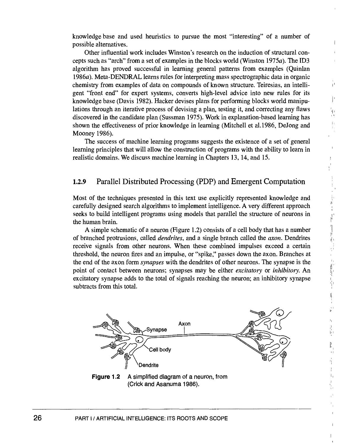
1.2.9 Parallel Distributed Processing (PDP) and Emergent Computation 26
1.2.10 AI and Philosophy 27
1.3 Artificial Intelligence—A Summary 28
1.4 Epilogue and References 29
1.5 Exercises 30
PART II
ARTIFICIAL INTELLIGENCE AS REPRESENTATION
AND SEARCH
Knowledge Representation 34
Problem Solving as Search 41
2 THE PREDICATE CALCULUS 47
2.0 Introduction 47
2.1 The Prepositional Calculus 47
2.1.1 Symbols and Sentences 47
2.1.2 The Semantics of the Prepositional Calculus 49
2.2 The Predicate Calculus 52
2.2.1 The Syntax of Predicates and Sentences 52
2.2.2 A Semantics for the Predicate Calculus 58
2.3 Using Inference Rules to Produce Predicate Calculus Expressions 64
2.3.1 Inference Rules 64
2.3.2 Unification 68
2.3.3 A Unification Example 72
2.4 Application: A Logic-Based Financial Advisor 75
XVi CONTENTS

2.5 Epilogue and References 79
2.6 Exercises 79
3 STRUCTURES AND STRATEGIES FOR STATE SPACE SEARCH 81
3.0 Introduction 81
3.1 Graph Theory 84
3.1.1 Structures for State Space Search 84
3.1.2 State Space Representation of Problems 87
3.2 Strategies for State Space Search 93
3.2.1 Data-Driven and Goal-Driven Search 93
3.2.2 Implementing Graph Search 96
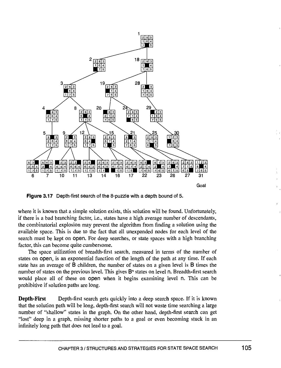
3.2.3 Depth-First and Breadth-First Search 99
3.2.4 Depth-First Search with Iterative Deepening 106
3.3 Using the State Space to Represent Reasoning with the Predicate Calculus 107
3.3.1 State Space Description of a Logical System 107
3.3.2 And/Or Graphs 109
3.3.3 Further Examples and Applications 111
3.4 Epilogue and References 121
3.5 Exercises 121
4 HEURISTIC SEARCH 123
4.0 Introduction 123
4.1 An Algorithm for Heuristic Search 127
4.1.1 Implementing "Best-First" Search 127
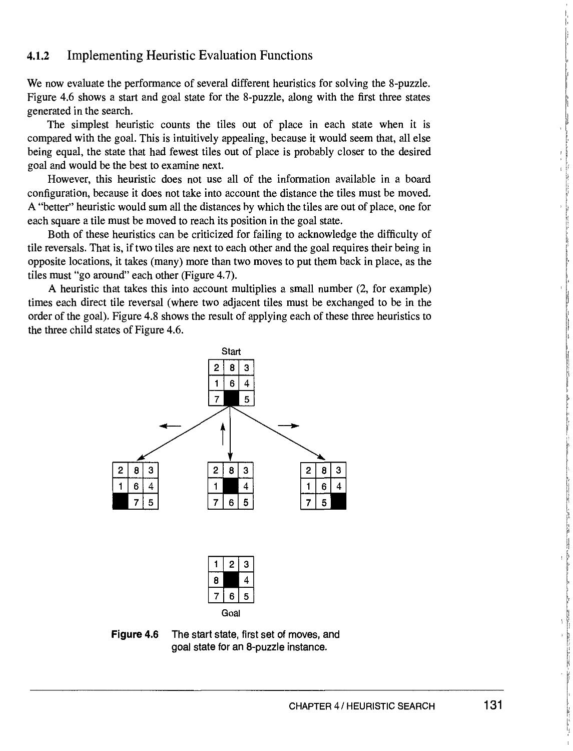
4.1.2 Implementing Heuristic Evaluation Functions 131
4.1.3 Heuristic Search and Expert Systems 136
4.2 Admissibility, Monotonicity, and Informedness 139
CONTENTS XVii

4.2.1 Admissibility Measures 139
4.2.2 Monotonicity 141
4.2.3 When One Heuristic Is Better: More Informed Heuristics 142
4.3 Using Heuristics in Games 144
4.3.1 The Minimax Procedure on Exhaustively Searchable Graphs 144
4.3.2 Minimaxing to Fixed Ply Depth 147
4.3.3 The Alpha-Beta Procedure 150
4.4 Complexity Issues 152
4.5 Epilogue and References 156
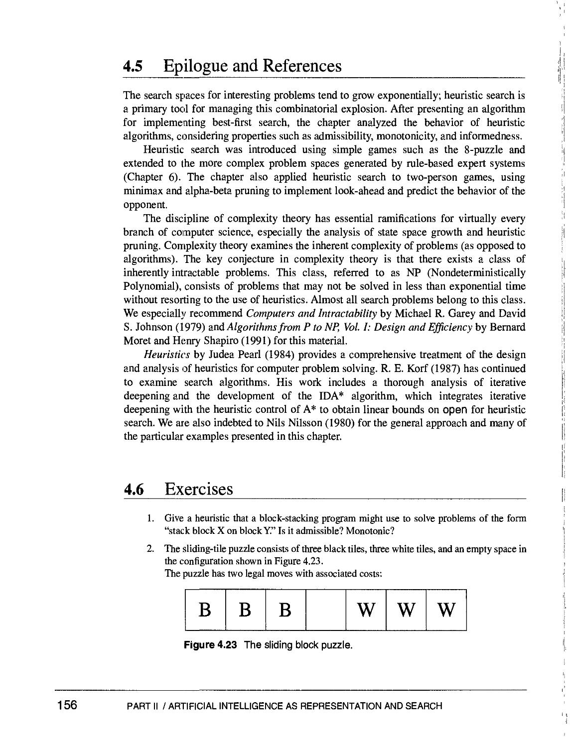
4.6 Exercises 156
5 CONTROL AND IMPLEMENTATION OF STATE SPACE SEARCH 159
5.0 Introduction 159
5.1 Recursion-Based Search 160
5.1.1 Recursion 160
5.1.2 Recursive Search 161
5.2 Pattern-Directed Search 164
5.2.1 Example: Recursive Search in the Knight's Tour Problem 165
5.2.2 Refining the Pattern-search Algorithm 168
5.3 Production Systems 171
5.3.1 Definition and History 171
5.3.2 Examples of Production Systems 174
5.3.3 Control of Search in Production Systems 180
5.3.4 Advantages of Production Systems for AI 184
5.4 Predicate Calculus and Planning 186
5.5 The Blackboard Architecture for Problem Solving 196
5.6 Epilogue and References 198
5.7 Exercises 199
xviii contents

PART III
REPRESENTATIONS FOR KNOWLEDGE-BASED
PROBLEM SOLVING
6 KNOWLEDGE-INTENSIVE PROBLEM SOLVING 207
6.0 Introduction 207
6.1 Overview of Expert System Technology 210
6.1.1 The Design of Rule-Based Expert Systems 210
6.1.2 Selecting a Problem for Expert System Development 212
6.1.3 The Knowledge Engineering Process 214
6.1.4 Conceptual Models and Their Role in Knowledge Acquisition 216
6.2 Rule-based Expert Systems 219
6.2.1 The Production System and Goal-driven Problem Solving 220
6.2.2 Explanation and Transparency in Goal-driven Reasoning 224
6.2.3 Using the Production System for Data-driven Reasoning 226
6.2.4 Heuristics and Control in Expert Systems 229
6.2.5 Conclusions: Rule-Based Reasoning 230
6.3 Model-based Reasoning 231
6.3.1 Introduction 231
6.4 Case-based Reasoning 235
6.4.1 Introduction 235
6.5 The Knowledge-Representation Problem 240
6.6 Epilogue and References 245
6.7 Exercises 246
CONTENTS XIX

7 REASONING WITH UNCERTAIN OR INCOMPLETE
INFORMATION 247
7.0 Introduction 247
7.1 The Statistical Approach to Uncertainty 249
7.1.1 Bayesian Reasoning 250
7.1.2 Bayesian Belief Networks 254
7.1.3 The Dempster-Shafer Theory of Evidence 259
7.1.4 The Stanford Certainty Factor Algebra 263
7.1.5 Causal Networks 266
7.2 Introduction to Nonmonotonic Systems 269
7.2.1 Logics for Nonmonotonic Reasoning 269
7.2.2 Logics Based on Minimum Models 273
7.2.3 Truth Maintenance Systems 275
7.2.4 Set Cover and Logic Based Abduction (Stern 1996) 281
7.3 Reasoning with Fuzzy Sets 284
7.4 Epilogue and References 289
7.5 Exercises 290
8 KNOWLEDGE REPRESENTATION 293
8.0 Knowledge Representation Languages 293
8.1 Issues in Knowledge Representation 295
8.2 A Survey of Network Representation 297
8.2.1 Associationist Theories of Meaning 297
8.2.2 Early Work in Semantic Nets 301
8.2.3 Standardization of Network Relationships 303
8.3 Conceptual Graphs: A Network Representation Language 309
8.3.1 Introduction to Conceptual Graphs 309
XX CONTENTS

8.3.2 Types, Individuals, and Names 311
8.3.3 The Type Hierarchy 313
8.3.4 Generalization and Specialization 314
8.3.5 Prepositional Nodes 317
8.3.6 Conceptual Graphs and Logic 318
8.4 Structured Representations 320
8.4.1 Frames 320
8.4.2 Scripts 324
8.5 Issues in Knowledge Representation 328
8.5.1 Hierarchies, Inheritance, and Exceptions 328
8.5.2 Naturalness, Efficiency, and Plasticity 331
8.6 Epilogue and References 334
8.7 Exercises 335
PART IV
LANGUAGES AND PROGRAMMING TECHNIQUES
FOR ARTIFICIAL INTELLIGENCE
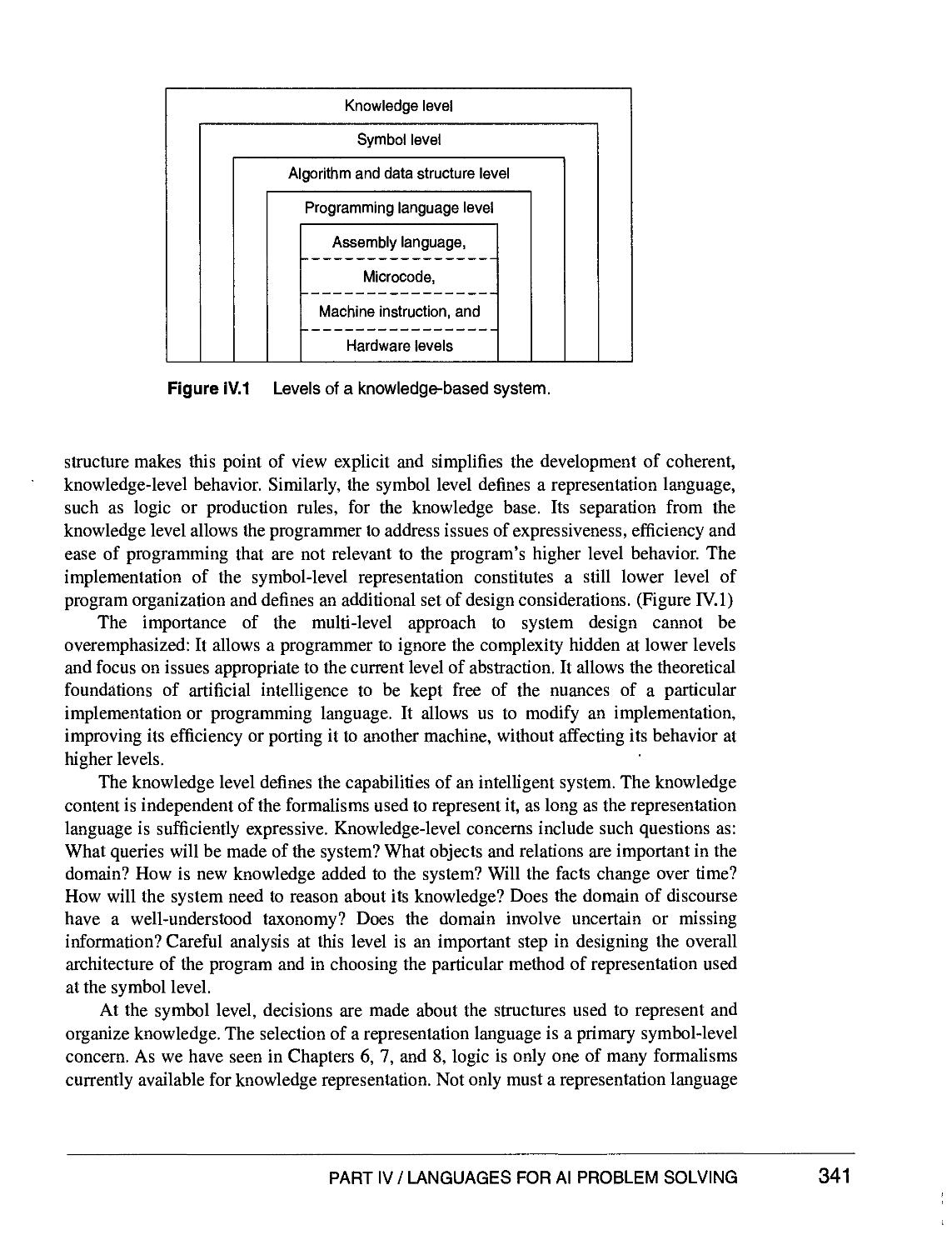
Languages, Understanding, and Levels of Abstraction 340
Desired Features of AI Language 342
An Overview of LISP and PROLOG 349
Object-Oriented Programming 352
Hybrid Environments 353
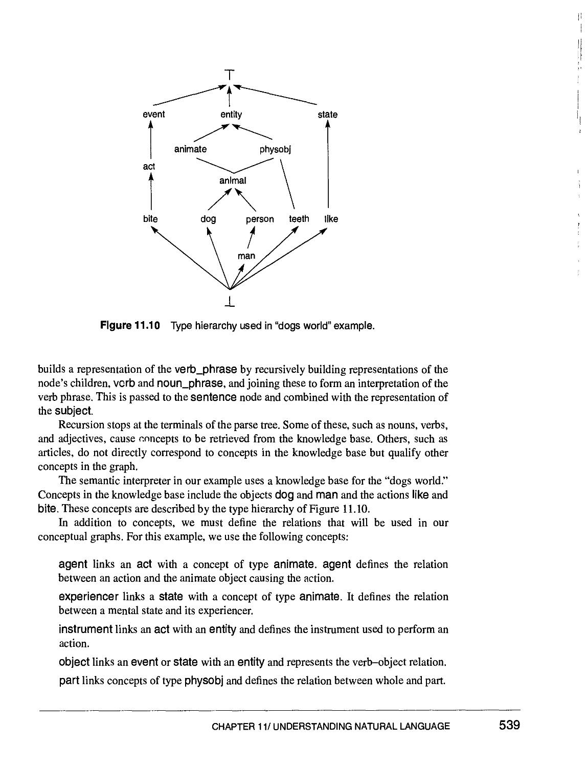
A Hybrid Example 354
Selecting an Implementation Language 356
CONTENTS XXI

9 AN INTRODUCTION TO PROLOG 357
9.0 Introduction 357
9.1 Syntax for Predicate Calculus Programming 358
9.1.1 Representing Facts and Rules 358
9.1.2 Creating, Changing, and Monitoring the PROLOG Environment 362
9.1.3 Recursion-Based Search in PROLOG 364
9.1.4 Recursive Search in PROLOG 366
9.1.5 The Use of Cut to Control Search in PROLOG 369
9.2 Abstract Data Types (ADTs) in PROLOG 371
9.2.1 The ADT Stack 371
9.2.2 The ADT Queue 373
9.2.3 The ADT Priority Queue 373
9.2.4 The ADT Set 374
9.3 A Production System Example in PROLOG 375
9.4 Designing Alternative Search Strategies 381
9.4.1 Depth-First Search Using the Closed List 381
9.4.2 Breadth-First Search in PROLOG 383
9.4.3 Best-First Search in PROLOG 384
9.5 A PROLOG Planner 386
9.6 PROLOG: Meta-Predicates, Types, and Unification 389
9.6.1 Meta-Logical Predicates 389
9.6.2 Types in PROLOG 391
9.6.3 Unification, the Engine for Predicate Matching and Evaluation 394
9.7 Meta-Interpreters in PROLOG 397
9.7.1 An Introduction to Meta-Interpreters: PROLOG in PROLOG 397
9.7.2 Shell for a Rule-B ased Expert System 401
9.7.3 Semantic Nets in PROLOG 410
9.7.4 Frames and Schemata in PROLOG 412
XXII CONTENTS

9.8 PROLOG: Towards Nonprocedural Computing 415
9.9 Epilogue and References 421
9.10 Exercises 422
10 AN INTRODUCTION TO LISP 425
10.0 Introduction 425
10.1 LISP: A Brief Overview 426
10.1.1 Symbolic Expressions, the Syntactic Basis of LISP 426
10.1.2 Control of LISP Evaluation: quote and eval 430
10.1.3 Programming in LISP: Creating New Functions 431
10.1.4 Program Control in LISP: Conditionals and Predicates 433
10.1.5 Functions, Lists, and Symbolic Computing 436
10.1.6 Lists as Recursive Structures 438
10.1.7 Nested Lists, Structure, and car/cdr Recursion 441
10.1.8 Binding Variables Using set 444
10.1.9 Defining Local Variables Using let 446
10.1.10 Data Types in Common LISP 448
10.1.11 Conclusion 449
10.2 Search in LISP: A Functional Approach to the Farmer, Wolf, Goat,
and Cabbage Problem 449
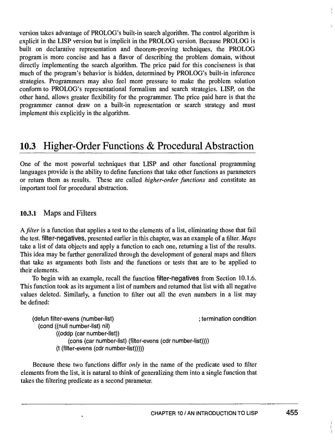
10.3 Higher-Order Functions and Procedural Abstraction 455
10.3.1 Maps and Filters 455
10.3.2 Functional Arguments and Lambda Expressions 457
10.4 Search Strategies in LISP 459
10.4.1 Breadth-First and Depth-First Search 459
10.4.2 Best-First Search 462
10.5 Pattern Matching in LISP 463
10.6 A Recursive Unification Function 465
CONTENTS XXIII

10.6.1 Implementing the Unification Algorithm 465
10.6.2 Implementing Substitution Sets Using Association Lists 467
10.7 Interpreters and Embedded Languages 469
10.8 Logic Programming in LISP 472
10.8.1 A Simple Logic Programming Language 472
10.8.2 Streams and Stream Processing 474
10.8.3 A Stream-Based Logic Programming Interpreter 477
10.9 Streams and Delayed Evaluation 482
10.10 An Expert System Shell in LISP 486
10.10.1 Implementing Certainty Factors 486
10.10.2 Architecture of lisp-shell 488
10.10.3 User Queries and Working Memory 490
10.10.4 Classification Using lisp-shell 491
10.11 Network Representations and Inheritance 494
10.11.1 Representing Semantic Nets in LISP 494
10.11.2 Implementing Inheritance 497
10.12 Object-Oriented Programming Using CLOS 497
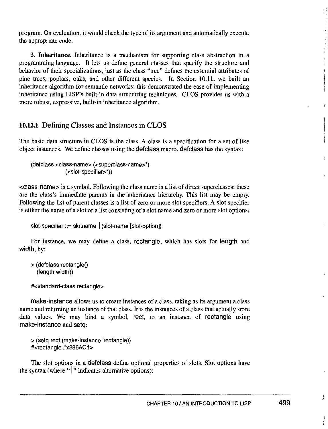
10.12.1 Defining Classes and Instances in CLOS 499
10.12.2 Defining Generic Functions and Methods 501
10.12.3 Inheritance in CLOS 503
10.12.4 Advanced Features of CLOS 505
10.12.5 Example: A Thermostat Simulation 505
10.13 Epilogue and References 511
10.14 Exercises 511
XXIV CONTENTS

PARTV
ADVANCED TOPICS FOR Al PROBLEM SOLVING
Natural Language, Automated Reasoning, and Learning 517
11 UNDERSTANDING NATURAL LANGUAGE 519
11.0 Role of Knowledge in Language Understanding 519
11.1 Language Understanding: A Symbolic Approach 522
11.1.1 Introduction 522
11.1.2 Stages of Language Analysis 523
11.2 Syntax 524
11.2.1 Specification and Parsing Using Context-Free Grammars 524
11.2.2 Transition Network Parsers 527
11.2.3 The Chomsky Hierarchy and Context-Sensitive Grammars 531
11.3 Combining Syntax and Semantics in ATN Parsers 534
11.3.1 Augmented Transition Network Parsers 534
11.3.2 Combining Syntax and Semantics 538
11.4 Stochastic Tools for Language Analysis 543
11.4.1 Introduction 543
11.4.2 A Markov Model Approach 545
11.4.3 A CART Tree Approach 546
11.4.4 Mutual Information Clustering 547
11.4.5 Parsing 548
11.4.6 Other Language Applications for Stochastic Techniques 550
11.5 Natural Language Applications 550
11.5.1 Story Understanding and Question Answering 550
11.5.2 A Database Front End 551
11.6 Epilogue and References 555
11.7 Exercises 557
CONTENTS XXV

12 AUTOMATED REASONING 559
12.0 Introduction to Weak Methods in Theorem Proving 559
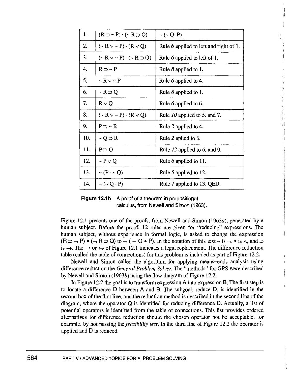
12.1 The General Problem Solver and Difference Tables 560
12.2 Resolution Theorem Proving 566
12.2.1 Introduction 566
12.2.2 Producing the Clause Form for Resolution Refutations 568
12.2.3 The Binary Resolution Proof Procedure 573
12.2.4 Strategies and Simplification Techniques for Resolution 578
12.2.5 Answer Extraction from Resolution Refutations 583
12.3 PROLOG and Automated Reasoning 587
12.3.1 Introduction 587
12.3.2 Logic Programming and PROLOG 588
12.4 Further Issues in Automated Reasoning 593
12.4.1 Uniform Representations for Weak Method Solutions 593
12.4.2 Alternative Inference Rules 597
12.4.3 Search Strategies and Their Use 599
12.5 Epilogue and References 600
12.6 Exercises 601
13 MACHINE LEARNING: SYMBOL-BASED 603
13.0 Introduction 603
13.1 A Framework for Symbol-based Learning 606
13.2 Version Space Search 612
13.2.1 Generalization Operators and the Concept Space 612
13.2.2 The Candidate Elimination Algorithm 613
13.2.3 LEX: Inducing Search Heuristics 620
13.2.4 Evaluating Candidate Elimination 623
XXVi CONTENTS

13.3 The ID3 Decision Tree Induction Algorithm 624
13.3.1 Top-Down Decision Tree Induction 627
13.3.2 Information Theoretic Test Selection 628
13.3.3 Evaluating ID3 632
13.3.4 Decision Tree Data Issues: Bagging, Boosting 632
13.4 Inductive Bias and Learnability 633
13.4.1 Inductive Bias 634
13.4.2 The Theory of Learnability 636
13.5 Knowledge and Learning 638
13.5.1 Meta-DENDRAL 639
13.5.2 Explanation-Based Learning 640
13.5.3 EBL and Knowledge-Level Learning 645
13.5.4 Analogical Reasoning 646
13.6 Unsupervised Learning 649
13.6.1 Discovery and Unsupervised Learning 649
13.6.2 Conceptual Clustering 651
13.6.3 COBWEB and the Structure of Taxonomic Knowledge 653
13.7 Epilogue and References 658
13.8 Exercises 659
14 MACHINE LEARNING: CONNECTIONIST 661
14.0 Introduction 661
14.1 Foundations for Connectionist Networks 663
14.1.1 Early History 663
14.2 Perceptron Learning 666
14.2.1 The Perceptron Training Algorithm 666
14.2.2 An Example: Using a Perceptron Network to Classify 668
14.2.3 The Delta Rule 672
CONTENTS XXVii

14.3 Backpropagation Learning 675
14.3.1 Deriving the Backpropagation Algorithm 675
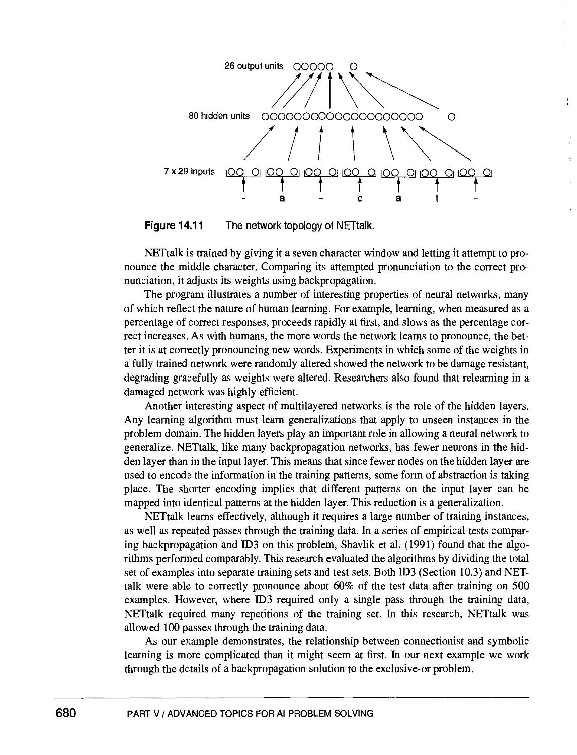
14.3.2 Backpropagation Example l:NETtalk 679
14.3.3 Backpropagation Example 2: Exclusive-or 681
14.4 Competitive Learning 682
14.4.1 Winner-Take-All Learning for Classification 682
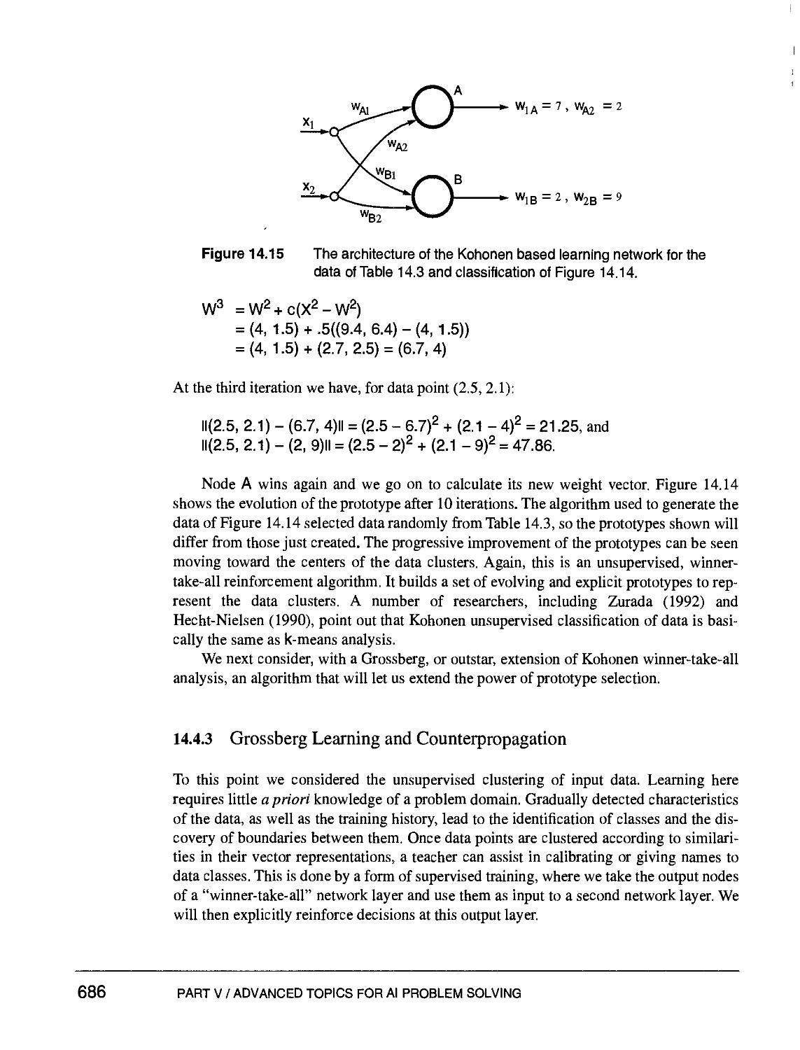
14.4.2 A Kohonen Network for Learning Prototypes 684
14.4.3 Grossberg Learning and Counterpropagation 686
14.5 Hebbian Coincidence Learning 690
14.5.1 Introduction 690
14.5.2 An Example of Unsupervised Hebbian Learning 691
14.5.3 Supervised Hebbian Learning 694
14.5.4 Associative Memory and the Linear Associator 696
14.6 Attractor Networks or "Memories" 701
14.6.1 Introduction 701
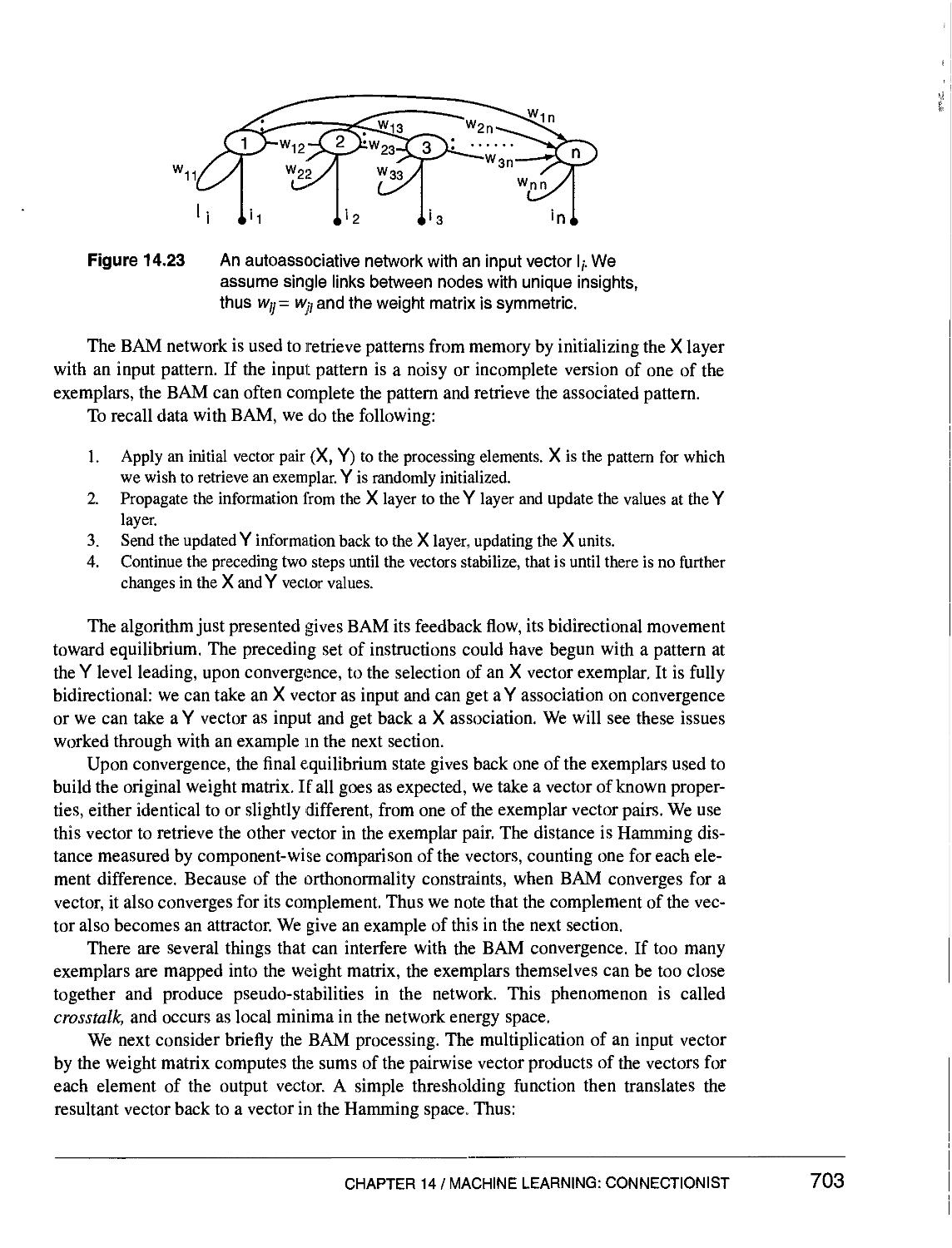
14.6.2 BAM, the Bi-directional Associative Memory 702
14.6.3 Examples of BAM Processing 704
14.6.4 Autoassociative Memory and Hopfield Nets 706
14.7 Epilogue and References 711
14.8 Exercises 712
15 MACHINE LEARNING: SOCIAL AND EMERGENT 713
15.0 Social and Emergent Models of Learning 713
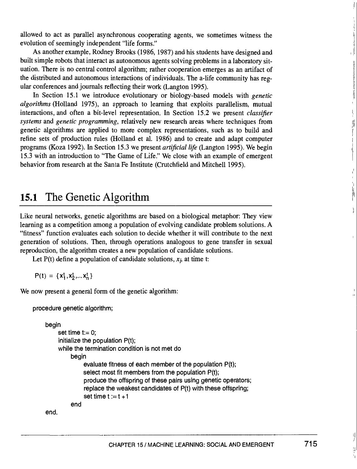
15.1 The Genetic Algorithm 715
15.1.3 Two Examples: CNF Satisfaction and the Traveling Salesperson 717
15.1.4 Evaluating the Genetic Algorithm 721
15.2 Classifier Systems and Genetic Programming 725
15.2.1 Classifier Systems 725
15.2.2 Programming with Genetic Operators 730
xxviii contents

15.3 Artificial Life and Society-based Learning 736
15.3.1 The "Game of Life" 737
15.3.2 Evolutionary Programming 740
15.3.3 A Case Study in Emergence (Crutchfield and Mitchell 1994) 743
15.4 Epilogue and References 747
15.5 Exercises 748
PART VI
EPILOGUE
Reflections on the Nature of Intelligence 751
16 ARTIFICIAL INTELLIGENCE AS EMPIRICAL
ENQUIRY 753
16.0 Introduction 753
16.1 Artificial Intelligence: A Revised Definition 755
16.1.1 Intelligence and the Physical Symbol System 756
16.1.2 Minds, Brains, and Neural Computing 759
16.1.3 Agents, Emergence, and Intelligence 761
16.1.4 Situated Actors and the Existential Mind 764
16.2 Cognitive Science: An Overview 766
16.2.1 The Analysis of Human Performance 766
16.2.2 The Production System and Human Cognition 767
16.3 Current Issues in Machine Learning 770
16.4 Understanding Intelligence: Issues and Directions 775
16.5 Epilogue and References 780
Bibliography 781
Author Index 803
Subject Index 809
Acknowledgements 823
CONTENTS XXJX

PARTI
ARTIFICIAL INTELLIGENCE:
ITS ROOTS AND SCOPE
Everything must have a beginning, to speak in Sanchean phrase; and that beginning must
be linked to something that went before. Hindus give the world an elephant to support it,
but they make the elephant stand upon a tortoise. Invention, it must be humbly admitted,
does not consist in creating out of void, but out of chaos; the materials must, in the first
place, be afforded....
—Mary Shelley, Frankenstein
Artificial Intelligence: An Attempted Definition
Artificial intelligence (AI) may be defined as the branch of computer science that is
concerned with the automation of intelligent behavior. This definition is particularly
appropriate to this text in that it emphasizes our conviction that AI is a part of computer
science and, as such, must be based on sound theoretical and applied principles of that
field. These principles include the data structures used in knowledge representation, the
algorithms needed to apply that knowledge, and the languages and programming
techniques used in their implementation.
However, this definition suffers from the fact that intelligence itself is not very well
defined or understood. Although most of us are certain that we know intelligent behavior
when we see it, it is doubtful that anyone could come close to defining intelligence in a
way that would be specific enough to help in the evaluation of a supposedly intelligent
computer program, while still capturing the vitality and complexity of the human mind.
Thus the problem of defining artificial intelligence becomes one of defining
intelligence itself: is intelligence a single faculty, or is it just a name for a collection of
distinct and unrelated abilities? To what extent is intelligence learned as opposed to having
an a priori existence? Exactly what does happen when learning occurs? What is
creativity? What is intuition? Can intelligence be inferred from observable behavior, or
does it require evidence of a particular internal mechanism? How is knowledge
represented in the nerve tissue of a living being, and what lessons does this have for the
design of intelligent machines? What is self-awareness, and what role does it play in

intelligence? Is it necessary to pattern an intelligent computer program after what is
known about human intelligence, or is a strict "engineering" approach to the problem
sufficient? Is it even possible to achieve intelligence on a computer, or does an intelligent
entity require the richness of sensation and experience that might be found only in a
biological existence?
These are all unanswered questions, and all of them have helped to shape the
problems and solution methodologies that constitute the core of modern AI. In fact, part of
the appeal of artificial intelligence is that it offers a unique and powerful tool for exploring
exactly these questions. AI offers a medium and a test-bed for theories of intelligence:
such theories may be stated in the language of computer programs and consequently
verified through the execution of these programs on an actual computer.
For these reasons, our initial definition of artificial intelligence seems to fall short of
unambiguously defining the field. If anything, it has only led to further questions and the
paradoxical notion of a field of study whose major goals include its own definition. But
this difficulty in arriving at a precise definition of AI is entirely appropriate. Artificial
intelligence is still a young discipline, and its structure, concerns, and methods are less
clearly defined than those of a more mature science such as physics.
Artificial intelligence has always been more concerned with expanding the capabili-
capabilities of computer science than with defining its limits. Keeping this exploration grounded
in sound theoretical principles is one of the challenges facing AI researchers in general
and this text in particular.
Because of its scope and ambition, artificial intelligence defies simple definition. For
the time being, we will simply define it as the collection of problems and methodologies
studied by artificial intelligence researchers. This definition may seem silly and meaning-
meaningless, but it makes an important point: artificial intelligence, like every science, is a human
endeavor and may best be understood in that context.
There are reasons that any science, AI included, concerns itself with a certain set of
problems and develops a particular body of techniques for approaching these problems. A
short history of artificial intelligence and the people and assumptions that have shaped it
will explain why a certain set of questions have come to dominate the field and why the
methods discussed in this text have been taken for their solution.
PART I / ARTIFICIAL INTELLIGENCE: ITS ROOTS AND SCOPE

Al: HISTORY AND
APPLICATIONS
Hear the rest, and you will marvel even more at the crafts and resources I have contrived.
Greatest was this: in the former times if a man fell sick he had no defense against the
sickness, neither healing food nor drink, nor unguent; but through the lack of drugs men
wasted away, until I showed them the blending of mild simples wherewith they drive out
all manner of diseases....
It was I who made visible to men's eyes the flaming signs of the sky that were before dim.
So much for these. Beneath the earth, man's hidden blessing, copper, iron, silver, and
gold—will anyone claim to have discovered these before I did? No one, I am very sure,
who wants to speak truly and to the purpose. One brief word will tell the whole story: all
arts that mortals have come from Prometheus.
—Aeschylus, Prometheus Bound
1.1 From Eden to ENIAC: Attitudes toward
Intelligence, Knowledge, and Human Artifice
Prometheus speaks of the fruits of his transgression against the gods of Olympus: his
purpose was not merely to steal fire for the human race but also to enlighten humanity
through the gift of intelligence or nous: the "rational mind." This intelligence forms the
foundation for all of human technology and ultimately all human civilization. The work of
the classical Greek dramatist illustrates a deep and ancient awareness of the extraordinary
power of knowledge. Artificial intelligence, in its very direct concern for Prometheus's
gift, has been applied to all the areas of his legacy—medicine, psychology, biology,
astronomy, geology—and many areas of scientific endeavor that Aeschylus could not have
imagined.
Though Prometheus's action freed humanity from the sickness of ignorance, it also
earned him the wrath of Zeus. Outraged over this theft of knowledge that previously

belonged only to the gods of Olympus, Zeus commanded that Prometheus be chained to a
barren rock to suffer the ravages of the elements for eternity. The notion that human efforts
to gain knowledge constitute a transgression against the laws of God or nature is deeply
ingrained in Western thought. It is the basis of the story of Eden and appears in the work of
Dante and Milton. Both Shakespeare and the ancient Greek tragedians portrayed
intellectual ambition as the cause of disaster. The belief that the desire for knowledge must
ultimately lead to disaster has persisted throughout history, enduring the Renaissance, the
Age of Enlightenment, and even the scientific and philosophical advances of the
nineteenth and twentieth centuries. Thus, we should not be surprised that artificial
intelligence inspires so much controversy in both academic and popular circles.
Indeed, rather than dispelling this ancient fear of the consequences of intellectual
ambition, modern technology has only made those consequences seem likely, even
imminent. The legends of Prometheus, Eve, and Faustus have been retold in the language
of technological society. In her introduction to Frankenstein (subtitled, interestingly
enough, The Modern Prometheus), Mary Shelley writes:
Many and long were the conversations between Lord Byron and Shelley to which I was a
devout and silent listener. During one of these, various philosophical doctrines were discussed,
and among others the nature of the principle of life, and whether there was any probability of its
ever being discovered and communicated. They talked of the experiments of Dr. Darwin (I
speak not of what the doctor really did or said iliat he did, but, as more to my purpose, of what
was then spoken of as having been done by him), who preserved a piece of vermicelli in a glass
case till by some extraordinary means it began to move with a voluntary motion. Not thus, after
all, would life be given. Perhaps a corpse would be reanimated; galvanism had given token of
such things: perhaps the component parts of a creature might be manufactured, brought
together, and endued with vital warmth.
Shelley shows us the extent to which scientific advances such as the work of Darwin
and the discovery of electricity had convinced even nonscientists that the workings of
nature were not divine secrets, but could be broken down and understood systematically.
Frankenstein's monster is not the product of shamanistic incantations or unspeakable
transactions with the underworld: it is assembled from separately "manufactured"
components and infused with the vital force of electricity. Although nineteenth-century
science was inadequate to realize the goal of understanding and creating a fully intelligent
agent, it affirmed the notion that the mysteries of life and intellect might be brought into
the light of scientific analysis.
1.1.1 Historical Foundations
By the time Mary Shelley finally and perhaps irrevocably joined modern science with the
Promethean myth, the philosophical foundations of modern work in artificial intelligence
had been developing for several thousand years. Although the moral and cultural issues
raised by artificial intelligence are both interesting and important, our introduction is more
properly concerned with AI's intellectual heritage. The logical starting point for such a
history is the genius of Aristotle, or, as Dante refers to him, "the master of those who
PART I / ARTIFICIAL INTELLIGENCE: ITS ROOTS AND SCOPE

know." Aristotle wove together the insights, wonders, and fears of the early Greek
tradition with the careful analysis and disciplined thought that were to become the
standard for more modern science.
For Aristotle, the most fascinating aspect of nature was change. In his Physics, he
defined his "philosophy of nature" as the "study of things that change." He distinguished
between the "matter" and "form" of things: a sculpture is fashioned from the "material"
bronze and has the "form" of a human. Change occurs when the bronze is molded to a new
form. The matter/form distinction provides a philosophical basis for modern notions such
as symbolic computing and data abstraction. In computing (even with numbers) we are
manipulating patterns that are the forms of electromagnetic material, with the changes of
form of this material representing aspects of the solution process. Abstracting the form
from the medium of its representation not only allows these forms to be manipulated
computationally but also provides the promise of a theory of data structures, the heart of
modern computer science.
In his Metaphysics (located just after, meta, the Physics in his writing), Aristotle
developed a science of things that never change, including his cosmology and theology.
More relevant to artificial intelligence, however, was Aristotle's epistemology or science
of knowing, discussed in his Logic. Aristotle referred to his logic as the "instrument"
(organon), because he felt that the study of thought itself was at the basis of all
knowledge. In his Logic, he investigated whether certain propositions can be said to be
"true" because they are related to other things that are known to be true. Thus if we know
that "all men are mortal" and that "Socrates is a man," then we can conclude that "Socrates
is mortal." This argument is an example of what Aristotle referred to as a syllogism using
the deductive form modus ponens. Although the formal axiomatization of reasoning
needed another two thousand years for its full flowering in the works of Gottlob Frege,
Bertrand Russell, Kurt Godel, Alan Turing, Alfred Tarski, and others, its roots may be
traced to Aristotle.
Renaissance thought, building on the Greek tradition, initiated the evolution of a
different and powerful way of thinking about humanity and its relation to the natural
world. Empiricism began to replace mysticism as a means of understanding nature. Clocks
and, eventually, factory schedules superseded the rhythms of nature for thousands of city
dwellers. Most of the modern social and physical sciences found their origin in the notion
that processes, whether natural or artificial, could be mathematically analyzed and
understood. In particular, scientists and philosophers realized that thought itself, the way
that knowledge was represented and manipulated in the human mind, was a difficult but
essential subject for scientific study.
Perhaps the major event in the development of the modern world view was the
Copernican revolution, the replacement of the ancient Earth-centered model of the
universe with the idea that the Earth and other planets actually rotate around the sun. After
centuries of an "obvious" order, in which the scientific explanation of the nature of the
cosmos was consistent with the teachings of religion and common sense, a drastically
different and not at all obvious model was proposed to explain the motions of heavenly
bodies. For perhaps the first time, our ideas about the world were seen as fundamentally
distinct from its appearance. This split between the human mind and its surrounding
reality, between ideas about things and things themselves, is essential to the modern study
CHAPTER 1 / Al: HISTORY AND APPLICATIONS

of the mind and its organization. This breach was widened by the writings of Galileo,
whose scientific observations further contradicted the "obvious" truths about the natural
world and whose development of mathematics as a tool for describing that world
emphasized the distinction between the world and our ideas about it. It is out of this
breach that the modern notion of the mind evolved: introspection became a common motif ■•
in literature, philosophers began to study epistemology and mathematics, and the
systematic application of the scientific method rivaled the senses as tools for \
understanding the world. I
Although the seventeenth and eighteenth centuries saw a great deal of work in '
epistemology and related fields, here we have space only to discuss the work of Rene
Descartes. Descartes is a central figure in the development of the modern concepts of
thought and the mind. In his famous Meditations, Descartes attempted to find a basis for
reality purely through cognitive introspection. Systematically rejecting the input of his t
senses as untrustworthy, Descartes was forced to doubt even the existence of the physical
world and was left with only the reality of thought; even his own existence had to be
justified in terms of thought: "Cogito ergo sum" (I think, therefore I am). After he
established his own existence purely as a thinking entity, Descartes inferred the existence
of God as an essential creator and ultimately reasserted the reality of the physical universe
as the necessary creation of a benign God.
We can make two interesting observations here: first, the schism between the mind
and the physical world had become so complete that the process of thinking could be
discussed in isolation from any specific sensory input or worldly subject matter; second,
the connection between mind and the physical world was so tenuous that it required the
intervention of a benign God to allow reliable knowledge of the physical world. This view
of the duality between the mind and the physical world underlies all of Descartes's
thought, including his development of analytic geometry. How else could he have unified 1
such a seemingly worldly branch of mathematics as geometry with such an abstract ;
mathematical framework as algebra?
Why have we included this philosophical discussion in a text on artificial
intelligence? There are two consequences of this analysis that are essential to the
enterprise of artificial intelligence:
1. By separating the mind and the physical world, Descartes and related thinkers
established that the structure of ideas about the world was not necessarily the
same as the structure of their subject matter. This underlies the methodology of
the field of AI, along with the fields of epistemology, psychology, much of higher
mathematics, and most of modern literature: mental processes had an existence
of their own, obeyed their own laws, and could be studied in and of themselves.
2. Once the mind and the body were separated, philosophers found it necessary to
find a way to reconnect the two, because interaction between the mental and the
physical is essential for human existence.
Although millions of words have been written on the mind-body problem, and
numerous solutions proposed, no one has successfully explained the obvious interactions
PART I / ARTIFICIAL INTELLIGENCE: ITS ROOTS AND SCOPE

between mental states and physical actions while affirming a fundamental difference
between them. The most widely accepted response to this problem, and the one that
provides an essential foundation for the study of AI, holds that the mind and the body are
not fundamentally different entities at all. In this view, mental processes are indeed
achieved by physical systems such as brains (or computers). Mental processes, like
physical processes, can ultimately be characterized through formal mathematics. Or, as
stated by the Scots philosopher David Hume, "Cognition is computation."
1.1.2 The Development of Logic
Once thinking had come to be regarded as a form of computation, its formalization and
eventual mechanization were logical next steps. In the seventeenth century, Gottfried Wil-
helm von Leibniz introduced the first system of formal logic and constructed machines for
automating calculation (Leibniz 1887). Euler, in the eighteenth century, with his analysis
of the "connectedness" of the bridges joining the riverbanks and islands of the city of
Konigsberg (see the introduction to Chapter 3), introduced the study of representations
that abstractly capture the structure of relationships in the world (Euler 1735).
The formalization of graph theory also afforded the possibility of state space search,
a major conceptual tool of artificial intelligence. We can use graphs to model the deeper
structure of a problem. The nodes of a state space graph represent possible stages of a
problem solution; the arcs of the graph represent inferences, moves in a game, or other
steps in a problem solution. Solving the problem is a process of searching the state space
graph for a path to a solution (Section 1.3 and Chapter 3). By describing the entire space
of problem solutions, state space graphs provide a powerful tool for measuring the struc-
structure and complexity of problems and analyzing the efficiency, correctness, and generality
of solution strategies.
As one of the originators of the science of operations research, as well as the designer
of the first programmable mechanical computing machines, Charles Babbage, a nineteenth
century mathematician, is arguably the earliest practitioner of artificial intelligence (Mor-
(Morrison and Morrison 1961). Babbage's "difference engine" was a special-purpose machine
for computing the values of certain polynomial functions and was the forerunner of his
"analytical engine." The analytical engine, designed but not successfully constructed dur-
during Babbage's lifetime, was a general-purpose programmable computing machine that
presaged many of the architectural assumptions underlying the modern computer.
In describing the analytical engine, Ada Lovelace A961), Babbage's friend, sup-
supporter, and collaborator, said:
We may say most aptly that the Analytical Engine weaves algebraical patterns just as the Jac-
quard loom weaves flowers and leaves. Here, it seems to us, resides much more of
originality than the difference engine can be fairly entitled to claim.
Babbage's inspiration was his desire to apply the technology of his day to liberate
humans from the drudgery of arithmetic calculation. In this sentiment, as well as his
conception of his computers as mechanical devices, Babbage was thinking in purely
CHAPTER 1 / AI: HISTORY AND APPLICATIONS

nineteenth-century terms. His analytical engine, however, included many modern notions,
such as the separation of memory and processor (the "store" and the "mill" in Babbage's
terms), the concept of a digital rather than analog machine, and programmability based on
the execution of a series of operations encoded on punched pasteboard cards. The most
striking feature of Ada Lovelace's description, and of Babbage's work in general, is its
treatment of the "pattern" of an intellectual activity as an entity that may be studied,
characterized, and finally implemented mechanically without concern for the particular
values that are finally passed through the "mill" of the calculating machine. This is an
implementation of the "abstraction and manipulation of form" first described by Aristotle.
The goal of creating a formal language for thought also appears in the work of George
Boole, another nineteenth-century mathematician whose work must be included in any
discussion of the roots of artificial intelligence (Boole 1847, 1854). Although he made
contributions to a number of areas of mathematics, his best known work was in the
mathematical formalization of the laws of logic, an accomplishment that forms the very
heart of modern computer science. Though the role of Boolean algebra in the design of
logic circuitry is well known, Boole's own goals in developing his system seem closer to
those of contemporary AI researchers. In the first chapter of An Investigation of the Laws
of Thought, on which are founded the Mathematical Theories of Logic and Probabilities,
Boole described his goals as
to investigate the fundamental laws of those operations of the mind by which reasoning is
performed: to give expression to them in the symbolical language of a Calculus, and upon this
foundation to establish the science of logic and instruct its method; ...and finally to collect
from the various elements of truth brought to view in the course of these inquiries some proba-
probable intimations concerning the nature and constitution of the human mind.
The greatness of Boole's accomplishment is in the extraordinary power and simplicity
of the system he devised: three operations, "AND" (denoted by * or a), "OR" (denoted by
+ or v), and "NOT" (denoted by -0, formed the heart of his logical calculus. These
operations have remained the basis for all subsequent developments in formal logic,
including the design of modern computers. While keeping the meaning of these symbols
nearly identical to the corresponding algebraic operations, Boole noted that "the Symbols
of logic are further subject to a special law, to which the symbols of quantity, as such, are
not subject." This law states that for any X, an element in the algebra, X*X=X (or that once
something is known to be true, repetition cannot augment that knowledge). This led to the
characteristic restriction of Boolean values to the only two numbers that may satisfy this
equation: 1 and 0. The standard definitions of Boolean multiplication (AND) and addition
(OR) follow from this insight. Boole's system not only provided the basis of binary
arithmetic but also demonstrated that an extremely simple formal system was adequate to
capture the full power of logic. This assumption and the system Boole developed to
demonstrate it form the basis of all modern efforts to formalize logic, from Russell and
Whitehead's Principia Mathematica (Whitehead and Russell 1950), through the work of
Turing and Godel, up to modern automated reasoning systems.
Gottlob Frege, in his Foundations of Arithmetic (Frege 1879, 1884), created a
mathematical specification language for describing the basis of arithmetic in a clear and
8 PART I / ARTIFICIAL INTELLIGENCE: ITS ROOTS AND SCOPE

precise fashion. With this language Frege formalized many of the issues first addressed by
Aristotle's Logic. Frege's language, now called the first-order predicate calculus, offers a
tool for describing the propositions and truth value assignments that make up the elements
of mathematical reasoning and describes the axiomatic basis of "meaning" for these
expressions. The formal system of the predicate calculus, which includes predicate
symbols, a theory of functions, and quantified variables, was intended to be a language for
describing mathematics and its philosophical foundations. It also plays a fundamental role
in creating a theory of representation for artificial intelligence (Chapter 2). The first-order
predicate calculus offers the tools necessary for automating reasoning: a language for
expressions, a theory for assumptions related to the meaning of expressions, and a
logically sound calculus for inferring new true expressions.
Russell and Whitehead's A950) work is particularly important to the foundations of
AI, in that their stated goal was to derive the whole of mathematics through formal opera-
operations on a collection of axioms. Although many mathematical systems have been con-
constructed from basic axioms, what is interesting is Russell and Whitehead's commitment to
mathematics as a purely formal system. This meant that axioms and theorems would be
treated solely as strings of characters: proofs would proceed solely through the application
of well-defined rules for manipulating these strings. There would be no reliance on intu-
intuition or the meaning of theorems as a basis for proofs. Every step of a proof followed from
the strict application of formal (syntactic) rules to either axioms or previously proven the-
theorems, even where traditional proofs might regard such a step as "obvious." What "mean-
"meaning" the theorems and axioms of the system might have in relation to the world would be
independent of their logical derivations. This treatment of mathematical reasoning in
purely formal (and hence mechanical) terms provided an essential basis for its automation
on physical computers. The logical syntax and formal rules of inference developed by
Russell and Whitehead are still a basis for automatic theorem-proving systems as well as
for the theoretical foundations of artificial intelligence.
Alfred Tarski is another mathematician whose work is essential to the foundations of
AI. Tarski created a theory of reference wherein the well-formed formulae of Frege or
Russell and Whitehead can be said to refer, in a precise fashion, to the physical world (Tar-
(Tarski 1944, 1956; see Chapter 2). This insight underlies most theories of formal semantics.
In his paper "The semantic conception of truth and the foundation of semantics," Tarski
describes his theory of reference and truth value relationships. Modern computer scien-
scientists, especially Scott, Strachey, Burstall (Burstall and Darlington 1977), and Plotkin have
related this theory to programming languages and other specifications for computing.
Although in the eighteenth, nineteenth, and early twentieth centuries the
formalization of science and mathematics created the intellectual prerequisite for the study
of artificial intelligence, it was not until the twentieth century and the introduction of the
digital computer that AI became a viable scientific discipline. By the end of the 1940s
electronic digital computers had demonstrated their potential to provide the memory and
processing power required by intelligent programs. It was now possible to implement
formal reasoning systems on a computer and empirically test their sufficiency for
exhibiting intelligence. An essential component of the science of artificial intelligence is
this commitment to digital computers as the vehicle of choice for creating and testing
theories of intelligence.
CHAPTER 1 / AI: HISTORY AND APPLICATIONS 9

Digital computers are not merely a vehicle for testing theories of intelligence. Their
architecture also suggests a specific paradigm for such theories: intelligence is a form of
information processing. The notion of search as a problem-solving methodology, for
example, owes more to the sequential nature of computer operation than it does to any
biological model of intelligence. Most AI programs represent knowledge in some formal
language that is then manipulated by algorithms, honoring the separation of data and
program fundamental to the von Neumann style of computing. Formal logic has emerged
as the lingua franca of AI research, whereas graph theory plays an indispensable role in the
analysis of problem spaces as well as providing a basis for semantic networks and
similar models of semantic meaning. These techniques and formalisms are discussed in
detail throughout the body of this text; we mention them here to emphasize the symbiotic
relationship between the digital computer and the theoretical underpinnings of artificial
intelligence.
We often forget that the tools we create for our own purposes tend to shape our
conception of the world through their structure and limitations. Although seemingly
restrictive, this interaction is an essential aspect of the evolution of human knowledge: a
tool (and scientific theories are ultimately only tools) is developed to solve a particular
problem. As it is used and refined, the tool itself seems to suggest other applications,
leading to new questions and, ultimately, the development of new tools.
1.1.3 The Turing Test
One of the earliest papers to address the question of machine intelligence specifically in
relation to the modern digital computer was written in 1950 by the British mathematician
Alan Turing. "Computing machinery and intelligence" (Turing 1950) remains timely in
both its assessment of the arguments against the possibility of creating an intelligent
computing machine and its answers to those arguments. Turing, known mainly for his con-
contributions to the theory of computability, considered the question of whether or not a
machine could actually be made to think. Noting that the fundamental ambiguities in the
question itself (what is thinking? what is a machine?) precluded any rational answer, he
proposed that the question of intelligence be replaced by a more clearly defined
empirical test.
The Turing test measures the performance of an allegedly intelligent machine against
that of a human being, arguably the best and only standard for intelligent behavior. The
test, which Turing called the "imitation game," places the machine and a human
counterpart in rooms apart from a second human being, referred to as the "interrogator"
(Figure 1.1). The interrogator is not able to see or speak directly to either of them, does not
know which entity is actually the machine, and may communicate with them solely by use
of a textual device such as a terminal. The interrogator is asked to distinguish the
computer from the human being solely on the basis of their answers to questions asked
over this device. If the interrogator cannot distinguish the machine from the human, then,
Turing argues, the machine may be assumed to be intelligent.
10 PART I / ARTIFICIAL INTELLIGENCE: ITS ROOTS AND SCOPE

Figure 1.1 The Turing test.
By isolating the interrogator from both the machine and the other human participant,
the test ensures that the interrogator will not be biased by the appearance of the machine or
any mechanical property of its voice. The interrogator is free, however, to ask any
questions, no matter how devious or indirect, in an effort to uncover the computer's
identity. For example, the interrogator may ask both subjects to perform a rather involved
arithmetic calculation, assuming that the computer will be more likely to get it correct than
the human; to counter this strategy, the computer will need to know when it should fail to
get a correct answer to such problems in order to seem like a human. To discover the
human's identity on the basis of emotional nature, the interrogator may ask both subjects
to respond to a poem or work of art; this strategy will require that the computer have
knowledge concerning the emotional makeup of human beings.
The important features of this test are:
1. It gives us an objective notion of intelligence, i.e., the behavior of a known
intelligent being in response to a particular set of questions. This provides a
standard for determining intelligence that avoids the inevitable debates over its
"true" nature.
2. It prevents us from being sidetracked by such confusing and currently
unanswerable questions as whether or not the computer uses the appropriate
internal processes or whether or not the machine is actually conscious of
its actions.
3. It eliminates any bias in favor of living organisms by forcing the interrogator to
focus solely on the content of the answers to questions.
Because of these advantages, the Turing test provides a basis for many of the schemes
actually used to evaluate modern AI programs. A program that has potentially achieved
intelligence in some area of expertise may be evaluated by comparing its performance on a
given set of problems to that of a human expert. This evaluation technique is just a
variation of the Turing test: a group of humans are asked to blindly compare the
performance of a computer and a human being on a particular set of problems. As we will
CHAPTER 1 / AI: HISTORY AND APPLICATIONS
11

see, this methodology has become an essential tool in both the development and
verification of modern expert systems.
The Turing test, in spite of its intuitive appeal, is vulnerable to a number of justifiable
criticisms. One of the most important of these is aimed at its bias toward purely symbolic
problem-solving tasks. It does not test abilities requiring perceptual skill or manual
dexterity, even though these are important components of human intelligence. Conversely,
it is sometimes suggested that the Turing test needlessly constrains machine intelligence to
fit a human mold. Perhaps machine intelligence is simply different from human
intelligence and trying to evaluate it in human terms is a fundamental mistake. Do we
really wish a machine would do mathematics as slowly and inaccurately as a human?
Shouldn't an intelligent machine capitalize on its own assets, such as a large, fast, reliable
memory, rather than trying to emulate human cognition? In fact, a number of modern AI
practitioners (e.g., Hayes and Ford 1995) see responding to the full challenge of Turing's
test as a mistake and a major distraction to the more important work at hand: developing
general theories to explain the mechanisms of intelligence in humans and machines, and
applying those theories to the development of tools to solve specific, practical problems.
Although we agree with their concerns in the large, we still see Turing's test as an impor-
important component in the verification and validation of modern AI software.
Turing also addressed the very feasibility of constructing an intelligent program on a
digital computer. By thinking in terms of a specific model of computation (an electronic
discrete state computing machine), he made some well-founded conjectures concerning
the storage capacity, program complexity, and basic design philosophy required for such a
system. Finally, he addressed a number of moral, philosophical, and scientific objections
to the possibility of constructing such a program in terms of an actual technology. The
reader is referred to Turing's article for a perceptive and still relevant summary of the
debate over the possibility of intelligent machines.
Two of the objections cited by Turing are worth considering further. "Lady
Lovelace's Objection," first stated by Ada Lovelace, argues that computers can only do as
they are told and consequently cannot perform original (hence, intelligent) actions. This
objection has become a reassuring if somewhat dubious part of contemporary
technological folklore. Expert systems (Section 1.2.3 and Chapter 6), for example, have
reached conclusions unanticipated by their designers. Indeed, a number of researchers
now feel that human creativity can be expressed in a computer program.
The other related objection, the "Argument from Informality of Behavior," asserts the
impossibility of creating a set of rules that will tell an individual exactly what to do under
every possible set of circumstances. Certainly, the flexibility that enables a biological
intelligence to respond to an infinite range of situations in a reasonable if not necessarily
optimal fashion is a hallmark of intelligent behavior. While it is true that the control struc-
structure used in most traditional computer programs does not demonstrate great flexibility or
originality, it is not true that all programs must be written in this fashion. Indeed, much of
the work done in AI over the past 25 years has been in the development of programming
languages and models such as production systems, object-based systems, network repre-
representations, and others discussed in this text that attempt to overcome this deficiency.
Modern AI programs generally consist of a collection of modular components, or
rules of behavior, that do not execute in a rigid order but rather are invoked as needed in
12 PART I / ARTIFICIAL INTELLIGENCE: ITS ROOTS AND SCOPE

response to the structure of a particular problem instance. Pattern matchers allow general
rules to apply over a range of instances. These systems have an extreme flexibility that
enables relatively small programs to exhibit a vast range of possible behaviors in response
to differing problems and situations.
Whether these systems can ultimately be made to exhibit the flexibility shown by a
living organism is still the subject of much debate. Nobel laureate Herbert Simon has
argued that much of the originality and variability of behavior shown by living creatures is
due to the richness of their environment rather than the complexity of their own internal
programs. In The Sciences of the Artificial, Simon A981) describes an ant progressing
circuitously along an uneven and cluttered stretch of ground. Although the ant's path
seems quite complex, Simon argues that the ant's goal is very simple: to return to its
colony as quickly as possible. The twists and turns in its path are caused by the obstacles it
encounters on its way. Simon concludes that
An ant, viewed as a behaving system, is quite simple. The apparent complexity of its behavior
over time is largely a reflection of the complexity of the environment in which it finds itself.
This idea, if ultimately proved to apply to organisms of higher intelligence as well as
to such simple creatures as insects, constitutes a powerful argument that such systems are
relatively simple and, consequently, comprehensible. It is interesting to note that if one
applies this idea to humans, it becomes a strong argument for the importance of culture in
the forming of intelligence. Rather than growing in the dark like mushrooms, intelligence
seems to depend on an interaction with a suitably rich environment. Culture is just as
important in creating humans as human beings are in creating culture. Rather than
denigrating our intellects, this idea emphasizes the miraculous richness and coherence of
the cultures that have formed out of the lives of separate human beings. In fact, the idea
that intelligence emerges from the interactions of individual elements of a society is one of
the insights supporting the approach to AI technology presented in the next section.
1.1.4 Biological and Social Models of Intelligence: Agent-Oriented Problem Solving
So far, we have approached the problem of building intelligent machines from the
viewpoint of mathematics, with the implicit belief of logical reasoning as paradigmatic of
intelligence itself, as well as with a commitment to "objective" foundations for logical
reasoning. This way of looking at knowledge, language, and thought reflects the rationalist
tradition of western philosophy, as it evolved through Plato, Galileo, Descartes, Leibniz,
and many of the other philosophers discussed in this chapter. It also reflects the
underlying assumptions of the Turing test, particularly its emphasis on symbolic reasoning
as a test of intelligence, and the belief that a straightforward comparison with human
behavior was adequate to confirming machine intelligence.
The reliance on logic as a way of representing knowledge and on logical inference as
the primary mechanism for intelligent reasoning are so dominant in Western philosophy
that their "truth" often seems obvious and unassailable. It is no surprise, then, that
CHAPTER 1 / AI: HISTORY AND APPLICATIONS 13

approaches based on these assumptions have dominated the science of artificial
intelligence from its inception through to the present day.
The latter half of the twentieth century has, however, seen numerous challenges to
rationalist philosophy. Various forms of philosophical relativism question the objective
basis of language, science, society, and thought itself. Ludwig Wittgenstein's later
philosophy (Wittgenstein 1953), has forced us to reconsider the basis on meaning in both
natural and formal languages. The work of Godel and Turing has cast doubt on the very
foundations of mathematics itself. Post-modern thought has changed our understanding of
meaning and value in the arts and society. Artificial intelligence has not been immune to
these criticisms; indeed, the difficulties that AI has encountered in achieving its goals are
often taken as evidence of the failure of the rationalist viewpoint (Winograd and
Flores 1986).
Two philosophical traditions, that of Wittgenstein A953) and that of Husserl A970,
1972) and Heidegger A962) are central to this re-appraisal of the Western philosophical
tradition. In his later work, Wittgenstein questioned many of the assumptions of the ratio-
rationalist tradition, including the foundations of language, science, and knowledge itself. Nat-
Natural language was a major focus of Wittgenstein's analysis, where he challenged the
notion that human language derived its meaning from any sort of objective foundation.
For Wittgenstein, as well as the speech act theory developed by Austin A962) and his
followers (Grice 1975, Searle 1969), the meaning of any utterance depends on its being
situated in a human, cultural context. My understanding of the meaning of the word
"chair," for example, is dependent on my having a physical body that conforms to a sitting
posture and the cultural conventions for using chairs. When, for example, is a large, flat
rock a chair? Why is it odd to refer to the throne of England as a chair? What is the
difference between a human being's understanding of a chair and that of a dog or cat that
are incapable of sitting in the human sense? Based on his attacks on the foundations of
meaning, he argued that we should view the use of language in terms of choices made and
actions taken in a shifting cultural context. Wittgenstein even extended his criticisms to
science and mathematics, arguing that they are just as much social constructs as is
language use.
Husserl A970, 1972), the father of phenomenology, was committed to abstractions as
rooted in the concrete "lavenswelt" or "life-world": a rationalist model was very much
secondary to the concrete world that supported it. For Husserl, as for his student
Heidegger A962), and their modern proponent Merleau-Ponty A962), intelligence was
not knowing what was true, but rather knowing how to cope in a world that was constantly
changing and evolving. Thus, for the existentialist/phenomenologist tradition, intelligence
is seen as survival in the world, rather than as a set of logical propositions about the world
(combined with an inferencing scheme).
Many authors, for example Dreyfus and Dreyfus A985) and Winograd and Flores
A986), have drawn on Wittgenstein's and the Husserl/Heidigger work in their criticisms
of AI. Although many AI practioners continue developing the rational/logical agenda
(also known as GOFAI, or Good Old-Fashioned AI), a growing number of researchers in
the field have incorporated these criticisms into new and exciting models of intelligence.
In keeping with Wittgenstein's emphasis on the anthropological and cultural roots of
14 PART I / ARTIFICIAL INTELLIGENCE: ITS ROOTS AND SCOPE

knowledge, they have turned to social, sometimes referred to as "situated," models of
intelligent behavior for their inspiration.
As an example of an alternative to a logic based approach, research in connectionist
networks (Section 1.2.9 and Chapter 14) de-emphasizes logic and the functioning of the
rational mind in an effort to achieve intelligence by modeling the architecture of the
physical brain. Neural models of intelligence emphasize the brain's ability to adapt to the
world in which it is situated by modifying the relationships between individual neurons.
Rather than representing knowledge in explicit logical sentences, they capture it
implicitly, as a property of patterns of relationships.
Another biologically based model of intelligence takes its inspiration from the
processes by which entire species adapt to their surroundings. Work in artificial life and
genetic algorithms (Chapter 15) applies the principles of biological evolution to the
problems of finding solutions to difficult problems. These programs do not solve
problems by reasoning logically about them; rather, they spawn populations of competing
candidate solutions and drive them to evolve ever better solutions through a process
patterned after biological evolution: Poor candidate solutions tend to die out, while those
that show promise of solving a problem survive and reproduce by constructing new
solutions out of components of their successful parents.
Social systems provide another metaphor for intelligence in that they exhibit global
behaviors that enable them to solve problems that would confound any of their individual
members. For example, although no individual could accurately predict the number of
loaves of bread to be consumed in New York City on a given day, the entire system of New
York bakeries does an excellent job of keeping the city stocked with bread, and doing so
with minimal waste. The stock market does an excellent job of setting the relative values
of hundreds of companies, even though each individual investor has only limited
knowledge of a few companies. A final example comes from modern science. Individuals,
located in university, industry, or government environments focus on common problems.
With conferences and journals as the main communication media, problems important to
society at large are attacked and (usually) solved by individual agents working
semi-independently.
These examples share two themes: first, the view of intelligence as rooted in culture
and society and, as a consequence, emergent. The second theme is that intelligence is
reflected by the collective behaviors of large numbers of very simple interacting,
semi-autonomous individuals, or agents. Whether we take these agents to be neural cells,
individual members of a species, or a single person in a society, their interactions produce
intelligence.
What are the main themes supporting an agent-oriented and emergent view of
intelligence? They include:
1. Agents are autonomous or semi-autonomous. That is, each agent has certain
responsibilities in problem solving with little or no knowledge of either what
other agents do or how they do it. Each agent does its own independent piece of
the problem solving and either produces a result itself (does something) or
reports its result back to others in the community of agents.
CHAPTER 1 / Al: HISTORY AND APPLICATIONS 15

2. Agents are "situated." Each agent is sensitive to its own surrounding environment
and (usually) has no knowledge of the full domain of all agents. Thus, an agent's
knowledge is limited to the tasks to hand: "the-file-I'm-processing" or "the-wall-
next-to-me" with no knowledge of the total range of files or physical constraints
in the problem solving task.
3. Agents are interactional. That is, they form a collection of individuals that
cooperate on a particular task. In this sense they may be seen as a "society" and,
as with human society, knowledge, skills, and responsibilities, even when seen as
collective, are distributed across the population of individuals.
4. The society of agents is structured. In most views of agent-oriented problem
solving each individual, although having its own unique environment and skill
set, will coordinate with other agents in the overall problem solving. Thus, a final
solution will not only be seen as collective, but also as cooperative.
5. Finally, the phenomenon of intelligence in this environment is "emergent."
Although individual agents are seen as possessing sets of skills and
responsibilities, the overall cooperative result of the society of agents can be
viewed as greater than the sum of its individual contributors. Intelligence is seen
as a phenomenon resident in and emerging from a society and not just a property
of an individual agent.
Based on these observations, we define an agent as an element of a society that can
perceive (often limited) aspects of its environment and affect that environment either
directly or through cooperation with other agents. Most intelligent solutions require a
variety of agents. These include rote agents, that simply capture and communicate pieces
of information, coordination agents that can support the interactions between other agents,
search agents that can examine multiple pieces of information and return some chosen bit
of it, learning agents that can examine collections of information and form concepts or
generalizations, and decision agents that can both dispatch tasks and come to conclusions
in the light of limited information and processing. Going back to an older definition of
intelligence, agents can be seen as the mechanisms supporting decision making in the
context of limited processing resources.
The main requisites for designing and building such a society are:
1. structures for the representation of information,
2. strategies for the search through alternative solutions, and
3. the creation of architectures that can support the interaction of agents.
The remaining chapters of our book include prescriptions for the construction of support
tools for this society of agents.
16 PART I / ARTIFICIAL INTELLIGENCE: ITS ROOTS AND SCOPE

Our preliminary discussion of the possibility of a theory of automated intelligence is
in no way intended to overstate the progress made to date or minimize the work that lies
ahead. As we emphasize throughout this text, it is important to be aware of our limitations
and to be honest about our successes. For example, there have been only limited results
with programs that in any interesting sense can be said to "learn." Our accomplishments in
modeling the semantic complexities of a natural language such as English have also been
very modest. Even fundamental issues such as organizing knowledge or fully managing
the complexity and correctness of very large computer programs (such as large knowledge
bases) require considerable further research. Knowledge-based systems, though they have
achieved marketable engineering successes, still have many limitations in the quality and
generality of their reasoning. These include their inability to perform commonsense
reasoning or to exhibit knowledge of rudimentary physical reality, such as how things
change over time.
But we must maintain a reasonable perspective. It is easy to overlook the
accomplishments of artificial intelligence when honestly facing the work that remains. In
the next section, we establish this perspective through an overview of several areas of
artificial intelligence research and development.
1.2 Overview of AI Application Areas
The Analytical Engine has no pretensions whatever to originate anything. It can do
whatever we know how to order it to perform.
—Ada Byron, Countess of Lovelace
I'm sorry Dave; I can't let you do that.
—Hal 9000 in 2007: A Space Odyssey by Arthur C. Clarke
We now return to our stated goal of defining artificial intelligence through an examination
of the ambitions and accomplishments of workers in the field. The two most fundamental
concerns of AI researchers are knowledge representation and search. The first of these
addresses the problem of capturing in a formal language, i.e., one suitable for computer
manipulation, the full range of knowledge required for intelligent behavior. Chapter 2
introduces predicate calculus as a language for describing the properties and relationships
among objects in problem domains that require qualitative reasoning rather than arith-
arithmetic calculations for their solutions. Later chapters F, 7, and 8) discuss the languages
that artificial intelligence has developed for representing the ambiguities and complexities
of areas such as commonsense reasoning and natural language understanding. Chapters 9
and 10 demonstrate the use of LISP and PROLOG to implement these representations
Search is a problem-solving technique that systematically explores a space of problem
states, i.e., successive and alternative stages in the problem-solving process. Examples of
CHAPTER 1 / AI: HISTORY AND APPLICATIONS 17

problem states might include the different board configurations in a game or intermediate
steps in a reasoning process. This space of alternative solutions is then searched to find a
final answer. Newell and Simon A976) have argued that this is the essential basis of
human problem solving. Indeed, when a chess player examines the effects of different
moves or a doctor considers a number of alternative diagnoses, they are searching among
alternatives. The implications of this model and techniques for its implementation are
discussed in Chapters 3, 4, and 5.
Like most sciences, AI is decomposed into a number of subdisciplines that, while
sharing an essential approach to problem solving, have concerned themselves with
different applications. In this section we outline several of these major application areas
and their contributions to artificial intelligence as a whole.
1.2.1 Game Playing
Much of the early research in state space search was done using common board games
such as checkers, chess, and the 15-puzzle. In addition to their inherent intellectual appeal,
board games have certain properties that made them ideal subjects for this early work.
Most games are played using a well-defined set of rules: this makes it easy to generate the
search space and frees the researcher from many of the ambiguities and complexities
inherent in less structured problems. The board configurations used in playing these games
are easily represented on a computer, requiring none of the complex formalisms needed to
capture the semantic subtleties of more complex problem domains. As games can be t
easily played, testing a game-playing program presents no financial or ethical burden. >t
State space search, the paradigm underlying most game-playing research, is presented in t
Chapters 3 and 4.
Games can generate extremely large search spaces. These are large and complex r
enough to require powerful techniques for determining what alternatives to explore in the f,
problem space. These techniques are called heuristics and constitute a major area of AI !
research. A heuristic is a useful but potentially fallible problem-solving strategy, such as .
checking to make sure that an unresponsive appliance is plugged in before assuming that it |
is broken or trying to protect your queen from capture in a chess game. Much of what we
call intelligence resides in the heuristics used by humans to solve problems. I
Because most of us have some experience with these simple games, it is possible to i
devise and test the effectiveness of our own heuristics. We do not need to find and consult »
an expert in some esoteric problem area such as medicine or mathematics (chess is an |
obvious exception to this rule). For these reasons, games provide a rich domain for the ;
study of heuristic search. Chapter 4 introduces heuristics using these simple games; ?
Chapter 6 extends their application to expert systems. Game-playing programs, in spite of ,
their simplicity, offer their own challenges, including an opponent whose moves may not |
be reliably anticipated. This presence of the opponent further complicates program design (
by adding an element of unpredictability and the need to consider psychological as well as '(
tactical factors in game strategy.
18 PART I / ARTIFICIAL INTELLIGENCE: ITS ROOTS AND SCOPE

1.2.2 Automated Reasoning and Theorem Proving
We could argue that automatic theorem proving is the oldest branch of artificial
intelligence, tracing its roots back through Newell and Simon's Logic Theorist (Newell
and Simon 1963a) and General Problem Solver (Newell and Simon 1963ft) to its origins in
Russell and Whitehead's efforts to treat all of mathematics as the purely formal derivation
of theorems from basic axioms. In any case, it has certainly been one of the most fruitful
branches of the field. Theorem-proving research was responsible for much of the early
work in formalizing search algorithms and developing formal representation languages
such as predicate calculus (Chapter 2) and the logic programming language PROLOG
(Chapter 9).
Most of the appeal of automated theorem proving lies in the rigor and generality of
logic. Because it is a formal system, logic lends itself to automation. A wide variety of
problems can be attacked by representing the problem description and relevant
background information as logical axioms and treating problem instances as theorems to
be proved. This insight is the basis of work in automatic theorem proving and
mathematical reasoning systems (Chapter 12).
Unfortunately, early efforts at writing theorem provers failed to develop a system that
could consistently solve complicated problems. This was due to the ability of any
reasonably complex logical system to generate an infinite number of provable theorems:
without powerful techniques (heuristics) to guide their search, automated theorem provers
proved large numbers of irrelevant theorems before stumbling onto the correct one. In
response to this inefficiency, many argue that purely formal, syntactic methods of guiding
search are inherently incapable of handling such a huge space and that the only alternative
is to rely on the informal, ad hoc strategies that humans seem to use in solving problems.
This is the approach underlying the development of expert systems, and it has proved to be
a fruitful one.
Still, the appeal of reasoning based in formal mathematical logic is too strong to
ignore. Many important problems such as the design and verification of logic circuits,
verification of the correctness of computer programs, and control of complex systems
seem to respond to such an approach. In addition, the theorem-proving community has
enjoyed success in devising powerful heuristics that rely solely on an evaluation of the
syntactic form of a logical expression, reducing the complexity of the search space
without resorting to the ad hoc techniques used by human problem solvers.
Another reason for the continued interest in automatic theorem provers is the
realization that such a system does not have to be capable of independently solving
extremely complex problems without human assistance. Many modern theorem provers
function as intelligent assistants, letting humans perform the more demanding tasks of
decomposing a large problem into subproblems and devising heuristics for searching the
space of possible proofs. The theorem prover then performs the simpler but still
demanding task of proving lemmas, verifying smaller conjectures, and completing the
formal aspects of a proof outlined by its human associate (Boyer and Moore 1979).
CHAPTER 1 / Al: HISTORY AND APPLICATIONS 19

1.2.3 Expert Systems
One major insight gained from early work in problem solving was the importance of
domain-specific knowledge. A doctor, for example, is not effective at diagnosing illness
solely because she possesses some innate general problem-solving skill; she is effective
because she knows a lot about medicine. Similarly, a geologist is effective at discovering
mineral deposits because he is able to apply a good deal of theoretical and empirical
knowledge about geology to the problem at hand. Expert knowledge is a combination of a
theoretical understanding of the problem and a collection of heuristic problem-solving
rules that experience has shown to be effective in the domain. Expert systems are
constructed by obtaining this knowledge from a human expert and coding it into a form
that a computer may apply to similar problems.
This reliance on the knowledge of a human domain expert for the system's
problem-solving strategies is a major feature of expert systems. Although some programs
are written in which the designer is also the source of the domain knowledge, it is far more
typical to see such programs growing out of a collaboration between a domain expert such
as a doctor, chemist, geologist, or engineer and a separate artificial intelligence specialist.
The domain expert provides the necessary knowledge of the problem domain through a
general discussion of her problem-solving methods and by demonstrating those skills on a
carefully chosen set of sample problems. The AI specialist, or knowledge engineer, as
expert systems designers are often known, is responsible for implementing this knowledge
in a program that is both effective and seemingly intelligent in its behavior. Once such a
program has been written, it is necessary to refine its expertise through a process of giving
it example problems to solve, letting the domain expert criticize its behavior, and making
any required changes or modifications to the program's knowledge. This process is
repeated until the program has achieved the desired level of performance.
One of the earliest systems to exploit domain-specific knowledge in problem solving
was DENDRAL, developed at Stanford in the late 1960s (Lindsay et al. 1980).
DENDRAL was designed to infer the structure of organic molecules from their chemical
formulas and mass spectrographic information about the chemical bonds present in the
molecules. Because organic molecules tend to be very large, the number of possible
structures for these molecules tends to be huge. DENDRAL addresses the problem of this
large search space by applying the heuristic knowledge of expert chemists to the structure
elucidation problem. DENDRAL's methods proved remarkably effective, routinely finding
the correct structure out of millions of possibilities after only a few trials. The approach
has proved so successful that descendants of the system are used in chemical laboratories
throughout the world.
Whereas DENDRAL was one of the first programs to effectively use domain-specific
knowledge to achieve expert level problem-solving performance, MYCIN established the
methodology of contemporary expert systems (Buchanan and Shortliff 1984). MYCIN
uses expert medical knowledge to diagnose and prescribe treatment for spinal meningitis
and bacterial infections of the blood.
MYCIN, developed at Stanford in the mid-1970s, was one of the first programs to
address the problems of reasoning with uncertain or incomplete information. MYCIN
provided clear and logical explanations of its reasoning, used a control structure
20 PART I / ARTIFICIAL INTELLIGENCE: ITS ROOTS AND SCOPE

appropriate to the specific problem domain, and identified criteria to reliably evaluate its
performance. Many of the expert system development techniques currently in use were
first developed in the MYCIN project (Chapter 8).
Other classic expert systems include the PROSPECTOR program for determining the
probable location and type of ore deposits based on geological information about a site
(Duda et al. 1979a, 1919b), the INTERNIST program for performing diagnosis in the area
of internal medicine, the Dipmeter Advisor for interpreting the results of oil well drilling
logs (Smith and Baker 1983), and XCON for configuring VAX computers. XCON has
been in use since 1981; every VAX sold by Digital Equipment Corporation is now
configured by XCON. Numerous other expert systems are currently solving problems in
areas such as medicine, education, business, design, and science (Waterman 1986). It is
interesting to note that most expert systems have been written for relatively specialized,
expert level domains. These domains are generally well studied and have clearly defined
problem-solving strategies. Problems that depend on a more loosely defined notion of
"common sense" are much more difficult to solve by these means (Part IV). In spite of the
promise of expert systems, it would be a mistake to overestimate the ability of this
technology. Current deficiencies include:
1. Difficulty in capturing "deep" knowledge of the problem domain. MYCIN, for
example, lacks any real knowledge of human physiology. It does not know what
blood does or the function of the spinal cord. Folklore has it that once, when
selecting a drug for treatment of meningitis, MYCIN asked whether the patient
was pregnant, even though it had been told that the patient was male. Whether
this actually occurred or not, it does illustrate the potential narrowness of
expert systems.
2. Lack of robustness and flexibility. If humans are presented with a problem
instance that they cannot solve immediately, they can generally return to an
examination of first principles and come up with some strategy for attacking the
problem. Expert systems generally lack this ability.
3. Inability to provide deep explanations. Because expert systems lack deep
knowledge of their problem domains, their explanations are generally restricted
to a description of the steps they took in finding a solution. They cannot tell
"why" a certain approach was taken.
4. Difficulties in verification. Though the correctness of any large computer system
is difficult to prove, expert systems are particularly difficult to verify. This is a
serious problem, as expert systems technology is being applied to critical
applications such as air traffic control, nuclear reactor operations, and weapons
systems.
5. Little learning from experience. Current expert systems are handcrafted; once the
system is completed, its performance will not improve without further attention
from its programmers. This leads to severe doubts about the intelligence of
such systems.
CHAPTER 1 / Al: HISTORY AND APPLICATIONS 21

In spite of these limitations, expert systems are proving their value in a number of
important applications. It is hoped that these limitations will only encourage the student to
pursue this important new branch of computer science. Expert systems are a major topic in
this text and are discussed in Chapters 6 and 7.
1.2.4 Natural Language Understanding and Semantic Modeling
One of the long-standing goals of artificial intelligence is the creation of programs that are
capable of understanding human language. Not only does the ability to understand natural
language seem to be one of the most fundamental aspects of human intelligence, but also
its successful automation would have an incredible impact on the usability and
effectiveness of computers themselves. Much effort has been put into writing programs
that understand natural language. Although these programs have achieved success within
restricted contexts, systems that can use natural language with the flexibility and
generality that characterize human speech are beyond current methodologies.
Understanding natural language involves much more than parsing sentences into their
individual parts of speech and looking those words up in a dictionary. Real understanding
depends on extensive background knowledge about the domain of discourse and the
idioms used in that domain as well as an ability to apply general contextual knowledge to
resolve the omissions and ambiguities that are a normal part of human speech.
Consider, for example, the difficulties in carrying on a conversation about baseball
with an individual who understands English but knows nothing about the rules, players, or
history of the game. Could this person possibly understand the meaning of the sentence:
"With none down in the top of the ninth and the go-ahead run at second, the manager
called his relief from the bull pen"? Even though all of the words in the sentence may be
individually understood, this sentence would be gibberish to even the most intelligent
non-baseball fan.
The task of collecting and organizing this background knowledge in such a way that it
may be applied to language comprehension forms the major problem in automating
natural language understanding. Responding to this need, researchers have developed
many of the techniques for structuring semantic meaning used throughout artificial
intelligence (Chapters 7, 8, and 11).
Because of the tremendous amounts of knowledge required for understanding natural
language, most work is done in well-understood, specialized problem areas. One of the
earliest programs to exploit this "micro world" methodology was Winograd's SHRDLU, a
natural language system that could "converse" about a simple configuration of blocks of
different shapes and colors (Winograd 1973). SHRDLU could answer queries such as
"what color block is on the blue cube?" and plan actions such as "move the red pyramid
onto the green brick." Problems of this sort, involving the description and manipulation of
simple arrangements of blocks, have appeared with surprising frequency in AI research
and are known as "blocks world" problems.
In spite of SHRDLU's success in conversing about arrangements of blocks, its
methods did not generalize from the blocks world. The representational techniques used in
the program were too simple to capture the semantic organization of richer and more
22 PART I / ARTIFICIAL INTELLIGENCE: ITS ROOTS AND SCOPE

complex domains in a useful way. Much of the current work in natural language
understanding is devoted to finding representational formalisms that are general enough to
be used in a wide range of applications yet adapt themselves well to the specific structure
of a given domain. A number of different techniques (most of which are extensions or
modifications of semantic networks) are explored for this purpose and used in the
development of programs that can understand natural language in constrained but
interesting knowledge domains. Finally, in current research (Grosz 1997, Marcus 1980)
stochastic models and approaches, describing how sets of words "co-occur" in language
environments, are used to characterize the semantic content of sentences. General natural
language understanding, however, remains beyond the current state of the art.
1.2.5 Modeling Human Performance
Although much of the above discussion uses human intelligence as a reference point in
considering artificial intelligence, it does not follow that programs should pattern
themselves after the organization of the human mind. Indeed, many AI programs are
engineered to solve some useful problem without regard for their similarities to human
mental architecture. Even expert systems, while deriving much of their knowledge from
human experts, do not really attempt to simulate human internal mental processes. If
performance is the only criterion by which a system will be judged, there may be little
reason to attempt to simulate human problem-solving methods; in fact, programs that take
nonhuman approaches to solving problems are often more successful than their human
counterparts. Still, the design of systems that explicitly model some aspect of human
problem solving has been a fertile area of research in both artificial intelligence and
psychology.
Human performance modeling, in addition to providing AI with much of its basic
methodology, has proved to be a powerful tool for formulating and testing theories of
human cognition. The problem-solving methodologies developed by computer scientists
have given psychologists a new metaphor for exploring the human mind. Rather than
casting theories of cognition in the vague language used in early research or abandoning
the problem of describing the inner workings of the human mind entirely (as suggested by
the behaviorists), many psychologists have adopted the language and theory of computer
science to formulate models of human intelligence. Not only do these techniques provide a
new vocabulary for describing human intelligence, but also computer implementations of
these theories offer psychologists an opportunity to empirically test, critique, and refine
their ideas (Luger 1994). Further discussion of the relationship between artificial
intelligence and efforts to understand human intelligence is found throughout the text and
summarized in Chapter 16.
1.2.6 Planning and Robotics
Planning is an important aspect of the effort to design robots that perform their task with
some degree of flexibility and responsiveness to the outside world. Briefly, planning
CHAPTER 1 / AI: HISTORY AND APPLICATIONS 23

assumes a robot that is capable of performing certain atomic actions. It attempts to find a
sequence of those actions that will accomplish some higher-level task, such as moving
across an obstacle-filled room.
Planning is a difficult problem for a number of reasons, not the least of which is the
size of the space of possible sequences of moves. Even an extremely simple robot is
capable of generating a vast number of potential move sequences. Imagine, for example, a
robot that can move forward, backward, right, or left, and consider how many different
ways that robot can possibly move around a room. Assume also that there are obstacles in
the room and that the robot must select a path that moves around them in some efficient
fashion. Writing a program that can intelligently discover the best path under these
circumstances, without being overwhelmed by the huge number of possibilities, requires
sophisticated techniques for representing spatial knowledge anr! controlling search
through possible environments.
One method that human beings use in planning is hierarchical problem
decomposition. If you are planning a trip to London, you will generally treat the problems
of arranging a flight, getting to the airport, making airline connections, and finding ground
transportation in London separately, even though they are all part of a bigger overall plan.
Each of these may be further decomposed into smaller subproblems such as finding a map
of the city, negotiating the subway system, and finding a decent pub. Not only does this
approach effectively restrict the size of the space that must be searched, but also allows
saving of frequently used subplans for future use.
While humans plan effortlessly, creating a computer program that can do the same is a
difficult challenge. A seemingly simple task such as breaking a problem into independent
subproblems actually requires sophisticated heuristics and extensive knowledge about the
planning domain. Determining what subplans should be saved and how they may be
generalized for future use is an equally difficult problem.
A robot that blindly performs a sequence of actions without responding to changes in
its environment or being able to detect and correct errors in its own plan could hardly be
considered intelligent. Often, a robot will have to formulate a plan based on incomplete
information and correct its behavior as it executes the plan. A robot may not have adequate
sensors to locate all obstacles in the way of a projected path. Such a robot must begin
moving through the room based on what it has "perceived" and correct its path as other
obstacles are detected. Organizing plans in a fashion that allows response to
environmental conditions is another major problem for planning.
Finally, robotics was one of the research areas in AI that produced many of the
insights supporting agent-oriented problem solving (Section 1.1.4). Frustrated by both the
complexities of maintaining the large representational space as well as the design of ade-
adequate search algorithms for traditional planning, researchers, including Agre and Chap-
Chapman A987) and Brooks A991a), restated the larger problem in terms of the interaction of
multiple semi-autonomous agents. Each agent was responsible for its own portion of the
problem task and through their coordination the larger solution would emerge. We present
the elements of planning algorithms in Chapters 5 and 9.
24 PART I / ARTIFICIAL INTELLIGENCE: ITS ROOTS AND SCOPE

1.2.7 Languages and Environments for AI
Some of the most important by-products of artificial intelligence research are advances in
programming languages and software development environments. For a number of
reasons, including the sheer size of most AI application programs, the tendency of search
algorithms to generate huge spaces, and the difficulty of predicting the behavior of
heuristically driven programs, AI programmers have been forced to develop a powerful set
of programming methodologies.
Programming environments include knowledge-structuring techniques such as
object-oriented programming and expert systems frameworks (these are discussed in Part
III). High-level languages, such as LISP and PROLOG (Part IV), which strongly support
modular development, help manage program size and complexity. Trace packages allow a
programmer to reconstruct the execution of a complex algorithm and make it possible to i
unravel the complexities of heuristically guided search. Without such tools and l
techniques, it is doubtful that many significant AI systems could have been built.
Many of these techniques are now standard tools for software engineering and have
little relationship to the core of AI theory. Others, such as object-oriented programming,
are of significant theoretical and practical interest.
The languages developed for artificial intelligence programming are intimately bound
to the theoretical structure of the field. We cover both LISP and PROLOG in this text and
prefer to remain apart from religious debates over the relative merits of these languages.
Rather, we adhere to the adage "a good worker knows all the tools." The language chapters
(9 and 10) discuss the advantages of each language for specific programming tasks.
1.2.8 Machine Learning
Learning has remained a difficult problem for AI programs, in spite of their success as
problem solvers. This shortcoming seems severe, particularly as the ability to learn is one
of the most important components of intelligent behavior. An expert system may perform
extensive and costly computations to solve a problem. Unlike a human being, however, if
it is given the same or a similar problem a second time, it will not remember the solution.
It performs the same sequence of computations again. This is true the second, third,
fourth, and every time it solves that problem—hardly the behavior of an intelligent
problem solver.
Most expert systems are hindered by the inflexibility of their problem-solving
strategies and the difficulty of modifying large amounts of code. The obvious solution to
these problems is for programs to learn on their own, either from experience, analogy, and
examples or by being "told" what to do.
Although learning is a difficult area of research, several programs have been written
that suggest that this is not an impossible goal. Perhaps the most striking such program is
AM, the Automated Mathematician, designed to discover mathematical laws (Lenat 1977,
1982). Initially given the concepts and axioms of set theory, AM was able to induce such
important mathematical concepts as cardinality and integer arithmetic and many of the
results of number theory. AM conjectured new theorems by modifying its current
CHAPTER 1 / AI: HISTORY AND APPLICATIONS 25

knowledge base and used heuristics to pursue the most "interesting" of a number of
possible alternatives.
Other influential work includes Winston's research on the induction of structural con-
concepts such as "arch" from a set of examples in the blocks world (Winston 1975a). The ID3
algorithm has proved successful in learning general patterns from examples (Quinlan
1986a). Meta-DENDRAL learns rules for interpreting mass spectrographic data in organic
chemistry from examples of data on compounds of known structure. Teiresias, an intelli-
intelligent "front end" for expert systems, converts high-level advice into new rules for its
knowledge base (Davis 1982). Hacker devises plans for performing blocks world manipu-
manipulations through an iterative process of devising a plan, testing it, and correcting any flaws
discovered in the candidate plan (Sussman 1975). Work in explanation-based learning has
shown the effectiveness of prior knowledge in learning (Mitchell et al.1986, DeJong and
Mooney 1986).
The success of machine learning programs suggests the existence of a set of general
learning principles that will allow the construction of programs with the ability to learn in
realistic domains. We discuss machine learning in Chapters 13,14, and 15.
1.2.9 Parallel Distributed Processing (PDP) and Emergent Computation j
Most of the techniques presented in this text use explicitly represented knowledge and !
carefully designed search algorithms to implement intelligence. A very different approach .
seeks to build intelligent programs using models that parallel the structure of neurons in ,
the human brain. |
A simple schematic of a neuron (Figure 1.2) consists of a cell body that has a number 1
of branched protrusions, called dendrites, and a single branch called the axon. Dendrites Ji,
receive signals from other neurons. When these combined impulses exceed a certain ,j
threshold, the neuron fires and an impulse, or "spike," passes down the axon. Branches at
the end of the axon form synapses with the dendrites of other neurons. The synapse is the j;
point of contact between neurons; synapses may be either excitatory or inhibitory. An sj>
excitatory synapse adds to the total of signals reaching the neuron; an inhibitory synapse i'
subtracts from this total. !
Axon
ynapse I
Cell body
Dendrite
Figure 1.2 A simplified diagram of a neuron, from
(Crick and Asanuma 1986).
26 PART I / ARTIFICIAL INTELLIGENCE: ITS ROOTS AND SCOPE

This description of a neuron is excessively simple, but it captures those features that
are relevant to neural models of computation. In particular, each computational unit
computes some function of its inputs and passes the result along to connected units in the
network. Instead of using explicit symbols and operations, the knowledge of the system
emerges out of the entire network of neural connections and threshold values.
Neural architectures are appealing as mechanisms for implementing intelligence for a
number of reasons. Traditional AI programs tend to be brittle and overly sensitive to noise:
rather than degrading gracefully, such programs tend to either be right or fail completely.
Human intelligence is much more flexible; we are good at interpreting noisy input, such as
recognizing a face in a darkened room from an odd angle or following a single conversa-
conversation in a noisy party. Even where a human may not be able to solve some problem, we gen-
generally can make a reasonable guess as to its solution. Neural architectures, because they
capture knowledge in a large number of fine-grained units, seem to have more potential for
partially matching noisy and incomplete data.
Neural architectures are also more robust because knowledge is distributed somewhat
uniformly around the network. Experience with people who have lost part of their brain
from disease or accident has shown that they do not lose specific memories; rather they
suffer more general degradations of their mental processes.
Neural architectures also provide a natural model for parallelism, because each
neuron is an independent unit. Hillis A985) has commented on the fact that humans get
faster at a task as they acquire more knowledge, while computers tend to slow down. This
slowdown is due to the cost of sequentially searching a knowledge base; a massively
parallel architecture like the human brain would not suffer from this problem. Finally,
something is intrinsically appealing about approaching the problems of intelligence from a
neural point of view. After all, the brain achieves intelligence and it does so using a neural
architecture. We present neural networks and other models of emergent computation,
including genetic algorithims and artificial life, in Chapters 14 and 15.
1.2.10 AI and Philosophy
In Section 1.1 we presented the philosophical, mathematical, and sociological roots of
artificial intelligence. It is important to realize that modern AI is not just a product of this
rich intellectual tradition but also contributes to it.
For example, the questions that Turing posed about intelligent programs also reflect
back on our understanding of intelligence itself. What is intelligence, and how may it be
described? What is the nature of knowledge? Can knowledge be represented? What is
skill? How does knowledge in an application area relate to problem-solving skill in that
domain? How does knowing what is true, Aristotle's theoria, relate to knowing how to
perform, his praxis?
Answers proposed to these questions make up an important part of what AI
researchers and designers do. In the scientific sense, AI programs can be viewed as
experiments. A design is made concrete in a program and the program is run as an
experiment. The program designers observe the results and then redesign and rerun the
experiment. In this manner we can determine whether our representations and algorithms
CHAPTER 1 / AI: HISTORY AND APPLICATIONS 27

are sufficient models of intelligent behavior. Newell and Simon A976) proposed this
approach to scientific understanding in their 1976 Turing Award lecture.
Newell and Simon A976) also propose a stronger model for intelligence with their
physical symbol system hypothesis: the necessary and sufficient condition for a physical
system to exhibit intelligence is that it be a physical symbol system. What this hypothesis
means in practice as well as how it may be criticized we take up in Chapter 16.
A number of AI's application areas also open up deep philosophical issues. In what
sense can we say that a computer can understand natural language expressions? To
produce or understand a language requires interpretation of symbols. It is not sufficient to
be able to say that a string of symbols is well formed. A mechanism for understanding
must be able to impute meaning or interpret symbols in context. What is meaning? What is
interpretation? In what sense does interpretation require responsibility?
Similar philosophical issues emerge from many AI application areas, whether they be
building expert systems to cooperate with human problem solvers, designing computer
vision systems, or designing algorithms for machine learning. We look at many of these
issues as they come up in the chapters of this book and address the general issue of
relevance to philosophy again in Chapter 16.
1.3 Artificial Intelligence—A Summary
We have attempted to define artificial intelligence through discussion of its major areas of
research and application. This survey reveals a young and promising field of study whose
primary concern is finding an effective way to understand and apply intelligent
problem-solving, planning, and communication skills to a wide range of practical
problems. In spite of the variety of problems addressed in artificial intelligence research, a
number of important features emerge that seem common to all divisions of the field; these
include:
1. The use of computers to do symbolic reasoning, pattern recognition, learning, or
some other form of inference.
2. A focus on problems that do not respond to algorithmic solutions. This underlies
the reliance on heuristic search as an AI problem-solving technique.
3. A concern with problem solving using inexact, missing, or poorly defined
information and the use of representational formalisms that enable the
programmer to compensate for these problems.
4. Reasoning about the significant qualitative features of a situation.
5. An attempt to deal with issues of semantic meaning as well as syntactic form.
6. Answers that are neither exact nor optimal, but are in some sense "sufficient."
This is a result of the essential reliance on heuristic problem-solving methods in
situations where optimal or exact results are either too expensive or not possible.
28 PART I / ARTIFICIAL INTELLIGENCE: ITS ROOTS AND SCOPE

7. The use of large amounts of domain-specific knowledge in solving problems.
This is the basis of expert systems.
8. The use of meta-level knowledge to effect more sophisticated control of
problem-solving strategies. Although this is a very difficult problem, addressed in
relatively few current systems, it is emerging as an essential area of research.
We hope that this introduction provides some feel for the overall structure and
significance of the field of artificial intelligence. We also hope that the brief discussions of
such technical issues as search and representation were not excessively cryptic and
obscure; they are developed in proper detail throughout the remainder of the text. They
were included here to demonstrate their significance in the more general organization of
the field.
As we mentioned in the discussion of agent-oriented problem solving, objects take on
meaning through their relationships with other objects. This is equally true of the facts,
theories, and techniques that constitute a field of scientific study. We have intended to give
a sense of those interrelationships, so that when the separate technical themes of artificial
intelligence are presented, they will find their place in a developing understanding of the
overall substance and directions of the field. We are guided by an observation made by
Gregory Batcson, the psychologist and systems theorist (Bateson 1979):
Break the pattern which connects the items of learning and you necessarily destroy all quality.
1.4 Epilogue and References
The challenging field of AI reflects some of the oldest concerns of Western civilization in
the light of the modern computational model. The notions of rationality, representation,
and reason are now under scrutiny as perhaps never before, because we computer
scientists demand to understand them algorithmically! At the same time, the political,
economic, and ethical situation of our species forces us to confront our responsibility for
the effects of our artifices. The interplay between applications and the more humanistic
aspirations for much of AI continues to inspire hosts of rich, challenging questions. We
hope you will glean from the following chapters both a familiarity with the contemporary
concepts and techniques of AI and an appreciation for the timelessness of the problems
they address.
Several excellent sources available on the topics raised in this chapter are Mind
Design (Haugheland 1981), Artificial Intelligence: The Very Idea (Haugeland 1985),
Brainstorms (Dennett 1978), Elbow Room (Dennett 1984), Consciousness Explained
(Dennett 1991), and Darwin's Dangerous Idea (Dennett 1995). Several of the primary
sources are also readily available, including Aristotle's Physics, Metaphysics, and Logic;
papers by Frege; and the writings of Babbage, Boole, and Russell and Whitehead. Turing's
papers are also very interesting, especially his discussions of the nature of intelligence and
the possibility of designing intelligent programs (Turing 1950). Turing's biography, Alan
CHAPTER 1 / AI: HISTORY AND APPLICATIONS 29

Turing: The Enigma (Hodges 1983), also makes excellent reading. A critique of the Tur-
Turing test may be found in Hayes and Ford A995).
Computer Power and Human Reason (Weizenbaum 1976) and Understanding
Computers and Cognition (Winograd and Flores 1986) offer sobering comments on the
limitations of and ethical issues in AI. The Sciences of the Artificial (Simon 1981) is a
positive statement on the possibility of artificial intelligence and its role in society.
The AI applications mentioned in Section 1.2 are intended to introduce the reader to
the broad interests of AI researchers and outline many of the important questions under
investigation. The Handbook of Artificial Intelligence (Barr and Feigenbaum 1989) offers
an introduction to each of these areas. Besides the Handbook we recommend, for extended
treatment of game playing, Principles of Artificial Intelligence (Nilsson 1980) and Heuris-
Heuristics (Pearl 1984); this is also an important topic in our Chapters 2 through 5. We discuss
automated reasoning in Chapters 2, 3, and 12; some of the highlights in the literature of
automated reasoning are Automated Reasoning (Wos et al. 1984), "Non-resolution theo-
theorem proving" (Bledsoe 1977), and A Computational Logic (Boyer and Moore 1979).
After reading our Chapters 6 and 7, the reader can get a good feel of the area for
expert systems in Expert Systems: Artificial Intelligence in Business (Harmon and King
1985), Building Expert Systems (Hayes-Roth et al. 1993), and A Guide to Expert Systems
(Waterman 1986). Natural language understanding is a dynamic field of study; some
important points of view are expressed in Natural Language Understanding (Allen 1987),
Language as a Cognitive Process (Winograd 1983), Inside Computer Understanding
(Schank and Riesbeck 1981), Computer Models of Thought and Language (Schank and
Colby 1973), and Grammar, Meaning and the Machine Analysis of Language (Wilks
1972); an introduction to the field is presented in our Chapters 8 and 11.
Using computers to model human performance, which we present in Chapter 16, is
discussed in some depth in Human Problem Solving (Newell and Simon 1972),
Computation and Cognition (Pylyshyn 1984), "Arguments concerning representations for
mental imagery" (Anderson 1978) and Cognitive Science: the Science of Intelligent
Systems (Luger 1994). Planning and robotics (see our Chapters 5 and 9) are well surveyed
in Volume 3 of the Handbook of Artificial Intelligence (Barr and Feigenbaum 1981).
The subject of Al-oriented languages and environments is explored in Chapters 9 and
10 of this text; see also Principles of Programming Languages (MacLennan 1987) and
Smalltalk/V (Anon. Digitalk 1986). Machine learning is discussed in some detail in
Chapters 13-15; the multi-volume set, Machine Learning (Michalski et al. 1983, 1986;
Kodratoff and Michalski 1989), and the Journal of Machine Learning are important
sources.
Chapters 14 and 15 present a view of intelligence that emphasizes its modular struc-
structure and adaptation within a social and natural context. Minsky's Society of Mind A985) is
one of the earliest and most thought provoking articulations of this point of view. Also see
Android Epistemology (Ford et al. 1995) and Artificial Life (Langton 1995).
1.5 Exercises
1. Create and justify your own definition of artificial intelligence.
30 PART I / ARTIFICIAL INTELLIGENCE: ITS ROOTS AND SCOPE

2. Give several other examples of Aristotle's distinction between "matter" and "form." Can you
show how your examples might fit into a theory of abstraction?
3. Much traditional Western thought has dwelt on the mind-body relationship. Are the mind
and body:
a. distinct entities somehow interacting, or
b. is mind an expression of "physical processes," or
c. is body just an illusion of the rational mind?
Discuss your thoughts on the mind-body problem and its importance for a theory of artificial
intelligence.
4. Criticize Turing's criteria for computer software being "intelligent."
5. Describe your own criteria for computer software to be considered "intelligent."
6. Although computing is a relatively new discipline, philosophers and mathematicians have
been thinking about the issues involved in automating problem solving for thousands of
years. What is your opinion of the relevance of these philosophical issues to the design of a
device for intelligent problem solving? Justify your answer.
7. Given the differences between the architectures of modern computers and that of the human
brain, what relevance does research into the physiological structure and function of
biological systems have for the engineering of AI programs? Justify your answer.
8. Pick one problem area that you feel would justify the energy required to design an expert
system solution. Spell the problem out in some detail. Based on your own intuition, which
aspects of this solution would be most difficult to automate?
9. Add two more benefits for expert systems to those already listed in the text. Discuss these in
terms of intellectual, social, or financial results.
10. List and discuss two potentially negative effects on society of the development of artificial
intelligence techniques.
CHAPTER 1 / AI: HISTORY AND APPLICATIONS 31

PART II
ARTIFICIAL INTELLIGENCE AS
REPRESENTATION AND
SEARCH
All sciences characterize the essential nature of the systems they study. These
characterizations are invariably qualitative in nature, for they set the terms with which
more detailed knowledge can be developed....
The study of logic and computers has revealed to us that intelligence resides in physical
symbol systems. This is computer science's most basic law of qualitative structure. Symbol
systems are collections of patterns and processes, the latter being capable of producing,
destroying and modifying the former. The most important property of patterns is that they
can designate objects, processes or other patterns, and that when they designate processes
they can be interpreted....
A second law of qualitative structure for artificial intelligence is that symbol systems solve
problems by generating potential solutions and testing them- that is by searching.
Solutions are usually sought by creating symbolic expressions and modifying them
sequentially until they satisfy the conditions for a solution.
—Newell and Simon, ACM Turing Award Lecture, 1976 (Newell and Simon 1976)
In their Turing Award lecture, Newell and Simon argue that intelligent activity, in either
human or machine, is achieved through the use of:
1. Symbol patterns to represent significant aspects of a problem domain.
2. Operations on these patterns to generate potential solutions to problems.
3. Search to select a solution from among these possibilities.
These assumptions form the basis for what is known as the physical symbol system
hypothesis (Section 16.1). This hypothesis justifies our efforts to build intelligent
machines and makes explicit the underlying assumptions of artificial intelligence research.
33

The physical symbol system hypothesis implicitly distinguishes between the patterns
formed by an arrangement of symbols and the medium used to implement them. If
intelligence derives only from the structure of a symbol system, then any medium that
successfully implements the correct patterns and processes will achieve intelligence,
regardless of whether it is composed of neurons, logic circuits, or Tinkertoys. The
possibility of building a machine that will pass the Turing test depends on this distinction.
According to the Church-Turing thesis (Machtey and Young 1979), computers are capable
of implementing any effectively described symbolic process. It follows that a properly
programmed digital computer will achieve intelligence.
The physical symbol system hypothesis also outlines the major foci of AI research
and application development: defining the symbol structures and operations necessary for
intelligent problem solving and developing strategies to efficiently and correctly search the
potential solutions generated by these structures and operations. These are the
interrelated issues of knowledge representation and search; together, they are at the heart
of modern research in artificial intelligence.
The physical symbol system hypothesis is disputed by critics who argue that
intelligence is inherently biological and existential, and cannot be captured symbolically
(Searle 1980; Winograd and Flores 1986). These arguments provide a well-considered
challenge to the dominant direction of AI research, and have influenced the direction of
research in neural networks, genetic algorithms and agent-based approaches. We examine
them in Chapter 16. In spite of these challenges, the assumptions of the physical symbol
system hypothesis underlie nearly all practical and theoretical work in expert systems,
planning, and natural language understanding.
Knowledge Representation
The function of any representation scheme is to capture the essential features of a problem
domain and make that information accessible to a problem-solving procedure. It is
obvious that a representation language must allow the programmer to express the
knowledge needed for a problem solution. Abstraction, the representation of only that
information needed for a given purpose, is an essential tool for managing complexity. It is
also important that the resulting programs be computationally efficient. Expressiveness
and efficiency are major dimensions for evaluating knowledge representation languages.
Many highly expressive representations are too inefficient for use in certain classes of
problems. Sometimes, expressiveness must be sacrificed to improve efficiency. This must
be done without limiting the representation's ability to capture essential problem-solving
knowledge. Optimizing the trade-off between efficiency and expressiveness is a major task
for designers of intelligent systems.
Knowledge representation languages are also tools for helping humans solve
problems. As such, a representation should provide a natural framework for expressing
problem-solving knowledge; it should make that knowledge available to the computer and
assist the programmer in its organization.
34 PART II / ARTIFICIAL INTELLIGENCE AS REPRESENTATION AND SEARCH

The real number:
The decimal equivalent:
The floating point representation:
3.1415927 ...
31416 1
* Exponent
Mantissa
The representation in computer memory: 11100010
Figure 11.1 Different representations of the real number n.
The computer representation of floating-point numbers illustrates these trade-offs (see
Fig. II. 1). In general, real numbers require an infinite string of digits to be fully described;
this cannot be accomplished on a finite device, indeed a finite-state machine. The best
answer to this dilemma is to represent the number in two pieces: its significant digits and
the location within those digits of the decimal point. Although it is not possible to actually
store a real number in a computer, it is possible to create a representation that functions
adequately in most practical applications.
Floating-point representation thus sacrifices full expressive power to make the
representation efficient, in this case to make it possible. The representation allows
algorithms for multiple-precision arithmetic, giving effectively infinite precision by
limiting round-off error to any prespecified tolerance. It also guarantees well-behaved
round-off errors. Like all representations, it is only an abstraction, a symbol pattern that
designates a desired entity and not the entity itself.
The array is another representation common in computer science. For many
problems, it is more natural and efficient than the memory architecture implemented in
computer hardware. This gain in naturalness and efficiency involves compromises in
expressiveness, as illustrated by the following example from image processing. Figure II.2
is a digitized image of human chromosomes in a stage called metaphase. The image is pro-
processed to determine the number and structure of the chromosomes, looking for breaks,
missing pieces, and other abnormalities.
The visual scene is made up of a number of picture points. Each picture point, or
pixel, has both a location and a number value representing its gray level. It is natural, then,
to collect the entire scene into a two-dimensional array where the row and column address
gives the location of a pixel (X and Y coordinates) and the content of the array element is
the gray level at that point. Algorithms are designed to perform operations like looking for
isolated points to remove noise from the image, finding threshold levels for discerning
objects and edges, summing contiguous elements to determine size or density, and in
various other ways transforming the picture point data. Implementing these algorithms is
straightforward, given the array representation and the FORTRAN language, for example.
This task would be quite cumbersome using other representations such as the predicate
calculus, records, or assembly code, because these do not have a natural fit with the mate-
material being represented.
PART II / ARTIFICIAL INTELLIGENCE AS REPRESENTATION AND SEARCH 35

Figure 11.2 Digitized image of chromosomes in metaphase.
When we represent the picture as an array of pixel points, we sacrifice fineness of
resolution (compare a photo in a newspaper to the original print of the same picture). In
addition, pixel arrays cannot express the deeper semantic organization of the image. For
example, a pixel array cannot represent the organization of chromosomes in a single cell
nucleus, their genetic function, or the role of metaphase in cell division. This knowledge is
more easily captured using a representation such as predicate calculus (Chapter 2) or
semantic networks (Chapter 8).
A representational scheme should:
1. Be adequate to express all of the necessary information.
2. Support efficient execution of the resulting code.
3. Provide a natural scheme for expressing the required knowledge.
McDermott and others have stated that the key to writing a successful knowledge-
based program is the selection of appropriate representational tools. Often, lower-level
language (BASIC, FORTRAN, C, etc.) programmers fail in building expert systems
simply because these languages do not provide the representational power and modularity
required for knowledge-based programming (McDermott 1981).
36
PART II / ARTIFICIAL INTELLIGENCE AS REPRESENTATION AND SEARCH

In general, the problems AI attempts to solve do not lend themselves to the
representations offered by more traditional formalisms such as arrays. Artificial
intelligence is concerned with qualitative rather than quantitative problem solving, with
reasoning rather than calculation, with organizing large and varied amounts of knowledge
rather than implementing a single, well-defined algorithm. To support these needs, an AI
representation language must:
A. Handle qualitative knowledge.
B. Allow new knowledge to be inferred from a set of facts and rules.
C. Allow representation of general principles as well as specific situations.
D. Capture complex semantic meaning.
E. Allow for meta-level reasoning.
These topics make up the remainder of our discussion of knowledge representation.
A. Handle qualitative knowledge.
Artificial intelligence programming requires a means of capturing and reasoning about the
qualitative aspects of a problem. As a simple example, consider Figure II.3, the
arrangement of blocks on a table:
A
B
Figure 11.3 A blocks world.
One way to represent this blocks arrangement would be to use a Cartesian coordinate
system, giving the X and Y coordinates of each vertex of a block. Although this approach
certainly describes the blocks world and is the correct representation for many tasks, it
fails to capture directly the properties and relations required for qualitative reasoning.
These include determining which blocks are stacked on other blocks and which blocks
have clear tops so that they can be picked up. Predicate calculus, a subset of formal logic,
directly captures this descriptive information. Using predicate calculus, the blocks world
could be described by the logical assertions:
PART II / ARTIFICIAL INTELLIGENCE AS REPRESENTATION AND SEARCH
37

clear(c).
clear(a).
ontable(a).
ontable(b).
on(c, b).
cube(b).
cube(a).
pyramid(c).
The first word of each expression (on, ontable, etc.) is a predicate denoting some
property or relationship among its arguments (appearing within parentheses). The
arguments are symbols denoting objects (blocks) in the domain. The collection of logical
clauses describes the important properties and relationships of the blocks world. Predicate
calculus provides artificial intelligence programmers with a well-defined language for
describing and reasoning about qualitative aspects of a system. Although it is not the only
approach to representation, it is probably the best understood. In addition, it is sufficiently
general to provide a foundation for other formal models of knowledge representation.
Predicate calculus is discussed in detail in Chapter 2.
The above example illustrates an explicit representation of the blocks of figure II. 3. It
is explicit in that there is an easily recognized relationship between elements of the
representation and our own understanding of the blocks. We may also represent
knowledge implicitly. For example, a neural network (Chapter 14) would represent this
blocks configuration in the patterns of interaction between artificial neurons. The
relationship between these patterns and the elements of the blocks world would not be
apparent on inspection of the network; in many cases, the only way we could understand
the knowledge content of the network would be to run it on examples. Nonetheless, we
ask many of the same questions about implicit representations as their explicit
counterparts: Is a given neural network capable of representing all the knowledge that is
relevant to our problem? Can the computer access and manipulate that knowledge
efficiently? Can we establish the validity of inferences made by the neural network?
B. Allow new knowledge to be inferred from a set of facts and rules.
The ability to infer additional knowledge from a world description is essential to any
intelligent entity. Humans, for example, do not store an inflexible description of every
situation encountered; this would be impossible. Rather, we are able to formulate and
reason from abstract descriptions of classes of objects and situations. A knowledge
representation language must provide this capability.
In the blocks world example, we might like to define a test to determine whether a
block is clear, that is, has nothing stacked on top of it. This is important if a robot hand is
to pick it up or stack another block on top of it. It is not necessary to explicitly add this to
our description for all such blocks. Instead, we define a general rule that allows the system
to infer this information from the given facts. In predicate calculus, the rule can be written
V X -, 3 Y on(Y,X) => clear(X)
38 PART II / ARTIFICIAL INTELLIGENCE AS REPRESENTATION AND SEARCH

or, "for all X, X is clear if there does not exist a Y such that Y is on X." This rule can be
applied to a variety of situations by substituting different values for X and Y. By letting the
programmer form general rules of inference, predicate calculus allows much greater
economy of representation, as well as the possibility of designing systems that are flexible
and general enough to respond intelligently to a range of situations.
Neural networks also infer knowledge from given facts, although the rules they use
are implicit. Classification is a common form of inference performed by such systems.
For example, we may train a neural network to recognize all block configurations that
have the pyramid sitting on top of a cube-shaped block.
C. Allow representation of general principles as well as specific situations.
In addition to demonstrating the use of logical rules to infer additional knowledge from
basic facts, the blocks example introduced the use of variables in the predicate calculus.
Because an intelligent system must be as general as possible, any useful representation
language needs variables. The requirements of qualitative reasoning make the use and
implementation of variables subtly different from their treatment in traditional
programming languages. The assignment, type, and scope rules we find in calculation-
oriented languages are too restrictive for reasoning systems. Good knowledge
representation languages handle the bindings of variable names, objects, and values in a
highly dynamic fashion (Chapters 2, 9, and 10). The ability to generalize well is a key
property of neural networks, learning systems and other adaptive systems. Effective
learning requires that the agent generalize from training data in order to correctly apply
learned knowledge to novel situations.
D. Capture complex semantic meaning.
Many artificial intelligence problem domains require large amounts of highly structured
interrelated knowledge. It is not sufficient to describe a car by listing its component parts;
a valid description must also describe the ways in which those parts are combined and the
interactions between them. This view of structure is essential to a range of situations
including taxonomic information, such as the classification of plants by genus and species,
or a description of complex objects such as a diesel engine or a human body in terms of
their component parts. In our blocks example, the interactions among predicates were the
basis of a complete description of the arrangement.
Semantic relationships are also important in describing the causal relationships
between events occurring over time. These are necessary to understand simple narratives
such as a child's story or to represent a robot's plan of action as a sequence of atomic
actions that must be executed in order.
Though all of these situations can ultimately be represented as collections of
predicates or similar formalisms, some higher-level notion of structure is desirable to help
both program and programmer deal with complex concepts in a coherent fashion. For
example, a simple description of a bluebird might be "a bluebird is a small blue-colored
PART II / ARTIFICIAL INTELLIGENCE AS REPRESENTATION AND SEARCH 39

bird and a bird is a feathered flying vertebrate." This may be represented as a set of
logical predicates:
hassize(bluebird,small).
hascovering(bird,feathers).
hascolor(bluebird,blue).
hasproperty(bird.flies).
isa(bluebird.bird).
isa(bird.vertebrate).
This description could also be represented graphically by using the arcs (or links) in a
graph instead of predicates to indicate relations (Fig. II.4). This description, called a
semantic network, is a fundamental technique for representing semantic meaning.
Because relationships are explicitly denoted by the links of the graph, an algorithm
for reasoning about the domain could make relevant associations simply by following
links. In the bluebird illustration, a system need only follow two links in order to
determine that a bluebird is a vertebrate. This is more efficient than exhaustively searching
a database of predicate calculus descriptions of the form isa(X,Y).
In addition, knowledge may be organized to reflect the natural class-instance structure
of the domain. Certain links in a semantic network (the ISA links in Fig. II.4) indicate class
membership and allow properties attached to a class description to be inherited by all
members of the class. This inheritance mechanism is built into the language itself and
allows knowledge to be stored at the highest possible level of abstraction. Inheritance is a
natural tool for representing taxonomically structured information and ensures that all
members of a class share common properties. Because of these gains in efficiency and
naturalness of expression and because they make the power of graph theory available for
reasoning about the structural organization of a knowledge base, semantic nets are an
important alternative to predicate calculus. Semantic networks are discussed in detail in
Chapter 8.
Because they represent knowledge through the interaction of many small elements,
neural networks and agent-based approaches excel at representing complex semantics.
vertebrate
feathers]-*
hascovering
ISA
hasproperty
bird ■ *~\ flies
hassize
small M-
ISA
hascolor
bluebird *H blue
Figure 11.4 Semantic network description of a bluebird.
40
PART II / ARTIFICIAL INTELLIGENCE AS REPRESENTATION AND SEARCH

Indeed, such representations, when used with appropriate learning algorithms, often
discover relationships unanticipated by their human designers.
E. Allow for meta-level reasoning.
An intelligent system not only should know things but also should know what it knows. It
should be able not only to solve problems but also to explain how it solved the problems
and why it made certain decisions. It should be able to describe its knowledge in both
specific and general terms, recognize the limitations of its knowledge, and learn from its
interactions with the world. This "knowing about what you know" constitutes a higher
level of knowledge called meta-knowledge, and its automation is essential to the design
and development of truly intelligent systems.
The problem of formalizing meta-knowledge was first explored by Bertrand Russell
in his theory of logical types. Briefly, if sets are allowed to be members of other sets (a sit-
situation analogous to having knowledge about knowledge), it is possible to have sets that
are members of themselves. As Russell discovered, this leads to irresolvable paradoxes.
Russell disallowed these paradoxes by classifying sets as being of different types depend-
depending on whether they were sets of individuals, sets of sets of individuals, etc. Sets could not
be members of sets of a smaller or equal type number. This corresponds to the distinctions
between knowledge and meta-knowledge. As Russell discovered, numerous difficulties
arise in attempting to formally describe this reasoning (Whitehead and Russell 1950).
The ability to learn from examples, experience, or high-level instructions (as opposed
to being programmed) depends on the application of meta-knowledge. The representa-
representational techniques developed for AI programming offer the flexibility and modifiability
required of learning systems and form a basis for this research (Chapters 13, 14, and 15).
To meet the needs of symbolic computing, artificial intelligence has developed
representation languages such as the predicate calculus, semantic networks, frames, and
objects (Chapters 2 and 8). LISP and PROLOG are languages for implementing these and
other representations. All of these tools are examined in detail throughout the text.
As our discussion of the properties needed for a knowledge representation language
suggests, a given problem may lend itself to many alternative representations. Selecting
the appropriate representation is an essential task for designers of artificially intelligent
computer programs. In spite of the great variety of representation languages used in AI,
all languages must meet similar tests of expressiveness, efficiency, and inferential sound-
soundness. The selection and evaluation of representation languages is a central concern of
researchers and application developers alike.
Problem Solving as Search
The second aspect of Newell and Simon's symbol system hypothesis, that problems are
solved by searching among alternative choices, is supported by a commonsense view of
human problem solving. Humans generally consider a number of alternative strategies on
PART II / ARTIFICIAL INTELLIGENCE AS REPRESENTATION AND SEARCH 41

their way to solving a problem. A chess player typically considers a number of alternative
moves, selecting the best according to such criteria as the opponent's possible responses or
the degree to which various moves support some global game strategy. A player also
considers short-term gain (such as taking the opponent's queen), opportunities to sacrifice
a piece for positional advantage, or conjectures concerning the opponent's psychological
makeup and level of skill. A mathematician will choose from a different but equally
complex set of strategies to find a proof for a difficult theorem, a physician may
systematically evaluate a number of possible diagnoses, and so on. This aspect of
intelligent behavior underlies the problem-solving technique of state space search.
Consider, as a simple example, the game of tic-tac-toe. Given any board situation,
there is only a finite number of moves that a player can make. Starting with an empty
board, the first player may place an X in any one of nine places. Each of these moves
yields a different board that will allow the opponent eight possible responses, and so on.
We can represent this collection of possible moves and responses by regarding each board
configuration as a node in a graph. The links of the graph represent legal moves from one
board configuration to another. These nodes thus correspond to different states of the
game board. The resulting structure is called a state space graph.
If we begin with an empty board (indicating the start of a game) and construct a graph
through the process of drawing links from the board to all board states that may be reached
through a legal move, we will construct the state space graph for the game of tic-tac-toe
(Fig. II.5). The significance of this construction is that by starting at the node representing
a new board and moving along arcs until we get to a state representing either a win or a tie,
it is possible to trace the sequence of moves in any potential game. The state space
representation thus enables us to treat all possible games of tic-tac-toe as different paths
through this state space graph. Given this representation, an effective game strategy will
search through the graph for the paths that lead to the most wins and fewest losses and
play in a way that always tries to force the game along one of these optimal paths. Not
only is this strategy an effective one but also, because of the regularity and precision of the
state space representation, it is straightforward to implement on a computer.
As an example of how search is used to solve a more complicated problem, consider
the task of diagnosing a mechanical fault in an automobile. Although this problem does
not initially seem to lend itself to state space search as easily as tic-tac-toe or chess, it
actually fits this strategy quite well. Instead of letting each node of the state space graph
represent a "board state," we let it represent a state of partial knowledge about the
automobile's mechanical problems. The process of examining the symptoms of the fault
and inducing its cause may be thought of as searching through states of increasing
knowledge. The starting node of the graph is empty, indicating that nothing is known
about the cause of the problem. The first thing a mechanic might do is ask the customer
which major system (engine, transmission, steering, brakes, etc.) seems to be causing the
trouble. This is represented by a collection of arcs from the start state to states that indicate
a focus on a single subsystem of the automobile (Fig. II.6).
Each of the states in the graph has arcs (corresponding to basic diagnostic checks) that
lead to states representing further accumulation of knowledge in the diagnostic process.
For example, the engine trouble node has arcs to nodes labeled engine starts and
engine won't start. From the won't start node we may move to nodes labeled turns over
42 PART II / ARTIFICIAL INTELLIGENCE AS REPRESENTATION AND SEARCH

and won't turn over. The won't turn over node has arcs to nodes labeled battery dead
and battery ok (Fig. II.7).
We can construct a graph that includes all possible diagnostic checks and leads to a
set of nodes that represent final diagnostic conclusions. A problem solver can diagnose car
trouble by searching for a path through this graph that is consistent with the symptoms of
a particular defective car. Note that the diagnostic checks performed in a given instance
are determined by the path through the graph, with each decision eliminating certain tests
from consideration. Although this problem is very different from that of finding an
optimal way to play tic-tac-toe, it is equally amenable to solution by state space search.
Although it is easy to loose sight of it, neural networks and other adaptive systems
also perform search, particularly during learning and adaptation. We can think of all
possible generalizations from data a learning program can form as constituting a space.
The task of a learning algorithm is to use training data to guide a search through this
space. In a neural network, for example, the space to be searched is the space of all sets of
possible weights on network connections; search modifies these weights based on
II I I ol I lol
X X X X X
i foi no ti it
||
X X X X X OX
i tTi n n
TxTo jxTo "Txfo xjxp" "jxfo [xTo
Figure 11.5 Portion of the state space for tic-tac-toe.
PART II / ARTIFICIAL INTELLIGENCE AS REPRESENTATION AND SEARCH
43

experience in an effort to find the set of connection weightings that best fit the
training data.
In spite of this apparent universality, state space search is not, by itself, sufficient for
automating intelligent problem-solving behavior; if it were, intelligent machines would
already be a reality. It would be fairly simple, for example, to write a program that plays
chess by searching through the entire state space for the sequence of moves most likely to
bring a victory. This problem-solving method is known as exhaustive search. Though
exhaustive search can be applied to any state space, the overwhelming size of the state
space for interesting problems makes this approach a practical impossibility. The game of
chess, for example, has approximately 10 different board states. This is a number larger
than the number of molecules in the universe or the number of nanoseconds that have
passed since the "big bang." Search of a space that large is well beyond the capabilities of
any computing device, whose dimensions must be confined to the known universe and
whose execution must be completed before that universe succumbs to the ravages of
entropy.
Throughout the text we show how state space search may be used to approach
practically any problem. Search provides a framework for automating problem solving,
but it is a framework devoid of intelligence. It enables us to give a problem a formal
description that can be implemented in a computer program, but simple exhaustive search
of a large space is generally impractical and intuitively fails to capture the substance of
intelligent activity.
Humans use search: a chess player considers a number of possible moves, a doctor
examines several possible diagnoses, a computer scientist entertains different designs
before beginning to write code. Human beings do not use exhaustive search: the chess
player examines only moves that experience has shown to be effective, the doctor does not
require tests that are not somehow indicated by the symptoms at hand, software design is
guided by experience and theoretical sophistication. Human problem solving seems to be
based on judgmental rules that guide our search to those portions of the state space that
seem somehow "promising."
These rules are known as heuristics, and they constitute one of the central topics of AI
research. A heuristic (the name is taken from the Greek word "to discover") is a strategy
for selectively searching a problem space. It guides our search along lines that have a high
probability of success while avoiding wasted or apparently stupid efforts. Human beings
use a large number of heuristics in problem solving. If you ask a mechanic why your car is
overheating, she may say something like, "Usually that means the thermostat is bad." If
you ask a doctor what could cause nausea and stomach pains, he might say it is "probably
either stomach flu or food poisoning."
Heuristics are not foolproof: even the best game strategy can be defeated, diagnostic
tools developed by expert physicians sometimes fail, experienced mathematicians
sometimes fail to prove a difficult theorem. Although it does not always guarantee an
optimal solution to a problem, a good heuristic can and should come close most of the
time. Most important, it employs knowledge about the nature of a problem to find a
solution efficiently.
If state space search gives us a means of formalizing the problem-solving process,
then heuristics allow us to infuse that formalism with intelligence. These techniques are
44 PART II / ARTIFICIAL INTELLIGENCE AS REPRESENTATION AND SEARCH

start ask:
where is the problem?
Figure 11.6 State space description of the first step in
diagnosing an automotive problem.
start ask:
where is the problem?
engine trouble
ask:
does the car start?
transmission
ask:...
engine starts
ask:...
engine won t start
ask:
Will engine turn over?
won t turn over
ask:
Do lights come on?
turns over
ask:...
Figure 11.7 State space description of the automotive
diagnosis problem.
discussed in detail in the early chapters of this text and remain at the heart of most modern
work in AI, including expert systems, natural language understanding, theorem provers
and learning.
Throughout the text we explore the theoretical aspects of knowledge representation
and search and the use of this theory in building effective programs. The treatment of
PART II / ARTIFICIAL INTELLIGENCE AS REPRESENTATION AND SEARCH
45

knowledge representation begins with the predicate calculus (Chapter 2). Although the
predicate calculus is only one of the schemes used in knowledge representation, it has the
advantage of a well-defined semantics and provably correct inference rules. Using logic,
we introduce the issues of knowledge representation and its relationship to search. Once
the reader has gained experience in these issues, we demonstrate limitations of the predi-
predicate calculus and introduce alternative representation schemes (Chapters 6, 7, and 8).
Chapter 3 introduces search in the context of simple games. By beginning with
games, we can study the issues involved in state space search without the problems
involved in representing real-world problems. This methodology is then applied to the
more complex state spaces defined by logic problem solvers and expert systems (Chapters
4, 5, 6, and 12).
In Chapter 4, we discuss the implementation of search algorithms, with particular
attention to the use of heuristics to guide search. Chapter 5 looks at production systems, a
general and powerful model of search-based problem solving. Chapter 5 also presents
problem solving with triangle tables and the blackboard architecture.
46 PART II / ARTIFICIAL INTELLIGENCE AS REPRESENTATION AND SEARCH

THE PREDICATE
CALCULUS
We come to the full possession of our power of drawing inferences, the last of our
faculties; for it is not so much a natural gift as a long and difficult art.
—C. S. Pierce
The essential quality of a proof is to compel belief.
—Fermat
2.0 Introduction
In this chapter we introduce the predicate calculus as a representation language for
artificial intelligence. The importance of the predicate calculus was discussed in the
introduction to Part II; these advantages include a well-defined formal semantics and
sound and complete inference rules. This chapter begins with a brief review of the
propositional calculus (Section 2.1). Section 2.2 defines the syntax and semantics of the
predicate calculus. In Section 2.3 we discuss predicate calculus inference rules and their
use in problem solving. Finally, the chapter demonstrates the use of the predicate calculus
to implement a knowledge base of financial investment advice.
2.1 The Propositional Calculus
2.1.1 Symbols and Sentences
The propositional calculus and, in the next subsection, the predicate calculus are first of all
languages. Using their words, phrases, and sentences, we can represent and reason about
properties and relationships in the world. The first step in describing a language is to
introduce the pieces that make it up: its set of symbols.
47

DEFINITION
PROPOSITIONAL CALCULUS SYMBOLS
The symbols of propositional calculus are the propositional symbols:
P,Q, R.S.T,...
truth symbols:
true, false
and connectives:
a, v, -i, =>, =
Propositional symbols denote propositions, or statements about the world that may be
either true or false, such as "the car is red" or "water is wet." Propositions are denoted by
uppercase letters near the end of the English alphabet. Sentences in the propositional cal-
calculus are formed from these atomic symbols according to the following rules:
DEFINITION
PROPOSITIONAL CALCULUS SENTENCES
Every propositional symbol and truth symbol is a sentence.
For example: true, P, Q, and R are sentences.
The negation of a sentence is a sentence.
For example: -> P and -> false are sentences.
The conjunction, or and, of two sentences is a sentence.
For example: P a -> P is a sentence.
The disjunction, or or, of two sentences is a sentence.
For example: P a -> P is a sentence.
The implication of one sentence for another is a sentence.
For example: P =* Q is a sentence.
The equivalence of two sentences is a sentence.
For example: P v Q = R is a sentence.
Legal sentences are also called well-formed formulas or WFFs.
In expressions of the form P a Q, P and Q are called the conjuncts. In P v Q, P and
Q are referred to as disjuncts. In an implication, P =* Q, P is the premise or antecedent
and Q, the conclusion or consequent.
48 PART II / ARTIFICIAL INTELLIGENCE AS REPRESENTATION AND SEARCH

In prepositional calculus sentences, the symbols ( ) and [ ] are used to group symbols
into subexpressions and so control their order of evaluation and meaning. For example,
(P v Q) = R is quite different from P v (Q = R), as can be demonstrated using truth tables
(Section 2.1.2).
An expression is a sentence, or well-formed formula, of the propositional calculus if
and only if it can be formed of legal symbols through some sequence of these rules. For
example,
((P a Q) => R) = -, P v -, Q v R
is a well-formed sentence in the propositional calculus because:
P, Q, and R are propositions and thus sentences.
P a Q, the conjunction of two sentences, is a sentence.
(P a Q) =* R, the implication of a sentence for another, is a sentence,
-i P and -i Q, the negations of sentences, are sentences,
-i P v -i Q, the disjunction of two sentences, is a sentence,
-i P v -i Q v R, the disjunction of two sentences, is a sentence.
((P a Q) => R) = -i P v -i Q v R, the equivalence of two sentences, is a sentence.
This is our original sentence, which has been constructed through a series of applications
of legal rules and is therefore well formed.
2.1.2 The Semantics of the Propositional Calculus
Section 2.1.1 presented the syntax of the propositional calculus by defining a set of rules
for producing legal sentences. In this section we formally define the semantics or
"meaning" of these sentences. Because AI programs must reason with their
representational structures, it is important to demonstrate that the truth of their
conclusions depends only on the truth of their initial knowledge, i.e., that logical errors are
not introduced by the inference procedures. A precise treatment of semantics is essential to
this goal.
A proposition symbol corresponds to a statement about the world. For example, P
may denote the statement "it is raining" or Q, the statement "I live in a brown house." A
proposition may be either true or false, given some state of the world. The truth value
assignment to propositional sentences is called an interpretation, an assertion about their
truth in some possible world.
Formally, an interpretation is a mapping from the propositional symbols into the set
(T, F}. As mentioned in the previous section, the symbols true and false are part of the set
of well-formed sentences of the propositional calculus; i.e., they are distinct from the truth
value assigned to a sentence. To enforce this distinction, the symbols T and F are used for
truth value assignment.
CHAPTER 2 / THE PREDICATE CALCULUS 49

Each possible mapping of truth value onto propositions corresponds to a possible
world of interpretation. For example, if P denotes the proposition "it is raining" and Q
denotes "I am at work," then the set of propositions {P, Q} has four different functional
mappings into the truth values (T, F}. These mappings correspond to four different inter-
interpretations. The semantics of propositional calculus, like its syntax, is defined inductively:
DEFINITION
PROPOSITIONAL CALCULUS SEMANTICS
An interpretation of a set of propositions is the assignment of a truth value, either T or
F, to each propositional symbol.
The symbol true is always assigned T, and the symbol false is assigned F.
The interpretation or truth value for sentences is determined by:
The truth assignment of negation, -> P, where P is any propositional symbol, is F
if the assignment to P is T, and T if the assignment to P is F.
The truth assignment of conjunction, a, is T only when both conjuncts have truth
value T; otherwise it is F.
The truth assignment of disjunction, v, is F only when both disjuncts have truth
value F; otherwise it is T.
The truth assignment of implication, =>, is F only when the premise or symbol
before the implication is T and the truth value of the consequent or symbol after
the implication is F; otherwise it is T.
The truth assignment of equivalence, =, is T only when both expressions have the
same truth assignment for all possible interpretations; otherwise it is F.
The truth assignments of compound propositions are often described by truth tables.
A truth table lists all possible truth value assignments to the atomic propositions of an
expression and gives the truth value of the expression for each assignment. Thus, a truth
table enumerates all possible worlds of interpretation that may be given to an expression.
For example, the truth table for P a Q, Figure 2.1, lists truth values for each possible truth
assignment of the operands. P a Q is true only when both P and Q are both T. Or (v), not
(->), implies (=*), and equivalence (=) are defined in a similar fashion. The construction
of these truth tables is left as an exercise.
Two expressions in the propositional calculus are equivalent if they have the same
value under all truth value assignments. This equivalence may be demonstrated using truth
tables. For example, a proof of the equivalence of P =* Q and -> P v Q is given by the
truth table of Figure 2.2.
By demonstrating that they have identical truth tables, we can prove the following
propositional calculus equivalences. For propositional expressions P, Q, and R:
50 PART II / ARTIFICIAL INTELLIGENCE AS REPRESENTATION AND SEARCH

(P v Q) = (-, P => Q)
the contrapositive law: (P => Q) = (-, Q => -, P)
de Morgan's law: -, (P v Q) = (-, P a -, Q) and -, (P a Q) = (-, P v-, Q)
the commutative laws: (P a Q) = (Q a P) and (P v Q) = (Q v P)
associative law: ((P a Q) a R) = (P a (Q a R))
associative law: ((P v Q) v R) = (P v (Q v R))
distributive law: P v (Q a R) = (P v Q) a (P v R)
distributive law: P a (Q v R) = (P a Q) v (P a R)
Identities such as these can be used to change propositional calculus expressions into
a syntactically different but logically equivalent form. These identities may be used
instead of truth tables to prove that two expressions are equivalent: find a series of identi-
identities that transform one expression into the other. An early AI program, the Logic Theorist
(Newell and Simon 1956), designed by Newell, Simon, and Shaw, used transformations
between equivalent forms of expressions to prove many of the theorems in Russell and
Whitehead's Principia Mathematica. The ability to change a logical expression into a dif-
different form with equivalent truth values is also important when using inference rules
(modus ponens, Section 2.3, and resolution, Chapter 12) that require expressions to be in a
specific form.
Q PaQ
T
T
F
F
T
F
T
F
T
F
F
F
Figure 2.1 Truth table for the operator a.
Q
>PvQ
-.PvQ)=(P=>Q)
T
T
F
F
T
F
T
F
F
F
T
T
T
F
T
T
T
F
T
T
T
T
T
T
Figure 2.2 Truth table demonstrating the equivalence of
P => Q and -, P v Q.
CHAPTER 2/THE PREDICATE CALCULUS
51

2.2 The Predicate Calculus
In propositional calculus, each atomic symbol (P, Q, etc.) denotes a proposition of some
complexity. There is no way to access the components of an individual assertion. Predicate
calculus provides this ability. For example, instead of letting a single propositional
symbol, P, denote the entire sentence "it rained on Tuesday," we can create a predicate
weather that describes a relationship between a date and the weather: weather(tuesday,
rain). Through inference rules we can manipulate predicate calculus expressions, access-
accessing their individual components and inferring new sentences.
Predicate calculus also allows expressions to contain variables. Variables let us create
general assertions about classes of entities. For example, we could state that for all values
of X, where X is a day of the week, the statement weather(X, rain) is true; i.e., it rains
every day. As with propositional calculus, we will first define the syntax of the language
and then discuss its semantics.
2.2.1 The Syntax of Predicates and Sentences
Before defining the syntax of correct expressions in the predicate calculus, we define an
alphabet and grammar for creating the symbols of the language. This corresponds to the
lexical aspect of a programming language definition. Predicate calculus symbols, like the
tokens in a programming language, are irreducible syntactic elements: they cannot be
broken into their component parts by the operations of the language.
In this text we represent predicate calculus symbols as strings of letters and digits
beginning with a letter. Blanks and nonalphanumeric characters cannot appear within the
string, although the underscore, _, may be used to improve readability.
DEFINITION
PREDICATE CALCULUS SYMBOLS
The alphabet that makes up the symbols of the predicate calculus consists of:
1. The set of letters, both upper- and lowercase, of the English alphabet.
2. The set of digits, 0, 1, ...,9.
3. The underscore, _.
Symbols in the predicate calculus begin with a letter and are followed by any sequence
of these legal characters.
Legitimate characters in the alphabet of predicate calculus symbols include
aR69p_z
Examples of characters not in the alphabet include
52 PART II / ARTIFICIAL INTELLIGENCE AS REPRESENTATION AND SEARCH

#%©/&""
Legitimate predicate calculus symbols include
George fire3 tom_andjerry bill XXXX friends_of
Examples of strings that are not legal symbols are
3jack "no blanks allowed" ab%cd ***71 duck!!!
Symbols, as we see in Section 2.2.2, are used to denote objects, properties, or
relations in a world of discourse. As with most programming languages, the use of
"words" that suggest the symbol's intended meaning assists us in understanding program
code. Thus, even though l(g,k) and likes(george, kate) are formally equivalent (i.e., they
have the same structure), the second can be of great help (for human readers) in indicating
what relationship the expression represents. It must be stressed that these descriptive
names are intended solely to improve the readability of expressions. The only meaning
that predicate calculus expressions may be said to have is through their formal semantics.
Parentheses "( )", commas ",", and periods "." are used solely to construct well-
formed expressions and do not denote objects or relations in the world. These are called
improper symbols.
Predicate calculus symbols may represent either variables, constants, functions, or
predicates. Constants name specific objects or properties in the world. Constant symbols
must begin with a lowercase letter. Thus george, tree, tall, and blue are examples of well-
formed constant symbols. The constants true and false are reserved as truth symbols.
Variable symbols are used to designate general classes of objects or properties in the
world. Variables are represented by symbols beginning with an uppercase letter. Thus
George, BILL, and KAte are legal variables, whereas geORGE and bill are not.
Predicate calculus also allows functions on objects in the world of discourse. Function
symbols (like constants) begin with a lowercase letter. Functions denote a mapping of one
or more elements in a set (called the domain of the function) into a unique element of
another set (the range of the function). Elements of the domain and range are objects in
the world of discourse. In addition to common arithmetic functions such as addition and
multiplication, functions may define mappings between nonnumeric domains.
Note that our definition of predicate calculus symbols does not include numbers or
arithmetic operators. The number system is not included in the predicate calculus primi-
primitives; instead it is defined axiomatically using "pure" predicate calculus as a basis (Manna
and Waldingerl985). While the particulars of this derivation are of theoretical interest,
they are less important to the use of predicate calculus as an Al representation language.
For convenience, we assume this derivation and include arithmetic in the language.
Every function symbol has an associated arity, indicating the number of elements in
the domain mapped onto each element of the range. Thus father could denote a function
of arity 1 that maps people onto their (unique) male parent, plus could be a function of
arity 2 that maps two numbers onto their arithmetic sum.
A function expression is a function symbol followed by its arguments. The arguments
are elements from the domain of the function; the number of arguments is equal to the
CHAPTER 2 / THE PREDICATE CALCULUS 53

arity of the function. The arguments are enclosed in parentheses and separated by
commas. For example,
f(X,Y)
father(david)
price(bananas)
are all well-formed function expressions.
Each function expression denotes the mapping of the arguments onto a single object
in the range, called the value of the function. For example, if father is a unary
function, then
father(david)
is a function expression whose value (in the authors' world of discourse) is george. If
plus is a function of arity 2, with domain the integers, then
plusB,3)
is a function expression whose value is the integer 5. The act of replacing a function with
its value is called evaluation.
The concept of a predicate calculus symbol or term is formalized in the following
definition:
DEFINITION
SYMBOLS AND TERMS
Predicate calculus symbols include:
1. Truth symbols true and false (these are reserved symbols).
2. Constant symbols are symbol expressions having the first character lowercase.
3. Variable symbols axe symbol expressions beginning with an uppercase character.
4. Function symbols are symbol expressions having the first character lowercase.
Functions have an attached arity indicating the number of elements of the domain
mapped onto each element of the range.
A function expression consists of a function constant of arity n, followed by n terms,
ti, ta, • • •, tn, enclosed in parentheses and separated by commas.
A term is either a constant, variable, or function expression.
Thus a predicate calculus term is either a constant, variable, or function expression.
Terms denote objects and properties in a problem domain. Examples of terms are:
54 PART II / ARTIFICIAL INTELLIGENCE AS REPRESENTATION AND SEARCH

cat
timesB,3)
X
blue
mother(jane)
kate
Symbols in predicate calculus may also represent predicates. Predicate symbols, like
constants and function names, begin with a lowercase letter. A predicate names a
relationship between zero or more objects in the world. The number of objects so related is
the arity of the predicate. Examples of predicates are
likes equals on near part_of
An atomic sentence in predicate calculus is a predicate of arity n followed by n terms
enclosed in parentheses and separated by commas. Predicate calculus sentences are
delimited by a period. Examples of atomic sentences are
likes(george.kate). likes(X.george).
likes(george.susie). likes(X.X).
likes(george,sarah,tuesday). friends(bill,richard).
friends(bill,george). friends(father(david),father(andrew)).
helps(bill,george). helps(richard,bill).
The predicate symbols in these expressions are likes, friends, and helps. Note that a
predicate symbol may be used with different numbers of arguments. In this example there
are two different likes, one with two and the other with three arguments. When a predicate
symbol is used in sentences with different arities, it is considered to represent two
different relations. Thus, a predicate relation is defined by its name and its arity. There is
no reason that the two different likes cannot make up part of the same description of the
world; however, good coding practice encourages us to avoid this whenever possible.
In the predicates above, bill, george, kate, etc., are constant symbols and represent
objects in the problem domain. The arguments to a predicate are terms and may also
include variables or function expressions. For example,
friends(father(david),father(andrew))
is a predicate describing a relationship between two objects in a domain of discourse.
These arguments are represented as function expressions whose mappings (given that the
father of david is george and the father of andrew is alien) form the parameters of the
predicate. After the function expressions are evaluated, the expression becomes
friends(george,allen).
These ideas are formalized in the following definition.
CHAPTER 2 / THE PREDICATE CALCULUS 55

DEFINITION
PREDICATES AND ATOMIC SENTENCES
Predicate symbols are symbols beginning with a lowercase letter.
Predicates have an associated positive integer referred to as the arity or "argument
number" for the predicate. Predicates with the same name but different arities are
considered distinct.
An atomic sentence is a predicate constant of arity n, followed by n terms,
ti, ta, • ■ ■, tn, enclosed in parentheses and separated by commas.
The truth values, true and false, are also atomic sentences.
Atomic sentences are also called atomic expressions, atoms, or propositions.
We may combine atomic sentences using logical operators to form sentences in the
predicate calculus. These are the same logical connectives used in propositional calculus:
a, v, -i, =>, and =.
When a variable appears as an argument in a sentence, it refers to unspecified objects
in the domain. Predicate calculus includes two symbols, the variable quantifiers V and 3,
that constrain the meaning of a sentence containing a variable. A quantifier is followed by
a variable and a sentence, such as,
3Yfriends(Y, peter).
V X likes(X,ice_cream).
The universal quantifier, V, indicates that the sentence is true for all values of the
quantified variable. In the example above, likes(X, ice_cream) is true for all values in the
domain of the definition of X. The existential quantifier, 3, indicates that the sentence is
true for some value(s) in the domain, f riends(Y, peter) is true for some objects, indicated
by the variable Y. Quantifiers are discussed in more detail in Section 2.2.2.
Sentences in the predicate calculus are defined inductively.
DEFINITION
PREDICATE CALCULUS SENTENCES
Every atomic sentence is a sentence.
1. If s is a sentence, then so is its negation, -i s.
2. If s-| and s2 are sentences, then so is their conjunction, s-| a s2.
3. If St and s2 are sentences, then so is their disjunction, Si v s2.
4. If St and s2 are sentences, then so is their implication, Si => s2.
5. If s1 and s2 are sentences, then so is their equivalence, s-| = s2.
56 PART II / ARTIFICIAL INTELLIGENCE AS REPRESENTATION AND SEARCH

6. If X is a variable and s a sentence, then V X s is a sentence.
7. If X is a variable and s a sentence, then 3 X s is a sentence.
Examples of well-formed predicate calculus sentences follow. Let times and plus be
function symbols of arity 2 and let equal and foo be predicate symbols with arity 2 and 3,
respectively.
plus(two,three) is a function and thus not an atomic sentence.
equal(plus(two,three), five) is an atomic sentence.
equal(plusB, 3), seven) is an atomic sentence. Note that this sentence, given the
standard interpretation of plus and equal, is false. Well-formedness and truth value
are independent issues.
3 X foo(X,two,plus(two,three)) a equal(plus(two,three),five) is a sentence because
both conjuncts are sentences.
(foo(two,two,plus(two,three))) => (equal(plus(three,two),five)=true) is a sentence
because all its components are sentences, appropriately connected by logical
operators.
The definition of predicate calculus sentences and the examples just presented suggest a
method for verifying that an expression is a sentence. This is written as a recursive
algorithm, verify_sentence. verify_sentence takes as argument a candidate expression
and returns success if the expression is a sentence.
procedure verify_sentence(expression);
begin
case
expression is an atomic sentence: return(success);
expression is of the form Q X s, where Q is either V or 3, X is a variable,
and s is a sentence,
if verify_sentence(s) returns success
then return(success);
expression is of the form -, s:
if verify_sentence(s) returns success
then return(success);
expression is of the form St op s2, where op is a binary logical operator:
if verify_sentence(s1) returns sucess and
verify_sentence(s2) returns success
then return(success);
otherwise: return(fail)
end
end.
CHAPTER 2 / THE PREDICATE CALCULUS 57

We conclude this section with an example of the use of predicate calculus to describe
a simple world. The domain of discourse is a set of family relationships in a biblical
genealogy:
mother(eve,abel).
mother(eve,cain).
father(adam,abel).
father(adam,cain).
" X " Y father(X, Y)/mother(X, Y) fi parent(X, Y).
" X " Y " Z parent(X, Y) Y parent(X, Z) fi sibling(Y, Z).
In this example we use the predicates mother and father to define a set of parent-
child relationships. The implications give general definitions of other relationships, such
as parent and sibling, in terms of these predicates. Intuitively, it is clear that these implica-
implications can be used to infer facts such as sibling(cain,abel). To formalize this process so
that it can be performed on a computer, care must be taken to define inference algorithms
and to ensure that such algorithms indeed draw correct conclusions from a set of predicate
calculus assertions. In order to do so, we define the semantics of the predicate calculus
(Section 2.2.2) and then address the issue of inference rules (Section 2.3).
2.2.2 A Semantics for the Predicate Calculus
Having defined well-formed expressions in the predicate calculus, it is important to
determine their meaning in terms of objects, properties, and relations in the world.
Predicate calculus semantics provide a formal basis for determining the truth value of
well-formed expressions. The truth of expressions depends on the mapping of constants,
variables, predicates, and functions into objects and relations in the domain of discourse.
The truth of relationships in the domain determines the truth of the corresponding
expressions.
For example, information about a person, George, and his friends Kate and Susie may
be expressed by
friends(george.susie).
friends(george,kate).
If it is indeed true that George is a friend of Susie and George is a friend of Kate then these
expressions would each have the truth value (assignment) T. If George is a friend of Susie
but not of Kate, then the first expression would have truth value T and the second would
have truth value F.
To use the predicate calculus as a representation for problem solving, we describe
objects and relations in the domain of interpretation with a set of well-formed expressions.
The terms and predicates of these expressions denote objects and relations in the domain.
This database of predicate calculus expressions, each having truth value T, describes the
58 PART II / ARTIFICIAL INTELLIGENCE AS REPRESENTATION AND SEARCH

"state of the world." The description of George and his friends is a simple example of such
a database. Another example is the blocks world in the introduction to Part II.
Based on these intuitions, we formally define the semantics of predicate calculus.
First, we define an interpretation over a domain D . Then we use this interpretation to
determine the truth value assignment of sentences in the language.
DEFINITION
INTERPRETATION
Let the domain D be a nonempty set.
An interpretation over D is an assignment of the entities of D to each of the constant,
variable, predicate, and function symbols of a predicate calculus expression,
such that:
1. Each constant is assigned an element of D.
2. Each variable is assigned to a nonempty subset of D; these are the allowable
substitutions for that variable.
3. Each function f of arity m is defined on m arguments of D and defines a mapping
from Dm into D.
4. Each predicate p of arity n is defined on n arguments from D and defines a
mapping from Dn into {T, F}.
Given an interpretation, the meaning of an expression is a truth value assignment over
the interpretation.
DEFINITION
TRUTH VALUE OF PREDICATE CALCULUS EXPRESSIONS
Assume an expression E and an interpretation I for E over a nonempty domain D. The
truth value for E is determined by:
1. The value of a constant is the element of D it is assigned to by I.
2. The value of a variable is the set of elements of D it is assigned to by I.
3. The value of a function expression is that element of D obtained by
evaluating the function for the parameter values assigned by the
interpretation.
4. The value of truth symbol "true: is T and "false" is F.
5. The value of an atomic sentence is either T or F, as determined by the
interpretation I .
CHAPTER 2 / THE PREDICATE CALCULUS 59

6. The value of the negation of a sentence is T if the value of the sentence is F
and is F if the value of the sentence is T.
7. The value of the conjunction of two sentences is T if the value of both
sentences is T and is F otherwise.
8.-10. The truth value of expressions using v, =>, and = is determined from the
value of their operands as defined in Section 2.1.2.
Finally, for a variable X and a sentence S containing X:
11. The value of V X S is T if S is T for all assignments to X under I, and it is F
otherwise.
12. The value of 3 X S is T if there is an assignment to X in the interpretation
under which S is T; otherwise it is F.
Quantification of variables is an important part of predicate calculus semantics. When
a variable appears in a sentence, such as X in likes(george,X) in the first example of
Section 2.2.2, the variable functions as a placeholder. Any constant allowed under the
interpretation can be substituted for it in the expression. Substituting for X in
likes(george,X) forms the statements likes(george,kate) and likes(george,susie).
The variable X stands for all constants that might appear as the second parameter of
the sentence. This variable name might be replaced by any other variable name, such as Y
or PEOPLE, without changing the meaning of the expression. In this sense the variable is
said to be a dummy. In predicate calculus, variables may be used or quantified in either of
two ways. In the first, the sentence is true for all constants that can be substituted for the
variable under the intended interpretation. In this case, the variable is said to be univer-
universally quantified.
The symbol indicating universal quantification is V. Parentheses are often used to
indicate the scope of quantification, that is, the instances of a variable name over which a
quantification holds. Thus
VX(p(X)vq(Y)=»r(X)).
indicates that X is universally quantified in both p(X) and r(X).
Universal quantification introduces problems in computing the truth value of a
sentence, because all the possible values of a variable symbol must be tested to see
whether the expression remains true. For example, to test the truth value of V X
likes(george,X), where X ranges over the set of all humans, all possible values for X must
be tested. If the domain of an interpretation is infinite, exhaustive testing of all substitu-
substitutions to a universally quantified variable is computationally impossible: the algorithm may
never halt. Because of this problem, the predicate calculus is said to be undecidable.
As the propositional calculus does not use variables, sentences have only a finite
number of possible truth assignments, and we can exhaustively test all possible
assignments. This is what is done in a truth table.
60 PART II / ARTIFICIAL INTELLIGENCE AS REPRESENTATION AND SEARCH

Variables may also be quantified existentially. In this case the expression containing
the variable is said to be true for at least one substitution from the domain of definition.
The existential quantifier is indicated by 3. The scope of an existentially quantified
variable is also indicated by enclosing the quantified occurrences of the variable in
parentheses.
Evaluating the truth of an expression containing an existentially quantified variable
may be no easier than evaluating the truth of expressions containing universally quantified
variables. Suppose we attempt to determine the truth of the expression by trying substitu-
substitutions until one is found that makes the expression true. If the domain of the variable is infi-
infinite and the expression is false under all substitutions, the algorithm will never halt.
Several relationships between negation and the universal and existential quantifiers
are given below. These relationships are used in resolution refutation systems described in
Chapter 11. The notion of a variable name as a dummy symbol that stands for a set of
constants is also noted. For predicates p and q and variables X and Y:
-,VXp(X) = 3X-,p(X)
3Xp(X) = 3Yp(Y)
VXq(X) = VYq(Y)
V X (p(X) a q(X)) = V X p(X) aV Y q(Y)
3X(p(X)vq(X))=3Xp(X)v3Yq(Y)
In the language we have defined, universally and existentially quantified variables
may refer only to objects (constants) in the domain of discourse. Predicate and function
names may not be replaced by quantified variables. This language is called the first-order
predicate calculus.
DEFINITION
FIRST-ORDER PREDICATE CALCULUS
First-order predicate calculus allows quantified variables to refer to objects in the
domain of discourse and not to predicates or functions.
For example,
V (Likes) Likes(george,kate).
is not a well-formed expression in the first-order predicate calculus. There are
higher-order predicate calculi where such expressions are meaningful. Some researchers
CHAPTER 2 / THE PREDICATE CALCULUS 61

(McCarthy 1968, Appelt 1985) have used higher-order languages to represent knowledge
in natural language understanding programs.
Almost any grammatically correct English sentence may be represented in first-order
predicate calculus using the symbols, connectives, and variable symbols defined in this
section. It is important to note that there is no unique mapping of sentences into predicate
calculus expressions; in fact, an English sentence may have any number of different
predicate calculus representations. A major challenge for AI programmers is to find a
scheme for using these predicates that optimizes the expressiveness and efficiency of the
resulting representation. Examples of English sentences represented in predicate
calculus are:
If it doesn't rain tomorrow, Tom will go to the mountains.
-i weather(rain,tomorrow) => go(tom,mountains)
Emma is a Doberman pinscher and a good dog.
gooddog(emma) a isa(emma,doberman)
All basketball players are tall.
V X (basketball_player(X) => tall(X))
Some people like anchovies.
3 X (person(X) a likes(X,anchovies)).
If wishes were horses, beggars would ride.
equal(wishes,horses) => ride(beggars).
Nobody likes taxes.
-,3Xlikes(X,taxes).
We conclude this section by giving an extended example of a truth value assignment
to a set of predicate calculus expressions. Suppose we want to model the blocks world of
Figure 2.3 to design a control algorithm for a robot arm. We can use predicate calculus
sentences to represent the qualitative relationships in the world: does a given block have a
clear top surface? can we pick up block a? etc. Assume that the computer has knowledge
of the location of each block and the arm itself and is able to keep track of these locations
(using three-dimensional coordinates) as the hand moves blocks about the table.
To pick up a block and stack it on another block, both blocks must be clear. In Figure
2.3, block a is not clear. Because the arm can move blocks, it can change the state of the
world and clear a block. Suppose it removes block c from block a and updates the
knowledge base to reflect this by deleting the assertion on(c,a). The program needs to be
able to infer that block a has become clear.
The following rule describes when a block is clear:
V X (-, 3Y on(Y,X) => clear(X)).
That is, for all X, X is clear if there does not exist a Y such that Y is on X.
This rule not only defines what it means for a block to be clear but also provides a
basis for determining how to clear blocks that are not. For example, block d is not clear,
because if variable X is given value d, substituting b for Y will make the statement false.
62 PART II / ARTIFICIAL INTELLIGENCE AS REPRESENTATION AND SEARCH

Figure 2.3
on(c,a).
on(b,d).
ontable(a).
ontable(d).
clear(b).
clear(c).
hand_empty.
A blocks world with its predicate
calculus description.
Therefore, to make this definition true, block b must be removed from block d. This is
easily done because the computer has a record of all the blocks and their locations.
Besides using implications to define when a block is clear, other rules may be added
that describe operations such as stacking one block on top of another. For example: to
stack X on Y first empty the hand, then clear X, then clear Y, and then pick_up X and
put_down XonY.
V X V Y ((hand_empty a clear(X) a clear(Y) a pick_up(X) a put_down(X,Y))
=> stack(X,Y)).
Note that in implementing the above description it is necessary to "attach" an action
of the robot arm to each predicate such as pick_up(X). It is also necessary for such an
implementation to augment the semantics of predicate calculus by requiring that the
actions be performed in the order in which they appear in a rule premise. However, much
is gained by separating these issues from the use of predicate calculus to define the
relationships and operations in the domain.
Figure 2.3 gives a semantic interpretation of these predicate calculus expressions.
This interpretation maps the constants and predicates in the set of expressions into a
domain D, here the blocks and relations between them. The interpretation gives truth value
T to each expression in the description. Another interpretation could be offered hy a
different set of blocks in another location, or perhaps by a team of four acrobats. The
important question is not the uniqueness of interpretations, but whether the interpretation
provides a truth value for all expressions in the set and whether the expressions describe
the world in sufficient detail that all necessary inferences may be carried out by
manipulating the symbolic expressions. The next section uses these ideas to provide a
formal basis for predicate calculus inference rules.
CHAPTER 2 / THE PREDICATE CALCULUS
63

2.3 Using Inference Rules to Produce Predicate
Calculus Expressions
2.3.1 Inference Rules
The semantics of predicate calculus provide a basis for a formal theory of
logical inference. The ability to infer new correct expressions from a set of true assertions
is an important feature of the predicate calculus. These new expressions are correct in that
they are consistent with all previous interpretations of the original set of expressions. First
we discuss these ideas informally and then we create a set of definitions to make
them precise.
An interpretation that makes a sentence true is said to satisfy that sentence. An
interpretation that satisfies every member of a set of expressions is said to satisfy the set.
An expression X logically follows from a set of predicate calculus expressions S if every
interpretation that satisfies S also satisfies X. This notion gives us a basis for verifying the
correctness of rules of inference: the function of logical inference is to produce new sen-
sentences that logically follow a given set of predicate calculus sentences.
It is important that the precise meaning of "logically follow" be understood: the
expression X is true for every interpretation that satisfies S (Figure 2.4).
The term itself, "logically follows," may be a bit confusing. It does not mean that X is
deduced from or even that it is deducible from S. It simply means that X is true for every
S: vX human(X) => mortal(X).
human (socrates).
Here Lies
Everyman
Here
Socrates
will lie
X: mortal(socrates).
Figure 2.4 S, a set of predicate calculus sentences; 1, an
interpretation; and X, an expression logically
following from S (also satisfied by 1).
64
PART II / ARTIFICIAL INTELLIGENCE AS REPRESENTATION AND SEARCH

(potentially infinite) interpretation that satisfies S. However, because systems of
predicates can have a potentially infinite number of possible interpretations, it is seldom
practical to try all interpretations. Instead, inference rules provide a computationally
feasible way to determine when an expression logically follows from another. The concept
"logically follows" provides a formal basis for proofs of the soundness and correctness of
inference rules.
An inference rule is essentially a mechanical means of producing new predicate
calculus sentences from other sentences. That is, inference rules produce new sentences
based on the syntactic form of given logical assertions. When every sentence X produced
by an inference rule operating on a set S of logical expressions logically follows from S,
the inference rule is said to be sound.
If the inference rule is able to produce every expression that logically follows from S,
then it is said to be complete. Modus ponens, to be introduced below, and resolution,
introduced in Chapter 11, are examples of inference rules that are sound and, when used
with certain appropriate strategies, complete. Logical inference systems generally use
sound rules of inference, although later chapters E, 9, 10, and 14) examine heuristic
reasoning and commonsense reasoning, both of which relax this requirement.
We formalize these ideas through the following definitions.
DEFINITION
SATISFY, MODEL, VALID, INCONSISTENT
For a predicate calculus expression S and an interpretation I:
If S has a value of T under I and a particular variable assignment, then I is said to
satisfy S.
If I satisfies S for all variable assignments, then I is a model of S.
S is satisfiable if and only if there exist an interpretation and variable assignment
that satisfy it; otherwise, it is unsatisfiable.
A set of expressions is satisfiable if and only if there exist an interpretation and
variable assignment that satisfy every element.
If a set of expressions is not satisfiable, it is said to be inconsistent.
If S has a value T for all possible interpretations, S is said to be valid.
In the blocks world example of Figure 2.3, the blocks world was a model for its
logical description. All of the sentences in the example were true under this interpretation.
When a knowledge base is implemented as a set of true assertions about a problem
domain, that domain is a model for the knowledge base.
The expression 3 X (p(X) a -> p(X)) is inconsistent, because it cannot be satisfied
under any interpretation or variable assignment. On the other hand, the expression V X
(p(X) v -, p(X)) is valid.
CHAPTER 2 / THE PREDICATE CALCULUS 65

The truth table method can be used to test validity for any expression not containing
variables. Because it is not always possible to decide the validity of expressions containing
variables (as mentioned above, the process may not terminate), the full predicate calculus
is "undecidable." There are proof procedures, however, that can produce any expression
that logically follows from a set of expressions. These are called complete proof
procedures.
DEFINITION
PROOF PROCEDURE
A proof procedure is a combination of an inference rule and an algorithm for applying
that rule to a set of logical expressions to generate new sentences.
We present proof procedures for the resolution inference rule in Chapter 11.
Using these definitions, we may formally define "logically follows."
DEFINITION
LOGICALLY FOLLOWS, SOUND, AND COMPLETE
A predicate calculus expression X logically follows from a set S of predicate calculus
expressions if every interpretation and variable assignment that satisfies S also
satisfies X.
An inference rule is sound if every predicate calculus expression produced by the rule
from a set S of predicate calculus expressions also logically follows from S.
An inference rule is complete if, given a set S of predicate calculus expressions, the
rule can infer every expression that logically follows from S.
Modus ponens is a sound inference rule. If we are given an expression of the form
P => Q and another expression of the form P such that both are true under an
interpretation I, then modus ponens allows us to infer that Q is also true for that
interpretation. Indeed, because modus ponens is sound, Q is true for all interpretations for
which P and P => Q are true.
Modus ponens and a number of other useful inference rules are defined below.
DEFINITION
MODUS PONENS, MODUS TOLENS, AND ELIMINATION, AND
INTRODUCTION, AND UNIVERSAL INSTANTIATION
If the sentences P and P => Q are known to be true, then modus ponens lets us
infer Q.
66 PART II / ARTIFICIAL INTELLIGENCE AS REPRESENTATION AND SEARCH

Under the inference rule modus tolens, if P => Q is known to be true and Q is
known to be false, we can infer -> P.
And elimination allows us to infer the truth of either of the conjuncts from the
truth of a conjunctive sentence. For instance, P a Q lets us conclude P and Q
are true.
And introduction lets us infer the truth of a conjunction from the truth of its
conjuncts. For instance, if P and Q are true, then P a Q is true.
Universal instantiation states that if any universally quantified variable in a true
sentence is replaced by any appropriate term from the domain, the result is a true
sentence. Thus, if a is from the domain of X, V X p(X) lets us infer p(a).
As a simple example of the use of modus ponens in the propositional calculus,
assume the following observations: "if it is raining then the ground will be wet" and "it is
raining." If P denotes "it is raining" and Q is "the ground is wet" then the first expression
becomes P => Q. Because it is indeed now raining (P is true), our set of axioms becomes
P=>Q
P
Through an application of modus ponens, the fact that the ground is wet (Q) may be added
to the set of true expressions.
Modus ponens can also be applied to expressions containing variables. Consider as an
example the common syllogism "all men are mortal and Socrates is a man; therefore
Socrates is mortal." "All men are mortal" may be represented in predicate calculus by
V X (man(X) => mortal(X)).
"Socrates is a man" is
man(socrates).
Because the X in the implication is universally quantified, we may substitute any value in
the domain for X and still have a true statement under the inference rule of universal
instantiation. By substituting socrates for X in the implication, we infer the expression
man(socrates) => mortal(socrates).
We can now apply modus ponens and infer the conclusion mortal(socrates). This is
added to the set of expressions that logically follow from the original assertions. An
algorithm called unification can be used by an automated problem solver to determine that
socrates may be substituted for X in order to apply modus ponens. Unification is
discussed in Section 2.3.2.
Chapter 11 discusses a more powerful rule of inference called resolution, which is the
basis of many automated reasoning systems.
CHAPTER 2 / THE PREDICATE CALCULUS 67

2.3.2 Unification
To apply inference rules such as modus ponens, an inference system must be able to
determine when two expressions are the same or match. In propositional calculus, this is
trivial: two expressions match if and only if they are syntactically identical. In predicate
calculus, the process of matching two sentences is complicated by the existence of
variables in the expressions. Universal instantiation allows universally quantified variables
to be replaced by terms from the domain. This requires a decision process for determining
the variable substitutions under which two or more expressions can be made identical
(usually for the purpose of applying inference rules).
Unification is an algorithm for determining the substitutions needed to make two
predicate calculus expressions match. We have already seen this done in the previous
subsection, where socrates in man(socrates) was substituted for X in V X(man(X) =>
mortal(X)). This allowed the application of modus ponens and the conclusion
mortal(socrates). Another example of unification was seen previously when dummy
variables were discussed. Because p(X) and p(Y) are equivalent, Y may be substituted for
X to make the sentences match.
Unification and inference rules such as modus ponens allow us to make inferences on
a set of logical assertions. To do this, the logical database must be expressed in an
appropriate form.
An essential aspect of this form is the requirement that all variables be universally
quantified. This allows full freedom in computing substitutions. Existentially quantified
variables may be eliminated from sentences in the database by replacing them with the
constants that make the sentence true. For example, 3 X parent(X,tom) could be replaced
by the expression parent(bob,tom) or parent(mary,tom), assuming that bob and mary
are tom's parents under the interpretation.
The process of eliminating existentially quantified variables is complicated by the fact
that the value of these substitutions may depend on the value of other variables in the
expression. For example, in the expression V X 3 Y mother(X,Y), the value of the
existentially quantified variable Y depends on the value of X. Skolemization replaces each
existentially quantified variable with a function that returns the appropriate constant as a
function of some or all of the other variables in the sentence. In the above example,
because the value of Y depends on X, Y could be replaced by a skolem function, f, of X.
This yields the predicate V X mother(X,f(X)). Skolemization is discussed in more detail
in Chapter 12.
Once the existentially quantified variables have been removed from a logical data-
database, unification may be used to match sentences in order to apply inference rules such as
modus ponens.
Unification is complicated by the fact that a variable may be replaced by any term,
including other variables and function expressions of arbitrary complexity. These
expressions may themselves contain variables. For example, fatherQack) may be
substituted for X in man(X) to infer that jack's father is mortal.
Some instances of the expression
foo(X,a,goo(Y)).
68 PART II / ARTIFICIAL INTELLIGENCE AS REPRESENTATION AND SEARCH

generated by legal substitutions are given below:
1) foo(fred,a,goo(Z))
2) foo(W,a,goo(jack))
3) foo(Z,a,goo(moo(Z)))
In this example, the substitution instances or unifications that would make the initial
expression identical to each of the other three are written as
1) {fred/X, Z/Y}
2) {W/X, jack/Y}
3) {TJX, moo(Z)/Y}
The notation X/Y,... indicates that X is substituted for the variable Y in the original
expression. Substitutions are also referred to as bindings. A variable is said to be bound to
the value substituted for it.
In defining the unification algorithm that computes the substitutions required to match
two expressions, a number of issues must be taken into account.
Although a constant may be systematically substituted for a variable, any constant is
considered a "ground instance" and may not be replaced. Neither can two different ground
instances be substituted for one variable.
A variable cannot be unified with a term containing that variable. X cannot be
replaced by p(X) as this creates an infinite expression: p(p(p(p(...X)...). The test for this
situation is called the occurs check.
Generally, a problem-solving process will require multiple inferences and,
consequently, multiple successive unifications. Logic problem solvers must maintain
consistency of variable substitutions. It is important that any unifying substitution be made
consistently across all occurrences of the variable in both expressions being matched. This
was seen before when socrates was substituted not only for the variable X in man(X) but
also for the variable X in mortal(X).
Once a variable has been bound, future unifications and inferences must take the
value of this binding into account. If a variable is bound to a constant, that variable may
not be given a new binding in a future unification. If a variable Xj is substituted for another
variable X2 and at a later time Xj is replaced by a constant, then X2 must also reflect this
binding. The complete set of substitutions used in a sequence of inferences is important,
because it may contain the answer to the original query (Section 12.2.5). For example, if
p(a,X) unifies with the premise of p(Y,Z) => q(Y,Z) under the substitution {a/Y, X/Z},
modus ponens lets us infer q(a,X) under the same substitution. If we match this result with
the premise of q(W,b) => r(W,b), we infer r(a,b) under the substitution set {a/W, b/X}.
Another important concept is the composition of unification substitutions. If S and S'
are two substitution sets, then the composition of S and S' (written S'S) is obtained by
applying S to the elements of S' and adding the result to S. Consider the example of com-
composing the sequence of substitutions
{X/Y, W/Z}, {V/X}, {a/V, f(b)/W}.
CHAPTER 2 / THE PREDICATE CALCULUS 69

These are equivalent to the single substitution
{a/Y, f(b)/Z}.
This was produced by composing {X/Y, W/Z} with {V/X} to yield {V/Y, W/Z} and then
composing this with {a/V, f(b)/W} to produce {a/Y, f(b)/Z}.
Composition is the method by which unification substitutions are combined and
returned in the recursive function unify, presented next. Composition can be shown to be
associative but not commutative. The exercises present these issues in more detail.
A final requirement of the unification algorithm is that the unifier be as general as pos-
possible: that the most general unifier be found for the two expressions. This is important, as
will be seen in the next example, because, if generality is lost in the solution process, it
will lessen the scope of the eventual solution or even eliminate the possibility of a
solution entirely.
For example, in unifying p(X) and p(Y) any constant expression such as {fred/X,
fred/Y} will do the trick. However, fred is not the most general unifier; any variable would
work and produce a more general expression: {Z/X, Z/Y}. The solutions obtained from the
first substitution instance would always be restricted by having the constant fred limit the
resulting inferences; i.e., fred would be a unifier, but it would lessen the generality of the
result.
DEFINITION
MOST GENERAL UNIFIER (mgu)
If s is any unifier of expressions E and g is the most general unifier of that set of
expressions, then for s applied to E there exists another unifier s' such that Es = Egs'
(where gs' is the composition of unifiers, as seen above).
The most general unifier for a set of expressions is unique except for alphabetic variations;
i.e., whether a variable is eventually called X or Y really does not make any difference to
the generality of the resulting unifications.
Unification is critically important for any artificial intelligence problem solver that
uses the predicate calculus as a representation language. Unification specifies the condi-
conditions under which two (or more) predicate calculus expressions may be said to be equiva-
equivalent. This underlies the possibility of using inference rules such as modus ponens or
resolution with logical representations such as PROLOG or the LISP-based logic pro-
programming language described in Chapter 10.
We conclude by presenting the pseudo-code for a function, unify, that computes the
unifying substitutions (when this is possible) between two predicate calculus expressions.
Unify takes as arguments two expressions in the predicate calculus and returns either the
most general unifying substitutions or the constant FAIL if no unification is possible. It is
defined as a recursive function: first, it recursively attempts to unify the initial components
of the expressions. If this succeeds, any substitutions returned by this unification are
applied to the remainder of both expressions. These are then passed in a second recursive
70 PART II / ARTIFICIAL INTELLIGENCE AS REPRESENTATION AND SEARCH

call to unify, which attempts to complete the unification. The recursion stops when either
argument is a symbol (a predicate, function name, constant, or variable) or the elements of
the expression have all been matched.
To simplify the manipulation of predicate calculus expressions, the algorithm
assumes a slightly modified expression syntax. Because unify simply performs syntactic
pattern matching, it can effectively ignore the predicate calculus distinction between
predicates, functions, and arguments. By representing a sentence as a list (an ordered
sequence of elements) with the predicate or function name as the first element followed by
its arguments, we simplify the manipulation of expressions. Expressions in which an
argument is itself a predicate or function expression are represented as lists within the list,
thus preserving the structure of the expression. Lists are delimited by parentheses, (), and
list elements are separated by spaces. Examples of expressions in both predicate calculus
(PC) and list syntax are:
PC SYNTAX LIST SYNTAX
p(a,b) (p a b)
p(f(a),g(X,Y)) (p(fa)(gXY))
equal(eve,mother(cain)) (equal eve (mother cain))
We next present the function unify:
function unify(E1, E2);
begin
case
both E1 and E2 are constants or the empty list: %recursion stops
if E1 = E2 then return {}
else return FAIL;
E1 is a variable:
if E1 occurs in E2 then return FAIL
else return {E2/E1};
E2 is a variable:
if E2 occurs in E1 then return FAIL
else return {E1/E2}
otherwise: %both E1 and E2 are lists
begin
HE1 := first element of E1;
HE2 := first element of E2;
SUBS1 :=unify(HE1,HE2);
if SUBS1 : = FAIL then return FAIL;
TE1 := apply(SUBS1, rest of E1);
TE2 : = apply (SUBS1, rest of E2);
SUBS2: = unify(TE1,TE2);
if SUBS2 = FAIL then return FAIL;
else return composition(SUBS1 ,SUBS2)
end
end %end case
end
CHAPTER 2 / THE PREDICATE CALCULUS 71

2.3.3 A Unification Example
The behavior of the preceding algorithm may be clarified by tracing the call
unify((parents X (father X) (mother bill)), (parents bill (father bill) Y)).
When unify is first called, because neither argument is an atomic symbol, the function will
attempt to recursively unify the first elements of each expression, calling
unify(parents, parents).
1. unify((parents X (father X) (mother bill)), (parents bill (father bill) Y))
Unify first elements
and apply N
* substitutions to rest
return {}
2. unify(parents, parents)
3. unify((X (father X) (mother bill)),(bill (father bill) Y))
Figure 2.5 Initial steps in the unification of (parents X
(father X) (mother bill)) and (parents bill
(father bill) Y).
1. unify((parents X (father X) (mother bill)), (parents bill (father bill) Y))
Unify first elements
and apply
substitutions to rest
return {}
2. unify(parents, parents)
4. unify(X.bill)
3. unify((X (father X) (mother bill)),(bill (father bill) Y))
Unify first elements
and apply
*■ substitutions to rest
"return {bill/X}
5. unify(((father bill) (mother bill)),((father bill) Y))
Figure 2.6 Further steps in the unification of (parents X
(father X) (mother bill)) and (parents bill (father
bill) Y).
72
PART II / ARTIFICIAL INTELLIGENCE AS REPRESENTATION AND SEARCH

This unification succeeds, returning the empty substitution, { }. Applying this to the
remainder of the expressions creates no change; the algorithm then calls
unify((X (father X) (mother bill)), (bill (father bill) Y)).
A tree depiction of the execution at this stage appears in Figure 2.5.
In the second call to unify, neither expression is atomic, so the algorithm separates
each expression into its first component and the remainder of the expression. This leads to
the call
unify(X, bill).
This call succeeds, because both expressions are atomic and one of them is a variable. The
call returns the substitution {bill/X}. This substitution is applied to the remainder of each
expression and unify is called on the results (Figure 2.6):
unify(((father bill) (mother bill)), ((father bill)Y)).
The result of this call is to unify (father bill) with (father bill). This leads to the calls
unify(father, father)
unify(bill, bill)
All of these succeed, returning the empty set of substitutions (Figure 2.7).
Unify is then called on the remainder of the expressions:
unify(((mother bill)), (Y)).
This, in turn, leads to calls
unify((motherbill),Y)
unify((),()).
In the first of these, (mother bill) unifies with Y. Notice that unification substitutes the
whole structure (mother bill) for the variable Y. Thus, unification succeeds and returns the
substitution {(mother bill)/Y}. The call
unify((),O)
returns { }. These are composed, along with the earlier substitution {bill/X}, to return the
answer {bill/X (mother bill)/Y}. A trace of the entire execution appears in Figure 2.7. Each
call is numbered to indicate the order in which it was made; the substitutions returned by
each call are noted on the arcs of the tree.
CHAPTER 2 / THE PREDICATE CALCULUS 73

1. unify((parents X (father X) (mother bill)), (parents bill (father bill) Y))
Unify first elements
and apply
4 substitutions to rest
return{}
return {(mother bill)/Y, bill/X}
2. unify(parents, parents)
3. unify((X (father x) (mother bill)), (bill (father bill) Y))
Unify first elements
and apply
substitutions to rest
'return {bill/X}
\return {(mother bill)/Y}
4. unify(X.bill)
5. unify(((father bill) (mother bill)), ((father bill) Y))
Unify first elements
and apply
.*■ substitutions to rest
return{}
6. unify((father bill), (father bill))
Unify first elements
and apply \
i
py \
substitutions to rest \
return {(mother bill)/Y}
return {}
7. unify(father, father)
11. unify(((mother bill)), (Y))
, Unify first elements y
and apply \ \
substitutions to rest
return {(mother bill)^
8. unify((bill), (bill)) 12. unify((mother bill), Y)
Unify first elements
and apply \
substitutions to rest \
13.unify((),0)
return {}
9. unify(bill, bill)
10. unify@. 0)
Figure 2.7 Final trace of the unification of (parents X
(father X) (mother bill)) and (parents bill
(father bill) Y).
74
PART II / ARTIFICIAL INTELLIGENCE AS REPRESENTATION AND SEARCH

2.4 Application: A Logic-Based Financial Advisor
As a final example of the use of predicate calculus to represent and reason about problem
domains, we design a simple financial advisor using predicate calculus. Although a simple
example, it illustrates many of the issues involved in realistic applications.
The function of the advisor is to help a user decide whether to invest in a savings
account or the stock market. Some investors may want to split their money between the
two. The investment that will be recommended for individual investors depends on their
income and the current amount they have saved according to the following criteria:
1. Individuals with an inadequate savings account should always make increasing
the amount saved their first priority, regardless of their income.
2. Individuals with an adequate savings account and an adequate income should
consider a riskier but potentially more profitable investment in the stock market.
3. Individuals with a lower income who already have an adequate savings account
may want to consider splitting their surplus income between savings and stocks,
to increase the cushion in savings while attempting to increase their income
through stocks.
The adequacy of both savings and income is determined by the number of dependents
an individual must support. Our rule is to have at least $5,000 in the bank for each
dependent. An adequate income must be a steady income and supply at least $15,000 per
year plus an additional $4,000 for each dependent.
To automate this advice, we translate these guidelines into sentences in the predicate
calculus. The first task is to determine the major features that must be considered. Here,
they are the adequacy of the savings and the income. These are represented by the
predicates savings_account and income, respectively. Both of these are unary
predicates, and their argument could be either adequate or inadequate. Thus,
savings_accou nt(adeq uate).
savings_account(inadequate).
income(adequate).
income(inadequate).
are their possible values.
Conclusions are represented by the unary predicate investment, with possible values
of its argument being stocks, savings, or combination (implying that the investment
should be split).
Using these predicates, the different investment strategies are represented by
implications. The first rule, that individuals with inadequate savings should make
increased savings their main priority, is represented by
savings_account(inadequate) => investment(savings).
CHAPTER 2 / THE PREDICATE CALCULUS 75

Similarly, the remaining two possible alternatives are represented by
savings_account(adequate) a income(adequate) => investment(stocks).
savings_account(adequate) a income(inadequate)
=> investment(combination).
Next, the advisor must determine when savings and income are adequate or
inadequate. This will also be done using implication. The need to do arithmetic
calculations requires the use of functions. To determine the minimum adequate savings,
the function minsavings is defined, minsavings takes one argument, the number of
dependents, and returns 5000 times that argument.
Using minsavings, the adequacy of savings is determined by the rules
V X amount_saved(X) a 3 Y (dependents(Y) a greater(X, minsavings(Y))) =>
savings_account(adequate).
V X amount_saved(X) a 3 Y (dependents(Y) a -, greater(X, minsavings(Y)))
=> savings_account(inadequate).
where minsavings(X) = 5000 * X.
In these definitions, amount_saved(X) and dependents(Y) assert the current
amount in savings and the number of dependents of an investor; greater(X,Y) is the
standard arithmetic test for one number being greater than another and is not formally
defined in this example.
Similarly, a function minincome is defined as
minincome(X) = 15000 + D000 * X).
minincome is used to compute the minimum adequate income when given the number of
dependents. The investor's current income is represented by a predicate, earnings.
Because an adequate income must be both steady and above the minimum, earnings takes
two arguments: the first is the amount earned, and the second must be equal to either
steady or unsteady. The remaining rules needed for the advisor are
V X earnings(X, steady) a 3 Y (dependents(Y) a greater(X, minincome(Y))) =>
income(adequate).
V X earnings(X, steady) a 3 Y (dependents(Y) a -, greater(X, minincome(Y)))
=> income(inadequate).
V X earnings(X, unsteady) => income(inadequate).
In order to perform a consultation, a description of a particular investor is added to
this set of predicate calculus sentences using the predicates amount_saved , earnings,
and dependents. Thus, an individual with three dependents, $22,000 in savings, and a
steady income of $25,000 would be described by
76 PART II / ARTIFICIAL INTELLIGENCE AS REPRESENTATION AND SEARCH

amount_savedB2000).
earningsB5000, steady).
dependentsC).
This yields a logical system consisting of the following sentences:
1. savings_account(inadequate) => investment(savings).
2. savings_account(adequate) a income(adequate) => investment(stocks).
3. savings_account(adequatG) a income(inadequate)
=> investment(combination).
4. V amount_saved(X) a 3 Y (dependents(Y) a
greater(X, minsavings(Y))) => savings_account(adequate).
5. V X amount_saved(X) a 3 Y (dependents(Y) a
-i greater(X, minsavings(Y))) => savings_account(inadequate).
6. V X earnings(X, steady) a 3 Y (dependents (Y) a
greater(X, minincome(Y))) => income(adequate).
7. V X earnings(X, steady) a 3 Y (dependents(Y) a
-i greater(X, minincome(Y))) => income(inadequate).
8. V X earnings(X, unsteady) => income(inadequate).
9. amount_savedB2000).
10. earningsB5000, steady).
11. dependentsC).
where minsavings(X) = 5000 * X and minincome(X) = 15000 + D000 * X).
This set of logical sentences describes the problem domain. The assertions are
numbered so that they may be referenced in the following trace.
Using unification and modus ponens, a correct investment strategy for this individual
may be inferred as a logical consequence of these descriptions. A first step would be to
unify the conjunction of 10 and 11 with the first two components of the premise of 1; i.e.,
earningsB5000,steady) a dependentsC)
unifies with
earnings(X,steady) a dependents(Y)
under the substitution {25000/X, 3/Y}. Performing this substitution yields the new
implication
earningsB5000, steady) a dependentsC) a -, greaterB5000, minincomeC))
=> income(inadequate).
CHAPTER 2 / THE PREDICATE CALCULUS 77

Evaluating the function minincome yields the expression
earningsB5000, steady) a dependentsC) a -, greaterB5000, 27000)
=> income(inadequate).
Because all three components of the premise are individually true, by 10, 3, and the
mathematical definition of greater, their conjunction is true and the entire premise is true.
Modus ponens may therefore be applied, yielding the conclusion income(inadequate).
This is added as assertion 12 .
12. income(inadequate).
Similarly,
amount_savedB2000) a dependentsC)
unifies with the first two elements of the premise of assertion 4 under the substitution
{22000/X, 3/Y}, yielding the implication
amount_savedB2000) a dependentsC) a greaterB2000, minsavingsC)) =>
savings_accou nt(adeq uate).
Here, evaluating the function minsavingsC) yields the expression
amount_savedB2000) a dependentsC) a greaterB2000, 15000) =>
savings_account(adequate).
Again, because all of the components of the premise of this implication are true, the
entire premise evaluates to true and modus ponens may again be applied, yielding the
conclusion savings_account(adequate), which is added as expression 13.
13. savings_account(adequate).
As an examination of expressions 3, 12, and 13 indicates, the premise of implication 3 is
also true. When we apply modus ponens a third time, the conclusion is
investment(combination). This is the suggested investment for this individual.
This example illustrates how predicate calculus may be used to reason about a
realistic problem, drawing correct conclusions by applying inference rules to the initial
problem description. We have not discussed exactly how an algorithm can determine the
correct inferences to make to solve a given problem or the way in which this can be
implemented on a computer. These topics are discussed in Chapters 3 and 4.
78 PART II / ARTIFICIAL INTELLIGENCE AS REPRESENTATION AND SEARCH

2.5 Epilogue and References
In this chapter we introduced predicate calculus as a representation language for AI
problem solving. The symbols, terms, expressions, and semantics of the language were
described and defined. Based on the semantics of predicate calculus, we defined inference
rules that allow us to derive sentences that logically follow a given set of expressions. We
defined a unification algorithm that determines the variable substitutions that make two
expressions match. Matching is essential to the application of inference rules. We
concluded the chapter with the example of a financial advisor that represents financial
knowledge in predicate calculus and demonstrates logical inference as a problem-solving
technique.
Predicate calculus is discussed in detail in a number of computer science books,
including: The Logical Basis for Computer Programming by Zohar Manna and Richard
Waldinger A985), Logic for Computer Science by Jean H. Gallier A986), Symbolic Logic
and Mechanical Theorem Proving by Chin-liang Chang and Richard Char-tung Lee
A973), and An Introduction to Mathematical Logic and Type Theory by Peter B. Andrews
A986).
Books that describe the use of predicate calculus as an artificial intelligence
representation language include: Logical Foundations of Artificial Intelligence by Michael
Genesereth and Nils Nilsson A987), Principles of Artificial Intelligence by Nils Nilsson
A980), Automated Reasoning by Larry Wos et al. A984), and Computer Modelling of
Mathematical Reasoning by Alan Bundy A983). Readings in Knowledge Representation
by Ronald Brachman and Hector Levesque A985) includes a number of articles on the use
of predicate calculus for knowledge representation.
2.6 Exercises
1. Using truth tables, prove the identities of Section 2.1.2.
2. A new operator, ffi , or exclusive-or, may be defined by the following truth table:
P©Q
T T F
TFT
F T T
F F F
Create a propositional calculus expression using only a, v, and -. that is equivalent to
P©Q.
Prove their equivalence using truth tables.
CHAPTER 2 / THE PREDICATE CALCULUS 79

3. The logical operator «=> is read "if and only if." P «=> Q is defined as being equivalent to
(P => Q) a (Q => P). Based on this definition, show that P «=> Q is logically equivalent to
(P v Q) =* (P a Q):
a. By using truth tables.
b. By a series of substitutions using the identities in Figure 2.2.
4. Prove that implication is transitive in the propositional calculus, that is, that ((P => Q )
a (Q =» R)) =f> (P =f> R).
5. a. Prove that modus ponens is sound for propositional calculus. Hint: use truth tables to
enumerate all possible interpretations.
b. Abduction is an inference rule that infers P from P => Q and Q. Show that abduction
is not sound (see Chapter 7).
c. Show modus tolens ((P => Q) a -i Q) => -. P is sound.
6. Attempt to unify the following pairs of expressions. Either show their most general
unifiers or explain why they will not unify.
a. p(X,Y) and p(a,Z)
b. p(X,X) and p(a,b)
c. ancestor(X,Y) and ancestor(bill,father(bill))
d. ancestor(X,father(X)) and ancestor(david,george)
e. q(X)and-,q(a)
7. a. Compose the substitution sets {a/X, Y/Z} and {X/W, b/Y}.
b. Prove that composition of substitution sets is associative.
c. Construct an example to show that composition is not commutative.
8. Implement the unify algorithm of Section 2.3.2 in the computer language of your choice.
9. Give two alternative interpretations for the blocks world description of Figure 2.3.
10. Jane Doe has four dependents, a steady income of $30,000, and $15,000 in her savings
account. Add the appropriate predicates describing her situation to the general investment
advisor of the example in Section 2.4 and perform the unifications and inferences needed
to determine her suggested investment.
11. Write a set of logical predicates that will perform simple automobile diagnostics (e.g., if
the engine won't turn over and the lights won't come on, then the battery is bad). Don't try
to be too elaborate, but cover the cases of bad battery, out of gas, bad spark plugs, and bad
starter motor.
12. The following story is from N. Wirth's A976) Algorithms + data structures = programs.
I married a widow (let's call her W) who has a grown-up daughter (call her D). My father
(F), who visited us quite often, fell in love with my step-daughter and married her. Hence
my father became my son-in-law and my step-daughter became my mother. Some months
later, my wife gave birth to a son (Si), who became the brother-in-law of my father, as
well as my uncle. The wife of my father, that is, my step-daughter, also had a son (S2).
Using predicate calculus, create a set of expressions that represent the situation in the
above story. Add expressions defining basic family relationships such as the definition of
father-in-law and use modus ponens on this system to prove the conclusion that "I am my
own grandfather."
80 PART II / ARTIFICIAL INTELLIGENCE AS REPRESENTATION AND SEARCH

STRUCTURES AND
STRATEGIES FOR STATE
SPACE SEARCH
In order to cope, an organism must either armor itself (like a tree or a clam) and "hope
for the best," or else develop methods for getting out of harm's way and into the better
neighborhoods of the vicinity. If you follow this later course, you are confronted with the
primordial problem that every agent must continually solve: Now what do I do?
—Daniel C. Dennett, "Consciousness Explained"
Two roads diverged in a yellow wood,
And sorry I could not travel both
And be one traveler, long I stood
And looked down one as far as I could
To where it bent in the undergrowth;
Then took the other...
—Robert Frost, "The Road Not Taken"
3.0 Introduction
Chapter 2 introduced predicate calculus as an example of an artificial intelligence
representation language. Well-formed predicate calculus expressions provide a means of
describing objects and relations in a problem domain, and inference rules such as modus
ponens allow us to infer new knowledge from these descriptions. These inferences define a
space that is searched to find a problem solution. Chapter 3 introduces the theory of state
space search.
To successfully design and implement search algorithms, a programmer must be able
to analyze and predict their behavior. Questions that need to be answered include:
Is the problem solver guaranteed to find a solution?
81

Will the problem solver always terminate, or can it become caught in an infinite loop?
When a solution is found, is it guaranteed to be optimal?
What is the complexity of the search process in terms of time usage? Space usage?
How can the interpreter most effectively reduce search complexity?
How can an interpreter be designed to most effectively utilize a representation
language?
The theory of state space search is our primary tool for answering these questions. By
representing a problem as a state space graph, we can use graph theory to analyze the
structure and complexity of both the problem and the procedures used to solve it.
A graph consists of a set of nodes and a set of arcs or links connecting pairs of nodes.
In the state space model of problem solving, the nodes of a graph are taken to represent
discrete states in a problem-solving process, such as the results of logical inferences or
configurations of a game board. The arcs of the graph represent transitions between states.
These transitions correspond to logical inferences or legal moves of a game. In expert
systems, for example, states describe our knowledge of a problem instance at some stage
of a reasoning process. Expert knowledge, in the form of if... then rules, allows us to
generate new information; the act of applying a rule is represented as an arc between
states.
Graph theory is our best tool for reasoning about the structure of objects and relations;
indeed, this is precisely the need that led to its creation in the early eighteenth century. The
Austrian mathematician Leonhard Euler invented graph theory to solve the "bridges of
Konigsberg problem." The city of Konigsberg occupied both banks and two islands of a
river. The islands and the riverbanks were connected by seven bridges, as indicated in
Figure 3.1.
Riverbank 1
Riverbank 2
Figure 3.1 The city of Konigsberg.
82 PART II / ARTIFICIAL INTELLIGENCE AS REPRESENTATION AND SEARCH

b2
b5
b7
Figure 3.2 Graph of the Konigsberg bridge system.
The bridges of Konigsberg problem asks if there is a walk around the city that crosses
each bridge exactly once. Although the residents had failed to find such a walk and
doubted that it was possible, no one had proved its impossibility. Devising a form of graph
theory, Euler created an alternative representation for the map, presented in Figure 3.2.
The riverbanks (rb1 and rb2) and islands (i1 and i2) are described by the nodes of a graph;
the bridges are represented by labeled arcs between nodes (b1, b2, ..., b7). The graph
representation preserves the essential structure of the bridge system, while ignoring
extraneous features such as distance and direction.
Alternatively, we may represent the Konigsberg bridge system using predicate
calculus. The connect predicate corresponds to an arc of the graph, asserting that two
land masses are connected by a particular bridge. Each bridge requires two connect
predicates, one for each direction in which the bridge may be crossed:
connect(i1,i2,b1).
connect(rb1,i1,b2).
connect(rb1,i1,b3).
connect rb1,i2,b4).
connect(rb2,i1,b5).
connect(rb2,i1,b6).
connect(rb2,i2,b7).
connect(i2,i1,b1).
connect(i1,rb1,b2).
connect(i1,rb1,b3).
connect(i2,rb1,b4).
connect(i1,rb2,b5).
connect(i1,rb2,b6).
connect(i2,rb2,b7).
CHAPTER 3 / STRUCTURES AND STRATEGIES FOR STATE SPACE SEARCH
83

This is equivalent to the graph representation in that the connectedness is preserved.
Indeed, an algorithm could translate between the two representations with no loss of
information. However, the structure of the problem can be visualized more directly in the
graph representation, whereas it is left implicit in the predicate calculus version. Euler's
proof illustrates this distinction.
In proving that the walk was impossible, Euler focused on the degree of the nodes of
the graph, observing that a node could be of either even or odd degree. An even degree
node has an even number of arcs joining it to neighboring nodes. An odd degree node has
an odd number of arcs.
With the exception of its beginning and ending nodes, the desired walk would have to
leave each node exactly as often as it entered it. Nodes of odd degree could be used only as
the beginning or ending of the walk, because such nodes could be crossed only a certain
number of times before they proved to be a dead end. The traveler could not exit the node
without using a previously traveled arc.
Euler noted that unless a graph contained either exactly zero or two nodes of odd
degree, the walk was impossible. If there were two odd-degree nodes, the walk could start
at the first and end at the second; if there were no nodes of odd degree, the walk could
begin and end at the same node. The walk is not possible for graphs containing any other
number of nodes of odd degree, as is the case with the city of Konigsberg. This problem is
now called finding an Euler path through a graph.
Note that the predicate calculus representation, though it captures the relationships
between bridges and land in the city, does not suggest the concept of the degree of a node.
In the graph representation there is a single instance of each node with arcs between the
nodes, rather than multiple occurrences of constants as arguments in a set of predicates.
For this reason, the graph representation suggests the concept of node degree and the focus
of Euler's proof. This illustrates graph theory's power for analyzing the structure of
objects, properties, and relationships.
After reviewing basic graph theory, we present the state space description of prob-
problems, along with graph search as a problem-solving methodology. Depth-first and breadth-
first search are two strategies for searching a state space. We compare these and make the
added distinction between goal-driven and data-driven search. Section 3.3 demonstrates
how state space search is used to characterize logical reasoning. Throughout the chapter,
we use graph theory to analyze the structure and complexity of a variety of problems.
3.1 Graph Theory
3.1.1 Structures for State Space Search
A graph is a set of nodes and arcs that connect them. A labeled graph has one or more
descriptors (labels) attached to each node that distinguish that node from any other node in
the graph. In a state space graph, these descriptors identify states in a problem-solving
process. If there are no descriptive differences between two nodes, they are considered the
same. The arc between two nodes is indicated by the labels of the connected nodes.
84 PART II / ARTIFICIAL INTELLIGENCE AS REPRESENTATION AND SEARCH

The arcs of a graph may also be labeled. Arc labels are used to indicate that an arc
represents a named relationship (as in a semantic network) or to attach weights to arcs (as
in the traveling salesperson problem). If there are different arcs between the same two
nodes (as in Figure 3.2), these can also be distinguished through labeling.
A graph is directed if arcs have an associated directionality. The arcs in a directed
graph are usually drawn as arrows or have an arrow attached to indicate direction. Arcs
that can be crossed in either direction may have two arrows attached but more often have
no direction indicators at all. Figure 3.3 is a labeled, directed graph: arc (a, b) may only be
crossed from node a to node b, but arc (b, c) is crossable in either direction.
A path through a graph connects a sequence of nodes through successive arcs. The
path is represented by an ordered list that records the nodes in the order they occur in the
path. In Figure 3.3, [a, b, c, d] represents the path through nodes a, b, c, and d, in
that order.
A rooted graph has a unique node, called the root, such that there is a path from the
root to all nodes within the graph. In drawing a rooted graph, the root is usually drawn at
the top of the page, above the other nodes. The state space graphs for games are usually
rooted graphs with the start of the game as the root. The initial moves of the tic-tac-toe
game graph are represented by the rooted graph of Figure II.5. This is a directed graph
with all arcs having a single direction. Note that this graph contains no cycles; players
cannot (as much as they might sometimes wish!) undo a move.
A tree is a graph in which two nodes have at most one path between them. Trees often
have roots, in which case they are usually drawn with the root at the top, like a rooted
graph. Because each node in a tree has only one path of access from any other node, it is
impossible for a path to loop or cycle continuously through a sequence of nodes.
Terms used to describe relationships between nodes include parent, child, and sibling.
These are used in the usual familial fashion with the parent preceding its child along a
directed arc. The children of a node are called siblings. Similarly, an ancestor comes
before a descendant in some path of a directed graph. In Figure 3.4, b is a parent of nodes
e and f (which are, therefore, children of b and siblings of each other). Nodes a and c are
ancestors of states g, h, and i, and g, h, and i are descendants of a and c.
Nodes = {a,b,c,d,e}
Arcs = {(a,b),(a,d),(b,c),(c,b),(c,d),(d,a),(d,e),(e,c),(e,d)}
Figure 3.3 A labeled directed graph.
CHAPTER 3 / STRUCTURES AND STRATEGIES FOR STATE SPACE SEARCH 85

Figure 3.4 A rooted tree, exemplifying
family relationships.
Before introducing the state space representation of problems we formally define
these concepts.
DEFINITION
GRAPH
A graph consists of:
A set of nodes 1^, N2, N3,... Nn..., which need not be finite.
A set of arcs that connect pairs of nodes.
(Arcs are often described as an ordered pair of nodes; i.e., the arc (N3, N4)
connects node N3 to node N4.)
A directed graph has an indicated direction for traversing each arc. For example,
a directed graph might have (N3, N4) as an arc but not (N4, N3). This would
indicate that a path through the graph could go from node N3 to N4 but not from
N4 to N3.
If a directed arc connects N, and Nk, then N, is called the parent of Nk and Nk, the
child of Nr If the graph also contains an arc (N,, N,), then Nk and N, are
called siblings.
A rooted graph has a unique node Ns from which all paths in the graph originate.
That is, the root has no parent in the graph.
A tip or leaf node is a node that has no children.
An ordered sequence of nodes [N^ N2, N3, ..., Nn], where each N, , Nl+1 in the
sequence represents an arc (N,, Nl+1), is called &path of length n - 1 in the graph.
On a path in a rooted graph, a node is said to be an ancestor of all nodes
positioned after it (to its right) as well as a descendant of all nodes before it (to its
left).
86 PART II / ARTIFICIAL INTELLIGENCE AS REPRESENTATION AND SEARCH

A path that contains any node more than once (some N: in the definition of path
above is repeated) is said to contain a cycle or loop
A tree is a graph in which there is a unique path between every pair of nodes.
(The paths in a tree, therefore, contain no cycles.)
The edges in a rooted tree are directed away from the root. Each node in a rooted
tree has a unique parent.
Two nodes in a graph are said to be connected if a path exists that includes
them both.
3.1.2 State Space Representation of Problems
In the state space representation of a problem, the nodes of a graph correspond to partial
problem solution states and the arcs correspond to steps in a problem-solving process. One
or more initial states, corresponding to the given information in a problem instance, form
the root of the graph. The graph also defines one or more goal conditions, which are solu-
solutions to a problem instance. State space search characterizes problem solving as the pro-
process of finding a solution path from the start state to a goal.
We now formally define the state space representation of problems.
DEFINITION
STATE SPACE SEARCH
A state space is represented by a four-tuple [N,A,S,GD], where:
N is the set of nodes or states of the graph. These correspond to the states in a
problem-solving process.
A is the set of arcs (or links) between nodes. These correspond to the steps in a
problem-solving process.
S, a nonempty subset of N, contains the start state(s) of the problem.
GD, a nonempty subset of N, contains the goal state(s) of the problem. The states
in GD are described using either:
1. A measurable property of the states encountered in the search.
2. A property of the path developed in the search.
A solution path is a path through this graph from a node in S to a node in GD.
A goal may describe a state, such as a winning board in tic-tac-toe (Figure II.5) or a
goal configuration in the 8-puzzle (Figure 3.5). Alternatively, a goal can describe some
property of the solution path itself. In the traveling salesperson problem (Figures 3.7 and
3.8), search terminates when the "shortest" path is found through all nodes of the graph. In
CHAPTER 3 / STRUCTURES AND STRATEGIES FOR STATE SPACE SEARCH 87

the parsing problem (Section 3.3), the path of successful analysis of a sentence indicates
termination.
Arcs of the state space correspond to steps in a solution process and paths through the
space represent solutions in various stages of completion. Paths are searched, beginning at
the start state and continuing through the graph, until either the goal description is satisfied
or they are abandoned. The actual generation of new states along the path is done by
applying operators, such as "legal moves" in a game or inference rules in a logic problem
or expert system, to existing states on a path.
The task of a search algorithm is to find a solution path through such a problem space.
Search algorithms must keep track of the paths from a start to a goal node, because these
paths contain the series of operations that lead to the problem solution.
One of the general features of a graph, and one of the problems that arise in the design
of a graph search algorithm, is that states can sometimes be reached through different
paths. For example, in Figure 3.3 a path can be made from state a to state d either through s
b and c or directly from a to d. This makes it important to choose the best path according t
to the needs of a problem. In addition, multiple paths to a state can lead to loops or cycles
in a solution path that prevent the algorithm from reaching a goal. A blind search for goal
state e in the graph of Figure 3.3 might search the sequence of states abcdabcdabcd .. .
forever!
If the space to be searched is a tree,as in Figure 3.4, the problem of cycles does not
occur. It is, therefore, important to distinguish between problems whose state space is a
tree and those that may contain loops. General graph search algorithms must detect and
eliminate loops from potential solution paths, whereas tree searches may gain efficiency
by eliminating this test and its overhead.
Tic-tac-toe and the 8-puzzle exemplify the state spaces of simple games. Both of
these examples demonstrate termination conditions of type 1 in the above definition.
Example 3.1.3, the traveling salesperson problem, has a goal description of type 2.
EXAMPLE 3.1.1: TIC-TAC-TOE
The state space representation of tic-tac-toe appears in Figure II.5. The start state is an
empty board, and the termination or goal description is a board state having three Xs in a
row, column, or diagonal (assuming that the goal is a win for X). The path from the start
state to a goal state gives the series of moves in a winning game.
The states in the space are all the different configurations of Xs and Os that the game
can have. Of course, although there are 39 ways to arrange (blank, X, 0} in nine spaces,
most of them could never occur in an actual game. Arcs are generated by legal moves of
the game, alternating between placing an X and an O in an unused location. The state
space is a graph rather than a tree, as some states on the third and deeper levels can be
reached by different paths. However, there are no cycles in the state space, because the
directed arcs of the graph do not allow a move to be undone. It is impossible to "go back
up" the structure once a state has been reached. No checking for cycles in path generation
is necessary. A graph structure with this property is called a directed acyclic graph, or
DAG, and is common in state space search.
88 PART II / ARTIFICIAL INTELLIGENCE AS REPRESENTATION AND SEARCH

1
12
11
10
2
13
■
9
3
14
15
8
4
5
6
7
15-puzzle 8-puzzle
Figure 3.5 The 15-puzzle and the 8-puzzle.
The state space representation provides a means of determining the complexity of the
problem. In tic-tac-toe, there are nine first moves with eight possible responses to each of
them, followed by seven possible responses to each of these, and so on. It follows that 9 x
8 x 7 x ... or 9! different paths can be generated. Although it is not impossible for a
computer to search this number of paths C62,880) exhaustively, many important problems
also exhibit factorial or exponential complexity, although on a much larger scale. Chess
has 10120 possible game paths; checkers has 1040, some of which may never occur in an
actual game. These spaces are difficult or impossible to search exhaustively. Strategies for
searching such large spaces rely on heuristics to reduce the complexity of the search
(Chapter 4).
EXAMPLE 3.1J2: THE 8-PUZZLE
In the 15-puzzle of Figure 3.5, 15 differently numbered tiles are fitted into 16 spaces on a
grid. One space is left blank so that tiles can be moved around to form different patterns.
The goal is to find a series of moves of tiles into the blank space that places the board in a
goal configuration. This is a common game that most of us played as children. (The
version we remember was about 3 inches square and had red and white tiles in a
black frame.)
A number of interesting aspects of this game have made it useful to researchers in
problem solving. The state space is large enough to be interesting but is not completely
intractable A6! if symmetric states are treated as distinct). Game states are easy to
represent. The game is rich enough to provide a number of interesting heuristics (see
Chapter 4).
The 8-puzzle is a 3 x 3 version of the 15-puzzle in which eight tiles can be moved
around in nine spaces. Because it generates a smaller state space than the full 15-puzzle, it
is used for many of the examples in this text.
Although in the physical puzzle moves are made by moving tiles ("move the 7 tile
right, provided the blank is to the right of the tile" or "move the 3 tile down"), it is much
simpler to think in terms of "moving the blank space" instead. This simplifies the
definition of move rules because there are eight tiles but only a single blank. The legal
moves are:
CHAPTER 3 / STRUCTURES AND STRATEGIES FOR STATE SPACE SEARCH
89

move the blank up t
move the blank right -»
move the blank down i
move the blank left <-
In order to apply a move, we must make sure that it does not move the blank off the board.
Therefore, all four moves are not applicable at all times; for example, when the blank is in
one of the corners only two moves are possible.
If we specify a beginning state and a goal state for the 8-puzzle, it is possible to give a
state space accounting of the problem-solving process (Figure 3.6). States could be
represented using a simple 3x3 array. A predicate calculus representation could use a
"state" predicate with nine parameters (for the locations of numbers in the grid). Four
procedures, describing each of the possible moves of the Diank, define the arcs in the
state space.
As with tic-tac-toe, the state space for the 8-puzzle is a graph (with most states having
multiple parents), but unlike tic-tac-toe, cycles are possible. The GD or goal description of
the state space is a particular state or board configuration. When this state is found on a
path, the search terminates. The path from the start to the goal is the desired series
of moves.
Right
1
7
5
4| 3 |
8 | 2 |
1
7
5
\
Up
4 I
6 | 3 |
8 2
\
1
7
5
Down
4 3
6 I 2
8 |
Figure 3.6 State space of the 8-puzzle generated by
"move blank" operations.
90
PART II / ARTIFICIAL INTELLIGENCE AS REPRESENTATION AND SEARCH

100
50
Figure 3.7 An instance of the traveling
salesperson problem.
It is interesting to note that the complete state space of the 8- and 15-puzzles consists
of two disconnected (and in this case equal-sized) subgraphs. This makes half the possible
states in the search space impossible to reach from any given start state. If we exchange
(by prying loose!) two immediately adjacent tiles, states in the other component of the
space become reachable.
EXAMPLE 3.1.3: THE TRAVELING SALESPERSON
Suppose a salesperson has five cities to visit and then must return home. The goal of the
problem is to find the shortest path for the salesperson to travel, visiting each city, and then
returning to the starting city. Figure 3.7 gives an instance of this problem. The nodes of the
graph represent cities, and each arc is labeled with a weight indicating the cost of traveling
that arc. This cost might be a representation of the miles necessary in car travel or cost of
an air flight between the two cities. For convenience, we assume the salesperson lives in
city A and will return there, although this assumption simply reduces the problem of n cit-
cities to a problem of (n - 1) cities.
The path [A,D,C,B,E,A], with associated cost of 450 miles, is an example of a
possible circuit. The goal description requires a complete circuit with minimum cost. Note
that the goal description is a property of the entire path, rather than of a single state. This is
a goal description of type 2 from the definition of state space search.
Figure 3.8 shows one way in which possible solution paths may be generated and
compared. Beginning with node A, possible next states are added until all cities are
included and the path returns home. The goal is the lowest-cost path.
As Figure 3.8 suggests, the complexity of exhaustive search in the traveling salesper-
salesperson problem is (N - 1)!, where N is the number of cities in the graph. For 9 cities we may
exhaustively try all paths, but for any problem instance of interesting size, for example
CHAPTER 3 / STRUCTURES AND STRATEGIES FOR STATE SPACE SEARCH 91

100
75
125
100N
250/
Di
300
Ei
375
A.
/
1
y
/27£
Ei
325
Di
425
Ai
B/l
50/175
/ Di
275
» Ci
400
» Ei
475
> Ai
175/
225
Dil
\250
Path: Path: Path:
ABCDEA ABCEDA ABDCEA
Cost:
375
Cost:
425
Cost:
475
Figure 3.8 Search of the traveling salesperson problem.
Each arc is marked with the total weight of all
paths from the start node (A) to its endpoint.
with 50 cities, simple exhaustive search cannot be performed within a practical length of
time. In fact complexity for an N! search grows so fast that very soon the search combina-
combinations become intractable.
Several techniques can reduce the search complexity. One is called branch and bound
(Horowitz and Sahni 1978). Branch and bound generates paths one at a time, keeping
track of the best circuit found so far. This value is used as a bound on future candidates. As
paths are constructed one city at a time, the algorithm examines each partially completed
path. If the algorithm determines that the best possible extension to a path, the branch, will
have greater cost than the bound, it eliminates that partial path and all of its possible
extensions. This reduces search considerably but still leaves an exponential number of
paths A.26N rather than N!).
Another strategy for controlling search constructs the path according to the rule "go to
the closest unvisited city." The "nearest neighbor" path through the graph of Figure 3.7 is
[A,E,D,B,C,A], at a cost of 375 miles. This method is highly efficient, as there is only one
path to be tried! The nearest neighbor heuristic is fallible, as graphs exist for which it does
not find the shortest path, see Figure 3.9, but it is a possible compromise when the time
required makes exhaustive search impractical.
Section 3.2 examines strategies for state space search.
92
PART II / ARTIFICIAL INTELLIGENCE AS REPRESENTATION AND SEARCH

100
75
Figure 3.9 An instance of the traveling salesperson problem
with the nearest neighbor path in bold. Note that
this path (A, E, D, B, C, A), at a cost of 550, is not
the shortest path. The comparatively high cost of
arc (C, A) defeated the heuristic.
3.2 Strategies for State Space Search
3.2.1 Data-Driven and Goal-Driven Search
A state space may be searched in two directions: from the given data of a problem instance
toward a goal or from a goal back to the data.
In data-driven search, sometimes called forward chaining, the problem solver begins
with the given facts of the problem and a set of legal moves or rules for changing state.
Search proceeds by applying rules to facts to produce new facts, which are in turn used by
the rules to generate more new facts. This process continues until (we hope!) it generates a
path that satisfies the goal condition.
An alternative approach is possible: take the goal that we want to solve. See what
rules or legal moves could be used to generate this goal and determine what conditions
must be true to use them. These conditions become the new goals, or subgoals, for the
search. Search continues, working backward through successive subgoals until (we hope!)
it works back to the facts of the problem. This finds the chain of moves or rules leading
from data to a goal, although it does so in backward order. This approach is called
goal-driven reasoning, or backward chaining, and it recalls the simple childhood trick of
trying to solve a maze by working back from the finish to the start.
To summarize: data-driven reasoning takes the facts of the problem and applies the
rules and legal moves to produce new facts that lead to a goal; goal-driven reasoning
focuses on the goal, finds the rules that could produce the goal, and chains backward
through successive rules and subgoals to the given facts of the problem.
CHAPTER 3 / STRUCTURES AND STRATEGIES FOR STATE SPACE SEARCH
93

In the final analysis, both data-driven and goal-driven problem solvers search the
same state space graph; however, the order and actual number of states searched can differ.
The preferred strategy is determined by the properties of the problem itself. These include
the complexity of the rules, the "shape" of the state space, and the nature and availability
of the problem data. All of these vary for different problems.
As an example of the effect a search strategy can have on the complexity of search,
consider the problem of confirming or denying the statement "I am a descendant of
Thomas Jefferson." A solution is a path of direct lineage between the "I" and Thomas
Jefferson. This space may be searched in two directions, starting with the "I" and working
along ancestor lines to Thomas Jefferson or starting with Thomas Jefferson and working
through his descendants.
Some simple assumptions let us estimate the size of the space searched in each
direction. Thomas Jefferson was born about 250 years ago; if we assume 25 years per
generation, the required path will be about length 10. As each person has exactly two
parents, a search back from the "I" would examine on the order of 210 ancestors. A search
that worked forward from Thomas Jefferson would examine more states, as people tend to
have more than two children (particularly in the eighteenth and nineteenth centuries). If
we assume an average of only three children per family, the search would examine on the
order of 310 nodes of the family tree. Thus, a search back from the "I" would examine
fewer nodes. Note, however, that both directions yield exponential complexity.
Problem solvers have been written using each of the data- and goal-driven
approaches; the decision is based on the structure of the problem to be solved. Goal-driven
search is suggested if:
1. A goal or hypothesis is given in the problem statement or can easily be
formulated. In a mathematics theorem prover, for example, the goal is the
theorem to be proved. Many diagnostic systems consider potential diagnoses in a
systematic fashion, confirming or eliminating them using goal-driven reasoning.
2. There are a large number of rules that match the facts of the problem and thus
produce an increasing number of conclusions or goals. Early selection of a goal
can eliminate most of these branches, making goal-driven search more effective
in pruning the space (Figure 3.10). In a mathematics theorem prover, for
example, the number of rules that conclude a given theorem is much smaller than
the number of rules that may be applied to the entire set of axioms.
3. Problem data are not given but must be acquired by the problem solver. In this
case, goal-driven search can help guide data acquisition. In a medical diagnosis
program, for example, a wide range of diagnostic tests can be applied. Doctors
order only those that are necessary to confirm or deny a particular hypothesis.
Goal-driven search thus uses knowledge of the desired goal to guide the search through
relevant rules and eliminate branches of the space.
Data-driven search is appropriate to problems in which:
1. All or most of the data are given in the initial problem statement. Interpretation
problems often fit this mold by presenting a collection of data and asking the
94 PART II / ARTIFICIAL INTELLIGENCE AS REPRESENTATION AND SEARCH

Direction of
reasoning
Goal
Data
Figure 3.10 State space in which goal-directed search
effectively prunes extraneous search paths.
Goal
2.
Data
Direction of
reasoning
Figure 3.11 State space in which data-directed search prunes
irrelevant data and their consequents and
determines one of a number of possible goals.
system to provide a high-level interpretation. Systems that analyze particular data
(such as the PROSPECTOR or Dipmeter programs, which interpret geological
data or attempt to find what minerals are likely to be found at a site) fit the
data-driven approach.
There are a large number of potential goals, but there are only a few ways to use
the facts and given information of a particular problem instance (Figure 3.11).
The DENDRAL program, an expert system that finds the molecular structure of
organic compounds based on their formula, mass spectrographic data, and
CHAPTER 3 / STRUCTURES AND STRATEGIES FOR STATE SPACE SEARCH
95

knowledge of chemistry, is an example of this. For any organic compound, there
are an enormous number of possible structures. However, the mass spectro-
graphic data on a compound allow DENDRAL to eliminate all but a few of these.
3. It is difficult to form a goal or hypothesis. In a DENDRAL consultation, for
example, little is initially known about the possible structure of a compound.
Data-driven search uses the knowledge and constraints found in the given data of a
problem to guide search along lines known to be true.
To summarize, there is no substitute for careful analysis of the particular problem,
considering such issues as the branching factor of rule applications (see Chapter 4; on
average, how many new states are generated by rule applications in both directions?),
availability of data, and ease of determining potential goals.
3.2.2 Implementing Graph Search
In solving a problem using either goal- or data-driven search, a problem solver must find a
path from a start state to a goal through the state space graph. The sequence of arcs in this
path corresponds to the ordered steps of the solution. If a problem solver were given an
oracle or other infallible mechanism for choosing a solution path, search would not be
required. The problem solver would move unerringly through the space to the desired
goal, constructing the path as it went. Because oracles do not exist for interesting
problems, a problem solver must consider different paths through the space until it finds a
goal. Backtracking is a technique for systematically trying all paths through a state space.
Backtracking search begins at the start state and pursues a path until it reaches either a
goal or a "dead end." If it finds a goal, it quits and returns the solution path. If it reaches a
dead end, it "backtracks" to the most recent node on the path having unexamined siblings
and continues down one of these branches. The algorithm's behavior at each node is
described in the following recursive rule:
If the present state S does not meet the requirements of the goal description, then generate its
first descendant SChndi> and apply the backtrack procedure recursively to this node. If backtrack
does not find a goal node in the subgraph rooted at Schi|d1, repeat the procedure for its sibling,
Schi|d2. This continues until either some descendant of a child is a goal node or all the children
have been searched. If none of the children of S leads to a goal, then backtrack "fails back" to
the parent of S, where it is applied to the siblings of S, and so on.
The algorithm continues in this fashion until it finds a goal or exhausts the state space.
Figure 3.12 shows the backtrack algorithm applied to a hypothetical state space. The
direction of the dashed arrows on the tree indicates the progress of search up and down the
space. The number beside each node indicates the order in which it is visited.
Below, we define an algorithm that performs a backtracking search. It uses three lists
to keep track of nodes in the state space:
96 PART II / ARTIFICIAL INTELLIGENCE AS REPRESENTATION AND SEARCH

SL, for state list, lists the states in the current path being tried. If a goal is found, SL
contains the ordered list of states on the solution path.
NSL, for new state list, contains nodes awaiting evaluation, i.e., nodes whose
descendants have not yet been generated and searched.
DE, for dead ends, lists states whose descendants have failed to contain a goal node.
If these states are encountered again, they will be detected as elements of DE and
eliminated from consideration immediately.
In defining the backtrack algorithm for the general case (a graph rather than a tree), it
is necessary to detect multiple occurrences of any state so that it will not be reentered and
cause (infinite) loops in the path. This is accomplished by testing each newly generated
state for membership in any of these three lists. If a new state belongs to any of these lists,
then it has already been visited and may be ignored.
function backtrack;
begin
SL := [Start]; NSL := [Start]; DE := [ ]; CS := Start; % initialize:
while NSL * [ ] % while there are states to be tried
do begin
if CS = goal (or meets goal description)
then return(SL); % on success, return list of states in path,
if CS has no children (excluding nodes already on DE, SL, and NSL)
then begin
while SL is not empty and CS = the first element of SL
do begin
add CS to DE; % record state as dead end
remove first element from SL; %backtrack
remove first element from NSL;
CS := first element of NSL;
end
add CS to SL;
end
else begin
place children of CS (except nodes already on DE, SL, or NSL) on NSL;
CS := first element of NSL;
add CS to SL
end
end;
return FAIL;
end.
In backtrack, the state currently under consideration is called CS for current state. CS is
always equal to the state most recently added to SL and represents the "frontier" of the
solution path currently being explored. Inference rules, moves in the game, or other
CHAPTER 3 / STRUCTURES AND STRATEGIES FOR STATE SPACE SEARCH 97

appropriate problem-solving operators are ordered and applied to CS. The result is an
ordered set of new states, the children of CS. The first of these children is made the new
current state and the rest are placed in order on NSL for future examination. The new
current state is added to SL and search continues. If CS has no children, it is removed
from SL (this is where the algorithm "backtracks") and any remaining children of its
predecessor on SL are examined.
A trace of backtrack on the graph of Figure 3.12 is given by:
Initialize: SL = [A]; NSL = [A]; DE = [ ]; CS = A;
AFTER ITERATION CS
0
1
2
3
4
5
6
7
8
CS
A
B
E
H
I
F
J
C
G
SL
[A]
[BA]
[EBA]
[H E B A]
[I EBA]
[FBA]
[J F B A]
[CA]
[GCA]
NSL
[A]
[B C D A]
[E F B C D A]
[H I E F B C D A]
[I E F B C D A]
[F B C D A]
[J F B C D A]
[CD A]
[G C D A]
DE
[]
[]
[]
[]
[H]
[EIH]
[EIH]
[B F J E I H]
[B F J E I H]
As presented here, backtrack implements data-driven search, taking the root as a start
state and evaluating its children to search for the goal. The algorithm can be restructured
Figure 3.12 Backtracking search of
a hypothetical state space.
98
PART II /ARTIFICIAL INTELLIGENCE AS REPRESENTATION AND SEARCH

into a goal-driven search by letting the goal be the root of the graph and evaluating
descendants back in an attempt to find a start state. If the goal description is of type 2 (see
Section 3.1.2), the algorithm must determine a goal state by examining the path on SL.
backtrack is an algorithm for searching state space graphs. The graph search
algorithms in the remainder of the text, including depth-first, breadth-first, and best-first
search, exploit the ideas used in backtrack, including:
1. The use of a list of unprocessed states (NSL) to allow the algorithm to return
(backtrack) to any of these states.
2. A list of "bad" states (DE) to prevent the algorithm from retrying useless paths.
3. A list of nodes (SL) on the current solution path that is returned if a goal is found.
4. Explicit checks for membership of new states in these lists to prevent looping.
The next section introduces search algorithms that, like backtrack, use lists to keep
track of states in a search space. These algorithms, including depth-first, breadth-first, and
best-first (Chapter 4) search, differ from backtrack in providing a more flexible basis for
implementing alternative graph search strategies.
3.2.3 Depth-First and Breadth-First Search
In addition to specifying a search direction (data-driven or goal-driven), a search algo-
algorithm must determine the order in which states are examined in the tree or the graph. This
section considers two possibilities for the order in which the nodes of the graph are con-
considered: depth-first and breadth-first search.
Consider the graph represented in Figure 3.13. States are labeled (A, B, C, . . .) so
that they can be referred to in the discussion that follows. In depth-first search, when a
state is examined, all of its children and their descendants are examined before any of its
siblings. Depth-first search goes deeper into the search space whenever this is possible.
Only when no further descendants of a state can be found are its siblings considered.
Depth-first search examines the states in the graph of Figure 3.13 in the order A, B, E, K,
S, L, T, F, M, C, G, N, H, O, P, U, D, I, Q, J, R. The backtrack algorithm of Section
3.2.2 implemented depth-first search.
Breadth-first search, in contrast, explores the space in a level-by-level fashion. Only
when there are no more states to be explored at a given level does the algorithm move on
to the next level. A breadth-first search of the graph of Figure 3.13 considers the states in
the order A, B, C, D, E, F, G, H, I, J, K, L, M, N, O, P, Q, R, S, T, U.
We implement breadth-first search using lists, open and closed, to keep track of
progress through the state space, open, like NSL in backtrack, lists states that have been
generated but whose children have not been examined. The order in which states are
removed from open determines the order of the search, closed records states that have
already been examined, closed is the union of the DE and SL lists of the backtrack
algorithm.
CHAPTER 3 / STRUCTURES AND STRATEGIES FOR STATE SPACE SEARCH 99

• J
Li M ; N* 0. P. Q* R\
Si T» Ui
Figure 3.13 Graph for breadth- and depth-first
search examples.
procedure breadth_first_search;
begin
open := [Start]; % initialize
closed := [ ];
while open * [ ] do% states remain
begin
remove leftmost state from open, call it X;
if X is a goal then return(success) % goal found
else begin
generate children of X;
put X on closed;
eliminate children of X on open or closed; % loop check
put remaining children on right end of open % queue
end
return(failure) % no states left
end.
Child states are generated by inference rules, legal moves of a game, or other state
transition operators. Each iteration produces all children of the state X and adds them to
open. Note that open is maintained as a queue, or first-in-first-out (FIFO) data structure.
States are added to the right of the list and removed from the left. This biases search
toward the states that have been on open the longest, causing the search to be
breadth-first. Child states that have already been discovered (already appear on either
open or closed) are eliminated. If the algorithm terminates because the condition of the
"while" loop is no longer satisfied (open = [ ]) then it has searched the entire graph
without finding the desired goal: the search has failed.
A trace of breadth_first_search on the graph of Figure 3.13 appears below. Each
successive number, 2,3,4,..., represents an iteration of the "while" loop. U is the desired
goal state.
100 PART II / ARTIFICIAL INTELLIGENCE AS REPRESENTATION AND SEARCH

1. open = [A]; closed = [ ]
2. open = [B,C,D]; closed = [A]
3. open = [C,D,E,F]; closed = [B,A]
4. open = [D,E,F,G,H]; closed = [ C,B,A]
5. open = [E,F,G,H,I,J ]; closed = [ D,C,B,A]
6. open = [F,G,H,I,J,K,L]; closed = [ E,D,C,B,A]
7. open = [G,H,I,J,K,L,M] (as L is already on open); closed = [F,E,D,C,B,A]
8. open = [H,I,J,K,L,M,N]; closed = [G,F,E,D,C,B,A]
9. and so on until either U is found or open = [ ]
Figure 3.14 illustrates the graph of Figure 3.13 after six iterations of
breadth_first_search. The states on open and closed are highlighted. States not shaded
have not been discovered by the algorithm. Note that open records the states on the
"frontier" of the search at any stage and that closed records states already visited.
Because breadth-first search considers every node at each level of the graph before
going deeper into the space, all states are first reached along the shortest path from the
start state. Breadth-first search is therefore guaranteed to find the shortest path from the
start state to the goal. Furthermore, because all states are first found along the shortest
path, any states encountered a second time are found along a path of equal or greater
length. Because there is no chance that duplicate states were found along a better path, the
algorithm simply discards any duplicate states.
It is often useful to keep other information on open and closed besides the names of
the states. For example, note that breadth_first_search does not maintain a list of states
on the current path to a goal as backtrack did on the list SL; all visited states are kept on
closed. If the path is required for a solution, it can be returned by the algorithm. This can
be done by storing ancestor information along with each state. A state may be saved along
with a record of its parent state, i.e., as a (state, parent) pair. If this is done in the search of
Figure 3.13, the contents of open and closed at the fourth iteration would be:
open = [(D,A), (E,B), (F,B), (G,C), (H,C)]; closed = [(C,A), (B,A), (A.nil)]
K
r
F G» Hi. I
L. M • N* 0. Pa Q* R •
Closed
S • T • U • Open
Figure 3.14 Graph of Figure 3.13 at iteration 6 of breadth-first search.
States on open and closed are highlighted.
CHAPTER 3 / STRUCTURES AND STRATEGIES FOR STATE SPACE SEARCH 101

The path (A, B, F) that led from A to F could easily be constructed from this
information. When a goal is found, the algorithm may construct the solution path by
tracing back along parents from the goal to the start state. Note that state A has a parent of
nil, indicating that it is a start state; this stops reconstruction of the path. Because
breadth-first search finds each state along the shortest path and retains the first version of
each state, this is the shortest path from a start to a goal.
Figure 3.15 shows the states removed from open and examined in a breadth-first
search of the graph of the 8-puzzle. As before, arcs correspond to moves of the blank up,
to the right, down, and to the left. The number next to each state indicates the order in
which it was removed from open. States left on open when the algorithm halted are
not shown.
Next we create a depth-first search algorithm. In examining the algorithm, note that
the descendant states are both added and removed from the left end of open: open is
maintained as a stack, or last-in-first-out (LIFO), structure. The organization of open as a
stack biases search toward the most recently generated states, giving search a depth-first
order.
Depth-first search is implemented by modifying the algorithm for breadth-first search:
procedure depth_first_search;
begin
open := [Start]; % initialize
closed := [ ];
while open * [ ] do % states remain
begin
remove leftmost state from open, call it X;
if X is a goal then return(success) % goal found
else begin
generate children of X;
put X on closed;
eliminate children of X on open or closed; % loop check
put remaining children on left end of open % stack
end
end;
return(failure) % no states left
end.
A trace of depth_first_search on the graph of Figure 3.13 appears below. Each
successive iteration of the "while" loop is indicated by a single line B, 3, 4, . . .). The
initial states of open and closed are given on line 1. Assume U is the goal state.
1. open = [A]; closed = []
2. open = [B,C,D]; closed = [A]
3. open = [E,F,C,D]; closed = [B,A]
4. open = [K,L,F,C,D]; closed = [E,B,A]
5. open = [S,L,F,C,D]; closed = [K,E,B,A]
102 PART II / ARTIFICIAL INTELLIGENCE AS REPRESENTATION AND SEARCH

33
34 35 36 37 38 39 40 41 42 43 44 45 46
Goal
Figure 3.15 Breadth-first search of the 8-puzzle, showing order
in which states were removed from open.
6. open = [L,F,C,D]; closed = [S,K,E,B,A]
7. open = [T,F,C,D]; closed = [L,S,K,E,B,A]
8. open = [F,C,D]; closed = [T,L,S,K,E,B,A]
9. open = [M,C,D], as L is already on closed; closed = [F,T,L,S,K,E,B,A]
10. open = [C,D]; closed = [M,F,T,L,S,K,E,B,A]
11. open = [G,H,D]; closed = [C,M,F,T,L,S,K,E,B,A]
and so on until either U is discovered or open = [ ].
As with breadth_first_search, open lists all states discovered but not yet evaluated
(the current "frontier" of the search), and closed records states already considered. Fig-
Figure 3.16 shows the graph of Figure 3.13 at the sixth iteration of the depth_first_search.
The contents of open and closed are highlighted. As with breadth_first_search, the
algorithm could store a record of the parent along with each state, allowing the algorithm
to reconstruct the path that led from the start state to a goal.
Unlike breadth-first search, a depth-first search is not guaranteed to find the shortest
path to a state the first time that state is encountered. Later in the search, a different path
may be found to any state. If path length matters in a problem solver, when the algorithm
CHAPTER 3 / STRUCTURES AND STRATEGIES FOR STATE SPACE SEARCH
103

Ka L. M • N« 0* Pa Q. R •
Closed
Open
Figure 3.16 Graph of Figure 3.13 at iteration 6 of depth-first search.
States on open and closed are highlighted.
encounters a duplicate state, the algorithm should save the version reached along the
shortest path. This could be done by storing each state as a triple: (state, parent,
length_of_path). When children are generated, the value of the path length is simply
incremented by one and saved with the child. If a child is reached along multiple paths,
this information can be used to retain the best version. This is treated in more detail in the
discussion of algorithm A in Chapter 4. Note that retaining the best version of a state in a
simple depth-first search does not guarantee that a goal will be reached along the
shortest path.
Figure 3.17 gives a depth-first search of the 8-puzzle. As noted previously, the space
is generated by the four "move blank" rules (up, down, left, and right). The numbers next
to the states indicate the order in which they were considered, i.e., removed from open.
States left on open when the goal is found are not shown. A depth bound of 5 was
imposed on this search to keep it from getting lost deep in the space.
As with choosing between data- and goal-driven search for evaluating a graph, the
choice of depth-first or breadth-first search depends on the specific problem being solved.
Significant features include the importance of finding the shortest path to a goal, the
branching of the state space, the available time and space resources, the average length of
paths to a goal node, and whether we want all solutions or only the first solution. In
making these decisions, there are advantages and disadvantages for each approach.
Breadth-First Because it always examines all the nodes at level n before proceeding to
level n + 1, breadth-first search always finds the shortest path to a goal node. In a problem
104
PART II / ARTIFICIAL INTELLIGENCE AS REPRESENTATION AND SEARCH

Figure 3.17 Depth-first search of the 8-puzzle with a depth bound of 5.
where it is known that a simple solution exists, this solution will be found. Unfortunately,
if there is a bad branching factor, i.e., states have a high average number of descendants,
the combinatorial explosion may prevent the algorithm from finding a solution using the
available space. This is due to the fact that all unexpanded nodes for each level of the
search must be kept on open. For deep searches, or state spaces with a high branching
factor, this can become quite cumbersome.
The space utilization of breadth-first search, measured in terms of the number of
states on open, is an exponential function of the length of the path at any time. If each
state has an average of B children, the number of states on a given level is B times the
number of states on the previous level. This gives Bn states on level n. Breadth-first search
would place all of these on open when it begins examining level n. This can be
prohibitive if solution paths are long.
Depth-First Depth-first search gets quickly into a deep search space. If it is known
that the solution path will be long, depth-first search will not waste time searching a large
number of "shallow" states in the graph. On the other hand, depth-first search can get
"lost" deep in a graph, missing shorter paths to a goal or even becoming stuck in an
infinitely long path that does not lead to a goal.
CHAPTER 3 / STRUCTURES AND STRATEGIES FOR STATE SPACE SEARCH
105

Depth-first search is much more efficient for search spaces with many branches
because it does not have to keep all the nodes at a given level on the open list. The space
usage of depth-first search is a linear function of the length of the path. At each level,
open retains only the children of a single state. If a graph has an average of B children per
state, this requires a total space usage of B x n states to go n levels deep into the space.
The best answer to the "depth-first versus breadth-first" issue is to examine the
problem space carefully and consult experts in the area. In chess, for example,
breadth-first search simply is not possible. In simpler games, breadth-first search not only
may be possible but also may be the only way to avoid losing.
3.2.4 Depth-First Search with Iterative Deepening
A nice compromise on these trade-offs is to use a depth bound on depth-first search. The
depth bound forces a failure on a search path once it gets below a certain level. This causes
a breadth-like sweep of the search space at that depth level. When it is known that a
solution lies within a certain depth or when time constraints, such as occur in an extremely
large space like chess, limit the number of states that can be considered; then a depth-first
search with a depth bound may be most appropriate. Figure 3.17 showed a depth-first
search of the 8-puzzle in which a depth bound of 5 caused the sweep across the space at
that depth.
This insight leads to a search algorithm that remedies many of the drawbacks of both
depth-first and breadth-first search. Depth-first iterative deepening (Korf 1987) performs a
depth-first search of the space with a depth bound of 1. If it fails to find a goal, it performs
another depth-first search with a depth bound of 2. This continues, increasing the depth
bound by one at each iteration. At each iteration, the algorithm performs a complete
depth-first search to the current depth bound. No information about the state space is
retained between iterations.
Because the algorithm searches the space in a level-by-level fashion, it is guaranteed
to find a shortest path to a goal. Because it does only depth-first search at each iteration,
the space usage at any level n is B x n, where B is the average number of children of
a node.
Interestingly, although it seems as if depth-first iterative deepening would be much
less time efficient than either depth-first or breadth-first search, its time complexity is
actually of the same order of magnitude as either of these: O(Bn). An intuitive explanation
for this seeming paradox is given by Korf A987):
Since the number of nodes in a given level of the tree grows exponentially with depth, almost
all the time is spent in the deepest level, even though shallower levels are generated an arith-
arithmetically increasing number of times.
Unfortunately, all the search strategies discussed in this chapter—depth-first,
breadth-first, and depth-first iterative deepening—may be shown to have worst-case
exponential time complexity. This is true for all uninformed search algorithms. The only
approaches to search that reduce this complexity employ heuristics to guide search.
106 PART II / ARTIFICIAL INTELLIGENCE AS REPRESENTATION AND SEARCH

Best-first search is a search algorithm that is similar to the algorithms for depth- and
breadth-first search just presented. However, best-first search .orders the states on the open
list, the current fringe of the search, according to some measure of their heuristic merit. At
each iteration, it considers neither the deepest nor the shallowest but the "best" state.
Best-first search is the main topic of Chapter 4.
3.3 Using the State Space to Represent Reasoning
with the Predicate Calculus
3.3.1 State Space Description of a Logical System
When we defined state space graphs in Section 3.1, we noted that nodes must be distin-
distinguishable from one another, with each node representing some state of the solution pro-
process. Predicate calculus can be used as the formal specification language for making these
distinctions as well as for mapping the nodes of a graph onto the state space. Furthermore,
inference rules can be used to create and describe the arcs between states. In this fashion,
problems in the predicate calculus, such as determining whether a particular expression is
a logical consequence of a given set of assertions, may be solved using search.
The soundness and completeness of predicate calculus inference rules guarantee the
correctness of conclusions derived through this form of graph-based reasoning. This
ability to produce a formal proof of the integrity of a solution through the same algorithm
that produces the solution is a unique attribute of much artificial intelligence and theorem
proving based problem solving.
Although many problems (such as tic-tac-toe) may be more naturally described by
other data structures (such as arrays), the power and generality of logical representation
allow most AI problem solving to use predicate calculus descriptions and inference rules
as just described. Other representations such as rules (Chapter 6), semantic networks, or
frames (Chapter 8) employ similar search strategies and may also be understood using the
graph search algorithms introduced in this chapter.
EXAMPLE 3.3.1
The first example of how a set of logical assertions may be viewed as defining a graph is
from the propositional calculus. Assume the following set of assertions:
v => q
s => r
t=>r
s => u
s
t
CHAPTER 3 / STRUCTURES AND STRATEGIES FOR STATE SPACE SEARCH 107

Figure 3.18 State space graph of a set of implications
in the propositional calculus.
A
q r
Figure 3.19 And/or graph of the expression q a r => p.
From this set of assertions and the inference rule modus ponens, certain propositions
(p, r, and u) may be inferred; others (such as V and q) may not be so inferred and indeed
do not logically follow from these assertions. The relationship between the initial
assertions and these inferences is expressed in the directed graph in Figure 3.18.
In Figure 3.18 the arcs correspond to logical implications (=*). Propositions that are
given as true (s and t) correspond to the given data of the problem. Propositions that are
logical consequences of this set of assertions correspond to the nodes that may be reached
along a directed path from a state representing a true proposition; such a path corresponds
to a sequence of applications of modus ponens. For example, the path [s, r, p] corresponds
to the sequence of inferences:
S and s => r yields r.
r and r => p yields p.
Given this representation, determining whether a given proposition is a logical conse-
consequence of a set of propositions becomes a problem of finding a path from a boxed node
(the start node) to the proposition (the goal node). It has been cast as a graph search prob-
problem. The search strategy used here is data-driven, because it proceeds from what is known
(the true propositions) toward the goal. Alternatively, a goal-directed strategy could be
applied to the same state space by starting with the proposition to be proved (the goal) and
searching back along arcs to find support for the goal among the true propositions. In addi-
addition, we can search this space of inferences in either a depth-first or breadth-first fashion.
108 PART II / ARTIFICIAL INTELLIGENCE AS REPRESENTATION AND SEARCH

3.3.2 And/Or Graphs
In Example 3.3.1, all of the assertions were simple implications of the form p => q. We did
not discuss the way in which the logical operators and and or could be represented in such
a graph. Expressing the logical relationships defined by these operators requires an
extension to the basic graph model known as an and/or graph. And/or graphs are an
important tool for describing the search spaces generated by many AI problems, including
those solved by logical theorem provers and expert systems.
In expressions of the form q a r => p, both q and r must be true for p to be true. In
expressions of the form q v r => p, the truth of either q or r is sufficient to prove p is true.
Because implications containing disjunctive premises may be written as separate
implications, this expression is often written as q => p, r => p. To represent these different
relationships graphically, and/or graphs distinguish between and nodes and or nodes. If
the premises of an implication are connected by an a operator, they are called and nodes
in the graph and the arcs from this node are joined by a curved link. The expression
q a r =* p is represented by the and/or graph of Figure 3.19.
The link connecting the arcs in Figure 3.19 captures the idea that both q and r must be
true to prove p. If the premises are connected by an or operator, they are regarded as or
nodes in the graph. Arcs from or nodes to their parent node are not so connected (Figure
3.20). This captures the notion that the truth of any one of the premises is independently
sufficient to determine the truth of the conclusion.
An and/or graph is actually a specialization of a type of graph known as a hypergraph,
which connects nodes by sets of arcs rather than by single arcs. A hypergraph is defined
as follows:
DEFINITION
HYPERGRAPH
A hypergraph consists of:
N, a set of nodes.
H, a set of hyperarcs defined by ordered pairs in which the first element of the
pair is a single node from N and the second element is a subset of N.
An ordinary graph is a special case of hypergraph in which all the sets of
descendant nodes have a cardinality of 1.
Hyperarcs are also known as k-connectors, where k is the cardinality of the set of
descendant nodes. If k = 1, the descendant may be thought of as an or node. If k > 1, the
elements of the set of descendants may be thought of as and nodes. In this case, the
connector is drawn with individual edges from the parent node to each of the descendant
nodes; these individual edges are then joined with a curved link as in the example above.
CHAPTER 3 / STRUCTURES AND STRATEGIES FOR STATE SPACE SEARCH 109

EXAMPLE 3.3.2
The second example is also from the propositional calculus but generates a graph that
contains both and and or descendants. Assume a situation in the world where the
following propositions are true:
a
b
c
a a b =* d
a a c =* e
bAd=*f
f=*g
a a e => h
This set of assertions generates the and/or graph in Figure 3.21.
Questions that might be asked (answers deduced by the search of this graph) are:
1. Is h true?
2. Is h true if b is no longer true?
3. What is the shortest path (i.e., the shortest sequence of inferences) to show that X
(some proposition) is true?
4. Show that the proposition p (note that p is not supported) is false. What does this
mean? What would be necessary to achieve this conclusion?
And/or graph search requires only slightly more record keeping than search in regular
graphs, an example of which was the backtrack algorithm, previously discussed. The or
descendants are checked as they were in backtrack: once a path is found connecting a
goal to a start node along or nodes, the problem will be solved. If a path leads to a failure,
the algorithm may backtrack and try another branch. In searching and nodes, however, all
of the and descendants of a node must be solved (or proved true) to solve the parent node.
In the example of Figure 3.21, a goal-directed strategy for determining the truth of h
first attempts to prove both a and e. The truth of a is immediate, but the truth of e requires
the truth of both c and a; these are given as true. Once the problem solver has traced all
, these arcs down to true propositions, the true values are recombined at the and nodes to
verify the truth of h.
A data-directed strategy for determining the truth of h, on the other hand, begins with
the known facts (c, a, and b) and begins adding new propositions to this set of known facts
according to the constraints of the and/or graph, e or d might be the first proposition added
to the set of facts. These additions make it possible to infer new facts. This process
continues until the desired goal, h, has been proved.
One way of looking at and/or graph search is that the a operator (hence the and nodes
of the graph) indicates a problem decomposition in which the problem is broken into
subproblems such that all of the subproblems must be solved to solve the original
110 PART II / ARTIFICIAL INTELLIGENCE AS REPRESENTATION AND SEARCH

q r
Figure 3.20 And/or graph of the expression q v r => p.
Figure 3.21 And/or graph of a set of propositional
calculus expressions.
problem. An v operator in the predicate calculus representation of the problem indicates a
selection, a point at which a choice may be made between alternative problem-solving
strategies, any of which, if successful, is sufficient to solve the problem.
3.3.3 Further Examples and Applications
EXAMPLE 3.3.3
One natural example of an and/or graph is a program for symbolically integrating
mathematical functions. MACSYMA is a well-known program that is used extensively by
mathematicians. The reasoning of MACSYMA can be represented as an and/or graph. In
performing integrations, one important class of strategies involves breaking an expression
into sub-expressions that may be integrated independently of one another, with the result
being combined algebraically into a solution expression. Examples of this strategy include
the rule for integration by parts and the rule for decomposing the integral of a sum into the
sum of the integrals of the individual terms. These strategies, representing the
decomposition of a problem into independent subproblems, can be represented by and
nodes in the graph.
Another class of strategies involves the simplification of an expression through
various algebraic substitutions. Because any given expression may allow a number of
CHAPTER 3 / STRUCTURES AND STRATEGIES FOR STATE SPACE SEARCH
111

different substitutions, each representing an independent solution strategy, these strategies
are represented by or nodes of the graph. Figure 3.22 illustrates the space searched by such
a problem solver. The search of this graph is goal-directed, in that it begins with the query
"find the integral of ???" and searches back to the algebraic expressions that define that
integral. Note that this is an example in which goal-directed search is the obvious strategy.
It would be practically impossible for a problem solver to determine the algebraic
expressions that formed the desired integral without working back from the query.
EXAMPLE 3.3.4
This example is taken from the predicate calculus and represents a goal-driven graph
search where the goal to be proved true is a predicate calculus expression, often containing
variables. The axioms are the logical descriptions of a relationship between a dog, Fred,
and his master, Sam.
The facts and rules of this example are given as English sentences followed by their
predicate calculus equivalents:
1. Fred is a collie
collie(fred).
2. Sam is Fred's master.
master(fred,sam).
3. It is Saturday,
day(saturday).
4. It is cold on Saturday.
-i (warm(saturday)).
5. Fred is a trained dog.
trained(fred).
6. Spaniels or collies that are trained are good dogs.
V X[spaniel(X) v (collie(X) a trained(X)) => gooddog(X)]
7. If a dog is a good dog and has a master then he will be with his master.
V (X.Y.Z) [gooddog(X) a master(X,Y) a location(Y,Z) => location(X.Z)]
8. If it is Saturday and warm, then Sam is at the park,
day(saturday) a warm(saturday) => location(sam,park).
9. If it is Saturday and not warm, then Sam is at the museum,
day(saturday) a -, (warm(saturday)) => location(sam,museum).
The goal is the expression 3 X location(fred,X), meaning "where is fred?" A backward
search algorithm examines alternative means of establishing this goal: "if fred is a good
dog and fred has a master and fred's master is at a location then fred is at that location
also." The premises of this rule are then examined: what does it mean to be a "good dog,"
etc.? This process continues, constructing the and/or graph of Figure 3.23.
112 PART II / ARTIFICIAL INTELLIGENCE AS REPRESENTATION AND SEARCH

Goal
J-
sofW
z =coty
dz
4A +z2)
I tan ydy
f32 ^ dz
J A +z2)A -z2L
Figure 3.22 And/or graph representing part of the state
space for integrating a function.
Let us examine the search of Example 3.3.4 in more detail, particularly because it is
the first example of goal-driven search using the predicate calculus and it illustrates the
role of unification in the generation of the search space. The problem to be solved is
"where is fred?" More formally, it may be seen as determining a substitution for the
variable X, if such a substitution exists, under which location(fred,X) is a logical
consequence of the initial assertions.
When it is desired to determine Fred's location, clauses are examined that have
location as their conclusion. The first of these is clause 7. This conclusion, location(P,Q),
is then unified with location(fred, X) by the substitutions {fred/P, X/Q}. The premises of
this rule, under the same substitution set, form the and descendants of the top goal in
the graph:
gooddog(fred) a master(fred,Y) a location(Y.Z).
CHAPTER 3 / STRUCTURES AND STRATEGIES FOR STATE SPACE SEARCH
113

This expression may be interpreted as meaning that one way to find Fred is to see if
Fred is a good dog, find out who Fred's master is, and find out where the master is. The
initial goal has thus been replaced by three subgoals. These are and nodes and all of them
must be solved.
To solve these subgoals, the problem solver first determines whether Fred is a good
dog. This matches the conclusion of clause 6. The premise of clause 6 is the or of two
expressions:
V X spaniel(X) v (collie(X) a trained(X))
The first of these or nodes is spaniel(X). The database does not contain this assertion, so
the problem solver must assume it is false. The other or node is (Collie(X) a trained(X)),
i.e., is Fred a collie and is Fred trained. Both of these need to be true, which they are by
clauses 1 and 5.
This proves that gooddog(fred) is true. The problem solver then examines the second
of the premises of clause 7: master(X,Y). Under the substitution {fred/X}, this becomes
master(fred,Y), which unifies with the fact (clause 2) of master(fred,sam). This
produces the unifying substitution of {sam/Y}, which also gives the value of sam to the
third subgoal of clause 7, creating the new goal location(sam,Z).
In solving this, assuming the problem solver tries rules in order, the goal
location(sam,Z) will first unify with the conclusion of clause 7. Note that the same rule is
being tried with different bindings for X. Recall (Chapter 2) that X is a "dummy" variable
and could have any name (any string beginning with an uppercase letter). Because the
extent of the meaning of any variable name is contained within the clause in which it
appears, the predicate calculus has no global variables. Another way of saying this is that
values of variables are passed to other clauses as parameters and have no fixed (memory)
locations. Thus, the multiple occurrences of X in different rules in this example indicate
different formal parameters (Section 12.3).
In attempting to solve the premises of rule 7 with these new bindings, the problem
solver will fail because sam is not a gooddog. Here, the search will backtrack to the goal
location(sam,Z) and try the next match, the conclusion of rule 8. This will also fail,
causing another backtrack and a unification with the conclusion of clause 9,
at(sam,museum).
Because the premises of clause 9 are supported in the set of assertions (clauses 3 and
4), it follows that the conclusion of clause 9 may be taken as true. This final unification
goes all the way back up the tree to finally answer location(fred,X)? with location(fred,
museum).
It is important to examine carefully the nature of the goal-driven search of a graph and
compare it with the data-driven search of Example 3.3.2. Further discussion of this issue,
including a more rigorous comparison of these two methods of searching a graph,
continues in the next example, but is seen in full detail only in the discussion of production
systems in Chapter 5 and in the application to expert systems in Part IV. Another point
implicit in this example is that the order of clauses affects the order of search. In the
example above, the multiple location clauses were tried in order, with backtracking search
eliminating those that failed to be proved true.
114 PART II / ARTIFICIAL INTELLIGENCE AS REPRESENTATION AND SEARCH

fcollie(X) 1 f trained(X) 1 f master(fred,sam) 1 [ day(saturday) ] f-. (warm(saturday))
Substitutions = {fred/X, sam/Y, museum/Z}
Figure 3.23 And/or graph showing fred is at the museum.
EXAMPLE 3.3.5
In the last example of Chapter 2 we used predicate calculus to represent a set of rules for
giving investment advice. In that example, modus ponens was used to infer a proper
investment for a particular individual. We did not discuss the way in which a program
might determine the appropriate inferences. This is, of course, a search problem; the
present example illustrates one approach to implementing the logic-based financial
advisor, using goal-directed, depth-first search with backtracking. The discussion uses the
predicates found in Section 2.4; these predicates are not duplicated here.
Assume that the individual has two dependents, $20,000 in savings, and a steady
income of $30,000. As discussed in Chapter 2, we can add predicate calculus expressions
describing these facts to the set of predicate calculus expressions. Alternatively, the
program may begin the search without this information and ask the user to add it as
needed. This has the advantage of not requiring data that may not prove necessary for a
solution. This approach, often taken in expert systems, is illustrated in this example.
In performing a consultation, the goal is to find an investment; this is represented as
the predicate calculus expression investment(X). Note the use of the unbound variable X
in the goal. This goal is also referred to a^ a query. There are three rules A,2, and 3) that
conclude about investments, because the query will unify with the conclusion of these
rules. If we select rule 1 for initial exploration, its premise savings_account(inade-
quate) becomes the subgoal, i.e., the child node that will be expanded next.
In generating the children of savings_account(inadequate), the only rule that may
be applied is rule 5. This produces the and node:
amount_saved(X) a dependents(Y) a -, greater(X,minsavings(Y))
CHAPTER 3 / STRUCTURES AND STRATEGIES FOR STATE SPACE SEARCH
115

If we attempt to satisfy these in left-to-right order, amount_saved(X) is taken as the first
subgoal. Because the system contains no rules that conclude this subgoal, it will query the
user. When amount_savedB0000) is added the first subgoal will succeed, with
unification substituting 20000 for X. Note that because an and node is being searched, a
failure here would eliminate the need to examine the remainder of the expression.
Similarly, the subgoal dependents(Y) leads to a user query, and the response,
dependentsB), is added to the logical description. The subgoal matches this expression
with the substitution {2/Y}. The search will then evaluate the truth of
-i greater(X, minsavings(Y)).
This evaluates to false, causing failure of the entire and node. The search then backtracks
to the parent node, savings_account(inadequate), and attempts to find an alternative
way to prove that node true. This corresponds to the generation of the next child in the
search. Because no other rules conclude this subgoal, search fails back to the top-level
goal, investment(X). The next rule whose conclusions unify with this goal is rule 2,
producing the new subgoals
savings_account(adequate) a income(adequate).
Continuing the search, savings_account(adequate) is proved true as the conclusion
of rule 4, and income(adequate) follows as the conclusion of rule 6. Although the details
of the remainder of the search will be left to the reader, the and/or graph that is ultimately
searched appears in Figure 3.24.
EXAMPLE 3.3.6
The final example is not from the predicate calculus but consists of a set of rewrite rules
for parsing sentences in a subset of English grammar. Rewrite rules take an expression and
transform it into another by replacing the pattern on one side of the arrow (<-») with the
pattern on the other side. For example, a set of rewrite rules could be defined to change an
expression in one language, such as English, into another language (perhaps French or a
predicate calculus clause). The rewrite rules given here transform a subset of English
sentences into higher level grammatical constructs such as noun phrase, verb phrase, and
sentence. These rules are used to parse sequences of words, i.e., to determine whether they
are well-formed sentences (are grammatically correct or not) and to model the linguistic
structure of the sentences.
Five rules for a simple subset of English grammar are:
1. A sentence is a noun phrase followed by a verb phrase,
sentence <-» np vp
2. A noun phrase is a noun,
np <-» n
1 16 PART II / ARTIFICIAL INTELLIGENCE AS REPRESENTATION AND SEARCH

I savings_account(inadequate) j
f amount_saved(X) j f dependents(Y) 1 f -i greater(X,minsavings(Y)) J
1
(amount_savedB0000)j [ dependentsB)
fail here and backtrack***
amount_saved(X)J I dependents(Y) J y greater(X,minsavings(Y))j
( amount_savedB0000)J \ dependentsB)
f income(adequate) J
f earnings(X,steady) j f dependents(Y) 1 f greater(X,minincome(Y)) J
[ earningsC0000, steady) j f dependentsB) J
Figure 3.24 And/or graph searched by the financial advisor.
3. A noun phrase is an article followed by a noun,
np <-» art n
4. A verb phrase is a verb.
vp<-»v
5. A verb phrase is a verb followed by a noun phrase,
vp <-> v np
In addition to these grammar rules, a parser needs a dictionary of words in the lan-
language. These words are called the terminals of the grammar. They are defined by their
parts of speech using rewrite rules. In the following "dictionary," "a," "the," "man," "dog,"
"likes," and "bites" are the terminals of our simple grammar:
CHAPTER 3 / STRUCTURES AND STRATEGIES FOR STATE SPACE SEARCH
117

6. art <-» a
7. art <-» the
("a" and "the" are articles)
8. n <-» man
9. n <-» dog
("man" and "dog" are nouns)
10. v <-> likes
11. v <^ bites
("likes" and "bites" are verbs)
These rewrite rules define the and/or graph of Figure 3.25. Sentence is the root. The
elements on the left of a rewrite rule correspond to and nodes in the graph. Multiple rules
with the same conclusion form the or nodes. Notice that the leaf or terminal nodes of this
graph are the English words in the grammar (hence, they are called terminals).
An expression is well formed in a grammar if it consists entirely of terminal symbols
and there is a series of substitutions in the expression using rewrite rules that reduce it to
the sentence symbol. Alternatively, this may be seen as constructing & parse tree that has
the words of the expression as its leaves and the sentence symbol as its root.
n art n v v
likes bites likes bites
man dog a the man dog f n ] | art ] | n
man dog a the man
Figure 3.25 And/or graph for the grammar of Example 3.3.6. Some
of the nodes (np, art, etc.) have been written more
than once to simplify drawing the graph.
118
PART II / ARTIFICIAL INTELLIGENCE AS REPRESENTATION AND SEARCH

dog bites the man
Figure 3.26 Parse tree for the sentence "The dog bites the man."
Note that this is a subtree of the graph of Figure 3.25.
For example, we may parse the sentence the dog bites the man, constructing the
parse tree of Figure 3.26. This tree is a subtree of the and/or graph of Figure 3.25 and is
constructed by searching this graph. A data-driven parsing algorithm would implement
this by matching right-hand sides of rewrite rules with patterns in the sentence, trying
these matches in the order in which the rules are written. Once a match is found, the part
of the expression matching the right-hand side of the rule is replaced by the pattern on the
left-hand side. This continues until the sentence is reduced to the symbol sentence
(indicating a successful parse) or no more rules can be applied (indicating failure). A trace
of the parse of the dog bites the man is:
1. The first rule that will match is 7, rewriting the as art. This yields: art dog bites
the man.
2. The next iteration would find a match for 7, yielding art dog bites art man.
3. Rule 8 will fire, producing art dog bites art n.
4. Rule 3 will fire to yield art dog bites np.
5. Rule 9 produces art n bites np.
6. Rule 3 may be applied, giving np bites np.
7. Rule 11 yields np V np.
8. Rule 5 yields np vp.
9. Rule 1 reduces this to sentence, accepting the expression as correct.
CHAPTER 3 / STRUCTURES AND STRATEGIES FOR STATE SPACE SEARCH
119

The above example implements a data-directed depth-first parse, as it always applies
the highest-level rule to the expression; e.g., art n reduces to np before bites reduces to V.
Parsing could also be done in a goal-directed fashion, taking sentence as the starting
string and finding a series of replacements of patterns that match left-hand sides of rules
leading to a series of terminals that match the target sentence.
Parsing is important, not only for natural language (Chapter 11) but also for construct-
constructing compilers and interpreters for computer languages (Aho and Ullman 1977). The litera-
literature is full of parsing algorithms for all classes of languages. These use various techniques
to manage the combinatorics of complex grammars. For example, many goal-directed
parsing algorithms look ahead in the input stream to determine which rule to apply next.
In this example we have taken a very simple approach of searching the and/or graph
in an uninformed fashion. One thing that is interesting in this example is the implementa-
implementation of the search. This approach of keeping a record of the current expression and trying
to match the rules in order is an example of using the production system to implement
search. This is a major topic of Chapter 5.
Rewrite rules are also used to generate legal sentences according to the specifications
of the grammar. Sentences may be generated by a goal-driven search, beginning with sen-
sentence as the top-level goal and ending when no more rules can be applied. This produces
a string of terminal symbols that is a legal sentence in the grammar. For example:
A sentence is a np followed by a vp (rule 1).
np is replaced by n (rule 2), giving n vp.
man is the first n available (rule 8), giving man vp.
Now np is satisfied and vp is attempted. Rule 3 replaces vp with V, man V.
Rule 10 replaces V with likes.
man likes is found as the first acceptable sentence.
If it is desired to create all acceptable sentences, this search may be systematically
repeated until all possibilities are tried and the entire state space has been searched
exhaustively. This generates sentences including a man likes, the man likes, and so on.
There are 84 correct sentences that are produced by an exhaustive search. These include
such semantic anomalies as the man bites the dog.
Parsing and generation can be used together in a variety of ways to handle different
problems. For instance, if it is desired to find all sentences to complete the string "the
man," then the problem solver may be given an incomplete string the man... It can work
upward in a data-driven fashion to produce the goal of completing the sentence rule (rule
1), where np is replaced by the man, and then work in a goal-driven fashion to determine
all possible vps that will complete the sentence. This would create sentences such as the
man likes, the man bites the man, and so on. Again, this example deals only with syn-
syntactic correctness. The issue of semantics (whether the string has a mapping into some
"world" with "truth") is entirely different. Chapter 2 examined the issue of constructing a
semantics for expressions in formal logic; for expressions in natural language, the issue is
much more difficult and is discussed in Chapters 8 and 12.
120 PART II / ARTIFICIAL INTELLIGENCE AS REPRESENTATION AND SEARCH

This last example illustrates the extreme flexibility with which state spaces may be
searched. In the next chapter we discuss the use of heuristics to focus search on the
smallest possible portion of the state space. Chapter 5 discusses the production system, a
formalism for controlling the application of problem-solving rules and other techniques
for implementing search in a variety of problems and representation languages.
3.4 Epilogue and References
Chapter 3 introduced the theoretical foundations of state space search, using graph theory
to analyze the structure and complexity of problem-solving strategies. In reviewing the
basics of graph theory, we showed how it may be used to model problem solving as a
search through a graph of problem states. The chapter compared data-driven and
goal-driven reasoning and depth-first and breadth-first search.
And/or graphs allow us to apply state space search to the implementation of logical
reasoning. The search strategies of Chapter 3 were demonstrated on a number of
examples, including the financial advisor introduced in Chapter 2.
Basic graph search is discussed in a number of textbooks on computer algorithms.
These include Introduction to Algorithms by Thomas Cormen, Charles Leiserson, and
Ronald Rivest A990), Walls and Mirrors by Paul Helman and Robert Veroff A986),
Algorithms by Robert Sedgewick A983), and Fundamentals of Computer Algorithms by
Ellis Horowitz and Sartaj Sahni A978). More complete algorithms for and/or graph search
are presented in Chapter 12, "Automated Reasoning," and are built in the PROLOG and
LISP chapters. —""'
The use of graph search to model intelligent problem solving is presented in Human
Problem Solving by Alan Newell and Herbert Simon A972). Artificial intelligence texts
that discuss search strategies include Nils Nilsson's Principles of Artificial Intelligence
A980), Patrick Winston's Artificial Intelligence A992), and Artificial Intelligence by
Eugene Charniak and Drew McDermott A985). Heuristics by Judea Pearl A984) presents
search algorithms and lays a groundwork for the material we present in Chapter 4.
Alternative perspectives on search may be found in Rich and Knight A991).
3.5 Exercises
1. A Hamiltonian path is a path that uses every node of the graph exactly once. What condi-
conditions are necessary for such a path to exist? Is there such a path in the KOnigsberg map?
2. Give the graph representation for the farmer, wolf, goat, and cabbage problem of Section
9.3 (see Figures 9.1 and 9.2). Let the nodes represent states of the world; e.g., the farmer
and the goat are on the west bank and the wolf and cabbage on the east. Discuss the advan-
advantages of breadth-first and depth-first for searching this space.
3. Give an instance of the traveling salesperson problem for which the nearest-neighbor
strategy fails to find an optimal path. Suggest another heuristic for this problem.
CHAPTER 3 / STRUCTURES AND STRATEGIES FOR STATE SPACE SEARCH 121

4. "Hand run" the backtrack algorithm on the graph in Figure 3.27. Begin from state A.
Keep track of the successive values of NSL, SL, CS, etc.
5. Implement a backtrack algorithm in a programming language of your choice.
6. Determine whether goal-driven or data-driven search would be preferable for solving each
of the following problems. Justify your answer.
a. Diagnosing mechanical problems in an automobile.
b. You have met a person who claims to be your distant cousin, with a common ancestor
named John Doe. You would like to verify her claim.
c. Another person claims to be your distant cousin. He does not know the common
ancestor's name but knows that it was no more than eight generations back. You
would like to either find this ancestor or determine that she did not exist.
d. A theorem prover for plane geometry.
e. A program for examining sonar readings and interpreting them, such as telling a large
submarine from a small submarine from a whale from a school of fish.
f. An expert system that will help a human classify plants by species, genus, etc.
7. Choose and justify a choice of breadth- or depth-first search for examples of Exercise 6.
8. Write a backtrack algorithm for and/or graphs.
9. Trace the good-dog problem of Example 3.3.4 in a data-driven fashion.
10. Give another example of an and/or graph search problem and develop part of the search
space.
11. Trace a data-driven execution of the financial advisor of Example 3.3.5 for the case of an
individual with four dependents, $18,000 in the bank, and a steady income of $25,000 per
year. Based on a comparison of this problem and the example in the text, suggest a
generally "best" strategy for solving the problem.
12. Add rules defining adjectives and adverbs to the grammar of Example 3.3.6.
13. Add rules for (multiple) prepositional phrases to Example 3.3.6.
14. Add grammar rules to Example 3.3.6 that allows complex sentences, such as,
sentence <-> sentence ?? sentence.
J K L M N OP
Figure 3.27 A graph to be searched.
122
PART II / ARTIFICIAL INTELLIGENCE AS REPRESENTATION AND SEARCH

HEURISTIC SEARCH
The task that a symbol system is faced with, then, when it is presented with a problem and
a problem space, is to use its limited processing resources to generate possible solutions,
one after another, until it finds one that satisfies the problem defining test. If the symbol
system had some control over the order in which potential solutions were generated, then
it would be desirable to arrange this order of generation so that actual solutions would
have a high likelihood of appearing early. A symbol system would exhibit intelligence to
the extent that it succeeded in doing this. Intelligence for a system with limited processing
resources consists in making wise choices of what to do next....
—Newell and Simon, 1976 Turing Award Lecture
/ been searchin'...
Searchin'... Oh yeah
Searchin' every which-a-way...
—LlEBERAND STOLLER
4.0 Introduction
George Polya defines heuristic as "the study of the methods and rules of discovery and
invention" (Polya 1945). This meaning can be traced to the term's Greek root, the verb
eurisco, which means "I discover." When Archimedes emerged from his famous bath
clutching the golden crown, he shouted "Eureka!" meaning "I have found it!". In state
space search, heuristics are formalized as rules for choosing those branches in a state
space that are most likely to lead to an acceptable problem solution.
AI problem solvers employ heuristics in two basic situations:
1. A problem may not have an exact solution because of inherent ambiguities in the
problem statement or available data. Medical diagnosis is an example of this. A
given set of symptoms may have several possible causes; doctors use heuristics to
123

choose the most likely diagnosis and formulate a plan of treatment. Vision is
another example of an inherently inexact problem. Visual scenes are often
ambiguous, allowing multiple interpretations of the connectedness, extent, and
orientation of objects. Optical illusions exemplify these ambiguities. Vision
systems use heuristics to select the most likely of several possible interpretations
of a given scene.
2. A problem may have an exact solution, but the computational cost of finding it
may be prohibitive. In many problems (such as chess), state space growth is
combinatorially explosive, with the number of possible states increasing
exponentially or factorially with the depth of the search. In these cases,
exhaustive, brute-force search techniques such as depth-first or breadth-first
search may fail to find a solution within any practical length of time. Heuristics
attack this complexity by guiding the search along the most "promising" path
through the space. By eliminating unpromising states and their descendants from
consideration, a heuristic algorithm can (its designer hopes) defeat this
combinatorial explosion and find an acceptable solution.
Unfortunately, like all rules of discovery and invention, heuristics are fallible. A
heuristic is only an informed guess of the next step to be taken in solving a problem. It is
often based on experience or intuition. Because heuristics use limited information, such as
the descriptions of the states currently on the open list, they are seldom able to predict the
exact behavior of the state space farther along in the search. A heuristic can lead a search
algorithm to a suboptimal solution or fail to find any solution at all. This is an inherent
limitation of heuristic search. It cannot be eliminated by "better" heuristics or more
efficient search algorithms (Gurey and Johnson 1979).
Heuristics and the design of algorithms to implement heuristic search have long been
a core concern of artificial intelligence research. Game playing and theorem proving are
two of the oldest applications in artificial intelligence; both of these require heuristics to
prune spaces of possible solutions. It is not feasible to examine every inference that can be
made in a mathematics domain or every possible move that can be made on a chessboard.
Heuristic search is often the only practical answer.
More recently, expert systems research has affirmed the importance of heuristics as an
essential component of problem solving. When a human expert solves a problem, he or
she examines the available information and makes a decision. The "rules of thumb" that a
human expert uses to solve problems efficiently are largely heuristic in nature. These
heuristics are extracted and formalized by expert systems designers.
It is useful to think of heuristic algorithms as consisting of two parts: the heuristic
measure and an algorithm that uses it to search the state space. In Section 4.1.1 we present
an algorithm for heuristic or best-first search. The design and evaluation of effective heu-
heuristics are covered in the remainder of the chapter.
Consider the game of tic-tac-toe, Figure II.5. The combinatorics for exhaustive search
are high but not insurmountable. Each of the nine first moves has eight possible responses,
which in turn have seven continuing moves, and so on. A simple analysis puts the total
number of states that need to be considered in an exhaustive search at 9 x 8 x 7 x 6 - or 9!
124 PART II / ARTIFICIAL INTELLIGENCE AS REPRESENTATION AND SEARCH

Figure 4.1 First three levels of the tic-tac-toe state space
reduced by symmetry.
Symmetry reduction can decrease the search space a little. Many problem configura-
configurations configurations may be actually equivalent under symmetric operations on the game
board. For example, there are really only three initial moves: to a corner, to the center of a
side, and to the center of the grid. Symmetry reductions on the second level of states fur-
further reduce the number of possible paths through the space to a total of 12 x 7! This
reduced space is seen in Figure 4.1. It is smaller than the original space but is still facto-
factorial in its growth.
A simple heuristic, however, can almost eliminate search entirely: we may move to
the board in which X has the most winning lines. (The first three states in the tic-tac-toe
game are so measured in Figure 4.2.) In case of states with equal numbers of potential
wins, take the first such state found. The algorithm then selects and moves to the state with
the highest heuristic value. In this case X takes the center of the grid. Note that not only
are the other alternatives eliminated, but so are all their descendants. Two-thirds of the
space is pruned away with the first move, Figure 4.3.
After the first move, the opponent can choose either of two alternative moves (as seen
in Figure 4.3). Whichever is chosen, the heuristic can be applied to the resulting state of
the game, again using the "most winning lines" heuristic to select among the possible
moves. As search continues, each move evaluates the children of a single node; exhaustive
search is not required. Figure 4.3 shows the reduced search after three steps in the game.
States are marked with their heuristic values.
CHAPTER 4/ HEURISTIC SEARCH
125

s
s
s
—
/
1
1
;^~
I
i
i
/
s
s
s
s
Three wins through Four wins through Two wins through
a corner square the center square a side square
Figure 4.2 The "most wins" heuristic applied to the first
children in tic-tac-toe.
Although it is difficult to compute the exact number of states that must be so
examined, a crude upper bound can be computed by assuming a maximum of nine moves
in a game and eight children per move. In reality, the number of states will be much
smaller, as the board fills and reduces our options. In addition, our opponent is
©00© ©00®
Figure 4.3 Heuristically reduced state space for tic-tac-toe.
126
PART II / ARTIFICIAL INTELLIGENCE AS REPRESENTATION AND SEARCH

responsible for half the moves. Nonetheless, even this crude upper bound of 8 x 9 or 72
states is an improvement of four orders of magnitude over 9!
The next section D.1) presents an algorithm for implementing heuristic search and
demonstrates its performance using various heuristics to solve the 8-puzzle. In Section 4.2
we discuss some theoretical issues related to heuristic search, such as admissibility and
monotonicity. Section 4.3 examines the use of minimax and alpha-beta pruning to apply
heuristics to multiple-person games. The final section examines the complexity of
heuristic search and reemphasizes its essential role in intelligent problem solving.
4.1 An Algorithm for Heuristic Search :
4.1.1 Implementing "Best-First" Search
The simplest way to implement heuristic search is through a procedure called hill climbing
(Pearl 1984). Hill-climbing strategies expand the current state in the search and evaluate !
its children. The best child is selected for further expansion; neither its siblings nor its
parent are retained. Search halts when it reaches a state that is better than any of its
children. Hill climbing is named for the strategy that might be used by an eager, but blind 'i
mountain climber: go uphill along the steepest possible path until you can go no farther.
Because it keeps no history, the algorithm cannot recover from failures of its strategy. ,
A major problem of hill-climbing strategies is their tendency to become stuck at local f
maxima. If they reach a state that has a better evaluation than any of its children, the ;
algorithm halts. If this state is not a goal, but just a local maximum, the algorithm fails to [
find a solution. That is, performance might well improve in a limited setting, but because
of the shape of the entire space, it may never reach the overall best. An example of local '
maxima in games occurs in the 8-puzzle. Very often, in order to move a particular tile to its ;
destination, other tiles that are already in goal position have to be moved. This is necessary
to solve the puzzle but temporarily worsens the board state. Because "better" need not be j
"best" in an absolute sense, hill-climbing methods are unable to distinguish between local I
and global maxima. There are various approaches to getting around this problem, such as
randomly perturbing the evaluation function to break out of local maxima, but in general j
there is no way of guaranteeing optimal performance with hill-climbing techniques. We •
give an example of hill climbing with Samuel's checker-playing program in Section 4.3.2. '|
In spite of its limitations, hill climbing can be used effectively if the evaluation ,',
function is sufficiently informative to avoid local maxima and infinite paths. In general, \
however, heuristic search requires a more informed algorithm: this is provided by best-first ji
search. \
Like the depth-first and breadth-first search algorithms of Chapter 3, best-first search i
uses lists to maintain states: open to keep track of the current fringe of the search and ij'
closed to record states already visited. An added step in the algorithm orders the states on j
open according to some heuristic estimate of their "closeness" to a goal. Thus, each d
CHAPTER 4 / HEURISTIC SEARCH 127

iteration of the loop considers the most "promising" state on the open list. The pseudo-
pseudocode for best-first search appears below.
procedure best_first_search;
begin
open := [Start]; % initialize
closed := [ ];
while open * [ ] do % states remain
begin
remove the leftmost state from open, call it X;
if X = goal then return the path from Start to X
else begin
generate children of X;
for each child of X do
case
the child is not on open or closed:
begin
assign the child a heuristic value;
add the child to open
end;
the child is already on open:
if the child was reached by a shorter path
1 then give the state on open the shorter path
the child is already on closed:
if the child was reached by a shorter path then
begin
remove the state from closed;
add the child to open
end;
end; % case
put X on closed;
re-order states on open by heuristic merit (best leftmost)
end;
return failure % open in empty
end.
At each iteration, best_first_search removes the first element from the open list. If
it meets the goal conditions, the algorithm returns the solution path that led to the goal.
Note that each state retains ancestor information to determine if it had previously been
reached by a shorter path and to allow the algorithm to return the final solution path. (See
Section 3.2.3.).
If the first element on open is not a goal, the algorithm applies all matching produc-
production rules or operators to generate its descendants. If a child state is already on open or
closed, the algorithm checks to make sure that the state records the shorter of the two par-
partial solution paths. Duplicate states are not retained. By updating the ancestor history of
nodes on open and closed when they are rediscovered, the algorithm is more likely to
find a shorter path to a goal.
128 PART II / ARTIFICIAL INTELLIGENCE AS REPRESENTATION AND SEARCH

A-5
B-4 C-4 D-6
E-5 F-5 G-4 H-3
\
/\A * /V\\
K L M N 0-2 P-3 Q R
i i
i i
i i
Y Y
S T
Figure 4.4 Heuristic search of a hypothetical
state space.
best_first_search then applies a heuristic evaluation to the states on open, and the
list is sorted according to the heuristic values of those states. This brings the "best" states
to the front of open. Note that because these estimates are heuristic in nature, the next
state to be examined may be from any level of the state space. When open, is maintained
as a sorted list, is often referred to as apriority queue.
Figure 4.4 shows a hypothetical state space with heuristic evaluations attached to
some of its states. The states with attached evaluations are those actually generated in
best_first_search. The states expanded by the heuristic search algorithm are indicated in
bold; note that it does not search all of the space. The goal of best-first search is to find the
goal state by looking at as few states as possible; the more informed (Section 4.2.3) the
heuristic, the fewer states are processed in finding the goal.
A trace of the execution of best_first_search on this graph appears below. Suppose
P is the goal state in the graph of Figure 4.4. Because P is the goal, states along the path to
P tend to have low heuristic values. The heuristic is fallible: the state O has a lower value
than the goal itself and is examined first. Unlike hill climbing, which does not maintain a
priority queue for the selection of "next" states, the algorithm recovers from this error and
finds the correct goal.
1. open = [A5]; closed = [ ]
2. evaluate A5; open = [B4,C4,D6]; closed = [A5]
3. evaluate B4; open = [C4,E5,F5,D6]; closed = [B4.A5]
4. evaluate C4; open = [H3,G4,E5,F5,D6]; closed = [C4,B4,A5]
5. evaluate H3; open = [O2,P3,G4IE5IF5,D6]; closed = [H3,C4,B4,A5]
CHAPTER 4/HEURISTIC SEARCH 129

A-5
B-4 C-4
,; a k
E 5 & H-3
K L M N 0-2 P-3 Q R
I I
S T
States on open States on closed
Figure 4.5 Heuristic search of a hypothetical
state space with open and closed
states highlighted.
6. evaluate 02; open = [P3,G4,E5,F5ID6]; closed = [02^3,04,64^5]
7. evaluate P3; the solution is found!
Figure 4.5 shows the space as it appears after the fifth iteration of the while loop. The
states contained in open and closed are indicated, open records the current frontier of the
search and closed records states already considered. Note that the frontier of the search is
highly uneven, reflecting the opportunistic nature of best-first search.
The best-first search algorithm always selects the most promising state on open for
further expansion. However, as it is using a heuristic that may prove erroneous, it does not
abandon all the other states but maintains them on open. In the event a heuristic leads the
search down a path that proves incorrect, the algorithm will eventually retrieve some
previously generated, "next best" state from open and shift its focus to another part of the
space. In the example of Figure 4.4, after the children of state B were found to have poor
heuristic evaluations, the search shifted its focus to state C. The children of B were kept on
open in case the algorithm needed to return to them later. In best_first_search, as in the
algorithms of Chapter 3, the open list allows backtracking from paths that fail to produce
a goal.
130 PART II / ARTIFICIAL INTELLIGENCE AS REPRESENTATION AND SEARCH

4.1.2 Implementing Heuristic Evaluation Functions
We now evaluate the performance of several different heuristics for solving the 8-puzzle.
Figure 4.6 shows a start and goal state for the 8-puzzle, along with the first three states
generated in the search.
The simplest heuristic counts the tiles out of place in each state when it is
compared with the goal. This is intuitively appealing, because it would seem that, all else
being equal, the state that had fewest tiles out of place is probably closer to the desired
goal and would be the best to examine next.
However, this heuristic does not use all of the information available in a board
configuration, because it does not take into account the distance the tiles must be moved.
A "better" heuristic would sum all the distances by which the tiles are out of place, one for
each square a tile must be moved to reach its position in the goal state.
Both of these heuristics can be criticized for failing to acknowledge the difficulty of
tile reversals. That is, if two tiles are next to each other and the goal requires their being in
opposite locations, it takes (many) more than two moves to put them back in place, as the
tiles must "go around" each other (Figure 4.7).
A heuristic that takes this into account multiplies a small number B, for example)
times each direct tile reversal (where two adjacent tiles must be exchanged to be in the
order of the goal). Figure 4.8 shows the result of applying each of these three heuristics to
the three child states of Figure 4.6.
Start
2
1
■
8
6
7
3
4
5
2
1
7
1
8
7
8
■
6
2
■
6
3
4
5
3
4
5
2
1
7
8
6
5
3
4
■
Figure 4.6
Goal
The start state, first set of moves, and
goal state for an 8-puzzle instance.
CHAPTER 4/ HEURISTIC SEARCH
131

2
8
7
1
■
5
3
4
6
1
8
7
2
■
6
3
4
5
Goal
Figure 4.7 An 8-puzzle state with a goal and two
reversals: 1 and 2, 5 and 6.
In Figure 4.8's summary of evaluation functions, the "sum of distances" heuristic
does indeed seem to provide a more accurate estimate of the work to be done than the sim-
simple count of the number of tiles out of place. Also, note that the tile reversal heuristic fails
to distinguish between these states, giving each an evaluation of 0. Although it is an intu-
intuitively appealing heuristic, it breaks down since none of these states have any direct rever-
reversals. A fourth heuristic, which may overcome the limitations of the tile reversal heuristic,
adds the sum of the distances out of place and 2 times the number of direct reversals.
This example illustrates the difficulty of devising good heuristics. Our goal is to use
the limited information available in a single state descriptor to make intelligent choices.
Each of the heuristics proposed above ignores some critical bit of information and is
subject to improvement. The design of good heuristics is an empirical problem; judgment
and intuition help, but the final measure of a heuristic must be its actual performance on
problem instances.
Because heuristics are fallible, it is possible that a search algorithm can be misled
down some path that fails to lead to a goal. This problem arose in depth-first search, where
a depth count was used to detect fruitless paths. This idea may also be applied to heuristic
search. If two states have the same or nearly the same heuristic evaluations, it is generally
preferable to examine the state that is nearest to the root state of the graph. This state will
have a greater probability of being on the shortest path to the goal. The distance from the
starting state to its descendants can be measured by maintaining a depth count for each
state. This count is 0 for the beginning state and is incremented by 1 for each level of the
search. It records the actual number of moves that have been used to go from the starting
state in the search to each descendant. This can be added to the heuristic evaluation of each
state to bias search in favor of states found shallower in the graph.
This makes our evaluation function, f, the sum of two components:
f(n) = g(n) + h(n)
where g(n) measures the actual length of the path from any state n to the start state and
h(n) is a heuristic estimate of the distance from state n to a goal.
In the 8-puzzle, for example, we can let h(n) be the number of tiles out of place.
When this evaluation is applied to each of the child states in Figure 4.6, their f values are 6,
4, and 6, respectively, see Figure 4.9.
The full best-first search of the 8-puzzle graph, using f as defined above, appears in
Figure 4.10. Each state is labeled with a letter and its heuristic weight, f(n) = g(n) + h(n).
132
PART II / ARTIFICIAL INTELLIGENCE AS REPRESENTATION AND SEARCH

2
1
8
6
7
3
4
5
2
1
7
8
6
5
3
4
■
Tiles out of
place
Sum of
distances out
of place
2xthe number
of direct tile
reversals
Goal
Figure 4.8 Three heuristics applied to states in the 8-puzzle.
The number at the top of each state indicates the order in which it was taken off the open
list. Some states (h, g, b, d, n, k, and i) are not so numbered, because they were still on
open when the algorithm terminated.
The successive stages of open and closed that generate this graph are:
1. open = [a4];
closed = [ ]
2. open = [c4, b6, d6];
closed = [a4]
3. open = [e5, f5, g6, b6, d6];
closed = [a4, c4]
4. open = [f5, h6, g6, b6, d6,17];
closed = [a4, c4, e5]
5. open = [ j5, h6, g6, b6, d6, k7, 17];
closed = [a4, c4, e5, f5]
6. open = [15, h6, g6, b6, d6, k7, 17];
closed = [a4, c4, e5, f5, j5]
7. open = [m5, h6, g6, b6, d6, n7, k7,17];
closed = [a4, c4, e5, f5, j5,15]
8. success, m = goal!
CHAPTER 4 / HEURISTIC SEARCH
133

Start
g(n) = O
9(n)=1
2
1
■
8
6
7
3
4
5
2
1
7
8
6
5
3
4
I
Values of f(n) for each state,
where:
f(n) = g(n) + h(n),
g(n) = actual distance from n
to the start state, and
h(n)= number of tiles out of place.
Goal
Figure 4.9 The heuristic f applied to states in the 8-puzzle.
In step 3 of the execution, both e and f have a heuristic evaluation of 5. State e is
examined first, producing its children, h and i. Although state h, the immediate child of e,
has the same number of tiles out of place as f, it is one level deeper in the state space. The
depth measure, g(n), therefore causes the algorithm to select f for evaluation in step 4. The
algorithm goes back to the shallower state and continues to the goal. The state space graph
at this stage of the search, with open and closed highlighted, appears in Figure 4.11.
Notice the opportunistic nature of best-first search.
In effect, the g(n) component of the evaluation function gives the search more of a
breadth-first flavor. This prevents it from being misled by an erroneous evaluation: if a
heuristic continuously returns "good" evaluations for states along a path that fails to reach
a goal, the g value will grow to dominate h and force search back to a shorter solution
path. This guarantees that the algorithm will not become permanently lost, descending an
infinite branch. Section 4.2 examines the conditions under which best-first search using
this evaluation function can actually be guaranteed to produce the shortest path to a goal.
To summarize:
1. Operations on states generate children of the state currently under examination.
2. Each new state is checked to see whether it has occurred before (is on either
open or closed), thereby preventing loops.
134
PART II / ARTIFICIAL INTELLIGENCE AS REPRESENTATION AND SEARCH

Level of search
9(n) =
State a
f(a) = 4
2
1
■
8
6
7
3
4
5
State c
f(c) = 4
2
■
7
8
1
6
3
4
5
■
2
7
8
1
6
3
4
5
State h
f(h) = 6
2
7
■
8
1
6
3
4
5
g(n) = 0
2
1
7
8
6
5
3
4
■
State d
f(d) = 6
9(n) = 1
State g
f(9) = 6
9(n) =
2
1
7
8 4
6| 5
State k
f(k) = 7
g(n) = 3
g(n) = 4
State m
f(m) = 5
1
7
■
2
8
6
3
4
5
State n
f(n) = 7
g(n) = 5
Goal
Figure 4.10 State space generated in heuristic search of the 8-puzzle graph.
3. Each state n is given an f value equal to the sum of its depth in the search space
g(n) and a heuristic estimate of its distance to a goal h(n). The h value guides
search toward heuristically promising states while the g value prevents search
from persisting indefinitely on a fruitless path.
4. States on open are sorted by their f values. By keeping all states on open until
they are examined or a goal is found, the algorithm can go back from fruitless
CHAPTER 4 / HEURISTIC SEARCH
135

paths. At any one time, open may contain states at different levels of the state
space graph, allowing full flexibility in changing the focus of the search.
5. The efficiency of the algorithm can be improved by careful maintenance of the
open and closed lists, perhaps as a heap or leftist tree.
Best-first search is a general algorithm for heuristically searching any state space
graph (as were the breadth- and depth-first algorithms presented earlier). It is equally
applicable to data- and goal-driven searches and supports a variety of heuristic evaluation
functions. It will continue (Section 4.2) to provide a basis for examining the behavior of
heuristic search. Because of its generality, best-first search can be used with a variety of
heuristics, ranging from subjective estimates of state's "goodness" to sophisticated mea-
measures based on the probability of a state leading to a goal. Bayesian statistical measures
(Chapter 7) offer an important example of this approach.
Another interesting approach to implementing heuristics is the use of confidence mea-
measures by expert systems to weigh the results of a rule. When human experts employ a heu-
heuristic, they are usually able to give some estimate of their confidence in its conclusions.
Expert systems employ confidence measures to select the conclusions with the highest
likelihood of success. States with extremely low confidences can be eliminated entirely.
This approach to heuristic search is examined in the next section and again in Chapter 7.
4.1.3 Heuristic Search and Expert Systems
Simple games such as the 8-puzzle are ideal vehicles for exploring the design and
behavior of heuristic search algorithms for a number of reasons:
1. The search spaces are large enough to require heuristic pruning.
2. Most games are complex enough to suggest a rich variety of heuristic evaluations
for comparison and analysis.
3. Games generally do not involve complex representational issues. A single node
of the state space is just a board description and usually can be captured in a
straightforward fashion. This allows researchers to focus on the behavior of the
heuristic, rather than the problems of knowledge representation.
4. Because each node of the state space has a common representation (e.g., a board
description), a single heuristic may be applied throughout the search space. This
contrasts with systems such as the financial advisor, where each node represents a
different subgoal with its own distinct description.
More realistic problems greatly complicate the implementation and analysis of heu-
heuristic search by requiring multiple heuristics to deal with different situations in the prob-
problem space. However, the insights gained from simple games generalize to problems such
as those found in expert systems applications, planning, intelligent control, and machine
learning. Unlike the 8-puzzle, a single heuristic may not apply to each state in these
136 PART II / ARTIFICIAL INTELLIGENCE AS REPRESENTATION AND SEARCH

domains. Instead, situation specific problem-solving heuristics are encoded in the syntax
and content of individual problem solving operators. Each solution step incorporates its
own heuristic that determines when it should be applied; the pattern matcher matches the
appropriate operation (heuristic) with the relevant state in the space.
State a
f{a) = 4
2
1
■
8
6
7
3
4
2
■
7
8
1
6
3
4
5
■
2
7
8
1
6
3
4
5
State h
f(h) = 6
v
\
State b
f(b) = 6
State e
2
7
■
\
\
8
1
6
3
4
5
State i
f(i) = 7
State c
f(c) = 4
2
1
7
8
6
5
3
4
■
State f
f(f) = 5
2
1
7
8
4
6
3
■
5
2
1
7
oo I co
6| 5
State d
f(d) = 6
State g
f(9) = 6
Closed list
Open list
Goal
1
7
■
2
8
6
3
4
5
Figure 4.11 open and closed as they appear after the third iteration
of heuristic search.
CHAPTER 4/ HEURISTIC SEARCH
137

EXAMPLE 4.1.1: THE FINANCIAL ADVISOR
Reconsider the financial advisor presented in Chapters 2 and 3. So far, the knowledge base
has been treated as a set of logical implications, whose conclusions are either true or false,
depending on the truth value of the premises. In actuality, these rules are highly heuristic
in nature. For example, one rule states that an individual with adequate savings and
income should invest in stocks:
savings_account(adequate) a income(adequate) => investment(stocks).
In reality, it is possible that such an individual may prefer the added security of a
combination strategy or even that of placing all investment money in savings. Thus, the
rule is a heuristic, and the problem solver should try to account for this uncertainty. We
could take additional factors, such as the age of the investor and the long-term prospects
for security and advancement in the investor's profession, into account to make the rules
more informed and capable of finer distinctions. However, this does not change the
fundamentally heuristic nature of financial advice.
One way in which expert systems have addressed this issue is to attach a numeric
weight (called a confidence measure or certainty factor) to the conclusion of each rule.
This measures the confidence that may be placed in their conclusions.
Each rule conclusion is given a confidence measure, a real number between -1 and 1,
with 1 corresponding to certainty (true) and -1 to a definite value of false. Values in
between reflect varying confidence in the conclusion. For example, the preceding rule may
be given a confidence of, say, 0.8, reflecting a small possibility that it may not be correct.
Other conclusions may be drawn with different confidence weights:
savings_account(adequate) a income(adequate) => investment(stocks)
with confidence = 0.8.
savings_account(adequate) a income(adequate) => investment(combination)
with confidence = 0.5.
savings_account(adequate) a income(adequate) => investment(savings)
with confidence = 0.1.
These rules reflect the common investment advice that although an individual with
adequate savings and income would be most strongly advised to invest in stocks, there is
some possibility that a combination strategy should be pursued and a slight chance that
they may want to continue investing in savings, Heuristic search algorithms can use these
certainty factors in a number of ways, For example, the results of all applicable rules could
be produced along with their associated confidences. This is an exhaustive search, with
varying certainties placed on multiple conclusions, Alternatively, the program might return
only the result with the strongest confidence value. This allows the program to ignore
other rules, radically pruning the search space, A more conservative pruning strategy could
ignore rules that draw a conclusion with a confidence less than a certain value, 0.2 for
example.
138 PART II / ARTIFICIAL INTELLIGENCE AS REPRESENTATION AND SEARCH

A number of important issues must be addressed in using confidence measures to
weight rule conclusions. What does it really mean to have a "numeric confidence
measure"? For example, how are the confidences handled if the conclusion of one rule is
used as the premise of others? How are confidences combined in the event that more than
one rule draws the same conclusion? How are the proper confidence measures assigned to
rules in the first place? These issues are discussed in detail in Chapter 7.
4.2 Admissibility, Monotonicity, and Informedness
We may evaluate the behavior of heuristics along a number of dimensions. For instance,
we may not only desire a solution but also may require the algorithm to find the shortest
path to the goal. This could be important when an application might have an excessive cost
for extra solution steps, such as planning a path for an autonomous robot through a
dangerous environment. Heuristics that find the shortest path to a goal whenever it exists
are said to be admissible. In other applications a minimal solution path might not be as
important as overall problem-solving efficiency.
We may want to ask whether any better heuristics are available, In what sense is one
heuristic "better" than another? This is the informedness of a heuristic.
When a state is discovered by using heuristic search, is there any guarantee that the
same state won't be found later in the search at a cheaper cost (with a shorter path from the
start state)? This is the property of monotonicity. The answers to these and other questions
related to the effectiveness of heuristics make up the content of this section.
4.2.1 Admissibility Measures
A search algorithm is admissible if it is guaranteed to find a minimal path to a solution
whenever such a path exists. Breadth-first search is an admissible search strategy. Because
it looks at every state at level n of the graph before considering any state at the level n + 1,
any goal nodes are found along the shortest possible path. Unfortunately, breadth-first
search is often too inefficient for practical use.
Using the evaluation function f(n) = g(n) + h(n) that was introduced in the last sec-
section, we may characterize a class of admissible heuristic search strategies. If n is a node in
the state space graph, g(n) measures the depth at which that state has been found in the
graph, and h(n) is the heuristic estimate of the distance from n to a goal, In this sense f(n)
estimates the total cost of the path from the start state through n to the goal state. In deter-
determining the properties of admissible heuristics, we define an evaluation function f*:
f*(n) = g*(n) + h*(n)
where g*(n) is the cost of the shortest path from the start node to node n and h* returns the
actual cost of the shortest path from n to the goal. It follows that f*(n) is the actual cost of
the optimal path from a start node to a goal node that passes through node n.
CHAPTER 4 / HEURISTIC SEARCH 139

If we employ best_first_search with the evaluation function f*, the resulting search
strategy is admissible. (Proof is left to the reader.) Although oracles such as f* do not exist
for most real problems, we would like the evaluation function f to be a close estimate of f*.
In algorithm A, g(n), the cost of the current path to state n, is a reasonable estimate of g*,
but they may not be equal: g(n) l> g*(n). These are equal only if the graph search has dis-
discovered the optimal path to state n.
Similarly, we replace h*(n) with h(n), a heuristic estimate of the minimal cost to a
goal state. Although we usually may not compute h*, it is often possible to determine
whether or not the heuristic estimate, h(n), is bounded from above, i.e., is always less than
or equal to the actual cost of a minimal path, h*(n). If algorithm A uses an evaluation
function f in which h(n) < h*(n), it is called algorithm A*.
DEFINITION
ALGORITHM A, ADMISSIBILITY, ALGORITHM A*
Consider the evaluation function f(n) = g(n) + h(n), where
n is any state encountered in the search.
g(n) is the cost of n from the start state.
h(n) is the heuristic estimate of the cost of going from n to a goal.
If this evaluation function is used with the best_first_search algorithm of
Section 4.1, the result is called algorithm A.
A search algorithm is admissible if, for any graph, it always terminates in the optimal
solution path whenever a path from the start to a goal state exists.
If algorithm A is used with an evaluation function in which h(n) is less than or equal
to the cost of the minimal path from n to the goal, the resulting search algorithm is
called algorithm A*(pronounced "A STAR").
It is now possible to state a property of A* algorithms:
All A* algorithms are admissible.
The admissibility of A* algorithms is a theorem and an exercise at the end of the
chapter give hints for its proof. The theorem says that any A* algorithm, i.e., one that uses
a heuristic h(n) such that h(n) < h*(n) for all n, is guaranteed to find the minimal path
from n to the goal, if such a path exists.
Note that breadth-first search may be characterized as an A* algorithm in which f(n) =
g(n) + 0. The decision for considering a state is based solely on its distance from the start
state. We will show (Section 4.2.3) that the set of nodes considered by an A* algorithm is a
subset of the states examined in breadth-first search.
140 PART II / ARTIFICIAL INTELLIGENCE AS REPRESENTATION AND SEARCH

Several heuristics from the 8-puzzle provide examples of A* algorithms. Although we
may not be able to compute the value of h*(n) for the 8-puzzle, we may determine when a
heuristic is bounded from above by the actual cost of the shortest path to a goal.
For instance, the heuristic of counting the number of tiles not in the goal position is
certainly less than or equal to the number of moves required to move them to their goal
position. Thus, this heuristic is admissible and guarantees an optimal (or shortest) solution
path. The sum of the direct distances of tiles out of place is also less than or equal to the
minimum actual path. Using small multipliers for direct tile reversals gives an admissible
heuristic.
This approach to proving admissibility of 8-puzzle heuristics may be applied to any
heuristic search problem. Even though the actual cost of the shortest path to a goal may
not always be computed, we can often prove that a heuristic is bounded from above by this
value. When this can be done, the resulting search will terminate in the discovery of the
shortest path to the goal, when such a path exists.
4.2.2 Monotonicity
Recall that the definition of A* algorithms did not require that g(n) = g*(n). This means
that admissible heuristics may initially reach non-goal states along a suboptimal path, as
long as the algorithm eventually finds an optimal path to all states on the path to a goal. It
is natural to ask if there are heuristics that are "locally admissible," i.e., that consistently
find the minimal path to each state they encounter in the search. This property is called
monotonicity.
DEFINITION
MONOTONICITY
A heuristic function h is monotone if
1. For all states n, and n,, where n, is a descendant of n,,
h(n,) - h(n,) < cost^.n,),
where cost(n,,nl) is the actual cost (in number of moves) of going from state
n, to n,.
2. The heuristic evaluation of the goal state is zero, or h(Goal) = 0.
One way of describing the monotone property is that the search space is everywhere
locally consistent with the heuristic employed. The difference between the heuristic
measure for a state and any one of its successors is bound by the actual cost of going
between that state and its successor. This is to say that the heuristic is everywhere
admissible, reaching each state along the shortest path from its ancestors.
CHAPTER 4/HEURISTIC SEARCH 141

If the graph search algorithm for best-first search is used with a monotonic heuristic,
an important step may be omitted. Because the heuristic finds the shortest path to any state
the first time that state is discovered, when a state is encountered a second time, it is not
necessary to check whether the new path is shorter. It won't be! This allows any state that
is rediscovered in the space to be dropped immediately without updating the path
information retained on open or closed.
When using a monotonic heuristic, as the search moves through the space, the
heuristic measure for each state n is replaced by the actual cost for generating that piece of
the path to n. Because the actual cost is equal to or larger than the heuristic in each
instance, f will not decrease; i.e., f is monotonically nondecreasing (hence the name).
A simple argument can show that any monotonic heuristic is admissible. This
argument considers any path in the space as a sequence of states S-,, s2,-.., sg, where S-, is
the start state and sg is the goal. For the sequence of moves in this arbitrarily selected path:
s, to s2 hfo) - h(s2) < costfo.S;,) by monotone property
s2 to s3 h(s2) - h(s3) < cost(s2ls3) by monotone property
s3 to s4 h(s3) - h(s4) < cost(s3ls4) by monotone property
by monotone property
by monotone property
s^ to sg h^) - h(sg) < cost^,Sg) by monotone property
Summing each column and using the monotone property of h(sg) = 0:
path s, to sg hfo) <
This means that monotone heuristic h is A* and admissible. It is left as an exercise whether
the admissibility property of a heuristic implies monotonicity.
4.2.3 When One Heuristic Is Better: More Informed Heuristics
The final issue of this subsection compares two heuristics' ability to find the minimal path.
An interesting case occurs when the heuristics are A*.
DEFINITION
INFORMEDNESS
For two A* heuristics hi and h2, if h^n) < h2(n), for all states n in the search space,
heuristic h2 is said to be more informed than \\v
142 PART II / ARTIFICIAL INTELLIGENCE AS REPRESENTATION AND SEARCH

We can use this definition to compare the heuristics proposed for solving the
8-puzzle. As pointed out previously, breadth-first search is equivalent to the A* algorithm
with heuristic h, such that h^x) = 0 for all states x. This is, trivially, less than h*. We have
also shown that h2, the number of tiles out of place with respect to the goal state, is a lower
bound for h*. In this case h-, < h2 < h*. It follows that the "number of tiles out of place"
heuristic is more informed than breadth-first search. Figure 4.12 compares the spaces
searched by these two heuristics. Both h, and h2 find the optimal path, but h2 evaluates
many fewer states in the process.
Similarly, we can argue that the heuristic that calculates the sum of the direct
distances by which all the tiles are out of place is again more informed than the calculation
Goal
Figure 4.12 Comparison of state space searched using heuristic search with
space searched by breadth-first search. The portion of the
graph searched heuristically is shaded. The optimal solution
path is in bold. Heuristic used is f(n) = g(n) + h(n) where h(n)
is tiles out of place.
CHAPTER 4 / HEURISTIC SEARCH
143

of the number of tiles that are out of place with respect to the goal state, and indeed this is
the case. One can visualize a sequence of search spaces, each smaller than the previous
one, converging on the direct optimal path solution.
If a heuristic h2 is more informed than h,, then the set of states examined by h2 is a
subset of those expanded by hv This can be verified by assuming the opposite (that there is
one state expanded by h2 and not by h,). However, because h2 is more informed tha'n h1;
for all n, h2(n) < h^n), which is contradicted by our assumption.
In general, then, the more informed an A* algorithm, the less of the space it needs to
expand to get the optimal solution. We must be careful, however, that the computations
necessary to employ the more informed heuristic are not so inefficient as to offset the
gains from reducing the number of states searched.
Computer chess programs provide an interesting example of this trade-off. One
school of thought uses simple heuristics and relies on the speed of the computer to search
as deeply as possible into the search space. These programs often use specialized hard-
hardware to increase the depth of the search. Another school relies upon more sophisticated
heuristics to reduce the number of board states searched. These heuristics include calcula-
calculations of piece advantages, control of board geography, possible attack strategies, defensive
strategies, passed pawns, and so on. Calculation of these heuristics can itself involve expo-
exponential complexity. As the total time for the first 40 moves of the game is limited, it is
extremely important to optimize this trade-off between search and evaluation of heuristics;
see also Figure 4.22. The optimal blend of search and heuristics remains an open empirical
question in computer chess.
4.3 Using Heuristics in Games
4.3.1 The Minimax Procedure on Exhaustively Searchable Graphs
Games have always been an important application area for heuristic algorithms.
Two-person games are more complicated than simple puzzles because of the existence of a
"hostile" and essentially unpredictable opponent. Thus, they provide some interesting
opportunities for developing heuristics, as well as greater difficulties in developing search
algorithms.
First we consider games whose state space is small enough to be exhaustively
searched; here the problem is systematically searching the space of possible moves and
countermoves by the opponent. Then we look at games in which it is either impossible or
undesirable to exhaustively search the game graph. Because only a portion of the state
space can be generated and searched, the game player must use heuristics to guide play
along a path to a winning state.
Consider nim, a game whose state space may be exhaustively searched. To play nim, a
number of tokens are placed on a table between the two opponents; at each move, the
player must divide a pile of tokens into two nonempty piles of different sizes. Thus, 6
tokens may be divided into piles of 5 and 1 or 4 and 2, but not 3 and 3. The first player who
144 PART II / ARTIFICIAL INTELLIGENCE AS REPRESENTATION AND SEARCH

Figure 4.13 State space for the game of nim.
Each state partitions the seven
matches into one or more piles.
can no longer make a move loses the game. For a reasonable number of tokens, the state
space can be exhaustively searched. Figure 4.13 illustrates the space for a game with
7 tokens.
In playing games whose state space may be exhaustively delineated, the primary diffi-
difficulty is in accounting for the actions of the opponent. A simple way to handle this assumes
that your opponent uses the same knowledge of the state space as you use and applies that
knowledge in a consistent effort to win the game. Although this assumption has its limita-
limitations (which are discussed in Section 4.3.2), it provides a reasonable basis for predicting
an opponent's behavior. Minimax searches the game space under this assumption.
The opponents in a game are referred to as MIN and MAX. Although this is partly for
historical reasons, the significance of these names is straightforward: MAX represents the
player trying to win, or to MAXimize her advantage. MIN is the opponent who attempts to
MINimize MAX's score. We assume that MIN uses the same information and always
attempts to move to a state that is worst for MAX.
In implementing minimax, we label each level in the search space according to whose
move it is at that point in the game, MIN or MAX. In the example of Figure 4.14, MIN is
allowed to move first. Each leaf node is given a value of 1 or 0, depending on whether it is
a win for MAX or for MIN. Minimax propagates these values up the graph through
successive parent nodes according to the rule:
CHAPTER 4/ HEURISTIC SEARCH
145

If the parent state is a MAX node, give it the maximum value among its children.
If the parent is a MIN node, give it the minimum value of its children.
The value that is thus assigned to each state indicates the value of the best state that this
player can hope to achieve (assuming the opponent plays as predicted by the minimax
algorithm). These derived values are used to choose among possible moves. The result of
applying minimax to the state space graph for nim appears in Figure 4.14.
The values of the leaf nodes are propagated up the graph using minimax. Because all
of MIN's possible first moves lead to nodes with a derived value of 1, the second player,
MAX, always can force the game to a win, regardless of MIN's first move. MIN could win
only if MAX played foolishly. In Figure 4.14, MIN may choose any of the first move
alternatives, with the resulting win paths for MAX in bold arrows.
Although there are games where it is possible to exhaustively search the state space,
the most interesting cases do not allow exhaustive search. We examine the heuristic
application of minimax in the next section.
MIN
MIN
3-1-1-1-1 ] [ 2-2-1-1-1
MAX
2-1-1-1-1-1
Figure 4.14 Exhaustive minimax for the game of nim. Bold lines indicate
forced win for MAX. Each node is marked with its derived
value @ or 1) under minimax.
146
PART II / ARTIFICIAL INTELLIGENCE AS REPRESENTATION AND SEARCH

4.3.2 Minimaxing to Fixed Ply Depth
In applying minimax to more complicated games, it is seldom possible to expand the state
space graph out to the leaf nodes. Instead, the state space is searched to a predefined
number of levels, as determined by available resources of time and memory. This strategy
is called an n-move look-ahead, where n is the number of levels explored. As the leaves of
this subgraph are not final states of the game, it is not possible to give them values that
reflect a win or a loss. Instead, each node is given a value according to some heuristic
evaluation function. The value that is propagated back to the root node is not an indication
of whether or not a win can be achieved (as in the previous example) but is simply the
heuristic value of the best state that can be reached in n moves from this start node.
Look-ahead increases the power of a heuristic by allowing it to be applied over a greater
area of the state space. Minimax consolidates these separate evaluations into a single value
of an ancestor state.
In a game of conflict, each player attempts to overcome the other, so many game
heuristics directly measure the advantage of one player over another. In checkers or chess,
piece advantage is important, so a simple heuristic might take the difference in the number
of pieces belonging to MAX and MIN and try to maximize the difference between these
piece measures. A more sophisticated strategy might assign different values to the pieces,
depending on their value (e.g., queen vs. pawn or king vs. ordinary checker) or location on
the board. Most games provide limitless opportunities for designing heuristics.
Game graphs are searched by level, or ply. As we saw in Figure 4.14, MAX and MIN
alternately select moves. Each move by a player defines a new ply of the graph.
Game-playing programs typically look ahead a fixed ply depth, often determined by the
space/time limitations of the computer. The states on that ply are measured heuristically
and the values are propagated back up the graph using minimax. The search algorithm
then uses these derived values to select among possible next moves.
After assigning an evaluation to each state on the selected ply, the program propagates
a value up to each parent state. If the parent is on a MIN level, the minimum value of the
children is backed up. If the parent is a MAX node, minimax assigns it the maximum
value of its children.
Maximizing for MAX parents and minimizing for MIN, the values go back up the
graph to the children of the current state. These values are then used by the current state to
select among its children. Figure 4.15 shows minimax on a hypothetical state space with a
four-ply look-ahead.
The earliest AI work in this area was Samuel's checker-playing program A959). This
program was exceptional for its time, particularly given the limitations of the 1950s
computers. Not only did Samuel's checker player apply heuristic search to checker
playing, but it also implemented a simple form of learning. Indeed, it pioneered many of
the techniques still used in game-playing and machine learning programs.
Samuel's program evaluated board states with a weighted sum of several different
heuristic measures:
CHAPTER 4 / HEURISTIC SEARCH 147

The x, in this sum was a feature of the game board such as piece advantage, piece location,
control of center position, opportunities to sacrifice pieces in order to jump more of the
opponent's pieces, and even a calculation of moments of inertia of one player's pieces
about an axis of the board. The coefficients of these X, were specially tuned weights that
tried to model the importance of that factor in the overall board evaluation. Thus, if piece
advantage was more important than control of the center, the piece advantage coefficient
would be greater.
Samuel's program would look ahead in the search space the desired number of plies
(usually imposed by space and/or time limitations of the computer) and evaluate all the
states at that level with the evaluation polynomial. Using a variation on minimax, it
propagated these values back up the graph. The checker player would then move to the
best state; after the opponent's move, the process would be repeated for the new
board state.
If the evaluation polynomial led to a losing series of moves, the program adjusted its
coefficients in an attempt to improve performance. Evaluations with large coefficients
were given most of the blame for losses and had their weights decreased, while smaller
weights were increased to give these evaluations more influence. If the program won, the
opposite was done. The program trained by playing either against a human partner or
against another version of itself.
Samuel's program thus took a hill-climbing approach to learning, attempting to
improve performance through local improvements on the evaluation polynomial. Samuel's
checker player was able to improve its performance until it played a very good game of
checkers. However, because it relied on hill climbing, it retained certain interesting
limitations. For example, because it had no notion of a global strategy, it was vulnerable to
strategies thai used the evaluation function to lead the program into traps. The learning
component of the program was vulnerable to inconsistencies in the opponent's play; for
example, if the opponent used widely varying strategies, or simply played foolishly, the
weights on the evaluation polynomial might begin to take on "random" values, leading to
an overall degradation of performance.
MAX
MIN
3 5
4 2 15 6
Figure 4.15 Minimax to a hypothetical state space. Leaf
states show heuristic values; internal states
show backed-up values.
148
PART II / ARTIFICIAL INTELLIGENCE AS REPRESENTATION AND SEARCH

We can make several final points about the minimax procedure. First, and most
important, evaluations to any (previously decided) fixed ply depth may be seriously mis-
misleading. When a heuristic is applied with a limited look-ahead, it is possible that the depth
of the look-ahead may not detect that a heuristically promising path leads to a bad situa-
situation later in the game. If your opponent in chess offers a rook as a lure to take your queen,
and the evaluation only looks ahead to the ply where the rook is offered, the evaluation is
going to be biased toward this state. Unfortunately, selection of the state may cause the
entire game to be lost! This is referred to as the horizon effect. It is usually countered by
searching several plies deeper from states that look exceptionally good. This selective
deepening of search in important areas will not make the horizon effect go away, however.
The search must stop somewhere and will be blind to states beyond that point.
There is another effect that occurs in minimaxing on the basis of heuristic evaluations.
The evaluations that take place very deep in the space can be biased by their very depth
(Pearl 1984). In the same way that the average of products differs from the product of
averages, the estimate of minimax (which is what we desire) is different from the minimax
of estimates (which is what we are doing). In this sense, deeper search with evaluation and
X has 6 possible win paths:
' O has 5 possible wins:
E(n) = 6-5 = 1
X has 4 possible win paths;
O has 6 possible wins
E(n) = 4 - 6 = -2
O
X has 5 possible win paths;
O has 4 possible wins
E(n) = 5-4=1
Heuristic is E(n) = M(n) - O(n)
where M(n) is the total of My possible winning lines
O(n) is total of Opponent's possible winning lines
E(n) is the total Evaluation for state n
Figure 4.16 Heuristic measuring conflict applied to
states of tic-tac-toe.
CHAPTER 4/ HEURISTIC SEARCH
149

minimax need not always mean better search. Further discussion of these issues and
possible remedies is found in Pearl A984).
In concluding the discussion of minimax, we present its application to tic-tac-toe
(Section 4.1) (Nilsson 1980). We use a slightly more complex heuristic, one that attempts
to measure the conflict in the game. The heuristic takes a state to be measured, counts all
winning lines open to MAX, and then subtracts the total number of winning lines open to
MIN. The search attempts to maximize this difference. If a state is a forced win for MAX,
it is evaluated as +°o; a forced win for MIN, as -e». Figure 4.16 shows this heuristic
applied to several sample states.
The three figures that follow show the heuristic of Figure 4.16 with a two-ply
minimax MAX (X) has the first move in the game. The next three Figures, 4.17, 4.18, and
4.19, show the heuristic evaluation, the minimax backup, and MAX's choice of move.
4.3.3 The Alpha-Beta Procedure
Straight minimax requires a two-pass analysis of the search space, the first to descend to
the ply depth and there apply the heuristic and the second to propagate values back up the
tree. Minimax pursues all branches in the space, including many that could be ignored or
pruned by a more intelligent algorithm. Researchers in game playing have developed a
class of search techniques called alpha-beta pruning to improve the efficiency of search in
two-person games (Pearl 1984).
The idea for alpha-beta search is simple: rather than searching the entire space to the
ply depth, alpha-beta search proceeds in a depth-first fashion. Two values, called alpha
and beta, are created during the search. The alpha value, associated with MAX nodes, can
CD —[—[—Start
node
MAX's move
1 5-5 = 06-5=1 5-5 = 04-5 = -
6-5
5-6 =-1 5-5 = 05-6 =-1 6-6 = 0 4-6 =-2
Figure 4.17 Two-ply minimax applied to the opening
move of tic-tac-toe.
150
PART II / ARTIFICIAL INTELLIGENCE AS REPRESENTATION AND SEARCH

Start
4-2 = 2 3-2=1 5-2 = 33-2=1 4-2 = 2 3-2=1
4-3=1 3-3=0 5-3=2 3-3=0 4-3=1 4-3=1
4-2=2 4-2=2 5-2=33-2=1 4-2=2 4-2=2
4-3=1 4-3=1 3-3=0
Figure 4.18 Two-ply minimax applied to X's second
move of tic-tac-toe.
never decrease, and the beta value, associated with MIN nodes, can never increase. Sup-
Suppose a MAX node's alpha value is 6. Then MAX need not consider any backed-up value
less than or equal to 6 that is associated with any MIN node below it. Alpha is the worst
that MAX can "score" given that MIN will also do its "best." Similarly, if MIN has a beta
value of 6, it need not consider any MAX node below it that has a value of 6 or more.
To begin alpha-beta search, we descend to full ply depth in a depth-first fashion and
apply our heuristic evaluation to a state and all its siblings. Assume these are MIN nodes.
The maximum of these MIN values is then backed up to the parent (a MAX node, just as
in minimax). This value is then offered to the grandparent of these MINs as a potential
beta cutoff.
Next, the algorithm descends to other grandchildren and terminates exploration of
their parent if any of their values is equal to or larger than this beta value. Similar
procedures can be described for alpha pruning over the grandchildren of a MAX node.
Two rules for terminating search, based on alpha and beta values, are:
1. Search can be stopped below any MIN node having a beta value less than or
equal to the alpha value of any of its MAX ancestors.
CHAPTER 4 / HEURISTIC SEARCH
151

— 2-2 = 0 2-2 = 0 3-2=1
Figure 4.19 Two-ply minimax applied to X's move near end game.
2. Search can be stopped below any MAX node having an alpha value greater than
or equal to the beta value of any of its MIN node ancestors.
Alpha-beta pruning thus expresses a relation between nodes at ply n and nodes at ply
n + 2 under which entire subtrees rooted at level n + 1 can be eliminated from consider-
consideration, As an example, Figure 4,20 takes the space of Figure 4.15 and applies alpha-beta
pruning. Note that the resulting backed-up value is identical to the minimax result and the
search saving is considerable,
With a fortuitous ordering of states in the search space, alpha-beta can effectively
double the depth of the search space considered with a fixed space/time computer commit-
commitment (Nilsson 1980). If there is a particular unfortunate ordering, alpha-beta searches no
more of the space than normal minimax; however, the search is done in only one pass.
4.4 Complexity Issues
The most difficult aspect of combinatorial problems is that the "explosion" often takes
place withoul program designers realizing that it is happening. Because most activity,
computing and otherwise, takes place in a world of linear algorithms and processing, we
have difficulty appreciating the full meaning of exponential growth. The complaint is too
152
PART II / ARTIFICIAL INTELLIGENCE AS REPRESENTATION AND SEARCH

MAX
MIN
A has p = 3 (A will be no larger than 3)
B is p pruned, since 5 > 3
C has a = 3 (C will be no smaller than 3)
D is a pruned, since 0 < 3
E is a pruned, since 2 < 3
Cis3
Figure 4.20 Alpha-beta pruning applied to state space of
Figure 4.15. States without numbers are
not evaluated.
often heard, "If only I had a larger (or faster or highly parallel...) computer my problem
would be solved." Such claims, often made in the aftermath of the explosion, are usually
rubbish. The problem wasn't understood properly and/or appropriate steps were not taken
to address the combinatorics of the situation.
The full extent of combinatorial growth staggers the imagination. It has been esti-
estimated that the number of states produced by a full search of the space of possible chess
moves is about 10120. This is not "just another large number;" it is comparable to the num-
number of molecules in the universe or the number of nanoseconds since the "big bang."
Several measures have been developed to help calculate complexity. One of these is
the branching factor of a space. This is defined as the average number of descendants that
emerge from any state in the space. The number of states at depth n of the search is equal
to the branching factor raised to the nth power. Once the branching factor is computed for
a space it is possible to estimate the search cost to generate a path of any particular length.
Figure 4.21 gives the relationship between B (branching), L (path length), and T (total
states in the search) for small values. The figure is logarithmic inT, so L is not the straight
line it looks in the graph.
Several examples using this figure show how bad things can get. If the branching
factor is 2 (in a binary tree, for example), it takes a search of about 100 states to examine
all paths that extend six levels deep into the search space. It takes a search of about 10,000
states to consider paths 12 moves deep. If the branching can be cut down to 1.5 (by some
heuristic or reformulation of the problem), then a path twice as long can be considered for
the same amount of states searched.
CHAPTER 4/ HEURISTIC SEARCH
153

The mathematical formula that produced the relationships of Figure 4.21 is
straightforward:
T = B + E32 + B3 + ■ ■ ■ + BL
where T is total states, L is path length, and B is branching factor. This equation
reduces to:
Measuring a search space is by and large empirical and done by considerable playing
about with and testing of a problem. Suppose, for example, we wish to establish the
branching factor of the 8-puzzle. We calculate the total number of possible moves: 2 from
each corner for a total of 8 corner moves, 3 from the center of each side for a total of 12,
and 4 from the center of the grid for a grand total of 24. This divided by 9, the different
number of passible locations of the blank, gives an average branching factor of 2.67. As
can be seen in Figure 4.21, this is not very good for a deep search. If we eliminate moves
directly back to a parent state (already built into the search algorithms of this chapter)
there is one move fewer from each state. This gives a branching factor of 1.67, a consider-
considerable improvement, which might (in some state spaces) make exhaustive search possible.
As we considered in Chapter 3, the complexity cost of an algorithm can also be
measured by the sizes of the open and closed lists. One method of keeping the size of
open reasonable is to save on open only a few of the (heuristically) best states. This can
produce a better focused search but has the danger of possibly eliminating the best, or even
the only, solution path. This technique of maintaining a size bound, often a function of the
number of steps taken in the search, is called beam search.
In the attempt to bring down the branching of a search or otherwise constrain the
search space, we presented the notion of more informed heuristics. The more informed the
search, the less the space must be searched to get the minimal path solution. As we pointed
out in Section 4.3, the computational costs of the additional information needed to further
cut down the search space may not always be acceptable. In solving problems on a
computer, it is not enough to find a minimum path. We must also minimize total cpu costs.
Figure 4.22, taken from an analysis by Nilsson A980), is an informal attempt to get at
these issues. The "informedness" coordinate marks the amount of information that is
included in the evaluation heuristic to improve its performance. The cpu coordinate marks
the cpu costs for implementing aspects of the search. As the information included in the
heuristic increases, the cpu cost of the heuristic increases. Similarly, as the heuristic gets
more informed, the cpu cost of evaluating states gets smaller, because fewer states are
considered. The critical cost, however, is the total cost of computing the heuristic PLUS
evaluating stales, and it is usually desirable that this cost be minimized.
Finally, heuristic search of and/or graphs is an important area of concern, as the state
spaces for expert systems are often of this form. The fully general search of these struc-
structures is made up entirely of the components already discussed in this and the preceding
chapter. Because all and children must be searched to find a goal, the heuristic estimate of
the cost of searching an and node is the sum of the estimates of searching the children.
154 PART II / ARTIFICIAL INTELLIGENCE AS REPRESENTATION AND SEARCH

1.0
10,000
Figure 4.21 Number of nodes generated as a function of branching factor,
B, for various lengths, L, of solution paths. The relating
equation is: T = B(BL - 1 )/(B - 1).
Total cost of the
problem solving
0 "Informedness"
Figure 4.22 Informal plot of cost of searching and cost of
computing heuristic evaluation against
informedness of heuristic.
Complete
CHAPTER 4 / HEURISTIC SEARCH
155

4.5 Epilogue and References
The search spaces for interesting problems tend to grow exponentially; heuristic search is
a primary tool for managing this combinatorial explosion. After presenting an algorithm
for implementing best-first search, the chapter analyzed the behavior of heuristic
algorithms, considering properties such as admissibility, monotonicity, and informedness.
Heuristic search was introduced using simple games such as the 8-puzzle and
extended to the more complex problem spaces generated by rule-based expert systems
(Chapter 6). The chapter also applied heuristic search to two-person games, using
minimax and alpha-beta pruning to implement look-ahead and predict the behavior of the
opponent.
The discipline of complexity theory has essential ramifications for virtually every
branch of computer science, especially the analysis of state space growth and heuristic
pruning. Complexity theory examines the inherent complexity of problems (as opposed to
algorithms). The key conjecture in complexity theory is that there exists a class of
inherently intractable problems. This class, referred to as NP (Nondeterministically
Polynomial), consists of problems that may not be solved in less than exponential time
without resorting to the use of heuristics. Almost all search problems belong to this class.
We especially recommend Computers and Intractability by Michael R. Garey and David
S. Johnson A979) and Algorithms from P to NP, Vol. I: Design and Efficiency by Bernard
Moret and Henry Shapiro A991) for this material.
Heuristics by Judea Pearl A984) provides a comprehensive treatment of the design
and analysis of heuristics for computer problem solving. R. E. Korf A987) has continued
to examine search algorithms. His work includes a thorough analysis of iterative
deepening and the development of the IDA* algorithm, which integrates iterative
deepening with the heuristic control of A* to obtain linear bounds on open for heuristic
search. We are also indebted to Nils Nilsson A980) for the general approach and many of
the particular examples presented in this chapter.
4.6 Exercises
1. Give a heuristic that a block-stacking program might use to solve problems of the form
"stack block X on block Y." Is it admissible? Monotonic?
2. The sliding-tile puzzle consists of three black tiles, three white tiles, and an empty space in
the configuration shown in Figure 4.23.
The puzzle has two legal moves with associated costs:
B
B
B
W
W
W
Figure 4.23 The sliding block puzzle.
156
PART II / ARTIFICIAL INTELLIGENCE AS REPRESENTATION AND SEARCH

A tile may move into an adjacent empty location. This has a cost of 1. A tile can hop
over one or two other tiles into the empty position. This has a cost equal to the
number of tiles jumped over.
The goal is to have all the white tiles to the left of all the black tiles. The position of the
blank is not important.
a. Analy7e the state space with respect to complexity and looping.
b. Propose a heuristic for solving this problem and analyze it with respect to
admissibility, monotonicity, and informedness.
3. Compare the three 8-puzzle heuristics of Figure 4.8 with the heuristic of adding the sum of
distances out of place to 2 times the number of direct reversals. Compare them in terms of:
a. Accuracy in estimating distance to a goal. This requires that you first derive the
shortest path solution and use it as a standard.
b. Informedness. Which heuristic most effectively prunes the state space?
c. Admissibility. Which of these heuristics are bounded from above by the actual cost of
a path to the goal? Either prove your conclusions for the general case or give a
counterexample.
4. a. As presented in the text, best-first search uses the closed list to implement loop
detection. What would be the effect of eliminating this test and relying on the depth
test, g(n), to detect loops? Compare the efficiencies of the two approaches,
b. best_first_search does not test a state to see whether it is a goal until it is removed
from the open list. This test could be performed when new states are generated.
What effect would doing so have on the efficiency of the algorithm? Admissibility?
5. Prove A* is admissible. Hint: the proof should show that:
a. During its execution there is always a node on open that lies on an optimal path to
the goal.
b. If there is a path to a goal, A* will terminate by finding the optimal path.
6. Does (or when does) admissibility imply monotonicity of a heuristic?
7. Prove that the set of states expanded by algorithm A* is a subset of those examined by
breadth-first search.
8. Prove that more informcd heuristics develop the same or less of the search space. Hint:
formalize the argument presented in Section 4.2.3.
9. A Caesar cipher is a simple encryption scheme based on cyclic permutations of the
alphabet, with the i th letter of the alphabet replaced by the (i + n)th letter of the alphabet.
For example, in a Caesar cipher with a shift of 4, "Caesar" would be encrypted
as "Geiwev."
a. Give three heuristics that might be used for solving Caesar ciphers.
b. In a simple substitution cipher, each letter is replaced by another letter under some
arbitrary one-to-one mapping. Which of the heuristics proposed for the Caesar cipher
may be used to solve substitution ciphers? Explain. (Thanks to Don Morrison for
this problem.)
10. Perform minimax on the tree shown in Figure 4.24.
11. Perform a left-to-right alpha-beta prune on the tree of Exercise 10. Perform a right-to-left
prune on the same tree. Discuss why different pruning occurs.
CHAPTER 4 / HEURISTIC SEARCH 1 57

MAX
Figure 4.24
12. Consider three-dimensional tic-tac-toe. Discuss representational issues; analyze the
complexity of the state space. Propose a heuristic for playing this game.
13. Perform alpha-beta pruning on the tic-tac-toe search of Figures 4.17, 4.18, and 4.19. How
many leaf nodes can be eliminated in each case?
14. a. Define an algorithm for heuristically searching and/or graphs. Note that all
descendants of an and node must be solved to solve the parent. Thus, in computing
heuristic estimates of costs to a goal, the estimate of the cost to solve an and node
must be at least the sum of the estimates to solve the different branches,
b. Use this algorithm to search the graph in Figure 4.25.
BO*
G*-*
h(A) = 1
h(B) = 2
h(C) = 5
h(D) = 3
h(E) = 2
h(F) = 5
h(G) = 1
h(H) = 3
h(l) = 1
Figure 4.25
158
PART II / ARTIFICIAL INTELLIGENCE AS REPRESENTATION AND SEARCH

CONTROL AND
IMPLEMENTATION OF
STATE SPACE SEARCH
o siSJi 8>SKts>
/f we carefully factor out the influences of the task environments from the influences of the
underlying hardware components and organization, we reveal the true simplicity of the
adaptive system. For, as we have seen, we need postulate only a very simple information
processing system in order to account for human problem solving in such tasks as chess,
logic, and cryptarithmetic. The apparently complex behavior of the information
processing system in a given environment is produced by the interaction of the demands of
the environment with a few basic parameters of the system, particularly characteristics of
its memories.
—A. Newell and H. A. Simon, "Human Problem Solving"
What we call the beginning is often the end
And to make an end is to make a beginning.
The end is where we start from...
T. S. Eliot, "Four Quartets"
5.0 Introduction
Chapters 3 and 4 represented problem solving as search through a set of problem states.
The state space model of problem solving allows graph theory to be used as a tool for
designing and analyzing intelligent programs. Chapter 3 defined a general backtracking
graph search algorithm as well as algorithms for both depth-first and breadth-first search.
Chapter 4 presented algorithms for heuristic search. The following definitions characterize
the data and control structures used to implement state space search:
1. Representation of a problem solution as a path from a start state to a goal.
2. Search to test systematically alternative paths to a goal.
159

3. Backtracking to allow an algorithm to recover from paths that fail to find a goal.
4. Lists to keep explicit records of states under consideration.
a. The open list allows the algorithm to explore untried states if necessary.
b. The closed list of visited states allows the algorithm to implement loop
detection and avoid repeating fruitless paths.
5. Implementation of the open list as a stack for depth-first search, a queue for
breadth-first search, and & priority queue for best-first search.
Chapter 5 introduces higher-level techniques for implementing search algorithms.
The first of these, recursive search, implements depth-first search with backtracking in a
more concise, natural fashion than in Chapter 3 and forms the basis for many of the algo-
algorithms in this text, Section 5.1. Recursive search is augmented through the use of unifica-
unification to search the state space generated by predicate calculus assertions. This pattern-
directed search algorithm, Section 5.2, is the basis of PROLOG, see Chapter 9, and many
of the expert system shells discussed in Chapter 6. Next, in Section 5.3 we introduce pro-
production systems, a general architecture for pattern-directed problem solving that has been
used extensively both to model human problem solving and to build expert systems and
other AI applications. In Section 5.4 we show how predicate calculus and pattern matching
may be used in robot planning or problem solving across time periods. Finally we present
another AI problem-solving technique, the blackboard.
5.1 Recursion-Based Search
5.1.1 Recursion
In mathematics, a recursive definition uses the term being defined as part of its own defini-
definition. In computer science, recursion is used to define and analyze both data structures and
procedures. A recursive procedure consists of:
1. A recursive step in which the procedure calls itself to repeat a sequence of
actions.
2. A terminating condition that stops the procedure from recurring endlessly (the
recursive version of an endless loop).
Both these components are essential and appear in all recursive definitions and algo-
algorithms. Recursion is a natural control construct for data structures that have no definite
size, such as lists, trees, and graphs, and particularly appropriate for state space search.
A simple example of recursion is an algorithm for determining if an item is a member
of a list. Lists are ordered sequences of elements and fundamental building blocks for
computer science data structures. Lists have already been used as an alternative syntax for
predicate calculus expressions (Chapter 2) and to implement the open and closed lists in
the search algorithms of Chapter 3. A procedure for testing whether an element is a mem-
member of a list is defined recursively by:
160 PART II / ARTIFICIAL INTELLIGENCE AS REPRESENTATION AND SEARCH

function member(item, list);
begin
if list is empty
then return (fail) % terminate
else
if item = first element of list
then return (success) % terminate
else
begin
tail:=list with its first item removed;
member(item, tail) % recur
end
end.
This procedure first tests whether list is empty; if so, the algorithm returns fail. Other-
Otherwise, it compares item to the first element of list; if these are equal, the procedure halts
with success. These are the terminating conditions of the procedure. If neither terminating
condition is met, member removes the first element from list and calls itself on the short-
shortened list. In this fashion, member examines each element of the list in turn. Note that
because list is finite and each step reduces its size by one element, the algorithm halts.
This algorithm uses two fundamental list operations: one that returns the first element
(the head) of a list and a tail operation, which returns the list with its first element
removed. When coupled with recursion, these operations are the basis for higher-level list
operations such as member. These operations are supported by both LISP and PROLOG
and are described in detail in the chapters on each language.
When supported by a programming language, recursion offers all the power of more
traditional control constructs such as loops and conditional branching. In other words,
anything that can be done using explicit iteration can be done recursively. The benefit of
recursive formulations is greater clarity and compactness of expression. Mathematical
notations such as logic or functions do not support such concepts as sequencing,
branching, and iteration; instead, they use recursion to indicate repetition. As recursion is
easier to describe mathematically than explicit iteration, it is easier to analyze formally the
correctness and complexity of recursive algorithms. Recursive formulations are also used
frequently by systems that automatically generate or verify programs, and they play an
important role in implementing compilers and interpreters. More important, however, is
the power and naturalness of recursion as a tool for implementing AI problem-solving
strategies such as graph search.
5.1.2 Recursive Search
A direct translation of the depth-first search algorithm of Chapter 3 into recursive form
illustrates the equivalence of recursion and iteration. This algorithm uses global variables
closed and open to maintain lists of states:
CHAPTER 5 / CONTROL AND IMPLEMENTATION OF STATE SPACE SEARCH 161

function depthsearch; % open & closed global
begin
if open is empty
then return(fail);
current_state := the first element of open;
if current_state is a goal state
then return(success)
else
begin
open := the tail of open;
closed := closed with current_state added;
for each child of current_state
if not on closed or open % build stack
then add the child to the front of open
end;
depthsearch % recur
end.
Breadth-first search can be designed with virtually the same algorithm, that is, by retaining
closed as a global data structure and by implementing the open list as a queue rather than
as a stack.
Depth-first search as just presented does not utilize the full power of recursion. It is
possible to simplify the procedure further by using recursion itself (rather than an explicit
open list) to organize states and paths through the state space. In this version of the algo-
algorithm, a global closed list is used to detect duplicate states and prevent loops, and the open
list is implict in the activation records of the recursive environment.
function depthsearch (current_state); % closed is global
begin
if current_state is a goal
then return(success);
add current_state to closed;
while current_state has unexamined children
begin
child := next unexamined child;
if child not member of closed
then if depthsearch(child) = success
then return(success)
end;
return(fail) % search exhausted
end
Rather than generating all children of a state and placing them on an open list, this
algorithm produces the child states one at a time and recursively searches the descendants
of each child before generating its sibling. Note that the algorithm assumes an order to the
162 PART II / ARTIFICIAL INTELLIGENCE AS REPRESENTATION AND SEARCH

state generation operators. In recursively searching a child state, if some descendant of
that state is a goal, the recursive call returns success and the algorithm ignores the siblings.
If the recursive call on the child state fails to find a goal, the next sibling is generated and
all of its descendants are searched. In this fashion, the algorithm searches the entire graph
in a depth-first order. The reader should verify that it actually searches the graph in the
same order as the depth-first search algorithm of Section 3.2.3.
The omission of an explicit open list is made possible through recursion. The
mechanisms by which a programming language implements recursion include a separate
activation record (Aho and Ullman 1977) of each recursive call. Each activation record
captures the local variables and state of execution of each procedure call. When the proce-
procedure is called recursively with a new state, a new activation record stores its parameters
(the state), any local variables, and the current state of execution. In a recursive search
algorithm, the series of states on the current path are recorded in the sequence of activation
records of the recursive calls. The record of each call also indicates the last operation used
to generate a child state; this allows the next sibling to be generated when needed.
Backtracking is effected when all descendants of a state fail to include a goal, causing
the recursive call to fail. This returns fail to the procedure expanding the parent state,
which then generates and recurs on the next sibling. In this situation, the internal mecha-
mechanisms of recursion do the work of the open list used in the iterative version of the algo-
algorithm. The recursive implementation allows the programmer to restrict his or her point of
view to a single state and its children rather than having to explicitly maintain an open list
of states. The ability of recursion to express global concepts in a closed form is a major
source of its power.
State space search is an inherently recursive process. To find a path from a current
state to a goal, move to a child state and recur. If that child state does not lead to a goal, try
its siblings in order. Recursion breaks a large and difficult problem (searching the whole
space) into smaller, simpler pieces (generate the children of a single state) and applies this
strategy (recursively) to each of them. This process continues until a goal state is
discovered or the space is exhausted.
Symbolic integration, discussed in Section 3.3.3, is an excellent example of the power
of a recursive approach to search problems. When attempting to integrate an expression, it
applies either a substitution or a decomposition to the expression, replacing it with one (in
the case of a substitution) or more (in the case of a decomposition) simpler subproblems.
These subproblems are then solved recursively, with the separate solutions being
recombined into a final answer. For example, after applying the rule that the integral of a
sum equals the sum of the integrals of the terms, it recursively attempts to integrate each
term. This may lead to further decompositions or substitutions, until each term has been
integrated. These results are then combined (summed) to produce the final result.
Recursion is a natural tool for systematically decomposing a problem and recombining
partial solutions into a final answer.
In the next section, this recursive approach to problem solving is extended into a
controller for a logic-based problem solver that uses unification and inference to generate
and search a space of logical relations. The algorithm supports the and of multiple goals
as well as back chaining from a goal to premises.
CHAPTER 5 / CONTROL AND IMPLEMENTATION OF STATE SPACE SEARCH 163

5.2 Pattern-Directed Search
In Section 5.2 we apply recursive search to a space of logical inferences; the result is a
general search procedure for predicate calculus.
Suppose, for example, we want to write an algorithm that determines whether a pred-
predicate calculus expression is a logical consequence of some set of assertions. The algorithm
must find a sequence of inferences that produce the goal expression. This suggests a goal-
directed search with the initial query forming the goal, and modus ponens defining the
transitions between states. Given a goal (such as p(a)), the algorithm uses unification to
select the implications whose conclusions match the goal (e.g., q(X) —> p(X)). Because
the algorithm treats implications as potential rules for solving the query, they are often
simply called rules. After unifying the goal with the conclusion of the implication (or rule)
and applying the resulting substitutions throughout the rule, the rule premise becomes a
new goal (q(a)). This is called a subgoal. The algorithm then recurs on the subgoal. If a
subgoal matches a fact in the knowledge base, search terminates. The series of inferences
that led from the initial goal to the given facts prove the truth of the original goal.
function pattern_search (current_goal);
begin
if current_goal is a member of closed % test for loops
then return fail
else add current_goal to closed;
while there remain in data base unifying facts or rules do
begin
case
current_goal unifies with a fact:
return success;
current_goal is a conjunction (p a ...):
begin
for each conjunct do
call pattern_search on conjunct;
if pattern_search succeeds for all conjuncts
then return success
else return fail
end;
current_goal unifies with rule conclusion (p in q -> p):
begin
apply goal unifying substitutions to premise (q);
call pattern_search on premise;
if pattern_search succeeds
then return success
else return fail
end;
end; % end case
return fail
end.
164 PART II / ARTIFICIAL INTELLIGENCE AS REPRESENTATION AND SEARCH

In the function pattern_search, search is performed by a modified version of the
recursive search algorithm that uses unification, Section 2.3.2, to determine when two
expressions match and modus ponens to generate the children of states. The current focus
of the search is represented by the variable current_goal. If current_goal matches with a
fact, the algorithm returns success. Otherwise the algorithm attempts to match
current_goal with the conclusion of some rule, recursively attempting to solve the
premise. If current_goal does not match any of the given assertions, the algorithm returns
fail. This algorithm also handles conjunctive goals such as are often found in the premise
of a rule.
For simplicity, this algorithm does not address the problem of maintaining
consistency among the variable substitutions produced by unification. This is important
when solving conjunctive queries with shared variables (as in p(X) a q(X) ). Not only
must both conjuncts succeed, but they must succeed with unifiable bindings for X, Section
2.3.2. This problem is addressed at the end of this section.
The major advantage of using general methods such as unification and modus ponens
to generate states is that the resulting algorithm may search any space of logical
inferences. The specifics of a problem are described using predicate calculus assertions.
Thus, we have a means of separating problem-solving knowledge from its control and
implementation on the computer. pattern_search provides our first implementation of
the separation of knowledge and control.
5.2.1 Example: Recursive Search in the Knight's Tour Problem
The use of predicate calculus with a general controller to solve search problems is illus-
illustrated through an example: a reduced version of the knight's tour problem. In the game of
chess, a knight can move two squares either horizontally or vertically followed by one
square in an orthogonal direction as long as it does not move off the board. There are thus
at most eight possible moves that the knight may make (Figure 5.1).
As traditionally defined, the knight's tour problem attempts to find a series of legal
moves in which the knight lands on each square of the chessboard exactly once. This
problem has been a mainstay in the development and presentation of search algorithms.
The example given in this chapter is a simplified version of the knight's tour problem: is
there a series of legal moves that will take the knight from one square to another on a
reduced-size C x 3) chessboard? (The details of the full knight's tour problem on an 8 x 8
chessboard are discussed in Examples 5.3.2 and 5.3.3.)
Figure 5.2 shows a 3 x 3 chessboard with each square labeled with integers 1 to 9.
This labeling scheme is used instead of the more general approach of giving each space a
row and column number in order to further simplify the example. Because of the reduced
size of the problem, we simply enumerate the alternative moves rather than developing a
general move operator. The legal moves on the board are then described in predicate
calculus using a predicate called move, whose parameters are the starting and ending
squares of a legal move. For example, moveA,8) takes the knight from the upper
left-hand corner to the middle of the bottom row. The predicates of Figure 5.2 enumerate
all possible moves for the 3 x 3 chessboard.
CHAPTER 5 / CONTROL AND IMPLEMENTATION OF STATE SPACE SEARCH 165

Figure 5.1 Legal moves of a chess knight.
moveA,8).
moveA,6).
moveB,9).
moveB,7).
moveC,4).
moveC,8).
moveD,9).
moveD,3).
moveF,1).
moveF,7).
moveG,2).
moveG,6).
move(8,3).
move(8,1).
move(9,2).
move(9,4).
1
4
7
2
5
8
3
6
9
Figure 5.2 A 3 x 3 chessboard with move rules.
These predicates form the knowledge base for the knight's tour problem. As an
example of hew unification is used to access this knowledge base, we test for the existence
of various moves on the board. To determine whether there is a move from 1 to 8, call
pattern_search(moveA,8)). Because this goal unifies with moveA,8) in the knowledge
base, the result is success, with no variable substitutions required.
Another request might be to find where the knight can move from a particular
location, such as square 2. The goal moveB,X) unifies with two different predicates in the
knowledge base, with the substitutions of {7/X} and {9/X}. Given the goal moveB,3), the
response is fall, because no moveB,3) exists in the knowledge base. The goal query
moveE,Y) also fails because no assertions exist that define a move from square 5.
166
PART II / ARTIFICIAL INTELLIGENCE AS REPRESENTATION AND SEARCH

The next task in constructing a search algorithm is to devise a general definition for a
path of successive moves around the board. This is done through the use of predicate cal-
calculus implications. These are added to the knowledge base as rules for creating paths of
successive moves. To emphasize the goal-directed use of these rules, we have reversed the
direction of the implication arrow; i.e., the rules are written as Conclusion <- Premise.
For example, a two-move path could be formulated as:
V X,Y [path2(X,Y) <- 3 Z [move(X,Z) a move(Z,Y)]]
This rule says that for all locations X and Y, a two-move path exists between them if there
exists a location Z such that the knight can move from X to Z and then move from Z to Y.
The general path2 rule can be applied in a number of ways. First, it may be used to
determine whether there is a two-move path from one location to another. If
pattern_search is called with the goal path2A,3), it matches the goal with the conse-
consequence of the rule path2(X,Y), and the substitutions are made in the rule's premise; the
result is a specific rule that defines the conditions required for the path:
path2A,3) <- 3 Z [moveA ,Z) a move(Z,3)]
pattern_search then calls itself on this premise. Because this is a conjunction of two
expressions, pattern_search will attempt to solve each subgoal separately. This requires
not only that both subgoals succeed but also that any variable bindings be consistent
across subgoals. Substituting 8 for Z allows both subgoals to succeed,
Another request might be to find all locations that can be reached in two moves from
location 2. This is accomplished by giving pattern_search the goal path2B,Y). Through
a similar process, a number of such substitutions may be found, including {6/Y} and {2/Y}
(with intermediate Z being 7) and {2/Y} and {4/Y} (with intermediate location 9). Further
requests could be to find a two-move path from a number to itself, from any number to 5,
and so on. Notice here one of the advantages of pattern-driven control: a variety of queries
may be taken as the initial goal.
Similarly, a three-move path is defined as including two intermediate locations that
are part of the path from the initial location to the goal. This is defined by;
V X,Y [path3(X,Y) <- 3 Z,W [move(X,Z) a move(Z,W) a move(W,Y)]]
This clause can solve such goals as path3A,2), path3A ,X), or even path3(X,Y). Tracing
the results of these queries is left as an exercise.
It soon becomes evident that the path moves are the same for a path of any length,
simply requiring the proper number of intermediate places to "land." It is also evident that
the path moves could be stated in terms of each other, such as:
V X,Y [path3(X,Y) <- 3 Z [move(X,Z) a path2(Z,Y)]]
This suggests the single, general recursive rule:
V X,Y [path(X,Y) <- 3 Z[move(X,Z) a path(Z,Y)]]
CHAPTER 5 / CONTROL AND IMPLEMENTATION OF STATE SPACE SEARCH 167

The last path rule can be used to determine whether a path of any length exists. The rule
may be stated as "to find a path from one square to another, first make a move from the
starting square to an intermediate location and then find a path from the intermediate to the
final square."
This recursive "path" rule is incomplete in that it includes no terminating condition.
Any attempt to solve a goal involving the path predicate would fail to halt because each
attempt to solve the rule premise would lead to another recursive call on path(Z,Y). There
is no test in the rule to determine whether the desired goal state is ever reached. This can
be remedied by adding the clause path(X,X) to the knowledge base. Because path(X,X)
will unify only with predicates such as pathC,3) or pathE,5), it defines the desired
terminating condition. The general recursive path definition is then given by two predicate
calculus formulas:
V X path(X,X)
V X,Y [path(X.Y) <- 3 Z [move(X,Z) a path(Z,Y)]]
Note once again the elegance and simplicity of the recursive formulation, When
combined with the recursive control provided by pattern_search, these rules will search
the space of possible paths in the knight's tour problem. Combined with the move rules,
this yields the complete problem description (or knowledge base):
moveA,8).
moveC,4).
moveF,1).
move(8,3).
moveA,6).
moveC,8).
moveF,7).
move(8,1).
moveB,9).
moveD,9).
moveG,2).
move(9,2).
moveB,7)
moveD,3)
moveG,6)
move(9,4)
V X path(X,X)
V X,Y [path(X,Y) <- 3 Z [move(X,Z) a path(Z,Y)]]
It is important to note that the solution to the problem is implemented through both
the logical descriptions that define the state space and the use of pattern_search to
control search of that space. Although the path rule is a satisfactory definition of a path, it
does not tell us how to find that path. Indeed, many undesirable or meaningless paths
around the chessboard also fit this definition. For example, without some way to prevent
loops, the goal pathA,3) could lead to a path that simply goes back and forth between 1
and 8, instead of finding the correct path from 1 to 8 to 3. Both the loop and the correct
path are logical consequences of the knowledge base. Similarly, if the recursive rule is
tried before the terminating condition, the fact that path C,3) should terminate the search
could be overlooked, allowing the search to continue meaninglessly.
5.2.2 Refining the Pattern-search Algorithm
Although the initial version of pattern_search defined the behavior of a search
algorithm for predicate calculus expressions, several subtleties must still be addressed.
These include the order with which the algorithm tries alternative matches and proper
168 PART II / ARTIFICIAL INTELLIGENCE AS REPRESENTATION AND SEARCH

handling of the full set of logical operators (a , v , and ->). Logic is nondeterministic: it
defines a space of possible inferences but does not tell a problem solver how to make the
useful ones.
To reason with predicate calculus, we need a control regime that systematically
searches the space, avoiding meaningless paths and loops. A control algorithm such as
pattern_search must try alternative matches in some sequential order. Knowing this
order allows the program designer to control search by properly ordering rules in the
knowledge base. The simplest way to define such an order is to require that the algorithm
try rules and facts in the order in which they appear in the knowledge base. In the knight's
tour, this ensures that the terminating condition (path(X,X)) is tried before the recursive
step.
A second issue is the existence of logical connectives in the rule premises: e.g.,
implications of the form "p <- q a r" or "p <- q v (r a s)." As will be recalled from the
discussion of and/or graphs, an a operator indicates that both expressions must be shown
to be true for the entire premise to be true. In addition, the conjuncts of the expression
must be solved with consistent variable bindings. Thus, to solve p(X) a q(X) , it is not
sufficient to solve p(X) with the substitution {a/X} and q(X) with the substitution {b/X}.
Both must be solved with the same or unifiable bindings for X. An or operator, on the
other hand, indicates that either expression must be found to be true. The search algorithm
must take this into account.
The last addition to the algorithm is the ability to solve goals involving logical
negation (->). pattern_search handles negated goals by first solving the operand of the ->.
If this subgoal succeeds, then pattern_search returns fail. If the operand fails, then
pattern_search returns an empty substitution set, indicating success. Note that even
though a subgoal may contain variables, the result of solving its negation may not contain
any substitutions. This is because -1 can succeed only if its operand fails; hence, it cannot
return any bindings for the operand.
Finally, the algorithm should not return success but should return the bindings
involved in the solution. Consider the goal moveA ,X); the substitutions {6/X} and {8/X}
are an essential part of the solution.
The complete version of pattern_search, which returns the set of unifications that
satisfies each subgoal, is:
function pattern_search(current_goal);
begin
if current_goal is a member of closed % test for loops
then return fail else add current_goal to closed;
while there remain unifying facts or rules do
begin
case
current_goal unifies with a fact:
return unifying substitutions;
CHAPTER 5 / CONTROL AND IMPLEMENTATION OF STATE SPACE SEARCH 169

current_goal is negated (-> p):
begin
call pattern_search on p;
if pattern_search returns fail
then return {}; % negation is true
else return fail;
end;
current_goal is a conjunction (p a ...):
begin
for each conjunct do
begin
call pattern_search on conjunct;
if pattern_search returns fail
then return fail;
else apply substitutions to other conjuncts;
end;
if pattern_search succeeds for all conjuncts
then return composition of unifications ;
else return fail;
end;
current_goal is a disjunction (p v ...):
begin
repeat for each disjunct
call pattern_search on disjunct
until no more disjuncts or success;
if pattern_search succeeds
then return substitutions
else return fail;
end;
current_goal unifies with rule conclusion (p in p «- q):
begin
apply goal unifying substitutions to premise (q);
call pattern_search on premise;
if pattern_search succeeds
then return composition of p and q substitutions
else return fail;
end;
end; % end case
return fail
end.
This algorithm for searching a space of predicate calculus rules and facts is the basis
of PROLOG and many goal-directed expert system shells. Its behavior is further
illustrated in Chapters 9 and 10. An alternative control structure for pattern-directed search
is provided by the production system, discussed in the next section.
170 PART II / ARTIFICIAL INTELLIGENCE AS REPRESENTATION AND SEARCH

5.3 Production Systems
5.3.1 Definition and History
The production system is a model of computation that has proved particularly important in
AI, both for implementing search algorithms and for modeling human problem solving. A
production system provides pattern-directed control of a problem-solving process and
consists of a set of production rules, a working memory, and a recognize-act control cycle.
DEFINITION
PRODUCTION SYSTEM
A production system is defined by:
1. The set of production rules. These are often simply called productions. A
production is a condition-action pair and defines a single chunk of problem-
solving knowledge. The condition part of the rule is a pattern that deter-
determines when that rule may be applied to a problem instance. The action part
defines the associated problem-solving step.
2. Working memory contains a description of the current state of the world in a
reasoning process. This description is a pattern that is matched against the
condition part of a production to select appropriate problem-solving actions.
When the condition element of a rule is matched by the contents of working
memory, the action associated with that condition may then be performed.
The actions of production rules are specifically designed to alter the contents
of working memory.
3. The recognize-act cycle. The control structure for a production system is
simple: Working memory is initialized with the beginning problem descrip-
description. The current state of the problem-solving is maintained as a set of pat-
patterns in working memory. These patterns are matched against the conditions
of the production rules; this produces a subset of the production rules, called
the conflict set, whose conditions match the patterns in working memory.
The productions in the conflict set are said to be enabled. One of the produc-
productions in the conflict set is then selected {conflict resolution) and the produc-
production is fired. To fire a rule, its action is performed, changing the contents of
working memory. After the selected production rule is fired, the control cycle
repeats with the modified working memory. The process terminates when the
contents of working memory do not match any rule conditions.
Conflict resolution chooses a rule from the conflict set for firing. Conflict
resolution strategies may be simple, such as selecting the first rule whose condition
CHAPTER 5 / CONTROL AND IMPLEMENTATION OF STATE SPACE SEARCH 171

matches the state of the world, or may involve complex rule selection heuristics. This j.'
is an important way in which a production system allows the addition of heuristic < j ]
control to a search algorithm. };
The pure production system model has no mechanism for recovering from dead ends !; ]
in the search; it simply continues until no more productions are enabled and halts. i| I
Many practical implementations of production systems allow backtracking to a ||!
previous state of working memory in such situations. P |
A schematic drawing of a production system is presented in Figure 5.3. j'
A very simple example of production system execution appears in Figure 5.4. This is
a production system program for sorting a string composed of the letters a, b, and c. In
this example, a production is enabled if its condition matches a portion of the string in
working memory. When a rule is fired, the substring that matched the rule condition is
replaced by the string on the right-hand side of the rule. Production systems are a general
model of computation that can be programmed to do anything that can be done on a
computer. Their real strength, however, is as an architecture for knowledge-based systems.
The idea for the "production"-based design for computing came originally from
writings of Post A943), who proposed a production rule model as a formal theory of
computation. The main construct of this theory was a set of rewrite rules for strings in
many ways similar to the parsing rules in Example 3.3.6. It is also closely related to the
approach taken by Markov algorithms (Markov 1954) and, like them, is equivalent in
power to a Turing machine.
An interesting application of production rules to modeling human cognition is found
in the work of Newell and Simon at the Carnegie Institute of Technology (now Carnegie
Mellon University) in the 1960s and 1970s. The programs they developed, including the
General Problem Solver, are largely responsible for the importance of production systems
in AI. In this research, human subjects were monitored in various problem-solving
activities such as solving problems in predicate logic and playing games like chess. The
protocol (behavior patterns, including verbal descriptions of the problem-solving process,
eye movements, etc.) of problem-solving subjects was recorded and broken down to its
elementary components. These components were regarded as the basic bits of problem-
solving knowledge in the human subjects and were composed as a search through a graph
(called the problem behavior graph). A production system was then used to implement
search of this graph.
The production rules represented the set of problem-solving skills of the human
subject. The present focus of attention was represented as the current state of the world. In
executing the production system, the "attention" or "current focus" of the problem solver
would match a production rule, which would change the state of "attention" to match
another production-encoded skill, and so on.
It is important to note that in this work Newell and Simon used the production system
not only as a vehicle for implementing graph search but also as an actual model of human
problem-solving behavior. The productions corresponded to the problem-soJving skills in
1 72 PART II / ARTIFICIAL INTELLIGENCE AS REPRESENTATION AND SEARCH

the human's long-term memory. Like the skills in long-term memory, these productions
are not changed by the execution of the system; they are invoked by the "pattern" of a par-
particular problem instance, and new skills may be added without requiring "recoding" of the
previously existing knowledge. The production system's working memory corresponds to
short-term memory or current focus of attention in the human and describes the current
stage of solving a problem instance. The contents of working memory are generally not
retained after a problem has been solved.
Working
Memory
Pattern
i
C3-W
Pattern
^3
-» Action
Cn-An
Figure 5.3 A production system. Control loops until
working memory pattern no longer matches
the conditions of any productions.
Production set:
1. ba -» ab
2. ca -» ac
3. cb -» be
Iteration #
0
1
2
3
4
5
6
Working memory
cbaca
cabca
acbca
acbac
acabc
aacbc
aabec
Conflict set
1,2,3
2
3,2
1,3
2
3
0
Rule fired
1
2
2
1
2
3
Halt
Figure 5.4 Trace of a simple production system.
CHAPTER 5 / CONTROL AND IMPLEMENTATION OF STATE SPACE SEARCH
173

This research is described in Human Problem Solving by Newell and Simon A972)
and in Luger A978, 1994). Newell, Simon, and others have continued to use production
rules to model the difference between novices and experts (Larkin et al. 1980; Simon and
Simon 1978) in areas such as solving algebra word problems and physics problems.
Production systems also form a basis for studying learning in both humans and computers
(Klahr et al. 1987); ACT* (Anderson 1983b) and SOAR (Newell 1990) build on this
tradition.
Production systems provide a model for encoding human expertise in the form of
rules and designing pattern-driven search algorithms, tasks that are central to the design of
the rule-based expert system. In expert systems, the production system is not necessarily
assumed to actually model human problem-solving behavior; however, the aspects of
production systems that make them useful as a potential model of human problem solving
(modularity of rules, separation of knowledge and control, separation of working memory
and problem-solving knowledge) make them an ideal tool for designing and building
expert systems.
An important family of Al languages comes directly out of the production system
language research at Carnegie Mellon. These are the OPS languages; OPS stands for
Official Production System. Although their origins are in modeling human problem
solving, these languages have proved highly effective for programming expert systems
and for other Al applications. OPS5 is the implementation language for the VAX
configurer XCON and other expert systems developed at Digital Equipment Corporation
(McDermott 1981, 1982; Soloway et al. 1987; Barker and O'Connor 1989). OPS
interpreters are widely available for PCs and workstations. CLIPS, implemented in the C
programming language, is a widely used, object-oriented version of a production system
built by NASA.
In the next section we give examples of how the production system may be used to
solve a variety of search problems.
5.3.2 Examples of Production Systems
EXAMPLE 5.3.1: THE 8-PUZZLE
The search space generated by the 8-puzzle, introduced in Chapter 3, is both complex
enough to be interesting and small enough to be tractable, so it is frequently used to
explore different search strategies, such as depth-first and breadth-first search, as well as
the heuristic strategies discussed in Chapter 4. It also lends itself to solution using a
production system.
Recall that we gain generality by thinking of "moving the blank space" rather than
moving a numbered tile. Legal moves are defined by the productions in Figure 5.5. Of
course, all four of these moves are applicable only when the blank is in the center; when it
is in one of the corners only two moves are possible. If a beginning state and a goal state
for the 8-puzzle are now specified, it is possible to make a production system accounting
of the problem's search space.
An actual implementation of this problem might represent each board configuration
with a "state" predicate with nine parameters (for nine possible locations of the eight tiles
174 PART II / ARTIFICIAL INTELLIGENCE AS REPRESENTATION AND SEARCH

Start state:
2
1
7
8
6
■
3
4
5
Goal state:
Production set:
Condition
Action
goal state in working memory -» halt
blank is not on the top edge -> move the blank up
blank is not on the right edge -> move the blank right
blank is not on the bottom edge -» move the blank down
blank is not on the left edge -> move the blank left
Working memory is the present board state and goal state.
Control regime:
1. Try each production in order.
2. Do not allow loops.
3. Stop when goal is found,
Figure 5.5 The 8-puzzle as a production system,
and the blank); rules could be written as implications whose premise performs the
required condition check. Alternatively, arrays or list structures could be used for
board states.
An example of the space searched in finding a solution for the problem given in
Figure 5.5 follows in Figure 5.6. Because this solution path can go very deep if
unconstrained, a depth bound has been added to the search. (A simple means for adding a
depth bound is to keep track of the length of the current path and to force backtracking if
this bound is exceeded.) A depth bound of 5 is used in the solution of Figure 5.6. Note that
the number of possible states of working memory grows exponentially with the depth of
the search.
EXAMPLE 5.3.2: THE KNIGHT'S TOUR PROBLEM
The 3x3 knight's tour problem presented in Section 5.2 may be solved using a production
system approach. Here each move would be represented as a rule whose condition is the
location of the knight on a particular square and whose action moves the knight to another
square. Sixteen productions represent all possible moves of the knight.
Working memory contains both the current board state and the goal state. The control
regime applies rules until the current state equals the goal state and then halts. A simple
conflict resolution scheme would fire the first rule that did not cause the search to loop.
Because the search may lead to dead ends (from which every possible move leads to a
CHAPTER 5 / CONTROL AND IMPLEMENTATION OF STATE SPACE SEARCH
175

previously visited state and, consequently, a loop), the control regime should also allow
backtracking: An execution of this production system that determines whether a path
exists from square 1 to square 2 is charted in Figure 5.7.
ACTION
move knight to square 8
move knight to square 6
move knight to square 9
move knight to square 7
move knight to square 4
move knight to square 8
move knight to square 9
move knight to square 3
RULE #
1
2
3
4
5
6
7
8
CONDITION
knight on square 1
knight on square 1
knight on square 2
knight on square 2
knight on square 3
knight on square 3
knight on square 4
knight on square 4
—>
—>
—>
—>
—>
—>
—>
—>
Figure 5.6 State space of the 8-puzzle searched by a production
system with loop detection and a depth bound of 5.
176
PART II /ARTIFICIAL INTELLIGENCE AS REPRESENTATION AND SEARCH

RULE*
g
10
11
12
13
14
15
16
CONDITION
knight on square 6
knight on square 6
knight on square 7
knight on square 7
knight on square 8
knight on square 8
knight on square g
knight on square g
—>
—>
—>
—>
—>
—>
—>
—»
ACTION
move knight to square 1
move knight to square 7
move knight to square 2
move knight to square 6
move knight to square 3
move knight to square 1
move knight to square 2
move knight to square 4
It is interesting to note that in implementing the path predicate in the knight's tour
example of Section 5.2, we have actually implemented this production system solution!
From this point of view, pattern__search is simply an interpreter, with the actual search
implemented by the path definition. The productions are the move facts, with the first
parameter specifying the condition (the square the piece must be on to make the move)
and the second parameter, the action (the square to which it can move). The recognize-act
cycle is implemented by the recursive path predicate. Working memory contains the
current state and the desired goal state and is represented as the parameters of the path
predicate. On a given iteration, the conflict set is all of the move expressions that will
unify with the goal move(X,Z). This program uses the simple conflict resolution strategy
of selecting and firing the first move predicate encountered in the knowledge base that
does not lead to a repeated state. The controller also backtracks from dead-end states. This
characterization of the path definition as a production system is given in Figure 5.8.
Production systems are capable of generating infinite loops when searching a state
space graph. These loops are panticularly difficult to spot in a production system because
the rules can fire in any order. That is, looping may appear in the execution of the system,
but it cannot easily be found from a syntactic inspection of the rule set. For example, with
Iteration #
0
1
2
3
4
5
Working rr
Current square
1
8
3
4
9
2
emory
Goal square
2
2
2
2
2
2
Conflict set
(rule #'s)
1,2
13,14
5,6
7,8
15,16
Fire rule
1
13
5
7
15
Halt
Figure 5.7 Production system solution to the 3 x 3
knight's tour problem.
CHAPTER 5 / CONTROL AND IMPLEMENTATION OF STATE SPACE SEARCH
177

Halt
Recursive call to path(X,Y) causes iteration.
Try to unify working
memory with
path(X,X).
Match move(X,Z)
against
productions.
Working memory
path(X,Y)
Set X equal to Z in
working memory
(i.e., call path(Z,Y)).
Productions
moveA,8).
moveA,6).
moveB,7).
moveB,9).
move (9,2).
I Conflict Resolution: |
Use first match that does H
^ not lead to a loop. J
Figure 5.8 Recursive path algorithm as a production system.
the "move" rules of the knight's tour problem ordered as in Section 5.2 and a conflict
resolution strategy of selecting the first match, the pattern moveB,X) would match with
moveB,9), indicating a move to square 9. On the next iteration, the pattern move(9,X)
would match with move(9,2), taking the search back to square 2, causing a loop.
To prevent looping, pattern_search checked a global list (closed) of visited states.
The actual conflict resolution strategy was therefore: select the first matching move that
leads to an unvisited state.
In a production system, the proper place for recording such case-specific data as a list
of previously visited states is not a global closed list but the working memory itself. We
can alter the path predicate to use working memory for loop detection.
Assume that pattern_search does not maintain a global closed list or otherwise
perform loop detection. Assume that our predicate calculus language is augmented by the
addition of a special construct, assert(X), which causes its argument X to be entered into
the working memory, assert is not an ordinary predicate but an action that is performed;
hence, it always succeeds.
assert is used to place a "marker" in working memory to indicate when a state has
been visited. This marker is represented as a unary predicate, been(X), which takes as its
argument a square on the board. been(X) is added to working memory when a new state X
is visited. Conflict resolution may then require that been(Z) must not be in working
memory before move(X,Z) can fire. For a specific value of Z this can be tested by
matching a pattern against working memory.
The modified recursive path definition is written:
178
PART II / ARTIFICIAL INTELLIGENCE AS REPRESENTATION AND SEARCH

V X path(X.X).
V X,Y path(X.Y)<- 3 Z move(X,Z) a -, (been(Z)) a assert(been(Z)) a path(Z,Y).
In this definition, move(X,Z) succeeds on the first match with a move predicate. This
binds a value to Z. If been(Z) matches with an entry in working memory, -.(been (Z))
will cause a failure (i.e., it will be false). pattern_search will then backtrack and try
another match for move(X,Z). If square Z is a new state, the search will continue, with
been(Z) asserted to the working memory to prevent future loops. The actual firing of the
production takes place when the path algorithm recurs. Thus, the presence of been
predicates in working memory implements loop detection in this production system.
Note that although predicate calculus is used as the language for both productions and
working memory entries, the procedural nature of production systems requires that the
goals be tested in left-to-right order in the path definition. This order of interpretation is
provided by pattern_search.
EXAMPLE 5.3.3: THE FULL KNIGHT'S TOUR
We may generalize the knight's tour solution to the full 8x8 chessboard. Because it
makes little sense to enumerate imoves for such a complex problem, we replace the 16
move facts with a set of 8 rules to generate legal knight moves. These moves (productions)
correspond to the 8 possible ways a knight can move (Figure 5.1).
If we index the chessboard by row and column numbers, we can define a production
rule for moving the knight down two squares and right one square;
CONDITION: current row < 6 a current column < 7
ACTION: new row = current row + 2 a new column = current column + 1
If we use predicate calculus to represent productions, then a board square could be
defined by the predicate square(R,C), representing the Rth row and Cth column of the
board. The above rule-could be rewritten in predicate calculus as:
move(square(Row, Column),square(Newrow, Newcolumn)) <-
less_than_or_equals(Row, 6) a
equals(Newrow, plus(Row, 2)) a
less_than_or_equals(Column, 7) a
equals(Newcolumn,plus(Column, 1)).
plus is a function for addition; less_than_or_equals and equals have the obvious arith-
arithmetic interpretations. Seven additional rules can be designed that similarly compute the
remaining possible moves. These eight rules replace the move facts in the 3 x 3 version of
the problem.
The path definition from the 3x3 example defines the control loop for this problem.
As we have seen, when predicate calculus descriptions are interpreted procedurally, such
as through the pattern_search algorithm, subtle changes are made to the semantics of
predicate calculus. One such change is the sequential fashion in which goals are solved.
This imposes an ordering, or procedural semantics, on predicate calculus expressions.
CHAPTER 5 / CONTROL AND IMPLEMENTATION OF STATE SPACE SEARCH 179

Production set:
1. p Aq -» goal
2. r as -> p
3. wAr ->q
4.1 All -» q
5. v -» s
6. start -» v a r a q
Trace of execution:
Iteration #
0
1
2
3
4
Working memory
start
start, v, r, q
start, v, r, q, s
start, v, r, q, s, p
start, v, r, q, s, p, goal
Conflict set
6
6,5
6,5,2
6, 5, 2,1
6, 5, 2,1
Rule fired
6
5
2
1
halt
Space searched by execution:
start
Direction
of search
V
Figure 5.9 Data-driven search in a production system.
Another change is the introduction of meta-logical predicates such as assert, which
indicate actions beyond the truth value interpretation of predicate calculus expressions.
These issues are discussed in more detail in the PROLOG, Chapter 9, and in the LISP
implementation of a logic programming engine, Chapter 10.
EXAMPLE S.3.4: THE FINANCIAL ADVISOR AS A PRODUCTION SYSTEM
In Chapters 2 and 3, we developed a small financial advisor, using predicate calculus to
represent the financial knowledge and graph search to make the appropriate inferences in a
consultation. The produrtion system provides a natural vehicle for its implementation. The
implications of the logical description form the productions. The case-specific information
(an individual's salary, dependents, etc.) is loaded into working memory. Rules are
enabled when their premises are satisfied. A rule is chosen from this conflict set and fired,
adding its conclusion to working memory. This continues until all possible top-level
conclusions have been added to the working memory. Indeed, many expert system
"shells" are production systems with added features for supporting the user interface, han-
handling uncertainty in the reasoning, editing the knowledge base, and tracing execution.
5.3.3 Control of Search in Production Systems
The production system model offers a range of opportunities for adding heuristic control
to a search algorithm. These include the choice of data-driven or goal-driven strategies, the
structure of the rules themselves, and the choice of strategies for conflict resolution.
180
PART II / ARTIFICIAL INTELLIGENCE AS REPRESENTATION AND SEARCH

Production set:
1. p Aq -> goal
2. r a s -» p
3. w a r -» p
4. t a u -» q
5. v -» s
6. start -» v a r a q
Trace of execution:
Iteration #
0
1
2
3
4
5
6
Working memory
goal
goal, p, q
goal, p, q, r, s
goal, p, q, r, s, w
goal, p, q, r, s, w, t, u
goal, p, q, r, s, w, t, u, v
goal, p, q, r, s, w, t, u, v, start
Conflict set
1
1,2,3,4
1,2,3,4,5
1,2,3,4,5
1, 2, 3, 4, 5
1,2,3,4,5,6
1,2,3,4,5,6
Rule fired
1
2
3
4
5
6
halt
Space searched by execution:
t u
Direction
of search
start
V
Figure 5.10 Goal-driven search in a production system.
Control through Choice of Data-Driven or Goal-Driven Search Strategy
Data-driven search begins with a problem description (such as a set of logical axioms,
symptoms of an illness, or a body of data that needs interpretation) and infers new
knowledge from the data. This is done by applying rules of inference, legal moves in a
game, or other state-generating operations to the current description of the world and
adding the results to that problem description. This process continues until a goal is
reached.
This description of data-driven reasoning emphasizes its close fit with the production
system model of computation. The "current state of the world" (data that have been either
assumed to be true or deduced as true with previous use of production rules) is placed in
working memory. The recognize-act cycle then matches the current state against the
(ordered) set of productions. When these data match (are unified with) the condition(s) of
one of the production rules, the action of the production adds (by modifying working
memory) a new piece of information to the current state of the world.
All productions have the form CONDITION -> ACTION. When the CONDITION
matches some elements of working memory, its ACTION is performed. If the production
rules are formulated as logical implications and the ACTION adds assertions to working
memory, then the act of firing a rule corresponds to an application of modus ponens. This
creates a new state of the graph.
CHAPTER 5 / CONTROL AND IMPLEMENTATION OF STATE SPACE SEARCH
181

Figure 5.9 presents a simple data-driven search on a set of productions expressed as
propositional calculus implications. The conflict resolution strategy is a simple one of
choosing the enabled rule that has fired least recently (or not at all); in the event of ties, the
first rule is chosen. Execution halts when a goal is reached. The figure also presents the
sequence of rule firings and the stages of working memory in the execution, along with a
graph of the space searched.
Although we have treated production systems in a data-driven fashion, they may also
be used to characterize goal-driven search. As defined in Chapter 3, goal-driven search
begins with a goal and works backward to establish its truth. To implement this in a
production system, the goal is placed in working memory and matched against the
ACTIONs of the production rules. These ACTIONs are matched (by unification, for
example) just as the CONDITIONS of the productions were matched in the data-driven
reasoning. All production rules whose conclusions (ACTIONs) match the goal form the
conflict set.
When the ACTION of a rule is matched, the CONDITIONS are added to working
memory and become the new subgoals (states) of the search. The new states are then
matched to the ACTIONs of other production rules. The process continues until a fact is
found, usually in the problem's initial description or, as is often the case in expert systems,
by directly asking the user for specific information. The search stops when the
CONDITIONS of all the productions fired in this backward fashion are found to be true.
These CONDITIONS and the chain of rule firings leading to the original goal form a proof
of its truth through successive inferences such as modus ponens. See Figure 5.10 for an
instance of goal-driven reasoning on the same set of productions used in Figure 5.9. Note
that the goal-driven search fires a different series of productions and searches a different
space than the data-driven version.
As this discussion illustrates, the production system offers a natural characterization
of both goal-driven and data-driven search. The production rules are the encoded set of
inferences (the "knowledge" in a rule-based expert system) for changing state within the
graph. When the current state of the world (the set of true statements describing the world)
matches the CONDITIONS of the production rules and this match causes the ACTION
part of the rule to create another (true) descriptor for the world, it is referred to as
data-driven search.
Alternatively, when the goal is matched against the ACTION part of the rules in the
production rule set and their CONDITIONS are then set up as subgoals to be shown to be
"true" (by matching the ACTIONs of the rules on the next cycle of the production
system), the result is goal-driven problem solving.
Because a set of rules may be executed in either a data-driven or goal-driven fashion,
we can compare and contrast the efficiency of each approach in controlling search. The
complexity of search for either strategy is measured by such notions as branching factor
or penetrance (Section 4.4). These measures of search complexity can provide a cost
estimate for both the data-driven and goal-driven versions of a problem solver and
therefore help in selecting the most effective strategy.
We can also employ combinations of strategies. For example, we can search in a
forward direction until the number of states becomes large and then switch to a goal-
directed search to use possible subgoals to select among alternative states. The danger in
182 PART II / ARTIFICIAL INTELLIGENCE AS REPRESENTATION AND SEARCH

Goal
States examined by
forward search
States examined by
backward search
Figure 5.11 Bidirectional search missing in both directions,
resulting in excessive search.
this situation is that, when heuristic or best-first search (Chapter 4) is used, the parts of the
graphs actually searched may "miss" each other and ultimately require more search than a
simpler approach, as in Figure 5.11. However, when the branching of a space is constant
and exhaustive search is used, a combined search strategy can cut back drastically the
amount of space searched. (See Figure 5.12)
Control of Search through Rule Structure
The structure of rules in a production system, including the distinction between the condi-
condition and the action and the order in which conditions are tried, determines the fashion in
which the space is searched. In introducing predicate calculus as a representation lan-
language, we emphasized the declarative nature of its semantics. That is, predicate calculus
expressions simply define true relationships in a problem domain and make no assertion
about the order in which their components are interpreted. Thus, an individual rule might
be V X (foo(X) a goo(X) -> moo(X)). Under the rules of predicate calculus, an alterna-
alternative form of the same rule is V X (foo(X) -> moo(X) v -, goo(X)). The equivalence rela-
relationship between these two clauses can be demonstrated by the truth table method of
Section 2.1.
Although these formulations are logically equivalent, they do not lead to the same
results when interpreted as productions because the production system implementation
imposes an order on the matching and firing of rules. For this reason, the specific form of
the rules determines the ease (or possibility) of matching a rule against a problem instance.
CHAPTER 5 / CONTROL AND IMPLEMENTATION OF STATE SPACE SEARCH
183

This is a result of differences in the way in which the production system interprets the
rules. The production system imposes a. procedural semantics on the declarative language
used to form the rules.
Because the production system tries rules in a specific order, the programmer may
control search through the structure and order of rules in the production set. Although
logically equivalent, V X (foo(X) a goo(X) -> moo(X)) and V X (foo(X) -> moo(X) v -,
goo(X)) do not have the same behavior in a search implementation.
Human experts encode crucial heuristics within their rules of expertise. The order of
premises encodes important procedural information for solving the problem. It is
important that this form be preserved in building a program that "solves problems like the
expert." When a mechanic says, "If the engine won't turn over and the lights don't come
on, then check the battery," he or she is suggesting a specific sequence of actions. This
information is not captured by the logically equivalent statement "the engine turns over or
the lights come on or check the battery." This form of the rules is critical in controlling
search, making the system behave logically, making traces of rule firings more
understandable, etc.
Control of Search through Conflict Resolution
Though production systems (like all architectures for knowledge-based systems) allow
heuristics to be encoded in the knowledge content of rules themselves, they offer other
opportunities for heuristic control through conflict resolution. Although the simplest such
strategy is to choose the first rule that matches the contents of working memory, any strat-
strategy may potentially be applied to conflict resolution. For example, conflict resolution
strategies supported by OPS5 (Brownston et al. 1985) include:
1. Refraction. Refraction specifies that once a rule has fired, it may not fire again
until the working memory elements that match its conditions have been modified.
This discourages looping.
2. Recency. The recency strategy prefers rules whose conditions match with the
patterns most recently added to working memory. This focuses the search on a
single line of reasoning.
3. Specificity. This strategy assumes that a more specific problem-solving rule is
preferable to a general rule. A rule is more specific than another if it has more
conditions. This implies that it will match fewer potential working
memory patterns.
5.3.4 Advantages of Production Systems for AI
As illustrated by the preceding examples, the production system offers a general
framework for implementing search. Because of its simplicity, modifiability, and
flexibility in applying problem-solving knowledge, the production system has proved to
be an important tool for the construction of expert systems and other AI applications. The
major advantages of production systems for artificial intelligence include:
184 PART II / ARTIFICIAL INTELLIGENCE AS REPRESENTATION AND SEARCH

Goal
S a es e am ned by
orwa d sea h o
States examined by
combination of
forward and
backward search
Figure 5.12 Bidirectional search meeting in the middle, eliminating much
of the space examined by unidirectional search
Separation of Knowledge and Control. The production system is an elegant model of
separation of knowledge and control in a computer program Control is provided by the
recogmze-act cycle of the production system loop, and the problem-solving knowledge is
encoded in the rules themselves. The advantages of this separation include ease of
modifying the knowledge base without requiring a change in the code for program control
and, conversely, the ability to alter the code for program control without changing the set
of production rules.
A Natural Mapping onto State Space Search. The components of a production system
map naturally into the constructs of state space search. The successive states of working
memory form the nodes of a state space graph. The production rules are the set of possible
transitions between states, with conflict resolution implementing the selection of a branch
in the state space. These rules simplify the implementation, debugging, and documenta-
documentation of search algorithms.
Modularity of Production Rules. An important aspect of the production system model
is the lack of any syntactic interactions between production rules. Rules may only effect
the firing of other rules by changing the pattern in working memory; they may not "call"
another rule directly as if it were a subroutine, nor may they set the value of variables in
other production rules. The scope of the variables of these rules is confined to the individ-
individual rule. This syntactic independence supports the incremental development of expert sys-
systems by successively adding, deleting, or changing the knowledge (rules) of the system.
CHAPTER 5 / CONTROL AND IMPLEMENTATION OF STATE SPACE SEARCH
185

Pattern-Directed Control. The problems addressed by AI programs require particular
flexibility in program execution. This goal is served by the fact that the rules in a
production system may fire in any sequence. The descriptions of a problem that make up
the current state of the world determine the conflict set and, consequently, the particular
search path and solution.
Opportunities for Heuristic Control of Search. (Described in the preceding section.)
Tracing and Explanation. The modularity of rules and the iterative nature of their exe-
execution make it easier to trace execution of a production system. At each stage of the recog-
nize-act cycle, the selected rule may be displayed. Because each rule corresponds to a
single "chunk" of problem-solving knowledge, the rule content should provide a meaning-
meaningful explanation of the system's current state and action. In contrast, a single line of code in
a traditional language such as Pascal or FORTRAN is virtually meaningless.
Language Independence. The production system control model is independent of the
representation chosen for rules and working memory, as long as that representation
supports pattern matching. We described production rules as predicate calculus
implications of the form A =* B, where the truth of A and the inference rule modus
ponens allow us to conclude B. Although there are many advantages to using logic as both
the basis for representation of knowledge and the source of sound inference rules, the
production system model may be used with other representations.
Although predicate calculus offers the advantage of logically sound inference, many
problems require reasoning that is not sound in the logical sense. Instead, they involve
probabilistic reasoning, use of uncertain evidence, and default assumptions. Later chapters
F, 7, and 8) discuss alternative inference rules that provide these capabilities. Regardless
of the type of inference rules employed, however, the production system provides a vehi-
vehicle for searching the state space.
A Plausible Model of Human Problem Solving. Modeling human problem solving
was among the first uses of production systems; they continue to be used as a model for
human performance in much cognitive science research (Chapter 16).
Pattern-directed search gives us the ability to explore the space of logical inferences
in the predicate calculus. Many problems build on this technique by using predicate
calculus to model specific aspects of the world such as time and change. Robot planning,
or often simply planning, must model the changes in the state of a world caused by actions
of a robot or other agent. We use add and delete lists to represent these changes to the
world and to specify new states of the search space.
5.4 Predicate Calculus and Planning
The task of a planner is to find a sequence of actions that allow a problem solver, often a
robot, to accomplish some specific task. In addition to its obvious robotics applications,
186 PART II / ARTIFICIAL INTELLIGENCE AS REPRESENTATION AND SEARCH

planning plays a role in expert systems when they must reason about events occurring over
time. Planning has many applications in manufacturing, such as automatic process control.
It is also important in natural language understanding, where humans frequently discuss
plans, goals, and intentions.
In this discussion, we use examples from robotics. The component steps in a plan are
the atomic actions of a robot. For planning purposes, we do not describe these capabilities
in hardware or micro-level terms such as "turn the sixth stepper motor one revolution."
Instead, planners specify actions at a higher level, in terms of their effect on the world. For
example, a planner for a blocks world robot might include such actions as "pick up object
a" or "go to location X." The micro control of steps to actually make a robot perform the
plans is built into these higher-level actions.
Thus, a sequence of actions to "go get block a from room b" might be:
1. put down what you have
2. go to room b
3. go over to block a
4. pick up block a
5. leave room b
6. return to original location
Plans are created by searching through a space of possible actions until the sequence
necessary to accomplish the task is discovered. This space represents states of the world
that are changed by applying each of the actions. The search terminates when the goal
state (the description of the world) is produced. Thus, many of the issues of heuristic
search, including finding A* algorithms, are also appropriate in this domain.
The act of planning does not necessarily depend on the existence of an actual robot to
carry out the plans. In the early years of computer planning A960s), entire plans were
formulated before the robot performed its first act. Thus plans were devised without the
presence of a robot at all! Only more recently, with the implementation of more
sophisticated sensing devices, has research focused on more integrated plan/action
sequencing.
Planning relies on search techniques, and raises a number of unique issues. For one,
the description of the states of the world may be considerably more complex than in
previous examples of search. Consider the number of predicates necessary to describe
rooms and corridors and objects in the robot's environment. Not only must we represent
the robot's world; we must also represent the effect of atomic actions on that world. The
full description of each state of the problem space can be quite extensive.
Another difference in planning is the need to characterize what is not changed by a
particular action. Picking up an object does change (a) the location of the object and (b)
the fact that the robot hand is now grasping the object. It does not change (a) the locations
of the doors and the rooms or (b) the locations of other objects. The specification of what
is true in one state of the world and exactly what is changed by performing some action in
the world has become known as the frame problem (McCarthy 1980, McCarthy and Hayes
CHAPTER 5 / CONTROL AND IMPLEMENTATION OF STATE SPACE SEARCH 187

b
a
c
e
d
Figure 5.13 The blocks world.
1969). As the complexity of the problem space increases, the issue of keeping track of the
changes that occur with each action and the features of a state description that remain
unchanged becomes more important. We present two solutions for coping with the frame
problem, but, as will be seen, neither of these is totally satisfactory.
Other important issues include generating plans, saving and generalizing good plans,
recovering from unexpected plan failures (part of the world might not be as expected,
perhaps by being accidentally moved from its anticipated location), and maintaining
consistency between the world and a program's internal model of the world.
In the examples of this section, we limit our robot's world to a set of blocks on a
tabletop and the robot's actions to an arm that can stack, unstack, and otherwise move the
blocks about the table. In Figure 5.13 we have five blocks, labeled a, b, C, d, e, sitting on
the top of a table. The blocks are all cubes of the same size, and stacks of blocks, as in the
figure, have blocks directly on top of each other. The robot arm has a gripper that can
grasp any clear block (one with no block on top of it) and move it to any location on the
tabletop or place it on top of any other clear block.
We assume the robot arm can perform the following tasks (U, V, W, X, Y, and Z are
variables):
goto(X, Y,Z) Goto location described by coordinates X, Y, and Z. This location
might be implicit in the command pickup (W) where block W has
location X, Y, Z.
pickup(W) Pick up block W from its current location and hold it. It is
assumed that the block has nothing on top, the gripper is empty at
the time of the pickup order, and the computer knows the location
of block W.
putdOWn(W) Place block W down at some location on the table and record the
new location for block W. W must be held by the gripper at
the time.
188
PART II / ARTIFICIAL INTELLIGENCE AS REPRESENTATION AND SEARCH

stack(U.V) Place block U on top of block V. The gripper must be holding U
and the top of V must be clear of other blocks.
unstack(U.V) Remove block U from the top of V. U must be clear of other
blocks, V must have block U on top of it, and the hand must be
empty before this command can be executed.
We represent the state of the world using a set of predicates and predicate
relationships:
IOcation(W,X,Y,Z) Block W is at coordinates X, Y, Z.
on(X, Y) Block X is immediately on top of block Y.
clear(X) Block X has nothing on top of it.
gripping(X) The robot arm is holding block X.
gripping() The robot gripper is empty.
ontable(W) Block W is on the table.
ontable(W) is a short form for the predicate location(W,X,Y,Z), where Z is the table
level. Similarly, on(X,Y) indicates that block X is located with its bottom coincident with
the top of block Y. We can greatly simplify the world descriptions by having the computer
record the present IOcation(X,Y,Z) of each block and keep track of its movements to new
locations. With this location assumption, the goto command becomes unnecessary; a
command such as pickup(X) or stack(X) implicitly contains the location of X.
A number of truth relations (in the declarative sense) or rules for performance (in the
procedural sense) are implicit in the blocks world descriptions seen so far, including
specifications for clear(X), ontable(X), and gripping():
1. (V X) (clear(X) <- -, C Y) (on(Y,X)))
2. (V Y) ( V X) -, (on(Y,X) <-- ontable(Y))
3. (V Y) gripping() <-> -, (gripping(Y))
The first statement says that if block X is clear, there does not exist any block Y such that Y
is on top of X. Interpreted procedurally, this can be read "to clear block X go and remove
any block Y that might be on top of X." The second relationship says that if any block is on
the table, it is not on top of any other block.
The blocks world of Figure 5.13 may now be represented by the following predicates.
We call this collection of predicates STATE 1 for our continuing example.
STATE 1
ontable(a).
ontable(c).
ontable(d).
on(b, a).
on(e, d).
gripping().
clear(b).
clear(c).
clear(e).
CHAPTER 5 / CONTROL AND IMPLEMENTATION OF STATE SPACE SEARCH 189

Because these predicates describing the state of the world for Figure 5.13 are all true
at the same time, the full state description is the conjunction (a) of these predicates. To
produce new states from this description, we design rules for operating on states. The four
operators (pickup, putdown, stack, unstack) are described by predicate calculus rules:
4. (V X) (pickup(X) -» (gripping(X) <- (gripping() a clear(X)))).
5. (V X) (putdown(X) -» ((gripping() a ontable(X) a clear(X)) <- gripping(X))).
6. (V X) (V Y) (stack(X.Y) -» ((on(X,Y) a gripping() a clear(X)) <- (clear(Y) a
gripping(X)))).
7. (V X)(V Y) (unstack(X.Y) -» ((clear(Y) a gripping(X)) <- (on(X,Y) a
clear(X) a gripping())).
The fourth rule states that for all blocks X, pickup(X) means gripping(X) if the hand
is empty and X is clear. Note the form of these rules: A-^(B«- C). This says that
operator A allows us to produce new predicate(s) B when condition(s) C is true. We use
these rules to generate new states in a space. That is, if predicates C are true in a state, then
B is true in its child state. In other words, operator A can be used to create a new state
described by predicates B when predicates C are true.
But we must first address the frame problem before we can use these rule relation-
relationships to generate new states of the blocks world. Frame relations are rules to tell what
predicates describing a state are not changed by rule applications and are thus carried over
intact to help describe the new state of the world. For example, if we apply the operator
pickup block b in Figure 5.13, then all predicates related to the rest of the blocks remain
true in the child state. For our world of blocks we can specify several such frame rules:
8. (V X) (V Y) (V Z) (unstack(Y.Z) -» (ontable(X) <- ontable(X))).
9. (V X) (V Y) (V Z) (stack(Y.Z) -» (ontable(X) <- ontable(X))).
These two rules say that ontable is not affected by the stack and unstack operators. This
is true even when X and Z are identical; if Y = Z either 6 or 7 above won't be true.
Other frame axioms say that on and clear are affected by stack and unstack
operators only when that particular on relation is unstacked or when a clear relation is
stacked. Thus, in our example, on(b,a) is not affected by unstack(c,d).
Similarly, frame axioms say that clear(X) relations are unaffected by gripping(Y)
even when X = Y or gripping( ) is true. More axioms say that gripping does not affect
on(X,Y) relations but affects only the ontable(X) relation where X is gripped. Thus, a
number of other frame relations need to be specified for our example.
Together, these operators and frame axioms define a state space, as illustrated by the
operator unstack. unstack(X.Y) requires three conditions to be true, namely that on(X,Y)
and gripping( ) and clear(X) are all true. When these conditions are met the new
predicates gripping(X) and clear(Y) are produced by unstack. A number of other
predicates also true for STATE 1 will remain true in STATE 2. These states are preserved
190 PART II / ARTIFICIAL INTELLIGENCE AS REPRESENTATION AND SEARCH

by the frame axioms. We now produce the nine predicates describing STATE 2 by apply-
applying the unstack operator and the frame axioms to the nine predicates of STATE 1:
STATE 2
ontable(a). on(b,a). clear(b).
ontable(c). clear(c). clear(d).
ontable(d). gripping(e). clear(e).
To summarize:
1. Planning may be seen as a state space search.
2. New states are produced by general operators such as stack and unstack plus
frame rules.
3. The techniques of graph search may be applied to find a path from the start state
to the goal state. The operations on this path constitute a plan.
Figure 5.14 shows an example of a state space searched by applying the operators as
described above. If a goal description is added to this problem-solving process, then a plan
may be seen as a set of operators that produces a path that leads from the present state of
this graph to the goal. (See Section 3.1.2.)
This characterization of the planning problem defines its theoretical roots in state
space search and predicate calculus representation and inferencing. However, it is
important to note how complex this manner of solution can be. In particular, using the
frame rules to calculate what remains unchanged between states can add exponentially to
the search, as can be seen from the complexity of the very simple blocks problem. In fact,
when any new predicate descriptor is introduced, for color, shape, or size, new frame rules
must be defined to relate it to all appropriate actions!
This discussion also assumes that the subproblems that make up a task are
independent and may thus be solved in an arbitrary order. This very seldom is the case in
interesting problem areas, where the actions required to achieve one subgoal can conflict
with the actions required to achieve another. Next we illustrate these problems and discuss
an approach to planning that greatly assists in handling this complexity.
STRIPS, developed at what is now SRI International, stands for STanford Research
Institute Planning System (Fikes and Nilsson 1971, Fikes et al. 1972). This controller was
used to drive the SHAKEY robot of the early 1970s. STRIPS addressed the problem of effi-
efficiently representing and implementing the operations of a planner. It addressed the prob-
problem of conflicting subgoals and provided an early model of learning; successful plans
were saved and generalized as macro operators, which could be used in similar future sit-
situations. In the remainder of this section, we present a version of STRIPS-style planning
and triangle tables, the data structure used to organize and store macro operations.
CHAPTER 5 / CONTROL AND IMPLEMENTATION OF STATE SPACE SEARCH 191

b
a
L J
c
e
d
a
[
b
c
e
d
a
c
]
e
d
b
Figure 5.14 Portion of the state space for a portion of the blocks world.
Using the blocks example, the four operators pickup, putdown, stack, and unstack
are represented as triples of descriptions. The first element of the triple is the set of
preconditions (P), or conditions the world must meet for an operator to be applied. The
second element of the triple is the add list (A), or the additions to the state description that
are a result of applying the operator. Finally, there is the delete list (D), or the items that
are removed from a state description to create the nr" state when the operator is applied.
These lists eliminate the need for separate frame axioms. We can represent the four
operators in this fashion:
P: gripping() a clear(X) a ontable(X)
pickup(X) A: gripping(X)
D: ontable(X) a gripping()
P: gripping(X)
putdown(X) A: ontable(X) a gripping() a clear(X)
D: gripping(X)
192
PART II / ARTIFICIAL INTELLIGENCE AS REPRESENTATION AND SEARCH

P: clear(Y) a gripping(X)
stack(X,Y) A: on(X,Y) a gripping() a clear(X)
D: clear(Y) a gripping(X)
P: clear(X) a gripping() a on(X,Y)
unstack(X.Y) A: gripping(X) a clear(Y)
D: gripping() a on(X,Y)
The important thing about the add and delete lists is that they specify everything that
is necessary to satisfy the frame axioms! Some redundancy exists in the add and delete list
approach. For example, in unstack the add of gripping(X) could imply the delete
of gripping(). But the gain of this redundancy is that every descriptor of a state that is not
mentioned by the add or delete remains the same in the new state description.
A related weakness of the precondition-add-delete list approach is that we are no
longer using a theorem-proving process to produce (by inference) the new states. This is
not a serious problem, however, as. proofs of the equivalence of the two approaches can
guarantee the correctness of the precondition-add-delete method.
The precondition-add-delete list approach may be used to produce the same results
we produced with the inference rules and frame axioms in our earlier example. The state
space search, as in Figure 5.14, would be identical for both approaches.
A number of other problems inherent in planning are not solved by either of the two
approaches presented so far. In solving a goal we often divide it into subproblems, for
instance, unstack(e.d) and unstack(b,a). Attempting to solve these subgoals
independently can cause problems if the actions needed to achieve one goal actually undo
the other. Incompatible subgoals may result from a false assumption of linearity
(independence) of subgoals. This can make solution searches unnecessarily difficult or
even impossible.
We now show a very simple example of an incompatible subgoal using the start state
STATE 1 of Figure 5.13. Suppose the goal of the plan is STATE G as in Figure 5.15, with
on(b,a) a on(a,c) and blocks d and e remaining as in STATE 1. It may be noted that one
of the parts of the conjunctive goal on(b,a) a on(a,c) is true in STATE 1, namely
on(b,a). This already satisfied part of the goal must be undone before the second subgoal,
on(a,c), can be accomplished.
The triangle table representation (Fikes and Nilsson 1972, Nilsson 1980) is aimed at
alleviating some of these anomalies. A triangle table is a data structure for organizing
sequences of actions, including potentially incompatible subgoals, within a plan. It
addresses the problem of conflicting subgoals by representing the global interaction of
sequences of operations. A triangle table relates the preconditions of one action with the
postconditions, the combined add and delete lists, of all the actions preceding it.
Triangle tables are used to determine when that macro operator could be used in
building a plan. By saving these macro operators and reusing them, STRIPS increases the
efficiency of its planning search. Indeed, we can generalize a macro operator, using
variable names to replace the block names in a particular example. Then we can call the
CHAPTER 5 / CONTROL AND IMPLEMENTATION OF STATE SPACE SEARCH 193

new generalized macro to prune search. In Chapter 12, with our presentation of learning,
we discuss techniques for generalizing macro operations.
The reuse of macro operators also helps to solve the problem of conflicting subgoals.
As the following example illustrates, once the planner has developed a plan for goals of
the form stack(X.Y) a stack(Y.Z) , it may store and reuse that plan. This eliminates the
need to break the goal into subgoals and avoids the complications that may follow.
Figure 5.16 presents a sample triangle table for the macro action Stack(X.Y) a
stack(Y.Z). This macro action can be applied to states where on(X,Y) a clear(X) a
clear(Z) is true. This triangle table is appropriate for starting STATE 1 with X = b, Y = a,
and Z = c.
The atomic acts of the plan are recorded along the diagonal. These are the four
actions, pickup, putdown, stack, and unstack, discussed in this section. The precondi-
preconditions of each of these acts are in the row preceding that act, and the postconditions of each
act are in the column below the act. For example, row 5 lists the preconditions for
pickup(X), and column 6 lists the postconditions (the add and delete lists) of pickup(X).
These postconditions are placed in the row of the action that uses them as its precondi-
preconditions, organizing them in a manner relevant to succeeding actions. Thus, the triangle
table's purpose is to properly interleave the preconditions and postconditions of each of
the smaller actions that make up the larger goal.
One advantage of triangle tables is the assistance they can offer in attempting to
recover from unexpected happenings, such as a block being slightly out of place, or
accidents, such as dropping a block. Often an accident can require backing up several
steps before the plan can be resumed. When something goes wrong with a solution the
planner can go back into the rows and columns of the triangle table to check what is still
true. Once the planner has figured out what is still true within the rows and columns, it
then knows what the next step must be if the larger solution is to be restarted. This is
formalized with the notion of a kernel.
b
a
c
e
d
Figure 5.15 Goal state for the blocks world.
194
PART II /ARTIFICIAL INTELLIGENCE AS REPRESENTATION AND SEARCH

The nth kernel is the intersection of all rows below and including the nth row and all
columns to the left of and including the nth column. In Figure 5.16 we have outlined the
third kernel in bold. In carrying out a plan represented in a triangle table, the ith operation
(that is, the operation in row i) may be performed only if all predicates contained in the ith
kernel are true. This offers a straightforward way of verifying that a step can be taken and
also allows us to recover systematically from any disruption of a plan. Given a triangle
table, we find and execute the highest-numbered action whose kernel is enabled. This not
only lets us back up in a plan but also allows for the possibility that an unexpected event
might let us jump forward in a plan.
The conditions in the leftmost column are the preconditions for the macro action as a
whole. The conditions in the bottom row are the conditions added to the world by the
macro operator. A triangle table may be saved as a macro operator with its own set of
preconditions and add and delete lists.
Of course, the triangle table approach does lose some of the semantic purity of the
previous planning models. Notice, for example, that only those postconditions of an act
are retained that are also precondilions of later acts. Thus, if guaranteed correctness is a
desired result, further verification of the triangle tables, perhaps with additional
information that might allow sequences of triangle tables to be composed, might
be desirable.
Other problems arise with the use of macro operators in planning. As the number of
macro operators increases, the planner has more powerful operations to use, decreasing
the size of the state space that must be searched. Unfortunately, at each step of the search,
all of these operators must be examined. The pattern matching needed to determine
grippingO
clear(X)
on(X,Y)
ontable(Y)
clear(Z)
unstack(X,Y)
gripping(X)
clear(Y)
putdown(X)
grippingO
clear(X)
ontable(X)
pickup(Y)
gripping(Y)
stack(Y,Z)
grippingO
clear(Y)
on(Y,Z)
pickup(X)
gripping(X)
stack(X,Y)
on(X,Y)
clear(X)
grippingO
1 2 3
Figure 5.16 Triangle table.
CHAPTER 5 / CONTROL AND IMPLEMENTATION OF STATE SPACE SEARCH
195

whether an operator may be applied can add considerable overhead to the search process,
counteracting the gains made by saving macro operations. The problems of determining
when a macro operation should be saved and the best way to determine the next operator
to use remain the subject of much research.
5.5 The Blackboard Architecture for Problem Solving
The blackboard is the final control mechanism presented in this chapter. Where pattern
search examined the states in a space of logical inferences in a very deterministic fashion,
production systems provide greater flexibility by allowing us to represent multiple partial
solutions simultaneously in working memory and to select the next state through conflict
resolution. Blackboards extend production systems by allowing us to organize working
memory into separate modules, each of which corresponds to a different subset of the
production rules. Blackboards allow us to integrate separate sets of production rules in a
single agent or to coordinate the actions of multiple cooperating problem solvers in a
single global structure.
Many problems require the coordination of a number of different types of knowledge.
For example, a speech understanding program must first manipulate an utterance
represented as a digitized waveform. As the understanding process continues, it must find
words in this utterance, form these into sentences, and finally produce a semantic
representation of the utterance's meaning.
A related problem occurs when multiple processes must cooperate to solve a single
problem. An example of this is the distributed sensing problem (Lesser and Corkill 1983).
Assume that we have a network of sensors, each of which is monitored by a separate
process. Assume also that the processes can communicate and that proper interpretation of
each sensor's data depends on the data received by other sensors in the network. This
problem arises in situations as diverse as tracking an airplane across multiple radar sites
and combining the readings of multiple sensors in a manufacturing process.
The blackboard architecture is a model of control that has been applied to these and
other problems requiring the coordination of multiple processes or knowledge sources. A
blackboard is a central global data base for the communication of independent asynchro-
asynchronous knowledge sources focusing on related aspects of a particular problem. Figure 5.17
gives a schematic of the blackboard design.
In Figure 5.17 each knowledge source KSj gets its data from the blackboard,
processes the data, and returns its results to the blackboard to be used by the other knowl-
knowledge sources. Each KS| is independent in that it is a separate process operating according
to its own specifications and, when a multiprocessing or multiprocessor system is used, it
is independent of the other processing in the problem. It is an asynchronous system in that
each KS| begins its operation whenever it finds appropriate input data posted on the
blackboard. When it finishes its processing it posts its results and awaits new input data.
The blackboard approach to organizing a large program was first presented in the
HEARSAY-II research (Erman et al. 1980, Reddy 1976). HEARSAY-II was a speech
understanding program; it was initially designed as the front end for a library database of
196 PART II / ARTIFICIAL INTELLIGENCE AS REPRESENTATION AND SEARCH

Global
blackboard
Figure 5.17 Blackboard architecture.
computer science articles. The user of the library would address the computer in spoken
English with queries such as, "Are any by Feigenbaum and Feldman?" and the computer
would answer the question with information from the library database. Speech
understanding requires that we integrate a number of different processes, all of which
require very different knowledge and algorithms, all of which can be exponentially
complex. Signal processing; recognition of phonemes, syllables, and words; syntactic
parsing; and semantic analysis mutually constrain each other in interpreting speech.
The blackboard architecture allowed HEARSAY-II to coordinate the several different
knowledge sources required for this complex task. The blackboard is usually organized
along two dimensions. With HEARSAY-II these dimensions were the time as the speech
act was produced and the level of analysis of the utterance. Each level of analysis was
processed by a different class of knowledge sources. The levels of analysis of the
utterance were:
KSi The waveform of the acoustic signal.
KS2 The phonemes or possible sound segments of the acoustic signal.
KS3 The syllables that the; phonemes could produce.
KS4 The possible words as analyzed by one KS.
KS5 The possible words as analyzed by a second KS (usually considering words
from different parts of the data).
KS6 A KS to try to generate possible word sequences.
KS7 A KS that puts word sequences into possible phrases.
We can visualize these processes as components of Figure 5.17. In processing spoken
speech, the waveform of the spoken signal is entered at the lowest level. Knowledge
sources for processing this entry are enabled and post their interpretations to the
blackboard, to be picked up by the appropriate process. Because of the ambiguities of
spoken language, multiple competing hypotheses may be present at each level of the
blackboard. The knowledge sources at the higher levels attempt to disambiguate these
competing hypotheses.
The analysis of HEARS AY-I1 should not be seen as simply one lower level producing
data that the higher levels can then analyze. It is much more complex than that. If a KS at
CHAPTER SI CONTROL AND IMPLEMENTATION OF STATE SPACE SEARCH
197

one level cannot process (make sense of) the data sent to it, that KS can request the KS
that sent it the data to go back for another try or to make another hypothesis about the data.
Furthermore, different KSs can be working on different parts of the utterance at the same
time. All the processes, as mentioned previously, are asynchronous and data-driven; they
act when they have input data, continue acting until they have finished their task, and then
post their results and wait for their next task.
One of the KSs, called the scheduler, handles the "consume-data post-result"
communication between the KSs. This scheduler has ratings on the results of each KS's
activity and thus is able to supply, by means of a priority queue, some direction in
problem solving. If no KS is active, the scheduler determines that the task is finished
the
and
shuts down.
When the HEARSAY program had a database of about 1,000 words it worked quite
well, although a bit slowly. When the database was further extended, the data for the
knowledge sources got more complex than they could handle. HEARS AY-III (Balzer et al.
1980, Erman et al. 1981) is a generalization of the approach taken by HEARSAY-II. The
time dimension of HEARSAY-II is no longer needed, but the multiple KSs for levels of
analysis are retained. The blackboard for HEARSAY-III is intended to interact with a
general-purpose relational database system. Indeed, HEARSAY-III is a general shell for
the design of expert systems.
An important change in HEARSAY-III has been to split off the scheduler KS (as
described above for HEARSAY-II) and to make it a separate blackboard controller for the
first (or domain) blackboard. This second blackboard allows the scheduling process to be
broken down, just as the domain of the problem is broken down, into separate KSs
concerned with different aspects of the solution procedure (for example, when and how to
apply the domain knowledge). The second blackboard can thus compare and balance
different solutions for each problem (Nii and Aiello 1979, Nii 1986a, 1986fc).
An alternative model of the blackboard scheme retains important parts of the
knowledge base in the blackboard, rather than distributing it across multiple knowledge
sources (Skinner and Luger 1991, 1992).
5.6 Epilogue and References
Chapter 5 discussed the implementation of the search strategies of Chapters 3 and 4. It
presented recursion as an important tool for programming graph search, implementing the
backtrack algorithm of Chapter 3 in recursive form. Pattern-directed search using
unification and inference rules (Chapter 2) simplifies the implementation of search
through a space of logical inferences.
The production system was shown as a natural architecture for modeling problem
solving and implementing search algorithms. The chapter concluded with examples of
production system implementations of data-driven and goal-driven search. The production
system is also an important architecture for cognitive science; see Section 16.3.
The references listed in the epilogue to Chapter 3 are also appropriate to this chapter.
For references on recursion see Chapter 5.
198 PART II / ARTIFICIAL INTELLIGENCE AS REPRESENTATION AND SEARCH

The production system has always been an important paradigm for AI programming,
beginning with work by Newell and Simon and their colleagues at Carnegie Mellon
University (Newell and Simon 1972, Klahr et al. 1987). Two references on current
implementations of production systems are Programming Expert Systems in OPS5 by Lee
Brownston et al. A985) and Pattern Directed Inference Systems by Donald Waterman and
Frederick Hayes-Roth A978).
The planning section demonstrates some of the data structures and search techniques
used for general-purpose planners. Further references include ABSTRIPS or ABstract
specification for STRIPS generator relationships (Sacerdotti 1974) and NOAH for
nonlinear or hierarchical planning (Sacerdotti 1975, 1977). For a more modern planner see
teleo-reactive planning, Section 15.3 (Benson and Nilsson 1995).
Meta-planning is a technique for reasoning not just about the plan but also about the
process of planning. This can be important in expert systems solutions. References include
Meta-DENDRAL for DENDRAL solutions (Lindsay et al. 1980) and Teiresias for
MYCIN solutions (Chapter 8). For plans that interact continuously with the world, that is,
model a changing environment, see McDermott A978).
Further research includes opportunistic planning using blackboards and planning
based on an object-oriented specification (Smoliar 1985). Finally, there are several surveys
of planning research in the Handbook of Artificial Intelligence (Barr and Feigenbaum
1989, Cohen and Feigenbaum 1982) and the Encyclopedia of Artificial Intelligence
(Shapiro 1987b).
Early work in blackboard models is described in HEARSAY-II research (Reddy 1976,
Erman et al. 1980). Later work is described in the HEARSAY-III work (Lesser and Corkill
1983, Nii 1986a, Nii 1986b). Current research may be found in Skinner and Luger A992).
Research in production systems, planning, and blackboard architectures remains an
active part of artificial intelligence. We recommend that the interested reader consult
recent proceedings of the American Association for Artificial Intelligence Conference and
the International Joint Conference on Artificial Intelligence. Morgan Kaufmann has
published other conference proceedings, as well as collections of readings on AI topics.
Readings in Planning (Allen et al. 1990) is particularly relevant to the material in this
chapter.
5.7 Exercises \\
1. The member algorithm of Section 5.1.1 recursively determines whether a given element is "f
a member of a list. <
a. Write an algorithm to count the number of elements in a list. ;|.
b. Write an algorithm to count the number of atoms in a list. j,
I
(The distinction between atoms and elements is that an element may itself be a list.) j
2. Write a recursive algorithm (using open and closed lists) to implement breadth-first jj*
search. Does recursion allow the omission of the open list when implementing breadth- ji
first search? Explain. I
CHAPTER 5 / CONTROL AND IMPLEMENTATION OF STATE SPACE SEARCH 199

3. Trace the execution of the recursive depth-first search algontnm (the version that does not
use an open list) on the state space of Figure 3.10.
4. In an ancient Hindu tea ceremony, there are three participants: an elder, a servant, and a
child. The four tasks they perform are feeding the fire, serving cakes, pouring tea, and
reading poetry; this order reflects the decreasing importance of the tasks. At the beginning
of the ceremony, the child performs all four tasks. They are passed one at a time to the
servant and the elder until, at the end of the ceremony, the elder is performing all four
tasks. No one can take on a less important task than those they already perform. Generate
a sequence of moves to transfer all the tasks from the child to the elder. Write a recursive
algorithm to perform the move sequence.
5. Using the IDOVG and path definitions for the knight's tour of Section 5.2, trace the
execution of patt6m_search on the goals:
a. path(l,9).
b. path(l,5).
c. pathG,6).
When the ID0V6 predicates are attempted in order, there is often looping in the search.
Discuss loop detection and backtracking in this situation.
6. Write the pseudo-code definition for a breadth-first version of pattem_S6arch
(Section 5.2). Discuss the time and space efficiency of this algorithm.
7. Using the rule in Example 5.3.3 as a model, write the eight move rules needed for the full
8X8 version of the knight's tour.
8. Using the goal and start states of Figure 5.5, hand run the production system solution to
the 8-puzzle:
a. In goal-driven fashion.
b. In data-driven fashion.
9. Consider the financial advisor problem discussed in Chapters 2, 3, and 4. Using predicate
calculus as a representation language:
a. Write the problem explicitly as a production system.
b. Generate the state space and stages of working memory for the data-driven solution
to the example in Chapter 3.
c. Repeat b for a goal-driven solution.
10. Section 5.3.3 presented the general conflict resolution strategies of refraction, recency, and
specificity. Propose and justify two more such strategies.
11. Create the remaining/rame axioms necessary for the four operators pickup, putdown,
Stack, and unstack described in rules 4 through 7 of Section 5.4.
12. Use the operators and frame axioms of the previous question to generate the search space
of Figure 5.14.
13. Show how the add and delete lists can be used to replace the frame axioms in the
generation of STATE 2 from STATE 1 in Section 5.4.
14. Use add and delete lists to generate the search space of Figure 5.14.
15. Suggest an automated controller that could use add and delete lists to generate a graph
search similar to that of Figure 5.14.
200 PART II / ARTIFICIAL INTELLIGENCE AS REPRESENTATION AND SEARCH

16. Show two more incompatible (precondition) subgoals in the blocks world operators of
Figure 5.14.
17. Read the ABSTRIPS research (Sacerdotti 1974) and show how it handles the linearity (or
incompatible subgoal) problem in planning.
18. A more modern planner has been created by Nilsson and his students at Stanford (Benson
and Nilsson 1995). Teleo-reactive planning allows actions described as durative, i.e., that
must continue to be true across time periods. See Section 15.3 and the reference for a
description of this planner. How might teleo-reactive planning be preferred over a
STRIPS-like planner? Build a teleo-reactive planner in PROLOG.
19. Suggest two applications appropriate for solution using the blackboard architecture.
Briefly characterize the organization of the blackboard and knowledge sources for each
implementation.
CHAPTER 5 / CONTROL AND IMPLEMENTATION OF STATE SPACE SEARCH 201

PARTIII
REPRESENTATIONS FOR
KNOWLEDGE-BASED
PROBLEM SOLVING
Nam et ipsa scientia potestas est (Knowledge is power).
—Francis Bacon
Horatio: O day and night but this is wondrous strange!
Hamlet: And therefore as a stranger give it welcome.
There are more things in heaven and earth, Horatio,
Than are dreamt of in your philosophy.
But come...
—William Shakespeare, Hamlet
In the late 1950s and early 1960s, Alan Newell and Herbert Simon wrote several computer
programs to test the hypothesis that intelligent behavior resulted from heuristic search.
Their first major program, the Logic Theorist, developed in conjunction with J. C. Shaw
(Newell and Simon 1963a), proved theorems in elementary logic using the notation and
axioms provided by Russell and Whitehead's Principia Mathematica. The authors
describe their research as being
aimed at understanding the complex processes (heuristics) that are effective in problem solving.
Hence, we are not interested in methods that guarantee solutions, but which require vast
amounts of computation. Rather we wish to understand how a mathematician, for example, is
able to prove a theorem even though he does not know when he starts how, or if, he is going
to succeed.
A later program, Newell and Simon's General Problem Solver (GPS) (Newell and
Simon 1963fo, 1972), continued this effort to find general principles of intelligent problem
solving. The GPS solved problems formulated as state space search; legal problem-solving
steps were a set of operations for modifying state representations. The General Problem
Solver searched for a sequence of operations that would transform the start state into the
203

goal state, searching a space of possible state transformations in the same fashion as the
search algorithms discussed in earlier chapters of this text.
GPS used means-ends analysis, a general heuristic for selecting among alternative
state transformation operations, to guide search through the problem space. Means-ends
analysis examines the syntactic differences between the current state and the goal state and
selects an operator that reduces these differences. Suppose, for example, that GPS is
attempting to prove the equivalence of two logical expressions. If the current state contains
an a operator and the goal does not contain an a, then means-ends analysis would select a
transformation such as de Morgan's law, to remove a from expressions.
Like all heuristics, means-ends analysis is not foolproof; it fails, for example, when
given expressions that must first have their differences temporarily increased in order to
find a solution path. Consider, for example, the 8-puzzle board of Figure III. 1. Although
only one tile, 3, is out of place, the only possible next step is to move either tile 2 or tile 4.
Because either of these moves increases the difference between the board and the goal, a
strictly applied difference reduction heuristic cannot select either of them. In fact, it would
be difficult for means-ends analysis to determine whether a solution exists in this case.
A fundamental aspect of the GPS is its restriction to a heuristic based solely on the
syntactic form of state descriptors. By using a heuristic that examines only the syntactic
form of states, it was hoped that GPS would indeed prove to be a general architecture for
intelligent problem solving, no matter what the domain. Programs like the GPS, which
restrict themselves to strategies that can be applied across a wide variety of applications,
are known as weak problem solvers. Because they attempt to implement general strategies,
such as those described in Chapters 2 through 5, weak problem solvers may only examine
the syntactic form of state descriptions. They may not use theoretical or empirical
knowledge about a specific problem domain.
Unfortunately, there does not seem to be a single heuristic that can successfully be
applied to all problem domains. In general, the methods we use to solve problems employ
a great deal of knowledge about the domain. Doctors are able to diagnose illness because
they have extensive knowledge of medicine, in addition to their general problem-solving
abilities. Architects are able to design houses because they know about architecture.
Indeed, the heuristics used in medical diagnosis would be useless in designing an office
building.
Weak methods stand in sharp contrast to strong methods, which use explicit
knowledge of a particular problem domain. For example, a strong method heuristic for
diagnosing automotive problems might be:
1
8
7
~3|4
6 I 5
Current state
Goal
Figure iii.1 A state that must temporarily be moved farther
from the goal in order to find a solution path.
204
PART III / REPRESENTATIONS FOR KNOWLEDGE-BASED PROBLEM SOLVING

if
the engine does not turn over, and
the lights do not come on
then
the problem is battery or cables
This heuristic, phrased as an if... then... rule, focuses search on the battery/cable
subsystem of the automobile, eliminating other components and pruning the search space.
Notice that this particular heuristic, unlike means-ends analysis, uses empirical knowl-
knowledge of how automobiles function, such as knowledge of the relationships between the
battery, lights, and starter. It is useless in any problem domain except auto repair.
Not only do strong method problem solvers use domain-specific heuristics, but they
generally require large amounts of such knowledge to be effective. The bad-battery heuris-
heuristic, for example, would not be of much use in diagnosing a bad carburetor; an automotive
diagnostic program must have a number of such specific rules to handle a range of possi-
possible diagnoses. A major challenge in designing a knowledge-based program is the acquisi-
acquisition and organization of large amounts of specific problem-solving knowledge.
Most of the techniques that Al has developed for solving these problems depend on
the separation of the knowledge and control aspects of the program. Levesque and Brach-
man A985) have given a simple illustration of the benefits of this separation in the form of
two logic programs:
% Version 1:
print_color(rose) <- write(red).
print_color(sky)«- write(yellow).
print_color(grass) <- write(green).
print_color(_) <- write('color not known').
% Version 2:
print_color(X) <- color(X,Y),write(Y).
print_color(_) <- writef color not known').
color(rose,red).
color(sky,yellow).
color(grass,green).
Although both of these programs have identical behavior, the second has represented
the relationship between an object and its color explicitly using the color predicate. These
color predicates constitute a knowledge base that is distinct from the control and
implementation details found in the definition of print_COlor. A knowledge-based system
is one that uses a separate base of explicitly represented problem-solving knowledge.
The separation of knowledge and control is so intuitively appealing and so common in
AI that it is often taken for granted as the best way to design an intelligent program.
Before proceeding with Part III, we would like to emphasize that in following this
approach, we are making certain assumptions about the nature of intelligent systems.
PART 111 / REPRESENTATIONS FOR KNOWLEDGE-BASED PROBLEM SOLVING 205

These assumptions have been formalized by Brian Smith A985) as the knowledge repre-
representation hypothesis. This hypothesis states that
any mechanically embodied intelligent process will be comprised of structural ingredients that
(a) we as external observers naturally take to represent a propositional account of the
knowledge that the overall process exhibits, and (b) independent of such external semantical
attribution, play a formal role in engendering the behavior that manifests that knowledge.
The important aspects of this hypothesis include the assumption that knowledge will
be represented propositionally, that is, in a form that explicitly represents the knowledge in
question and that may be seen by an outside observer as a "natural" description of that
knowledge. The second major assumption is that the behavior of the system should be
directly caused by the propositions in the knowledge base and that this behavior should be
consistent with our perceived meaning of those propositions. Note that this assumption
does not require a particular syntax for the representation, such as expressions in formal
logic; it only requires that we be able to understand the intended meaning by examining
the contents of the knowledge base. In fact, the knowledge representation hypothesis
makes explicit the assumptions underlying the majority of work in AI, and most especially
that in knowledge-based problem solving.
In Chapter 6 we discuss rule-based systems and examine the problems involved in the
acquisition, formalization, and debugging of a knowledge base. We also present different
inference schemes for rule systems, including goal-driven and data-driven reasoning.
Besides rule-based reasoning, we present two other knowledge-intensive approaches to
reasoning: model-based and case-based reasoning. The first of these tries to represent
explicitly the theoretical foundations and functionality of a domain, e.g., an electronic
circuit, while the second approach builds an explicit database of past successes and
failures in a problem domain to assist with future problem solving.
In Chapter 7 we present a number of techniques that address the problem of reasoning
in situations of vagueness and uncertainty. Much interesting and important problem
solving does not fit comfortably under the umbrella of deductive logic. For reasoning in
these situations, sometimes termed abductive, we introduce a number of other potent
tools. Along with the best-first approach of Chapter 4, we introduce the Bayesian, Demp-
ster-Shafer, and Stanford Certainty Factor based approaches to inference. We also present
nonmonotonic and truth-maintenance logics. We also have a section on fuzzy
reasoning. We conclude with some comments on evaluating reasoning systems operating
in uncertain domains.
In spite of the benefits of logical and rule-based representations, the demands of
knowledge-based problem solving have continued to stimulate work in the design of
knowledge representation languages. In Chapter 8 we examine the major alternatives to
rules and logic, including semantic networks, frames, and objects. We present these data
and control structures from an evolutionary viewpoint, showing how modern tools grew
from forty years of AI research.
In Part IV we build many of these problem solving representations in both LISP and
PROLOG.
206 PART III / REPRESENTATIONS FOR KNOWLEDGE-BASED PROBLEM SOLVING

KNOWLEDGE-INTENSIVE
PROBLEM SOLVING
it
The first principle of knowledge engineering is that the problem-solving power exhibited "
by an intelligent agent's performance is primarily the consequence of its knowledge base,
and only secondarily a consequence of the inference method employed. Expert systems
must be knowledge-rich even if they are methods-poor. This is an important result and one
that has only recently become well understood in AI. For a long time AI has focused its
attentions almost exclusively on the development of clever inference methods; almost any
inference method will do. The power resides in the knowledge. -t
I
—Edward Feigenbaum, Stanford University
6.0 Introduction
Human experts are able to perform at a high level because they know a great deal about
their areas of expertise. This simple, seemingly obvious observation is the underlying
rationale for the design of knowledge-based problem solvers. An expert system, as these
programs are often called, uses domain specific knowledge to provide "expert quality"
performance in a problem domain. Generally, expert system designers acquire this
knowledge with the help of human domain experts, and the system emulates their
methodology and performance. As with skilled humans, expert systems tend to be
specialists, focusing on a narrow set of problems. Also, like humans, their knowledge is
both theoretical and practical: the human experts that provide the system's knowledge
have generally augmented their own theoretical understanding of the problem domain
with tricks, shortcuts, and heuristics for using that knowledge they have gained through
problem-solving experience. Unlike a human, however, current programs cannot learn
from their own experience: knowledge must be extracted from humans and encoded in a
formal language. This is the major task facing designers of knowledge-intensive problem
solvers.
Expert systems should not be confused with cognitive modeling programs, which
attempt to simulate human mental architecture in detail. Expert systems neither copy the
207

structure of the human mind, nor are they mechanisms for general intelligence. They are
practical programs that use heuristic strategies developed by humans to solve specific
classes of problems.
Because of the heuristic, knowledge-intensive nature of expert-level problem-solving,
expert systems generally:
1. Support inspection of their reasoning processes, both in presenting intermediate
steps and in answering questions about the solution process.
2. Allow easy modification, both in adding and in deleting skills from the
knowledge base.
3. Reason heuristically, using (often imperfect) knowledge to obtain useful problem
solutions.
The reasoning of an expert system should be open to inspection, providing
information about the state of its problem-solving, and explanations of the choices and
decisions that the program is making. Explanations are important for several reasons: first,
if a human expert such as a doctor or an engineer is to accept a recommendation from the
computer, he or she must be satisfied the solution is correct. Indeed, few human experts
will accept advice from another human, let alone a machine, without understanding the
justifications for it. This need to have answers explained is more than mistrust on the part
of users: explanations help people relate the advice to their existing understanding of the
domain and apply it in a more confident and flexible manner.
Second, when a solution is open to inspection, we can evaluate every decision taken
during the solution process, allowing for partial agreement and the addition of new
information or rules to improve performance. This helps greatly in debugging the system
and refining the knowledge base.
The exploratory nature of AI and expert system programming requires that programs
be easily prototyped, tested, and changed. AI programming languages and environments
are designed to support this iterative development methodology. In a pure production
system, for example, the modification of a single rule has no global syntactic side effects.
Rules may be added or removed without requiring further changes to the larger program.
Expert system designers have commented that easy modification of the knowledge base is
a major factor in producing a successful program (McDermott 1981).
The third feature of expert systems is their use of heuristic problem-solving methods.
As expert system designers have discovered, informal "tricks of the trade" and "rules of
thumb" are an essential complement to the standard theory presented in textbooks and
classes. Sometimes these rules augment theoretical knowledge in understandable ways;
often they are simply shortcuts that seem unrelated to the theory but have been empirically
shown to work.
The heuristic nature of expert problem-solving knowledge creates problems in the
evaluation of program performance. Although we know that heuristic methods will
occasionally fail, it is not clear exactly how often a program must be correct to be
accepted: 98% of the time? 90%? 80%? Perhaps the best way to evaluate a program is to
208 PART III / REPRESENTATIONS FOR KNOWLEDGE-BASED PROBLEM SOLVING

compare its results to those obtained by human experts in the same area. This suggests a
variation of the Turing test (Chapter 1) for evaluating the performance of expert systems: a
program has achieved expert-level performance if people working in the area
cannot differentiate, in a blind evaluation, between the best human efforts and those of the
program. For example, MYCIN was an early expert system for diagnosing meningitis
infections. Its developers asked a number of infectious-disease experts to blindly evaluate
the performance of both MYCIN and a number of human specialists in infectious diseases.
MYCIN's ranking was comparable to that of the human specialists (Buchanan & Short-
liffe 1984). Similarly, Digital Equipment Corporation decided that XCON, a program for
configuring VAX computers, was ready for commercial use when its performance was
comparable to that of human engineers (McDermott 1981).
Expert systems have been built to solve a range of problems in domains such as
medicine, mathematics, engineering, chemistry, geology, computer science, business, law,
defense, and education. These programs have addressed a wide range of problem types;
the following list, adapted from Waterman A986), is a useful summary of general expert
system problem categories.
1. Interpretation—forming high-level conclusions or descriptions from collections
of raw data.
2. Prediction—projecting probable consequences of given situations.
3. Diagnosis—determining the cause of malfunctions in complex situations based
on observable symptoms,
4. Design—finding a configuration of system components that meets performance
goals while satisfying a set of design constraints.
5. Planning—devising a sequence of actions that will achieve a set of goals given
certain starting conditions and run-time constraints.
6. Monitoring—comparing a system's observed behavior to its expected behavior.
7. Debugging and Repair—prescribing and implementing remedies for
malfunctions.
8. Instruction—detecting and correcting deficiencies in students' understanding of a
subject domain.
9. Control—governing the behavior of a complex environment.
In this chapter we first (Section 6.1) examine the technology that makes knowledge
intensive problem-solving possible. Successful knowledge engineering must address a
range of problems, from the choice of an appropriate application domain, to the design of
the basic software architecture, to the acquisition and formalization of problem-solving
knowledge. In Section 6.2 we present the production system as a basic software
architecture for rule-based problem-solving. Section 6.3 examines techniques for model-
based reasoning. Case-based reasoning (Section 6.4) emulates yet another common
human problem-solving strategy: reasoning directly from collected examples of previous
problem-solving experiences. Rather than applying general rules or models to problem-
CHAPTER 6 / KNOWLEDGE-INTENSIVE PROBLEM SOLVING 209

solving, case-based reasoners begin with a set of cases, representing solutions to specific
problems: on encountering a new problem, a case-based reasoner will select a solution to a
similar problem, and attempt to modify it for the new situation. Section 6.5 summarizes
knowledge-based problem-solving by considering the strengths and weakness of each of
the approaches presented in this chapter. Chapter 7, presenting methods for reasoning in
situations of uncertainty, and Chapter 8, describing a broad set of knowledge
representation techniques, address further important issues in knowledge-intensive
problem solving.
6.1 Overview of Expert System Technology
6.1.1 The Design of Rule-Based Expert Systems
Figure 6.1 shows the most important modules that make up a rule-based expert system.
The user interacts with the expert system through a user interface that simplifies
communication and hides much of the system complexity (e.g., the internal structure of
the rule base). Expert systems employ a variety of interface styles, including question-and-
answer, menu-driven, natural language, or graphics interfaces, where the final decision on
interface type is a compromise between user needs and the requirements of the knowledge
base and inferencing system.
The heart of the expert system is the general knowledge base, which contains the
problem-solving knowledge of the particular application. In a rule-based expert system
this knowledge is represented in the form of if... then... rules, as in our examples of
Section 6.2. The knowledge base contains both general knowledge as well as case-specific
information.
The inference engine applies the knowledge to the solution of actual problems. It is
essentially an interpreter for the knowledge base. In the production system, the inference
User
User interface
may employ:
question-and-
answer,
menu-driven,
natural
language, or
graphics
interface
styles
Knowledge-base
editor
Inference engine
Explanation
subsystem
knowled
Case-s
da
*
i
pecific
a
Figure 6.1 Architecture of a typical expert system.
210
PART 111 / REPRESENTATIONS FOR KNOWLEDGE-BASED PROBLEM SOLVING

engine performs the recognize-aet control cycle. The procedures that implement the
control cycle are separate from the: production rules themselves. It is important to maintain
this separation of the knowledge base and inference engine for several reasons:
1. The separation of the problem-solving knowledge and the inference engine
makes it possible to represent knowledge in a more natural fashion. If ... then-
rules, for example, are closer to the way in which human beings describe their
own problem-solving techniques than a program that embeds this knowledge in
lower-level computer code.
2. Because the knowledge base is separated from the program's lower-level control
structures, expert system builders can focus directly on capturing and organizing
problem-solving knowledge rather than on the details of its computer
implementation.
3. The separation of knowledge and control, along with the modularity provided by
rules and other representational structures used in building knowledge bases,
allows changes to be made in one part of the knowledge base without creating
side effects in other parts of the program.
4. The separation of the knowledge and control elements of the program allows the
same control and interface software to be used in a variety of systems. The expert
system shell has all the components of Figure 6.1 except that the knowledge base
and, of course, the case-specific data contain no information. Programmers can
use the "empty shell" and create a new knowledge base appropriate to their
application. The broken lines of Figure 6.1 indicate the shell modules.
5. As illustrated in the discussion of production systems (Chapter 5), this
modularity allows us to experiment with alternative control regimes for the same
rule base.
The program must keep track of case-specific data: the facts, conclusions, and other
information relevant to the case under consideration. This includes the data given in a
problem instance, partial conclusions, confidence measures of conclusions, and dead ends
in the search process. This information is separate from the general knowledge base.
The explanation subsystem allows the program to explain its reasoning to the user.
These explanations include justifications for the system's conclusions (in response to how
queries, as discussed in Section 6.2), explanations of why the system needs a particular
piece of data {why queries, Section 6.2), and, where useful, tutorial explanations or deeper
theoretical justifications of the program's actions.
Many systems also include a knowledge-base editor. Knowledge-base editors help the
programmer locate and correct bugs in the program's performance, often accessing the
information provided by the explanation subsystem. They also may assist in the addition
of new knowledge, help maintain correct rule syntax, and perform consistency checks on
the updated knowledge base.
The use of an expert system shell can reduce the design and implementation time of a
program considerably. For example, the MYCIN expert system for diagnosing spinal
CHAPTER 6/KNOWLEDGE-INTENSIVE PROBLEM SOLVING 211

meningitis was developed in about 20 person-years. EMYCIN (Empty MYCIN) is a
general expert system shell that was produced by removing the specific domain
knowledge from the MYCIN program. Using EMYCIN, knowledge engineers
implemented PUFF, a program to analyze pulmonary problems in patients, in about 5
person-years. This is a remarkable saving and an important aspect of the commercial
viability of expert system technology. Expert system shells are available for all classes
of computers.
It is important that the programmer choose the proper expert system shell. Different
problems often require different reasoning processes: goal-driven vs. data-driven search,
for instance. The control strategy provided by the shell must be appropriate to the
application; the medical reasoning required for the PUFF application was much like that
used in the original MYCIN work; this made the use of the EMYCIN shell appropriate. If
the shell does not support the appropriate reasoning processes, its use can be a mistake and
worse than starting from nothing. As we shall see, part of the responsibility of the expert
system builder is to correctly characterize the reasoning processes required for a given
problem situation and then to either select or construct an inference engine that
implements these structures.
Unfortunately, shell programs do not solve all of the problems involved in building
expert systems. Although the separation of knowledge and control, the modularity of the
production system architecture, and the use of an appropriate knowledge representation
language all help with the building of an expert system, the acquisition and formalization
of domain knowledge remain very difficult tasks.
6.1.2 Selecting a Problem for Expert System Development
Expert systems often involve a considerable investment of money and human effort.
Attempts to solve a problem that is too complex, too poorly understood, or otherwise
unsuited to the available technology can lead to costly and embarrassing failures.
Researchers have developed an informal set of guidelines for determining whether a
problem is appropriate for expert system solution:
1. The need for the solution justifies the cost and effort of building an expert
system. For example, Digital Equipment Corporation had experienced considerable finan-
financial expense because of errors in configuring VAX and PDP-11 computers. If a computer
is shipped with missing or incompatible components, the company is obliged to correct
this situation as quickly as possible, often incurring added shipping expense or absorbing
the cost of parts not taken into account when the original price was quoted. Because this
expense was considerable, DEC was extremely interested in automating the configuration
task. The resulting expert system, XCON, has paid for itself in both financial savings and
customer goodwill (McDermott and Bachant 1984). Similarly, many expert systems have
been built in domains such as mineral exploration, business, defense, and medicine where
a large potential exists for savings in money, time, and human life. In recent years, the cost
of building expert systems has gone down as software tools and expertise in AI are more
available. The range of potentially profitable applications has grown correspondingly.
212 PART III / REPRESENTATIONS FOR KNOWLEDGE-BASED PROBLEM SOLVING

2. Human expertise is not available in all situations where it is needed. Much
expert system work has been done in medicine, for example, because the specialization
and technical sophistication of modern medicine have made it difficult for doctors to keep
up with advances in diagnostics and treatment methods. Specialists with this knowledge
are rare and expensive, and expert systems are seen as a way of making their expertise
available to a wider range of doctors. In geology, there is a need for expertise at remote
mining and drilling sites. Often, geologists and engineers find themselves traveling large
distances to visit sites, with resulting expense and wasted time. By placing expert systems
at remote sites, many problems may be solved without needing a visit by a human expert.
Similarly, loss of valuable expertise through employee turnover or pending retirement may
justify building an expert system. Many other jobs in our society require expertise that is
not always available. These jobs include insurance claims adjustment, credit approval,
regulatory compliance, and forms handling.
3. The problem may be solved using symbolic reasoning techniques. Problem
solutions should not require physical dexterity or perceptual skill. Although robots and
vision systems are available, they currently lack the sophistication and flexibility of human
beings. Expert systems should be restricted to problems that humans can solve through
symbolic reasoning.
4. The problem domain is well structured and does not require commonsense
reasoning. Although expert systems have been built in a number of areas requiring
specialized technical knowledge, more mundane commonsense reasoning is well beyond
current capabilities. Highly technical fields have the advantage of being well studied and
formalized", terms are well defined and domains have clear and specific conceptual
models. Most significantly, however, the amount of knowledge required to solve such
problems is small in comparison to the amount of knowledge used by human beings in
commonsense reasoning.
5. The problem may not be solved using traditional computing methods. Expert
system technology should not be used to "reinvent the wheel." If a problem can be solved
satisfactorily using more traditional techniques such as numerical, statistical, or operations
research methods, then it is not a candidate for an expert system. Because expert systems
rely on heuristic approaches, it is unlikely that an expert system will outperform an
algorithmic solution if such a solution exists.
6. Cooperative and articulate experts exist. The knowledge used by expert sys-
systems is seldom found in textbooks but comes from the experience and judgment of
humans working in the domain. It is important that these experts be both willing and able
to share that knowledge. This implies that the experts should be articulate and believe that
the project is both practical and beneficial. If, on the other hand, the experts feel threatened
by the system, fearing that they may be replaced by it or that the project cannot succeed
and is therefore a waste of time, it is unlikely that they will give it the necessary time and
effort. It is also important that management support the project and allow domain experts
to take time from their usual responsibilities to work with the knowledge engineers.
CHAPTER 6 / KNOWLEDGE-INTENSIVE PROBLEM SOLVING 213

7. The problem is of proper size and scope. It is important that the problem not
exceed the capabilities of current technology. For example, a program that attempted to
capture all of the expertise of a medical doctor would not be feasible; a program that
advised MDs on the use of a particular piece of diagnostic equipment would be more
appropriate. As a rule of thumb, problems that require days or weeks for human experts to
solve are probably too complex for current expert system technology.
Although a large problem may not be amenable to expert system solution, it may be
possible to break it into smaller, independent subproblems that are. This corresponds to
the "top-down" decomposition strategy used in traditional software engineering.
Alternatively, we may be able to start with a simple program that solves a portion of the
problem and gradually increase its functionality to handle more of the problem domain.
This strategy is often called a "thin line" strategy, alluding to its goal of producing a
prototype that sacrifices breadth of applicability in favor of providing a complete solution
to a small set of test problems. It has proven a useful technique for exploring complex,
poorly understood problem domains. This was done successfully in the creation of
XCON: initially the program was designed only to configure VAX 780 computers; later it
was expanded to include the full VAX and PDP-11 series (Bachant and McDermott 1984).
6.1.3 The Knowledge Engineering Process
The primary people involved in building an expert system are the knowledge engineer, the
domain expert, and the end user.
The knowledge engineer is the AI language and representation expert. His or her main
task is to select the software and hardware tools for the project, help the domain expert
articulate the necessary knowledge, and implement that knowledge in a correct and effi-
efficient knowledge base. Often, the knowledge engineer is initially ignorant of the
application domain.
The domain expert provides the knowledge of the problem area. The domain expert is
generally someone who has worked in the domain area and understands its problem-
solving techniques, such as shortcuts, handling imprecise data, evaluating partial solu-
solutions, and all the other skills that mark a person as an expert problem solver. The domain
expert is primarily responsible for spelling out these skills to the knowledge engineer.
As in most applications, the end user determines the major design constraints. Unless
the user is happy, the development effort is by and large wasted. The skills and needs of
the user must be considered throughout the design cycle: Will the program make the user's
work easier, quicker, more comfortable? What level of explanation does the user need?
Can the user provide correct information to the system? Is the user interface appropriate?
Does the user's work environment place any restrictions on the program's use? An
interface that required typing, for example, would not be appropriate for use in the cockpit
of a jet fighter.
Like most AI programming, building expert systems requires a nontraditional devel-
development cycle based on early prototyping and incremental revision of the code. This
exploratory programming methodology (described in the introduction to Part IV) is
complicated by the interaction between the knowledge engineer and the domain expert.
214 PART III / REPRESENTATIONS FOR KNOWLEDGE-BASED PROBLEM SOLVING

Generally, work on the system begins with the knowledge engineer attempting to gain
some familiarity with the problem domain. This helps in communicating with the domain
expert. This is done in initial interviews with the expert, by observing experts during the
performance of their job, or by reading introductory texts in the domain area. Next, the
knowledge engineer and expert begin the process of extracting the expert's problem-
solving knowledge. This is often done by giving the domain expert a series of sample
problems and having him or her explain the techniques used in their solution. We have
found the use of video and/or audio tapes to be essential in this process.
It is often useful for the knowledge engineer to be a novice in the problem domain.
Human experts are notoriously unreliable in explaining exactly what goes on in solving a
complex problem. Often they forget to mention steps that have become obvious or even
automatic to them after years of work in their field. Knowledge engineers, by virtue of
their relative naivete in the domain, should be able to spot these conceptual jumps and ask
for clarification.
Once the knowledge engineer has obtained a general overview of the problem domain
and gone through several problem-solving sessions with the expert, he or she is ready to
begin actual design of the system: selecting a way to represent the knowledge, such as
rules or frames, determining the search strategy, forward, backward, depth-first, best-first
etc., and designing the user interface. After making these design commitments, the
knowledge engineer builds a prototype.
This prototype should be able to solve problems in a small area of the domain and
provide a test bed for preliminary design assumptions. Once the prototype has been
implemented, the knowledge engineer and domain expert test and refine its knowledge by
giving it problems to solve and correcting its shortcomings. Should the assumptions made
in designing the prototype prove correct, the prototype can be built into a final system.
Expert systems are built by progressive approximations, with the program's mistakes
leading to corrections or additions to the knowledge base. In a sense, the knowledge base
is "grown" rather than constructed. Figure 6.2 presents a flow chart describing the
exploratory programming development cycle. This approach to programming was
investigated by Seymour Papert with his LOGO language (Papert 1980) as well as Alan
Kay's work at Xerox PARC. The LOGO philosophy argues that watching the computer
respond to the improperly formulated ideas represented by the code leads to their
correction (being debugged) and clarification with more precise code. This process of
trying and correcting candidate designs is common to expert systems development, and
contrasts with such neatly hierarchical processes as top-down design.
It is also understood that the prototype may be thrown away if it becomes too
cumbersome or if the designers decide to change their basic approach to the problem. The
prototype lets program builders explore the problem and its important relationships by
actually constructing a program to solve it. After this progressive clarification is complete,
they can then often write a cleaner version, usually with fewer rules (McDermott 1981).
The second major feature of expert system programming is that the program need
never be considered "finished." A large heuristic knowledge base will always have limita-
limitations. The modularity of the production system model make it natural to add new rules or
make up for the shortcomings of the present rule base at any time.
CHAPTER 6/ KNOWLEDGE-INTENSIVE PROBLEM SOLVING 215

( Begin
Define problems and goals
Design and
construct prototype
Test/use system
Analyze and
correct
shortcomings
Are design
assumptions
still correct?
no / Ready for \ yes
final evaluation?
passed
Figure 6.2 Exploratory development cycle.
6.1.4 Conceptual Models and Their Role in Knowledge Acquisition
Figure 6.3 presents a simplified model of the knowledge acquisition process that will serve
as a useful "first approximation" for understanding the problems involved in acquiring and
formalizing human expert performance. The human expert, working in an application
area, operates in a domain of knowledge, skill, and practice. This knowledge is often
vague, imprecise, and only partially verbalized. The knowledge engineer must translate
216
PART III / REPRESENTATIONS FOR KNOWLEDGE-BASED PROBLEM SOLVING

Knowledge Acquisition
lfp(x)Aq(X.Y)
then r(Y)
«u(X)av(Y)
then s(X.Y)
lfr(Y)AS(X,Y)
then t(X.Y)
u
Expertise Implemented System
Figure 6.3 The standard view of building an expert system.
this informal expertise into a formal language suited to a computational system. The sim-
simplified model of Figure 6.3 helps us articulate several important problems in knowledge
acquisition:
1. Human skill is often inaccessible to the conscious mind. As Aristotle points out in
his Ethics, "what we have to learn to do, we learn by doing." Skills such as those
possessed by medical doctors are learned as much in years of internship and resi-
residency, with their constant focus on patients, as they are in physiology
lectures, where emphasis is on experiment and theory. Delivery of medical care is
to a great extent practice driven. After years of performance these skills become
highly integrated and function at a largely unconscious level. It may be difficult
for experts to describe exactly what they do in problem-solving.
2. Human expertise often takes the form of knowing how to cope in a situation
rather than knowing what a rational characterization of the situation might be, of
developing skilled performance mechanisms rather than a fundamental
understanding of what these mechanisms are. An obvious example of this is
riding a unicycle: the successful rider is not, in real time, consciously solving
multiple sets of simultaneous differential equations to keep in balance; rather she
is using an intuitive combination of feelings of "gravity," "momentum," and
"inertia" to form a usable control procedure. In fact, we find a huge gap often
exists between human expertise in an application area and any precise accounting
of this skill. Many of the reasons behind this have been considered by cognitive
scientists and philosophers, as we present in Chapter 16 (see also Luger 1994).
3. We often think of knowledge acquisition as gaining factual knowledge of an
objective reality, the so-called "real world." As both theory and practice have
shown, human expertise represents an individual's or a community's model of the
world. Such models are as influenced by convention, social processes, and hidden
agendas as they are by empirical methodologies.
CHAPTER 6 / KNOWLEDGE-INTENSIVE PROBLEM SOLVING
217

4. Expertise changes. Not only do human experts gain new knowledge, but also
existing knowledge may be subject to radical reformulation, as evidenced by
ongoing controversies in both scientific and nonscientific fields.
Consequently, knowledge engineering is difficult and should be viewed as spanning
the life cycle of any expert system. To simplify this task, it is useful to have, as in
Figure 6.4, a conceptual model that lies between the human expertise and the implemented
program. By conceptual model, we mean the knowledge engineer's evolving conception
of the domain knowledge. Although this is undoubtedly different from the domain
expert's, it is this model that actually determines the construction of the formal
knowledge base.
Because of the complexity and multiple sources of ambiguity in the problem, we
should not take this intermediate stage for granted. Knowledge engineers should docu-
document and make public their assumptions about the domain through common software
engineering methodologies. An expert system should include a requirements document;
however, because of the constraints of exploratory programming, expert system
requirements should be treated as co-evolving with the prototype. Data dictionaries,
graphic representations of state spaces, and comments in the code itself are all part of this
model. By publicizing these design decisions, we reduce errors in both the implementation
and maintenance of the knowledge base.
Conceptual Model
Knowledge Acquisition
Expertise Implemented System
Figure 6.4 The role of mental or conceptual models in problem-solving.
218
PART III / REPRESENTATIONS FOR KNOWLEDGE-BASED PROBLEM SOLVING

Knowledge engineers should save recordings of interviews with domain experts.
Often, as knowledge engineers' understanding of the domain grows, they form new
interpretations or discover new information about the domain. The recordings, along with
documentation of the interpretation given them, play a valuable role in reviewing design
decisions and testing prototypes. Finally, this model serves an intermediate role in the
formalization of knowledge. The choice of a representation language exerts a strong
influence on a knowledge engineer's model of the domain.
The conceptual model is not formal or directly executable on a computer. It is an
intermediate design construct, a template to begin to constrain and codify human skill. It
can, if the knowledge engineer uses a predicate calculus model, begin as a number of
simple networks representing the expert's states of reasoning through typical problem-
solving situations. Only after further refinement does this network become explicit if...
then... rules.
Questions often asked in the context of a conceptual model include: Is the problem
solution deterministic or search-based? Is the reasoning data-driven, perhaps with a
generate-and-test flavor, or goal-driven, based on a small set of hypotheses about
situations? Are there stages of reasoning? Is the domain well understood and capable of
providing deep predictive models, or is all problem-solving knowledge essentially
heuristic? Can we use examples of past problems and their solutions to solve future
problems directly, or must we first convert these examples into general rules? Is the
knowledge exact or is it "fuzzy" and approximate, lending itself to numeric ratings of
certainty (Sections 7.1 and 7.3)? Will our reasoning strategies allow us to infer stable facts
about the domain, or do change and uncertainty require nonmonotonic reasoning, the
ability to make assertions about the domain that may later be modified or retracted
(Section 7.2)? Does the structure of the domain knowledge require us to abandon rules and
rule-based inference entirely in favor of such alternative representations as neural
networks or genetic algorithms?
The eventual users' needs should also be addressed in the context of the conceptual
model: What are their expectations of the eventual program? Where is their level of
expertise: novice, intermediate, or expert? What levels of explanation are appropriate?
What interface best serves their needs?
Based on the answers to these and other questions, the knowledge obtained from
domain experts and the resulting conceptual model, we can begin development of the
expert system. Because the production system, first presented in Chapter 5, offers a num-
number of inherent strengths for organizing and applying knowledge, it is often used as the
basis for knowledge representation in rule-based expert systems.
6.2 Rule-based Expert Systems
Rule-based expert systems represent problem-solving knowledge as if... then... rules. This
approach lends itself to the architecture of Figure 6.1, and is one of the oldest techniques
for representing domain knowledge in an expert system. It is also one of the most natural,
and remains widely used in practical and experimental expert systems.
CHAPTER 6 / KNOWLEDGE-INTENSIVE PROBLEM SOLVING 219

6.2.1 The Production System and Goal-driven problem-solving
The architecture of rule-based expert systems may be understood in terms of the
production system model for problem-solving presented in Part II. In fact, the parallel
between the two is more than a simple analogy: the production system was the intellectual
precursor of modern expert system architecture. When Newell and Simon began
developing the production system model, their goal was to find a way to model human
performance in problem-solving.
If we regard the expert system architecture in Figure 6.1 as a production system, the
knowledge base is the set of production rules. In a rule-based system, these
condition-action pairs are represented as if... then... rules, with the premises of the rules,
the if portion, corresponding to the condition, and the conclusion, the then portion,
corresponding to the action: when the condition is satisfied, the expert system takes the
action of asserting the conclusion as true. Case-specific data are kept in the working
memory. The inference engine implements the recognize-act cycle of the production
system; this control may be either data-driven or goal-driven.
Many problem domains seem to lend themselves more naturally to forward search. In
an interpretation problem, for example, most of the data for the problem are initially given
and it is often difficult to formulate an hypotheses or goal. This suggests a forward
reasoning process in which the facts are placed in working memory and the system
searches for an interpretation. These issues were first discussed in Chapter 3, and in more
detail in Section 6.2.3.
In a goal-driven expert system, the goal expression is initially placed in working
memory. The system matches rule conclusions with the goal, selecting one rule and
placing its premises in the working memory. This corresponds to a decomposition of the
problem's goal into simpler subgoals. The process continues in the next iteration of the
production system, with these premises becoming the new goals to match against rule con-
conclusions. The system thus works back from the original goal until all the subgoals in work-
working memory are known to be true, indicating that the hypothesis has been verified. Thus,
backward search in an expert system corresponds roughly to the process of hypothesis
testing in human problem-solving.
In an expert system, subgoals are often solved by asking the user for information.
Most expert system shells allow the system designer to specify which subgoals may be
solved by asking the user. Other inference engines simply ask about all subgoals that fail
to match the conclusion of some rule in the knowledge base; i.e., if the program cannot
infer the truth of a subgoal, it asks the user.
As a more detailed example of goal-driven problem-solving, consider the following
small expert system for diagnosing automotive problems:
Rulel: if
the engine is getting gas, and
the engine will turn over,
then
the problem is spark plugs.
220 PART III / REPRESENTATIONS FOR KNOWLEDGE-BASED PROBLEM SOLVING

Rule 2: if
the engine does not turn over, and
the lights do not come on
then
the problem is battery or cables.
Rule 3: if
the engine does not turn over, and
the lights do come on
then
the problem is the starter motor.
Rule 4: if
there is gas in the fuel tank, and
there is gas in the carburetor
then
the engine is getting gas.
To run this knowledge base under a goal-directed control regime, place the top-level
goal, the problem is X, in working memory as shown in Figure 6.5. X is a variable that
can match with any phrase, for example the problem is battery or cables; it will become
bound to the solution when the problem is solved.
Three rules match with the expression in working memory: rule 1, rule 2, and rule 3.
If we resolve conflicts in favor of the lowest-numbered rule, then rule 1 will fire. This
causes X to be bound to the value spark plugs and the premises of rule 1 to be placed in
the working memory as in Figure 6.6. The system has thus chosen to explore the possible
Working memory
the problem is X
F
1
Production rules
Rule 1
Rule 2
Rule 3
Rule 4
Figure 6.5 The production system at the start of a
consultation in the car diagnostic example.
CHAPTER 6 / KNOWLEDGE-INTENSIVE PROBLEM SOLVING
221

Working memory
the engine is
getting gas
the engine will
turn over
the problem is
spark plugs
Production rules
Rulei
Rule 2
Rule 3
Rule 4
t_
Figure 6.6 The production system after Rule 1 has fired.
hypothesis that the spark plugs are bad. Another way to look at this is that the system has
selected an or branch in an and/or graph (Chapter 3).
Note that there are two premises to rule 1, both of which must be satisfied to prove the
conclusion true. These are and branches of the search graph representing a decomposition
of the problem (finding whether the problem is spark plugs) into two subproblems
(finding whether the engine is getting gas and whether the engine will turn over). We
may then fire rule 4, whose conclusion matches with the engine is getting gas, causing
its premises to be placed in working memory as in Figure 6.7.
Working memory
gas in fuel tank
gas in carburetor
the engine is
getting gas
the engine will
turn over
the problem is
spark plugs
Production rules
Rulei
Rule 2
Rule 3
Rule 4
Figure 6.7 The production system after Rule 4 has fired.
222
PART III / REPRESENTATIONS FOR KNOWLEDGE-BASED PROBLEM SOLVING

Rule 1:
the problem is
spark plugs
the engine Is
getting gas
the engine
will turn
over
the problem is X 1
Rule 2:
the problem is battery
or cables
Rule 3:
the problem is
the starter motor
the engine
does not
turn over
the lights
do not
come on
the engine
does not
turn over
Rule 4:
the engine is
getting gas
gas in fuel tank gas in carburetor
Figure 6.8 The and/or graph searched in the car diagnosis example.
At this point, there are three entries in working memory that do not match with any
rule conclusions. Our expert system will, in this situation, query the user directly about
these subgoals. If the user confirms all three of these as true, the expert system will have
successfully determined that the car will not start because the spark plugs are bad. In
finding this solution, the system has searched the leftmost branch of the and/or graph pre-
presented in Figure 6.8.
This is, of course, a very simple example. Not only is its automotive knowledge
limited at best, but it also ignores a number of important aspects of real implementations.
The rules are phrased in English, rather than a formal language. On finding a solution, a
real expert system will tell the user its diagnosis (our model simply stops). Also, we
should maintain enough of a trace of the reasoning to allow backtracking if necessary. In
our example, had we failed to determine that the spark plugs were bad, we would have
needed to back up to the top level and try rule 2 instead. Notice that this information is
CHAPTER 6 / KNOWLEDGE-INTENSIVE PROBLEM SOLVING
223

implicit in the ordering of subgoals in working memory of Figure 6.7 and in the graph of
Figure 6.8. In spite of its simplicity, however, this example underscores the importance of
production system based search and its representation by the and/or graph as the founda-
foundation for rule-based expert systems.
At the beginning of this chapter, we emphasized that an expert system needed to be
open to inspection, easily modified, and heuristic in nature. The production system archi-
architecture is an important factor in each of these requirements. Ease of modification, for
example, is made possible by the syntactic independence of production rules: each rule is
a chunk of knowledge that can be independently modified. The next section discusses the
way in which the production system architecture supports explanations and inspection of
the reasoning process.
6.2.2 Explanation and Transparency in Goal-driven Reasoning
The production system implements a graph search. The explanation routines of Figure 6.1
keep track of the graph search and use a trace of the search to answer user queries. The
production rules themselves document each step of the reasoning process.
In general, the two questions answered by rule-based expert systems are why? and
how? A why query occurs when the program asks the user for information and the user
responds with why, meaning "why did you ask for that information?". The answer is the
current rule that the production system is attempting to fire. The answer to "how did you
get that result?" is the sequence of rules that were used to conclude a goal.
Suppose our automotive expert system has an explanation facility, and assume that the
consultation has reached the stage represented by the working memory configuration in
Figure 6.7. The following dialogue begins with the computer asking the user about the
goals present in working memory. User responses are in bold type.
gas in fuel tank?
yes
gas in carburetor?
yes
engine will turn over?
why
Here the user enters a why query, i.e., why do you want to know whether the engine will
turn over? The system responds:
It has been established that:
1. the engine is getting gas,
therefore if
2. the engine will turn over,
then the problem is spark plugs.
224 PART III / REPRESENTATIONS FOR KNOWLEDGE-BASED PROBLEM SOLVING

Because the user answered yes to the first two questions, rule 4 was able to fire,
verifying the first premise of rule 1. When the why query was made, the system was trying
to solve the second premise of rule 1. Note that the explanation for the system's behavior
is just a restatement of the current rule under consideration. However, this provides an
adequate explanation for why the program wants to know whether the engine will turn
Over. In the response to the why query, the system states that it has concluded that the
engine is getting gas. Suppose the user then asks:
how the engine is getting gas
The system will respond to how it concluded that the engine is getting gas. The
response is a trace of the reasoning that led to this conclusion, working back from the goal
along the rules that support it to the user responses:
This follows from rule 4:
if
gas in fuel tank, and
gas in carburetor
then
engine is getting gas.
gas in fuel tank was given by the user
gas in carburetor was given by the user
Once again, the production system architecture provides an essential basis for these
explanations. Each cycle of the control loop selects and fires another rule. The program
may be stopped after each cycle and inspected. Because each rule represents a complete
chunk of problem-solving knowledge, the current rule provides a context for the
explanation. Contrast this production system approach with more traditional program
architectures: if we stop a C or C++ program in mid execution, it is doubtful that the
current statement will have much meaning.
In summary, the knowledge-based system answers why queries by showing the
current rule that it is attempting to fire; it answers how queries by giving a trace of the rea-
reasoning that led to a goal. Although the mechanisms are conceptually simple, they can
exhibit remarkable explanatory power if the knowledge base is organized in a logical
fashion. The chapters on LISP and PROLOG, Part IV, demonstrate the use of rule stacks
and proof trees to implement these explanations.
If explanations are to behave logically, it is important not only that the knowledge
base get the correct answer but also that each rule correspond to a single logical step in the
problem-solving process. If a knowledge base combines several steps into a single rule or
if it breaks up the rules in an arbitrary fashion, it may get correct answers but seem vague,
arbitrary or illogical in responding to how and why queries. This not only undermines the
user's faith in the system but also makes the program much more difficult for its builders
to understand and modify.
CHAPTER 6 / KNOWLEDGE-INTENSIVE PROBLEM SOLVING 225

6.2.3 Using the Production System for Data-driven Reasoning
The automobile diagnosis demonstration of Section 6.2.1 illustrated the use of a
production system to implement goal-driven search. Search was also depth-first in that it
searched each subgoal found in the rule base exhaustively before moving onto any sibling
goals. As we saw in Section 5.3, however, the production system is also an ideal
architecture for data-driven reasoning. Example 5.3.1 demonstrated this process with the
8-puzzle and Examples 5.3.2 and 5.3.3 with the Knight's Tour. In each of these problems
we did conflict resolution by taking the first rule found in the knowledge base and then fol-
followed the results of that rule. This gave the search a depth-first flavor, although there was
no mechanism, such as backtracking, to handle the problem of "dead ends" in the search
space.
Breadth-first search is even more common in data-driven reasoning. The algorithm for
this is simple: Compare the contents of working memory with the conditions of each rule
in the rule base using the ordering of the rule base. If the data in working memory supports
a rule's firing the result is placed in working memory and then control moves on to the
next rule. Once all rules have been considered search starts again at the beginning of the
rule set.
Consider, for example, the automobile diagnosis problem and the rules of Section
6.2.1. If a piece of information that makes up (part of) the premise of a rule is not the
conclusion of some other rule then that fact will be deemed "askable" when control comes
to the situation (rule) where that information is needed. For example, thG engine is
getting gas is not askable in the premise of rule 1, because that fact is a conclusion of
another rule, namely rule 4.
The breadth-first, data-driven example begins as in Figure 6.5, except that there is no
information in working memory, as in Figure 6.9, and we examine premises of the four
rules in order to see what information is "askable." The premise, the engine is getting
gas is not askable, so rule 1 fails and control moves to rule 2. The engine does not turn
Over is askable. Suppose the answer to this query is false, so the engine will turn over is
placed in working memory, as in Figure 6.10.
Working Memory
1
1
3roduction rules
Rulei
Rule 2
Rule 3
Rule 4
Figure 6.9 The production system in the start of a consultation
for data-driven reasoning.
226
PART III / REPRESENTATIONS FOR KNOWLEDGE-BASED PROBLEM SOLVING

Working Memory
The engine
turns over
Production Rules
Rulei
^^ n i ii ■ i o
^ 1 lUlb £.
Rule 3
Rule 4
Figure 6.10 The production system after evaluating the first
premise of Rule 2, which then fails.
Working Memory
The engine is
getting gas
There is gas in
the carburetor
There is gas in
the fuel tank
The engine
turns over
Production Rules
^^ ■. ■
"^ Rule 1
Rule 2
Rule 3
Rule 4
Figure 6.11 The data-driven production system after
considering Rule 4, beginning its second
pass through the rules.
But rule 2 fails, since the first of two and premises is false, and consideration moves
to rule 3, where again, the first premise fails. At rule 4, both premises are askable. Suppose
the answer to both questions is true. Then there is gas in the fuel tank and there is gas
in the carburetor are placed in working memory, as is the conclusion of the rule, the
engine is getting gas.
At this point all the rules have been considered so search now returns, with the new
contents of working memory, to consider the rules in order a second time. As is seen in
Figure 6.11, when the working memory is matched to rule 1, its conclusion, the problem
is spark plugs, is placed in working memory. In this example no more rules will match
and fire and the problem-solving session is completed. A graph of the search process, with
the information content of working memory (WM) as the nodes of the graph, is presented
as Figure 6.12.
An important refinement on the breadth-first search strategy used in the previous
example is what is called opportunistic search. This search strategy is simple: whenever a
rule fires to conclude new information, control moves to consider those rules which have
CHAPTER 6 / KNOWLEDGE-INTENSIVE PROBLEM SOLVING
227

that new information as a premise. This makes any new concluded information (search
does not change as the result of "askable" premises) the controlling force for finding the
next rules to fire. This is termed opportunistic because each conclusion of new information
drives the search. By the accident of rule ordering, the very simple example just presented
was also opportunistic.
We conclude this section on data-driven reasoning with several comments on
explanation and transparency in forward chaining systems. First, in comparison with
goal-driven systems, Sections 6.2.1-2, data-driven reasoning is much less "focused" in its
search. The reason for this is obvious: in a goal-driven system, reasoning is in pursuit of a
particular goal; that goal is broken into subgoals that support the top-level goal and these
subgoals may be even further broken down. As a result search is always directed through
this goal and subgoal hierarchy. In data-driven systems this goal orientation does not exist.
Rather the search moves about the tree depending only on rule order and the discovery of
new information. As a result, the progress of search can often seem very diffuse
and unfocused.
First pass of rules
WM:
Rule t
WM:
WM:
Rule 2/ Rule 3
WM:
Rule fails
Rule fails
Rule fails
Rule fires
Second pass of rules
WM:
as in Fig. 6.11, plus
the problem is
spark plugs
Rule 4
Halt with no further
rules matching
Rule fires
Figure 6.12 The search graph as described by the contents of
working memory (WM) for the data-driven breadth-
first search of the rule set of Section 6.2.1.
228
PART III / REPRESENTATIONS FOR KNOWLEDGE-BASED PROBLEM SOLVING

Second, and as a direct result of the first point, the explanation available to the user at
any time in the search is quite limited. There is always a rule-level accountability in that
when the user asks why some information is required, the current rule under consideration
can be presented. We saw this response to the why query in Section 6.2.2. The explanation
cannot go much further, however, unless explicit rule tracking information is added into
the system, say with opportunistic search. The diffuse nature of the data-driven search
makes this difficult to do. Finally, when a goal is achieved, getting a full how explanation
for that goal is also difficult. About the only thing that can be used as a partial and very
limited explanation is a presentation of the contents of the working memory or a list of
rules fired. But again, these will not offer the consistent focused accountability we saw
with goal-driven reasoning.
6.2.4 Heuristics and Control in Expert Systems
Because of the separation of the knowledge base and the inference engine, and the fixed l|
control regimes provided by the inference engine, a further important manner in which the w
programmer can control the search is through the structuring and ordering of the rules in |:
the knowledge base. This micro-managing of the rule set offers an important opportunity, ]<!'
as the control strategies required for expert-level problem-solving tend to be domain 1i
specific and knowledge intensive. Although a rule of the form if p, q, and r then s If
resembles a logical expression, it may also be interpreted as a series of procedures for ' f
solving a problem: to do s, first do p, then do q, then do r. The role of rule and premise |;
ordering was implicit in the examples of Section 6.2 just presented. |ji
Although the procedural interpretation of rules reduces many of the advantages of I
"purely" declarative representation, it is an essential component of practical knowledge i-||
engineering and often reflects the human expert's solution strategy. For example, we may |
order the premises of a rule so that the premise that is most likely to fail or is easiest to ?,
confirm will be tried first. This gives the opportunity of eliminating a rule (and hence a ;j
portion of the search space) as early in the search as possible. Rule 1 in the automotive |
example tries to determine whether the engine is getting gas before it asks if the engine ')■
turns over. This is inefficient, in that trying to determine whether the engine is getting gas f
invokes another rule and eventually asks the user two questions. By reversing the order of 1
the premises, a negative response to the query "engine will turn over?" eliminates this rule ill
from consideration before the more involved condition is examined. f
Also, it makes more sense to determine whether the engine is turning over before f
checking to see whether it is getting gas; if the engine won't turn over it doesn't matter j,(
whether it is getting gas! Rule 4 asks the user to check for gas in the fuel tank before h
asking that the user open up the carburetor and look there. In this situation, it is j>
performing the easier check first. ji
In addition to the ordering of a rule's premises, the content of a rule itself may be |
fundamentally heuristic in nature. In the automotive example, all the rules are heuristic. |!
Consequently, the system may obtain erroneous results. For example, if the engine is li
getting gas and turning over, the problem may be a bad distributor rather than bad |,
spark plugs. S:
CHAPTER 6 / KNOWLEDGE-INTENSIVE PROBLEM SOLVING 229

Data-driven reasoning provides additional problems and opportunities for control of
reasoning. Some of these include the high level-heuristics, such as refraction, recency
(opportunistic search), and specificity presented in Section 5.3.3. A more domain-specific
approach groups sets of rules according to stages of the solution process. For example, in
diagnosing car problems we might create the four distinct stages of 1) organize situation,
2) collect the data, 3) do the analysis (there may be more than one problem with the car),
and finally, 4) report the conclusions and recommended fixes.
This staged problem-solving can be accomplished by creating descriptors for each
stage of the solution and placing that description as the first premise in all rules that belong
to that stage. For example, we might begin by placing the assertion organize situation in
working memory. If no other stage descriptions occur in working memory, then only rules
that have organize situation in their set of premises will fire. Of course, this should be the
first premise for each of these rules. We would move to the next stage by having the last
rule to fire in the organizational stage remove (retract) the fact that stage is organize
solution and assert the new fact that the stage is data collection. All the rules in the data
collection stage would then have their first premise IF stage is data collection and . . .
When the data collection stage is finished, the last rule would retract this fact, and assert
the data analysis fact into working memory to match only those rules whose premises
begin with the fact IF stage is data analysis ....
In our discussion so far, we have described the behavior of the production system in
terms of exhaustive considerations of the rule base. Although this is expensive, it captures
the intended semantics of the production system. There are, however, a number of
algorithms such as RETE (Forgy 1982) that can be used to optimize search for all
potentially usable rules. Essentially, the RETE algorithm compiles rules into a network
structure that allows the system to match rules with data by directly following a pointer to
the rule. This algorithm greatly speeds execution, especially for larger rule sets, while
retaining the semantic behavior we have described in this section.
6.2.5 Conclusions: Rule-Based Reasoning
Rules are the oldest approach to knowledge representation in expert systems, and remain
an important technique for building knowledge-intensive problem solvers. Typically, an
expert system's rules attempt to capture human expert knowledge as it is used in practice;
consequently, they are often a blend of theoretical knowledge, heuristics derived from
experience, and special-purpose rules for handling odd cases and other exceptions to nor-
normal practice. In many situations, this approach has proven effective. Nonetheless, strongly
heuristic systems may fail, either on encountering a problem that does not fit any available
rules, or by misapplying a heuristic rule to an inappropriate situation. Human experts do
not suffer from these proolems, because they have a deeper, theoretical understanding of
the problem domain that allows them to apply the heuristic rules intelligently, or resort to
reasoning from "first principles" in novel situations. Model-based approaches, described
in Section 6.3, attempt to give an expert system this power and flexibility.
The ability to learn from examples is another human capability that knowledge-
intensive problem solvers have recently attempted to emulate. Case-based reasoners,
230 PART III / REPRESENTATIONS FOR KNOWLEDGE-BASED PROBLEM SOLVING

discussed in Section 6.4, maintain a knowledge base of example problem solutions, or
cases. When confronted with a new problem, the reasoner will select from this stored set a
case that resembles the present problem, and then attempt to apply a form of its solution
strategy to this problem. Legal reasoning, especially argument through precedent, is one of
the best and most common examples of case-based reasoning.
6.3 Model-based Reasoning
6.3.1 Introduction
Human expertise is an extremely complex amalgamation of theoretical knowledge,
experience-based problem-solving heuristics, examples of past problems and their solu-
solutions, perceptual and interpretive skills and other abilities that are so poorly
understood that we can only describe them as intuitive. Through years of experience,
human experts develop very powerful rules for dealing with commonly encountered
situations. These rules are often highly "compiled," taking the form of direct associations
between observable symptoms and final diagnoses, and hiding their theoretical, more
deeply explanatory foundations.
For example, the MYCIN expert system would propose a diagnosis based on such
observable symptoms as "headaches," "nausea," or "high fever." Although these
parameters can be indicative of an illness, rules that link them directly to a diagnosis do
not reflect any deeper, causal understanding of human physiology. MYCIN's rules
indicate the results of an infection, but do not explain its causes. A more deeply
explanatory approach would detect the presence of infecting agents, note the resulting
inflammation of cell linings, the presence of inter-cranial pressures, and infer the causal
connection to the observed symptoms of headache, elevated temperatures and nausea.
In an example from semiconductor failure analysis, an approach based on descriptive
symptoms might base a diagnosis of circuit failure on such symptoms as the discoloration
of components (possibly indicating a burned out component), the history of faults in
similar devices, or even observations of component interiors using an electron micro-
microscope. However, approaches that use rules to link observations and diagnoses do not offer
the benefits of a deeper analysis of the device's structure and function. A more robust,
deeply explanatory approach would begin with a detailed model of the physical structure
of the circuit and equations describing the expected behavior of each component and their
interactions. It would base its diagnosis on signal readings from various locations in the
device, using this data and its model of the circuit to determine the exact points of failure.
Because first generation expert systems relied upon heuristic rules gained from the
human expert's description of his or her problem-solving techniques, they exhibited a
number of fundamental limitations (Clancy 1985). If a problem instance did not match
their heuristics, they simply failed, even though a more theoretical analysis would have
found a solution. Often, expert systems applied heuristics in inappropriate situations,
situations where a deeper understanding of the problem would have indicated a different
course. These are the limitations that model-based approaches attempt to address. A
knowledge-based reasoner whose analysis is founded directly on the specification and
functionality of a physical system is called a model-based system. In its design and use, a
CHAPTER 6 / KNOWLEDGE-INTENSIVE PROBLEM SOLVING 231

model-based reasoner creates a software simulation of the function of that which we want
to understand or fix.
The earliest model-based reasoners appeared in the mid-1970s and continued to
mature through the 1980s (Davis and Hamscher 1988). It is interesting to note that some
of the earliest work was intended to create software models of various physical devices,
such as electronic circuits, for instructional purposes (deKleer 1976, Brown et al. 1982). In
these early intelligent tutoring situations, the specifications for a device or circuit were
reflected in sets of rules (Kirchoff's and Ohm's laws, for example). It was the task of the
tutoring system both to test the student's knowledge of the device or circuit as well as to
convey to the student any knowledge he or she might be missing. Rules were both the rep-
representation of the functionality of the hardware as well as the medium for conveying this
knowledge to the student.
From these early tutoring systems, where the task was to both model and teach the
functionality of a system, model-based reasoners moved to trouble-shooting systems. In
trouble-shooting faults in a physical system the model leads to sets of predicted behaviors.
A fault is reflected in the discrepancy between predicted and observed behavior. The
model-based system tells its user what to expect, and when observations differ from these
expectations, how these discrepancies lead to identification of faults.
Model-based diagnosis requires:
1. A description of each component in the device. These descriptions can simulate
the behavior of the component.
2. A description of the device's internal structure. This is typically a representation
of its components and their interconnections, along with the ability to simulate
component interaction.
3. Diagnosis of a particular problem requires observations of the device's actual
performance, typically measurements of its inputs and outputs. I/O
measurements are easiest to obtain, but in fact, any measure could be used.
The task is then to determine which of the components could have failed in a way that
accounts for the observed behaviors. This requires additional rules that describe known
failure modes for the different components and their interconnections. The reasoner must
find the most probable failures that can explain the observed system behavior.
A number of data structures can be used for representing the causal and structural
information in models. Many model-based program designers use rules to reflect the
causality and functionality of a device. Rules can also be used to capture the relationships
between components. An object-oriented system, see Section 8.5, also offers an excellent
representational tool for reflecting device and component structure within a model, with
the slots of an object representing a device or component's state, and its methods defining
its functionality.
To be more concrete in the design and evaluation of a model, we now consider several
examples of device and circuit analysis from Davis and Hamscher A988). Device
behavior will be represented by a set of expressions that capture the relationships between
232 PART III / REPRESENTATIONS FOR KNOWLEDGE-BASED PROBLEM SOLVING

C-B /
DC
C-A
Figure 6.13 The behavior description of an adder
(after Davis and Hamscher 1988).
values on trie terminals of the device. For the adder of Figure 6.13, for example, there will
be three expressions:
If we know the values at A and B, the value of C is A + B (the solid line).
If we know C and A the value at B is C - A (the dashed line).
If we know C and B, the value at A is C - B (the dotted line).
We need not have used an algebraic form to represent these relationships. We could
equally well have used relational tuples or represented the constraints with LISP func-
functions. The goal in model-based reasoning is to represent the knowledge that captures the
functionality of the adder.
In a second example, consider the circuit of three multipliers and two adders linked as
in Figure 6.14. In this example the input values are given at A - E and the output values at
F and G. The expected output values are given in () and the actual outputs in [ ]. The task
is to determine where the fault lies that will explain this discrepancy. At F we have a
conflict, expecting a 12 and getting a 10. We check the dependencies at this point and
determine that the value at F is a function of ADD-1 which in turn depends on the outputs
of MULT-1 and MULT-2. One of these three devices must have a fault, and so we have
three hypotheses to consider: either the adder behavior is bad or one of its two inputs was
incorrect, and the problem lies further back in the circuit.
Reasoning from the result A0) at F and assuming correct behavior of ADD-1 and one
of its inputs X F), input Y to ADD-1 must be a 4. But that conflicts with the expectation of
6, which is the correct behavior of MULT-2 and inputs B and D. We have observed these
inputs and know they are correct, so along this line of reasoning MULT-2 must be faulty. In
a parallel argument, our second hypothesis is that ADD-1 is correct and MULT-1 is faulty.
Continuing our reasoning, if the first input X to ADD-1 is correct and ADD-1 itself is
correct, then the second input Y must be a 4. If it were a 4, G would be 10 rather than 12,
so the output of MULT-2 must be a 6 and correct. We are left with the hypotheses that the
CHAPTER 6/ KNOWLEDGE-INTENSIVE PROBLEM SOLVING
233

A=3
(F=12)
[F=10]
(G=12)
E=3
Figure 6.14 Taking advantage of direction of information flow
(after Davis and Hamscher 1988).
fault lies in either MULT-1 or ADD-1 and we can continue to constrain these devices with
further testing.
In our reasoning about the situation of Figure 6.14 we had three tasks:
1. Hypothesis generation, in which, given a discrepancy, we hypothesized which
components of the device could have caused it.
2. Hypothesis testing, in which, given a collection of potential faulty components,
we determined which of them could have explained the observed behavior.
3. Hypothesis discrimination, in which when more than one hypothesis survives the
testing phase, as happened in the case of Figure 6.14, we must determine what
additional information can be gathered to continue the search for the fault.
Finally, we should note that in the example of Figure 6.14 there was assumed to be a sin-
single faulty device. The world is not always this simple, although a single fault assumption
is a useful, and often correct, heuristic.
Because they are based on a theoretical understanding of the devices in question,
model-based techniques remedy many of the limitations of more heuristic approaches.
Rather than reasoning directly from observed phenomena to causal explanations, model-
based approaches attempt to represent devices and configurations of devices on a causal or
functional level. The program code reflects both the function of devices and the
dependencies within a system of devices. Such models are usually more robust than
heuristic approaches; however, the down side of this explicit modeling of function is that
the knowledge acquisition stage can be quite demanding and the resulting program large,
cumbersome, and slow. Because heuristic approaches "compile" typical cases into a single
rule, they will always be more efficient, so long as the system has the appropriate rules.
234
PART III / REPRESENTATIONS FOR KNOWLEDGE-BASED PROBLEM SOLVING

There are deeper problems, however, with this approach. The. model of a system is
just that, a model. It will of necessity be an abstraction of the system, and at some level of
detail, be incorrect. For example, consider the input wires of Figure 6.14. In our discussion
we considered these values as given and correct. We did not examine the state of the wire
itself, and in particular, the other end where it joined the multipliers. What if the wire was
broken, or had a faulty connection to the multiplier? If the user failed to detect this faulty
connection, the model would not match the actual device.
Any model attempts to describe the ideal situation, what the system is supposed to do,
and not necessarily what the system does do. A "bridging" fault is a contact point in the
system where two wires or devices are inadvertently linked, as when a bad solder joint
bridges between two wires that should not be in contact. Model-based reasoning can never
hypothesize a bridging fault because of the assumptions underlying the model and the
search method for determining anomalies. Bridges are simply wires that don't show up in
the design. There is an implicit "closed world assumption" with the model, that the
structure description is assumed to be complete and anything not in the model simply
doesn't exist.
But, in spite of these shortcomings, model-based reasoning is an important addition to
the knowledge engineer's tool kit. Researchers continue to expand our understanding of
diagnosis, both how human experts do it so efficiently, as well as how better algorithms
can be implemented on machines (Stern and Luger 1997).
6.4 Case-based Reasoning
6.4.1 Introduction
Heuristic rules and theoretical models are two types of information human experts use to
solve problems. Another powerful strategy experts use is reasoning from cases, examples
of past problems and their solutions. Case-based reasoning (CBR) uses an explicit
database of problem solutions to address new problem-solving situations. These solutions
may be collected from human experts through the knowledge engineering process or may
reflect the results of previous search-based successes or failures. For example, medical
education does not rely solely on theoretical models of anatomy, physiology, and disease;
it also depends heavily on case histories and the intern's experience with other patients and
their treatment. CASEY (Koton 1988a, b) and PROTOS (Bareiss etal. 1988) are examples
of case-based reasoning applied to medicine.
A lawyer will select past law cases that are similar to her client's and that suggest a
favorable decision, and try to convince the court that these similarities merit finding in her
client's favor. Although general laws are made by democratic processes, their
interpretation by the courts is usually based on legal precedents. How a law was
interpreted in some earlier situation is critical for its current interpretation. Thus, an
important component of legal reasoning is identifying from case law precedents for
decisions in a particular case. Rissland A983) and Rissland and Ashley A987) have
designed case-based reasoners to support legal arguments.
CHAPTER 6 / KNOWLEDGE-INTENSIVE PROBLEM SOLVING 235

Computer programmers often reuse their code, adapting an old program to fit a new
situation with similar structure. Architects draw on their knowledge of esthetically pleas-
pleasing and useful buildings of the past to design new buildings that people find pleasing and
comfortable. Historians use stories from the past to help statesmen, bureaucrats, and citi-
citizens understand past events and plan for the future. The ability to reason from cases is fun-
fundamental to human intelligence.
Other obvious areas for reasoning from cases include design, where aspects of a
successfully executed artifact may be appropriate for a new situation, and diagnosis,
where the failures of the past often recur. Hardware diagnosis is a good example of this.
An expert in this area, besides using extensive theoretical knowledge of electronic and
mechanical systems, brings past successful and failed experiences in diagnosis to bear on
the current problem. CBR has been an important component of many hardware diagnostic
systems, including work on the maintenance of signal sources and batteries in earth
orbiting satellites (Skinner and Luger 1992) and the failure analysis of discrete component
semiconductors (Stern and Luger 1997).
CBR offers a number of advantages for the construction of expert systems.
Knowledge acquisition can be simplified if we record a human expert's solutions to a
number of problems and let a case-based reasoner select and reason from the appropriate
case. This would save the knowledge engineer the trouble of building general rules from
the expert's examples; instead, the reasoner would generalize the rules automatically,
through the process of applying them to new situations.
Case-based approaches can also enable an expert system to learn from its experience.
After reaching a search based solution to a problem, a system can save that solution, so
that next time a similar situation occurs, search would not be necessary. It can also be
important to retain in the case base information about the success or failure of previous
solution attempts; thus, CBR offers a powerful model of learning. An early example of this
is Samuel's A959, Section 4.3.2) checker-playing program, where board positions that
were found through search or experience to be important are retained in the chance that
this position might occur again in a later game.
All case-based reasoners share a common structure. On addressing a new problem,
the case-based reasoner must:
1. Retrieve appropriate cases from its memory. A case is appropriate if its solution
may be successfully applied to the new situation. Since reasoners cannot know
this in advance, reasoners typically use the heuristic of choosing cases that are
similar to the problem instance. Both humans and artificial reasoners determine
similarity on the basis of common features: for example, if two patients share a
number of common features in their symptoms and medical histories, there is a
good probability that they have the same disease and will respond to the same
treatment. Retrieving cases efficiently also requires that the case memory be
organized to aid such retrieval. Typically, cases are indexed by their significant
features, enabling efficient retrieval of cases that have the most features in
common with the current problem. The identification of salient features is highly
situation dependent. We will discuss this further.
236 PART III / REPRESENTATIONS FOR KNOWLEDGE-BASED PROBLEM SOLVING

2. Modify a retrieved case so that it will apply to the current situation. Typically a
case recommends a sequence of operations that transform a starting state into a
goal state. The reasoner must transform the stored solution into operations
suitable for the current problem. Analytic methods, such as curve fitting of
parameters common to stored cases and new problems may be useful, as in
determining temperatures or materials for automated welding. When analytic
relations between cases are not available more heuristic methods may be
appropriate, as in help desks for hardware diagnosis.
3. Apply the transformed case to the new problem. Step 2 modifies a stored case for
the new situation. This may not guarantee the production of a satisfactory solu-
solution in the new situation. This may require further modifications in the solution
process.
4. Save the solution, with a record of its success or failure, for future use. Storage of
the new case requires updating of the index structure. There are methods that can
be used to maintain indices, including clustering algorithms (Fisher 1987) and
other techniques from machine learning (Stubblefield and Luger 1996).
The data structures for case-based reasoning can be quite varied. In the simplest
situation, cases are recorded as relational tuples where a subset of the arguments record
the features to be matched and other arguments point to solution steps. Cases can also be
represented as more complex structures, such as proof trees. A fairly common mechanism
for storing cases is to represent the cases as a set of large situation-action rules. The facts
that describe the situation of the rule are the salient features of the recorded case and the
operators that make up the action of the rule are the transformations to be used in the new
situation. When this type of rule representation is used algorithms such as RETE (Forgy
1982) can be used to organize and optimize the search for appropriate cases.
The most difficult issue in case-based problem-solving, regardless of the data struc-
structure selected for case representation, is the selection of salient features for the indexing
and retrieval of cases. Kolodner A993) and others actively involved in case-based prob-
problem-solving set as a cardinal rule that cases be organized by the goals and needs of the
problem solver. That is, that a careful analysis be made of case descriptors in the context
of how these cases will be used in the solution process.
For example, suppose a weak communication signal problem occurs in a satellite at
10:24:35 GMT. Analysis is made, and it is also determined that the power system is low.
The low power can occur because the solar panels are not properly oriented towards the j
sun. The ground controllers make adjustments in the satellite's orientation, the power \
improves, and the communication signal is again strong. There are a number of salient fea- ;
tures that might be used to record this case, the most obvious that there is a weak commu- \.
nication signal or that the power supply is low. Another feature to describe this case is that -J
the time of the problem was 10:24:35 GMT. The goals and needs of the problem solver in I
this case suggest that the salient features are weak communication signal and/or low ;i
power supply; the time this all happens may well be irrelevant, unless, of course, the fault I
occurs just after the sun disappears over the horizon (Skinner and Luger 1995). )
CHAPTER 6/ KNOWLEDGE-INTENSIVE PROBLEM SOLVING 237

Another essential problem to be addressed is the representation of such notions as
weak signal or low power. Since the precise situation will probably never again be
matched, e.g., some exact real number describing signal strength, the reasoner will
probably represent the values as a range of real numbers, i.e., good, borderline-good,
weak, and danger-alert levels.
Kolodner A993) offers a set of possible preference heuristics to help organize the
storage and retrieval of cases. These include:
1. Goal-directed preference. Organize cases, at least in part, by goal descriptions.
Retrieve cases that have the same goal as the current situation.
2. Salient-feature preference. Prefer cases that match the most important features or
those matching the largest number of important features.
3. Specify preference. Look for as exact as possible matches of features before con-
considering more general matches.
4. Frequency preference. Check first the most frequently matched cases.
5. Recency preference. Prefer cases used most recently.
6. Ease of adaptation preference. Use first cases most easily adapted to the current
situation.
Case-based reasoning has a number of advantages for the design of expert systems.
Once knowledge engineers have arrived at the proper case representation, continued
knowledge acquisition is straightforward: simply gather and store more cases. Often, case
acquisition can be done from historical records or by monitoring current operations,
minimizing demands on the human expert's time.
In addition, CBR raises a number of important theoretical questions relating to human
learning and reasoning. One of the most subtle and critical issues raised by CBR is the
question of defining similarity. Although the notion that similarity is a function of the
number of features two cases have in common is quite reasonable, it masks a number of
profound subtleties. For example, most objects and situations have an infinite number of
potential descriptive properties; case-based reasoners typically select cases on the basis of
a tiny retrieval vocabulary. Typically, case-based reasoners require that the knowledge
engineer define an appropriate vocabulary of highly relevant features. Although there has
been work on enabling a reasoner to determine relevant features from its own experience
(Stubblefield 1995), determining relevance remains a difficult problem.
Another important problem in case-based reasoning deals with store/compute
trade-offs. As a case-based reasoner acquires more cases, it becomes more intelligent,
better able to solve a variety of target problems. Indeed, as we add cases to a reasoner, its
performance will improve - up to a point. The problem is that as the case-base grows, the
time needed to retrieve an appropriate case also grows. Eventually, the cost of finding a
case will be greater than the time needed to infer a solution by reasoning from rules or
238 PART III / REPRESENTATIONS FOR KNOWLEDGE-BASED PROBLEM SOLVING

models. The obvious solution to this problem is to only save the "best" cases, deleting
those that are redundant or used infrequently; i.e., the reasoner can "forget" those cases
that fail to prove useful. See Samuel's A959) retention algorithm for saving checker board
positions for an important early example of this. In general, however, it is not clear how
we can automate such decisions; this remains an active research area (Kolodner 1993).
An automated explanation for why a solution is recommended is also difficult for a
case-based reasoner. When asked why a solution was selected to remedy a current situa-
situation, the only explanation the system can provide is to say that this particular fix worked at
a previous time period. There may also be weak explanations based on similarities of top-
level goal descriptions between the current situation and a set of stored cases. In the exam-
example of the satellite communication problem, the relevant case was chosen on the basis of a
weak communication signal. This mode of reasoning has no deeper explanation than that
it worked before in a similar situation. But as noted previously, this may be sufficient
explanation for many situations.
Many researchers, however, feel that the simple repetition of top-level goals and the
case to be applied offers insufficient explanation (Leake 1992, Stern and Luger 1992),
especially when we need an explanation of why some fix doesn't work. Take the satellite
situation again. Suppose the solar panel reorientation works but three hours later the signal
again becomes weak. Using both the frequency and recency heuristics, we again reorient
the solar panel. In three hours the weak signal recurs. And again three hours later; we
always apply the same fix. This example is based on an actual satellite situation in which it
was found that a more complex problem existed, namely a gyroscope was overheating and
giving a distorted reading that disoriented the satellite. The expert system that finally
solved the problem used a model-based reasoner to simulate the behavior of the system
with respect to its functional description to determine the root causes of the weak
communication signal (Skinner and Luger 1995).
Case-based reasoning is related to the problem of learning through analogy. To reuse
past experiences we must both recognize the salient features of the past as well as build a
mapping of how that experience may be used in the present situation. Transformational
analogy (Carbonell 1983) is an example of a case-based approach to problem-solving. It
solves new problems by modifying existing solutions until they may be applied to the new
instance. Operators that modify complete problem solutions define a higher-level space in
which states are problem solutions and operators transform these solutions, as in
Figure 6.15. The goal is to transform a source solution into a solution to the target
problem. Operators modify solutions in ways such as inserting or deleting steps in a
solution path, reordering steps in a solution, splicing new solutions into a portion of an old
solution, or changing the bindings of parameters in the current solution.
Transformational analogy typifies the approach used by case-based problem-solving.
Later work has refined the approach, considering such issues as the representation of
cases, strategies for organizing a memory of prior cases, retrieval of relevant prior cases,
and the use of cases in solving new problems. For further information on case-based
reasoning, see Hammond A989) and Kolodner A988a, b).
Reasoning through analogies is discussed further in the context of symbol-based
machine learning (see Section 13.5.4).
CHAPTER 6 / KNOWLEDGE-INTENSIVE PROBLEM SOLVING 239

Original space
T-space
Figure 6.15 Transformational analogy (Carbonell 1983).
6.5 The Knowledge-Representation Problem
Successes in building expert systems that solve hard, practical problems have
demonstrated the truth of the central idea behind knowledge-based systems: that the power
of a reasoner is in its domain knowledge rather than the sophistication of its reasoning
methods. This observation, however, raises one of the central issues in artificial
intelligence: that of knowledge representation. At a practical level, every knowledge
engineer must make choices about how to represent domain knowledge in a way that will
be most appropriate to the given domain. Knowledge representation also raises a number
of theoretically important, intellectually difficult issues, such as the handling of missing
and uncertain information, the measurement of a representation's expressiveness, the
relationship between a representation language and such issues as learning, knowledge
acquisition, and the efficiency of a reasoner. Chapters 7 and 8 further explore the subtleties
inherent in these problems.
In this chapter, we considered a number of basic approaches to knowledge
representation: rule-based expert systems, model-based reasoners and case-based reason-
ers. As an aid to practical knowledge engineering, we summarize the strengths and weak-
weaknesses of each knowledge-intensive approach to problem solving.
Rule-based Reasoning
The advantages of a rule-based approach include:
240
PART III / REPRESENTATIONS FOR KNOWLEDGE-BASED PROBLEM SOLVING

1. The ability to use, in a very direct fashion, experiential knowledge acquired from
human experts. This is particularly important in domains that have not been well
formalized, or that rely heavily on heuristics to manage complexity or missing
information.
2. The modularity of rules eases construction and maintenance. This supports the
iterative development cycle required for expert systems.
3. Good performance is possible in limited domains. Because of the large amounts
of knowledge required for intelligent problem-solving, expert systems are limited
to narrow domains. However, there are many such domains where design of an
appropriate system can prove extremely useful.
4. Good explanation facilities. Although the basic rule-based reasoning framework
supports flexible, problem-specific explanations, it must be mentioned that the
ultimate quality of these explanations depends upon the structure and content of
the rules. Knowledge engineers must pay attention to these issues in designing
rules. We have also shown how explanation facilities differ widely between
data-driven and goal-driven rule systems.
5. Rules map naturally into state space search.
6. Rule chaining is fairly easy to trace and debug. Good explanation facilities
further support debugging.
7. Steps within the problem solution process are open to inspection. This supports
both explanations and debugging. It also gives user interface designers a very
flexible means of designing interactive user dialogs.
8. The separation of knowledge from control further simplifies development of
expert systems by enabling an iterative development process where the engineer
acquires, implements and tests individual rules.
Disadvantages of rule-based reasoning:
1. Often the rules obtained from human experts are highly heuristic in nature, and
lack a deeper, functional knowledge of the domain.
2. Heuristic rules tend to be "brittle" and cannot handle missing information or
unexpected data values.
3. Another aspect of the brittleness of rules is a tendency to degrade rapidly near j
"edges" of the domain knowledge. Unlike humans, rule-based expert systems are !
usually unable to fall back on first principles when confronted with novel f
problems. I
4. Explanations function at the descriptive level only, omitting deeper, theoretical j
explanations. This follows from the fact that heuristic rules gain much of their "<
power by directly associating problem symptoms with solutions, without ]
requiring (or enabling) deeper reasoning.
CHAPTER 6 / KNOWLEDGE-INTENSIVE PROBLEM SOLVING 241

5. The knowledge tends to be very task dependent. Unlike human intelligence, for-
formalized domain knowledge tends to be very specific in its applicability. Cur-
Currently, knowledge representation languages cannot approach human flexibility.
Case-based Reasoning
Case-based reasoning is a valuable knowledge representation technique that has a number
of advantages:
1. The ability to encode historical knowledge directly. In many domains, cases can
be obtained from existing case histories, repair logs, or other sources, eliminating
the need for intensive knowledge acquisition with a human expert.
2. Allows shortcuts in reasoning. If an appropriate case can be found, new problems
can often be solved in much less time than it would take to generate a solution
from rules or models.
3. It allows a system to avoid past errors and exploit past successes. CBR provides a
model of learning that is both theoretically interesting and practical enough to
apply to complex problems.
4. Extensive analysis of domain knowledge is not required. Unlike a rule-based
system, where the knowledge engineer must anticipate rule interactions, CBR
allows a simple accretive model of knowledge acquisition. This happens once an
appropriate representation for cases, a useful retrieval index, and a case
adaptation strategy are designed.
5. Knowledge acquisition and coding are relatively easy.
6. Appropriate indexing strategies add insight and problem-solving power. The
ability to distinguish differences in target problems and select an appropriate case
is an important source of a case-based reasoner's power; often, indexing
algorithms can provide this functionality automatically.
Disadvantages of case-based reasoners:
1. Cases lack deeper knowledge of the domain. This handicaps explanation
facilities. In many situations, it allows the possibility that cases may be
misapplied, leading to wrong or poor quality advice.
2. A large case base can suffer problems from store/compute trade-offs.
3. It is difficult to get good criteria for indexing and matching of cases. Currently,
retrieval vocabularies and similarity matching algorithms must be carefully hand
crafted. This can offset many of the advantages CBR offers for knowledge
acquisition.
242 PART III / REPRESENTATIONS FOR KNOWLEDGE-BASED PROBLEM SOLVING

Model-based Reasoning
Model-based reasoning with its explicit functional accounting of situations has
advantages:
1. The ability to use functional/structural knowledge of the domain in problem-
solving. This increases the reasoner's ability to handle a variety of problems,
including those that may not have been anticipated by the system's designers.
2. Unlike rule-based expert systems, model-based reasoners tend to be very robust.
For the same reasons that humans often retreat to first principles when
confronted with a novel problem, model-based reasoners tend to be robust and
flexible problem solvers.
3. Some knowledge is transferable between tasks. Model-based reasoners are often
built using scientific, theoretical knowledge. Because science strives for gener-
generally applicable theories, this generality often extends to model-based reasoners.
4. Often, model-based reasoners can provide causal explanations. These can convey
a deeper understanding of the fault to human users, and can also play an
important tutorial role (see also Section 16.2).
Disadvantages of model-based reasoning include:
1. A lack of experiential (descriptive) knowledge of domain. The heuristic methods
used by rule-based approaches reflect a valuable class of expertise.
2. It requires an explicit domain model. Many domains, such as the diagnosis of
failures in electronic circuits, have a strong scientific basis that supports
model-based approaches. However, many domains, such as some medical
specialties, most design problems or many financial applications lack a well
defined scientific theory. Model-based approaches cannot be used in such cases.
3. High complexity. Model-based reasoning generally operates at a level of detail
that leads to significant complexity; this is, after all, one of the main reasons
human experts develop heuristics in the first place.
4. Exceptional situations. Unusual circumstances, such as a bridging fault in an
electronic circuit, can alter the functionality of a system in ways impossible to
predict a priori.
Hybrid Design
An interesting and important area of research and potential application is the hybrid
combination of different reasoning models. With a hybrid architecture two or more
reasoning paradigms are integrated to get a cooperative effect where the strengths of one
CHAPTER 6 / KNOWLEDGE-INTENSIVE PROBLEM SOLVING 243

system can compensate for the weakness of another. In combination, we can address some
of the disadvantages noted in the previous discussion.
For example, the combination of rule-based and case-based systems can:
1. Offer a natural first check against known cases before undertaking rule-based
reasoning and the associated search costs.
2. Provide a record of examples and exceptions to solutions through the case base.
3. Assist in addressing incomplete or inconsistent reasoning situations by resorting
to cases that have proven useful in the past.
4. Record search-based results as cases for future use. By saving appropriate cases,
a reasoner can avoid duplicating costly search.
The combination of rule-based and model-based systems can:
1. Enhance explanations with functional knowledge. This can be particularly useful
in tutorial applications.
2. Improve robustness when rules fail. If there are no heuristic rules that apply to a
given problem instance, the reasoner can resort to reasoning from first principles.
3. Add heuristic search to model-based search. This can help manage the complex-
complexity of model-based reasoning and allow the reasoner to choose intelligently
between possible alternatives.
The combination of model-based and case-based systems can:
1. Give more mature explanations to the situations recorded in cases.
2. Offer a natural first check against stored cases before beginning the more
extensive search required by model-based reasoning.
3. Provide a record of examples and exceptions in a case base that can be used to
guide model-based inference.
4. Record results of model-based inference for future use.
Because of their promise, hybrid methods deserve the attention of researchers and
application developers alike. However, building such systems is not a simple matter,
requiring the resolution of such problems as determining which reasoning method to apply
in a given situation, deciding when to change reasoning methods, resolving differences
between reasoning methods and designing representational strategies that allow
knowledge to be shared by different approaches. Research continues on all these
dimensions.
244 PART III / REPRESENTATIONS FOR KNOWLEDGE-BASED PROBLEM SOLVING

6.6 Epilogue and References
The architecture for the rule-based expert system is the production system. Whether the
final product is data-driven or goal-driven, the model for the software is production sys-
system-generated graph search. This approach was presented in Chapter 5. We implement
simple production system-based expert system shells in PROLOG and LISP in Chapters 9
and 10, respectively. These shells, and some sample rules presented with them, are able to
create a goal-driven search much like MYCIN's. The rules can include certainty measures
in a limited form for design of a heuristic based search.
A number of references complement the material presented in this chapter; especially
recommended is a collection of the original MYCIN publications from Stanford entitled
Rule-Based Expert Systems by Buchanan and Shortliffe A984). For a robust implementa-
implementation of data-driven rule-based search we recommend the CLIPS software, distributed by
NASA. An excellent reference for CLIPS is Giarratano and Riley A989).
Other important books on general knowledge engineering include Building Expert
Systems by Hayes-Roth et al. A984), A Guide to Expert Systems by Waterman A986),
Expert Systems: Concepts and Examples by Alty and Coombs A984), Expert Systems
Technology: A Guide by Johnson and Keravnou A985), Expert Systems: Tools and
Applications by Harmon et al. A988), and Expert Systems and Fuzzy Systems by Negoita
A985). See also Introduction to Expert Systems by Ignizio A991), An Introduction to
Expert Systems by Mockler and Dologite A992), and Expert Systems: Design and Develp-
ment by John Durkin A994).
Because of the domain specificity of expert system solutions, case studies are an
important source of knowledge in the area. Books in this category include Expert Systems:
Techniques, Tools and Applications by Klahr and Waterman A986), Competent Expert
Systems: A Case Study in Fault Diagnosis by Keravnou and Johnson A986), The CRI
Directory of Expert Systems by Smart and Langeland-Knudsen A986), Developments in
Expert Systems by Coombs A984), and Development and Management of Expert Systems
by Prerau A990). We especially recommend Expert Systems: Design and Development by
Durkin A994) for its vast number of practical suggestions on building systems.
A number of techniques for knowledge acquisition have been developed. For more
information on specific methodologies see Knowledge Acquisition: Principles and
Guidelines by McGraw and Harbison-Briggs A989) and Knowledge Engineering by
Chorafas A990), as well as An Introduction to Expert Systems by Mockler and Dologite
A992) and other books on expert systems.
Case-based reasoning is an offshoot of earlier research by Schank's group at Yale and
their work on scripts and mops (see Sections 8.2 and 8.4). Case-Based Reasoning by
Kolodner A993) is a comprehensive introduction to the area as well as offering valuable
insights into the design and building of these systems. Leake A992, 1996) offers impor-
important comment on explanations in case-based systems. There are now available a number of
commercial software products supporting the case-based technology.
Model-based reasoning has its beginning in the explicit representation of log circuits
and mathematical domains for the purpose of teaching (Brown and Burton 1978, Brown
and VanLehn 1980, Brown et al.1982). More modern research issues are presented in
CHAPTER 6 / KNOWLEDGE-INTENSIVE PROBLEM SOLVING 245

Model-based Diagnosis (edited by Hamscher et al. 1992) and Diagnosis Based on
Description of Structure and Function (Davis et al. 1982). Skinner and Luger A995) and
other writers on agent architectures (Russell & Norvig 1995) describe hybrid expert sys-
systems, where the interactions of multiple approaches to problem solving can create a syner-
gistic effect with the strengths of one system compensating for the weaknesses of others.
6.7 Exercises
1. In Section 6.2 we introduced a set of rules for diagnosing automobile problems. Identify
possible knowledge engineers, domain experts, and potential end users for such an
application. Discuss the expectations, abilities, and needs of each of these groups.
2. Take Exercise 1 above. Create in English or pseudocode 15 if-then rules (other than those
prescribed in Section 8.2) to describe relations within this domain. Create a graph to
represent the relationships among these 15 rules.
3. Consider the graph of Exercise 2 above. Do you recommend data-driven or goal-driven
search? breadth-first or depth-first search? In what ways could heuristics assist the search?
Justify your answers to these questions.
4. Pick another area of interest for designing an expert system. Answer Exercises 1-3 for this
application.
5. Implement an expert system using a commercial shell program. These are widely available
for personal computers as well as larger machines. We especially recommend CLIPS from
NASA (Giarratano and Riley 1989).
6. Critique the shell you used to do Exercise 5. What are its strengths and weaknesses? What
would you do to improve it? Was it appropriate to your problem? What problems are best
suited to that tool?
7. Create a model-based reasoning system for a simple electronic device. Combine several
small device to make a larger system. You can use if... then... rules to characterize the
system functionality.
8. Read and comment on the paper Diagnosis based on description of structure and function
(Davis etal., 1982.)
9. Read one of the early papers using model-based reasoning to teach children arithmetic
(Brown & Burton 1978) or electronic skills (Brown & VanLehn 1980). Comment on this
approach.
10. Build a case-based reasoner for an application of your choice. One area might be for the
selection of computer science courses to complete an undergraduate major or a
MS degree.
11. Use commercial software for building the case-based reasoning system of exercise 10. If
no software is immediately available, consider building such a system in PROLOG, LISP,
or Java.
12. Read and comment on Improving human decision making through case-based decision
aiding (Kolodner 1991).
246 PART 111 / REPRESENTATIONS FOR KNOWLEDGE-BASED PROBLEM SOLVING

REASONING WITH
UNCERTAIN OR
INCOMPLETE INFORMATION
All traditional logic habitually assumes that precise symbols are being employed. It is
therefore not applicable to this terrestrial life but only to an imagined celestial existence.
—Bertrand Russell
It is the mark of an instructed mind to rest satisfied with that degree of precision which the
nature of the subject admits, and not to seek exactness where only an approximation of the
truth is possible.
—Aristotle
So far as the laws of mathematics refer to reality they are not certain. And so far as they
are certain they do not refer to reality.
—Albert Einstein
7.0 Introduction
Through Parts I and II, and much of Chapter 6, our inference procedures followed the
model of reasoning used in the predicate calculus: from correct premises, sound inference
rules produce new, guaranteed correct conclusions. As we saw in Chapter 6, however,
there are many situations that will not fit this approach; that is, we must draw useful
conclusions from poorly formed and uncertain evidence using unsound inference rules.
Drawing useful conclusions from incomplete and imprecise data with unsound rea-
reasoning is not an impossible task; we do it very successfully in almost every aspect of our
daily life. We deliver correct medical diagnoses and recommend treatment from ambigu-
ambiguous symptoms; we analyze problems with our cars or stereos; we comprehend language
247

statements that are often ambiguous or incomplete; we recognize friends from their voices
or their gestures; and so on.
To demonstrate the problem of reasoning in ambiguous situations, consider Rule 2
from the automobile expert system presented in Chapter 6:
if
the engine does not turn over, and
the lights do not come on
then
the problem is battery or cables.
On the surface, this rule looks like a normal predicate relation to be used in sound
inferencing (modus ponens). However, it is not; it is heuristic in nature. It could be
possible, though very unlikely, that the battery and cables are fine but that the car simply
has a bad starter motor and burned-out headlights. Failure of the engine to turn over and
the lights to come on does not necessarily imply that the battery and cables are bad. It is
interesting that the converse of the rule is true:
if
the problem is battery or cables
then
the engine does not turn over, and
the lights do not come on.
Barring the supernatural, with a dead battery, neither the lights nor the starter will work!
Our expert system offers an example of abductive reasoning. Formally, abduction
states that from P —» Q and Q it is possible to infer P. Abduction is an unsound rule of
inference, meaning that the conclusion is not necessarily true for every interpretation in
which the premises are true (Section 2.2). In knowledge-based systems, we often attach a
certainty factor to the rule to measure our confidence in its conclusion. For example, the
rule, P —» Q (.9), expresses the belief "If you believe P to be true, then you believe Q will
happen 90% of the time." Thus, heuristic rules can express an explicit policy for belief.
Another constraining problem for expert system reasoning is that useful results must
be drawn from data sets with missing, incomplete, or incorrect information. We may also
use certainty factors to reflect our belief in the quality of the data, for example, the lights
do come on (.2) can indicate that the headlights do come on, but are weak and barely vis-
visible. Finally, beliefs and imperfect data are propagated through rule sets. This chapter
shows how heuristic rules can be combined to extend beliefs.
Although abduction is unsound, it is often essential to solving problems. The
"logically correct" version of the battery rule is not very useful in diagnosing car troubles
since its premise, the bad battery, is our goal and its conclusions are the observable
symptoms with which we must work. The rule must be used in an abductive fashion, as are
rules in most diagnostic expert systems. Faults or diseases cause (imply) symptoms, not
the other way around; but diagnosis must work from symptoms back to their causes.
248 PART III / REPRESENTATIONS FOR KNOWLEDGE-BASED SYSTEMS

In this chapter, we discuss several ways of managing abductive inference and
uncertainty, especially as it is required for knowledge-intensive problem solving. In
Section 7.1, we consider the Bayesian approach to uncertainty, Bayesian belief networks,
and the Dempster-Shafer theory of evidence. We end Section 7.1 with the Stanford
certainty factor algebra and causal networks, simple calculi designed to address some of
the inadequacies of the Bayesian approach.
In Section 7.2, we return to the formalisms of logic to consider nonmonotonic reason-
reasoning, circumscriptive logic, and truth maintenance systems. In Section 7.3, we present
fuzzy reasoning, another algebra for handling ambiguity. Finally, in Section 7.4, we con-
consider the MYCIN experiments, a case study of expert reasoning, and also discuss evalua-
evaluation techniques available for knowledge-based software.
7.1 The Statistical Approach to Uncertainty
Using probability theory, we can determine, often from a priori argument, the chances of
events occurring. We can also describe how combinations of events influence each other.
Although the final touches on probability theory awaited the mathematicians of the early
twentieth century, including Fisher, Neyman, and Pearson, the attempt to create a combi-
combinatorial algebra goes back through the middle ages to the Greeks, including Llull, Por-
Porphyry, and Plato (Glymour et al. 1995a). The insight supporting probability theory is that
we can understand the frequency with which events occur and reason about the frequen-
frequencies of combinations of events. For example, we may use probability to compute the
chances of having a winning ticket in an honest lottery, or the chances in poker of drawing
the cards needed for an inside straight.
There are a number of situations when probabilistic analysis is appropriate. First,
when the world is genuinely random, as in playing a game with well-shuffled cards, or
spinning a fair roulette wheel. In cards, for example, the next card to be dealt is a function
of the type of deck (pinochle, poker) and the cards already seen. Another situation for
probability theory is to describe the "normal" world. Although events in the world may not
be truly random, it is often impossible to know and measure all causes and their
interactions well enough to predict events. Statistical correlations are a useful substitute
for this causal analysis. A further use of probabilities is to predict possible exceptions to
general relationships. The statistical approach groups all exceptions to a relationship
together and then uses this measure to describe how often an exception of any type might
be expected to occur. Another important role for statistics is as a basis for induction and
learning (see, for example, the ID3 algorithm in Section 13.3).
In knowledge-based problem solving we often find ourselves reasoning with limited
knowledge and incomplete information. A number of research groups have used forms of
probabilistic reasoning to guide their work. In this section, we first present Bayesian
correlational analysis, followed by a restricted form of Bayesian inference called belief
networks. We then present the Dempster-Shafer theory of evidence, the Stanford certainty
factor algebra used in the MYCIN program, and finally, causal networks, an approach to
reasoning often used in medical diagnosis.
CHAPTER 7 / REASONING WITH UNCERTAIN OR INCOMPLETE INFORMATION 249

7.1.1 Bayesian Reasoning
Bayesian reasoning is based in formal probability theory and is used extensively in several
current areas of research, including pattern recognition and classification. Assuming a
random sampling of events, Bayesian theory supports the calculation of more complex
probabilities from previously known results. In simple probability calculations, we are
able to conclude, for example, how cards might be distributed to a number of players.
Suppose that I am one person of a four-person card game where all the cards are equally
distributed. If I do not have the queen of spades, I can conclude that each of the other
players has it with probability 1 /3 . Similarly, I can conclude that each player has the ace
of hearts with probability 1 /3 and that any one player has both cards with probability
1/3 x 1/3,or 1/9.
In the mathematical theory of probability, individual probabilities are either computed
analytically, through combinatorial methods, or empirically, by sampling a population.
Combinations of probabilities are computed using rules such as:
probability(A & B) = probability(A) x probability(B)
given that A and B are independent.
DEFINITION
PRIOR PROBABILITY
The prior probability, often called the unconditioned probability, of an event is the
probability assigned to an event in the absence of knowledge supporting its occur-
occurrence or absence, that is, the probability of the event prior to any evidence. The prior
probability of an event is symbolized: P(event).
POSTERIOR PROBABILITY
The posterior (after the fact) probability, often called the conditional probability, of
an event is the probability of an event given some evidence. Posterior probability is
symbolized P(event I evidence).
The prior probability of getting a two or a three on the roll of a fair die is the sum of
these two options divided by the total number of possible options or 2/6. The prior
probability of a person having a disease is the number of people with the disease divided
by the number of people in the domain of concern.
The posterior probability of a person having a disease d with symptom s is:
P(d|s) = £gH
where "l"s surrounding a set indicate the number of elements in that set. The right side of
this equation can be read, "the number of people having both (intersection) the disease d
and symptom s divided by the total number of people having the symptom s."
250 PART III / REPRESENTATIONS FOR KNOWLEDGE-BASED SYSTEMS

Bayes (given one disease and one symptom) calculates P(d I s) by:
PC,.,.
This formula can be proven by using the previous definitions and simplifying:
|dns| = |d| ?{
|s| |population| r |s| \
VlpopulationlJ
The important thing about Bayes' theorem is that the numbers on the right-hand side of
the equation for P(d I s) are easily available, at least when compared to the left-hand side
of the equation. For example, because the population is smaller, it is much easier to deter-
determine the number of meningitis patients who have headaches than it is to determine the
percentage of headache sufferers with meningitis. Even more importantly, for the simple
case of a single disease and a single symptom, not very many numbers are needed. Trou-
Troubles begin, however, when we consider multiple diseases dm from the domain of diseases
D and multiple symptoms sn from a set S of possible symptoms. When we consider each
disease from D and each symptom from S singly, we have m x n measures to collect and
integrate. (Actually m x n posterior probabilities plus (m + n) prior probabilities.)
Unfortunately, our analysis is about to get much more complex. To this point, we con-
considered symptoms singly. In actual situations, single symptoms are rarely the case. When a
doctor is considering a patient, for instance, there are often many combinations of symp-
symptoms she must consider. We require a form of Bayes with multiple symptoms.
With one disease and a single symptom we needed only m X n measurements. Now, for
every pair of symptoms S| and Sj and a disease d, we need to know both P(S| & Sj I d) and
P(s, & s,). The number of such pairs is n x (n - 1), or approximately n2, when there are n
symptoms in S. Now, if we want to use Bayes, there will be about (m x n2 conditional
probabilities) + (n2 symptom probabilities) + (m disease probabilities) or about m x n2 +
n2 + m pieces of information to collect. In a realistic medical system with 200 diseases
and 2000 symptoms, this value is over 800,000,000!
There is some hope, however. Many of these symptom pairs will be independent, that
is P(s, I s,) = P(S|). Independence means, of course, that the probability of S| is not
affected by the presence of sj. In medicine, for example, most symptoms are not related,
e.g., hair loss and sore elbow. But even if only ten percent of our example symptoms are
not independent, there are still about 80,000,000 relationships to consider.
In many diagnostic situations, we must also deal with negative information, e.g.,
when a patient does not have a symptom, for instance bad blood pressure. We require both:
P(not s) = 1 - P(s) and P(not dls) = 1 - P(dls).
CHAPTER 7 / REASONING WITH UNCERTAIN OR INCOMPLETE INFORMATION 251

Finally, it should be noted that P(sld) and P(dls) are not the same and, in any situa-
situation, may have different values. These different relationships, and the need to avoid circu-
circular reasoning using their values, is important to Bayesian belief networks (Section 7.1.2).
We next present one of the most important results of probability theory, the general
form of Bayes' theorem. Bayes provides a way of computing the probability of a
hypothesis H,, following from a particular piece of evidence, given only the probabilities
with which the evidence follows from actual causes (hypotheses).
p(H| E> .
P(E|Hk) x P(Hk))
where:
P(Hj | E) is the probability that H| is true given evidence E.
P(H|) is the probability that Hj is true overall.
P(E I Hj) is the probability of observing evidence E when Hj is true,
n is the number of possible hypotheses.
As an example, suppose we want to examine the geological evidence at some location
to see whether it is suited to finding copper. We must know in advance the probability of
finding each of a set of minerals and the probability of certain evidence being present
when each particular mineral is found. Then we can use Bayes' theorem to determine the
likelihood that copper will be present, using the evidence we collect at the location. This
approach is used by PROSPECTOR, built at Stanford University and SRI International
and employed in mineral exploration (copper, molybdenum, and others). PROSPECTOR
has found commercially significant mineral deposits at several sites (Duda et al. 1979a).
There are two major requirements for the use of Bayes' theorem: first all the probabil-
probabilities on the relationships of the evidence with the various hypotheses must be known, as
well as the probabilistic relationships among the pieces of evidence. Second, and
sometimes more difficult to establish, is that all relationships between evidence and
hypotheses, or P(E| Hk), must be independent. In general, and especially in areas such as
medicine, this assumption of independence cannot be justified.
A final problem, which again makes keeping the statistics of complex Bayesian sys-
systems intractable, is the need to rebuild probability tables when new relationships between
hypotheses and evidence are discovered. In many active research areas such as medicine,
new discoveries happen continuously. Bayesian reasoning requires complete and up-to-
date probabilities, including joint probabilities, if its conclusions are to be correct. In many
domains, such extensive data collection and verification are not possible.
Where these assumptions are met, Bayesian approaches offer the benefit of a
mathematically founded handling of uncertainty. Most expert system domains do not meet
these requirements and must rely on heuristic approaches. Furthermore, we know that the
human expert does not use full Bayesian techniques for successful problem solving. We
252 * PART III / REPRESENTATIONS FOR KNOWLEDGE-BASED SYSTEMS

cause 1
cause 2
cause m
Figure 7.1 A set of symptom/cause relationships
for diagnosis.
s, s2
/
cause i
sn ... s3 s4
1, ..- 1
s7
/
5
cause m • ■ ■ cause 2
Figure 7.2 A symptom/cause network mediated
by intermediate states, i. In medicine
these states are called pathological.
end this section with a brief example to show how an heuristic Bayesian approach might
work to simplify hypothesis/evidence relationships. Figure 7.1 shows how a set of symp-
symptoms might be related to a set of causes. This jungle of interwoven relationships may be
close to the viewpoint of the non-expert viewing an application domain. The expert in a
diagnostic area, however, both through training and practice, learns to group together
related symptoms with their possible causes. This discovery of invariances in hypothesis/
evidence sets is a hallmark of the expert. In a solution domain, these invariances generally
will be given names, as in Figure 7.2, and will play important intermediate points in the
search for causes of an observed set of symptoms.
Experts enforce a heuristic decomposition of a diagnostic domain into clusters of
symptoms and their relations to causes. These clusters of patterns are often given names,
for example, a coeval volcanic rock formation, in the search for minerals, or kidney infec-
infection, in medical diagnosis. Although in theory it is possible to reason without these inter-
intermediary states, they provide an effective way of managing the complexity of Bayesian
reasoning; furthermore, their use by human experts suggests that our programs might ben-
CHAPTER 7 / REASONING WITH UNCERTAIN OR INCOMPLETE INFORMATION
253

efit from this approach. These clusters offer a valuable structure for data collection and
hypothesis generation. The most important result of these groupings, however, is that they
define the dependences within the elements of the hypothesis/symptom set for the use of
Bayes' theorem, rule-based inferencing, or other abductive scheme. In the next
sections, we describe belief networks and certainty theory, further heuristic approaches
that make the management of uncertainty more tractable.
7.1.2 Bayesian Belief Networks
Although Bayesian probability founds uncertain reasoning on the principles of probability
theory, the complexity encountered in applying it to realistic problem domains can be pro-
prohibitive. Fortunately, we can often prune this complexity by focusing on a smaller set of
more highly relevant events and evidence. Bayesian belief networks relax several con-
constraints of the full Bayesian approach. Three insights support their use: The first is that the
modularity of a problem domain may allow us to relax many of the dependence/indepen-
dependence/independence constraints required for Bayes. In most reasoning situations, it is not necessary to
build a large joint probability table in which the probabilities for all possible combinations
of events and evidence are listed. Rather, we select the local phenomena that we know will
interact and obtain probability measures that reflect only these clusters of events. We
assume all other events are either conditionally independent or their correlations are so
small that their interactions may be ignored. We saw one example of this approach in Fig-
Figures 7.1 and 7.2.
The second assumption is that the links between the nodes of the belief network are
represented by conditioned probabilities. Thus for nodes A and B of the network, the link
between A and B, denoted A —» B (c), reflects evidence A's support for the belief in B with
some confidence c, sometimes referred to as a causal influence measure.
The third assumption implicit in the use of Bayesian belief networks is that coherent
patterns of reasoning may be reflected as paths through cause/symptom relationships. The
cause/symptom relationships of the problem domain will be reflected in a network. Paths
within this network represent the use of different possible arguments.
In Section 7.1.1, we discussed the many relationships between diagnoses and sets of
symptoms. We pointed out the dual relationship between the sets of events and the way
they influence each other's likelihood. Specifically, causes can influence the likelihood of
their symptoms and the presence of a symptom can affect the likelihood of all its possible
causes. To create a belief network we must make a clear distinction between these two
kinds of potential influence, and then select the path our reasoning will take through the
network. No reasoning path can be circular, for example, a likelihood of fever cannot itself
support a likelihood of fever.
We use a directed acyclic graph (see Section 3.1) to reflect the argument path through
the cause/symptom network. The graph is directed to indicate how events influence the
likelihood of each other. It is acyclic so that no reasoning can be circular. The presence or
absence of data supporting nodes in the net both shapes and limits the argument path.
Thus, the presence or absence of data both constrains and simplifies reasoning.
We will soon (Figure 7.4) present a cause/symptom influence network for automobile
254 PART III / REPRESENTATIONS FOR KNOWLEDGE-BASED SYSTEMS

lubrication problems and analyze several argument paths within that network. First, we
formalize the intuition of how the evidence for a node in a belief network can affect an
argument by defining the d-separation of symptom/cause relationships:
DEFINITION
d-SEPARATION
Two nodes (variables) A and B in a Bayesian belief or qualitative probabilistic
network are d-separated if for all paths between A and B, there is an intermediate
node (variable) V such that either:
the connection is serial or diverging and the state of V is known, or
the connection is converging and neither V nor any of V's children have evidence.
We give examples of serial, diverging, and converging node relations and how they
influence argument paths in Figure 7.3.
The causal influence relations of Figure 7.3 reflect the relationships between
subgraphs of a Bayesian belief or qualitative probabilistic network. The directions of the
arrows linking states indicate how states can (probabalistically) influence each other. Let
us consider each influence relationship in more detail. In Figure 7.3(a) there is a possible
serial relationship of A on B and B on C, with A —» B (c-|) and B —» C (c2), where c-| and
c2 are the causal influence measures. If there is no evidence supporting B then A and C are
a.
b.
Figure 7.3 Figure 7.3a is the serial connection of nodes where influence
runs between A and C unless B is uninstantiated. Figure 7.3b
is the diverging connection, where influence runs between A's
children, unless A is uninstantiated. In Figure 7.3c, if nothing is
known about A then its parents are independent, otherwise
relations exist between its parents.
CHAPTER 7 / REASONING WITH UNCERTAIN OR INCOMPLETE INFORMATION 255

d-separated and independent. If there is evidence of B then C cannot support A, although
evidence for B can support A.
In Figure 7.3(b), the diverging connections, B, C, ... E are not independent, because
there exists a single event, namely A, that can make them all true. If we know that A does
not occur, then B, C, .., E are d-separated and independent. Finally, in the converging
graph of Figure 7.3(c), if A is known to be true then B, C, ... E are not independent; if A is
unknown then B, C, .., E are d-separated and independent. We give examples of these sit-
situations in the following influence graph.
Our next example, adapted from Druzdzel A996), shows how the reasoning paths
change in a belief network as different pieces of evidence are discovered. Suppose we
have a network of probabilities for the oil-loss problems in an automobile engine. Rather
than depict mathematical correlation measures, as would be required for a Bayesian belief
network, we will show how the information discovered in a problem domain affects the
influence nodes have on each other. The influence relationships for the oil-loss problem
are depicted in Figure 7.4, where the links between nodes indicate the primary direction of
influence and the + or - indicate whether the influence is positive or negative. For
instance, excessive oil consumption has a negative influence on clean exhaust. When
only the affect of data on node paths in the graph is represented, that is, there are no quan-
quantitative causal influence measures, we have a Qualitative Probabilistic Network (Wellman
1990).
The influence variables in the network of Figure 7.4 are binary: worn piston rings
can influence excessive oil consumption, which in turn causes not clean exhaust and a
low oil level. Low Oil can also be influenced by an oil leak, perhaps through a loose bolt
or cracked gasket. Oil leak and/or oil spill in filling can cause a greasy engine block.
Low Oil level is indicated by an oil gauge working only if the car battery power is suffi-
sufficient to power the oil gauge.
worn piston
rings loose bolt
excessive oil
consumption
Figure 7.4
clean exhaust
cracked
gasket
oil spill
oil gauge
ireasy engine
block
battery power
radio
An example of a qualitative probabilistic network. Arrows
represent the influence relation and + or - indicates whether
the influence is positive or negative, from Druzdzel A996).
256
PART III / REPRESENTATIONS FOR KNOWLEDGE-BASED SYSTEMS

worn piston
rings loose bolt
© (
V
excessive oH_l\
consumptioiTrJ
"// \
_^(O) low oiV
\J level V
clean exhaust
—)
V.
(—
\, @
cracked
gasket
G3
f
/ oil spill
)oil leak (o)
Vh +/
( ^greasy engine
\_f block
) battery power
oil gauge
radio
Figure 7.5 Example of qualitative belief propagation. Arrows next to
links in network indicate direction of influence. The +, -, or 0
within a node indicates the affect of the new information on
that node, adapted from Druzdzel A996).
worn piston
rings
excessive
consumptii
low oil
level
ireasy engine
block
Figure 7.6 Qualitative influence explanation (Druzdzel 1996).
Given the causal influence network of Figure 7.4, Figure 7.5 demonstrates how
discovery of new support for a node in the network caused influence patterns to change.
The arrows in Figure 7.5 indicate the direction of influence, and the +, -, or 0 within a
node indicate whether influence is positive, negative, or neutral. To see how influence
changes with data acquisition, note that there is a negative interaction between the nodes
for excessive oil consumption and oil leak with respect to low oil level. In the absence
of any low oil level data we can assume oil consumption and oil leak are independent.
This reflects the converging situation of Figure 7.3(c), where the parents of low oil level
are d-separated and independent if there is no evidence for low oil level. Once we know
that there is a low oil level, however, their independence vanishes. Suppose we obtain evi-
evidence for Oil leak, perhaps by observing the greasy engine block. This new evidence
CHAPTER 7/ REASONING WITH UNCERTAIN OR INCOMPLETE INFORMATION
257

causes the likelihood of excessive Oil consumption to decrease: the Oil leak "explains
away" excessive oil consumption. We describe this influence path next.
Figure 7.6 reflects influence propagation across the graph of Figure 7.5: Given a low
Oil level and observing a greasy engine block, supports an oil leak and diminishes
support of excessive oil consumption and worn piston rings. Thus, a greasy engine
block in the context of a low oil level is evidence against worn piston rings. It should
also be noted with this example that the low oil level is pivotal in the influence graph: with
no information on low oil level there is no relationship between the greasy engine block
and worn piston rings. Thus, missing pieces of evidence can separate the graph into inde-
independent pieces, making search simpler and influence propagation much more tractable.
A further example of the d-separation of converging nodes is that although oil leak
and oil spill are independent a priori, once greasy engine block is observed they become
dependent. Similarly, using d-separation through serial influence, knowledge of
excessive oil consumption relates not clean exhaust to low oil level. Finally, in an
example of d-separation in a diverging graph, no excessive oil consumption makes
clean exhaust and low oil level independent.
Our lubrication example is very small. In an actual application, it is not unusual for
probabilistic models to have thousands of components. Each of the nodes will be relevant
for some types of reasoning, but only rarely will more than a small percentage of the nodes
be part of a single query. It is important, therefore, to identify that subset of the model that
includes only those elements of the domain directly needed for particular problems.
As we have just witnessed in the greasy engine block example, an important
method for reducing the size of the model is by instantiating evidence. Observed evidence
may be sufficient to fix values for other yet unobserved nodes; for instance, no excessive
Oil consumption implies that the rings are okay. Similarly, observing evidence can imply
other nodes that are causally necessary for that evidence; for instance, that the radio works
supports belief that the battery power is okay and the Oil gauge is giving a correct
reading. Each piece of evidence instantiation reduces the number of uncertain variables,
possibly de-couples parts of the search graph, and thus reduces the computational
complexity of inference. Lack of evidence, for instance no low oil level information, can
also screen off other variables, making them independent of the nodes of interest, again
leading to graph reduction, search simplification, and lower computation cost.
A final comment: Bayesian belief and influence networks seem to reflect how humans
reason in complex domains where some factors are known and related a priori. As
reasoning proceeds by progressive instantiation of information, search is further restricted,
and as a result, more efficient. This search efficiency stands in stark contrast to the naive
notion, supported by a strict application of Bayes, that more information entails an expo-
exponentially larger need for statistical relations and a broader search.
There are a number of algorithms available for building belief and influence networks
and propagating arguments as new evidence is acquired. We recommend especially Pearl's
A988) message passing approach and the clique triangulation method proposed by Lau-
ritzen and Spiegelhalter A988). Druzdzel and Henrion A993) have proposed algorithms
for propagating influence in a network. We also recommend the discussion of these algo-
algorithms in the Encyclopedia ofAI (Shapiro 1992). Next, we make different assumptions on
the constraints of Bayesian reasoning with the Dempster-Shafer theory of evidence.
258 PART III / REPRESENTATIONS FOR KNOWLEDGE-BASED SYSTEMS

7.1.3 The Dempster-Shafer Theory of Evidence
To this point in our discussion of reasoning under uncertainty, we described techniques
which consider individual propositions and assign to each a causal influence or a numeric
estimate of the degree of belief that we might have, given sets of evidence. One of the lim-
limitations of probabilistic approaches to uncertainty is their use of a single quantity to mea-
measure what may be a very complex situation. Often, uncertainty results from a combination
of missing evidence, the inherent limitations of heuristic rules and the limitations of our
own knowledge. An alternative approach, called the Dempster-Shafer theory of evidence,
considers sets of propositions and assigns to each of them an interval [belief, plausibility]
within which the degree of belief for each proposition must lie. This belief measure,
denoted bl, ranges from zero, indicating no evidence of support for a set of propositions, to
one, denoting certainty. The plausibility of a proposition p, pl(p), is defined:
pl(p) = 1 - bl(not (p))
Thus, plausibility also ranges between zero and one and reflects how evidence of not (p)
relates to the possibility for belief in p. If we have certain evidence of not (p) then
bl(not(p)) will be one and pl(p) will be zero. The only possible value for bl(p) is also zero.
Suppose we have two competing hypotheses h^ and h2. When we have no information
supporting either hypothesis, they each have the belief/plausibility range [0,1]. As evi-
evidence is gathered, we expect these intervals to shrink, representing the increased confi-
confidence for the hypotheses. In a Bayesian domain, we would probably begin (with no
evidence) by distributing the prior probabilities equally among the two hypotheses, giving
each P(h|) = 0.5. Dempster-Shafer makes it clear that we have no evidence when we start;
the Bayesian approach, on the other hand, can result in the same probability measure no
matter how much data we have. Thus, Dempster-Shafer can be very useful when it is
important to make a decision based on the amount of evidence that has been collected.
To summarize, Dempster and Shafer address the problem of measuring certainty by
asking for a fundamental distinction between lack of certainty and ignorance. In probabil-
probability theory we are forced to express the extent of our knowledge about an hypothesis h in a
single number, P(h). The problem with this approach, say Dempster and Shafer, is that we
simply cannot always know the values of prior probabilities, and therefore, any particular
choice of P(h) may not be justified.
The Dempster-Shafer belief functions satisfy axioms that are weaker than those of
probability theory, that is, it reduces to probability theory when all probabilities are
obtainable. Belief functions allow us to use our knowledge to bound the assignment of
probabilities to events in the absence of exact probabilities.
The Dempster-Shafer theory is based on two ideas: first, the idea of obtaining degrees
of belief for one question from subjective probabilities for related questions, and second,
the use of a rule for combining these degrees of belief when they are based on independent
items of evidence. This combination rule was originally proposed by Dempster A968).
Next we present an informal example of Dempster-Shafer reasoning, then present
Dempster's rule, and finally, apply that rule to a more realistic situation.
CHAPTER 7 / REASONING WITH UNCERTAIN OR INCOMPLETE INFORMATION 259

Suppose I have subjective probabilities for the reliability of my friend Melissa. The
probability that she is reliable is 0.9, and that she is unreliable, 0.1. Suppose Melissa tells
me that my computer was broken into. This statement is true if Melissa is reliable, but it is
not necessarily false if she is unreliable. So Melissa's testimony alone justifies a degree of
belief of 0.9 that my computer was broken into and a 0.0 belief that it was not. Belief of
0.0 does not mean that I am sure that my computer was not broken into, as a probability of
0.0 would. It merely means that Melissa's testimony gives me no reason to believe that my
computer was not broken into. The plausibility measure, pi, in this situation is:
pl(computer_broken_into) = 1 - bl(not (computer_broken_into)) = 1-0.0
or 1.0, and my belief function for Melissa is [0.9 1.0]. Note that there is still no evidence
that my computer was not broken into.
We next consider Dempster's rule for combining evidence. Suppose my friend Bill
also tells me that my computer was broken into. Suppose the probability that Bill is
reliable is 0.8 and that he is unreliable is 0.2.1 also must suppose that Bill's and Melissa's
testimonies about my computer are independent of each other, that is, they have separate
reasons for telling me they think my computer was broken into. The event that Bill is
reliable must also be independent of Melissa's reliability. The probability that both Bill
and Melissa are reliable is the product of their reliabilities, or 0.72; the probability that
they both are unreliable is the product 0.02. The probability that at least one of the two is
reliable is 1 - 0.02, or 0.98. Since they both said that my computer was broken into and
there is a probability of 0.98 that at least one of them is reliable, I will assign to the event
of my computer being broken into a [0.98 1.0] degree of belief.
Suppose that Bill and Melissa disagree on whether my computer was broken into:
Melissa says that it was, and Bill says that it was not. In this case, they cannot both be
correct and they cannot both be reliable. Either both are unreliable or only one is reliable.
The prior probability that only Melissa is reliable is 0.9 x A - 0.8) = 0.18, that only Bill is
reliable is 0.8 x A - 0.9) = 0.08, and that neither is reliable is 0.2 x 0.1 = 0.02. Given that
at least one is not reliable, @.18 + 0.08 + 0.02) = 0.28, we can also compute the posterior
probabilities that only Melissa is reliable as 0.09/0.28 = 0.321 and my computer was
broken into, or the posterior probability that only Bill was right, 0.08/0.28 = 0.286, and my
computer was not broken into.
We have just used the Dempster rule to combine beliefs. When Melissa and Bill both
reported the computer break-in, we summed the three hypothetical situations that sup-
supported the break-in: Bill and Melissa are both reliable; Bill is reliable and Melissa not; and
Melissa is reliable and Bill not. The belief, 0.98, was the sum of these possible supporting
hypothetical scenarios. In the second use of the Dempster rule, the witnesses disagreed.
Again we summed all the possible scenarios. The only impossible situation was that they
were both reliable; thus Melissa was reliable and Bill not, Bill was reliable and Melissa
not, or neither was reliable. The sum of these three gives a belief of break-in of 0.28. The
belief that it was not broken into (Bill's opinion) was 0.286, and since the plausibility of
break-in is 1 - belief(not(break in)) or 0.714, the belief measure is [0.28 0.714].
To use the Dempster rule, we obtain degrees of belief for one question (Was my
computer broken into?) from probabilities for another question (Are the witnesses
260 PART III / REPRESENTATIONS FOR KNOWLEDGE-BASED SYSTEMS

reliable?). The rule begins with the assumption that the questions for which we have
probabilities are independent, but that this independence is only a priori. It disappears
when we have conflict between the different items of evidence.
Using the Dempster-Shafer approach in a specific situation involves solving two
related problems. First, we sort the uncertainties of the situation into a priori independent
pieces of evidence. Second, we carry out Dempster's rule. These two tasks are related:
Suppose, again, that Bill and Melissa told me, independently, that they believed my
computer was broken into. Suppose also that I had called a repair person to check my
computer, and that both Bill and Melissa had witnessed this. Because of this common
event, I can no longer compare degrees of belief. However, if I consider explicitly the
possibility of the repair person's working on my computer, then I have three independent
items of evidence: Melissa's reliability, Bill's reliability, and evidence for the presence of
the repair person, which I can then combine with Dempster's rule. Dempster's rule states:
m (Z) =
= (|)m1(X)m2(Y)
The belief in an hypothesis Z, or m3 (Z), is the sum of the products of the hypothetical
situations, m1 (X) and m2(Y), whose co-occurrence supports Z, that is, X n Y = Z. The
denominator of Dempster's rule acknowledges that, as we see in the following example,
there are times when X and Y have an empty intersection, and the sum of the confidences
must be normalized by one minus the sum of these values.
We next apply Dempster's rule to a situation of medical diagnosis. We let H represent
the domain of our focus, containing four hypotheses: that a patient has a cold (C), flu (F),
migraine headaches (H), or meningitis (M). Our task is to associate measures of belief
with hypothesis sets within H. These are hypothesis sets since evidence need not support
individual hypotheses exclusively. For example, having a fever could support {C,F,M}.
Since the elements of H are treated as mutually exclusive hypotheses, evidence in favor of
some may effect belief in others. In a true Bayesian model, we could handle this by listing
all the combinations of conditional probabilities. Our goal is to avoid this complex and
often impossible task. The Dempster-Shafer approach addresses interactions by handling
the sets of hypotheses directly.
We next define a probability density function, m, for all subsets of the set H, where
the quantity m(h,) represents the belief that is currently assigned to each h( of H and the
sum of all the m(h|) is one. If H contains n elements then there are 2n subsets of H. Even
though addressing 2n values may appear daunting, it usually turns out that many of the
subsets will never occur, and these values can be ignored, since they have no utility in the
problem domain. Finally, the plausibility of H is pl(H) = 1 - E m(h|), where the h| are the
sets of hypotheses that have some supporting belief. If we have no information about any
hypotheses, as is often the case when we start a diagnosis, then pl(H) = 1.0.
Suppose our first piece of evidence is that our patient has a fever, and that this
supports {C,F,M} at 0.6. We call this first belief m^ and if this is our only hypothesis, then
= 0.6, where m^H) = 0.4 to account for the remaining distribution of belief. It
CHAPTER 7 / REASONING WITH UNCERTAIN OR INCOMPLETE INFORMATION 261

is crucial to note that 0.4 represents the remainder of our belief distribution, that is, all
other possible beliefs across H and not our belief in the complement of {C,F,M}.
Suppose that we now acquire some new data for our diagnosis, say the patient has
extreme nausea, which suggests {C,F,H} with support level 0.7. For this belief, call it m2,
we have m2{C,F,H} = 0.7 and m2(H) = 0.3. We use Dempster's rule to combine these two
beliefs, m1 and m2. Let X be the set of subsets of H to which m1 assigns a nonzero value
and Y be the set of subsets of H to which m2 assigns a nonzero value. We create a
combination belief, m3 defined on subsets Z of H by using Dempster's rule.
In applying Dempster's rule to the diagnoses, first note that there are no sets XnY
that are empty, so the denominator of the equation is 1. The belief distribution for m3 is
then as seen in Table 7.1.
mi{C,F,M} =
m1(Q) = 0.4
m1{C,F,M} =
1^@) = 0.4
0.6
0.6
m2{C,F,H} = 0.7
m2{C,F,H} = 0.7
m2(Q) = 0.3
m (Q) = 0.3
m3{C,F} = 0.42
m3{C,F,H} = 0.28
m3{C,F,M} = 0.18
m3(Q) = 0.12
Table 7.1 Using Dempster's rule to obtain a belief distribution for m3.
Using Dempster's rule, the four sets Z, all possible ways of intersecting X and Y make up
the rightmost column of Table 7.1. Their belief level is computed by multiplying the
beliefs for the corresponding elements of X and Y under m1 and m2 respectively. Note also
that, in this example, each set in Z is unique, which is often not the case.
We extend our example one final time to show how empty belief sets are factored into
the analysis. Suppose we have a new fact, the results of a lab culture that is associated with
meningitis. We now have m4{M} = 0.8 and m4(H) = 0.2. We may use Dempster's formula
to combine m3, the results of our previous analysis, with m4 to get m5, as can be seen in
Table 7.2.
m3 m4 m5 (without denominator)
m3{C,F} = 0.42 m4{M} = 0.8 m5{} = 0.336
m3(Q) = 0.12 m4{M} = 0.8 m5{M} = 0.096
m3{C,F} = 0.42 m4(Q) = 0.2 m5{C,F} = 0.084
m3(Q) = 0.12 m4(Q) = 0.2 m5(Q) = 0.024
m3{C,F,H} = 0.28 m4{M} = 0.8 m5{} = 0.224
m3(C,F,M) = 0.18 m4{M} = 0.8 m5{M} = 0.144
m3{C,F,H} = 0.28 m4(Q) = 0.2 m5{C,F,H} = 0.056
m3(C.F,M) = 0.18 m4(Q) = 0.2 m5{C,F,M} = 0.036
Table 7.2 Using Dempster's rule to combine m3 and m4 to get mg.
262 PART III / REPRESENTATIONS FOR KNOWLEDGE-BASED SYSTEMS

First, note that ms{M} is produced by the intersections of two different pairs of sets, so
the total ms{M} = 0.240. We also have the case where several set intersections produce the
empty set, {}. Thus the denominator for Dempster's equation is 1 — @.336 + 0.224) = 1 -
0.56 = 0.44. The final combined belief function for m5 is:
ms{M} = 0.545 ms{C, F} = 0.191 ms{} = 0.56
m5{C,F,H} = 0.127 ms{C,F,M} = 0.082 ms(Q) = 0.055
Three final comments. First, a large belief assigned to the empty set, as in this final
ms{} = 0.56, indicates that there is conflicting evidence within the belief sets mj. In fact,
we designed our example to show several features of Dempster-Shafer reasoning, and, as
a consequence, sacrificed medical integrity. Second, when there are large hypothesis sets
as well as complex sets of evidence, the calculations for belief sets can get cumbersome,
even though, as pointed out earlier, the amount of computation is still considerably less
than that for Bayesian reasoning. Finally, the Dempster Shafer approach is a very useful
tool when the stronger Bayesian conclusions may not be justified.
Dempster-Shafer is an example of an algebra supporting the use of subjective
probabilities in reasoning, as contrasted with the objective probabilities of Bayes. In sub-
subjective probability theory, we build a reasoning algebra, often by relaxing some of the con-
constraints of Bayes. It is often felt that subjective probabilities better reflect human expert
reasoning. In the next section we consider another use of subjective probabilities, the cer-
certainty factor algebra created at Stanford for use in the MYCIN expert system. The origins
of this algebra grew out of the frustration of attempting to use traditional objective proba-
probabilities for medical diagnosis.
7.1.4 The Stanford Certainty Factor Algebra
Several early expert system projects (besides PROSPECTOR) attempted to adapt Baye-
Bayesian techniques to their problem-solving needs. The independence assumptions, continu-
continuous updates of statistical data, and the calculations required to support statistical inference
gradually stimulated the search for other measures of "confidence." The most important
alternative approach was used at Stanford in developing the MYCIN program (Buchanan
and Shortliffe 1984). Unlike Bayesian approaches, which attempt to measure the probabil-
probability with which evidence supports a conclusion, certainty theory attempts to measure the
confidence merited by a given heuristic. When reasoning with heuristic knowledge, human
experts are able to give adequate, useful estimates of the confidence we are justified in
having in their conclusions. They weight them with terms like "highly probable,"
"unlikely," "almost certainly," or "possible." These weights are clearly not based in careful
analysis of probabilities. Instead, they are themselves heuristics derived from experience
in reasoning about the problem domain. Certainty theory is an effort to formalize this heu-
heuristic approach to reasoning with uncertainty.
Stanford certainty theory is based on a number of observations. The first is that in tra-
traditional probability theory, the sum of confidence for a relationship and confidence against
the same relationship must add to one. However, it is often the case that an expert might
CHAPTER 7 / REASONING WITH UNCERTAIN OR INCOMPLETE INFORMATION 263

have confidence 0.7 (say) that some relationship is true and have no feeling of it being not
true. We saw in Section 7.1.3 how Dempster-Shafer handled with this one-sum constraint.
Another assumption that underpins certainty theory is that the knowledge content of
the rules is much more important than the algebra of confidences that holds the system
together. Confidence measures correspond to the informal evaluations that human experts
attach to their conclusions, such as "it is probably true," "it is almost certainly true" or "it
is highly unlikely."
The Stanford certainty theory makes some simple assumptions for creating
confidence measures and has some equally simple rules for combining these confidences
as the program moves toward its conclusion. The first assumption is to split "confidence
for" from "confidence against" a relationship:
Call MB(H | E) the measure of belief of a hypothesis H given evidence E.
Call MD(H | E) the measure of disbelief of a hypothesis H given evidence E.
Now either:
1 > MB(H IE) > 0 while MD(H I E) = 0, or
1 > MD(H IE) > 0 while MB(H I E) = 0.
These two measures constrain each other in that a given piece of evidence is either for or
against a particular hypothesis, an important difference between certainty theory and
probability theory. Once the link between measures of belief and disbelief has been
established, they may be tied together again, by:
CF(H | E) = MB(H | E) - MD(H | E).
As the certainty factor (CF) approaches 1, the evidence is stronger for a hypothesis;
as CF approaches -1, the confidence against the hypothesis gets stronger; and a CF
around 0 indicates that either little evidence exists for or against the hypothesis or that the
evidence for and against the hypothesis is balanced.
When experts put together a rule base, they must agree on a CF to go with each rule.
This CF reflects their confidence in the rule's reliability. Certainty measures may be
adjusted to tune the system's performance, although slight variations in the confidence
measure tend to have little effect on the overall running of the system. This second role of
certainty measures confirms the belief that "the knowledge gives the power," that is, the
integrity of the knowledge itself best supports the production of correct diagnoses.
The premises for each rule are formed of ands and ors of a number of facts. When a
production rule is used, the certainty factors associated with each condition of the premise
are combined to produce a certainty measure for the overall premise as follows:
For P1 and P2, premises of the rule,
CF(P1 and P2) = MIN(CF(P1), CF(P2)), and
CF(P1 or P2) = MAX(CF(P1), CF(P2)).
264 PART III / REPRESENTATIONS FOR KNOWLEDGE-BASED SYSTEMS

The combined CF of the premises, using the above rules, is then multiplied by the CF of
the rule itself to get the CF for the conclusions of the rule.
For example, consider the rule in a knowledge base:
(P1 and P2) or P3 -» R1 (.7) and R2 (.3)
where P1, P2, and P3 are premises and R1 and R2 are the conclusions of the rule, having
CFs 0.7 and 0.3, respectively. These numbers are added to the rule when it is designed and
represent the expert's confidence in the conclusion if all the premises are known with
complete certainty. If the running program has produced P1, P2, and P3 with CFs of 0.6,
0.4, and 0.2, respectively, then R1 and R2 may be added to the collected case-specific
results with CFs 0.28 and 0.12, respectively. Here are the calculations for this example:
CF(P1(O.6) and P2@.4)) = MIN@.6,0.4) = 0.4.
CF(@.4) or P3@.2)) = MAX@.4,0.2) = 0.4.
The CF for R1 is 0.7 in the rule, so R1 is added to the set of case specific knowledge
with the associated CF of @.7) x @.4) = 0.28.
The CF for R2 is 0.3 in the rule, so R2 is added to the set of case specific knowledge
with the associated CF of 0(.3) x @.4) = 0.12.
One further measure is required: how to combine multiple CFs when two or more
rules support the same result R. This rule reflects the certainty theory analog of the
probability theory procedure of multiplying probability measures to combine independent
evidence. By using this rule repeatedly one can combine the results of any number of rules
that are used for determining a result R. Suppose CF(R1) is the present certainty factor
associated with result R and a previously unused rule produces result R (again) with
CF(R2); then the new CF of R is calculated by:
CF(R1) + CF(R2) - (CF(R1) x CF(R2)) when CF(R1) and CF(R2) are positive,
CF(R1) + CF(R2) + (CF(R1)xCF(R2)) when CF(R1) and CF(R2) are negative,
and
CF(R1) + CF(R2)
1-MIN( I CF(R1) I , I CF(R2) I)
otherwise,
where | X | is the absolute value of X.
Besides being easy to compute, these combination equations have other desirable
properties. First, the CFs that result from applying this rule are always between 1 and -1.
Second, the result of combining contradictory CFs is that they cancel each other, as is
desired. Finally, the combined CF measure is a monotonically increasing (decreasing)
function in the manner one would expect for combining evidence.
Finally, the confidence measures of the Stanford certainty factor tradition are a human
(subjective) estimate of symptom/cause probability measures. As noted in Section 7.1.2, in
CHAPTER 7 / REASONING WITH UNCERTAIN OR INCOMPLETE INFORMATION 265

the Bayesian tradition if A, B, and C all influence D, we need to isolate and
appropriately combine all the prior and posterior probabilities, including P(D), P(DIA),
P(DIB), P(DIC), P(AID), when we want to reason about D. The Stanford Certainty Factor
tradition allows the knowledge engineer to wrap all these relationships together into one
confidence factor, CF, attached to the rule; that is, if A and B and C then D (CF). It is
felt that this simple algebra better reflects how human experts combine and propagate
beliefs.
Certainty theory may be criticized as being excessively ad hoc. Although it is defined
in a formal algebra, the meaning of the certainty measures is not as rigorously founded as
is formal probability theory. However, certainty theory does not attempt to produce an
algebra for "correct" reasoning. Rather it is the "lubrication" that lets the expert system
combine confidences as it moves along through the problem at hand. Its measures are
ad hoc in the same sense that a human expert's confidence in his or her results is
approximate, heuristic, and informal. When MYCIN is run, the CFs are used in the
heuristic search to give a priority for goals to be attempted and a cutoff point when a goal
need not be considered further. But even though the CF is used to keep the program
running and collecting information, the power of the program remains invested in the
quality of the rules.
7.1.5 Causal Networks
Causal models usually depict relationships as links between nodes in a graph or a network
of nodes. These models are used quite extensively in a number of areas of reasoning,
including diagnosis in medicine, the analysis of faults in electronic circuits, and to
understand the discourse of simple stories. The approach in these applications is straight-
straightforward: map observations onto a network of nodes and then link the network nodes in a
causally coherent pattern. There is little or no attempt to propagate probabilities of events
across the network.
One of the first efforts to build an explicit model of causal relationships was for the
diagnosis of various forms of the eye disease glaucoma. This program, CASNET (Weiss
et al. 1977), was a kind of semantic network (Section 8.2.3) that represented a dynamic
process occurring over time as a causal relationship among states. This network also
related the nodes of the causal process to external manifestations; the observations, the
evidence, and in this case medical classifications, that is, to diagnostic categories. More
precisely, this representation has three connected levels: first, a level of
pathophysiological states, second, a level of observations, and finally, a level of disease
categories.
At the core of the model is the network of pathophysiological states connected by
causal links. "Causal links" is interpreted loosely and not intended for exact Bayesian cor-
correlational analysis. The links connecting states are "weighted" with numerical confidence
measures from 1, rarely causes, to 5, almost always causes, the pathophysiological states.
A complete causal pathway from a start node to a terminal node represents a complete
disease process, while pathways that end in non-terminal nodes represent partial or
incomplete evolution of a disease process. Confirmation of a state is derived either from
266 PART III / REPRESENTATIONS FOR KNOWLEDGE-BASED SYSTEMS

associated observations, where the links between observations and pathophysiological
states also have weights, or indirectly through the causal link to another state for which
there is some evidence. Activation of the network proceeds by a weight-propagation
algorithm (Weiss et al. 1977). The network state then drives an investigation based on the
selection of tests suggested by the linked states. The final diagnosis is reflected by the clas-
classification of the paths found through the causal network.
The CASNET model handles causality somewhat superficially, representing causal
processes as linear associations between states. Furthermore, the topological structure of
the network is built by the system designer before the analysis begins, and modeling the
physiological process involves little more then weight propagation and node activation
through this pre-assembled net. A more sophisticated use of causal representations for
diagnosis appeared shortly after CASNET. ABEL (Patil et al. 1981) reasons about Acid
Base and ELectrolyte imbalances in patients. ABEL's architecture is based on the observa-
observation that clinicians consider a case at several levels of detail that are eventually integrated
into a higher level categorical understanding of the disease process, affording a detailed
interpretation of the data collected.
Given patient data, ABEL develops a patient-specific model consisting of an
interpretation of the data in an hierarchical casual network. ABEL uses initial patient data
to generate a patient specific model. It then uses the same procedures to suggest clinical
measurements and patient specific model revision. Unlike CASNET, where the causal
network is constructed when the program was designed, ABEL dynamically instantiates
its general medical knowledge in response to the data. ABEL's network has three levels,
reflecting the different levels of detail at which human diagnosticians typically reason.
These levels, as can be seen in Figure 7.7, are the clinical, the pathophysiological, and an
intermediate transfer level.
Construction of the causal network is accomplished through five operators:
aggregation, elaboration, decomposition, summation, and projection. Aggregation
summarizes the description of the causal network at a given level into the next higher
aggregate level. There are two types of aggregation, focal aggregation, which summarizes
a node and its immediate causally connected neighborhood by a single node, and causal
aggregation, which summarizes a chain of cause-effect relations by a single cause and
effect relation. Elaboration is the inverse of aggregation, serving to expand the causal
relationships represented at a given level into a more detailed set of relations at a lower
level. There are two types of elaboration, the focal and the causal, the duals of the
aggregation operators just mentioned.
The decomposition and summation operators relate components at the same level of
detail, constraining a causally connected region of the network and enforcing the
consistency of the s'ummation of quantities distributed over causal links. Projection,
perhaps the most interesting operator, is similar to elaboration in that it serves to expand a
region of the network. It is essentially an abductive operator in that it is used to extrapolate
the hypothetical causal relationships needed to account for otherwise unexplainable states
or quantities in the network. Projection can serve to generate expectations and motivates
the collection of diagnostic data.
A causal link in ABEL is a mapping relation that takes attributes of cause-instance
pairs into attributes of an effect-instance. Causal links themselves have contextual
CHAPTER 7 / REASONING WITH UNCERTAIN OR INCOMPLETE INFORMATION 267

clinical-level
diarrhea-1
hypokalemia-1
causes
aciderma-1 metabolic-acidosis-1
intertnediate-level
hypobicarbona
causes
causesV causes \ diarrhea-1
.. m, , ihypocapnia-1,
hypervemilation-1
metabolic-acido^is-1 x lower-gi-loss-1
\ \
* pathopHysiological-level
serurrj-K7l' K-loss-
catses causes^^'
causes I
K-shift-out-of-cells-11
increased-respiration
no-HCO3-change-1 \ \
lower-gi%>ss-l
reduced-renal-HCO3-threshold-l
normal-HCO3-buffer-bindmg-l
low
hyperventilation-1
HCO3-loss-l
Figure 7.7
no-HCU3-change-2
An example of a PSM in ABEL, from
Clancy and Shortliffe A984ft, p. 388).
attributes which, when they differ from default information, can induce functional changes
in the mapping relation. This mapping relation supports the numerical summation and
decomposition operators, which allow the system to reason about quantitative information
such as electrolyte levels and pH. ABEL represented the state-of-the-art in clinical
reasoning for its time and still remains unsurpassed in its hierarchical integration of causal
reasoning across multiple levels of detail.
Another approach to causal reasoning in well-understood contexts, scripts, will be
described in Section 8.4.2. In scripts there are no certainty factors, simply a set of data
structures that are intended to represent reasoning within well-understood situations, such
as going to a restaurant or attending a child's birthday party.
268
PART III / REPRESENTATIONS FOR KNOWLEDGE-BASED SYSTEMS

7.2 Introduction to Nonmonotonic Systems
All of the methods examined in Section 7.1 can be criticized for using quantitative
approximations of uncertainty. Many applications seem to require a more qualitative
approach to the problem. For example, numeric measures do not provide adequate
explanations of the causes of uncertainty. If we ask human experts why their conclusions
are uncertain, they can usually answer in terms of the qualitative relationships between
features of the problem instance. In the models of uncertainty of Section 7.1, qualitative
information is "hidden" by numeric measures. Furthermore, numeric approaches do not
address the problem of changing data. What should the system do if a piece of uncertain
information is later determined to be true or false? A possible alternative to numeric mea-
measures is the use of predicate calculus. With logic, pieces of knowledge are explicitly used
in reasoning, and, as we saw in Chapter 6, are part of the explanations of conclusions. But
traditional logic also has its limitations, especially in areas where information is missing
or uncertain, and as we saw in Section 7.1, in situations where sound inference procedures
are not always usable.
In Section 7.2, we consider extensions to logic that let it describe a world of changing
information and beliefs. Traditional mathematical logic is monotonic: It begins with a set
of axioms, assumed to be true, and infers their consequences. If we add new information
to this system, it may cause the set of true statements to increase. Adding knowledge will
never make the set of true statements decrease. This monotonic property leads to problems
when we attempt to model reasoning based on beliefs and assumptions. In reasoning with
uncertainty, humans draw conclusions based on their current set of beliefs; however,
unlike mathematical axioms, these beliefs, along with their consequences, may change as
more information becomes available.
Nonmonotonic reasoning addresses the problem of changing beliefs. A nonmonotonic
reasoning system handles uncertainty by making the most reasonable assumptions in light
of uncertain information. It then proceeds with its reasoning as if these assumptions were
true. At a later time, a belief may change, necessitating a reexamination of any
conclusions derived from that belief.
7.2.1 Logics for Nonmonotonic Reasoning
Nonmonotonicity is an important feature of human problem solving and commonsense
reasoning. In most planning, for example when we drive to work, we make numerous
assumptions about the roads and traffic. If we find that one of these assumptions is
violated, perhaps by construction or an accident on our usual route, we change our plans
and find an alternative route.
Conventional reasoning using predicate logic is based on three important
assumptions. First, the predicate descriptions must be sufficient with respect to our
application domain. That is, all the information necessary to solve the problem must be
represented. Second, the information base must be consistent; that is, pieces of knowledge
cannot contradict each other. Finally, through the use of inference rules, the known
CHAPTER 7/ REASONING WITH UNCERTAIN OR INCOMPLETE INFORMATION 269

information grows monotonically. If any of these three assumptions is not satisfied, the
conventional logic-based approach will not work.
Nonmonotonic systems address each of these three issues. First, reasoning systems
are often faced with a lack of knowledge about a domain. There is an important issue here:
suppose we have no knowledge about the predicate p; does lack of knowledge mean that
we are not sure whether p is true or we are sure that not p is true. This question can be
answered in a number of ways. PROLOG, see Chapter 9, uses the closed world
assumption to determine as false anything that its reasoning system cannot prove to be
true. As humans, we often take the alternative approach of assuming something to be true
unless it can be explicitly shown to be false.
Another approach to the lack of knowledge problem is to make explicit assumptions
of truth. In human reasoning, we assume the innocence of people not directly connected to
a crime. We would probably even go further and assume the innocence of those that could
not benefit from the crime. The result of these limiting assumptions is to effectively fill in
missing details of our knowledge and extend our reasoning to reach new conclusions
based on these assumptions. We discuss the closed world assumption and its alternatives
in Section 7.2.2.
We humans also reason based on how the world usually works: Most birds fly. Parents
usually love and support their children. We often make inferences based on the
consistency of reasoning with our assumptions about the world. In this section we discuss
the addition of modal operators, such as is consistent with and unless, to perform
assumption based reasoning.
The second assumption required of traditional logic-based systems is that the
knowledge supporting reasoning must be consistent. For human reasoners this would be a
very limiting assumption. In diagnosing a problem we often entertain multiple possible
explanations for a situation, assuming something is true until an alternative assumption
proves to be more fruitful. In analysis of an airline accident, for example, a crash expert
will consider a number of alternative causes, only eliminating some as new information is
discovered. We humans use knowledge of the world as it usually is to try to direct
reasoning through possible alternative scenarios. This topic is also addressed in the
present section.
Finally, if we wish to use logic we must address the problem of how a knowledge base
is updated. There are two issues here: first, how can we possibly add knowledge that is
based on assumption only, and secondly, what can we-do when one of our assumptions is
later shown to be incorrect. To address the first issue, we can allow the addition of new
knowledge based on assumptions. This new knowledge is assumed to be correct and so it
may, in turn, be used to infer more new knowledge. The cost of this practice is that we
must keep track of all reasoning and proofs that are based on assumptions: We must be
prepared to reconsider any knowledge based on these assumptions.
Nonmonotonic reasoning, because conclusions must sometimes be reconsidered, is
called defeasible; that is, new information may sometimes invalidate previous results.
Representations and search procedures that keep track of the reasoning steps of a logic
system are called truth maintenance systems or TMS. In defeasible reasoning, the TMS
preserves the consistency of the knowledge base, keeping track of conclusions that might
later need to be questioned. We consider several approaches to truth maintenance in
270 PART III / REPRESENTATIONS FOR KNOWLEDGE-BASED SYSTEMS

Section 7.2.3. We now consider operators that can make traditional logic-based reasoning
systems defeasible.
In implementing nonmonotonic reasoning, we may extend our logic with the operator
unless, unless supports inferences based on the belief that its argument is not true.
Suppose we have the following set of predicate logic sentences:
p(X) unless q(X) =» r(X)
P(Z)
r(W) =» s(W)
The first rule means that we may infer r(X) if p(X) is true and we do not believe q(X) to be
true. When these conditions are met, we infer r(X) and, using r(X), can then infer s(X).
Subsequently, if we change our belief, or find that q(X) is true, r(X) and also s(X) must be
retracted. Note that unless deals with matters of belief rather than truth. Consequently,
changing the value of its argument from "either unknown or believed false" to "believed or
known to be true" can cause us to retract all inferences that depend upon these beliefs. By
extending our logic to reason with beliefs that may later be retracted, we introduce non-
monotonicity into the reasoner.
The reasoning scheme just described can also be used to encode default rules (Reiter
1980). If we replace p(X) unless q(X) =» r(X) with p(X) unless ab p(X) =» r(X), where ab
p(X) represents abnormal p(X), we state that unless we have an abnormal instance of p,
such as a bird with a broken wing, we can make the inference that if X is a bird then X can
fly. Other representations for exception handling are presented in Chapter 8.
A second modal operator for extending logic systems is suggested by McDermott and
Doyle A980). They augment first-order predicate logic with the modal operator M, which
placed before a predicate is read as is consistent with. For example:
V X good_student(X) a M study_hard(X) =» graduates(X)
This clause can be read: For all X where X is a good student, and if the fact that X studies
hard is consistent with everything else we know, then X will graduate. Of course, the
difficult part here is defining precisely what is consistent with everything else we know
might mean.
We first note that is consistent with everything else we know may not be decidable.
The reason is that a modal operator forms a superset of an already undecidable system, see
Section 2.2.2, and will thus be undecidable. There are two ways to address undecidability.
First, we can use a negation as failure proof to demonstrate is consistent with. In our
example, we would attempt the proof of not(study_hard(X)) and if we couldn't prove
that X doesn't study, then we assume that X does study. We often use this approach in a
PROLOG-like approximation of predicate logic. Unfortunately, negation as failure may
unduly restrict our domain of interpretation.
A second approach to the is consistent with problem is to make a heuristic-based and
limited (time or memory limited) search for the truth of the predicate, in our example
study_hard(X), and then assume it is true with the understanding that we may have to
later retract the graduates conclusion and all further conclusions based on it.
CHAPTER 7 / REASONING WITH UNCERTAIN OR INCOMPLETE INFORMATION 271

We can also produce potentially contradictory results using the is consistent with
operator. Suppose a person, Peter, is a good student but also seriously enjoys parties. We
might then have the following set of predicates that describe the situation:
V X good_student(X) a M study_hard(X) => graduates(X)
V Y party_person(Y) a M not(study_hard(Y)) =» not(graduates(Y))
good_student(peter)
party_person(peter)
With this set of clauses, where we have no further information about Peter's study habits,
whether he studies hard or not, we can infer both that Peter will graduate and also that he
will not graduate.
One reasoning method that guards against such contradictory results is to keep track
of the variable bindings used with the modal operator is consistent with. Thus, once Peter
was bound to either the study_hard or the not(study_hard) predicate, the system would
prevent the binding of Peter to the other predicate. Other nonmonotonic logic systems
(McDermott and Doyle 1980) are even more conservative and prevent any conclusions
from such potentially contradictory clause sets. We can create another anomaly:
V Y very_smart(Y) a M not(study_hard(Y)) =» not(study_hard(Y))
V X not(very_smart(X)) a M not(study_hard(X)) =» not(study_hard(X))
From these clauses we can infer a new clause:
VZM not(study_hard(Z)) =»not(study_hard(Z))
Further developments of the semantics of the is consistent with operator address such
anomalous reasoning. One further extension is autoepistemic logic (Moore 1985).
Another nonmonotonic logic system is default logic, created by Reiter A980). Default
logic employs a new set of inference rules of the form:
A(Z) a : B(Z) =» C(Z)
which is read: If A(Z) is provable and it is consistent with what we know to assume B(Z)
then conclude C(Z).
To this point default logic sounds exactly like McDermott and Doyle's nonmonotonic
logic just described. An important difference between the two is the method in which
reasoning is performed. In default logic, these special inference rules are used to infer sets
of plausible extensions of the original axiom/theorem set. Each extension, a "possible
world," is created by using one, and only one, of the default logic inferencing rules on the
knowledge represented by the original axiom/theorem set. Thus, it would be quite natural
to have a number of plausible extensions to an original knowledge base. This can be seen
with the graduates clauses:
V X good_student(X) a : study_hard(X) =» graduates(X)
V Y party(Y) a : not(study_hard(Y)) => not(graduates(Y))
272 PART III / REPRESENTATIONS FOR KNOWLEDGE-BASED SYSTEMS

Each clause would be used to create a unique plausible extension, or possible world, based
on the original set of knowledge
Default logic then allows any theorem inferred in a plausible extension to be admitted
as an axiom for further reasoning. There must be some other decision-making guide when
we must finally determine which extension is to be used for the problem solving. Default
logic says nothing about how to choose among possible plausible extensions of a
knowledge-base. Research by Reiter and Criscuolo A981) and Touretzky A986) continue
to develop these issues.
Finally, there is a nonmonotonic reasoning situation created by inheritance search
over representations where objects can inherit from more than one parent. Peter, the
party-loving good student mentioned earlier, could inherit one set of properties from being
a good student, i.e., that he would graduate. Peter could inherit other, and in this case
partially conflicting, properties from being a party person, i.e., that he would not graduate.
We present multiple inheritance systems in detail in Section 8.5.
7.2.2 Logics Based on Minimum Models
In the previous section, we extended logic by several different modal operators that were
specifically designed to reason about the world as it usually is, relaxing the requirement
that our knowledge of the world be somehow complete. These operators were born of the
necessity of creating a more flexible and revisable view of the world. In this section we
present logics designed specifically for two situations: first, to reason where a set of asser-
assertions specifies only those things that are true, and second, to reason where, because of the
nature of a problem solving task, sets of conjectures are usually true. In the first
situation we use the closed world assumption and in the second circumscription. Both of
these approaches to logic are often referred to as reasoning over minimal models.
We saw in Section 2.3 that a model is an interpretation that satisfies S, a set of
predicate expressions, for all variable assignments. There are a number of ways of
defining what is meant by a minimum model. We define a minimum model as a model such
that there are no smaller models that can satisfy the set of expressions S for all
variable assignments.
The idea that makes minimum models important for describing reasoning is this:
There are a (potentially) infinite number of predicates that can be used to describe
situations in the world. We will consider, for example, the limitless predicates that can be
used to describe the situation for the missionaries and cannibals problem(Section 9.10,
Exercise 7): the boat is not slowly sinking, the river banks are close enough that rowing
will get the boat across, the wind is not a relevant factor, etc. When we describe a problem
we are usually quite parsimonious in our descriptions. We create only those predicates that
are both relevant and needed to solve the problem.
The closed world assumption is based on this minimum model of the world. Exactly
those predicates that are necessary for a solution are created. The closed world assumption
effects the semantics of negation in reasoning. For example, if we wanted to determine
whether a student is an enrolled member of a class, we could go to the enrollment data-
database, and if the student is not explicitly listed in that database (the minimal model), he or
CHAPTER 7 / REASONING WITH UNCERTAIN OR INCOMPLETE INFORMATION 273

she would not be enrolled. Similarly, if we wanted to know if two cities were directly con-
connected by a plane flight, we would go to the listing of all airline connections. We would
infer, if the direct flight is not listed there (the minimal model), that it does not exist.
The closed world assumption is a statement that if our computational system cannot
conclude that p(X) is true, then not(p(X)) must be true. As we will see in Section 12.4, the
closed world assumption supports PROLOG inferencing. In Section 12.4 we see the three
assumptions (axioms) implicit in the use of minimal models. These axioms are the unique
name, i.e., that all atoms with distinct names are distinct; the closed world, i.e., the only
instances of a relation are those implied by the clauses present; and domain closure, i.e.,
the atoms of the domain are exactly those of the model. When these three are satisfied, a
minimum model becomes a full logic-based specification. If the axioms are not satisfied, a
truth maintenance algorithm is required.
If the closed world requires that all the predicates that make up a model be stated,
circumscription (McCarthy 1980, Lifschitz 1984, McCarthy 1986) requires that only those
predicates relevant to the problem solving are stated. In circumscription, axioms are added
to a system that forces a minimal interpretation on the predicates of the knowledge base.
These "meta-predicates" (predicates about the problem statement's predicates) describe
the manner in which particular predicates are to be interpreted. That is, they delimit, or
circumscribe, the possible interpretations of predicates.
McCarthy A980) introduced circumscription with a thought experiment on the
missionaries and cannibals problem. The problem statement asks the solver to devise a
series of moves in which six characters, under a set of constraints, can use a boat to cross a
river. McCarthy brings up a large number of absurd situations that, quite legitimately, can
be asked about the problem statement. A number of these, such as a slowly sinking boat or
a wind factor, were presented earlier in this section. Although humans regard these situa-
situations as absurd, the reasoning we use to do so is not obvious. The circumscription axioms
that McCarthy would add to the problem specification, would precisely delimit the predi-
predicates that describe the problem.
As another example of circumscription, consider a predicate expression from an
object-oriented common sense reasoning specification, Section 8.5:
V X bird(X) a not (abnormal(X)) => flies(X)
This expression might occur in reasoning where one of the properties of bird is flies. But
what could possibly limit the definition of the predicate abnormall That the bird is not a
penguin, that it does not have a broken wing, that it is not dead? The specification of the
predicate abnormal is potentially undecidable.
Circumscription uses an axiom schema, or set of meta rules, within first-order
predicate calculus to generate predicates for the problem domain. The schema rules cause
certain formulae to have the smallest possible extensions. For example, if B is a belief
system including world knowledge K and domain knowledge A(p) about a predicate p,
then we may consider p to be minimized, in that as few atoms aj as possible satisfy p(a) as
is consistent with A(p). The world knowledge K together with A(p) and the
circumscription schema are used to derive conclusions in standard first-order predicate
calculus, These conclusions are then added to B, the belief system.
274 PART III / REPRESENTATIONS FOR KNOWLEDGE-BASED SYSTEMS

Suppose in the blocks world, Section 5.4, we have the expression:
isblock(A) a isblock(B) a isblock(C)
asserting that A, B, and C are blocks. Circumscribing the predicate isblock gives the
ftYnrpQQinn'
expression:
VX (isblock(X) «= (X=A v X = B v X = C))
This expression asserts that the only blocks are A, B, and C, i.e., just those objects that the
isblock predicate requires to be blocks. In a similar fashion the predicate:
isblock(A) v isblock(B)
can be circumscribed to indicate that either block A or block B is the only block in the
domain. For full details, including the schema axioms used to derive these results, see
McCarthy A980, Section 4).
Circumscription, when used with operators such as abnormal, is equivalent to the
closed world assumption in that it produces exactly those variable bindings that abnormal
can support. The circumscription algebra, however, allows us to extend this reasoning
across predicate representations in that, as we just noted, if we have the predicate p(X) V
q(X), we may circumscribe either predicate p or q or both. Thus, unlike the closed world
assumption, circumscription allows us to describe the instantiations possible across sets of
predicate descriptions.
Further research in circumscriptive logics may be found in Genesereth and Nilsson
A987). Lifschitz A986) has made an important contribution by proposing a point-wise
circumscription in which the minimum model can be carried out for particular predicates
and their possible instantiations, rather than for the full domain. Another research
contribution is that of Perlis A988) where reasoning can be about a particular agent's lack
of knowledge.
Probably the most important problem facing nonmonotonic reasoning systems is in
efficiently revising a set of conclusions in the light of changing beliefs. If, for example, we
use the predicate r to infer s, then removing r removes also the support for s, as well as
every other conclusion that used s. Unless there is an independent set of inferences
supporting s, it must be retracted. Implementing this retraction process requires, in the
worst case, that we recompute all the conclusions of the knowledge base each time a belief
changes. Truth maintenance systems, presented next, offer mechanisms for maintaining
the consistency of knowledge bases.
7.2.3 Truth Maintenance Systems
A Truth maintenance system (TMS) may be employed to protect the logical integrity of
the conclusions of an inferencing system. As pointed out in the previous section, it is
necessary to recompute support for items in a knowledge base whenever beliefs expressed
by the clauses of the knowledge base are revised. Reason maintenance systems address
CHAPTER 7 / REASONING WITH UNCERTAIN OR INCOMPLETE INFORMATION 275

this issue by storing justifications for each inference and then reconsidering support for
conclusions in the light of new beliefs.
One way of viewing this problem is to review the backtrack algorithm first presented
in Section 3.2.2. Backtracking is a systematic method for exploring all the alternatives for
decision points in search-based problem solving. An important shortcoming of the
backtrack algorithm, however, is the way it systematically (and blindly) backs out of dead
end states of the space and looks for alternatives from its most recent choices. This
approach is sometimes called chronological backtracking. Granted that chronological
backtracking will systematically check all alternatives in the space; however, the way it
proceeds is time-consuming, inefficient, and in a very large space, useless.
What we really want in logic-based search is the ability to backtrack directly to the
point in the space where the problem occurs, and to make adjustments to the solution at
that state. This approach is called dependency-directed backtracking. Consider an example
from nonmonotonic reasoning. We need to find out about p, which we cannot directly
infer. There is, however, a plausible assumption q, which, if true, will support p. So we
assume q and derive p. Our reasoning continues and based on p we conclude r and s. We
continue on in our reasoning and conclude without the support of p, r, or s the results t and
U. Finally, we prove that our earlier assumption of q is false. What are we to do?
Chronological backtracking would revisit our reasoning steps in the reverse order in
which they were made. Dependency-directed backtrack would go immediately back to the
source of the contradictory information, namely the first assumption of q. Then it would
go forward retracting p, r, and s. We may, at this time check to see if r and s can be derived
independently of p and q. Just because they were originally produced with an incorrect
assumption, does not mean that they are not otherwise supported. Finally, because t and u
were derived independent of p, r, and s, we would not need to reconsider them.
In order to use dependency directed backtracking in a reasoning system, we must:
1. Associate with the production of each conclusion its justification. This
justification indicates the derivation process for that conclusion. The justification
must contain all the facts, rules, and assumptions used to produce the conclusion.
2. Provide a mechanism that, when given a contradiction along with its justification,
finds the false assumption within that justification that led to the contradiction.
3. Retract the false assumption.
4. Create a mechanism that follows up the retracted assumption and retracts any
conclusion that uses within its justifications the retracted false assumption.
Of course, all retracted conclusions are not necessarily false, so they must be rechecked to
see if they can be justified independent of the retracted clauses. We next present two
methods for building dependency directed backtracking systems.
Jon Doyle A979) created one of the earliest truth maintenance systems, called a
justification based truth maintenance system or JTMS. Doyle was the first researcher to
explicitly separate the truth maintenance system, a network of propositions and their
justifications, from the reasoning system operating in some domain. The result of this split
276 PART III / REPRESENTATIONS FOR KNOWLEDGE-BASED SYSTEMS

is that the JTMS communicates with the problem solver, perhaps an automated theorem
prover, receiving information about new propositions and justifications and in turn
supplying the problem solver with information about which propositions should be
believed based on the current existing justifications.
There are three main operations that are performed by the JTMS. First, the JTMS
inspects the network of justifications. This inspection can be triggered by queries from the
problem solver such as: Should I believe in proposition p? Why should I believe
proposition p? What assumptions underlie proposition p?
The second operation of the JTMS is to modify the dependency network, where
modifications are driven by information supplied by the problem solver. Modifications
include adding new propositions, adding or removing premises, adding contradictions,
and justifying the belief in a proposition. The final operation of the JTMS is to update the
network. This operation is executed whenever a change is made in the dependency
network. The update operation recomputes the labels of all propositions in a manner that
is consistent with existing justifications.
To make the JTMS more precise we construct a simple dependency network.
Consider the modal operator M presented in Section 7.2.1, which placed before a
predicate is read as is consistent with. For example:
V X good_student(X) a M study_hard(X) =» study_hard(X)
V Y party_person(Y) =» not (study_hard(Y))
good_student(peter)
party_person(peter)
We now make this set of propositions into a justification network.
In a JTMS, each predicate representing a belief is associated with two other sets of
beliefs. The first set, labeled IN in Figure 7.8, is the set of propositions that should be
believed for the proposition to hold. The second, labeled OUT, are propositions that
should not be believed for the proposition to hold. Figure 7.8 represents the justification
that supports study_hard(peter) derived from the predicates just listed. The notations of
Figure 7.8 are adapted from Goodwin A982) and explained in Figure 7.9. The premises of
justifications are labeled as in Figure 7.9(a) and the combinations of propositions that
support a conclusion are labeled as in Figure 7.9(b).
With the information of the network of Figure 7.8, the problem solver can reason that
study_hard(peter) is supported, because the premise good_student(peter) is believed
and it is consistent that good students study hard. There is also no evidence or other
indication that Peter does not study hard.
Suppose we now add in the premise party_person(peter). This addition enables the
derivation not(study_hard(peter)), and the belief study_hard(peter) is no longer
supported. The justifications for this new situation are reflected in Figure 7.10. Note the
relabeling of IN and OUT.
As Figures 7.8 and 7.10 demonstrate, the JTMS does not directly represent the
predicate relationships as expressed in the original set of propositions. Rather the JTMS is
a simple network that only considers the relations between atomic propositions and their
negation and organizes these into support relationships for beliefs. The full set of predicate
CHAPTER 7 / REASONING WITH UNCERTAIN OR INCOMPLETE INFORMATION 277

D—■"( good_student(peter)
(not(study hard (peter))
study_hard(peter) j
D +-C party_person(peter) \
OUT
Figure 7.8 A justification network to believe that
Pete studies hard.
Figure 7.9 7.9(a) represents a premise justification,
and 7.9(b) the ANDing of two beliefs, a
and not b, to support c (Goodwin 1982).
connectives and inferencing schemes (VX, a, v, =», etc.) are used within the problem
solver itself. The more recent systems of McAllester A978) and Martins and Shapiro
A988) merged the TMS and the problem solver into a single representation.
A JTMS is only concerned with the dependencies among beliefs and has no concern
with the contents of these beliefs. Therefore, we can replace the beliefs by identifiers,
often of the form n-|, n£, ..., which are associated with objects in the network called
nodes. Then the algebra of INs and OUTs that we saw implemented in the study_hard
example allows the JTMS to reason about the support for beliefs.
To summarize, a JTMS works with sets of nodes and justifications. Nodes stand for
beliefs, and justifications support belief in nodes. Associated with nodes are the labels IN
and OUT, which indicate the belief status of the associated node. We can reason about the
support for any node by relating it to the INs and OUTs of the other nodes that make up its
justification(s). The primary operations of the JTMS algebra is to accomplish the
inspection, modification, and updating operators noted above. Finally, since justification
checking is enforced by backing over the links of the justification network itself, we have
an example of dependency-based backtracking. For further information on the node
algebra support for JTMS see Doyle A983) or Reinfrank A989).
A second type truth maintenance system is the assumption-based truth maintenance
system (ATMS). The term assumption-based was first introduced by deKleer A984),
although similar ideas may be found in Martins and Shapiro A983). In these systems, the
labels for nodes in the network are no longer IN and OUT but rather the sets of premises
278 PART III / REPRESENTATIONS FOR KNOWLEDGE-BASED SYSTEMS

(assumptions) underlying their derivation. deKleer also makes a distinction between
premise nodes that hold universally and nodes that can be assumptions made by the
problem solver and that may later be retracted.
An advantage of ATMS over JTMS stems from the additional flexibility the ATMS
provides in dealing with multiple possible states of belief. By labeling beliefs with the sets
of premises under which they hold, there is no longer a single state of belief (in JTMS all
the nodes labeled IN), but lather a number of possible states, the set of all subsets of the
supporting premises. The creation of different belief sets, or possible worlds, allows a
comparison of results from different choices of premises, the existence of different
solutions for the problem, and the detection of and recovery from contradictions. The
disadvantages of ATMS include the inability to represent premise sets that are themselves
nonmonotonic and the control over the problem solver. However, see Dressier A988) and
Forbus and deKleer A988) for alternatives.
The communication between the ATMS and the problem solver is similar to that
between JTMS and its problem solver with operators for inspection, modification, and
updating. The only difference is that with ATMS there is no longer a single state of belief
but rather subsets of potential supporting premises. The goal of computation within the
ATMS is to find minimal sets of premises sufficient for the support of each node. This
computation is done by propagating and combining labels, beginning with the labels for
the premises.
We next present a detailed example adapted from Martins A991). Suppose we have
the ATMS network of Figure 7.11. In this network, n-|, n£, rty, and ruj are premises and
assumed true. The dependency network also reflects the relations that from premise n-|
and ri2 we support 113, with 113 we support (\j, with 114 we support (\j, with 114 and 115 we
support rig, and finally, with rig we support r\j.
Figure 7.12 presents the subset/superset lattice for the premise dependencies of
Figure 7.11. This lattice of subsets of premises offers a useful way to visualize the space
of combinations of premises. Thus, if some premise is found to be suspect, the ATMS will
be able to determine how that premise relates to other premise support subsets. For
example, node 113 in Figure 7.11 will be supported by all sets of premises that are above
{n-i.r^} in the lattice of Figure 7.12.
D »/good_student(peter)
OUT
iot(study hard (peter)))
[) ►/party_person(peter) \
Figure 7.10 The new labeling of Figure 7.8
associated with the new
premise party_person(peter)
CHAPTER 7 / REASONING WITH UNCERTAIN OR INCOMPLETE INFORMATION 279

«nl,n2))
((nl,n2),(n4))
n7)
Figure 7.11 An ATMS labeling of nodes
in a dependency network.
((nl,n2, n4,n5))
((nl,n2.n4))((nl.n2.n5'))
(n2)n4)n5)
n5)(n4, n5)
Figure 7.12
(n5)
The lattice for the premises of the
network of Figure 7.11. Circled sets
indicate the hierarchy of inconsis-
inconsistencies (after Martins 1991).
The ATMS reasoner removes contradictions by removing from the nodes those sets of
premises that are discovered to be inconsistent. Suppose, for example, we revise the
support for the reasoning reflected by Figure 7.11 to make 113 a contradiction node. Since
the label for 113 is {n-|, ri2}, this set of premises is determined to be inconsistent. When
this inconsistency is discovered, all the sets of premises that are in the superset relation to
{n-|, ri2} in Figure 7.12 are marked as inconsistent and removed from the dependency net-
network. In this situation, one of the possible labellings supporting r\y will have to be
removed. A full description of the contradiction-removal algorithm may be found in deK-
leerA986).
280
PART III / REPRESENTATIONS FOR KNOWLEDGE-BASED SYSTEMS

There are several other important contributions to TMS reasoning. Logic-based TMS
is based on the work of McAllester A978). In LTMS, relationships between propositions
are represented by clauses which can be used to deduce the truth values of any of the
propositions they describe. Another approach, the multiple belief reasoner MBR is similar
to the ATMS reasoner except that the problem solver and the truth maintenance system are
merged into a single system. MBR is based on a logic language called SWM* which
describes knowledge states. Each knowledge state is composed of a pair of descriptors, the
first reflecting a knowledge base and the second a set of sets of known inconsistent
premises within the knowledge base. Algorithms for checking inconsistencies during
reasoning may be found in Martins A991).
7.2.4 Set Cover and Logic-based Abduction (Stern 1996)
As noted in the introduction of Chapter 7, in abductive reasoning, we have rules of the
form p =» q, along with a reasonable belief in q. We wish then to make a case for the truth
of predicate p. Abductive reasoning is not sound, but what is often called reasoning to the
best explanation for the presence of the data q. In this section, we look more closely at the
generation of explanations in domains of abductive inference.
Besides the accounts of abductive reasoning already presented in Chapter 7, AI
researchers have also used set cover and logic analyses. The set cover approach to
abduction attempts to explain the act of adopting a revocable belief in some explanatory
hypothesis on the grounds that it explains an otherwise unexplainable set of facts. The
logic-based approach to abduction describes inference rules for abduction along with a
definition of their legitimate form(s) for use.
The set cover approach, defines an abductive explanation as a covering of predicates
describing observations by predicates describing hypotheses. Reggia et al. A983)
describes a cover based on a binary causal relation R where R is a subset of {Hypotheses
X Observations}. Thus, an abductive explanation of a set of facts S2 is another set of
facts S1 sufficient to cause S2. An optimal explanation according to set cover approach, is
the minimal set cover of S2. The weakness of this approach is that it reduces explanation
to a simple list of causes. In situations where there are interrelated or interacting causes or
where an understanding of the structure or sequencing of causal interactions is required,
the set cover model is inadequate.
Logic-based approaches to abduction on the other hand, rest on a more sophisticated
notion of explanation. Levesque A989) defines an abductive explanation of some
previously unexplained set of observations O as a minimal set of hypotheses H consistent
with an agent's background knowledge K. The hypotheses H together with the background
knowledge K must entail O. More formally:
abduce(K, O) = H, if and only if
1. Kdoes not entail O
2. H u K entails O
3. H u K is consistent, and
4. No subset of H has properties 1, 2, and 3.
CHAPTER 7 / REASONING WITH UNCERTAIN OR INCOMPLETE INFORMATION 281

Note that in general many sets of hypotheses may exist; that is, there may be many
potential abductive sets of explanations for a given set of observations O.
The logic-based definition of abductive explanation suggests a corresponding
mechanism for explanation discovery in the context of a knowledge-based system. If the
explanatory hypotheses must entail the observations O, then the way to construct a com-
complete explanation is to reason backwards from O. As we saw in Sections 3.3 and 6.2, we
may start from the conjunctive components of O and reason back from consequents to
antecedents.
This backchaining approach also seems natural because the conditionals which
support the backchaining can readily be thought of as causal laws, thus capturing the
pivotal role which causal knowledge plays in the construction of explanations. The model
is also convenient because it fits nicely with something which the AI community already
has experience: backchaining and computational models for deduction.
There are also clever ways of finding the complete set of abductive explanations.
Assumption-based truth-maintenance systems ATMS (deKleer 1986, Section 7.2.3),
contain an algorithm for computing minimal support sets, the set of (non-axiom)
propositions that logically entail a given proposition in a theory. To find all possible
abductive explanations for a set of observations, we merely take the Cartesian product
over the support sets.
As simple, precise, and convenient as the logic-based account of abduction is, there
are two related shortcomings: high computational complexity and semantic weakness.
Selman and Levesque A990) found the complexity of abduction tasks similar to that
involved in computing support sets for an ATMS. The standard proof that the ATMS prob-
problem is NP-hard depends on the existence of problem instances with an exponential number
of solutions. Selman and Levesque avoid the number of potential solutions complexity
issue by asking whether finding a smaller set of solutions is also NP-hard. Given a Horn
clause knowledge base, see Section 12.2, Selman and Levesque produce an algorithm that
finds a single explanation in order O(kxn) where k indicates the number of propositional
variables and n the number of occurrences of literals. However, when restrictions are
placed on the kinds of explanations sought, the problem again becomes NP-hard, even for
Horn clauses.
One interesting result from the Selman and Levesque A990) analysis is the fact that
adding certain kinds of goals or restrictions to the abduction task actually makes
computation significantly harder. From the naive viewpoint of the human problem solver,
this added complexity is surprising: the human assumes that the addition of further
constraints to the search for relevant explanations makes the task easier. The reason the
abduction task is harder in the logic-based model is that it only contributes additional
clauses to the problem, not additional structure to the problem solving.
Explanation discovery in the logic-based model is characterized as the task of finding
a set of hypotheses with certain logical properties. These properties, including consistency
with the background knowledge and entailment of what is to be explained, are meant to
capture the necessary conditions of explanations: the minimal conditions which a set of
explanatory hypotheses must satisfy in order to count as an abductive explanation.
Proponents of this approach believe that by adding additional constraints, the approach
can be extended to provide a characterization of good or reasonable explanations.
282 PART III / REPRESENTATIONS FOR KNOWLEDGE-BASED SYSTEMS

One simple strategy for producing quality explanations is to define a set of fact
clauses that are abducible, that is, from which candidate hypotheses must be chosen. This
clause set allows search to be restricted in advance to those factors that can potentially
play a causal role in the chosen domain. Another strategy is to add selection criteria for
evaluating and choosing between explanations. Various selection criteria have been
proposed, including set minimality, which prefers one hypothesis set over another, where
both are consistent and entail what is to be explained, if the first is contained in the second.
A simplicity criterion gives preference to parsimonious hypothesis sets, those containing
fewer unverified assumptions (Levesque 1989).
Both minimality and simplicity can be seen as applications of Occam's razor.
Unfortunately, set minimality is of limited power as a search pruning tool; it only
eliminates final explanations which are supersets of existing explanations. Simplicity
alone is also of questionable validity as a search selection criterion. It is not difficult to
construct examples in which an explanation requiring a larger hypothesis set is preferable
to some simpler but shallower set of hypotheses. Indeed, complex causal mechanisms will
usually require larger hypothesis sets; however, the abduction of such causal mechanisms
may well be justified, particularly when the presence of certain key elements of that
mechanism have already been verified by observation.
Two other mechanisms for explanation selection are also interesting because they take
into account both properties of the hypothesis set as well as properties of the proof
procedure. First, cost-based abduction places a cost on potential hypotheses as well as a
cost on rules. The total cost of the explanation is computed on the basis of the total cost of
the hypotheses plus the cost of the rules used to abduce the hypotheses. Competing
hypothesis sets are then compared according to cost. One natural semantic that can be
attached to this scheme is the probabilistic one (Charniak and Shimony 1990, Section
11.4). Higher costs for hypotheses represent less likely events; higher costs for rules repre-
represent less probable causal mechanisms. Cost-based metrics can be combined with least-
cost search algorithms, such as best first search, see Chapter 4, considerably reducing the
computational complexity of the task.
A second mechanism, coherence-based selection, is particularly appealing when what
is to be explained is not a simple proposition but rather a set of propositions. Ng and
Mooney A990) have argued that a coherence metric is superior to a simplicity metric for
choosing explanations in the analysis of natural language text. They define coherence as a
property of a proof graph where explanations with more connections between any pair of
observations and fewer disjoint partitions are more coherent. The coherence criterion is
based on the heuristic assumption that what we are asked to explain is a single event or
action with multiple aspects. The justification for a coherence metric in natural language
understanding is based on Gricean felicity conditions, that is the speaker's obligation to be
coherent and pertinent (Grice 1975). It is not difficult to extend their argument to a variety
of other situations. For example in diagnosis, the observations which comprise the initial
set of things to be explained are brought together because they are believed to be related to
the same underlying fault or failure mechanism.
In Sections 7.1 and 7.2, we considered architectures for reasoning that supported the
manipulation of clause-based descriptions of the world. In the next section, we describe an
alternative logic that relaxes the classical notion of the meaning of words and references.
CHAPTER 7 / REASONING WITH UNCERTAIN OR INCOMPLETE INFORMATION 283

7.3 Reasoning with Fuzzy Sets
There are two assumptions that are essential for the use of traditional formal logic. The
first is with respect to set membership: for any element and a set belonging to some
universe, the element is either a member of the set or else it is a member of the
complement of the set. The second assumption, referred to as the law of excluded middle,
states that an element cannot belong to both a set and also to its complement. Both these
assumptions are violated in Lotfi Zadeh's/wzz;y set theory. In fact, the sets and reasoning
laws of traditional logic are referred to as crisp, from the fuzzy set viewpoint.
Zadeh's main contention (Zadeh 1983) is that, although probability theory is
appropriate for measuring randomness of information, it is inappropriate for measuring
the meaning of information. Indeed, much of the confusion surrounding the use of English
words and phrases is related to lack of clarity (vagueness) rather than randomness. This is
a crucial point for analyzing language structures and can also be important in creating a
measure of confidence in production rules. Zadeh proposes possibility theory as a measure
of vagueness, just as probability theory measures randomness.
Zadeh's theory expresses lack of precision in a quantitative fashion by introducing a
set membership function that can take on real values between 0 and 1. This notion of a
fuzzy set can be described as follows: let S be a set and s a member of that set. A fuzzy
subset F of S is defined by a membership function mF(s) that measures the "degree" to
which s belongs to F.
A standard example of a fuzzy set is for S to be the set of positive integers and F to be
the fuzzy subset of S called "small integers." Now various integer values can have a
"possibility" distribution defining their "fuzzy membership" in the set of small integers:
mF A) = 1.0, mF B) = 1.0, mF C) = 0.9, mFD) = 0.8,..., mF E0) = 0.001, etc. For
the statement that positive integer X is a "small integer," mF creates a possibility
distribution across all the positive integers (S), as is shown in Figure 7.13.
Fuzzy set theory is not concerned with how these possibility distributions are created,
but rather with the rules for computing the combined possibilities over expressions that
contain fuzzy variables. Thus, it includes rules for combining possibility measures for
expressions containing fuzzy variables. The laws for the or, and, and not of these expres-
expressions are similar to those just presented for the Stanford certainty factor algebra; see Sec-
Section 7.1.4.
Figure 7.13 is a representation of the set membership function for the set of small
integers. Each integer belongs to this set with an associated confidence measure. In the
1 2 3
Figure 7.13 The fuzzy set representation
for "small integers."
284
PART III / REPRESENTATIONS FOR KNOWLEDGE-BASED SYSTEMS

1
Small
H
H 4'
\
4'6"
X
5'
Medium
^>
5'6"
\
6'
Tall
6'6"
Figure 7.14 A fuzzy set representation
for the sets small, median,
and tall males.
traditional logic of crisp sets, the confidence of an element being in a set must be either 1
or 0. Figure 7.14 offers a set membership function for the concept of short, medium, and
tall male humans. Note that any one person can belong to more than one set, for example,
a 5' 10" male belongs to both the set of medium as well as to the set of tall males.
We next demonstrate (Figure 7.15) rules for combining and propagating fuzzy mea-
measures by presenting part of a problem, now classic in the fuzzy set literature, a control
regime for an inverted pendulum. Figure 7.15 presents a pendulum, inverted, which we
desire to keep in balance and pointing upward. We keep the pendulum in balance by mov-
moving the base of the system to offset the force of gravity acting on the pendulum. There are
sets of differential equations that can deterministically keep the pendulum in equilibrium
(Ross 1995). The advantage of the fuzzy approach to controlling this pendulum system, is
that an algorithm may be established to control the system efficiently and in real time. We
next show this control regime.
We simplify the pendulum problem by presenting it in two dimensions. There are two
measurements we use as input values to the controller, as may be seen in Figure 7.15: First
the angle 0, deviation of the pendulum from the vertical, and secondly the speed d0/dt at
which the pendulum is moving. Both these measures are positive in the quadrant to the
Figure 7.15
The inverted pendulum
and the angle 0 and d0/dt
input values.
CHAPTER 7 / REASONING WITH UNCERTAIN OR INCOMPLETE INFORMATION
285

Universe of discourse
-1
Universe of discourse
z
-2-1 0 1 2 Xi -5 -4 -3 -2 -1 0 1 2 3 4 5 X,
Figure 7.16 The fuzzy regions for the input
values 0 a. and d0/dt b.
NB N
-24 -20 -16-12-8 -4
8 12 16 20 24
Figure 7.17 The fuzzy regions of the output
value u, indicating the movement
of the pendulum base.
right of vertical and negative to the left. These two values are given to the fuzzy controller
at each iteration of the system. The output of the controller is a movement and a direction
for the base of the system the movement and direction instructions are intended to keep the
pendulum in balance
To clarify the actions of the fuzzy controller we describe the fuzzy set solution
process. Data describing the state of the pendulum, 0 and dG/dt, are interpreted as fuzzy
measures and presented to a fuzzy rule set. This step is often made very efficient by use of
a structure called a fuzzy associative matrix or FAM, where input/output relations are
directly encoded. Rules are not chained together as in traditional rule-based problem
solving. Rather, all matched rules fire and then their results are combined. This result,
usually represented by an area of the fuzzy output parameter space, which is then defuzzi-
fied to return the control response. Note that both the original input and eventual output of
the controller are crisp values. These are exact readings of some monitor, the inputs, and a
precise instruction for control, the output.
We next describe the fuzzy regions for the input values, 0 and d0/dt. This example
simplifies the situation, for example, in the number of fuzzy regions of input values, but
shows the full cycle of rule application and the response of the controller. The input value
0 is partitioned into three regions, Negative, Zero, and Positive, where 0 ranges between
-2 and +2 radians, as may be seen in Figure 7.16a. Figure 7.16b represents the three
regions into which the second input value, d0/dt, is partitioned, again Negative, Zero,
and Positive, ranging between -5 and +5 degrees per second.
286
PART III / REPRESENTATIONS FOR KNOWLEDGE-BASED SYSTEMS

Figure 7.17 represents the partitioning of the output space, where we use the middle
five regions, Negative Big, Negative, Zero, Positive, and Positive Big. The measure,
between -24 and +24 represents the movement and direction of each response.
Suppose the simulation begins and the first values given to the controller are 0 = 1 and
d0/dt = -4. Figure 7.18 reflects the fuzzification of these input measures. In each situation,
the input value impacts two regions of the fuzzy input space. For 0, the values are Zero,
with 0.5, and Positive, with 0.5 possibility measures. For d0/dt, they are Negative with
0.8, and Zero with 0.2 possibility measures.
Figure 7.19 presents a simplified form of the fuzzy associative matrix for this prob-
problem. The input values to the table for 0, or x1t are down the left side, and for d0/dt, or x2,
are across the top of the matrix. The 3x3 table of the lower right corner of the FAM then
gives the output values. For example, if the 0 is Positive, and d0/dt is Negative, the FAM
returns the value of Zero movement of the pendulum system. Note that the response still
must be defuzzified from the Zero output region of Figure 7.17.
In this case, because each input value touched on two regions of the input space, four
rules must be applied. As noted above, the combination rules for fuzzy systems are similar
to those of the Stanford certainty factor algebra. In fact, Zadeh (Buchanan and Shortliffe
N Z
/ 1 \
/
(
\
p
-2 -1
Xi@) =
-5-4-3-2-1012345
X2@) = -4
Figure 7.18 The fuzzification of the input
measures Xi=1, x2 = -4.
x2
p
Z
N
P
PB
P
Z
Z
P
z
N
N
Z
N
NB
Figure 7.19 The Fuzzy Associative Matrix (FAM) for
the pendulum problem. The input values
are on the left and top.
CHAPTER 7 / REASONING WITH UNCERTAIN OR INCOMPLETE INFORMATION
287

i i r
0 4 8 12 16
a.
Mu
.5
/
-16
1.0
\
0
\-2
1
16
u@) = -2
b.
Figure 7.20 The fuzzy consequents (a) and their
union (b). The centroid of the union
(-2) is the crisp output.
1984) was the first (historically) to propose these combination rules for the algebra of
fuzzy reasoning. If the measures of two premises are ANDed together, the minimum of
their measures is taken as the measure of the rule. If two premises are ORed, the maxi-
maximum of their measures is taken.
In our example, all the premise pairs are ANDed together, so the minimum of their
measures is taken as the measure of the rule result:
IF x, = P AND x2 = Z THEN u = P
min@.5, 0.2) = 0.2 P
IF x, = P AND x2 = N THEN u = Z
min@.5, 0.8) = 0.5 Z
288
PART III/ REPRESENTATIONS FOR KNOWLEDGE-BASED SYSTEMS

IF x, = Z AND x2 = Z THEN u = Z
min@.5, 0.2) = 0.2 Z
IF x, = Z AND x2 = N THEN u = N
min@.5, 0.8) = 0.5 N
Next the output results are combined. In our example, we union together the two areas
of Figure 7.17, indicated by the results of the rules firing. There are a number of possible
defuzzification techniques (Ross 1995). We choose one of the commonest, the centroid
method. To use this method the centroid of the union of the areas of the output values is the
final value the controller applies to the pendulum. The union, as well as the centroid for
the union, are presented in Figure 7.20. After this output or result is applied to the system,
q and dq/dt are sampled again and the control cycle is repeated.
There are a number of issues we have not addressed in describing fuzzy reasoning
systems, including patterns of oscillations within the convergence process and optimum
sampling rates. Fuzzy systems, especially in the area of control, offer engineers a powerful
and efficient tool for dealing with imprecision in measurement.
7.4 Epilogue and References
We implement simple expert system shells in PROLOG and LISP in Chapters 9 and 10,
respectively. These shells are able to create a goal-driven search much like MYCIN's. The
shells include certainty measures and use abductive inference in a limited form. A number
of references show how different expert system applications use forms of abductive reason-
reasoning; these include Durkin A994), Expert Systems: design and development, Jackson
A986), Introduction to Expert Systems, Charniak and McDermott A986), An Introduction
to Artificial Intelligence, and Rich and Knight A991), Artificial Intelligence. We especially
recommended the collection of the original MYCIN publications from Stanford entitled
Rule-Based Expert Systems by Buchanan and Shortliffe A984). This work describes the
early Stanford certainty factor algebra.
Because of the domain specificity of expert system solutions, case studies are an
important source of knowledge in the area. Books in this category include Expert Systems:
Techniques, Tools and Applications by Klahr and Waterman A986), Competent Expert
Systems: A Case Study in Fault Diagnosis by Keravnou and Johnson A986), The CRI
Directory of Expert Systems by Smart and Langeland-Knudsen A986), Developments in
Expert Systems by Coombs A984), and Development and Management of Expert Systems
byPrerauA990).
For further algorithms to implement Bayesian belief networks we recommend Pearl's
A988) message passing approach and a clique triangulation method proposed by Lauritzen
and Spiegelhalter A988). We also recommend the discussion of these algorithms as found
in the Encyclopedia of AI (Shapiro 1992). The spring 1996 issue of the AISB Quarterly
contains an excellent introduction to Bayesian belief networks (van der Gaag 1996); we
recommend the discussion of qualitative probabilistic networks by Druzdzel.
One of the first efforts to build an explicit model of causal relationships was for the
CHAPTER 7 / REASONING WITH UNCERTAIN OR INCOMPLETE INFORMATION 289

diagnosis of various forms of the eye disease glaucoma CASNET (Weiss et al. 1977). A
more sophisticated use of causal representations was ABEL (Patil et al. 1981) reasons
about Acid Base and ELectrolyte imbalances.
There are several other important contributions to truth maintenance systems (TMS)
reasoning. Logic-based TMS is based on the work of McAllester A978). In LTMS
relationships between propositions are represented by clauses which can be used to deduce
the truth values of any of the propositions they describe. Another approach, the multiple
belief reasoner MBR is like the ATMS reasoner (deKleer 1984) although similar ideas may
be found in Martins and Shapiro A983). MBR is based on a logic language called SWM*
which describes knowledge states. Algorithms for inconsistency checking across reasoning
in the knowledge base may be found in Martins A991). For further information on the node
algebra support for JTMS see Doyle A983) or Reinfrank A989).
Default logic will allow any theorem inferred in an extension of a system to be admit-
admitted as a axiom for further reasoning. Research by Reiter and Criscuolo A981) and Touretz-
ky A986) continue to develop these issues.
There is now a rich literature on nonmonotonic reasoning, belief logics, and truth
maintenance; besides the original papers in the area (Doyle 1979, Reiter 1985, deKleer
1986, McCarthy 1980), a useful introduction to this literature includes Probabilistic Rea-
Reasoning in Intelligent Systems by Pearl A988), Readings in Uncertain Reasoning by Shafer
and Pearl A990), Representations of Common Sense Knowledge by Davis A990), and
numerous articles in recent AAAI and IJCAl conference proceedings. We strongly recom-
recommend The Encyclopedia of Artificial Intelligence, edited by Stuart Shapiro Bnd edition
1992), for coverage of many of the reasoning models and techniques presented in this
chapter. Josephson and Josephson A994) have edited an important collection of papers in
Abductive Inference Computation, Philosophy, and Technology. Also see Formal Theories
of the Commonsense World (Hobs and Moore 1985).
Further research in circumscriptive logics may be found in Genesereth and Nilsson
A987), Lifschitz A986), and McCarthy A986). Another contribution to circumscriptive in-
inference is Perlis' A988) reasoning about a particular agent's lack of knowledge. Ginsburg
A987), has edited an important collection of papers on nonmonotonic systems, Readings
in Nonmonotonic Reasoning.
For further reading on fuzzy systems we recommend the original paper by Lotfi
Zadeh's A983) and the more modern integrations of this technology found in Fuzzy Sets,
Neural Networks and Soft Computing by Yager and Zadeh A994) and Fuzzy Logic with
Engineering Applications by Timothy Ross A995). The control system for the inverted
pendulum problem presented in Section 7.3 was adopted from Ross.
7.5 Exercises
1. Identify three application domains where reasoning under conditions of uncertainty is nec-
necessary. Pick one of these areas and design six inference rules reflecting reasoning in that
domain.
2. Pick a problem domain and list a number of cause —> effect relationships. Structure the
reasoning by identifying invariances as done in Figures 7.1 and 7.2.
290 PART III / REPRESENTATIONS FOR KNOWLEDGE-BASED SYSTEMS

3. Find, for the lubrication-oil example of Figure 7.4, two more examples of each of the three
types of d-separation identified in Figure 7.3. Describe for each situation how the reason-
reasoning changes as new information is acquired.
4. Create an algorithm for Bayesian belief propagation and apply it to the lubrication-oil
domain of Section 7.1.2. You might begin this task by reviewing Pearl's A988) message
passing approach or the clique triangulation method proposed by Lauritzen and Spiegel-
halter A988).
5. In the influence diagram of Figure 7.4, suppose that low oil level has been detected and
now we observe not clean exhaust. Describe how the +, -, and 0 influences are
propagated across the nodes of the graph.
6. Druzdzel and Henrion A993) have proposed algorithms for influence propagation in belief
networks. Either use the Druzdzel and Henrion approach or build you own algorithm to
perform belief propagation in the lube-oil domain of Section 7.1.2.
7. Create a influence diagram for another application, for example medical diagnosis,
geological discovery, or automobile fault analysis. Point out examples of d-separation and
create several influence paths through this network.
8. Given the following rules in a "back-chaining" expert system application:
A A not(B) =» C (.9)
CVD=>E (.75)
F =» A (.6)
G => (.8)
The system can conclude the following facts (with confidences):
F(.9)
B(-.8)
G(.7)
Use the Stanford certainty Factor algebra to determine E and its confidence.
9. Consider the simple MYCIN-like rule if A A (B V C) =» D (.9) a E (.75). How many and
which probability measure would be necessary to use this information in a Bayesian con-
context? How might this rule be handled in Dempster-Shafer reasoning.
10. Create an example causal network in an area where you have some expertise. Recall that
this network will have three "layers," an observable data layer connected to a causal layer
by an intermediate level that organizes data relative to causes.
11. Use the schema axioms presented in McCarthy A980, Section 4) to create the circum-
circumscription results presented in Section 7.2.3.
12. Create another reasoning network similar to that of Figure 7.11 and show the dependency
lattice for its premises, as was done in Figure 7.12.
13. Reasoning by assumption of a minimum model is important in human everyday life. Work
out two more examples that assume minimum models.
CHAPTER 7 / REASONING WITH UNCERTAIN OR INCOMPLETE INFORMATION 291

14. Continue the inverted pendulum example of Section 7.3. Make two more iterations of the
fuzzy controller where the output of one iteration make up the input values for the next
iteration.
15. Write a program that implements the fuzzy controller of Section 7.3.
16. Go to the literature, for example Ross A995), and describe two other areas where fuzzy
control might be appropriate. Construct a set of fuzzy rules for those domains.
292 PART III / REPRESENTATIONS FOR KNOWLEDGE-BASED SYSTEMS

KNOWLEDGE
REPRESENTATION
When you notice a cat in profound meditation,
The reason, I tell you, is always the same:
His Mind is engaged in a rapt contemplation of the
Thought, of the thought, of the thought of his name.
—T. S. Eliot, Old Possum's Book of Practical Cats
We have always two universes of discourse—call them "physical" and "phenomenal," or
what you will—one dealing with questions of quantitative and formal structure, the other
with those qualities that constitute a "world." All of us have our own distinctive mental
worlds, our own inner journeyings and landscapes, and these, for most of us, require no
clear neurological "correlate."
—Oliver Sacks, The Man Who Mistook His Wife for a Hat
8.0 Knowledge Representation Languages
In building a knowledge base, a programmer must select the significant objects and
relations in the domain and map these into a formal language. The resulting program must
contain sufficient knowledge to solve problems in the domain, it must make correct
inferences from this knowledge, and it must do so efficiently.
We can think of a knowledge base in terms of a mapping between the objects and
relations in a problem domain and the computational objects and relations in a program
(Bobrow 1975). The results of inferences on the knowledge base should correspond to the
results of actions or observations in the world. The computational objects, relations, and
inferences available to programmers are determined by the knowledge representation
language they select. The proper language can help the programmer acquire, organize, and
debug the knowledge base.
293

There are general principles of knowledge organization that apply across a variety of
domains and can be directly supported by a representation language. For example, class
hierarchies are found in both scientific and common sense classification systems. How
may we provide a general mechanism for representing them? How may we represent defi-
definitions? Exceptions? When should a knowledge-based system make default assumptions
about missing information and how should it adjust its reasoning if these assumptions
prove wrong? How may we best represent time? Causality? Uncertainty? Progress in
knowledge-based systems depends on discovering the principles of knowledge organiza-
organization and supporting them in higher-level representational tools.
It is useful to distinguish between a representational scheme and the medium of its
implementation (Hayes 1974). This is similar to the distinction between data structures
and programming languages. Programming languages are the medium of implementation;
the data structure is the scheme. Generally, knowledge representation languages are more
constrained than predicate calculus or programming languages such as LISP and
PROLOG. The constraints take the form of explicit structures for representing categories
of knowledge. The medium in which they are implemented might be PROLOG, LISP, or a
conventional language such as C, C++, or Java.
Over the past 25 years, numerous representational schemes have been proposed and
implemented, each of them having its own strengths and weaknesses. Mylopoulos and
Levesque A984) have classified these into four categories:
1. Logical representation schemes. This class of representations uses expressions
in formal logic to represent a knowledge base. Inference rules and proof
procedures apply this knowledge to problem instances. First-order predicate
calculus is the most widely used logical representation scheme, but it is only one
of a number of logical representations (Turner 1984). PROLOG is an ideal
programming language for implementing logical representation schemes.
2. Procedural representation schemes. Procedural schemes represent knowledge
as a set of instructions for solving a problem. This contrasts with the declarative
representations provided by logic and semantic networks. In a rule-based system,
for example, an if... then.. . rule may be interpreted as a procedure for solving
a goal in a problem domain, by solving the premises in order. A production
system may be seen as an example of a procedural representation scheme.
3. Network representation schemes. Network representations capture knowledge
as a graph in which the nodes represent objects or concepts in the problem
domain and the arcs represent relations or associations between them. Examples
of network representations include semantic networks, conceptual dependencies,
and conceptual graphs.
4. Structured representation schemes. Structured representation languages
extend networks by allowing each node to be a complex data structure consisting
of named slots with attached values. These values may be simple numeric or
symbolic data, pointers to other frames, or even procedures for performing a
particular task. Examples of structured representations include scripts, frames,
and objects (Chapter 15).
294 PART III / REPRESENTATIONS FOR KNOWLEDGE-BASED PROBLEM SOLVING

Logical representations are discussed in Chapters 2 and 12; procedural approaches are
discussed throughout the text, particularly in the discussion of production systems in Sec-
Section 5.3. This chapter introduces network and structured representation schemes.
8.1 Issues in Knowledge Representation
A number of important issues have dominated research in knowledge representation. In
this section we introduce these issues and the difficulties they present to designers and
users of knowledge representation schemes. Much of this work is motivated by the effort
to program a computer to understand human languages such as English. Because of the
breadth and complexity of the knowledge required for understanding natural language,
Chapter 11, this application has motivated much of the research in representation.
In a pivotal paper, Woods criticized the tendency to base representation languages on
intuitive responses to specific domains (Woods 1985). Generally speaking, Woods argued
that it was not sufficient to examine the semantics of natural language and implement
structures that seemed to capture these features, but that more attention should be paid to
the semantics of the representation formalism itself. This representation language is the
basis for all inferences that will be made by the system and therefore determines what can
be known and ultimately expressed. A number of questions must be asked in designing a
representation language.
Exactly what "things" can be represented by the objects and relations in the language?
For example, if a predicate relates an object to a value, such as hascolor(car, red), how
can that predicate be used to represent "John's car is redder than Mary's"? Here, the
second argument is not a value at all but a comparison with the color of Mary's car; how
should we capture this in our notation?
A related question concerns the granularity of the representation. In predicate
calculus and semantic networks we can denote objects in the domain only by using simple
symbols. Other representations, such as frames and objects, let us define complex
structures by encapsulating multiple features and attributes to indicate a single object in
the domain. For example, a person is a single entity that requires many properties for its
description. This has the advantage of placing all the information about an object in one
place, making it easier to access, update, or delete.
How can representations distinguish between intensional and extensional knowledge?
Briefly, the extension of a concept is the set of all things denoted by a given concept; for
example, "ball" has as its extension the set of all balls. The intension determines what a
concept means in the abstract, such as the definition of a ball in terms of its roundness, its
ability to roll, bounce, and be thrown, or its use in games. Though these two different
definitions characterize the same set of objects, their role in understanding is very
different. This issue is important if we are linking an expert system and a database. The
database enumerates objects and relations of a domain (its extension), whereas the expert
system includes the intensional knowledge used to reason about these objects.
How can we best represent meta-knowledge, or knowledge about the objects and
structures of the representation language itself? This is important if we wish to reason
CHAPTER 8 / KNOWLEDGE REPRESENTATION 295

about knowledge, as in describing the sentence "George believes that Tom knows that
Mary's car is red." Knowledge base editors, such as Teiresias for MYCIN (Davis 1982),
use meta-knowledge to reason about knowledge and proofs.
Another important feature of knowledge is its organization into class hierarchies. The
ability to represent the relationship between an object and its class or between a class and
its superclass has proved so useful that many representation languages include
mechanisms that define these relationships. Inheritance is a relation by which an
individual assumes the properties of its class and by which properties of a class are passed
on to its subclass.
For example, if chimpanzee is a subclass of primate and Bonzo is a chimpanzee, we
may assume that Bonzo has all the properties of chimpanzees and primates. Inheritance
provides a natural tool for representing taxonomically structured knowledge, as well as an
economical means of expressing properties common to a class of objects. It provides
benefits such as guaranteeing that all members of a class inherit the appropriate properties,
ensuring consistency with the class definition. It reduces the size of the knowledge base, as
properties are defined once for the most general type that shares these properties rather
than for all subclasses or individuals. For example, the property of having flexible hands
would be defined for primates and inherited by chimps, gorillas, humans, etc. Properties
such as being small and highly intelligent, which are not common to all primates, would
be specified for the appropriate class, such as chimpanzee. The property of having a spine
would be defined at a higher level of abstraction, the type vertebrate, and inherited by all
subtypes, including primate and chimpanzee.
Inheritance is also used to implement default values and exceptions. For example, we
may state that all chimpanzees live in the jungle, except Bonzo, who lives in the circus.
Default values are simply inherited from the appropriate superclass. We can represent
exceptions to these defaults by redefining the property at a lower level in the hierarchy,
such as for Bonzo (Section 8.5).
Type hierarchies may assume a number of different forms, including trees, lattices, or
arbitrary graphs. In a tree hierarchy, each type has only one supertype. This is a simple and
well-behaved model, but it is not as expressive as hierarchies that allow multiple parent
types. Most natural classification systems allow individuals to belong to multiple types
and let types have multiple supertypes. For example, Bonzo belongs not only to the type
chimpanzee but also to the type circus performer. Although multiple inheritance
hierarchies can introduce difficulties in the definition of representation languages, their
benefits are great enough to offset these disadvantages. The lattice is a common form for
multiple inheritance.
Finally, it is often helpful to attach procedures to object descriptions. These
procedures, sometimes referred to as methods or demons, are executed when an object is
changed or created and provide a vehicle for implementing graphics, I/O, consistency
checks, and interactions between objects.
Our discussion illustrates the subtlety and complexity of the knowledge representa-
representation problem. Outside of logic, network schemes make up the oldest representational
device for AI. In the next section we show how many issues are addressed in the context of
specific network association systems.
296 PART III / REPRESENTATIONS FOR KNOWLEDGE-BASED PROBLEM SOLVING

8.2 A Survey of Network Representations
8.2.1 Associationist Theories of Meaning
Logical representations grew out of the efforts of philosophers and mathematicians to
characterize the principles of correct reasoning. The major concern of this work is the
development of formal representation languages with sound and complete inference rules.
Consequently, the semantics of predicate calculus emphasizes truth-preserving operations
on well-formed expressions. An alternative line of research has grown out of the efforts of
psychologists and linguists to characterize the nature of human understanding. This work
is less concerned with establishing a science of correct reasoning than with describing the
way in which humans actually acquire and use knowledge of their world. As a result, this
work has proved particularly useful to the AI application areas of natural language
understanding and commonsense reasoning.
The problems that arise in mapping commonsense reasoning into formal logic can be
illustrated through an example. It is common to think of the operators v and —> as
corresponding to the English "or" and "if ... then ..." However, these operators are
concerned solely with truth values and ignore the fact that the English "if ... then ..."
suggests a specific relationship (generally causal) between its premises and its conclusion.
For example, the English sentence "If a bird is a cardinal then it is red" may be written in
predicate calculus as:
V X (cardinal(X) -> red(X)).
This may be changed, through a series of truth-preserving operations, Chapter 2, into the
logically equivalent expression
V X (-, red(X) -> -, cardinal(X)).
These two expressions are logically equivalent; that is, the second is true if and only if the
first is true. However, truth value equivalence overlooks the more subtle connotations of
the original English sentence. If we were to look for physical evidence of the truth of these
statements, the fact that this sheet of paper is not red and also not a cardinal is evidence for
the truth of the second expression. Because the two expressions are logically equivalent, it
follows that it is also evidence for the truth of the first statement. This leads to the
conclusion that the whiteness of the sheet of paper is evidence that cardinals are red.
Though logically sound, this line of reasoning strikes us as meaningless and rather
silly. The reason for this incongruity is that logical implication only expresses a
relationship between the truth values of its operands, while the original English sentence
implies a causal relationship between membership in a class and the possession of
properties of that class. The fact of being a cardinal causes a bird to be red. This
relationship is lost in the second version of the expression. Although the fact that the paper
is not red is consistent with the truth of both sentences, it is simply irrelevant to the color
of birds.
CHAPTER 8 / KNOWLEDGE REPRESENTATION 297

To take another example, consider the logical expression
B + 2 = 5) -> color(elephants,green).
Because 2 + 2 = 5 is false and elephants are not green we have an expression that
evaluates to false -> false; this has, Chapter 2, a truth value of true. On the other hand,
our commonsense response to this expression is that it is meaningless. Again, this
anomaly is a result of predicate calculus's concern with truth value assignments rather
than the semantic relationships between components of a world.
One answer to these problems is to be more careful in establishing conventions for
mapping knowledge into predicate calculus or to extend the language with special
operators that correspond to specific categories of knowledge.
The limitations of predicate calculus are largely a result of Tarskian semantics: the
assignment of a truth value to logical expressions based on an interpretation in some
possible world. It is not always enough to know that a statement such as "snow is white" is
true; the meaning of the atomic symbols must also be addressed (Woods 1975). The
representation should be able to answer questions about these objects such as: "What is
snow made of?", "What temperature is Frosty the Snowman?", "If snow is white then
what color is a snowman?". This requires that the representation not only preserve truth
values when combining expressions but also have some means of making truth assign-
assignments based on knowledge of a particular world.
Associationist theories define the meaning of an object in terms of a network of
associations with other objects in a mind or a knowledge base. Although symbols denote
objects in a world, this denotation is mediated by our store of knowledge. When we
perceive and reason about an object, that perception is first mapped into a concept in our
minds. This concept is part of our entire knowledge of the world and is connected through
appropriate relationships to other concepts. These relationships form an understanding of
the properties and behavior of objects such as snow. For example, through experience we
associate the concept snow with other concepts such as cold, white, snowman, slippery,
and ice. Our understanding of snow and the truth of statements such as "snow is white"
manifests itself out of this network of associations.
There is psychological evidence that in addition to their ability to associate concepts,
humans also organize their knowledge hierarchically, with information kept at the highest
appropriate levels of the taxonomy. Collins and Quillian A969) modeled human
information storage and management using a semantic network (Figure 8.1). The structure
of this hierarchy was derived from laboratory testing of human subjects. The subjects were
asked questions about different properties of birds, such as, "Is a canary a bird?" or "Can a
canary sing?" or "Can a canary fly?".
As obvious as the answers to these questions may seem, reaction time studies
indicated that it took longer for subjects to answer "Can a canary fly?" than it did to
answer "Can a canary sing?" Collins and Quillian explain this difference in response time
by arguing that people store information at its most abstract level. Instead of trying to
recall that canaries fly, and robins fly, and swallows fly, all stored with the individual bird,
humans remember that canaries are birds and that birds have (usually) the property of
flying. Even more general properties such as eating, breathing, and moving are stored at
298 PART III / REPRESENTATIONS FOR KNOWLEDGE-BASED PROBLEM SOLVING

Assumed hierarchy that
explains response data
Breathe
A canary lias skin
CANARY
A
Sing Yellow
A canary s an animal
Fly
Figure 8.1
Complexity" of sentence -
Semantic network developed by Collins and Quillian
in their research on human information storage and
response times (Harmon and King 1985).
the "animal" level, and so trying to recall whether a canary can breathe should take longer
than recalling whether a canary can fly. This is, of course, because the human must travel
further up the hierarchy of memory structures to get the answer.
The fastest recall was for the traits specific to the bird, say, that it can sing or is
yellow. Exception handling also seemed to be done at the most specific level. When
subjects were asked whether an ostrich could fly, the answer was produced faster than
when they were asked whether an ostrich could breathe. Thus the hierarchy ostrich —»bird
—» animal seems not to be traversed to get the exception information: it is stored directly
with ostrich. This knowledge organization has been formalized in inheritance systems.
Inheritance systems allow us to store information at the highest level of abstraction,
which reduces the size of knowledge bases and helps prevent update inconsistencies. For
example, if we are building a knowledge base about birds, we can define the traits
common to all birds, such as flying or having feathers, for the general class bird and allow
a particular species of bird to inherit these properties. This reduces the size of the
knowledge base by requiring us to define these essential traits only once, rather than
requiring their assertion for every individual. Inheritance also helps us to maintain the
consistency of the knowledge base when adding new classes and individuals. Assume that
we are adding the species robin to an existing knowledge base of birds. When we assert
that robin is a subclass of songbird; robin automatically inherits all of the common
properties of both songbirds and birds. It is not up to the programmer to remember (or
possibly forget) to add this information.
CHAPTER 8 / KNOWLEDGE REPRESENTATION
299

Graphs, by providing a means of explicitly representing relations using arcs and
nodes, have proved to be an ideal vehicle for formalizing associationist theories of
knowledge. A semantic network represents knowledge as a graph, with the nodes
corresponding to facts or concepts and the arcs to relations or associations between
concepts. Both nodes and links are generally labeled. For example, a semantic network
that defines the properties of snow and ice appears in Figure 8.2. This network could be
used (with appropriate inference rules) to answer a range of questions about snow, ice, and
snowmen. These inferences are made by following the appropriate links to related con-
concepts. Semantic networks also implement inheritance; for example, frosty inherits all the
properties of snowmen.
The term "semantic network" encompasses a family of graph-based representations.
These representations differ chiefly in the names that are allowed for nodes and links and
the inferences that may be performed on these structures. However, a common set of
assumptions and concerns is shared by all network representation languages; these are
form of
made of
water
hardness
soft
texture
slippery
color
white
temperature
cold
snowman
instance of
frosty
temperature
ice
form of
texture
hardness
hard
color
clear
Figure 8.2 Network representation of properties of snow and ice.
300
PART III / REPRESENTATIONS FOR KNOWLEDGE-BASED PROBLEM SOLVING

illustrated by a discussion of the history of network representations. In Section 8.4 we
examine conceptual graphs (Sowa 1984), a modern network representation language that
integrates many of these ideas.
8.2.2 Early Work in Semantic Nets
Network representations have almost as long a history as logic; Frege, for example,
developed a tree notation for logical expressions. Perhaps the earliest work to have a direct
influence on contemporary semantic nets was Charles S. Pierce's system of existential
graphs, developed in the nineteenth century (Roberts 1973). Pierce's theory had all the
expressive power of first-order predicate calculus, with an axiomatic basis and formal
rules of inference.
Graphs have long been used in psychology to represent structures of concepts and
associations. Selz A913, 1922) pioneered this work, using graphs to represent concept
hierarchies and the inheritance of properties. He also developed a theory of schematic
anticipation that influenced AI work in frames and schemata. Anderson, Norman,
Rumelhart, and others have used networks to model human memory and intellectual
performance (Anderson and Bower 1973, Norman et al. 1975).
Much of the research in network representations has been done in the arena of natural
language understanding. In the general case, natural language understanding requires far
more knowledge than the specialized domains of expert systems. It includes an
understanding of commonsense, the ways in which physical objects behave, the
interactions that occur between humans, and the way in which human institutions are
organized. A natural language program must understand intentions, beliefs, hypothetical
reasoning, plans, and goals. Because it requires such large amounts of broad-based
knowledge, natural language understanding has always been a driving force for research in
knowledge representation.
The first computer implementations of semantic networks were developed in the early
1960s for use in machine translation. Masterman A961) defined a set of 100 primitive
concept types and used them to define a dictionary of 15,000 concepts. Wilks A972)
continued to build on Masterman's work in semantic network-based natural language
systems. Other early AI workers who explored network representations include Ceccato
A961), Raphael A968), Reitman A965), and Simmons A966).
An influential program that illustrates many of the features of early semantic
networks was written by Quillian in the late 1960s (Quillian 1967). This program defined
English words in much the same way that a dictionary does: a word is defined in terms of
other words, and the components of the definition are defined in the same fashion. Rather
than formally defining words in terms of basic axioms, each definition simply leads to
other definitions in an unstructured and possibly circular fashion. In looking up a word, we
traverse this "network" until we are satisfied that we understand the original word.
Each node in Quillian's network corresponded to a word concept, with associative
links to other word concepts that formed its definition. The knowledge base was organized
into planes, where each plane was a graph that defined a single word. Figure 8.3, taken
from a paper by Quillian A967), illustrates three planes that capture three different
CHAPTER 8 / KNOWLEDGE REPRESENTATION 301

definitions of the word "plant:" a living organism (plant 1), a place where people work
(plant 2), and the act of putting a seed in the ground (plant 3).
The program used this knowledge base to find relationships between pairs of English
words. Given two words, it would search the graphs outward from each word in a
breadth-first fashion, searching for a common concept or intersection node. The paths to
this node represented a relationship between the word concepts. For example, Figure 8.4,
from the same paper, shows the intersection paths between cry and comfort.
Using this intersection path, the program was able to conclude:
cry 2 is among other things to make a sad sound. To comfort 3 can be to make 2 something less
sad (Quillian 1967).
The numbers in the response indicate that the program has selected from among different
meanings of the words.
Quillian suggested that this approach to semantics might provide a natural language
understanding system with the ability to:
Plant:1) Living structure that is not an animal, frequently
with leaves, getting its food from air, water, earth.
2) Apparatus used for any process in industry.
3) Put (seed, plant, etc.) in earth for growth.
/' live animal with 3
/' /' /' Vieaf
7 7
\
/ ,' L*- industry
\ /
Figure 8.3 Three planes representing three definitions
of the word "plant" (Quillian 1967).
302
PART III / REPRESENTATIONS FOR KNOWLEDGE-BASED PROBLEM SOLVING

cry 2
less 2
Figure 8.4 Intersection path between "cry" and "comfort"
(Quillian 1967).
1. Determine the meaning of a body of English text by building up collections of
these intersection nodes.
2. Choose between multiple meanings of words by finding the meanings with the
shortest intersection path to other words in the sentence. For example, it could
select a meaning for "plant" in "Tom went home to water his new plant" based on
the intersection of the word concepts "water" and "plant."
3. Answer a flexible range of queries based on associations between word concepts
in the queries and concepts in the system.
Although this and other early work established the power of graphs to model associa-
associative meaning, it was limited by the extreme generality of the formalism. Knowledge is
generally structured in terms of specific relationships such as object/property, class/sub-
class/subclass, and agent/verb/object. Research in network representations has often focused on the
specification of these relationships.
8.2.3 Standardization of Network Relationships
In itself, a graph notation of relationships has little advantage over predicate calculus; it is
just another notation for relationships between objects. The power of network
representations comes from the definition of links and associated inference rules that
define a specific inference such as inheritance.
Though Quillian's early work established most of the significant features of the
semantic network formalism, such as labeled arcs and links, hierarchical inheritance, and
CHAPTER 8/ KNOWLEDGE REPRESENTATION
303

inferences along associational links, it proved limited in its ability to deal with the
complexities of many domains. One of the main reasons for this failure was the poverty of
relationships (links) that captured the deeper semantic aspects of knowledge. Most of the
links represented extremely general associations between nodes and provided no real basis
for the structuring of semantic relationships. The same problem is encountered in efforts
to use pure predicate calculus to capture semantic meaning. Although the formalism is
highly expressive and can represent literally any kind of knowledge, it is too
unconstrained and places the full burden of constructing appropriate sets of facts and rules
on the programmer.
Much of the work in network representations that followed Quillian's focused on
denning a richer set of link labels (relationships) that would more fully model the
semantics of natural language. By implementing the fundamental semantic relationships
of natural language as part of the formalism, rather than as part of the domain knowledge
added by the system builder, knowledge bases require less handcrafting and achieve
greater generality and consistency.
Brachman A979) has stated:
The key issue here is the isolation of the primitives for semantic network languages. The
primitives of a network language are those things that the interpreter is programmed in advance
to understand, and that are not usually represented in the network language itself.
Simmons A973) addressed this need for standard relationships by focusing on the
case structure of English verbs. In this verb-oriented approach, based on work by Fillmore
A968), links define the roles played by nouns and noun phrases in the action of the
sentence. Case relationships include agent, object, instrument, location, and time. A
sentence is represented as a verb node, with various case links to nodes representing other
participants in the action. This structure is called a case frame. In parsing a sentence, the
program finds the verb and retrieves the case frame for that verb from its knowledge base.
It then binds the values of the agent, object, etc. to the appropriate nodes in the case frame.
Using this approach, the sentence "Sarah fixed the chair with glue" might be
represented by the network in Figure 8.5.
Thus, the representation language itself captures much of the deep structure of natural
language, such as the relationship between a verb and its subject (the agent relation) or
time
sarah
agent
<
ohiArt
fix | ■ >
Instrument
past
chair
glue
Figure 8.5 Case frame representation of the sentence
"Sarah fixed the chair with glue."
304 PART III / REPRESENTATIONS FOR KNOWLEDGE-BASED PROBLEM SOLVING

that between a verb and its object. Knowledge of the case structure of the English
language is part of the network formalism itself. When the individual sentence is parsed,
these built-in relationships indicate that Sarah is the person doing the fixing and that glue
is used to put the chair together. Note that these linguistic relationships are stored in a
fashion that is independent of the actual sentence or even the language in which the
sentence was expressed. A similar approach is also taken in network languages proposed
by Norman A972) and Rumelhart et al. A972, 1973).
A number of major research endeavors attempted to standardize link names even
further (Masterman 1961, Wilks 1972, Schank and Colby 1973, Schank and Nash-Webber
1975). Each effort worked to establish a complete set of primitives that could be used to
represent the semantic structure of natural language expressions in a uniform fashion.
These were intended to assist in reasoning with language constructs and to be independent
of the idiosyncrasies of individual languages or phrasing.
Perhaps the most ambitious attempt to model formally the deep semantic structure of
natural language is Roger Schank's conceptual dependency theory (Schank and Rieger
1974). Conceptual dependency theory offers a set of four primitive conceptualizations
from which the world of meaning is built. These are equal and independent. They are:
ACTs actions
PPs objects (picture producers)
AAs modifiers of actions (action aiders)
PAs modifiers of objects (picture aiders)
For example, all actions are assumed to reduce to one or more of the primitive ACTs.
These primitives, listed below, are taken as the basic components of action, with more
specific verbs being formed through their modification and combination.
ATRANS transfer a relationship (give)
PTRANS transfer physical location of an object (go)
PROPEL apply physical force to an object (push)
MOVE move body part by owner (kick)
GRASP grab an object by an actor (grasp)
INGEST ingest an object by an animal (eat)
EXPEL expel from an animal's body (cry)
MTRANS transfer mental information (tell)
MBUILD mentally make new information (decide)
CONC conceptualize or think about an idea (think)
SPEAK produce sound (say)
ATTEND focus sense organ (listen)
These primitives are used to define conceptual dependency relationships that describe
meaning structures such as case relations or the association of objects and values.
Conceptual dependency relationships are conceptual syntax rules and constitute a
grammar of meaningful semantic relationships. These relationships can be used to
construct an internal representation of an English sentence. A list of basic conceptual
CHAPTER 8 / KNOWLEDGE REPRESENTATION 305

dependencies (Schank and Rieger 1974) appears in Figure 8.6. These capture the
fundamental semantic structures of natural language. For example, the first conceptual
dependency in Figure 8.6 describes the relationship between a subject and its verb, and the
third describes the verb-object relation. These can be combined to represent a simple tran-
transitive sentence such as "John throws the ball" (see Figure 8.7).
Finally, tense and mode information must be added to the conceptualizations. Schank
supplies a list of attachments or modifiers to the relationships. A partial list of these is:
p
f
t
k
ts
?
t,
c
/
nil
delta?
past
future
transition
continuing
start transition
interrogative
finish transition
conditional
negative
present
timeless
PPoACT
O
ACT*- PP
indicates that an actor acts.
indicates that an object has a certain attribute.
indicates the object of an action.
ACT*-1~^ indicates the recipient and the donor of an object
within an action.
DrH
ACTf-
ACT*-
indicates the direction of an object within an action.
indicates the instrumental conceptualization
for an action.
y
" indicates that conceptualization X caused conceptualization Y.
• When written with a C this form denotes that X COULD cause Y.
r*-PA2
PP*= indicates a state change of an object.
PP1*-PP2
indicates that PP2 is either PART OF or the
POSSESSOR OF PP1.
Figure 8.6 Conceptual dependencies (Schank and Rieger 1974).
306
PART III / REPRESENTATIONS FOR KNOWLEDGE-BASED PROBLEM SOLVING

John<f
Figure 8.7
J> 'PROPEL*
V
Ball
Conceptual dependency representation of
the sentence "John throws the ball."
3.
4. pp
t
PA
5. pp
ft
PP
6.
ACT*-0- PP
ACT
ACT
PP
10.
PA
11. (a) <=>(b)<=>
12.
Figure 8.8
John<Z^>PTRANS
John <7=j> height (>average)
John f ^ doctor
boy
t
nice
dog
fi POSSBY
John
John <Z^> PROPEL<-°- cart
John<=J>ATRANS
to
book
Rr—»John
'—CMary
INGEST <
to
ice cream
John
plants
<^>
PTRANS
to
fertilizer
John
do
to
spoon
field
■—<
■—>s
I—<
size>x
size=x
Bill C^> PROPEL <-°- bullet
health (-10)
Bob
Jill—* h
P1 <
yesterday
n<^>
P
John<^>PTRANS
P
gun
John ran.
John is tall.
John is a doctor.
A nice boy
John's dog
John pushed
the cart.
John took the
book from Mary.
John ate ice
cream.
John fertilized
the field.
The plants grew.
Bill shot Bob.
John ran
yesterday.
Some basic conceptual dependencies and their use
in representing more complex English sentences,
adapted from Rich and Knight A991).
These relations are the first-level constructs of the theory, the simplest semantic
relationships out of which more complex structures can be built. Further examples of how
these basic conceptual dependencies can be composed to represent the meaning of simple
English sentences appear in Figure 8.8.
CHAPTER 8 / KNOWLEDGE REPRESENTATION
307

Based on these primitives, the English sentence "John ate the egg" is represented as
shown in Figure 8.9, where the symbols have the following meanings:
<- indicates the direction of dependency
<=> indicates the agent-verb relationship
p indicates past tense
INGEST is a primitive act of the theory
O object relation
D indicates the direction of the object in the action
Another example of the structures that can be built using conceptual dependencies is
the representation graph for "John prevented Mary from giving a book to Bill" (Figure
8.10). This particular example is interesting because it demonstrates how causality can be
represented.
Conceptual dependency theory offers a number of important benefits. By providing a
formal theory of natural language semantics, it reduces problems of ambiguity. Second,
the representation itself directly captures much of natural language semantics, by attempt-
attempting to provide a canonical form for the meaning of sentences. That is, all sentences that
have the same meaning will be represented internally by syntactically identical, not just
semantically equivalent, graphs. This cannonical representation is an effort to simplify the
inferences required for understanding. For example, we can demonstrate that two sen-
sentences mean the same thing with a simple match of conceptual dependency graphs; a rep-
representation that did not provide a canonical form might require extensive operations on
differently structured graphs.
Unfortunately, it is questionable whether a program may be written to reliably reduce
sentences to canonical form. As Woods A985) and others have pointed out, reduction to a
canonical form is provably uncomputable for monoids, a type of algebraic group that is far
simpler than natural language. Furthermore, there is no evidence that humans store their
knowledge in any sort of canonical form.
Other criticisms of this point of view object to the computational price paid in
reducing everything to such low-level primitives. Besides this, the primitives themselves
are not adequate to capture many of the more subtle concepts that are important in natural
language use. For example, the representation of "tall" in the second sentence of Figure
8.8 does not address the ambiguity of this term as carefully as is done in systems such as
fuzzy logic (Zadeh 1983 and Section 7.3).
However, no one can say that the conceptual dependency model has not been fully
automated and tested. More than a decade of research guided by Schank has focused on
refining and extending the model. Important extensions of conceptual dependencies
include research in scripts and memory organization packets, or MOPs. The research in
scripts examines the organization of knowledge in memory and the role this organization
plays in reasoning, see Section 8.4.2. MOPs provided one of the supporting research areas
for the design of case-based reasoners, Section 6.4. Conceptual dependency theory is a
fully developed model of natural language semantics with consistency of purpose and
wide applicability.
308 PART III / REPRESENTATIONS FOR KNOWLEDGE-BASED PROBLEM SOLVING

p o
John o *INGESr-*-^—Egg
-•INSIDE* -* John
:*MOUTH*-* John
Figure 8.9 Conceptual dependency representing "John
ate the egg" (Schank and Rieger 1974).
John o *D0*
t
c/ o
Mary o *ATRANS*-*-^-Book
Rr^Bill
-< Mary
Figure 8.10 Conceptual dependency representation of the
sentence "John prevented Mary from giving a
book to Bill" (Schank and Rieger 1974).
8.3 Conceptual Graphs: A Network
Representation Language
A number of network languages have been developed to model the semantics of natural
language and other domains. In this section, we examine a particular language in detail, to
show how the problems of representing meaning have been addressed. John Sowa's
conceptual graphs (Sowa 1984) is an example of a modern network representation
language. We define the rules for forming and manipulating conceptual graphs and the
conventions for representing classes, individuals, and relationships. In Chapter 11 we
continue developing this formalism and show how it may be used to represent meaning in
natural language understanding.
8.3.1 Introduction to Conceptual Graphs
A conceptual graph is a finite, connected, bipartite graph. The nodes of the graph are either
concepts or conceptual relations. Conceptual graphs do not use labeled arcs; instead the
conceptual relation nodes represent relations between concepts. Because conceptual
graphs are bipartite, concepts can only have arcs to conceptual relations, and vice versa. In
Figure 8.11 dog and brown are concept nodes and color is a conceptual relation. To
distinguish these types of nodes, we represent concepts as boxes and conceptual relations
as ellipses.
CHAPTER 8 / KNOWLEDGE REPRESENTATION 309

In conceptual graphs, concept nodes represent either concrete or abstract objects in
the world of discourse. Concrete concepts, such as a cat, telephone, or restaurant, are
characterized by our ability to form an image of them in our minds. Note that concrete
concepts include generic concepts such as cat or restaurant along with concepts of specific
cats and restaurants. We can still form an image of a generic cat. Abstract concepts include
things such as love, beauty, and loyalty that do not correspond to images in our minds.
Conceptual relation nodes indicate a relation involving one or more concepts. One
advantage of formulating conceptual graphs as bipartite graphs rather than using labeled
arcs is that it simplifies the representation of relations of any arity. A relation of arity n is
represented by a conceptual relation node having n arcs. Figure 8.11 illustrates conceptual
relations of different arities.
Each conceptual graph represents a single proposition. A typical knowledge base will
contain a number of such graphs. Graphs may be arbitrarily complex but must be finite.
bird
Flies is a 1-ary relation.
*- brown
Color is a 2-ary relation.
child
father
parents
mother
Parents is a 3-ary relation.
Figure 8.11 Conceptual relations of different arities.
person:mary
person:john -*
(object
book
Figure 8.12 Conceptual graph of the sentence "Mary
gave John the book."
310
PART III / REPRESENTATIONS FOR KNOWLEDGE-BASED PROBLEM SOLVING

For example, one graph in Figure 8.11 represents the proposition "A dog has a color of
brown." Figure 8.12 is a graph of somewhat greater complexity that represents the
sentence "Mary gave John the book." This graph uses conceptual relations to represent the
cases of the verb "to give" and indicates the way in which conceptual graphs are used to
model the semantics of natural language.
8.3.2 Types, Individuals, and Names
Many early designers of semantic networks were careless in defining class/member and
class/subclass relationships, with resulting semantic confusion. For example, the relation
between an individual and its class is different from the relation between a class (such as
dog) and its superclass (carnivore). Similarly, certain properties belong to individuals, and
others belong to the class itself; the representation should provide a vehicle for making
this distinction. The properties of having fur and liking bones belong to individual dogs;
the class "dog" does not have fur or eat anything. Properties that are appropriate to the
class include its name and membership in a zoological taxonomy.
In conceptual graphs, every concept is a unique individual of a particular type. Each
concept box is labeled with a type label, which indicates the class or type of individual
represented by that node. Thus, a node labeled dog represents some individual of that
type. Types are organized into a hierarchy. The type dog is a subtype of carnivore, which
is a subtype of mammal, etc. Boxes with the same type label represent concepts of the
same type; however, these boxes may or may not represent the same individual concept.
Each concept box is labeled with the names of the type and the individual. The type
and individual labels are separated by a colon, ":" . The graph of Figure 8.13 indicates that
the dog "Emma" is brown. The graph of Figure 8.11 asserts that some unspecified entity of
type dog has a color of brown. If the individual is not indicated, the concept represents an
unspecified individual of that type.
Conceptual graphs also let us indicate specific but unnamed individuals. A unique
token called a marker indicates each individual in the world of discourse. This marker is
written as a number preceded by a #. Markers are different from names in that they are
unique: individuals may have one name, many names, or no name at all, but they have
exactly one marker. Similarly, different individuals may have the same name but may not
have the same marker. This distinction gives us a basis for dealing with the semantic
ambiguities that arise when we give objects names. The graph of Figure 8.14 asserts that a
particular dog, #1352, is brown.
Markers allow us to separate an individual from its name. If dog #1352 is named
"Emma," we can use a conceptual relation called name to add this to the graph. The result
is the graph of Figure 8.15. The name is enclosed in double quotes to indicate that it is a
string. Where there is no danger of ambiguity, we may simplify the graph and refer to the
individual directly by name. Under this convention, the graph of Figure 8.15 is equivalent
to the graph of Figure 8.13.
Although we frequently ignore it both in casual conversation and in formal
representations, this distinction between an individual and its name is an important one
that should be supported by a representation language. For example, if we say that "John"
CHAPTER 8 / KNOWLEDGE REPRESENTATION 311

dog:emma
brown
Figure 8.13 Conceptual graph indicating that the dog
named emma is brown.
dog:#1352
brown
Figure 8.14 Conceptual graph indicating that a particular
(but unnamed) dog is brown.
dog:#1352
brown
"emma"
Figure 8.15 Conceptual graph indicating that a dog
named emma is brown.
is a common name among males, we are asserting a property of the name itself rather than
of any individual named "John." This allows us to represent such English sentences as
"'Chimpanzee' is the name of a species of primates." Similarly, we may want to represent
the fact that an individual has several different names. The graph of Figure 8.16 represents
the situation described in the song lyric: "Her name was McGill and she called herself Lil,
but everyone knew her as Nancy" (Lennon and McCartney 1968).
In addition to indicating an individual by its marker or name, we can use the generic
marker * to indicate an unspecified individual. By convention, this is often omitted from
concept labels; a node given just a type label, dog, is equivalent to a node labeled dog:*.
In addition to the generic marker, conceptual graphs allow the use of named variables.
These are represented by an asterisk followed by the variable name (e.g., *X or *foo). This
is useful if two separate nodes are to indicate the same, but unspecified, individual. The
graph of Figure 8.17 represents the assertion "The dog scratches its ear with its paw."
Although we do not know which dog is scratching its ear, the variable *X indicates that the
paw and the ear belong to the same dog that is doing the scratching.
To summarize, each concept node indicates an individual of a specified type. This
individual is the referent of the concept and is indicated by either an individual marker or
the generic marker. If it is an individual marker, the concept is an individual concept. If the
referent is the generic marker, then the concept is a generic concept.
312
PART 111 / REPRESENTATIONS FOR KNOWLEDGE-BASED PROBLEM SOLVING

person:#941765
"McGill"
"Nancy"
"Lll"
Figure 8.16 Conceptual graph of a person with three names.
Figure 8.17 Conceptual graph of the sentence "The dog
scratches its ear with its paw."
8.3.3 The Type Hierarchy
The type hierarchy, as illustrated by Figure 8.18, is a partial ordering on the set of types,
indicated by the symbol < . If s and t are types and t < s, then t is said to be a subtype of s
and s is said to be a supertype of t. Because it is a partial ordering, a type may have more
than one supertype and more than one subtype. If s, t, and u are types, with t < s and t <
u, then t is said to be a common subtype of s and u. Similarly, if s <. V and u <_ V then V is
a common supertype of s and u.
The type hierarchy of conceptual graphs is a lattice, a common form of multiple
inheritance system. In a lattice, types may have multiple parents and children. However,
every pair of types must have a minimal common supertype and a maximal common
subtype. For types s and u, V is a minimal common supertype if s < V , u < V, and for any
w, a common supertype of s and u, v <. w. Maximal common subtype has a corresponding
CHAPTER 8 / KNOWLEDGE REPRESENTATION
313

Figure 8.18 A type lattice illustrating subtypes, supertypes,
the universal type, and the absurd type. Arcs
represent the relationship.
definition. The minimal common supertype of a collection of types is the appropriate place
to define properties common only to those types. Because many types, such as
emotion and rock, have no obvious common supertypes or subtypes, it is necessary to
add types that fill these roles. To make the type hierarchy a true lattice, conceptual graphs
include two special types. The universal type, indicated by T, is a supertype of all types.
The absurd type, indicated by _L, is a subtype of all types.
8.3.4 Generalization and Specialization
The theory of conceptual graphs includes a number of operations that allow us to form
new graphs from existing graphs. These allow for the creation of a new graph by either
specializing or generalizing an existing graph. This is done through four operations called
copy, restrict, join, and simplify, as seen in Figure 8.19. Assume that g1 and g2 are
conceptual graphs. Then:
314
PART III / REPRESENTATIONS FOR KNOWLEDGE-BASED PROBLEM SOLVING

The copy rule allows us to form a new graph, g, that is the exact copy of g,.
Restriction allows concept nodes in a graph to be replaced by a node representing
their specialization. There are two cases:
1. If a concept is labeled with a generic marker, the generic marker may be replaced
by an individual marker.
2. A type label on a concept may be replaced by one of its subtypes, as long as this
is consistent with the referent of the concept. In Figure 8.19 we can replace
animal with dog because Emma is a dog.
The join rule lets us combine two graphs into a single graph. If there is a concept node
Cj in the graph S! that is identical to a concept node c2 in s2, then we can form a new graph
by deleting c2 and linking all of the relations incident on c2 to C^. Join is a restriction rule,
because the resulting graph is less general than either of its components.
If a graph contains two duplicate relations, then one of them may be deleted, along
with all its arcs. This is the simplify rule. Duplicate relations often occur as the result of a
join operation, as in graph g4 of Figure 8.19.
One use of restriction rules is to make two concepts match so that a join can be
performed. Together, join and restrict allow the implementation of inheritance. For
example, the replacement of a generic marker by an individual implements the inheritance
of the properties of a type by an individual. The replacement of a type label by a subtype
label defines inheritance between a class and a superclass. By joining one graph to another
and restricting certain concept nodes, we can implement inheritance of a variety of
properties. Figure 8.20 shows how chimpanzees inherit the property of having a hand from
the class primates by replacing a type label with its subtype. It also shows how the
individual, Bonzo, inherits this property by instantiating a generic concept.
Similarly, we can use joins and restrictions to implement the plausible assumptions
that play a role in common language understanding. If we are told that "Mary and Tom
went out for pizza together," we automatically make a number of assumptions: they ate a
round Italian bread covered with cheese and tomato sauce. They ate it in a restaurant and
must have had some way of paying for it. This reasoning can be done using joins and
restrictions. We form a conceptual graph of the sentence and join it with the conceptual
graphs (from our knowledge base) for pizzas and restaurants. The resulting graph lets us
assume that they ate tomato sauce and paid their bill.
Join and restrict are specialization rules. They define a partial ordering on the set of
derivable graphs. If a graph g, is a specialization of g2, then we may say that g2 is a
generalization of gv Generalization hierarchies are important in knowledge
representation. Besides providing the basis for inheritance and other commonsense
reasoning schemes, generalization hierarchies are used in many learning methods,
allowing us, for instance, to construct a generalized assertion from a particular training
instance.
These rules are not rules of inference. They do not guarantee that true graphs will be
derived from true graphs. For example, in the restriction of the graph of Figure 8.19, the
result may not be true; Emma may be a cat. Similarly, the join example of Figure 8.19 is
CHAPTER 8 / KNOWLEDGE REPRESENTATION 315

g; r agent
eat
bone
dog
->-C color
brown
92: animal:"emma"
->- C location
brown
*- porch
The restriction of g •
dog:"emma"
brown
porch
The join of g.and gj
i 3
• v.
agent j-< 1 eat
dog:"emma"
7
color ) ( color
The simplify of g :
-. .
95: C agent
dog:"emma"
brown
eat
-*■ C location
brown
bone
porch
bone
porch
Figure 8.19 Examples of restrict, join, and simplify operations.
316
PART III / REPRESENTATIONS FOR KNOWLEDGE-BASED PROBLEM SOLVING

primate
A conceptual graph
chimpanzee
hand
Inheritance of a property by a subclass
chimpanzee:bonzo
hand
Inheritance of a property by an individual
Figure 8.20 Inheritance in conceptual graphs.
not truth-preserving either: the dog on the porch and the dog that eats bones may be
different animals. These operations are canonical formation rules, and although they do
not preserve truth, they have the subtle but important property of preserving
"meaningfulness." This is an important guarantee when we use conceptual graphs to
implement natural language understanding. Consider the three sentences:
Albert Einstein formulated the theory of relativity.
Albert Einstein plays center for the Los Angeles Lakers.
Conceptual graphs are yellow flying popsicles.
The first of these sentences is true and the second is false. The third sentence, how-
however, is meaningless; though grammatically correct, it makes no sense. The second sen-
sentence, although false, is meaningful. I can imagine Albert Einstein on a basketball court.
The canonical formation rules enforce constraints on meaningfulness; they do not allow us
to form nonsensical graphs from meaningful ones. Although they are not sound inference
rules, canonical formation rules form a basis for much of the plausible reasoning done in
natural language understanding and common sense reasoning; see Chapter 11.
8.3.5 Propositional Nodes
In addition to using graphs to define relations between objects in the world, we may also
want to define relations between propositions. Consider, for example, the statement "Tom
believes that Jane likes pizza." "Believes" is a relation that takes a proposition as
its argument.
Conceptual graphs include a concept type, proposition, that takes a set of conceptual
graphs as its referent and allows us to define relations involving propositions.
Propositional concepts are indicated as a box that contains another conceptual graph.
These proposition concepts may be used with appropriate relations to represent knowledge
CHAPTER 8/ KNOWLEDGE REPRESENTATION
317

person:Tom
believe
proposition
person:jane
pizza
)
(
likes
1 f
"^objecP)
Figure 8.21 Conceptual graph of the statement "Tom believes
that Jane likes pizza," showing the use of a
propositional concept.
about propositions. Figure 8.21 shows the conceptual graph for the above assertion about
Jane, Tom, and pizza. The experiencer relation is loosely analogous to the agent relation
in that it links a subject and the verb. The experiencer link is used with belief states based
on the notion that they are something one experiences rather than does.
Figure 8.21 shows how conceptual graphs with propositional nodes may be used to
express the modal concepts of knowledge and belief. Modal logics are concerned with the
various ways propositions are entertained: believed, asserted as possible, probably or
necessarily true, intended as a result of an action, or counterfactual (Turner 1984).
8.3.6 Conceptual Graphs and Logic
Using conceptual graphs, we can easily represent conjunctive concepts such as 'The dog
is big and hungry," but we have not established any way of representing negation or
disjunction. Nor have we addressed the issue of variable quantification.
We may implement negation using propositional concepts and a unary operation
called neg. neg takes as argument a proposition concept and asserts that concept as false.
The graph of Figure 8.22 uses neg to represent the statement "There are no pink dogs."
Using negation and conjunction, we may form graphs that represent disjunctive
assertions according to the rules of logic. To simplify this, we may also define a relation
Or, which takes two propositions and represents their disjunction.
In conceptual graphs, generic concepts are assumed to be existentially quantified. For
example, the generic concept dog in the graph of Figure 8.11 actually represents an
existentially quantified variable. This graph corresponds to the logical expression:
3 X 3 Y (dog(X) a color(X,Y) a brown(Y)).
318
PART III / REPRESENTATIONS FOR KNOWLEDGE-BASED PROBLEM SOLVING

Figure 8.22 Conceptual graph of the proposition "There are no
pink dogs."
Using negation and existential quantification, we can also represent universal
quantification. For example, the graph of Figure 8.22 could be thought of as representing
the logical assertion:
V X V Y (-1 (dog(X) a color(X,Y) a pink(Y))).
Conceptual graphs are equivalent to predicate calculus in their expressive power. As
these examples suggest, there is a straightforward mapping from conceptual graphs into
predicate calculus notation. The algorithm for changing a conceptual graph, g, into a
predicate calculus expression is:
1. Assign a unique variable, x,, x2 xn, to each of the n generic concepts in g.
2. Assign a unique constant to each individual concept in g. This constant may
simply be the name or marker used to indicate the referent of the concept.
3. Represent each concept node by a unary predicate with the same name as the
type of that node and whose argument is the variable or constant assigned to that
node.
4. Represent each n-ary conceptual relation in g as an n-ary predicate whose name
is the same as the relation. Let each argument of the predicate be the variable or
constant assigned to the corresponding concept node linked to that relation.
5. Take the conjunction of all atomic sentences formed under 3 and 4. This is the
body of the predicate calculus expression. All the variables in the expression are
existentially quantified.
For example, the graph of Figure 8.13 is given by the predicate calculus expression
3 X, (dog(emma) a colorCemma^) a brown(X1))
Although we can reformulate conceptual graphs into predicate calculus syntax, conceptual
graphs support a number of special-purpose inferencing mechanisms, such as join and
restrict, not normally part of the predicate calculus.
CHAPTER 8/ KNOWLEDGE REPRESENTATION
319

We have presented the syntax of conceptual graphs and denned the restriction
operation as a means of implementing inheritance. We have not yet examined the full
range of operations and inferences that may be performed on these graphs, nor have we
addressed the problem of denning the concepts and relations needed for domains such as
natural language. We address these issues in Chapter 11 and use the resulting language to
implement a knowledge base for a simple natural language understanding program.
8.4 Structured Representations
8.4.1 Frames
Using network representations, we view knowledge as organized using explicit links or
associations between objects in the knowledge base. Alternatively, we can organize
knowledge into more complex units that represent situations or objects in the domain.
These units are called frames or schemas.
In a 1975 paper, Minsky describes a frame:
Here is the essence of the frame theory: When one encounters a new situation (or makes a
substantial change in one's view of a problem) one selects from memory a structure called a
"frame." This is a remembered framework to be adapted to fit reality by changing details as
necessary (Minsky 1975).
According to Minsky, a frame may be viewed as a static data structure used to
represent well-understood stereotyped situations. Framelike structures seem to organize
our own knowledge of the world. We adjust to ever new situations by calling up
information structured by past experiences. We then specially fashion or revise the details
of these past experiences to represent the individual differences for the new situation.
Anyone who has stayed in one or two hotel rooms has no trouble with entirely new
hotels and their rooms. One expects to see a bed, a bathroom, a place to open a suitcase, a
telephone, price and emergency evacuation information on the back of the door, and so on.
The details of each room can be supplied when needed: color of the curtains, location and
use of light switches, etc. There is also default information supplied with the hotel room
frame: no sheets; call housekeeping; need ice: look down the hall; and so on. We do not
need to build up our understanding for each new hotel room we enter. All of the pieces of
a generic hotel room are organized into a conceptual structure that we access when
checking into a hotel; the particulars of an individual room are supplied as needed.
We could represent these higher-level structures directly in a semantic network by
organizing it as a collection of separate networks, each of which represents some
stereotypic situation. Frames, as well as object-oriented systems, provide us with a vehicle
for this organization, representing knowledge as structured objects consisting of named
slots with attached values. The notion of a frame or schema as a single complex entity is
thus reinforced by the notation.
320 PART III / REPRESENTATIONS FOR KNOWLEDGE-BASED PROBLEM SOLVING

firm
hotel bed
superclass: bed
use: sleeping
size: king
frame)
mattress
superclass: cushion
firmness: firm
Figure 8.23 Conceptual graph and frame descriptions of
a hotel bed.
Figure 8.23 shows how a hotel bed may be represented using both conceptual graph
and frame approaches. A hotel bed is a specialization of the general bed object. Many of
the values in both versions are default assumptions about hotel beds. These include the
size and firmness relations. Specific instances of hotel beds may or may not inherit these
values. See Section 8.5 for a more detailed discussion of the inheritance and default
knowledge. The slot names in the frame loosely correspond to the relations in the
conceptual graph. The slot values may be values; pointers to other frames, as in the case of
the mattress, or even attached procedures for performing some function, such as getting
the bed made.
The components of a hotel room can be described by a number of individual frames.
In addition to the bed, a frame could represent a chair: expected height is 20 to 40 cm,
number of legs is 4, a default value, is designed for sitting. A further frame represents the
hotel telephone: this is a specialization of a regular phone except that billing is through the
room, there is a special hotel operator (by default), and a person is able to use the hotel
phone to get meals served in the room and other services. Figure 8.24 gives a frame repre-
representing the hotel room.
Each individual frame may be seen as a data structure, similar in many respects to the
traditional "record," that contains information relevant to stereotyped entities. The slots in
the frame contain information such as:
1. Frame identification information.
CHAPTER 8/ KNOWLEDGE REPRESENTATION
321

hotel room
specialization of: room
location: hotel
contains: (hotel chair
hotel phone
hotel bed)
hotel chair
specialization of: chair
height: 20-40 cm
:4
use: sitting
hotel phone
specialization of: phone
use: (calling
room service)
billing: through room
hotel bed
superclass: bed
use: sleeping
size: king
part: (mattress
frame)
mattress
superclass: cushion
firmness: firm
Figure 8.24 Portion of the frame description of a hotel room.
2. Relationship of this frame to other frames. The "hotel phone" might be a special
instance of "phone," which in turn might be an instance of a "communication
device."
3. Descriptors of requirements for frame match. A chair, for instance, has its seat
between 20 and 40 cm from the floor, its back higher than 60 cm, etc. These
requirements may be used to determine when new objects fit the stereotype
defined by the frame.
4. Procedural information on use of the structure described. An important feature of
frames is the ability to attach procedural code to a slot.
5. Frame default information. These are slot values that are taken to be true when
no evidence to the contrary has been found. For instance, chairs have four legs,
telephones are pushbutton, or hotel beds are made by the staff.
6. New instance information. Many frame slots may be left unspecified until given a
value for a particular instance or when they are needed for some aspect of prob-
problem solving. For example, the color of the bedspread may be left unspecified in
the definition of bed.
The presence, absence, or amount of detail in each of the six slots above depend on the
particular problem-solving situation addressed.
322
PART III / REPRESENTATIONS FOR KNOWLEDGE-BASED PROBLEM SOLVING

A
\
E \
B
Right
\
B
Right
Left
Spatial frame
Pictorial frames
Relation markers in
common-terminal structure
can represent more
invariant (e.g., three-
dimensional) properties
Figure 8.25 Spatial frame for viewing a cube (Minsky 1975).
Frames extend semantic networks in a number of important ways. Although the frame
and network descriptions of hotel beds in Figure 8.23 are equivalent, the frame version
makes it much clearer that we are describing a bed with its various attributes. In the
network version, there is simply a collection of nodes and we depend more on our
interpretation of the structure to see the hotel bed as the primary object being described.
This ability to organize our knowledge into such structures is an important attribute of a
knowledge base.
Frames make it easier to organize our knowledge hierarchically. In a network, every
concept is represented by nodes and links at the same level of specification. Very often,
however, we may like to think of an object as a single entity for some purposes and only
consider details of its internal structure for other purposes. For example, we usually are
not aware of the mechanical organization of a car until something breaks down; only then
do we pull up our "car engine schema" and try to find the problem.
Procedural attachment is a particularly important feature of frames because certain
knowledge does not adapt well to declarative representations. For example, we may want
to include the ability to generate graphic images in a knowledge base. A graphics language
is more appropriate for this than a network language. We use procedural attachment to
create demons. A demon is a procedure that is invoked as a side effect of some other action
in the knowledge base. For example, we may wish the system to perform type checks or to
run consistency tests whenever a certain slot value is changed.
Frame systems support class inheritance. The slots and default values of a class frame
are inherited across the class/subclass and class/member hierarchy. For instance, a hotel
phone could be a subclass of a regular phone except that A) all out-of-building dialing
goes through the hotel switchboard (for billing) and B) hotel services may be dialed
directly. Default values are assigned to selected slots to be used only if other information
is not available: assume that hotel rooms have beds and are, therefore, appropriate places
to go if you want to sleep; if you don't know how to dial the hotel front desk try "zero;"
the phone may be assumed (no evidence to the contrary) to be pushbutton.
CHAPTER 8 / KNOWLEDGE REPRESENTATION
323

When an instance of the class frame is created, the system will attempt to fill its slots,
either by querying the user, accepting the default value from the class frame, or executing
some procedure or demon to obtain the instance value. As with semantic nets, slots and
default values are inherited across a class/subclass hierarchy. Of course, default
information can cause the data description of the problem to be nonmonotonic, letting us
make assumptions about default values that may not always prove correct.
Minsky's own work on vision provides an example of frames and their use in default
reasoning: the problem of recognizing that different views of an object actually represent
the same object. For example, the three perspectives of the one cube of Figure 8.25
actually look quite different. Minsky A975) proposed a frame system that recognizes
these as views of a single object by inferring the hidden sides as default assumptions.
The frame system of Figure 8.25 represents four of the faces of a cube. The broken
lines indicate that a particular face is out of view from that perspective. The links between
the frames indicate the relations between the views represented by the frames. The nodes,
of course, could be more complex if there were colors or patterns that the faces contained.
Indeed, each slot in one frame could be a pointer to another entire frame. Also, because
given information can fill a number of different slots (face E in Figure 8.25), there need be
no redundancy in the information that is stored.
Frames add to the power of semantic nets by allowing complex objects to be
represented as a single frame, rather than as a large network structure. This also provides a
natural way to represent stereotypic entities, classes, inheritance, and default values.
Although frames, like logical and network representations, are a powerful tool, many of
the problems of acquiring and organizing a complicated knowledge base must still be
solved by the programmer's skill and intuition (see Section 8.5). Nonetheless, because of
their power and generality, frames have emerged as an important representation in AI.
8.4.2 Scripts
A natural language understanding program must use a large amount of background
knowledge to understand even the simplest conversation (Section 11.0). There is evidence
that humans organize this knowledge into structures corresponding to typical situations
(Bartlett 1932). If we are reading a story about restaurants, baseball, or politics, we resolve
any ambiguities in the text in a way consistent with restaurants, baseball, or politics. If the
subject of a story changes abruptly, there is evidence that people pause briefly in their
reading, presumably to change knowledge structures. It is hard to understand a poorly
organized or structured story, possibly because we cannot easily fit it into any of our
existing knowledge structures. There is also a tendency for errors in understanding when
the subject of a conversation changes abruptly, presumably because we are confused over
which context or schema to use in resolving pronoun references and other ambiguities in
the conversation.
A script is a structured representation describing a stereotyped sequence of events in a
particular context. The script was originally designed by Schank and his research group
(Schank and Abelson 1977) as a means of organizing conceptual dependency structures
into descriptions of typical situations. Scripts are used in natural language understanding
324 PART III / REPRESENTATIONS FOR KNOWLEDGE-BASED PROBLEM SOLVING

systems to organize a knowledge base in terms of the situations that the system is
to understand.
Most adults are quite comfortable (i.e., they know what to expect and how to act) in a
restaurant. They are met at the entrance or by a sign indicating that they should continue in
and be directed to a seat. Either a menu is available at the table or presented by the waiter
or the customer asks for it. We understand the routines for ordering food, eating, paying,
and leaving.
In fact, the restaurant script is quite different from other eating scripts such as the
"fast-food" model or the "formal family meal." In the fast-food model the customer enters,
gets in line to order, pays for the meal (before eating), waits about for a tray with the food,
takes the tray and tries to find a clean table, and so on. These are two different stereotyped
sequences of events, and each has a potential script.
The components of a script are:
Entry conditions or descriptors of the world that must be true for the script to be
called. In a restaurant script, these include a restaurant that is open and a customer
who is hungry.
Results or facts that are true once the script has terminated; for example, the customer
is full and poorer, the restaurant owner has more money.
Props or the "things" that support the content of the script. These might include
tables, waiters, and menus. This allows reasonable default assumptions about the
situation: a restaurant is assumed to have tables and chairs unless stated otherwise.
Roles are the actions that the individual participants perform. The waiter takes orders,
delivers food, and presents the bill. The customer orders, eats, and pays.
Scenes. Schank breaks the script into a sequence of scenes each of which presents a
temporal aspect of the script. In the restaurant there is entering, ordering, eating, etc.
The elements of the script, the basic "pieces" of semantic meaning, are represented
using conceptual dependency relationships. Placed together in a framelike structure, they
represent a sequence of meanings, or an event sequence. The restaurant script taken from
this research is presented in Figure 8.26.
The program reads a small story about restaurants and parses it into an internal con-
conceptual dependency representation. Because the key concepts in this internal description
match with the entry conditions of the script, the program binds the people and things
mentioned in the story to the roles and props mentioned in the script. The result is an
expanded representation of the story contents, using the script to fill in any missing infor-
information and default assumptions. The program then answers questions about the story by
referring to the script. The script allows the reasonable default assumptions that are essen-
essential to natural language understanding. For example:
EXAMPLE 8.4.1
John went to a restaurant last night. He ordered steak. When he paid he noticed he was
running out of money. He hurried home since it had started to rain.
CHAPTER 8 / KNOWLEDGE REPRESENTATION 325

Using the script, the system can correctly answer questions such as: Did John eat
dinner last night (the story only implied this)9 Did John use cash or a credit card? How
could John get a menu? What did John buy?
EXAMPLE 8.4.2
Sue went out to lunch. She sat at a table and called a waitress, who brought her a menu.
She ordered a sandwich.
Questions that might reasonably be asked of this story include: Why did the waitress
bring Sue a menu? Was Sue in a restaurant? Who paid? Who was the "she" who ordered
the sandwich? This last question is difficult. The most recently named female is the
waitress, an incorrect conclusion. Script roles help to resolve pronoun references and other
ambiguities.
Scripts can also be used to interpret unexpected results or breaks in the scripted
activity. Thus, in scene 2 of Figure 8.26 there is the choice point of "food" or "no food"
delivered to the customer. This allows the following example to be understood.
EXAMPLE 8.4.3
Kate went to a restaurant. She was shown to a table and ordered steak from the waitress.
She sat there and waited for a long time. Finally, she got mad and left.
Questions that can be answered from this story using the restaurant script include:
Who is the "she" who sat and waited? Why did she wait? Who was the "she" who got mad
and left? Why did she get mad? Note that there are other questions that the script cannot
answer, such as why do people get mad when the waiter does not come promptly? Like
any knowledge-based system, scripts require the knowledge engineer to correctly
anticipate the knowledge required.
Scripts, like frames and other structured representations, are subject to certain
problems, including the script match problem and the between-the-lines problem.
Consider Example 8.4.4, which could call either the restaurant or concert scripts. The
choice is critical because "bill" can refer to either the restaurant check or the playbill of
the concert.
EXAMPLE 8.44
John visited his favorite restaurant on the way to the concert. He was pleased by the bill
because he liked Mozart.
It is often difficult to determine which of two or more potential scripts should be used.
The script match problem is "deep" in the sense that no algorithm exists for guaranteeing
correct choices. It requires heuristic knowledge about the organization of the world, and
scripts assist only in the organization of that knowledge.
The between-the-lines problem is equally difficult: it is not possible to know ahead of
time the possible occurrences that can break a script. For instance:
326 PART 111 / REPRESENTATIONS FOR KNOWLEDGE-BASED PROBLEM SOLVING

Script: RESTAURANT
Track: Coffee Shop
Props: Tables
Menu
F = Food
Check
Money
Roles: S = Customer
W = Waiter
C = Cook
M = Cashier
0 = Owner
Entry conditions: S is hungry.
S has money.
Results: S has less money
0 has more money
S is not hungry
S is pleased (optional)
Scene 1: Entering
S PTRANS S into restaurant
S ATTEND eyes to tables
S MBUILD where to sit
S PTRANS S to table
S MOVE S to sitting position
Scene 2: Ordering
(Menu on table) (W brings menu) ^ ^ m(j
S PTRANS menu to S s MTRANS W
\ ^^^ W PTRANS W to table
\ W PTRANS W to table S MTRANS'need menu'to W
\ W ATRANS menu to S W PTRANS W to menu
\ /
S MTRANS food list to CP (S)
•S MBUILD choice of F
S MTRANS signal to W
W PTRANS W to table
S MTRANS '1 want P to W
~—««^_ W PTRANS W to C
^^_____ W MTRANS (ATRANS F) to C
C MTRANS 'no P to W \
W PTRANS W to S \
W MTRANS 'no F1 to S ^
C DO (prepare F script)
(go back to') or
to Scene 3
(go to Scene 4 at no pay path)
Scene 3: Eating
C ATRANS FtoW
W ATRANS F to S
S INGEST F
(Option: Return to Scene 2 to order more;
otherwise, go to Scene 4) ^^^^
Scene 4: Exiting
^\
S MTRANS to W
^^-—• (W ATRANS check to S)
W MOVE (write check)
W PTRANS W to S
W ATRANS check to S
S ATRANS tip to W
S PTRANS S to M
S ATRANS money to M
(No pay path) S PTRANS S to out of restaurant
Figure 8.26 A restaurant script (Schank and Abelson 1977).
CHAPTER 8/KNOWLEDGE REPRESENTATION
327

EXAMPLE 8.4.S
John was eating dinner at his favorite restaurant when a large piece of plaster fell from the
ceiling and landed on his date....
Questions: Was John eating a date salad? What did John do next? Was John's date
plastered? As this example illustrates, structured representations can be inflexible.
Reasoning can be locked into a single script, even though this may not be appropriate.
Memory organization packets (MOPs) address the problem of script inflexibility by
representing knowledge as smaller components (MOPs) along with rules for dynamically
combining them to form a schema that is appropriate to the current situation (Schank
1982). The organization of knowledge in memory is particularly important to implementa-
implementations of case-based reasoning, in which the problem solver must efficiently retrieve a
relevant prior problem solution from memory (Kolodner 1988a, Section 6.4).
The problems of organizing and retrieving knowledge are difficult and inherent to the
modeling of semantic meaning. Eugene Charniak A972) illustrated the amount of
knowledge required to understand even simple children's stories. Consider a statement
about a birthday party: "Mary was given two kites for her birthday so she took one back to
the store." We must know about the tradition of giving gifts at a party; we must know what
a kite is and why Mary might not want two of them; we must know about stores and their
exchange policies. In spite of these problems, programs using scripts and other semantic
representations can understand natural language in limited domains. An example of this
work is a program that interprets messages coming over the news wire services. Using
scripts for natural disasters, coups, or other stereotypic stories, programs have shown
remarkable success in this limited but realistic domain (Schank and Riesbeck 1981).
8.5 Issues in Knowledge Representation
8.5.1 Hierarchies, Inheritance, and Exceptions
Inheritance across class or type hierarchies is an important feature of almost all network
and structured representation languages. Inheritance is implemented through relations
such as the type hierarchy of conceptual graphs, as well as through various links including
ISA, AKO (A Kind Of), and SUPERC (SUPER Class). Figure 8.27 shows a frame-based
representation of knowledge about birds and their properties with directed arcs indicating
the inheritance hierarchy.
A common, although controversial, use of inheritance is to implement default values
and exceptions. In the birds example, we have established a class flightless bird, which
does not fly. If we assume that the inheritance algorithm searches the hierarchy in
bottom-up order, it would encounter the flightless bird frame before the bird frame and
correctly infer that opus cannot fly. Here we have established flying as a default value for
birds with the subclass flightless bird overriding that default value. Several authors
(Brachman 1985, Touretzky 1986) have pointed out a number of anomalies that arise in
328 PART III / REPRESENTATIONS FOR KNOWLEDGE-BASED PROBLEM SOLVING

inheritance, particularly in multiple inheritance hierarchies and in the use of inheritance to
implement defaults.
The network of Figure 8.27 illustrates single or tree inheritance. Each node has only a
single parent. Tree hierarchies are well behaved, because an algorithm need only search
straight up the hierarchy until it encounters the desired property. If it reaches the top node
and still has not found the property, it fails. There is no need for decisions in the
inheritance search. The situation is complicated, however, if we allow multiple
inheritance, such as in a lattice. Multiple inheritance is supported in many knowledge
representation languages, including LISP (Section 10.12), because natural entities often
belong to more than one class. In the network of Figure 8.28, we have added the class
cartoon character and made opus an instance of this class as well as a penguin.
Cartoon characters have a habitat of funny papers. It is no longer clear whether opus
lives at the South Pole or in the funnies.
This problem may be solved in several ways. Most inheritance systems allow the pro-
programmer to specify the order with which parent nodes are searched; here we could require
that opus inherit the properties of cartoon character before those of penguin. This solu-
solution has the undesirable property of violating the declarative semantics of the representa-
representation. We must rely on knowledge of the order of search to resolve any ambiguities.
bird
superclass: vertebrate
reproduces_by: lays_eggs
covering: feathers
flies: t
flightless bird
superclass: bird
flies: nil
songbird
superclass: bird
diet: (bugs seeds)
scavenger
superclass: bird
diet: (garbage carrion)
penguin
superclass: flightless bird ■ -1
habitat: south pole
diet: fish
canary
superclass: songbird- —I
habitat: tropical
sparrow
superclass: songbird —'
habitat: north america
opus
instance of: penguin
tweety
instance of: songbird- —'
Figure 8.27 Inheritance system description of birds.
CHAPTER 8/ KNOWLEDGE REPRESENTATION
329

Furthermore, this would not help us if there were two conflicts and we wished to
resolve one in favor of penguin and the other in favor of cartoon character. For
example, we may state that penguins eat herring and cartoon characters eat hamburgers.
How could we represent the fact that opus lives in the funnies and eats fish? We could do
this by defining a new class for opus, called cartoon penguin, a subclass of both
penguin and cartoon character and resolve these conflicts explicitly, as in Figure 8.29.
This resolves the problem, although in many cases, introduction of new classes seems
artificial and can lead to further problems and restructuring of the network on later
updates.
In addition, multiple problems occur when inheritance is used to implement defaults
and exceptions. In the network of Figure 8.27, the class flightless bird is introduced to
handle exceptions to the rule that birds fly. It seems reasonable to treat class membership
as a transitive relation; from the fact that penguin is a subclass of flightless bird and
flightless bird is a subclass of bird, we should be able to infer that penguin is a subclass
of bird. Unfortunately, if we allow this intuitively appealing inference and add this link to
the graph, we confuse the inheritance of the flies property, as in Figure 8.30. We may
prohibit these inferences, but that is no more appealing than the other remedies to
multiple-inheritance anomalies.
There is a deeper problem in the use of inheritance to handle defaults and exceptions:
it compromises the nature of definitions themselves (Brachman 1985a). It seems
appropriate to view a frame as a definition of a class. However, if we define a penguin as a
bird that does not fly, what is to prevent us from asserting that a block of wood is a bird
that does not fly, does not have feathers, and does not lay eggs? This careless use of
inheritance to implement exception handling illustrates the subtleties that arise in
knowledge representation. One solution would be to restrict the representation to a form
that does not allow these problems, such as tree inheritance without exception handling.
This also eliminates much of the expressive power of inheritance. Another approach is to
penguin
superclass: flightless bird - J
habitat: south pole
diet: fish
cartoon character
superclass: celebrity - -1
habitat: funny papers
diet: hamburgers
opus
instance of: (penguin
cartoon character)
Figure 8.28 An ambiguous multiple inheritance situation.
330
PART III / REPRESENTATIONS FOR KNOWLEDGE-BASED PROBLEM SOLVING

examine carefully and refine the semantics of the representation. Touretzky A986) has
addressed many of these ambiguities.
Unfortunately, most commercially available inheritance software does not provide a
clean enough implementation of inheritance to avoid these problems. This is because
many of these issues have not yet been solved or the solutions that are available are either
too new or too inefficient to affect the design of current programs. The most
effective approach to these problems still requires the programmer to be careful in
structuring the knowledge base.
8.5.2 Naturalness, Efficiency, and Plasticity
In this text, we examine the major alternatives for knowledge representation, including the
use of logic, rules, semantic networks, and frames. The results of careful study include an
increased understanding of the advantages and limitations of each of these representations.
Nonetheless, debate continues over the relative naturalness, efficiency, and appropriate-
appropriateness of each approach. Regardless of the representation language selected, a number of
important problems remain in the area of knowledge representation.
The first of these is the selection and granularity of atomic symbols for the knowledge
base. Objects in the world constitute the domain of the mapping; computational objects in
the knowledge base are the range. The nature of the atomic elements in the language
penguin
superclass: flightless bird - J
habitat: south pole
diet: fish
cartoon character
superclass: celebrity - J
habitat: funny papers
diet: hamburgers
cartoon penguin
instance of: (penguin
cartoon character)
habitat: funny papers
diet: fish
opus
Instance of: cartoon penguin
Figure 8.29 Introduction of a new class to resolve ambiguity.
CHAPTER 8 / KNOWLEDGE REPRESENTATION
331

bird
superclass: vertebrate
reproduces_by: lays_eggs
covering: feathers
flies: t
flightless bird
superclass: bird —'
flies: nil
penguin
superclass: (flightless bird-
bird)
habitat: south pole
diet: fish
opus
instance of: penguin - J
Figure 8.30 Introduction of an anomaly through the transitivity
of the subclass relation.
largely determines what can be described about the world. For example, if a "car" is the
smallest atom of the representation, then the system cannot reason about engines, wheels,
or any of the component parts of a car. However, if the atoms correspond to these parts,
then a larger structure may be required to represent "car" as a single concept. This
introduces a cost in efficiency in manipulating this larger structure and expressiveness in
that the larger structure may obscure the fact that a car is a single conceptual entity.
Another example of the trade-off in the choice of atomic symbols comes from work in
natural language understanding. Programs that use single words as elements of meaning
may have difficulty in representing complex concepts that do not have a one-word
denotation. There is also difficulty in distinguishing between different meanings of the
same word or different words with the same meaning. One approach to this problem is to
use semantic primitives, language-independent conceptual units, as the basis for
representing the meaning of natural language. Conceptual dependency theory takes this
approach, and although it avoids the problems of using single words as units of meaning, it
332
PART III / REPRESENTATIONS FOR KNOWLEDGE-BASED PROBLEM SOLVING

involves other trade-offs: many words require complex structures for their definitions;
also, by relying on a small set of primitives, many subtle distinctions, such as push vs.
shove or yell vs. scream, are difficult to express.
Exhaustiveness is a property of a knowledge base that is assisted by an appropriate
representation. A mapping is exhaustive with respect to a property or class of objects if all
occurrences correspond to an explicit element of the representation. Geographic maps are
assumed to be exhaustive to some level of detail; a map with a missing city or river would
not be well regarded as a navigational tool. Exhaustiveness of the map would also allow it
to serve as a minimum model for that domain, see Section 7.2.2. Although most knowl-
knowledge bases are not exhaustive, exhaustiveness with respect to certain properties or objects
is a desirable goal. For example, the ability to assume that a representation is exhaustive
may allow a planner to ignore possible effects of the frame problem.
When we describe problems as a state of the world that is changed by a series of
actions or events, these actions or events generally change only a few components of the
description; the program must be able to infer side effects and implicit changes in the
world description. The problem of representing the side effects of actions is called the
frame problem. For example, a robot stacking heavy boxes on a truck must compensate for
the lowering of the truck bed due to the weight of the boxes. If a representation is
exhaustive, there will be no unspecified side effects, and the frame problem effectively
disappears. The difficulty of the frame problem results from the fact that it is impossible to
build a completely exhaustive knowledge base for most domains. A representation
language should assist the programmer in deciding what knowledge may safely be omitted
and help deal with the consequences of this omission. (Section 5.4 discusses the frame
problem in planning.)
Related to exhaustiveness is the plasticity or modifiability of the representation: the
addition of knowledge in response to deficiencies is the primary solution to a lack of
exhaustiveness. Because most knowledge bases are not exhaustive, it should be easy to
modify or update them. In addition to the syntactic ease of adding knowledge, a represen-
representation should help to guarantee the consistency of a knowledge base as information is
added or deleted. Inheritance, by allowing properties of a class to be inherited by new
instances, is an example of how a knowledge representational scheme may help ensure
consistency.
Another useful property of representations concerns the extent to which the mapping
between the world and the knowledge base is homomorphic. Here, homomorphic implies
a one-to-one correspondence between objects and actions in the world and the
computational objects and operations of the language. In a homomorphic mapping the
knowledge base reflects the perceived organization of the domain and can be organized in
a more natural and intuitive fashion.
In addition to naturalness, directness, and ease of use, representational schemes may
also be evaluated by their computational efficiency. Levesque and Brachman A985)
discuss the trade-off between expressiveness and efficiency. Logic, when used as a
representational scheme, is highly expressive as a result of its completeness; however,
systems based on unconstrained logic pay a considerable price in efficiency. We address
this issue again in Chapter 12.
CHAPTER 8 / KNOWLEDGE REPRESENTATION 333

8.6 Epilogue and References
Knowledge representation is a large and difficult domain that lies at the heart of modern
artificial intelligence. In this chapter we introduced the major problems in representation
and offered techniques for their solution. This chapter brings the reader through the early
representational formalisms of AI. We continue our presentation of representational
issues, including the connectionist or sub-symbolic, in the remaining chapters.
An important area that we have overlooked involves modifications and extensions to
logic that enable it to address the problems of knowledge representation while retaining its
well-defined semantics and inference strategies. Important alternatives to first-order
predicate calculus include:
1. Multiple-valued logics. These extend logic by adding new truth values such as
unknown to the standard values of true and false. This can, for example,
provide a vehicle for distinguishing between assertions that are known to be false
and those that are simply not known to be true.
2. Modal logics. Modal logic adds operators that enable it to deal with problems of
knowledge and belief, necessity and possibility.
3. Temporal logics. Temporal logics enable us to quantify expressions with regard
to time, indicating, for example, that an expression is always true or will be true
at some time in the future.
4. Higher-order logics. Many categories of knowledge involve higher-order con-
concepts, where predicates, and not just variables, may be quantified. Do we really
need higher-order logics to deal with this knowledge, or can it all be done in first-
order logic? If higher-order logics are needed, how may they best be formulated?
5. Logical formulations of definitions, prototypes, and exceptions. As we illus-
illustrated in the discussion of inheritance, exceptions are a necessary feature of a def-
definitional system. However, careless use of exceptions undermines the semantics
of a representation. Another issue is the difference between a definition and a
prototype, or representation of a typical individual. What is the exact difference
between the properties of a class and the properties of a typical member? How
should prototypical individuals be represented? When is a prototype more appro-
appropriate than a definition?
Logical representation continues to be an important area of research (McCarthy 1968,
Hayes 1979, Weyhrauch 1980, Moore 1982). Logics for Artificial Intelligence by Turner
A984) is an overview of work done in nonstandard logics.
Associationist theories have been studied as models of both computer and human
memory and reasoning (Selz 1913, 1922, Anderson and Bower 1973, Sowa 1984, Collins
and Quillian 1969).
Our overview of conceptual graphs owes a considerable debt to John Sowa's book
Conceptual Structures A984). The reader is referred to this book for details that we have
omitted. In its full treatment, conceptual graphs combine the expressive power of predicate
334 PART III / REPRESENTATIONS FOR KNOWLEDGE-BASED PROBLEM SOLVING

calculus, as well as modal and higher-order logic, with a rich set of built-in concepts and
relations derived from epistemology, psychology, and linguistics.
Schema-based reasoning, in many ways similar to frames, was pursued by researchers
at the AI Department of the University of Edinburgh (Bundy et al. 1979, Luger 1981).
Other important work in structured knowledge representation languages includes Bobrow
and Winograd's representation language KRL (Bobrow and Winograd 1977) and
Brachman's A979) representation language KL-ONE, which pays particular attention to
the semantic foundations of structured representations.
There are a number of other approaches of interest to the representation problem. For
example, Brachman, Fikes, and Levesque have proposed a representation that emphasizes
functional specifications; that is, what information can be asked of or told to a knowledge
base (Brachman et al. 1985, Levesque 1984).
A number of books can help with an advanced study of these issues. Readings in
Knowledge Representation by Brachman and Levesque A985) is a compilation of
important articles in this area. Many of the articles referred to in this chapter may be found
there, although they were referenced in their original source. Representation and
Understanding by Bobrow and Collins A975), Representations of Commonsense
Knowledge by Davis A990), Readings in Qualitative Reasoning about Physical Systems
by Weld and deKleer A990), and the proceedings of any of the annual conferences on
artificial intelligence in general or knowledge representation in particular, such as
Principles of Knowledge Representation and Reasoning by Brachman et al. A990), are
helpful sources. Knowledge representation also lies in the middle ground between AI and
Cognitive Science, for issues in this domain see Cognitive Science: The Science of
Intelligent Systems (Luger 1994). Computation and Intelligence (Luger 1995) is a collec-
collection of classic papers that emphasizes the development of knowledge representation.
8.7 Exercises
1. Commonsense reasoning employs such notions as causality, analogy, and equivalence but
uses them in a different way from formal languages. For example, if we say "Inflation
caused Jane to ask for a raise," we are suggesting a more complicated causal relationship
than that found in simple physical laws. If we say "Use a knife or chisel to trim the wood,"
we are suggesting an important notion of equivalence. Discuss the problems of translating
these and other such concepts into a formal language.
2. In Section 8.2.1 we presented some of the arguments against the use of logic for
representing commonsense knowledge. Make an argument for the use of logic in
representing this knowledge.
3. Translate each of the following sentences into predicate calculus, conceptual dependen-
dependencies, and conceptual graphs:
"Jane gave Tom an ice cream cone."
"Basketball players are tall."
"Paul cut down the tree with an axe."
"Place all the ingredients in a bowl and mix thoroughly."
CHAPTER 8 / KNOWLEDGE REPRESENTATION 335

John
pizza
Figure 8.31 Two conceptual graphs to be translated Into English.
4. Read "What's in a Link" by Woods A985). Section IV of this article lists a number of
problems in knowledge representation. Suggest a solution to each of these problems using
logic, conceptual graphs, and frame notations.
5. Translate the conceptual graphs of Figure 8.31 into English sentences.
6. The operations join and restrict define a generalization ordering on conceptual graphs.
Show that the generalization relation is transitive.
7. Specialization of conceptual graphs using join and restrict is not a truth-preserving
operation. Give an example that demonstrates that the restriction of a true graph is not
necessarily true. However, the generalization of a true graph is always true; prove this.
8. Define a specialized representation language to describe the activities of a public library.
This language will be a set of concepts and relations using conceptual graphs. Do the same
thing for a retail business. What concepts and relations would these two languages have in
common? Which would exist in both languages but have a different meaning?
336
PART III / REPRESENTATIONS FOR KNOWLEDGE-BASED PROBLEM SOLVING

9. Translate the conceptual graphs of Figure 8.31 into predicate calculus.
10. Translate the financial advisor knowledge base, Section 2.4, into conceptual graph form.
11. Give evidence from your own experience that suggests a script-like or frame-like
organization of human memory.
12. Using conceptual dependencies, define a script for:
a. A fast-food restaurant.
b. Interacting with a used-car salesperson.
c. Going to the opera.
13. Construct a hierarchy of subtypes for the concept vehicle; for example, subtypes of
vehicle might be land_vehicle or ocean-vehicle. These would have further subtypes. Is
this best represented as a tree, lattice, or general graph? Do the same for the concept
move; for the concept angry.
14. Construct a type hierarchy in which some types do not have a common supertype. Add
types to make this a lattice. Could this hierarchy be expressed using tree inheritance? What
problems would arise in doing so?
15. Each of the following sequences of characters is generated according to some general rule.
Describe a representation that could be used to represent the rules for:
a.
b.
c.
d.
e.
16.
2,4,6,8,...
. 1,2,4,8,16,...
1,1,2,3,5,8,...
l,a,2,c,3,f,4,...
o,t,t,f,f,s,s,...
Describe a representation that could be used in a program to solve analogy problems like
that in Figure 8.32. This class of problems was addressed by T. G. Evans A968). The
representation must be capable of representing the essential features of size, shape, and
relative position.
is to
is to
Choose one:
A B
A
Figure 8.32 Example of an analogy test problem.
CHAPTER 8 / KNOWLEDGE REPRESENTATION
337

P A R T IV
LANGUAGES AND PROGRAMMING
TECHNIQUES FOR ARTIFICIAL
INTELLIGENCE
looking through a glass onion...
—Lennon and McCartney
for now we see as through a glass darkly...
—Paul to the Corinthians
The map is not the territory; the name is not the thing named.
—Alfred Korzybski
What have I learned but the proper use of several tools?
—Gary Snyder, "What Have I Learned"
In Part IV we discuss the issues involved in selecting a language for artificial intelligence
programming, and introduce a number of the techniques used in building intelligent
systems. The primary function of AI programming is to construct the representation and
control structures needed for symbolic computing; the nature of these structures to a great
extent determines the features that an implementation language should provide. In this
introduction, we enumerate the language features desired for symbolic programming and
introduce the LISP and PROLOG programming languages. Not only are these two of the
most frequently used languages in artificial intelligence: their syntactic and semantic
features also encourage powerful ways of thinking about problems and their solutions.
The remarkable influence these languages have had on the development of AI is as much a
product of their ability to function as "tools for thinking" as it is a reflection of their
strengths as programming languages.
339

Languages, Understanding, and Levels of Abstraction
The ability to form higher-level abstractions from the particulars of experience is one of
the most powerful and fundamental abilities of the human mind. Abstraction allows us to
consolidate the details of a complicated domain into a general characterization of its
organization and behavior; these abstractions allow us to understand the full range of
particulars found in that domain. If we enter a strange house, for example, we will be able
to find our way around: the organization of the living room, bedrooms, kitchen, and
bathrooms generally conforms to a standard model of a house. The abstraction lets us
make sense of the variations found in different houses. A picture may be worth a thousand
words, but an abstraction can concisely represent the important features of an entire class
of pictures.
When we form theories to describe chsses of phenomena, the significant qualitative
and quantitative features of the class are abstracted out from the details that characterize
its individual members. This loss of detail is compensated by the descriptive and
predictive power of a valid theory. Abstraction is an essential tool for understanding and
managing the complexity of the world around us, as well as that of our own mental
structures. Indeed, this process of abstraction occurs continuously and recursively in the
act of knowing: knowledge is built in layers of abstraction, from the mechanisms that
extract structure from the chaos of raw sensory stimuli all the way up to the most subtle of
scientific theories. Ultimately, most of our ideas are about other ideas.
Hierarchical abstraction, the organization of experience into increasingly abstract
classes and descriptions, is an essential tool for understanding the behavior and
organization of complex systems, including computer programs. Just as the behavior of an
animal may be studied without concern for the underlying physiology of its nervous
system, an algorithm has a characterization of its own, quite separate from the program
that implements it.
Consider, for example, two different implementations of binary search, one written in
FORTRAN using arrays and calculations on array indices and the other written in C++
using pointers to implement binary search trees. In a deep sense, these programs are the
same, even though the particulars of their implementations differ. This separation of an
algorithm from the code used to implement it is only one example of hierarchical
abstraction in computer science.
Allen Newell has distinguished between the knowledge level and the symbol level of
describing an intelligent system (Newell 1982). The symbol level is concerned with the
particular formalisms used to represent problem-solving knowledge; the discussion of
predicate logic as a representation language in Chapter 2 is an example of such a
symbol-level consideration. Above the symbol level is the knowledge level, which is
concerned with the knowledge content of the program and the way in which that
knowledge is used.
This distinction is reflected in the architecture of knowledge-based systems and the
development style it supports. Because users understand programs in terms of their knowl-
knowledge and capabilities, it is important that AI programs have a clear knowledge level char-
characterization. The separation of the knowledge base from the underlying control
340 PART IV / LANGUAGES FOR AI PROBLEM SOLVING

Knowledge level
Symbol level
Algorithm and data structure level
Programming language level
Assembly language,
Microcode,
Machine instruction, and
Hardware levels
Figure iV.1 Levels of a knowledge-based system.
structure makes this point of view explicit and simplifies the development of coherent,
knowledge-level behavior. Similarly, the symbol level defines a representation language,
such as logic or production rules, for the knowledge base. Its separation from the
knowledge level allows the programmer to address issues of expressiveness, efficiency and
ease of programming that are not relevant to the program's higher level behavior. The
implementation of the symbol-level representation constitutes a still lower level of
program organization and defines an additional set of design considerations. (Figure IV.l)
The importance of the multi-level approach to system design cannot be
overemphasized: It allows a programmer to ignore the complexity hidden at lower levels
and focus on issues appropriate to the current level of abstraction. It allows the theoretical
foundations of artificial intelligence to be kept free of the nuances of a particular
implementation or programming language. It allows us to modify an implementation,
improving its efficiency or porting it to another machine, without affecting its behavior at
higher levels.
The knowledge level defines the capabilities of an intelligent system. The knowledge
content is independent of the formalisms used to represent it, as long as the representation
language is sufficiently expressive. Knowledge-level concerns include such questions as:
What queries will be made of the system? What objects and relations are important in the
domain? How is new knowledge added to the system? Will the facts change over time?
How will the system need to reason about its knowledge? Does the domain of discourse
have a well-understood taxonomy? Does the domain involve uncertain or missing
information? Careful analysis at this level is an important step in designing the overall
architecture of the program and in choosing the particular method of representation used
at the symbol level.
At the symbol level, decisions are made about the structures used to represent and
organize knowledge. The selection of a representation language is a primary symbol-level
concern. As we have seen in Chapters 6, 7, and 8, logic is only one of many formalisms
currently available for knowledge representation. Not only must a representation language
PART IV / LANGUAGES FOR Al PROBLEM SOLVING
341

be able to express the knowledge required for an application, but it also must be concise,
modifiable, computationally efficient and must assist the programmer in acquiring and
organizing the knowledge base. These goals often conflict and necessitate trade-offs in the
design of representation languages.
Just as we have distinguished between the knowledge and symbol levels of a program,
we can also distinguish between the symbol level and the algorithms and data structures
used to implement it. For example, with the exception of efficiency, the behavior of a
logic-based problem solver should be unaffected by the choice between a hash table and a
binary tree to implement a table of its symbols. These are implementation decisions and
should be invisible at the symbol level. Many of the algorithms and data structures used in
implementing representation languages for AI are common computer science techniques
such as binary trees and tables; others are more specific to AI and are presented in pseudo-
pseudocode throughout the text and in the chapters on LISP and PROLOG.
Below the algorithm/data structure level is the language level. It is here that the imple-
implementation language for the program becomes significant. Even though good programming
style requires that we build barriers of abstraction between the particular features of a pro-
programming language and the layers above it, the unique needs of symbol-level program-
programming exert a profound influence on the design and use of AI programming languages. In
addition, language design must accommodate the constraints it inherits from still lower
levels of computer architecture, including the operating system, the underlying hardware
architecture and the limitations physical computers must place on resources such as mem-
memory and processor speed. The techniques LISP and PROLOG use to mediate the needs of
the symbol level and the requirements of the underlying architecture are both a source of
their utility; and also an intellectual achievement of great importance and elegance.
In the remainder of this section, we discuss the constraints this knowledge-level
approach to programming places on an implementation language. We then introduce the
major AI programming languages: LISP and PROLOG.
Desired Features of an AI Language
An important feature of hierarchical abstraction in program organization is the
insensitivity of higher levels to the underlying implementation language. This observation
has been verified in practice, with successful knowledge-based systems implemented in
languages as diverse as LISP, PROLOG, Java, C++, C, Pascal, and even FORTRAN.
Similarly, several programs have originally been implemented in LISP or PROLOG and
then later ported to C to improve their efficiency and portability. In both cases, behavior at
the symbol level was largely unaffected.
However, the abstraction barriers defined in a complex program are not perfect.
Higher-level structures exert strong constraints on underlying layers, and the demands that
AI programming places on the symbol level are repeated at the language level. For
example, the data structures needed for symbolic computation do not lend themselves to
such highly regular formalisms as arrays; lists, objects and logical predicates are much
more flexible and natural implementation tools.
342 PART IV / LANGUAGES FOR AI PROBLEM SOLVING

In addition, because of the difficulty inherent in many AI problems, we often must
begin development before we have a full understanding of the final form the program will
assume. AI development is necessarily experimental and exploratory in nature; this
requirement also places demands on a language and the tools it must provide. A language
not only should be adequate to implement higher-level structures; it should also be an
effective tool for navigating the entire software life-cycle, from problem analysis through
program maintenance.
In the next five subsections, we discuss in more detail the requirements that the
symbol-level structures of AI programs place on an implementation language. These are:
Support of symbolic computation.
Flexibility of control.
Support of exploratory programming methodologies.
Dynamic binding and constraint propagation.
A clear and well-defined semantics.
Support of Symbolic Computation. Although there are numerous ways of organizing
knowledge at the symbol level, all of them are ultimately implemented as actions on
patterns of symbols. This methodological commitment is summarized in Newell and
Simon's physical symbol system hypothesis, discussed in the introduction to Part II. The
physical symbol system hypothesis underscores the need for a programming language that
simplifies the implementation of a range of operations on symbolic rather than numeric
data. Even neural networks and other forms of emergent computation must handle
symbolic information in their inputs and outputs. The numeric data types and operations
emphasized by traditional programming languages are not well suited for implementing
search algorithms or AI representation languages. Instead, an AI language should simplify
the creation of arbitrary symbol structures and operations on them. This is the most
fundamental requirement for an AI programming language.
Predicate calculus, described in Chapter 2, is a powerful and general tool for
constructing qualitative descriptions of a problem domain. The significant features of a
domain may be represented as sets of logical assertions. Through the use of variables, it is
possible to create general assertions about classes of entities; logical implications allow
the representation of dependencies and other relationships between objects in a domain.
PROLOG is a general programming language based on the first-order predicate calcu-
calculus. As an implementation of formal logic, PROLOG is sometimes used directly as a rep-
representation language at the symbol level. However, its real power is as a language for
implementing more specialized and complex representations such as frames and networks
in a concise and systematic fashion. Many symbol-level structures are easily built using
the higher-level constructs of PROLOG. In Chapter 9, we show how PROLOG may be
used to implement search algorithms, an expert system shell, and a semantic network.
Another important tool for building symbol structures is the list. A list is a sequence
of elements in which each element may be either another list or an atomic symbol. Several
examples of lists, using the syntax of the LISP programming language, are:
PART IV / LANGUAGES FOR AI PROBLEM SOLVING 343

(this is a list)
((this is) (a list) (of lists))
(times (plus 1 3) (plus 2 3))
(A2 3) D 5 6) G 8 9))
Note that several of these examples include lists nested within lists; this allows us to
represent structural relations. The power of lists is largely a result of their ability to
represent any symbol structure, regardless of its complexity or the operations it must
support. This includes trees, arbitrary graphs, collections of logical predicates, arrays, data
bases allowing keyword retrieval—in short, any conceivable structure may be captured in
an appropriate arrangement of lists and operations on them. Lists are such important
representational building blocks that both LISP and PROLOG provide the user with the
data elements and operations for manipulating and composing them into more
complicated structured types.
Whereas PROLOG is based directly in the predicate calculus and includes lists as an
additional representational tool, LISP uses the list as the basis of both data types and
programs. All LISP structures are built from lists, and the language provides a rich set of
tools for manipulating these structures and defining new functions for creating, accessing,
and changing them. LISP's syntactic uniformity and extensibility make it easy to construct
interpreters for any representation language. By taking an abstract data type approach, the
LISP programmer can define the symbol structures and operations needed for any
higher-level formalism, including search controllers, logic theorem provers, and other
high-level representations.
Flexibility of Control. One of the hallmarks of intelligent behavior is its flexibility.
Indeed, it is difficult to imagine that intelligence could be achieved through the step-by-
step execution of fixed instruction sequences exhibited by traditional computer programs.
Fortunately, this is not the only way of organizing computation.
One of the oldest and most important paradigms for building an AI program is the
production system, described in Chapter 5. In a production system, the program is a set of
rules. In data-driven reasoning these rules are executed in an order determined by the
pattern of the data in a given problem instance. Production rules can fire in virtually any
order in response to a given situation. In this fashion, a production system can provide
both the flexibility and the coherency required for intelligent behavior.
Though AI uses a number of different control structures, many of them are related to
production systems, and virtually all of them involve pattern matching. Pattern-directed
control allows knowledge to be applied opportunistically in response to the features of a
particular problem instance. Pattern matching algorithms, such as unification, determine
when the features of a problem instance match a particular chunk of program knowledge,
selecting that knowledge for application to the problem. It is important that an AI language
either provide this directly or simplify the development of pattern-directed control.
In PROLOG, unification (Chapter 2) and search algorithms are built into the language
itself, forming the heart of the PROLOG interpreter. Using this built-in unification
algorithm, it is simple to construct any pattern-driven control regime: depth-first search is
344 PART IV / LANGUAGES FOR AI PROBLEM SOLVING

given as a default, and other regimes such as breadth-first or best-first search are
constructed with just a few lines of code.
LISP does not provide pattern-matching directly, but the sophistication of its
symbolic computing facilities and the easy extensibility of the language simplify
construction of pattern matchers and interpreters of arbitrary complexity and organization.
One advantage of this approach is that the pattern matcher and associated control
structures may easily be tailored to fit the demands of a particular problem or
representation.
More recent approaches to artificial intelligence, such as neural networks, collabora-
collaborative agents and other forms of emergent computation may eschew operations on symbol
structures, but they do not avoid the need for flexible control. Neural networks must be
able to dynamically configure themselves. Agents rely on message passing between differ-
different modules, often on different machines. Genetic algorithms require the creation and
destruction of numerous individuals as the population of candidate problem solutions
evolves. The ability of AI languages to provide easy pointer manipulation, automatic
memory management, simple data retrieval faculties, dynamic binding of variables and
procedures, and strong forms of program encapsulation, such as object-oriented program-
programming, has led to their widespread use in implementing these newer tools of AI.
Support of Exploratory Programming Methodologies. The problems that AI
addresses do not always respond to such standard software engineering approaches as
top-down design, successive refinement, and program development from detailed formal
specifications. Because of the very nature of AI problems, it is seldom possible to give a
correct and complete specification of the final form of an AI program before building at
least a prototype. Often, our understanding of the problem the program is intended to
solve evolves through the course of program development. Reasons for this include:
1. Most AI problems are initially poorly specified. Because of the extreme
complexity needed to support rich knowledge-level behavior, it is seldom
possible to examine a problem and determine conclusively the exact approach
that should be taken to its solution. The best symbol-level structures to be used in
a given program are seldom evident in its knowledge-level specification. This
complexity and ambiguity do not lend themselves to traditional software engi-
engineering techniques where complete and accurate problem specifications are
developed (and necessary) before coding starts.
A complex reasoning task is inherently more difficult to characterize for-
formally than is a task such as sorting a list or maintaining a file system. Exactly
what does it mean, for example, to design a circuit or diagnose an illness? How
does a human expert perform these tasks? What is a satisfactory level of perfor-
performance for a given problem domain? What knowledge is required? What difficul-
difficulties will be caused by missing or unreliable information? Because the answers to
these and other questions often require us to explore alternative solution strate-
strategies, most AI programs are initially specified in general terms and made more
specific as code development illuminates the deeper structure of the problem to
be solved.
PART IV / LANGUAGES FOR AI PROBLEM SOLVING 345

2. The approaches taken to solving problems tend to be domain specific.
Although there are general frameworks for AI problem solving, e.g., production
systems, search, and representation languages, each problem domain tends to
require unique strategies. Thus successful solutions to problems seldom general-
generalize fully to new domains: each application is, to some extent, a new ball game.
3. Heuristic methods are inherently empirical. Even the techniques used by
human experts have been developed through trial and error. This means that
heuristic strategies, unlike algorithms, must be implemented and tested before
their value can be fully known. In this sense, every AI program is an experiment
whose outcome cannot be known in advance.
4. The structures and formalisms for AI representations continue to be devel-
developed and refined. The development of AI representations is an ongoing
subject of research. The development of practical AI systems is, in many ways,
an extension of this process. Although experience helps greatly in choosing and
applying a representation, there is currently no substitute for trying an idea and
seeing how it works.
For these reasons, AI programming is inherently exploratory; the program is often the
vehicle through which we explore the problem domain and discover solution strategies;
indeed the tool with which we come to understand the problem. The challenge for AI pro-
programming is to support exploratory programming. Among the features that an exploratory
programming language should provide are:
1. Modularity.
2. Extensibility.
3. Useful high-level constructs.
4. Support of early prototyping.
5. Program "readability."
6. Interpreted and compiled modes.
7. Software support for exploratory programming.
We discuss these topics in the following paragraphs:
1. Modularity and modifiability of code. It is important that a language for
exploratory programming support frequent modifications of its code. This implies that
programs should consist of small, well-bounded chunks rather than large bodies of
complex code. The interactions between program components should be limited and
clearly defined. This includes avoiding side effects and global variables, and ensuring that
the behavior of any single module in the program's execution is easily determined.
LISP programs are written as collections of individual functions; in a well-written
LISP program, each function is small and performs a single, well-defined task. Thus, it is
usually simple to locate and correct the cause of any deficiencies. The parameter passing
346 PART IV / LANGUAGES FOR AI PROBLEM SOLVING

(a variation of "pass by value") and variable scoping rules of LISP also serve to reduce
function side effects. Global variables, although supported by the language, are avoided in
good LISP code. In addition, LISP supports object-oriented encapsulation through the
Common LISP Object System, CLOS.
In PROLOG the basic unit of the program is the rule. PROLOG rules, like LISP func-
functions, tend to be small and specialized. Because the scope of variables in PROLOG is
always restricted to a single rule and the language does not allow global variables, modifi-
ability is simplified. Both LISP and PROLOG include trace facilities, which, when com-
combined with a clear program structure, simplify debugging.
2. Extensibility and embedded languages. Exploratory programming usually
proceeds in a bottom-up fashion, with the higher-level structures of the program emerging
as the code is developed. An important technique for doing this in a systematic and
well-structured fashion is the development of an embedded language.
Often it is not possible to specify the final form of an AI program, but it is possible to
determine the higher-level structures useful for exploring the problem domain. These
structures can include pattern matchers, search controllers, and functions for defining a
representation language. Essentially, this approach says "if you can't determine the final
structure a program will take, attempt to define the language constructs that will help
develop that structure."
To support this methodology, a programming language should be easily extensible
and should simplify the development of interpreters. By extensibility, we mean the ability
to define new language constructs with maximum freedom and flexibility. LISP,
PROLOG, and their object-oriented extensions, such as CLOS, all allow easy definition of
new functions, predicates, and objects. Once defined, these user-created constructs behave
exactly like the built-in components of the language. One programs these languages by
extending their basic capabilities from the bottom up until a solution is achieved. In a
sense, we say that traditional programs are "constructed" but AI programs are "grown."
This contrasts with the sharp distinction that traditional languages make between
built-in features and user-developed programs. In C++, for example, we may define new
functions or procedures, but their syntax is more restricted than the syntax of the built-in
constructs of the language; this limits the flexibility and utility of these extensions.
LISP and PROLOG also simplify the writing of interpreters to execute specialized
variations of the underlying language. In LISP, both programs and data are syntactically
represented as lists. This makes it easy to write programs that manipulate LISP code as if
they were data, greatly simplifying the development of interpreters. Many historically and
commercially important AI languages such as PLANNER, ROSIE, KEE, and OPS were
built on these capabilities of LISP. (We design a meta-interpreter in LISP in Chapter 10.)
PROLOG provides this capability through a number of "meta-predicates," predicates for
manipulating other PROLOG predicates, again simplifying the writing of arbitrary inter-
interpreters. As with LISP, a number of higher-level AI languages have been built on PROLOG
using this methodology. (We present several meta-interpreters for PROLOG in Chapter 9.)
3. Existence of useful high-level constructs. Exploratory programming is aided
by the existence of powerful high-level constructs in the language. These powerful but
PART IV / LANGUAGES FOR AI PROBLEM SOLVING 347

general abstractive constructs allow the programmer to quickly develop specialized
structures for knowledge representation and program control.
In LISP, these include the basic list data type, which allows the construction of arbi-
arbitrarily complex data structures, as well as powerful functions for defining operations on
them. Because LISP is extensible and has been used for several decades, the most general
and powerful of these user-defined functions have become standard features of the lan-
language. The Common LISP specification includes literally hundreds of functions for creat-
creating data structures, building interfaces, tracing execution, and editing LISP structures.
PROLOG has remained a comparatively small language, partly because of its
newness and partly out of a commitment to simplicity and compactness. However,
PROLOG allows users to create their own library of specialized predicates, and the most
useful of these have found their way into standard implementations.
4. Support for early prototyping. Another important exploratory programming
methodology is early prototyping. Here, the programmer builds a "quick and dirty"
solution to the problem and uses it to explore the problem space. Once we have explored
the problem and outlined a viable solution strategy, we throw the prototype away and build
a final program that emphasizes correctness and efficiency of implementation. Although it
is generally difficult to throw away something that has required as much work to build as a
computer program, doing so often saves time in the long run and improves the quality of
the final program. The structures and methods provided by AI languages greatly speed up
the development of prototypes.
5. Program readability and documentation. Because most AI programs are
modified extensively through their lifetime, it is important that the code be readable and
well documented. While there is no substitute for clear natural language comments in the
code, AI languages, with modules composed of high-level constructs, simplifies this task.
6. Interpretation versus compilation. Most AI languages are interpreted rather
than compiled during program development. This means the programmer does not have to
wait for lengthy recompilations every time the code is changed. To address the
performance problems of interpreted code, modern AI languages allow individual
modules to be individually compiled to an intermediate form that can be interpreted more
efficiently. Incremental compilation improves program speed while retaining the benefits
of interpreted execution. In addition, many implementations allow programmers to
compile the final versions of programs.
7. Powerful development environments. Modern AI languages include rich pro-
programming environments, providing tools for tracing the execution of either whole pro-
programs or sections of programs. Debuggers allow the programmer to step through program
execution incrementally, to temporarily change the value of program variables or even the
code itself, to insert break points that halt program execution at prespecified points, and to
freeze the execution environment at the point where an error is detected so that the pro-
program state may be examined. In addition, many language implementations include intelli-
intelligent editors that spot syntax errors as code is being written. Because of the complexity of
AI programs and the difficulty of predicting the behavior of such flexible control regimes
as production systems, the importance of these support facilities cannot be overestimated.
348 PART IV / LANGUAGES FOR AI PROBLEM SOLVING

Dynamic Binding and Constraint Propagation. Traditional languages require that most
of a program's bindings be determined at compile time. These include the binding of
variables to memory locations and the binding of procedures to their names. However,
many advanced programming techniques, such as object-oriented programming, require
that these bindings be determined dynamically, while the program is being executed. Both
LISP and PROLOG support dynamic binding.
From an AI standpoint, one of the most important benefits of dynamic binding is its
support for constraint-based programming. Often, the problems addressed by an AI
program require that the values of certain entities remain unknown until sufficient
information has been gathered. This information may be seen as a series of constraints on
the values that a variable may assume; as constraints are accumulated, the set of possible
values is reduced, ultimately converging on a solution that satisfies all the constraints.
A simple example of this approach may be seen in a medical diagnostic system that
gathers information about a patient's symptoms until the possible explanations have been
reduced to a single diagnosis. The programming language analog of this methodology is
late variable binding, or the ability to maintain a variable as explicitly unbound while
manipulating it in the program code. Both LISP and PROLOG allow variables to be
defined and manipulated as explicitly unbound, while defining the relationships and
dependencies between those variables and other program units. This enables the easy and
natural implementation of constraint propagation.
A Clear and Well-Defined Semantics. This is a need that AI languages share with any
programming language intended for the development of large, complicated, yet reliable
systems. Unfortunately, traditional programming languages such as FORTRAN and
Pascal tend to have complex and difficult semantic definitions. This shortcoming can be
traced to the fact that such languages are essentially higher-level characterizations of the
architecture of the underlying von Neumann computer and inherit many of the
complexities of that physical system. Because AI languages have often been based on
mathematical formalisms such as logic (PROLOG) or recursive function theory (LISP),
they tend to have simpler semantics, inheriting much of the notational power and elegance
of the underlying mathematics. This makes these languages particularly useful for
researchers in areas such as implementing knowledge representation tools, proving
programs correct, and automating the generation of efficient code from formal
specifications.
It should also be noted that although the function of most AI programs is highly
complex, the code that implements that function should strive for simplicity and clarity.
Large blocks of complex opaque code do not imply good AI. A well-defined language
semantics is an important tool for achieving these ends.
An Overview of LISP and PROLOG
By meeting the needs outlined in the previous section, LISP and PROLOG have emerged
both as rich and mature programming languages as well as the dominant languages for AI
PART IV / LANGUAGES FOR AI PROBLEM SOLVING 349

research and development. When learning these languages, the student should keep these
needs in mind and think about the ways in which they are supported by the specific fea-
features of each language.
PROLOG
PROLOG is the best-known example of a logic programming language. A logic program
is a set of specifications in formal logic; PROLOG uses the first-order predicate calculus.
Indeed, the name itself comes from PROgramming in LOGic. An interpreter executes the
program by systematically making inferences from logic specifications. The idea of using
the representational power of the first-order predicate calculus to express specifications for
problem solving is one of the central contributions PROLOG has made to computer
science in general and to artificial intelligence in particular. The benefits of using
first-order predicate calculus for a programming language include a clean and elegant
syntax and well-defined semantics.
The implementation of PROLOG has its roots in research on theorem proving by
J.A. Robinson A965), especially the creation of algorithms for resolution refutation. Rob-
Robinson designed a proof procedure called resolution, which is the primary method for com-
computing with PROLOG. The chapter on automated theorem proving demonstrates
resolution refutation systems; see Sections 12.2 and 12.3.
Because of these features, PROLOG has proved to be a useful vehicle for investigat-
investigating such experimental programming issues as automatic code generation, program verifi-
verification, and design of high-level specification languages. PROLOG and other logic-based
languages support a declarative programming style—that is, constructing a program in
terms of high-level descriptions of a problem's constraints—rather than a procedural pro-
programming style—writing programs as a sequence of instructions for performing an algo-
algorithm. This mode of programming essentially tells the computer "what is true" and "what
needs to be done" rather than "how to do it." This allows programmers to focus on prob-
problem-solving as sets of specifications for a domain rather than the details of writing low-
level algorithmic instructions for "what to do next."
The first PROLOG program was written in Marseille, France, in the early 1970s as
part of a project in natural language understanding (Colmerauer et al. 1973, Roussel 1975,
Kowalski 1979a). The theoretical background for the language is discussed in the work of
Kowalski, Hayes, and others (Kowalski 1979a, 1919b, Hayes 1977, Lloyd 1984). The
major development of the PROLOG language was carried out from 1975 to 1979 at the
department of artificial intelligence of the University of Edinburgh. The group in
Edinburgh responsible for the implementation of PROLOG were David H.D. Warren and
Fernando Pereira. They produced the first PROLOG interpreter robust enough for delivery
to the general computing community. This product was built on the DEC-system 10 and
could operate in both interpretive and compiled modes (Warren et al. 1979). Further
descriptions of this early code and comparisons of PROLOG with LISP may be found in
Warren et al. A977). This "Warren and Pereira" PROLOG became the early standard, and
the book Programming in PROLOG (Clocksin and Mellish 1984) was the chief vehicle for
delivering PROLOG to the computing community. Our text uses this standard, which has
come to be known as the Edinburgh syntax.
350 PART IV / LANGUAGES FOR Al PROBLEM SOLVING

The advantages of the language have been demonstrated by research projects
designed to evaluate and extend the expressive power of logic programming. Discussion
of many such applications can be found in the Proceedings of the International Joint Con-
Conference on Artificial Intelligence and the Symposium on Logic Programming. See also the
references at the end of Chapter 9.
LISP
LISP was first proposed by John McCarthy in the late 1950s. The language was originally
intended as an alternative model of computation based on the theory of recursive
functions. In an early paper, McCarthy A960) outlined his goals: to create a language for
symbolic rather than numeric computation, to implement a model of computation based
on the theory of recursive functions (Church 1941), to provide a clear definition of the
language's syntax and semantics, and to demonstrate formally the completeness of this
computational model. Although LISP is one of the oldest computing languages still in
existence (along with FORTRAN and COBOL), the careful thought given to its original
design and the extensions made to the language through its history have kept it in the
vanguard of programming languages. In fact, this programming model has proved so
effective that a number of other languages have been based on functional programming,
e.g., SCHEME, ML, FP.
The list is the basis of both programs and data structures in LISP: LISP is an acronym
for LISt Processing. LISP provides a powerful set of list-handling functions implemented
internally as linked pointer structures. LISP gives programmers the full power and gener-
generality of linked data structures while freeing them from the responsibility for explicitly
managing pointers and pointer operations.
Originally, LISP was a compact language, consisting of functions for constructing
and accessing lists, defining new functions, detecting equality, and evaluating expressions.
The only means of program control were recursion and a single conditional. More
complicated functions, when needed, were defined in terms of these primitives. Through
time, the best of these new functions became part of the language itself. This process of
extending the language by adding new functions led to the development of numerous
dialects of LISP, often including hundreds of specialized functions for data structuring,
program control, real and integer arithmetic, input/output (I/O), editing LISP functions,
and tracing program execution. These dialects are the vehicle by which LISP has evolved
from a simple and elegant theoretical model of computing into a rich, powerful, and
practical environment for building large software systems. Because of the proliferation of
early LISP dialects, the Defense Advanced Research Projects Agency in 1983 proposed a
standard dialect of the language, known as Common LISP.
Although Common LISP has emerged as the lingua franca of LISP dialects, a number
of simpler dialects continue to be widely used. One of the most important of these is
SCHEME, an elegant rethinking of the language that has been used both for AI
development and for teaching the fundamental concepts of computer science. The dialect
we use throughout the remainder of our text is Common LISP.
PART IV / LANGUAGES FOR AI PROBLEM SOLVING 351

Object-Oriented Programming
Object-oriented programming, unlike LISP and PROLOG, has its roots in software
engineering and simulation rather than in abstract mathematics. Smalltalk, the first
"object-oriented" language, was developed in the early 1970s at Xerox Palo Alto Research
Center by Alan Kay. Building on ideas from Simula, the Norwegian simulation language
developed in the 1960s, and Seymour Papert's work in using LOGO to teach children pro-
programming, "Small" talk was intended to be simple enough for children to learn and to use
to communicate. Smalltalk influenced work on the Dynabook, a portable computer the
size of a loose-leaf binder, intended to be a general tool for the non-computer scientist.
Because of their target user, the operating system and applications software needed to
be nontechnical and easily understood. Their solution to this problem was a graphics inter-
interface based on the "desktop" metaphor: multiple process windows, like papers scattered on
a desk; use of menus, graphic icons, and pointing devices; a mouse or a touch screen for
selecting options; and a rich set of programs for editing, graphics, and communications.
The user interface design of the Dynabook has influenced the design of user interfaces for
a range of computers, including personal computer operating systems such as the Apple
Macintosh, Microsoft Windows, workstations hosting the X-windows system, and the
numerous specialized environments available for AI program development.
In a Smalltalk program, everything is represented as an object, an active
computational structure of arbitrary complexity. Objects include not only the data types
needed to define a computational entity but also the methods (executable code) necessary
to compute the object's state. The values of an object are represented as slots as in frames.
Objects may be class objects, describing all instances of a type, or instances, representing
a single member. When instances of a data type are defined as objects, these instance
objects inherit (Chapter 8) both the type definitions and the associated methods from their
class. For example, the number 3 is a member of the class integers and inherits the integer
operators (+, -, *, DFV, MOD) from the class. To perform an operation on an object, a
message is sent to the object invoking the appropriate method. For example, to add 3 and
4, the message +4 is sent to the object 3; Integer 3 responds with the answer 7.
By providing a means for combining data types and the operations on them into a
single entity, called the object, Smalltalk supports the development of modular code and
applies strong typing to both data elements and the code for their manipulation. Because
Smalltalk objects are organized into a network of classes, with more specialized objects
inheriting part or all of the methods of the more general, it is simple to create new program
structures that incorporate the functionality of existing program objects. Thus, a program
can readily incorporate the full power of the underlying system, including graphics,
editing, and communications. In addition, important software development techniques
such as information hiding, operator overloading, code reuse through class inheritance,
on-line documentation, and embedded languages are supported in a natural fashion.
Object-oriented programming languages incorporate many of the features found in
frame-based knowledge representations, including class inheritance and the ability to
represent structured knowledge. For these reasons, object-oriented languages are widely
used in AI programming.
352 PART IV / LANGUAGES FOR AI PROBLEM SOLVING

Most important, Smalltalk defined the methodology of object-oriented programming.
Object-oriented programming techniques are being adopted in software engineering, data
base design, and the teaching of programming and data structures. The methodology has
emerged as an important AI programming technique, especially in development of hybrid
AI environments. Object-oriented design in CLOS is presented in Section 10.12.
Hybrid Environments
The demands of knowledge-based programming have led to the development of a number
of programming and representation techniques, including production systems, rules, and
frame/object-based representations. A hybrid system combines multiple representation
paradigms into a single integrated programming environment. Although hybrid
environments differ, they generally include the following features:
1. Frame or object-oriented representations of domain objects. Such systems
support inheritance of class properties and often include a message-passing
mechanism for object interactions.
2. Rules for representing heuristic knowledge. Although frames and objects are
the preferred means of describing taxonomies of objects, rules remain the most
natural means of describing heuristic problem-solving knowledge. The if...
then... syntax fits the way human experts describe their decision-making
process. Rules are able to access information in objects, either through use of a
language that directly reads and writes to slots in an object or by using message
passing to query an object indirectly.
3. Support for a variety of search strategies. Most systems support both forward
and backward search. Generally, presentation of a goal query initiates a
backward-chaining search. Addition of a new fact to working memory may
initiate forward reasoning from rules enabled by this new fact.
4. Definition of demons to implement interactions and side effects. A demon is a
procedure that is invoked as a side effect of some other action. A conventional
example of the use of demons is a controller in a time-sharing system that is
invoked periodically to monitor a printer or other device. Demons are not called
directly but are invoked by a clock. AI environments extend this idea, allowing
the creation of demons that are called, for example, whenever an object or slot is
created or modified. Such demons are used to update a display in response to a
changed slot value, to perform consistency checks when the modification of one
entity requires a change in a different object, or to implement the interactions
between objects in a simulation. Typical demons include if changed demons that
run whenever the value of a variable is changed, read demons that run whenever
a variable value is read in, when created demons that run when an instance is
created, timed demons that refresh the value of time-sensitive data, and active
values or active images that link a graphic with the value of a variable.
PART IV / LANGUAGES FOR AI PROBLEM SOLVING 353

5. Rich graphics-based interfaces. These include a range of trace facilities that
allow both continuous and stepwise monitoring of executions. For example,
graphic displays can describe the rule structure of a knowledge base as a tree
structure. An important feature of hybrid environments is the ability to attach,
using demons, a graphic display to a slot in an object. This allows a gauge, for
example, or other graphic to display its value in real time. Similarly, most
environments provide high-level support for graphics input devices such as
buttons or sliders that may be set using a mouse or other pointing device.
6. Escapes to an underlying language. Methods are represented in a special lan-
language defined by the environment or, more often, in LISP, PROLOG, or even C,
C++, or Pascal. This allow both a natural description of procedural knowledge,
and also a knowledge-based program to call more conventional languages to per-
perform arithmetic, array manipulation, sensor monitoring, or other actions that are
better implemented using conventional algorithmic techniques.
7. The ability to compile a knowledge base for faster execution or delivery on a
smaller machine. Once a knowledge-based program is completed, the rich inter-
interpreted development environment is often an overhead that slows down
execution. Most modern AI environments allow applications to be compiled and
run under a faster, simpler, often also smaller and cheaper delivery machine.
A Hybrid Example
A good many problems are naturally thought of in terms of objects, relationships, and the
interactions between them. In Figure IV.2 we present a battery connected with a switch to
=n-
\
Figure iV.2 Many problems are naturally thought of in
terms of objects and relations.
354
PART IV / LANGUAGES FOR AI PROBLEM SOLVING

a light bulb. The bulb, battery, and switch may each be represented by classes that describe
properties of batteries, switches, and bulbs in general. The electronic components of
Figure IV.2 may then be represented as particular instances of these general classes. Note
that instances take on particular instance values of their class object. The controls slot of
each component is appropriately linked to simulate the system. For example, if the state of
switchi is changed to off, the controls slot indicates that lighti is affected. We show part
of a class/instance hierarchy in Figure IV.3.
Class: circuit
component
Class: switch
State:
If changed:
tell user to check
state of self-controls
Controls:
Class: lightbulb
State:
Class: battery
Status:
Object:
Class:
State:
switchi
switch
on
Controls: lighti
Object:
Class:
State:
lighti
lightbulb
off
Object:
Class:
Status:
batteryl
battery
charged
Figure iV.3 In a hybrid system, rules access the slots of
classes and objects.
PART IV / LANGUAGES FOR Al PROBLEM SOLVING
355

A rule may be created to reason about these components:
IF the light won't come on AND the switch is closed AND the battery is okay
THEN look for a broken connection.
In the hybrid representation, the rules access properties, or more properly, the instance
values of the classes and objects. As can be noted in Figure IV.3, the condition information
for this rule is checked by accessing the appropriate slot values of the object instances in
the domain. The rule may be seen as part of a back-chaining rule system attempting to
debug this circuit, or it may be demon-driven, asking for a check of the state of a switch's
control's state value whenever the state of the switch is changed.
Selecting an Implementation Language
As artificial intelligence has matured and demonstrated its applicability to a range of
practical problems, its almost exclusive reliance on LISP and PROLOG has diminished.
The circumstances of software development, such as the need to easily interface with
legacy code, the use of AI in smaller modules of large, conventional programs, and the
need to conform to development standards imposed by corporate or governmental
customers has led to the development of AI systems in a variety of languages, including
Smalltalk, C, C++, and Java. Nonetheless, LISP and PROLOG continue to dominate the
development and prototyping of AI systems in industry and academia. A working
knowledge of these languages is an important part of any AI programmer's skill set.
In addition, these languages have served as proving grounds for many of the features
that continue to be incorporated into modern programming languages. Perhaps the best
example of this is the Java language, which profits from its use of dynamic binding,
automatic memory management, and other features that were pioneered in these earlier
languages. It often seems as though the rest of the programming language world is still
trying to catch up to the standards set by these languages. As this evolution continues,
knowledge of LISP, PROLOG, or Smalltalk and the programming techniques they enable
will only increase in value. We are confident that this will be true, whether you continue to
use one of these classic AI languages, or find yourself programming in C++, Objective C,
Java or one of their other competitors, descendants, or distant cousins.
356 PART Wl/I LANGUAGES FOR AI PROBLEM SOLVING

AN INTRODUCTION
TO PROLOG
All the objects of human reason or inquiry may naturally be divided into two kinds, to wit,
"Relations of Ideas" and "Matters of Fact."
—David Hume, "An Inquiry Concerning Human Understanding"
The only way to rectify our reasonings is to make them as tangible as those of the mathe-
mathematicians, so that we can find our error at a glance, and when there are disputes among
persons we can simply say, "Let us calculate... to see who is right."
—Leibniz, The Art of Discovery
9.0 Introduction
As an implementation of logic as a programming language, PROLOG has made many
interesting contributions to AI problem solving. These include its declarative semantics, a
means of directly expressing problem relationships in AI, as well as, with built-in unifica-
unification, some high-powered techniques for pattern matching and search. We address many of
the important issues of logic programming in this chapter.
In Section 9.1 we present the basic PROLOG syntax and several simple programs.
These programs demonstrate the use of the predicate calculus as a representation lan-
language. We show how to monitor the PROLOG environment and demonstrate the use of the
cut with PROLOG'S implicit depth-first control to improve efficiency.
In Section 9.2 we create abstract data types (ADTs) in PROLOG. These ADTs
include stacks, queues, and priority queues, which are then used to build a production sys-
system in Section 9.3 and to design control structures for the search algorithms of Chapters 3,
4, and 6 in Section 9.4. In Section 9.5 we create a planner, after the material presented in
Section 5.4. In Section 9.6 we introduce meta-predicates, predicates whose domains of
interpretation are PROLOG expressions themselves. For example atom(X) succeeds if X
is bound to an atom. Meta-predicates may be used for imposing type constraints on
357

PROLOG interpretations. In Section 9.7 meta-predicates are used for building meta-
interpreters in PROLOG. Meta-interpreters are used to build a PROLOG interpreter in
PROLOG, as well as to build interpreters for rule chaining and inheritance searches.
In Section 9.8 we examine PROLOG as a nonprocedural problem-solving
representation and give several small examples, including the design of context-free and
context-sensitive parsers, to emphasize this important concept. The chapter ends with the
discussion of the general issues of programming in logic and procedural versus declarative
problem solving.
9.1 Syntax for Predicate Calculus Programming
9.1.1 Representing Facts and Rules
Although there are numerous dialects of PROLOG, the syntax used throughout this text is
the original Warren and Pereira C-PROLOG (Clocksin and Mellish 1984). To simplify our
presentation of PROLOG, our version of predicate calculus syntax in Chapter 2 used many
PROLOG conventions. There are, however, a number of differences between PROLOG
and predicate calculus syntax. In C-PROLOG, for example, the symbol:- replaces the «-
of first-order predicate calculus. Other symbols differ from those used in Chapter 2:
ENGLISH PREDICATE CALCULUS PROLOG
and a
or v ;
only if <r- :-
not -i not
As in Chapter 2, predicate names and bound variables are expressed as a sequence of
alphanumeric characters beginning with an alphabetic. Variables are represented as a
string of alphanumeric characters beginning (at least) with an uppercase alphabetic. Thus:
likes(X, susie).
or, better,
likes(Everyone, susie).
could represent the fact that "everyone likes Susie." Or,
likes(george,Y), likes(susie.Y).
358 PART IV / LANGUAGES FOR Al PROBLEM SOLVING

could represent the set of things (or people) that are liked by both George and Susie.
Similarly, suppose it was desired to represent in PROLOG the following
relationships: "George likes Kate and George likes Susie." This could be stated as:
likes(george, kate), likes(george, susie).
Likewise, "George likes Kate or George likes Susie":
likes(george, kate); likes(george, susie).
"George likes Susie if George likes Kate":
likes(george, susie):- likes(george, kate).
Finally, the negation of a predicate, "Kate does not like Susie":
not(likes(kate, susie)).
These examples show how the predicate calculus connectives a, v, —i, and <— are
expressed in PROLOG. The predicate names (likes), the number or order of parameters,
and even whether a given predicate always has the same number of parameters are deter-
determined by the design requirements (the implicit "semantics") of the problem. There are no
expressive limitations other than the syntax of well-formed formulaee in the language.
A PROLOG program is a set of specifications in the first-order predicate calculus
describing the objects and relations in a problem domain. The set of specifications, or
what is true about a particular problem situation, is referred to as the database for that
problem. The PROLOG interpreter responds to questions about this set of specifications.
Queries to the database are patterns in the same logical syntax as the database entries. The
PROLOG interpreter uses pattern-directed search to find whether these queries
logically follow from the contents of the database (see the abstract specification of
PROLOG search in Section 9.7).
The interpreter processes queries, searching the database to find out whether the
query is a logical consequence of the database of specifications. PROLOG is primarily an
interpreted language. Some versions of PROLOG run in interpretive mode only, while
others allow compilation of part or all of the set of database specifications for faster
execution. PROLOG is an interactive language; the user enters queries in response to the
PROLOG prompt: ?-. This prompt appears in all PROLOG examples in this chapter.
Suppose that we wish to describe a "world" consisting of George's, Kate's, and
Susie's likes and dislikes. The database might contain the following set of predicates:
likes(george, kate).
likes(george, susie).
likes(george, wine).
likes(susie, wine).
likes(kate, gin).
likes(kate, susie).
CHAPTER 9 / AN INTRODUCTION TO PROLOG 359

This set of specifications has the obvious interpretation, or mapping, into the world of
George and his friends. This world is a model for the database (Section 2.3). The
interpreter may then be asked questions:
?- likes(george, kate).
yes
?- likes(kate, Susie).
yes
?- likes(george, X).
X = kate
X = susie
X = wine
no
?- likes(george, beer).
no
Note several things in these examples. First, in the request likes(george, X),
successive user prompts (;) cause the interpreter to return all the terms in the database
specification that may be substituted for the X in the query. They are returned in the order
in which they are found in the database: kate before susie before wine. Although it goes
against the philosophy of nonprocedural specifications, a determined order of evaluation is
a property of most interpreters implemented on sequential machines. The PROLOG
programmer must be aware of the order in which PROLOG searches entries in the
database.
Also note that further responses to queries are produced when the user prompts with
the ; (or). This forces a backtrack on the most recent result. Continued prompts force
PROLOG to find all possible solutions to the query. When no further solutions exist, the
interpreter responds no.
The above example also illustrates the closed world assumption or negation as
failure. PROLOG assumes that "anything is false whose opposite is not provably true." In
the query likes(george, beer), the interpreter looks for the predicate likes(george, beer)
or some rule that could establish likes(george, beer). Failing this, the request is false.
Thus, PROLOG assumes that all knowledge of the world is present in the database.
The closed world assumption inuoJuces a number of practical and philosophical
difficulties in the language. For example, failure to include a fact in the database often
means that its truth is unknown; the closed world assumption treats it as false. If a
predicate were omitted or there were a misspelling, such as likes(george, beeer), the
response remains no. The negation-as-failure issue is a very important topic in AI
research. Though negation as failure is a simple way to deal with the problem of
unspecified knowledge, more sophisticated approaches, such as multivalued logics (true,
false, unknown) and nonmonotonic reasoning (see Chapter 7), provide a richer interpretive
context. Several of these issues are addressed again in the chapters on advanced
representations.
360 PART IV / LANGUAGES FOR AI PROBLEM SOLVING

The PROLOG expressions used in the database above are examples of fact
specifications. PROLOG also lets us define rules to describe relationships between facts
using the logical implication, :- . In creating a PROLOG rule, only one predicate is
permitted on the left-hand side of the if symbol, :- ; this predicate must be a positive
literal, which means it cannot be negated (Section 13.3). All predicate calculus
expressions that contain implication or equivalence relationships (<-,->, and «-») must
be reduced to this form, referred to as Horn clause logic. In Horn clause form, the left-
hand side (conclusion) of an implication must be a single positive literal. The Horn clause
calculus is equivalent to the full first-order predicate calculus for proofs by refutation.
(See Chapter 12.)
Suppose we add to the specifications of the previous database a rule for determining
whether two people are friends. This may be defined:
friends(X, Y):- likes(X, Z), likes(Y, Z).
This expression might be interpreted as "X and Y are friends if there exists a Z such that X
likes Z and Y likes Z ." Two issues are important here. First, because neither the predicate
calculus nor PROLOG has global variables, the scope (extent of definition) of X, Y, and Z
is limited to the friends rule. Second, values bound to, or unified with, X, Y, and Z are
consistent across the entire expression. The treatment of the friends rule by the PROLOG
interpreter is seen in the following example.
With the friends rule added to the set of specifications of the preceding example, we
can query the interpreter:
?- friends(george, susie).
yes
To solve the query, PROLOG searches the database using the backtrack algorithm
presented in Chapters 3 and 5. The query friends(george, susie) is matched or unified
with the conclusion of the rule friends(X, Y) :- likes(X, Z), likes(Y, Z), with X as george
and Y as susie. The interpreter looks for a Z such that likes(george, Z) is true. This is
first attempted using the first fact in the database, with Z as kate.
The interpreter then tries to determine whether likes(susie, kate) is true. When it is
found to be false, using the closed world assumption, the value for Z (kate) is rejected.
The interpreter then goes back to the database (backtracks) to find a second value for Z in
likes(george, Z).
likes(george, Z) then matches the second clause in the database, with Z bound to
susie. The interpreter then tries to match likes(susie, susie). When this also fails, the
interpreter goes back to the database (backtracks) for yet another value for Z. This time
wine is found in the third predicate, and the interpreter goes on to show that likes(susie,
wine) is true. In this case wine is the binding that ties george and susie. Note that
PROLOG tries to match goals with patterns in the order in which these patterns are
entered in the database.
It is important to state the relationship between universal and existential quantification
in the predicate calculus and the treatment of variables in a PROLOG program. When a
CHAPTER 9 / AN INTRODUCTION TO PROLOG 361

variable is placed in the specifications of a PROLOG database, the variable is assumed to
be universally quantified. For example, likes(susie, Y) means, according to the semantics
of the previous examples, "Susie likes everyone." In the course of interpreting some query,
any term, or list or predicate, may be bound to Y. Similarly, in the rule friends(X, Y) :-
likes(X, Z), likes(Y, Z), any X, Y, and Z that meet the specifications of the expression are
acceptable variable bindings.
To represent an existentially quantified variable in PROLOG, we may take two
approaches. First, if the existential value of a variable is known, that value may be entered
directly into the database. Thus, likes(george, wine) is an instance of likes(george, Z)
and may be thus entered into the database, as it was in the previous examples.
Second, to find an instance of a variable that makes an expression true, we query the
interpreter. For example, to find whether a Z exists such that likes(george, Z) is true, we
put this query directly to the interpreter. It will find whether a value of Z exists under
which the expression is true. Some PROLOG interpreters find all existentially quantified
values; C-PROLOG requires repeated user prompts (;) to get all values.
9.1.2 Creating, Changing, and Monitoring the PROLOG Environment
In creating a PROLOG program the database of specifications must first be created. In the
interactive PROLOG environment the PROLOG predicate assert is used to add a new
predicate to the present set of specifications. Thus:
?- assert(likes(david, sarah)).
adds this predicate to the computing specifications. Now, with the query:
?- likes(david, X).
X = sarah.
is returned, assert allows further control in adding new specifications to the database:
asserta(P) asserts the predicate P at the beginning of all the predicates P, and assertz(P)
adds P at the end of all the predicates named P. This is important for search priorities and
building heuristics, as is discussed in Chapters 5, 6, 7, and 12. To remove a predicate P
from the database of specifications retract(P) may be used.
It soon becomes tedious to create a set of specifications using the predicates assert
and retract. Instead, the programmer takes her favorite editor and creates a file containing
all the PROLOG specifications. Once this file is created (let's call it myfile) and PROLOG
is called, then the file is placed in the database by the PROLOG command consult. Thus:
?- consult(myfile).
yes
adds the predicates in myfile to the database. A short form of the consult predicate, and
better for adding multiple files to the database, uses the list notation, to be seen shortly:
362 PART IV / LANGUAGES FOR Al PROBLEM SOLVING

?- [myfile].
yes
The predicates read and write are important for user communication. read(X) takes
the next term from the current input stream and binds it to X. Input expressions are
terminated with a ".". write(X) puts X in the output stream. If X is unbound then an integer
preceded by an underline is printed (_69). This integer represents the internal
bookkeeping on variables necessary in a theorem-proving environment (Chap. 12) and can
be useful in debugging.
The PROLOG predicates see and tell are used to read information from and place
information into files. see(X) opens the file X and defines the current input stream as
originating in X. If X is not bound to an available file see(X) fails. Similarly, tell(X) opens
a file for the output stream. If no file X exists, tell(X) creates a file named by the bound
value of X. seen(X) and told(X) close the respective files.
A number of PROLOG predicates are important in helping us keep track of the state
of the PROLOG database as well as the state of computing about the database; the most
important of these are listing, trace, and spy. If we use listing(predicate_name) where
predicate_name is the name of a predicate, such as member (Section 9.1.3), all the
clauses with that predicate name in the database are returned by the interpreter. Note that
the number of arguments of the predicate is not indicated; in fact, all uses of the predicate,
regardless of the number of arguments, are returned.
trace allows the user to monitor the progress of the PROLOG interpreter. This moni-
monitoring is accomplished by printing to the output file every goal that PROLOG attempts,
which is often more information than the user wants to have. The tracing facilities in many
PROLOG environments are rather cryptic and take some study and experience to
understand. The information available in a trace of a running PROLOG program usually
includes the following:
1. The depth level of recursive calls (marked left to right on line).
2. When a goal is tried for the first time (sometimes call is used).
3. When a goal is successfully satisfied (with an exit).
4. When a goal has further matches possible (a retry).
5. When a goal fails because all attempts to satisfy it have failed (fail is often used).
6. The goal notrace stops the exhaustive tracing.
When a more selective trace is required the goal spy is useful. This predicate usually
takes a predicate name as argument but sometimes is defined as a prefix operator where
the predicate to be monitored is listed after the operator. Thus, spy member causes the
interpreter to print to output all uses of the predicate member, spy can also take a list of
predicates followed by their arities: spy[member/2,append/3] sets monitoring of the
interpreter on all uses of the goals member with two arguments and append with three,
nospy removes these spy points.
CHAPTER 9 / AN INTRODUCTION TO PROLOG 363

9.1.3 Recursion-Based Search in PROLOG
The previous subsections presented PROLOG syntax in several simple examples. These
examples introduced PROLOG as an engine for computing with predicate calculus
expressions (in Horn clause form). This is consistent with all the principles of predicate
calculus inference presented in Chapter 2. PROLOG uses unification for pattern matching
and returns the bindings that make an expression true. These values are unified with the
variables in a particular expression and are not bound in the global environment.
Recursion is the primary control mechanism for PROLOG programming. We will
demonstrate this with several examples. But first we consider some simple list-processing
examples. The list is a data structure consisting of ordered sets of elements (or, indeed,
lists). Recursion is the "natural" way to process the list structure. Unification and
recursion come together in list processing in PROLOG. List elements are enclosed by
brackets [ ] and are separated by commas. Examples of PROLOG lists are:
[1,2,3,4]
[[george, kate], [alien, amy], [don, pat]]
[torn, dick, harry, fred]
The first elements of a list may be separated from the tail of the list by the bar operator, |.
The tail of a list is the list with its first element removed. For instance, when the list is
[torn,dick,harry,fred], the first element is torn and the tail is the list [dick, harry, fred].
Using the vertical bar operator and unification, we can break a list into its components:
If [torn,dick,harry.fred] is matched to [X|Y], then X = torn and Y =
[dick.harry.fred].
If [torn,dick.harry.fred] is matched to [X,Y IZ], then X = torn , Y = dick , and Z =
[harry.fred].
If [tom,dick,harry,fred] is matched to [X,Y,Z|W], then X = torn, Y = dick, Z =
harry, and W = [fred].
If [torn,dick,harry.fred] is matched to [W,X,Y,Z IV], then W = torn, X = dick, Y =
harry, Z = fred, and V = [ ].
[torn,dick,harry.fred] will not match [V.W.X.Y.Z | U].
[tom.dick.harry.fred] will match [tom.X I [harry.fred]], to give X = dick.
Besides "tearing lists apart" to get at particular elements, unification can be used to
"build" the list structure. For example, if X = torn, Y = [dick], and L unifies with [X | Y],
then L will be bound to [tom.dick]. Thus terms separated by commas before the | are all
elements of the list, and the structure after the | is always a list, the tail of the list.
Let's take a simple example of recursive processing of lists: the member check. We
define a predicate to determine whether an item, represented by X, is in a list. This
predicate member takes two arguments, an element and a list, and is true if the element is
a member of the list. For example:
364 PART IV / LANGUAGES FOR Al PROBLEM SOLVING

?- member(a, [a, b, c, d, e]).
yes
?-member(a, [1,2, 3, 4]).
no
?- member(X, [a, b, c]).
X = b
no
To define member recursively, we first test if X is the first item in the list:
member(X,[X IT]).
This tests whether X and the first element of the list are identical. If they are not, then it is
natural to check whether X is an element of the rest (T) of the list. This is defined by.
member(X,[Y IT]):- member(X,T).
The two lines of PROLOG for checking list membership are then:
member(X,[X|T]).
member(X,[Y IT]):- member(X,T).
This example illustrates the importance of PROLOG'S built-in order of search with
the terminating condition placed before the recursive call. Thus termination is tested
before the algorithm recurs. If the order of the predicates is reversed, the terminating
condition may never be checked. We now trace member(c,[a,b,c]), with numbering:
1:member(X,[X|T]).
2: member(X,[Y | T]):- member(X,T).
?- member(c,[a,b,c]).
call 1.fail, since c*a
call 2. X = c, Y = a, T = [b,c], member(c,[b,c])?
call 1.fail, since c*b
call 2. X = c, Y = b, T = [c], member(c,[c])?
call 1. success, c = c
yes (to second call 2.)
yes (to first call 2.)
yes
Good PROLOG style suggests the use of anonymous variables. These serve as an
indication to the programmer and interpreter that certain variables are used solely for
CHAPTER 9 / AN INTRODUCTION TO PROLOG 365

pattern-matching purposes, with the variable binding itself not part of the computation
process. Thus, when we test whether the element X is the same as the first item in the list
we usually say: member(X,[XI_J). The use of the _ indicates that even though the tail of
the list plays a crucial part in the unification of a query, the content of the tail of the list is
unimportant. In the member check the anonymous variable should be used in the recursive
statement as well, where the value of the head of the list is unimportant:
member(X,[X IJ).
member(X,[_ | T]):- member(X,T).
Of course, many programmers also prefer more specific variable names, such as Item
rather than X and Tail rather than T.
Writing out a list one element to a line is a nice exercise for understanding both lists
and recursive control. Suppose we wish to write out the list [a,b,c,d]. We could define the
recursive command:
writelist([ ]).
writelist([H |T]):- write(H), nl, writelist(T).
This predicate writes one element of the list on each line, as nl requires the output stream
controller to begin a new line. If we wish to write out a list in reversed order the recursive
predicate must come before the write command. This guarantees that the list is traversed
to the end before any element is written. At that time the last element of the list is written
followed by each preceding element as the recursive control comes back up to the top. A
reverse write of a list would be:
reverse_writelist([ ]).
reverse_writelist([H | T]):- reverse_writelist(T), write(H), nl.
The reader should run writelist and reverse_writelist with trace to observe the behavior
of these predicates.
9.1.4 Recursive Search in PROLOG
In Section 5.2 we introduced the 3 x 3 knight's tour problem for the predicate calculus. We
represented the board squares for the knight moves like this:
1
4
7
2
5
8
3
6
9
366
PART IV / LANGUAGES FOR Al PROBLEM SOLVING

The legal moves are represented in PROLOG using a move predicate. The path predicate
defines an algorithm for finding a path of zero or more moves between its arguments. Note
that path is defined recursively:
moveA,6). moveC,4). moveF,7). move(8,3).
moveA,8). moveC,8). moveF,1). move(8,1).
moveB,7). moveD,3). moveG,6). move(9,4).
moveB,9). moveD,9). moveG,2). move(9,2).
path(Z,Z).
path(X.Y):- move(X,W), not(been(W)), assert(been(W)), path(W.Y).
This definition of path is a PROLOG implementation of the algorithm defined in
Chapter 5. As noted above, assert is a built-in PROLOG predicate that always succeeds
and has the side effect of placing its argument in the database of specifications. The been
predicate is used to record previously visited states and avoid loops.
This use of the been predicate violates the program designer's goal of creating
predicate calculus specifications that do not use global variables. Thus beenC), when
asserted into the database, is indeed a fact available to any other procedure in the database
and, as such, has global extension. Even more important, creating global structures to alter
program control violates the basic tenet of the production system model, where the logic
(of problem specifications) is kept separate from the control of the program. Here been
structures were created as global specifications to modify the execution of the
program itself.
As we proposed in Chapter 3, a list may be used to keep track of visited states and
thus keep the path call from looping. The member predicate is used to detect duplicate
states (loops). This approach remedies the problems of using global been(W) assertions.
The PROLOG-based specification of the following clauses exactly implements the
depth-first graph search with the backtracking algorithm of Chapters 3 and 5:
path(Z,Z,L).
path(X,Y,L):- move(X,Z), not(member(Z,L)), path(Z,Y,[Z IL]).
where:
member(X,[X|T]).
member(X,[Y IT]):- member(X,T).
The third parameter of path is the local variable representing the list of states that
have already been visited. When a new state is generated (using the move predicate) and
this state is not already on the list of visited states, not(member(Z,L)), it is placed on the
front of the state list [Z | L] for the next path call.
It should be noted that all the parameters of path are local and their current values
depend on where they are called in the graph search. Each recursive call adds a state to this
list. If all continuations from a certain state fail, then that particular path call fails. When
the interpreter backs up to the parent call, the third parameter, representing the list of states
CHAPTER 9 / AN INTRODUCTION TO PROLOG 367

visited, has its previous value. Thus, states are added to and deleted from this list as the
backtracking search moves through the graph.
When the path call finally succeeds, the first two parameters are identical. The third
parameter is the list of states visited on the solution path, in reverse order. Thus we can
print out the steps of the solution. The PROLOG specification for the knight's tour
problem using lists and a depth-first search employing backtrack may be obtained by
using this definition of path with the move specifications and member predicates just
presented.
The call to the PROLOG interpreter path(X,Y,[X]), where X and Y are replaced by
numbers between 1 and 9, finds a path from state X to state Y, if the path exists. The third
parameter initializes the path list with the starting state X. Note that there is no typing
distinction in PROLOG: the first two parameters are any representation of states in the
problem space and the third is a list of states. Unification makes this generalization of
pattern matching across data types possible. Thus, path is a general depth-first search
algorithm that may be used with any graph. In Section 9.3 we use this to implement a
production system solution to the farmer, wolf, goat, and cabbage problem, with state
specifications replacing square numbers in the call to path.
We now present the trace of a solution for the 3x3 knight's tour. It is left as an
exercise for the reader to design the set of specifications for the full 8x8 knight's tour
problem in PROLOG. (See exercises in Chapters 5 and 6.)
For this example we refer to the two parts of the path algorithm by number:
1.ispath(Z,Z,L).
2. is path(X,Y,L):- move(X.Z), not (member(Z,L)), path(Z,Y,[Z| L]).
pathA,3,[1]) attempts to match 1. fail 1 * 3.
pathA,3,[1]) matches 2. X is 1, Y is 3, L is [1]
moveA,Z) matches Z as 6, not(memberF,[1])) is true, call pathF,3[6,1])
pathF,3,[6,1]) attempts to match 1. fail 6*3.
pathF,3,[6,1]) matches 2. X is 6, Y is 3, L is [6,1].
moveF,Z) matches Z as 7, not(memberG,[6,1])) is true, pathG,3,[7,6,1])
pathG,3,[7,6,1]) attempts to match 1. fail 7*3.
pathG,3,[7,6,1]) matches 2. X is 7, Y is 3, L is [7,6,1].
moveG,Z) is Z = 6, not(memberF,[7,6,1])) fails, backtrack!
moveG,Z) is Z = 2, not(memberB,[7,6,1])) true, pathB,3,[2,7,6,1])
path call attempts 1, fail, 2*3.
path matches 2, X is 2, Y is 3, L is [2,7,6,1]
move matches Z as 7, not(member(...)) fails, backtrack!
move matches Z as 9, not(member(...)) true, path(9,3,[9,2,7,6,1])
path fails 1,9*3.
path matches 2, X is 9, Y is 3, L is [9,2,7,6,1]
368 PART IV / LANGUAGES FOR Al PROBLEM SOLVING

move is Z = 4, not(member(...)) true, pathD,3,[4,9,2,7,6,1])
path fails 1, 4*3.
path matches 2, X is 4, Y is 3, L is [4,9,2,7,6,1]
move Z = 3, not(member(...)) true, pathC,3,[3,4,9,2,7,6,1])
path attempts 1, true, 3 = 3, yes
yes
yes
yes
yes
yes
yes
In summary, the recursive path call is a shell or general control structure for search in
a graph. All the checks are made for a graph search algorithm: in path(X,Y,L), X is the
present state; Y is the goal state. When X and Y are identical, the recursion terminates. L is
the list of states on the current path to state Y, and as each new state Z is found with the call
move(X,Z) it is placed on the list: [ZIL]. The state list is checked, using
not(member(Z,L)), to be sure the path does not loop.
The difference between the state list L in the path call above and closed in Chapter 5 is
that closed records all states visited, while the state list L keeps track of only the present
path. It is straightforward to expand the record keeping in the path call to record all visited
states and we do this in Section 9.4.
9.1.5 The Use of Cut to Control Search in PROLOG
The cut is represented by an exclamation point, !. The syntax for cut is that of a goal with
no arguments. It has several side effects: first, when originally encountered it always
succeeds and, second, if it is "failed back to" in the normal course of backtracking, it
causes the entire goal in which it is contained to fail.
For a simple example of the effect of the cut, recall the two-move path call from the
knight's tour example of Section 4.2. There the predicate path2 could be created:
path2(X,Y):- move(X.Z), move(Z,Y).
(There is a two-move path between X and Y if there exists an intermediate stop Z between
them.) For this example, assume part of the knight's database:
moveA,6).
moveA,8).
CHAPTER 9 / AN INTRODUCTION TO PROLOG 369

moveF,7).
moveF,1).
move(8,3).
move(8,1).
The interpreter is asked to find all the two-move paths from 1; there are four answers:
?-path2A,W).
W = 7
W = 1
W = 3
W=1
no
When path2 is altered to contain the cut and the same goal is presented:
path2(X,Y):- move(X,Z),!, move(Z.Y).
?-path2A,W).
only two answers result:
W = 7
W=1
no
This happens because variable Z takes on only one value (the first value it is bound to),
namely 6. Once the first subgoal succeeds, Z is bound to 6 and the cut is encountered. This
prohibits further backtracking to the first subgoal and no further bindings for Z.
There are several uses for the cut in programming. First, as this example
demonstrated, it allows the programmer to control explicitly the shape of the search tree.
When further (exhaustive) search is not required, the tree can be explicitly pruned at that
point. This allows PROLOG code to have the flavor of function calling: when one set of
values (bindings) is "returned" by a PROLOG predicate (or set of predicates) and the cut
is encountered, the interpreter does not search for other unifications. If that set of values
does not lead on to a solution then no further values are attempted.
A second use of cut controls recursion. For example in the path call:
path(Z,Z,L).
path(X,Z,L):- move(X,Y), not(member(Y,L)), path(Y,Z,[YIL]),!.
370 PART IV / LANGUAGES FOR Al PROBLEM SOLVING

the addition of cut means that (at most) one solution to the graph search is produced. Only
one solution is produced because further solutions occur after the clause path(Z,Z,L) is
satisfied. If the user asks for more solutions, path(Z,Z,L) fails, and the second path call is
reinvoked to continue the (exhaustive) search of the graph. When the cut is placed after the
recursive path call, the call cannot be reentered (backed into) for further search.
Important side effects of the cut are to make the program run faster and to conserve
memory locations. When cut is used within a predicate, the pointers in memory needed for
backtracking to predicates to the left of the cut are not created. This is, of course, because
they will never be needed. Thus, cut produces the desired solution, and only the desired
solution, with more efficient use of memory.
The cut can also be used with recursion to reinitialize the path call for further search
within the graph. When searching through a series of rules, PROLOG stores an activation
record of each unification on an internal stack. This stack keeps track of the successive
calls to a recursive predicate. Sometimes in a recursive predicate we need to retain only
the most recent bindings of the parameters. The cut is then placed after the recursive call to
keep the interpreter from recording all parent calls on the stack. This prevents the stack
from getting too cumbersome and makes the program more efficient. We will use the cut
in this fashion when we build the open and closed lists with breadth-first and best-first
search algorithms in Section 9.4.
9.2 Abstract Data Types (ADTs) in PROLOG
Programming in any environment is enhanced by procedural abstractions and information
hiding. Because the set, stack, queue, and priority queue data structures were the
support constructs for the graph search algorithms of Chapters 3, 4, and 5, we build them
in PROLOG in the present section and then use them in the design of the PROLOG search
algorithms presented later in this chapter.
Recursion, lists, and pattern matching, as emphasized throughout this book, are the
primary tools for building and searching graph structures. These are the pieces with which
we build our ADTs. All list handling and recursive processing are "hidden" within the
ADT abstraction.
9.2.1 The ADT Stack
A stack is a linear structure with access at one end only. Thus all elements must be added
to, pushed, and removed, popped, from the structure at that end of access. The stack is
sometimes referred to as a last-in-first-out (LIFO) data structure. We saw its use with
depth-first search in Section 3.2.3. The operators defined for a stack are:
1. Test whether the stack is empty.
2. Push an element onto the stack.
CHAPTER 9 / AN INTRODUCTION TO PROLOG 371

3. Pop, or remove, an element from the stack.
4. Peek at the next element on the stack without popping it.
Stack operators are sometimes augmented by:
5. Member_stack, which checks whether an element is in the stack.
6. Addjist, which adds a list of elements to the stack.
Both 5 and 6 may be built from 1-4.
We now build these operators in PROLOG. As just noted, we use the list primitives:
1. empty_stack([ ]). This predicate can be used either to test a stack to see whether
it is empty or to generate a new empty stack.
2-4. stack(Top, Stack, [Top I Stack]). This predicate performs the push, pop, and
peek predicates depending on the variable bindings of its arguments. For
instance, push produces a new stack as the third argument when the first two
arguments are bound. Likewise, pop produces the top element of the stack when
the third argument is bound to the stack. The second argument will then be bound
to the new stack, once the top element is popped. Finally, if we keep the stack as
the third argument, the first argument lets us peek at its top element.
5. member_stack(Element, Stack):- member(Element,Stack). This allows us
to determine whether an element is a member of the stack. Of course, the same
result could be produced by creating a recursive call that peeked at the next
element of the stack and then, if this element did not match Element, popped the
stack. This would continue until the empty stack predicate was true.
6. add_list_to_stack(List,Stack,Result) :- append(List,Stack,Result). This
adds List to Stack to produce Result, a new stack. Of course, the same result
could be obtained by popping List and pushing each element onto a temporary
stack until empty stack is true of List. We then pop the temporary stack and push
each element onto the Stack until empty stack is true of the temporary stack.
append is described in detail in Section 9.8.
A final predicate for printing a stack in reverse order is reverse_print_stack. This is
very useful when a stack has, in reversed order, the current path from the start state to the
present state of the graph search. We see several examples of this in the next subsections.
reverse_print_stack(S):- empty_stack(S).
reverse_print_stack(S) :-
stack(E, Rest, S),
reverse_print_stack(Rest),
write(E), nl.
372 PART IV / LANGUAGES FOR Al PROBLEM SOLVING

9.2.2 The ADT Queue
A queue is a first-in-first-out (FIFO) data structure. It is often characterized as a list where
elements are taken off (dequeued) from one end and added to (enqueued) at the other end.
The queue was used for defining breadth-first search in Chapters 3 and 4. The queue
operators are:
1. empty_queue([ ]). This predicate either tests whether a queue is empty or
initializes a new empty queue.
2. enqueue(E,[ ],[E]).
enqueue(E,[HIT],[HITnew]) :- enqueue(E,T,Tnew). This recursive predicate
adds the element E to a queue, the second argument. The new augmented queue
is the third argument.
3. dequeue(E,[E | T],T). This predicate produces a new queue, the third argument,
that is the result of taking the next element, the first argument, off the original
queue, the second argument.
4. dequeue(E,[E | T], _). This predicate lets us peek at the next element, E, of the
queue.
5. member_queue(Element,Queue):- member(Element,Queue). This allows
us to determine whether Element is a member of Queue.
6. add_list_to_queue(List,Queue,Newqueue) :-
append(Queue,List,Newqueue). This enqueues an entire list of elements.
Of course, 5 and 6 can be created using only 1—4; append is presented in Section 9.8.
9.2.3 The ADT Priority Queue
A priority queue orders the elements of a regular queue so that each new entrant to the
priority queue is placed in its sorted order. The dequeue operator removes the "best"
sorted element from the priority queue. We used the priority queue in the design of
best-first search in Chapter 4.
Because the priority queue is a sorted queue, many of its operators are the same as the
queue operators, in particular, empty_queue , member_queue , dequeue (the "best"
of the sorted elements will be next for the dequeue), and peek. We will call enqueue in
a priority queue the insert_pq operator, as each new item must be placed in its proper
sorted order.
insert_pq(State,[ UState]).
insert_pq(State,[H| Tail],[State,H I Tail]) :-
precedes(State.H).
insert_pq(State,[H I T],[H | Tnew]) :-
insert_pq(State,T,Tnew).
CHAPTER 9 /AN INTRODUCTION TO PROLOG 373

The first argument of this predicate is the new element that is to be inserted. The second
argument is the previous priority queue, and the third argument is the augmented priority
queue. The precedes predicate that checks the order of elements is defined by the
application.
Another priority queue operator is insert_list_pq. This predicate is used to merge an
unsorted list or set of elements into the priority queue, as is necessary when adding the
children of a state to the priority queue for best-first search (Chapter 4 and Section 9.4.3).
insert_list_pq uses insert_pq to put each individual new item into the priority queue:
insert_list_pq([ ], L, L).
insert_list_pq([State | Tail], L, New_L) :-
insert_pq(State, L, L2),
insert_list_pq(Tail, 12, New_L).
9.2.4 The ADT Set
Finally, we describe the ADT set. A set is a collection of elements with no element
repeated. Sets can be used for collecting all the children of a state or for maintaining
closed in a search algorithm, as in Chapters 3 and 4. A set of elements, e.g., {a,b}, is
represented as a list, [a,b], with order not important. The set operators include empty_set,
member_set, delete_if_in, and add_if_not_in. We have operators for combining and
comparing sets, including union, intersection, set_difference, subset, and equal_set.
empty_set([]).
member_set(E,S) :-
member(E,S).
delete_if_in_set(E,[ ],[]).
delete_if_in_set(E,[E|T],T):-!.
delete_if_in_set(E,[H I T],[H | T_new]) :-
delete_ifjn_set(E,T,T_new),!.
add_if_not_in_set(X,S,S) :-
member(X,S),!.
add_if_not_in_set(X,S,[X IS]).
union([],S,S).
union([H | T],S,S_new) :-
union(T,S,S2),
add_if_notJn_set(H,S2,S_new),!.
subset([ ],_).
subset([H|T],S):-
member_set(H,S),
subset(T.S).
374 PART IV / LANGUAGES FOR Al PROBLEM SOLVING

intersection^ ],_,[ ]).
intersection([H I T],S,[H I S_new])
member_set(H,S),
intersection(T,S,S_new),!.
intersection^ |T],S,S_new) :-
intersection(T,S,S_new),!.
set_diff([ ],_,[]).
set_diff([H | T],S,T_new) :-
member_set(H,S),
set_diff(T,S,T_new),!.
set_diff([H | T],S,[H I T_new]) :-
set_diff(T,S,T_new),!.
equal_set(Si,S2) :-
subset(Si,S2),
subset(S2,Si).
9.3 A Production System Example in PROLOG
In this section we write a production system solution to the farmer, wolf, goat, and
cabbage problem. This problem is stated as follows:
A farmer with his wolf, goat, and cabbage come to the edge of a river they wish to cross. There
is a boat at the river's edge, but, of course, only the farmer can row. The boat also can carry only
two things (including the rower) at a time. If the wolf is ever left alone with the goat, the wolf
will eat the goat; similarly, if the goat is left alone with the cabbage, the goat will eat the
cabbage. Devise a sequence of crossings of the river so that all four characters arrive safely on
the other side of the river.
In the next paragraphs we present a production system solution to this problem. First,
we observe that the problem may be represented as a search through a graph. To do this we
consider the possible moves that might be available at any time in the solution process.
Some of these moves are eventually ruled out because they produce states that are unsafe
(something will be eaten).
For the moment, suppose that all states are safe, and simply consider the graph of
possible states. The boat can be used in four ways: to carry the farmer and wolf, the farmer
and goat, the farmer and cabbage, and the farmer alone. A state of the world is some
combination of the characters on the two banks. Several states of the search are
represented in Figure 9.1. States of the world are represented using a predicate, state(F,
W, G, C), with the location of the farmer as first parameter, location of the wolf as second
parameter, the goat as third, and the cabbage as fourth. We assume that the river runs
"north to south" and that the characters are on either the east, e, or west, w, bank. Thus,
state(w, w, w, w) has all characters on the west bank to start the problem.
CHAPTER 9 / AN INTRODUCTION TO PROLOG 375

N
j,
state(w, w, w, w)
state(e, w, e, w)
state(w, w, e, w)
state(e, w, e, e)
state(w, w, w, e)
state(e, e, w, e)
state(w, e, w, e)
FWGC
WC
FWC
W
FWG
FG
W-
FG
FCG
FWC
WC
Figure 9.1 Sample crossings for the farmer, wolf, goat,
and cabbage problem.
It must be pointed out that these choices are conventions that have been arbitrarily
chosen by the authors. Indeed, as researchers in AI continually point out, the selection of
an appropriate representation is often the most critical aspect of problem solving. These
conventions are selected to fit the predicate calculus representation in PROLOG. Different
states of the world are created by different crossings of the river, represented by changes in
the values of the parameters of the state predicate as in Figure 9.1. Other representations
are certainly possible.
We now describe a general graph for this river-crossing problem. For the time being,
we ignore the fact that some states are unsafe. In Figure 9.2 we see the beginning of the
graph of possible moves back and forth across the river. Note that in this graph it is not
necessary to have a separate representation for the location of the boat (why?). Figure 9.2
represents part of the graph that is to be searched for a solution path.
The recursive path call previously described provides the control mechanism for the
production system search. The production rules are the rules for changing state in the
search. We define these as move rules in PROLOG form.
Because PROLOG uses Horn clauses, a production system designed in PROLOG
must either represent production rules directly in Horn clause form or translate rules to
376
PART IV / LANGUAGES FOR AI PROBLEM SOLVING

state(w, w, w, w)
state(e, e, w, w)
state(e, w, e, w)
state(e, w, w, w)
state(w, e, w, w) state(w, w, e, w)
state(e, e, e, w)
state(w, w, w, e)
state(e, e, w, e) state(e, w, e, e,)
Figure 9.2 Portion of the state space graph of the farmer, wolf, goat,
and cabbage problem (including unsafe states.
this format. We take the former option here and the latter in Section 12.2. Horn clauses
require that the pattern for the present state and the pattern for the next state both be placed
in the head of the Horn clause (or to the left of :-). These are the arguments to the move
predicate. The conditions that the production rule requires to fire (and return the next state)
are placed to the right of:-. As shown in the following example, these conditions are also
expressed as unification constraints.
The first rule we define is for the farmer to take the wolf across the river. This rule
must account for both the transfer from east to west and the transfer from west to east, and
it must not be applicable when the farmer and wolf are on opposite sides of the river. Thus,
it must transform state(e,e,G,C) to state(w,w,G,C) and state(w,w,G,C) to
state(e,e,G,C). It must also fail for state(e,w,G,C) and state(w,e,G,C ). The variables
G and C represent the fact that the third and fourth parameters can be bound to either e or
w. Whatever their values, they remain the same after the move of the farmer and wolf.
Some of the states produced may indeed be "unsafe."
The following move rule operates only when the farmer and wolf are in the same
location and takes them to the opposite side of the river. Note that the goat and cabbage do
not change their present location (whatever it might be).
move(state(X,X,G,C), state(Y,Y,G,C)) :- opp(X.Y).
opp(e.w).
opp(w.e).
CHAPTER 9 / AN INTRODUCTION TO PROLOG
377

This rule fires when a state (the present location in the graph) is presented to the first
parameter of move in which the farmer and wolf are at the same location. When the rule
fires, a new state, the second parameter of move, is produced with the value of X opposite,
opp, the value of Y. Two conditions are satisfied to produce the new state: first, that the
values of the first two parameters are the same and, second, that their new location is
opposite the old.
The first condition was checked implicitly in the unification process, in that move is
not even called unless the first two parameters are the same. This test may be done
explicitly by using the following rule:
move(state(F,W,G,C), state(Z,Z,G,C)):- F = W, opp(F.Z).
This equivalent move rule first tests whether F and W are the same and, only if they are,
assigns the opposite value of F to Z. Note that PROLOG can do "assignment" by the
binding of variable values in unification. Bindings are shared by all occurrences of a
variable in a clause, and the scope of a variable is limited to the clause in which it occurs.
Pattern matching, a powerful tool in AI programming, is especially important in prun-
pruning search. States that do not fit the patterns in the rule are automatically pruned. In this
sense, the first version of the move rule presented is a more efficient representation,
because unification does not even consider the clause if the first two parameters are not
identical.
Next, we create a predicate to test whether each new state is safe, so that nothing is
eaten in the process of crossing the river. Again, unification plays an important role in this
definition. Any state where the second and third parameters are the same and opposite the
first parameter is unsafe; the wolf eats the goat. Alternatively, if the third and fourth
parameters are the same and opposite the first parameter, the state is unsafe: the goat eats
the cabbage. These unsafe situations may be represented with the following rules.
unsafe(state(X,Y,Y,C)):- opp(X.Y).
unsafe(state(X,W,Y,Y)):- opp(X.Y).
Several points should be mentioned here. First, if a state is to be not unsafe (i.e.,
safe), according to the definition of not in PROLOG, neither of these unsafe predicates
can be true. Thus, neither of these predicates can unify with the current state or, if they do
unify, their conditions must not be satisfied. Second, not in PROLOG is not exactly
equivalent to the logical -i of the first-order predicate calculus; not is rather "negation by
failure of its opposite." The reader should test a number of states to verify that unsafe
does what it is intended to do.
Now, a not unsafe test may be added to the previous production rule:
move(state(X,X,G,C), state(Y,Y,G,C))
:- opp(X.Y), not(unsafe(state(Y,Y,G,C))).
The not unsafe test calls unsafe, as mentioned above, to see whether the generated state
is an acceptable new state in the search. When all criteria are met, including the check in
the path algorithm that the new state is not a member of the visited-state list, path is
378 PART IV / LANGUAGES FOR AI PROBLEM SOLVING

(recursively) called on this state to go deeper into the graph. When path is called, the new
state is added to the visited-state list.
In a similar fashion, we can create the three other production rules to represent the
farmer taking the goat, cabbage, and himself across the river. We have added a writelist
command to each production rule to print a trace of the current rule.
The reverse_print_stack command is used in the terminating condition of path to
print out the final solution path. Finally, we add a fifth "pseudorule" that always fires,
because no conditions are placed on it, when all previous rules have failed; it indicates that
the path call is backtracking from the current state, and then it itself fails. This pseudorule
is added to assist the user in seeing what is going on as the production system is running.
We now present the full production system program in PROLOG to solve the farmer,
wolf, goat, and cabbage problem. The PROLOG predicates unsafe, writelist, and the
ADT stack predicates of Section 9.2.1, must also be included:
move(state(X,X,G,C), state(Y,Y,G,C)) :-
opp(X.Y), not(unsafe(state(Y,Y,G,C))),
writelist(['try farmer takes wolf',Y,Y,G,C]).
move(state(X,W,X,C), state(Y,W,Y,C)) :-
opp(X.Y), not(unsafe(state(Y,W,Y,C))),
writelist(['try farmer takes goat',Y,W,Y,C]).
move(state(X,W,G,X), state(Y,W,G,Y)) :-
opp(X.Y), not(unsafe(state(Y,W,G,Y))),
writelist(['try farmer takes cabbage',Y,W,G,Y]).
move(state(X,W,G,C), state(Y,W,G,C)) :-
opp(X.Y), not(unsafe(state(Y,W,G,C))),
writelist(['try farmer takes self',Y,W,G,C]).
move(state(F,W,G,C), state(F,W,G,C)) :-
writelist([' BACKTRACK from:',F,W,G,C]), fail.
path(Goal, Goal, Been_stack) :-
write('Solution Path Is:'), nl,
reverse_print_stack(Been_stack).
path(State, Goal, Been_stack) :-
move(State, Next_state),
not(member_stack(Next_state, Been_stack)),
stack(Next_state, Been_stack, New_been_stack),
path(Next_state, Goal, New_been_stack), 1.
opp(e.w).
opp(w.e).
The code is called by requesting go, which initializes the recursive path call. To make
running the program easier, we present a predicate, test, that simplifies the input:
CHAPTER 9 / AN INTRODUCTION TO PROLOG 379

go(Start, Goal) :-
empty_stack(Empty_been_stack),
stack(Start, Empty_been_stack, Been_stack),
path(Start, Goal, Been_stack).
test:- go(state(w,w,w,w), state(e,e,e,e)).
The algorithm backtracks from states that allow no further progress. You may also use
trace to monitor the various variable bindings local to each call of path. It may also be
noted that this program is a general program for moving the four creatures from any
(legal) position on the banks to any other (legal) position, including asking for a path from
the goal back to the start state. Other interesting features of production systems, including
the fact that different orderings of the rules can produce different searches through the
graph, are presented in the exercises. A trace of the execution of the program is:
?- test.
try farmer takes goat e w e w
try farmer takes self w w e w
try farmer takes wolf e e e w
try farmer takes goat w e w w
try farmer takes cabbage e e w e
try farmer takes wolf w w w e
try farmer takes goat e w e e
BACKTRACK from e,w,e,e
BACKTRACK from w,w,w,e
try farmer takes self w e w e
try farmer takes goat e e e e
Solution Path Is:
state(w,w,w,w)
state(e,w,e,w)
state(w,w,e,w)
state(e,e,e,w)
state(w,e,w,w)
state(e,e,w,e)
state(w,e,w,e)
state(e,e,e,e)
In summary, this PROLOG program implements a production system solution to the
farmer, wolf, goat, and cabbage problem. The move rules make up the content of the
production memory. The working memory is represented by the arguments of the path
call. The production system control mechanism is defined by the recursive path call. We
show how this control may be altered in the next subsections. Finally, the ordering of rules
for generation of children from each state (conflict resolution) is determined by the order
in which the rules are placed in the production memory.
380 PART IV / LANGUAGES FOR Al PROBLEM SOLVING

9.4 Designing Alternative Search Strategies
As the previous subsection demonstrated, and as is made more precise in Section 9.7,
PROLOG itself uses depth-first search with backtracking. We now show how the
alternative search strategies of Chapters 3, 4, and 5 can be implemented in PROLOG. Our
implementations of depth-first, breadth-first, and best-first search use open and closed
lists to record states in the search. When search fails at any point we do not go back to the
preceding values of open and closed. Instead, open and closed are updated within the
path call and the search continues with these new values. The cut is used to keep
PROLOG from storing the old versions of open and closed.
9.4.1 Depth-First Search Using the Closed List
Because the values of variables are restored when recursion backtracks, the list of visited
states in the depth-first path algorithm of Section 9.3 records states only on the current
path to the goal. Although the test for membership in this list prevents loops, it still allows
branches of the space to be reexamined if they are reached along paths generated earlier
but abandoned at that time as unfruitful. A more efficient implementation keeps track of all
the states that have ever been encountered. This more complete collection of states made
up the list called closed in Chapter 3, and Closed_set in the following algorithm.
Closed_set holds all states on the current path plus the states that were rejected when
we backtracked out of them; thus, it no longer represents the path from the start to the
current state. To capture this path information, we create the ordered pair [State, Parent]
to keep track of each state and its parent; the Start state is represented by [Start, nil].
These state-parent pairs will be used to re-create the solution path from the Closed_Set.
We now present a shell structure for depth-first search in PROLOG, keeping track of
both open and closed and checking each new state to be sure it was not previously
visited, path has three arguments, the Open_stack, Closed_set, maintained as a set, and
the Goal state. The current state, State, is the next state on the Open_stack. The stack
and set operators are found in Section 9.2.
Search starts by a go predicate that initializes the path call. Note that go places the
Start state with the nil parent, [Start, nil], alone on Open_stack; Closed_set is empty:
go(Start, Goal) :-
empty_stack(Empty_open),
stack([Start, nil], Empty_open, Open_stack),
empty_set(Closed_set),
path(Open_stack, Closed_set, Goal).
The three-argument path call is:
path(Open_stack,_,_) :-
empty_stack(Open_stack),
write('No solution found with these rules').
CHAPTER 9 / AN INTRODUCTION TO PROLOG 381

path(Open_stack, Closed_set, Goal) :-
stack([State, Parent],_, Open_stack), State = Goal,
write('A Solution is Found!'), nl,
printsolution([State, Parent], Closed_set),
path(Open_stack, Closed_set, Goal) :-
stack([State, Parent], Rest_open_stack, Open_stack),
get_children(State, Rest_open_stack, Closed_set, Children),
add_list_to_stack(Children, Rest_open_stack, New_open_stack),
union([[State, Parent]], Closed_set, New_closed_set),
path(New_open_stack, New_closed_set, Goal),!.
get_children(State, Rest_open_stack, Closed_set, Children) :-
bagof(Child, moves(State, Rest_open_stack,
Closed_set, Child), Children).
moves(State, Rest_open_stack, Closed_set, [Next, State]) :-
move(State, Next),
not(unsafe(Next)), % test depends on problem
not(member_stack([Next,_], Rest_open_stack)),
not(member_set([Next,_], Closed_set)).
We assume a set of move rules, and, if necessary, an unsafe predicate:
move(Present_state, Next_state):-... % test first rule.
move(Present_state, Next_state) :-... % test second rule.
These move rules and the unsafe predicate reflect the change of state operators of the
particular problem situation.
The first path call terminates search when the Open_stack is empty, which means
there are no more states on the open list to continue the search. This usually indicates that
the graph has been exhaustively searched. The second path call terminates and prints out
the solution path when the solution is found. Since the states of the graph search are
maintained as [State, Parent] pairs, printsolution will go to the Closed_set and
recursively rebuild the solution path. Note that the solution is printed from start to goal.
printsolution([State, nil], _) :-
write(State), nl.
printsolution([State, Parent], Closed_set) :-
member_set([Parent, Grandparent], Closed_set),
printsolution([Parent, Grandparent], Closed_set),
write(State), nl.
The third path call uses bagof, a PROLOG predicate standard to most interpreters,
bagof lets us gather all the unifications of a pattern into a single list. The second
382 PART IV / LANGUAGES FOR Al PROBLEM SOLVING

parameter to bagof is the pattern predicate to be matched in the database. The first
parameter specifies the components of the second parameter that we wish to collect. For
example, we may be interested in the values bound to a single variable of a predicate. All
bindings of the first parameter resulting from these matches are collected in a list and
bound to the third parameter.
In this program, bagof collects the states reached by firing all of the enabled
production rules. Of course, this is necessary to gather all descendants of a particular state
so that we can add them, in proper order, to open. The second argument of bagof, a new
predicate named moves, calls the move predicates to generate all the states that may be
reached using the production rules. The arguments to moves are the present state, the
open list, the closed set, and a variable that is the state reached by a good move. Before
returning this state, moves checks that the new state, Next, is not a member of either
rest_open_stack, open once the present state is removed, or closed_set. bagof calls
moves and collects all the states that meet these conditions. The third argument of bagof
thus represents the new states that are to be placed on the Open_stack.
In some implementations, bagof fails when no matches exist for the second argument
and thus the third argument is empty. This can be remedied by substituting (bagof(X,
moves(S,T,C,X), List); List = [ ]) for the current calls to bagof in the code.
Finally, because the states of the search are represented as state-parent pairs, the
member check predicates must be revised to reflect the structure of the pattern matching.
We test to see if the first element of a state-parent pair is identical to the first element of a
list of state-parent pairs:
member([State,_],
member([State,J,[JT]):- member([State,_], T).
9.4.2 Breadth-First Search in PROLOG
We now present the shell of an algorithm for breadth-first search using explicit open and
closed lists. The shell can be used with the move rules and unsafe predicates for any
search problem. This algorithm is called by:
go(Start, Goal) :-
empty_queue(Empty_open_queue),
enqueue([Start, nil], Empty_open_queue, Open_queue),
empty_set(Closed_set),
path(Open_queue, Closed_set, Goal).
Start and Goal have their obvious values. Again we create the ordered pair [State,
Parent], as we did with depth and breadth search, to keep track of each state and its
parent; the Start state is represented by [Start, nil]. This will be used by printsolution to
re-create the solution path from the Closed_set. The first parameter of path is the
Open_queue, the second is the Closed_set, and the third is the Goal. Don't care
variables, those whose values are not used in a clause, are written as _.
CHAPTER 9 / AN INTRODUCTION TO PROLOG 383

path(Open_queue, _, _) :-
empty_queue(Open_queue),
writefGraph searched, no solution found.').
path(Open_queue, Closed_set, Goal) :-
dequeue([State, Parent], Open_queue,_), State = Goal,
write('Solution path is:'), nl,
printsolution([State, Parent], Closed_set).
path(Open_queue, Closed_set, Goal) :-
dequeue([State, Parent],Open_queue, Rest_open_queue),
get_children(State, Rest_open_queue, Closed_set, Children),
add_list_to_queue(Children, Rest_open_queue, New_open_queue),
union([[State, Parent]], Closed_set, New_closed_set),
path(New_open_queue, New_closed_set, Goal),!.
get_children(State, Rest_open_queue, Closed_set, Children) :-
bagof(Child, moves(State, Rest_open_queue,
Closed_set, Child), Children).
moves(State, Rest_open_queue, Closed_set, [Next.State]) :-
move(State.Next),
not(unsafe(Next)), % test depends on problem
not(member_queue([Next,_], Rest_open_queue)),
not(member_set([Next,_], Closed_set)).
This algorithm is a shell in that no move rules are given. These must be supplied to fit the
specific problem domain. The queue and set operators are found in Section 9.2.
The first path termination condition is defined for the case that path is called with its
first argument, Open_queue, empty. This happens only when no more states in the graph
remain to be searched and the solution has not been found. A solution is found in the
second path predicate when the head of the open_queue and the Goal state are identical.
When path does not terminate, the algorithm uses the bagof and moves predicates to
gather all the children of the current state and maintain the queue. The actions of these
predicates were described in the previous section. Note also, in order to recreate the
solution path, it was necessary to save each state as a state-parent pair, [State, Parent].
The start state has the parent nil. As noted in Section 9.4.1, the state-parent pair
representation makes necessary a slightly more complex pattern matching in the member,
moves, and print_solution predicates.
9.4.3 Best-First Search in PROLOG
Our shell for best-first search is a modification of the breadth-first algorithm in which the
open queue is replaced by a priority queue, ordered by heuristic merit, for each new call to
path. In our algorithm, we attach a heuristic measure permanently to each new state on
open and use this measure for ordering states on open. We also retain the parent of each
384 PART IV / LANGUAGES FOR Al PROBLEM SOLVING

state. This information is used by printsolution, as in breadth-first search, to build the
solution path once the goal is found.
To keep track of all required search information, each state is represented as a list of
five elements: the state description, the parent of the state, an integer giving the depth in
the graph of its discovery, an integer giving the heuristic measure of the state, and the
integer sum of the third and fourth elements. The first and second elements are found in
the usual way; the third is determined by adding one to the depth of its parent; the fourth is
determined by the heuristic measure of the particular problem. The fifth element, used for
ordering the states on the open_pq, is f(n) = g(n) + h(n), as presented in Chapter 4.
As before, the move rules are not specified; they are defined to fit the specific
problem. The ADT operators for set and priority queue are presented in Section 9.2.
heuristic, also specific to each problem, is a measure applied to each state to determine its
heuristic weight, the value of the fourth parameter in its descriptive list.
This algorithm, as with breadth-first search above, has two termination conditions.
The algorithm is called by:
go(Start, Goal) :-
empty_set(Closed_set),
empty_pq(Open),
heuristic(Start, Goal, H),
insert_pq([Start, nil, 0, H, H], Open, Open_pq),
path(Open_pq, Closed_set, Goal).
nil is the parent of Start and H is the heuristic evaluation of Start. The code for best-first
search is:
path(Open_pq,_,) :-
empty_pq(Open_pq),
write('Graph searched, no solution found.')
path(Open_pq, Closed_set, Goal) >
dequeue_pq([State, Parent,_,_,_], Open_pq,_),
State = Goal,
writefThe solution path is:'), nl,
printsolution([State, Parent,_,_,_], Closed_set).
path(Open_pq, Closed_set, Goal) :-
dequeue_pq([State, Parent, D, H, S], Open_pq, Rest_open_pq),
get_children([State, Parent, D, H, S], Rest_open_pq, Closed_set, Children, Goal),
insert_list_pq(Children, Rest_open_pq, New_open_pq),
unlon([[State, Parent, D, H, S]], Closed_set, New_closed_set),
path(New_open_pq, New_closed_set, Goal),!.
get_children is a predicate that generates all the children of State. It uses bagof and
moves predicates as in the previous searches. Details are found in Section 9.4.1. Move
rules, a safe check for legal moves, and a heuristic must be specifically defined for each
application. The member check must be specifically designed for five element lists.
CHAPTER 9 / AN INTRODUCTION TO PROLOG 385

get_children([State,_,D,_,J, Rest_open_pq, Closed_set, Children, Goal) :-
bagof(Child, moves([State,_,D,_,J, Rest_open_pq,
Closed_set, Child, Goal), Children).
moves([State,_,Depth,_,J, Rest_open_pq, Olnsed_set,
[Next, State, New_D, H, S], Goal) :-
move(State, Next),
not(unsafe(Next)), % determined by application
not(member_pq([Next,_,_,_,J, Rest_open_pq)),
not(member_set([Next,_,_,_,J, Closed_set)),
New_D is Depth + 1,
heuristic(Next, Goal, H), % determined by application
S is New_D + H.
Finally, printsolution prints the solution path. It recursively finds State-Parent
pairs by matching the first two elements in the state description with the first two elements
of all the five element lists that make up the Closed_set. The start state has nil as its par-
parent.
printsolution([State, nil,_,_,_],_) :-
write(State), nl.
printsolution([State, Parent,_,_,_], Closed_set) :-
member_set([Parent, Grandparent,_,_,_], Closed_set),
printsolution([Parent, Grandparent,_,_,J, Closed_set),
write(State), nl.
9.5 A PROLOG Planner
In Section 5.4 we described a predicate calculus-based planning algorithm. It was
predicate calculus (PC) based in that the PC representation was chosen for both the state
of the planning world descriptions as well as the change of state rules. In this section we
create a PROLOG version of that algorithm.
We represent the states of the world, including the begin and goal states, as lists of
predicates. Two states, the start and goal states for our example, are described:
start = [handempty, ontable(b), ontable(c), on(a.b), clear(c), clear(a)]
goal = [handempty, ontable(a), ontable(b), on(c,b), clear(a), clear(c)]
These states are seen, along with a portion of the search space, in Figures 9.3 and 9.4.
The moves in this world are described using add and delete lists, as in Section 5.4.
Four of the moves within this world may be described:
move(pickup(X),[handempty, clear(X), on(X,Y)],
[del(handempty), del(clear(X)), del(on(X,Y)),
add(clear(Y)), add(holding(X))]).
386 PART IV / LANGUAGES FOR Al PROBLEM SOLVING

move(pickup(X), [handempty, clear(X), ontable(X)],
[del(handempty), del(clear(X)), del(ontable(X)),
add(holding(X))]).
move(putdown(X), [holding(X)],
[del(holding(X)), add(ontable(X)),
add(clear(X)), add(handempty)]).
B
B
The start state The goal state
Figure 9.3 The start and goal states for the blocks world problem.
A
A
IWfti >.
B
c
A
B
B
B.
A
B
Figure 9.4 The initial levels of the blocks world state space.
CHAPTER 9 /AN INTRODUCTION TO PROLOG
387

move(stack(X,Y), [holding(X), clear(Y)],
[del(holding(X)), del(clear(Y)), add(handempty),
add(on(X,Y)), add(clear(X))]).
The move predicates have three arguments. First is the move predicate name with its
arguments. The second argument is the list of preconditions: the predicates that must be
true in the description of the state of the world for the move rule to be applied to that state.
The third argument is the add and delete list: the predicates that are added to and deleted
from the state of the world to create the new state of the world that results from applying
the move rule. Notice how useful the ADT set operators of union, intersection, set differ-
difference, etc., will be in manipulating the preconditions and the add and delete lists.
Finally, we have the recursive controller for the plan generation. The first plan
predicate gives the successful termination conditions for the plan, namely, when the goal
is produced. The final plan predicate states that after exhaustive search, no plan is
possible. The recursive plan generator:
1. Searches for a move relationship.
2. Checks, using the subset operator, whether the state's Preconditions are met.
3. The change_state predicate produces a new Child_state using the add and
delete list.
4. member_stack makes sure the new state has not been visited before.
5. The stack operator pushes the new Child_state onto the New_moves_stack.
6. The stack operator pushes the original Name state onto the New_been_stack.
7. The recursive plan call searches for the next state using the Child_State and an
updated New_move_stack and Been_stack.
A number of supporting utilities, built on the stack and set ADTs of Sections 9.2.1
and 9.2.4 are included. Of course, the search being stack-based, is depth-first with
backtracking and terminates with the first path found to a goal. It is left as an exercise to
build breadth-first and best-first planners.
plan(State, Goal,_, Move_stack) :-
equal_set(State, Goal),
write('moves are'), nl,
reverse_print_stack(Move_stack).
plan(State, Goal, Been_stack, Move_stack) :-
move(Name, Preconditions, Actions),
conditions_met(Preconditions, State),
change_state(State, Actions, Child_state),
not(member_stack(Child_state, Been_stack)),
stack(Name, Been_stack, New_been_stack),
stack(Child_state, Move_stack, New_move_stack),
plan(Child_state, Goal, New_been_stack, New_move_stack),!.
388 PART IV / LANGUAGES FOR Al PROBLEM SOLVING

plan(_,_,_):- write('No plan possible with these moves!').
conditions_met(R S) :-
subset(P, S).
change_state(S, Q, S).
change_state(S, [add(P) \j], S_new) :-
change_state(S, T, S2),
add_if_not_in_set(R S2, S_new),!.
change_state(S, [del(P) I T], S_new) :-
change_state(S, T, S2),
delete_if_in_set(R S2, S_new),!.
reverse_print_stack(S) :-
empty_stack(S).
reverse_print_stack(S) :-
stack(E, Rest, S),
reverse_print_stack(Rest),
write(E), nl.
Finally, we create a go predicate to initialize the arguments for plan, as well as a test
predicate to demonstrate an easy method to save repeated creation of the same
input string.
go(Start, Goal) :-
empty_stack( Move_stack),
empty_stack(Been_stack),
stack(Start, Been_stack, New_been_stack),
plan(Start, Goal, New_been_stack, Move_stack).
test :-
go([handempty, ontable(b), ontable(c), on(a,b), clear(c), clear(a)],
[handempty, ontable(a), ontable(b), on(c,b), clear(a), clear(c)]).
9.6 PROLOG: Meta-Predicates, Types, & Unification
9.6.1 Meta-Logical Predicates
Meta-logical constructs extend the expressive power of any programming environment.
We refer to these predicates as meta because they are designed to match, query and manip-
manipulate other predicates that make up the specifications of the problem domain. That is, they
can be used to reason about PROLOG predicates rather than the terms or objects these
other predicates denote. We need meta-predicates in PROLOG for (at least) five reasons:
CHAPTER 9 / AN INTRODUCTION TO PROLOG 389

1. To determine the "type" of an expression.
2. To add "type" restrictions to logic programming.
3. To build, take apart, and evaluate PROLOG structures.
4. To compare values of expressions.
5. To convert predicates passed as data to executable code.
We have already described how global structures, which are those that can be
accessed by the entire clause set, are entered into a PROLOG program. The command
assert(C) adds the clause C to the current set of clauses.
There are dangers associated with programming with assert and retract. Because
they create and remove global structures, these commands introduce side effects and may
cause other problems associated with poorly structured programs. Yet, it is sometimes
necessary to use global structures. We do this when creating semantic nets and frames in a
PROLOG environment. We may also use global structures to describe new results as they
are found with our rule-based shell. We want this information to be global so that other
predicates (rules) may access it when appropriate.
Other meta-predicates that are useful for manipulating representations include:
var(X) succeeds only when X is an unbound variable.
nonvar(X) succeeds only when X is bound to a nonvariable term.
=.. creates a list from a predicate term.
For example, foo(a,b,c) =.. Y unifies Y with [foo,a,b,c]. The head of the list Y is the
function name, and its tail is the function's arguments. =.. also can be used "backward," of
course. Thus, if X =.. [foo,a,b,c] succeeds, then X has the value foo(a,b,c).
functor(A, B, C) succeeds with A a term whose principal functor has name B and
arity C.
For example, functor(foo(a,b),X,Y) will succeed with X = foo and Y = 2.
functor(A,B,C) can also be used with any of its arguments bound in order to produce the
others, such as all the terms with a certain name and/or arity.
clause(A,B) unifies B with the body of a clause whose head unifies with A.
If p(X) :- q(X) exists in the database, then clause(p(a),Y) will succeed with
Y = q(a). This is useful for controlling rule chaining in an interpreter.
any_predicate(...,X,...) :- X executes predicate X, the argument of any predicate.
Thus a predicate, here X, may be passed as a parameter and executed at any desired
time in the computation.
390 PART IV / LANGUAGES FOR Al PROBLEM SOLVING

call(X), where X is a clause, also succeeds with the execution of predicate X.
This short list of meta-logical predicates will be very important in building and
interpreting the AI data structures of the preceding chapters. Because PROLOG can
manipulate its own structures in a straightforward fashion, it is easy to implement
interpreters that modify the PROLOG semantics. For example, in building a meta-
interpreter for production rules (Section 13.2), it is important to be able to distinguish a
rule (clause) from a fact (true) and to be able to create new predicates or relationships
as needed.
9.6.2 Types in PROLOG
For a number of problem-solving applications, the unconstrained use of unification can
introduce unintended error. PROLOG is an untyped language; unification simply matches
patterns, without restricting them according to type. For example, append(nil,6,6) is
deducible from the definition of append. Strongly typed languages such as Pascal have
shown how type checking can help the programmer avoid these problems. A number of
researchers have proposed the introduction of types to PROLOG (Neves et al. 1986,
Mycroft and O'Keefe 1984).
Typed data are particularly appropriate in a relational date base (Neves et al. 1986,
Malpas 1987). The rules of logic can be used as constraints on the data and the data can be
typed to enforce consistent and meaningful interpretation of the queries.
Suppose that there is a department store database of inventory, suppliers,
supplieMnventory, and other appropriate relations. We define the database as relations
with named fields; these can be thought of as sets of data tuples. For example, inventory
might consist of a set of 4-tuples, where:
< Pname, Pnumber, Supplier, Weight > e inventory
only when Supplier is the supplier name of an inventory item numbered Pnumber that is
called Pname and has weight Weight. Suppose also
< Supplier, Snumber, Status, Location > e suppliers
only when Supplier is the name of a supplier numbered Snumber who has status Status
and lives in city Location, and
< Supplier, Pnumber, Cost, Department > e supplieMnventory
only if Supplier is the name of a supplier of part number Pnumber in the amount of Cost
to department Department.
We may define PROLOG rules that implement various queries and perform type
checking in these relations. For instance, the query "are there suppliers of part number 1
that live in London?" is given in PROLOG as:
CHAPTER 9 / AN INTRODUCTION TO PROLOG 391

?- getsuppliers (Supplier,1,london).
The rule: )
V
getsuppliers (Supplier, Pnumber, City):- f
cktype (City, suppliers, city), (;
suppliers (Supplier,_,_,City), j)
cktype (Pnumber, inventory, number), |t
supplier_inventory (Supplier, Pnumber,_,_), ;„
cktype (Supplier, inventory, name). |>
I
implements this query and also enforces the appropriate constraints across the tuples of ','
the database. First the variables Pnumber and City are bound when the query unifies with )
the head of the rule; our predicate cktype tests that Supplier is an element of the set of •
suppliers, that 1 is a legitimate inventory number, and that london is a suppliers city. )
We define cktype to take three arguments—a value, a relation name, and a field
name—and to check that each value is of the appropriate type for that relation. For ,
example, we may define lists of legal values for Supplier, Pnumber, and City and enforce f
data typing by requiring member checks of candidate values across these lists. |
Alternatively, we may define logical constraints on possible values of a type; for example, '
we may require that inventory numbers be less than 1000. ^
We should note the differences in type checking between standard languages such as ]
Pascal and PROLOG. We might define a Pascal data type for suppliers as: '
type supplier = record
sname: string; >
snumber: integer;
status: boolean; ^
location: string '
end !
1
The Pascal programmer defines new types, here supplier, in terms of already defined
types, such as boolean or integer. When the programmer uses variables of this type, the '
compiler automatically enforces type constraints on their values. )
In PROLOG, we could represent the supplier relation as instances of the form:
supplier(sname(Supplier), i
snumber(Snumber),
status(Status),
location(Location)).
We would implement type checking on these instances using rules such as getsuppliers
and cktype.
The distinction between Pascal and PROLOG type checking is clear and important:
the Pascal type declaration tells the compiler the form for both the entire structure
(record) and the individual components (boolean, integer, string) of the data type. In
392 PART IV / LANGUAGES FOR Al PROBLEM SOLVING

Pascal we declare variables to be of a particular type (record) and then create procedures
to access these typed structures.
procedure changestatus (X: supplier);
begin
if X.status then....
Because it is nonprocedural, PROLOG does not separate the declaration from the use
of data types, and any type checking must be done as the program is executing. Consider
the rule:
supplier_name(supplier(sname(Supplier),
snumber(Snumber),
status(true),
location (london))) :-
integer(Snumber), write(Supplier).
supplier_name takes as argument an instance of the supplier predicate and writes the
name of the supplier. However, this rule will succeed only if the supplier's number is an
integer, the status is active (true), and the supplier lives in London. An important part of
the type check is handled by the unification algorithm (true, london) and the rest is the
built-in system predicate integer. Further constraints could restrict values to be from a
particular list; for example, Snumber could be constrained to be from a list of supplier
numbers. We define constraints on database queries using rules such as cktype and
supplier_name to implement type checking when the program is executed.
So far, we have seen three ways that data may be typed in PROLOG. First, and most
powerful, is the use of unification to constrain variable assignment. Second, PROLOG
itself provides predicates to do limited type checking. We saw this with meta-predicates
such as var(X), clause(X.Y), and integer(X). The third limited use of typing occurred in
the inventory example where rules checked lists of legitimate suppliers, pnumbers, and
cities to enforce type constraints.
A fourth, and more radical, approach is the complete predicate and data type check
proposed by Mycroft and O'Keefe A984). Here all predicate names are typed and given a
fixed arity. Furthermore, all variable names are themselves typed. A strength of this
approach is that the constraints on the constituent predicates and variables of the
PROLOG program are themselves enforced by a (meta) PROLOG program. Even though
the result may be slower program execution, the security gained through total type
enforcement may justify this cost.
Rather than providing built-in type checking as a default, PROLOG allows run-time
type checking under complete programmer control. This approach offers a number of
benefits for AI programmers, including the following:
1. The programmer is not forced to adhere to strong type checking at all times. This
allows us to write predicates that work across any type of object. For example,
the member predicate performs general member checking, regardless of the type
of elements in the list.
CHAPTER 9 / AN INTRODUCTION TO PROLOG 393

2. Flexibility in typing helps exploratory programming. Programmers can relax
type checking in the early stages of program development and introduce it to
detect errors as they come to better understand the problem.
3. AI representations seldom conform to the built-in data types of languages such as
Pascal, C++, or Java. PROLOG allows types to be defined using the full power of
predicate calculus. The database example showed the advantages of this flexibil-
flexibility.
4. Because type checking is done at run time rather than compile time, the
programmer determines when the program should perform a check. This allows
programmers to delay type checking until it is necessary or until certain variables
have become bound.
5. Programmer control of type checking at run time also lets us write programs that
create and enforce new types during execution. This could be of use in a learning
program, for example.
9.6.3 Unification, the Engine for Predicate Matching and Evaluation
An important feature of PROLOG programming is the interpreter's behavior as a
resolution-based theorem prover, presented in Section 12.3. As a theorem prover
PROLOG performs a series of resolutions on database entries, rather than sequentially
evaluating statements and expressions like a traditional language. This has an important
result: variables are bound (assigned values, instantiated, ...) by unification and not by
evaluation unless, of course, an evaluation is explicitly requested. This programming
paradigm has several implications.
The first and perhaps most important result is the relaxation of the requirement to
specify variables as input or output. We have already seen some of the power of this in the
append predicate, which could either join lists together, test whether two lists are
correctly appended, or break a list into parts consistent with the definition of append. We
also see unification as a matcher and constraint handler for parsing and generating
sentences in Section 9.8.
Unification is a powerful technique for rule-based and frame-based expert systems.
All production sj'stems require a form of this matching, and it is often necessary to write a
unification algorithm in languages that don't provide it (see, for example, Section 10.6 for
a LISP implementation of unification).
An important difference between unification-based computing and the use of more
traditional languages is that unification performs syntactic matches (with appropriate
parameter substitutions) on structures. It does not evaluate expressions. Suppose, for
example, we wished to create a successor predicate that succeeds if its second argument
is the arithmetic successor of its first. Not understanding unification, one might be tempted
to define successor:
successor (X, Y):- Y = X + 1.
394 PART IV / LANGUAGES FOR AI PROBLEM SOLVING

This will fail because the = operator does not evaluate its arguments but only attempts
to unify the expressions on either side. This predicate succeeds if Y unifies with the
structure X + 1. Because 4 does not unify with 3 + 1, the call successorC, 4) fails! On
the other hand, = can test for equivalence, as defined by unification, of any two
expressions.
To correctly define successor and other arithmetic predicates, we need to evaluate
arithmetic expressions. PROLOG provides an operator, is, for this evaluation, is evaluates
the expression on its right-hand side and attempts to unify the result with the object on its
left. Thus,
XisY + Z
unifies X with the value of Y added to Z. Because it performs arithmetic evaluation:
1. If Y and Z do not have values (are not bound at execution time) evaluation of the
is causes a run-time error. Thus
2. X is Y + Z cannot (as one might think with a declarative programming language)
give a value to Y when X and Z are bound.
3. Programs must use is to evaluate expressions containing arithmetic operators, +,
-, *, /, and mod.
Finally, as in the predicate calculus, variables in PROLOG may have one and only one
binding. Once given a value, through local assignment or unification, they can never take
on a new value, except through a backtrack in the and/or search space of the current
interpretation. Thus, is does not function like a traditional assignment operator; an
expression such as X is X + 1 will always fail.
Using is, we can now properly define successor(X, Y) as:
successor (X, Y):- Y is X + 1.
This will have the correct behavior as long as X is bound to a numeric value. It can be used
either to compute Y, given X, or to test values of X and Y:
?- successor C,X).
X = 4
yes
?- successor C,4).
yes
?- successor D,2).
no
?- successor (Y,4).
failure, error in arithmetic expression
As this discussion illustrates, PROLOG does not evaluate expressions as a default as
in traditional languages. The programmer must explicitly indicate evaluation using is.
CHAPTER 9 / AN INTRODUCTION TO PROLOG 395

Though this feature would be problematic in a language such as FORTRAN, which is used
chiefly for arithmetic computing, it is extremely useful for symbolic computing. Explicit
control of evaluation makes it easy to treat expressions as data, passing them as parameters
and creating or modifying them in the program. We do not evaluate the expression until
the appropriate time.
This feature, like the ability to manipulate predicate calculus expressions as data and
execute them using call, greatly simplifies the development of different interpreters, such
as the expert system shell of the next section.
We close this discussion of the power of unification-based computing with an
example that does string catenation through the use of difference lists. As an alternative to
the standard PROLOG list notation, we can represent a list as the difference of two lists.
For example, [a,b] is equivalent to [a,b | []]-[] or [a,b,c] - [c]. This representation has
certain expressive advantages over the traditional list syntax. When the list [a,b] is
represented as the difference [a,b | Y] - Y, it actually describes the potentially infinite
class of all lists that have a and b as their first two elements. Now this representation has
an interesting property, namely addition:
X-Z=X-Y+Y-Z
We can use this property to define the following single-clause logic program where
X - Y is the first list, Y - Z is the second list, and X - Z is the result of catenating them:
catenated-Y,Y-Z, X-Z).
This operation joins two lists of any length in constant time by unification on the list
structures, rather than by repeated assignment based on the length of the lists (as with
append). Thus the call:
?- catenate ([a,b IY] - Y, [1,2,3] - [ ],W).
gives:
Y = [1,2,3]
W = [a,b,1,2,3]-[]
As noted in Figure 9.5, the (subtree) value of Y in the second parameter is unified with
both occurrences of Y in the first parameter of catenate. This demonstrates the power of
unification, not simply for substituting values for variables but also for matching general
structures: all occurrences of Y take the value of the entire subtree. The example also
illustrates the advantages of an appropriate representation. This algorithm is made
possible by the ability of difference lists to represent a whole class of lists, including the
desired catenation.
In this section we have discussed a number of idiosyncrasies and advantages of
PROLOG'S unification-based approach to computing. Unification is at the heart of
PROLOG'S declarative semantics.
396 PART IV / LANGUAGES FOR Al PROBLEM SOLVING

Addition of difference lists:
X-Y+Y-Z
b Y
3 [1
After binding Y to [1, 2, 3], binding Z to [ ], and performing the addition:
3 []
Figure 9.5 Tree diagrams of catenation using difference lists.
9.7 Meta-interpreters in PROLOG
9.7.1 An Introduction to Meta-interpreters: PROLOG in PROLOG
In both LISP and PROLOG, it is easy to write programs that manipulate expressions
written in the language syntax. We call such programs meta-interpreters. For example, an
expert system shell interprets a set of rules and facts that describe a particular problem.
CHAPTER 9 /AN INTRODUCTION TO PROLOG
397

Although the rules of a problem situation are written in the syntax of the underlying lan-
language, the meta-interpreter redefines their semantics.
As an example of a meta-interpreter, we define the semantics of pure PROLOG using
PROLOG itself, solve takes as its argument a PROLOG goal and processes it according to
the semantics of PROLOG:
solve(true):-!.
solve(not A):- not(solve(A)).
solve((A,B)):-!, solve(A), solve(B).
solve(A):- clause(A,B), solve(B).
If we assume the following simple set of assertions,
p(X,Y):-q(X),r(Y).
q(X):- s(X).
r(X):-t(X).
s(a).
t(b).
t(c).
solve has the behavior we expect of PROLOG:
?- solve(p(a,b)).
yes
?- solve(p(X,Y)).
X = a, Y = b;
X = a, Y = c;
no
?- solve(p(f,g)).
no
solve implements the same left-to-right, depth-first, goal-directed search as the built-in
PROLOG interpreter.
The ability to easily write meta-interpreters for a language has certain theoretical
advantages. For example, McCarthy wrote a simple LISP meta-interpreter as part of a
proof that the language is Turing complete (McCarthy 1960). From a more practical
standpoint, we can use meta-interpreters to extend or modify the semantics of the
underlying language to better fit our application. This is the programming methodology of
meta-linguistic abstraction, the creation of a high-level language that is designed to help
solve a specific problem.
For example, we may wish to modify the standard PROLOG semantics so that it will
ask the user about the truth value of any goal that does not succeed in the knowledge base.
We can do so by adding the following clause at the end of the previous definitions
of solve:
solve(A):- askuser(A).
398 PART IV / LANGUAGES FOR Al PROBLEM SOLVING

We define askuser as:
askuser(A):- write(A),
write('? Enter true if the goal is true, false otherwise'),nl,
read(true).
Because we add this definition to the end of the other solve rules, it is called only if
all of these fail, solve invokes askuser to query the user for the truth value of the goal A.
askuser prints the goal and instructions for answering, read(true) attempts to unify the
user's input with the term true, failing if the user enters false (or anything that will not
unify with true). In this way we have changed the semantics of solve and extended the
behavior of PROLOG. An example, using the simple knowledge base defined above,
illustrates the behavior of the augmented solve predicate:
?- solve(p(f,g)).
s(f)? Enter true if the goal is true, false otherwise
true.
t(g)? Enter true if the goal is true, false otherwise
true,
yes
Another extension to the meta-interpreter allows it to respond to "why" queries. When
the interpreter asks the user a question, the user can respond with why; the appropriate
response to this query is the current rule that the program is trying to solve. We implement
this by storing the stack of rules in the current line of reasoning as the second parameter to
solve. Whenever solve calls clause to backward chain on a goal, it places the selected
rule on the stack. Thus, the rule stack records the chain of rules from the top-level goal to
the current subgoal.
Because the user may now enter two valid responses to a query, askuser calls
respond, which either succeeds if the user enters true (as before) or prints the top rule on
the stack if the user enters why. respond and askuser are mutually recursive, so that after
printing the answer to a why query, respond calls askuser to query the user about the
goal again. Note, however, that it calls askuser with the tail of the rule stack. Thus, a
series of why queries will simply chain back up the rule stack until the stack is exhausted,
letting the user trace the entire line of reasoning.
solve(true,_):-!.
solve(not(A),Rules):- not(solve(A,Rules)).
solve((A,B),Rules):-!, solve(A,Rules), solve(B,Rules).
solve(A,Rules):- clause(A,B), solve(B,[(A :- B) I Rules]).
solve(A, Rules):- askuser(A,Rules).
askuser(A,Rules):- write(A),
writef? Enter true if goal is true, false otherwise'),nl,
read(Answer), respond(Answer,A,Rules).
CHAPTER 9 / AN INTRODUCTION TO PROLOG 399

respond(true,_,_).
respond(why,A,[Rule | Rules]):- write(Rule),nl,
askuser(A,Rules).
respond(why,A,[ ]):- askuser(A,[ ]).
For example, we may run this version of solve on the simple database introduced
earlier in the section. Note how successive why queries trace back up the line of reasoning.
?-solve(p(f,g),[]).
s(f)? Enter true if goal is true, false otherwise
why.
q(f) > s(f)
s(f)? Enter true if goal is true, false otherwise
why.
P(f.g) > (q@.r(g))
s(f)? Enter true if goal is true, false otherwise
true.
t(g)? Enter true if goal is true, false otherwise
true,
yes
Another useful extension to the solve predicate constructs a proof tree for any
successful goal. The ability to build proof trees provides expert system shells with the
means of responding to "how" queries; it is also important to any algorithm, such as
explanation-based learning (Section 13.5), that reasons about the results of a problem
solver.
We may modify the pure PROLOG interpreter to recursively build a proof tree for a
goal as it solves that goal. In the definition that follows, the proof is returned as the second
parameter of the solve predicate. The proof of the atom true is that atom; this halts the
recursion. In solving a goal A using a rule A :- B, we construct the proof of B and return
the structure (A :- ProofB). In solving a conjunction of goals, A and B, we simply conjoin
the proof trees for each goal: (ProofA.ProofB).
The definition of a meta-interpreter that constructs proof trees is:
solve(true, true):-!.
solve(not(A), not ProofA):- not (solve(A, ProofA)).
solve((A,B),(ProofA,ProofB)):- solve(A,ProofA), solve(B.ProofB).
solve(A,(A :- ProofB)):- clause(A,B), solve(B.ProofB).
solve(A,(A:-given)):- askuser(A).
askuser(A.Proof):- write(A),
write('enter true if goal is true, false otherwise'),
read(true).
Running this on our simple database gives the results:
?- solve(p(a,b), Proof).
400 PART IV / LANGUAGES FOR Al PROBLEM SOLVING

Proof = p(a,b) :-
«q(a) :■
(s(a) :-
true)),
(r(b) :-
(t(b) :-
true)))
In the next section, we use these techniques to implement an expert system shell.
exshell uses a knowledge base in the form of rules to solve problems. It asks the user for
needed information, keeps a record of case-specific data, responds to how and why
queries, and implements the certainty factor algebra of Chapter 8. Although this program,
exshell, is much more complex than the PROLOG meta-interpreters discussed above, it is
just an extension of this methodology. Its heart is a solve predicate that implements a
back-chaining search of rules and facts.
9.7.2 Shell for a Rule-Based Expert System
In this section we present the key predicates used in the design of an interpreter for a
goal-driven, rule-based expert system. At the end of this section, we demonstrate the
performance of exshell using an automotive diagnostic knowledge base. If the readci
would prefer to read through this trace before examining exshell's key predicates, we
encourage looking ahead.
An exshell knowledge base consists of rules and specifications of queries that can be
made to the user. Rules are represented using a two-parameter rule predicate of the form
rule(R, CF). The first parameter is an assertion to the knowledge base, written using
standard PROLOG syntax. Assertions may be PROLOG rules, of the form (G :- P), where
G is the head of the rule and P is the conjunctive pattern under which G is true. The first
argument to the rule predicate may also be a PROLOG fact. CF is the confidence the
designer has in the rule's conclusions, exshell implements the certainty algebra of
MYCIN, presented in Chapter 8. CFs range from 100, a fact that is true, to -100,
something that is known to be false. If the CF is around 0, the truth value is unknown.
Typical rules from a knowledge base for diagnosing automotive failures are:
rule((bad_ component(starter):- (bad_system(starter_system),
lights(come_on))), 50).
rule(fix(starter, 'replace starter'),100).
The first rule states that if the bad system is shown to be the starter system and the lights
come on, then conclude that the bad component is the starter, with a certainty of 50. The
second asserts the fact that we may fix a broken starter by replacing it, with a certainty of
100. exshell uses the rule predicate to retrieve those rules that conclude about a given
goal, just as the simpler versions of solve used the built-in clause predicate to retrieve
rules from the global PROLOG database.
CHAPTER 9 / AN INTRODUCTION TO PROLOG 401

exshell supports user queries for unknown data; however, because we do not want the
interpreter to ask for every unsolved goal, we allow the programmer to specify exactly
what information may be so obtained. We do this with the askable predicate; the
argument to askable is the goal under consideration. For example:
askable(car_starts).
specifies that the interpreter may ask the user for the truth of the car_StartS goal when
nothing is known or can be concluded about that goal.
In addition to the programmer-defined knowledge base of rules and askables, exshell
maintains its own record of case-specific data. Because the shell asks the user for
information, it needs to remember what it has been told; this prevents the program from
asking the same question twice during a consultation (decidedly non-expert behavior!).
The heart of the exshell meta-interpreter is a predicate of four arguments called,
surprisingly, solve. The first of these arguments is the goal to be solved. On successfully
solving the goal, exshell binds the second argument to the confidence in the goal as
computed from the knowledge base. The third argument is the rule stack, used in
responding to why queries, and the fourth is the cutoff threshold for the certainty factor
algebra. This allows pruning of the search space if the confidence falls below the
threshold.
In attempting to satisfy a goal, G, solve/4 first tries to match G with any facts that it
already has obtained from the user. We represent known facts using the two-parameter
known(A.CF) predicate. For example, known(car_starts, 85) indicates that the user has
already told us that the car starts, with a confidence of 85. If the goal is unknown, solve/4
attempts to solve the goal using its knowledge base. It handles the negation of a goal by
solving the goal and multiplying the confidence in that goal by -1. It solves conjunctive
goals in left-to-right order. If G is a positive literal, SOlve/4 tries any rule whose head
matches G. If this fails, solve queries the user. On obtaining the user's confidence in a
goal, solve/4 asserts this information to the database using a known/2 predicate.
% Case 1: truth value of goal is already known
solve(Goal, CR_, Threshold) :-
known(Goal, CF),!,
above_threshold(CR Threshold). % Test confidence threshold
% Case 2: negated goal
solve(not(Goal), CR Rules, Threshold):-!,
invert_threshold(Threshold, Newjhreshold),
solve(Goal, CF_goal, Rules, Newjhreshold),
negate_cf(CF_goal, CF).
% Case 3: conjunctive goals
solve((Goal_1,Goal_2), CR Rules, Threshold):-!,
solve(Goal_1, CF_1, Rules, Threshold),
above_threshold(CF_1, Threshold),
solve(Goal_2, CF_2, Rules, Threshold),
above_threshold(CF_2, Threshold),
and_cf(CF_1, CF_2, CF). % Compute CF for and
402 PART IV / LANGUAGES FOR Al PROBLEM SOLVING

% Case 4: back chain on a rule in knowledge base
solve(Goal, CF, Rules, Threshold) :-
rule((Goal:- (Premise)), CF_rule),
solve(Premise, CF_premise, [rule((Goal:- Premise), CF_rule)IRules], Threshold),
rule_cf(CF_rule, CF_premise, CF),
above_threshold(CF, Threshold).
% Case 5: fact assertion in knowledge base
solve(Goal, CF,_, Threshold) :-
rule(Goal, CF),
above_threshold(CF, Threshold).
% Case 6: ask user
solve(Goal, CF, Rules, Threshold) :-
askable(Goal),
askuser(Goal, CF, Rules),!,
assert(known(Goal, CF)),
above_threshold(CF, Threshold).
We start a consultation using a two-argument version of solve. The first argument is
the top-level goal in the knowledge base, and the second is a variable that will be bound to
the confidence in the goal's truth as inferred from the knowledge base, solve/2 prints a set
of instructions to the user, calls retractall(known(_,_)) to clean up any residual
information saved in the previous use of exshell, and calls solve/4 with appropriate
values for its arguments.
solve(Goal, CF) :-
printjnstructions,
retractall(known(_,_)),
solve(Goal, CF,[],20), % A threshold of 20
printjnstructions tells the user the allowable responses to an exshell query.
printjnstructions :-
nl, write('Response must be either:'),
nl, writef A confidence in the truth of the query.'),
nl, write(' This is a number between -100 and 100.'),
nl, write(' why.'),
nl, writef how(X), where X is a goal'), nl.
The next set of predicates computes certainty factors. (P*:sheil uses a form of the
Stanford certainty factor algebra presented in Section 7.1.4.) The certainty factor of the
and of two goals is the minimum of the certainty factors of the individual goals; the
certainty factor of the negation of a fact is -1 times the certainty of that fact. Confidence in
a fact concluded using a rule equals the certainty of the premise times the certainty factor
in the rule. above_threshold determines whether the value of a certainty factor is too low
given a particular threshold, exshell uses the threshold value to prune a goal if its certainty
gets too low. Note that we define above_threshold separately for negative and positive
values of the threshold. A positive threshold enables us to prune if the goal's confidence is
CHAPTER 9 / AN INTRODUCTION TO PROLOG 403

less than the threshold. However, a negative threshold indicates that we are trying to prove
a goal false. Thus for negative goals we prune search if the value of the goal's confidence
is greater than the threshold. invertjhreshold is called to multiply the threshold by -1.
and_cf(A,B,A) :-
A = <B.
and_cf(A,B,B) :-
B<A.
negate_cf(CF,Negated_CF) :-
Negated_CF is -1 * CF.
rule_cf(CF_rule,CF_premise,CF) :-
CF is (CF_rule * CF_premise/100).
above_threshold(CF,T) :-
T>=0,CF>=T.
above_threshold(CF,T) :-
T < 0, CF =< T.
invert_threshold(Threshold,New_threshold) :-
New_threshold is -1 * Threshold.
askuser writes out a query and reads the user's answer; the respond predicates take
the appropriate action for each user input.
askuser(Goal,CF,Rules):- % Ask user for answer to goal
nl, writefUser query:'),
write(Goal), nl, writef?'),
read(Answer),
respond(Answer,Goal,CF,Rules). % Processes answer
The user can respond to the query with a CF between 100 and -100, indicating his
confidence in the goal's truth, why to ask why the question was asked, or how(X) to
inquire how result X was established.
The response to a why query is the rule currently on top of the rule stack. As with our
previous implementation, successive why queries will chain back up the rule stack,
enabling the user to reconstruct the entire line of reasoning. If the user answer matches
how(X), respond calls build_proof to build a proof tree for X and write_proof to print
that proof in a readable form. There is a "catchall" respond for unknown input values.
% Case 1: user enters a valid confidence factor
respond(CF, _, CF, _) :-
number(CF),
CF=<100, CF>=-100.
404 PART IV / LANGUAGES FOR Al PROBLEM SOLVING

% Case 2: user enters a why query
respond(why, Goal, CF, [Rule] Rules]) :-
write_rule(Rule),
askuser(Goal, CF, Rules).
respond(why, Goal, CF, [ ]) :-
write('Back to top of rule stack.'),
askuser(Goal, CF, [ ]).
% Case 3: user enters a how query. Build and print a proof
respond(how(X), Goal, CF, Rules) :-
build_proof(X, CF_X, Proof),!,
write(X), writef was concluded with certainty'), write(CF_X), nl, nl,
writefThe proof is '), nl, nl,
write_proof(Proof, 0), nl, nl,
askuser(Goal, CF, Rules).
% User enters how query, could not build proof
respond(how(X), Goal, CF, Rules) :-
writefThe truth of'), write(X), nl,
write('is not yet known.'), nl,
askuser(Goal, CF, Rules).
% Case 4: unrecognized input
respond(_, Goal, CF, Rules) :-
writefUnrecognized response.'), nl,
askuser(Goal, CF, Rules).
The definition of build_proof is almost completely parallel to that of SOlve/4.
However, build_proof does not ask the user for unknown facts, as these have already been
saved as case-specific data. build_proof constructs a proof tree as it proves the goal.
build_proof(Goal,CF,(Goal,CF:- given)) :-
known(Goal,CF),!.
build_proof(not Goal.CF.not Proof) :-
!, build_proof(Goal,CF_goal,Proof), negate_cf(CF_goal,CF).
build_proof((GoaL1, Goal_2),CF, (Proof_1, Proof_2)) :-
!, build_proof(Goal_1,CF_1,Proof_1),
build. proof(Goal_2,CF_2,Proof_2), and_cf(CF_1 ,CF_2,CF).
build_proof(Goal,CF,(Goal,CF:- Proof)) :-
rule((Goal:- Premise),CF_rule),
build_proof(Premise,CF_premise,Proof),
rule_cf(CF_rule,CF_premise,CF),
build_proof(Goal,CF,(Goal,CF:- fact)) :-
rule(Goal,CF).
CHAPTER 9 / AN INTRODUCTION TO PROLOG 405

The final predicates create a simple user interface. As is so often true, the interface
requires the bulk of the code! First, we define a predicate to write out a rule in a readable
format:
write_rule(rule((Goal:- (Premise)), CF)) :-
write(Goal), writef:-'), nl,
write_premise(Premise), nl,
write('CF = '), write(CF), nl.
write_rule(rule(Goal, CF)) :-
write(Goal), nl,
writefCF = '), write(CF), nl.
write_premise writes the conjuncts of a rule premise:
write_premise((Premise_1, Premise_2)) :-
!, write_premise(Premise_1),
write_premise(Premise_2).
write_premise(not Premise) :-
!, write(' '), write(not), writef '). write(Premise), nl.
write_premise(Premise) :-
write(' '), write(Premise), nl.
write_proof prints out a proof, using indentation to show the structure of the tree:
write_proof((Goal, CF :- given), Level):- % Prints proof tree, with
indent(Level), write(Goal), % indentation for levels of tree
write(' CF='), write(CF),
writef was given by the user'), nl,!.
write_proof((Goal, CF:- fact), Level) :-
indent(Level), write(Goal), writef CF ='), write(CF),
writef was a fact in the knowledge base'), nl,!.
write_proof((Goal, CF :- Proof), Level) :-
indent(Level), write(Goal), writef CF ='), write(CF), writef:-'),
nl, Newjevel is Level + 1, write_proof(Proof,New_level),!.
write_proof(not Proof, Level) :-
indent(Level), write((not)), nl,
New_level is Level + 1, write_proof(Proof,New_level),!.
write_proof((Proof_1, Proof_2),Level) :-
write_proof(Proof_1 .Level), write_proof(Proof_2,Level),!.
indent(O).
indent(l) :-
writef '), l_new is I - 1, indent(Lnew).
406 PART IV / LANGUAGES FOR Al PROBLEM SOLVING

As an illustration of the behavior of exshell, consider the following sample
knowledge base for diagnosing car problems. The top-level goal is fix/1. The knowledge
base decomposes the problem solution into finding the bad system, finding the bad
component within that system, and finally linking the diagnosis to the advice for its
solution. Note that the knowledge base is incomplete; there are sets of symptoms that it
cannot diagnose. In this case, exshell simply fails. Extending the knowledge base to some
of these cases and adding a rule that succeeds if all others fail are interesting challenges
and left as exercises.
rule((fix(Advice):- % Top-level query
(bad_component(X), fix(X,Advice))), 100).
rulerule((bad_component(starter) :-
(bad_system(starter_system), lights(come_on))), 50).
rule((bad_component(battery) :-
(bad_system(starter_system), not lights(come_on))), 90).
rule((bad_component(timing) :-
(bad_system(ignition_system), not tuned_recently)), 80).
rule((bad_component(plugs) :-
(bad_system(ignition_system), plugs(dirty))), 90).
rule((bad_component(ignition_wires) :-
(bad_system(ignition_system), not plugs(dirty), tuned_recently)), 80).
rule((bad_system(starter_system) :-
(not car_starts, not turns_over)), 90).
rule((bad_system(ignition_system) :-
(not car_starts, turns_over, gas_in_carb)), 80).
rule((bad_system(ignition_system) :-
(runs(rough), gas_in_carb)), 80).
rule((bad_system(ignition_system) :-
(car_starts, runs(dies), gas_in_carb)), 60).
rule(fix(starter,'replace starter'), 100). %Advice for problems
rule(fix(battery,'replace or recharge battery'), 100).
rule(fix(timing,'get the timing adjusted'), 100).
rule(fix(plugs,'replace spark plugs'), 100).
rule(fix(ignition_wires,'check ignition wires'), 100).
askable(car_starts). % May ask user about goal
askable(turns_over).
askable(lights(J).
askable(runs(_)).
askable(gas_in_carb).
askable(tuned_recently).
askable(plugs(J).
The following consultation shows a run of exshell using this knowledge base; there
are no how or why queries. Figure 9.6 illustrates the space searched in the consultation. In
CHAPTER 9 / AN INTRODUCTION TO PROLOG 407

solve(fix(X)).
bad_component(X).
bad_component bad_component
(starter). (battery).
bad_system bad_system
(starter_system). (starter_system).
fix(X,Advice).
bad_component fix(timing,'get the timing adjusted'),
(timing).
succeed
not starts not not starts not not starts turns
turns over turns over over
bad_system not tuned_recently
(ignition_system).
succeed
gasjn
_carb
succeed fail succeed fail succeed succeed succeed
Figure 9.6 Graph searched in automotive diagnostic consultation.
Dashed lines indicate branches pruned from consideration;
bold lines indicate final solutions.
Figure 9.6, the solid lines indicate branches searched, bold lines indicate the successful
solution, and dotted lines indicate branches not searched.
?- solve(fix(X), CF).
Response must be either:
A confidence in the truth of the query.
This is a number between -100 and 100.
why.
how(X), where X is a goal
User query:car_starts
User query:turns_over
?85.
User query:gas_in_carb
?75.
User query:tuned_recently
?-90.
X = 'get the timing adjusted', CF = 48.0
408
PART IV / LANGUAGES FOR Al PROBLEM SOLVING

We now run the same problem situation with how and why queries. Compare the
responses with the corresponding subtrees and paths in Figure 9.6:
?- solve(fix(X), CF).
Response must be either:
A confidence in the truth of the query.
This is a number between -100 and 100.
why.
how(X), where X is a goal
User query:car_starts
User query:turns_over
?why.
bad_system(starter_system):-
not car_starts
not turns_over
CF = 90
User query:turns_over
? why.
bad_component(starter):-
bad_system(starter_system)
lights(come_on)
CF = 50
User query:turns_over
?why.
fix(_O):-
bad_component(starter)
fix(starter,_O)
CF = 100
User query:turns_over
? why.
Back to top of rule stack.
User query:turns_over
?85.
User query:gas_in_carb
?75.
User query:tuned_recently
?why.
CHAPTER 9 / AN INTRODUCTION TO PROLOG 409

bad_component(timing):-
bad_system(ignition_system)
not tuned_recently
CF = 80
User query:tuned_recently
? how(bad_system(ignition_system)).
bad_system(ignition_system) was concluded with certainty 60.0
The proof is
bad_system(ignition_system) CF= 60.0 :-
not
car_starts CF= -100 was given by the user
turns_over CF 85 was given by the user
gas_in_carb CF= 75 was given by the user
User query:tuned_recently
?-90.
X = 'get the timing adjusted', CF = 48.0
9.7.3 Semantic Nets in PROLOG
In this section, we discuss the implementation of inheritance for a simple semantic
network language (Chapter 8). Our language lacks the full power and generality of a
language such as conceptual graphs; in particular, we ignore the important distinction
between classes and instances (see also Chapter 8). This restricted language simplifies the
implementation.
In the semantic net of Figure 9.7, nodes represent individuals such as the canary
tweety and classes such as ostrich, crow, robin, bird, and vertebrate, isa links represent
the class hierarchy relationship.
For representational clarity and consistency as well as for ease in building search
procedures, we adopt canonical forms for the data relationships within the net. We use an
isa(Type, Parent) predicate to indicate that Type is a member of Parent and a
hasprop(Object, Property, Value) predicate to represent property relations, hasprop
indicates that Object has Property with Value. Object and Value are nodes in the
network, and Property is the name of the link that joins them.
A partial list of predicates describing the bird hierarchy of Figure 9.7 with a semantic
network is:
isa (canary, bird). isa (robin, bird),
isa (ostrich, bird). isa (penguin, bird),
isa (bird, animal). isa (fish, animal),
isa (opus, penguin). isa (tweety, canary).
410 PART IV / LANGUAGES FOR Al PROBLEM SOLVING

hasprop (tweety, color, white),
hasprop (canary, color, yellow),
hasprop (bird, travel, fly),
hasprop (ostrich, travel, walk),
hasprop (robin, sound, sing),
hasprop (bird, cover, feathers).
hasprop (robin, color, red),
hasprop (penguin, color, brown),
hasprop (fish, travel, swim),
hasprop (penguin, travel, walk),
hasprop (canary, sound, sing),
hasprop (animal, cover, skin).
We create a recursive search algorithm to find whether an object in our semantic net
has a particular property. Properties are stored in the net at the most general level at which
they are true. Through inheritance, an individual or subclass acquires the properties of its
superclasses. Thus the property fly holds for bird and all its subclasses. Exceptions are
located at the specific level of the exception. Thus, ostrich and penguin travel by
animal
fly
travel
isa
feathers
covering
covering
skin
isa
bird
fish
travel
isa
isa
ostrich
swim
isa
isa
penguin
travel
travel
walk
isa
canary
isa
color
brown
opus
robin
color
yellow
sound
sing
sound
color
red
tweety
color
white
Figure 9.7 Portion of a semantic network describing birds and
other animals.
CHAPTER 9 /AN INTRODUCTION TO PROLOG
411

walking instead of flying. The hasproperty predicate begins search at a particular object.
If the information is not directly attached to that object, hasproperty follows isa links to
superclasses. If no more superclasses exist and hasproperty has not located the property,
it fails.
hasproperty(Object, Property, Value) :-
hasprop(Object, Property, Value).
hasproperty(Object, Property, Value) :-
isa(Object, Parent),
hasproperty(Parent, Property, Value).
hasproperty searches the inheritance hierarchy in a depth-first fashion. In the next
section, we show how inheritance can be applied to a frame-based representation and
implement both tree and multiple-inheritance relations.
9.7.4 Frames and Schemata in PROLOG
Semantic nets can be partitioned, with additional information added to node descriptions,
to give them a frame structure. We redefine the bird example of the previous subsection
using frames, where each frame represents a collection of relationships of the semantic net
and the isa slots of the frame define the frame hierarchy (Fig. 9.8).
The first slot of each frame names the node, such as name(tweety) or
name(vertebrate). The second slot gives the inheritance links between the node and its
parents. Because our example has a tree structure, each node has only one link, the isa
name: bird
isa: animal
properties: flies
feathers
default:
name: canary
isa: bird
properties: color(yellow)
sound(sing)
default: slze(small)
name: animal
isa: animate
properties: eats
skin
default:
name: tweety
isa: canary
properties:
default: color(white)
Figure 9.8 Frames from a knowledge base of birds.
412
PART IV / LANGUAGES FOR Al PROBLEM SOLVING

predicate with one argument. The third slot in the node's frame is a list of features that
describe that node. In this list we use any PROLOG predicate such as flies, feathers, or
COlor(brown). The final slot in the frame is the list of exceptions and default values for the
node, again either a single word or predicate indicating a property.
In our frame language, each frame organizes its slot names into lists of properties and
default values. This allows us to distinguish these different types of knowledge and give
them different behaviors in the inheritance hierarchy. Although our implementation allows
subclasses to inherit properties from both lists, other representations are possible and may
be useful in certain applications. We may wish to specify that only default values are
inherited. Or we may wish to build a third list containing the properties of the class itself
rather than the members, sometimes called class values. For example, we may wish to
state that the class canary names a species of songbird. This should not be inherited by
subclasses or instances: tweety does not name a species of songbird. Readers are asked to
define and build different frame representations and inheritance schemes in the exercises
at the end of the chapter.
We now represent the relationships in Figure 9.8 with the PROLOG fact predicate
frame with four arguments. We may use the methods suggested in Section 9.6.2 to check
the parameters of the frame predicate for appropriate type, for instance, to ensure that the
third frame slot is a list that contains only values from a fixed list of properties.
frame(name(bird),
isa(animal),
[travel(flies), feathers],
frame(name(penguin),
isa(bird),
[color(brown)],
[travel(walks)]).
frame(name(canary),
isa(bird),
[color(yellow), call(sing)],
[size(small)]).
f rame(n ame(tweety),
isa(canary),
[].
[color(white)]).
Once the full set of descriptions and inheritance relationships are defined for the
frame of Figure 9.8, we create procedures to infer properties from this representation:
get(Prop, Object) :-
frame(name(Object),_, List_of_properties,_),
member(Prop, List_of_properties).
CHAPTER 9 / AN INTRODUCTION TO PROLOG 413

get(Prop, Object) :-
frame(name(Object),_,_List_of_defaults),
member(Prop, List_of_defaults).
get(Prop, Object) :-
frame(name(Object), isa(Parent),_,_),
get(Prop, Parent).
If the frame structure allows multiple inheritance of properties (Section 8.5), we make
this change both in our representation and in our search strategy. First, in the frame
representation we make the argument of the isa predicate the list of superclasses of the
Object. Thus, each superclass in the list is a parent of the entity named in the first
argument of frame. If opus is a penguin and a cartoon_char, as in Figure 8.27, we rep-
represent this:
frame(name(opus),
isa([penguin, cartoon_char]),
[color(black)],
[])■
Now, we test for properties of opus by recurring up the isa hierarchy for both
penguin and cartoon_char. We add the additional solve definition between the third and
fourth get predicates of the previous example.
get(Prop, Object) :-
frame(name(Object), isa(List),_,_),
get_multiple(Prop, List).
We define get_multiple by:
get_multiple(Prop, [Parent IJ) :-
get(Prop, Parent).
get_multiple(Prop, [_ I Rest]) :-
get_multiple(Prop, Rest).
With this inheritance preference, properties of penguin and its superclasses will be
examined before those of cartoon_char.
Finally, any PROLOG procedure may be attached to a frame slot. As we have built the
frame representation in our examples, this would entail adding a PROLOG rule, or list of
PROLOG rules, as a parameter of frame. This is accomplished by enclosing the entire
rule in parentheses, as we did for rules in exshell, and making this structure an argument
of the frame predicate. For example, we could design a list of response rules for opus,
giving him different responses for different questions.
This list of rules, each rule in parentheses, would then become a parameter of the
frame and, depending on the value of X passed to the opus frame, would define the
appropriate response. More complex examples could be rules describing the control of a
41 4 PART IV / LANGUAGES FOR Al PROBLEM SOLVING

thermostat or creating a graphic image appropriate to a set of values. These examples are
presented in Chapter 10, where attached procedures, often called methods, play an
important role in object-oriented representations.
9.8 PROLOG: Towards Nonprocedural Computing
In traditional computer languages such as FORTRAN and C, the logic for the problem's
specificiation and the control for executing the solution algorithm are inextricably mixed
together. A program in these languages is simply a sequence of things to be done to get an
answer. This is the accepted notion of & procedural language.
One of the goals of the designers of PROLOG has been to separate the logic or
specification for a problem from the execution of that specification. There are several
reasons for this separation, not the least of which is the ability to determine after the
specifications are created what might be the best control for executing them.
Another goal of this sepnration of logic from control is that each aspect of the
problem may be analyzed separately. The specifications may themselves be translated to
other specifications before execution. Specifications may be checked for correctness or
otherwise evaluated independently of their execution.
In the future, it might even be possible to send a logic specification to a number of
processors, where the number of processors and the distribution of the specification
predicates among the processors are seen as a deterministic aspect of the specifications
themselves.
Needless to say, PROLOG has not yet achieved this state of computing nirvana! It is
still possible, however, to show how logic programming, as represented by the PROLOG
language, exhibits some benefits of a nonprocedural semantics. How the interpreter
achieves these features can be clearly understood only after the subsection on Horn clause
resolution in Chapter 12. We now present several examples of the declarative nature
of PROLOG.
For the first example consider the predicate append. This predicate is defined:
append([ ], L, L).
append([X | T], L, [X | NL]):- append(T, L, NL)
append is nonprocedural in that it defines a relationship between lists rather than a series
of operations for joining two lists. Consequently, different queries will cause it to
compute different aspects of this relationship. We can understand append by tracing its
execution in joining two lists together. If the following call is made, the response is:
?- append([a,b,c], [d,e],Y).
Y = [a,b,c,d,e]
The execution of append is not tail recursive, in that the local variable values are
accessed after the recursive call has succceeded. In this case, X is placed on the head of
CHAPTER 9 / AN INTRODUCTION TO PROLOG 415

the list ([X | NL]) after the recursive call has finished. This requires that a record of each
call be kept on the PROLOG stack. For purposes of reference in the following trace:
1. is append([], L, L).
2. is appendtfX 1T], L, [X | NL]):- append(T, L, NL).
?-append([a,b,c], [d,e],Y).
try match 1, fail [a,b,c] # [ ]
match 2, X is a, T is [b,c], L is [d,e], call append([b,c], [d,e], NL)
try match 1, fail [b,c] * [ ]
match 2, X is b, T is [c], L is [d,e], call append([c], [d,e], NL)
try match 1, fail [c] * [ ]
match 2, X is c, T is [ ], L is [d,e], call append([ ], [d,e], NL)
match 1, L is [d,e] (for BOTH parameters), yes
yes, N is [d,e], [XI NL] is [c,d,e]
yes, NL is [c.d.e], [X | NL] is [b,c,d,e]
yes, NL is [b,c,d,e], [X | NL] is [a,b,c,d,e]
Y = [a,b,c,d,e], yes
In the PROLOG algorithms shown in this chapter, the parameters of the predicates
seem to be intended as either "input" or "output"; most definitions assume that certain
parameters would be bound in the call and others would be unbound. This need not be so.
In fact, there is no commitment at all to parameters being input or output in PROLOG!
PROLOG code is intended to be simply a set of specifications of what is true, a statement
of the logic of the situation. Thus, append specifies the relationship between three lists,
such that the third list is the catenation of the first onto the front of the second.
To demonstrate this fact we can give append a different set of goals:
?- append([a,b], [c], [a,
yes
?- append([a], [c], [a,b,c]).
no
We can also use an unbound variable for different parameters of the call to append:
?- append(X, [b,c], [a,b,c]).
?- append(X,Y, [a,b,c]).
Y = [a,b,c]
416 PART IV / LANGUAGES FOR Al PROBLEM SOLVING

Y = [b,c]
X = [a,b]
Y = [c]
X = [a,b,c]
Y = []
no
In the last query, PROLOG returns all the lists X and Y that, appended together, give
[a,b,c]—four pairs of lists in all. As mentioned above, append is a statement of the logic
of a relationship among three lists. What the interpreter produces depends on the specific
query it is given.
Our second example of the nonprocedural nature of logic programming is a simple
program that is both a parser and a generator of sentences. We selected this example both
to demonstrate nonprocedurality and to show a common method of parsing and generating
sentences using PROLOG. This is also a direct implementation of the "parser" in the
applications section of Chapter 3 and a precursor of parsing and grammars in Chapter 11.
Consider the subset of English grammar rules below. These rules are nonprocedural in
that they simply define relationships among parts of speech. With this subset of rules a
large number of simple sentences can be judged as well formed or not.
Sentence <-» Noun Phrase VerbPhrase
Noun Phrase <-» Noun
NounPhrase <-» Article Noun
VerbPhrase <-» Verb
VerbPhrase <-» Verb NounPhrase
Adding some vocabulary to the grammar rules:
Article(a)
Article(the)
Noun(man)
Noun(dog)
Verb(likes)
Verb(bites)
The parse tree of a simple sentence ("the man bites the dog") is shown in Figure 9.9.
The specification rules of the grammar are transcribed into PROLOG rules in a
natural fashion. For example, a sentence is a nounphrase and a verbphrase. This is
represented as the PROLOG rule:
sentence(Start,End):- nounphrase(Start.Rest), verbphrase(Rest,End).
CHAPTER 9 / AN INTRODUCTION TO PROLOG 417

Figure 9.9 Parse tree for the sentence 'The man bites
the dog."
Each PROLOG rule takes two parameters. The first is a sequence of words in list
form. The rule attempts to determine whether some initial part of the list is a legal part of
speech. Any remaining suffix of the list not parsed will match the second parameter. Thus,
we are implementing a left-to-right parse of the sentence. If the sentence rule succeeds, the
second parameter of sentence will have the value of what remains after the nounphrase
and verbphrase parse; if the list is a correct sentence, this is [ ]. The two alternative forms
of noun phrases and verb phrases as similarly defined.
The sentence itself, for simplicity, is case as a list: [the,man,likes,the,dog]. The list
is now broken up and passed to the various grammar rules to be examined for syntactic
correctness. Note how the "pattern matching" works on the list in question: pulling off the
head, or the head and second element; passing on what is left over; and so on.
The complete grammar is defined below. The utterance predicate takes the list to be
parsed as its argument and calls the sentence rule. It initializes the second parameter of
sentence to [ ], indicating that nothing should remain in the list after a successful parse.
utterance(X):- sentence(X,[ ]).
sentence(Start,End):- nounphrase(Start,Rest), verbphrase(Rest.End).
nounphrase([Noun | End], End):- noun(Noun).
nounphrase([Article,Noun | End], End):- article(Article), noun(Noun).
verbphrase([Verb
verbphrase([Verb
End], End):- verb(Verb).
Rest], End):- verb(Verb), nounphrase(Rest,End).
418
PART IV / LANGUAGES FOR Al PROBLEM SOLVING

article(a).
article(the).
noun(man).
noun(dog).
verb(likes).
verb(bites).
Example sentences may be tested for well-formedness:
?- utterance([the,man,bites,the,dog]).
yes
?- utterance([the,man,bites,the]).
no
New, partial sentences may be proposed and the interpreter asked to fill in potential
remaining words so that the sentence is syntactically correct:
?- utterance([the,man,likes,X]).
X = man
X = dog
no
PROLOG finds all legitimate ways in which the sentence may be concluded!
Finally, the same code may be used to generate the set of all well-formed sentences
using this limited dictionary and set of grammar rules:
?- utterance(X).
[man,likes]
[man.bites]
[manjikes.man]
[manjikes.dog]
etc.
If the user continues asking for more solutions, eventually all possible well-formed
sentences that can be generated from the grammar rules and our vocabulary are returned
as values for X. Note that the PROLOG search is left to right and depth-first.
The grammar rules are the specification set for well-formedness of expressions in this
subset of legitimate sentences of English. The PROLOG code represents this set of logic
specifications. The interpreter is asked questions about this set of specifications. Thus, the
answer is a function of the specifications and the question asked. This is a major advantage
of computing with a language that is itself a theorem prover operating on specifications!
Further details on PROLOG as a theorem prover are provided in Chapter 12.
CHAPTER 9 / AN INTRODUCTION TO PROLOG 419

The previous example can be extended in a straightforward fashion. Suppose we
desire to have proper noun-verb agreement in sentences. In the dictionary entry for each
word its singular or plural form can be noted as such. Then in the grammar specifications
for nounphrase and verbphrase a further parameter can be entered to signify the
number of each phrase. Thus, a singular noun has to be associated with a singular verb.
This modification increases the power of the grammar considerably. Whereas the first
version implemented a context-free grammar, this version implements a context-sensitive
grammar (Chapter 11). It retains the contextual information needed to check number
agreement. These additions are made to the previous code:
utterance(X):- sentence(X, [ ]).
sentence(Start, End):- nounphrase(Start, Rest, Number),
verbphrase(Rest, End, Number).
nounphrase([Noun | End], End, Number):- noun(Noun, Number).
nounphrase([Article, Noun | End], End, Number):- noun(Noun, Number),
article(Article, Number).
verbphrase([Verb | End], End, Number):- verb(Verb, Number).
verbphrase([Verb | Rest], End, Number):- verb(Verb,N umber),
nounphrase(Rest, End,_).
article(a, singular).
article(these, plural).
article(the, singular).
article(the, plural).
noun(man, singular).
noun(men, plural).
noun(dog, singular).
noun(dogs, plural).
verb(likes, singular).
verb(like, plural).
verb(bites, singular).
verb(bite, plural).
New sentences may now be tested:
?- utterance([the,men,like,the,dog]).
yes
?- utterance([the,men,likes,the,dog]).
no
The answer to the second query is no, because the subject (men) and the verb (likes) do
not agree in number. If we enter the goal:
?- utterance([the,men | X]).
420 PART IV / LANGUAGES FOR Al PROBLEM SOLVING

X returns all well-formed verb phrases for completing the sentence "the men. . ." with
noun-verb number agreement! As before, we may request all legitimate sentences,
according to the grammar and dictionary:
?- utterance(X).
The present example uses the parameters on dictionary entries to introduce more
information on the meanings in the sentence. This approach may be generalized to a
powerful parser for natural language. More and more information may be included in the
dictionary about the items described in the sentences, implementing a knowledge base of
the meaning of English words. For example, men are animate and human. Similarly, dogs
may be described as animate and nonhuman. With these descriptions new rules may be
added for parsing, such as "humans do not bite animate nonhumans" to eliminate
sentences such as [the,man,bites,the,dog]. If the nonhuman is no longer animate, of
course, it might be eaten in a restaurant! These ideas are developed further in Chapter 11.
Semantic networks and other representations of this sort have played an important
role in artificial intelligence research. These topics are also seen in Chapters 8 and 10.
9.9 Epilogue and References
PROLOG is a general-purpose language, and we ignored a great number of its important
concepts because of the space limitations of our book. We recommend that the interested
reader pursue some of the many excellent texts available, such as Programming in Prolog
(Clocksin and Mellish 1984), Computing with Logic (Maier and Warren 1988), The Art of
PROLOG (Sterling and Shapiro 1986), The Craft of PROLOG (O'Keefe 1990), Tech-
Techniques of PROLOG Programming (VanLe 1993), Mastering PROLOG (Lucas 1996), or
Advanced PROLOG: Techniques and Examples (Ross 1989). Knowledge Systems through
PROLOG (King 1991) and Natural Language Processing in PROLOG (Gazdar and Mel-
Mellish 1989) examine the use of PROLOG in a number of important application areas.
The most important topic of this chapter, however, is the introduction of the language
itself. The notion of solving a problem based on a set of specifications for correct
relationships in a domain area coupled with the action of a theorem prover is exciting and
important. It has proven its power in areas as diverse as natural language understanding,
deductive databases, compiler writing, machine learning, and the generation of computer
programs from high-level specifications.
Of course, PROLOG is not a pure "nonprocedural" language. Such a language
probably will not be created using computing architectures as they are currently known.
However, the move that PROLOG offers toward a fully declarative specification language
is important. Indeed, a strength of PROLOG interpreters is that they are open to a
procedural as well as a declarative conceptualization (Kowalski 1979ft). Thus a clause
such as:
A :- B, C, D.
CHAPTER 9 / AN INTRODUCTION TO PROLOG 421

might in one instance be a specification logic:
A is true if B and C and D are true,
and in another instance be a procedure for doing something:
To accomplish A go out and first do B and then do C and finally do D.
This procedural interpretation lends representational flexibility to the PROLOG language.
How the PROLOG interpreter works cannot be properly understood without the
concepts of resolution theorem proving, especially the Horn clause refutation process.
This is presented in detail in Chapter 12.
Most PROLOG texts (Sterling and Shapiro 1986, Walker et al. 1987) treat the
meta-predicates, type constraints, and difference lists as presented in Section 13.1. A more
complete discussion of types, as well as suggestions for building a type checker, is
presented in A Polymorphic Type System for Prolog by Alan Mycroft and Richard
O'Keefe A984). The use of rule stacks and proof trees in the design of meta-interpreters
for rule-based expert systems was suggested by Leon Sterling and Ehud Shapiro A986).
Building AI representations such as semantic nets, frames, and objects is discussed in
a number of books, especially Knowledge Systems and Prolog by Adrian Walker, Michael
McCord, John Sowa, and Walter Wilson A987) and PROLOG: A Relational Language
and Its Applications by John Malpas A987).
The PROLOG representation medium is so applicable for natural language
understanding that many projects use PROLOG to model language. The first PROLOG
interpreter was designed to analyze French using metamorphosis grammars (Colmerauer
1975). Fernando Pereira and David Warren A980) created definite clause grammars.
Veronica Dahl A977), Dahl and McCord A983), Michael McCord A982,1986), and John
Sowa (Sowa 1984, Walker et al. 1987) have all contributed to this research.
The intellectual roots of PROLOG reside in the theoretical concepts of using logic for
problem specification and solution. The main commentator on these issues is Robert
Kowalski. Expecially recommended are Logic for Problem Solving (Kowalski 1979ft) and
"Algorithm = logic + control" (Kowalski 1979a). Further references are found in the
introduction to Part IV.
9.10 Exercises
1. Create a relational database in PROLOG. Represent the data tuples as facts and the
constraints on the data tuples as rules. Suitable examples might be from stock in a
department store or records in a personnel office.
2. Write a PROLOG program to answer Wirth's "I am my own grandfather" problem
(Chapter 2, Exercise 12).
3. Write the "member check" program in PROLOG. What happens when an item is not in the
list? Query to the "member" specification to break a list into its component elements.
422 PART IV / LANGUAGES FOR Al PROBLEM SOLVING

4. Design a PROLOG program unique(Bag,Set) that takes a Bag (a list that may contain
duplicate elements) and returns a Set (no elements are repeated).
5. Write a PROLOG program to count the elements in a list (a list within the list counts as
one element). Write a program to count the atoms in a list (count the elements within any
sublist). Hint: several meta-predicates such as atom() can be helpful.
6. Write the PROLOG code for the farmer, wolf, goat, and cabbage problem.
a. Execute this code and draw a graph of the search space.
b. Alter the rule ordering to produce alternative solution paths.
c. Use the shell in the text to produce a breadth-first problem.
d. Describe a heuristic that might be appropriate for this problem.
e. Build the heuristic search solution.
7. Do a to e as in Exercise 6 for the missionary and cannibal problem:
Three missionaries and three cannibals come to the bank of a river they wish to cross.
There is a boat that will hold only two, and any of the group is able to row. If there are ever
more missionaries than cannibals on any side of the river the cannibals will get converted.
Devise a series of moves to get all the people across the river with no conversions.
8. Use your code to check alternative forms of the missionary and cannibal problem—for
example, when there are four missionaries and four cannibals and the boat holds only two.
What if the boat can hold three? Try to generalize solutions for the whole class of
missionary and cannibal problems.
9. Write PROLOG code to solve the full 8x8 knight's tour problem. Use the production
system architecture proposed in this chapter and Chapter 5. Do tasks a to e in Ex. 6.
10. Do a to e as in Exercise 6 for the water jugs problem;
There are two jugs, one holding 3 and the other 5 gallons of water. A number of things can
be done with the jugs: they can be filled, emptied, and dumped one into the other either
until the poured-into jug is full or until the poured-out-of jug is empty. Devise a sequence
of actions that will produce 4 gallons of water in the larger jug. (Hint: use only integers.)
11. Take the path algorithm presented for the knight's tour problem in the text. Rewrite the
path call in the recursive code to the following form:
path(X.Y):- path(X,W), move(W,Y).
Examine the trace of this execution and describe what is happening.
12. Write the PROLOG code for a subset of English grammar rules, as in Section 6.6. Add:
a. Adjectives and adverbs that can modify verbs and nouns, respectively.
b. Prepositional phrases. (Can you do this with a recursive call?)
c. Compound sentences (two sentences joined by a conjunction).
13. The simple natural language parser presented in this chapter will accept grammatically
correct sentences that may not have a commonsense meaning, such as "the man bites the
dog." These sentences may be eliminated from the grammar by augmenting the parser to
include some notion of what is semantically plausible. Design a small "semantic network"
in PROLOG (see comments in text) to allow you to reason about some aspect of the
possible interpretations of the English grammar rules, such as when it is reasonable for
"the man to bite the dog."
CHAPTER 9 / AN INTRODUCTION TO PROLOG 423

14. Write a program to pass values up to the top level of a game tree or graph:
a. Using MIN-MAX.
b. Using alpha-beta pruning of the tree.
c. Using both of these on the game of tic-tac-toe.
15. Write a PROLOG program to build the search process for the financial advisor program
that was used in Chapters 2r5. Use the production system architecture. Add several more
advisory rules to make the program more interesting.
16. Finish the code for the planner of Section 6.5. Add code for a situation that requires a new
set of moves, such as adding a pyramid or sphere that could not be stacked on.
17. Design a breadth-first search planner for the planner of Section 6.5. Add heuristics to the
search of your planning algorithm. Can you specify a heuristic that is admissible?
18. Create a triangle table-like structure to use with your planner. Use it to save, and
generalize, where possible, successful move sequences.
19. Create the full set of ADT predicates for the priority queue in Section 6.2.
20. Create a type check that prevents the append(nil,6,6) anomaly.
21. Is the difference list append really a linear time append (Section 9.6)? Explain.
22. Create the "inventory supply" database of Section 9.6.2. Build type checks for a set of six
useful queries on these data tuples.
23. Extend the simple definition of PROLOG in PROLOG (Section 9.7) to include or and to
include cut.
24. Fill out the rules used with the exshell cars example in the text. You might add new
subsystems such as the transmission or brakes.
25. Create a knowledge base in a new domain for exshell.
26. Create another example semantic network and design a hasproperty-like inference
mechanism to test whether entities in the net have properties.
27. Take the conceptual graphs used to describe the "dogs world" of Section 11.3. Translate
each of the graphs used into PROLOG notation. Design PROLOG rules for the restrict,
join, and simplify operations. Hint: create a list of the propositions whose conjunction
make up a graph; then operations on the graphs become manipulations of the lists.
28. Implement a frame system with inheritance that allows us to define three kinds of slots:
properties of a class that may be inherited by subclasses, properties that are inherited by
instances of the class but not by subclasses, and properties of the class and its subclasses
that are not inherited by instances (class properties). Discuss the benefits, uses, and
problems with this distinction.
29. Build in PROLOG the ATN parser of Section 11.2.4. Add who and what questions.
30. Currently, if exshell cannot solve a goal using the rule base, it fails. Extend exshell so if it
cannot prove a goal using the rules, and if it is not askable, it will call that goal as a PRO-
PROLOG query. Adding this option requires changes to both solve/4 and build_proof/3.
31. exshell allows the user to respond to queries by entering a confidence in the query's truth,
a why query, or a how query. Extend respond to allow the user to answer with y if the
query is true, n if it is false. This corresponds to certainty factors of 100 and -100.
424 PART IV / LANGUAGES FOR Al PROBLEM SOLVING

AN INTRODUCTION
TO LISP
"The name of the song is called 'Haddocks'Eyes,' "
"Oh, that's the name of the song, is it?" Alice said, trying to feel interested.
"No, you don't understand," the Knight said, looking a little vexed. "That's what the name
is called. The name really is 'The Aged Aged Man.' "
"Then I ought to have said 'That's what the song is called'?" Alice corrected herself.
"No, you oughtn't: that's quite another thing! The song is called 'Ways and Means': but
that's only what it's called you know!"
"Well, what is the song, then?" said Alice, who was by this time completely bewildered.
"I was coming to that," the Knight said.
—Lewis Carroll, Through the Looking Glass
See simplicity in the complicated.
—LAO Tzu
10.0 Introduction
For the 35 years of its existence, LISP has been the dominant language for artificial
intelligence programming. Originally designed for symbolic computing, LISP has been
extended and refined over its lifetime in direct response to the needs of AI applications.
Like most traditional programming languages, LISP is procedural: LISP programs
describe how to perform an algorithm. This contrasts with declarative languages such as
PROLOG, whose programs are assertions that define relationships and constraints in a
problem domain. However, unlike traditional procedural languages (FORTRAN, Pascal,
etc.), LISP is functional: its syntax and semantics are derived from the mathematical
425

theory of recursive functions. The power of functional programming, combined with a
rich set of high-level tools for building symbolic data structures such as predicates,
frames, networks, and objects, is responsible for LISP's popularity in the AI community.
LISP is widely used as a language for implementing AI tools and models, particularly in
the research community, where its high-level functionality and rich development environ-
environment make it an ideal language for building and testing prototype systems.
In this chapter we introduce the syntax and semantics of Common LISP, with
particular emphasis on the features of the language that make it useful for AI
programming: the use of lists to create symbolic data structures, and the implementation
of interpreters and search algorithms to manipulate these structures. Examples of LISP
programs that we develop in this chapter include search engines, pattern matchers,
theorem provers, rule-based expert system shells, semantic networks, and object-oriented
simulations. It is not our goal to provide a complete introduction to LISP; a number of
excellent texts (see the epilogue to this chapter) do this in far greater detail than our space
allows. Instead, we focus on using LISP to implement the representation languages and
algorithms of artificial intelligence programming.
10.1 LISP: A Brief Overview
10.1.1 Symbolic Expressions, the Syntactic Basis of LISP
The syntactic elements of the LISP programming language are symbolic expressions, also
known as s-expressions. Both programs and data are represented as s-expressions: an
s-expression may be either an atom or a list. LISP atoms are the basic syntactic units of the
language and include both numbers and symbols. Symbolic atoms are composed of letters,
numbers, and the following non-alphanumeric characters:
*- + /@$%A&_<>~.
Examples of LISP atoms include:
3.1416
100
x
hyphenated-name
*some-global*
nil
A list is a sequence of either atoms or other lists separated by blanks and enclosed in
parentheses. Examples of lists include:
A2 3 4)
(torn mary john joyce)
426 PART IV / LANGUAGES FOR AI PROBLEM SOLVING

(a(bc)(d(ef)))
0
Note that lists may be elements of lists. This nesting may be arbitrarily deep and
allows us to create symbol structures of any desired form and complexity. The empty list,
"()", plays a special role in the construction and manipulation of LISP data structures and
is given the special name nil. nil is the only s-expression that is considered to be both an
atom and a list.
Lists are extremely flexible tools for constructing representational structures. For
example, we can use lists to represent expressions in the predicate calculus:
(on block-1 table)
(likes bill X)
(and (likes george kate) (likes bill merry))
We use this syntax to represent predicate calculus expressions in the unification
algorithm of this chapter. The next two examples suggest ways in which lists may be used
to implement the data structures needed in a database application. Section 10.1.5
describes the implementation of a simple data retrieval system using these representations.
(B467 (lovelace ada) programmer) C592 (babbage Charles) computer-designer))
((key-1 value-1) (key-2 value-2) (key-3 value-3))
An important feature of LISP is its use of LISP syntax to represent programs as well
as data. For example, the lists,
(-(+3 4O)
may be interpreted as arithmetic expressions in a prefix notation. This is exactly how LISP
treats these expressions, with (* 7 9) representing the product of 7 and 9. When LISP is
invoked on the computer, the user enters an interactive dialogue with the LISP interpreter.
The interpreter prints a prompt (in the examples in this text: >), reads the user input,
attempts to evaluate that input, and, if successful, prints the result. For example:
>(*79)
63
Here, the user enters (* 7 9) and the LISP interpreter responds with 63, i.e., the value asso-
associated with that expression. LISP then prints another prompt and waits for more user
input. This cycle is known as the read-eval-print loop and is the heart of the LISP
interpreter.
When given a list, the LISP evaluator attempts to interpret the first element of the list
as the name of a function and the remaining elements as its arguments. Thus, the
s-expression (f X y) is equivalent to the more traditional mathematical function notation
CHAPTER 10 / AN INTRODUCTION TO LISP 427

f(x,y). The value printed by LISP is the result of applying the function to its arguments.
LISP expressions that may be meaningfully evaluated are called forms. If the user enters
an expression that may not be correctly evaluated, LISP prints an error message and
allows the user to trace and correct the problem. A sample LISP session appears below:
>(+14 5)
19
> (+ 1 2 3 4)
10
28
> (= (+ 2 3) 5)
t
> (> (* 5 6) (+ 4 5))
t
> (a b c)
Error: invalid function: a
Several of the examples have arguments that are themselves lists, such as
(- (+ 3 4) 7). This indicates the composition of functions, in this case "subtract 7 from the
result of adding 3 to 4." The word "result" is emphasized here to indicate that the function
- is not passed the s-expression "(+ 3 4)" as an argument but rather the result of
evaluating that expression.
In evaluating a function, LISP first evaluates its arguments and then applies the
function indicated by the first element of the expression to the results of these evaluations.
If the arguments are themselves function expressions, LISP applies this rule recursively to
their evaluation. Thus, LISP allows nested function calls of arbitrary depth. It is important
to remember that, by default, LISP evaluates everything. LISP uses the convention that
numbers always evaluate to themselves. If, for example, 5 is typed into the LISP
interpreter, LISP will respond with 5. Symbols, such as X, may have a value bound to
them. If a symbol is bound, the binding is returned when the symbol is evaluated (one way
in which symbols become bound is in a function call; see Section 10.1.2). If a symbol is
unbound, it is an error to evaluate that symbol.
For example, in evaluating the expression (+ (* 2 3) (* 3 5)), LISP first evaluates the
arguments, (* 2 3) and (* 3 5). In evaluating (* 2 3), LISP evaluates the arguments 2 and
3, which return their respective arithmetic values; these values are multiplied to yield 6.
Similarly, (* 3 5) evaluates to 15. These results are then passed to the top-level addition,
which is evaluated, returning 21. A diagram of this evaluation appears in Figure 10.1.
In addition to arithmetic operations, LISP includes a large number of functions that
operate on lists. These include functions to construct and combine lists, to access elements
of lists, and to test various properties. For example, list takes any number of arguments
and constructs a list of those elements, nth takes a number and a list as arguments and
returns the indicated element of the list. By convention, nth begins counting with 0.
Examples of these and other list manipulation functions include:
428 PART IV / LANGUAGES FOR Al PROBLEM SOLVING

Figure 10.1 Tree diagram of the evaluation of a simple
LISP function.
> (list 12 3 4 5)
A2 3 4 5)
> (nth 0 '(a b c d))
a
> (nth 2 (list 12 3 4 5))
3
>(nth2l((a1)(b2)(c3)(d4)))
(c3)
> (length '(a b c d))
4
> (member 7 'A 2 3 4 5))
nil
> (null ())
t
We discuss list-handling functions in greater detail in Section 10.1.5. The concepts of
this section are summarized in the following definition.
DEFINITION
S-EXPRESSION
An s-expression is defined recursively:
1. An atom is an s-expression.
2. If s,, S2,..., sn are s-expressions,
then so is the list (s, S2... Sn).
A list is a nonatomic s-expression.
CHAPTER 10 / AN INTRODUCTION TO LISP 429

A form is an s-expression that is intended to be evaluated. If it is a list, the first
element is treated as the function name and the subsequent elements are evaluated to
obtain the function arguments.
In evaluating an s-expression:
If the s-expression is a number, return the value of the number.
If the s-expression is an atomic symbol, return the value bound to that symbol; if
it is not bound it is an error.
If the s-expression is a list, evaluate the second through the last arguments and
apply the function indicated by the first argument to the results.
LISP represents both programs and data as s-expressions. Not only does this simplify
the syntax of the language but also, when combined with the ability to control the
evaluation of s-expressions, it makes it easy to write programs that treat other LISP
programs as data. This simplifies the implementation of interpreters in LISP.
10.1.2 Control of LISP Evaluation: quote and eval
In the previous section, several of the examples included arguments that were lists
preceded by a single quotation mark:'. The purpose of the quote, which can also be repre-
represented by the function quote, is to prevent evaluation of an s-expression that should be
treated as data rather than an evaluable form.
When evaluating an s-expression, LISP will first try to evaluate all of its arguments. If
the interpreter is given the expression (nth 0 (a b c d)), it will first try to evaluate the
argument (a b c d). This attempted evaluation will result in an error, because a, the first
element of this s-expression, does not represent any known LISP function. To prevent this,
LISP provides the user with the built-in function quote, quote takes one argument and
returns that argument without evaluating it. For example:
> (quote (a b c))
(a be)
> (quote (+ 1 3))
(+13)
Because quote is used so often, LISP allows it to be abbreviated by a single quotation
mark. Thus, the preceding examples could be written:
> '(a b c)
(a be)
>'(+ 1 3)
(+13)
430 PART IV / LANGUAGES FOR Al PROBLEM SOLVING

In general, quote is used to prevent the evaluation of arguments to a function when
these arguments are intended to be treated as data rather than evaluable forms. In the
earlier examples of simple arithmetic, quote was not needed, because numbers always
evaluate to themselves. Consider the effect of quote in the following calls to the list
function:
> (list (+ 1 2) (+ 3 4))
C 7)
> (list'(+ 1 2)'(+ 3 4))
((+12) (+3 4))
In the first example, the arguments are not quoted; they are therefore evaluated and
passed to list according to the default evaluation scheme. In the second example, quote
prevents this evaluation, with the s-expressions themselves being passed as arguments to
list. Even though (+ 1 2) is a meaningful LISP form, quote prevents its evaluation. The
ability to prevent evaluation of programs and manipulate them as data is an important
feature of LISP.
As a complement to quote, LISP also provides a function, eval, that allows the
programmer to evaluate an s-expression at will, eval takes one s-expression as an
argument: this argument is evaluated as is usual for arguments to functions; however, the
result is then evaluated again and this final result is returned as the value of the eval
expression. Examples of the behavior of eval and quote include:
> (quote (+ 2 3))
(+2 3)
> (eval (quote (+ 2 3)}) ; eval undoes the effect of quote
5
> (list '* 2 5) ; this constructs an evaluable s-expression
(*2 5)
> (eval (list '* 2 5)) : this constructs and evaluates it
10
The eval function is precisely what is used in the ordinary evaluation of
s-expressions. By making quote and eval available to the programmer, LISP greatly
simplifies the development of meta-interpreters: variations on the standard LISP
interpreter that define alternative or extended behaviors for the LISP language. This
important programming methodology is illustrated in the "infix-interpreter" of Section
10.7 and the design of an expert system shell in Section 10.10.
10.1.3 Programming in LISP: Creating New Functions
Common LISP includes a large number of built-in functions, including:
A full range of arithmetic functions, supporting integer, rational, real and complex
arithmetic.
CHAPTER 10 / AN INTRODUCTION TO LISP 431

A variety of looping and program control functions.
List manipulation and other data structuring functions.
Input/output functions.
Forms for the control of function evaluation.
Functions for the control of the environment and operating system.
LISP includes too many functions to list in this chapter; for a more detailed discussion,
consult a specialized LISP text or the manual for your particular implementation.
In LISP, we program by defining new functions, constructing programs from this
already rich repertoire of built-in functions. These new functions are defined using defun,
which is short for define function. Once a function is defined it may be used in the same
fashion as functions that are built into the language.
Suppose, for example, the user would like to define a function called square that
takes a single argument and returns the square of that argument, square may be created
by having LISP evaluate the following expression:
(defun square (x)
(•xx))
The first argument to defun is the name of the function being defined; the second is a list
of the formal parameters for that function, which must all be symbolic atoms; the
remaining arguments are zero or more s-expressions, which constitute the body of the new
function, the LISP code that actually defines its behavior. Unlike most LISP functions,
defun does not evaluate its arguments; instead, it uses them as specifications to create a
new function. As with all LISP functions, however, defun returns a value, although the
value returned is simply the name of the new function.
The important result of evaluating a defun is the side effect of creating a new function
and adding it to the LISP environment. In the above example, square is defined as a
function that takes one argument and returns the result of multiplying that argument by
itself. Once a function is defined, it must be called with the same number of arguments, or
"actual parameters," as there are formal parameters specified in the defun. When a
function is called, the actual parameters are bound to the formal parameters. The body of
the function is then evaluated with these bindings. For example, the call (square 5) causes
5 to be bound to the formal parameter X in the body of the definition. When the body
(* X x) is evaluated, LISP first evaluates the arguments to the function. Because X is bound
to 5 by the call, this leads to the evaluation of (* 5 5).
More concisely, the syntax of a def un expression is:
(defun <function name> (<formal parameters>) <function body>)
In this definition, descriptions of the elements of a form are enclosed in angle brackets:
< >. We use this notational convention throughout this text to define LISP forms. Note that
the formal parameters in a defun are enclosed in a list.
432 PART IV / LANGUAGES FOR Al PROBLEM SOLVING

A newly defined function may be used just like any built-in function. Suppose, for
example, that we need a function to compute the length of the hypotenuse of a right
triangle given the lengths of the other two sides. This function may be defined according
to the Pythagorean theorem, using the previously defined square function along with the
built-in function sqrt. We have added a number of comments to this sample code. LISP
supports "end of line comments": it ignores all text from the first";" to the end of the same
line.
(defun hypotenuse (x y) ; the length of the hypotenuse is
(sqrt (+ (square x) ; the square root of the sum of
(square y)))) ; the squares of the other sides.
This example is typical in that most LISP programs are built up of relatively small
functions, each performing a single well-defined task. Once defined, these functions are
used to implement higher-level functions until the desired "top-level" behavior has
been defined.
10.1.4 Program Control in LISP: Conditionals and Predicates
LISP branching is also based on function evaluation: control functions perform tests and,
depending on the results, selectively evaluate alternative forms. Consider, for example, the
following definition of the absolute value function (note that LISP has a built-in function,
abs, that computes absolute value):
(defun absolute-value (x)
(cond ((< x 0) (- x)) ; if x is less than 0, return -x
((>= x 0) x))) ; otherwise, return x unchanged
This example uses the function, cond, to implement a conditional branch, cond takes as
arguments a number of condition-action pairs:
(cond (< condition, > < action, >)
(< condition > < action2 >)
(< condition,, > < actionn >))
Conditions and actions may be arbitrary s-expressions, and each pair is enclosed in
parentheses. Like defun, cond does not evaluate all of its arguments. Instead, it evaluates
the conditions in order until one of them returns a non-nil value. When this occurs, it
evaluates the associated action and returns this result as the value of the cond expression.
None of the other actions and none of the subsequent conditions are evaluated. If all of the
conditions evaluate to nil, cond returns nil.
An alternative definition of absolute-value is:
CHAPTER 10 / AN INTRODUCTION TO LISP 433

(defun absolute-value (x)
(cond ((< x 0) (- x)) ; if x is less than 0, return -x
(t x))) ; otherwise, return x unchanged
This version notes that the second condition, (>= X 0), is always true if the first is false.
The "t" atom in the final condition of the cond statement is a LISP atom that roughly
corresponds to "true." By convention, t always evaluates to itself; this causes the last
action to be evaluated if all preceding conditions return nil. This construct is extremely
useful, as it provides a way of giving a cond statement a default action that is evaluated if
and only if all preceding conditions fail.
Although any evaluable s-expressions may be used as the conditions of a cond,
generally these are a particular kind of LISP function called a predicate. A predicate is
simply a function that returns a value of either true or false depending on whether or not its
arguments possess some property. The most obvious examples of predicates are the
relational operators typically used in arithmetic such as =, >, and >=. Here are some
examples of arithmetic predicates in LISP:
>(=9(+45))
t
>(>=17 4)
t
>(<8(+42))
nil
> (oddp 3) ; oddp tests whether its argument is odd or not
t
> (minusp 6) ; minusp tests whether its argument is less than 0
nil
> (numberp 17) ; numberp tests whether its argument is numeric
t
> (numberp nil)
nil
> (zerop 0) ; zerop is true if its argument is 0, nil otherwise
t
> (plusp 10) ; plusp is true if its argument is strictly greater than 0
t
> (plusp -2)
nil
Note that the predicates in the above examples do not return "true" or "false" but
rather t or nil. LISP is defined so that a predicate may return nil to indicate "false" and
anything other than nil (not necessarily t) to indicate "true." An example of a function that
uses this feature is the member predicate, member takes two arguments, the second of
which must be a list. If the first argument is a member of the second, member returns the
suffix of the second argument, which contains the first argument as its initial element; if it
is not, member returns nil. For example:
434 PART IV / LANGUAGES FOR Al PROBLEM SOLVING

> (member 3 'A 2 3 4 5))
C 4 5)
One rationale for this convention is that it allows a predicate to return a value that, in the
"true" case, may be of use in further processing. It also allows any LISP function to be
used as a condition in a cond form.
As an alternative to cond, the if form takes three arguments. The first is a test. If
evaluates the test; if it returns a non-nil value, the if form evaluates its second argument
and returns the result, otherwise it returns the result of evaluating the third argument. In
cases involving a two-way branch, the if construct generally provides cleaner, more
readable code than cond. For example, absolute-value could be defined using the
if form:
(defun absolute-value (x)
(if(<xO)(-x) x))
In addition to if and cond, LISP offers a wide selection of alternative control
constructs, including iterative constructs such as do and while loops. Although these
functions provide LISP programmers with a wide range of control structures that fit
almost any situation and programming style, we will not discuss them in this section; the
reader is again referred to a more specialized LISP text for this information.
One of the more interesting program control techniques in LISP involves the use of
the logical connectives and, or, and not. not takes one argument and returns t if its
argument is nil and nil otherwise. Both and and or may take any number of arguments and
behave as you would expect from the definitions of the corresponding logical operators. It
is important to note, however, that and and or are based on conditional evaluation.
In evaluating an and form, LISP evaluates its arguments in left-to-right order,
stopping when any one of the arguments evaluates to nil or the last argument has been
evaluated. Upon completion, the and form returns the value of the last argument
evaluated. It therefore returns non-nil only if all its arguments return non-nil. Similarly, the
or form evaluates its arguments only until a non-nil value is encountered, returning this
value as a result. Both functions may leave some of their arguments unevaluated, as may
be seen by the behavior of the print statements in the following example. Note that in
addition to printing its argument, print returns a value of nil on completion.
> (and (oddp 2) (print "second statement was evaluated"))
nil
> (and (oddp 3) (print "second statement was evaluated"))
second statement was evaluated
> (or (oddp 3) (print "second statement was evaluated"))
t
> (or (oddp 2) (print "second statement was evaluated"))
second statement was evaluated
Because (oddp 2) evaluates to nil in the first of the above expressions, the and simply
returns nil without evaluating the print form. In the second expression, however, (oddp 3)
CHAPTER 10 / AN INTRODUCTION TO LISP 435

evaluates to t and the and form then evaluates the print. A similar analysis may be applied
to the or examples. It is important to be aware of this behavior, particularly if some of the
arguments are forms whose evaluations have side effects. (Sources of possible side effects,
in addition to the print function, may include changes in a global variable, as discussed in
Section 10.1.8.)
The conditional evaluation of logical connectives makes them useful in controlling
the flow of execution of LISP programs. For example, an or form may be used to try
alternative solutions to a problem, evaluating them in order until one of them returns a
non-nil result. An example of this may be found in the implementation of the farmer, wolf,
goat, and cabbage problem, see Section 10.2.
10.1.5 Functions, Lists, and Symbolic Computing
Although the preceding sections introduced LISP syntax and demonstrated a few useful
LISP functions, they did so in the context of simple arithmetic examples. The real power
of LISP, is in symbolic computing and is based on the use of lists to construct arbitrarily
complex data structures of symbolic and numeric atoms, along with the forms needed for
manipulating them. We illustrate the ease with which LISP handles symbolic data
structures, as well as the naturalness of data abstraction techniques in LISP, with a simple
database example. Our database application requires the manipulation of employee
records containing name, salary, and employee number fields.
These records are represented as lists, with the name, salary, and number fields as the
first, second, and third elements of a list. Using nth, it is possible to define access
functions for the various fields of a data record. For example:
(defun name-field (record)
(nth 0 record))
will have the behavior:
> (name-field '((Ada Lovelace) 45000.00 38519))
(Ada Lovelace)
Similarly, the functions salary-field and number-field may be defined to access the
appropriate fields of a data record. Because a name is itself a list containing two elements,
a first name and a last name, it is useful to define functions that take a name as argument
and return either the first or last name as a result.
(defun first-name (name)
(nth 0 name))
will have the behavior:
> (first-name (name-field '((Ada Lovelace) 45000.00 338519)))
Ada
436 PART IV / LANGUAGES FOR Al PROBLEM SOLVING

In addition to accessing individual fields of a data record, it is also necessary to
implement functions to create and modify data records. These are defined using the
built-in LISP function: list, list takes any number of arguments, evaluates them, and
returns a list containing those values as its elements. For example:
> (list 12 3 4)
A2 3 4)
> (list '(Ada Lovelace) 45000.00 338519)
((Ada Lovelace) 45000.00 338519)
As the second of these examples suggests, list may be used to define a constructor for
records in the database:
(defun build-record (name salary emp-number)
(list name salary emp-number))
will have the behavior:
> (build-record '(Alan Turing) 50000.00 135772)
((Alan Turing) 50000.00 135772)
Now, using build-record and the access functions, we may construct functions that
return a modified copy of a record. For example:
(defun replace-salary-field (record new-salary)
(build-record (name-field record)
new-salary
(number-field record)))
will behave:
> (replace-salary-field '((Ada Lovelace) 45000.00 338519) 50000.00)
((Ada Lovelace) 50000.00 338519)
Note that this function does not actually update the record itself but produces a
modified copy of the record. This updated version may be saved by binding it to a global
variable using setf (Section 10.1.8). Although LISP provides forms that allow a particular
element in a list to be modified in the original structure (i.e. without making a copy), good
LISP programming style generally avoids their use, and they are not covered in this text.
For LISP applications involving all but extremely large structures, modifications are
generally done by creating a new copy of the structure.
In the above examples, we created an abstract data type for employee records. The
various access and update functions defined in this section implement a specialized lan-
language appropriate to the meaning of the records, freeing the programmer from concerns
about the actual list structures being used to implement the records. This
CHAPTER 10 / AN INTRODUCTION TO LISP 437

tl
simplifies development of higher-level code, as well as making that code much easier to
maintain and understand.
Generally, AI programs manipulate large amounts of varied knowledge about
problem domains. The data structures used to represent this knowledge, such as objects \
and semantic networks, are complex, and humans generally find it easier to relate to this
knowledge in terms of its meaning rather than the particular syntax of its internal
representation. Therefore, data abstraction techniques, always good computer science, are
essential tools for the AI programmer. Because of the ease with which LISP supports the
definition of new functions, it is an ideal language for data abstraction.
10.1.6 Lists as Recursive Structures
In the previous section, we used nth and list to implement access functions for records in a
simple "employee" database. Because all employee records were of a determinate length
(three elements), these two functions were sufficient to access the fields of records.
However, these functions are not adequate for performing operations on lists of unknown
length, such as searching through an unspecified number of employee records. To do this,
we must be able to scan a list iteratively or recursively, terminating when certain
conditions are met (e.g., the desired record is found) or the list is exhausted. In this section
we introduce list operations, along with the use of recursion to create list-processing
functions.
The basic functions for accessing the components of lists are car and cdr. car takes a
single argument, which must be a list, and returns the first element of that list, cdr also
takes a single argument, which must be a list, and returns that list with its first argument
removed. For example:
> (car '(a b c)) ; note that the list is quoted
a
> (cdr '(a b c))
(be)
> (car '((a b) (c d))) ; the first element of a list may be a list
(ab)
>(cdr'((ab)(cd)))
((cd))
> (car (cdr '(a b c d)))
b
The way in which car and cdr operate suggests a recursive approach to manipulating
list structures:
To perform an operation on each of the elements of a list:
1. If the list is empty, quit.
2. Perform the operation on the first element of the list and recur on the remainder
of the list.
438 PART IV / LANGUAGES FOR AI PROBLEM SOLVING

Using this scheme, we can define a number of useful list-handling functions. For
example, Common LISP includes the predicates member, which determines whether one
s-expression is a member of a list, and length, which determines the length of a list. We
may define our own versions of these functions, my-member takes two arguments, an
arbitrary s-expression and a list. It returns nil if the s-expression is not a member of the
list; otherwise it returns the portion of the list containing the s-expression as its
first element:
(defun my-member (element list)
(cond ((null list) nil) ; element not in list
((equal element (car list)) list) ; element found
(t (my-member element (cdr list))))) ; recursive step
my-member has the behavior:
> (my-member 4 'A 2 3 4 5 6))
D 5 6)
> (my-member 5 '(a b c d))
nil
Similarly, we may define our own versions of length and nth:
(defun my-length (list)
(cond ((null list) 0)
(t(+ (my-length (cdr list)) 1))))
(defun my-nth (n list)
(cond ((zerop n) (car list)) ; zerop tests if its argument is zero
(t (my-nth (-n1) (cdr list)))))
It is interesting to note that these examples, though presented here to illustrate the use
of car and cdr, reflect the historical development of LISP. Early versions of the language
did not include as many built-in functions as Common LISP does; programmers defined
their own functions for checking list membership, length, etc. Over time, the most
generally useful of these functions have been incorporated into the language standard. As
an easily extensible language, Common LISP makes it easy for programmers to create and
use their own library of reusable functions.
In addition to the functions car and cdr, LISP provides a number of functions for
constructing lists. One of these, list, which takes as arguments any number of
s-expressions, evaluates them, and returns a list of the results, was introduced in
Section 10.1.1. A more primitive list constructor is the function cons, that takes two
s-expressions as arguments, evaluates them, and returns a list whose car is the value of the
first argument and whose cdr is the value of the second:
> (cons 1 'B 3 4))
A2 3 4)
CHAPTER 10 / AN INTRODUCTION TO LISP 439

> (cons '(a b) '{c d e))
((a b) c d e)
cons bears an inverse relationship to car and cdr in that the car of the value returned by a
cons form is always the first argument to the cons, and the cdr of the value returned by a
cons form is always the second argument to that form:
> (car (cons 1 'B 3 4))) 4
1 I
> (cdr (cons 1 'B 3 4)))
B 3 4) J
An example of the use of cons is seen in the definition of the function
filter-negatives, which takes a list of numbers as an argument and returns that list with
any negative numbers removed, filter-negatives recursively examines each element of the i
list; if the first element is negative, it is discarded and the function returns the result of
filtering the negative numbers from the cdr of the list. If the first element of the list is
positive, it is "consed" onto the result of filtering negatives from the rest of the list:
(defun filter-negatives (number-list)
(cond ((null number-list) nil) ; termination condition ,
((plusp (car number-list)) (cons (car number-list) j
(filter-negatives (cdr number-list))))
(t (filter-negatives (cdr number-list)))))
This function behaves: ,
> (filter-negatives 'A -12-2 3 -4))
A23)
This example is typical of the way cons is often used in recursive functions on lists.
car and cdr tear lists apart and "drive" the recursion; cons selectively constructs the result
as the recursion "unwinds." Another example of this use of cons is in redefining the ,
built-in function append:
(defun my-append (listi Iist2)
(cond ((null listi) Iist2)
(t (cons (car listi) (my-append (cdr listi) Iist2)))))
which yields the behavior:
> (my-append 'A 2 3) 'D 5 6)) i
A2 3 4 5 6) ,
Note that the same recursive scheme is used in the definitions of my-append, '
my-length, and my-member. Each definition uses the Cdr function to remove an element
from the list, allowing a recursive call on the shortened list; the recursion "bottoms out" on i
440 PART IV / LANGUAGES FOR Al PROBLEM SOLVING

12 3 4 12 3 4
A2 3 4) (A 2) 3 4)
Figure 10.2 Mapping lists onto trees, showing
structural differences.
the empty list. As the recursion unwinds, the cons function reassembles the solution. This
particular scheme is known as Cdr recursion, because it uses the cdr function to linearly
scan the elements of a list.
10.1.7 Nested Lists, Structure, and car/cdr Recursion
Although both cons and append may be used to combine smaller lists into a single list, it
is important to note the difference between these two functions. If cons is called with two
lists as arguments, it makes the first of these a new first element of the second list, whereas
append returns a list whose elements are the elements of the two arguments:
> (cons 'A 2) 'C 4))
(A2K 4)
> (append 'A 2) 'C 4))
A2 3 4)
The lists A 2 3 4) and (A 2) 3 4) have fundamentally different structures. This difference
may be noted graphically by exploiting the isomorphism between lists and trees. The
simplest way to map lists onto trees is to create an unlabeled node for each list, with
descendants equal to the elements of that list. This rule is applied recursively to the
elements of the list that are themselves lists; elements that are atoms are mapped onto leaf
nodes of the tree. Thus, the two lists mentioned above generate the different tree structures
illustrated in Figure 10.2.
This example illustrates the representational power of lists, particularly as a means of
representing any tree structure such as a search tree or a parse tree (Figure 10.1). In
addition, nested lists provide a way of hierarchically structuring complex data. In the
employee records example of Section 10.1.4, the name field was itself a list consisting of a
first name and a last name. This list could be treated as a single entity or its individual
components could be accessed.
The simple cdr-recursive scheme discussed in the previous section is not sufficient to
implement all manipulations on nested lists, because it does not distinguish between items
that are lists and those that are simple atoms. Suppose, for example, that the length
function defined in Section 10.1.6 is applied to a nested list structure:
CHAPTER 10 /AN INTRODUCTION TO LISP 441

> (length '(A 2) 3 A D E)))))
3
In the above example, length returns 3 because the list has 3 elements, A 2), 3, and
A D E))). This is, of course, the correct and desired behavior for a length function.
On the other hand, if we want the function to count the number of atoms in the list, we
need a different recursive scheme, one that, in addition to scanning along the elements of
the list, "opens up" non-atomic list elements and recursively applies itself to the task of
counting their atoms. This function, which will be called count-atoms, is defined:
(defun count-atoms (list)
(cond ((null list) 0)
((atom list) 1)
(t (+ (count-atoms (car list)) ; open up an element
(count-atoms (cdr list)))))) ; scan down the list
which behaves:
> (count-atoms '(A 2) 3 ((D 5 F))))))
6
The above definition is an example of car-cdr recursion. Instead of just recurring on
the cdr of the list, count-atoms also recurs on the car of its argument, with the + function
combining the two components into an answer. Recursion halts when it encounters an
atom or empty list. One way of thinking of this scheme is that it adds a second dimension
to simple cdr recursion, that of "going down into" each of the list elements. Compare the
diagrams of calls to length and count-atoms in Figure 10.3. Note the similarity between
the structure of car-cdr recursion and the recursive definition of s-expressions given in
Section 10.1.1.
Another example of the use of car-cdr recursion is in the definition of the function
flatten, flatten takes as argument a list of arbitrary structure and returns a list that consists
of the same atoms in the same order but with all the atoms at the same level. Note the
similarity between the definition of flatten and that of count-atoms: both use car-cdr
recursion to tear apart lists and drive the recursion, both terminate when the argument is
either null or atomic, and both use a second function (append or +) to construct an answer
from the results of the recursive calls.
(defun flatten Ast)
(cond ((null 1st) nil)
((atom 1st) (list 1st))
(t (append (flatten (car lst))(flatten (cdr 1st))))))
Examples of the behavior of flatten include:
> (flatten '(a (b c) (((d) e f))))
(a b c d e f)
> (flatten '(a b c)) ; this list is already flattened
442 PART IV / LANGUAGES FOR Al PROBLEM SOLVING

Linear or cdr recursion: (length(A 2) 3 A DE)))))
1 (lengthC ADE)))))
(length(ADE)))))
(lengthQ)
Tree or car-cdr recursion: (count-atoms(A 2) 3 A DE)))))
(count-atomsA 2))
(count-atomsCADE)))))
(count-atomsB))
(count-atoms(ADE)))))
1 0
Figure 10.3 Diagrams of linear and tree recursive executions.
(a be)
> (flatten 'A B 3) D E 6) 7)))
A2 3 4 5 6 7)
car-cdr recursion is the basis of our implementation of unification in Section 10.6.
CHAPTER 10 / AN INTRODUCTION TO LISP
443

10.1.8 Binding Variables Using set
LISP is based on the theory of recursive functions; early LISP was the first example of a
functional or applicative programming language. An important aspect of purely functional
languages is the lack of any side effects as a result of function execution. This means that
the value returned by a function call depends only on the function definition and the value
of the parameters in the call. Although LISP is based on mathematical functions, it is
possible to define LISP forms that violate this property. Consider the following LISP inter-
interaction:
>(f4)
5
>(f4)
6
>(f4)
7
Note that f does not behave as a true function in that its output is not determined solely by
its actual parameter: each time it is called with 4, it returns a different value. Execution of
the function creates a side effect that influences the behavior of future calls, f is
implemented using a LISP built-in function called set:
(defun f (x)
(set 'inc (+ inc 1))
(+ x inc))
set takes two arguments. The first must evaluate to a symbol; the second may be an
arbitrary s-expression. set evaluates the second argument and binds this value to the
symbol defined by the first argument. In the above example, if inc is first set to 0 (by the
call (set 'inc 0)), each subsequent evaluation will increment its parameter by one more
than the previous evaluation.
set requires that its first argument evaluate to a symbol. In many cases, the first
argument is simply a quoted symbol. Because this is done so often, LISP provides an
alternative form, setq, that doe« not evalute its first argument. Instead, setq requires that
the first argument be a symbol. For example, the following forms are equivalent:
> (set 'x 0)
0
> (setq x 0)
0
Although this use of set makes it possible to create LISP objects that are not pure
functions in the mathematical sense, the ability to bind a value to a variable in the global
environment is a useful feature. Many programming tasks are most naturally implemented
using this ability to define objects whose state persists across function calls. The classic
example of this is the "seed" in a random number generator: each call to the function
444 PART IV / LANGUAGES FOR Al PROBLEM SOLVING

changes and saves the value of the seed. Similarly, it would be natural for a database
program (such as was described in Section 10.1.3) to store the database by binding it to a
variable in the global environment.
So far, we have seen two ways of binding a value to a symbol: explicitly, using set or
setq, or implicitly, when a function call binds the calling parameters to the formal
parameters in the definition. In the examples seen so far, all variables in a function body
were either bound or free. A bound variable is one that appears as a formal parameter in
the definition of the function, while a free variable is one that appears in the body of the
function but is not a formal parameter. When a function is called, any bindings that a
bound variable may have in the global environment are saved and the variable is rebound
to the calling parameter. After the function has completed execution, the original bindings
are restored. Thus, setting the value of a bound variable inside a function body has no
effect on the global bindings of that variable, as illustrated by the following LISP
interaction:
> (defun foo (x)
(setq x (+ x 1)) ; increment bound variable x
x) ; return its value
foo
> (setq y 1)
1
> (foo y)
2
> y ; note that value of y is unchanged
1
In the example that began this section, X was bound in the function f, whereas inc was
free in that function. As we demonstrated in the example, free variables in a function
definition are the primary source of side effects in functions.
An interesting alternative to set and setq is the generalized assignment function,
setf. Instead of binding a value to a symbol, setf evaluates its first argument to obtain a
memory location and places the value of the second argument in that location. When
binding a value to a symbol, setf behaves like setq:
> (setq x 0)
0
> (setf x 0)
0
However, because we may call setf with any form that corresponds to a memory
location, it allows a more general semantics. For example, if we make the first argument to
setf a call to the car function, setf will replace the first element of that list. If the first
argument to setf is a call to the cdr function, setf will replace the tail of that list. For
example:
> (setf x '(a be)) ; x is bound to a list
(a be)
CHAPTER 10 /AN INTRODUCTION TO LISP 445

> x ; the value of x is a list
(a be)
> (setf (car x) 1) ; the car of x corresponds to a location in memory
1
> x ; note that setf changed the value of the car of x
Abc)
> (setf (cdr x) 'B 3))
B 3)
> x ; note that x now has a new tail
A2 3)
We may call setf with most LISP forms that correspond to a memory location; these
include symbols and functions such as car, cdr, and nth. Thus, setf allows us great flexi-
flexibility in creating, manipulating, and even replacing components of LISP data structures.
10.1.9 Defining Local Variables Using let
let is another useful function for explicitly controlling the binding of variables, let allows
the creation of local variables. As an example of the use of let, consider a function to
compute the roots of a quadratic equation. This function takes as arguments the three
parameters (a, b, and c) of the equation
ax2 + bx + c = 0
and returns a list of the two roots of the equation. For example:
> (quad-roots 1 2 1)
(-1.0-1.0)
> (quad-roots 1 6 8)
(-2.0 -4.0)
These roots would be calculated from the formula
—
2a
In computing the two roots, the value of
is used twice. For reasons of efficiency, as well as elegance, we should compute this value
only once, saving it in a variable for use in computing the two roots. Based on this idea, an
initial implementation of quad-roots might be:
(defun quad-roots-1 (a b c)
446 PART IV / LANGUAGES FOR Al PROBLEM SOLVING

(setq temp (sqrt (- (* b b) (* 4 a c))))
(list (/ (+ (- b) temp) (* 2 a))
(/(-(-b) temp) f 2 a))))
Note that the above implementation assumes that the equation does not have
imaginary roots, as attempting to take the square root of a negative number would cause
the sqrt function to halt with an error condition. Modifying the code to handle this case is
straightforward and not relevant to this discussion.
Although, with this exception, the code is correct, evaluation of the function body will
have the side effect of setting the value of temp in the global environment:
> (quad-roots-1 1 2 1)
(-1.0-1.0)
>temp
0.0
It is much more desirable to make temp local to the function quad-roots, thereby
eliminating this side effect. This can be done through the use of a let block. A let
expression has the syntax:
(let (<local-variables>) <expressions>)
where the elements of (<local-variables>) are either symbolic atoms or pairs of the form:
(<symbol> <expression>)
When a let form (or block as it is usually called) is evaluated, it establishes p local
environment consisting of all of the symbols in (<local-variables>). If a symbol is the
first element of a pair, the second element is evaluated and the symbol is bound to this
result; symbols that are not included in pairs are bound to nil. If any of these symbols are
already bound in the global environment, these global bindings are saved and restored
when the let block terminates.
After these local bindings are established, the <expressions> are evaluated in order
within this environment. When the let statement terminates, it returns the value of the last
expression evaluated within the block.
The behavior of the let block is illustrated by the following example:
> (setq a 0)
0
> (let ((a 3) b)
(setq b 4)
(+ab))
7
> a
0
>b
CHAPTER 10 / AN INTRODUCTION TO LISP 447

ERROR - b is not bound at top level.
In this example, before the let block is executed, a is bound to 0 and b is unbound at the
top-level environment. When the let is evaluated, a is bound to 3 and b is bound to nil. The
setq binds b to 4, and the sum of a and b is returned by the let statement. Upon
termination of the let, a and b are restored to their previous values, including the unbound
status of b.
Using the let statement, quad-roots can be implemented with no global side effects:
(defun quad-roots-2 (a b c)
(let (temp)
(setq temp (sqrt (- (* b b) (* 4 a c))))
(list (/ (+ (- b) temp) (* 2 a))
(/(-(-b) temp) f 2 a)))))
Alternatively, temp may be bound when it is declared in the let statement, giving a
somewhat more concise implementation of quad-roots. In this final version, the
denominator of the formula, 2a, is also computed once and saved in a local variable,
denom:
(defun quad-roots-3 (a b c)
(let ((temp (sqrt (- (* b b) (* 4 a c))))
(denom (* 2 a)))
(list (/ (+ (- b) temp) denom)
(/ (- (- b) temp) denom))))
In addition to avoiding side effects, quad-roots-3 is the most efficient of the three
versions, because it does not recompute values unnecessarily.
10.1.10 Data Types in Common LISP
LISP provides the user with a number of built-in data types. These include integers, float-
floating-point numbers, strings, and characters. LISP also includes such structured types as
arrays, hash tables, sets, and structures. All of these types include the appropriate
operations on the type and predicates for testing whether an object is an instance of the
type. For example, lists are supported by such functions as listp, which identifies an object
as a list; null, which identifies the empty list, and constructors and accessors such as list,
nth, car, and cdr.
However, unlike such strongly typed languages as C or Pascal, it is the data objects
that are typed, rather than variables. Any LISP symbol may bind to any object. This
provides the programmer with the power of strong typing but also with a great deal of flex-
flexibility in manipulating objects of different or even unknown types. For example, because
we may bind any object to any variable at run time; this means that we may define data
structures such as frames and not specify the type of the values stored in them.
448 PART IV / LANGUAGES FOR Al PROBLEM SOLVING

To support this flexibility, LISP implements run-time type checking. Although we may
bind any value to a symbol, if we attempt to use the value in an erroneous fashion, the
LISP interpreter will detect an error. For example:
> (setq x 'a)
a
> > Error: a is not a valid argument to +.
> > While executing: +
Users may implement their own type checking using either built-in or user-defined
type predicates. This allows programmers to detect type errors and manage them as they
see fit.
10.1.11 Conclusion
The preceding pages are not a complete description of LISP. Instead, they are intended to
call the reader's attention to interesting features of the language that will be of use in
implementing AI data structures and algorithms. These features include:
1. The naturalness with which LISP supports a data abstraction approach
to programming.
2. The use of lists to create symbolic data structures.
3. The use of cond and recursion to control program flow.
4. The recursive nature of list structures and the recursive schemes involved in their
manipulation.
5. The use of quote and eval to control function evaluation.
6. The use of set and let to control variable bindings and side effects.
The remainder of this chapter builds on these ideas to demonstrate the use of LISP for
typical AI programming tasks such as pattern matchers and search algorithms.
10.2 Search in LISP: A Functional Approach to the
Farmer, Wolf, Goat, and Cabbage Problem
As an introduction to AI programming in LISP, we solve the farmer, wolf, goat, and
cabbage problem:
A farmer with his wolf, goat, and cabbage come to the edge of a river they wish to cross. There
is a boat at the river's edge, but, of course, only the farmer can row it. The boat also can carry
CHAPTER 10 /AN INTRODUCTION TO LISP 449

only two things (including the rower) at a time. If the wolf is ever left alone with the goat, the
wolf will eat the goat; similarly, if the goat is left alone with the cabbage, the goat will eat the
cabbage. Devise a sequence of crossings of the river so that all four characters arrive safely on
the other side of the river.
This problem was first presented and solved in PROLOG in Chapter 9. The LISP ver-
version searches the same space and has structural similarities to the PROLOG solution; how-
however, it differs in ways that reflect LISP's procedural orientation. The LISP solution
searches the state space in a depth-first fashion using a list of visited states to avoid loops.
The heart of the program is a set of functions that define states of the world as an
abstract data type. These functions hide the internals of state representation from
higher-level components of the program. Internally, states are represented as lists of four
elements, where each element denotes the location of the farmer, wolf, goat, or cabbage,
respectively. Thus, (e w e w) represents the problem state in which the farmer (the first
element) and the goat (the third element) are on the east bank and the wolf and cabbage
are on the west bank. The basic functions defining the state data type will be a constructor,
make-state, which takes as arguments the locations of the farmer, wolf, goat, and
cabbage and returns a state, and four access functions, farmer-side, wolf-side, goat-
side, and cabbage-side, which take a state and return the location of an individual. These
functions are defined:
(defun make-state (f w g c) (list fwgc))
(defun farmer-side (state)
(nth 0 state))
(defun wolf-side (state)
(nth 1 state))
(defun goat-side (state)
(nth 2 state))
(defun cabbage-side (state)
(nth 3 state))
The rest of the program is built on these state access and construction functions. In
particular, they are used to implement the four possible actions the farmer may take:
rowing across the river alone or with either the wolf, goat, or cabbage.
Each move uses the access functions to tear a state apart into its components. A
function called opposite (to be defined shortly) determines the new location of the
individuals that cross the river, and make-state reassembles these into the new state. For
example, the function farmer-takes-self may be defined:
(defun farmer-takes-self (state)
(make-state (opposite (farmer-side state))
(wolf-side state)
(goat-side state)
(cabbage-side state)
450 PART IV / LANGUAGES FOR Al PROBLEM SOLVING

Note that this function returns the new state, regardless of whether it is safe or not. A
state is unsafe if the farmer has left the goat alone with the cabbage or left the wolf alone
with the goat. The program must find a solution path that does not contain any unsafe
states. Although this "safe" check may be done at a number of different stages of the
program, our approach is to perform it in the move functions. This is implemented by
using a function called safe, which we also define shortly, safe has the following
behavior:
> (safe '(w www)) ; safe state, return unchanged,
(w w w w)
> (safe '(e w w e)) ; wolf eats goat, return nil.
nil
> (safe '(vv wee)) ; goat eats cabbage, return nil.
nil
safe is used in each move function to filter out the unsafe states. Thus, any move that
moves to an unsafe state will return nil instead of that state. The recursive path algorithm
can check for this nil and use it to prune that state. In a sense, we are using safe to
implement a production system style condition-check prior to determining if a move rule
can be applied. Using safe, a final definition of farmer-takes-self is:
(defun farmer-takes-self (state)
(safe (make-state (opposite (farmer-side state))
(wolf-side state)
(goat-side state)
(cabbage-side state))))
The remaining move functions are defined similarly but include a conditional test to
determine whether the farmer and the prospective passenger are on the same side of the
river. If a move cannot be made because the farmer and the passenger are not on the same
bank, these functions return nil:
(defun farmer-takes-wolf (state)
(cond ((equal (farmer-side state) (wolf-side state))
(safe (make-state (opposite (farmer-side state))
(opposite (wolf-side state))
(goat-side state)
(cabbage-side state))))
(t nil)))
(defun farmer-takes-goat (state)
(cond ((equal (farmer-side state) (goat-side state))
(safe (make-state (opposite (farmer-side state))
(wolf-side state)
(opposite (goat-side state))
(cabbage-side state))))
(t nil)))
CHAPTER 10 / AN INTRODUCTION TO LISP 451

(defun farmer-takes-cabbage (state)
(cond ((equal (farmer-side state) (cabbage-side state))
(safe (make-state (opposite (farmer-side state))
(wolf-side state)
(goat-side state)
(opposite (cabbage-side state)))))
(t nil)))
These definitions use the state manipulation functions from above and a function
opposite, which returns the opposite of a given side:
(defun opposite (side)
(cond ((equal side 'e) 'w)
((equal side 'w) 'e)))
It is worth noting the use of the predicate equal in the previous definitions. LISP provides
a number of different predicates for testing equality. The most stringent, eq, is true only if
its arguments evaluate to the same object, which means they point to the same memory
location, equal is less strict: it requires that its arguments be syntactically identical. The
following transcript illustrates the difference between these two different definitions of
equality:
> (setq 11 'A 2 3))
A2 3)
> (setq 12 'A 2 3))
A2 3)
> (equal 11 12)
t
> (eq 11 12)
nil
> (setq 13 11)
A2 3)
> (eq 11 13)
t
We define safe using a cond to check for the two unsafe conditions: A) the farmer on
the opposite bank from the wolf and the goat and B) the farmer on the opposite bank from
the goat and the cabbage. If the state is safe, it is returned unchanged; otherwise, safe
returns nil:
(defun safe (state)
(cond ((and (equal (goat-side state) (wolf-side state)) ; wolf eats goat
(not (equal (farmer-side state) (wolf-side state)))) nil)
((and (equal (goat-side state) (cabbage-side state)) ; goat eats cabbage
(not (equal (farmer-side state) (goat-side state)))) nil)
(t state)))
452 PART IV / LANGUAGES FOR Al PROBLEM SOLVING

path implements the backtracking search of the state space. It takes as arguments a
state and a goal and first checks to see whether they are equal, indicating a successful
termination of the search. If they are not equal, path generates all four of the neighboring
states in the state space graph, calling itself recursively on each of these neighboring states
in turn to try to find a path from them to a goal. Translating this simple definition directly
into LISP yields:
(defun path (state goal)
(cond ((equal state goal) 'success)
(t (or (path (farmer-takes-self state) goal)
(path (farmer-takes-wolf state) goal)
(path (farmer-takes-goat state) goal)
(path (farmer-takes-cabbage state) goal)))))
This version of the path function is a simple translation of the recursive path
algorithm from English into LISP and has several "bugs" that need to be corrected. It does,
however, capture the essential structure of the algorithm and should be examined before
continuing on to correct the bugs. The first test in the cond statement is necessary for a
successful completion of the search algorithm. When the equal state goal pattern
matches, the recursion stops and the atom success is returned. Otherwise, path generates
the four descendant nodes of the search graph and then calls itself on each of the nodes in
turn.
In particular, note the use of the or form to control evaluation of its arguments. Recall
that an or evaluates its arguments in turn until one of them returns a non-nil value. When
this occurs, the or terminates without evaluating the other arguments and returns this
non-nil value as a result. Thus, the or not only is used as a logical operator but also
provides a way of controlling branching within the space to be searched. The or form is
used here instead of a cond because the value that is being tested and the value that should
be returned if the test is non-nil are the same.
One problem with this definition is that a move function may return a value of nil if
the move may not be made or if it leads to an unsafe state. To prevent path from
attempting to generate the children of a nil state, it must first check whether the current
state is nil. If it is, path should return nil.
The other issue that needs to be addressed in the implementation of path is that of
detecting potential loops in the search space. If the above implementation of path is run,
the farmer will soon find himself going back and forth alone between the two banks of the
river; that is, the algorithm will be stuck in an infinite loop between identical states, both
of which it has already visited. To prevent this from happening, path is given a third
parameter, been-list, a list of all the states that have already been visited. Each time that
path is called recursively on a new state of the world, the parent state will be added to
been-list. path uses the member predicate to make sure the current state is not a member
of been-list, i.e., that it has not already been visited. This is accomplished by checking the
current state for membership in been-list before generating its descendants, path is now
defined:
CHAPTER 10 /AN INTRODUCTION TO LISP 453

(defun path (state goal been-list)
(cond ((null state) nil)
((equal state goal) (reverse (cons state been-list)))
((not (member state been-list :test #'equal))
(or (path (farmer-takes-self state) goal (cons state been-list))
(path (farmer-takes-wolf state) goal (cons state been-list))
(path (farmer-takes-goat state) goal (cons state been-list))
(path (farmer-takes-goat state) goal (cons state been-list))
In the above implementation, member is a Common LISP built-in function that
behaves in essentially the same way as the my-member function defined in this chapter.
The only difference is the inclusion of :test #'equal in the argument list. Unlike our
"home-grown" member function, the Common LISP built-in form allows the
programmer to specify the function that is used in testing for membership. This wrinkle
increases the flexibility of the function and should not cause too much concern in this
discussion.
Rather than having the function return just the atom success, it is better to have it
return the actual solution path. Because the series of states on the solution path is already
contained in the been-list, this list is returned instead. Because the goal is not already on
been-list, it is consed onto the list. Also, because the list is constructed in reverse order
(with the start state as the last element), the list is reversed (constructed in reverse order
using another LISP built-in function, reverse) prior to being returned.
Finally, because the been-list parameter should be kept "hidden" from the user, a
top-level calling function may be written that takes as arguments a start and a goal state
and calls path with a nil value of been-list:
(defun solve-fwgc (state goal) (path state goal nil))
Let us compare the LISP version of the farmer, wolf, goat, and cabbage problem with the
PROLOG solution presented in Chapter 9. Not only does the LISP program solve the
same problem, but it also searches exactly the same state space as the PROLOG version.
This underscores the point that the state space conceptualization of a problem is
independent of the implementation of a program for searching that space. Because both
programs search the same space, the two implementations have strong similarities; the
differences tend to be subtle but provide an interesting contrast between declarative and
procedural programming styles.
States in the PROLOG version are represented using a predicate, State(e,e,e,e), and
the LISP implementation uses a list. These two representations are more than syntactic
variations on one another. The LISP representation of state is defined not only by its list
syntax but also by the access and move functions that constitute the abstract data type
"state." In the PROLOG version, states are patterns; their meaning is determined by the
way in which they match other patterns in PROLOG rules, which indeed, could also
be lists.
The LISP version of path is slightly longer than the PROLOG version. One reason
for this is that the LISP version must implement a search strategy, whereas the PROLOG
454 PART IV / LANGUAGES FOR Al PROBLEM SOLVING

version takes advantage of PROLOG'S built-in search algorithm. The control algorithm is
explicit in the LISP version but is implicit in the PROLOG version. Because PROLOG is
built on declarative representation and theorem-proving techniques, the PROLOG
program is more concise and has a flavor of describing the problem domain, without
directly implementing the search algorithm. The price paid for this conciseness is that
much of the program's behavior is hidden, determined by PROLOG'S built-in inference
strategies. Programmers may also feel more pressure to make the problem solution
conform to PROLOG'S representational formalism and search strategies. LISP, on the
other hand, allows greater flexibility for the programmer. The price paid here is that the
programmer cannot draw on a built-in representation or search strategy and must
implement this explicitly in the algorithm.
10.3 Higher-Order Functions & Procedural Abstraction
One of the most powerful techniques that LISP and other functional programming
languages provide is the ability to define functions that take other functions as parameters
or return them as results. These are called higher-order functions and constitute an
important tool for procedural abstraction.
10.3.1 Maps and Filters
A filter is a function that applies a test to the elements of a list, eliminating those that fail
the test, filter-negatives, presented earlier in this chapter, was an example of a filter. Maps
take a list of data objects and apply a function to each one, returning a list of the results.
This idea may be further generalized through the development of general maps and filters
that take as arguments both lists and the functions or tests that are to be applied to
their elements.
To begin with an example, recall the function filter-negatives from Section 10.1.6.
This function took as its argument a list of numbers and returned that list with all negative
values deleted. Similarly, a function to filter out all the even numbers in a list may
be defined:
(defun filter-evens (number-list) ; termination condition
(cond ((null number-list) nil)
((oddp (car number-list))
(cons (car number-list) (filter-evens (cdr number-list))))
(t (filter-evens (cdr number-list)))))
Because these two functions differ only in the name of the predicate used to filter
elements from the list, it is natural to think of generalizing them into a single function that
takes the filtering predicate as a second parameter.
CHAPTER 10 /AN INTRODUCTION TO LISP 455

This may be defined using a LISP form called funcall, which takes as arguments a
function and a series of arguments and applies that function to those arguments:
(defun filter (list-of-elements test)
(cond ((null list-of-elements) nil)
((funcall test (car list-of-elements))
(cons (car list-of-elements) (filter (cdr list-of-elements) test)))
(t (filter (cdr list-of-elements) test))))
The function, filter, applies the test to the first element of the list. If the test returns
non-nil, it conses the element onto the result of filtering the cdr of the list; otherwise, it
just returns the filtered cdr. This function may be used with different predicates passed in
as parameters to perform a variety of filtering tasks:
> (filter 'A 3-9 5-2 -7 6) #'plusp) ; Filter out all negative numbers
A3 5 6)
> (filter 'A23456789) #'evenp) ;Filter out all odd numbers
B 4 6 8)
> (filter 'A a b 3 c 4 7 d) #'numberp) ; Filter out all non-numbers
A347)
When a function is passed as a parameter, as in the above examples, it should be
preceded by a #' instead of just'. The purpose of this convention is to flag arguments that
are functions so that they may be given appropriate treatment by the LISP interpreter. In
particular, when a function is passed as an argument in Common LISP, the bindings of its
free variables (if any) must be retained. This combination of function definition and
bindings of free variables is called a lexical closure; the #' informs LISP that the lexical
closure must be constructed and passed with the function.
More formally, funcall is defined as having the syntax:
(funcall <function> <arg,> <arg2> ... <argn>)
In this definition, <function> is a LISP function and <arg,> ... <argn> are zero or more
arguments to the function. The result of evaluating a funcall is the same as the result of
evaluating <function> with the specified arguments as actual parameters.
apply is a similar function that performs the same task as funcall but requires that its
arguments be in a list. Except for this syntactic difference, apply and funcall behave the
same; the programmer can choose the function that seems more convenient for a given
application. These two functions are similar to eval in that all three of them allow the user
to specify that function evaluation should take place. The difference is that eval requires
its argument to be an s-expression that is evaluated, while funcall and apply take a
function and its arguments as separate parameters. Examples of the behavior of these
functions are:
> (funcall #'plus 2 3)
5
456 PART IV / LANGUAGES FOR Al PROBLEM SOLVING

> (apply #'plus 'B 3))
5
> (eval '(plus 2 3))
5
> (funcall #'car '(a b c))
a
> (apply #'car '((a b c)))
a
Another important class of higher-order functions consists of mapping functions,
functions that will apply a given function to all the elements of a list. Using funcall, we
define the simple mapping function map-simple, which returns a list of the results of
applying a functional argument to all the elements of a list:
(defun map-simple (func list)
(cond ((null list) nil)
(t (cons (funcall func (car list))
(map-simple func (cdr list))))))
For example, map-simple has the behavior:
> (map-simple #'1+ 'A 2 3 4 5 6))
B34567)
> (map-simple #'listp 'A 2 C 4) 5 F 7 8)))
(nil nil t nil t)
map-simple is actually a simplified version of a LISP built-in function called
mapcar, that allows more than one argument list. This enables functions of more than one
argument to be applied to corresponding elements of several lists:
> (mapcar #'1+ 'A2345 6)) ; this is the same as map-simple
B34567)
> (mapcar #'+ 'A 2 3 4) 'E 6 7 8))
F 8 1012)
> (mapcar #'max 'C 9 1 7) 'B 5 6 8))
C 9 6 8)
mapcar is only one of many mapping functions provided by LISP, as well as only one of
many higher-order functions built into the language.
10.3.2 Functional Arguments and Lambda Expressions
In the preceding examples, function arguments were passed by their name and applied to a
series of arguments. This requires that the functions be previously defined in the global
CHAPTER 10 /AN INTRODUCTION TO LISP 457

environment. Frequently, however, it is desirable to pass a function definition directly,
without first defining the function globally. This is made possible through the lambda
expression.
Essentially, the lambda expression allows us to separate a function definition from
the function name. The origin of lambda expressions is in the lambda calculus, a
mathematical model of computation that provides (among other things) a particularly
thoughtful treatment of this distinction between an object and its name. The syntax of a
lambda expression is similar to the function definition in a defun, except that the function
name is replaced by the term lambda. That is:
(lambda (<formal-parameters>) <body>)
Lambda expressions may be used in place of a function name in a funcall or apply. The
funcall will execute the body of the lambda expression with the arguments bound to the
parameters of the funcall. As with named functions, the number of formal parameters and
the number of actual parameters must be the same. For example:
> (funcall #'(lambda (x) (* x x)) 4)
16
Here, X is bound to 4 and the body of the lambda expression is then evaluated. The result,
the square of 4, is returned by funcall. Other examples of the use of lambda expressions
with funcall and apply are:
> (apply #'(lambda (x y) (+ (* x x) y)) 'B 3))
7
> (funcall #'(lambda (x) (append x x)) '(a b c))
(a b c a b c)
> (funcall #'(lambda (x1 x2) (append (reverse x1) x2)) '(a b c) '(d e f))
(c b a d e f)
Lambda expressions may be used in a higher-order function such as mapcar in place
of the names of globally defined functions. For example:
> (mapcar #'(lambda (x) (* x x)) 'A2 3 4 5))
A 4 9 16 25)
> (mapcar #'(lambda (x) (* x 2)) 'A2 3 4 5))
B4 6 8 10)
> (mapcar #'(lambda (x) (and (> x 0) (< x 10))) 'A 24 5 -9 8 23))
(t nil t nil t nil)
Without lambda expressions the programmer must define every function in the global
environment using a defun, even though that function may be used only once. Lambda
expressions free the programmer from this necessity: if it is desired to square each element
in a list, the lambda form is passed to mapcar as the first of the above examples illustrates.
It is not necessary to define a squaring function first.
458 PART IV / LANGUAGES FOR Al PROBLEM SOLVING

10.4 Search Strategies in LISP
The use of higher-order functions provides LISP with a powerful tool for procedural
abstraction. In this section, we use this abstraction technique to implement general
algorithms for breadth-first, depth-first, and best-first search. These algorithms implement
the search algorithms from Chapters 3 and 4, using open and closed lists to manage
search through the state space. The moves for a given problem are a parameter to the
search algorithm; the algorithms apply moves to states using funcall.
10.4.1 Breadth-First and Depth-First Search
The LISP implementation of breadth-first search maintains the open list as a first-in-first-
out (FIFO) structure. We define open and closed as global variables. This is done for
reasons of efficiency, avoiding the overhead of passing large lists as parameters to each
call to breadth-first search. Though this approach digresses from the purely functional
style, efficiency often dictates such strategies. In this situation, because open and closed
may be large and are of global importance to the algorithm, their use as global variables
seems justified. In addition, since the code is using global variables, we will make the goal
global. By convention, global variables in Common LISP are written to begin and
end with *.
Breadth-first search is defined:
(defun breadth-first ()
(cond ((null *open*) nil)
(t (let ((state (car *open*)))
(cond ((equal state *goal*) 'success)
(t (setq *closed* (cons state *closed*))
(setq *open* (append (cdr *open*)
(generate-descendants state *moves*)))
(breadth-first)))))))
(defun run-breadth (start goal)
(setq *open* (list start))
(setq *closed* nil)
(setq *goal* goal)
(breadth-first))
In this implementation, the *open* list is tested: if it is nil, the algorithm returns nil,
indicating failure; otherwise it examines the first element of *open*. If this is equal to the
goal, the algorithm halts and returns success; otherwise, it calls generate-descendants
to produce the children of the current state, adds them to the *open* list, and recurs,
run-breadth is an initialization function that sets the initial values of *open*, *closed*,
and *goal*. generate-descendants is passed both the state and *moves* as parameters.
*moves* is a list of the functions that generate moves. In the farmer, wolf, goat, and
CHAPTER 10 /AN INTRODUCTION TO LISP 459

cabbage problem, assuming the move definitions of Section 10.2, *moves* would be
defined by:
(setq *moves*
'(farmer-takes-self farmer-takes-wolf farmer-takes-goat farmer-takes-cabbage))
generate-descendants takes a state and returns a list of its children. In addition to
generating child states, it disallows duplicates in the list of children and eliminates any
children that are already in the open or closed list. In addition to the state,
generate-descendants is given a list of moves; these may be the names of defined
functions, or they may be lambda definitions, generate-descendants uses a let block to
save the result of a move in the local variable child. We define generate-descendants:
(defun generate-descendants (state moves)
(cond ((null moves) nil)
(t (let ((child (funcall (car moves) state))
(rest (generate-descendants state (cdr moves))))
(cond ((null child) rest)
((member child rest :test #'equal) rest)
((member child *open* :test #'equal) rest)
((member child *closed* :test #'equal) rest)
(t (cons child rest)))))))
The calls to the member function use an additional parameter: :test #'equal. The
member function allows the user to specify any test for membership. This allows us to
use predicates of arbitrary complexity and semantics to test membership. Though LISP
does not require that we specify the test, the default comparison is the predicate eq. eq
requires that two objects be identical, which means they have the same location in mem-
memory; we are using a weaker comparison, equal, that only requires that the objects have the
same value.
By binding the global variable *moves* to an appropriate set of move functions, the
search algorithm just presented may be used to search any state space graph in a breadth-
first fashion.
One difficulty that remains with this implementation is its inability to print the list of
states along the path from a start to a goal. Although all the states that lead to the goal are
present in the closed list when the algorithm halts, these are mixed with all other states
from earlier levels of the search space. We can solve this problem by recording both the
state and its parent, and reconstructing the solution path from this information. For
example, if the state (eeee) generates the state (w e w e), a record of both states, ((w e
w e) (e e e e)), is placed on *open*. Later, after the children of the state have been
generated, the same (<State> <parent>) pair is placed on *closed*.
When the current state is found to equal the goal, this ancestor information can be
used to reconstruct the path from the goal back to the start state by tracing back along
successive parents. This augmented version of breadth-first search begins by defining state
records as an abstract data type:
460 PART IV / LANGUAGES FOR Al PROBLEM SOLVING

(defun build-record (state parent) (list state parent))
(defun get-state (state-tuple) (nth 0 state-tuple))
(defun get-parent (state-tuple) (nth 1 state-tuple)
(defun retrieve-by-state (state list)
(cond ((null list) nil)
((equal state (get-state (car list))) (car list))
(t (retrieve-by-state state (cdr list)))))
build-record constructs a (<state> <parent>) pair, get-state and get-parent
access the appropriate fields of a record, retrieve-by-state takes a state and a list of state
records and returns the record whose state field matches that state.
build-solution uses retrieve-by-state to chain back from state to parent, constructing
a list of successive states that led to a goal. When initializing *open*, we will give the
starting state a parent of nil; build-solution stops when passed a null state.
(defun build-solution (state)
(cond ((null state) nil)
(t (cons state (build-solution (get-parent (retrieve-by-state state *closed*)))))))
The remainder of the algorithm is a straightforward modification of the simple
breadth-first search algorithm:
(defun run-breadth (start goal)
(setq *open* (list (build-record start nil)))
(setq *closed* nil)
(setq *goal* goal)
(breadth-first))
(defun breadth-first ()
(cond ((null *open*) nil)
(t (let ((state (car *open*)))
(setq *closed* (cons state *closed*))
(cond ((equal (get-state state) *goal*) (build-solution *goal*))
(t (setq *open*
(append (cdr *open*)
(generate-descendants (get-state state) *moves*)))
(breadth-first)))))))
(defun generate-descendants (state moves)
(cond ((null moves) nil)
(t (let ((child (funcall (car moves) state))
(rest (generate-descendants state (cdr moves))))
(cond ((null child) rest)
((retrieve-by-state child rest) rest)
((retrieve-by-state child *open*) rest)
((retrieve-by-state child *closed*) rest)
(t (cons (build-record child state) rest)))))))
CHAPTER 10 / AN INTRODUCTION TO LISP 461

Depth-first search may be implemented by modifying breadth-first search to maintain
open as a stack. This simply involves reversing the order of the arguments to append and
is left to the reader.
10.4.2 Best-First Search
Best-first search may be implemented through straightforward modifications to the
breadth-first search algorithm. Specifically, the heuristic evaluation is saved along with
each state. The tuples on *open* are then sorted according to this evaluation. The data
type definitions for state records are a simple extension of those used in
breadth-first search:
(defun build-record (state parent depth weight)
(list state parent depth weight))
(defun get-state (state-tuple) (nth 0 state-tuple))
(defun get-parent (state-tuple) (nth 1 state-tuple))
(defun get-depth (state-tuple) (nth 2 state-tuple))
(defun get-weight (state-tuple) (nth 3 state-tuple))
(defun retrieve-by-state (state list)
(con ((null list) nil)
((equal state (get-state (car list))) (car list))
(t (retrieve-by-state state (cdr list)))))
best-first and generate-descendants are defined:
(defun best-first ()
(cond ((null *open*) nil)
(t (let ((state (car *open*)))
(setq *closed* (cons state *closed*))
(cond ((equal (get-state state) *goal*) (build-solution *goal*))
(t (setq *open*
(insert-by-weight
(generate-descendants (get-state state)
A + (get-depth state)) *moves*) (cdr *open*)))
(best-first)))))))
(defun generate-descendants (state depth moves)
(cond ((null moves) nil)
(t (let ((child (funcall (car moves) state))
(rest (generate-descendants state depth (cdr moves))))
(cond ((null child) rest)
((retrieve-by-state child rest) rest)
((retrieve-by-state child *open*) rest)
((retrieve-by-state child *closed*) rest)
(t (cons (build-record child state depth (+ depth (heuristic child))) rest)))))))
462 PART IV / LANGUAGES FOR Al PROBLEM SOLVING

The only differences between best-first and breadth-first search are the use of
insert-by-weight to sort the records on *open* by heuristic weights and the computation
of search depth and heuristic weights in generate-descendants.
Completion of best-first requires a definition of insert-by-weight. This function
takes an unsorted list of state records and inserts them, one at a time, into their appropriate
positions in *open*. It also requires a problem-specific definition of heuristic. This
function takes a state and, using the global *goal*, computes a heuristic weight for that
state. We leave the definition of these functions as an exercise for the reader.
10.5 Pattern Matching in LISP
Pattern matching is an important AI methodology that has already been discussed in the
PROLOG chapters and the discussion of production systems. In this section we implement
a recursive pattern matcher and use it to build a pattern-directed retrieval function for a
simple database.
The heart of this retrieval system is a function called match, which takes as
arguments two s-expressions and returns t if the expressions match. Matching requires that
both expressions have the same structure, as well as having identical atoms in
corresponding positions. In addition, match allows the inclusion of variables, denoted by
?, in an s-expression. Variables are allowed to match with any s-expression, either a list or
an atom, but do not save bindings, as with full unification. Examples of the desired
behavior for match appear below. If the examples seem reminiscent of the PROLOG
examples in Chapter 9, this is because match is actually a simplified version of the unifi-
unification algorithm that forms the heart of PROLOG, as well as many other
pattern-directed AI systems. In Section 10.6 we expand match into the full unification
algorithm by allowing named variables and returning a list of bindings required for
a match.
> ( match '(likes bill wine) '(likes bill wine))
t
> (match '(likes bill wine) '(likes bill milk))
nil
> (match '(likes bill ?) '(likes bill wine)) ; example with a variable
t
> (match '(likes ? wine) '(likes bill ?)) ; note variables in both expressions
t
> (match '(likes bill ?) '(likes bill (prolog lisp Smalltalk))
t
> (match '(likes ?) '(likes bill wine))
nil
match is used to define a function called get-matches, which takes as arguments
two s-expressions. The first argument is a pattern to be matched against elements of the
second s-expression, which must be a list, get-matches returns a list of the elements of
CHAPTER 10 / AN INTRODUCTION TO LISP 463

the list that match the first argument. In the example below, get-matches is used to
retrieve records from an employee database as described earlier in this chapter.
Because the database is a large and relatively complex s-expression, we have bound it
to the global variable *database* and use that variable as an argument to get-matches.
This was done to improve readability of the examples.
> (setq *database* '(((lovelace ada) 50000.00 1234)
((turing alan) 45000.00 3927)
((shelley mary) 35000.00 2850)
((vonNeumann John) 40000.00 7955)
((simon herbert) 50000.00 1374)
((mccarthy John) 48000.00 2864)
((russell bertrand) 35000.00 2950))
*database*
> (get-matches '((turing alan) 45000.00 3927) *database*)
((turing alan) 45000.00 3927)
> (get-matches '(? 50000.00 ?) *database*) ; all people who make 50000
(((lovelace ada) 50000.00 1234) ((simon herbert) 50000.00 1374))
> (get-matches '((? John) ? ?) *database*) ; all people named John
(((vonNeumann John) 40000.00 7955) ((mccarthy John) 48000.00 2864))
We implement get-matches through a straightforward use of cdr recursion to look
for elements that match with the first argument (the pattern). All elements of the database
that match the pattern are consed together to form the answer for the pattern, get-
matches is defined:
(defun get-matches (pattern database)
(cond ((null data-base) ())
((match pattern (car data-base)) ; match found, add to result
(cons (car data-base) (get-matches pattern (cdr data-base))))
(t (get-matches pattern (cdr data-base)))))
The heart of the system is the match function, a predicate that determines whether or
not two s-expressions containing variables actually match, match is based on the idea that
two lists match if and only if their respective cars and cdrs match, suggesting a car-cdr
recursive scheme for the algorithm. The recursion terminates when either of the arguments
is atomic (this includes the empty list, nil, which is both an atom and a list). If both
patterns are the same atom or if one of the patterns is a variable atom, ?, which can match
with anything, then termination is with a successful match; otherwise, the match will fail.
Notice that if either of the patterns is a variable, the other pattern need not be atomic;
variables may match with s-expressions of arbitrary complexity.
Because the handling of the terminating conditions is complex, the implementation of
match uses a function called match-atom that takes two arguments, one or both of which
is an atom, and checks to see whether the patterns match. By hiding this complexity in
match-atom the car-cdr recursive structure of match is more apparent:
464 PART IV / LANGUAGES FOR Al PROBLEM SOLVING

(defun match (patterni pattem2)
(cond (or (atom patterni) (atom pattern2)) ; one of the patterns is atomic
(match-atom patterni pattern2)) ; call match-atom, otherwise
(t (and (match (car pattern 1) (car pattern2)) ; match both car and cdr
(match (cdr pattern 1) (cdr pattern 2))))))
The implementation of match-atom makes use of the fact that when it is called, at
least one of the arguments is an atom. Because of this assumption, a simple test for
equality of patterns is all that is needed to test that both patterns are the same atom
(including both being a variable); it will fail either if the two patterns are different atoms
or if one of them is nonatomic. If the first test fails, the only way a match can succeed is if
one of the patterns is a variable. This check constitutes the remainder of the function
definition. Finally, a function variable-p is defined to test whether or not a pattern is a
variable. Treating variables as an abstract data type now will simplify later extensions to
the function (for example, the extension of the function to named variables as in PRO-
PROLOG).
(defun match-atom (patterni pattern2)
(or (equal patterni pattern2) ; both patterns are the same, or
(variable-p pattern 1) ; one of them is a variable,
(variable-p pattern 2)))
(defun variable-p (x) (equal x'?))
10.6 A Recursive Unification Function
In Section 10.5 we implemented a recursive pattern-matching algorithm that allowed the
inclusion of unnamed variables in patterns. Now we extend this simple pattern matcher
into the full unification algorithm presented in Chapter 2. The function, unify, allows
named variables in both of the patterns to be matched, and returns a list of the variable
bindings required for the match. This unification function is the basis of the inference
systems developed later in this chapter.
10.6.1 Implementing the Unification Algorithm
As in Section 10.5, patterns are either constants, variables, or list structures. In a full unifi-
unification algorithm, variables may be distinguished from one another by their names. Named
variables are going to be represented as lists of the form (var <name>), where <name> is
usually an atomic symbol, (var X), (var y), and (var newstate) are all examples of legal
variables.
The function unify takes as arguments two patterns to be matched and a set of variable
substitutions (bindings) to be employed in the match. Generally, this set will be empty
(nil) when the function is first called. On a successful match, unify returns a (possibly
CHAPTER 10 / AN INTRODUCTION TO LISP 465

empty) set of substitutions required for a successful match. If no match was possible,
unify returns the symbol failed; nil is used to indicate an empty substitution set, i.e., a
match in which no substitutions were required. An example of the behavior of unify, with
comments, appears below.
> (unify '(p a (var x)) '(p a b) ()) ; returns substitution of b for (var x)
(((varx).b))
> (unify '(p (var y) b) '(p a (var x)) ()) ; variables appear in both patterns
(((varx).b)((vary).a))
> (unify '(P (var x)) '(p (q a (var y))) ()) ; variable bound to more complex pattern
(((var x) q a (var y)))
> (unify '(p a) '(P a) ()) ; nil indicates no substitution required
nil
> (unify '(p a) '(q a) ()) ; returns the atom failed to indicate failure
failed
We explain the "." notation, as in ((var x).6), in Section 10.6.2, where we describe the
implementation of substitution sets, unify, like the pattern matcher of Section 10.5, uses a
car-cdr recursive scheme and is defined by:
(defun unify (patterM pattern2 substitution-list)
(cond ((equal substitution-list 'failed) 'failed)
((varp pattern"!) (match-var patterM pattern2 substitution-list)) ; varp tests
((varp pattern2) (match-var pattern2 patterni substitution-list)) ; if variable
((is-constant-p patterni)
(cond ((equal patterni pattern2) substitution-list)
(t 'failed)))
((is-constant-p pattern2) 'failed)
(t (unify (cdr pattern 1) (cdr pattern2)
(unify (car patterni) (car pattern2) substitution-list)))))
On entering unify, the algorithm first checks whether the substitution list is equal to
failed. This could occur if a prior attempt to unify the cars of two patterns had failed. If
this condition is met, the function returns failed.
Next, if either pattern is a variable, the function match-var is called to perform
further checking and possibly add a new binding to the substitution list. If neither pattern
is a variable, unify tests whether either is a constant, returning the unchanged substitution
list if they are the same constant, failed otherwise.
The last item in the cond statement implements the tree-recursive decomposition of
the problem: first, the cars of the patterns are unified using the bindings in
substitution-list. The result is passed as the third argument to the call of unify on the cdrs
of both patterns. This allows the variable substitutions made in matching the cars to be
applied to other occurrences of those variables in the cdrs of both patterns.
match-var, which handles the case of matching a variable and a pattern, is
defined by:
466 PART IV / LANGUAGES FOR Al PROBLEM SOLVING

(defun match-var (var pattern substitution-list)
(cond ((equal var pattern) substitution-list)
(t (let ((binding (get-binding var substitution-list)))
(cond (binding (unify (get-binding-value binding) pattern substitution-list))
((occursp var pattern) 'failed)
(t (add-substitution var pattern substitution-list)))))))
match-var first checks whether the variable and the pattern are the same; unifying a
variable with itself requires no added substitutions, so substitution-list is returned
unchanged.
If var and pattern are not the same, match-var checks whether the variable is already
bound. If a binding exists, unify is called recursively to match the value of the binding
with pattern. Note that this binding value may be a constant, a variable, or a pattern of
arbitrary complexity; this requires a call to the full unification algorithm to complete the
match.
If no binding currently exists for var, the function calls occursp to test whether var
appears in pattern. The occurs check is needed to prevent attempts to unify a variable with
a pattern containing that variable, leading to a circular structure. For example, if
(var x) was bound to (p (var x)), any attempt to apply those substitutions to a pattern
would result in an infinite loop. If var appears in pattern, match-var returns failed;
otherwise, it adds the new substitution pair to SUbstitution-list using add-substitution.
unify and match-var are the heart of the unification algorithm, occursp (which
performs a tree walk on a pattern to find any occurrences of the variable in that pattern),
varp, and is-constant-p (which test whether their argument is a variable or a constant,
respectively) appear below. Functions for handling substitution sets are discussed in the
next section.
(defun occursp (var pattern)
(cond ((equal var pattern) t)
((or (varp pattern) (is-constant-p pattern)) nil)
(t (or (occursp var (car pattern))
(occursp var (cdr pattern))))))
(defun is-constant-p (item)
(atom item))
(defun varp (item)
(and (listp item)
(equal (length item) 2)
(equal (car item) Var)))
10.6.2 Implementing Substitution Sets Using Association Lists
Sets of substitutions are represented using a built-in LISP data type called the association
list or a-list. This is the basis for the functions add-substitutions, get-binding, and
binding-value. An association list is a list of data records, or key/data pairs. The car of
CHAPTER 10 / AN INTRODUCTION TO LISP 467

each record is a key for its retrieval; the cdr of each record is called the datum. The datum
may be a list of values or a single atom. Retrieval is implemented by the function assoc,
which takes as arguments a key and an association list and returns the first member of the
association list that has the key as its car. An optional third argument to assoc specifies
the test to be used in comparing keys. The default test is the Common LISP function eql, a
form of equality test requiring two arguments be the same object (i.e., either the same
memory location or the same numeric value). In implementing substitution sets, we will
specify a less strict test, equal, which requires only that the arguments match syntactically
(i.e., are designated by identical names). An example of assoc's behavior appears below:
> (assoc 3 '(A a) B b) C c) D d)))
C c)
> (assoc 'd '((a b c) (b c d e) (d e f) (c d e)) :test #'equal)
(del)
> (assoc 'c '((a . 1) (b . 2) (c . 3) (d . 4)) :test #'equal)
(c.3)
Note that assoc returns the entire record matched on the key; the datum may be
retrieved from this list by the cdr function. Also, notice that in the last call the members of
the a-list are not lists but a structure called dotted pairs, e.g., (a . 1).
The dotted pair, or cons pair, is actually the fundamental constructor in LISP. It is the
result of consing one s-expression onto another; the list notation that we have used
throughout the chapter is just a notational variant of dotted pairs. For example, the value
returned by (cons 1 nil) is actually A . nil) ; this is equivalent to A). Similarly, the list
A 2 3) may be written in dotted pair notation as A .B.C. nil))). Although the actual
effect of a cons is to create a dotted pair, the list notation is cleaner and is
generally preferred.
If two atoms are consed together, the result is always written using dotted pair
notation. The cdr of a dotted pair is the second element in the pair, rather than a list
containing the second atom. For example:
> (cons 'a 'b)
(a.b)
> (car '(a . b))
a
> (cdr '(a . b))
b
Dotted pairs occur naturally in association lists when one atom Is used as a key for
retrieving another atom, as well as in other applications that require the formation and
manipulation of pairs of atomic symbols. Because unifications often substitute a single
atom for a variable, dotted pairs appear often in the association list returned by the
unification function.
Along with assoc, Common LISP defines the function aeons, which takes as
arguments a key, a datum and an association-list and returns a new association list whose
first element is the result of consing the key onto the datum. For example:
468 PART IV / LANGUAGES FOR Al PROBLEM SOLVING

> (aeons 'a 1 nil)
((a.D)
Note that when aeons is given two atoms, it adds their cons to the association list:
> (aeons 'pets '(emma jack clyde)
'((name . bill) (hobbies music skiing movies) (job . programmer)))
((pets emma jack clyde) (name . bill) (hobbies music skiing movies)
Qob. programmer))
Members on an association list may be either dotted pairs or lists.
Association lists provide a convenient way to implement a variety of tables and other
simple data retrieval schemes. In implementing the unification algorithm, we use
association lists to represent sets of substitutions: the keys are the variables, and the data
are the values of their bindings. The datum may be a simple variable or constant or a more
complicated structure.
Using association lists, the substitution set functions are defined:
(defun get-binding (var substitution-list)
(assoc var substitution-list :test #'equal))
(defun get-binding-value (binding) (cdr binding)
(defun add-substitution (var pattern substitution-list)
(aeons var pattern substitution-list))
This completes the implementation of the unification algorithm. We will use it in
Section 10.8 to implement a simple PROLOG interpreter, and in Section 10.10 to build an
expert system shell.
10.7 Interpreters and Embedded Languages
The top level of the LISP interpreter is known as the read-eval-print loop. This describes
the interpreter's behavior in reading, evaluating, and printing the value of s-expressions
entered by the user. The eval function, defined in Section 10.1.4, is the heart of the LISP
interpreter; using eval, it is possible to write LISP's top-level read-eval-print loop in
LISP itself. In the next example, we develop a simplified version of this loop. This version
is simplified chiefly in that it does not have the error-handling abilities of the built-in loop,
although LISP does provide the functionality needed to implement such capabilities.
To write the read-eval-print loop, we use two more LISP functions, read and print,
read is a function that takes no parameters; when it is evaluated, it simply returns the next
s-expression entered at the keyboard, print is a function that takes a single argument,
evaluates it, and then prints that result to standard output. On completion, print returns a
CHAPTER 10 / AN INTRODUCTION TO LISP 469

value of nil. Another function that will prove useful is terpri, a function of no arguments
that causes a newline character to be sent to standard output, terpri also returns a value of
nil on completion.
Using these functions, the read-eval-print loop is based on a simple nested
s-expression:
(print (eval (read)))
When this is evaluated, the innermost s-expression, (read), is evaluated first. The value
returned by the read, the next s-expression entered by the user, is passed to eval, where it
is evaluated. The result of this evaluation is passed to print, where it is sent to the display
screen. To complete the loop we add a print expression to output the prompt, a terpri to
output a newline after the result has been printed, and a recursive call to repeat the cycle.
Thus, the final read-eval-print loop is defined:
(defun my-read-eval-print () ; this function takes no arguments
(print':) ; output a prompt, ours is a":"
(print (eval (read))) ; read-eval-print
(terpri) ; output a newline
(my-read-eval-print)) ; do it all again
This may be used "on top of the built-in interpreter:
> (my-read-eval-print)
:(+ 1 2) ; note the new prompt
3
: ; etc.
As this example illustrates, by making functions such as quote and eval available to
the user, LISP gives the programmer a high degree of control over the handling of
functions. Because LISP programs and data are both represented as s-expressions, we may
write programs that perform any desired manipulations of LISP expressions prior to
evaluating them. This underlies much of LISP's power as a procedural representation
language, because it allows arbitrary LISP code to be stored, modified, and evaluated
when needed. It also makes it simple to write specialized interpreters that may extend or
modify the behavior of the built-in LISP interpreter in some desired fashion. This
capability is at the heart of many LISP-based expert systems, that read user queries and
respond to them according to the expertise contained in their knowledge base.
As an example of the way in which such a specialized interpreter may be
implemented in LISP, we may modify my-read-eval-print so that it evaluates arithmetic
expressions in an infix rather than a prefix notation, as in the following example (note the
modified prompt, infix->):
infix-> A + 2)
3
470 PART IV / LANGUAGES FOR Al PROBLEM SOLVING

infix-> G - 2)
5
infix-> (E + 2) * C -1)) ; the loop should allow nesting of expressions
14
To simplify the example, the infix interpreter handles only arithmetic expressions. A
further simplification restricts the interpreter to binary operations and requires that all
expressions be fully parenthesized, eliminating the need for more sophisticated parsing
techniques or worries about operator precedence. However, it does allow expressions to be
nested to arbitrary depth and handles the binary arithmetic operators supported by LISP.
We modify the previously developed read-eval-print loop by adding a function that
translates infix expressions into prefix expressions prior to passing them on to eval. A first
attempt at writing this function might look like:
(defun simple-in-to-pre (exp)
(list (nth 1 exp) ; middle element (operator) becomes first element,
(nth 0 exp) ; first operand
(nth 2 exp) ; second operand
Simple-in-to-pre is effective in translating simple expressions; however, it is not able
to correctly translate nested expressions, that is, expressions in which the operands are
themselves infix expressions. To handle this situation properly, the operands must also be
translated into prefix notation. Recursion is halted by testing the argument to determine
whether it is a number, returning it unchanged if it is. The completed version of the
infix-to-prefix translator is:
(defun in-to-pre (exp)
(cond ((numberp exp) exp)
(t (list (nth 1 exp)
(in-to-pre (nth 0 exp))
(in-to-pre (nth 2 exp))))))
Using this translator, the read-eval-print loop may be modified to interpret infix
expressions, as defined below:
(defun in-eval ()
(print 'infix->)
(print (eval (in-to-pre (read))))
(terpri)
(in-eval))
This allows the interpretation of binary expressions in infix form:
> (in-eval)
infix->B + 2)
4
CHAPTER 10 / AN INTRODUCTION TO LISP 471

infix->(C * 4) - 5)
7
In the above example, we have implemented a new language, the language of infix
arithmetic, in LISP. Because of the facilities LISP provides for symbolic computing (lists
and functions for their manipulation) along with the ability to control evaluation, this was
much easier to do than in many other programming languages. This example illustrates an
important AI programming methodology, that of meta-linguistic abstraction. Very often in
AI programming, a problem is not completely understood, or the program required to
solve a problem is extremely complex. Meta-linguistic abstraction uses the underlying
programming language, in this case, LISP, to implement a specialized, high-level language
that may be more effective for solving a particular class of problems. The term
"meta-linguistic abstraction" refers to our use of the base language to implement this other
programming language, rather than to directly solve the problem. As we saw in Section
9.6, PROLOG also gives the programmer the power to create meta-level interpreters. The
power of meta-interpreters to support programming in complex domains was also dis-
discussed in the introduction to Part IV.
10.8 Logic Programming in LISP
As an example of meta-linguistic abstraction, we develop a LISP-based logic program-
programming interpreter, using the unification algorithm from Section 10.6. Like PROLOG, our
logic programs consist of a database of facts and rules in the predicate calculus. The inter-
interpreter processes queries (or goals) by unifying them against entries in the logic database.
If a goal unifies with a simple fact, it succeeds; the solution is the set of bindings generated
in the match. If it matches the head of a rule, the interpreter recursively attempts to satisfy
the rule premise in a depth-first fashion, using the bindings generated in matching the
head. On success, the interpreter prints the original goal, with variables replaced by the
solution bindings.
For simplicity's sake, this interpreter supports conjunctive goals and implications: or
and not are not defined, nor are features such as arithmetic, I/O, or the usual PROLOG
built-in predicates. Although we do not implement full PROLOG, and the exhaustive
nature of the search and absence of the cut prevent the proper treatment of recursive
predicates, the shell captures the basic behavior of the logic programming languages. The
addition to the interpreter of the other features just mentioned is an interesting and valu-
valuable exercise.
10.8.1 A Simple Logic Programming Language
Our logic programming interpreter supports Horn clauses, a subset of full predicate
calculus. We 11-formed formulas consist of terms, conjunctive expressions, and rules
written in a LISP-oriented syntax. A compound term is a list in which the first element is a
472 PART IV / LANGUAGES FOR AI PROBLEM SOLVING

predicate name and the remaining elements are the arguments. Arguments may be either
constants, variables, or other compound terms. As in the discussion of unify, we represent
variables as lists of two elements, the word var followed by the name of the variable.
Examples of terms include:
(likes bill music)
(on block (var x))
(friend bill (father robert))
A conjunctive expression is a list whose first element is and and whose subsequent
arguments are either simple terms or conjunctive expressions:
(and (smaller david sarah) (smaller peter david))
(and (likes (var x) (var y)) (likes (var z) (var y)))
(and (hand-empty) (and (on block-1 block-2) (on block-2 table)))
Implications are expressed in a syntactically sweetened form that simplifies both their
writing and recognition:
(rule if <premise> then <conclusion> )
where <premise> is either a simple or conjunctive proposition and <conclmion> is always
a simple proposition. Examples of rules include;
(rule if (and (likes (var x) (var z))
(likes (var y) (var z)))
then (friend (var x) (var y)))
(rule if (and (size (var x) small)
(color (var x) red)
(smell (var x) fragrant))
then (kind (var x) rose))
The logical database is a list of facts and rules bound to a global variable,
*assertions*. We can define an example knowledge base of likes relationships by a call to
setq:
(setq *assertions*
'((likes george beer)
(likes george kate)
(likes george kids)
(likes bill kids)
(likes bill music)
(likes bill pizza)
(likes bill wine)
CHAPTER 10 / AN INTRODUCTION TO LISP 473

(rule
if (and (likes (var x) (var z))
(likes (var y) (var z)))
then (friend (var x) (var y)))))
The top level of the interpreter is a function, logic-shell, that reads goals and attempts
to satisfy them against the logic database bound to *assertions*. Given the above data-
database, logic-shell will have the following behavior (comments follow the ;):
> (logic-shell)
?(likes bill (var x))
(likes bill kids)
(likes bill music)
(likes bill pizza)
(likes bill wine)
; logic-shell prompts with a ?
; successful queries are printed with substitutions
?(likes george kate)
(likes george kate)
?(likes george taxes)
?(friend bill george)
(friend bill george)
?(friend bill roy)
?(friend bill (var x))
(friend bill george)
(friend bill bill)
(friend bill bill)
(friend bill bill)
(friend bill bill)
?quit
bye
; failed query returns nothing
; from (and(likes bill kids)(likes george kids))
; roy does not exist in knowledge base, query fails
; from (and(likes bill kids)(likes george kids))
; from (and(likes bill kids)(likes bill kids))
; from (and(likes bill music)(likes bill music))
; from (and(likes bill pizza)(likes bill pizza))
; from (and(likes bill wine)(likes bill wine)
Before discussing the implementation of the logic programming interpreter, we
introduce the stream data type.
10.8.2 Streams and Stream Processing
As the preceding example suggests, even a small knowledge base can produce complex
behaviors. It is necessary not only to determine the truth or falsity of a goal but also to
determine the variable substitutions that make that goal true in the knowledge base. A sin-
single goal can match with different facts, producing different substitution sets;
474
PART IV / LANGUAGES FOR Al PROBLEM SOLVING

conjunctions of goals require that all conjuncts succeed and also that the variable bindings
be consistent throughout. Similarly, rules require that the substitutions formed in matching
a goal with a rule conclusion be made in the rule premise when it is solved. The
management of these multiple substitution sets is the major source of complexity in the
interpreter. Streams help us to address this complexity by focusing on the movement of a
sequence of candidate variable substitutions through the constraints defined by the logic
database.
A stream is a sequence of data objects. Perhaps the most common example of stream
processing is a typical interactive program. The data from the keyboard are viewed as an
endless sequence of characters, and the program is organized around reading and
processing the current character from the input stream. Stream processing is a
generali7ation of this idea: streams need not be produced by the user; they may also be
generated and modified by functions. A generator is a function that produces a continuing
stream of data objects. A map function applies some function to each of the elements of a
stream. A filter eliminates selected elements of a stream according to the constraints of
some predicate.
The solutions returned by an inference engine may be represented as a stream of
different variable substitutions under which a goal follows from a knowledge base. The
constraints defined by the knowledge base are used to modify and filter a stream of
candidate substitutions, producing the result.
Consider the conjunctive goal
(and (likes bill (var z))
(likes george (var z)))
using the logic database from the preceding section. The stream-oriented view regards
each of the conjuncts in the expression as & filter for a stream of substitution sets. Each set
of variable substitutions in the stream is applied to the conjunct and the result is matched
against the knowledge base. If the match fails, that set of substitutions is eliminated from
the stream; if it succeeds, the match may create new sets of substitutions by adding new
bindings to the original substitution set.
Figure 10.4 illustrates the stream of substitutions passing through this conjunctive
goal. It begins with a stream of candidate substitutions containing only the empty
substitution set and grows after the first proposition matches against multiple entries in the
database. It then shrinks to a single substitution set as the second conjunct eliminates
substitutions that do not allow (likes george (var z)) to succeed. The resulting stream,
((((var z) . kids))), contains the only variable substitution that allows both subgoals in the
conjunction to succeed in the knowledge base.
As this example illustrates, a goal and a single set of substitutions may generate
several new substitution sets, one for each match in the knowledge base. Alternatively, a
goal will eliminate a substitution set from the stream if no match is found. The stream of
substitution sets may grow and shrink as it passes through a series of conjuncts.
The basis of stream processing is a set of functions to create, augment, and access the
elements of a stream. We can define a simple set of stream functions using lists and the
CHAPTER 10 / AN INTRODUCTION TO LISP 475

@)
(likes bill (var z))
(((var z). kids)
((var z). music)
((var z). pizza)
((var z). wine))
(likes george (var z))
((((varz). kids)))
Figure 10.4 Stream of variable substitutions filtered through
conjunctive subgoals.
standard list manipulators. The functions that constitute a list-based implementation of the
stream data type are:
; Cons-stream adds a new first element to a stream
(defun cons-stream (element stream) (cons element stream))
; head-stream returns the first element of the stream
(defun head-stream (stream) (car stream))
; tail-stream returns the stream with its first element deleted,
(defun tail-stream (stream) (cdr stream))
; empty-stream-p is true if the stream is empty
(defun empty-stream-p (stream) (null stream))
; make-empty-stream creates an empty stream
(defun make-empty-stream () nil)
476 PART IV / LANGUAGES FOR Al PROBLEM SOLVING

; combine-stream appends two streams,
(defun combine-streams (streami stream2)
(cond ((empty-stream-p streami) stream2)
(t (cons-stream (head-stream streami)
(combine-streams
(tail-stream stream 1)
(stream2)))))
Although the implementation of streams as lists does not allow the full power of
stream-based abstraction, the definition of a stream data type helps us to view the program
from a data flow point of view. For many problems, such as the logic programming inter-
interpreter of Section 10.8.3, this provides the programmer with a powerful tool for organizing
and simplifying the code. Tn Section 10.9 we discuss some limitations of this list-based
implementation of streams and present an alternative approach using streams with delayed
evaluation.
10.8.3 A Stream-Based Logic Programming Interpreter
We invoke the interpreter through a function called logic-shell, a straightforward
variation of the read-eval-print loop discussed in Section 10.7. After printing a prompt,
"?," it reads the next s-expression entered by the user and binds it to the symbol goal. If
goal is equal to quit, the function halts; otherwise, it calls solve to generate a stream of
substitution sets that satisfy the goal. This stream is passed to print-solutions, which
prints the goal with each of these different substitutions. The function then recurs,
logic-shell is defined by:
(defun logic-shell ()
(print'?)
(let ((goal (read)))
(cond ((equal goal 'quit) 'bye)
(t (print-solutions goal (solve goal nil))
(terpri)
(logic-shell)))))
solve is the heart of the interpreter, solve takes a goal and a set of substitutions and
finds all solutions that are consistent with the knowledge base. These solutions are
returned as a stream of substitution sets; if there are no matches, solve returns the empty
stream. From the stream processing point of view, solve is a source, or generator, for a
stream of solutions, solve is defined by:
(defun solve (goal substitutions)
(declare (special *assertions*))
(if (conjunctive-goal-p goal)
(filter-through-conj-goals (body goal)
(cons-stream substitutions (make-empty-stream)))
CHAPTER 10 / AN INTRODUCTION TO LISP 477

The declaration at the beginning of this definition tells the LISP compiler that
*assertions* is a special, or global, variable and should be bound dynamically in the
environment in which solve is called.
solve first tests whether the goal is a conjunction; if it is, solve calls filter-through-
conj-goals to perform the filtering described in Section 10.8.2. If goal is not a
conjunction, solve assumes it is a simple goal and calls infer, defined below, to solve it
against the knowledge base.
solve calls filter-through-conj-goals with the body of the conjunction (i.e., the
sequence of conjuncts with the and operator removed) and a stream that contains only the
initial substitution set. The result is a stream of substitutions representing all of the
solutions for this goal. We define filter-through-conj-goals by:
(defun filter-through-conj-goals (goals substitution-stream)
(if (null goals)
substitution-stream
(filter-through-conj-goals (cdr goals)
(filter-through-goal (car goals) substitution-stream))))
If the list of goals is empty, the function halts, returning substitution stream
unchanged. Otherwise, it calls filter-through-goal to filter substitution-stream through
the first goal on the list. It passes this result on to a recursive call to filter-through-
conj-goals with the remainder of the goal list. Thus, the stream is passed through the
goals in left-to-right order, growing or shrinking as it passes through each goal.
filter-through-goal takes a single goal and uses it as a filter to the stream of
substitutions. This filtering is done by calling solve with the goal and the first set of
substitutions in the substitution stream. The result of this call to solve is a stream of
substitutions resulting from matches of the goal against the knowledge base. This stream
will be empty if the goal does not succeed under any of the substitutions contained in the
stream, or it may contain multiple substitution sets representing alternative bindings. This
stream is combined with the result of filtering the tail of the input stream through the
same goal:
(defun filter-through-goal (goal substitution-stream)
(if (empty-stream-p substitution-stream)
(make-empty-stream)
(combine-streams
(solve goal (head-stream substitution-stream))
(filter-through-goal goal (tail-stream substitution-stream)))))
To summarize, filter-through-conj-goals passes a stream of substitution sets through
a sequence of goals, and filter-through-goal filters the substitution stream through a
single goal. A recursive call to solve solves the goal under each substitution set.
Whereas solve handles conjunctive goals by calling filter-through-conj-goals,
simple goals are handled by the function infer, defined next, which takes a goal and a sub-
substitution set and finds all solutions in the knowledge base, infer's third parameter, kb, is a
database of logical expressions. When solve first calls infer, it passes the knowledge base
478 PART IV / LANGUAGES FOR Al PROBLEM SOLVING

contained in the global variable *assertions*. infer searches kb sequentially, trying the
goal against each fact or rule conclusion.
The recursive implementation of infer builds the backward-chaining search typical of
PROLOG and most expert system shells. It first checks whether kb is empty, returning an
empty stream if it is. Otherwise, it binds the first item in kb to the symbol assertion using
a let* block, let* is like let except it is guaranteed to evaluate the initializations of its local
variables in order. It also defines the variable match: if assertion is a rule, let initializes
match to the substitutions required to unify the goal with the conclusion of the rule; if
assertion is a fact, let binds match to those substitutions required to unify assertion
with the goal. After attempting to unify the goal with the first element of the knowledge
base, infer tests whether the unification succeeded. If it failed to match, infer recurs,
attempting to solve the goal using the remainder of the knowledge base. If the unification
succeeded and assertion is a rule, infer calls solve on the premise of the rule using the
augmented set of substitutions bound to match, combine-stream joins the resulting
stream of solutions to that constructed by calling infer on the rest of the knowledge base.
If assertion is not a rule, it is a fact; infer adds the solution bound to match to those pro-
provided by the rest of the knowledge base. Note that once the goal unifies with a fact, it is
solved; this terminates the search. We define infer:
(defun infer (goal substitutions kb)
(if (null kb)
(make-empty-stream)
(let* ((assertion (rename-variables (car kb)))
(match (if (rulep assertion)
((unify goal (conclusion assertion) substitutions)
(unify goal assertion substitutions))))
(if (equal match 'failed)
(infer goal substitutions (cdr kb))
(if (rulep assertion)
(combine-streams
(solve (premise assertion) match)
(infer goal substitutions (cdr kb)))
(cons-stream match (infer goal substitutions (cdr kb))))))))
Before the first element of kb is bound to assertion, it is passed to
rename-variables to give each variable a unique name. This prevents name conflicts
between the variables in the goal and those in the knowledge base entry; e.g., if (var x)
appears in a goal, it must be treated as a different variable than a (var x) that appears in the
rule or fact. The simplest way to handle this is by renaming all variables in the
assertion with unique names. We define rename-variables at the end of this section.
This completes the implementation of the core of the logic programming interpreter.
To summarize, solve is the top-level function and generates a stream of substitution sets
that represent solutions to the goal using the knowledge base, filter-through-conj-goals
solves conjunctive goals in a left-to-right order, using each goal as a filter on a stream of
candidate solutions: if a goal cannot be proven true against the knowledge base using a
substitution set in the stream, filter-through-conj-goals eliminates those substitutions
CHAPTER 10 / AN INTRODUCTION TO LISP 479

from the stream. If the goal is a simple literal, solve calls infer to generate a stream of all
substitutions that make the goal succeed against the knowledge base. Like PROLOG, our
logic programming interpreter takes a goal and finds all variable bindings that make it true
against a given knowledge base.
All that remain are a number of straightforward functions for accessing components
of knowledge base entries, managing variable substitutions, and printing solutions,
print-solutions takes as arguments a goal and a stream of substitutions. For each set of
substitutions in the stream, it prints the goal with variables replaced by their bindings in
the substitution set.
(defun print-solutions (goal substitution-stream)
(cond ((empty-stream-p substitution-stream) nil)
(t (print (apply-substitutions goal (head-stream substitution-stream)))
(terpri)
(print-solutions goal (tail-stream substitution-stream)))))
The replacement of variables with their values under a substitution set is done by
apply-substitutions, which does a car-cdr recursive tree walk on a pattern. If the pattern
is a constant, it is returned unchanged. If it is a variable, apply-substitutions tests if it is
bound. If it is unbound, the variable is returned; if it is bound, apply-substitutions calls
itself recursively on the value of this binding. Note that the binding value may be either a
constant, another variable, or a pattern of arbitrary complexity.
(defun apply-substitutions (pattern substitution-list)
(cond ((is-constant-p pattern) pattern)
((varp pattern)
(let ((binding (get-binding pattern substitution-list)))
(cond (binding (apply-substitutions (binding-value binding)
substitution-list))
(t pattern))))
(t (cons (apply-substitutions (car pattern) substitution-list)
(apply-substitutions (cdr pattern) substitution-list)))))
infer renamed the variables in each knowledge base entry before matching it with a
goal. This is necessary to prevent undesired name collisions in matches. For example, the
goal (p a (var x)) should match with the knowledge base entry (p (var x) b), because the
scope of each (var x) is restricted to a single expression. As unification is defined,
however, this match will not occur. Name collisions are prevented by giving each variable
in an expression a unique name. The basis of our renaming scheme is a Common LISP
built-in function called gensym that takes no arguments; each time it is called, it returns a
unique symbol consisting of a number preceded by #:G. For example:
> (gensym)
#:G4
> (gensym)
#:G5
480 PART IV / LANGUAGES FOR Al PROBLEM SOLVING

> (gensym)
#:G6
Our renaming scheme replaces each variable name in an expression with the result of
a call to gensym. rename-variables performs certain initializations (described below)
and calls rename-rec to make substitutions recursively in the pattern. When a variable is
encountered, the function rename is called to return a new name. To allow multiple
occurrences of a variable in a pattern to be given consistent names, each time a variable is
renamed, the new name is placed in an association list bound to the special variable
*name-list*. The special declaration makes all references to the variable dynamic and
shared among these functions. Thus, each access of *name-list* in rename will access
the instance of *name-list* declared in rename-variables. rename-variables initializes
*name-list* to nil when it is first called. These functions are defined:
(defun rename-variables (assertion)
(declare (special *name-list*))
(setq *name-list* nil)
(rename-rec assertion))
(defun rename-rec (exp)
(declare (special *name-list*))
(cond ((is-constant-p exp) exp)
((varp exp) (rename exp))
(t (cons (rename-rec (car exp))(rename-rec (cdr exp))))))
(defun rename (var)
(declare (special *name-list*))
(list 'var (or (cdr (assoc var *name-list* :test #'equal))
(let ((name (gensym)))
(setq *name-list* (aeons var name *name-list*))name))))
The final functions access components of rules and goals and are self-explanatory:
(defun premise (rule) (nth 2 rule))
(defun conclusion (rule) (nth 4 rule))
(defun rulep (pattern)
(and (listp pattern)
(equal (nth 0 pattern) 'rule)))
(defun conjunctive-goal-p (goal)
(and (listp goal)
(equal (car goal) 'and)))
(defun body (goal) (cdr goal))
CHAPTER 10 /AN INTRODUCTION TO LISP 481

10.9 Streams and Delayed Evaluation
As we demonstrated in the implementation of logic-shell, a stream-oriented view can help
with the organization of a complex program. However, our implementation of streams as
lists did not provide the full benefit of stream processing. In particular, this
implementation suffers from inefficiency and an inability to handle infinitely long
data streams.
In the list implementation of streams, all of the elements must be computed before
that stream (list) can be passed on to the next function. In logic-shell this leads to an
exhaustive search of the knowledge base for each intermediate goal in the solution
process. In order to produce the first solution to the top-level goal, the program must
produce a list of all solutions. Even if we want only the first solution on this list, the pro-
program must still search the entire solution space. What we would really prefer is for the
program to produce just the first solution by searching only that portion of the space
needed to produce that solution and then to delay finding the rest of the goals until they are
needed.
A second problem is the inability to process infinitely long streams. Although this
problem does not arise in logic-shell, it occurs naturally in the stream-based solution to
many problems. Assume, for example, that we would like to write a function that returns a
stream of the first n odd Fibonacci numbers. A straightforward implementation would use
a generator to produce a stream of Fibonacci numbers, a filter to eliminate even-valued
numbers from the stream, and an accumulator to gather these into a solution list of n ele-
elements; see Figure 10.5. Unfortunately, the stream of Fibonacci numbers is infinite in
length and we cannot decide in advance how long a list will be needed to produce the first
n odd numbers.
Instead, we would like the generator to produce the stream of Fibonacci numbers one
at a time and pass each number through the filter until the accumulator has gathered the n
values required. This behavior more closely fits our intuitive notion of evaluating a stream
than does the list-based implementation. We will accomplish this through the use of
delayed evaluation.
Instead of letting the generator run to completion to produce the entire stream of
results, we let the function produce the first element of the stream and then freeze or delay
its execution until the next element is needed. When the program needs the next element
of the stream, it causes the function to resume execution and produce only that element
and again delay evaluation of the rest of the stream. Thus, instead of containing the entire
list of numbers, the stream consists of just two components, its first element and the frozen
computation of the rest of the stream; see Figure 10.6.
We use function closures to create the delayed portion of the stream illustrated in
Figure 10.4. A closure consists of a function, along with all its variable bindings in the
current environment; we may bind a closure to a variable, or pass it as a parameter, and
evaluate it using funcall. Essentially, a closure "freezes" a function application until a later
time. We can create closures using the LISP form function. For example, consider the
following LISP transcript:
482 PART IV / LANGUAGES FOR Al PROBLEM SOLVING

Generator:
Produces a stream of
Fibonacci numbers
Filter:
Eliminates even-valued
numbers from the stream
Accumulator:
Accumulates the first n
numbers from the stream
Figure 10.5 Stream implementation of a program to find the
first n odd Fibonacci numbers.
A list-based stream containing an indeterminate number of elements:
A stream with delayed evaluation of its tail containing only two elements but capable
of producing any number of elements:
(e1 . <delayed evaluation of remainder of stream>)
Figure 10.6 List-based versus delayed evaluation implementations
of streams.
>(setq v 10)
10
> (let ((v 20)) (setq Lclosure (function (lambda () v))))
#<COMPILED-LEXICAL-CLOSURE#x28641E>
> (funcall Lclosure)
20
> V
10
CHAPTER 10 /AN INTRODUCTION TO LISP
483

The initial setq binds v to 10 in the global environment. In the let block, we create a
local binding of v to 20 and create a closure of a function that returns this value of v. It is
interesting to note that this binding of V does not disappear when we exit the let block,
because it is retained in the function closure that is bound to f_closure. It is a lexical
binding, however, so it doesn't shadow the global binding of V. If we subsequently
evaluate this closure, it returns 20, the value of the local binding of v, even though the
global v is still bound to 10.
The heart of this implementation of streams is a pair of functions, delay and force. ']
delay takes an expression as argument and does not evaluate it; instead it takes the '
unevaluated argument and returns a closure, force takes a function closure as argument i
and uses funcall to force its application. These functions are defined:
']
(defmacro delay (exp) '(function (lambda () ,exp))) !j
j
(defun force (function-closure) j
(funcall function-closure)) ]
delay is an example of a LISP form called a macro. We cannot define delay using
defun because all functions so defined evaluate their arguments before executing the body.
Macros give us complete control over the evaluation of their arguments. We define macros
using the defmacro form. When a macro is executed, it does not evaluate its
arguments. Instead, it binds the unevaluated s-expressions in the call to the formal
parameters and evaluates its body twice. The first evaluation is called a macro-expansion;
the second evaluates the resulting form.
To define the delay macro, we introduce another LISP form, the backquote. Back-
quote prevents evaluation just like a quote, except that it allows us to evaluate selectively
elements of the backquoted expression. Any element of a backquoted s-expression pre-
preceded by a comma is evaluated and its value inserted into the resulting expression.
For example, assume the call (delay (+ 2 3)). The expression (+ 2 3) is not
evaluated; instead it is bound to the formal parameter, exp. When the body of the macro is
evaluated the first time, it returns the backquoted expression with the formal parameter,
exp, replaced by its value, the unevaluated s-expression (+ 2 3). This produces the
expression (function (lambda () (+ 2 3))). This is evaluated again, returning a
function closure.
If we later pass this closure to force, it wiil evaluate the expression
(lambda () (+ 2 3)). This is a function that takes no arguments and whose body evaluates
to 5. Using force and delay, we can implement streams with delayed evaluation. We
rewrite cons-stream as a macro that takes two arguments and conses the value of the first
onto the delayed evaluation of the second. Thus, the second argument may be a
function that will return a stream of any length; it is not evaluated. We define tail-stream
so that it forces the evaluation of the tail of a stream. These are defined:
(defmacro cons-stream (exp stream) '(cons, exp (delay, stream)))
(defun tail-stream (stream) (force (cdr stream)))
484 PART IV / LANGUAGES FOR Al PROBLEM SOLVING

We also redefine combine-streams as a macro that takes two streams but does not
evaluate them. Instead, it uses delay to create a closure for the second stream and passes
this and the first stream to the function comb-f. comb-f is similar to our earlier definition
of combine-streams, except that in the event that the first stream is empty, it forces
evaluation of the second stream. If the first stream is not empty, the recursive call to
comb-f is done using our delayed version of cons-Stream. This freezes the recursive call
in a closure for later evaluation.
(defmacro combine-streams (streami stream2)
'(comb-f, streami (delay, stream2)))
(defun comb-f (streami stream2)
(if (empty-stream-p streami)
(force stream2)
(cons-stream (head-stream streami)
(comb-f (tail-stream streami) stream2))))
If we add these definitions to the versions of head-stream, make-empty-stream, and
empty-stream-p from Section 10.8.2, we have a complete stream implementation with
delayed evaluation.
We can use these functions to solve our problem of producing the first n odd
Fibonacci numbers, fibonacci-stream returns a stream of all the Fibonacci numbers; note
that fibonacci-stream is a nonterminating recursive function. Delayed evaluation
prevents it from looping forever; it produces the next element only when needed,
filter-odds takes a stream of integers and eliminates the even elements of the stream,
accumulate takes a stream and a number n and returns a list of the first n elements of the
stream.
(defun fibonacci-stream (fibonacci-1 fibonacci-2)
(cons-stream (+ fibonacci-1 fibonacci-2)
(fibonacci-stream fibonacci-2 (+ fibonacci-1 fibonacci-2))))
(defun filter-odds (stream)
(cond ((evenp (head-stream stream)) (filter-odds (tail-stream stream)))
(t (cons-stream (head-stream stream) (filter-odds (tail-stream stream))))))
(defun accumulate-into-list (n stream)
(cond ((zerop n) nil)
(t (cons (head-stream stream) (accumulate-into-list
(-n 1)(tail-stream stream))))))
To obtain a list of the first 25 odd Fibonacci numbers, we simply evaluate the function
accumulate-into-list:
(accumulate-into-list 25 (filter-odds (fibonacci-stream 0 1)))
CHAPTER 10 / AN INTRODUCTION TO LISP 485

We may use these stream functions in the definition of the logic programming
interpreter of Section 10.8 to improve its efficiency under certain circumstances. Assume
that we would like to modify print-solutions so that instead of printing all solutions to a
goal, it prints the first and waits for the user to ask for the additional solutions. Using our
implementation of lists as streams, the algorithm would still search for all solutions before
it could print out the first. Using delayed evaluation, the first solution will be the head of a
stream, and the function evaluations necessary to find the additional solutions will be
frozen in the tail of the stream.
In the next section we modify this logic programming interpreter to implement a
LISP-based expert system shell. Before presenting the expert system shell, however, we
mention two additional stream functions that are used in its implementation. In
Section 10.3, we presented a general mapping function and a general filter for lists. These
functions, map-simple and filter, can be straightforwardly modified to function on
streams. We use filter-stream and map-stream in the next section; their implementation
is left as an exercise.
10.10 An Expert System Shell in LISP
The expert system shell developed in this section is an extension of the backward-chaining
engine of Section 10.8. The major modifications include the use of certainty factors to
manage uncertain reasoning, the ability to ask the user for unknown facts, and the use of a
working memory to save user responses. This expert system shell is called lisp-shell.
10.10.1 Implementing Certainty Factors
The logic programming interpreter returned a stream of the substitution sets under which a
goal logically followed from a database of logical assertions. Bindings that did not allow
the goal to be satisfied using the knowledge base were either filtered from the stream or
not generated in the first place. In implementing reasoning with certainty factors, however,
simple truth values are replaced by a numeric value between -1 and 1.
This requires that the stream of solutions to a goal not only contain the variable
bindings that allow the goal to be satisfied; they must also include measures of the
confidence under which each solution follows from the knowledge base. Consequently,
instead of processing streams of substitution sets, lisp-shell processes streams of pairs: a
set of substitutions and a number representing the confidence in the truth of the goal under
those variable substitutions.
We implement stream elements as an abstract data type: the functions for
manipulating the substitution and certainty factor pairs are subst-record, which
constructs a pair from a set of substitutions and a certainty factor; subst-list, which
returns the set of bindings from a pair; and subst-cf, which returns the certainty factor.
Internally, records are represented as dotted pairs, of the form ^substitution list>. <c/>).
The functions that handle these pairs are:
486 PART IV / LANGUAGES FOR Al PROBLEM SOLVING

; Returns the list of variable bindings from a substitution/certainty factor pair,
(defun subst-list (substitutions)
(car substitutions))
; Returns the certainty factor from a substitution/certainty factor pair,
(defun subst-cf (substitutions)
(cdr substitutions))
; Forms a substitution set/certainty factor pair,
(defun subst-record (substitutions cf)
(cons substitutions cf))
Similarly, rules and facts are stored in the knowledge base with an attached certainty
factor. Facts are represented as dotted pairs, (<assertion>. <cf>), where <assertion> is a
positive literal and <c/> is its certainty measure. Rules are in the format (rule if <premise>
then <conclusion> <c/>), where <c/> is the certainty factor. A sample rule for the domain
of recognizing flowers is:
(rule
if (and (rose (var x)) (color (var x) red))
then (kind (varx) american-beauty) 1)
The functions for handling rules and facts are:
; Returns the premise of a rule,
(defun premise (rule)
(nth 2 rule))
; Returns the conclusion of a rule,
(defun conclusion (rule)
(nth 4 rule))
; Returns the cf of a rule,
(defun rule-cf (rule)
(nth 5 rule))
; Tests whether a given pattern is a rule,
(defun rulep (pattern)
(and (listp pattern)
(equal (nth 0 pattern) 'rule)))
; Returns the pattern part of a fact,
(defun fact-pattern (fact)
(car fact))
; Returns the cf of a fact,
(defun fact-cf (fact)
(cdr fact))
CHAPTER 10 / AN INTRODUCTION TO LISP 487

Using these functions, we implement the balance of the rule interpreter through a
series of modifications to the logic programming interpreter (Section 10.8).
10.10.2 Architecture of lisp-Shell
solve is the heart of lisp-shell, solve does not return a solution stream directly but first
passes it through a filter that eliminates any substitutions whose certainty factor is less
than 0.2. This prunes results that lack sufficient confidence.
(defun solve (goal substitutions)
(filter-stream
(if (conjunctive-goal-p goal)
(filter-through-conj-goals
(cdr (body goal))
(solve-(car (body goal)) substitutions))
(solve-simple-goal goal substitutions))
# '(lambda (x) (< 0.2 (subst-cf x)))))
This has changed only slightly from the definition of solve in logic-shell. It is still a
conditional statement that distinguishes between conjunctive goals and simple goals. One
difference is the use of the general filter filter-stream to prune all solutions whose
certainty factor falls below a certain value. This test is passed as a lambda expression that
checks whether or not the certainty factor of a substitution set/cf pair is less than 0.2. The
other major difference is the use of solve-simple-goal in place of infer. The treatment of
simple goals is complicated by the ability to ask the user for information. We define solve-
simple-goal as:
(defun solve-simple-goal (goal substitutions)
(declare (special *assertions*))
(declare (special *case-specific-data*))
(or (told goal substitutions *case-specific-data*)
(infer goal substitutions *assertions*)
(ask-for goal substitutions)))
solve-simple-goal uses an or form to try three different solution strategies in order.
First it calls told to check whether the goal has already been solved by the user in response
to a previous query. User responses are bound to the global variable
*case-specific-data*; told searches this list to try to find a match for the goal. This keeps
lisp-shell from asking for the same piece of information twice. If this fails,
solve-simple-goal attempts to infer the goal using the rules in *assertions*. Finally, if
these fail, it calls ask-for to query the user for the information. These functions are
defined below.
The top-level read-solve-print loop has changed little, except for the inclusion of a
statement initializing *case-specific-data* to nil before solving a new goal. Note that
when solve is called initially, it is not just passed the empty substitution set, but a pair
488 PART IV / LANGUAGES FOR Al PROBLEM SOLVING

consisting of the empty substitution set and a cf of 0. This certainty value has no real
meaning: it is included for syntactic reasons until a meaningful substitution set and
certainty factor pair is generated by user input or a fact in the knowledge base.
(defun lisp-shell ()
(declare (special *case-specific-data*))
(setq *case-specific-data* ())
(prini 'lisp-shell> ) ; prini does not output a new line
(let ((goal (read)))
(terpri)
(cond ((equal goal 'quit) 'bye)
(t (print-solutions goal (solve goal (subst-record nil 0)))
(terpri)
(lisp-shell)))))
filter-through-conj-goals is not changed, but filter-through-goal must compute the
certainty factor for a conjunctive expression as the minimum of the certainties of the
conjuncts. To do so, it binds the first element of substitution-stream to the symbol subs
in a let block. It then calls solve on the goal and this substitution set; the result is passed
through the general mapping function, map-stream, which takes the stream of
substitution pairs returned by solve and recomputes their certainty factors as the
minimum of the certainty factor of the result and the certainty factor of the initial
substitution set, subs. These functions are defined:
(defun filter-through conj-goals (goals substitution-stream)
(if (null goals)
substitution-stream
(filter-through-conj-goals
(cdr goals)
(filter-through-goal (car goals) substitution-stream))))
(defun filter-through-goal (goal substitution-stream)
(if (empty-stream-p substitution-stream)
(make-empty-stream)
(let ((subs (head-stream substitution-stream)))
(combine-streams
(map-stream (solve goal subs)
# '(lambda (x) (subst-record (subst-list x)(min (subst-cf x)
(subst-cf subs)))))
(filter-through-goal goal (tail-stream substitution-stream))))))
The definition of infer has been changed to take certainty factors into account.
Although its overall structure reflects the version of infer written for the logic
programming interpreter, we must now compute the certainty factor for solutions to the
goal from the certainty factors of the rule and the certainties of solutions to the rule
premise, solve-rule calls solve to find all solutions to the premise and uses map-stream
to compute the resulting certainties for the rule conclusion.
CHAPTER 10 / AN INTRODUCTION TO LISP 489

(defun infer (goal substitutions kb)
(if (null kb)
(make-empty-stream)
(let* ((assertion (rename-variables (car kb)))
(match (if (rulep assertion)
(unify goal conclusion assertion) (subst-list substitutions))
(unify goal assertion (subst-list substitutions)))))
(if (equal match 'failed)
(infer goal substitutions (cdr kb))
(if (rulep assertion)
(combine-streams
(solve-rule assertion (subst-record match (subst-cf substitutions)))
(infer goal substitutions (cdr kb)))
(cons-stream (subst-record match (fact-cf assertion))
(infer goal substitutions (cdr kb))))))))
((defun solve-rule (rule substitutions)
(map-stream (solve (premise rule) substitutions)
# '(lambda (x) (subst-record
(subst-list x)
(* (subst-cf x) (rule-cf rule))))))
Finally, print-solutions is modified to take certainty factors into account:
(defun print-solutions (goal substitution-stream)
(cond ((empty-stream-p substitution-stream) nil)
(t (print (apply-substitutions goal (subst-list (head-stream substitution-stream))))
(write-string "cf =")
(prini (subst-cf (head-stream substitution-stream)))
(terpri)
(print-solutions goal (tail-stream substitution-stream)))))
The remaining functions, such as apply-substitutions and functions for accessing
components of rules and goals, are unchanged from their definition in Section 10.8.
10.10.3 User Queries and Working Memory
The remainder of lisp-shell consists of the functions ask-for and told, which handle user
interactions. These are straightforward, although the reader should note that we have made
some simplifying assumptions. In particular, the only response allowed to queries is either
"y" or "n." This causes the binding set passed to ask-for to be returned with a cf of either
1 or -1, respectively; the user may not give an uncertain response directly to a query,
ask-rec prints a query and reads the answer, repeating until the answer is either y or n.
The reader may expand ask-rec to take on any uncertain value within the -1 to 1 range.
askable verifies whether the user may be asked for a particular goal. Any asked goal
must exist as a pattern in the global list *askables*; the architect of an expert system may
490 PART IV / LANGUAGES FOR Al PROBLEM SOLVING

in this way determine which goals may be asked and which may only be inferred from the
knowledge base, told searches through the entries in the global *case-specific-data* to
find whether the user has already answered a query. It is similar to infer except it assumes
that everything in *case-specific-data* is stored as a fact. We define these functions:
(defun ask-for (goal substitutions)
(declare (special *askables*))
(declare (special *case-specific-data*))
(if (askable goal *askables*)
(let* ((query (apply-substitutions goal (subst-list substitutions)))
(result (ask-rec query)))
((setq *case-specific-data* (cons (subst-record query result)
*case-specific-data*))
(cons-stream (subst-record (subst-list substitutions) result)
(make-empty-stream)))))
(defun ask-rec (query)
(prini query)
(write-string ">")
(let ((answer (read)))
(cond ((equal answer 'y) 1)
((equal answer 'n) - 1)
(t (print "answer must be y or n")
(terpri)
(ask-rec query)))))
(defun askable (goal askables)
(cond ((null askables) nil)
((not (equal (unify goal (car askables) ()) 'failed)) t)
(t (askable goal (cdr askables)))))
(defun told (goal substitutions case-specific-data)
(cond ((null case-specific-data) (make-empty-stream))
(t (combine-streams
(use-fact goal (car case-specific-data) substitutions)
(told goal substitutions (cdr case-specific-data))))))
This completes the implementation of our LISP-based expert system shell. In the next
section we use lisp-shell to build a simple classification expert system.
10.10.4 Classification Using lisp-shell
We now present a small expert system for classifying trees and bushes. Although it is far
from botanically complete, it illustrates the use and behavior of the tool. The knowledge
base resides in two global variables: *assertions*, which contains the rules and facts of
the knowledge base, and *askables*, which lists the goals that may be asked of the user.
The knowledge base used in this example is constructed by two calls to setq:
CHAPTER 10 / AN INTRODUCTION TO LISP 491

(setq *assertions*'(
(rule
if (and (size (var x) tall) (woody (var x)))
then (tree (var x)) .9)
(rule
if (and (size (var x) small) (woody (var x)))
then (bush (var x)) .9)
(rule
if (and (tree (var x)) (evergreen (var x))(color (var x) blue))
then (kind (var x) spruce) .8)
(rule
if (and (tree (var x)) (evergreen (var x))(color (var x) green))
then (kind (var x) pine) .9)
(rule
if (and (tree (var x)) (deciduous (var x)) (bears (var x) fruit))
then (fruit-tree (varx)) 1)
(rule
if (and (fruit-tree (var x)) (color fruit red) (taste fruit sweet))
then (kind (var x) apple-tree) .9)
(rule
if (and (fruit-tree (var x)) (color fruit yellow) (taste fruit sour))
then (kind (var x) lemon-tree) .8)
(rule
if (and (bush (var x)) (flowering (var x)) (thorny (var x)))
then (rose (varx)) 1)
(rule
if (and (rose (var x)) (color (var x) red))
then (kind (varx) american-beauty) 1)))
(setq *askables*'(
(size (var x) (var y))
(woody (var x))
(soft (var x))
(color (var x) (var y))
(evergreen (var x))
(thorny (var x))
(deciduous (var x))
(bears (var x) (var y))
(taste (var x) (var y))
(flowering (var x))))
492 PART IV / LANGUAGES FOR Al PROBLEM SOLVING

A sample run of the trees knowledge base appears below. The reader is encouraged to
trace through the rule base to observe the order in which rules are tried, the propagation of
certainty factors, and the way in which possibilities are pruned when found to be false:
> (lisp-shell)
lisp-shell>(kind tree-1 (var x))
(size tree-1 tall) >y
(woody tree-1) >y
(evergreen tree-1) >y
(color tree-1 blue) >n
color tree-1 green) >y
(kind tree-1 pine) cf 0.81
(deciduous tree-1) >n
(size tree-1 small) >n
lisp-shell>(kind bush-2 (var x))
(size bush-2 tall) >n
(size bush-2 small) >y
(woody bush-2) >y
(flowering bush-2) >y
(thorny bush-2) >y
(color bush-2 red) >y
(kind bush-2 american-beauty) cf 0.9
lisp-shell>(kind tree-3 (var x))
(size tree-3 tall) >y
(woody tree-3) >y
(evergreen tree-3) > n
(deciduous tree-3) >y
(bears tree-3 fruit) >y
(color fruit red) >n
(color fruit yellow) >y
(taste fruit sour) >y
(kind tree-3 lemon-tree) cf 0.7200000000000001
(size tree-3 small) >n
lisp-shell>quit
bye
In this example, several anomalies may be noted. For example, the shell occasionally
asks whether a tree is small even though it was told the tree is tall, or it asks whether the
CHAPTER 10 / AN INTRODUCTION TO LISP 493

tree is deciduous even though the tree is an evergreen. This is typical of the behavior of
expert systems. The knowledge base does not know anything about the relationship
between tall and small or evergreen and deciduous: they are just patterns to be matched.
Because the search is exhaustive, all rules are tried. If a system is to exhibit deeper
knowledge than this, the relationships must be coded in the knowledge base. For example,
a rule may be written that states that small implies not tall. In this example, lisp-shell is
not capable of representing these relationships because we have not implemented the not
operator. This extension is left as an exercise.
10.11 Network Representations and Inheritance
This section introduces the implementation of semantic networks in LISP. As a family of
representations, semantic networks provide a basis for a large variety of inferences; we do
not discuss all of these, but focus on a basic approach to constructing network
representations using property lists. After these are discussed and used to define a simple
semantic network, we define a function for class inheritance. The ideas illustrated in this
section are important precursors of the object-oriented programming techniques of
Section 10.12.
10.11.1 Representing Semantic Nets in LISP
LISP is a convenient language for representing any graph structure, including semantic
nets. Lists provide the ability to create computational objects of arbitrary complexity and
these objects may be bound to names, allowing for easy reference and the definition of
relationships between them. Indeed, all LISP data structures are based on an internal
implementation as chains of pointers, a natural isomorph to graph structures.
For example, labeled graphs may be represented using association lists: each node is
an entry in an association list with all the arcs out of that node stored in the datum of the
node as a second association list. Arcs are described by an association list entry that has
the arc name as its key and the arc destination as its datum. Using this representation, the
built-in association list functions are used to find the destination of a particular arc from a
given node. For example, the labeled, directed graph of Figure 10.7 is represented by the
association list:
(bB.c))
(cB.b)C.a)))
This approach is the basis of many network implementations. Another way to
implement semantic networks is through the use of property lists.
Essentially, property lists are a built-in feature of LISP that allow named relationships
to be attached to symbols. Rather than using setq to bind an association list to a symbol,
494 PART IV / LANGUAGES FOR Al PROBLEM SOLVING

a >• b
3\ /2
c
Figure 10.7 A simple labeled directed graph.
with property lists we can program the direct attachment of named attributes to objects in
the global environment. These are bound to the symbol not as a value but as an additional
component called the property list.
Functions for managing property lists are get, setf, remprop, and symbol-plist. get,
which has the syntax
(get <symbol> <property-name>)
retrieves a property from <symbol> by its <property-name>. For example, if the symbol
rose has a color property of red and a smell property of sweet, then get would have
the behavior:
(get 'rose 'color)
red
(get 'rose 'smell)
sweet
(get 'rose 'party-affiliation)
nil
As the last of these calls to get illustrates, if an attempt is made to retrieve a
nonexistent property, one that is not on the property list, get returns a value of nil.
Properties are attached to objects using the setf function, which has the syntax:
(setf <form> <value>)
setf is a generalization of setq. The first argument to setf is taken from a large but
specific list of forms that evaluate to a memory location. This list includes such forms as
car and cdr. setf places the value of its second argument in that location. For example, we
may use setf along with list functions to modify lists in the global environment, as the
following transcript shows:
? (setq x '(a b c d e))
(a b c d e)
? (setf (nth 2 x) 3)
3
CHAPTER 10 / AN INTRODUCTION TO LISP 495

?x
(a b 3 d e)
We use setf, along with get, to change the value of properties. For instance, we may
define the properties of a rose by:
> (setf (get 'rose 'color) 'red)
red
> (setf (get 'rose 'smell) 'sweet)
sweet
remprop takes as arguments a symbol and a property name and causes a named
property to be deleted. For example:
> (get 'rose 'color)
red
> (remprop 'rose 'color)
color
> (get 'rose 'color)
nil
symbol-plist takes as argument a symbol and returns its property list. For example:
> (setf (get 'rose 'color) 'red)
red
> (setf (get 'rose 'smell) 'sweet)
sweet
> (plist 'rose)
(smell sweet color red)
Using property lists, it is straightforward to implement a semantic network. For
example, the following calls to setf implement the semantic network description of
species of birds from Figure 9.7. The isa relations define inheritance links.
(setf (get 'animal 'covering) 'skin)
(setf (get 'bird 'covering) 'feathers)
(setf (get 'bird 'travel) 'flies)
(setf (get 'bird 'isa) animal)
(setf (get 'fish 'isa) animal)
(setf (get 'fish 'travel) 'swim)
(setf (get 'ostrich 'isa) 'bird)
(setf (get 'ostrich 'travel) 'walk)
(setf (get 'penguin 'isa) 'bird)
(setf (get 'penguin 'travel) 'walk)
(setf (get 'penguin 'color) 'brown)
(setf (get 'opus 'isa) 'penguin)
(setf (get 'canary 'isa) 'bird)
496 PART IV / LANGUAGES FOR Al PROBLEM SOLVING

(setf (get 'canary 'color) 'yellow)
(setf (get 'canary 'sound) 'sing)
(setf (get 'tweety 'isa) 'canary)
(setf (get 'tweety 'color) 'white)
(setf (get 'robin 'isa) 'bird)
(setf (get 'robin 'sound) 'sings)
(setf (get 'robin 'color) 'red)
10.11.2 Implementing Inheritance
Using this representation of semantic nets, we now define hierarchical inheritance. This is
simply a search along isa links until a parent is found with the desired property. The
parents are searched in a depth-first fashion, and search stops when an instance of the
property is found. This is typical of the inheritance algorithms provided by many
commercial systems. Variations on this approach include the use of breadth-first search as
a search strategy.
inherit-get is a variation of get that first tries to retrieve a property from a symbol; if
this fails, inherit-get calls get-from-parents to implement the search, get-from-parents
takes as its first argument either a single parent or a list of parents; the second argument is
a property name. If the parameter parents is nil, the search halts with failure. If parents is
an atom, it calls inherit-get on the parent to either retrieve the property from the parent
itself or continue the search. If parents is a list, get-from-parents calls itself recursively
on the car and cdr of the list of parents. These functions are defined:
(defun inherit-get (object property)
(or (get object property)
(get-from-parents (get object 'isa) property)))
(defun get-from-parents (parents property)
(cond ((null parents) nil)
((atom parents) (inherit-get parents property))
(t (or (get-from-parents (car parents) property)
(get-from-parents (cdr parents) property)))))
10.12 Object-Oriented Programming Using CLOS
In spite of the many advantages of functional programming, some problems are best
conceptualized in terms of objects that have a state that changes over time. Simulation
programs are typical of this. Imagine trying to build a program that will predict the ability
of a steam heating system to heat a large building: we can simplify the problem by
thinking of it as a system of objects (rooms, thermostats, boilers, steam pipes, etc.) that
interact to change the temperature and behavior of each other over time. Object-oriented
languages support an approach to problem solving that lets us decompose a problem into
CHAPTER 10/AN INTRODUCTION TO LISP 497

interacting objects. These objects have a state that can change over time, and a set of
functions or methods that define the object's behaviors. Essentially, object-oriented
programming lets us solve problems by constructing a model of the problem domain as we
understand it. This model-based approach to problem solving is a natural fit for artificial
intelligence, an effective programming methodology in its own right, and a powerful tool
for thinking about complex problem domains.
There are a number of languages that support object-oriented programming. Some of
the most important are Smalltalk, C++, Java and the Common LISP Object System
(CLOS). At first glance, LISP, with its roots in functional programming, and object orien-
orientation, with its emphasis on creating objects that retain their state over time, may seem
worlds apart. However, many features of the language, such as dynamic type checking
and the ability to create and destroy objects dynamically, make it an ideal foundation for
constructing an object-oriented language. Indeed, LISP was the basis for many of the
early object-oriented languages, such as Flavors, KEE, and ART. As the Common LISP
standard was developed, the LISP community has accepted CLOS as the preferred way to
do object-oriented programming in LISP.
In order to fully support the needs of object-oriented programming, a programming
language must provide three capabilities: 1) encapsulation, 2) polymorphism, and 3)
inheritance. The remainder of this introduction defines these capabilities and gives an
introduction to the way in which CLOS supports them.
1. Encapsulation. All modern programming languages allow us to create complex
data structures that combine atomic data items into a single entity. Object-oriented
encapsulation is unique in that it combines both data items and the procedures used for
their manipulation into a single structure, called a class. In some object-oriented
languages, such as Smalltalk, the encapsulation of procedures (or methods as they are
called in the object-oriented community) in the object definition is explicit. CLOS takes a
different approach, using LISP's type-checking to provide this same ability. CLOS
implements methods as generic functions. These functions check the type their
parameters to guarantee that they can only be applied to instances of a certain object class.
This gives us a logical binding of methods to their objects.
2. Polymorphism. The word polymorphic comes from the roots "poly," meaning
many, and "morph," meaning form. A function is polymorphic if it has many different
behaviors, depending on the types of its arguments. Perhaps the most intuitive example of
polymorphic functions and their importance is a simple drawing program. Assume that
we define objects for each of the shapes (square, circle, line) that we would like to draw. A
natural way to implement this is to define a method named draw for each object class.
Although each individual method has a different definition, depending on the shape it is to
draw, all of them have the same name. Every shape in our system has a draw behavior.
This is much simpler and more natural, than to define a differently named function
(draw-square, draw-circle, etc.) for every shape. CLOS supports polymorphism through
generic functions. A generic function is one whose behavior is determined by the types of
its arguments. In our drawing example, CLOS would enable us to define a generic
function, draw, that would include code for drawing each of the shapes defined in the
498 PART IV / LANGUAGES FOR Al PROBLEM SOLVING

program. On evaluation, it would check the type of its argument and automatically execute
the appropriate code.
3. Inheritance. Inheritance is a mechanism for supporting class abstraction in a
programming language. It lets us define general classes that specify the structure and
behavior of their specializations, just as the class "tree" defines the essential attributes of
pine trees, poplars, oaks, and other different species. In Section 10.11, we built an
inheritance algorithm for semantic networks; this demonstrated the ease of implementing
inheritance using LISP's built-in data structuring techniques. CLOS provides us with a
more robust, expressive, built-in inheritance algorithm.
10.12.1 Defining Classes and Instances in CLOS
The basic data structure in CLOS is the class. A class is a specification for a set of like
object instances. We define classes using the defclass macro, defclass has the syntax:
(defclass <class-name> (<superclass-name>*)
(<slot-specifier>*))
<class-name> is a symbol. Following the class name is a list of direct superclasses; these
are the class's immediate parents in the inheritance hierarchy. This list may be empty.
Following the list of parent classes is a list of zero or more slot specifiers. A slot specifier
is either the name of a slot or a list consisting of a slot name and zero or more slot options:
slot-specifier ::= slotname I (slot-name [slot-option])
For instance, we may define a class, rectangle, which has slots for length and
width, by:
> (defclass rectangle()
(length width))
#<standard-class rectangle>
make-instance allows us to create instances of a class, taking as its argument a class
name and returning an instance of that class. It is the instances of a class that actually store
data values. We may bind a symbol, rect, to an instance of rectangle using
make-instance and setq:
> (setq rect (make-instance 'rectangle))
#<rectangle #x286AC1>
The slot options in a defclass define optional properties of slots. Slot options have
the syntax (where " |" indicates alternative options):
CHAPTER 10/AN INTRODUCTION TO LISP 499

slot-option ::= :reader <reader-function-name> I
writer <writer-function-name> I
:accessor <reader-function-name> I
:allocation <allocation-type> I
:initarg <initarg-name> |
.-initform <form>
We declare slot options using keyword arguments. Keyword arguments are a form of
optional parameter in a LISP function. The keyword, which always begins with a ":",
precedes the value for that argument. Available slot options include those that provide
accessors to a slot. The :reader option defines a function called reader-function-name
that returns the value of a slot for an instance. The :writer option defines a function named
writer-function-name that will write to the slot. :accessor defines a function that may
read a slot value or may be used with setf to change its value. In the following transcript,
we define rectangle to have slots for length and width, with slot accessors get-length
and get-width, respectively. After binding rect to an instance of rectangle using
make-instance, we use the accessor, get-length, with setf to bind the length slot to a
value of 10. Finally, we use the accessor to read this value.
> (defclass rectangle ()
((length :accessor get-length)
(width :accessor get-width)))
#<standard-class rectangle>
> (setq rect (make-instance 'rectangle))
#<rectangle #x289159>
> (setf (get-length rect) 10)
10
> (get-length rect)
10
In addition to defining accessors, we can access a slot using the primitive function
slot-value, slot-value is defined for all slots; it takes as arguments an instance and a slot
name and returns the value of that slot. We can use it with setf to change the slot value.
For example, we could use slot-value to access the width slot of rect:
> (setf (slot-value rect 'width) 5)
5
> (slot-value rect 'width)
5
:allocation lets us specify the memory allocation for a slot, allocation-type may be
either :instance or :class. If allocation type is :instance, then CLOS allocates a local slot
for each instance of the type. If allocation type is :class, then all instances share a single
location for this slot. In class allocation, all instances will share the same value of the slot;
changes made to the slot by any instance will affect all other instances. If we omit the
:allocation specifier, allocation defaults to :instance.
500 PART IV / LANGUAGES FOR Al PROBLEM SOLVING

:initarg allows us to specify an argument that we can use with make-instance to
specify an initial value for a slot. For example, we can modify our definition of rectangle
to allow us to initialize the length and width slots of instances:
> (defclass rectangle ()
((length :accessor get-length :initarg init-length)
(width :accessor get-width :initarg init-width)))
#<standard-class rectangle>
>(setq rect (make-instance 'rectangle 'init-length 100 'init-width 50))
#<rectangle #x28D081>
> (get-length rect)
100
> (get-width rect)
50
:initform lets us specify a form that CLOS evaluates on each call to make-instance
to compute an initial value of the slot. For example, if we would like our program to ask
the user for the values of each new instance of rectangle, we may define a function to do
so and include it in an initform:
> (defun read-value (query) (print query)(read))
read-value
> (defclass rectangle ()
((length :accessor get-length :initform (read-value "enter length"))
(width :accessor get-width :initform (read-value "enter width"))))
#<standard-class rectangle>
> (setq rect (make-instance 'rectangle))
"enter length" 100
"enter width" 50
#<rectangle #x290461>
> (get-length rect)
100
> (get-width rect)
50
10.12.2 Defining Generic Functions and Methods
A generic function is a function whose behavior depends upon the type of its arguments.
In CLOS, generic functions contain a set of methods, indexed by the type of their
arguments. We call generic functions with a syntax like that of regular functions; the
generic function retrieves and executes the method associated with the type of
its parameters.
CLOS uses the structure of the class hierarchy in selecting a method in a generic
function; if there is no method defined directly for an argument of a given class, it uses the
CHAPTER 10 /AN INTRODUCTION TO LISP 501

method associated with the "closest" ancestor in the hierarchy. Generic functions provide
most of the advantages of "purer" approaches of methods and message passing, including
inheritance and overloading. However, they are much closer in spirit to the functional
programming paradigm that forms the basis of LISP. For instance, we can use generic
functions with mapcar, funcall, and other higher-order constructs in the LISP language.
We define generic functions using either defgeneric or defmethod. defgeneric lets
us define a generic function and several methods using one form, defmethod enables us
to define each method separately, although CLOS combines all of them into a single
generic function.
defgeneric has the (simplified) syntax:
(defgeneric f-name lambda-list <method-description>*)
where
<method-description> ::= (:method specialized-lambda-list form)
defgeneric takes a name of the function, a lambda list of its arguments, and a series of
zero or more method descriptions. In a method description, specialized-lambda-list is
just like an ordinary lambda list in a function definition, except that a formal parameter
may be replaced with a (symbol parameter-specializer) pair: symbol is the name of the
parameter, and parameter-specializer is the class of the argument. If an argument in a
method has no parameter specializer, its type defaults to t, which is the most general class
in a CLOS hierarchy. Parameters of type t can bind to any object. The specialized lambda
list of each method specifier must have the same number of arguments as the lambda list in
the defgeneric. A defgeneric creates a generic function with the specified methods,
replacing any existing generic functions.
As an example of a generic function, we may define classes for rectangles and circles
and implement the appropriate methods for finding areas:
(defclass rectangle ()
((length -.accessor get-length :initarg init-length)
(width :accessor get-width :initarg init-width)))
(defclass circle ()
((radius -.accessor get-radius :initarg init-radius)))
(defgeneric area (shape)
(:method ((shape rectangle))
(* (get-length shape)
(get-width shape)))
(•.method ((shape circle))
(* (get-radius shape) (get-radius shape) pi)))
(setq rect (make-instance 'rectangle 'init-length 10 'init-width 5))
(setq circ (make-instance 'circle 'init-radius 7))
502 PART IV / LANGUAGES FOR Al PROBLEM SOLVING

We can use the area function to compute the area of either shape:
> (area rect)
50
> (area circ)
153.93804002589985
We can also define methods using defmethod. Syntactically, defmethod is similar to
defun, except it uses a specialized lambda list to declare the class to which its arguments
belong. When we define a method using defmethod, if there is no generic function with
that name, defmethod creates one; if a generic function of that name already exists,
defmethod adds a new method to it. For example, we could add the class square to the
above definitions by:
(defclass square ()
((side :accessor get-side rinitarg init-side)))
(defmethod area ((shape square))
(* (get-side shape)
(get-side shape)))
(setq sqr (make-instance 'square 'init-side 6))
defmethod does not change the previous definitions of the area function; it simply adds a
new method to the generic function:
> (area sqr)
36
> (area rect)
50
> (area circ)
153.93804002589985
10.12.3 Inheritance in CLOS
CLOS is a multiple-inheritance language. As we have discussed in some detail (see Sec-
Section 8.5), multiple inheritance introduces the potential for anomalies when inheriting slots
and methods: if two or more ancestors have defined the same method, it is crucial to know
which method any instance of those ancestors will inherit. CLOS resolves potential ambi-
ambiguities by defining a class precedence list, which is a total ordering of all classes within a
class hierarchy.
Each defclass lists the direct parents of a class in left-to-right order. Using the order
of direct parents for each class, CLOS computes a partial ordering of all the ancestors in
the inheritance hierarchy. From this partial ordering, it derives the total ordering of the
class precedence list through a topological sort.
CHAPTER 10 /AN INTRODUCTION TO LISP 503

The class precedence list follows two simple rules:
1. Any direct parent class precedes any more distant ancestor.
2. In the list of immediate parents in defclass, each class precedes those to the right
of it.
CLOS computes the class precedence list for an object by topologically sorting its
ancestor classes according to the following algorithm. Let C be the class for which we are
defining the precedence list:
1. Let Sc be the set of C and all its superclasses.
2. For each class, C, in Sc, define the set of ordered pairs:
Rc = {(c, c,), (c,, c2), (c2, c3) ...(cn_,, cn)}
where C1 through cn are the direct parents of C in the order they are listed in
defclass. Note that each Rc defines a total order.
3. Let R be the union of the Rcs for all elements of Sc. R may or may not define a
partial ordering. If it does not define a partial ordering, then the hierarchy is
inconsistent and the algorithm will detect this.
4. Topologically sort the elements of R by:
4.1 Begin with an empty precedence list, P.
4.2 Find a class in R having no predecessors. Add it to the end of P and
remove the class from Sc and all pairs containing it from R. If there are
several classes in Sc with no predecessor, select the one that has a direct
subclass nearest the end in the current version of P.
4.3 Repeat steps 4.1 and 4.2 until no element can be found that has no
predecessor in R.
5. If Sc is not empty, then the hierarchy is inconsistent; it may contain ambiguities
that cannot be resolved using this technique.
Because the resulting precedence list is a total ordering, it resolves any ambiguous
orderings that may have existed in the class hierarchy. CLOS uses the class precedence list
in the inheritance of slots and the selection of methods.
In selecting a method to apply to a given call of a generic function, CLOS first selects
all applicable methods. A method is applicable to a generic function call if each parameter
specializer in the method is consistent with the corresponding argument in the generic
function call. A parameter specializer is consistent with an argument if the specializer
either matches the class of the argument or the class of one of its ancestors.
CLOS then sorts all applicable methods using the precedence lists of the arguments.
CLOS determines which of two methods should come first in this ordering by comparing
504 PART IV / LANGUAGES FOR Al PROBLEM SOLVING

their parameter specializes in a left-to-right fashion. If the first pair of corresponding
parameter specializes are equal, CLOS compares the second, continuing in this fashion
until it finds corresponding parameter specializers that are different. Of these two, it
designates as more specific the method whose parameter specializer appears leftmost in
the precedence list of the corresponding argument.
After ordering all applicable methods, the default method selection applies the most
specific method to the arguments. For more details, see Steele A990).
10.12.4 Advanced Features of CLOS
CLOS is an extremely complex language, and we have described only a few of its features.
For instance, most of CLOS's functionality is defined in a set of objects called
meta-classes. All classes belong to a meta-class. The behavior of classes, such as the
inheritance algorithm described above, is defined in the meta-class. In CLOS, these
meta-classes are open to the programmer, allowing bold individuals to modify the
semantics of the language.
Another interesting feature of the language is the ability to combine methods.
Whereas the default method inheritance simply uses the first method encountered in the
precedence list, CLOS lets us specify method combinations. These allow us to select com-
components of a method from different classes in the hierarchy and evaluate them in order.
This technique augments the opportunities for abstraction provided by simple method
inheritance; we can abstract out common portions of a method and place them high in the
hierarchy, implementing more specialized aspects of a method lower in the hierarchy.
Though space limitations prevent us from discussing these and other features, we
have presented the most important aspects of CLOS. These sections capture the heart of
the language and are sufficient for most implementations.
10.12.5 Example: A Thermostat Simulation
The properties of object-oriented programming that make it a natural way to organize
large and complex software implementations are equally applicable in the design of
knowledge bases. In addition to the benefits of class inheritance for representing
taxonomic knowledge, the message-passing aspect of object-oriented systems simplifies
the representation of interacting components.
As a simple example, consider the task of modeling the behavior of a steam heater for
a small office building. We may naturally view this problem in terms of interacting
components. For example:
Each office has a thermostat that turns the heat in that office on and off; this functions
independently of the thermostats in other offices.
The boiler for the heating plant turns itself on and off in response to the heat demands
made by the offices.
CHAPTER 10 /AN INTRODUCTION TO LISP 505

When the demand on the boiler increases, there may be a time lag while more steam
is generated.
Different offices place different demands on the system; for example, corner offices
with large windows lose heat faster than inner offices. Inner offices may even gain
heat from their neighbors.
The amount of steam that the system may route to a single office is affected by the
total demand on the system.
These points are only a few of those that must be taken into account in modeling the
behavior of such a system; the possible interactions are extremely complex. An
object-oriented representation allows the programmer to focus on describing one class of
objects at a time. We would represent thermostats, for example, by the temperature at
which they call for heat, along with the speed with which they respond to changes
in temperature.
The steam plant could be characterized in terms of the maximum amount of heat it
can produce, the amount of fuel used as a function of heat produced, the amount of time it
takes to respond to increased heat demand, and the rate at which it consumes water.
A room could be described in terms of its volume, the heat loss through its walls and
windows, the heat gain from neighboring rooms, and the rate at which the radiator adds
heat to the room.
The knowledge base is built up of classes such as room and thermostat, which
define the properties of the class, and instances such as room-322 and thermostat-211,
which model individuals.
The interactions between components are described by messages between instances.
For example, a change in room temperature would cause a message to be sent to an
instance of the class thermostat. If this new temperature is low enough, the thermostat
would switch after an appropriate delay. This would cause a message to be sent to the
steam plant requesting more heat. This would cause the steam plant to consume more oil,
or, if the plant is already operating at maximum capacity, to route some heat away from
other rooms to respond to the new demand. This would cause other thermostats to trip, and
so on.
Using this simulation, we can test the ability of the system to respond to external
changes in temperature, measure the effect of heat loss, or determine whether the
projected heating is adequate. We could use this simulation in a diagnostic program to
verify that a hypothesized fault could indeed produce a particular set of symptoms. For
example, if we have reason to believe that a heating problem is caused by a blocked steam
pipe, we could introduce such a fault into the simulation and see whether it produces the
observed symptoms.
The significant thing about this example is the way in which an object-oriented
approach allows knowledge engineers to deal with the complexity of the simulation. It
enables them to build the model a piece at a time, focusing only on the behaviors of simple
classes of objects. The full complexity of the system behavior emerges when we execute
the model.
506 PART IV / LANGUAGES FOR Al PROBLEM SOLVING

Figure 10.8 Class hierarchy for thermostat simulation.
The basis of our CLOS implementation of this model is a set of object definitions.
Thermostats have a single slot called setting. The setting of each instance is initialized to
65 using initform. heateMhermostats are a subclass of thermostat for controlling
heaters (as opposed to air conditioners); they have a single slot that will be bound to an
instance of the heater class. Note that the heater slot has a class allocation; this captures
the constraint that thermostats in different rooms of a building control the same heater.
(defclass thermostat ()
((setting :initform 65
:accessor therm-setting)))
(defclass heater-thermostats (thermostat)
((heater allocation :class
•.initarg heater-obj)))
A heater has a State (on or Off) which is initialized to off, and a location. It also has
a slot, rooms-heated, that will be bound to a list of objects of type room. Note that
instances, like any other structure in LISP, may be elements of a list.
(defclass heater ()
((state :initform 'off
:accessor heater-state)
(location :initarg loc)
(rooms-heated)))
room has slots for temperature, initialized to 65 degrees; thermostat, which will be
bound to an instance of thermostat; and name, the name of the room.
CHAPTER 10/AN INTRODUCTION TO LISP
507

(defclass room ()
((temperature :initform 65
:accessor room-temp)
(thermostat :initarg therm
:accessor room-thermostat)
(name :initarg name
:accessor room-name)))
These class definitions define the hierarchy of Figure 10.8.
We represent our particular simulation as a set of instances of these classes. We will
implement a simple system of one room, one heater, and one thermostat:
(setf office-heater (make-instance 'heater 'loc 'office))
(setf room-325 (make-instance 'room
'therm (make-instance 'heater-thermostats
'heater-obj office-heater)
'name 'room-325))
(setf (slot-value office-heater 'rooms-heated) (list room-325))
Figure 10.9 shows the definition of instances, the allocation of slots, and the bindings of
slots to values.
We define the behavior of rooms through the methods change-temp, check-temp,
and change-setting, change-temp sets the temperature of a room to a new value, prints
a message to the user, and calls check-temp to determine whether the heater should come
on. Similarly, change-setting changes the thermostat setting and calls check-temp,
check-temp simulates the thermostat. If the temperature of the room is less than the
setting of the thermostat, it sends the heater a message to turn on; otherwise it sends the
heater an "off message.
(defmethod change-temp ((place room) temp-change)
(let ((new-temp (+ (room-temp place) temp-change)))
(setf (room-temp place) new-temp)
(terpri)
(prini "the temperature in")
(prini (room-name place))
(prini "is now")
(prini new-temp)
(terpri)
(check-temp place)))
(defmethod change-setting ((room room) new-setting)
(let ((therm (room-thermostat room)))
(setf (therm-setting therm) new-setting)
(prini "changing setting of thermostat in")
(prini (room-name room))
(prini "to")
(prini new-setting)
(terpri)
(check-temp room)))
508 PART IV / LANGUAGES FOR Al PROBLEM SOLVING

instance
setting: 65
J
i
instance: office-heater
state: off
location: office
rooms-heated: (
)
instance: room-325
temperature: 65
name: room-325
Figure 10.9
Thermostat simulation showing instances,
initial values and slot allocation.
(defmethod check-temp ((room room))
(let* ((therm (room-thermostat room))
(heater (slot-value therm 'heater)))
(cond ((> (therm-setting therm) (room-temp room))
(send-heater heater 'on))
(t (send-heater heater 'off)))))
The heater methods control the state of the heater and change the temperature of the
rooms, send-heater takes as arguments an instance of heater and a message, new-state.
If new-State is on it calls the turn-on method to start the heater; if new-State is Off it
shuts the heater down. After turning the heater on, send-heater calls heat-rooms to
increase the temperature of each room by one degree.
(defmethod send-heater ((heater heater) new-state)
(case new-state
(on (if (equal (heater-state heater) 'off)
(turn-on heater))
(heat-rooms (slot-value heater 'rooms-heated) 1))
(off (if (equal (heater-state heater) 'on)
(turn-off heater)))))
CHAPTER 10 / AN INTRODUCTION TO LISP
509

(defmethod turn-on ((heater heater))
(setf (heater-state heater) 'on)
(prini "turning on heater in")
(prini (slot-value heater 'location))
(terpri))
(defmethod turn-off ((heater heater))
(setf (heater-state heater) 'off)
(prini "turning off heater in")
(prini (slot-value heater 'location))
(terpri))
(defun heat-rooms (rooms amount)
(cond ((null rooms) nil)
(t (change-temp (car rooms) amount)
(heat-rooms (cdr rooms) amount))))
The following transcript illustrates the behavior of the simulation.
> (change-temp room-325 -5)
"the temperature in "room-325" is now 0
"turning on heater in "office
"the temperature in "room-325" is now 1
"the temperature in "room-325" is now 2
"the temperature in "room-325" is now 3
"the temperature in "room-325" is now 4
"the temperature in "room-325" is now 5
"turning off heater in "office
nil
> (change-setting room-325 70)
"changing setting of thermostat in "room-325" to 0
"turning on heater in "office
"the temperature in "room-325" is now 6
"the temperature in "room-325" is now 7
"the temperature in "room-325" is now 8
"the temperature in "room-325" is now 9
510 PART IV / LANGUAGES FOR Al PROBLEM SOLVING

"the temperature in "room-325" is now 0
"turning off heater in "office
nil
10.13 Epilogue and References
Both PROLOG and LISP are based on formal mathematical models of computation:
PROLOG on logic and theorem proving, LISP on the theory of recursive functions. This
sets these languages apart from more traditional languages whose architecture is just a
refinement of the architecture of the underlying computing hardware. By deriving their
syntax and semantics from mathematical notations, LISP and PROLOG inherit both
expressive power and clarity.
Although PROLOG, the newer of the two languages, has remained close to its
theoretical roots, LISP has been extended until it is no longer a purely functional
programming language. LISP is, above all, a practical programming language that has
grown to support the full range of modern techniques. These techniques include functional
programming, data abstraction, stream processing, delayed evaluation, and object-oriented
programming.
The strength of LISP, then, is that it has built up a range of modern programming
techniques as extensions of its core model of functional programming. This set of tech-
techniques, combined with the power of lists to create a variety of symbolic data structures,
forms the basis of modern LISP programming. We hope this chapter has helped to illus-
illustrate that style.
In designing the algorithms of this chapter, we have been influenced by Abelson and
Sussman's book The Structure and Interpretation of Computer Programs A985). Steele
A990) is an essential guide to using Common LISP. Valuable tutorials on LISP program-
programming include Common LISP: A Gentle Introduction to Symbolic Computation (Touretzky
1990), Common LISP Programming for Artificial Intelligence (Hasemer and Domingue
1989), and On LISP: Advanced Techniques for Common LISP (Graham 1994).
A number of books explore the use of LISP in the design of AI problem solvers.
Building Problem Solvers (Forbus and deKleer 1993) is an encyclopedic treatment of AI
algorithms in LISP and an invaluable reference for AI practitioners. Also, see any of a
number of general AI texts that take a more LISP-centered approach to the basic material,
including Artificial Intelligence with Common LISP (Noyes 1992) and The Elements of
Artificial Intelligence Using Common LISP by Steven Tanimoto A990).
10.14 Exercises
1. Newton's method for solving roots takes an estimate of the value of the root and tests it for
accuracy. If the guess does not meet the required tolerance, it computes a new estimate and
repeats. Pseudo-code for using Newton's method to take the square root of a number is:
CHAPTER 10 /AN INTRODUCTION TO LISP 511

function root-by-newtons-method (x, tolerance)
begin
guess := 1;
repeat
guess := 1/2(guess + x/guess)
until absolute-value(x - guess'guess) < tolerance
Write a recursive LISP function to compute square roots by Newton's method.
2. a. Write a recursive LISP function that will reverse the elements of a list. (Do not use
the built-in reverse function.) What is the complexity of your implementation? It is
possible to reverse a list in linear time; can you do so?
b. Write a LISP function that will take a list nested to any depth and print the mirror
image of that list. For instance, the function should have the behavior:
> (mirror '((a b) (c (d e))))
(((e d) c) (b a))
3. Write a random number generator in LISP. This function must maintain a global variable,
seed, and return a different random number each time the function is called. For a
description of a reasonable random number algorithm, consult any basic algorithms text.
4. Write the functions initialize, push, top, pop, and list-stack to maintain a global stack.
These functions should behave:
> (initialize)
nil
> (push 'foo)
foo
> (push 'bar)
bar
> (top)
bar
> (list-stack)
(bar foo)
> (Pop)
bar
> (list-stack)
(foo)
5. Sets may be represented using lists. Note that these lists should not contain any duplicate
elements. Write your own LISP implementations of the set operations of union, intersec-
intersection, and set difference. (Do not use Common LISP's built-in versions of these func-
functions.)
6. The towers of Hanoi problem is based on the following legend:
In a Far Eastern monastery, there is a puzzle consisting of three diamond needles and
64 gold disks. The disks are of graduated sizes. Initially, the disks are all stacked on a
512 PART IV / LANGUAGES FOR Al PROBLEM SOLVING

single needle in decreasing order of size. The monks are attempting to move all the
disks to another needle under the following rules:
a. Only one disk may be moved at a time.
b. No disk can ever rest on a smaller disk.
Legend has it that when the task has been completed, the universe will end.
Write a LISP program to solve this problem. For safety's sake (and to write a program that
will finish in your lifetime) do not attempt the full 64-disk problem. Three or four disks is
more reasonable.
7. Write a compiler for arithmetic expressions of the form:
(op operandl operand2)
where op is either +, -, *, or / and the operands are either numbers or nested expressions.
An example of a legal expression is (* (+ 3 6) (- 7 9)). Assume that the target machine
has instructions:
(move value register)
(add register-1 register-2)
(subtract register-1 register-2)
(times register-1 register-2)
(divide register-1 register-2) AAI
All the arithmetic operations will leave the result in the first register argument. To sim-
simplify, assume an unlimited number of registers. Your compiler should take an arithmetic
expression and return a list of these machine operations.
8. Implement a depth-first backtracking solution (such as was used to solve the farmer, wolf,
goat, and cabbage problem in Section 10.2) to the missionary and cannibal problem:
Three missionaries and three cannibals come to the bank of a river they wish to cross.
There is a boat that will hold only two people, and any of the group is able to row it.
If there are ever more missionaries than cannibals on any side of the river the canni-
cannibals will get converted. Devise a series of moves to get all the people across the river
with no conversions.
9. Implement a depth-first solution to the water jugs problem:
There are two jugs, one holding 3 gallons and the other 5 gallons of water. A number
of things that can be done with the jugs: they can be filled, emptied, and dumped one
into the other either until the poured-into jug is full or until the poured-out-of jug is
empty. Devise a sequence of actions that will produce 4 gallons of water in the larger
jug. (Hint: only integer values of water are used.)
10. Implement build-solution and eliminate-duplicates for the breadth-first search
algorithm of Section 10.3.
11. Use the breadth-first search algorithm of Exercise 10 to solve:
a. The fanner, wolf, goat, and cabbage problem (see Section 10.2).
b. The missionary and cannibal problem (see Exercise 8).
c. The water jugs problem (see Exercise 9).
CHAPTER 10 / AN INTRODUCTION TO LISP 513

Compare the breadth-first results to the depth-first results. The differences will probably
be the most telling for the water jugs problem. Why?
12. Finish implementing best-first search using the general path algorithm described in
Section 10.3.3. Use this along with appropriate heuristics to solve each of the three
problems mentioned in Exercise 11.
13. Write a LISP program to solve the 8-queens problem. (This problem is to find a way to
place eight queens on a chessboard so that no queen may capture any other through a
single move, i.e., no two queens are on the same row, column, or diagonal.)
14. Write a LISP program to solve the full 8x8 version of the knight's tour problem.
15. Although we have implemented breadth-first and best-first search using a recursive
function, these algorithms are suited to an iterative implementation. Using the generalized
looping function do (see a LISP manual for its definition), implement iterative versions of
these functions.
16. The implementations of breadth-first, depth-first, and best-first search using open and
closed lists are all very similar; they differ only in the way in which open is maintained.
Write a general search function that can implement any of these three searches by defining
the function for maintaining open as a parameter.
17. Rewrite print-solutions in the logic programming interpreter so that it prints the first
solution and waits for a user response (such as a carriage return) before printing the
second solution.
18. Modify the logic programming interpreter to handle or and not. Disjunctive expressions
should succeed if at least one of the disjuncts succeeds; in processing a disjunctive
expression, the interpreter should return the union of all the solutions returned by
the disjuncts.
Negation is a bit more difficult, since a negated goal can succeed only if the goal
itself fails. Thus, it is not possible to return any variable bindings for a negated goal. This
is a result of the closed world assumption and the negation as failure rules described in
Section 12.3.
19. Implement the general map and filter functions, map-stream and filter-stream, described
in Section 10.8.
20. Rewrite the solution to the first n odd Fibonacci numbers problem so that it uses the
general stream filter, filter-stream, instead of filter-Odds. Modify this to return the first n
even Fibonacci numbers and then modify it again to return the squares of the first n
Fibonacci numbers.
21. Expand the logic programming interpreter to include LISP write statements. This will
allow rules to print messages directly to the user. Hint: modify solve first to examine if a
goal is a write statement. If it is, evaluate the write and return a stream containing the
initial substitution set.
22. Expand the logic programming language to include arithmetic comparisons, =, <, and >.
Hint: as in Exercise 21, modify solve to detect these comparisons before calling infer. If
an expression is a comparison, replace any variables with their values and evaluate it. If it
returns nil, solve should return the empty stream; if it returns non-nil, solve should return
a stream containing the initial substitution set. Assume that the expressions do not contain
514 PART IV / LANGUAGES FOR Al PROBLEM SOLVING

unbound variables. For a more challenging exercise, define = so that it will function like
the PROLOG is operator and assign a value to an unbound variable and simply do an
equality test if all elements are bound.
23. Use the logic programming interpreter with arithmetic (Exercise 21) to solve the financial
advisor problem of Chapter 2.
24. Select a problem such as automotive diagnosis or classifying different species of animals
and solve it using lisp-shell.
25. Expand the expert system shell of Section 10.10 to allow the user responses other than y or
n. For example, we may want the user to be able to provide bindings for a goal. This may
be done by changing ask-for and the related functions to let the user also enter a pattern,
which is matched against the goal. If the match succeeds, ask for a certainty factor.
26. Extend lisp-shell to include not. For an example of how to treat negation using uncertain
reasoning, refer to Chapter 6 or the PROLOG-based expert system shell in Chapter 9.
27. Write an ATN parser (Section 11.3) for a subset of English.
CHAPTER 10 /AN INTRODUCTION TO LISP 515

PART V
ADVANCED TOPICS FOR
Al PROBLEM SOLVING
Precision is not truth...
—Henri Matisse
Time present and time past
are both perhaps present in time future
and time future is contained in time past...
—T. S. Eliot, "Burnt Norton"
.. .each larger pattern comes into being as the end product of a long sequence of tiny acts.
—Christopher Alexander
Natural Language, Automated Reasoning, and Learning
Part V examines three important artificial intelligence applications: natural language
understanding, automated reasoning, and machine learning. Our solutions to these prob-
problems build on the tools and techniques introduced in the earlier sections of this text. Also,
because of their importance, these problems have exerted a profound influence on the
development of those tools and the overall direction of AI itself.
When asked what intellectual skills are most essentially human and most difficult to
computerize, people usually mention artistic creativity, social interaction, ethical decision
making and social responsibility. Language and learning are also included in most enu-
enumerations of uniquely human intellectual skills. Over the years, these problems have func-
functioned as goals, challenges, and touchstones for the progress of AI. One of the reasons
language and learning are difficult, yet important, research areas is that they encompass
these other human capabilities. If we are ever to make claims of creating an artificial intel-
intelligence, we must address language, reasoning, and learning.
517

There are many reasons why language understanding has proven a difficult problem
for AI. Among the most important are the amounts of knowledge, ability, and experience
required to support language use. Successful language understanding requires an under-
understanding of the natural world, human psychology, and social convention. It draws on skills
as varied as logical reasoning and metaphor interpretation. Because of the complexity and
ambiguity of human language, natural language understanding has motivated much of the
research in knowledge representation. To date, these efforts have been partly successful:
using a knowledge-based approach, researchers have successfully developed programs
that understand natural language in specific domains. Whether these techniques will even-
eventually solve the language understanding problem continues to be a subject of debate.
The representational techniques presented in Chapter 8, such as semantic networks,
scripts, and frames have dominated work in natural language. More recently, the correla-
correlational analysis of language patterns has played a role in language understanding. Lan-
Language utterances are not random creations of sounds or words, but happen in patterns.
Bayesian techniques can model these language constructs. In Chapter 11 we examine syn-
syntactic, semantic, and stochastic techniques for natural language understanding.
In the introduction to Part III we discussed the pluses and minuses of weak method
problem solvers. Problems of weak methods include the complexity of search spaces and
the difficulties of representing knowledge of the world with general representations. In
spite of the successes of expert systems and similar strong method solvers, many domains
require general methods; in fact, the control strategies of expert systems themselves
depend on good weak problem-solving methods. Much promising work on weak method
problem solvers continues to be done by the automatic theorem proving community. These
techniques have found application in a number of important areas including integrated cir-
circuit design and verification, proofs of program correctness, and indirectly, the creation of
PROLOG. In Chapter 12 we address issues surrounding automated reasoning.
Chapters 13, 14, and 15 introduce machine learning, one of the central research prob-
problems of contemporary artificial intelligence. In Chapter 13, we consider symbol-based
learning methods. Beginning with a set of symbols that represent the entities and relation-
relationships of a problem domain, symbolic learning algorithms attempt to infer novel, valid, and
useful generalizations that can be expressed using these symbols. In contrast, the connec-
tionist approaches discussed in Chapter 14 represent knowledge as patterns of activity in
networks of small, individual processing units. Inspired by the architecture of animal
brains, connectionist networks learn by modifying their structure in response to training
data. Rather than searching the possible generalizations afforded by a symbolic represen-
representation language, connectionist models recognize invariant patterns in data and represent
these patterns in their own structure.
Just as connectionist networks are inspired by the biological neural system, the emer-
emergent models of Chapter 15 are inspired by genetic and evolutionary analogues. Genetic
algorithms begin with a population of candidate problem solutions. Candidate solutions
are evaluated according to their ability to solve problem instances: only the fittest survive
and combine with each other to produce the next generation of possible solutions. Thus,
increasingly powerful solutions emerge in a Darwinian universe. It is oddly fitting that
these approaches should seek the origins of intelligence in the same processes that gave
rise to life itself.
51 8 PART V / ADVANCED TOPICS FOR AI PROBLEM SOLVING

UNDERSTANDING
NATURAL LANGUAGE
Quid opus est verbis? (What need is therefor words?)
—Terence
/ understand a fury in your words,
But not the words.
—William Shakespeare, Othello
They have been at a great feast of languages,
and stolen the scraps.
—William Shakespeare, Love's Labour's Lost
I wish someone would tell me what "Ditty wah ditty " means.
—Arthur Blake
11.0 Role of Knowledge in Language Understanding
Communicating with natural language, whether as text or as speech, depends heavily on
our knowledge and expectations of the domain of discourse. Understanding is not merely
the transmission of words: it also requires inferences about the speaker's goals and
assumptions, and about the context of the interaction. Implementing a natural language
understanding program requires that we represent knowledge and expectations of the
domain and reason effectively about them. We must consider such issues as nonmonoto-
nicity, belief revision, metaphor, planning, learning, and the practical complexities of
human interaction. These are the central problems of artificial intelligence.
519

Consider, for example, the following lines from Shakespeare's Sonnett XVIII:
Shall I compare thee to a summer's day?
Thou art more lovely and more temperate:
Rough winds do shake the darling buds of May,
And summer's lease hath all too short a date:
We cannot understand these lines through a simplistic, literal treatment of meaning.
Instead, we must address such issues as:
1. What were Shakespeare's intentions in writing these lines? We must know a great
deal about human love and the social conventions surrounding it to begin to
understand his intensions.
2. Why did Shakespeare compare his beloved to a summer's day? Does he mean
that she is 24 hours long and can cause sunburn or that she makes him feel the
warmth and beauty of summer?
3. What inferences does the passage require? Shakespeare's intended meaning does
not reside explicitly in the text; it must be inferred using metaphors, analogies,
and background knowledge. For instance, how can we come to interpret the
references to rough winds and the brevity of summer as lamenting the shortness
of human life and love?
4. How does metaphor shape our understanding of these lines, as well as the
semantics of human language in general? The words are not mere references to
explicit objects such as blocks on a table; the heart of the poem's meaning is in
the selective attribution of properties of a summer's day to the beloved. Which
properties are attributed, and which are not, and above all, why are some proper-
properties important while others are ignored?
5. What is the relationship between the syntactic structure of the lines and the
knowledge and inferences involved in understanding the meaning and purpose of
the poem?
We cannot merely chain together the dictionary meanings of Shakespeare's words and
call the result understanding. Instead, we must employ a complex process of parsing the
sentence to determine the parts of speech, constructing a representation of the semantic
meaning, and interpreting this meaning in light of our prior understanding of the problem
domain. This chapter provides an introduction to the problems of natural language
understanding and the computational techniques developed for their solution. Throughout
the chapter, we focus on the problems of understanding written text. Speech understanding
systems must also solve these problems, as well as the additional difficulties associated
with the recognition and disambiguation of words spoken in context.
Because of the knowledge required to understand unconstrained natural language,
much progress in the area has come by restricting our focus to microworlds, limited
applications that require little domain knowledge. One of the earliest programs to take this
approach was Terry Winograd's SHRDLU (Winograd 1972), which could converse about
520 PART V / ADVANCED TOPICS FOR Al PROBLEM SOLVING

a blocks world consisting of differently shaped and colored blocks and a hand for moving
them about, as in Figure 11.1.
SHRDLU could respond to English-language queries and commands such as "What
is sitting on the red block?" "What shape is the blue block on the table?" or "Place the
green pyramid on the red brick." It could handle pronoun references such as "Is there a red
block? Pick it up." It could even understand ellipses, such as "What color is the block on
the blue brick? Shape?" Because of the simplicity of the blocks world, it was possible to
provide the system with complete knowledge of the world. Because the blocks world did
not involve the more difficult problems of commonsense reasoning such as understanding
time, causality, possibilities, or beliefs, the techniques for representing this knowledge
were relatively straightforward. In spite of its narrow subject matter, SHRDLU did provide
a model for the integration of syntax and semantics and demonstrated that a program with
sufficient knowledge of the domain of discourse could communicate meaningfully in
natural language.
An alternative to the knowledge intensive approach to language understanding just
described is to build a model of the patterns and expectations in the language expressions
themselves. Markov Chains offer us a powerful tool for capturing these regularities. In
language use, for example, articles generally precede nouns rather than follow them and
certain nouns and verbs tend to occur together. Markov models can also capture the
relationships between language patterns and the worlds they describe.
In Section 11.1 we introduce the knowledge intensive approach to the analysis of
language. Section 11.2 presents a syntactic analysis; Section 11.3 combines syntax and
semantics using augmented transition network parsing. Section 11.4 presents the
stochastic approach to capturing regularities in language expressions. Finally, in Section
11.5 we consider two applications where natural language understanding programs are
useful: question answering and accessing information in databases.
Figure 11.1 A blocks world.
CHAPTER 11/ UNDERSTANDING NATURAL LANGUAGE
521

11.1 Language Understanding: A Symbolic Approach
11.1.1 Introduction
Language is a complicated phenomenon, involving processes as varied as the recognition
of sounds or printed letters, syntactic parsing, high-level semantic inferences, and even the
communication of emotional content through rhythm and inflection. To manage this
complexity, linguists have defined different levels of analysis for natural language:
1. Prosody deals with the rhythm and intonation of language. This level of analysis
is difficult to formalize and often neglected; however, its importance is evident in
the powerful effect of poetry or religious chants, as well as the role played by
rhythm in children's wordplay and the babbling of infants.
2. Phonology examines the sounds that are combined to form language. This branch
of linguistics is important to work in computerized speech recognition
and generation.
3. Morphology is concerned with the components (morphemes) that make up
words. These include the rules governing the formation of words, such as the
effect of prefixes (un-, non-, anti-, etc.) and suffixes (-ing, -ly, etc.) that modify
the meaning of root words. Morphological analysis is important in determining
the role of a word in a sentence, including its tense, number, and part of speech.
4. Syntax studies the rules for combining words into legal phrases and sentences,
and the use of those rules to parse and generate sentences. This has been the best
formalized and consequently the most successfully automated level of linguistic
analysis.
5. Semantics considers the meaning of words, phrases, and sentences and the ways
in which meaning is conveyed in natural language.
6. Pragmatics is the study of the ways in which language is used and its effects on
the listener. For example, pragmatics would address the reasons that "Yes" is
usually an inappropriate answ cr to the question "Do you know what time it is?"
7. World knowledge includes knowledge of the physical world, the world of human
social interaction, and the role of goals and intentions in communication. This
general background knowledge is essential to understand the full meaning of a
text or conversation.
Although these levels of analysis seem natural and are supported by psychological
evidence, they are, to some extent, artificial divisions that have been imposed on language.
All of these interact extensively, with even low-level intonations and rhythmic variations
having an effect on the meaning of an utterance, e.g., sarcasm. This interaction is evident
in the relationship between syntax and semantics, and although some division along these
lines seems essential, the exact boundary is difficult to characterize. For example,
sentences such as "They are eating apples" have multiple parsings that can be resolved
522 PART V / ADVANCED TOPICS FOR Al PROBLEM SOLVING

only by attention to meaning and context. Conversely, syntax affects semantics, as will be
illustrated by the role of phrase structure in interpreting the meaning of a sentence.
Although the exact nature of the distinction between syntax and semantics is often
debated, both the psychological evidence and its utility in managing the complexity of the
problem argue for its retention. We address issues of language understanding and interpre-
interpretation again in Chapter 16.
11.1.2 Stages of Language Analysis
Although the specific organization of natural language understanding programs varies
with different philosophies and applications—e.g., a front end for a datnbase, an
automatic translation system, a story understanding program—all of them must translate
the original sentence into an internal representation of its meaning. Generally, natural
language understanding follows the stages of Figure 11.2.
1 Input: Tarzan kissed Jane. 1
Parsing
<
parse tree: sentence
"--—
verb phrase
noun phrase / noun phrase
noun verb noun
Tarzan kissed Jane
Semantic Interpretation
internal representation:
Contextual/world
knowledge Interpretation
expanded representation:
pet: cheetah
To:
question answerer,
database query handler,
translator, etc.
Figure 11.2 Stages in producing an internal representation
of a sentence.
CHAPTER 11/ UNDERSTANDING NATURAL LANGUAGE
523

The first stage is parsing, which analyzes the syntactic structure of sentences. Parsing
not only verifies that sentences are syntactically well formed but also determines their lin-
linguistic structure. By identifying the major linguistic relations such as subject-verb, verb-
object, and noun-modifier, the parser provides a framework for semantic interpretation.
This is often represented as a parse tree. The parser employs knowledge of language syn-
syntax, morphology, and some semantics.
The second stage is semantic interpretation, which produces a representation of the
meaning of the text. In Figure 11.2 this is shown as a conceptual graph. Other
representations commonly used include conceptual dependencies, frames, and logic-based
representations. Semantic interpretation uses knowledge about the meaning of words and
linguistic structure, such as case roles of nouns or the transitivity of verbs. In Figure 11.2,
the program used knowledge of the meaning of kiss to add the default value of lips for the
instrument of kissing. This stage also performs semantic consistency checks. For example,
the definition of the verb kiss may include constraints that require the object to be a
person if the agent is a person, that is, Tarzan kisses Jane and does not (normally) kiss
Cheetah.
In the third stage, structures from the knowledge base are added to the internal
representation of the sentence to produce an expanded representation of the sentence's
meaning. This adds the necessary world knowledge required for complete understanding,
such as the facts that Tarzan loves Jane, that Jane and Tarzan live in the jungle, and that
Cheetah is Tarzan's pet. This resulting structure represents the meaning of the natural
language text and is used by the system for further processing.
In a database front end, for example, the extended structure would combine the
representation of the query's meaning with knowledge about the organization of the data-
database. This could then be translated into an appropriate query in the database language. In a
story understanding program, this extended structure would represent the meaning of the
story and be used to answer questions about it (see the discussion of scripts in Chapter 8).
These stages exist in all systems, although they may or may not correspond to distinct
software modules. For example, many programs do not produce an explicit parse tree but
generate the internal semantic representation directly. Nevertheless, the tree is implicit in
the parse of the sentence. Incremental parsing (Allen 1987) is a commonly used technique
in which a fragment of the internal representation is produced as soon as a significant part
of the sentence is parsed. These fragments are combined into a complete structure as the
parse proceeds. They are also used to resolve ambiguities and guide the parser.
11.2 Syntax
11.2.1 Specification and Parsing Using Context-Free Grammars
Chapters 4 and 9 introduced the use of rewrite rules to specify a grammar. The rules listed
below define a grammar for simple transitive sentences such as "The man likes the dog."
The rules are numbered for reference.
524 PART V / ADVANCED TOPICS FOR Al PROBLEM SOLVING

1. sentence <-> noun_phrase verb_phrase
2. noun_phrase o noun
3. noun_phrase o article noun
4. verb_phrase o verb
5. verb_phrase <-> verb noun_phrase
6. article o a
7. article o the
8. noun <-> man
9. noun <-> dog
10. verb <-> likes
11. verb o bites
Rules 6 through 11 have English words on the right-hand side; these rules form a
dictionary of words that may appear in sentences of the grammar. These words are the
terminals of the grammar. Terms that describe higher-level linguistic concepts (sentence,
noun_phrase, etc.) are called nonterminals. Nonterminals appear in this typeface. Note
that terminals do not appear in the left-hand side of any rule.
A legal sentence is any string of terminals that can be derived using these rules. A
derivation begins with the nonterminal symbol sentence and produces a string of
terminals through a series of substitutions defined by the rules of the grammar. A legal
substitution replace* a symbol that matches the left-hand side of a rule with the symbols
on the right-hand side of that rule. At intermediate stages of the derivation, the string may
contain both terminals and nonterminals and is called a sentential form. A derivation of the
sentence "The man bites the dog" is given by:
STRING APPLY RULE #
sentence 1
noun_phrase verb_phrase 3
article noun verb_phrase 7
The noun verb_phrase 8
The man verb_phrase 5
The man verb noun_phrase 11
The man bites noun_phrase 3
The man bites article noun 7
The man bites the noun 9
The man bites the dog
This is an example of a top-down derivation: it begins with the sentence symbol and
works down to a string of terminals. A bottom-up derivation starts with a string of
terminals and replaces right-hand-side patterns with those from the left-hand side,
terminating when all that remains is the sentence symbol.
A derivation may be represented as a tree structure, known as a parse tree, in which
each node is a symbol from the set of rules of the grammar. The interior nodes of the tree
CHAPTER 11/ UNDERSTANDING NATURAL LANGUAGE 525

Sentence
Noun_phrase
Verb_phrase
Article Noun Verb Noun_phrase
The
Article Noun
man bites the
dog
Figure 11.3 Parse tree for the sentence 'The man bites
the dog."
are nonterminals; each node and its children correspond, respectively, to the left-hand side
and right-hand side of a rule in the grammar. The leaf nodes are terminals and the sen-
sentence symbol is the root of the tree. The parse tree for "The man bites the dog" appears in
Figure 11.3.
Not only does the existence of a derivation or parse tree prove that a sentence is legal
in the grammar, but it also determines the structure of the sentence. The phrase structure
of the grammar defines the deeper linguistic organization of the language. For example,
the breakdown of a sentence into a noun_phrase and a verb_phrase specifies the
relation between an action and its agent. This phrase structure plays an essential role in
semantic interpretation by defining intermediate stages in a derivation at which semantic
processing may take place.
Parsing is the problem of constructing a derivation or a parse tree for an input string
from a formal definition of a grammar. Parsing algorithms fall into two classes: top-down
parsers, which begin with the top-level sentence symbol and attempt to build a tree
whose leaves match the target sentence, and bottom-up parsers, which start with the words
in the sentence (the terminals) and attempt to find a series of reductions that yield the
sentence symbol.
In parsing, the difficulty is in determining which of several potentially applicable
rules should be used at each step of the derivation. If the wrong choice is made, the parser
may fail to recognize a legal sentence. For example, in attempting to parse the sentence
"The dog bites" in a bottom-up fashion, rules 7, 9, and 11 produce the string article noun
verb. At this point, an erroneous application of rule 2 would produce article
noun_phrase verb; this could not be reduced to the sentence symbol. The parser should
use rule 3 instead. Similar problems can occur in a top-down parse.
The problem of selecting the correct rule at any stage of the parse is handled either by
allowing the parser to backtrack if an incorrect choice is made (as in recursive descent
parsers) or by using look-ahead to check the input string for features that will determine
the proper rule to apply. With either approach, we must take care to control the complexity
of execution while guaranteeing a correct parse.
526
PART V / ADVANCED TOPICS FOR Al PROBLEM SOLVING

The inverse problem is that of generation, or producing legal sentences from an inter-
internal semantic representation. Generation starts with a representation of some meaningful
content (such as a semantic network or conceptual dependency graph) and constructs a
grammatically correct sentence that communicates this meaning. However, generation is
not merely the reverse of understanding; it encounters unique difficulties and requires sep-
separate methodologies.
Because parsing is particularly important in the processing of programming
languages as well as natural language, researchers have developed a number of different
parsing algorithms. These include both top-down and bottom-up strategies. Though a
complete survey of parsing algorithms is beyond the scope of this chapter, we do consider
transition network parsers in some detail. Although transition network parsers themselves
are not sufficiently powerful for the analysis of natural language, they form the basis for
augmented transition networks, which have proved to be a powerful tool for natural lan-
language work.
11.2.2 Transition Network Parsers
A transition network parser represents a grammar as a set of finite-state machines or
transition networks. Each network corresponds to a single nonterminal in the grammar.
Arcs in the networks are labeled with either terminal or nonterminal symbols. Each path
through the network, from the start state to the final state, corresponds to some rule for that
nonterminal; the sequence of arc labels on the path is the sequence of symbols on the
right-hand side of the rule. The grammar of Section 11.2.1 is represented by the transition
networks of Figure 11.4. When there is more than one rule for a nonterminal, the
corresponding network has multiple paths from the start to the goal. For example, the rules
noun_phrase <-> noun and noun_phrase <-> article noun are captured by alternative
paths through the noun_phrase network of Figure 11.4.
Finding a successful transition through the network for a nonterminal corresponds to
the replacement of that nonterminal by the right-hand side of a grammar rule. For
example, to parse a sentence, a transition network parser must find a transition through the
sentence network. It begins in the start state (Sjnitia|) and takes the noun_phrase transition
and then the verb_phrase transition to reach the final state (Stina|). This is equivalent to
replacing the original sentence symbol with the pair of symbols noun_phrase
verb_phrase.
In order to cross an arc, the parser examines its label. If the label is a terminal symbol,
the parser checks the input stream to see whether the next word matches the arc label. If it
does not match, the transition cannot be taken. If the arc is labeled with a nonterminal
symbol, the parser retrieves the network for that nonterminal and recursively attempts to
find a path through it. If the parser fails to find a path through this network, the top-level
arc cannot be traversed. This causes the parser to backtrack and attempt another path
through the network. Thus, the parser tries to find a path through the sentence network; if
it succeeds, the input string is a legal sentence in the grammar.
Consider the simple sentence "Dog bites." The first steps in parsing this sentence are
illustrated in Figure 11.5:
CHAPTER 11/ UNDERSTANDING NATURAL LANGUAGE 527

Sentence:
Noun_phrase s-—-n. Verb_phrase
Noun_phrase:
Verb_phrase:
Article:
Verb:
likes
Noun:
man
Figure 11.4 Transition network definition of a simple
English grammar.
1. The parser begins with the sentence network and tries to move along the arc
labeled noun_phrase. To do so, it retrieves the network for noun_phrase.
2. In the noun_phrase network, the parser first tries the transition marked article.
This causes it to branch to the network for article.
3. It fails to find a path to the finish node of the article network because the first
word of the sentence, "Dog," matches neither of the arc labels. The parser fails
and backtracks to the noun_phrase network.
4. The parser attempts to follow the arc labeled noun in the noun_phrase network
and branches to the network for noun.
5. The parser successfully crosses the arc labeled "dog," because this corresponds to
the first word of the input stream.
528
PART V / ADVANCED TOPICS FOR Al PROBLEM SOLVING

6. The noun network returns success. This allows the arc labeled noun in the
noun_phrase network to be crossed to the final state.
7. The noun_phrase network returns success to the top-level network, allowing the
transition of the arc labeled noun_phrase.
8. A sequence of similar steps is followed to parse the verb_phrase portion of the
sentence.
Pseudo-code for a transition network parser appears below. It is defined using two
mutually recursive functions, parse and transition. Parse takes a grammar symbol as
argument: if the symbol is a terminal, parse checks it against the next word in the input
stream. If it is a nonterminal, parse retrieves the transition network associated with the
symbol and calls transition to find a path through the network. Transition takes a state in
a transition network as argument and tries to find a path through that network in a
depth-first fashion. To parse a sentence, call parse(sentence).
8. call
Verb_phrase
5. read "dog"
from input
Figure 11.5 Trace of a transition network parse of the
sentence "Dog bites."
CHAPTER 11/ UNDERSTANDING NATURAL LANGUAGE
529

function parse(grammar_symbol);
begin
save pointer to current location in input stream;
case
grammar_symbol is a terminal:
if grammar_symbol matches the next word in the input stream
then return (success)
else begin
reset input stream;
return (failure)
end;
grammar_symbol is a nonterminal:
begin
retrieve the transition network labeled by grammar symbol;
state := start state of network;
if transition(state) returns success
then return (success)
else begin
reset input stream;
return (failure)
end
end
end.
function transition (current_state);
begin
case
current_state is a final state:
return (success)
current_state is not a final state:
while there are unexamined transitions out of current_state
do begin
grammar_symbol := the label on the next unexamined transition;
if parse(grammar_symbol) returns (success)
then begin
next_state := state at end of the transition;
if transition(next_state) returns success;
then return (success)
end
end
end case;
return (failure)
end.
530 PART V / ADVANCED TOPICS FOR AI PROBLEM SOLVING

Because the parser may make a mistake and have to backtrack, parse retains a
pointer to the current location in the input stream. This allows the input stream to be reset
to this location in the event the parser backtracks.
This transition network parser determines whether a sentence is grammatically
correct, but it does not construct a parse tree. This may be accomplished by having the
functions return a subtree of the parse tree instead of the symbol success. Modifications
that would accomplish this are:
1. Each time the function parse is called with a terminal symbol as argument and
that terminal matches the next symbol of input, it returns a tree consisting of a
single leaf node labeled with that symbol.
2. When parse is called with a nonterminal, grammar_symbol, it calls transition.
If transition succeeds, it returns an ordered set of subtrees (described below).
Parse combines these into a tree whose root is grammar_symbol and whose
children are the subtrees returned by transition.
3. In searching for a path through a network, transition calls parse on the label of
each arc. On success, parse returns a tree representing a parse of that symbol.
Transition saves these subtrees in an ordered set and, on finding a path through
the network, returns the ordered set of parse trees corresponding to the sequence
of arc labels on the path.
11.2.3 The Chomsky Hierarchy and Con text-Sensitive Grammars
In Section 11.2.1, we defined a small subset of English using a context-free grammar. A
context-free grammar allows rules to have only a single nonterminal on their left-hand
side. Consequently, the rule may be applied to any occurrence of that symbol, regardless
of its context. Though context-free grammars have proved to be a powerful tool for
defining programming languages and other formalisms in computer science, there is
reason to believe that they are not powerful enough, by themselves, to represent the rules
of natural language syntax. For example, consider what happens if we add both singular
and plural nouns and verbs to the grammar of Section 11.2.1:
noun <-» men
noun <-» dogs
verb <-> bite
verb <-> like
Although the resulting grammar will parse such sentences as "The dogs like the men,"
it will also accept ungrammatical sentences such as "A men likes a dogs." The parser will
accept the erroneous sentence because the rules cannot use context to determine when the
singular or plural forms must be used. For example, the rule defining a sentence as a
noun_phrase followed by a verb_phrase cannot require that the subject and verb agree
on number; the same problem occurs in trying to enforce article/noun agreement.
CHAPTER 11/ UNDERSTANDING NATURAL LANGUAGE 531

Languages defined by context-free grammars are only one in a hierarchy of classes of
formal languages. This is the Chomsky hierarchy (Hopcroft and Ullman 1979, Chomsky
1965). At the bottom of the hierarchy is the class of regular languages. A regular language
is one whose grammar may be defined using a finite-state machine. Although regular lan-
languages have many uses in computer science, they are not powerful enough to represent the
syntax of most programming languages.
The context-free languages are above the regular languages in the Chomsky hierar-
hierarchy. Context-free languages are defined using rewrite rules such as in Section 11.2.1; con-
context-free rules may only have one nonterminal symbol on their left-hand side. Transition
network parsers are able to parse the class of context-free languages. It is interesting to
note that if we do not allow recursion in a transition network parser (i.e., arcs may be
labeled only with terminal symbols, transitions may not "call" another network), then the
class of languages that may be so defined corresponds to regular expressions. Thus, regu-
regular languages are a proper subset of the context-free languages.
The context-sensitive languages form a proper superset of the context-free languages.
These are defined using context-sensitive grammars which allow more than one symbol on
the left-hand side of a rule and make it possible to define a context in which that rule can
be applied. This is used to ensure satisfaction of global constraints such as number
agreement and other semantic checks. The only restriction on context-sensitive grammar
rules is that the right-hand side be at least as long as the left-hand side of the rule
(Hopcroft and Ullman 1979).
A fourth class, forming a superset of the context-sensitive languages, is the class of
recursively enumerable languages. Recursively enumerable languages may be defined
using unconstrained production rules; because these rules are less constrained than
context-sensitive rules, the recursively enumerable languages are a proper superset of the
context-sensitive languages. This class is not of interest in defining the syntax of natural
language, although it is important in the theory of computer science. The remainder of this
section focuses on English as a context-sensitive language.
A context-sensitive grammar for sentences of the form article noun verb that
enforces number agreement both between article and noun and between subject and verb
is given by:
sentence o noun_phrase verb_phrase
noun_phrase o article number noun
noun_phrase <-> number noun
number o singular
number <-> plural
article singular o a singular
article singular <-> the singular
article plural o some plural
article plural <-> the plural
singular noun <-» dog singular
singular noun <-> man singular
plural noun <-> men plural
plural noun <-> dogs plural
532 PART V / ADVANCED TOPICS FOR Al PROBLEM SOLVING

singular verb_phrase o singular verb
plural verb_phrase o plural verb
singular verb <-> bites
singular verb <-> likes
plural verb <-> bite
plural verb <-> like
In this grammar, the nonterminals singular and plural provide a context to determine
when different article, noun, and verb_phrase rules can be applied. This ensures number
agreement. A derivation of the sentence "The dogs bite" using this grammar is given by:
sentence.
noun_phrase verb_phrase.
article plural noun verb_phrase.
The plural noun verb_phrase.
The dogs plural verb_phrase.
The dogs plural verb.
The dogs bite.
Similarly, we can use context-sensitive grammars to perform checks for semantic
agreement. For example, we could disallow sentences such as "Man bites dog" by adding
a nonterminal, act_of_biting, to the grammar. This nonterminal could be checked in the
rules to prevent any sentence involving "bites" from having "man" as its subject.
Though context-sensitive grammars can define language structures that cannot be
captured using context-free grammars, they have a number of disadvantages for the design
of practical parsers:
1. Context-sensitive grammars increase drastically the number of rules and
nonterminals in the grammar. Imagine the complexity of a context-sensitive
grammar that would include number, person, and all the other forms of
agreement required by English.
2. They obscure the phrase structure of the language that is so clearly represented in
the context-free rules.
3. By attempting to handle more complicated checks for agreement and semantic
consistency in the grammar itself, they lose many of the benefits of separating the
syntactic and semantic components of language.
4. Context-sensitive grammars do not address the problem of building a semantic
representation of the meaning of the text. A parser that simply accepts or rejects
sentences is not sufficient; it must return a useful representation of the sentence's
semantic meaning.
In the next section we examine augmented transition networks (ATNs), an extension
of transition networks that can define context-sensitive languages but has several
advantages over context-sensitive grammars in the design of parsers.
CHAPTER 11/ UNDERSTANDING NATURAL LANGUAGE 533

11.3 Combining Syntax and Semantics in ATN Parsers
An alternative to context-sensitive grammars is to retain the simpler structure of
context-free grammar rules but augment these rules with attached procedures that perform
the necessary contextual tests. These procedures are executed when a rule is invoked in
parsing. Rather than using the grammar to describe such notions as number, tense, and
person, we represent these as features attached to terminals and nonterminals of the
grammar. The procedures attached to the rules of the grammar access these features to
assign values and perform the necessary tests. Grammars that use augmentations of
context-free grammars to implement context sensitivity include augmented phrase
structure grammars (Heidorn 1975, Sowa 1984), augmentations of logic grammars
(Allen 1987), and the augmented transition network (ATN).
In this section we present ATN parsing and outline the design of a simple ATN parser
for sentences about the "dogs world" introduced in Section 11.2.1. We address the first
two steps of Figure 11.2: creation of a parse tree and its use to construct a representation of
the sentence's meaning. We use conceptual graphs in this example, although ATN parsers
can also be used with script, frame, or logic representations.
11.3.1 Augmented Transition Network Parsers
Augmented transition networks extend transition networks by allowing procedures to be
attached to the arcs of the networks. An ATN parser executes these attached procedures
when it traverses the arcs. The procedures may assign values to grammatical features and
perform tests, causing a transition to fail if certain conditions (such as number agreement)
are not met. These procedures also construct a parse tree, which is used to generate an
internal semantic representation of the sentence's meaning.
We represent both terminals and nonterminals as identifiers (e.g., verb,
noun_phrase) with attached features. For example, a word is described using its
morphological root, along with features for its part of speech, number, person, etc.
Nonterminals in the grammar are similarly described. A noun phrase is described by its
article, noun, number, and person. Both terminals and nonterminals can be represented
using framelike structures with named slots and values. The values of these slots specify
Sentence
Noun phrase:
Verb phrase:
Noun phrase
Determiner:
Noun:
Number:
Verb phrase
Verb:
Number:
Object:
Figure 11.6 Structures representing the sentence, noun
phrase, and verb phrase nonterminals of
the grammar.
534
PART V / ADVANCED TOPICS FOR Al PROBLEM SOLVING

grammatical features or pointers to other structures. For example, the first slot of a
sentence frame contains a pointer to a noun phrase definition. Figure 11.6 shows the
Lames for the sentence, noun_phrase, and verb_phrase nonterminals in our
simple grammar.
Individual words are represented using similar structures. Each word in the dictionary
is defined by a frame that specifies its part of speech (article, noun, etc.), its morphological
root, and its significant grammatical features. In our example, we are only checking for
number agreement and only record this feature. More sophisticated grammars indicate
person and other features. These dictionary entries may also indicate the conceptual graph
definition of the word's meaning for use in semantic interpretation. The complete
dictionary for our grammar appears in Figure 11.7.
Word
Definition
Word
Definition
bite
bites
dog
dogs
PART_OF_SPEECH:
ROOT: a
NUMBER: singular
PART_OF_SPEECH:
ROOT: bite
NUMBER: plural
PART_OF_SPEECH:
ROOT: bite
NUMBER: singular
PART_OF_SPEECH:
ROOT: dog
NUMBER: singular
PART_OF_SPEECH:
ROOT: dog
NUMBER: plural
article
verb
verb
noun
noun
like
likes
man
men
the
PART_OF_SPEECH:
ROOT: like
NUMBER: plural
PART_OF_SPEECH:
ROOT: like
NUMBER: singular
PART_OF_SPEECH.
ROOT: man
NUMBER: singular
PART_OF_SPEECH
ROOT: man
NUMBER: plural
PART_OF_SPEECH
ROOT: the
verb
verb
noun
noun
article
NUMBER: plural or singular
Figure 11.7 Dictionary entries for a simple ATN.
CHAPTER 11/ UNDERSTANDING NATURAL LANGUAGE
535

Figure 11.8 defines an ATN for our grammar, with pseudo-code descriptions of the
tests performed at each arc. Arcs are labeled with both nonterminals of the grammar (as in
Figure 11.4) and numbers; these numbers are used to indicate the procedure attached to
each arc. The procedure must run successfully in order to traverse the arc.
When the parser calls a network for a nonterminal, it creates a new frame for that
non-terminal. For example, on entering the noun_phrase network it creates a new
noun_phrase frame. The slots of the frame are rilled by the procedures for that network.
sentence:
noun_phrase
verb_phrase
procedure sentence-1;
begin
NOUN_PHRASE := structure returned by
noun_phrase network;
SENTENCE.SUBJECT := NOUN_PHRASE;
end.
procedure sentence-2;
begin
VERB_PHRASE := structure returned by
verb_phrase network;
if NOUN_PHRASE.NUMBER =
VERB_PHRASE.NUMBER
then begin
SENTENCE.VERB_PHRASE := VERB_PHRASE;
return SENTENCE
end
else fail
end.
noun_phrase:
article
procedure noun_phrase-i;
begin
ARTICLE := definition frame for next word of input;
if ARTICLE.PART_OF_SPEECH=article
then NOUN_PHRASE.DETERMINER := ARTICLE
else fail
end.
procedure noun_phrase-2;
begin
NOUN := definition frame for next word of Input;
if NOUN.PART_OF_SPEECH=verb and
NOUN.NUMBER agrees with
NOUN_PHRASE.DETERMINER.NUMBER
then begin
NOUN_PHRASE.NOUN := NOUN;
NOUN_PHRASE.NUMBER := NOUN.NUMBER
return NOUN_PHRASE
end
else fail
end.
Figure 11.8 An ATN grammar that checks number
agreement and builds a parse tree.
536
PART V / ADVANCED TOPICS FOR Al PROBLEM SOLVING

These slots may be assigned values of grammatical features or pointers to components of
the syntactic structure (e.g., a verb_phrase consists of a verb and a noun phrase). When
the final state is reached, the network returns this structure.
When the network traverses arcs labeled noun, article, and verb, it reads the next
word from the input stream and retrieves that word's definition from the dictionary. If the
word is not the expected part of speech, the rule fails; otherwise the definition frame
is returned.
procedure noun_phrase-3
begin
NOUN := definition frame for next word of input;
if NOUN.PART_OF_SPEECH=noun
then begin
NOUN_PHRASE.DETERMINER := unspecified;
NOUN_PHRASE.NOUN := NOUN
NOUN_PHRASE.NUMBER := NOUN.NUMBER
end
else fail
end.
verb_phrase:
verb
procedure verb_phrase-1
begin
VERB := definition frame for next word of input;
if VERB.PART_OF_SPEECH=verb
then begin
VERB_PHRASE.VERB := VERB;
VERB_PHRASE.NUMBER := VERB.NUMBER;
end;
end.
procedure verb_phrase-2
begin
NOUN_PHRASE := structure returned by
noun_phrase network;
VERB_PHRASE.OBJECT := NOUN_PHRASE;
return VERB_PHRASE
end.
procedure verb_phrase-3
begin
VERB := definition frame for next word of input;
if VERB.PART_OF_SPEECH=verb
then begin
VERB_PHRASE.VERB := VERB;
VERB_PHRASE.NUMBER := VERB.NUMBER;
VERB_PHRASE.OBJECT := unspecified;
return VERB_PHRASE;
end;
end.
Figure 11.8 (cont'd) An ATN grammar that checks number
agreement and builds a parse tree.
CHAPTER 11/ UNDERSTANDING NATURAL LANGUAGE
537

Noun_phrase
Determiner
Noun:
Number: s
PART_OF_SPEECH:
article
ROOT: the
NUMBER: plural or
singular
ngular
Sentence
Noun_phrase: —
Verb_phrase:
PART_OF_SPEECH:
noun
ROOT: dog
NUMBER: singular
PART_OF_SPEECH:
verb
ROOT: likes
NUMBER: singular
Verb_phrase
Verb: —
Number: singular
Object-.
Noun_phrase
Determiner: —
Noun:
Number: singular
1
PART_OF_SPEECH:
article
ROOT: a
NUMBER: singular
PART_OF_SPEECH:
noun
ROOT: man
NUMBER: singular
Figure 11.9 Parse tree for the sentence 'The dog likes a man"
returned by an ATN parser.
In Figure 11.8 frames and slots are indicated using a Frame.Slot notation; e.g., the
number slot of the verb frame is indicated by VERB.NUMBER.
As the parse proceeds, each procedure builds and returns a frame describing the
associated syntactic structure. This structure includes pointers to structures returned by
lower-level networks. The top-level sentence procedure returns a sentence structure
representing the parse tree for the input. This structure is passed to the semantic
interpreter. Figure 11.9 shows the parse tree that is returned for the sentence "The dog
likes a man."
The next phase of natural language processing takes the parse tree (such as in
Figure 11.9) and builds a semantic representation of the meaning.
11.3.2 Combining Syntax and Semantics
The semantic interpreter constructs a representation of the input string's meaning by
beginning at the root, or sentence node, and traversing the parse tree. At each node, it
recursively interprets the children of that node and combines the results into a single
conceptual graph; this graph is passed up the tree. For example, the semantic interpreter
538
PART V / ADVANCED TOPICS FOR Al PROBLEM SOLVING

dog person teeth like
Figure 11.10 Type hierarchy used in "dogs world" example.
builds a representation of the verb_phrase by recursively building representations of the
node's children, verb and noun_phrase, and joining these to form an interpretation of the
verb phrase. This is passed to the sentence node and combined with the representation of
the subject.
Recursion stops at the terminals of the parse tree. Some of these, such as nouns, verbs,
and adjectives, cause concepts to be retrieved from the knowledge base. Others, such as
articles, do not directly correspond to concepts in the knowledge base but qualify other
concepts in the graph.
The semantic interpreter in our example uses a knowledge base for the "dogs world."
Concepts in the knowledge base include the objects dog and man and the actions like and
bite. These concepts are described by the type hierarchy of Figure 11.10.
In addition to concepts, we must define the relations that will be used in our
conceptual graphs. For this example, we use the following concepts:
agent links an act with a concept of type animate, agent defines the relation
between an action and the animate object causing the action.
experiencer links a state with a concept of type animate. It defines the relation
between a mental state and its experiencer.
instrument links an act with an entity and defines the instrument used to perform an
action.
object links an event or state with an entity and represents the verb-object relation,
part links concepts of type physobj and defines the relation between whole and part.
CHAPTER 11/ UNDERSTANDING NATURAL LANGUAGE
539

The verb plays a particularly important role in building an interpretation, as it defines
the relationships between the subject, object, and other components of the sentence. We
represent each verb using a case frame that specifies:
1. The linguistic relationships (agent, object, instrument, and so on) appropriate to
that particular verb. Transitive verbs, for example, have an object; intransitive
verbs do not.
2. Constraints on the values that may be assigned to any component of the case
frame. For example, in the case frame for the verb "bites," we have asserted that
the agent must be of the type dog. This causes "Man bites dog" to be rejected as
semantically incorrect.
3. Default values on components of the case frame. In the "bites" frame, we have a
default value of teeth for the concept linked to the instrument relation.
The case frames for the verbs like and bite appear in Figure 11.11.
We define the actions that build a semantic representation with rules or procedures for
each potential node in the parse tree. Rules for our example are described as pseudo-code
procedures. In each procedure, if a specified join or other test fails, that interpretation is
rejected as semantically incorrect:
like
animate
entity
bite
->- C instrument.
dog
entity
teeth
CjLart
Figure 11.11 Case frames for the verbs "like" and "bite."
540
PART V / ADVANCED TOPICS FOR Al PROBLEM SOLVING

procedure sentence;
begin
call noun_phrase to get a representation of the subject;
call verb_phrase to get a representation of the verb_phrase;
using join and restrict, bind the noun concept returned for the subject to
the agent of the graph for the verb_phrase
end.
procedure noun_phrase;
begin
call noun to get a representation of the noun;
case
the article is indefinite and number singular: the noun concept is generic;
the article is definite and number singular: bind marker to noun concept;
number is plural: indicate that the noun concept is plural
end case
end.
procedure verb_phrase;
begin
call verb to get a representation of the verb;
if the verb has an object
then begin
call noun_phrase to get a representation of the object;
using join and restrict, bind concept for object to object of the verb
end
end.
procedure verb;
begin
retrieve the case frame for the verb
end.
procedure noun;
begin
retrieve the concept for the noun
end.
Articles do not correspond to concepts in the knowledge base but determine whether
their noun concept is generic or specific. We have not discussed the representation of
plural concepts; refer to Sowa A984) for their treatment in conceptual graphs.
Using these procedures, along with the concept hierarchy of Figure 11.10 and the case
frames of Figure 11.11, we trace the actions of the semantic interpreter in building a
CHAPTER 11/ UNDERSTANDING NATURAL LANGUAGE 541

semantic representation of the sentence "The dog likes a man" from the parse tree of
Figure 11.9. This trace appears in Figure 11.12.
The actions taken in the trace are (numbers refer to Figure 11.12):
Beginning at the sentence node, call sentence.
sentence calls noun_phrase.
noun_phrase calls noun.
noun returns a concept for the noun dog A in Figure 11.12).
Because the article is definite, noun_phrase binds an individual marker to the
concept B) and returns this concept to sentence.
sentence calls verb_phrase.
verb_phrase calls verb, which retrieves the case frame for like C).
verb_phrase calls noun_phrase, calls noun to retrieve the concept for man D).
Because the article is indefinite, noun_phrase leaves this concept generic E).
The verb_phrase procedure restricts the entity concept in the case frame and joins it
with the concept for man F). This structure is returned to sentence.
sentence joins the concept dog: #1 to the experiencer node of the case frame G).
This conceptual graph represents the meaning of the sentence.
Language generation is a related problem addressed by natural language understand-
understanding programs. The generation of English sentences requires the construction of a semanti-
cally correct output from an internal representation of meaning. For example, the agent
relation indicates a subject-verb relationship between two concepts. Simple approaches
allow the appropriate words to be plugged into stored sentence templates. These templates
are patterns for sentences and fragments, such as noun phrases and prepositional phrases.
The output is constructed by walking the conceptual graph and combining these frag-
fragments. More sophisticated approaches to language generation use transformational
grammars to map meaning into a range of possible sentences (Winograd 1972, Allen
1987).
In Section 11.5 we will show how a program can build an internal representation of
natural language text. This representation is used by the program in a number of ways,
depending on the particular application. Two applications are presented. But first, in
Section 11.4, we present stochastic approaches for capturing the patterns and regularities
of language.
542 PART V / ADVANCED TOPICS FOR Al PROBLEM SOLVING

7:
experience^—»-| animate ..
Figure 11.12 Construction of a semantic representation
from the parse tree of Figure 11.9.
11.4 Stochastic Tools for Language Analysis
11.4.1 Introduction
Statistical natural language techniques are methods which arise when we view natural lan-
language as a random process. In everyday parlance, randomness suggests lack of
structure, definition or understanding. However, viewing natural language as a random
process generalizes the deterministic viewpoint. That is, statistical (or stochastic)
techniques can accurately model both those parts of language which are well defined as
well as those parts which indeed do have some degree of randomness.
Viewing natural language as a random process allows us to redefine the basic
problems within natural language understanding in a rigorous, mathematical manner. To
CHAPTER 11/ UNDERSTANDING NATURAL LANGUAGE
543

show these redefinitions and the techniques we can use to solve the new problems, we con-
consider first the problem of part of speech tagging.
Most people are familiar with this problem from grammar class. We want to label
each word in a sentence as a noun, verb, preposition, adjective, etc. In addition, if the word
is a verb, we may want to know if it is active, passive, transitive, etc. If the word is a noun,
whether it is singular or plural and so on. Difficulty arises with words like "swing." If we
say, "front porch swing," swing is a noun but if we say "swing at the ball" then swing is a
verb. Following is a quote from Picasso with its correct part of speech labels:
Art is a lie that lets us see the truth.
Noun Verb Article Noun Pronoun Verb Pronoun Verb Article Noun
To begin our analysis, we first define the problem formally. We have a set of words in
our language Sw= {w^ wn}, for example {a, aardvark zygote}, and a set of parts of
speech or tags S, = ft tm}. A sentence with n words is a sequence of n random
variables \N^\NZ ■■■ Wn. These are called random variables because they can take on any of
the values in Sw with some probability. The tags, T1(T2 Tn, are also a sequence of
random variables. The value that T, takes on will be denoted t, and the value of W, is W|.
We want to find the sequence of values for these tags which is most likely, given the words
in the sentence. Formally, we want to pick ^ tn to maximize:
POW, Tn = 1nIW1 = w1 Wn = wn)
Recall from Chapter 7, that P(XIY) stands for the probability ofX given that Y has
occurred. It is customary to drop reference to the random variables and just write:
P(ti Uwi wn) equation 1
Note that if we knew this probability distribution exactly and if we had enough time to
maximize over all possible tag sets, we would always get the best possible set of tags for
the words considered. In addition, if there really is only one correct sequence of tags for
each sentence, an idea your grammar teacher may have espoused, this probabilistic
technique will always find that correct sequence; thus the probability for the correct
sequence would be 1 and that for all other sequences 0. This is what we meant above when
we said that the statistical viewpoint can generalize the deterministic one.
In reality, because of limited storage space, data, and time, we can not use the above
technique and must come up with some type of approximation. The rest of this section
deals with better and better ways to approximate equation 1.
First note that we can rewrite equation 1 in a more useful manner:
Pft tn I W! wn) = Pft tn, w, wn) / P(w1 wn)
and since we maximize this by choosing ^ tn, we can simplify equation 1 to:
P(t1,...tn,w1,...wn) =
544 part V / ADVANCED TOPICS FOR Al PROBLEM SOLVING

P(t1)P(W1 I t^Pfla I t1>Wi) ... P(tn I W1 Wn , t, tn.,) =
ft P ft I1, ti_-,, w, wN1) P(w, 11, tj_-,, w, w,.,) equation 2
Notice that equation 2 is equivalent to equation 1.
11.4.2 A Markov Model Approach
In practice, it is usually a complex task to maximize equations with probabilities condi-
conditioned on many other random variables, such as we find in equation 2. There are three
reasons for this: first, it is difficult to store the probability of a random variable condi-
conditioned on many other random variables because the number of possible probabilities
increases exponentially with the number of conditioning variables. Secondly, even if we
could store all of the probability values, it is often difficult to estimate their values. Esti-
Estimation is usually done empirically by counting the number of occurrences of an event in a
hand-tagged training set and thus, if an event occurs only a few times in the training set,
we will not get a good estimate of its probability. That is, it is easier to estimate P(cat I
the) than P(cat I The dog Chased the) since there will be fewer occurrences of the latter
in the training set. Finally, finding the chain of tags that maximizes structures like equa-
equation 2 would take too long, as will be shown next.
First, we need to make some useful approximations of equation 2. The first rough
attempt is:
P(ti 11, tj_1f W! Wi_0 approaches P(t, I tN1)
and
P(w, 11, tj_ -,, w, w,.,) approaches P(w, 11,).
These are called Markov assumptions because they assume that the present thing under
consideration is independent of things in the far past.
Plugging these approximations back into equation 2, we get
ft
p(t, lti_1)P(wilt,) equation 3
Equation 3 is straightforward to work with because its probabilities can be easily
estimated and stored. Recall that equation 3 is just an estimate of P(t1 tn I w^ wn)
and we still need to maximize it by choosing the tags (i.e., ^ tn). Fortunately, there is a
dynamic programming algorithm called the Viterbi algorithm (Forney 1973) which will
allow us to do this. The Viterbi algorithm calculates the probability of t2 tag sequences for
each word in the sentence where t is the number of possible tags. For a particular step, the
tag sequences under consideration are of the following form:
CHAPTER 11/ UNDERSTANDING NATURAL LANGUAGE 545

article article {best tail}
article verb {best tail}
article noun {best tail}
noun article {best tail}
noun noun {best tail}
Where {best tail} is the most likely sequence of tags found dynamically for the last n - 2
words for the given n - 1 tag.
There is an entry in the table for every possible value for tag number n - 1 and tag
number n (hence we have the t2 tag sequences). At each step, the algorithm finds the max-
maximal probabilities and adds one tag to each best tail sequence. This algorithm is guaranteed
to find the tag sequence which maximizes equation 3 and it runs in O(t2 s), where t is the
number of tags and s is the number of words in the sentence. If P(t,) is conditioned on the
last n tags rather than the last two, the Viterbi Algorithm will take O(tn s). Thus we see
why conditioning on too many past variables increases the time taken to find a maximizing
value.
Fortunately, the approximations used in equation 3 work well. With about 200
possible tags and a large training set to estimate probabilities, a tagger using these
methods is about 97% accurate, which approaches human accuracy. The surprising
accuracy of the Markov approximation along with its simplicity makes it useful in many
applications. For example, most speech recognition systems use what is called the trigram
model to provide some "grammatical knowledge" to the system for predicting words the
user has spoken. The trigram model is a simple Markov model which estimates the
probability of the current word conditioned on the last two words used. It uses the Viterbi
algorithm and other techniques just described.
11.4.3 A CART Tree Approach
An obvious problem with the Markov approach is that it considers only local context. If
instead of tagging words with simple parts of speech, we wish to do things like identify an
agent, identify an object, or decide whether verbs are active or passive, then a richer
context is required. The following sentence illustrates this problem:
The policy announced in December by the President guarantees lower taxes.
In fact, the President is the agent but a program using a Markov model would likely
identify the policy as agent and announced as an active verb. We can imagine that a
program would get better at probabilistically choosing the agent of this type of sentence if
it could ask questions like, "Is the current noun inanimate?" or "Does the word by appear a
few words before the noun under consideration?"
546 PART V / ADVANCED TOPICS FOR Al PROBLEM SOLVING

Recall that the tagging problem is equivalent to maximizing equation 2, i.e.,
ft 11! t,_1f w, wN1) P(wj 11! t,_1f w, wN1).
Theoretically, considering a larger context involves simply finding better estimates for
these probabilities. This suggests that we might want to use answers to the grammatical
questions above to refine the probabilities.
There are several ways we can address this issue. First, we can combine the Markov
approach with the parsing techniques presented in the first three sections of this chapter. A
second method allows us to find probabilities conditioned on yes or no questions with the
ID3 algorithm (presented in detail in Section 13.3). ID3 trees have the added bonus that
out of a large set of possible questions, they will choose only those which are good at
refining probability estimates. For more complicated natural language processing tasks
such as parsing, ID3 based trees are often preferred over Markov models. The next section
describes the use of ID3 to construct a decision tree for use in parsing.
11.4.4 Mutual Information Clustering
Recall that in the above section we asked the question "Is the current noun inanimate?".
We can ask questions like this only if we know which words are animate and which words
aren't. In fact there is an automated technique which can assign words to these types of
classes for us. The technique is called mutual information clustering. The Mutual
Information between two random variables X and Y is defined as
xe X ye Y
To do mutual information clustering over a vocabulary of words, we start by putting
each word in the vocabulary into a distinct set. At each step, we compute the average
mutual information between sets using a bigram, that is a next word model, and a merge of
two word sets is chosen which minimizes the loss in average mutual information for all
classes.
For example, if initially we have the words cat, kitten, run, and green, at the first
step of the algorithm, we have the sets:
{cat} {kitten} {run} {green}.
It is likely that the probability of the next word, given that the previous word was cat, is
about equal to the probability of the next word, given that the previous word was kitten. In
other words:
P(eats I cat) is about the same as P(eats I kitten)
P(meows I cat) is about the same as P(meows I kitten)
CHAPTER 11/ UNDERSTANDING NATURAL LANGUAGE 547

Thus, if we let X1, X2, Y1, and Y2 be random variables such that:
X1 = {{cat}, {kitten}, {run}, {green}}
Y1 = word following X1
X2 = {{cat, kitten}, {run}, {green}}
Y2 = word following X2,
then the mutual information between X2 and Y2 is not much less than the mutual
information between X1 and Y1, thus cat and kitten will likely be combined. If we
continue this procedure until we have combined all possible classes, we get a binary tree.
Then, we assign bit codes can be assigned to words based on the branches taken within the
tree that reaches the leaf node that has that word in it. This reflects the semantic meaning
of the word. For example:
cat =01100011
kitten = 01100010
We might also find that "noun-like" words will be all those that have a 1 in the leftmost bit
and that words which likely represent inanimate objects may be those whose 3rd bit is a 1.
This new encoding of dictionary words allows the parser to more effectively ask ques-
questions. Note that the clustering does not take context into account so that even though
"book" may be clustered as a "noun-like" word, we will want our model to tag it as a verb
when it is found in the phrase "book a flight."
11.4.5 Parsing
The use of statistical methods in parsing was first motivated by the problem of ambiguity.
Ambiguity arises from the fact that there are often several possible parses for a given sen-
sentence and we need to choose which parse might be the correct one. For example, the sen-
sentence Print the file on the printer can be parsed using either of the two trees presented in
Figure 11.13.
In situations such as this, grammar rules alone are not sufficient for choosing the
correct parse. In the Print the file on the printer case we need to consider some informa-
information about context and semantics. In fact, the primary use of stochastic techniques in the
parsing domain is to help resolve ambiguities. In the current example, we can use the same
tool used in part of speech tagging, the ID3 algorithm, see Section 13.3. ID3 assists us in
predicting the probability that a parse is correct based on semantic questions about the
sentence. In the case when there is some syntactic ambiguity in the sentence, we can then
choose that parse which has the highest probability of being correct. As usual, this tech-
technique requires a large training corpus of sentences with their correct parses.
Recently, people in the statistical natural language modeling community have become
more ambitious and have tried to use statistical techniques without a grammar to do
parsing. Although the details of grammarless parsing are beyond the scope of this book,
548 PART V / ADVANCED TOPICS FOR Al PROBLEM SOLVING

Sentence
Noun Phrase
Prepositional Phrase
Preposition Noun Phrase
on Article
a.
the
Noun
printer
Sentence
Verb
Print
b.
Verb Phrase
Prepositional Phrase
Preposition
on
the
printer
Noun Phrase
Article
Noun Phrase the
Article Noun
Noun
file
Figure 11.13. Two different parses of "Print the file on the printer."
suffice it to say that it is related more to pattern recognition than to the traditional parsing
techniques covered earlier in this chapter.
Grammarless parsing has been quite successful. In a recent experiment comparing a
traditional grammar-based parser with a grammarless one on the task of parsing the same
set of sentences, the grammar-based parser achieved a score (using a popular metric, the
"crossing-brackets" measure) of 69% and the grammarless parser 78% (Magerman 1994).
CHAPTER 11/ UNDERSTANDING NATURAL LANGUAGE
549

The grammar in the traditional parser was developed meticulously by a trained linguist
over the course of about ten years, while the grammarless parser used essentially no hard-
coded linguistic information, only sophisticated mathematical models which could infer
the needed information from the training data.
11.4.6 Other Language Applications for Stochastic Techniques
Stochastic techniques have already been used in many domains of computational
linguistics and there is still a great deal of opportunity to apply them to areas which have
resisted traditional, symbolic approaches.
Speech understanding and handwriting recognition are two areas which have a long
history of using stochastic methods for modeling language. The most commonly used
statistical method in these areas is the trigram model for next word prediction. The
strength of this model is in its simplicity: it simply predicts the next word based on the last
two words. Recently, there has been work in the statistical language community to
maintain the simplicity and ease of use of this model while incorporating grammatical
constraints and longer distance dependencies. This new approach uses what are called
grammatical trigrams. The grammatical digrams are informed by basic associations
between pairs of words (i.e., subject-verb, article-noun and verb-object). Collectively,
these associations are called a link grammar. The link grammar is much simpler and easier
to construct than the traditional grammars used by linguists and works well with
probabilistic methods.
Berger et al. A994) describe a statistical program, Candide, which translates French
text to English text. Candide uses both statistics and information theory to develop a
probability model of the translation process. It trains only on a large corpus of French and
English sentence pairs and gets results comparable to and in some cases better than
Systran (Berger et al. 1994), a commercial translation program. Of particular interest is the
fact that the Candide system does no traditional parsing in the translation process. Instead
it uses the grammatical trigrams and link grammars just mentioned.
There are several other areas where rigorous stochastic language modeling techniques
have not yet been tried but where they may yield useful results. Information extraction, or
the problem of obtaining a certain amount of concrete information from a written text
along with WWW searching are two of these potential areas.
11.5 Natural Language Applications
11.5.1 Story Understanding and Question Answering
An interesting test for natural language understanding technology is to write a program
that can read a story or other piece of natural language text and answer questions about it.
In Chapter 8 we discussed some of the representational issues involved in story
understanding, including the importance of combining background knowledge with the
550 PART V / ADVANCED TOPICS FOR Al PROBLEM SOLVING

love
person: ?
person: "jane"
Figure 11.14 Conceptual graph for the question "Who
loves Jane?"
explicit content of the text. As illustrated in Figure 11.2, a program can accomplish this by
performing network joins between the semantic interpretation of the input and conceptual
graph structures in a knowledge base. More sophisticated representations, such as scripts,
can help to model more complex situations involving events occurring over time.
Once the program has built an expanded representation of the text, it can intelligently
answer questions about what it has read. The program parses the question into an internal
representation and matches that query against the expanded representation of the story.
Consider the example of Figure 11.2. The program has read the sentence "Tarzan kissed
Jane" and built an expanded representation.
Assume that we ask the program "Who loves Jane?" In parsing the question, the
interrogative, who, what, why, etc., indicates the intention of the question. Who questions
ask for the agent of the action; what questions ask for the object of the action; how
questions ask for the means by which the action was performed, and so on. The question
"Who loves Jane?" produces the graph of Figure 11.14. The agent node of the graph is
marked with a ? to indicate that it is the goal of the question. This structure is then joined
with the expanded representation of the original text. The concept that becomes bound to
the person: ? concept in the query graph is the answer to the question: "Tarzan
loves Jane."
11.5.2 A Database Front End
The major bottleneck in designing natural language understanding programs is the acqui-
acquisition of sufficient knowledge about the domain of discourse. Current technology is lim-
limited to narrow domains with well-defined semantics. An application area that meets these
criteria is the development of natural language front ends for databases. Although data-
databases store enormous amounts of information, that information is highly regular and nar-
narrow in scope; furthermore, database semantics are well defined. These features, along with
the utility of a database that can accept natural language queries, make database front ends
an important application of natural language understanding technology.
The task of a database front end is to translate a question in natural language into a
well-formed query in the database language. For example, using the SQL database
language as a target (Ullman 1982), the natural language front end would translate the
question "Who hired John Smith?" into the query.
CHAPTER 11/ UNDERSTANDING NATURAL LANGUAGE
551

SELECT MANAGER
FROM MANAGER_OF_HIRE
WHERE EMPLOYEE = 'John Smith'
In performing this translation, the program must do more than translate the original
query; it must also decide where to look in the database (the MANAGER_OF_HIRE
relation), the name of the field to access (MANAGER), and the constraints on the query
(EMPLOYEE = 'John Smith'). None of this information was in the original question; it
was found in a knowledge base that knew about the organization of the database and the
meaning of potential questions.
A relational database organizes data in relations across domains of entities. For
example, suppose we are constructing a database of employees and would like to access
the salary of each employee and the manager who hired her. This database would consist
of three domains, or sets of entities: the set of managers, the set of employees, and the set
of salaries. We could organize these data into two relations, employee_salary, which
relates an employee and her salary, and manager_of_hire, which relates an employee and
her manager. In a relational database, relations are usually displayed as tables that
enumerate the instances of the relation. The columns of the tables are often named; these
names are called attributes of the relation. Figure 11.15 shows the tables for the
employee_salary and the manager_of_hire relations. Manager_of_hire has two
attributes, the employee and the manager. The values of the relation are the pairs of
employees and managers.
If we assume that employees have a unique name, manager, and salary, then the
employee name can be used as a key for both the salary and the manager attributes. An
attribute is a key for another attribute if it uniquely determines the value of elements for
the other attribute. A valid query indicates a target attribute and specifies a value or set of
constraints; the database returns the specified values of the target attribute. We can indicate
the relationship between keys and other attributes graphically in a number of ways, includ-
including entity-relationship diagrams (Ullman 1982) and data flow diagrams (Sowa 1984).
Both of these approaches display the mapping of keys onto attributes using directed
graphs.
manager_of_hire:
employee_salary:
employee
John Smith
Alex Barrero
Don Morrison
Jan Claus
Anne Cable
manager
employee
Jane Martinez
Ed Angel
Jane Martinez
Ed Angel
Bob Veroff
John Smith
Alex Barrero
Don Morrison
Jan Claus
Anne Cable
salary
$35,000.00
$42,000.00
$50,000.00
$40,000.00
$45,000.00
Figure 11.15 Two relations in an employee database.
552
PART V / ADVANCED TOPICS FOR Al PROBLEM SOLVING

We can extend conceptual graphs to include diagrams of these relationships (Sowa
1984). The database relation that defines the mapping is indicated by a rhombus, which is
labeled with the name of the relation. The attributes of the relation are expressed as
concepts in a conceptual graph and the direction of the arrows indicates the mapping of
keys onto other attributes. The entity-relation graphs for the employee_salary and
manage r_of_hi re relations may be seen in Figure 11.16.
In translating from English to a formal query, we must determine the record that
contains the answer, the field of that record that must be returned, and the values of the
keys that determine that field. Rather than translating directly from English into the data-
database language, we first translate into a more expressive language such as conceptual
graphs. This is necessary because many English queries are ambiguous or require
additional interpretation to produce a well-formed database query. The use of a more
expressive representation language helps this process.
manager
salary
employee
Figure 11.16 Entity-relationship diagrams of the manager_of_hire
and employee_salary relations.
Figure 11.17 Knowledge base entry for "hire" queries.
CHAPTER 11/ UNDERSTANDING NATURAL LANGUAGE
553

Semantic interpretation of
natural language query:
hire
person: "John smith"
Expanded graph for query: hire
manager: ?
employee: "John smith"
Query in SQL data-
database language:
SELECT MANAGER
FROM MANAGER_OF_HIRE
WHERE EMPLOYEE = "John smith"
Figure 11.18 Development of a database query from
the graph of a natural language input.
The natural language front end parses and interprets the query into a conceptual
graph, as described earlier in this chapter. It then combines this graph with information in
the knowledge base using join and restrict operations. In this example, we want to handle
queries such as "Who hired John Smith?" or "How much does John Smith earn?" For each
potential query, we store a graph that defines its verb, the case roles for that verb, and any
relevant entity-relationship diagrams for the question. Figure 11.17 shows the knowledge
base entry for the verb "hire."
The semantic interpreter produces a graph of the user's query and joins this graph
with the appropriate knowledge base entry. If there is an attached entity relation graph that
maps keys into the goal of the question, the program can use this entity relation graph to
form a database query. Figure 11.18 shows the query graph for the question "Who hired
John Smith?" and the result of joining this with the knowledge base entry from Figure
11.17. It also shows the SQL query that is formed from this graph. Note that the name of
the appropriate record, the target field, and the key for the query were not specified in the
natural language query. These were inferred by the knowledge base.
554
PART V / ADVANCED TOPICS FOR Al PROBLEM SOLVING

In Figure 11.18 the agent and object of the original query were known only to be of
type person. To join these with the knowledge base entry for hire, they were first
restricted to types manager and employee, respectively. The type hierarchy could thus
be used to perform type checking on the original query. If John smith were not of type
employee, the question would be invalid and the program could detect this.
Once the expanded query graph is built, the program examines the target concept,
flagged with a ?, and determines that the manager_of_hire relation mapped a key onto
this concept. Because the key is bound to a value of John smith, the question was valid
and the program could form the proper database query. Translation of the entity
relationship graph into SQL or some other language is straightforward.
Although this example is simplified, it illustrates the use of a knowledge-based
approach to building a natural language database front end. The ideas in our example are
expressed in conceptual graphs but could be mapped into other representations such as
frames or logic-based languages.
11.6 Epilogue and References
As this chapter suggests, there are a number of approaches to defining grammars and pars-
parsing sentences in natural language. We have presented ATN parsers and Markov models as
a typical examples of these approaches, although the serious student should be aware of
other possibilities. These include transformational grammars, semantic grammars, case
grammars, and feature and function grammars (Winograd 1983, Allen 1995).
Transformational grammars use context-free rules to represent the deep structure, or
meaning, of the sentence. This deep structure may be represented as a parse tree that not
only consists of terminals and nonterminals but also includes a set of symbols called
grammatical markers. These grammatical markers represent such features as number,
tense, and other context-sensitive aspects of linguistic structure. Next, a higher-level set of
rules called transformational rules transform between this deep structure and a surface
structure, which is closer to the actual form the sentence will have. For example, "Tom
likes Jane" and "Jane is liked by Tom" will have the same deep structure but different
surface structures.
Transformational rules act on parse trees themselves, performing the checks that
require global context and produce a suitable surface structure. For example, a
transformational rule may check that the number feature of the node representing the
subject of a sentence is the same as the number feature of the verb node. Transformational
rules may also map a single deep structure into alternative surface structures, such as
changing active to passive voice or forming an assertion into a question. Although
transformational grammars are not discussed in this text, they are an important alternative
to augmented phrase structure grammars.
The various grammars presented here are not intended as models of the way in which
human beings process natural language. This misconception was at the root of many of the
criticisms aimed at Chomsky and other early workers in natural language by people who
felt that the extreme formality of these approaches was not plausibly implemented in the
CHAPTER 11/ UNDERSTANDING NATURAL LANGUAGE 555

human mind. Instead, as these linguists have emphasized, these models should be seen as
mathematical abstractions that capture the knowledge of syntax that is used by people in
the act of producing or understanding language. People may not have automated transition
networks in their heads, but they do use equivalent knowledge of syntax and semantics in
their everyday understanding. ATNs are a computationally feasible way of capturing this
knowledge. Pinker's The Language Instinct A994), discusses language as a biologically
based social skill with many common aspects across situations and populations.
A comprehensive treatment of grammars and parsing for natural language is Terry
Winograd's Language as a Cognitive Process A983). This book offers a particularly thor-
thorough treatment of transformational grammars. Natural Language Understanding by
James Allen A987) provides an overview of the design and implementation of natural lan-
language understanding programs. Introduction to Natural Language Processing by Mary
Dee Harris A985) is another general text on natural language expanding the issues raised
in this chapter. We also recommend Gerald Gazdar and Chris Mellish A989): Natural
Language Processing in LISP. Eugene Charniak A993), Statistical Language Learning,
presents further material supporting the statistical analysis of language structure and use.
The semantic analysis of natural language involves a number of difficult issues that
are addressed in the literature on knowledge representation (Chapter 9). In Computational
Semantics, Charniak and Wilks A976) have collected articles that address these issues in
the context of natural language understanding.
Because of the difficulty in modeling the knowledge and social context required for
natural language interaction, many authors have questioned the possibility of moving this
technology beyond constrained domains. Understanding Computers and Cognition by
Winograd and Flores A986), Minds, Brains, and Programs by John Searle A980) and On
the Origin of Objects (Smith 1996) address these issues.
Inside Computer Understanding by Schank and Riesbeck A981) discusses natural
language understanding using conceptual dependency technology. Scripts, Plans, Goals
and Understanding by Schank and Abelson A977) discusses the role of higher-level
knowledge organization structures in natural language programs.
Speech Acts by John Searle A969) discusses the role of pragmatics and contextual
knowledge in modeling discourse. Fass and Wilks A983) have proposed semantic prefer-
preference theory as a vehicle for modeling natural language semantics. Semantic preference is
a generalization of case grammars that allows transformations on case frames. This pro-
provides greater flexibility in representing semantics and allows the representation of such
concepts as metaphor and analogy.
For a full discussion of the Chomsky hierarchy the reader may refer to any text on
formal language theory (Hopcroft and Ullman 1979). We are indebted to John Sowa's
Conceptual Structures A984) for our treatment of conceptual graphs, including the
discussion of modeling data base semantics.
Excellent references for keeping up with the research trends in natural language
understanding, both from the traditional as well as from the stochastic viewpoints, are the
annual proceedings of the AI conferences: AAAI and IJCAI, published by AAAI Press
through MIT Press as well as the Journal of the Association for Computational Linguis-
Linguistics.
556 PART V / ADVANCED TOPICS FOR AI PROBLEM SOLVING

11.7 Exercises
1. Classify each of the following sentences as either syntactically incorrect, syntactically
correct but meaningless, meaningful but untrue, or true. Where in the understanding
process is each of these problems detected?
Colorless green ideas sleep furiously.
Fruit flies like a banana.
Dogs the bite man a.
George Washington was the fifth president of the USA.
This exercise is easy.
I want to be under the sea in an octopus's garden in the shade.
2. Discuss the representational structures and knowledge necessary to understand the
following sentences.
The brown dog ate the bone.
Attach the large wheel to the axle with the hex nut.
Mary watered the plants.
The spirit is willing but the flesh is weak.
My kingdom for a horse!
3. Parse each of these sentences using the "dogs world" grammar of Section 10.2.1. Which of
these are illegal sentences? Why?
The dog bites the dog.
The big dog bites the man.
Emma likes the boy.
The man likes.
Bite the man.
4. Extend the dogs world grammar so it will include the illegal sentences in Exercise 3.
5. Parse each of these sentences using the context-sensitive grammar of Section 10.2.3.
The men like the dog.
The dog bites the man.
6. Produce a parse tree for each of the following sentences. You will have to extend our
simple grammars with more complex linguistic constructs such as adverbs, adjectives, and
prepositional phrases. If a sentence has more than one parsing, diagram all of them and
explain the semantic information that would be used to choose a parsing.
Time flies like an arrow but fruit flies like a banana.
Tom gave the big, red book to Mary on Tuesday.
Reasoning is an art and not a science.
To err is human, to forgive divine.
7. Extend the dogs world grammar to include adjectives in noun phrases. Be sure to allow an
indeterminate number of adjectives. Hint: use a recursive rule, adjective_list, that either
is empty or contains an adjective followed by an adjective list. Map this grammar into
transition networks.
CHAPTER 11/ UNDERSTANDING NATURAL LANGUAGE 557

8. Add the following context-free grammar rules to the dogs world grammar of
Section 10.2.1. Map the resulting grammar into transition networks.
sentence <-> noun_phrase verb_phrase prepositionaLphrase
prepositionaLphrase <-> preposition noun_phrase
preposition <-> with
preposition <-> to
preposition <-> on
9. Define an ATN parser for the dogs world grammar with adjectives (Exercise 7) and
prepositional phrases (Exercise 8).
10. Define concepts and relations in conceptual graphs needed to represent the meaning of the
grammar of Exercise 9. Define the procedures for building a semantic representation from
the parse tree.
11. Extend the context-sensitive grammar of Section 11.2.3 to test for semantic agreement
between the subject and verb. Specifically, men should not bite dogs, although dogs can
either like or bite men. Perform a similar modification to the ATN grammar.
12. Expand the ATN grammar of Section 11.2.4 to include who and what questions.
13. Describe how the Markov models of Section 11.4 might be combined with the more
symbolic approach to understanding language of Section 11.1 - 11.3.
14. Extend the database front end example of Section 11.6.2 so that it will answer questions of
the form "How much does Don Morrison earn?" You will need to extend the grammar, the
representation language, and the knowledge base.
15. Assume that managers are listed in the employee_salary relation with other employees
in the example of 11.6.2. Extend the example so that it will handle queries such as "Find
any employee that earns more than his or her manager."
16. How might the stochastic approaches of Section 11.4 be combined with the techniques for
data base analysis found in Section 11.5.
17. Use of the stochastic approach for discovering patterns in a relational database is an
important area of current research, sometime referred to as data mining ( see Section
13.3). How might this work be used to answer queries, such as those posed in Section 11.5
about relational databases?
558 PART V / ADVANCED TOPICS FOR Al PROBLEM SOLVING

AUTOMATED
REASONING
For how is it possible, says that acute man, that when a concept is given me, I can go
beyond it and connect with it another which is not contained in it, in such a manner as if
the latter necessarily belonged to the former?
—Immanuel Kant, "Prolegomena to a Future Metaphysics"
Any rational decision may be viewed as a conclusion reached from certain premises....
The behavior of a rational person can be controlled, therefore, if the value and factual
premises upon which he bases his decisions are specified for him
—Simon, Decision-Making and Administrative Organization, 1944
Reasoning is an art and not a science....
—Wos et al., Automated Reasoning, 1984
12.0 Introduction to Weak Methods
in Theorem Proving
Wos et al. A984) describe an automated reasoning program as one that "employs an
unambiguous and exacting notation for representing information, precise inference rules
for drawing conclusions, and carefully delineated strategies to control those inference
rules." They add that applying strategies to inference rules to deduce new information is an
art: "A good choice for representation includes a notation that increases the chance for
solving a problem and includes information that, though not necessary, is helpful. A good
choice of inference rules is one that meshes well with the chosen representation. A good
choice for strategies is one that controls the inference rules in a manner that sharply
increases the effectiveness of the reasoning program."
559

Automated reasoning, as just described, uses weak problem-solving methods. It uses
a uniform representation such as the first-order predicate calculus (Chapter 2), the Horn
clause calculus (Chapter 9), or the clause form used for resolution (Section 12.2). Its
inference rules are sound and, whenever possible, complete. It uses general strategies such
as breadth-first, depth-first, or best-first search and, as we see in this chapter, heuristics
such as set of support and unit preference to combat the combinatorics of exhaustive
search. The design of search strategies, and especially heuristic search strategies, is very
much an art; we cannot guarantee that they will find a useful solution to a problem using
reasonable amounts of time and memory.
Weak method problem solving is an important tool in its own right as well as an
essential basis for strong method problem solving. Production systems and rule-based
expert system shells are both examples of weak method problem solvers. Even though the
rules of the production system or rule-based expert system encode strong problem-solving
heuristics, their application is supported by general (weak method) inference strategies.
Techniques for weak method problem solving have been the focus of AI research
from its beginning. Often these techniques come under the heading of theorem proving,
although we prefer the more generic title automated reasoning. We begin this chapter
(Section 12.1) with an early example of automated reasoning, the General Problem
Solver, and its use of means-ends analysis and difference tables to control search.
In Section 12.2 we present an important product of research in automated reasoning,
the resolution theorem prover. We discuss the representation language, the resolution
inference rule, the search strategies, and the answer extraction processes used in resolution
theorem proving. As an example of Horn clause reasoning, in Section 12.3 we describe the
inference engine for PROLOG, and show how that language contributes to a philosophy of
declarative programming with an interpreter based on a resolution theorem prover. We
conclude this chapter (Section 12.4) with some brief comments on natural deduction,
equality handling, and more sophisticated inference rules.
12.1 The General Problem Solver
and Difference Tables •
The General Problem Solver (GPS) (Newell and Simon 1963ft; Ernst and Newell 1969)
came out of research by Allen Newell and Herbert Simon at Carnegie Mellon University,
then Carnegie Institute of Technology. Its roots are in an earlier computer program called
the Logic Theorist (LT) of Newell, Shaw, and Simon (Newell and Simon 1963a). The LT
program proved many of the theorems in Russell and Whitehead's Principia Mathematica
(Whitehead and Russell 1950).
As with all weak method problem solvers, the Logic Theorist employed a uniform
representation medium and sound inference rules and adopted several strategies or
heuristic methods to guide the solution process. The Logic Theorist used the propositional
calculus (Section 2.1) as its representation medium. The inference rules were substitution,
replacement, and detachment.
560 PART V / ADVANCED TOPICS FOR AI PROBLEM SOLVING

Substitution allows any expression to be substituted for every occurrence of a symbol
in a proposition that is an axiom or theorem already known to be true. For instance,
(B v B) -> B may have the expression -1 A substituted for B to produce (-, A v -, A)
->-,A.
Replacement allows a connective to be replaced by its definition or an equivalent
form. For example, the logical equivalence of -1 A v B and A -» B can lead to the
replacement of(-iAv-iA) with (A ->-1 A).
Detachment is the inference rule we called modus ponens (Chapter 2).
The LT applies these inference rules in a breadth-first, goal-driven fashion to the
theorem to be proved, attempting to find a series of operations that lead to axioms or
theorems known to be true. The strategy of LT consists of four methods organized in an
executive routine:
First, the substitution method is directly applied to the current goal, attempting to
match it against all known axioms and theorems.
Second, if this fails to lead to a proof, all possible detachments and replacements are
applied to the goal and each of these results is tested for success using substitution. If
substitution fails to match any of these with the goal, then they are added to a
subproblem list.
Third, the chaining method, employing the transitivity of implication, is used to find a
new subproblem that, if solved, would provide a proof. Thus, if a -> c is the problem
and b -> c is found, then a -> b is set up as a new subproblem.
Fourth, if the first three methods fail on the original problem, go to the subproblem
list and select the next untried subproblem.
The executive routine continues to apply these four methods until either the solution
is found, no more problems remain on the subproblem list, or the memory and time
allotted to finding the proof are exhausted. In this fashion, the logic theorist executes a
goal-driven, breadth-first search of the problem space.
Part of the executive routine that enables the substitution, replacement, and
detachment inference rules is the matching process. Suppose we wish to prove
p -» (q -» p). The matching process first identifies one of the axioms, p -> (q v p), as
more appropriate than the others—i.e., more nearly matching in terms of a domain-defined
difference—because the main connective, here —>, is the same in both expressions.
Second, the matching process confirms that the expressions to the left of the main
connective are identical. Finally, matching identifies the difference between expressions to
the right of the main connective. This final difference, between -> and v, suggests the
obvious replacement for proving the theorem. The matching process helps control the
(exhaustive) search that would be necessary for applying all substitutions, replacements,
and detachments. In fact, the matching eliminated enough of the trial and error to make the
LT into a successful problem solver.
A sample LT proof shows the power of the matching process. Theorem 2.02 of
Principia Mathematica is p -> (q -» p). Matching finds the axiom p -> (q v p) as
appropriate for replacement. Substitution of -i q for q proves the theorem. Matching,
CHAPTER 12 / AUTOMATED REASONING 561

controlling substitution, and replacement rules proved this theorem directly without any
search through other axioms or theorems.
In another example, suppose we wish LT to prove:
(p -» -, p) -» -, p.
1. (AvA)^A Matching identifies "best" axiom of five available.
2. j-,Av-,A)^-,A Substitution of -i A for A in order to apply
3. (A^-!A)^-iA replacement of -»for v and -i,
4. (p -» -i p) -» -i p substitution of p for A.
QED
The original LT proved this theorem in about 10 seconds using five axioms. The actual
proof took two steps and required no search. Matching selected the appropriate axiom for
the first step because its form was much like the conclusion it was trying to establish:
(expression) -» proposition. Then -i A was substituted for A. This allowed the
replacement of the second and final step, which was itself motivated by the goal requiring
a -» rather than a v.
The Logic Theorist not only was the first example of an automated reasoning system
but also demonstrated the importance of search strategies and heuristics in a reasoning
program. In many instances LT found solutions in a few steps that exhaustive search might
never find. Some theorems were not solvable by the LT, and Newell et al. pointed out
improvements that might make their solution possible.
At about this time, researchers at Carnegie and others at Yale (Moore and Anderson
1954) began to examine think-aloud protocols of human subjects solving logic problems.
Although their primary goal was to identify human processes that could solve this class of
problem, researchers began to compare human problem solving with computer programs,
such as the Logic Theorist. This was to become the first instance of what is now referred to
as information processing psychology, where an explanation of the observed behavior of
an organism is provided by a program of primitive information processes that generates
that behavior (Newell et al. 1958). This research was also some of the first work that
founded the modern discipline of Cognitive Science (see Section 16.2, Luger 1994).
Closer scrutiny of these first protocols showed many ways that LT's solutions differed
from those of the human subjects. The human behavior showed strong evidence of a
matching and difference reduction mechanism referred to as a means-ends analysis. In
means-ends analysis the difference reduction methods (the means) were strongly linked to
the specific differences to be reduced (the ends): the operators for difference reduction
were indexed by the differences they could reduce.
In a very simple example, if the start statement was p —» q and the goal was —i p v q,
the differences would include the -» symbol in the start and v in the goal (as well as the
difference of p in the start and -i p in the goal). The difference table would contain the
different ways that a -» could be replaced by a v and that -i could be removed. These
transformations would be attempted one at a time until the differences were removed and
the theorem was proven.
562 PART V / ADVANCED TOPICS FOR Al PROBLEM SOLVING

In most interesting problems the differences between start and goal could not be
directly reduced. In this case an operator (from the table) was sought to partially reduce
the difference. The entire procedure was applied recursively to these results until no
differences existed. This might also require following different search paths, represented
by different applications of reductions.
Rl.
R2.
R3.
R4.
R5.
R6.
R7.
R8.
R9.
RIO.
R 11.
R12.
A-B ->BA
AvB->B vA
AdB^-Bd-A
A-A<->A
AvA«A
A • (B • C) <-» (A • B) • C
Av(BvQf>(AvB)vC
AvBh-(-A.-B)
A z> B <-> ~A v B
A ■ (B v C) <-> (A ■ B) v (A ■ C)
A v (B ■ C) <-> (A v B) ■ (A v C)
AB->A
AB->B
A->AvX
A}^A.B
aW-b
£!?}-»A=>c
Applies to main
expression only.
Applies to main
expression only.
A and B are two
main expressions.
A and A z> B are two
main expressions.
A z> B and B z> C are two
main expressions.
Applies to main
expression only.
Applies to main
expression only.
A and B are two
main expressions.
A and A z> B are two
main expressions.
A z> B and B z> C are two
main expressions.
Figure 12.1 a Transformation rules for a logic problems, from
Newell and Simon A963).
CHAPTER 12/AUTOMATED REASONING
563

1.
2.
3.
4.
5.
6.
7.
8.
9.
10.
11.
12.
13.
14.
(Rd~P)'(~RdQ)
(~ R v ~ P) • (R v Q)
(~Rv~P)-(~R3Q)
Rd~P
~Rv~P
~RdQ
RvQ
(-Rv-P)-(RvQ)
Pd~R
~QdR
PdQ
~PvQ
~(P-Q)
~ (~ Q • P)
~ (~ Q- P)
Rule 6 applied to left and right of 1.
Rule 6 applied to left of 1.
Rule 8 applied to 1.
Rule 6 applied to 4.
Rule 8 applied to 1.
Rule 6 applied to 6.
Rule 10 applied to 5. and 7.
Rule 2 applied to 4.
Rule 2 aplied to 6.
Rule 12 applied to 6. and 9.
Rule 6 applied to 11.
Rule 5 applied to 12.
Rule 1 applied to 13. QED.
Figure 12.1b A proof of a theorem in propositional
calculus, from Newell and Simon A963).
Figure 12.1 presents one of the proofs, from Newell and Simon A963a), generated by a
human subject. Before the proof, 12 rules are given for "reducing" expressions. The
human subject, without experience in formal logic, is asked to change the expression
(R 3 -i P) • (-i R 3 Q) to -i ( -i Q • P). In Ae notation of this text ~ is —■, • is a, and 3
is -». The -» or <-» of Figure 12.1 indicates a legal replacement. The difference reduction
table (called the table of connections) for this problem is included as part of Figure 12.2.
Newell and Simon called the algorithm for applying means-ends analysis using
difference reduction the General Problem Solver. The "methods" for GPS were described
by Newell and Simon A963ft) using the flow diagram of Figure 12.2.
In Figure 12.2 the goal is to transform expression A into expression B. The first step is
to locate a difference D between A and B. The subgoal, reduce D, is identified in the
second box of the first line, and the reduction method is described in the second line of the
diagram, where the operator Q is identified for reducing difference D. Actually, a list of
potential operators is identified from the table of connections. This list provides ordered
alternatives for difference reduction should the chosen operator not be acceptable, for
example, by not passing the feasibility test. In the third line of Figure 12.2 the operator is
applied and D is reduced.
564
PART V / ADVANCED TOPICS FOR Al PROBLEM SOLVING

Goal: Transform object A into object B
Match A to B
to find difference D
Subgoal:
Reduce D
A'.
Subgoal:
Transform A into B
success.
Success
none
Success
fail
Fail
fail
Fail
Goal: Reduce difference D between object A and object B
Search for
operator Q relevant
to reducing D
jnone
Test if feasible
(preliminary)
yes,,
no
Sub;
Apply
produc
)oal:
n tn A
:ing A
fail
A
•-Success
Fail
Goal: Apply operator Q to object A
Match condition
find difference D
none
Produce result
D
A",
Subgoal:
Reduce D
fail
Fail
Success
Subgoal:
Apply Q to A
fail
Fail
A"
■-Success
For the logic task of the text:
Feasibility test (preliminary)
Is the mean connective the same (e.g., A»B -> B fails against FvQ)?
Is the operator too big (e.g., (AvB)«(AvC)-»Av(B«C) fails against PO)?
Is the operator too easy (e.g., A->A»A applies to anything)?
Are the side conditions satisfied (e.g., R8 applies only to main expressions)?
R1 R2 R3 R4 R5 R6 R7 R8 R9R10R11R12
X
X
X
X
X
X
X
X
X
X
X
X
X
X
X
X
X
X
X
X
X
X
Table of connections
Add terms
Delete terms
Change connective
Change sign
Change lower sign
Change grouping
Change position
X means some variant of the rule is relevant. GPS will pick the appropriate variant.
Figure 12.2 Flow chart and difference reduction
table for the General Problem Solver.
The GPS model of problem solving requires two components. The first is a general
procedure for comparing state descriptions and recognizing differences in them. This is
similar to the matching process of the LT. The second component of the GPS model is the
set of differences or table of connections appropriate to a particular application area. One
table, like that in Figure 12.2, represents differences in propositional calculus expressions.
Another could be for reducing differences between algebraic forms, and further tables
could list the moves for tasks such as towers of Hanoi or more complex games such as
chess. A number of the different application areas of the GPS technique are described by
Ernst and Newell A969).
CHAPTER 12/AUTOMATED REASONING
565

The structuring of the difference reductions of a problem domain helps organize the
search for that domain. A heuristic or priority order for reduction of different difference
classes is implicit in the order of the transformations within the difference reduction table.
This priority order might put the more generally applicable transformations before the
specialized ones or give whatever order some domain expert might deem most
appropriate.
A number of research directions evolved from work in the General Problem Solver.
One of these is the use of AI techniques to analyze human problem-solving behavior. In
particular, the production system replaced the means—ends methods of GPS as the
preferred form for modeling human information processing (Chapter 16). The production
rules in modern rule-based expert systems replaced the specific entries in GPS's table of
differences.
In another interesting evolution of GPS, the difference table itself evolved in a further
fashion, becoming the operator table for planning such as STRIPS and ABSTRIPS.
Planning is important in robot problem solving. To accomplish a task, such as to go to the
next room and bring back an object, the computer must develop a plan. This plan
orchestrates the actions of the robot: put down anything it is now holding, go to the door of
the present room, go through the door, find the required room, go through the door, go
over to the object, and so on. Plan formation for STRIPS, the Stanford Research Institute
Problem Solver (Fikes and Nilsson 1971, 1972, Sacerdotti 1974) uses an operator table
not unlike the GPS table of differences. Each operator (primitive act of the robot) in this
table has an attached set of preconditions that are much like the feasibility tests of Figure
12.2. The operator table also contains add and delete lists, which update the model of the
"world" once the operator is applied. We presented a STRIPS-like planner in Chapters 5
and 9.
To summarize, the first models of automated reasoning in AI are found in the Logic
Theorist and General Problem Solver developed at Carnegie Institute. Already these
programs offered the full prerequisites for weak method problem solving: a uniform
representation medium, a set of sound inference rules, and a set of methods or strategies
for applying these rules. The same components make up the resolution proof procedures, a
modern and more powerful basis for automated reasoning.
12.2 Resolution Theorem Proving
12.2.1 Introduction
Resolution is a technique for proving theorems in the propositional or predicate calculus
that has been a part of AI problem-solving research from the mid-1960s (Bledsoe 1977,
Robinson 1965, Kowalski 1979ft). Resolution is a sound inference rule that, when used to
produce a refutation (Section 12.2.3), is also complete. In an important practical
application, resolution theorem proving, particularly the resolution refutation system, has
made the current generation of PROLOG interpreters possible (Section 12.3).
566 PART V / ADVANCED TOPICS FOR AI PROBLEM SOLVING

The resolution principle, introduced in an important paper by Robinson A965),
describes a way of finding contradictions in a database of clauses with minimum use of
substitution. Resolution refutation proves a theorem by negating the statement to be
proved and adding this negated goal to the set of axioms that are known (have been
assumed) to be true. It then uses the resolution rule of inference to show that this leads to a
contradiction. Once the theorem prover shows that the negated goal is inconsistent with
the given set of axioms, it follows that the original goal must be consistent. This proves the
theorem.
Resolution refutation proofs involve the following steps:
1. Put the premises or axioms into clause form A2.2.2).
2. Add the negation of what is to be proved, in clause form, to the set of axioms.
3. Resolve these clauses together, producing new clauses that logically follow from
them A2.2.3).
4. Produce a contradiction by generating the empty clause.
5. The substitutions used to produce the empty clause are those under which the
opposite of the negated goal is true A2.2.4).
Resolution is a sound inference rule in the sense of Chapter 2. However, it is not
complete. Resolution is refutation complete; that is, the empty or null clause can always be
generated whenever a contradiction in the set of clauses exists. More is said on this topic
when we present strategies for refutation in Section 12.2 A.
Resolution refutation proofs require that the axioms and the negation of the goal be
placed in a normal form called clause form. Clause form represents the logical database as
a set of disjunctions of literals. A literal is an atomic expression or the negation of an
atomic expression.
The most common form of resolution, called binary resolution, is applied to two
clauses when one contains a literal and the other its negation. If these literals contain
variables, the literals must be unified to make them equivalent. A new clause is then
produced consisting of the disjuncts of all the predicates in the two clauses minus the
literal and its negative instance, which are said to have been "resolved away." The
resulting clause receives the unification substitution under which the predicate and its
negation are found as "equivalent."
Before this is made more precise in the subsequent subsections, we take a simple
example. Resolution produces a proof similar to one produced already with modus
ponens. This is not intended to show that these inference rules are equivalent (resolution is
actually more general than modus ponens) but to give the reader a feel for the process.
We wish to prove that "Fido will die" from the statements that "Fido is a dog" and "all
dogs are animals" and "all animals will die." Changing these three premises to predicates
and applying modus ponens gives:
1. All dogs are animals: V(X) (dog (X) -> animal (X)).
2. Fido is a dog: dog (fido).
CHAPTER 12 / AUTOMATED REASONING 567

3. Modus ponens and {fido/X} gives: animal (fido).
4. All animals will die: V(Y) (animal (Y) -»die (Y)).
5. Modus ponens and {fido/Y} gives: die (fido).
Equivalent reasoning by resolution converts these predicates to clause form:
PREDICATE FORM CLAUSE FORM
1. V(X) (dog) (X) -»animal (X)) -, dog (X) v animal (X)
2. dog (fido) dog (fido)
3. V(Y) (animal (Y) -»die (Y)) -, animal (Y) v die (Y)
Negate the conclusion that Fido will die:
4. -, die (fido) -, die (fido)
Resolve clauses having opposite literals, producing new clauses by resolution as in
Figure 12.3. This process is often called dashing.
The symbol □ in Figure 12.3 indicates that the empty clause is produced and the
contradiction found. The □ symbolizes the clashing of a predicate and its negation: the
situation where two mutually contradictory statements are present in the clause space.
These are clashed to produce the empty clause. The sequence of substitutions (unifica-
(unifications) used to make predicates equivalent also gives us the value of variables under which
a goal is true. For example, had we asked whether something would die, our negated goal
would have been -i C (Z) die (Z)), rather than -i die(fido). The substitution {fido/Z} in
Figure 12.3 would determine that fido is an instance of an animal that will die. The issues
implicit in this example are made clear in the remainder of Section 12.2.
12.2.2 Producing the Clause Form for Resolution Refutations
The resolution proof procedure requires all statements in the database describing a situa-
situation to be converted to a standard form called clause form. This is motivated by the fact
that resolution is an operator on pairs of disjuncts to produce new disjuncts. The form the
database takes is referred to as a conjunction of disjuncts. It is a conjunction because all
the clauses that make up the database are assumed to be true at the same time. It is a dis-
disjunction in that each of the individual clauses is expressed with disjunction (or v) as the
connective. Thus the entire database of Figure 12.3 may be represented in clause form as:
(-, dog (X) v animal (X)) a (animal (Y) v die (Y)) a (dog (fido)).
To this expression we add (by conjunction) the negation of what we wish to prove, in this
case -i die(fido). Generally, the database is written as a set of disjunctions and the a
operators are omitted.
568 PART V / ADVANCED TOPICS FOR Al PROBLEM SOLVING

-i dog(X) v anlmal(X)
-< animal(Y) v die(Y)
dog(fido)
{fido/Y}
-< die(fido)
Figure 12.3 Resolution proof for the "dead dog" problem.
We now present an algorithm, consisting of a sequence of transformations, for
reducing any set of predicate calculus statements to clause form. It has been shown
(Chang and Lee 1973) that these transformations may be used to reduce any set of
predicate calculus expressions to a set of clauses that are inconsistent if and only if the
original set of expressions is inconsistent. The clause form will not be strictly equivalent to
the original set of predicate calculus expressions in that certain interpretations may be lost.
This occurs because skolemization restricts the possible substitutions for existentially
quantified variables (Chang and Lee 1973). It will, however, preserve unsatisfiability. That
is, if there was a contradiction (a refutation) within the original set of predicate calculus
expressions, a contradiction exists in the clause form. The transformations do not sacrifice
completeness for refutation proofs.
We demonstrate this process of conjunctive normal form reduction through an
example and give a brief description rationalizing each step. These are not intended to be
proofs of the equivalence of these transformations across all predicate calculus
expressions.
In the following expression, according to the conventions of Chapter 2, uppercase
letters indicate variables (W, X, Y, and Z); lowercase letters in the middle of the alphabet
indicate constants or bound variables (I, m, and n); and early alphabetic lowercase letters
indicate the predicate names (a, b, C, d, and e). To improve readability of the expressions,
CHAPTER 12/AUTOMATED REASONING
569

we use two types of brackets: () and [ ]. Where possible in the derivation, we remove
redundant brackets: The expression we will reduce to clause form is:
(i) (VX)([a(X) a b(X)] -» [c(X,l) a CY)(CZ)[c(Y,Z)] -» d(X,Y))]) v (VX)(e(X))
1. First we eliminate the -» by using the equivalent form proved in Chapter 2: a -» b =
-iavb. This transformation reduces the expression in (i) above:
(ii) (VX)(-, [a(X) a b(X)] v [c(X,l) a CY)h CZ)[c(Y,Z)] v d(X,Y))]) v (VX)(e(X))
2. Next we reduce the scope of negation. This may be accomplished using a number of
the transformations of Chapter 2. These include:
, CX) a(X) = (VX) -, a(X)
, (VX) b(X) = CX) -, b(X)
-i(avb)=-iaA-.b
Using the second and fourth equivalences (ii) becomes:
(iii) (VX)(h a(X) v -, b(X)] v [c(X,l) a CY)((VZ)[ -, c(Y,Z)] v d(X,Y))]) v (VX)(e(X))
3. Next we standardize by renaming all variables so that variables bound by different
quantifiers have unique names. As indicated in Chapter 2, because variable names are
"dummies" or "place holders," the particular name chosen for a variable does not
affect either the truth value or the generality of the clause. Transformations used at
this step are of the form:
((VX)a(X) v (VX)b(X)) = (VX)a(X) v (VY)b(Y)
Because (iii) has two instances of the variable X, we rename:
(iv) (VX)(h a.(X) v -, b(X)] v [c(X,l) a CY)((VZ) [-, c(Y,Z)] v d(X,Y))]) v (VW)(e(W))
4. Move all quantifiers to the left without changing their order. This is possible because
step 3 has removed the possibility of any conflict between variable names, (iv) now
becomes:
(v) (VX)CY)(VZ)(VW)(h a(X) v -, b(X)] v [c(X,l) a (-, c(Y,Z) v d(X,Y))] v e(W))
After step 4 the clause is said to be in prenex normal form, because all the quantifiers
are in front as & prefix and the expression or matrix follows after.
570 PART V / ADVANCED TOPICS FOR Al PROBLEM SOLVING

5. At this point all existential quantifiers are eliminated by a process called
skolemization. Expression (v) has an existential quantifier for Y. When an
expression contains an existentially quantified variable, for example, CZ)(foo(...,
Z,...)), it may be concluded that there is an assignment to Z under which foo is true.
Skolemization identifies such a value. Skolemization does not necessarily show how
to produce such a value; it is only a method for giving a name to an assignment that
must exist. If k represents that assignment, then we have foo(.. .,k,...). Thus:
CX)(dog (X)) may be replaced by dog(fido)
where the name fido is picked from the domain of definition of X to represent that
individual X. fido is called a skolem constant. If the predicate has more than one
argument and the existentially quantified variable is within the scope of universally
quantified variables, the existential variable must be a function of those other
variables. This is represented in the skolemization process:
(VX) (BY) (mother (X,Y))
This expression indicates that every person has a mother. Every person is an X and the
existing mother will be a function of the particular person X that is picked. Thus
skolemization gives:
(VX)mother (X, m(X))
which indicates that each X has a mother (the m of that X). In another example:
(VX)(VY)CZ)(VW)(foo(X,Y,Z,W))
is skolemized to:
(VX)(VY)(VW)(foo(X,Y,f(X,Y),W)).
We note that the existentially quantified Z was within the scope (to the right of)
universally quantified X and Y. Thus the skolem assignment is a function of X and Y
but not of W. With skolemization (v) becomes:
(vl) (VX)(VZ)(VW)(h a(X) v -, b(X)] v [c(X,l) a (-, c(f(X),Z) v d(X,f(X)))]) v e(W))
where f is the skolem function of X that replaces the existential Y. Once the
skolemization has occurred, step 6 can take place, which simply drops the prefix.
6. Drop all universal quantification. By this point only universally quantified variables
exist (step 5) with no variable conflicts (step 3). Thus all quantifiers can be dropped,
and any proof procedure employed assumes all variables are universally quantified.
Formula (vi) now becomes:
CHAPTER 12 / AUTOMATED REASONING 571

(vii) [-, a(X) v -, b(X)] v [c(X,l) a (-, c(f(X),Z) v d(X,f(X)))] v e(W)
7. Next we convert the expression to the conjunct of disjuncts form. This requires using
the associative and distributive properties of a and v. Recall from Chapter 2 that
a v (b v c) = (a v b) v c
a a (b a c) = (a a b) a c
which indicates that a or v may be grouped in any desired fashion. The distributive
property of Chapter 2 is also used, when necessary. Because
a a (b v c)
is already in clause form, a is not distributed. However, v must be distributed across
a using:
a v (b a c) = (a v b) a (a v c)
The final form of (vii) is:
(viii) [-, a(X) v -, b(X) v c(X,l) v e(W)] a
h a(X) v -, b(X) v -, c(f(X),Z) v d(X,f(X)) v e(W)]
8. Now call each conjunct a separate clause. In the example (viii) above there are
two clauses:
(ixa) -, a(X) v -, b(X) v c(X,l) v e (W)
(ixb) -, a(X) v -, b(X) v -, c (f(X),Z) v d (X,f(X)) v e (W)
9. The final step is to standardize the variables apart again. This requires giving the
variable in each clause generated by step 8 different names. This procedure arises
from the equivalence established in Chapter 2 that
(VX) (a(X) a b(X)) = (VX) a (X) a (VY) b(Y)
which follows from the nature of variable names as place holders, (ixa) and (ixb) now
become, using new variable names U and V:
(xa) -, a(X) v -, b(X) v c(X,l) v e (W)
(xb) -, a(U) v -, b(U) v -, c(f(U),Z) v d (U,f(U)) v e (V)
The importance of this final standardization becomes apparent only as we present the
unification steps of resolution. We find the most general unification to make two predicates
within two clauses equivalent, and then this substitution is made across all the variables of
the same name within each clause. Thus, if some variables (needlessly) share names with
572 PART V / ADVANCED TOPICS FOR Al PROBLEM SOLVING

others, these may be renamed by the unification process with a subsequent (possible) loss
of generality in the solution.
This nine-step process is used to change any set of predicate calculus expressions to
clause form. The completeness property of resolution refutations is not lost. Next we dem-
demonstrate the resolution procedure for generating proofs from these clauses.
12.2.3 The Binary Resolution Proof Procedure
The resolution refutation proof procedure answers a query or deduces a new result by
reducing the set of clauses to a contradiction, represented by the null clause (□). The
contradiction is produced by resolving pairs of clauses from the database. If a resolution
does not produce a contradiction directly, then the clause produced by the resolution, the
resolvent, is added to the database of clauses and the process continues.
Before we show how the resolution process works in the predicate calculus, we give
an example from the propositional or variable-free calculus. Consider two parent clauses
p1 and p2 from the propositional calculus:
p1: a, v a2 v • • • v an
p2: b, v b2 v • • • v bm
having two literals a{ and bj, where 1 < i < n and 1 < j < m, such that -i at = bj. Binary
resolution produces the clause:
a, v-- • va,_, va, + 1v- •• vanvb, v- • • vbh, vbl + 1v- • • vbm.
The notation above indicates that the resolvent is made up of the disjunction of all the
literals of the two parent clauses except the literals a-t and bj.
A simple argument can give the intuition behind the resolution principle. Suppose
a v -i b and b v c
are both true statements. Observe that one of b and -i b must always be true and one
always false (b v -i b is a tautology). Therefore, one of
a vc
must always be true, a v C is the resolvent of the two parent clauses av-ib and b v c.
Consider now an example from the propositional calculus, where we want to prove a
from the following axioms:
a <— b a c
b
c<- d a e
CHAPTER 12 / AUTOMATED REASONING 573

e vf
dA-,f i,
We reduce the first axiom to clause form:
a <r- b a c I •
a v -i (b a c) by I -» m = -. I v m '
av-ibv-iC byde Morgan's law ' ''•
The remaining axioms are reduced, and we have the following clauses: i'
av-ibv-ic 'vl
b
c v-id v-ie
e vf 'i
d !,
f
The resolution proof is found in Figure 12.4. First, the goal to be proved, a, is negated i
and added to the clause set. The derivation of □ indicates that the database of clauses is j
inconsistent. '
To use binary resolution in the predicate calculus, where each literal may contain
variables, there must be a process under which two literals with different variable names, |
or one with a constant value, can be seen as equivalent. Unification was defined in i.
Chapter 2 as the process for determining consistent and most general substitutions for
making two predicates equivalent. i
The algorithm for resolution on the predicate calculus is very much like that on the '
propositional calculus except that: '
1. A literal and its negation in parent clauses produce a resolvent only if they unify ;
under some substitution 0. 0 is then applied to the resolvent before adding it to
the clause set.
2. The unification substitutions used to find the contradiction offer variable bindings j,
under which the original query is true. We explain this process, called answer
extraction, shortly. |
Occasionally, two or more literals in one clause have a unifying substitution. When
this occurs there may not exist a refutation for a set of clauses containing that clause, even
though the set may be contradictory. For instance, consider the clauses:
p(X) v p(f(Y))
574 PART V / ADVANCED TOPICS FOR Al PROBLEM SOLVING

a v-i b v->c
c v -i d v -i e
fv-.d
-.f
□
Figure 12.4 One r-resolution proof for an example
from the prepositional calculus.
The reader should note that with simple resolution these clauses can be reduced only to a
tautological form and not to a contradiction.
This situation may be handled by factoring such clauses. If a subset of the literals in a
clause has a most general unifier (Section 2.3.2), then the clause is replaced by a new
clause, called a factor of that clause. The factor is the original clause with the most general
unifier substitution applied and then redundant literals removed. For example, the two
literals of the clause p(X) v p(f(Y)) will unify under the substitution {X/f(Y)}. We make
the substitution in both literals to obtain the clause p(X) v p(X) and then replace this
clause with its factor: p(X). Any resolution refutation system that includes factoring is
refutation complete. Standardizing variables apart, Section 12.2.2 step 3, can be
interpreted as a trivial application of factoring. Factoring may also be handled as part of
the inference process in hyperresolution described in Section 12.4.2.
We now present an example of a resolution refutation for the predicate calculus.
Consider the following story of the "lucky student":
Anyone passing his history exams and winning the lottery is happy. But anyone who studies or
is lucky can pass all his exams. John did not study but he is lucky. Anyone who is lucky wins
the lottery. Is John happy?
First change the sentences to predicate form:
CHAPTER 12/AUTOMATED REASONING
575

Anyone passing his history exams and winning the lottery is happy.
V X (pass (X.history) a win (X.lottery) -> happy (X))
Anyone who studies or is lucky can pass all his exams.
V X V Y (study (X) v lucky (X) -> pass (X,Y))
John did not study but he is lucky.
-i study Gohn) a lucky Gohn)
Anyone who is lucky wins the lottery.
V X (lucky (X) -» win (X.lottery))
These four predicate statements are now changed to clause form (Section 12.2.2):
1. -i pass (X, history) v -i win (X, lottery) v happy (X)
2. -, study (Y) v pass (Y, Z)
3. -, lucky (W) v pass (W, V)
4. -, study Gohn)
5. lucky Gohn)
6. -i lucky (U) v win (U, lottery)
Into these clauses is entered, in clause form, the negation of the conclusion:
7. -i happy Gohn)
The resolution refutation graph of Figure 12.5 shows a derivation of the contradiction and,
consequently, proves that John is happy.
As a final example for this subsection, suppose:
All people who are not poor and are smart are hqppy. Those people who read are not stupid.
John can read and is wealthy. Happy people have exciting lives. Can anyone be found with an
exciting life?
We assume VX (smart (X) = -, stupid (X)) and VY (wealthy (Y) = -, poor (Y)), and get:
VX (-, poor (X) a smart (X) -»happy (X))
VY (read (Y) -»smart (Y))
read Qohn) a -. poor Gohn)
VZ (happy (Z) -» exciting (Z))
576 PART V / ADVANCED TOPICS FOR Al PROBLEM SOLVING

-i pass(X, history) v -. win(X, lottery) v happy(X) wln(u, lottery) v -. lucky(U)
{U/X}
-> pass(U, history) v happy(U) v -■ lucky(U) -i happy(john)
Gohn/U}
luckyCohn) -■ passflohn, history) v -■ luckyCohn)
lucky(V) v pass(v, W)
{john/V, history/W}
-i luckyflohn)
lucky (John)
Figure 12.5 One resolution refutation for the "happy student" problem.
The negation of the conclusion is:
-i 3 W (exciting (W))
These predicate calculus expressions for the happy life problem are transformed into the
following clauses:
poor (X) v -i smart (X) v happy (X)
-i read (Y) v smart (Y)
read Oohn)
-i poor Q"ohn)
-i happy (Z) v exciting (Z)
-i exciting (W)
The resolution refutation for this example is found in Figure 12.6.
CHAPTER 12/AUTOMATED REASONING
577

-> exciting(W)
-i happy(Z) v exciting(Z)
poor(X) v -i smart(X) v happy(X)
-i read(Y) v smart(Y)
{john/Y}
Figure 12.6 Resolution proof for the "exciting life" problem.
12.2.4 Strategies and Simplification Techniques for Resolution
A different proof tree within the search space for the problem of Figure 12.6 appears in
Figure 12.7. There are some similarities in these proofs; for example, they both took five
resolution steps. Also, the associative application of the unification substitutions found
that John was the instance of the person with the exciting life in both proofs.
However, even these two similarities need not have occurred. When the resolution
proof system was defined (Section 12.2.3) no order of clause combinations was implied.
This is a critical issue: when there are N clauses in the clause space, there are N2 ways of
combining them or checking to see whether they can be combined at just the first level!
The resulting set of clauses from this comparison is also large; if even 20% of them
produce new clauses, the next round of possible resolutions will contain even more
combinations than the first round. In a large problem this exponential growth will quickly
get out of hand.
For this reason search heuristics are very important in resolution proof procedures, as
they are in all weak method problem solving. As with the heuristics we considered in
578
PART V /ADVANCED TOPICS FOR Al PROBLEM SOLVING

-i happy(Z) v exciting(Z)
{Z/X}
poor(X) v -. smart(X) v happy(X)
-i read(Y) v smart(Y)
exciting(Z) v poor(Z) v -. smart(Z)
-> read(Y) v exciting(Y) v poor(Y)
{john/Y}
read(john) -> read(john) v exc!ting(john)
-> poor(john)
-< exciting(W)
Figure 12.7 Another resolution refutation for the example
of Figure 12.6.
Chapter 4, there is no science that can determine the best strategy for any particular prob-
problem. Nonetheless, some general strategies can address the exponential combinatorics.
Before we describe our strategies, we need to make several clarifications. First, based
on the definition of unsatisfiability of an expression in Chapter 2, a set of clauses is unsat-
unsatisfiable if no interpretation exists that establishes the set as satisfiable. Second, an infer-
inference rule is refutation complete if, given an unsatisfiable set of clauses, the unsatisfiability
can be established by use of this inference rule alone. Resolution with factoring has this
property (Chang and Lee 1973). Finally, a strategy is complete if by its use with a refuta-
refutation-complete inference rule we can guarantee finding a refutation whenever a set of
clauses is unsatisfiable. Breadth-first is an example of a complete strategy.
The Breadth-First Strategy The complexity analysis of exhaustive clause comparison
just described was based on breadth-first search. Each clause in the clause space is
compared for resolution with every clause in the clause space on the first round. The
clauses at the second level of the search space are generated by resolving the clauses
produced at the first level with all the original clauses. We generate the clauses at the nth
level by resolving all clauses at level n - 1 against the elements of the original clause set
and all clauses previously produced.
CHAPTER 12/AUTOMATED REASONING
579

This strategy can quickly get out of hand for large problems. It does have an
interesting property, however. Like any breadth-first search, it guarantees finding the
shortest solution path, because it generates every search state for each level before going
any deeper. It also is a complete strategy in that, if it is continued long enough, it is
guaranteed to find a refutation if one exists. Thus, when the problem is small, as are the
ones we have presented as examples, the breadth-first strategy can be a good one.
Figure 12.8 applies the breadth-first strategy to the "exciting life" problem.
The Set of Support Strategy An excellent strategy for large clause spaces is called the
set of support (Wos and Robinson 1968). For a set of input clauses, S, we can specify a
subset, T of S, called the set of support. The strategy requires that one of the resolvents in
each resolution have an ancestor in the set of support. It can be proved that if S is
unsatisfiable and S - T is satisfiable, then the set of support strategy is refutation complete
(Wosetal. 1984).
If the original set of clauses is consistent, then any set of support that includes the
negation of the original query meets these requirements. This strategy is based on the
insight that the negation of what we want to prove true is going to be responsible for
causing the clause space to be contradictory. The set of support forces resolutions between
clauses of which at least one is either the negated goal clause or a clause produced by
resolutions on the negated goal.
Figure 12.6 is an example of the set of support strategy applied to the exciting life
problem. Because a set of support refutation exists whenever any refutation exists, the set
of support can be made the basis of a. complete strategy. One way to do this is to perform a
breadth-first search for all possible set of support refutations. This, of course, will be much
more efficient than breadth-first search of all clauses. One need only be sure that all
resolvents of the negated goal clause are examined, along with all their descendants.
The Unit Preference Strategy Observe that in the resolution examples seen so far, the
derivation of the contradiction is indicated by the clause with no literals. Thus, every time
poor(X)v-.smart(X)
vhappy(X)
poor(X) v -. read(X) v
happy(X)
-. read(Y) v
smart{Y)
-i poor(john)
excitmg(W)
readQohn) v
happy Oohn)
poor(Z) v
-i read(X) v
-i readOohn) v -> smart(john)
happyGohn) v
excitmg(Z) axcitmgOohn)
poor(prin) v
happyGohn)
poor(]ohn) v
Figure 12.8 Complete state space for the "exciting life" problem
generated by breadth-first search (to two levels).
580
PART V / ADVANCED TOPICS FOR Al PROBLEM SOLVING

-i exciting(W)
-> happy(Z) v exciting(Z)
poor(X) v -i smart(X) v happy(X)
-> poor(john)
{john/X}
-i read(Y) v smart(Y)
{john/Y}
readQohn) -> read(john)
Figure 12.9 Using the unit preference strategy on the
"exciting life" problem.
we produce a resultant clause that has fewer literals than the clauses that are resolved to
create it, we are closer to producing the clause of no literals. In particular, resolving with a
clause of one literal, called a unit clause, will guarantee that the resolvent is smaller than
the largest parent clause. The unit preference strategy uses units for resolving whenever
they are available. Figure 12.9 uses the unit preference strategy on the exciting life
problem. The unit preference strategy along with the set of support can produce a more
efficient complete strategy.
Unit resolution is a related strategy that requires that one of the resolvents always be a
unit clause. This is a stronger requirement than the unit preference strategy. We can show
that unit resolution is not complete using the same example that shows the incompleteness
of linear input form.
The Linear Input Form Strategy The linear input form strategy is a direct use of the
negated goal and the original axioms: take the negated goal and resolve it with one of the
axioms to get a new clause. This result is then resolved with one of the axioms to get
another new clause, which is again resolved with one of the axioms. This process contin-
continues until the empty clause is produced.
CHAPTER 12/AUTOMATED REASONING
581

At each stage we resolve the clause most recently obtained with an axiom derived
from the original problem statement. We never use a previously derived clause, nor do we
resolve two of the axioms together. The linear input form is not a complete strategy, as can
be seen by applying it to the following set of four clauses (which are obviously unsatisfi-
able). Regardless of which clause is taken as the negation of the goal, the linear input strat-
strategy cannot produce a contradiction:
-.a v-i b
av-ib
-.a v b
a v b
Other Strategies and Simplification Techniques We have not attempted to present an
exhaustive set of strategies or even the most sophisticated techniques for proving theorems
using resolution inference. These are available in the literature, such as Wos et al. A984)
and Wos A988). Our goal is rather to introduce the basic tools for this research area and to
describe how these tools may be used in problem solving. The resolution proof procedure
is but another weak method problem-solving technique.
In this sense, resolution may serve as an inference engine for the predicate calculus,
but an engine that requires much analysis and careful application of strategies before suc-
success. In a problem large enough to be interesting, randomly clashing expressions together
with resolution is as hopeless as striking random terminal keys and hoping a quality paper
will result. The number of combinations is that large!
The examples used in this chapter are trivially small and have all the clauses neces-
necessary (and only those necessary) for their solution. This is seldom true of interesting prob-
problems. We have given several simple strategies for combating these combinatorial
complexities, and we will conclude this subsection by describing a few more important
considerations in designing a resolution-based problem solver. Later we show (in Section
12.3) how a resolution refutation system, with an interesting combination of search strate-
strategies, provides a "semantics" for logic programming, especially for the design of PROLOG
interpreters.
A combination of strategies can be quite effective in controlling search—for instance,
the use of set of support plus unit preference. Search heuristics may also be built into the
design of rules (by creating a left-to-right ordering of literals for resolving). This order can
be most effective for pruning the search space. This implicit use of strategy is important in
PROLOG programming (Section 12.3).
The generality of conclusions can be a criterion for designing a solution strategy. On
one side it might be important to keep intermediate solutions as general as possible, as this
allows them to be used more freely in resolution. Thus the introduction of any resolution
with clauses that require specialization by binding variables, such as {john/X}, should be
put off as long as possible. If, on the other side, a solution requires specific variable
bindings, such as in the analysis of whether John has a staph infection, the {john/Person}
and {staph/lnfection} substitutions may restrict the search space and increase the
probability and speed of finding a solution.
582 PART V / ADVANCED TOPICS FOR Al PROBLEM SOLVING

An important issue in selecting a strategy is the notion of completeness. It might be
very important in some applications to know that a solution will be found (if one exists).
This can be guaranteed by using only complete strategies.
We can also increase efficiency by speeding up the matching process. We can
eliminate needless (and costly) unifications between clauses that cannot possibly produce
new resolvents by indexing each clause with the literals it contains and whether they are
positive or negative. This allows us directly to find potential resolvents for any clause.
Also, we should eliminate certain clauses as soon as they are produced. First, any
tautological clause need never be considered; these can never be falsified and so are of no
use in a solution attempt.
Another type of clause that gives no new information is one that can be subsumed,
that is, when a new clause has a more general instance already in the clause space. For
example, if pGohn) is deduced for a space that already contains V X(p(X)), then pGohn)
may be dropped with no loss; in fact, there is a saving because there are fewer clauses in
the clause space. Similarly, p(X) subsumes the clause p(X) v q(X). Less general informa-
information does not add anything to more general information when both are in the clause space.
Finally, procedural attachment evaluates or otherwise processes without further
search any clause that can yield new information. It does arithmetic, makes comparisons
between atoms or clauses, or "runs" any other deterministic procedure that can add con-
concrete information to the problem solving or in any manner constrain the solution process.
For example, we may use a procedure to compute a binding for a variable when enough
information is present to do so. This variable binding then restricts possible resolutions
and prunes the search space.
In the next section we show how answers may be extracted from the resolution
refutation process.
12.2.5 Answer Extraction from Resolution Refutations
The instances under which an hypothesis is true are exactly the substitutions with which
the refutation is found. Therefore, retaining information on the unification substitutions
made in the resolution refutation gives information for the correct answer. In this subsec-
subsection we give three examples of this and introduce a bookkeeping method for extracting
answers from a resolution refutation.
The answer recording method is simple: retain the original conclusion that was to be
proved and, into that conclusion, introduce each unification that is made in the resolution
process. Thus the original conclusion is the "bookkeeper" of all unifications that are made
as part of the refutation. In the computational search for resolution refutations, this might
require extra pointers, such as when more than one possible choice exists in the search for
a refutation. A control mechanism such as backtracking may be necessary to produce
alternative solution paths. But still, with a bit of care, this added information may
be retained.
Let us see some examples of this process. In Figure 12.6, where a proof was found for
the existence of a person with an exciting life, the unifications of Figure 12.10 were made.
CHAPTER 12/AUTOMATED REASONING 583

If we retain the original goal and apply all the substitutions of the refutation to this clause,
we find the answer of which person it is who has an exciting life.
Figure 12.10 shows how a resolution refutation not only can show that "no one leads
an exciting life" is false but also, in the process of that demonstration, can produce a happy
person, John. This is a general result, where the unifications that produce a refutation are
the same ones that produce the instances under which the original query is true.
A second example is the simple story:
Fido the dog goes wherever John, his master, goes. John is at the library. Where is Fido?
First we represent this story in predicate calculus expressions and then reduce these
expressions to clause form. The predicates:
at Qohn.X) -»at (fido.X)
at Q'ohn,library)
The clauses:
-i at O'ohn.Y) v at (fido.Y)
at Q'ohn,library)
Figure 12.10 Unification substitutions of Figure 12.6
applied to the original query.
584
PART V / ADVANCED TOPICS FOR Al PROBLEM SOLVING

The conclusion negated:
-i at (fido.Z), Fido is nowhere!
Figure 12.11 gives the answer extraction process. The literal keeping track of
unifications is the original question (where is Fido?):
at (fido,Z)
Once again, the unifications under which the contradiction is found tell how the original
query is true: Fido is at the library.
The final example shows how the skolemization process can give the instance under
which the answer may be extracted. Consider the following situation:
Everyone has a parent. The parent of a parent is a grandparent. Given the person John, prove
that John has a grandparent.
The following sentences represent the facts and relationships in the situation above.
First, Everyone has a parent:
(VX)CY)p(X,Y)
A parent of a parent is a grandparent.
(V X)(V Y)(V Z) p(X,Y) a p(Y,Z) -» gp(X,Z)
The goal is to find a W such that gp(john,W) or 3 (W)(gp(john,W)). The negation of the
goal is -i 3 (W)(gp(john,W)) or:
-i gpQ'ohn.W)
at(fido, Z) -. at(fido, Z) -. atO'ohn, X) v at(fido, X)
atO'ohn, library)
{X/Z}
at(fido, X)
{library/X}
at(fido, library)
Figure 12.11 Answer extraction process on the
"finding fido" problem.
CHAPTER 12/AUTOMATED REASONING
585

gp O'ohn, V) -. gp florin, V) -. p(W,Y) v -. p(Y,Z) v gp(W,Z)
{john/W, V/Z}
gp (John, V) -. p(john, Y) v -. p(Y,V) P(X,pa(X))
{john/X, pa(X)/Y}
gp O'ohn, V)
-. p(pa(john), V)
p(X,pa(X))
{paGohn)/X, pa(X)/V}
gp Gohn, pa(paO'ohn)))
Figure 12.12 Skolemization as part of the answer
extraction process.
In the process of putting the predicates above in clause form for the resolution
refutation, the existential quantifier in the first predicate (everyone has a parent) requires a
skolem function. This skolem function would be the obvious function: take the given X
and find the parent of X. Let's call this the pa(X) for "find a parental ancestor for X ." For
John this would be either his father or his mother. The clause form for the predicates of
this problem is:
p(X,pa(X))
-i gp(john,V)
The resolution refutation and answer extraction process for this problem are presented
in Figure 12.12. Note that the unification substitutions in the answer are
gpQ'ohn,pa(paGohn)))
The answer to the question of whether John has a grandparent is to "find the parental
ancestor of John's parental ancestor." The skolemized function allows us to compute this
result.
The general process for answer extraction just described may be used in all resolution
refutations, whether they be with the general unifications as in Figures 12.10 and 12.11 or
from evaluating the skolem function as in Figure 12.12. The process will yield an answer.
The method is really quite simple: the instances (unifications) under which the contradic-
586
PART V / ADVANCED TOPICS FOR Al PROBLEM SOLVING

tion is found are exactly those under which the opposite of the negated conclusion (the
original query) is true. Although this subsection has not demonstrated how this is true in
every instance, it has shown several examples of how the process works; further discus-
discussion can be found in the literature (Nilsson 1980, Wos et al.1984).
12.3 PROLOG and Automated Reasoning
12.3.1 Introduction
Only by understanding the implementation of a computer language can we properly guide
its use, control its side effects, and have confidence in its results. In this section we
describe the semantics of PROLOG, and relate it to the issues in automated reasoning
presented in the previous section.
A serious criticism of the resolution proof procedure, Section 12.2, is that it requires a
totally homogeneous database to represent the problem. When predicate calculus descrip-
descriptors are reduced or transformed to clause form, important problem-solving information is
left out. The omitted information is not the truth or fallacy of any part of the problem but
rather the control hints or procedural descriptions on how to use the information. For
example, a negated goal clause in a resolution format might be of the form:
av-ibvcv-id
where a, b, C, and d are literals. The resolution inference mechanism applies a search
strategy to deduce the empty clause. All literals are open to the strategy and the one used
depends on the particular strategy selected. The strategies used to guide resolution
theorem proving are weak heuristics; they do not incorporate deep knowledge of a specific
problem domain.
For example, the negated goal clause in the resolution example above might be a
transformation of the predicate calculus statement:
a <— bA—iCAd
This can be understood as "to see whether a is true go out and see whether b is true and C
is false and d is true." The rule was intended as a procedure for solving a and implements
heuristic information specific to this use. Indeed, the subgoal b might offer the easiest way
to falsify the entire predicate, so the order "try b then see whether c is false then test d"
could save much problem-solving time. The implicit heuristic says "test the easiest way to
falsify the problem first, then if this is passed go ahead and generate the remaining
(perhaps much more difficult) part of the solution." Human experts design procedures and
relationships that not only are true but also contain information critical for using this truth.
In most interesting problem-solving situations we cannot afford to ignore these heuristics
(Kowalski 1979ft).
CHAPTER 12/AUTOMATED REASONING 587

In the next section we introduce Horn clauses and use their procedural interpretation
as an explicit strategy that preserves this heuristic information.
12.3.2 Logic Programming and PROLOG
To understand the mathematical foundations of PROLOG, we first define logic
programming. Once we have made this definition, we will add an explicit search strategy
to logic programming to approximate the search strategy, sometimes referred to as the
procedural semantics, of PROLOG. To get full PROLOG, we also discuss the use of not
and the closed world assumption.
Consider the database of clauses prepared for resolution refutation, as in Section 12.2.
If we restrict this set to clauses that have at most one positive literal (zero or more negative
literals), we have a clause space with some interesting properties. First, problems describ-
able with this set of clauses preserve unsatisfiability for resolution refutations, or are refu-
refutation complete, Section 12.2. Second, an important benefit of restricting our
representation to this subclass of all clauses is a very efficient search strategy for refuta-
refutations: a linear input form, unit preference based, left-to-right and depth-first goal reduc-
reduction. With well-founded recursion (recursive calls that eventually terminate) and occurs
checking, this strategy guarantees finding refutations if the clause space is unsatisfiable
(van Emden and Kowalski 1976). A Horn clause contains at most one positive literal,
which means it is of the form
a v -i b, v -i b2 v • • • v -i bn
where a and all the b,s are positive literals. To emphasize the key role of the one positive
literal in resolutions, we generally write Horn clauses as implications with the positive
literal as the conclusion:
a <— b, a b2 a • • • a bn
Before we discuss further the search strategy, we formally define this subset of
clauses, called Horn clauses. These, together with a nondeterministic goal reduction
strategy, are said to constitute a logic program.
DEFINITION
LOGIC PROGRAM
A logic program is a set of universally quantified expressions in first-order predicate
calculus of the form:
a <— b, a b2 a b3 a • • • a bn
The a and b, are all positive literals, sometimes referred to as atomic goals. The a is
the clause head, the conjunction of b,, the body.
588 PART V / ADVANCED TOPICS FOR Al PROBLEM SOLVING

These expressions are the Horn clauses of the first-order predicate calculus. They
come in three forms: first, when the original clause has no positive literals; second,
when it has no negative literals; and third, when it has one positive and one or more
negative literals. These cases are 1, 2, and 3, respectively:
1. <— b, a b2 a • • • a bn
called a headless clause or goals to be tried: b, and b2 and ... and bn.
2. a, <-
called the facts.
3. a <— b, a • • • a bn
called a rule relation.
Horn clause calculus allows only the forms just presented; there may be only one
literal to the left of <— and this literal must be positive. All literals to the right of <— are also
positive.
The reduction of clauses that have at most one positive literal into Horn form requires
three steps. First, select the positive literal in the clause, if there is a positive literal, and
move this literal to the very left (using the commutative property of v). This single
positive literal becomes the head of the Horn clause, as just defined. Second, change the
entire clause to Horn form by the rule:
a v -, b, v -, b2 v • • • v -, bn s a <—i (-, b, v -, b2 v • • • v -, bn)
Finally, use de Morgan's law to change this specification to:
a <— b, a b2 • • • a bn
where the commutative property of a can be used to order the b, subgoals.
It should be noted that it may not be possible to transform clauses from an arbitrary
clause space to Horn form. Some clauses, such as —i p v —i q, have no Horn form. To create
a Horn clause, there can be at most one positive literal in the original clause. If this
criterion is not met it may be necessary to rethink the original predicate calculus
specification for the problem. The payoff for Horn form representation is an efficient refu-
refutation strategy, as we see shortly.
The computation algorithm for logic programs proceeds by nondeterministic goal
reduction. At each step of the computation where there is a goal of the form:
<— a, a a2 a • • • a an
the interpreter arbitrarily chooses some a, for 1 < i < n. It then nondeterministically
chooses a clause:
CHAPTER 12 / AUTOMATED REASONING 589

a1 <— b, a b2 a • • • a bn
such that the a1 unifies with a, with substitution c, and uses this clause to reduce the goal.
The new goal then becomes:
(a, a • • • a a,., a b, a b2 a • • • a bn a a1+1 a • • • a an)q
This process of nondeterministic goal reduction continues until the computation termi-
terminates with the goal set empty.
If we eliminate the nondeterminism by imposing an order on the reduction of
subgoals, we do not change the result of the computation. All results that can be found
nondeterministically can be found through an exhaustive ordered search. However, by
reducing the amount of nondeterminism, we can define strategies that prune unnecessary
branches from the space. Thus, a major concern of practical logic programming languages
is to provide the programmer with facilities to control and, when possible, reduce the
amount of nondeterminism. These facilities allow the programmer to influence both the
order in which the goals are reduced and the set of clauses that are used to reduce
each goal.
The abstract specification of a logic program has a very clean semantics, that of the
resolution refutation system. It can be shown (van Emden and Kowalski 1976) that the
smallest interpretation on which a logic program is true is the interpretation of the
program. The price paid by practical programming languages (such as PROLOG) for
control is that programs executed by these interpreters may compute only a subset of their
associated interpretations (Shapiro 1987).
Sequential PROLOG is an approximation to an interpreter for the logic programming
model, designed for efficient execution on von Neumann computers. This is the interpreter
that we have used so far in this text. Sequential PROLOG uses both the order of goals in a
clause and the order of clauses in the program to control the search for a proof. When a
number of goals are available, PROLOG always pursues them left to right. In the search
for a unifiable clause on a goal, the possible clauses are checked in the order they are
presented by the programmer. When each selection is made, a backtracking pointer is
placed with the recorded unification that allows other clauses to be used (again, in the
programmer's order) should the original selection of a unifiable clause fail. If this attempt
fails across all possible clauses in the clause space, then the computation fails. When cut is
used the interpreter may not, in fact, visit all clause combinations in the search space.
More formally, given a goal:
<— a, a &2 a a3 • • • a an
and a program P, the PROLOG interpreter sequentially searches for the first clause in P
whose head unifies with a,. This clause is then used to reduce the goals. If:
a1 <— b, a b2 a ... a bn
is the reducing clause with t, the unification, the goal clause then becomes:
590 PART V / ADVANCED TOPICS FOR Al PROBLEM SOLVING

(b, a b2 a • • • a bn a a2 a a3 a • • • a
The PROLOG interpreter then continues by trying to reduce the leftmost goal, b, in
this example, using the first clause in the program P that unifies with b,. Suppose it is:
b1 <— c, a c2 a • • • a cp
under unification <)>. The goal then becomes:
(c, a c2 a • • • a cp a b2 a • • • a bn a a2 a a3 a • • • a an)^ <j>
Note that the goal list is treated as a stack enforcing depth-first search. If the
PROLOG interpreter ever fails to find a unification that solves a goal it then backtracks to
its most recent unification choice point, restores all bindings made since that choice point,
and chooses the next clause that will unify (by the order in P). In this way, PROLOG
implements its left-to-right, depth-first search of the clause space.
If the goal is reduced to the null clause (□) then the composition of unifications that
made the reductions:
(□£<!>••-co
(here t, <)>••• co), provides an interpretation under which the original goal clause was true.
Besides backtracking on the order of clauses in a program, sequential PROLOG
allows the cut or "!". As described in Chapter 9, a cut may be placed in a clause as a goal
itself. The interpreter, when encountering the cut, is committed to the current execution
path and in particular to that subset of unifications made since the choice of the clause
containing the cut. It also commits the interpreter to the choice of that clause itself as the
only method for reducing the goal. Should failure be encountered within the clause after
the cut, the entire clause fails.
Procedurally, the cut makes it unnecessary to retain backtrack pointers for the
reducing clause and all its components before the cut. Thus, cut can mean that only some
of the possible interpretations of the model are ever computed.
We summarize our discussion of sequential PROLOG by comparing it to the
resolution refutation model of Section 12.2.
1. The resolution clause space is a superset of Horn clause expressions in logic pro-
programming. Each clause must have at most one positive literal to be in Horn form.
2. The following structures represent the problem in Horn form:
a. The goals,
<— b-( a \>2 a • • • a bn
are a list of clause statements that make up the goals to be tested by
resolution refutation. Each a, is in turn negated, unified with, and reduced
until the empty clause is found (if this is possible).
CHAPTER 12/AUTOMATED REASONING 591

b. The facts,
an<-
are each separate clauses for resolution. Finally,
c. The Horn clause rules or axioms,
a <— b, a b2 a • • • a bn
allow us to reduce matching subgoals.
3. With a unit preference, linear input form strategy (always preferring fact clauses
and using the negated goal and its descendant resolvents; see Section 12.2.4) and
applying a left-to-right, depth-first (with backtracking) order for selecting clauses
for resolutions, the resolution theorem prover is acting as a PROLOG interpreter.
Because this strategy is refutation complete, its use guarantees that the solution
will be found (provided that part of the set of interpretations is not pruned away
by using cut).
4. Finally, the composition of unifications in the proof provides the answer
(interpretation) for which the goal is true. This is exactly equivalent to the answer
extraction process of Section 12.2.5. Recording the composition of unifications
in the goal literal produces each answer interpretation.
An important issue with current PROLOG interpreters is the closed world assumption
implicit in their implementation. In predicate calculus, the proof of -i p(X) is exactly the
proof that p(X) is logically false. That is, p(X) is false under every interpretation that
makes the axiom set true. The PROLOG interpreter, based on the unification algorithm of
Chapter 2, offers a more restricted result than the general resolution refutation of
Section 12.2. Rather than trying all interpretations, it examines only those explicit in the
database. We now axiomatize these constraints to see exactly the restrictions implicit in
PROLOG.
For every predicate p, and every variable X belonging to p, suppose a,, a2, . . . , an
make up the domain of X. The PROLOG interpreter, using unification, enforces:
1. The unique name axiom. For all atoms of the domain a, i a, unless they are
identical. This implies that atoms with distinct names are distinct.
2. The closed world axiom.
p(X) -* p(a,) v p(a2) v • • • v p(an).
This means the only possible instances of a relation are those implied by the
clauses present in the problem specification.
592 PART V / ADVANCED TOPICS FOR Al PROBLEM SOLVING

3. The domain closure axiom.
(X = a1)v(X = a2)v..-v(X = an).
This guarantees that the atoms occurring in the problem specification constitute
all and the only atoms.
These three axioms are implicit in the action of the PROLOG interpreter. They mlay
be seen as added to the set of Horn clauses making up a problem description and thus as
constraining the set of possible interpretations to a PROLOG query.
Intuitively, this means that PROLOG assumes as false all goals that it cannot prove to
be true. This can introduce anomalies: if a goal's truth value is actually unknown to the
current database, PROLOG will assume it to be false.
Other limitations are implicit in PROLOG, as they seem to be in all computing lan-
languages. The most important of these, besides the problem of negation as failure, represent
violations of the semantic model for logic programming. In particular, there are the lack of
an occurs check (see Chapters 2 and 9; this allows a clause to unify with a subset of itself)
and the use of cut. The current generation of PROLOG interpreters should be looked at
pragmatically. Some problems arise because "no efficient way is currently known" to get
around the issue (the occurs check); others arise from attempts to optimize use of the
depth-first with backtrack search (the cut). Many of the anomalies of PROLOG are a result
of trying to implement the nondeterministic semantics of pure logic programming on a
sequential computer. This includes the problems introduced by the cut.
In the final section of Chapter 12 we introduce alternative inferencing schemes for
automated reasoning.
12.4 Further Issues in Automated Reasoning
We described weak method problem solvers as using (a) a uniform representation medium
for (b) sound inference rules that focus on syntactic features of the representation and are
guided by (c) methods or strategies for combating the combinatorics of exhaustive search.
We conclude this chapter with further comments on each of these aspects of the weak
method solution process.
12.4.1 Uniform Representations for Weak Method Solutions
The resolution proof procedure requires us to place all our axioms in clause form. This
uniform representation then allows us to resolve clauses and simplifies the design of
problem-solving heuristics. One major disadvantage of this approach is that much
valuable heuristic information can be lost in this uniform encoding.
The if ... then format of a rule often conveys more information for use of modus
ponens or production system search than one of its syntactic variants. It also offers us an
efficient way to use the rule. For instance, If the engine does not turn over and the
CHAPTER 12 / AUTOMATED REASONING 593

lights do not come on then the battery may be dead tells us exactly how to check the
battery.
The disjunctive form of the same rule obscures this heuristic information about how
the rule should be applied. If we express this rule in predicate calculus -i turns_over a
-. lights -» battery, the clause form of this rule is this: turns_over v lights v battery.
This clause can have a number of equivalent forms, and each of these represents a different
implication.
(-1 turns_over a -, lights) -» battery
(-1 turns_over -> (battery v lights))
(-i battery a -. lights) -»turns_over
(-i battery -» (turns_over v lights))
and so on.
To retain heuristic information in the automated reasoning process several
researchers, including Nilsson A980), advocate reasoning methods that encode heuristics
by forming rules according to the way in which the human expert might design the rule
relationships. We have proposed this approach already in our and/or graph reasoning in
Section 3.3. and the PROLOG form of automated reasoning of Section 12.3. Rule-based
expert systems also allow the programmer to control search through the structure of rules.
We develop the idea further with the next two examples, one data-driven and the second
goal-driven. Both of these retain the form of implications and use this information to guide
search through an and/or graph.
Consider, for use in data-driven reasoning, the following facts, rules (axioms), and
goal:
Fact:
(a v (b a c))
Rules (or axioms):
(a -»(d a e))
(b-»f)
(c-»(gv h))
Goal:
e vf
The proof of e v f is found in the and/or graph of Figure 12.13. Note the use of and
connectors on v relations and the or connectors on a relations in the data-driven search
space. If we are given that either a or b a C is true, then we must reason with both
disjuncts to guarantee that our argument is truth preserving; hence these two paths are
conjoined. When b and c are true, on the other hand, we can continue to explore either of
594 PART V / ADVANCED TOPICS FOR Al PROBLEM SOLVING

these conjuncts. Rule matching takes any intermediate state, such as c, and replaces it with
the conclusion of a rule, such as (g v h), whose premise matches that state. The discovery
of both states e and f in Figure 12.13 indicates that the goal (e v f) is established.
In a similar fashion we can use matching of rules on and/or graphs for goal-driven
reasoning. When a goal description includes a v, as in the example of Figure 12.14, then
either alternative can be explored independently to establish the goal. If the goal is a
conjunction, then, of course, both conjuncts must be established.
Goal:
(a v (b a c))
Rules (or axioms):
(f a d) -> a
(e -> (b a c))
Fact:
Direction
of search
Fact: a v (b a c)
Figure 12.13 Data-driven reasoning with an and/or graph
in the propositional calculus.
CHAPTER 12/AUTOMATED REASONING
595

Although these examples are taken from the propositional calculus, a similar search is
generated using predicate calculus facts and rules. Unification makes literals compatible
for applying inference rules across different branches of the search space. Of course,
unifications must be consistent (that is, unifiable) across different and branches of the
search space.
This subsection has suggested solution methods to help preserve heuristic information
within the representational medium for weak method problem solving. This is essentially
the way the inference engines of expert systems allow the programmer to specify control
and heuristic information in a rule. Expert systems rely on the rule form, such as the order-
ordering of rules or the ordering of the premises within a rule, for control of search rather than
depending totally on general weak problem-solving methods. What is lost in this approach
is the ability to apply uniform proof procedures, such as resolution, across the full set of
rules. As can be noted in the examples of Figures 12.13 and 12.14, modus ponens may still
be used, however. Production system control using either depth-first, breadth-first, or best-
first search offers one weak method reasoning architecture for implementing rule systems
(see examples in Chapters 4, 5, 9, and 10).
Goal: lav (b a c)
Direction
of search
Figure 12.14 Goal-driven reasoning with an and/or graph
in the propositional calculus.
596
PART V / ADVANCED TOPICS FOR Al PROBLEM SOLVING

12.4.2 Alternative Inference Rules
Resolution is the most general sound inference rule we have presented so far. Several more
sophisticated inference rules have been created in an attempt to make resolution more
efficient. We briefly consider two of these: hyperresolution and paramodulation.
Resolution, as we have presented it, is actually a special variant called binary
resolution: exactly two parent clauses are clashed. A successful application of
hyperresolution replaces a sequence of binary resolutions to produce one clause.
Hyperresolution clashes, in a single step, a clause with some negative literals, referred to
as the nucleus, and a number of clauses with all positive literals, called the satellites.
These satellites must have one positive literal that will match with a negative literal of the
nucleus. There must also be one satellite for each negative literal of the nucleus. Thus the
result of an application of hyperresolution is a clause with all positive literals.
An advantage of hyperresolution is that a clause of all positive literals is produced
from each hyperresolution inference, and the clause space itself is kept smaller because no
intermediate results are produced. Unifications across all clauses in the inference step
must be consistent.
As an example of hyperresolution, consider the following clause set:
-i married(X,Y) v -, mother(X,Z) v father(Y.Z)
married(kate,george) v likes(george,kate)
mother(kate,sarah)
We draw a conclusion in one step using hyperresolution:
father(george.sarah) v likes(george.kate)
The first clause in the example is the nucleus; the second two are satellites. The
satellites are all positive, and there is one for each negative literal in the nucleus. Note how
the nucleus is just the clause form for the implication:
likes(X.Y) a mother(X,Z) -»father(Y.Z)
The conclusion of this rule is part of the final result. Note that there are no intermediate
results, such as:
-i mother(kate,Z) v father(george.Z) v married(george,kate)
which we would find in any binary resolution proof applied to the same clause space.
Hyperresolution is sound and complete when used by itself. When combined with
other strategies, such as set of support, completeness may be compromised (Wos et al.
1984). It does require special search strategies to organize the satellite and nucleus
clauses, although in most environments where hyperresolution is used, the clauses are
often indexed by the name and positive or negative property of each literal. This makes it
efficient to prepare the nucleus and satellite clauses for the hyperresolution inference.
CHAPTER 12 / AUTOMATED REASONING 597

Perhaps the most difficult issue in the design of theorem-proving mechanisms is the
control of equality. Especially difficult are application areas, such as mathematics, where
most facts and relationships have multiple representations, such as can be obtained by
applying the associative and commutative properties to expressions. To convince yourself
of this with a very simple example, consider the multiple ways the arithmetic expression
3 + D + 5) can be represented, including 3 + (D + 0) + 5). This is a difficult issue in that
expressions need to be substituted for, unified with, and checked for equality with other
expressions within automated mathematical problem solving.
Demodulation is the process of rephrasing or rewriting expressions so they
automatically take on a chosen canonical form. The unit clauses used to produce this
canonical form are demodulators. Demodulators specify the equality of different
expressions, allowing us to replace an expression with its canonical form. With proper use
of demodulators all newly produced information is reduced to a specified form before it is
placed in the clause space. For example, we might have a demodulator:
equal(father(father(X)),grandfather(X))
and the new clause:
age(father(father(sarah) ),86).
Before adding this new clause to the clause space, we apply the demodulator and add
instead:
age(grandfather(sarah),86).
The equality problem here is one of naming. Do we wish to classify a person as
father(father(X)) or grandfather(X)? Similarly, we can pick out canonical names for all
family relations: a brother(father(Y)) is uncle(Y), etc. Once we pick the canonical names
to store information under, we then design demodulators such as the equal clause to
reduce all new information to this determined form. Note that demodulators are always
unit clauses.
Paramodulation is a generalization of equality substitution at the term level. For
example, given the expression:
older(mother(Y),Y)
and the equality relationship:
equal(mother(sarah),kate)
we can conclude with paramodulation:
older(kate.sarah)
598 PART V / ADVANCED TOPICS FOR Al PROBLEM SOLVING

Note the term-level matching and replacement of {sarah/Y} and mother(sarah) for
kate. A vital difference between demodulation and paramodulation is that the latter allows
a nontrivial replacement of variables in both the arguments of the equality predicate and
the predicate into which the substitution is made. Demodulation does replacement based
on the demodulator. Multiple demodulators may be used to get an expression into its final
form; paramodulation is usually used only once in any situation.
We have given simple examples of these powerful inference mechanisms. They
should be seen as more general techniques for use in a resolution clause space. Like all the
other inference rules we have seen, these are tightly linked to the chosen representation
and must be controlled by appropriate strategies.
12.4.3 Search Strategies and Their Use
Sometimes the domain of application puts special demands on the inference rules and
heuristics for guiding their use. We have already seen the use of demodulators for
assistance in equality substitution. Bledsoe, in his natural deduction system, identifies two
important strategies for preparing theorems for resolution proof. He calls these strategies
split and reduce (Bledsoe 1971).
Bledsoe designed his strategies for use in mathematics and, in particular, for
application to set theory. The effect of these strategies is to break a theorem into parts to
make it easier to prove by conventional methods such as resolution. Split takes various
mathematical forms and splits them to appropriate pieces. The proof of A a B is
equivalent to the proof of A and the proof of B. Similarly, the proof of A <-» B is the proof
of A -» B and the proof of A <— B.
The heuristic reduce also attempts to break down large proofs to their components.
For example, the proof of s e A n B may be decomposed into the proofs of s e A and
S e B. Another example might be to prove some property true of -i (A u B) by proving
the property for -i A and for -i B. By breaking up larger proofs into smaller pieces, Bled-
Bledsoe hopes to contain the search space. His heuristics also include a limited use of equality
substitution.
As mentioned throughout this book, the appropriate use of heuristics is very much an
art that takes into account the application area as well as the representation and inference
rules used. We close this chapter by citing some general proverbs, all of which are
sometimes false but which can, with careful use, be very effective. These proverbs sum up
thoughts taken from researchers in the area (Bledsoe 1971, Nilsson 1980, Wos et al. 1984,
Wos 1988) as well as our own reflections on weak method problem solvers. We state them
without further comment.
Use, whenever possible, clauses with fewer literals.
Break the task into subtasks before employing general inferencing.
Use equality predicates whenever this is appropriate.
Use demodulators to create canonical forms.
CHAPTER 12/AUTOMATED REASONING 599

Use paramodulation when inferencing with equality predicates.
Use strategies that preserve "completeness."
Use set of support strategies, for these contain the potential contradiction.
Use units within resolution, as these shorten the resulting clause.
Perform subsumption checks with new clauses.
Use an ordering mechanism on clauses and literals within the clauses that reflect your
intuitions and problem-solving expertise.
12.5 Epilogue and References
Automated reasoning programs and other weak method problem solvers are very
important in artificial intelligence. They are used both to design general search strategies
in game playing and theorem proving and to support much of our knowledge-based
reasoning. Thus we see them in the design of "shells" for expert systems and inference
mechanisms for network representations.
Weak method solvers require choosing a representational medium, inference
mechanisms, and search strategies. These three choices are intricately interwoven and
cannot be made in isolation from each other. The application domain also affects the
choice of representation, inference rules, and strategies. The "proverbs" at the end of the
previous section should be considered in making these choices.
Resolution is the process of constraining possible interpretations until it is seen that
the clause space with the inclusion of the negated goal is inconsistent. This text does not
go into the soundness of resolution or the completeness of resolution refutations. The
arguments for these important issues are based on Herbrand's theorem (Chang and Lee
1973) and the notion of possible interpretations of the clause set. The interested reader is
encouraged to go to the references for these proofs.
A number of other references are appropriate: Chang and Lee A973) is a very
readable introductory text. Automated Theorem Proving: A Logical Basis offers a formal
approach (Loveland 1978). A number of classic early papers in the field are collected in a
series The Automation of Reasoning: Collected Papers, 1957 to 1970 (Siekmann and
Wrightson 1983a, b). Nilsson A980), Genesereth and Nilsson A987), Kowalski A979ft),
Lloyd A984) Wos et al. A984), and Wos A988) offer valuable summaries of important
concepts in automated reasoning. Robinson A965) and Bledsoe A977) have made funda-
fundamental contributions to the field. An important theorem-proving research contribution is
made by Boyer and Moore A979). The early theorem-proving work by Newell and Simon
and their colleagues at Carnegie Institute of Technology is reported in Computers and
Thought (Feigenbaum and Feldman 1963) and Human Problem Solving (Newell and
Simon 1972).
600 PART V / ADVANCED TOPICS FOR Al PROBLEM SOLVING

12.6 Exercises
1. Take the logic-based financial advisor of Section 2.4, put the predicates describing the
problem into clause form, and use resolution refutations to answer queries such as whether
a particular investor should make an investment(combination).
2. Use resolution to prove Wirth's statement in Exercise 12, Chapter 2.
3. Use resolution to answer the query in Example 3.3.4.
4. In Chapter 5 we presented a simplified form of the knight's tour. Take the path3 rule, put
it in clause form, and use resolution to answer queries such as path3C,6). Next, use the
recursive path call, in clause form, to answer queries.
5. How might you use resolution to implement a "production system" search?
6. How would you do data-driven reasoning with resolution? Use this to address the search
space of Exercise 1. What problems might arise in a large problem space?
7. Use resolution for queries in the farmer, wolf, goat, and cabbage problem of Section 9.3.
8. Use resolution to solve the following puzzle problem from Wos et al. A984). There are
four people: Roberta, Thelma, Steve, and Pete. The four hold eight different jobs. Each
person has exactly two jobs. The jobs are, without sex bias, chef, guard, nurse, telephonist,
police officer, teacher, actor, and boxer. The nurse is a male. The husband of the chef is the
telephonist. Roberta is not a boxer. Pete has no education pa*t the ninth grade. Roberta, the
chef, and the police officer went golfing together. Who holds which jobs? Show how the
addition of a sex bias changes the problem.
9. Work out two examples for hyperresolution where the nucleus has at least four literals.
10. Write a demodulator for sum that would cause clauses of the form equal(ans, sumE,
sumF, minusF)))) to be reduced to equal(ans, sumE, 0)). Write a further demodula-
demodulator to reduce this last result to equal(ans, 5).
11. Pick a "canonical set" of six family relations. Write demodulators to reduce alternative
forms of relations to the set. For example, your "mother's brother" is "uncle."
12. Take the happy student problem of Figure 12.5 and apply three of the refutation strategies
of Section 12.2.4 to its solution.
13. Put the following predicate calculus expression in clause form:
V (X)(p(X) -»{V (Y)[p(Y) -» p(f(X,Y))] a -, V (Y)[q(X,Y) -»p(Y)]})
14. Create the and/or graph for the following data-driven predicate calculus deduction.
Fact: -, d(f) v [b(f) a c(f)].
Rules: -, d(X) -» -, a(X) and b(Y) -» e(Y) and g(W) <- c(W).
Prove: -. a(Z) v e(Z).
CHAPTER 12/AUTOMATED REASONING 601

15. Prove the linear input form strategy is not refutation complete.
16. Create the and/or graph for the following problem. Why is it impossible to conclude the
goal:
r(Z) v s(Z)?
Fact: p(X) v q(X).
Rules: p(a) -> r(a) and q(b) -> s(b).
17. Use factoring and resolution to produce a refutation for the following clauses:
p(X) v p(f(Y)) and -. p(W) v -. p(f(Z)). Try to produce a refutation without factoring.
18. Derive a resolution proof of the theorem of Figure 12.1.
19. An alternative semantic model for logic programming is that of Flat Concurrent PRO-
PROLOG. Compare the semantics of PROLOG seen in Section 12.3 with that of Rat Concur-
Concurrent PROLOG (Shapiro 1987).
602 PART V / ADVANCED TOPICS FOR Al PROBLEM SOLVING

MACHINE LEARNING:
SYMBOL-BASED
The mind being, as I have declared, furnished with a great number of the simple ideas
conveyed in by the senses, as they are found in exterior things, or by reflection on its own
operations, takes notice, also, that a certain number of these simple ideas go constantly
together... which, by inadvertency, we are apt afterward to talk of and consider as one
simple idea.
—John Locke, Essay Concerning Human Understanding
The mere observing of a thing is no use whatever. Observing turns into beholding, behold-
beholding into thinking, thinking into establishing connections, so that one may say that every
attentive glance we cast on the world is an act of theorizing. However, this ought to be
done consciously, with self criticism, with freedom, and to use a daring word, with irony.
—Goethe
13.0 Introduction
The ability to learn must be part of any system that would claim to possess general
intelligence. Indeed, in our world of symbols and interpretation, the very notion of an
unchanging intellect is a contradiction in terms. Intelligent agents must be able to change
through the course of their interactions with the world, as well as through the experience
of their own internal states and processes. We present three chapters on machine learning,
reflecting three approaches to the problem, first from the symbol-based view, second, from
the connectionist view, and finally, from the genetic or evolutionary perspective
Learning is important for practical applications of artificial intelligence. Feigenbaum
and McCorduck A983) have called the "knowledge engineering bottleneck" the major
obstacle to the widespread use of expert systems. This "bottleneck" is the cost and
difficulty of building expert systems using traditional knowledge acquisition techniques.
One solution to this problem would be for programs to begin with a minimal amount of
603

knowledge and learn from examples, high-level advice, or their own explorations of
the domain.
Herbert Simon defines learning as:
any change in a system that allows it to perform better the second time on repetition
of the same task or on another task drawn from the same population (Simon, 1983).
This definition, although brief, suggests many of the issues involved in developing
programs that learn. One important issue is the undjerconstrained nature of empirical
learning. Learning involves generalization from experience: performance should improve
not only on the "repetition of the same task," but also on similar tasks in the domain.
Because interesting domains tend to be large, a learner may only examine a fraction of all
possible examples; from this limited experience, the learner must acquire knowledge that
will generalize correctly to unseen instances of the domain. This is the problem of induc-
induction, and it is central to learning. In most learning problems, the available training data are
not sufficient to guarantee optimal generalization, no matter what algorithm the learner
uses. Learning algorithms must generalize heuristically: they must select those aspects of
their experience that are most likely to prove effective in the future. Such selection criteria
are known as inductive biases.
Simon's definition describes learning as allowing the system to "perform better the
second time." As the previous paragraph indicates, selecting the possible changes to a sys-
system that will allow it to improve is a difficult task. Learning research must address the pos-
possibility that changes may actually degrade performance. Preventing and detecting such
problems is another problem for a learning algorithm.
Learning involves changes in the learner; this is obvious. However, the exact nature of
those changes and the best way to represent them are far from obvious. One approach
models learning as the acquisition of explicitly represented domain knowledge. Based on
its experience, the learner constructs or modifies expressions in a formal language, such as
logic, and retains this knowledge for future use. Symbolic approaches, characterized by
the algorithms of Sections 13.2 through 13.6, build on the assumptions of knowledge-
based systems: the primary influence on the program's behavior is its base of explicitly
represented domain knowledge.
Neural or connectionist networks, in contrast, do not learn by acquiring sentences in a
symbolic language. Like an animal brain, which consists of a large number of
interconnected nerve cells, neural networks are systems of interconnected, artificial
neurons. The program's knowledge is implicit in the organization and interaction of these
neurons. Rather than constructing an explicit model of the world, they are shaped by it.
Neural nets do not learn by adding representations to their knowledge base, instead, they
learn by modifying their overall structure in order to adapt to the contingencies of the
world they inhabit. In Chapter 14, we examine the neural or connectionist approach.
In Chapter 15, we consider genetic and evolutionary learning. Certainly one of the
strongest models of learning we have may be seen in the human and animal systems that
have evolved towards equilibration with the world. This approach to learning through
adaptation is reflected in genetic algorithms, genetic programming, and artificial life
research.
604 PART V / ADVANCED TOPICS FOR Al PROBLEM SOLVING

Machine learning has proven to be a fruitful area of research, spawning a number of
different problems and algorithms for their solution. These algorithms vary in their goals,
in the available training data, and in the learning strategies and knowledge representation
languages they employ. However, all of these algorithms learn by searching through a
space of possible concepts to find an acceptable generalization. In Section 13.1, we outline
a framework for symbol-based machine learning that emphasizes the common assump-
assumptions behind all of this work.
Although Section 13.1 outlines a variety of learning tasks, this chapter focuses
primarily on inductive learning. Induction, which is learning a generalization from a set of
examples, is one of the most fundamental learning tasks. Concept learning is a typical
inductive learning problem: given examples of some concept, such as "cat," "soybean
disease," or "good stock investment," we attempt to infer a definition that will allow the
learner to correctly recognize future instances of that concept. Sections 13.2 and 13.3
examine two algorithms used for concept induction, version space search and ID3.
Section 13.4 considers the role of inductive bias in learning. The search spaces
encountered in learning tend to be extremely large, even by the standards of search-based
problem solving. These complexity problems are exacerbated by the problem of choosing
among the different generalizations supported by the training data. Inductive bias refers to
any method a learning program uses to constrain the space of possible generalizations.
The algorithms of Sections 13.2 and 13.3 are data-driven. They use no prior
knowledge of the learning domain but rely on large numbers of examples to define the
essential properties of a general concept. Algorithms that generalize on the basis of
patterns in training data are referred to as similarity-based. In contrast to similarity-based
methods, a learner may use prior knowledge of the domain to guide generalization. For
example, humans, particularly as they move out of infancy, do not require large numbers
of examples to learn effectively. Often, a single example, analogy, or high-level bit of
advice is sufficient to communicate a general concept. Humans are able to learn in this
fashion because we draw on our existing knowledge of the domain. The effective use of
such knowledge can help an agent to learn more efficiently, and with less likelihood of
error. Section 13.5 examines explanation-based learning, learning by analogy and other
techniques that utilize prior knowledge to learn from a limited amount of training data.
The algorithms presented in Sections 13.2 through 13.5, though they differ in search
strategies, representation languages, and the amount of prior knowledge used, all assume
that the training data are classified by a teacher or some other means. The learner is told
whether an instance is a positive or negative example of a target concept. This reliance on
training instances of known classification defines the task of supervised learning.
Section 13.6 continues the study of induction by examining unsupervised learning,
which addresses how an intelligent agent can acquire useful knowledge in the absence of
correctly classified training data. This important area of investigation underlies tasks as
diverse as scientific discovery, learning in autonomous robots, and modeling human
cognition. Category formation, or conceptual clustering, is a fundamental problem in
unsupervised learning. Given a set of objects exhibiting various properties, how may an
agent divide the objects into useful categories? How do we know whether a category is
useful? What is the best way to represent those categories? In this section, we examine
CLUSTER/2 and COBWEB, two category formation algorithms. All of the approaches in
CHAPTER 13/MACHINE LEARNING: SYMBOL-BASED 605

this chapter have one thing in common: they model learning as a variety of state space
search. In the next section, we outline a general, search-based framework for research in
machine learning.
13.1 A Framework for Symbol-Based Learning
Learning algorithms may be characterized along several dimensions, as in Figure 13.1:
1. The data and goals of the learning task. One of the primary ways in which we
characterize learning problems is according to the goals of the learner and the
data it is given. The concept learning algorithms of Sections 13.2 and 13.3, for
example, begin with a collection of positive (and usually negative) examples of a
target class; the goal is to infer a general definition that will allow the learner to
recognize future instances of the class. In contrast to the data-intensive approach
taken by these algorithms, explanation-based learning (Section 13.5), attempts to
infer a general concept from a single training example and a prior base of
domain-specific knowledge. The conceptual clustering algorithms discussed in
Section 13.6 illustrate another variation on the induction problem: instead of a set
of training instances of known categorization, these algorithms begin with a set
of unclassified instances. Their task is to discover categorizations that may have
some utility to the learner.
Representation language
Concept space
Data and goals of
the learning task
Figure 13.1 A general modei of the iearning process.
606
PART V / ADVANCED TOPICS FOR Al PROBLEM SOLVING

Examples are not the only source of training data. Humans, for instance,
often learn from high-level advice. In teaching programming, professors gener-
generally tell their students that all loops must achieve a terminating condition. This
advice, though correct, is not directly useful: it must be translated into specific
rules for manipulating loop counters or logical conditions in a programming lan-
language. Analogies (Section 13.5.4) are another type of training data that must be
correctly interpreted before they can be of use. If a teacher tells a student that
electricity is like water, the student must infer the correct intent of the analogy: as
water flows through a pipe, electricity flows through a wire. As with flowing
water, we may measure the amount of electricity (amperage) and the pressure
behind the flow (voltage). Unlike water, however, electricity does not make
things wet or help us wash our hands. The interpretation of analogies involves
finding the meaningful similarities and avoiding false or meaningless inferences.
We may also characterize a learning algorithm by the goal, or target, of the
learner. The goal of many learning algorithms is a concept, or a general
description of a class of objects. Learning algorithms may also acquire plans,
problem-solving heuristics, or other forms of procedural knowledge.
The properties and quality of the training data itself are another dimension
along which we classify learning tasks. The data may come from a teacher from
the outside environment, or it may be generated by the program itself. Data may
be reliable or may contain noise. It can be presented in a well-structured fashion
or consist of unorganized data. It may include both positive and negative exam-
examples or only positive examples. Data may be readily available, the program may
have to construct experiments, or perform some other form of data acquisition.
2. The representation of learned knowledge. Machine learning programs have made
use of all the representation languages discussed in this text. For example, pro-
programs that learn to classify objects may represent these concepts as expressions
in predicate calculus or they may use a structured representation such as frames
or objects. Plans may be described as a sequence of operations or a triangle table.
Heuristics may be represented as problem-solving rules.
A simple formulation of the concept learning problem represents instances
of a concept as conjunctive sentences containing variables. For example,
instances of the concept "ball" may be represented by:
size(obj1, small) a color(obj1, red) a shape(obj1, round)
size(obj2, large) a color(obj2, red) a shape(obj2, round)
and the general concept "ball" would be defined by:
size(X, Y) a color(X, Z) a shape(X, round)
Any sentence that unifies with this general definition represents a ball.
3. A set of operations. Given a set of training instances, the learner must construct a
generalization, heuristic rule, or plan that satisfies its goals. This requires the
ability to manipulate representations. Typical operations include generalizing or
CHAPTER 13 / MACHINE LEARNING: SYMBOL-BASED 607

specializing symbolic expressions, adjusting the weights in a neural network, or
otherwise modifying the program's representations.
In the concept learning example just introduced, a learner may generalize a
definition by replacing constants with variables. If we begin with the concept:
size(obj1, small) a color(obj1, red) a shape(obj1, round)
replacing a single constant with a variable produces the generalizations:
size(obj1, X) a color(obj1, red) a shape(obj1, round)
size(obj1, small) a color(obj1, X) a shape(obj1, round)
size(obj1, small) a color(obj1, red) a shape(obj1, X)
size(X, small) a color(X, red) a shape(X, round)
4. The concept space. The representation language, together with the operations
described above, defines a space of potential concept definitions. The learner
must search this space to find the desired concept. The complexity of this concept
space is a primary measure of the difficulty of a learning problem.
5. Heuristic search. Learning programs must commit to a direction and order of
search, as well as to the use of available training data and heuristics to search
efficiently. In our example of learning the concept "ball," a plausible algorithm
may take the first example as a candidate concept and generalize it to include
subsequent examples. For instance, on being given the single training example
size(obj1, small) a color(obj1, red) a shape(obj1, round)
the learner will make that example a candidate concept; this concept correctly
classifies the only positive instance seen.
If the algorithm is given a second positive instance
size(obj2, large) a color(obj2, red) a shape(obj2, round)
the learner may generalize the candidate concept by replacing constants with
variables as needed to form a concept that matches both instances. The result is a
more general candidate concept that is closer to our target concept of "ball."
size(X, Y) a color(X, red) a shape(X, round)
Patrick Winston's work A975a) on learning concepts from positive and negative
examples illustrates these components. His program learns general definitions of
structural concepts, such as "arch," in a blocks world. The training data is a series of
positive and negative examples of the concept: examples of blocks world structures that fit
in the category, along with near misses. The latter are instances that almost belong to the
category but fail on one property or relation. The near misses enable the program to single
out features that can be used to exclude negative instances from the target concept.
Figure 13.2 shows positive examples and near misses for the concept "arch."
608 PART V / ADVANCED TOPICS FOR Al PROBLEM SOLVING

The program represents concepts as semantic networks, as in Figure 13.3. It learns by
refining a candidate description of the target concept as training instances are presented.
Winston's program refines candidate descriptions through generalization and specializa-
specialization. Generalization changes the graph to let it accommodate new examples of the con-
concept. Figure 13.3a shows an arch built of three bricks and a graph that describes it. The
next training example, Figure 13.3b is an arch with a pyramid rather than a brick on top.
This example does not match the candidate description. The program matches these
graphs, attempting to find a partial isomorphism between them. The graph matcher uses
the node names to guide the matching process. Once the program matches the graphs, it
may detect differences between them. In Figure 13.3, the graphs match on all components
except that the top element in the first graph is brick and the corresponding node of the
second example is pyramid. Part of the program's background knowledge is a
generalization hierarchy of these concepts, Figure 13.3c. The program generalizes the
graph by replacing this node with the least common supertype of brick and pyramid; in
this example, it is polygon. The result is the concept of Figure 13.3d.
When presented with a near miss, an example that differs from the target concept in a
single property, the program specializes the candidate description to exclude the example.
Figure 13.4a is a candidate description. It differs from the near miss of Figure 13.4b in the
Arch
Arch
Near miss Near miss
Figure 13.2 Examples and near misses for the concept "arch."
CHAPTER 13/ MACHINE LEARNING: SYMBOL-BASED
609

touch relations of the near-miss example. The program specializes the graph by adding
must-not-touch links to exclude the near miss, Figure 13.4c. Note that the algorithm
depends heavily upon the closeness of the negative examples to the target concept. By
differing from the goal in only a single property, a near miss helps the algorithm to
determine exactly how to specialize the candidate concept.
a. An example of an arch and its network description.
b. An example ot another arch and Its network description.
c. Given background knowledge that bricks and pyramids are both types of
polygons.
isa,
brick
polygon
.tea
pyramid
d. Generalization that Includes both examples.
Figure 13.3 Generalization of descriptions to include
multiple examples.
610
PART V / ADVANCED TOPICS FOR Al PROBLEM SOLVING

These operations—specializing a network by adding links and generalizing it by
replacing node or link names with a more general concept—define a space of possible
concept definitions. Winston's program performs a hill climbing search on the concept
space guided by the training data. Because the program does not backtrack, its perfor-
performance is highly sensitive to the order of the training examples; a bad ordering can lead the
program to dead ends in the search space. Training instances must be presented to the pro-
program in an order that assists learning of the desired concept, much as a teacher organizes
lessons to help a student learn. The quality and order of the training examples are also
important to the program's graph matching algorithm; efficient matching requires that the
graphs not be too dissimilar.
a. Candidate description of an arch.
b. A near miss and Its description.
part
part
part
brick
> c
\/
brick
polygon
—c
touch
-<
supports j 1
)
^upportT)-|
c. Arch description specialized to exclude the near miss.
part^_>—
must-not-toi
^paiQ—
partj)—
—»H brick | Q
—»-j brick ~|~*"<r
—»\ polygon ■*
^supports^)
juppon^>-|
Figure 13.4 Specialization of a description to exclude a
near miss.
CHAPTER 13/MACHINE LEARNING: SYMBOL-BASED
611

Although an early example of inductive learning, Winston's program illustrates the
features and problems shared by the majority of machine learning techniques: the use of
generalization and specialization operations to define a concept space, the use of data to
guide search through that space, and the sensitivity of the learning algorithm to the quality
of the training data. The next sections examine these problems and the techniques that
machine learning has developed for their solution.
13.2 Version Space Search
Version space search (Mitchell 1982) illustrates the implementation of inductive learning
as search through a concept space. Version space search takes advantage of the fact that
generalization operations impose an ordering on the concepts in a space, and then uses this
ordering to guide the search.
13.2.1 Generalization Operators and the Concept Space
Generalization and specialization are the most common types of operations for defining a
concept space. The primary generalization operations used in machine learning are:
1. Replacing constants with variables. For example,
color(ball, red)
generalizes to
color(X, red)
2. Dropping conditions from a conjunctive expression.
shape(X, round) a size(X, small) a color(X, red)
generalizes to
shape(X, round) a color(X, red)
3. Adding a disjunct to an expression.
shape(X, round) a size(X, small) a color(X, red)
generalizes to
shape(X, round) a size(X, small) a (color(X, red) v color(X, blue))
4. Replacing a property with its parent in a class hierarchy. If we know that
primary_color is a superclass of red, then
612 PART V / ADVANCED TOPICS FOR Al PROBLEM SOLVING

color(X, red)
generalizes to
color(X, primary_color)
We may think of generalization in set theoretic terms: let P and Q be the sets of
sentences matching the predicate calculus expressions p and q, respectively. Expression p
is more general than q iff P 2 Q. In the above examples, the set of sentences that match
color(X, red) contains the set of elements that match color(ball, red). Similarly, in
example 2, we may think of the set of round, red things as a superset of the set of small,
red, round things. Note that the "more general than" relationship defines a partial ordering
on the space of logical sentences. We express this using the ">" symbol, where p > q
means that p is more general than q. This ordering is a powerful source of constraints on
the search performed by a learning algorithm.
We formalize this relationship through the notion of covering. If concept p is more
general than concept q, we say that p covers q. We define the covers relation: let p(x) and
q(x) be descriptions that classify objects as being positive examples of a concept. In other
words, for an object X, p(x) -■> positive(x) and q(x) -■> positive(x). p covers q iff q(x) -■>
positive(x) is a logical consequence of p(x) -■> positive(x).
For example, Color(X, Y) covers Color(ball, Z), which in turn covers Color(ball, red).
As a simple example, consider a domain of objects that have properties and values:
size = {large, small}
colors = {red, white, blue}
shape = {ball, brick, cube}
These objects can be represented using the predicate obj(Size, Color, Shape). The
generalization operation of replacing constants with variables defines the space of
Figure 13.5. We may view inductive learning as searching this space for a concept that is
consistent with all the training examples.
13.2.2 The Candidate Elimination Algorithm
This section presents three algorithms (Mitchell 1982) for searching the concept space.
These algorithms rely upon the notion of a version space, which is the set of all concept
descriptions consistent with the training examples. These algorithms work by reducing the
size of the version space as more examples become available. The first two algorithms
reduce the version space in a specific to general direction and a general to specific direc-
direction, respectively. The third algorithm, called candidate elimination, combines these
approaches into a bi-directional search. We next describe and evaluate these algorithms.
These algorithms are data driven; they generalize based on regularities found in the
training data. Also, in using training data of known classification, these algorithms
perform a variety of supervised learning.
CHAPTER 13 / MACHINE LEARNING: SYMBOL-BASED 613

ob](X, Y, Z)
obj(X, Y, ball) obj(X, red, Y) obj(small, X, Y)
obj(X, red, ball) obj(small, X, ball) obj(small, red, X)
obj(small, red, ball)
obj(large, red, ball)
obj(small, white, ball)
Figure 13.5 A concept space.
As with Winston's program for learning structural descriptions, version space search
uses both positive and negative examples of the target concept. Although it is possible to
generalize from positive examples only, negative examples are important in preventing the
algorithm from overgeneralizing. Not only must the learned concept be general enough to
cover all positive examples; it also must be specific enough to exclude all negative
examples. In the space of Figure 13.5, one concept that would cover all sets of exclusively
positive instances would simply be obj(X, Y, Z). However, this concept is probably too
general, because it implies that all instances belong to the target concept. One way to
avoid overgeneralization is to generalize as little as possible to cover positive examples;
another is to use negative instances to eliminate overly general concepts. As Figure 13.6
illustrates, negative instances prevent overgeneralization by forcing the learner to special-
specialize concepts in order to exclude negative instances. The algorithms of this section use both
of these techniques. We define specific to general search, for hypothesis set S, as:
Begin
Initialize S to the first positive training instance;
N is the set of all negative instances seen so far;
For each positive instance p
Begin
For every s e S, if s does not match p, replace s with its most specfic
generalizations that match p;
Delete from S all hypotheses more general than some other hypothesis in S;
Delete from S all hypotheses that match a previously observed negative
instance in N;
End;
614
PART V / ADVANCED TOPICS FOR Al PROBLEM SOLVING

For every negative instance n
Begin
Delete all members of S that match n;
Add n to N to check future hypotheses for overgeneralization;
End;
End
Specific to general search maintains a set, S, of hypotheses, or candidate concept
definitions. To avoid overgeneralization, these candidate definitions are the maximally spe-
specific generalizations from the training data. A concept, C, is maximally specific if it covers
all positive examples, none of the negative examples, and for any other concept, c', that
covers the positive examples, C < c'. Figure 13.7 shows an example of applying this algo-
algorithm to the version space of Figure 13.5.
We may also search in a general to specific direction. This algorithm maintains a set,
G, of maximally general concepts that cover all of the positive and none of the negative
instances. A concept, C, is maximally general if it covers none of the negative training
instances, and for any other concept, c\ that covers no negative training instance, c > c'. In
this algorithm, negative instances lead to the specialization of candidate concepts; the
algorithm uses positive instances to eliminate overly specialized concepts.
Begin
Initialize G to contain the most general concept in the space;
P contains all positive examples seen so far;
For each negative instance n
Begin
For each g e G that matches n, replace g with its most general specializations
that do not match n;
Delete from G all hypotheses more specific than some other hypothesis in G;
Delete from G all hypotheses that fail to match some positive example in P;
End;
For each positive instance p
Begin
Delete from G all hypotheses that fail to match p;
Add p to P;
End;
End
Figure 13.8 shows an example of applying this algorithm to the version space of
Figure 13.5. In this example, the algorithm uses background knowledge that size may
have values {large, small}, color may have values {red, white, blue}, and shape may
have values {ball, brick, cube}. This knowledge is essential if the algorithm is to
specialize concepts by substituting constants for variables.
The candidate elimination algorithm combines these approaches into a bi-directional
search of the version space. As we shall see, this bi-directional approach has a number of
benefits for the learner. The algorithm maintains two sets of candidate concepts: G is the
CHAPTER 13 / MACHINE LEARNING: SYMBOL-BASED 615

Concept induced from
positive examples only
Concept induced from
positive and negative examples
Figure 13.6 The role of negative examples in
preventing overgeneralization.
S:0
Positive: obj(small, red, ball)
S: {obj(small, red, ball)}
Positive: obj(small, white, ball)
S: {obj(small, X, ball)}
Positive: obj(large, blue, ball)
S: {obj(Y, X, ball)}
Figure 13.7 Specific to general search of the version
space learning the concept "ball."
set of maximally general candidate concepts, and S is the set of maximally specific
candidates. The algorithm specializes G and generalizes S until they converge on the
target concept. The algorithm is defined:
Begin
Initialize G to be the most general concept in the space;
Initialize S to the first positive training instance;
616
PART V / ADVANCED TOPICS FOR Al PROBLEM SOLVING

For each new positive instance p
Begin
Delete all members of G that fail to match p;
For every s e S, if s does not match p, replace s with its most specific
generalizations that match p;
Delete from S any hypothesis more general than some other hypothesis in S;
Delete from S any hypothesis not more specific than some hypothesis in G;
End;
For each new negative instance n
Begin
Delete all members of S that match n;
For each g e G that matches n, replace g with its most general specializations
that do not match n;
Delete from G any hypothesis more specific than some other hypothesis in G;
Delete from G any hypothesis more specific than some hypothesis in S;
End;
If G = S and both are singletons, then the algorithm has found a single concept that
is consistent with all the data and the algorithm halts;
If G and S become empty, then there is no concept that covers all positive instances
and none of the negative instances;
End
G: {obJ(X,Y,Z)} Negative: obj(small, red, brick)
G: {obj(large, Y, Z), obJ(X, white, Z),
ob,(X, blue, Z), obKX. Y, ball), obi(X, y, cube)}
G: {obi(large, Y, Z),
obKX. white, Z), obl(X. Y, ball)} Negaflve; ^^ b|ue cube)
G: {ob|(large, white, Z),
obj(X, white, Z), obj(X, Y, ball)}
Positive: obj(small, blue, ball)
G: {obj(X, Y, ball)}
Figure 13.8 General to specific search of the version
space learning the concept "ball."
CHAPTER 13 / MACHINE LEARNING: SYMBOL-BASED 617

Figure 13.9 illustrates the behavior of the candidate elimination algorithm in
searching the version space of Figure 13.5. Note that the figure does not show those
concepts that were produced through generalization or specialization but eliminated as
overly general or specific. We leave the elaboration of this part of the algorithm as
an exercise.
Combining the two directions of search into a single algorithm has several benefits.
The G and S sets summarize the information in the negative and positive training
instances respectively, eliminating the need to save these instances. For example, after
generalizing S to cover a positive instance, the algorithm uses G to eliminate concepts in
S that do not cover any negative instances. Because G is the set of maximally general
concepts that do not match any negative training instances, any member of S that is more
general than any member of G must match some negative instance. Similarly, because S is
the set of maximally specific generalizations that cover all positive instances, any new
member of G that is more specific than a member of S must fail to cover some positive
instance and may also be eliminated.
Figure 13.10 gives an abstract description of the candidate elimination algorithm. The
"+" signs represent positive training instances; "-" signs indicate negative instances. The
G: {obj(X, Y, Z)}
Positive: obj(small, red, ball)
G: {obi(X, Y, Z)}
S: {ob|(small, red, ball)}
Negative: obj(small, blue, brick)
G: {obJ(X, red, Z), obj(X, Y, ball)}
S: {obj(small, red, ball)}
Positive: obj(large, red, ball)
G: {obj(X, red, Z), obj(X, Y, ball)}
S: (obj(X, red, ball)}
Negative: obj(large, red, cube)
G: {ob|(X, red, ball)}
S: {obi(X, red, ball)}
Figure 13.9 The candidate elimination algorithm
learning the concept "red ball."
618
PART V / ADVANCED TOPICS FOR Al PROBLEM SOLVING

Boundary of G
Potential target concepts
Boundary of S
Figure 13.10 Converging boundaries of the G and S sets in
the candidate elimination algorithm.
innermost circle encloses the set of known positive instances covered by the concepts in S.
The outermost circle encloses the instances covered by G; any instance outside this circle
is negative. The shaded portion of the graphic contains the target concept, along with con-
concepts that may be overly general or specific (the ?s). The search "shrinks" the outermost
concept as necessary to exclude negative instances; it "expands" the innermost concept to
include new positive instances. Eventually, the two sets converge on the target concept. In
this fashion, candidate elimination can detect when it has found a single, consistent target
concept. When both G and S converge to the same concept the algorithm may halt. If G
and S become empty, then there is no concept that will cover all positive instances and
none of the negative instances. This may occur if the training data is inconsistent or if the
goal concept may not be expressed in the representation language (Section 13.2.4).
An interesting aspect of candidate elimination is its incremental nature. An
incremental learning algorithm accepts training instances one at a time, forming a usable,
although possibly incomplete, generalization after each example. This contrasts with batch
algorithms (see for example ID3, Section 13.3), which require all training examples to be
present before they may begin learning. Even before the candidate elimination algorithm
converges on a single concept, the G and S sets provide usable constraints on that concept:
if c is the goal concept, then for all g e G and seS,s<C<g. Any concept that is
more general than some concept in G will cover negative instances; any concept that is
more specific than some concept in S will fail to cover some positive instances. This
suggests that instances that have a "good fit" with the concepts bounded by G and S are at
least plausible instances of the concept.
In the next section, we clarify this intuition with an example of a program that uses
candidate elimination to learn search heuristics. LEX (Mitchell et al. 1983) learns
CHAPTER 13/MACHINE LEARNING: SYMBOL-BASED
619

heuristics for solving symbolic integration problems. Not only does this work demonstrate
the use of G and S to define partial concepts; it also illustrates such additional issues as the
complexities of learning multistep tasks, credit/blame assignment, and the relationship
between the learning and problem-solving components of a complex system.
13.2.3 LEX: Inducing Search Heuristics
LEX learns heuristics for solving symbolic integration problems. LEX integrates algebraic
expressions through heuristic search, begining with the expression to be integrated and
searching for its goal: an expression that contains no integral signs. The learning
component of the system uses data from the problem solver to induce heuristics that
improve the problem solver's performance.
LEX searches a space defined by operations on algebraic expressions. Its operators
are the typical transformations used in performing integration. They include:
OP1: Jrf(x)dx->rjf(x)dx
OP2: Judv->uv-Jvdu
PO3: 1*f(x)->f(x)
OP4: J (f, (x) + f2(x)) dx -> J f, (x) dx + J f2(x) dx
Operators are rules, whose left-hand side defines when they may be applied. Although
the left-hand side defines the circumstances under which the operator may be used, it does
not include heuristics for when the operator should be used. LEX must learn usable
heuristics through its own experience. Heuristics are expressions of the form:
If the current problem state matches P then apply operator O with bindings B.
For example, a typical heuristic that LEX might learn is: ■
If a problem state matches J x transcendental(x) dx,
then apply op2 with bindings
u = x
dv = transcendental(x) dx
Here, the heuristic suggests applying integration by parts to solve the integral of X times
some transcendental function (e.g., a trigonometric function) in X.
LEX's language for representing concepts consists of the symbols described in
Figure 13.11. Note that the symbols exist in a generalization hierarchy, with any symbol
matching any of its descendants in the hierarchy. LEX generalizes expressions by
replacing a symbol with its ancestor in this hierarchy.
For example, given the expression:
J 3x cos(x) dx
LEX may replace COS with trig. This yields the expression:
620 PART V / ADVANCED TOPICS FOR Al PROBLEM SOLVING

J 3x trig(x) dx
Alternatively, it may replace 3 with the symbol k, which represents any integer:
I kx cos(x) dx
Figure 13.12 shows a version space for OP2 as defined by these generalizations.
The overall architecture of LEX consists of four components:
1. a generalizer that uses candidate elimination to find heuristics
2. a problem solver that produces traces of problem solutions
3. a critic that produces positive and negative instances from a problem trace
4. a problem generator that produces new candidate problems
expr
(farg)
(combff)
1 0 1 1.5 2 3.1416...
sin cos tan In
Figure 13.11 A portion of LEX's hierarchy of symbols.
CHAPTER 13 / MACHINE LEARNING: SYMBOL-BASED
621

G: Jf1(x)f2B)dx —► apply 0P2
Jpoly(x)f2(x)dx
—► apply 0P2
Jtransc(x)f2(x)dx
—► apply OP2
J kx cos(x) dx
—*■ apply OP2
J 3x trig(x) dx
— apply OP2
S: J 3x cos(x) dx —- apply OP2
Figure 13.12 A version space for OP2 (Mitchell et al. 1983).
LEX maintains a set of version spaces. Each version space is associated with an oper-
operator and represents a partially learned heuristic for that operator. The generalizer updates
these version spaces using positive and negative examples of the operator's application, as
generated by the critic. On receiving a positive instance, LEX determines whether a ver-
version space associated with that operator includes the instance. A version space includes a
positive instance if the instance is covered by some of the concepts in G. LEX then uses
the positive instance to update that heuristic. If no existing heuristic matches the instance,
LEX creates a new version space, using that instance as the first positive example. This
can lead to creating multiple version spaces, for different heuristics, and one operator.
LEX's problem solver builds a tree of the space searched in solving an integration
problem. It limits the CPU time the problem solver may use to solve a problem. LEX per-
performs best-first search, using its own developing heuristics. An interesting aspect of LEX's
performance is its use of G and S as partial definitions of a heuristic. If more than one
operator may apply to a given state, LEX chooses the one that exhibits the highest degree
of partial match to the problem state. Degree of partial match is defined as the
percentage of all the concepts included between G and S that match the current state.
Because the computational expense of testing the state against all such candidate concepts
would be prohibitive, LEX estimates the degree of match as the percentage of entries
actually in G and S that match the state. Note that performance should improve steadily as
LEX improves its heuristics. Empirical results have confirmed this conjecture.
622
PART V / ADVANCED TOPICS FOR Al PROBLEM SOLVING

LEX obtains positive and negative examples of operator applications from the
solution trace generated by the problem solver. In the absence of a teacher, LEX must
classify operator applications as positive or negative; this is an example of the credit
assignment problem. When learning is undertaken in the context of multistep problem
solving, it is often unclear which action in a sequence should be given responsibility for
the result. If a problem solver arrives at a wrong answer, how do we know which of several
steps actually caused the error? LEX's critic approaches this problem by assuming that the
solution trace returned by the problem solver represents a shortest path to a goal. LEX
classifies applications of operators along this (assumed) shortest path as positive instances;
operator applications that diverge from this path are treated as negative instances.
However, in treating the problem solver's trace as a shortest path solution, the critic
must address the fact that LEX's evolving heuristics are not guaranteed to be admissible
(Chapter 4). The solution path found by the problem solver may not actually be a shortest
path solution. To ensure that it has not erroneously classified an operator application as
negative, LEX first extends the paths begun by such operators to make sure they do not
lead to a better solution. Usually, a problem solution produces 2 to 20 training instances.
LEX passes these positive and negative instances on to the generalizer, which uses them to
update the version spaces for the associated operators.
The problem generator is the least developed part of the program. Although various
strategies were used to automate problem selection, most examples involved hand-chosen
instances. However, a problem generator was constructed that explored a variety of
strategies. One approach generates instances that were covered by the partial heuristics for
two different operators, in order to make LEX learn to discriminate between them.
Empirical tests show that LEX is effective in learning useful heuristics. In one test,
LEX was given 5 test problems and 12 training problems. Before training, it solved the 5
test problems in an average of 200 steps; these solutions used no heuristics to guide the
search. After developing heuristics from the 12 training problems, it solved these same test
problems in an average of 20 steps.
LEX addresses a number of issues in learning, including such problems as credit
assignment, the selection of training instances, and the relationship between the problem
solving and generalization components of a learning algorithm. LEX also underscores the
importance of an appropriate representation for concepts. Much of LEX's effectiveness
stems from the hierarchical organization of concepts. This hierarchy is small enough to
constrain the space of potential heuristics and to allow efficient search, while being rich
enough to represent effective heuristics.
13.2.4 Evaluating Candidate Elimination
The candidate elimination algorithm demonstrates the way in which knowledge
representation and state space search can be applied to the problem of machine learning.
However, as with most important research, the algorithm should not be evaluated in terms
of its successes alone. It raises problems that continue to form a sizeable portion of
machine learning's research agenda.
CHAPTER 13 / MACHINE LEARNING: SYMBOL-BASED 623

Search-based learning, like all search problems, must deal with the combinatorics of
problem spaces. Because the candidate elimination algorithm performs breadth-first
search, it can be inefficient. If an application is such that G and S grow excessively, it
may be useful to develop heuristics for pruning states from G and S, implementing a beam
search (see Chapter 4) of the space.
Another approach to this problem, discussed in Section 13.4, involves using an
inductive bias to reduce the size of the concept space. Such biases constrain the language
used to represent concepts. LEX imposed a bias through the choice of concepts in its
generalization hierarchy. Though not complete, LEX's concept language was strong
enough to capture many effective heuristics; of equal importance, it reduced the size of the
concept space to manageable proportions. Biased languages are essential in reducing the
complexity of the concept space, but they may leave the learner incapable of representing
the concept it is trying to learn. In this case, candidate elimination would fail to converge
on the target concept, leaving G and S empty. This trade-off between expressiveness and
efficiency is an essential issue in learning.
Failure of the algorithm to converge may also be due to some noise or inconsistency
in the training data. The problem of learning from noisy data is particularly important in
realistic applications, where data cannot be guaranteed to be complete or consistent. Can-
Candidate elimination is not particularly noise resistant. Even a single misclassified training
instance can prevent the algorithm from converging on a consistent concept. One solution
to this problem maintains multiple G and S sets. In addition to the version space derived
from all training instances, it maintains additional spaces based on all but 1 of the training
instances, all but 2 of the training instances, etc. If G and S fail to converge, the algorithm
can examine these alternatives to find those that remain consistent. Unfortunately, this
approach leads to a proliferation of candidate sets and is too inefficient to be practical in
most cases.
Another issue raised by this research is the role of prior knowledge in learning. LEX's
concept hierarchy summarized a great deal of knowledge about algebra; this knowledge
was essential to the algorithm's performance. Can greater amounts of domain knowledge
make learning even more effective? Section 13.5 examines this problem.
An important contribution of this work is its explication of the relationship between
knowledge representation, generalization, and search in inductive learning. Although
candidate elimination is only one of many learning algorithms, it raises general questions
concerning complexity, expressiveness, and the use of knowledge and data to guide
generalization. These problems are central to all machine learning algorithms; we
continue to address them throughout this chapter.
13.3 The ID3 Decision Tree Induction Algorithm
ID3 (Quinlan 1986a), like candidate elimination, induces concepts from examples. It is
particularly interesting for its representation of learned knowledge, its approach to the
management of complexity, its heuristic for selecting candidate concepts, and its potential
for handling noisy data. ID3 represents concepts as decision trees, a representation that
624 PART V / ADVANCED TOPICS FOR Al PROBLEM SOLVING

allows us to determine the classification of an object by testing its values for certain
properties.
For example, consider the problem of estimating an individual's credit risk on the
basis of such properties as credit history, current debt, collateral, and income. Table 13.1
lists a sample of individuals with known credit risks. The decision tree of Figure 13.13
represents the classifications in Table 13.1, in that this tree can correctly classify all the
objects in the table. In a decision tree, each internal node represents a test on some
property, such as credit history or debt; each possible value of that property corresponds
to a branch of the tree. Leaf nodes represent classifications, such as low or moderate risk.
An individual of unknown type may be classified by traversing this tree: at each internal
node, test the individual's value for that property and take the appropriate branch. This
continues until reaching a leaf node and the object's classification.
Note that in classifying any given instance, this tree does not use all the properties
present in Table 13.1. For instance, if a person has a good credit history and low debt, we
may, according to the tree, ignore her collateral and income and classify her as a low risk.
In spite of omitting certain tests, this tree correctly classifies all the examples.
NO.
1.
2.
3.
4.
5.
6.
7.
8.
9.
10.
11.
12.
13.
14.
Table 13.1
RISK
high
high
moderate
high
low
low
high
moderate
low
low
high
moderate
low
high
Data from Credit
CREDIT
HISTORY
bad
unknown
unknown
unknown
unknown
unknown
bad
bad
good
good
good
good
good
bad
History of
DEBT
high
high
low
low
low
low
low
low
low
high
high
high
high
high
Loan Application
COLLATERAL
none
none
none
none
none
adequate
none
adequate
none
adequate
none
none
none
none
INCOME
$0 to $15k
$15 to $35k
$15to$35k
$0to$15k
over $35k
over $35k
$0to$15k
over $35k
over $35k
over $35k
$0 to $15k
$15to$35k
over $35k
$15to$35k
CHAPTER 13/MACHINE LEARNING: SYMBOL-BASED
625

credit history?
unknown bad good
debt? collateral?
juate
\
high low
debt?
A
high low
high risk | collateral? | high risk | | moderate risk | collateral?
none adi
Income?
A
none adequate
Income? |
$0 to $15k $15 to $35k over $35k
$0to$15k $15to$35k over$35k
I high risk | | moderate risk | | low risk | | high risk | | moderate risk | | low risk
Figure 13.13 A decision tree for credit risk assessment.
Income?
crsdlt history?
unknown bad good
low risk moderate risk low risk
| high risk | | moderate risk]
Figure 13.14 A simplified decision tree for credit risk assessment.
In general, the size of the tree necessary to classify a given set of examples varies
according to the order with which properties are tested. Figure 13.14 shows a tree that is
considerably simpler than that of Figure 13.13 but that also classifies the examples in
Table 13.1.
626
PART V / ADVANCED TOPICS FOR Al PROBLEM SOLVING

Given a set of training instances and a number of different decision trees that correctly
classify them, we may ask which tree has the greatest likelihood of correctly classifying
unseen instances of the population. The ID3 algorithm assumes that this is the simplest
decision tree that covers all the training examples. The rationale for this assumption is the
time-honored heuristic of preferring simplicity and avoiding unnecessary assumptions.
This principle, known as Occam's Razor, was first articulated by the medieval logician
William of Occam in 1324:
It is vain to do with more what can be done with less. . . . Entities should not be multiplied
beyond necessity.
A more contemporary version of Occam's Razor argues that we should always accept the
simplest answer that correctly fits our data. In this case, it is the smallest decision tree that
correctly classifies all given examples.
Although Occam's Razor has proven itself as a general heuristic for all manner of
intellectual activity, its use here has a more specific justification. If we assume that the
given examples are sufficient to construct a valid generalization, then our problem
becomes one of distinguishing the necessary properties from the extraneous ones. The
simplest decision tree that covers all the examples should be the least likely to include
unnecessary constraints. Although this idea is intuitively appealing, it is an assumption
that must be empirically tested; Section 12.3.3 presents some of these empirical results.
Before examining these results, however, we present the ID3 algorithm for inducing
decision trees from examples.
13.3.1 Top-Down Decision Tree Induction
ID3 constructs decision trees in a top-down fashion. Note that for any property, we may
partition the set of training examples into disjoint subsets, where all the examples in a
partition have a common value for that property. ID3 selects a property to test at the
current node of the tree and uses this test to partition the set of examples; the algorithm
then recursively constructs a subtree for each partition. This continues until all members of
the partition are in the same class; that class becomes a leaf node of the tree. Because the
order of tests is critical to constructing a simple decision tree, ID3 relies heavily on its
criteria for selecting the test at the root of each subtree. To simplify our discussion, this
section describes the algorithm for constructing decision trees, assuming an appropriate
test selection function. In Section 13.3.2, we present the selection heuristic of the
ID3 algorithm.
For example, consider the way in which ID3 constructs the tree of Figure 13.14 from
Table 13.1. Beginning with the full table of examples, ID3 selects income as the root
property using the selection function described in Section 13.3.2. This partitions the
example set as shown in Figure 13.15, with the elements of each partition being listed by
their number in the table.
The induction algorithm begins with a sample of correctly classified members of the
target categories. ID3 constructs a decision tree according to the algorithm:
CHAPTER 13 / MACHINE LEARNING: SYMBOL-BASED 627

function induce_tree (example_set, Properties)
begin
if all entries in example_set are in the same class
then return a leaf node labeled with that class
else if Properties is empty
then return leaf node labeled with disjunction of all classes in example_set
else begin
select a property, P, and make it the root of the current tree;
delete P from Properties;
for each value, V, of P,
begin
create a branch of the tree labeled with V;
let partition be elements of example_set with values V for property P;
call induce_tree(partitionv, Properties), attach result to branch V
end
end
end
ID3 applies the induce_tree function recursively to each partition. For example, the
partition {1, 4, 7, 11} consists entirely of high-risk individuals; ID3 creates a leaf node
accordingly. ID3 selects the credit history property as the root of the subtree for the
partition {2, 3, 12, 14}. In Figure 13.16, credit history further divides this partition into
{2,3}, {14}, and {12}. Continuing to select tests and construct subtrees in this fashion,
ID3 eventually produces the tree of Figure 13.14. We let the reader work through the
remaining stages of this construction.
Before presenting ID3's test selection heuristic, it is worth examining the relationship
between the tree construction algorithm and our view of learning as search through a
concept space. We may think of the set of all possible decision trees as defining a version
space. Our operations for moving through this space consist of adding tests to a tree. ID3
implements a form of hill climbing in the space of all possible trees: it adds a subtree to
the current tree and continues its search; it does not backtrack. This makes the algorithm
highly efficient; it also makes it dependent upon the criteria for selecting properties to test.
13.3.2 Information Theoretic Test Selection
We may think of each property of an instance as contributing a certain amount of
information to its classification. For example, if our goal is to determine the species of an
animal, the discovery that it lays eggs contributes a certain amount of information to that
goal. ID3 measures the information gained by making each property the root of the current
subtree. It then picks the property that provides the greatest information gain.
Information theory (Shannon 1948) provides a mathematical basis for measuring the
information content of a message. We may think of a message as an instance in a universe
of possible messages; the act of transmitting a message is the same as selecting one of
these possible messages. From this point of view, it is reasonable to define the information
628 PART V / ADVANCED TOPICS FOR Al PROBLEM SOLVING

income?
$0to$15k $15to$35k over$35k
examples {1,4,7,11} examples {2,3,12,14} examples {5,6,8,9,10,13}
Figure 13.15 A partially constructed decision tree.
income?
$0 to 15k
$15to$35k
credit history?
over $35k
| high risk |
bid gi
/
examples {2,3} examples {14} examples {12}
Figure 13.16 Another partially constructed decison tree.
examples {5,6,8, 9,10,13}
content of a message as depending upon both the size of this universe and the frequency
with which each possible message occurs.
The importance of the number of possible messages is evident in an example from
gambling: compare a message correctly predicting the outcome of a spin of the roulette
wheel with one predicting the outcome of a toss of an honest coin. Because roulette can
have more outcomes than a coin toss, a message concerning its outcome is of more value
to us: winning at roulette also pays better than winning at a coin toss. Consequently, we
should regard this message as conveying more information.
The influence of the probability of each message on the amount of information is
evident in another gambling example. Assume that I have rigged a coin so that it will come
up heads 3/4 of the time. Because I already know enough about the coin to wager correctly
3/4 of the time, a message telling me the outcome of a given toss is worth less to me than it
would be for an honest coin.
Shannon formalized these intuitions by defining the amount of information in a
message as a function of the probability of occurrence of each possible message. Given a
universe of messages, M = {m-,, m2, ... mn} and a probability, p(m|), for the occurrence of
each message, the information content of a message in M is given by:
CHAPTER 13/MACHINELEARNING: SYMBOL-BASED
629

Iog2(p(m,))
The information in a message is measured in bits. For example, the information
content of a message telling the outcome of the flip of an honest coin is:
l(Cointoss) = -p(heads)log2(p(heads))-p(tails)log2(p(tails))
= 1 bit
However, if the coin has been rigged to come up heads 75% of the time, then the
information content of a message is:
= -|*(-0.415)-J*(-2)
= 0.811 bits
This definition formalizes many of our intuitions about the information content of
messages. Information theory is widely used in computer science and telecommunica-
telecommunications, including such applications as determining the information-carrying capacity of
communications channels, developing data compression algorithms, and developing noise
resistant communication strategies. ID3 uses information theory to select the test that
gives the greatest information gain in classifying the training examples.
We may think of a decision tree as conveying information about the classification of
examples in the decision table; the information content of the tree is computed from the
probabilities of the different classifications. For example, if we assume that all the exam-
examples in Table 13.1 occur with equal probability, then:
p(risk is high) = 6/i4, p(risk is moderate) = 3M p(risk is low) = 5/i4
It follows that the information in the table, and, consequently, any tree that covers
those examples, is:
l(Table13.1) = -£ log2 (£)-£ log2 (£)-£ log2 (£
= -£*(-1 -222) - JL*(-2.222) - ^*(-1.485)
= 1.531 bits
630 PART V / ADVANCED TOPICS FOR Al PROBLEM SOLVING

The information gain provided by making a test at the root of the current tree is equal
to the total information in the tree minus the amount of information needed to complete
the classification after performing the test. The amount of information needed to complete
the tree is defined as the weighted average of the information in all its subtrees. We com-
compute the weighted average by multiplying the information content of each subtree by the
percentage of the examples present in that subtree and summing these products.
Assume a set of training instances, C. If we make property P, with n values, the root
of the current tree, this will partition C into subsets, {C-|, C2, . . . Cn}. The expected
information needed to complete the tree after making P the root is:
E(P)= £Bfl(C|)
i = 1 lcl
The gain from property P is computed by subtracting the expected information to
complete the tree from the total information content of the tree:
galn(P) = l(C)-E(P)
In the example of Table 13.1, if we make income the property tested at the root of the
tree, this partitions the table of examples into the partitions C^ = {1,4,7,11} , C2 =
{2,3,12,14}, and C3 = {5,6,8,9,10,13}. The expected information needed to complete the
tree is:
E(income) = ±* |(C1) + :i* l(C2) + ~* I(C3)
= ^* 0.0 + 1*1.0 + 1*0.650
= 0.564 bits
The information gain is:
gain(income) = l(table 12.1) - E(income)
= 1.531 -0.564
= 0.967 bits
Similarly, we may show that
gain(credit history) = 0.266
gain(debt) = 0.581
gain (collateral) = 0.756
Because income provides the greatest information gain, ID3 will select it as the root
of the tree. The algorithm continues to apply this analysis recursively to each subtree until
it has completed the tree.
CHAPTER 13 / MACHINE LEARNING: SYMBOL-BASED 631

13.3.3 Evaluating ID3
Although the ID3 algorithm produces simple decision trees, it is not obvious that such
trees will be effective in predicting the classification of unknown examples. ID3 has been
evaluated in both controlled tests and applications and has proven to work well in practice.
Quinlan, for example, has evaluated ID3's performance on the problem of learning to
classify boards in a chess endgame (Quinlan 1983). The endgame involved white, playing
with a king and a rook, against black, playing with a king and a knight. ID3's goal was to
learn to recognize boards that led to a loss for black within 3 moves. The attributes were
different high-level properties of boards, such as "an inability to move the king safely."
The test used 23 such attributes.
Once board symmetries were taken into account, the entire problem domain consisted
of 1.4 million different boards, of which 474,000 were a loss for black in 3 moves. ID3
was tested by giving it a randomly selected training set and then testing it on 10,000
different boards, also randomly selected. Quinlan's tests gave the results found in
Table 13.2. The predicted maximum errors were derived from a statistical model of ID3's
behavior in the domain. For details see Quinlan A983).
These impressive results are supported by further empirical studies and by anecdotal
results from further applications. Variations of ID3 have been developed to deal with such
problems as noise and excessively large training sets. For more details, see Quinlan
A986a, b).
Table 13.2 The Evaluation of ID3
Size of Training Set
200
1,000
5,000
25,000
125,000
Percentage of
Whole Universe
0.01
0.07
0.36
1.79
8.93
Errors in 10,000
Trials
199
33
8
6
2
Predicted
Maximum Errors
728
146
29
7
1
13.3.4 Decision Tree Data Issues: Bagging, Boosting
Quinlan A983) was the first to suggest the use of information theory to produce subtrees
in decision tree learning and his work was the basis for our presentation. Our examples
were clean, however, and their use straightforward. There are a number of issues that we
did not address, each of which often occurs in a large data set:
1. The data is bad. This can happen when two (or more) identical attribute sets give
different results. What can we do if we have no a priori reason to get rid of data?
632 PART V / ADVANCED TOPICS FOR Al PROBLEM SOLVING

2. Data from some attribute sets is missing, perhaps because it is too expensive to
obtain. Do we extrapolate? Can we create a new value "unknown?" How can we
smooth over this irregularity?
3. Some of the attribute sets are continuous. We handled this by breaking the
continuous value "income" into convenient subsets of values, and then used these
groupings. Are there better approaches?
4. The data set may be too large for the learning algorithm. How do you
handle this?
Addressing these issues produced new generations of decision tree learning
algorithms after ID3. The most notable of these is C4.5 (Quinlan 1996). These issues also
led to techniques such as bagging and boosting. Since the data for classifier learning
systems are attribute-value vectors or instances, it is tempting to manipulate the data to see
if different classifiers are produced.
Bagging produces replicate training sets by sampling with replacement from the
training instances. Boosting uses all instances at each replication, but maintains a weight
for each instance in the training set. This weight is intended to reflect that vector's
importance. When the weights are adjusted, different classifiers are produced, since the
weights cause the learner to focus on different instances. In either case, the multiple
classifiers produced are combined by voting to form a composite classifier. In bagging,
each component classifier has the same vote, while boosting assigns different voting
strengths to component classifiers on the basis of their accuracy.
In working with very large sets of data, it is common to divide the data into subsets,
build the decision tree on one subset, and then test its accuracy on other subsets. The
literature on decision tree learning is now quite extensive, with a number of data sets
on-line, and a number of empirical results published showing the results of using various
versions of decision tree algorithms on this data.
Finally, it is straight forward to convert a decision tree into a comparable rule set.
What we do is make each possible path through the decision tree into a single rule. The
pattern for the rule, its left-hand side (Chapter 5), consists of the decisions leading to the
leaf node. The action or right-hand side is the leaf node or outcome of the tree. This rule
set may be further customized to capture subtrees within the decision tree. This rule set
may then be run to classify new data.
13.4 Inductive Bias and Leamability
So far, our discussion has emphasized the use of empirical data to guide generalization.
However, successful induction also depends upon prior knowledge and assumptions about
the nature of the concepts being learned. Inductive bias refers to any criteria a learner uses
to constrain the concept space or to select concepts within that space. In the next section,
we examine the need for bias and the types of biases that learning programs typically
CHAPTER 13 / MACHINE LEARNING: SYMBOL-BASED 633

employ. Section 13.4.2 introduces theoretical results in quantifying the effectiveness of
inductive biases.
13.4.1 Inductive Bias
Learning spaces tend to be large; without some way of pruning them, search-based
learning would be a practical impossibility. For example, consider the problem of learning
a classification of bit strings (strings of Os and 1 s) from positive and negative examples.
Because a classification is simply a subset of the set of all possible strings, the total
number of possible classifications is equal to the power set, or set of all subsets, of the
entire population. If there are m instances, then there are 2m possible classifications. But
for strings of n bits, there are 2n different strings. Thus, there are 2 to the power 2n differ-
different classifications of bit strings of length n! Without some heuristic constraints, it would
be impossible for a learner to effectively search such spaces in all but the most trivial
domains.
Another reason for the necessity of bias is the nature of inductive generalization itself.
Generalization is not truth preserving. For example, if we encounter an honest politician,
are we justified in assuming that all politicians are honest? How many honest politicians
must we encounter before we are justified in making this assumption? Hume discussed
this problem, known as the problem of induction, several hundred years ago:
You say that the one proposition is an inference from the other; but you must confess that the
inference is not intuitive, neither is it demonstrative. Of what nature is it then? To say it is
experimental is begging the question. For all inferences from experience suppose, as their
foundation, that the future will resemble the past and that similar powers will be conjoined with
similar sensible qualities (Hume 1748).
In induction, the training data are only a subset of all instances in the domain;
consequently, any training set may support many different generalizations. In our example
of a bit string classifier, assume that the learner has been given the strings {1100,1010} as
positive examples of some class of strings. Many generalizations are consistent with these
examples: the set of all strings beginning with " and ending with ," the set of all
strings beginning with ," the set of all strings of even parity, or any other subset of the
entire population that includes {1100, 1010}. What criteria can the learner use to choose
one of these generalizations? The data alone are not sufficient; all of these choices are
consistent with those data. The learner must make additional assumptions about the nature
of likely concepts.
In learning, these assumptions often take the form of heuristics for choosing a branch
of the search space. The information theoretic test selection function used by ID3
(Section 13.3.2) is an example of such a heuristic. ID3 performs a hill-climbing search
through the space of possible decision trees. At each stage of the search, it examines all the
tests that could be used to extend the tree and chooses the test that gains the most
information. This is a "greedy" heuristic: it favors branches of the search space that seem
to move the greatest distance toward a goal state.
634 PART V / ADVANCED TOPICS FOR Al PROBLEM SOLVING

This heuristic allows ID3 to efficiently search the space of decision trees, and it also
addresses the problem of choosing plausible generalizations from limited data. ID3
assumes that the smallest tree that correctly classifies all the given examples will be the
most likely to classify future training instances correctly. The rationale for this assumption
is that small trees are less likely to make assumptions not supported by the data. If the
training set is large enough and truly representative of the population, such trees should
include all and only the essential tests for determining class membership. As discussed in
Section 13.3.3, empirical evaluations have shown this assumption to be quite justified.
This preference for simple concept definitions is used in a number of learning algorithms,
such as the CLUSTER/2 algorithm of Section 13.6.2.
Another form of inductive bias consists of syntactic constraints on the representation
of learned concepts. Such biases are not heuristics for selecting a branch of the concept
space. Instead, they limit the size of the space itself by rftquiring that learned concepts be
expressed in a constrained representation language. Decision trees, for example, are a
much more constrained language than full predicate calculus. The corresponding
reduction in the size of the concept space is essential to ID3's efficiency.
An example of a syntactic bias that might prove effective in classifying bit strings
would limit concept descriptions to patterns of symbols from the set {0, 1, #}. A pattern
defines the class of all matching strings, where matching is determined according to the
following rules:
If the pattern has a " in a certain position, then the target string must have a " in the
corresponding position.
If the pattern has a " in a certain position, then the target string must have a " in the
corresponding position.
A "#" in a given position can match either a " or a ".
For example, the pattern, "l##0" defines the set of strings {1110, 1100,1010,1000}. Hol-
Holland A986) uses such a definition for patterns of bit strings, the schema, in genetic algo-
algorithms; see Section 15.1.
Considering only those classes that could be represented as a single such pattern
reduces the size of the concept space considerably. For strings of length n, we may define
3n different patterns. This is considerably smaller than the 2 to the power 2n possible con-
concepts in the unconstrained space. This bias also allows straightforward implementation of
version space search, where generalization involves replacing a 1 or a 0 in a candidate pat-
pattern with a #. However, the cost we incur for this bias is the inability to represent (and con-
consequently learn) certain concepts. For example, a single pattern of this type cannot
represent the class of all strings of even parity.
This trade-off between expressiveness and efficiency is typical. LEX, for example,
does not distinguish between odd or even integers in its taxonomy of symbols.
Consequently, it cannot learn any heuristic that depends upon this distinction. Although
work has been done in programs that can change their bias in response to data (Utgoff
1986), most learning programs assume a fixed inductive bias.
CHAPTER 13 / MACHINE LEARNING: SYMBOL-BASED 635

Machine learning has explored a number of representational biases:
Conjunctive biases restrict learned knowledge to conjunctions of literals. This is
particularly common because the use of disjunction in concept descriptions creates
problems for generalization. For example, assume that we allow arbitrary use of dis-
juncts in the representation of concepts in the candidate elimination algorithm.
Because the maximally specific generalization of a set of positive instances is simply
the disjunction of all the instances, the learner will not generalize at all. It will add
disjuncts ad infinitum, implementing a form of rote learning (Mitchell 1980).
Limitations on the number of disjuncts. Purely conjunctive biases are too limited for
many applications. One approach that increases the expressiveness of a representation
while addressing the problems of disjunction is to allow a small, bounded number
of disjuncts.
Feature vectors ait a representation that describes objects as a set of features whose
values differ from object to object. The objects in Table 13.1 are represented as sets
of features.
Decision trees are a concept representation that has proven effective in the
ID3 algorithm.
Horn clauses (Section 12.2) require a restriction on the form of implications that has
been used in automated reasoning as well as by a number of programs for learning
rules from examples.
In addition to the syntactic biases discussed in this section, a number of programs use
domain-specific knowledge to consider the known or assumed semantics of the domain.
Such knowledge can provide an extremely effective bias. Section 13.5 examines these
knowledge-based approaches. However, before considering the role of knowledge in
learning, we briefly examine theoretical results quantifying inductive bias. We also present
a summary discussion of inductive bias in learning systems in Section 16.3.
13.4.2 The Theory of Learnability
The goal of inductive bias is to restrict the set of target concepts in such a way that we may
both search the set efficiently and find high-quality concept definitions. An interesting
body of theoretical work addresses the problem of quantifying the effectiveness of an
inductive bias,
We define the quality of concepts in terms of their ability to correctly classify objects
that were not included in the set of training instances. It is not hard to write a learning
algorithm that produces concepts that will correctly classify all the examples that it has
seen; rote learning would suffice for this. However, due to the large number of instances in
most domains, algorithms can only afford to examine a portion of the possible examples.
636 PART V / ADVANCED TOPICS FOR Al PROBLEM SOLVING

Thus, the performance of a learned concept on new instances is critically important. In
testing learning algorithms, we generally divide the set of all instances into
nonintersecting sets of training instances and test instances. After training a program on
the training set, we test it on the test set.
It is useful to think of efficiency and correctness as properties of the language for
expressing concepts (i.e., the inductive bias) rather than a particular learning algorithm.
Learning algorithms search a space of concepts; if this space is of manageable complexity
and contains high-quality concept definitions, any reasonable learning algorithm should
find these definitions; if the space is not, no algorithm will succeed. An extreme example
may clarify this point.
The concept of "ball" is obviously learnable, given a suitable language for describing
the properties of objects. After seeing a relatively small number of balls, a person will be
able to define them concisely: balls are round. Contrast this with a concept that is
obviously not learnable: suppose a team of people runs around the planet and selects a set
of several million objects entirely at random, calling the resulting class "bunch_of_stuff."
Not only would a concept induced from any sample of bunch_of_stuff require an
extremely complex representation, but it also is highly unlikely that this concept would
correctly classify unseen members of the set.
These observations make no assumption about the learning algorithms used, other
than that they search in a reasonable fashion. "Ball" is learnable because we can define it
in terms of a few features: the concept can be expressed in a biased language. Attempting
to describe the concept "bunch_of_stuff' would require a concept definition at least as
long as a list of all the properties of all the objects in the class. The space of all expressions
in such a language would not allow efficient learning, regardless of the algorithm used.
Thus, rather than defining learnability in terms of specific algorithms, we define it in
terms of the language used to represent concepts. Also, to achieve generality, we do not
define learnability over specific problem domains, such as learning "bunch_of_stuff."
Instead we define it in terms of the syntactic properties of the concept definition language.
In defining learnability, we must not only take efficiency into account; we must also
deal with the fact that induction is not sound. No learning algorithm is guaranteed to
produce a correct concept from an incomplete sample of training instances. Consequently,
the correctness of a concept is the probability, over the entire population of instances, that
it will correctly classify an instance.
We still have not solved all our problems. In addition to the correctness of learned
concepts, we must also consider the likelihood with which an algorithm may find such
concepts. We may think of a concept as defining a distribution of instances (the positive
instances) in the entire population of instances. A set of training examples is a sample of
this population. A particular distribution of positive instances, or a particular training set
selected from these instances, may or may not be sufficient to select a high-quality
concept. We must therefore be concerned with the probability that the algorithm will find a
quality concept.
To summarize, learnability is a property of concept spaces and is determined by the
language required to represent concepts. In evaluating these spaces, we must take into
account both the probability that an algorithm will find a quality concept and the
probability with which the resulting concept will correctly classify instances. Valiant has
CHAPTER 13 / MACHINE LEARNING: SYMBOL-BASED 637

formalized these intuitions in the theory of Probably Approximately Correct (PAC)
learning A984).
A class of concepts is learnable if an algorithm exists that executes efficiently and has
a high probability of finding an "approximately correct" concept. By approximately
correct, we mean that the concept correctly classifies a high percentage of possible
instances.
Formally, Valiant defines leamability as follows. Let C be a set of concepts and I a set
of instances. The concepts may be algorithms, patterns, or some other means of dividing I
into positive and negative instances. Assume that an algorithm may query the set of
instances, obtaining as many positive examples of a concept as it needs; the only
restriction is that the algorithm must run in polynomial time. Note that this prevents
exhaustive search of the example set, as doing so would require exponential time.
C is learnable if there exists an algorithm with the following properties:
1. The execution time for the algorithm is polynomial in the size of the concept
learned, the number of properties examined, and adjustable parameters, e and o.
2. For all distributions of positive examples, the program will, with probability of at
least (l-o), produce a concept C e C such that C fails to correctly classify
instances in I with probability of less than e.
Note that we do not expect the algorithm to find an optimal concept definition; this is
not possible given the inherent limitations of induction. We only expect it to find, with a
high probability, a concept that is very likely to be correct. An interesting aspect of this
definition is that it does not depend upon the distribution of positive examples in the
instance space. It only depends upon the nature of the concept language (i.e., the bias) and
the desired degree of correctness.
Using this definition of PAC leamability, researchers have shown the tractability of
several inductive biases. For example, Valiant A984) proves that the class of k-CNF
expressions is learnable. k-CNF expressions are sentences in conjunctive normal form
with a bound on the number of disjuncts; expressions are formed of the conjunction of
clauses, C| a c2 a . . . cn, where each C, is the disjunction of no more than k literals. This
theoretical result supports the common restriction of concepts to conjunctive form used in
many learning algorithms. We do not duplicate the proof here but refer the reader to
Valiant's paper, where he proves this result, along with the leamability of other biases. For
additional results in leamability and inductive bias, see Haussler A988).
13.5 Knowledge and Learning
ID3 and the candidate elimination algorithm generalize on the basis of regularities in
training data. Such algorithms are often referred to as similarity based, in that
generalization is primarily a function of similarities across training examples. The biases
employed by these algorithms are limited to syntactic constraints on the form of learned
638 PART V / ADVANCED TOPICS FOR Al PROBLEM SOLVING

knowledge; they make no strong assumptions about the semantics of the domains. In this
section, we examine algorithms, such as explanation-based learning, that use prior
domain knowledge to guide generalization.
Initially, the idea that prior knowledge is necessary for learning seems contradictory.
However, both machine learning and cognitive scientist researchers have made a case for
exactly that notion, arguing that the most effective learning occurs when the learner
already has considerable knowledge of the domain. One argument for the importance of
knowledge in learning is the reliance of similarity-based learning techniques on relatively
large amounts of training data. Humans, in contrast, can form reliable generalizations
from as few as a single training instance, and many practical applications require that a
learning program do the same.
Another argument for the importance of prior knowledge recognizes that any set of
training examples can support an unlimited number of generalizations, most of which are
either irrelevant or nonsensical. Inductive bias is one means of making this distinction. In
this section, we examine algorithms that go beyond purely syntactic biases to consider the
role of strong domain knowledge in learning.
13.5.1 Meta-DENDRAL
Meta-DENDRAL (Buchanan and Mitchell 1978) is one of the earliest and still one of the
best examples of the use of knowledge in inductive learning. Meta-DENDRAL acquires
rules to be used by the DENDRAL program for analyzing mass spectrographic data.
DENDRAL infers the structure of organic molecules from their chemical formula and
mass spectrographic data.
A mass spectrograph bombards molecules with electrons, causing some of the
chemical bonds to break. Chemists measure the weight of the resulting pieces and
interpret these results to gain insight into the structure of the compound. DENDRAL
employs knowledge in the form of rules for interpreting mass spectrographic data. The
premise of a DENDRAL rule is a graph of some portion of a molecular structure. The con-
conclusion of the rule is that graph with the location of the cleavage indicated.
Meta-DENDRAL infers these rules from spectrographic results on molecules of
known structure. Meta-DENDRAL is given the structure of a known compound, along
with the mass and relative abundance of the fragments produced by spectrography. It
interprets these, constructing an account of where the breaks occurred. These explanations
of breaks in specific molecules are used as examples for constructing general rules.
In determining the site of a cleavage in a training run, DENDRAL uses a "half-order
theory" of organic chemistry. This theory, though not powerful enough to support the
direct construction of DENDRAL rules, does support the interpretation of cleavages
within known molecules. The half-order theory consists of rules, constraints, and heuris-
heuristics such as:
Double and triple bonds do not break.
Only fragments larger than two carbon atoms show up in the data.
CHAPTER 13 / MACHINE LEARNING: SYMBOL-BASED 639

Using the half-order theory, meta-DENDRAL constructs explanations of the cleavage.
These explanations indicate the likely sites of cleavages along with possible migrations of
atoms across the break.
These explanations become the set of positive instances for a rule induction program.
This component induces the constraints in the premises of DENDRAL rules through a
general to specific search. It begins with a totally general description of a cleavage: X1*X2.
This pattern means that a cleavage, indicated by the asterisk, can occur between any two
atoms. It specializes the pattern by:
adding atoms: X,*X2 -* X3 - X,*X2
where the "-" operator indicates a chemical bond, or
instantiating atoms or attributes of atoms: X,*X2 -> C*X2
Meta-DENDRAL learns from positive examples only and performs a hill-climbing
search of the concept space. It prevents overgeneralization by limiting candidate rules to
cover only about half of the training instances. Subsequent components of the program
evaluate and refine these rules, looking for redundant rules or modifying rules that may be
overly general or specific.
The strength of meta-DENDRAL is in its use of domain knowledge to change raw
data into a more usable form. This gives the program noise resistance, through the use of
its theory to eliminate extraneous or potentially erroneous data, and the ability to learn
from relatively few training instances. The insight that training data must be so interpreted
to be fully useful is the basis of explanation-based learning.
13.5.2 Explanation-Based Learning
Explanation-based learning uses an explicitly represented domain theory to construct an
explanation of a training example, usually a proof that the example logically follows from
the theory. By generalizing from the explanation of the instance, rather than from the
instance itself, explanation-based learning filters noise, selects relevant aspects of
experience, and organizes training data into a systematic and coherent structure.
There are several alternative formulations of this idea. For example, the STRIPS
program for representing general operators for planning (see Sections 5.4 and 9.5) has
exerted a powerful influence on this research (Fikes et al. 1972). Meta-DENDRAL, as we
have just discussed, established the power of theory-based interpretation of training
instances. More recently, a number of authors (DeJong and Mooney 1986, Minton 1988)
have proposed alternative formulations of this idea. The Explanation-Based Generaliza-
Generalization algorithm of Mitchell et al. A986) is also typical of the genre. In this section, we
examine a variation of the explanation-based learning (EBL) algorithm developed by
DeJong and Mooney A986).
EBL begins with:
640 PART V / ADVANCED TOPICS FOR Al PROBLEM SOLVING

1. A target concept. The learner's task is to determine an effective definition of this
concept. Depending upon the specific application, the target concept may be a
classification, a theorem to be proven, a plan for achieving a goal, or a heuristic
for a problem solver.
2. A training example, an instance of the target.
3. A domain theory, a set of rules and facts that are used to explain how the training
example is an instance of the goal concept.
4. Operationality criteria, some means of describing the form that concept defini-
definitions may take.
To illustrate EBL, we present an example of learning about when an object is a cup.
This is a variation of a problem explored by Winston et al. A983) and adapted to
explanation-based learning by Mitchell et al. A986). The target concept is a rule that may
be used to infer whether an object is a cup:
premise(X) -> cup(X)
where premise is a conjunctive expression containing the variable X.
Assume a domain theory that includes the following rules about cups:
liftable(X) a holdsJiquid(X) -> cup(X)
part(Z, W) a concave(W) a points_up(W) -> holdsJiquid(Z)
light(Y) a part(Y, handle) -> liftable(Y)
small(A) -> light(A)
made_pf(A, feathers) -> light(A)
The training example is an instance of the goal concept. That is, we are given:
cup(obji)
small(obji)
part(obj1, handle)
owns(bob, obj1)
part(obj1, bottom)
part(obj1, bowl)
points_up(bowl)
concave(bowl)
color(obj1, red)
Finally, assume the operationality criteria require that target concepts be defined in terms
of observable, structural properties of objects, such as part and points_up. We may
provide domain rules that enable the learner to infer whether a description is operational,
or we may simply list operational predicates.
Using this theory, a theorem prover may construct an explanation of why the example
is indeed an instance of the training concept: a proof that the target concept logically
follows from the example, as in the first tree in Figure 13.17. Note that this explanation
CHAPTER 13 / MACHINE LEARNING: SYMBOL-BASED 641

eliminates such irrelevant concepts as Color(obj1, red) from the training data and captures
those aspects of the example known to be relevant to the goal.
The next stage of explanation-based learning generalizes the explanation to produce a
concept definition that may be used to recognize other cups. EBL accomplishes this by
substituting variables for those constants in the proof tree that depend solely on the
particular training instance, as in Figure 13.17. Based on the generalized tree, EBL defines
a new rule whose conclusion is the root of the tree and whose premise is the conjunction
of the leaves:
small(X) a part(X, handle) a part(X, W) a concave(W) a points_up(W) -> cup(X).
In constructing a generalized proof tree, our goal is to substitute variables for those
constants that are part of the training instance while retaining those constants and
constraints that are part of the domain theory. In this example, the constant handle
Proof that obJ1 Is a cup
oup(obji)
kght(obji)
small(obji)
part(obj1, handle)
part(obj1, bowl) oonoave(bowl) points_up(bowl)
Generalized proof that x Is a cup
oup(X)
light(X)
part(X, handle) part(X, W) oonoave(W) points_up(W)
small(X)
Figure 13.17 Specific and generalized proof that an object, X, is a cup.
642
PART V / ADVANCED TOPICS FOR Al PROBLEM SOLVING

cup(obji)
cup(X)
liftable(X)
II
liftable(Y)
holds_liquid(X)
II
holds_liquid(Z)
light(Y) part(Y, handle) partfZ.W) concave(W) points_up(W)
II II II II II
light(A) Part(obj1, handle) part(Z| w) concave(bowl) points_up(bowl)
small (A)
II
small(obji)
Figure 13.18 An explanation structure of the cup example.
originated in the domain theory rather than the training instance. We have retained it as an
essential constraint in the acquired rule.
We may construct a generalized proof tree in a number of ways using a training
instance as a guide. Mitchell et al. A986) accomplish this by first constructing a proof tree
that is specific to the training example and subsequently generalizing the proof through a
process called goal regression. Goal regression matches the generalized goal (in our
example, Cup(X)) with the root of the proof tree, replacing constants with variables as
required for the match. The algorithm applies these substitutions recursively through the
tree until all appropriate constants have been generalized. See Mitchell et al. A986) for a
detailed description of this process.
DeJong and Mooney A986) propose an alternative approach that essentially builds
the generalized and the specific trees in parallel. This is accomplished by maintaining a
variation of the proof tree consisting of the rules used in proving the goal distinct from the
variable substitutions used in the actual proof. This is called an explanation structure, as
in Figure 13.18, and represents the abstract structure of the proof. The learner maintains
two distinct substitution lists for the explanation structure: a list of the specific
substitutions required to explain the training example and a list of general substitutions
required to explain the generalized goal. It constructs these substitution lists as it builds
the explanation structure.
We construct the lists of general and specific substitutions as follows: let Ss and Sg be
the lists of specific and general substitutions, respectively. For every match between
CHAPTER 13 / MACHINE LEARNING: SYMBOL-BASED
643

expressions e-\ and ez ln the explanation structure, update ss and Sg according to the
following rule:
if e, is in the premise of a domain rule and e2 is the conclusion of a domain rule
then begin
Ts = the most general unifier of e,ss and e2ss % unify e, and e2 under ss
ss = ssTs % update ss by composing it with Ts
Tg = the most general unifier of e,sg and e2sg % unify e, and e2 under sg
sg = sgTg °/o uPdate sg bY composing it with Tg
end
if e, is in the premise of a domain rule and e2 is a fact in the training instance
then begin % only update ss
Ts = the most general unifier of e,ss and e2ss % unify e, and e2 under ss
ss = ss Ts % update ss by composing it with Ts
end
In the example of Figure 13.18:
ss = {obji/X, obj1/Y, obj1/A, obj1/Z, bowl/W}
sg = {X/Y, X/A, X/Z}
Applying these substitutions to the explanation structure of Figure 13.18 gives the specific
and general proof trees of Figure 13.17.
Explanation-based learning offers a number of benefits:
1. Training examples often contain irrelevant information, such as the color of the
cup in the preceding example. The domain theory allows the learner to select the
relevant aspects of the training instance.
2. A given example may allow numerous possible generalizations, most of which
are either useless, meaningless, or wrong. EBL forms generalizations that are
known to be relevant to specific goals and that are guaranteed to be logically
consistent with the domain theory.
3. By using domain knowledge EBL allows learning from a single training instance.
4. Construction of an explanation allows the learner to hypothesize unstated
relationships between its goals and its experience, such as deducing a definition
of a cup based on its structural properties.
EBL has been applied to a number of learning problems. For instance, Mitchell et al.
A983) discuss the addition of EBL to the LEX algorithm. Suppose that the first positive
example of the use of OP1 is in solving the instance J 7 X2 dx. LEX will make this instance
a member of S, the set of maximally specific generalizations. However, a human would
644 PART V / ADVANCED TOPICS FOR Al PROBLEM SOLVING

immediately recognize that the techniques used in solving this instance do not depend
upon the specific values of the coefficient and exponent but will work for any real values,
so long as the exponent is not equal to -1. The learner is justified in inferring that OP1
should be applied to any instance of the form J i^ x(r2*~1) dx, where ^ and and r2 are any
real numbers. LEX has been extended to use its knowledge of algebra with
explanation-based learning to make this type of generalization.
13.5.3 EBL and Knowledge-Level Learning
Although it is an elegant formulation of the role of knowledge in learning, EBL raises a
number of important questions. One of the more obvious ones concerns the issue of what
an explanation-based learner actually learns. Pure EBL can only learn rules that are within
the deductive closure of its existing theory. This means the learned rules could have been
inferred from the knowledge base without using the training instance at all. The sole
function of the training instance is to focus the theorem prover on relevant aspects of the
problem domain. Consequently, EBL is often viewed as a form of speed up learning or
knowledge base reformulation; EBL can make a learner work faster, because it does not
have to reconstruct the proof tree underlying the new rule. However, because it could
always have reconstructed the proof, EBL cannot make the learner do anything new. This
distinction has been formalized by Dietterich in his discussion of knowledge-level
learning A986).
There are three responses to this objection. The first is to question its importance. For
example, consider the game of chess: a minimal knowledge of the rules of chess, when
coupled with an ability to perform unlimited look-ahead on board states, would allow a
computer to play extremely well. Unfortunately, chess is too complex for this approach.
An explanation-based learner that could master chess strategies would indeed learn
something that was, for all practical purposes, new.
A second approach is to abandon the requirement that the learner have a complete and
correct theory of the domain and focus on techniques for refining incomplete theories
within the context of EBL. Here, the learner constructs a partial solution tree. Those
branches of the proof that cannot be completed indicate deficiencies in the theory. A
number of interesting questions remain to be examined in this area. These include the
development of heuristics for reasoning with imperfect theories, credit assignment
methodologies, and choosing which of several failed proofs should be repaired.
The third approach to this problem is to focus on integrating explanation-based
learning and similarity-based approaches. Again, a number of basic schemes suggest
themselves, such as using EBL to refine training data where the theory applies and then
passing this partially generalized data on to a similarity-based learner for further
generalization. Alternatively, we could use failed explanations as a means of targeting
deficiencies in a theory, thereby guiding data collection for a similarity-based learner.
Other issues in EBL research include techniques for reasoning with unsound theories,
alternatives to theorem proving as a means of constructing explanations, methods of
dealing with noisy or missing training data, and methods of determining which generated
rules to save.
CHAPTER 13 / MACHINE LEARNING: SYMBOL-BASED 645

13.5.4 Analogical Reasoning
Whereas "pure" EBL is limited to deductive learning, analogies offer a more flexible
method of using existing knowledge. Analogical reasoning assumes that if two situations
are known to be similar in some respects, it is likely that they will be similar in others. For
example, if two houses have similar locations, construction, and condition, then they
probably have the same sales value. Unlike the proofs used in EBL, analogy is not
logically sound. In this sense it is like induction. As Russell A989) and others have
observed, analogy is a species of single instance induction: in our house example, we are
inducing properties of one house from what is known about another.
Analogy allows great flexibility in applying existing knowledge to new situations. For
example, assume that a student is trying to learn about the behavior of electricity, and
assume that the teacher tells her that electricity is analogous to water, with voltage
corresponding to pressure, amperage to the amount of flow, and resistance to the capacity
of a pipe. Using analogical reasoning, the student may more easily grasp such concepts as
Ohm's law.
The standard computational model of analogy defines the source of an analogy to be a
problem solution, example, or theory that is relatively well understood. The target is not
completely understood. Analogy constructs a mapping between corresponding elements of
the target and source. Analogical inferences extend this mapping to new elements of the
target domain. Continuing with the "electricity is like water" analogy, if we know that this
analogy maps switches onto valves, amperage onto quantity of flow, and voltage onto
water pressure;, we may reasonably infer that there should be some analog to the capacity
(i.e., the cross-sectional area) of a water pipe; this could lead to an understanding of
electrical resistance.
A number of authors have proposed a unifying framework for computational models
of analogical reasoning (Hall 1989, Kedar-Cabelli 1988, Wolstencroft 1989). A typical
framework consists of the following stages:
1. Retrieval. Given a target problem, it is necessary to select a potential source
analog. Problems in analogical retrieval include selecting those features of the
target and source that increase the likelihood of retrieving a useful source analog
and indexing knowledge according to those features. Generally, retrieval
establishes the initial elements of an analogical mapping.
2. Elaboration. Once the source has been retrieved, it is often necessary to derive
additional features and relations of the source. For example, it may be necessary
to develop a specific problem-solving trace (or explanation) in the source domain
as a basis for analogy with the target.
3. Mapping and inference. This stage involves developing the mapping of source
attributes into the target domain. This involves both known similarities and
analogical inferences.
4. Justification. Here we determine that the mapping is indeed valid. This stage may
require modification of the mapping.
646 PART V / ADVANCED TOPICS FOR Al PROBLEM SOLVING

5. Learning. In this stage the acquired knowledge is stored in a form that will be
useful in the future.
These stages have been developed in a number of computational models of analogical
reasoning. For example, structure mapping theory (Falkenhainer 1990, Falkenhainer et al.
1989, Gentner 1983) not only addresses the problem of constructing useful analogies but
also provides a plausible model of how humans understand analogies. A central question
in the use of analogy is how we may distinguish expressive, deep analogies from more
superficial comparisons. Gentner argues that true analogies should emphasize systematic,
structural features of a domain over more superficial similarities. For example, the
analogy, "the atom is like the solar system" is deeper than "the sunflower is like the sun,"
because the former captures a whole system of causal relations between orbiting bodies
whereas the latter describes superficial similarities such as the fact that both sunflowers
and the sun are round and yellow. This property of analogical mapping is called
systematicity.
Structure mapping formalizes this intuition. Consider the example of the atom/solar
system analogy, as in Figure 13.19 as explicated by Gentner A983). The source domain
includes the predicates:
yellow(sun)
blue(earth)
hotter-than(sun, earth)
causes(more-massive(sun, earth), attract(sun, earth))
causes(attract(sun, earth), revolves-around(earth, sun))
The target domain that the analogy is intended to explain includes
more-massive(nucleus, electron)
revolves-around(electron, nucleus)
Structure mapping attempts to transfer the causal structure of the source to the target.
The mapping is constrained by the following rules:
1. Properties are dropped from the source. Because analogy favors systems of
relations, the first stage is to eliminate those predicates that describe superficial
properties of the source. Structure mapping formalizes this by eliminating
predicates of a single argument (unary predicates) from the source. The rationale
for this is that predicates of higher arity, by virtue of describing a relationship
between two or more entities, are more likely to capture the systematic relations
intended by the analogy. In our example, this eliminates such assertions as
yellow(sun) and blue(earth). Note that the source may still contain assertions,
such as hotter-than(sun, earth), that are not relevant to the analogy.
2. Relations map unchanged from the source to the target; the arguments to the
relations may differ. In our example, such relations as revolves-around and
more-massive are the same in both the source and the target. This constraint is
CHAPTER 13 / MACHINE LEARNING: SYMBOL-BASED 647

object:
relation:
second-order relation:
analogical mapping*.
Figure 13.19 An analogical mapping.
used by many theories of analogy and greatly reduces the number of possible
mappings. It is also consistent with the heuristic of giving relations preference in
the mapping.
3. In constructing the mapping, higher-order relations are preferred as a focus of the
mapping. In our example, causes is a higher-order relation, because it takes
other relations as its arguments. This is called the systematicity principle.
These constraints lead to the mapping:
sun ■-■> nucleus
earth —> electron
Extending the mapping leads to the inference:
causes(more-massive(nucleus, electron), attract(nucleus, electron))
causes(attract(nucleus, electron), revolves-around(electron, nucleus))
Structure mapping theory has been implemented and tested in a number of domains.
Though it remains far from a complete theory of analogy, failing to address such problems
as source analog retrieval, it has proven both computationally practical and able to explain
648
PART V / ADVANCED TOPICS FOR Al PROBLEM SOLVING

many aspects of human analogical reasoning. Finally, we noted in our presentation of
case-based reasoning, see Section 6.3, the essential role of analogy in creating and apply-
applying a useful case base.
13.6 Unsupervised Learning
The learning algorithms discussed so far implement forms of supervised learning. They
assume the existence of a teacher, fitness function, or some other external method of
classifying training instances. Unsupervised learning eliminates the teacher and requires
that the learner form and evaluate concepts on its own. Science is perhaps the best
example of unsupervised learning in humans. Scientists do not have the benefit of a
teacher. Instead, they propose hypotheses to explain observations; evaluate their
hypotheses using such criteria as simplicity, generality, and elegance; and test hypotheses
through experiments of their own design.
13.6.1 Discovery and Unsupervised Learning
AM (Davis and Lenat 1982, Lenat and Brown 1984) is one of the earliest and most
successful discovery programs, deriving a number of interesting, even if not original,
concepts in mathematics. AM began with the concepts of set theory, operations for creat-
creating new knowledge by modifying and combining existing concepts, and a set of
heuristics for detecting "interesting" concepts. By searching this space of mathematical
concepts, AM discovered the natural numbers along with several important concepts of
number theory, such as the existence of prime numbers.
For example, AM discovered the natural numbers by modifying its notion of "bags."
A bag is a generalization of a set that allows multiple occurrences of the same element.
For example, {a, a, b, c, c} is a bag. By specializing the definition of bag to allow only a
single type of element, AM discovered an analogy of the natural numbers. For example,
the bag {1, 1, 1, 1} corresponds to the number 4. Union of bags led to the notion of
addition: {l,l}u{l,l} = {l,l,l,l},or2 + 2 = 4. Exploring further modifications of these
concepts, AM discovered multiplication as a series of additions. Using a heuristic that
defines new operators by inverting existing operators, AM discovered integer division. It
found the concept of prime numbers by noting that certain numbers had exactly two
divisors (themselves and 1).
On creating a new concept, AM evaluates it according to a number of heuristics,
keeping those concepts that prove "interesting." AM determined that prime numbers were
interesting based on the frequency with which they occur. In evaluating concepts using
this heuristic, AM generates instances of the concept, testing each to see whether the
concept holds. If a concept is true of all instances it is a tautology, and AM gives it a low
evaluation. Similarly, AM rejects concepts that are true of no instances. If a concept is true
of a significant portion of the examples (as is the case with prime numbers), AM evaluates
it as interesting and selects it for further modification.
CHAPTER 13 / MACHINE LEARNING: SYMBOL-BASED 649

Although AM discovered prime numbers and several other interesting concepts, it
failed to progress much beyond elementary number theory. In a later analysis of this work,
Lenat and Brown A984) examine the reasons for the program's success and its limitations.
Although Lenat originally believed that AM's heuristics were the prime source of its
power, this later evaluation attributed much of the program's success to the language used
to represent mathematical concepts. AM represented concepts as recursive structures in a
variation of the LISP programming language. Because of its basis in a well-designed
programming language, this representation defined a space that contained a high density
of interesting concepts. This was particularly true in the early stages of the search. As
exploration continued, the space grew combinatorially, and the percentage of interesting
concepts "thinned out." This observation further underscores the relationship between
representation and search.
Another reason AM failed to continue the impressive pace of its early discoveries is
its inability to "learn to learn." It did not acquire new heuristics as it gained mathematical
knowledge; consequently, the quality of its search degraded as its mathematics grew more
complex. In this sense, AM never developed a deep understanding of mathematics. Lenat
has addressed this problem in later work on a program called EURISKO, which attempts
to learn new heuristics (Lenat 1983).
A number of other programs have continued to explore the problems of automatic
discovery. IL (Sims 1987) applies a variety of learning techniques to mathematical
discovery, including analytical methods such as theorem proving and explanation-based
learning (Section 13.5).
BACON (Langley et al. 1987) has developed computational models of the formation
of quantitative scientific laws. For example, using data that related the distances of the
planets from the sun and the period of the planets' orbits, BACON "re-discovered"
Kepler's laws of planetary motion. By providing a plausible computational model of how
humans may have achieved discovery in a variety of domains, BACON has provided a
useful tool and methodology for examining the process of human scientific discovery.
SCAVENGER (Stubblefield 1995, 1996) used a variation of the ID3 algorithm to improve
its ability to form useful analogies. Shrager and Langley A990) describe a number of
other discovery systems.
Although scientific discovery is an important research area, progress to date has been
slight. A more basic, and perhaps more fruitful problem in unsupervised learning,
concerns the discovery of categories. Lakoff A987) suggests that categorization is
fundamental to human cognition: higher-level theoretical knowledge depends upon the
ability to organize the particulars of our experience into coherent taxonomies. Most of our
useful knowledge is about categories of objects, such as cows, rather than about specific
individual cows, such as Blossom or Ferdinand. Nordhausen and Langley have empha-
emphasized the formation of categories as the basis for a unified theory of scientific discovery
(Nordhausen and Langley 1990). In developing explanations of why chemicals react in the
ways they do, chemistry built on prior work in classifying compounds into categories such
as "acid" and "alkaline."
In the next section, we examine conceptual clustering, which is the problem of dis-
discovering useful categories in unclassified data.
650 PART V / ADVANCED TOPICS FOR Al PROBLEM SOLVING

13.6.2 Conceptual Clustering
The clustering problem begins with a collection of unclassified objects and some means of
measuring the similarity of objects. Its goal is organizing the objects into a hierarchy of
classes that meet some standard of quality, such as maximizing the similarity of objects in
the same class.
Numeric taxonomy is one of the oldest approaches to the clustering problem. Numeric
methods rely upon the representation of objects as a collection of features, each of which
may have some numeric value. A reasonable similarity metric treats each object (a vector
of n feature values) as a point in n-dimensional space. The similarity of two objects is the
euclidean distance between them in this space.
Using this similarity metric, a common clustering algorithm builds clusters in a
bottom-up fashion. This approach, often called an agglomerative clustering strategy,
forms categories by:
1. Examining all pairs of objects, selecting the pair with the highest degree of
similarity, and making that pair a cluster.
2. Defining the features of the cluster as some function, such as average, of the
features of the component members and then replacing the component objects
with this cluster definition.
3. Repeating this process on the collection of objects until all objects have been
reduced to a single cluster.
The result of this algorithm is a binary tree whose leaf nodes are instances and whose
internal nodes are clusters of increasing size.
We may extend this algorithm to objects represented as sets of symbolic, rather than
numeric, features. The only problem is in measuring the similarity of objects defined using
symbolic rather than numeric values. A reasonable approach defines the similarity of two
objects as the proportion of features that they have in common. Given the objects
objecti = {small, red, rubber, ball}
object2 = {small, blue, rubber, ball}
object3 = {large, black, wooden, ball}
this metric would compute the similarity values:
similarity(object1, object2) = 3A
similarity(object1, object3) = similarity(object2, object3) = 1/4
However, similarity-based clustering algorithms do not adequately capture the
underlying role of semantic knowledge in cluster formation. For example, humans did not
define constellations of stars on the basis of their closeness in the sky. Instead, these
definitions were formed on the basis of existing human concepts, such as "the big dipper."
In defining categories, we cannot give all features equal weight. In any given context,
CHAPTER 13 / MACHINE LEARNING: SYMBOL-BASED 651

certain of an object's features are more important than others; simple similarity metrics
treat all features equally. Human categories depend upon the goals of the categorization
and prior knowledge of the domain much more than on surface similarity. Consider, for
example, the classification of whales as mammals instead of fish. Surface similarities
cannot account for this classification, which depends upon the wider goals of biological
classification and extensive physiological and evolutionary evidence.
Traditional clustering algorithms not only fail to take goals and background
knowledge into account, but they also fail to produce meaningful semantic explanations of
the resulting categories. These algorithms represent clusters extensionally, which means
by enumerating all of their members. The algorithms produce no intensional definition, or
no general rule that defines the semantics of the category and that may be used to classify
both known and future members of the category. For example, an extensional definition of
the set of people who have served as secretary-general of the United Nations would simply
list those individuals. An intensional definition, such as:
{X | X has been elected secretary-general of the United Nations}
would have the added benefits of defining the class semantically and allowing us to
recognize future members of the category.
Conceptual clustering addresses these problems by using machine learning
techniques to produce general concept definitions and apply background knowledge to the
formation of categories. CLUSTER/2 (Michalski and Stepp 1983) is a good example of
this approach. It uses background knowledge in the form of biases on the language used to
represent categories.
CLUSTER/2 forms k categories by constructing individuals around k seed objects, k
is a parameter that may be adjusted by the user. CLUSTER/2 evaluates the resulting
clusters, selecting new seeds and repeating the process until its quality criteria are met.
The algorithm is defined:
1. Select k seeds from the set of observed objects. This may be done randomly or
according to some selection function.
2. For each seed, using that seed as a positive instance and all other seeds as
negative instances, produce a maximally general definition that covers all of the
positive and none of the negative instances. Note that this may lead to multiple
classifications of other, nonseed, objects.
3. Classify all objects in the sample according to these descriptions. Replace each
maximally general description with a maximally specific description that covers
all objects in the category. This decreases likelihood that classes overlap on
unseen objects.
4. Classes may still overlap on given objects. CLUSTER/2 includes an algorithm
for adjusting overlapping definitions.
5. Using a distance metric, select an element closest to the center of each class. The
distance metric could be similar to the similarity metric discussed above.
652 PART V / ADVANCED TOPICS FOR Al PROBLEM SOLVING

0 + 0
After selecting seeds (step 1).
After generating general
descriptions (steps 2 and 3).
Note that the categories overlap.
After specializing concept After eliminating duplicate
descriptions (step 4). There are elements (step 5).
still intersecting elements.
Figure 13.20 The steps of a CLUSTER/2 run.
6. Using these central elements as new seeds, repeat steps 1-5. Stop when clusters
are satisfactory. A typical quality metric is the complexity of the general
descriptions of classes. For instance, a variation of Occam's Razor might prefer
clusters that yield syntactically simple definitions, such as those with a small
number of conjuncts.
7. If clusters are unsatisfactory and no improvement occurs over several iterations,
select the new seeds closest to the edge of the cluster, rather than those at
the center.
Figure 13.20 shows the stages of a CLUSTER/2 execution.
13.6.3 COBWEB and the Structure of Taxonomic Knowledge
Many clustering algorithms, as well as many supervised learning algorithms such as ID3,
define categories in terms of necessary and sufficient conditions for membership. These
conditions are a set of properties possessed by all members of a category and only by
members of the category. Though many categories, such as the set of all United Nations
delegates, may be so defined, human categories do not always fit this model. Indeed,
human categorization is characterized by greater flexibility and a much richer structure
than we have so far examined.
For example, if human categories were indeed defined by necessary and sufficient
conditions for membership, we could not distinguish degrees of category membership.
However, psychologists have noted a strong sense of prototypicality in human
categorization (Rosch 1978). For instance, we generally think of a robin as a better
CHAPTER 13/MACHINE LEARNING: SYMBOL-BASED
653

example of a bird than a chicken; an oak is a more typical example of a tree than a palm (at
least in northern latitudes).
Family resemblance theory (Wittgenstein 1953) supports these notions of
prototypicality by arguing that categories are defined by complex systems of similarities
between members, rather than by necessary and sufficient conditions for membership.
Such categories may not have any properties shared by all of their members. Wittgenstein
cites the example of games: not all games require two or more players, such as solitaire;
not all games are fun for the players, such as pro football; not all games have
well-articulated rules, such as children's games of make believe; and not all games involve
competition, such as jumping rope. Nonetheless, we consider the category to be
well-defined and unambiguous.
Human categories also differ from most formal inheritance hierarchies (Chapter 8) in
that not all levels of human taxonomies are equally important. Psychologists (Rosch 1978)
have demonstrated the existence of base-level categories. The base-level category is the
classification most commonly used in describing objects, the terminology first learned by
children, and the level that in some sense captures the most fundamental classification of
an object. For example, the category "chair" is more basic than either its generalizations,
such as "furniture," or its specializations, such as "office chair." "Car" is more basic than
either "sedan" or "vehicle."
Common methods of representing class membership and hierarchies, such as logic,
inheritance systems, feature vectors, or decision trees, do not account for these effects. Yet
doing so is not only important to cognitive scientists, whose goal is the understanding of
human intelligence; it is also valuable to the engineering of useful AI applications. Users
evaluate a program in terms of its flexibility, its robustness, and its ability to behave in
ways that seem reasonable by human standards. Although we do not require that AI
algorithms parallel the architecture of the human mind, any algorithm that proposes to
discover categories must meet user expectations as to the structure and behavior of
those categories.
COBWEB (Fisher 1987) addresses these issues. Although it is not intended as a
model of human cognition, it does account for base-level categorization and degrees of
category membership. In addition, COBWEB learns incrementally: it does not require that
all instances be present before it begins learning. In many applications, the learner
acquires data over time. In these situations, it must construct usable concept descriptions
from an initial collection of data and update those descriptions as more data become
available. COBWEB also addresses the problem of determining the correct number of
clusters. CLUSTER/2 produced a prespecified number of categories. Although the user
could vary this number or the algorithm could try different values in an effort to improve
categorization, such approaches are not particularly flexible. COBWEB uses global
quality metrics to determine the number of clusters, the depth of the hierarchy, and the
category membership of new instances.
Unlike the algorithms we have seen so far, COBWEB represents categories
probabilistically. Instead of defining category membership as a set of values that must be
present for each feature of an object, COBWEB represents the probability with which
each feature value is present. p(f, = Vy | Ck) is the conditional probability with which feature
fi will have value Vy, given that an object is in category Ck.
654 PART V / ADVANCED TOPICS FOR AI PROBLEM SOLVING

Category
Feature
Tails
Color
Nuclei
C2
Value
One
Two
Light
Dark
One
Two
Three
P(C2)=1/4
p(vlc)
1.0
0.0
1.0
0.0
1.0
0.0
0.0
Category
Feature
Tails
Color
Nuclei
^^
Category
Feature
Tails
Color
Nuclei
C1
Value
One
Two
Light
Dark
One
Two
Three
C3
Value
One
Two
Light
Dark
One
Two
Three
P(C1)=4M
p(vlc)
0.50
0.50
0.50
0.50
0.25
0.50
0.25
^^
P(C3)=2M
P(vlc)
0.0
1.0
0.50
0.50
0.0
1.0
0.0
Category
Feature
Tails
Color
Nuclei
C5
Value
One
Two
Ught
Dark
One
Two
Three
P(C5)=1/4
p(vlc)
0.0
1.0
1.0
0.0
0.0
1.0
0.0
Category
Feature
Tails
Color
Nuclei
C4
Value
One
Two
Light
Dark
One
Two
Three
P(C4)=1/4
p(vlc)
1.0
0.0
0.0
1.0
0.0
0.0
1.0
Category
Feature
Tails
Color
Nuclei
ce
Value
One
Two
Light
Dark
One
Two
Three
P(C6)=1/4
p(vlc)
0.0
1.0
0.0
1.0
0.0
1.0
0.0
Figure 13.21
A COBWEB clustering for four one-celled
organisms (Gennari et al.1989).
Figure 13.21 illustrates a COBWEB taxonomy taken from Gennari et al. A989). In
this example, the algorithm has formed a categorization of the four single-cell animals at
the bottom of the figure. Each animal is defined by its value for the features: number of
tails, color, and number of nuclei. The members of category C3, for example, have a 1.0
probability of having 2 tails, a 0.5 probability of having light color, and a 1.0 probability
of having 2 nuclei.
As the figure illustrates, each category in the hierarchy includes probabilities of
occurrence for all values of all features. This is essential to both categorizing new
CHAPTER 13 / MACHINE LEARNING: SYMBOL-BASED
655

instances and modifying the category structure to better fit new instances. Indeed, as an
incremental algorithm, COBWEB does not separate these actions. When given a new
instance, COBWEB considers the overall quality of either placing the instance in an
existing category or modifying the hierarchy to accommodate the instance. The criterion
COBWEB uses for evaluating the quality of a classification is called category utility
(Gluck and Corter 1985). Category utility was developed in research on human
categorization. It accounts for base-level effects and other aspects of human category
structure.
Category utility attempts to maximize both the probability that two objects in the
same category have values in common and the probability that objects in different
categories will have different property values. Category utility is defined:
j
k i J
This sum is taken across all categories, Ck, all features, fj, and all feature values, Vy.
p(fi = Vjj I Ck), called predictability, is the probability that an object has value Vj,- for feature
f; given that the object belongs to category Ck. The higher this probability, the more likely
two objects in a category share the same feature values. p(Ck|fj = Vy), called
predictiveness, is the probability with which an object belongs to category Ck given that it
has value Vy for feature f,. The greater this probability, the less likely objects not in the
category will have those feature values. p(f| = Vy) serves as a weight, assuring that
frequently occurring feature values will exert a stronger influence on the evaluation. By
combining these values, high category utility measures indicate a high likelihood that
objects in the same category will share properties, while decreasing the likelihood of
objects in different categories having properties in common.
The COBWEB algorithm is defined:
cobweb(Node, instance)
begin
if Node is a leaf
then begin
create two children of Node, L, and L2;
set the probabilities of L, to those of Node;
initialize the probabilities for L2 to those of Instance;
add Instance to Node, updating Node's probabilities;
end
else begin
add Instance to Node, updating Node's probabilities;
for each child, C, of Node, compute the category utility of the clustering
achieved by placing Instance in C;
let St be the score for the best categorization, C,;
let S2 be the score for the second best categorization, C2;
let S3 be the score for placing instance in a new category;
let S4 be the score for merging (^ and C2 into one category;
let S5 be the score for splitting C, (replacing it with its child categories)
end
656 PART V / ADVANCED TOPICS FOR Al PROBLEM SOLVING

If S, is the best score
then cobweb^, Instance) % place the instance in C,
else if S3 is the best score
then initialize the new category's probabilities to those of Instance
else if S4 Is the best score
then begin
let Cm be the result of merging C, and C2;
cobweb(Cm, Instance)
end
else if S5 is the best score
then begin
split C^
cobweb(Node, Instance)
end;
end
COBWEB performs a hill-climbing search of the space of possible taxonomies using
category utility to evaluate and select possible categorizations. It initializes the taxonomy
to a single category whose features are those of the first instance. For each subsequent
instance, the algorithm begins with the root rategory and moves through the tree. At each
level it uses category utility to evaluate the taxonomies resulting from:
1. Placing the instance in the best existing category.
2. Adding a new category containing only the instance.
3. Merging two existing categories into one and adding the instance to that category.
4. Splitting an existing category and placing the instance in the best category in the
resulting taxonomy.
Figure 13.22 illustrates the processes of merging and splitting nodes. To merge two
nodes, the algorithm creates a new node and makes the existing nodes children of that
node. It computes the probabilities for the new node by combining the probabilities for the
children. Splitting replaces a node with its children.
This algorithm is efficient and produces taxonomies with a reasonable number of
classes. Because it allows probabilistic membership, its categories are flexible and robust.
In addition, it has demonstrated base-level category effects and, through its notion of
partial category matching, supports notions of prototypicality and degree of membership.
Instead of relying on two-valued logic to achieve soundness and completeness in
reasoning, COBWEB, like fuzzy logic, views the often frustrating vagueness of human
cognition as a necessary component for learning and reasoning in a flexible and intelligent
fashion. This point of view is partly motivated by the brittleness that plagues symbolic
approaches to AI. Systems including COBWEB, fuzzy reasoning, and certainty theory
(Chapter 7) attempt to solve these problems in a symbolic context. The following chapter
examines subsymbolic or connectionist models of intelligence and their success in solving
such problems.
CHAPTER 13 / MACHINE LEARNING: SYMBOL-BASED 657

grandparent
Split
child 1
child 2
child 1
child 2
child 1
parent
child 2
Merge
child 1
child 2
Figure 13.22 Merging and splitting of nodes.
13.7 Epilogue and References
Machine learning is one of the most exciting subfields in artificial intelligence, addressing
a problem that is central to intelligent behavior and raising a number of important
questions about knowledge representation, search, and even the basic assumptions of AI
itself. In particular, it has focused attention on some of the weaknesses of purely symbolic
approaches and led to the development of alternative metaphors for intelligent
architectures, as we see in subsequent chapters.
One of the best surveys of work in the field is found in Machine Learning: An
Artificial Intelligence Approach (Kodratoff and Michalski 1990, Michalski et al. 1983,
Michalski et al. 1986). This series consists of three volumes (to date) and includes both
introductory material, surveys, and papers on specific research. Readings in Machine
Learning (Shavlik and Dietterich 1990) collects a number of important papers in the field,
going back as far as 1958. By placing all this research in a single volume, the editors have
provided a valuable service to both researchers and those seeking an introduction to the
field. Production System Models of Learning and Development (Klahr et al. 1987) collects
a number of papers in machine learning, including work that reflects a cognitive approach.
658
PART V / ADVANCED TOPICS FOR Al PROBLEM SOLVING

Computer Systems That Learn (Weiss and Kulikowski 1991) is an introductory survey
of the whole field, including treatments of neural networks, statistical methods, and
machine learning techniques. Readers interested in a deeper discussion of analogical
reasoning should examine Carbonell A983,1986), Holyoak A985), Kedar-Cabelli A988),
and Thagard A988). For those interested in discovery and theory formation, see Scientific
Discovery: Computational Explorations of the Creative Processes (Langley et al. 1987)
and Computational Models of Scientific Discovery and Theory Formation (Shrager and
Langley 1990). Concept Formation: Knowledge and Experience in Unsupervised Learn-
Learning (Fisher et al. 1991) presents a number of papers on clustering, concept formation, and
other forms of unsupervised learning.
ID3 has a long history within the machine learning community. EPAM, the
Elementary Perceiver And Memorizer (Feigenbaum and Feldman 1963), used a type of
decision tree, called a discrimination net, to organize sequences of nonsense syllables.
Quinlan was the first to use information theory to generate children in the decision tree. In
recent years Quinlan A993) and others have extended ID3 to C4.5, and continue to
address issues such as noise and the use of continuous attributes in the data (Quinlan 1996,
Auer et al. 1995). Stubblefield and Luger have applied ID3 to the problem of improving
the retrieval of sources in an analogical reasoner A996).
Machine Learning is the primary journal of the field. Other sources of current
research include the yearly proceedings of the International Conference on Machine
Learning and the European Conference on Machine Learning as well as the proceedings
of the American Association of Artificial Intelligence Conference and the International
Joint Conference on Artificial Intelligence.
We present connectionist models of learning in Chapter 14, and social and emergent
learning in Chapter 15. We discuss the role of inductive bias in learning in Section 16.3.
13.8 Exercises
1. Consider the behavior of Winston's concept learning program when learning the concept
"step," where a step consists of a short box and a tall box placed in contact with each other,
as in Figure 13.23. Create semantic net representations of three or four examples and near
misses and show the development of the concept.
Figure 13.23 A step.
2. The run of the candidate elimination algorithm shown in Figure 13.9 does not show
candidate concepts that were produced but eliminated because they were either overly
general, overly specific, or subsumed by some other concept. Re-do the execution trace,
showing these concepts and the reasons each was eliminated.
CHAPTER 13 / MACHINE LEARNING: SYMBOL-BASED 659

3. Build the version space search algorithms in PROLOG (or the language of your choice).
4. Using the information theoretic selection function of Section 13.4.3, show in detail how
ID3 constructs the tree of Figure 13.14 from examples in Table 13.1. Be sure to show the
calculations used in computing the information gain for each test and the resulting
test selections.
5. Using Shannon's formula, show that a message about the outcome of a spin of a roulette
wheel has more information than one about the outcome of a coin toss.
6. Develop a simple table of examples in some domain, such as classifying animals by
species, and trace the construction of a decision tree by the ID3 algorithm.
7. Implement ID3 in a language of your choice and ran it on the credit history example from
the text.
8. Discuss problems that can arise from using continuous attributes in data, such as cost or
height. Suggest some method for addressing this problem.
9. Other problems using the ID3 are bad and missing data. Data is bad if one set of attributes
has two different outcomes. Data is missing if part of the attribute is not present, perhaps
because in some instances it was too expensive to obtain. How might these issues be dealt
with?
10. From Quinlan A993) obtain the C4.5 decision tree algorithm and test it on a data set.
11. Develop a domain theory in some problem area of your choice. Trace the behavior of an
explanation-based learner in applying this theory to several training instances.
660 PART V / ADVANCED TOPICS FOR Al PROBLEM SOLVING

MACHINE LEARNING:
CONNECTIONIST
A cat that once sat on a hot stove will never again sit on a hot stove or on a cold one
either...
—Mark Twain
Everything is vague to a degree you do not realize till you have tried to make it precise...
—Bertrand Russell
... as if a magic lantern threw the nerves in patterns on a screen...
—T. S. Eliot, The Love Song ofj. Alfred Prufrock
14.0 Introduction
In Chapter 13 we emphasized a symbol-based approach to learning. A central aspect of
this hypothesis is the use of symbols to refer to objects and relations in a domain. In the
present chapter, we introduce neurally or biology inspired approaches to learning.
Neurally inspired models, also known as parallel distributed processing (PDP) or
connectionist systems, de-emphasize the explicit use of symbols in problem solving.
Instead, they hold that intelligence arises in systems of simple, interacting components
(biological or artificial neurons) through a process of learning or adaptation by which the
connections between components are adjusted. Processing in these systems is distributed
across collections or layers of neurons. Problem solving is parallel in the sense that all the
neurons within the collection or layer process their inputs simultaneously and indepen-
independently. These systems also tend to degrade gracefully because information and processing
are distributed across the network's nodes and layers.
In connectionist models there is, however, a strong representational character both in
the creation of input parameters as well as in the interpretation of output values. To build a
661

neural network, for example, the designer must create a scheme for encoding patterns in
the world into numerical quantities in the net. The choice of an encoding scheme can play
a crucial role in the eventual success or failure of the network to learn.
In connectionist systems, processing is parallel and distributed with no manipulation
of symbols as symbols. Patterns in a domain are encoded as numerical vectors. The con-
connections between components, or neurons, are also represented by numerical values.
Finally, the transformation of patterns is the result of a numerical operations, usually,
matrix multiplications. These "designer's choices" for a connectionist archicture consti-
constitute the inductive bias of the system.
The algorithms and architectures that implement these techniques are usually trained
or conditioned rather than explicitly programmed. Indeed, this is a major strength of the
approach: an appropriately designed network architecture and learning algorithm can
often capture invariances in the world, even in the form of strange attractors, without being
explicitly programmed to recognize them. How this happens makes up the material of
Chapter 14.
The tasks for which the connectionist approach is well suited include:
classification, deciding the category or grouping to which an input value belongs;
pattern recognition, identifying structure in sometimes noisy data;
memory recall, including the problem of content addressable memory;
prediction, such as identifying disease from symptoms, causes from effects;
optimization, finding the "best" organization of constraints; and
noise filtering, or separating signal from background, factoring out the irrelevant com-
components of a signal
The methods of this chapter work best on those tasks that symbolic models seem to handle
poorly. This typically includes tasks in which the problem domain requires perception
based skills, or lacks a clearly defined syntax.
In Section 14.1 we introduce neurally inspired learning models from an historical
viewpoint. We present the basic components of neural network learning, including the
"mechanical" neuron, and describe some historically important early work, including the
McCulloch-Pitts A943) neuron. The evolution of the network training paradigms over the
past 40 years offers important insights into the present state of the discipline.
In Section 14.2, we continue the historical presentation with the introduction of per-
ceptron learning, and the delta rule. We present an example of the perceptron used as a
classifier. In Section 14.3 we introduce nets with hidden layers, and the backpropagation
learning rule. These innovations were introduced in the evolution of artificial neural net-
networks to overcome problems the early systems had in generalizing across data points that
were not linearly separable. Backpropagation is an algorithm for apportioning "blame" for
incorrect responses to the nodes of a multilayered system with continuous thresholding.
In Section 14.4 we present models for competitive learning developed by Kohonen
A984) and Hecht-Nielsen A987). In these models, network weight vectors are used to
represent patlerns rather than connection strengths. The winner-take-all learning algorithm
selects the node whose pattern of weights is most like the input vector and adjusts it to
make it more like the input vector. It is unsupervised in that winning is simply identifying
662 PART V / ADVANCED TOPICS FOR Al PROBLEM SOLVING

the node whose current weight vector most closely resembles the input vector. The combi-
combination of Kohonen and Grossberg A982) layers in a single network offers an interesting
model for stimulus-response learning called counter-propagation learning.
In Section 14.5 we present Hebb's A949) model of reinforcement learning. Hebb
conjectured that each time one neuron contributes to the firing of another neuron, the
strength of the pathway between the neurons is increased. Hebbian learning is modeled by
a simple algorithm for adjusting connection weights. We present both unsupervised and
supervised versions of Hebbian learning. We also introduce the linear associator, a Heb-
Hebbian based model for pattern retrieval from memory.
Section 14.6 introduces a very important family of networks called attractor net-
networks. These networks employ feedback connections to repeatedly cycle a signal within
the network. The network output is considered to be the network state upon reaching equi-
equilibrium. Network weights are constructed so that a set of attractors is created. Input pat-
patterns within an attractor basin reach equilibrium at that attractor. The attractors can
therefore be used to store patterns in a memory. Given an input pattern, we retrieve either
the closest stored pattern in the network or a pattern associated with the closest stored pat-
pattern. The first type of memory is called autoassociative, the second type heteroassociative.
John Hopfield A982), a theoretical physicist, defined a class of attractor networks whose
convergence can be represented in terms of energy minimization. Hopfield networks can
be used to solve constraint problems, such as the traveling salesperson problem, by map-
mapping the optimization function into an energy function.
After introducing evolutionary models of learning in Chapter 15, including genetic
algorithms and artificial life, we discuss the representational issues and bias involved in
learning as well as the strengths of each learning paradigm in Section 16.3.
14.1 Foundations for Connectionist Networks
14.1.1 Early History
Connectionist architectures are often thought of as a recent development, however we can
trace their origins to early work in computer science, psychology, and philosophy. John
von Neumann, for example, was fascinated by both cellular automata and neurally
inspired approaches to computation. Early work in neural learning was influenced by psy-
psychological theories of animal learning, especially that of Hebb A949). In this section, we
outline the basic components of neural network learning, and present historically impor-
important early work in the field.
The basis of neural networks is the artificial neuron, as in Figure 14.1. An artificial
neuron consists of:
Input signals, X\. These data may come from the environment, or the activation of
other neurons. Different models vary in the allowable range of the input values; typi-
typically inputs are discrete, from the set {0, 1} or {-1, 1}, or real numbers.
CHAPTER 14/MACHINE LEARNING: CONNECTIONIST 663

V
w,
wn
Figure 14.1 An artificial neuron, input vector X|, weights on each input line, and a
thresholding function f that determines the neuron's output value.
A set of real valued weights, Wj. The weights are used to describe connection
strengths, and as we see shortly, the strengths of bias links.
An activation level EW/Xj. The neuron's activation level is determined by the cumula-
cumulative strength of its input signals where each input signal is scaled by the connection
weight w; along that input line. The activation level is thus computed by taking the
sum of the scaled inputs, that is,
A threshold Junction, f. This function computes the neuron's final or output state by
determining how far the neuron's activation level is below or above some threshold
value. The threshold function is intended to produce the on/off state of actual neurons.
In addition to these properties of individual neurons, a neural network is also charac-
characterized by global properties such as:
The network topology. The topology of the network is the pattern of connections
between the individual neurons. This topology is a primary source of the nets induc-
inductive bias.
The learning algorithm used. A number of algorithms for learning are presented in
this chapter.
The encoding scheme. This includes the interpretation placed on the data to the net-
network and the results of its processing.
The earliest example of neural computing is the McCuUoch—Pitts neuron (McCuUoch
and Pitts 1943). The inputs to a McCulloch-Pitts neuron are either excitatory (+1) or
inhibitory (-1). The activation function multiplies each input by its corresponding weight
and sums the results; if the sum is greater than or equal to zero, the neuron returns 1, oth-
otherwise, —1. McCuUoch and Pitts showed how these neurons could be constructed to com-
compute any logical function, demonstrating that systems of these neurons provide a complete
computational model.
664
PART V /ADVANCED TOPICS FOR Al PROBLEM SOLVING

X
y
1
+
+
i
1
2
X
y_
i
+
_
i
—»■
i
Figure 14.2 McCulloch-Pitts neurons to calculate the logic functions and and or.
Figure 14.2 shows the McCulloch-Pitts neurons for computing logical functions. The
and neuron has three inputs: X and y are the values to be conjoined; the third, sometimes
called a bias, has a constant value of +1. The input data and bias have weights of +1, +1,
and -2, respectively. Thus, for any values of X and y, the neuron computes the value of X +
y-2: if this value is less than 0, it returns-1, otherwise a 1. Table 14.1 illustrates the neu-
neuron computing X and y. In a similar fashion, the weighted sum of input data for the or neu-
neuron, see Figure 14.2, is greater than or equal to 0 unless both X and y equal -1.
X
1
1
0
0
y
1
0
1
0
x + y-2
0
-1
-1
-2
Output
1
-1
-1
-1
Table 14.1 The McCulloch-Pitts model for logical and.
Although McCulloch and Pitts demonstrated the power of neural computation, inter-
interest in the approach only began to flourish with the development of practical learning algo-
algorithms. Early learning models drew heavily on the work of the psychologist D. O. Hebb
A949), who speculated that learning occurred in brains through the modification of syn-
synapses. Hebb theorized that repeated firings across a synapse increased its sensitivity and
the future likelihood of its firing. If a particular stimulus repeatedly caused activity in a
group of cells, those cells come to be strongly associated. In the future, similar stimuli
would tend to excite the same neural pathways, resulting in the recognition of the stimuli.
Hebb's model of learning worked purely on reinforcement of used paths and ignored inhi-
inhibition, punishment for error, or attrition. Modern psychologists attempted to recreate
Hebb's model but failed to produce general results without addition of an inhibitory mech-
mechanism (Rochester et al. 1988, Quinlan 1991). We consider the Hebbian model of learning
in Section 14.5.
In the next section we extend the McCulloch-Pitts neural model by adding layers of
connected neural mechanisms and algorithms for their interactions. The first version of
this was called the perceptron.
CHAPTER 14/MACHINE LEARNING: CONNECTIONIST
665

14.2 Perception Learning
14.2.1 The Perceptron Training Algorithm
In the late 1950s, Frank Rosenblatt devised a learning algorithm for a type of single layer
network called a perceptron (Rosenblatt 1958). In its signal propagation the perceptron
was similar to the McCulloch-Pitts neuron, see, for example, Figure 14.6. The input val-
values and activation levels of the perceptron are either -1 or 1; weights are real valued. The
activation level of the perceptron is given by summing the weighted input values, EXjWj.
Perceptions use a simple hard-limiting threshold function, where an activation above a
threshold results in an output value of 1, and -1 otherwise. Given input values x;, weights
W;, and a threshold, t, the perceptron computes its output value as:
-1 ifEXjW|<t
The perceptron uses a simple form of supervised learning. After attempting to solve a
problem instance, a teacher gives it the correct result. The perceptron then changes its
weights in order to reduce the error. The following rule is used. Let C be a constant whose
size determines the learning rate and d be the desired output value. The adjustment for the
weight on the ith component of the input vector, AWj, is given by:
Awj = c(d - sign(EXjWj)) xf
The sign(EXjWj) is the perceptron output value. It is +1 or -1. The difference between
the desired output and the actual output values will thus be 0, 2, or -2. Therefore for each
component of the input vector:
If the desired output and actual output values are equal, do nothing.
If the actual output value is —1 and should be 1, increment the weights on the ith line
by 2CX|.
If the actual output value is 1 and should be -1, decrement weights on the ith line by -
2cX|.
This procedure has the effect of producing a set of weights which minimize the average
error over the entire training set. If there exists a set of weights which give the correct out-
output for every member of the training set, the perceptron learning procedure will learn it
(Minsky and Papert 1969).
Perceptrons were initially greeted with enthusiasm. However, Nils Nilsson A965) and
others analyzed the limitations of the perceptron model. They demonstrated that percep-
perceptrons could not solve a certain difficult class of problems, namely problems in which the
data points are not linearly separable. Although various enhancements of the perceptron
666 PART V / ADVANCED TOPICS FOR Al PROBLEM SOLVING

model, including multilayered perceptrons, were envisioned at the time, Marvin Minsky
and Seymour Papert, in their book Perceptrons A969), argued that the linear separability
problem could not be overcome by any form of the perceptron network.
An example of a nonlinearably separable classification is exclusive-or. Exclusive-or
may be represented by the truth table:
1
1
0
0
x2
1
0
1
0
Output
0
1
1
0
Table 14.2 The truth table for exclusive-or.
Consider a perceptron with two inputs, X-|, X2, two weights, W-|, W2, and threshold t. In
order to learn this function, a network must find a weight assignment that satisfies the fol-
following inequalities:
w^i + w2*1 < t, from line 1 of the truth table.
w^i + 0 > t, from line 2 of the truth table.
0 + w2*1 > t, from line 3 of the truth table.
0 + 0 < t, or t must be positive, from the last line of the table.
This series of equations on w-|, W2, and t has no solution, proving that a perceptron
that solves exclusive-or is impossible. Although multilayer networks would eventually be
built that could solve the exclusive-or problem, see Section 14.3.3, the perceptron learning
algorithm only worked for single layer networks.
What makes exclusive-or impossible for the perceptron is that the two classes to be
distinguished are not linearly separable. This can be seen in Figure 14.3. It is impossible
to draw a straight line in two dimensions that separates the data points {@,0), A,1)} from
{@,1), A,0)}.
We may think of the set of data values for a network as defining a space. Each param-
parameter of the input data corresponds to one dimension, with each input value defining a point
in the space. In the exclusive-or example, the four input values, indexed by the X-|, X2 coor-
coordinates, make up the data points of Figure 14.3. The problem of learning a binary classifi-
classification of the training instances reduces to that of separating these points into two groups.
For a space of n dimensions, a classification is linearly separable if its classes can be sepa-
separated by an n - 1 dimensional hyperplane. (In two dimensions an n-dimensional hyper-
plane is a line; in three dimension it is a plane, etc.).
As a result of the linear separability limitation, research shifted toward work in sym-
symbol-based architectures, slowing progress in the connectionist methodology. Subsequent
work in the 1970s and 1980s has shown these problems to be solvable, however.
CHAPTER 14 / MACHINE LEARNING: CONNECTIONIST
667

@,0)
Figure 14.3 The exclusive-or problem. No straight line in 2-dimensions can separate
the @,1) and A, 0) data points from @, 0) and A,1).
In Section 14.3 we discuss backpropagation, an extension of perceptron learning that
works for multilayered networks. Before examining backpropagation, we offer an exam-
example of a perceptron network that performs classifications. We end Section 14.2 by defining
the delta rule, a generalization of the perceptron learning algorithm that is used in many
neural network architectures, including backpropagation.
14.2.2 An Example: Using a Perceptron Network to Classify
Figure 14.4 offers an overview of the classification problem. Raw data from a space of
possible points are selected and transduced to a new data/pattern space. In this new pattern
space features are identified, and finally, the entity these features represent is classified. An
example would be sound waves recorded on a digital recording device. From there the
acoustic signals are translated to a set of amplitude and frequency parameters. Finally, a
classifier system might recognize these feature patterns as the voiced speech of a particular
person. Another example would be the capture of information by medical test equipment.
The features found in this pattern space would then be used to classify symptom sets into
different disease categories.
In our classification example, the transducer and feature extractor of Figure 14.4
translates the problem information into parameters of a two-dimensional Cartesian space.
Figure 14.5 presents the two-feature perceptron analysis of the information in Table 14.3.
The first two columns of the table present the data points on which the network was
trained. The third column represents the classification, +1 or -1, used as feedback in net-
network training. Figure 14.5 is a graph of the training data of the problem, showing the lin-
linear separation of data classes created when the trained network was run on each data point.
We discuss first the general theory of classification. Each data grouping that a classi-
classifier identifies is represented by a region in multidimensional space. Each class Rj has a dis-
discriminant function g, measuring membership in that region. Within the region R|, the ith
discriminant function has the largest value:
9i(x) > g,(x) for all j, 1< j < n.
668 PART V / ADVANCED TOPICS FOR Al PROBLEM SOLVING

Transducer
Data
Pattern
Space
Feature
Extractor
Features
Feature
Space
Classifier
Class
Classifier
Classj
Features
Figure 14.4 A full classification system.
In the simple example of Table 14.3, the two input parameters produce two obvious
regions or classes in the space, one represented by 1, the other by -1.
1.0
9.4
2.5
8.0
0.5
7.9
7.0
2.8
1.2
7.8
x2
1.0
6.4
2.1
7.7
2.2
8.4
7.0
0.8
3.0
6.1
Output
1
-1
1
-1
1
-1
-1
1
1
-1
Table 14.3 A data set for perception classification.
An important special case of discriminant functions is one which evaluates class
membership based on the distance from some central point in the region. Classification
based on this discriminant function is called minimum distance classification. A simple
argument shows that if the classes are linearly separable there is a minimum distance clas-
classification.
If the regions of Rj and Rj are adjacent, as are the two regions in Figure 14.5, there is
a boundary region where the discriminant functions are equal:
9i(x) = gj(x) or gi(x) - gj(x) = 0.
CHAPTER 14 / MACHINE LEARNING: CONNECTIONIST
669

0.0 1.0 2.0 3.0 4.0 5.0 6.0 7.0 8.0 9.0 10.0
Figure 14.5 A two-dimensional plot of the data points in Table 14.3. The percep-
perceptron of Section 14.2.1 provides a linear separation of the data sets.
If the classes are linearly separable, as in Figure 14.5, the discriminant function sepa-
separating the regions is a straight line, or gi(x) - gj(x) is linear. Since a line is the locus of
points equally distant from two fixed points, the discriminant functions, g|(x) and gj(x),
are minimum distance functions, measured from the Cartesian center of each of the
regions.
The perceptron of Figure 14.6 computes precisely this linear function. We need two
input parameters and will have a bias with a constant value of 1. The perceptron computes:
f(net) = f(w1*x1 + w2*x2 + w3*1), where f(x) is the sign of x.
When f(x) is +1, x is interpreted as being in one class, when it is -1, x is in the other
class. This thresholding to +1 or -1 is called linear bipolar thresholding (see Figure 14.7a).
The bias serves to shift the thresholding function on the horizontal axis. The extent of this
shift is learned by adjusting the weight w3 during training.
We now use the data points of Table 14.3 to train the perceptron of Figure 14.6. We
assume random initialization of the weights to [.75, .5, -.6] and use the perceptron training
algorithm of Section 14.2.1. The superscripts represent the iteration of the algorithm.We
start by taking the first data point in the table:
f(netI = f(.75* 1 + .5*1 - .6*1) = f(.65) = 1
Since f(netI = 1, the correct output value, we do not adjust the weights. Thus W2 =
W1. For our second data point:
f(netJ = f(.75* 9.4 + .5*6.4 - .6*1) = f(9.65) = 1
670
PART V / ADVANCED TOPICS FOR Al PROBLEM SOLVING

Figure 14.6 The perceptron net for the example data of Table 14.3. The
thresholding function is linear and bipolar (see Figure 14.7a).
This time our result should have been -1 so we have to apply the learning rule,
described in Section 14.1.1:
W' = W' 
- sign (Wl  * X1 )) X
H
where C is the learning constant, X and W are the input and weight vectors, and t the itera-
iteration of the net. d' is the desired result at time t - 1, or in our situation, at t = 2. The net
output at t = 2 is 1. Thus the difference between the desired and actual net output, d2 -
sign (W X2), is -2. In fact, in a hard limited bipolar perceptron, the learning increment
will always be either +2c or else -2c times the training vector. We let the learning constant
be a small positive real number, 0.2. We update the weight vector:
W3 = W2 + 0.2(-1-1)X2 =
We now consider the third data point with the newly adjusted weights'.
f(netK = f(- 3.01* 2.5 - 2.06*2.1 - 1.0*1) = f(-12.84) = -1
Again, the net result is not the desired output. We show the W4 adjustment:
W4 = W3 +0.2A-(-1))X3 = _;
0.75
0.50
-0.60
-0
.4
9
6
1
.4
.4
.0
=
-3.01
-2.06
-1.00
-3.01
-2.06
-1.00
+ 0.4
2
2
1
.5
.1
•Q.
=
-2
-0
.01
.22
.60
After 10 iterations of the perceptron net, the linear separation of Figure 14.5 is pro-
produced. After repeated training on the data set, about 500 iterations in total, the weight vec-
vector converges to [-1.3, -1.1, 10.9]. We are interested in the line separating the two classes.
In terms of the discriminant functions gj and gj, the line is defined as the locus of points at
which g, (x) = gj (x) or g( (x) - ^ (x) = 0, that is, where the net output is 0. The equation
for the net output is given in terms of the weights. It is:
output = w-|Xi + w2x2 + w3.
CHAPTER 14 / MACHINE LEARNING: CONNECTIONIST
671

f(x)
f(x)
f(x)
-X large
% small
x
-1
a. A hard limiting
and bipolar
linear threshold.
b. A sigmoidal and
unipolar threshold.
c. The sigmoidal, biased
and squashed. As X
gets larger the sigmoid
approximates a
linear threshold.
Figure 14.7 Thresholding functions.
Consequently, the line separating the two classes is defined by the linear equation:
-1.3*X1 +-1.1*X2 +10.9 = 0.
14.2.3 The Delta Rule
A straightforward way to generalize the perception network is to replace its hard limiting
thresholding function with other types of activation functions. For example, continuous
activation functions offer the possibility of more sophisticated learning algorithms by
allowing for a finer granularity in error measurement.
Figure 14.7 shows the graph of some thresholding functions: a linear bipolar thresh-
threshold function, Figure 14.7a, similar to that used by the perceptron, and a number of sigmoi-
sigmoidal functions. Sigmoidal functions are so called because their graph is an "S"-shaped
curve, as in Figure 14.7b. A common sigmoidal activation function, called the logistic
function, is given by the equation:
f(net) = 1/A + e "x*net), where net =Exiwi
As with previously defined functions, Xj is the input on line i, Wj is the weight on line
i, and X a "squashing parameter" used to fine-tune the sigmoidal curve. As X gets large, the
sigmoid approaches a linear threshold function over {0,1}; as it gets closer to 1 it
approaches a straight line.
These threshold graphs plot the input values, the activation level of the neuron,
against the scaled activation or output of the neuron. The sigmoidal activation function is
continuous, which allows a more precise measure of error. Like the hard limiting thresh-
thresholding function, the sigmoidal activation function maps most values in its domain into
regions close; to 0 or 1. However, there is a region of rapid but continuous transition
between 0 and 1. In a sense, it approximates a thresholding behavior while providing a
continuous output function. The use of A. in the exponent adjusts the slope of the sigmoid
shape in the Iransition region. A weighted bias shifts the threshold along the x-axis.
672
PART V /ADVANCED TOPICS FOR Al PROBLEM SOLVING

\N-\
Figure 14.8 An error surface in two dimensions. Constant c dictates the size of
the learning step.
The historical emergence of networks with continuous activation functions suggested
new approaches to error reduction learning. The Widrow-Hoff A960) learning rule is
independent of the activation function, minimizing the squared error between the desired
output value and the network activation, netj = WXj. Perhaps the most important learning
rule for continuous activation functions is the delta rule (Rumelhart et al. 1986).
Intuitively, the delta rule is based on the idea of an error surface, as illustrated in Fig-
Figure 14.8. This error surface represents cumulative error over a data set as a function of net-
network weights. Each possible network weight configuration is represented by a point on
this error surface. Given a weight configuration, we want our learning algorithm to find the
direction on this surface which most rapidly reduces the error. This approach is called gra-
gradient descent learning because the gradient is a measure of slope, as a function of direc-
direction, from a point on a surface.
To use the delta rule, the network must use an activation function which is continuous
and therefore differentiable. The logistic formula just presented has this property. The
delta rule learning formula for weight adjustment on the jth input to the ith node is:
c (d| - O,) f' (net,) x,-,
where c is the constant controlling the learning rate, dj and Oj are the desired and actual
output values of the ith node. The derivative of the activation function for the ith node is f,
and Xj is the jth input to node i. We now show the derivation of this formula.
The mean squared network error is found by summing the squared error for each
node:
Error = A/2)X(di-OiJ
i
where dj is the desired value for each output node and Oj is the actual output of the node.
We square each error so that the individual errors, some possibly with negative and others
with positive values, will not, in summation, cancel each other out.
CHAPTER 14 / MACHINE LEARNING: CONNECTIONIST
673

We consider here the case where the node is in the output layer; we describe the gen-
general case when we present networks with hidden layers in Section 14.3. We want first to
measure the rate of change of network error with respect to output of each node. To do this
we use the notion of a partial derivative, which gives us the rate of change of a multivari-
able function with respect to a particular variable. The partial derivative of the total error
with respect to each output unit i is:
SError _ 8A*)'^-O|J _ 5A/2)^^- 0,)^
80| 80j 80-,
The second simplification is possible because we are considering a node on the output
layer, where its error will not affect any other node. Taking the derivative of this quantity,
we get:
8A/2)*(d:-OiJ
What we want is the rate of change of network error as a function of change in the
weights at node i. To get the change in a particular weight, W|<, we rely on the use of the
partial derivative, this time taking the partial derivative of the error at each node with
respect to the weight, w^, at that node. The expansion on the right side of the equal sign is
given us by the chain rule for partial derivatives:
SError _ 5Error^Oj
8wk 8O~ 8wk
This gives us the pieces we need to solve the equation. Using our earlier result, we obtain:
' " 8w
owk owk
We continue by considering the right most factor, the partial derivative of the actual
output at the ith node taken with respect to each weight at that node. The formula for the
output of node i as a function of its weights is:
0| = f(W|Xi), where W^ = netj.
Since f is a continuous function, taking the derivative we get:
80,
5—! = xk*f'(WlXi) = f'(neti)*xk
owk
Substituting in the previous equation:
674 PART V / ADVANCED TOPICS FOR Al PROBLEM SOLVING

Forward
Network
Activation
L-LJL
Output Layer
Hidden Layer
1
1
Input Layer
TTTTTT
Backwards
Error
Propagation
Figure 14.9 Backpropagation in a connectionist network having a hidden layer.
The minimization of the error requires that the weight changes be in the direction of
the negative gradient component. Therefore:
Awk = -
= -c[-{d|-O|)*f'(nel|)*xk] = c(di-Oi)f'(neti)*xk
We observe that the delta rule is like hillclimbing, Section 4.1, in that at every step, it
attempts to minimize the local error measure by using the derivative to find the slope of the
error space in the region local to a particular point. This makes delta learning vulnerable to
the problem of distinguishing local from global minima in the error space.
The learning constant, C, exerts an important influence on the performance of the
delta rule, as further analysis of Figure 14.8 illustrates. The value of c determines how
much the weight values move in a single learning episode. The larger the value of c, the
more quickly the weights move toward an optimal value. However, if c is too large, the
algorithm may overshoot the minimum or oscillate around the optimal weights. Smaller
values of C are less prone to this problem, but do not allow the system to learn as quickly.
The optimal value of the learning rate, sometimes enhanced with a momentum factor
(Zurada 1992), is a parameter adjusted for a particular application through experiment.
Although the delta rule does not by itself overcome the limitations of single layer net-
networks, its generalized form is central to the functioning of backpropagation, an algorithm
for learning in a multilayer network. This algorithm is presented in the next section.
14.3 Backpropagation Learning
14.3.1 Deriving the Backpropagation Algorithm
As we have seen, single layer perceptron networks are limited as to the classifications that
they can perform. We show in Sections 14.3 and 14.4 that the addition of multiple layers
CHAPTER 14 / MACHINE LEARNING: CONNECTIONIST
675

can overcome many of these limitations. In Section 16.3 we observe that multilayered net-
networks are computationally complete, that is, equivalent to the class of Turing machines.
Early researchers, however, were not able to design a learning algorithm for their use. We
present in this section the generalized delta rule, which offers one solution to this problem.
The neurons in a multilayer network (see Figure 14.9) are connected in layers, with
units in layer k passing their activations only to neurons in layer k+1. Multilayer signal
processing means that errors deep in the network can spread and evolve in complex, unan-
unanticipated ways through successive layers. Thus, the analysis of the source of error at the
output layer is complex. Backpropagation provides an algorithm for apportioning blame
and adjusting weights accordingly.
The approach taken by the backpropagation algorithm is to start at the output layer
and propagate error backwards through the hidden layers. When we analyzed learning
with the delta rule, we saw that all the information needed to update the weights on a neu-
neuron was local to that neuron, except for the amount of error. For output nodes, this is easily
computed as the difference between the desired and actual output values. For nodes in hid-
hidden layers, it is considerably more difficult to determine the error for which a node is
responsible. The activation function for backpropagation is usually the logistic function:
f(net) = 1/A + e -x*net), where net = EXjWj.
This function is used for three reasons. First, it has the sigmoid shape. Second, as a contin-
continuous function, it has a derivative everywhere. Third, the value of the derivative is greatest-
where the sigmoidal function is changing most rapidly, causing assignment of the most
error responsibility to those nodes whose activation was least certain. Finally, the deriva-
derivative is easily computed by a subtraction and multiplication:
f (net) = f A/A + e ~x*net)) = f(net) * A - f(net)).
Backpropagation training uses the generalized delta rule. This uses the same gradient
descent approach presented in Section 14.2. The difference is that for nodes in the hidden
layer we look at their contribution to the error at the output layer. The formulas for com-
computing the adjustment of the kth weight of the ith node in backpropagation training are:
1) AWjk = —c(dj - O|) * Oj A — Oj) xik, for nodes on the output layer, and
2) AWj(, = -c * Oj A - O|) Z (- deltaj * Wy) xik, for nodes on hidden layers.
In 2), j is the index of the nodes in the next layer to which i's signals fan out and:
delta, = -^-r = (d,-O,)*Ol(l-Ol).
We now show the derivation of these formulae. First we derive 1), the formula for
weight adjustment on nodes in the output layer. As before, what we want is the rate of
change of network error as a function of change in the kth weight, wk, of node i. We
treated this situation in the derivation of the delta rule, Section 14.2.3, and showed that:
676 PART V / ADVANCED TOPICS FOR Al PROBLEM SOLVING

output layer
Oi O2 O-'-Oj
hidden layer Q Q1 Q2
O1 O2 O
o
Ok O
Figure 14.10 Z, deltaj*wjj js the total contribution of node i to the error at the
J output. Our derivation gives the adjustment for wki.
Since/is now the logistic activation function, we have:
f (net) = f A/A + e ~x*net)) = f (net) * A - f (net)).
Recall that f (netj) is simply Oj. Substituting in the previous equation, we get:
§j|H = -(d.-O^Oi^i -Oi)*xk
Since the minimization of the error requires that the weight changes be in the direc-
direction of the negative gradient component, we multiply by -c to get the weight adjustment
for the ith node of the output layer:
Awk = -c(dj - Oj) * Oj A - O|) xk.
We next derive the weight adjustment for hidden nodes. For the sake of clarity we ini-
initially assume a single hidden layer. We take a single node i on the hidden layer and analyze
its contribution to the total network error. We do this by initially considering node i's con-
contribution to the error at a node j on the output layer. We then sum these contributions across
all nodes on the output layer. Finally, we describe the contribution of the kth input weight
on node i to the network error. Figure 14.10 illustrates this situation.
We first look at the partial derivative of the network error with respect to the output of
node i on the hidden layer. We get this by applying the chain rule:
SError
80; " 8net, 50;
CHAPTER 14/MACHINE LEARNING: CONNECTIONIST
677

The negative of the first term on the right-hand side, (8Error) / Enetj), is called
deltaj.Therefore, we can rewrite the equation as:
Recall that the activation of node j, netj, on the output layer is given by the sum of the
product of its weights and the output values of the nodes on the hidden layer:
netj = JWijO,
i
Since we are taking the partial derivative with respect to only one component of the
sum, namely the connection between node i and node j, we get:
Snetj
■507 = VV
where Wy is the weight on the connection from node i in the hidden layer to node j in the
output layer. Substituting this result:
If - -<""v»»
Now we sum over all the connections of node i to the output layer:
8 Error v-
80,
j
This gives us the sensitivity of network error to the output of node i on the hidden layer.
We next determine the value of delta^ the sensitivity of network error to the net activation
at hidden node i. This gives the sensitivity of network error to the incoming weights of
node i. Using the chain rule again:
Hnl. SError 8 Error,, 50;
-delt3i = -sHitr= 107
Since we are using the logistic activation function,
80,
We now substitute this value in the equation for deltaj to get:
-delta, = O,*(l-O,)*£-delta,*wiJ
j
Finally, we can evaluate the sensitivity of the network error on the output layer to the
incoming weights on hidden node i. We examine the kth weight on node i, wk. By the
678 PART V / ADVANCED TOPICS FOR Al PROBLEM SOLVING

chain rule:
SError SError 8netj Snet,
otrror = otrror* , = _de|ta* . = _de|ta*x
Swki Sneti 8wki ' 8wki ! *
where Xk is the kth input to node i.
We substitute into the equation the value of -delta,:
Since the minimization of the error requires that the weight changes be in the direction of
the negative gradient component, we get the weight adjustment for the kth weight of i by
multiplying by the negative of the learning constant:
-°i>I<-deltai*vvxk ■
ki j
For networks with more than one hidden layer, the same procedure is applied recursively
to propagate the error from hidden layer n to hidden layer n - 1.
Although it provides a solution to the problem of learning in multilayer networks,
backpropagation is not without its own difficulties. As with hillclimbing, it may converge
to local minima, as in Figure 14.8. Finally, backpropagation can be expensive to compute,
especially when the network converges slowly.
14.3.2 Backpropagation Example 1: NETtalk
NETtalk is an interesting example of a neural net solution to a difficult learning problem
(Sejnowski and Rosenberg 1987). NETtalk learned to pronounce English text. This is a
difficult task for an explicit symbol-based approach, since English pronunciation is highly
irregular. Although rule-based programs have been written for this task, they are complex
and do not perform perfectly.
NETtalk learned to read a string of text and return a phoneme and an associated stress
for each letter in the string. A phoneme is the basic unit of sound in a language; the stress
is the relative loudness of that sound. Because the pronunciation of a single letter depends
upon the letters around it, NETtalk was given a seven character window. As the text moves
through this window, NETtalk returns a phoneme/stress pair for each letter.
Figure 14.11 shows the architecture of NETtalk. The network consists of three layers
of units. The input units correspond to the seven character window on the text. Each posi-
position in the window is represented by 29 input units, one for each letter of the alphabet, and
3 for punctuation and spaces. The letter in each position activates the corresponding unit.
The output units encode phonemes using 21 different features of human articulation. The
remaining five units encoded stress and syllable boundaries. NETtalk has 80 hidden units,
26 output values, and 18,629 connections.
CHAPTER 14 / MACHINE LEARNING: CONNECTIONIST 679

26 output units OOOOO
80 hidden units OOOOOOOOOOOOOOOOOOOO
7 x 29 inputs lOQ Q| lOO Oi lOQ Oi |QO Q| |QQ Q| |QQ Q| |QQ Q|
Figure 14.11 The network topology of NETtalk.
NETtalk is trained by giving it a seven character window and letting it attempt to pro-
pronounce the middle character. Comparing its attempted pronunciation to the correct pro-
pronunciation, it adjusts its weights using backpropagation.
The program illustrates a number of interesting properties of neural networks, many
of which reflect the nature of human learning. For example, learning, when measured as a
percentage of correct responses, proceeds rapidly at first, and slows as the percentage cor-
correct increases. As with humans, the more words the network learns to pronounce, the bet-
better it is at correctly pronouncing new words. Experiments in which some of the weights in
a fully trained network were randomly altered showed the network to be damage resistant,
degrading gracefully as weights were altered. Researchers also found that relearning in a
damaged network was highly efficient.
Another interesting aspect of multilayered networks is the role of the hidden layers.
Any learning algorithm must learn generalizations that apply to unseen instances in the
problem domain. The hidden layers play an important role in allowing a neural network to
generalize. NETtalk, like many backpropagation networks, has fewer neurons in the hid-
hidden layer than in the input layer. This means that since fewer nodes on the hidden layer are
used to encode the information in the training patterns, some form of abstraction is taking
place. The shorter encoding implies that different patterns on the input layer can be
mapped into identical patterns at the hidden layer. This reduction is a generalization.
NETtalk learns effectively, although it requires a large number of training instances,
as well as repeated passes through the training data. In a series of empirical tests compar-
comparing backpropagation and ID3 on this problem, Shavlik et al. A991) found that the algo-
algorithms performed comparably. This research evaluated the algorithms by dividing the total
set of examples into separate training sets and test sets. Both ID3 (Section 10.3) and NET-
NETtalk were able to correctly pronounce about 60% of the test data after training on 500
examples. However, where ID3 required only a single pass through the training data,
NETtalk required many repetitions of the training set. In this research, NETtalk was
allowed 100 passes through the training data.
As our example demonstrates, the relationship between connectionist and symbolic
learning is more complicated than it might seem at first. In our next example we work
through the details of a backpropagation solution to the exclusive-or problem.
680 PART V / ADVANCED TOPICS FOR Al PROBLEM SOLVING

Bias ^ ,,,.._ Bias
Figure 14.12 A backpropagation net to solve the exclusive-or problem.
The Wjj are the weights and H is the hidden node.
14.3.3 Backpropagation Example 2: Exclusive-or
We end this section by presenting a simple hidden layer solution to the exclusive-or prob-
problem. Figure 14.12 shows a network with two input nodes, one hidden node and one output
node. The network also has two bias nodes, the first to the hidden node and the second to
the output node. The net values for the hidden and output nodes are calculated in the usual
manner, as the vector product of the input values times their trained weights. The bias is
added to this sum. The weights aire trained by backpropagation and the activation function
is sigmoidal.
It should be noted that the input nodes are also directly linked, with trained weights,
to the output node. This additional linking can often let the designer get a network with
fewer nodes on the hidden layer and quicker convergence. In fact there'is nothing unique
about the network of Figure 14.12; any number of different networks could be used to
compute exclusive-or.
We trained our randomly initialized network with multiple instances of the four pat-
patterns that represent the truth values of exclusive-or:
A total of 1400 training cycles using these four instances produced the following values,
rounded to the nearest tenth, for the weight parameters of Figure 14.12:
WHi = -7.0 WHB = 2.6 WO1 = -5.0 W0H = -11.0
WH2 = -7.0 W0B = 7.0 W02 = -4.0
With input values @, 0), the output of the hidden node is:
f@*(-7.0) + 0*(-7.0) + 1 *2.6) = fB.6) -> 1
The output of the output node for @,0) is:
CHAPTER 14/MACHINE LEARNING: CONNECTIONIST 681

f@*(-5.0) + 0*(-4.0) + 1 *(-11.0) + 1 *G.0)) = f(-4.0) -» 0
With input values A, 0), the output of the hidden node is:
fA*(-7.0) + 0*(-7.0) + 1*2.6) = f(-4.4) -» 0
The output of the output node for A,0) is:
fA *(-5.0) + 0*(-4.0) + 0*(-11.0) + 1 *G.0)) = fB.0) -»1
The input value of @, 1) is similar. Finally, let us check our exclusive-or network with
input values of A, 1). The output of the hidden node is:
fA *(-7.0) + 1 *(-7.0) + 1 *2.6) = f(-11.4) -» 0
The output of the output node for A,1) is:
fA *(-5.0) + 1 *(-4.0) + 0*(-11.0) + 1 *G.0)) = f(-2.0) -»0
The reader can see that the backpropagation network made a nonlinear separation of
these data points. The threshold function f is the sigmoidal of Figure 14.7b, the learned
biases have translated it slightly in the positive direction.
We next consider models of competitive learning.
14.4 Competitive Learning
14.4.1 Winner-Take-All Learning for Classification
The winner-take-all algorithm (Kohonen 1984, Hecht-Nielsen 1987) works with the single
node in a layer of nodes that responds most strongly to the input pattern. Winner-take-all
may be viewed as a competition among a set of network nodes, as in Figure 14.13. In this
figure we have a vector of input values, X=(x1, X2,..., Xm), passed into a layer of network
nodes, A, B,..., N. The diagram shows node B the winner of the competition, with an out-
output signal of 1.
Learning for winner-take-all is unsupervised in that the winner is determined by a
"maximum activation" test. The weight vector of the winner is then rewarded by bringing
its components closer to those of the input vector. For the weights, W, of the winning node
and components X of the input vector, the increment is:
AW^cfX1 -W'),
where c is a small positive learning constant that usually decreases as the learning pro-
proceeds. The winning weight vector is then adjusted by adding AW.
682 PART V / ADVANCED TOPICS FOR Al PROBLEM SOLVING

Figure 14.13 A layer of nodes for application of a winner-take-all algorithm.
The old input vectors support the winning node.
This reward increments or decrements each component of the winner's weight vector
by a fraction of the Xj - Wj difference. The effect is, of course, to make the winning node
match more closely the input vector. The winner-take-all algorithm does not need to
directly compute activation levels to find the node with the strongest response. The activa-
activation level of a node is directly related to the closeness of its weight vector to the input vec-
vector. For a node i with a normalized weight vector Wj, the activation level, WjX, is a
function of the Euclidean distance; between Wj and the input pattern X. This can be seen by
calculating the Euclidean distance1,, with normalized Wj:
||X-Wi|| = V(X-WiJ = 7(X2-2XWj-1)
From this equation it can be seen that for a set of normalized weight vectors, the
weight vector with the smallest Euclidean distance, II X - W II, will be th'e weight vector
with the maximum activation value, WX. In many cases it is more efficient to determine
the winner by calculating Euclidean distances rather than comparing activation levels on
normalized weight vectors.
We consider the "winner-take-all" Kohonen learning rule for several reasons. First,
we consider it as a classification method and compare it to perceptron classification. Sec-
Second, it may be combined with other network architectures to offer more sophisticated
models of learning. We look at the combination of Kohonen prototype learning with an
outstar, supervised learning network. This hybrid, first proposed by Robert Hecht-Nielsen
A987, 1990), is called a counterpropagation network. We see, in Section 14.4.3, how we
can describe conditioned learning using counterpropagation.
Before we leave this introduction, there are a number of issues important for "winner-
take-all" algorithms. Sometimes a "conscience" parameter is set and updated at each itera-
iteration to keep individual nodes from winning too often. This ensures that all network nodes
CHAPTER 14 / MACHINE LEARNING: CONNECTIONIST 683

eventually participate in representing the pattern space. In some algorithms, rather than
identifying a winner that takes all, a set of closest nodes are selected and the weights of
each are differentially incremented. Another approach is to differentially reward the neigh-
neighboring nodes of the winner. Weights are typically initialized at random values and then
normalized during this learning method (Zurada 1992). Hecht-Nielsen A990) shows how
"winner-take-all" algorithms may be seen as equivalent to the k-means analysis of a set of
data. In the next section we present Kohonen's winner-take-all unsupervised method for
the learning of clusters.
14.4.2 A Kohonen Network for Learning Prototypes
Classification of data and the role of prototypes in learning are constant concerns of psy-
psychologists, linguists, computer scientists, and cognitive scientists (Wittgenstein 1953,
Rosch 1978, Lakoff 1987). The role of prototypes and classification in intelligence is also
a constant theme of this book. We demonstrated symbol based-classification and probabi-
probabilistic clustering algorithms with COBWEB and CLUSTER/2 in Section 13.5. In connec-
tionist models, we demonstrated perceptron-based classification in Section 14.2 and now
show a Kohonen A984) winner-take-all clustering algorithm.
Figure 14.14 presents again the data points of Table 14.3. Superimposed on these
points are a series of prototypes created during network training. The perception training
algorithm converged after a number of iterations, resulting in a network weight configura-
configuration defining a linear separation between the two classes. As we saw, the line defined by
these weights was obtained by implicitly computing the Euclidean "center" of each clus-
cluster. This center of a cluster serves in perceptron classification as a prototype of the class.
Kohonen learning, on the other hand, is unsupervised, with a set of prototypes ran-
randomly created and then refined until they come to explicitly represent the clusters of data.
As the algorithm continues, the learning constant is progressively reduced so that each
new input vector will cause less perturbation in the prototypes.
Kohonen learning, like CLUSTER/2, has a strong inductive bias in that the number of
desired prototypes is explicitly identified at the beginning of the algorithm and then con-
continuously refined. This allows the net algorithm designer to identify a specific number of
prototypes to represent the clusters of data. Counterpropagation (Section 14.4.3) allows
further manipulation of this selected number of prototypes.
Figure 14.15 is a Kohonen learning network for classification of the data of Table
14.3. The data are represented in Cartesian two dimensional space, so prototypes to repre-
represent the data clusters will also be ordered pairs. We select two prototypes, one to represent
each data cluster. We have randomly initialized node A to G, 2) and node B to B, 9). Ran-
Random initialization only works in simple problems such as ours; an alternative is to set the
weight vectors equal to representatives of each of the clusters.
The winning node will have a weight vector closest to that of the input vector. This
weight vector for the winning node will be rewarded by being moved even closer to the
input data, while the weights on the losing nodes are left unchanged. Since we are explic-
explicitly calculating the Euclidean distance of the input vector from each of the prototypes we
will not need to normalize the vectors, as described in Section 14.4.1.
684 PART V / ADVANCED TOPICS FOR Al PROBLEM SOLVING

10.0
8.0-
6.0-
4.0-
2.0-
0.0-
prototype 2 after
10 iterations
A A
AA prototype 1 after
•A A 10 iterations
A
A
A
A
0.0
2.0
I
4.0
6.0
r
8.0
10.0
• data poin
A prototype
Figure 14.14 The use of a Kohonen layer, unsupervised, to generate a
sequence of prototypes to represent the classes of Table 14.3.
Kohonen learning is unsupervised, in that a simple measure of the distance between
each prototype and the data point allows selection of the winner. Classification will be
"discovered" in the context of this self-organizing network. Although Kohonen learning
selects data points for analysis in random order, we take the points of Table 14.3 in top to
bottom order. For point A,1), we: measure the distance from each prototype:
11A, 1) - G, 2)ll = A - if + A - 2J = 37, and
11A, 1) - B, 9)ll = A - 2J + A - 9J = 65.
Node A G, 2) is the winner since it is closest to A, 1). 11A, 1) - G, 2)ll represents the
distance between these two points; we do not need to apply the square root function in the
Euclidean distance measure because the relation of magnitudes is invariant. We now
reward the winning node, using the learning constant c set to 0.5. For the second iteration:
W2 =W1 +c(X1 -W1)
= G, 2) + .5(A, 1) - G, 2)) = G, 2) + .5(A - 7), A - 2))
= G, 2)+ (-3,-.5) = D, 1.5)
At the second iteration of the learning algorithm we have, for data point (9.4, 6.4):
ll(9.4, 6.4) - D, 1.5)ll = (9.4 - 4J + F.4 - 1.5J = 53.17 and
ll(9.4, 6.4) - B, 9)ll = (9.4 - 2J + F.4 - 9J = 60.15
Again, node A is the winner. The weight for the third iteration is:
CHAPTER 14/ MACHINE LEARNING: CONNECTIONIST
685

*1
W1B = 2 , W2B = 9
Figure 14.15 The architecture of the Kohonen based learning network for the
data of Table 14.3 and classification of Figure 14.14.
W3 =W2+c(X2-W2)
= D, 1.5) + .5((9.4,6.4)-D, 1.5))
= D, 1.5)+ B.7, 2.5) = F.7, 4)
At the third iteration we have, for data point B.5, 2.1):
11B.5, 2.1) - F.7, 4)ll = B.5 - 6.7J + B.1 - 4J = 21.25, and
llB.5, 2.1) - B, 9)ll = B.5 - 2J + B.1 - 9J = 47.86.
Node A wins again and we go on to calculate its new weight vector. Figure 14.14
shows the evolution of the prototype after 10 iterations. The algorithm used to generate the
data of Figure 14.14 selected data randomly from Table 14.3, so the prototypes shown will
differ from those just created. The progressive improvement of the prototypes can be seen
moving toward the centers of the data clusters. Again, this is an unsupervised, winner-
take-all reinforcement algorithm. It builds a set of evolving and explicit prototypes to rep-
represent the data clusters. A number of researchers, including Zurada A992) and
Hecht-Nielsen A990), point out that Kohonen unsupervised classification of data is basi-
basically the same as k-means analysis.
We next consider, with a Grossberg, or outstar, extension of Kohonen winner-take-all
analysis, an algorithm that will let us extend the power of prototype selection.
14.4.3 Grossberg Learning and Counterpropagation
To this point we considered the unsupervised clustering of input data. Learning here
requires little a priori knowledge of a problem domain. Gradually detected characteristics
of the data, as well as the training history, lead to the identification of classes and the dis-
discovery of boundaries between them. Once data points are clustered according to similari-
similarities in their vector representations, a teacher can assist in calibrating or giving names to
data classes. This is done by a form of supervised training, where we take the output nodes
of a "winner-take-all" network layer and use them as input to a second network layer. We
will then explicitly reinforce decisions at this output layer.
686 PART V / ADVANCED TOPICS FOR Al PROBLEM SOLVING

Input
X
Winner-
Take-All
Layer
Output
Layer
Supervisor
Y
Figure 14.16 The "outstar" of node J, the "winner" in a winner-take-all net
work. The Y vector supervises the response on the output layer in
Grossberg training. The "outstar" is bold with all weights 1; all
other weights are 0.
This supervised training and then reinforced output allows us, for example, to map
the results of a Kohonen net into an output pattern or class. A Grossberg A982, 1988)
layer, implementing an algorithm called outstar, allows us to do this. The combined net-
network, a Kohonen layer joined to a Grossberg layer, is called counterpropagation and was
first proposed by Robert Hecht-Nielsen A987, 1990).
In Section 14.4.2 we considered in some detail the Kohonen layer; here we consider
the Grossberg layer. Figure 14.16 shows a layer of nodes, A, B,..., N, where one node, J,
is selected as the winner. Grossberg learning is supervised in that we wish, with feedback
from a teacher, represented by vector Y, to reinforce the weight connecting J to the node I
in the output layer which is supposed to fire. With outstar learning, we identify and
increase the weight Wj| on the outbound link of J to I.
To train the counterpropagation net we first train the Kohonen layer. When a winner is
found, the values on all the links going out from it will be 1, while all the output values of
its competitors remain 0. That node, together with all the nodes on the output layer to
which it is connected, form whai. is called an outstar (see Figure 14.16). Training for the
Grossberg layer is based on outstar components.
If each cluster of input vectors represents a single class and we want all members of a
class to map onto the same value at the output layer, we do not need an iterative training.
We need only determine which node in the winner-take-all layer is linked to which class
and then assign weights from those nodes to output nodes based on the association
between classes and desired output values. For example, if the Jth winner-take-all unit
wins for all elements of the cluster for which I = 1 is the desired output of the network, we
set Wj| = 1 and WJK = 0 for all other weights on the outstar of J.
CHAPTER 14/ MACHINE LEARNING: CONNECTIONIST
687

Winner-
Take-All Output
Layer Layer
Engine
Temperature
Figure 14.17 A counterpropagation network to recognize the classes in Table
14.3. We train the outstar weights of node A, wSA and wDA.
If the desired output for elements of a cluster vary, then there is an iterative procedure,
using the supervision vector Y, for adjusting outstar weights. The result of this training
procedure is to average the desired output values for elements of a particular cluster. We
train the weights on the outstar connections from the winning node to the output nodes
according to the equation:
W1 +1 = W + C(Y - W')
where C is a small positive learning constant, W* is the weight vector of the outstar compo-
component, and Y is the desired output vector. Note that this learning algorithm has the effect of
increasing the connection between node J on the Kohonen layer and node I on the output
layer precisely when I is a winning node with an output of 1 and the desired output of J is
also 1. This makes it an instance of Hebbian learning, a form of learning in which a neural
pathway is strengthened every time one node contributes to the firing of another. We dis-
discuss Hebbian learning in more detail in Section 14.5.
We next apply the rule for training a counterpropagation network to recognize the
data clusters of Table 14.3. We also show with this example how counterpropagation nets
implement conditioned learning. Suppose the X! parameter in Table 14.3 represents engine
speed in a propulsion system. X2 represents engine temperature. Both the speed and the
temperature of the system are calibrated to produce data points in the range [0, 10]. Our
monitoring system samples data points at regular intervals. Whenever speed and tempera-
temperature are excessively high, we want to broadcast a warning. Let us rename the output values
688 PART V / ADVANCED TOPICS FOR Al PROBLEM SOLVING

of Table 14.3 from +1 to "safe" and from -1 to "dangerous." Our counterpropagation net-
network will look like Figure 14.17.
Since we know exactly what values we want each winning node of the Kohonen net to
map to on the output layer of the Grossberg net, we could directly set those values. To
demonstrate outstar learning, however, we will train the net using the formula just given. If
we make the (arbitrary) decision that node S on the output layer should signal safe situa-
situations and node D dangerous, then the outstar weights for node A on the output layer of the
Kohonen net should be [1, 0] and the outstar weights for B should be [0, 1]. Because of the
symmetry of the situation, we show the training of the outstar for node A only.
The Kohonen net must have stabilized before the Grossberg net can be trained. We
demonstrated the Kohonen convergence of this same net in Section 14.4.2. The input vec-
vectors for training the A outstar node are of the form [Xi, X2, 1,0]. x-| and X2 are values from
Table 14.3 that are clustered at Kohonen output node A and the last two components indi-
indicate that when A is the Kohonen winner, safe is "true" and dangerous is "false," as in Fig-
Figure 14.15. We initialize the outstar weights of A to [0, 0] and use .2 as the learning
constant:
W1 = [0, 0] + .2[[1, 0] - [0, 0]] = [0, 0] + [.2, 0] = [.2, 0]
W2 = [.2, 0] + .2[[1, 0] - [.2, 0]] = [.2, 0] + [.16, 0] = [.36, 0]
W3 = [.36, 0] + .2[[1, 0] - [.36, 0]] = [.36, 0] + [.13, 0] = [.49, 0]
W4 = [.49, 0] + .2[[1, 0] - [.49, 0]] = [.49, 0] + [.10, 0] = [.59, 0]
W5 = [.59, 0] + .2[[1, 0] - [.59, 0]] = [.59, 0] + [.08, 0] = [.67, 0].
As we can see, with training these weights are moving toward [1, 0]. Of course, since in
this case elements of the cluster associated with A always map into [1,0], we could have
used the simple assignment algorithm rather than the averaging algorithm for training.
We now show that this assignment gives the appropriate response from the counter-
propagation net. When the first input vector from Table 14.3 is applied to the network in
Figure 14.17, we get activation of [1, 1] for the outstar weights of node A and [0, 0] for the
outstar of B. The dot product of activation and weights for node S of the output layer is [ 1,
0] * [1,0]; this gives activation 1 to the S output node. With outstar weights of B trained to
[0, 1], the activation for node D is [1, 0] * [0,1]; these are the values that we expect. Test-
Testing the second row of data points on Table 14.3, we get activation [0, 0] from the A node
and [1,1] from the B at the winner-take-all level. The dot product of these values and the
trained weights gives 0 to the S node and 1 to D, again what is expected. The reader may
continue to test other data from Table 14.3.
From a cognitive perspective, we can give an associationist interpretation to the coun-
counterpropagation net. Consider again Figure 14.17. The learning on the Kohonen layer can
be seen as acquiring a conditioned stimulus, since the network is learning patterns in
events. The learning on the Grossberg level, on the other hand, is an association of nodes
(unconditioned stimuli) to some response. In our situation the system learns to broadcast a
danger warning when data fit into a certain pattern. Once the appropriate response is
learned, then even without the continued coaching of a teacher, the system responds
appropriately to new data.
A second cognitive interpretation of counterpropagation is in terms of the reinforce-
CHAPTER 14/ MACHINE LEARNING: CONNECTIONIST 689

ment of memory links for pattern of phenomena. This is similar to building a lookup table
for responses to data patterns.
Counterpropagation has, in certain cases, a considerable advantage over backpropaga-
tion. Like backpropagation it is capable of learning nonlinearly separable classifications. It
does this, however, by virtue of the preprocessing which goes on in the Kohonen layer,
where the data set is partitioned into clusters of homogenous data. This partitioning can
result in a significant advantage over backpropagation in learning rate since the explicit
partitioning of data into separate clusters replaces the often extensive search required on
the hidden layers in backpropagation networks.
14.5 Hebbian Coincidence Learning
14.5.1 Introduction
Hebb's theory of learning is based on the observation that in biological systems when one
neuron contributes to the firing of another neuron, the connection or pathway between the
two neurons is strengthened. Hebb A949) stated:
When an axon of cell A is near enough to excite a cell B and repeatedly or
persistently takes place in firing it, some growth process or metabolic
change takes place in one or both cells such that A's efficiency, as one of
the cells firing B, is increased.
Hebbian learning is appealing because it establishes behavior-based reward concepts
on the neuronal level. Neural physiological research has confirmed that Hebb's idea is at
least approximately correct. There are other mechanisms modifying cells at the neuron
level, including chemical metabolism, cell attrition, and the production of new cells.
Nonetheless in response to Hebb's pioneering contributions to neuroscience, the particular
learning law presented in this section is now referred to as Hebbian learning. This learning
belongs to the coincidence category of learning laws which cause weight changes in
response to localized events in neural processing. We describe the learning laws of this
category by their local time and space properties.
Hebbian learning has been used in a number of network architectures. It is used in
both supervised and unsupervised learning modes. The effect of strengthening the connec-
connection between two neurons, when one contributes to the firing of another, may be simulated
mathematically by adjusting the weight on their connection by a constant times the sign of
the product of their output values.
Let's see how this works. Suppose neurons i and j are connected so that the output of i
is an input of j. We can define the weight adjustment on the connection between them, AW,
as the sign of C * @|*0j), where c is a constant controlling the learning rate. In Table 14.4,
Oj is the sign of the output value of i and Oj of the output of j. From the first line of the
table we see that when O| and Oi are both positive, the weight adjustment, AW, is positive.
This has the effect of strengthening the connection between i and j when ii has contributed
to j's "firing."
690 PART V / ADVANCED TOPICS FOR Al PROBLEM SOLVING

Oi
+
+
-
—
0)
+
-
+
-
Oi*Oj
+
-
-
+
Table 14.4 The signs and product of signs of node output values.
In the second and third rows of Table 14.4, i and j have opposite signs. Since their
signs differ, we want to inhibit i's contribution to j's output value. Therefore we adjust the
weight of the connection by a negative increment. Finally, in the fourth row, i and j again
have the same sign. This means that we increase the strength of their connection. This
weight adjustment mechanism has the effect of reinforcing the path between neurons
when they have similar signals and inhibiting them otherwise.
In the next sections we consider two types of Hebbian learning, unsupervised and
supervised. We begin by examining an unsupervised form.
14.5.2 An Example of Unsupervised Hebbian Learning
Recall that in unsupervised learning a critic is not available to provide the "correct" output
value; thus the weights are modified solely as a function of the input and output values of
the neuron. The training of this network has the effect of strengthening the network's
responses to patterns that it has already seen. In the next example, we show how Hebbian
techniques can be used to model conditioned response learning, where an arbitrarily
selected stimulus can be used as a condition for a desired response.
Weight can be adjusted, AW, for a node i in unsupervised Hebbian learning with:
AW = c * f(X, W) * X
where C is the learning constant, a small positive number, f(X, W) is i's output, and X is the
input vector to i.
We now show how a network can use Hebbian learning to transfer its response from a
primary or unconditioned stimulus to a conditioned stimulus. This allows us to model the
type of learning studied in Pavlov's experiments, where by simultaneously ringing a bell
every time food was presented, a dog's salivation response to food was transferred to the
bell. The network of Figure 14.18 has two layers, an input layer with six nodes and an out-
output layer with one node.The output layer returns either +1, signifying that the output neu-
neuron has fired, or a -1, signifying that it is quiescent.
We let the learning constant be the small positive real number 0.2. In this example we
train the network on the pattern [1, -1, 1, -1, 1 -1] which is the concatenation of the two
patterns, [1, -1, 1] and [-1, 1, -1]. The pattern [1, -1, 1] represents the unconditioned
stimulus and [-1, 1, -1] represents the new stimulus.
CHAPTER 14/ MACHINE LEARNING: CONNECTIONIST
691

Visual
Information
Auditory
Information
Figure 14.18 An example neuron for application of a Hebbian learning node.
Learning is supervised.
We assume that the network already responds positively to the unconditioned stimu-
stimulus but is neutral with respect to the new stimulus. We simulate the positive response of the
network to the unconditioned stimulus with the weight vector [1, -1, 1], exactly matching
the input pattern, while the neutral response of the network to the new stimulus is simu-
simulated by the weight vector [0, 0,0]. The concatenation of these two weight vectors gives us
the initial weight vector for the network, [1,-1, 1, 0, 0, 0].
We now train the network on the input pattern, hoping to induce a configuration of
weights which will produce a positive network response to the new stimulus. The first iter-
iteration of the network gives:
W*X =A *1) + (-1 *-1) + A * 1) + @ * -1) + @ * 1) + @ * -1)
= A) + A) + A) = 3
fC) = signC) = 1.
We now create the new weight W2:
W2 = [1,-1, 1, 0, 0, 0]+ .2 *A) •[1,-1,1,-1. 1.-1]
= [1,-1, 1, 0, 0, 0] + [.2, -.2, .2, -.2, .2, -.2]
= [1.2, -1.2, 1.2, -.2, .2, -.2.]
We expose the adjusted network to the original input pattern:
W * X = A.2 * 1) + (-1.2 * -1) + A.2 * 1) + (-.2 * -1) + (.2 * 1) + (-.2 * -1)
= A.2) + (.1.2) + A.2) + (+.2) + (.2) + (.2) = 4.2 and
signD.2) = 1.
We now create the new weight W3:
W3 = [1.2, -1.2, 1.2, -.2, .2, -.2] + .2 * A) * [1, -1, 1, -1, 1 -1]
= [1.2, -1.2, 1.2, -.2, .2, -.2] + [.2, -.2, .2, -.2, .2, -.2]
= [1.4,-1.4, 1.4, -.4, .4, -.4.]
692
PART V / ADVANCED TOPICS FOR Al PROBLEM SOLVING

It can now be seen that the vector product, W * X, will continue to grow in the positive
direction, with the absolute value of each element of the weight vector increasing by .2 at
each training cycle. After 10 more iterations of the Hebbian training the weight vector will
be:
v
W13 = [3.4, -3.4, 3.4, -2.4, 2.4, -2.4].
We now use this trained weight vector to test the network's response to the two partial
patterns. We would like to see if the network continues to respond to the unconditioned
stimulus positively and, more importantly, if the network has now acquired a positive
response to the new, conditioned stimulus. We test the network first on the unconditioned
stimulus [1,-1, 1]. We fill out the last three arguments of the input vector with random 1,
and -1 assignments. For example, we test the network on the vector [1,-1, 1, 1, 1,-1]:
sign(W*X) = sign(C.4*1) + (-3.4*-1) + C.4*1)
+ (-2.4*1) + B.4*1) + (-2.4*-1))
= signC.4 + 3.4 + 3.4 - 2.4 + 2.4 + 2.4)
= signA2.6) = +1.
The network thus still responds positively to the original unconditioned stimulus. We now
do a second test using the original unconditioned stimulus and a different random vector in
the last three positions: [1,-1, 1, 1,-1,-1]:
sign(W*X) = sign(C.4*1) +- (-3.4M) + C.4*1)
+ (-2.4*1) + B.4*-1) + (-2.4*-1))
= signC.4 + 3.4 + 3.4 - 2.4 - 2.4 + 2.4)
= signG.8) = +1.
The second vector also produces a positive network response. In fact we note in these
two examples that the network's sensitivity to the original stimulus, as measured by its raw
activation, has been strengthened, due to repeated exposure to that stimulus.
We now test the network's response to the new stimulus pattern, [-1, 1, -1], encoded
in the last three positions of the input vector. We fill the first three vector positions with
random assignments from the set {1,-1} and test the network on the vector [1, 1, 1,-1, 1,
-1]:
sign(W*X) = sign(C.4*1) + (-3.4*-1) + C.4*1)
+ (-2.4*1) + B.4*1) + (-2.4*-1))
= signC.4 - 3.4 + 3.4 + 2.4 + 2.4 + 2.4)
= signA0.6) = +1.
The pattern of the secondary stimulus is also recognized!
We do one final experiment, with the vector patterns slightly degraded. This could
represent the stimulus situation where the input signals are slightly altered, perhaps
CHAPTER 14/ MACHINE LEARNING: CONNECTIONIST 693

because a new food and a different sounding bell are used. We test the network on the
input vector [1, -1, -1, 1, 1, -1], where the first three parameters are one off the original
unconditioned stimulus and the last three parameters are one off the conditioned stimulus:
sign(W*X) = sign(C.4*1) + (-3.4*-1) + C.4*1)
+ (-2.4*1) + B.4*1) + (-2.4*-1))
= signC.4 + 3.4 - 3.4 - 2.4 + 2.4 + 2.4)
= signE.8) = +1.
Even the partially degraded stimulus is recognized!
What has the Hebbian learning model produced? We created an association between a
new stimulus and an old response by repeatedly presenting the old and new stimulus
together. The network learns to transfer its response to the new stimulus without any
supervision. This strengthened sensitivity also allows the network to respond in the same
way to a slightly degraded version of the stimuli. This was achieved by using Hebbian
coincidence learning to increase the strength of the network's response to the total pattern,
an increase which has the effect of increasing the strength of the network's response to
each individual component of the pattern.
14.5.3 Supervised Hebbian Learning
The Hebbian learning rule is based on the principle that the strength of the connection
between neurons is increased whenever one neuron contributes to the firing of another.
This principle can be adapted to a supervised learning situation by basing the weight
adjustment for this connection on the desired output of the neuron rather than the actual
output. For example, if the input of neuron A to neuron B is positive, and the desired
response of neuron B is a positive output, then the weight on the connection from A to B is
increased.
We examine an application of supervised Hebbian learning showing how a network
can be trained to recognize a set of associations between patterns. The associations are
given by a set of ordered pairs, {<X1,Y1>, <X2,Y2>,..., <Xt, Yt>}, where Xj andYj are
the vector patterns to be associated. Suppose that the length of the Xj is n and the Yj is m.
Therefore, the network we use has two layers, an input layer of size n and an output layer
of size m, as in Figure 14.19.
The learning formula for this network can be derived by starting with the Hebbian
learning formula from the previous section:
AW = c * f(X, W) * X
where f(X, W) is the actual output of the network node. In supervised learning, we replace
this actual output of a node with the desired output vector D, giving us the formula:
AW = c * D * X
694 PART V / ADVANCED TOPICS FOR Al PROBLEM SOLVING

Figure 14.19 A supervised Hebbian network for learning pattern association.
Given a vector pair, <X,Y> from the set of associated pairs, we apply this learning rule to
the kth node in the output layer:
AWik = c * dk* X,,
where AWjk is the weight adjustment on the ith input to the kth node in the output layer, dk
is the desired output of the kth node, and X| is the ith element of X. We apply this formula
to adjust all the weights on all the nodes in the output layer. The vector <X-|, X2, .., Xn> is
just the input vector X and the vector <d-|, d2, .., dm> is the output vector Y. Applying the
formula for individual weight adjustments across the entire output layer and collecting
terms, we can write the formula for the weight adjustment on the output layer as:
AW = c*Y*X,
where the vector product Y*X is the outer vector product. We explain how to compute
outer products in the next section.
To train the network on the entire set of associated pairs, we cycle through these pairs,
adjusting the weight for each pair <Xj, Yj> according to the formula:
For the entire training set we get:
W1 =W° + c(Y1*X1+Y2*X2 + ...+Yt*Xt),
where W° is the initial weight configuration. If we initialize W° to the 0 vector, <0, 0,
...,0>, and set the learning constant C to 1, we get the following formula for assigning net-
network weights:
W=Y1*X1+Y2*X2+...+Yt*Xt.
CHAPTER 14/MACHINELEARNING: CONNECTIONIST
695

y\ = w
y'z = W2
^m = Wm
x12 +.. w1n x1n
■■ W2n X2n
+ wm2 xm2 + ■■ wmn xmn
X'
Figure 14.20 The linear association network. The vector X, is entered as input
and the associated vector Y' is produced as output. y'| is a lin-
linear combination of the x input. In training each y1, is supplied
with its correct output signals.
A network which maps input vectors to output vectors using this formula for weight
assignment is called a linear associator. We have shown that linear associator networks
are based on the Hebbian learning rule. In practice this formula can be applied directly to
initialize network weights without explicit training.
We next analyze the properties of the linear associator. This model, as we have just
seen, stores multiple associations in a matrix of weight vectors. This raises the possibility
of interactions between stored patterns. We analyze the problems created by these interac-
interactions in the next sections.
14.5.4 Associative Memory and the Linear Associator
The linear associator network was first proposed by Tuevo Kohonen A972) and James
Anderson et al. A977). In this section we present the linear associator network as a
method for storing and recovering patterns from memory. We examine different forms of
memory retrieval, including the heteroassociative, autoassociative, and interpolative mod-
models. We analyze the linear associator network as an implementation of interpolative mem-
memory based on the Hebbian learning model. We end this section by considering problems
with interference or crosstalk which arise when encoding multiple patterns in memory.
We begin our examination of memory with some definitions. Patterns and memory
values are represented as vectors. There is always an inductive bias in reducing the repre-
representation of a problem to a set of feature vectors. The associations which are to be stored
in memory are represented as sets of vector pairs, {<X-|, Y-|>, <X2, Y2>,.... <Xt, Yt>}. For
each vector pair <Xj, Yj>, the Xj pattern is a key for retrieval of the Yj pattern. There are
696
PART V / ADVANCED TOPICS FOR Al PROBLEM SOLVING

three types of associative memories:
1. Heteroassociative: This is a mapping from X to Y such that if an arbitrary vector
X is closer to the vector Xj than any other exemplar, then the associated vector Y|
is returned.
2. Autoassociative: This mapping is the same as the heteroassociative except that Xj
= Yj for all exemplar pairs. Since every pattern Xj is related to itself, this form of
memory is primarily used when a partial or degraded stimulus pattern serves to
recall the full pattern.
3. Interpolative: This is a mapping $ of X to Y such that when X differs from an
exemplar, that is, X = Xj + A,-, then the output of the $(X) = <E>(Xj + Aj) = Yj + E
where E = O(Aj). In an interpolative mapping, if the input vector is one of the
exemplars Xj the associated Yj is retrieved. If it differs from one of the exemplars
by the vector A then the output vector also differs by the vector difference E,
where E =
The autoassociative and heteroassociative memories are used for retrieval of one of
the original exemplars. They constitute memory in the true sense, in that the pattern that is
retrieved is a literal copy of the stored pattern. We also may want to construct an output
pattern that differs from the patterns stored in memory in some systematic way. This is the
function of an interpolative memory.
The linear associator network in Figure 14.20 implements a form of interpolative
memory. As shown in Section 14.5.3, it is based on the Hebbian learning model. The net-
network weight initialization is described by the equation derived in Section 14.5.3:
W =Yi * Xi + Y2 * X2 + ... + Yt *Xt.
Given this weight assignment, the network will retrieve with an exact match one of the
exemplars; otherwise it produces an interpolative mapping.
We next introduce some concepts and notation to help us analyze the behavior of this
network. First we want to introduce a metric that allows us to define precisely distance
between vectors. All our pattern vectors in the examples are Hamming vectors, that is vec-
vectors composed of +1 and -1 values only. We use Hamming distance to describe the dis-
distance between two Hamming vectors. Formally, we define a Hamming space:
Hn = {X = (x-i, x2 xn)}, where eachXje {+1,-1}.
Hamming distance is defined for any two vectors from a Hamming space as:
IIX, Yll = the number of components by which X and Y differ.
For example, the Hamming distance, in four-dimensional Hamming space, between:
CHAPTER 14/MACHINELEARNING: CONNECTIONIST 697

A,-1,-1, 1)andA,1,-1,1)is1
(-1,-1,-1, 1)andA, 1, 1,-1) is 4
A,-1,1,-1) and A,-1, 1,-1) is 0.
We need two further definitions. First, the complement of a Hamming vector is that
vector with each of its elements changed: +1 to -1 and -1 to +1. For example, the comple-
complement of A,-1,-1,-1) is (-1, 1, 1, 1).
Second, we define the orthonormality of vectors. Vectors that are orthonormal are
orthogonal, or perpendicular, and of unit length. Two orthonormal vectors, when multi-
multiplied together with the dot product, have all their cross-product terms go to zero. Thus, in
an orthonormal set of vectors, when any two vectors, Xj and Xj, are multiplied the product
is 0, unless they are the same vector:
jXj = 8jj where 8jj = 1 when i = j and 0 otherwise.
We next demonstrate that the linear associator network defined above has the follow-
following two properties, with $(X) representing the mapping function of the network. First, for
an input pattern Xj which exactly matches one of the exemplars, the network output,
$(Xj), is Yj, the associated exemplar. Second, for an input pattern X^, which does not
exactly match one of the exemplars, the network output, <3>(Xj), is Y^, that is the linear
interpolation of X^. More precisely, if X|< = Xj +Aj, where Xj is an exemplar, the network
returns:
Yk=Yj + E, where E = $(Aj).
We first show that, when the network input Xj is one of the exemplars, the network returns
the associated exemplar.
$(Xj) = WXj, by the definition of the network activation function.
Since W = Y^ + Y2X2 + ... + Y,Xj + ... + YnXn, we get:
+ Y2X2 + ... + YjXj + ... + YnXn)Xj
= Y1X1Xi + Y2X2Xj + ... +YjXjXj + ... + YnXnXj, by distributivity.
Since, as defined above, XjXj = Sjj:
$(Xj) =Y151i + Y252i + ... + Yj8jj + ... + Yn5ni.
By the orthonormality condition, 5jj = 1 when i = j and 0 otherwise. Thus we get:
j) =Y1*0 + Y2*0 + ... +Yj*l + ... +Yn*0 =Yj.
It can also be shown that, for X|< not equal to any of the exemplars, the network per-
performs an interpolative mapping. That is, for X|< = Xj + Aj, where Xj is an exemplar,
698 PART V / ADVANCED TOPICS FOR Al PROBLEM SOLVING

Y
Figure 14.21 A linear associator network for the example in Section 14.5.4.
The weight matrix is calculated using the formula presented
in the previous section.
where Y| is the vector associated with X, and
...+YnXn)Ai.
We omit the details of the proof.
We now give an example of linear associator processing. Figure 14.21 presents a sim-
simple linear associator network that maps a four-element vector X into a three-element vec-
vector Y Since we are working in a Hamming space, the network activation function f is the
sign function used earlier.
If we want to store the following two vector associations <X-|, Y-|>, <X2, Y2> and:
= [1,-1,-1,-1]
= [-1,1,1],
The outer vector productYX is defined in general as the matrix:
YX =
y2 . X1 y2 • x2 ... y2 . xm
Using the weight initialization formula for linear associators:
W = Y1X1 + Y2X2 + Y3X3 + ... + YNXN,
CHAPTER 14 / MACHINE LEARNING: CONNECTIONIST
699

we calculate Y-|Xi + Y2X2, the weight matrix for the network:
W =
1
1
1
-1
-1
1
-1
-1
1
_-\
_-\
+-
-1
1
-1
-1
1
-1
-1
1
-1
1
_-\
1
=
-2002
2 0 0-2
0-2-2 0
We run the linear associator on one of the exemplars. We start with X = [1, -1,-1,-1]
from the first exemplar pair to get back the associated Y:
yi = (-2*1) + (O*-1) + @*-1) + B*-1) = -4, and sign(-4) = -1,
y2 = B*1) + @*-1) + @*-1) + (-2*-1) = 4, and signD) = 1, and
y3 = @*1) + (-2*-1) + (-2*-1) + @*-1) = 4, and signD) = 1.
=[-1, 1, 1], the other half of the exemplar pair, is returned.
We next show an example of linear interpolation of an exemplar. Consider the X vec-
vector [1,-1, 1,-1]:
yi = (-2*1) + @*-1) + @*1) + B*-1) = -4, and sign(-4) = -1,
y2 = B*1) + @*-1) + @*1) + (-2*-1) = 4, and signD) = 1, and
y3 = @*1) + (-2*-1) + (-2*1) + @*-1) = 0, and sign@) = 1.
Notice that Y = [-1, 1, 1] is not one of the original Y exemplars. Notice that the mapping
preserves the values which the two Y exemplars have in common. In fact [1,-1, 1, -1], the
X vector, has a Hamming distance of 1 from each of the two X exemplars; the output vec-
vector [-1, 1, 1 ] also has a Hamming distance of 1 from each of the other Y exemplars.
We summarize with a few observations regarding linear associators. The desirable
properties of the linear associator depend on the requirement that the exemplar patterns
comprise an orthonormal set. This restricts its practicality in two ways. First, there may be
no obvious mapping from situations in the world to orthonormal vector patterns. Second,
the number of patterns which can be stored is limited by the dimensionality of the vector
space. When the orthonormality requirement is violated, interference between stored pat-
patterns occurs, causing a phenomenon called crosstalk.
Observe also that the linear associator retrieves an associated Y exemplar only when
the input vector exactly matches an X exemplar. When there is not an exact match on the
input pattern, the result is an interpolative mapping. It can be argued that interpolation is
not memory in the true sense. We often want to implement a true memory retrieval func-
function where an approximation to an exemplar retrieves the exact pattern that is associated
with it. What is required is a basin of attraction to capture vectors in the surrounding
region.
In the next section, we demonstrate an attractor version of the linear associator net-
network.
700
PART V / ADVANCED TOPICS FOR Al PROBLEM SOLVING

14.6 Attractor Networks or "Memories"
14.6.1 Introduction
The networks discussed to this point are feedforward. In feedforward networks informa-
information is presented to a set of input nodes and the signal moves forward through the nodes or
layers of nodes until some result emerges. Another important class of connectionist net-
networks art feedback networks. The architecture of these nets is different in that the output
signal of a node can be cycled back, directly or indirectly, as input to that node.
Feedback networks differ from feedforward networks in several important ways:
1. the presence of feedback connections between nodes,
2. a time delay, i.e., noninstantaneous signal propagation,
3. output of the network is the network's state upon convergence,
4. network usefulness depends on convergence properties.
When a feedback network reaches a time in which it no longer changes, it is said to be
in a state of equilibrium. The state which a network reaches on equilibrium is considered
to be the network output.
In the feedback networks of Section 14.6.2, the network state is initialized with an
input pattern. The network processes this pattern, passing through a series of states until it
reaches equilibrium. The network state on equilibrium is the pattern retrieved from mem-
memory. In Section 14.6.3, we consider networks that implement a heteroassociative memory,
and in Section 14.6.4, an autoassociative memory.
The cognitive aspects of these memories are both interesting and important. They
offer us a model for content addressable memory. This type of associator can describe the
retrieval of a phone number, the feeling of sadness from an old memory, or even the recog-
recognition of a person from a partial facial view. Researchers have attempted to capture many
of the associative aspects of this type of memory in symbol-based data structures, includ-
including semantic networks, frames, and object systems, as seen in Chapter 8.
An attractor is defined as a state toward which states in a neighboring region evolve
across time. Each attractor in a network will have a region where any network state inside
that region evolves toward that attractor. That region is called its basin. An attractor can
consist in a single network state or a series of states through which the network cycles.
Attempts to understand attractors and their basins mathematically have given rise to
the notion of a network energy function (Hopfield 1984). Feedback networks with an
energy function that has the property that every network transition reduces total network
energy are guaranteed to converge. We describe these networks in Section 14.6.3.
Attractor networks can be used to implement content addressable memories by
installing the desired patterns as attractors in memory. They can also be used to solve opti-
optimization problems, such as the traveling salesperson problem, by creating a mapping
between the cost function in the optimization problem and the network energy. The solu-
solution of the problem then comes through the reduction of total network energy. This type of
problem solving is done with what is called a Hopfield network.
CHAPTER 14 / MACHINE LEARNING: CONNECTIONIST 701

Figure 14.22 A BAM network for the examples of Section 14.6.2. Each node
may also be connected to itself.
14.6.2 BAM, the Bi-directional Associative Memory
The BAM network, first described by Bart Kosko A988), consists of two fully intercon-
interconnected layers of processing elements. There can also be a feedback link connecting each
node to itself. The BAM mapping of an n dimensional input vector Xn into the m dimen-
dimensional output vector Ym is presented in Figure 14.22. Since each link from X to Y is bi-
bidirectional, there will be weights associated with the information flow going in each direc-
direction.
Like the weights of the linear associator, the weights on the BAM network can be
worked out in advance. In fact we use the same method for calculating network weights as
that used in the linear associator. The vectors for the BAM architecture are taken from the
set of Hamming vectors.
Given the N vector pairs that make up the set of exemplars we wish to store, we build
the matrix as we did in Section 14.5.4:
W=Y1*X1+Y2*X2 + ...+Yt*Xt.
This equation gives the weights on the connections from the X layer to the Y layer, as can
be seen in Figure 14.22. For example, w32 is the weight on the connection from the second
unit on the X layer to the third unit on the Y layer. We assume that any two nodes only have
one pathway between them. Therefore, the weights connecting nodes on the X and Y lay-
layers are identical in both directions. Thus, the weight matrix from Y to X is the transpose of
the weight matrix W.
The BAM network can be transformed into an autoassociative network by using the
same weight initialization formula on the set of associations <X-|, X-|>, <Y-2< X2>,... Since
the X and Y layers resulting from this procedure are identical we can eliminate the Y layer,
resulting in a network which looks like Figure 14.23. We look at an example of an autoas-
autoassociative network in Section 14.6.4.
702
PART V / ADVANCED TOPICS FOR Al PROBLEM SOLVING

Figure 14.23 An autoassociative network with an input vector I/. We
assume single links between nodes with unique insights,
thus wtj= Wjj and the weight matrix is symmetric.
The BAM network is used to retrieve patterns from memory by initializing the X layer
with an input pattern. If the input pattern is a noisy or incomplete version of one of the
exemplars, the BAM can often complete the pattern and retrieve the associated pattern.
To recall data with BAM, we do the following:
1. Apply an initial vector pair (X, Y) to the processing elements. X is the pattern for which
we wish to retrieve an exemplar. Y is randomly initialized.
2. Propagate the information from the X layer to the Y layer and update the values at the Y
layer.
3. Send the updated Y information back to the X layer, updating the X units.
4. Continue the preceding two steps until the vectors stabilize, that is until there is no further
changes in the X and Y vector values.
The algorithm just presented gives BAM its feedback flow, its bidirectional movement
toward equilibrium. The preceding set of instructions could have begun with a pattern at
the Y level leading, upon convergence, to the selection of an X vector exemplar. It is fully
bidirectional: we can take an X vector as input and can get a Y association on convergence
or we can take a Y vector as input and get back a X association. We will see these issues
worked through with an example in the next section.
Upon convergence, the final equilibrium state gives back one of the exemplars used to
build the original weight matrix. If all goes as expected, we take a vector of known proper-
properties, either identical to or slightly different, from one of the exemplar vector pairs. We use
this vector to retrieve the other vector in the exemplar pair. The distance is Hamming dis-
distance measured by component-wise comparison of the vectors, counting one for each ele-
element difference. Because of the orthonormality constraints, when BAM converges for a
vector, it also converges for its complement. Thus we note that the complement of the vec-
vector also becomes an attractor. We give an example of this in the next section.
There are several things that can interfere with the BAM convergence. If too many
exemplars are mapped into the weight matrix, the exemplars themselves can be too close
together and produce pseudo-stabilities in the network. This phenomenon is called
crosstalk, and occurs as local minima in the network energy space.
We next consider briefly the BAM processing. The multiplication of an input vector
by the weight matrix computes the sums of the pairwise vector products of the vectors for
each element of the output vector. A simple thresholding function then translates the
resultant vector back to a vector in the Hamming space. Thus:
CHAPTER 14 / MACHINE LEARNING: CONNECTIONIST
703

Weights for
Taking X to Y
Weights for
Taking Y to X
Figure 14.24 A BAM network for the examples of Section 14.6.3.
net (Y) = WX, or for each Yf component, net (Yj) = EWjj*yj,
with similar relationships for the X layer. The thresholding function f for net at time t +1 is
also straightforward:
[ +j if net > 0
f(nett+1) = if (net') if net = 0
[ -1 if net < 0
In the next section we illustrate this bidirectional associative memory processing with
several examples.
14.6.3 Examples of BAM Processing
Figure 14.24 presents a small BAM network, a simple variation of the linear associator
presented in Section 14.5.4. This network maps a four element vector X into a three ele-
element vector Y and vice versa. Suppose we want to create the two vector pair exemplars:
x^IL-i.-i.-ijoy^ [1,1,1], and
We now create the weight matrix according to the formula presented in the previous
section:
W =Y1X1t + Y2X2l + Y3X3l + ... + YNXNl
W=
1
1
1
-1
-1
-1
-1
-1
-1
-1
-1
-1
+-
1
1
1
-1
1
-1
-1
1
-1
1
-1
1
0
2
0
-2-2
0 0
-2-2
0
-2
0
704
PART V / ADVANCED TOPICS FOR Al PROBLEM SOLVING

The weight vector for the mapping from Y to X is the transpose of W, or:
0
-2
-2
0
2
0
0
-2
0
-2
-2
0
We now select several vectors and test the BAM associator. Let's start with an exem-
exemplar pair, choosing the X component and seeing if we get the Y. Let X = [ 1, -1, -1, -1 ]:
Y1 = @*1) + (-2*-1) + (-2*-1) + (-1*0) = 4, and fD) = 1,
Y2 = A*2) + (-1*0) + (-1*0) + (-1*-2) = 4, and fD) = 1, and
Y3 = A*0) + (-1*-2) + (-1*-2) + (-1*0) = 4, andfD) = 1.
Thus the other half of the exemplar pair is returned. The reader can make this Y vector an
input vector and verify that the original X vector [1, -1, -1, -1] is returned.
For our next example, consider the X vector [1, 1, 1, -1], with Y randomly initialized.
We map X with our BAM network:
\^ = A*0) + A*-2) + A*-2) + (-1*0) = -4, and fD) = -1,
Y2 = A*2) + (-1*0) + A*0) + (-1*-2) = 4, and fD) = 1,
Y3 = A*0) + (-1*-2) + A*-2) + (-1*0) = -4, and fD) = -1.
This result, with the thresholding function f applied to [-4, 4, -4], is [-1, 1, -1]. Mapping
back to X gives:
X1 = (-1*0) + A*2) + (-1*0) = 2,
X2 = (-1*-2) + A*0) + (-1*-2) = 4,
X3 = (-1*-2) + A*0) + (-r-2) = 4,
X4 = (-1*0) + A*-2) + (-1*0) = -2.
The threshold function applied, again as above, gives the original vector [1, 1, 1,-1].
Since the starting vector produced a stable result with its first translation, we might think
we have just discovered another prototype exemplar pair. In fact, the example we selected
is the complement of the original <X2, Y2> vector exemplar! It turns out that in a BAM
network, when a vector pair is established as an exemplar prototype, so is its complement.
Therefore, our BAM network includes two more prototypes:
=-1,-1,-1], and
= [-1,1,-1].
Let us next select a vector near an X exemplar, [1,-1, 1, -1]. Note that the Hamming dis-
distance from the closest of the four X exemplars is 1. We next randomly initialize the vector
Y to [-1,-1,-1]:
CHAPTER 14 / MACHINE LEARNING: CONNECTIONIST 705

Y/+1 = A*0) + (-1*-2) + A*-2) + (-1*0) = 0,
Y2T+1 = A*2) + (-1*0) + A*0) + (-1*-2) = 4,
Y3T+1 = A*0) + (-1*-2) + A*-2) + (-1*0) = 0.
The evaluation of the net function f(Yjt+1) = f(Yit) when Vjt+1 = 0, from the threshold equa-
equation at the end of Section 14.6.2. Thus, Y is [-1, 1, -1] due to the random initialization of
the first and third parameters of the YT to -1. We now take Y back to X:
X1 = (-1*0) + A*2) + (-1*0) = 2,
X2 = (-1*-2) + A*0) + (-1*-2) = 4,
X3 = (-1*-2) + A*0) + (-1*-2) = 4,
X4 = (-1*0) + A*-2) + (-1*0) = -2.
The threshold function maps this result to the vector X = [1, 1, 1,-1]. We repeat the
process taking this vector back to Y:
Y1 = A*0) + A*-2) + A*-2) + (-1*0) = -4,
Y2 = A*2) + (-1*0) + A*0) + (-1*-2) = 4,
Y3 = A*0) + (-1*-2) + A*-2) + (-1*0) = -4.
The threshold function applied to [—4, 4, -4] again gives Y = [-1, 1, -1]. This vector
is identical to the most recent version of Y, so the network is stable. This demonstrates that
after two passes through the BAM net, a pattern that was close to X4 converged to the
stored exemplar. This would be similar to recognizing a face or other stored image with
part of the information missing or obscured. The Hamming distance between the original
X vector [1, -1, 1, -1] and the X4 prototype [1, 1, 1, -1] was 1. The vector settled into the
<X4, Y4> exemplar pair.
In our BAM examples we started processing with the X element of the exemplar pair.
Of course, we could have designed the examples from the Y vector, initializing X when
necessary.
Hecht-Nielsen A990, p. 82) presents an interesting analysis of the BAM network. He
demonstrates that the orthonormal property for the linear associator network support for
BAM is too restrictive. He gives an argument showing that the requirement for building
the network is that the vectors be linearly independent, that is, that no vector can be cre-
created from a linear combination of other vectors in the space of exemplars.
14.6.4 Autoassociative Memory and Hopfield Nets
The research of John Hopfield, a physicist at California Institute of Technology, is a major
reason connectionist architectures have their current credibility. He studied network con-
convergence properties, using the concept of energy minimization. He also designed a family
of networks based on these principles. As a physicist, Hopfield understood stabilities of
physical phenomena as energy minimization points of the physical system. An example of
this approach is the simulated annealing analysis of the cooling of metals.
706 PART V / ADVANCED TOPICS FOR Al PROBLEM SOLVING

Let us first review the basic characteristics of feedback associative networks. These
networks begin with an initial state consisting of the input vector. The network then pro-
processes this signal through feedback pathways until it reaches a stable state. To use this
architecture as an associative memory we would like the network to have two properties.
First, starting from any initial state we would like a guarantee that the network will con-
converge on some stable state. Second, we would like this stable state to be the one closest to
the input state by some distance metric.
We look first at an autoassociative network built on the same principles as the BAM
network. We noted in the previous section that BAM networks can be transformed into
autoassociative networks by using identical vectors in the X and Y positions. The result of
this transformation, as we see next, is a symmetric square weight matrix. Figure 14.23 of
Section 14.6.2 offered an example.
The weight matrix for the autoassociative network that stores a set of vector exem-
exemplars {X-|, X2 Xn} is created by:
W =
for i = 1, 2 n.
When we create the autoassociative memory from the heteroassociative, the weight
from node X| to Xj will be identical to that from Xj to Xj and so the weight matrix will be
symmetric. This assumption only requires that the two processing elements be connected
by one path having a single weight. We may also have the special case, again with neural
plausibility, that no network node is directly linked to itself, that is, there are no Xj to X;
links. In this situation the main diagonal of the weight matrix, Wy where i = j, is all zeros.
As with BAM, we work out the weight matrix based on the patterns to be stored in
memory. We clarify this with a simple example. Consider the three vector exemplar set:
X1= [1,-1, 1,-1,1],
X2 = H, 1,1,-1,-1],
X3 = [1, 1,-1, 1,1]-
We next calculate the weight matrix using W = SXjXj1 for i = 1, 2, 3:
W =
1
-1
1
-1
1
-1
1
-1
1
-1
1
-1
1
-1
1
_1
1
-1
1
-1
1
-1
1
— 1
1
+
1
-1
-1
1
1
-1
1
1
-1
-1
-1
1
1
-1
-1
1
-1
-1
1
1
1
-1
-1
1
1
+
11-111
1 1-11 1
-1 -1 1 -1 -1
11-111
1 1-11 1
and,
W =
3-1-11 3
-13-11 -1
_1 _l 3 _3 _i
1 1-3 3 1
3-1-11 3
CHAPTER 14 / MACHINE LEARNING: CONNECTIONIST
707

We use the thresholding function:
if net > 0
f(nett + 1) = ^(net1) if net = 0
if net < 0
We first test the network with an exemplar, X3 =[1,1,-1, 1,1], and obtain:
X3*W = [7,3,-1,9,7],
and with the threshold function, [1, 1, -1, 1, 1]. We see this vector stabilizes immediately
on itself. This illustrates that the exemplars are themselves stable states or attractors.
We next test a vector which is Hamming distance 1 from the exemplar X3. The net-
network should return that exemplar. This is equivalent to retrieving a memory pattern from
partially degraded data. We select X = [1, 1,1, 1, 1]:
X*W = [5, 1,-3,3,5].
Using the threshold function gives the X3 vector [1, 1, -1, 1, 1].
We next take a third example, this time a vector whose Hamming distance is 2 away
from its nearest prototype, let X = [1, -1, -1, 1, -1]. It can be checked that this vector is 2
away from X3, 3 away from X-|, and 4 away from X2. We begin:
X*W = [3,-1,1,5, 3], which with threshold yields [1,-1,1,1,1].
This doesn't seem to resemble anything, nor is it a stability point, since:
[1,-1, 1,1,1]*W = [7, -3, -1, 1,7], which is [1,-1,-1,1, 1].
We still do not have one of the prototypes. We check again for stability:
[1,-1,-1, 1, 1]*W = [9,-3,-1,3, 9], which is [1,-1,-1, 1, 1].
The net is now stable, but not with one of the original stored memories! Have we found
another energy minimum? On closer inspection we note that this new vector is the com-
complement of the original X2 exemplar [-1, 1, 1, -1, -1]. Again, as in the case of the het-
eroassociative BAM network, our autoassociative network creates attractors for the
original exemplars as well as for their complements, in this case, six attractors in all.
To this point in our presentation, we have looked at autoassociative networks based on
a linear associator model of memory. One of John Hopfield's goals was to give a more
general theory of autoassociative networks which would apply to any single-layer feed-
feedback network meeting a certain set of simple restrictions. For this class of single layer
feedback networks Hopfield proved that there would always exist a network energy func-
function guaranteeing convergence.
A further goal of Hopfield was to replace the discrete time updating model used previ-
708 PART V / ADVANCED TOPICS FOR Al PROBLEM SOLVING

ously with one that more closely resembles the continuous time processing of actual neu-
neurons. A common way to simulate continuous time asynchronous updating in Hopfield
networks is to update nodes individually rather than as a layer. This is done using a ran-
random selection procedure for picking the next node to be updated, while also applying
some method for ensuring that on average all the nodes in the network will be updated
equally often.
The structure of a Hopfield network is identical to that of the autoassociative network
above: a single layer of nodes completely connected (see Figure 14.23). The activation and
thresholding also work as before. For node i,
vnew
Xi
= T,-
,-
Given this architecture, only one further restriction is required to characterize a
Hopfield net. If Wn is the weight on the connection into node i from node j, we define a
Hopfield network as one which respects the weight restrictions:
wn = 0 for all i,
w,j = Wjj for all i, j.
The Hopfield network does not typically have a learning method associated with it. Like
the BAM, its weights are usually calculated in advance.
The behavior of Hopfield networks is now better understood than any other class of
networks except perceptrons. This is because its behavior can be characterized in terms of
a concise energy function discovered by Hopfield:
We will now show that this energy function has the property that every network tran-
transition reduces the total network energy. Given the fact that H has a predetermined mini-
minimum and that each time H decreases it decreases by at least a fixed minimum amount, we
can infer that from any state the network converges.
We first show that for an arbitrary processing element k which is the most recently
updated, k changes state if and only if H decreases. The change in energy AH is:
AH = H(Xnew) - H(Xold).
Expanding this equation using the definition of H, we get:
AH = -X X wij xfnewXjnew + 2£Tix[iew + £ JWijX.oldXjoid + 2£T,xf*i
i j i i j i
CHAPTER 14 / MACHINE LEARNING: CONNECTIONIST 709

Since only xk has changed, xpew = X|old for i not equal to k. This means that the terms of
the sum that do not contain X|< cancel each other out. Rearranging and collecting terms we
get:
AH = -2x^w^wkJxJnew+2Tkx^w + 2x^ld^wkjxJold-2Tkx^ld.
j j
Using the fact that Wjj = 0 and Wjj = Wjj we can finally rewrite this as:
To show that AH is negative we consider two cases. First, suppose X|< has changed
from -1 to +1. Then the term in square brackets must have been positive to make xgew be
+ 1. Since x^ld-x[Jew is equal to -2, AH must be negative. Suppose that X|< has changed
from 1 to -1. By the same line of reasoning, AH must again be negative. If xk has not
changed state, x£|d - x^ew =0 and AH = 0.
Given this result, from any starting state the network must converge. Furthermore, the
state of the network on convergence must be a local energy minimum. If it were not then
there would exist a transition that would further reduce the total network energy and the
update selection algorithm would eventually choose that node for updating.
We have now shown that Hopfield networks have one of the two properties which we
want in a network that implements associative memory. It can be shown, however, that
Hopfield networks do not, in general, have the second desired property: they do not always
converge on the stable state nearest to the initial state. There is no general known method
for fixing this problem.
Hopfield networks can also be applied to the solution of optimization problems, such
as the traveling salesperson problem. To do this the designer needs to find a way to map
the cost function of the problem to the Hopfield energy function. By moving to an energy
minimum the network will then also be minimizing the cost with respect to a given prob-
problem state. Although such a mapping has been found for some interesting problems, includ-
including the traveling salesperson problem, in general, this mapping from problem states to
energy states is very difficult to discover.
In this section we introduced heteroassociative and autoassociative feedback net-
networks. We analyzed the dynamical properties of these networks and presented very simple
examples showing evolution of these systems toward their attractors. We showed how the
linear associator network could be modified into an attractor network called the BAM. In
our discussion of continuous time Hopfield networks, we saw how network behavior could
be described in terms of an energy function. The class of Hopfield networks have guaran-
guaranteed convergence because every network transition can be shown to reduce total network
energy.
There still remain some problems with the energy-based approach to connectionist
networks. First, the energy state reached need not be a global minimum of the system.
Second, Hopfield networks need not converge to the attractor nearest to the input vector.
This makes them unsuitable for implementing content addressable memories. Third, in
71 0 PART V / ADVANCED TOPICS FOR Al PROBLEM SOLVING

using Hopfield nets for optimization, there is no general method for creating a mapping of
constraints into the Hopfield energy function. Finally, there is a limit to the total number of
energy minima that can be stored and retrieved from a network, and even more impor-
importantly, this number cannot be set precisely. Empirical testing of these networks shows that
the number of attractors is a small fraction of the number of nodes in the net. These and
other topics are ongoing issues for research (Hecht-Nielsen 1990, Zurada 1992, Freeman
and Skapura 1991).
Biology-based approaches, such as genetic algorithms and cellular automata, attempt
to mimic the learning implicit in the evolution of life forms. Processing in these models is
also parallel and distributed. In the genetic algorithm model, for example, a population of
patterns represents the candidate solutions to a problem. As the algorithm cycles, this pop-
population of patterns "evolves" through operations which mimic reproduction, mutation, and
natural selection. We consider these approaches in Chapter 15.
14.7 Epilogue and References
We introduced learning with connectionist networks in this chapter. We introduced them
from an historical perspective in Section 14,1. For further reading we recommend McCul-
loch and Pitts A943), Oliver Selfridge A959), Claude Shannon A948), and Frank Rosen-
Rosenblatt A958). Early psychological models are also important, especially those of Donald
Hebb A949). Cognitive science has continued to explore the relationship between cogni-
cognition and brain architecture. Contemporary sources include An Introduction to Natural
Computation (Ballard 1997), Artificial Minds (Franklin 1995), The Cognitive Neuro-
science of Action (Jeannerod 1997), and Rethinking Innateness: A Connectionist Perspec-
Perspective on Development (Elman et all. 1996),
We have not addressed many important mathematical as well as computational
aspects of connectionist architectures. For an overview, we recommend Robert Hecht-
Nielsen A990), Jacek Zurada A992), and James Freeman and David Skapura A991).
There are many issues, both representational and computational, that the learning
research scientist must consider. These include architecture and connectivity selection for
the network as well as determining what cognitive parameters of the environment are to be
processed and what the results might "mean." There is also the issue of neural-symbol
hybrid systems and how these might reflect different aspects of intelligence.
The backpropagation network is probably the most commonly used connectionist
architecture, and thus we gave considerable space to its origins, use, and growth. The two
volumes of Parallel Distributed Processing (Rumelhart et al. 1986b) give an introduction
to neural networks both as computational and cognitive tools. Neural Networks and Natu-
Natural Intelligence (Grossberg 1988) is another thorough treatment of the subject.
There are also further questions for use of the backpropagation networks, including
the number of hidden nodes and layers, selecting the training set, fine-tuning the learning
constant, the use of bias nodes, and so on. Many of these issues come under the general
heading of inductive bias: the role of the knowledge, expectations, and tools that the prob-
problem solver brings to problem solving. We address many of these issues in Chapter 16.
CHAPTER 14 / MACHINE LEARNING: CONNECTIONIST 71 1

Many of the original connectionist network architecture designers are still actively
working in the field and we refer the reader directly to their publications. These include
John Anderson et al. A977), Stephan Grossberg A976, 1988), Geoffrey Hinton and Ter-
rance Sejnowski A986), Robert Hecht-Nielsen A989, 1990), JohnHopfield A982, 1984),
Tuevo Kohonen A972, 1984), Bart Kosko A988), and Carver Mead A989). We highly
recommend reviewing their referenced materials
14.8 Exercises
1. Make a McCulloch-Pitts neuron that can calculate the logic function implies, =>.
2. Build a perceptron net in LISP and ran it on the classification example of Section 14.2.2.
a. Generate another data set similar to that of Table 14.3 and ran your classifier on it.
b. Take the results of running the classifier and use the weights to determine the specifi-
specification for the line separating the sets.
3. Build a backpropagation network in LISP or C++ and use it to solve the exclusive-or prob-
problem of Section 14.3.3. Solve the exclusive-or problem with a different backpropagation
architecture, perhaps having two hidden nodes and no bias nodes. Compare the conver-
convergence speeds using the different architectures.
4. Write a Kohonen net in LISP or C++ and use it to classify the data of Table 14.3. Compare
your results with those of Sections 14.2.2 and 14.4.2.
5. Write a counterpropagation net to solve the exclusive-or problem. Compare your results
with those of backpropagation net of Section 14.3.3. Use your counterpropagation net to
discriminate between the classes of Table 14.3.
6. Use a backpropagation net to recognize the ten (hand drawn) digits. One approach would
be to build a 4 x 6 array of points. When a digit is drawn on this grid it will cover some ele-
elements, giving them value 1, and miss others, value 0. This 24 element vector would be the
input value for your net. You would build your own training vectors. Do the same task with
a counterpropagation net; compare your results.
7. Select a different input pattern then that we used in Section 14.5.2. Use the unsupervised
Hebbian learning algorithm to recognize that pattern.
8. Section 14.5.4 used the linear associator algorithm to make two vector pair associations.
Select three (new) vector pair associations and solve the same task. Test whether your lin-
linear associator is interpolative; that is, can it associate near misses of the exemplars? Make
your linear associator autoassociative.
9. Consider the bidirectional associative memory (BAM) of Section 14.6.3. Change the asso-
association pairs given in our example and create the weight matrix for the associations. Select
new vectors and test your BAM associator.
10. Describe the differences between the BAM memory and the linear associator. What is
crosstalk and how can it be prevented?
11. Write a Hopfield net to solve the traveling salesperson problem for ten cities.
71 2 PART V / ADVANCED TOPICS FOR Al PROBLEM SOLVING

«, <,
MACHINE LEARNING: *&;„*
SOCIAL AND EMERGENT *? f
HTiaf //m/f can we /?nf to f/w's /Jowe?; acting during long ages and rigidly scrutinizing the
whole constitution, structure and habits of each creature -favoring the good and reject-
rejecting the bad? I can see no limit to this power in slowly and beautifully adapting each form
to the most complex relations of life.
—Charles Darwin, On the Origin of Species
The First Law of Prophecy:
When a distinguished but elderly scientist states that something is possible, he is almost
certainly right. When he states that something is impossible, he is very probably wrong.
The Second Law:
The only way of discovering the limits of the possible is to venture a little way past them
into the impossible.
The Third Law:
Any sufficiently advanced technology is indistinguishable from magic.
—Arthur C. Clarke, Profiles of the Future
15.0 Social and Emergent Models of Learning
Just as connectionist networks received much of their early support and inspiration from
the goal of creating an artificial neural system, so also have a number of other biological
analogies influenced the design of machine learning algorithms. This chapter considers
learning algorithms patterned after the processes underlying evolution: shaping a popula-
population of individuals through the survival of its most fit members. The power of selection
across a population of varying individuals has been demonstrated in the emergence of spe-
species in natural evolution, as well as through the social processes underlying cultural
change. It has also been formalized through research in cellular automata, genetic algo-
713

rithms, genetic programming, artificial life, and other forms of emergent computation.
Emergent models of learning simulate nature's most elegant and powerful form of
adaptation: the evolution of plant and animal life forms. Charles Darwin saw "...no limit to
this power of slowly and beautifully adapting each form to the most complex relations of
life..." Through this simple process of introducing variations into successive generations
and selectively eliminating less fit individuals, adaptations of increasing capability and
diversity emerge in a population. Evolution and emergence occur in populations of
embodied individuals, whose actions affect others and that, in turn, are affected by others.
Thus, selective pressures come not only from the outside environment, but also from inter-
interactions between members of a population. An ecosystem has many members, each with
roles and skills appropriate to their own survival, but more importantly, whose cumulative
behavior shapes and is shaped by the rest of the population.
Because of their simplicity, the processes underlying evolution have proven
remarkably general. Biological evolution produces species by selecting among changes in
the genome. Similarly, cultural evolution produces knowledge by operating on socially
transmitted and modified units of information. Genetic algorithms and other formal
evolutionary analogs produce increasingly capable problem solutions by operating on
populations of candidate problem solutions.
When the genetic algorithm is used for problem solving, it has three distinct stages:
First, the individual potential solutions of the problem domain are encoded into
representations that support the necessary variation and selection operations; often, these
representations are as simple as bit strings. In the second stage, mating and mutation
algorithms, analogous to the sexual activity of biological life forms, produce a new gener-
generation of individuals that recombine features of their parents. Finally, a fitness function
judges which individuals are the "best" life forms, that is, most appropriate for the even-
eventual solution of the problem. These individuals are favored in survival and reproduction,
shaping the next generation of potential solutions. Eventually, a generation of individuals
will be interpreted back to the original problem domain as solutions for the problem.
Genetic algorithms are also applied to more complex representations, including pro-
production rules, to evolve rule sets adapted to interacting with an environment. For example,
genetic programming combines and mutates fragments of computer code in an attempt to
evolve a program for solving problems such as capturing the invariants in sets of data.
An example of learning as social interaction leading to survival can be found in games
such as The Game of Life, which was originally created by the mathematician John Horton
Conway and introduced to the larger community by Martin Gardner in Scientific American
A970, 1971). In this game, the birth, survival, or death of individuals is a function of their
own state and that of their near neighbors. Typically, a small number of rules, usually 3 or
4, are sufficient to define the game. In spite of this simplicity, experiments with the game
of life have shown it to be capable of evolving structures of extraordinary complexity and
ability, including self replicating, multi-cellular "organisms" (Poundstone 1985).
Work in artificial life, or a-life, has simulated the conditions of biological evolution
through the interactions of finite state machines, complete with sets of states and transition
rules. These automata are able to accept information from outside themselves, in particu-
particular, from their closest neighbors. Their transition rules include instructions for birth, con-
continuing in life, and dying. When a population of such automata is set loose in a domain and
714 PART V / ADVANCED TOPICS FOR Al PROBLEM SOLVING

allowed to act as parallel asynchronous cooperating agents, we sometimes witness the
evolution of seemingly independent "life forms."
As another example, Rodney Brooks A986, 1987) and his students have designed and
built simple robots that interact as autonomous agents solving problems in a laboratory sit-
situation. There is no central control algorithm; rather cooperation emerges as an artifact of
the distributed and autonomous interactions of individuals. The a-life community has reg-
regular conferences and journals reflecting their work (Langton 1995).
In Section 15.1 we introduce evolutionary or biology-based models with genetic
algorithms (Holland 1975), an approach to learning that exploits parallelism, mutual
interactions, and often a bit-level representation. In Section 15.2 we present classifier
systems and genetic programming, relatively new research areas where techniques from
genetic algorithms are applied to more complex representations, such as to build and
refine sets of production rules (Holland et al. 1986) and to create and adapt computer
programs (Koza 1992). In Section 15.3 we present artificial life (Langton 1995). We begin
15.3 with an introduction to "The Game of Life." We close with an example of emergent
behavior from research at the Santa Fe Institute (Crutchfield and Mitchell 1995).
15.1 The Genetic Algorithm
Like neural networks, genetic algorithms are based on a biological metaphor: They view
learning as a competition among a population of evolving candidate problem solutions. A
"fitness" function evaluates each solution to decide whether it will contribute to the next
generation of solutions. Then, through operations analogous to gene transfer in sexual
reproduction, the algorithm creates a new population of candidate solutions.
Let P(t) define a population of candidate solutions, xj, at time t:
P(t) = {x},x^,...x<}
We now present a general form of the genetic algorithm:
procedure genetic algorithm;
begin
set time t:= 0;
initialize the population P(t);
while the termination condition is not met do
begin
evaluate fitness of each member of the population P(t);
select most fit members from the population P(t);
produce the offspring of these pairs using genetic operators;
replace the weakest candidates of P(t) with these offspring;
set time t :=t +1
end
end.
CHAPTER 15 / MACHINE LEARNING: SOCIAL AND EMERGENT 715

This algorithm articulates the basic framework of genetic learning; specific imple-
implementations of the algorithm instantiate that framework in different ways. What percentage
of the population is retained? What percentage mate and produce offspring? How often
and to whom are operators such as mutation applied? The procedure "replace the weakest
candidates of P(t)" may be implemented in a simple fashion, by eliminating a fixed per-
percentage of the weakest candidates. More sophisticated approaches may order a population
by fitness and then associate a probability measure for elimination with each member,
where the probability of elimination is an inverse function of its fitness. Then the replace-
replacement algorithm uses this measure as a factor in selecting candidates to eliminate. Although
the probability of elimination would be very low for the fittest members of the society,
there is a chance that even the best individuals could be removed. The advantage of this
scheme is that it may save some individual whose overall fitness is poor but that includes
some component that may contribute to a more powerful solution. This replacement algo-
algorithm is called the Monte Carlo or wheel of fortune approach.
Although the examples of Section 15.1.3 introduce more complex representations, we
will introduce the representation issues related to genetic algorithms using simple bit
strings to represent problem solutions. For example, suppose we want a genetic algorithm
to learn to classify strings of Is and Os. We can represent a population of bit strings as a
pattern of 1 s, Os, and #s, where # is a "don't care," that may match with either 0 or 1. Thus,
the pattern l##00##l represents all strings of eight bits that begin and end with 1 and that
have two Os in the middle.
The genetic algorithm initializes P@) to a population of candidate patterns. Typically,
initial populations are selected randomly. Evaluation of candidate solutions assumes a
fitness function, f(x{) that returns a measure of the candidate's fitness at time t. A
common measure of a candidate's fitness tests it on a set of training instances and returns
the percentage of correct classifications. Using such a fitness function, an evaluation
assigns each candidate solution the value:
f(xf)/m(P,t)
where m(P,t) is the average fitness over all members of the population. It is also common
for the fitness measure to change across time periods, thus fitness could be a function of
the stage of the overall problem solution, orf(x(i,t)).
After evaluating each candidate, the algorithm selects pairs for recombination.
Recombination uses genetic operators to produce new solutions that combine components
of their parents. As with natural evolution, the fitness of a candidate determines the extent
to which it reproduces, with those candidates having the highest evaluations being given a
greater probability of reproducing. As just noted, selection is often probabilistic, where
weaker members are given a smaller likelihood of reproducing, but are not eliminated
outright. That some less fit candidates survive is important since they can still contain
some essential component of a solution, for instance part of a bit pattern, and reproduction
may extract this component.
There are a number of genetic operators that produce offspring having features of
their parents; the most common of these is crossover. Crossover takes two candidate solu-
solutions and divides them, swapping components to produce two new candidates. Figure 15.1
illustrates crossover on bit string patterns of length 8. The operator splits them in the mid-
71 6 PART V / ADVANCED TOPICS FOR Al PROBLEM SOLVING

die and forms two children whose initial segment comes from one parent and whose tail
comes from the other. Note that splitting the candidate solution in the middle is an arbi-
arbitrary choice. This split may be at any point in the representation, and indeed, this splitting
point may be randomly adjusted or changed systematically during the solution process.
For example, suppose the target class is the set of all strings beginning and ending
with a 1. Both the parent strings in Figure 15.1 would have performed relatively well on
this task. However, the first offspring would be much better than either parent: it would not
have any false positives and would fail to recognize fewer strings that were actually in the
solution class. Note also that its sibling is worse than either parent and will probably be
eliminated over the next few generations.
Mutation is another important genetic operator. Mutation takes a single candidate and
randomly changes some aspect of it. For example, mutation may randomly select a bit in
the pattern and change it, switching a 1 to a 0 or #. Mutation is important in that the initial
population may exclude an essential component of a solution. In our example, if no
member of the initial population has a 1 in the first position, then crossover, because it
preserves the first four bits of the parent to be the first four bits of the child, cannot
produce an offspring that does. Mutation would be needed to change the values of these
bits. Other genetic operators, e.g., inversion, could also accomplish this task, and are
described in Section 15.1.3.
The genetic algorithm continues until some termination requirement is met, such as
having one or more candidate solutions whose fitness exceeds some threshold. In the next
section we give examples of genetic algorithm encodings, operators, and fitness evalua-
evaluations for two situations: the CNF constraint satisfaction and the traveling salesperson
problems.
15.1.3 Two Examples: CNF Satisfaction and the Traveling Salesperson
We next select two problems and discuss representation issues and fitness functions
appropriate for their solutions. Three things should be noted: First, all problems are not
easily or naturally encoded as bit level representations. Second, the genetic operators must
preserve crucial relationships within the population, for example, the presence and unique-
uniqueness of all the cities in the traveling salesperson tour. Finally, we discuss an important rela-
relationship between the fitness function(s) for the states of a problem and the encoding of that
problem.
Input Bit Strings:
1 1 #0
1 01 # # 1 1 0: # 0 # 1
Resulting New Strings:
11# 0 # 0 #1 #110 10 1*
Figure 15.1 Use of crossover on two bit strings of length eight. # is "don't care."
CHAPTER 15/MACHINE LEARNING: SOCIAL AND EMERGENT 717

The CNF-satisfaction problem
The conjunctive normal form (CNF) satisfiability problem is straightforward: An
expression of propositions is in conjunctive normal form when it is a sequence of clauses
joined by an and ( a ) relation. Each of these clauses is in the form of a disjunction, the or
( v ), of literals. For example, if the literals are, a, b, c, d, e, and f, then the expression
(-,a v c) a (-,a v c v -,e) a (-.b vcvdv -,e) a (a v -,b v c) a (-.e v f)
is in CNF. This expression is the conjunction of five clauses, each clause is the disjunction
of two or more literals. We introduced propositions and their satisfaction in Chapter 2. We
discussed the CNF form of propositional expressions, and offered a method of reducing
expressions to CNF, when we presented resolution inferencing in Section 12.2.
CNF satisfiability means that we must find an assignment of true or false A or 0) to
each of the six literals, so that the CNF expression evaluates to true. The reader should
confirm that one solution for the CNF expression is to assign false to each of a, b, and e.
Another solution has e false and c true.
A natural representation for the CNF satisfaction problem is a sequence of six bits,
each bit, in order, representing true A) or false @) for each of the six literals, again in the
order of a, b, c, d, e, and f. Thus:
101010
indicates that a, c, and e are true and b, d, and f are false, and the example CNF
expression is therefore false. The reader can explore the results of other truth assignments
to the literals of the expression.
We require that the actions of each genetic operator produce offspring that are truth
assignments for the CNF expression, thus each operator must produce a six-bit pattern of
truth assignments. An important result of our choice of the bit pattern representation for
the truth values of the literals of the CNF expression is that any of the genetic operators
discussed to this point will leave the resulting bit pattern a legitimate possible solution.
That is, crossover and mutation leave the resulting bit string a possible solution of the
problem. Even other less frequently used genetic operators, such as inversion (reversing
the order of the bits within the six-bit pattern) or exchange (interchanging two different
bits in the pattern) leave the resulting bit pattern a legitimate possible solution of the CNF
problem. In fact, from this viewpoint, it is hard to imagine a better suited representation
than a bit pattern for the CNF satisfaction problem.
The choice of a fitness function for this population of bit strings is not quite as
straightforward. From one viewpoint, either an assignment of truth values to literals will
make the expression true or else the expression will be false. If a specific assignment
makes the expression true, then the solution is found; otherwise it is not. At first glance it
seems difficult to determine a fitness function that can judge the "quality" of bit strings as
potential solutions.
There are a number of alternatives, however. One would be to note that the full CNF
expression is made up of the conjunction of five clauses. Thus we can make up a rating
71 8 PART V / ADVANCED TOPICS FOR Al PROBLEM SOLVING

system that will allow us to rank potential bit pattern solutions in a range of 0 to 5,
depending on the number of clauses that pattern satisfies. Thus the pattern:
1 1 0 0 1 0 has fitness 1,
0 10 0 10 has fitness 2,
0 1 0 0 1 1 has fitness 3, and
10 10 11 has fitness 5, and is a solution.
This genetic algorithm offers a reasonable approach to the CNF satisfaction problem. One
of its most important properties is the use of the implicit parallelism afforded by the
population of solutions The genetic operators have a natural fit to this representation.
Finally, the solution search seems to fit naturally a parallel "divide and conquer" strategy,
as fitness is judged by the number of problem components that are satisfied. In the chapter
exercises the reader is encouraged to consider other aspects of this problem.
The traveling salesperson problem
The traveling salesperson problem (TSP) is classic to AI and computer science. We
introduced it with our discussion of graphs in Section 3.1. Its full state space requires the
consideration of N! states where N is the number of cities to be visited. It has been shown
to be NP-hard, with many researchers proposing heuristic approaches for its solution. The
statement of the problem is simple:
A salesperson is required to visit N cities as part of a sales route. There is a cost (e.g., mileage,
air fare) associated with each pair of cities on the route. Find the least cost path for the salesper-
salesperson to start at one city, visit all the other cities exactly once and return home.
The TSP has some very nice applications, including circuit board drilling, X-ray
crystallography, and routing in VLSI fabrication. Some of these problems require visiting
tens of thousands of points (cilies) with a minimum cost path. One very interesting
question in the analysis of the TSP class of problems is whether it is worth running an
expensive workstation for many hours to get a near optimal solution or run a cheap PC for
a few minutes to get "good enough" results for these applications. TSP is an interesting
and difficult problem with many ramifications of search strategies.
How might we use a genetic algorithm to solve this problem? First, the choice of a
representation for the path of cities visited, as well as the creation of a set of genetic
operators for this path, is not trivial. The design of a fitness function, however, is very
straightforward: all we need do is evaluate the path length. We could then order the paths
by their length, the shorter the better.
Let's consider some obvious representations that turn out to have complex
ramifications. Suppose we have nine cities to visit,l, 2,..., 9, so we make the representation
of a path the ordered listing of these nine integers. Suppose we simply make each city a
four-bit pattern, 0001, 0010,. .. L001. Thus, the pattern:
0001 0010 0011 0100 0101 0110 0111 1000 1001
CHAPTER 15 / MACHINE LEARNING: SOCIAL AND EMERGENT 71 9

represents a visit to each city in the order of its numbering. We have inserted blanks into
the string only to make it easier to read. Now, what about the genetic operators? Crossover
is definitely out, since the new string produced from two different parents would most
probably not represent a path that visits each city exactly once. In fact, with crossover,
some cities could be removed while others are visited more than once. What about
mutation? Suppose the leftmost bit of the sixth city, 0110, is mutated to 1 ? 1110, or 14, is
no longer a legitimate city. Inversion, and the swapping of cities (the four bits in the city
pattern) within the path expression would be acceptable genetic operators, but would these
be powerful enough to obtain a satisfactory solution? In fact, one way to look at the search
for the minimum path would be to generate and evaluate all possible permutations of the N
elements of this city list. The genetic operators must be able to produce all permutations.
Another approach to the TSP would be to ignore the bit pattern representation and
give each city an alphabetic or numeric name, e.g., 1, 2, ..., 9; make the path through the
cities an ordering of these nine digits, and then select appropriate genetic operators for
producing new paths. Mutation, as long as it was a random exchange of two cities in the
path, would be okay, but the crossover operator between two paths would be useless. The
exchange of pieces of a path with other pieces of the same path, or any operator that
shuffled the letters of the path (without removing, adding, or duplicating any cities) would
work. These approaches, however, make it difficult to combine into offspring the "better"
elements of patterns within the paths of cities of the two different parents.
A number of researchers (Davis 1985, Oliver et al. 1987) have created crossover oper-
operators that will overcome these problems and let us work with the ordered list of cities vis-
visited. For example, Davis has defined an operator called order crossover. Suppose we have
nine cities, 1, 2,..., 9, and the order of the integers represents the order of visited cities.
Order crossover builds offspring by choosing a subsequence of cities within the path
of one parent. It also preserves the relative ordering of cities from the other parent. First,
select two cut points, indicated by a "I", which are randomly inserted into the same
location of each parent. The locations of the cut points are random, but once selected, the
same locations are used for both parents. For example, for two parents p1 and p2, with cut
points after the third and seventh cities:
p1 = A 9 2 I 4 6 5 7 I 8 3)
p2 = D 5 9 I 1 8 7 6 I 2 3)
two children d and c2 are produced in the following way. First, the segments between cut
points are copied into the offspring:
d = (x x x I 4 6 5 7 I x x)
c2 = (x x x I 1 8 7 6 I x x)
Next, starting from the second cut point of one parent, the cities from the other parent
are copied in the same order, omitting cities already present. When the end of the string is
reached, continue on from the beginning. Thus, the sequence of cities from p2 is:
234591876
720 PART V / ADVANCED TOPICS FOR Al PROBLEM SOLVING

Once cities 4, 6, 5, and 7 are removed, since they are already part of the first child, we get
the shortened list 2, 3, 9, 1, and 8, which then makes up, preserving the ordering found in
p2, the remaining cities to be visited by c1:
d = B 3 9 I 4 6 5 7 I 1 8)
In a similar manner we can create the second child c2:
C2 = (8 3 9 I 1 8 7 6 I 2 4)
To summarize, in order crossover, pieces of a path are passed on from one parent, p1,
to a child, d, while the ordering of the remaining cities of the child d is inherited from
the other parent, p2. This supports the obvious intuition that the ordering of cities will be
important in generating the least costly path, and it is therefore crucial that pieces of this
ordering information be passed on from fit parents to children.
The order crossover algorithm also guarantees that the children would be legitimate
tours, visiting all cities exactly once. If we wished to add a mutation operator to this result
we would have to be careful, as noted earlier, to make it an exchange of cities within the
path. The inversion operator, simply reversing the order of all the cities in the tour, would
not work (there is no new path when all cities are inverted). However, if a piece within the
path is cut out and inverted and then replaced, it would be an acceptable use of inversion.
For example, using the cut I indicator as before, the path:
d = B 3 9 I 4 6 5 7 I 1 8),
becomes under inversion of the middle section,
C1 = B 3 9 I 7 5 6 4 I 1 8)
A new mutation operator could be defined that randomly selected a city and placed it
in a new randomly selected location in the path. This mutation operator could also operate
on a piece of the path, for example, to take a subpath of three cities and place them in the
same order in a new location within the path. Other suggestions are in the exercises.
15.1.4 Evaluating the Genetic Algorithm
The preceding examples highlight genetic algorithm's unique problems of knowledge
representation, operator selection, and the design of a fitness function. The representation
selected must support the genetic operators. Sometimes, as with the CNF satisfaction
problem, the bit level representation is natural. In this situation, the traditional genetic
operators of crossover and mutation could be used directly to produce potential solutions.
The traveling salesperson problem was an entirely different matter. First, there did not
seem to be any natural bit level representations for this problem. Secondly, new mutation
and crossover operators had to be devised that preserved the property that the offspring
CHAPTER 15/MACHINE LEARNING: SOCIAL AND EMERGENT 721

had to be legal paths through all the cities, visiting each only once.
Finally, genetic operators must pass on "meaningful" pieces of potential solution
information to the next generation. If this information, as in CNF satisfiability, is a truth
value assignment, then the genetic operators must preserve it in the next generation. In the
TSP problem, path organization was critical, so as we discussed, components of this path
information must be passed on to descendants. This successful transfer rests both in the
representation selected as well as in the genetic operators designed for each problem.
We leave representation with one final issue, the problem of the "naturalness" of a
selected representation. Suppose, as a simple, if somewhat artificial, example, we want our
genetic operators to differentiate between the numbers 6, 7, 8, and 9. An integer represen-
representation gives a very natural and evenly spaced ordering, because, within base ten integers,
the next item is simply one more than the previous. If we change to a binary representa-
representation, however, this naturalness disappears. Consider the bit patterns for 6, 7, 8, and 9:
0110 0111 1000 1001
Observe that between 6 and 7 as well as between 8 and 9 there is a 1 bit change.
Between 7 and 8, however, all four bits change! This representational anomaly can be
huge in trying to generate a solution that requires any organizing of these four bit patterns.
A number of techniques, usually under the general heading of gray coding, address this
problem of non-uniform representation. For instance, a gray coded version of the first
sixteen binary numbers may be found in Table 15.1. Note that each number is exactly one
bit different from its neighbors. Using gray coding instead of standard binary numbers, the
genetic operator's transitions between states of near neighbors is natural and smooth.
Binary Gray
0000 0000
0001 0001
0010 0011
0011 0010
0100 0110
0101 0111
0110 0101
0111 0100
1000 1100
1001 1101
1010 1111
1011 1110
1100 1010
1101 1011
1110 1001
1111 1000
Table 15.1 The gray coded bit patterns for the binary numbers 0,1,..., 15.
722 PART V / ADVANCED TOPICS FOR Al PROBLEM SOLVING

Solution
Quality
Solution
Quality
Search Space
a. The beginning search space
Search Space
b. The search space after
n generations
Figure 15.2 Genetic algorithms visualized as parallel hill
climbing. Adapted from Holland A986).
An important strength of the genetic algorithm is in the parallel nature of its search.
Genetic algorithms implement a powerful form of hill climbing that maintains multiple
solutions, eliminates the unpromising, and improves good solutions. Figure 15.2, adapted
from Holland A986), shows multiple solutions converging toward optimal points in a
search space. In this figure, the horizontal axis represents the possible points in a solution
space, while the vertical axis reflects the quality of those solutions. The dots on the curve
are members of the genetic algorithm's current population of candidate solutions. Initially,
the solutions are scattered through the space of possible solutions. After several
generations, they tend to cluster around areas of higher solution quality.
When we describe our genetic search as "hill climbing" we implicitly acknowledge
moving across a "fitness landscape." This landscape will have its valleys, peaks, with local
maxima and minima. In fact, some of the discontinuities in the space will be artifacts of
the representation and genetic operators selected for the problem. This discontinuity, for
example, could be caused by a lack of gray coding, as just discussed. Note also that
genetic algorithms, unlike sequential forms of hill climbing, as in Section 4.1, do not
immediately discard unpromising solutions. Through genetic operators, even weak
solutions may continue to contribute to the makeup of future candidate solutions.
Another difference between genetic algorithms and the state space heuristics pre-
presented in Chapter 4 is the analysis of the present-state/goal-state difference. The informa-
information content supporting the A* algorithm, as in Section 4.2, required an estimate of
"effort" to move between the present state and a goal state. No such measure is required
with genetic algorithms, simply some measure of fitness of each of the current generation
of potential solutions. There is also no strict ordering required of next states on an open list
as we saw in state space search; rather, there is simply a population of fit solutions to a
problem, each potentially available to help produce new possible solutions within a
paradigm of parallel search.
An important source of the genetic algorithm's power is the implicit parallelism
inherent in the evolutionary operators. In comparison with state space search and an
ordered open list, search moves in parallel, operating on entire families of potential solu-
CHAPTER 15 / MACHINE LEARNING: SOCIAL AND EMERGENT
723

tions. By restricting the reproduction of weaker candidates, genetic algorithms may not
only eliminate that solution, but all of its descendants. For example, the string, 101#0##l,
if broken at its midpoint, can parent a whole family of strings of the form 101# . If the
parent is found to be unfit, its elimination also removes all of these potential offspring.
As genetic algorithms are more widely used in applied problem solving as well as in
scientific modeling, there is increasing interest in attempts to understand their theoretical
foundations. Several questions that naturally arise are:
1. Can we characterize types of problems for which GAs will perform well?
2. For what problem types do they perform poorly?
3. What does it even "mean" for a GA to perform well or poorly for a problem type?
4. Are there any laws that can describe the macrolevel of behavior of GAs? In
particular, are there any predictions that can be made about the changes in fitness
of subgroups of the population over time?
5. Is there any way to describe the differential effects of different genetic operators,
crossover, mutation, inversion, etc., over time?
6. Under what circumstances (what problems and what genetic operators) will GAs
perform better than traditional AI search methods?
Addressing many of these issues goes well beyond the scope of our book. In fact, as
Mitchell A996) points out, there are still more open questions at the foundations of
genetic algorithms than there are generally accepted answers. Nonetheless, from the
beginning of work in GAs, researchers, including Holland A975), have attempted to
understand how GAs work. Although they address issues on the macro level, such as the
six questions just asked, their analysis begins with the micro or bit level representation.
Holland A975) introduced the notion of a schema as a general pattern and a "building
block" for solutions. A schema is a pattern of bit strings that is described by a template
made up of 1, 0, and # (don't care). For example, the schema 1 0 # # 0 1, represents the
family of six-bit strings beginning with a 1 0 and ending with a 0 1. Since, the middle
pattern # # describes four bit patterns, 0 0, 0 1, 1 0, 1 1, the entire schema represents four
patterns of six Is and 0s. Traditionally, each schema is said to describe a hyperplane
(Goldberg 1989); in this example, the hyperplane cuts the set of all possible six-bit
representations. A central tenet of traditional GA theory is that schemata are the building
blocks of families of solutions. The genetic operators of crossover and mutation are said to
manipulate these schemata towards potential solutions. The specification describing this
manipulation is called the schema theorem (Holland 1975, Goldberg 1989). According to
Holland, an adaptive system must identify, test, and incorporate structural properties
hypothesized to give better performance in some environment. Schemata are meant to be a
formalization of these structural properties.
Holland's schema analysis suggests that the fitness selection algorithm increasingly
focuses the search on subsets of the search space with estimated best fitness; that is, the
724 PART V / ADVANCED TOPICS FOR AI PROBLEM SOLVING

subsets are described by schemas of above average fitness. The genetic operator crossover
puts high fitness building blocks together in the same string in an attempt to create ever
more fit strings. Mutation helps guarantee that (genetic) diversity is never removed from
the search; that is, that we continue to explore new parts of the fitness landscape. The
genetic algorithm can thus be seen as a tension between opening up a general search
process and capturing and preserving important (genetic) features in that search space.
Although Holland's original analysis of GA search focused at the bit level, more recent
work has extended this analysis to alternate representational schemes (Goldberg 1989). In
the next section we apply GA techniques to more complex representations.
15.2 Classifier Systems and Genetic Programming
Early research in genetic algorithms focused almost exclusively on low-level representa-
representations, such as strings of {0, 1, #}. In addition to supporting straightforward instantiations
of genetic operators, bit strings and similar representations give genetic algorithms much
of the power of other subsymbolic approaches, such as connectionist networks. There are
problems, however, such as the traveling salesperson, that have a more natural encoding at
a more complex representational level. We can further ask whether genetic algorithms can
be defined for still richer representations, such as if... then... rules or pieces of computer
code. An important aspect of such representations is their ability to combine distinct,
higher level knowledge sources through rule chaining or function calls to meet the require-
requirements of a specific problem instance.
Unfortunately, it is difficult to define genetic operators that capture the syntactic and
semantic structure of logical relationships while enabling effective application of opera-
operators such as crossover or mutation. One possible way to marry the reasoning power of
rules with genetic learning is to translate logical sentences into bit strings and use the stan-
standard crossover operator. Unfortunately, under many translations most of the bit strings
produced by crossover and mutation will fail to correspond to meaningful logical sen-
sentences. As an alternative to representing problem solutions as bit strings, we may define
variations of crossover that can be applied directly to higher level representations such as
if... then... rules or chunks of code in a higher level programming language. This section
discusses examples of each approach to extending the power of genetic algorithms.
15.2.1 Classifier Systems
Holland A986) developed a problem-solving architecture called classifier systems that
applies genetic learning to rules in a production system. A classifier system (Figure 15.3)
includes the familiar elements of a production system: production rules (here called
classifiers), working memory, input sensors (or decoders) and outputs, or effectors.
Unusual features of a classifier system include the use of competitive bidding for conflict
resolution, genetic algorithms for learning and the bucket brigade algorithm to assign
credit and blame to rules during learning. Feedback from the outside environment
CHAPTER 15/MACHINE LEARNING: SOCIAL AND EMERGENT 725

input
output
feedback -
decoder
input message list
working memory
internal messages
effector
output message list
genetic
operators for
rule changes
production memory
classifier rules
decoder
bucket bngade
credit assignment
Figure 15.3 A classifier system interacting with the environment,
after Holland A986).
provides a means of evaluating the fitness of candidate classifiers, as required in genetic
learning. The classifier system of Figure 15.3 has the following major components.
1. Detectors of input messages from the environment.
2. Detectors of feedback messages from the environment.
3. Effectors translating results of rule applications back to the environment.
4. A production rule set made up of a population of classifiers. Each classifier has
an associated fitness measure.
5. A working memory for the classifier rules. This memory integrates the results of
production rule firing with input information.
6. A set of genetic operators for production rule modification.
7. A system for giving credit to rules involved in producing successful actions.
In problem solving, the classifier performs as a traditional production system. The
environment sends a message, perhaps a move in a game, to the classifier system's
detectors. This event is decoded and placed as a pattern on the internal message list, the
working memory for the production system. These messages, in the normal action of
data-driven production system, match the condition patterns of the classifier rules. The
selection of the "strongest activated classifiers" is determined by a bidding scheme, where
726
PART V / ADVANCED TOPICS FOR Al PROBLEM SOLVING

a bid is a function of both the accumulated fitness of the classifier and the quality of the
match between the input stimulus and its condition pattern. The classifiers with the closest
match add messages (the action of the fired rules) to working memory. The revised
message list may send messages to the effectors which act upon the environment or
activate new classifier rules as the production system processing continues.
Classifier systems implement a form of supervised learning. Based on feedback from
a teacher or fitness evaluation function, the learner computes the fitness of a population of
candidate rules and adapts this population using a variation of genetic learning. Classifier
systems learn in two ways. First, there is a reward system that adjusts the fitness measures
of the classifier rules, rewarding successful rule firings and penalizing errors. The credit
assignment algorithm passes part of the reward or penalty back to any other classifier rules
that have contributed to the final rule firing. This distribution of differential rewards across
interacting classifiers as well as those that enabled their firing is often implemented in a
bucket brigade algorithm. The bucket brigade algorithm addresses the problem of
assigning credit or blame in situations where the system's output may be the product of a
sequence of rule firings. In the event of an error, how do we know which rule to blame? Is
the responsibility that of the last rale to fire, or of some previous rule that provided it with
faulty information? The bucket brigade algorithm allocates both credit and blame across a
sequence of rule applications according to measures of each rule's contribution to the final
conclusion (An analogous assignment of blame for error was described with the
backpropagation algorithm of Section 14.3). See (Holland 1986) for more details.
The second form of learning modifies the rules themselves using genetic operators
such as mutation and crossover. This allows the most successful rules to survive and
combine to make new classifiers, while unsuccessful rule classifiers disappear.
Each classifier rule consists of three components: The rule's condition matches data in
the working memory in the typical production system sense. In learning, genetic
operators modify the conditions of the production rules. The second component of the rule
is the action, unchanged by the genetic operators, whose effect is to change the internal
message list (the production memory). Finally, each rule has a fitness measure. This
parameter is changed, as just noted, both by successful as well as by unsuccessful activity.
This measure is originally assigned to each rule on its creation by the genetic operators;
for example, it may be set as the average fitness of its two parents.
A simple example illustrates the interactions of these components of a classifier sys-
system. Assume that a set of objects to be classified are defined by six attributes (conditions
cl, c2,..., c6), and further suppose that each of these attributes can have five different val-
values. Although the possible values of each attribute are of course different (for example, the
value of c3 might be color, while c5 might describe the weather) we will, without loss of
generality, simply give each attribute an integer value from {1,2,..., 5}. Suppose that the
conditions of these rules place their matching object in one of four classes: A1, A2,..., A4.
Based on these constraints, each classifier will have the form:
(d c2 c3 c4 c5 c6) -> A,, where i = 1, 2, 3, 4.
where each ci in the condition pattern denotes the value A, 2,..., 5) of the ith attribute of
the condition. Usually, conditions can also assign a value of # or "don't care" to an
CHAPTER 15 / MACHINE LEARNING: SOCIAL AND EMERGENT 727

A #
B#
(##
A #
(##
etc.
##
#3
43
##
43
1
#
#
#
#
#)
#)
#)
#)
#)
—»
—»
—>
—>
A1
A1
A2
A2
A3
attribute. Ai denotes the classification, A1, A2, A3, or A4. Table 15.2 presents a set of
classifiers. Note that different condition patterns can have the same classification, as in
rules 1 and 2, or the same patterns, as in rules 3 and 5, can lead to different classifications.
Condition (Attributes) Action (Classification) Rule Number
1
2
3
4
5
Table 15.2 A set of condition -> action classifiers to be "learned."
As described so far, a classifier system is simply another form of the ubiquitous
production system. The only really novel feature of classifier rules is their use of strings of
Os, Is, and #s to represent condition patterns. However, it is this representation of condi-
conditions that enables the application of genetic algorithms to the rules. The remainder of the
discussion describes genetic learning in classifier systems.
In order to simplify the remainder of the example, we will only consider the classifier
system's performance in learning the classification A1. That is, we will ignore the other
classifications, and assign condition patterns a value of 1 or 0 depending on whether or not
they support classification A1. Note that there is no loss of generality in this simplifica-
simplification; it may be extended to problems of learning more than one classification by using a
vector to indicate the classifications that match a particular condition pattern. For example,
the classifiers of Table 15.2 may be summarized by:
A # # # 1 #) -» A 0 0 0)
B # # 3 # #) -» A 0 0 0)
A #####)-» @ 1 0 0)
(# # 4 3 # #) -» @ 1 1 0)
In this example, the last of these summaries indicates that the condition attributes support
classification rules A2 and A3 and not A1 or A4. By replacing the 0 or 1 assignment with
these vectors, the learning algorithm can evaluate the performance of a rule across multi-
multiple classifications.
In this example, we will use the rules in Table 15.2 to indicate the correct classifica-
classifications; essentially, they will function as teachers or evaluators of the fitness of rules in the
learning system. As with most genetic learners, we begin with a random population of
rules. Each condition pattern is also assigned a strength, or fitness, parameter (a real num-
number between 0.0, no strength, and 1.0, full strength. This strength parameter, s, is com-
computed from the fitness of each rule's parents, and measures its historical fitness.
At each learning cycle, the rules attempt to classify the inputs and are then ranked by
the teacher or fitness metric. For example, assume that at some cycle, the classifier has the
728 PART V / ADVANCED TOPICS FOR AI PROBLEM SOLVING

following population of candidate classification rules:
(#
(#
B
(#
#
#
1
4
#2
3#
##
##
1
#
#
#
#)
5)
#)
2)
->1
->0
->1
->0
s = 0.6
s = 0.5
s = 0.4
s = 0.23
Suppose a new input message arrives from the environment: A4 3 2 15), and the
teacher (using the rules of Table 15.2) classifies this input vector as a positive example of
A1. Let's consider what happens when working memory receives this pattern and the four
candidate classifier rules try to match it. Rules 1, 2, and 4 match. Conflict resolution is
done through competitive bidding among matching rules. In our example, bidding is a
function of the sum of the matches of the attribute values times the strength measure of the
rule. "Don't care" matches have the value 0.5, while exact matches have value 1. Since the
input vector matches the first classifier with one exact and one "don't care," its bid is @.5
+ l)*0.6, or 0.9. The second and fourth classifiers match with two "don't cares" so their
bids are 0.5 and 0.23 respectively, In our example, only the classifier making the highest
bid fires, but in more complex situations, it may be desirable for a percentage of the bids to
be accepted.
The first rule wins and posts its action, a 1, indicating that this pattern is an example
of A1. Since this action is correct, the fitness measure of rule 1 is increased to between its
present value and 1.0. Had the action of this rule been incorrect, the fitness measure would
have been lowered. If the system required multiple firings of the rule set to produce some
result on the environment, all the rules responsible for this result would receive some pro-
proportion of the reward. The exact procedure by which the rule's fitness is calculated varies
across systems and may be fairly complex, involving the use of the bucket brigade algo-
algorithm or some similar credit assignment technique. See (Holland 1986) for details.
Once the fitness of the candidate rules has been computed, the learning algorithm
applies genetic operators to create the next generation of rules. Because of the representa-
representation of conditions as strings of {(), 1, #}, the genetic operators, crossover and mutation,
may be defined as in the previous section. First, a selection algorithm will decide the most
fit members of the rule set. This selection is based on the fitness measure, but may also
include an additional random value. The random value gives rules with a poor fitness the
opportunity to reproduce, helping to avoid a too hasty elimination of rules that, while per-
performing poorly overall, may incorporate some element of the desired solution. Suppose
the first two classifier rules from our example are selected to survive and reproduce. Ran-
Randomly selecting a crossover position between the fourth and fifth elements,
(# # # 2 I 1 #) -» 1 s = 0.6
(# # 3 # I # 5) -> 0 s = 0.5
produces the offspring:
(# # 3 # I 1 #) -> 0 s = 0.53
(# # # 2 I # 5) -> 1 s = 0.57
CHAPTER 15/MACHINE LEARNING: SOCIAL AND EMERGENT 729

The fitness measure of the children is a weighted function of the fitness of the parents.
The weighting is a function of where the crossover point lies. The first offspring has 1/3 of
the original 0 6 classifier and 2/3 of the original 0.5 classifier. Thus, the first offspring has
strength of A/3 * 0.6) + B/3 * 0.5) = 0.53. With a similar calculation, the fitness of the
second child is 0.57. The result of firing the classifier rule, always 0 or 1, goes with the
majority of the attributes, thus preserving the intuition that these patterns are important in
the outcomes of the rules. In a typical classifier system these two new rules, along with
their parents, would make up the subset of classifiers for the operation of the system at the
next time step.
A mutation operator may also be defined. A simple mutation rule would be to ran-
randomly change; any attribute pattern to some other valid attribute pattern; for example, a 5
could be mutated to 1, 2, 3, 4 or #. Again, as noted in our discussion of GAs, mutation
operators are seen as forcing diversity into the search for classifiers, while crossover
attempts to preserve and build new children from successful pieces of parental patterns.
Our example was simple and intended primarily for illustrating the main components
of the classifier system. In an actual system, more than one rule might fire and each pass
their results along to the production memory. There is often a taxation scheme that keeps
any classifier from becoming too prominent in the solution process by lowering its fitness
each time it wins a bid. We also did not illustrate the bucket brigade algorithm, differen-
differentially rewarding rules supporting successful output messages to the environment. Also, the
genetic operators do not usually rework the classifiers at every operation of the system.
Rather, there is some general parameter for each application that decides, perhaps on anal-
analysis of feedback from the environment, when the classifiers should be evaluated and the
genetic operators applied.
Finally, our example is taken from the classifier systems that Holland A986) at the
University of Michigan proposed. The Michigan approach can be viewed as a computa-
computational model of cognition, where the knowledge (the classifiers) of a cognitive entity are
exposed to a reacting environment and as a result undergo modification over time. We
evaluate the success of the entire system over time, while the importance of the individual
classifier is minimal. Alternative classifier systems have also been investigated, including
work at the University of Pittsburgh (Michalski 1983). The Pittsburgh classifier focuses on
the roles of individual rules in producing new generations of classifiers. This approach
implements a model of inductive learning proposed by Michalski.
In the next section we consider a different and particularly exciting application for
GAs, the evolution of computer programs.
15.2.2 Programming with Genetic Operators
Through the last several subsections we have seen GAs applied to progressively larger
representational structures. What began as genetic transformations on bit strings evolved
to operations on if. . . then .. . rules. It can quite naturally be asked if genetic and evolu-
evolutionary techniques might be applied to the production of other larger scale computational
tools. There have been two major examples of this: the generation of computer programs
and the evolution of systems of finite state machines.
730 PART V / ADVANCED TOPICS FOR Al PROBLEM SOLVING

Koza A992) suggested that a successful computer program might evolve through
successive applications of genetic operators. In genetic programming, the structures being
adapted are hierarchically organized segments of computer programs. The learning
algorithm maintains a population of candidate programs. The fitness of a program will be
measured by its ability to solve a set of tasks, and programs are modified by applying
crossover and mutation to program subtrees. Genetic programming searches a space of
computer programs of varying size and complexity; in fact, the search space is the space
of all possible computer programs composed of functions and terminal symbols appropri-
appropriate to the problem domain. As with all genetic learners, this search is random, largely
blind and yet surprisingly effective.
Genetic programming starts with an initial population of randomly generated pro-
programs made up of appropriate program pieces. These pieces, suitable for a problem
domain, may consist of standard arithmetic operations, other related programming opera-
operations, and mathematical functions, as well as logical and domain-specific functions. Pro-
Program components include data items of the usual types: boolean, integer, floating point,
vector, symbolic, or multiple-valued.
After initialization, thousands of computer programs are genetically bred. The
production of new programs comes with application of genetic operators. Crossover,
mutation, and other breeding algorithms must be customized for the production of com-
computer programs. We will see several examples shortly. The fitness of each new program is
then determined by seeing how well it performs in a particular problem environment. The
nature of the fitness measure will vary according to the problem domain. Any program that
does well on this fitness task will survive to help produce the children of the next genera-
generation.
To summarize, genetic programming includes six components, many very similar to
the requirements for GAs:
1. A set of structures that undergo transformation by genetic operators.
2. A set of initial structures suited to a problem domain.
3. A fitness measure, again domain dependent, to evaluate structures.
4. A set of genetic operators to transform structures.
5. Parameters and state descriptions that describe members of each generation.
6. A set of termination conditions.
In the following paragraphs we address each of these topics in more detail.
Genetic programming manipulates hierarchically organized program modules. LISP
was (and still remains) the primary representation for the programming language compo-
components: Koza represents program segments as LISP symbol expressions, or s-expressions.
(See Chapter 10 for a discussion of s-expressions, their natural representation as tree
structures, and their evaluation as programs.)
CHAPTER 15/MACHINE LEARNING: SOCIAL AND EMERGENT 731

Genetic operators manipulate s-expressions. In particular, operators map tree
structures of s-expressions (LISP program segments) into new trees (new LISP program
segments). Although this s-expression is the basis for Koza's early work, other researchers
have more recently applied this approach to different programming paradigms.
Genetic programming will construct useful programs, given that the atomic pieces
and evaluable predicates of the problem domain are available. When we set up a domain
for the generation of a programs sufficient to address a set of problems, we must first ana-
analyze what terminals are required for units in its solution as well as what functions are nec-
necessary to produce these terminals. As Koza notes A992, p.86) "... the user of genetic
programming should know ... that some composition of the functions and terminals he
supplies can yield a solution of the problem."
To initialize the structures for adaptation by genetic operators, we must create two
sets: F, the set of functions andT, the set of terminal values required for the domain. F can
be as simple as {+, *, -, /} or may require more complex functions such as sin(X), cos(X),
or functions for matrix operations. T may be the integers, reals, matrices, or more complex
expressions. The symbols in T must be closed under the functions defined in F.
Next, a population of initial "programs" is generated by randomly selecting elements
from the union of sets F and T. For example, if we begin by selecting an element of T, we
have a degenerate tree of a single root node. More interestingly, when we start with an
element from F, say +, we get a root node of a tree with two potential children. Suppose
the initializer next selects * (with two potential children) from F, as the first child, and then
the terminal 6 from T as the second child. Another random selection might yield the termi-
terminal 8, and then the function + from F. Assume it concludes by selecting 5 and 7 from T.
The program we have randomly produced is represented in Figure 15.4. Figure 15.4a
gives the tree after the first selection of +, 15.4b after selecting the terminal 6, and 15.4c
the final program. A population of similar programs is created to initialize the genetic pro-
programming process. Sets of constraints, such as the maximum depth for programs to
evolve, can help prune this population. Descriptions of these constraints, as well as differ-
different methods for generating initial populations, may be found in Koza A992).
The discussion to this point addresses the issues of representation (s-expressions) and
the set of tree structures necessary to initialize a situation for program evolution. Next, we
require a fitness measure for populations of programs. The fitness measure is problem
domain dependent and usually consists of a set of tasks the evolved programs must
address. The fitness measure itself is a function of how well each program does on these
tasks. A simple raw fitness score would add the differences between what the program
produced and the results that the actual task from the problem domain required. Thus, raw
fitness could be seen as the sum of errors across a set of tasks. Other fitness measures are
possible, of course. Normalized fitness divides raw fitness by the total sum of possible
errors and thus puts all fitness measures within the range of 0 to 1. Normalization can have
an advantage when trying to select from a large population of programs. A fitness measure
can also include an adjustment for the size of the program, for example, to reward smaller,
more parsimonious programs.
Genetic operators on programs include both transformations on a tree itself as well as
the exchange of structures between trees. Koza A992) describes the primary transforma-
transformations as reproduction and crossover. Reproduction simply selects programs from the
732 PART V / ADVANCED TOPI CS FOR Al PROBLEM SOLVING

*) 6
a. b. c.
Figure 15.4 The random generation of a program to initialize.
The circled nodes are from the set of functions.
present generation and copies them (unchanged) into the next generation. Crossover
exchanges subtrees between the trees representing two programs. For example, suppose
we are working with the two parent programs of Figure 15.5, and that the random points
indicated by I in parent a and parent b are selected for crossover. The resulting children are
shown in Figure 15.6. Crossover can also be used to transform a single parent, by inter-
interchanging two subtrees from that parent. Two identical parents can create different children
with randomly selected crossover points. The root of a program can also be selected as a
crossover point.
There are a number of secondary, and much less used, genetic transforms of program
trees. These include mutation, which simply introduces random changes in the structures
of a program. For example, replacing a terminal value with another value or a function
subtree. The permutation transform, similar to the inversion operator on strings, also
works on single programs, exchanging terminal symbols, or subtrees, for example.
The state of the solution is reflected by the current generation of programs. There is
no record keeping for backtrack or any other method for skipping around the fitness land-
landscape. In this aspect genetic programming is much like the hill-climbing algorithm
described in Section 4.1. The genetic programming paradigm parallels nature in that the
evolution of new programs is a continuing process. Nonetheless, lacking infinite time and
computation, termination conditions are set. These are usually a function both of program
fitness and computational resources.
The fact that genetic programming is a technique for the computational generation of
computer programs places it witfrin the automatic programming research tradition. From
the earliest days of AI, researchers have worked to automatically produce computer
programs from fragmentary information (Shapiro 1992). Genetic programming can be
seen as another tool for this important research domain. We conclude this section with a
simple example of genetic programming taken from Mitchell A996).
CHAPTER 15 / MACHINE LEARNING: SOCIAL AND EMERGENT 733

a.
b.
Figure 15.5 Two programs, selected on fitness for crossover. Point I
from a and b are randomly selected for crossover.
10
a.
Figure 15.6 The child programs produced by crossover
of the points in Figure 15.5.
Evolving a program to reflect Kepler's Third Law of Planetary Motion
Koza A992) describes many applications of genetic programming to solve interesting
problems, but most of these examples are large and too complex for our present purposes.
Mitchell A996), however, has created a simple example that illustrates many of the
concepts of genetic programming. Kepler's Third Law of Planetary Motion describes the
functional relationship between the orbital period, P, of a planet and its average distance,
A, from the sun. This function is
734
PART V / ADVANCED TOPICS FOR Al PROBLEM SOLVING

P2 = cA3
where c is a constant. If we assume that P is expressed in units of earth years, and A is
expressed in units of earth's average distance from the sun, then c = 1. The s-expression of
this relationship is:
P = (sqrt (* A (* A A)))
Thus, the program we want to evolve is represented by the tree structure of Figure 15.7.
The selection of the set of terminal symbols in this example is simple; it is the single
real value given by A. The set of functions could be equally simple, say {+, -, *, /, sq,
sqrt}. Next we will create a beginning random population of programs. The initial popula-
population might include:
(* A (- (* A A) (sqrt A))) fitness: 1
(/ A (/ (/ A A) (/ A A))) fitness: 3
(+ A (* (sqrt A) A)) fitness: 0
(We explain the attached fitness measures shortly). As noted earlier in this section this ini-
initializing population often has a priori limits both of size and depth, given knowledge of the
problem domain. These three examples are described by the programs trees of Figure
15.8.
Next we determine a suite of tests for the population of programs. Suppose we know
some planetary data we want our evolved program to explain. For example, we have the
planetary data in Table 15.3, taken from Urey A952), which gives us a set of data points
that our evolving programs must explain.
Planet A (input) P (output)
Venus
Earth
Mars
Jupiter
Saturn
Uranus
0.72
1.0
1.52
5.2
9.53
19.1
Table 15.3 A set of fitness cases, with dI;
0.61
1.0
1.84
11.9
29.4
83.5
anetarv data takei
Urey A952). A is Earth's semi-major axis of orbit and P
is in units of earth-years.
Since the fitness measure is a function of the data points we want to explain, we
define fitness as the number of outputs of the program that come within 20% of the correct
output values. We use this definition to create the fitness measures of the three programs of
Figure 15.8. It remains for the reader to create more members of this initial population, to
build crossover and mutation operators that can produce further generations of programs,
and to determine termination conditions.
CHAPTER 15 / MACHINE LEARNING: SOCIAL AND EMERGENT 735

Figure 15.7 The target program relating orbit
to period for Kepler's Third Law.
SQRT) A
Figure 15.8 Members from the initial population of programs
to solve the orbital period problem.
15.3 Artificial Life and Society-Based Learning
Earlier in this chapter, we described a simplified version of "The Game of Life." This
game, most effectively shown in computational visual simulations where succeeding
generations rapidly change and evolve on a screen display, has a very simple specification.
It was first proposed as a board game by the mathematician John Horton Conway, and
made famous through Martin Gardner's discussion of it in Scientific American A970,
1971). The Game of Life is a simple example of a model of computation called cellular
automata (CA.). Cellular automata are families of simple, finite-state machines that exhibit
interesting, emergent behaviors through their interactions in a population.
736
PART V / ADVANCED TOPICS FOR Al PROBLEM SOLVING

DEFINITION
FINITE-STATE MACHINE or CELLULAR AUTOMATON
1. A set I called the input alphabet.
2. A set S of states that the automaton can be in.
3. A designated state s0, the initial state.
4. A next state function N: S X I —» S, that assigns a next state to each
ordered pair cosisting of a current state and a current input.
The output of Finite State Machines, or FSMs, is a function of their present states and
the states of their near neighboring finite state machines. Thus, the state of a FSM at time
(t + 1) is a function of its state and the state of its neighbors at time t. It is through these
interactions with their neighbors that collections of cellular automata can achieve much
richer behaviors than the simple definitions of individual automata would indicate. This
emergence of complexity is one of the most fascinating properties of populations of
cellular automata. Because the output of a state is a function of its neighboring states, we
describe the evolution of a set of neighboring FSMs as society-based adaptation.
For the societies described in this section, there is no explicit evaluation of the fitness
of individual members. Fitness results from interactions in the population, interactions that
may lead to the "death" of individual automata. Fitness is implicit in the survival of indi-
individuals from generation to generation. Learning among cellular automata is typically
unsupervised; as occurs in natural evolution, adaptation is shaped by the actions of other,
co-evolving members of the population.
A global, or society-oriented viewpoint also allows an important perspective on learn-
learning. We no longer need to focus exclusively on the individual, but can rather see invari-
ances and regularities emerging within the society as a whole. The emergence of
invariances will be an important aspect of the Crutchfield-Mitchell research presented in
Section 15.3.2.
Finally, unlike supervised learning, evolution need not be "intentional." That is, the
society need not be seen as "going somewhere," say to some "omega" point. We had a
convergence bias when we used the explicit fitness measures in the earlier sections of this
chapter, i.e., we were evolving towards some testable convergence point. Now the only
success is continued existence, and the patterns that emerge are the patterns of a society.
15.3.1 The "Game of Life"
Consider the simple two-dimensional grid or game board of Figure 15.9. Here we have
one square occupied, in black, with its eight nearest neighbors indicated by gray shading.
The board is transformed over time periods, where the state of each square at time t + 1 is
a function of its state and the state of these indicated nearest neighbors at time t. Three
simple rules can drive evolution in the game: First, if any square, occupied or not, has
exactly three of its nearest neighbors occupied, it will be occupied at the next time period.
CHAPTER 15 / MACHINE LEARNING: SOCIAL AND EMERGENT 737

Figure 15.9 The shaded region indicates the set
of neighbors for the "game of life."
Second, if any occupied square has exactly two of its nearest neighbors occupied, it will be
occupied in the next time period. Finally, for all other situations the square will not be
occupied at the next time period.
One interpretation of these rules is that, for each generation or time period, life at any
location, that is, whether or not the square is occupied and has state value 1, is a result of
its own as well as its neighbors' life during the previous generation. Specifically, too dense
a population of surrounding neighbors (more than three) or too sparse a neighboring popu-
population (less than two) at any time period will not allow life for the next generation.
Consider, for example, the state of life for Figure 15.10a. Here exactly two squares,
indicated by an X, have exactly three occupied neighbors. At the next life cycle Figure
15.10b will be produced. Here again there are exactly two squares, indicated by y, with
exactly three occupied neighbors. It can be seen that the state of the world will cycle back
and forth between Figures 15.10a and 15.10b. The reader can determine what the next
state will be for Figures 15.11a and 15.11b and examine other possible "world"
configurations. Poundstone A985) describes the extraordinary variety and richness of the
structures that can emerge in the game of life, such as gliders, patterns of cells that move
across the world through repeated cycles of shape changes.
Because of their ability to produce rich collective behaviors through the interactions
of simple cells, cellular automata have proven a powerful tool for studying the mathemat-
mathematics of the emergence of life from simple, inanimate components. Artificial life is defined as
life made by human effort rather than by nature. As can be seen in the previous example,
artificial life has a strong "bottom up" flavor; that is, the atoms of a life-system are defined
and assembled and their physical interactions "emerge." Regularities of this life form are
captured by the rules of the finite state machine.
But how might a-life constructs be used? In biology, for example, the set of living
entities provided by nature, as complex and diverse as they may be, are dominated by
accident and historical contingency. We trust that there are logical regularities at work in
the creation of this set, but it is unlikely that we will discover many of the total possible
regularities when we restrict our view to the set of biological entities that nature actually
provides. It is critical to explore the full set of possible biological regularities, some of
738
PART V /ADVANCED TOPICS FOR Al PROBLEM SOLVING

I
■
X
■
X
■
I
a.
b.
Figure 15.10 A set of neighbors generating the "blinking"
light phenomenon.
-
MIL
LN
LNT
m
"III
a.
Figure 15.11 What happens to these patterns at the next
time cycle?
which may have been eliminated by historical accident. We can always wonder what the
present world would be like had not the dinosaurs' existence been peremptorily
terminated. To have a theory of the actual, it is necessary to understand the limits of
the possible.
Besides the determined effort of anthropologists and other scientists to fill in the gaps
in knowledge of our actual evolution, there is continued speculation about rerunning the
story of evolution itself. What might happen if evolution started off with different initial
conditions? What if there were alternative intervening "accidents" within our physical and
biological surroundings? What might emerge? What would remain constant? The
evolutionary path that actually did occur on earth is but one of many possible trajectories.
Some of these questions might be addressed if we could generate some of the many
biologies that are possible.
A-life technology is not just an artifact of computational or biological domains.
Research scientists from areas as diverse as chemistry and pharmacology have built
synthetic artifacts, many related to the knowledge of actual entities existing in our world.
For example, in the field of chemistry, research into the constitution of matter and the
CHAPTER 15 / MACHINE LEARNING: SOCIAL AND EMERGENT
739

time 0 time 1 time 2 time 3
Figure 15.12 A "glider" moves across the display.
time 4
time 0 time 1 time 2 time 3 time 4
Figure 15.13 A "glider8 is "consumed" by another "entity."
many compounds that nature provides has led to analysis of these compounds, their
constituent pieces, and their bonds. This analysis and recombination has led to the creation
of numerous compounds that do not exist naturally. Our knowledge of the building blocks
of nature has led us to our own synthetic versions, putting components of reality together
in new and different patterns. It is through this careful analysis of natural chemical com-
compounds that we come to some understanding of the set of possible compounds.
One tool for understanding possible worlds is to simulate and analyze society based
movement and interaction effects. We have simple examples of this in the Game of Life.
The sequence of time cycles demonstrated in Figure 15.12 implements the glider that was
mentioned earlier. The glider sweeps across the game space by cycling among a small
number of patterns. Its action is simple as it moves, in four time periods, to a new location
one row further to the left and one row closer to the bottom of the grid.
An interesting aspect of the game of life is that entities such as the glider persist until
interacting with other members of their society; what then happens can be difficult to
understand and predict. For example, in Figure 15.13, we see the situation where two glid-
gliders emerge and engage. After four time periods, the glider moving down and to the left is
"consumed" by the other entity. It is interesting to note that our ontological descriptions,
that is, our use of terms such as "entity," "blinking light," "glider," "consumed," reflects
our own anthiropocentric biases on viewing life forms and interactions, whether artificial
or not. It is very human of us to give names to regularities as they emerge within our social
structures.
15.3.2 Evolutionary Programming
The "Game of Life" is an intuitive, highly descriptive example of cellular automata. We
can generalize our discussion of cellular automata by characterizing them as finite state
740
PART V / ADVANCED TOPICS FOR AI PROBLEM SOLVING

machines. We now discuss societies of linked FSMs and analyze them as emergent enti-
entities. This study is sometimes called evolutionary programming.
The history of evolutionary programming goes back to the beginning of computers
themselves. John von Neumann, in a series of lectures in 1949, explored the question of
what level of organizational complexity was required for self-replication to occur (Burks
1970). Burks cites von Neumann's goal as "...not trying to simulate the self-reproduction
of a natural system at the level of genetics and biochemistry. He wished to abstract from
the natural self-reproduction problem its logical form."
By removing chemical, biological, and mechanical details, von Neumann was able to
represent the essential requirements for self-replication, von Neumann went on to design
(it was never built) a self-reproducing automaton consisting of a two-dimensional cellular
arrangement containing a large number of individual 29-state automata, where the next
state for each automaton was a function of its current state and the states of its four
immediate neighbors (Burks 1970, 1987).
Interestingly, von Neumann designed his self-replicating automaton, estimated to
contain at least 40,000 cells, to have the functionality of a Universal Turing Machine. This
universal computation device was also construction universal, in the sense that it was
capable of reading an input tape, interpreting the data on the tape, and, through use of a
construction arm, building the configuration described on the tape in an unoccupied part
of the cellular space. By putting a description of the constructing automaton itself on the
tape, von Neumann created a self-reproducing automaton (Arbib 1966).
Later Codd A968) reduced the number of states required for a computationally
universal, self-reproducing automaton from 29 to 8, but required an estimated
100,000,000 cells for the full design. Later Devore simplified Codd's machine to occupy
only about 87,500 cells. In modern times, Langton created a self-replicating automaton,
without computational universality, where each cell had only eight states and occupied
just 100 cells (Langton 1983, Hightower 1992, Codd 1992). Current descriptions of these
research efforts may be found in the proceedings of the a-life conferences (Langton 1989,
Langton et al. 1992).
Thus, the formal analysis of self-replicating machines has deep roots in the theory of
computation. Perhaps even more exciting results are implicit in empirical studies of a-life
forms. The success of these programs is not indicated by some a priori fitness function,
but rather by the simple fact that they can survive and replicate. Their mark of success is
that they survive. On the darker side, we have experienced the legacy of computer viruses
and worms that are able to work their way into foreign hosts, replicate themselves (usually
destroying any information in the memory required for replication), and move on to infect
yet other foreign hosts.
We conclude this section by summarizing the empirical research of two projects in
a-life, that of Rodney Brooks at MIT and Nils Nilsson and his students at Stanford.
Rodney Brooks A991a, b) at MIT has built a research program based on the premise
of a-life, namely that intelligence emerges through the interactions of a number of
autonomous agents. Brook's approach, often described as "intelligence without
representation" calls for a different approach to the creation of an artificial intelligence.
Brooks argues:
CHAPTER 15 / MACHINE LEARNING: SOCIAL AND EMERGENT 741

We must incrementally build up the capabilities of intelligent systems, having complete systems
at each step of the way and thus automatically ensure that the pieces and their interfaces
are valid.
At each step we should build complete intelligent systems that we let loose in the real world with
real sensing and real action. Anything less provides a candidate with which we can delude
ourselves.
We have been following this approach and have built a series of autonomous mobile robots. We
have reached an unexpected conclusion:
When we examine very simple levels of intelligence we find that explicit representations and
models of the world simply get in the way. It turns out to be better to use the world as its
own model.
Brooks has built a set of robots that are able to sense obstacles and move around the
offices and hallways at MIT. They are able to wander about, explore, and avoid other
objects. Each of these entities is based on Brooks notion of a subsumption architecture,
which "embodies the fundamental ideas of decomposition into layers of task achieving
behaviors, and incremental composition through debugging in the real world." The
intelligence of this system is an artifact of their simple organization and their embodied
interactions with their environment. Brooks states that "We wire finite state machines
together into layers of control. Each layer is built on top of existing layers. Lower level
layers never rely on the existence of higher level layers." Further information on this
research may be found in Brooks A986, 1987, 1991).
Nils Nilsson and his students at Stanford, especially Scott Benson, have designed a
system for teleo-reactive agent control. In comparison with the efforts of Brooks, Nils-
son's research offers a more global agent architecture along with component subsystems
that can integrate the functions needed for robust, flexible performance in dynamic envi-
environments. These abilities include the appropriate reaction to environmental situations
based on the agent's goals; selective attention to multiple competing goals; planning new
action routines when innovation beyond designer-provided routines is necessary; and
finally, learning the effects of actions so that the planner can use them to build ever more
reliable plans.
Nilsson and his students (Nilsson 1994, Benson 1995, Benson and Nilsson 1996)
have designed a teleo-reactive (T-R) program for agent control, a program that directs an
agent towards a goal in a manner that continuously takes into account changing environ-
environmental circumstances. This program operates very much with the flavor of a production
system (Chapter 5) but also supports durative action, or action that takes place across arbi-
arbitrary time periods, such as go forward until.... Thus, unlike ordinary production systems,
conditions must be continuously evaluated, and the action associated with the current
highest true condition is always the one being executed.
To summarize:
1. This research supports an architecture for planning that requires stereotypical
programs of responses. The architecture also supports planning that allows
742 PART V / ADVANCED TOPICS FOR Al PROBLEM SOLVING

agents to react appropriately and rapidly to commonly occurring situations (thus
reactive). The agents' actions are also dynamic and reflect their goals (thus
teleo).
2. The agents must be able to maintain multiple time-varying goals and take actions
that correspond to this organization of goals.
3. Since it is impossible to store all possible stereotypical situations, it is important
for the agent to dynamically plan sequences of actions, and as environmental
situations change, to re-plan as necessary.
4. In conjunction with continuously replanning according to environmental
circumstances, it is important for the system to learn. This research, besides
allowing the human to occasionally recode T-R programs, incorporates learning
and adaptation methods that enable the agent to change its program automati-
automatically.
The interested reader is directed to Nilsson A994), Benson A995), Benson and Nils-
son 1996) for further information on this exciting research project.
These two research efforts are samples from a very large population of agent-based
research efforts. These projects are fundamentally experimental. They ask questions of the
natural world. The natural world responds with survival and growth for successful
algorithms or the annihilation of the system incapable of adaptation. We discuss this issue
of Artificial Intelligence as empirical enquiry in more detail in the Epilogue, Chapter 16.
Finally, we consider research from the Santa Fe Institute: a case study in emergence.
15.3.3 A Case Study in Emergence (Crutchfield and Mitchell 1994)
Crutchfield and Mitchell explore the ability of evolution and interaction within simple
systems to create higher-level collective information processing relationships. Their
research offers an example of the (evolutionary or genetic algorithm supported) emer-
emergence of instances of global computation across a spatial system consisting of distributed
and locally interacting cells or processors. The term emergent computation describes the
appearance of global information processing structures in these systems. The goal of the
Crutchfield and Mitchell research is to describe an architecture and mechanisms sufficient
to evolve and support methods for emergent computation.
Specifically, a cellular automaton (CA) is made up of a number of individual cells; in
fact, there are 149 cells in each automaton of the examples we present. These binary-state
cells are distributed across a one-dimensional space with no global coordination. Each cell
changes state as a function of its own state and the states of its two immediate neighbors.
The CA forms a two-dimensional lattice as it evolves across time periods. The lattice
starts out with an initial randomly generated set of N cells. In the example of Figure 15.14,
there are 149 cells represented through the first 149 time steps of their evolution. (There is
CHAPTER 15 / MACHINE LEARNING: SOCIAL AND EMERGENT 743

a zero time period and the cells are numbered from 0, 1, ..., 148).Two examples of these
cellular automata's behavior may be seen in the space-time diagrams of Figure 15.14. In
these diagrams the ones are given as black cells and the zeros as white cells. Of course,
different rules for the cell neighborhoods will produce different patterns in the space-time
diagram of the CA.
Next we describe the rule set that determines the activity of the cells that make up
each CA. Figure 15.15 presents a one-dimensional binary-state nearest neighbor CA, with
N = 11 cells. Both the lattice and the rule table for updating the lattice are presented. The
lattice is shown changing across one time step. The lattice is actually a cylinder, with the
left end and the right end of the lattice at each time period being neighbors (this is impor-
important for applying the rule set). The rule table supports the local majority vote rule: if a local
neighborhood of three cells has a majority of ones, then the center cell becomes a one at
the next time step; otherwise, it becomes a zero at the next time step.
Crutchfield and Mitchell want to find a CA that performs the following collective
computation, here called majority wins: if the initial lattice contains a majority of ones, the
CA should evolve across time to all ones; otherwise, it should evolve to all zeros. They use
CAs with neighborhoods containing seven cells, a center cell with three neighbors on each
side. An interesting aspect of this research is that it is difficult to design a CA rule that per-
performs the majority wins computation. In fact, in Mitchell et al. A996), they show that the
simple seven-neighbor "majority vote" rule does not perform the "majority wins" compu-
computation. The GA is used to search for a rule that will.
The genetic algorithm (GA), Section 15.1, is used to create the rule tables for different
experiments with the CAs. Specifically, a GA is used to evolve the rules for the
Time
Figure 15.14 Space-time diagrams showing the behavior of two
CAs, discovered by the genetic algorithm on different
runs. They employ embedded particles for the non
local computation required in density classification.
Each space-time diagram iterates over a range of
time steps, with 1s given as black cells, 0s as white
cells; time increases down the page (from Crutchfield
and Mitchell, 1994).
744
PART V / ADVANCED TOPICS FOR Al PROBLEM SOLVING

one-dimensional binary-state cell population that makes up each CA. A fitness function is
designed to reward those rules that support the majority wins result for the CA itself. Thus,
over time, the GA built a rule set whose fitness was a function of its eventual success in
enforcing global majority rules. The fittest rules in the population were selected to survive
and randomly combined by crossover to produce offspring, with each offspring subject to
a small probability of mutation. This process was iterated for 100 generations, with fitness
estimated for a new set of initial cells at each generation. Full details may be found in
Crutchfield and Mitchell A994).
How can we quantify the emergent computation the more successful CAs are
supporting? Like many spatially extended natural processes, the cell configurations often
organize over time into spatial regions that are dynamically homogenous. Ideally, the
analysis and determination of underlying regularities should be an automated process. In
fact, Hanson and Crutchfield A992) have created a language for minimal deterministic
finite automaton and use it for describing the attractor-basins within each cellular automa-
automaton. This language can be used to describe our example.
Sometimes, as in Figure 15.14a, these regions are obvious to the human viewer as
invariant domains, that is, regions in which the same pattern recurs. We will label these
domains as A values, and then filter out the invariant elements, in order to better describe
the interactions or computations effected by the intersections of these domains. Table 15.4
describes three A regions: A0, the repeated 0s; A1, the repeated Is; and A2, the repeated
pattern 10001. There are other A domains in Figure 15.14a, but we now only discuss this
subset.
Rule table:
neighborhood:000 001 010 011 100 101 110 111
output bit: 0 0 0 1 0 11 l
Lattice
Neighborhood
,-o\
t=l
1
0
0
1
1
0
0
0
0
0
1
1
1
1
1
1
0
1
1
0
0
1
Figure 15.15 Illustration of a one-dimensional, binary-state, nearest-neighbor
cellular automaton with N = 11. Both the lattice and the rule table
for updating the lattice are illustrated. The lattice configuration is
shown over one time step. The cellular automaton is circular in
that the two end values are neighbors.
CHAPTER 15/MACHINE LEARNING: SOCIAL AND EMERGENT
745

A° = 0*
a~A1A°
y~A2A°
r,~A2A1
decay
react
annihilate
Regular Domains
A1 = l*
Particles (Velocities)
A)
(-2)
D/3)
p~A°
8~A°
H~A1
Interactions
a->Y + n
t,+h->01iY+8->
A2
A1
A2
A2
Y-
0(
= A0001)*
@)
A/2)
C)
H + y^a
)
Table 15.4 Catalog of regular domains, particles (domain boundaries),
particle velocities (in parentheses), and particle interactions of
the space-time behavior of the CA of Figure 15.14a. The nota-
notation p - A*A? means that p is the particle forming the boundary
between regular domains A' and A?.
With the filtering out of invariant elements of the A domains, we can see the
interactions of these domains. In Table 15.4, we describe the interaction of six A areas, for
example, the particles at the frontiers of the A1 and A0 domains. The frontier, where the all
1 domain meets the all 0 domain, is called the embedded particle a. Crutchfield and
Mitchell claim that the collection of embedded particles is a primary mechanism for carry-
carrying information (or signals) over long space-time continua. Logical operations on these
particles or signals occur when they collide. Thus the collection of domains, domain walls,
particles, and particle interactions for a CA represent the basic information-processing
elements embedded in the CAs behavior, that is, the CA's intrinsic computation.
As an example, Figure 15.16 describes the emergent logic of Figure 15.14a. The A
domain areas have been filtered of their invariant content to allow the domain wall parti-
particles to be easily observed. Each of the magnified regions of Figure 15.16 demonstrates the
logic of two of the interacting embedded particles. The particle interaction a + 8 -» u,,
shown in the upper right, implements the logic of mapping a spatial configuration repre-
representing signals a and 8 into the signal \l. Similar detail is shown for the particle interaction
|i, + y -» a, that maps a configuration representing u, and Y to the signal a. A more com-
complete listing of the particle interactions of Figure 15.16 may be found in Table 15.4.
To summarize, an important result of the Crutchfield-Mitchell research is the
discovery of methods for describing emergent computation within a spatially distributed
system consisting of locally interacting cell processors. The locality of communication in
746
PART V /ADVANCED TOPICS FOR Al PROBLEM SOLVING

Time
Site
148
Figure 15.16 Analysis of the emergent logic for density classification of
15.14a. This CA has three domains, six particles, and six
particle iterations, as noted in Table 15.3. The domains have
been filtered out using an 18-state nonlinear transducer
(figure adapted from Crutchfield and Mitchell, 1994).
the cells imposes a constraint of global communication, The role of the GAs is to discover
local cell rules whose effect is to perform information processing over "large" space-time
distances. Crutchfield and Mitchell have used ideas adopted from formal language theory
to characterize these space-time patterns.
For Crutchfield and Mitchell, the result of the evolving automaton reflects an entirely
new level of behavior that is distinct from the lower level interactions of the distributed
cells. Global particle-based interactions demonstrate how complex coordination can
emerge within a collection of simple individual actions. The result of the GA operating on
local cell rules showed how an evolutionary process, by taking advantage of certain non-
nonlinear pattern-forming actions of cells, produced a new level of behavior and the delicate
balance necessary for effective emergent computation.
The results of the Crutchfield-Mitchell research are important in that they have, with
GA support, demonstrated the emergence of higher level invariances within a cellular
automaton. Furthermore, they present computational tools, adapted from formal language
theory, that can be used to describe these invariances. Continued research has the potential
to elucidate the emergence of complexity: the defining characteristic of living things, and
fundamental to understanding the origins of minds, species, and ecosystems.
15.4 Epilogue and References
Research on genetic algorithms and biology-based learning began with John Holland's
design of genetic algorithms. His early research includes Adaptation in Natural and
Artificial Systems A975) and Escaping Brittleness: The possibilities of general purpose
learning algorithms applied to parallel rule-based systems A986). This latter paper intro-
CHAPTER 15/MACHINE LEARNING: SOCIAL AND EMERGENT
747

duces the classifier system. Some examples of work on the analysis of genetic systems can
be found in Forrest and Mitchell (Forrest 1990, Mitchell 1996, Forrest & Mitchell 1993a,
1993b). Other researchers, especially Goldberg A989), Mitchell A996), and Koza A992,
1994) have continued the formal analysis of genetic algorithms and learning.
As noted above, Holland A986) was also responsible for the original design of
classifier systems. Classifiers create a macro or complete-system viewpoint of learning.
Another similar view is represented by the SOAR project (Rosenbloom and Newell 1987,
Rosenbloom et al. 1993).
John Koza is the primary designer of the genetic programming research area. His
major contributions are described in: Genetic Programming: On the programming of com-
computers by means of natural selection A992) and Genetic Programming II: Automatic dis-
discovery of reusable programs A994). The example of using genetic programs to learn
Kepler's Third Law, Section 15.2.2, was suggested by Mitchell A996).
The Game of Life was originally presented by the mathematician John Horton
Conway, but made famous by Martin Gardner's discussion of it in Scientific American
A970, 1971). Research in the computational power of finite state machines goes back to
the design of the first digital computers. John von Neumann was very active in this
research, and in fact was the first to show that the FSM had the computational power of
Turing's Universal Machine. Most of von Neumann's early research is presented in the
writings of Arthur Burks A966, 1970, 1987). Other researchers (Hightower 1992, Koza
1992) describe how a-life research evolved from this early work on FSMs. Other research-
researchers in artificial life include Langton A986) and Ackley and Littmann A992). Proceedings
of the early a-life conferences were edited by Langton A989, 1990).
Dennett, Darwin's Dangerous Ideas A995), and other philosophers have addressed
the importance of evolutionary concepts in philosophical thinking. We also recommend
Full House: The Spread of Excellence from Plato to Darwin (Gould 1996).
Besides the brief descriptions of agent research is Section 15.3 (Brooks 1986, 1987,
1991a, b; Nilsson 1994; Benson and Nilsson 1996), there are many other projects in this
domain, including Maes A989, 1990) model of spreading activation in behavior networks,
the extension of the blackboard architecture by Hayes-Roth et al. A993) and others. The
proceedings of the AAAI and UCAI contain multiple articles from this important research
domain. Crutchfield and Mitchell A994) supported our presentation of Section 15.3.3.
15.5 Exercises
1. The genetic algorithm is intended to support the search for genetic diversity along with the
survival of important skills (represented by genetic patterns) for a problem domain.
Describe how different genetic operators can simultaneously support both these goals.
2. Discuss the problem of designing representations for genetic operators to search for
solutions in different domains? What is the role of inductive bias here?
3. Consider the CNF-satisfaction problem of Section 15.1.3. How does the role of the
number of disjuncts in the CNF expression bias the solution space? Consider other
possible representations and genetic operators for the CNF-satisfaction problem. Can you
design another fitness measure?
748 PART V / ADVANCED TOPICS FOR Al PROBLEM SOLVING

4. Build a genetic algorithm to solve the CNF-satisfaction problem.
5. Consider the traveling salesperson problem of Section 15.1.3. Discuss the problem of
selecting an appropriate representation for this problem. Design other appropriate genetic
operators and fitness measures for this problem.
6. Build a genetic algorithm to search for a solutiom for the traveling salesperson problem.
7. Discuss the role of representational techniques such as gray coding for shaping the search
space for the genetic algorithm. Discuss two other problem domains where similar
techniques will be important.
8. Read Holland's Schema Theorem (Mitchell 1996, Koza 1992). How does Holland's
schema theory describe the evolution of the GA solution space? What does it have to say
about problems not encoded as bit strings?
9. How does the Bucket Brigade Algorithm (Holland 1986) relate to the backpropagation
algorithm (Section 14.3)?
10. Write a program to solve Kepler's Third Law of Motion Problem, described with a
preliminary representation offered in Section 15.2.2.
11. Discuss the constraints (presented in Section 13.2.2) on using genetic programming
techniques to solve problems. For example, what components of a solution cannot be
evolved within the genetic programming paradigm?
12. Read the early discussion of the Game of Life in Gardner's column of Scientific American
A970, 1971). Discuss other a-life structures, similar to the glider, presented in
Section 15.3.1.
13. Write an a-life program that implements the functionality of Figures 15.10 - 15.13.
14. The area of agent-based research was introduced in Section 15.3. We recommend further
reading on any of the projects mentioned, but especially the Brooks, Nilsson and Benson,
or Crutchfield and Mitchell research. Write a short paper on one of these topics.
15. Discuss the role of inductive bias in the representations, search strategies, and operators
used in the models of learning presented in Chapter 15. Is this issue resolvable? That is,
does the genetic model of learning work solely because of its representational assumptions
or can it be translated into broader domains?
16. For further insights into evolution and the emergence of complexity, read and discuss
Darwin's Dangerous Idea (Dennett 1995) or Full House: The Spread of Excellence from
Plato to Darwin (Gould 1996).
CHAPTER 15/MACHINE LEARNING: SOCIAL AND EMERGENT 749

PARTVI
EPILOGUE
The potential of computer science, if fully explored and developed, will take us to a higher
plane of knowledge about the world. Computer science will assist us in gaining a greater
understanding of intellectual processes. It will enhance our knowledge of the learning
process, the thinking process, and the reasoning process. Computer science will provide
models and conceptual tools for the cognitive sciences. Just as the physical sciences have
dominated humanity's intellectual endeavors during this century as researchers explored
the nature of matter and the beginning of the universe, today we are beginning the explo-
exploration of the intellectual universe of ideas, knowledge structures, and language. I foresee
significant advances continuing to be made that will greatly alter our lives. The work Tar-
jan and I started in the 1970s has led to an understanding of data structures and how to
manipulate them. Looking ahead, I can foresee an understanding of how to organize and
manipulate knowledge.
—J. Hopcroft, ACM Turing Award Lecture, 1987
What is mind? No matter.
What is matter? Never mind.....
—Homer Simpson
It's what we learn after we know it all that is important.
—Earl Weaver, Baltimore Orioles
Reflections on the Nature of Intelligence
Although this book has flirted with the larger philosophical implications of artificial intel-
intelligence, it has chiefly emphasized the engineering techniques used to build intelligent
computer programs. In these final pages, we would like to return to those deeper issues, to
consider the philosophical foundations of artificial intelligence, to re-evaluate the possibil-
possibility of a science of intelligence using AI techniques, and to speculate on the future progress
of artificial intelligence.
751

As we have noted throughout this text, research on human cognition and problem
solving has made important contributions to the theory of artificial intelligence and the
design of AI programs. In examining the foundations of AI, we would like to revive this
eclectic spirit and consider such issues as the limits of symbolic representations, the
importance of physical embodiment to mental processes and the role of culture in the
growth and interpretation of knowledge. These questions lead us to deeper scientific and
philosophical questions, such as those surrounding the falsifiability of models and the
nature and capabilities of the scientific method itself. These observations lead us to argue
for an interdisciplinary approach that couples work in AI with the findings of psychology,
biology, anthropology, epistemology, and other fields that explore the full range of human
thought and its products. We believe that by exploring both the intersections of these disci-
disciplines and the tensions between them, we can better understand the processes that underlie
intelligence, whether in humans, animals, or machines.
Traditionally, work in artificial intelligence is based on the physical symbol system
hypothesis (Newell and Simon 1976). Work in this tradition has produced increasingly
sophisticated data structures and search strategies and led to many important successes
both in creating tools that can achieve elements of intelligent behavior, and in illuminating
the many components that make up human intelligence. Still, it is worth noting that "main-
"mainstream" AI rests on a number of assumptions, many of which derive from philosophical
rationalism. As defined by the rationalist tradition, intelligence itself is largely a process of
logical reasoning, scientific problem solving, and a straightforward, empirical approach to
understanding the universe. Philosophical rationalism has constrained both the methods of
artificial intelligence and the scope of its inquiry.
More recent developments in connectionist learning, agent-based problem solving,
models of embodied intelligence, and situated action theories, as well as the insights of
evolutionary computation and artificial life, offer much needed alternatives to this rational-
rationalist bias. By building on biological and social models of intelligence, they have demon-
demonstrated the limits of simple rationalism. By exploring the deeper problems of learning, they
have traced the ambiguities, biases, and interpretive complexities underlying even the
most straightforward empirical knowledge. They have shown that intelligence is very
much a product of our bodies and senses, of our cultural and social institutions, of the art
we have enjoyed and the stories we have been told. By establishing methods for building
computer simulations of complex processes such as evolution or the adaptation of neural
patterns in the human brain, these newer approaches have given AI a new and powerful set
of tools to complement such traditional techniques as logical reasoning and state space
search.
Artificial intelligence, like most of computer science, is a young field. Where physics
and biology measure their progress across centuries, modern computing still reckons its
age in decades. Much work needs to be done before we can integrate the findings of AI's
different approaches into a unified science of intelligent action. We must let science and
engineering, philosophy, and our aesthetic judgment lead us in our continuing creation of
new scientific artifacts, which when used appropriately, offer insight into those mental
processes we still do not fully understand.
752 PART VI / EPILOGUE

ARTIFICIAL
INTELLIGENCE AS
EMPIRICAL ENQUIRY
Computer science is an empirical discipline. We would have called it an experimental
science, but like astronomy, economics, and geology, some of its unique forms of
observation and experience do not fit a narrow stereotype of the experimental method.
Nonetheless, they are experiments. Each new machine that is built is an experiment.
Actually constructing the machine poses a question to nature; and we listen for the answer
by observing the machine in operation and analyzing it by all analytical and measurement
means available. Each new program that is built is an experiment. It poses a question to
nature, and its behavior offers clues to an answer. Neither machines nor programs are
black boxes; they are artifacts that have been designed, both hardware and software, and
we can open them up and look inside. We can relate their structure to their behavior and
draw many lessons from a single experiment.
—A. Newell and H. A. Simon, ACM Turing Award Lecture, 1976
The study of thinking machines teaches us more about the brain than we can learn by
introspective methods. Western man is externalizing himself in the form of gadgets.
—William S. Burroughs, Naked Lunch
Where is the knowledge we have lost in information?
—T. S. Eliot, Choruses from the Rock
16.0 Introduction
For many people, one of the most surprising aspects of work in artificial intelligence is the
extent to which AI, and, indeed, much of computer science, turns out to be an empirical
discipline. This is surprising, because most people initially think of these fields in terms of
their mathematical, or alternatively their engineering, foundations. From the mathematical
753

viewpoint, there is the rationalist desire to bring standards of proof and analysis to the
design of intelligent machines. From the engineering perspective, the task is often viewed
as simply making successful artifacts that society wants to call "intelligent." Unfortunately
(or fortunately, depending on your temperament and philosophy), the complexity of intel-
intelligent software and the ambiguity inherent in its interactions with the worlds of nature and
human activity frustrate analysis from the mathematical or engineering perspectives.
Rather, a mixture of analytic and empirical techniques are required. Each AI program can
be viewed as an experiment: it proposes a question to the natural world and the results of
running that program are nature's response. Nature's response to our design commitments
shapes our understanding of formalism, mechanism, and intelligence.
Unlike the traditional study of human cognition, we as designers of intelligent com-
computer programs can also inspect the internal workings of our subjects. We can stop pro-
program execution, examine internal state, and modify structure at will. As Newell and Simon
note, the structure of computers and their programs indicates their potential behavior: they
may be examined, and their representations and search algorithms understood. The power
of computers as tools for understanding intelligence is a product of this duality: they are
both capable of achieving levels of semantic and behavioral complexity that beg to be
characterized in psychological terms and also offer an opportunity for a detailed inspec-
inspection of their internal states that is largely denied scientists studying humans.
Techniques from AI also influence the design of practical computer applications. The
excitement of AI is a result of its potential for solving important problems often thought to
require human intelligence: delivering financial advice or medical care, configuring com-
computers, troubleshooting hardware, assisting in the design of circuits and machines, control-
controlling particle accelerators, and monitoring processes in factories and spaceflights.
In this final chapter we return to the questions asked in Chapter 1: What is intelli-
intelligence? Can it be formalized? How can we build mechanisms that exhibit it? In Section
16.1 we begin with a revised definition of artificial intelligence and show how much cur-
current work in AI is rooted in the physical symbol system hypothesis of Newell and Simon.
Then, we explore alternative approaches to questions of intelligence, and consider their
potential for the design of intelligent machines. In Section 16.2 we show how the tools of
AI may be used to better understand intelligence itself. The discipline that uses AI tech-
techniques to explore the nature of human intelligence is called Cognitive Science.
In Sections 16.3 and 16.4 we consider the philosophical foundations of intelligence.
The traditional approach, good old-fashioned AI, is guilty of a rationalist reductionism:
"We know intelligence and recognize it when we see it," is the mantra. "Our scripts,
frames, and semantic networks are an exercise in building our expectations into our mod-
models." This is a natural bias of intelligence: what we see is a function of what we expect to
see. Alternatively, the neural net, GA, and a-life researchers define the world from a Dar-
Darwinian viewpoint: "What is, is what survives." Knowledge is "knowing how" in a complex
situated world, rather than "knowing what." In these final sections, we discuss the future
of AI by exploring the philosophical questions that must be addressed in a computational
science of intelligence. There remain a number of fundamental limitations to our current
understanding of intelligence, but as we will see, these are none other than the limitations
of the empirical method itself: the current AI methodology is our best and only tool for
exploring the nature of intelligence.
754 PART VI/EPILOGUE

16.1 Artificial Intelligence: A Revised Definition
Based on our experience of the last 15 chapters, we offer a revised definition of artificial
intelligence:
AI is the study of the mechanisms underlying intelligent behavior through the construction and
evaluation of artifacts that enact those mechanisms.
Under this definition, artificial intelligence is less a theory about the mechanisms underly-
underlying intelligence than it is a methodology for constructing such a theory. It is a commitment
to the scientific method of designing, running, and evaluating experiments with the goal of
model refinement and further experiment. Most importantly, however, this definition, like
the field of AI itself, directly attacks centuries of philosophical obscurantism about the
nature of mind. It gives people who would understand what is perhaps our defining char-
characteristic an alternative to religion, superstition, Cartesian dualism, new-age placebos, and
the search for intelligence in some yet undiscovered quirk of quantum mechanics (Penrose
1989). If the science of artificial intelligence has made any contribution to human knowl-
knowledge, it is in confirming that intelligence is not some mystic vapor permeating men and
angels, but rather the effect of a set of general principles that can be understood and
applied to the design of intelligent machines.
Historically, the dominant approach to artificial intelligence involves the construction
of representational formalisms and the corresponding search-based reasoning mecha-
mechanisms. The guiding principle of this representational AI methodology is the physical sym-
symbol system hypothesis, first articulated by Newell and Simon A976). This hypothesis
states that:
The necessary and sufficient condition for a physical system to exhibit general intelligent action
is that it be a physical symbol system.
Sufficient means that intelligence can be achieved by any appropriately organized physical
symbol system.
Necessary means that any agent that exhibits general intelligence must be an instance of a
physical symbol system. The necessity of the physical symbol system hypothesis requires that
any intelligent agent, whether human, space alien, or computer, achieve intelligence through
the physical implementation of operations on symbol structures.
General intelligent action means the same scope of action seen in human action. Within
physical limits, the system exhibits behavior appropriate to its ends and adaptive to the
demands of its environment.
Both AI and cognitive science have explored the territory delineated by the physical
symbol system hypothesis. Both have supported its conjectures and clarified its scope.
Newell and Simon have summarized the arguments for both the necessity and sufficiency
of the hypothesis (Newell and Simon 1976, Newell 1981, Simon 1981).
The physical symbol system hypothesis leads us to four significant methodological
commitments: (a) the use of symbols and systems of symbols (representations) to describe
the world; (b) the design of search mechanisms, especially heuristic search, to explore the
space of potential inferences those symbol systems provide; (c) the disembodiment of
CHAPTER 16 / ARTIFICIAL INTELLIGENCE AS EMPIRICAL ENQUIRY 755

cognitive architecture, by which we mean that an appropriately designed symbol system
can provide a full causal account of intelligence, regardless of its medium of implementa-
implementation; and (d) the empirical view of computer programs as experiments. As an empirical
science, AI takes a constructive approach: we attempt to understand intelligence by build-
building a working model of it.
As the science of artificial intelligence has explored the ramifications of the physical
symbol system hypothesis, it has developed its own challenges to this dominant view. Tra-
Traditionally, artificial intelligence has been dominated by the effort to build symbolic reason-
ers that can solve problems that would be taken as evidence of intelligence in humans.
However, as illustrated in the later chapters of this book, symbolic reasoning is not the
only possible basis for intelligence. Models of computing based on the architecture of the
animal brain and on the processes of biological evolution also provide possible frame-
frameworks for understanding intelligence in terms of scientifically knowable, empirically
reproducible processes. The remainder of this section explores the ramifications of each of
these approaches in turn.
16.1.1 Intelligence and the Physical Symbol System
Tokens in a formal language, referred to as symbols, can denote or reference something
other than themselves. Like verbal tokens in a natural language, symbols can stand for or
refer to other things in an intelligent agent's world of experience. Tarski demonstrated the
possibility of a science of meaning in this object-referent relationship (Chapter 2).
AI's use of symbols goes beyond the questions addressed in Tarskian semantics,
extending them to represent all forms of knowledge, skill, intention, and causality. How-
However, all such constructive efforts rely on the fact that symbols, together with their seman-
semantics, can be embedded in formal systems. These define a representation language. This
ability to formalize symbolic models of intelligence is essential to the modeling of intelli-
intelligence as a running computer program. We have studied several representations in detail:
the predicate calculus, semantic networks, scripts, conceptual graphs, frames, and objects.
The mathematics of formal systems allows us to argue such issues as soundness, com-
completeness, and the organization of knowledge.
The evolution of representational formalisms has allowed us to establish more com-
complex (richer) semantic relationships. For example, inheritance systems constitute a seman-
semantic theory of taxonomic knowledge and its role in intelligence. By formally defining a
model of class inheritance, such languages both simplify the construction of expert sys-
systems and provide testable models of the organization of categories in the human mind.
Closely bound to representational schemata and their use in reasoning is the notion of
search. Search is the step-by-step examination of instances within the representational
framework, looking for solutions, subproblem goals, problem symmetries, or whatever
aspect of the problem is under consideration.
Representation and search are linked because a commitment to a particular represen-
representation determines a state space to be searched. Indeed, some problems can be made more
difficult, or even impossible, through a poor choice of a representation language. The dis-
discussion of inductive bias in Part V illustrates this point.
756 PART VI / EPILOGUE

" m
Figure 16.1 Truncated chessboard with two squares
covered by a domino.
A dramatic and often cited example of the interplay between search and representa-
representation and the difficulty of choosing an appropriate representation is the problem of placing
dominos on a truncated chessboard. Assume that we have a chessboard and a set of domi-
nos such that each domino will cover exactly two squares of the board. Also, assume that
the board has some missing squares; in Figure 16.1 the upper left-hand corner and lower
right-hand corner have been truncated.
The truncated chessboard problem asks whether there is a way of placing dominos on
the board so that each square is covered and each domino covers exactly two squares.We
might try to solve the problem by trying all placements of dominos on the board; this is the
obvious search-based approach and is a natural consequence of representing the board as a
simple matrix, ignoring such seemingly irrelevant features as the color of squares. The
complexity of such a search is enormous, and would require heuristics for an efficient
solution. For example, we might prune partial solutions that leave single squares isolated.
We could also start by solving the problem for a smaller board, such as 2 x 2 or 3 x 3, and
attempt to extend the solution to the 8 x 8 case.
A more sophisticated solution, and one that is often found by humans, would note that
every placement of a domino must cover both a black and a white square. This truncated
board has 32 black squares but only 30 white squares; thus, the desired placement is not
possible. This raises a serious question for symbol-based reasoners: how could we design
a representation that allows a problem solver to access knowledge with this degree of flex-
flexibility and creativity?
Heuristics are the third component, along with representation and search, of symbol-
based AI. A heuristic is a mechanism for organizing search across the alternatives offered
by a particular representation. Heuristics are designed to overcome the complexity of
exhaustive search, the barrier to useful solutions for many classes of interesting problems.
In computers, just as in humans, intelligence requires the informed choice of "what to do
next." Throughout the history of AI research, heuristics have taken many forms.
The earliest problem-solving techniques, such as hill climbing in Samuel's checker-
playing program (Chapter 4) or means-ends analysis in Newell, Shaw, and Simon's Gen-
CHAPTER 16 /ARTIFICIAL INTELLIGENCE AS EMPIRICAL ENQUIRY
757

eral Problem Solver (Chapter 11), came into AI from other disciplines, such as
operations research, and gradually matured into general techniques for AI problem
solving. Search properties, including admissibility, monotonicity, and informedness, ait
important results from these early studies. These techniques are often referred to as weak
methods. Weak methods were general search strategies intended to be applicable across
entire classes of problem domains (Newell and Simon 1972, Ernst and Newell 1969). We
saw these methods and their properties in Chapters 3,4, and 11.
We introduced strong methods for AI problem solving with the rule-based expert sys-
system. In contrast to weak problem solvers, strong methods focus on the information spe-
specific to each problem area, such as internal medicine or integral calculus, rather than on
designing heuristic methods that generalize across problem areas. Strong methods under-
underlie expert systems and other knowledge-intensive approaches to problem solving. Strong
methods emphasize such issues as the amount of knowledge needed for problem solving,
learning and knowledge acquisition, the syntactic representation of knowledge, the man-
management of uncertainty, and the quality of knowledge.
The amount of knowledge in a strong problem solver determines its power. An essen-
essential feature of human expertise in areas such as medicine, mathematics, or design is the
fact that these humans know a lot of things. It has been estimated that a grandmaster chess
player has on the order of 50,000 patterns guiding his or her play. The large amounts of
knowledge required to solve realistic problems is a major obstacle to the design of strong
problem solvers.
In spite of these problems, the power of large rule sets is now available in many expert
system application programs. The computer configuration expert at Digital Equipment
Corporation contains over 6,000 rules (Soloway et al. 1987). CYC (Lenat and Guha 1990)
employs several hundred thousand rules in an attempt to represent commonsense knowl-
knowledge of the world. CYC represents a valuable experiment on the possibility of symboli-
symbolically representing commonsense knowledge. CYC has addressed a number of issues in
knowledge representation, acquiring and integrating new knowledge, and the use of
knowledge in continued learning. The large amounts of knowledge required for such prob-
problems represent a departure from the "toy" domains or microworld applications of much
early AI research. Viable knowledge representation and problem-solving strategies must
scale up in such large applications, effectively managing the combinatorics of growth.
A second source of heuristic power is the representation of individual rules and its
effect on a program's behavior. We saw in Chapters 2 and 12 that there are often several
equivalent expressions for any predicate calculus relationship. For instance:
With the equivalence of various forms of the same relationship, the way the rule is pre-
presented is important for using it within a reasoning scheme, such as back chaining. Often
the human expert can assist us in structuring rules and guiding inferences. Perhaps the
most important of the human expert's skills is the ability to pick the relevant issues from a
myriad of possible alternatives and, focusing on the important details in data, use these to
prune the search space and draw appropriate conclusions. We often try to mimic this skill
in our rule- and object-based problem solving.
758 PART VI / EPILOGUE

A third aspect of heuristic search in knowledge-based programs is the management of
the uncertainty introduced by heuristic reasoning. A certainty factor measures the confi-
confidence the expert has in the rule. The use of an algebra for combining and propagating cer-
certainty measures is a weak heuristic method, in that it is a general method applicable to a
number of problem domains. The assignment of certainty measures to rules in a particular
condition-action form is part of a strong method, in that it represents a domain specific
piece of knowledge. A more complete picture of reasoning under uncertain conditions was
presented in Chapter 7.
Of course, as we saw in Chapter 6, the success of any knowledge-based system rests
on the integrity of the knowledge base. The most difficult part of producing a knowledge-
based program involves uniquely human skills: eliciting problem-solving skill from
human experts, dealing with subtly interconnected and sometimes misleading descrip-
descriptions, creating and maintaining the knowledge base, and adding, without inconsistencies,
new knowledge. But when everything does come together, we are reminded again of
Bacon's famous claim: in knowledge is power!
16.1.2 Minds, Brains, and Neural Computing
Perhaps the most significant alternative to the physical symbol system hypothesis has been
brought by research into neural networks and other biologically inspired models of com-
computing. Neural networks are computational, physically instantiate models of cognition
that do not rely on symbols to describe the world. Because the knowledge in a neural net-
network is distributed across the structure of the network, it is very difficult, if not impossible,
to isolate individual concepts to specific regions of the network. A given portion of the net-
network may be instrumental in the representation of many different concepts. Consequently,
neural networks are a strong counter-example to at least the necessity clause of the physi-
physical symbol system hypothesis.
Neural networks shift the emphasis of artificial intelligence away from problems of
symbolic representation and sound inference strategies to problems of learning and adap-
adaptation. Neural networks, like human beings and other animals, are mechanisms for adapt-
adapting to the world: the structure of a trained neural network is shaped by learning, as much
as by design. The intelligence of a neural network does not require that the world be recast
in an explicit symbolic model. Rather, the network is shaped by its interactions with the
world, replacing explicit models with the implicit traces of experience. This approach has
made a number of contributions to our understanding of intelligence, giving us a plausible
model of the mechanisms underlying the physical embodiment of mental processes, a
more viable account of learning and development, a demonstration of the ability of simple,
local rules of adaptation to shape a complex system in response to actual data, and a pow-
powerful research tool for cognitive neuroscientists.
Precisely because they are so different, neural nets can answer a number of questions
that may be outside the expressive abilities of symbol-based AI. An important class of
such questions concerns perception. Nature is not so generous as to deliver our percep-
perceptions as neat bundles of predicate calculus expressions. Neural networks offer a model of
how we can recognize "meaningful" patterns in the chaos of sensory stimuli.
CHAPTER 16/ARTIFICIAL INTELLIGENCE AS EMPIRICAL ENQUIRY 759

Because of their distributed representation, neural networks are often more robust
than their symbolic counterparts. A properly trained neural network can effectively cate-
categorize completely novel instances, exhibiting a human-like perception of similarity rather
than strict logical necessity. Similarly, the loss of a few neurons will not seriously compro-
compromise the performance of a large neural network. This results from the extensive redun-
redundancy inherent in the network model.
The most appealing aspect of neural networks is their ability to learn. Rather than
attempting to construct a detailed symbolic model of the world, neural networks rely on
the plasticity of their own structure to adapt directly to experience. They do not construct a
model of the world so much as they are shaped by their experience within the world. We
feel that learning is one of the most important aspects of intelligence. It is also the problem
of learning that raises some of the hardest questions for work in neural computing.
One of the more difficult questions facing researchers in neural networks concerns the
role of innate knowledge in learning. Can effective learning occur on a tabula rasa, or
"blank slate," starting with no initial knowledge and learning entirely from experience; or
must it start out with some prior inductive bias? Experience in the design of machine
learning programs suggests that some sort of prior knowledge, usually expressed as an
inductive bias, is necessary for learning in complex environments. This applies to neural
networks as well as symbolic learning models: the ability of neural networks to converge
on a meaningful generalization from a set of training data has proven sensitive to the num-
number of artificial neurons, the network topology, and the specific learning algorithms used in
training. Together, these factors constitute as strong an inductive bias as can be found in
any symbolic representation. Research into human development supports this conclusion.
There is increasing evidence that human infants inherit a range of "hard-wired" cognitive
biases that enable the learning of concept domains such as language and commonsense
physics. Characterizing innate biases in neural networks is an active area of research
(Elman et al. 1996).
This problem becomes even harder if we consider more complex learning problems.
For example, suppose we are developing a computational model of scientific discovery
and want to model Copernicus' shift from a geocentric to heliocentric view of the uni-
universe. This requires that we represent both the Copernican and Ptolemaic views in a com-
computer program. Although we could represent these views as patterns of activations in a
neural network, our networks would tell us nothing about their behavior as theories.
Instead, we prefer explanations such as "Copernicus was troubled by the complexity of the
Ptolemaic system and preferred the simpler model of letting the planets revolve around the
sun." Explanations such as this require symbols. Clearly, neural networks must be capable
of supporting symbolic reasoning; after all, human beings are neural networks, and they
seem to manipulate symbols tolerably well. Still, the neural foundation of symbolic rea-
reasoning is an important and open research problem.
Another problem is the role of development in learning. Human children cannot sim-
simply learn on the basis of available data. Their ability to learn in specific domains appears in
well-defined developmental stages (Karmiloff-Smith 1992). An interesting question is
whether this developmental progression is solely a result of human biology, or whether it
reflects some logically necessary limits on the ability of an intelligence to learn about the
world. Could developmental stages function as a mechanism for decomposing the problem
760 PART VI/EPILOGUE

of learning about the world into more manageable subproblems? Might a series of artifi-
artificially imposed developmental restrictions provide artificial networks with a necessary
framework for learning about a complex world?
Agent-based computation and modular theories of cognition raise another set of
research problems for work in neural networks. One important school of thought in cogni-
cognitive science holds that the mind is organized into sets of specialized functional units, or
modules (Minsky 1985, Fodor 1983). These modules are specialists. They employ a range
of innate structures, from "hard-wired" problem solving to inductive biases, to account for
the diversity of problems any practical intelligence must solve. This makes sense: how can
a single neural network be trained to handle functions as diverse as perception, motor con-
control, memory, and higher-level reasoning? Modular theories provide both a framework for
answering these questions and a direction for continued research into such issues as the
nature of innate biases in individual modules and the mechanisms of module interaction.
The application of neural networks to practical problems raises a number of addi-
additional research problems. The very properties of neural networks that make them so
appealing, i.e., adaptability, sub-symbolic representation and robustness in light of miss-
missing or ambiguous data, also create problems for their practical application. Because net-
networks are trained, rather than programmed, their behavior is difficult to predict. There are
few solid guidelines for designing networks that will converge properly in a given problem
domain. Explanations for the reasons a network arrived at a given conclusion are difficult
to construct and often take the form of complex, statistical arguments. These are all areas
of ongoing research.
Neural networks and symbolic AI are, it is clear, veiy different models of intelligence.
Still, they share a number of important commonalities. Both are mathematical models of
mind, and, as such, are fundamentally bounded by formal computational limits such as the
Church/Turing hypothesis. Both approaches offer theoretical models of mind that have
been shaped by application to practical problems. Most importantly, both approaches deny
philosophical dualism and place the foundations of intelligence in the structure of physi-
physically realized computational systems.
We believe that a final reconciliation of these two very different approaches to intelli-
intelligence is inevitable. When it is accomplished, a theory of how symbols reduce to patterns
in a network and, in turn, influence future adaptation of that network, will be an extraordi-
extraordinary contribution, allowing a number of developments, such as integrating network-based
perceptual and knowledge-based reasoning facilities into a single intelligence. In the
meantime, however, both approaches have considerable work to do, and we see no reason
they cannot co-exist for the foreseeable future. For researchers who may feel uncomfort-
uncomfortable with two incommensurable models of intelligence, we point out that even physics
functions quite well with the seemingly contradictory notion that light is sometimes best
understood as a wave and sometimes as a particle.
16.1.3 Agents, Emergence, and Intelligence
Genetic and emergent models of computation (Holland 1995) provide one of the newest
and most exciting approaches to understanding both human and artificial intelligence. By
CHAPTER 16 / ARTIFICIAL INTELLIGENCE AS EMPIRICAL ENQUIRY 761

demonstrating how globally intelligent behavior can arise from the cooperation of large
numbers of restricted, independent, embodied, individual agents, genetic and emergent
theories can address the issue of complex intelligence expressed in the interrelationships
of relatively simple structures. The mechanisms that keep a large city, such as New York,
supplied with bread demonstrate the fundamental processes underlying the emergence of
intelligence in an agent-based system. It is unlikely that we could write a centralized plan-
planner that would successfully supply New Yorkers with the rich variety of daily breads to
which they are accustomed. Indeed, the Communist world's unfortunate experiment with
central planning revealed the limitations of such approaches. However, in spite of the prac-
practical impossibility of writing a centralized planning algorithm that will keep New York
supplied with bread, the loosely coordinated efforts of the city's many bakers, truckers,
suppliers of raw materials, and retailers, solve the problem quite nicely. As in all agent-
based emergent systems, there is no central plan. No one baker has more than a very lim-
limited knowledge of the city's bread requirements; each baker simply tries to optimize his or
her own business. The solution to the global problem emerges from the collective activi-
activities of these independent agents.
By demonstrating how highly goal-directed, robust, nearly optimal behaviors can
arise from the interactions of simple individual agents, these models provide yet another
answer to old philosophical questions of the origins of mind. The central lesson of emer-
emergent approaches to intelligence is that full intelligence can and does arise from the interac-
interactions of many simple, individual, embodied agents.
The second major feature of emergent models is their reliance on Darwinian selection
as the basic mechanism that shapes the behavior of the individual agents. In the bakery
example, it is obvious that individual bakers do behave in a manner that is, in some sense,
close to optimal. The source of this optimality is not a central design; it is the simple fact
that bakers who do a poor job of satisfying their customers generally fail. It is through the
tireless, persistent operations of these selective pressures that individual bakers arrive at
the behaviors that lead to their individual survival and a useful emergent behavior.
The combination of a distributed, agent-based architecture and the adaptive pressures
of natural selection are a powerful model of the origins and operations of mind. Evolution-
Evolutionary psychologists (Cosmides and Tooby 1992, 1994; Barkow et al. 1992) have provided a
model of the way in which natural selection has shaped the development of the innate
structure and biases in the human mind. The basis of evolutionary psychology is a view of
the mind as highly modular, as a system of interacting, highly specialized agents. Indeed,
discussions of evolutionary psychology often compare the mind to a Swiss army knife, a
collection of specialized tools that can be applied to solving different problems. There is
increasing evidence that human minds are, indeed, highly modular. Fodor A983) offers a
philosophical argument for the modular structure of mind. Minsky A985) has explored
the ramifications of modular theories for artificial intelligence. This architecture is impor-
important to theories of the evolution of mind. It would be difficult to imagine how evolution
could shape a single system as complex as a mind. It is, however, plausible that evolution,
working over millions of years, could successively shape individual, specialized cognitive
units. As evolution of the brain continued, it could also work on combinations of modules,
forming the mechanisms that enable the modules to interact, to share information and to
cooperate to perform increasingly complex cognitive tasks (Mithen 1996).
762 PART VI/EPILOGUE

Theories of neuronal selection (Edelman 1992) show how these same processes can
account for the adaptation of the individual neural network. Neural Darwinism models the
adaptation of neural systems in Darwinian terms: the strengthening of particular circuits in
the brain and the weakening of others is a process of selection in response to the world. In
contrast to symbolic learning methods, which attempt to extract information from training
data and use that information to build models of the world, theories of neuronal selection
examine the effect of selective pressures on populations of neurons and their interactions.
Edelman A992, page 81) states:
In considering brain science as a science of recognition I am implying that recognition is
not an instructive process. No direct information transfer occurs, just as none occurs in
evolutionary or immune processes. Instead, recognition is selective.
Agent technologies offer models of social cooperation as well. Using agent-based
approaches, economists have constructed informative (if not completely predictive) mod-
models of economic markets. Agent technologies have exerted an increasing influence on the
design of distributed computing systems, the construction of internet search tools and
implementation of cooperative work environments.
Agent-based models have exerted an influence on theories of consciousness. For
example, Daniel Dennett A991) has based an account of the function and structure of con-
consciousness on an agent architecture of mind. He begins by arguing that it is incorrect to ask
where consciousness is located in the mind/brain. Instead, his multiple draft theory of con-
consciousness focuses on the role of consciousness in the interactions of agents in a distrib-
distributed mental architecture. In the course of perception, motor control, problem solving,
learning, and other mental activities, we form coalitions of interacting agents. These coali-
coalitions are highly dynamic, changing in response to the needs of different situations. Con-
Consciousness, for Dennett, serves as a binding mechanism for these coalitions, supporting
agent interaction and raising critical coalitions of interacting agents to the foreground of
cognitive processing.
Emergent approaches have opened up a number of problems that must be solved if
their promise is to be realized. For example, we have yet to fill in all the steps that have
enabled the evolution of higher-level cognitive abilities such as language. Like paleontolo-
paleontologists' efforts to reconstruct the evolution of species, tracing the development of these
higher level problems will take a great deal of additional detailed work. We must both enu-
enumerate the agents that underlie the architecture of mind and trace their evolution across
time. Another important problem for agent-based theories is in explaining the interactions
between modules. Although the "Swiss army knife" model of mind is a useful intuition
builder, the modules that compose mind are not as independent as the blades of a pocket
knife. Minds exhibit extensive, highly fluid interactions between cognitive domains: we
can talk about things we see, indicating an interaction between visual and linguistic mod-
modules. We can construct buildings that enable a specific social purpose, indicating an inter-
interaction between technical and social intelligence. Poets can construct tactile metaphors for
visual scenes, indicating a fluid interaction between visual and tactile modules. Defining
the representations and processes that enable these inter-module interactions is an active
area of research (Karmiloff-Smith 1992, Mithen 1996).
CHAPTER 16 /ARTIFICIAL INTELLIGENCE AS EMPIRICAL ENQUIRY 763

Practical applications of agent-based technologies are also becoming increasingly
important. Using agent-based computer simulations, it is possible to model complex sys-
systems that have no closed-form mathematical description, and were heretofore impossible
to study in this detail. Simulation-based techniques have been applied to a range of phe-
phenomena, such as the adaptation of the human immune system and the control of complex
processes, including particle accelerators, the behavior of global currency markets, and the
study of weather systems. The representational and computational issues that must be
solved to implement such simulations continue to drive research in knowledge representa-
representation, algorithm design, and even the design of computer hardware.
Perhaps the most exciting aspect of emergent theories of mind is their potential for
placing mental activities within a unified model of the emergence of order from chaos.
Even the brief overview provided in this section has cited work using emergent theories to
model a range of processes, from the evolution of the brain over time, to the forces that
enable learning in individuals to the construction of economic and social models of behav-
behavior. There is something extraordinarily appealing in the notion that the same processes of
emergent order as shaped by Darwinian processes can explain intelligent behavior at a
variety of resolutions, from the interactions of individual neurons, to the shaping of the
modular structure of the brain, to the functioning of economic markets and social systems.
It is almost as if intelligence has a fractal geometry, where the same processes appear at
whatever level of resolution we view the system.
16.1.4 Situated Actors and the Existential Mind
Symbolic reasoning, neural computing, and the various forms of emergent computation
are the dominant approaches to modern artificial intelligence. Another line of thought that
has influenced all of these approaches is exemplified by situated action theories of mind
(Suchman 1987). Situated action theories argue that intelligence is not a result of manipu-
manipulations on explicit models of the mind. Instead, it is best viewed in terms of actions taken
by an agent that is situated in the world. As a metaphor for the difference between the two
approaches, Lucy Suchman A987) offers a comparison between European methods of
navigation and less formal navigation methods such as practiced by the Trukese islanders.
European navigation techniques require keeping track of the ship's location at every step
of a voyage. To accomplish this, navigators rely on extensive, detailed models of world
geography. In contrast, Truckese navigators, like many other native sailors, do not rely on
charts and other tools to define their position at every step of a voyage. Instead, they use
stars, winds, and currents to continue progress in the direction of their destination, impro-
improvising a route that responds more directly to the specific circumstances of their journey.
Instead of relying on models of the world to pinpoint their position, Trukese navigators
rely on their interaction with the world itself to reach their destination. Although they may
not know their location at every moment of a voyage, they do reach their destination in a
highly reliable, flexible fashion.
Situated action theories argue that we should not view intelligence as a process of
building and evaluating models of the world, so much as a less structured process of acting
in the world and responding to the results. This view places a great emphasis on our ability
764 PART VI / EPILOGUE

to sense the world around us, to act purposefully and to respond quickly and continuously
to changes in that world. It emphasizes the bodies and senses that situate us in the world
over the higher level processes that reason about it. It places greater value on our ability to
act than on our ability to explain those actions.
The influence of such a viewpoint on neural networks and agent-based approaches is
obvious. It is at the heart of their rejection of general symbolic methods in favor of pro-
processes of adaptation and learning. Work in artificial life (Langton 1995) is perhaps the pur-
purest example of research that has been influenced by situated action theories. These models
of mind have influenced the approach taken to robotics by Rodney Brooks A989) and his
associates. They argue that AI was mistaken in starting with higher level reasoning pro-
processes in modeling mind. This emphasis on logical reasoning took us down the wrong
path, away from the underlying processes that enable an agent to be situated in the world
and act productively in that world. Instead, Brooks has argued, we should begin by con-
constructing and evaluating small, simple robots, creatures that operate at the level of insects
but which enable us to study the processes by which both simple and complex creatures
act in the world. After building a number of such simple robots, Brooks and his associates
are attempting to apply the insights they have gained to the construction of COG, a more
complex robot that is hoped to approach human capabilities.
However, situated action theory has also influenced symbolic approaches to AI. For
example, work in reactive planning (Benson 1995, Benson and Nilsson 1995, Klein et al.
1997) has rejected traditional planning techniques that attempt to lay out a complete plan
that will take an agent all the way from a starting state to a desired goal. Such plans rarely
work properly, since there are simply too many errors or unanticipated problems that can
occur along the way. Instead, reactive planning systems implement a cycle of constructing
a partial plan, acting on that plan, and then reassessing the situation for new plans.
Situated action theories have also exerted a strong influence on human-computer
interaction (Suchman 1987). Because they emphasize trie importance of context and situ-
atedness to intelligent action, they are able to provide software designers with a powerful
model of the way in which humans will interact with computer programs.
Situated action theories seem to incorporate many of the ideas of existential philoso-
philosophy. The existentialists held that people defined themselves through their actions in the
world; what people believed (or professed to believe) was less important than what they
did in critical situations. This emphasis on action is becoming increasingly important to
artificial intelligence. Researchers have become aware of the importance of placing intelli-
intelligent programs within an application domain, rather than cocooning them safely in a labo-
laboratory. This underlies a resurging interest in robotics and problems of perception. It is also
reflected in the interest AI researchers have taken in the internet. There is considerable
excitement in the design of Web agents, or "Softbots," programs that go out into the Web
and perform useful, intelligent tasks. Much of the appeal of the Web to AI researchers is its
ability to offer intelligent programs to a world that is far more complex than anything built
in the laboratory, a world that equals the worlds of nature and society in complexity and a
world that intelligent programs can inhabit without requiring bodies that can sense and act
in a physical world.
We believe that situated action theories will continue to influence artificial intelli-
intelligence, leading us to place greater emphasis on such issues as the importance of embodi-
CHAPTER 16/ARTIFICIAL INTELLIGENCE AS EMPIRICAL ENQUIRY 765

ment to an intelligent agent, the influence of social, cultural, and economic factors on
learning, and the way the world that an agent is situated within affects its evolution.
To summarize, the development of models of intelligence based on the empirical
methods afforded by AI research supports understanding of intelligence as it exists in
humans and animals. Next we examine cognitive science and its relationship to AI. In the
final section we address theoretical limits of using AI tools to understand intelligence.
16.2 Cognitive Science: An Overview
It is not a coincidence that a major subgroup of the artificial intelligence community has
focused its research on understanding human intelligence. Humans provide the best exam-
example of intelligent activity, and AI engineers, even though they are usually not committed to
"making their programs act like humans," seldom ignore the human's solution. Some
applications, such as delivering medical care, are deliberately modeled on the solution
processes of human experts working in the area. Most importantly, understanding human
intelligence is a fascinating and open scientific challenge in itself.
Modern cognitive science began with the advent of the digital computer, even though,
as we saw in Chapter 1, there were many intellectual forebears of this discipline, from
Aristotle through Descartes to more modern theorists such as Turing, McCulloch, and
Pitts, the founders of the neural net model, and John von Neumann. The study became a
science, however, with the ability to design and run experiments based on these theoretical
notions; that is, with the arrival of the computer.
16.2.1 The Analysis of Human Performance
Early research in cognitive science examined human solutions to logic problems, simple
games, planning, and concept learning. At the beginning of Chapter 12 we described the
Logic Theorist, a program by Newell, Shaw, and Simon, that proved many of the theorems
in Russell and Whitehead's Principia Mathematica. Heuristic mechanisms, such as replac-
replacing a problem with a series of simpler subproblems, were used to manage the combinato-
combinatorics involved in exhaustive search.
Coincident with their work on the Logic Theorist, Newell and Simon began to com-
compare their computational heuristics with search strategies used by human subjects. Their
data consisted of think-aloud protocols, descriptions by human subjects of their conscious
thoughts during the process of devising a logic proof. Newell and Simon then compared
these protocols with the behavior of the computer program solving the same problem. The
researchers found remarkable similarities and interesting differences across both problems
and subjects (Feigenbaum and Feldman 1963, Newell and Simon 1972, Simon 1981).
In the research that eventually led to the General Problem Solver (GPS), Newell and
Simon proposed a theory of human problem solving and tested that theory with an imple-
implemented program. The difference reduction algorithm that compared two states of the prob-
problem and attempted to reduce the differences between them was called means-ends
766 PART VI / EPILOGUE

analysis. The link between the differences in the states of the problem was the table of
connections, that is, the problem-specific information that linked states of the problem
solution. The table of connections allowed the solution to progress from state to state (see
Section 12.1 and Figure 12.2).
Models for memory and concept learning also got attention early in the history of
cognitive science. The work of Collins and Quillian on human associative memory, see
Section 8.2, is an important example of this. The semantic network representation that
resulted from this research has had a far-reaching influence on AI data structures.
During the period 1956 to 1964, Edward Feigenbaum and Herbert Simon developed a
program called EPAM: Elementary Perceiver And Memorizer. This program modeled
human rote learning of nonsense syllables, an area of research called verbal learning
behavior. The task involves the memorization of syllables consisting of two constants with
a vowel between them, such as JUK, JIR, DAX. These syllables are designed to be free of
any meaning that might affect their encoding by the human. A data structure called a
discrimination net was created by Feigenbaum and Simon that modeled the learning
behavior of human subjects on this task (Feigenbaum 1963).
These early projects established the methodology that cognitive science would
employ during the following decades:
1. Based on data from humans solving particular classes of problems, design a rep-
representational scheme and related search strategy for solving the problem.
2. Run this computer-based model to produce a trace of its problem-solving
behavior.
3. Observe human subjects working on these problems and keep track of measur-
measurable parameters of their solution process, such as think-aloud protocols, eye
movements, written partial results, or whatever might aid the researchers in
understanding the solution process.
4. Analyze and compare the human and computer solutions.
5. Revise the computer model for the next test and comparison.
This approach closely reflects the empirical methodologies described in Newell and
Simon's Turing Award Lecture (quoted at the beginning of this chapter); these are the
methods that underlie science in general. An important aspect of cognitive science is the
use of experiments to validate a problem-solving architecture, perhaps a production sys-
system or an architecture based on the interaction of distributed agents.
16.2.2 The Production System and Human Cognition
The production system is supported as a cognitive architecture by decades of research in a
number of diverse application areas (Chapter 5, Newell and Simon 1972, Rosenbloom and
Newell 1987, Rosenbloom et al. 1993). In viewing the production system as a model of
human problem solving, the production memory takes the role of the human's long-term
memory or permanent store of problem-solving skills; these might range from generating
CHAPTER 16/ARTIFICIAL INTELLIGENCE AS EMPIRICAL ENQUIRY 767

moves in chess to delivering medical treatment. Working memory represents the human's
short-term memory or attention. The control mechanism, matching the contents of work-
working memory to the set of production rules, models the current focus of attention, triggering
one or more of the skills represented as production rules. This, in turn, changes the focus
of attention.
The production system offers an important link between strong and weak heuristic
methods for problem solving. The division between the logic or knowledge and the
control mechanism for using the knowledge allows focus either on the general (weak) heu-
heuristic methods as used in the control mechanism, or on the number and power of the pro-
production rules in the knowledge base (strong methods).
In recent years, a number of research projects have used the production system model
to describe human problem-solving performance. Areas of research interest include:
Intelligent tutoring systems. If we conjecture that a person's problem-solving skills
can be represented by a set of production rules, then errors in problem-solving efforts can
be described by the absence, incorrectness, or misuse of one of these rules. Intelligent
computer-aided instruction seeks to identify the missing or incorrect rule and then to teach
the learner that skill or rule. This approach has been used in the areas of:
1. Teaching children subtraction skills (Brown and Burton 1978, Brown and
VanLehn 1980).
2. Teaching skills in algebra problem solving (Sleeman and Smith 1981,
Sleeman 1982).
3. Teaching concepts in debugging electronic circuits (Brown et al. 1982).
4. Teaching computer programming skills (Soloway et al. 1983, Johnson and
Keravnou 1985, Anderson 1983fc).
5. Teaching medical skills to doctors (Clancy 1983; Clancy and Shortliffe, 1984a).
Analysis of game-playing and problem-solving skills. A most thorough analysis of
subjects solving cryptarithmetic problems, playing chess, and proving theorems in the
propositional calculus is found in Newell and Simon A972). This early work influenced
the design of the General Problem Solver (Section 12.1), as well as in supporting the
production system as a viable model of human problem-solving performance. Simon and
his colleagues (Simon 1975) have also studied subjects in the process of acquiring
problem-solving skills on the task of solving the four- and five-ring tower of Hanoi
problem and its isomorphs (Simon 1975, Luger and Bauer 1978).
Analysis of problem-solving skills in applied mathematics. This problem area
includes human performance on distance rate time problems, moment of inertia problems,
and energy problems (Hinsley et al. 1977, deKleer 1975, Novak 1977). Research at the
University of Edinburgh showed that search strategies responsible for generating systems
of simultaneous equations to represent the relationships within these problems could be
produced with goal-driven search on a set of production rules, each representing potential
relationships within the problem (Bundy et al. 1979, Luger 1981). Other work at Carnegie
Mellon University characterized the knowledge, referred to as problem related schemata,
that high school students possessed for successfully solving algebra word problems. Sev-
768 PART VI / EPILOGUE

eral researchers constructed such schemata and tested them in computational models to
determine their sufficiency for the problem-solving task (Hinsley et al. 1977, Luger 1981).
Genesereth has created a consultation program for MACSYMA users (Genesereth 1982).
Comparisons of novices' and experts' problem-solving skills. These studies
describe and compare skills within a particular problem area, such as the differences
between the novice and expert problem solver in physics (Larkin et al. 1980) or in solving
algebra word problems (Simon and Simon 1978). Studying these novice/expert differ-
differences can lead to better designs for rule bases or object specifications for expert systems,
as well as offering suggestions for teaching these skills in the classroom.
Modeling developmental skills. A related use of production rules or object
representations is to describe the developmental stages of language or other skills. Piaget
A954, 1970), Anderson A982), and others have shown how the human problem solver
matures through distinct growth periods. Recognition, conservation, and use skills evolve
through fixed invariant stages. These stages can be described at each level of development
by precise algorithms, and then compared to better understand their evolution. These
stages are studied for seriation tasks by Young A976), for object permanence by Luger et
al. A984), and for language development Luger A994).
The separation of knowledge and control and the modularity of the production rules
make the production system ideally suited for experimentally modeling skilled
problem-solving behavior, where altered results can be achieved by removing, adding, or
simply changing the priority of the rules (Luger 1981, Neches et al. 1987). Alternatively,
criticisms of this very simplicity, a number of which were mentioned in Chapters 8, 11,
and Section 16.1 have led to more advanced representations for Al problem solving. These
have also played an important role in modeling human performance.
The organization of memory is an important feature of human intelligence that is not
fully explained by the production system. Human memory does not appear to be an
unstructured collection of productions. Instead, it is organized into thematically related
structures called schemata that enable a human to efficiently retrieve the knowledge that
may be needed in a given context. Schemata also provide a reasonable source of default
assumptions. There is also evidence that human memory exploits the organization of
knowledge into class hierarchies. Such representations as semantic networks, frames,
scripts, and objects provide formal models of this organization.
Research at Carnegie Mellon (Bhaskar and Simon 1977) used a schema-based repre-
representation to account for problem solving in applied mal hematics. Researchers at the Uni-
University of Edinburgh examined subjects solving classes of pulley problems. The result of
this research was to simulate experts' search behavior and offer explicit information con-
content for knowledge schemata (Bundy et al. 1979, Luger 1981, Stern and Luger 1996).
Research in English language understanding also used Al data structures to model
human behavior. Simple tree hierarchies provided models for Linde's A974) research on
apartment descriptions and Grosz's A977) work on task-based dialogues. Grosz's research
is interesting in that she models performance in a complex task: working with an expert to
build a pump. This interaction is modeled with a task-subtask hierarchy More recently, t
Bayesian models has shed light on the patterns of human language (Section 11.4).
COBWEB (Section 13.6.3) addresses the problems of category formation and a fam-
family resemblance model of category structure. Though not intended as a model of human
CHAPTER 16 / ARTIFICIAL INTEELLIGENCE AS EMPIRICAL ENQUIRY 769

categorization, it provides a plausible account of such human characteristics as base level
category effects and the distribution of properties throughout a taxonomy. Lakoff A987)
offers an extensive survey of results on human category structure.
A number of researchers are attempting to model the full range of human perception,
problem solving, and learning. This project offers an opportunity to integrate many of the
issues that are too often addressed in a manner isolated from the rest of intellectual
activity. This attempt at integrating models into a larger explanatory unit offers important
constraints on its individual pieces as well as the total model.
ACT* (Anderson 1983£>) is one of the first efforts to establish a complete theory of
human cognition. ACT* combines declarative knowledge (semantic nets) with procedural
knowledge (production rules). ACT* learns through knowledge compilation, a process of
forming new procedures through the combination of existing production rules.
SOAR (Rosenbloom and Newell 1986, Newell et al. 1989) attempts to model human
cognition through an extension of the production system architecture. SOAR solves prob-
problems by defining and searching a problem space. An important issue in the SOAR archi-
architecture is the management of attention across different problem spaces. It models learning
through a mechanism called chunking, which is related to explanation-based learning.
ACT* and SOAR are similar in attempting to provide a comprehensive account of intelli-
intelligence in terms of a single uniform architecture.
An alternative approach, presented in Section 16.1, argues that a single architecture
cannot account for all intelligent behavior. Instead, intelligence results from the coopera-
cooperation of highly specialized agents. Minsky's A985) The Society of Mind outlines such a
model. In this model, mind consists of a collection of specialized agents; each agent con-
contributes a particular ability to such tasks as understanding visual data, communicating in
natural language, or high-level problem solving. Intelligence results from the cooperation
of groups of these agents. Other proponents of this cooperating multi-agent view of mind
include Selfridge A959), Fodor A983), Brooks A989), and Dennett A991).
Even with the help of powerful representation techniques and some impressive early
successes, cognitive science is a discipline yet to reach its promise. Several deep issues
that both support its power as well as plague its progress are presented in the final section.
16.3 Current Issues in Machine Learning
If you don't know where you are going, you will wind up somewhere else...
—Yogi Berra
The development of artificial intelligence has been shaped by a number of important chal-
langes and questions. Natural language understanding, planning, problem solving, and
learning are all typical of those types of problems that capture some essential aspect of
intelligent behavior. In the last three chapters of Part V, we introduced models for machine
learning that touched on many issues in this interesting and dynamic area. We presented
machine learning for three reasons:
770 PART VI / EPILOGUE

First, we felt that by exploring at least one key problem area in artificial intelligence
in some depth, we could give the reader a more honest, complete flavor of the practice of
artificial intelligence at the leading edge of research. Second, advances in machine learn-
learning, particularly neural networks, genetic algorithms, and other emergent approaches, hold
great potential for revolutionizing the field of AI. Finally, we find learning to be one of the
most exciting areas of work in artificial intelligence.
However, in spite of this progress, learning remains one of the most difficult prob-
problems facing artificial intelligence. In this section, we discuss three important issues limit-
limiting our current research progress: first, the problem of generalization and overlearning,
second, the role of "inductive bias" in learning, and third, the "empiricist's dilemma" of
understanding constraint-free evolution. The last two problems are related: The implicit
inductive bias of many learning algorithms is an expression of the rationalists' problem of
being biased by expectations, that is, what we learn is a direct function of what we expect
to learn. From the opposite viewpoint, as we saw in a-life research, there are very few a
priori expectations of what is learned. Is it sufficient to say, "Build it and it will happen"?
Or conversely, is Yogi Berra correct: "If you don't know where you are going, you will
wind up somewhere else..."? In the following paragraphs, we briefly address these issues.
The generalization problem
The examples we used to introduce the various learning models, symbol-based, connec-
tionist, and emergent, were usually very constrained. For example, connectionist architec-
architectures often contained only a few nodes or one partial layer. This is appropriate in that the
main learning laws can be adequately explained in the context of single neurons or partial
layers. It can be very misleading in that neural net applications are usually considerably
larger and the problem of scale IS important. For instance, for backpropagation learning, a
large number of training examples with larger networks is generally required to solve
problems of any significant practical interest. Many researchers comment extensively on
the matter of selecting appropriate numbers of input values, the ratio between input
parameters and hidden nodes, and the training trials necessary before convergence can be
expected (Hecht-Nielsen 1990, Zurada 1992, Freeman and Skapura 1991). In fact, other
than acknowledging that these are difficult, important, and often open issues, this type of
"engineering" discussion has not been addressed in our book. This same analysis is true
for our presentation of GAs and symbol-based learning.
The quality and quantity of training data is an important issue for any learning algo-
algorithm. Without extensive built-in knowledge of a domain, a learning algorithm can be
totally misled attempting to find patterns in noisy, insufficient, or bad data.
Another related problem is the issue of "sufficiency" in learning. When can we say
our algorithms are sufficient for capturing the important constraints or invariants of a prob-
problem domain? Do we reserve a portion of our original data to test our learning algorithms?
Does the amount of data we have relate to the quality of learning? Perhaps the sufficiency
judgement is heuristic or aesthetic: we humans judge our algorithms as "good enough."
Let us illustrate this generalization problem with an example, using backpropagation
to induce a general function from a set of data points. Figure 16.2 might represent data
points we are asking our algorithm to generalize from. The lines across this set of points
CHAPTER 16/ARTIFICIAL INTEELLIGENCE AS EMPIRICAL ENQUIRY 771

Figure 16.2 A set of data points and three function
approximations.
represent functions induced by the learning algorithm. Remember that once the algorithm
is trained we will want to offer it new data points and have the algorithm produce a good
generalization for these data also.
The induced function fj might represent a fairly accurate least mean squares fit. With
further training the system might produce f2, which seems a fairly "good" fit to the set of
data points; but still, f2 does not exactly capture the data points. Further training can pro-
produce functions that exactly fit the data but may offer terrible generalizations for further
data. This phenomena is referred to as overtraining a network. One of the strengths of
backpropagation learning is that in many application domains it is known to produce
effective generalizations, that is, functional approximations which fit the training data well
and also handle new data correctly. However, identifying the point where a network passes
from an undertrained to an overtrained state is nontrivial. It is naive to think that one can
present a neural network, or for that matter any other learning technique, with raw data
and then simply step aside and watch while it produces the most effective and useful gen-
generalizations for its problem domain.
Research on parameters for problem and solution generalization continues.
Inductive bias, the rationalists'
The automated learning techniques of Chapters 13 to 15 reflected the a priori biases of
their creators. The problem of inductive bias is that the resulting representations and
search strategies give us a medium for encoding an already interpreted world. They do not
offer us mechanisms for questioning our interpretations, generating new viewpoints, or for
backtracking and changing perspectives when they are unproductive. This implicit bias
leads to the rationalist epistemological trap of seeing in the world exactly and only what
we expect or are trained to see.
The role of inductive bias must be. made explicit in each learning paradigm. (The
alternative statement says that just because no inductive bias is acknowledged, that doesn't
mean it does not exist and critically affect the parameters of learning.) In symbol-based
772
PART VI / EPILOGUE

learning the inductive bias is usually obvious, for example, using a semantic net for con-
concept learning. In Winston's A975a) learning algorithms, biases include the conjunctive
relationship representation and the importance of using "near misses" for constraint
refinement. We see similar biases in the use of predicates in version space search, Section
13.1, decision trees in ID3, Section 13.3, or even rules forMeta-DENDRAL, Section 13.5.
As we have intimated throughout Chapters 14 and 15, however, many aspects of con-
nectionist and genetic behavior also assume an inductive bias. For instance, the limitations
of perceptron networks led to the introduction of hidden nodes. We may well ask what
contribution the hidden nodes make in solution generation. One way of understanding
what hidden nodes do is to note that they add dimensions to the representation space. As a
simple example of this, we saw in Section 14.3.3 that the data points for the exclusive-or
problem were not linearly separable in two dimensions. The learned weight on the hidden
node, however, provides another dimension to the representation. In three-space, the
points are separable using a two-dimensional plane. Given the two dimensions of the input
space and the hidden node, the output layer of this network can then be seen as an ordinary
perceptron, which is finding a plane which separates the points in three dimensions.
A complementary perspective is that many of the "different" learning paradigms
shared (sometimes not obvious) common inductive biases. We pointed out many of these:
the relationship between clustering with CLUSTER/2 in Section 13.5, the perceptron in
Section 14.2, and prototype networks in Section 14.3. We noted that counterpropagation,
the coupled network that uses unsupervised competitive learning on a Kohonen layer
together with supervised Hebbian learning on a Grossberg layer, is in many ways similar
to backpropagation learning. In counterpropagation, clustered data on the Kohonen layer
play a role similar to the generalizations learned by the hidden nodes of backpropagation.
In many important ways, the tools we presented are similar. In fact, even the discov-
discovery of prototypes representing clusters of data offers the complementary case to function
approximation. In the first situation, we are attempting to classify sets of data; in the sec-
second, we are generating functions that explicitly divide data clusters from each other. We
saw this when the minimum distance classification algorithm used by the perceptron also
gave the parameters defining the linear separation.
Even the generalizations that produce functions can be seen from many different
viewpoints. Statistical techniques, for example, have for a long time been able to discover
data correlations. Iterative expansion of Taylor series can be used to approximate most
functions. Polynomial approximation algorithms have been used for over a century to
approximate functions from data points.
The empiricist's dilemma
If the symbol-based approach to machine learning possesses a dominant inductive bias,
the genetic and connectionist approaches have to grapple with the opposite problem,
sometimes called the empiricist's dilemma. A constant theme of these research areas is that
solutions will emerge, alternatives are evolved, or a solution reflects the survival of the fit-
fittest. This is powerful stuff, especially when it is situated in the context of parallel and dis-
distributed search power. But there remains a problem: How can we know we are someplace
if we are not sure where we are going?
CHAPTER 16 / ARTIFICIAL INTELLIGENCE AS EMPIRICAL ENQUIRY 773

Plato long ago posed this problem in the words of the slave Meno (Plato 1961):
And how can you enquire, Socrates, into that which you do not already know? What
will you put forth as the subject of the enquiry? And if you find out what you want,
how will you ever know that this is what you did not know?
Perhaps the empiricist requires the remnants of an inductive bias to save the science!
Nonetheless, there is great excitement about connectionist and evolutionary models of
learning, for example, in creating networks based on exemplars or energy minimization,
which can be seen as fixed-point attractors or basins for complex relational invariances.
We watch as data points "settle" toward attractors and are tempted to see these new archi-
architectures as tools for modeling dynamic phenomena. What, we might ask, are the limits of
computation in these paradigms?
In fact, researchers have shown (Siegelman and Sontag 1991) that recurrent networks
are computationally complete, that is, equivalent to the class of Turing Machines. This
Turing equivalence extends earlier results: Kolmogorov A957) showed that for any con-
continuous function there exists a neural network that computes that function. It has also been
shown that a one hidden-layer backpropagation network can approximate any of a more
restricted class of continuous functions (Hecht-Nielsen 1989). Similarly, we saw in Sec-
Section 15.3, that von Neumann created finite state automata that were Turing complete. Thus
connectionist networks and finite state automata appear to be but two more classes of algo-
algorithms capable of computing virtually any computable function. It is how these paradigms
are used that adds to their power and promise.
So what is it that the connectionist learning architectures or evolving finite state
machines in their various forms offer us?
1. One of the most attractive features of connectionist learning is that most models
are data or example driven. That is, they are not explicitly programmed, as are the
symbol-based learning architectures. They learn by example, generalizing from
data in a particular problem domain.
2. Genetic algorithms also support a powerful and flexible search of a problem
space. Genetic search is driven both by the diversity enforced by mutation and by
operators, such as crossover and inversion, that preserve important aspects of
parental information for succeeding generations.
3. Both genetic algorithms and connectionist architectures may be viewed as
instances of parallel asynchronous processing. They provide us with results
achievable through parallel processing that we do not yet know how to produce
using explicit sequential programming.
4. Even though the neural and sociological inspiration is not important for many
modern practitioners of connectionist and genetic learning, these techniques do
reflect many important aspects of human evolution. We saw models for error
reduction learning with perceptron, backpropagation, and Hebbian models. We
774 PART VI / EPILOGUE

also saw the autoassociative Hopfield nets in Section 14.3.4. Various models of
evolution were reflected in the paradigms of Chapter 15.
5. Finally, all learning paradigms are tools for empirical enquiry. As we capture the
invariants of our world, we can begin to ask further questions related to the nature
of perception, understanding, learning, and problem solving.
There are a number of excellent books available now, many mentioned in the Epilogue and
References sections of Chapters 13-15, that can takes the reader deeper into any of the
domains and issues we have introduced.
16.4 Understanding Intelligence: Issues and Directions
like the geometer who strives
to square the circle and cannot find
by thinking the principle needed,
was I at that new sight. . .
—Dante, Paradiso
Although the use of AI techniques to solve practical problems has demonstrated its utility,
the use of these techniques to found a general science of intelligence is a difficult and con-
continuing problem. In this final section we return to the questions that led us to enter the field
of artificial intelligence and to write this book: is it possible to give a formal, computa-
computational account of the processes that enable thought?
The computational characterization of intelligence begins with the abstract specifica-
specification of computational devices. Research through the 1930s, 40s, and 50s began this task,
with Turing, Post, Markov, and Church all contributing formalisms describing computa-
computation. The goal of this research was not just to specify what it meant to compute, but rather
to specify limits on what could be computed. The Universal Turing Machine (Turing
1950), is the most commonly studied specification, although Post's rewrite rules, the basis
for production system computing (Post 1943), are an important contribution. Church's
model A941), based on partially recursive functions, is also an important support for mod-
modern high-level functional languages, such as LISP, Scheme (Abelson and Sussman 1985),
and Standard ML (Milner et al. 1990, Milner and Tofte 1991).
Theoreticians have proven that all of these formalisms have equivalent computational
power in that any function computable by one is computable by the others. In fact, it is
possible to show that the universal Turing machine is equivalent to any modern computa-
computational device. Based on these results, the Church-Turing thesis makes the even stronger
argument that no model of computation can be defined which is more powerful than these
known models. Once we establish equivalence of computational specifications, we have
freed ourselves from the medium of mechanizing these specifications: we can implement
CHAPTER 16/ARTIFICIAL INTELLIGENCE AS EMPIRICAL ENQUIRY 775

our algorithms with vacuum tubes, silicon, protoplasm, or tinker toys. The automated
design in one medium can be seen as equivalent to mechanisms in another. This makes the
empirical enquiry method even more critical, as we experiment in one medium to test our
understanding of mechanism implemented in another.
One of the possibilities we are exploring is that the universal machine of Turing and
Post may be too general. Paradoxically, intelligence may require a less powerful computa-
computational mechanism with more focused control. Levesque and Brachman A985) have sug-
suggested that human intelligence may require more computationally efficient (although less
expressive) representations, including the use of Horn clauses for reasoning, the restriction
of factual knowledge to ground literals, and the use of computationally tractable truth
maintenance systems. Our agent-based and emergent models of intelligence also seem to
espouse this philosophy.
Another point addressed by the formal equivalence of our models of mechanism is the
duality issue and the mind-body problem. At least since Descartes (see Section 1.1), phi-
philosophers have asked the question of the interaction and integration of mind, conscious-
consciousness, and a physical body. Philosophers have offered every possible response, from total
materialism to the denial of material existence, even to the supporting intervention of a
benign god. AI and cognitive science research reject Cartesian dualism in favor of a mate-
material model of mind based on the physical implementation or instantiation of symbols, the
formal specification of computational mechanisms for manipulating those symbols, the
equivalence of representational paradigms, and the mechanization of knowledge and skill
in embodied models. The success of this research is an indication of the validity of this
model (Johnson-Laird 1988, Dennett 1987, Luger 1994).
Many consequential issues remain, however, within the epistemological foundations
of intelligence in a physical system. We present several of these issues.
1. Representational indeterminacy. Anderson's representational indeterminacy
conjecture (Anderson 1978) suggests that it may in principle be impossible to
determine what representational scheme best approximates the human problem
solver in the context of a particular act of skilled performance. This conjecture is
founded on the fact that every representational scheme is inextricably linked to a
larger computational architecture, as well as search strategies. In the detailed
analysis of human skill, it may be impossible to control the process sufficiently
so that we can determine the representation; or establish a representation to the
point where a process might be uniquely determined. As with the uncertainty
principle of physics, this is an important concern for constructing models of
intelligence but need not limit their utility, as we show below.
2. The assumptions of the physical symbol system hypothesis. Newell and
Simon hypothesized that the physical symbol system and its potential for search
are necessary and sufficient explanations for intelligence (see Section 16.1).
Many researchers in cognitive science take this hypothesis literally. In what sense
may it be demonstrated? Or is it simply a conjecture necessary to support much
of the research in the area? Are the successes of the neural or sub-symbolic mod-
models, and of the genetic and emergent approaches to intelligence refutations of the
physical symbol hypothesis?
776 PART VI / EPILOGUE

Even a weak interpretation of this hypothesis—that the physical symbol
system is a sufficient model for intelligence—has produced many powerful and
useful results in the modern field of cognitive psychology. What this argues is
that we can implement physical symbol systems that will demonstrate intelligent
behavior. Sufficiency allows creation and testing of symbol-based models for
many aspects of human performance (Pylyshyn 1984, Posner 1989). But the
strong interpretation—that the physical symbol system and search are necessary
for intelligent activity—is open to question (Searle 1980, Weizenbaum 1976,
Winograd and Hores 1986, Dreyfus and Dreyfus 1985, Penrose 1989).
3. The role of embodiment in cognition. One of the main assumptions of the phys-
physical symbol system hypothesis is that the particular instantiation of a physical
symbol system is irrelevant to its performance; all that matters is its formal struc-
structure. This has been challenged by a number of thinkers (Searle 1980, Johnson
1987, Agre and Chapman 1987, Brooks 1989, Varela et al. 1993) who essentially
argue that the requirements of intelligent action in the world require a physical
embodiment that allows the agent to be fully situated in that world. The architec-
architecture of modern computers does not allow this degree of situatedness, requiring
that an artificial intelligence interact with the world through the narrow straw
provided by contemporary input and output devices. If this challenge is correct,
then, although machine intelligence may be possible, it will require a very differ-
different sort of architecture than is afforded by contemporary computers.
4. Culture and intelligence. Traditionally, artificial intelligence has focused on the
individual mind as the sole source of intelligence; we have acted as if an explana-
explanation of the way the brain encodes and manipulates knowledge would be a com-
complete explanation of the origins of intelligence. However, we could also argue that
knowledge can best be regarded as a social, rather than an individual, construct. It
is possible that an understanding of the social context of knowledge and human
behavior is just as important to a theory of intelligence as an understanding of the
dynamics of the individual brain or the logical manipulation of predicate calculus
expressions.
5. The necessity of designing computational models that are falsifiable. Popper
A959) and others have argued that scientific theories must be falsifiable. This
means that there must exist circumstances under which the model is not a suc-
successful approximation of the phenomenon. The obvious reason for this is that any
number of confirming experimental instances is not sufficient for confirmation of
a model. Much research is done in response to the failure of existing theories.
The general nature of the physical symbol system hypothesis as well as situ-
situated and emergent models of intelligence may make them impossible to falsify
and therefore of limited use as models. The same criticism can also be made of
the conjectures of the phenomenological tradition (see point 6). Some AI data
structures, such as the semantic network, are so general that they can model
almost anything describable, or as with the universal Turing machine, any com-
computable function. When a cognitive scientist is asked under what conditions his or
CHAPTER 16 / ARTIFICIAL INTELLIGENCE AS EMPIRICAL ENQUIRY 777

her model for intelligent activity does not work, the answer is often as difficult as
determining the limitations of any scientific theory.
6. Characterizing the nature of interpretation. Most computational models in the
representational tradition work with an already interpreted domain: that is, there
is an implicit and a priori commitment of the system's designers to an interpre-
interpretive context. Under this commitment there is little ability to shift contexts, goals,
or representations as the problem solving evolves. Currently, there is also little
effort at illuminating the process by which humans construct interpretations.
The Tarskian view of a semantic commitment as a mapping between sym-
symbols and objects is certainly too weak and doesn't explain, for example, the fact
that one domain may have different interpretations in the light of different practi-
practical goals. Linguists generally try to remedy the limitations of Tarskian semantics
by adding a theory of pragmatics (Austin 1962, and see Section 11.1). Research
in discourse analysis, with its fundamental dependence on symbol use in context,
has dealt with these issues extensively in recent years, although the problem is
much broader in that it deals with the use and failure of referential tools in gen-
general (Lave 1988, Grosz and Sidner 1990).
The semiotic tradition started by C. S. Peirce A958) and continued by Eco,
Seboek, and others (Eco 1976, Grice 1975, Seboek 1985) takes a more radical
approach to language. It places symbolic expressions within the wider context of
signs and sign interpretation. This suggests that the meaning of a symbol can
only be understood in the context of its role as interpretant, that is, in the context
of an interpretation and interaction with the environment.
7. The limitations of the scientific method. A number of researchers (Winograd
and Hores 1986, Weizenbaum 1976) claim that the most important aspects of
intelligence are not and, in principle, cannot be modeled, and in particular not
with a symbolic representation. These areas include learning, understanding nat-
natural language and the production of speech acts. Many of these issues have deep
roots in philosophical tradition. Winograd and Flores's criticisms, for example,
are based on issues raised in phenomenology (Husserl 1970, Heidegger 1962).
Most of the assumptions of modern AI can trace their roots back from Car-
nap, Frege, and Leibniz through Hobbes, Locke, and Hume to Aristotle. This tra-
tradition argues that intelligent processes conform to universal laws and are, in
principle, understandable.
Heidegger and his followers represent an alternative approach to understand-
understanding intelligence. For Heidegger, reflective awareness is founded in a world of
embodied experience (life-world). This position, shared by Winograd and Flores,
Dreyfus, and others, argues that a person's understanding of things is rooted in
the practical activity of coping with the everyday world. This world is essentially
a context of socially organized roles and purposes. This context, and human func-
functioning within it, is not something explained by propositions and understood by
theorems. It is rather a flow that shapes and is itself continuously created. In a
fundamental sense, human expertise is not knowing that, but rather, in a world of
evolving social norms and implicit purposes, knowing how. We are inherently
778 PART VI / EPILOGUE

unable to place our knowledge and most of our intelligent behavior into lan-
language, either formal or natural.
Let us consider this point of view. First, as a criticism of the pure rationalist
tradition, it is correct. Rationalism asserts that all human activity, intelligence,
and responsibility can, in principle at least, be represented, formalized, and
understood. Most reflective people do not believe this to be the case, reserving
important roles for emotion, self-affirmation and responsible commitment (at
least!). Aristotle himself said, in his Essay on Rational Action, "Why is it that I
don't feel compelled to perform that which is entailed?" There are many human
activities outside the realms of the scientific method that play an essential role in
responsible human interaction; these cannot be reproduced by or abrogated to
machines.
This being said, however, the scientific tradition of examining data, con-
constructing models, running experiments, and examining results with model refine-
refinement for further experiments has brought an important level of understanding,
explanation, and ability to predict to the human community. The scientific
method is a powerful tool for increasing human understanding. Nonetheless,
there remain a number of caveats to this approach that scientists must understand.
First, scientists must not confuse the model with the phenomenon being
modeled. The model allows us to progressively approximate the phenomenon:
there will, of necessity, always be a "residue" that is not empirically explained. In
this sense also representational indeterminacy is not an issue. A model is used to
explore, explain, and predict; and if it allows scientists to accomplish this it is
successful (Kuhn 1962). Indeed, different models may successfully explain dif-
different aspects of a single phenomenon, for instance the wave and particle theories
of light.
Furthermore, when researchers claim that aspects of intelligent phenomena
are outside the scope and methods of the scientific tradition, this statement itself
can be verified only by using that very tradition. The scientific method is the only
tool we have for explaining in what sense issues may still be outside our current
understanding. Every viewpoint, even that from the phenomenological tradition,
if it is to have any meaning, must relate to our current notions of explanation—
even to give a coherent explanation of the sense in which phenomena cannot be
explained.
Perhaps the most exciting aspect of work in AI is that to be coherent and contribute to
the endeavor we must address these issues. To understand problem solving, learning, and
language we must comprehend the philosophical level of representations and knowledge.
In a humbling way we are asked to resolve Aristotle's tension between theoria and praxis,
to fashion a union of understanding and practice, of the theoretical and practical, to live
between science and art.
We are tool makers. Our representations, algorithms, and languages are tools for
designing and building mechanisms that exhibit intelligent behavior. Through experiment
we test both their computational adequacy for solving problems as well as our own under-
understanding of our environment.
CHAPTER 16 / ARTIFICIAL INTELLIGENCE AS EMPIRICAL ENQUIRY 779

Indeed, we have a tradition of this: Hobbes, Leibniz, Descartes, Babbage, Turing, and
others whose contributions we presented in Chapter 1. Engineering and philosophy, the
nature of ideas, knowledge, and skill, the power and limitations of formalism and mecha-
mechanism; these are the limitations and tensions with which we must live and from which we
continue our explorations.
16.5 Epilogue and References
We refer the reader to the references at the end of Chapter 1 and add Computation and
Cognition (Pylyshyn 1984) and Understanding Computers and Cognition (Winograd and
Flores 1986). For issues in cognitive science see Norman A981), Newell and Simon
A972), Posner A989), Luger A994), Ballard A997), Franklin A995), Jeannerod A997),
and Elmanetal. A996).
Haugeland A981, 1997), Dennett A978) and Smith A996) describe the philosophical
foundations of cognitive science. Anderson's book on cognitive psychology offers valu-
valuable examples of information processing models (Anderson 1990). Pylyshyn A984) and
Anderson A978) give detailed descriptions of many critical issues in cognitive science,
including a discussion of representational indeterminacy. Dennett A991) applies the meth-
methodology of cognitive science to an exploration of the structure of consciousness itself. We
also recommend books on the philosophy of science (Popper 1959, Kuhn 1962, Bechtel
1988; Hempel 1965, Lakatos 1976, Quine 1963).
We leave the reader with address information on two important groups:
The American Association for Artificial Intelligence
445 Burgess Drive
Menlo Park, CA 94025
Computer Professionals for Social Responsibility
P.O. Box 717
Palo Alto, CA 94301
780 PART VI / EPILOGUE

BIBLIOGRAPHY
Abelson, H., and Sussman, G. J. 1985. Structure and Interpretation of Computer
Programs. Cambridge, MA: MIT Press.
Ackley, D. H., Hinton, G. E., and Sejnowski, T. J. 1985. A learning algorithm for
Boltzmann machines. Cognitive Science 9.
Ackley, D. H. and Littman, M. 1992. Interactions between learning and evolution. In Langton et al.
A992).
Agre, P. and Chapman, D. 1987. Pengi: an implementation of a theory of activity. Proceedings of the
Sixth National Conference on Artificial Intelligence, pp. 268-272. CA: Morgan Kaufmann.
Aho, A. V. and Ullman, J. D. 1977. Principles of Compiler Design. Reading, MA: Addison-Wesley.
Allen, J. 1987. Natural Language Understanding. Menlo Park, CA: Benjamin/Cummings.
Allen, J. 1995. Natural Language Understanding, 2nd ed. Menlo Park, CA: Benjamin/Cummings.
Allen, J., Hendler, J., and Tate, A. 1990. Readings in Planning. Los Altos, CA: Morgan Kaufmann.
Alty, J. L. and Coombs, M. J. 1984. Expert Systems: Concepts and Examples. Manchester: NCC Pub-
Publications.
Anderson, J. A., Silverstein, J. W., Ritz, S. A., and Jones, R. S. 1977. Distinctive features, categorical
perception and probability learning: Some applications of a neural model. Psychological Re-
Review, 84:413-451.
Anderson, J. R. 1978. Arguments concerning representations for mental imagery.
Psychological Review, 85:249-277.
Anderson, J. R. 1982. Acquisition of cognitive skill. Psychological Review, 89:369-406.
Anderson, J. R. 1983a. Acquisition of proof skills in geometry. InMichalski etal. A983).
Anderson, J. R. 1983&. The Architecture of Cognition. Cambridge, MA: Harvard University Press.
Anderson, J. R. 1990. Cognitive Psychology and its Implications. New York: W. H. Freeman.
Anderson, J. R. and Bower, G. H. 1973. Human Associative Memory. Hillsdale, NJ: Erlbaum.
Andrews, P. 1986. An Introduction to Mathematical Logic and Type Theory: To Truth Through Proof.
New York: Academic Press.
anon. Digitalk. 1986. Smalltalk^: Tutorial and Programming Handbook. Los Angeles:Digitalk.
Appelt, D. 1985. Planning English Sentences. London: Cambridge University Press.
Arbib, M. 1966. Simple self-reproducing universal automata. Information and Control 9: 177-189.
Aspray, W. and Burks, A. W., ed. 1987. Papers of John Von Neumann on Computing and Computer
Theory. Cambridge, MA: MIT Press.
Auer, P., Holte, R. C, and Maass, W. 1995. Theory and application of agnostic pac-learning with
small decision trees. Proceedings of the Twelfth International Conference on Machine Learning,
pp. 21-29. San Francisco: Morgan Kaufmann.
781

Austin, J. L. 1962. How to do Things with Words, Cambridge, MA: Harvard University Press.
Bach, E. and Harms, R., eds. 1968. Universals of Linguistic Theory. New York: Holt, Rinehart and
Winston.
Bachant, J. and McDermott, J. 1984. Rl revisited: Four years in the trenches. AlMagazine 5C).
Backus, J. 1978. Can programming be liberated from the Von Neumann style? A functional style and
its algebra of programs, Communications of the ACM, 21(8):613-641.
Ballard, D. 1997. An Introduction to Natural Computation. Cambridge, MA: MIT Press.
Balzer, R., Erman, L. D., London, P. E., and Williams, C. 1980. HEARSAY III: A domain indepen-
independent framework for expert systems. Proceedings AAAI1980.
Bareiss, E. R., Porter, B. W., and Weir, C. C. 1988. Protos: An exemplar-based learning
apprentice. International Journal of Man-Machine Studies, 29:549-561.
Barker, V. E. and O'Connor, D. E. 1989. Expert Systems for configuration at DIGITAL: XCON and
Beyond. Communications of the ACM, 32C):298-318.
B arkow, J. H., Cosmides, L., and Tooby, J. 1992. The Adapted Mind. New York: Oxford Univ. Press.
Ban, A. and Feigenbaum, E., eds. 1981. Handbook of Artificial Intelligence. Los Altos, CA: William
Kaufman.
Bartlett, F. 1932. Remembering. London: Cambridge University Press.
Bateson, G. 1979. Mind and Nature: A Necessary Unity. New York: Dutton.
Bechtel, W. 1988. Philosophy of Mind. Hillsdale, NJ: Lawrence Erlbaum.
Benson, S. 1995. Action Model Learning and Action Execution in a Reactive Agent. Proceedings of
the International Joint Conference on Artificial Intelligence (IJCAI-95).
Benson, S. and Nilsson, N. 1995. Reacting, Planning and Learning in an Autonomous Agent. Ma-
Machine Intelligence 14. Edited by K. Furukawa, D. Michie, and S. Muggleton. Oxford: Clarendon
Press.
Berger, A., Brown, P., Delia Pietra, S., Delia Pietra, V., Gillett, J., Lafferty, J., Mercer, R., Printz, H.,
and Ures, L. 1994. The Candide System for Machine Translation. Human Language Technolo-
Technology: Proceedings of the ARPA Workshop on Speech and Natural Language. San Mateo, CA:
Morgan Kaufmann.
Bhaskar, R. and Simon, H. A. 1977. Problem solving in semantically rich domains. Cog. Sci. 1.
Bledsoe, W. W. 1971. Splitting and reduction heuristics in automatic theorem proving.
Artificial Intelligence, 2:55-77.
Bledsoe, W. W. 1977. Non-resolution theorem proving. Artificial Intelligence, 9.
Bobrow, D. G. 1975. Dimensions of representation. In Bobrow and Collins A975).
Bobrow, D. G. and Collins A., eds. 1975. Representation and Understanding. NY: Academic Press.
Bobrow, D. G. and Winograd, T. 1977. An overview of KRL, a knowledge representation language.
Cognitive Science 1A).
Boole, G. 1847. The Mathematical Analysis of Logic. Cambridge: MacMillan, Barclay & MacMillan.
Boole, G. 1854. An Investigation of the Laws of Thought. London: Walton & Maberly.
Boyer, R. S. and Moore, J. S. 1979. A Computational Logic. New York: Academic Press.
Brachman, R. J. 1979. On the epistemological status of semantic networks. In Brachman and
LevesqueA985).
Brachman, R. J. 1985.1 lied about the trees. AI Magazine 6C).
Brachman, R. J. and Levesque, H. J. 1985. Readings in Knowledge Representation. Los Altos, CA:
Morgan Kaufmann.
Brachman, R. J., Fikes, R. E., and Levesque, H. J. 1985. KRYPTON: A functional approach to
knowledge representation. In Brachman and Levesque A985).
Brachman, R. J., Levesque, H. J., and Reiter, R., ed. 1990. Proceedings of the First
International Conference on Principles of Knowledge Representation and Reasoning, Los Al-
Altos, CA: Morgan Kaufmann.
782 BIBLIOGRAPHY

Breiman, L., Friedman, J., Olsen, R., and Stone, C. 1984. Classification and Regression Trees.
Monterey, CA: Wadsworth.
Brodie, M. L., Mylopoulos, J., and Schmidt, J. W. 1984. On Conceptual Modeling. New York:
Springer-Verlag.
Brooks, R. A. 1986. A robust layered control system for a mobile robot. IEEE Journal of Robotics
and Automation. 4:14-23.
Brooks, R. A. 1987. A hardware retargetable distributed layered architecture for mobile
robot control. Proceedings IEEE Robotics and Automation, pp. 106-110. Raliegh, NC.
Brooks R. A. 1989. A robot that walks: Emergent behaviors from a carefully evolved
network. Neural Computation lB):253-262.
Brooks, R. A. 1991a. Intelligence without reason. Proceedings ofIJCAI-91, pp. 569-595. San Ma-
teo, CA: Morgan Kaufmann.
Brooks, R. A. \99\b. Challenges for complete creature architectures. In Meyer and Wilson 1991.
Brown, J. S. and Burton, R. R. 1978. Diagnostic models for procedural bugs in basic
mathematical skills. Cognitive Science, 2.
Brown, J. S. and VanLehn, K. 1980. Repair theory: A generative theory of bugs in procedural skills.
Cognitive Science, 4:379-426.
Brown, J. S-, Burton, R. R., and deKleer, J. 1982. Pedagogical, natural language and
knowledge engineering techniques in SOPHIE. In Sleeman and Brown A982).
Brownston, L., Farrell, R., Kant E., and Martin, N. 1985. Programming Expert Systems in OPS5: An
Introduction to Rule-Based Programming. Reading, MA: Addison-Wesley.
Buchanan, B. G. and Mitchell, T. M. 1978. Model-directed learning of production rules. In Waterman
and Hayes-Roth A978).
Buchanan, B. G. and Shortliffe, E. H. eds. 1984. Rule-Based Expert Systems: The MYCIN Experi-
Experiments of the Stanford Heuristic Programming Project. Reading, MA: Addison-Wesley.
Bundy, A. 1983. Computer Modelling of Mathematical Reasoning. New York: Academic Press.
Bundy, A., Byrd, L., Luger, G., Mellish, C, Milne, R., and Palmer, M. 1979. Solving
mechanics problems using meta-level inference. Proceedings ofIJCAI-1979, pp. 1017-1027.
Bundy, A. and Welham, R. 1981. Using meta-level inference for selective application of multiple re-
rewrite rules in algebraic manipulation, Artificial Intelligence, 16:189-212.
Burks, A. W. 1966. Theory of Self Reproducing Automata. University of Illinois Press.
Burks, A. W. 1970. Essays on Cellular Automata. University of Illinois Press.
Burks, A. W. 1987. Von Neumann's self-reproducing automata. In Aspray and Burks A987).
Burstall, R. M. and Darlington, J. A. 1977. A transformational system for developing
recursive programs. JACM, 24 (January).
Burstein, M. 1986. Concept formation by incremental analogical reasoning and debugging. In
Michalskietal. A986).
Carbonell, J. G. 1983. Learning by analogy: Formulating and generalizing plans from past experi-
experience. In Michalski et al. A983).
Carbonell, J. G. 1986. Derivational analogy: A theory of reconstructive problem solving and exper-
expertise acquisition. In Michalski et al. A986).
Carbonell, J. G., Michalski, R. S., and Mitchell, T. M. 1983. An Overview of Machine Learning. In
Michalskietal. A983).
Carpenter, P. A. and Just, M. A. 1977. Cognitive processes in Comprehension. Hillsdale, NJ: Er-
lbaum.
Ceccato, S. 1961. Linguistic Analysis and Programming for Mechanical Translation. New York:
Gordon & Breach.
Chang, C. L. and Lee, R. C. T. 1973. Symbolic Logic and Mechanical Theorem Proving. New York:
Academic Press.
BIBLIOGRAPHY 783

Charniak, E. 1972. Toward a model of children's story comprehension. Report No. TR-266, AI Lab-
Laboratory, MIT.
Charniak, E. 1993. Statistical Language Learning. Cambridge, MA: MIT Press.
Charniak, E., Hendrickson, C, Jacobson, N., and Perkowitz, M. 1993. Equations for Part-of-speech
Tagging. Proceedings of the Eleventh National Conference on Artificial Intelligence. Menlo
Park, CA: AAAI/MIT Press.
Charniak, E. and McDermott, D. 1985. Introduction to Artificial Intelligence. Reading, MA: Addi-
son-Wesley.
Charniak, E., Riesbeck, C. K., McDermott, D. V., and Meehan, J. R. 1987. Artificial
Intelligence Programming, 2nd ed. Hillsdale, NJ: Erlbaum.
Charniak, E. and Shimony, S. 1990. Probabilistic Semantics for Cost Based Abduction. Proceedings
of the Eighth National Conference on Artificial Intelligence, pp. 106-111. Menlo Park, CA:
AAAI Press/ MIT Press.
Charniak, E. and Wilks, Y. 1976. Computational Semantics. Amsterdam: North-Holland.
Chomsky, N. 1965. Aspects of the Theory of Syntax. Cambridge, MA: MIT Press.
Chorafas, D. N. 1990. Knowledge Engineering. New York: Van Nostrand Reinhold.
Church, A. 1941. The calculi of lambda-conversion. Annals of Mathematical Studies. Vol. 6. Prince-
Princeton: Princeton University Press.
Churchland, P. S., 1986, Neurophilosophy: Toward a Unified Science of the Mind/Brain, Cambridge,
MA: MIT Press.
Clancy, W. J. 1983. The advantages of abstract control knowledge in expert system design. AAAI-3.
Clancy, W. J. 1985. Heuristic Classification. Artificial Intelligence, 27:289-350.
Clancy, W. J. and Shortliffe, E. H. 1984a. Introduction: Medical artificial intelligence programs. In
Clancy and Shortliffe A9846).
Clancy, W. J. and Shortliffe, E. H., eds. 19846. Readings in Medical Artificial Intelligence: the First
Decade. Reading, MA: Addison Wesley.
Clocksin, W. F. and Mellish, C. S. 1984. Prog, in PROLOG, 2nd ed. New York: Springer-Verlag.
Codd, E. F. 1968. Cellular Automata. New York: Academic Press.
Codd, E. F. 1992. Private communication to J. R. Koza. In Koza A992).
Cohen, P. R. andFeigenbaum, E. A. 1982. The Handbook of Artificial Intelligence. Vol. 3. Los Altos,
CA: William Kaufmann.
Cole, P. and Morgan, J. L. ed. 1975. Studies in Syntax. Vol. 3. New York: AcademicPress.
Collins A. and Quillian, M. R. 1969. Retrieval time from semantic memory. Journal of
Verbal Learning & Verbal Behavior, 8:240-247.
Colmerauer, A. 1975. Les Grammaires de Metamorphose, Groupe Intelligence Artificielle, Univer-
site Aix-Marseille II.
Colmerauer, A., Kanoui, H., Pasero, R., and Roussel, P. 1973. Un Systeme de
Communication Homme-machine en Francois. Research Report, Groupe Intelligence Artifi-
Artificielle, Universite Aix-Marseille II, France.
Coombs, M. J., ed. 1984. Developments in Expert Systems. New York: Academic Press.
Cormen, T. H., Leiserson, C. E., and Rivest, R. J. 1990. Introduction to Algorithms. Cambridge, MA:
MIT Press.
Cosmides, L. and Tooby, J. 1992. Cognitive adaptations for social exchange. In Barkow et al. A992)
Cosmides, L. and Tooby, J. 1994. Origins of domain specificity: the evolution of functional organi-
organization. In Hirschfeld and Gelman A994).
Crick, F. H. and Asanuma, C. 1986. Certain aspects of the anatomy and physiology of the cerebral
cortex. In McClelland et al. A986).
Crutchfield, J. P. and Mitchell, M. 1994. The Evolution of Emergent Computation. Working Paper
94-03-012. Santa Fe Institute.
784 BIBLIOGRAPHY

Dahl, V. 1977. Un Systeme Deductif d'Interrogation de Banques de Donnes en Espagnol, PhD thesis,
Universite Aix-Marseille.
Dahl, V. and McCord, M. C. 1983. Treating Coordination in Logic Grammars. American Journal of
Computational Linguistics, 9:69-91.
Dallier, J. H. 1986. Logic for Computer Science: Foundations of Automatic Theorem Proving. New
York: Harper & Row.
Davis, E. 1990. Representations of Commonsense Knowledge Los Altos, CA: Morgan Kaufmann.
Davis, L. 1985. Applying Adaptive Algorithms to Epistatic Domains. Proceedings of the
International Joint Conference on Artificial Intelligence, pp. 162-164.
Davis, R. 1982. Applications of meta level knowledge to the construction, maintenance, and use of
large knowledge bases. In Davis and Lenat A982).
Davis, R. and Lenat, D. B. 1982. Knowledge-based Systems in Artificial Intelligence. New York:
McGraw-Hill.
Davis, R. and Hamscher, W. 1992. Model-based Reasoning: Trouble Shooting. In Hamscher et al.
A992).
Davis. R., Shrobe, H., Hamscher, W., Wieckert, K., Shirley, M., and Polit, S. 1982. Diagnosis Based
on Description of Structure and Function. Proceedings of the National Conference on Artificial
Intelligence. Menlo Park, California:AAAI Press.
DeJong, G. and Mooney, R. 1986. Explanation-based learning: An alternative view.
Machine Learning, 1 B): 145-176.
deKleer, J. 1975. Qualitative and quantitative knowledge of classical mechanics. Technical Report
AI-TR-352, AI Laboratory, MIT.
deKleer, J. 1976. Local methods for localizing faults in electronic circuits (MIT AI Memo 394). Cam-
Cambridge: MIT.
deKleer, J. 1984. Choices without backtracking. Proceedings of the Fourth National Conference on
Artificial Intelligence, Austin, TX, pp. 79-84. Menlo Park, CA: AAAI Press.
deKleer, J. 1986. An assumption based truth maintenance system, Artificial Intelligence, 28.
Dempster, A. P. 1968. A generalization of Bayesian inference. Journal of the Royal
Statistical Society, 30 (Series B):l-38.
Dennett, D. C. 1978. Brainstorms: Philosophical Essays on Mind and Psychology. Montgomery, AL:
Bradford.
Dennett, D. C. 1984. Elbow Room: The Varieties of Free Will Worth Wanting. London: Cambridge
University Press.
Dennett, D. C. 1987. The Intentional Stance. Cambridge MA: MIT Press.
Dennett, D. C. 1991. Consciousness Explained. Boston: Little, Brown.
Dennett, D. C. 1995. Darwin's Dangerous Idea: Evolution and the Meanings of Life. New York: Si-
Simon & Schuster.
Dietterich, T. G. 1986. Learning at the knowledge level. Machine Learning, 1C):287—316.
Dietterich, T. G. and Michalski, R. S. 1981. Inductive learning of structural descriptions: Evaluation
criteria and comparative review of selected methods. Proceedings IJCAI6.
Dietterich, T. G. and Michalski, R. S. 1986. Learning to predict sequences. In Michalski et al. A986).
Doyle, J. 1979. A truth maintenance system. Artificial Intelligence, 12.
Doyle, J. 1983. Some theories of reasoned assumptions: An essay in rational psychology. Tech. Re-
Report CS-83-125. Pittsburgh: Carnegie Mellon University.
Dressier, O. 1988. An extended basic ATMS. Proceedings of the Second International Workshop on
Non-Monotonic Reasoning, pp. 143-163. Edited by Reinfrank, deKleer, Ginsberg and Sande-
wall. Lecture Notes in Artificial Intelligence 346. Heidelberg: Springer-Verlag.
Dreyfus, H. L. and Dreyfus, S. E. 1985. Mind Over Machine. New York: Macmillan/The Free Press.
Druzdel, M. J. 1996. Qualitative Verbal Explanations in Bayesian Belief Networks. AISB Quar. 94.
BIBLIOGRAPHY 785

Druzdel, M. J. and Henrion, M. 1993. Efficient reasoning in qualitative probabilistic
networks. Proceedings of the 11 thNationalConferen.ee on Artificial Intelligence (AAAI-93), pp.
548-553.
Duda, R. O., Gaschnig, J., and Hart, P. E. 1979a. Model design in the PROSPECTOR
consultant system for mineral exploration. In Michie A979).
Duda, R. O., Hart, P. E., Konolige, K., and Reboh, R. \979b. A computer-based consultant for min-
mineral exploration. SRI International.
Durkin, J. 1994. Expert Systems: Design and Development. New York: Macmillan.
Eco, Umberto. 1976. A Theory of Semiotics. Bloomington, Indiana: University of Indiana Press.
Edelman, G. M. 1992. Bright Air, Brilliant Fire: On the Matter of the Mind. Basic Books:New York.
Elman, J. L., Bates, E. A., Johnson, M. A., Karmiloff-Smith, A., Parisi, D., and Plunkett, K. 1996.
Rethinking Innateness: A Connectionist Perspective on Development. Camb., MA: MIT Press.
Erman, L. D., Hayes-Roth, R, Lesser, V., and Reddy, D. 1980. The HEARSAY II speech understand-
understanding system: Integrating knowledge to resolve uncertainty. Computing Surveys, 12B):213—253.
Erman, L. D., London, P. E., and Fickas, S. F. 1981. The design and an example use of HEARSAY
III. In Proceedings IJCAI7.
Ernst, G. W. and Newell, A. 1969. GPS: A Case Study in Generality and Problem Solving. New York:
Academic Press.
Etherington, D. W. and Reiter, R. 1983. On inheritance hierarchies with exceptions.
Proceedings AAAI-83, pp. 104-108.
Euler, L. 1735. The seven bridges of Konigsberg. In Newman A956).
Evans, T. G. 1968. A heuristic program to solve geometric analogy problems. In Minsky A968).
Falkenhainer, B. 1990. Explanation and theory formation. In Shrager and Langley A990).
Falkenhainer, B., Forbus, K. D., and Gentner, D. 1989. The structure mapping engine: Algorithm and
examples. Artificial Intelligence, 41A):1—64.
Fass, D. and Wilks, Y. 1983. Preference semantics with ill-formedness and metaphor. American
Journal of Computational Linguistics IX, pp. 178-187.
Feigenbaum, E. A. 1963. The simulation of verbal learning behavior. In Feigenbaum and Feldman
A963).
Feigenbaum, E. A., and Feldman, J., eds. 1963. Computers and Thought. New York: McGraw-Hill.
Feigenbaum, E. A. and McCorduck, P. 1983. The Fifth Generation: Artificial Intelligence and Ja-
Japan's Computer Challenge to the World. Reading, MA: Addison-Wesley.
Fikes, R. E. and Nilsson, N. J. 1971. STRIPS: A new approach to the application of theorem proving
to artificial intelligence. Artificial Intelligence, 1B).
Fikes, R. E., Hart, P. E., and Nilsson, N. J. 1972. Learning and executing generalized robot plans.
Artificial Intelligence, 3D):251-88.
Fillmore, C. J. 1968. The case for case. In Bach and Harms A968).
Fisher, D. H. 1987. Knowledge acquisition via incremental conceptual clustering. Machine Learning,
2:139-172.
Fisher, D. H., Pazzani, M. J., and Langley, P. 1991. Concept Formation: Knowledge and Experience
in Unsupervised Learning. San Mateo, CA: Morgan Kaufmann Publishing.
Fodor, J. A. 1983. The Modularity of Mind. Cambridge, MA: MIT Press.
Forbus, K. D. and deKleer, J. 1988. Focusing the ATMS. Proceedings of the Seventh
National Conference on Artificial Intelligence, pp. 193-198. Menlo Park, CA.
Forbus, K. D. and deKleer, J. 1993. Building Problem Solvers. Cambridge, MA: MIT Press.
Ford. K. M. and Hayes, P. J. 1995. Turing Test Considered Harmful. Proceedings of
International Joint Conference on Artificial Intelligence, Montreal.
Forgy, C. L. 1982. RETE: a fast algorithm for the many pattern/many object pattern match problem.
Artificial Intelligence, 19( 1): 17-37.
786 BIBLIOGRAPHY

Forney, G. D., Jr. 1973. The Viterbi Algorithm. Proceedings of the IEEE (March), pp. 268-278.
Forrest, S. 1990. Emergent Computation: Self-organizing, collective, and cooperative phenomena in
natural and artificial computing networks. Physica D, 42:1-11.
Forrest, S. and Mitchell, M. 1993a. What makes a problem hard for a genetic algorithm? Some anom-
anomalous results and their explanation. Machine Learning, 13:285-319.
Forrest, S. and Mitchell, M. 1993b. Relative building block fitness and the building block hypothesis.
InL. D.WhitleyA993).
Franklin, S. 1995. Artificial Minds. Cambridge, MA: MIT Press.
Freeman, J. A. and Skapura, D. M. 1991. Neural Networks: Algorithms, Applications and Program-
Programming Techniques. New York: Addison-Wesley.
Frege, G. 1879. Begriffsschrift, eine der arithmetischen nachgebildete Formelsprache des reinen
Denkens. Halle: L. Niebert.
Frege, G. 1884. Die Grundlagen der Arithmetic. Breslau: W. Koeber.
Gadamer, H. G. 1976. Philisophical Hermeneutics. Translated by D. E. Linge. Berkeley: University
of California Press.
Gallier, J. H. 1986. Logic for Computer Science: Foundations of Automatic Theorem Proving. New
York: Harper and Row.
Gardner, M. 1970. Mathematical Games. Scientific American (October 1970).
Gardner, M. 1971. Mathematical Games. Scientific American (February 1971).
Garey, M. and Johnson, D. 1979. Computers and Intractability: A Guide to the Theory ofNP-Com-
pleteness. San Francisco: Freeman.
Gazdar, G. and Mellish, C. 1989. Natural Language Processing in PROLOG: An Introduction to
Computational Linguistics. Reading, MA: Addison-Wesley.
Genesereth, M. andNilsson, N. 1987. Logical Foundations of Artificial Intelligence. Los Altos, CA:
Morgan Kaufmann.
Genesereth, M. R. 1982. The role of plans in intelligent teaching systems. In Sleeman and Brown
A982).
Gennari, J. H., Langley, P., and Fisher, D. 1989. Models of incremental concept formation. Artificial
Intelligence, 40(l-3):\\-62.
Gentner, D. 1983. Structure-mapping: A theoretical framework for analogy. Cognitive
Science, 7:155-170.
Giarratano, J. and Riley. 1989. Expert Systems: Principles and Programming. PWS-Kent Publishing
Co.
Gluck, M. and Corter, J. 1985. Information, uncertainty and the utility of categories. Seventh Annual
Conference of the Cognitive Science Society in Irvine, Calif.
Glymour, C, Ford, K., and Hayes, P. 1995a. The Prehistory of Android Epistemology. In Glymour
etal.A995fc).
Glymour, C, Ford, K., and Hayes, P. \995b. Android Epistemology. Menlo Park, CA: AAAI Press.
Goldberg, A. and Robson, D. 1983. Smalltalk 80: The Language and Its Implementation. Reading,
MA: Addison-Wesley.
Goldberg, D. E. 1989. Genetic Algorithms in Search, Optimization and Machine Learning. Reading,
MA: Addison-Wesley.
Goldstine, H. H. 1972. The Computer from Pascal to Von Neumann. Princeton, NJ:
Princeton University Press.
Goodman, N. 1954. Fact, Fiction and Forecast, 4th ed. Cambridge, MA: Harvard University Press.
Goodwin, J. 1982. An Improved Algorithm for Non-Monotonic Dependency Net Update. Technical
Report LITH-MAT-R-82-23. Department of Computer Science and Information Science,
Linkoping University, Linkoping, Sweden.
Gould, S. J. 1996. Full House: The Spread of Excellence from Plato to Darwin. NY: Harmony Books.
BIBLIOGRAPHY 787

Graham, P. 1994. On LISP: Advanced Techniques for Common LISP. Englewood Cliffs, NJ: Prentice
Hall.
Grice, H. P. 1975. Logic and conversation. In Cole and Morgan A975).
Grossberg, S. 1976. Adaptive pattern classification and universal recoding. I. Parallel
development and coding of neural feature detectors. Biological Cybernetics, 23:121-134.
Grossberg, S. 1982. Studies of Mind and Brain: Neural Principles of Learning, Perception, Develop-
Development, Cognition and Motor Control. Boston: Reidel Press.
Grossberg, S., ed. 1988. Neural Networks and Natural Intelligence. Cambridge, MA: MIT Press.
Grosz, B. 1977. The representation and use of focus in dialogue understanding. PhD
thesis, University of California, Berkeley.
Hall, R.P. 1989. Computational approaches to analogical reasoning: A comparative
analysis, 39(l):39-120.
Hammond, K., ed. 1989. Case Based Reasoning Workshop. San Mateo, CA: Morgan Kaufmann.
Hamscher, W., Console, L., and deKleer, J. 1992. Readings in Model-based Diagnosis. San Mateo:
Morgan Kaufmann.
Hanson, J. E. and Crutchfield, J. P. 1992. The Attractor-basin portrait of a cellular
automaton. Journal of Statistical Physics, 66E/6): 1415—1462.
Harmon, P. and King, D. 1985. Expert Systems: Artificial Intelligence in Business. New York: Wiley.
Harmon, P., Maus, R., and Morrissey, W. 1988. Expert Systems: Tools and Applications. New York:
Wiley.
Harris, M. D. 1985. Introduction to Natural Language Processing. Reston, VA: Reston.
Hasemer, T. and Domingue, J. 1989. Common LISP Programming for Artificial
Intelligence. Reading, MA: Addison-Wesley.
Haugeland, J., ed. 1981. Mind Design: Philosophy, Psychology, Artificial Intelligence. Cambridge,
MA: MIT.
Haugeland, J. 1985. Artificial Intelligence: the Very Idea. Cambridge/Bradford, MA: MIT Press.
Haugeland, J., ed. 1997. Mind Design: Philosophy, Psychology, Artificial Intelligence, 2nd ed. Cam-
Cambridge, MA: MIT.
Haussler, D. 1988. Quantifying inductive bias: AI learning algorithms and Valiant's
learning framework. Artificial Intelligence, 36:177-222.
Hayes, P. J. 1974. Some problems and non-problems in representation theory. Proc. AISB Summer
Conference, pp. 63-69, University of Sussex.
Hayes, P. J. 1977. In defense of logic. Proceedings IJCAI-77, pp. 559-564, Cambridge, MA.
Hayes, P. J. 1979. The logic of frames. In Metzing A979).
Hayes-Roth, B., Pfleger, K., Morignot, P., and Lalanda, P. 1993. Plans and Behavior in
Intelligent Agents. Technical Report, Knowledge Systems Laboratory (KSL-95-35).
Hayes-Roth, F., and McDermott, J. 1983. An inference matching technique for inducing
abstractions. Communications of the ACM 26:401-410.
Hayes-Roth, F., Waterman, D., and Lenat, D. 1984. Building Expert Systems. Reading, MA: Addi-
son-Wesley.
Hebb, D. O. 1949. The Organization of Behavior. New York: Wiley.
Hecht-Nielsen, R. 1982. Neural analog processing. Proc. SPIE, 360, pp. 180-189. Bellingham, WA.
Hecht-Nielsen, R. 1987. Counterpropagation networks. Applied Optics, 26:4979-4984
(December 1987). ■
Hecht-Nielsen, R. 1989. Theory of the backpropagation neural network. Proceedings of the Interna-
International Joint Conference on Neural Networks, I, pp. 593-611. New York: IEEE Press.
Hecht-Nielsen, R. 1990. Neurocomputing. New York: Addison-Wesley.
Heidegger, M. 1962. Being and Time. Translated by J. Masquarrie and E. Robinson. New York:
Harper & Row.
788 BIBLIOGRAPHY

Heidorn, G. E. 1975. Augmented phrase structure grammar. In Schank and Nash-Webber A975).
Helman, P. and Veroff, R. 1986. Intermediate Problem Solving and Data Structures: Walls and Mir-
Mirrors, Menlo Park, CA: Benjamin/Cummings.
Hempel, C. G. 1965. Aspects of Scientific Explanation. New York: The Free Press.
Henderson, Peter. 1980. Functional programming: Application and Implementation.
Englewood Cliffs NJ: Prentice-Hall.
Hightower, R. 1992. The Devore universal computer constructor. Presentation at the Third Workshop
on Artificial Life, Santa Fe, NM.
Hillis, D. W. 1985. The Connection Machine. Cambridge: MIT Press.
Hinsley, D., Hayes, J., and Simon, H. 1977. From words to equations: Meaning and representation in
algebra word problems. In Carpenter and Just A977).
Hinton, G. E. and Sejnowski, T. J. 1986. Learning and relearning in Boltzmann machines. In McClel-
McClelland etal. A986).
Hinton, G. E. and Sejnowski, T. J. 1987. Neural network architectures for AI. Tutorial, AAAI Con-
Conference.
Hirschfeld, L. A. and Gelman, S. A., ed. 1994. Mapping the Mind: Domain Specificity in Cognition
and Culture. Cambridge: Cambridge University Press.
Hobbs, J. R. and Moore, R. C. 1985. Formal Theories of the Commonsense World. Norwood, NJ:
Ablex.
Hodges, A. 1983. Alan Turing: The Enigma. New York: Simon and Schuster.
Holland, J. H. 1975. Adaptation in Natural and Artificial Systems. University of Michigan Press.
Holland, J. H. 1976. Studies of the spontaneous emergence of self-replicating systems using cellular
automata and formal grammars. In Lindenmayer and Rozenberg A976).
Holland, J. H. 1986. Escaping brittleness: The possibilities of general purpose learning
algorithms applied to parallel rule-based systems. In Michalski et al. A986).
Holland, J. H. 1995. Hidden Order: How Adaptation Builds Complexity. Reading, MA: Addison-
Wesley.
Holland, J. H., Holyoak, K. J, Nisbett, R. E., and Thagard, P. R. 1986. Induction: Processes of Infer-
Inference, Learning and Discovery. Cambridge, MA: MIT Press.
Holyoak, K. J. 1985. The pragmatics of analogical transfer. The Psychology of Learning and Motiva-
Motivation, 19:59-87.
Hopcroft, J. E. and Ullman, J. D. 1979. Introduction to Automata Theory, Languages and Computa-
Computation. Reading, MA: Addison-Wesley.
Hopfield, J. J. 1982. Neural networks and physical systems with emergent collective
computational abilities. Proceedings of the National Academy of Sciences 79.
Hopfield, J. J. 1984. Neural networks and physical systems with emergent collective
computational abilities. Proceedings of the National Academy of Sciences, 79:2554-2558.
Horowitz, E. and Sahni, S. 1978. Fundamentals of Computer Algorithms. Rockville, MD: Computer
Science Press.
Hume, D. 1748. An Inquiry Concerning Human Understanding. New York: Bobbs-Merrill.
Husserl, E. 1970. The Crisis of European Sciences and Transcendental Phenomenology. Translated
by D. Carr. Evanston, II: Northwestern University Press.
Husserl, E. 1972. Ideas: General Introduction to Pure Phenomenology. New York: Collier.
Ignizio, J. P. 1991. Introduction to Expert Systems: The Development and Implementation of Rule-
Based Expert Systems. New York: McGraw-Hill.
Jackson, P. 1986. Introduction to Expert Systems. Reading, MA: Addison-Wesley.
Jeannerod, M. 1997. The Cognitive Neuroscience of Action. Oxford: Blackwell.
Johnson, L. and Keravnou, E. T. 1985. Expert Systems Technology: A Guide. Cambridge, MA: Aba-
Abacus Press.
BIBLIOGRAPHY 789

Johnson, M. 1987. The Body in the Mind: The Bodily Basis of Meaning, Imagination and Reason.
Chicago: University of Chicago Press.
Johnson, W. L. and Soloway, E. 1985. Proust. Byte (April).
Johnson-Laird, P. 1983. Mental Models. Cambridge, MA: Harvard University Press.
Johnson-Laird, P. N. 1988. The Computer and the Mind. Cambridge, MA: Harvard University Press.
Josephson, J. R. and Josephson, S. G., ed. 1994. Abductive Inference: Computation, Philosophy and
Technology. New York: Cambridge University Press.
Karmiloff-Smith, A., 1992. Beyond Modularity: A Developmental Perspective on Cognitive Science.
Cambridge, MA: MIT Press.
Kedar-Cabelli, S. T. 1988. Analogy - From a unified perspective. In Helman A988).
Kedar-Cabelli, S. T. and McCarty, L. T. 1987. Explanation based generalization as
resolution theorem proving. Proceedings of the Fourth International Workshop on Machine
Learning.
Keravnou, E. T. and Johnson, L. 1986. Competent Expert Systems: A Case Study in Fault Diagnosis.
London: Kegan Paul.
King, S. H. 1991. Knowledge Systems Through PROLOG. Oxford: Oxford University Press.
Klahr, D., Langley, P., and Neches, R., ed. 1987. Production System Models of Learning and Devel-
Development. Cambridge, MA: MIT Press.
Klahr, D. and Waterman, D. A. 1986. Expert Systems: Techniques, Tools and Applications. Reading,
MA: Addison-Wesley.
Klein, W. B., Westervelt, R. T., and Luger, G. F. 1997. A general purpose intelligent control system
for particle accelerators. Journal of Intelligent & Fuzzy Systems. New York: John Wiley.
Kodratoff, Y. and Michalski, R. S., ed. 1990. Machine Learning: An Artificial Intelligence Approach.
Vol. 3. Los Altos, CA: Morgan Kaufmann.
Kohonen, T. 1972. Correlation matrix memories, IEEE Transactions Computers, 4:353-359.
Kohonen, T. 1984. Self-Organization and Associative Memory. Berlin: Springer-Verlag.
Kolmogorov, A. N. 1957. On the representation of continuous functions of many variables by super-
superposition of continuous functions of one variable and addition (in Russian). Dokl. Akad Nauk
USSR, 114:953-956.
Kolodner, J. L. 1987. Extending problem solver capabilities through case based inference. Proceed-
Proceedings of the Fourth International Workshop on Machine Learning. CA: Morgan Kaufmann.
Kolodner, J. L. 1988a. Retrieving events from a case memory: A parallel implementation. Proceed-
Proceedings of the Case Based Reasoning Workshop. Los Altos, CA: Morgan Kaufmann.
Kolodner, J. L., ed. 1988fc. Case Based Reasoning Workshop. San Mateo, CA: Morgan Kaufmann.
Kolodner, J. L. 1991. Improving human decision making through case-based decision aiding. AI
Magazine, 12B):52-68.
Kolodner, J. L. 1993. Case-based Reasoning. San Mateo, CA: Morgan Kaufmann.
Korf, R. E. 1987. Search. In Shapiro A987k).
Kosko, B. 1988. Bidirectional associative memories. IEEE Transactions Systems, Man & Cybernet-
Cybernetics, 18:49-60.
Koton, P. 1988a. Reasoning about evidence in causal explanation. Proceedings of AAAI-88. Cam-
Cambridge, MA: AAAI Press/MIT Press.
Koton, P. 1988£>. Integrating case-based and causal reasoning. Proceedings of the Tenth Annual Con-
Conference of the Cognitive Science Society. Northdale, NJ: Erlbaum.
Kowalski, R. 1979a. Algorithm = Logic + Control. Communications of the ACM, 22:424-436.
Kowalski, R. \979b. Logic for Problem Solving. Amsterdam: North-Holland.
Koza, J. R. 1991. Genetic evolution and co-evolution of computer programs. In Langton et al. A991).
Koza, J. R. 1992. Genetic Programming: On the Programming of Computers by Means of Natural
Selection. Cambridge, MA: MIT Press.
790 BIBLIOGRAPHY

Koza, J. R. 1994. Genetic Programming II: Automatic Discovery of Reusable Programs. Cambridge,
MA: MIT Press.
Kuhn, T. S. 1962. The Structure of Scientific Revolutions. Chicago: University of Chicago Press.
Laird, J., Rosenbloom, P., and Newell, A. 1986a. Chunking in SOAR: The Anatomy of a General
Learning Mechanism. Machine Learning 1A).
Laird, J., Rosenbloom, P., and Newell, A. 1986fc. Universal Subgoaling and Chunking: The automat-
automatic Generation and Learning of Goal Hierarchies. Dordrecht: Kluwer.
Lakoff, G. 1987. Women, Fire and Dangerous Things. Chicago: University of Chicago Press.
Lakatos, - I. 1976. Proofs and Refutations: The Logic of Mathematical Discovery.
Cambridge University Press.
Langley, P., Bradshaw, G. L., and Simon, H. A. 1981. Bacon5: The discovery of conservation laws.
Proceedings of the Seventh International Joint Conference on Artificial Intelligence.
Langley, P., Simon, H. A., Bradshaw, G. L., and Zytkow, J. M. 1987. Scientific Discovery: Compu-
Computational Explorations of the Creative Processes. Cambridge, MA: MIT Press.
Langley, P., Zytkow, J., Simon, H. A., and Bradshaw, G. L. 1986. The search for regularity: Four as-
aspects of scientific discovery. In Michalski et al. A986).
Langton, C. G. 1986. Studying artificial life with cellular automata. Physica D, 120-149.
Langton, C. G. 1989. Artificial Life: Santa Fe Institute Studies in the Sciences of Complexity, VI.
Reading, MA: Addison-Wesley.
Langton, C. 1990. Computation at the edge of chaos: Phase transitions and emergent
computation. Physica D., 42:12-37.
Langton, C. G. 1995. Artificial Life: An Overview. Cambridge, MA: MIT Press.
Langton, C. G., Taylor, C, Farmer, J. D., and Rasmussen, S. 1992. Artificial Life II, SFI Studies in
the Sciences of Complexity. Vol. 10. Reading, MA: Addison-Wesley.
Larkin, J. H., McDermott, J., Simon, D.P., and Simon, H. A. 1980. Models of Competence in solving
physics problems. Cognitive Science, 4.
Lauritzen, S. L. and Spiegelhalter, D. J. 1988. Local computations with probabilities on graphical
structures and their application to expert systems. Journal of the Royal Statistical Society, B
50B): 157-224.
Lave, J. 1988. Cognition in Practice. Cambridge:Cambridge University Press.
Leake, D. B. 1992. Constructing Explanations: A Content Theory. Northdale, NJ: Erlbaum.
Leake, D. B., ed. 1996. Case-based Reasoning: Experiences, Lessons and Future Directions. Menlo
Park: AAAI Press.
Leibniz, G. W. 1887. Philosophische Schriften. Berlin.
Lenat, D. B. 1977. On automated scientific theory formation, a case study using the AM program.
Machine Intelligence, 9:251-256.
Lenat, D. B. 1982. AM: an artificial intelligence approach to discovery in mathematics as heuristic
search. In Davis and Lenat A982).
Lenat, D. B. 1983. EURISKO: A program that learns new heuristics. Artificial Intelligence, 21A,
2):61-98.
Lenat, D. B. and Brown, J. S. 1984. Why AM and Eurisko appear to work. Artificial
Intelligence, 23C).
Lenat, D. B. and Guha, R. V. 1990. Building Large Knowledge Based Systems, Reading MA: Addi-
son-Wesley.
Lennon, J. and McCartney, P. 1968. Rocky Raccoon. The White Album. Apple Records.
Lesser, V. R. and Corkill, D. D. 1983. The distributed vehicle monitoring testbed. AIMagazine, 4C).
Levesque, H. 1984. Foundations of a functional approach to knowledge representation.
Artificial Intelligence, 23B).
BIBLIOGRAPHY 791

Levesque, H. J. 1989. A knowledge level account of abduction. Proceedings of the
Eleventh International Joint Conference on Artificial Intelligence, pp. 1051-1067. San Mateo,
CA: Morgan Kaufman.
Levesque, H. J. and Brachman, R. J. 1985. A fundamental tradeoff in knowledge representation and
reasoning (revised version). In Brachman and Levesque A985).
Lifschitz, V. 1984. Some Results on Circumscription. AAAI1984.
Lifschitz, V. 1986. Pointwise Circumscription: Preliminary Report. Proceedings of the Fifth National
Conference on Artificial Intelligence, pp. 406-410. Menlo Park, CA: AAAI Press.
Linde, C. 1974. Information structures in discourse. PhD thesis, Columbia University.
Lindenmayer, A. and Rosenberg, G., ed. 1976. Automata, Languages, Development. New York:
North-Holland.
Lindsay, R. K. Buchanan, B. G. Feigenbaum, E. A., and Lederberg, J. 1980. Applications of artificial
intelligence for organic chemistry: the DENDRAL project. New York: McGraw-Hill.
Lloyd, J. W. 1984. Foundations of Logic Programming. New York: Springer- Verlag.
Lovelace, A. 1961. Notes upon L. F. Menabrea's sketch of the Analytical Engine invented by Charles
Babbage. In Morrison and Morrison A961).
Loveland, D. W. 1978. Automated Theorem Proving: a Logical Basis. New York: North-Holland.
Lucas, R. 1996. Mastering PROLOG. London: UCL Press.
Luger, G. F. 1978. Formal analysis of problem solving behavior, in Cognitive Psychology: Learning
and Problem Solving, Milton Keynes:Open University Press.
Luger, G. F. 1981. Mathematical model building in the solution of mechanics problems: human pro-
protocols and the MECHO trace. Cognitive Science, 5:55-77.
Luger, G. F., Wishart, J. G., and Bower, T. G. R. 1984. Modelling the stages of the identity theory of
object-concept development in infancy. Perception, 13:97-115.
Luger, G. F. 1994. Cognitive Science: The Science of Intelligent Systems. San Diego and New York:
Academic Press.
Luger, G. F. 1995. Computation & Intelligence: Collected Readings. CA: AAAI Press/MIT Press.
Luger, G. F. and Bauer, M. A. 1978. Transfer effects in isomorphic problem solving. Acta Psycholo-
gia, 42.
Machtey, M. and Young, P. 1979. An Introduction to the General Theory of Algorithms. Amsterdam:
North-Holland.
MacLennan, B. J. 1987. Principles of Programming Languages: Design, Evaluation, and Implemen-
Implementation, 2nd ed. New York: Holt, Rinehart & Winston.
Maes, P. 1990. Designing Autonomous Agents. Cambridge, MA: MIT Press.
Maes, P. 1989. The dynamics of action selection. Proceedings of the 11th international Joint Confer-
Conference on Artificial Intelligence, pp. 991-997. Los Altos, CA: Morgan Kaufmann.
Magerman, D. 1994. Natural Language as Statistical Pattern Recognition. PhD dissertation, Stanford
University, Department of Computer Science.
Maier, D. and Warren, D. S. 1988. Computing with Logic. Menlo Park, CA: Benjamin/Cummings.
Malpas, J. 1987. PROLOG: A Relational Language and its Applications. Englewood Cliffs, NJ: Pren-
Prentice Hall.
Manna, Z. and Waldinger, R. 1985. The Logical Basis for Computer Programming. Reading, MA:
Addi son-Wesley.
Marcus, M. 1980. A Theory of Syntactic Recognition for Natural Language. Camb., MA: MIT Press.
Markov, A., 1954. A theory of algorithms, National Academy of Sciences, USSR.
Martins, J. 1990. The Truth, the Whole Truth, and Nothing but the Truth: An Indexed Bibliography to
the Literature on Truth Maintenance Systems. AIMagazine, 11E):7-25.
Martins, J. 1991. A structure for epistemic states. New Directions for Intelligent Tutoring Systems.
Costa, ed. NATO ASI Series F. Heidelberg: Springer-Verlag.
792 BIBLIOGRAPHY

Martins, J. and Shapiro, S. C. 1983. Reasoning in multiple belief spaces. Proceedings of the Eighth
IJCAI. San Mateo, CA: Morgan Kaufmann.
Martins, J. and Shapiro, S. C. 1988. A Model for Belief Revision. Artificial Intelligence. 35A), 25-
79.
Masterman, M. 1961. Semantic message detection for machine translation, using
Interlingua. Proceedings of the 1961 International Conference on Machine Translation.
McAllester, D. A. 1978. A three-valued truth maintenance system. MIT AI Lab., Memo 473.
McCarthy, J. 1960. Recursive functions of symbolic expressions and their computation by machine.
Communications of the ACM, 3D).
McCarthy, J. 1968. Programs with common sense. In Minsky A968), pp. 403-418.
McCarthy, J. 1977. Epistemological problems in artificial intelligence. Proceedings IJCAI-77, pp.
1038-1044.
McCarthy, J. 1980. Circumscription- A form of non-monotonic reasoning. Artificial Intelligence 13.
McCarthy, J. 1986. Applications of Circumscription to Formalizing Common Sense Knowledge. Ar-
Artificial Intelligence, 28:89-116.
McCarthy, J. and Hayes, P. J. 1969. Some philosophical problems from the standpoint of artificial
intelligence. In Meltzer and Michie A969).
McClelland, J. L., Rumelhart, D. R, and The PDP Research Group. 1986. Parallel
Distributed Processing. 2 vols. Cambridge, MA: MIT Press.
McCord, M. C. 1982. Using slots and modifiers in logic grammars for natural language. Artificial In-
Intelligence, 18:327-367.
McCord, M. C. 1986. Design of a PROLOG based machine translation system. Proceedings of the
Third International Logic Programming Conference, London.
McCulloch, W. S. and Pitts, W. 1943. A logical calculus of the ideas immanent in nervous activity.
Bulletin of Mathematical Biophysics, 5:115-133.
McDermott, D. 1978. Planning and acting. Cognitive Science 2, 71-109.
McDermott, D. and Doyle, J. 1980. Non-monotonic logic I. Artificial Intelligence, 13:14-72.
McDermott, J. 1981. Rl, The formative years. AI Magazine (summer 1981).
McDermott, J. 1982. Rl: A rule based configurer of computer systems. Artificial Intelligence, 19.
McDermott, J. and Bachant, J. 1984. Rl revisited: Four years in the trenches. AI Magazine, 5C).
McGraw, K. L. and Harbison-Briggs, K. 1989. Knowledge Acquisition: Principles and Guidelines,
Englewood Cliffs, N. J.: Prentice-Hall.
Mead, C. 1989. Analog VLSI and Neural Systems. Reading, MA: Addison-Wesley.
Meltzer, B. and Michie, D. 1969. Machine Intelligence 4. Edinburgh: Edinburgh University Press.
Merleau-Ponty, M. 1962. Phenomenology of Perception. London: Routledge & Kegan Paul.
Metzing, D., ed. 1979. Frame Conceptions and Text Understanding. Berlin: Walter de Gruyter and
Co.
Meyer, J. A. and Wilson, S. W., ed. 1991. From animals to animals. Proceedings of the First Inter-
International Conference on Simulation of Adaptive Behavior. Cambridge, MA: MIT Press/Bradford
Books.
Michalski, R. S., Carbonell, J. G., and Mitchell, T. ML. ed. 1983. Machine Learning: An
Artificial Intelligence Approach. Vol. 1. Palo Alto, CA: Tioga.
Michalski, R. S., Carbonell, J. G., and Mitchell, T. ML. ed. 1986. Machine Learning: An
Artificial Intelligence Approach. Vol. 2. Los Altos, CA: Morgan Kaufmann.
Michalski, R. S. and Stepp, R. E. 1983. Learning from observation: conceptual clustering. In Michal-
Michalski etal. A983).
Michie, D., ed. 1979. Expert Systems in the Micro-electronic Age. Edinburgh: Edinburgh Univ. Press.
Milner, R., Tofte, ML, and Harper, R. 1990. Definition of Standard ML. Cambridge, MA: MIT Press,
1990.
BIBLIOGRAPHY 793

Milner, R. and Tofte, M. 1991. Commentary on Standard ML, Cambridge, MA: MIT Press.
Minsky, M. 1975. A framework for representing knowledge. In Brachman and Levesque A985).
Minsky, M. 1985. The Society of Mind, New York: Simon and Schuster.
Minsky, M. and Papert, S. 1969. Perceptrons: An Introduction to Computational
Geometry. Cambridge, MA: MIT Press.
Minsky, M., ed. 1968. Semantic Information Processing. Cambridge, MA:MIT Press.
Minton, S. 1988. Learning Search Control Knowledge. Dordrecht: Kluwer Academic Publishers.
Mitchell, M. 1996. An Introduction to Genetic Algorithms. Cambridge, MA: The MIT Press.
Mitchell, M, Crutchfield, J., and Das, R. 1996. Evolving cellular automata with genetic
algorithms: A review of recent work. Proceedings of the First International Conference on Evo-
Evolutionary Computation and Its Applications. Moscow, Russia: Russian Academy of Sciences.
Mitchell, T. M. 1978. Version spaces: an approach to concept learning. Report No. STAN-CS-78-711,
Computer Science Dept., Stanford University.
Mitchell, T. M. 1979. An analysis of generalization as a search problem. Proceedings IJCAI, 6.
Mitchell, T. M. 1980. The need for biases in learning generalizations. Technical Report CBM-TR-
177. Department of Computer Science, Rutgers University, New Brunswick, NJ.
Mitchell, T. M. 1982. Generalization as search. Artificial Intelligence, 18B):203-226.
Mitchell, T. M., Utgoff, P. E., and Banarji, R. 1983. Learning by experimentation: Acquiring and re-
refining problem solving heuristics. In Michalski, Carbonell, and Mitchell A983).
Mitchell, T. M., Keller, R. ML, and Kedar-Cabelli, S. T. 1986. Explanation-based generalization: A
unifying view. Machine Learning, 1A):47—80.
Mithen, S. 1996. The Prehistory of the Mind. London: Thames & Hudson.
Mockler, R. J. and Dologite, D. G. 1992. An Introduction to Expert Systems, New York: Macmillan.
Moore, O. K. and Anderson, S. B. 1954. Modern logic and tasks for experiments on problem solving
behavior. Journal of Psychology, 38:151-160.
Moore, R. C. 1982. The role of logic in knowledge representation and commonsense
reasoning. Proceedings AAAI-82.
Moore, R. C. 1985. Semantical considerations on nonmonotonic logic. Artificial
Intelligence, 25(l):75-94.
Moret, B. M. E. and Shapiro, H. D. 1991. Algorithms from P to NP, vol 1. Redwood City, CA:Ben-
jamin/Cummings.
Morrison, P. & Morrison, E., ed. 1961. Charles Babbage and His Calculating Machines. NY: Dover.
Mostow, D. J. 1983. Machine transformation of advice into a heuristic search procedure. In Michalski
etal. A983).
Mycroft, A. and O'Keefe, R. A. 1984. A polymorphic type system for PROLOG. Artificial Intelli-
Intelligence, 23:295-307.
Mylopoulos, J. and Levesque, H. J. 1984. An overview of knowledge representation in Brodie et al.
A984).
Nagel, E. and Newman, J. R. 1958. Godel's Proof. New York: New York University Press.
Neches, R., Langley, P. and Klahr, D. 1987. Learning, development and production systems. In Klahr
etal. A987).
Negoita, C. 1985. Expert Systems and Fuzzy Systems. Menlo Park, CA: Benjamin/Cummings.
Neves, J. C. F. M, Luger, G. F., and Carvalho, J. M. 1986. A formalism for views in a logic data base.
In Proceedings of the ACM Computer Science Conference, Cincinnati, OH.
Newell, A. 1981. Physical symbol systems. In Norman A981).
Newell, A. 1982. The knowledge level. Artificial Intelligence, 18A):87-127.
Newell, A. 1990. Unified Theories of Cognition. Cambridge, MA:Harvard University Press.
Newell, A., Rosenbloom, P. S., and Laird, J. E. 1989. Symbolic architectures for cognition. In Posner
A989).
794 BIBLIOGRAPHY

Newell, A., Shaw, J. C, and Simon, H. A. 1958. Elements of a theory of human problem solving.
Psychological Review, 65:151-166.
Newell, A. and Simon, H. 1956. The logic theory machine. IRE Transactions of Information Theory,
2:61-79.
Newell, A. and Simon, H. 1963a. Empirical explorations with the Logic Theory Machine: a case
study in heuristics. In Feigenbaum and Feldman A963).
Newell, A. and Simon, H. 1963b. GPS: a program that simulates human thought. In Feigenbaum and
Feldman A963).
Newell, A. and Simon, H. 1972. Human Problem Solving. Engelwood Cliffs, N. J.: Prentice Hall.
Newell, A. and Simon, H. 1976. Computer science as empirical inquiry: symbols and search. Com-
Communications of the ACM, 19C): 113-126.
Newman, J. R. 1956. The World of Mathematics. New York: Simon and Schuster.
Ng, H. T. and Mooney, R. J. 1990. On the Role of Coherence in Abductive Explanation. Proceedings
of the Eighth National Conference on Artificial Intelligence, pp. 347-342. Menlo Park, CA:
AAAI Press/ MIT Press.
Nii, H. P. 1986a. Blackboard systems: The blackboard model of problem solving and the evolution
of blackboard architectures. AI Magazine, 7B).
Nii, H. P. 1986i>. Blackboard systems: Blackboard application systems from a knowledge based per-
perspective. AI Magazine, 7C).
Nii, H. P. and Aiello, N. 1979. AGE: A knowledge based program for building knowledge based pro-
programs. Proceedings IJCAI6.
Nilsson, N. J. 1965. Learning Machines. New York.Mcgraw-Hill.
Nilsson, N. J. 1980. Principles of Artificial Intelligence. Palo Alto, CA: Tioga.
Nilsson, N. J. 1994. Teleo-Reactive Programs for Agent Control. Journal of Artificial
Intelligence Research, 1:139-158.
Nordhausen, B. and Langley, P. 1990. An integrated approach to empirical discovery. In Shrager and
Langley A990).
Norman, D. A. 1972. Memory, knowledge and the answering of questions. CHIP Technical Report
25, Center for Human Information Processing, University of California, San Diego.
Norman, D. A. 1981. Perspectives on Cognitive Science. Hillsdale, NJ: Erlbaum.
Norman, D. A., Rumelhart, D. E., and the LNR Research Group. 1975. Explorations in Cognition.
San Francisco: Freeman.
Novak, G. S. 1977. Computer understanding of physics problems stated in natural
language. Proceedings IJCAI 5.
Noyes, J. L. 1992. Artificial Intelligence with Common LISP: Fundamentals of Symbolic and Numeric
Computing. Lexington, MA: D. C. Heath and Co.
O'Keefe, R. 1990. The Craft of PROLOG. Cambridge, MA: MIT Press.
Oliver, I. M., Smith, D. J., and Holland, J. R. C. 1987. A Study of Permutation Crossover Operators
on the Traveling Salesman Problem. Proceedings of the Second International Conference on
Genetic Algorithms, pp. 224-230. Hillsdale, NJ: Erlbaum & Assoc.
Papert, S. 1980. Mindstorms. New York: Basic Books.
Patil, R., Szolo vits, P., and Schwartz, W. 1981. Causal understanding of patient illness in medical di-
diagnosis. Proceedings of the International Joint Conference on Artificial Intelligence. Palo Alto:
Morgan Kaufmann.
Pearl, J. 1984. Heuristics: Intelligent Strategies for Computer Problem Solving. Reading, MA: Ad-
di son-Wesley.
Pearl, J. 1988. Probabilistic Reasoning in Intelligent Systems: Networks of Plausible Inference. Los
Altos, CA: Morgan Kaufmann.
Peirce, C. S. 1958. Collected Papers 1931-1958. Cambridge MA:Harvard University Press.
BIBLIOGRAPHY 795

Penrose, R. 1989. The Emperor's New Mind. Oxford: Oxford University Press.
Pereira, L. M. and Warren, D. H. D. 1980. Definite clause grammars for language analysis - A survey
of the formalism and a comparison with augmented transition networks. Artificial Intelligence,
13:231-278.
Perlis, D. 1988. Autocircumscription. Artificial Intelligence, 36:223-236.
Piaget, J. 1954. The Construction of Reality in The Child. New York: Basic Books.
Piaget, J. 1970. Structuralism. New York: Basic Books.
Pinker, S. 1994. The Language Instinct. New York: William Morrow and Company.
Polya, G. 1945. How to Solve It. Princeton, NJ: Princeton University Press.
Popper, K. R. 1959. The Logic of Scientific Discovery. London: Hutchinson.
Posner, M. I. 1989. Foundations of Cognitive Science. Cambridge, MA: MIT Press.
Post, E. 1943. Formal reductions of the general combinatorial problem. American Journal of Mathe-
Mathematics, 65:197-268.
Poundstone, W. 1985. The Recursive Universe: Cosmic Complexity and the Limits of
Scientific Knowledge. New York: William Morrow and Company.
Pratt, T. W. 1984. Programming Languages: Design and Implementation. Englewood Cliffs, N. J.:
Prentice-Hall.
Prerau, D. S. 1990. Developing and Managing Expert Systems: Proven Techniques for Business and
Industry. Reading, MA: Addison-Wesley.
Pylyshyn, Z. W. 1973. What the mind's eye tells the mind's brain: a critique of mental
imagery. Psychological Bulletin, 80:1-24.
Pylyshyn, Z. W. 1980. The causal power of machines. Behavioral and Brain Sciences 3:442-444.
Pylyshyn, Z. W. 1984. Computation and Cognition: Toward a Foundation for Cognitive Science.
Cambridge: MIT Press.
Quillian, M. R. 1967. Word concepts: A theory and simulation of some basic semantic capabilities. In
Brachman and Levesque A985).
Quine, W. V. O. 1963. From a Logical Point of View. 2nd Ed. New York:Harper Torchbooks.
Quinlan, J. R. 1983. Learning efficient classification procedures and their application to chess end-
endgames. In Michalski et al. A983).
Quinlan, J. R. 1986a. Induction of decision trees. Machine Learning, 1A):81-1O6.
Quinlan, J. R. 1986£>. The effect of noise on concept learning. In Michalski et al. A986).
Quinlan, J. R. 1996. Bagging, Boosting and CN4.5. Proceedings AAAl 96. Menlo Park: AAAI Press.
Quinlan, P. 1991. Connectionism and Psychology. Chicago, IL: University of Chicago Press.
Raphael, B. 1968. SIR: A computer program for semantic information retrieval. In Minsky A968).
Reddy, D. R. 1976. Speech recognition by machine: A review. Proceedings of the IEEE 64 (May
1976).
Reggia, J., Nau, D. S., and Wang, P. Y. 1983. Diagnostic expert systems based on a set
covering model. International Journal of Man-Machine Studies, 19E):43 7-460.
Reinfrank, M. 1989. Fundamental and Logical Foundations of Truth Maintenance. Linkoping Studies
in Science and Technology, Dissertation 221, Department of Computer and Information Sci-
Science, Linkoping University, Linkoping, Sweden.
Reiter, R. 1978. On closed world databases. In Webber and Nilsson A981).
Reiter, R. 1980. A logic for default reasoning. Artificial Intelligence, 13:81-132.
Reiter, R. 1985. On reasoning by default. In Brachman and Levesque A985).
Reiter, R. and Crisculo, G. 1981. On interacting defaults. Proceedings of the International Joint Con-
Conference on Artificial Intelligence.
Reitman, W. R. 1965. Cognition and Thought. New York: Wiley.
Rendell, L. 1986. A general framework for induction and a study of selective induction. Machine
Learning, 1B).
796 BIBLIOGRAPHY

Rich, E. and Knight, K. 1991. Artificial Intelligence, 2nd ed. New York: McGraw-Hill.
Rissland, E. L. 1983. Examples in legal reasoning: Legal hypotheticals. Proceedings ofIJCAI-83. San
Mateo, CA: Morgan Kaufman.
Rissland, E. L. and Ashley, K. 1987. HYPO: A case-based system for trade secrets law. Proceedings,
First International Conference on Artificial Intelligence and Law.
Roberts, D. D. 1973. The Existential Graphs of Charles S. Pierce. The Hague: Mouton.
Robinson, J. A. 1965. A machine-oriented logic based on the resolution principle. Journal of the
ACM, 12:23-41.
Rochester, N., Holland, J. H., Haibit, L. H., and Duda, W. L. 1988. Test on a cell assembly theory of
the actuation of the brain, using a large digital computer. In J. A. Anderson and E. Rosenfeld,
ed. Neurocomputing: Foundations of Research. Cambridge, MA: MIT Press.
Rosch, E. 1978. Principles of categorization. In Rosch and Lloyd A978).
Rosch, E. and Lloyd, B. B., ed. 1978. Cognition and Categorization, Hillsdale, NJ: Erlbaum.
Rosenblatt, F. 1958. The perceptron: A probabilistic model for information storage and
organization in the brain. Psychological Review, 65:386-408.
Rosenblatt, F. 1962. Principles of Neuro dynamics. New York, Spartan.
Rosenbloom, P. S. and Newell, A. 1986. The chunking of goal hierarchies: A generalized model of
practice. In Michalski et al. A986).
Rosenbloom, P. S. and Newell, A. 1987. Learning by chunking, a production system model of prac-
practice. In Klahr et al. A987).
Rosenbloom, P. S., Lehman, J. F., and Laird, J. E. 1993. Overview of Soar as a unified theory of cog-
cognition: Spring 1993. Proceedings of the Fifteenth Annual Conference of the Cognitive Science
Society. Hillsdale, NJ:Erlbaum.
Ross, P. 1989. Advanced PROLOG. Reading, MA: Addison-Wesley.
Ross, T. 1995. Fuzzy Logic with Engineering Applications. New York: McGraw-Hill.
Roussel, P. 1975. PROLOG: Manuel de Reference et d'Utilisation. Groupe d'Intelligence Artiflcielle,
Universite d'Aix-Marseille, Luminy, France.
Rumelhart, D. E., Lindsay, P. H., and Norman, D. A. 1972. A process model for long-term memory.
In Tulving and Donaldson A972).
Rumelhart, D. E. and Norman, D. A. 1973. Active semantic networks as a model of human memory.
Proceedings IJCAI-3.
Rumelhart, D. E., Hinton, G. E., and Williams, R. J. 1986a. Learning internal representations by error
propagation. In McClelland et al. A986).
Rumelhart, D. E., McClelland, J. L., and The PDP Research Group. 1986Z?. Parallel
Distributed Processing. Vol. 1. Cambridge, MA: MIT Press.
Russell, S. J. 1989. The Use of Knowledge in Analogy and Induction. San Mateo, CA:
Morgan Kaufmann.
Russell, S. J. and Norvig, P. 1995. Artificial Intelligence: A Modem Approach. Englewood Cliffs, NJ:
Prentice-Hall.
Sacerdotti, E. D. 1974. Planning in a hierarchy of abstraction spaces. Artificial Intelligence, 5:115-
135.
Sacerdotti, E. D. 1975. The non linear nature of plans. Proceedings IIJCAI4.
Sacerdotti, E. D. 1977. A Structure of Plans and Behavior. New York: Elsevier.
Samuel, A. L. 1959. Some studies in machine learning using the game of checkers, IBM Journal of
R&D,-i:2U-229.
Schank, R. C. 1982. Dynamic Memory: A Theory of Reminding and Learning in Computers and Peo-
People. London: Cambridge University Press.
Schank, R.C. and Abelson, R. 1977. Scripts, Plans, Goals and Understanding. Hillsdale, NJ: Er-
Erlbaum.
BIBLIOGRAPHY 797

Schank, R. C. and Colby, K. M., ed. 1973. Computer Models of Thought and Language. San Fran-
Francisco: Freeman.
Schank, R. C. and Nash-Webber, B. L., ed. 1975. Theoretical Issues in Natural Language Processing.
Association for Computational Linguistics.
Schank, R. C. and Rieger, C. J. 1974. Inference and the computer understanding of natural language.
Artificial Intelligence 5D):373-412.
Schank, R. C. and Riesbeck, C. K., ed. 1981. Inside Computer Understanding: Five Programs Plus
Miniatures. Hillsdale, N. J.: Erlbaum.
Searle, J. 1969. Speech Acts. London: Cambridge University Press.
Searle, J. R. 1980. Minds, brains and programs. The Behavioral and Brain Sciences, 3:417-424.
Seboek, T. A. 1985. Contributions to the Doctrine of Signs. Lanham, MD: Univ, Press of America.
Sedgewick, R. 1983. Algorithms. Reading, MA: Addison-Wesley.
Sejnowski, T. J. and Rosenberg, C. R. 1987. Parallel networks that learn to pronounce english text.
Complex Systems, 1:145-168.
Selfridge, O. 1959. Pandemonium: A paradigm for learning. Symposium on the Mechanization of
Thought. London: HMSO.
Selman, B. and Levesque, H. J. 1990. Abductive and Default Reasoning: A Computational Core. Pro-
Proceedings of the Eighth National Conference on Artificial Intelligence, pp. 343-348. Menlo Park,
CA: AAAI Press/MIT Press.
Selz, O. 1913. Uber die Gesetze des Geordneten Denkverlaufs. Stuttgart: Spemann.
Selz, O. 1922. Zur Psychologie des Produktiven Denkens und des Irrtums. Bonn: Friedrich Cohen.
Shafer, G., Pearl, J., ed. 1990. Readings in Uncertain Reasoning, Los Altos, CA: Morgan Kaufmann.
Shannon, C. 1948. A mathematical theory of communication. Bell System Technical Journal.
Shapiro, E. 1987. Concurrent Prolog: Collected Papers, 2 vols. Cambridge, MA: MIT Press.
Shapiro, S. C, ed. 1987. Encyclopedia of Artificial Intelligence. New York: Wiley-Interscience.
Shapiro, S. C, ed. 1992. Encyclopedia of Artificial Intelligence. New York: Wiley.
Shavlik, J. W. and Dietterich, T. G. ed. 1990. Readings in Machine Learning. San Mateo, CA: Mor-
Morgan Kaufmann.
Shavlik, J. W., Mooney, R. J., and Towell, G. G. 1991. Symbolic and neural learning algorithms: An
experimental comparison. Machine Learning, 6A): 111-143.
Shrager, J. and Langley, P., ed. 1990. Computational Models of Scientific Discovery and Theory For-
Formation. San Mateo, CA: Morgan Kaufmann.
Siegelman, H. and Sontag, E. D. 1991. Neural networks are universal computing devices. Technical
Report SYCON 91-08. New Jersey: Rutgers Center for Systems and Control.
Siegler, ed. 1978. Children's Thinking: What Develops. Hillsdale, NJ: Erlbaum.
Siekmann, J. H. and Wrightson, G., ed, 1983a. The Automation of Reasoning: Collected Papers from
1957 to 1970. Vol I. New York: Springer-Verlag.
Siekmann, J. H. and Wrightson, G., ed. 1983fc. The Automation of Reasoning: Collected Papers from
1957 to 1970. Vol II. New York: Springer-Verlag.
Simmons, R. F. 1966. Storage and retrieval of aspects of meaning in directed graph
structures. Communications of the ACM, 9:211-216.
Simmons, R. F. 1973. Semantic networks: Their computation and use for understanding
english sentences. In Schank A972).
Simon, D. P. and Simon, H. A. 1978. Individual differences in solving physics problems. In Siegler
A978).
Simon, H. A. 1944. Decision making and administrative organization. Public Administration Review,
4:16-31.
Simon, H. A. 1975. The functional equivalence of problem solving skills. Cognitive
Psychology, 7:268-288.
798 BIBLIOGRAPHY

Simon, H. A. 1981. The Sciences of the Artificial, 2nd ed. Cambridge, MA: MIT Press.
Simon, H. A. 1983. Why should machines learn? In Michalski et al. A983).
Sims, M. H. 1987. Empirical and analytic discovery in IL. Proceedings of the Fourth
International Workshop on Machine Learning. Los Altos, CA: Morgan Kaufmann.
Skinner, J. M. and Luger, G. F. 1991. A Synergistic Approach to Reasoning for
Autonomous Satellites. Proceedings for NATO Conference of the Advisory Group for Aerospace
Research and Development.
Skinner, J. M. and Luger, G. F. 1992. An Architecture for Integrating Reasoning Paradigms.
Principles of Knowledge Representation and Reasoning. Edited by B. Nobel, C. Rich and W.
Swartout. San Mateo, CA: Morgan Kaufmann.
Skinner, J. M. and Luger, G. F. 1995. Contributions of a case-based reasoner to an
integrated reasoning system. Journal of Intelligent Systems. London: Freund.
Sleeman, D. 1982. Assessing aspects of competence in basic algebra. In Sleeman and Brown A982).
Sleeman, D. and Smith, M. J. 1981. Modelling students' problem solving. AI Journal, pp. 171-187.
Sleeman, D. and Brown, J. S. 1982. Intelligent Tutoring Systems. New York: Academic Press.
Smalltalk/V: Tutorial and Programming Handbook. 1986. Los Angeles: Digitalk.
Smart, G. and Langeland-Knudsen, J. 1986. The CRI Directory of Expert Systems. Oxford: Learned
Information (Europe) Ltd.
Smith, B. C. 1985. Prologue to reflection and semantics in a procedural language. In Brachman and
Levesque A985).
Smith, B. C. 1996. On the Origin of Objects. Cambridge, MA: MIT Press.
Smith, R. G. and Baker, J. D. 1983. The dipmeter advisor system: a case study in commercial expert
system development. Proc. 8th IJCAI, pp. 122-129.
Smoliar, S. W. 1985. A View of Goal-oriented Programming, Schlumberger-Doll Research Note.
Soloway, E., Rubin, E., Woolf, B., Bonar, J., and Johnson, W. L. 1983. MENO-II: an Al-based pro-
programming tutor. Journal of Computer Based Instruction,, 10A,2).
Soloway, E., Bachant, J., and Jensen, K. 1987. Assessing the maintainability of XCON-in-RIME:
Coping with the problems of a very large rule base. Proceedings AAAI-87. Los Altos, CA: Mor-
Morgan Kaufmann.
Sowa, J. F. 1984. Conceptual Structures: Information Processing in Mind and Machine. Reading,
MA: Addison-Wesley.
Steele, G. L., 1990, Common LISP: The Language, 2nd ed. Bedford, MA: Digital Press.
Steflk, M., Bobrow, D., Mittal, S., and Conway, L. 1983. Knowledge programming in LOOPS: Re-
Report on an experimental course. Artificial Intelligence, 4C).
Sterling, L. and Shapiro, E. 1986. The Art of Prolog: Advanced Programming Techniques. Cam-
Cambridge, MA: MIT Press.
Stern, C. R. 1996. An Architecture for Diagnosis Employing Schema-based Abduction. PhD disser-
dissertation, Department of Computer Science, University of New Mexico.
Stern, C. R. and Luger, G. F. 1992. A Model for Abductive Problem Solving Based on
Explanation Templates and Lazy Evaluation. International Journal of Expert Systems,
5C):249-265.
Stern, C. R. and Luger, G. F. 1997. Abduction and Abstraction in Diagnosis: A
Schema-Based Account. Situated Cognition: Expertise in Context. Ford et. al. ed. Cambridge,
MA: MIT Press.
Stubblefield, W. A. 1995. Source Retrieval in Analogical Reasoning: An Interactionist Approach.
PhD dissertation, Department of Computer Science, University of New Mexico.
Stubblefield, W. A. and Luger, G. F. 1996. Source Selection for Analogical Reasoning: An Empirical
Approach. Proceedings: Thirteenth National Conference on Artificial Intelligence.
BIBLIOGRAPHY 799

Suchman, L. 1987. Plans and Situated Actions; The Problem of Human Machine
Communication. Cambridge: Cambridge University Press.
Sussman, G. J. 1975. A Computer Model of Skill Acquisition. Cambridge: MIT.
Tanimoto, S. L. 1990. The Elements of Artificial Intelligence using Common LISP. New York: W. H.
Freeman.
Tarski, A. 1944. The semantic conception of truth and the foundations of semantics. Philos. and Phe-
nom.Res., 4:341-376.
Tarski, A. 1956. Logic, Semantics, Metamathematics. London: Oxford University Press.
Thagard, P. 1988. Dimensions of analogy. In Helman A988).
Touretzky, D. S. 1986. The Mathematics of Inheritance Systems. Los Altos, CA: Morgan Kaufmann.
Touretzky, D. S. 1990. Common LISP: A Gentle Introduction to Symbolic Computation. Redwood
City, CA: Benjamin/Cummings.
Tulving, E. and Donaldson, W. 1972. Organization of Memory. New York: Academic Press.
Turing, A. A. 1950. Computing machinery and intelligence. Mind, 59:433-460.
Turner, R. 1984. Logics for Artificial Intelligence. Chichester: Ellis Horwood.
Ullman, J. D. 1982. Principles of Database Systems. Rockville, MD: Computer Science Press.
Urey, H. C. 1952. The Planets: Their Origin and Development. Yale University Press.
Utgoff, P. E. 1986. Shift of bias in inductive concept learning. In Michalski et al. A986).
Valiant, L. G. 1984. A theory of the learnable. CACM, 27:1134-1142.
van der Gaag, L. C, ed. 1996. Special issue on Bayesian Belief Networks. AISB Quarterly. 94.
van Emden, M. and Kowalski, R. 1976. The semantics of predicate logic and a
programming language. Journal of the ACM, 23:733-742.
VanLe, T. 1993. Techniques of PROLOG Programming with Implementation of Logical Negation
and Quantified Goals. New York: Wiley.
Varela, F. J., Thompson, E., and Rosch, E. 1993. The Embodied Mind: Cognitive Science andHuman
Experience. Cambridge, MA: MIT Press.
Vere, S. A. 1975. Induction of concepts in the predicate calculus. Proceedings IJCAI4.
Vere, S. A. 1978. Inductive learning of relational productions. In Waterman and Hayes-Roth A978).
Walker, A., McCord, ML, Sowa, J. F., and Wilson, W. G. 1987. Knowledge Systems and PROLOG: A
Logical Approach to Expert Systems and Natural Language Processing. Reading, MA: Addi-
son-Wesley.
Warren, D. H. D. 1976. Generating conditional plans and programs. Proc. AISB Summer Conference,
Edinburgh, pp. 334-354.
Warren, D. H. D. 1980. Logic programming and compiler writing. Software-Practice and Experi-
Experience, 10A1).
Warren, D. H. D., Pereira, F., and Pereira, L. M. 1979. User's Guide to DEC-System 10 PROLOG.
Occasional Paper 15, Department of Artificial Intelligence, University of Edinburgh.
Warren, D. H. D., Pereira, L. ML, and Pereira, F. 1977. PROLOG-the language and its
implementation compared with LISP. Proceedings, Symposium on AI and
Programming Languages, SIGPLANNotices, 12:8.
Waterman, D. and Hayes-Roth, F. 1978. Pattern Directed Inference Systems. New York:
Academic Press.
Waterman, D. A. 1968. Machine Learning of Heuristics. Report No. STAN-CS-68-118,
Computer Science Dept., Stanford University.
Waterman, D. A. 1986. A Guide to Expert Systems. Reading, MA: Addison-Wesley.
Webber, B. L. and Nilsson, N. J. 1981. Readings in Artificial Intelligence. Los Altos, CA: Tioga
Press.
Weiss, S. M. and Kulikowski, C. A. 1991. Computer Systems that Learn. San Mateo, CA: Morgan
Kaufmann.
800 BIBLIOGRAPHY

Weiss, S. M., Kulikowski, C. A., Amarel, S., and Safir, A. 1977. A model-based method for comput-
computer-aided medical decision-making. Artificial Intelligence, 11A-2): 145-172.
Weizenbaum, J. 1976. Computer Power and Human Reason. San Francisco: W. H. Freeman.
Weld, D. S. and deKleer, J., ed. 1990. Readings in Qualitative Reasoning about Physical Systems.
Los Altos, CA: Morgan Kaufmann.
Welham, R. 1976. Geometry Problem Solving. Research Report 14, Department of
Artificial Intelligence, University of Edinburgh.
Wellman, M. P. 1990. Fundamental concepts of qualitative probabilistic networks.
Artificial Intelligence, 44C):257-303.
Weyrauch, R. W. 1980. Prolegomena to a theory of mechanized formal reasoning.
Artificial Intelligence, 13( 1,2): 133-170.
Whitehead, A. N. and Russell, B. 1950. Principia Mathematica, 2nd ed. London:
Cambridge University Press.
Whitley, L. D., ed. 1993. Foundations of Genetic Algorithms 2. Los Altos, CA: Morgan Kaufmann.
Widrow, B. and Hoff, M. E. 1960. Adaptive switching circuits. 1960 IRE WESTCON
Convention Record, pp. 96-104. New York.
Wilensky, R. 1986. Common LISPCraft, Norton Press.
Wilks, Y. A. 1972. Grammar, Meaning and the Machine Analysis of Language. London: Routledge
& Kegan Paul. '
Winograd, T. 1972. Understanding Natural Language. New York: Academic Press.
Winograd, T. 1973. A procedural model of language understanding. In Schank and Colby A973).
Winograd, T. 1983. Language as a Cognitive Process: Syntax. Reading, MA: Addison-Wesley.
Winograd, T. and Flores, F. 1986. Understanding Computers and Cognition. Norwood, N. J.: Ablex.
Winston, P. H. 1975a. Learning structural descriptions from examples. In Winston A975fc).
Winston, P. H., ed. 1975fc. The Psychology of Computer Vision. New York: McGraw-Hill.
Winston, P. H. 1986. Learning by augmenting rules and accumulating censors. In Michalski et al.
A986).
Winston, P. H. 1992. Artificial Intelligence, 3rd ed. Reading, MA: Addison-Wesley.
Winston, P. H., Binford, T. O., Katz, B., and Lowry, M. 1983. Learning physical descriptions from
functional definitions, examples and precedents. National Conference on Artificial Intelligence
in Washington, D. C, Morgan Kaufmann, pp. 433-439.
Winston, P. H. and Horn, B. K. P. 1984. LISP. Reading, MA: Addison-Wesley.
Winston, P. H. and Prendergast, K. A., ed. 1984. The Al Business. Cambridge, MA: MIT Press.
Wirth, N. 1976. Algorithms + Data Structures = Programs. Engelwood Cliffs, N. J.: Prentice-Hall.
Wittgenstein, L. 1953. Philosophical Investigations. New York: Macmillan.
Wolstencroft, J. 1989. Restructuring, reminding and repair: What's missing from models of analogy.
AICOM, 2B):58-71.
Woods, W. 1985. What's in a Link: Foundations for Semantic Networks. In Brachman and Levesque
A985).
Wos, L. and Robinson, G. A. 1968, Paramodulation and set of support, Proceedings of the IRIA Sym-
Symposium on Automatic Demonstration, Versailles, France, New York: Springer-Verlag, pp. 367-
410.
Wos, L. 1988. Automated Reasoning, 33 Basic Research Problems. NJ: Prentice Hall.
Wos, L., Overbeek, R., Lusk, E., and Boyle, J. 1984. Automated reasoning: Introduction and Appli-
Applications. Englewood Cliffs, NJ: Prentice-Hall.
Yager, R. R. and Zadeh, L. A. 1994. Fuzzy Sets, Neural Networks and Soft Computing. New York:
Van Nostrand Reinhold.
Young, R. M. 1976. Seriation by Children: An Artificial Intelligence Analysis of a Piagetian Task.
Basel: Birkhauser.
BIBLIOGRAPHY 801

Yuasa, T. and Hagiya, M. 1986. Introduction to Common LISP. Boston: Academic Press.
Zadeh,L. A. 1983. Commonsense knowledge representation based on fuzzy logic. Computer, 16:61-
65.
Zurada, J. M. 1992. Introduction to Artificial Neural Systems. New York: West Publishing.
802 BIBLIOGRAPHY

AUTHOR INDEX
Abelson,H. 324,511,556,775
Ackley, D.H. 747
Aeschylus 3
Agre.P. 24,777
Aho,A. 121
Aiello, N. 198
Alexander, C. 517
Allen. J. 30,199, 520, 542, 555-556
Alty, J. 245
Amarel, S. 266, 290
Anderson, J. A. 696,712
Anderson, J. R. 30,174, 301, 334, 562, 696, 712,
769-770,776,780
Andrews, P. B. 79
Appelt, D. 62
Arbib,M. 741
Aristotle 4-5 , 8-9, 29-31, 217, 247, 778
Ashley, K. 235
Asunuma, C. 26
Auer, P. 659
Austin, J. L. 14,778
Babbage, C. 7-8, 29
Bacon, F. 203
Baker, J. D. 21
Ballard, D. 711,780
Balzer, R. 198
Bareiss.E. R. 235
Barker, V. 174
Barkow,J. H. 762
Barr,A. 30,199
Bartlett,F. 324
Bates, E. A. 711,780
Bateson, G. 29
Bauer, M. A. 768
Bechtel,W. 780
Benson, S. 199,201,742,748,765
Berger.A. 550
Bhaskar,R. 769
Blake, A. 519
Bledsoe, W. 30, 566, 599-600
Bobrow, D. 293, 335
Boole, G. 8,29
Bower, G. H. 301,334
Boyer, R. S. 19, 30, 600
Brachman, R. 79, 205, 304, 328, 330, 333, 335,776
Brooks, R. A. 24,715, 741-742,747, 765,770,777
Brown, J. S. 232, 245,649-650, 768
Brown, P. 550
Brownston, L. 184,199
Buchanan, B. G. 20, 245, 263, 287, 289, 639
Bundy, A. 79, 335, 768-769
Burks, A. W. 740,747
Burroughs, W. S. 753
Burstall, R. M. 9
Burton, R.R. 245,768
Byron, A. 4,17
Carbonell, J. G. 239, 659
Carnap, R. 778
Carroll, L. 425
Ceccato, S. 301
Chang, C.L. 81,569,579,600
Chapman, D. 24,777
Charniak, E. 121, 283,289, 328, 556
Chomsky, N. 532
Chorfas, D. N 245
Church, A. 351,775
Clancy, W. J. 231,768
Clarke, A. C. 17,713
Clocksin, W. F. 350, 358,421
Codd,E.F. 741
Cohen, PR. 199
Colby, K.M. 30,304
803

Collins, A. 298,334-335,767
Colmerauer, A. 350
Conway,J. H. 714,736,747
Coombs, M. J. 245,289
Copernicus, N. 5
Corkill.D. D. 199
Cotmen, T. 121
Corter.J. 656
Cosmides, L. 762
Crick, F. 26
Crisculo, G. 273, 290
Crutchfield, J. P. 715,743-745,748
Dahl.V. 422
Dante 4
Darlington, J. A. 9
Darwin, C. 4,713
Das.R. 744
Davis, E. 335
Davis, L. 688,720
Davis, R. 26,233,245-246, 290, 649
DeJong.G. 26,640,643
deKleer, J. 232,278-282, 290, 335, 511,768
Delia Pietra, S. 550
Delia Pietra, V. 550
Dempster, A. P. 259
Dennett, D. C. 29, 81,747,749,763,770,776,780
Descartes, R. 6,13,776
Dietterich, T. G. 645,658
Dologite, D. G. 245
Domingue, J. 511
Doyle, J. 271-272,276,278,290
Dressier, O. 279
Dreyfus, H. L. 14,777-778
Dreyfus, S.E. 14,777-778
Druzdel, M. J. 256,258,289, 291
Duda,W.L. 21,665
Durkin.J. 245,289
Eco.U. 778
Edelman, G. M. 763
Einstein, A. 247
Eliot, T. S. 159,293,517,661,753
Elman.J. L. 711,760,780
Erman, L. D. 196,198-199
Ernst, G.W. 560,565,758
Euler.L. 7,82
Evans, T.G. 337
Falkenhainer, B. 647
Fass, D. 556
Feigenbaum. E. A. 30,199, 207,600,603,659,
766-767
Feldman.J. 600,766
Fermat, P. de 47
Fikes.R.E. 192-193,335,566,640
Fillmore, C. J. 304
Fisher, D. H. 237,654,659
Flores, F. 14, 30, 34, 556,777-778,780
Fodor.J.A. 761,770
Forbus.K. D. 279,511
Ford.K. 12,30,249
Forgy.C.L. 230,237
Forney, G. D. 545
Forrest, S. 747
Franklin, S. 711,780
Freeman, J. A. 711,771
Frege, G. 5,8-9,29,778
Frost, R. 81
Galileo 6,13
Gallier, J. H. 79
Gardner, M. 714,736,747-748,762
Garey.M. 124
Gazdar.G. 421
Genesereth, M 79, 275,290,600
Gennari, J. H. 655
Gentner, D. 647
Giarratano, J. 245-246
Gillett,J. 550
Gluck.M. 656
Glymour.C. 30,249
Godel.K. 5,8,14
Goethe, J.W. 603
Goldberg, D. E. 724,747
Goodwin, J. 277
Gould, S.J. 747,749
Graham, P. 511
Grice.H. P. 14,283,778
Grossberg, S. 663,687,711-712
Grosz,B. 23,769,778
Guha,R.V. 758
Haibit, L. H. 665
Hall, R. P. 646
Hammond, K. 239
Hamscher.W. 233,246
Hanson, J. E. 745
Harbison-Briggs, K. 245
Harmon, P. 30,245,299
Harris, M. D. 556
Hasemer, T. 511
Haugeland.J. 29,780
Haussler, D. 638
Hayes, J. 30
Hayes, P. 12, 187,249, 294, 334, 350
Hayes-Roth, B. 748
Hayes-Roth, F. 30,199,245
804
AUTHOR INDEX

Hebb, D. O. 663,665,690,711
Hecht-Nielsen, R. 662,682-683,686-687,706,
711-712,771,774
Heidegger, M. 14,778
Heidorn, G. E. 534
Helman, P. 121
Hempel, C. G. 780
Henrion,M. 258,291
Hightower, R. 741,747
Hillis.D.W. 27
Hinsley, D. 768-769
Hinton, G.E. 712
Hobbes.T. 778
Hobbs,J. R. 290
Hodges, A. 30
Hoff,M.E. 673
Holland, J. H. 665,683,691,715,723-727,
747-748,761
Holte,R. C. 659
Holyoak,K.J. 659
Hopcroft, J. E. 532,556
Hopfield, J. J. 663,701,706,712
Horowitz, E. 92,121
Hume.D. 7,357,634,778
Husserl.E. 14,778
Ignizio, J. P. 245
Jackson, P 289
Jeannerond, M. 711,780
Johnson, D. 124
Johnson, L. 245, 289,768
Johnson, M. 777
Johnson, M A. 711,780
Johnson, P. 769
Johnson-Laird, P. 776
Jones, R. S. 696,712
Josephson, J. R. 291
Josephson, S. G. 291
Kant, I. 559
Karmiloff-Smith, A. 711,763,780
Kay, A. 352
Kedar-Cabelli, S. 646,659
Keravnou, E. T. 245, 289,768
King, D. 30
King, S. H. 421
Klahr, D. 658
Klahr.P. 199,245,289
Klein, W. B. 765
Knight, K. 121,289
Kodratoff.Y. 30,658
Kohonen,T. 662-663,682,684,696,712
Kolmogorov, A. N. 774
Kolodner, J. L. 237-239, 245-246, 328
Korf.R.E. 106
Korzybski.A. 339
Kosko, B. 702,712
Koton, R 235
Kowalski, R. 250,421-422, 566, 587-588, 590,600
Koza, J. R. 715,731-733,747-748
Kuhn, T. S. 780
Kulikowski, C. A. 266, 290,659
Lafferty.J. 550
Lakatos.I. 780
Lakoff.G. 650,684,770
Lalanda,P. 748
Langeland-Knudsen, J. 245, 289
Langley.P. 650,659
Langton, C. G. 30,683,715,741, 747,765
LaoTzu 425
Larkin,J. 174,769
Lauritzen, S. L. 258,289, 291
Leake, D. B. 239, 245
Lee, R. C. 79, 569, 579, 600
Lehman, J.F. 747
Leibniz, G. W. von 7,13, 357,778
Leiserson, C. 121
Lenat, D. B. 25,649-650,758
Lennon,J. 312,339
Lesser, V. R. 199
Levesque, H. J. 79, 205,281-283, 294, 333,
335,776
Lieber.J. 123
Lifschitz, V. 274-275, 290
Linde,C. 769
Lindsay, R. K. 20, 199
Littman, M. 747
Lloyd, J.W. 350
Locke, J. 603,778
Lovelace, A. 7-8,12,17
Loveland, D. W. 600
Lucas, R. 421
Luger, G. F. 23, 30,174,198-199, 217,235-237,
239,246, 335,562,768-769,776,780
Maass.W. 659
Machtey, M. 34
Maclennan, B. J. 30
Maes, P. 748
Magerman.D. 549
Maier, D. 421
Malpas.J. 391,422
Manna, Z. 79
Marcus, M. 23
Markov, A. 172
Martins, J. 278-279, 281, 290
AUTHOR INDEX
805

Masterman, M. 301,304
Matisse, H. 517
McAUester, D. A. 278,281,290
McCarthy, J. 62,187, 274-275,290-291, 334, 351
McCartney, P. 312,339
McCelland, J. L. 673
McCord.M. 422
McCorduck, P. 603
McCulloch, W. S. 662,664,711
McDetmott, D. 121,199,271-272, 289
McDetmott,J. 36,174,208,215
McGraw, K. L. 245
Mead.C. 712
Mellish,C. 350,358,421
Mercer, R. 550
Merleau-Ponty, M. 14
Michalewicz, 747
Michalski, R. 30,652,658, 730
Milner, R. 775
Milton, J. 4
Minsky, M. 30, 320, 323-324,666-667,761,770
Minton, S. 640
Mitchell, M. 30,692,715,724,733,743-748,
Mitchell, T. 26,612,619, 639-641,643-644
Mithen, S. 762-763
Mockler,R. J. 245
Mooney, R. 283,640,643
Moore, J. S. 19,30,600
Moore,O.K. 562
Moore, R. C. 272,290,334
Morignot, P. 748
Morrison, E. 7
Morrison, P. 7
Mycroft,A. 391,393,422
Mylopoulos, J. 294
Nash-Webber, B. L. 304
Nau, D. S. 281
Neches.R. 769
Negoita, C. 245
Neves, J. C. F. M. 391
Newell, A. 7,18-19,28,30, 33,41, 51,121,123,
159,172,174,199,203, 340, 560,562-565,
600,747,753,755,757-758,766-768,770,
776,780
Ng, H.T. 283
Nii, P. 198-199
Nilsson, N. 30,79,121,150,152,192-193,199,
201,275, 290, 566, 594, 599-600,666,741-
742,748,765
Nordhausen, B. 650
Norman, D. A. 301,304,780
Norvig, P. 246
Novak, G. S. 768
Noyes,J. L. 511
O'Conner, D. E. 174
O'Keefe.R. 393,421-422
Oliver, I. M. 688,720
Papert, S. 215, 352,666-667
Parisi,D. 711,780
Patil,R. 290
Pearl, J. 30,121, 127,149,258,289-291
Peirce,C. S. 301,778
Penrose,R. 755,777
Pereira,F. 350,422
Perlis,D. 275,290
Pfleger,K. 748
Piaget.J. 769
Pierce, C.S. 47
Pitts, W. 662,664,711
Plato 13
Plunkett,K. 711,780
Polya,G. 123
Popper, K. 777,780
Porter, B.W. 235
Posner.M. 777,780
Post,E. 172,775
Poundstone, R. 714,738
Prerau, D. S. 245,289
Printz,H. 550
Pylyshyn,Z. 30,777,780
Quillian, M. R. 298, 301-303, 334,767
Quine,W.V.O. 780
Quinlan.J.R. 26,624,659
Quinlan, P. 665
Raphael, B. 301
Reddy.D. 196,199
Reggia,J. 281
Reinfrank 278,290
Reiter,R. 271-273,290
Reitman.W. R. 301
Rich,E. 121,289,307
Rieger.C.J. 304-306
Riesbeck, C. K. 30,328,556
Riley 245-246
Rissland, E. 235
Ritz, S.A. 696,712
Rivers, R. 121
Roberts, D. D. 301
Robinson, J. A. 350, 566-567, 580,600
Rochester, S. 665
Rosch.E. 653-654,684
Rosenberg 679
Rosenblatt, F. 666,711
806
AUTHOR INDEX

Rosenbloom, P. S. 747, 767,770
Ross, P. 421
Ross,T. 289-290,292
Roussel, P. 350
Rumelhart, D. E. 301, 304,673,711
Russell, B. 5, 8-9,19,29,41,51,203,246-247, 560,
661
Russell, S. 646
Sacerdotti, E. 199,201,566
Sacks, O. 293
Safir.A. 266,290
Sahni, S. 92,121
Samuels, A. 236,239,757
Schank, R. 30, 245, 304-306, 324, 327-328,556
Schwartz, W. 290
Searle.J. 14,34,556,777
Seboek.T.A. 778
Sedgewick, R. 121
Sejnowski, T. 679,712
Selfridge, O. 711,770
Selman, B. 282
Selz, O. 301,334
Shafer, G. 290
Shakespeare, W. 4, 203, 519-520
Shannon, C. 628,711
Shapiro, E. 421-422
Shapiro, S. C. 199,258,278,289-290, 590,602,733
Shavlik.J.W. 658,680
Shaw, J. C. 52,203,757,766
Shelley, M. 1,4
Shelley, P. 4
Shimony, S. 283
Shortliffe, E. H. 20, 245, 263,288-289,768
Shrager.J. 650,659
Siegelman, H. 774
Siekmann, J. H. 600
Silverstein, J. W. 696,712
Simmons, R. F. 301,304
Simon, D. P. 174,769
Simon, H. A. 13,18-19,28, 30, 33, 41, 51,121,123,
159,172,174,199, 203, 559-560, 563-564,
600,604, 753,755,757-758,766-769,776,
780
Sims, M. H. 650
Skapura, D. M. 711,771
Skinner, J. M. 198-199,236-237, 239,246
Sleeman, D. 768
Smart, G. 245,289
Smith,B.C. 206,556,780
Smith, J. C. 688,720
Smith, M. 768
Smith, R. G. 21
Smolier, S. 199
Snyder.G. 339
Socrates 5
Soloway.E. 174,758
Sontag, E. D. 774
Sowa, J. 309, 334, 422, 534,541, 552, 556
Spiegelhalter, D. J. 258, 289, 291
Steele.G. 505,511
Stepp.R.E. 652
Sterling, L. 421-422
Stern, C. 235-236,281,769
Stoller,M. 123
Stubblefield, W. A. 237-238,650
Suchman,L. 764-765
Sussman,G.J. 26,511,775
Szolovits, P. 290
Tanimoto, S. L. 511
Tarski.A. 5,9
Terrence 519
Thagard, P. 659
Tofte, M. 775
Tooby.J. 762
Touretzky, D. S. 273, 290, 328, 331, 511
Turing, A. 5, 8,10,12-14, 27-31,766,775
Turner, R. 294,318,334
Twain, M. 661
Ullman, J. D. 532, 551-552, 556
Ures,L. 550
Urey, H. C. 735
Utgoff, P. E. 635
Valient, L. G. 637-638
vanEmden, M. 588,590
VanLe,T. 421
vanLehn, K. 245,768
Varela,F. J. 777
Veroff.R. 121
von Neumann, J. 10, 663,740,747,766
Waldinger,R. 79
Walker, A. 422
Wang, P. Y. 281
Warren, D. H. D. 350
Warren, D. S. 421-422
Waterman, D. 21, 30,199,209, 245, 289
Weir,C.C. 235
Weiss, S. M. 266, 290,659
Weizanbaum, J. 30,777-778
Weld, D. S. 335
Wellman, M. P. 256
Weyrauch, R. W. 334
Whitehead, A. N. 8-9,19,29, 41, 52, 203,
560
AUTHOR INDEX
807

Widrow,B. 673 Woods, W. 295,298,308,336
Wilks.Y 30,301,304,556 Wos,L. 30,79,559,580-581,597,599-601
Wilson, W. 422
Winograd, T. 14, 22,30, 34, 335, 520,542, 555-556, Yager, R. R. 290
777-780 Young, R.M. 34,769
Winston, P. H. 26, 121,608,641
Wirth, N. 82, 422 Zadeh, L. A. 284, 287, 290, 308
Wittgenstein, L. 14,654,684 Zurada, J. M. 675,686,711,771
Wolstencroft, J. 646
808 AUTHOR INDEX

SUBJECT INDEX
15-puzzle 18,89
8-puzzle 88-91,102-105, 131-144,174-175,204,
226
abduction 80,206, 248, 281-283
coherence-based selection 283
cost-based 283
logic-based 281-283
set cover 281
ABEL 267-268, 290
ABSTRIPS 199,566
ACT* 174,770
active images 353
active values 353
admissibility 127, 139-142,156-157,758
agent-based systems 761-764
agents 13-17, 293, 345, 440,770,774; see also
emergent computation
agglomerative clustering 651
Algorithm A 140
Algorithm A* 140-144,156-157,723
alpha-beta pruning 127,150-152,156
AM 25,649-650
analogy 25,607,646-649
inference 646
retrieval 646
structure mapping 647
systematicity 648-649
analytic engine 7-8,17
and elimination 66-67
and introduction 66-67
and/or graph search 164-165,169
and/or graphs 109-121,154,164-169, 222-223,594
answer extraction 574, 583-587, 592
arity 53-54,56
artificial intelligence defined 1-2, 28-29,755
artificial life 15,604,714-715,736-747; see also
emergent computation
associationist representation 297-309, 334
associationist theories 297-309,334
associative law 51
associative memory 696-711,767; see also semantic
networks, conceptual graphs
assumption-based truth maintenance 278-281
attractor network 663,701-711
augmentations of logic grammars 534
augmented phrase structure grammars 534, 555
augmented transition networks 528, 533-538, 556
autoassociative memory 663,696-711
autoepistemic logic 272
automated reasoning 8-9,15,19, 30,45,67,
517-518, 559-601
and logic programming 587-593
and PROLOG 587-593.
answer extraction 574,583-587,592
binary resolution 567, 573-578, 597
breadth-first strategy 579-580
clause form 567-573, 593
completeness 566
conjunctive normal form 569-572
converting to clause form 568-573, 576
demodulation 598-599
factoring 575
General Problem Solver 172-174, 203-204,
560-566,757-758,766,768
Herbrand's theorem 600
heuristics 578-583, 593-596
horn clause 361, 472, 588-589, 593,636
hyperresolution 575, 597
linear input form 581, 592
literal 567, 573, 589
logic theorist 203, 560-562
means-ends analysis 204,560-566,757,766-767
natural deduction 560, 599-600
809

automated reasoning (continued)
paramodulation 598-600
prenix normal form 570
refutation 566-567, 573-577
refutation completeness 566-567,579
resolution 30,66-67, 350, 560, 566-577
resolution refutation 566-577
rule-based approaches 593-596
set of support 560,580,600
skolemization 68, 569-571
soundness 65-67, 566, 593
subsumption 583,600
unit preference 560,580-581,592
unit resolution 581,600
weak methods 593
axon 26
back chaining 758
backpropagation 662, 668,675-682,771
backtracking 96-101,110,130,160,163,176,198,
223, 361, 368,592
backward chaining 93-96,112-116
base-level categories 654
Bayes'theorem 251
Bayesian belief networks 252-258
causal influence measure 252
d-separation 255
qualitative probabilistic network 256-258
qualitative influence graph 256-258
Bayesian reasoning 249-258, 263, 518,769
Bayes theorem 251
belief networks 252-258
complexity 251
beam search 624
behaviorism 23
best-first search 99,107,127-136, 156,384-386,
462-463, 560
implementation 131-136
bidirectional associative memory 702-706
binary resolution 567, 573-578, 597
binding 39,69-70, 343,428
blackboard architecture 46,160,196-199
blocks world 22,26,37,62-63,188-196, 386-389,
520-521,608-612
boolean algebra 8
bottom-up parsing 526
branch and bound 92
branching factor 96,153-154,182
breadth-first search 99-105,159,162,174, 383-384,
459-461, 560-561, 579-580
bridges of Konigsberg problem 7, 82-84,121
bucket brigade algorithm 725-730
candidate elimination algorithm 613-620
car/cdr recursion 441-443
CART trees 546-547
case-based reasoning 206,209-210,235-242
case retrieval 236-238
case adaptation 237
case frame 540
case-grammars 555
CASEY 235
CASNET 266-267,290
category formation 605
category utility 656
causal influence measure 252
causal networks 266-268
CBR see case-based reasoning
cellular automata 713-714,736-747
certainty factor algebra see certainty theory
certainty theory 206, 249,263-266,402-411
checkers 18,127,147-148
chess 18,42-44,164-170
Chomsky hierarchy 531-533, 556
chronological backtracking 276
circumscription 249, 274-275
classifier systems 715,725-730
and production systems 726-728
bucket brigade algorithm 725-730
condition strength 728-730
fitness function 727
fitness measures 714-719,727,735-736,744
clause form 567-573,593
CLIPS 174
CLOS 347,497-511
class precedence list 503-505
defining classes 499
function
defclass 499-501
defgeneric 501-503
defmethod 503
generic functions 498-503
inheritance 503-505
meta-classes 505
multiple inheritance 503-505
simulation 505-511
slot options 499-501
slot-specifiers 499-501
thermostat simulation 505-511
closed world assumption 235,270,273-274,360,
592-593
CLUSTER/2 605,635,773
CNF Satisfaction 717-719
COBWEB 605,769
COG 765
cognitive neuroscience 759
cognitive science 23, 30, 760-762,766-770,776,
779
810
SUBJECT INDEX

coincidence learning see Hebbian learning
Common LISP Object System see CLOS
commonsense reasoning 17, 21,213, 521
commutative law 51
competitive learning 662,682-690
completeness 65-67, 566
complexity 88-92,105-106,124-127,152-155
and Bayesian reasoning 251
composition of substitutions 69-70
concept learning 605
concept space 606-608
conceptual clustering 605-606
conceptual dependencies 294,305-309,324-328,
556
conceptual graphs 309-320, 334, 534, 538-543,
551-556,756
absurd type 314
and frames 321
and modal logic 318-320
and predicate calculus 318-320
canonical formation rules 316
concepts 309-310
conceptual relations 309-310
copy rule 314
existential quantification 318-319
generalization 314-316
individuals 311-312
inheritance 314-316
join 314-317
marker 311-312
names 311-312
proposition nodes 316-318
quantification 318-320
referent 312
restrict 314-316
simplify 314
specialization 314-316
subtype 311-313
type hierarchy 313-316
type lattice 313
types 311-312
universal quantification 318-319
universal type 314
conceptual models 216-219
condition 171-186
conflict resolution 171-186
recency 184
refraction 184
specificity 184
conflict set 171-186
conjunction 48-50, 56, 59-60,568
conjunctive normal form 569-572
connectionist models of intelligence 15,26-27, 518,
603-604,661-712,759-761,773-774
activation level 664
associative memory 696-711
attractor 701
attractor network 663,701-711
autoassociative memory 663,696-711
backpropagation 662, 668,675-682, 771
backpropagation & exclusive or 681-682
bidirectional associative memory 702-706
classification 668,672
competitive learning 662,682-690
counter propagation 663,683,686-690
delta rule 662,668,672-676
early history 663-665
feedback networks 701
feedforward networks 701
gradient descent learning 673; see also delta rule
Grossberg learning 686-690
Hebbian learning 663, 688-696,773
heteroassociative memory 663,697
Hopfield network 701,706-711
interpolative memory 697-700
Kohonen networks 684-689
linear associator network 697-711
McCulloch-Pitts neuron 662-666
NETtalk 679-680
ID3 compared 680
network topology 664
neurons 26-27, 34,38,663-665
perceptron learning 666-675
perceptrons 662,675
self-organizing networks 685
supervised Hebbian learning 694-696
threshold function 664
unsupervised Hebbian learning 691-694
winner take all learning 682-690
consciousness 763
constraint propogation 343, 348
context-free grammars 524-533
context-sensitive grammars 532-533
contrapositive law 51
counter propagation 663,683,686-690
covering a concept 613
credit assignment 623; see also bucket brigade
algorithm
crossover 716-721,727-735
CYC 758
d-separation 255
DAG see directed acyclic graph
data-driven search 93-96,121,181-183,198,206,
226-230, 594-595
data-driven parsing 119
data-driven reasoning see data-driven search
data flow diagrams 552
SUBJECT INDEX
811

declarative representation 350,415-421
declarative semantics 357
default logic 272-273
defeasability 270
delayed evaluation 482-486
delta rule 662, 668,672-676
demodulation 598-599
demons 296,323,353
de Morgan's law 51, 204, 589
Dempster-Shafer theory of evidence 206, 249,
259-263
Dempster's rule 261
plausibility measures 259-260
probability density function 261
subjective probabilities 259-260
DENDRAL 20, 95-96,199,639-640
dendrite 26
dependency-directed backtracking 276
depth-first iterative deepening 106
depth-first search 99,102-106,159-163,174,
367-369, 381-383,449-455,459-460,
560, 592
development, modeling human 763,769-770
difference engine 7
Dipmeter advisor 95
directed acyclic graph 88
directed graph 85
disjunction 48-50, 56, 59-60, 568
distributive law 51
domain expert 20,214-219
domain of a function 53
Dynabook 352
dynamic binding 343-345, 348
embodiment and cognition 777
emergent computation 15-16,26-27, 34, 219, 345,
518,604,713-749,761-764
artificial life 15,604,714-715
cellular automata 713-714,736-747
classifier systems 715,725-730
evolutionary programming 740-743
finite state machines 736-742
Game of Life 714-715,737-740
genetic algorithms 15, 34, 219,345, 518,604,
713-725,730-736,774
genetic programming 715,730-736
Santa Fe Institute 715
society-based learning 736-747
subsumption architecture 741-742
teleo-reactive agents 742
EMYCIN 211-212
entity-relationship diagrams 552
EPAM 767
epistemology 5-10, 27-28
equivalence 48-50, 56, 59-60
Eulerpath 84
evolutionary programming 740-743
exclusive or 84,667,681-682
existential quantification 56-58, 61-63, 318-319,
361-362, 570-571, 585-586
existentialism 14, 765
expert systems 20-22, 28-31, 34, 45-46,136-139,
156,160,174,203-256, 343,401-411,486-
494, 560,756,758
certainty factors 486-488
conceptual models 216-219
expert system shell 486-494
explanation 20-21, 208, 211, 224-225, 241
exploratory programming 214-219
how query 211,224-225
model-based reasoning 230-235
problem selection 212-214
separation of knowledge and control 205-206,
210-211
why query 211,224-225
validation 208-209
expert systems shell 210-211, 343,401-411,
486-494
explanation-based learning 206,605-606,641-645
explanation structure 643
generalization 642-643
goal regression 643
knowledge-level learning 645
operationality criteria 641
speed-up learning 645
explanations 208, 224-225,241; see also
explanation-based learning
exploratory programming 208, 214-219, 343-348
expressiveness 34,40-41
extensibility of a programming language 347
extensional definition 295,652
factoring 575
falsifiability of models 777
family resemblance theory 654
fanner, wolf, goat, and cabbage problem 121,
375-380,449-455
feedback networks 701
feedforward networks 701
financial advisor 75-78,115-116,136-139,180
finite state machine 35-36, 527-538,556,736-742
first-order predicate calculus 9,17, 35-41, 46-47,
52-84,90,107-120,160,164-170,179,
183-184,188-196,294, 297-298, 318-320,
343,350, 358-361,427, 560, 566-589, 593,
607-608,758-759; see also automated
reasoning; resolution
and planning 188-196
ii
812
SUBJECT INDEX

first-order predicate calculus (continued)
and the knight's tour problem 164-170
atomic sentence 55-59
clause form 568-573,576
closed world assumption 592-593
completeness 65-67
conjunction 56, 59-60,169-170
conjunctive normal form 569-572
constant 53-54, 64-66
converting to clause form 568-573, 576
declarative semantics 183-184
disjunction 56, 59-60, 170
equivalence 56, 59-60
existential quantifier 56-58,61-63,68
function 53-58
function expression 53-55
horn clause 588-589, 593
implication 56, 59-60
improper symbols 53
inconsistent 65-66
inference 38,46
interpretation 59-60
model 65-67
negation 56, 59-60, 169-170
predicate 38, 53-58
prenix normal form 570
procedural semantics 183-184
proof procedures 66
quantification 39, 56-58,61-63
resolution 66
rules of inference 64-74
satisfiability 65-67
searching the space of inferences 164-170
semantics 46-47, 52, 58-63, 298
sentences 56-58
skolemization 569-571
soundness 65-67
symbols 52-58
term 54
truth symbol 53-54
truth value 59-60
undecidability 60-61
universal quantifier 56-58,61-63,68
unsatisfiability 65-67
validity 65-67
variable 53-63
FORTRAN 35-36, 340, 342, 351
forward chaining 93-96
FP 351
frame problem 187-188,190-191,333
frames 206,294, 320-324, 335, 353,412-415,
534, 538,756
and vision 323-324
default information 322
demons 323
procedural attachment 323
slots 321
free variable 445
function 53-58
closure 482-483
domain 53
evaluation 54
expression 53-55
range 53
functional programming 425-426
fuzzy associative matrix 286
fuzzy reasoning 284-289
fuzzy sets 284-289
Game of Life 714-715,737-740
game playing 18,42-44,124,127,144-152,
156-157,164-170,768
alpha-beta pruning 127,150-152,156
checkers 18,127,147-148
chess 18,42-44,164-170
heuristics 144-152
horizon effect 149
minimax 127,144-152,156-157
minimax to fixed ply depth 147-150
n-move look ahead 147
nim 144-146
ply 147
Samuel's checker player 127,148,757
tic-tac-toe 42, 88-89,107,124-127,149-152
games see game-playing
General Problem solver 172-174,203-204,
560-566,757-758,766,768
difference table 560-566
means-ends analysis 560-566
generic functions 498, 501-503
genetic algorithms 15, 34, 219,345, 518,604,
713-725,730-736,774
artificial life 736-747
classifier systems 725-730
CNF Satisfaction Problem 717-719
crossover 716-721,727,729-735
defined 715-716
genetic operators see crossover, mutation,
inversion, order crossover, permutation
genetic programming 730-736
gray coding 722
hill climbing 723
implicit parallelism 723
inversion 717-718
Monte Carlo replacement algorithms 716
mutation 717-718,721,727-733,736
order crossover 720-721
performance evaluation 721-725
SUBJECT INDEX
813

genetic algorithms (continued)
permutation 733
traveling salesperson 717-721
genetic operators see crossover, mutation, inversion,
order crossover, permutation
genetic programming 715,730-736
goal-directed search 167,181-183,198, 206,
220-225,561,595-596
goal-driven search 93-96,112-116,121
goal-driven reasoning 206,220-225
goal regression 643
goal state 87
GOFAI 14
GPS see General Problem solver
gradient descent learning 673; see also delta rule
grammar 116-121
graph theory 7,10, 42, 84-88
ancestor 85-86
arc 40
child 85-86
connected nodes 87
cycle 85-88
descendant 85-86
directed acyclic graph 88
directed graph 85
Hamiltonian path 121
labeled graph 84-85
leaf node 86
link 40,42
loop 85-88
node 42,84-88, 121
parent 85-86
path 85-86
rooted graph 85-86
sibling 85-86
tree 85-87
gray coding 722
Grossberg learning 686-690
ground instance 69
Hacker 26
Hamiltonian path 121
Hamming distance 697-700, 703-706
HEARSAY-II 196-199
HEARS AY-III 198-199
Hebbian learning 663,688-696,773
Herbrand's theorem 600
heteroassociative memory 663,697
heuristics 18-20, 24-25, 28,30,44,46,92,106,121,
123-159, 204, 208, 215, 229-234, 346, 353,
560-566, 578-583, 593-596,605, 607,
619-636, 645, 755,759
admissibility 127,139-142,156-157
Algorithm A 140
AlgorithmA* 140-144,156-157
alpha-beta pruning 127,150-152,156
and expert systems 136-139
and the 8-puzzle 131-144
best-first search 156
branching factor 153-154
complexity 124-127,152-155
evaluation function 131-136,139-143
game playing 144-152
hill climbing 127,129,148,757
horizon effect 149
implementation 131-136
in and/or graphs 154
information theoretic 628-631
informedness 129,139,142-144,153-157
means-ends analysis 204,757
minimax 127,144-152,156-157
monotonicity 127,139-142,156
nearest neighbor 92,121
Samuel's checker player 127,148
strong methods 204-206
tic-tac-toe 149-152
weak methods 204
hierarchical abstraction 340
hierarchical problem decomposition 24
higher order functions 455-458
higher order predicate calculi 61-62
hill climbing 127, 129, 628, 657,675, 723,757
homomorphism 333
Hopfield networks 701,706-711
horizon effect 149
Horn clause 361,472, 588-589, 593,636
how query 211,224-225,400-401
human associative memory 767; see also associative
memory
human development 763,769-770
human performance modeling 23
human problem solving 41, 186
hybrid design 243-244
hybrid programming environments 353
hyperarc 109
hypergraph 109
hyperresolution 575, 597
ID3 26, 249,547-548,605,619, 624-636,650, 680
and hill climbing 628
bagging 633
boosting 633
information theoretic test selection 628-631
performance evaluation 632-633
top-down decision tree induction 627-628
image processing 35-36
imitation game see Turing Test
implication 48-50,56, 59-60,198
814
SUBJECT INDEX

improper symbols 53
inconsistant 65-66
induction 603-633, 771-775
inductive bias 604-605,624,633-639,662,772-773
inference engine 210
informality of behavior 12
information theory 628-631
informedness 129,139,142-144,153-155, 758
inheritance 40, 294-300, 303, 313-316, 328-331,
355,411-415,497,503-505
intensional definition 295, 652
INTERNIST 21
interpolative memory 697-700
interpretation 49-50, 59-60
inversion 717-718
Java 342
justification-based truth maintenance 276-279
k-connector see hyperarc
KEE 347
knight's tour problem 164-170, 175-180,226,
366-369
knowledge acquisition 216-219
knowledge-base editor 211
knowledge-based system 17-18, 20, 25-26, 36,47,
203-246,758; see also expert system
knowledge engineering 20, 209-219, 235
knowledge level 340-342, 345, 645
knowledge-level learning 645
knowledge representation 1,17, 24, 33-41, 45, 206,
240-244, 293-337,411-421,497,503-505,
534,538-543, 556, 756-757
associationist representation 297-309, 334
conceptual dependencies 294, 305-309, 324-328,
556
conceptual graphs 309-320, 334, 534,538-543,
551-556, 756
declarative representation 415-421
demons 296
efficiency 333
exceptions 329-331
exhaustiveness 333
extensional representation 295
frame problem 187-191,333
frames 206, 294, 320-324, 335, 353,412-415,
534, 538, 756
higher-order logics 334
homomorphism 333
inheritance 40, 294-300, 303,313-316,328-331,
355,411-415,497,503-505
intensional representation 295
meta-knowledge 295
modal logics 334
MOPs 308, 328
multiple-valued logics 334, 360
naturalness 331-333
plasticity 333
schemas see frames
scripts 294, 308, 324-328, 756
semantic network 10, 23, 36, 40,107, 206, 294,
299-309, 343, 411-412, 494-497, 518, 527,
756, 767
standardization of network relationships 303-309
taxonomy of representation schemes 294
temporal logics 334
knowledge representation hypothesis 206
Kohonen networks 684-689
KRL 335
KR-ONE 335
labeled graph 84-85
Lady Lovelace's objection 12
lambda expressions 457-458
law of the excluded middle 284
learnability 633-638
learning see machine learning
LEX 619-623, 635, 644
lexical closure 482-483
linear associator network 696-700, 702,711
linear input form 581,592
linear inseparability 773
link grammars 550
LISP 17, 25, 41,70,161, 180, 206, 225, 289, 294,
339, 342-349,351, 397-398, 425-515, 731,
see also CLOS, Lisp functions
a-list 467-469
and functional programming 425-426
and global variables 459
and symbolic computing 436-438
applying functions 428
association lists 467-469
atom 426
best-first search 462-463
binding 428
binding variables 444-446
bound variable 444-456
breadth-first search 459-461
car/cdr recursion 441-443
class precedence list 503-505
CLOS 347,497-511
Common Lisp Object System see CLOS
conditionals 433-436
control of evaluation 430-431
data abstraction 436-438
datatypes 448-449
defining classes 499
defining functions 431-433
SUBJECT INDEX
815

LISP (continued)
delayed evaluation 482-486
depth-first search 449-455,459-460
dotted pairs 468
evaluation 427-431
expert system shell 486-494
fanner, wolf, goat cabbage problem 449-455
filters 455-457
form 428-430
free variable 445
function closure 482-483
functional arguments 457-458
generic functions 498, 501-503
higher-order functions 455-458
inheritance 497,503-505
lambda expressions 457-458
lexical closure 482-483
list defined 426-427
local variables 446-448
logic programming 472-481
maps 455-457
meta-classes 505
meta-interpreters 469-472
meta-linguistic abstraction 472
multiple inheritance 503-505
nil 427
pattern matching 463-469
predicates 433-436
procedural abstraction 455-458
program control 433-436,453-454
property list 494-497
read-eval-print loop 427, 469-472
recursion 438-443
s-expression 426, 429-430, 731
semantic networks 494-497
simulation 505-511
slot options 499-501
slot-specifiers 499-501
special declaration 481
state-space search 449-455
streams 474-476,482-486
streams and delayed evaluation 482-486
thermostat simulation 505-511
tree-recursion 441-443
unification 463-469
LISP functions
* 428
+ 428
- 428
< 434
= 428-434
> 428
>= 434
aeons 469
and 435
append 441
apply 456-457
assoc 468-469
car 438-439
case 509
cdr 438-439
cond 433-434
cons 439
declare 481
defclass 499-501
defgeneric 501-503
defmethod 503
defun 432-433
eq 452
equal 439
eval 430-431,456-457
funcall 456-457
gensym 480-481
get 495
if 435
length 429
let 446-448
list 429
listp 448
mapcar 457-458
member 429,434-435,460
minusp 434
nth 428-429
null 429,448
numberp 434
oddp 434-435
or 435
plusp 434
print 435-436
quote 430-431
read 470
remprop 496
set 444
setf 446
setf 444,495
terpri 470
zerop 434
/ 428
literal 567,573, 589
logic 5,7-10,13-15,19,33, 37-41,46-84, 90,
107-120, 160,164-170, 179,183-184,
188-196, 294, 297-298, 318-320, 343, 350,
358-361,427,560,566-589,593,607-608,
758-759; see also prepositional calculus; first
order predicate calculus; automated reasoning
logic programming 347, 350,472-481, 587-593
in LISP 472-481
logic theorist 203,560-562
816
SUBJECT INDEX

logical inference 107-108
logically follows 64-66
LOGO 215, 352
long-term memory 173
LT see Logic Theorist
machine learning 16-17, 21, 25, 28, 30,41,43,45,
237,351,517-518,520, 603-712,760,
770-775
AM 25,649-650
analogical 607,646-649
autoassociative memory 696-711
BACON 650
bidirectional associative memory 702-706
candidate elimination algorithm 613-620
category formation 605
classification 668, 672
CLUSTER/2 605, 635, 652-653, 684 •
COBWEB 605,653-658, 684
competitive learning 662, 682-690
concept learning 605
concept space 606, 608
conceptual clustering 605-606, 651-653
conjunctive bias 636
connectionist 603-604,661-712
counterpropagation 663, 683, 686-690
covering a concept 613
credit assignment 623; see also bucket brigade
algorithm
decision trees 624-633, 636
discovery 649-650
emergent computation 713-749
empiricist's dilemma 771,773-775
EURISKO 650
evolutionary learning see genetic learning
explanation-based 605-606, 638-646
generalization 607-615, 620-621, 642-643,771
genetic learning 604
Grossberg learning 686-690
Hebbian learning 688-696
heuristics 607,619-624, 634-636, 645
hill climbing 675
Hopfieldnets 701,706-711
ID3 26, 249,547-548, 605, 619, 624-636, 650,
680
IL 650
induction 603-633, 771-775
inductive bias 604-605, 624,633-639, 662,
772-773
information theoretic selection 628-631
knowledge-level learning 645
Kohonen networks 684-689
learnability 633-638
learning search heuristics 619-623
LEX 619-623, 635,644
meta-DENDRAL 26, 199,639-640, 773
near miss 608-610
negative instances and overgeneralization
615-616
neural networks see connectionist models of
intelligence
operationally criteria 641
overgeneralization 615-616
PAC learning 638
performance evaluation 623-624,632-633,680,
721-725
similarity-based learning 605, 638
specialization 608-615
speed-up learning 645
supervised Hebbian learning 694-696
supervised learning 605, 613, 694-696
symbol-based 603-660
taxonomic learning 651-658
top-down decision tree induction 627-628
unsupervised Hebbian learning 691-694
unsupervised learning 605, 649-658,691-694
version space search 605,612-624
winner-take-all learning 682-690
macro operator 193-196
MACSYMA 111-113
Markov algorithm 172
Markov chains 522
Markov models 545-546
McCulloch-Pitts neuron 662-666
means-ends analysis 204, 560-566,757,766-767
meta-knowledge 180
meta-classes 505
meta-DENDRAL 26,199,639-640, 773
meta-interpreters 357-358, 389-391, 397-415,
469-472
meta-linguistic abstraction 398, 472
meta-planning 199
metaphor 520
mgu see most general unifier
micro-world 22
mind-body problem 6-7,30
minimax 127,144-152, 156-157
to fixed ply depth 147-150
minimum distance classification 669
minimum models 273-275
modal logics 334
model 65-67
model-based reasoning 206, 230-235, 243
modular theories of mind 763
modus ponens 5,65-68,77-78, 81,164-165,561,
567, 593, 596
modus tolens 66-67, 80
monotonicity 127,139,141-142,156, 758
SUBJECT INDEX
817

Monte Carlo replacement algorithms 716
MOPs 308, 328
morphology 522, 535
most general unifier 70
multi-value logics 334, 360
multiple belief reasoner 281
multiple inheritance 329,503-505
mutation 717-718,721,727-733,736
mutual information clustering 547-548
MYCIN 20-21,199, 209, 211-212, 230, 249,
263-266, 289, 296
n-move look ahead 147
natural deduction 560, 599-600
natural language understanding 17, 22-23, 28, 30,
34, 45,116-121, 301-306, 350, 417-421,
517-557
and databases 523, 551-555
applications 550-555
augmentations of logic grammars 534
augmented phrase structure grammars 534,555
augmented transition networks 528,533-538,556
bottom-up parsing 526
CART trees 546-547
case frame 540
case-grammars 555
Chomsky hierarchy 531-533, 556
combining syntax and semantics 534-542
context-free grammars 524-528,531-533
context-sensitive grammars 532-533
deep structure 555
generation 527, 542
grammar 116-121,524-528,532-534,555;
see also parsing
grammatical markers 555
link grammars 550
Markov chains 522
Markov models 545-546
metaphor 556
morphology 522, 535
mutual information clustering 547-548
parsetree 118-119,525-526,537-538
parsing 22, 116-121,417-421,520,523-531,
543-550
phonology 522
phrase structure 526
pragmatics 522, 556
prosody 522
recursive descent parsing 526
semantic grammars 555
semantic interpretation 523-524
sentential form 525
SHRDLU 22, 521
statistical techniques see stochastic analysis
stochastic analysis 543-550
story understanding 550-551
subject-verb number agreement 532
surface structure 555
syntax 521-542
top-down parsing 525
transformational grammars 555-556
transition network parsers 527-531
Viterbi algorithm 545-546
near miss 608-610
nearest neighbor heuristic 92,121
negation 48-50, 56, 59-60
as failure 360
NETtalk 679-680
neural networks see connectionist systems
neuron 26-27, 34, 38,663-665
nim 144-146
NOAH 199
nonprocedural computing 415-421
nonmonotonic reasoning 206, 219, 249, 269-283,
360, 520
autoepistemic logic 272
circumscription 274-275
closed world assumption 273-274
default logic 272-273
defeasibility 270
minimum models 273-275
modal operators 270-272
truth maintenance systems 270, 275-281
NP completeness 156
numeric taxonomy 651
object-oriented programming 12, 25, 206, 294, 334,
345, 352-356, 360, 497-511, 756
encapsulation 498
inheritance 499
polymorphism 498
object-oriented simulation 505-511
Occam's Razor 627,653
occurs check 69,467,593
operationally criteria 641
opportunistic planning 199
OPS 347
0PS5 174,184,199
order crossover 720-721
overgeneralization 615-616
PAC learning 638
parallel distributed processing see connectionist
models of intelligence
paramodulation 598-600
parsetree 118-119,525-526,537-538
parsing 22,116-121, 417-421, 520-531, 543-
550
818
SUBJECT INDEX

pattern-directed search 164-170, 177; see also
production systems
pattern matching see unification
PDP (parallel distributed processing) see also
connectionist models of intelligence
penetrance 182
perceptrons 666-675
and exclusive or 667
linear seperability 666-667, 670
permutation 733
phenomenology 14
philosophical relativism 14
phonology 522
phrase structure 526
physical symbol system hypothesis 28, 33-34,41,
343, 756-759, 776
planning 23-24, 30, 34, 39, 160,186-196,199,357,
386-389,520,566
planning-triangle table 193-196
plausibility measures 259-260
ply 147
possibility theory 284
possible world 49
post-modern 14
posterior probability 250
pragmatics 522, 556
predicate 53-58
predicate calculus see first-order predicate calculus
prenix normal form 570
prior probability 250
probability density function 261
probability theory 249-268, 544,629-630
procedural abstraction 455-458
procedural attachment 323, 583
procedural semantics 179-180, 229-230
production rule 171-186
production systems 12, 46,120-121, 171-186,
220-231, 375-380,726-728,767-770
action 171-186
advantages 184-185
and classifier systemss 726-728
condition 171-186
conflict resolution 171-186
conflict set 171-186
control 180-184
data-driven reasoning 226-230
goal-driven reasoning 220-225
production rule 171-186
recognize-act cycle 171-186
working memory 171-186
PROLOG predicates
I 364
! 369-371
* 395
+ 395
- 395
/ 395
= 395
=.. 390
append 363
assert 362
atom 357
bagof 382-383
call 391
clause 390
consult 362
functor 390
is 395
listing 363
member 363, 365
MOD 395
nl 366
nonvar 390
nospy 363
retract 362
see 363
seen 363
spy 363
tell 363
told 363
trace 363
var 390
write 366
[] 363-364
PROLOG 17,19, 25,41, 70,161,180, 206, 225,
270, 289, 294, 339, 342-351, 357-424,450,
454-455, 463,472, 511, 518,560,566, 582,
587-594
abstract data types 357, 371-375
and automated reasoning 587-593
and horn clauses 361
and logic programming 587-593
and relational databases 391-394
and resolution theorem proving 587-593
anonymous variables 365-366
best-first search 384-386
breadth-first search 383-384
closed world assumption 360, 592-593
cut 369-371, 591
datatypes 391-394
declarative representation 415-421
declarative semantics 357
depth-first search 367-369, 381-383
difference lists 396
evaluation 394-396
expert system shell 401-411
fact 358
frames 412-415
SUBJECT INDEX
819

PROLOG (continued)
meta-interpreters 358, 397-415
meta-predicates 347, 357, 389-391
negation as failure 360
non procedural computing 415-421
occurs check 593
parsing 417-421
planning 357, 386-389
priority-queue 373-374
production system 375-380
PROLOG in PROLOG 397-399
proof trees 400-401
quantification 361-362
queue 373
recursion 364-369
semantic networks 411-412
set 375-376
stack 371-372
unification 394-396
variables 358
proof procedures 66
proof tree 400-401, 569, 575, 578, 642-643
prepositional calculus 47-51,107-108,110-111,
573-575
conjunction 48-50
disjunction 48-50
implication 48-50
interpretation 49-50
negation 48-50
propositions 48-49
semantics 49-51
sentence 47-49
symbols 47-48
syntax 47-49
truth symbol 48-49
truth table 50-51
well-formed formula 48-49
prosody 522
PROSPECTOR 21, 95, 252, 263
protocol analysis 766
PROTOS 235
PUFF 212
qualitative probabilistic network 256-258
quantification 56-58, 61-63, 318-320, 361-362,
569-572, 585-586
range of a function 53
rationalism 13-14,772-773
read-eval-print loop 427, 469-472
reasoning with uncertainty 248-292
recency 184
recognize-act cycle 171-186,220
recursion 160-163, 364-369, 438-443; see also
and search 161-170
recursive descent parsing 526
recursive function theory 351
recursively enumerable languages 532
refraction 184
refutation 566-577
refutation completeness 566-567, 579
relational database 552
representational indeterminacy 776
resolution 30,66-67, 350, 560,566-577, 580-593,
597-600
resolution refutation 566, 568-577
and logic programming 587-593
and PROLOG 587-593
answer extraction 574,583-587,592
binary resolution 567, 573-578, 597
breadth-first strategy 579-580
clashing 568
clause form 567-573
completeness 566
converting to clause form 568-573, 576
demodulation 598-599
factoring 575
heuristics 578-583
hyperresolution 575, 597
linear input form 581, 592
literal 567
paramodulation 598-600
prenix normal form 570
refutation 566-567, 573-577
refutation completeness 566-567, 579
resolution refutation 568-573
set of support 580,600
soundness 566
subsumption 583, 600
unit preference 580-581,592
unit resolution 581, 600
RETE algorithm 230, 237
robot see robotics
robotics 23-24, 30, 39,160, 186-196,765
rooted graph 85-86
ROSE 347
rule-based expert systems 206-246; see also
expert-systems
s-expression 426, 429-430, 731
Samuel's checker player 127, 148,757
Santa Fe Institute 715
satisfiability 65-67
schemas see frames
SCHEME 351
scope of quantifier 60
scripts 294, 308, 324-328, 756
and conceptual dependencies 324
820
SUBJECT INDEX

scripts (continued)
between-the-lines problem 326
entry conditions 325
roles 325
search see state-space search
self-organizing networks 685
semantic grammars 555
semantic network 10,23, 36,40,107, 206,294,299-
309, 343, 411-412, 494-497,518,527,756,
767
semantics 22-23, 27-28, 37-41, 47,49-52,58-63,
120,179-180,349,778
set of support 560,580,600
SHAKEY 192
short-term memory 173
SHRDLU 22,521
similarity-based learning 605
Simula 352
simulation 505-511
situated action theory 764-766
situatedness 14-16
skolem function 68
skolemization 68, 569-571
Smalltalk 30, 352
SOAR 174,770
social models of learning 736-747; see also
emergent computation
society of mind 770
solution path 87
soundness 65-67, 566, 593
specificity 184
speech understanding 196-198
speed-up learning 645
SQL 551-554
standardization of network relationships 303-309
Stanford certainty factor algebra see certainty factor
algebra
start state 87
state space search 7,17, 25-26, 29,33-34,41-46,
81-122,127,130,132-134,139-144,152-157,
159-201, 227, 361, 364-371,449-455, 459-
460,560,592,628,657,723,755,757-758
admissibility 127,139-142,156-157, 758
Algorithm A 140
Algorithm A* 127,139-144,156-157
alpha-beta pruning 127,150-152,156
and logical inference 108-120
and planning 190-196
and prepositional calculus 107-111
and/or graphs 109-121
backtracking 96-101, 110, 130, 160,163,176,
198, 223, 361, 368, 592
backward chaining 93-96,112-116
beam search 154
best-first search 99, 107,124,127-130,156
branch and bound 92
branching factor 96
breadth-first search 99-105,124
complexity 88-89, 91-92,105-106,124-127,
152-155
data driven search 93-96, 121,181-183,198,
206, 226-230,594-595
defined 87
depth-first iterative deepening 106
depth-first search 99,102-106,124,159-163,
174, 367-369, 381-383,449-460,560, 592
exhaustive search 91
forward chaining 93-96
goal driven search 93-96,112-116,121
hill-climbing 127,129,628, 657,675,723, 757
implementation 96-106,159-201
informedness 129,139,142-144,153-155, 758
minimax 127,144-152,156-157
monotonicity 127
opportunistic search 227
pattern-directed search 164-170; see also
production systems
production systems 160,171-186
recursive search 161-170
shortest path 132-134,139-142
solution path 87
state 42
subgoal 93
uninformed search 106
statistical approaches to uncertainty 249-268
stochastic analysis 543-550
story understanding 550-551
streams 474-476, 482-486
and delayed evaluation 482-486
STRIPS 192-196, 199, 566,640
strong methods 758
structure mapping 647
subgoal 93,164,167
subjective probabilities 259-260
subsumption 583,600
subsumption architecture 741-742
supervised learning 605,613,694-696
syllogism 67
symbol level 340-342
symbolic computing 436-438
synapse 26
syntax 47-49
systematicity 648-649
Tarskian semantics see first-order predicate calculus;
semantics; prepositional calculus; semantics
taxonomy 769-770
taxonomy of representation schemes 294
SUBJECT INDEX
821

Teiresias 199, 269
teleo-reactive agents 742
teleo-reactive planning 199
temporal logics 334
term 54
theorem proving see automated reasoning
thermostat simulation 505-511
tic-tac-toe 42, 88-89,107,124-127,149-152
top-down decision tree induction 627-628
top-down parsing 525
towers of Hanoi 768
transformational analogy 239-240
transformational grammars 555-556
transition network parsers 527-531
traveling salesperson 91-92,121,717,719-721
tree-recursion 441-443
triangle table 46,193-196
truth maintenance systems 249,270, 275-281
assumption-based truth maintenance 278-281
chronological backtracking 276
dependency-directed backtracking 276
justification-based truth maintenance 276-279
logic-based 281
multiple belief reasoner 281
truth symbol 48-49,53-54
truth table 50-51,79
truth value 59-60
Turing Test 10-13,30,31,34,209
tutoring systems 768
type hierarchy 529-543
uncertainty see reasoning with uncertainty
undecidability 60-61
unification 67-78,113-114,160,165,169,181,344,
364, 368, 394-396,463-469,583-587
algorithm defined 71-74
and PROLOG 394-396
answer extraction 583-587,592
binding 69-70
composition of substitutions 69-70, 592
ground instance 69
in LISP 463-469
most general unifier (mgu) 70
occurs check 69, 467
substitution 69
uninformed search 106
unit preference 560,580-581,592
unit resolution 581,600
universal instantiation 66-68
universal quantification 56-58,61-63, 318-319,
361-362, 569-572
unsatisfiability 65-67
unsupervised learning 605, 649-658,691-694
validity 65-67
variable 53-63
verification 19, 21
version space search 605, 612-624
Viterbi algorithm 545-546
weak methods 518,560,758
well-formed formula 9, 48-49
WFF see well-formed formula
why query 211, 224-225, 399-400
winner-take-all learning 682-690
working memory 171-186,227
XCON 21,174, 209,212,214,758
822
SUBJECT INDEX

ACKNOWLEDGEMENTS
Figure 3.22 from Problem Solving Methods in Artificial Intelligence by N. Nilsson. Copyright ©
1971 by McGraw-Hill. Reprinted by permission.
Figure 4.22 from Principles in Artificial Intelligence by N. Nilsson. Copyright © 1980 by Morgan
Kaufmann. Reprinted by permission.
Figure 8.1 from Expert Systems: AI in Business by P. Harmon and D. King. Copyright © 1985 by
John Wiley & Sons. Reprinted by permission.
Figures 8.3 and8.4 from Word Concepts: A Theory and Simulation of Some Basic Capabilities by
Ross Quillian. Copyright © 1967 by Society of General Systems Research. Reprinted by permis-
permission.
Figures 8.6, 8.9, and 8.10 from "Inference and the Computer Understanding of Natural Language"
by R. Schank and C.J. Rieger in Artificial Intelligence. Copyright © 1974 by Elsevier Science
Publishers. Reprinted by permission.
Figure 8.8 from Computer Models of Thought and Language by R. Schank and K. Colby.
Copyright © 1973 by W.H. Freeman and Co. Reprinted by permission.
Figure 9.25 from "A Framework for Representing Knowledge" by M. Minsky in Psychology of
Computer Vision by P. Winston. Copyright © 1975 by McGraw-Hill. Reprinted by permission.
Figure 8.26 from Scripts, Plans, Goals, and Understanding by R. Schank and R. Abelson.
Copyright © 1977 by Lawrence Erlbaum Assoc. Reprinted by permission.
Figure 12.1 from "GPS: A Program that Simulates Human Thought" by A. Newell and H.A. Simon
in Lemende Automaten. Copyright © 1961 by R. Oldenbourg. Reprinted by permission.
Figure 12.2 from Computers and Thought, edited by E.A. Feigenbaum and J. Feldman. Copyright ©
1963 by McGraw-Hill. Reprinted by permission.
Part II, p. 33; Chapter 4, p. 123; and Chapter 16, p. 751: A Newell and H.A. Simon, ACM Turing
Award Lecture, 1976. Copyright © 1976, Association for Computing Machinery, Inc.
823

Chapter 6, p. 207: Excerpt from Knowledge Based Systems in Artificial Intelligence by Randall
Davis. Copyright © 1982, p. 330. Reprinted with permission from McGraw-Hill Publishing, Inc.
Part VI, p. 751: J. Hopcroft, ACM Turing Award Lecture, 1987. Copyright © 1987, Association for
Computing Machinery, Inc.
Chapter 3, p. 81: Copyright © 1916 by Holt, Rinehart and Winston, Inc., and renewed 1944 by
Robert Frost. Reprinted from The Poetry of Robert Frost, edited by Edward Connery Lathem, by
permission of Henry Holt and Company, Inc.
Chapter 4, p. 123: Copyright © 1957 Jerry Lieber Music, Mike Stoller Music, Chappell & Co.
(renewed). All rights reserved. Used by permission.
Chapter 12, p. 559: Larry Wos, Automated Reasoning, Copyright © 1984, p. 450. Prentice-Hall, Inc.,
Englewood Cliffs, New Jersey. Excerpt from "Decision-Making and Administrative Organization"
by H.A. Simon from Pub. Admin. Rev., 4: Winter, 1944. American Soc. for Public Administration.
Chapter 5, p. 159: Excerpt from "Little Gidding" in Four Quartets, Copyright © 1943 by T.S. Eliot,
renewed 1971 by Esme Valerie Eliot, reprinted in the U.S. by permission of Harcourt Brace
Jovanovich, Inc. Reprinted outside the U.S. by permission of Faber & Faber Ltd. from Four Quar-
QuartetsbyT.S. Eliot.
Chapter 16, p. 753: Excerpt from "Choruses from the Rock" by T.S. Eliot, Copyright © 1936 by
Harcourt Brace Jovanovich, Inc., Copyright © 1963,1964 by T.S. Eliot, reprinted in the U.S. by per-
permission of Faber and Faber Ltd. from Collected Poems 1909-1962 by T.S. Eliot.
Chapter 8, p. 293: Excerpt from "The Naming of Cats" in Old Possum's Book of Practical Cats,
Copyright © 1939 by T.S. Eliot, renewed 1978 by Esme Valerie Eliot, reprinted in the U.S. by
permission of Harcourt Brace Jovanovich, Inc. Reprinted outside the U.S. by permission of Faber &
Faber Ltd. from Old Possum's Book of Practical Cats by T.S. Eliot.
Chapter 14. p. 661-712, appereared in an earlier form in Cogintive Science: The Science of Intelli-
Intelligent Systems, by George F. Luger, Copyright © 1994 by Academic Press, Orland Fl. Used by per-
permission.
Chapter 15,Figures 15.14,15.15,and 15.16, adapted from Evolving Cellular Automata with Genetic
Algorithms: A Review of Recent Work, by Mitchell et al., Copyright © 1996, Moscow: Russian
Academy of Sciences. Used by Permission.
824 ACKNOWLEDGEMENTS